3 Dynamics of complex biofluids - NYU Courant

978–0–19–960583–5 03-Ben-Amar-c03 BenAmar (Typeset by SPi) 65 of 94 March 4, 2011 12:50

OUP UNCORRECTED PROOF – REVISES, 4/3/2011, SPi

3

Dynamics of complex biofluids

Christel Hohenegger and Michael J. Shelley

Courant Institute of Mathematical Sciences, New York University



66 Dynamics of complex biofluids

3.1 Introduction

Complex fluids, such as polymer solutions, particulate suspensions, and many biolog-ical fluids, form a broad class of liquids whose mechanical and dynamical propertiesmust be described on multiple length scales. In recent years, biological flow phenomenainvolving complex fluids, such as peristaltic pumping and sperm motility in thereproductive tracts, have received much attention. It has also been fruitful to considersystems such as bacterial baths as complex fluids themselves when describing themat the macroscopic scale. One of the most challenging issues when characterizing thetransport properties of these systems is capturing the interactions between the fluidand the suspended microstructures (e.g. polymer coils, colloidal particles, flexible andrigid fibers, and “active” particles such as bacteria). This is important, as it is thesecouplings that lead to very complicated dynamical structures and large-scale flowassociated with mixing or enhanced swimming efficiency. In many cases, numericalsimulations are as challenging as model development, since complex fluid systems canhave many degrees of freedom.

The general field of complex fluids presents many interesting flow phenomena andimportant applications, such as elastic turbulence and low-Reynolds-number mixing(Groisman and Steinberg 2001, 2004), microscopic to macroscopic instabilities suchas coil-stretch (Arratia et al. 2006; Thomases and Shelley 2009) and stretch-coil(Young and Shelley 2007), and the use of viscoelastic nonlinearities to perform logicaloperations in microfluidic chips (Groisman and Quake 2004). Of particular interesthere are transport phenomena in active suspensions and complex fluids. This includesmixing, pumping, and swimming, both of single organisms and collectively. The mostclassical problem of swimming, in a biological fluid is that of sperm motility. Instudies of collective dynamics, Dombrowski et al. (2004) have observed the emergenceof large-scale vortices and jets in suspensions of swimming B. subtilis. The possibleutility of the transport and mixing in these systems has driven the development ofartificial analogues, such as the chemically driven synthetic microswimmers fabricatedby Paxton et al. (2004), which mimic the motile behavior of swimming bacteria.

The general mathematical framework for the derivation of many complex fluidmodels can be summarized as follows. Consider a small fluid volume moving with thefluid, filled with many “particles”, and over which the macroscopic velocity field andits gradient can be assumed uniform. Given the current configuration of the particles,approximate the “extra” stress that these particles induce in the surrounding fluid.The evolution of the particle configuration (location, orientation, distension, etc.), fromwhich one approximates this extra stress, is described by a Smoluchowski equation (orconservation of probability). The inclusion of the extra stress as a source of force in themacroscopic momentum balance equations for a continuous medium often closes thesystem. In Section 3.2 we develop these ideas, which from the basics of non-Newtonianfluid mechanics. We then focus on the two main examples, of rod-shaped and dumbbell-shaped immersed particles. The latter is a necessary element in the derivation of theOldroyd-B model and is described in Section 3.3. In order to find the extra stressdue to a suspension of rod-like bodies, the Kirkwood formula is recalled in Section3.2.3 and its application to an actively swimming rod is presented. The last section,



Basics of non-Newtonian fluid mechanics 67

Section 3.4, consists of an overview of recent work on two important applications,pumping and swimming. In-depth details are given about the continuum modeldescribing a suspension of active rods and its stability behavior around a state ofuniformity and isotropy.

3.2 Basics of non-Newtonian fluid mechanics

3.2.1 Conservation of probability

We consider a particle whose initial configuration (e.g. orientation, center of mass,length, and volume) is given by z and which evolves according to

dZdt

= V(Z, t), Z(z, 0) = z.

Example 1 (dumbbell). The configuration variables are the position of the centerof mass Xc and the end-to-end vector R.

Example 2 (rod). The configuration variables are the position of the center of massXc and the orientation vector p, with |p| = 1.

Let Ψ(Z, t) be the probability density for realizing a set of configuration variablesZ at time t, and let Ω(t) ⊂ R

n be an arbitrary volume that tracks a set of particletrajectories from the initial configuration z through configuration space.

The “number” of particles in this evolving set, defined as N =∫Ω(t)

Ψ(Z, t) dVZ ,is taken to be conserved. Diffusional processes will be added later. To express Nin the Lagrangian frame, we define the flow map J = ∇zZ. The derivation of theconservation of probability follows the same argument as for the conservation of massin a continuum medium. First, by a change of variable, we express N in the referenceconfiguration Ω(0). Next, using Liouville’s formula ∂tJ = (∇Z · V)J (J = detJ) andthe fact that N is conserved, we have

0 =dN

dt=

∫

Ω(0)

[∂Ψ∂t

+ V · ∇ZΨ + (∇Z · V)Ψ]

J dVZ .

Transforming back to the arbitrary Ω(t), we arrive at the Smoluchowski equation,

∂Ψ∂t

+ ∇Z · (VΨ) = 0. (3.1)

In order to close eqn (3.1), we need boundary and initial conditions, as well asequations for the particle fluxes V.

3.2.2 Kinematics of rods and dumbbells

We now develop kinematic equations for immersed rod and dumbbell- shaped particles.




3.2.2.1 Rods

First, consider a slender object immersed in a Newtonian Stokesian fluid, describedby its centerline X(s, t), with s being its arc length (Batchelor 1970b; Keller andRubinow 1976; Johnson 1980). Here, we make use of the local slender-body-theoryapproximation to the centerline velocity V(s, t),

8πμ [V(s, t) − U(X, t)] = −c(I + XsXTs )f , (3.2)

where c = ln(eε2) < 0, with ε � 1 being the particle aspect ratio, U(X, t) is thebackground velocity field, and f is the force per unit length exerted by the rod uponthe fluid. For brevity, we define η = 8πμ/(−c) > 0.

We will study three examples in detail: a straight rod in a linear background flow,and a straight rod that locomotes through a prescribed surface stress, considered bothin the absence of a background flow and in a linear background flow.

Example 3 (straight rod in a linear background flow). Consider a rigid rod offixed length l described by its center of mass and orientation: X(s, t) = Xc(t) + sp(t)for −l/2 ≤ s ≤ l/2 and |p| = 1. The background flow is taken as linear: U(X) = AX,with tr(A) = 0. We determine f and the evolution equations for Xc and p under theconditions of zero net force and torque. Integrating eqn (3.2) with respect to s andusing the zero-force condition yields

Xc = AXc, f = sf1, (3.3)

where Xc = ∂X/∂t. From the zero-torque condition it follows that f1 = αp. Substi-tuting eqn (3.3) into eqn (3.2) gives η(p − Ap) = 2αp. Since p · p = 0, α is found bytaking the dot product of the last equality with p. Combining everything, we obtainJeffery’s equation (Jeffery 1922),

p = (I − ppT)Ap. (3.4)

The force per unit length is therefore f = −(ηs/2)(pT Ap)p.

Example 4 (propulsive rod with no background flow). Consider a rod wherea constant propulsive tangential stress −f‖p = −2πagp, where a is the particle radiusand g is the magnitude of the stress, is imposed on one half of its length (without lossof generality, for s < 0) and a no-slip condition is imposed on the other half (s > 0)(Saintillan and Shelley 2007). This model is an idealization of a “Pusher”, such asB. subtilis, which generates a thrust (via rotary flagellar motion) through its trailingflagellar bundle (schematically illustrated in Fig. 3.1). In this case, eqn (3.2) becomes

η[U + u‖(s)

]p = (I + ppT)f1, − l

2≤ s ≤ 0, (3.5)

ηUp = (I + ppT)f2, 0 ≤ s ≤ l

2, (3.6)

where f1 = −f‖p = −2πagp is the motive force per unit length exerted by the rodon the fluid, Xc = Up is the translational velocity of the rod, us = us(s)p is the




Motion

Xc, s = 0

p, �p� = 1

aIPropulsive stress

on –l/2 £ s £ 0

No slip on 0 £ s £ l/2

Fig. 3.1 An ellipsoidal rod with propulsive stress on the posterior half of its body.

surface slip velocity, and f2(s) = f1p is the drag force. The zero-force condition yieldsf2 = f‖, and thus we have U = (2/η)f‖ and us = −(4/η)f‖. Using the fact that η =8πμ/| ln(eε2)|, we rewrite U as

U =ε| ln(ε2e)|

2lg

μ= κ2

lg

μ, (3.7)

where κ2 = ε| ln(ε2e)|/2 is a purely geometric constant. We will use this expressionlater as the individual swimming speed in a suspension of many rods.

Example 5 (propulsive rod in linear background flow). We now look at thesame rod model swimming within a linear background flow U = AX. Equation (3.2)becomes

η[Xc + usp + sp − A(Xc + sp)

]= (I + ppT)f1(s), − l

2≤ s ≤ 0, (3.8)

η[Xc + sp − A(Xc + sp)

]= (I + ppT)f2(s), 0 ≤ s ≤ l

2. (3.9)

From the zero-torque condition, both f1 and f2 are in the p-direction. Therefore, weset f1 = −f‖(s)p = −(f0 + f1s)p and f2 = (f2 + f3s)p. As in Example 4, we consideronly a constant propulsive force f0 = 2πag and thus a slip velocity us(s) independentof s. Upon integration of eqns (3.8) and (3.9) with respect to arc length, we obtainthe kinematic equation of the center of mass,

Xc = AXc −us

2p. (3.10)

Substituting into eqns (3.8) and (3.9), taking the dot product with p, and comparingcoefficients in s allows us to find all the remaining unknowns: us = −4/ηf0, f2 = f0,f1 = (η/2)pTAp, and f3 = −(η/2)pTAp. From these expressions, we obtain againJeffery’s equation (3.4), and Xc = AX + (2/η) f0p.

Summarizing the kinematic equations for a general disturbance flow whose rate-of-strain tensor is constant, we denote by u the linearized velocity field around the bodyand denote its gradient by ∇xu. Again, we impose a constant propulsive stress f‖ =f0 = 2πag on the posterior half of the body, and we let U = κ2lg/μ be the swimmingspeed of an individual rod of length l. We have




Xc = u + Up − dx∇x ln Ψ, (3.11)

p = (I − ppT)∇xup − dp∇p ln Ψ, (3.12)

where we have introduced translational and rotational diffusion processes withphase space (not particle) diffusion coefficients dx and dp, respectively (Doi andEdwards 1986). Equations 3.11 and 3.12 give the particle fluxes of the Smoluchowskiequation.

3.2.2.2 Dumbbells

We now consider a dumbbell, or bead–spring, model. This model arises when a longpolymer chain is modeled as a succession of beads and springs as in Fig. 3.2. Thechange in conformation of the chain is represented by its end-to-end displacementvector R, and its response to distension is represented through the entropic springforce

Fs = 2kBTβ2R, β2 =3

2Nb2, (3.13)

where kB is the Boltzmann constant, T is the temperature, N is the number of links,and b is the length of a link (Doi and Edwards 1986; Larson 1995). Henceforth, theend-to-end vector will be considered as that of a simple dumbbell. Assuming that thebeads are spherical and neglecting hydrodynamic effects between them, the drag forceis Fd = (1/2) ζ

(R −∇uR

), where ζ = 6πμa is the Stokes drag and ∇uR is the rate

of stretching of a fluid element containing the beads. The Brownian force is given byFB = kBT∇R ln Ψ. The balance of forces on the dumbbell gives R:

R = ∇uR − 2kBT

ζ

[2β2R + ∇R ln Ψ

]. (3.14)

Equation (3.11) and eqn (3.12) or (3.14) define the particle fluxes in the Smolu-chowski equation (3.1). However, this requires knowledge of u (and hence ∇xu), which

Bead Spring

End-to-end vector

Fig. 3.2 Polymer chain modeled with beads and springs.




is obtained by including both the particle stress produced by the suspension and theNewtonian solvent stress in the macroscopic momentum balance equation:

ρDuDt

− μΔxu + ∇xq = ∇x · σ(p), (3.15)

where q is the pressure, μ is the Newtonian solvent viscosity, and ρ is the density.Incompressibility is usually assumed, i.e. ∇x · u = 0. The extra stress σ(p) is given bythe Kirkwood formula, which is the subject of the next section.

3.2.3 Kirkwood formula

The Kirkwood formula provides a means for determining the additional or “extra”stress created by particles (rods as dumbbells) suspended in a Newtonian solvent.Details can be found in Doi and Edwards (1986), Larson (1995), and Bird et al. (1987).

Example 6 (dumbbells). One basic construction of the Kirkwood formula assumesthat the suspension is composed of pairs of beads, with a connecting vector Rm,between which there is a “nonhydrodynamic” force Fm. In particular, given a controlvolume V , the Kirkwood formula for a suspension of N bead pairs is

σ(p) = − 1V

N∑

m=1

〈FmRTm〉. (3.16)

As in statistical physics, for large N it is useful to replace the average (1/N)∑N

n=1 fn

by 〈f〉, the distributional average of f with respect to the probability density func-tion Ψ.Therefore, by defining the particle density as n = N/V , eqn (3.16) becomes

σ(p) = −n〈FRT〉. (3.17)

The Kirkwood formula as given by eqn (3.17) is particularly suitable for the dumbbellmodel. Application of eqn (3.17) to the dumbbell model, where F is the entropic springforce given by eqn (3.13), gives

σ(p) = 2nkBTβ2〈RRT〉. (3.18)

Example 7 (rods). Another form of the extra stress in a suspension, with slenderbodies in mind, was proposed by Batchelor (1970a, 1977). Let σ be the microscopicstress evaluated on the surfaces ∂Bm of N bodies. Then in a volume V , Batchelor’sformula is

σ(p) =1V

N∑

m=1

∫

∂Bm

dA [σnXTc − μ(unT + nuT)]. (3.19)

Here n is the unit outward normal to the surface and u is the microscopic velocity onthe surface. For slender bodies, the surface velocity is only a function of the arc lengthalong the centerline, and therefore the surface integral containing u = u(s) vanishes.




Denoting by f = −σn the force the body exerts on the fluid, eqn (3.19) thereforereduces to

σ(p) = − 1V

N∑

p=1

∫ds fXT. (3.20)

The Kirkwood formula given by eqn (3.20) leads to the calculation of the extra stressgenerated by a single rod and then by a suspension of such rods.

Applying eqn (3.20) to a propulsive rod as described in Example 4 gives thecontribution to the stress from a single swimmer stress,

S = −κ1l3gppT = −σ0ppT, (3.21)

where κ1 = (πε)/2 is another geometric constant. We remark that the units of σ0 =κ1l

3g are force times length; note these are the units of the strength of a force dipoleor stresslet.

Next, we combine eqns (3.20) and (3.21) to find the volume-averaged extra stressin a box of volume L3 containing N such swimmers. We assume that there are Mswimmers in a smaller control volume L3

M and that the rate-of-strain tensor is constantover this smaller volume. Further, we assume a separation of scales l ≤ LM ≤ L. Aftersome manipulation, we find

σ(p) = −nCσ01M

M∑

m=1

ppT, (3.22)

where n = N/L3 is the number density and C = (M/L3M )/(N/L3) is the local con-

centration.For large M , the weighted sum converges to the configurational average with

respect to ΨM , the probability density function for finding a rod with a given center-of-mass position and orientation in the small volume. In passing from the localdistribution function and concentration to the macroscopic distribution function, wewrite ΨM = Ψ/C and the extra stress becomes σ(p) = −nσ0〈ppT〉. Redefining Ψ asnΨ, we obtain the extra stress generated by a suspension of rear-activated swimmers,

σ(p) = −σ0〈ppT〉. (3.23)

As an aside, we note that the normalization of Ψ is∫

dVx

∫dSp Ψ = nL3.

3.3 Viscoelastic fluid

One of the simplest models of a viscoelastic fluid is given by the Oldroyd-B equations.There, the polymer chains are modeled as dumbbells (see Fig. 3.2) that have a linearforce response to distension. The Smoluchowski equation, eqn (3.1), gives the evolutionof a probability density function whose configuration variables are the end-to-enddisplacement vector R and the center-of-mass location Xc:



Viscoelastic fluid 73

Ψt + ∇x · (XcΨ) + ∇R · (RΨ) = 0. (3.24)

Again, the Oldroyd-B model assumes that the force exerted by the dumbbell is thatof a linear spring given by eqn (3.13). The particle fluxes are given by Xc = u andeqn (3.14) for R (here, the effect of center-of-mass diffusion has been neglected). Themacroscopic velocity u satisfies the momentum conservation equation (3.15), whichbalances viscous stress against the extra stress given by the Kirkwood formula, eqn(3.18).

Because of the simple Hookean response in the Oldroyd-B model, a macroscopicevolution equation for σ(p) can be found directly, without recourse to any “closureapproximation”. Substituting the expressions for the particle fluxes into eqn (3.24)together with incompressibility yields

Ψt + u · ∇xΨ + ∇R ·[

Ψ∇xuR − 2kBT

ζ

(2β2RΨ + ∇RΨ

)]

= 0. (3.25)

Since σ(p) is proportional to 〈RRT〉, the evolution equation for σ(p) is found bymultiplying eqn (3.25) by RRT and integrating over the R volume. The derivationrequires the following tensor equalities (Larson 1995):

∫dVR RRTΨt =

∂

∂t〈RRT〉,

∫dVR RRT∇R · (Ψ∇uR) = −

[∇u〈RRT〉 + 〈RRT〉∇uT

],

∫dVR RRT∇R · (ΨR) = −2〈RRT〉,

∫dVR RRT∇R · (∇RΨ) = 2I.

Applying these identities, we find

D

Dtσ(p) −

(∇xuσ(p) + σ(p)∇xuT

)+ τ−1(σ(p) − GI) = 0, (3.26)

where D/Dt = ∂/∂t + u · ∇ is the material derivative, τ = ζ/(8kBTβ2), and G =νkBT . Defining the upper convective derivative

�σ = D/Dtσ − (∇xuσ + σ∇xuT), eqn

(3.26) takes the form

τ�σ

(p)

+ (σ(p) − GI) = 0. (3.27)

In a state of rest with no flow, the extra-stress tensor is isotropic: σ(p) = GI. Equation(3.27) is called the upper convected Maxwell equation or the Oldroyd-B equation, andis a simple model for a so-called Boger fluid.

Phenomenologically, viscoelastic fluids are characterized by a relaxation time forstress fluctuations. In the Oldroyd-B equations, this timescale is provided by τ . To seethis, we rewrite eqn (3.27) in the Lagrangian frame. We denote by X the Lagrangian




variable which gives initial data to the Lagrangian flow map x = χ(X, t), where xis the Eulerian spatial variable. Let Fij(t) = ∂xi/∂Xj be the deformation tensor andC(t) = FTF be the right Cauchy–Green tensor. It is straightforward to show thatF = ∇xuF. Multiplying eqn (3.26) by F−1 on the left and by F−T on the right, weobtain

(F−1σ(p)F−T

)

t+

1τ

(F(−1)σ(p)F−T

)=

G

τC−1. (3.28)

Integrating with respect to time then gives

σ(p)(t) = e−t/τFσ(p)(0)FT +G

τ

∫ t

0

ds e−(t−s)/τF(t)C−1(s)FT(t), (3.29)

where F(0) = I. Equation (3.29) shows that memory of the current stress state is loston a timescale of O(τ).

To nondimensionalize the Oldroyd-B equation, eqn (3.27), let τf be some timescalecharacterizing the fluid flow; for example, given a system length scale L and an externalforce of size F , this gives τf = μ/(ρLF ), and we can define the dimensionless relaxationtime, the Deborah number, as De = τ/τf . For a shear flow with characteristic timeγ−1 = L/U (where L is the channel height and U is the velocity), the Deborah numberis replaced by the Weissenberg number Wi = τ γ.

Rescaling time by τf , length by L, extra stress by G, and velocity by L/τf , eqn (3.15)becomes

ReDuDt

= −∇xp + �xu + β∇x · σ(p),

where β = Gτf/μ measures the dimensionless size of the extra-stress-to-overall-momentum balance, and Re = ρUL/μ is the Reynolds number. Equation (3.27)becomes

De�

σ(p) = −(σ(p) − I).

Note that De β = τG/μs is the ratio of the polymer viscosity to the solvent viscosity,and is a material constant. Moreover, in the limit of large Weissenberg number, theNavier–Stokes/Oldroyd-B equations describe an incompressible neo-Hookean solid.

In the next section (Section 3.4), we discuss applications to pumping and toswimming of small organisms, which is characterized by a low Reynolds number butusually not by a low Weissenberg number. Therefore, we replace the Navier–Stokesequations by the Stokes equations and obtain the Stokes–Oldroyd-B (Stokes-OB)equations

−∇xp + �xu = −β∇x · σ − f , ∇x · u = 0, (3.30)

Wi�σ = −(σ − I), (3.31)

where f is some external force. Here we have dropped the subscript (p) and are usinga Weissenberg number rather than a Deborah number.



Viscoelastic fluid 75

Before moving on to applications, we discuss some properties of eqns (3.30) and(3.31). First, we note that the existence of global solutions is unknown, even for two-dimensional flows. A good measure of the stress fluctuations in the system is therelative strain energy E = 1

2

∫dVx tr(σ(p) − I). The first property gives an equation

for the time evolution of E , while the other two are more general properties and pertainto the mathematical structure of the Stokes-OB equations.

3.3.1 Properties

1. If E is the symmetric rate-of-strain tensor, then

E + Wi−1 E = β−1

(∫u · f − 2

∫E : E

)

.

Physically,∫

u · f is the input power from the background force and∫

E : E isthe rate of viscous dissipation.

2. Equations (3.30) and (3.31) lack scale-dependent dissipation.3. Unlike the Newtonian Stokes equations, eqns (3.30) and (3.31) are not time-

reversible.

Proof

1. By the transport theorem, we have E = (1/2) tr∫

Dσ/Dt and, with Dσ/Dt givenby eqn (3.31),

E =12tr

∫ [∇xuσ + σ∇xuT

]− Wi−1 E .

This equation can be further simplified by integrating by parts, assuming eitherperiodic or no-slip boundary conditions, to give

E = −12

∫[ui(∇xσ)i + ui(∇xσ)i] − Wi−1 E = −

∫u · (∇xσ) − Wi−1 E .

Substituting eqn (3.30) for σ, the claim follows by another integration by parts.2. To understand dissipation in the Stokes-OB equations, we study the dynamics

under a small background force perturbation f = εg. Setting σ = I + εT andp = εq, eqns (3.30) and (3.31) are easily linearized. The linearized polymer extra-stress equation is

Wi(

∂T∂t

− (∇xv + ∇xvT))

= −T. (3.32)

Assuming a periodicity of 2π, we transform the linearized equations using aspatial Fourier transform with wave vector k. After manipulation of the Fouriertransform of the Stokes equations, we obtain the following equation for thek−component of the Fourier transform of T:

Wi∂Tk

∂t= −Tk − βWi Q

(k|k|

)

Tk − iWik

P(

k|k|

)

gk,




Fig. 3.3 Cylindrical pegs used to mix and then unmix a Stokes-OB fluid, showing thetime irreversibility of the equations. The gray level represents the normal stress in the fluid.Reproduced with permission from Teran et al. (2008).

where Q is a rank-four tensor and P is a rank-three tensor. Since Q dependsonly upon the direction of the wave vector and not its amplitude, there is noscale-dependent damping.

3. This is immediately apparent from the energy dissipation law of Property 1,and follows by replacing t with −t in eqn (3.31). A striking illustration of thisirreversibility is provided by Fig. 3.3, from Teran et al. (2008). This figure showsthe simulated motion of material points in an Oldroyd-B fluid as a pair of mixingpegs undergo a displacement with time-reversal symmetry (the pegs depart fromand arrive back at their initial positions along the same spatio-temporal path).If the dynamics were time reversible, then the labeling “Re � 1′′ in the figure,transported as material lines by the flow, would reappear undeformed at thefinal time. The evolution of the polymer stress is shown by the gray level of thebackground.

We conclude with two simple rheological flows for the Stokes-OB model thatillustrate the model’s properties and limitations.

Example 8 (shear flow). We consider a shear flow u = (γy, 0, 0), where γ is theshear rate between two plates at z = 0 and z = L, and seek the tensor σ(p) in thesteady state. From eqn (3.27), we have

σ(p) = G

⎛

⎝2Wi2 + 1 Wi 0

Wi 1 00 0 1

⎞

⎠.



Applications 77

The first normal-stress difference is N1 = σ11 − σ22 = 2GWi2 > 0, showing that thissystem develops normal stresses, as is typically found in viscoelastic fluids. This isunlike the case of a Newtonian fluid, for which N1 = 0. The shear viscosity is likewisecalculated as μ = σ12/γ = μs + τG, showing that μ is independent of γ, and hence thesystem does not capture shear thinning. In this sense, the Oldroyd-B equations modela Boger fluid (Larson 1995).

Example 9 (extensional flow). Consider an extensional flow u = (εx,−εy/2,−εz/2), where ε is the elongation rate. The steady-state solution for σ(p) is givenby

σ(p) = G

⎛

⎝1/(1 − 2ετ) 0 0

0 1/(1 + ετ) 00 0 1/(1 + ετ)

⎞

⎠.

The extensional viscosity is μe = (σ11 − σ22)/ε and is divergent at ε = 1/(2τ). Thisdivergence of viscosity at a finite strain rate is a consequence of the assumption of alinear force response to distension in the microscopic model. That is, there is no limitto the stretching of polymer coils in the Oldroyd-B model.

That said, recent numerical studies by Thomases and Shelley (2007) suggestthat such divergences are only realized exponentially in time, and their singularcharacter is strongly dependent upon the Weissenberg number and the flow geometry.Further, flows associated with polymer stretching in hyperbolic stagnation can undergosymmetry-breaking instabilities at critical values of the Weissenberg number of theflow, and these instabilities can lead to new dynamical states associated with coherentstructures and fluid mixing (Arratia et al. 2006; Thomases and Shelley 2009).

The Oldroyd-B model is one of the simplest models of a viscoelastic fluid thatis derived from microscopic principles. It has the advantage of being closed at themacroscopic level, but it is limited by the absence of shear thinning and, more notably,by the lack of a limit on polymer distension. FENE (finitely extensible nonlinear elasticspring) models overcome the latter shortcoming by using a nonlinear spring law thatdiverges at a finite distension length. However, FENE models do not generally closeat the macroscopic level, requiring the evolution of a Smoluchowski equation at everypoint in the domain. A commonly used closure approximation is the so-called FENE-Pmodel, which replaces tr(RRT) in the nonlinear force law by tr〈RRT〉. Other modelswith different transport operators and nonlinearities include the Johnson–Segalmanmodel and the Giesekus model (Larson 1995).

3.4 Applications

Owing to the wide range of elastic moduli (0.1–10Pa), viscosities (0.1–10Pa s), andrelaxation times (1–10 s) (Lauga 2007; Smith et al. 2009), relating complex biologicalfluids to viscoelastic flow models can be challenging. We focus now on two applica-tions, peristaltic pumping and swimming, which illustrate the effect of viscoelasticityupon these fundamental means of biological transport. The examples show complex




dynamical behavior fundamentally different from that in a Newtonian fluid, and fallinto the broad category of complex biofluids.

3.4.1 Pumping a viscoelastic fluid

We start by first considering peristaltic pumping, which is a fundamental transportmechanism for bulk fluids and materials, in both biological and industrial settings.Peristalsis occurs when contractile waves propagate down a fluid-containing tubeand is schematically illustrated in Fig. 3.4a. It is the dominant means of materialmovement in digestive and reproductive tracts, and can involve complex biofluidssuch as cervical mucus. Fauci and Dillon (2006) have reviewed this area within thecontext of reproductive fluid dynamics.

As already stated, in many biological settings the pumped fluid is non-Newtonian.To study peristaltic pumping of such fluids, Teran et al. (2008) developed a numericalmethod based on the immersed boundary method of Peskin (2002) for the simulationof the Stokes-OB equations in a time-dependent geometry. For boundaries with movingperistaltic waves of deformation (see Fig. 3.4(a), Teran et al. showed that viscoelastic-ity produces fundamentally different results from the Newtonian case. Figure 3.4(b)shows the mean flow rate Θ as a function of the occlusion ratio χ (the ratio of thewave amplitude to the mean channel width; χ = 1 means complete occlusion), forvarious Weissenberg numbers. The flow rate Θ was computed at long times in orderto remove the effect of the particular initial data for the polymer extra stress. Forsmall Weissenberg numbers, Θ increases monotonically with χ in a fashion similar tothat for a Newtonian fluid, albeit with smaller values. For larger Weissenberg numbers,the flow rate reaches its maximum and then declines, well before complete occlusionoccurs. In short, viscoelasticity can significantly limit pumping by peristalsis.

L

V, wave speed

u, bulk flow0.1

0.1

0.2

0.3

0.4

0.5

q

0.6

0.7

0.8Jaffrin

Stokes computed

Stokes-OB, Wi = .5

Stokes-OB, Wi = 1

Stokes-OB, Wi = 2

Stokes-OB, Wi = 5

0.15 0.2 0.25 0.3c

0.35 0.1 0.45 0.5

(b)(a)

Fig. 3.4 (a) A peristaltic wave of wall deformation propagates with speed V down a channelin the direction of the bulk fluid flow. (b) The dimensionless mean flow rate Θ as a functionof the wave amplitude ratio χ and Weissenberg number Wi. The upper curve compares theasymptotic result of Jaffrin and Shapiro (1971) with a Newtonian Stokes simulation (secondcurve from top). The other curves are for nonzero Wi. Reproduced with permission from Teranet al. (2008).



Applications 79

35

500 1200

1000

800

600

400

200

400

300

200

100

30

25

20

15

10

5

1

(a) Contour lines of s11

(a) Contour lines of s12

0.8

0.6

0.4

0.2

00 0.2 0.4 0.6 0.8 1 0 0.2 0.4 0.6 0.8 1 0 0.2 0.4 0.6 0.8 1

1

0.8

6

4

2

0

–2

–4

–6

–8

60

200

100

0

–100

–200

–300

40

20

0

–20

–40

–60

0.6

0.4

0.2

00 0.2 0.4 0.6 0.8 1 0 0.2 0.4 0.6 0.8 1 0 0.2 0.4 0.6 0.8 1

Fig. 3.5 Contours of the polymer stress components at t0 = 0.63, t1 = t0 + 2, and t2 = t0 +9, for Wi = 5 and χ = 0.5. The peristaltic wave moves from right to left. Reproduced withpermission from Teran et al. (2008).

As an illustrative example of the dramatic effects of viscoelasticity, Fig. 3.5, fromTeran et al. (2008), shows the evolving polymer stress components σ11 and σ12 fromsimulations with Wi = 5 and χ = 0.5. Unlike the case of a Newtonian Stokes flow, thematerial stresses now show strong time dependencies, and develop asymmetries thatare associated with flow irreversibility. Over time, the viscoelastic polymer stresses alsodevelop strong gradients in the neighborhood of the pump neck, and these structuresare implicated in the strong viscoelastic refluxes that can inhibit pumping at evenmoderate occlusion ratios.

3.4.2 Swimming

The study of undulatory swimming at low Reynolds number in Newtonian fluids datesback to classical work by Taylor (1951), Lighthill (1960), and Purcell (1977). Thiscontinues to be a very active area, and recent example studies include those by Tamand Hosoi (2007) and Spagnolie and Lauga (2010), who both studied optimization ofswimming strokes for speed and efficiency in a Newtonian fluid. In the Newtonianregime, there are a wealth of numerical and analytical tools, such as singularityand boundary integral methods that reduce representations of three-dimensionalStokes flows to two- or even one-dimensional problems; see Pozrikidis (1992). Aswith peristaltic pumping, the situation is more difficult when one studies the effect ofviscoelasticity upon swimming.




3.4.2.1 Swimming sheet

For the Newtonian case, an analysis of swimming by a periodic bi-infinite sheet wasprovided by Taylor (1951), who performed a small-amplitude analysis and showed thatwith a sinusoidal deformation of amplitude A, the swimming speed scaled like O(A2).This problem was reexamined by Lauga (2007) for the viscoelastic case. He consideredsolutions that are steady in the traveling-wave frame, found the same small-amplitudescaling as Taylor, and showed that a swimmer in a Newtonian Stokes fluid was alwaysfaster than a Stokes-OB swimmer. A similar study was performed by Fu et al. (2007,2009) for small-amplitude flagellar swimming.

To study the influence of viscoelasticity on the speed and efficiency of undulatoryswimming in the time-dependent, large-amplitude case, Teran et al. (2010) developeda numerical model, based on the immersed boundary method of Peskin (2002), forthe swimming of an undulating sheet immersed in a Stokes-OB fluid. The immersedsheet is an effectively inextensible surface along which a traveling bending wave moves.Wave motion is induced through an immersed boundary force derived from an elasticenergy with a time-dependent preferred curvature (Fauci and Peskin 1988).

For small amplitudes and doubly periodic sheets, Teran et al. (2010) recovered theTaylor/Lauga scaling of swimming speed. Moreover, they found that as the amplitudeincreased, the Newtonian swimmer (i.e. an infinite sheet in a Newtonian liquid) wasalways faster than an Oldroyd-B swimmer, as predicted by Lauga (2007).

If the sheet is allowed to have a head and a tail, i.e. is a free swimmer, these resultschange drastically at large amplitudes. Figure 3.6(a) shows the horizontal displacementof the center of mass of the swimmer for varying De with β = 1/2, for a swimmingstroke whose amplitude increases towards the tail, as is typical of sperm locomotion.Since the initial data for the polymer stress was the identity in all cases, all swimmersstart off at the same speed. However, at long times, the swimming speeds rearrangethemselves and reveal that the fastest swimmer has an O(1) Deborah number. Figure3.6(b) shows the fastest swimmer (De = 1), the slowest (De = 5, the largest valueconsidered), and the Newtonian case, at the final time t = 20. Despite the substantiallyslower speed of the De = 5 swimmer, it is almost tied with the Newtonian free swimmerat this final time owing to its faster swimming speed at intermediate times.

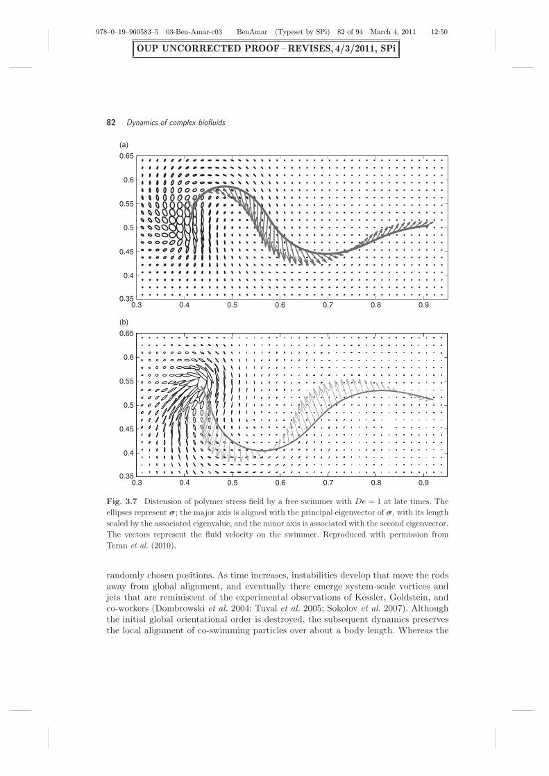
Figure 3.7 shows graphically the distension of the polymer stress field at late timesfor the fastest swimmer (De = 1). In Fig. 3.7a, the free swimmer is very near thetime of peak forward velocity during its stroke, when the backward moving wavehas approached the tail, which is itself moving slightly upwards. Owing to the strongstraining of the fluid by the motion of the tail, there is a large concentration of polymerstress concentration aft of the swimmer. Figure 3.7(b) is about one-quarter of a strokelater. The stress is now much more anisotropic, and the swimmer is actually slippingbackwards. However, in comparison with the Newtonian case, the backwards slippageis of smaller magnitude, leading to an overall faster swimmer.

Note that these results for large-amplitude free swimmers are different from thoseof Lauga (2007) for small-amplitude periodic sheets. In particular, the study of Teranet al. (2010) predicts that both swimming speed and efficiency are maximized at aDeborah number of O(1), when the stroke period is nearly matched to the relaxation



Applications 81

StokesDe = .5

1

0.8

0.6Xc

0.4

0.20 5 10t 15 20

Wi = 1Wi = 2Wi = 3Wi = 4Wi = 5

(a) Center of mass

0.6

0.55

0.5

0.45

0.4

0.350.5 0.6 0.7 0.8 0.9 1 1.1

StokesDe = 1ee = 5

1.2(b) Free-swimmer displacement

Fig. 3.6 (a) The location of the x-component of the center of mass of a free swimmer withA = 0.05 and various values of De. Inset: long-time behavior. (b) Shape and displacement ofthree free swimmers (De = 0, 1, 5) after 20 periods. Reproduced with permission from Teranet al. (2010).

time of the fluid. These results seem to be in qualitative agreement with recentexperimental work of Smith et al. (2009), who found that human spermatozoa swim ata Deborah number of O(1) in synthetic cervical mucus, and show greater displacementper stroke than in less viscoelastic media.

3.4.2.2 Active suspensions of swimming rods

The previous example considered the locomotion of single microswimmers in a vis-coelastic fluid and showed the fundamental differences from locomotion in a Newtonianfluid. We now address instead the collective hydrodynamics of many active swimmersin a Newtonian fluid, i.e., an active suspension. Experiments by Kessler, Goldstein,and co-workers (Dombrowski et al. 2004; Tuval et al. 2005; Sokolov et al. 2007)showed that in the case of concentrated bacterial baths, large-scale vortices and jetsemerged. These flow features were reproduced qualitatively by Graham and co-workers(Hernandez-Ortiz et al. 2005; Underhill et al. 2008), using a force-dipole (dumbbell)model, and by Saintillan and Shelley (2007) using a more detailed model of therod-like swimmer described in Example 4. Figure 3.8 shows a particle simulationfrom Saintillan and Shelley (2007) of 2500 Pusher particles (rods) in a box of size10 × 10 × 3 (in units of particle length). Initially, the rods are aligned, though with




0.65

(a)

0.6

0.55

0.5

0.45

0.4

0.350.3 0.4 0.5 0.6 0.7 0.8 0.9

0.3 0.4 0.5 0.6 0.7 0.8 0.9

0.65

(b)

0.6

0.55

0.5

0.45

0.4

0.35

Fig. 3.7 Distension of polymer stress field by a free swimmer with De = 1 at late times. Theellipses represent σ; the major axis is aligned with the principal eigenvector of σ, with its lengthscaled by the associated eigenvalue, and the minor axis is associated with the second eigenvector.The vectors represent the fluid velocity on the swimmer. Reproduced with permission fromTeran et al. (2010).

randomly chosen positions. As time increases, instabilities develop that move the rodsaway from global alignment, and eventually there emerge system-scale vortices andjets that are reminiscent of the experimental observations of Kessler, Goldstein, andco-workers (Dombrowski et al. 2004; Tuval et al. 2005; Sokolov et al. 2007). Althoughthe initial global orientational order is destroyed, the subsequent dynamics preservesthe local alignment of co-swimming particles over about a body length. Whereas the



Applications 83

(a) (b)

(c) (d)

t = 0.0

t = 2.0 t = 25.0

t = 1.0

Fig. 3.8 Particle simulation of 2500 initially aligned Pushers in a box of size 10 × 10 × 3 (inunits of particle length) at an effective volume fraction ν = ν/8 = 1, showing the different stagesof the dynamics (a)–(d). Reproduced with permission from Saintillan and Shelley (2007).

background flow is on the scale of the system, the individual swimmers show randomwalk statistics, where the random-walk seems to result from pair interactions, at leastat lower volume concentrations. The onset of the large-scale instabilities appears todepend upon the effective volume concentration ν = ν/8 (ν = (Nl3)/L3) of swimmers(see Fig. 2b of Saintillan and Shelley 2007).

Saintillan and Shelley (2008a,b) subsequently developed a continuum model todescribe large-scale macroscopic phenomena, based on the evolution of the probabilitydistribution function (see Section 3.2), which we now discuss.

The configuration variables of a swimming rod are its center-of-mass position andits orientation. Therefore, the Smoluchowski equation (3.1) becomes

∂Ψ∂t

= −∇x · (xΨ) −∇p · (pΨ). (3.33)

The particle fluxes are given by eqns (3.11) and (3.12). Recall that the normalizationof Ψ is such that

∫dVx

∫dSpΨ = nL3:

x = Up + u − Dp∇x ln Ψ, (3.34)

p = (I − ppT) · ∇up − dp∇p ln Ψ. (3.35)




The background flow satisfies the incompressible Stokes equations, forced by the extrastress generated by the swimming rods:

−μΔxu + ∇xq = ∇x · σ, ∇x · u = 0. (3.36)

We consider two broad categories of swimmers: Pushers and Pullers. A Pusher, whosemotion is actuated along the posterior of the body, served as motivation in Example4. In contrast, the motion of a Puller is actuated along the anterior of the body,resulting in an oppositely signed extra-stress contribution (while moving in the samedirection). Bacteria such as B. subtilis might be described as Pushers, while algae suchas Chlamydomonas might be roughly described as Pullers. Figure 3.9 illustrates theflow lines for Pushers and Pullers and shows schematic pictures. We remark thatthere are other swimming microorganisms, such as the multicellular algae Volvoxand densely covered ciliates, that may not fall into these categories. Following thediscussion in Section 3.2, the extra stress for a Pusher is σ = −σ0

∫dSp(ppT − I/3)Ψ

(see also eqn (3.23)); for a Puller, σ is identical in magnitude but oppositely signed.To nondimensionalize eqns (3.33)–(3.36), we choose the rescaling x → lcx, u →

Uu, t → (lc/U)t, and Ψ → nΨ. Here lc is an intrinsic length scale to be determined.With the appropriate rescaled pressure, we obtain the following for the Smoluchowskiequation and particle fluxes:

∂Ψ∂t

= −∇x · (xΨ) −∇p · (pΨ), (3.37)

x = p + u − D∇x ln Ψ, (3.38)

p = (I − ppT)∇xup − d∇p ln Ψ. (3.39)

The forced Stokes equations become

−Δu + ∇q = ∇ · Σa, ∇x · u = 0, (3.40)

Σa = α

∫dVx

∫dSp (ppT − I/3)Ψ. (3.41)

The nondimensional constants are D = Dp/(lcU0), d = dplc/U0, L = L/lc, and α =−(lcσ0n)/(μU0).

Drag Thrust

Pullers: α > 0

DragThrust

Pushers: α < 0

MotionMotion

Fig. 3.9 Flow lines for Pushers (α < 0) and Pullers (α > 0).



Applications 85

To determine lc, we rewrite α using the expressions for σ0 and U derived inExamples. 7 and 4, respectively, σ0 = κ1l

3g and U = κ2lg/μ. With these substitutionsand ν = (Nl3)/L3 for the volume concentration, we obtain α = −(lcν/l)(κ1/κ2).Choosing lc = l/ν turns α into a purely geometric constant, α = −κ1/κ2.

In their particle simulations of rod-like swimmers, Saintillan and Shelley (2007)observed that at low volume concentrations (up to effective volume concentrationssomewhat greater than ν = ν/8 = 1) dp ≈ νdp and Dp ≈ ν−1Dp. If we assume theseobserved scalings of dp and Dp with ν, the nondimensional diffusion coefficients become

d =ldp

U0and D =

Dp

lU0.

That is, d and D depend only upon the speed and length, of the swimmer, and thesystem size and the volume concentration of swimmers appear only in the normalizedsystem size L.

We are interested in the nonlinear dynamics of this system, of partial differentialequations, and its stability around simple steady states. Before getting into thespecifics, we introduce the configurational entropy, which is a natural measure ofthe fluctuations in this system. The relative configurational entropy is defined asS =

∫dVx

∫dSp (Ψ/Ψ0) ln(Ψ/Ψ0), where Ψ0 is the constant value taken by Ψ when

the system is uniform and isotropic (no concentration or orientation fluctuations).This quantity has the following properties:

1. S ≥ 0, and S = 0 if and only if Ψ ≡ Ψ0. That is, a nonzero S measures the sizeof the fluctuations away from uniform isotropy, realized when Ψ = Ψ0.

2. The entropy evolves via

Ψ0S = − 6α

∫dVx E : E −

∫dSp

∫dVxΨ

[D|∇x ln Ψ|2 + d|∇p ln Ψ|2

],

where E is the symmetric rate-of-strain tensor. The first term on the right-hand side is proportional to the rate of viscous dissipation, and the second isstrictly negative and reflects diffusional processes which serve to drive S towardsits minimum (the uniform and isotropic state). The scalings of the system usedhere give Ψ0 = 4π.

We omit the proofs, which are straightforward, of these statements.The configurational entropy and its evolution establish the uniform isotropic state

as a natural steady state to be examined for this system. Given their relevance tothe study of biological flocking, the stability of aligned suspensions has also beenexamined, by Simha and Ramaswamy (2002) and by Saintillan and Shelley (2007,2008a,b), among others. These authors find that aligned suspensions are genericallyunstable, particularly in the absence of diffusional processes, regardless of swimmertype (Pusher or Puller). Here we focus on the stability of the uniform isotropic state,which relates naturally to measures of fluctuations in the system, and whose analysisreveals strong differences depending on swimmer type and geometry.




We now turn our attention to the details of the stability of a uniform, isotropicsuspension of active swimmers. First, some general conclusions can be drawn fromProperty 2 of the configurational entropy. For suspensions of Pullers, where α > 0,we have S < 0, and fluctuations away from the uniform, isotropic state are expectedto decay. On the other hand, for Pushers (α < 0), the leading term is now positive,which allows the possibility of fluctuation growth and eventual balance with diffusion.Furthermore, if there is no diffusion, fluctuations should grow. These issues wereanalyzed in a detailed study of a system linearized near uniform isotropy (Hoheneggerand Shelley 2010).

Let Ψ = 1/(4π) (1 + εψ), v = εu, and q → εq with ε � 1. Keeping only linear-order terms and using the identity ∇p · (f1θ + f2φ) = (1/ sin φ)(∂θf1 + ∂φ(sin φf2)),eqns (3.37)–(3.41) become

ψt + p · ∇xψ − 3ppT : ∇xu = D∇2xψ + d∇2

pψ, (3.42)

− Δxu + ∇xq = ∇x · σ, ∇x · u = 0, (3.43)

where σ = (α/4π)∫

dSp ψ (pp − I/3).The first step of the stability analysis is to transform the equations using a spatial

Fourier transform in x, fk =∫

dV e−ik·xf(x), to decouple eqns (3.42) and (3.43) inthe wave vector k (k = |k|, k = kk). From eqn (3.43), uk = (i/k)(I − kkT) · σk · k,and eqn (3.42) then becomes

∂tψk = − ikk · p ψk − Dk2ψk + d∇2pψk − 3ppT : (I − kkT) · σk · kk. (3.44)

The explicit dependence of eqn (3.44) on the direction of k can be removed by arotation, k = Rz, which defines q through p = Rq. Let θ ∈ [0, 2π] be the azimuthalangle and let φ ∈ [0, π] be the polar angle on the unit q-sphere. Equation (3.44) thenbecomes

∂tψk = − ik cos φ ψk − Dk2ψk + d∇2qψk − 3 cos φq · (I − zzT) · RT · σk · R · z.

A further decoupling in θ is achieved by introducing a Fourier series in θ, ψk =∑

n

An,k(φ, t)einθ. After some algebra, we find

∂tAn,k + An,k

(ik cos φ + Dk2

)+ d

(n2

sin2 φAn,k − 1

sin φ∂φ(sin φ ∂φAn,k)

)

= −3α

4cos φ sin φ F [An,k]δn,1,

(3.45)

where the scalar operator F is

F [h] =∫ π

0

dφ′ h(φ′) sin2 φ′ cos φ′

and δn,1 is the Kronecker delta symbol.



Applications 87

The main feature of eqn (3.45) is that the entire stability is controlled by the firstazimuthal mode on the sphere.

We now look for exponential solutions to eqn (3.45) in the special case whenD = d = 0 and α < 0 (Pushers). Hence we assume that A1,k(φ, t) = γk(φ)eσt and notethat there is no a priori expectation that A1,k can be represented in this fashion, aseqn (3.45) depends explicitly on φ. Nonetheless, inserting the exponential ansatz intoeqn (3.45) and applying F to both sides yields the eigenvalue relation

−34α

∫ π

0

dφ′ sin3 φ′ cos2 φ′

σ + ik cos φ′ = 1. (3.46)

This complex-valued integral can be evaluated by substitution and separation intoreal and imaginary parts. Some algebra produces the complex equation

−α

[

4iσk3 + 6iσ3k − 3σ2(σ2 + k2) lniσ − k

iσ + k

]

= 4ik5, (3.47)

where the complex logarithm is defined as ln(a + ib) = ln√

a2 + b2 + i arctan(b/a).Note that eqn (3.47) is valid only if Re(σ) �= 0. Figure 3.10 shows a numerical solutionof eqn (3.47), plotting the real and imaginary parts of σ for α = −1. For small k, thereare two branches of unstable eigenvalues with zero imaginary part, and the decreasein growth rate suggests a crossing of the k-axis to become negative at medium k.Saintillan and Shelley (2008b) gave an asymptotic solution for k � 1 for the upperbranch in Fig. 3.10,

σ(k) = −α

5+

[157α

− D

]

k2 + O(k3). (3.48)

For a suspension of Pushers (α < 0), eqn (3.48) implies the existence of a long-waveinstability with limk→0 σ(k) = −α/5 > 0, corresponding to the upper branch in Fig.3.10. In contrast, for Pullers, there is no long-wave instability.

0 0.2 0.4 0.60

0.05

0.1

0.15

0.2(a)

k

Re(s)

k1k0

0 0.2 0.4 0.6−0.4

–0.2

0

0.2

0.4(b)

k

Im(s

)

k1k0

Fig. 3.10 Real and imaginary parts of the growth rate σ(k) for α = −1 (Pushers) with D =d = 0. Reproduced with permission from Hohenegger and Shelley (2010).




One of the striking features of the analysis of the eigenvalue problem (Hoheneggerand Shelley 2010) is that there is no crossing to negative k, contrary to the intuitiongathered from Fig. 3.10. As a matter of fact, a singular behavior develops in thecorresponding eigenvector as k approaches k1, the zero-growth-rate value. The singularbehavior results from a discontinuous pole singularity in the integral in eqn (3.46) asRe(σ) approaches 0.

Finally, we remark that if k = k1 is indeed a point of stability transition, thenthere exists a critical system size L or volume concentration ν above which the systembecomes unstable. This follows from having scaled by the intrinsic length lc, so thatk′1 = (k1/2π)(νL/l). As the first allowable mode in the periodic box has k′ = 1, the

system is unstable if k′1 ≈ 0.089(νL/l) > 1, and is stable otherwise.

As just highlighted, the eigenvalue analysis does not provide solutions for k > k1.The dynamics in these cases was found numerically and was confirmed by a largek analysis (Hohenegger and Shelley 2010). Figure 3.11 illustrates these numericallydetermined solutions in the absence of diffusion. In each case, the initial condition isA1,k(φ, 0) = sin(φ). In Fig. 3.11, the real and imaginary parts of A1,k for k = 0.4,k = 0.8, and k = 10 are plotted at t = 50 and t = 100 for Pushers (α = −1). Fork = 0.4, the real and imaginary parts (Fig. 3.11(a)) grow as predicted by the eigenvalueanalysis. The values k = 0.8 and k = 10 are out of the range of exponential growthand both the real and the imaginary parts of the solution show oscillations. Thenumber of oscillations increases with time, as illustrated with Figs. 3.11(b) and (c), andFig. 3.11(d) shows that for large k, the envelope of the oscillations is determined by theinitial condition (and is as determined analytically by Hohenegger and Shelley 2010).

We expect rotational diffusion (i.e. d > 0) to remove the singular behavior in theeigenvalue problem, and to yield exponentially decaying solutions past a crossing value.To investigate this, we assume again that A1,k(φ, t) = γk(φ)eσt in eqn (3.45) andrenormalize the problem so that F [γk] = 1. Upon substitution into eqn (3.45), thisleads to the system

γk(σ + ik cos φ + Dk2) + d

(1

sin2 φγk − 1

sin φ∂φ (sin φ ∂φγk)

)

= −3α

4cos φ sin φ,

(3.49)∫ π

0

dφ′γk(φ′, t) sin2 φ cos φ = 1. (3.50)

Equations (3.49) and (3.50) were solved by discretizing the φ-derivatives and solvingthe resulting nonlinear system via Newton iteration starting from the known solutionfor d = 0.

In Fig. 3.12, the real part of σ(k) obtained from eqns (3.49) and (3.50) with d = 0and d = 0.01 is plotted. For this moderate degree of rotational diffusion, a downwardshift of the branches is seen, leaving the long-wave instability intact but suppressingthe lower branch. Not only does rotational diffusion reduce growth rates, but it alsosuppresses the eigenfunction singularity. For a suspension of Pullers, there are nopositive growth rates for d ≥ 0, as would be expected from the generic decay of theentropy.



Applications 89

0 1 2 3−30

−20

−10

0

10

20

30(a)

φ

Re(A1,k)

Im(A1,k)

sin(φ)

0 1 2 3−3

−2

−1

0

1

2

3

(b)

Re(A1,k) Im(A1,k) sin(φ)

φ

0 1 2 3−3

−2

−1

0

1

2

3

(c)

φ


0 1 2 3

−1

−0.5

0

0.5

1

(d)


φ

(a) k = 0.4, t = 50 (b) k = 0.8, t = 50

(c) k = 0.8, t = 100 (d) k = 0.10, t = 100

Fig. 3.11 Real and imaginary parts of the first Fourier modes A1,k(φ, t) for α = −1 (Pushers)and D = d = 0, from a single-mode sinusoidal initial condition. The increasing wavenumbersk show growth (top left), saturation in amplitude with an increasing number of oscillations intime (top right and bottom left), and convergence of the wave envelope to that of the initialcondition. Reproduced with permission from Hohenegger and Shelley (2010).

The theoretical considerations above allow a comparison with the rod simulationsof Saintillan and Shelley (2007). First, we remark that for saintillan and shelley’srod model, we estimate α ≈ −0.9, close to the value of −1 that we have used inthe theoretical study described above. Using values for dp and Dp gleaned fromSaintillan and Shelley (2007), we have solved the eigenvalue problem of eqns (3.49)and (3.50). This yields the crossing value k1 ≈ 0.086, and hence instability is foundif k′

1 = (k1/2π)(νLp/l) > 1. Taking l = 1 and Lp = 10, this analysis predicts theexistence of a critical volume concentration ν = 0.9 (ν = ν/8) for the emergence of a




0 0.2 0.4 0.6

−0.05

0

0.05

0.1

0.15

0.2

k

Re(

s)

d = 0d = 0.01

Fig. 3.12 Continuation of the real part of the growth rate σ(k) for positive rotational diffusiond = 0.01, α = −1 (Pushers), and D = 0. Reproduced with permission from Hohenegger andShelley (2010).

(a) (b)

(c) (d)

t = 0 t = 100

t = 300t = 200

Fig. 3.13 Fluid mixing by an active suspension of Pushers (α = −1). The gray levels showthe configuration of a passive scalar field in the suspension at different times. Reproduced withpermission from Saintillan and Shelley (2008b).



Conclusions 91

long-wave instability. This is consistent with the result of Saintillan and Shelley (2007)that organized dynamics emerges at volume concentrations in the neighborhood ofν = 0.5.

Using kinetic theory, Saintillan and Shelley (2008a,b) simulated this instabilitystarting from uniform isotropy in the special case of two-dimensional flows. Fig-ure 3.13 shows the evolution away from uniform isotropy through the dynamics ofa scalar field being advected by the background velocity field. The fully developednonlinear dynamics is quasi-periodic, has persistent concentration fluctuations (notpredicted by linear theory), and yields efficient mixing of the scalar field throughrepeated folding and stretching of fluid elements. It was also found that the sys-tem reached a state of statistical equilibrium where the growth of configurationalentropy saturates and where fluctuation growth is balanced, on average, by diffusionalprocesses.

3.5 Conclusions

In our lectures and in these notes, we have reviewed the basics of non-Newtonian fluidmechanics and established formulae for the extra-stress contribution to the macro-scopic stress tensor, in the particular cases of dumbbell- and- rod shaped particles.We discussed the derivation and properties of the Oldroyd-B model. We then focusedon pumping and swimming in viscoelastic fluids as important biological examples.Both of these problems concern complex fluid–body interactions and required thedevelopment and use of sophisticated numerical methods (which we did not discuss inany detail). We then developed and analyzed the continuum theory of active particlesuspensions put forward by Saintillan and Shelley (2008a,b), focusing on its structurenear a state of uniform isotropy.

There are of course many other fascinating problems which could have beendiscussed if time had allowed. Among many such examples are the study of syntheticswimmers (e.g. Zerrouki et al. 2008; Keaveny and Shelley 2009), and microfluidicpumps produced by carpets of bacteria bound to channel walls (Kim and Breuer2008).

Similarly, there are many directions in which the problems discussed here canevolve. We conclude by briefly mentioning some of these. Peristaltic pumping wasshown to be hindered by viscoelasticity. Therefore a natural question to ask pertainsto the optimal wave shape that minimizes the input power. Walker and Shelley (2010)developed a shape optimization algorithm for the Newtonian case, but the extensionto a viscoelastic fluid is open. The continuum model of swimming rods gave riseto complex large-scale behavior, but the linearized analysis around uniformity andisotropy did not show growth in concentration fluctuations (on the contrary, thesedecayed). Furthermore, it is believed that in bacterial baths, other effects such aschemotaxis or oxygen-taxis (Sokolov et al. 2007), which were not included here, canplay a significant role. Finally, motile microorganisms such as bacteria also thrive andmove in other yet more complicated media, such as gel-like soft tissues and mucus.




Acknowledgments

The authors thank Saverio E. Spagnolie for useful comments. We are grateful forsupport from the Department of Energy and the National Science Foundation, as wellas from the NYU-MRSEC Center.

References

Arratia P. E., Thomas C. C., Diorio J., and Gollub J. P. (2006). Elastic instabilitiesof polymer solutions in cross-channel flow. Physical Review Letters, 96, 144502.

Batchelor G. K. (1970a). The stress system in a suspension of force-free particles.Journal of Fluid Mechanics, 41, 545–570.

Batchelor G. K. (1970b). Slender-body theory for particles of arbitrary cross-sectionin Stokes flow. Journal of Fluid Mechanics, 44, 419–440.

Batchelor G. K. (1977). The effect of Brownian motion on the bulk stress in asuspension of spherical particles. Journal of Fluid Mechanics, 83, 97–117.

Bird R. B., Armstrong R. C., and Hassager O. (1987). Dynamics of Polymeric Fluids:Kinetic Theory. Wiley.

Doi M. and Edwards S. F. (1986). The Theory of Polymer Dynamics. Oxford Univer-sity Press.

Dombrowski C., Cisneros L., Chatkaew S., Goldstein R. E., and Kessler J. O. (2004).Self-concentration and large-scale coherence in bacterial dynamics. Physical ReviewLetters, 93, 098103.

Fauci L. J. and Peskin C. S. (1988). A computational model of aquatic animallocomotion. Journal of Computational Physics, 77, 85–108.

Fauci L. J. and Dillon R. (2006). Biofluidmechanics of reproduction. Annual Reviewof Fluid Mechanics, 38, 371–394.

Fu H. C., Powers T. R., and Wolgemuth C. W. (2007). Theory of swimming filamentsin viscoelastic media. Physical Review Letters, 99, 258101.

Fu H. C., Wolgemuth C. W., and Powers T. R. (2009). Swimming speeds of filamentsin nonlinearly viscoelastic fluids. Physics of Fluids, 21, 033102.

Groisman A. and Quake S. R. (2004). A microfluidic rectifier: Anisotropic flowresistance at low Reynolds numbers. Physical Review Letters, 92, 094501.

Groisman A. and Steinberg V. (2001). Efficient mixing at low Reynolds numbers usingpolymer additives. Nature, 410, 905–908.

Groisman A. and Steinberg V. (2004). Elastic turbulence in curvilinear flows ofpolymer solutions. New Journal of Physics, 6, 29.

Hernandez-Ortiz J. P., Stolz C. G., and Graham M. D. (2005). Transport and collectivedynamics in suspensions of confined swimming particles. Physical Review Letters,95, 204501.

Hohenegger C. and Shelley M. J. (2010). Stability of active suspensions. PhysicalReview E, 81, 046311.

Jaffrin M. and Shapiro A. (1971). Peristaltic pumping. Annual Review of FluidMechanics, 3, 13.



References 93

Jeffery G. B. (1922). The motion of ellipsoidal particles immersed in a viscous fluid.Proceedings of the Royal Society of London, 102, 161–179.

Johnson R. E. (1980). An improved slender-body theory for Stokes-flow. Journal ofFluid Mechanics, 99, 411–431.

Keaveny E. E. and Shelley M. J. (2009). Hydrodynamic mobility of chiral colloidalaggregates. Physical Review E, 79, 051405.

Keller J. B. and Rubinow S. I. (1976). Slender-body theory for slow viscous-flow.Journal of Fluid Mechanics, 75, 705–714.

Kim M. J. and Breuer K. S. (2008). Self-organizing bacteria-powered microfluidicpump. Small, 4, 111–118.

Larson R. G. (1995). The Structure and Rheology of Complex Fluids. Oxford UniversityPress.

Lauga E. (2007). Propulsion in a viscoelastic fluid. Physics of Fluids, 19, 081304.Lighthill M. J. (1960). Note on the swimming of slender fish. Journal of Fluid

Mechanics, 9, 305–317.Paxton W. F., Kistler K. C., Olmeda C. C., Sen A., St. Angelo S. K., Cao Y., Mallouk

T. E., Lammert P. E., and Crespi V. H. (2004). Catalytic nanomotors: Autonomousmovement of striped nanorods. Journal of the American Chemical Society, 126,13424.

Peskin C. (2002). The immersed boundary method. Acta Numerica, 11, 479.Pozrikidis C. (1992). Boundary Integral and Singularity Methods for Linearized Vis-

cous Flow. Cambridge University Press.Purcell E. M. (1977). Life at low Reynolds number. American Journal of Physics,

45, 11.Saintillan D. and Shelley M. J. (2007). Orientational order and instabilities in suspen-

sions of self-locomoting rods. Physical Review Letters, 99, 058102.Saintillan D. and Shelley M. J. (2008a). Instabilities and pattern formation in active

particle suspensions: Kinetic theory and continuum simulations. Physical ReviewLetters, 100, 178103.

Saintillan D. and Shelley M. J. (2008b). Instabilities, pattern formation, and mixingin active suspensions. Physics of Fluids, 20, 123304.

Simha R. A. and Ramaswamy S. (2002). Hydrodynamic fluctuations and instabilitiesin ordered suspensions of self-propelled particles. Physical Review Letters, 89, 58101.

Smith D. J, Gaffney E. A., Gadelha H., Kapur N., and Kirkman-Brown J. C. (2009).Bend propagation in the flagella of migrating human sperm, and its modulation byviscosity. Cell Motility and the Cytoskeleton, 66, 220–236.

Sokolov A., Aranson I. S., Kessler J. O., and Goldstein R. E. (2007). Concentrationdependence of the collective dynamics of swimming bacteria. Experiments in Fluids,43, 737.

Spagnolie S. E. and Lauga E. (2010). The optimal elastic flagellum. Physics of Fluids,22, 031901.

Tam D. and Hosoi A. E. (2007). Optimal stroke patterns for Purcell’s three-linkswimmer. Physical Review Letters, 98, 68105.




Taylor G . I. (1951). Analysis of the swimming of microscopic organisms. Proceedingsof the Royal Society of London, Series A, Mathematical and Physical Sciences, 209,447–461.

Teran J., Fauci L. J., and Shelley M. J. (2008). Peristaltic pumping and irreversibilityof a Stokesian viscoelastic fluid. Physics of Fluids, 20, 073101.

Teran J., Fauci L. J., and Shelley M. J. (2010). Viscoelastic fluid response can increasethe speed and efficiency of a free swimmer. Physical Review Letters, 104, 38101.

Thomases B. and Shelley M. J. (2007). Emergence of singular structures in Oldroyd-Bfluids. Physics of Fluids, 19, 103103.

Thomases B. and Shelley M. J. (2009). Transition to mixing and oscillations in aStokesian viscoelastic flow. Physical Review Letters, 103, 094501.

Tuval I., Cisneros L., Dombrowski C., Wolgemuth C. W., Kessler J. O., and Gold-stein R. E. (2005). Bacterial swimming and oxygen transport near contact lines.Proceedings of the National Academy of Sciences, 102, 2277.

Underhill P. T., Hernandez-Ortiz J. P., and Graham M. D. (2008). Diffusion andspatial correlations in suspensions of swimming particles. Physical Review Letters,100, 248101.

Walker S. W. and Shelley M. J. (2010). Shape optimization of peristaltic pumping.Journal of Computational Physics, 229, 1260–1291.

Young Y. N. and Shelley M. J. (2007). Stretch-coil transition and transport of fibersin cellular flows. Physical Review Letters, 99, 58303.

Zerrouki D., Baudry J., Pine D., Chaikin P., and Bibette J. (2008). Chiral colloidalclusters. Nature, 455, 380–382.

3 Dynamics of complex biofluids - NYU Courant

Documents

Transcript of 3 Dynamics of complex biofluids - NYU Courant