
Projection of populations by level of educational attainment, age, and sex for 120 countries for...
92
Demographic Research a free, expedited, online journal of peer-reviewed research and commentary in the population sciences published by the Max Planck Institute for Demographic Research Konrad-Zuse Str. 1, D-18057 Rostock · GERMANY www.demographic-research.org DEMOGRAPHIC RESEARCH VOLUME 22, ARTICLE 15, PAGES 383-472 PUBLISHED 16 MARCH 2010 http://www.demographic-research.org/Volumes/Vol22/15/ DOI: 10.4054/DemRes.2010.22.15 Research Article Projection of populations by level of educational attainment, age, and sex for 120 countries for 2005-2050 Samir KC Bilal Barakat Anne Goujon Vegard Skirbekk Warren Sanderson Wolfgang Lutz © 2010 Samir KC et al. This open-access work is published under the terms of the Creative Commons Attribution NonCommercial License 2.0 Germany, which permits use, reproduction & distribution in any medium for non-commercial purposes, provided the original author(s) and source are given credit. See http:// creativecommons.org/licenses/by-nc/2.0/de/
Transcript of Projection of populations by level of educational attainment, age, and sex for 120 countries for...

Demographic Research a free, expedited, online journal of peer-reviewed research and commentary in the population sciences published by the Max Planck Institute for Demographic Research Konrad-Zuse Str. 1, D-18057 Rostock · GERMANY www.demographic-research.org
DEMOGRAPHIC RESEARCH VOLUME 22, ARTICLE 15, PAGES 383-472 PUBLISHED 16 MARCH 2010 http://www.demographic-research.org/Volumes/Vol22/15/ DOI: 10.4054/DemRes.2010.22.15 Research Article
Projection of populations by level of educational attainment, age, and sex for 120 countries for 2005-2050
Samir KC
Bilal Barakat
Anne Goujon
Vegard Skirbekk
Warren Sanderson
Wolfgang Lutz
© 2010 Samir KC et al. This open-access work is published under the terms of the Creative Commons Attribution NonCommercial License 2.0 Germany, which permits use, reproduction & distribution in any medium for non-commercial purposes, provided the original author(s) and source are given credit. See http:// creativecommons.org/licenses/by-nc/2.0/de/

Table of Contents
1 Introduction 384 2 Approach 386 3 Existing projections 390 4 Methodology 392 4.1 Raw data and adjustments 392 4.2 Educational fertility differentials 392 4.3 Educational mortality differentials 398 4.4 Migration assumptions 400 4.5 Educational progression assumptions 401 4.6 Mean years of schooling 403 5 Scenarios 405 5.1 Demographic scenario 405 5.2 Education scenarios 406 5.2.1 Constant enrollment number (CEN) scenario 406 5.2.2 Constant enrollment ratio (CER) scenario 407 5.2.3 Global education trend (GET) scenario 407 5.2.4 The fast-track (FT) scenario 411 5.3 A note on educational policy discontinuities since 1990 412 6 Results and discussion 413 6.1 Sample output 413 6.2 Discussion 416 7 Future refinements 430 8 Conclusions and outlook 431 References 433 Appendix A 442 Appendix B 444 Appendix C 471

Demographic Research: Volume 22, Article 15 Research Article
http://www.demographic-research.org 383
Projection of populations by level of educational attainment, age, and sex for 120 countries for 2005-2050
Samir KC1
Bilal Barakat2
Anne Goujon3
Vegard Skirbekk4
Warren Sanderson5
Wolfgang Lutz6
Abstract
Using demographic multi-state, cohort-component methods, we produce projections for 120 countries (covering 93% of the world population in 2005) by five-year age groups, sex, and four levels of educational attainment for the years 2005-2050. Taking into account differentials in fertility and mortality by education level, we present the first systematic global educational attainment projections according to four widely differing education scenarios. The results show the possible range of future educational attainment trends around the world, thereby contributing to long-term economic and social planning at the national and international levels, and to the assessment of the feasibility of international education goals.
1 Corresponding Author: Dr. Samir KC, Research Scholar, World Population Program, International Institute for Applied Systems Analysis (IIASA), Schlossplatz 1, A-2361 Laxenburg, Austria, tel.: +43-2236-807-424, fax: +43-2236-71313, e-mail: [email protected]. 2 Dr. Bilal Barakat, Research Scholar, World Population Program, IIASA; and Research Scholar, Vienna Institute of Demography of the Austrian Academy of Sciences; e-mail: [email protected]. 3 Dr. Anne Goujon, Research Scholar, World Population Program, IIASA; and Research Scholar, Vienna Institute of Demography of the Austrian Academy of Sciences; e-mail: [email protected]. 4 Dr. Vegard Skirbekk, Leader, Age and Cohort Change Project, IIASA; e-mail: [email protected]. 5 Prof. Dr. Warren Sanderson, Departments of Economics and History, Stony Brook University, New York, USA; and Institute Scholar, World Population Program, IIASA; email: [email protected]. 6 Prof. Dr. Wolfgang Lutz, Leader, World Population Program, IIASA; Director, Vienna Institute of Demography of the Austrian Academy of Sciences; Professor of Applied Statistics, Vienna University of Economics and Business; and Professorial Research Fellow, Oxford Institute of Ageing; e-mail: [email protected]

Samir KC et al.: Projection of populations by educational attainment
384 http://www.demographic-research.org
1. Introduction
This paper is part of an ambitious, multiphase project, the aims of which include the production of a new national level dataset on educational attainment by age and sex for as many countries in the world as possible over the period 1970-2000, the analysis of these new data, the preparation of projections of educational attainment by age and sex for those countries through 2050, and the assessment of the likely effects of future changes in educational structure. The project is a joint effort of the World Population Program at the International Institute for Applied Systems Analysis (IIASA) and the Vienna Institute of Demography (VID). Version 1.0 of both the educational attainment reconstructions and projections is now complete.7 In this paper, we describe the methods used for projecting the educational attainment distributions for 120 countries for the years 2000-2050 using the methods of multi-state demographic modeling (see Appendix C).
Education-specific population projections are important, both because the information they produce is of intrinsic and practical interest, and because taking education into account improves the accuracy of the population projection itself. The latter is true because all three fundamental demographic components of fertility, mortality, and migration are strongly affected by education. In most societies, fertility levels vary significantly between women with different education levels (Jejeebhoy 1995; Bledsoe et al. 1999). Not just the number of children, but also the timing of births and marriage are strongly influenced by education levels. With regard to mortality, many factors contribute to a general pattern of higher life expectancy among the more educated (for instance, Kitagawa and Hauser 1973; Ahlburg, Kelley, and Mason 1996; Alachkar and Serow 1988; Preston and Taubman 1994; Doblhammer 1997; Lleras-Muney 2005), relating to healthy behavior (Kenkel 1991; Lantz et al. 1998), the gathering and appreciation of medical information (Niederdeppe 2008), better access to health care (Cleland and van Ginneken 1988), higher urbanization, etc. Finally, the highly educated are more likely to migrate and to move greater distances, and they are less likely to return to their country of origin.
As a result, population projections may lead to substantively different results in the presence of education variables than in their absence. Without education, they may also be less useful than they could be otherwise. Education is one of the keys to development. Interactions have been demonstrated with most development dimensions, including human rights, health, democracy, culture, economic growth, etc. (Sen 1999; Collier and Hoeffler 2000). Conversely, educational processes are affected by all of the above. Health affects absenteeism. The government’s respect for human rights influences access to schools for minorities; as one of the largest items of public
ex.html. 7 The database can be accessed at http://www.iiasa.ac.at/Research/POP/Edu07FP/ind

Demographic Research: Volume 22, Article 15
http://www.demographic-research.org 385
spending, education is tied closely to the economic development of the country. As such, education is both a means and an end to development.
Accordingly, an understanding of the educational level of the population is important when speculating about future development trajectories. Recently, we prepared a database for the population subdivided by age, sex, and education for the period 1970-2000 (Lutz et al. 2007). Using the UN’s age and sex distribution for the period, the proportions of each age and gender group who had attained different levels of education were reconstructed from data on education distributions compiled in and around 2000 (United Nations 2005). The dataset has been used by many researchers in different fields for analyzing effects of education on different variables. By applying their insights to the education profiles of future populations, it becomes possible to engage in informed speculation on the opportunities for development over the next four decades in various regions of the world.
Since the effects of educational attainment can also be expected to differ by age (e.g., one might expect that the education of 25-34-year-olds should be more important for economic growth than that of persons beyond retirement age) as well as by sex, having full age details for men and women can be considered a great asset for a comprehensive projection of future economic growth prospects. While some partial efforts at projecting levels of educational attainment have been developed at a more aggregated level, in the past, projections over several decades by age, sex, and level of education were not available for a large set of countries, including both industrialized and developing countries (but see the section on existing projections for a discussion of the closest alternative).
This projection exercise focuses strictly on levels of educational attainment, which are measures of the quantity and formal level of schooling obtained. Educational quality also has an important effect on human capital. Standard measures of skills acquired—such as the PISA (Programme for International Student Assessment), PIRLS (Progress in International Reading Literacy Study) school performance databases, or IALS (International Adult Literacy Survey) for adults—are based on actual testing of samples of the population, and show strong variations between countries that could explain other differentials associated with education. While such datasets based on the direct testing of skills are so far only available for a small number of (mostly OECD) countries, efforts are underway (e.g., by the UNESCO Institute of Statistics) to collect this type of information for a larger number of countries. In the future, we plan to incorporate educational quality and skills assessed on the basis of testing into our measures for countries where data are available, but this will be done in a later phase of the project.
Following this introduction, this paper has six sections. Section 2 introduces the basic idea of demographic multi-state projections and discusses earlier applications. Section 3 discusses the existing projections and how the present exercise differs.

Samir KC et al.: Projection of populations by educational attainment
386 http://www.demographic-research.org
Section 4, the main body of the paper, describes our method. It begins with a concise summary of the different steps involved, and then discusses at some length the key dimensions of the method: the raw data and adjustments to the data, the assumptions made about fertility, and mortality differentials and migration. In addition, Section 4 outlines our approaches to dealing with the age when progressing to higher attainment categories, describes the different demographic and educational scenarios, and discusses current limitations that may be overcome in future revisions. Section 5 gives a brief discussion of selected results, and Section 6 presents some sensitivity analyses. The concluding section provides a short outlook on the kinds of studies that may be possible with these projections.
2. Approach
In this section, we briefly describe the general approach taken in producing these new educational attainment projections. Starting from one empirical dataset for each country for the year 2000, distributions by level of education are projected along cohort lines.
The projections are based on the demographic method of multi-state population projection. This approach was developed at IIASA during the 1970s, and is now widely accepted by technical demographers. Our baseline year providing the empirical starting point is 2000, the same as in our reconstruction of the education distribution in the past. This allows us to connect the backward and forward projections in a gapless time series. We chose 2000 as the base year, since the data for 2005 were not available for a vast majority of countries.
The basic idea of projection is straightforward. Assuming that the educational attainment of a person remains invariant after a certain age, we can, for example, derive directly the proportion of women without any formal education aged 50-54 in 2005 from the proportion of women without any formal education aged 45-49 in 2000. Again assuming that this proportion is constant along cohort lines, the proportion of women without education aged 95-99 in 2050 for the same cohort can be derived directly. In a similar manner, the proportions for each educational category and each age group of men and women can simply be moved to the next older five-year age group as we progress forward in time in five-year steps.
These proportions would be precisely correct if no individual were to move up to the category with primary education after the age of 15, and if mortality and migration did not differ by level of education. This follows directly from the fact that the size of a birth cohort as it ages over time can only change through mortality and migration. However, strong links do in fact exist between the educational level on the one hand, and mortality, fertility, and migration behavior on the other. Accordingly, the above

Demographic Research: Volume 22, Article 15
http://www.demographic-research.org 387
approach is adjusted to correct for these effects. The size of birth cohorts is dependent on the levels of education of women of childbearing age, where a negative relationship is traditionally observed. In projecting these cohorts forward, differential survival rates are applied to the education groups. The differentials are based on a comprehensive literature review, as well on modeling exercises based on past data. The details of these adjustments are provided in later sections.
The above treats the different education groups essentially as separate sub-populations. In addition, at younger years transitions between the education categories may occur. These are described in detail in later sections. The analysis is simplified by the assumption that changes in educational attainment are uni-directional; i.e., that individuals can only move from the ‘no education’ status to primary, and on to secondary and possibly to tertiary; but can never revert to a lower status.
In reality, the likelihood of an individual making the transition from one educational attainment level to the next highest is strongly dependent on the education of the parents. This educational inheritance mechanism is not, however, modeled explicitly here. Instead, the assumptions regarding the transition rates and their future development are statistically derived from the aggregate behavior of education systems in the past. Since this expansion is partly the result of the inheritance mechanism—i.e., the fact that many parents aspire for their children to reach an education level at least as high as they themselves did—inheritance is implicitly reflected in the projection, even though it is not formally part of the model. Such an approach appears preferable at this time because data on the aggregate growth patterns of education systems, on which assumptions for the future can be based, are much more readily available than robust data on the micro-process of educational inheritance.
The starting point for the projection is data collected for each country (typically around the year 2000) which gives the total population by sex, five-year age groups, and four attainment categories based on the current International Standard Classification of Education (ISCED 1997). These categories are no education, primary, secondary, and tertiary (see Table 1).
Table 1: Education categories Category Definition No education (E1) No formal education or less than one year primary Primary (E2) Uncompleted primary, completed primary (ISCED 1), and uncompleted lower
secondary Secondary (E3) Completed lower secondary (ISCED 2), uncompleted and completed higher
secondary (ISCED 3/4), and uncompleted tertiary education Tertiary (E4) Completed tertiary education (ISCED 5/6)

Samir KC et al.: Projection of populations by educational attainment
388 http://www.demographic-research.org
When a single set of categories is applied to all countries, regardless of their state of educational development, it is inevitable that some compromises will have to be made. Surveys used exclusively in developing countries have historically provided little differentiation at higher education levels. Conversely, data collected in industrialized countries may not differentiate below completed primary level. For the present purposes, the entire spectrum, from no education to completed tertiary, needs to be covered. At the same time, a large number of detailed categories would be unwieldy, and would limit the number of countries for which data are available. Consequently, a relatively small number of categories is used to cover the entire spectrum. This means that the categories are relatively broad. Note, for instance, that ‘primary’ does not refer to completed primary, but to having more than one year of primary schooling. Likewise, for the purposes of this study, ‘secondary’ refers to lower secondary, not completed upper secondary. As a result, the ‘secondary’ category is quite broad, encompassing ISCED levels 2-4. The reason for not splitting off ISCED 4 is that the distinction between ISCED 3 and 4 is one of the least clear-cut, and also that ISCED 4 programs “are often not significantly more advanced than programmes at ISCED 3” (UNESCO Institute for Statistics 2009:258). As a result, attempting to distinguish between ISCED 3 and 4 would have undermined the straightforward hierarchical interpretation of our education categories.
Our procedure for each country can be summarized as follows:
• A baseline population distribution by five-year age group, sex, and level of educational attainment is derived for the year 2000.
• For each five-year time step, cohorts move to the next highest five-year age group.
• Mortality rates are applied, specific to each age, sex, and education group, and to each period.
• Age, and sex-specific educational transition rates are applied. • Age, sex, and education-specific net migrants are added to or removed
from the population. • Fertility rates are applied, specific to each age, sex, and education group,
and to each period, to determine the size of the new 0-5 age group. • The new population distribution by age, sex, and level of educational
attainment is noted, and the above steps are repeated for the next five-year time step.

Demographic Research: Volume 22, Article 15
The aim of the projection is to obtain a dataset with the population distributed by five-year age groups (starting at age 15 and ending with the age group 100+), by sex, and by four levels of educational attainment over a period of 50 years in five-year intervals, from 2000 (base year) to 2050.
To illustrate the kind of information that this projection method generates for 120 countries in the world, Figure 1 gives an example in terms of age pyramids by level of education for South Africa. The first pyramid (Fig. 1a) shows the structure by age, sex, and level of education for the year 2000, which is the empirical baseline information used for the reconstruction. The second pyramid (Fig. 1b) gives the projected structure for the year 2050, resulting from our method.
Figure 1a: Structure by age, sex, and level of education for South Africa
for the year 2000
3000 2000 1000 0 1000 2000 3000
15-1920-2425-2930-3435-3940-4445-4950-5455-5960-6465-6970-7475-7980-8485-8990-9495-99100+
Males Population in Thousands Females
No Education Primary Secondary Tertiary
http://www.demographic-research.org 389

Samir KC et al.: Projection of populations by educational attainment
Figure 1b: Projected structure for South Africa for the year 2050
3000 2000 1000 0 1000 2000 3000
15-1920-2425-2930-3435-3940-4445-4950-5455-5960-6465-6970-7475-7980-8485-8990-9495-99100+
Males Population in Thousands Females
No Education Primary Secondary Tertiary
3. Existing projections
While the increasing awareness of the importance of human capital in economic growth and development has inspired several attempts to estimate the past educational composition of the population, few attempts have been made to actually project future levels of education. Ahuja and Filmer (1995) projected educational attainment for 71 developing counties and four education categories by superimposing onto existing United Nations population projections an educational distribution estimated for two broad age groups (6–24 and 25+). They used the perpetual inventory method, in which long time series of total school enrollment are translated into estimates of educational attainment of the adult population. On top of the problems related to the quality of enrollment indicators, this approach has a number of drawbacks. Long time series are rarely available, and this method involves numerous assumptions in constructing those time series. The European Commission has applied a modified perpetual inventory methodology in projecting the levels of educational attainment based on projections of the average years of schooling by age groups following a cohort approach (European Commission 2003, 2004) and the translation of enrollment rates into levels of educational attainment. The projections are carried out for the EU-15 countries and for both sexes. They show that, for some countries, such as Germany, the scope for
390 http://www.demographic-research.org

Demographic Research: Volume 22, Article 15
http://www.demographic-research.org 391
improvements are rather small, as younger cohorts are almost as educated as older ones; whereas in other countries, like Spain, the scope for improvements is broader.
The multi-state approach, the base for the present projections, was developed at IIASA by Andrei Rogers (Rogers 1975), and was first applied in Mauritius by a group of IIASA researchers to human capital projections in a study of future development options, the so-called Population Development Environment (PDE) studies (Lutz 1994). It was then applied in Cape Verde (Wils 1996), the Yucatan Peninsula (Lutz, Prieto, and Sanderson 2000), Botswana (Sanderson, Hellmuth, and Strzepek 2001), Namibia (Sanderson et al. 2001), and Mozambique (Wils et al. 2001). Independently of those PDE studies, Yousif, Goujon, and Lutz (1996) used this methodology to project the population of six North African countries by age, sex, and education. Additional case studies include projections for India at the state level (Goujon and McNay 2003), for some countries in the Arab region (Goujon 2002), for China by urban and rural areas (Cao 2000), for Southeast Asia (Goujon and KC 2006), and for Egyptian governorates (Goujon et al. 2007). Several publications have aimed at evaluating this approach, such as Lutz, Goujon, and Doblhammer-Reiter (1999); and, more recently Lutz, Goujon, and Wils (2008). The method has been applied to produce the first global-level (for 13 world regions) projections by age, sex, and educational attainment to 2030 by Lutz and Goujon (2001).
The closest approach to the IIASA educational attainment projections is that of the Education Policy and Data Center (EPDC), whose educational attainment model (EDPOP) was developed by Annababette Wils, a former IIASA researcher. In 2007, they produced projections for 83 developing countries and three education categories to 2025 based on the extrapolation of country-specific trajectories (Wils 2007). The EPDC developed a tool for education projections that promises greater accuracy in the short-term by explicitly modeling school and enrollment dynamics in terms of empirical and country-specific student flows (e.g., progression, repetition, and dropout rates). The EPDC model also includes a feedback mechanism between parents’ education and the educational attainment of children that the present version of our projections lacks. However, the enrollment-based methodology makes it difficult to scale up the time frame much beyond a full education cycle of 10-15 years. In addition, the great demands on country data limit the possibility of including a large majority of countries. Models for projecting school enrollment and the resources required for the projected pupils have also been developed at national levels by government ministries, as well as by international agencies, such as UNESCO and the World Bank. These models can be helpful in the planning process, and have been particularly useful as negotiation tools. But because these models end when pupils graduate, they have not been used to project the impact of changing enrollment on educational attainment.

Samir KC et al.: Projection of populations by educational attainment
392 http://www.demographic-research.org
By comparison, the current version of our projections focuses on education scenarios of a convergence to global trends (defined below), rather than on an extrapolation of country-specific trajectories. While less accurate with respect to individual countries in the short-term, this allows for greater coverage in the geographical and time dimensions, and permits us to draw broader conclusions about the global implications of changes in educational attainment. It may be argued that the EPDC approach is more suited to forecasting, while the present approach is more flexible with regard to engaging in ‘what if’ scenario reasoning regarding future global economic growth or health prospects.
4. Methodology
4.1 Raw data and adjustments
As a baseline for the projections, we need population distributions by age, sex, and level of educational attainment for all the countries included in the study. No single source of data provides this, so an integration of a diverse range of datasets was required. The baseline year 2000 was chosen partly because data for or around the year 2005 was not yet available for all countries at the time of data collection.
Various adjustments were necessary for creating the integrated year 2000 baseline dataset. These included adjustments for data from other years in the interval 1998-2002, the standardization of education categories, the mapping of data on 10-year age groups to our five-year age groups, the mapping of different aggregate ‘old age’ categories (such as 60+ versus 65+), and other minor corrections. Details of these adjustments, as well as the list of data sources, are documented in the report on the back-projection exercise (Lutz et al. 2007) and the validation exercises (Riosmena et al. 2008), with which the present projection shares the baseline dataset. Using this procedure, the starting populations by age, sex, and four levels of attainment for the year 2000 were obtained for 120 countries.
4.2 Educational fertility differentials
Female education has long been identified as one of the most powerful determinants of fertility at the individual level. Exceptions exist, but in the overwhelming majority of settings, women with more schooling initiate childbearing later and have fewer children at the end of the reproductive period (Abou-Gamrah 1982; Chaudhury 1984; Cleland 2002; Huq and Cleland 1990; Jones 1982; Khalifa 1976; Malawi National Statistical

Demographic Research: Volume 22, Article 15
http://www.demographic-research.org 393
Office 1993; Smits, Ultee, and Lammers 2000; United Nations 1995). This relationship has been observed in countries at all stages of development, and from a wide range of cultural traditions. Several interrelated behavioral, economic, institutional, and social factors are likely to be at work. Education can affect preferences for fertility timing and outcomes, encourage female autonomy, increase contraceptive use, and raise the opportunity costs of childbearing (Goldin and Katz 2002; Jejeebhoy 1995; Skirbekk, Kohler, and Prskawetz 2004; Westoff and Ryder 1977).
The fertility impact of women’s schooling can be highly context-specific, varying by region of the world, level of development, and time (Jejeebhoy 1995). Women’s education may also be affected by cultural conditions, particularly by the position women occupy in a traditional kinship structure. Jejeebhoy further suggests that education affects fertility in a non-linear fashion, with some schooling leading to somewhat higher fertility, but additional schooling lowering it. Skirbekk (2008), however, tests this relationship based on 506 samples, and finds that schooling generally lowers fertility, even at the intermediary levels.
Jain (1981) and Gustavsson and Kalwij (2006) suggest that the labor market situation can explain the magnitude of the schooling-fertility relationship. Education is more negatively related to fertility the more opportunity costs increase with schooling, as is the case when employment and income correlates with educational levels. Moreover, a perceived negative relationship between children’s education and status and the number of children—i.e., the ‘quality versus quantity’ of offspring— could decrease fertility outcomes (Angrist, Lavy, and Schlosser 2006; Becker 1991). The very low fertility levels of highly educated women in countries characterized by below-replacement fertility is not likely to be intentional. Highly educated women have high—and, according to some evidence, higher—fertility ideals than others; it is realized fertility that is low (Noack and Lyngstad 2000; Symeonidou 2000; Testa and Grilli 2006; Van Peer 2002).
Demographic behavior in early adulthood has been characterized by a very typical sequence, in which the completion of education is followed first by entry into the labor market, and then by the birth of the first child (Marini 1984; Corijn 1996). Moreover, the global extension of education in recent decades has shifted the onset of this sequence to increasingly older ages. Consistent with this argument, Blossfeld and Huinink (1991) show that few women have children during their time in education.
In developing countries, education has a stronger fertility-reducing effect than in developed countries. For those with little or no education, children will more likely represent net benefits and social security even in a relatively short term, especially when the children work from an early age and receive low health and education investments (Caldwell 1982; Cochrane 1979). A rapid mortality decline may imply that many will miscalculate the number of children who will survive to adulthood, and lead

Samir KC et al.: Projection of populations by educational attainment
394 http://www.demographic-research.org
to higher fertility among those with less schooling (Cleland 2001; Heer 1983). The less-educated are likely to be laggards in the fertility transition, and educational fertility differences may be indicative of a late fertility decline (Casterline 2001; Kravdal 2002).
The level of education is generally lower in developing countries, and increasing schooling from low levels rather than from medium levels can have stronger fertility-reducing implications (Cochrane 1979; United Nations 1995). Lower levels of education can be associated with less knowledge about reproduction and less access to contraception. Those with lower educational levels also tend to be less urbanized, are more likely to have traditional gender views, and are more prone to believe social status is increased by higher fertility (Birdsall and Griffin 1988; Cochrane 1979; Jejeebhoy 1995). Adherence to religious leaders and the belief that religious practice requires high fertility or prohibits contraceptive use have also been found to be more prevalent among the less-educated (Avong 2001; McQuillan 2004).
Education is likely to have a causal effect on both the timing and the outcome of fertility; however, its magnitude depends on the socioeconomic and cultural setting. Skirbekk (2008) finds that women’s fertility is, on average, significantly lower for the more educated—around 30% lower when the highest and the least educated groups are compared—and that this gap is even greater in poorer, high fertility contexts. The negative effect is stronger for Asia, Africa, Middle East, and Latin America than for Europe and North America. Relative fertility differentials by education persist for countries at the end of the fertility transition, albeit of somewhat smaller magnitude.
In explanations of the timing and level of fertility in developed countries, the role of education and human capital investments has often been emphasized. Despite the emphasis on the role of education in postponing and depressing fertility, only a few studies have identified the causal effects of the ‘age at school graduation’ on fertility patterns. Comparing individuals across educational attainment leads to selection problems, as individuals with more education also differ in terms of their preferences, abilities, labor market opportunities, and other factors relevant to the timing and outcome of fertility. Standard analyses of the relationship between education and fertility that compare individuals with different levels of educational attainment are therefore likely to be distorted, as many unobserved characteristics associated with higher graduation ages tend to be poorly measured or omitted. Analyses that overcome the above problem frequently rely on instrumental variable techniques, fixed-effect models, or ‘natural experiments’ (Rosenzweig and Wolpin 2000).
Several econometric approaches have been used to overcome the endogeneity problems associated with analyses of education and fertility behavior (e.g., Rodgers et al. 2008), who study the relationship between cognitive ability, education and fertility timing). Kravdal and Rindfuss (2007) and Bloemen and Kalwij (2001) attempt to use detailed data and simultaneous modeling to disentangle the impact of schooling from
Demographic Research: Volume 22, Article 15
http://www.demographic-research.org 395
other factors on childbearing patterns. Often these studies rely on strong assumptions to identify any “causal influences” of education on fertility and human capital.
While the exact causal mechanism of the education-fertility link remains unclear, and may well differ in different settings, there is a strong case for explicitly modeling only the resulting differentials in outcome. In the projection model, the above fertility differentials were modeled as fixed relative ratios between the Total Fertility Rates (TFR) of different education groups.
A database of the relative differences in TFR for each country was prepared from a wide variety of data sources, including Demographic and Health Surveys (DHS), World Fertility Surveys (WFS), Reproductive Health Surveys (RHS), World Values Surveys (WVS), national censuses, and International Public Use Micro-Sample (IPUMS) census data. In total, around 100 countries were represented from all major regions and levels of development. The education categories were matched as closely as possible to those used in the projection. Fertility data referred either to TFR or completed cohort fertility for an age group above the age of 40 (or 35 if no higher age was available). Because of these differences in indicators, and also in terms of the time period the data refer to, fertility differences were extracted from this database in the form of relative ratios (RR) of the education-specific TFR (ESTFR), rather than absolute values. Typical values range from a 10% or lower fertility penalty of the highest relative to the lowest education group in some Nordic countries, to 50% or more in many developing countries.
Imputations were performed in some cases where the data was fully or partially missing. Values from neighboring groups that are nearly identical, or from other very similar education groups, were used for the imputation.
Given the RR-ESTFR, ESTFR can be derived from a country’s overall TFR (obtained from the UN projection). However, fertility rates are ultimately required for projections that are not only country- and education-specific, but also age-specific. Since these exact rates are rarely available, and such a large number of parameters cannot be estimated directly from the available empirical data, a number of structural assumptions are required. A parametric model is assumed to describe the relative age-specific fertility rates (ASFR). If this model can be reduced to depend only on a single parameter related to the overall level of fertility, it can be used for any given country to derive education-specific ASFRs (ESASFR) from the ESTFR obtained above.
The parametric model was derived as follows, in analogy to Booth (1984). The idea is to specify ASFRs relative to a reference distribution. This reference ASFR was based on data from the UN’s 2006 world population projections (United Nations 2007) for 193 countries in the years 1995-2000. We chose this period as these data are less recent, and are hence less likely than data from 2000-2005 to undergo further revision.

Samir KC et al.: Projection of populations by educational attainment
396 http://www.demographic-research.org
( )t xFollowing a suitable (empirically determined) transformation of the age-axis, the reference, or ‘standard’, cumulative ASFR can be described by a Gompertz function. This is an s-shaped function similar to a logistic function, but which differs from the latter in that it is asymmetrical, with faster initial growth and slower saturation. From this point on, ‘age’ is taken to refer to transformed age as above. The ‘Gompit’ is defined as
( ) log( log( )).Y x x= − − x , i.e., FLet ( )x be the cumulative relative ASFR at age
( )
0
xASFR y
TFR dy∫ .
Let equal Gompit(Fs(x)) of the above standard fertility schedule. Then a new ASFR schedule Y x can be defined in terms of Y as
( )sY x( ) s ( )x
0 0( ) ( )sY x Y xα β= + (1) A cumulative ASFR schedule may be recovered from Y x by reversing the above
transformations. Intercept ( )
α indicates the start of childbearing with 0 0α < indicating that fertility starts later than in the standard, and 0α indicating that fertility starts earlier. Slope 0 1β = 1 means the spread is same as in the standard; 0β < indicates a wider spread (natural fertility), and 0 1β > a narrow spread.
For each country, we empirically estimated α0 and β0 using Eq. (1). Next, for each education group represented by subscript i , we assume
( ) ( )i i i sY x Y xα β= + (2) From Eqs. (1) and (2), eliminating and rearranging we obtain the following
equation: ( )sY x
0
0 0( ) ( )i
i iY x Y xα ββ βα= − + (3)
The next task is to estimate the iα and iβ . For the latter, we aim to relate β to the TFR. Based on maximum R-square, we found a Power fit was best with the following relationship for β :
0.42181.4395TFRβ −= (4) 2 0.7559R =
Using this relationship, the education-specific βi can be derived from the ESTFRs in each country.
For the α , a different approach is required, since it was found that the overall TFR does not determine α to the same degree as β , and that no relationship with a

Demographic Research: Volume 22, Article 15
http://www.demographic-research.org 397
2Rsimilarly high was found. Hence, α cannot be reliably derived from the ESTFRs alone. Regarding iα , assumptions based on our domain knowledge are required. It is well-established that the age of the mother at first birth is later among women with a higher level of education. Therefore, we set
0i id+ (5) α α=where represents the difference in alpha between the base educational category and
education category. We assume the values of (with no education as base group) to be 0, -0.1, -0.25, -0.50. These values were experimentally derived, by adjusting the factors until the shapes of the implied ESASFR plausibly reflected typical postponement patterns, and take into account the qualitative arguments outlined at the beginning of this section. In other words, the levels of the
idi id
iα are country-specific, but their relative differences are not.
α and Using Eqs. (1) and (3) and the estimates for the β described above, country ESTFRs can be transformed into country-specific ESASFRs as required for the projection. The country TFR implied by the ESTFR corresponds to the average ESTFR, weighted by size of the education group. The ESTFR can be chosen to satisfy both the constraints on their relative ratios and the condition that the implied TFR match the actual country TFR. Ideally, however, the country’s whole ASFR should remain intact. In other words, at each age the weighted average of the ESASFR should match the ASFR. An exact match of all ASFR cannot be guaranteed at the same time.
An iterative procedure is performed starting with the ESTFR for the secondary group equal to the population TFR. This ESTFR for the secondary group was changed during the iterative procedure until the difference in the age-specific births between the UN projection and our procedure was minimal. More precisely, the sum across age groups of the squared error in age-specific births was minimized. Any difference remaining was adjusted proportionally.
Visual inspection of the graphs of the resulting ESASFR suggests that these are plausible for most countries, except in few countries with either extremely high fertility (such as Niger or Uganda) or in countries with extremely low fertility (Macao), and in Mongolia.
Procedure (2000-2005): 1. TFR for 2000-2005 is drawn from the UN. 2. ASFR for 2000-2005 is drawn from the UN. 3. Country-specific relative ratio of ESTFRs is derived/imputed from various
sources. 4. The level of country-specific ESTFRs that is consistent with the overall TFR
and ASFR is not known, as it depends on both education distribution and age

Samir KC et al.: Projection of populations by educational attainment
398 http://www.demographic-research.org
distribution. We start by anchoring the TFR of the secondary education group to the overall TFR.
5. ESTFR is calculated using relative ratio of ESTFR. (1, 3-4). 6. For each education group, the relative ratios of ESASFRs are derived from the
Gompertz Relational Logit, as explained above. 7. The ESTFRs (from step 5) are distributed using the relative ratio of ESASFR
pattern of 2000-2005 (from step 6). 8. Mid-year populations for 2000-2005 are estimated from a projection (using
mortality and migration components). 9. The number of AS-ES-births are calculated and aggregated over educational
levels (7-8). 10. The number of births by age using overall ASFR for 2000-2005 is calculated.
(2, 8). 11. The difference between the aggregated (step 9) and overall births (step 10) for
each age group is calculated. (9-10). 12. The differences are squared and summed across the age groups. (11). 13. The goal is to minimize this sum by changing the value of TFR (anchored in
secondary). 14. The final values are the ESASFR to be used as starting point for the projection. This procedure was repeated for all periods.
4.3 Educational mortality differentials
Demographers are aware that mortality rates differ substantially among different socioeconomic groups in the population (Kitagawa and Hauser 1973; Preston, Haines, and Pamuk 1981; Pamuk 1985; Alachkar and Serow 1988; Duleep 1989; Feldman et al. 1989; Elo and Preston 1996; Rogot, Sorlie, and Johnson 1992; Pappas et al. 1993; Huisman et al. 2004). For the educational reconstruction, these mortality differentials were crucial, since the information being reconstructed was precisely the educational attainment profile of those who had died between 1970 and 2000 (those alive in 2000 were present in the baseline data). For the purposes of projection, however, in particular of the projection of the working age population 15-60 or 15-65, mortality plays a much smaller role. Accordingly, this issue is discussed only briefly here, and more attention is paid to the question of fertility differentials, which are more important for forward projection. For details on the mortality component omitted here, please refer to the reconstruction report (Lutz et al. 2007).
Because the direct measurement of mortality by level of education requires a reliable and comprehensive death registration system, together with information on the

Demographic Research: Volume 22, Article 15
education of the deceased and the corresponding risk populations, such empirical data are limited to a few industrialized countries and are virtually absent in the developing world. This leaves only a sequence of censuses as a source of insight. An extensive exercise comparing education-specific cohort survival over three to four decennial censuses for eight countries from different world regions and development stages was carried out at IIASA in 2005. The findings were reported in separate papers (Sanderson 2005; Figoli 2006; Fotso 2006; Woubalem 2006), and cannot be repeated here in any detail.
http://www.demographic-research.org 399
15
15
15ie
For several reasons, we decided to parameterize the educational mortality differentials in terms of differences in life expectancy at age 15 ( e in standard life-table notation). Later educational attainment of an individual cannot causally affect survival at lower ages. We assumed that the effect of an individual’s education on mortality starts at around age 15, the age at which cohorts begin to join the labor force; and that the types of jobs individuals get at that age are related to their current educational attainment, and, to some extent, their expected future educational attainment.
For the countries studied, we found that, with reference to the secondary educational category, the average difference in was three years less in the no-educational category, two years less in the primary category, and two years more in the tertiary category. It is interesting to note that practically all of the countries studied showed this pattern of a smaller differential between the lowest two categories. Also, this pattern of two years’ difference in life expectancy between the highest categories fits well with the general pattern of educational mortality differentials directly measured in some industrialized countries with complete population registers.
15e
Using a technique very similar to the one described above, which was used to derive age- and education-specific fertility rates that are consistent with the age-specific rates provided by the UN, education-specific mortality rates were derived:
1. We start with e of the population in 2000 (UN projection) and estimate
for the four education categories based on the education proportions at age 15 for the base year. Formally, with i = 1, 2, 3, and 4 representing education categories E1, E2, E3, and E4, the were chosen to satisfy 15
ie
15 15 15i i
ie p e= ∑
subject to 1
15 15 15i ie e d= +
where the are the empirically determined mortality differentials described above. This is achieved by setting
id

Samir KC et al.: Projection of populations by educational attainment
115 15 15 15
i i
ie e p d= −∑
2. Using a Brass-Gompertz Relational Model, we estimated the relative age pattern of mortality for each educational attainment category based on the reference mortality pattern of the population as a whole. We obtained xL
for each category, with 15ie known from the above equation.
3. We assume that there will be no differential in mortality by education below age 15. So below age 15 the same xL from the UN will be used for all education groups.
4. The above education-specific rates were used to calculate the number of deaths in each educational group (by age and sex). These numbers were then aggregated over attainment levels to compare with the numbers from the UN projection. An iterative procedure was used to optimize the choice of , without altering the . The remaining residual discrepancies were proportionally adjusted.
15ie id
This method was repeated for every period.
4.4 Migration assumptions
For each sex and period, the difference in the population distribution by age at the end of the period between the UN projection and our projection (aggregated over education categories) was calculated. Positive differences imply positive net migration. Accordingly, no explicit assumptions were made regarding time trends in migration. The net-migration figures are implied by the migration assumptions incorporated in the UN population forecasts (United Nations 2007). These assume constant net migration from 2025-2030.
In cases of negative net migrants for any age group, the age-specific negative net migrants are drawn proportionally from the education groups in the relevant age group (at the end of the period distribution). In the absence of detailed information on the migration flows between individual dyads of sending and receiving countries, the age-sex-education distribution of emigrants from sending countries was pooled for each period.
In the case of age-specific positive net migration, the shares from the pooled distribution are used to distribute the positive net migrants to the four education categories. Effectively, this implies, first, that the educational profile of migrants is representative of their country of origin; and, second, that receiving countries are on the whole not selective with regard to the origin or educational profile of their net
400 http://www.demographic-research.org

Demographic Research: Volume 22, Article 15
immigrants. Neither of these assumptions is strictly plausible; however, in the absence of more detailed data to account for educational selectivity and flows specific to pairs of sending and receiving countries, the present approach seems preferable to ignoring migration altogether. Indeed, doing so would amount to assuming total net migration (across all education categories) to be zero, which would make it impossible to match the results to the UN projections, which do not make this assumption.
In some cases, the assumption that the education profile of net immigrants to a particular country is representative of the global migrant pool would result in the arrival of individuals with education level in a country where the population share of this category is close to zero. In order to moderate the counterintuitive implications of this assumption, the net immigrants in age groups below 60 are added to the next higher non-empty education category if the share of their original education level is below 1% in the receiving population. Net immigrants aged 60+ are distributed proportionally among the receiving population education categories in the corresponding age group. These corrections theoretically lead to an upward bias in the aggregate global education distribution, but of negligible magnitude. Despite this correction, it may happen that some industrialized receiving countries appear to make little progress in universalizing secondary attainment, or even to be regressing, as a result of the assumed arrival of merely primary-schooled migrants.
iE
Recent evidence suggests that, with respect to highly skilled migration in particular, a relatively small number of receiving countries (chiefly the OECD plus a few other countries in the Middle East) account for the overwhelming share of immigration (Docquier and Marfouk 2006). At the same time, these are countries for which better data may most easily be available. Accordingly, migration is one area where future revisions of the projections may be significantly improved even in the absence of truly global migration data.
4.5 Educational progression assumptions
Changes in educational attainment by age and sex follow a hierarchical multi-state model, which implies that transitions from one educational category to another can only go in one direction, and have to follow a predefined sequence. This means that, over time, people can only move to the next higher educational attainment category step by step, and cannot move backward. An individual who has completed tertiary education will maintain this status throughout his/her life, no matter what happens to the person’s actual skills or abilities. This follows from the definition of a formal level of educational attainment chosen here, which is the only approach possible given the nature of the empirical data. Should more systematic information on actual skills by age
http://www.demographic-research.org 401

Samir KC et al.: Projection of populations by educational attainment
402 http://www.demographic-research.org
become available for several points in time, it may be feasible to apply models that explicitly capture the possible deterioration of skills.
In the case of forward projections, it is both the timing and the quantum of transitions that matters. Since in this projection we begin with the 15-19 age group, transitions that typically happen before this age need not be of concern here. This is clearly the case for the transition from the category of no formal education (E1) to that of some primary education (E2). But the issue already becomes more problematic for transitions from primary (E2) to the completed lower secondary education (E3) and completed tertiary categories, in which a certain proportion may be expected to happen between ages 15 and 19. The transitions to completed tertiary (E4) clearly can happen in a broad range of age groups. While the timing of transitions to E3 will only require some assumptions about the age group 15-19, the transitions to tertiary clearly require more consideration. The main problem is that the ages at transitions to E4 vary greatly between countries. For example, before 1997 the bachelor’s degree in Nepal only took two years, and many people finished at the age of 20. In contrast, in some African countries, it is not uncommon to receive the first university degree after the age of 40. For this reason, we need some country-specific assumptions for the transitions to E4.
For the transition from no education (E1) to at least some primary (E2), it is assumed that all transitions happen before the age of 15. For the transition to completed lower secondary (E3), which in most countries typically happens around the age of 14, the following method is applied to each country individually. The proportion of the 10-15 age group in 2000 that will eventually transition from E2 to E3 is provided by the global education trend (GET) scenario assumptions. The proportions that have already made the transition are known empirically from the share of E3 among the 10-15 age group in the baseline data. A ratio can be derived by describing the proportion of transitions from E2 to E3 that occur before and after the age of 15. The assumed change in this ratio is described below. The same principle is applied to the transition from E2 to E3, i.e., to tertiary. In this case however, the transitions are spread over three five-year intervals, since the empirical baseline suggests that a significant proportion of first tertiary degrees are obtained as late as the early thirties, especially in some African countries.
The timing of the transitions partly reflect particular features of national school systems, such as the official age of entry, the number of grades in primary and lower secondary school, and so on. Because these differences will not necessarily persist over decades to come, it is assumed that the age of transition from the primary to the secondary category will—for those who make the transition at all—converge to age 15 for all countries. This convergence is assumed to begin in 2010, and to be completed by 2030. Before this convergence sets in, the proportion of the primary category may

Demographic Research: Volume 22, Article 15
http://www.demographic-research.org 403
change dramatically between the 15-19 and 20-24 age groups in countries where, prior to 2000, lower secondary school was typically completed after the age of 15.
It is important to note the exact definitions of the education levels as indicated in Table 1. In particular, the need for a relatively small number of categories that would be applied uniformly across countries at different stages of development means the choice is not optimal for, or corresponds to common usage in, either less developed or fully industrialized countries. In particular, because the definition of ‘secondary’ requires the completion of only the lower secondary level, in some countries—such as New Zealand, Finland, or Austria—that report 100% attainment at secondary level, policy debates may still be taking place about the failure to achieve universal completion of the upper secondary level. Moreover, ISCED definitions notwithstanding, it may well be that, with reference to the educational structure of comparable countries, New Zealand, Finland, or Austria would be considered to have their share of mere primary-level attainers.
Another limitation that needs to be taken into account affects a number of countries, particularly in Central Europe. In these countries, including Germany, Poland, and Slovakia, lower and upper secondary are not necessarily successive phases, but may be parallel alternatives. In other words, after primary school, some students may enroll in a school type that leads straight to an upper secondary certificate. As a result, such students will be counted as having attained only primary, even after having completed the number of school years that corresponds to lower secondary. In terms of timing, these students only enter the ‘secondary’ category at the age of transition to upper secondary, not lower secondary. This explains why, in the projections for these countries, an implausible share of students do not appear to have made the transition to E2 until the age of 18, even though E2 only requires lower secondary, which is normally attained much earlier.
4.6 Mean years of schooling
The calculation of mean years of schooling (MYS) from a set of given distributions by educational attainment—which is the original empirical source for most calculations of MYS—is not as straightforward as it may seem. Theoretically, there are two very different ways of approaching this:
1. One way is to look at country-specific data to determine for each specific school system how many years on average the people in the given ISCED category spent in school. Typically, this approach tries to exclude years spent in school due to repetition. For a given country, we calculated the average years of schooling in each education category by age and sex by considering a) the minimum duration of schooling

Samir KC et al.: Projection of populations by educational attainment
404 http://www.demographic-research.org
necessary for the given level according to the country’s specific school system, and b) the level of educational attainment in the country as a weighing factor. For example, in Mexico, the duration of primary completion is six years, while that of lower secondary is three years. Someone in the E2 category in Mexico might have spent anywhere from one day to nine years less one day in school. We assumed that the average years of schooling for those in the E2 category would be within the inner 50% range of the 0-9 years range, i.e., between 2.25 and 6.75 years. To then arrive at a single country-specific average which is sensitive to the overall distribution, we used the following algorithm: If there are no people in E1, then the average duration of schooling for E2 will be 6.75 years; if there are no people with at least secondary (E3+E4), the average will be 2.25 years. For the less extreme distributions, we used the relative weights of the proportions with E1 and at least secondary (E3+E4) to calculate the average years of schooling for E2. Similarly, for E3 proportions, E2 and E4 were used. For E4, the minimum duration needed to enter the E4 category was used. These average years of schooling for each education category were then used to calculate the aggregate MYS across all four categories.
Making different country-specific assumptions on the issues described above is the main reason for differences between existing datasets on mean years of schooling. But, generally, under this approach to calculating MYS, the assumption is that the years actually spent in school (without counting repetitions) are a better indicator of educational attainment across countries than being a member of a specific ISCED category.
2. The alternative is to strictly adhere to the given attainment distribution, and to focus on producing a summary indicator that does not take any additional country-specific information into account. It assumes that people in a given ISCED category have the same educational attainment in all countries of the world. Here the result is an index of average education (which can be specific for age groups) that results from applying fixed weights to each education category. We will call it the “Mean Years of Schooling Equivalent” (MYSE). The weights were chosen in such a way that they reflect the global level averages of the above-described MYS. They are based on the following calculations. We calculated the average of years of schooling in each category as under 1) above for the World in 2000. The averages were 5.2 years for E2, 11.4 years for E3, and 15.5 years for E4. By definition, the average for E1 is 0.0. These average durations are then applied to all countries, irrespective of country-specific variations in the minimum lengths of studies according to the respective education system.

Demographic Research: Volume 22, Article 15
http://www.demographic-research.org 405
An empirical comparison between the two measures of mean years of schooling shows that the levels are very similar for countries up to about 13 years of schooling. Thereafter, the values of MYS tend to be a bit higher than those of MYSE because of the higher country-specific durations of tertiary education in the education systems of some of the most highly educated countries in Europe and Asia.
5. Scenarios
5.1 Demographic scenario
A trajectory of a future fertility is always uncertain. However, this uncertainty may be characterized with some degree of confidence. There are two issues in creating a most likely trajectory of fertility: the overall level of the fertility, TFR (period or cohort); and the distribution of the overall level among ages. The UN, Eurostat, IIASA, the US Census Bureau, and many other national statistical offices, independent institutes, and individuals publish estimates of future demographic developments. Some provide a single baseline trajectory, plus a number of variants. Others use a probabilistic approach, combining an extrapolation of the past with a random component of variation. In both types of projection methodology, a baseline scenario is typically defined; in the case of probabilistic projections, by removing the random variation component. Hence, we will first establish a reference scenario for the overall population by reproducing the UN projection (United Nations 2007).
The UN Population Division regularly publishes population projections by age and sex for 193 countries of the world. The projections include different variants. The UN medium variant indicates the most likely future scenario. We obtained the assumptions regarding mortality, fertility, and migration from the published sources, personal correspondence with the UN authors, as well as from our own calculations (for the age-sex specific migration distribution). Given the UN assumptions, we introduced the education component with differentials in mortality, fertility, and migration. We matched our initial projection to the UN projections by ensuring that the aggregated data from our projection exactly match the UN’s projection in terms of deaths, births, and migration; and, therefore, the population distribution.
For 44 countries, the assumptions regarding the future development of fertility deviate from the UN projections, while the migration and mortality assumptions remain the same as for the UN scenario. Specifically, Eurostat assumptions were used for the EU27, excluding Luxembourg, Switzerland, and Norway. For Russia, Ukraine, Croatia, Macedonia, and Turkey, fertility projections produced at the Vienna Institute of Demography (Scherbov, Mamolo, and Lutz 2008) were followed. Finally, for China,

Samir KC et al.: Projection of populations by educational attainment
406 http://www.demographic-research.org
Japan, South Korea, Thailand, Singapore, Macao, and Hong Kong, where recent evidence suggests that the UN fertility assumptions may be inappropriate, fertility assumptions were formulated at IIASA. The UN’s ASFRs were proportionally adjusted to match the TFRs in these scenarios. The actual fertility parameters assumed (where these differ from the UN) are included in Appendix A.
5.2 Education scenarios
Making assumptions about future educational development over the course of several decades is a seemingly impossible task. However, it is not intrinsically more difficult than making assumptions about reproductive behavior or mortality. Like variant projections of demographic indicators, the education scenarios below are not to be interpreted as predictions or forecasts, but as exercises in ‘what if’ reasoning. As such, they serve the important purpose of illustrating the consequences of different kinds of trends and policy environments on global human capital. In any case, the notion that we can avoid making assumptions about future educational attainment trends is a fallacy; since fertility is influenced by education levels, population projections inevitably make implicit assumptions about the population’s future educational attainment, even if these remain unstated. In our view, it is preferable to be explicit about these assumptions.
In addition, the analyses underlying the global education trend scenario (see below) show that, the complexity of the social dynamics of school expansion notwithstanding, there are indeed some robust historical trends that provide reasonable guides for assumptions about future expansion.
5.2.1 Constant enrollment number (CEN) scenario
This is, in a sense, a worst-case scenario, as it assumes zero expansion of schooling. This scenario is not presented as a likely future, but is presented for reference purposes only. Its technical definition is straightforward.
The assumption is that, in each country, the number in each cohort (by gender) making each educational transition at the appropriate age remains constant over time. Accordingly, the relative share of the attainment levels can rise and fall depending on changes in cohort size.

Demographic Research: Volume 22, Article 15
http://www.demographic-research.org 407
5.2.2 Constant enrollment ratio (CER) scenario
Like the previous scenario, the projection of constant transition rates between attainment levels (and, as a result, constant proportions in each level within each cohort) serves largely illustrative purposes. It demonstrates the implications of extending the status quo into the future, without regard for contextual change. In its disregard of historical upward trends, and of the opportunity for ‘no-cost expansion’ when cohort size declines, it is a somewhat pessimistic scenario.
The technical definition of the CER scenario is straightforward. In each country, the proportion of each cohort (by gender) making each educational transition at the appropriate age remains constant over time. Note that these constant proportions are applied not to cohorts at birth, but to cohorts of survivors at the relevant age. This ensures that a decrease in infant mortality by itself will not reduce the educational transitions of surviving children under the assumption of constant proportions.
5.2.3 Global education trend (GET) scenario
This is the first ‘complex’ scenario that is not derived from a single, simple assumption. Informally, the GET scenario assumes that a country’s educational expansion will converge on an expansion trajectory based on the historical global trend.
Identification of the global trend is based on a data-driven judgmental analysis. This means it is neither derived by mechanistically applying a statistical model, nor is it a mere ‘expert estimate’. Instead, it is based on the application of domain knowledge to the empirical data.
From a theoretical perspective, the limiting constraints of educational expansion differ at different stages. Initially, expansion in enrollment is likely to be essentially limited by the available supply of school places. As long as only a small fraction of each cohort is enrolled in primary school, it seems plausible that each additional school that is built can be filled with willing students. At this stage, enrollment is largely supply-limited. Once the vast majority of each cohort is enrolled, say 90% or more, the fact that the remaining 10% are not enrolled is unlikely to be the result of a lack of school places. In fact, by the time 90% are enrolled, cohort growth will typically have fallen considerably, meaning that raising the enrollment ratio further does not require physical expansion. Instead, enrolling the last few percent is typically a matter of accessing hard-to-reach populations, such as children in remote rural areas, working children, those suffering from disabilities, and so on. Complete enrollment of these groups in school requires not school expansion, but well-designed and targeted demand-side interventions.
Samir KC et al.: Projection of populations by educational attainment
408 http://www.demographic-research.org
In the full complexity of the underlying dynamics, some constraints act on the absolute number of attainers, while others act on attainment proportions. However, the benefit of explicitly modeling these complexities needs to be weighed against a number of practical concerns. First, the historic data and the projection are in five-year—not in annual—intervals. While the ‘true’ model would logically describe the year-on-year change, its application to the projection would effectively require the computation of a ‘rolling average’. This reduces the potential benefit of a ‘conceptually tidy’ domain model, because the five-year model does not necessarily share qualitative features of the underlying annual model. If the annual model was piece-wise linear, for instance, the five-year model would not be. Second, while in theory convergence to universal attainment may be asymptotic and never reach a true 100%, in practice this convergence is cut short in the data because national statistical offices perform rounding operations; moreover, these may not be consistent across countries. Third, a two-part model (such as a supply-limited phase followed by a demand-limited phase) introduces the computational complexity of checking whether the threshold for switching models has been crossed after each five-year step, and if backtracking and recalculating are necessary to account for this. In seeking to address these concerns, it was found that the trajectories of attainment proportions resulting from these complex dynamics are well approximated by the judicious choice of a simple model acting directly on the proportions in five-year intervals.
Both accelerating and decelerating phases of attainment expansion are found to be modeled well by cubic splines at all attainment levels. The placement of the point at which the curve switches from accelerating to decelerating expansion was chosen to ensure the splines connect smoothly. The exact placement is non-critical, since the curve is approximately linear for much of the central section. Fitting such bi-cubic models to each country shows good individual fits (in the vast majority of cases, with an adjusted R-squared greater than 0.8), and the resulting parameters, indicating the ‘pace’ with which different countries traverse the cubic curve, turn out to have a unimodal, fairly symmetric, and tightly clustered distribution. The parameter means across the individual country models may therefore reasonably be considered to constitute the ‘typical’ global trend. Countries that had already achieved 99% or higher participation were excluded in determining the overall mean expansion parameter. The projected trajectories resulting from applying these global trend parameters were examined for their plausibility.
Figure 2 superimposes the derived growth trend for female primary education on the national 30-year segments from the 1970-2000 reconstruction. It may appear as if there are more national trajectories that are steeper than the trend, but this is an optical illusion; especially in the central section of the curve, the steeper national trajectories are visually longer than the flatter ones, despite the fact that they all represent 30 years

Demographic Research: Volume 22, Article 15
in time and have equal weight. As a result, steeper trajectories are over-represented in terms of ‘ink’ on the graph. A plot of the relative slopes shows that the national trajectories are actually symmetrically distributed around the central trend. However, it is true that some countries have enjoyed much faster attainment growth than the central trend. As can be seen from the graph, the most successful countries have managed an accelerated development, achieving in 15 years what on average takes 65.
Figure 2: Country and average growth pattern
In the case of an education level that already has more than 50% participation, and with an expansion rate that is beginning to decelerate, the parameters indicate the slope of the cubic root of the proportion over time in each cohort that fails to attain this level. During the acceleration phase, the slopes of the opposite sign conversely indicate the annual increase in the cubic root of the proportion of attainers. These slopes are -0.0054 for male/primary, -0.0052 for male/secondary, -0.0027 for male/tertiary, -0.0082 for female/primary, -0.0074 for female/secondary, and -0.0049 for female/tertiary. These values are difficult to interpret on their own, and an illustrative translation into growth over time is provided below. However, even the raw parameters indicate the consistency of the model. First, overtaking is impossible, since the pace of expansion is
http://www.demographic-research.org 409

Samir KC et al.: Projection of populations by educational attainment
slower for the higher attainment levels. This is not a pre-specified constraint, but an empirical outcome of the model. Second, the parameters reflect the fact that, despite having started later and starting the study period at a lower level, female attainment has been growing more rapidly than male attainment, and is in the process of catching up.
The growth curves implied by these parameters are shown in Figure 3. Note that, for display purposes, the figure assumes that all phases start their expansion at the same time. In reality, different lags between schooling phases and attainment rates for males and females occur in different countries. Note also that the times indicated in the figure should be interpreted with caution, as they indicate the time required to reach true 100% starting from true zero. The model does not aim to fit the extreme tails, since in any case rounding occurs in actual statistical reports, and ‘universal’ schooling is generally considered to be achieved when 99%, or even 98%, is reached. Also, these are average times across stagnating and succeeding countries. What the comparison of the average growth patterns across phases and genders shows, however, is that, while the schooling of girls may have started later, it has been expanding at a much faster pace. The gender difference is more or less the same at primary and secondary levels, but dramatically greater at the tertiary level. Between 1970 and 2000, female tertiary attainment growth has been closer to the pace of male primary or secondary expansion in the past.
Figure 3: Relative rate of expansion of different education phases by gender
410 http://www.demographic-research.org

Demographic Research: Volume 22, Article 15
http://www.demographic-research.org 411
In this context, the different levels of confidence in the primary/secondary and tertiary growth patterns need to be noted. The first two are derived from past observations all along the growth curve. As such, it is fairly clear what the trend curve is, and it is reasonable to expect that countries at its lower end will move along it. With regard to tertiary expansion, however, the projection is a genuine extrapolation beyond levels currently observed, and should be treated more carefully.
The application of the GET scenario will normally result in more optimistic trajectories of educational attainment than either the CEN or CER scenarios. However, it is important to note that, in the case of the latter, this is not by definition. In the context of rapidly falling cohort sizes, the assumption of constant enrollment may in principle translate into increases in the proportions at higher attainment levels that are higher than the increases implied by the global education trend scenario. In fact, it could be argued that the GET scenario is rather conservative. The above parameters imply, for instance, that it takes a typical country about 40 years to raise female participation in primary schooling from 50% to 90%, and over 30 years after that to reach 99%. The latter in particular may seem discouragingly slow (moreover, female primary participation has been the fastest process over the period studied), but reflects the empirical average. While some countries have expanded access much more quickly, others have stagnated and made even less progress during the final decades of the 20th century, and this is reflected in the average slope.
5.2.4 The fast-track (FT) scenario
In addition to the above scenarios that define the lower bounds, or the worst case or ‘no change’ environments, an optimistic scenario has been defined. This is based on the GET scenario defined above, but assumes the achievement of certain milestones. If stated targets in attainment are not reached by certain years (both of which are defined below) under the assumptions of the GET scenario, then an accelerated rate of growth is applied that meets these targets.
As a result, the increases over the global education trend scenario do not come in the form of uniformly faster growth, but in the lifting up of the countries that are furthest behind. This reflects the actual political dynamics through which such acceleration has been attempted in the past. Both the Millennium Development Goals (MDGs) and the Education for All (EFA) goals took the form of a ‘milestones’ approach, and the EFA Fast Track Initiative (FTI) shows that international support will not be indiscriminate and thinly spread, but will rather be focused on those countries lagging furthest behind.

Samir KC et al.: Projection of populations by educational attainment
412 http://www.demographic-research.org
Our fast-track scenario illustrates the implications of a new round of similar policy initiatives focusing on secondary education (the next logical step after the achievement of universal primary education). Since our category E3 is based on completed lower secondary, it is assumed that the target proportion will eventually be universal attainment of E3 by 2050. Since this target is very far off, however, a more achievable intermediate target is assumed for 2030. While no international policy frameworks have so far recommended specific targets for tertiary participation, the rapid pace of tertiary expansion in many parts of the world demonstrates a great amount of ambition in this regard, both individual and national. As an explicitly optimistic scenario, the achievement of a proportion of 60% at attainment level E4 is assumed to be reached by 2050. While this is as high as some of the very highest levels observed today, it is already exceeded by the aspirations of teenagers in some developing and transitional countries (OECD 2007). Even if the assumptions turn out to be over-optimistic (given that it appears increasingly unlikely that the EFA goals for enrollment will be achieved in 2015), the scenario will serve as a useful comparison with actual developments that can be helpful in assessing how much human capital has been ‘lost’ by missing the targets.
For the primary level (E2), the attainment of 99% transition to E2 by 2015 is assumed under the fast-track scenario, corresponding approximately to the achievement of the EFA goals. Lower secondary schooling (E3) is assumed to reach 50% of each cohort by 2030, and 90% by 2050. Tertiary (E4) is assumed to reach 60% by 2050.
5.3 A note on educational policy discontinuities since 1990
The back-projection dataset on which the global trend is estimated ends in the year 2000. Since the primary school attainment of 15-19-year-olds is considered, this indicator reflects primary intake ratios of 10 years before. Effectively, the data on the primary schooling of 15-19-year-olds up to the year 2000 reflects primary school experiences up to 1990. The year 1990 was, however, marked by the World Conference on Education For All in Jomtien, Thailand, at which the initial EFA goals were set. In the intervening years, a number of other international policy frameworks for educational development, including the MDGs and the FTI, were introduced.
The question therefore arises of whether, at the primary level, an extrapolation of trends prior to 1990 is misleading. It might be assumed that educational expansion has since accelerated as a result of the increased international attention. However, it is far from obvious to what extent this is actually the case.
In principle, an option is to use intake ratios from 1991-2005 as an additional data source. These are available from the UNESCO Institute for Statistics. While our

Demographic Research: Volume 22, Article 15
http://www.demographic-research.org 413
educational attainment projections concern attainment levels, not enrollment, at the primary level there is a convenient near-equivalence between intake ratios and our attainment levels; since the transition from our level E1 to E2 is based on having received even a single year of primary schooling, the proportion in each year cohort in levels E2 and above is approximately equal to the intake ratio into primary school for that cohort.
The first difficulty arises from the need to match the single-year primary intake data with our five-year data. This is made more difficult by the fact that the intake statistics are not relative to a fixed age cohort, but are relative to the ‘official age of school entry’, which varies between countries, and is not given in the data. More serious, however, is the problem that, while the UNESCO statistics provide data on net intake ratios for children of the official school-entry age and those over or under the age by one year, in many cases a significant proportion of entrants appear to be more than one year over age. Using the gross intake ratio does not resolve these problems.
Unfortunately, the UNESCO data is far from complete for all countries in our database for the years 1991-2005. Concerns have also been raised about their consistency and reliability. Enrollment data are notoriously inflated. For these reasons, it was decided that primary intake statistics cannot be used to validate the continuity of the historical trend at this stage until their inconsistencies have been weeded out and the methodological issues resolved.
6. Results and discussion
6.1 Sample output
As an example of the kind of results obtained through the projection, Appendix B shows the full projection output for Pakistan, including age pyramids by education at various points in time and for the different education scenarios, as well as tabular output of the full age-sex-education population distribution in five-year intervals from the baseline year 2000 to 2050. The results for Pakistan clearly show the tremendous difference in the education level of the population between the different scenarios, and over time under the GET scenario.
From projection results such as the above, various derived measures can be computed and compared across scenarios or countries. For comparison of time series, parts of the full age- and sex-specific profile of particular interest will normally be selected. Figures 4-6 illustrate this for the TFR and the secondary attainment of the important group of women aged 20-39. The comparison of the latter measured across scenarios in Pakistan shows the tremendous potential impact that educational expansion

Samir KC et al.: Projection of populations by educational attainment
trends have on the education levels of future generations of mothers, and may serve as an input into estimates of future levels of child mortality and the level of literacy that future school children may be expected to be exposed to at home. The GET and FT scenarios are quite close, indicating that, in order to meet fairly ambitious targets, Pakistan would only need to follow a trajectory of expansion on secondary education participation that has many historical precedents, and can therefore be considered feasible. At the same time, the negative trend of the CEN scenario indicates that such a positive development is far from automatic, and requires considerable effort in terms of absolute expansion. Because of high population growth and momentum, constant school capacity would imply no improvement during 2000-2050, falling far short of what is achievable under the GET scenario. Figure 6 places the Pakistani projection under the GET scenario in the context of a number of other new IIASA member countries. Reflecting their similar starting position, India, and Pakistan share a similar projected trajectory. A second group is formed by Chile, China, and South Africa, all of which may reach near universal secondary attainment among women aged 20-39 by the end of the projection period.
Figure 4: Total fertility rate in Pakistan for four educational scenarios,
2000-2050
00.51
1.52
2.53
3.54
4.5
2000‐2005
2005‐2010
2010‐2015
2015‐2020
2020‐2025
2025‐2030
2030‐2035
2035‐2040
2040‐2045
2045‐2050
Total Fertility Ra
te
GET FT CEN CER
414 http://www.demographic-research.org

Demographic Research: Volume 22, Article 15
Figure 5: Proportion of Pakistani women with at least a secondary education aged 20-39 for four education scenarios, 2000-2050
0
0.2
0.4
0.6
0.8
1
2000 2005 2010 2015 2020 2025 2030 2035 2040 2045 2050
Prop
ortion
At least S
econ
dary
GET FT CEN CER
Figure 6: Proportion of women with at least a secondary education aged 20-39
for the global education trend scenario, selected countries, 2000-2050
0
0.2
0.4
0.6
0.8
1
1.2
2000 2005 2010 2015 2020 2025 2030 2035 2040 2045 2050
Prop
ortion
at least second
ary
Republic of Korea Chile
China South Africa
India Pakistan
http://www.demographic-research.org 415

Samir KC et al.: Projection of populations by educational attainment
6.2 Discussion
The development of China and India, the two largest populations by far, is shown in Figures 7 and 8. Both are set for substantial progress in educational attainment development: China predominantly in terms of the composition of its working-age population; India in terms of the number of highly qualified people added to the potential labor force.
Figure 7: The population of China aged 20-64 by education level, 1970-2050
0
200000
400000
600000
800000
1000000
1200000
1970 1980 1990 2000 2010 2020 2030 2040 2050
Popu
latio
n in
Tho
usan
ds
Years
No Education Primary Secondary Tertiary
Figure 8: The population of India aged 20-64 by education level, 1970-2050
416 http://www.demographic-research.org
0
200000
400000
600000
800000
1000000
1200000
1970 1980 1990 2000 2010 2020 2030 2040 2050
Popu
latio
n in
Tho
usan
ds
Years
No Education Primary Secondary Tertiary

Demographic Research: Volume 22, Article 15
The warning that the projections for individual countries are not predictions, but merely demonstrate the consequences of certain assumptions, is well illustrated by the case of Zimbabwe. Based on the situation in the year 2000, purely in terms of the demographic dynamics and even very average educational expansion (i.e., following the GET scenario), Zimbabwe’s educational attainment prospects are quite promising. In 2050, the population aged 15-64 could be overwhelmingly educated to at least the secondary level, with the proportion of tertiary education running, at almost 20%, twice as high as the proportion of those failing to complete primary, at less than 10% (see Figure 9). However, given the known development crisis in Zimbabwe during the last decade, such a scenario seems extremely optimistic. Nevertheless it serves a useful purpose; when assessing the actual situation in 2015 or later, this gives an indication of how much progress potential could otherwise have reasonably been expected, but was lost to the crisis and wasted. In fact, considering only the modeled dynamics, Zimbabwe had the potential for one of the most dramatic improvements in educational attainment between 2000 and 2050.
Figure 9: The proportion aged 20-64 by education level, Zimbabwe, 1970-2050
http://www.demographic-research.org 417
0%
10%
20%
30%
40%
50%
60%
70%
80%
90%
100%
1970 1980 1990 2000 2010 2020 2030 2040 2050
Prop
ortio
n
Years
Tertiary Secondary Primary No Education
At the level of attainment transitions in the young cohorts, ‘overtaking’ is not
possible in the GET scenario because all countries are assumed to progress along the same curve showing how the attainment of consecutive cohorts improves year after year. Note, however, that at the population level, overtaking is indeed possible. This is because, depending on the rate of population growth, it takes different amounts of time in different countries before changes in the education of the young are reflected in the education profile of the population as a whole. Population attainment reacts slowly to
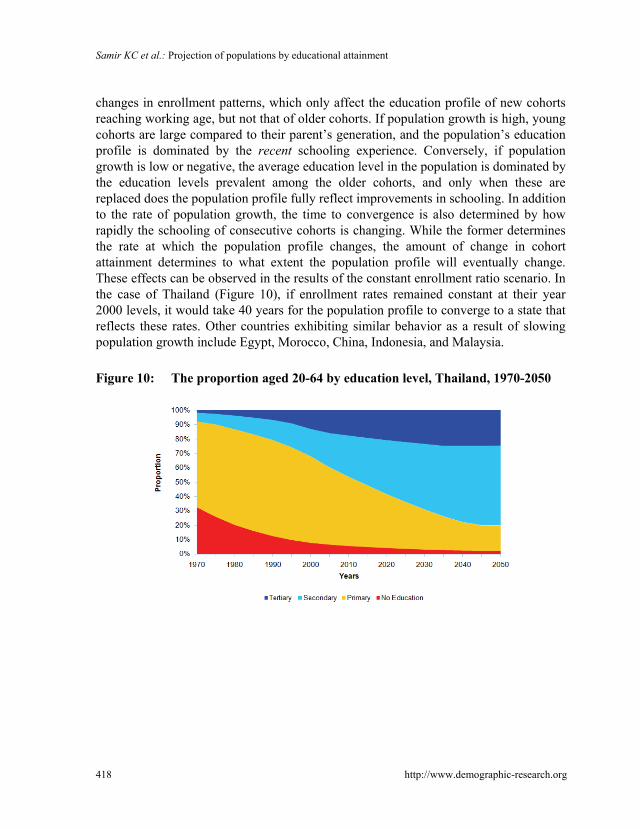
Samir KC et al.: Projection of populations by educational attainment
changes in enrollment patterns, which only affect the education profile of new cohorts reaching working age, but not that of older cohorts. If population growth is high, young cohorts are large compared to their parent’s generation, and the population’s education profile is dominated by the recent schooling experience. Conversely, if population growth is low or negative, the average education level in the population is dominated by the education levels prevalent among the older cohorts, and only when these are replaced does the population profile fully reflect improvements in schooling. In addition to the rate of population growth, the time to convergence is also determined by how rapidly the schooling of consecutive cohorts is changing. While the former determines the rate at which the population profile changes, the amount of change in cohort attainment determines to what extent the population profile will eventually change. These effects can be observed in the results of the constant enrollment ratio scenario. In the case of Thailand (Figure 10), if enrollment rates remained constant at their year 2000 levels, it would take 40 years for the population profile to converge to a state that reflects these rates. Other countries exhibiting similar behavior as a result of slowing population growth include Egypt, Morocco, China, Indonesia, and Malaysia.
Figure 10: The proportion aged 20-64 by education level, Thailand, 1970-2050
418 http://www.demographic-research.org

Demographic Research: Volume 22, Article 15
By contrast, despite rapid change in the years leading up to 2000, if enrollment rates in the Comoros remained constant after that point, the population attainment profile would reflect these rates more rapidly, within 20 years (see Figure 11).
Figure 11: The proportion aged 20-64 by education level, Comoros, 1970-2050
http://www.demographic-research.org 419
0%
10%
20%
30%
40%
50%
60%
70%
80%
90%
100%
1970 1980 1990 2000 2010 2020 2030 2040 2050
Prop
ortio
n
Years
Tertiary Secondary Primary No Education
In this context, it becomes evident that raising enrollment prior to a decline in
fertility (and, by implication, a leveling off or even decline in cohort size) shortens the time it takes for the attainment profile of the population as a whole to be significantly improved. At the same time, it is clear that it is precisely after fertility has begun to decline that improvements in enrollment are easiest to achieve, because less (or even no) absolute expansion may be required. Countries that may be expected to make the first effect work in their favor can be found across Africa, Asia, and Latin America, including Eritrea, Cameroon, Ghana, Nigeria, Zambia, Nepal, Pakistan, Cambodia, Jordan, Saudi Arabia, and Nicaragua. As Figure 12 illustrates for the example of Chad, tremendous population growth may be expected until 2050, but nearly all of this growth could occur in the secondary and higher categories, giving such countries the opportunity to add huge numbers of highly qualified people to their working-age population.

Samir KC et al.: Projection of populations by educational attainment
Figure 12: The population of Chad aged 20-64 by education level, 1970-2050
420 http://www.demographic-research.org
0
2000
4000
6000
8000
10000
12000
14000
16000
18000
1970 1980 1990 2000 2010 2020 2030 2040 2050
Popu
latio
n in
Tho
usan
ds
Years
No Education Primary Secondary Tertiary
A different set of countries could benefit from the second effect. In these countries,
even under the constant enrollment number scenario, substantial improvements would be possible because falling cohort sizes would allow greater participation rates to be achieved at constant capacity. This includes industrialized countries, such as the UK or Spain; transitional countries, such as Croatia, Slovakia, Poland, or the Czech Republic; and a number of developing countries, such as Myanmar, Indonesia, and Mauritius. Figure 13 illustrates the effect for Mauritius.
Figure 13: The proportion aged 20-64 by education level, Mauritius, 1970-2050
0%
10%
20%
30%
40%
50%
60%
70%
80%
90%
100%
1970 1980 1990 2000 2010 2020 2030 2040 2050
Prop
ortio
n
Years
Tertiary Secondary Primary No Education

Demographic Research: Volume 22, Article 15
An even greater impact on the varying country patterns is caused by the fact that countries differ dramatically in the time lag between the growth periods of different education levels. In some countries, secondary education did not become a mass phenomenon until long after the introduction of primary education, or when primary education was already nearly universal. Elsewhere, the universalization of secondary schooling followed that of primary schooling much more quickly; and in some countries, there were substantial proportions of the population with tertiary education, while many others still had no schooling. This difference can be illustrated by contrasting Belize and Haiti. By the time more than 20% of the working population were educated at the secondary level or higher in Belize in the 1980s, primary schooling was already at 90%, having exceeded 20% many decades before. By contrast, in Haiti in recent decades, secondary attainment in the working population has been crossing thresholds that primary attainment crossed a mere 30 years earlier, and, when secondary diffusion reached 20%, primary attainment was only about 40 percentage points ahead. An even more extreme example of the latter pattern is provided by the Maldives, where the diffusion of secondary schooling lagged only about 10 years behind that of primary schooling (see Figures 14-16).
Figure 14: The proportion aged 20-64 by education level, Belize, 1970-2050
http://www.demographic-research.org 421
0
50
100
150
200
250
300
350
1970 1980 1990 2000 2010 2020 2030 2040 2050
Popu
latio
n in
Tho
usan
ds
Years
N no Educatio Primary Secondary Tertiary

Samir KC et al.: Projection of populations by educational attainment
Figure 15: The proportion aged 20-64 by education level, Haiti, 1970-2050
422 http://www.demographic-research.org
0%
10%
20%
30%
40%
50%
60%
70%
80%
90%
100%
1970 1980 1990 2000 2010 2020 2030 2040 2050
Prop
ortio
n
Years
Te yrtiar Secondary Primary No Education
Figure 16: The proportion aged 20-64 by education level, Maldives, 1970-2050
0%
10%
20%
30%
40%
50%
60%
70%
80%
90%
100%
1970 1980 1990 2000 2010 2020 2030 2040 2050
Prop
ortio
n
Years
Tertiary Secondary Primary No Education

Demographic Research: Volume 22, Article 15
With regard to the lag between tertiary and lower levels, examples for an extreme lag are provided by many Central Asian republics, especially Turkmenistan and Uzbekistan, where the proportion of the tertiary-educated working-age population only exceeded 15% when secondary schooling was already almost universal. By contrast, this threshold was crossed by tertiary education in Portugal when less than half of the working population had secondary attainment. The implication for the projected educational attainment in 2050 is that, in countries with big lags, only two categories will account for the vast majority of the population because the non-educated have all but disappeared by the time tertiary gains any kind of significance; while in countries with short lags, three or even all four categories may still be substantially represented, as in Morocco (Figure 17).
Figure 17: The population of Morocco aged 20-64 by education level, 1970-2050
http://www.demographic-research.org 423
A pattern that may be interpreted either as a warning to moderate expectations or
as an argument for intensified effort, depending on the perspective, is provided by Ethiopia (see Figure 18), Mali, Niger, or Burkina Faso.
0
5000
10000
15000
20000
25000
30000
1970 1980 1990 2000 2010 2020 2030 2040 2050
Popu
latio
n in
Tho
usan
ds
Years
No Education Primary Secondary Tertiary

Samir KC et al.: Projection of populations by educational attainment
Figure 18: The population of Ethiopia aged 20-64 by education level, 1970-2050
424 http://www.demographic-research.org
0
20000
40000
60000
80000
100000
120000
1970 1980 1990 2000 2010 2020 2030 2040 2050
Popu
latio
n in
Tho
usan
ds
Years
No Education Primary Secondary Tertiary
The low starting position in 2000 implies that, even under the assumption of
reasonable progress (i.e., GET scenario), by 2050 nearly 40% of the working population in the case of Ethiopia, and 35% in the case of Burkina Faso, may be educated to less than primary level. It is noteworthy that, by 2050, the average proportion of the “less than primary” category exceeds 10% only in ten countries, all but one of them in Africa. This means that, if the above situation arises, these countries will have fallen hopelessly behind compared to the rest of the world. It should be noted, however, that some of the countries not included in the study due to non-availability of data are also likely to suffer equally bad or even worse prospects (such as Afghanistan or Sierra Leone, among others). Nevertheless, there is a genuine threat that sub-Saharan Africa may remain the most problematic development region for another hundred years, if not longer.
As a result of the lag in convergence discussed above, in the case of Ethiopia, even under the fast-track scenario that assumes the meeting of the EFA targets, as late as 2030, 20% of the working-age population would still be uneducated. This represents a substantial gain over the GET scenario. Another illustration of the difference a fast-track scenario could make to a country’s future is provided by Niger. Comparing the GET (Figure 19) and FT scenarios (Figure 20), it is evident that the socioeconomic outlook of the country in 2050 could be improved dramatically by the latter compared to the former.
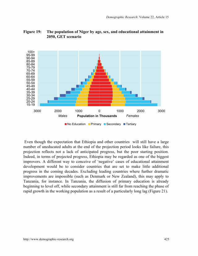
Demographic Research: Volume 22, Article 15
Figure 19: The population of Niger by age, sex, and educational attainment in 2050, GET scenario
3000 2000 1000 0 1000 2000 3000
15-1920-2425-2930-3435-3940-4445-4950-5455-5960-6465-6970-7475-7980-8485-8990-9495-99100+
Males Population in Thousands Females
No Education Primary Secondary Tertiary
Even though the expectation that Ethiopia and other countries will still have a large number of uneducated adults at the end of the projection period looks like failure, this projection reflects not a lack of anticipated progress, but the poor starting position. Indeed, in terms of projected progress, Ethiopia may be regarded as one of the biggest improvers. A different way to conceive of ‘negative’ cases of educational attainment development would be to consider countries that are set to make little additional progress in the coming decades. Excluding leading countries where further dramatic improvements are impossible (such as Denmark or New Zealand), this may apply to Tanzania, for instance. In Tanzania, the diffusion of primary education is already beginning to level off, while secondary attainment is still far from reaching the phase of rapid growth in the working population as a result of a particularly long lag (Figure 21).
http://www.demographic-research.org 425

Samir KC et al.: Projection of populations by educational attainment
Figure 20: The population of Niger by age, sex, and educational attainment in 2050, FT scenario
3000 2000 1000 0 1000 2000 3000
15-1920-2425-2930-3435-3940-4445-4950-5455-5960-6465-6970-7475-7980-8485-8990-9495-99100+
Males Population in Thousands FemalesNo Education Primary Secondary Tertiary
Figure 21: The proportion aged 20-64 by education level, Tanzania,
1970-2050
426 http://www.demographic-research.org
0%
10%
20%
30%
40%
50%
60%
70%
80%
90%
100%
1970 1980 1990 2000 2010 2020 2030 2040 2050
Prop
ortio
n
Years
Tertiary Secondary Primary No Education

Demographic Research: Volume 22, Article 15
As a result, compared to countries that are about to enter a phase of rapid expansion of all three schooling levels in rapid succession, Tanzania’s projected progress between 2000 and 2050 under the GET scenario is relatively modest. Over time, as the primary level becomes near universal almost everywhere, how far ahead a country is at this level will matter less and less, and a country’s position on the growth trajectory of secondary and tertiary education will matter more and more. A country that was ahead in the race for primary expansion, but behind in the race for secondary, will see its position decline as the global focus shifts to higher levels.
In terms of promising results, a long list of countries are about to enter or to continue a steep trajectory of progress, and are thus likely to undergo tremendous improvements in the educational attainment profile of their working population through 2050, whether purely by attainment proportions or numbers. Substantial improvements are projected even under the conservative assumption of expansion patterns similar to those of the past (i.e., under the GET scenario). For some, this means the virtual elimination of the unschooled category, while for others it means great expansion at secondary and higher levels. It should be noted that the list is not limited to developing countries. As Figure 22 shows, even Portugal could significantly improve the attainment levels of its working population by 2050.
Figure 22: The population of Portugal aged 20-64 by education level, 1970-2050
http://www.demographic-research.org 427
0
1000
2000
3000
4000
5000
6000
7000
1970 1980 1990 2000 2010 2020 2030 2040 2050
Popu
latio
n in
Tho
usan
ds
Years
No Education Primary Secondary Tertiary

Samir KC et al.: Projection of populations by educational attainment
A number of regional patterns deserve further comment. In Southern and Southeastern Asia, numerous countries are set to undergo dramatic improvements in educational attainment: in particular, Bangladesh, Nepal, Thailand, and the Philippines, but also Myanmar, Lao PDR and India. Figure 23 shows the dramatic improvement projected for Nepal.
Figure 23: The proportion aged 20-64 by education level, Nepal, 1970-2050
428 http://www.demographic-research.org
0%
10%
20%
30%
40%
50%
60%
70%
80%
90%
100%
1970 1980 1990 2000 2010 2020 2030 2040 2050
Prop
ortio
n
Years
Tertiary Secondary Primary No Education
Substantial improvements would occur under the GET scenario across sub-
Saharan Africa (SSA), but, as noted above, this region also includes many of the countries with the poorest prospects. By contrast, the Latin American region as a whole is poised to undergo a veritable universal educational attainment revolution by 2050. For a number of countries across the region, population dynamics and attainment trajectories near the steepest phase of progress combine to create opportunities for spectacular improvements, especially in the Dominican Republic, Haiti, El Salvador, Panama, Bolivia, Chile, and Paraguay. As a whole, the region has the opportunity to almost catch up with Europe in terms of the population’s attainment profile (see Figures 24 and 25).
A regional analysis of the Arab countries would be particularly interesting. Unfortunately, only a minority of Arab countries are represented in the baseline dataset. This reflects the comparably limited availability of detailed demographic data in the region (see, e.g., Lutz and Goujon 2009).

Demographic Research: Volume 22, Article 15
Figure 24: The proportion aged 20-64 by education level, El Salvador, 1970-2050
http://www.demographic-research.org 429
0%
10%
20%
30%
40%
50%
60%
70%
80%
90%
100%
1970 1980 1990 2000 2010 2020 2030 2040 2050
Prop
ortio
n
Years
Tertiary Secondary Primary No Education
Figure 25: The proportion aged 20-64 by education level, Bolivia, 1970-2050
0%
10%
20%
30%
40%
50%
60%
70%
80%
90%
100%
1970 1980 1990 2000 2010 2020 2030 2040 2050
Prop
ortio
n
Years
Tertiary Secondary Primary No Education
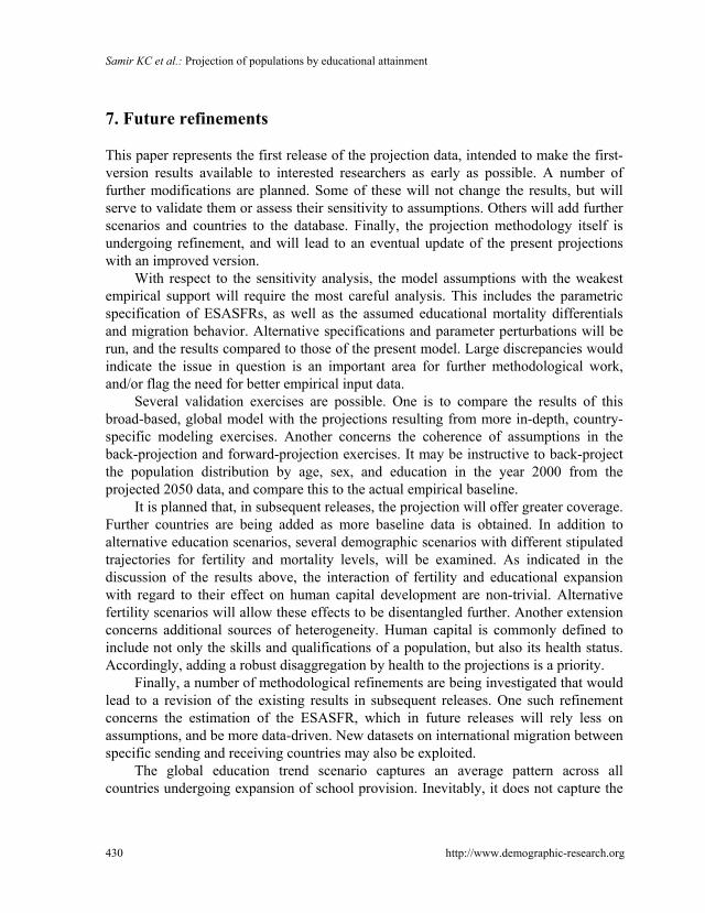
Samir KC et al.: Projection of populations by educational attainment
430 http://www.demographic-research.org
7. Future refinements
This paper represents the first release of the projection data, intended to make the first-version results available to interested researchers as early as possible. A number of further modifications are planned. Some of these will not change the results, but will serve to validate them or assess their sensitivity to assumptions. Others will add further scenarios and countries to the database. Finally, the projection methodology itself is undergoing refinement, and will lead to an eventual update of the present projections with an improved version.
With respect to the sensitivity analysis, the model assumptions with the weakest empirical support will require the most careful analysis. This includes the parametric specification of ESASFRs, as well as the assumed educational mortality differentials and migration behavior. Alternative specifications and parameter perturbations will be run, and the results compared to those of the present model. Large discrepancies would indicate the issue in question is an important area for further methodological work, and/or flag the need for better empirical input data.
Several validation exercises are possible. One is to compare the results of this broad-based, global model with the projections resulting from more in-depth, country-specific modeling exercises. Another concerns the coherence of assumptions in the back-projection and forward-projection exercises. It may be instructive to back-project the population distribution by age, sex, and education in the year 2000 from the projected 2050 data, and compare this to the actual empirical baseline.
It is planned that, in subsequent releases, the projection will offer greater coverage. Further countries are being added as more baseline data is obtained. In addition to alternative education scenarios, several demographic scenarios with different stipulated trajectories for fertility and mortality levels, will be examined. As indicated in the discussion of the results above, the interaction of fertility and educational expansion with regard to their effect on human capital development are non-trivial. Alternative fertility scenarios will allow these effects to be disentangled further. Another extension concerns additional sources of heterogeneity. Human capital is commonly defined to include not only the skills and qualifications of a population, but also its health status. Accordingly, adding a robust disaggregation by health to the projections is a priority.
Finally, a number of methodological refinements are being investigated that would lead to a revision of the existing results in subsequent releases. One such refinement concerns the estimation of the ESASFR, which in future releases will rely less on assumptions, and be more data-driven. New datasets on international migration between specific sending and receiving countries may also be exploited.
The global education trend scenario captures an average pattern across all countries undergoing expansion of school provision. Inevitably, it does not capture the

Demographic Research: Volume 22, Article 15
http://www.demographic-research.org 431
specific circumstances of individual countries. At the global or regional level, the projection appears plausible. However, country-level trajectories should not be interpreted as an anticipation of actual future development, but as indicative of educational development under the assumption that the country converges with global trends, barring discontinuities and external ‘shocks’. A possible future extension is to combine a country-effects model for parameter estimation with qualitative country-specific scenarios for select cases.
Another avenue for future refinement is to explicitly link parental and child education. As mentioned previously, the effects of parents’ education on the educational attainment of their children is incorporated implicitly rather than explicitly in the current projections. It is reflected in the projections because the historical expansion patterns on which the projections are based were partly shaped by this effect. It is, however, not explicitly included in the sense that the modeled cohort of births instantly ‘forget’ their parents’ education.
An option for the future is to retain the distribution of parents’ education for the first five or 10 years of simulated life. This would not only allow for differentials in infant mortality by parental education to be taken into account, but also to track developments over time. Because fertility declines with increasing education, the educational attainment level of the parents of the average child will be significantly lower than the average educational attainment of the population of childbearing age. By implication, projections of population attainment will overestimate the education environment that children will be exposed to at home. Projecting the latter separately is therefore of intrinsic interest.
8. Conclusions and outlook
This paper provides an overview of the demographic projection method that was used to estimate a new comprehensive and detailed dataset on educational attainment by age and sex for the years 2000-2050. But beyond the interest in education per se, this new dataset facilitates the analysis of a great range of issues that education is assumed to influence positively. Health and survival are strongly linked with better education. Fertility levels tend to vary greatly with the level of education, and even such difficult-to-measure aspects of our quality of life at the societal level, such as the quality of institutions, the rule of law, and democratic participation, are presumably facilitated by the fact that large segments of the population are educated enough to exert the checks and balances that are necessary to establish or maintain a democracy and improve governance. For these conditions to be achieved, adequate education of large parts of

Samir KC et al.: Projection of populations by educational attainment
432 http://www.demographic-research.org
the population, and not just of a small group of elites, is probably a necessity, though not sufficient by itself.
Using this new dataset, projections can be produced of how these other development dimensions may be expected to develop until 2050 in various countries, based on their edu-demographic profile. This may provide insights into which countries or regions may be expected to enter phases of turmoil.
Based on the new model of the educational attainment contribution to economic growth estimated from the reconstruction dataset, education-sensitive projections of future economic growth can be produced for a large number of countries that potentially differ dramatically from those based on an extrapolation of historic time-series data. A historical example is provided by South Korea. In the 1960s, based on historical growth data, the economic outlook would have been modest, but projections of its future educational attainment profile may have indicated that it was about to enter a window of opportunity combining high qualifications with low dependency ratios.
It may also become possible to contribute to debates surrounding the future sustainability of public pension systems by providing estimates of expected productivity increases resulting from the changing qualification profile of the future workforce.

Demographic Research: Volume 22, Article 15
http://www.demographic-research.org 433
References
Abou-Gamrah, H. (1982). Fertility levels and differentials by mother’s education in some countries of the ECWA region. In: Determinants of Fertility in Some African and Asian Countries. Cairo: Cairo Demographic Centre: 191-211. (Research Monograph Series, No. 10).
Ahlburg, A.A., Kelley, A.C., and Mason, K.O. (eds.) (1996). The Impact of Population Growth on Well-Being in Developing Countries. Berlin: Springer Verlag.
Ahuja, V. and Filmer, D. (1995). Educational attainment in development countries: New estimates and projections disaggregated by gender. Journal of Educational Planning and Administration X(3): 229-254.
Alachkar, A. and Serow, W.J. (1988). The socioeconomic determinants of mortality: An international comparison. Genus 44(3-4): 131-151.
Angrist, J., Lavy, V., and Schlosser, A. (2006). New evidence on the causal link between the quantity and quality of children. Bonn: Institute for the Study of Labour. (IZA Discussion Paper, No. 2075, April 2006).
Avong, H.N. (2001). Religion and fertility among the Atyap in Nigeria. Journal of Biosocial Science 33(1): 1-12. doi:10.1017/S0021932001000013.
Becker, G. (1991). A Treatise on the Family. Cambridge, MA: Harvard University Press.
Birdsall, N.M. and Griffin, C.C. (1988). Fertility and poverty in developing countries. Journal of Policy Modeling 10(1): 29-55. doi:10.1016/0161-8938(88)90034-8.
Bledsoe, C.H., Casterline, J.B., Johnson-Kuhn, J.A., and Haaga, J.G. (1999). Critical Perspectives on Schooling and Fertility in the Developing World. Washington, DC: National Academy Press.
Bloemen, H. and Kalwij, A.S. (2001). Female labor market transition and the timing of births: A simultaneous analysis of the effects of schooling. Labour Economics 8(5): 593-620. doi:10.1016/S0927-5371(01)00043-4.
Blossfeld, H.-P. and Huinink, J. (1991). Human capital investments or norms of role transition? How women’s schooling and career affect the process of family formation. American Journal of Sociology 97(1): 143-168. doi:10.1086/229743.
Booth, H. (1984). Transforming Gompertz’s Function for fertility analysis: The development of a standard for the relational Gompertz Function. Population Studies 38(3): 495-506. doi:10.2307/2174137.
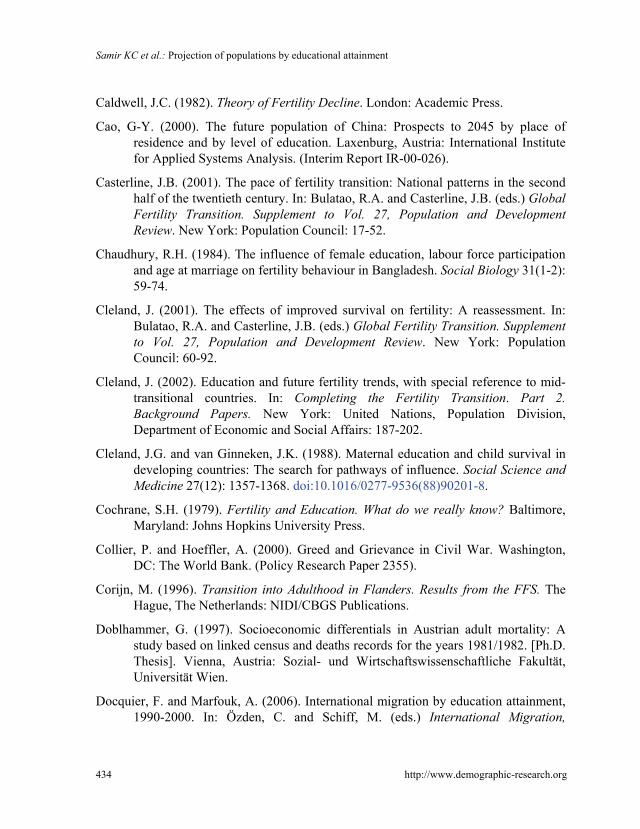
Samir KC et al.: Projection of populations by educational attainment
434 http://www.demographic-research.org
Caldwell, J.C. (1982). Theory of Fertility Decline. London: Academic Press.
Cao, G-Y. (2000). The future population of China: Prospects to 2045 by place of residence and by level of education. Laxenburg, Austria: International Institute for Applied Systems Analysis. (Interim Report IR-00-026).
Casterline, J.B. (2001). The pace of fertility transition: National patterns in the second half of the twentieth century. In: Bulatao, R.A. and Casterline, J.B. (eds.) Global Fertility Transition. Supplement to Vol. 27, Population and Development Review. New York: Population Council: 17-52.
Chaudhury, R.H. (1984). The influence of female education, labour force participation and age at marriage on fertility behaviour in Bangladesh. Social Biology 31(1-2): 59-74.
Cleland, J. (2001). The effects of improved survival on fertility: A reassessment. In: Bulatao, R.A. and Casterline, J.B. (eds.) Global Fertility Transition. Supplement to Vol. 27, Population and Development Review. New York: Population Council: 60-92.
Cleland, J. (2002). Education and future fertility trends, with special reference to mid-transitional countries. In: Completing the Fertility Transition. Part 2. Background Papers. New York: United Nations, Population Division, Department of Economic and Social Affairs: 187-202.
Cleland, J.G. and van Ginneken, J.K. (1988). Maternal education and child survival in developing countries: The search for pathways of influence. Social Science and Medicine 27(12): 1357-1368. doi:10.1016/0277-9536(88)90201-8.
Cochrane, S.H. (1979). Fertility and Education. What do we really know? Baltimore, Maryland: Johns Hopkins University Press.
Collier, P. and Hoeffler, A. (2000). Greed and Grievance in Civil War. Washington, DC: The World Bank. (Policy Research Paper 2355).
Corijn, M. (1996). Transition into Adulthood in Flanders. Results from the FFS. The Hague, The Netherlands: NIDI/CBGS Publications.
Doblhammer, G. (1997). Socioeconomic differentials in Austrian adult mortality: A study based on linked census and deaths records for the years 1981/1982. [Ph.D. Thesis]. Vienna, Austria: Sozial- und Wirtschaftswissenschaftliche Fakultät, Universität Wien.
Docquier, F. and Marfouk, A. (2006). International migration by education attainment, 1990-2000. In: Özden, C. and Schiff, M. (eds.) International Migration,

Demographic Research: Volume 22, Article 15
http://www.demographic-research.org 435
Remittances and the Brain Drain. Washington, DC: The World Bank. (chapter 5).
Duleep, H.O. (1989). Measuring socioeconomic mortality differentials over time. Demography 26(2): 345-351. doi:10.2307/2061531.
Elo, I.T. and Preston, S.H. (1996). Educational differentials in mortality: United States, 1979-1985. Social Science and Medicine 42(1): 47-57. doi:10.1016/0277-9536(95)00062-3.
European Commission (2003). Education, training and growth. In: EU Economy 2003 Review, European Economy, No. 6. Luxembourg: Office for Official Publications of the EU. (chapter 3).
European Commission (2004). Investment in education: The implications for economic growth and public finances. Brussels: Directorate-General for Economic and Financial Affairs, the European Commission. (Economic Papers No. 217).
Eurostat (2006). Long-term Population Projections at National Level. Brussels: European Communities. (Catalogue number: KS-NK-06-003-EN-N).
Feldman, J.J., Makuc, D.M., Kleinman, J.C., and Cornoni-Huntley, J. (1989). National trends in educational differentials in mortality. American Journal of Epidemiology 129(5): 919-933.
Figoli, M. (2006). Educational attainment in Brazil: An analysis of the rates between 1970 and 2000. Laxenburg, Austria: International Institute for Applied Systems Analysis. (Interim Report IR-06-005).
Fotso, J.-C. (2006). Malawi’s future human capital: Is the country on track to meeting the MDGs on education? Laxenburg, Austria: International Institute for Applied Systems Analysis. (Interim Report IR-06-020).
Goldin, C. and Katz, L.F. (2002). The power of the pill: Oral contraceptives and women’s career and marriage decisions. Journal of Political Economy 110(4): 730-770. doi:10.1086/340778.
Goujon, A. (2002). Population and education prospects in the Arab region. In: Serageldin, I. (ed.) Human Capital: Population Economics in the Middle East. Cairo: The American University in Cairo Press: 116-140.
Goujon, A. and KC, S. (2006). Past and future of human capital in Southeast Asia: From 1970 to 2030. Vienna: Vienna Institute of Demography, Austrian Academy of Sciences. (VID Working Paper 07/2006).

Samir KC et al.: Projection of populations by educational attainment
436 http://www.demographic-research.org
Goujon, A. and McNay, K. (2003). Projecting the educational composition of the population of India: Selected state-level perspectives. Applied Population and Policy 1(1): 25-35.
Goujon, A., Alkitkat, H., Lutz, W., and Prommer, I. (2007). Population and human capital growth in Egypt: Projections for governorates to 2051. Laxenburg, Austria: International Institute for Applied Systems Analysis. (Interim Report IR-07-010).
Gustavsson, S. and Kalwij, A. (eds.) (2006). Education and Postponement of Maternity. Economic Analyses for Industrialized Countries. Dordrecht, The Netherlands: Kluwer Academic Publishers and Springer. doi:10.1007/1-4020-4716-9.
Heer, D. (1983). Infant and child mortality and the demand for children. In: Bulatao, R. and Lee, R. (eds.) Determinants of fertility in Developing Countries. New York: Academic Press: 369-387.
Huisman, M., Kunst, A.E., Andersen, O., Bopp, M., Borgan, J.-K., Borrell, C., Costa, G., Deboosere, P., Desplanques, G., Donkin, A., Gadeyne, S., Minder, C., Regidor, E., Spadea, T., Valkonen, T., and Mackenbach, J.P. (2004). Socioeconomic inequalities in mortality among elderly people in 11 European populations. Journal of Epidemiology and Community Health 58(6): 468-475. doi:10.1136/jech.2003.010496.
Huq, M.N. and Cleland, J. (1990). Bangladesh Fertility Survey 1989. Dhaka: National Institute of Population Research and Training. (Main Report).
Jain, A.K. (1981). The effect of female education on fertility: A simple explanation. Demography 18(4): 577-595. doi:10.2307/2060948.
Jejeebhoy, S.J. (1995). Women’s Education, Autonomy and Reproductive Behaviour: Experience from Developing Countries. Oxford: Clarendon Press.
Jones, E. (1982). Socio-economic Differentials in Achieved Fertility. Voorburg, The Netherlands: International Statistical Institute. (World Fertility Survey Comparative Studies 21)
Kenkel, D.S. (1991). Health behavior, health knowledge, and schooling. The Journal of Political Economy 99(2): 287-305. doi:10.1086/261751.
Khalifa, A.M. (1976). The influence of wife’s education on fertility in rural Egypt. Journal of Biosocial Science 8(1): 53-60. doi:10.1017/S0021932000010464.
Kitagawa, E. and Hauser, P. (1973). Differential Mortality in the United States: A Study of Socioeconomic Epidemiology. Cambridge, MA: Harvard University Press.

Demographic Research: Volume 22, Article 15
http://www.demographic-research.org 437
Kravdal, Ø. (2002). Education and fertility in sub-Saharan Africa: Individual and community effects. Demography 39(2): 233-250. doi:10.2307/3088337.
Kravdal, Ø. and Rindfuss, R.R. (2007). Changing relationships between education and fertility – A study of women and men born 1940-64. Oslo: University of Oslo, Economics Department (mimeo).
Lantz, P.M, House, J.S., Lepkowski, J.M., Williams, D.R., Mero, R.P., and Chen, J. (1998). Socioeconomic factors, health behaviors, and mortality. Results from a nationally representative prospective study of US adults. JAMA 279(21): 1703-1708. doi:10.1001/jama.279.21.1703.
Lleras-Muney, A. (2005). The relationship between education and adult mortality in the United States. Review of Economic Studies 72(1): 189-221. doi:10.1111/0034-6527.00329.
Lutz, W. (ed.) (1994). Population-Development-Environment: Understanding Their Interactions in Mauritius. Berlin: Springer Verlag.
Lutz, W. and Goujon, A. (2001). The world’s changing human capital stock: Multi-state population projections by educational attainment. Population and Development Review 27(2): 323-339. doi:10.1111/j.1728-4457.2001.00323.x.
Lutz, W. and Goujon, A. (2009). Capital Humano, Género y envejecimiento en el Mediterráneo. Perspectivas a medio y largo plazo [Human capital, gender and aging in the Mediterranean]. PapersIEMed 7: 19-29. (Barcelona: Edicion Instituto Europeo del Mediterráneo, in Spanish).
Lutz, W., Goujon, A., and Doblhammer-Reiter, G. (1999). Demographic dimensions in forecasting: Adding education to age and sex. In: Lutz, W., Vaupel, J.W., and Ahlburg, D.A. (eds.) Frontiers of Population Forecasting. Supplement to Volume 24, 1998, Population and Development Review. New York: The Population Council: 42-58.
Lutz, W., Goujon, A., KC, S., and Sanderson, W. (2007). Reconstruction of populations by age, sex and level of educational attainment for 120 countries for 1970–2000. Vienna Yearbook of Population Research 2007: 193-235. doi:10.1553/populationyearbook2007s193.
Lutz, W., Goujon, A., and Wils, B. (2008). The population dynamics of human capital accumulation. In: Prskawetz, A., Bloom, D.E., and Lutz, W. (eds.) Population Aging, Human Capital Accumulation, and Productivity Growth. Supplement to Volume 34, 2008, Population and Development Review. New York: The Population Council: 149-188.

Samir KC et al.: Projection of populations by educational attainment
438 http://www.demographic-research.org
Lutz, W., Prieto, L., and Sanderson, W. (2000). Population, Development, and Environment on the Yucatán Peninsula: From Ancient Maya to 2030. Laxenburg, Austria: International Institute for Applied Systems Analysis. (Research Report RR-00-14).
Malawi National Statistical Office (1993). Malawi Demographic and Health Survey 1992: First Report. Columbia, MD: Macro International Inc.
Marini, M.M. (1984). The order of events in the transition to adulthood. Sociology of Education 57(2): 63-84. doi:10.2307/2112630.
McQuillan, K. (2004). When does religion influence fertility? Population and Development Review 30(1): 25-56. doi:10.1111/j.1728-4457.2004.00002.x.
Niederdeppe, J. (2008). Beyond knowledge gaps: Examining socioeconomic differences in response to cancer news. Human Communication Research 34(3): 423-447. doi:10.1111/j.1468-2958.2008.00327.x.
Noack, T. and Lyngstad, T.H. (2000). Norske fruktbarhetsidealer 1977-1999: Idealene består. Samfunnsspeilet 3: 30-34.
OECD (2007). Education at a Glance. Paris: Organisation for Economic Co-operation and Development.
Pamuk, E.R. (1985). Social class inequality in mortality from 1921 to 1972 in England and Wales. Population Studies 39(1): 17-31. doi:10.1080/0032472031000141256.
Pappas, G., Queen, S., Hadden, W., and Fisher, G. (1993). The increasing disparity in mortality between socioeconomic groups in the United States, 1960 and 1986. New England Journal of Medicine 329(2): 103-109. doi:10.1056/NEJM199307083290207.
Preston, S.H. and Taubman, P. (1994). Socioeconomic differences in adult mortality and health status. In: Martin, L.G. and Preston, S.H. (eds.) Demography of Aging. Washington, DC: National Academy Press: 279-318.
Preston, S.H., Haines, M.R., and Pamuk, E.R. (1981). Effects of industrialization and urbanization on mortality in developed countries. In: International Union for the Scientific Study of Population. International Population Conference, Manila, 1981: Solicited Papers, Vol. 2. Liege: Ordina Editions: 233-254.
Riosmena, F., Prommer, I., Goujon, A., and KC, S. (2008). An evaluation of the IIASA/VID Education-Specific Back Projections. Laxenburg, Austria:

Demographic Research: Volume 22, Article 15
http://www.demographic-research.org 439
International Institute for Applied Systems Analysis. (Interim Report IR-08-019).
Rodgers, J.L., Kohler, H.-P., McGue, M., Behrman, J.R., Petersen, I., Bingley, P., and Christensen, K. (2008). Education and cognitive ability as direct, mediated, or spurious influences on female age at first birth: Behavioral genetic models fit to Danish twin data. American Journal of Sociology 114(S1): S202-S232. doi:10.1086/592205.
Rogers, A. (1975). Introduction to Multiregional Mathematical Demography. New York: John Wiley & Sons.
Rogot, E., Sorlie, P.D., and Johnson, N.J. (1992). Life expectancy by employment status, income and education in the national longitudinal mortality study. Public Health Reports 107(4): 457-461.
Rosenzweig, M.R. and Wolpin, K.I. (2000). Natural “natural experiments” in economics. Journal of Economic Literature 38(4): 827-874.
Sanderson, W.C. (2005). Education forecasts and backcasts: Lessons from the summer of 2005. [Unpublished Note].
Sanderson, W.C., Fuller, B., Hellmuth, M.E., and Strzepek, K.M. (2001). Namibia’s Future. Modeling Population and Sustainable Development Challenges in the Era of HIV/AIDS. Executive Summary. Laxenburg, Austria: International Institute for Applied Systems Analysis.
Sanderson, W.C., Hellmuth, M.E., and Strzepek, K.M. (2001). Botswana’s Future. Modeling Population and Sustainable Development Challenges in the Era of HIV/AIDS. Executive Summary. Laxenburg, Austria: International Institute for Applied Systems Analysis.
Scherbov, S., Mamolo, M., and Lutz, W. (2008). Probabilistic population projections for the 27 EU member countries based on Eurostat Projections. Vienna: Vienna Institute of Demography, Austrian Academy of Sciences. (European Demographic Research Papers, No. 2).
Sen, A. (1999). Development as Freedom. Oxford: Oxford University Press.
Skirbekk, V. (2008). Fertility trends by social status. Demographic Research 18(5): 145-180. doi:10.4054/DemRes.2008.18.5.
Skirbekk, V., Kohler, H.-P., and Prskawetz, A. (2004). Birth month, school graduation and the timing of births and marriages. Demography 41(3): 547-568. doi:10.1353/dem.2004.0028.

Samir KC et al.: Projection of populations by educational attainment
440 http://www.demographic-research.org
Smits, J., Ultee, W., and Lammers, J. (2000). More or less educational homogamy? A test of different versions of modernization theory using cross-temporal evidence for 60 countries. American Sociological Review 65(5): 781-788. doi:10.2307/2657547.
Symeonidou, H. (2000). Expected and actual family size in Greece: 1983-1997. European Journal of Population 16(4): 335-352. doi:10.1023/A:1006441411252.
Testa, M.R. and Grilli, L. (2006). The influence of childbearing regional contexts on ideal family size in Europe. Population 61(1-2): 109-138.
UNESCO Institute for Statistics (UIS) (2009). Global Education Digest 2009: Comparing Education Statistics Across the World. Montreal: UIS.
United Nations (1995). Women’s education and fertility behaviour: Recent evidence from the Demographic and Health Surveys. New York: United Nations. (ST/ESA/SER.R/137).
United Nations (2005). World Population Prospects: The 2004 Revision. New York: United Nations, Department of Economic and Social Affairs, Population Division.
United Nations (2007). World Population Prospects: The 2006 Revision. New York: United Nations, Department of Economic and Social Affairs, Population Division.
Van Peer, C. (2002). Desired and realized fertility in selected FFS-countries. In: Macura, M. and Beets, G. (eds.) Dynamics of Fertility and Partnership in Europe: Insights and Lessons from Comparative Research, Vol. 1. New York and Geneva: United Nations: 117-142.
Westoff, C.F. and Ryder, N.B. (1977). The Contraceptive Revolution. Princeton, NJ: Princeton University Press.
Wils, A. (1996). PDE-Cape Verde: A systems study of population, development, and environment. Laxenburg, Austria: International Institute for Applied Systems Analysis. (Working Paper WP-96-009).
Wils, A. (2007). Window on the Future: 2025 – Projections of Education Attainment and Its Impact. Washington, DC: Academy for Educational Development.
Wils, A., da Costa Gaspar, M., Hellmuth, M.E., Ibraimo, M., Prommer, I., and Sebastiao, E. (2001). Mozambique’s Future. Modeling Population and

Demographic Research: Volume 22, Article 15
http://www.demographic-research.org 441
Sustainable Development Challenges. Executive Summary. Laxenburg, Austria: International Institute for Applied Systems Analysis.
Woubalem, Z. (2006). Estimates of excess adult deaths due to HIV/AIDS in Kenya. Laxenburg, Austria: International Institute for Applied Systems Analysis. (Interim Report IR-06-013).
Yousif, H.M., Goujon, A., and Lutz, W. (1996). Future population and education trends in the countries of North Africa. Laxenburg, Austria: International Institute for Applied Systems Analysis. (Research Report RR-96-11).

Samir KC et al.: Projection of populations by educational attainment
442 http://www.demographic-research.org
Appendix A
Appendix Table A1: Total Fertility Rates (other than the UN estimate) used in the projection of population in the global education trend scenario Source
Country 2000-2005 2045-2050 2000-2005
2005-2010
2010-2015
2015-2020
2020-2025
2025-2030
2030-2035
2035-2040
2040-2045
2045-2050
China Own Estimate Own Estimate 1.50 1.50 1.50 1.50 1.50 1.50 1.50 1.50 1.50 1.50 China, Hong Kong SAR UN 2007 Own Estimate 0.94 0.98 1.02 1.06 1.10 1.14 1.18 1.22 1.26 1.30
China, Macao SAR UN 2007 Own Estimate 0.84 0.89 0.94 0.99 1.05 1.10 1.15 1.20 1.25 1.30
Japan UN 2007 Own Estimate 1.29 1.31 1.34 1.36 1.38 1.41 1.43 1.45 1.48 1.50
Republic of Korea UN 2007 Own Estimate 1.24 1.27 1.30 1.33 1.36 1.39 1.41 1.44 1.47 1.50
Singapore UN 2007 Own Estimate 1.35 1.37 1.38 1.40 1.42 1.43 1.45 1.47 1.48 1.50
Thailand Own Estimate Own Estimate 1.60 1.59 1.58 1.57 1.56 1.54 1.53 1.52 1.51 1.50
Turkey UN 2007 Scherbov et al. 2008 2.23 2.18 2.18 2.18 2.19 2.19 2.19 2.19 2.19 2.19
Bulgaria UN 2007 Eurostat 1.26 1.38 1.40 1.41 1.43 1.45 1.46 1.48 1.50 1.51
Czech Republic UN 2007 Eurostat 1.18 1.33 1.35 1.37 1.39 1.40 1.42 1.44 1.46 1.48
Hungary UN 2007 Eurostat 1.30 1.35 1.36 1.38 1.40 1.41 1.43 1.45 1.47 1.48
Poland UN 2007 Eurostat 1.25 1.27 1.29 1.31 1.33 1.35 1.37 1.39 1.41 1.43
Romania UN 2007 Eurostat 1.29 1.32 1.34 1.36 1.38 1.39 1.41 1.43 1.45 1.47
Russian Federation UN 2007 Scherbov et al. 2008 1.30 1.30 1.35 1.40 1.44 1.49 1.52 1.52 1.52 1.52
Slovakia UN 2007 Eurostat 1.22 1.25 1.26 1.29 1.31 1.33 1.35 1.37 1.39 1.41
Ukraine UN 2007 Scherbov et al. 2008 1.15 1.31 1.33 1.36 1.39 1.41 1.43 1.43 1.43 1.43
Denmark UN 2007 Eurostat 1.76 1.85 1.85 1.85 1.85 1.85 1.85 1.85 1.85 1.85
Estonia UN 2007 Eurostat 1.39 1.55 1.56 1.57 1.58 1.59 1.60 1.61 1.62 1.63
Finland UN 2007 Eurostat 1.75 1.84 1.84 1.84 1.84 1.84 1.84 1.84 1.84 1.84
Ireland UN 2007 Eurostat 1.97 1.90 1.90 1.90 1.89 1.89 1.89 1.89 1.89 1.89
Latvia UN 2007 Eurostat 1.25 1.36 1.37 1.39 1.40 1.42 1.44 1.46 1.47 1.49
Lithuania UN 2007 Eurostat 1.28 1.35 1.36 1.38 1.40 1.42 1.44 1.46 1.48 1.49
Norway UN 2007 Eurostat 1.80 1.90 1.90 1.90 1.90 1.90 1.89 1.89 1.89 1.89
Sweden UN 2007 Eurostat 1.67 1.85 1.85 1.85 1.85 1.85 1.85 1.85 1.85 1.85
United Kingdom UN 2007 Eurostat 1.70 1.84 1.84 1.84 1.84 1.84 1.84 1.84 1.84 1.84
Croatia UN 2007 Scherbov et al. 2008 1.35 1.39 1.44 1.48 1.53 1.58 1.61 1.61 1.61 1.61
Greece UN 2007 Eurostat 1.28 1.41 1.42 1.44 1.45 1.47 1.48 1.50 1.51 1.53
Italy UN 2007 Eurostat 1.29 1.38 1.40 1.41 1.43 1.45 1.46 1.48 1.50 1.51
Malta UN 2007 Eurostat 1.46 1.38 1.40 1.41 1.43 1.45 1.46 1.48 1.49 1.51
Portugal UN 2007 Eurostat 1.45 1.36 1.38 1.39 1.41 1.43 1.44 1.46 1.48 1.50

Demographic Research: Volume 22, Article 15
http://www.demographic-research.org 443
Appendix Table A1: (Continued) Source
Country 2000-2005 2045-2050 2000-2005
2005-2010
2010-2015
2015-2020
2020-2025
2025-2030
2030-2035
2035-2040
2040-2045
2045-2050
Slovenia UN 2007 Eurostat 1.23 1.32 1.34 1.36 1.37 1.39 1.41 1.43 1.45 1.47
Spain UN 2007 Eurostat 1.29 1.39 1.40 1.42 1.43 1.45 1.46 1.48 1.50 1.51
TFYR Macedonia UN 2007 Scherbov et al. 2008 1.56 1.48 1.57 1.65 1.74 1.82 1.88 1.88 1.88 1.88
Austria UN 2007 Eurostat 1.38 1.41 1.42 1.44 1.45 1.47 1.48 1.50 1.52 1.53
Belgium UN 2007 Eurostat 1.64 1.75 1.76 1.76 1.76 1.77 1.77 1.77 1.78 1.78
France UN 2007 Eurostat 1.88 1.98 1.98 1.97 1.97 1.96 1.96 1.96 1.95 1.95
Germany UN 2007 Eurostat 1.35 1.34 1.35 1.37 1.39 1.41 1.42 1.44 1.46 1.48
Luxembourg UN 2007 Eurostat 1.67 1.65 1.66 1.66 1.67 1.68 1.68 1.69 1.70 1.71
Netherlands UN 2007 Eurostat 1.73 1.72 1.72 1.73 1.73 1.74 1.74 1.75 1.75 1.76
Switzerland UN 2007 Eurostat 1.42 1.44 1.45 1.47 1.48 1.50 1.51 1.53 1.54 1.55
Canada UN 2007 Own Estimate 1.52 1.52 1.52 1.52 1.52 1.52 1.52 1.52 1.52 1.70 United States of America UN 2007 Own Estimate 2.04 2.04 2.04 2.04 2.04 2.04 2.04 2.04 2.04 1.90
Australia UN 2007 Own Estimate 1.76 1.76 1.76 1.76 1.76 1.76 1.76 1.76 1.76 1.90
New Zealand UN 2007 Own Estimate 1.96 1.96 1.96 1.96 1.96 1.96 1.96 1.96 1.96 1.90

Samir KC et al.: Projection of populations by educational attainment
444 http://www.demographic-research.org
Appendix B
The full projection output for Pakistan, including age pyramids by education at various points in time and for the different education scenarios, as well as tabular output of the full age-sex-education population distribution in five-year intervals from the baseline year 2000 to 2050, are shown below.
Appendix Table B1: Population in Thousands by Education, Age, and Sex in
Pakistan - Global Education Trend Scenario
Male
Age Group noedu pri Sec ter MYS MYSE
2000 15-19 2033.6 2039.8 4104.5 0.0 5.93 7.00
20-24 1747.9 1228.8 3108.2 407.4 6.67 7.40
25-29 1661.4 1005.6 2098.6 495.5 6.35 6.99
30-34 1688.7 848.4 1543.3 533.3 5.96 6.55
35-39 1750.4 777.2 1288.3 378.1 5.21 5.85
40-44 1642.1 616.7 1061.3 301.2 4.89 5.50
45-49 1337.2 578.6 822.9 225.0 4.67 5.35
50-54 1149.1 395.8 517.1 146.8 3.97 4.62
55-59 940.0 315.4 364.9 117.5 3.72 4.38
60-64 873.8 218.4 263.3 72.8 3.08 3.68
65-69 721.2 154.5 164.0 46.1 2.55 3.11
70-74 532.1 97.4 91.0 26.0 2.08 2.60
75-79 326.9 50.9 41.9 12.1 1.67 2.15
80+ 278.5 34.1 23.6 7.0 1.21 1.61
15+ 16682.9 8361.6 15492.8 2768.8 5.34 6.06
25+ 12901.3 5092.9 8280.0 2361.4 4.87 5.49
2005 15-19 2189.3 2427.4 5426.2 0.0 6.31 7.40
20-24 1987.8 1322.6 4146.0 546.0 7.13 7.80
25-29 1702.3 1197.7 2781.3 650.7 6.96 7.57
30-34 1624.1 984.0 1897.3 646.4 6.54 7.12
35-39 1653.0 831.6 1516.2 524.9 5.97 6.56

Demographic Research: Volume 22, Article 15
http://www.demographic-research.org 445
Appendix Table B1: (Continued)
Male
Age Group noedu pri Sec ter MYS MYSE
40-44 1707.4 759.6 1263.5 371.9 5.23 5.87
45-49 1587.9 598.2 1034.9 295.0 4.91 5.53
50-54 1272.0 553.0 793.2 218.4 4.71 5.38
55-59 1065.7 369.8 489.4 140.5 4.02 4.68
60-64 837.5 283.9 334.8 109.6 3.80 4.46
65-69 735.2 186.3 230.3 65.2 3.18 3.78
70-74 559.5 121.8 133.4 38.6 2.65 3.22
75-79 368.9 68.6 66.5 19.7 2.18 2.71
80+ 316.3 46.3 37.5 11.3 1.59 2.05
15+ 17607.0 9750.8 20150.6 3638.4 5.85 6.57
25+ 13429.9 6000.8 10578.4 3092.4 5.41 6.02
2010 15-19 1931.6 2378.6 5858.7 0.0 6.64 7.76
20-24 2144.2 1517.2 5460.1 724.7 7.60 8.24
25-29 1940.4 1292.1 3721.2 868.9 7.44 7.98
30-34 1667.2 1174.1 2526.3 844.1 7.16 7.71
35-39 1591.7 965.6 1865.6 636.7 6.55 7.13
40-44 1614.6 813.8 1488.4 516.6 5.99 6.57
45-49 1655.5 738.6 1234.7 364.9 5.26 5.89
50-54 1516.8 574.0 1001.0 287.2 4.95 5.57
55-59 1185.5 519.0 753.9 209.8 4.77 5.44
60-64 956.1 335.1 451.9 131.9 4.11 4.76
65-69 709.7 243.8 294.8 98.8 3.92 4.56
70-74 576.3 148.4 189.3 55.3 3.30 3.90
75-79 393.4 87.1 99.0 29.8 2.78 3.35
80+ 363.7 63.7 60.7 18.8 2.08 2.59
15+ 18246.7 10851.0 25005.6 4787.5 6.35 7.04
25+ 14170.9 6955.2 13686.8 4062.7 5.96 6.55

Samir KC et al.: Projection of populations by educational attainment
446 http://www.demographic-research.org
Appendix Table B1: (Continued)
Male
Age Group noedu pri Sec ter MYS MYSE
2015 15-19 1653.2 2054.4 6347.2 0.0 7.05 8.24
20-24 1905.5 1437.9 5902.1 795.8 8.05 8.65
25-29 2114.2 1497.0 4945.2 1164.8 7.94 8.44
30-34 1915.2 1276.3 3405.6 1135.8 7.66 8.14
35-39 1643.9 1159.0 2498.5 836.1 7.17 7.72
40-44 1563.1 949.8 1840.3 629.5 6.57 7.14
45-49 1573.5 795.1 1461.0 509.0 6.01 6.60
50-54 1591.0 712.9 1200.6 357.0 5.29 5.92
55-59 1423.9 542.5 957.6 277.6 5.01 5.62
60-64 1071.7 473.9 700.9 198.2 4.85 5.52
65-69 818.9 290.8 402.1 120.0 4.22 4.87
70-74 562.6 196.4 245.2 84.7 4.06 4.70
75-79 411.4 107.8 142.8 43.3 3.45 4.05
80+ 407.1 84.7 94.7 29.9 2.66 3.21
15+ 18655.2 11578.5 30143.7 6181.6 6.83 7.49
25+ 15096.5 8086.3 17894.4 5385.8 6.52 7.08
2020 15-19 1323.1 1614.4 6426.9 0.0 7.44 8.70
20-24 1633.1 1318.4 6143.4 846.9 8.48 9.03
25-29 1882.0 1421.0 5345.6 1281.1 8.42 8.86
30-34 2092.0 1482.3 4532.5 1526.3 8.17 8.60
35-39 1892.9 1262.7 3375.1 1127.2 7.67 8.15
40-44 1618.3 1142.6 2469.7 828.2 7.18 7.73
45-49 1527.2 930.2 1810.2 621.3 6.59 7.16
50-54 1516.5 769.5 1423.9 499.0 6.05 6.63
55-59 1500.0 676.5 1152.7 346.1 5.35 5.98
60-64 1295.0 498.2 895.1 263.4 5.10 5.71
65-69 923.7 413.9 627.5 181.4 4.97 5.63

Demographic Research: Volume 22, Article 15
http://www.demographic-research.org 447
Appendix Table B1: (Continued)
Male
Age Group noedu pri Sec ter MYS MYSE
70-74 655.9 236.8 337.9 103.9 4.37 5.01
75-79 405.9 144.3 187.0 67.1 4.23 4.87
80+ 443.2 109.0 142.1 45.5 3.33 3.90
15+ 18708.8 12019.9 34869.5 7737.3 7.27 7.89
25+ 15752.6 9087.2 22299.2 6890.4 7.02 7.54
2025 15-19 1248.6 1435.1 7683.3 0.0 7.79 9.14
20-24 1306.8 1132.5 5971.8 846.1 8.89 9.38
25-29 1613.8 1303.4 5554.2 1363.8 8.87 9.25
30-34 1863.6 1408.0 4894.9 1679.8 8.65 9.03
35-39 2070.7 1468.6 4497.7 1516.5 8.18 8.61
40-44 1866.7 1247.0 3341.0 1117.9 7.68 8.16
45-49 1584.4 1121.3 2433.2 818.6 7.20 7.75
50-54 1475.5 902.3 1767.6 610.0 6.62 7.20
55-59 1433.8 732.1 1370.0 484.6 6.11 6.69
60-64 1370.5 624.1 1081.9 329.7 5.44 6.06
65-69 1123.8 438.1 806.5 242.6 5.22 5.82
70-74 745.1 339.4 531.0 158.1 5.13 5.78
75-79 478.8 176.1 261.0 83.4 4.55 5.18
80+ 460.1 145.4 197.2 70.9 4.08 4.69
15+ 18642.1 12473.4 40391.4 9322.0 7.67 8.27
25+ 16086.8 9905.8 26736.3 8475.8 7.47 7.95
2030 15-19 1149.5 1160.3 8987.9 0.0 8.13 9.57
20-24 1234.7 1153.2 6867.9 1004.7 9.28 9.71
25-29 1291.2 1119.5 5383.4 1362.4 9.29 9.62
30-34 1598.8 1292.1 5077.0 1789.1 9.11 9.44
35-39 1846.1 1396.0 4860.0 1669.7 8.66 9.04
40-44 2045.1 1452.3 4457.5 1505.6 8.19 8.62

Samir KC et al.: Projection of populations by educational attainment
448 http://www.demographic-research.org
Appendix Table B1: (Continued)
Male
Age Group noedu pri Sec ter MYS MYSE
45-49 1831.0 1225.8 3296.5 1106.4 7.70 8.17
50-54 1534.3 1089.9 2380.2 804.9 7.24 7.78
55-59 1399.0 860.8 1704.6 593.5 6.68 7.25
60-64 1314.2 677.4 1289.3 462.6 6.20 6.77
65-69 1196.1 551.8 980.0 305.0 5.56 6.18
70-74 914.2 362.2 688.3 213.2 5.39 5.97
75-79 548.7 254.7 413.9 128.0 5.32 5.95
80+ 518.9 185.9 277.5 97.0 4.60 5.21
15+ 18421.6 12781.9 46664.1 11042.1 8.06 8.63
25+ 16037.4 10468.4 30808.3 10037.5 7.87 8.31
2035 15-19 991.6 1089.2 9573.1 0.0 8.33 9.82
20-24 1137.8 1150.4 7731.7 1172.2 9.65 10.01
25-29 1221.4 1141.3 6178.1 1619.5 9.69 9.96
30-34 1279.4 1109.9 4907.8 1787.4 9.54 9.82
35-39 1584.7 1281.8 5042.8 1778.9 9.12 9.45
40-44 1824.8 1381.6 4819.8 1658.6 8.67 9.05
45-49 2009.2 1429.7 4403.6 1491.5 8.21 8.63
50-54 1776.9 1193.8 3230.2 1089.4 7.73 8.20
55-59 1458.3 1042.2 2299.9 784.4 7.29 7.83
60-64 1286.3 798.8 1608.4 567.9 6.77 7.33
65-69 1151.1 601.1 1171.6 429.2 6.32 6.89
70-74 979.8 459.5 842.1 269.9 5.73 6.33
75-79 679.8 274.5 542.1 174.4 5.59 6.16
80+ 599.8 259.4 427.5 143.5 5.28 5.89
15+ 17980.8 13213.2 52778.7 12966.9 8.43 8.97
25+ 15851.4 10973.6 35473.9 11794.7 8.27 8.68

Demographic Research: Volume 22, Article 15
http://www.demographic-research.org 449
Appendix Table B1: (Continued)
Male
Age Group noedu pri Sec ter MYS MYSE
2040 15-19 801.9 963.9 9630.4 0.0 8.51 10.04
20-24 982.1 1080.3 8195.9 1292.0 9.99 10.28
25-29 1126.6 1139.5 6935.4 1891.2 10.07 10.28
30-34 1211.3 1132.4 5618.5 2126.4 9.94 10.18
35-39 1268.6 1101.3 4875.6 1777.3 9.55 9.83
40-44 1567.7 1269.4 5003.6 1767.7 9.13 9.45
45-49 1794.9 1361.5 4765.2 1644.1 8.69 9.06
50-54 1953.5 1394.8 4321.0 1470.4 8.23 8.66
55-59 1692.8 1144.3 3127.3 1063.3 7.78 8.25
60-64 1344.7 969.8 2175.1 752.0 7.37 7.90
65-69 1131.1 711.5 1466.5 528.5 6.89 7.44
70-74 947.0 502.7 1011.0 381.2 6.49 7.04
75-79 734.6 351.2 669.0 222.7 5.93 6.51
80+ 732.1 312.6 601.4 204.5 5.71 6.28
15+ 17288.8 13435.3 58396.1 15121.4 8.80 9.28
25+ 15504.8 11391.1 40569.8 13829.4 8.67 9.03
2045 15-19 632.3 837.5 9538.6 0.0 8.67 10.24
20-24 794.2 955.9 8197.6 1347.5 10.32 10.53
25-29 972.9 1070.6 7323.9 2085.4 10.42 10.57
30-34 1118.1 1131.4 6287.3 2484.7 10.32 10.51
35-39 1202.0 1124.4 5585.0 2115.6 9.95 10.18
40-44 1255.6 1091.2 4839.3 1766.5 9.55 9.83
45-49 1543.4 1252.0 4950.3 1753.2 9.14 9.47
50-54 1747.7 1330.0 4680.7 1622.1 8.71 9.09
55-59 1865.0 1339.7 4190.3 1437.0 8.28 8.70
60-64 1565.7 1067.8 2964.6 1021.3 7.86 8.32
65-69 1186.8 866.9 1989.4 701.6 7.49 8.00

Samir KC et al.: Projection of populations by educational attainment
450 http://www.demographic-research.org
Appendix Table B1: (Continued)
Male
Age Group noedu pri Sec ter MYS MYSE
70-74 935.4 598.1 1271.7 471.5 7.05 7.59
75-79 714.2 386.5 808.0 316.4 6.70 7.23
80+ 842.3 391.9 786.2 275.4 6.08 6.64
15+ 16375.4 13443.9 63412.9 17398.2 9.14 9.58
25+ 14948.9 11650.5 45676.7 16050.7 9.05 9.38
2050 15-19 503.4 740.3 9650.2 0.0 8.81 10.42
20-24 626.3 830.4 8067.1 1386.2 10.63 10.77
25-29 786.9 947.4 7291.2 2175.2 10.74 10.84
30-34 966.0 1063.4 6613.4 2741.0 10.67 10.82
35-39 1110.2 1124.1 6253.1 2473.2 10.32 10.51
40-44 1190.6 1114.9 5546.8 2103.8 9.95 10.19
45-49 1237.1 1077.0 4790.1 1752.6 9.57 9.84
50-54 1504.8 1224.5 4866.9 1730.8 9.16 9.49
55-59 1671.7 1279.6 4545.1 1586.8 8.75 9.12
60-64 1729.4 1253.2 3980.3 1382.4 8.36 8.77
65-69 1386.8 957.7 2719.8 955.4 7.97 8.42
70-74 985.8 731.8 1732.2 628.2 7.65 8.15
75-79 709.6 462.6 1022.6 393.7 7.26 7.77
80+ 884.5 458.3 983.2 385.0 6.68 7.20
15+ 15293.0 13265.4 68061.8 19694.3 9.47 9.86
25+ 14163.3 11694.8 50344.5 18308.0 9.41 9.70

Demographic Research: Volume 22, Article 15
http://www.demographic-research.org 451
Appendix Table B1: (Continued)
Female
Age Group noedu pri Sec ter MYS MYSE
2000 15-19 3313.0 1450.9 2907.7 0.0 4.33 5.29
20-24 1747.9 1228.8 3108.2 407.4 4.41 4.99
25-29 1661.4 1005.6 2098.6 495.5 3.29 3.80
30-34 1688.7 848.4 1543.3 533.3 2.55 3.04
35-39 1750.4 777.2 1288.3 378.1 2.26 2.77
40-44 1642.1 616.7 1061.3 301.2 1.69 2.07
45-49 1337.2 578.6 822.9 225.0 1.56 1.93
50-54 1149.1 395.8 517.1 146.8 1.26 1.55
55-59 940.0 315.4 364.9 117.5 0.87 1.14
60-64 873.8 218.4 263.3 72.8 0.56 0.74
65-69 721.2 154.5 164.0 46.1 0.50 0.67
70-74 532.1 97.4 91.0 26.0 0.45 0.61
75-79 326.9 50.9 41.9 12.1 0.40 0.55
80+ 296.3 8.3 8.6 0.6 0.35 0.48
15+ 26911.6 4773.0 7808.6 1272.2 2.74 3.27
25+ 20528.6 2449.0 3183.2 872.7 1.92 2.31
2005 15-19 3448.8 1829.0 4162.7 0.0 5.00 6.02
20-24 1987.8 1322.6 4146.0 546.0 5.18 5.79
25-29 1702.3 1197.7 2781.3 650.7 4.45 5.02
30-34 1624.1 984.0 1897.3 646.4 3.30 3.81
35-39 1653.0 831.6 1516.2 524.9 2.56 3.05
40-44 1707.4 759.6 1263.5 371.9 2.27 2.78
45-49 1587.9 598.2 1034.9 295.0 1.70 2.08
50-54 1272.0 553.0 793.2 218.4 1.58 1.95
55-59 1065.7 369.8 489.4 140.5 1.28 1.57
60-64 837.5 283.9 334.8 109.6 0.89 1.16

Samir KC et al.: Projection of populations by educational attainment
452 http://www.demographic-research.org
Appendix Table B1: (Continued)
Female
Age Group noedu pri sec ter MYS MYSE
65-69 735.2 186.3 230.3 65.2 0.57 0.76
70-74 559.5 121.8 133.4 38.6 0.52 0.70
75-79 368.9 68.6 66.5 19.7 0.47 0.64
80+ 376.4 11.7 12.8 1.0 0.41 0.55
15+ 28723.6 6246.8 11355.9 1871.2 3.38 3.95
25+ 22041.5 3210.0 4730.8 1281.2 2.45 2.89
2010 15-19 2942.2 1807.8 4865.0 0.0 5.65 6.73
20-24 2144.2 1517.2 5460.1 724.7 6.00 6.59
25-29 1940.4 1292.1 3721.2 868.9 5.23 5.83
30-34 1667.2 1174.1 2526.3 844.1 4.46 5.03
35-39 1591.7 965.6 1865.6 636.7 3.31 3.82
40-44 1614.6 813.8 1488.4 516.6 2.57 3.06
45-49 1655.5 738.6 1234.7 364.9 2.28 2.79
50-54 1516.8 574.0 1001.0 287.2 1.71 2.10
55-59 1185.5 519.0 753.9 209.8 1.60 1.97
60-64 956.1 335.1 451.9 131.9 1.31 1.60
65-69 709.7 243.8 294.8 98.8 0.93 1.19
70-74 576.3 148.4 189.3 55.3 0.60 0.79
75-79 393.4 87.1 99.0 29.8 0.55 0.73
80+ 501.8 17.5 20.2 1.8 0.48 0.64
15+ 29922.2 7595.8 15328.2 2738.9 4.01 4.61
25+ 23606.6 4276.3 6962.2 1882.9 3.08 3.55
2015 15-19 2407.3 1634.5 5455.5 0.0 6.28 7.42
20-24 1905.5 1437.9 5902.1 795.8 6.84 7.38
25-29 2114.2 1497.0 4945.2 1164.8 6.06 6.63
30-34 1915.2 1276.3 3405.6 1135.8 5.24 5.83
35-39 1643.9 1159.0 2498.5 836.1 4.47 5.04

Demographic Research: Volume 22, Article 15
http://www.demographic-research.org 453
Appendix Table B1: (Continued)
Female
Age Group noedu pri sec ter MYS MYSE
40-44 1563.1 949.8 1840.3 629.5 3.32 3.83
45-49 1573.5 795.1 1461.0 509.0 2.58 3.08
50-54 1591.0 712.9 1200.6 357.0 2.30 2.81
55-59 1423.9 542.5 957.6 277.6 1.74 2.12
60-64 1071.7 473.9 700.9 198.2 1.64 2.01
65-69 818.9 290.8 402.1 120.0 1.35 1.65
70-74 562.6 196.4 245.2 84.7 0.97 1.24
75-79 411.4 107.8 142.8 43.3 0.64 0.83
80+ 605.3 23.3 28.4 2.8 0.56 0.74
15+ 30617.7 8751.9 19745.1 3799.0 4.62 5.22
25+ 25309.7 5640.9 10204.4 2774.1 3.78 4.29
2020 15-19 1829.6 1356.7 5638.1 0.0 6.84 8.06
20-24 1633.1 1318.4 6143.4 846.9 7.64 8.11
25-29 1882.0 1421.0 5345.6 1281.1 6.90 7.42
30-34 2092.0 1482.3 4532.5 1526.3 6.06 6.63
35-39 1892.9 1262.7 3375.1 1127.2 5.25 5.84
40-44 1618.3 1142.6 2469.7 828.2 4.48 5.05
45-49 1527.2 930.2 1810.2 621.3 3.33 3.84
50-54 1516.5 769.5 1423.9 499.0 2.60 3.10
55-59 1500.0 676.5 1152.7 346.1 2.33 2.84
60-64 1295.0 498.2 895.1 263.4 1.77 2.16
65-69 923.7 413.9 627.5 181.4 1.69 2.07
70-74 655.9 236.8 337.9 103.9 1.41 1.71
75-79 405.9 144.3 187.0 67.1 1.03 1.31
80+ 727.4 31.0 39.6 4.4 0.65 0.85
15+ 30655.2 9659.8 24085.4 5012.8 5.19 5.79
25+ 26448.6 6942.6 13973.2 3839.0 4.45 4.97

Samir KC et al.: Projection of populations by educational attainment
454 http://www.demographic-research.org
Appendix Table B1: (Continued)
Female
Age Group noedu pri sec ter MYS MYSE
2025 15-19 1632.0 1301.8 6829.1 0.0 7.34 8.64
20-24 1306.8 1132.5 5971.8 846.1 8.38 8.78
25-29 1613.8 1303.4 5554.2 1363.8 7.71 8.16
30-34 1863.6 1408.0 4894.9 1679.8 6.91 7.42
35-39 2070.7 1468.6 4497.7 1516.5 6.07 6.64
40-44 1866.7 1247.0 3341.0 1117.9 5.26 5.85
45-49 1584.4 1121.3 2433.2 818.6 4.49 5.06
50-54 1475.5 902.3 1767.6 610.0 3.35 3.86
55-59 1433.8 732.1 1370.0 484.6 2.63 3.13
60-64 1370.5 624.1 1081.9 329.7 2.37 2.88
65-69 1123.8 438.1 806.5 242.6 1.83 2.22
70-74 745.1 339.4 531.0 158.1 1.77 2.15
75-79 478.8 176.1 261.0 83.4 1.50 1.80
80+ 837.2 52.0 57.6 15.0 0.95 1.20
15+ 30384.9 10559.5 29376.3 6304.3 5.75 6.35
25+ 26946.6 8089.9 18056.2 5050.4 5.09 5.60
2030 15-19 1410.6 1184.0 8047.4 0.0 7.79 9.17
20-24 1234.7 1153.2 6867.9 1004.7 9.07 9.39
25-29 1291.2 1119.5 5383.4 1362.4 8.45 8.83
30-34 1598.8 1292.1 5077.0 1789.1 7.71 8.16
35-39 1846.1 1396.0 4860.0 1669.7 6.91 7.43
40-44 2045.1 1452.3 4457.5 1505.6 6.08 6.65
45-49 1831.0 1225.8 3296.5 1106.4 5.27 5.86
50-54 1534.3 1089.9 2380.2 804.9 4.52 5.09
55-59 1399.0 860.8 1704.6 593.5 3.39 3.90
60-64 1314.2 677.4 1289.3 462.6 2.68 3.18
65-69 1196.1 551.8 980.0 305.0 2.44 2.95

Demographic Research: Volume 22, Article 15
http://www.demographic-research.org 455
Appendix Table B1: (Continued)
Female
Age Group noedu pri sec ter MYS MYSE
70-74 914.2 362.2 688.3 213.2 1.92 2.31
75-79 548.7 254.7 413.9 128.0 1.87 2.26
80+ 964.8 69.7 105.8 26.0 1.40 1.69
15+ 29784.3 11368.6 35395.7 7917.0 6.33 6.91
25+ 26760.2 8999.3 22074.8 6329.5 5.67 6.17
2035 15-19 1132.2 1097.7 8754.9 0.0 8.13 9.58
20-24 1137.8 1150.4 7731.7 1172.2 9.70 9.94
25-29 1221.4 1141.3 6178.1 1619.5 9.14 9.45
30-34 1279.4 1109.9 4907.8 1787.4 8.46 8.83
35-39 1584.7 1281.8 5042.8 1778.9 7.72 8.17
40-44 1824.8 1381.6 4819.8 1658.6 6.92 7.44
45-49 2009.2 1429.7 4403.6 1491.5 6.09 6.66
50-54 1776.9 1193.8 3230.2 1089.4 5.30 5.89
55-59 1458.3 1042.2 2299.9 784.4 4.56 5.12
60-64 1286.3 798.8 1608.4 567.9 3.44 3.95
65-69 1151.1 601.1 1171.6 429.2 2.75 3.25
70-74 979.8 459.5 842.1 269.9 2.54 3.05
75-79 679.8 274.5 542.1 174.4 2.03 2.43
80+ 1183.2 117.6 170.8 51.2 1.84 2.20
15+ 28795.2 12143.5 41512.2 9914.9 6.89 7.45
25+ 26266.6 9872.2 26754.3 7946.5 6.28 6.75
2040 15-19 842.3 953.8 8957.7 0.0 8.41 9.93
20-24 982.1 1080.3 8195.9 1292.0 10.27 10.45
25-29 1126.6 1139.5 6935.4 1891.2 9.77 10.01
30-34 1211.3 1132.4 5618.5 2126.4 9.15 9.45
35-39 1268.6 1101.3 4875.6 1777.3 8.46 8.84
40-44 1567.7 1269.4 5003.6 1767.7 7.72 8.17

Samir KC et al.: Projection of populations by educational attainment
456 http://www.demographic-research.org
Appendix Table B1: (Continued)
Female
Age Group noedu pri sec ter MYS MYSE
45-49 1794.9 1361.5 4765.2 1644.1 6.94 7.45
50-54 1953.5 1394.8 4321.0 1470.4 6.12 6.68
55-59 1692.8 1144.3 3127.3 1063.3 5.33 5.92
60-64 1344.7 969.8 2175.1 752.0 4.62 5.18
65-69 1131.1 711.5 1466.5 528.5 3.53 4.04
70-74 947.0 502.7 1011.0 381.2 2.86 3.36
75-79 734.6 351.2 669.0 222.7 2.67 3.18
80+ 1494.4 174.0 241.6 88.2 2.13 2.51
15+ 27384.8 12707.2 47344.1 12242.4 7.44 7.96
25+ 25421.0 10664.8 32007.3 9944.5 6.90 7.34
2045 15-19 602.8 808.6 8999.3 0.0 8.66 10.23
20-24 794.2 955.9 8197.6 1347.5 10.78 10.91
25-29 972.9 1070.6 7323.9 2085.4 10.35 10.52
30-34 1118.1 1131.4 6287.3 2484.7 9.78 10.01
35-39 1202.0 1124.4 5585.0 2115.6 9.15 9.45
40-44 1255.6 1091.2 4839.3 1766.5 8.47 8.84
45-49 1543.4 1252.0 4950.3 1753.2 7.74 8.18
50-54 1747.7 1330.0 4680.7 1622.1 6.96 7.47
55-59 1865.0 1339.7 4190.3 1437.0 6.15 6.72
60-64 1565.7 1067.8 2964.6 1021.3 5.39 5.98
65-69 1186.8 866.9 1989.4 701.6 4.71 5.27
70-74 935.4 598.1 1271.7 471.5 3.66 4.16
75-79 714.2 386.5 808.0 316.4 3.01 3.51
80+ 1759.3 273.3 406.5 120.6 2.63 3.09
15+ 25604.4 13039.5 52780.4 14784.4 7.95 8.44
25+ 24167.2 11285.2 37433.9 12253.9 7.51 7.91

Demographic Research: Volume 22, Article 15
http://www.demographic-research.org 457
Appendix Table B1: (Continued)
Female
Age Group noedu pri sec ter MYS MYSE
2050 15-19 427.3 691.5 9208.7 0.0 8.90 10.48
20-24 626.3 830.4 8067.1 1386.2 11.20 11.32
25-29 786.9 947.4 7291.2 2175.2 10.90 10.99
30-34 966.0 1063.4 6613.4 2741.0 10.30 10.53
35-39 1110.2 1124.1 6253.1 2473.2 9.80 10.02
40-44 1190.6 1114.9 5546.8 2103.8 9.20 9.46
45-49 1237.1 1077.0 4790.1 1752.6 8.50 8.85
50-54 1504.8 1224.5 4866.9 1730.8 7.80 8.20
55-59 1671.7 1279.6 4545.1 1586.8 7.00 7.50
60-64 1729.4 1253.2 3980.3 1382.4 6.20 6.77
65-69 1386.8 957.7 2719.8 955.4 5.50 6.06
70-74 985.8 731.8 1732.2 628.2 4.80 5.40
75-79 709.6 462.6 1022.6 393.7 3.80 4.33
80+ 2020.6 363.0 549.9 188.2 3.05 3.54
15+ 23535.0 13152.8 57959.5 17497.2 8.44 8.90
25+ 22510.7 11659.7 42576.4 14754.2 8.08 8.45

Samir KC et al.: Projection of populations by educational attainment
458 http://www.demographic-research.org
Appendix Table B1: (Continued)
Both Sexes
Age Group noedu pri sec ter MYS MYSE
2000 15-19 5346.6 3490.7 7012.2 0.0 5.16 6.17
20-24 3495.9 2457.6 6216.4 814.8 5.58 6.23
25-29 3322.8 2011.2 4197.2 991.0 4.88 5.45
30-34 3377.5 1696.8 3086.6 1066.6 4.31 4.86
35-39 3500.8 1554.4 2576.6 756.2 3.79 4.37
40-44 3284.2 1233.4 2122.5 602.3 3.36 3.86
45-49 2674.3 1157.2 1645.7 450.0 3.19 3.72
50-54 2298.2 791.6 1034.2 293.7 2.65 3.13
55-59 1879.9 630.8 729.7 235.0 2.30 2.75
60-64 1747.6 436.9 526.5 145.6 1.81 2.20
65-69 1442.4 309.0 328.0 92.2 1.51 1.88
70-74 1064.3 194.7 182.0 51.9 1.22 1.56
75-79 653.8 101.7 83.8 24.3 1.03 1.34
80+ 574.7 42.4 32.2 7.6 0.80 1.07
15+ 43594.5 13134.5 23301.3 4040.9 4.08 4.71
25+ 33429.9 7541.9 11463.3 3234.1 3.43 3.94
2005 15-19 5638.1 4256.3 9588.9 0.0 5.67 6.73
20-24 3975.5 2645.2 8292.1 1092.1 6.19 6.83
25-29 3404.5 2395.4 5562.6 1301.4 5.75 6.34
30-34 3248.3 1968.1 3794.7 1292.8 4.98 5.52
35-39 3305.9 1663.1 3032.5 1049.9 4.32 4.87
40-44 3414.8 1519.2 2527.0 743.7 3.81 4.38
45-49 3175.9 1196.4 2069.9 590.0 3.38 3.88
50-54 2544.1 1106.1 1586.4 436.9 3.21 3.75
55-59 2131.4 739.5 978.8 281.1 2.69 3.16
60-64 1675.1 567.9 669.6 219.3 2.33 2.79

Demographic Research: Volume 22, Article 15
http://www.demographic-research.org 459
Appendix Table B1: (Continued)
Both Sexes
Age Group noedu pri sec ter MYS MYSE
65-69 1470.5 372.6 460.6 130.4 1.85 2.24
70-74 1119.0 243.6 266.8 77.3 1.56 1.93
75-79 737.8 137.3 133.0 39.4 1.28 1.61
80+ 692.7 58.0 50.3 12.3 1.01 1.31
15+ 46330.6 15997.6 31506.6 5509.7 4.65 5.30
25+ 35471.5 9210.8 15309.2 4373.6 3.97 4.50
2010 15-19 4873.8 4186.4 10723.7 0.0 6.16 7.26
20-24 4288.4 3034.4 10920.1 1449.5 6.83 7.44
25-29 3880.9 2584.1 7442.5 1737.8 6.37 6.94
30-34 3334.3 2348.2 5052.5 1688.2 5.85 6.41
35-39 3183.4 1931.1 3731.3 1273.3 4.99 5.53
40-44 3229.3 1627.5 2976.8 1033.2 4.33 4.88
45-49 3311.0 1477.2 2469.4 729.7 3.82 4.40
50-54 3033.7 1148.0 2002.1 574.5 3.40 3.90
55-59 2371.0 1038.1 1507.7 419.6 3.25 3.78
60-64 1912.1 670.2 903.8 263.8 2.73 3.21
65-69 1419.4 487.6 589.7 197.6 2.39 2.84
70-74 1152.7 296.8 378.7 110.6 1.91 2.29
75-79 786.8 174.3 198.0 59.5 1.62 1.99
80+ 865.4 81.1 80.9 20.6 1.26 1.58
15+ 48168.9 18446.9 40333.8 7526.4 5.22 5.86
25+ 37777.5 11231.5 20649.0 5945.7 4.56 5.09
2015 15-19 4060.6 3688.9 11802.6 0.0 6.68 7.84
20-24 3811.0 2875.8 11804.2 1591.6 7.46 8.03
25-29 4228.5 2994.0 9890.4 2329.6 7.03 7.56
30-34 3830.4 2552.6 6811.2 2271.6 6.49 7.02
35-39 3287.9 2318.0 4997.0 1672.2 5.86 6.42

Samir KC et al.: Projection of populations by educational attainment
460 http://www.demographic-research.org
Appendix Table B1: (Continued)
Both Sexes
Age Group noedu pri sec ter MYS MYSE
40-44 3126.1 1899.5 3680.7 1259.0 5.00 5.54
45-49 3147.0 1590.3 2922.0 1018.0 4.35 4.89
50-54 3181.9 1425.7 2401.2 714.0 3.85 4.42
55-59 2847.9 1085.0 1915.1 555.1 3.43 3.93
60-64 2143.4 947.8 1401.8 396.4 3.30 3.82
65-69 1637.7 581.7 804.2 240.1 2.79 3.26
70-74 1125.1 392.8 490.3 169.4 2.46 2.91
75-79 822.7 215.6 285.5 86.6 1.98 2.37
80+ 1012.5 108.1 123.1 32.7 1.58 1.93
15+ 49272.9 20330.5 49888.8 9980.7 5.76 6.39
25+ 40406.1 13727.1 28098.8 8159.9 5.19 5.72
2020 15-19 3152.7 2971.1 12065.1 0.0 7.15 8.39
20-24 3266.3 2636.8 12286.7 1693.8 8.07 8.58
25-29 3764.0 2842.0 10691.1 2562.2 7.68 8.16
30-34 4183.9 2964.6 9065.0 3052.6 7.15 7.65
35-39 3785.8 2525.4 6750.2 2254.4 6.49 7.03
40-44 3236.5 2285.3 4939.3 1656.4 5.88 6.43
45-49 3054.3 1860.5 3620.3 1242.6 5.02 5.56
50-54 3033.0 1538.9 2847.8 997.9 4.37 4.92
55-59 3000.0 1353.0 2305.3 692.1 3.88 4.45
60-64 2590.0 996.4 1790.2 526.9 3.48 3.98
65-69 1847.5 827.8 1254.9 362.7 3.36 3.89
70-74 1311.8 473.6 675.8 207.9 2.88 3.34
75-79 811.8 288.7 374.1 134.2 2.55 3.00
80+ 1170.7 140.1 181.6 49.9 1.93 2.31
15+ 49364.0 21679.7 58954.9 12750.1 6.26 6.87
25+ 42201.2 16029.8 36272.4 10729.4 5.77 6.29

Demographic Research: Volume 22, Article 15
http://www.demographic-research.org 461
Appendix Table B1: (Continued)
Both Sexes
Age Group noedu pri sec ter MYS MYSE
2025 15-19 2880.6 2736.9 14512.5 0.0 7.57 8.90
20-24 2613.6 2265.0 11943.5 1692.3 8.64 9.09
25-29 3227.5 2606.9 11108.4 2727.7 8.30 8.72
30-34 3727.2 2816.0 9789.8 3359.6 7.81 8.25
35-39 4141.5 2937.2 8995.3 3032.9 7.16 7.65
40-44 3733.3 2493.9 6682.1 2235.9 6.51 7.04
45-49 3168.7 2242.6 4866.3 1637.1 5.89 6.45
50-54 2951.1 1804.6 3535.3 1220.1 5.04 5.58
55-59 2867.6 1464.3 2740.1 969.1 4.41 4.95
60-64 2740.9 1248.2 2163.8 659.3 3.94 4.50
65-69 2247.5 876.1 1612.9 485.1 3.55 4.05
70-74 1490.3 678.8 1062.1 316.3 3.46 3.97
75-79 957.7 352.2 522.0 166.8 2.99 3.45
80+ 1297.3 197.4 254.8 85.9 2.44 2.86
15+ 49027.1 23032.9 69767.6 15626.3 6.74 7.33
25+ 43033.4 17995.7 44792.4 13526.3 6.31 6.80
2030 15-19 2560.0 2344.3 17035.3 0.0 7.96 9.38
20-24 2469.4 2306.4 13735.8 2009.3 9.18 9.55
25-29 2582.3 2239.0 10766.8 2724.8 8.88 9.24
30-34 3197.6 2584.3 10154.0 3578.2 8.43 8.82
35-39 3692.2 2792.0 9720.0 3339.4 7.81 8.26
40-44 4090.1 2904.6 8915.0 3011.2 7.17 7.66
45-49 3662.0 2451.6 6593.1 2212.7 6.52 7.05
50-54 3068.6 2179.8 4760.5 1609.8 5.92 6.47
55-59 2798.0 1721.5 3409.2 1187.1 5.08 5.62
60-64 2628.3 1354.8 2578.6 925.2 4.46 5.00
65-69 2392.2 1103.6 1959.9 610.0 4.01 4.57

Samir KC et al.: Projection of populations by educational attainment
462 http://www.demographic-research.org
Appendix Table B1: (Continued)
Both Sexes
Age Group noedu pri sec ter MYS MYSE
70-74 1828.3 724.5 1376.6 426.4 3.65 4.14
75-79 1097.4 509.3 827.9 256.1 3.58 4.08
80+ 1483.7 255.6 383.3 122.9 2.94 3.38
15+ 48205.8 24150.5 82059.8 18959.1 7.22 7.80
25+ 42797.6 19467.7 52883.1 16367.0 6.80 7.27
2035 15-19 2123.9 2186.9 18328.0 0.0 8.23 9.70
20-24 2275.6 2300.8 15463.4 2344.3 9.67 9.98
25-29 2442.7 2282.5 12356.3 3238.9 9.42 9.71
30-34 2558.7 2219.8 9815.6 3574.8 9.02 9.34
35-39 3169.4 2563.5 10085.7 3557.8 8.44 8.82
40-44 3649.7 2763.2 9639.5 3317.2 7.82 8.26
45-49 4018.3 2859.5 8807.2 2983.1 7.18 7.68
50-54 3553.8 2387.6 6460.4 2178.9 6.54 7.08
55-59 2916.6 2084.4 4599.9 1568.9 5.95 6.51
60-64 2572.6 1597.7 3216.7 1135.9 5.13 5.67
65-69 2302.2 1202.2 2343.2 858.5 4.54 5.07
70-74 1959.5 919.0 1684.2 539.7 4.11 4.67
75-79 1359.6 549.1 1084.1 348.8 3.77 4.25
80+ 1783.0 377.0 598.3 194.7 3.51 3.99
15+ 46776.0 25356.7 94290.8 22881.8 7.68 8.23
25+ 42118.0 20845.8 62228.2 19741.3 7.30 7.74
2040 15-19 1644.2 1917.7 18588.1 0.0 8.46 9.99
20-24 1964.2 2160.5 16391.9 2583.9 10.13 10.36
25-29 2253.2 2279.0 13870.7 3782.3 9.92 10.15
30-34 2422.6 2264.8 11237.0 4252.8 9.56 9.82
35-39 2537.1 2202.6 9751.3 3554.7 9.02 9.35
40-44 3135.3 2538.8 10007.3 3535.5 8.44 8.83

Demographic Research: Volume 22, Article 15
http://www.demographic-research.org 463
Appendix Table B1: (Continued)
Both Sexes
Age Group noedu pri sec ter MYS MYSE
45-49 3589.7 2723.0 9530.5 3288.2 7.83 8.28
50-54 3906.9 2789.6 8642.0 2940.8 7.20 7.70
55-59 3385.6 2288.6 6254.6 2126.7 6.58 7.11
60-64 2689.4 1939.7 4350.2 1504.0 6.01 6.56
65-69 2262.1 1423.0 2933.0 1057.0 5.21 5.74
70-74 1894.1 1005.4 2022.0 762.5 4.65 5.17
75-79 1469.3 702.4 1338.0 445.3 4.25 4.79
80+ 2226.6 486.6 843.1 292.8 3.85 4.32
15+ 44673.6 26142.5 105740.2 27363.7 8.13 8.64
25+ 40925.8 22056.0 72577.0 23773.9 7.80 8.21
2045 15-19 1235.1 1646.0 18537.9 0.0 8.66 10.23
20-24 1588.4 1911.9 16395.2 2695.0 10.55 10.71
25-29 1945.8 2141.1 14647.8 4170.8 10.38 10.55
30-34 2236.2 2262.9 12574.6 4969.5 10.06 10.27
35-39 2403.9 2248.9 11170.1 4231.1 9.56 9.83
40-44 2511.1 2182.3 9678.5 3533.1 9.03 9.35
45-49 3086.8 2504.0 9900.6 3506.3 8.46 8.84
50-54 3495.4 2660.0 9361.4 3244.1 7.85 8.29
55-59 3730.0 2679.5 8380.7 2874.0 7.24 7.73
60-64 3131.4 2135.7 5929.2 2042.6 6.64 7.16
65-69 2373.7 1733.7 3978.9 1403.3 6.10 6.64
70-74 1870.7 1196.2 2543.3 942.9 5.33 5.85
75-79 1428.3 773.0 1616.0 632.8 4.79 5.30
80+ 2601.5 665.2 1192.7 396.0 4.26 4.77
15+ 41979.8 26483.4 116193.3 32182.6 8.56 9.02
25+ 39116.1 22935.7 83110.6 28304.6 8.30 8.66

Samir KC et al.: Projection of populations by educational attainment
464 http://www.demographic-research.org
Appendix Table B1: (Continued)
Both Sexes
Age Group noedu pri sec ter MYS MYSE
2050 15-19 930.7 1431.8 18858.9 0.0 8.83 10.45
20-24 1252.5 1660.8 16134.2 2772.5 10.93 11.04
25-29 1573.8 1894.9 14582.3 4350.3 10.80 10.92
30-34 1932.0 2126.8 13226.8 5482.0 10.51 10.67
35-39 2220.4 2248.3 12506.1 4946.3 10.06 10.27
40-44 2381.3 2229.8 11093.7 4207.6 9.57 9.83
45-49 2474.3 2153.9 9580.2 3505.1 9.04 9.36
50-54 3009.7 2449.0 9733.8 3461.6 8.48 8.86
55-59 3343.3 2559.2 9090.1 3173.6 7.89 8.33
60-64 3458.9 2506.5 7960.6 2764.9 7.30 7.78
65-69 2773.6 1915.5 5439.6 1910.8 6.73 7.24
70-74 1971.5 1463.7 3464.3 1256.4 6.22 6.75
75-79 1419.1 925.3 2045.2 787.3 5.48 5.98
80+ 2905.0 821.3 1533.0 573.2 4.74 5.24
15+ 38827.9 26418.2 126021.3 37191.5 8.97 9.39
25+ 36674.0 23354.5 92921.0 33062.2 8.76 9.08

Demographic Research: Volume 22, Article 15
http://www.demographic-research.org 465
Appendix Table B1: (Continued) Male Female Both Sexes
noedu prim sec ter noedu prim sec ter noedu prim sec ter
2000 15-19 0.25 0.25 0.50 0.00 0.43 0.19 0.38 0.00 0.34 0.22 0.44 0.00
20-24 0.27 0.19 0.48 0.06 0.27 0.19 0.48 0.06 0.27 0.19 0.48 0.06
25-29 0.32 0.19 0.40 0.09 0.32 0.19 0.40 0.09 0.32 0.19 0.40 0.09
30-34 0.37 0.18 0.33 0.12 0.37 0.18 0.33 0.12 0.37 0.18 0.33 0.12
35-39 0.42 0.19 0.31 0.09 0.42 0.19 0.31 0.09 0.42 0.19 0.31 0.09
40-44 0.45 0.17 0.29 0.08 0.45 0.17 0.29 0.08 0.45 0.17 0.29 0.08
45-49 0.45 0.20 0.28 0.08 0.45 0.20 0.28 0.08 0.45 0.20 0.28 0.08
50-54 0.52 0.18 0.23 0.07 0.52 0.18 0.23 0.07 0.52 0.18 0.23 0.07
55-59 0.54 0.18 0.21 0.07 0.54 0.18 0.21 0.07 0.54 0.18 0.21 0.07
60-64 0.61 0.15 0.18 0.05 0.61 0.15 0.18 0.05 0.61 0.15 0.18 0.05
65-69 0.66 0.14 0.15 0.04 0.66 0.14 0.15 0.04 0.66 0.14 0.15 0.04
70-74 0.71 0.13 0.12 0.03 0.71 0.13 0.12 0.03 0.71 0.13 0.12 0.03
75-79 0.76 0.12 0.10 0.03 0.76 0.12 0.10 0.03 0.76 0.12 0.10 0.03
80+ 0.81 0.10 0.07 0.02 0.94 0.03 0.03 0.00 0.87 0.06 0.05 0.01
15+ 0.39 0.19 0.36 0.06 0.66 0.12 0.19 0.03 0.52 0.16 0.28 0.05
25+ 0.45 0.18 0.29 0.08 0.76 0.09 0.12 0.03 0.60 0.14 0.21 0.06
2005 15-19 0.22 0.24 0.54 0.00 0.37 0.19 0.44 0.00 0.29 0.22 0.49 0.00
20-24 0.25 0.17 0.52 0.07 0.25 0.17 0.52 0.07 0.25 0.17 0.52 0.07
25-29 0.27 0.19 0.44 0.10 0.27 0.19 0.44 0.10 0.27 0.19 0.44 0.10
30-34 0.32 0.19 0.37 0.13 0.32 0.19 0.37 0.13 0.32 0.19 0.37 0.13
35-39 0.37 0.18 0.34 0.12 0.37 0.18 0.34 0.12 0.37 0.18 0.34 0.12
40-44 0.42 0.19 0.31 0.09 0.42 0.19 0.31 0.09 0.42 0.19 0.31 0.09
45-49 0.45 0.17 0.29 0.08 0.45 0.17 0.29 0.08 0.45 0.17 0.29 0.08
50-54 0.45 0.19 0.28 0.08 0.45 0.19 0.28 0.08 0.45 0.19 0.28 0.08
55-59 0.52 0.18 0.24 0.07 0.52 0.18 0.24 0.07 0.52 0.18 0.24 0.07
60-64 0.53 0.18 0.21 0.07 0.53 0.18 0.21 0.07 0.53 0.18 0.21 0.07
65-69 0.60 0.15 0.19 0.05 0.60 0.15 0.19 0.05 0.60 0.15 0.19 0.05
70-74 0.66 0.14 0.16 0.05 0.66 0.14 0.16 0.05 0.66 0.14 0.16 0.05
75-79 0.70 0.13 0.13 0.04 0.70 0.13 0.13 0.04 0.70 0.13 0.13 0.04

Samir KC et al.: Projection of populations by educational attainment
466 http://www.demographic-research.org
Appendix Table B1: (Continued) Male Female Both Sexes
noedu prim sec ter noedu prim sec ter noedu prim sec ter
80+ 0.77 0.11 0.09 0.03 0.94 0.03 0.03 0.00 0.85 0.07 0.06 0.02
15+ 0.34 0.19 0.39 0.07 0.60 0.13 0.24 0.04 0.47 0.16 0.32 0.06
25+ 0.41 0.18 0.32 0.09 0.71 0.10 0.15 0.04 0.55 0.14 0.24 0.07
2010 15-19 0.19 0.23 0.58 0.00 0.31 0.19 0.51 0.00 0.25 0.21 0.54 0.00
20-24 0.22 0.15 0.55 0.07 0.22 0.15 0.55 0.07 0.22 0.15 0.55 0.07
25-29 0.25 0.17 0.48 0.11 0.25 0.17 0.48 0.11 0.25 0.17 0.48 0.11
30-34 0.27 0.19 0.41 0.14 0.27 0.19 0.41 0.14 0.27 0.19 0.41 0.14
35-39 0.31 0.19 0.37 0.13 0.31 0.19 0.37 0.13 0.31 0.19 0.37 0.13
40-44 0.36 0.18 0.34 0.12 0.36 0.18 0.34 0.12 0.36 0.18 0.34 0.12
45-49 0.41 0.18 0.31 0.09 0.41 0.18 0.31 0.09 0.41 0.18 0.31 0.09
50-54 0.45 0.17 0.30 0.09 0.45 0.17 0.30 0.09 0.45 0.17 0.30 0.09
55-59 0.44 0.19 0.28 0.08 0.44 0.19 0.28 0.08 0.44 0.19 0.28 0.08
60-64 0.51 0.18 0.24 0.07 0.51 0.18 0.24 0.07 0.51 0.18 0.24 0.07
65-69 0.53 0.18 0.22 0.07 0.53 0.18 0.22 0.07 0.53 0.18 0.22 0.07
70-74 0.59 0.15 0.20 0.06 0.59 0.15 0.20 0.06 0.59 0.15 0.20 0.06
75-79 0.65 0.14 0.16 0.05 0.65 0.14 0.16 0.05 0.65 0.14 0.16 0.05
80+ 0.72 0.13 0.12 0.04 0.93 0.03 0.04 0.00 0.83 0.08 0.08 0.02
15+ 0.31 0.18 0.42 0.08 0.54 0.14 0.28 0.05 0.42 0.16 0.35 0.07
25+ 0.36 0.18 0.35 0.10 0.64 0.12 0.19 0.05 0.50 0.15 0.27 0.08
2015 15-19 0.16 0.20 0.63 0.00 0.25 0.17 0.57 0.00 0.21 0.19 0.60 0.00
20-24 0.19 0.14 0.59 0.08 0.19 0.14 0.59 0.08 0.19 0.14 0.59 0.08
25-29 0.22 0.15 0.51 0.12 0.22 0.15 0.51 0.12 0.22 0.15 0.51 0.12
30-34 0.25 0.17 0.44 0.15 0.25 0.17 0.44 0.15 0.25 0.17 0.44 0.15
35-39 0.27 0.19 0.41 0.14 0.27 0.19 0.41 0.14 0.27 0.19 0.41 0.14
40-44 0.31 0.19 0.37 0.13 0.31 0.19 0.37 0.13 0.31 0.19 0.37 0.13
45-49 0.36 0.18 0.34 0.12 0.36 0.18 0.34 0.12 0.36 0.18 0.34 0.12
50-54 0.41 0.18 0.31 0.09 0.41 0.18 0.31 0.09 0.41 0.18 0.31 0.09
55-59 0.44 0.17 0.30 0.09 0.44 0.17 0.30 0.09 0.44 0.17 0.30 0.09
60-64 0.44 0.19 0.29 0.08 0.44 0.19 0.29 0.08 0.44 0.19 0.29 0.08

Demographic Research: Volume 22, Article 15
http://www.demographic-research.org 467
Appendix Table B1: (Continued) Male Female Both Sexes
noedu prim sec ter noedu prim sec ter noedu prim sec ter
65-69 0.50 0.18 0.25 0.07 0.50 0.18 0.25 0.07 0.50 0.18 0.25 0.07
70-74 0.52 0.18 0.23 0.08 0.52 0.18 0.23 0.08 0.52 0.18 0.23 0.08
75-79 0.58 0.15 0.20 0.06 0.58 0.15 0.20 0.06 0.58 0.15 0.20 0.06
80+ 0.66 0.14 0.15 0.05 0.92 0.04 0.04 0.00 0.79 0.08 0.10 0.03
15+ 0.28 0.17 0.45 0.09 0.49 0.14 0.31 0.06 0.38 0.16 0.39 0.08
25+ 0.32 0.17 0.39 0.12 0.58 0.13 0.23 0.06 0.45 0.15 0.31 0.09
2020 15-19 0.14 0.17 0.69 0.00 0.21 0.15 0.64 0.00 0.17 0.16 0.66 0.00
20-24 0.16 0.13 0.62 0.09 0.16 0.13 0.62 0.09 0.16 0.13 0.62 0.09
25-29 0.19 0.14 0.54 0.13 0.19 0.14 0.54 0.13 0.19 0.14 0.54 0.13
30-34 0.22 0.15 0.47 0.16 0.22 0.15 0.47 0.16 0.22 0.15 0.47 0.16
35-39 0.25 0.16 0.44 0.15 0.25 0.16 0.44 0.15 0.25 0.16 0.44 0.15
40-44 0.27 0.19 0.41 0.14 0.27 0.19 0.41 0.14 0.27 0.19 0.41 0.14
45-49 0.31 0.19 0.37 0.13 0.31 0.19 0.37 0.13 0.31 0.19 0.37 0.13
50-54 0.36 0.18 0.34 0.12 0.36 0.18 0.34 0.12 0.36 0.18 0.34 0.12
55-59 0.41 0.18 0.31 0.09 0.41 0.18 0.31 0.09 0.41 0.18 0.31 0.09
60-64 0.44 0.17 0.30 0.09 0.44 0.17 0.30 0.09 0.44 0.17 0.30 0.09
65-69 0.43 0.19 0.29 0.08 0.43 0.19 0.29 0.08 0.43 0.19 0.29 0.08
70-74 0.49 0.18 0.25 0.08 0.49 0.18 0.25 0.08 0.49 0.18 0.25 0.08
75-79 0.50 0.18 0.23 0.08 0.50 0.18 0.23 0.08 0.50 0.18 0.23 0.08
80+ 0.60 0.15 0.19 0.06 0.91 0.04 0.05 0.01 0.76 0.09 0.12 0.03
15+ 0.26 0.16 0.48 0.11 0.44 0.14 0.35 0.07 0.35 0.15 0.41 0.09
25+ 0.29 0.17 0.41 0.13 0.52 0.14 0.27 0.07 0.40 0.15 0.34 0.10
2025 15-19 0.12 0.14 0.74 0.00 0.17 0.13 0.70 0.00 0.14 0.14 0.72 0.00
20-24 0.14 0.12 0.65 0.09 0.14 0.12 0.65 0.09 0.14 0.12 0.65 0.09
25-29 0.16 0.13 0.56 0.14 0.16 0.13 0.56 0.14 0.16 0.13 0.56 0.14
30-34 0.19 0.14 0.50 0.17 0.19 0.14 0.50 0.17 0.19 0.14 0.50 0.17
35-39 0.22 0.15 0.47 0.16 0.22 0.15 0.47 0.16 0.22 0.15 0.47 0.16
40-44 0.25 0.16 0.44 0.15 0.25 0.16 0.44 0.15 0.25 0.16 0.44 0.15
45-49 0.27 0.19 0.41 0.14 0.27 0.19 0.41 0.14 0.27 0.19 0.41 0.14

Samir KC et al.: Projection of populations by educational attainment
468 http://www.demographic-research.org
Appendix Table B1: (Continued) Male Female Both Sexes
noedu prim sec ter noedu prim sec ter noedu prim sec ter
50-54 0.31 0.19 0.37 0.13 0.31 0.19 0.37 0.13 0.31 0.19 0.37 0.13
55-59 0.36 0.18 0.34 0.12 0.36 0.18 0.34 0.12 0.36 0.18 0.34 0.12
60-64 0.40 0.18 0.32 0.10 0.40 0.18 0.32 0.10 0.40 0.18 0.32 0.10
65-69 0.43 0.17 0.31 0.09 0.43 0.17 0.31 0.09 0.43 0.17 0.31 0.09
70-74 0.42 0.19 0.30 0.09 0.42 0.19 0.30 0.09 0.42 0.19 0.30 0.09
75-79 0.48 0.18 0.26 0.08 0.48 0.18 0.26 0.08 0.48 0.18 0.26 0.08
80+ 0.53 0.17 0.23 0.08 0.87 0.05 0.06 0.02 0.71 0.11 0.14 0.05
15+ 0.23 0.15 0.50 0.12 0.40 0.14 0.38 0.08 0.31 0.15 0.44 0.10
25+ 0.26 0.16 0.44 0.14 0.46 0.14 0.31 0.09 0.36 0.15 0.38 0.11
2030 15-19 0.10 0.10 0.80 0.00 0.13 0.11 0.76 0.00 0.12 0.11 0.78 0.00
20-24 0.12 0.11 0.67 0.10 0.12 0.11 0.67 0.10 0.12 0.11 0.67 0.10
25-29 0.14 0.12 0.59 0.15 0.14 0.12 0.59 0.15 0.14 0.12 0.59 0.15
30-34 0.16 0.13 0.52 0.18 0.16 0.13 0.52 0.18 0.16 0.13 0.52 0.18
35-39 0.19 0.14 0.50 0.17 0.19 0.14 0.50 0.17 0.19 0.14 0.50 0.17
40-44 0.22 0.15 0.47 0.16 0.22 0.15 0.47 0.16 0.22 0.15 0.47 0.16
45-49 0.25 0.16 0.44 0.15 0.25 0.16 0.44 0.15 0.25 0.16 0.44 0.15
50-54 0.26 0.19 0.41 0.14 0.26 0.19 0.41 0.14 0.26 0.19 0.41 0.14
55-59 0.31 0.19 0.37 0.13 0.31 0.19 0.37 0.13 0.31 0.19 0.37 0.13
60-64 0.35 0.18 0.34 0.12 0.35 0.18 0.34 0.12 0.35 0.18 0.34 0.12
65-69 0.39 0.18 0.32 0.10 0.39 0.18 0.32 0.10 0.39 0.18 0.32 0.10
70-74 0.42 0.17 0.32 0.10 0.42 0.17 0.32 0.10 0.42 0.17 0.32 0.10
75-79 0.41 0.19 0.31 0.10 0.41 0.19 0.31 0.10 0.41 0.19 0.31 0.10
80+ 0.48 0.17 0.26 0.09 0.83 0.06 0.09 0.02 0.66 0.11 0.17 0.05
15+ 0.21 0.14 0.52 0.12 0.35 0.13 0.42 0.09 0.28 0.14 0.47 0.11
25+ 0.24 0.16 0.46 0.15 0.42 0.14 0.34 0.10 0.33 0.15 0.40 0.12
2035 15-19 0.09 0.09 0.82 0.00 0.10 0.10 0.80 0.00 0.09 0.10 0.81 0.00
20-24 0.10 0.10 0.69 0.10 0.10 0.10 0.69 0.10 0.10 0.10 0.69 0.10
25-29 0.12 0.11 0.61 0.16 0.12 0.11 0.61 0.16 0.12 0.11 0.61 0.16
30-34 0.14 0.12 0.54 0.20 0.14 0.12 0.54 0.20 0.14 0.12 0.54 0.20

Demographic Research: Volume 22, Article 15
http://www.demographic-research.org 469
Appendix Table B1: (Continued) Male Female Both Sexes
noedu prim sec ter noedu prim sec ter noedu prim sec ter
35-39 0.16 0.13 0.52 0.18 0.16 0.13 0.52 0.18 0.16 0.13 0.52 0.18
40-44 0.19 0.14 0.50 0.17 0.19 0.14 0.50 0.17 0.19 0.14 0.50 0.17
45-49 0.22 0.15 0.47 0.16 0.22 0.15 0.47 0.16 0.22 0.15 0.47 0.16
50-54 0.24 0.16 0.44 0.15 0.24 0.16 0.44 0.15 0.24 0.16 0.44 0.15
55-59 0.26 0.19 0.41 0.14 0.26 0.19 0.41 0.14 0.26 0.19 0.41 0.14
60-64 0.30 0.19 0.38 0.13 0.30 0.19 0.38 0.13 0.30 0.19 0.38 0.13
65-69 0.34 0.18 0.35 0.13 0.34 0.18 0.35 0.13 0.34 0.18 0.35 0.13
70-74 0.38 0.18 0.33 0.11 0.38 0.18 0.33 0.11 0.38 0.18 0.33 0.11
75-79 0.41 0.16 0.32 0.10 0.41 0.16 0.32 0.10 0.41 0.16 0.32 0.10
80+ 0.42 0.18 0.30 0.10 0.78 0.08 0.11 0.03 0.60 0.13 0.20 0.07
15+ 0.19 0.14 0.54 0.13 0.31 0.13 0.45 0.11 0.25 0.13 0.50 0.12
25+ 0.21 0.15 0.48 0.16 0.37 0.14 0.38 0.11 0.29 0.14 0.43 0.14
2040 15-19 0.07 0.08 0.85 0.00 0.08 0.09 0.83 0.00 0.07 0.09 0.84 0.00
20-24 0.09 0.09 0.71 0.11 0.09 0.09 0.71 0.11 0.09 0.09 0.71 0.11
25-29 0.10 0.10 0.63 0.17 0.10 0.10 0.63 0.17 0.10 0.10 0.63 0.17
30-34 0.12 0.11 0.56 0.21 0.12 0.11 0.56 0.21 0.12 0.11 0.56 0.21
35-39 0.14 0.12 0.54 0.20 0.14 0.12 0.54 0.20 0.14 0.12 0.54 0.20
40-44 0.16 0.13 0.52 0.18 0.16 0.13 0.52 0.18 0.16 0.13 0.52 0.18
45-49 0.19 0.14 0.50 0.17 0.19 0.14 0.50 0.17 0.19 0.14 0.50 0.17
50-54 0.21 0.15 0.47 0.16 0.21 0.15 0.47 0.16 0.21 0.15 0.47 0.16
55-59 0.24 0.16 0.44 0.15 0.24 0.16 0.44 0.15 0.24 0.16 0.44 0.15
60-64 0.26 0.19 0.41 0.14 0.26 0.19 0.41 0.14 0.26 0.19 0.41 0.14
65-69 0.29 0.19 0.38 0.14 0.29 0.19 0.38 0.14 0.29 0.19 0.38 0.14
70-74 0.33 0.18 0.36 0.13 0.33 0.18 0.36 0.13 0.33 0.18 0.36 0.13
75-79 0.37 0.18 0.34 0.11 0.37 0.18 0.34 0.11 0.37 0.18 0.34 0.11
80+ 0.40 0.17 0.32 0.11 0.75 0.09 0.12 0.04 0.58 0.13 0.22 0.08
15+ 0.17 0.13 0.56 0.15 0.27 0.13 0.47 0.12 0.22 0.13 0.52 0.13
25+ 0.19 0.14 0.50 0.17 0.33 0.14 0.41 0.13 0.26 0.14 0.46 0.15

Samir KC et al.: Projection of populations by educational attainment
470 http://www.demographic-research.org
Appendix Table B1: (Continued) Male Female Both Sexes
noedu prim sec ter noedu prim sec ter noedu prim sec ter
2045 15-19 0.06 0.08 0.87 0.00 0.06 0.08 0.86 0.00 0.06 0.08 0.87 0.00
20-24 0.07 0.08 0.73 0.12 0.07 0.08 0.73 0.12 0.07 0.08 0.73 0.12
25-29 0.08 0.09 0.64 0.18 0.08 0.09 0.64 0.18 0.08 0.09 0.64 0.18
30-34 0.10 0.10 0.57 0.23 0.10 0.10 0.57 0.23 0.10 0.10 0.57 0.23
35-39 0.12 0.11 0.56 0.21 0.12 0.11 0.56 0.21 0.12 0.11 0.56 0.21
40-44 0.14 0.12 0.54 0.20 0.14 0.12 0.54 0.20 0.14 0.12 0.54 0.20
45-49 0.16 0.13 0.52 0.18 0.16 0.13 0.52 0.18 0.16 0.13 0.52 0.18
50-54 0.19 0.14 0.50 0.17 0.19 0.14 0.50 0.17 0.19 0.14 0.50 0.17
55-59 0.21 0.15 0.47 0.16 0.21 0.15 0.47 0.16 0.21 0.15 0.47 0.16
60-64 0.24 0.16 0.45 0.15 0.24 0.16 0.45 0.15 0.24 0.16 0.45 0.15
65-69 0.25 0.18 0.42 0.15 0.25 0.18 0.42 0.15 0.25 0.18 0.42 0.15
70-74 0.29 0.18 0.39 0.14 0.29 0.18 0.39 0.14 0.29 0.18 0.39 0.14
75-79 0.32 0.17 0.36 0.14 0.32 0.17 0.36 0.14 0.32 0.17 0.36 0.14
80+ 0.37 0.17 0.34 0.12 0.69 0.11 0.16 0.05 0.54 0.14 0.25 0.08
15+ 0.15 0.12 0.57 0.16 0.24 0.12 0.50 0.14 0.19 0.12 0.54 0.15
25+ 0.17 0.13 0.52 0.18 0.28 0.13 0.44 0.14 0.23 0.13 0.48 0.16
2050 15-19 0.05 0.07 0.89 0.00 0.04 0.07 0.89 0.00 0.04 0.07 0.89 0.00
20-24 0.06 0.08 0.74 0.13 0.06 0.08 0.74 0.13 0.06 0.08 0.74 0.13
25-29 0.07 0.08 0.65 0.19 0.07 0.08 0.65 0.19 0.07 0.08 0.65 0.19
30-34 0.08 0.09 0.58 0.24 0.08 0.09 0.58 0.24 0.08 0.09 0.58 0.24
35-39 0.10 0.10 0.57 0.23 0.10 0.10 0.57 0.23 0.10 0.10 0.57 0.23
40-44 0.12 0.11 0.56 0.21 0.12 0.11 0.56 0.21 0.12 0.11 0.56 0.21
45-49 0.14 0.12 0.54 0.20 0.14 0.12 0.54 0.20 0.14 0.12 0.54 0.20
50-54 0.16 0.13 0.52 0.19 0.16 0.13 0.52 0.19 0.16 0.13 0.52 0.19
55-59 0.18 0.14 0.50 0.17 0.18 0.14 0.50 0.17 0.18 0.14 0.50 0.17
60-64 0.21 0.15 0.48 0.17 0.21 0.15 0.48 0.17 0.21 0.15 0.48 0.17
65-69 0.23 0.16 0.45 0.16 0.23 0.16 0.45 0.16 0.23 0.16 0.45 0.16
70-74 0.24 0.18 0.42 0.15 0.24 0.18 0.42 0.15 0.24 0.18 0.42 0.15
75-79 0.27 0.18 0.40 0.15 0.27 0.18 0.40 0.15 0.27 0.18 0.40 0.15

Demographic Research: Volume 22, Article 15
http://www.demographic-research.org 471
Appendix Table B1: (Continued) Male Female Both Sexes
noedu prim sec ter noedu prim sec ter noedu prim sec ter
80+ 0.33 0.17 0.36 0.14 0.65 0.12 0.18 0.06 0.50 0.14 0.26 0.10
15+ 0.13 0.11 0.59 0.17 0.21 0.12 0.52 0.16 0.17 0.12 0.55 0.16
25+ 0.15 0.12 0.53 0.19 0.25 0.13 0.47 0.16 0.20 0.13 0.50 0.18
Appendix C
Appendix Table C1: List of 120 countries
Africa Asia Europe Latin America
Benin Armenia Austria Argentina
Burkina Faso Bahrain Belgium Bahamas
Cameroon Bangladesh Bulgaria Belize
Central African Republic Cambodia Croatia Bolivia
Chad China Czech Republic Brazil
Comoros China, Hong Kong SAR Denmark Chile
Côte d'Ivoire China, Macao SAR Estonia Colombia
Egypt Cyprus Finland Costa Rica
Eritrea India France Cuba
Ethiopia Indonesia Germany Dominican Republic
Gabon Iran (Islamic Republic of) Greece Ecuador
Ghana Japan Hungary El Salvador
Guinea Jordan Ireland Guatemala
Kenya Kazakhstan Italy Guyana
Madagascar Kyrgyzstan Latvia Haiti
Malawi Malaysia Lithuania Honduras
Mali Maldives Luxembourg Mexico
Mauritania Mongolia Malta Nicaragua
Mauritius Nepal Netherlands Panama

Samir KC et al.: Projection of populations by educational attainment
472 http://www.demographic-research.org
Appendix Table C1: (Continued)
Africa Asia Europe Latin America
Morocco Pakistan Norway Paraguay
Mozambique Philippines Poland Peru
Namibia Republic of Korea Portugal Uruguay
Niger Saudi Arabia Romania
Nigeria Singapore Russian Federation
North America/Oceania
Rwanda Sri Lanka Slovakia Canada
South Africa Syrian Arab Republic Slovenia United States of America
Togo Thailand Spain Australia
Uganda Turkey Sweden New Zealand United Republic of Tanzania Turkmenistan Switzerland
Zambia Uzbekistan TFYR Macedonia
Zimbabwe Viet Nam Ukraine
United Kingdom