ORIGINAL PAPER

Progressive design methodology for complex engineering systemsbased on multiobjective genetic algorithms and linguistic decisionmaking

P. Kumar Æ P. Bauer

Published online: 24 September 2008

� The Author(s) 2008. This article is published with open access at Springerlink.com

Abstract This work focuses on a design methodology

that aids in design and development of complex engi-

neering systems. This design methodology consists of

simulation, optimization and decision making. Within this

work a framework is presented in which modelling, multi-

objective optimization and multi criteria decision making

techniques are used to design an engineering system. Due

to the complexity of the designed system a three-step

design process is suggested. In the first step multi-objective

optimization using genetic algorithm is used. In the second

step a multi attribute decision making process based on

linguistic variables is suggested in order to facilitate the

designer to express the preferences. In the last step the fine

tuning of selected few variants are performed. This meth-

odology is named as progressive design methodology. The

method is applied as a case study to design a permanent

magnet brushless DC motor drive and the results are

compared with experimental values.

Keywords BLDC motors � PDM �Voltage source inverter � Genetic algorithms �Linguistic variables � Multi attribute decision making �Multi-objective optimization (MOOP)

1 Introduction

The design of complex engineering systems involves many

objectives and constraints and requires application of

knowledge from several disciplines (multidisciplinary) of

engineering (Balling and Sobieszczanski 1996; Lewis and

Mistree 1998; Sobieszczanski-Sobieski and Haftka 1997).

The multidisciplinary nature of complex systems design

presents challenges associated with modelling, simulation,

computation time and integration of models from different

disciplines. In order to simplify the design problems,

assumptions based on the designer’s understanding of the

system are introduced. The ability and the experience of

the designer usually lead to good but not necessarily an

optimum design. Hence there is a need to introduce formal

mathematical optimisation techniques, in design method-

ologies, to offer an organised and structured way to tackle

design problems.

A review of different methods for design and optimi-

sation of complex systems is given in (Tappeta et al. 1998;

Sobieszczanski et al. 1998, 2000, 2002; Alexandrov and

Lewis 2002). The increase in complexity of systems, as

well as the number of design parameters needed to be co-

ordinated with each other in an optimal way, have led to

the necessity of using mathematical modelling of systems

and application of optimisation techniques. In this situation

the designer focuses on working out an adequate mathe-

matical model and the analysis of the results obtained while

the optimisation algorithms choose the optimal parameters

for the system being designed. Marczyk (2000) presented

stochastic simulation using the Monte Carlo technique as

an alternative to traditional optimisation. In recent years

probabilistic design analysis and optimisation methods

have also been developed (Tong 2000; Koch et al. 2000;

Egorov et al. 2002) to account for uncertainty and ran-

domness through stochastic simulation and probabilistic

analysis. Much work has been proposed to achieve high-

fidelity design optimisation at reduced computational cost.

Booker et al. (1999) developed a direct search Surrogate

Based Optimisation (SBO) framework that converges to an

P. Kumar � P. Bauer (&)

Delft University of Technology, Mekelweg 4, 2628 CD Delft,

The Netherlands

e-mail: P.Bauer@tudelft.nl; P.Bauer@TUDelft.nl

123

Soft Comput (2009) 13:649–679

DOI 10.1007/s00500-008-0371-3

objective function subject only to bounds on the design

variables and it does not require derivative evaluation.

Audet et al. (2000) extended that framework to handle

general non-linear constraints using a filter for step

acceptance (Audet and Dennis 2004).

The primary shortcoming of many existing design

methodologies is that they tend to be hard coded, that is

they are discipline or problem specific and have limited

capabilities when it comes to incorporation of new tech-

nologies. There appears to be a need for a new

methodology that can exploit different tools, strategies and

techniques which strive to simplify the design cycle of

engineering systems. The other drawback of the existing

methodologies is that the designer needs extensive

knowledge of the process itself. In order to overcome these

problems a new design methodology, progressive design

methodology (PDM), has been proposed. In the following

sections the details of PDM are laid down. In the next

section the various steps of PDM are explained. In Sect. 3

the first step of PDM, viz. the Synthesis Phase is described.

Section 4 deals with the second step of PDM, the Inter-

mediate Analysis. An explanation of the third step of PDM,

Final Analysis is given in Sect. 5. In Sect. 6 the application

of the Synthesis Phase of PDM to design of a BLDC motor

drive is presented. The application of Intermediate Anal-

ysis Phase to PDM to BLDC motor drive is given in Sects.

7 and 8 deals with the application Final Analysis Phase to

BLDC motor drive design. Finally the conclusions are

drawn in Sect. 9.

2 Progressive design methodology

A design method is a scheme for organising reasoning

steps and domain knowledge to construct a solution

(Dasgupta 1989). Design methodologies are concerned

with the question of how to design whereas the design

process is concerned with the question of what to design.

A good design methodology has following characteristics

(Shakeri 1998):

• Takes less time and causes fewer failures,

• produces better design,

• works for a wide range of design requirements,

• integrates different disciplines,

• consumes less resources: time, money, expertise,

• requires less information.

An ideal condition in the design of an engineering sys-

tem will be if all the objectives and constraints can be

expressed by a simple model. However in practical design

problems this is seldom the case due to the complexity of

the system. Hence a trade-off has to be made between the

complexity of the model and time to compute the model.

A complex model will enable us to represent all the

objectives and constraints of the system but will be com-

putationally intensive. On the other hand a simple model

will be computationally inexpensive but will limit the

scope of objectives and constraints that can be expressed.

In order to overcome this problem PDM consists of three

main phases:

• Synthesis phase of PDM,

• intermediate analysis phase of PDM,

• final design phase of PDM.

Since in the first step (synthesis phase) of PDM the

detailed knowledge is unavailable hence the optimisation

process is exhaustive. If complex models are used in this

phase then the computational burden will be overwhelm-

ing. In order to facilitate the initial optimisation process

only those objectives and constraints are considered that

can be expressed by simple mathematical models of the

system. In the synthesis phase a set of feasible solutions

(Pareto Optimal Solutions) is obtained. The Fig. 1 illus-

trates a set of Pareto Optimal Solutions for a problem

where two objectives (f1 and f2) are simultaneously mini-

mised. The set of feasible solutions is obtained by using

multi objective optimisation. Hence the engineering design

problem is a multi objective optimisation problem

(MOOP). The primary purpose of the synthesis phase is to

develop simple models of the system and translate the

problem as to a multi-objective optimisation problem. The

details of the synthesis phase are explained in Sect. 3.

The most important task in engineering design prob-

lems, besides developing suitable mathematical models, is

to generate various design alternatives and then to make

preliminary decision to select a design or a set of designs

that meets a set of criterion. Hence the engineering design

problem is also a multicriteria decision making (MCDM)

problem as well. In the conceptual stages of design, the

f1 (minimise)

f2 (minimise)

Fig. 1 A set of Pareto optimal solutions for an optimisation problem

with two objectives

650 P. Kumar, P. Bauer

123

design engineer faces the greatest uncertainty in the prod-

uct attributes and requirements (e.g. dimensions, features,

materials and performance). The evolution of design is

greatly affected by decisions made during the conceptual

stage and these decisions have a considerable impact on

overall cost.

In the intermediate analysis phase multicriteria decision

making process is carried out. This step is a screening

process where the set of solutions obtained from the syn-

thesis phase is subjected to the process of screening. In

order to achieve the screening additional constraints are

taken into consideration. The constraints considered here

are those that cannot be expressed explicitly in mathe-

matical terms. The details of the intermediate analysis

phase are given in Sect. 4.

In the final design phase detail model of the system is

developed. After having executed the synthesis phase a

better understanding of the system is obtained and it is

possible to develop a detail model of the system. In this

phase all the objectives and constraints that could not be

considered in the synthesis phase are taken into consider-

ation. In this phase exhaustive optimisation is not carried

out, rather fine tuning of the variables is performed in order

to satisfy all the objectives and constraints. The outline of

the final design phase are given in Sect. 5.

3 Synthesis phase of PDM

In the synthesis phase the requirements of the system to be

designed are identified. Based on these requirements sys-

tem boundaries are defined and performance criterion/

criteria are determined. The next step is to determine the

independent design variables that will be changed during

the optimisation process. The various steps involved in the

synthesis phase are:

1. System requirements analysis,

2. definition of system boundaries,

3. determination of performance criterion/criteria,

4. selection of variables and sensitivity analysis,

5. development of system model,

6. deciding on the optimisation strategy.

The implementation of the above steps is shown in

Fig. 2. From Fig. 2 it can be seen that the six steps

involved in the synthesis phase are not executed in purely

sequential manner. After the sensitivity analysis has been

done and a set of independent design variables (IDV) has

been identified, the designer has to decide if the set of

IDV obtained is appropriate to proceed with the model-

ling process. The decision about the appropriateness of

the set of IDV can be made based on previous experience

or discussions with other experts. If the set of IDV is not

sufficient then it is prudent to go back to system

requirement analysis and perform the loop again. This

loop can be repeated until a satisfactory set of IDV is

identified. Similarly after the model of the system to be

designed (target system) is developed, it is important to

check if the model includes the system boundaries and the

set of IDV. In reality the selection of variables and the

development of the model have to be done iteratively

since both depend on each other. The choice of variables

has influence on modelling and the modelling process

itself will influence of the variables needed. The details of

each of the above steps are given in the following

subsections.

Definition of system boundaries

Selection of variables and sensitivity analysis

Deciding the optimisation strategy

System requirements analysis

Determination of performance criteria

Development of system model

Perform system MOOP

Set of Pareto optimal solutions

Independent Design variable (IDV)

All IDV identified ?

Preliminary check of the models

Is the model simple andencompasses all the

relevant components ?

yes

no

no

yes

Fig. 2 Steps in the synthesis phase of progressive design methodol-

ogy (PDM)

Progressive design methodology for complex engineering systems 651

123

3.1 System requirements analysis

The requirements of the system to be designed are analysed

in this phase. The purpose of system requirement analysis

is to develop a clear and detailed understanding of the

needs that the system has to full fill. Hence this phase can

be a challenging task since the requirements form the basis

for all subsequent steps in the design process. The quality

of the final product is highly dependent on the effectiveness

of the requirement identification. The primary goal of this

phase is to develop a detailed functional specification

defining the full set of system capabilities to be

implemented.

3.2 Definition of system boundaries

Before attempting to optimise a system, the boundaries of

the system to be designed should be identified and clearly

defined. The definition of the clear system boundaries helps

in the process of approximating the real system (Chong and

Zak 2001). Since an engineering system consists of many

subsystems it may be necessary to expand the system

boundaries to include those subsystems that have a strong

influence on the operation of the system that is to be

designed. As the boundaries of the system increases, i.e.

more the number of subsystems to be included, the com-

plexity of the model increases. Hence it is prudent to

decompose the complex system into smaller subsystems

that can be dealt with individually. However care must be

exercised while decomposing the system as too much

decomposition may result in misleading simplifications of

the reality. For example a brushless direct current (BLDC)

motor drive system consists of three major subsystems viz.

• The BLDC motor,

• voltage source inverter (VSI),

• feedback control.

Usually a BLDC motor is designed for a rated load, i.e.

the motor is required to deliver a specified amount of tor-

que at specified speed for continuous operation at a

specified input voltage. During design process the motor is

the primary system under design. However, optimised

design of the motor based only on the magnetic circuit may

result in misleading results. It is possible that this opti-

mised motor has a high electrical time constant and the VSI

is not able to provide sufficient current resulting in lower

torque at rated speed and given input voltage. Hence, for

the successful design of the BLDC motor it is important to

include the VSI in the system, i.e. the boundary of the

system is expanded. Of course, it is a different matter that

the model of the system that includes the BLDC motor and

the VSI is more complicated but nevertheless is closer to

the reality.

3.3 Determination of performance criterion/criteria

Once the proper boundaries of the system have been

defined, performance criterion/criteria are determined. The

criterion/criteria form the basis on which the performance

of the system is evaluated so that the best design can be

identified. In engineering design problems different types

of criteria can be classified as depicted in Fig. 3 (Chong

and Zak 2001):

• Economic criterion/criteria: In engineering system

design problems the economic criterion involves total

capital cost, annual cost, annual net profit, return on

investment, cost-benefit ration or net present worth.

• Technological criterion/criteria: The technological cri-

terion involves production time, production rate, and

manufacturability.

• Performance criterion/criteria: Performance criterion is

directly related to the performance of the engineering

system such as torque, losses, speed, mass, etc.

In the synthesis phase of PDM the Performance crite-

rion/criteria are taken into consideration because they can

be expressed explicitly in the mathematical model of the

system. The economic and technological criteria are suit-

able for Intermediate analysis and Final design phases of

PDM because by then detailed knowledge about the engi-

neering systems performance and dimensions are available.

3.4 Selection of variables and sensitivity analysis

The next step is selection of variables that are adequate to

characterise the possible candidate design. The design

variables can be broadly classified as, Fig. 4:

• Engineering variables: The engineering variables are

specific to the system being designed. These are

variables with which the designer deals.

• Manufacturing variables: These variables are specific

to the manufacturing domain.

Criteria

Economic Criteria Performance CriteriaTechnological Criteria

Fig. 3 Classification of

criterion

652 P. Kumar, P. Bauer

123

• Price variables: This variable is the price of the product

or the system being designed.

In the synthesis phase of PDM engineering variables are

considered. There are two factors to be taken into account

while selecting the engineering variables. First it is

important to include all the important variables that influ-

ence the operation of the system or affect the design.

Second, it is important to consider the level of detail at

which the model of the system is developed. While it is

important to treat all the key engineering variables, it is

equally important not to obscure the problem by the

inclusion of a large number of finer details of secondary

importance (Chong and Zak 2001). In order to select the

proper set of variables, sensitivity analysis is performed.

For sensitivity analysis all the engineering variables are

considered and its influence on the objective parameters is

considered. The sensitivity analysis enables to discard the

engineering variables that have least influence on the

objectives.

3.4.1 Development of system model

A model is any incomplete representation of reality, an

abstraction but could be close to reality. The purpose in

developing a model is to answer a question or a set of

questions. If the questions that the model has to answer,

about the system under investigation, are specific then it is

easier to develop a suitable and useful model. The models

that have to answer a wide range of questions or generic

questions are most difficult to develop. The most effective

process for developing a model is to begin by defining the

questions that the model should be able to answer. Broadly

models can be classified into following categories (Buede

1999), Fig. 5:

• Physical models: These models are full-scale mock-up,

sub-scale mock-up or electronic mock up.

• Quantitative models: These models give numerical

answers. These models can be either analytical,

simulation or judgmental. These models can be

dynamic or static. An analytical model is based on

system of equations that can be solved to produce a

set of closed form solutions. However finding exact

solutions of analytical equations is not always feasi-

ble. Simulation models are used in situations where

analytical models are difficult to develop or are not

realistic. The main advantage of analytical models is

that they are faster than numerical models and hence

are suited for MOOP. The major aspect of analytical

model is that certain approximations are required to

develop analytical models. However in certain cases

where approximations cannot be made and a very

deep insight of the system are required then numer-

ical simulation methods such as Finite element

method (FEM), Computational fluid dynamics

(CFD), etc. have to be adopted. The main drawback

of numerical models is that they are computationally

intensive and are not suitable for exhaustive optimi-

sation process.

Models

Physical Quantitative

Static Dynamic Static Dynamic

Analytical Numerical

Fig. 5 Classification of models

Variables

Engineering PriceManufacturing

Fig. 4 Classification of

variables

Progressive design methodology for complex engineering systems 653

123

3.5 Deciding on optimising strategy

Multi-objective optimisation results in a set of Pareto

optimal solutions specifying the design variables and their

objective tradeoffs. These solutions can be analysed to

determine if there exist some common principles between

the design variables and the objectives (Deb and Srinivasan

2005). If a relation between the design variables and

objectives exit they will be of great value to the system

designers. This information will provide knowledge of how

to design the system for a new application without resort-

ing to solving a completely new optimisation problem

again.

The principles of multi-objective optimisation are dif-

ferent from that of a single objective optimisation. When

faced with only a single objective an optimal solution is

one that minimises the objective subject to the constraints.

However, in a multi-objective optimisation problem

(MOOP) there are more than one objective functions and

each of them may have a different individual optimal

solution. Hence, many solutions exist for such problems.

The MOOP can be solved in four different ways depending

on when the decision maker articulates his preference

concerning the different objectives (Hwang and Yoon

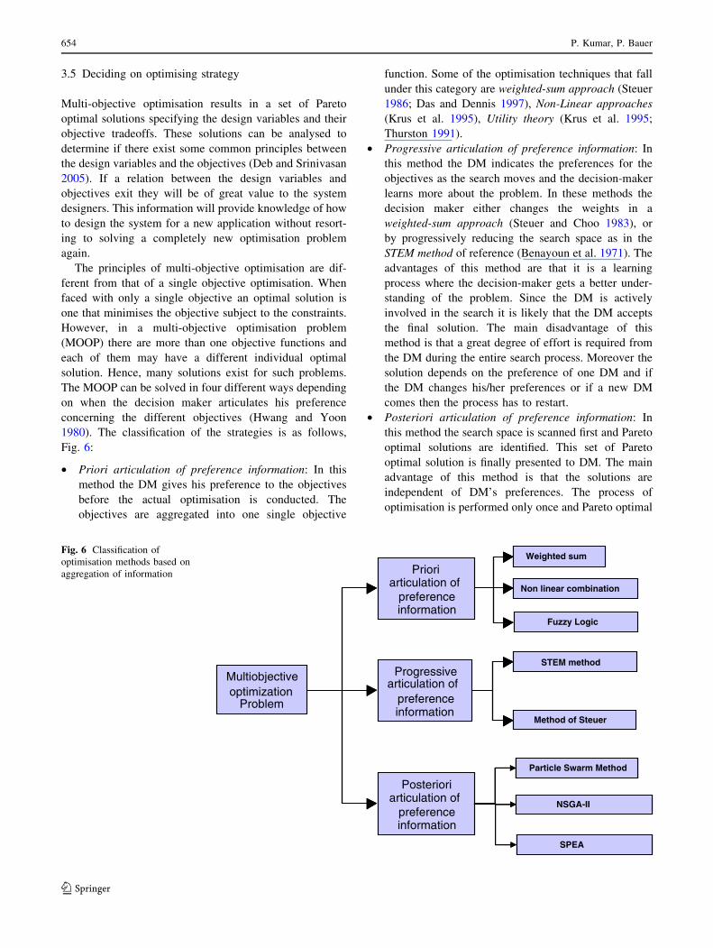
1980). The classification of the strategies is as follows,

Fig. 6:

• Priori articulation of preference information: In this

method the DM gives his preference to the objectives

before the actual optimisation is conducted. The

objectives are aggregated into one single objective

function. Some of the optimisation techniques that fall

under this category are weighted-sum approach (Steuer

1986; Das and Dennis 1997), Non-Linear approaches

(Krus et al. 1995), Utility theory (Krus et al. 1995;

Thurston 1991).

• Progressive articulation of preference information: In

this method the DM indicates the preferences for the

objectives as the search moves and the decision-maker

learns more about the problem. In these methods the

decision maker either changes the weights in a

weighted-sum approach (Steuer and Choo 1983), or

by progressively reducing the search space as in the

STEM method of reference (Benayoun et al. 1971). The

advantages of this method are that it is a learning

process where the decision-maker gets a better under-

standing of the problem. Since the DM is actively

involved in the search it is likely that the DM accepts

the final solution. The main disadvantage of this

method is that a great degree of effort is required from

the DM during the entire search process. Moreover the

solution depends on the preference of one DM and if

the DM changes his/her preferences or if a new DM

comes then the process has to restart.

• Posteriori articulation of preference information: In

this method the search space is scanned first and Pareto

optimal solutions are identified. This set of Pareto

optimal solution is finally presented to DM. The main

advantage of this method is that the solutions are

independent of DM’s preferences. The process of

optimisation is performed only once and Pareto optimal

Multiobjectiveoptimization

Problem

Prioriarticulation of

preferenceinformation

Progressivearticulation of

preferenceinformation

Posterioriarticulation of

preferenceinformation

Weighted sum

Non linear combination

Fuzzy Logic

STEM method

Method of Steuer

Particle Swarm Method

NSGA-II

SPEA

Multiobjectiveoptimization

Problem

Prioriarticulation of

preferenceinformation

Progressivearticulation of

preferenceinformation

Posterioriarticulation of

preferenceinformation

Weighted sum

Non linear combination

Fuzzy Logic

STEM method

Method of Steuer

Particle Swarm MethodParticle Swarm Method

NSGA-IINSGA-II

SPEASPEA

Fig. 6 Classification of

optimisation methods based on

aggregation of information

654 P. Kumar, P. Bauer

123

set does not change as long as the problem description

remains unchanged. The disadvantage of this method is

that they need large number of computations to be

performed and the DM is presented with too many

solutions to choose from.

The principle goal of multi-objective optimisation

algorithms is to find well spread set of Pareto optimal

solutions. Each of the solutions in the Pareto optimal set

corresponds to the optimum solution of a composite

problem trading-off different objective among the objec-

tives. Hence each solution is important with respect to

some trade-off relation between the objectives. However

in real situations only one solution is to be implemented.

Therefore, the question arises about how to choose among

the multiple solutions. The choice may not be difficult to

answer in the presence of many trade-off solutions, but is

difficult to answer in the absence of any trade-off infor-

mation. If a designer knows the exact trade-off among

objective functions there is no need to find multiple

solutions (Pareto optimal solutions) and a priori articula-

tion methods will be well suited. However, a designer is

seldom certain about the exact trade-off relation among

the objectives. In such circumstance it is better to find a

set of Pareto optimal solutions first and then choose one

solution from the set by using additional higher level

information about the system being designed. With this in

view in PDM posteriori based optimisation method is

used. In principle any posteriori based multiobjective

optimisation algorithm such as NSGA-II (Deb et al.

2000), SPEA 2 (Zitzler et al. 2001), etc. can be used in

PDM. In this work the NBGA (Kumar et al. 2006) was

used. Choosing a suitable solution from the Pareto opti-

mal set forms the second phase of PDM and is described

in the next section.

4 Intermediate analysis phase of PDM

Once the synthesis process is done and a set of Pareto

optimal solutions is determined the next step involves

analysis of the solutions. In the conceptual stages of

design, the design engineer faces the greatest uncertainty

in the product attributes and requirements (e.g. dimen-

sions, features, materials, and performance). Because the

evolution of the design is greatly affected by decisions

made during the conceptual stage, these decisions have a

considerable impact on overall cost. In the intermediate

analysis phase the various alternatives obtained from the

previous step (synthesis phase) are analysed and a small

set of solutions are selected for deeper analysis. The most

important tasks in engineering design, besides modelling

and simulation, are to generate various design alternatives

and then to make preliminary decision to select a design

or a set of designs that fulfils a set of criteria. Hence the

engineering design decision problem is a multi criteria

decision-making problem.

It is a general assumption that evaluation of a design on

the basis of any individual criterion is a simple and

straightforward process. However in practice, the deter-

mination of the individual criterion may require

considerable engineering judgement (Scott and Antonsson

1999). An extensive literature survey on multi criteria

decision making is given in the work of Bana de Costa

(Costa and Vincke 1990). Carlsson and Fuller (1996) gave

a survey of fuzzy multi criteria decision making methods

with emphasis on fuzzy relations between interdependent

criteria. A new elicitation method for assigning criteria

importance based on linguistic variables is presented in

(Ribeiro 1996). Roubens (1997) introduced a new pair wise

preferred approach that permitted a homogeneous treat-

ment of different kinds of criteria evaluations. A fuzzy

model for design evaluation based on multiple criteria

analysis in engineering systems is presented by Martinez

and Liu (2006).

In the initial phase of development of an engineering

system the details of a design are unknown and design

description is still imprecise that the most important deci-

sions are made (Whitney 1988). In this initial engineering

design phase, the final values of the design variables are

uncertain. Hence at this stage decision making using fuzzy

linguistic variables is appropriate. After a decision is made

and an alternative or set of alternatives is selected, detailed

modelling of the system using standard tools (such as finite

element Analysis, etc) serve to calculate the performance

of the system and also help in reducing the uncertainty in

the design variables.

In the initial stage of decision making the designers

represent their preferences for different values of design

variables using a set of fuzzy linguistic variables. Each

value of design variable is assigned a preference between

absolutely unacceptable and absolutely acceptable. The

values of design variables have linguistic preference

values. Hence the designer’s judgement and experience

are formally included in the preliminary design problem.

The general problem is thus a Multi Criteria Decision-

Making problem, where the designer is to choose the

highest performing design configuration from the avail-

able set of design alternatives and each design is judged

by several, even competing, performance criteria or

variables.

A multi criteria decision-making problem (mcdm) is

expressed as:

Progressive design methodology for complex engineering systems 655

123

c1 c2 . . . cn

D ¼

A1

A2

..

.

Am

x11 x12 . . . x1n

x21 x22 . . . x2n

..

. ...� � � ..

.

xm1 xm2 . . . xmn

0BBBB@

1CCCCA

w ¼ w1;w2; . . .wnð Þ

where Ai, i = 1, … , m are the possible alternatives; cj,

j = 1, … , n are the criteria with which alternative per-

formances are measured and xij is the performance score of

the alternative Ai with respect to attribute cj and wj are the

relative importance of attributes.

The alternative performance rating xij can be crisp,

fuzzy, and/or linguistic. The linguistic approach is an

approximation technique in which the performance ratings

are represented as linguistic variable (Zadeh 1975a, b, c).

The classical MCDM problem consists of two phases:

• an aggregation phase of the performance values with

respect to all the criteria for obtaining a collective

performance value for alternatives,

• an exploitation phase of the collective performance

value for obtaining a rank ordering, sorting or choice

among the alternatives.

The various parts of intermediate analysis phase of PDM

are:

1. Identification of new set of criteria,

2. linguistic term set,

3. semantic of linguistic term set,

4. aggregation operator for linguistic weighted

information.

The flow chart of the above steps is shown in Fig. 7.

4.1 Identification of new set of criteria

In the synthesis stage the constraints imposed on the system

are engineering constraints. The engineering constraints are

specific to the system being designed and can be considered

as criteria based on which decision making is done. Besides

engineering constraints there are other non-engineering

constraints such as manufacturing limitations. It may be

possible that certain Pareto optimal solutions obtained in the

synthesis stage may not be feasible from the manufacturing

point of view or may be too expensive to manufacture.

Hence, in order to determine these constraints a high level of

information is to be collected from various experts.

4.1.1 Linguistic term set

After determining all the constraints, the next step is to

determine the linguistic term set. This phase consists of

establishing the linguistic expression domain used to pro-

vide the linguistic performance values for an alternative

according to different criteria. The first step in the solution

of a MCDM problem is selection of linguistic variable set.

There are two ways to choose the appropriate linguistic

description of term set and their semantic (Bordogna and

Passi 1993). In the first case by means of a context-free

grammar, and the semantic of linguistic terms is repre-

sented by fuzzy numbers described by membership

functions based on parameters and a semantic rule

(Bordogna and Passi 1993; Bonissone 1986) . In the second

case the linguistic term set by means of an ordered struc-

ture of linguistic terms, and the semantic of linguistic terms

is derived from their own ordered structure which may be

either symmetrically/asymmetrically distributed on the

[0,1] scale. An example of a set of seven terms of ordered

structured linguistic terms is as follows:

S ¼ s0 ¼ none; s1 ¼ very low; s2 ¼ low; s3 ¼ medium;fs4 ¼ high; s5 ¼ very high; s6 ¼ perfectg

Identification of New set of criteria

Linguistic term set

Semantic of linguistic term set

Pareto Optimal Solutions From SynthesisPhase

All constraintsdetermined?

no

yes

Aggregation operator

Multi criteria decision making

Reduced set of solution

Fig. 7 Steps in the intermediate analysis phase of PDM

656 P. Kumar, P. Bauer

123

4.1.2 The semantic of linguistic term set

The semantics of the linguistic term set can be broadly

classified into three categories (Fig. 8), (a) Semantic based

on membership functions and semantic rule (Bonissone and

Decker 1986; Bordogna et al. 1997; Delgado et al. 1992),

(b) Semantic based on the ordered structure of the lin-

guistic term set (Bordogna and Passi 1993; Herrera and

Herrera-Viedma 2000; Torra 1996; Herrera and Verdegay

1996) and (c) Mixed semantic (Herrera and Herrera-

Viedma 2000; Herrera and Verdegay 1996).

4.1.3 Aggregation operator for linguistic weighted

information

Aggregation of information is an important aspect for all

kinds of knowledge based systems, from image processing

to decision making. The purpose of aggregation process is

to use different pieces of information to arrive at a con-

clusion or a decision. Conventional aggregation operators

such as the weighted average are special cases of more

general aggregation operators such as Choquet integrals

(Gabrish et al. 1999). The conventional aggregation oper-

ators have been articulated with logical connectives arising

from many-valued logic and interpreted as fuzzy set unions

or intersections (Dubois and Prade 2004). The latter have

been generalised in the theory of triangular norms

(Klement et al. 2000). Other aggregation operators that

have been proposed are symmetric sums (Sivert 1979),

null-norms (Calvo et al. 2001), uninorm (Yager and Fodor

1997), apart from other.

The aggregation operators can be grouped into the fol-

lowing broad classes (Dubois and Prade 2004):

i. Operators generalising the notion of conjunction are

basically the minimum and all those functions f

bounded from above by the minimum operators.

ii. Operators generalising the notion of disjunction are

basically the maximum and all those functions f

bounded from below by the maximum operations.

iii. Averaging operators are all those functions lying

between the maximum and minimum.

For linguistic weighted information the aggregation

operators mentioned above have to be modified for lin-

guistic variables and can be placed under two categories

(Herrera and Herrera-Viedma 1997) Linguistic Weighted

Disjunction (LWD) and Linguistic Weighted Conjunction

(LWC). In Fig. 9 the detailed classification of the linguistic

aggregation operators is shown. In the following subsec-

tions the mathematical formulation of LWD and LWC is

Semantic of Linguistic Term Set

Based on membershipfunction and semantic rule

Based on orderedstructure

Based on mixedsemantic

SymmetricallyDistributed terms

Non SymmetricallyDistributed terms

Fig. 8 Classification of

semantic of linguistic term set

Linguistic AggregationOperators

Linguistic Weighted Disjunction Linguistic Weighted Conjunction

Min Operator

Nilpotent Min Operator

Weakest Conjunction

Kleene-Dienes’s

Gödel’s Linguistic

Fodor’s Linguistic

Lukasiewicz’s Linguistic

Fig. 9 Classification of

aggregation operator for

linguistic variables

Progressive design methodology for complex engineering systems 657

123

given. In order to illustrate each of the above mentioned

linguistic aggregation operators the following example is

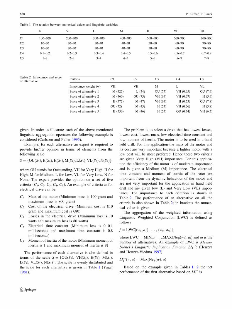
considered (Carlsson and Fuller 1995):

Example: for each alternative an expert is required to

provide his/her opinion in terms of elements from the

following scale

S ¼ OU S7ð Þ;HðS6Þ;H S5ð Þ;M S4ð Þ;L S3ð Þ;VL S2ð Þ;N S1ð Þf g

where OU stands for Outstanding, VH for Very High, H for

High, M for Medium, L for Low, VL for Very Low, N for

None. The expert provides the opinion on a set of five

criteria {C1, C2, C3, C4, C5}. An example of criteria as for

electrical drive can be:

C1 Mass of the motor (Minimum mass is 100 gram and

maximum mass is 800 gram)

C2 Cost of the electrical drive (Minimum cost is €10

gram and maximum cost is €80)

C3 Losses in the electrical drive (Minimum loss is 10

watts and maximum loss is 80 watts)

C4 Electrical time constant (Minimum loss is 0 0.1

milliseconds and maximum time constant is 0.8

milliseconds)

C5 Moment of inertia of the motor (Minimum moment of

inertia is 1 and maximum moment of inertia is 8)

The performance of each alternative is also defined in

terms of the scale S = {OU(S7), VH(S6), H(S5), M(S4),

L(S3), VL(S2), N(S1)}. The scale is evenly distributed and

the scale for each alternative is given in Table 1 (Yager

1981).

The problem is to select a drive that has lowest losses,

lowest cost, lowest mass, low electrical time constant and

low moment of inertia. The motor is to be used in a hand

held drill. For this application the mass of the motor and

its cost are very important because a lighter motor with a

low cost will be most preferred. Hence these two criteria

are given Very High (VH) importance. For this applica-

tion the efficiency of the motor is of moderate importance

and is given a Medium (M) importance. The electrical

time constant and moment of inertia of the rotor are

important from the dynamic behaviour of the motor and

are not very important for the application in hand held

drill and are given low (L) and Very Low (VL) impor-

tance. The importance to each criterion is shown in

Table 2. The performance of an alternative on all the

criteria is also shown in Table 2; in brackets the numer-

ical value is given.

The aggregation of the weighted information using

Linguistic Weighted Conjunction (LWC) is defined as

follows

f ¼ LWC w1; a1ð Þ; . . . ; wm; amð Þ½ �

where LWC ¼ MINi¼1; ... ;mMAX Neg wið Þ; aið Þ and m is the

number of alternatives. An example of LWC is Kleene-

Dienes’s Linguistic Implication Function LI1?: (Herrera

and Herrera-Viedma 1997)

LI!1 w; að Þ ¼ Max Neg wð Þ; að Þ

Based on the example given in Tables 1, 2 the net

performance of the first alternative based on LI1? is

Table 1 The relation between numerical values and linguistic variables

N VL L M H VH OU

C1 100–200 200–300 300–400 400–500 500–600 600–700 700–800

C2 10–20 20–30 30–40 40–50 50–60 60–70 70–80

C3 10–20 20–30 30–40 40–50 50–60 60–70 70–80

C4 0.1–0.2 0.2–0.3 0.3–0.4 0.4–0.5 0.5–0.6 0.6–0.7 0.7–0.8

C5 1–2 2–3 3–4 4–5 5–6 6–7 7–8

Table 2 Importance and score

of alternativeCriteria C1 C2 C3 C4 C5

Importance weight (w) VH VH M L VL

Score of alternative 1 M (425) L (34) OU (77) VH (0.65) OU (7.6)

Score of alternative 2 M (460) OU (75) VH (64) VH (0.67) H (5.6)

Score of alternative 3 H (572) M (47) VH (64) H (0.53) OU (7.8)

Score of alternative 4 OU (72) M (45) H (53) VH (0.66) H (5.8)

Score of alternative 5 H (550) M (46) H (55) OU (0.74) VH (6.5)

658 P. Kumar, P. Bauer

123

f1 ¼ MIN LI!1 VH,Mð Þ; LI!1 VH,Lð Þ; LI!1 M,OUð Þ;�

LI!1 L,VHð Þ; LI!1 VL,OUð Þ�

¼ MIN M,L,OU,VH,OU½ � ¼ L

The final score of the second alternative is

f2 ¼ MIN LI!1 VH,Mð Þ; LI!1 VH,OUð Þ; LI!1 M,VHð Þ;�

LI!1 L,VHð Þ; LI!1 VL,Hð Þ�

¼ MIN M,OU,VH,VH,VH½ � ¼ M

The final score of the third alternative is

f3 ¼ MIN LI!1 VH,Hð Þ; LI!1 VH,Mð Þ; LI!1 M,VHð Þ;�

LI!1 L,Hð Þ; LI!1 VL,OUð Þ�

¼ MIN H,M,VH,H,OU½ � ¼ M

The final score of the fourth alternative is

f4 ¼ MIN LI!1 VH,OUð Þ; LI!1 VH,Mð Þ; LI!1 M,Hð Þ;�

LI!1 L,VHð Þ; LI!1 VL,Hð Þ�

= MIN OU,M,H,VH,VH½ � = M

The final score of the fifth alternative is

f5 ¼ MIN LI!1 VH,Mð Þ; LI!1 VH,Mð Þ; LI!1 M,Hð Þ;�

LI!1 L,OUð Þ; LI!1 VL,Hð Þ�

¼ MIN M,M,H,OU,VH½ � ¼ M

Hence on the basis of LI1? the final score of all the

alternatives is [L, M, M, M, M].

The results of total score of all the five alternatives

based on different aggregation operators is summarised

below in Table 3.

From the above the following conclusions can be drawn:

• The choice of linguistic aggregation operator can

influence the results of the intermediate analysis

process.

• The linguistic weighted disjunction aggregation oper-

ators in general give an optimistic average value to

alternatives. The Weakest linguistic disjunction gives

the least optimistic value to the alternatives.

• The linguistic weighted conjunction aggregation oper-

ators in general give a pessimistic average value to the

alternatives.

• Out of all the conjunction operators the Lukasiewicz’s

implication operator gives the least pessimistic final

score to all the alternatives.

• The disjunction aggregation operators are suitable if

it is required to select a set of as many alternatives

as possible. This situation can arise in the initial

design phase when the designer wants to include

as many alternatives as possible for further

investigation.

• In the initial design process if the number of alterna-

tives is large and there is limited capability, in terms of

manpower and computing power, to investigate each

alternative then linguistic weighted conjunction oper-

ators are preferred.

5 Final analysis phase of PDM

In the final analysis detailed simulation model of the target

system is developed. After intermediate analysis the set of

plausible solutions is greatly reduced and hence a detailed

simulation for each solution is feasible. After setting up of

the simulation model a new set of Independent design

variables and objectives is identified. The steps involved in

this stage are:

Step1: Detailed simulation model of the target system is

developed.

Step2: Independent design variables and objectives are

identified.

Step3: Each solution in the reduced solution set is

optimised for the new objectives and a set of

solutions is obtained.

Step4: Final decision is made.

In the next section the PDM is applied for design of a

BLDC motor. The various aspects of PDM are used in the

design of BLDC motor.

6 Synthesis phase of progressive design methodology

for design of a BLDC motor drive

Since the emergence of new high field permanent magnet

materials brushless DC motors (BLDC) drives have

become increasingly attractive in a wide range of appli-

cations. They have smaller volume compared with

equivalent wound field machines, operate at higher speed,

dissipate heat better, require less maintenance, and are

more efficient and reliable than conventional motors.

Table 3 The result of total score of all the alternatives using different

aggregation operators

Alternative ? 1 2 3 4 5

Min LD1? M VH H VH H

Nilpotent LD2? M VH H VH H

Weakest LD3? M VH VL VH L

Kleene-Dienes’s LI1? L M M M M

Godel’s LI2? L M M M M

Fodor’s LI3? L M M M M

Lukasiewicz’s LI4? M H M H H

Progressive design methodology for complex engineering systems 659

123

Many researchers have made efforts to improve motor

performance in terms of efficiency, maximum torque,

back EMF, power/ weight ratio, and minimum losses in

iron, coils, friction, and windage. A scheme for optimi-

sation of a three phase electric motor based on genetic

algorithms (GA) was presented by Bianchi (1998). As a

demonstration of this technique the authors took a surface

mounted permanent magnet motor as an example and

applied genetic algorithm to minimise the permanent

magnet weight. Similarly an optimal design of Interior

Permanent Magnet Synchronous Motor using genetic

algorithms was performed by Sim et al. (1997). In this

case the efficiency of the motor was taken as the

objective function. In recent years research has been

pursued in the area of multiobjective optimisation of PM

motors. Multiobjective optimisation of PM motor using

genetic algorithms was performed by Yamada et al.

(1997). A surface mounted PM synchronous motor was

taken for optimisation and e-constraint method was used

to obtain the solution. The objective functions that were

considered for optimisation were motor weight and

material cost. The authors used a two step method for

optimisation. First a preliminary design was carried out in

which the design is formulated as a constraint non-linear

programming problem by using space harmonic analysis.

Then the motor configuration was optimised using a

procedure that combined the finite element method

(FEM) with the optimisation algorithm. Sim et al. (1997)

implemented multiobjective optimisation for a permanent

magnet motor design using a modified genetic algorithm.

The genetic algorithm used in this case was adjusted to

the vector optimisation problem. Multiobjective optimi-

sation of an interior permanent magnet synchronous

motor was carried out again by Sim et al. (Cho et al.

1999). In both cases the authors chose weight of the

motor and the loss as objective functions. In the present

work the MOOP of PM motors is taken a step further.

The optimisation of the motor so far laid focus mainly on

the magnetic circuit of the motor. In this work a meth-

odology is presented for design of BLDC motor drive.

The BLDC motor drive considered here consists of the

BLDC motor and voltage source inverter. Here the entire

system is considered while designing the motor and

hence the system design approach is used to design the

BLDC motor.

In this section the PDM is applied for the design of a

BLDC motor for a specific application. All the steps of

PDM are applied and the motor is designed that optimal

with respect to the system in which it has to work. In the

next subsection the customer requirements are elicited and

validated.

6.1 System requirement analysis

The specified parameters of the motor are:

Rated speed 800 rpm (mechanical)

Torque at speed 0.2 Nm

Input voltage 24 V

Number of phases 3

The aim of the problem is to design a motor with a

cogging torque of less than 20 mNm, maximum efficiency,

and minimum mass and trapezoidal back emf.

Inverter Full bridge voltage

source inverter

Motor topology Inner rotor with surface

mount magnets

Phase connection The phases are connected

in star

The additional constraints of the motor are

Outer stator diameter 40 mm

Max. length 50 mm

Air gap length 0.2 mm

6.2 Definition of system boundaries

The BLDC motor to be designed is driven by a voltage

source inverter (VSI) and a fixed voltage of 24 V. Hence

while designing the motor it is important to include the VSI

in the system boundaries. This will ensure that the designed

motor will produce the required torque when it is integrated

with the VSI. During the design of the motor the parame-

ters of the VSI itself will not be optimised. In the current

scenario motor is the primary system under investigation.

The model of the system that includes the BLDC motor and

the VSI is more complicated but will ensure a well

designed motor. Hence the system boundary under con-

sideration in the synthesis phase consists of:

• The BLDC motor (primary system),

• three phase VSI.

660 P. Kumar, P. Bauer

123

6.3 Determining of performance criteria

From the requirement analysis the primary objectives that

have to be satisfied are:

• Minimum cogging torque,

• maximum efficiency,

• minimum mass,

• sinusoidal shape of back EMF.

In the synthesis phase of PDM only simple model of the

BLDC drive is developed. However determining parame-

ters like cogging torque and shape of the back emf required

detailed analytical models or FEM models. The mass and

efficiency of the motor can be calculated with relative ease

compared to the cogging torque and back emf shape.

Hence in the synthesis phase the objectives that will be

considered are

• Minimise the mass,

• maximise the efficiency.

A generic topology of BLDC motor with surface mount

magnets as shown in Fig. 10 are considered. This topology

is optimised for minimum mass and maximum efficiency.

In the final design the parameters of this optimised generic

topology are fine-tuned to reduce the cogging torque and

obtain sinusoidal back emf shape.

6.4 Selection of variables and sensitivity analysis

The following set of independent design variables are

identified

• Number of poles (Np),

• number of slots (Nm),

• length of the motor (Lmot),

• ratio of inner diameter of motor to outer diameter (ad),

• ratio of magnet angle to pole pitch (am),

• height of the magnet (hm),

• reminance field of the permanent magnets (Br),

• maximum allowable field density in the lamination

material for linear operation (Bfe),

• number of turns in the coils of the motor (Nturns).

Sensitivity analysis is performed to determine influence

of the engineering variables on the objectives viz. mass

and efficiency. In Figs. 11 to 24 the sensitivity curves of

losses and mass w.r.t. single design variables are shown.

From Fig. 11 it can be seen that as the number of turns in

the coil increases the losses in the motor decrease. This is

due to the fact that with higher number of turns the induced

back emf increases as a result of this the difference

between the input voltage (24 V in the present case) and

the back emf reduces thereby reducing the magnitude of

the phase current and hence the Ohmic losses, proportional

to square of the current, reduce. The losses of the motor are

also sensitive to length of the motor (length of the motor is

same as length of the magnet in the present analysis) and

reach a minimum value as the length increases Fig. 12. The

ratio of inner diameter to outer diameter of the stator has an

influence on the losses in the motor, Fig. 13. As the ratio

increases the losses reduce because the stator yoke is

thicker and as a result of this the field density in the yoke is

less resulting in reduction of eddy current and hysteresis

losses. As the ratio of magnet angle to pole pitch increases

the losses reduces, Fig. 14. A smaller ratio ratio of magnet

angle to pole pitch results in smaller magnet and hence less

field density in the iron part,thereby reducing the eddy and

hysteresis losses in the iron partsofthe motor. The remi-

nance field of the permanent magnet and maximum

allowable field density in iron for linear characteristics

have influence on the losses, Figs. 15 and 16, respectively.

The height of the magnet also influences the losses in the

motor, Fig. 17.

The mass of the motor more or less remaining constant

with increase in the number of turns of the coil, Fig. 18.Fig. 10 The generic topology of the BLDC motor with surface

mount magnets

Number ofturns in coil vs. Loss

0

500

1000

1500

2000

2500

6050403020100

Number of turns

Lo

ss [

Wat

ts]

Fig. 11 Sensitivity of loss w.r.t. number of turns the in the coil

Progressive design methodology for complex engineering systems 661

123

This is due to the fact that the slot fill ratio is kept constant

in the present analysis, hence increase in the number turns

does have an influence on the total mass of copper. The

mass is directly proportional to motor length, Fig. 19. As

the ratio of stator inner and outer diameter increases the

mass of the motor reduces because the amount of iron in

the stator reduces, Fig. 20. The mass reach a maximum as

the ratio of the magnet angle to the pole pitch increases,

Fig. 21. The influence of reminance field density of the

permanent magnet on the mass of the motor is shown in

Length of motor vs. Losses

0

200

400

600

800

1000

1200

1400

50403020100

Length of motor[mm]

Lo

ss [

Wat

ts]

Fig. 12 Sensitivity of loss w.r.t. length of motor

Ratio of inner stator diameter to outer satator diameter vs. Losses

0

200

400

600

800

1000

1200

Ratio of inner to outer satator diameter

Lo

ss [

Wat

ts]

0.750.70.650.60.550.5

Fig. 13 Sensitivity of loss w.r.t. ratio of inner to outer stator

diameters

Ratio of magnet angle to pole pitch VS. Losses

0

200

400

600

800

1000

1200

Ratio of magnet angle to pole pitch

Lo

sses

[W

atts

]

10.90.80.70.60.50.40.30.2

Fig. 14 Sensitivity of loss w.r.t. ratio of magnet angle to pole pitch

Reminance field of permanent magnet VS. Losses

0

200

400

600

800

1000

1200

Reminance field of permanent magnet [Tesla]

Lo

ss [

Wat

ts]

1 1.1 1.2 1.30.90.80.70.60.5

Fig. 15 Sensitivity of loss w.r.t. reminance field allowable Density of

permanent magnet characteristics

Biron VS. Losses

0

200

400

600

800

1000

1200

1400

Biron [Tesla]

Lo

sses

[W

atts

]

2.521.510.50

Fig. 16 Sensitivity of loss w.r.t. maximum field density in iron for

linear

Height of magnet VS. Losses

0

100

200

300

400

500

600

700

800

900

1000

32.521.510.5

Height of magnet [mm]

Lo

sses

[W

atts

]

Fig. 17 Sensitivity of loss w.r.t. height of magnet

662 P. Kumar, P. Bauer

123

Fig. 22. Similarly the influence of maximum allowable

field density in iron for linear characteristics on motor mass

is shown in Fig. 23. The height of the magnet has influence

on the mass as shown in Fig. 24.

The result of the sensitivity analysis show that the

selected engineering variable have an influence on the

objectives (mass and losses) selected for synthesis analysis.

After having performed sensitivity analysis the next step is

to determine the optimisation strategy and set up the

problem for optimisation. These steps are described in next

subsection.

Number of turns in coil vs. Mass

0

0.01

0.02

0.03

0.04

0.05

0.06

0.07

0.08

0 10 20 30 40 50 60

Number of turns

Mas

s [K

g]

Fig. 18 Sensitivity of mass w.r.t. number of turns

Length of motor vs. Mass

0

0.05

0.1

0.15

0.2

0.25

0.3

Length of motor[mm]

Mas

s [K

g]

0 5 10 15 20 25 30 35 40 45 50

Fig. 19 Sensitivity of mass w.r.t. motor length

Ratio of inner stator diameter to outer satator diameter vs. Mass

0

0.01

0.02

0.03

0.04

0.05

0.06

0.07

0.08

0.09

Ratio of inner to outer satator diameter

Mas

s [K

g]

0.750.70.650.60.550.5

Fig. 20 Sensitivity of mass w.r.t. ratio of stator inner and outer

diameter

Ratio of magnet angle to pole pitch VS. Mass

0.0652

0.0654

0.0656

0.0658

0.066

0.0662

0.0664

0.0666

0.0668

0.067

0.2 0.3 0.4 0.5 0.6 0.7 0.8 0.9 1Ratio of magnet angle to pole pitch

Mas

s [K

g]

Fig. 21 Sensitivity of mass w.r.t. ratio of magnet to pole pitch

Reminance field of permanent magnet VS. Mass

0.0663

0.0664

0.0665

0.0666

0.0667

0.0668

0.0669

0.067

0.5 0.6 0.7 0.8 0.9 1 1.1 1.2 1.3

Reminance field of permanent magnet [Tesla]

Mas

s [K

g]

Fig. 22 Sensitivity of mass w.r.t. reminance field density of perma-

nent magnet

Biron VS. Mass

0.0658

0.066

0.0662

0.0664

0.0666

0.0668

0.067

Biron [Tesla]

Mas

s [K

g]

2.521.510.50

Fig. 23 Sensitivity of mass w.r.t. maximum allowable field density in

iron for linear characteristics

Progressive design methodology for complex engineering systems 663

123

6.5 Development of system model

6.5.1 Motor model

In this section a simple design methodology for the surface

mounted BLDC motor is given (Hanselmann 2003). To

develop this model certain assumptions have been made.

The assumptions made are:

• No saturation in iron parts,

• magnets are symmetrically placed,

• slots are symmetrically placed,

• back emf is trapezoidal in shape,

• motor has balanced windings,

• permeability of iron is infinite.

The general configuration of the motor is shown in

Fig. 28. The motor design equations are developed in the

following sequence:

• Electrical design,

• general sizing,

• inductance and resistance calculation.

6.5.1.1 Electrical design (back emf and torque) The back

emf voltage induced in a stator coil due to magnet flux

crossing the air gap is given by

eph ¼dkdt¼ dh

dt

dkdh¼ xm

dkdh

ð1Þ

where xm is the mechanical speed of the rotor (radians/s)

and k is the flux linked by the coil.

The magnitude of back emf is given by

eph

�� �� ¼ 2BgNturnsLstackRroxm ð2Þ

where Nturns is the number of turns in a coil, Lstack is the

length rotor of the stack, Rro is the outer radius of the Bg is

the air gap field density given by

Bg ¼ Br

hm

hm þ gð3Þ

where hm is the height of the magnet, g is the airgap and the

outer radius of the rotor Rro is given by

Rro ¼ adRo ð4Þ

Height of magnet VS. Mass

0

0.01

0.02

0.03

0.04

0.05

0.06

0.07

0.08

0.5 1 1.5 2 2.5 3

Height of magnet [mm]

Mas

s [K

g]

Fig. 24 Sensitivity of mass w.r.t. height of magnet

Fig. 25 Flux distribution in a typical BLDCmotor

Fig. 26 The general shape of the slots and main dimensions

Loss Vs. Mass

0

0.05

0.1

0.15

0.2

0.25

0.3

2000 400 600 800 1000 1200

Loss [Watts]

Mas

s [K

g]

Fig. 27 Pareto optimal solutions for a BLDC motor with Ns = 6 and

Np = 4

664 P. Kumar, P. Bauer

123

where the Ro is outer radius of the stator and ad. is the ratio

of outer diameter of the rotor to the outer diameter of the

stator.

For fractional pitched magnets the coil back emf is

given by

eph ¼ 2amBgNturnsLstackRroxm ð5Þ

6.5.1.2 General sizing If the alternating direction of flux

flow over alternating magnet faces is ignored, the total flux

crossing the air gap is given by

/total ¼ BgAg ¼ 2pBgRroLstack ð6Þ

where Bg is the amplitude of the air gap flux density and is

given by (9) and Ag is area of the airgap. This flux is

divided among the teeth on the stator and the direction of

the flux depends on the polarity of the magnet under each

tooth. As a result, the magnitude of the flux flowing in each

tooth is given by

/t ¼/total

Ns

¼ 2pBgRroLstack

Ns

ð7Þ

where NS is the number of slots on the stator.

This flux travels through the body of the tooth resulting

in a flux density Bt whose magnitude is given by

Bt ¼/t

wtbLstackð8Þ

where wtb is the width of the tooth.

The value of Bt is generally known, as it is the max-

imum allowable flux density in iron. Hence once the

value of Bt is determined the width of the tooth is given

from Eqs. 7 and 8

wtb ¼2pRroBg

NsBt

ð9Þ

From the above expression it can be seen that the tooth

width is directly dependent on the rotor outer radius and

inversely proportional to number of slots. As the number of

Loss vs. Mass

0.02

0.03

0.04

0.05

0.06

0.07

0.08

100 200 300 400 500 600 700 8000

Loss [Watts]

Mas

s [K

g]

Fig. 28 Pareto optimal solutions for a BLDC motor with Ns = 9 and

Np = 6

Loss vs. Mass

0.07

0.09

0.11

0.13

0.15

0.17

0.19

0.21

0.23

0.25

200175150125100

Loss [Watts]

Mas

s [K

g]

Fig. 29 Pareto optimal solutions for a BLDC motor with Ns = 9 and

Np = 8

Loss Vs. Mass

0

0.05

0.1

0.15

0.2

0.25

450400350300250200150100500

Loss [Watts]

Mas

s [K

g]

Fig. 30 Pareto optimal solutions for a BLDC motor with Ns = 9 and

Np = 10

Loss vs. Mass

0.04

0.06

0.08

0.1

0.12

0.14

0.16

0.18

20 30 40 50 60 70 80 90 100

Loss [Watts]

Mas

s [K

g]

Fig. 31 Pareto optimal solutions for a BLDC motor with Ns = 12

and Np = 8

Progressive design methodology for complex engineering systems 665

123

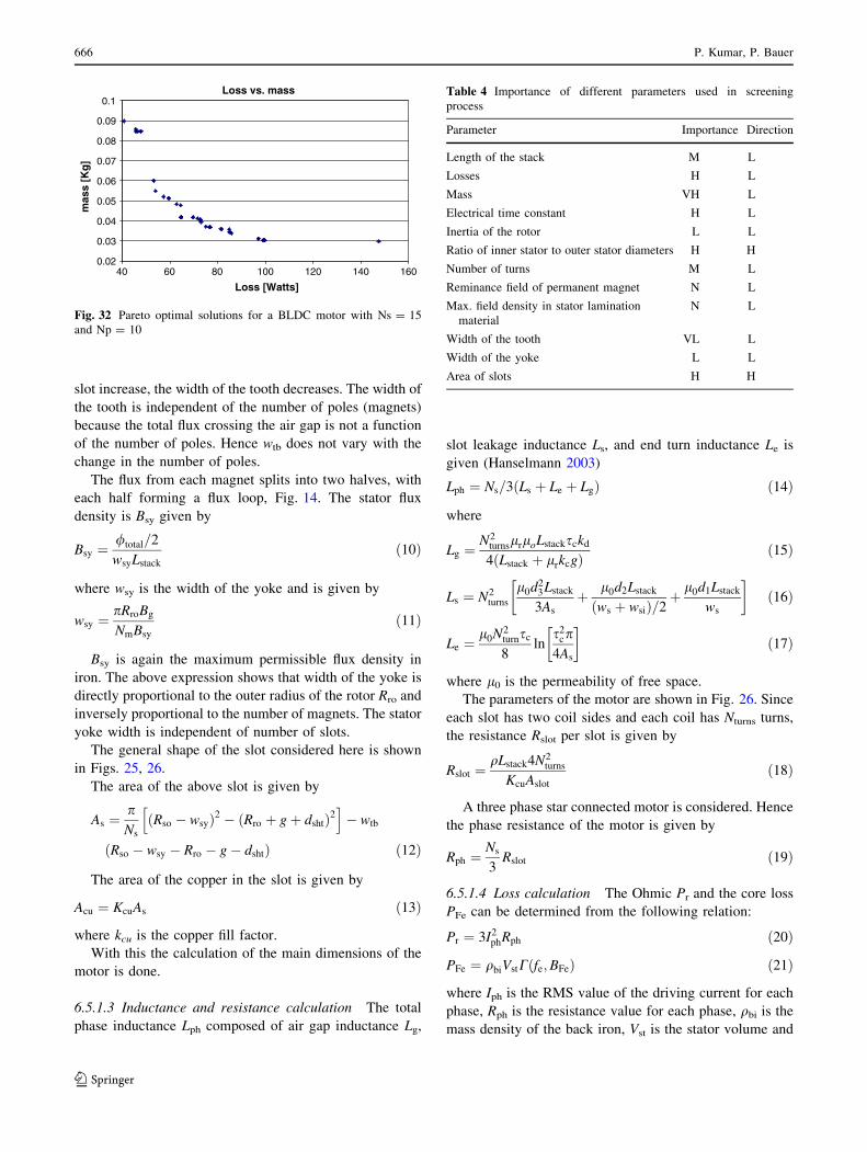
slot increase, the width of the tooth decreases. The width of

the tooth is independent of the number of poles (magnets)

because the total flux crossing the air gap is not a function

of the number of poles. Hence wtb does not vary with the

change in the number of poles.

The flux from each magnet splits into two halves, with

each half forming a flux loop, Fig. 14. The stator flux

density is Bsy given by

Bsy ¼/total=2

wsyLstack

ð10Þ

where wsy is the width of the yoke and is given by

wsy ¼pRroBg

NmBsy

ð11Þ

Bsy is again the maximum permissible flux density in

iron. The above expression shows that width of the yoke is

directly proportional to the outer radius of the rotor Rro and

inversely proportional to the number of magnets. The stator

yoke width is independent of number of slots.

The general shape of the slot considered here is shown

in Figs. 25, 26.

The area of the above slot is given by

As ¼pNs

ðRso � wsyÞ2 � ðRro þ gþ dshtÞ2h i

� wtb

ðRso � wsy � Rro � g� dshtÞ ð12Þ

The area of the copper in the slot is given by

Acu ¼ KcuAs ð13Þ

where kcu is the copper fill factor.

With this the calculation of the main dimensions of the

motor is done.

6.5.1.3 Inductance and resistance calculation The total

phase inductance Lph composed of air gap inductance Lg,

slot leakage inductance Ls, and end turn inductance Le is

given (Hanselmann 2003)

Lph ¼ Ns=3ðLs þ Le þ LgÞ ð14Þ

where

Lg ¼N2

turnslrloLstacksckd

4ðLstack þ lrkcgÞ ð15Þ

Ls ¼ N2turns

l0d23Lstack

3As

þ l0d2Lstack

ðws þ wsiÞ=2þ l0d1Lstack

ws

� �ð16Þ

Le ¼l0N2

turnsc

8ln

s2cp

4As

� �ð17Þ

where l0 is the permeability of free space.

The parameters of the motor are shown in Fig. 26. Since

each slot has two coil sides and each coil has Nturns turns,

the resistance Rslot per slot is given by

Rslot ¼qLstack4N2

turns

KcuAslot

ð18Þ

A three phase star connected motor is considered. Hence

the phase resistance of the motor is given by

Rph ¼Ns

3Rslot ð19Þ

6.5.1.4 Loss calculation The Ohmic Pr and the core loss

PFe can be determined from the following relation:

Pr ¼ 3I2phRph ð20Þ

PFe ¼ qbiVstCðfe;BFeÞ ð21Þ

where Iph is the RMS value of the driving current for each

phase, Rph is the resistance value for each phase, qbi is the

mass density of the back iron, Vst is the stator volume and

Loss vs. mass

0.02

0.03

0.04

0.05

0.06

0.07

0.08

0.09

0.1

40 60 80 100 120 140 160

Loss [Watts]

mas

s [K

g]

Fig. 32 Pareto optimal solutions for a BLDC motor with Ns = 15

and Np = 10

Table 4 Importance of different parameters used in screening

process

Parameter Importance Direction

Length of the stack M L

Losses H L

Mass VH L

Electrical time constant H L

Inertia of the rotor L L

Ratio of inner stator to outer stator diameters H H

Number of turns M L

Reminance field of permanent magnet N L

Max. field density in stator lamination

material

N L

Width of the tooth VL L

Width of the yoke L L

Area of slots H H

666 P. Kumar, P. Bauer

123

Table 5 The results of screening for the motor with Ns = 6 and Np = 4

Direction L L L L L H L L L H Final value

Importance M H VH H L H M VL L H

Alternatives Lstack Losses Mass Time constant Inertia DiDo Nturns wt wy Aslots

1 39.080 102.921 0.266 0.0002397 5.058 0.600 59 7.083 5.312 3.111 VL

2 39.075 103.171 0.266 0.0002412 4.993 0.600 59 7.071 5.303 3.111 VL

3 39.076 109.431 0.265 0.0002846 4.860 0.600 59 6.924 5.193 3.164 VL

4 23.731 124.825 0.172 0.0002911 3.710 0.581 59 7.093 5.320 3.203 L

5 23.778 125.444 0.164 0.0002917 3.035 0.595 60 6.805 5.104 3.299 L

6 23.789 127.760 0.163 0.0002988 3.087 0.600 59 6.688 5.016 3.356 L

7 23.789 128.071 0.163 0.0003007 3.082 0.600 59 6.681 5.011 3.363 L

8 22.637 129.909 0.161 0.0003286 2.828 0.580 60 6.929 5.197 3.317 L

9 22.664 139.730 0.160 0.0003093 2.673 0.581 53 6.993 5.245 3.263 L

10 17.241 159.536 0.124 0.0003367 2.305 0.581 59 6.714 5.036 3.554 L

11 17.174 162.847 0.123 0.0003636 2.101 0.581 60 6.602 4.952 3.723 L

12 17.174 166.638 0.121 0.0003473 2.577 0.599 60 6.339 4.755 3.901 L

13 14.710 167.018 0.104 0.0003287 2.110 0.599 59 6.304 4.728 3.972 L

14 14.439 170.149 0.102 0.0003425 1.931 0.599 59 6.232 4.674 4.122 L

15 13.216 174.275 0.096 0.0003213 2.216 0.600 59 6.231 4.673 4.098 L

16 13.216 176.200 0.095 0.0003275 2.162 0.600 59 6.204 4.653 4.156 L

17 11.973 188.203 0.086 0.0003321 1.805 0.600 59 6.101 4.576 4.399 L

18 11.973 189.799 0.086 0.000332 1.805 0.600 59 6.101 4.575 4.399 L

19 11.991 194.382 0.086 0.0003491 1.678 0.600 59 6.027 4.520 4.587 L

20 11.451 196.572 0.083 0.0003423 1.728 0.600 59 6.014 4.511 4.620 L

21 11.433 200.977 0.083 0.0003562 1.682 0.599 59 5.971 4.478 4.769 L

22 11.447 201.833 0.083 0.0003556 1.676 0.600 59 5.954 4.466 4.784 L

23 11.447 203.203 0.083 0.0003611 1.611 0.600 59 5.930 4.448 4.852 L

24 11.429 207.990 0.082 0.0003738 1.555 0.600 59 5.873 4.404 5.020 L

25 10.437 214.082 0.077 0.0003576 1.544 0.599 59 5.878 4.408 5.044 L

26 10.450 215.020 0.076 0.0003645 1.396 0.599 59 5.847 4.385 5.137 L

27 9.858 221.809 0.073 0.0003605 1.355 0.595 59 5.861 4.396 5.188 L

28 9.817 222.447 0.073 0.000363 1.289 0.595 59 5.847 4.385 5.236 L

29 9.785 223.964 0.072 0.0003632 1.375 0.600 59 5.760 4.320 5.370 L

30 8.172 261.767 0.064 0.0003974 0.998 0.581 59 5.701 4.276 6.147 L

31 8.148 306.782 0.062 0.000323 1.262 0.600 49 5.760 4.320 5.381 L

32 6.516 307.858 0.056 0.0003963 0.956 0.570 59 5.544 4.158 7.069 L

33 6.510 313.504 0.056 0.0004111 0.877 0.570 59 5.461 4.096 7.430 L

34 6.517 316.436 0.056 0.0004174 0.838 0.570 59 5.428 4.071 7.579 L

35 6.507 318.500 0.056 0.0004168 0.836 0.570 59 5.429 4.072 7.574 L

36 6.523 325.143 0.056 0.0004387 0.755 0.570 59 5.316 3.987 8.103 L

37 6.573 358.582 0.055 0.0003779 0.829 0.570 53 5.660 4.245 6.587 L

38 6.507 361.755 0.055 0.0003759 0.807 0.570 53 5.656 4.242 6.605 L

39 6.583 381.327 0.054 0.0003302 0.879 0.581 47 5.765 4.324 5.908 M

40 6.551 396.263 0.052 0.0003356 0.875 0.600 47 5.414 4.060 6.642 M

41 6.510 408.011 0.051 0.0002838 0.956 0.600 44 5.709 4.282 5.545 L

42 5.069 424.016 0.051 0.0004663 0.594 0.526 59 5.355 4.016 9.121 L

43 5.012 428.063 0.051 0.0004665 0.572 0.526 59 5.329 3.997 9.264 L

44 5.863 457.472 0.049 0.0003225 0.708 0.581 44 5.645 4.234 6.355 M

Progressive design methodology for complex engineering systems 667

123

C is the core loss density of the stator material at the flux

density BFe and frequency fe.

6.5.2 Dynamic performance of BLDC motor

The derivation of this model is based on the assumptions

that the induced currents in the rotor due to the stator

harmonic fields are neglected.

The coupled circuit equations of the stator windings in

terms of the motor electrical constants are

V½ � ¼ R½ � i½ � þ L½ � d i½ �dtþ e½ � ð22aÞ

where V½ � ¼ Va;Vb;Vc½ �0 ð22bÞ

R½ � ¼Rph 0 0

0 Rph 0

0 0 Rph

24

35 ð22cÞ

i½ � ¼ ia; ib; ic½ �0 ð22dÞ

L½ � ¼Lph 0 0

0 Lph 0

0 0 Lph

24

35 ð22eÞ

e½ � ¼ ea; eb; ec½ �0 ð22fÞ

where Rph and Lph are the phase resistance and phase

inductance values, respectively defined earlier and Va, Vb,

and Vc are the input voltages to each phase a, b and c,

respectively. The induced emf ea, eb, ec are sinusoidal in

shape and their peak values are given by Eq. 2. The

electromagnetic torque is given by

Te ¼ ½eaia þ ebib þ ecic�1

xm

ð23Þ

where xm is the mechanical speed of the motor.

The analytical solution of the Eq. 27a is given by

Nucera et al. (Nucera et al. 1989). In this work the model

developed by Nucera et al. has been used.

6.6 Optimisation strategy

In the present case study optimisation strategy based on

Posteriori articulation of preference information is used.

To achieve the multiobjective optimisation the Nondomi-

nated sorting Biologically Motivated Genetic Algorithm

(NBGA) (Kumar et al. 2006) is used. The parameters of

NBGA are as follows

Number of generations = 50

Number of individuals = 100

Crossover probability = 80%

Single point crossover was used.

The mutation rate was fixed between 0 and 10%

Hence the multiobjective optimisation problem to be

solved is expressed mathematically as

minimisef1ðx~Þ ¼ Pcu þ Phys þ Peddy

f2ðx~Þ ¼ Miron þMmagnet

�

where Pcu, Phys and Peddy are the copper loss, hysteresis

loss in the stator yoke and the eddy current loss in the stator

yoke, respectively and Miron and Mmagnet are the mass of

yoke (stator and rotor) and mass of permanent magnets,

respectively.

subject to hðx~Þ ¼ Tmotor� 0:2 Nm

where x~¼ ðBr;BFe; hm; Lmotor; am; ad;Nm;Ns;NturnsÞ are the

independent design variables

Table 6 The results of screening for the motor with Ns = 9 Np = 10

Direction L L L L L H L L L H Final value

Importance M H VH H L H M VL L H

Alternative Lstack Losses Mass Time constant Jmot DiDo Nturns wt wy Aslots

1 31.119 117.451 0.214 0.0026401 2.380 0.508 60 3.288 1.479 32.508 VL

2 24.722 124.145 0.171 0.0027403 1.829 0.508 60 2.685 1.208 38.803 VL

3 20.866 136.246 0.147 0.0025642 1.811 0.516 60 2.642 1.189 38.770 L

4 18.946 143.236 0.138 0.0024483 1.492 0.508 60 2.841 1.279 37.140 L

5 17.614 149.605 0.130 0.002309 1.378 0.508 60 3.018 1.358 35.261 L

6 15.732 159.273 0.118 0.0023229 1.240 0.508 60 2.738 1.232 38.254 L

7 14.713 166.044 0.111 0.0022571 1.162 0.508 60 2.740 1.233 38.202 L

8 13.751 175.540 0.106 0.0021383 1.072 0.508 60 2.882 1.297 36.682 L

9 13.788 180.009 0.103 0.0020036 1.270 0.537 60 2.788 1.254 35.755 L

10 8.046 205.460 0.062 0.0008258 1.014 0.600 60 4.478 2.015 17.609 L

11 8.009 207.324 0.062 0.0008158 1.010 0.600 60 4.514 2.031 17.371 L

12 5.077 254.040 0.046 0.0006926 0.651 0.599 60 3.993 1.797 21.016 L

668 P. Kumar, P. Bauer

123

and 0:5�Br� 1:2; 0:5�BFe� 2

1� hm� 3; 1� Lmotor� 100

0:1� am� 1; 0:1� ad� 0:7

2�Nm� 10; 3�Ns� 15

1�Nturns� 100

The results of the optimisation are given the next

subsection.

6.7 Results of multiobjective optimisation

The results of optimisation are given in Figs. 27, 28, 29,

30, 31, 32. From the results it can be seen that for each pole

slot combination a number of Pareto optimal solutions are

present and as the mass of the motor increases the losses

decreases. Since the number of feasible solutions is large

the results have to be screened so that a reduced set is

obtained. Detailed analysis can be then performed on the

reduced set. In the next section the screening process is

performed.

7 Intermediate analysis phase of progressive design

methodology for design of a BLDC motor drive

In this section the results obtained from the multi-criteria

multiobjective optimisation obtained in the previous

Table 7 The results of screening for the motor with Ns = 9 Np = 6

Direction L L L L L H L L L H Final

valueImportance M H VH H L H M VL L H

Alternative Lstack Losses Mass Time

constant

Jmot DiDo Nturns wt wy Aslots

1 9.786 157.634 0.072 0.0003752 1.688 0.600 60 5.054 3.790 8.263 VL

2 9.786 164.114 0.072 0.000383 1.613 0.600 59 5.012 3.759 8.470 VL

3 9.786 171.410 0.072 0.0003836 1.602 0.600 60 5.009 3.757 8.486 VL

4 9.794 172.560 0.071 0.000397 1.486 0.600 60 4.940 3.705 8.838 VL

5 9.792 173.388 0.071 0.0004052 1.421 0.600 60 4.897 3.673 9.061 VL

6 9.799 174.509 0.070 0.0004174 1.334 0.600 60 4.836 3.627 9.386 VL

7 9.804 175.171 0.070 0.0004244 1.288 0.600 60 4.801 3.601 9.576 VL

8 9.786 177.536 0.070 0.0004294 1.292 0.600 60 4.773 3.580 9.727 VL

9 9.786 182.972 0.070 0.0004283 1.291 0.600 59 4.779 3.584 9.695 VL

10 9.786 183.042 0.070 0.0004283 1.291 0.600 59 4.779 3.584 9.695 VL

11 8.427 196.408 0.063 0.0004116 1.381 0.600 60 4.680 3.510 10.254 L

12 7.344 197.133 0.055 0.0004021 1.033 0.600 60 4.548 3.411 11.035 L

13 7.331 198.013 0.055 0.0004066 0.995 0.600 60 4.520 3.390 11.204 L

14 6.667 211.152 0.052 0.0003902 1.150 0.600 60 4.478 3.358 11.467 L

15 6.641 213.407 0.052 0.0004011 1.052 0.600 60 4.409 3.307 11.897 L

16 6.650 215.335 0.052 0.0004138 0.965 0.600 60 4.340 3.255 12.347 L

17 6.642 218.685 0.051 0.0004337 0.849 0.600 60 4.228 3.171 13.092 L

18 6.641 218.706 0.051 0.0004337 0.848 0.600 60 4.228 3.171 13.095 L

19 6.659 241.040 0.051 0.0003775 0.936 0.600 52 4.550 3.413 11.021 L

20 5.231 253.763 0.044 0.0003926 0.933 0.600 58 4.085 3.063 14.091 L

21 5.231 254.492 0.044 0.0003927 0.932 0.600 58 4.084 3.063 14.095 L

22 5.146 257.163 0.043 0.0003925 0.917 0.600 58 4.058 3.043 14.282 L

23 5.176 261.857 0.043 0.0003957 0.867 0.600 60 4.048 3.036 14.353 L

24 5.191 264.120 0.043 0.0004153 0.753 0.600 60 3.934 2.950 15.191 L

25 5.191 266.084 0.043 0.0004225 0.705 0.600 60 3.891 2.918 15.513 L

26 5.155 267.243 0.043 0.0004205 0.696 0.600 60 3.891 2.918 15.513 L

27 5.137 269.628 0.043 0.0004277 0.678 0.600 60 3.842 2.882 15.885 L

28 5.146 307.658 0.042 0.0003999 0.699 0.600 52 4.013 3.010 14.609 L

29 5.138 362.249 0.042 0.0003071 0.806 0.600 42 4.619 3.464 10.609 L

30 5.150 370.205 0.041 0.000323 0.699 0.600 42 4.512 3.384 11.253 L

31 5.150 370.205 0.041 0.000323 0.699 0.600 42 4.512 3.384 11.253 L

32 5.144 439.331 0.041 0.0002639 0.780 0.600 34 4.939 3.704 8.840 L

Progressive design methodology for complex engineering systems 669

123

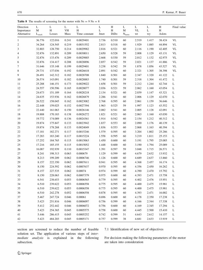
section are screened to reduce the number of feasible

solution set. The application of various steps of inter-

mediate analysis is explained in the following

subsection.

7.1 Identification of new set of objectives

For decision making the following parameters of the motor

are taken into consideration

Table 8 The results of screening for the motor with Ns = 9 Ns = 8

Direction L L L L L H L L L H Final value

Importance M H VH H L H M VL L H

Alternative Lstack Losses Mass Time constant Jmot DiDo Nturns wt wy Aslots

1 36.776 122.016 0.241 0.0029401 2.736 0.510 60 2.519 1.417 38.424 VL

2 34.264 124.545 0.219 0.0031552 2.813 0.518 60 1.929 1.085 44.894 VL

3 32.803 128.750 0.214 0.0029982 2.816 0.521 60 2.116 1.190 42.405 VL

4 32.876 132.891 0.209 0.0030011 2.650 0.528 59 2.008 1.129 43.131 VL

5 32.876 133.476 0.209 0.0029885 2.668 0.530 59 2.012 1.132 42.975 VL

6 32.876 134.417 0.208 0.0028896 2.857 0.542 59 2.021 1.137 41.886 VL

7 31.646 135.148 0.199 0.0029401 3.238 0.542 59 1.878 1.056 43.527 VL

8 29.731 137.036 0.192 0.0026618 2.891 0.542 60 2.321 1.305 38.398 VL

9 26.491 142.312 0.182 0.0028708 1.840 0.501 60 2.347 1.320 41.122 L

10 26.574 143.091 0.182 0.0028883 1.740 0.501 59 2.318 1.304 41.472 L

11 25.288 146.151 0.173 0.0029022 1.658 0.501 59 2.212 1.244 42.744 L

12 24.557 150.596 0.165 0.0028077 2.036 0.521 59 2.062 1.160 43.054 L

13 24.673 151.189 0.164 0.0028218 2.134 0.521 60 2.039 1.147 43.321 L

14 24.635 153.936 0.162 0.0026879 2.286 0.541 60 2.006 1.129 42.070 L

15 26.522 158.045 0.162 0.0023082 2.768 0.595 60 2.061 1.159 36.646 L

16 22.448 159.025 0.152 0.0027394 1.963 0.525 59 1.997 1.123 43.552 L

17 22.440 161.063 0.150 0.0026146 2.082 0.541 60 2.005 1.128 42.091 L

18 19.888 170.183 0.138 0.0026272 1.821 0.521 60 2.063 1.160 43.030 L

19 19.772 174.089 0.136 0.0024361 1.914 0.542 60 2.154 1.212 40.312 L

20 19.874 175.847 0.133 0.0023942 1.837 0.553 60 2.090 1.176 40.139 L

21 19.874 178.268 0.133 0.0024049 1.836 0.553 60 2.068 1.163 40.394 L

22 17.181 182.271 0.117 0.0015246 1.579 0.595 60 3.204 1.802 25.286 L

23 17.283 183.240 0.117 0.0015224 1.558 0.595 60 3.219 1.811 25.153 L

24 17.252 184.765 0.115 0.0015063 1.450 0.600 60 3.191 1.795 25.085 L

25 17.216 185.155 0.115 0.0015052 1.448 0.600 60 3.190 1.794 25.089 L

26 16.087 192.939 0.110 0.0015347 1.391 0.597 59 3.048 1.715 26.571 L

27 8.241 198.313 0.063 0.000679 1.129 0.599 60 4.679 2.632 13.932 L

28 8.213 199.209 0.062 0.0006746 1.126 0.600 60 4.689 2.637 13.860 L

29 8.157 222.350 0.062 0.0007611 0.941 0.595 60 4.368 2.457 16.174 L

30 8.150 224.592 0.062 0.0007637 0.970 0.595 60 4.356 2.450 16.262 L

31 8.157 227.535 0.062 0.00074 0.974 0.599 60 4.390 2.470 15.792 L

32 8.150 228.063 0.062 0.0007379 0.975 0.600 60 4.393 2.471 15.758 L

33 6.541 238.653 0.053 0.0006565 0.779 0.595 60 4.402 2.476 15.951 L

34 6.510 239.622 0.053 0.0006558 0.775 0.595 60 4.400 2.475 15.981 L

35 6.510 239.622 0.053 0.0006558 0.775 0.595 60 4.400 2.475 15.981 L

36 6.510 242.278 0.052 0.0006558 0.878 0.595 60 4.393 2.471 16.002 L

37 5.467 247.724 0.046 0.00061 0.696 0.600 60 4.178 2.350 17.238 L

38 5.423 251.816 0.046 0.0006097 0.756 0.599 60 4.166 2.344 17.338 L

39 5.412 252.442 0.046 0.0006072 0.756 0.600 60 4.169 2.345 17.294 L

40 5.423 254.365 0.045 0.0005575 0.758 0.600 60 4.445 2.500 15.410 L

41 5.446 286.415 0.045 0.0005252 0.742 0.599 51 4.643 2.612 14.157 L

42 5.423 484.203 0.045 0.0005171 0.757 0.599 38 4.681 2.633 13.919 L

670 P. Kumar, P. Bauer

123

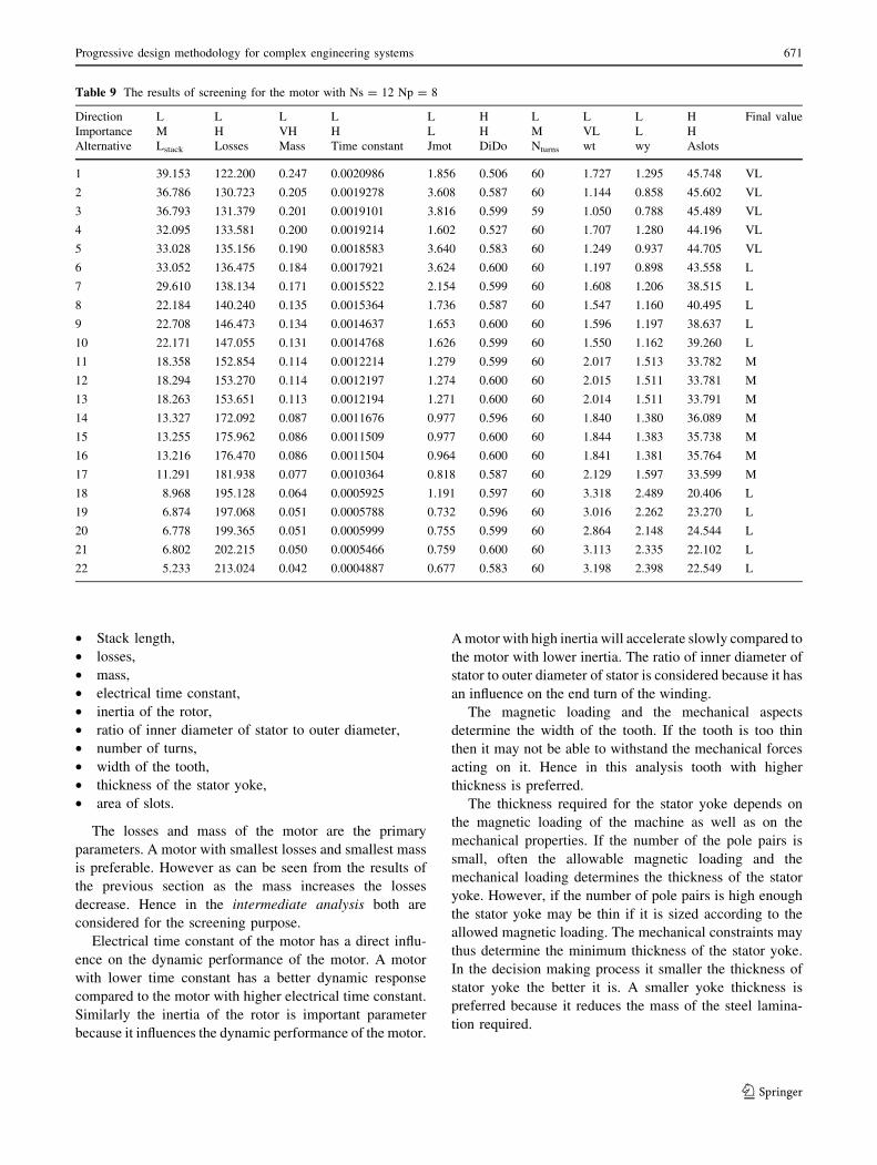
• Stack length,

• losses,

• mass,

• electrical time constant,

• inertia of the rotor,

• ratio of inner diameter of stator to outer diameter,

• number of turns,

• width of the tooth,

• thickness of the stator yoke,

• area of slots.

The losses and mass of the motor are the primary

parameters. A motor with smallest losses and smallest mass

is preferable. However as can be seen from the results of

the previous section as the mass increases the losses

decrease. Hence in the intermediate analysis both are

considered for the screening purpose.

Electrical time constant of the motor has a direct influ-

ence on the dynamic performance of the motor. A motor

with lower time constant has a better dynamic response

compared to the motor with higher electrical time constant.

Similarly the inertia of the rotor is important parameter

because it influences the dynamic performance of the motor.

A motor with high inertia will accelerate slowly compared to

the motor with lower inertia. The ratio of inner diameter of

stator to outer diameter of stator is considered because it has

an influence on the end turn of the winding.

The magnetic loading and the mechanical aspects

determine the width of the tooth. If the tooth is too thin

then it may not be able to withstand the mechanical forces

acting on it. Hence in this analysis tooth with higher

thickness is preferred.

The thickness required for the stator yoke depends on

the magnetic loading of the machine as well as on the

mechanical properties. If the number of the pole pairs is

small, often the allowable magnetic loading and the

mechanical loading determines the thickness of the stator

yoke. However, if the number of pole pairs is high enough

the stator yoke may be thin if it is sized according to the

allowed magnetic loading. The mechanical constraints may

thus determine the minimum thickness of the stator yoke.

In the decision making process it smaller the thickness of

stator yoke the better it is. A smaller yoke thickness is

preferred because it reduces the mass of the steel lamina-

tion required.

Table 9 The results of screening for the motor with Ns = 12 Np = 8

Direction L L L L L H L L L H Final value

Importance M H VH H L H M VL L H

Alternative Lstack Losses Mass Time constant Jmot DiDo Nturns wt wy Aslots

1 39.153 122.200 0.247 0.0020986 1.856 0.506 60 1.727 1.295 45.748 VL

2 36.786 130.723 0.205 0.0019278 3.608 0.587 60 1.144 0.858 45.602 VL

3 36.793 131.379 0.201 0.0019101 3.816 0.599 59 1.050 0.788 45.489 VL

4 32.095 133.581 0.200 0.0019214 1.602 0.527 60 1.707 1.280 44.196 VL

5 33.028 135.156 0.190 0.0018583 3.640 0.583 60 1.249 0.937 44.705 VL

6 33.052 136.475 0.184 0.0017921 3.624 0.600 60 1.197 0.898 43.558 L

7 29.610 138.134 0.171 0.0015522 2.154 0.599 60 1.608 1.206 38.515 L

8 22.184 140.240 0.135 0.0015364 1.736 0.587 60 1.547 1.160 40.495 L

9 22.708 146.473 0.134 0.0014637 1.653 0.600 60 1.596 1.197 38.637 L

10 22.171 147.055 0.131 0.0014768 1.626 0.599 60 1.550 1.162 39.260 L

11 18.358 152.854 0.114 0.0012214 1.279 0.599 60 2.017 1.513 33.782 M

12 18.294 153.270 0.114 0.0012197 1.274 0.600 60 2.015 1.511 33.781 M

13 18.263 153.651 0.113 0.0012194 1.271 0.600 60 2.014 1.511 33.791 M

14 13.327 172.092 0.087 0.0011676 0.977 0.596 60 1.840 1.380 36.089 M

15 13.255 175.962 0.086 0.0011509 0.977 0.600 60 1.844 1.383 35.738 M

16 13.216 176.470 0.086 0.0011504 0.964 0.600 60 1.841 1.381 35.764 M

17 11.291 181.938 0.077 0.0010364 0.818 0.587 60 2.129 1.597 33.599 M

18 8.968 195.128 0.064 0.0005925 1.191 0.597 60 3.318 2.489 20.406 L

19 6.874 197.068 0.051 0.0005788 0.732 0.596 60 3.016 2.262 23.270 L

20 6.778 199.365 0.051 0.0005999 0.755 0.599 60 2.864 2.148 24.544 L

21 6.802 202.215 0.050 0.0005466 0.759 0.600 60 3.113 2.335 22.102 L

22 5.233 213.024 0.042 0.0004887 0.677 0.583 60 3.198 2.398 22.549 L

Progressive design methodology for complex engineering systems 671

123

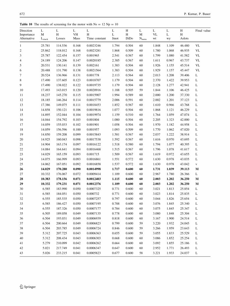
Table 10 The results of screening for the motor with Ns = 12 Np = 10

Direction L L L L L H L L L H Final value

Importance M H VH H L H M VL L H

Alternative Lstack Losses Mass Time constant Jmot DiDo Nturns wt wy Aslots

1 25.781 114.536 0.168 0.0023246 1.794 0.504 60 1.848 1.109 46.480 VL

2 25.862 118.012 0.168 0.0023281 1.868 0.509 60 1.780 1.068 46.935 VL

3 25.787 122.454 0.157 0.001965 2.541 0.567 60 1.799 1.080 41.582 VL

4 24.189 124.206 0.147 0.0020185 2.385 0.567 60 1.611 0.967 43.737 VL

5 20.531 130.141 0.139 0.002161 1.383 0.504 60 1.926 1.155 45.514 VL

6 20.488 131.790 0.138 0.0021564 1.383 0.504 60 1.929 1.157 45.447 VL

7 20.524 136.966 0.131 0.001778 2.113 0.564 60 2.013 1.208 39.406 L

8 17.490 137.605 0.123 0.0018707 1.179 0.504 60 2.370 1.422 39.953 L

9 17.490 138.022 0.122 0.0019735 1.179 0.504 60 2.128 1.277 42.941 L

10 17.493 143.015 0.120 0.0020916 1.188 0.505 59 1.844 1.106 46.425 L

11 18.237 145.270 0.115 0.0015907 1.994 0.589 60 2.000 1.200 37.330 L

12 18.185 146.264 0.114 0.0015779 2.006 0.591 60 2.002 1.201 37.123 L

13 17.386 149.075 0.111 0.0018453 1.852 0.567 60 1.610 0.966 43.768 L

14 14.858 150.121 0.106 0.0019816 1.077 0.504 60 1.868 1.121 46.229 L

15 14.895 152.044 0.104 0.0019974 1.159 0.510 60 1.764 1.059 47.074 L

16 14.044 154.792 0.103 0.001804 1.080 0.504 60 2.205 1.323 42.000 L

17 14.059 155.033 0.102 0.001901 1.058 0.504 60 1.970 1.182 44.958 L

18 14.059 156.596 0.100 0.001957 1.093 0.509 60 1.770 1.062 47.020 L

19 14.850 159.208 0.099 0.0015843 1.581 0.567 60 2.037 1.222 38.914 L

20 14.925 160.043 0.098 0.0017538 1.592 0.567 60 1.616 0.970 43.695 L

21 14.904 163.174 0.097 0.0016122 1.518 0.580 60 1.794 1.077 40.395 L

22 14.084 164.641 0.094 0.0016468 1.515 0.567 60 1.796 1.078 41.617 L

23 14.029 165.159 0.093 0.001715 1.509 0.567 60 1.619 0.972 43.655 L

24 14.075 166.999 0.093 0.0016861 1.551 0.572 60 1.630 0.978 43.035 L

25 14.062 167.051 0.092 0.0016858 1.537 0.572 60 1.630 0.978 43.042 v

26 14.029 170.280 0.090 0.0014998 1.717 0.600 60 1.731 1.039 39.113 M

27 10.332 176.067 0.072 0.0009414 1.109 0.600 60 2.967 1.780 26.366 L

28 10.383 178.156 0.071 0.0012403 1.115 0.600 60 2.003 1.202 36.250 M

29 10.332 179.231 0.071 0.0012376 1.109 0.600 60 2.003 1.202 36.250 M

30 6.585 183.990 0.050 0.0007325 0.771 0.600 60 3.021 1.813 25.854 L

31 6.585 184.051 0.050 0.000732 0.771 0.600 60 3.023 1.814 25.835 L

32 6.555 185.535 0.050 0.0007257 0.797 0.600 60 3.044 1.826 25.654 L

33 6.585 186.427 0.050 0.0007195 0.788 0.600 60 3.076 1.845 25.340 L

34 6.555 187.326 0.050 0.0007177 0.784 0.600 60 3.075 1.845 25.347 L

35 6.505 189.058 0.049 0.0007135 0.778 0.600 60 3.080 1.848 25.304 L

36 6.504 193.031 0.049 0.0006939 0.818 0.600 60 3.167 1.900 24.514 L

37 6.504 200.664 0.049 0.0006823 0.799 0.600 59 3.220 1.932 24.045 L

38 6.504 203.785 0.049 0.0006724 0.846 0.600 59 3.266 1.959 23.643 L

39 5.312 207.725 0.043 0.0006363 0.655 0.600 59 3.055 1.833 25.529 L

40 5.312 208.434 0.043 0.0006303 0.668 0.600 60 3.086 1.852 25.254 L

41 5.279 210.099 0.042 0.0006262 0.664 0.600 60 3.092 1.855 25.186 L

42 5.021 217.749 0.041 0.0006347 0.647 0.600 60 2.952 1.771 26.493 L

43 5.026 233.215 0.041 0.0005823 0.677 0.600 58 3.221 1.933 24.037 L

672 P. Kumar, P. Bauer

123

Table 11 Results of final screening process

Direction L L L L L H L L L H Ns Np Final value

Importance M H VH H L H M VL VL H

Alternative Lstack Losses Mass Time constant Jmot DiDo Nturns wt wy Aslots

1 6.583 381.327 0.054 0.0003302 0.879 0.581 47 5.765 4.324 5.908 6 4 L

2 6.551 396.263 0.052 0.0003356 0.875 0.600 47 5.414 4.060 6.642 6 4 L

3 5.863 457.472 0.049 0.0003225 0.708 0.581 44 5.645 4.234 6.355 6 4 L

4 8.427 196.408 0.063 0.0004116 1.381 0.600 60 4.680 3.510 10.254 9 6 L

5 7.344 197.133 0.055 0.0004021 1.033 0.600 60 4.548 3.411 11.035 9 6 L

6 7.331 198.013 0.055 0.0004066 0.995 0.600 60 4.520 3.390 11.204 9 6 L

7 6.667 211.152 0.052 0.0003902 1.150 0.600 60 4.478 3.358 11.467 9 6 L

8 6.641 213.407 0.052 0.0004011 1.052 0.600 60 4.409 3.307 11.897 9 6 L

9 6.650 215.335 0.052 0.0004138 0.965 0.600 60 4.340 3.255 12.347 9 6 L

10 6.642 218.685 0.051 0.0004337 0.849 0.600 60 4.228 3.171 13.092 9 6 L

11 6.641 218.706 0.051 0.0004337 0.848 0.600 60 4.228 3.171 13.095 9 6 L

12 6.659 241.040 0.051 0.0003775 0.936 0.600 52 4.550 3.413 11.021 9 6 L

13 5.231 253.763 0.044 0.0003926 0.933 0.600 58 4.085 3.063 14.091 9 6 L

14 5.231 254.492 0.044 0.0003927 0.932 0.600 58 4.084 3.063 14.095 9 6 L

15 5.146 257.163 0.043 0.0003925 0.917 0.600 58 4.058 3.043 14.282 9 6 L

16 5.176 261.857 0.043 0.0003957 0.867 0.600 60 4.048 3.036 14.353 9 6 L

17 5.191 264.120 0.043 0.0004153 0.753 0.600 60 3.934 2.950 15.191 9 6 L

18 5.191 266.084 0.043 0.0004225 0.705 0.600 60 3.891 2.918 15.513 9 6 L

19 5.155 267.243 0.043 0.0004205 0.696 0.600 60 3.891 2.918 15.513 9 6 L

20 5.137 269.628 0.043 0.0004277 0.678 0.600 60 3.842 2.882 15.885 9 6 L

21 5.146 307.658 0.042 0.0003999 0.699 0.600 52 4.013 3.010 14.609 9 6 L

22 5.138 362.249 0.042 0.0003071 0.806 0.600 42 4.619 3.464 10.609 9 6 L

23 5.150 370.205 0.041 0.000323 0.699 0.600 42 4.512 3.384 11.253 9 6 L

24 5.150 370.205 0.041 0.000323 0.699 0.600 42 4.512 3.384 11.253 9 6 L

25 5.144 439.331 0.041 0.0002639 0.780 0.600 34 4.939 3.704 8.840 9 6 L

26 26.491 142.312 0.182 0.0028708 1.840 0.501 60 2.347 1.320 41.122 9 8 VL

27 26.574 143.091 0.182 0.0028883 1.740 0.501 59 2.318 1.304 41.472 9 8 VL

28 25.288 146.151 0.173 0.0029022 1.658 0.501 59 2.212 1.244 42.744 9 8 VL

29 24.557 150.596 0.165 0.0028077 2.036 0.521 59 2.062 1.160 43.054 9 8 VL

30 24.673 151.189 0.164 0.0028218 2.134 0.521 60 2.039 1.147 43.321 9 8 VL

31 24.635 153.936 0.162 0.0026879 2.286 0.541 60 2.006 1.129 42.070 9 8 VL

31 26.522 158.045 0.162 0.0023082 2.768 0.595 60 2.061 1.159 36.646 9 8 VL

33 22.448 159.025 0.152 0.0027394 1.963 0.525 59 1.997 1.123 43.552 9 8 VL

34 22.440 161.063 0.150 0.0026146 2.082 0.541 60 2.005 1.128 42.091 9 8 VL

35 19.888 170.183 0.138 0.0026272 1.821 0.521 60 2.063 1.160 43.030 9 8 VL

36 19.772 174.089 0.136 0.0024361 1.914 0.542 60 2.154 1.212 40.312 9 8 VL

37 19.874 175.847 0.133 0.0023942 1.837 0.553 60 2.090 1.176 40.139 9 8 VL

38 19.874 178.268 0.133 0.0024049 1.836 0.553 60 2.068 1.163 40.394 9 8 VL

39 17.181 182.271 0.117 0.0015246 1.579 0.595 60 3.204 1.802 25.286 9 8 M

40 17.283 183.240 0.117 0.0015224 1.558 0.595 60 3.219 1.811 25.153 9 8 M

41 17.252 184.765 0.115 0.0015063 1.450 0.600 60 3.191 1.795 25.085 9 8 M

42 17.216 185.155 0.115 0.0015052 1.448 0.600 60 3.190 1.794 25.089 9 8 M

43 16.087 192.939 0.110 0.0015347 1.391 0.597 59 3.048 1.715 26.571 9 8 M

44 8.241 198.313 0.063 0.000679 1.129 0.599 60 4.679 2.632 13.932 9 8 L

45 8.213 199.209 0.062 0.0006746 1.126 0.600 60 4.689 2.637 13.860 9 8 L

46 8.157 222.350 0.062 0.0007611 0.941 0.595 60 4.368 2.457 16.174 9 8 L

47 8.150 224.592 0.062 0.0007637 0.970 0.595 60 4.356 2.450 16.262 9 8 L

Progressive design methodology for complex engineering systems 673

123

The area of the slot is considered as an objective

because it influences the winding. A slot with smaller area

is difficult to wind. Hence in this analysis a larger slot area

is preferred.

7.2 Linguistic term set

For the screening purpose the Linguistic term set Based on

the Ordered Structure is used. A set of seven terms of

ordered structured linguistic terms is used here:

S ¼ S0 ¼ none; s1 ¼ very low; s2 ¼ low; s3 ¼ medium;fs4 ¼ high; s5 ¼ very high; s6 ¼ perfectg

where sa \ sb iff a \ b. The linguistic terms set in addition

satisfy the following conditions:

i. Negation operator: Neg (si) = sj, j = T - i (T ? 1 is

the cardinality),

ii. maximisation operator: Max (si, sj) = si, if si C sj,

iii. minimisation operator: Min (si, sj) = si, if si B sj.

7.3 The semantic of linguistic term set

In this case the Semantic Based on the Ordered Structure is

used. The terms are symmetrically distributed, i.e. it is

Table 11 continued

Direction L L L L L H L L L H Ns Np Final value

Importance M H VH H L H M VL VL H

Alternative Lstack Losses Mass Time constant Jmot DiDo Nturns wt wy Aslots

48 8.157 227.535 0.062 0.00074 0.974 0.599 60 4.390 2.470 15.792 9 8 L

49 8.150 228.063 0.062 0.0007379 0.975 0.600 60 4.393 2.471 15.758 9 8 L

50 6.541 238.653 0.053 0.0006565 0.779 0.595 60 4.402 2.476 15.951 9 8 L

51 6.510 239.622 0.053 0.0006558 0.775 0.595 60 4.400 2.475 15.981 9 8 L

52 6.510 239.622 0.053 0.0006558 0.775 0.595 60 4.400 2.475 15.981 9 8 L

53 6.510 242.278 0.052 0.0006558 0.878 0.595 60 4.393 2.471 16.002 9 8 L

54 5.467 247.724 0.046 0.00061 0.696 0.600 60 4.178 2.350 17.238 9 8 L

55 5.423 251.816 0.046 0.0006097 0.756 0.599 60 4.166 2.344 17.338 9 8 L

56 5.412 252.442 0.046 0.0006072 0.756 0.600 60 4.169 2.345 17.294 9 8 L

57 5.423 254.365 0.045 0.0005575 0.758 0.600 60 4.445 2.500 15.410 9 8 L

58 5.446 286.415 0.045 0.0005252 0.742 0.599 51 4.643 2.612 14.157 9 8 L

59 5.423 484.203 0.045 0.0005171 0.757 0.599 38 4.681 2.633 13.919 9 8 L

60 20.866 136.246 0.147 0.0025642 1.811 0.516 60 2.642 1.189 38.770 9 10 VL

61 18.946 143.236 0.138 0.0024483 1.492 0.508 60 2.841 1.279 37.140 9 10 VL

62 17.614 149.605 0.130 0.002309 1.378 0.508 60 3.018 1.358 35.261 9 10 VL

63 15.732 159.273 0.118 0.0023229 1.240 0.508 60 2.738 1.232 38.254 9 10 VL

64 14.713 166.044 0.111 0.0022571 1.162 0.508 60 2.740 1.233 38.202 9 10 VL

65 13.751 175.540 0.106 0.0021383 1.072 0.508 60 2.882 1.297 36.682 9 10 VL

66 13.788 180.009 0.103 0.0020036 1.270 0.537 60 2.788 1.254 35.755 9 10 VL

67 8.046 205.460 0.062 0.0008258 1.014 0.600 60 4.478 2.015 17.609 9 10 VL

68 8.009 207.324 0.062 0.0008158 1.010 0.600 60 4.514 2.031 17.371 9 10 VL

69 5.077 254.040 0.046 0.0006926 0.651 0.599 60 3.993 1.797 21.016 9 10 VL

70 18.358 152.854 0.114 0.0012214 1.279 0.599 60 2.017 1.513 33.782 12 8 M

71 18.294 153.270 0.114 0.0012197 1.274 0.600 60 2.015 1.511 33.781 12 8 M

72 18.263 153.651 0.113 0.0012194 1.271 0.600 60 2.014 1.511 33.791 12 8 M

73 13.327 172.092 0.087 0.0011676 0.977 0.596 60 1.840 1.380 36.089 12 8 M

74 13.255 175.962 0.086 0.0011509 0.977 0.600 60 1.844 1.383 35.738 12 8 M

75 13.216 176.470 0.086 0.0011504 0.964 0.600 60 1.841 1.381 35.764 12 8 M

76 11.291 181.938 0.077 0.0010364 0.818 0.587 60 2.129 1.597 33.599 12 8 M

77 10.383 178.156 0.071 0.0012403 1.115 0.600 60 2.003 1.202 36.250 12 10 M

78 10.332 179.231 0.071 0.0012376 1.109 0.600 60 2.003 1.202 36.250 12 10 M

79 14.029 170.280 0.090 0.0014998 1.717 0.600 60 1.731 1.039 39.113 12 10 M

674 P. Kumar, P. Bauer

123

assumed that linguistic term sets are distributed on a scale

with an odd cardinal and the mid term representing an

assessment of ‘‘approximately 0.5’’ and the rest of the

terms are placed symmetrically around it.

7.4 Aggregation operator for linguistic weighted

information

In this case the Linguistic Weighted conjunction aggrega-

tion operator is used.

Table 12 Parameters of the set of solutions

Alternative number Lstack Losses Mass DiDo am hm Nturns Bmag Biron wt wy Ns Np

1 17.181 182.271 0.117 0.595 0.587 1.784 60 1.19 1.51 3.204 1.802 9 8

2 17.283 183.240 0.117 0.595 0.616 1.675 60 1.16 1.51 3.219 1.811 9 8

3 17.252 184.765 0.115 0.600 0.601 1.574 60 1.18 1.51 3.191 1.795 9 8

4 17.216 185.155 0.115 0.600 0.601 1.575 60 1.18 1.51 3.190 1.794 9 8

5 16.087 192.939 0.110 0.597 0.587 1.674 59 1.20 1.58 3.048 1.715 9 8

6 18.358 152.854 0.114 0.599 0.523 1.505 60 1.20 1.58 2.017 1.513 12 8

7 18.294 153.270 0.114 0.600 0.522 1.505 60 1.20 1.58 2.015 1.511 12 8

8 18.263 153.651 0.113 0.600 0.522 1.505 60 1.20 1.58 2.014 1.511 12 8

9 13.327 172.092 0.087 0.596 0.547 1.534 60 1.12 1.68 1.840 1.380 12 8

10 13.255 175.962 0.086 0.600 0.546 1.522 60 1.12 1.68 1.844 1.383 12 8

11 13.216 176.470 0.086 0.600 0.547 1.504 60 1.12 1.68 1.841 1.381 12 8

12 11.291 181.938 0.077 0.587 0.577 1.505 60 1.18 1.58 2.129 1.597 12 8

13 10.383 178.156 0.071 0.600 0.802 1.510 60 0.81 1.53 2.003 1.202 12 10

14 10.332 179.231 0.071 0.600 0.802 1.510 60 0.81 1.53 2.003 1.202 12 10

15 14.029 170.280 0.090 0.600 0.838 1.636 60 0.82 1.91 1.731 1.039 12 10

Table 13 Parameters of the final set of solution

Alternative number Lstack DiDo am hm Nturns Bmag Biron wt wy Ns Np

1 17.233 0.597 0.601 1.652 60 1.179 1.506 3.201 1.801 9 8

2 16.087 0.597 0.587 1.674 59 1.198 1.577 3.048 1.715 9 8

3 18.305 0.600 0.522 1.505 60 1.200 1.582 2.015 1.511 12 8

4 13.266 0.599 0.547 1.520 60 1.121 1.684 1.842 1.381 12 8

5 11.291 0.587 0.577 1.505 60 1.184 1.579 2.129 1.597 12 8

6 10.358 0.600 0.802 1.510 60 0.805 1.534 2.003 1.202 12 10

7 14.029 0.600 0.838 1.636 60 0.821 1.909 1.731 1.039 12 10

Cogging Torque

-0.15

-0.1

-0.05

0

0.05

0.1

0.15

4035302520151050

Angle [mechanical °]

Co

gg

ing

To

rqu

e [N

m]

Mot1

Mot2

Mot3

Mot4

Mot5

Mot6

Mot7

Fig. 33 Cogging Torque for all the seven motors

Back EMF

-8

-6

-4

-2

0

2

4

6

8

360270180900

Angle [electrical °]

Bac

k E

MF

[V

olt

s]

Mot1

Mot2

Mot3

Mot4

Mot5

Mot6

Mot7

Fig. 34 Back EMF for all the seven motors

Progressive design methodology for complex engineering systems 675

123

7.5 The screening process

The importance of different parameters discussed in the

previous section is shown in Table 4.

The length of the motor stack is given medium impor-

tance and the smaller the length of the motor the better it is,

i.e. a smaller stack length is preferred over the larger

length. For the losses a high importance is given and lower

the losses the better. Similarly for the mass a very high

importance is given and smaller the mass the more pre-

ferred is the motor. The electrical time constant of the

motor is given a high importance and the lower value is

better. Ratio of inner to outer stator diameter is given a

higher value and higher the value the better it is. A medium

importance is given to number of turns and lower the

number of turns is preferred. The reminance field of per-

manent magnet and maximum allowable field density of

stator lamination is given no importance. The width of the

tooth and width of the yoke are given very low and low

importance, respectively and lower the values of both the

parameters the better it is. The area of the slot is given a

Table 14 Parameters of the refine set of solution

Alternative number Lstack DiDo am hm Nturns Bmag Biron wt wy Ns Np

1 10 0.597 1 1.652 60 1.179 1.506 3.201 1.801 9 8

2 10 0.6 1 1.505 60 0.65 1.577 2.015 1.511 12 8

3 18 0.5 1 1.636 60 0.82 1.909 1.731 1.039 12 10

Back EMF

-0.02

-0.015

-0.01

-0.005

0

0.005

0.01

0.015

0.02

0 5 10 15 20 25 30 35

Angle [Electrical °]

Bac

k E

MF

[V

olt

s]

Mot1

Mot2

Mot3

Fig. 35 Cogging Torque for the final three motors

Back EMF

-5

-4

-3

-2

-1

0

1

2

3

4

5

0 90 180 270 360

Angle [Electrical °]

Bac

k E

MF

[V

olt

s]

Mot1

Mot2

Mot3

Fig. 36 Back EMF for the final three motors

Power Vs. Speed

0

5

10

15

20

25

30

35

40

45

50

1000 1500 25002000 3000

Speed [RPM]

Po

wer

[W

atts

]

Measurements

Analytical

Fig. 37 Power versus speed characteristics comparison between

simulation and experiments

Current Vs. Speed

0

1

2

3

4

5

6

7

8

9

10

1000 1500 2000 2500 3000

Speed [RPM]

Cu

rren

t [A

mp

s, r

ms]

Measurements

Analytical

Fig. 38 Current versus speed characteristic comparison between

simulations and experiment values

676 P. Kumar, P. Bauer

123

high importance and the higher value of the slot area is

preferred. The results of the multicriteria decision for

motors with different number of poles and slots are given

in Tables 5, 6, 7, 8, 9, 10.

In the above table the motors selected for further analysis

are marked in bold. The designs three to seven are equally

good and are considered for further analysis. Hence in total

the feasible solutions is 79 out of 195 total solutions. The

first phase of screening process is able to eliminate 60% of

solutions and only 40% of solutions are selected.

In the second phase of screening the 79 competent

solutions obtained so far are again subjected to multicri-

teria decision making. The results of second phase of

screening are given in Table 11.

From the second phase of screening 15 feasible solu-

tions are obtained. All the solutions having the highest final

value are chosen. The relevant parameters of the 15 solu-

tions are given in Table 12. For all the motors the outer

diameter of the motor is 40 mm and the air-gap length is

0.2 mm.

From the above table it can be seen that alternatives

one to four have almost the same geometric parameters.

Similarly 6 to 8 have similar parameters and 9 to 11

have almost similar parameters. The alternatives 13 and

14 are also similar geometrically. Hence in order to

reduce the number of alternatives for detailed simulation

the geometrically similar alternatives are replaced by

single alternative and its geometric parameters are aver-

age of the similar alternatives. Hence instead of

considering alternatives one to four, a single alternative

with parameters that are average of parameters of alter-

natives one to four is considered. The new set of

alternatives that are considered for detailed modelling are

given in Table 13.

Hence these seven solutions that will be considered

for detailed analysis. For detailed analysis FEM mod-

els of the motor are developed using FEMAG and

smartFEM. In the section the results of final analysis are

give.

8 Final analysis phase of progressive design

methodology for design of a BLDC motor drive

In this section detailed analysis of the motors obtained in

the previous section is done. For the detailed analysis FEM

model of the motors were developed in FEMAG and

smartFEM. The results of cogging torque and back emf for

all the seven alternatives in Table 13 are shown in Figs. 33

and 34, respectively.

From the above figures it can be seen that motors three,

four and five have higher cogging torque compared to other

motors. None of the motors have trapezoidal back emf. To

obtain trapezoidal back emf the geometric parametrs of the

motors have to be varied. The parameter that will have an

impact on the shape of the back emf is ratio of magnet

angle to pole pitch (am). The parameters that was varied is

Bmag. The new dimensions of the motors are given in

Table 14.

The values of back emf and cogging torques for the

above motor configurations are shown in Figs. 35 and 36,

respectively.

From Fig. 35 it is seen that all the three motors have a

cogging toruqe of less than 20 mNm and the back emf of

all the motors is as close to trapezoidal shape as possible.

Hence all the three motors are competitent. Finally a pro-

totype based on configuration 2 given in Table 14 was

made. The characteristics curves of the prototype are givn

in Figs. 37, 38, 39, 40.

The comparison between the simulated and experi-

mental cogging torque is shown in Fig. 40. From the above

figures it can be seen that the performance of the motor is

close to the simulated values.

Torque Vs. Speed

0

0.1

0.2

0.3

0.4

0.5

0.6

1100 1300 1500 1700 1900 2100 2300 2500 2700 2900 3100 3300

Speed [RPM]

Cu

rren

t [A

mp

s]

Measurement

Speed

Fig. 39 Torque versus speed characteristic comparison

Cogging Torque

-0.02

-0.015

-0.01

-0.005

0

0.005

0.01

0.015

0.02

0 5 10 15 20 25 30 35

Angle [Mechanical °]

Co

gg

ing

To

rqu

e [N

m]

Measurements

Analytical

Fig. 40 Cogging torque comparison between simulation and expri-

mental values

Progressive design methodology for complex engineering systems 677

123

9 Conclusion

In this work the progressive design methodology (PDM) is

proposed. This methodology is suitable for designing

complex systems, such as electrical drive and power

electronics, from conceptual stage to final design. The main

aspects of PDM discussed are as follows:

• PDM allows effective and efficient practices and

techniques to be used from the start of the project.

• PDM ensures that each component of the system is

compatible with each other.

• The computation time required for optimisation is

reduced as the bulk of optimisation is done in the

synthesis phase and the models of the components of

the target system are simple in the synthesis phase.

• The experience of design engineers and production

engineers are included in the intermediate analysis

thus ensuring that the target system is feasible to

manufacture.

In PDM the decision making factor is critical as proper

decisions about dimensions, features, materials, and per-

formance in the conceptual stage will ensure a robust and

optimal design of the system. The different stages of PDM

are explained using the example of the design of a BLDC

motor and the results are validated by experiments. It is

shown that using PDM an optimal design of the motor can

be obtained that meets the performance requirements.

Open Access This article is distributed under the terms of the

Creative Commons Attribution Noncommercial License which per-

mits any noncommercial use, distribution, and reproduction in any

medium, provided the original author(s) and source are credited.

References

Alexandrov NM, Lewis RM (2002) Analytical and computational

aspects with multidisciplinary design. AIAA 40:301–309

Audet C, Dennis J (2004) A pattern search filter method for nonlinear

programming without derivatives. SIAM J Optim 14:980–1010.

doi:10.1137/S105262340138983X

Audet C, Dennis J, Moore DW, Booker A, Frank PD (2000) A

Surrogate model based method for constraint optimization. In:

Proceedings of the 8th AIAA/USAF/NASA/ISSMO symposium

on multidisciplinary analysis and optimization, Long Beach

Balling RJ, Sobieszczanski JS (1996) Optimization of coupled

systems: a critical overview of approaches. AIAA 34:6–17. doi:

10.2514/3.13015

Benayoun R, Montgolfier JD, Tergny J, Laritchev O (1971) Linear

programming with multiple objective functions: step method

(STEM). Math Program 1:366–375. doi:10.1007/BF01584098

Bianchi N (1998) Design optimization of electrical motors by genetic

algorithms. IEEE Proc Electr Power Appl 145:475–483. doi:

10.1049/ip-epa:19982166

Bonissone PP (1986) A fuzzy sets based linguistic approach,

approximate reasoning in decision analysis, pp 329–339

Bonissone PP, Decker KS (1986) Selecting uncertainty calculi and

granularity: an experiment in trading-off precision and com-

plexity, uncertainty in artificial intelligence, pp 217–247

Booker A, Dennis J, Frank P, Serafini D, Torczon V, Trosset M

(1999) A rigorous framework for optimization of expensive

functions by surrogates. Struct Optim 17:1–13

Bordogna G, Passi G (1993) A fuzzy linguistic approach generalizing

boolean information retrieval: a model and its evaluation. J Am

Soc Inf Sci 44:70–82. doi:10.1002/(SICI)1097-4571(199303)

44:2\70::AID-ASI2[3.0.CO;2-I

Bordogna G, Fedrizzi M, Passi G (1997) A linguistic modeling of

consensus in group decision making based on OWA operators.

IEEE Trans Syst Man Cybern A Syst Hum 27:126–132. doi:

10.1109/3468.553232

Buede DM (1999) The engineering design of systems: models and

methods. Wiley, London

Calvo T, Baets BD, Fodor J (2001) The functional equations of Alsina

and Frank for uniforms and null-norms. Fuzzy Sets Syst

120:385–394. doi:10.1016/S0165-0114(99)00125-6

Carlsson C, Fuller R (1995) On fuzzy screening systems, presented at

EUFIT’95, Aachen

Carlsson C, Fuller R (1996) Fuzzy multiple criteria decision making:

recent developments. Fuzzy Sets Syst 78:139–153. doi:10.1016/

0165-0114(95)00165-4

Cho DH, Sim DJ, Jung HK (1999) Multiobjective optimal design of

interior permanent magnet synchronous motors considering

improved core loss formula. IEEE Trans Energ Convers

14:1347–1352. doi:10.1109/60.815071

Chong EPK, Zak SH (2001) An introduction to optimization, 2nd edn.

Wiley, London

Costa B, Vincke P (1990) Multiple criteria decision aid: an overview,

readings in multiple criteria decision aid, pp 3–14

Das I, Dennis JE (1997) A close look at drawbacks of minimizing

weighted sums of objectives for Pareto set generation in multi-

criteria optimization problems. Struct Optim 14:63–69. doi:

10.1007/BF01197559

Dasgupta S (1989) The structure of design process. Adv Comput

28:1–67

Deb K, Srinivasan A (2005) INNOVIZATION: innovative

design principles through optimization, I. I. T Kanpur, India

2005007

Deb K, Agrawal S, Pratap A, Meyarivan T (2000) A fast elitist

nondominated sorting genetic algorithm for multi-objective

optimization. In: Proceedings of the parallel problem solving

from nature VI(PPSN-VI), pp 849–858

Delgado M, Verdegay JL, Vila MA (1992) Linguistic decision

making models. Int J Intellect Syst 7:479–492. doi:10.1002/

int.4550070507

Dubois D, Prade H (2004) On the use of aggregation operations in

information fusion process. Fuzzy Sets Syst 142:143–161. doi:

10.1016/j.fss.2003.10.038

Egorov N, Kretinin GV, Leshchenko IA (2002) Stochastic optimiza-

tion of parameters and control laws of aircraft gas-turbine

engines––a step to a robust design. Inverse Probl Eng Mech III

345–353

Gabrish M, Murofushi T, Sugeno M (1999) Fuzzy measures and

integrals. Physica-Verlag, Heidelberg

Hanselmann DC (2003) Brushless permanent magnet motor design,

the writer’s collective, 2nd edn

Herrera F, Herrera-Viedma E (1997) Aggregation operators for

linguistic weighted information. IEEE Trans Syst Man Cybern A

Syst Hum 27:646–656. doi:10.1109/3468.618263

Herrera F, Herrera-Viedma E (2000) Linguistic decision analysis:

steps for solving decision problems under linguistic information.

Fuzzy Sets Syst 115:67–82. doi:10.1016/S0165-0114(99)

00024-X

678 P. Kumar, P. Bauer

123

Herrera F, Verdegay JL (1996) A linguistic decision process in group

decision making. Group Decis Negot 5:165–176. doi:

10.1007/BF00419908

Higuchi T, Yamada E, Oyama J, Chiricozzi E, Parasiliti F, Villani M

(1997) Optimization procedure of surface pm synchronous

motors. IEEE Trans Magn 33:1943–1946. doi:10.1109/20.

582673

Hwang SPC, Yoon K (1980) Mathematical programming with

multiple objectives: a tutorial. Comput Oper Res 7:5–31. doi:

10.1016/0305-0548(80)90011-8

Klement EP, Mesiar R, Pap E (2000) Triangular norms. Kluwer,

Dordrecht

Koch PN, Wujek B, Golovidov O (2000) A multi-stage, parallel

implementation of probabilistic design optimitzation in an mdo

framework. In: Proceedings of 8th AIAA/USAF/NASA/ISSMO

symposium on multidisciplinary analysis and optimization, Long

Beach

Krus P, Palmberg JO, Lohr F, Backlund G (1995) The impact of

computational performance on optimisation in aircraft design.

In: I MECH E, AEROTECH 95, Birmingham

Kumar P, Gospodaric D, Bauer P (2006) Improved genetic algorithm

inspired by biological evolution, soft computing––a fusion of

foundations. Methodol Appl 11:923–941

Lewis K, Mistree F (1998) Collaboration, sequential and isolated

decision design. ASME J Mech Des 120:643–652. doi:10.1115/

1.2829327

Marczyk J (2000) Stochastic multidisciplinary improvement: beyond

optimization. In: Proceedings of 8th AIAA/USAF/NASA/IS-

SMO symposium on multidisciplinary analysis and optimization,

Long Beach

Martinez L, Liu J (2006) A fuzzy model for design evaluation based

on multiple-criteria analysis in engineering systems. Int J

Uncertain Fuzziness Knowl Based Syst 14:317–336. doi:

10.1142/S0218488506004035

Nucera RR, Sundhoff SD, Krause PC (1989) Computation of steady

state performance of an electronically commutated motor. IEEE

Trans Ind Appl 25:1110–1111. doi:10.1109/28.44249

Ribeiro RA (1996) Fuzzy multiple attribute decision making: a

review and new preference elicitation techniques. Fuzzy Sets

Syst 78:155–181. doi:10.1016/0165-0114(95)00166-2

Roubens M (1997) Fuzzy sets and decision analysis. Fuzzy Sets Syst

90:199–206. doi:10.1016/S0165-0114(97)00087-0

Scott MJ, Antonsson EK (1999) Arrow’s theorem and engineering

design decision making. Res Eng Des 11:218–228. doi:10.1007/

s001630050016

Shakeri C (1998) Discovery of design methodologies for the

integration of multi-disciplinary design

Sim DJ, Cho DH, Chun JS, Jung HK, Chung TK (1997a) Efficiency

optimization of interior permanent magnet synchronous motor

using genetic algorithms. IEEE Trans Magn 33:1880–1883. doi:

10.1109/20.582651

Sim DJ, Jung HK, Hahn SY, Won JS (1997b) Application of

vector optimization employing modified genetic algorithm to

permanent magnet motor design. IEEE Trans Magn 33:1888–

1891. doi:10.1109/20.582654

Sivert W (1979) A class of operations fuzzy sets, IEEE Trans Syst

Man Cybern A Syst Hum 9

Sobieszczanski JS (1998) Optimization by decomposition: a step from

hierarchic to non-hierarchic system. In: Second NASA/USAF

symposium on recent advances in multidisciplinary analysis and

optimization

Sobieszczanski JS, Agte JS, Sandusky RJ (2000) Bilevel integrated

system synthesis. AIAA 38:164–172

Sobieszczanski JS, Altus TD, Philips M, Sandusky RJ (2002) Bilevel

integrated system synthesis (bliss) for concurrent and distributed

processing. In: 9th AIAA/ISSMO symposium on multidisciplin-

ary analysis and optimisation

Sobieszczanski-Sobieski J, Haftka RT (1997) Multidisciplinary

design optimization. Struct Optim 14:1–23. doi:10.1007/

BF01197554

Steuer R (1986) Multiple criteria optimization: theory, computation

and application. Wiley, London

Steuer R, Choo E-U (1983) An interactive weighted Tchebycheff

procedure for multiple objective programming. Math Program

26:326–344. doi:10.1007/BF02591870

Tappeta R, Nagendra S, Renand JE and Badhrinath K (1998) Concurrent

sub-space optimization (CSSO) code using iSIGHT, GE

Thurston D (1991) A formal method for subjective design evaluation

with multiple attributes. Res Eng Des 3:105–122. doi:10.1007/

BF01581343

Tong MT (2000) A probabilistic approach to aeropropulsion system

assessment. In: Proccedings of ASME TURBOEXPO, Munich

Torra V (1996) Negation functions based semantics for ordered

linguistic labls. Int J Intellect Syst 11:975–988. doi:10.1002/

(SICI)1098-111X(199611)11:11\975::AID-INT5[3.0.CO;2-W

Whitney DE (1988) Manufacturing by design. Harv Bus Rev

66(4):83–91

Yager RR (1981) A new methodology for ordinal multiple aspect

decision based on fuzzy sets. Decis Sci 12:589–600. doi:

10.1111/j.1540-5915.1981.tb00111.x

Yager R, Fodor J (1997) Structure of uninorms. J Uncertain Fuzziness

Knowl Based Syst 5:411–427

Zadeh LA (1975a) The concept of a linguistic variable and its

applications to approximate reasoning. Part III. Inf Sci 9:43–80.

doi:10.1016/0020-0255(75)90017-1

Zadeh LA (1975b) The concept of a linguistic variable and its

applications to approximate reasoning. Part I. Inf Sci 8:301–357.

doi:10.1016/0020-0255(75)90046-8

Zadeh LA (1975c) The concept of a linguistic variable and its

applications to approximate reasoning. Part II. Inf Sci 8:357–377

Zitzler E, Laumanns M, Thiele L (2001) SPEA2: improving the

strength pareto evolutionary alorithm

Progressive design methodology for complex engineering systems 679

123