
Program Synthesis for Program Analysis - CORE
45
David, C., Kesseli, P., Kroening, D., & Lewis, M. (2018). Program Synthesis for Program Analysis. ACM Transactions of Programming Languages and Systems, 40(2), 1-45. [5]. https://doi.org/10.1145/3174802 Peer reviewed version Link to published version (if available): 10.1145/3174802 Link to publication record in Explore Bristol Research PDF-document This is the author accepted manuscript (AAM). The final published version (version of record) is available online via Association for Computing Machinery at https://doi.org/10.1145/3174802 . Please refer to any applicable terms of use of the publisher. University of Bristol - Explore Bristol Research General rights This document is made available in accordance with publisher policies. Please cite only the published version using the reference above. Full terms of use are available: http://www.bristol.ac.uk/pure/about/ebr-terms brought to you by CORE View metadata, citation and similar papers at core.ac.uk provided by Explore Bristol Research
-
Upload
khangminh22 -
Category
Documents
-
view
0 -
download
0
Transcript of Program Synthesis for Program Analysis - CORE
David, C., Kesseli, P., Kroening, D., & Lewis, M. (2018). Program Synthesisfor Program Analysis. ACM Transactions of Programming Languages andSystems, 40(2), 1-45. [5]. https://doi.org/10.1145/3174802
Peer reviewed version
Link to published version (if available):10.1145/3174802
Link to publication record in Explore Bristol ResearchPDF-document
This is the author accepted manuscript (AAM). The final published version (version of record) is available onlinevia Association for Computing Machinery at https://doi.org/10.1145/3174802 . Please refer to any applicableterms of use of the publisher.
University of Bristol - Explore Bristol ResearchGeneral rights
This document is made available in accordance with publisher policies. Please cite only the publishedversion using the reference above. Full terms of use are available:http://www.bristol.ac.uk/pure/about/ebr-terms
brought to you by COREView metadata, citation and similar papers at core.ac.uk
provided by Explore Bristol Research
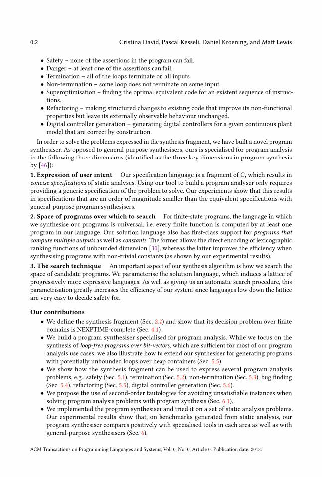
Program Synthesis for Program Analysis
CRISTINA DAVID, University of Oxford, UK
PASCAL KESSELI, University of Oxford, UK
DANIEL KROENING, University of Oxford, UK
MATT LEWIS, University of Oxford, UK
In this paper, we propose a unified framework for designing static analysers based on program synthesis. For thispurpose, we identify a fragment of second-order logic with restricted quantification that is expressive enough
to model numerous static analysis problems (e.g., safety proving, bug finding, termination and non-termination
proving, refactoring). As our focus is on programs that use bit-vectors, we build a decision procedure for this
fragment over finite domains in the form of a program synthesiser. We provide instantiations of our framework
for solving a diverse range of program verification tasks such as termination, non-termination, safety and
bug finding, superoptimisation and refactoring. Our experimental results show that our program synthesiser
compares positively with specialised tools in each area as well as with general-purpose synthesisers.
CCS Concepts: • Theory of computation→ Automated reasoning; • Software and its engineering→
Source code generation; Automated static analysis; Formal software verification;
Additional Key Words and Phrases: Program synthesis, program termination
ACM Reference Format:Cristina David, Pascal Kesseli, Daniel Kroening, and Matt Lewis. 2018. Program Synthesis for Program Analysis.
ACM Trans. Program. Lang. Syst. 0, 0, Article 0 ( 2018), 44 pages. https://doi.org/0000001.0000001
1 INTRODUCTIONFundamentally, every static program analysis is searching for a program proof. For safety analysers
this proof takes the form of a program invariant [31], for bug finders it is a counter-model [25],
for termination analysis it can be a ranking function [40], whereas for non-termination it is a
recurrence set [50]. Algorithmic methods for the computation of each of these proofs was subject to
extensive research resulting in a multitude of specialised techniques. This specialisation complicates
combinations of techniques, and precludes synergies between their implementations.
In this paper, we propose a program synthesis-based framework for designing program analysers.
This framework allows implementing new analyses easily by only providing a description of the
corresponding program proofs. This essentially enables a declarative way of designing program
analyses, where we specify what we want to achieve rather than the details of how to achieve it.
In order for a program analysis problem to be solved with our framework, it must be expressible
in a fragment of second-order logic with restricted quantification, which we call the synthesisfragment. We show that the synthesis fragment is general enough to capture many such problems
by providing instantiations of our framework for the following diverse set of tasks:
Authors’ addresses: Cristina David, University of Oxford, Wolfson Building, Parks Road, Oxford, UK; Pascal Kesseli,
University of Oxford, Wolfson Building, Parks Road, Oxford, UK; Daniel Kroening, University of Oxford, Wolfson Building,
Parks Road, Oxford, UK; Matt Lewis, University of Oxford, Wolfson Building, Parks Road, Oxford, UK.
Permission to make digital or hard copies of all or part of this work for personal or classroom use is granted without fee
provided that copies are not made or distributed for profit or commercial advantage and that copies bear this notice and
the full citation on the first page. Copyrights for components of this work owned by others than ACM must be honored.
Abstracting with credit is permitted. To copy otherwise, or republish, to post on servers or to redistribute to lists, requires
prior specific permission and/or a fee. Request permissions from [email protected].
© 2018 Association for Computing Machinery.
0164-0925/2018/0-ART0 $15.00
https://doi.org/0000001.0000001
ACM Transactions on Programming Languages and Systems, Vol. 0, No. 0, Article 0. Publication date: 2018.
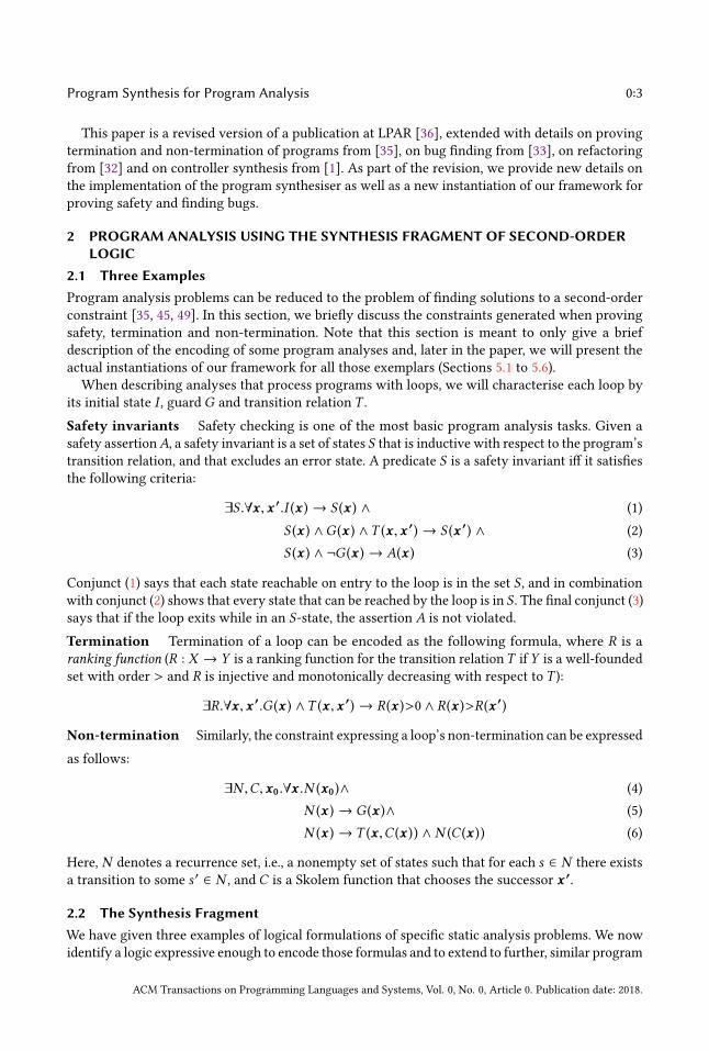
0:2 Cristina David, Pascal Kesseli, Daniel Kroening, and Matt Lewis
• Safety – none of the assertions in the program can fail.
• Danger – at least one of the assertions can fail.
• Termination – all of the loops terminate on all inputs.
• Non-termination – some loop does not terminate on some input.
• Superoptimisation – finding the optimal equivalent code for an existent sequence of instruc-
tions.
• Refactoring – making structured changes to existing code that improve its non-functional
properties but leave its externally observable behaviour unchanged.
• Digital controller generation – generating digital controllers for a given continuous plant
model that are correct by construction.
In order to solve the problems expressed in the synthesis fragment, we have built a novel program
synthesiser. As opposed to general-purpose synthesisers, ours is specialised for program analysis
in the following three dimensions (identified as the three key dimensions in program synthesis
by [46]):
1. Expression of user intent Our specification language is a fragment of C, which results in
concise specifications of static analyses. Using our tool to build a program analyser only requires
providing a generic specification of the problem to solve. Our experiments show that this results
in specifications that are an order of magnitude smaller than the equivalent specifications with
general-purpose program synthesisers.
2. Space of programs over which to search For finite-state programs, the language in which
we synthesise our programs is universal, i.e. every finite function is computed by at least one
program in our language. Our solution language also has first-class support for programs thatcompute multiple outputs as well as constants. The former allows the direct encoding of lexicographic
ranking functions of unbounded dimension [30], whereas the latter improves the efficiency when
synthesising programs with non-trivial constants (as shown by our experimental results).
3. The search technique An important aspect of our synthesis algorithm is how we search the
space of candidate programs. We parameterise the solution language, which induces a lattice of
progressively more expressive languages. As well as giving us an automatic search procedure, this
parametrisation greatly increases the efficiency of our system since languages low down the lattice
are very easy to decide safety for.
Our contributions• We define the synthesis fragment (Sec. 2.2) and show that its decision problem over finite
domains is NEXPTIME-complete (Sec. 4.1).
• We build a program synthesiser specialised for program analysis. While we focus on the
synthesis of loop-free programs over bit-vectors, which are sufficient for most of our program
analysis use cases, we also illustrate how to extend our synthesiser for generating programs
with potentially unbounded loops over heap containers (Sec. 5.5).
• We show how the synthesis fragment can be used to express several program analysis
problems, e.g., safety (Sec. 5.1), termination (Sec. 5.2), non-termination (Sec. 5.3), bug finding
(Sec. 5.4), refactoring (Sec. 5.5), digital controller generation (Sec. 5.6).
• We propose the use of second-order tautologies for avoiding unsatisfiable instances when
solving program analysis problems with program synthesis (Sec. 6.1).
• We implemented the program synthesiser and tried it on a set of static analysis problems.
Our experimental results show that, on benchmarks generated from static analysis, our
program synthesiser compares positively with specialised tools in each area as well as with
general-purpose synthesisers (Sec. 6).
ACM Transactions on Programming Languages and Systems, Vol. 0, No. 0, Article 0. Publication date: 2018.
Program Synthesis for Program Analysis 0:3
This paper is a revised version of a publication at LPAR [36], extended with details on proving
termination and non-termination of programs from [35], on bug finding from [33], on refactoring
from [32] and on controller synthesis from [1]. As part of the revision, we provide new details on
the implementation of the program synthesiser as well as a new instantiation of our framework for
proving safety and finding bugs.
2 PROGRAM ANALYSIS USING THE SYNTHESIS FRAGMENT OF SECOND-ORDERLOGIC
2.1 Three ExamplesProgram analysis problems can be reduced to the problem of finding solutions to a second-order
constraint [35, 45, 49]. In this section, we briefly discuss the constraints generated when proving
safety, termination and non-termination. Note that this section is meant to only give a brief
description of the encoding of some program analyses and, later in the paper, we will present the
actual instantiations of our framework for all those exemplars (Sections 5.1 to 5.6).
When describing analyses that process programs with loops, we will characterise each loop by
its initial state I , guard G and transition relation T .
Safety invariants Safety checking is one of the most basic program analysis tasks. Given a
safety assertionA, a safety invariant is a set of states S that is inductive with respect to the program’s
transition relation, and that excludes an error state. A predicate S is a safety invariant iff it satisfies
the following criteria:
∃S .∀x ,x ′.I (x ) → S (x ) ∧ (1)
S (x ) ∧G (x ) ∧T (x ,x ′) → S (x ′) ∧ (2)
S (x ) ∧ ¬G (x ) → A(x ) (3)
Conjunct (1) says that each state reachable on entry to the loop is in the set S , and in combination
with conjunct (2) shows that every state that can be reached by the loop is in S . The final conjunct (3)says that if the loop exits while in an S-state, the assertion A is not violated.
Termination Termination of a loop can be encoded as the following formula, where R is a
ranking function (R : X → Y is a ranking function for the transition relationT if Y is a well-founded
set with order > and R is injective and monotonically decreasing with respect to T ):
∃R.∀x ,x ′.G (x ) ∧T (x ,x ′) → R (x )>0 ∧ R (x )>R (x ′)
Non-termination Similarly, the constraint expressing a loop’s non-termination can be expressed
as follows:
∃N ,C,x0.∀x .N (x0)∧ (4)
N (x ) → G (x )∧ (5)
N (x ) → T (x ,C (x )) ∧ N (C (x )) (6)
Here, N denotes a recurrence set, i.e., a nonempty set of states such that for each s ∈ N there exists
a transition to some s ′ ∈ N , and C is a Skolem function that chooses the successor x ′.
2.2 The Synthesis FragmentWe have given three examples of logical formulations of specific static analysis problems. We now
identify a logic expressive enough to encode those formulas and to extend to further, similar program
ACM Transactions on Programming Languages and Systems, Vol. 0, No. 0, Article 0. Publication date: 2018.
0:4 Cristina David, Pascal Kesseli, Daniel Kroening, and Matt Lewis
analysis problems. We refer to the logic as the synthesis fragment1, a fragment of second-order
logic with restrictions on the use of quantification.
Definition 2.1 (Synthesis Fragment (SF )). A formula is in the synthesis fragment iff it is of the
form
∃P .Qx .σ (x ,P )
where each element P (of the vector P ) ranges over functions, eachQ is either ∃ or ∀, each x ranges
over ground terms and σ is a quantifier-free formula.
If a pair (x ,P ) is a satisfying model for a formula in the synthesis fragment, then we write
(x ,P ) |= σ . For the remainder of the presentation, we drop the vector notation and write x for x ,with the understanding that all quantified variables range over vectors.
3 SOLVING THE SYNTHESIS FRAGMENT USING PROGRAM SYNTHESISA satisfying model for a formula in SF is an assignment mapping each of the second-order variables
to some function of the appropriate type and arity. We are interested in generating programs that
compute these functions. For this purpose, we make use of program synthesis.The synthesis problem is given in the form of a specification σ , which is a function taking a
program P and input x as parameters and returning a boolean telling us whether P did “the right
thing” on input x . Basically, the synthesis problem is to determine the truth of the formula given in
Definition 2.1.
Definition 3.1 (Synthesis Formula). A synthesis formula is of the form:
∃P .∀x .σ (x , P ).
Note that, as opposed to Definition 2.1, the first order variables in the synthesis formula are all
universally quantified.
While SF is obviously undecidable, we can sketch the design of an incomplete solver for it: we
will convert the SF satisfiability problem into an equisatisfiable synthesis problem, which we will
then solve with a program synthesiser. This design will be elaborated next, followed by describing
how to instantiate it for the synthesis finite-state programs in Sec. 4 and for synthesising programs
with unbounded loops in Sec. 5.5.
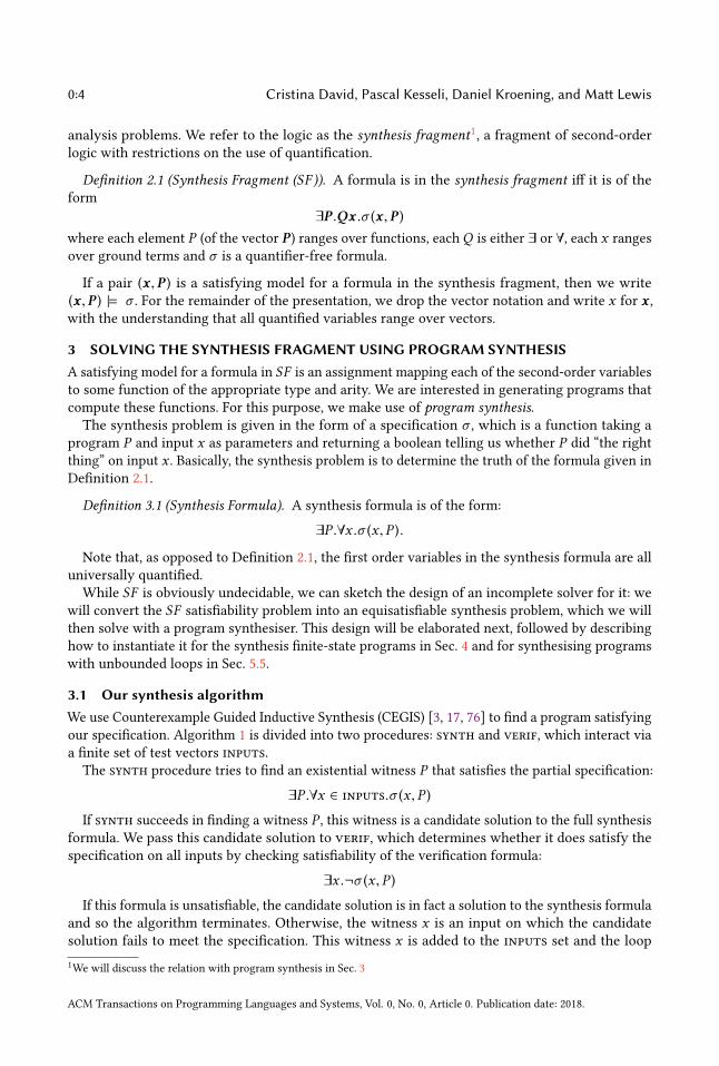
3.1 Our synthesis algorithmWe use Counterexample Guided Inductive Synthesis (CEGIS) [3, 17, 76] to find a program satisfying
our specification. Algorithm 1 is divided into two procedures: synth and verif, which interact via
a finite set of test vectors inputs.
The synth procedure tries to find an existential witness P that satisfies the partial specification:
∃P .∀x ∈ inputs.σ (x , P )
If synth succeeds in finding a witness P , this witness is a candidate solution to the full synthesis
formula. We pass this candidate solution to verif, which determines whether it does satisfy the
specification on all inputs by checking satisfiability of the verification formula:
∃x .¬σ (x , P )
If this formula is unsatisfiable, the candidate solution is in fact a solution to the synthesis formula
and so the algorithm terminates. Otherwise, the witness x is an input on which the candidate
solution fails to meet the specification. This witness x is added to the inputs set and the loop
1We will discuss the relation with program synthesis in Sec. 3
ACM Transactions on Programming Languages and Systems, Vol. 0, No. 0, Article 0. Publication date: 2018.
Program Synthesis for Program Analysis 0:5
ALGORITHM 1: Abstract refinement algorithm
1 function Synth(inputs)2 (i1, . . . , iN ) ← inputs;3 query← ∃P .σ (i1, P ) ∧ . . . ∧ σ (iN , P );4 result← Decide(query);5 if result.satisfiable then6 return result.model;
7 else return UNSAT ;
8 function Verif(P)9 query← ∃x .¬σ (x , P );
10 result← Decide(query);11 if result.satisfiable then12 return result.model;
13 else return VALID;
14 function Refinement Loop
15 inputs← ∅;16 while true do17 candidate← Synth(inputs);18 if candidate = UNSAT then19 return UNSAT ;
20 result← Verif(candidate);21 if result = valid then22 return candidate;
23 else inputs← inputs ∪ result;
Synth Verif Done
Candidate program
Counterexample input
Valid
Fig. 1. Abstract synthesis refinement loop
iterates again. It is worth noting that each iteration of the loop adds a new input to the set of inputs
being used for synthesis. The refinement loop is described in Fig 1.
3.2 Program generation strategiesAn important aspect of our synthesis algorithm is the manner in which we search the space of
candidate programs. We employ the following strategies in parallel:
(1) Explicit Proof Search. The simplest strategy for finding candidates is to just exhaustively
enumerate them all, starting with the shortest and progressively increasing the number of
instructions.
(2) Symbolic Bounded Model Checking. Another complete method for generating candidates is to
simply use BMC on the synth.c program.
(3) Genetic Programming and Incremental Evolution. Our final strategy is genetic programming
(GP) [18, 65].
The third option provides an adaptive way of searching through the space of programs for an
individual that is “fit” in some sense. We measure the fitness of an individual by counting the
number of tests in inputs for which it satisfies the specification. To bootstrap GP in the first
iteration of the CEGIS loop, we generate a population of random programs. We then iteratively
evolve this population by applying the genetic operators crossover and mutate. Crossover
ACM Transactions on Programming Languages and Systems, Vol. 0, No. 0, Article 0. Publication date: 2018.
0:6 Cristina David, Pascal Kesseli, Daniel Kroening, and Matt Lewis
combines selected existing programs into new programs, whereas mutate randomly changes parts
of a single program. Fitter programs are more likely to be selected.
Rather than generating a random population at the beginning of each subsequent iteration of the
CEGIS loop, we start with the population we had at the end of the previous iteration. The intuition
here is that this population contained many individuals that performed well on the k inputs we
had before, so they will probably continue to perform well on the k + 1 inputs we have now. In the
parlance of evolutionary programming, this is known as incremental evolution [44].
4 SYNTHESIS FOR PROGRAM VARIABLES WITH BIT-VECTOR DOMAINSProgramming languages such as C and Java use numerical data types with finite ranges, and give
semantics to the arithmetic operators using fixed-width binary encodings, otherwise known as
bit-vectors. We are interested in solving static analysis problems for these programming languages.
For this purpose, we investigate the special case of the synthesis fragment over finite domains
(Sec 4.1) followed by using finite-state program synthesis in order to decide it (Sec 4.2).
4.1 The synthesis fragment over finite domainsWhen interpreting the ground terms over a finite domainD, the synthesis fragment is decidable
and its decision problem is NEXPTIME-complete.
Theorem 4.1 (SFD is NEXPTIME-complete). For an instance of Definition 2.1 with n first-order variables, where the ground terms are interpreted over D, checking the truth of the formula isNEXPTIME-complete.
Proof. For this proof we make use of Fagin’s Theorem [39], which says that the class of sets Arecognisable in time ∥A∥k , for some k , by a nondeterministic Turing machine is exactly the class of
sets definable by existential second-order sentences.
In order to apply Fagin’s Theorem, we must establish the size of the universe implied by it. Since
Definition 2.1 uses n D variables, the universe is the set of interpretations of the n variables. This
set has size |D|n , and so by Fagin’s Theorem, Definition 2.1 over finite domains defines exactly
the class sets recognisable in ( |D|n )k time by a nondeterministic Turing machine. This is the
class NEXPTIME, and so checking validity of an arbitrary instance of Definition 2.1 over D is
NEXPTIME-complete.
We write SFD to denote the synthesis fragment over a finite domainD. The finite-state synthesis
problem checks the truth of of the formula given in the following Definition.
Definition 4.2 (Finite Synthesis Formula). A finite synthesis formula is of the form:
∃P .∀x ∈ D.σ (x , P ),
where D is a finite domain.
Note that, as opposed to the synthesis formula (Definition 3.1), the first order variables in the
finite synthesis formula are interpreted over a finite domain D.
Satisfiability of SFD can be reduced to finite-state program synthesis, as shown by Theorem 4.3.
Theorem 4.3 (SFD is Polynomial Time Reducible to Finite Synthesis). Every instance ofDefinition 2.1, where the ground terms are interpreted over D is polynomial-time reducible to a finitesynthesis formula (i.e., an instance of Definition 4.2).
Proof. We first Skolemise the instance of Definition 2.1 to produce an equisatisfiable second-
order sentence with the first-order part only having universal quantifiers (i.e., bring the formula
into Skolem normal form). This process will have introduced a function symbol for each first
ACM Transactions on Programming Languages and Systems, Vol. 0, No. 0, Article 0. Publication date: 2018.
Program Synthesis for Program Analysis 0:7
order existentially quantified variable and would have taken linear time. Now we just existentially
quantify over the Skolem functions, which again takes linear time and space. The resulting formula
is an instance of Definition 4.2.
Corollary 4.4. Finite-state program synthesis is NEXPTIME-complete.
4.2 A decision procedure for SFD based on program synthesisWe will now show how the generic construction of Section 3 can be instantiated to produce a
finite-state program synthesiser. A natural choice for such a synthesiser would be to work in the
logic of quantifier-free propositional formulae and to use a propositional SAT or SMT-BV solver as
the decision procedure. However, we propose a slightly different tack, which is to use a decidable
fragment of C as a “high level” logic. We call this fragment C−. The characteristic property of a
C−program is that safety can be decided for it using a single query to a Bounded Model Checker.
A C−program is just a C program with the following restrictions:
(i) all loops in the program must have a constant bound;
(ii) all recursion in the program must be limited to a constant depth;
(iii) all arrays must be statically allocated (i.e., not using malloc), and be of constant size.
C−programs may use nondeterministic values, assumptions and types with arbitrary but fixed
width.
Since each loop is bounded by a constant, and each recursive function call is limited to a constant
depth, a C−program necessarily terminates and in fact does so in O (1) time. If we call the largest
loop bound k , then a Bounded Model Checker with an unrolling bound of k will be a complete
decision procedure for the safety of the program. For a C−program of size l and with largest loop
bound k , a Bounded Model Checker will create a SAT problem of size O (lk ). Conversely, a SATproblem of size s can be converted trivially into a loop-free C
−program of size O (s ). The safety
problem for C−is therefore NP-complete, which means it can be decided fairly efficiently for many
practical instances.
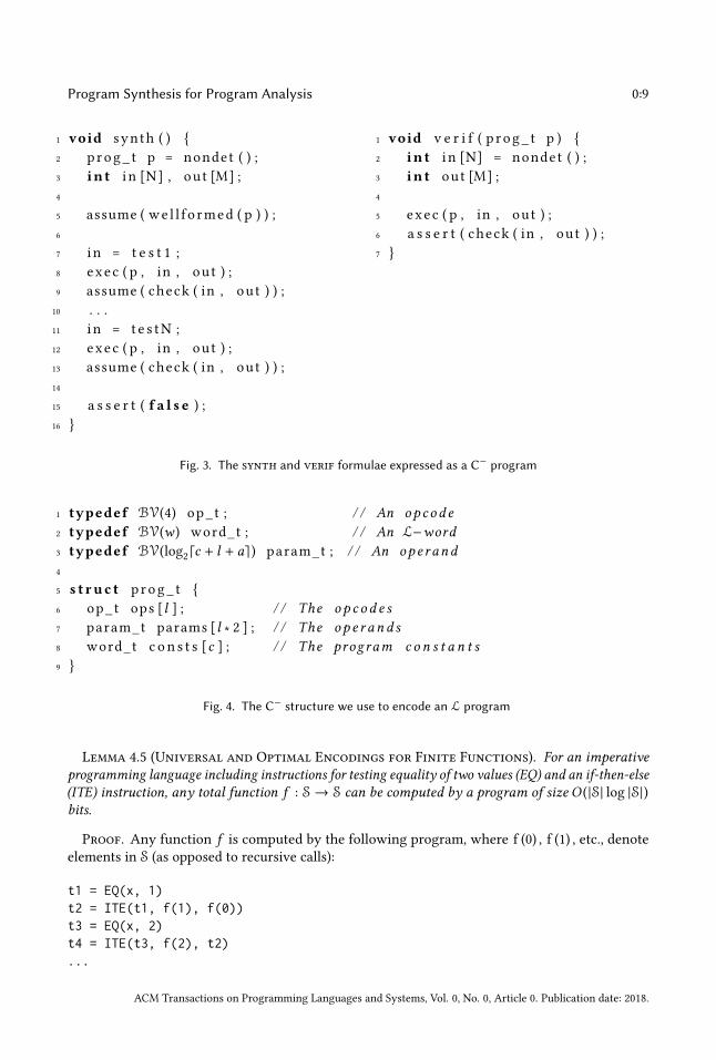
4.3 Encoding the synthesis problemWe now express the synth and verif formulae as safety properties of C
−programs as shown in
Fig. 3.
In the synth portion of the CEGIS loop, we construct a program synth.c, which takes as
parameters a candidate program P and test inputs. The program contains an assertion which fails iff
P meets the specification for each of the inputs. Finding a new candidate program is then equivalent
to checking the safety of synth.c. The synth program is a C−program, which means we can check
its safety with Bounded Model Checking (BMC).
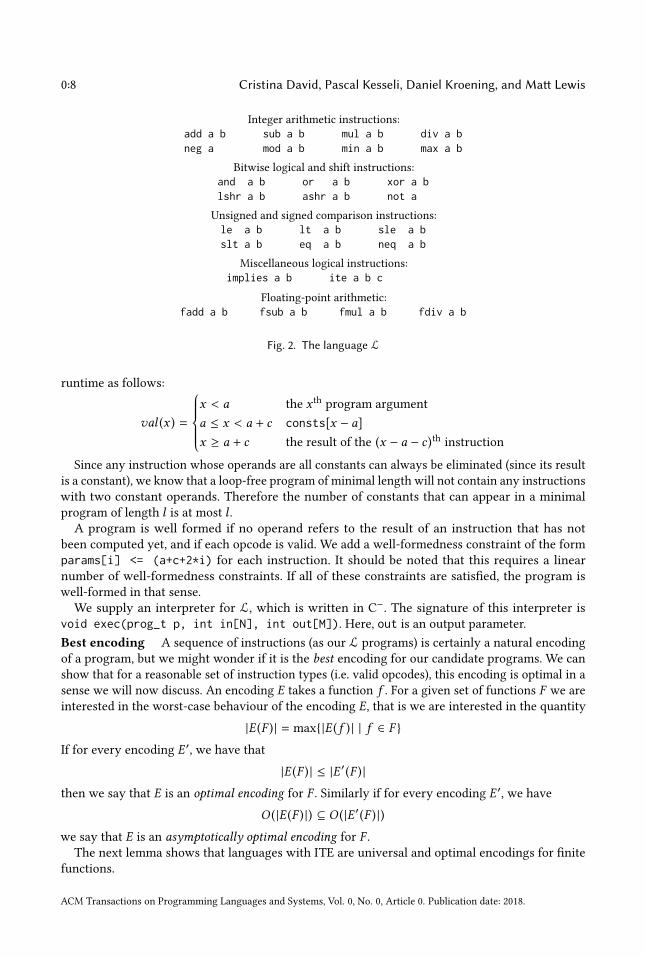
A candidate solution P is written in a simple RISC-like language L, whose syntax is given in
Fig. 2. The exact C−encoding of an L program is shown in Fig. 4. Note that we use bit-vector types
of configurable size: BV(n) denotes a bit-vector type of size n bits and its semantics are equivalent
to an unsigned int type of the corresponding bit width n.The prog_t structure encodes a program, which is a sequence of instructions. The parameter
a is the number of arguments the program takes. The i-th instruction has opcode ops[i], leftoperand params[i*2] and right operand params[i*2 + 1]. An operand refers to either a program
constant, a program argument or the result of a previous instruction, and its value is determined at
ACM Transactions on Programming Languages and Systems, Vol. 0, No. 0, Article 0. Publication date: 2018.
0:8 Cristina David, Pascal Kesseli, Daniel Kroening, and Matt Lewis
Integer arithmetic instructions:
add a b sub a b mul a b div a bneg a mod a b min a b max a b
Bitwise logical and shift instructions:
and a b or a b xor a blshr a b ashr a b not a
Unsigned and signed comparison instructions:
le a b lt a b sle a bslt a b eq a b neq a b
Miscellaneous logical instructions:
implies a b ite a b c
Floating-point arithmetic:
fadd a b fsub a b fmul a b fdiv a b
Fig. 2. The language L
runtime as follows:
val (x ) =
x < a the x th program argument
a ≤ x < a + c consts[x − a]
x ≥ a + c the result of the (x − a − c )th instruction
Since any instruction whose operands are all constants can always be eliminated (since its result
is a constant), we know that a loop-free program of minimal length will not contain any instructions
with two constant operands. Therefore the number of constants that can appear in a minimal
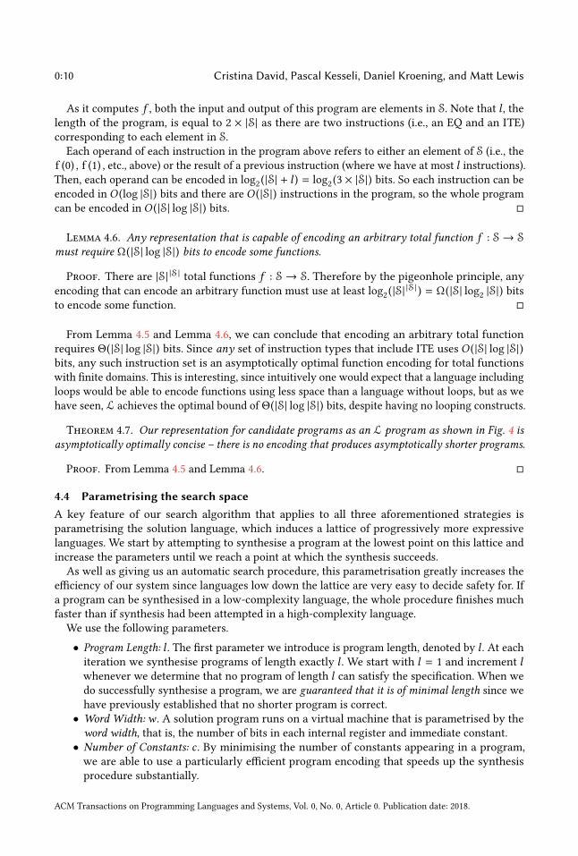
program of length l is at most l .A program is well formed if no operand refers to the result of an instruction that has not
been computed yet, and if each opcode is valid. We add a well-formedness constraint of the form
params[i] <= (a+c+2*i) for each instruction. It should be noted that this requires a linear
number of well-formedness constraints. If all of these constraints are satisfied, the program is
well-formed in that sense.
We supply an interpreter for L, which is written in C−. The signature of this interpreter is
void exec(prog_t p, int in[N], int out[M]). Here, out is an output parameter.
Best encoding A sequence of instructions (as our L programs) is certainly a natural encoding
of a program, but we might wonder if it is the best encoding for our candidate programs. We can
show that for a reasonable set of instruction types (i.e. valid opcodes), this encoding is optimal in a
sense we will now discuss. An encoding E takes a function f . For a given set of functions F we are
interested in the worst-case behaviour of the encoding E, that is we are interested in the quantity
|E (F ) | = max|E ( f ) | | f ∈ F
If for every encoding E ′, we have that
|E (F ) | ≤ |E ′(F ) |
then we say that E is an optimal encoding for F . Similarly if for every encoding E ′, we have
O ( |E (F ) |) ⊆ O ( |E ′(F ) |)
we say that E is an asymptotically optimal encoding for F .The next lemma shows that languages with ITE are universal and optimal encodings for finite
functions.
ACM Transactions on Programming Languages and Systems, Vol. 0, No. 0, Article 0. Publication date: 2018.
Program Synthesis for Program Analysis 0:9
1 void synth ( )
2 prog_ t p = nondet ( ) ;
3 in t i n [N] , out [M] ;
4
5 assume ( we l l fo rmed ( p ) ) ;
6
7 i n = t e s t 1 ;
8 exec ( p , in , out ) ;
9 assume ( check ( in , out ) ) ;
10 . . .
11 i n = t e s tN ;
12 exec ( p , in , out ) ;
13 assume ( check ( in , out ) ) ;
14
15 a s s e r t ( f a l s e ) ;
16
1 void v e r i f ( p rog_ t p )
2 in t i n [N] = nondet ( ) ;
3 in t out [M] ;
4
5 exec ( p , in , out ) ;
6 a s s e r t ( check ( in , out ) ) ;
7
Fig. 3. The synth and verif formulae expressed as a C− program
1 typedef BV(4) op_t ; / / An op c od e2 typedef BV(w ) word_t ; / / An L−word3 typedef BV(log
2⌈c + l + a⌉) param_t ; / / An ope rand
4
5 s t ruc t prog_ t
6 op_t ops [l ] ; / / The o p c o d e s7 param_t params [l ∗ 2 ] ; / / The o p e r and s8 word_t c on s t s [c ] ; / / The program c o n s t a n t s9
Fig. 4. The C− structure we use to encode an L program
Lemma 4.5 (Universal and Optimal Encodings for Finite Functions). For an imperativeprogramming language including instructions for testing equality of two values (EQ) and an if-then-else(ITE) instruction, any total function f : S→ S can be computed by a program of size O ( |S| log |S|)bits.
Proof. Any function f is computed by the following program, where f (0) , f (1) , etc., denote
elements in S (as opposed to recursive calls):
t1 = EQ(x, 1)t2 = ITE(t1, f(1), f(0))t3 = EQ(x, 2)t4 = ITE(t3, f(2), t2)...
ACM Transactions on Programming Languages and Systems, Vol. 0, No. 0, Article 0. Publication date: 2018.
0:10 Cristina David, Pascal Kesseli, Daniel Kroening, and Matt Lewis
As it computes f , both the input and output of this program are elements in S. Note that l , thelength of the program, is equal to 2 × |S| as there are two instructions (i.e., an EQ and an ITE)
corresponding to each element in S.
Each operand of each instruction in the program above refers to either an element of S (i.e., the
f (0) , f (1) , etc., above) or the result of a previous instruction (where we have at most l instructions).Then, each operand can be encoded in log
2( |S| + l ) = log
2(3 × |S|) bits. So each instruction can be
encoded in O (log |S|) bits and there are O ( |S|) instructions in the program, so the whole program
can be encoded in O ( |S| log |S|) bits.
Lemma 4.6. Any representation that is capable of encoding an arbitrary total function f : S→ S
must require Ω( |S| log |S|) bits to encode some functions.
Proof. There are |S| |S | total functions f : S → S. Therefore by the pigeonhole principle, any
encoding that can encode an arbitrary function must use at least log2( |S| |S | ) = Ω( |S| log
2|S|) bits
to encode some function.
From Lemma 4.5 and Lemma 4.6, we can conclude that encoding an arbitrary total function
requires Θ( |S| log |S|) bits. Since any set of instruction types that include ITE uses O ( |S| log |S|)bits, any such instruction set is an asymptotically optimal function encoding for total functions
with finite domains. This is interesting, since intuitively one would expect that a language including
loops would be able to encode functions using less space than a language without loops, but as we
have seen, L achieves the optimal bound of Θ( |S| log |S|) bits, despite having no looping constructs.
Theorem 4.7. Our representation for candidate programs as an L program as shown in Fig. 4 isasymptotically optimally concise – there is no encoding that produces asymptotically shorter programs.
Proof. From Lemma 4.5 and Lemma 4.6.
4.4 Parametrising the search spaceA key feature of our search algorithm that applies to all three aforementioned strategies is
parametrising the solution language, which induces a lattice of progressively more expressive
languages. We start by attempting to synthesise a program at the lowest point on this lattice and
increase the parameters until we reach a point at which the synthesis succeeds.
As well as giving us an automatic search procedure, this parametrisation greatly increases the
efficiency of our system since languages low down the lattice are very easy to decide safety for. If
a program can be synthesised in a low-complexity language, the whole procedure finishes much
faster than if synthesis had been attempted in a high-complexity language.
We use the following parameters.
• Program Length: l . The first parameter we introduce is program length, denoted by l . At eachiteration we synthesise programs of length exactly l . We start with l = 1 and increment lwhenever we determine that no program of length l can satisfy the specification. When we
do successfully synthesise a program, we are guaranteed that it is of minimal length since we
have previously established that no shorter program is correct.
• Word Width:w . A solution program runs on a virtual machine that is parametrised by the
word width, that is, the number of bits in each internal register and immediate constant.
• Number of Constants: c . By minimising the number of constants appearing in a program,
we are able to use a particularly efficient program encoding that speeds up the synthesis
procedure substantially.
ACM Transactions on Programming Languages and Systems, Vol. 0, No. 0, Article 0. Publication date: 2018.
Program Synthesis for Program Analysis 0:11
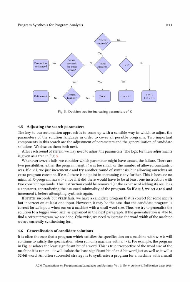
Synth
succeeds?
Verif
succeeds?
c < l?
Done!
Verif
succeeds
for small
words?
c := c + 1c := 0
l := l + 1
Genera-
lisation?
Parameters
unchanged
Refinement
Yes
No
Yes
No
Yes
No
Yes
No
YesNo
Fig. 5. Decision tree for increasing parameters of L
4.5 Adjusting the search parametersThe key to our automation approach is to come up with a sensible way in which to adjust the
parameters of the solution language in order to cover all possible programs. Two important
components in this search are the adjustment of parameters and the generalisation of candidate
solutions. We discuss them both next.
After each round of synth, we may need to adjust the parameters. The logic for these adjustments
is given as a tree in Fig. 5.
Whenever synth fails, we consider which parameter might have caused the failure. There are
two possibilities: either the program length l was too small, or the number of allowed constants cwas. If c < l , we just increment c and try another round of synthesis, but allowing ourselves an
extra program constant. If c = l , there is no point in increasing c any further. This is because no
minimal L-program has c > l , for if it did there would have to be at least one instruction with
two constant operands. This instruction could be removed (at the expense of adding its result as
a constant), contradicting the assumed minimality of the program. So if c = l , we set c to 0 and
increment l , before attempting synthesis again.
If synth succeeds but verif fails, we have a candidate program that is correct for some inputs
but incorrect on at least one input. However, it may be the case that the candidate program is
correct for all inputs when run on a machine with a small word size. Thus, we try to generalise the
solution to a bigger word size, as explained in the next paragraph. If the generalisation is able to
find a correct program, we are done. Otherwise, we need to increase the word width of the machine
we are currently synthesising for.
4.6 Generalisation of candidate solutionsIt is often the case that a program which satisfies the specification on a machine withw = k will
continue to satisfy the specification when run on a machine withw > k . For example, the program
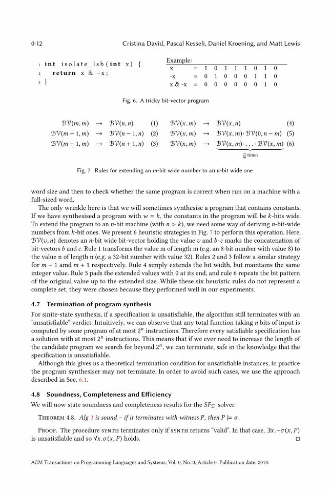
in Fig. 6 isolates the least-significant bit of a word. This is true irrespective of the word size of the
machine it is run on – it will isolate the least-significant bit of an 8-bit word just as well as it will a
32-bit word. An often successful strategy is to synthesise a program for a machine with a small
ACM Transactions on Programming Languages and Systems, Vol. 0, No. 0, Article 0. Publication date: 2018.
0:12 Cristina David, Pascal Kesseli, Daniel Kroening, and Matt Lewis
1 in t i s o l a t e _ l s b ( in t x )
2 return x & −x ;
3
Example:
x = 1 0 1 1 1 0 1 0
-x = 0 1 0 0 0 1 1 0
x & -x = 0 0 0 0 0 0 1 0
Fig. 6. A tricky bit-vector program
BV(m,m) → BV(n,n) (1)
BV(m − 1,m) → BV(n − 1,n) (2)
BV(m + 1,m) → BV(n + 1,n) (3)
BV(x ,m) → BV(x ,n) (4)
BV(x ,m) → BV(x ,m)·BV(0,n −m) (5)
BV(x ,m) → BV(x ,m)· . . . ·BV(x ,m)︸ ︷︷ ︸nm times
(6)
Fig. 7. Rules for extending anm-bit wide number to an n-bit wide one
word size and then to check whether the same program is correct when run on a machine with a
full-sized word.
The only wrinkle here is that we will sometimes synthesise a program that contains constants.
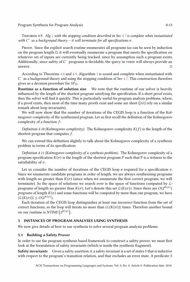
If we have synthesised a program with w = k , the constants in the program will be k-bits wide.To extend the program to an n-bit machine (with n > k), we need some way of deriving n-bit-widenumbers from k-bit ones. We present 6 heuristic strategies in Fig. 7 to perform this operation. Here,
BV(v,n) denotes an n-bit wide bit-vector holding the value v and b· c marks the concatenation of
bit-vectors b and c . Rule 1 transforms the value m of length m (e.g. an 8-bit number with value 8) to
the value n of length n (e.g. a 32-bit number with value 32). Rules 2 and 3 follow a similar strategy
form − 1 amdm + 1 respectively. Rule 4 simply extends the bit width, but maintains the same
integer value. Rule 5 pads the extended values with 0 at its end, and rule 6 repeats the bit pattern
of the original value up to the extended size. While these six heuristic rules do not represent a
complete set, they were chosen because they performed well in our experiments.
4.7 Termination of program synthesisFor sinite-state synthesis, if a specification is unsatisfiable, the algorithm still terminates with an
“unsatisfiable” verdict. Intuitively, we can observe that any total function taking n bits of input is
computed by some program of at most 2ninstructions. Therefore every satisfiable specification has
a solution with at most 2ninstructions. This means that if we ever need to increase the length of
the candidate program we search for beyond 2n, we can terminate, safe in the knowledge that the
specification is unsatisfiable.
Although this gives us a theoretical termination condition for unsatisfiable instances, in practice
the program synthesiser may not terminate. In order to avoid such cases, we use the approach
described in Sec. 6.1.
4.8 Soundness, Completeness and EfficiencyWe will now state soundness and completeness results for the SFD solver.
Theorem 4.8. Alg 1 is sound – if it terminates with witness P , then P |= σ .
Proof. The procedure synth terminates only if synth returns “valid”. In that case, ∃x .¬σ (x , P )is unsatisfiable and so ∀x .σ (x , P ) holds.
ACM Transactions on Programming Languages and Systems, Vol. 0, No. 0, Article 0. Publication date: 2018.
Program Synthesis for Program Analysis 0:13
Theorem 4.9. Alg 1 with the stopping condition described in Sec 4.7 is complete when instantiatedwith C− as a background theory – it will terminate for all specifications σ .
Proof. Since the explicit search routine enumerates all programs (as can be seen by induction
on the program length l), it will eventually enumerate a program that meets the specification on
whatever set of inputs are currently being tracked, since by assumption such a program exists.
Additionally, since safety of C−programs is decidable, the query in verif will always provide an
answer.
According to Theorems 4.8 and 4.9, Algorithm 1 is sound and complete when instantiated with
C−as a background theory and using the stopping condition of Sec 4.7. This construction therefore
gives as a decision procedure for SFD.
Runtime as a function of solution size We note that the runtime of our solver is heavily
influenced by the length of the shortest program satisfying the specification. If a short proof exists,
then the solver will find it quickly. This is particularly useful for program analysis problems, where,
if a proof exists, then most of the time many proofs exist and some are short ([60] rely on a similar
remark about loop invariants).
We will now show that the number of iterations of the CEGIS loop is a function of the Kol-
mogorov complexity of the synthesised program. Let us first recall the definition of the Kolmogorov
complexity of a function f :
Definition 4.10 (Kolmogorov complexity). The Kolmogorov complexity K ( f ) is the length of the
shortest program that computes f .
We can extend this definition slightly to talk about the Kolmogorov complexity of a synthesis
problem in terms of its specification:
Definition 4.11 (Kolmogorov complexity of a synthesis problem). The Kolmogorov complexity of a
program specification K (σ ) is the length of the shortest program P such that P is a witness to the
satisfiability of σ .
Let us consider the number of iterations of the CEGIS loop n required for a specification σ .Since we enumerate candidate programs in order of length, we are always synthesising programs
with length no greater than K (σ ) (since when we enumerate the first correct program, we will
terminate). So the space of solutions we search over is the space of functions computed by L-
programs of length no greater than K (σ ). Let’s denote this set L(K (σ )). Since there are O (2K (σ ) )programs of length K (σ ) and some functions will be computed by more than one program, we have
|L(K (σ )) | ≤ O (2K (σ ) ).Each iteration of the CEGIS loop distinguishes at least one incorrect function from the set of
correct functions, so the loop will iterate no more than |L(K (σ )) | times. Therefore another bound
on our runtime is NTIME(2K (σ )).
5 INSTANCES OF PROGRAM ANALYSES USING SYNTHESISWe now give details of how to use synthesis to solve several program analysis problems.
5.1 Building a Safety ProverIn order to use the program synthesis based framework to construct a safety prover, we must first
look at the formulation of safety invariants (which is inside the synthesis fragment).
Safety invariants Given a safety assertionA, a safety invariant is a set of states S that is inductivewith respect to the program’s transition relation, and that excludes an error state. A predicate S
ACM Transactions on Programming Languages and Systems, Vol. 0, No. 0, Article 0. Publication date: 2018.
0:14 Cristina David, Pascal Kesseli, Daniel Kroening, and Matt Lewis
Definition 5.1 (Safety Invariant [SI]).
∃S .∀x ,x ′.I (x ) → S (x ) ∧
S (x ) ∧G (x ) ∧ B (x ,x ′) → S (x ′) ∧
S (x ) ∧ ¬G (x ) → A(x )
Fig. 8. Existence of a safety invariant for a single loop
1 while ( x > 0 )
2 x = ( x − 1 ) & x ;
3
1 y = 1 ;
2
3 while ( x > 0 )
4 x = x − y ;
5
(a) (b)
1 while ( x > 0 )
2 x ++ ;
3
1 while ( i < M | | j < N)
2 i = i + 1 ;
3 j = j + 1 ;
4
(c) (d)
Fig. 9. Termination examples – (a) is taken from [28], (d) is taken from [70]
is a safety invariant iff it satisfies the criteria in Figure 8. The first criterion says that each state
reachable on entry to the loop is in the set S , the second that every state that can be reached by the
loop is in S . The final criterion says that if the loop exits while in an S-state, the assertion A is not
violated.
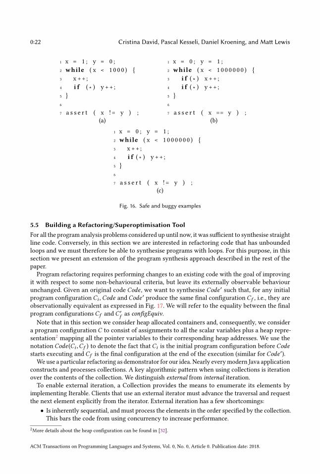
Example 5.2. The program in Fig. 16(a) is safe as x and y are inequal regardless how many times
y gets incremented inside the loop (x is already ahead by 1). Thus, the safety invariant that our
framework synthesises is S (x ,y) = x,y.
As we are only dealing with over-approximations, the generation of constraints corresponding
to proving the safety of a program with nested loops is straightforward and we will not cover it in
the paper.
5.2 Building a Termination ProverIn this section, we describe how to use our program synthesis based framework in order to build a
termination prover. In Sec. 2, we have presented the constraint required when proving unconditional
termination of an isolated loop. Next, we provide more details on how to model both conditional
and unconditional termination for programs with potentially nested loops using the synthesis
fragment. We start by introducing some preliminary notions on termination proving.
A program P is represented as a transition system with state space X and transition relation
T ⊆ X × X . For a state x ∈ X with T (x ,x ′) we say x ′ is a successor of x under T .
ACM Transactions on Programming Languages and Systems, Vol. 0, No. 0, Article 0. Publication date: 2018.
Program Synthesis for Program Analysis 0:15
Definition 5.3 (Unconditional termination). A program is said to be unconditionally terminating if
there is no infinite sequence of states x1,x2, . . . ∈ X with ∀i . T (xi ,xi+1).
We can prove that the program is unconditionally terminating by finding a ranking function
for its transition relation. Not every terminating program has a computable ranking function [79].
However, since we are restricting our attention to programs with finite state spaces, our halting
problem is decidable, as every terminating, finite-state program does have a computable ranking
function.
Definition 5.4 (Ranking function). A function R : X → Y is a ranking function for the transition
relation T if Y is a well-founded set with order > and R is injective and monotonically decreasing
with respect to T . That is to say:
∀x ,x ′ ∈ X .T (x ,x ′) ⇒ R (x ) > R (x ′)
Definition 5.5 (Lexicographic ranking function). For Y = Zm, we say that a ranking function
R : X → Y is lexicographic if it maps each state in X to a tuple of values such that the loop
transition leads to a decrease with respect to the lexicographic ordering for this tuple. The total
order imposed on Y is the lexicographic ordering induced on tuples of Z ’s. So for y = (z1, . . . , zm )and y ′ = (z ′
1, . . . , z ′m ):
y > y ′ ⇐⇒ ∃i ≤ m.zi > z ′i ∧ ∀j < i .zj = z ′j
Wenote that if the program under analysis operates overmathematical integers, some termination
arguments require lexicographic ranking functions, or alternatively, ranking functions whose co-
domain is a countable ordinal, rather than justN. Since we focus on the case of finite-space programs,
in principle we do not need to construct lexicographic ranking functions – it would be sufficient
to find a ranking function whose co-domain is at least as large as the state space of the program
under analysis. However due to technicalities of our implementation, it would be difficult for us
to synthesise programs whose output words were larger than their input words, so it is easier to
generated lexicographic ranking functions where each component of the ranking function is a
fixed width word. Synthesising a lexicographic ranking function producing an N -tuple of k-bitwords is of course equivalent to synthesising a ranking function producing a single Nk-bit word.
5.2.1 Unconditional termination. We will begin our discussion by showing how to encode in the
synthesis fragment the termination of a program consisting of a single loop with no nesting. For
the time being, a loop L(G,T ) is defined by its guard G and body T such that states x satisfying
the loop’s guard are given by the predicateG (x ). The body of the loop is encoded as the transition
relation T (x ,x ′), meaning that state x ′ is reachable from state x via a single iteration of the loop
body. For example, the loop in Figure 9 (a) is encoded as:
G (x ) = x | x > 0
T (x ,x ′) = ⟨x ,x ′⟩ | x ′ = (x − 1) &x
We will abbreviate this with the notation:
G (x ) ≜ x > 0
T (x ,x ′) ≜ x ′ = (x − 1) &x
A loop L(G,T ) is unconditionally terminating iff it eventually terminates regardless of the state it
starts in. To prove unconditional termination, it suffices to find a ranking function for T ∩ (G × X ),i.e., T restricted to states satisfying the loop’s guard.
As the existence of a ranking function is equivalent to the satisfiability of the formula [UT] inFig. 10, a satisfiability witness is a ranking function and thus a proof of L’s unconditional termination.
ACM Transactions on Programming Languages and Systems, Vol. 0, No. 0, Article 0. Publication date: 2018.
0:16 Cristina David, Pascal Kesseli, Daniel Kroening, and Matt Lewis
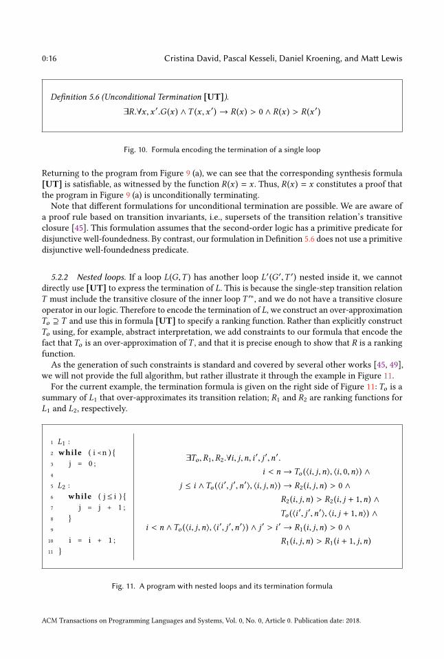
Definition 5.6 (Unconditional Termination [UT]).
∃R.∀x ,x ′.G (x ) ∧T (x ,x ′) → R (x ) > 0 ∧ R (x ) > R (x ′)
Fig. 10. Formula encoding the termination of a single loop
Returning to the program from Figure 9 (a), we can see that the corresponding synthesis formula
[UT] is satisfiable, as witnessed by the function R (x ) = x . Thus, R (x ) = x constitutes a proof that
the program in Figure 9 (a) is unconditionally terminating.
Note that different formulations for unconditional termination are possible. We are aware of
a proof rule based on transition invariants, i.e., supersets of the transition relation’s transitive
closure [45]. This formulation assumes that the second-order logic has a primitive predicate for
disjunctive well-foundedness. By contrast, our formulation in Definition 5.6 does not use a primitive
disjunctive well-foundedness predicate.
5.2.2 Nested loops. If a loop L(G,T ) has another loop L′(G ′,T ′) nested inside it, we cannot
directly use [UT] to express the termination of L. This is because the single-step transition relation
T must include the transitive closure of the inner loop T ′∗, and we do not have a transitive closure
operator in our logic. Therefore to encode the termination of L, we construct an over-approximation
To ⊇ T and use this in formula [UT] to specify a ranking function. Rather than explicitly construct
To using, for example, abstract interpretation, we add constraints to our formula that encode the
fact that To is an over-approximation of T , and that it is precise enough to show that R is a ranking
function.
As the generation of such constraints is standard and covered by several other works [45, 49],
we will not provide the full algorithm, but rather illustrate it through the example in Figure 11.
For the current example, the termination formula is given on the right side of Figure 11: To is asummary of L1 that over-approximates its transition relation; R1 and R2 are ranking functions for
L1 and L2, respectively.
1 L1 :
2 while ( i <n )
3 j = 0 ;
4
5 L2 :
6 while ( j ≤ i )
7 j = j + 1 ;
8
9
10 i = i + 1 ;
11
∃To ,R1,R2.∀i, j,n, i′, j ′,n′.
i < n → To (⟨i, j,n⟩, ⟨i, 0,n⟩) ∧
j ≤ i ∧To (⟨i′, j ′,n′⟩, ⟨i, j,n⟩) → R2 (i, j,n) > 0 ∧
R2 (i, j,n) > R2 (i, j + 1,n) ∧
To (⟨i′, j ′,n′⟩, ⟨i, j + 1,n⟩) ∧
i < n ∧To (⟨i, j,n⟩, ⟨i′, j ′,n′⟩) ∧ j ′ > i ′ → R1 (i, j,n) > 0 ∧
R1 (i, j,n) > R1 (i + 1, j,n)
Fig. 11. A program with nested loops and its termination formula
ACM Transactions on Programming Languages and Systems, Vol. 0, No. 0, Article 0. Publication date: 2018.
Program Synthesis for Program Analysis 0:17
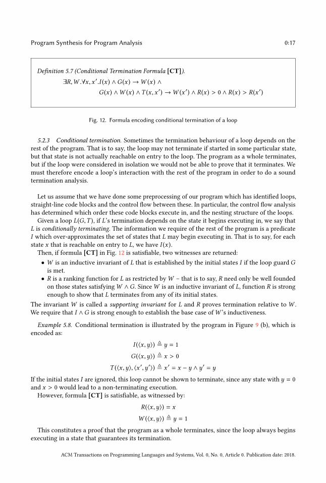
Definition 5.7 (Conditional Termination Formula [CT]).
∃R,W .∀x ,x ′.I (x ) ∧G (x ) →W (x ) ∧
G (x ) ∧W (x ) ∧T (x ,x ′) →W (x ′) ∧ R (x ) > 0 ∧ R (x ) > R (x ′)
Fig. 12. Formula encoding conditional termination of a loop
5.2.3 Conditional termination. Sometimes the termination behaviour of a loop depends on the
rest of the program. That is to say, the loop may not terminate if started in some particular state,
but that state is not actually reachable on entry to the loop. The program as a whole terminates,
but if the loop were considered in isolation we would not be able to prove that it terminates. We
must therefore encode a loop’s interaction with the rest of the program in order to do a sound
termination analysis.
Let us assume that we have done some preprocessing of our program which has identified loops,
straight-line code blocks and the control flow between these. In particular, the control flow analysis
has determined which order these code blocks execute in, and the nesting structure of the loops.
Given a loop L(G,T ), if L’s termination depends on the state it begins executing in, we say that
L is conditionally terminating. The information we require of the rest of the program is a predicate
I which over-approximates the set of states that L may begin executing in. That is to say, for each
state x that is reachable on entry to L, we have I (x ).Then, if formula [CT] in Fig. 12 is satisfiable, two witnesses are returned:
• W is an inductive invariant of L that is established by the initial states I if the loop guard Gis met.
• R is a ranking function for L as restricted byW – that is to say, R need only be well founded
on those states satisfyingW ∧G . SinceW is an inductive invariant of L, function R is strong
enough to show that L terminates from any of its initial states.
The invariantW is called a supporting invariant for L and R proves termination relative toW .
We require that I ∧G is strong enough to establish the base case ofW ’s inductiveness.
Example 5.8. Conditional termination is illustrated by the program in Figure 9 (b), which is
encoded as:
I (⟨x ,y⟩) ≜ y = 1
G (⟨x ,y⟩) ≜ x > 0
T (⟨x ,y⟩, ⟨x ′,y ′⟩) ≜ x ′ = x − y ∧ y ′ = y
If the initial states I are ignored, this loop cannot be shown to terminate, since any state with y = 0
and x > 0 would lead to a non-terminating execution.
However, formula [CT] is satisfiable, as witnessed by:
R (⟨x ,y⟩) = x
W (⟨x ,y⟩) ≜ y = 1
This constitutes a proof that the program as a whole terminates, since the loop always begins
executing in a state that guarantees its termination.
ACM Transactions on Programming Languages and Systems, Vol. 0, No. 0, Article 0. Publication date: 2018.
0:18 Cristina David, Pascal Kesseli, Daniel Kroening, and Matt Lewis
5.2.4 Bit-vector semantics vs. integer semantics. While computer programs manipulate fixed-
width machine integers (bit-vectors) and IEEE floats, the majority of existing termination analyses
are designed to work with mathematical integers and reals [10, 16, 29, 54, 64, 71].
Thus, when applied to bit-vector programs, these techniques ignore the wrap-around behaviour
caused by overflows, which can be unsound. For illustration, the loop Fig. 9(c) is terminating for
bit-vectors since x will eventually overflow and become negative. Conversely, the same program is
non-terminating using integer arithmetic since x > 0→ x + 1 > 0 for any integer x . Conversely,the loop in Fig. 9(d) breaks the assumption that bit-vector and integer semantics are identical “the
other way”: it terminates for integers but not for bit-vectors. If each of the variables is stored in an
unsigned k-bit word, the following entry state will lead to an infinite loop:
M = 2k − 1, N = 2
k − 1, i = M, j = N − 1
Our termination prover takes into consideration the wrap-around behaviour caused by overflows
and thus provides acurate results for programs running on physical computers.
5.3 Building a Non-termination ProverDually to termination, we might want to consider the non-termination of a loop. If a loop terminates,
we can prove this by finding a ranking function witnessing the satisfiability of formula [UT]. What
then would a proof of non-termination look like?
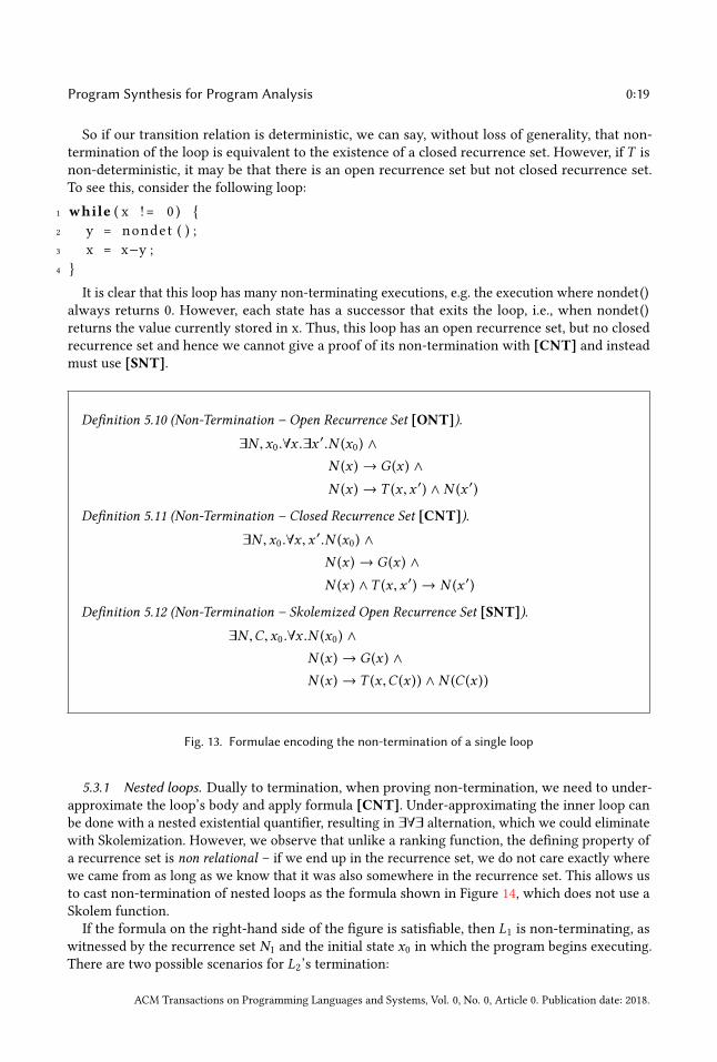
Since our program’s state space is finite, a transition relation induces an infinite execution
iff some state is visited infinitely often, or equivalently ∃x .T + (x ,x ). Deciding satisfiability of
this formula directly would require a logic that includes a transitive closure operator, •+. Rather
than introduce such an operator, we will characterise non-termination using the synthesis formula
[ONT] (Definition 5.10, Figure 13) encoding the existence of an (open) recurrence set, i.e., a nonempty
set of states N such that for each s ∈ N there exists a transition to some s ′ ∈ N [50].
If this formula is satisfiable, N is an open recurrence set for L, which proves L’s non-termination.
The issue with this formula is the additional level of quantifier alternation as compared to the
synthesis fragment (it is an ∃∀∃ formula). To eliminate the innermost existential quantifier, we
introduce a Skolem function C that chooses the successor x ′, which we then existentially quantify
over. This results in formula [SNT] (Definition 5.12, Figure 13).
This extra second-order term introduces some complexity to the formula, which we can avoid if
the transition relation T is deterministic.
Definition 5.9 (Determinism). A relationT is deterministic iff each state x has exactly one successor
under T :
∀x .∃x ′.T (x ,x ′) ∧ ∀x ′′.T (x ,x ′′) → x ′′ = x ′
In order to describe a deterministic program in a way that still allows us to sensibly talk about
termination, we assume the existence of a special sink state s with no outgoing transitions and
such that ¬G (s ) for any of the loop guardsG . The program is deterministic if its transition relation
is deterministic for all states except s .When analysing a deterministic loop, we can make use of the notion of a closed recurrence set
introduced by Chen et al. in [20]: for each state in the recurrence set N , all of its successors must be
in N . The existence of a closed recurrence set is equivalent to the satisfiability of formula [CNT]in Definition 5.11, which is already in the synthesis fragment without needing Skolemization.
We note that if T is deterministic, every open recurrence set is also a closed recurrence set
(since each state has at most one successor). Thus, the non-termination problem for deterministic
transition systems is equivalent to the satisfiability of formula [CNT] from Figure 13.
ACM Transactions on Programming Languages and Systems, Vol. 0, No. 0, Article 0. Publication date: 2018.
Program Synthesis for Program Analysis 0:19
So if our transition relation is deterministic, we can say, without loss of generality, that non-
termination of the loop is equivalent to the existence of a closed recurrence set. However, if T is
non-deterministic, it may be that there is an open recurrence set but not closed recurrence set.
To see this, consider the following loop:
1 while ( x != 0 )
2 y = nondet ( ) ;
3 x = x−y ;
4
It is clear that this loop has many non-terminating executions, e.g. the execution where nondet()
always returns 0. However, each state has a successor that exits the loop, i.e., when nondet()
returns the value currently stored in x. Thus, this loop has an open recurrence set, but no closed
recurrence set and hence we cannot give a proof of its non-termination with [CNT] and instead
must use [SNT].
Definition 5.10 (Non-Termination – Open Recurrence Set [ONT]).
∃N ,x0.∀x .∃x′.N (x0) ∧
N (x ) → G (x ) ∧
N (x ) → T (x ,x ′) ∧ N (x ′)
Definition 5.11 (Non-Termination – Closed Recurrence Set [CNT]).
∃N ,x0.∀x ,x′.N (x0) ∧
N (x ) → G (x ) ∧
N (x ) ∧T (x ,x ′) → N (x ′)
Definition 5.12 (Non-Termination – Skolemized Open Recurrence Set [SNT]).
∃N ,C,x0.∀x .N (x0) ∧
N (x ) → G (x ) ∧
N (x ) → T (x ,C (x )) ∧ N (C (x ))
Fig. 13. Formulae encoding the non-termination of a single loop
5.3.1 Nested loops. Dually to termination, when proving non-termination, we need to under-
approximate the loop’s body and apply formula [CNT]. Under-approximating the inner loop can
be done with a nested existential quantifier, resulting in ∃∀∃ alternation, which we could eliminate
with Skolemization. However, we observe that unlike a ranking function, the defining property of
a recurrence set is non relational – if we end up in the recurrence set, we do not care exactly where
we came from as long as we know that it was also somewhere in the recurrence set. This allows us
to cast non-termination of nested loops as the formula shown in Figure 14, which does not use a
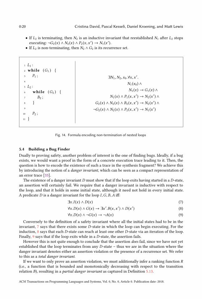
Skolem function.
If the formula on the right-hand side of the figure is satisfiable, then L1 is non-terminating, as
witnessed by the recurrence set N1 and the initial state x0 in which the program begins executing.
There are two possible scenarios for L2’s termination:
ACM Transactions on Programming Languages and Systems, Vol. 0, No. 0, Article 0. Publication date: 2018.
0:20 Cristina David, Pascal Kesseli, Daniel Kroening, and Matt Lewis
• If L2 is terminating, then N2 is an inductive invariant that reestablished N1 after L2 stopsexecuting: ¬G2 (x ) ∧ N2 (x ) ∧ P2 (x ,x
′) → N1 (x′).
• If L2 is non-terminating, then N2 ∧G2 is its recurrence set.
1 L1 :
2 while (G1 )
3 P1 ;
4
5 L2 :
6 while (G2 )
7 B2 ;
8
9
10 P2 ;
11
∃N1,N2,x0.∀x ,x′.
N1 (x0) ∧
N1 (x ) → G1 (x ) ∧
N1 (x ) ∧ P1 (x ,x′) → N2 (x
′) ∧
G2 (x ) ∧ N2 (x ) ∧ B2 (x ,x′) → N2 (x
′) ∧
¬G2 (x ) ∧ N2 (x ) ∧ P2 (x ,x′) → N1 (x
′)
Fig. 14. Formula encoding non-termination of nested loops
5.4 Building a Bug FinderDually to proving safety, another problem of interest is the one of finding bugs. Ideally, if a bug
exists, we would want a proof in the form of a concrete execution trace leading to it. Then, the
question is how to encode the existence of such a trace in the synthesis fragment? We achieve this
by introducing the notion of a danger invariant, which can be seen as a compact representation of
an error trace [33].
The existence of a danger invariant D must show that if the loop exits having started in a D-state,an assertion will certainly fail. We require that a danger invariant is inductive with respect to
the loop, and that it holds in some initial state, although it need not hold in every initial state.
A predicate D is a danger invariant for the loop I ,G,B,A iff:
∃x .I (x ) ∧ D (x ) (7)
∀x .D (x ) ∧G (x ) → ∃x ′.B (x ,x ′) ∧ D (x ′) (8)
∀x .D (x ) ∧ ¬G (x ) → ¬A(x ) (9)
Conversely to the definition of a safety invariant where all the initial states had to be in the
invariant, 7 says that there exists some D-state in which the loop can begin executing. For the
induction, 8 says that each D-state can reach at least one other D-state via an iteration of the loop.
Finally, 9 says that if the loop exits while in a D-state, the assertion fails.
However this is not quite enough to conclude that the assertion does fail, since we have not yetestablished that the loop terminates from any D-state – thus we are in the situation where the
danger invariant denotes either an assertion violation or the presence of a recurrence set. We refer
to this as a total danger invariant.If we want to only prove an assertion violation, we must additionally infer a ranking function R
(i.e., a function that is bounded and monotonically decreasing with respect to the transition
relation B), resulting in a partial danger invariant as captured in Definition 5.13.
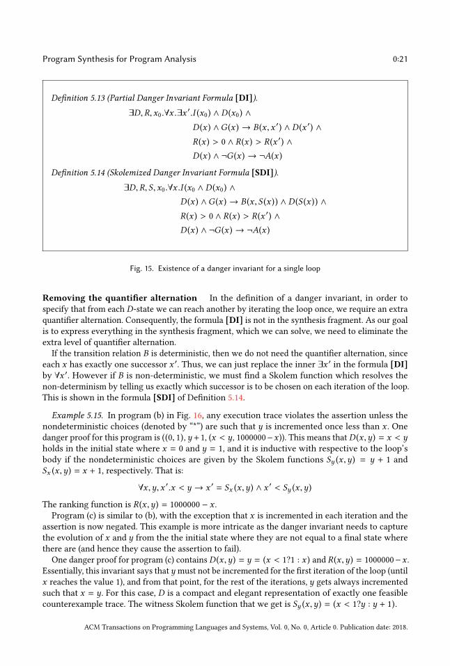
ACM Transactions on Programming Languages and Systems, Vol. 0, No. 0, Article 0. Publication date: 2018.
Program Synthesis for Program Analysis 0:21
Definition 5.13 (Partial Danger Invariant Formula [DI]).
∃D,R,x0.∀x .∃x′.I (x0) ∧ D (x0) ∧
D (x ) ∧G (x ) → B (x ,x ′) ∧ D (x ′) ∧
R (x ) > 0 ∧ R (x ) > R (x ′) ∧
D (x ) ∧ ¬G (x ) → ¬A(x )
Definition 5.14 (Skolemized Danger Invariant Formula [SDI]).
∃D,R, S,x0.∀x .I (x0 ∧ D (x0) ∧
D (x ) ∧G (x ) → B (x , S (x )) ∧ D (S (x )) ∧
R (x ) > 0 ∧ R (x ) > R (x ′) ∧
D (x ) ∧ ¬G (x ) → ¬A(x )
Fig. 15. Existence of a danger invariant for a single loop
Removing the quantifier alternation In the definition of a danger invariant, in order to
specify that from each D-state we can reach another by iterating the loop once, we require an extra
quantifier alternation. Consequently, the formula [DI] is not in the synthesis fragment. As our goal
is to express everything in the synthesis fragment, which we can solve, we need to eliminate the
extra level of quantifier alternation.
If the transition relation B is deterministic, then we do not need the quantifier alternation, since
each x has exactly one successor x ′. Thus, we can just replace the inner ∃x ′ in the formula [DI]by ∀x ′. However if B is non-deterministic, we must find a Skolem function which resolves the
non-determinism by telling us exactly which successor is to be chosen on each iteration of the loop.
This is shown in the formula [SDI] of Definition 5.14.
Example 5.15. In program (b) in Fig. 16, any execution trace violates the assertion unless the
nondeterministic choices (denoted by “*”) are such that y is incremented once less than x . Onedanger proof for this program is ((0, 1), y+1, (x < y, 1000000−x )). This means that D (x ,y) = x < yholds in the initial state where x = 0 and y = 1, and it is inductive with respective to the loop’s
body if the nondeterministic choices are given by the Skolem functions Sy (x ,y) = y + 1 and
Sx (x ,y) = x + 1, respectively. That is:
∀x ,y,x ′.x < y → x ′ = Sx (x ,y) ∧ x′ < Sy (x ,y)
The ranking function is R (x ,y) = 1000000 − x .Program (c) is similar to (b), with the exception that x is incremented in each iteration and the
assertion is now negated. This example is more intricate as the danger invariant needs to capture
the evolution of x and y from the the initial state where they are not equal to a final state where
there are (and hence they cause the assertion to fail).
One danger proof for program (c) contains D (x ,y) = y = (x < 1?1 : x ) and R (x ,y) = 1000000−x .Essentially, this invariant says thaty must not be incremented for the first iteration of the loop (until
x reaches the value 1), and from that point, for the rest of the iterations, y gets always incremented
such that x = y. For this case, D is a compact and elegant representation of exactly one feasible
counterexample trace. The witness Skolem function that we get is Sy (x ,y) = (x < 1?y : y + 1).
ACM Transactions on Programming Languages and Systems, Vol. 0, No. 0, Article 0. Publication date: 2018.
0:22 Cristina David, Pascal Kesseli, Daniel Kroening, and Matt Lewis
1 x = 1 ; y = 0 ;
2 while ( x < 1 0 0 0 )
3 x ++ ;
4 i f ( ∗ ) y ++ ;
5
6
7 a s s e r t ( x != y ) ;
(a)
1 x = 0 ; y = 1 ;
2 while ( x < 1000000 )
3 i f ( ∗ ) x ++ ;
4 i f ( ∗ ) y ++ ;
5
6
7 a s s e r t ( x == y ) ;
(b)
1 x = 0 ; y = 1 ;
2 while ( x < 1000000 )
3 x ++ ;
4 i f ( ∗ ) y ++ ;
5
6
7 a s s e r t ( x != y ) ;
(c)
Fig. 16. Safe and buggy examples
5.5 Building a Refactoring/Superoptimisation ToolFor all the program analysis problems considered up until now, it was sufficient to synthesise straight
line code. Conversely, in this section we are interested in refactoring code that has unbounded
loops and we must therefore be able to synthesise programs with loops. For this purpose, in this
section we present an extension of the program synthesis approach described in the rest of the
paper.
Program refactoring requires performing changes to an existing code with the goal of improving
it with respect to some non-behavioural criteria, but leave its externally observable behaviour
unchanged. Given an original code Code , we want to synthesise Code ′ such that, for any initial
program configuration Ci , Code and Code′produce the same final configuration Cf , i.e., they are
observationally equivalent as expressed in Fig. 17. We will refer to the equality between the final
program configurations Cf and C ′f as configEquiv.Note that in this section we consider heap allocated containers and, consequently, we consider
a program configuration C to consist of assignments to all the scalar variables plus a heap repre-
sentation2mapping all the pointer variables to their corresponding heap addresses. We use the
notation Code (Ci ,Cf ) to denote the fact that Ci is the initial program configuration before Codestarts executing and Cf is the final configuration at the end of the execution (similar for Code ′).
We use a particular refactoring as demonstrator for our idea. Nearly everymodern Java application
constructs and processes collections. A key algorithmic pattern when using collections is iteration
over the contents of the collection. We distinguish external from internal iteration.To enable external iteration, a Collection provides the means to enumerate its elements by
implementing Iterable. Clients that use an external iterator must advance the traversal and request
the next element explicitly from the iterator. External iteration has a few shortcomings:
• Is inherently sequential, and must process the elements in the order specified by the collection.
This bars the code from using concurrency to increase performance.
2More details about the heap configuration can be found in [32].
ACM Transactions on Programming Languages and Systems, Vol. 0, No. 0, Article 0. Publication date: 2018.
Program Synthesis for Program Analysis 0:23
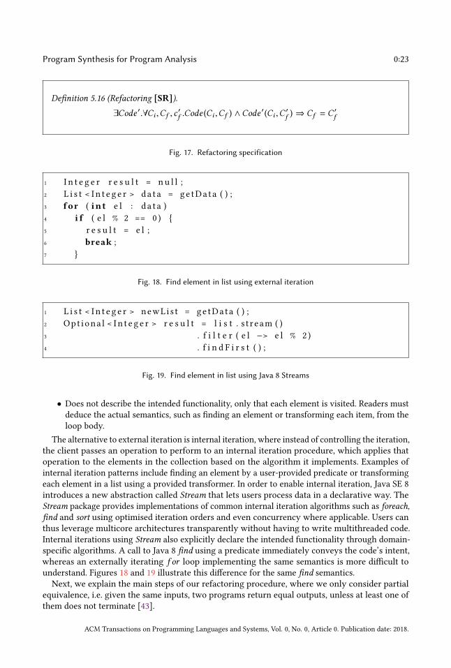
Definition 5.16 (Refactoring [SR]).
∃Code ′.∀Ci ,Cf , c′f .Code (Ci ,Cf ) ∧Code
′(Ci ,C′f ) ⇒ Cf = C
′f
Fig. 17. Refactoring specification
1 I n t e g e r r e s u l t = n u l l ;
2 L i s t < I n t e g e r > da t a = ge tDa ta ( ) ;
3 for ( in t e l : d a t a )
4 i f ( e l % 2 == 0 )
5 r e s u l t = e l ;
6 break ;
7
Fig. 18. Find element in list using external iteration
1 L i s t < I n t e g e r > newLis t = ge tDa ta ( ) ;
2 Opt iona l < I n t e g e r > r e s u l t = l i s t . s t ream ( )
3 . f i l t e r ( e l −> e l % 2 )
4 . f i n d F i r s t ( ) ;
Fig. 19. Find element in list using Java 8 Streams
• Does not describe the intended functionality, only that each element is visited. Readers must
deduce the actual semantics, such as finding an element or transforming each item, from the
loop body.
The alternative to external iteration is internal iteration, where instead of controlling the iteration,
the client passes an operation to perform to an internal iteration procedure, which applies that
operation to the elements in the collection based on the algorithm it implements. Examples of
internal iteration patterns include finding an element by a user-provided predicate or transforming
each element in a list using a provided transformer. In order to enable internal iteration, Java SE 8
introduces a new abstraction called Stream that lets users process data in a declarative way. The
Stream package provides implementations of common internal iteration algorithms such as foreach,find and sort using optimised iteration orders and even concurrency where applicable. Users can
thus leverage multicore architectures transparently without having to write multithreaded code.
Internal iterations using Stream also explicitly declare the intended functionality through domain-
specific algorithms. A call to Java 8 find using a predicate immediately conveys the code’s intent,
whereas an externally iterating f or loop implementing the same semantics is more difficult to
understand. Figures 18 and 19 illustrate this difference for the same find semantics.
Next, we explain the main steps of our refactoring procedure, where we only consider partial
equivalence, i.e. given the same inputs, two programs return equal outputs, unless at least one of
them does not terminate [43].
ACM Transactions on Programming Languages and Systems, Vol. 0, No. 0, Article 0. Publication date: 2018.
0:24 Cristina David, Pascal Kesseli, Daniel Kroening, and Matt Lewis
(i) First, we reduce the partial equivalence check to checking the partial correctness of the
following triple:
Ci Code configEquivEssentially, we check that, starting with a configuration Ci , every terminating trace ends up in
a state where configEquiv holds (remember that configEquiv denotes equality between the final
program configurations in the original code and the refactored code, respectively).
(ii) Given some logical encoding, the aforementioned correctness check can be further reduced
to checking the implication Post (Ci ,Code ) ⇒ configEquiv, where Post computes the postcondition
ofCode starting from the initial program configurationCi . While it is easy to compute the postcon-
dition Post (Ci ,Code ) for loop-free code,Code will most probably contain (potentially nested) loops.
In such situations, we must find safety invariant Inv that make the postcondition configEquiv hold.
For illustration, we provide the constraint corresponding to the scenario where the original code is
denoted by a loop L(G,T ):
∃configEquiv, Inv .∀Ci ,x ,x′.Ci (x ) ⇒ Inv (x )∧
Inv (x ) ∧G (x ) ∧T (x ,x ′) ⇒ Inv (x ′)∧
Inv (x ) ∧ ¬G (x ) ⇒ configEquiv (x )
(iii)We synthesise both the safety invariant Inv and configEquiv. We use a heap graph encoding
for configEquiv and define the JST logic over this representation. An informal description of JST
is provided Fig. 20 and a set of example properties in JST over our graph encoding is provided in
Fig. 21. Since JST contains representations for all supported operations in the Java 8 Stream library,
transforming a synthesised JST program to Java 8 Streams is a trivial mapping. More details on the
exact logical encoding are given in [32]. Given that configEquiv is a postcondition of the original
code, the refactored code is guaranteed to be equivalent to the original one by construction.
The notions of program refactoring and superoptimisation are closely related as they both aim at
improving existent code with respect to some criteria but leave its externally observable behaviour
unchanged. Thus, the same synthesis specification given in Fig. 17 is applicable to both problems.
5.6 Synthesising digital controllersAs a further examplar, we show how to use our synthesis framework to generate stable digital
controllers for a given model of a physical plant. In particular, we are interested in closed-loop
feedback architectures, where outputs of discrete plantG (z) are fed back and compared to a reference
signal towards which a controller C (z) should steer [6]. Fig. 22 depicts a typical closed-loop digital
control system.
We consider systems with a single input and a single output (SISO) given as transfer functions.
In such a setting, the discretized plant, G (z) and the digital controller, C (z), are given as fractions,
with denominators Gd (z) and Cd (z), respectively, and nominators Gn (z) and Cn (z), respectively.We are interested in synthesising feedback digital controllers that make the closed-loop system
asymptotically stable. Asymptotic stability is a property that amounts to convergence of the model
executions to an equilibrium point, starting from any states in a neighborhood of the point. In order
to prove stability, we will use Jury’s criterion [6]. Essentially, Jury’s criterion is a means to determine
the stability of a linear discrete time system by analysis of the coefficients of its characteristic
polynomial, S (z), which can be computed as:
S (z) = Cn (z)Gn (z) +Cd (z)Gd (z);
Let’s now assume that the characteristic polynomial has the following form:
S (z) = a0zN + a1z
N−1 + . . . + aN−1z + aN = 0,a0 , 0
ACM Transactions on Programming Languages and Systems, Vol. 0, No. 0, Article 0. Publication date: 2018.
Program Synthesis for Program Analysis 0:25
Next, the following Jury matrixM = [mi j ](2N−2)×N is built from S (z) coefficients:
M =
*.....,
V (0)
V (1)
...
V (N−2)
+/////-
,
where V (k ) = [v (k )i j ]2×N such that:
v (0)i j =
aj−1, if i = 1
v0
(1) (N−j+1), if i = 2
v (k )i j =
0, if j > n − k
v (k−1)1j −v (k−1)
2j .v (k−1)11
v (k−1)21
, if j ≤ n − k and i = 1
vk(1) (N−j+1), if j ≤ n − k and i = 2
where k ∈ Z, such that 0 < k < N − 2. Observe that S (z) is the characteristic polynomial of a
stable system if and only if the following four conditions hold: R1 : S (1) > 0; R2 : (−1)N S (−1) > 0;
R3 : |a0 | < aN ; R4 :m11 > 0 ∧m31 > 0 ∧m51 > 0 ∧ . . . ∧m (2N−3) (1) > 0.
Thus, the specification for the controller synthesis is:
∃C .∀z.R1 (z) ∧ R2 (z) ∧ R3 (z) ∧ R4 (z) (10)
We illustrate our approach with a classical cruise control example from the literature [5]. We are
given a discrete plant model (with a time step of 0.2 s), represented by the following z-expression:
G (z) =0.0264
z − 0.9998.
By providing specification 10 to our program synthesiser, we synthesise the following controller:
C (z) =11.035202z2+5.846100z+4.901855
1.097901z2+0.063110z+0.128357.
Given that we only want to illustrate the synthesis approach, we do not discuss in this section
the numerical representation of the plant and the truncation and rounding errors introduced by it.
More details about this can be found in [1] and [2].
6 IMPLEMENTATION AND EXPERIMENTAL RESULTSWe implemented our decision procedure for SFD in several tools, which we discuss in this section.
6.1 Avoiding Unsatisfiable InstancesAs described in Sec. 4.8, our program synthesiser is efficient at finding satisfying assignments,
when such assignments have low Kolmogorov complexity. However, if a formula is unsatisfiable,
the procedure may not terminate in practice. This illustrates one of the current shortcomings of our
program synthesis based decision procedure: we can only conclude that a formula is unsatisfiable
once we have examined candidate solutions up to a very high length bound.
However, we note that many interesting properties of programs can be expressed as tautologies.
For illustration, let us consider that we are trying to prove that a loop L terminates. Thus, following
Sections 5.2 and 5.3, we can construct two formulae: one that is satisfiable iff L is terminating and
another that is satisfiable iff L is non-terminating. We will call these formulae ϕ and ψ , respec-tively, and we denote by PN and PT the proofs of non-termination and termination, respectively:
∃PT .∀x ,x′.ϕ (PT ,x ,x
′) and ∃PN .∀x .ψ (PN ,x ).
ACM Transactions on Programming Languages and Systems, Vol. 0, No. 0, Article 0. Publication date: 2018.
0:26 Cristina David, Pascal Kesseli, Daniel Kroening, and Matt Lewis
We can combine these: (∃PT .∀x ,x′.ϕ (PT ,x ,x
′)) ∨ (∃PN .∀x .ψ (PN ,x )).Which simplifies to: ∃PT , PN .∀x ,x
′,y.ϕ (PT ,x ,x′) ∨ψ (PN ,y).
Since L either terminates or does not terminate, this formula is a tautology in the synthesis
fragment. Thus, either PN or PT must exist. Similarly, when proving safety, a program is either safe
of has a bug. In this manner we avoid the bad case where we try to synthesise a solution for an
unsatisfiable specification.
6.2 LimitationsWe present in this chapter an experimental evaluation for each of our prover implementations. Our
benchmark suite is based on publicly accessible benchmarks, such as SVCOMP. Since all of our
tools are research prototypes, we are unable to maintain support for all C language features and
have to exclude certain benchmarks from the experiment. Most importantly, the current front-end
implementations to not support arrays and are limited to non-nested loops where invariants need
to be synthesised.
6.3 Termination and non-terminationThe program synthesis based termination and non-termination prover is named Juggernaut and
was run on 47 benchmarks taken from the literature and the termination-crafted-lit directory of
SV-COMP’15 [77]. We omitted exactly those SVCOMP’15 benchmarks that made use of arrays
or recursion. We do not have arrays in our logic and we had not implemented recursion in our
frontend (although the latter can be syntactically rewritten to our input format). Note that these
experiments include those from [35].
To provide a comparison point, we also ran ARMC [75] on the same benchmarks. Each tool was
given a time limit of 180 s, and was run on an unloaded 8-core 3.07 GHz Xeon X5667 with 50GB of
RAM. The results of these experiments are given in Table 1.
It should be noted that the comparison here is imperfect, since ARMC is solving a different
problem – it checks whether the program under analysis would terminate if run with unbounded
integer variables, while we are checking whether the program terminates with bit-vector variables.
This means that ARMC’s verdict differs from ours in 3 cases (due to the differences between integer
and bit-vector semantics). There are a further 7 cases where our tool is able to find a proof and
ARMC cannot, which we believe is due to our more expressive proof language. In 3 cases, ARMC
times out while our tool is able to find a termination proof. Of these, 2 cases have nested loops
and the third has an infinite number of terminating lassos. This is not a problem for us, but can be
difficult for provers that enumerate lassos.
On the other hand, ARMC is much faster than our tool. While this difference can partly be
explained by much more engineering time being invested in ARMC, we feel that the difference is
probably inherent to the difference in the two approaches – our solver is more general than ARMC,
in that it provides a complete proof system for both termination and non-termination, which comes
at the cost of efficiency.
Of the 46 benchmarks, 2 use nonlinear operations in the program (loop6 and loop11), and 5
have nested loops (svcomp6, svcomp12, svcomp18, svcomp40, svcomp41). Juggernaut handles the
nonlinear cases correctly and rapidly. It solves 4 of the 5 nested loops in less than 30 s, but times
out on the 5th.
In conclusion, these experiments confirm our conjecture that program synthesis can be used
effectively to prove termination and non-termination. In particular, for programs with nested loops,
nonlinear arithmetic and complex termination arguments, the versatility given by a general purpose
solver is very valuable.
ACM Transactions on Programming Languages and Systems, Vol. 0, No. 0, Article 0. Publication date: 2018.
Program Synthesis for Program Analysis 0:27
6.4 Safety and dangerTo evaluate our safety and danger synthesis, we have implemented the Dangerzone module for
the bounded model checker CBMC 5.5. We ran the resulting prover on 50 programs from the
loop-acceleration and loops directories in SV-COMP 2016 [78]. We picked this specific category
as it has benchmarks with deep bugs and we were interested in challenging our hypothesis that
danger invariants are well-suited to expose deep bugs and can complement the capabilities of
existing approaches such as BMC. Unfortunately we had to exclude programs that make use of
arrays, since these are not yet supported by the synthesiser. In addition to this, we also introduced
altered versions of the selected SV-COMP 2016 benchmarks with extended loop guards to create
deeper bugs, challenging our hypothesis even further. These are benchmarks loop1 to loop11. Alldanger and safety benchmarks are available for download: https://www.cs.ox.ac.uk/files/9174/
cegis_danger_benchmarks.zip.
For each benchmark we try to synthesise both a partial danger invariant (i.e., a danger invari-
ant, a ranking function, an initial state and Skolem functions witnessing the nondeterminism
corresponding to partial correctness in Def. 5.14) and a total danger invariant (i.e., a danger in-
variant, an initial state and Skolem functions as given by equations 7, 8 and 9 in Sec. 5.4). To
provide a comparison point, we also ran two state-of-the-art bounded model checking (BMC)
tools, CBMC 5.5 and SMACK+CORRAL 1.5.1 [52] on the same benchmarks. In addition to this,
we ran the benchmarks against CPAchecker 1.4 [13], the overall winner of SV-COMP 2015, and
Seahorn 2.6 [51], the second-placed tool in the loops category after CPAchecker. We reproduced
each tool’s SV-COMP 2015 configuration, with small alterations to account for the benchmarks
where we increased loop guards. Finally, we manually translated the benchmarks to be compatible
with Microsoft’s Static Driver Verifier Research Platform (SDVRP [8]) with the Yogi 2.0 [69] back
end. Yogi’s main algorithms are Synergy, Dash, Smash and Bolt.
We say that a benchmark contains a deep bug if it is only reachable after at least 1’000’000
unwindings. Each tool was given a time limit of 300 s, and was run on a 12-core 2.40GHz Intel
Xeon E5-2440 with 96GB of RAM. The full result table of these experiments is given in Tab. 2.
The results demonstrate that the Dangerzone module outperforms all other tools on programs
with deep bugs. It solves 37 (partial) and 38 (total) out of the 50 benchmarks in standalone mode,
and 46 when used with CBMC. By itself, CBMC only finds 27, SMACK+CORRAL 24, CPAchecker
26 and Seahorn 31 bugs. This result can be explained by the fact that the complexity of finding a
danger invariant is orthogonal to the number of unwindings necessary to reach it. Dangerzone’s
success is not determined by how deep the bug is, but by the complexity of the invariant describing
it. As a result, we perform comparably on both deep and shallow bugs and are able to expose 18
out of the 20 deep bugs in the benchmark set. This supports our hypothesis that danger invariants
are well-suited for this category of errors.
6.5 SuperoptimisationWe implemented our superoptimiser as the kalashnikov tool. To evaluate the tool we used the 29
bit-vector programs from [57] and [48]. The majority of these are “bit twiddling hacks” taken from
Hacker’s Delight [82]. The code we used to perform the experiments, along with the benchmarks, is
available at http://www.cprover.org/kalashnikov. We performed our experiments on a 4-core,
2.40 GHz Xeon E5-2665 with 32GB of RAM.
To give a reference point, we present the results given for brahma on the same benchmarks, as
reported in [48] and [57]. These experiments were performed on an 8-core, 1.86GHz Xeon with
3https://github.com/diffblue/cbmc/archive/bbae05d8faecfec18a42724e72336d8f8c4e3d8d.zip
ACM Transactions on Programming Languages and Systems, Vol. 0, No. 0, Article 0. Publication date: 2018.
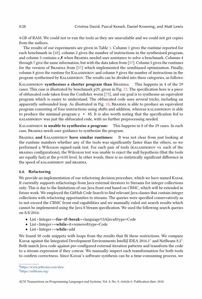
0:28 Cristina David, Pascal Kesseli, Daniel Kroening, and Matt Lewis
4GB of RAM. We could not re-run the tools as they are unavailable and we could not get copies
from the authors.
The results of our experiments are given in Table 3. Column 1 gives the runtime reported for
each benchmark in [48], column 2 gives the number of instructions in the synthesised program,
and column 3 contains a when Brahma needed user assistance to solve a benchmark. Columns 4
through 7 give the same information, but with the data taken from [57]. Column 5 gives the runtimes
for the version of Brahma from [57] which implemented the semibiased optimisation. Finally,
column 8 gives the runtime for Kalashnikov and column 9 gives the number of instructions in the
program synthesised by Kalashnikov. The results can be divided into three categories, as follows:
Kalashnikov synthesises a shorter program than Brahma: This happens in 4 of the 29
cases. This case is illustrated by benchmark p29, given in Fig. 23. The specification here is a piece
of obfuscated code taken from the Conficker worm [73], and our goal is to synthesise an equivalent
program which is easier to understand. The obfuscated code uses several tricks, including an
apparently unbounded loop. As illustrated in Fig. 24, Brahma is able to produce an equivalent
program consisting of four instructions using shifts and addition, whereas kalashnikov is able
to produce the minimal program y * 45. It is also worth noting that the specification fed to
kalashnikov was just the obfuscated code, with no further preprocessing needed.
Kalashnikov is unable to synthesise a program: This happens in 8 of the 29 cases. In each
case, Brahma needs user guidance to synthesise the program.
Brahma and Kalashnikov have similar runtimes: It was not clear from just looking at
the runtime numbers whether any of the tools was significantly faster than the others, so we
performed a Wilcoxon signed-rank test. For each pair of tools (kalashnikov vs. each of the
brahma configurations), the Wilcoxon test was unable to reject the null hypothesis (that the tools
are equally fast) at the p=0.05 level. In other words, there is no statistically significant difference in
the speed of kalashnikov and brahma.
6.6 RefactoringWe provide an implementation of our refactoring decision procedure, which we have named Kayak.
It currently supports refactorings from Java external iterators to Streams for integer collections
only. This is due to the limitations of our Java front-end based on CBMC, which will be extended in
future work. We employed the GitHub Code Search to find relevant Java classes that contain integer
collections with refactoring opportunities to streams. The queries were specified conservatively as
to not exceed the CBMC front-end capabilities and we manually ruled out search results which
cannot be implemented using the Java 8 Stream specification. We used the following search queries
on 8/8/2016:
• List <Integer>+for+if+break++language%3AJava&type=Code• List <Integer>+while+it+remove&type=Code
• List <Integer>+while+add
We found 50 code snippets with loops from the results that fit these restrictions. We compare
Kayak against the Integrated Development Environments IntelliJ IDEA 2016.14and NetBeans 8.2
5.
Both match Java code against pre-configured external iteration patterns and transform the code
to a stream expression if they concur. We manually inspect each transformation for both tools
to confirm correctness. Since Kayak’s software synthesis can be a time-consuming process, we
4https://www.jetbrains.com/idea/
5https://netbeans.org/
ACM Transactions on Programming Languages and Systems, Vol. 0, No. 0, Article 0. Publication date: 2018.
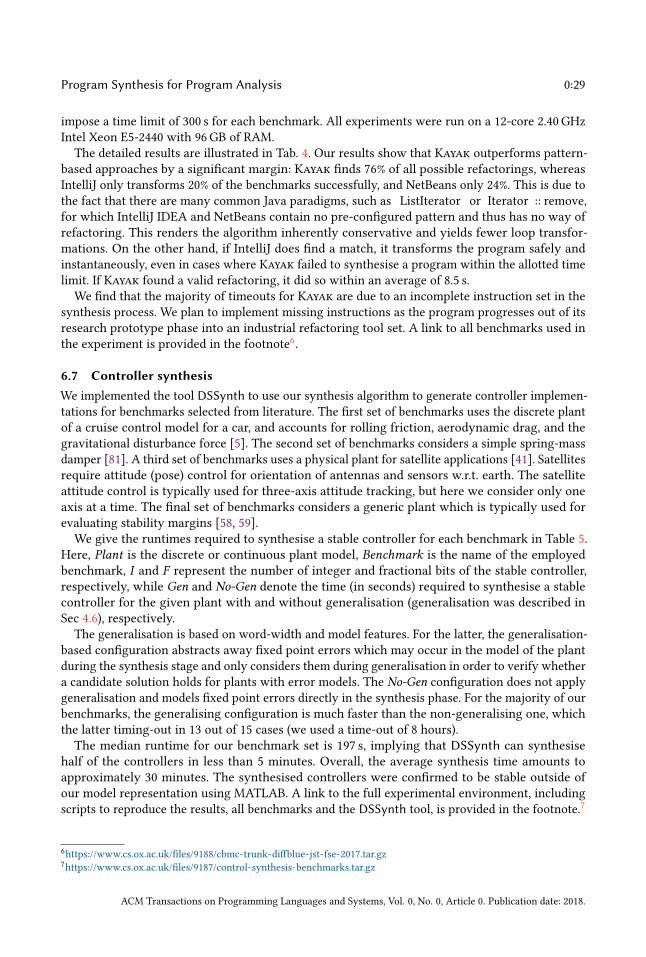
Program Synthesis for Program Analysis 0:29
impose a time limit of 300 s for each benchmark. All experiments were run on a 12-core 2.40GHz
Intel Xeon E5-2440 with 96GB of RAM.
The detailed results are illustrated in Tab. 4. Our results show that Kayak outperforms pattern-
based approaches by a significant margin: Kayak finds 76% of all possible refactorings, whereas
IntelliJ only transforms 20% of the benchmarks successfully, and NetBeans only 24%. This is due to
the fact that there are many common Java paradigms, such as ListIterator or Iterator :: remove,
for which IntelliJ IDEA and NetBeans contain no pre-configured pattern and thus has no way of
refactoring. This renders the algorithm inherently conservative and yields fewer loop transfor-
mations. On the other hand, if IntelliJ does find a match, it transforms the program safely and
instantaneously, even in cases where Kayak failed to synthesise a program within the allotted time
limit. If Kayak found a valid refactoring, it did so within an average of 8.5 s.
We find that the majority of timeouts for Kayak are due to an incomplete instruction set in the
synthesis process. We plan to implement missing instructions as the program progresses out of its
research prototype phase into an industrial refactoring tool set. A link to all benchmarks used in
the experiment is provided in the footnote6.
6.7 Controller synthesisWe implemented the tool DSSynth to use our synthesis algorithm to generate controller implemen-
tations for benchmarks selected from literature. The first set of benchmarks uses the discrete plant
of a cruise control model for a car, and accounts for rolling friction, aerodynamic drag, and the
gravitational disturbance force [5]. The second set of benchmarks considers a simple spring-mass
damper [81]. A third set of benchmarks uses a physical plant for satellite applications [41]. Satellites
require attitude (pose) control for orientation of antennas and sensors w.r.t. earth. The satellite
attitude control is typically used for three-axis attitude tracking, but here we consider only one
axis at a time. The final set of benchmarks considers a generic plant which is typically used for
evaluating stability margins [58, 59].
We give the runtimes required to synthesise a stable controller for each benchmark in Table 5.
Here, Plant is the discrete or continuous plant model, Benchmark is the name of the employed
benchmark, I and F represent the number of integer and fractional bits of the stable controller,
respectively, while Gen and No-Gen denote the time (in seconds) required to synthesise a stable
controller for the given plant with and without generalisation (generalisation was described in
Sec 4.6), respectively.
The generalisation is based on word-width and model features. For the latter, the generalisation-
based configuration abstracts away fixed point errors which may occur in the model of the plant
during the synthesis stage and only considers them during generalisation in order to verify whether
a candidate solution holds for plants with error models. The No-Gen configuration does not apply
generalisation and models fixed point errors directly in the synthesis phase. For the majority of our
benchmarks, the generalising configuration is much faster than the non-generalising one, which
the latter timing-out in 13 out of 15 cases (we used a time-out of 8 hours).
The median runtime for our benchmark set is 197 s, implying that DSSynth can synthesise
half of the controllers in less than 5 minutes. Overall, the average synthesis time amounts to
approximately 30 minutes. The synthesised controllers were confirmed to be stable outside of
our model representation using MATLAB. A link to the full experimental environment, including
scripts to reproduce the results, all benchmarks and the DSSynth tool, is provided in the footnote.7
6https://www.cs.ox.ac.uk/files/9188/cbmc-trunk-diffblue-jst-fse-2017.tar.gz
7https://www.cs.ox.ac.uk/files/9187/control-synthesis-benchmarks.tar.gz
ACM Transactions on Programming Languages and Systems, Vol. 0, No. 0, Article 0. Publication date: 2018.
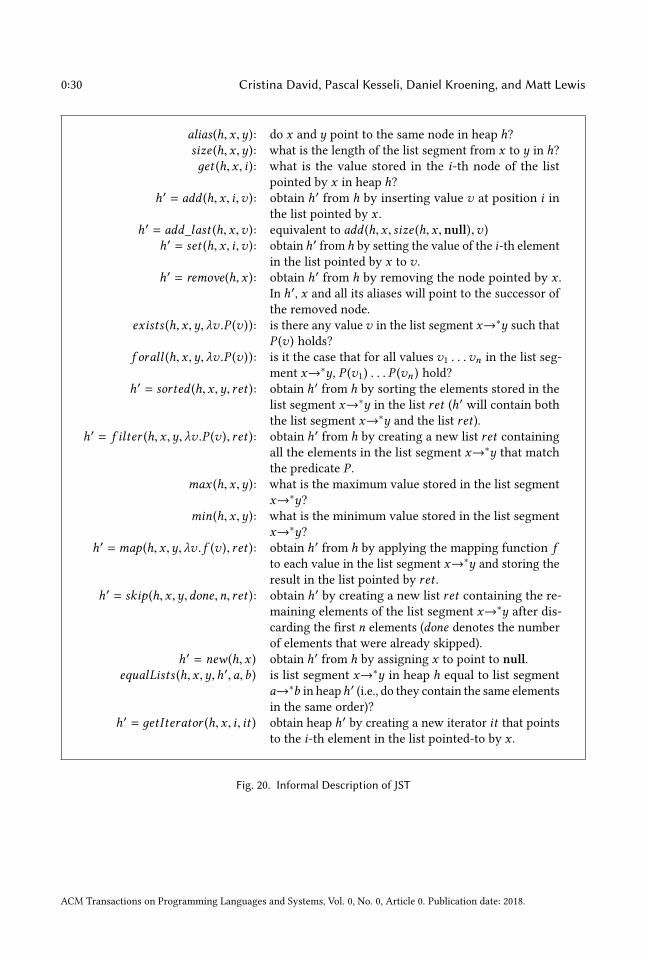
0:30 Cristina David, Pascal Kesseli, Daniel Kroening, and Matt Lewis
alias(h,x ,y): do x and y point to the same node in heap h?size (h,x ,y): what is the length of the list segment from x to y in h?дet (h,x , i ): what is the value stored in the i-th node of the list
pointed by x in heap h?h′ = add (h,x , i,v ): obtain h′ from h by inserting value v at position i in
the list pointed by x .h′ = add_last (h,x ,v ): equivalent to add (h,x , size (h,x ,null),v )
h′ = set (h,x , i,v ): obtainh′ fromh by setting the value of the i-th element
in the list pointed by x to v .h′ = remove(h,x ): obtain h′ from h by removing the node pointed by x .
In h′, x and all its aliases will point to the successor of
the removed node.
exists (h,x ,y, λv .P (v )): is there any valuev in the list segment x→∗y such that
P (v ) holds?f orall (h,x ,y, λv .P (v )): is it the case that for all values v1 . . .vn in the list seg-
ment x→∗y, P (v1) . . . P (vn ) hold?h′ = sorted (h,x ,y, ret ): obtain h′ from h by sorting the elements stored in the
list segment x→∗y in the list ret (h′ will contain both
the list segment x→∗y and the list ret ).h′ = f ilter (h,x ,y, λv .P (v ), ret ): obtain h′ from h by creating a new list ret containing
all the elements in the list segment x→∗y that match
the predicate P .max (h,x ,y): what is the maximum value stored in the list segment
x→∗y?min(h,x ,y): what is the minimum value stored in the list segment
x→∗y?h′ =map (h,x ,y, λv . f (v ), ret ): obtain h′ from h by applying the mapping function f
to each value in the list segment x→∗y and storing the
result in the list pointed by ret .h′ = skip (h,x ,y,done,n, ret ): obtain h′ by creating a new list ret containing the re-
maining elements of the list segment x→∗y after dis-
carding the first n elements (done denotes the number
of elements that were already skipped).
h′ = new (h,x ) obtain h′ from h by assigning x to point to null.equalLists (h,x ,y,h′,a,b) is list segment x→∗y in heap h equal to list segment
a→∗b in heaph′ (i.e., do they contain the same elements
in the same order)?
h′ = дetIterator (h,x , i, it ) obtain heap h′ by creating a new iterator it that pointsto the i-th element in the list pointed-to by x .
Fig. 20. Informal Description of JST
ACM Transactions on Programming Languages and Systems, Vol. 0, No. 0, Article 0. Publication date: 2018.
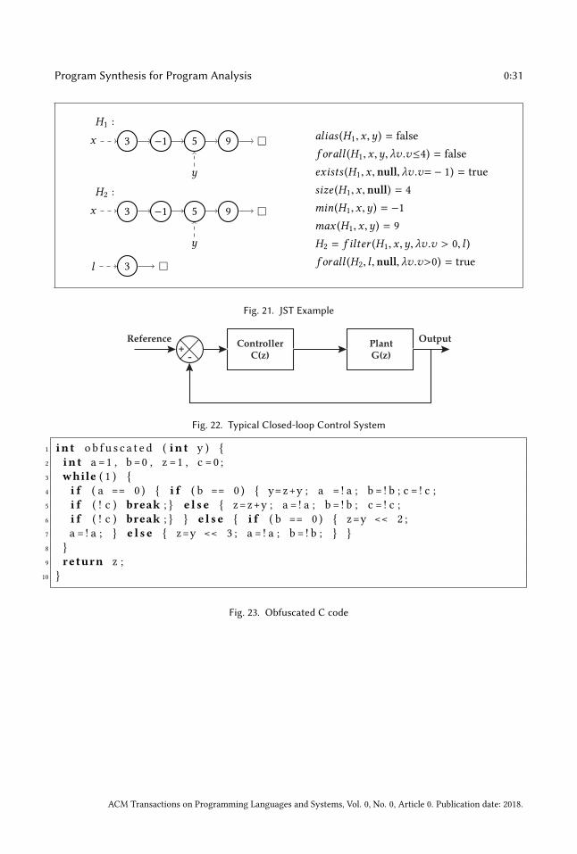
Program Synthesis for Program Analysis 0:31
H1 :
3 −1 5 9 x
y
H2 :
3 −1 5 9
3
x
y
l
alias (H1,x ,y) = false
f orall (H1,x ,y, λv .v≤4) = false
exists (H1,x ,null, λv .v= − 1) = true
size (H1,x ,null) = 4
min(H1,x ,y) = −1
max (H1,x ,y) = 9
H2 = f ilter (H1,x ,y, λv .v > 0, l )
f orall (H2, l ,null, λv .v>0) = true
Fig. 21. JST Example
Reference OutputControllerC(z)
PlantG(z)
+-
Fig. 22. Typical Closed-loop Control System
1 in t ob f u s c a t e d ( in t y )
2 in t a =1 , b =0 , z =1 , c =0 ;
3 while ( 1 )
4 i f ( a == 0 ) i f ( b == 0 ) y=z+y ; a = ! a ; b = ! b ; c = ! c ;
5 i f ( ! c ) break ; e l se z=z+y ; a = ! a ; b = ! b ; c = ! c ;
6 i f ( ! c ) break ; e l se i f ( b == 0 ) z=y << 2 ;
7 a = ! a ; e l se z=y << 3 ; a = ! a ; b = ! b ;
8
9 return z ;
10
Fig. 23. Obfuscated C code
ACM Transactions on Programming Languages and Systems, Vol. 0, No. 0, Article 0. Publication date: 2018.
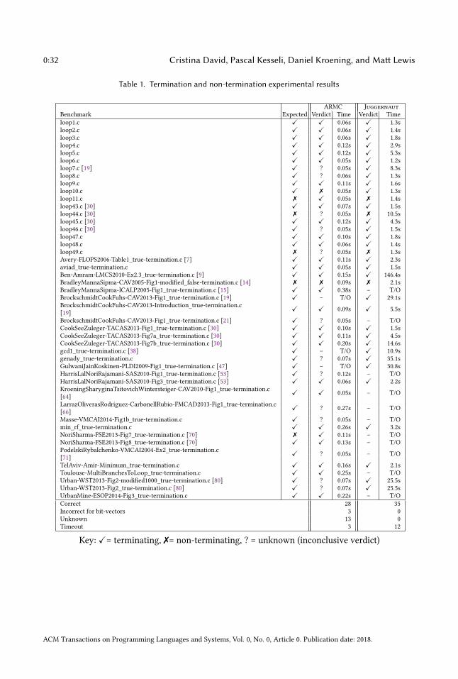
0:32 Cristina David, Pascal Kesseli, Daniel Kroening, and Matt Lewis
Table 1. Termination and non-termination experimental results
ARMC Juggernaut
Benchmark Expected Verdict Time Verdict Time
loop1.c 0.06s 1.3s
loop2.c 0.06s 1.4s
loop3.c 0.06s 1.8s
loop4.c 0.12s 2.9s
loop5.c 0.12s 5.3s
loop6.c 0.05s 1.2s
loop7.c [19] ? 0.05s 8.3s
loop8.c ? 0.06s 1.3s
loop9.c 0.11s 1.6s
loop10.c 0.05s 1.3s
loop11.c 0.05s 1.4s
loop43.c [30] 0.07s 1.5s
loop44.c [30] ? 0.05s 10.5s
loop45.c [30] 0.12s 4.3s
loop46.c [30] ? 0.05s 1.5s
loop47.c 0.10s 1.8s
loop48.c 0.06s 1.4s
loop49.c ? 0.05s 1.3s
Avery-FLOPS2006-Table1_true-termination.c [7] 0.11s 2.3s
aviad_true-termination.c 0.05s 1.5s
Ben-Amram-LMCS2010-Ex2.3_true-termination.c [9] 0.15s 146.4s
BradleyMannaSipma-CAV2005-Fig1-modified_false-termination.c [14] 0.09s 2.1s
BradleyMannaSipma-ICALP2005-Fig1_true-termination.c [15] 0.38s – T/O
BrockschmidtCookFuhs-CAV2013-Fig1_true-termination.c [19] – T/O 29.1s
BrockschmidtCookFuhs-CAV2013-Introduction_true-termination.c 0.09s 5.5s
[19]
BrockschmidtCookFuhs-CAV2013-Fig1_true-termination.c [21] ? 0.05s – T/O
CookSeeZuleger-TACAS2013-Fig1_true-termination.c [30] 0.10s 1.5s
CookSeeZuleger-TACAS2013-Fig7a_true-termination.c [30] 0.11s 4.5s
CookSeeZuleger-TACAS2013-Fig7b_true-termination.c [30] 0.20s 14.6s
gcd1_true-termination.c [38] – T/O 10.9s
genady_true-termination.c ? 0.07s 35.1s
GulwaniJainKoskinen-PLDI2009-Fig1_true-termination.c [47] – T/O 30.8s
HarrisLalNoriRajamani-SAS2010-Fig1_true-termination.c [53] ? 0.12s – T/O
HarrisLalNoriRajamani-SAS2010-Fig3_true-termination.c [53] 0.06s 2.2s
KroeningSharyginaTsitovichWintersteiger-CAV2010-Fig1_true-termination.c 0.05s – T/O
[64]
LarrazOliverasRodriguez-CarbonellRubio-FMCAD2013-Fig1_true-termination.c ? 0.27s – T/O
[66]
Masse-VMCAI2014-Fig1b_true-termination.c ? 0.05s – T/O
min_rf_true-termination.c 0.26s 3.2s
NoriSharma-FSE2013-Fig7_true-termination.c [70] 0.11s – T/O
NoriSharma-FSE2013-Fig8_true-termination.c [70] 0.13s – T/O
PodelskiRybalchenko-VMCAI2004-Ex2_true-termination.c ? 0.05s – T/O
[71]
TelAviv-Amir-Minimum_true-termination.c 0.16s 2.1s
Toulouse-MultiBranchesToLoop_true-termination.c 0.25s – T/O
Urban-WST2013-Fig2-modified1000_true-termination.c [80] ? 0.07s 25.5s
Urban-WST2013-Fig2_true-termination.c [80] ? 0.07s 25.5s
UrbanMine-ESOP2014-Fig3_true-termination.c 0.22s – T/O
Correct 28 35
Incorrect for bit-vectors 3 0
Unknown 13 0
Timeout 3 12
Key: = terminating, = non-terminating, ? = unknown (inconclusive verdict)
ACM Transactions on Programming Languages and Systems, Vol. 0, No. 0, Article 0. Publication date: 2018.
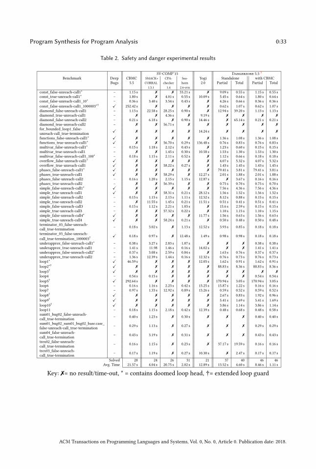
Program Synthesis for Program Analysis 0:33
Table 2. Safety and danger experimental results
SV-COMP’15 Dangerzone 5.53
Benchmark Deep CBMC SMACK+ CPA- Sea- Yogi Standalone with CBMC
Bugs 5.5 CORRAL checker horn 2.0 Partial Total Partial Total
1.5.1 1.4 2.6-svn
const_false-unreach-call1∗
– 1.15 s 33.21 s 9.09 s 0.55 s 1.15 s 0.55 s
const_true-unreach-call1∗
– 1.80 s 4.01 s 0.55 s 10.09 s 5.45 s 0.64 s 1.80 s 0.64 s
const_false-unreach-call1_10∗
– 0.36 s 3.40 s 3.54 s 0.43 s 4.26 s 0.66 s 0.36 s 0.36 s
const_false-unreach-call1_1000003∗† 252.42 s 0.62 s 1.07 s 0.62 s 1.07 s
diamond_false-unreach-call1 – 1.13 s 22.58 s 28.25 s 0.90 s 12.94 s 39.20 s 1.13 s 1.13 s
diamond_true-unreach-call1 – 4.36 s 9.19 s diamond_false-unreach-call2 – 0.21 s 6.18 s 0.90 s 14.46 s 65.14 s 0.21 s 0.21 s
diamond_true-unreach-call2 – 56.71 s for_bounded_loop1_false- 14.24 s unreach-call_true-termination
functions_false-unreach-call1∗ 1.36 s 1.08 s 1.36 s 1.08 s
functions_true-unreach-call1∗ 56.70 s 0.29 s 136.48 s 0.76 s 0.83 s 0.76 s 0.83 s
multivar_false-unreach-call1∗
– 0.15 s 1.18 s 2.12 s 0.43 s 1.23 s 0.60 s 0.15 s 0.15 s
multivar_true-unreach-call1 – 1.45 s 0.30 s 10.58 s 1.53 s 1.30 s 1.53 s 1.30 s
multivar_false-unreach-call1_100∗
– 0.18 s 1.15 s 2.11 s 0.52 s 1.12 s 0.66 s 0.18 s 0.18 s
overflow_false-unreach-call1∗ 4.07 s 5.32 s 4.07 s 5.32 s
overflow_true-unreach-call1 58.22 s 0.27 s 1.43 s 1.45 s 1.43 s 1.45 s
phases_false-unreach-call1∗ 79.41 s 3.81 s 79.41 s 3.81 s
phases_true-unreach-call1 58.29 s 12.27 s 2.01 s 1.88 s 2.01 s 1.88 s
phases_false-unreach-call2 – 0.16 s 1.20 s 2.15 s 1.15 s 12.87 s 3.67 s 0.16 s 0.16 s
phases_true-unreach-call2 – 56.39 s 0.75 s 0.70 s 0.75 s 0.70 s
simple_false-unreach-call1∗ 7.56 s 4.36 s 7.56 s 4.36 s
simple_true-unreach-call1 58.31 s 0.21 s 28.12 s 1.56 s 1.52 s 1.56 s 1.52 s
simple_false-unreach-call2 – 0.15 s 1.15 s 2.13 s 1.11 s 12.52 s 8.12 s 0.88 s 0.15 s 0.15 s
simple_true-unreach-call2 – 11.55 s 1.45 s 0.21 s 11.51 s 0.51 s 0.41 s 0.51 s 0.41 s
simple_false-unreach-call3 – 0.15 s 1.12 s 2.21 s 1.03 s 13.6 s 2.59 s 0.15 s 0.15 s
simple_true-unreach-call3 – 57.32 s 0.22 s 1.10 s 1.15 s 1.10 s 1.15 s
simple_false-unreach-call4∗ 11.77 s 1.56 s 0.63 s 1.56 s 0.63 s
simple_true-unreach-call4 58.24 s 0.21 s 0.50 s 0.48 s 0.50 s 0.48 s
terminator_03_false-unreach-
– 0.18 s 3.02 s 1.13 s 12.52 s 3.93 s 0.85 s 0.18 s 0.18 s
call_true-termination
terminator_03_false-unreach- 0.18 s 0.97 s 12.48 s 1.49 s 0.98 s 0.98 s 0.18 s 0.18 s
call_true-termination_1000003†
underapprox_false-unreach-call1∗
– 0.38 s 3.27 s 2.83 s 1.07 s 0.38 s 0.38 s
underapprox_true-unreach-call1 – 1.41 s 11.98 1.46 s 0.16 s 14.02 s 1.41 s 1.41 s
underapprox_false-unreach-call2∗
– 0.37 s 3.08 s 2.59 s 0.84 s 1.63 s 0.76 s 0.37 s 0.37 s
underapprox_true-unreach-call2 – 1.36 s 12.39 s 1.44 s 0.16 s 12.32 s 0.76 s 0.73 s 0.76 s 0.73 s
loop1∗ 46.59 s 12.05 s 1.62 s 0.91 s 1.62 s 0.91 s
loop2∗† 88.83 s 8.36 s 88.83 s 8.36 s
loop3†
loop4 – 0.54 s 0.15 s 0.54 s 0.54 s
loop5† 292.64 s 170.94 s 3.05 s 170.94 s 3.05 s
loop6 – 0.16 s 1.16 s 2.23 s 0.42 s 13.25 s 15.87 s 1.22 s 0.16 s 0.16 s
loop7 – 0.97 s 1.33 s 12.92 s 0.89 s 13.26 s 0.59 s 0.52 s 0.59 s 0.52 s
loop8† 2.67 s 0.83 s 1.92 s 0.96 s
loop9† 5.41 s 1.69 s 5.41 s 1.69 s
loop10† 3.86 s 1.14 s 3.86 s 1.14 s
loop11 – 0.18 s 1.15 s 2.18 s 0.42 s 12.39 s 0.48 s 0.68 s 0.48 s 0.58 s
sum01_bug02_false-unreach-
– 0.40 s 1.23 s 0.30 s 0.40 s 0.40 s
call_true-termination
sum01_bug02_sum01_bug02_base.case_
– 0.29 s 1.13 s 0.27 s 0.29 s 0.29 s
false-unreach-call_true-termination
sum04_false-unreach-
– 0.43 s 3.19 s 0.31 s 0.43 s 0.43 s
call_true-termination
trex02_false-unreach-
– 0.16 s 1.15 s 0.23 s 37.17 s 19.59 s 0.16 s 0.16 s
call_true-termination
trex03_false-unreach-
– 0.17 s 1.19 s 0.27 s 10.30 s 2.47 s 0.17 s 0.17 s
call_true-termination
Solved 28 24 26 31 21 37 40 46 46
Avg. Time 21.57 s 4.04 s 20.75 s 2.02 s 12.89 s 13.52 s 4.60 s 8.46 s 1.11 s
Key: = no result/time-out, * = contains doomed loop head, †= extended loop guard
ACM Transactions on Programming Languages and Systems, Vol. 0, No. 0, Article 0. Publication date: 2018.
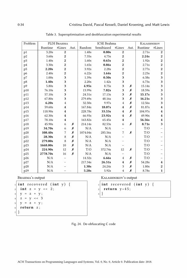
0:34 Cristina David, Pascal Kesseli, Daniel Kroening, and Matt Lewis
Table 3. Superoptimisation and deobfuscation experimental results
Problem PLDI Brahma ICSE Brahma Kalashnikov
Runtime #Lines Aut. Random Semibiased #Lines Aut. Runtime #Lines
p1 3.20s 2 1.48s 0.80s 2 2.71s 2p2 3.60s 2 7.35s 4.75s 2 2.24s 2p3 1.40s 2 1.60s 0.65s 2 1.92s 2p4 3.30s 2 1.65s 0.86s 2 2.71s 2p5 2.20s 2 3.92s 2.28s 2 2.77s 2p6 2.40s 2 6.22s 1.64s 2 2.23s 2p7 1.00s 3 1.39s 0.50s 3 6.38s 3p8 1.40s 3 2.20s 1.42s 3 6.73s 3p9 5.80s 3 4.95s 8.75s 3 15.14s 3p10 76.10s 3 13.99s 7.82s 3 18.59s 3p11 57.10s 3 24.31s 17.13s 3 15.17s 3p12 67.80s 3 279.49s 48.16s 3 16.21s 3p13 6.20s 4 32.50s 9.97s 4 12.56s 3p14 59.60s 4 167.84s 18.07s 4 81.87s 4p15 118.90s 4 228.78s 33.53s 4 104.97s 4p16 62.30s 4 66.93s 23.92s 4 49.90s 4p17 78.10s 4 163.82s 65.45s 4 56.56s 4p18 45.90s 6 214.14s 82.53s 6 8.71s 3p19 34.70s 6 N/A N/A – T/O –
p20 108.40s 7 1074.04s 285.56s 7 T/O –
p21 28.30s 8 N/A N/A – T/O –
p22 279.00s 8 N/A N/A – T/O –
p23 1668.00s 10 N/A N/A – T/O –
p24 224.90s 12 T/O 372.74s 12 T/O –
p25 2778.70s 16 N/A N/A – T/O –
p26 N/A – 14.32s 6.66s 4 T/O –
p27 N/A – 217.34s 26.51s 4 54.28s 4p28 N/A – 1.38s 24.24s 3 1.80s 2p29 N/A – 5.28s 5.92s 4 8.78s 1
Brahma’s output
1 in t r e cove r ed ( in t y )
2 in t z = y << 2 ;
3 y = z + y ;
4 z = y << 3
5 y = z + y ;
6 return z ;
7
Kalashnikov’s output
1 in t r e cove r ed ( in t y )
2 return y ∗ 4 5 ;
3
Fig. 24. De-obfuscating C code
ACM Transactions on Programming Languages and Systems, Vol. 0, No. 0, Article 0. Publication date: 2018.
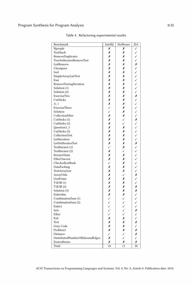
Program Synthesis for Program Analysis 0:35
Table 4. Refactoring experimental results
Benchmark IntelliJ NetBeans JSA
Npeople TestStack RemoveDuplicates TreeSetIteratorRemoveTest ListRemove
Chympara Sort SimpleArrayListTest Esai RemoveDuringIteration Solution (1) Solution (2) ExerciseTwo
CutSticks A_1 ExerciseThree Solution CollectionFilter CutSticks (1)
CutSticks (2) Question3_5 CutSticks (3) CollectionTest ListIteration ListSetIteratorTest
TestIterator (1) TestIterator (2) IteratorMain FilterUneven CheckedListBash DataPacking TestArrayList ArrayUtils
GenPrime T1E3R (1) T1E3R (2)
Solution (3)
Euler68m CombinationSum (1) CombinationSum (2) Euler2 Sets
Filter Ex8 Test
Gray Code Problem3
Distance
DistributedNumberOfInboundEdges Eratosthenes
Total 10 11 38
ACM Transactions on Programming Languages and Systems, Vol. 0, No. 0, Article 0. Publication date: 2018.
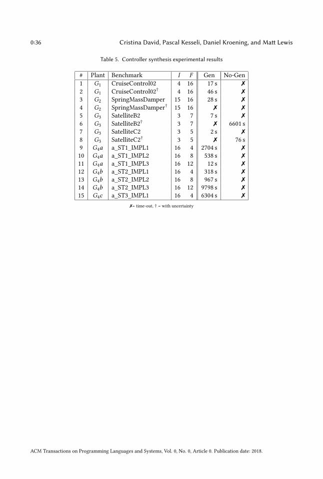
0:36 Cristina David, Pascal Kesseli, Daniel Kroening, and Matt Lewis
Table 5. Controller synthesis experimental results
# Plant Benchmark I F Gen No-Gen
1 G1 CruiseControl02 4 16 17 s
2 G1 CruiseControl02†
4 16 46 s 3 G2 SpringMassDamper 15 16 28 s
4 G2 SpringMassDamper†
15 16 5 G3 SatelliteB2 3 7 7 s
6 G3 SatelliteB2†
3 7 6601 s
7 G3 SatelliteC2 3 5 2 s
8 G3 SatelliteC2†
3 5 76 s
9 G4a a_ST1_IMPL1 16 4 2704 s 10 G4a a_ST1_IMPL2 16 8 538 s 11 G4a a_ST1_IMPL3 16 12 12 s 12 G4b a_ST2_IMPL1 16 4 318 s 13 G4b a_ST2_IMPL2 16 8 967 s 14 G4b a_ST2_IMPL3 16 12 9798 s 15 G4c a_ST3_IMPL1 16 4 6304 s
= time-out, † = with uncertainty
ACM Transactions on Programming Languages and Systems, Vol. 0, No. 0, Article 0. Publication date: 2018.
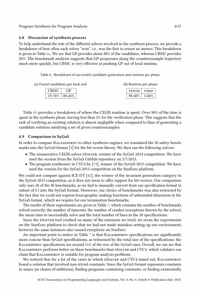
Program Synthesis for Program Analysis 0:37
6.8 Discussion of synthesis processTo help understand the role of the different solvers involved in the synthesis process, we provide a
breakdown of how often each solver “won”, i.e., was the first to return an answer. This breakdown
is given in Table 6a. We see that GP provides about 80% of the candidates, whereas CBMC provides
20%. The benchmark analysis suggests that GP progresses along the counterexample trajectory
much more quickly, but CBMC is very effective at pushing GP out of local minima.
Table 6. Breakdown of successful candidate generation and runtime per phase
(a) Found candidates per back end
CBMC GP
19.74% 80.26%
(b) Runtime per phase
synth verif
98.40% 1.60%
Table 6b provides a breakdown of where the CEGIS runtime is spent. Over 98% of the time is
spent in the synthesis phase, leaving less than 2% for the verification phase. This suggests that the
task of verifying an existing solution is almost negligible when compared to than of generating a
candidate solution satisfying a set of given counterexamples.
6.9 Comparison to SyGuSIn order to compare Kalashnikov to other synthesis engines, we translated the 20 safety bench-
marks into the SyGuS format [4] for the bit-vector theory. We then ran the following solvers:
• The enumerative CEGIS solver eSolver, winner of the SyGuS 2014 competition. We have
used the version from the SyGuS GitHub repository on 5/7/2015.
• The program synthesiser in CVC4 by [74], winner of the SyGuS 2015 competition. We have
used the version for the SyGuS 2015 competition on the StarExec platform.
We could not compare against ICE-DT [42], the winner of the invariant generation category in
the SyGuS 2015 competition, as it does not seem to offer support for bit-vectors. Our comparison
only uses 20 of the 96 benchmarks, as we had to manually convert from our specification format (a
subset of C) into the SyGuS format. Moreover, our choice of benchmarks was also restricted by
the fact that we could not express lexicographic ranking functions of unbounded dimension in the
SyGuS format, which we require for our termination benchmarks.
The results of these experiments are given in Table 7, which contains the number of benchmarks
solved correctly, the number of timeouts, the number of crashes (exceptions thrown by the solver),
the mean time to successfully solve and the total number of lines in the 20 specifications.
Since the eSolver tool crashed on many of the instances we tried, we reran the experiments
on the StarExec platform to check that we had not made mistakes setting up our environment,
however the same instances also caused exceptions on StarExec.
An important point to notice in Table 7 is that Kalashnikov specifications are significantly
more concise than SyGuS specifications, as witnessed by the total size of the specifications: the
Kalashnikov specifications are around 11% of the size of the SyGuS ones. Overall, we can see that
Kalashnikov performs better on these benchmarks than eSolver and CVC4, which validates our
claim that Kalashnikov is suitable for program analysis problems.
We noticed that for a lot of the cases in which eSolver and CVC4 timed out, Kalashnikov
found a solution that involved non-trivial constants. Since the SyGuS format represents constants
in unary (as chains of additions), finding programs containing constants, or finding existentially
ACM Transactions on Programming Languages and Systems, Vol. 0, No. 0, Article 0. Publication date: 2018.
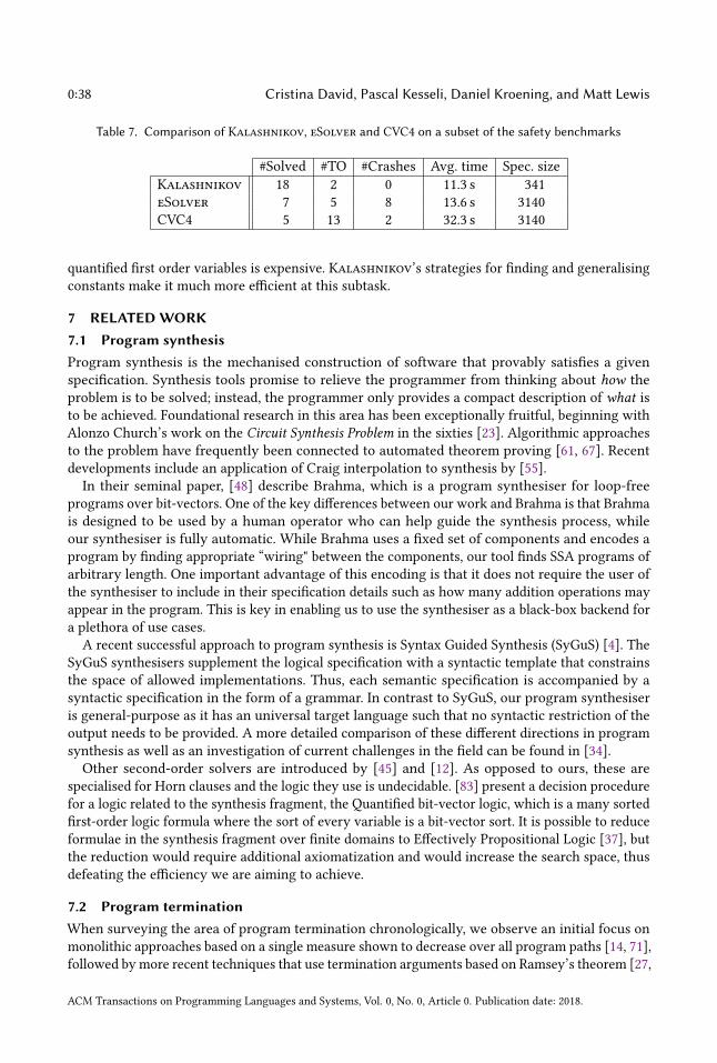
0:38 Cristina David, Pascal Kesseli, Daniel Kroening, and Matt Lewis
Table 7. Comparison of Kalashnikov, eSolver and CVC4 on a subset of the safety benchmarks
#Solved #TO #Crashes Avg. time Spec. size
Kalashnikov 18 2 0 11.3 s 341
eSolver 7 5 8 13.6 s 3140
CVC4 5 13 2 32.3 s 3140
quantified first order variables is expensive. Kalashnikov’s strategies for finding and generalising
constants make it much more efficient at this subtask.
7 RELATEDWORK7.1 Program synthesisProgram synthesis is the mechanised construction of software that provably satisfies a given
specification. Synthesis tools promise to relieve the programmer from thinking about how the
problem is to be solved; instead, the programmer only provides a compact description of what isto be achieved. Foundational research in this area has been exceptionally fruitful, beginning with
Alonzo Church’s work on the Circuit Synthesis Problem in the sixties [23]. Algorithmic approaches
to the problem have frequently been connected to automated theorem proving [61, 67]. Recent
developments include an application of Craig interpolation to synthesis by [55].
In their seminal paper, [48] describe Brahma, which is a program synthesiser for loop-free
programs over bit-vectors. One of the key differences between our work and Brahma is that Brahma
is designed to be used by a human operator who can help guide the synthesis process, while
our synthesiser is fully automatic. While Brahma uses a fixed set of components and encodes a
program by finding appropriate “wiring" between the components, our tool finds SSA programs of
arbitrary length. One important advantage of this encoding is that it does not require the user of
the synthesiser to include in their specification details such as how many addition operations may
appear in the program. This is key in enabling us to use the synthesiser as a black-box backend for
a plethora of use cases.
A recent successful approach to program synthesis is Syntax Guided Synthesis (SyGuS) [4]. The
SyGuS synthesisers supplement the logical specification with a syntactic template that constrains
the space of allowed implementations. Thus, each semantic specification is accompanied by a
syntactic specification in the form of a grammar. In contrast to SyGuS, our program synthesiser
is general-purpose as it has an universal target language such that no syntactic restriction of the
output needs to be provided. A more detailed comparison of these different directions in program
synthesis as well as an investigation of current challenges in the field can be found in [34].
Other second-order solvers are introduced by [45] and [12]. As opposed to ours, these are
specialised for Horn clauses and the logic they use is undecidable. [83] present a decision procedure
for a logic related to the synthesis fragment, the Quantified bit-vector logic, which is a many sorted
first-order logic formula where the sort of every variable is a bit-vector sort. It is possible to reduce
formulae in the synthesis fragment over finite domains to Effectively Propositional Logic [37], but
the reduction would require additional axiomatization and would increase the search space, thus
defeating the efficiency we are aiming to achieve.
7.2 Program terminationWhen surveying the area of program termination chronologically, we observe an initial focus on
monolithic approaches based on a single measure shown to decrease over all program paths [14, 71],
followed by more recent techniques that use termination arguments based on Ramsey’s theorem [27,
ACM Transactions on Programming Languages and Systems, Vol. 0, No. 0, Article 0. Publication date: 2018.
Program Synthesis for Program Analysis 0:39
29, 72]. The latter proof style builds an argument that a transition relation is disjunctively well
founded by composing several small well-foundedness arguments. Themain benefit of this approach
is the simplicity of local termination measures in contrast to global ones. For instance, there are
cases in which linear arithmetic suffices when using local measures, while corresponding global
measures require nonlinear functions or lexicographic orders.
One drawback of the Ramsey-based approach is that the validity of the termination argument
relies on checking the transitive closure of the program, rather than a single step. As such, there is
experimental evidence that most of the effort is spent in reachability analysis [29, 64], requiring the
support of powerful safety checkers: there is a tradeoff between the complexity of the termination
arguments and that of checking their validity.
As Ramsey-based approaches are limited by the state of the art in safety checking, recent research
by [64] and [30] reverts to more complex termination arguments that are easier to check. Following
the same trend, the ranking functions we synthesise may involve nonlinearity and lexicographic
orders: we do not commit to any particular syntactic form, and do not use templates. Furthermore,
our approach allows us to simultaneously search for proofs of non-termination, which take the form
of recurrence sets.
7.3 Bug findingStatic bug finders that use techniques such as BoundedModel Checking (BMC) search for proofs that
safety can be violated and have the attractive property that once an assertion fails, a counterexample
trace is returned, which can be inspected by the user [24]. The counterexample is thus the proof that
an assertion violation occurs. In order to construct such a danger proof, bounded model checkers
compute underapproximations of the reachable program states by progressively unwinding the
transition relation. The downside of this approach is that static bug finders fail to scale when
analysing programs with bugs that require many iterations of a loop. The computational effort
required to discover an assertion violation (i.e., to obtain an intersection with the small ellipse
labelled “error states”) typically grows exponentially with the depth of the bug.
Notably, the scalability problem is not limited to procedures that implement BMC. Approaches
based on a combination of over- and underapproximations such as predicate abstraction [26]
and lazy abstraction with interpolants [68] are not optimised for finding deep bugs either. The
reason for this is that they can only detect counterexamples with deep loops after the repeated
refutation of increasingly longer spurious counterexamples. The analyser first considers a potential
error trace with one loop iteration, only to discover that this trace is infeasible. Consequently,
the analyser increases the search depth, usually by considering one further loop iteration. This
repeated unwinding suffers from the same exponential blow-up as BMC.
Danger invariants allow proving the existence of a bug without explicitly showing an error trace.
This allows for much more compact and intuitive proofs, which in turn allows for much more
scalable analyses that do not suffer from false alarms.
With respect to the verification of temporal properties, a danger invariant for a loop with an
assertionA essentially proves the CTL property EF¬A over the loop. While there exist CTL verifiers
based on a reduction to exist-forall quantified Horn clauses [11, 12], we specialise the concept for
finding deep bugs and describe a modular constraint generation technique over arbitrary programs,
rather than for transition systems.
Another successful technique for finding deep bugs without false alarms is loop acceleration [62,
63]. This approach works by taking a single path at a time through a loop, computing a symbolic
representation of the exact transitive closure of the path (an accelerator) and adding it back into
the program before using an off-the-shelf bug finder such as a bounded model checker. Loop
acceleration requires that each accelerated path can be represented in closed-form by a polynomial
ACM Transactions on Programming Languages and Systems, Vol. 0, No. 0, Article 0. Publication date: 2018.
0:40 Cristina David, Pascal Kesseli, Daniel Kroening, and Matt Lewis
over the program variables, which is not always possible. In contrast, danger invariants are complete
– a program has a corresponding danger invariant iff it has a bug. Loop acceleration could be used
in concert with danger invariants, since if an accelerator can be found, it is the strongest inductive
fact about a loop and as such makes a good candidate danger invariant.
7.4 Program refactoringCheung et al. describe a system that automatically transforms fragments of application logic into
SQL queries [22]. Moreover, similar to our approach, the authors rely on synthesis technology to
generate invariants and postconditions that validate their transformations (a similar approach is
presented in [56]). The main difference (besides the actual goal of the work, which is different from
ours) to our work is that the lists they operate on are immutable and do not support operations
such as remove. Capturing the potential side effects caused by such operations is one of our work’s
main challenges.
8 CONCLUSIONSWe have shown that the synthesis fragment is well-suited for a variety of program analysis tasks by
applying it to directly encode safety, danger, liveness, refactoring and superoptimisation properties.
We built a decision procedure for SFD via a reduction to finite-state program synthesis. The
synthesis algorithm is optimised for program analysis and uses a combination of symbolic model
checking, explicit state model checking and stochastic search. An important strategy is generalisa-
tion – we find simple solutions that solve a restricted case of the specification, then try to generalise
to a full solution.We evaluated the program synthesiser on several static analysis problems, showing
the tractability of the approach.
ACKNOWLEDGMENTSThis work is supported by EPSRC EP/H017585/1, the H2020 FET OPEN project 712689 SC
2and
ERC project 280053 “CPROVER”.
REFERENCES[1] Alessandro Abate, Iury Bessa, Dario Cattaruzza, Lucas Cordeiro, Cristina David, Pascal Kesseli, and Daniel Kroening.
2017. Sound and Automated Synthesis of Digital Stabilizing Controllers for Continuous Plants. In Proceedings of the20th International Conference on Hybrid Systems: Computation and Control (HSCC ’17). ACM, New York, NY, USA,
197–206. https://doi.org/10.1145/3049797.3049802
[2] Alessandro Abate, Iury Bessa, Dario Cattaruzza, Lucas C. Cordeiro, Cristina David, Pascal Kesseli, Daniel Kroening,
and Elizabeth Polgreen. 2017. Automated Formal Synthesis of Digital Controllers for State-Space Physical Plants. In
Computer Aided Verification - 29th International Conference, CAV. 462–482. https://doi.org/10.1007/978-3-319-63387-9_23[3] Rajeev Alur, Rastislav Bodík, Garvit Juniwal, Milo M. K. Martin, Mukund Raghothaman, Sanjit A. Seshia, Rishabh
Singh, Armando Solar-Lezama, Emina Torlak, and Abhishek Udupa. 2013. Syntax-guided synthesis. In Formal Methodsin Computer-Aided Design, FMCAD 2013, Portland, OR, USA, October 20-23, 2013. 1–8.
[4] Rajeev Alur, Rastislav Bodík, Garvit Juniwal, Milo M. K. Martin, Mukund Raghothaman, Sanjit A. Seshia, Rishabh
Singh, Armando Solar-Lezama, Emina Torlak, and Abhishek Udupa. 2013. Syntax-guided synthesis. In Formal Methodsin Computer-Aided Design (FMCAD). IEEE, 1–8.
[5] Karl Johan Astrom and Richard M. Murray. 2008. Feedback Systems: An Introduction for Scientists and Engineers.Princeton University Press, Princeton, NJ, USA.
[6] Karl J. Åström and Björn Wittenmark. 1990. Computer-controlled Systems: Theory and Design. Prentice-Hall, Inc., UpperSaddle River, NJ, USA.
[7] James Avery. 2006. Size-Change Termination and Bound Analysis. In Proceedings of the 8th International Conference onFunctional and Logic Programming (FLOPS’06). Springer, 192–207. https://doi.org/10.1007/11737414_14
[8] Thomas Ball, Ella Bounimova, Vladimir Levin, Rahul Kumar, and Jakob Lichtenberg. 2010. Computer Aided Verification:22nd International Conference, CAV 2010, Edinburgh, UK, July 15-19, 2010. Proceedings. Springer, Chapter The StaticDriver Verifier Research Platform, 119–122. https://doi.org/10.1007/978-3-642-14295-6_11
ACM Transactions on Programming Languages and Systems, Vol. 0, No. 0, Article 0. Publication date: 2018.
Program Synthesis for Program Analysis 0:41
[9] Amir M. Ben-Amram. 2010. Size-Change Termination, Monotonicity Constraints and Ranking Functions. LogicalMethods in Computer Science 6, 3 (2010).
[10] Amir M. Ben-Amram and Samir Genaim. 2013. On the Linear Ranking Problem for Integer Linear-constraint Loops. In
Proceedings of the 40th Annual ACM SIGPLAN-SIGACT Symposium on Principles of Programming Languages (POPL ’13).ACM, New York, NY, USA, 51–62. https://doi.org/10.1145/2429069.2429078
[11] Tewodros A. Beyene, Marc Brockschmidt, and Andrey Rybalchenko. 2014. CTL+FO Verification As Constraint Solving.
In Proceedings of the 2014 International SPIN Symposium on Model Checking of Software (SPIN 2014). ACM, New York,
NY, USA, 101–104. https://doi.org/10.1145/2632362.2632364
[12] Tewodros A. Beyene, Corneliu Popeea, and Andrey Rybalchenko. 2013. Solving Existentially Quantified Horn
Clauses. In Proceedings of the 25th International Conference on Computer Aided Verification (CAV’13). Springer, 869–882.https://doi.org/10.1007/978-3-642-39799-8_61
[13] Dirk Beyer and M.Erkan Keremoglu. 2011. CPAchecker: A Tool for Configurable Software Verification. In ComputerAided Verification, Ganesh Gopalakrishnan and Shaz Qadeer (Eds.). Lecture Notes in Computer Science, Vol. 6806.
Springer, 184–190. https://doi.org/10.1007/978-3-642-22110-1_16
[14] Aaron R. Bradley, Zohar Manna, and Henny B. Sipma. 2005. Linear Ranking with Reachability. In Proceedings of the17th International Conference on Computer Aided Verification (CAV’05). Springer, 491–504. https://doi.org/10.1007/
11513988_48
[15] Aaron R. Bradley, Zohar Manna, and Henny B. Sipma. 2005. The Polyranking Principle. In Proceedings of the 32NdInternational Conference on Automata, Languages and Programming (ICALP’05). Springer, 1349–1361. https://doi.org/10.1007/11523468_109
[16] Aaron R. Bradley, Zohar Manna, and Henny B. Sipma. 2005. Termination of Polynomial Programs. In Proceedings of the6th International Conference on Verification, Model Checking, and Abstract Interpretation (VMCAI’05). Springer, 113–129.https://doi.org/10.1007/978-3-540-30579-8_8
[17] Martin Brain et al. 2006. TOAST: Applying Answer Set Programming to Superoptimisation. In ICLP.[18] M.F. Brameier and W. Banzhaf. 2007. Linear Genetic Programming. Springer.[19] Marc Brockschmidt, Byron Cook, and Carsten Fuhs. 2013. Better Termination Proving Through Cooperation. In
Proceedings of the 25th International Conference on Computer Aided Verification (CAV’13). Springer, 413–429. https://doi.org/10.1007/978-3-642-39799-8_28
[20] Hong-Yi Chen, Byron Cook, Carsten Fuhs, Kaustubh Nimkar, and Peter O’Hearn. 2014. Proving Nontermination viaSafety. Springer, 156–171. https://doi.org/10.1007/978-3-642-54862-8_11
[21] Hong Yi Chen, Shaked Flur, and Supratik Mukhopadhyay. 2012. Termination Proofs for Linear Simple Loops. In StaticAnalysis (SAS). Springer, 422–438.
[22] Alvin Cheung, Armando Solar-Lezama, and Samuel Madden. 2013. Optimizing Database-backed Applications with
Query Synthesis. In Proceedings of the 34th ACM SIGPLAN Conference on Programming Language Design and Implemen-tation (PLDI ’13). ACM, New York, NY, USA, 3–14. https://doi.org/10.1145/2491956.2462180
[23] Alonzo Church. 1962. Logic, Arithmetic, Automata. In Proc. Internat. Congr. Mathematicians. Inst. Mittag-Leffler,
Djursholm, 23–35.
[24] Edmund Clarke, Armin Biere, Richard Raimi, and Yunshan Zhu. 2001. Bounded Model Checking Using Satisfiability
Solving. Form. Methods Syst. Des. 19, 1 (July 2001), 7–34. https://doi.org/10.1023/A:1011276507260
[25] Edmund Clarke, Daniel Kroening, and Karen Yorav. 2003. Behavioral Consistency of C and Verilog Programs Using
Bounded Model Checking. In Proceedings of the 40th Annual Design Automation Conference (DAC ’03). ACM, New York,
NY, USA, 368–371. https://doi.org/10.1145/775832.775928
[26] Edmund M. Clarke, Orna Grumberg, and David E. Long. 1994. Model Checking and Abstraction. ACM Trans. Program.Lang. Syst. 16, 5 (Sept. 1994), 1512–1542. https://doi.org/10.1145/186025.186051
[27] Michael Codish and Samir Genaim. 2003. Proving Termination One Loop at a Time. In The 13th Workshop on LogicProgramming Environments. 48–59.
[28] Byron Cook, Daniel Kroening, Philipp Rümmer, and Christoph M. Wintersteiger. 2010. Ranking Function Synthesis
for Bit-vector Relations. In Proceedings of the 16th International Conference on Tools and Algorithms for the Constructionand Analysis of Systems (TACAS’10). Springer, 236–250. https://doi.org/10.1007/978-3-642-12002-2_19
[29] Byron Cook, Andreas Podelski, and Andrey Rybalchenko. 2006. Termination proofs for systems code. In Proceedings ofthe ACM SIGPLAN 2006 Conference on Programming Language Design and Implementation, Ottawa, Ontario, Canada,June 11-14, 2006. 415–426. https://doi.org/10.1145/1133981.1134029
[30] Byron Cook, Abigail See, and Florian Zuleger. 2013. Ramsey vs. Lexicographic Termination Proving. In Tools andAlgorithms for the Construction and Analysis of Systems - 19th International Conference, TACAS 2013. 47–61. https://doi.org/10.1007/978-3-642-36742-7_4
[31] Patrick Cousot and Radhia Cousot. 1977. Abstract Interpretation: A Unified Lattice Model for Static Analysis of
Programs by Construction or Approximation of Fixpoints. In Conference Record of the Fourth ACM Symposium on
ACM Transactions on Programming Languages and Systems, Vol. 0, No. 0, Article 0. Publication date: 2018.
0:42 Cristina David, Pascal Kesseli, Daniel Kroening, and Matt Lewis
Principles of Programming Languages, POPL. 238–252. https://doi.org/10.1145/512950.512973[32] Cristina David, Pascal Kesseli, and Daniel Kroening. 2016. Kayak: Safe Semantic Refactoring to Java Streams. Technical
Report (2016). https://www.cs.ox.ac.uk/files/9156/stream-extended.pdf
[33] Cristina David, Pascal Kesseli, Daniel Kroening, and Matt Lewis. 2016. Danger Invariants. In FM 2016: Formal Methods- 21st International Symposium. 182–198. https://doi.org/10.1007/978-3-319-48989-6_12
[34] Cristina David and Daniel Kroening. 2017. Program Synthesis: Challenges and Opportunities. In PhilosophicalTransactions of the Royal Society A. To appear.
[35] Cristina David, Daniel Kroening, and Matt Lewis. 2015. Unrestricted Termination and Non-termination Arguments
for Bit-Vector Programs. In Programming Languages and Systems - 24th European Symposium on Programming, ESOP.183–204. https://doi.org/10.1007/978-3-662-46669-8_8
[36] Cristina David, Daniel Kroening, and Matt Lewis. 2015. Using Program Synthesis for Program Analysis. In Logicfor Programming, Artificial Intelligence, and Reasoning - 20th International Conference, LPAR-20. 483–498. https:
//doi.org/10.1007/978-3-662-48899-7_34
[37] Leonardo Mendonça de Moura and Nikolaj Bjørner. 2008. Deciding Effectively Propositional Logic Using DPLL and
Substitution Sets. In Automated Reasoning, 4th International Joint Conference, IJCAR. 410–425. https://doi.org/10.1007/978-3-540-71070-7_35
[38] Nachum Dershowitz, Naomi Lindenstrauss, Yehoshua Sagiv, and Alexander Serebrenik. 2001. A General Framework
for Automatic Termination Analysis of Logic Programs. Appl. Algebra Eng. Commun. Comput. 12, 1/2 (2001), 117–156.[39] Ronald Fagin. 1974. Generalized First-Order Spectra and Polynomial-Time Recognizable Sets. In Complexity of
Computation, R. Karp (Ed.).
[40] Robert W. Floyd. 1993. Assigning Meanings to Programs. Springer Netherlands, Dordrecht, 65–81. https://doi.org/10.1007/978-94-011-1793-7_4
[41] Gene F. Franklin, David J. Powell, and Abbas Emami-Naeini. 2001. Feedback Control of Dynamic Systems (4th ed.).
Prentice Hall PTR, Upper Saddle River, NJ, USA.
[42] Pranav Garg, Christof Löding, P. Madhusudan, and Daniel Neider. 2014. ICE: A Robust Framework for Learning Invariants.Springer International Publishing, Cham, 69–87. https://doi.org/10.1007/978-3-319-08867-9_5
[43] Benny Godlin and Ofer Strichman. 2010. Time for Verification. Springer, Chapter Inference Rules for Proving the
Equivalence of Recursive Procedures, 167–184. http://dl.acm.org/citation.cfm?id=1880443.1880451
[44] Faustino Gomez and Risto Miikkulainen. 1997. Incremental Evolution of Complex General Behavior. Adaptive Behavior(1997).
[45] Sergey Grebenshchikov, Nuno P. Lopes, Corneliu Popeea, and Andrey Rybalchenko. 2012. Synthesizing software
verifiers from proof rules. In ACM SIGPLAN Conference on Programming Language Design and Implementation, PLDI.405–416. https://doi.org/10.1145/2254064.2254112
[46] Sumit Gulwani. 2010. Dimensions in Program Synthesis. In Proceedings of the 12th International ACM SIGPLANSymposium on Principles and Practice of Declarative Programming (PPDP ’10). ACM, New York, NY, USA, 13–24.
https://doi.org/10.1145/1836089.1836091
[47] Sumit Gulwani, Sagar Jain, and Eric Koskinen. 2009. Control-flow refinement and progress invariants for bound
analysis. In Proceedings of the 2009 ACM SIGPLAN Conference on Programming Language Design and Implementation,PLDI. 375–385. https://doi.org/10.1145/1542476.1542518
[48] Sumit Gulwani, Susmit Jha, Ashish Tiwari, and Ramarathnam Venkatesan. 2011. Synthesis of Loop-free Programs. In
Proceedings of the 32Nd ACM SIGPLAN Conference on Programming Language Design and Implementation (PLDI ’11).ACM, New York, NY, USA, 62–73. https://doi.org/10.1145/1993498.1993506
[49] Sumit Gulwani, Saurabh Srivastava, and Ramarathnam Venkatesan. 2008. Program analysis as constraint solving. In
Proceedings of the ACM SIGPLAN 2008 Conference on Programming Language Design and Implementation, PLDI. 281–292.https://doi.org/10.1145/1375581.1375616
[50] Ashutosh Gupta, Thomas A. Henzinger, Rupak Majumdar, Andrey Rybalchenko, and Ru-Gang Xu. 2008. Proving
Non-termination. SIGPLAN Not. 43, 1 (Jan. 2008), 147–158. https://doi.org/10.1145/1328897.1328459[51] Arie Gurfinkel, Temesghen Kahsai, and JorgeA. Navas. 2015. SeaHorn: A Framework for Verifying C Programs
(Competition Contribution). In Tools and Algorithms for the Construction and Analysis of Systems, Christel Baierand Cesare Tinelli (Eds.). Lecture Notes in Computer Science, Vol. 9035. Springer, 447–450. https://doi.org/10.1007/
978-3-662-46681-0_41
[52] Arvind Haran, Montgomery Carter, Michael Emmi, Akash Lal, Shaz Qadeer, and Zvonimir Rakamarić. 2015.
SMACK+Corral: A Modular Verifier (Competition Contribution). In Proceedings of the 21st International Confer-ence on Tools and Algorithms for the Construction and Analysis of Systems (TACAS) (Lecture Notes in Computer Science),Christel Baier and Cesare Tinelli (Eds.), Vol. 9035. Springer, 450–453.
[53] William R. Harris, Akash Lal, Aditya V. Nori, and Sriram K. Rajamani. 2010. Alternation for Termination. In StaticAnalysis - 17th International Symposium, SAS. 304–319. https://doi.org/10.1007/978-3-642-15769-1_19
ACM Transactions on Programming Languages and Systems, Vol. 0, No. 0, Article 0. Publication date: 2018.
Program Synthesis for Program Analysis 0:43
[54] Matthias Heizmann, Jochen Hoenicke, Jan Leike, and Andreas Podelski. 2013. Linear Ranking for Linear Lasso Programs.Springer International Publishing, Cham, 365–380. https://doi.org/10.1007/978-3-319-02444-8_26
[55] Georg Hofferek, Ashutosh Gupta, Bettina Könighofer, Jie-Hong Roland Jiang, and Roderick Bloem. 2013. Synthesizing
Multiple Boolean Functions using Interpolation on a Single Proof. http://arxiv.org/abs/1308.4767. CoRR abs/1308.4767
(2013).
[56] Ming-Yee Iu, Emmanuel Cecchet, and Willy Zwaenepoel. 2010. JReq: Database Queries in Imperative Languages.
In Proceedings of the 19th Joint European Conference on Theory and Practice of Software, International Conference onCompiler Construction (CC’10/ETAPS’10). Springer, 84–103. https://doi.org/10.1007/978-3-642-11970-5_6
[57] Susmit Jha, Sumit Gulwani, Sanjit A. Seshia, and Ashish Tiwari. 2010. Oracle-guided Component-based Program
Synthesis. In Proceedings of the 32Nd ACM/IEEE International Conference on Software Engineering - Volume 1 (ICSE ’10).ACM, New York, NY, USA, 215–224. https://doi.org/10.1145/1806799.1806833
[58] Lee H. Keel and Shankar P. Bhattacharyya. 1997. Robust, fragile, or optimal? IEEE Trans. on Automatic Control 42, 8(1997), 1098–1105. https://doi.org/10.1109/9.618239
[59] Lee H. Keel and Shankar P. Bhattacharyya. 1998. Stability margins and digital implementation of controllers. In Proc.American Control Conference, Vol. 5. 2852–2856. https://doi.org/10.1109/ACC.1998.688377
[60] Soonho Kong, Yungbum Jung, Cristina David, Bow-Yaw Wang, and Kwangkeun Yi. 2010. Automatically InferringQuantified Loop Invariants by Algorithmic Learning from Simple Templates. Springer, 328–343. https://doi.org/10.1007/978-3-642-17164-2_23
[61] Ina Kraan, David Basin, and Alan Bundy. 1993. Logic Program Synthesis via Proof Planning. In Logic Program Synthesisand Transformation. 1–14. https://doi.org/10.1007/978-1-4471-3560-9_1
[62] Daniel Kroening, Matt Lewis, and Georg Weissenbacher. 2013. Under-Approximating Loops in C Programs for Fast
Counterexample Detection. In Proceedings of the 25th International Conference on Computer Aided Verification (CAV’13).Springer, 381–396. https://doi.org/10.1007/978-3-642-39799-8_26
[63] Daniel Kroening, Matt Lewis, and Georg Weissenbacher. 2015. Proving Safety with Trace Automata and Bounded
Model Checking. In FM 2015: Formal Methods - 20th International Symposium. 325–341. https://doi.org/10.1007/
978-3-319-19249-9_21
[64] Daniel Kroening, Natasha Sharygina, Aliaksei Tsitovich, and Christoph M. Wintersteiger. 2010. Termination Analysis
with Compositional Transition Invariants. In Computer Aided Verification, 22nd International Conference, CAV 2010,Edinburgh, UK, July 15-19, 2010. Proceedings. 89–103. https://doi.org/10.1007/978-3-642-14295-6_9
[65] William B. Langdon and Riccardo Poli. 2002. Foundations of Genetic Programming. Springer.[66] Daniel Larraz, Albert Oliveras, Enric Rodríguez-Carbonell, and Albert Rubio. 2013. Proving termination of imperative
programs using Max-SMT. In 2013 Formal Methods in Computer-Aided Design. 218–225. https://doi.org/10.1109/FMCAD.
2013.6679413
[67] Zohar Manna and Richard J. Waldinger. 1971. Toward Automatic Program Synthesis. Commun. ACM 14, 3 (March
1971), 151–165. https://doi.org/10.1145/362566.362568
[68] Kenneth L. McMillan. 2006. Lazy Abstraction with Interpolants. In Proceedings of the 18th International Conference onComputer Aided Verification (CAV’06). Springer, 123–136. https://doi.org/10.1007/11817963_14
[69] Aditya V. Nori and Sriram K. Rajamani. 2010. An Empirical Study of Optimizations in Yogi. In International Conferenceon Software Engineering (ICSE). Association for Computing Machinery, Inc. http://research.microsoft.com/apps/pubs/
default.aspx?id=117670
[70] Aditya V. Nori and Rahul Sharma. 2013. Termination Proofs from Tests. In Proceedings of the 2013 9th Joint Meeting onFoundations of Software Engineering (ESEC/FSE 2013). ACM, New York, NY, USA, 246–256. https://doi.org/10.1145/
2491411.2491413
[71] Andreas Podelski and Andrey Rybalchenko. 2004. A Complete Method for the Synthesis of Linear Ranking Functions.
In Verification, Model Checking, and Abstract Interpretation, 5th International Conference, VMCAI. 239–251. https:
//doi.org/10.1007/978-3-540-24622-0_20
[72] Andreas Podelski and Andrey Rybalchenko. 2004. Transition Invariants. In Proceedings of the 19th Annual IEEESymposium on Logic in Computer Science (LICS ’04). IEEE Computer Society, Washington, DC, USA, 32–41. https:
//doi.org/10.1109/LICS.2004.50
[73] Phillip Porras, Hassen Saïdi, and Vinod Yegneswaran. 2009. A Foray into Conficker’s Logic and Rendezvous Points. In
Proceedings of the 2Nd USENIX Conference on Large-scale Exploits and Emergent Threats: Botnets, Spyware, Worms, andMore (LEET’09). USENIX Association, Berkeley, CA, USA, 7–7. http://dl.acm.org/citation.cfm?id=1855676.1855683
[74] Andrew Reynolds, Morgan Deters, Viktor Kuncak, Cesare Tinelli, and Clark Barrett. 2015. Counterexample-GuidedQuantifier Instantiation for Synthesis in SMT. Springer International Publishing, Cham, 198–216. https://doi.org/10.
1007/978-3-319-21668-3_12
[75] Andrey Rybalchenko. 2011. ARMC. http://www7.in.tum.de/~rybal/armc. (2011).
ACM Transactions on Programming Languages and Systems, Vol. 0, No. 0, Article 0. Publication date: 2018.
0:44 Cristina David, Pascal Kesseli, Daniel Kroening, and Matt Lewis
[76] Armando Solar-Lezama, Liviu Tancau, Rastislav Bodík, Sanjit A. Seshia, and Vijay A. Saraswat. 2006. Combinato-
rial sketching for finite programs. In Proceedings of the 12th International Conference on Architectural Support forProgramming Languages and Operating Systems, ASPLOS 2006, San Jose, CA, USA, October 21-25, 2006. 404–415.
[77] SV-COMP. 2015. (2015). http://sv-comp.sosy-lab.org/2015/.
[78] SV-COMP. 2016. (2016). http://sv-comp.sosy-lab.org/2016/.
[79] Alan Turing. 1936. On computable numbers with an application to the Entscheidungsproblem. Proceeding of theLondon Mathematical Society 2 (1936), 230–265.
[80] Caterina Urban. 2013. The Abstract Domain of Segmented Ranking Functions. In Static Analysis - 20th InternationalSymposium, SAS. 43–62. https://doi.org/10.1007/978-3-642-38856-9_5
[81] Timothy E. Wang, Pierre-Loïc Garoche, Pierre Roux, Romain Jobredeaux, and Eric Feron. 2016. Formal Analysis of
Robustness at Model and Code Level. In Proceedings of the 19th International Conference on Hybrid Systems: Computationand Control, HSCC. 125–134.
[82] Henry S. Warren. 2002. Hacker’s Delight. Addison-Wesley Longman Publishing Co., Inc., Boston, MA, USA.
[83] Christoph M. Wintersteiger, Youssef Hamadi, and Leonardo Moura. 2013. Efficiently Solving Quantified Bit-vector
Formulas. Form. Methods Syst. Des. 42, 1 (Feb. 2013), 3–23. https://doi.org/10.1007/s10703-012-0156-2
ACM Transactions on Programming Languages and Systems, Vol. 0, No. 0, Article 0. Publication date: 2018.