INTERACTIVE PROGRAM FOR ANALYSIS AND ... - CORE
300
N AFML-TR-71-268 INTERACTIVE PROGRAM FOR ANALYSIS AND DESIGN PROBLEMS IN ADVANCED COMPOSITES TECHNOLOGY T. A. CRUSE J. L. SWEDLOW TECHNICAL REPORT AFML-TR-71-268 i 196 9 T nniv.) A. CSCL 1 1D G3/1.8 tor. oublic. release: distribution g (ACCESSION NUMBER) (THRU) (NASA CR ORTOx'OR AD NUMBER) (cAfEGORY) J AIR FORCE MATERIALS LABORATORY AIR FORCE SYSTEMS COMMAND WRIGHT PATTERSON AIR FORCE BASE, OHIO https://ntrs.nasa.gov/search.jsp?R=19720010933 2020-03-11T18:40:03+00:00Z
-
Upload
khangminh22 -
Category
Documents
-
view
0 -
download
0
Transcript of INTERACTIVE PROGRAM FOR ANALYSIS AND ... - CORE
N
AFML-TR-71-268
INTERACTIVE PROGRAM
FOR ANALYSIS AND DESIGN PROBLEMS
IN ADVANCED COMPOSITES TECHNOLOGY
T. A. CRUSE
J. L. SWEDLOW
TECHNICAL REPORT AFML-TR-71-268
i1969 Tnniv . )
A. CSCL 1 1D G3/1.8
tor. oublic. release: distribution
g (ACCESSION NUMBER) (THRU)
(NASA CR ORTOx'OR AD NUMBER) (cAfEGORY)
J
AIR FORCE MATERIALS LABORATORY
AIR FORCE SYSTEMS COMMAND
WRIGHT PATTERSON AIR FORCE BASE, OHIO
https://ntrs.nasa.gov/search.jsp?R=19720010933 2020-03-11T18:40:03+00:00Z

NOTICE
When Government drawings, specifications, or other data are used for any purpose
other than in connection with a definitely related Government procurement operation,
the United States Government thereby incurs no responsibility nor any obligation
whatsoever; and the fact that the government may have formulated, furnished, or in
any way supplied the said drawings, specifications, or other data, is not to be regardedby implication or otherwise as in any manner licensing the holder or any other person
or corporation, or conveying any rights or permission to manufacture, use, or sell any
patented invention that may in any way be related thereto.
Copies of this report should not be returned unless return is required by securityconsiderations, contractual obligations, or notice on a specific document.
™ AFML-TR-71-268
INTERACTIVE PROGRAMFOR ANALYSIS AND DESIGN PROBLEMS
IN ADVANCED COMPOSITES TECHNOLOGY
T. A. CRUSE
J. L. SWEDLOW
DEPARTMENT OF MECHANICAL ENGINEERING
CARNEGIE INSTITUTE OF TECHNOLOGY
CARNEGIE-MELLON UNIVERSITY .
PITTSBURGH, PENNSYLVANIA
DECEMBER 1971
Approved for public release: distribution unlimited
FOREWORD
This report describes work performed 1n the Department ofMechanical Engineering, Carnegie-Mellon University, Pittsburgh, Pennsyl-vania, 15213, under A1r Force Contract F33615-70-C-1146, Project 6169 CW;Subject: "Research for the development of design and analytical techniquesfor advanced composite structures". This work was accomplished between1 November 1969 and 31 October 1971. The Program Manager for the A1r ForceMaterials Laboratory was Mr. George E. Husman, AFML/MAC. The researchprojects 1n this report were undertaken by several graduate students underthe direction of the Principal Investigators, Drs. T. A. Cruse and J. L.Swedlow and 1t 1s a pleasure to acknowledge Messrs. H. J. Konlsh, Jr.(fracture project), J. P. Waszczak (mechanically fastened joints), W. B.Bamford (numerical studies using Integral equations) and S. J. Marulls(optimization); 1t 1s also a pleasure to acknowledge the work on advancedtopics 1n Integral equations performed on a consulting basis by ProfessorFrank J. R1zzo, University of Kentucky.
Since the emphasis of the program was on Interaction with Indus-try It 1s a pleasure to acknowledge Messrs. C. W. Rogers, P. D. Shockey,M. E. Waddoups, R. 6. Pipes and many others 1h the advanced compositesgroup of Convalr Aerospace Division, General Dynamics, Fort Worth, Texas;also the staffs at Boelng/Vertol, GrummanAerospacei North American Rock-well and Southwest Research Institute.
Portions of the reported work were also supported by NASA GrantNGR-39-002-023 (fracture project) and by General Dynamics P. 0. No. 499527(joint design). The authors would finally like to acknowledge M1ssKathleen Sokol for her careful and selfless devotion to the preparationof this document.
This report was submitted by the Authors on 6 December 1971.
This technical report has been reviewed and 1s approved,
Robert C. Tomashot TTechnical Area ManagerAdvanced Composites Division
11
ABSTRACT
The Carnegie-Mellon University team has completed the initialInteractive Program in Advanced Composites Technology. The program hashad significant impact as the CMU team, working closely with engineersfrom industry, has made significant technical progress in several problemareas of current importance. Results on these problems are reported inthis Report. During the past year an experimental program in the fractureof advanced fiber composites has been completed. The experimental programhas given direction to additional experimental and theoretical work. Asynthesis program for designing low weight multifastener joints in compos-ites is proposed, based on extensive analytical background. A number offailed joints have been thoroughly analyzed to evaluate the failure hy-pothesis used in the synthesis procedure. Finally, the Report includesnew solution methods for isotropic and anisotropic (mid-plane symmetric)laminates using the boundary-integral method. The solution method offerssignificant savings of computer core and time for important problems.
iii
PRECEDING PAGE BLANK NOT FILMED
TABLE OF CONTENTS
CHAPTER PAGE
I SUMMARY OF THE INTERACTIVE PROGRAM 1
1.1 Introduction 1
1.2 First and Second Year Programs 2
1.2.1 Phase I 21.2.2 Phase II 31.2.3 Phase III 5
1.3 Research Projects Completed 6
1.3.1 Fracture of Advanced Composites 71.3.2 Strength of Mechanically Fastened Joints 71.3.3 Optimization Methods 71.3.4 Boundary-Integral Equation Solution Methods 7
1.4 Evaluation and Recommendations 8
1.5 References 11
1.6 Appendix A: Summary of Educational Material 12
1.7 Appendix B: Trip Reports 18
1.8 Appendix C: Research Documents 20
II FRACTURE OF ADVANCED COMPOSITES 23
2.1 Stress Analysis of a Cracked Anisotropic Beam 23
2.1.1 Introduction 232.1.2 Review of Previous Work 232.1.3 Analytical Study 272.1.4 References 31
2.2 Experimental Investigation of Fracture in anAdvanced Fiber Composite 34
2.2.1 Introduction ' 342.2.2 Test Procedures; Program 352.2.3 Data Reduction; Results 372.2.4 Discussion 382.2.5' Conclusions 412.2.6 References 42
CHAPTER PAGE
III STRENGTH OF MECHANICALLY FASTENED JOINTS 54
3.1 An Investigation of Stress Concentrations Inducedin Composite Bolt Bearing Specimens 54
3.1.1 Introduction 543.1.2 Analysis Method 553.1.3 Strength and Failure Mode Predictions 573.1.4 Future Work 613.1.5 References 62
3.2 Toward a Design Procedure for Mechanically FastenedJoints Made of Composite Materials 78
3.2.1 Introduction 783.2.2 investigation of the Characteristic Crack
Length Hypothesis 823.2.3 Review of Past Design Programs Involving
Composite Joints 873.2.4 Evaluation of Load Partitioning in Joints 89
3.2.4.1 Point Strain Matching Technique 893.2.4.2 Displacement Matching Technique 91
3.2.5 Computer Analysis of Experimentally FailedComposite Joints 93
3.2.6 Proposed Mechanically Fastened Joint DesignProgram 103
3.2.6.1 Outline of Proposed SynthesisProgram 103
3.2.6.2 Discussion of Program Details 104
3.2.6.2.1 Input Data 1043..2.6.2.2 Design Variables 1073.2.6.2.3 Design Constraints 1093.2.6.2.4 Design Procedures 112
3.2.7 Areas of Future Work 1173.2.8 References 120
vi
CHAPTER PAGE
IV OPTIMIZATION METHODS 142
4.1 Introduction 142
4.2 Structural Optimization 142
4.2.1 Background 1424.2.2 Variational Method 1434.2.3 Non-linear Programming Methods 144
4.3 Torsion of an Elliptic Bar - Variational Example 145
4.4 Bolt Bearing Problem - Non-Linear ProgrammingExample 148
4.5 Discussion 151
4.6 References 153
V BOUNDARY-INTEGRAL EQUATION SOLUTION METHODS : 160
5.1 Two Dimensional Isotropic Boundary-IntegralEquation Method 160
5.1.1 Introduction 1605.1.2 Review of the Isotropic Boundary-Integral
Equation Method 1615.1.3 Use of the Isotropic Computer Program 163
5.1.3.1 Dimension Statements 1645.1.3.2 Definition of Key Parameters;
Matrices 1655.1.3.3 Boundary Conditions 1665.1.3.4 Input Cards 1675.1.3.5 Example Problem 167
5.1.4 References 168
5.1.5 Listing for Isotropic Boundary-IntegralEquation Computer Program 169
vn
CHAPTER PAGE
5.2 Two Dimensional Anisotropic Boundary-IntegralEquation Method
5.2.1 Formulation of the Field Equations 1865.2.2 Fundamental Solution: Point Force Problem 1915.2.3 Boundary Integral Equation 1955.2.4 Somigliana's Identity for Interior Strains, Stresses 1995.2.5 Numerical Solution 2015.2.6 Usage Guide for ANISOT 205
5.2.6.1 Problem Size Specifications 2055.2.6.2 Specification of Material Constants 2065.2.6.3 Use of AXCALC 2075.2.6.4 Identification of Parameters for ANISOT 2085.2.6.5 Boundary Conditions 2095.2.6.6 Input Data for ANISOT . 211
5.2.7 References 2125.2.8 Listing for AXCALC Computer Program 2135.2.9 Listing for ANISOT Computer Program 220
5.3 Example Solutions for Isotropic and Anisotropic 237Boundary-Integral Equation Method
5.3.1 Tension of an Isotropic Plate 237
5.3.1.1 Circular Cutout 2375.3.1.2 Elliptical Cutout 238
5.3.2 Tension of an Anisotropic Plate with Circular 240Cutout
5.3.2.1 Orthotropic Material 2405.3.2.2 Anisotropic Material 241
5.4 Advanced Topics in Anisotropic Integral Equation 256Solution Methods
5.4.1 Introduction 2565.4.2 Fundamental Three-Dimensional Anisotropic 257
Singularity
5.4.2.1 Via John 2575.4.2.2 Via Fredholm 264
5.4.3 Investigation of the Interlaminar Shear Problem 2665.4.4 References 273
LIST OF FIGURES
SECTION FIGURE TITLE PAGE
2.1 1 Three-point bend specimen, with 32global (x,y and r,e) and material(1,2) coordinate systems shown(insert). The applied load P ismodeled as point load. The specimenthickness is denoted by B.
2 A plot of (3(a/w» vs. a/W. The 33degree of correspondence betweenthe discrete points (obtained nu-merically) and the continuous curve(obtained from [8]) is a measure ofthe applicability of an anisotropiccontinuum analysis [4] to advancedfiber composite materials.
2.2 1 Three-point bend specimen geometry, 44with crack shape shown in inserts,both schematic (left) and actual(right). Fiber direction given bya, crack length by a. Specimen thick-ness 0.5 in (nom); all dimensionsgiven in inches.
2 Test jig at beginning of loading. 45
3 Typical trace of load applied to 46specimen vs. cross-head displacement,showing method used to determine P<j.
4 Failure surfaces for a = 0° specimens 47of three starter crack lengths (a = 0.6,0.4, 0.2 in).
5 Failure surfaces for a = 45° specimens 48of three starter crack lengths (a = 0.6,0.4, 0.2 in).
6 Failure surfaces for a = 90° specimens 49of three starter crack lengths (a = 0.6,0.4, 0.2 in).
7 Failure surfaces for a = (±45°) speci- 50mens of three starter crack lengths(a =0.6, 0.4, 0.2 in).
IX
SECTION FIGURE TITLE PAGE
2.2 8 Failure surfaces for a = (0'6/±45°/ 5190°) specimens of two starter cracklengths (a = 0.6, 0.4 1n).
9 Failed but unbroken specimen (a = 52(00/±45°/900)s, a = 0.2 in).
10 Traces of load vs. cross-head dis- 53placement for five specimens used 1nreproduclblHty tests for a uni-directional laminate (a = 0°, a = 0.4in).
11 Traces of load vs. cross-head dis- 54placement for five specimens used inreproducibllity tests for a multi-directional laminate (o = (0°/±45°/
3.1
90°)s, a = 0.4 in).
12
3a
3b
4
5
6
7a
7b
7c
7d
Bolt bearing test specimen
Bolt bearing grid representation fore/d-5.0, s/d-10.0 and £/d-20.0.
Isojtropic bolt bearing verification:o¥/o vs. y..A • •
I sotropi c bol t beari ng veri f i ca ti on :a /a vs. x.
Polar plot of edge stresses for an1 sotropi c test run.
Variations about the cosine distribu-tion of normal stress.
Bolt bearing test specimen failuremodes.
Net tension failure +45° lamina
Net tension failure -45° lamina
Net tension failure 90° lamina
Net tension failure 0° lamina
6.3
64
65
66
67
68
69
70
71
72
73
SECTION FIGURE TITLE PAGE
3.1 8 Slug shear-out failure 0° lamina 74
9 Bearing failure 0° lamina 75
10 Combination and net tension failure, 76+45° lamina.
3.2 1 Distortional energy contour plots for 125the 1.0" diameter, anisotropic tensioncoupon at the experimental failure load.
2a Distortional energy contour plots for 126the initial bolt bearing specimen de-sign at the predicted failure load.
2b Distortional energy contour plots for 127the revised bolt bearing specimen de-sign at the predicted failure load.
3 Double shear joint configuration. 128
4 Bolt bearing modeling procedure for 129joints.
5 Bolt load distribution for Specimens 1301 thru 6.
6 Skin stress boundary conditions at the 131leading edge of a bolt bearing model.
7 Specimen 1: Distortional energy con- 132tour plots for the experimentalfailure load.
8 Specimen 2: Distortional energy con- 133tour plots for the experimentalfailure load.
9 , Specimen 3: Distortional energy con- 134tour plots for the experimentalfailure load.
10 Specimen 4: Distortional energy con- 135tour plots for the experimentalfailure load.
SECTION FIGURE TITLE PAGE
3.2 11 Specimens: Distortional energy con- 136tour plots for the experimentalfailure load.
12 Specimen 6: Dlstortional energy con- 137tour plots for the experimentalfailure load.
13 The principle of superposition applied 140to an infinite bolt bearing model.
14 Schematic of a proposed joint design 141showing the seventeen possible designvariables.
4 1 Weight vs, load for fixed orientations. 157
2 Weight vs. load for variable 158orientations.
3 Summary of weight vs. load results. 159
5.3 1 Local geometry at boundary. 242
2 Local geometry at boundary. 242
3 Accuracy of DIPOME r Circular hole. 244
4 Accuracy of DIPOME - Elliptical cutout. 251
5.4 1 Geometry for interlaminar shear 272problems.
2 Individual lamina notation. 272
xii
LIST OF TABLES
;CTION2.2
3.1
3.2
4
5.3
TABLE
I
I
I
II '
III
IV
I
II
III
I
II
III
IV
V
VI
VII
VIII
TITLE
Experimental results.
Summary of bolt bearing specimen data.
Initial bolt bearing specimen design.
Revised bolt bearing specimen design.
Description of the six specimensselected for analysis.
Summary of significant data fromFigures 7 thru 12.
Coupon weights for fixed orientations.
Coupon weights for variable orienta-tions .
Coupon weights allowing orientationsto be eliminated.
Interior stress solutions -DIPOME(a/b = 1.0; ox).
Interior stress solutions - DIPOME(a/b = 2.0; O'x)-.
Interior stress solutions - DIPOME(a/b =2.0; a )•y ,Interior stress solutions - DIPOME(a/b = 4.5; a)().
Interior stress solutions - DIPOME(a/b = 4.5; Oy).
Interior stress solutions - DIPOME(a/b = 19.5; ox).
Interior stress solutions -;' DIPOME(a/b = 19.5; ay).
Surface hoop stress comparisons
PAGE
43
77
122
122
123
124
154
155
156
243
245
246
247
248
249
250
252(a =0° ) .
xiii
SECTION TABLE TITLE PAGE
5.3 IX Surface hoop stress comparisons 253(a = 90°).
X Surface hoop stress comparisons 254(a » 45°; 90 Segments).
XI Surface hoop stress comparisons 255(a « 45°; 20 Segments).
x1v
LIST OF SYMBOLS AND NOTATION
SECTION SYMBOL DESCRIPTIONi
1 r, e Polar coordinates, with theorigin at the crack-tip.(See Fig. 1).
x, y Cartesian coordinates, withthe origin at the crack- tip;these are the global coordi-nates. (See Fig. 1).
1, 2 Cartesian coordinates basedon the material principaldirections (See Fig. 1).
B Thickness of the three-pointbend specimen.
S Span of the three-point bendspecimen.
W Depth of the three-point bendspecimen.
a Crack- length.
a Angle of rotation between theglobal and lamina coordinatesystems (See Fig. 1).
a Tensile stresses in the globalcoordinate system.
Displacement normal to thecrack-axis.
Applied load on the three-point bend specimen.
Roots of the characteristicequation.
Components of the globalcompliance matrix.
xv
CHAPTER SECTION SYMBOL DESCRIPTION
H 1 KT IT Stress intensity factors cor-' responding to symmetric and
anti-symmetric loading re-spectively. A subscript cindicates a critical valueof K, i.e., a value at whichthe crack propagates catas-trophically.
2 KO A candidate value of the critical^ stress-intensity factor.
The average value of KQ for agiven laminate, obtained byaveraging the KQ values obtainedfor several specimens of thelaminate.
GO Strain-energy release rate.
M Initial slope of the experimentalplot of load vs. specimendeflection (See Fig. 12).
PS Load corresponding to the inter-section of the secant of slopeM with the curve of load vs.specimen deflection (See Fig. 12).
PO Applied load at which crack^ propagation occurred.
a Crack-length (See Fig. 1).
a Angle of rotation between theglobal and lamina coordinatesystems (See Fig. 1).
xv i
CHAPTER SECTION
III V .
SYMBOL
e
d
s
t
t
ffr°1u
DIST
FTUFSUFBRUS
E
t
D/
L
N
F
DESCRIPTION
Specimen edge distance.
Bolt bearing diameter.
Total specimen width.
Total specimen length.
Specimen thicknessth1— principal lamina stress.
1—principal ultimate laminastress.
Normalized distortlonal energy.
Effective tension strength.
Effective shear-out strength.
Effective bearing strength.
Bolt bearing specimen width.
Bolt bearing specimen edge distance.
Bolt bearing specimen thickness.
Bolt bearing specimen diameter.
Bolt bearing specimen length.
Total joint length.
Number of bolts per column.
Maximum load to be carried percolumn of bolts
xv 11
CHAPTER SECTION SYMBOL DESCRIPTION
III 2 Subscripts and Superscripts
m Main plate
s Splice plate
B Bolt material
u Ultimate allowable
t Tension
c Compression
XV111
CHAPTER
IV
SECTION SYMBOL
M
a, b
XL
-tu
rSU
DESCRIPTION
Weight function of a compositeplate.
Variables of a composite plate.
Constraint functions on W(X.)«
Lagrange multipliers for theconstraint functions.
Objective function forminimization.
Applied torsional moment.
Semi-major and semi-mi nor axesof the ellipse.
Shear stress.
Thickness of the bolt bearingspecimen.
Width of the bolt bearingspecimen.
Distance from the center ofthe bolt hole to the near edgeof the bolt bearing specimen.
Diameter of the bolt hole inthe bolt bearing specimen.
Distance from the bolt holeto the far edge of the boltbearing specimen.
Load applied to the boltbearing specimen.
Failure stress for the tensionmode failure of the bolt bear-ing specimen.
Failure stress for the shearout mode failure of the boltbearing specimen.
xix
CHAPTER SECTION SYMBOL DESCRIPTION
IV 4 P u failure stress for the bear-Ing mode failure of the boltbearing specimen.
L Percentage of 0° plies 1n thebolt bearing specimen.
M Percentage of 90° plies 1nthe bolt bearing specimen.
N Percentage of ±45° piles 1nthe bolt bearing specimen.
xx
CHAPTER SECTION SYMBOL DESCRIPTION
V 2ax* °y* axy Stress field.
Ex' ey* Yxy Strain field.u
x» uy Displacement field.
B.JJ Material compliances.
EX, Ey, Gxy Axial, shear moduli.
vxy' nxy,y* nxy,x CouP1-in9 coefficients.ajj Material stiffness.
F» FI » Fg Stress functions.
z, z^ Characteristic directions.
M Roots of the characteristic equation.
*!• «2 Derivatives of F^z^, F2(z2).R[ 3 Real part of [ ] .
P|(> k Constants.tx' *y Traction components.nx»
ny Outward normal .
*il< Stress function.
6 . . Kronecker delta .' J
A.., C.., D.. Complex, real constants.
U.. Fundamental displacement tensor.J •
T.. j Fundamental traction tensor.J '
P.. , Q Complex constants.IK 1 K
e . Strain field.• j
Tensor kernels for e^ . .
xxi
CHAPTER SECTION SYMBOL DESCRIPTION
V 1 x. Cartesian coordinates.
U,. Singular Influence tensor,i jP(x), Q(x) Boundary points.
r(P,Q) Distance between P(x), Q(x).
v Polsson's ratio.
v Shear modulus.
tr P1.
6.. Kronecker delta.ij .•.u. Displacement vector.
t| Traction vector.
o.. Stress tensor.
n. Unit outward normal vector.
T.. Singular Influences tensor.
3R Surface of the body, R.
N Number of boundary segments.
Pm, Q' . Discrete boundary points.
[I] Identity matrix.
[AT], [AU] Coefficient matrices.
{t> Traction vector.
{u} Displacement vector.
Integrals of Influence tensors.
xxii
CHAPTER SECTION SYMBOL
ux(D,Ux(2)
£
Y*
SCF
a
b
c
k
TU
eij
L1J
UiJx, y
3R, r
DESCRIPTION
x-direction strain.
x-direct1on displacement atsegment number 1; segmentnumber 2.
Distance between midpointsof adjacent boundary segments,as shown in Fig. 1 and Fig. 2.
y-coordinate of last validdata point obtained for in-terior solution points, be-fore data diverge from thetheoretical solution.
Stress concentration factor.
Semi-major axis of an ellipse.
Semi-minor axis of an ellipse.
Semi-focal distance,
x-direction stress,
y-direction stress.
Elastic constant tensor.
Displacement vector.
Stress tensor.
Strain tensor.
Second order, linear operator.
Singular influence tensor.
Spatial points.
Surfaces.
Singular influence tensor
Traction vector.
xxiii
CHAPTER SECTION SYMBOL DESCRIPTION
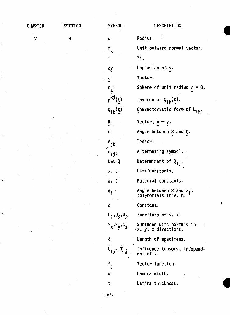
e Radius.
rv Unit outward normal vector.• K
TT PI.
Ay Laplaclan at y.
E Vector.
n Sphere of unit radius £ = 0.£
pkJU) Inverse of O...U).~ I Iv -.
Characteristic form of L. .
R Vector, x -y.
ij; Angle between R and £.
A.. Tensor,JK
e.-k Alternating symbol.
Det Q Determinant of Q^..
X, y Lame'constants.
a, 3 Material constants.
ij». Angle between R and x.;polynomials 1n~£, n.
c Constant.
U,,U2»U3 Functions of y, z.
S ,Sv,S Surfaces with normals 1ny x, y, z directions.
I Length of specimens.A A
U.., T.. Influence tensors, independ-1J 1J ent of x.
f. Vector function.J
w Lamina width,
t Lamina thickness.
xxiv
CHAPTER I
SUMMARY OF THE INTERACTIVE PROGRAM
1.1 INTRODUCTION.
The Carnegie-Mellon University team of faculty and students has
developed a unique program of interaction between the University team,
the Air Force Materials Laboratory, and certain aerospace industries,
notably General Dynamics, Convair Aerospace Division (Fort Worth). The
interactive program has focused on the application of mechanics capabili-
ties of the CMU team to the stress and strength analysis of advanced
fiber composite structures. The broad objectives of the program are the
following:
1. Creation of new and effective means of communication and
interaction between CMU and General Dynamics and other
aerospace industries.
2. Involvement of the CMU team in the solution of fundamental
engineering problems arising from the application of advanced
composites in aerospace structures.
3. Development by the CMU team of new stress analysis capabili-
ties and results, strength criteria, design information and
educational material for advanced composites technology.
To accomplish these goals, a two year effort was initiated at
CMU under Air Force sponsorship in November, 1969. The two year program
has been completed and has successfully met the goals delineated above.
The purpose of this Final Report is to summarize the achievements of the
Interactive Program. This first Chapter discusses results for all of the
objectives. Following Chapters discuss in detail the results for
objectives 2 and 3.
The principal investigators for this program originally adopted
the position that the second objective would be promoted through extensive
contacts with Industry, and that student members of the CMU team would be
select senior undergraduate and first- and second-year graduate students.
This position precluded supporting Ph.D. and faculty research by the
program. However, two student members of the CMU team have passed the
Ph.D. qualifying exam and are doing their research based on their project
experience (Fracture of Composites; Design of Mechanically Fastened Joints).
To date, five undergraduate and fifteen graduate students have partici-
pated to some extent in the Interactive Program. Faculty other than the
Principal Investigators have participated in the educational program to
become familiarized with advanced composites technology and to lend
particular expertise as needed.
1.2 FIRST AND SECOND YEAR PROGRAMS
1.2.1 Phase I
During each year the Interactive program has been divided Into
three phases: education, project research, and reporting. The education
phase is based on a Fall Semester course. Mechanics of Fiber Composite
Materials. The purpose of the course is to bring the students "up-to-
speed" in advanced composites technology such that they can contribute
significantly to the solution of engineering problems. In the second
year of the program, Dr. Cruse offered an advanced course,.Two Dimensional
Anisotropia Elasticity, which was based on the analytical solution of
membrane problems of composites using the complex variable approach. A
summary of the educational program is included in Appendix I, Chapter I.
This summary Includes course outlines and descriptions, references, and
homework problem titles.
The emphasis in the course work is on the identification of
state-of-the-art knowledge and on solving meaningful homework problems.
An example of this is the use of the "pressure vessel" problem. Students
are asked to find the optimal winding angle (±a) and maximum pressure.for
a cylindrical pressure vessel, using a fixed material (e.g. graphite-epoxy)
and each of the proposed failure criteria. The problem forces the student
to exercise lamination theory and allows a comparison of the allowable
pressures.
Another important problem area that was used is the stress con-
centration factors in composite plates subject to in-plane loading. The
fact that these factors are always higher than for isotropic materials is
emphasized. The discussion leads to other measures of strength such as
associated with sharp flaws.
The students make considerable use of the computer and in-house
analysis programs such as finite element and boundary-integral methods
for boundary value problems and a pattern search program for optimization
and synthesis. Through all of the exercises the student develops insight
into the fundamental mechanics questions and spends very little time on
the nature of the analysis programs.
1.2.2 Phase II
The second phase lasts through the Spring Semester and sometimes,
for significant problems, through the summer. The purpose of the second
phase is to involve the students in engineering problems in advanced
composites technology. The students, with faculty and industry guidance,
select problems of Interest to the student and industry. The process
of problem selection for new members of the team was a major portion of
the second half of the Fall Semester course.
In January of each year Dr. Cruse presented the project problems
at General Dynamics for evaluation and recommendations. At the same time
engineers at General Dynamics were identified who would act as the indus-
trial contact for the student working on a particular project.
A major portion of the budget of the Program was devoted to
travel support. The reasoning is that the CMU team, to be effective, must
have considerable visibility of the industrial problems in composites
technology. Thus, during the second phase the University team made
several visits to industrial locations, technical meetings, program reviews,
and special Air Force programs. These trips have also served to give the
CMU team visibility as a group doing significant work in the area of ad-
vanced composites technology. A complete list of trip report titles is
presented in Appendix II, Chapter I. This list illustrates the breadth and
depth of the CMU team contacts with other teams in the technology area.
In the first year of the program, the CMU team made a group
visit to General Dynamics. This trip was for presenting student progress
reports on their projects; it also was a chance for the student members
of the team to see manufacturing and test programs in progress. In the
second year, the new member of the CMU team to pursue project work visited
Boeing/Vertol to see their advanced composites manufacturing and test
program. However, the rest of the members of the team doing project re-
search were in their second year, and thus a team visit to industry
was not made during the second phase of the second year.
The telephone is used heavily during the second phase. By
identifying engineers, perhaps at different industrial locations, who had
an interest in the student project problem, each student could ask
questions and receive advice, data, and evaluation without the necessity
of a full visit with the engineer. The CMU team found that continual
contact with engineers played a major role in the success of the
Interactive Program.
1.2.3 Phase III
.The third phase of the program is the reporting phase for each
project problem. Each student, upon reaching a major milestone, or when
completing his participation in the program, is required to provide a
written project report which is typed and filed. Thus, the reporting
phase is interweaved throughout the program. A list of the titles of all
reports generated and on file is given in Appendix III, Chapter I. The re-
ports contain major homework problem solutions from Phase I work, project
proposals and progress reports, tutorial material, and final project
reports.
Some of the project reports are significant enough to be published
in technical journals [1,2] and to be presented at technical meetings
[3,4]. In addition other reports have been submitted for presentation
to the 13th AIAA/ASME Structures, Structural Dynamics and Materials
Conference [5,6], while another has been accepted for the 1972 ASTM
References are denoted by brackets [ ] and are found at the end of eachmajor segment of this Report.
meeting on composites [7]. These papers serve to/give to CMU team greater
visibility 1n the composites community as well as to report important
results.
In addition to the above major reports, the program had a
requirement for monthly letter reports, at the request of the Principal
Investigators. These reports required monthly student progress reports
while the students were doing project research. The monthly report served
to force each member of the team to be fully aware of his own and others'
progress. In addition the reports kept the Industrial team informed of
project progress.
At the end of the summer, each year, the CMU team prepared final
project reports which were presented at the Air Force Materials Laboratory
and at General Dynamics. This final reporting has been the most important
facet of Phase III as the CMU team seeks critical review of its programs
by the active researchers and engineers at both locations. The final
report meetings served as the focal point for examination of progress,
but they also provided an opportunity to explore new areas of project
work, team emphasis, and Industrial support.
1.3 RESEARCH PROJECTS COMPLETED
A sizeable number of project research problems have been solved
to date and the titles are listed in Appendix II, Chapter I. Listed
below are the major project titles, the responsible investigator, a
summary of the project and project reports as found in the SM file in
the Mechanical Engineering Department. The following Chapters of this
Final Report present in detail the major accomplishments of each project.
1.3.1 Fracture of Advanced Composites (H. J. Konish, Jr.)
This project includes analytical and experimental investigations
of the fracture of moderately thick graphite/epoxy specimens. Information
to date has been very encouraging in that a considerable amount of linear
elastic fracture mechanics theory seems applicable to the material.
(SM Reports 31, 41, 53, 64, 74, 80, 81; work in progress).
1.3.2 -Strength of Mechanically-Fastened Joints (J. P. Waszczak)
This project has gone from .the analysis of single-fastener test
coupons to the analysis of joints with many fasteners. Due to the weight
penalty associated with these joints, a program has been begun to develop
a synthesis procedure for designing multifastener joints. This program
has a strong coupling with the engineering team at General Dynamics.
(SM Reports 28, 34, 63, 76; work in progress).
1.3.3 Optimization Methods (S. J. Marulis; Ford Motor Co.)
The project was to investigate the use of an in-house, pattern-
search optimization method for composite design problems. The design of
mechanically-fastened joints was considered, using the in-house program.
An effort to couple the optimization program to the available finite
element program was unsuccessful but may be completed in the future.
The optimization program has been found suitable, if not optimal, for
use by Mr. Waszczak in his project research.
(Report SM-71; work suspended).
1.3.4 Boundary-Integral Equation Solution Methods (T. A. Cruse, W. H.Bamford, F. J. Rizzo)
Three separate efforts have been completed in this area. The
first reported is the development of an isotropic, two dimensional
boundary-integral equation method and a subsequent investigation of its
ability to model cutouts under tension. The second reported 1s the
development of a boundary-Integral method for fully-anisotropic (mid-plane
symmetric) laminates. (Currently, the anisotropic program Is being veri-
fied on cutout problems and some of these results are report.) The third,
completed by Prof. F. J. Rizzo of the University of Kentucky, concerns
solutions to Kelvin's problem 1n anisotropic three dimensional bodies,
and the Interlaminar shear problem.
(SM Reports 45, 50, 66, 68, 70, 72; work 1n progress).
1.4 EVALUATION AND RECOMMENDATIONS
It is clear that the goals of the Interactive Program at CMU
have been met. The project reports contained In this Final Report give
ample evidence of the extent to which the CMU team has become competent
1n research and application problems in advanced composites technology.
There now exists considerable interaction and support between the General
Dynamics team and the CMU team. In particular, General Dynamics has
provided test specimens for the Fracture Program and a summer contract
for the Joint Project.
However, the level of confidence in the CMU team expressed by
General Dynamics has come late in the program. Communication and inter-
action took place during the first year of the program but the depth of
both was not satisfying to either team. One reason for this was that
during the first year the CMU team was just coming up to speed in advanced
composites technology. However, based on the results of the program re-
view at the end of the first year, the support from the General Dynamics
team increased rapidly. The other reason for the slow start was the lack
8
of constant contact between the CMU team and the General Dynamics team.
During the second year, much more contact was made, principally by Dr.
Cruse visiting General Dynamics and liberal use of the telephone.
Frequent personal contacts are critically important to the success of an
interactive program such as ours.
The impact to date on the educational program at CMU has been
minor. The two courses cited in Appendix I plus project work (counts as
course work) are the extent of highly visible composites activities in
the educational program. However, seminars given by General Dynamics and
AFML personnel, and by the Principal Investigators have served to make
other faculty aware of the questions of materials selection, and composites
in particular. During one semester Dr. Cruse taught a section of Senior
Design which was concerned with the rationale for materials selection.
At the present time Dr. Cruse is involved in an effort to expand the CMU
Post-College Professional Education Program. This effort includes a course
on fiber composites. ;
At a harder level to document, instructors in the basic solid
mechanics courses in the Mechanical Engineering Department have the speci-
mens and knowledge to demonstrate simple anisotropic effects. It is hoped
that more of this information can be meaningfully involved in the under-
graduate courses. One of the biggest problems which mitigates against
new courses in the undergraduate or graduate program is the financial
state of the University. The1process of cutting-back is .underway and
will likely last a few more years.
Finally, the question arises as to the impact the Program has
had in developing graduates with a competence in advanced composites,
who will use this competence in the aerospace industry. To date this
impact has been nearly zero, as most of the students who have done
significant project work have yet to graduate. An early graduate with
contact with the Interactive Program went to Pratt and Whitney; another
graduate went to Ford Motor Company. Several graduate students with
other research areas have taken one or both of the courses offered to
date. Those in the Program who are still doing project work are
commissioned officers in the United States Army. Thus the personnel
impact will require more time to develop.
Two years ago, CMU had no active research in the area of advanced
composites. In that period the CMU team has developed an effective
education — project program that is closely related to fundamental
engineering problems in advanced composites technology. Members of the
CMU team have presented and published an increasing number of research
papers, and have participated in several Air Force review meetings. The
depth and breadth of research accomplishments are reported in the re-
maining Chapters of this Final Report. Other measures of the Program
require additional time to mature.
10
1.5 REFERENCES
[1] J. P. Waszczak, T. A. Cruse, "Failure Mode and Strength Predictionsof Anlsotropic Bolt Bearing Specimens", J. Comp. Materials 5,(July 1971).
[2] H. J. Kom'sh, Jr., J. L. Swedlow, T. A. Cruse, "Experimental Investi-gation of Fracture in an Advanced Fiber Composite", Report SM-74,J. Comp. Materials (to appear).
[3] J. P. Waszczak, T. A. Cruse, "Failure Mode and Strength Predictionsof Anisotropic Bolt Bearing Specimens", Fifth St. Louis Symposiumon Composite Material?, (April 1971).
[4] J. P. Waszczak, T. A. Cruse, "Failure Mode and Strength Predictionsof Anlsotropic Bolt Bearing Specimens", Proceedings of the 12thAIAA/ASME Structures, Structural Dynamics and Materials Conference(April 1971).
[5] H. J. Konish, Jr., J. L. Swedlow, T. A. Cruse, "On Fracture in Ad-vanced Fiber Composites", Report SM-80, (Submitted to AIAA/ASME)(October 1971).
[6] T. A. Cruse, "Boundary-Integral Equation Solution Method for PlaneStress Analysis of Composites (Extended Abstract), Report SM-75,(Submitted to AIAA/ASME 13th Structures and Structural DynamicsMeeting) (September 1971).
[7] H. J. Konish, Jr., J. L. Swedlow, T. A. Cruse, "A Proposed Methodfor Estimating Critical Stress Intensity Factors for Cross-Plied,Mid-Plane Symmetric Composite Laminates", Report SM-81, (Extendedabstract submitted to ASTM) (October 1971).
11
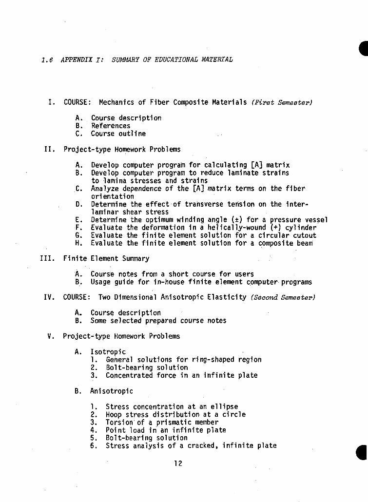
1.6 APPENDIX I: SUMMARY OF EDUCATIONAL MATERIAL
I. COURSE: Mechanics of Fiber Composite Materials (First Semester)
A. Course descriptionB. ReferencesC. Course outline
II. Project-type Homework Problems
A. Develop computer program for calculating [A] matrixB. Develop computer program to reduce laminate strains
to lamina stresses and strainsC. Analyze dependence of the [A] matrix terms on the fiber
orientationD. Determine the effect of transverse tension on the inter-
laminar shear stressE. Determine the optimum winding angle (±) for a pressure vesselF. Evaluate the deformation in a helically-wound (+) cylinder6. Evaluate the finite element solution for a circular cutoutH. Evaluate the finite element solution for a composite beam
III. Finite Element Summary
A. Course notes from a short course for usersB. Usage guide for in-house finite element computer programs
IV. COURSE: Two Dimensional Anisotropic Elasticity (Second Semester)
A. Course descriptionB. Some selected prepared course notes
V. Project-type Homework Problems
A. Isotropic1. General solutions for ring-shaped region2. Bolt-bearing solution3. Concentrated force in an inf ini te plate
B. Anisotropic
1. Stress concentration at an ellipse2. Hoop stress distribution at a circle3. Torsion of a prismatic member4. Point load in an infinite plate5. Bolt-bearing solution6. Stress analysis of a cracked, infinite plate
12
MECHANICS OF FIBER COMPOSITE MATERIALS
Text Material:
T. A. Cruse, Mechanics of Laminated Fiber Composites(notes in preparation)
J. E. Ashton et al, Primer on Composite Materials: AnalysisTechnomic (1969)
Course Abstract:
This course deals with the stress and strength analysis oftwo dimensional anisotropic fiber composite structural mater-ials. These materials have applications in structural reinforce-ments, pressure vessels, and aerospace structures. Typicalmaterials that can be considered include reinforced concrete,fiberglass, and some of the new, advanced fiber compositessuch as boron-epoxy and graphite-epoxy. Major topics includethe development of the anisotropic stiffness matrix for in-plane and out-of-plane loading of plates and shells/theoriesof strength and experimental procedures, and stress and dis-placement analysis of simple plate and shell structures.Students will participate in a number of project problems de-signed to involve the student in some of the real design prob-lems associated with composite materials. Existing solutiontechniques such as finite elements, integral equations, andoptimization computer programs, as well as analytic solutioncapabilities will be exercised as appropriate. The studentis assumed to have completed the normal undergraduate coursesin strength of materials including some introduction to thetheory of elasticity.
13
MECHANICS OF FIBER COMPOSITE MATERIALS
Supplementary Reference Material:
BOOKS:
S. A. Ambartsumyan, Theory of Anisotropio Plates, Technomic (1970)
J. E. Ashton, J. M. Whitney, Theory of Laminated Plates,Technomic (1970)
G. S. G. Beveridge, R. S. Schechter, Optimization: Theoryand Practice,.McGraw-Hill (1970)
S. W. Tsai, et al (Editors), Composite Materials Workshop,Technomic (1968)
L. J. Brou tman ,R . H. Krock (Editors), Modern CompositeMaterials, Addison Wesley (1967)
f Metal Matrix Composites, ASTM STP 438 (1968)
j Interfaces in Composites, ASTM STP 452 (1969)
REPORTS:
j Composite Materials: Testing and Design, ASTM STP460(1969)
T. A. Cruse, J. L. Swedlow, Interactive Program in AdvancedComposites Technology: First Annual Report, Report SM-46,Carnegie-Mellon University, Pittsburgh, Pennsylvania (1970)
M. S. Howeth, Design, Materials and Structures, Report SMD-028,General Dynamics, Fort Worth, Texas (1969).
S. W. Tsai, Mechanics of Composite Materials, AFML-TR-66-199
14
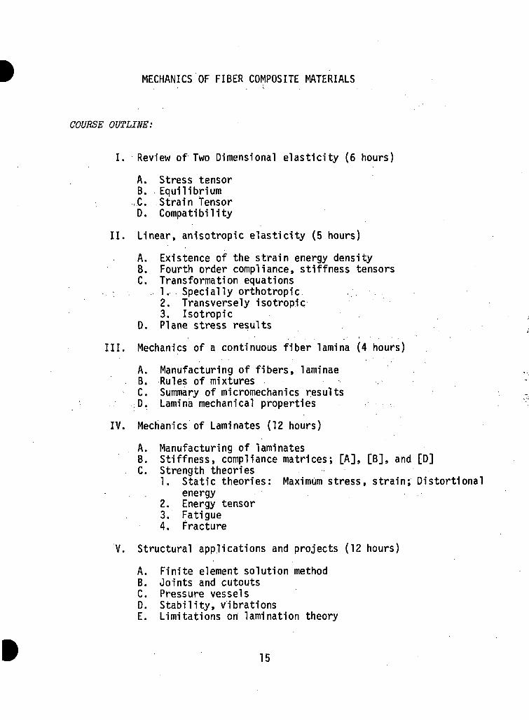
MECHANICS OF FIBER COMPOSITE MATERIALS
CODESE OUTLINE:
I. Review of Two Dimensional elasticity (6 hours)
A. Stress tensorB. Equilibrium,C. Strain tensorD. Compatibility
II. Linear, anisotropic elasticity (5 hours)
A. Existence of the strain energy densityB. Fourth order compliance, stiffness tensorsC. Transformation equations
. 1. Specially orthotropic2. Transversely isotropic3. Isotropic
D. Plane stress results
III. Mechanics of a continuous fiber lamina (4 hours)
A. Manufacturing of fibers, laminaeB. Rules of mixturesC. Summary of micromechanics results.D. Lamina mechanical properties •
IV. Mechanics of Laminates (12 hours)
A. Manufacturing of laminatesB. Stiffness, compliance matrices; [A], [B], and [D]C. Strength theories
1. Static theories: Maximum stress, strain; Distortionalenergy
2. Energy tensor3. Fatigue4. Fracture
V. Structural applications and projects (12 hours)
A. Finite element solution methodB. Joints and cutoutsC. Pressure vesselsD. Stability, vibrationsE. Limitations on lamination theory
15
TWO DIMENSIONAL PROBLEMS IN THE THEORY OF ANISOTROPIC ELASTICITY
Recommended Textbooks:
N. I. MuskhelishvlH, Some Basic Problems of theMathematical Theory of Elasticity, Noordhoff (1963)
S. G. Lekhnltskii, Theory of Elasticity of anAnisotropic Elastic Body, Hoi den-Day (1963)
Course Abstract:
The first half of the course 1s devoted to the formulationand solution of the two dimensional, Isotroplc elasticproblem using complex variable methods. Solutions areobtained using the Laurent series expansion for multiply-connected bodies. The second half of the course is de-voted to the analysis of anisotroplc, two dimensionalproblems, again using the complex variable method. Exampleproblems and projects are chosen for their relevancy tocurrent engineering problems in anisotroplc media, suchas advanced fiber composites. Existing numerical solutionmethods such as finite elements and Integral equationsare used and compared to the analytic results when possible.The course assumes a knowledge of the basic theorems ofanalysis of functions of a complex variable as well as thebasic theory of elasticity.
16
TWO DIMENSIONAL PROBLEMS IN THE THEORY OF ANISOTROPIC ELASTICITY
COURSE OUTLINE:
I. Review of complex variable theory (6 hours)
A. Analytic functionsB. Green's theoremC. Cauchy integral theoremsD. Series
II; Plane theory of isotropic elasticity (18 hours)
A. Equilibrium; stress functionB. Strains; Hooke's lawC. Goursat formulaD. DisplacementsE. TractionsF. Kolosov formulaG. Forces on a contourH. Single-valued displacements, stressesI. Laurent series for the stress functionsJ. Infinite region with a holeK. Polar coordinate form of the equationsL. Mapping functions; curvilinear coordinatesM. Transformed field equationsN. Example solutions
III. Plane theory of anisotropic elasticity (15 hours)
A. Hooke's law for various types of anisotropyB. Stress functionC. Characteristic surfaces for the stress functionD. Roots of the characteristic equation £«(y) = 0E. Stresses and displacementsF. Forces on a contourG. Infinite region with a holeH. Single-valued stresses and displacementsI. Mapping functionsJ. Fourier analysis of the boundary conditionsK. General expansion form of the solutionL. Example solutions
17
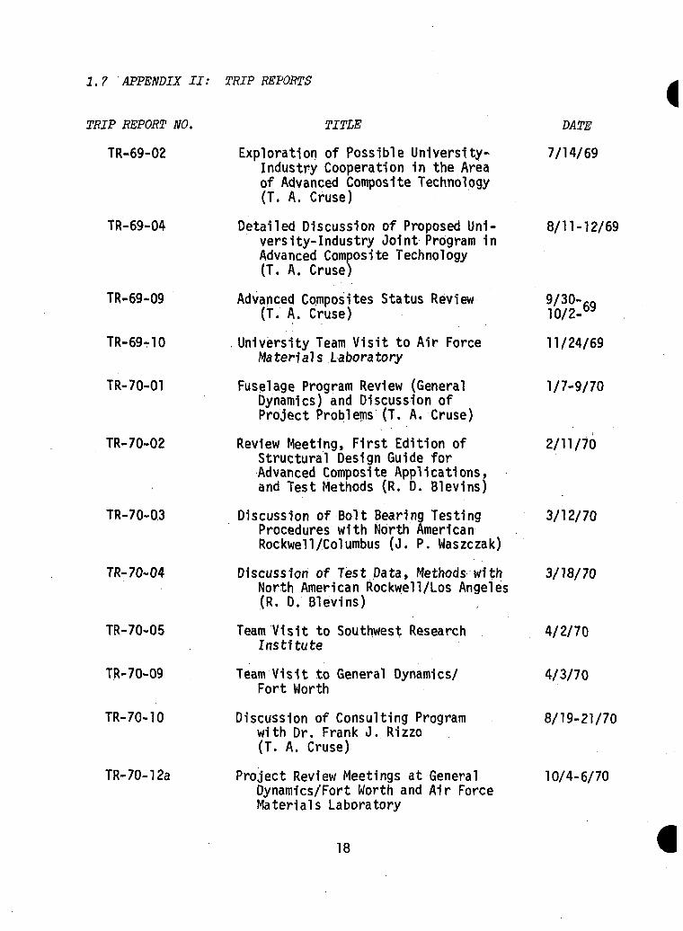
1.7 APPENDIX II: TRIP REPORTS
TRIP REPORT NO.
TR-69-02
TR-69-04
TR-69-09
TR-69-10
TR-70-01
TR-70-02
TR-70-03
TR-70-04
TR-70-05
TR-70-09
TR-70-10
TR-70-12a
TITLE DATE
Exploration of Possible University- 7/14/69Industry Cooperation in the Areaof Advanced Composite Technology(T. A. Cruse)
Detailed Discussion of Proposed Uni- 8/11-12/69versity-Industry Joint Program inAdvanced Composite Technology(T. A. Cruse)
Advanced Composites Status Review 9/30-(T. A. Cruse) 10/2-169
University Team Visit to Air Force 11/24/69Materials Laboratory
Fuselage Program Review (General 1/7-9/70Dynamics) and Discussion ofProject Problems (T. A. Cruse)
Review Meeting, First Edition of 2/11/70Structural Design Guide forAdvanced Composite Applications,and Test Methods (R. D. Blevins)
Discussion of Bolt Bearing Testing 3/12/70Procedures with North AmericanRockwell/Columbus (J. P. Waszczak)
Discussion of Test Data, Methods with 3/18/70North American Rockwell/Los Angeles(R. D. Blevins)
Team Visit to Southwest Research 4/2/70Institute
Team Visit to General Dynamics/ 4/3/70Fort Worth
Discussion of Consulting Program 8/19-21/70with Dr. Frank 0. Rizzo(T. A. Cruse)
Project Review Meetings at General 10/4-6/70Dynamics/Fort Worth and A1r ForceMaterials Laboratory
18
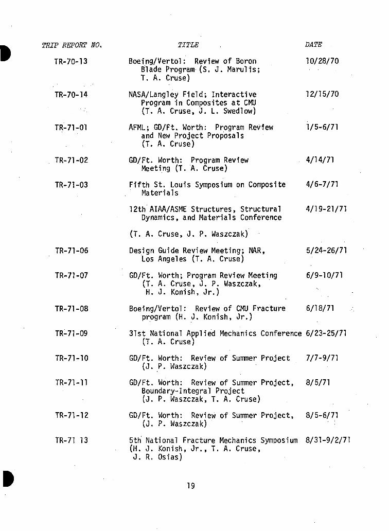
2HZP REPORT NO,
TR-70-13
TR-70-14
TR-71-01
TR-71-02
TR-71-03
TR-71-06
TR-71-07
TR-71-08
TR-71-09
TR-71-10
TR-71-11
TR-71-12
TR-71 13
TITLE
Boelng/Vertol: Review of BoronBlade Program (S, J. Marulls;T. A. Cruse)
NASA/Langley Field; InteractiveProgram in Composites at CMU(T. A. Cruse, J. L. Swedlow)
AFML; GD/Ft. Worth: Program Reviewand New Project Proposals(T. A. Cruse)
GD/Ft. Worth: Program ReviewMeeting (T. A. Cruse)
Fifth St. Louis Symposium on CompositeMaterials
12th AIAA/ASME Structures, StructuralDynamics, and Materials Conference
(T. A. Cruse, J. P. Waszczak)
Design Guide Review Meeting; NAR,Los Angeles (T. A. Cruse)
GD/Ft. Worth; Program Review Meeting(T. A. Cruse, J. P. Waszczak,H. J. Konish, Jr.)
Boeing/Vertol: Review of CMU Fractureprogram (H. J. Konish, Jr.)
31st National Applied Mechanics Conference(T. A. Cruse)
GD/Ft. Worth: Review of Summer Project(J. P. Waszczak)
GD/Ft. Worth: Review of Summer Project,Boundary-Integral Project(J. P. Waszczak, T. A. Cruse)
GD/Ft. Worth: Review of Summer Project,(J. P. Waszczak)
5th National Fracture Mechanics Symposium(H. J. Konish, Jr., T. A. Cruse,J. R. Osias)
DATE
10/28/70
12/15/70
1/5-6/71
4/14/71
4/6-7/71
4/19-21/71
5/24-26/71
6/9-10/71
6/18/71
6/23-25/71
7/7-9/71
8/5/71
8/5-6/71
8/31-9/2/71
19
1.8 APPENDIX III: RESEARCH DOCUMENTS
REPORT NUMBER TITLE DATE
SM-22 Anisotropic Stress Strain Program January 1970Layer Usage Guide (H. J. Konish, Jr.)
SM-23 Project Problems for Air Force Con- January 1970tract F33615-70-C-1146 (T. A. Cruse)
SM-24 Summary of the Direct Potential January 1970Method (T. A. Cruse)
SM-25 Interactive Program in Advanced February 1970Composites Technology (T. A. Cruse)
SM-27 Symmetric Laminate Constitutive February 1970Equation Program-EMAT Usage Guide(J. P. Waszczak)
SM-28 Bolt Bearing Specimen Co-ordinate April 1970Transformation Program - Usage GuideTRANS (J. P. Waszczak)
SM-29 Certain Aspects of Design with Ad- April 1970vanced Fibrous Composites (R. D. Blevins)
SM-31 Stress Analysis of a Cracked Ad- April 1970vanced Composite Beam (H. J. Konish, Jr.)
SM-32 An Investigation of Fracture in April 1970Advanced Composites (W. H. Bamford)
SM-34 An Investigation of Stress Concentra- May 1970tions Induced in Anisotropic PlatesLoaded by Means of a Single FastenerHole (J. P. Waszczak)
SM-38 Integral Equation Methods in Potential August 1970Theory (T. A. Cruse)
SM-41 Stress Analysis of a Cracked Aniso- September 1970tropic Bleam (H. J. Konish, J. L.Swedlow) ;
SM-42 An Investigation of Stress Concentra- September 1970tions Induced in Anisotropic PlatesLoaded by Means of 'a Single FastenerHole (J. P. Waszczak, T. A. Cruse)
SM-45 The Use of Singular Integral Equations October 1970with Application to Problems ofComposite Materials (F. J. Rizzo)
20
REPORT NUMBER TITLE DATE
SM-49
SM-50
SM-52
SM-53
SM-63
SM-64
SM-65
SM-68
SM-70
SM-71
SM-72
Report on the Relation Between the StiffnessMatrix and the Angle of Rotation of aLamina (J. Kolter)
Numerical Solution Accuracy for the Infin-ite Plate with a Cutout — ProgressReport (W. Bamford)
Failure Mode and Strength Predictions ofAnisotropic Bolt Bearing Specimens(J. P. Waszczak; T. A. Cruse)
A Proposed Experimental Investigation ofFracture Phenomena in Advanced FiberComposite Materials (H. J. Konish, Jr.)
Loaded Circular Hole in an AnisotropicPlate (J. P. Waszczak)
Stress Analysis of the Crack-Tip Regionin a Cracked Anisotropic Plate(H. J. Konish, Jr.)
Numerical Calculation of the Character-istic Directions for a GenerallyAnisotropic Plate - MULTMU UsageGuide (H. J. Konish, Jr.)
Solution to Kelvin's Problem for PlanarAnisotropy (W. Bamford)
USER'S DOCUMENT: Two DimensionalBoundary-Integral Equation Program(T. A. Cruse)
Optimization of Advanced Composite Plates(S. Marulis)
Two Dimensional Anisotropic Boundary-Integral Equation Method (W. H. Bamford,T. A. Cruse)
November 1970
December 1970
September 1970
February 1971
May 1971
May 1971
June 1971
June 1971
June 1971
June 1971
August 1971
21
REPORT NUMBER TITLE DATE
SM-74
SM-76
SM-77
SM-80
SM-81
Experimental Investigation of Fracturein an Advanced Fiber Composite(H. J. Konish, J. L. Swedlow, T. A. Cruse) September 1971
Toward a Design Procedure for MechanicallyFastened Joints Made of CompositeMaterials (J. P. Waszczak)
Review of: Structural Design Guide forAdvanced Composite Applications, 2ndEdition, Appendix A: TheoreticalMethods (T. A. Cruse)
On Fracture in Advanced Fiber Composites(H. J. Konish, Jr., J. L. Swedlow,T. A. Cruse)
A Proposed Method for Estimating CriticalStress Intensity Factors for Cross-Plied,Mid-Plane Symmetric Composite Laminates,(Abstract) (H. J. Konish, Jr., J. L.Swedlow, T. A. Cruse)
September 1971
May 1971
October 1971
October 1971
22
CHAPTER II
FRACTURE OF ADVANCED COMPOSITES ^ -
2.1 STRESS ANALYSIS OF A CRACKED ANISOTROPIC BEAM
2.1.1 Introduction
The high specific strength and specific stiffness of advanced
fiber composite materials have made them very attractive to the aerospace
industry. The fact that they are both anisotropic and inhomogeneous, how-
ever, has somewhat retarded their use, as the design and analysis pro-
cedures developed for metals are not strictly applicable; thus, it is
necessary to adapt old procedures, or develop new ones, which can deal
with the more complex composite materials.
The project discussed in this chapter deals with one such effort.
The specific problem under consideration is the effect of a crack in a
unidirectional advanced fiber composite material. Although this problem
is one of great significance in aerospace structures, it has not yet been
extensively treated. An analytic solution has been derived for the elastic
stresses and strains induced by a crack in a loaded anisotropic plate [1],
The solution does assume material homogeneity, but this is a good approxi-
mation for advanced fiber composite materials on a macroscopic scale.
However, relatively little has been done to follow up the analytic work.
2.1.2 Review of Previous Work
The most extensive investigation of fracture of composites in
the literature is that done by Professor E. M. Wu of Washington University,
St. Louis. He considers the problem of a central crack, aligned with the
fibers of a unidirectional composite material, which are, in turn, a-
ligned with the edges of a plate subjected to general edge loadings.
23
Wu demonstrates that linear-elastic fracture mechanics are applicable to
this problem [2]. His analysis yields results of the form
a = KjF^Tr (1)
Kj= ft G (2)
where F is a function of the external loading and G is a function of
specimen geometry, material constants, and external loading. These re-
sults are similar in form to the results obtained from the analysis
of an isotropic problem.
Wu verified his analysis experimentally [2,3]. His experimental
work, (done with fiberglass plates), does demonstrate the applicability of
a linear elastic fracture mechanics analysis to his particular problem.
It further shows that the critical stress intensity factors K, (cor-
responding to symmetric loading on the plate) and «,, (corresponding to
skew-symmetric loading on the plate) are material constants. Under com-
bined external loading, the following empirical relationship is observed
to be valid at incipient unstable crack propagation:
KIc II
This result is not, however, particularly surprising in view of [1],
where it is analytically shown that any arbitrary two-dimensional fracture
problem in an anisotropic material may be decomposed into two independent
problems, one symmetric and one skew-symmetric. Thus, only the form of
(3) may be considered as original; its existence is predicted by analysis.
Wu has also investigated the problem of an external loading of
combined compression and shear [4]. This loading will lead to crack
propagation by the second, or "sliding" mode. Three possible subcases
24
are considered analytically: Relative displacement of the crack surfaces,
over a portion of the crack surfaces, and over none of the crack surfaces.
This analysis was verified by an experimental program carried
out on fiberglass. The results show that, for ratios of compressive load
to shear load greater than approximately 0.4, failure does not occur by
unstable crack propagation; the crack velocity remains quasi-stable until
the specimen fails from propagation of the crack completely through it.
If the ratio of compressive load to shear load is increased, internal
buckling of the fibers and separation of the fibers from the matrix is
observed; at most, the crack will propagate some small distance at an
angle of 45° from its initial direction, then diffuse and die out. The
specimen buckles thereafter with no additional crack propagation. Wu
thus concludes that fracture mechanics is only applicable to this problem
when the ratio of compressive stress to shear stress is less than 0.4.
The second subcase of the analysis gives the best agreement between
analysis and experiment when fracture mechanics are applicable. The
quasi-stable crack propagation found to occur experimentally when the
ratio of compressive load to shear load is approximately 0.4 seems to be
well-described by the first subcase of the analysis. The third subcase
of the analysis is believed to be applicable when the compressive load
is sufficiently large to prevent crack extension; however, buckling,
rather than crack propagation, becomes the dominant mode of failure be-
fore this load is .reached, so the presence of the crack not significant
in the failure of the specimen.
Wu notes that stable crack propagation occurs in an intermittent
manner in fiberglass [2]; he postulates that this is caused by the crack
25
crossing the reinforcing fibers. This hypothesis is investigated both
analytically and experimentally [5].
The analysis is based on the assumption that crack growth is
primarily caused by the component of tensile stress perpendicular to the
direction of crack growth, as the intermittent stable crack propagation
is most frequently observed under skew-symmetric loading. It indicates
that the crack does not necessarily propagate in a direction collinear
with itself, but rather at an angle.where the combination of the size of
a sub-critical flaw and the maximum tensile stress reaches some critical
value, causing the flaw to grow. Under skew-symmetric loading, the maxi-
mum tensile stress is not perpendicular to the crack direction, and, as-
suming that flaws of any given size are uniformly distributed in the
material, the crack will propagate at some angle to its initial direction.
Since the initial direction of the crack is collinear with the fibers, the
propagating crack must cross fibers. The direction of crack growth is
thus a function of the direction of the shear loading.
It is noteworthy that Wu finds the Griffith energy criterion to
be applicable to composite materials only when the crack propagates across
fibers. Although Wu offers no explanation for this anomaly, it may be
due to the fact that, for this particular geometry, the crack propagates
only through resin unless it crosses fibers. Thus, the crack would "sense"
a brittle, high-strength material, for which the Griffith criterion is
applicable, only when it crosses fibers.
Wu's specimen is also analyzed for symmetric loading by Bowie
and Freese [6]. They use a modified mapping-boundary collocation technique
to derive the stress intensity factor numerically. Of particular interest
26
is the result of Bowie and Freese that, when the .strength of the material
in a direction transverse to the crack is much larger than the strength
of the material collinear with the crack, the stress intensity factor is
not longer the same for both the isotropic and anisotropic cases, as pre-
dicted by Sih, Paris, and Irwin [1]. However, Bowie and Freese do note
that, when the strength of the material in the direction collinear with
the crack is greater than or equal to the strength of the material in a
direction transverse to the crack, the two stress-intensity factors
agree to within five per cent.
2.1.3 Analytical Study
The efforts described above comprise the significant work now
available in open literature on macroscopic analysis of fracture in aniso-
tropic materials. Both of them consider only cracks which are aligned
with the fibers of the composite material, and must therefore be con-
sidered incomplete, as no provision has been made for cracks with arbi-
trary orientation to the material axes. The purpose of the project
described in this section is to investigate the behavior of a crack in an
anisotropic material where the crack is not, in general, collinear with
one of the material axes (though these cases are considered). Information
is also sought on the behavior of the stress-intensity factor as the
orientation of the crack with respect to the material axes and the speci-
men geometry are varied. Finally, it is desired to obtain verification
of either Bowie and Freese [6], or Sih, Paris, and Irwin [1] concerning
the differences, if any, between the isotropic and anisotropic stress
intensity factors.
27
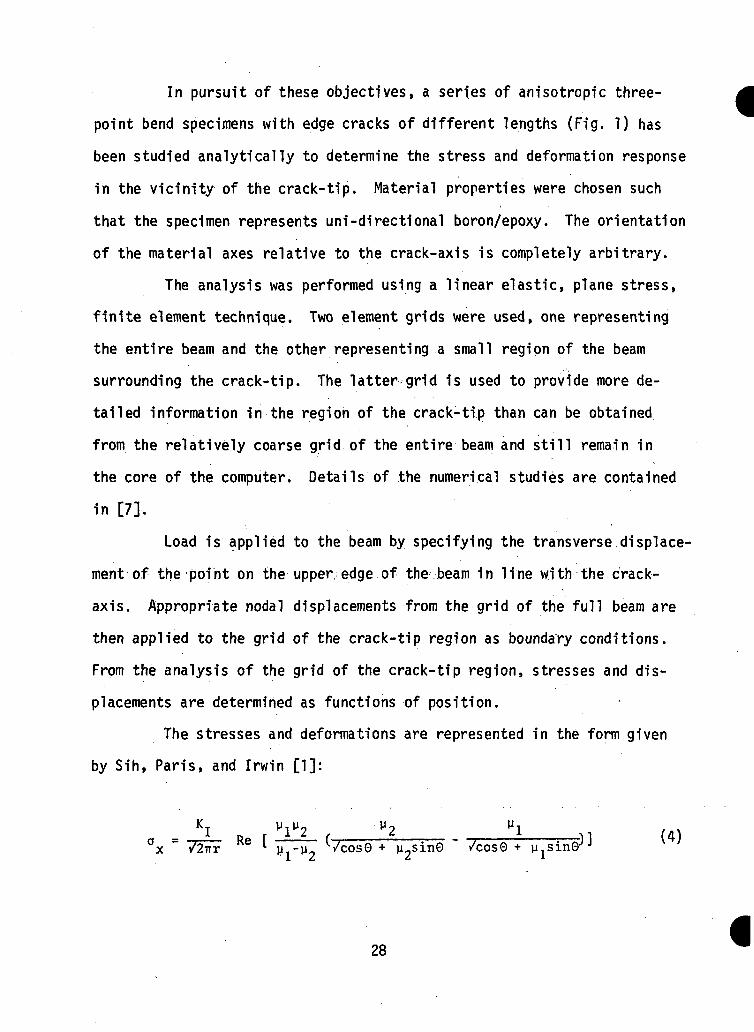
In pursuit of these objectives, a series of anlsotroplc three-
point bend specimens with edge cracks of different lengths (F1g. 1) has
been studied analytically to determine the stress and deformation response
in the vicinity of the crack-tip. Material properties were chosen such
that the specimen represents uni-directional boron/epoxy. The orientation
of the material axes relative to the crack-axis is completely arbitrary.
The analysis was performed using a linear elastic, plane stress,
finite element technique. Two element grids were used, one representing
the entire beam and the other representing a small region of the beam
surrounding the crack-tip. The latter grid is used to provide more de-
tailed information in the region of the crack-tip than can be obtained
from the relatively coarse grid of the entire beam and still remain in
the core of the computer. Details of the numerical studies are contained
in [7].
Load is applied to the beam by specifying the transverse displace-
ment of the point on the upper edge of the: beam in line with the crack-
axis. Appropriate nodal displacements from the grid of the full beam are
then applied to the grid of the crack-tip region as boundary conditions.
From the analysis of the grid of the crack-tip region, stresses and dis-
placements are determined as functions of position.
The stresses and deformations are represented in the form given
by Sih, Paris, and Irwin [1]:
_ _~_ n_ r , _ ___ , ---------- , - ,-x ~ 72TTT L J J j -VU VcosG + y2sin0 /cos© + y1sin0'/
/ « \(4)
28
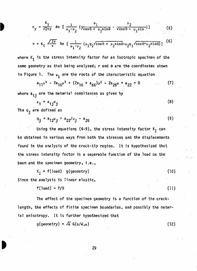
KI 1 yl M2°y = 72rrr Re * V , - W n ^/cosG + y^sinG " /cos0 + u,sin ^ (5)7 1 2 r 2 1
v = KT / Re [ (n q /cosQ + vusinG-vuq.. /cosG+p9sinG) ]i TT W l-y2 i i 2. tl I
where K. is the stress intensity factor for an isotropic specimen of the
same geometry as that being analyzed; r and e are the coordinates shown
in Figure 1. The v, are the roots of the characteristic equation
^t 9a 3 + /9a 4«a ^2" 9a ^ a — fi ^7
II 10 10 DO CO 22
where a.. are the material compliances as given by
ei = aijajThe q^ are defined as
q. = a,0y. + a09/M_. - aocj 11 j cc j <:o
Using the equations (4-9), the stress intensity factor K, can
be obtained in various ways from both the stresses and the displacements
found in the analysis of the crack-tip region. It is hypothesized that
the stress intensity factor is a separable function of the load on the
beam and the specimen geometry, i.e.,
Kj = f(load) g(geometry) (10)
Since the analysis is linear elastic,
f(load) = P/B (11)
The effect of the specimen geometry is a function of the crack-
length, the effects of finite specimen boundaries, and possibly the mater-
ial anisotropy. It is further hypothesized that
g(geometry) = & G(a/W,a) (12)
29
where the function G contains the effects of the finite boundaries of
the specimen and any effect of the material anisotropy. Thus, combining
equations (10-12)
Kj = (P^T/B) G (a/W,o)
or (13)
G (a/W,a) = KjB/Pv/a
The function G(a/W,a) has been obtained analytically for three
values of a and five values of a/W,.using values of K, obtained from both
stress and displacement data. Each G(a/W,a) was then normalized on the
value G (0.2,a) for corresponding methods of determining Kj. The resulting
value, denoted as G~ (a/W,a) is shown plotted as function of a/W in Figure
2. On the same graph is shown a curve representing G~ (a/W) for an iso-
tropic specimen, as obtained from [8], The data points show satisfactory
agreement with the curve, in view of the numerical noise introduced by
two finite element grids which are not entirely compatible. Thus, G"
(a/W,a) is identical, with G"(a/W). This, in turn, implies that the
anisotropic stress intensity factor is the isotropic stress intensity
factor.
Although the stress intensity factor in equations (4-6) is the
isotropic stress intensity factor, stress and deformation are functions
of material constants. Thus, fracture in advanced fiber composite
materials cannot be ascribed solely to any combination of the stress in-
tensity factors. To some extent, therefore, the applicability of fracture
mechanics to composite materials is questionable. Exactly what importance
a crack has in composite materials, and what role the material properties
play in describing it, are questions which were investigated experimentally
and are reported in Section 2.2.
30
2.1.4 .References
IT] G. C. Sin., P. C. Paris, and G. R. Irwin, "On Cracks in RectilinearlyAnisotropic Bodies", International Journal of Fracture Mechanics, I,(September 1965} 189-203.
[2] E. M. Wu, "Application of Fracture Mechanics to Orthotropic Plates",Department of Theoretical and Applied Mechanics., University ofIllinois, Urbana, Illinois (June 1963).
[3] E. M. Wu and R. C. Reuter, "Crack-Extension in Fiberglass-reinforcedPlastics", Department of Theoretical and Applied Mechanics, Universityof Illinois, Urbana, Illinois (February 1965).
[4] E. M. Wu, "A Fracture Criterion for Orthotropic Plates Under theInfluence of Compression and Shear", Department of Theoretical andApplied Mechanics, University of Illinois, Urbana, Illinois(September 1965).
[5] E. M. Wu, "Discontinuous Mode of Crack Extension in UnidirectionalComposites", Department of Theoretical and Applied Mechanics,• Uni-versity of Illinois, Urbana, Illinois (February 1968).
[6] 0. L. Bowie and C. E. Freese, Unpublished Results, Army Materialsand Mechanics Research Agency, Watertown, Massachusetts (1970).
[7] H. J. Konish, Jr. and J. L. Swedlow, "Stress Analysis of a CrackedAnisotropic Beam", Report SM-41, Department of Mechanical Engineering,Carnegie-Mellon University, Pittsburgh, Pennsylvania (September 1970).
[8] J. E. Srawley and W. F. Brown, Jr., Plane Strain Crack ToughnessTesting of High Strength Metallic Materials, ASTM STP 410,American Society for Testing and Materials, Philadelphia,Pennsylvania (1967) 13.
31
w
V .\\\
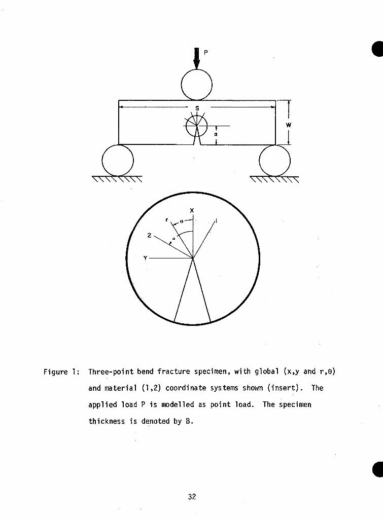
Figure 1: Three-point bend fracture specimen, with global (x,y and r,e)
and material (1,2) coordinate systems shown (insert). The
applied load P is modelled as point load. The specimen
thickness is denoted by B.
32
200
150
90° 45<
O
ISOTROPIC G(a/W)FROM [8]
100 -t ,0 1
o-" o
1 1
02 03
i i i
04 05 06
a / W
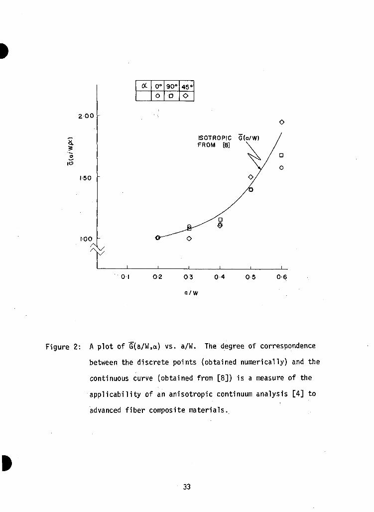
Figure 2: A plot of G(a/W,a) vs. a/W. The degree of correspondence
between the discrete points (obtained numerically) and the
continuous curve (obtained from [8]) is a measure of the
applicability of an anisotropic continuum analysis [4] to
advanced fiber composite materials.
33
2.2 EXPERIMENTAL INVESTIGATION OF FRACTURE IN AN ADVANCED FIBER COMPOSITE
2.2.1 Introduction
Linear elastic fracture mechanics (LEFM) is now accepted as the
rationale for characterizing crack toughness of materials that are osten-
sibly homogeneous and isotropic, the outstanding examples being a wide
range of metallic alloys. The basic experience that supports this approach
is that presence of a macro crack dominates the response of a structure to
remote loading. With the advent of advanced fiber composites, however,
there arises the question of the degree of homogeneity of the structure
surrounding the crack that is necessary for LEFM to be applicable. In
particular, there is concern over whether heterogeneity and anisotropy will
preclude practical use of LEFM in composites.
Vigorous discussion of this issue is important and widespread,
but the interchanges so far have tended to be theoretical and even specu-
lative. In an effort to supply some physically based information, a pilot
series of experiments has been performed, to answer two specific questions:
1. If a cracked, composite specimen is loaded to.failure,
is the path of crack prolongation determined by the geometry
of the initial crack and the loading, or by material
orientation?
2. Can LEFM, suitably modified to account for material
anisotropy, be usefully applied to composites?
The data now in hand, although limited, indicates that a crack in a
composite is at least influential in determining failure patterns and, in
many cases, the crack is dominant; furthermore that LEFM provides useful
34
procedures for evaluating crack toughness of composites.
This section gives a brief review of the test procedures, methods
of data reduction, and experimental results. Observations .made during the
course of the tests are reported, and failure surfaces are shown. Analyti-
cal work stimulated by these results is underway and will be reported
subsequently.
2.2.2 Test Procedures; Program . . ..
It was obvious from the objective of the test program that the
test procedures should follow those developed within the framework of
conventional fracture mechanics. There is, in fact, a wealth of literature
on this subject including an ASTM Tentative Method [1] and extensive
interpretation of it (see, e.g., [2,3]). Departures from the specifica-
tions in [1] were minimal and were dictated either by the special nature
of the material under test or by simple practicality.
The three-point bend specimen prescribed in [1] was chosen largely
to bypass problems associated with gripping the test piece. (See Figure 1.)
In the extensive data base that now exists for metals testing, results for
this configuration compare well to those for other geometries so that,
among other matters, there was no reason to expect that the bearing load
opposite the crack front should influence unduly the processes of crack
prolongation. In fact, the data reduction scheme in [1] accounts for such
details of specimen geometry and load arrangement.
The specimen proportions shown in Figure 1 follow.the recommenda-
tions in [1] except that the crack front was not sharpened under fatigue
loading. Instead, the notch was produced by a sawcut followed by a final
lengthening and sharpening using an ultrasonic cutter.
35 -
As shown in Figure 2, each specimen was centered on two parallel
rollers (1 in dia) whose centerlines were 4 in apart. A third parallel
roller was then located directly above the crack, and the specimen was
loaded vertically downward. Testing was performed in an Instron machine-2of 10,000 Ib capacity, and cross-head motion was set at 10 in/min to
minimize dynamic effects. Load and cross-head motion were monitored during
each test and then cross-plotted to give the basic data for later reduction.
While the requirement of [1] is to record crack-mouth opening by means of
a special clip gauge, both the basic linearity of material response and
the rigidity of the test machine, relative to the specimen, seemed to make
this degree of fidelity to [1] unnecessary for the pilot test series.
The program involved twenty-three specimens, thus allowing for
two reproducibility tests, and for the testing of both uni- and multi-
directional laminates having a range of starter crack lengths. The
material used was a NARMCO graphite-epoxy with Morganite II fibers' in
5206 resin.
Reproducibility was evaluated by testing two sets of five speci-
mens, each set of the same lay-up and geometry. The first set was a
uni-directional laminate (a = 0°) and had an initial crack length of 0.4
in. The second set was multi-directional (a = (00/±450/90°)s) and had
the same starter crack length. Single tests were run for a = 0°, 45°,-90°;
(±45°)s; and (0°/±45°/90°)s. Starter crack lengths were 0.2, 0.4, and 0.6
in, the shortest of which was less than the requirements in [1], Such
specimens were included to permit evidence of material dominance to
develop.
36
2.2.3 Data Reduction; Results
A typical load-cross-head displacement trace is reproduced, in ,
Fiigure 3. There is an initial region of increasing slope during which
slack in the load train is taken up, and bearing surfaces under the loading
rollers develop. This is followed by a linear region in which the specimen
deforms elastically. A.third region of decreasing slope then begins as a
result both of nonlinear load-displacement behavior and of damage initiation.
Finally the load peaks and falls off as the test piece breaks in two.
In order to differentiate the nonlinear effects from those
ascribable to damage, the Tentative Method prescribes the following data
reduction scheme.^ The slope M of the linear portion of the curve is
identified, and a line of slope 5% less than M is drawn as shown in
Figure 3. This line intersects the curve at a load termed P<j. If P<- is
the greatest load withstood by the specimen to that point in the test, PS
is set equal to PQ. If any load maximum precedes Pr, then PQ is equated
to that maximum value. In either case, the experience in metals testing
has shown PQ to correspond reasonably well to the point of failure initi-
ation. In the absence of a suitable data base for composites, this pro-
cedure was used to find PQ-, the data obtained is thus surely consistent
and probably conservative. Together with specimen geometry, PQ is then
used to compute KQ, the critical stress intensity or candidate fracture
It should be borne in mind that the present discussion is but an abstractof a most explicitly defined procedure; the interested reader is urgedto consult [1] for complete details.
37
2toughness. See [2,3].
For each laminate, the KQ values were averaged to give Kg which,
in turn, was used to find a critical strain energy release rate Gg - see
[3,4]. The results are shown in Table I. Also of interest are the
failure surfaces, depicted in Figures 4-8; a specimen that did not part
fully is shown in Figure 9.
2.2.4 Discussion
At the outset, two questions were posed regarding the utility of
LEFM in characterizing fracture of composites. The first concerns paths
of crack prolongation; the answer may be inferred from inspection of the
failure surface. The second involves use of LEFM as a data reduction
scheme; the answer to this question comes from physical measurements.
The appearance of the failure surfaces suggests that, in the
main, the crack and loading dominate fracture. In Figure 4 (specimens for
which a =0°), the path of crack growth is observed to be roughly coplanar
with the starter crack. Note that in the case of the longest crack
(a = 0.6 in), where a longitudinal secondary crack formed, the path is
generally forward, Indeed, the crack seems to have made a series of
sharp turns to regain its coplanar path.
It is not surprising, on the other hand, to see that, in the
a = 45° specimens, the crack grew along a plane containing no fibers.
This is clear in Figure 5 and, although fracture occurred as the result
In metals testing, certain additional steps are taken to establish thevalidity of an individual test result. Since these steps necessitateuse of the yield stress, they cannot be followed in this work. Thus onlycandidate values of fracture toughness, or Kg, are reported.. The datacannot be presumed to give Kj for these materials because compliancewith the strict requirements Of [1] are definitionally impossible.
38
of crack propagation (in the matrix), the mode is a mixture of opening
and sliding £3]. More sophisticated instrumentation would have permitted
articulation of the relative presence of each mode, but such instrumenta-
tion was not used in this program. ;
Forward crack growth is evident for the a = 90° specimens as
depicted in Figure 6. Growth again was along a plane containing no fibers
which, in this case, is coplanar with the starter crack.
During testing the uni-directional specimens described above
emitted popping noises prior to failure. Because the fracture process
also involved matrix breaking of one sort or another, the two phenomena
are believed to be related. Even in the a = 0° specimens, the crack ap-
pears at the outset to have operated on virtually independent fiber bundles
as they pulled out from the matrix. The resulting failure surfaces are
very rough for the early stages of growth but then become more nearly
uniform. The noise levels for the remaining specimens were much lower,
and their failure surfaces are less suggestive of matrix cracking.
Figure 7 is instructive in that it shows for the a = (±45°)
test pieces an increasing crack dominances as the starter crack is made
longer. For a = 0.2 in, the crack path almost immediately turns 45° from
its initial orientation, there being but a slight indication of forward
growth. A greater tendency toward coplanar growth is apparent when a = 0.4
in, and crack dominance is manifest when a = 0.6 in. Crack growth is not
possible on a plane containing no fibers — there being none by virtue of
the lay-up - and some zig-zagging is apparent. This group of specimens
thus shows a transition from some material dominance where the starter
39
crack is shorter than required by the Tentative Method to a fracture
pattern fully dominated by the starter crack, as the length of the starter
crack occurs.
Crack dominance is also clear in Figure 8, which shows failure
surfaces for a = (0°/±450/90°) . In these specimens, the crack moved in
its own plane but apparently grew further in the interior of the test
piece than on its surface. An indication of this behavior, not uncommon
in metals testing, is shown in Figure 9.
The use of KQ to characterize behavior of these specimens appears,
on the whole, to be warranted. The reproducibility tests on the a = 0°•5
specimens and the a = (0°/±45°/90°)s specimens were satisfactory. Load-
displacement traces are shown in Figures 10 and 11, and the average
values found are
a = 0° : K = 28.8 x }Q3 Ib/in2/in *°'
a = (0°/±45°/90°)s : KQ = 21.7 x 10³ Ib/in2/in *J'
The scatter is not unlike that found in metals testing. For three
laminates, the data are fairly consistent with values obtained independ-
ently by Halpin [5] (25-28 x 103 Ib/in2/in, a = (0°/±45°/90°)s) and by
Weiss [6] (31 x 103 Ib/in2/in, a = 0°; 19 x 103 Ib/in2/in, a = (±4'5°)s)
using other specimen geometries (shape and thickness) and load arrangements.
Inspection of Table I will show further that the KQ values for
various starter crack sizes are within a reasonable range of the average
KQ for each laminate. It should also be noted that the majority of largest
deviations occur for subsize starter cracks, and none o>f these is serious.
One exception occurred for the a = 0° specimen: set; because it was thefirst specimen of the entire series tested!, ft is presumably due tolack of experience with the test procedure, rather than material variation.
40
2.2.5 Conclusions
This pilot test series has been successful, for it has answered i
the questions posed at the outset. The failure mechanism of the specimen
tested is crack dominated in most cases, and the procedures of LEFM can
be applied even where the overt failure mechanism is not so obviously
dominated by the starter crack. , , . . ,
There remains, however, a variety of questions about cracks in
an advanced fiber composite material. Some concern the effects of speci-
men geometry and load arrangement, and can be answered only by further
testing. Such work is needed, first, to define and delineate more fully
the respective influence of cracks and material. Further, the entire
matter of fracture in composites needs for its resolution an extensive
data base similar to that which has evolved for metals. The building of
this kind of experience is important not only to determine what constitutes
meaningful laboratory work, but also to provide guidance in treating
service situations. Experimentally determined KQ values for given :
laminates might also be related to the properties of individual laminae
within other laminates. Ultimately, the designer should be in a position
to use fracture toughness as he would other material properties.
It would now appear that efforts to address these questions are
warranted, for the present test series indicates that, when suitably
modified to account for anisotropy, linear elastic fracture mechanics may
usefully be applied to advanced fiber composite materials.
41
2.S.6 References
[1] Tentative Method of Test E 399 for Plane-Strain Fracture Toughness ofMetallic Material, 1971 Annual Book of ASTM Standards, Part 31,American Society for Testing and Materials, Philadelphia (1971).
[2] J. E. Srawley and W. F. Brown, Jr., Plane Strain Croak ToughnessTesting of High Strength Metallic Materials, ASTM STP 410, AmericanSociety for Testing and Materials, Philadelphia (1967).
[3] Fracture Toughness Testing and its Applications, ASTM STP 381,American Society for Testing and Materials, Philadelphia (1965).(n.b. p. 52 et seq.)
[4] G. C. Sih, P. C. Paris, and G. R. Irwin, "On Cracks in RectilinearlyAnisotropic Bodies", International Journal of Fracture Mechanics1 (1965) 189-203.
[5] J. C. Hal pin, U. S. Air Force Materials Laboratory, private communi-cation, 1971.
[6] 0. E. Weiss, Convair Aerospace Division, General Dynamics Corporation,Fort Worth, private communication, 1971.
42
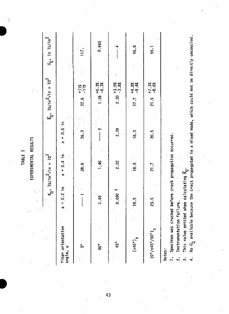
COI—_J00UJ
1-4 Di
LU —I— 1 *£CO I—«« z=I- UJ
t— i
LUa.XUJ
CMC•r-^_jar""
c
•k
^P
COo
X
c•r~s.
CMC
•r™^*^.0.r~
'
COO
X
c
CM• c
•r-
JDr—
A
I f
^c^
• ( .
c•r-
vooIIre
. c•r-
^-•O.
II
re
c•r—CM
•
O
II
re
co•r-^_>re•icCU
£ £3O
t- CUcuf—
JD C7I•i- C<4- re
•f *.
r—r~~
^jg ^jj^— r—r~ r~+ i
VO
CMCO
CO
VOCO
ooocCM
T^v
OO
CO^J*o>
•
o
^o ijjpCO CO
• •VO VO+ 1cpinr—
CM
VO
•^«
VOVO
,_!
0o.
r >
^^ &£c% oo• •.CO CO+ 1oCO
CM
OlCO
CM
CMCM
•CM
w>
O
, to
o
oin
o*in
<s^ ^c00 *^• •*^ o>+ 1
f*>,
pi**
^~
CO
VOffm
in*CO
in
00
VI^-^oin•d-+i
r—•
inun
fe^ ^^CO VO
• •r>. oo+ i
en^~CM
. inoCM
1 •
^-CM
in
COCM
«/>^^0Ocn0tn~+ioO
-oCU
r—Ci.3OOC3
OCUt-
^r^
4^OC
T3
3OO
-Co
JCT
CUT3g
"SCU Xi- •!-S- E
u reoo c
. c "~•i- CU
T3 fl3Dl . . O)re - " • rea. cr Q.0 |^0
Q- cn o.c
o - C ore re reS- r— S-0 3 0
Ua> «— QJi. re J=
cu cu c: cuJ3 J_ CU 01
3 JZ 3•o. •— .» reCU -r- ' Ox: re *o cui/i t- a> .a3 4->t- C 4-> CUU O •!- r—
•i- E JQw> ••-> o rere re i—S •«-» CU T-
c 3 reC CU i— >cu E re reE 3 >••- i. crO 4J 01 CDCU 01 •!-
•• 0. C JC O
cu *"*o * • • •
ZZ »-* Cxi ro ^J1
43
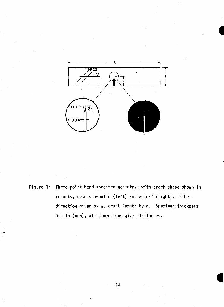
FIBRES
Figure 1: Three-point bend specimen geometry, with crack shape shown in
inserts, both schematic (left) and actual (right). Fiber
direction given by a, crack length by a. Specimen thickness
0.5 in (nom); all dimensions given in inches.
44
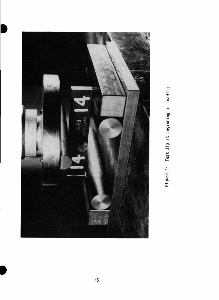
CD
T3toO
O
CD
CDO).0
fD
CD
toO)
OlS-
CD
45
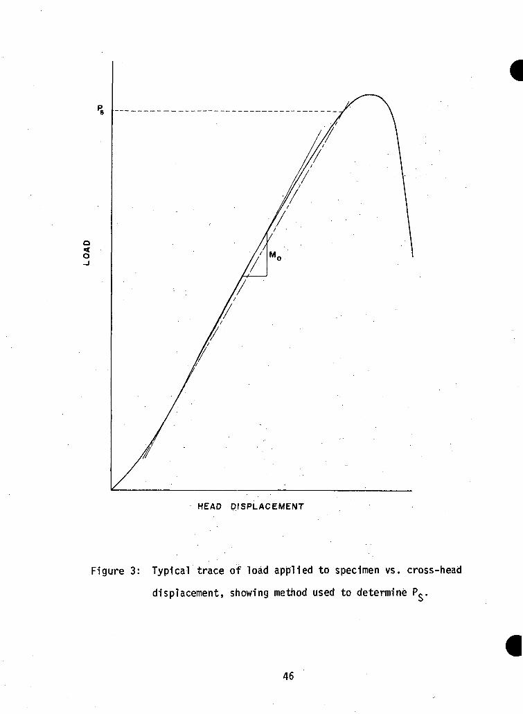
P8
O<O
HEAD DISPLACEMENT
Figure 3: Typical trace of load applied to specimen vs. cross-head
displacement, showing method used to determine P.
46
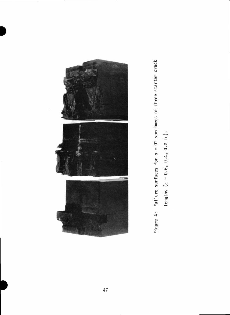
o
ro•)->to
O)<D
•M
1/1c
oOJQ.
oO
II
8
CVJ•
O
to 10<L>O O10<4- IIs.3 iato —O) (O
i— O)•i- C(O 04
CD•i—Q-
47
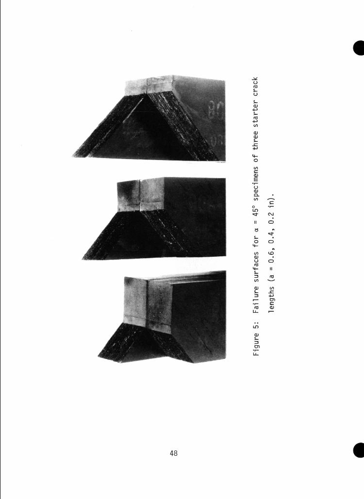
oto0
to
O)
2!
oinCL)
•i—oOJQ.
oID
s-o4-
OlO(O4-s-3inO)S-
i— CT>••- C(O OJ
Ll_ i—
IT)
CM•
O
oII
48
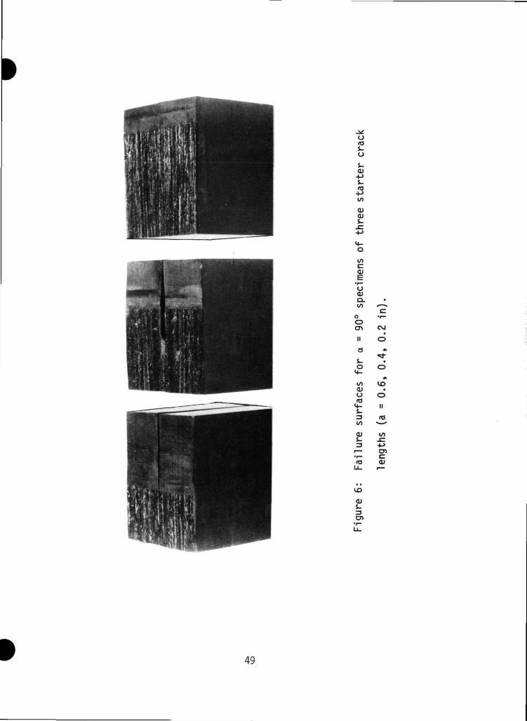
.Vos-oS-01
to
OJOJ
ooocQJ
O<uo.
oo
IIas-o4-
00O)O03
S-300
£
(O
<DS_
CM•
O
O
II
00
(U
49
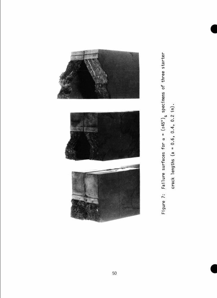
cu-ps_<T3-t->CO
co
oo-CO
oLT>
«*+1
II
as-o4-
co<uO(O
M-
3CO
2:
oII
co
4->cr>(U
jn:o(O
o
en
50
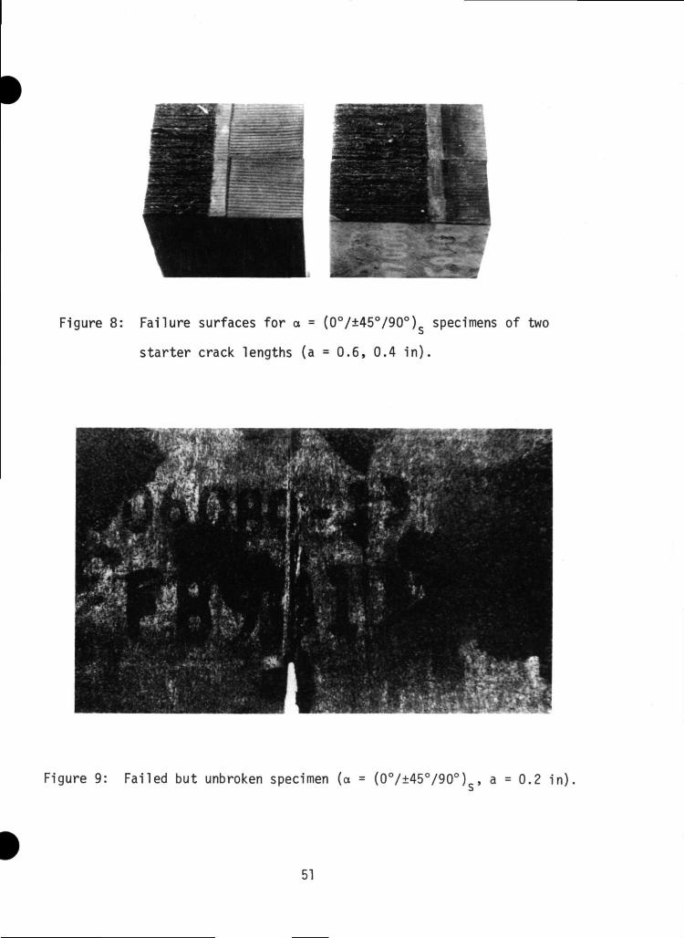
Figure 8: Failure surfaces for a = (0°/±45°/90°)s specimens of two
starter crack lengths (a = 0.6, 0.4 in).
Figure 9: Failed but unbroken specimen (a = (0°/±45°/90°)s, a = 0.2 in)
51
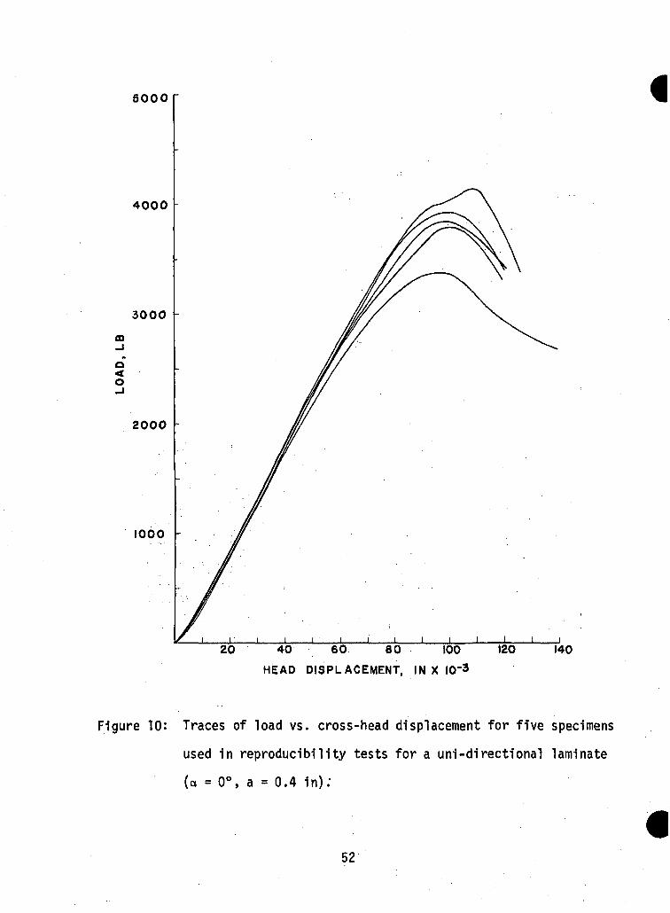
5000
4000
3000
m_J
o<o
2000
1000
i i i i i i20 40 60 80 100 120 140
HEAD DISPLACEMENT, IN X I0"3
Figure 10: Traces of load vs. cross-head displacement for five specimens
used in reproducibility tests for a uni-directional laminate
(o = 0°, a = 0.4 in);
52
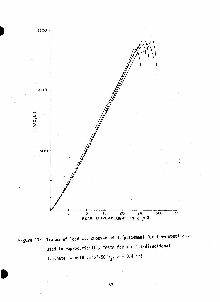
1500
1000 h
m_i
o<o
500
10 15 20 25 30HEAD DISPLACEMENT, IN X KT3
Figure 11: Traces of load vs. cross-head displacement for five specimens
used in reproducibility tests for a multi-directional
laminate (a = (0°/±45°/90°)s, a = 0.4 in).
53
CHAPTER III
STRENGTH OF MECHANICALLY FASTENED JOINTS
3.1 AN INVESTIGATION OF STRESS CONCENTRATIONS INDUCED IN COMPOSITEBOLT BEARING SPECIMENS
3.1.1 Introduction
This study is concerned with materials which consist of parallel,
high strength fibers supported in a relatively ductile matrix material.
The fibers act as load carriers while the matrix serves principally as a
load transfer medium. In particular, it is concerned with advanced fibers,
such as boron or graphite, in an epoxy matrix.
Because of their superior specific strength and specific stiff-
ness, advanced fiber composite materials have a vast potential in the aero-
space industry. Lamina, which are single layers of parallel fibers sur-
rounded by the matrix material, are stacked at various orientations relative
to one another to form a laminate. This procedure enables the designer to
achieve desired strength and stiffness properties and to increase the
structural efficiency of a given amount of material.
The strength and stiffness properties, however, are highly
directional; panels fabricated out of layers of unidirectional composite
tape are anisotropic. The designer therefore has the difficulty of includ-
ing the effects of this anisotropy in his calculations. .
One particular problem area in a structure made of composite
materials is the bolted joint. The bolted joint in a composite material
has a significantly lower efficiency than the same joint in metals.
Furthermore, the composite joint may fail in unique modes not found in
metal joints.
54
This study, therefore, investigates the stress concentrations
induced in anisotropic plates loaded by means of a single fastener hole.
The study is an attempt to further understand the failure characteristics
of such bolted joints. The development of a prediction capability for
both the failure mode and ultimate load is the major goal of the early
part of this work. Such a capability would allow synthesis rather than
analysis to be used in the future design of fastener joints. An implied
goal in this study is an evaluation of the three proposed anisotropic
failure criterion; maximum stress, maximum strain, and distortional
energy.
3.1.2 Analysis Method
A constant strain, finite element computer program using tri-
angular elements was modified to handle anisotropic composite materials
using lamination theory as presented in [1]. The experimental work done
on bolt bearing specimens, from which this study draws heavily, only con-
sidered cross-plied laminates which were mid-plane symmetric. As a result,
this numerical study is also limited to this class of laminates. It is
important to remember that the use of lamination theory ignores inter-
laminar shear; consequently, it is expected that the degree of error in
the results will vary with specimen anisotropy.
The design of a finite element grid representation to simulate
the bolt bearing test specimen was subject to two major considerations.
First, the grid had to be sufficiently detailed around the.bolt hole to
pick up the large stress gradients which are induced in this area.
Secondly, the number of elements and nodes was restricted by the storage
55
capacity of the computer. Taking advantage of the two lines of specimen
symmetry shown in Figure 1 only one-fourth of the specimen was included
in the finite element simulation. Figure 2 shows a computer plot of the
specimen section for e/d = 5.0, s/d = 10.0, and £/d = 20.0. The grid
representation used contains 480 elements and 279 nodes. The conditions
of specimen symmetry are met by forcing the x-displacement of the vertical
line of symmetry and the y-displacement of the horizontal line of sym-
metry to be zero in each computer run. A computer subroutine was also
developed which transforms the co-ordinates of the grid shown in Figure 2
to any desired specimen geometry, i.e., e/d, s/d, £/d.
To check whether or not the grid was sufficiently detailed around
the. hole an isotropic test case and several anisotropic test cases were
run. A uniform tension stress was applied to the ends of each specimen.
Comparison with the isotropic results presented in [2] (See Figures 3a and
3b) and the anisotropic results of [3] indicated that further refinement
of the finite element mesh around the hole was not necessary. The observa-
tion that the computed finite element values of stress are higher than the
exact values agrees well with the results illustrated in [4].
A cosine distribution of normal stress acting over the upper half
of the hole surface was used to simulate the resulting stress distribution
caused by the bolt. The interaction was, therefore, assumed to be fric-
tionless. Bickley [5] shows this to be an excellant approximation for
isotropic bolt bearing specimens. A finite element analysis of the bolt-
specimen interaction in certain composite laminates was performed at
General Dynamics [6]. The cosine distribution of normal stress was again
shown to be a realistic approximation of the interaction stresses.
56
Further confidence was gained in both the cosine distribution and
the grid mesh by running an isotropic bolt bearing test problem and ob-
serving the qualitative agreement of the computed stress field around the
hole surface (See Figure 4) with work by Coker and Filon [7]. The speci-
men used in their study had significantly larger values of e/d and s/d
and thus a quantitative comparison was not possible.
Finally, two other normal distributions of stress, which were
significantly different from the cosine distribution (See Figure 5), were
used as the bolt-specimen interface stress boundary condition for one of
the composite material specimen runs.
The net force in the load direction in each case was equivalent.
It was observed that significant variance about the cosine distribution
resulted in insignificant alterations of the calculated stress fields for
the specimen considered.
3.1.3 Strength and Failure Mode Predictions
The selection of specimen geometries for this investigation was
made from data which has been published by General Dynamics [8,9] and
Grumman Aerospace [10]. Included were two net-tension failure specimens,
two shear-out failure specimens, one bearing failure specimen and one
specimen which exhibited failures in a transition region between a net
tension and combination failure mode. See Figure 6 for illustrations of
these various failure modes.
Performing a strength analysis on a laminated composite material
may be based on the strengths of its individual lamina. The strength of
a single orthotropic lamina can, in theory, first be determined experiment-
ally, producing an ultimate strength envelope for that material. This
57
three dimensional surface (in terms of principal lamina stresses) could
then be used to analytically predict the ultimate strength of the total
laminate. The state-of-the-art has yet to reach this level of sophisti-
cation. The present three dimensional ultimate strength envelope is con-
structed using only five points on the stress axes due to the, as yet,
unsolved problems encountered in off-axis testing.
The Hill failure criterion is a widely accepted representation of
this three dimensional envelope; it has been found in this study to be
the only reliable means of predicting bolt bearing specimen failure modes.
As shown in [11] lamina failure is predicted to occur when the following
set of principal stress ratios (normalized on their respective ultimate
stresses) add to a number, DIST, greater than or equal to one.
nisi = ' ' -•- ' i •*• i i — i - 11 11 i ' •\j L *j i
Figures 7 through 10 are plots of DIST for typical net tension, shear-out,
bearing, and combination failure modes respectively. An initial applica-
tion of the experimental failure load was used as the applied load for
each computer run. The resulting contour plots were sufficient to predict
the failure modes in all but the shear-out cases. For these specimens it
was sometimes necessary to consider the ratios of lamina principal stresses
to their respective ultimate stresses to differentiate between a plug type
shear-out mode and a bending, tear-out mode.
Figures 7a through 7d represent DIST contour plots of four laminae whichcompose a net tension failure specimen. A single plot of the major loadcarrying lamina for each of the other three failure modes is included toillustrate the contour patterns for these various modes.
58
Prediction of failure load was also made on the basis of the .
Hill criterion. The values of DIST in the first row of circumferential
elements around the hole were considered for each lamina. A successive
failure analysis similar to that discussed in [12] was used to predict
ultimate load. As soon as an element in any given lamina achieved a value
of DIST equal to 1.0 that lamina was assumed to have failed and was locally
removed from the laminate. The load was then redistributed among the re-
maining laminae and all values of DIST were recalculated. If all recalcu-
lated values of DIST were less than 1.0 more load was applied until another
lamina reached failure. This process was repeated until total laminate
failure occurred.
The predictions of failure load based on equation (1) were always
conservative. The degree of conservatism varied with failure mode, but
more importantly it appeared to be a function of specimen anisotropy. To
date only 0°/90°/±45° specimens have been considered. The predicted
failure loads for the net tension specimens improve greatly as the percen-
tage of ±45° lamina decreases (See Table 1). For example, for a 100%
(±45°) laminate the predicted failure load is about one-half the experimen-
tal failure load. For a (±45°/90°) laminate which contains 62.5% (±45°)
lamina the predicted failure load is about nine-tenths the experimental
failure load. This same type of behavior was reported by Grumman Aerospace
[13] in a study they performed on laminate tension data.
The Hill criterion was the only criterion of the three which was
conservative in predicting failure load for each specimen investigated.
Both the maximum strain failure criterion and the maximum stress failure
59
criterion overpredicted at least one specimen ultimate load. That is,
even when the experimentally determined failure load was applied the ratio
of principal strains (or stresses) to their respective ultimate strains
(or stresses) did not exceed 1.0 as is required by these two criterion
respectively.
Investigation of experimentally failed specimens exhibit excellent
agreement with predicted failure behavior. For example, specimens which
failed according to a slug type shear-out mode exhibited relatively smooth,
clean fracture surfaces. The high values of DIST for the shear-out
failure mode pictured in Figure 8 are a result of very high principal
shear stress ratios in these regions, which would lend to rather smooth
shear fracture surfaces. On the other hand, specimens which failed by a
bending, tear-out failure mode (which is also considered a shear-out
failure mode by some investigators) exhibited a very coarse, jagged frac-
ture surface. This behavior is again expected from the computed stress
ratios. 'Along lines at ±45° in a (0°/900/±45°) specimen, where the
values of DIST are high, the largest stress ratios act in the first
principal direction. These are the stresses which are trying to break
fibers in tension. As a result, as the triangular section is being torn
away from the specimen, fibers along these failure lines at ±45° are be-
ing broken in tension; resulting in a very coarse, jagged fracture surface.
Another interesting feature of the experimentally failed speci-
mens was the presence of a highly localized region of laminate destruction
at the bolt-specimen interface. It was observed that a bearing failure of
variable magnitude had occurred in conjunction with almost every other
60
type of experimental failure mode. This behavior was again predictable
as is shown in Figures 7c, 7d, 8, 9 and 10.
3.1.4 Future Work
Three important areas in this analysis where simplifications have
been made will be investigated in the future.
1) The effects of interlaminar shear on the stress field
near the hole.
2) The significant variation in material properties and
ultimate allowables reported in the literature.
3) The non-linear stress-strain response of the composite
materials.
The need for reliable off-axis failure data is also critical to the com-
plete understanding of the failure of a composite structure under compli-
cated loading. It is felt that continued investigation of the simple
bolt bearing problem will yield further clues as to the mechanisms of
failure due to stress concentrations.
It was also felt at the completion of this project that a similar
failure analysis could be performed on more complex mechanically fastened
joints made of composite materials. Such an investigation has been
performed by this investigator and is reported in the next section.
61
3.1.5 References
[I] 0. E. Ashton, J. C. Halpin, and P. H. Petit, Primer on CompositeMaterials: Analysis, Technomic Publishing Company, Stanford,Connecticut (1969),
[2] S. Timoshenko and J. N. Goodier, Theory of Elasticity, SecondEdition, McGraw-Hill Book Company, 80 (1951).
[3] S. G. Lekhnitskii, Theory of Elasticity for Anisotropic ElasticBody, Holden-Day, Inc., 170 (1963).
;[4] 0. C. Zienkiewicz, The Finite Element Method, McGraw-Hill PublishingCompany, 38 (1967).
[5] W. Bickley, "The Distribution of Stress Round a Circular Hole ina Plate", Phil. Trans. Roy., Soc., A. (London), 227, 383 (1928).
[6] Advanced Composite Technology, Fuselage Program - Phase I, SecondQuarterly Progress Report, General Dynamics, 164-172, (1 November1969).
[7] E. G. Coker and L. N. G. Filon, Photo-Elasticity, Cambridge, 524-530(1957).
[8] Advanced Composite Technology, Fuselage Program - Phase I, SecondQuarterly Progress Report, General Dynamics, 90-110, (1 November 1969)
[9] Advanced Composite Technology, Fuselage Program - Phase I, ThirdQuarterly Progress Report, General Dynamics, 107-122, (1 February1970).
[10] Advanced Composite Wing Structures Boron-Epoxy Design Data - VolumeII, Grumman Aerospace Corporation, 187-191, (November 1969).
[II] J. E. Ashton, J. C. Halpin, and P. H. Petit, Primer on CompositeMaterials: Analysis, Technomic Publishing Company, Stanford,Connecticut, 26 (1969).
[12] Investigation of Joints in Advanced Fibrous Composites for AircraftStructures, Air Force Flight Dynamics Laboratory, 13, (June 1969).
[13] Advanced Composite Wing .Structures Boron-Epoxy Design Data - VolumeII, Grumman Aerospace Corporation, (November 1969).
62
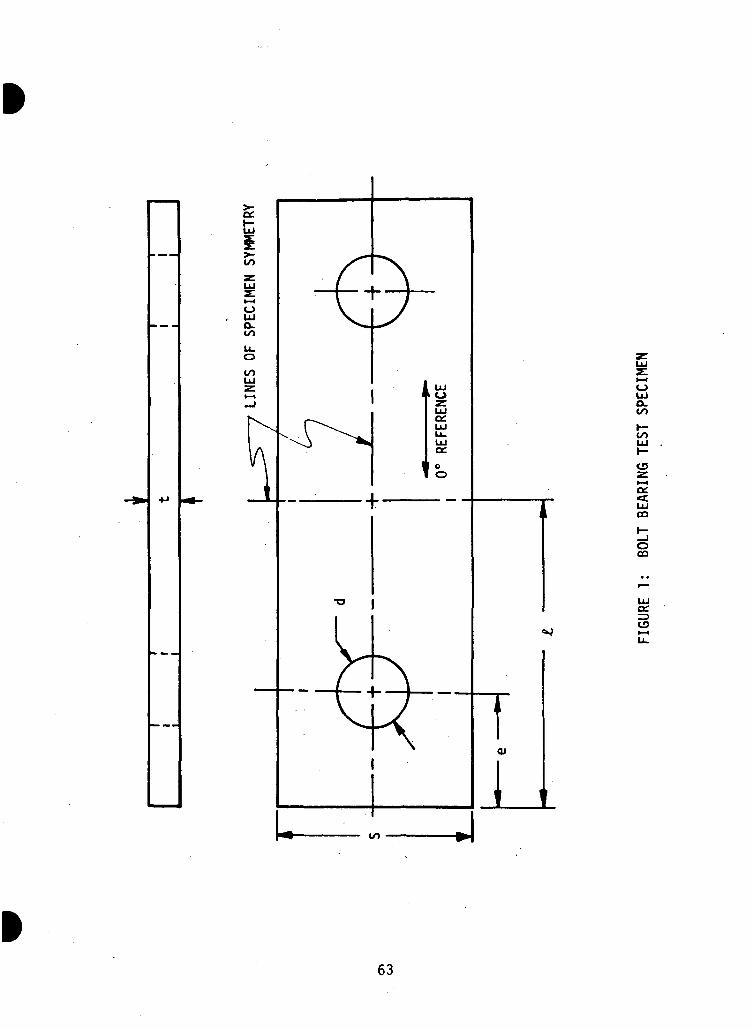
oLUO.
tozI-Ha:2CO
oCO
a:rsCD
63
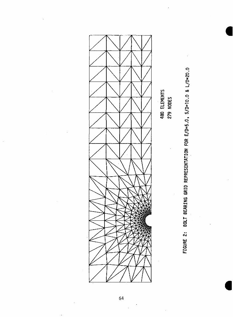
UJ (/>z: ujUl Q_J O
CM
oB
O•
OI'-llQ
CO
iio
UJcoUlo:Q-LU0£.
QC
2CO
oen
CM
UlDC
vs
64
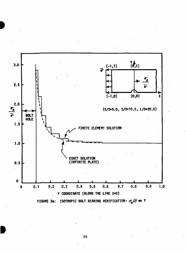
3.0
2.5
2.0
BOLTHOLE
1.5
1.0
0.5
r r*(-1.1) (0*1)
(-1.0) (0,0)
(E/D=5.0, S/D-10.0, L/D-20.0)
FINITE ELEMENT SOLUTION
EXACT SOLUTION(INFINITE PLATE)
0.1 0.2 0.3 0.4 0.5 0.6 0.7
Y COORDINATE (ALONG THE LINE X»0)
FIGURE 3a: ISOTROPIC BOLT BEARING VERIFICATION:
0.8 0.9 1.0
65
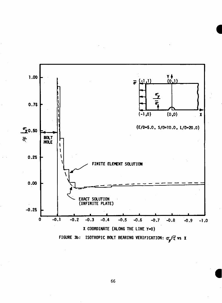
1.00
0.75
•yQ.SO
0.25
0.00
-0.25
BOLTHOLE
t
;-i•»-
1) (0.1)
-i1 J>
(-1,0) (0,0)
(E/D-5.0. S/D«10.0f L/D-20.0)
FINITE ELEMENT SCUttlON
EXACT SOLUTION(INFINITE PLATE)
-0.1 -0.2 -0.3 -0.4 -0.5 -0.6 -0.7 -0.8 -0.9 -1.0
X COORDINATE (ALONG THE LINE Y=0)
FIGURE 3b: ISOTROPIC BOLT BEARING VERIFICATION: <?qf vs X
66
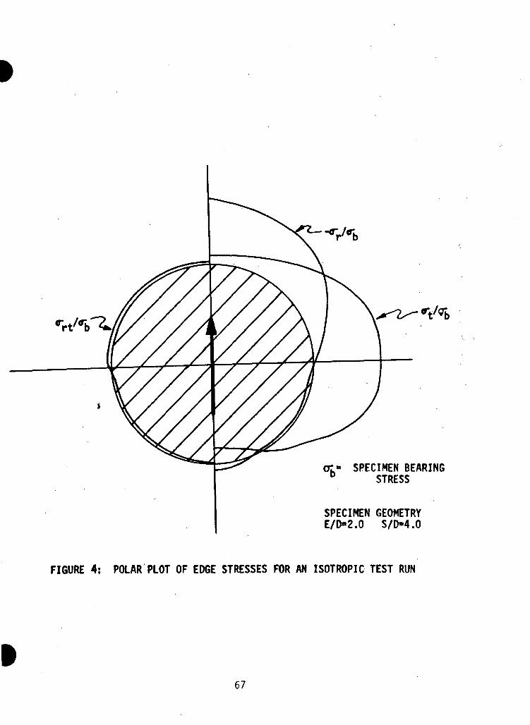
«rt/<rb
SPECIMEN BEARINGSTRESS
SPECIMEN GEOMETRYE/D-2.0 S/D-4.0
FIGURE 4; POLAR PLOT OF EDGE STRESSES FOR AN ISOTROPIC TEST RUN
67
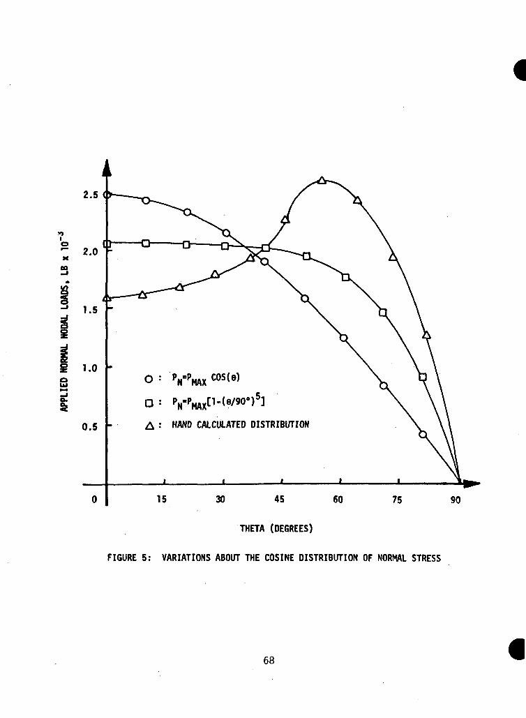
x
3
§ 1.00: PN"
PMAX cos(e)
D :
A : HAND CALCULATED DISTRIBUTION
45 60 75 90
THETA (DEGREES)
FIGURE 5: VARIATIONS ABOUT THE COSINE DISTRIBUTION OF NORMAL STRESS
68
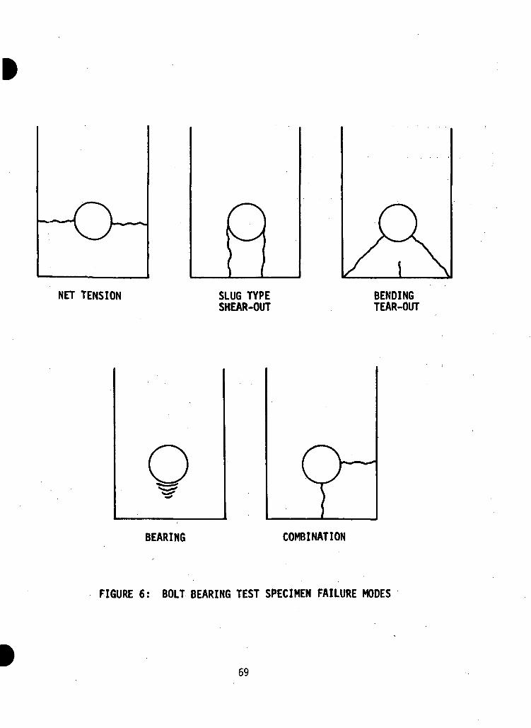
oNET TENSION SLUG TYPE
SHEAR-OUTBENDINGTEAR-OUT
OBEARING COMBINATION
FIGURE 6: BOLT BEARING TEST SPECIMEN FAILURE MODES
69
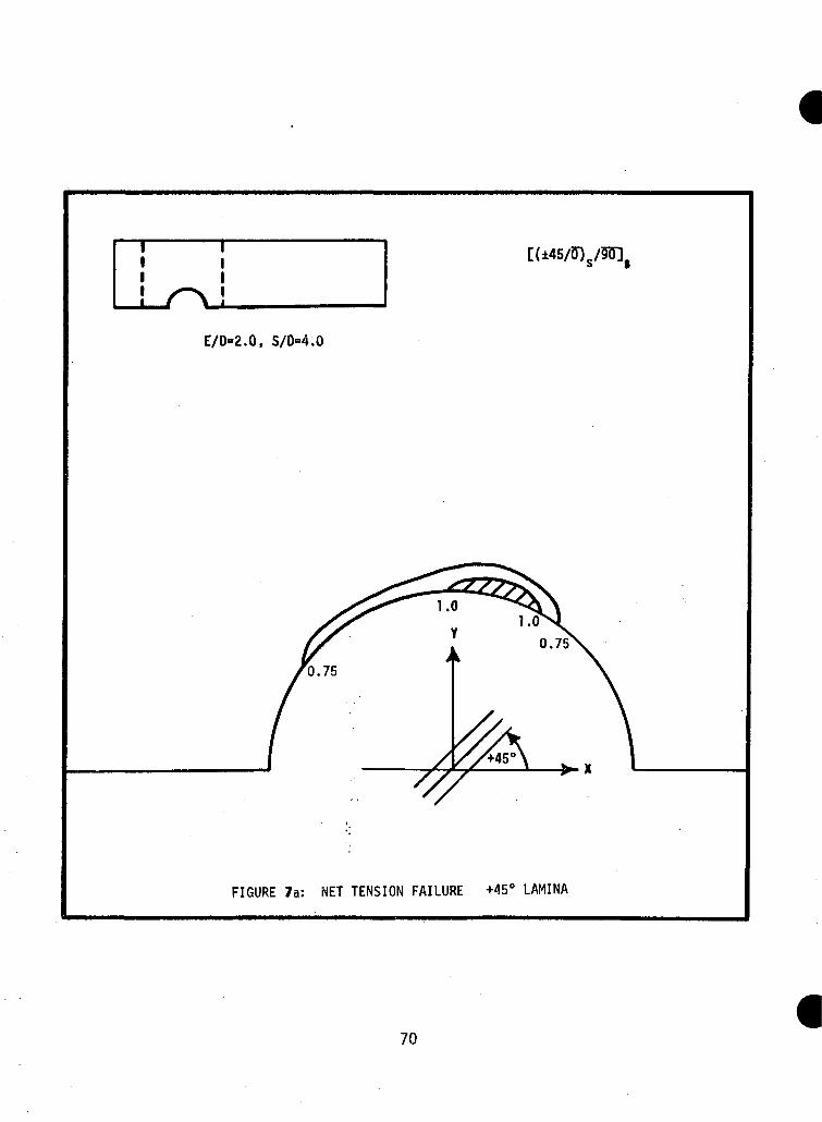
1111 X
111
-\ !
[(±45/5)s/9ff]g
E/D-2.0, 5/0=4.0
FIGURE 7a: NET TENSION FAILURE +45° LAMINA
70
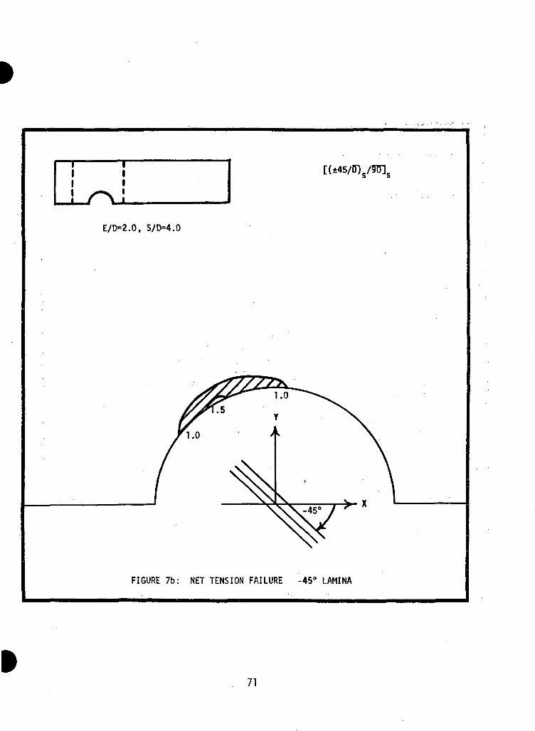
[(±45/ff)s/9ITJs
E/D=2.0, S/D=4.0
FIGURE 7b: NET TENSION FAILURE -45° LAMINA
71
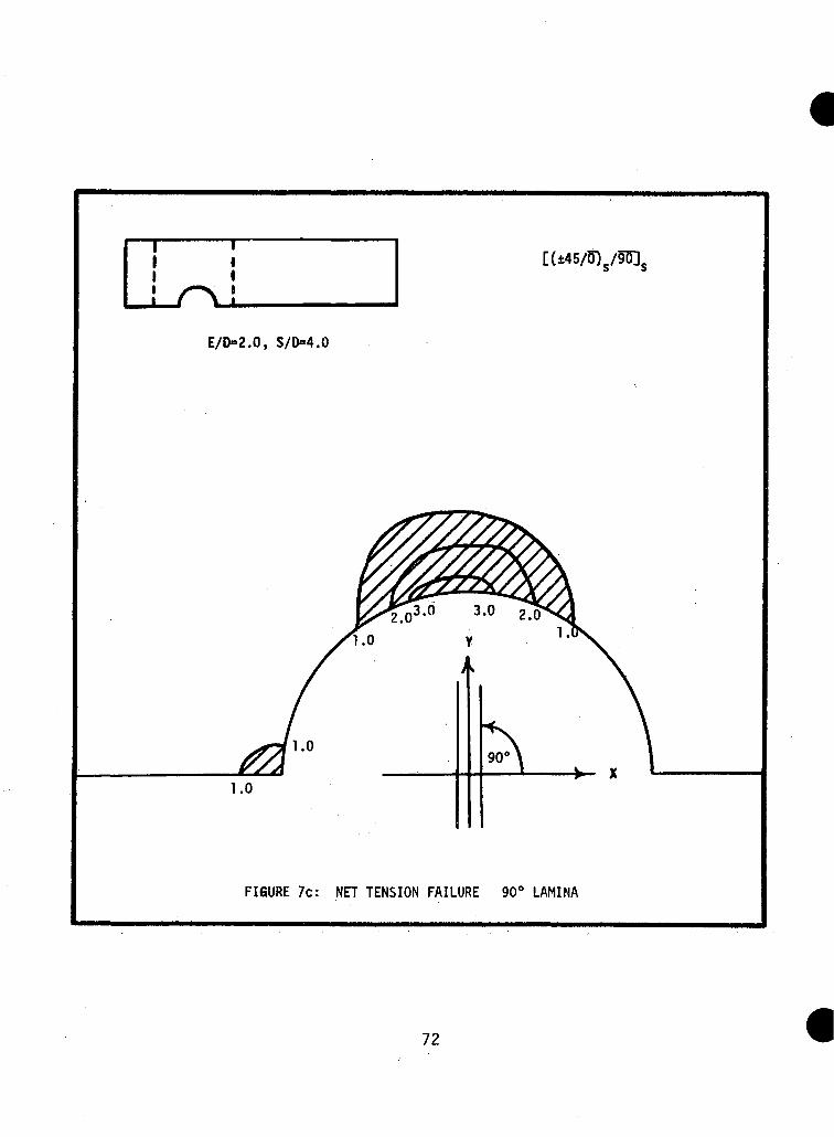
1111 X
111
"N !
E/D-2.0, S/D=4.0
FIGURE 7c: NET TENSION FAILURE 90° LAMINA
72
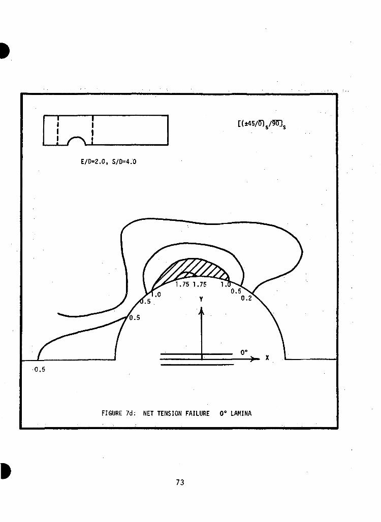
I I
LTN!E/D=2.0, S/D=4.0
FIGURE 7d: NET TENSION FAILURE 0° LAMINA
73
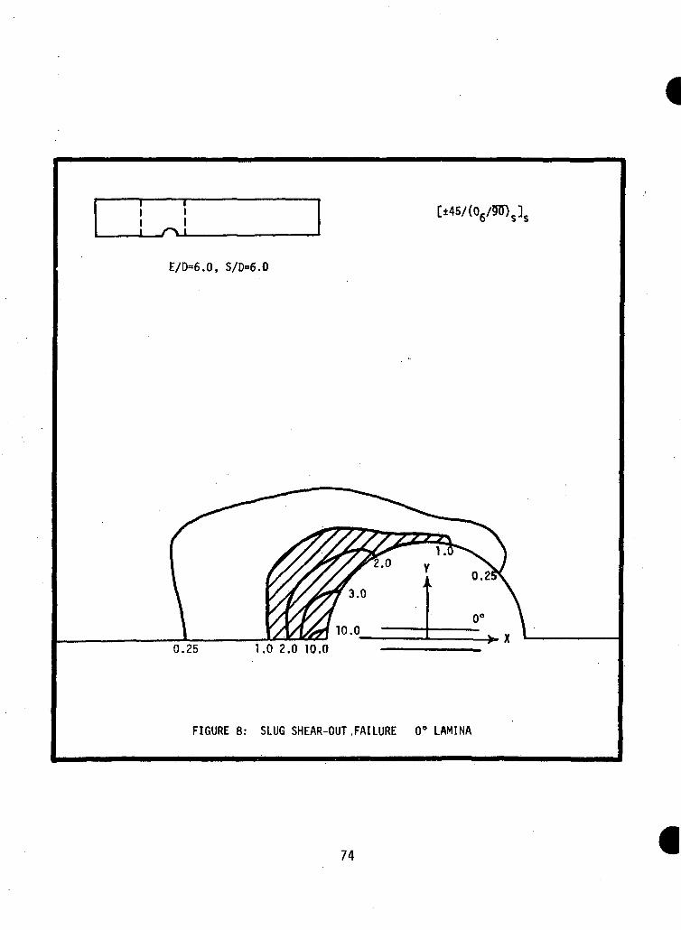
I II I [±45/(06/90)s]s
E/D=6.0, S/D=6.0
fa.o t
0°
0.25 1.0 2.0 10.0
FIGURE 8: SLUG SHEAR-OUT .FAILURE 0° LAMINA
74
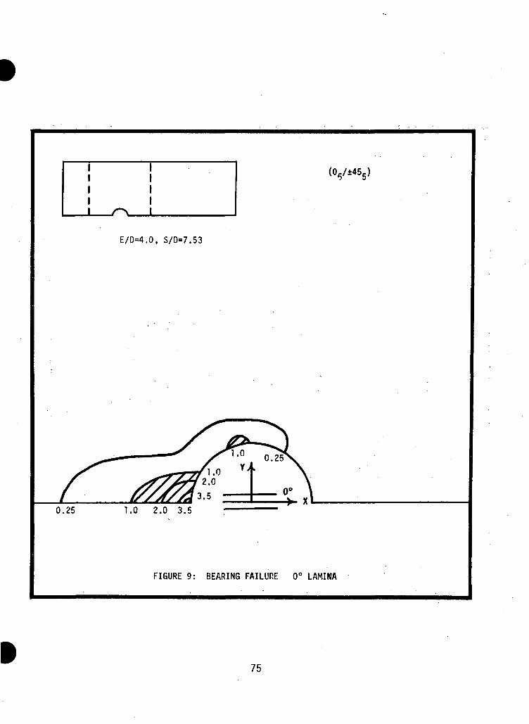
i Ii ii ii i1 /-N 1
(06/±455)
E/0=4.0, S/D=7.53
0.25 1.0 2.0 3.5
FIGURE 9: BEARING FAILURE 0° LAMINA
75
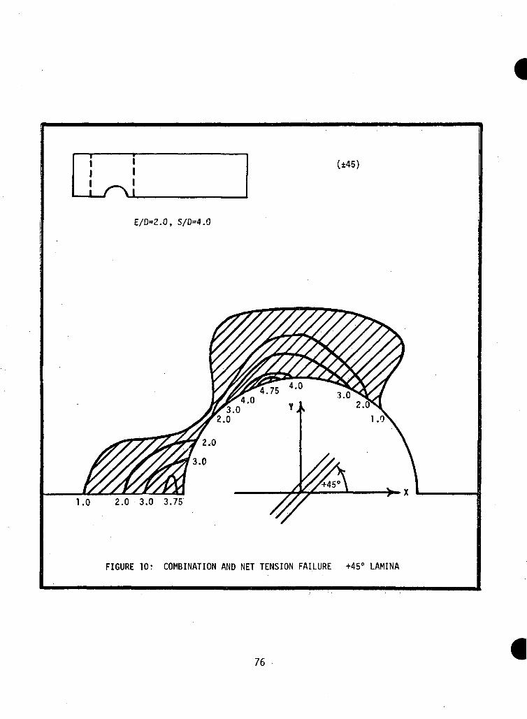
i : (±45)
E/D-Z.O, S/D=4.0
1.0 2.0 3.0 3.75
FIGURE 10: COMBINATION AND NET TENSION FAILURE +45° LAMINA
76
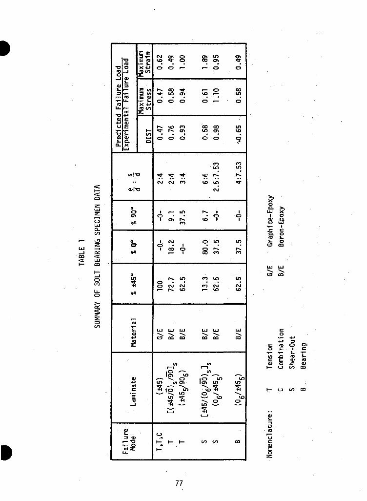
ca«=C
LUa.oo
CQ
OCO
o>-
oo
E C|*O Enat ••- l.
XJ O x +Jre —i «3 too s:
2? -— E to3-1- 3 toi — at E <U•i- U. .i-l.(O X 4->
"i5 s! *"
OJ C4J COu E•r- -i- 1—•o t- ooCO CO H-ls- o. aa. x
UJ
..
CO I'D
oOO^
**
°oW
OLO
*^"M
Vi
to'£•M<a
<ufOc
•r—E(O_J
e3 (U
U.
CM Cf» O^O 1" CD• • • •o o >—
r*^ co ^~«*• in cr>o o o
r^ vo co^* r^ o^O O CD
CM CM CO
i r— inO
** co
1 CMO • 1
1 CO O
I-* LOOO CM CM
LU LU LU
O CO CO
tof 1
lO *~*Icn vo
in 10 ov^^ ^™ ^^^
"f-l I CD ^^S^^ "NS^ tO
U") ^«f "VI
L^^
0M
t- 1— 1—
1—
S inen
•— CD
i— Ovo •—O i—
CO COLO O^
*• •0 0
COin
• * • •
vo inCM
i*» i• o
VO 1
o m
co co
co in• • .
CO CMr— \Q
UJ LU
CO 00
I/I
10 *~LnIcn in^^^ ^^- l££ f.\
O ^>.^** VO^ oin — •
oo oo
5o
00ino
invo
9
coin
•
5
io
1
in
CO
in•
CMVO
LU
CO
'"ininj-
-M" VOO
ca
oa. >>LU xI O<u a.+-> LU
•i- iJ= Ca. o(O L.s- o
C3 CO
co ca
•r- -r- t. T-l/l .O IT3 *-c E at <aO) O JC 0)
t— o oo co
oo co
77
3.2 TOWARD A DESIGN PROCEDURE FOR MECHANICALLY FASTENED JOINTSMADE OF COMPOSITE MATERIALS
3.2.1 Introduction
Currently much emphasis is being directed toward replacing
metal components in weight sensitive structures, such as aircraft,
with composite materials, due to their superior specific strength
and specific stiffness properties. The potential weight savings which
could result from such practices, however, have not, as yet, been
realized.
Significant weight savings can be achieved throughout
the bulk of a replacement component by tailoring the composite
material to efficiently carry the loads which are known to occur in
the existing metal component. The weight savings which result,2however, are usually eliminated due to the inefficient joint designs
which are proposed by the designer to fasten the replacement component
to the remainder of the existing structure. The measure of efficiency
used here is simply load carried per pound of material. Thus, if a
given load is to be carried by a structural member, the load carrying
efficiency of that member increases as its weight is decreased.
In the design of metal joints only three failure modes
need be considered; net tension, shear-out, and bearing. For a given
metal the values of FTU, FSU, and FBRU can be experimentally determined
and used to specify the joint parameters S, E, and t respectively,
given the bolt diameter. Thus, the design of metal joints is based
on a very limited amount of experimental data.
The term joint will imply a mechanically fastened joint throughoutthe report.
78
Consider the complications which would arise if a similar
empirical design procedure.were used for joints made of composite
materials. First of all, several additional failure modes are ex-
hibited by composite joints which do not occur in metal joints, due
to the anisotropy of composite materials. Thus, for a given laminate
the amount of data required for design purposes would be about
doubled. The major problem, however, is that the feasibility of
obtaining effective stress allowables which can be related to geometric
parameters for splitting, shear-out, or bending tear-out failure modes
in composite materials has yet to be determined.
Secondly, consider the problems associated with the
selection of joint lamination. The designer is using a material
which may be tailored to satisfy certain design constraints which
are application dependent. The number of possible lay up patterns
which could be considered during a single design are innumerable.
Thus, the amount of data acquisition which would be necessary to
support an empirical design procedure in composite joints is prohibi-
tive.
As a result, the designer is presently forced to select
a laminate for which some data does exist. Since laminate effective
stresses for the various failure modes are unknown, an overly con-
servative design must be proposed by the designer based on his
interpretation of the available data. An overly conservative design,
unfortunately, implies that additional material has been used wherever
79
necessary to compensate for a lack of confidence in predicting various
failure modes. Such practices, of course, lead to inefficient designs.
There is one other important difference between metal joints
and composite joints which should be mentioned. It can be deduced,
using the results from [1], that the stress concentration factor
which results in an aflfsotropic joint is greater than that which
occurs in a geometrically similar isotropic joint. This ii-s, of course,
a .disadvantage associated with using composite materials in joints.
It is, however, more than compensated for by the materials specific
strength and specific stiffness properties.
To recover the potential! weight savings of designing with
composite materials new design procedures must be proposed which
will result in optimum joint designs with respect to total joint
weight. It is the purpose of the *ne.ported study to investigate
such improved design procedures.
A first attempt at such design procedures is proposed and
is discussed in detail in Section 3.2.6. The procedures are sufficiently
general that they may be used in conjunction with most available
optimization routines. The results are being programmed by this
investigator using an in-house pattern search optimization routine.
Given valid input data, the program is designed to output that joint
design in design space which has the minimum total joint weight
while satisfying all the imposed design constraints. The results will,
of course, only be as accurate as the assumptions on which the analysis
80
is based. As a result, further investigations regarding the accuracy
of these assumptions is warranted and will be performed by this investi-
gator.
As mentioned above, three failure modes have been observed
in metal joints: net tension, shear-out, and bearing. Each of these
modes exhibits ductile fracture behavior. In composite joints not
only are there additional' modes of failure to consider but fracture
behavior ranges from ductile to brittle, depending on the failure mode
being considered.
Finite element stress analyses of bearing and shear-out
failures in composite materials [2] have shown that large regions
of laminate destruction, on the order of a hole diameter in size,
occur prior to actual laminate failure. It was also found that
highly localized regions of laminate failure, about two orders of
magnitude smaller than those required for bearing and shear-out
failures, were present when net tension failures occurred. It is
apparent, therefore, that these various failure mechanisms must
be understood before a truly optimum joint design can be achieved,
since a single failure criterion is not applicable to all the possible
modes of failure in composite materials.
A recent study [3] has postulated the existence of a small
but finite region of intense energy which supposedly governs failure
in composite tension coupons. If stress concentrations induce such
regions of intense energy in composite tension coupons a similar
81
phenomenon should occur in composite bolt bearing specimens. The
results reported in [2], therefore, tend to support such a theory.
To further understand the phenomenon, a finite element
study was performed for several composite tension coupons and is
reported in Section 3.2.2. Again, very small, highly localized regions
of laminate destruction were observed prior to actual failure. As
a logical extension to the tension coupon experimental study [3]
four geometrically similar bolt bearing specimens were designed,
Section 3.2.2, to fail in net tension using a quasi-isotropic boron-
epoxy material. These specimens are presently being fabricated and
will be tested at General Dynamics, Fort Worth. If a characteristic
crack length hypothesis is indeed valid, significant differences in
applied failure stresses for these specimens should be observed.
These differences should be predictable from the theory presented
in [3].
The design procedures outlined and discussed in Section
3.2.6 are only intended to represent an initial attempt at moving
toward the desired design procedures for joints made from composite
materialsi In Section 3.2.7 those areas which require further investi-
gation are indicated.
3.2.2 Investigation of the Characteristic Crack Length Hypothesis
Past experience with predicting net tension failure in
anisotropic bolt bearing specimens using the distortional energy
82
failure criterion3 [2] has shown that a small but finite region of
material at the hole surface is always "past the point of failure"
before laminate failure occurs. These regions were originally considered
to result from an inherent conservatism of the finite element solution
technique. A recent sutdy performed at General Dynamics [3] has postulated
the existence of a region of intense energy in composite tension •c.oup.ons
which seems to govern failure. The finite element results [2] in
retrospect appear to support such a theory.
In the study performed at GD a series of graphite/epoxy tension
coupons were designed and tested to failure. The specimens were identical
in overall size and lamination but the sizes of the circular cutouts
varied. If a similar series of metal specimens were tested it would
be possible to predict the failure loads of all the specimens from the
experimental failure load of a single specimen, using scaling factors
which are only geometry dependent. In the case of the graphite/epoxy
coupons a simple scaling of failure loads was not possible. It was
found, however, that the observed failure behavior could be explained
via fracture mechanics if the existence of a region of intense energy
or a characteristic crack length was hypothesized. For a given laminate
the size of the region was assumed constant. ,
It is well known that the Hill failure criterion is not a distortionalstress energy. However, because of the close similarity with the iso-tropic failure criterion of distortional energy, the phrase "distortionalenergy failure criterion" will denote the Hill failure criterion as usedin Section 3.1.
83
As previously mentioned highly localized regions of predicted
laminate failure have been observed via finite elements in composite
bolt bearing specimens. An investigation to determine whether or
not similar regions could be observed via finite elements in composite
tension coupons has since been completed. Two specimens v/ere selected
from [3] for analysis. The failure loads predicted by the theory [3]
for these two specimens were used as applied loads for the computer
runs. Using the most recent graphite/epoxy material constants and
ultimate allowables it was found that for a tension coupon containing
a 1.0 inch diameter hole the region of localized failure measured
50 mils. Likewise, for a specimen containing a 0.2 inch diameter
hole the region measured 31 mils. The characteristic crack length
proposed for the laminate used in the actual specimens was approxi-
mately 40 mils and agrees quite well with the finite element results.
Distortional energy contour plots for the various laminae in the 1.0
inch diameter specimen are shown in Figure 1. Localized lamina
failure is predicted to occur when the value of the normalized
distortional energy exceeds 1.0 [2].
There are several reasons to suspect that the values of
the distortional energies near the hole are not entirely accurate.
Finite element size differences in the two specimens at the hole
surface, the effects of interlaminar shear at the circular boundaries,
and uncertainties regarding the cross term in the distortional energy
84
failure criterion probably account for a large percentage of any
possible error. The fact that a small region of material appears to
be "past the point of failure" in both specimens before laminate
failure occurs, however, is the significant result rather than the
actual sizes of these regions.
If a region of intense energy actually governs failure in
composite tension coupons it should also govern failure in bolt bearing
specimens made of the same material. Thus, four geometrically similar
bolt bearing specimens were sized using a quasi-isotropic graphite/
epoxy laminate to see if differences in experimental failure loads
could be observed and explained using the characteristic crack length
hypothesis. The equations presented in [4] were used to size the ini-
tial design, Table 1. The ultimate load predicted by the equations
for a net tension failure was slightly less than that necessary for
a bearing failure and only about two thirds that necessary for a
shear-out failure. A computer analysis of the proposed specimen
configuration indicated that a net tension failure would occur at
precisely the load predicted by the equations. The resulting dis-
tortional energy plots for the initial design are shown in Figure 2a.
Note, however, that the results reported in [2] indicate
that before a bearing failure may occur in a bolt bearing specimen
a large region of material directly ahead of the bolt must exhibit
normalized distortional energies greater than 1.0. Thus, the computer
85
analysis predicts a net tension failure to occur well ahead of any
possible bearing failures, Figure 2a. This, however, disagrees with
the behavior predicted by the equations.
At the request of Mr. J. R. Eisenmann the specimen was
resized to eliminate even the remotest possibility of premature
bearing failures since such failures would give no information re-
garding the possible presence of a characteristic crack length. In
the revised design (Table 2) the specimen width has been decreased
and the edge distance increased. The equations now predict a net
tension failure to occur well ahead of both bearing and shear-out
failures. A computer analysis of the revised design again indicated
that a net tension failure would occur (See Figure 2b). The failure
load predicted by the computer analysis, however, was 58% greater
than the failure load predicted by the equations. Both the equations
and the finite element analysis agree that a net tension failure
will occur well ahead of both bearing and shear-out failures. The
two methods disagree significantly, however, on the predicted
failure loads.
These differences in predicted failure loads indicate
clearly that basing bolt bearing specimen failure predictions on
the equations presented in [4] is very dangerous. The equations are
empirical in origin and only apply to a limited range of specimen
geometries. The revised design is obviously outside the region
of applicability.
86
3.2. S Review of Past Design Programs Involving Composite Joints
Two programs involving the design and testing of joints
made of composite materials were recently completed at General
Dynamics, Fort Worth. In the original program [5] specimens were
sized to fail in net tension at the innermost row of bolts. The
maximum load to be carried by a joint was first specified. An
estimate as to bolt load partitioning was next made based on the
designers understanding of load distributions in isotropic joints.
The laminate to be used was selected and the joint dimensions were
then scaled from existing single- and double-fastener coupon data.
During testing, eight of the nine specimen designs
failed in a splitting mode rather than the desired net tension mode.
Thus the techniques used in sizing these joints proved to be un-
satisfactory.
In the second joints program [6] only one joint was designed
and tested. The maximum load to be carried by the joint was again
specified. The designer assumed that each bolt in the joint would
carry an equal percentage of the total joint load at failure. The
longitudinal strains in the splice plate and main plate were set
equal at two locations in the joint; midway between the first two
rows and last two rows of bolts. The specimen was sized at these two
locations to fail in' net tension at the innermost row of bolts. A
linear taper in both geometry and lamina thicknesses was then em-
ployed. The resulting joint design was built and tested. It failed
in net tension at the innermost row of bolts as desired.
87
The major criticism of the latter design procedure is
that it ignores the interaction between bolt load partitioning and
joint geometry. The design procedures proposed by this investigator
include such interaction relationships. The following section,
Section 3.2.4 describes the proposed load partitioning analysis in
detail. In Section 3.2.5 the analysis technique is used to predict
bolt load distributions for six specimens selected from [5] and [6].
The results are used as input data for finite element analyses of
the various specimens. A joint failure criterion is then proposed
which,,when applied to the finite element results, successfully
predicts failure modes and conservatively predicts failure loads
for each of the specimens.
88
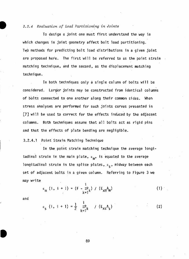
3.2.4 Evaluation of Load Partitioning in Joints
To design a joint one must first understand the way in
which changes in joint geometry affect bolt load partitioning.
Two methods for predicting bolt load distributions in a given joint
are proposed here. The first will be referred to as the point strain
matching technique, and the second, as the displacement matching
technique.
In both techniques only a single column of bolts will be
considered. Larger joints may be constructed from identical columns
of bolts connected to one another along their common sides. When
stress analyses are performed for such joints curves presented in
[7] will be used to correct for the effects induced by the adjacent
columns. Both techniques assume that all bolts act as rigid pins
and that the effects of plate bending are negligible.
3.2.4.1 Point Strain Matching Technique
In the point strain matching technique the average longi-
tudinal strain in the main plate, em, is equated to the average
longitudinal strain in the splice plates, ES, midway between each
set of adjacent bolts in a given column. Referring to Figure 3 we
may write
and
e, (i, i + 1) =i sPk / (E A ) (2)s i k=1k xs s
89
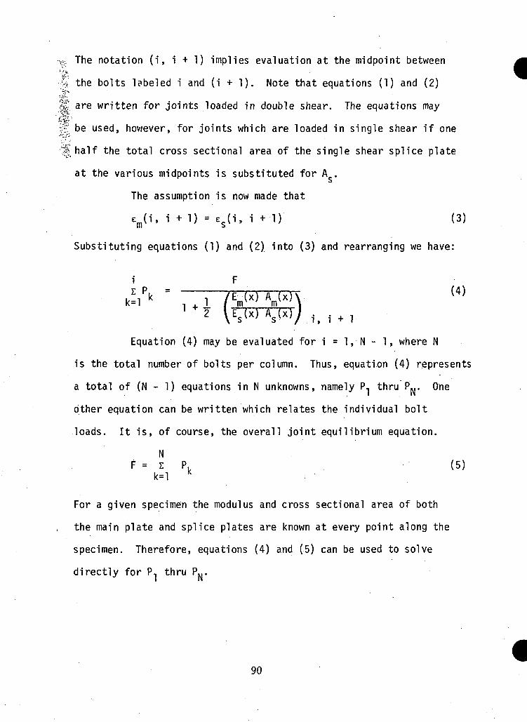
•v. The notation (i, i + 1) implies evaluation at the midpoint between
4 the bolts labeled i and (i + 1). Note that equations (1) and (2)• .iv,
H. are written for joints loaded in double shear. The equations may: -f4T3i
•££'s'f. be used, hov/ever, for joints which are loaded in single shear if one
-|| half the total cross sectional area of the single shear splice plate
at the various midpoints is substituted for A .
The assumption is now made that
em(1, i + 1) = es(i, i +1) (3)
Substituting equations (1) and (2) into (3) and rearranging we have:
£ ' i.
k=lK IAS(X i, i
Equation (4) may be evaluated for i = 1, N - 1, where N
is the total number of bolts per column. Thus, equation (4) represents
a total of (N - 1) equations in N unknowns, namely P, thru P.,. One
other equation can be written which relates the individual bolt
loads. It is, of course, the overall joint equilibrium equation.
NF = Z P. (5)
k=l K
For a given specimen the modulus and cross sectional area of both
the main plate and splice plates are known at every point along the
specimen. Therefore, equations (4) and (5) can be used to solve
directly for P, thru P...
90
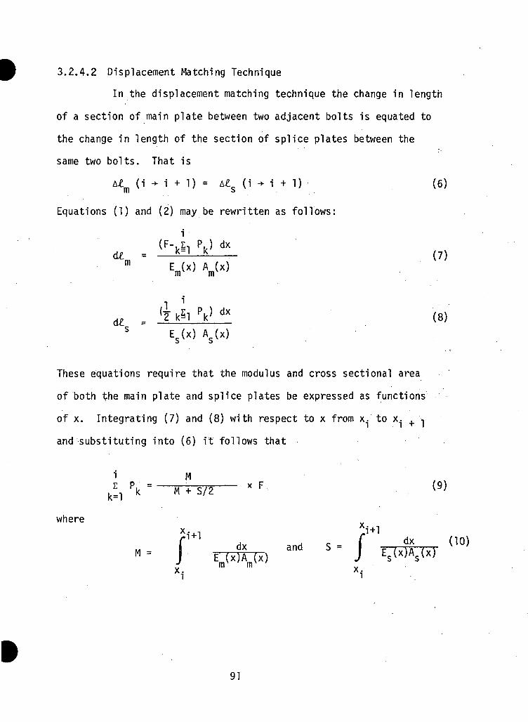
3.2.4.2 Displacement Matching Technique
In the displacement matching technique the change in length
of a section of main plate between two adjacent bolts is equated to
the change in length of the section of splice plates between the
same two bolts. That is
A£m (i ->• i + 1) = A£s (i -*- i + 1) (6)
Equations (1) and (2) may be rewritten as follows:
i(F-I,£I PJ dx
d£ = ^—* (7)m r /., \ ft /., \
dX (8)
Es(x) As(x)
These equations require that the modulus and cross sectional area
of both the main plate and splice plates be expressed as functions
of x. Integrating (7) and (8) with respect to x from x. to x. + -,
and substituting into (6) it follows that
X Fk— FT172
where
M =
X
and S .=m in i
/
91
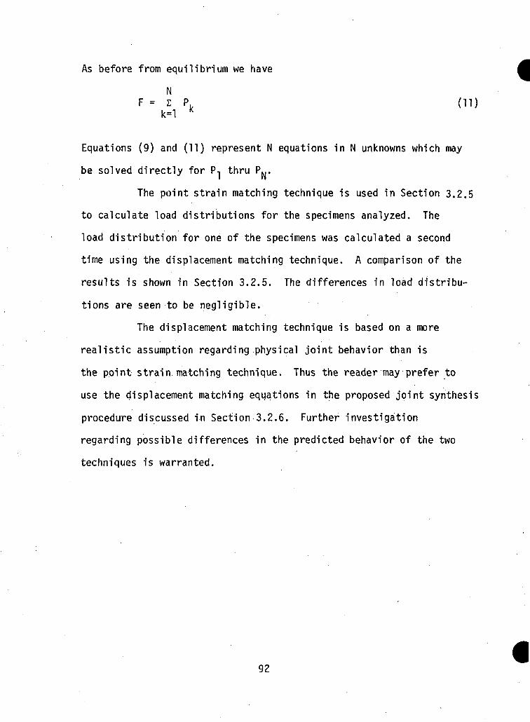
As before from equilibrium we have
NF = z P (11)
k=l k
Equations (9) and (11) represent N equations in N unknowns which may
be solved directly for P-| thru P^.
The point strain matching technique is used in Section 3.2.5
to calculate load distributions for the specimens analyzed. The
load distribution for one of the specimens was calculated a second
time using the displacement matching technique. A comparison of the
results is shown in Section 3.2.5. The differences in load distribu-
tions are seen to be negligible.
The displacement matching technique is based on a more
realistic assumption regarding physical joint behavior than is
the point strain matching technique. Thus the reader may prefer to
use the displacement matching equations in the proposed joint synthesis
procedure discussed in Section 3.2.6. Further investigation
regarding possible differences in the predicted behavior of the two
techniques is warranted.
92
3.2.5 Computer Analysis of Experimentally Failed Composite Joints
The purpose of the analysis phase was to establish a pro-
posed joint failure criterion which could be automated and included
in the final optimization program. The proposed criterion should
be able to predict both joint failure location and failure mode. It
should also be conservative in predicting failure loads and as simple
operationally as possible.
Six joints designed and tested at General Dynamics were
selected from [5] and [6] and were analyzed via finite elements.
Table 3 describes these various joints in detail.
Analyzing a complete joint in a single finite element run
with any degree of accuracy was impossible due to computer storage
limitations. It was, in fact, only possible to analyze one hole
at a time to achieve suitable accuracy.
Thus, the following analysis procedure was used. Each of
the joints analyzed consisted of a number of identical columns of
bolts as illustrated in Figure 4a. It was assumed that each column
could be analyzed separately and that each carried an equal share
of the total joint load which was present at failure. The joint
geometries of six specimens selected for investigation were such
that if the joints were made of an isotropic material the effects
of adjacent columns of bolts would be negligible [7]. The equations
from [1] indicate that the stress concentration factors which result
93
in anisotropic tension coupons are always greater than the stress con-
centration factors which result in geometrically similar isotropic
tension coupons. It is reasonable to assume that the same holds
true for bolt bearing specimens. Thus the assumption was made that
the effects of adjacent columns of bolts were negligible in the
actual composite joints since for the same applied loads a greater
stress concentration factor implies a more rapid stress field decay.
To determine the effects of adjacent columns of bolts
on the column of interest in the synthesis routine the graphical
results from [7] will be used due to a lack of similar information
for composite materials. Thus, conservative designs with respect to
specimen width will result. Excessive conservatism implies a wasting
of material and unwanted weight. Thus the degree of conservatism
which results from using the correction factors from [7] will be
investigated in the future.
The point strain matching technique was used to determine
the bolt load distribution for each of the six joints. The resulting
distributions are shown in Figure 5. The displacement matching
technique was only applied to one specimen, specimen 6, for reasons
of comparison with the point strain matching technique. The displace-
ment matching results are included in Figure 5 and are denoted by the
dashed lines. The differences between the two sets of results are
seen to be negligible.
94
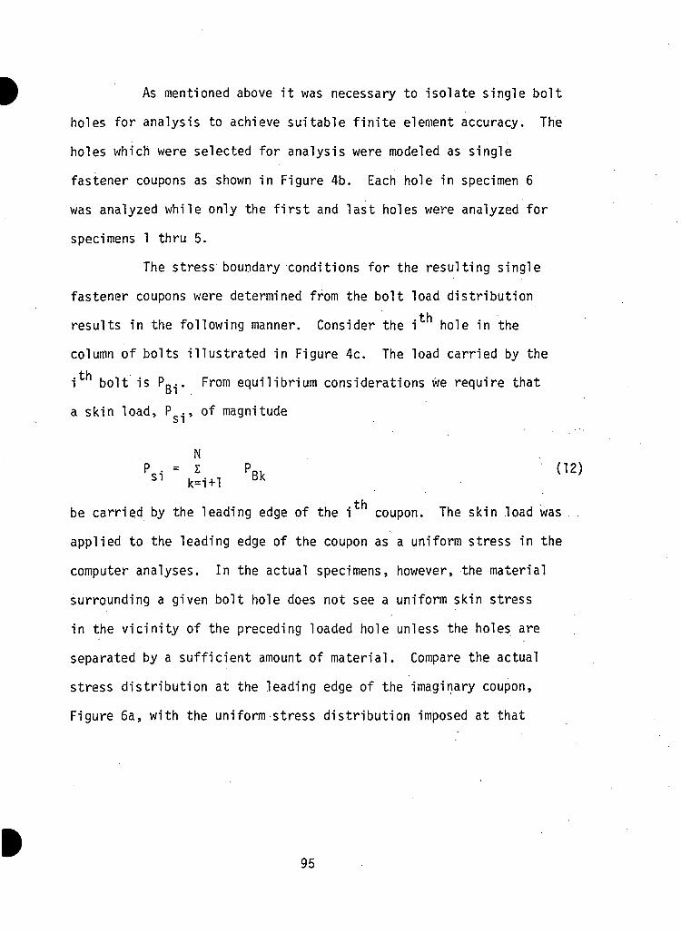
As mentioned above it was necessary to isolate single bolt
holes for analysis to achieve suitable finite element accuracy. The
holes which were selected for analysis were modeled as single
fastener coupons as shown in Figure 4b. Each hole in specimen 6
was analyzed while only the first and last holes were analyzed for
specimens 1 thru 5.
The stress boundary conditions for the resulting single
fastener coupons were determined from the bolt load distribution
results in the following manner. Consider the i hole in the
column of bolts illustrated in Figure 4c. The load carried by the
i bolt is Pg.. From equilibrium considerations we require that
a skin load, P ., of magnitude
P., = z PBk (12)SI k=i+1 Bk
a. L
be carried by the leading edge of the i coupon. The skin load was .
applied to the leading edge of the coupon as a uniform stress in the
computer analyses. In the actual specimens, however, the material
surrounding a given bolt hole does not see a uniform skin stress
in the vicinity of the preceding loaded hole unless the holes are
separated by a sufficient amount of material. Compare the actual
stress distribution at the leading edge of the imaginary coupon,
Figure 6a, with the uniform stress distribution imposed at that
95
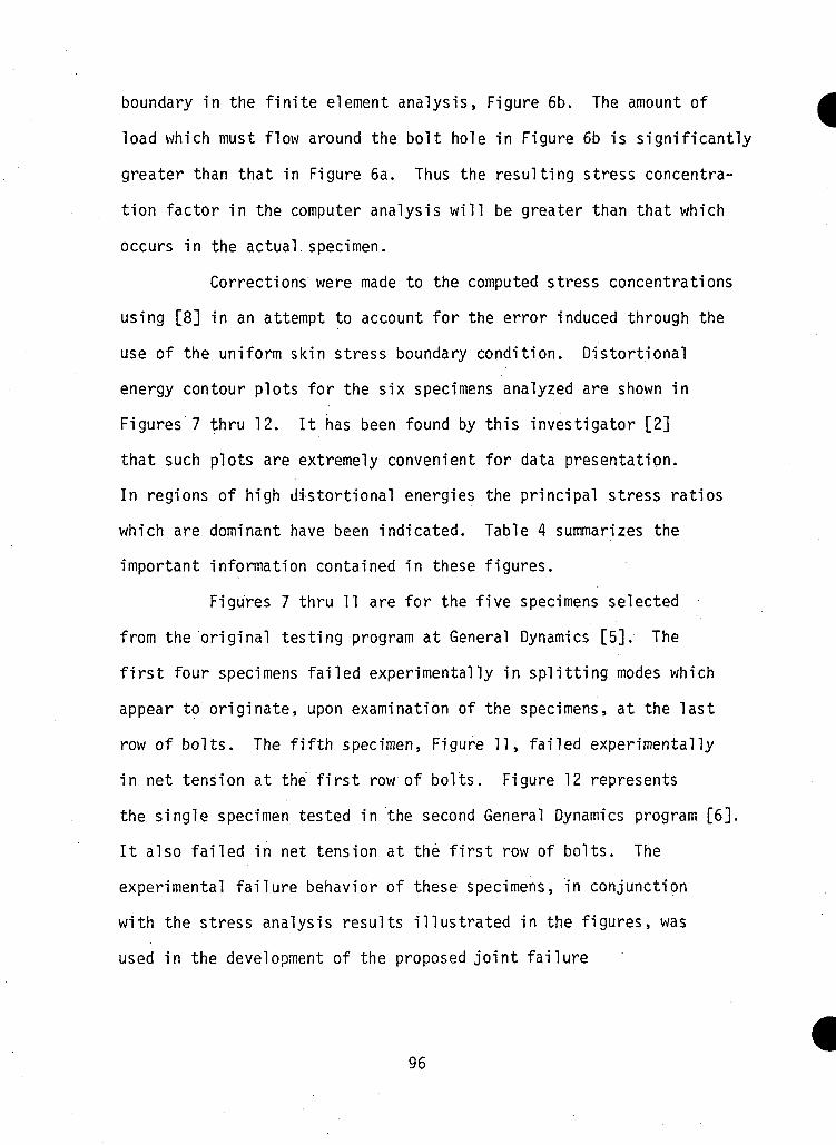
boundary in the finite element analysis, Figure 6b. The amount of
load which must flow around the bolt hole in Figure 6b is significantly
greater than that in Figure 6a. Thus the resulting stress concentra-
tion factor in the computer analysis will be greater than that which
occurs in the actual specimen.
Corrections were made to the computed stress concentrations
using [8] in an attempt to account for the error induced through the
use of the uniform skin stress boundary condition. Distortional
energy contour plots for the six specimens analyzed are shown in
Figures 7 thru 12. It has been found by this investigator [2]
that such plots are extremely convenient for data presentation.
In regions of high distortional energies the principal stress ratios
which are dominant have been indicated. Table 4 summarizes the
important information contained in these figures.
Figures 7 thru 11 are for the five specimens selected
from the original testing program at General Dynamics [5]. The
first four specimens failed experimentally in splitting modes which
appear to originate, upon examination of the specimens, at the last
row of bolts. The fifth specimen, Figure 11, failed experimentally
in net tension at the first row of bolts. Figure 12 represents
the single specimen tested in the second General Dynamics program [6].
It also failed in net tension at the first row of bolts. The
experimental failure behavior of these specimens, in conjunction
with the stress analysis results illustrated in the figures, was
used in the development of the proposed joint failure
96
criterion. . A description of how the criterion evolved is presented
below. - ,- .. - .
Consider for the moment Figures 7 thru 10. The stress
patterns are identical; the values only differ slightly. The dis-
cussion which follows for Figure 7 is also valid for Figures 8 thru -10.
A region of very high distortional energies occurs in the 0° laminae
directly, ahead of the last row of bolts in the specimen. The a2/a2 t
stress ratios are dominant in the region, which implies local matrix
failure (splitting). The maximum value of ol/al in the region is
0.49. Results from [2] indicate that once the 0° laminae split
(i.e., a2/cr2 t > 1.0) a value of QI/VI z 0.65 is necessary to cause .
a bearing failure to occur. Thus, even though the 0° laminae have
split, Figure 7, the values of aj/oj are not large enough to cause
a bearing failure to occur.
It has been assumed here that matrix failure does not
significantly degrade the laminate since the percentage of hoop load
carried by the 0° laminae directly ahead of the bolt was small. How-
ever, in specimens where a large percentage of the hoop load is carried
by the. matrix prior to fai.lure a similar assumption is not possible.
Consider a specimen consisting of almost all 0° laminae and only a
few ±45° laminae. Matrix failures in the 0° laminae would result in
significant load transfer from the 0° laminae to the ±45° laminae.
Even if laminate failure did not occur as a result of the load transfer
the laminate would be significantly damaged. It .is apparent, therefore,
97
that a successive failure analysis must be included in the final design
procedure to account for such load redistribution.
High distortional energies also result in the 0° laminae
at 0 = 90°, Figure 7, at both the first and last row of bolts due to
large values of a^/ai t in these regions. The maximum distortional
energy value at the last row of bolts, 2.0, is greater than the maximum
value at the first row, 1.5. The same is true of the maximum values
of tfi/oiut in these two regions. If the 0° laminae were to fail, the
±45° laminae would not be able to carry the additional load transferred
to them from the 0° laminae; as a result, laminate failure would occur.
Thus a net tension failure at the last row of bolts is the most probable
failure mode indicated from the results so far.
The assumption that matrix failure does not significantly
degrade the laminate is valid throughout specimen 1. The regions of
high distortional energies1which result from large o2/a2 . ratios are
therefore eliminated from consideration. The only remaining region
of interest is the one in the +45° laminae which occurs at the last
row of bolts where the fibers are tangent to the hole. Both the
maximum distortional energy value and maximum oj/oj . value in this
region are greater than the corresponding values which indicated a
net tension failure at the same hole. Once the +45° fibers break
in tension the remainder of the laminate cannot carry the existing
load and laminate of failure also occurs. Thus a splitting mode
is favored over the net tension mode previously indicated for
98
specimen 1. Since all the possible regions of failure initiation have
been examined a splitting mode is predicted by the analysis. The
actual specimen did indeed fail in a splitting mode. The predicted
failure load is conservative. If Pp is the actual experimental
failure load for specimen 1 the distortional energy failure criterion
predicts failure to occur at Pp//2.5 or 0.64 Pp. The maximum stress
failure criterion predicts failure to occur at Pp/1.5 or 0.67 Pp.
Analyses of specimens 2 thru 4 yield very similar results.
Following the same procedure it can be deduced that a
bearing failure does not occur in specimen 5, Figure 11. Both the
distortional energy and maximum stress failure criteria conservatively
predict a net tension failure to occur at the first row of bolts,
which again agrees with the experimental failure mode.
Predicting failure for specimen 6 is slightly more compli-
cated. The finite element results, Figure 12, indicate that oj/aju
reaches 0.65 at the last row of bolts in the 0° laminae prior to
matrix failure, o2/a2ut =1.0. A bearing failure is predicted to
occur in such a case at that load where either a2/a2ut reaches 1.0
or o\/a\ reaches 1.0, whichever occurs first. The assumption
is made at bearing failure initiation that the bolt causing the
bearing failure to occur is unable to carry any additional load during
subsequent specimen loading. The additional applied load is dis-
tributed among the remaining bolts in the column in proportion to
99
the loads which they carried at bearing failure initiation. Figure
12 is the finite element representation of the state of stress
present in specimen 6 when the experimental failure load was applied.
Notice that o2/a2 t = 1.0 and a\/ol = 0.80 in the 0° laminaeU.u UC
directly ahead of the last row of bolts. The material ahead of
the last row of bolts has failed in bearing and load redistribution,
as described above, has taken place. A load distribution plot for
specimen 6 is illustrated in Figure 12. Note that the revised load
distribution plot is much more uniform than that of Figure 5(f).
Observe that regions of high distortional energies do not
occur in the vicinity 0 = +45° at any of the bolt holes except at
the last row of bolts in the -45° laminae. Matrix failure is on
the verge of occurring here. Net tension failures, however, are
indicated at various locations along the specimen which would occur
prior to matrix failure in the -45° laminae. A splitting mode is,
therefore, definitely not indicated by the distortional energy plots.
Regions of high distortional energies in the 0° laminae
at 0 = 90° are present at the first and third through sixth rows
of bolts. The maximum distortional energy value, 1.2, occurs at
the fifth row. The largest value of 01/01 . in these four regions
of interest is 1.03, which also occurs at the fifth row. Thus,
both the distortional energy and maximum stress failure criteria
predict a net tension failure to occur in specimen 6 at the fifth
100
row of bolts at 0.97 Pp, where Pp is the actual experimental failure
load for the specimen. The predicted failure load is again conserva-
tive but only by about 3% as opposed to about 35% for specimens 1
thru 5. The predicted failure mode was again correct but the location
was not.
The analysis of specimen 6 shows that the design was a
good one, in that each hole was close to failure when the joint
failed experimentally. Notice also that the various bolts were
fairly equally loaded when joint failure occurred. Some designers
feel that such a bolt load distribution is necessary if a joint
is to carry load efficiently. The validity of such a statement can
only be determined by further analytical and experimental investi-
gation.
Thus a joint failure criterion has been proposed which
has successfully satisfied the requirements imposed on it
at the beginning of Section 3.2.5. The criterion was able to predict
both failure location and failure mode in all but Specimen 6
where it incorrectly predicted failure location.
More importantly it was able to conservatively predict failure loads
for each specimen. It was found that the maximum stress failure
criterion agreed with the distortional energy failure criterion
to within just a few percent in predicting failure loads. It was also
found that failure was always initiated at locations around hole
101
surfaces where fibers were being broken in tension and were tangent
to the hole surface.
Therefore, to make the failure criterion as operationally
simple as possible we need only check for fiber failures where the
fibers run tangent to the hole surface. A successive failure
analysis must be performed at these locations to insure against
premature failures induced by matrix failures in other laminae.
The successive failure analysis should also be performed in regions
where fibers are perpendicular to the hole surface since matrix
failures in these laminae may also induce premature laminate
failures.
102
3.2.6 Proposed Meahanioatly Fastened Joint Design Program
The preceding sections explain the procedures one would
go through if a given joint were to be analyzed. A method is now
proposed by which a joint may be designed to meet certain design
constraints while attempting to minimize total joint weight.
An outline of the proposed mechanically fastened joint
synthesis program is presented below to give a general understanding of
the procedures involved in arriving at an optimum joint design with
respect to total joint weight. The various procedures are then
discussed in detail.
3.2.6.1 Outline of Proposed Synthesis Program
(A) Specify the known input data.
(B) Determine the design variables and their range of allowable values.
(C) Specify the necessary design constraint equations which will
insure that joint failure does not occur until the design
ultimate load is reached. The design ultimate load will be
included as part of the input data.
(D) Specify an initial design.
(E) Calculate the various bolt loads for the current proposed geometry
using the bolt load partitioning results, Section 3.2.4.
(F) Perform a stress analysis of the proposed design to determine the
average laminate stresses at various critical points along each of
the circular boundaries. A closed form solution to the problem
103
illustrated in Figure 13a, based on the theory presented in [9],
will be used to perform the required stress analyses. Corrections
will be made to account for the effects of finite specimen size
from [10].
(G) Transform these average laminate stresses to lamina stresses.
(H) Determine whether any of the lamina stresses exceed the design
constraints imposed in (C).
(I) Assign penalty functions to the weight function for each design
constraint which is not satisfied and calculate the total weight
for the proposed joint design.
(J) Select a new design by moving in design space along a path
which tends to decrease the total weight function.
(K) Repeat (E) thru (J) until a suitable optimum design is achieved.
(L) If desired, a detailed stress analysis may be performed for the
proposed optimum design using finite elements, Section 3.2.5. A
final check may be necessary since the stress analyses performed
in (F) are based on isotropic correction factors.
3.2.6.2 Discussion of Program Details
3.2.6.2.1 Input Data
The following information will be read into computer program
as input data. It may be desirable in later work to include one or
more of these parameters as program variables. The diameters of the4
bolts used in a given joint will all be the same, _D . The actual size
Underlined symbols and phrases denote input information.
104
will be dictated by joint application as well as by standard size
limitations. Given an effective shear allowable for the bolt material,- E"SU
D
FQM , and the maximum load to be carried by the joint per column of
fasteners, £, one may determine a safe number of bolts, N^, to be used
in a given column since it appears from the analysis of specimen 6
that a fairly uniform load distribution is desirable.
Selection of the splice plate material will be application
dependent. The material will probably be either a high strengthS S Ssteel or titanium. In either case the values of FTI, , FCII, and FDDIIIU oil DKU
must be input so that constraint relationships may be later defined
to insure against splice plate failures in net tension, shear-out
and bearing respectively. In the load partitioning calculations
the splice plate modulus, E<-, is also required.
Similarly a decision must be made as to whether boron/epoxy
or graphite/epoxy will be used as the main plate material. The
material properties and ultimate allowables must be input for the
material system selected.
The leading edge distance of the main plate must be de-
fined since values of F<... are not tabulated for composite laminates.
Such information would be very valuable to the current effort since
excessively large edge distances result in low joint efficiencies.
A value of E/D = 4.0 will be used for the leading edge of the
composite main plate. A value of E/D may be calculated for the
105
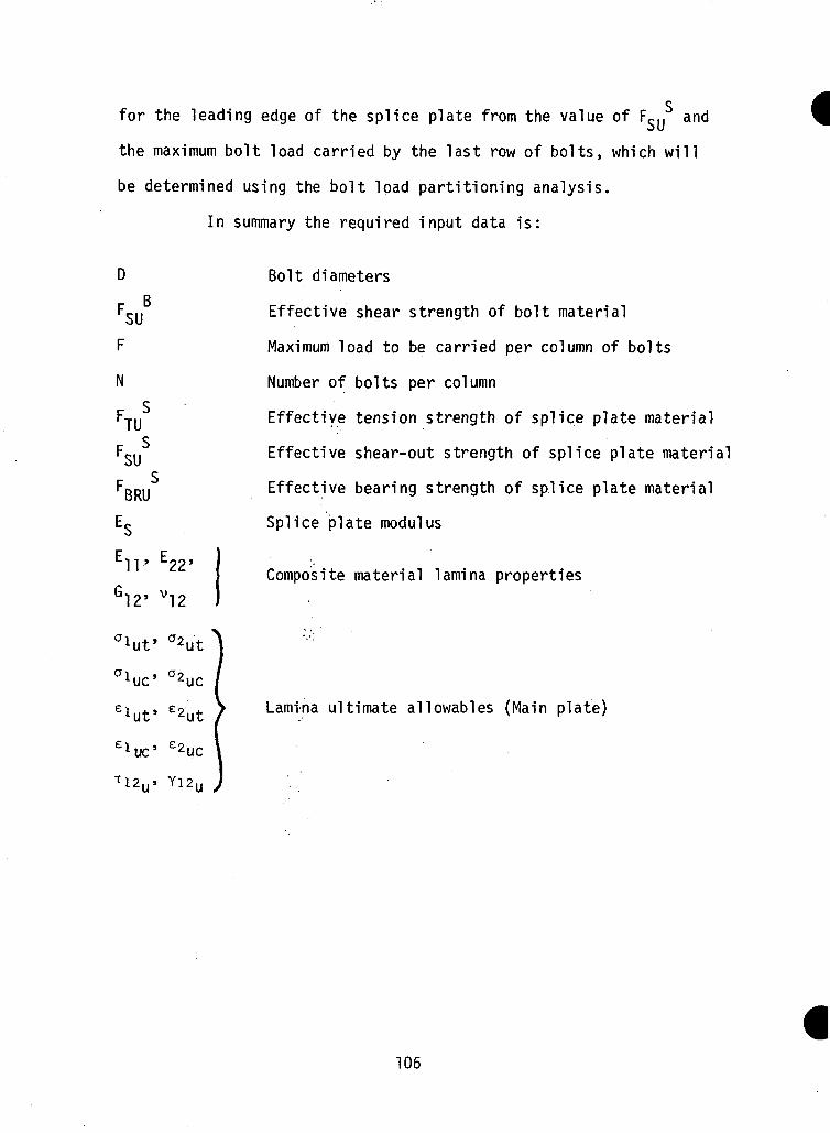
for the leading edge of the splice plate from the value of FSU and
the maximum bolt load carried by the last row of bolts, which will
be determined using the bolt load partitioning analysis.
In summary the required input data is:
D
F;
F
N
SU
TU- SSU
t,"BRU*
E1T E22'
G12' V12
lut' °2utLuc' °2uc
lut' £2ut
LUC' £2uc
L2U. Y12U
Bolt diameters
Effective shear strength of bolt material
Maximum load to be carried per column of bolts
Number of bolts per column
Effective tension strength of splice plate material
Effective shear-out strength of splice plate material
Effective bearing strength of splice plate material
Splice plate modulus
Composite material lamina properties
Lamina ultimate allowables (Main plate)
106
3.2.6.2.2 Design Variables
In this section seventeen parameters are defined which
can be used in conjunction with the input data to completely define
a given joint. If restrictions are not imposed on the design once
the input data is determined, the seventeen parameters would represent
seventeen design variables. If restrictions are imposed the number
of design variables would be less than seventeen.
At the beginning of the program, just after the input data
is read in, flags will be used to indicate which of the seventeen
parameters are to be predefined. The values of these predefined
parameters will then be read in as additional input data. The remaining
parameters will represent the design variables.
In some cases the design variables have been restricted to
a certain range of allowable values. Optimization routines require
a well defined design space within which they may search for local
minima. Therefore, where limits have not been specified for design
variables it is up to the programmer to do so.
The program has been restricted to the (0/±a/±3/90) class
of laminates; a and 3 being design variables; The values of a and 6
are restricted to the range 15° to 75°. It may be desirable later
to restrict the possible values of a and 3 to integer values, but for
the present work integer optimization procedures will not be used.
It will also be required that at least one ply of each of the four
lamina orientations be present in each proposed design. In this
107
manner we are assured that fiber failures will accompany laminate
failure regardless of failure mode. A design where a and 3 are set
equal, (0/±a/90), is also acceptable since fiber failures still must
accompany all possible laminate failure modes. The total thicknesses
of the various lamina orientations are assumed to be, at most, linear
functions of x, the position along the joint. More complicated lay
up patterns will not be included in the present study.
Consider the joint design shown in Figure 14. The seventeen
possible design variables are indicated on the figure. As previously
mentioned the values of (E/D) and (E/D) will be specified by the
program. If a joint is being designed which will consist of a number
of identical columns of bolts the widths of the main plate and splice
plates must be equal and constant along their lengths. The designer
must input such information as described above.
In summary the seventeen possible design paramters are as
follows:
Parameters Description Range
a, 6 Lamina orientations 15° ->• 75°W (0), W (L) Width of splice plate at x=0, L 3D -»t (0), t^(L) Thickness of splice plate at x=0, L -»-WS(0), W:(L) Width of main plate at x=0, L 3D •>Lm Joint length [2(N-1)+4]Dtn(0), tn(L) Thickness of 0° laminae at x=0, L 1 plyW°)' ton(L) Thickness of 90° laminae at x=0, L 1 ply -*•V(0), %U(L) Thickness of ±a° laminae at x=0, L 1 ply -»•t7«(0), t:"(L) Thickness of ±3° laminae at x=0, L 1 ply +ip ip
108
The lower limits on the widths and length measurements are based on
a minimum separation of free surfaces of one diameter. These values
may be changed by the programmer if desired. The upper and lower
limits which have not been specified must be provided by the programmer.
3.2.6.2.3 Design Constraints
Once a design is proposed it must be loaded to design
ultimate. The joint failure criterion, Section 3.2.5, must then be
applied to determine whether or not the proposed design can indeed
carry the design ultimate load, as required. In order to automate
the process of examining the joint for possible failure at the i
critical location an equality constraint, F(i), must be defined.
For the in-house pattern search optimization routine, the equation
must be written in such a form that F(i) < 0 if failure is not indi-
cated. If failure is predicted to occur, then F(i) > 0. As previously
mentioned a penalty function is added to the weight function when
F(i) > 0. To minimize the total weight of the joint the design must
move in design space in a direction which tends to reduce the penalty
functions.
Consider the possible failures which could occur at each
hole along the joint.. They are:
(1) Bolt failure in shear.
(2) Splice plate failures in bearing, shear-out, or net tension.
(3) Main plate failures "in bearing, shear-out, net tension,
splitting, bending tear-out, or combination modes.
109
An inequality constraint equation must be written for each of the
possible failure initiation sites.
To test for bolt failure in shear we calculate the maximum
shear stress, TAU, acting on the bolt cross sectional area.
TAU = PB / (uR2) U3)
PB represents the bolt load acting at the hole of interest.
The magnitude of Pg is determined via the bolt load partitioning
analysis, Section 3.2.4.
To insure against a bolt failure in shear we require thatD
TAU z Fgy . Stating this in the form of a valid inequality constraint
we have:
- F B (14)
Similarly, to insure against splice plate failures at a
given hole in bearing, net tension or shear-out we have respectively:
F(2) = P B / Dt - FBRUS (15)
F(3) = (PB + Ps) / t(S - D) - FTUS (16)
F(4) = PB / 2tE - FSUS (17)
The skin load, PS, is calculated from equation (12). The values of
t, E, and S for a given bolt bearing model are determined as was shown
in Figure 4.
Now consider the possible composite main plate failures.
Once a stress analysis is performed, checks for possible failure
initiation must be made at four locations (possibly only three if
110
a equals 3) around each hole as discussed in Section 3.2.5. Bearing
failures may or may not be considered desirable. If they are, the
load redistribution procedures discussed in Section 3.2.5 can be built
into the computer logic. To simplify the following discussion assume
that bearing failures are undesirable.
Thus, if at 0 = 0°, a matrix failure occurs in the 0°
laminae (02/02 t * 1.0) a bearing failure would be predicted to
occur when QI/OI = 0.65. If matrix failures do not occur during
loading then ai/ai > 1.0 would be necessary for a bearing failureUC . -
to occur. Since the likelihood of a bearing failure is only dependent
on the stresses at 0 = 0° in the 0° laminae, an inequality constraint
equation may be written at that location of the form
ai/aiuc -1.0 if(18)
cr1/aluc - 0.65 if °2/%t > 1.-0
It was postulated in Section 3.2.5 that all failure modes,
except bearing, have one thing in common. They all seem to occur
at locations where fibers are tangent to a hole surface. In a
(0 /±a/±6/90) laminate fibers are tangent to the hole surface at
0 = 90°, (90 - a)°, (90 - 6)°, and 0° in the 0°, +a°, +3°, and 90°
laminae respectively. If, at ultimate load, matrix failures have
occurred at any of these hole locations load redistribution among the
111
various laminae must be considered. The stresses in the remaining
laminae would be recalculated. A check would then be made in the
laminae which are tangent to the hole surface to see whether or not
the fibers have failed in tension. The inequality constraint used
for this purpose is:
F(6) = ai/oiut - 1.0 (19)
Equation (19) must be applied four times per hole; to the 0° fibers
at 0 = 90°, the 90° fibers at 0 = 0°, the +«° fibers at 0 = (90 -a)°,
and the +0° fibers at 0 = (90 - 3)°. Thus, a total of nine inequality
constraints must be satisfied at each and every hole.
In the past, designers have designed for net tension failures
at the innermost row of bolts. An equality constraint of the form
oi/olut - 1 . 0 = 0 ' (20)
could be imposed on the stress field in the 0° laminae at the innermost
row of holes to force the design to fail there in net tension. Such a
restriction is not justified, however. When an optimum design is
arrived at using the nine inequality constraint equations per hole, one
of the nine equations will, in the process, be automatically forced
to zero. This will specify joint failure mode and location. Net
tension failures at the innermost row of bolts may not result when
minimum weight designs are required.
3.2.6.2.4 Design Procedures
In order to begin the design process an initial design
112
must be selected. The initial design must, of course, be in the
design space which is defined by the upper and lower limits placed
on the design variables.
If the designer has a design in mind he may use it to
activate the program. Otherwise, the program will specify an initial
design. The in-house pattern search routine uses a random number
generator for the purpose of specifying initial values for the design
variables. It may be desirable to use several random starting points,
if run times are not excessively long, to check for possible local
minimum in the design space.
Once an initial design is proposed the bolt load partitioning
results would be used to calculate the bolt load distribution for the
geometry and lamination selected. To perform such calculations the
main plate and splice plate cross sectional areas as well as the
main plate modulus must be defined as functions of x. Referring
back to Figure 14 it can be shown that
Am(x).= C(tm(L)-y0)) (x/L) + y°)] C(Wm(L)"Wm(0)) (x/L) + Wm(0)]
As(x) = [(ts(L)-ts(0)) (x/L) + ts(0)] [(Ws(L)-Ws(0)) (x/L) + Ws(0)] (22)
It has been found by this investigator that a quadratic polynomial in
x can be used to represent the modulus of the main plate to within
a few percent when linear variations in lamina thicknesses are employed.
113
Thus, the modulus of the main plate may be determined at several locations
along the joint using lamination theory and a second order curve of the
form
E (x) = Ax2 + Bx + C (23)
may be fit to the resulting modulus values. The values of A, B, and
C will be determined automatically by an internal curve fitting
subroutine for the proposed design.
The only remaining unknowns which are needed to calculate
the bolt load distribution are the coordinate locations of the N
bolts. Since L, the joint length, and (E/D) , the leading edge
distance of the composite main plate, are known, we may express
the N bolt locations as:
= |fj L- (f) where. I = 1, NX(I) = f L- where. I = 1, N (24)
The bolt loads could then be calculated using equations (4) and
(5) or equations (9) and (11).
The next step in the design procedure is to perform a row
by row stress analysis of the proposed design. The column of bolts
is broken down into individual bolt bearing specimens as shown in
Figure 4. The value of P . would be calculated using equation (12).
Thus, each bolt bearing model is acted on by a bolt load, Pg. and
a skin stress, a . = P ./St. Since a finite element solution ofj I o I * '
each bolt bearing specimen is too costly the following procedures will
be followed.
114
The problem of an infinite plate containing a circular cutout
which is loaded as shown in Figure 13a will be solved. This investigator's
solution [11] to the problem illustrated in Figure 13b will be added
to the solution of the problem illustrated in Figure 13c, which is
presented in [12]. Corrections to the stress concentration factors
induced at 0 = 90° and 0 = 0° will be made to account for the effects
of finite specimen size using the results presented in [13] and [14].
Corrections to the average laminate stresses along the circular boundary
from 0 = 0° to 0 = 90° can then be estimated.
The corrected average laminate stresses would be transformed
to lamina stresses and checks would then be made to see if the design
constraints discussed in Section 3.2.6.2.3 were satisfied. Penalty
functions would be assigned to the weight function for each of the
constraint equations which was not satisfied and the total joint
weight would then be calculated. The optimization procedure would
determine a preferred path and select a new design along that path
which would have a lower total joint weight while more closely
satisfying all the imposed design constraints.
The entire process, beginning with the calculation of bolt
loads for the new design would be repeated until the design constraints
were all satisfied and a local minimum weight were achieved.
Since the design procedure uses isotropic correction
factors to account for finite specimen size there is, of course, some
115

doubt concerning the actual failure behavior of the proposed optimum
design. Therefore, it may be desirable to perform a complete stress
analysis for the proposed optimum design to see how closely the
predicted failure behavior would agree with the desired failure
behavior. The analysis method described in Section 3.2.5 would be used
if the final check were to be made.
116
3.2.7 Areas of Future Work
Several important questions have been raised regarding the
solution technique thus far which deserve mention and in most cases
warrant further investigation. The first involves the basically
different failure mechanisms which can occur in a given joint made
of composite materials. Net tension failures appear to behave as
brittle failures once a very small but finite region of localized
laminate destruction occurs. Bearing failures and shear-out failures,
on the other hand, do not occur unless extensive laminate damage
has resulted during loading. Thus bearing and shear-out failures
behave in a relatively ductile manner. Additional analytical and
experimental work must be done to understand the various failure
mechanisms which occur in composite joints before truly optimum
designs can be achieved. The results of the proposed geometrically
similar bolt bearing specimen testing program should bring us
closer to such an understanding.
In metals, effective bearing strengths, FBRU» and effective
shear-out strengths, FSU, have been experimentally determined and
are used in the design process to specify such parameters as leading
edge distances. Similar information is generally not available for
composites due to the number of possible laminates which could be
used for design purposes. Such "material properties" would be
invaluable, however, in the design of composite joints and deserve
further investigation.
117
Similarly, a lack of data concerning the effects of finite
size on stress concentrations induced at circular cut-outs in composite
plates has forced us to predict these effects from available isotropic
data. Making corrections from isotropic data results in a conservative
design and is, therefore, partially satisfactory. The need for
correction factors could be eliminated, however, if the in-house two
dimensional am'sotropic integral equation program developed by Dr. T. A.
Cruse could be built into the optimization program in such a way as
to not result in excessive computer run times. One other technique
would be to derive the necessary correction factors for various
laminates using the integral equation program and use such data in
place of the isotropic correction factors which are now being used.
Both possibilities are presently being investigated.
The following questions will also be considered:
(1) Are uniform bolt load distributions and net tension failures at
the innermost row of bolts requirements for optimum joint designs?
(2) Is it advantageous to use the displacement matching technique
rather than the strain matching technique to predict bolt load
distributions?
(3) How should load redistribution in a joint be handled once a
bearing failure occurs either in the main plate or splice plates?
(4) Is the uncertainty regarding the cross term in the distortional
energy failure criterion, as discussed in [15], a major problem
to be considered? A preliminary investigation performed during
118

the contract period has shown that in certain cases the cross
term may be the most important term in the energy relationship.
These questions will be pursued as part of this investigator's doctoral
thesis during the current academic year.
119
3.2.8 References
[I] S. G. Lekhnitskii, Theory of Elasticity of an AnisotropicElastic Body, Holden-Day, Inc., 170 (1963).
[2] J. P. Waszczak, T. A. Cruse, "Failure Mode and StrengthPredictions of Anisotropic Bolt Bearing Specimens", Journalof Composite Materials, 421 (July 1971).
[3] M. E. Waddoups, J. R. Eisenmann, and B. E. Kaminski,"Macroscopic Fracture Mechanics of Advanced CompositeMaterials", Convair Aerospace Division of General Dynamics,FZM-5670, (February 1971).
[4] Advanced Composite Wing Structures, Boron-Epoxy Design Data-Volume II, Grummon Aerospace Corporation, 180-186, TR-AC-SM-ST-8085, (November 1969).
[5] Advanced Development of Boron Composite Wing StructuralComponents, Convair Aerospace Division of General Dynamics,AFML-TR-70-261, 66 (December 1970).
[6] R. H. Roberts, Personal communication, Convair AerospaceDivision of General Dynamics, Drawing Number FW7006048,(June 1971).
[7] R. E. Peterson, Stress Concentration Design Factors,John Wiley and Sons, Inc., 92 (1966).
[8] R. E. Peterson, Stress Concentration Design Factors,John Wiley and Sons, Inc., 91 & 94, (1966).
[9] S. G. Lekhnitskii, Theory of Elasticity of an AnisotropicElastic Body, Holden-Day, Inc., (1963).
[10] R. E. Peterson, Stress Concentration Design Factors,John Wiley and Sons, Inc., (1966).
[II] J. P. Waszczak, "Stress Analysis of a Loaded Circular Holein an Anisotropic Plate," Report SM-63, Department of MechanicalEngineering, Carnegie-Institute of Technology, Carnegie-MellonUniversity, Pittsburgh, Pennsylvania (May 1971).
[12] S. G. Lekhnitskii, Theory of Elasticity of an AnisotropicElastic Body, Holden-Day, Inc., 170 (1963).
120
[13] R. E. Peterson, Stress Concentration Design. Factors,John Wiley and Sons, Inc., 84 & 99 (1966).
[14] S. Timoshenko, J. N. Goodler, Theory of Elasticity,Second Edition, McGraw-Hill Book Company, 62 & 123 (1951)
[15] S. W. Tsai, E. M. Wu, "A General Theory of Strength forAnisotropic Materials", Journal of Composite Materials,58 (January 1971).
121
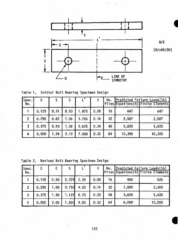
L±~ fcrLINE OFSYMMETRY
Table 1. Initial Bolt Bearing Specimen Design
B/E
Spec.No.
1
2
3
4
D
0.125
0.250
0.375
0.500
E
0.31
0.62
0.93
1.24
S
0.53
1.06
1.59
2.12
L'
1.875
3.750
5.625
7.500
t
0.08
0.16
0.24
0.32
No.Plies
16
32
48
64
Predicted Failure Loads (Ib)Equations(4)
647
2,587
5,820
10,350
Finite Elements
647
2,587
5,820
10*350
Table 2. Revised Bolt Bearing Specimen Design
Spec.No.
1
2
3
4
D
0.125
0.250
0.375
0.500
E
0.50
1.00
1.50
2.00
S
0.375
0.750
1.125
1.500
L'
2.25
4.50
6.75
9.00
t
0.08
0.16
0.24
0.32
No.Plies
16
32
48
64
Predicted Failure Loads(lb)Equations(4)
400
1,600
3,600
6,400
Finite Elements
625
2,500
5,620
10,000
122
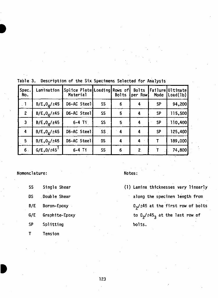
Table 3. Description of the Six Specimens Selected for Analysis
Spec.No.
1
2
3
4
5
6,
Lamination
B/E,04/*45
B/E,04/f45
B/E,04/f45
B/E,04/f45
B/E,02/f45
G/E,0/±451
Splice PlateMaterial
D6-AC Steel
D6-AC Steel
6-4 T1
D6-AC Steel
D6-AC Steel
6-4 T1
Loading
SS
SS
SS
SS
OS
SS
Rows ofBolts
6
5
5
4
4
6
Boltsper Row
4
4
4
4
4
2
FailureMode
SP
SP
SP
SP
T
T
UltimateLoad(lb)
94,200
115,500
110,400
125,400
189,000
74,800
Nomenclature:
SS Single Shear
DS Double Shear
B/E Boron-Epoxy
G/E Graphite-Epoxy
SP Splitting
T Tension
Notes:
(1) Lamina thicknesses vary linearly
along the specimen length from
02/f45 at the first row of bolts
to 02/±453 at the last row of
bolts.
123
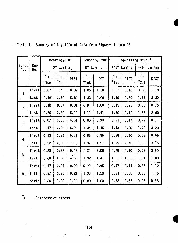
Table 4. Summary of Significant Data from Figures 7 thru 12
Spec.No.
1
2
3
4
5
6
RowNo.
First
Last
First
Last
First
Last
First
Last
First
Last
First
Fifth
Sixth
Bearing, 0=0°
0° Lamina
? °1
°luc
0.07
0.49
0.10
0.50 s
0.07
0.47
0.13
0.52
0.30
0.60
0.17
0.37
0.80
°2
°2ut
c*
2.50
0.04
2.30
0.05
2.50
0.29
2.80
0;56
2.00
0.04
0.26
1.00
DIST
0.02
5.80
0.01
5.10
0.01
6.00
0.11
7.95
0.42
4.00
0.03
0.21
1.90
Tension, 0=90°
0° Lamina
CT1alut
1.05
1.33
0.91
1.11
0.83
1.34
0.85
1.07
1.29
1.02
0.90
1.03
0.80
DIST
1.50
2.00
1.00
1.41
0.90
1.45
0.85
1.51
2.00
1.41
0.95
1.20
1.00
Splitting,0=+45°
+45° Lamina
alalut
0.21
1.50
0.42
1.30
0.63
1.43
' 0.58
1.55
0.79
1.15
0.57
0.63
0.63
DIST
0.10
2.50
0.25
2.10
0.47
2.50
0.40
2.70
0.90
1.65
0.44
0.60
0.65
-45° Lamina
°202ut
0.83
1.65
0.80
1.55
0.79
1.73
0.69
1.90
0.92
1.21
0.75
0.83
0.95
DIST
1.10
3.20
0.75
2.60
0.71
3.00
0.55
3.75
0.90
1.88
1.12
1.15
0.95
Compressive stress
124
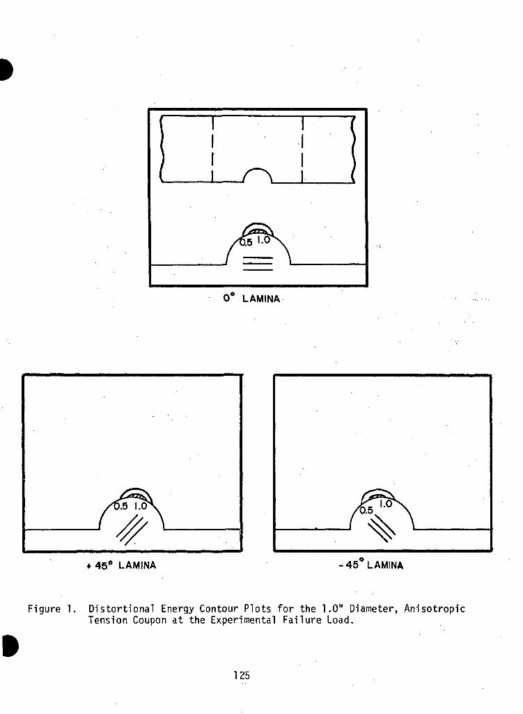
0° LAMINA
45° LAMINA -45 LAMINA
Figure 1. Distortional Energy Contour Plots for the 1.0" Diameter, AnisotropicTension Coupon at the Experimental Failure Load.
125
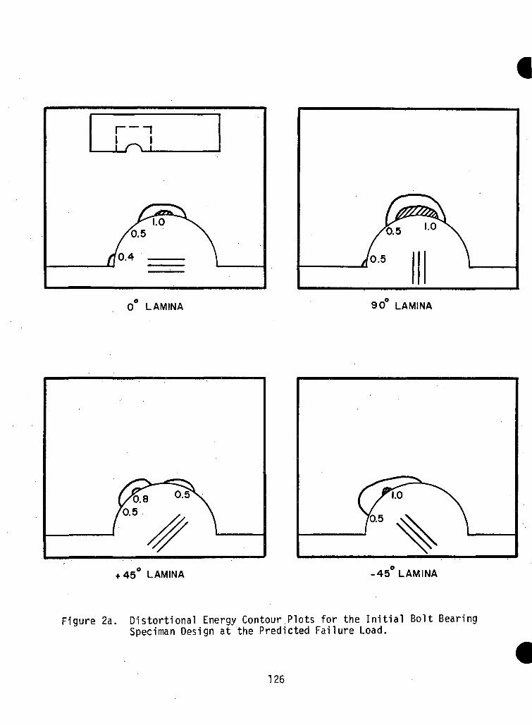
I 1
0 LAMINA 90 LAMINA
45 LAMINA -45 LAMINA
Figure 2a. Distortional Energy Contour Plots for the Initial Bolt BearingSpeciman Design at the Predicted Failure Load.
126
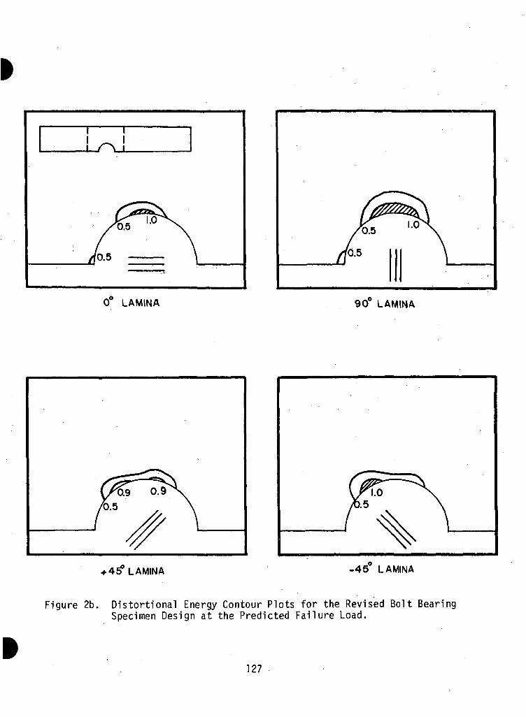
I I
0° LAMINA
/F III \90° LAMINA
• 45? LAMINA -45 LAMINA
Figure 2b. Distortional Energy Contour Plots for the Revised Bolt BearingSpecimen Design at the Predicted Failure Load.
127
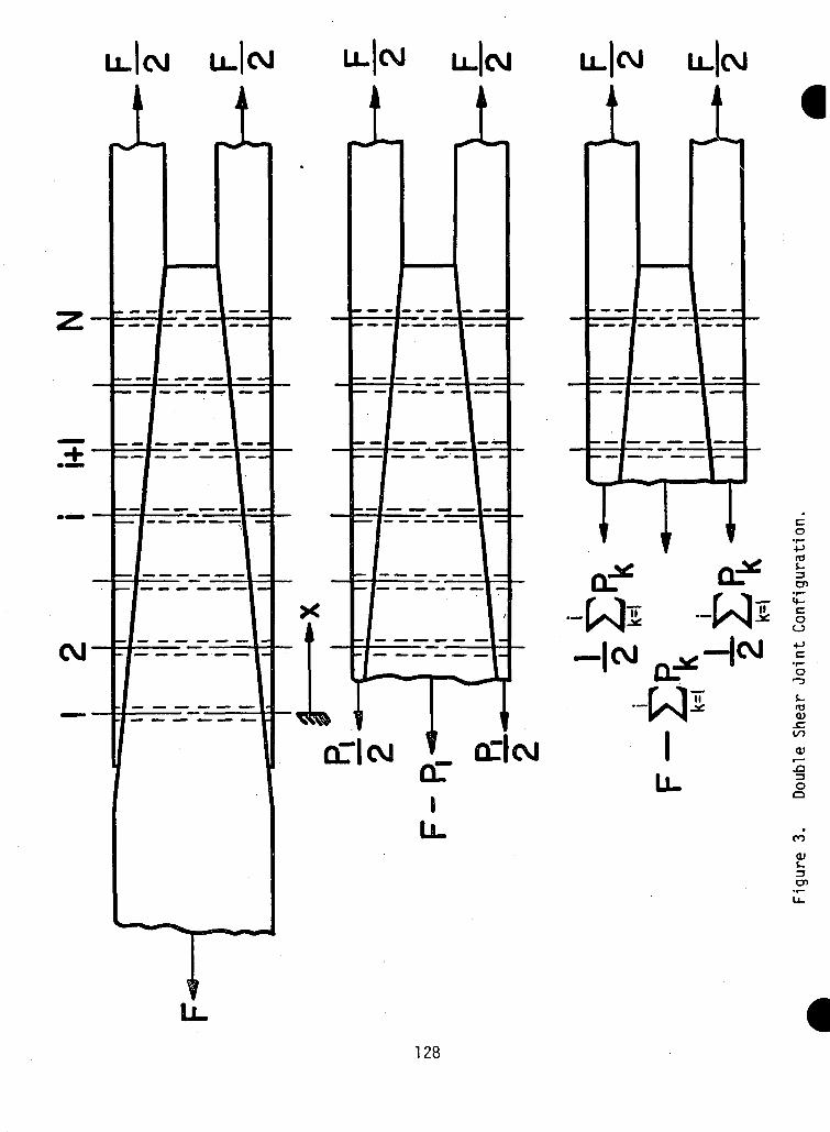
U C V I UJCVI U.CM li-CVl
-W:
I
u.
c.a•r*-M
1cn
O
O'-3J_<uO)
O)
.a3OQ
nO)i-3CD
128
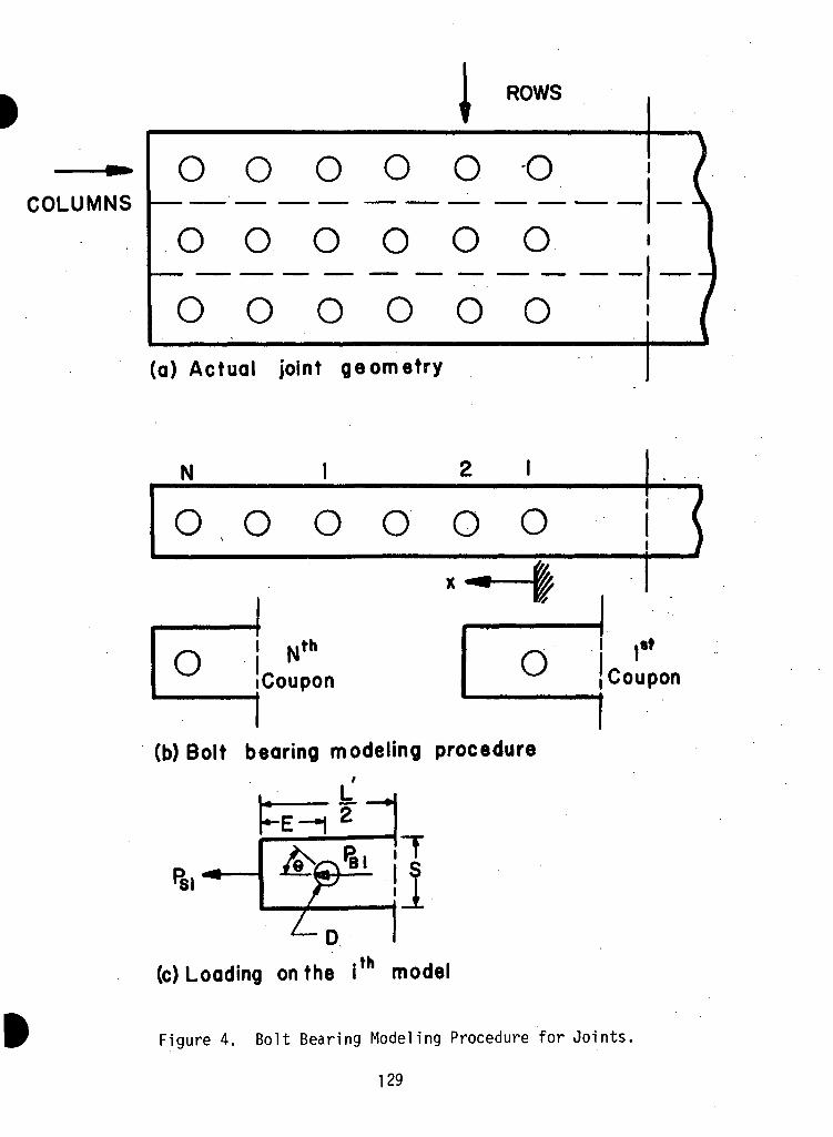
I ROWS
COLUMNSo o o o o oO O O O O O
O O O O O O
(a) Actual joint geometry
N I 2 1
O , O O O O O
O
X
Nth
Coupon
— 11'
Cou
j
t
pon
(b) Bolt bearing modeling procedure
PS.
k_H
44s
(c) Loading on the ith model
Figure 4. Bolt Bearing Modeling Procedure for Joints.
129
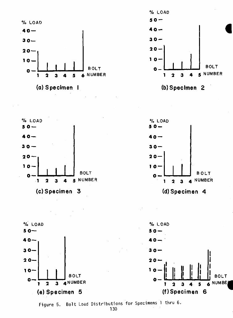
% LOAD
40 —
30-
20 —
10 —
0 — I I I I BOLT
1 2 3 4 5 6 NUMBER
(a) Specimen I
% LOAD
50-
40-
30-
20-
1 0 —
O- 1 1 BOLT
1 2 3 4 5 NUMBER
(b)Specimen 2
% LOAD
50 —
4O —
30 —
20 —
1 0-
0 —I I I BOLT
1 2 3 4 5 NUMBER
(c) Specimen 3
% LOAD50-
40-
30 —
20 —
1 0 —
0-BOLT
1 2 3 4 NUMBER
(d) Specimen 4
% LOAD
50—
40 —
30—
20—
10-BOLT
'l 2 3 4NUMBER
(e) Specimen 5
%50
4O
30
20
1 0
o
LOAD
—
— '
—_
-1' l> 1! ! I81 M ' ' !u 1! li i 1
111
BOLT
1 2 3 4 5 4
(f)Specimen 6
Figure 5. Bolt Load Distributions for Specimens 1 thru 6.130
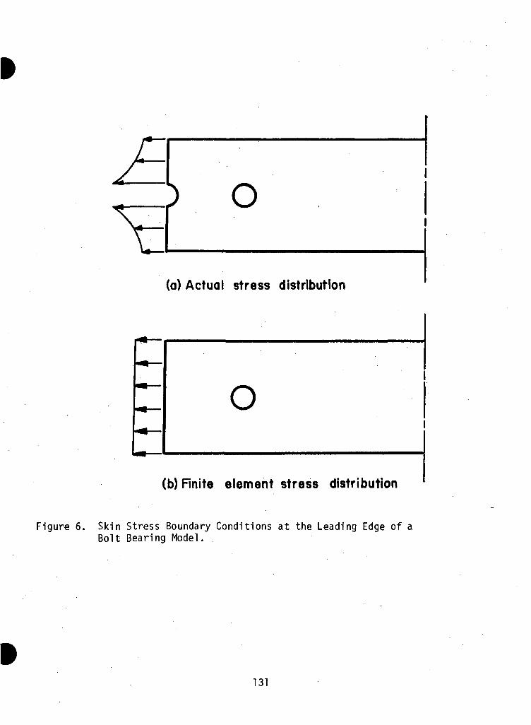
O
(a) Actual stress distribution
O
(b) Finite element stress distribution
Figure 6. Skin Stress Boundary Conditions at the Leading Edge of aBolt Bearing Model.
131
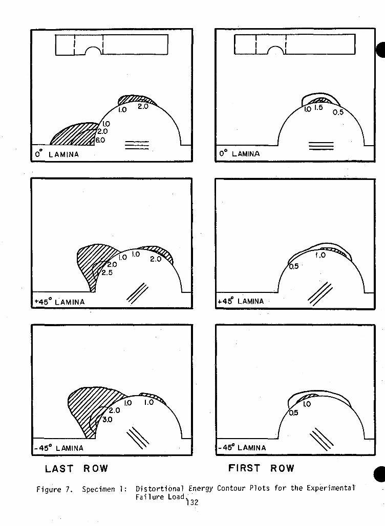
0 LAMINA
1 I
0° LAMINA
M5 LAMINA *45 LAMINA
-45° LAMINA
LAST ROW
-45° LAMINA
FIRST ROW
Figure 7. Specimen 1: Distortional Energy Contour Plots for the ExperimentalFailure Load.
I O £.
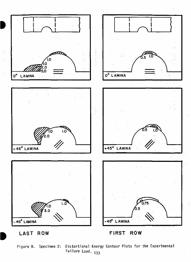
1 ~T
0 LAMINA
T T
0° LAMINA
1.0
+ 45° LAMINA +45° LAMINA
-45 LAMINA
LAST ROW
5
-45? LAMINA
FIRST ROW
Figure 8. Specimen 2: Distortional Energy Contour Plots for the ExperimentalFailure Load. -133
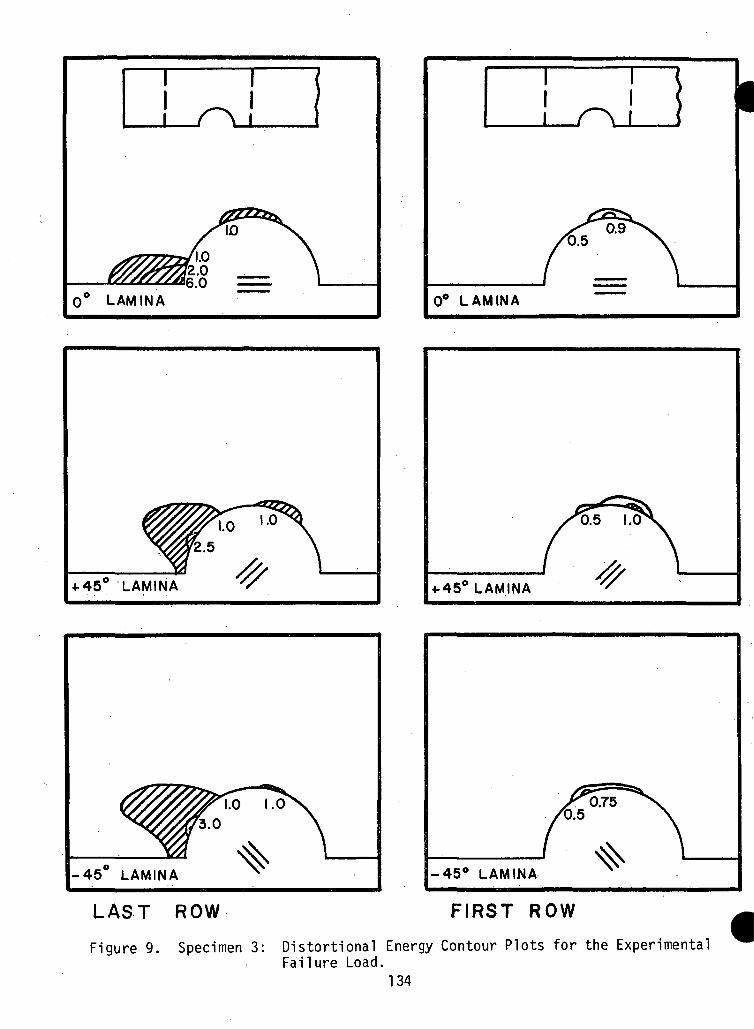
i r
0° LAMINA
1 T
0° LAMINA
4-45 LAMINA 4-45° LAMINA
-45 LAMINA
LAST ROW
-45° LAMINA
FIRST ROW
Figure 9. Specimen 3: Distort!onal Energy Contour Plots for the ExperimentalFailure Load.
134
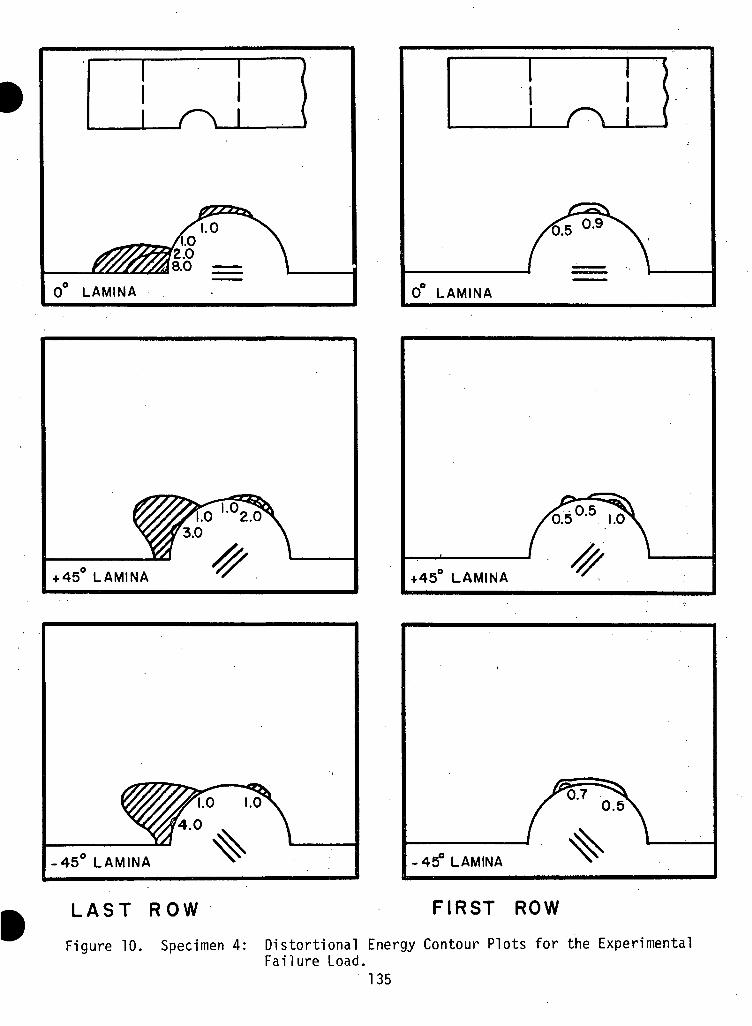
0 LAMINA
1 f
0 LAMINA
+ 45 LAMINA
'0.5 °'5
Y+ 45 LAMINA
-45 LAMINA
LAST R O W
-45° LAMINA
FIRST ROW
Figure 10. Specimen 4: Distortional Energy Contour Plots for the ExperimentalFailure Load.
135
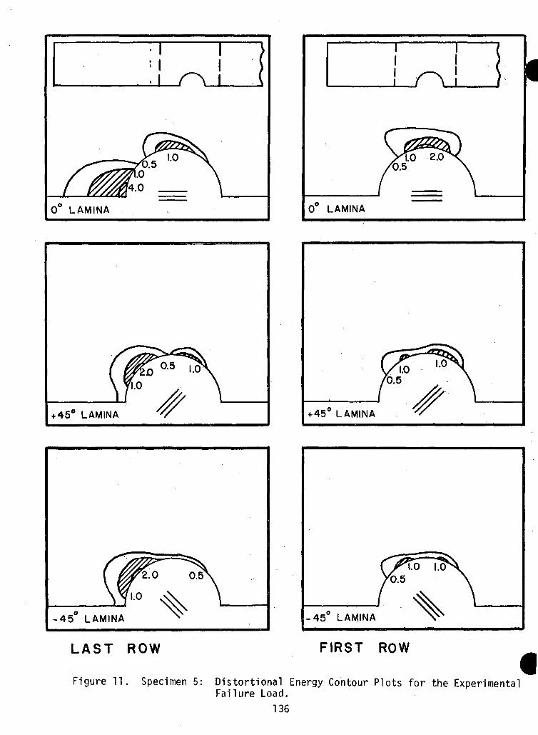
• i i I
0 LAMINA
T TI I1 rVj f VI
0 LAMINA
45° LAMINA *45 LAMINA
-45 LAMINA
LAST ROW
-45 LAMINA
FIRST ROW
Figure 11. Specimen 5: Distortional Energy Contour Plots for the ExperimentalFailure Load.
136
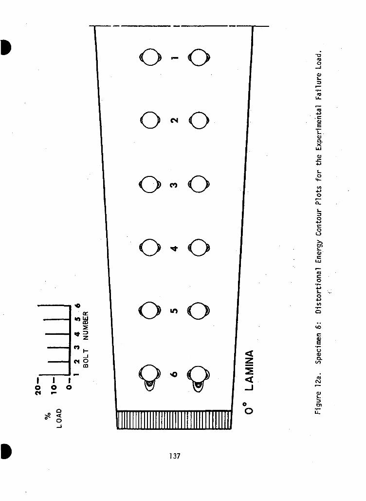
TJ<0O
O - O
O - O
O - O
3
<O
<a
s_<uQ.X
a>
to•MO
51
3O4->CO
IcuCUJ
O•l~•M
O
o
I I IO O OC1 •-
oO
a.oo
CSJ
§
137
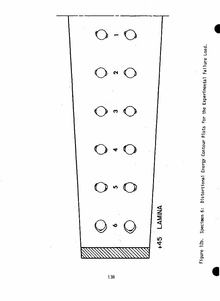
o •« o
-o<OO
QJ
tO4->C
CO
o - o
o - o
<UCLX
<u
s_o
to4-)O
=3O4JCOo
S-(Uc
roco
O-P
<
<
in
OCUQ.oo
cvj
cu
138
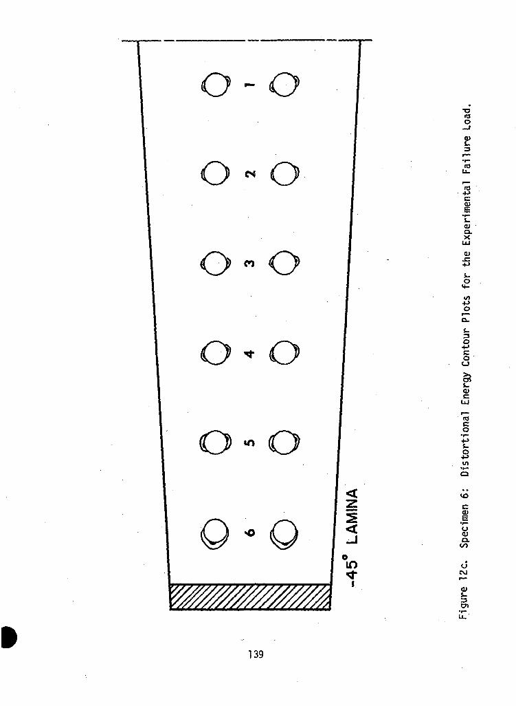
o - o
o«o ro
O n O0.XUJ
CD
<s>o
ex.$_
oCJ
(U
o o
5
s<-J
oLO
I
vo
O)
0)a.to
CO
a»
C7)
139
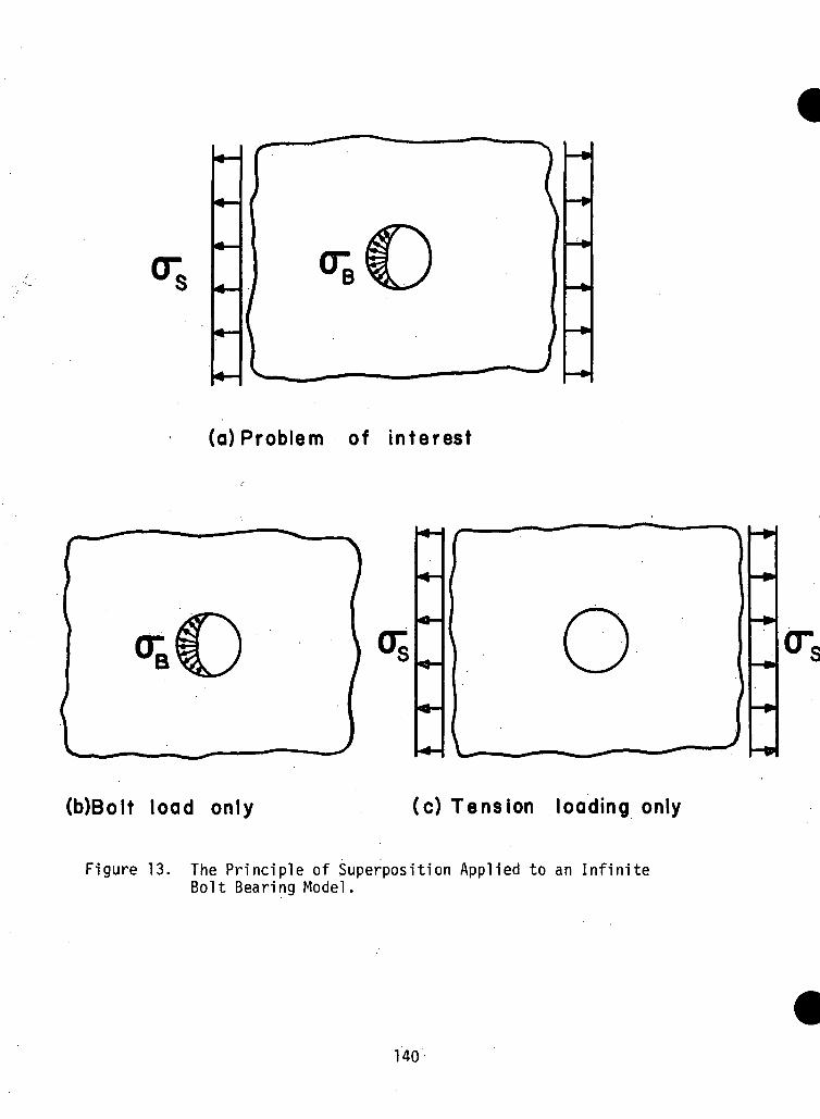
(a) Problem of interest
O
(b)Bolt load only (c) Tension loading only
Figure 13. The Principle of Superposition Applied to an InfiniteBolt Bearing Model.
140
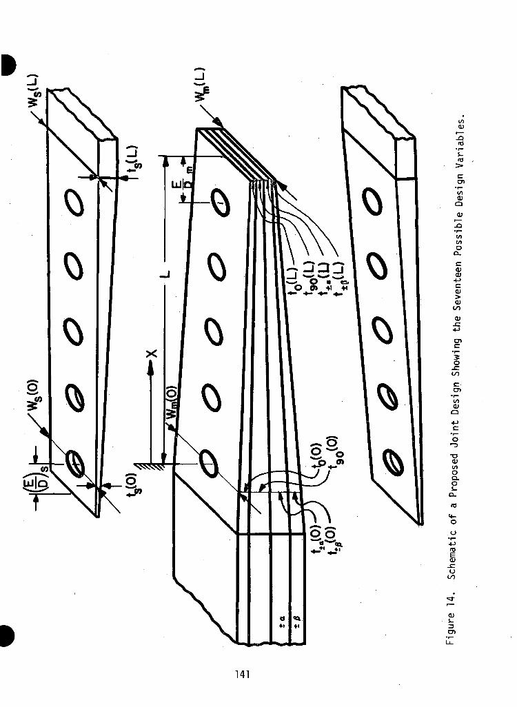
to<D
cCD
0)Q
O)
Oa.ca;ai
OJ
<DooO)
01
O
CO
c-C7)
OJQ
-MC
T3(Uv>Oa.oa.
oo
<J
3O)
141
CHAPTER IV
OPTIMIZATION METHODS
4.1 INTRODUCTION
A computer program for optimization using non-linear programming
by pattern search (OPTIM), written by Martin Schussel [1] was used for this
study. Some time was spent studying this program and a sample problem was
run (torsion of an elliptic bar). The time spent 1n finding the predicted
result of this problem yielded much insight into optimization techniques
and the OPTIM program itself.
The bolt-bearing problem was analyzed, using OPTIM, which included
variation of the ply orientations. This study involved a problem with six
variables and four constraints. For a given load, the minimum weightx • • ' • .
dimensions and orientations were found. The results of this study are
discussed 1n some detail.
4.2 STRUCTURAL OPTIMIZATION
4.2.1 Background
The structural optimization project consisted of finding the min-
imum weight design of a structure for which certain limitations were posed.
The limitations or constraints can be of the following form:
a) Geometric - Maximum overall dimensions of the structure
- Maximum thickness, cross-section, length, width,
etc. of an internal member
- Maximum deflection of a member
- Maximum rates of deflection
142
b) Mechanical - Yield criterion
- Failure modes
- Fatigue properties
- Natural frequencies
- Buckling loads
If the structure can be analytically solved for an internal
stress state as a function of the external loads (given) and the dimensions
of the piece (to be used as variables) then the problem becomes a mathe-
matical one: Find the extreme values of a non-linear function of several
variables, subject to one or several non-linear constraints. The function
is usually the weight of the structure and the variables are its dimensions.
The constraints can be in the form of equalities or inequalities. The
equality constraints would generally concern a total dimension which is not
fixed but is the sum of a number of internal dimensions. Inequality con-
straints are far more common, they usually insure that yield stresses,
buckling loads, etc. are not exceeded.
4.2.2 Vari-ational Method
There are several methods of mathematically solving the problem,
but non-linear programming is the only reliable one. Graphical methods
have a very limited use as they can only be used in two-dimensional
problems. Transformation into a series of linear problems by use of Taylor
series expansions is tedious and inaccurate. The use of penalty functions
transforms the problem into an unconstrained minimization. Lagrange
multipliers are an example; the formulation of the problem with Lagrange
multipliers is as follows:
Assume we want to minimize a weight function W(X.) where X.
(i = 1,...,N) are the variables. The constraints to be satisfied are
143
are MX.) = 0 (j = 1,.. .,M) . The Lagrange multipliers (xj are added and m
we form an unconstrained objective function (P) to be minimized.
P = WfXj) + Aj Fj (Xj)
Now setting the derivatives to zero will find the extreme:
|| = 0 1 = 1.....N
I?- = 0 j = 1.....M3Xj
The problem now requires the solution of N + M simultaneous non-
linear algebraic equations in N + M unknowns. Solutions are difficult to
find and are not unique, so this method is useless for large, complicated
problems.
4.2.3 Non-linear Programming Methods
By far the most useful methods for solving non-linear optimization
problems are searching techniques. There are many methods of search
mentioned in the literature (pattern search, directed search, Fibonacci
search, steepest ascent search), but basically they all consist of search-
ing the domain of the variables until no further improvement can be found
in the objective function.
Included 1n the Appendix of [2] are the listing and instructions
for a pattern search optimization program (OPTIM) by Martin Schussel,
CarnegleTMellon University 1968. The program works 1n the following way:
An objective function 1s defined:
P = COST + E A(K) ( F(K) )2
where COST = weight function
A(K) = penalty functions
F(K) = constraints
144
COST and F(K) which are functions of the variables ( X(I) ) are
defined by the user of the program in a subroutine called CALC.
The program increases and decreases the variables and recalculates
COST and F(K) until the improvement in the objective function is smaller
percentagewise than 10" .
The program is best suited to handle inequality constraints (less
than or equal) which it handles in the following way: If the constraint
becomes negative during the search it is neglected, but if it becomes
positive it is multiplied by a penalty (some large number A(K)). When the
objective function is minimized the constraints will either approach zero
or remain negative.
The application of optimization to design of structures using
advanced fiber composite materials adds another facet to the problem.
The orientations of the plies become variables as well as the dimensions.
In some cases, the problem can be handled similarly to the above procedure
with the orientations merely being additional variables. However, analyti-
cal equations for composite materials are difficult to derive and are
usually not solvable in closed form. The bolt bearing problem was solved
using empirical equations which relate the failure loads to the dimensions
of the piece and ply orientations.
4.3 TORSION OF AN ELLIPTIC BAR - VAPIATIONAL EXAMPLE
The problem is to find the values of the major and minor axes of
an elliptic bar for minimum weight for a given applied torsional moment
M. The weight is proportional to the cross sectional area
A = irab (1)
145
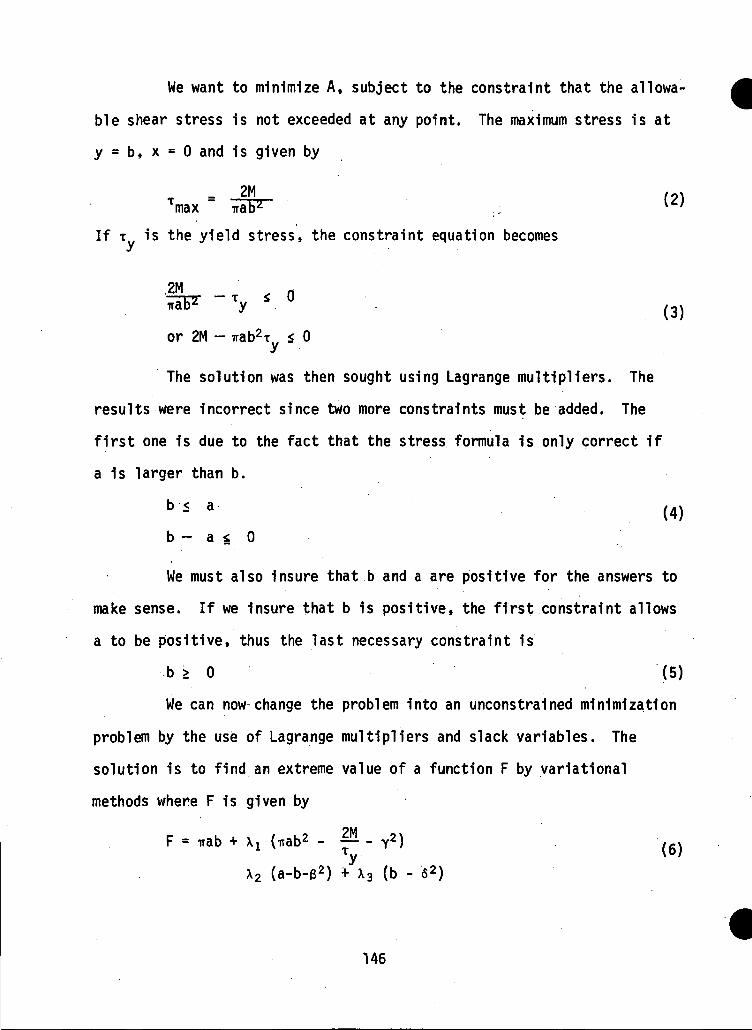
We want to minimize A, subject to the constraint that the allowa-
ble shear stress is not exceeded at any point. The maximum stress is at
y = b, x = 0 and is given by
T = 2M, (2)max irabz
If T is the yield stress, the constraint equation becomes
2M ' 0ira y (3j
or 2M - irab2t s 0
The solution was then sought using Lagrange multipliers. The
results were incorrect since two more constraints must be added. The
first one is due to the fact that the stress formula is only correct if
a is larger than b.
b-s a (4)
b - a < 0
We must also insure that b and a are positive for the answers to
make sense. If we Insure that b is positive, the first constraint allows
a to be positive, thus the last necessary constraint is
b ;> 0 (5)
We can now change the problem Into an unconstrained minimization
problem by the use of Lagrange multipliers and slack variables. The
solution is to find an extreme value of a function F by variational
methods where F is given by
F = -irab + Xi Uab2 - -
X2 (a-b-e2) * X3 (b - 5
2)
146
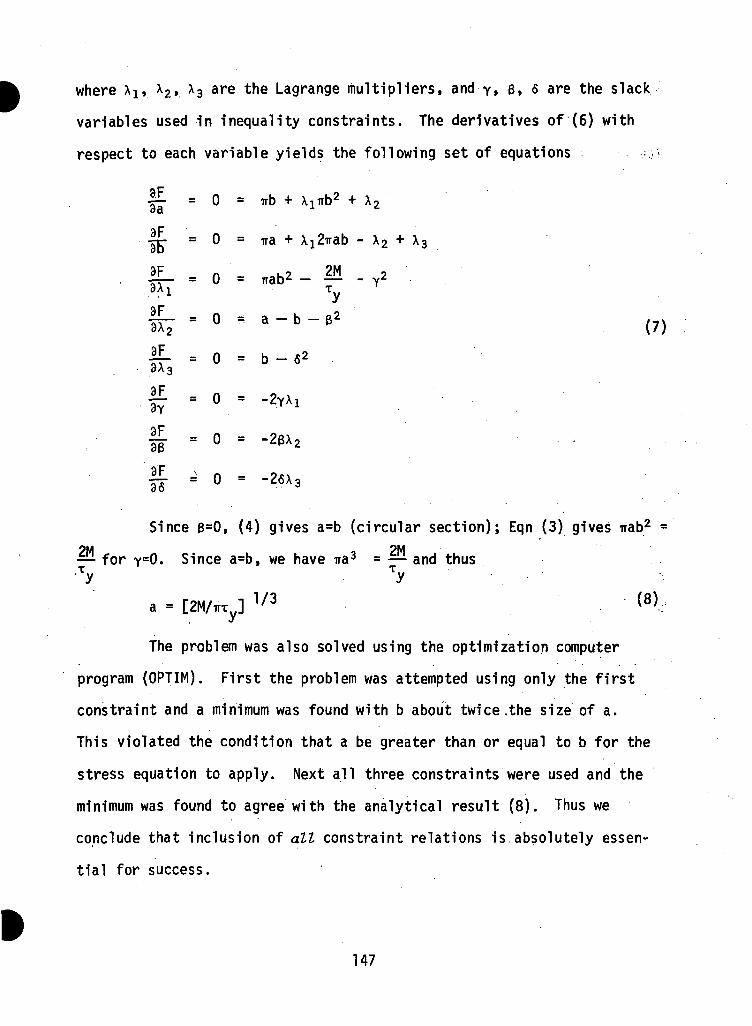
where xls X2, *3 are the Lagrange multipliers, and y» 3, <s are the slack
variables used in inequality constraints. The derivatives of (6) with
respect to each variable yields the following set of equations r-
|£ = 0 = Trb + XlTrb2 + X2da
j£ = 0 = ira + \j2irab - X2 + X3
3F n .9 2M 2_ . o = rrab2 - - - Y2
Ife " ° " a-b-e' (7)
Jf3 " ° = b^2
f = 0 = -23X2
& = ° = -26X3
Since 6=0, (4) gives a=b (circular section); Eqn (3) gives irab2 =
— for y=0. Since a=b, we have Tra3 = — and thusTy Tya = [2M/TTTy] 1/3 (8)
The problem was also solved using the optimization computer
program (OPTIM). First the problem was attempted using only the first
constraint and a minimum was found with b about twice .the size of a.
This violated the condition that a be greater than or equal to b for the
stress equation to apply. Next all three constraints were used and the
minimum was found to agree with the analytical result (8). Thus we
conclude that inclusion of all constraint relations is absolutely essen-
tial for success.
147
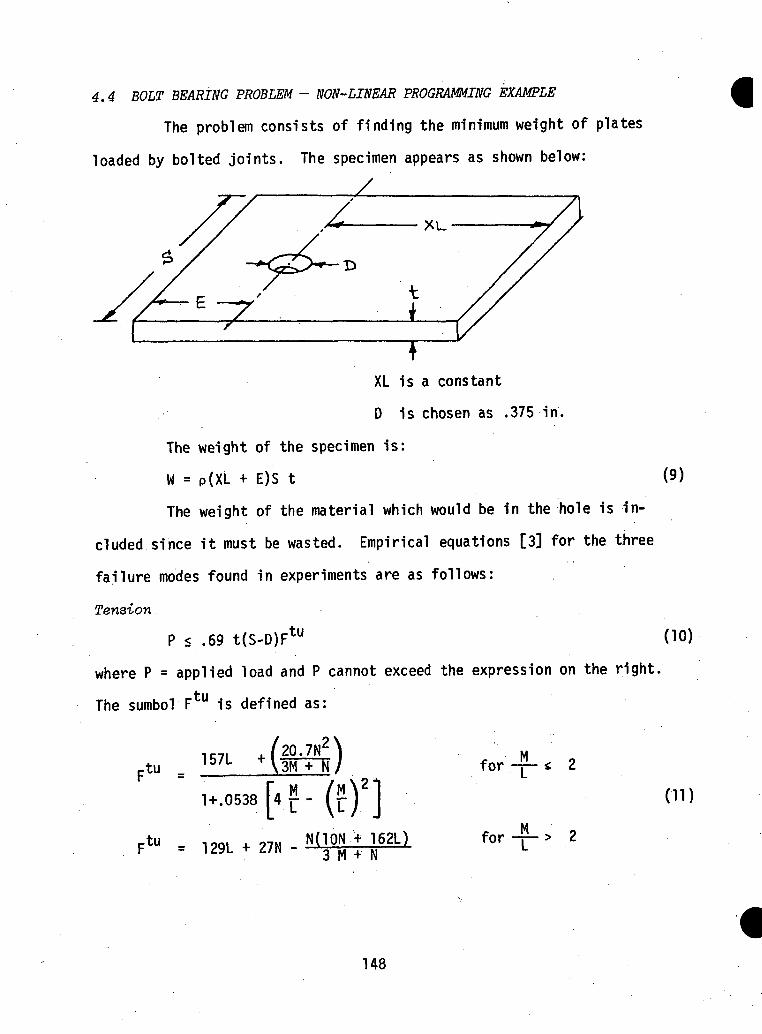
4.4 BOLT BEARING PROBLEM - NON-LINEAR PROGRAMMING EXAMPLE
The problem consists of finding the minimum weight of plates
loaded by bolted joints. The specimen appears as shown below:
XL is a constant
D is chosen as .375 in.
The weight of the specimen is:
W = p(XL + E)S t (9)
The weight of the material which would be in the hole is in-
cluded since it must be wasted. Empirical equations [3] for the three
failure modes found in experiments are as follows:
Tension
P < .69 t(S-D)F•tu (10)
where P = applied load and P cannot exceed the expression on the right.
The sumbol Ftu is defined as:
-tu _ 157L 3M + N for * 2
1+.0538['•HO') (11)
-tu _= 129L + 27N - N(10N .'* 162L)3 M + N
for _JL> 2
148
where L = % 0° plies
M = % 90° plies
N = % ±45° plies
The constraint for this failure mode is F(l) = P - .69 t(S-D)Ftu.
If this quantity stays negative then P is below failure load. If it
is near zero, failure in this mode is impending. The problem was
treated from two different viewpoints.
First the orientation percentages L, M, and N were held constant
and the dimensions for minimum weight of the specimen were found. The
answer in this case yields the optimum dimensions for the orientations
chosen.
The second way of treating the problem was to leave the orienta-
tions as variable. This way, both the dimensions and the orientations/-"'. •
were optimized. The results showed a 20-30% improvement over the fixed
orientations case. The orientations chosen were those of an experimental
specimen which failed at P = 1020 Ib. The program gave a weight reduction
for failure at the same load and with the same orientations.
The problem also included equations for failure in two other
modes-shear out and bearing. These were the second and third constraints.
The failure mode in a given problem is found by checking which of the
three constraints is closest to zero. The constraints are
Shear Out .
P < 2tEFsu
F(2) = P - 2tEF
where
su
Fsu = 40N N > .23
Fsu =9.2 N < .23
149
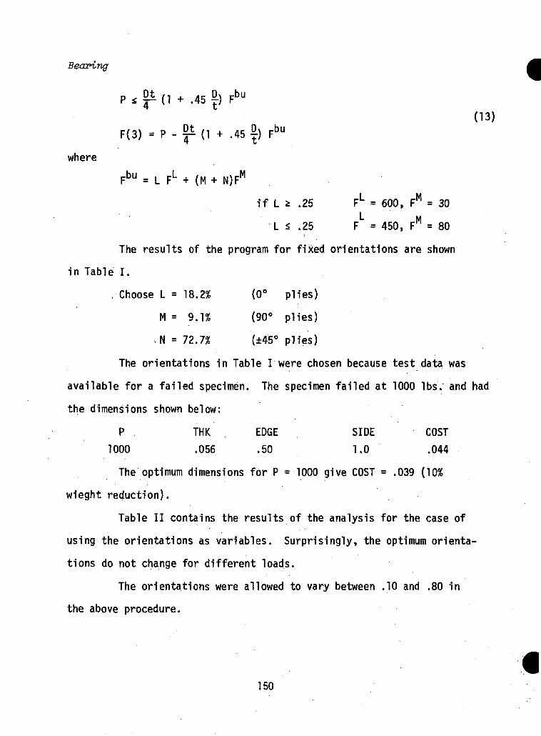
Bearing
-bu.45 £) FL
(13)
where
F(3) = P - - (1 + .45 ) Fbu
Fbu = L FL + (M + N)FM
if L * .25 FL = 600, FM = 30
L < .25 F = 450, FM = 80
The results of the program for fixed orientations are shown
in Table I.
, Choose L = 18.2% (0° plies)
M = 9.1% (90° plies)
^N = 72.7% (±45° plies)
The orientations in Table I were chosen because test data was
available for a failed specimen. The specimen failed at 1000 Ibs. and had
the dimensions shown below:
P THK EDGE SIDE COST
1000 .056 .50 1.0 .044
The optimum dimensions for P =1000 give COST = .039 (10%
wieght reduction).
Table II contains the results of the analysis for the case of
using the orientations as variables. Surprisingly, the optimum orienta-
tions do not change for different loads.
The orientations were allowed to vary between .10 and .80 in
the above procedure.
150
The results in Table m were found for variable orientations
with the possibility of eliminating certain plies. There is some doubt
of the applicability of the equations for less than 10% of any of the
plies, but it is informative to see what will happen in this case.
The results for all three cases are plotted together for
comparison in Fig 3.
4.5 DISCUSSION
The OPTIM program has proven to be very effective in dealing with
problems for which analytical equations can be derived. The elliptic bar
and bolt bearing problems treated above are examples.
The bolt-bearing problem is unusual for composite materials in
that analytical equations are available which allow us to optimize both
the dimensions and the lamina orientations. The equations are empirical
and therefore introduce doubt as to their accuracy. There also may be
ranges of dimensions or orientation percentages in which they are not
applicable.
Table I shows optimum dimensions for varying load with the ply
orientations fixed. The case of P = 1000 Ib. shows a 10% weight reduction
over the experimental specimen. The values of the constraints show this
to be a simultaneous failure in tension and shear out. The cases of P
(applied load) between 3000 Ibs. and 15,000 Ibs. show failure in all
three modes simultaneously. There is no apparent pattern in the variation
of optimum dimensions with load. The weight is seen to vary non-linearly
with load as can be inferred from Fig 1.
If we allow the orientation percents to vary between 10% and 80%
the optimum laminate will be found with respect to both dimensions and
151
orientations. OPTIM found values of five of the six variables which were
optimum for all loads considered. Only the total thickness changed and it
varied linearly with load. This situation forced the weight to vary
linearly with load also as seen in Fig 2. For each load, the specimen
exhibited failure in tension and shear out simultaneously with bearing
failure not being a factor. The orientations chosen for each load were
L = 73%, M = 17%, N = 10%. The fact that N was brought to the minimum
of its range led to the results in Table 3 where N was allowed to vary
between 0% and 80%. The results are similar to those in Table 2 except
that N goes to zero with L and M increasing proportionately. As noted,
the equations may not apply for N less than 10%, but the results indicate
that the ±45° laminae are of little benefit 1n the bolt bearing specimen.
The thickness and weight vary linearly with load as in the previous case.
All three cases are plotted in Fig 3. The variable orientation case shows
an improvement on the fixed case of between 30% and 100%, with the case
for N = 0 about 15% better still.
The results show a .useful and convenient relationship for design.
The designer is given the optimum orientations and side and edge distances
and he merely chooses his thickness to suit the load which must be carried.
The empirical nature of the equations suggests that experiments should be
run to verify the derived results before putting them into use as a design
criterion.
152
4.6 REFERENCES
[1] M. D. Schussel, "Optimization by Pattern Search Program Descriptionand Usage Instructions", prepared for GE-580, Department ofMechanical Engineering, Carnegie-Mellon University (1968).
[2] S. J. Marulis, "Optimization of Advanced Composite Plates", ReportSM-71, Department of Mechanical Engineering, Carnegie-MellonUniversity, Pittsburgh, Pennsylvania (June 1971).
[3] Advanced Composite Wing Structures, Boron-Epoxy Design Data —Volume II, Grumman Aerospace Corporation, 180-186, TR-AC-SM-ST-8085 (November 1969).
153
I/)o•r-•Pra
(U•r-
O
"8
o
to•M£Lcn•r-<U
CO• o.oo
0)
jQ(O
pCO 5O rHu BJ
V f
§|tO OS i-J' — ' <! rHtt. UJ <
CO U.
fern/ ^ D c2v3e* *JU-, < rH
s S5CO
_§Uj
t-i i-< 3v-'CO -JU. 2 t-n
UJ E- U,
E-co1— 1aUJa
E-COI-H0
UJ
aUJ
COCOUJ
u5E-
/— "voa, <;
3.
too
LO00<s >i— 1
'
toO)o0
1
1— (VOoo
1
(N*»
to
• 1— ttor-J'
i— tO
o0orH
rHrH
frH•1
to(-•*
o0o
1
5oo1
t--00
C<J
,o1— 1
00fo
oooIO
rj-10
g>rH•
•1
00CvlO
1
too
1
00rH
rH
LO
to*
"(*N.to•
ooLOr-
tof .T
orH(N•1
OCM
1
rHtoo•1
a>orH
rHto
O)LOLO•
ooporH
CM
x
oo^•
i
ooLO
1
o>VOO•
|
toorH
oo(N
\0rHa>
oooLOi— i
154
co
<uro<u!are
•i—s_
o
CO•M
OJ
OO
CM
<u.0re
ptD
r . | i
to LUu -*--
oLO
+1o\°
O
,-J 000\°
CJ3 UQ
to 2 305 H-J0, < rH
tu <CQ U-,
§CM o: H v— ' <£ . »-Jtin m o *-*
ITJ *to P-cS 3
-, rH 3rH tO I-J*— s I-HIX UJ <
f pj^
UU f-Q tOHH HH
U4 HQ 1-1IU Q
^ toCJ tO1-1 . UJ
t — \Q
CL, 0.v — /
LO
0•
0
.•
OO
•
CMr-•
fCMOvOvO
1
00vO00
1
00
oo
1
CMLO
CMtoto
vOI-HO
0oor-H
LO
o. •
o.
v£>
•
t***•
t
r-oCMvO
1
O>i-H0
1
to1— 10o
1
0>
.
to10
oo
oooto
CMi-H•
0.
r--.•
to1*•
f*
fLOLO
1
00CM0
1
tor— 10
1
toLO
CM
to
CM000
oo0LO
vOOOi-H•
o.
^• •
tot•
m
00000T 1
1
orHo•1
toCM0o•1
i-HLO
i-Htoto
LOCMr— 1
ooLOI"x
rHLOCM
••
O.
00
•
CM
^•
t
LO00vOLO
1
00rHO•|
rHVO0
1
0
8to
vOrH
O0o
•»0i-H'
tofx.10•
o.
vO
•
t•
.
oLOtoCM
1
•-H
o•1
totooo' •1
oLO
LOtoto
to•CM•
ooo
•V
LOrH
155
•o(U
(O
OJJO
o•**vt
o•r—4->
$
OJ•r-
O
(U
coQ.3OO
CO
(U
H
& 6O rHU W
•— — •••— — •_.
•H
OCT1
S e\°
o-3 P
f— \ rH HDto B5 *J\ J ^£ hH
tu w <CO U.
« 1sjS'Srfu, x o <:
CO U.
§ g,-^rH 3
rH tO "JV— ' Jj£ rH
UH LU <
f- tu
U4 E-HQ CO
CO Q
e is"Q rHw a
COCOLU
su
H
0<lj
IX O
ti
oo
oo
to
£
of~^f^.
1
ooo
•«*00ooo
1
CMtorH
o•
to
LOrHo
ooorH
oo
oo
0
i
**00vO
1
rH
oo .
1
CMoo
•
1
toCM
rH
to•
"*
^fo•
oo5?
rH
orH
oo
rH
£•r)ooLO
o1
CM^fo
•
1
CTi10
^
oo• •
to
CMr-.0
oooLO
vOoLOt— t
o0
oCM
8
tor-lLO1
rH
oo
•
1
a,frOo
•
1
CMto1— t
rHfx
•
to
0>0rH
•
o0LO
oooo
oo
ors)
o00
VO
rH
I
ooo
1
vOrH
o•
1
rH
•"=>•rH
CM00
•to
torH
•
oooorH
tooto
oo
0CM
* iCMtoo\O
1
rHCMoo
1
vOLOo .
•
1
torH
to•
to
t--rHCM
•
oooLOi-H
156
.7
.6
WEIGHT vs. LOAD
L = 18.2%M= 9.1%N= 72.7%
f ixed
.5
.4
LU
.2
.1
00 5 10
LOAD (ibs. xlO3)
FIGURE 1: WEIGHT VS. LOAD FOR FIXED ORIENTATIONS
15
157
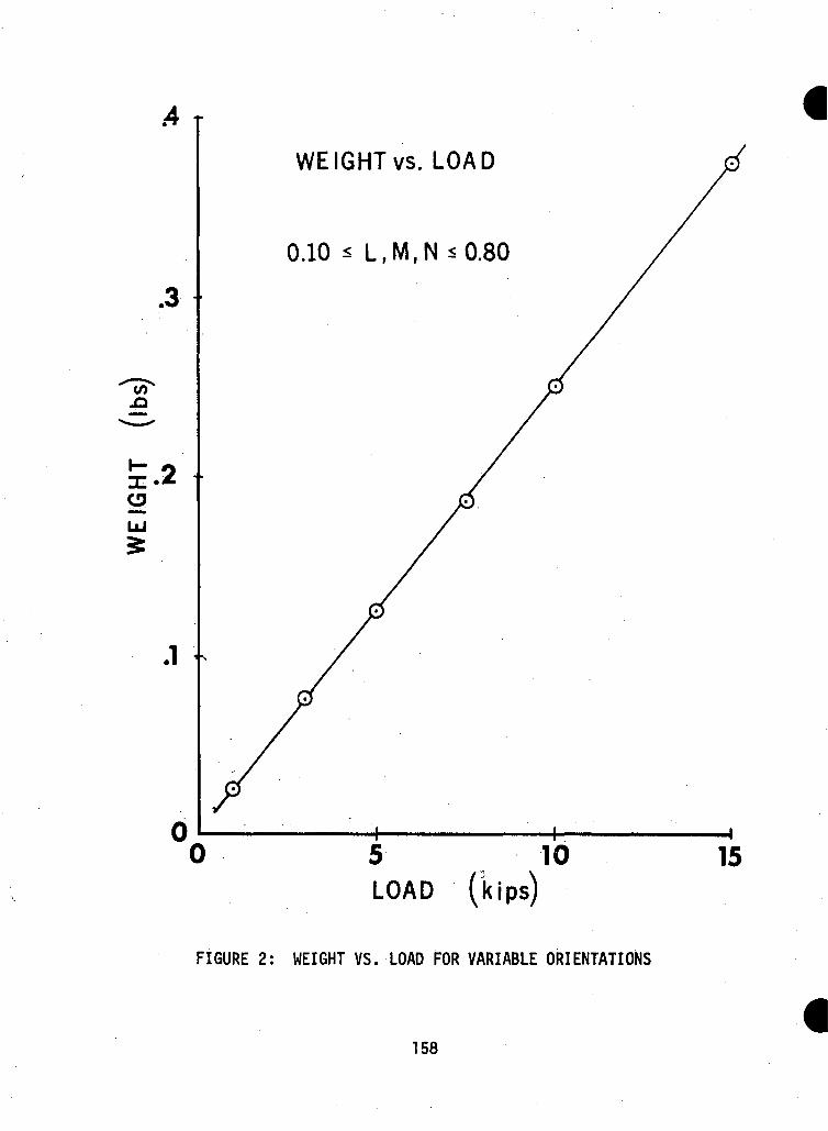
.4
.3
CO
S2UJ£
.1
WEIGHT vs. LOAD
0.10 * L,M,N *0.80
5 10LOAD (kjps)
FIGURE 2: WEIGHT VS. LOAD FOR VARIABLE ORIENTATIONS
—4
15
158
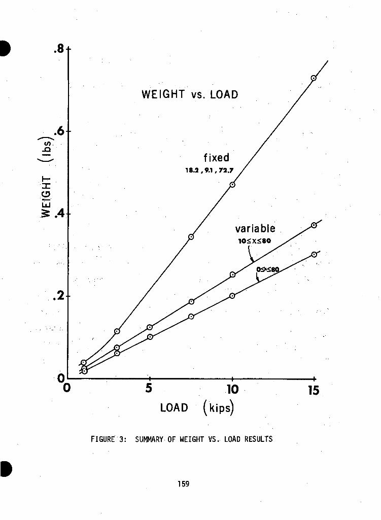
.8
.6
OLJ
.2
WEIGHT vs. LOAD
fixed18.2,9.1,72.7
variable10<X<80
5 10LOAD (kips)
FIGURE 3: SUMMARY OF WEIGHT VS. LOAD RESULTS
159
CHAPTER V
BOUNDARY-INTEGRAL EQUATION SOLUTION METHODS
5.1 TWO DIMENSIONAL ISOTROPIC BOUNDARY-INTEGRAL EQUATION METHOD
5.1.1 Introduction
The boundary-Integral equation method 1s a new tool for the
solution of many problems 1n solid mechanics. The method has significant
advantages over the finite element method. Numerical approximations are
not made over the field but over the surface, thereby Increasing accuracy.
The dimension of the problem 1s reduced by one, allowing many problems too
large for today's computers to be solved. Both of these features permit
the analyst to obtain highly refined data In the vicinity of stress concen-
trations such as near cracks and notches.
Important to the user of the boundary-Integral equation (BIE)
method, 1s the ease of data preparation and the rapidity of solution. The
BIE method utilizes a numerical solution of a boundary constraint equation.
This equation relates all of the surface displacements to all of the sur-
face tractions. The analyst specifies how he wishes to subdivide the sur-
face and specifies the boundary data; all well-posed problems are accepta-
ble Including mixed-mixed problems. The geometry 1s completely general and
may be multiply-connected. Once the surface solution 1s found the stresses
may be generated at any points that the analyst desires on the Interior
of the region.
The BIE method has been widely adapted to many problems in solid
mechanics, as can be seen by the literature [1-8]. The purpose for
presenting 1t 1n this report 1s twofold. First, the tool is being
160
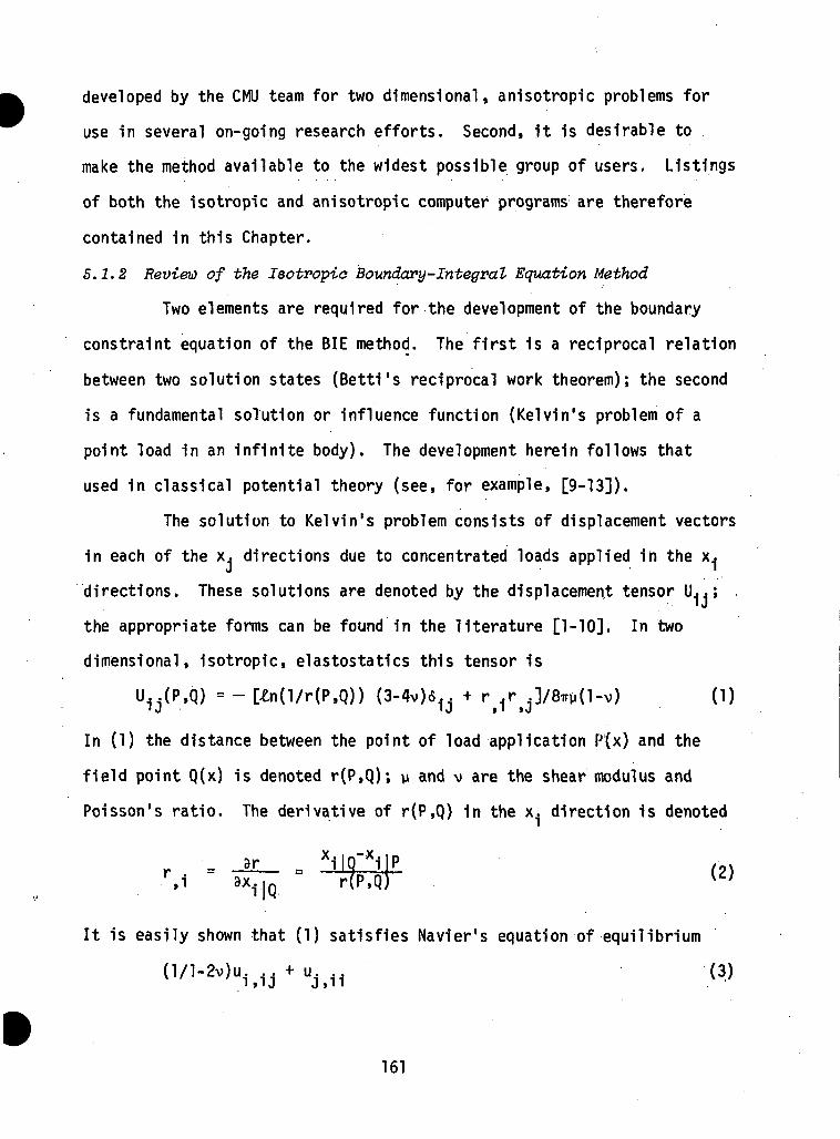
developed by the CMU team for two dimensional, anisotropic problems for
use in several on-going research efforts. Second, it is desirable to
make the method available to the widest possible group of users. Listings
of both the isotropic and anisotropic computer programs are therefore
contained in this Chapter.
5.1.2 Revieu of the leotropia Boundary -Integral Equation Method
Two elements are required for the development of the boundary
constraint equation of the BIE method. The first is a reciprocal relation
between two solution states (Betti's reciprocal work theorem); the second
is a fundamental solution or influence function (Kelvin's problem of a
point load in an infinite body). The development herein follows that
used in classical potential theory (see, for example, [9-13]).
The solution to Kelvin's problem consists of displacement vectors
in each of the x. directions due to concentrated loads applied in the Xj
directions. These solutions are denoted by the displacement tensor U..;
the appropriate forms can be found in the literature [1-10]. In two
dimensional, isotropic, elastostatics this tensor is
U i :J(P,Q) = - [£n(l/r(P,Q)) (3-^)6^. + ry ^/STryO-v) (1)
In (1) the distance between the point of load application P{x) and the
field point Q(x) is denoted r(P,Q); y and v are the shear modulus and
Poisson's ratio. The derivative of r(P,Q) in the x.. direction is denoted
9r i l Q iKP.Q
It is easily shown that (1) satisfies Navier's equation of equilibrium
0/l-2v)u. .. + u. (3)i > i j j > 1 1 . '
161
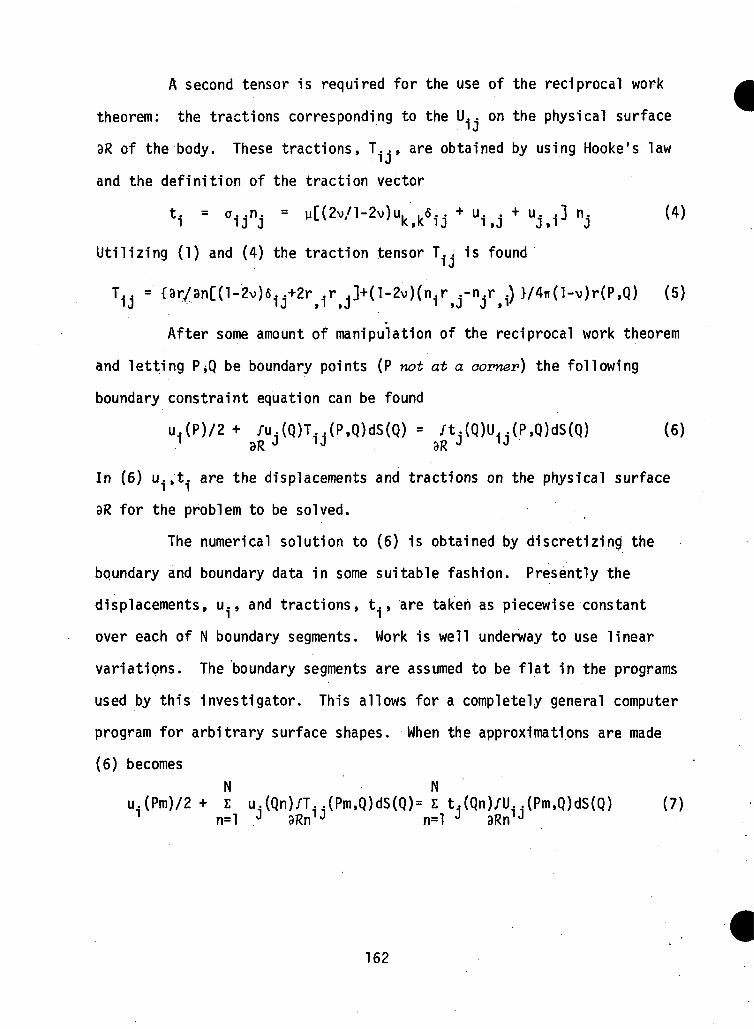
A second tensor is required for the use of the reciprocal work
theorem: the tractions corresponding to the U.. on the physical surface
aR of the body. These tractions, T. . , are obtained by using Hooke's law
and the definition of the traction vector
t. = a..n. = P [ {2v /1-2v)uk,k6 i j+u i , j+u j , i ]n j
Utilizing (1) and (4) the traction tensor T.. is found
T... = Or/an[(l-2v)6. j+2r).rJ]+(l-2v)(n.r j-y ^ }/4Tr(l-v)r(P,Q) (5)
After some amount of manipulation of the reciprocal work theorem
and letting PjQ be boundary points (P not at a corner) the following
boundary constraint equation can be found
u.(P)/2 + /u.(Q)T..(P,Q)dS(Q) = / t . (Q)U..(P,Q)dS(Q) (6)i 3R J ij 3R J U
In (6) u.»t. are the displacements and tractions on the physical surface
9R for the problem to be solved.
The numerical solution to (6) is obtained by discretizing the
boundary and boundary data in some suitable fashion. Presently the
displacements, u., and tractions, t., are taken as piecewise constant
over each of N boundary segments. Work is well underway to use linear
variations. The boundary segments are assumed to be flat in the programs
used by this investigator. This allows for a completely general computer
program for arbitrary surface shapes. When the approximations are made
(6) becomesN N
u.(Pm)/2+ E u.(Qn)/T..(Pm,Q)dS(Q)= E t,(Qn)/U..(Pm,Q)dS(Q) (7)1 n=l J 9Rn1J n=l J 3Rn1J
162
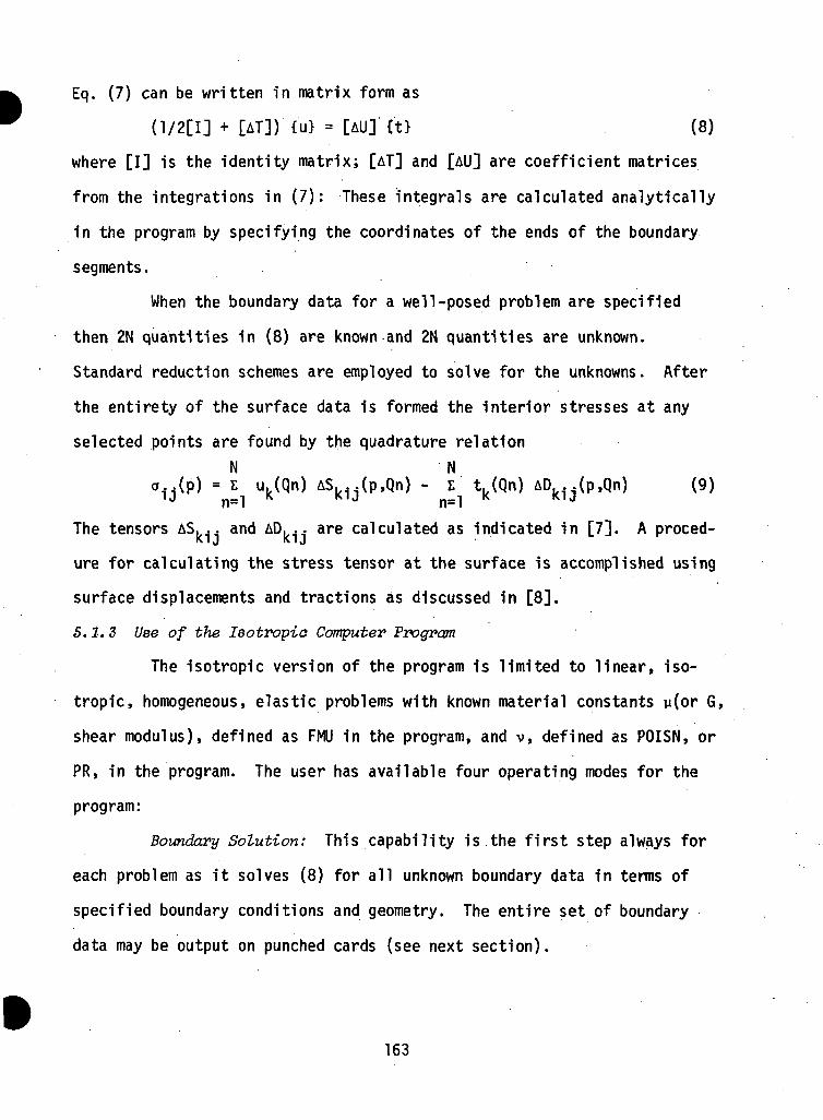
Eq. (7) can be written In matrix form as
(1/2[I] + [AT]) {u} = [AU] £t> (8)
where [I] is the identity matrix; [AT] and [AU] are coefficient matrices
from the integrations in (7): These integrals are calculated analytically
in the program by specifying the coordinates of the ends of the boundary
segments.
When the boundary data for a well-posed problem are specified
then 2N quantities in (8) are known and 2N quantities are unknown.
Standard reduction schemes are employed to solve for the unknowns. After
the entirety of the surface data is formed the interior stresses at any
selected points are found by the quadrature relationN N
oij(p) = £ uR(Qn) ASk1j(p,Qn) - £ tR(Qn) ADk...(p,qn) (9)
The tensors AS. .. and AD... are calculated as indicated in [7]. A proced-
ure for calculating the stress tensor at the surface is accomplished using
surface displacements and tractions as discussed in [8].
5.1. 3 Use of the Isotropia Computer Program
The isotropic version of the program is limited to linear, iso-
tropic, homogeneous, elastic problems with known material constants y(or 6,
shear modulus), defined as FMU in the program, and v, defined as POISN, or
PR, in the program. The user has available four operating modes for the
program:
Boundary Solution: This capability is the first step always for
each problem as it solves (8) for all unknown boundary data in terms of
specified boundary conditions and geometry. The entire set of boundary
data may be output on punched cards (see next section).
163
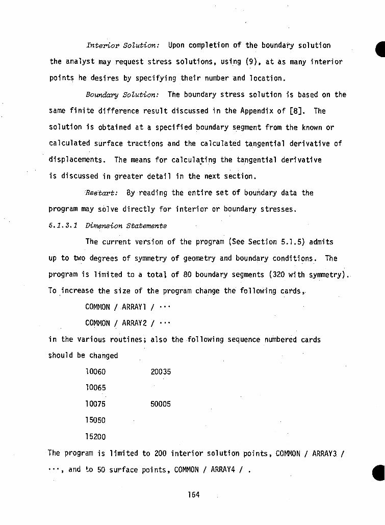
Interior Solution: Upon completion of the boundary solution
the analyst may request stress solutions, using (9), at as many interior
points he desires by specifying their number and location.
Boundary Solution: The boundary stress solution is based on the
same finite difference result discussed in the Appendix of [8]. The
solution is obtained at a specified boundary segment from the known or
calculated surface tractions and the calculated tangential derivative of
displacements. The means for calculating the tangential derivative
is discussed in greater detail in the next section.
Restart: By reading the entire set of boundary data the
program may solve directly for interior or boundary stresses.
5.1.3.1 Dimension Statements
The current version of the program (See Section 5.1.5) admits
up to two degrees of symmetry of geometry and boundary conditions. The
program is limited to a total of 80 boundary segments (320 with symmetry).
To increase the size of the program change the following cards,
COMMON / ARRAY1 / •••
COMMON / ARRAY2 / • • •
in the various routines; also the following sequence numbered cards
should be changed
10060 20035
10065
10075 50005
15050
15200
The program is limited to 200 interior solution points, COMMON / ARRAY3 /
•••, and to 50 surface points, COMMON / ARRAY4 / .
164
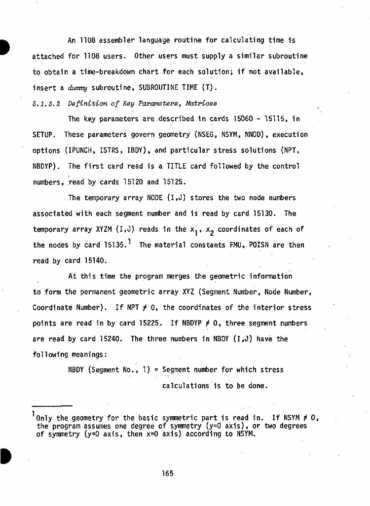
An 1108 assembler language routine for calculating time is
attached for 1108 users. Other users must supply a similar subroutine
to obtain a time-breakdown chart for each solution; if not available,
insert a dummy subroutine, SUBROUTINE TIME (T).
5.1.3.2 Definition of Key Parameters, Matrices
The key parameters are described in cards 15060 - 15115, in
SETUP. These parameters govern geometry (NSEG, NSYM, NNOD), execution
options (IPUNCH, ISTRS, IBDY), and particular stress solutions (NPT,
NBDYP). The first card read is a TITLE card followed by the control
numbers, .read by cards 15120 and 15125.
The temporary array NODE (1,0) stores the two node numbers
associated with each segment number and is read by card 15130. The
temporary array XYZM (1,0) reads in the x,, /„ coordinates of each of
the nodes by card 15135. The material constants FMU, POISN are then
read by card 15140.
At this time the program merges the geometric information
to form the permanent geometric array XYZ (Segment Number, Node Number,
Coordinate Number). If NPT ?* 0, the coordinates of the interior stress
points are read in by card 15225. If NBDYP ^ 0, three segment numbers
are read by card 15240. The three numbers in NBDY (1,0) have the
following meanings:
NBDY (Segment No., 1) = Segment number for which stress
calculations is to be done.
Only the geometry for the basic symmetric part is read in. If NSYM f 0,the program assumes one degree of symmetry (y=0 axis), or two degreesof symmetry (y=0 axis, then x=0 axis) according to NSYM.
165
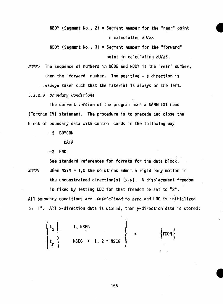
NBDY (Segment No., 2) = Segment number for the "rear" point
in calculating AU/AS.
NBDY (Segment No., 3) = Segment number for the "forward"
point in calculating AU/AS.
NOTE: The sequence of numbers in NODE and NBDY is the "rear" number,
then the "forward" number. The positive - s direction is
always taken such that the material is always on the left.
5.1.3.3 Boundary Conditions
The current version of the program uses a NAMELIST read
(Fortran IV) statement. The procedure is to precede and close the
block of boundary data with control cards in the following way
-$ BDYCON
DATA
-$ END
See standard references for formats for the data block.
NOTE: When NSYM = 1,0 the solutions admit a rigid body motion in
the unconstrained direction(s) (x,y). A displacement freedom
is fixed by letting LDC for that freedom be set to "2".
All boundary conditions are initialized to aero and LDC is initialized
to "1". All x-direction data is stored, then y-direction data is stored:
1, NSEG
NSE6 + 1,2* NSEG
TCON
166
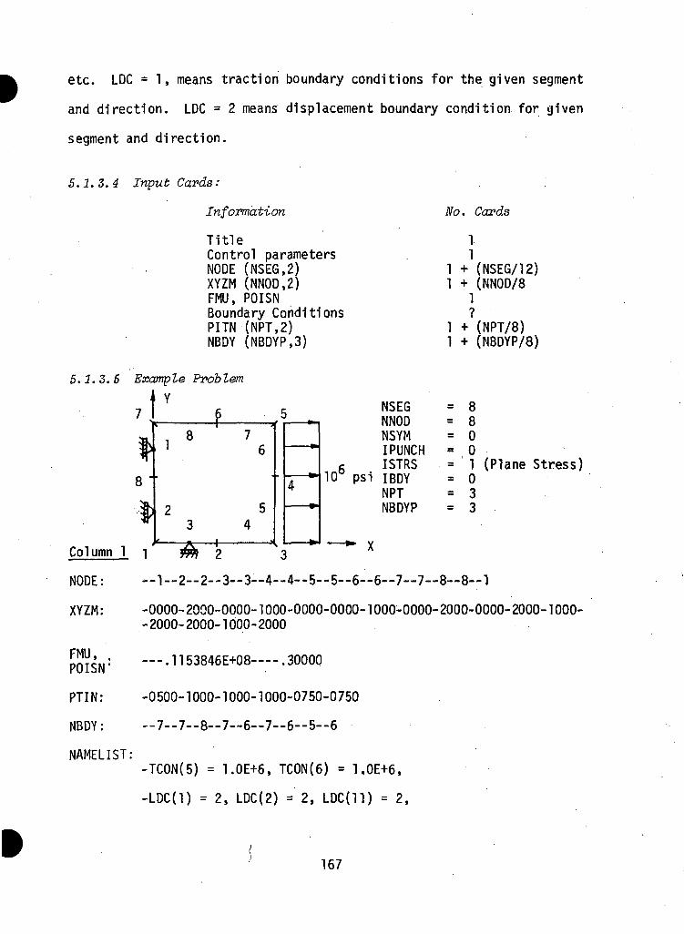
etc. LDC = 1, means traction boundary conditions for the given segment
and direction. LDC = 2 means displacement boundary condition for given
segment and direction.
5.1.3.4 Input Cards:
Information
TitleControl parametersNODE (NSEG.2)XYZM (NNOD.2]FMU, POISNBoundary ConditionsPITN (NPT.2)NBDY (NBDYP.3)
5.1.3.5 Example Problem
Column 1
NODE:
XYZM:
FMU, .POISN'
PTIN:
NBDY:
NAMELIST:
Y
, f8 7
1 6
2 53 4
i . 1 >
c
4
fci
NSE6NNODNSYMI PUNCH
6 ISTRS10° psi IBDY
NPTNBDYP
No. Cards
11
1 + (NSEG/12)1 + (NNOD/8
1?
1 + (NPT/8)1 + (NBDYP/8)
= Q
= 8= 0= 0= 1 (Plane Stress)= 0= 3= 3
i m 2 3— 1—2-2—3—3—4—4—5—5—6—6—7—7—8—8—1
-0000-2000-0000-1000-0000-0000-1000-0000-2000-0000-2000-1000--2000-2000-1000-2000
—.1153846E+08 .30000
-0500-1000-1000-1000-0750-0750
— 7—7—8—7—6—7—6—5—6
-TCON(5) = l.OE+6, TCON(6) = l.OE+6,
-LDC(l) = 2, LDC(2) =2, LDC(ll) = 2,
167
5.1. 4 References
[I] F. J. Rizzo, An Integral Approach to Boundary Value Problems ofClassical Elastostatics, Quarterly of Applied Mathematics 25,(1967) 83-95.
[2] T. A. Cruse and F. 0. Rizzo, A Direct Formulation and NumericalSolution of the General Transient Elastodynamic Problem - I,Journal of Mathematical Analysis and Applications 22, (1968) 244-259.
[3] T. A. Cruse, A Direct Formulation and Numerical Solution of theGeneral Transient El astodynamic Problem - II, Journal of MathematicalAnalysis and Applications 22, (1968) 341-355.
[4] T. A. Cruse, Numerical Solutions in Three Dimensional Elastostatics,International Journal of Solids Structures 5, (1969) 1259-1274.
[5] T. A.' Cruse and W. Van Buren, Three Dimensional Elastic StressAnalysis of a Fracture Specimen with an Edge Crack, InternationalJournal of Fracture Mechanics 6 (1970).
[6] T. A. Cruse and J. L. Swedlow, A Direct Method for Solving Three-Dimensional Problems of Elasto-Plastic Flow, Report SM-43, Departmentof Mechanical Engineering, Carnegie-Mellon University (1970).
[7] F. J. Rizzo and D. J. Snippy, A Formulation and Solution Procedurefor the General Non-Homogeneous Elastic Inclusion Problem,International Journal of Solids Structures •$, (1968) 1161-1179.
[8] F. J. Rizzo and D. J. Snippy, A Method for Stress Determination inPlane Anistropic Elastic Bodies, Journal of Composite Materials,4, (1970) 36-61.
[9] W. V. Lovitt, Linear Integral Equations, Dover (1950).
[10] 0. D. Kellogg, Foundations of Potential Theory, Dover (1953).
[II] V. D. Kupradze, Potential Methods in the Theory of Elasticity,D. Davey & Co. (1965).
[12] S. G. Mikhlin, Multidimensional Singular Integrals and IntegralEquations, Pergamon Press (1965).
[13] C. E. Pearson, Theoretical Elasticity, Ch. VI, Harvard UniversityPress (1959).
168
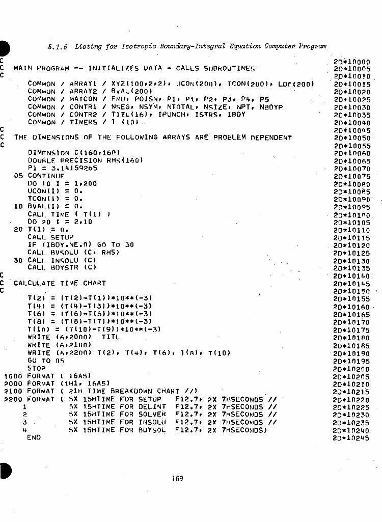
5.2.5 Listing for Isotropio Boundary-Integral Equation Computer Program
MAIN PROGRAM — INITIALIZES DATA - CALLS SUBROUTINES
COMMON / ARRAYl / XYZdOO»2*2)» UCOM(20())» TCON<200)» LDr(200)COMMON / ARRAY2 / BwAL(200)COMMON / MATCON / FMU» POISN* Pi* P1 * P2» P3» P<*» P5COMMON / CONTR1 / NSEG* NSYM* NTOTAL* NSI2E. NPT, NBDYPCOMMON / CONTR2 / T1TL(16)» IPUNCH* ISTRS* IBDYCOMMON / TIMERS / T (10)
THE DIMENSIONS OF THE FOLLOWING ARRAYS ARE PROBLEM DEPENDENT
DIMENSION C(160»160)DOUHLP PRECISION RHSdftO)PI = 3.1 159265
05 CONTINUEDO 10 I = 1»200UCON(I) r 0.TCONlI) =0.
10 BVAI.(I) = 0.CALL TIME ( T(I> )00 90 I = 2>10
20 T(I) = 0.CALL SETUP
CCC
IF (IBDY.NE.O) GO To 30CALL BVSOLU (C» RHS)
30 CALL INSOLU (C)CALL BOYSTR (C)
CALCULATE TIME CHART
T(2) = (T(2)-T(1) )*10**(-3)TC*) = (TU)-T<3))*10**(-3)T(6) = (T(6)-T(b))*10**(-3)T(8) = (T(8)-T(7) )*10**(-3)T(ln) = (T(lO)-T(9))*10**(-3)WRITE (6*2000) TITLWRITE (ft*2lOO)WRITE (*»2200) T(2>. T(4)» T(6)» 1 (n) »GO TO 05STOP
1000 FORMAT ( 16A5)2000 FORMAT (1H1» 16A5)2100 FORMAT ( ?IH TIME BREAKDOWN CHART //)2200 FORMAT i sx ISHTIME FOR SETUP Fi2.7»
1 SX 15HTIME FOR DELINT F12.7*2 5X 15HTIME FOR SOLVER F12.7r3 SX 15HTIME FOR INSOLU F12.7*ti SX 15HTIME FOR BDYSOL F12.7*
\ •
T(10)
2X 7HSECOMDS2X 7HSECONDS ,2X 7HSECOWDS ,2X 7HSECOMDS .,2X 7HSECOMDS)
END
20*1000020*1000520*1001.020*1001520*1002020*1002520*1003020*1003520*100^020*100^520*1005020*1005520*1006020*1006520*1007020*1007520*1008020*1008520*100*3020*100952D*10ino20*1010520*1011020*1011520*1012020*1012520*1013020*1013520*1014020*101«i520*1015020*1015520*1016020*1016520*1017020*101752D*101PO2D*101«520*1019020*1019520*1020020*1020520*1021020*1021520*1022020*1022520*1023020*102352D*102«*020*102^5
169
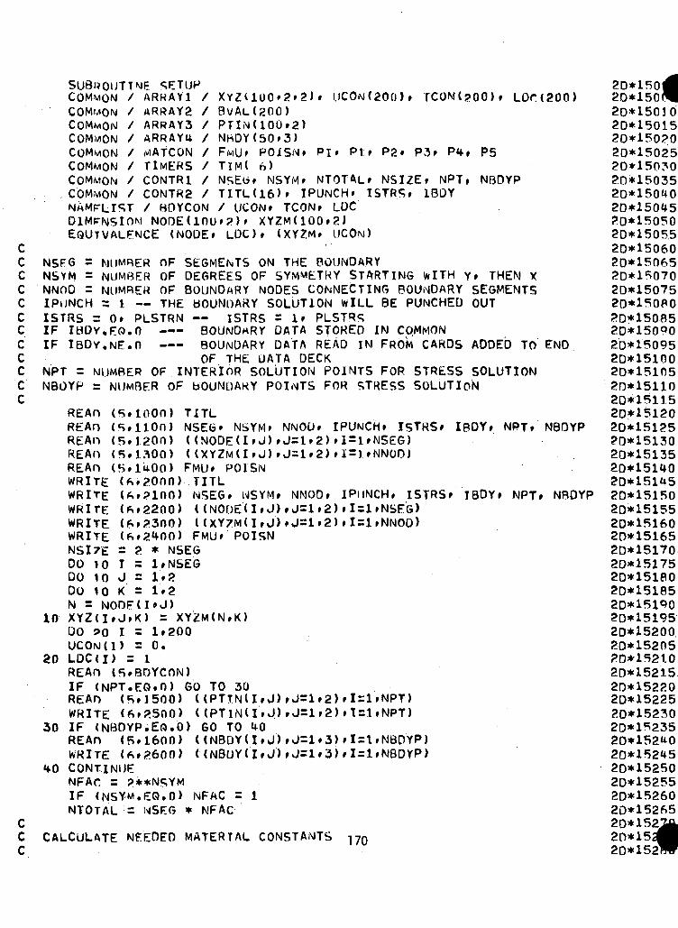
SUBROUTINE SETUPCOMMON / ARRAYlCOMMONCOMMONCOMMONCOMMONCOMMONCOMMONCOMMON
ARRAY2 /ARRAYS /ARRAY4 /MATC'ON /TIMERS /CONTR1 /CONTR2 // HOYCON
XYZdOO»2»2)BVAL(200)PTIN(100»2)NBDY(50»3)
UCO(M(200)» TCOM(?00)» LDr.(200)
Pt* P2» P3* P<*» P5TTM( 6)
NSYM* NTOTAL* NSIZE* NPT»TITL(16)» IPUNCH. ISTRS, 1BDY/ UCON* TCON* LOC
NBDYP
cccccccccc
D1MFN5IOM NOOEUOO.?)* XYZM(100»2)EQUIVALENCE (NODE* LOO. (XYZM* UCON)
NSFG = MUMRER OF SEGMENTS ON THE BOUNDARYNSYM = NUMBER OF DEGREES OF SYMMETRY STA-RTING WITH Y» THEN XNNOO - NUMBER OF BOUNDARY NODES CONNECTING BOUNDARY SEGMENTSIPUNCH = 1 — THE bOUNDARY SOLUTION WILL BE PUNCHED OUT
— ISTRS = 1* PLSTRSBOUNDARY DATA STORED IN COMMONBOUNDARY DATA READ IN FROM CARDS ADDED TO ENDOF THE DATA DECK
INTERIOR SOLUTION POINTS FOR STRESS SOLUTION
ISTRS =IF
0» PLSTRN
,0 —-IF IBDY.NF..o —
NPT = NUMBER OFC NBOYP =C
REAnREAnREAnREAnREAnWRITEWRITEWRITEWRITEWRITENSI7EDO 10
NUMBER OF BOUNDARY POINTS FOR STRESS SOLUTION
(s.iion)(5»l20n)
TITLNSEG* NSYM* NNOO* IPUNCH*((NODE(I*J)*J=1»2)* 1 = 1*NSEG)((XYZM(I»J)*J=1»2)»I=)»NNOO)FMU* POISN
(6*2.000)-.TITLNSEG. NSYM* NNOD* iPllNCH.((NOOEd»J).J=l»2)»I = l((XYZM(I.J)*J=1»2)>I=1»NNOD)FMU* POISN
IBOY. NPT* NBDYP
IBDY» NPT» NBDYP
00DO
1010
ccc
(6*2200)(6.2300)(6*2400)= 2 * NSEGI = l.NSEGJ = 1*2K = 1*2
N = NOOF(I»J)10 XYZ(I.J.K) = XYZM(N.K)
DO 90 I = 1.200UCON(l) =0.
20 LDC(I) = 1REAn (B.BOYCON)IF (NPT.EG.0) GO TO 30R£An (5*1500) KPTIN(I»J)»J=1»2)»I=1*NPT)WRITE (6.2500) ((PT1NII.J)»J=1*2)»I=1»NPT)
30 IF (NBOYP.EO.O) GO TO 40REAn (5*1600) ((NBDY(I.J)»J=1»3)»I=1.NBDYP)WRITE (6.2600) ((NBUY(I»J)»J=l*3)* 1=1.NBDYP)
40 CONTINUENFAC = ?**NC;YMIF (NSYM.EQ.O) NFAC = 1NTOTAL = NSEG * NFAC
CALCULATE NEEDED MATERIAL CONSTANTS 170
20*1501020*15015
20*1502520*1503020*150352D*150UO2D*150«*520*1505020*1505520*1506020*1506520*1507020*1507520*1508020*1508520*1509020*1509520*1510020*1510520*1511020*1511520*1512020*1512520*1513020*1513520*1511020*1514520*1515020*1515520*1516020*1516520*1517020*1517520*1518020*1518520*1519020*1519520*1520020*1520520*1521020*1521520*1522020*1522520*1523020*1523520*152 020*1524520*1525020*1525520*1526020*1526520*152;20*15220*1521
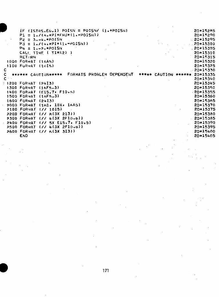
» IF (ISTRS.EG.D POI5N =PI r l./(8,*PI*F,MU*(l.-POISN) >P2 = 3.-4.*POISNP3 = !./(<*.*PI*tl.-P01SN) )P4 = l.-?.*P01SNCALL TIME ( T1M12) )RETURN
1000 FORMAT <1100 FORMAT (
(l.+POISN)
ccc
****** CAUTION***** FORMATS PROBLEM DEPENDENT
if»A5)
1200 FORMAT1300 FORMAT1«*00 FORMAT <E15.7» FIO.S)1500 FORMAT dftFB.3)i6oo FORMAT <s»i*i3?ooo FORMAT <IHI.?ioo FORMAT <// 1015)?2o;o FORMAT (// «<3x 2i3»9300 FORMAT (// t*(3X 2F10.b»?UOO FORMAT <// 5X E15.7» F10. 5)?500 FORMAT <// U(3X ?.F10.6J)?600 FORMAT (// M3X 3I3)>
END
20*1528520*15290.20*1529520*15300,20*1530520*1531020*1531520*1532020*1532520*15330
***** CAUTION ****** 20*1533520*1534020*1534520*15350.20*1535520*1536020*1536520*1537020*1537520*1538020*1538520*1539020*1539520*1540020*15405
171
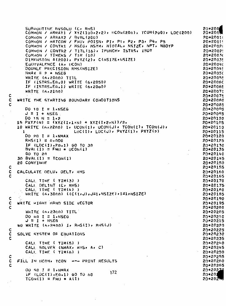
SURWOUTTNF. RVSOLUCOMMON / ARRAY!COMMON / ARRAY2COMMON / MATCONCOMMON / CONTKICOMMON / CONTR2COMMON / TIMERSDIMENSION A(?00)EliUTVALFNCE <A»
<C> RhS)/ X Y Z ( 1 0 0 » 2 » 2 )/ B\/AL(200)/ FwU» POISN* PI» Pi> P2» P3» Pf»/ NSEG» NSYMf N70TAL* N<>IZE» NPT>/ TITL(16)» IPUNCH* ISTR5» I9DY/ TJM (10), P X Y Z ( 2 ) » C(NSIZE»NSIZE)UCON)
MCOw(20n)» TCON(?uO)» LOC(200)
P5N80YP
CCC
CCC
CCC
CCC
CCC
DOURLF: PRECISION RHS(NSIZE)NMA* = ? * NSEGWRITE (f.» 000) TITLIF aSTRS.EO.Q) WRITE <6»2050>IF (ISTR5.E0.1) WRITE (6»2060)WRITE (f.»2ino)
WRITE THE STARTING BOUNDARY CONDITIONS
DO 10 I = 1>NSEGJ = I + NSEG00 1B N = l»g
15 PXY7(N) = (XY2(I»1»N) + XY2( I »2»N) ) /2.10 WRITE <6»<>2nO) I» UCON(l)r UCON(J)» TCON(I>» TCON(J)»
I Li.)C(I)» LOC(J)» PXYZ(1)» PXYZ<9)00 PO I = 1»NMAXRHS<D = n.ODOIF (LOC(I). F.O.I) GO TO 30BVAL(I) = FM(J * UCON(J)GO TO ?n
30 8VALU) = TCON(I)20 CONTINljr
CALCULATE OELU. OELT» RHS
CALL TIMF ( TIM (3) )CALL DEL INT <c» RMS)CALL TIME ( TIM(a) )WRITE (ft»3000) ((C(I»J) »J=1»MSIZF) »I=lrNSlZE>
WRITE WIGHT HAND SIDE V/ECTORWHITE <*.2300) TITLDO uo I = 1.IMSEGJ = I + NSEG
«*0 WHITE (*S»<>i+nO) It RHS<I)» RHS(J)
SOLVE ^YSTFM OF EQUATIONS
CALL TIME ( TIM(5) )CALL SOLVER (NMAX» HHS» A» C)CALL TIMF ( TIM(6) )
FILL IM UCON, TCON --- PRINT RESULTS
00 SO I = IrNMAXIF (LDC(I).EO.l) GO TOTCON(I) = FMU * Ad)
?D*200H20*2001!20*200?!20*200?!20*200.?(20*20031
20*200^52D*2005C20*2005?20*2006C20*2006520*2007020*20075
20*20065
20*2009520*2010020*2010520*2011020*2011520*2012020*201?520*2013020*20135
2D*201U520*2015020*2015520*2016020*2016520*2017020*2017520*201flO20*2018520*2019020*2019520*2020020*2020520*2021020*202152D*202?020*2022520*2023020*2023520*202 020*2024520*2025020*2025520*2026020*20265
60172
20*20
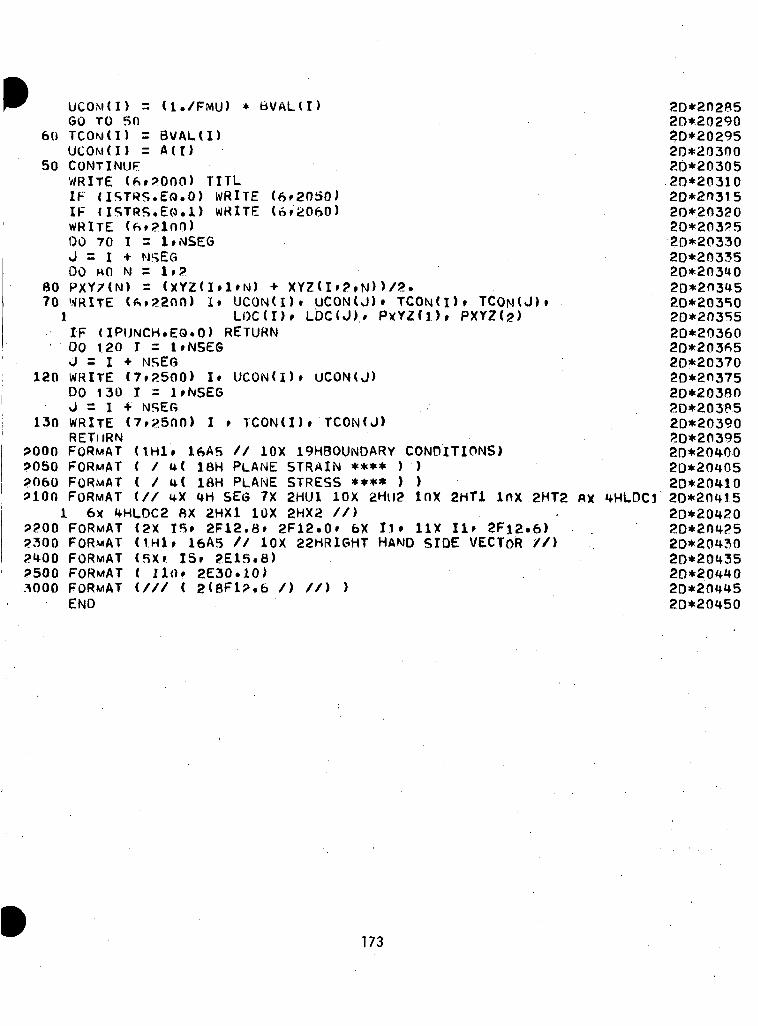
UCOMU) = (l./FMU) * BVAL(I)GO TO 50
60 TCOM(I) = BVAL(l)UCOM(I) = A(I)
50 CONTINIJFWRITE <fc»9000) TITLIF (ISTRS.EQ.-0) WRITEIF dSTRS.EO.l) WRITEWRITE (f>»?100)DO 70 I = IrNSEGJ = I + NSEGDO HO N = 1.9
80 PXY7CN) = (XYZdil'N) + XYZ (I »2 »N> >/2.70 WRITE (f»» 220-0) It UCON(I)t UCON(J)t TCOMD» TCOM(J)»
1 LOC(I)» LDC<J).» PXYZ<1), PXYZ(g)IF dPUNCH.EQ.O) RETURN00 120 I = 1»NSEGJ = I + NSE6
120 WRITE <7»2500) I» UCONd>» UCON(J)DO 130 I = 1»NSEGJ = I + NSEG
130 WRITE (7»?..500) I » TCON( I) » TCON< J)RETURN
9000 FORMAT (1H1» 16A5 // 10X 19H80UNDARY CONDITIONS)9050 FORMAT ( / 4( 18H PLANE STRAIN **** ) )2060 FORMAT ( / M ISH PLANE STRESS **** ) )9100 FORMAT (// UX 4H SE6 7X 2HUI 10X 2Hll2 10X 2HT1 InX 2HT2
1 6x 4HLDC2 8X 2HX1 10X 2HX2 //)9200 FORMAT <2X I5» 2F12,8» 2F12.0» 6X Il» 11X Il» 2F12.6)2300 FORMAT (1Hl» 16A5 // 10X 22HR1GHT HAND SIDE VECTOR //)9.400 FORMAT (5X» I5» 2E15.8)9500 FORMAT ( Iln» 2E30.10)3000 FORMAT (/// ( 2(8F19.6 /) //) )
END
20*2028520*2029020*2029520*2030020*2030520*2031020*2031520*2032020*2039520*2033020*2033520*2034020*203 520*2035020*2035520*2036020*2036520*2037020*2037520*2038020*203P520*2039020*2039520*20*4-0020*2040520*2041020*2041520*2042020*2049.520*2043020*2043520*2044020*2044520*20450
173
ccccccc
CCC
CCC
SUBROUTINE HELINT («, RHS)COMMON / ARRAYl / XYZ < 1<)0» 2»? > » UCOu(200)» TCON<200)» LDC(?00)COMMON / ARRAY2 / B\/AL(?00)COMMON / MATCON / FMU» P01SN' Pi» Pi» P2» P3» P4, P5COMMON / CONTR1 / NSEG, NSYM* NTOTAL, NSIZE> NPT, NBDYPCOMMON / CONTR2 / TITL<16)» IPUNCHr ISTKS» 130YDIMENSION A(?), El<2)» E2(2)» P(2)»DIMFNSIOM ISYM(2) »U<2»2.) ,T(2»2) ,OOUHLE PRECISION RHS(NSIZE)» XII, X)2, XI3» XIU, Xl5DO 10 I = l.NSIZEDO 10 J = 1,NSIZE
10 G(I.J) = 0.00 ?0 M = 1,NTOTALIFLft = nJFLfi =0Ml = (M-l)/NSEGM2 = M - Ml*NSEG
IF (LDC(M?!) ,EQ.1.ANU.ABS(BVAL(M2) ) .LT.1.0.AND.
IF (LDC(M?)!E0.2.ANU,ABS(BVAL(M2)).LT.1.OE-08.AND.1 LDC(M3),EW.2.ANO,ABS(BVAL(M3)).LT.l.OE-08) JFLG = 1
COMPUTF SYMMETRY COEFFICIENTS USING Y» THEN X
IFLaG = 1.DO 16 K = 1»?J = 3 - K1 = (M-1)/(NSEG*((2**J)/2))ISYM(K) = (-!)**!IF (I.EO.O) ISYM(K) =1
16 IFLAG = IFLAG * ISYM(K)DO ^0 J = 1,2IF (IFLAG.Gf.O) GO TO 25X(l.J) = XYZ(M2,2»J) * 1SYM(J)X(2.J) = XYZ(M2»1»J) * ISYM(J)GO TO 35
25 X(1,J) = XY7(M2»1»J) * ISYM(J)X(2»J) = XYZ(M2»2rJ) * ISYM(J)
35 CONTINUE
DEFINE DIRECTION OF THE LINE SEGMENT F2 = A(J) / AMAG
30 A(J) = X(2»J) - X(1,J)AMAfi = SORT (A(l)**2 + A(2)**2)DO ^3 I = 1,2E2(T) = A(I)/AMAGJ = 3 - I
33 El(.l) = E2(I) * (-1)**<J+1)
CALCULATE THE ANGLES Tl AND T2 AND THE DISTANCE D
00 90 N = 1,NSEGDO 15 J = 1»2P(J) = (XYZ(N»1,J) ••• XYZ(N»2»J) )/2.RKd) = X(1,J) - P<J) 174R2(.l) = X(2»J) - P(J)
20*250?0*2501020*2501520*2502020*2502520*2503020*2503520*250^020*250^520*2505020*2505520*2506020*2506520*2507020*250752D*250PO20*2508520*2509020*25095?0*2510020*2510520*2511020*251152Q*251?020*2512520*2513020*2513520*2514020*2511520*2515020*2515520*2516020*2516520*2517020*2517520*2510020*2518520*2519020*2519520*2520020*2520520*2521020*2521520*2522020*2522520*2523020*2523520*252 020*252^520*2525020*252.5520*2526020*2526520*25;20*25;20*2521
15
DO 15 I = 1.U(I.J) = 0.ni.j) = o.CALL DOTPRDCALL. DOTPRDCALL DOTPRDCALL DOTPrtDCALl OOTPRDRlMAG = SttRTR2MA6 = SORT
2
(Rl» El.(Rl» E2.(R2f E2.(Rl. Rl»(R2» R2»(R1MAG)(R2MAS)
D)R12)R22)RlMAG)R2MAG)
60 TO 40
(l.-SIGD)*PI/2.(l.-Sl6D>*PI/2.
CCC
CCC
CCC
RA = ABS(Kl2)RB = ABSCR22)RMAR = AMAX1 (RA» RB)IF <ABS(D /RMAG).LT.1,OE-03)SIGO = n / ABS(D)Tl = ATAN(R1?/D) -T2 = ATAN(RJ>2/D) -ST1 = R12 / RlMAGST2 = R?2 / R2MAGCT1 = 0 / RlMAGCT2 = D / R2MAGTNI = R12 / 0TN2 = R22 / D
DIAGNOSTIC PRINT -— OCCURS ONLY IN THE CASE' OF SERIOUS DATA ERROR
IF ( (CT1/CT2) .GT. 0.) GOTO 500WRITE (ft.2000) M» N. X. Pr Rl» R2» El» E2. Tl» T2» CT1» CT2» D
500 CONTINUEXL1 = ALOG(D/CT1)XL2 = ALOfi(D/CT2)
CALCULATE OELU INTEGRAL FOR O.NE.O
IF (IFLG.EQ.l) GO To 15XII = D*(TN2*XL2-TN2-H2-TNl*XLl-»-TNl-Tl)XI2 =: D*(T2-T1)XI3 = D*(XL2-XL1)XI4 = D*(TN?-TN1-T2+T1>00 SO IX = 1»2DO RO JX = IX»2DEL = 0.IF (IX.FO.JX) DEL = 1.UXY = P1*(P?*DEL*Xll-El(IX)*Ei(JX)*Xl2-(Ei(lX)*E2(JX)*El(jX)*E21 ) )*XI3-E2UX)*£2(JX)*XI<UU(Iy»JX) = UXY * ISYM(JX)IF (IX.FO.JX) GO TO 50U(JXflX) = UXY * ISYMIIX)
50 CONTINUE
CALCULATE OELT INTEGRAL FOR O.NE.O
t*5 IF (JFLG.EQ.l) GO TO 75XII = TP-T1XI2 = T?+ST2*CT2-T1-ST1*CT1XI3 = ST?**2-ST1**2Xi4 = T?-ST2*CT2-T1+ST1*CT1XI5 = ALOG(CT1/CT2)
20*2529520*2-529020*2529520*2530020*2530520*2531020*253152D*253?>02D*253?520*2533020*2533520*253 020*2534520*2535020*2535520*2536020*2536520*2537020*25375•20*2538020*2538520*2539020*2539520*2540020*2540520*2541020*2541520*2542020*2542520*2543020*2543520*2544020*2544520*25450
' 20*2545520*2546020*2546520*2547020*2547520*2548020*254 520*2549020*25495
(1X20*2550020*2550520*2551020*2551520*2552020*2552520*2553020*2553520*2554020*255^520*2555020*2555520*2556020*2556520*25570
00 f.0 TV = 1»200 *0 J* = IX » 2TXY = 0.IF (IX.Fft.JX.ANO.M.FQ.N) GO TO hOD£L = 0.IF (IX.FO.JX) DEL = 1.TXY = P3*(PU*DEL*XIH-E1(IX)*E1(JX)*XI2-HE1<IX)*E2<JX)+-E2<IX)*1 FKJX) )*XI3+E2(IX)*E2<JX)*XI4)T(IV»JX) = TXY * ISYM(JX)IF (IX.FQ.JX) 60 TO 60TSTAR = -P3*P4*(E2<IX)*E1(JX)-E1<IX)*E2(JX»*XI5T(IXfJX) = (TXY+TSTAR)*ISYM(JX)T(JX»IX) = <TXY-TSTAR)*ISYM(IX)
60 CONTINUFGO TO 75
40 CONTINUFXII = R?2*(ALOG(RB)-1.)-R12*(AL06(RA)-1.)XI2 = R?? - R12XI3 = ALOfi(RB) - ALOG(RA)
C CALCULATE OELU FOR D.EQ.OIF (IFLG.EQ.l) GO To 65DO 70 IX = 1»2DO 70 JX •= IX»2DEL =0.IF (IX.FR.JX) DEL = 1.UXY = P1*(P?*OEL*XI1-'E2<IX)*E2(JX)*XI2)U(IVfJX) = UXY * ISYM(JX)IF (IX.FQ.JX) GO TO 70U(JX»1X) = UXY * ISYM(IX)
70 CONTINUFCC CALCULATE OF.LT INTEGRAL FOR D.EQ.O
65 IF (JFLG.EO.l) GO To 75DO RO IX = 1»2DO «0 JX = TX»2IF (IX.FO.JX) GO TO 80TXY = -P3*P4*IE2(IX)*£1<JX)-E1<IX)*E2<JX))*XI3T(Iy,JX) = TXY * ISYM(JX)
=-TXY * ISYM(IX)8075
T(JX»IX)CONTINUFDO «5 IX
«5 JX= N=• M?
DON4
= 1»2= 1»2
-»• (IX-1)*NSFG+ (JX-1)*NSFG
IF (IX.FO.JX.ANQ.M.EQ.N) T(IXrJX) = -0.50IF (LOC(M4).EQ.i) GO TO 90TRAiMS = IJ(IXrJX)U(Ix»JX) = -U./FMU) * T(IX»JX)T(IV»JX) = -FMU * TRANS
90 RHS(N4) = RHS(N4) + U(IX»JX) *85 G(Na»MU) = G(N4»M4) + T(IX»JX)20 CONTINUE
RETURN9000 FORMAT (// 5X 215 / (2F10.5 /»
END 176
20*25520*255120*255^020*255 5?0*2560020*2560520*2561020*2561520*2562020*2562520*2563020*2563520*2564020*256 520*2565020*2565520*2566020*2566520*2567020*2567520*2568020*2568520*2569020*2569520*2570020*2570520*2571020*2571520*2572020*2572520*2573020*257352D*257UQ20*2574520*2575020*2575520*2576020*2576520*2577020*2577520*2578020*2578520*2579020*2579520*2580020*2580520*2581020*2581520*2582020*2582520*2583020*2583520*2584020*2584520*25«
SUBROUTINE INSOLlM C )IJCON(200)» TCON(?00)» LDC(200)
Pt . » P2» P3» P5
NBDYP
• COMMON / ARRAY! / XYZ(100.2»2) .W COMMON / ARRAY3 / PTINU00.2)COMMON / M.ATCON / FMU. POISN. PI»COMMON / TIMERS / TIM (10)COMMON / CONTR1 / NSEG. NSYM. NfOTAL* NSIZEr NPT.COMMON / CONTR2 / TITL(16)» IPUNCH. ISTRS. IBDYDIMENSION C(100,3)' A(4). PXYZ(3)IF (IBOY.NE.O) GO TO 100
110 IF (NPT.EG).0) RETURNCALL TIME ( TIM(7) )WRITE (6.2000) TITLIF (ISTRS.EO.O) WRITE (6.2050)IF (ISTRS.EG.l) WRITE (6»2060) .
CC CALL FOR CALCULATION OF OELD AND DELSC
WRITE (6.2100)A(4) =0.CALi OELSO (C)DO 10 NP = l.NPTDO 90 I = 1.3
20 Ad) = C(NP.I)IF (ISTRS.EQ.l) GO TO 30A(4) = POISN * (A(l) + A(3))
30 CONTINUETHETA = (A(1) + A(3) * A(4))/3.TAUOCT = SQRT(2.*(A<1)**2+A(3)**?+A(4)**2-A(1)*A(3)-A(3)*A(«*)-
10
100
120
130
1501*10
NP» (A(K) »K=l.^)»THETAfTAUOCTfPTlN(NP»l) »PTIM(NP»2)WRITE (*CONTINDFCALl TIME ( TIM(8) )RETURNWRITE (*»20riO) TITLDO 120 I = 1»NSESJ = I -f MSEfiREAO (5.1100) Nr UCON(I)» UCON(J)DO 130 T = 1»NSEGJ = I + NSEGR£An (R.1100) Nr TCON(I)» TCON(J)WRITE (ft»2300)DO 140 I = l»NSEGJ = I + NSEGDO 150 N = Ir2PXY7(N) = (XY2(Irl»N) + XYZ( I »2»N) )WRITE (ft. 2100) I, UCON(I)f UCON(J) »
1 1009000905090609100
]2
200300
10)
TCON(I>» TCON(J)»LOC(I). LDC(J). PxYZ(l).. PXYZ(?)
GO TO 110FORMAT (110,FORMAT (IHI.FORMAT ( / 4( IBM PLANE STRAIN **** ) )FORMAT ( / 4( ISH PLANE STRESS **** ) )FORMAT (6HOPOINT, 2X 10H SIGMA(XX) 2X lOH
ION SlGMA(YY) 2X 10H SIGMAIZZ) 4X 6H5X 2H X 6X 2H Y)
FORMAT (2X I3» 2X 6F12.2. 2F8.4)FORMAT (// 4X 4H SEG 7X 2HU1 10X 2Hii2 lOX 2HT1 InX 2HT2 8X 4HLDC1
177
2E30,10X.
4( 16H4( 18H
SIGMA(yY) 2XTHETA 6X 7H TAIIOCT
20*3000020*3000520*3001020*3001520*3002020*3002520*300302D*300?520*300^0
20*3005020*3005520*3006020*300^520*3007020*3007520*3008020*300^520*3009020*3009520*3010020*3010520*3011020*3011520*3012020*3012520*3013020*3013520*3014020*3014520*3015020*3015520*3016020*3016520*3017020*3017520*3018020*3018520*3019020*3019520*3020020*3020520*3021020*3021520*3022020*3022520*3023020*3023520*3024020*3024520*3025020*3025520*3026020*3026520*3027020*3027520*30280
1 6* 4HI.OC2 BX 2HX1 10X 2HX2 //) 20*30?FORMAT (?X IS, 2F12.a» 2F12.0» 6X Il» 11X Ilr 2F12.6) 20*302END 20*3021
178
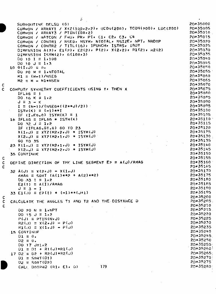
SUBPQUTIMF. OELSD (6)UCOrj<200), TCON(?00)» LDC(200)
CCC
CCC
COMMON / ARRAY1 / XYZ(100»2»2>COMMON / ARRAYS / PTIN(l*OOr2)COMMON / MATCON / F«lUr PR» PI» Cl» C2» C3» C«*COMMON / CONTR1 / NSE6> NSYM. NTOTAL* NSIZE» NPT, NBDYPCOMMON / CONTR2 / TlTL(16)r IPUNCH. ISTRSr IBQYOIMFNSION A(?)» E l < ? > » E2<2>» P(2)» X(2»2>» Rl<2)» R2(2)DIMFNSIOM ISYM(2)» fi(100»3)DO 10 I = IrlOO00 1.0 J = 1»3
10 G(I.J) = 0.DO ?0 M = l.NTOTALMl = (M-D/NSEGM2 = M - Ml*NSE(i
COMPUTF SYMMETRY COEFFICIENTS USING Y» THEN XIFLAG = 1DO 16 K = 1.2J = 3 - K1 = (M-1 )/(NSEG*( (2**J)/2»iSYw(K) = (-!)**!IF (I.FO.O) ISYM(K) = 1
16 IFLAG = IFLAG * ISYM(K)DO *?. J = 1.2IF (IFLAG.GT.O) GO TO 23X(l.J) r XYZ(M2»2»J) * ISYM(J)X(2.J) r XY7(M2.1»J> * ISYM(J)GO TO 35
23 X(l.J) = XYZ(M2»1»J) * ISYM(J)X(2.J) = XY?(M2»2.fJ) * ISYM(J)
35 CONTINUE
DEFINE DIRECTION OF THE LINE SEGMENT E? = A(j)/AMAG
32 A(J) = *(2'J) - X(l.J)AMAR = SQHT (A(l)**2 + A(2)**2)DO *3 I = 1»2E2(T) = A(I)/AMAGJ = 3 - I
33 E1(J) = E?(I) * (-D**(J-H>
CALCULATE THE ANGLES Tl AND T2 AND THE DISTANCE D
00 90 N = l.NPTDO 15 J = 1»2P(J) = PTIN(N.J)R2(J) = X(2.J) - P(J)Rl(.l) =
15 CONTINUFDl = 0.D2 = 0.DO 17 J=J. »201 = 01 •*• Rl(J)*Rl<vJ)
17 02 = 02 + R2(J)*R2(J)01 = SOHT(Dl)02 r SORT(D2)CALL OOTPRD (Rl» El. 0) 179
20*3500020*3500520*3501020*350152D*350?02D*350?520*3503020*350?520*350^020*350^520*3505020*3505520*3506020*3506520*3507020*3507520*350802D*350ft520*3509020*3509520*3510020*3510520*3511020*3511520*3512020*351^520*3513020*351352D*351UO20*3514520*3515020*3515520*3516020*3516520*3517020*3517520*3518020*3518520*3519020*3519520*3520020*35205:20*3521020*35215.20*3522020*3522520*3523020*3523520*352^020*3524520*3525020*3525520*35260<20*35265:20*3527020*3527520*35280:
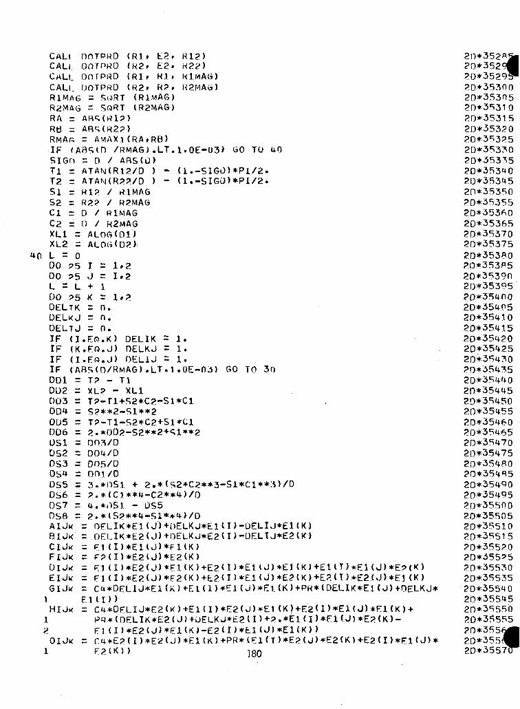
CALl OOTPRD (Rl» E2» R12)CALl. DOTPRD (R2» E2» K22)CALL OOTPRD (Rlr Rlr KlMAG)CALL DOTPRO (R2» R?» K2MAG)RiMAG = SORT (Rl.viAG)R2MAG = SORT (R2MAG)RA = ABStRl?)Rb = ARS(R22)RMAfi = AMAXl (RA»RB)IF (ABS<D /RMAGJ .LT.l.OE-03) GO TO 40SIGn = 0 / ABS(O)Tl = ATANHR12/D ) - ( 1 .-SIGO) *Pl/2.T2 r ATAM(R??/D ) - ( 1 .-SIGO) *PI/2.Si - Rl? / R1MAGS2 = R2? / R2MAGCl = D / RlMAGC2 = 0 / R2MAGXL1 = ALOG(Dl')XL2 = AL06(02)L = 0DO 95 I = 1»200 95 J = I»2L = L + 1DO 95 K r 1,2DELTK = 0.OELKJ = 0.DELTJ = 0.IF (I.EO.K) OELIK = 1.IF (K.FO.J) DELKJ = 1.IF (I.EfJ.J) OELIJ = 1.IF (ABS(0/RMAG) .LT.V .OE-03) GO TO 3oDD1 = T? - Tl002 = XL? - XL1003 = T9-ri+S2*C2-Sl*Cl004 = S2**2-S1**2OU5 = T?-Tl-S2*C2>Sl*Cl006 = 2.*DD2-S2**2+S1**2OS1 = 003/0DS2 = D04/DDS3 = 005/0OS4 = OD1/DOSS = 3.*OSl + 2.*(S2*C2**3-Sl*Cl**.'i)/DDS6 = 2.*(C1**4-C2**4)/0OS7 = 4.*OSl - OSSOS8 = 2.*(S2**4-S1**4)/DAUk = OFLIK*E1 (J)+OELKJ*E1(I)-OELU*£1(K)BUK = OELlK*E2(J)+nELKJ*E2a)-OELU*E2(K)CUk = F1 (I)*E1U)*F1U)FUK = F?(I)*E2(J)*E2(K)01JK = F5 (I)*E2(J)*El(K)+E2(I>*EMJ)*EllK)+£in)*El(J)*E?(K)EUi^ = Fl (I)*E2(J)*F2(K)+E2(D*E1 ( J) *E2 (K)+E2 ( T ) *E2 ( J) *E] (K)G1JK = C4*DFLIJ*E1 (K)^EK1)*E1 ( J) *El. (K )+PK* (DELIK*E1 (J)+OELKJ*
Eld))HIJ^ = C4*OFLIJ*E2<K)+E1(I)*E2( J)*E1 (K)+E2 ( I )*E1 ( J)*E1(K)+
PR*(OELIK*E2( J)+OELKJ*E2(I)+?.*EKI)*EKJ)*E2(K)-! tTl(I)*E2(J)*El(K)-E2<n*El(J)*EKK') )OIJK = (:4*E?(I)*E2<J)*E1(K)+PR*(F1(T)*E2(J>*E2<K)+E2<I)*F1<J)*
F2(K)> ion
20*352"i20*352920*3529?20*3530020*3530520*3531020*3531520*3532020*3532520*3533020*3533520*3534020*3534520*3535020*3535520*3536020*3536520*3537020*3537520*3538020*3538520*3539020*3539520*3540020*3540520*354.1020*354.1520*3542020*3542520*3543020*3543520*3544020*3544520*3545020*3545520*3546020*3546520*35 7020*3547520*3548020*3548520*3549020*3549520*3550020*3550520*3551020*3551520*3552020*3552520*3553020*3553520*3554020*3554520*3555020*3555520*35520*3552D*3557(T
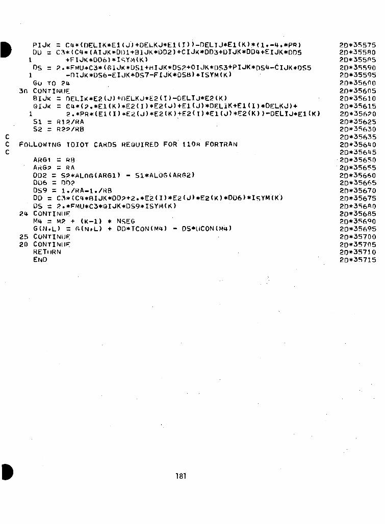
CCC
PlJk = CU*(OELIK*E1<J)+OELKJ*E1(I»-DELIJ*E1(K)*(1.-U.*PR)DL) = C3*<C4*(AIJK*DDl-»-BlJK*D02)+CIJK*DD3+QlJK*DDU+ElJ|<*OD51 +FIJK*D06)*I^Y,v)(K)DS = ?.*FMU*C3*(GlJK*DSl+HIJK*DS2+OlJK*DS3+PUK*DS^-CIJK*r)S51 -OIJK*DS6-EIJK*DS7-FIJK*DSB)*ISYM(K)Go TO ?U
3n CONTINUE8IJK = OELIK*E2(J)+OELKJ*E2(I)-DELTJ*E2(K)QIJK = CU*(?.*El(K)»E2(I)*E2(J)+El(J)*DELiK+El(I)*DELKJ)+1 ?.*PR*(EKI>*E2(J)*E2<K)+E2(I)*E1(J)*E2<K) )-DELI J*E1 <51 = R1P/RA52 = R29/RB
FOLLOWING IDIOT CARDS REQUIRED FOR 110* FORTRAN
- S1*ALOG( AR<52>
2520
ARG1 = R8ARGP = RADD2 = S5>*ALOG(ARG1)006 = DO?DS9 = l./RA-l./RBDO = C.1*(CH*BIJK*OD?+2.*E2(I)*E2<J)*E2(K)*006)*I«;YM(K)DS = 2.*FMU*C3*QIJK*DS9*ISYM(K)CONTINUEM<4. = MP + (K-l) * NSEGG(N.L> = G(N»L) + DD*TCON(M^) - DS*UCON(M4)CONTINUECONTINUERETURNEND
20*3557520*3558020*3558520*3559020*3559520*356flO20*3560520*3561020*356152D*356?020*3562520*3563020*3563520*3564020*3564520*3565020*3565520*3566020*3566520*3567020*3567520*356 020*3568520*3569020*3569520*3570020*3570520*3571020*35715
181
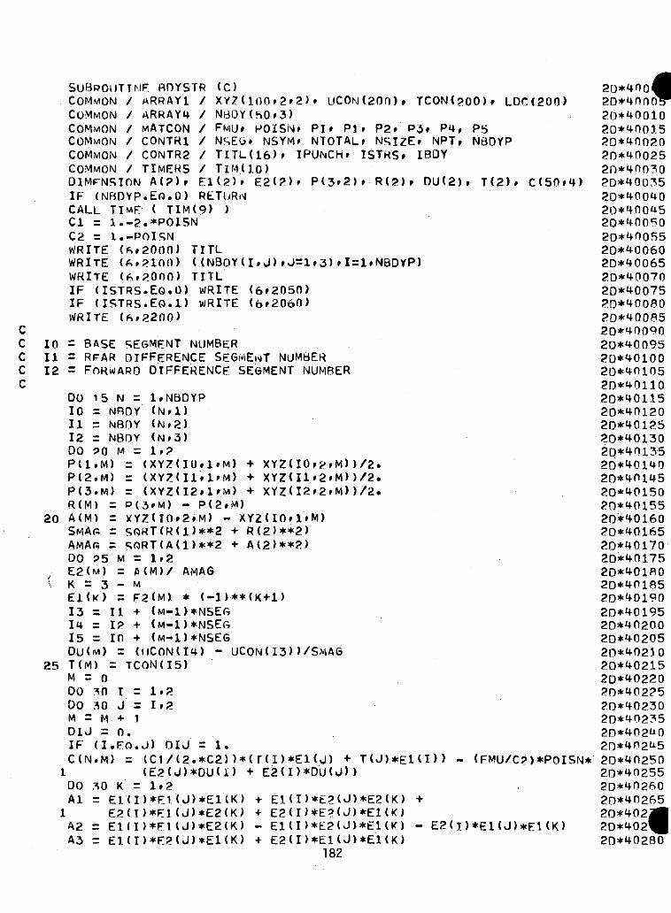
SUBROUTINECOMMONCOMMONCOMMONCOMMONCOMMONCOMMON
CC 10C IIC 12C
25
RDYSTR//////
ARRAY1ARRAY4MATCONCONTR1CONTR2TIMERS
D1MFNSION A(2)»IF (NBDYP.EO.O)CALL TIMF. ( TIM(9> )Cl = l.-2.*POISNC2 = 1.-POISNWRITE (ft.2000) TITLWRITE (6.2100) ((NBOY(I.J)»J=1.3).I-1.N6DYP)WRITE (6.2000) TITLIF (ISTRS.EO.O) WRITE (6.2050)IF (ISTRS.EO.l) WRITE (6.2060)WRITE (ft.2200)
= BASE SEGMENT NUMBER= RFAR DIFFERENCE SEGMENT NUMBER= FORWARD DIFFERENCE SEGMENT NUMBER
UCON(200). TCON(?00)» LDC(200)(C)XY7(100»2»2)NBOY(50.3)FMU. POISN. PI» PI » P2» P3f P«*»NSEG. NSYM» NTOTALf NSIZE» NPTrTITL(16)» IPUNCH» ISTRS» IBDYTIM(IO)
EK?)» E2<?)» P(3»2)» R(?)r OU<2)»RETURN
NBDYP
T(2)
0010II12DOP(l.M)P(2.M)P(3.M)R(M) =A(M) =SMAR =
15 N r= NROY= NBDY= NBOYPO M =
l.NBDYP(N.I)(N.2)
1.2= (XYZ(IO.l.M) XYZCIO»2»M))/2.
XYZ<Il»2»M))/2.XYZ(I2»2»M))/2.r (XYZ(I2»1»M)
P(3»M) - P(2»M)XYZ(IO»2»M) - XYZ(IO»1»M)
R(2)**2>A(2)**2)
A(M)/ AMAGMF2(M) * (-1)**+ (M-l)*NSEft+ (M-1)*NSEG+ (M-1)*NSEG(oCoN(i4) - UCON(I3))/SMAG
TCON(I5)
= SP)RT(A(1)**2DO 25 M = 1.2E2(M) =K = 3 -Ei(K) =13 = II14 = 1215 = 10DU(M) =T(M) =M = 0DO 30DO 30M = MDIJ =IF (I.F.O.J) DIJ = 1.C(N.M) = (C1/(2.*C2))*
L (E2(J)*DU(I)30 K = 1.2= E1(I)*E1<J)*E1(K)E2(T)*E1(J)*E2(K)
= El(I)*El(J)*E2(K)= E1(I)*E2(J)*EKK)
IJ4-
0,
1.21.2
1
DOAl
l
A2A3
T(I)*E1(J) +E2(I)*DU(J»
E1(I>*E2(J)*E2(K)E2(I)*E?(J)*E1(K)EKI)*E2(J)*E1(K)E2(I)*E1(J)*E1(K)
182
- (FMU/C?) *POISN*
- E2(I)*E1(J)*EKK)
I20* 0020*400020*4001020*4001520*4002020*4002520*4003020*4003520*4004020*4004520*4005020*4005520*4006020*4006520*4007020*4007520*4008020*4008520*4009020*4009520*4010020*4010520*4011020*4011520*4012020*4012520*4013020*4013520*4014020*4014520*4015020*4015520*4016020*4016520*4017020*4017520*4-018020*4018520*4019020*4019520*4020020*4020520*4021020*4021520*4022020*4022520*4023020*4023520*402 020*402^520*4025020*4025520*4026020*4026520*40220*40220*40280
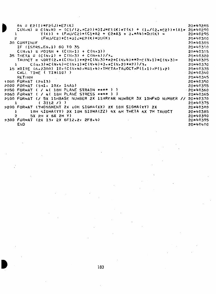
(l./(2.*C2))*(A1*3.*A4)*DU(K) -
A4 = E2U >*F?<J)*E?IK>C(N.M) = C(N»M) - (C1/(2.*C2»*DIJ*EUK)*T<K)1 T(K)> + lF.viU/C2)*<Cl*A2 + C2*A32 (FMU/C2)*C1*UIJ*E?.<K)*DU<K)
3o CONTINUEIF (ISTRS.Efc.l) GO TO 35C(N.4) = POISN * (C(N»1) + C(Nr3))
35 THETA = (C(Nrl) + C(Nr3) + C(N»4))/3.TAUOCT = sQRT<2.*<C(N»l)**2+C(Nf3)**2+C(NN4>**2-ClN»l)*C(N»3)-1 C(N»3)*C(N»4)-C(N»1)*C(N ' ' ' "*
!300) I0»(C(N»M)»M=1( TIM(IO) )
15
1000?0009050?0609100
WRITE (6»CALL TIMERETURNFORMAT (?FORMAT (\FORMAT (FORMAT (FORMAT (/
»THF,TArTAUOCT»P{lrl) »P(1»2)
10X» 16A5)/ u( ISM PLANE STRAIN/ 4( ISM PLANE STRESS5X 11HBASE NUMBER 2X
1 ( 3112 /) )?200 FORMAT (7HOSGMENT 2X iOH SISMA(XX) ?
1 IOH SIGMA(YY) 2X IOH SIGMA(ZZ)2 5X 2H X 6X 2H Y)
9300 FORMAT (2X I3» 2X 6F12.2* 2F8.4)END
**** ) )**** ) )IIHRFAR NUMBER 3X 10HFWD NUMBER //
IOH SIGMA(XY) 2X6H THETA fiX 7H TAUOCT
20*40?.B520* 029020*402 520*403002D*4030520*4031.020*4031520*403202D*403?520*4033020*4033520*4034020*4034520*4035020*4035520*4036020*4036520*4037020*403752D*403«020*4038520*4039020*4039520* 0400
183

•END 2o*^5(
20*15020*^50
184
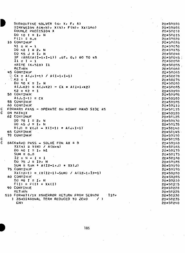
SUBROUTINE SOLVER (Nr X» F» A)DIMFNSION A(N»N)» X(N)» F(N)» XX<16n)OOURUE PRECISION XDO 10 T = 1» NFU) = O.I)
10 CONTINUENl = -N - 100 60 I = 2» N00 R5 J = I» NIF (ABS(A(I-1»I-1) ) .GT. 0.) GO TO U511 = I - 1WRITE <6»510> IIRETURN
45 CONTINUEsj'-cx = A(ja-r) / A(i-i»i-i)
• LK2 = IDO SO K = I. NA(J,K2) = A(J»K2) - CX * A(I-1»K2>K2 = K2 + 1
50 CONTINUFA(J,I-l) = CX
55 CONTINUEAO CONTINUE
C FORWARD PASS - OPERATE ON RIGHT HAND SIDE ASC ON MATPIX
62 CONTINUEDO 70 I = 2» NDO *5 J = I» NX(J) = X(J) - X(I-l) * A(J»I-1)
65 CONTINUE70 CONTINUF
CC BACKWARD PASS - SOLVE FOR AX = B
XX(W) = X(N) / A(N»N)DO ftO I = 1» NlSUM =0.012 = N - I 4- 1DO 75 J = IP» NSUM = SUM + A(I2-1»J) * XX(J)
75 CONTINUEXX(T2-1) = .(XU2-D-SUM) / A(I2-1»I?-D
80 CONTINUEDO 00 I = 1. NF(I) = F(I) ^ XX(I)
90 CONTINUERETURN
510 FORMAT1/1X 25HERROR RETURN FROM SEQSOVJ 35HOIAGONAL TERM REDUCED TO ZERO / )END
IlOr
20*5000020*5000520*5001020*5001520*5002020*5002520*5003020*500352D*500UO20*5004520*5005020*5005520*5006020*5006520*5007020*5007520*500802D*500Q520*5009020*5009520*5010020*5010520*5011020*5011520*5012020*5012520*5013020*5013520*5014020*5011520*5015020*5015520*5016020*5016520*5017020*501752D*501AO20*5018520*5019020*5019520*5020020*5020520*502102D*502!520*5022020*5022520*5023020*5023520*502'<-0
185
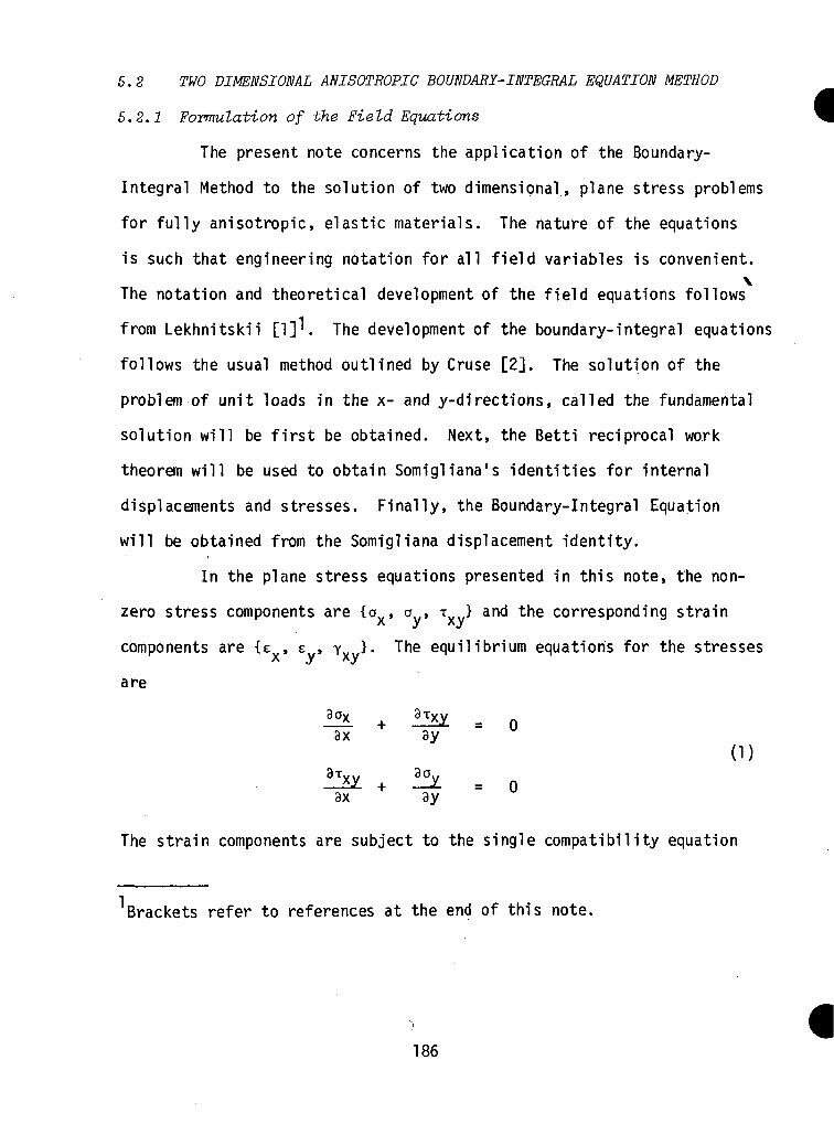
5.2 TWO DIMENSIONAL ANISOTEOPIC BOUNDARY -INTEGRAL EQUATION METHOD
5.2.1 Formulation of the Field Equations
The present note concerns the application of the Boundary-
Integral Method to the solution of two dimensional, plane stress problems
for fully anisotropic, elastic materials. The nature of the equations
is such that engineering notation for all field variables is convenient.\
The notation and theoretical development of the field equations follows
from Lekhnitskii [1]'. The development of the boundary- integral equations
follows the usual method outlined by Cruse [2]. The solution of the
problem of unit loads in the x- and y-directions, called the fundamental
solution will be first be obtained. Next, the Betti reciprocal work
theorem will be used to obtain Somigliana's identities for internal
displacements and stresses. Finally, the Boundary-Integral Equation
will be obtained from the Somigliana displacement identity.
In the plane stress equations presented in this note, the non-
zero stress components are {o , o , T } and the corresponding strainx y xy
components are {e , e , y }. The equilibrium equations for the stressesx y xy
are
3x By (1)3TVW 3 a..— M. + — JL = o8X 9y
The strain components are subject to the single compatibility equation
Brackets refer to references at the end of this note.
186
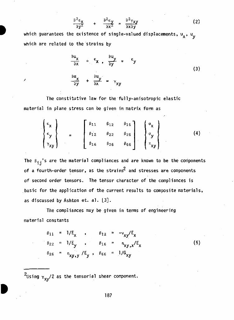
3x3y(2)
which guarantees the existence of single-valued displacements, u , ux ywhich are related to the strains by
3U
3X
3U.
' 3y(3)
3X xy
The constitutive law for the fully-anisotropic elastic
material in plane stress can be given in matrix form as
ex
eyYxy
=
3u 612 3i6~
3 12 322 ^26
3l6 326 366
°x
°yTxy
(4)
The 3..j's are the material compliances and are known to be the components* J
of a fourth-order tensor, as the strains^ and stresses are components
of second order tensors. The tensor character of the compliances is
basic for the application of the current results to composite materials,
as discussed by Ashton et. al. [3].
The compliances may be given in terms of engineering
material constants
322 = 1/E%
326 = nxy,y /Ey
3i2 = -V
3i6 = n
066 =
xy,x' x (5)
"Using y /2 as the tensorial shear component,xy
187
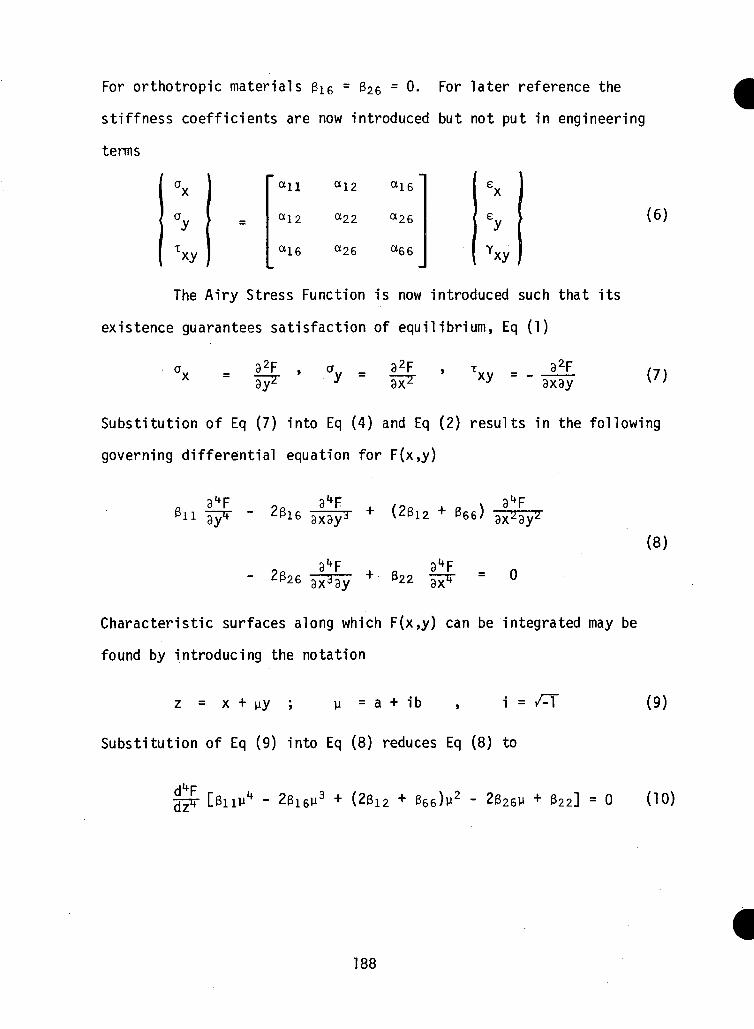
For orthotropic materials 3ig = $25 = ^- F°r later reference the
stiffness coefficients are now introduced but not put in engineering
terms
°xayTxy
=
an a12 a16
a12 a22 <*26
«16 a26 a66
exeyYxy
(6)
The Airy Stress Function is now introduced such that its
existence guarantees satisfaction of equilibrium, Eq (1)
92F 'y = 92F9XZ
xy = -y 9x9y (7)
Substitution of Eq (7) into Eq (4) and Eq (2) results in the following
governing differential equation for F(x,y)
(8)
i3y • ~z* 9xt = 0
Characteristic surfaces along which F(x,y) can be integrated may be
found by introducing the notation
z = x + py ; y = a + ib , i = /T
Substitution of Eq (9) into Eq (8) reduces Eq (8) to
(9)
£22] = o (10)
188
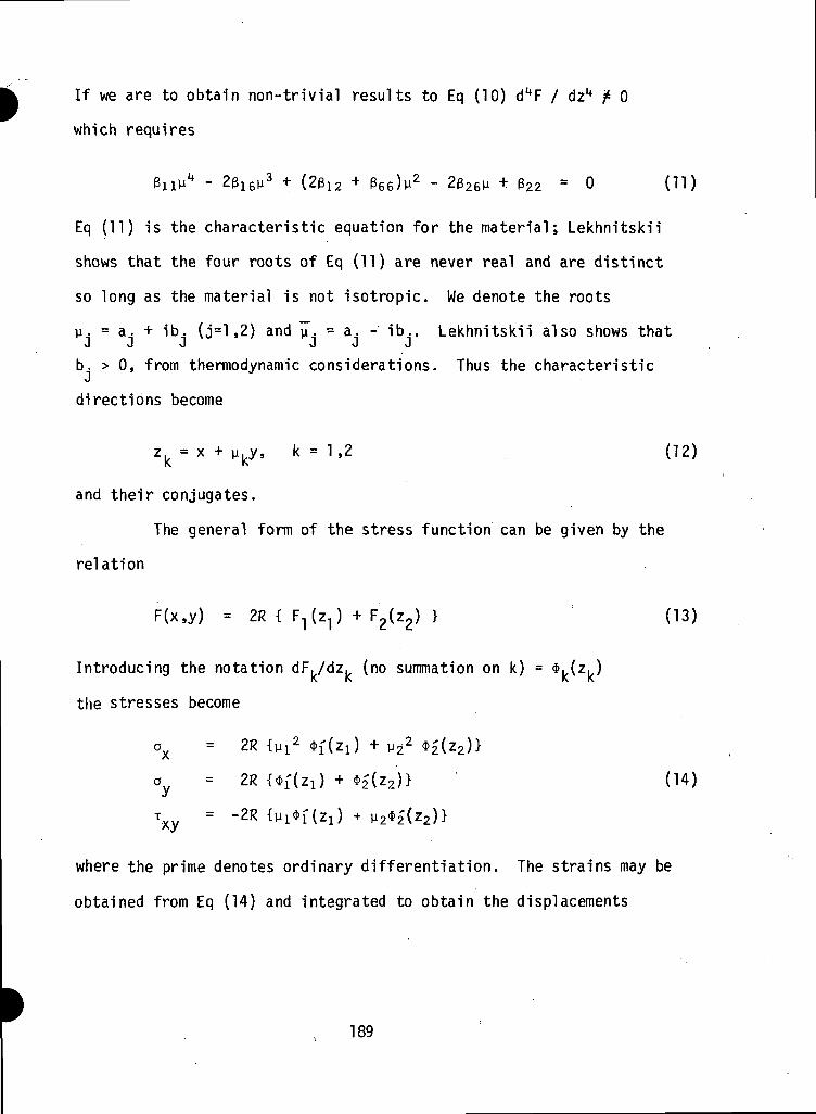
If we are to obtain non-trivial results to Eq (10) d**F / dz1* £ 0
which requires
BiiM1* - 2Si6u3 + (20i2 + e6e)p
2 - 2026P ^322 = 0 (11)
Eq (11) is the characteristic equation for the material; Lekhnitskii
shows that the four roots of Eq (11) are never real and are distinct
so long as the material is not isotropic. We denote the roots
y. = a. + ib. (j=l,2) and y~. = a. - ib.. Lekhnitskii also shows thatJ J J J J Jb. > 0, from thermodynamic considerations. Thus the characteristicJ
directions become
zk = x + nky, k = 1,2 (12)
and their conjugates.
The general form of the stress function can be given by the
relation
F(x,y) = 2R { F^) + F2(z2) } (13)
Introducing the notation dF./dz^ (no summation on k) = ^ (ZL,)
the stresses become
ox = 2R {Ml2 «f(z!) + y2
2 $£(Z2)>
ay = 2R {*f(zi) + $£(Z2)> (14)
Txy = "2R {MI$I(ZI) + H2^£(Z2)>
where the prime denotes ordinary differentiation. The strains may be
obtained from Eq (14) and integrated to obtain the displacements
189
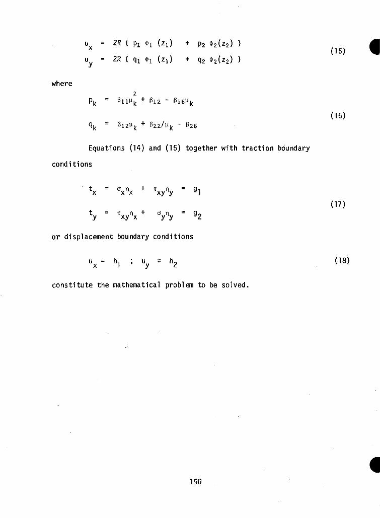
u = 2R { P! *! (Zi) + p2 *2(z2) }x (15)
uy = 2R { ql *! (zj + q2
where
Pk ~
(16)
(17)
Equations (14.) and (15) together with traction boundary
conditions
*X = °xnx + Txyny = gl
*y = Txynx+ Vy = 92
or displacement boundary conditions
ux = h1 ; uy = h2 (18)
constitute the mathematical problem to be solved.
190
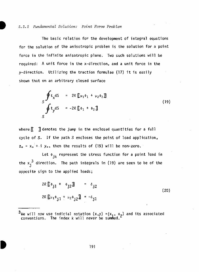
5.2.2 Fundamental Solution: Point Force Problem
The basic relation for the development of integral equations
for the solution of the anisotropic problem is the solution for a point
force in the infinite anisotropic plane. Two such solutions will be
required: A unit force in the x-direction, and a unit force in the
y-direction. Utilizing the traction formulae (17) it is easily
shown that on an arbitrary closed surface
/
= 2R_
(19)
tydS = -2R
where [f J denotes the jump in the enclosed quantities for a full
cycle of S. If the path S encloses the point of load application,
z0 = x0 + i y0» then the results of (19) will be non-zero.
Let $.. represent the stress function for a point load inJKthe x. direction. The path integrals in (19) are seen to be of the
«J
opposite sign to the applied loads;
2R (E$jl + »J2J = 6.2
(20)
We will now use indicia! notation (x,y) =(x,, x?) and its associatedconventions. The index k will never be summed.
191
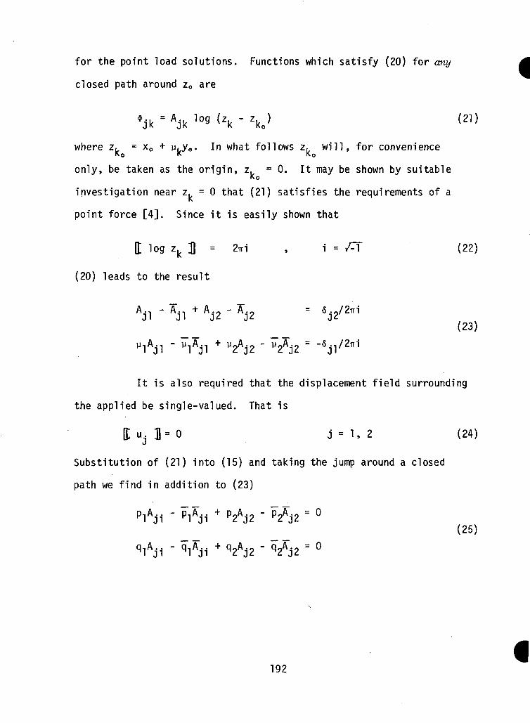
for the point load solutions. Functions which satisfy (20) for any
closed path around z0 are
*jk • Ajk ]°9 <2k - Zk.>
where z, = x0 + v.ye. In what follows z. will, for convenienceKO K KO
only, be taken as the origin, z. = 0. It may be shown by suitableKo
investigation near z. = 0 that (21) satisfies the requirements of a
point force [4]. Since it is easily shown that
It log zk B = 2*1 , 1 = /T (22)
(20) leads to the result
AJ2 - AJ2 = V2'1(23)
It is also required that the displacement field surrounding
the applied be single-valued. That is
I u. 1= 0 j = 1, 2 (24)J
Substitution of (21) into (15) and taking the jump around a closed
path we find in addition to (23)
PlAJ1 - PlAji + P2AJ2 - P2AJ2 = °(25)
= 0
192
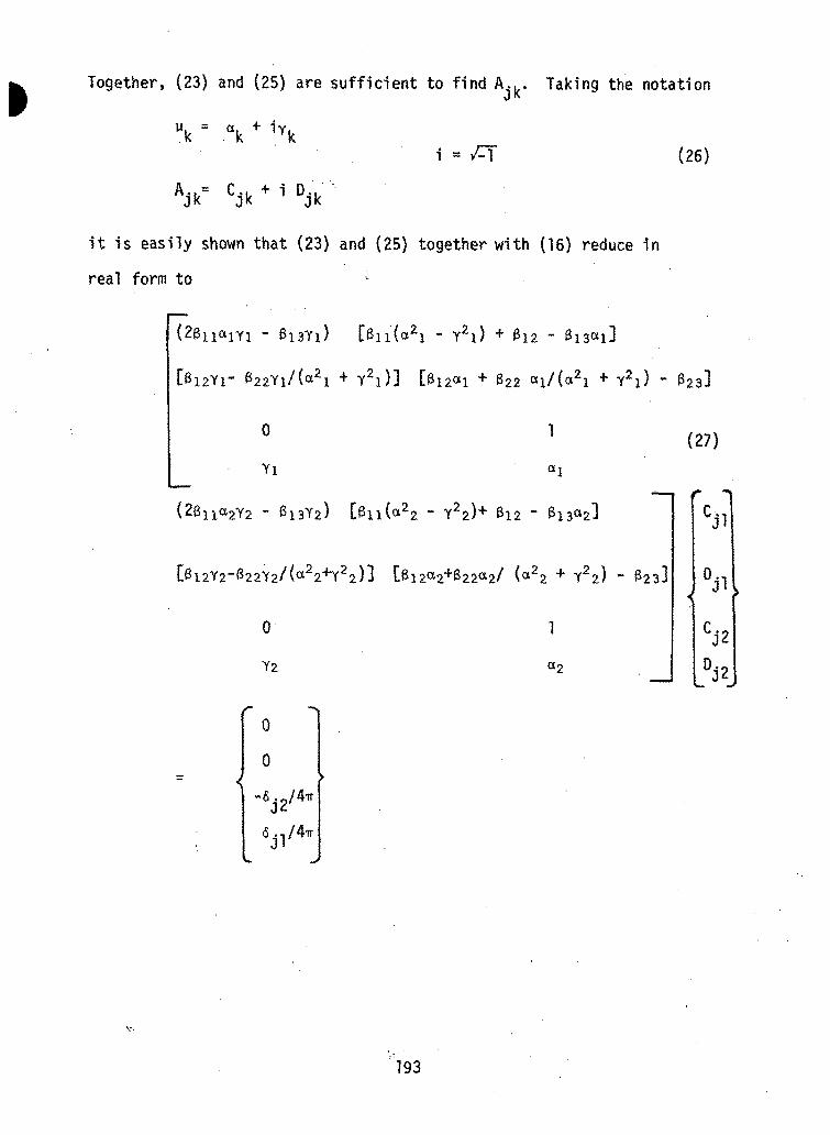
Together, (23) and (25) are sufficient to find A-k. Taking the notation
Vk =
V
1 - /T (26)
it is easily shown that (23) and (25) together with (16) reduce in
real form to - .
[B12Yl-
0
Yl
0
Y2
0
0
U2! - Y 2 l ) + 612 - 81301]
Y 2 l ) ] [812011 + 622 «1/(«21 + Y2 l ) -
1 (27)
[0ii(a22 - Y22)+ 812 -
Y22) ~
a2
193
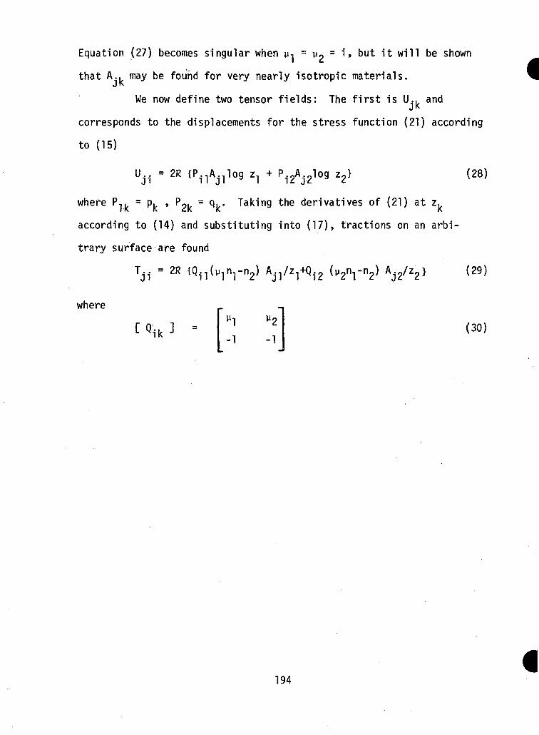
Equation (27) becomes singular when v-, = v~ = i , but it will be shown
that A., may be found for very nearly isotropic materials.
We now define two tensor fields: The first is U.. and
corresponds to the displacements for the stress function (21) according
to (15)
U... = 2R Z2>
where P,. = p. , Ppk = q,. Taking the derivatives of (21) at z.
according to (14) and substituting into (17), tractions on an arbi-
trary surface are found
where
= 2R
c "IK]
AJ2/Z2>
-1 -1
(29)
(30)
194
5.2.3 Boundary-Integral Equation
Since the governing partial differential equation (10)
admits no real characteristic surface the problem is elliptic and
the stresses and displacements are continuous. Under such circum-
stances it is easily verified that Betti's reciprocal work theorem
at the surface must be valid
J.^dS (31)
S+T S+T
The surface r is a circle of vanishing radius e surrounding the point
load; it is added to exclude the singularity from the volume. The
second integral in (31) is convergent as e -»• 0. For continuous u.
it is sufficient to investigate the behavior of the integral
Lim0 / T..<J .11e -> U I l.,dS (32)
v *
r
At a circle centered at the applied load it is seen that
yknl~n2 = -UiCose — sine) (33)
and dS = ede, 0 < 0 < 2ir. Extracting from (32) the variable part
it is sufficient to find
2lT 2TT
' viscose-sinedo( Vrn2 ds - _ /• v;
J z J yksine+cosecose-sine t~A\
195
which, upon rearrangement becomes
_p
AKtane) ,, 2} f coseJ l-p£tan*e ~ U Vy (l+p
e d (cose) (35)
Equation (35) can then be integrated directly to obtain
T"2 dS = — log [cose - u.sine]
27T
(36)
Taking the real part of the argument of the log
P| = (cose - aksine)2 + (bksine)2
and the imaginary part-1 b,s1na
cose — a.sineIJ
the result to (36) is found to be
2*
dS = 2Tri
(37)
(38)
(39)
Substitution of (39) into (32) and using (23) leads to the usual
Somigliana identity for the interior displacement
196
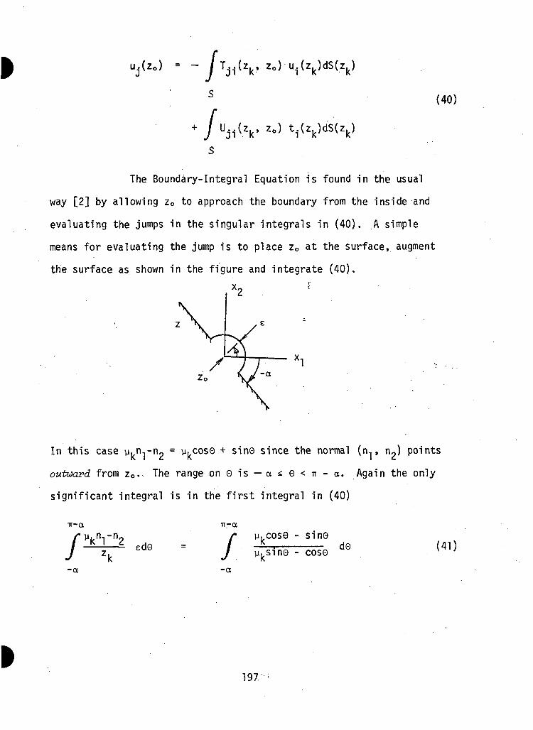
Uj(Zo) = - /VV Zo) u.(zk)dS(zk)
!..(z. , z0) t .(z.)dS(z.)J 1 • l\ I Ix IN
(40)
The Boundary-Integral Equation is found in the usual
way [2] by allowing z0 to approach the boundary from the inside and
evaluating the jumps in the singular integrals in (40). A simple
means for evaluating the jump is to place z0 at the surface, augment
the surface as shown in the figure and integrate (40).
In this case v^i'^p = ^i,0050 + s"in0 since the normal (n,, n2) points
outward from z0. The range o n 0 i s - a i 0 < i r - a . Again the only
significant integral is in the first integral in (40)
TT-CI
ed0
-a
ir-a
-a
y,cos0 - sine
y.sin0 - cose (41)
197-
which, by the same steps as above, becomes
TT-Ot TT-Ot
(42)/
Wn
-4-a -a
Substitution of the limits in (42) yields
•a
/ W t"l~"9K '—- edG = - iu (43)
-.Again using the relations (23), (40) becomes
V2 + /Vids '/Vi* (44)s s
Equation (44) is the Boundary-Integral Equation which relates unknown
boundary data to known boundary data. Once (44) has been solved
numerically (§V), (40) can be used to obtain interior displacements
and stresses.
198
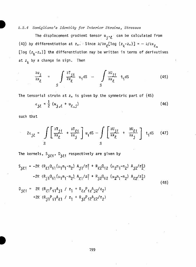
5.2.4 Somigliana's Identity for Interior Strains, Stresses
The displacement gradient tensor u.,/, can be calculated from
(40) by differentiation at z0. • Since 3/3xJlog (z. -z0)] = - 3 /3x«
[log (Z . -ZQ) ] the differentiation may be written in terms of derivatives
at z. by a change in sign. Then
3u .(45)( 3Tii ( 9Uii
J ^f UidS - J ^f
The tensorial strain at z0 is given by the symmetric part of (45)
£ = ( u + u ) <46>
such that
/T8Tii 3T/i 1 /" F8Uii aU/i "1- / f _ II + _ ±1. u dS - / J1 + — ilJ L9^ ^ JU idS J [3X, 3X. J
The kernels, S.». , D.«. respectively are given by
T^J VZ1 + R£2Qi2 Z"!' AJ2/Z2}
(48)Op rp P A / -7 4-D P A / -j \dK iK^^^A^ / Z] + K£/ iz
Aj2/Z2}
199
where R^k = 1, R2k = P.. It is assumed that the boundary is piecewise M
flat. Then (47) becomes
2EJ£ = / Sj£1 UidS ~ / ViV5 (49)
The stresses can be determined by substitution of (49), with
Yxy = 2e12, ex = en, ey = e22, into (6).
200
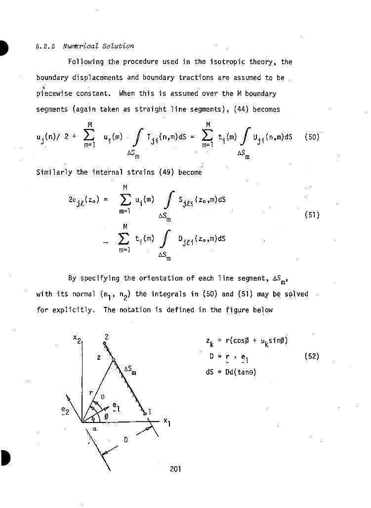
5.2.5 Numerical Solution
Following the procedure used in the isotropic theory, the
boundary displacements and boundary tractions are assumed to be*
piecewise constant. When this is assumed over the M boundary
segments (again taken as straight line segments), (44) becomes
M M
,m)dSm=l
u.(m) f T..(n,m)dS = £ t.(m) /U..(n,1 J J1 m=l 1 J J1
ASm ASm
Similarly the internal strains (49) become
M
m=l
Mm
m=l
D..£ i(zo,m)dS
ASm
(50)
(51)
By specifying the orientation of each line segment, AS ,
with its normal (n, , nj the integrals in (50) and (51) may be solved
for explicitly. The notation is defined in the figure below
ASm
zk = r(cos|3 +
D = r • e,
dS = Dd(tan0)
(52)
201
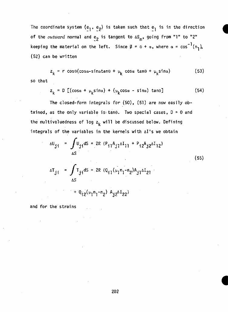
The coordinate system (e,, e2) is taken such that e, is in the direction
of the outuard normal and e« is tangent to AS , going from "1" to "2"
keeping the material on the left. Since 0 = 0 + a, where a = cos" (n,),
(52) can be written
z. = r cos0(cosa-sinatane + y. cosa tane + y.sina) (53)
so that
z. = D [(cosa + y.sina) + (y.cosa - sina) tane] (54)
The closed-form integrals for (50), (51) are now easily ob-
tained, as the only variable isi tane. Two special cases, D = 0 and
the multivaluedness of log z. will be discussed below. Defining
integrals of the variables in the kernels with Al ' -s we obtain
AU^ = /U,,dS = 2R
AS(55)
AS
and for the strains
202
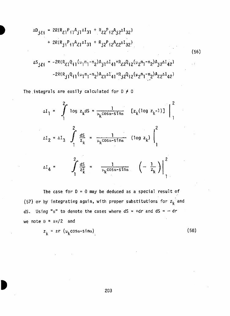
I AVi = 2R{R£lPilAjlAl31 + R£2Pi2Aj2Al32}
(56)
The integrals are easily calculated for D f 0
•Al, = log zkdS =y.COSa-Sina
[zk(log
i
dSy. COSa-Sina
1
The case for D = 0 may be deduced as a special result of
(57) or by integrating again, with proper substitutions for z. and
dS. Using "±" to denote the cases where dS = +dr and dS = - dr
we note 0 - ±ir/2 and
z. = +r (ykcosa-sina) j (58)
203
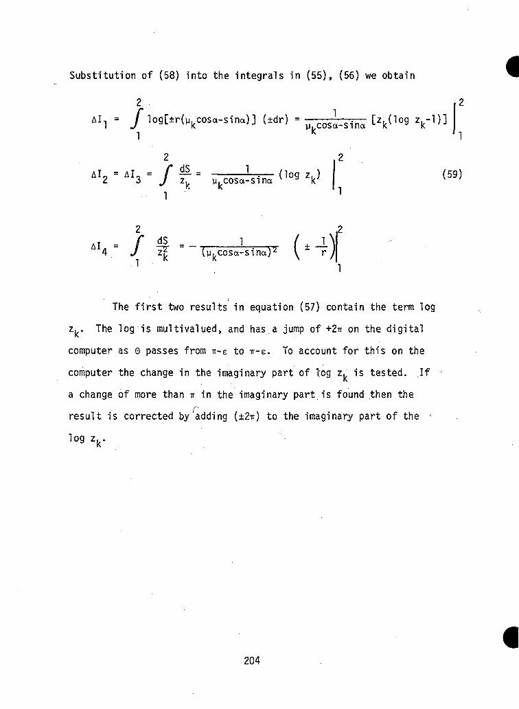
Substitution of (58) into the integrals in (55), (56) we obtain
= /log[±r(ykcosa-s1na)] (±dr) • „ C0j.s1na [zkOog
AI2 = AI3 =dS _
y. cosa-sina ^ °9 zk (59)
2 ,2dS - 1 ( + -±\\Z? (y.COSa-Sina)2 V r /K K \ /(
11
The first two results in equation (57) contain the term log
z. . The log is multivalued, and has a jump of +2ir on the digital
computer as e passes from ir-e to'ir-e. To account for this on the
computer the change in the imaginary part of log z. is tested. If J
a change of more than u in the imaginary part is found then the
result is corrected by'adding (±277) to the imaginary part of the -
log z.
204
5. 2. 6 Usage Guide for ANISOT
The computer program is divided into three major sections,
along the same lines as the solution just detailed. The first
section solves the boundary-integral equations (44), producing
a fully known set of boundary tractions and displacements. The
next section utilizes Somigliana's identity (51) to obtain
stresses at specified interior points. The final section deter-
mines stresses at the surface of the body, using the tractions
obtained in section one, and the tangential derivatives of the
displacements.
The boundary solution may be output on punched cards
if desired. This option allows the user to input the boundary
solution directly, and the program will begin execution of
sections two and three.
5.2.6.1 Problem Size Specifications
The program allows up to two degrees of symmetry of
geometry and boundary conditions. Present array dimensions limit
the number of boundary segments to 80 (320 with symmetry), but
capacity may be increased by changing the common statements labeled
ARRAY! and ARRAY2. A number of other cards should also be modified,
and are listed below, by card number:
ANI10065 ANI15235
ANI10070 ANI20035
ANI10100 v ANI5005
ANI15050
205
The number of interior points which may be specified is
limited to 200, while the limit on surface stress points is 50.
These limits may be increased by changing ARRAYS and ARRAY4,
respectively.
The time required for execution of each subroutine is
calculated through an assembly language subroutine, TIME. Users
of computers other than the Uhivac 1108 should provide their own
routine for this purpose, or insert a dummy routine, TIME(T).
5.2.6.2 Specification of Material Constants
Material constants are specified through four matrices,
listed below:
STIFF, stiffness matrix (6)
FLEX, compliance matrix (4)
MU, solutions to the characteristic equation (11)
AX, coefficients of the net load terms in
Lekhnitskii's stress function (see §11)
The coefficients AX are calculated in a program called
AXCALC, which serves as an auxiliary program. All the matrices
described above may be obtained as punched output from AXCALC, and
inserted directly into the data deck.
206
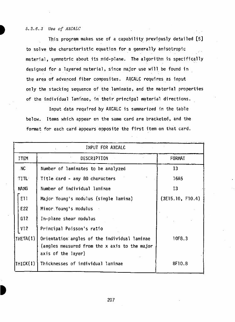
5. 2. 6. 3 Use of AXCALC
This program makes use of a capability previously detailed [5]
to solve the characteristic equation for a generally anisotropic
material, symmetric about its mid-plane. The algorithm is specifically
designed for a layered material, since major use will be found in
the area of advanced fiber composites. AXCALC requires as input
only the stacking sequence of the laminate, and the material properties
of the individual laminae, in their principal material directions.
Input data required by AXCALC is summarized in the table
below. Items which appear on the same card are bracketed, and the
format for each card appears opposite the first item on that card.
INPUT FOR AXCALC
ITEM
NC
TITL
NANG
Ell
E22
G12
V12
THETA(I)
THICK(I)
DESCRIPTION
Number of laminates to be analyzed
Title card - any 80 characters
Number of individual laminae
Major Young's modulus (single lamina)
Minor Young's modulus
In-plane shear modulus
Principal Poisson's ratio
Orientation angles of the individual laminae(angles measured from the x axis to the majoraxis of the layer)
Thicknesses of individual laminae
FORMAT
13
16A5
13
(3E15.10, F10.4)
10F8.3
8F10.8
207
5.2.6. 4 Identification of Parameters in ANISOT
All parameters necessary for use of the integral equation
program are defined below. For easy reference, the more important
ones are defined on cards numbered ANI5065 - ANI15120 in subroutine
SETUP. All the descriptions below are summarized in Table 2, and
parameters which may be described concisely appear only in Table 2.
NODE (I,J) - a temporary array which stores the two node
numbers associated with each segment number
('rear1 number, then 'forward' number)
XYZM (I,J) - a temporary array containing the x, and x2
coordinates of each node* in that order.
PTIN (I,J) - coordinates of the interior stress solution
points (x,,Xp). These are read only if NPT
f 0.
NBDY (I,J) - three segment numbers necessary for the
surface stress solution, read only if NBDYP
^ 0. For each segment on which a stress
solution is desired, three segment numbers
are read, in the following order: segment
number on which stress solution is desired;
segment number for /the "rear" difference value
of AU/AS; segment number for the "forward"
difference value of AU/AS. The 'forward' direction
208
is taken as the positive "s" direction, always
directed along the boundary of the body with
the material on the left.
5.2.6. 5 Boundary Conditions
Both traction and displacement boundary conditions are possible,
and are input by means of a NAMELIST read statement. The boundary
data is preceded and followed by control cards, as shown below:
_$ BDYCON
J DATA
All boundary conditions are initialized to zero and the
boundary condition key, LDC(I), is initialized to 1, meaning a traction
boundary condition is assumed for each segment. Setting LDC = 2
means a displacement boundary condition will be specified for the
given segment and direction. Traction conditions are specified by
a parameter TCON(I), while displacement conditions are specified by
UCON(I).
All x-j-direct!on boundary data is stored, followed by
x2-direction data. The value of the subscript I for the boundary
parameters (UCON, TCON, LDC) is determined in the following manner.
For data specified in the x, direction,
I = the segment number (N), but for the x2 direction
I = N + NSE6, where NSEG is the total number of boundary segments.
For example consider a body which has been represented by 24 segments.
209
Tractions specified on segment 6:
_TCON(6) = .100E04, (KI traction)
_TCON(30) = .325E04, (\2 traction)
Displacements specified on segment 9:
_LDC(9) = 2, LDC(33) =2,
_UCON(9) = 0.001, (x1 displacement)
_UCON(33) = 0.004, (x2 displacement)
Displacements set at zero on segment 1:
_LDC(1) = 2, (X])
_LDC(25) =2, (x2)
210
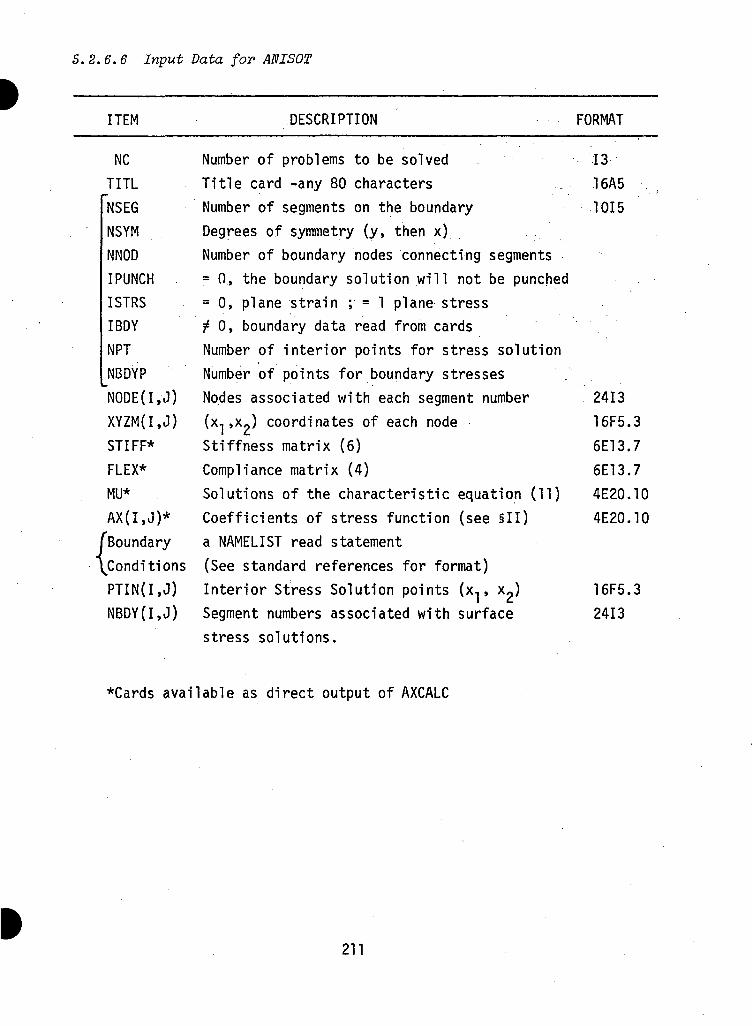
5.2.6.6 Input Data for ANISOT
ITEM
NC
TITL
NSEGNSYM
NNOD
I PUNCH .
ISTRS
IBDY
NPT
NBDYP
"NODE(I.J)XYZM(I.J)
STIFF*
FLEX*
MU*
AX(I,J)*
^Boundary"\Conditions
PTIN(I.J)NBDY(I,J)
DESCRIPTION
Number of problems to be solvedTitle card -any 80 charactersNumber of segments on the boundaryDegrees of symmetry (y, then x)Number of boundary nodes connecting segments= 0, the boundary solution will not be punched= 0, plane strain ; = 1 plane stressf 0, boundary data read from cardsNumber of interior points for stress solutionNumber of points for boundary stressesNodes associated with each segment number(x, ,x?) coordinates of each nodeStiffness matrix (6)Compliance matrix (4)Solutions of the characteristic equation (11)Coefficients of stress function (see §11)a NAMELIST read statement(See standard references for format)Interior Stress Solution points (x, , x«)Segment numbers associated with surfacestress solutions.
FORMAT
13
16A5 . ;
1015
2413
16F5.3
6E13.7
6E13.7
4E20.10
4E20.10
16F5.3
2413
*Cards available as direct output of AXCALC
211
5.2.7 References
[1] S. G. Lekhnitskii, Theory of Elasticity of an Elastic Body,Hoi den-Day (1963).
[2] T. A. Cruse, Application of the Boundary-Integral EquationMethod to Problems of Solid Mechanics (In preparation).
[3] J. E. Ashton, J. C. Halpin, P. H. Petit, Primer on CompositeMaterials: Analysis, Technomic (1969).
[4] E. Sternberg, R. A. Eubanks, "On the Concept of ConcentratedLoads and an Extension of the Uniqueness Theorem in the LinearTheory of Elasticity", Journal of Rational Mechanics andAnalysis, 4 (1955).
[5] H. J. Konish, Jr., "Numerical Calculation of the CharacteristicParameters for a Generally Anisotropic Plate - MULTMU UsageGuide", Report SM-65, Carnegie-Mellon University, (June 1971).
212
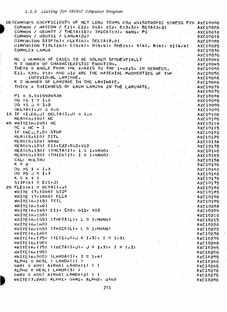
5.2.8 Listing for- AXCALC Computer Program
DETERMINES COEFFICIENTS OF NET LOAD TERMS FOR AN1SOTROPIC STRESSCOMMON / MATCON / Ell. E22. G12» Vl2» E<3.3)» BETA(3.3)COMMON / GEOMTY / THETA(IO). THICKdO). NANG» PICOMMON / ROOTS1 / LAMUA(2U)DIMFNSION STlF(b). FLEX(6). DELTA(2,2)DIMENSION TITL(16). CU.4). BU.t*). RHSU). XU), RU) .' XI <H » tCOMPLEX LAMOA
NC = NUMBER OF CASES TO BE SOLVED SEQUENTIALLYN = ORDFR OF CHARACTERISTIC EQUATION.THETA = ANGLE FROM THE X-AXIS TO THE I-KXIS. IN DEGREES.Ell, £22. V12» AND «lid ARE THE MATERIAL PROPERTIES OF THF
INDIVIDUAL LAMINAE.K = NUMBER OF LAMINAE IN THE LAMINATE.THICK = THICKNESS OF EACH LAMINA IN THE LAMINATE.
PI = 3. HU5926536OQ 15 I = 1.2L>0 15 J = 1.2OELTA(I.J) =0.0
15 IF (I.EQ.J) DELTA(I.J) = 1.0REAP) (S.I 00) NC
45 WRITE(ft.105) NCNC = NC - 1IF (NC.LT.O) STOPREAO(5.110) TITLREAn(5.120) NANGREAn(S»125) E11.E22.G12.V12REAO(5.130) (THETA(I). 1 = l.NANG)REAn(S.J35) (THICK(l). I = l.NANG)CALL MULTMUK = 0DO P5 I = 1.3DO ?5 J = I»3K = K + 1STIF(K) = E(I»J)
25 FLEV(K) = BETA(i.J)WRITE (7.1000) STIFWRITE (7.1000) FLEXWRITE<6.115) TITL
WRlTE(ft. 1*4.5) Ell. E22» G12. V12WRlTE(fS.lSO)WRlTE(ft»lft5) (THETA(L). L = l.NAN(i)WHlTE<6».1.ftO)WKlTE(6»lh5) (THICK(L). L = l
WRITE((S,175) ((E(I'J)»J = 1.3). I = 1.3)WRlTE(ft»190)WRlTE(ft.175) ((dETA(I.J). J = 1.3). I = 1.3)
WRlTE(6r?00) (LAMDA(I). I = l.t*)ALPM1 = REAL ( LAMDA(i) )6AM1 = ABS( AIMAG( LAMDA(l) ) )ALPH2 = REAL( LAMDA(3) )GAM? = ABS< AIMAG( LAMDA(3) ) )WRITE(7.2«0) ALPH1 . GAM1. ALPH2. t»AM?
FTM AXCIOOOO.AxcmoosAXC10010AXC10015Axcion?o
) A'XC 10025AXC10030AXC.10035AXC10010AXC100U5
AXCino55AXC10060AXC10065AXC10070AXC10075AXC100POAXC100P5AXC10090AXC10095AxcmiooAXClOinsAxcmiroAXC10115AXC10120AXC10125AXC10130AXC10135Axcinmo.AxcloiasAxcinisoAXC10155AXC10160AxciniissAXC10170AXC10175AXCIOIPOAXCIOIPSAXC10190AXC101Q5AXC10200AXC10205AXC10210AXC10215AXC10220AXC10225AXC10230AXC10235AXC10240AXC102U5AXC10250AXC10255AXC102ftOAXCin2ft5AXC10270AXC10275AXC102PO
213
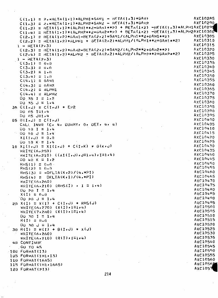
C(l.l) = P.*HtTAC(1.3) = ->.*BETAC(1.2> = rtETA(l»Cli.tf) = BETA(1»C (2.1) = BETA (lrC(2.2) = BETA(1»
I - BETA(9.3)C 12 . 3 ) = MET A (1 rC12.4) = HETA(1»
o.oD.O1.01.0GAMtGAM?.ALPH1ALPH2
05
10
20
30
100105110115120
(1»1)*ALPHl*GAMl - BETAU »3)*GAMi(111) *ALPH2*GAM2 - BETA(1.3)*GAM?1 )*(ALPHl**2-bAMl**?) + P£TA(1»2) -BETA(1»3)1)*(ALPH2**2-6AM2**9) + B£TA(Jl»2) -OETA (1. »3)?.) *GAMl-BETA (2 » 2) *GAM1/ ( ALPhl **2-«-GAMl**2 )2)*ALPB1 + l3ETA(2f2)*ALPHl/{ALPHl**2+GAiVl1**2
? ) *(^AM2-BETA (2 » 2 ) *GAM2/ ( Al_PH?.**2+6AM2**? )?)*ALVH2 * t>ETA(2»2)*ALPH2/<ALPH?**2+GAivi?**2
C(3 .1 )C ( 3 . 3 )C ( 3 . 2 >C ( 3 » 4 )CCU'l)C14.3)C ( 4 . 2 )
DO 35Do :^5C(I.J)DO 05DO 05
J = 1»4= C( I»J ) * E?2
1 = 1.4
DUMMY i Or DETrCALL INVR (c.DO 1o i = i.4DO 10 J =1.4XK T f J) = 0 . 0DO 10 K = 1.4X I ( T . J ) = XI(I .J) + C ( I . K )
u)
6(K»J>
WHITE 1 6. 2 10) ( (xi(i»J) »j=i»4DO ao K = IfPRHS(l) =0.0RHS(2) = 0.0RhS(3) = -DFLTAlKr2)/U.*PI)
4) = DELTAIK»1)/(4.*PI)
WRITE ( ft » 2 1.0) (RH5(I) » I = !•«*)DO 90 I = 1»UX ( I ) = 0 . 000 ?0 J = !»<+X(I) = X( I) -«- C l l » J) * RHS(J)WR.IT£(6.270) (X(I)»1=1»4.)WRITE(7.2HO) (X(I) » I. = l»4)DO :*0 I = 1»4R ( I ) = 0.0DO * J =
* X(J)WRlTE( f t . ? f>0 )WRlTEl f> .210) (CONTINUEGO TO 45FORMAT(i3)FORMAT(iHir13)FORMAT(iftA5)FORMATdHI»FORMAT(9I3)
AXCin2A5AXC10290
*AI.PM1AXC102P*ALPH2AXC1030
AXC10305) AXC10310
AXC10315AXC103?0
) AXC103P5AXC10330AXC10335AXC10340AXC10345AXCin350AXCl'0355AXC10360AXC1036.5AXC'10370AXC10375AXC103BOAXC10385AXC10390
AXC1D405AXC10410AXC104.1.5AXCln4?0AXC10495AXC10430AXC10435
Axri0455AXCin4P.OAXC10465AXC10470AXC10475AXC104«0
AXC10500
AXC10510AXC10515AXC10520AXC10525AXC 10530AXC10535AXC10540AXC10545AXC10550AXC10555AXC10560AXC105A,AXC105
214
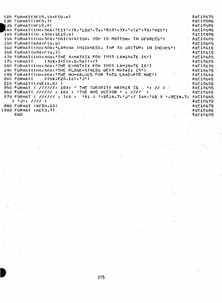
1.50
1*0
1501551601651701751 U f \A 0 1 '
190195200210250260270
ij280
FORMATFORMATFORMATFORMATFORMATFORMATFORMATFORMATFORMATFORMATFORMATFORMATFORMATFORMATFORMATFORMATFORMATFORMATFORMAT
FORMAT
(3E15(10F8(HF10
( IH »( 1 HO »(URX»( 1HO»((((((((
URX '1HO»
1HO»1HO»1HO»
(/uE
. 1 0 r F 1 0 . U )
. 3 )
.tt)3f>X» «E11' »7X» 'E22» »7X»30XfbE10.1)30X» 'ORIFNI ATION» TOPF 1 0 . b )30X» 'LAMINA THICKNESS*F1U.snx»(. OX30X>?snx»20X»2 (5X11.8
( //////(
/r
//////( ////// f f
0.10
7)'THE» 3 ( E 1'THE'THE'THE»F20.) )» 10X» 10X
> in
,
A-MATRIX<4.•5»5X ) )E-MATRIX
FOR• / )FOR
PLANE-STRESSMU-VALUES FOR
ti
X
e) • ' J' )
» THE> 'THE' *A1
10 BOTTOM' IN
TOP TO BOTTOM
THIS
THISBETATHIS
LAMINATE
LAMINATEMATKlX ISLAMINATE
IDENDITY MATRIX ISRHS VECTOR= » » 2El<*.
' » ////
•7X»»V21»
DEGREES')
» IN INCH
IS' )
IS')')ARE')
'» // ))
7» »J» »/ 10Y» »A2 =
looo FORMATEND
(6E13.7)
AXC10575AXC105ROAXC105R5
AXC10600AxcinensAxcinisio
AXC106?5AXC10630AXC10635AXC106UOAXC10645AXC10650
AXC10660
AXC10670AXC10675AXC10680AXC10605
215
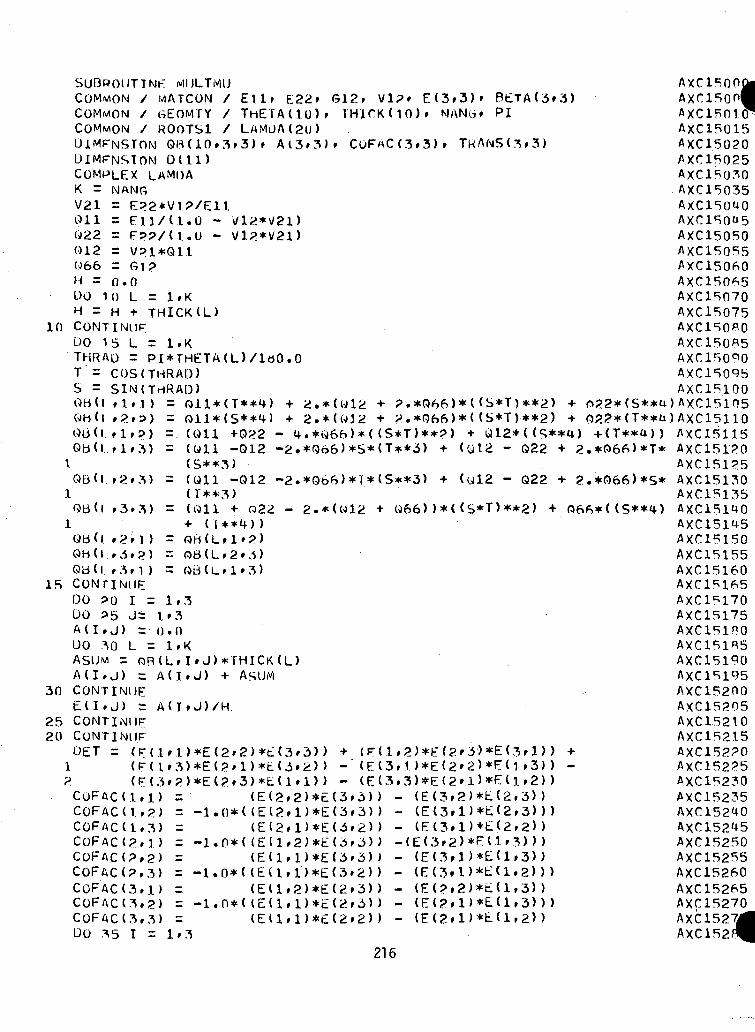
SUBROUTINE MIJLTMUCOMMON / MATCON / Ellf E22» G12. VI?. E(3.3)» RETA<3»3)COMMON / GEOMTY / ThETAdO). IHlCKdO)* NANti* PICOMMON / ROOTS1 / LAMUA(2D)DIMENSION Q6(10.3f3)f Al3f3)f COFAC(3.3). TRANS(3.3)D1MFNSTON 0(11)COMPLEX LAMOAK = NANGV21 = E?2*V1?/E11
1AXC1500AXC15Q01
AXC15010'AXC15015AXC150?0AXC15025
AXC15035AXC150UO
Oil022012066H =DO 1H =
00H
Ell/d.E??/d.V?1*Q11fV l?
.0L = l.K+ THICK
00
(L)10 CONTINIIF
DO 15 L = l.KTHRAD = PI*THETA(L)/lttO.OT = COS(THRAD)S = SIN(THRAO)
If 1 ) = Oil*OB (IOB (I »?.P) = Oil*OB(l fl.P) = (OilOB (1.1.3) = (Oil
LQBd. . ?..,
LQBd..3»:
-012 -2
(b*T)**2)(S*T)**2)
<S*T)**?) +• Q12**Q66)*S*<T**3) + (Q12 - 022
Q2?*(T**u) +(T**^))
+ 2.*066)*T*
= (Oil -012 -2.*066>)*T*(S**3)(T**3)
= (Oil + Q22 - 2.*(012 + 066)
•+• (Q12 - 022 + 2.*066)*S*
*( (S*T)**2) +
AXC15050AXC15055AXC15060AXC15065AXC15Q70AXC1CS075AXC150POAXC15005AXC15090AXC15095AXC1S100)AXC15105)AXC15110AXC15115AXC15170AXC151?5AXC15130AXC15135
OB (I f 2f 1 ) = OB(Lf If 2)OB (I f3.P) ~ oB(Lf2f3)OB (I . 3. 1 ) = OB (L. If 3)
IB CONTINUEDO 90 I = 1.3DO ?5 J= 1»3A (I. J) r i). nDO 30 L = l.KASUM = OR(LfIfJ)*THICK(L)A(I.J) = A(I.J) + ASUM
30 CONTINUEE(I.J) = A(I.J)/H
25 C O N T I N I I F20 CONT1IMUF
D£T = (F(lf D*E(2f2)*t(3f3)>
AXC15145AXC15150AXC15155AXC15160
COFACCOFACCOFACCOFACCOFACCOFACCOFACCOFACCOFACDO 35
ddd(?(?(?(3(3(3I
t........
1)2)3)1 )2)3)1)2)3)
1.
-1
-1
Ml 1
-1
3
.0*
.0*
.0*
.0*
((((( ((( ((( ((
0*((E12»1)*E(3»3)(E(2»D*E(3»2>
- (E(3,3)*E(2»l)*E(l. f2) )3.3)) - (E(3»2)*E(2r3))
- (E(3-»1)*E(2»3»)- (E(3fl)*£<2f2))
AXC15170AXC15175AXC15180AXC1S105AXC15190AXC15195AXC15200AXC15205AXC15210AXC15215AXC15220AXC152?5AXC15230AXC15235
(Edf2)*E(2f3) ) -(E(l.l)*E(2f3)) -(Edf D*E(2f2) ) -
216
AXC15250AXC15255AXC15260AXC15265AXC15270AXC15271AXC152?
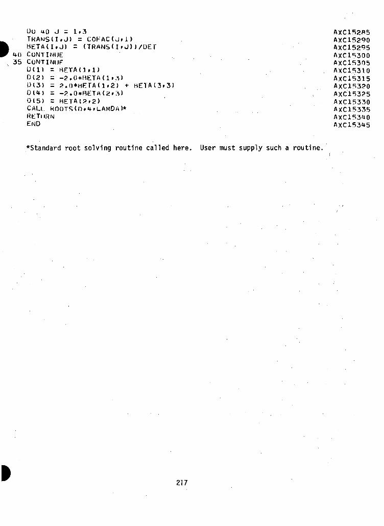
00 UO J = 1.3 AXC152B5TKANS(I.J) = COFAC(J»1) . AXC15290BETA(I.J) = (TRANS(I»J))/OET AXC15295CONTINUE Axci'ssooCONTINUF AXCISSOS0(1) = HETA(1,1) AXC153100(2) = -2.0*HETA(1»3) AXC153150(3) = ?.{)*HETA(1»2) + BETA(3f3) . AxC153?00(1) = -2.0*R£TA(2».}) AXC153250(5) = HETA(J>»2) AXC15330CALl KOOTS(n»M-»LAMDA)* AXC15335RETURN AXC15310END AXC153U5
*Standard root solving routine called here. User must supply such a routine.(
217
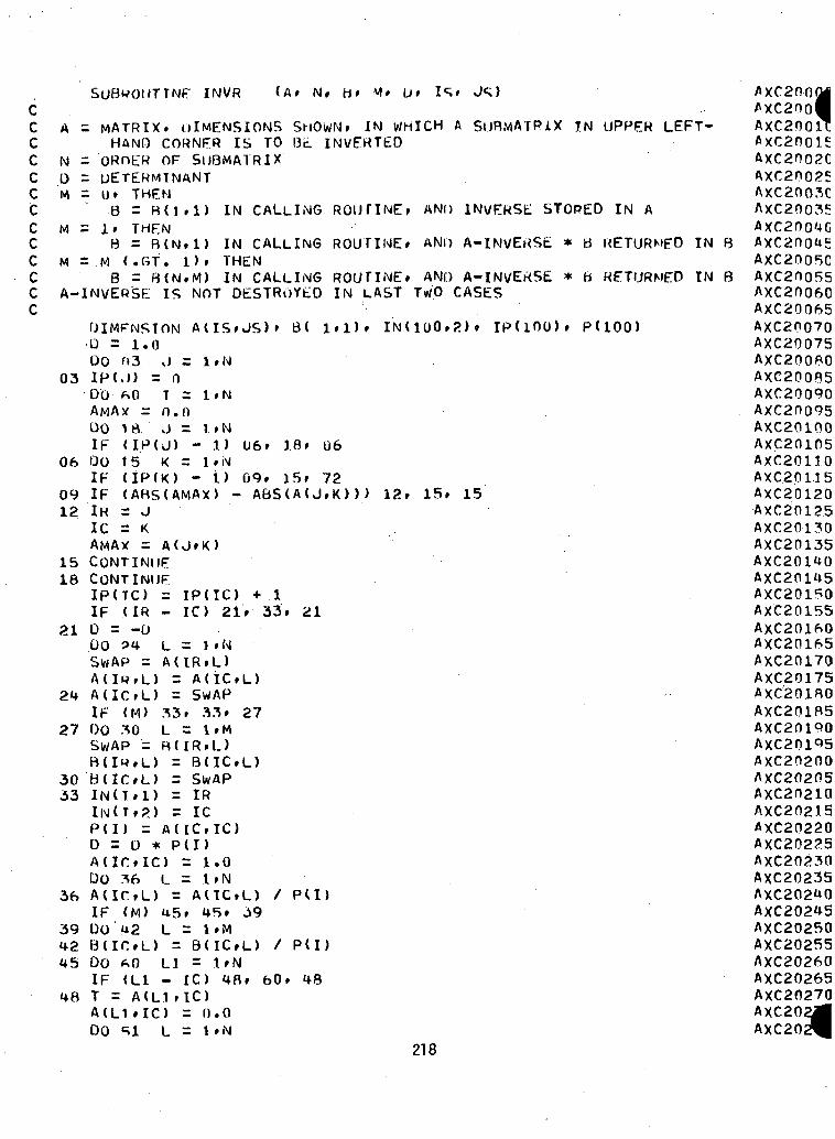
SUBROUTINE INVR (A» N» H» M* U*Ccccccccccccc
A
NDM
M
M
A-
03
06
0912
= MATRIX. DIMENSIONS ShOWN* IN WHICH A S t J R M A T P A X IN UPPER LEFT-HAND CORNER IS TO 131. INVERTED
= ORnER OF SllBMATRIX= DETERMINANT= 0* THEN
8 = B(J.l) IN CALLING ROUTINE* AN() INVERSE STORED IN A= 1* THEN
B = R(N»1) IN CALLING ROUTINE* AND A-INVEKSE * B RETURNED IN B= M (.GT. D* THEN
B = B(N.M) IN CALLING ROUTINE* AMI) A-INVERSE * B RETURNED IN BINVERSE IS NOT DESTROYED IN LAST Tm/'.O CASES
DIMFNSTON A(IS»JS>* B( I.D* iN(ioo.2)» ip(ioo)* p(ioo)•D = 1.0DO f>3 J = l.NIP(.I) = n
• DO- *0 T = 1»N= n.o
IB J = l.N<IP(J) - 1)15 K = 1»N(IP(K) - 1)
1518
21
24
27
3033
36
39
45
48
DOIF00IFIFIR1C
U6» 18 » 06
(ARS(AMAX)= J= K
AMAV = A(J»K)CONTINUECONTINUEIP(TC) = IP(IC) +1IF (IR - 1C) 21* 33* 21D = -DDO ?4 L = 1»NSWAP = A(IR.L)A(Ia*L) = A(IC»L)A(IC*L) = SWAPIF (M) 33. 33* 27DO 30 L = 1*MSWAP = R(IR.L)Bdw.L) = B(IC*L)B(IC»L) = SWAPIN(T»1) = IRIN(T,2) = 1CP(I) = A(IC.IC)D = D * P(I)A(IC»IC) = 1.0DO 36 L = 1*NA(IC*L) = A(IC*L) / P<I)IF (M) 45* 45* 59DO 12 L = 1*MB(IC*L) = B(IC*L) / P(I)DO *0 LI = l*N
09* 15* 72- A6S(A(J,K») 12* 15* 15
IF (LI - 1C) 4fT = A(L1»IC)A(L1»IC) = 0.0DO SI L = 1*N
60* 18
)ll
AXC200(AXC2po|AXC200'AXC2001EAXC2002CAXC2002EAXC2003CAXC20Q3SAXC2D04GAXC20Q45AXC20050
AXC20060AXC20065AXC20Q70AXC20075AXC200BOAXC200B5AXC20090AXC20095AXC20100AXC20105AXC20110AXC.201.15AXC20120AXC20125AXC2013QAXC20135AXC20140AXC20145AXC20150AXC20155AXC20160AXC20165AXC20170AXC.20175AXC201ROAXC201B5AXC20190AXC20195AXC20200AXC20205AXC20210AXC20215AXC20220AXC20225AXC20230AXC20235AXC20240AXC20245AXC20250AXC20255AXC20260AXC20265AXC20270AXC.202AXC20J
)C. I UI218
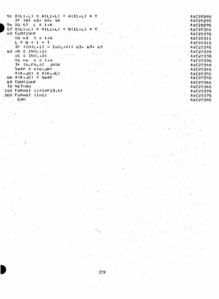
51 A(L1rL) = A(L1.L)IF (M) 60. 60. bU
k 54 DO S7 L = 1.MF 57 B(L1.L) = B(Ll.L)60 CONTINIIF
oo ^9 T = i.NL = N + 1 - IIF (IN(L.l) - IN(I
63 JR = IN(L.I)JC = INHL.2)UO ^6 K = I.NIF (N.Fft.O) JR=KSWAP = A(K.JR)A(K.JW) = A(K.JC)
66 A(K.JC) = SWAP69 CONTINIJF72 RETURN100 FORMAT (/,300 FORMAT (IHD
A(IC.L) * T
B(IC.L) * T
>)) 63. 69. <
AXC20285AXC20290AXC20295
AXC20305AXC20310.AXC20315AXC203?0
AXC20330>XC20335AXC203UOAXC203U5AXC20350AXC2D355AXC20360AXC20365AXC20370AXG20375AXC203BO
219
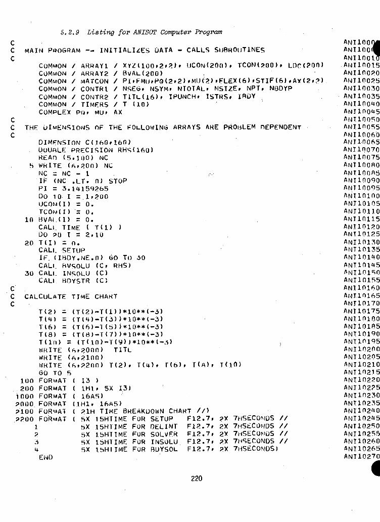
ccc
5.2.9 Listing for ANISOT Computer Program
M A I N P R O G R A M — I N I T I A L I S E S D A T A - CALLS SUBROUTINES
COMMON /COMMON /COMMON /COMMON /COMMON /COMMON /COMPLEX F
ARRAY1ARRAY2MATCONCONTR1CONTR2TIMERS>O. MUr
ccc
ccc
2 » 2 ) » UCOf \ j (200)» T C O N ( 2 0 0 ) » LOCC200)/ B \ /AL(200)/ PI»FMU»PQ(2.2)»MU(2)»FLEX(6).STlF<6).AY<2.?)/ NSEG. NSYM. NTOTAL. MSIZE. NPT. N8DYP/ T1TL(16)» IPUNCH* ISTRS* IRDY/ T (10)AX
THE DIMENSIONS OF THE FOLLOWING ARRAYS ARE PROBLEM DEPENDENT
DIMENSION C(.1.f>0»160>DOURLE PRECISION RHS(KSO)READ (5.100) NC
5 WRITE (fc.200) NCNC = NC' - 1IF (NC .LT. 0) STOPPI = 3.1415926500 101 = 1.200UCOM(I) =0.TCOwd ) = 0.
10 BVAl.(I) r 0.CALL TIME ( T(l) )DO 90 I = 2.10
20 T(I) = n.CALL SETUPIF. (IBDY.NE.O) GO To 30CALL BVSOLU (C. RHS)
30 CALL INSOLU (C)CALL BHYSTR (C)
CALCULATE TIME CHART
T(2) =T(4) =T(6) =T(8) =T(lii) =WRITE (WRITE (WRITE (GO TO F>
100 FORMAT200 FORMAT
iooo FORMAT?ooo FORMAT?ioo FORMAT?200 FORMAT
i
(T(2)-T(1))*10**(-3)(T(H)-T(3))*lO**(-3)(T(f>)-T(b) )*10**l-3)(T(8)-T(7))*10**(-3)(T-(.10)-T(9> )*10**(-3)
fS.2000) T1TLft.2100)f=,.?200) T(2). T(4). T(6) T( T(10)
34
( 13 )( 1H1. 5X 13)( 16A5)(1H1. 16A5)( ?IH TIME BREAKUOWN CHART //)( SX5X5XsxP>X
15HTIME15HVIbHlIbHTI SHI
IMEIMEIMEIME
FORFORFORFORFOR
SETUPOELINTSOLVERINSOLUBDYSOL
F12F12F12F12F12
.7,
.7,
.7,
.7,
.7.
?x2X2V2X2X
7HSECOMDS //7HSECOMDS //7HSECOMDS //7HSECONDS //7HSECONDS)
ANIIOOIANTIOOI
A N.I 10.0 30ANT10035
ANT10050
ANI10060ANI1-0065ANI10070ANIin075ANTIOOBOANT100B5ANT10090ANT ino95ANIIOIOO-ANI10105ANI10110ANT10115ANI10120ANT10125ANI10130ANT10135ANI101UOANI10145
END
ANI10160ANI-10165ANT10170ANT10175ANI10100ANI10185ANI10190ANI10195ANI10200ANT10205ANI10210ANT102T5ANT10220ANI10225ANT10230ANT10235ANI102UOANI10245ANT10250ANI10255ANT10260ANI10265ANT10270
220
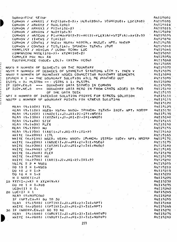
SUBWOUTINF. SETUPCOMMON / ARRAY1 ,COMMONCOMMONCOMMONCOMMONCOMMON
l.lCOu(20n) » TCON(goO)» LOC(200)ARRAY2ARRAYSARRAYSWlATCONflMFjKSCONTR1CONTH2
Bv'AL(20D)PTIN(100»2)
r)Ql?»2) »MU(?) »FL£Xlf>) »STIF(6) ./TIM 110)
COMMON / CONTR1 / NSEb, NSYM»~ NTOTAL, NSIZE» NPT, NoOYPCOMMON / CONTH2 / TITL<16)» IKJNCH, TSTRS, iBQYNAMPLIST / HOYCON / UCON, TCON, LDCOIMFNSIONJ NOOEdOO'?)' XYZM(100»2>COMPLEX POr MUf AXEQUIVALENCE (NODE, LDO, (XYZM, UCON)
= NUMBER OF SEGMENTS ON THE BOUNDARYNSYM = NUMBER OF DEGREES OF SYMMETRY STARTING WITH Y» THEN VNNOD = NUMBER OF BOUNDARY NODES CONNECTING BOUNDARY SEGMENTSIPtJNCH =1 — THE BOUNDARY SOLUTION Wlt.L BE PUNCHED OUT
PLSTRN — . ISTRS = 1. PLSTRSBOUNDARY DATA STORED IN COMMONBOUNDARY DATA READ IN FROM CARDS ADDED TO ENDOF THE UATA DECK
NPT = MUMBFR OF INTERIOR SOLUTION POINTS FOR STRESS SOLUTIONNBDYP = NUMBER OF BOUNDARY POINTS FOR STRESS SOLUTION
ISTRS =IF IBDY.EQ.O —IF IQDv.NE.n
REARREADREAnREADREAOREAOREAnREAnWRITEWRITEWRITEWRITEWRITEWRITEWRITEWRITENSI/EDO 10DO 10
lion)
1300)1400)
(5»170n)(5»1 700)
TITLNSEGr NSYM, NNOD, IPUNCH. ISTRS» IBDY, NPT, NOOYP((NODE(I»J),J=1»2)»I=1{(XYZM(i»J),J=1»2)^1=1STIFFLEXMU
I ITLNSEG, NSYM> NNOD, IPllNCH, ISTRS* IBDY» NPT, NBDYP((NODEtI,J),J=lr2)»I=l»NSEG)( (XYZMU»J>»J=1»2)»I = 1»NNOD)STIFFLEXMU((AX(I,J),J=lr2),1=1,2)
= 2 * NSEGI = 1,NSEGJ = 1»?
(6,?3on)
(<s,?.7no)
in
2n
3n
DO 10N = NODE<I'J)XYZ(I»J,K) = XYZM(N,K*DO 30 I = 1»?00UCOM(I) = 0.LUC(I) = 1REAn (5'BI)YCON)IF (NPT.EO.O) GO TO 30REAn (5,1500) ((PTIN(I,J),J=1,2),1=1,NPT)WRITE (fc>2500) ((PTINII,J),J=1»2)»I=1»NPT)IF (NBDYP.EO.O) GO TO 40REAI1 (5,16nO) ((NBDY(I,J) . _. .. .WRITE <ft,26nO) I (NBDY(I,J),J=1»3)»I=1»NBDYP)
AN|T15onOAMI 15005ANT15010AN I 150] 5ANI15020ANT150P5ANT 150^0ANI15035
ANT150U5ANI15050ANI15055ANI150/SOANT 15065ANI15070ANT15075ANI15n«0ANT150«5ANI15090AN! 15095AN! 15100ANI15105ANT 151 10ANT i5i 15ANI15120ANT 15125ANI15130AN I 15135ANI151UOANJI151«i'5AK1J15150ANI 15155ANI15160ANI15165ANI15170ANI15175ANI15180ANI151R5ANT15190ANI15195ANI15200AMI 15205ANU5210ANI15215ANI152?0ANI15225AN I 15230AN I 15235ANI152<40ANT152t+5ANI15250ANI15255ANI15260ANI15265ANI15270ANT15275ANI152RO
221
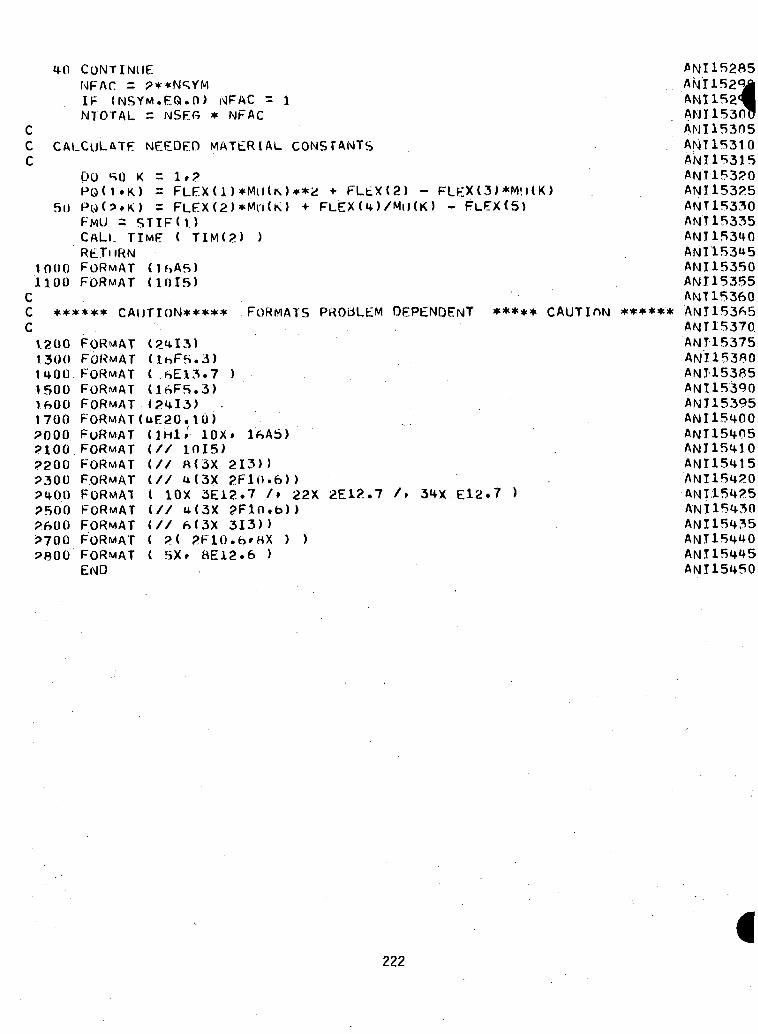
ccc
to CONTINUENFAC = ?**N<;YMIF (NSYM.EQ.O) iMF AC = 1NTOTAL = NSF.fi * NFAC
CALCULATE NEEDED MATERIAL CONSTANTS
DO SO K = If?PQd.K) = FLEX(l)*Mu(K)**i> + FLtX<2) - FLEX (3) *M'i(K)
5U-PQ(!>»K) = FLF.X(2)*Mt')<K) + FLEX U) /Mil (K) - Fl_F_X(5)FMU = STIF(I)CALL TIME ( TIM(£) )RETURN
ANI15285
iooo FORMAT df>As)1100 FORMAT unis)
cc ****** CAUTION***** FORMATS
12001300itoo.1500Vf>001700?0002100?200?3002too250026002700?BOO
FORMATFORMATFORMATFORMATFORMATFORMATFORMATFORMATFORMATFORMATFORMATFORMATFORMATFORMATFORMATEND
(2tI3)(KSFH.3)( (SE13.7 )(16F5.3)(2UI3)(UE20.10)(IHlf lOXf IfSAb)(// ini5J(// 8<3X 213) )(// U(3X 2F10.6))( 10X 3E12.7 /» 22X(// u(3X 2Fln.b))(// M3X 313) )( 2( 2F10.6»MX ) )( SXf 8E12.6 )
2E12.7 /» £12.7 )
AN I 1530ANI15305ANT 15310ANI15315ANI15320ANI15325ANT15330ANT 15335ANI153UO
ANH5350ANI15355ANT15360
DEPENDENT ***** CAUTION ******AMI 15370ANT15375ANI15380ANI153R5AN I 15390ANI15395AN.I15400ANT15405
ANI15415
AN I 15^30
ANJ15415ANT15450
222
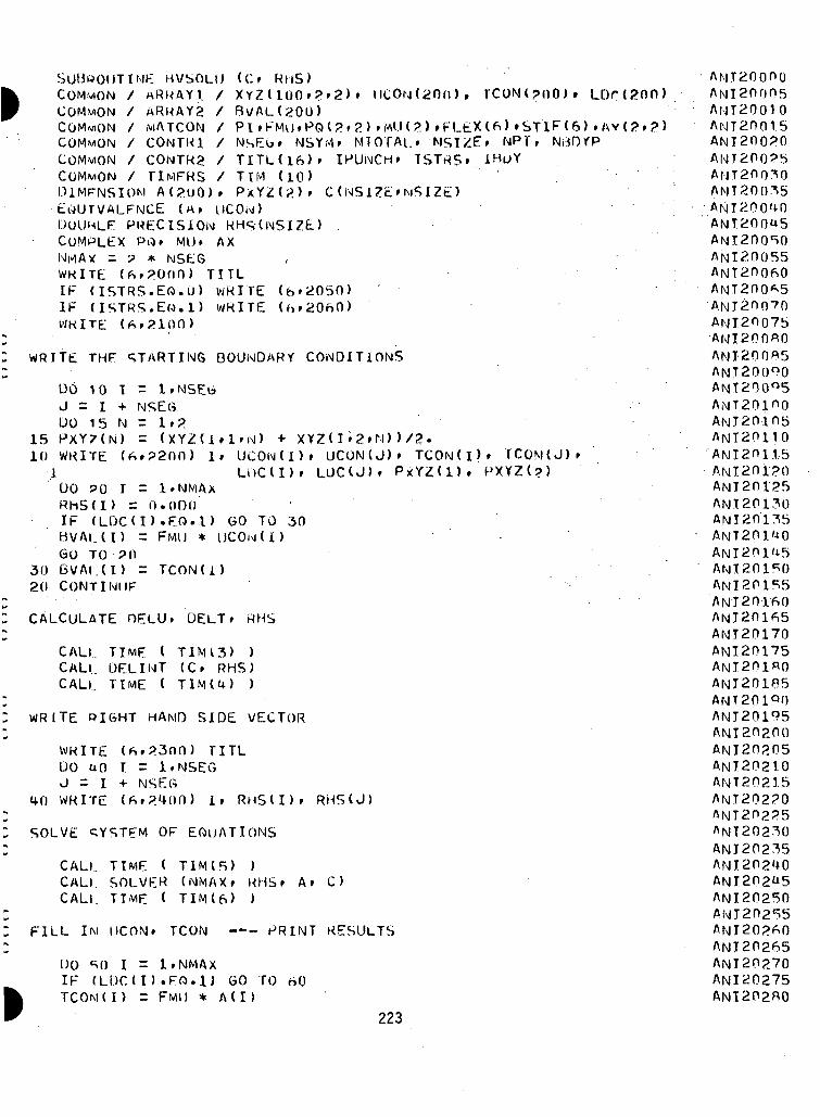
SUBROUTINE HVSOLUCOMMONCOMMONCOMMONCOMMONCOMMONCOMMON
ARKAY.1.ARRAY2MA ICON)CONTR1CONTRA
I ICOiM<200), T C O N < ? 0 0 ) . LDr<200)
TlTLdfc)»TIM (10)
D1MFNSIOM A(?uO)» PxYZ(2)»EQUIVALENCE (A> UCO.M)DOUHLE PRECISIONCOMPLEX PO» MU» AXNMAv = y * NSEGWRITE ( 6 r J > O f l O ) TITLIF ( ISTRS.EO.U) WRITEIF (ISTRS.EO.D WRITEWHITE (ft
(O RHS)X Y Z ( 1 0 0 » ? » 2 )BVAH20U)
? » 2 ) »MU(2) rFL£X«S) »SflF(6) .r NTOTAl .» 'MSI^P» NPT» NrtDYPIPUNCH» TSTRS*
(hr2060)
WRITE THF STARTING BOUNDARY CONDITIONS
06 10 iJ = I +DO 1 5 NPXY7(N)WRITE (
1510
3020
NSEG= 1 > ?= ( X Y 2 ( l » l n M ) + X Y Z ( I » 2 » M ) ) /2.»?2nn) 1» U C O N ( I ) » UCON(J)» TCON( I )» T C O M ( J ) r
LI)CII)» LL)C(J)» PxYZ( l ) r P X Y Z ( ? )DO 90 I = 1'NMAxRhS(I) = n.ODOIF ( L O C ( I ) .EO.l) GO TO 30BVAl.. ( I) = FMU * UCOixi( i )GO TO ?nBVAl.(I) = TCON(l)CONTINUE
CALCULATE OELU. DELT t RHS
CALL TIME ( TIM13) )CALL DELINT (c» RHS)CALL TIME ( T1M(U) )
WRITE BIGHT HAND SIDE VECTOR
WRITE (*.?3nO) TITLDO UO I = l.NSEGJ = I + NSEG
40 WRITE (A. '+00) if RHS(I)» RHS(J)
SOLVE SYSTEM OF EQUATIONS
CALl. TIME < TIM(R) )CALL SOLVER (NMAXf «HS» A» C)CALL TIME ( TIM(f>) )
FILL IM TCON --- PRINT RESULTS
DO SO I = l.NMAXIF (LDC(I).EO.l) GO TOTCOM(I) = FMU * A(I)
A M T 2 0 0 0 0ANI20005A f j T 2 0 0 1 0ANT200T5ANI200PO
ANT200U5ANI200 ISOANI20055
ANI2I1070
ANI20000ANI20085ANT200QQANT200C)5
AN!20-inSANI20110"AMI 20 11,5ANI201?0ANT20I25ANT20170
ANT201UOAN 1 2 01 U5AN 1 20
ANT20160
ANT20170ANI20175ANI20100ANI20185ANT201QOANI20195ANI20200ANI20205ANI20210ANT2021SANI202POANI202P5
ANJ20235ANI202UOANI20215ANI20250ANT20255
ANI20265ANI20270ANI20275ANI202RO
223
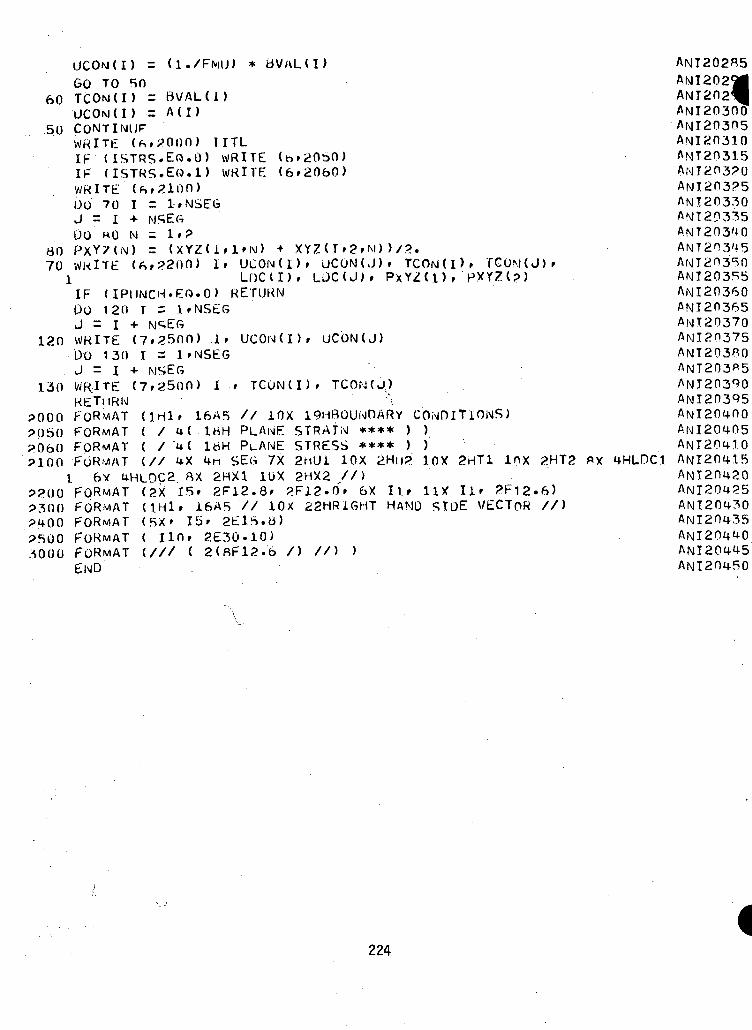
60
50
8070
120
130
9000
UCOM(I) = (l./FMU) * BVrtL(I)
GO TO 50TCOM(I) = BVAL(i)UCOM(I) = A(I)CONTINUEWRITE (ftf?000) TITLIF (ISTRS-EO.O) WRITE (h»2050)IF (ISTRS.EO.l) WRITE (6f2060)WRITE (ftf2ion)DO 70 I = IfNSEGJ = I + NSEftDO «0 N = If?PXY71N) rWHITE (ftf
IfIM) + XYZ(T»2fN)>/2.UCON(I)f UCON(J)f TCON(l)f TCOM(J)fLf)C(I)f LOC(J)f PxYZ(l)f PXYZ(?)
RETURN
?060?100
??00?300
.SO 00
FORMATFORMATFORMATFORMAT
L 6Y tiHLOC2FORMAT (2x :FORMATFORMATFORMATFORMATEND
UCOlM(I)» UCON(J)
f TGON(I)f TCON(J)
IF ( IPllNCH.EO.O)DO 120 I =J = I 4WRITE (7.2500) IfDO 130 I = IfNSEGJ = I + MSEGWRITE (7f2500) 1RETnRN
(iHlf 16AFS // 10X 19HBOUNOARY CONDITIONS)( / u( irtH PLANE STRAIN **** ) )( / <4( IBM PLANE STRESS **** ) )(// UX In SEG 7X 2hUl 10X 2Hu?. 10X
ax 2WX1 1UX 2HX2 //)[Sf 2Fl2.8f 2F12.0'f 6X Il»
(IHlf 16A5 '// 10X 22HRIGHT HAND(SX> I5f 2E1.S.B)( IlOf 2E30.10)
2(RF12.6
ANI202B5ANI202^
2HT1 inx 2HT2
11X II' ?F12.6)SIOE VECTOR //)
1HLDCX
ANI20300"ANI20305ANI20310AMT20315ANT20320ANI203P5ANI20330AMT2P335ANT203UOANT20345
ANT203ci5AMI20360
ANI20370ANI20375ANT20380ANT.203^5
ANI20395ANI204-00A.NI20405ANI20410
ANI20430
ANI20445ANI204.50
224
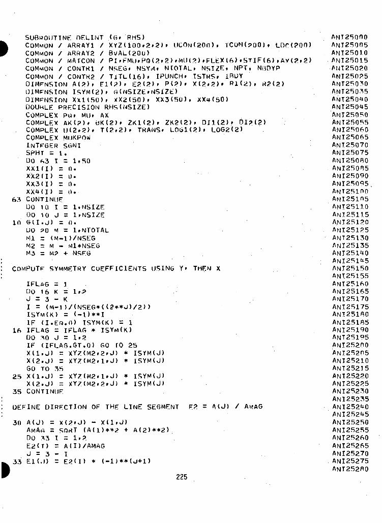
SUBWOUTTNE DELINT <G» RHS)X Y Z ( l ' 0 0 » 2 » 2 >Bv/AL(20U)
IPUNCH.
, X X 2 ( 5 0 ) »RHS(NSIZE)
MU» AXA K < ? ) » b K ( 2 ) » Z K 1 ( 2 ) » Z K 2 ( 2 ) » DIH2)r DI?(2)l l ( 2»2 )» T ( 2 » 2 ) » THAiMS* L061<2)» LOG2<2>MUKPOW
COMMON / ARRAYlCOMMON / ARRAY2COMMON / MATCONCOMMON / CONTR1 / NSEG»COMMON / CONTR2 / TiTL(l6)»DIMENSION A(2)» El<?)» E2(2OIMFNSION ISYM(2DIMENSION XXH50DOUBLE PRECISIONCOMPLEXCOMPLEXCOMPLEXCOMPLEXINTEGER SGNISPHT = i.DO ^3 I = 1»50xxid) = n.X X 2 ( D = 0.xx3( i ) = n.XX1(I) r 0.
63 CONTINUEDO 10 I = l.NSIZEoo 10 J = I»NSI/:E
in G (. i. j) = n.DO X) iwi = 1»NTOTALMl = (M-D/NSEGM2 = M - ivil*NSE6M3 = M? + NSEG
COMPUTF SYMMETRY COEFFICIENTS USING Y» THEN X
IFLflG = ]. .00 16 K = If?.J = 3 - K1 = (M-1)/(NSEG*((2**J)/2))ISYM(K) = (-l)**IIF (I.ED.n) ISYM(K) = 1
16 IFLAG = IFLAG * ISY^(K)00 *0 J = 1»2IF (IFLAG.GT.O) GO TO 25
UCO,\i(20fl) . iCOM(?00)» L0r(?00)
?) »FLEX(6) »STJF(6) » AY* N5IZE, NPT» NBDYPISTR5. 1ROYX(2,2)» Rl<2)» K2(2)
ANT25nno
25
35
X(l .J) =X(2 . J ) =GO TO 35X(1,J) =X(2 . J ) =CONTINUE
XYZ(M2»2rJ) *XY7<M2»1»J) *
XY7(M2»1»J) *XY?(M2»2»J) *
ISYM(J)ISYM(J)
ISYM(J)ISYM(J)
DEFINE DIRECTION OF THE LINE SEGMENT
30 A(J) = X(2'J) - X(l.J)AwAa = SORT (A(l)**2 + A(2)**2>DO .^3 I = 1»?E2(T) = A(I)/AMAGJ = 3 - I
33 El(.l) = E?d) * (-1)**(J+1)
= A ( J ) / AMAG
AMI25010ANI25015ANT250POANT250?5
ANI250U5ANI25050ANT25055
ANI25065ANI25070ANI25075ANI250BOANI250B5ANI25090ANI25095,
ANI251H5ANT251.rOAIMI251J.5ANI25120ANT251?5ANT25130ANI25135ANT251UOANI251U5ANT25150ANT25155ANT25160ANI25165ANI25170ANI25175ANI251BOANI25185ANI25190A.NT25195ANI252HOA.NI25205ANI25210ANI25215ANI25220ANI25225ANI252750ANI25235
ANI252U5ANI25250ANI25255ANI25260ANI25265ANI25270ANI25275ANT252BO
225
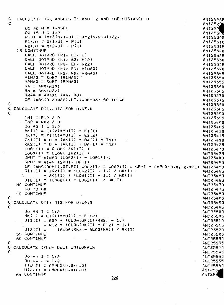
cc
CALCULATE THE AIM6LLS T.I AND T? AND THE DISTANCE U
DO 30 N = l»NSEt>DO 15 J = 1»?P(J) = (XYZ(N»1»J)
ANI252ft5
RK.I) = X(l» J) -R2<-l) = X(2»J) -
IB CONTINUECALL OOTPRD
OOTPRDOOTPRDOOTPRDOOTPRD
SORTSORT
P(J)P<J)
CCC
(Rl» El» O)(Rl» E2» R12)(R2» E?f R22)(Rl. Rl» RlMAG)(R2» R2. R2i«iAG)(RlMAG)(R2MAG)
RA = ARS(R1?)R8 = AH<;(j<2?)RMAft = AMAXl (RA» RB)IF (ABS(D /RMAG).LT.1.0E-U3)
CALCULATE nil. 012 FOR O.NE.O
CALLCALlCALLCALlR1MAG =R2MAG =
GO TO
TNI =Tlvl2 =00 SOA K ( T )B K ( T )
R12R??I =
EK2)BK(I)BK(I))
TNI)TN2)
LOG2 ( I ) -) / HK (I )) / HK(I)BK ( I )
CCC
CCC
= F1(1)*MU(I)ZKKI) = - L ) * ( A K ( 1 )Z K 2 < I ) = 0 * ( A K ( I )LOG!( I ) = CL06( ZKllI)LOG9(I) = CLOG( ZK2( I ) )DPHT = AlMAfi (LOG2<I) - LOGl(D)SPHT = SIGN (SPhlr OPhI)IF (AHS(DPHI) .GT.PI) LOG2(I>011(1) = ZK2( I ) * (LOG2(I) -
1 - /K.I (I) * (LOGKI) -DI2(D = (LOG2U) - LOGKD)
sn CONTINUFGO TO (sn
HO CONTINUF
CALCULATE On.. DI2 FOR O.EQ.O
00 S5 I = 1.2BK(T) = FI(1)*MU(D - El(2)011(1) = R2P * lCLOG(bK(I)*R22) - 1.)
1 - R12 * (CLOt7(oK(I) * R12) - 1.)012(1) = (ALOG(RH) - ALOG(RA)) / BK(I)
5S CONTINUE60 CONTINUF
CALCULATE DFLU» DELT INTEGRALS
00*41=1.?OO *4 J = 1»?T(J.I) = CMPLX(O.OH).O)U(J.I) = CMPLX(U.OM).O)
64 CONTINUF226
SPHI * CMPLX(0.n, 2.*PI)
ANI25JANI2S3?ANT2S305
ANT2R315ANT2S3?0ANI25325
ANT 25350ANI25355
ANI25370ANI2537SANI253BOANI253P5ANT25390•ANT25395ANT254.noANI25M.OSANI25410ANI2541S
A.NI254.30ANI2545S
ANT254FSOANI2545SANT25460
ANI254-°0ANT25495AMI25500ANT25505ANI25510ANT2551SANI25520ANT255P5ANI25530
ANT255UOANI255U5ANJT25550ANI25555
ANT255
DO ft5 I = 1•?00 ftS J = 1»•?.
DO ftb K = 1»PSiiNT = ( -1>**(3- I )MUKPOW = M.U(K ) ** (2-1 )UIJ.I) = U(J.I) + P f l < i » K ) * A X ( J » K ) * D l l ( K )T(J.1) = T (J > I) + ' • (MU(K
ANI25575
75
90
CONTINUE
XXIXX2XX3XX4DODON<+M4IFIF
(N)(N)(N)(N)«5 I«5 J= N= M?(IX.( LOG
zz
—»XX
XXIXX?XX3XXu= 1«• 1
+ (I
(N)(N)(N)(N)»2.2X-l
+ (JX-1E(Q. JXMO.) .
))
.ANUE«.1
+ 2.*KEAL+ 2.*KEAL+ 2.*KEAL•f 2.*KEHt_
*NSEG*NSh6.M.EQ.N)
((((
T
TTTT
(
((((
1»1»?_»?»
IX»
1.) )2) )1) )2) )
JX)) GO TO 90
~ CMPLX(0 .25»0.0)
TRAMS = udx.jx)u d Y f j x ) = -d./FMU) * rdx r j x )
-FMU * TKANS•«• 2.*REAL(UUX» JX) )
2.*REAL(T(IX»JX)) * ISYM(Jy)
TdY.JX) =RHS(N4) =G(Nu» MU) zCONTINUFCONTINUEWRlTE(6»?60n) TITLFORMAT (1 HI. »16A5//lOX»i7HCOLUMN SUM CHECKS//)DO Q5 I = l.NSEGWRITE (ftr?500) I» XXI(I). XX2(I)»
3F8.5»lUF9.b2F2().10r
* TSYM(JX)
POOO FORMAT(9100 FORMATP200 FORMAT(P300 FORMAT?400 FORMATP500 FORMAT
END< 3 X » I4»
» 6Elb.7)HF20.15)
ANT 25590ANT255°5ANI2B600ANT25605
ANT25615
ANT 25630AN I 25635
ANT 256*45ANI25650ANI25655ANT25660AN I 25665ANT25670ANI25675ANT256BOANI256R5ANI25690AMT25695ANI25700ANT25705AN 1 2 57 1.0ANT2571.5ANI257?0AMT257P5ANT25730ANT25735ANT257UOAN I 25745ANI25750AN I 25755ANT25760
227
SUBROUTINE INSOLUi C )
COMMONCOMMONCOMMON
ARRAY1ARRAY3MATCONTIMERSCONTR1CONTR2
ccc
COMMON / ARRAY1 / X YZ 1 1 00 r 2» 2 ) » l)CON(200), TCON<?00). LQC(?00)/ P I Ii\l ( 100 .2 )/ PI .FMU.PQ(2»2) . MlJ ( 2 ) »FL£X(6 ) »STIF(6) » A X ( 2 » 2 >/ TIM do)/ NSEb. NSYM. NTOTAt» NSTZF. NPT , NBDYP/ TITL (16) » TPUiMCh. ISTRS. IBUY
DIMENSION CdOO.6)' A(M-), PXYZCi)COMPLEX PQ. MU. AXIF (IBOY./xJE.O) 60 TO 100IF (NPT.EO.O) RETURNCALL TIME (, TIM (7) )WRITE; (fc.pono) IITLIF dSTRS.Efl.O) WRITE (6»20.40)IF "( ISTRS.E0.1) WRITE (6*2060)
CALL FOR CALCULATION OF DELD AND DELS
110
WRITE (*A (4) = n.CALl DEL SO (C)DO 10 NP = 1 »NPTC(NP.S) = C(NPrb)
NP
* 2
STIF(6)+C(NP»5)STIF(5)*C<NP,5) STIF(u)*C(NP,6)
>» PTiN(NP.2) .10
100
120
130
IbO
1 100POOOP050P060PI 00
P2002300
A(2) = <;TIF(3)A (3) = <;TIF(?JWRITE (6.2200)CONTINUFCALl TIME ( TIM(fl) )RETURNWRITE (£,.2000) IITLDO 120 T = l.NSEGJ .- I + NSEGREAn. (R.I ion) N. UCONd). UCON(J)DO 130 I = IrNSEGJ = I + NSEttREAD (5.HOO) N. TCON(I). TCON(J)WRITE (6.2300)UO 1UO I = I.NSEGJ - 1 + NSEGDO 15(1 M = 1 .2PXY7(N) = (XYZ(l.l.N) + XYZd »2.M) )/?.WRITE (6.2400) I. UCOivi(l). UCON(J)» TCON(I). TCOM(J).
1 LOCd). LDC(J). PxYZ(l). PXYZt?)GO TO 110FORMAT (no.FORMATFORMATFORMATFORMAT
(1H1.2E30,10X.
( / M 18H( / U( 1HH(6HOPOINI.
1
1(1)l6Ab)PLANE STRX\IN **** ) )Pl.Ai-gE STRESS **** ) )2X 10H SIGMA(XX) ?X 10H
10H SIGMA(YY) 2X 10H SIGMA(ZZ) 5X 2HFORMAT (2X 13. 2X 4F12.2. 2F8.4)
H SE« 7X 2HU1 10X 2Hll?. 10X 2HT1 lr>X 2HT22HX1 10X 2HX2 //)2F12.8. ?.F12.0. bX II. UX H. 2F12.6)
SIGMA(XY) 2XX 6X 2H Y)
FORMAT (// UX6Y 4HLDC2 «X
FORMAT <PX JS.END
4HLDC1
ANI300KANI300H
ANT30CWANI300'iJANT300ciO
ANT30065A^4I30070ANI30075ANI300BOANT30085ANT30090ANI30095ANT30100ANT30105ANI30110ANI30115ANI3ni?0ANI30125ANI30130ANI30135ANI30HIO
ANI30150ANI30155
ANI30165ANT30170ANT30175ANT301flO
ANT30190ANT30195'ANI30200ANJI302HSANT3P210ANT3021.5ANI30220ANT30225ANI302.30
ANT302ciO
ANT3D26;ANT3027IANI302J "
228
SUBROUTINE DELSU (G)COMMON / A R R A Y l / XY21100,2»2)» UCOw(200). TCON(?oO), LUr(?00)COMMON / ARRAY3 / PlIi\i(10U»2)COMMON /MATCON / PI »FMU»PQ I ?.»•?.) » MU ( 2) »FL£X(f») »bTlF(6) »AY(?»?)COMMON / CONTRI / NSEG, NSYI«I» NTOTAL, NSTZE, NPT,COMMON / CONTR2 / TITL<16)» IPUMCH* ISTRS. 1BOY
"2 ) » X(2» 2 ) ' 91(2) , H
OS
A<?), El<?)r E2(2)»DIMENSION ISYM(2)» G(100»b)COMPLEX POt MUr AXCOMPLEX AK(?)» uK(2)» ZKKP)-»COMPLEX LOGI (2)» L0<-;2i2)SHHT = 1 .DO 10 I = 1.100DO 10 J = l»ft
10 G(I.J) = 0.DO ?0 M = l.NTOTALMl = (M-1)/NSEGM2 = M - Ml*NSEG
COi^PUTF SYMMETRY COEFFICIENTS USING Y» THEN XIFLflG = 1DO 16 K = 1, ?J = 3 - KI = (M-1)/(NSEG*((2**J)/2))ISYw(K) = (-1)**!IF (I.EQ.O) ISYM(K) =1
16 IFLAG = IFLAG * ISYivi(K)DO .^2 J = 1»2IF (IFLAG.GT.O) GO TO 23X(l.J) = XY7(M2»2»J) * ISYM(J)X(2.J) = XYZ(M2»1»J) * ISYM(J)GO TO 35
23 X(l.J) = XY7(M2»1»J) * ISYM(J)X(2.J) =- XY7(M2r2,J) * ISYM(J)
35 CONTINUE
DEFINE DIRECTION OF THE LINE SEGMENT E? = A(J)/AMA6
3 2 A U ) = X ( ? » J ) - X ( l r J )AwAa = SORT (A(l)**? + A(2)**2)DO ^3 I = 1»2E2(T) = A(I)/AMAGJ = 3 - I
33 EK.I) = E2<I) * (-1)**(J-H)
CALCULATE THE ANGLES Tl AND T2 AND THE DISTANCE D
DO PO N = l.NPT .DO 15 J = 1,2P(J) = PTIN(N,J)R2(.D = X(2,J) - P(J)
15 CONTINUFDl = I).D2 - 0.DO 17 J=l»2Dl = 01 + R.I. (J)*R1(J)
229
ANI3S010ANI3SQ15
ANT350?5ANT3F1070'ANT35035
ANI350"5
ANI35055ANT35060ANI35065ANT3507Q
ANI3SOPOANI350P5ANT35090ANI35095ANI35100ANI35105ANI35110ANI3S115ANT
ANT35130ANI35135
ANI3S1U5ANI35150ANI35155ANI35160ANI35165ANT35170ANT35175
ANI351P5ANT35190ANI351Q5ANI352HOAN I 3520 5ANT35210ANI35215ANT35220ANT35225ANI35230ANI35235ANT352"0ANI352U5AMI35250ANI35255
ANT35265ANI35270ANI35275ANI352BO
17 L>2 = D? -f K;>(J)*R2lJ)01 = SORT (01)02 - SORT(D?)CALl DOTPRD (RlCALl DOTPRD (RlCALl DOTPKD (R2CALl. DOTPKD (RlCALl DOTPKD (R2
E .1 • D )E2» K12)E2» RP2)Rl » K IMAGR2» K2MAG
KiMAG = SuRT (R1MAG)
CCC
CcC
CCC
R2MAG - SORTRA - ARC, (Hi?)RB = ARS(K2?)KMAft = AMAXl(KAfRB)IF (AHS(D /RMAG).LT.l.OE-03) GO TO uOTNI = Rl? / DTN2 - R?? / D
CALCULATE OT3f 014 FOR D.NE.O
DO u5 I = lr?AK ( T ) = R!l(?. )*MU(D + El(l)
HK ( T ) = Eld) *MU ( I ) - E1 ( 2 }2!K1(I) = D * ( A K ( D + BMi) * TNI )ZK2(D = D * ( A K ( i ) + BK( I ) * Ti\i2)L O G 1 ( I ) = CLOG( ZKl ( I ) )LOG?( 1 ) = CL()G( 7K2( I ) )QPHT = A IMAG (LOG2<D - LOGKD)SPHT = SIGN (SPHI> OPHI)IF {ABS(Or > HT ) .GT.PI ) LOG2(D = LOG2(T ) - 'DI3(I) = (LOG2(1) - LOGKD) / BK (I )014(1) = -d. /ZK2d) - 1./ZKKI) ) / PK(
45 CONTINUEGo TO 5n
CALCULATE DI3r DI4 FOR O.Ert.O
40 CONTINUEDO 55 I = 1»P.tlK(T) = E1<1)*MU(D - El (2)013(1) = (ALOG(RB) - ALOG(HA)) / BK(I)014(1) = -(1./R22 - 1./R12) / BKd>**2
5b CONTINUE50 CONTINUE
CALCULATE OD» DS» STRAINS AND STRESSES
* CMPLX<0.n, 2.*PI)
LI =00DOLIDODODsDODD
?S I95 L= L.1.?5 J
1.2I1»2
= CMP|.x(n.Of 0.0)
^0 K r 1,?=((P0(JrK)*AX(I»K)*OI3(K)+lMU(K)**(L-T))
+P0( J'»K)*Ax(L»K)*Oi3(K)*(MU(K) *•*(!-! ) ) ) )/2.+ Di i= (-(MlHK) *tl d. )-El 12) )*MU(K) **(2-J)*AX( It K ) *M| I ( K ) ** (L-l) *DI4 ( K*((-l)**(3-j))
230
AlxlT352nsAMI 352c
ANT352f5 r; p q n
352fl3^301?
AMI 353 TOANI35315AMI35320ANT 3532.5
ANT353.715
ANT35345ANT 35350ANT35355A l J T 353^0ANT 353^5
ANT35370ANI35375ANT353POANI35385ANT35390
ANT3540nANI35405ANT35410ANI35415
ANI354P5ANT35430
ANT35UUQANI35415ANT35450ANI35455ANT 35460
ANT35470ANT35475ANT35480ANI354B5ANI354QOANI35495ANT35500ANT35505ANI35510ANT35515ANT35520AMI355?5ANT35530ANT35535
ANT355U5AMT35550AMI35555
ANT355ANI35SI
? -<MI.J(K)*E1(1 )-FK2) >*MU<K)*+<2-J)*AX{L»K)*Mn(K)**(I-l)*niMK)ANl355753 *((-l)**(3-J)))/2. + L)S
30 CONTINIIFM^ = M2 + (j-l)*NSEti ANT35590G(N,LD= tt(N»Ll)- 2.*KEAL(OL))*TCON(M^)*ISYM{J) AMT3«=i5951 + 2.*KEAL(DS)*UCON(M'*)*ISrM(J) ANI35600
2s CONTINUE: ANI3560520 CONTINUE ANI35610
WETilRN ANI35615
231
SUBROUTINE RDYS1RCOMMONCOMMONCOMMONCOMMONCOMMONCOMMONDIMFNSTONDI.MFNSIONDIMFNSIONCOMPLEX pr
//////
( rt )X Y 2 ( 1 ( I O » 2 » 2 ) » I ICON<200), T C O N ( ? Q O ) > LOC(?00)
/ N r t O Y ( b O » 3 )/ PI»KMU»PO(2»2) »MUC>) »FLEX(6) »STIF<6) »AX<?»2)/ NSEGf NSYM» NTOTAL* NSI2E» NPT, NBDYP
IPUNCH» ISTRS, 1BDY
E ( 3» 3) »
ARRAY1ARWAY4MATCONCONTR1CONTR2TIMERS / TlMUlJ)A(?)» El<?.)» E2Q ( 3» 3) »RHS(3)»
5» MU» AXIF (NUQYP.Ett.O) RETURNCALl TIME ( TIM(9) )WRITE (P,t2000) TITLWRITE ((Sf2l()0) ( (NBDY(I»J) »J=1»3)WRITE (ftr20oO) TITLIF (ISTRS.EO.O) WRITE (h»2050)IF (ISTRS.EO.l) WRITE (hf20bO)WRITE <h»?200)
C O F A C < 3 » 3 > » T ( 3 » 3 ) »T C N ( i > ) » T E M P ( 3 » 3 ) »
= 1»MBDYP)
Tl(3»3)ANS(3)
CCCCC
10 = BASE SEGMENT11 = RFAR DIFFERENCE SEGMENT NUMBER12 = FORWARD DIFFERENCE SEGMENT
20
DO 15 N-= 1.NBDYP10 = NHOY (N»l)11 = NBOY (N.2)12 = NBOY (Nt3)DO ?0 M = 1»?Pll.M) = (XY?(IO»1»M)P(2.M) = (XYZ(H»1»M)P(3.M)•= (XYZ(I2»1'M)R(M) = PC-SrM) - P(2»M)A(M). = XY£(IO»2»M) - XY2(10>1»M)SMAr; - SORT(R(1)**2 + R(2)**?)
X Y Z ( I 1 » 2 » M >X Y Z ( I 2 » 2 » M )
= SORT(A(1 ) * *2CCC
CALCULATE nil/DS» TKAC FOR GLOBAL CORROlNATF SYSTEM
K = 3 -E1(K) =13 = II14 = I?15 = 10DU(M) =
M = 1»?= A(M)/
MAMAG
+ (M-1)*NSEG+ (M-1)*NSEG+ (M-l)*NSEfi(IICON(I4) - UCONU3) ) /SMAG
25 TRAc(M) = TCON(IS)CC
C
TRANSFORM nU/DS INTO EPS --- TRAC INTO TCN, IN LOCAL COORDINATES
CALl. DOTPRD (DU» E2» EPS)DO uo I = 1»2
40 TCN( I ) =D .DO a5 T = 1.?TCN(D = TClM( l )
45 TCN(2) =E l ( i ) * T R A C ( l )E? ( I ) *TRAC ( i )
AlMT400fAMT400IANT400!
ANI40Q?0ANT40025
ANT40050ANI40055
AMT40070)ANT40075)ANT40QRO
ANT40100ANTM-0105ANI10110ANI10115
ANT40125jANI40130)ANI40135)
AN I 40 170
ANT401ROANT40185ANI40190
ANI40200ANl^n2p5ANI40210ANI^0215ANIM-02PO
ANT40240
ANT40250ANT40255ANI40260ANT4-0265ANI'+027QANT402ANI402
232
CALCULATE TRANSFORMATION MATRIX T(I.J) AND ITS INVERSE TI(I.J) ANT4P290
C = EK1 )
Td.l) = C*C
T(2.D =T(2.2) = C*CT(2.3) =-S*C*2,T13.1) = -S*C ANI403UOT(3.2) = S*CT(3.3) = C*C - S*S
C .C ************ ************ ANT4P360C
Tl(1 .1) = T(l»l)TJ(1.2) = T(1.2)TK1.3) =-T(l»3) ANIUP380Tl(?.l) = T(2»l)TI(J>.2) = T(2»2)Tl(?.3) =-T(2»3)TK3.1.) =-T(3.1)TI(3.2) =-T(3»2)Tl(3r3) = T(3»3)
C ANT40415C CALCULATE MATERIAL STIFFNESSES IN LOCAL COORDINATE SYSTEMC
K = 0 ANT4P430DO SO I = 1»3DO SO J = 1.3K = K + 1Qd.J) = STIF(K) * (2.**(J/3)>IF (I.EO.J) GO TO 5ilQ(J.I) = STIF(K)
so CONTINUEDO S5 I = 1.3DO SS J = 1.3TEMP(I.J) = n.DO S5 K = 1.3
5«S TEMPd.J) = TEMP(IrJ) + 0 (I .K) *TI (K , J)' . DO *0 I = 1»3
DO AO J = 1.3 ANI105POQd.J) = 0* ANI40505DO f*Q K = 1.3 ANI^OSIO
60 Q(I.J) = 0(1.J) -f Td.K)*TEMP(K» J) 0(1,3) = Q(l,3) /2. ANT40515C Q(2,3) = 0(2,3) 12. ANI10520C CALCULATE COEFFICIENTS OF REARRANGED EoUATIONS 0(3,3) = Q(3,3)./2. ANI40525
Ed.l) = 0(1.1) - Q(1.2)*Q(1»2)/0(2.?)Ell.2) = 0(1.2)Ed.3> = 0(1.3) - Qd»2)*Q(2'3)/Q(2,2)El 2.1) =-0(1.2)E(2.2)=0(2.2)E(2.3) =-0(2.3)E(3.1) = 0(1.3) - Qd»2)*Q(2»3)/Q(2.2) ANI40565E(3.2> = 0(2»3) ANI40570
233
E(3,3) = 0(3,3) - 0DET = (F(1»!)*£(?»2
I (F(l»3)*E(2»l? (F(3»2)*E(2»3COFAC(l»l> =COFAC(1»2> = -l.n*(COFAC(1,3) =COFAC(?»1) = -1.0*COFAC(2,2) =COFAC(9»3) = -1.0*COFAC(3,D =COFAC(3»?) = -1.0*COFAC(3»3) =DO f.5 I = 1»3DO *5 J = 1»3TEMP(IrJ) = COFAC(RHS(l) = TCN(i)RHS(2) = EPS*Q(2»2RHS(3) = TCN(2)
)
(2»3)*Q(2,3)/0(2»?))*E(3»3)> + (E(1,?.)*E(2'3)*E(3,1) ) +)*E(3»2>) - (E(3»D*E(2»2)*E(1»3) ) -)*£(!»!)) - (E(3,3)*E(2»D*E(1,2)(E(2,2)*£(3,3)) - (E(3,2)*£(2,3))(E(2»1)*E<3»3)) - (E(3»1)*E(2,3))
(EC3,1)*E(2,2> )(E(3»2)*E(1»3»>(E(3,!)*£<!,3))(E(3,D*£(1'2) )(E(2,2)*£(l,3))
ANIH0575
(E(1*2)*E(3»3)) -(E(1,1)*E(3,3)) -(E(l».l)*E(3»2)) -(E(l,2)*l£(2,3) ) -(Ell,l)*E(2r5)) -(E(1,1)*E(2,2)) - (E(?,l)*EU,2)
J,I)/UET
)
CCc
CALCULATE UNKNOWN HOOP STRESS
70
DO 70 T = 1,3ANS(I) = 0.DO 70 J = 1.3
ANS(I)TCN(l)TCNC2)
TEMP(I»J)*RHS(J)
100IS
1000POOO
2> * Q(2>2)EPSANS(l)ANSC3)100) STIF »-(// (3(JE12.7
?obo>ioo
1
ANS(I)G(N.l)G(N.2>G(N,3)G(N.4)G(N.5)G(N,6)WRITE (ft,100) STIF , tl, T» TI»FORMAT ( // (3(3E12.7 /)//))WRITE (fS»2300) I0» (G(N,M)»M=1CALl TIME ( TIM(IO) )RETURNFORMAT (2ui?s)FORMAT (1H1, 10X, IfcAb)FORMAT ( / u( IHH PLANE STRAIN **** )FORMAT ( / u( IBM PLANE STRESS **** )FORMAT (/ sx IIHBASE NUMBER 2x IIHRFAR
( 3112 /) )(7HOSGMENT 2X 10H NORMAL ST 2X 10H
RHS» ANS
•4 ) ,P( l , l ) ,H(1»2)
ANTU0600
ANT1061.0ANIU0615
ANT40635
ANT406R5
ANI40710ANI40715
ANI40730ANI40735
ANI40760
NUMBf-lR 3X 10HFWD NUMBERANI40775
// ANI407POANIU07R5
9?oo FORMAT1 10H HOOP STRS ?.X 10H
9300 FORMAT <?X I3» 2XEND
HOOP STRNFl?..9f
SHEAR STR 2X5X 2H X 6X 2H Y)
ANT40800ANI40805
234
SUBROUTINE OOTPRD (A» B, c)OlMFNSTON A l ? ) , H(2 )C •= AH
h:ND
235
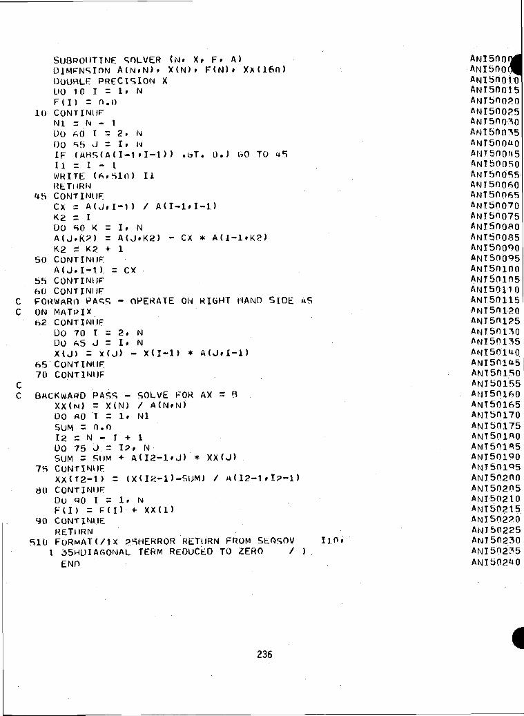
SUBROUTINE SOLVER (w» x» F» A)DIMENSION A(N»N)» X(N)» F(N)» XX(160)DOUBLE PRECISION xDO 10 I = 1» NF (I) = n. o
lo CONTINUENl = N - IDO £.0 I =2. NDO S5 J = I» NIF (AHS(A(I-1 »I-1 ) ) .bT. 0.) liO TO u511 = I - IWRITE (ftr'SlO) IIRETURN
45 CONTINUECX = A(Jrl-l) / A(I-lrl-l)K2 = IDO «SO K = I» NA(J,K2) = A(J»K2) - CX * A(I-1»K?)if i~\ . —' 1/1 A 1f\ £ y- IV f. T JL
so CONTINUEA(J.I-l). = CX
55 CONTINUE60 CONTINUE
C FORWARD PASS - OPERATE ON RIGHT HAND SIDE «SC ON MAT»IX
62 CONTINUEDO 70 I = 2. NDO *5 J = I» NX(J) = X(J) - X(I-l) * A(J»1-1)
65 CONTINUE70 CONTINUE
cC BACKWARD PASS - SOLVE FOR AX = B
XX(M) = XIN) / A(N»N)DO «0 T = 1» NlSUM =0.012 = N - I + 1DO 75 J = I?» NSUM = SUM + A(I2-1»J) * XX(J)
75 CONTINUEXXCT2-1) = (X(I2-D-SUM) / M (12-1»I?-l >
ao CONTINUEDO oo i = i» NF(I) = E( I) -i- XX(I)
90 CONTINUERETURN
510 FORMAT(/I X ?5HERROR RETURN FROM SEOSOV1 35HUIARONAL TERM REDUCED TO ZERO / )END
ANlSOOf
AN i so 01.0ANT soo is
ANI50Q?5ANT 50 0*0
ANI500U5ANlb0050
ANI50Q60ANI50065ANT5007QANI50Q75ANI50080ANI50085ANI50090ANT50Q95ANT50100ANI50105ANI50110ANI50115
no»
ANI501?5ANT 50 130ANI50135AMI501UOANI501U5ANT50150ANT 50 155ANT 5o 160ANT50165ANT50170ANI50175ANT501flOANT501B5ANT50190ANI501P5ANI50200ANT50205ANI50210ANI50.215ANI502?0ANT50225ANT 50230ANI 50235ANI502UO
236
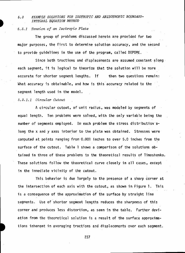
5. 3 EXAMPLE SOLUTIONS FOR ISOTROPIC AND ANISOTROPIC BOUNDARY-INTEGRAL EQUATION METHOD
5.3.1 Tension of an Isotropic Plate
The group of problems discussed herein are provided for two
major purposes, the first to determine solution accuracy, and the second
to provide guidelines in the use of the program, called DIPOME.
Since both tractions and displacements are assumed constant along
each segment, it is logical to theorize that the solution will be more
accurate for shorter segment lengths. If then two questions remain:
What accuracy is obtainable, and how is this accuracy related to the
segment length used in the model.
5.3.1.1 Civoular Cutout
A circular cutout, of unit radius, was modeled by segments of
equal length. Ten problems were solved, with the only variable being the
number of segments employed. In each problem the stress distribution a-
long the x and y axes interior to the plate was obtained. Stresses were
computed at points ranging from 0.001 inches to over 5.0 inches from the
surface of the cutout. Table 1 shows a comparison of the solutions ob-
tained in three of these problems to the theoretical results of Timoshenko.
These solutions follow the theoretical curve closely in all cases, except
in the immediate vicinity of the cutout.
This behavior is due largely to the presence of a sharp corner at
the intersection of each axis with the cutout, as shown in Figure 1. This
is a consequence of the approximation of the surface by straight line
segments. Use of shorter segment lengths reduces the sharpness of this
corner and produces less distortion, as seen in the table. Further devi-
ation from the theoretical solution is a result of the surface approxima-
tions inherent in averaging tractions and displacements over each segment.
237 .
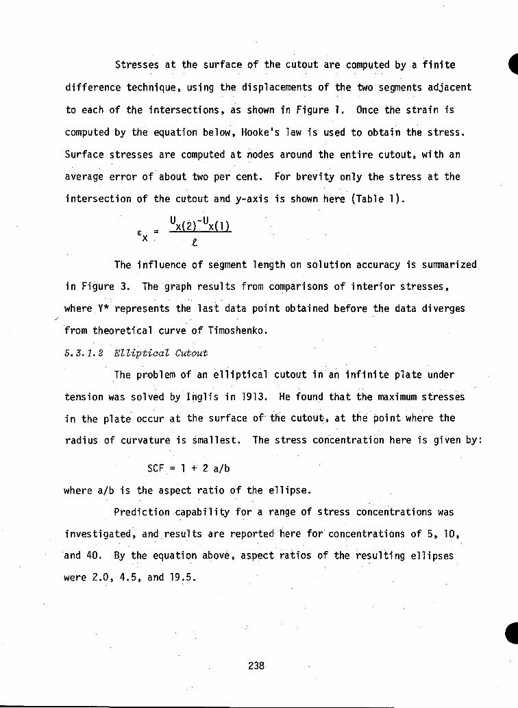
Stresses at the surface of the cutout are computed by a finite
difference technique, using the displacements of the two segments adjacent
to each of the intersections, as shown in Figure 1. Once the strain is
computed by the equation below, Hooke's law is used to obtain the stress.
Surface stresses are computed at nodes around the entire cutout, with an
average error of about two per cent. For brevity only the stress at the
intersection of the cutout and y-axis is shown here (Table 1).
The influence of segment length on solution accuracy is summarized
in Figure 3. The graph results from comparisons of interior stresses,
where Y* represents the last data point obtained before the data diverges
from theoretical curve of Timoshenko.
5.3.1.2 ElHptieal Cutout
The problem of an elliptical cutout in an infinite plate under
tension was solved by Inglis in 1913. He found that the maximum stresses
in the plate occur at the surface of the cutout, at the point where the
radius of curvature is smallest. The stress concentration here is given by:
SCF = 1 + 2 a/b
where a/b is the aspect ratio of the ellipse.
Prediction capability for a range of stress concentrations was
investigated, and results are reported here for concentrations of 5, 10,
and 40. By the equation above, aspect ratios of the resulting ellipses
were 2.0, 4.5, and 19.5.
238
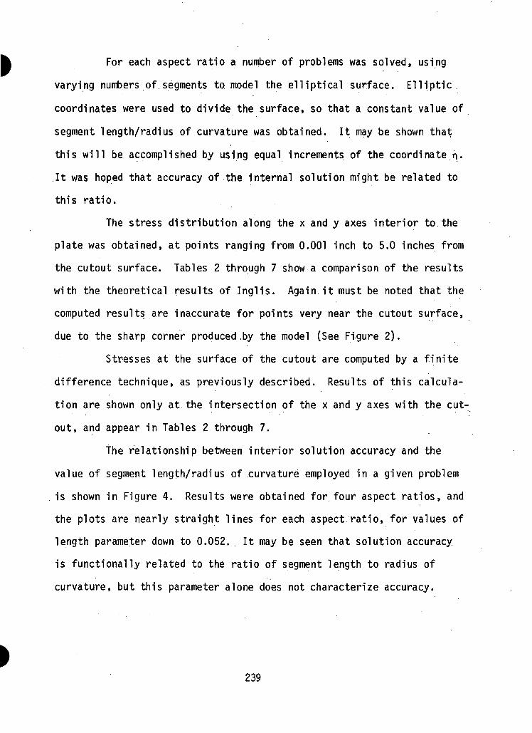
For each aspect ratio a number of problems was solved, using
varying numbers of segments to model the elliptical surface. Elliptic,
coordinates were used to divide the surface, so that a constant value of
segment length/radius of curvature was obtained. It may be shown that
this will be accomplished by using equal increments of the coordinate n-
It was hoped that accuracy of the internal solution might be related to
this ratio.
The stress distribution along the x and y axes interior to the
plate was obtained, at points ranging from 0.001 inch to 5.0 inches from
the cutout surface. Tables 2 through 7 show a comparison of the results
with the theoretical results of Inglis. Again it must be noted that the
computed results are inaccurate for points very near the cutout surface,
due to the sharp corner produced ,by the model (See Figure 2).
Stresses at the surface of the cutout are computed by a finite
difference technique, as previously described. Results of this calcula-
tion are shown only at the intersection of the x and y axes with the cut-
out, and appear in Tables 2 through 7.
The relationship between interior solution accuracy and the
value of segment length/radius of curvature employed in a given problem
is shown in Figure 4. Results were obtained for four aspect ratios, and
the plots are nearly straight lines for each aspect ratio, for values of
length parameter down to 0.052. It may be seen that solution accuracy
is functionally related to the ratio of segment length to radius of
curvature, but this parameter alone does not characterize accuracy.
239
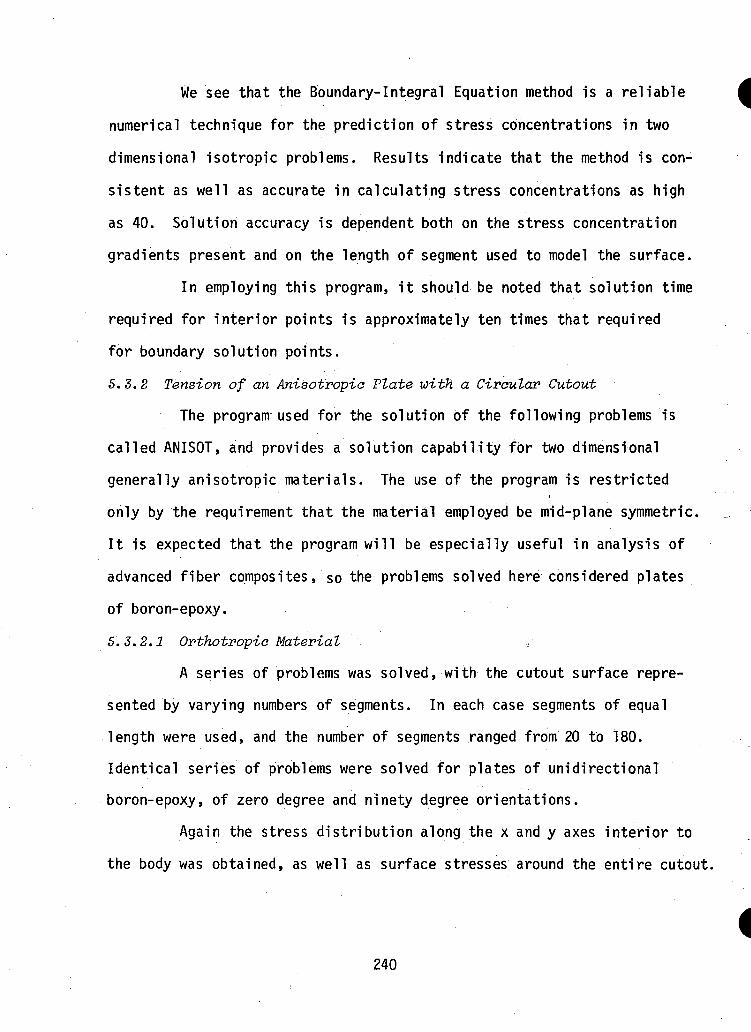
We see that the Boundary-Integral Equation method is a reliable
numerical technique for the prediction of stress concentrations in two
dimensional isotropic problems. Results indicate that the method is con-
sistent as well as accurate in calculating stress concentrations as high
as 40. Solution accuracy is dependent both on the stress concentration
gradients present and on the length of segment used to model the surface.
In employing this program, it should be noted that solution time
required for interior points is approximately ten times that required
for boundary solution points.
5. 3. 2 Tension of an Anisotropic Plate with a Circular Cutout
The program used for the solution of the following problems is
called ANISOT, and provides a solution capability for two dimensional
generally anisotropic materials. The use of the program is restricted
only by the requirement that the material employed be mid-plane symmetric.
It is expected that the program will be especially useful in analysis of
advanced fiber composites, so the problems solved here considered plates
of boron-epoxy.
5.3.2.1 Orthotropic Material ,
A series of problems was solved, with the cutout surface repre-
sented by varying numbers of segments. In each case segments of equal
length were used, and the number of segments ranged from 20 to 180.
Identical series of problems were solved for plates of unidirectional
boron-epoxy, of zero degree and ninety degree orientations.
Again the stress distribution along the x and y axes interior to
the body was obtained, as well as surface stresses around the entire cutout.
240
The hoop stresses around the cutout at the surface were compared to the
theoretical results of Lekhnitskii, and res.ults appear in Tables 8 and 9.
These stresses are computed directly from displacements and tractions, and
thus provide a means of evaluating the boundary solution capability of
the program. Results compared.extremely well with the theoretical calcu-
lations, even for the higher stress concentrations.
The accuracy of the solutions obtained are dependent on both the
stress concentration gradients present and length of segment used in the
model. This behavior is expected, since the basic algorithms employed are
similar to those of the isotropic program, DIPOME. Time required for
interior solution points was again about ten times that for boundary
points. ;
5.3.3.2 Anisotropic Material . •
The problem of a circular cutout in an infinite plate was next
solved for a completely anisotropic material, unidirectional boron-epoxy
at an orientation of 45 degrees. There was no symmetry about either the
x or y axis, as had been present before, so the entire cutout surface
was modeled.
As before, the hoop stresses at the surface of the cutout were
obtained and are compared with the results of Lekhnitskii in Tables 10
and 11. Two problems were solved, one employing 20 segments, and the
other 90 segments, to represent the surface. Here again agreement with
theoretical results was excellent along the entire surface.
241
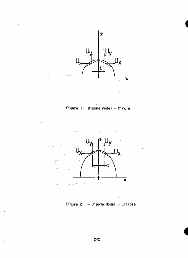
Figure 1: Dipome Model —Circle
Figure 2: — Dipome Model - Ellipse
242
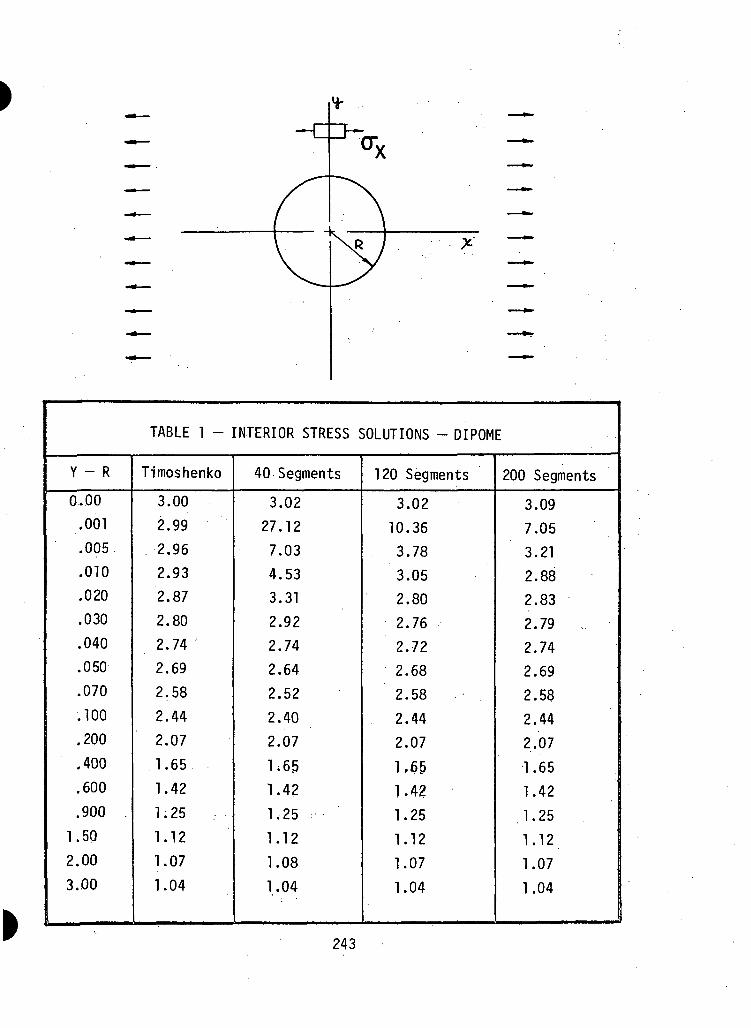
X
TABLE 1 - INTERIOR STRESS SOLUTIONS - DIPOME
Y - R
0.00
.001
.005
.010
.020
.030
.040
.050
.070
.100
.200
.400
.600
.900 .
1.50
2.00
3.00
Timoshenko
3.00
2.99
2.96
2.93
2.87
2.80
2.74 '2.69
2.58
2.44
2.07
1.65
1.42
1.25
1.12
1.07
1.04
40 Segments
3.02
27.12
7.03
4.53
3.31
2.92
2.74
2.64
2.52
2.40
2.07
1.65
1.42
1.25 :••
1.12
1.08
1.04
120 Segments
3.02
10.36
3.78
3.05
2.80
2.76
2.72
2.68
2.58
2.44
2.07
1.65
1.42
1.25
1.12
1.07
1.04
200 Segments
3.09
7.05
3.21
2.88
2.83
2.79 ,.
2.74
2.69
2.58
2.44
2.07
1.65
1.421.25
1.12
1.07
1.04
243
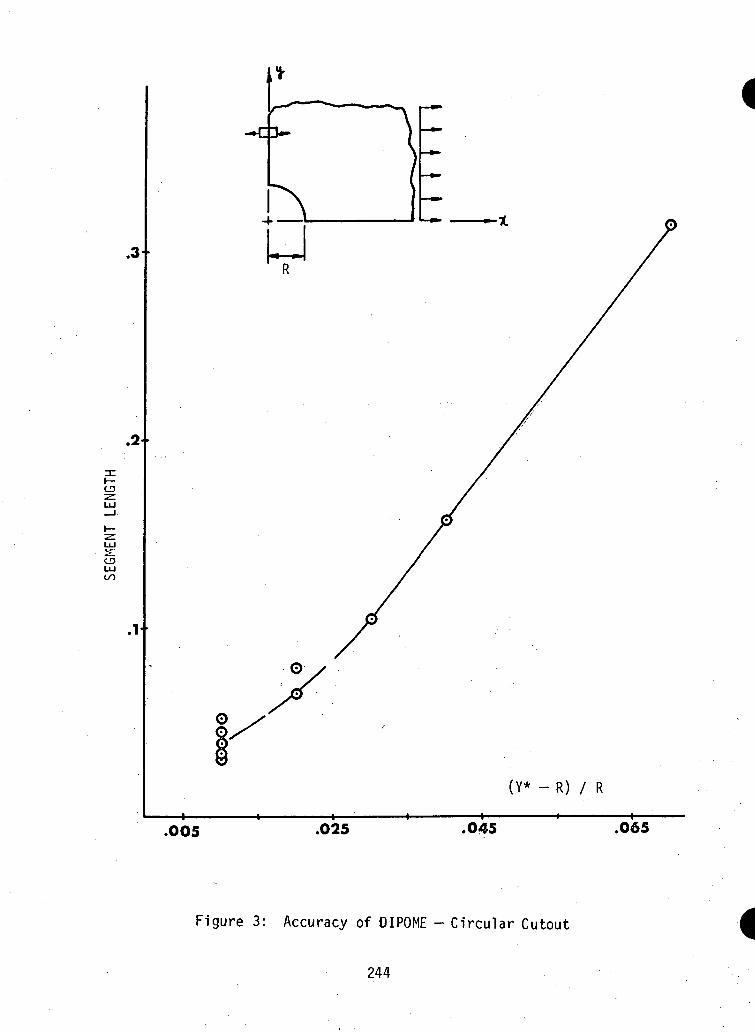
.3
.2-
n:CJ3
CDUJCO
.1
(Y* - R) / R
.005 .025 .045 .065
Figure 3: Accuracy of 01POME - Circular Cutout
244
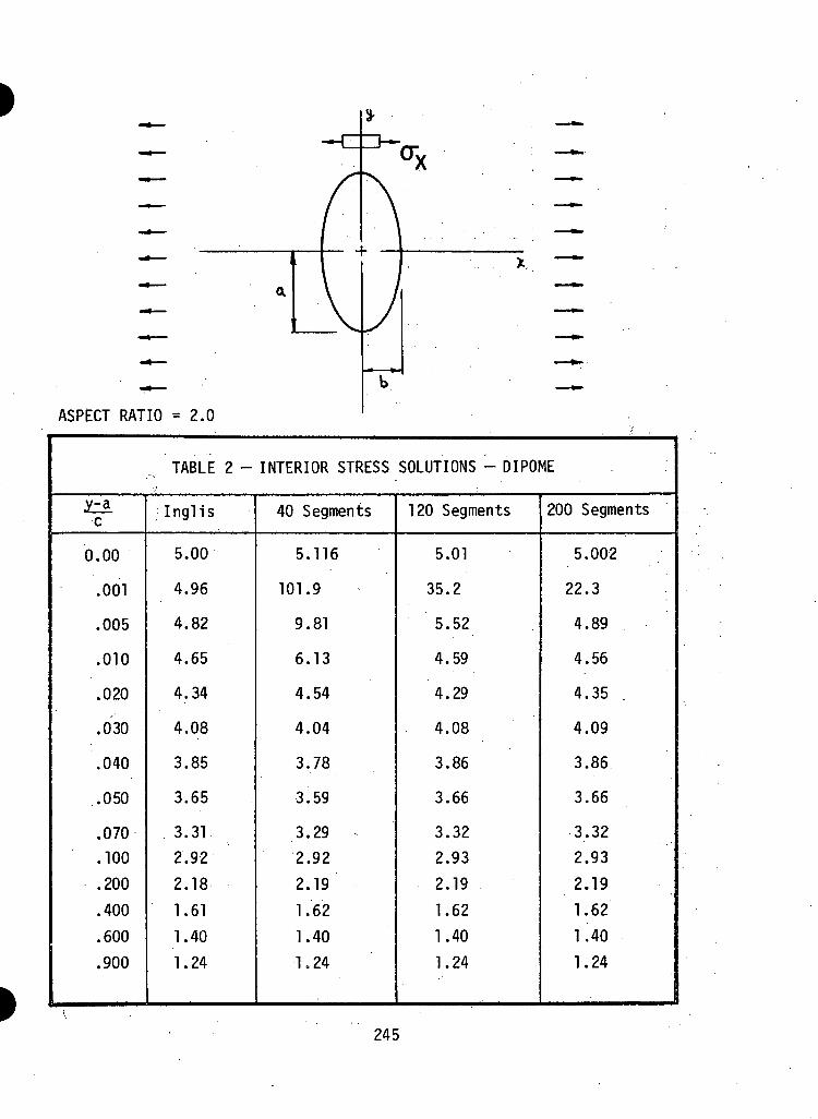
ASPECT RATIO = 2 . 0
. TABLE 2 - INTERIOR STRESS SOLUTIONS - DIPOME
£Ac
0.00
.001
.005
.010
.020
.030
.040
.050
.070
.100
.200
.400
.600
.900
; Inglis
5.00
4.96
4.82
4.65
4.34
4.08
3.85
3.65
3.31
2.92
2.18
1.61
1.40
1.24
40 Segments
5.116
101.9
9.81
6.13
4.54
4.04
3.78
3.59
3.29 -
2.92
2.19
1.62
1.40
•1 . 24
120 Segments
5.01
35.2
5.52
4.59
4.29
4.08
3.86
3.66
3.32
2.93
2.19
1.62
1.40
1.24
200 Segments
5.002
22.3
4.89
4.56
4.35
4.09
3.86
3.66
3.32
2.93
2.19
1.62
1.40
1.24
245
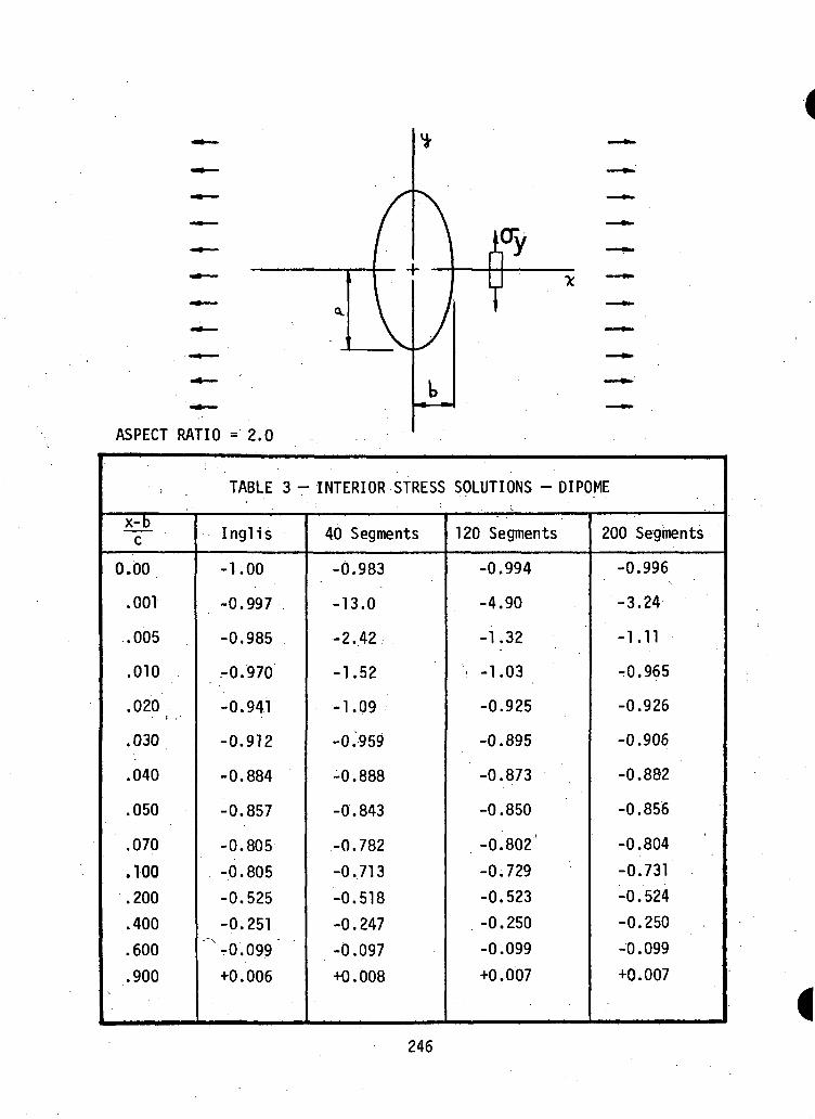
ASPECT RATIO = 2.0
y —
TABLE 3 - INTERIOR STRESS SOLUTIONS - DIPOME• : i - v
x-Bc
0.00
.001
.005
.010
.020t • '
.030
.040
.050
.070
.TOO
.200
.400
.600
.900
Inglis
-1.00
-0.997
-0.985
-0.970
-0.941
-0.912
-0.884
-0.857
-0.805
-0.805
-0.525
-0.251
~ -0.099
+0.006
40 Segments
-0.983
-13.0
-2.42
-1.52
-1.09
-0.959
-0.888
-0.843
-0.782
-0.713
-0.518
-0.247
-0.097
+0.008
120 Segments
-0.994
-4.90
-1.32
-1.03
-0.925
-0.895
-0.873
-0.850
-0.802'
-0.729-0.523
. -0.250-0.099
+0.007
200 Segments
-0.996
-3.24
-1.11
-0.965
-0.926
-0.906
-0.882
-0.856
-0.804
-0.731
-0.524
-0.250
-0.099
+0.007
246
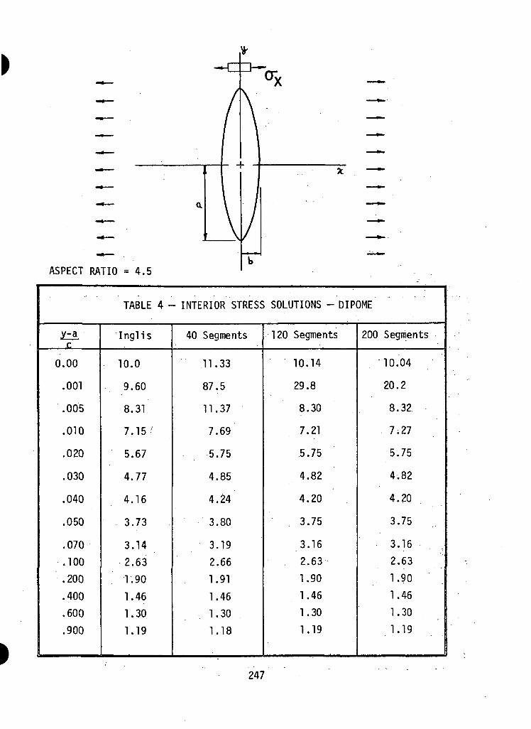
ASPECT RATIO = 4 . 5
TABLE 4- INTERIOR STRESS SOLUTIONS -DIPOME
Jta../c
0.00
.001
.005
.010
.020
.030
.040
.050
.070
.100
.200
.400
.600
.900
Inglis
10.0
9.60
8.31
7.15'
5.67
4.77
4.16
3.73
3.14
2.63
1.90
1.46
1.30
1.19
40 Segments
11.33
87.5
11.37
7.69
5.75
4.85
4.24
3.80
3.19
2.66
1.91
1.46
1.30
1.18
120 Segments
10.14
29.8
8.30
7.21
5.75
4.82
4.20
3.75
3.16
. 2.63
1.90
1.46
1.30
1.19
200 Segments
10.04
20.2
8.32
7.27
5.75
4.82
4.20
3.75
3.16
2.63
1.90
1.46
1.30
1.19
247
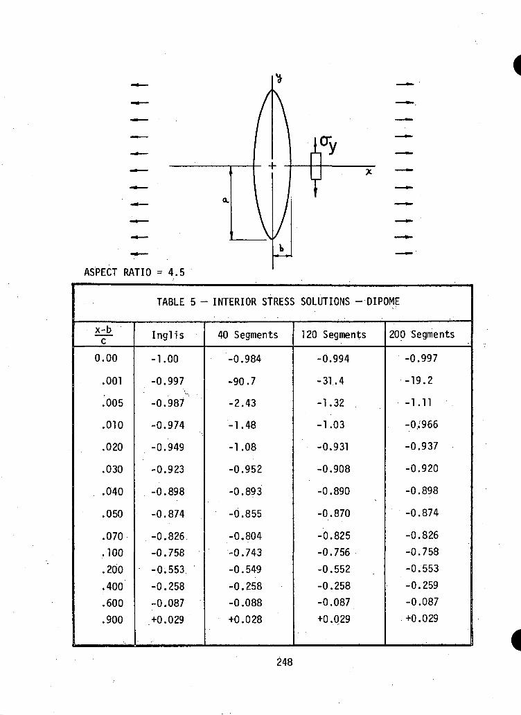
ASPECT RATIO = 4 . 5
TABLE 5 - INTERIOR STRESS SOLUTIONS - DIPOME
x-bc
0.00
.001
.005
.010
.020
.030
.040
.050
.070
.100
.200
.400
.600
.900
Inglis
-1.00
-0.997
-0.987
-0.974
-0.949
-0.923
-0.898
-0.874
-0.826-0.758
-0.553
-0.258
-0.087
,+0.029
40 Segments
-0.984
-90.7
-2.43
-1.48
-1.08
-0.952
-0.893
-0.855
-0.804-0.743
-0.549
-0.258
-0.088
+0.028
1 20 Segments
-0.994
-31.4
-1.32
-1.03
-0.931
-0.908
-0.890
-0.870
-0.825
-0.756
-0.552
-0.258-0.087
+0.029
200 Segments
-0.997
-19.2
-1.11
-0;966
-0.937
-0.920
-0.898
-0.874
-0.826
-0.758
-0.553
-0.259
-0.087
+0.029
248
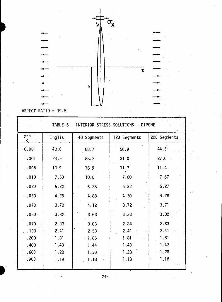
ASPECT RATIO = 1 9 . 5
TABLE 6 - INTERIOR STRESS SOLUTIONS - DIPOME
£±c
0.00
.001
.005
.010
.020
.030
.040
.050
.070
, .100
.200
.400
.600
.900
Inglis
40.0
23.5
10.9
7.50
5.22
4.26
3.70
3.32
2.83
2.41
1.81
1.43
1.28
1.18
40 Segments
88*7
88.2
16.9
10.0
6.28
4.88
4.12
3.63
3.03
2.53
1.85
1.44
1.28
1.18
120 Segments
50.9
31.0
11.7
7.80
5.32
4.30
3.72
3.33
2.84
2.41 .
1.81
1.43
1.28
1.18
200 Segments
44.5
27.0
11.4
7.67
5.27
4.28
3.71
3.32
2.83
2.41
1.81
1.42
1.28
1.18
249
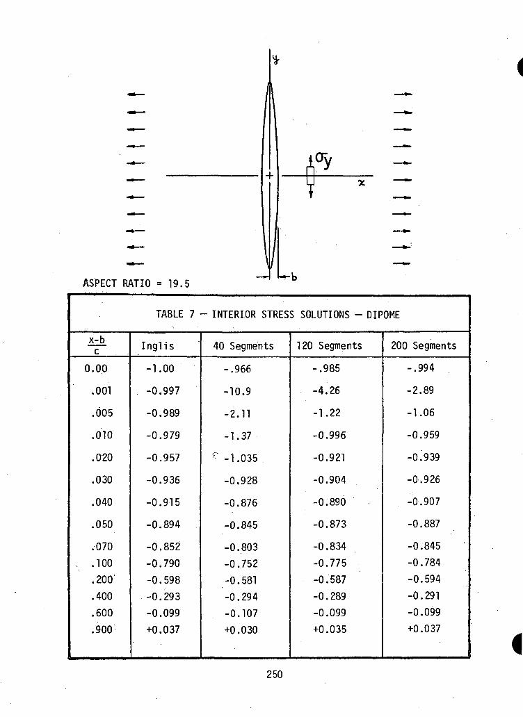
ASPECT RATIO = 1 9 . 5
TABLE 7 - INTERIOR STRESS SOLUTIONS - DIPOME
X-bc
0.00
.001
.005
.010
.020
.030
.040
.050
.070
. .100
.200
.400
.600
.900
Inglis
-1.00
-0.997
-0.989
-0.979
-0.957
-0.936
-0.915
-0.894
-0.852
-0.790
-0.598-0.293-0.099
+0.037
40 Segments
-.966
-10.9
-2.11
-1.37
e -1.035
-0.928
-0.876
-0.845
-0.803
-0.752
-0.581
-0.294-0.107
+0.030
120 Segments
-.985
-4.26
-1.22
-0.996
-0.921
-0.904
-0.890
-0.873
-0.834
-0.775
-0.587-0,289-0.099
+0.035
200 Segments
-.994
-2.89
-1.06
-0.959
-0.939
-0.926
-0.907
-0.887
-0.845-0.784
-0.594-0.291
-0.099
+0.037
250
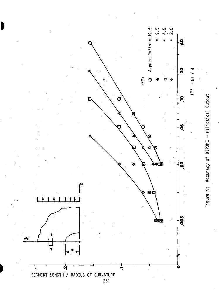
in in in oCD cr> **• co
M M
to
<o
I*
s
o4JQ.
I
LU
OO.1—4
O
4-O
<J
S-3Ou«t
OJS-3
IOOO
SEGMENT LENGTH / RADIUS OF CURVATURE251
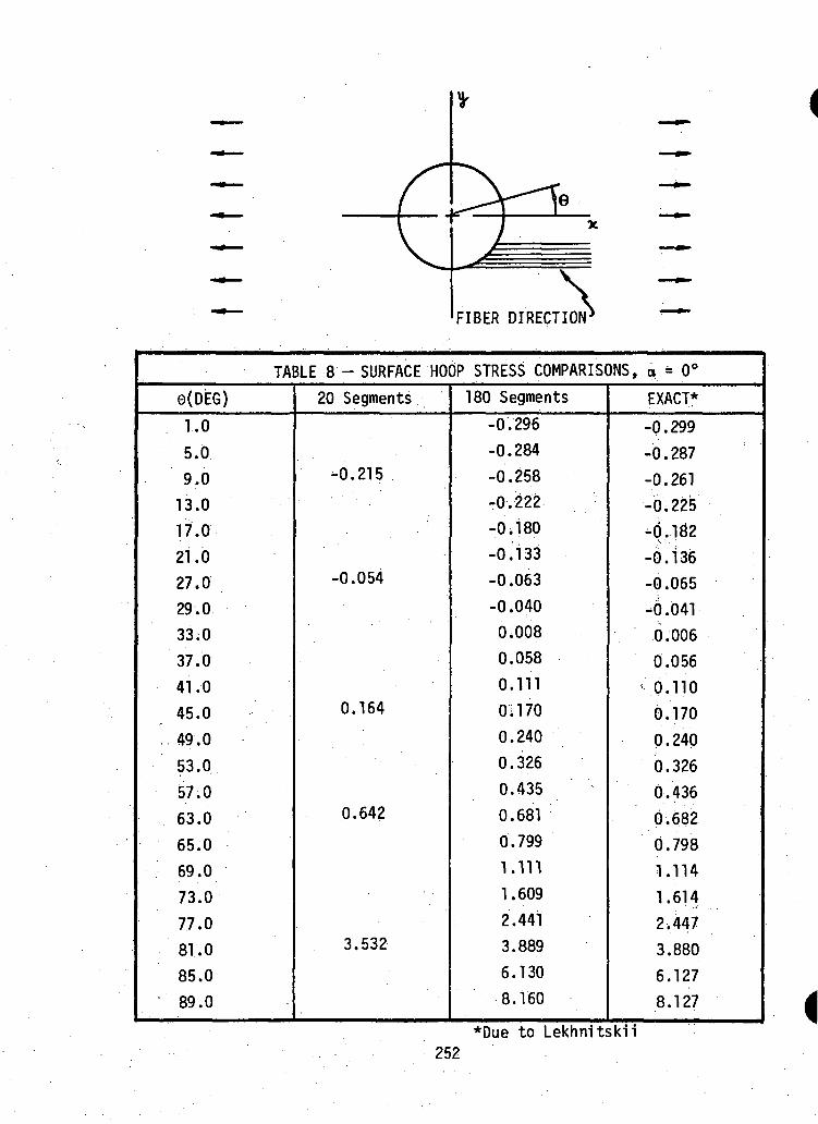
FIBER DIRECTION-
TABLE 8 - SURFACE HOOP STRESS COMPARISONS, a = 0°
0(DEG)
1.0
5.0
9.0
13.0
17;0
21.0
27.0
29.0
33 ;0
37.0
41 .0
45.0
. 4 9 . 0
53.0.
57.0
63.0
65.0
69.0
73.0
77.0
81 .0
85.0
89.0
20 Segments
-0.215
-0.054
0.164
0.642
3.532
180 Segments
-0.296
-0.284
-0.258
-0.222
-OilSO
-0.133
-0.063
-0.040
0.008
0.058
0.111
Oil 70
0.240
0.326
0.435
0.681
0.799
1.111
1.609
2.441
3.889
6.130
8.160
EXACT*
-0.299
-0.287
-0.261
-0.225
-6.162
-6.136
-0.065
-6.041
0.006
0.056
'0.110
0.170
0.240
0.326
0.436
0.682
0.798
1.114
1.614
2.447
3.880
6.127
8.127
*Due to Lekhnitskii252
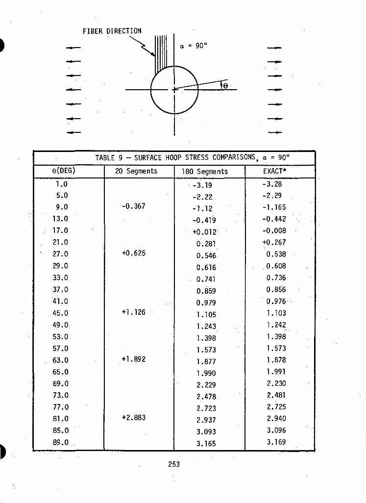
FIBER DIRECTION
a = 90<
TABLE 9 -SURFACE HOOP STRESS COMPARISONS, a = 90°
0(DE6)
1.0
5.0
9.0
13.0
17.0
21.0
27.0
29.0
33.0
37.0
41.0
45.0
49.0
53.0
57.0
63.0
65.0
69.0
73.0
77.0
81.0
85.0
89.0 .
20 Segments
-0.367
+0.625
+1.126
+1.892
+2.883
180 Segments
-3.19
-2.22
-1.12
-0.419
+0.012
0.281
0.546
0.616
0.741
0.859
0.979
1.105
1.243
1.398
1.573
1.877
1.990
2.229
2.478
2.723
2.937
3.093
3.165
EXACT*
-3.28
-2.29
-1.165
-0.442
-0.008
+0.267
0.538
0.608
0.736
0.856
0.976
1.103
1.242
1.398
1.573
1.878
1.991
2.230
2.481
2.725
2.940
3.096
3.169
253
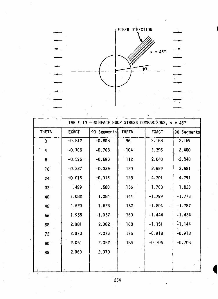
FIBER DIRECTION
TABLE 10 -SURFACE HOOP STRESS COMPARISONS, a = 45°
THETA
0
4
8
16
24
32
40
48
56
68
72
80
88
•' \* . it'
EXACT
-0.812
-0.706
-0.596
-0.337
+0.015
.499
1.082
1.620
1.955
2.081
2.073
2.051
2.069
90 Segments
-0.808
-0.703
-0.593
-0.335
+0.016
.500
1.084
1.623
1.957
2.082
2.073
2.052
2.070
THETA
96
104
112
120
128
136
144
152
160
168
176
184
EXACT
2.168
2.396
2.840
3.659
4.701
1.703
-1.799
-1.804
-1.444
-1.151
-0.918
-0.706
90 Segments
2.169
2.400
2.848
3.681
4.791
1.823
-1.773
-1.787
-1.434
-1.144
-0.913
-0.703
254
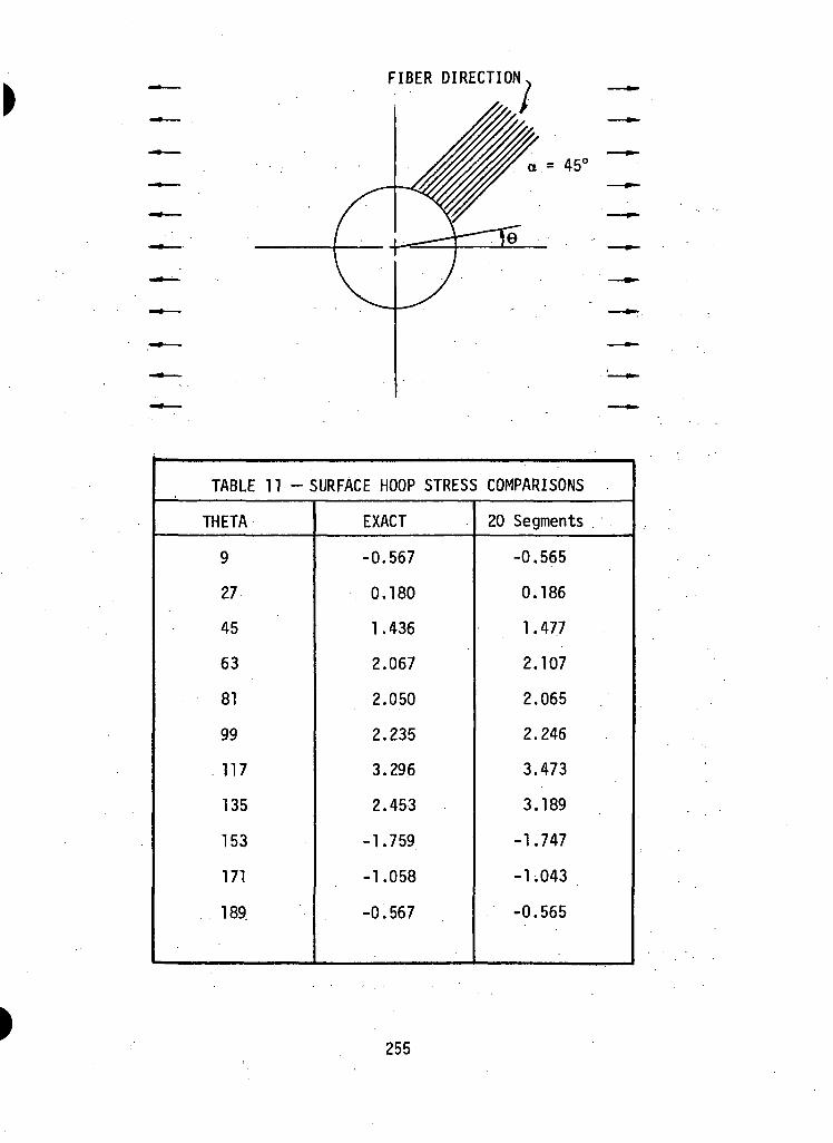
FIBER DIRECTION,
= 45C
TABLE 11 -SURFACE HOOP STRESS COMPARISONS
THETA
9
27
45
63
81
99
117
135
153
171
189.
EXACT
-0.567
0.180
1.436
2.067
2.050
2.235
3.296
2.453
-1.759
-1.058
-0.567
20 Segments
-0.565
0.186
1.477
2.107
2.065
2.246
3.473
3.189
-1.747
-1.043
-0.565
255
5.4 ADVANCED TOPICS. IN ANISOTROPIC INTEGRAL EQUATION SOLUTION METHODS
5.4.1 Introduction
The "integral equation method" referred to in this Section is
basically a technique for obtaining accurate approximate solutions for a
wide variety of physical problems governed by linear partial differential
equations. As is clear from a number of papers e.g. [1,2,3,4,5] the method
has reached a considerable stage of development and is emerging as an im-
portant tool comparable to and potentially, we think, better than finite
element and finite difference techniques for certain problems. This ap-
pears to be particularly true for a variety of problems involving material
composites.
A glance at the work cited above reveals that the method depends
crucially on the existence and explicit definition of a fundamental singu-
lar solution to the appropriate governing partial differential equations.
Therefore, in an attempt to open up the field of linear three-dimensional
anisotropi'o elasticity to attack, via the integral equation method, con-
siderable effort was directed toward investigating what is known of the
necessary singular solution. As noted earlier, this solution is
the field due to a concentrated force in an infinite anisotropic media.
Two major works [6] and [7] were found on this topic, and examined with
respect to the stated objective. Details primarily concerned with making
representations of the singular solution available for practical purposes
are given later in this Section.
The problem of interlaminar shear was investigated with
a view toward attacking this problem (as defined by R. B. Pipes [8]) via
the integral equation method. Under the/appropriate assumptions, the
256
relevant surface integrals reduce to path integrals around each of the
layers. While the problem is not completely two-dimensional in nature,
significant advantages still seem to be present with the integral equation
method for both isotropic and anisotropic layers to warrant further
investigation with test problems. Details of the formulation for isotropic
layer assumptions and a discussion ,of the possibilities for anisotropic
layers are included in this Section..
5.4.2 Fundamental Three-Dimensional ,Anisotrqpio Singularity
5.4.2.1 Via John [7J] .
.The work ;by John [7] which is fin essence "a somewhat'heterogeneous
collection of results ;o,n parti ail diififenen-tiail .equations" .contains, in
Ch. HI, .a itneittiod f,p,r .constructing the so-called fundamental, singular
solution for an elliptic system of linear partial differential equations
with analytic coefficients. Since our main concern here is with homogene-
ous anisotropic elasticity theory, we will specialize John's development
at the outset and explicitly deal with the system of equations
Cijkluk,lj =0 f1)..
Equations (1) are the equations of equilibrium in the absence of body
forces for a linear elastic solid obeying the constitutive relation
Tij = Cijklekl (2)
in which C.- k l are constants, and T.. , e.. , u. the stress, strain,
and displacement components assuming the linearized theory. As usual
we take
Cijkl = Cklij <3)
together with necessary symmetries in the .first and second pair of indices
s.u,ch that C. .., implies at most twenty-one independent constants.
257
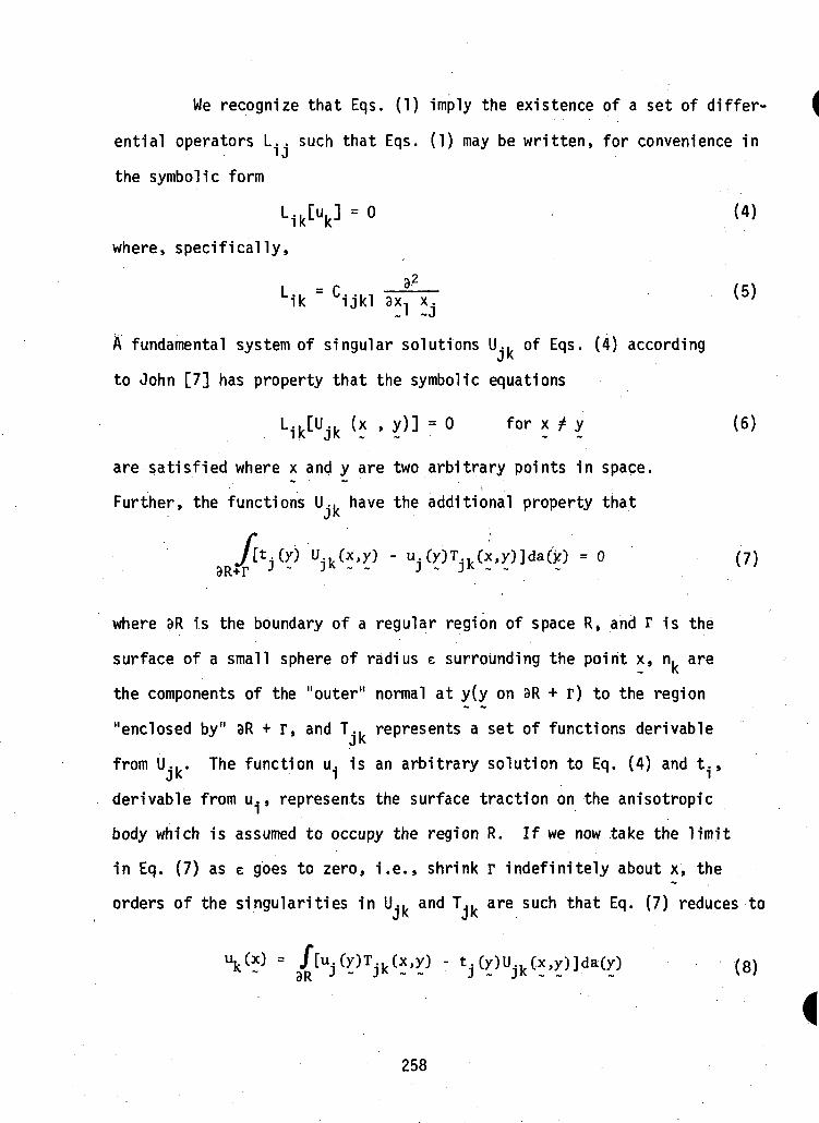
We recognize that Eqs. (1) imply the existence of a set of differ-
ential operators L.. such that Eqs. (1) may be written, for convenience inI J
the symbolic form
Ljk[uk] - 0 (4)
where, specifically,
I = r 2-l _ » i V / » » i ^ik ijkl ax, x.
A fundamental system of singular solutions U.. of Eqs. (4) according
to John [7] has property that the symbolic equations
L.k[Ujk (x , y)] = 0 for x t y (6)
are satisfied where x and y are two arbitrary points in space.
Further, the functions U.. have the additional property thatJK
y[t,(y) U (x,y) - u (y)T (x,y)]da(x) = 0 (7)8R+T J - JK ~ ~ J - JK - ~
where 8R is the boundary of a regular region of space R, and r is the
surface of a small sphere of radius e surrounding the point x, nk are
the components of the "outer" normal at y(y on 3R + r) to the region
"enclosed by" 3R + r, and T.k represents a set of functions derivable
from U-k. The function u. is an arbitrary solution to Eq. (4) and t.,
derivable from u., represents the surface traction on the anisotropic
body which is assumed to occupy the region R. If we now take the limit
in Eq. (7) as e goes to zero, i.e., shrink r indefinitely about x, the
orders of the singularities in U-k and T-k are such that Eq. (7) reduces to
258
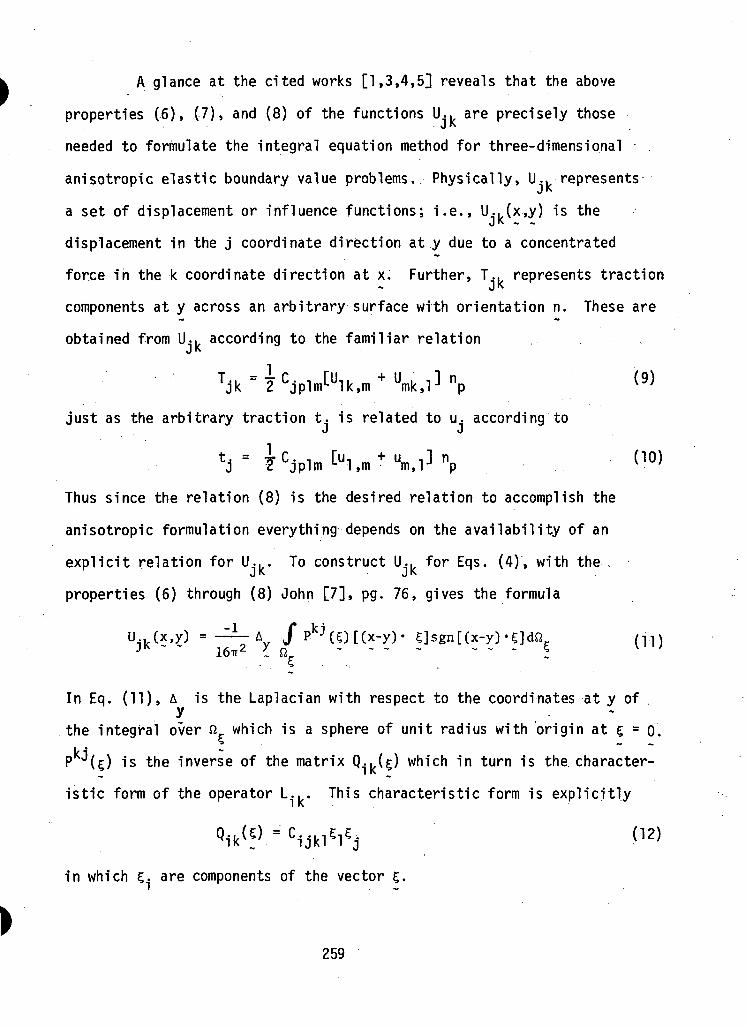
A glance at the cited works [1,3,4,5] reveals that the above
properties (6), (7), and (8) of the functions U.. are precisely those
needed to formulate the integral equation method for three-dimensional
anisotropic elastic boundary value problems. Physically, U.. represents
a set of displacement or influence functions; i.e., U..(x,y) is theJK _ „displacement in the j coordinate direction at y due to a concentrated
force in the k coordinate direction at x. Further, T.. represents tractionJKcomponents at y across an arbitrary surface with orientation n. These are
obtained from U-k according to the familiar relation
just as the arbitrary traction t. is related to u. according toJ J
V ?CjP l rn [ u l ,m+ Vl ]np
Thus since the relation (8) is the desired relation to accomplish the
anisotropic formulation everything depends on the availability of an
explicit relation for U-. To construct U- for Eqs. (4), with the ,
properties (6) through (8) John [7], pg. 76, gives the formula
167T
In Eq. (11), A is the Laplacian with respect to the coordinates at y of ' . .
the integral over fi which is a sphere of unit radius with origin at £ = o.
P (g) is the inverse of the matrix Q..-^?) which in turn is the character-
istic form of the operator L... . This characteristic form is explicitly1 K
in which 5- are components of the vector
259
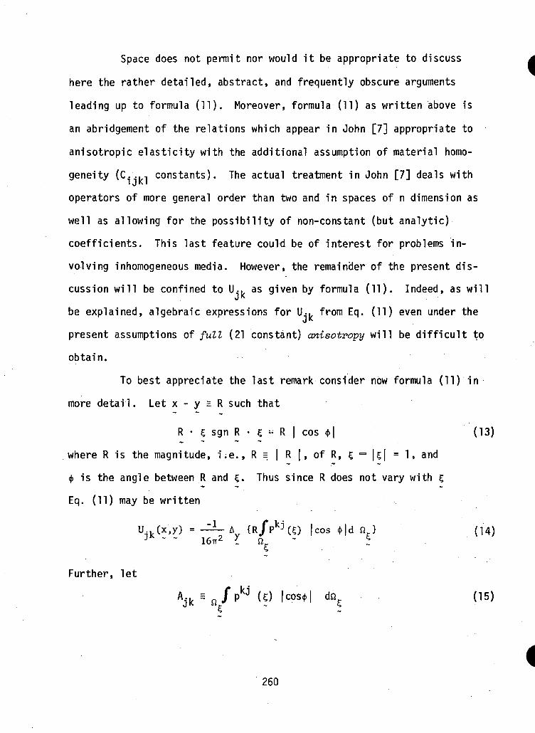
Space does not permit nor would it be appropriate to discuss
here the rather detailed, abstract, and frequently obscure arguments
leading up to formula (11). Moreover, formula (11) as written above is
an abridgement of the relations which appear in John [7] appropriate to
anisotropic elasticity with the additional assumption of material homo-
geneity (C.-kl constants). The actual treatment in John [7] deals with
operators of more general order than two and in spaces of n dimension as
well as allowing for the possibility of non-constant (but analytic)
coefficients. This last feature could be of interest for problems in-
volving inhomogeneous media. However, the remainder of the present dis-
cussion will be confined to U.. as given by formula (11). Indeed, as willJK
be explained, algebraic expressions for U.. from Eq. (11) even under the
present assumptions of full (21 constant) anisotropy will be difficult to
obtain.
To best appreciate the last remark consider now formula (11) in
more detail. Let x - y = R such that
R • 5 sgn R • £ " R | cos t| (13)
where R is the magnitude, i .e. , R = | R | , of R, E, = \E,\ = 1, and
<(> is the angle between R and £. Thus since R does not vary with £
Eq. (11) may be written
16TT2
Further, let
U. k (x ,y ) = - - A { R P ( 5 ) |cos * | d f l } (14)J ~ ~ 2 *
(15)
260
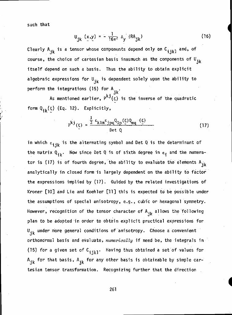
such that
V IIV 06)
Clearly A., is a tensor whose components depend only on C..., and, of
course, the choice of cartesian basis inasmuch as the components of U..
itself depend on such a basis. Thus the ability to obtain explicit
algebraic expressions for U.. is dependent solely upon the ability toJK
perform the integrations (15) for A .ki Jk
As mentioned earlier, P (5) is the inverse of the quadratic
form Q ik(p (Eq. 12). Explicitly,
Det Q
in which e... is the alternating symbol and Det Q is the determinant of
the matrix Q.. . Now since Det Q is of sixth degree in e- and the numera-1 K I
tor is (17) is of fourth degree, the ability to evaluate the elements A..
analytically in closed form is largely dependent on the ability to factor
the expressions implied by (17). Guided by the related investigations of
Kroner [10] and Lie and Koehler [11] this is expected to be possible under
the assumptions of special anisotropy, e.g., cubic or hexagonal symmetry.
However, recognition of the tensor character of A., allows the followingJK "
plan to be adopted in order to obtain explicit practical expressions for
U.. under more general conditions of anisotropy. Choose a convenientJKorthonormal basis and evaluate, numerically if need be, the integrals in
(15) for a given set of C..-,. Having thus obtained a set of values for
A., for that basis, A., for any other basis is obtainable by simple car-
tesian tensor transformation. Recognizing further that the direction
261
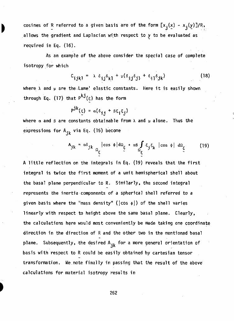
cosines of R referred to a given basis are of the form [x.(x) - x.(y)]/R,~ J ~ J ~ , ;
allows the gradient and Laplacian with respect to y to be evaluated as•V
required in Eq. (16).
As an example of the above consider the special case of complete
isotropy for which
where X and p are the.Lame' elastic constants. Here it is easily shown
through Eq. (17) that Pkj(?) has the form
PjkU) = a(6.j + ue^j)
where a and e are constants obtainable from X and u alone. Thus the
expressions for A., via Eq. (15) become
Ajk = aiSjk 'cos *ldn£ * aB'/'Cj5k 'cos *l dJ2Cfl^ ~ fl^ ,
A little reflection on the integrals in Eq. (19) reveals that the first
integral is twice the first moment of a unit hemispherical shell about
the basal plane perpendicular to R. Similarly, the second integral
represents the inertia components of a spherical shell referred to a
given basis where the "mass density" (|cos <j>|) of the shell varies
linearly with respect to height above the same basal plane. Clearly,
the calculations here would most conveniently be made taking one coordinate
direction in the direction of R and the other two in the mentioned basal
plane. Subsequently, the desired A., for a more general orientation ofJ K
basis with respect to R could be easily obtained by cartesian tensor
transformation. We note finally in passing that the result of the above
calculations for material isotropy results in
262

[(3-4v)6.k + cos * cos/ ?fl \
in which v=A/2 (A+y) and *. is the angle between the vector R and theJ •-
x. axis. Expression (20) is the fundamental isotropic singular solution
(see e.g. Cruse [3]). .
The key feature of the above proposed method is the ability to
perform, if need be, part of the calculation numerically and still obtain
all dependence of U.. on x,y and basis orientation with respect to x-yJK ^ „ „ _analytically. This is important since gradients of U.. at y are required
for the integral equation method and such gradients may therefore be taken
analytically. Thus, in light of the goal of this portion of the research,
i.e., obtaining an explicit, usable, algebraic form for U., for complete
anisotropy, it appears, despite numerical evaluation of certain integrals
in general, that the job can be done via the outlined method.
263
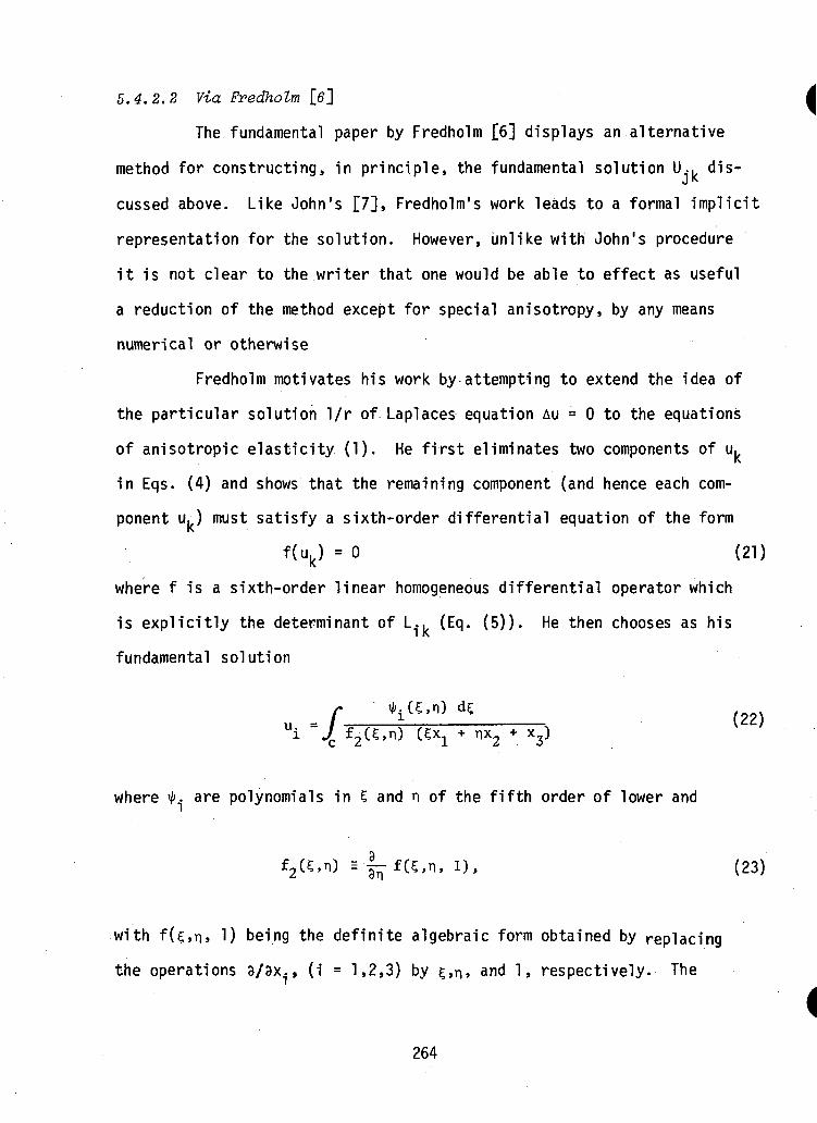
5.4.2.2 Via Fredholm
The fundamental paper by Fredholm [6] displays an alternative
method for constructing, in principle, the fundamental solution U.. dis-JK
cussed above. Like John's £7], Fredholm's work leads to a formal implicit
representation for the solution. However, unlike with John's procedure
it is not clear to the writer that one would be able to effect as useful
a reduction of the method except for special anisotropy, by any means
numerical or otherwise
Fredholm motivates his work by attempting to extend the idea of
the particular solution 1/r of Laplaces equation AU = 0 to the equations
of anisotropic elasticity (1). He first eliminates two components of u.
in Eqs. (4) and shows that the remaining component (and hence each com-
ponent u. ) must satisfy a sixth-order differential equation of the form
f(uk) = 0 (21)
where f is a sixth-order linear homogeneous differential operator which
is explicitly the determinant of L.. (Eq. (5)). He then chooses as his
fundamental solution
fUi J
(22)
where ty. are polynomials in 5 and n of the fifth order of lower and
f2(S,n) =-|-fC5,n, 1), (23)
with fU,n» 1) being the definite algebraic form obtained by replacing
the operations 3/3-x., (i = 1,2,3) by g,n, and 1, respectively. The
264
integration is around a closed contour c in £ space containing only
those singular points which are roots of fU,n ) = 0 where n is given by
5X1 + V2 + X3 = ° (24)
The polynomials $. above are complicated algebraic expressions (see [6]
pg. 14) obtained from L... Fredholm then goes on to show that each
component of the required tensor field U.. is of the form (22) and
rigorously establishes all of the properties of the solution.
It seems clear from the work of Kroner [10] and Lie and Koehler
[11] that any attempt to reduce Fredholm1s method to something useful for
other than hexagonal or cubic crystal symmetry assumptions would be most
difficult indeed. Detailed information on the particulars of this can
best be obtained by careful study of the references [10,11] plus Fredholm's
original paper [6]. It should be clear; however, that if the previous
discussion and reduction of John's [7] approach is valid as outlined, it
must be possible to accomplish the same task via Fredholm also since the
desired U- is unique. Nevertheless, the transformation of contour
integral in space to one over the unit sphere, of functions which are
necessarily related but not explicitly so, is bound to be an extremely
difficult task. Further, for practical purposes and in light of the
previous section the effort seems hardly worthwhile in the near future.
It is my judgement that to formulate the integral equation
method for general anisotropic elasticity, the method of John as pre-
viously outlined is by far the most promising at this point. Indeed, the
outlined reduction with the ability to obtain the necessary functional
variational analytically is better than was hoped for at the start of the
265
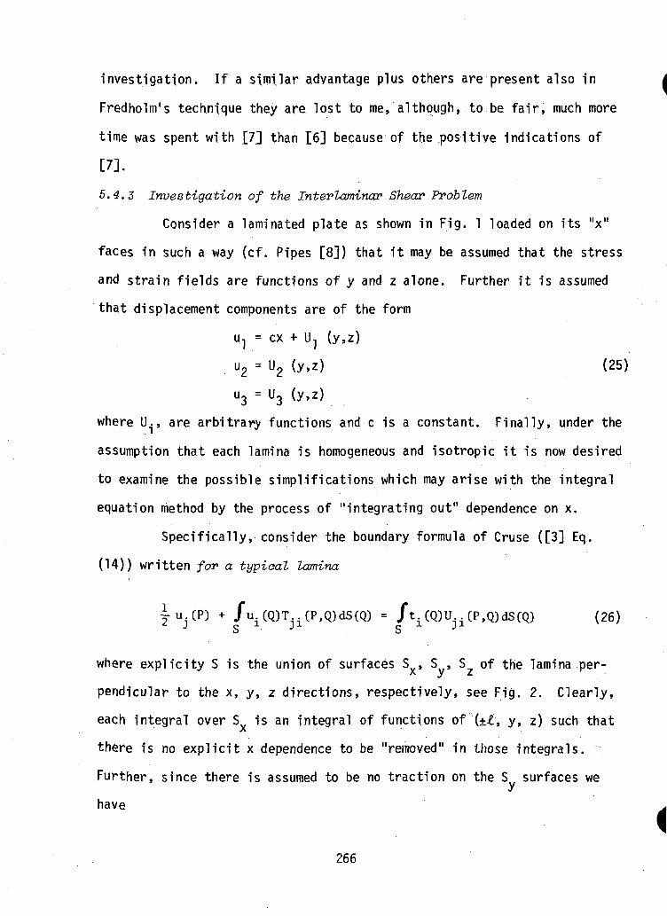
investigation. If a similar advantage plus others are present also in
Fredholm's technique they are lost to me, although, to be fair, much more
time was spent with J7J than 16] because of the positive indications of
[7].
5.4.3 Investigation of the Interlaminar Shear Problem
Consider a laminated plate as shown in Fig. 1 loaded on its "x"
faces in such a way (cf . Pipes [8]) that it may be assumed that the stress
and strain fields are functions of y and z alone. Further it is assumed
that displacement components are of the form
u1 = ex + U] (y,z)
u2 = U2 (y,z) (25)
u3 = U3 (y,z)
where U., are arbitrary functions and c is a constant. Finally, under the
assumption that each lamina is homogeneous and isotropic it is now desired
to examine the possible simplifications which may arise with the integral
equation method by the process of "integrating out" dependence on x.
Specifically, consider the boundary formula of Cruse ([3] Eq.
(14)) written for a typical lamina
iu.(P) + /u (Q)T (P,Q)dS(Q) = /t. (Q)U (P,Q)dS(Q) (26)S S
where explicity S is the union of surfaces S , S , S of the lamina per-A y z
pendicular to the x, y, z directions, respectively, see Fig. 2. Clearly,
each integral over S is an integral of functions of (±£, y, z) such thatX ' . •
there is no explicit x dependence to be "removed" in those integrals.
Further, since there is assumed to be no traction on the S surfaces we
have
266
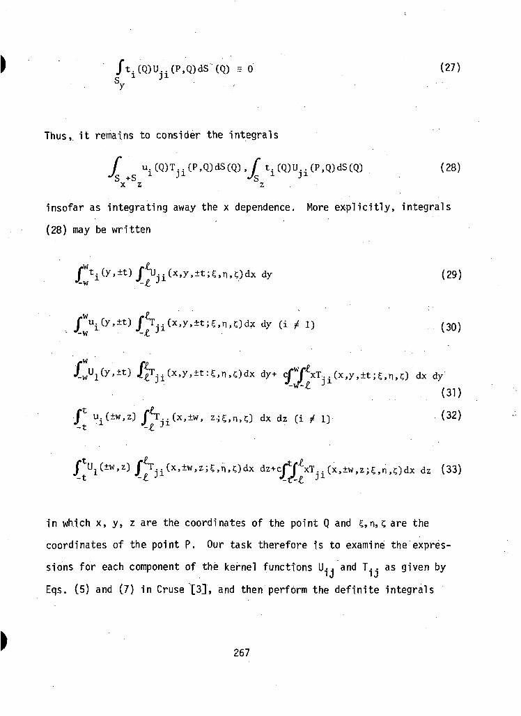
ft (Q)U. (P,Q)dS (Q) E 0 (27)<-* J- J -Lsy
Thus, it remains to consider the integrals
f ui(Q)Tji(P,Q)dS(Q),y ti(Q)Uji(P,Q)dS(Q) _ (28)
X Z Z
insofar as integrating away the x dependence. More explicitly, integrals
(28) may be written
dy (29)-w
j ( y , ± t ) j ^x .y . t t ^ .n , ? )^ dy (i ^ 1) .. (3Q)*~ ' *"
T j i(x )y,±t ;? , n ,0 dx dy
(31)
u (±w,z) fV (x,±w, z,;£,n ,C) dx dz (i ^ 1) (32)t -£ J1
^Ciw.z) jV. (x ,±w, Z ;C,n ,Odx dz+c^xT j i(x,±w,z;5,n,Odx dz (33)™ " t > - -
in which x, y, z are the coordinates of the point Q and ?,n,C are the
coordinates of the point P. Our task therefore is to examine the expres-
sions for each component of the kernel functions U** and T.. as given by
Eqs. (5) and (7) in Cruse [3], and then perform the definite integrals
267
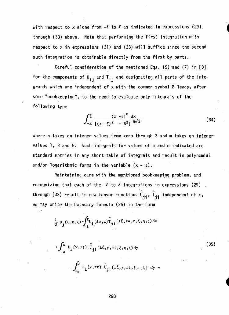
with respect to x alone from -I to I as indicated in expressions (29)
through (33) above. Note that performing the first integration with
respect to x in expressions (31) and (33) will suffice since the second
such integration is obtainable directly from the first by parts.
Careful consideration of the mentioned Eqs. (5) and (7) in [3]
for the components of U.. and T. . and designating all parts of the inte-i J I J
grands which are independent of x with the common symbol B leads, after
some "bookkeeping", to the need to evaluate only integrals of the
following type
l _ (x -g)n dx
where n takes on integer values from zero through 3 and m takes on integer
values 1, 3 and 5. Such integrals for values of m and n indicated are
standard entries in any short table of integrals and result in polynomial
and/or logarithmic forms in the variable (x - £) •
Maintaining care with the mentioned bookkeeping problem, and
recognizing that each of the -I to I integrations in expressions (29)A ^
through (33) result in new tensor functions U.., T.. independent of x,
we may write the boundary formula (26) in the form
(35)"• i/j^"-,/ * •• I3x-,y,±t;£,n,udy
-w •*
-w
268
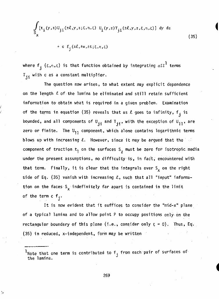
J [t.(y,z)U..(±£,y,z;?,n,C) U.(y,z)T (±£,y,z,C,n,C)] dy dz fS
(35)
+ c f..(±£,±w,±t;C,n,O
where f. U,n,c) is that function obtained by integrating all terms
T.. with c as a constant multiplier.«J '
The question now arises, to what extent may explicit dependence
on the length t of the lamina be eliminated and still retain sufficient
information to obtain what is required in a given problem. Examination
of the terms in equation (35) reveals that as L goes to infinity, f. isJ
bounded, and all components of U.. and T.., with the exception of U,,, are
zero or finite. The U,, component, which alone contains logarithmic terms
blows up with increasing £. However, since it may be argued that the
component of traction t, on the surfaces S must be zero for isotropic media
under the present assumptions, no difficulty is, in fact, encountered with
that term. Finally, it is clear that the integrals over Sv on the rightX
side of Eq. (35) vanish with increasing £, such that all "input" informa-
tion on the faces S indefinitely far apart is contained in the limit/\
of the term c f..
It is now evident that it suffices to consider the "mid-x" plane
of a typical lamina and to allow point P to occupy positions only on the
rectangular boundary of this plane (i.e., consider only c = 0). Thus, Eq.
(35) in reduced, x-independent, form may be written
that one term is contributed to f - from each pair of surfaces ofthe lamina.
269
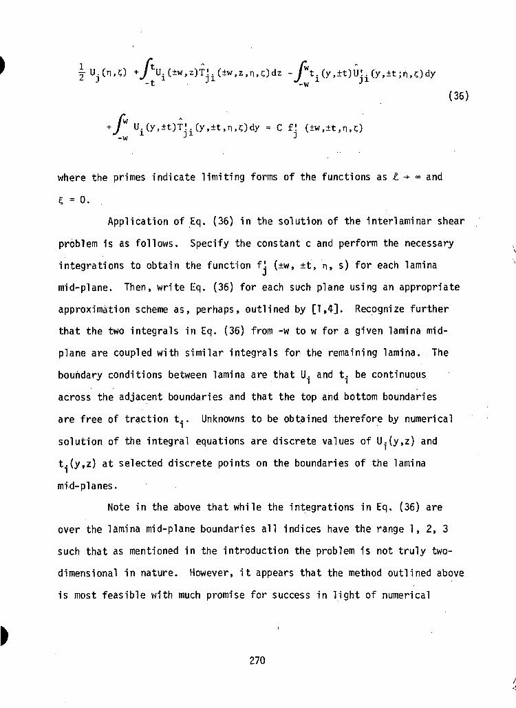
-t J •'-w J
(36)
A „ r+ I u. f v. ±J !*•' ' = C f! (±w,±t,n,O-w
where the primes indicate limiting forms of the functions as £ -»• °° and
5 = 0.,
Application of Eq. (36) in the solution of the interlaminar shear
problem is as follows. Specify the constant c and perform the necessary
integrations to obtain the function f'. (±w, ±t, n, s) for each laminaJ
mid-plane. Then, write Eq. (36) for each such plane using an appropriate
approximation scheme as, perhaps, outlined by [1,4]. Recognize further
that the two integrals in Eq. (36) from -w to w for a given lamina mid-
plane are coupled with similar integrals for the remaining lamina. The
boundary conditions between lamina are that U. and t. be continuous
across the adjacent boundaries and that the top and bottom boundaries
are free of traction t.. Unknowns to be obtained therefore by numerical
solution of the integral equations are discrete values of U..(y,z) and
t.(y,z) at selected discrete points on the boundaries of the lamina
mid-planes.
Note in the above that while the integrations in Eq. (36) are
over the lamina mid-plane boundaries all indices have the range 1, 2, 3
such that as mentioned in the introduction the problem is not truly two-
dimensional in nature. However, it appears that the method outlined above
is most feasible with much promise for success in light of numerical
270

f work already accomplished for both two and three dimensional problems
(e.g. [2,3,9,12]). Most important, coupling the above ideas with those
set forth in the previous section, it is possible to attack the difficult
interlaminar shear problem under the assumption of fully anisotropic or
specially anisotropic lamina.
271
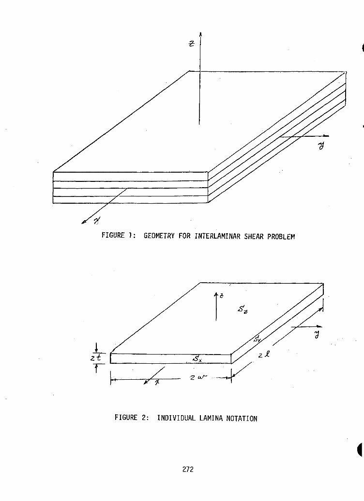
FIGURE 1: GEOMETRY FOR INTERLAMINAR SHEAR PROBLEM
FIGURE 2: INDIVIDUAL LAMINA NOTATION
272
5.4.4 References
[I] F. J. Rizzo, "An Integral Equation Approach to Boundary ValueProblems of Classical Elastostatics", Quart. Appl. Math., 25,(1967) 83-95.
[2] T. A. Cruse, "A Direct Formulat ion and Numerical Solution ofthe General Transient Elastodynamic Problem I I" , J. Math. Anal. Appl.,22, (1968) 341-355.
[3] T. A. Cruse, "Numerical Solutions in Three-Dimensional Elastostatics",Int. J. Solids Structures, 5, (1969) 1259-1274.
[4] F. J. Rizzo and D. J. Snippy, "A Formulation and Solution Procedurefor the General Non-Homogeneous Elastic Inc lus ion Problem", Int. J.Sol. Struc., 4, (1968) 1161-1179.
[5] F. J. Rizzo and D. J. Shippy, "A Method of Solut ion for CertainProblems of Transient Heat Conduct ion, AIAA J,, (to appear)(1970).
[6] I. Fredholm, "Sur les equations de 1 ' equ i l ib re d ' u n corps solideelastique", Aota Math., 23, (1900) 1-42.
[7] F. John, "Plane Waves and Spherical Means Appl ied to PartialDifferent ia l Equat ions" , Interscience, No. 2, New York, London,-(1955).
[8] B. Pipes, "Effects of Inter laminar Shear Stress Upon LaminateMembrane Performance", AFML/Industry Sponsored IRAD Status Reporton Adv . Comp. M a t ' l s . , (1970).
[9] W. V. Lovitt, Linear Integral Equations, Dover, New York , (1950).
[10] E. Kroner, "Das Fundamental integral der anisotropen elastischenDif fe ren t ia lg le ichungen" , Zeitschrift fur Physio, Bd. 136,(1953) 402-410.
[II] K. H. C. Lie and J. S. Koehler , "The Elast ic Stress Field Producedby a Point Force in a Cubic Crystal", Adv. in Physics, 17, No. 67,(1968) 421.
[12] F. J. Rizzo and D. J. Shippy, "A Method for Stress Determination inPlane Anisotropic Elastic Bodies", J. Comp. Mat'ls., 4, (1970)36-61.
273
UNCLASSIFIEDSecurity Classification
1 4.K E Y WORDS
Composite Materials
Education
Mechanically Fastened Joints
Fracture Mechanics
Stress Concentrations
Numerical Solution Methods
Aoisotropic Elasticity
Optimization
Synthesis
LINK A
RO LE W T
LINK B
ROLE W T
-
LINK C
ROLE W T
J
IV
VV
UNCLASSIFIEDSecurity Classification
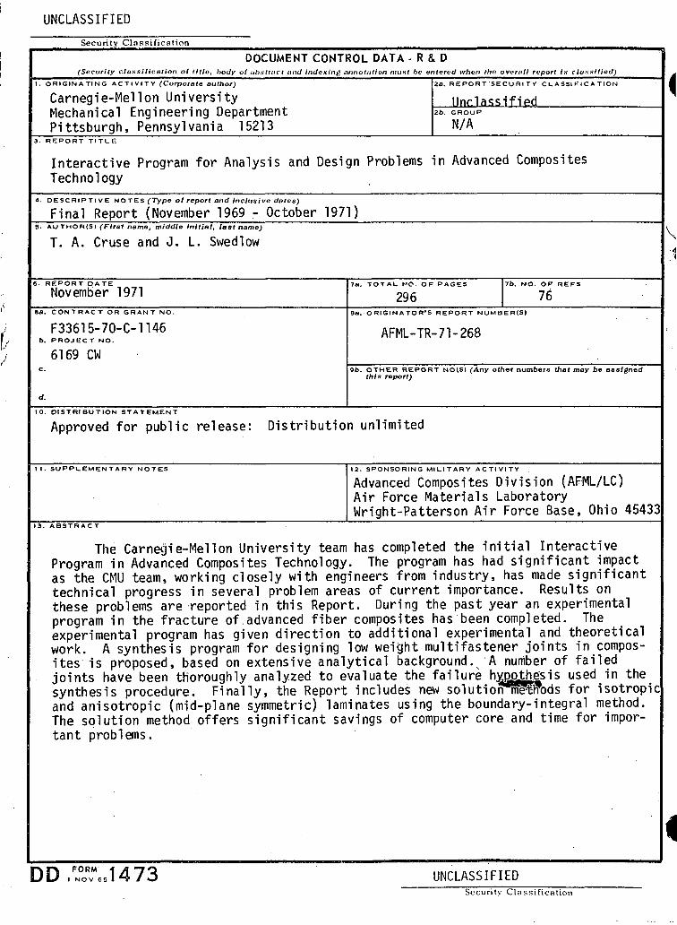
UNCLASSIFIED
Security Class i f ica t ion
DOCUMENT CONTROL DATA - R & D(Security classification of title, body ot nbstrtir.t and indexing annotation mutit he entered when the overall report In classified)
I. ORIGINATING A C T I V I T Y (Corporate author)
Carnegie-Mellon UniversityMechanical Engineering DepartmentPittsburgh, Pennsylvania 15213
20. REPORT S E C U R I T Y C L A S S I F I C A T I O N
Unclassified26. GROUP
N/A3. REPORT TITLE
Interactive Program for Analysis and Design Problems in Advanced CompositesTechnology
4. DESCRIPTIVE NOTES (Type ol report and Inclusive deles)
Final Report (November 1969 - October 1971)S. A O T H O R ( S ) (First name, middle Initial, last name)
T. A. Cruse and J. L. SwedlowV
-16 . REPORT D A T E
November 19718a. C O N T R A C T OR G R A N T NO.
F33615-70-C-1146b. PROJECT NO.
6169 CWc.
d.
7a. T O T A L MO. OF PAGES 76. NO. OF REFS
296 769a. ORIGINATOR'S REPORT NUMBER(S)
AFML-TR-71-268
9b. OTHER REPORT NO(S) (Any other numbers that may be ea signedthis report)
10. DISTRIBUTION STATEMENT
Approved for public release: Distribution unlimited
II. SUPPLEMENTARY NOTES 12. SPONSORING MIL ITARY A C T I V I T Y
Advanced Composites Division (AFML/LC)Air Force Materials LaboratoryWright-Patterson Air Force Base, Ohio 45433
13. A B S T R A C T
The Carnegie-Mellon University team has completed the initial InteractiveProgram in Advanced Composites Technology. The program has had significant impactas the CMU team, working closely with engineers from industry, has made significanttechnical progress in several problem areas of current importance. Results onthese problems are reported in this Report. During the past year an experimentalprogram in the fracture of advanced fiber composites has been completed. Theexperimental program has given direction to additional experimental and theoreticalwork. A synthesis program for designing low weight multifastener joints in compos-ites is proposed, based on extensive analytical background. A number of failedjoints have been thoroughly analyzed to evaluate the failure hmo>thesis used in thesynthesis procedure. Finally, the Report includes new solution^newods for isotropi<and anisotropic (mid-plane symmetric) laminates using the boundary-integral method.The solution method offers significant savings of computer core and time for impor-tant problems.
FORM1 NOV 651473 UNCLASSIFIED
Security Class i f icat ion