Production capacity estimation by reservoir numerical simulation of northwest (NW) Sabalan...

lable at ScienceDirect

Energy 36 (2011) 4552e4569

Contents lists avai

Energy

journal homepage: www.elsevier .com/locate/energy

Production capacity estimation by reservoir numerical simulation of northwest(NW) Sabalan geothermal field, Iran

Younes Noorollahi a,*, Ryuichi Itoi b

aDep. of Renewable Energy, Faculty of New Science and Technology, University of Tehran, Tehran, IranbDep. of Earth Resources Engineering, Kyushu University, No. 418 West Building 2, 744 Motooka, Nishi-ku 819-0395, Fukuoka, Japan

a r t i c l e i n f o

Article history:Received 13 July 2010Received in revised form15 February 2011Accepted 19 March 2011Available online 29 April 2011

Keywords:Reservoir simlationCapacity assessmentGeothermalSabalanIran

* Corresponding author. Tel.: þ98 912 2132885; faxE-mail address: [email protected] (Y. Noor

0360-5442/$ e see front matter � 2011 Elsevier Ltd.doi:10.1016/j.energy.2011.03.046

a b s t r a c t

A three dimensional numerical model of the northwest (NW) Sabalan geothermal system was developedon the basis of the designed conceptual model from available field data. A numerical model of thereservoir was expressed with a grid system of a rectangular prism of 12 km� 8 km with 4.6 km height,giving a total area of 96 km2. The model has 14 horizontal layers ranging in thickness between 100 m to1000 m extending from a maximum of 3600 to �1000 m a.s.l. Fifteen rock types were used in the modelto assign different horizontal permeabilities from 5.0� 10�18 to 4.0� 10�13 m2 based on the conceptualmodel.

Natural state modeling of the reservoir was performed, and the results indicated good agreementswith measured temperature and pressure in wells. Numerical simulations were conducted for predictingreservoir performances by allocating production and reinjection wells at specified locations. Threedifferent exploitation scenarios were examined for sustainability of reservoir for the next 30 years.Effects of reinjection location and required number of makeup wells to maintain the specified fluidproduction were evaluated. The results showed that reinjecting at Site B, immediate adjacent toproduction zone, is most effective for pressure maintenance of the system.

On the base of existing data and assumptions the reservoir can sustain producing fluid equivalent to50 MWe of electricity for more than 30 years. The reservoir can produce the maximum amount of fluidsequivalent to 90e100 MWe for only 5 years, but the production capacity decreases to 50 MWe after 20years of operation because of pressure and enthalpy drop. The reservoir can sustain 50 MWe over 100years that can be defined as a sustainable production level of the field.

� 2011 Elsevier Ltd. All rights reserved.

1. Introduction geological and reservoir condition. The maximum temperature of

A project for geothermal power generation in Iranwas started in1995 at northwest (NW) Sabalan. The NW Sabalan geothermal fieldis located on the northwestern flank of the Sabalan trachyandesiticstratovolcano, in the province of Ardebil in the northwest Iranwhere a significant amount of geo-scientific studies has been per-formed by Iranian Ministry of Energy since 1975 [1]. The projectarea locates within the Moeil Valley on the northwest slope ofSabalan. Fig. 1 shows the geological map of the Mt. Sabalan withmain structures and hot springs.

Surface exploration and feasibility studies have been carried outsince 1995 and five promising areas were selected. Among others,the NW Sabalan geothermal filed was nominated for detailedexplorations by drilling explorationwells. From 2002 to 2004 threedeep exploration wells were drilled for evaluating subsurface

: þ98 21 4486 5002.ollahi).

All rights reserved.

240 �C at a depth of 3197 m was measured in one of the wells [2].In this study, natural state and capacity assessment simulations

of the reservoir were undertaken for the primary purpose of pre-dicting and assessing the response of the NW Sabalan geothermalreservoir to the planned development scenarios. The computercodes of TOUGH2 [3] and AUTOUGH2 [3] were used with theequation of state of water and steam (EOS1). Different productionscenarios were examined by numerical simulations for evaluatingthe reservoir responses, and consequently the optimum futuredevelopment scenario was defined.

2. Exploration drilling

Three exploration wells, NWS1, NWS3 and NWS4, were drilledin the study area based on the results of geological, geochemicaland geophysical studies. According to the geophysical surveys, deepgeothermal reservoir may extend from northeast to southwest

mailto:[email protected]

www.sciencedirect.com/science/journal/03605442

http://www.elsevier.com/locate/energy

http://dx.doi.org/10.1016/j.energy.2011.03.046



Fig. 1. Geological map of the Sabalan area with grid system.

Y. Noorollahi, R. Itoi / Energy 36 (2011) 4552e4569 4553

where exploration wells were drilled along this suitability area.Data for three wells are summarized in Table 1 [4e7].

3. Conceptual model of NW Sabalan reservoir

Before a numerical simulation model of a given geothermal fieldbeing set up, a conceptual model must be developed. Adequateunderstanding on the important aspects of the structure of thesystem and the significant physical and chemical processes thatoccur in the system can be discussed in a conceptual model. Themodel is usually represented by sketches showing a plan view andvertical sections of the geothermal system. On these sketches themost important features such as geothermal surface manifesta-tions, hydrological boundaries, main geologic features such asfaults and geological layers, zones of high and low permeabilities,location of deep inflows and boiling zones need to be involved.

Table 1Specification of three exploration wells.

Well NWS1 NWS3 NWS4

Location (UTM_WGS84_Zone 39N) 739108E 737028E 738712E4238580N 4240784N 4239833N

Longitude 47�4400200 47�4302300 47�4202400

Latitude 38�1504900 38�1603000 38�1700600

Well head elevation (m a.s.l.) 2632 2277 2487Drilled well depth (m) 3197 3177 2266Permeable zones (m a.s.l) 1800e1400 No permeable

zone1050e900

200e0 880e890�200 to �350

Maximum temperature (�C) 240 148 229

Thus, developing a conceptual model requires the synthesis ofinformation from a multi-disciplinary team composed of geolo-gists, geophysicists, geochemists, reservoir engineers, and projectmanagers.

The geological map of the Sabalan area with main surfacemanifestation, geological structures shown in Fig. 1. A conceptualmodel of the study area was drawn along AB line, 12 km length,from north to south of the study area. Three explorationwells wereprojected on the AB line. The elevations of several specified pointsalong the cross section were extracted from a digital elevation mapin Geographical Information System (GIS) environment and usedfor developing a conceptual model. There is no information on dipof faults which is assumed to be vertical [8].

3.1. Subsurface geology and permeability

A simulation grid block was overlaid on the geological map ofthe study area (Fig. 1). Subsurface geology of the area is describedalong cross section AB, using geological data and information fromthree deep and two shallow exploration wells.

In the central part of the model, Dizu formation presents andextends to the depth of about 200 m a.s.l. This formation consists ofterrace deposits mainly of conglomerates with occasional sandintercalations. This formation clearly exposed in the area wherewells NWS1 and NWS3 are located throughout the Moil Valley. Thearea where these wells located are named as Site A and Site Brespectively.

Valhezir formation reaches to the surface in the east of wellNWS4 and extends to 700 m depth in the whole study area fromtop or below Dizu formation. This formation consists of andesitic

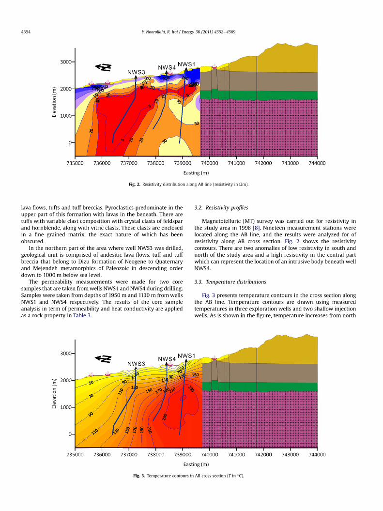
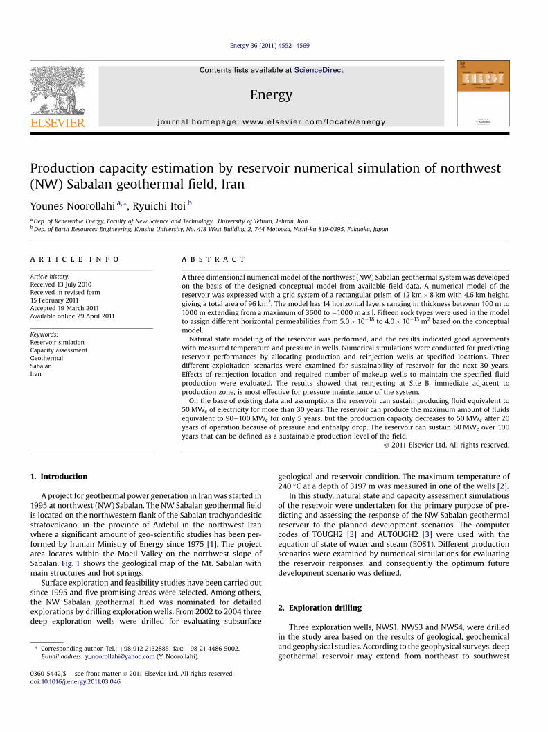
Fig. 2. Resistivity distribution along AB line (resistivity in Um).

Y. Noorollahi, R. Itoi / Energy 36 (2011) 4552e45694554

lava flows, tufts and tuff breccias. Pyroclastics predominate in theupper part of this formation with lavas in the beneath. There aretuffs with variable clast composition with crystal clasts of feldsparand hornblende, along with vitric clasts. These clasts are enclosedin a fine grained matrix, the exact nature of which has beenobscured.

In the northern part of the area where well NWS3 was drilled,geological unit is comprised of andesitic lava flows, tuff and tuffbreccia that belong to Dizu formation of Neogene to Quaternaryand Mejendeh metamorphics of Paleozoic in descending orderdown to 1000 m below sea level.

The permeability measurements were made for two coresamples that are taken fromwells NWS1 and NWS4 during drilling.Samples were taken from depths of 1950 m and 1130 m fromwellsNWS1 and NWS4 respectively. The results of the core sampleanalysis in term of permeability and heat conductivity are appliedas a rock property in Table 3.

Fig. 3. Temperature contours in

3.2. Resistivity profiles

Magnetotelluric (MT) survey was carried out for resistivity inthe study area in 1998 [8]. Nineteen measurement stations werelocated along the AB line, and the results were analyzed for ofresistivity along AB cross section. Fig. 2 shows the resistivitycontours. There are two anomalies of low resistivity in south andnorth of the study area and a high resistivity in the central partwhich can represent the location of an intrusive body beneath wellNWS4.

3.3. Temperature distributions

Fig. 3 presents temperature contours in the cross section alongthe AB line. Temperature contours are drawn using measuredtemperatures in three exploration wells and two shallow injectionwells. As is shown in the figure, temperature increases from north

AB cross section (T in �C).


to south which suggests that an upflow zone of high temperaturefluid likely present in the southern part of the field. Thus, FaultsNW3, NNW5, NE5, NNW2 and NW4 play as upflow zone of thesystem.

3.4. Data integration and conceptual model calibration

By integrating the subsurface geology from the wells withresistivity and temperature data, the geological cross section of theAB line can be illustrated in Fig. 4. Differences of subsurface geologyrevealed from drilling betweenwells NWS4 and NWS3 support thepresence of Fault NE2. Temperature profiles of these two wells alsoshow differences, which implies that Fault NE2 plays as an imper-meable or low permeable boundary. Furthermore, Fault NE2appears to be the northern boundary of the field between wellsNWS4 and NWS3. The presence of slightly high resistivity zonebeneath Site B can be interpreted as the existence of a dioriteporphyry intrusive body.

It has been assumed that geothermal fluids ascend throughFaults NW3, NNW5, NE5, NNW2 and NW4. This faulted area can bean upflow zone of the system. The fluids would ascend through thisfault zone to higher elevations and then flow horizontally inshallow layers to the northward due mainly to gravitational forceand discharge through hot springs in lower elevations.

4. Development of numerical model

4.1. TOUGH2-simulator brief description

TOUGH2 is a general-purpose numerical simulation program formulti-dimensional fluid and heat flows of multiphase, multicom-ponent fluidmixtures in porous and fracturedmedia. The TOUGH2-simulator used in this work belongs to MULCOM family ofnumerical simulators developed at Lawrence Berkeley NationalLaboratory (LBNL), USA [3,9] for simulation of multi-dimensionalmass and heat flow for multicomponent and multiphase fluids inporous and fracture media.

The governing equations of TOUGH2-simulator are mass- andenergy-balance equations since heat and mass transfer are simu-lated. The object of modeling (porous-fractured medium) is

Fig. 4. Conceptual model of the N

considered as set of elements connected to each other. Mass andheat accumulated in each element, mass and heat flow throughboundaries of element and possible mass/heat sinks/sources(inflow, wells, hot springs) have to be defined. Therefore, mass- andenergy-balance equations for each element of volume V are writtenas [3]:

ddt

%V

ZMðkÞdV ¼

I

G

ZFðkÞ$ n!dGþ %

V

ZqðkÞdV

where first term is mass/heat accumulation in element V, secondterm is mass/heat flow through the surfaces of element V, and thirdterm contains sinks/sources of heat andmass. Index kmay be equalto: 1 (water), 2 (air), 3 (heat), 4 (tracer), etc.

Mass and heat accumulation are given as:

MðkÞ ¼ FXb¼ l;g

sbrbXðkÞb

Mð3Þ ¼ ð1� FÞrRCRT þ FXb¼ l;g

sbrbXðkÞb

where

Fð3Þb

¼ �kkrbmb

rbXðkÞb

�VPb � rbg

�

All equations are non-linear, therefore, they can be solved onlyby numerical methods. In simulating a geothermal reservoir, weusually assume that fluid is of one component only (water). In thiscase, we have 2 equations of 2 unknowns for each element.Unknowns are pressure and temperature (in single-phase condi-tions) or pressure and saturation (in two-phase conditions). Forsystem ofN elements we have 2N equation system of 2N unknowns.It is solved by NewtoneRaphson iteration scheme [3].

4.2. Grid system

The NW Sabalan geothermal system was modeled with a rect-angular prism 12 km long, 8 km wide giving a total area of 96 km2

W Sabalan geothermal field.


and 4.6 km depth. The upper layer has variable thickness toapproximate the surface elevation, which increases to the south.

The model has 14 horizontal layers, AA to PP, ranging in thick-ness between 100 m and 1000 m extending from a maximum of3600 to �1000 m a.s.l. The model has 2595 grid blocks in total. Forneglecting watereair unsaturated zone, first two top layers, AA andBB, were discarded from the model.

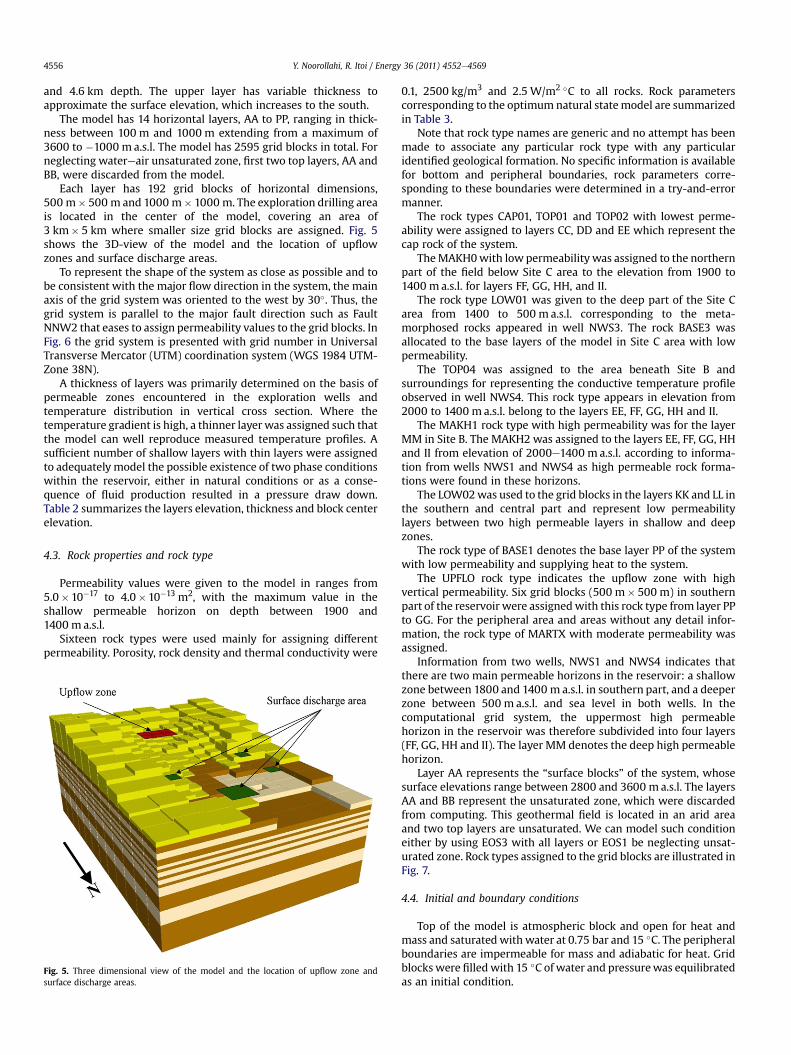
Each layer has 192 grid blocks of horizontal dimensions,500 m� 500 m and 1000 m� 1000 m. The exploration drilling areais located in the center of the model, covering an area of3 km� 5 km where smaller size grid blocks are assigned. Fig. 5shows the 3D-view of the model and the location of upflowzones and surface discharge areas.

To represent the shape of the system as close as possible and tobe consistent with the major flow direction in the system, the mainaxis of the grid system was oriented to the west by 30�. Thus, thegrid system is parallel to the major fault direction such as FaultNNW2 that eases to assign permeability values to the grid blocks. InFig. 6 the grid system is presented with grid number in UniversalTransverse Mercator (UTM) coordination system (WGS 1984 UTM-Zone 38N).

A thickness of layers was primarily determined on the basis ofpermeable zones encountered in the exploration wells andtemperature distribution in vertical cross section. Where thetemperature gradient is high, a thinner layerwas assigned such thatthe model can well reproduce measured temperature profiles. Asufficient number of shallow layers with thin layers were assignedto adequately model the possible existence of two phase conditionswithin the reservoir, either in natural conditions or as a conse-quence of fluid production resulted in a pressure draw down.Table 2 summarizes the layers elevation, thickness and block centerelevation.

4.3. Rock properties and rock type

Permeability values were given to the model in ranges from5.0�10�17 to 4.0�10�13 m2, with the maximum value in theshallow permeable horizon on depth between 1900 and1400 m a.s.l.

Sixteen rock types were used mainly for assigning differentpermeability. Porosity, rock density and thermal conductivity were

Fig. 5. Three dimensional view of the model and the location of upflow zone andsurface discharge areas.

0.1, 2500 kg/m3 and 2.5 W/m2 �C to all rocks. Rock parameterscorresponding to the optimum natural statemodel are summarizedin Table 3.

Note that rock type names are generic and no attempt has beenmade to associate any particular rock type with any particularidentified geological formation. No specific information is availablefor bottom and peripheral boundaries, rock parameters corre-sponding to these boundaries were determined in a try-and-errormanner.

The rock types CAP01, TOP01 and TOP02 with lowest perme-ability were assigned to layers CC, DD and EE which represent thecap rock of the system.

TheMAKH0with low permeability was assigned to the northernpart of the field below Site C area to the elevation from 1900 to1400 m a.s.l. for layers FF, GG, HH, and II.

The rock type LOW01 was given to the deep part of the Site Carea from 1400 to 500 m a.s.l. corresponding to the meta-morphosed rocks appeared in well NWS3. The rock BASE3 wasallocated to the base layers of the model in Site C area with lowpermeability.

The TOP04 was assigned to the area beneath Site B andsurroundings for representing the conductive temperature profileobserved in well NWS4. This rock type appears in elevation from2000 to 1400 m a.s.l. belong to the layers EE, FF, GG, HH and II.

The MAKH1 rock type with high permeability was for the layerMM in Site B. The MAKH2 was assigned to the layers EE, FF, GG, HHand II from elevation of 2000e1400 m a.s.l. according to informa-tion from wells NWS1 and NWS4 as high permeable rock forma-tions were found in these horizons.

The LOW02was used to the grid blocks in the layers KK and LL inthe southern and central part and represent low permeabilitylayers between two high permeable layers in shallow and deepzones.

The rock type of BASE1 denotes the base layer PP of the systemwith low permeability and supplying heat to the system.

The UPFLO rock type indicates the upflow zone with highvertical permeability. Six grid blocks (500 m� 500 m) in southernpart of the reservoir were assignedwith this rock type from layer PPto GG. For the peripheral area and areas without any detail infor-mation, the rock type of MARTX with moderate permeability wasassigned.

Information from two wells, NWS1 and NWS4 indicates thatthere are two main permeable horizons in the reservoir: a shallowzone between 1800 and 1400 m a.s.l. in southern part, and a deeperzone between 500 m a.s.l. and sea level in both wells. In thecomputational grid system, the uppermost high permeablehorizon in the reservoir was therefore subdivided into four layers(FF, GG, HH and II). The layer MM denotes the deep high permeablehorizon.

Layer AA represents the “surface blocks” of the system, whosesurface elevations range between 2800 and 3600 m a.s.l. The layersAA and BB represent the unsaturated zone, which were discardedfrom computing. This geothermal field is located in an arid areaand two top layers are unsaturated. We can model such conditioneither by using EOS3 with all layers or EOS1 be neglecting unsat-urated zone. Rock types assigned to the grid blocks are illustrated inFig. 7.

4.4. Initial and boundary conditions

Top of the model is atmospheric block and open for heat andmass and saturatedwith water at 0.75 bar and 15 �C. The peripheralboundaries are impermeable for mass and adiabatic for heat. Gridblockswere filled with 15 �C of water and pressurewas equilibratedas an initial condition.

Fig. 6. Grid system overlaid with faults.

Table 2Horizontal layers used in computational grid.

Layer name Elevation (m a.s.l.) Layer thickness (m) Block centerelevation (m a.s.l.)

Atmospher InfiniteAA Vary 200e1000 VaryBB 2400e2200 200 2300CC 2200e2100 100 2150DD 2100e2000 100 2050EE 2000e1900 100 1950FF 1900e1800 100 1850GG 1800e1650 150 1725HH 1650e1550 100 1600II 1550e1400 150 1475JJ 1400e1300 100 1350KK 1300e1000 300 1150LL 1000e500 500 750MM 500e0 500 250PP 0e1000 1000 �500


High temperature fluid recharges at a rate of 90 kg/s of 1159 kJ/kg from the bottom layer, PP, was given through regional faults inthe southwest region. This specific enthalpy corresponds to satu-rated water of 265 �C. The temperature of inflow geothermal fluidwas calculated using geochemical geothermometers (SKM, [9]) andalso slightly changed by trial-and-error manner through iterativeprocess of natural state simulation. According to a verticaltemperature distribution across AB cross section using data fromthe wells an upflow zone may present about 2.5 km to the south-east of well NWS1. The recharge was assigned to the grid blocks of89, 92, 103, 105, 109 and 111 in PP layer (Fig. 7). A flow rate of 8 kg/sof low temperature, 130 �C, inflowwas assigned to the grid number4 in northwestern part of the field to simulate the temperature andpressure condition of the northern part close to well NWS3. Thelocations and flow rates of recharges were also determined by trial-and-error manner.

Natural discharge from the field was modeled using deliver-ability method. The productivity index (PI) was calculated ondeliverability model [3] and well bottom pressures (Pwb) were

Table 3Rock parameters of the best natural-state model.

Rock type Density (kg/m3) Porosity (%) Permeability (m2) Thermal cond. (W/m2 �C) Specific heat (J/kg �C)

kx ky kz

ATMOS 2500 99 2.5� 10�14 2.5� 10�14 2.5� 10�14 2.50 9.0� 105

CAP01 2500 10 2.0� 10�16 2.0� 10�16 7.0� 10�17 2.50 1.0� 103

BASE1 2500 10 6.0� 10�15 6.0� 10�15 3.0� 10�15 2.50 1.0� 103

BOND1 2500 10 9.5� 10�16 9.5� 10�16 6.6� 10�16 2.50 1.0� 103

TOP01 2500 10 5.5� 10�16 5.5� 10�16 1.1� 10�16 2.50 1.0� 103

TOP04 2500 10 5.0� 10�15 5.0� 10�15 1.1� 10�15 2.50 1.0� 103

BASE3 2500 10 1.0� 10�17 1.0� 10�17 5.0� 10�17 2.50 1.0� 103

LOW01 2500 10 6.0� 10�14 6.0� 10�14 1.0� 10�14 2.50 1.0� 103

MAKH3 2500 10 2.0� 10�13 2.0� 10�13 5.0� 10�14 2.50 1.0� 103

MATRX 2500 10 5.0� 10�15 5.0� 10�15 1.0� 10�15 2.50 1.0� 103

TOP02 2500 10 5.0� 10�16 5.0� 10�16 2.0� 10�16 2.50 1.0� 103

MAKH0 2500 10 5.0� 10�15 2.0� 10�15 5.5� 10�16 2.50 1.0� 103

LOW02 2500 10 7.0� 10�16 7.0� 10�16 1.5� 10�16 2.50 1.0� 103

MAKH1 2500 10 1.0� 10�15 1.0� 10�15 5.0� 10�16 4.30 1.6� 103

MAKH2 2500 10 4.0� 10�13 4.0� 10�13 7.0� 10�14 3.28 1.45� 103

UPFLO 2500 10 3.0� 10�13 3.0� 10�13 3.0� 10�13 2.50 1.0� 103


obtained by trial-and-error manner (Table 4). Mass flow rate ondeliverability is proportional to the pressure difference betweenthe grid block and a prescribed pressure that is lower than that ofthe block. Thus, once the grid block pressure decreases due to fluidproduction, the flow rate to the surface discharge decreases andeventually stops as the pressure difference approaches zero.

Fig. 7. Rock types assigne

There is several natural discharge of geothermal fluid throughhot springs and in river bed mostly in northern part of the area. Thesurface discharge temperatures are from25 �C to 85 �C and the flowrate of hot springs are about 25e30 kg/s in total. There are, however,several discharges in river bed and banks which are unable tomeasure for the flow rates. Thus, we assumed that the total outflow

d to the grid blocks.

Table 4Productivity index (PI) and well bottom pressure (Pwb) of well deliverability blocks.

Grid block ProductivityIndex (m3)

Pwb (Pa) Thickness oflayer (m)

Productionrate (kg/s)

FF 78 2.9� 10�7 4.0� 106 100 12FF 51 2.9� 10�7 4.1� 106 100 15FF 183 2.9� 10�7 4.4� 106 100 12II 130 2.9� 10�7 8.1� 107 150 11


from the system is about 40e50 kg/s. In order to reproduce the hotspring activity in the numerical model, fluid production based ondeliverability was utilized in three blocks in layers FF (grid numbers51, 78, and 183) and one block in layer II (130) below the locationcorresponding to these surface manifestations.

4.5. Heat source and sink

Heat flux was given to the blocks in the bottom layer, PP, of themodel as a conductive heat supply. A heat flux of 200 mW/m2 wasused as the initial basis for calculating the heat inflow to each blockin southern and central parts. No heat inflow was then given toachieve a match the deep temperatures in northern part (Site Carea). Conductive heat loss to the atmosphere occurs from the layerCC because the layers AA and BB are discarded from the modelcalculation.

4.6. Wells data matching and model validation

The validationprocess normally involvesmatching of the naturalstate conditions in the system, as defined by available subsurface

Fig. 8. Measured and simulated tempe

information. During the natural state simulation of NW Sabalanreservoir, the computed results were compared against measuredtemperature and reservoir pressure in three wells. This pressure ismeasured as stationary pressure measurement of single major feedzone during well testing. The matches between the measured andcomputed values were improved primarily by adjusting thepermeability, fluid flow rate and specific enthalpy of the high-temperature recharge assigned to the bottom six grid blocks. Alsothe lower temperature in well NWS3 was reproduced in the modelby assigning an inflow from grid block 4 in the northwestern part.

The well NWS3 is deviated and the corresponding temperatureand pressure of layers CC to EE of grid block 59 and layers FF to PP ofgrid block 49 from “best model” were used to match the measuredand simulated data. For well NWS4 the grid blocks of 165 for layersCC to GG and 164 for layers HH to PP were used. Well NWS1 isa vertical well and grid block of 150 was used for whole well depthfor matching. In Figs. 8 and 9 the measured and computed naturalstate temperature profiles of three wells are compared. WellsNWS1 andNWS4 are expected being close to the upflow zone in thesouthern part of the field. Well NWS3 in the northern part,however, is exterior of the geothermal reservoir. Fault NE2 acts asan impermeable fault and plays as northern boundary of the fieldand its presence may cause large temperature differences of 80 �Cat the same depth of wells NWS3 and NWS4.

Simulated pressures were markedly affected by changing thepermeability of the layers, particularly layers of CC and DD, inflowof recharge zone, and outflow from natural surface dischargesblock. The measured and computed natural-state pressure profilesare shown in Fig. 9, and show good agreement. The plane views ofsimulated temperature in layers II to PP for natural state simulation

rature of wells NWS1 and NWS3.

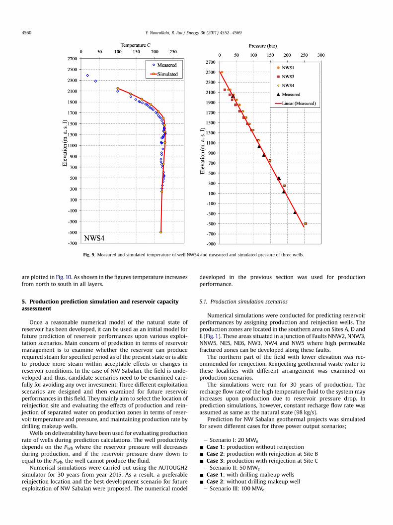
Fig. 9. Measured and simulated temperature of well NWS4 and measured and simulated pressure of three wells.


are plotted in Fig. 10. As shown in the figures temperature increasesfrom north to south in all layers.

5. Production prediction simulation and reservoir capacityassessment

Once a reasonable numerical model of the natural state ofreservoir has been developed, it can be used as an initial model forfuture prediction of reservoir performances upon various exploi-tation scenarios. Main concern of prediction in terms of reservoirmanagement is to examine whether the reservoir can producerequired steam for specified period as of the present state or is ableto produce more steam within acceptable effects or changes inreservoir conditions. In the case of NW Sabalan, the field is unde-veloped and thus, candidate scenarios need to be examined care-fully for avoiding any over investment. Three different exploitationscenarios are designed and then examined for future reservoirperformances in this field. They mainly aim to select the location ofreinjection site and evaluating the effects of production and rein-jection of separated water on production zones in terms of reser-voir temperature and pressure, and maintaining production rate bydrilling makeup wells.

Wells on deliverability have been used for evaluating productionrate of wells during prediction calculations. The well productivitydepends on the Pwb where the reservoir pressure will decreasesduring production, and if the reservoir pressure draw down toequal to the Pwb, the well cannot produce the fluid.

Numerical simulations were carried out using the AUTOUGH2simulator for 30 years from year 2015. As a result, a preferablereinjection location and the best development scenario for futureexploitation of NW Sabalan were proposed. The numerical model

developed in the previous section was used for productionperformance.

5.1. Production simulation scenarios

Numerical simulations were conducted for predicting reservoirperformances by assigning production and reinjection wells. Theproduction zones are located in the southern area on Sites A, D andE (Fig. 1). These areas situated in a junction of Faults NNW2, NNW3,NNW5, NE5, NE6, NW3, NW4 and NW5 where high permeablefractured zones can be developed along these faults.

The northern part of the field with lower elevation was rec-ommended for reinjection. Reinjecting geothermal waste water tothese localities with different arrangement was examined onproduction scenarios.

The simulations were run for 30 years of production. Therecharge flow rate of the high temperature fluid to the system mayincreases upon production due to reservoir pressure drop. Inprediction simulations, however, constant recharge flow rate wasassumed as same as the natural state (98 kg/s).

Prediction for NW Sabalan geothermal projects was simulatedfor seven different cases for three power output scenarios;

e Scenario I: 20 MWe

- Case 1: production without reinjection- Case 2: production with reinjection at Site B- Case 3: production with reinjection at Site Ce Scenario II: 50 MWe

- Case 1: with drilling makeup wells- Case 2: without drilling makeup welle Scenario III: 100 MWe

Fig. 10. Plane view of simulated temperature for natural state simulation for layers II to PP.


- Case 1: with drilling makeup wells- Case 2: without drilling makeup well

In these scenarios, declines of pressure, temperature, enthalpyand mass rates of fluid and steam productions of wells were eval-uated. Themass production rates of fluid and steamwere calculatedfrom fluid discharges of production blocks at a separator pressureof 5.5 bar. The reinjection rate of waste water and its enthalpy intoreservoir were given as that of the separator pressure andtemperature of 155 �C.

On the basis of discharge data fromwell NWS4, required amountof geothermal fluid for a proposed single flash power plant wascalculated using Engineering Equation Solver (EES) [10]. The inputparameters are; produced fluid enthalpy 985 kJ/kg, separationpressure 5.5 bar, condenser pressure, 0.1 bar, outlet temperature46 �C and isentropic efficiency of the turbine 0.78. By assigning these

inputs and output information, required production rate ofgeothermal fluid for different scenarios and number of wells aresummarized in Table 5.

5.2. Scenario I: 20 MWe power production and reinjection siteselection

The production of 20 MWe in the first phase of NW Sabalanproject was given as a base case for evaluation of the field responsesto the production and to define the suitable location for reinjectionsite. Three kinds of production and reinjection schemes (Case) wereassigned and simulated for 30 years.

e Case 1: production without reinjectione Case 2: production with reinjection at Site Be Case 3: production with reinjection at Site C

Table 5Characteristics of the production scenarios.

Item Scenario I Scenario II Scenario III

Case 1 Case 2 Case 3 Case 1 Case 2

Power output (MWe) 20 20 20 50 50 100Total fluid production (kg/s) 275 275 275 690 690 1380Steam production (kg/s) 42 42 42 106 106 212Brine production (kg/s) 233 233 233 584 584 1168Number of production well 5 5 5 13 13 35Number of reinjection well None 3 3 7 7 16Production grid block number 124, 132, 134, 139, 150 83, 106, 108, 119,

121, 123, 124, 132,134, 137, 139, 150,156

83, 88, 89, 92, 100, 103, 105, 106, 107, 108, 109, 110, 111,119, 120, 121, 122, 123, 124, 125, 126, 132, 134, 135, 137,138, 139, 140, 141, 150, 155, 156, 187, 188, 189

Reinjection grid block numbers None 165, 168, 178 34, 47, 49 148, 161,162, 165,173, 178

49, 104, 144, 146, 147, 161, 163, 165, 168, 173, 177,178, 183, 59, 73

Number of makeup wells 0 1 2 7 0 5


The responses of field to these cases were examined and theoptimum case was selected. As shown in Table 5 for production of275 kg/s of geothermal fluid, drilling five geothermal wells wasplanned for all three cases. Production wells were proposed to drillat Sites A, D, and E in the southern part of the field at grid blocks of124, 132, 134, 139 and 150 (Fig. 6). The wells are planned to producefrom layer MM of the model.

In Cases 2 and 3, the produced brine was reinjected into thereservoir. About 85% (233 kg/s) of produced fluid was reinjectedinto the reservoir from three wells at Site B in Case 2 and threewells at Site C in Case 3. The reinjection wells were assigned onlayer MM, 500e0 m a.s.l., into the grid blocks of 165, 168 and 178for Case 2, and the grid blocks of 34, 47, and 49 for Case 3 (Fig. 6).The injection from same layer as production maintains thepressure.

When the production rate decreases below 85% (36 kg/s ofsteam) of the designated level a makeup well was assigned tocompensate the deficit.

5.2.1. Total mass and flow rate and flowing enthalpySimulation results of total mass and steam flow rates of the

production wells in all three cases are presented in Figs. 11 and 12.The total mass flow rate of five production wells in Case 1(without reinjection) decreases from 275 kg/s to 120 kg/s in 17

Fig. 11. Total production rate change with t

years and continues slightly decreasing in the following years. Thesteam flow rate also decreases in the same manner. The mass andsteam flow rates in Case 1 drop to 44% of the initial values after 15years which means the power production drops by 56% in 15years, and continues decreasing to less than 40% in 30 years ofproduction. To compensate the production decline makeup wellswere assigned. However, simulation results show that onemakeup well per year is necessary to keep the production atdesignated level.

In Case 2, the total production rate decreases down to 85% of theinitial rate, from 275 kg/s to 234 kg/s, after 11 years operation andthe first makeup well needs to start production in 2026. By addingthis makeup well production rate remains at designated level over30 years.

Total production rate inCase3decreases to 85%of the initial value,275e234 kg/s, within 3 years. Thus, the first makeup well needs toproduce. By adding the first makeup well, the production flow rateincreases up to 255 kg/s. Themass flow rate, however, drops again tobelow 85% of designated level in the following 7 years. This requiresthe secondmakeupwell after 3 years. Twomakeupwells can sustainthe production of required steam over 30 years.

The simulation result reveals that the field cannot sustaina specified steam production rate without reinjection as for Case 1.In Case 2, reservoir pressure maintain by reinjection is more

ime for Cases 1, 2, and 3 in Scenario I.

Fig. 12. Steam flow rate change with time for Cases 1, 2, and 3 in Scenario I.


effective than that in Case 3, because of location of reinjectionwells.In Case 2 only one makeup well is required after 11 years ofproduction but in Case 3 twomakeup wells are required after 3 and10 years. Total steam and mass flow rates by adding one makeupwell in Case 2 is higher than those in Case 3 with two additionalmakeup wells.

According to the amount of production flow rate and number ofthe required makeup wells, Case 2 can be judged as the best planamong three cases. Furthermore, the Site B can be a preferred areafor locating reinjection wells in future development.

The flowing enthalpy of the produced fluid versus time isplotted in Fig. 13. As shown in figure the flowing enthalpies in Case1 remain constant. In Case 2, by adding the makeup well itdecreases because the new well produces lower enthalpy fluid. InCase 3 the flowing enthalpy decreases when the first makeup wellwas added same as Case 2 but the flowing enthalpy increases byadding the second makeup well in 2025 which was assigned toa grid block closer to the upflow zone of the system.

Fig. 13. Flowing enthalpy of produced fluid wi

5.2.2. Predicted temperature and pressureTemperature and pressure changes in the main producing layer

MM were evaluated for all cases. Fig. 14 shows the amount oftemperature drop from the initial in Layer MM for three cases. ForCase 1, temperature change is negligible small. For Case 2 and Case3 the cooling occurs in reinjection area because of lower temper-ature waste water into reinjection zone. The amount of thetemperature drop in Case 3 is larger than that of Case 2 in rein-jection area in the northern part.

A plan view of the pressure changes from natural state in layerMM is illustrated in Fig.15. In Case 1 pressure drop occurs in a rangefrom 10 bar to 24 bar over the simulated area. In Case 2, however,the maximum pressure drop shows only 5 bar. In Case 3 pressuredrop in the production zone reaches up to 10 bar. This implies thatthe reinjection of waste water at Site B is more effective tomoderate the pressure drop in production area as indicated for Case2. The pressure generally increases in reinjection zone in both Cases2 and 3.

th time for Cases 1, 2, and 3 in Scenario I.

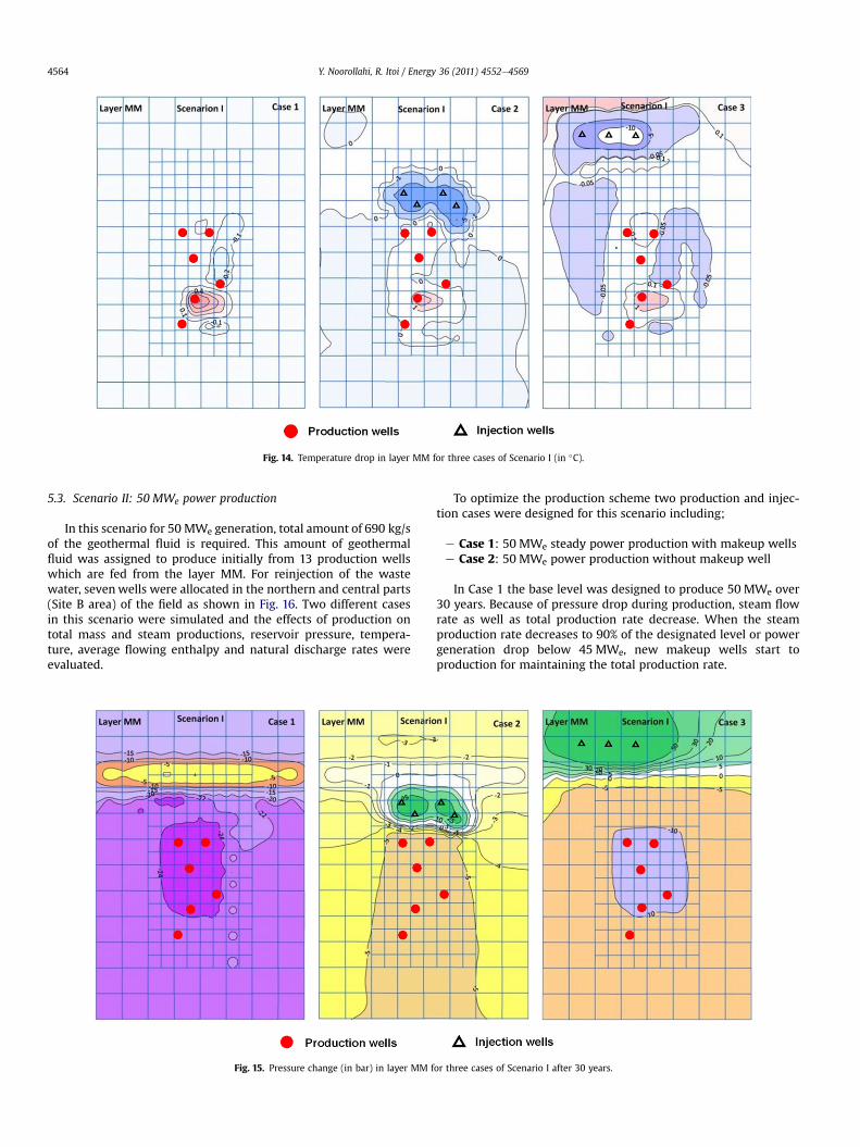
Fig. 14. Temperature drop in layer MM for three cases of Scenario I (in �C).


5.3. Scenario II: 50 MWe power production

In this scenario for 50 MWe generation, total amount of 690 kg/sof the geothermal fluid is required. This amount of geothermalfluid was assigned to produce initially from 13 production wellswhich are fed from the layer MM. For reinjection of the wastewater, sevenwells were allocated in the northern and central parts(Site B area) of the field as shown in Fig. 16. Two different casesin this scenario were simulated and the effects of production ontotal mass and steam productions, reservoir pressure, tempera-ture, average flowing enthalpy and natural discharge rates wereevaluated.

Fig. 15. Pressure change (in bar) in layer MM f

To optimize the production scheme two production and injec-tion cases were designed for this scenario including;

e Case 1: 50 MWe steady power production with makeup wellse Case 2: 50 MWe power production without makeup well

In Case 1 the base level was designed to produce 50 MWe over30 years. Because of pressure drop during production, steam flowrate as well as total production rate decrease. When the steamproduction rate decreases to 90% of the designated level or powergeneration drop below 45 MWe, new makeup wells start toproduction for maintaining the total production rate.

or three cases of Scenario I after 30 years.

Fig. 16. Production and reinjection grid blocks for Scenario II.


In Case 2 nomakeupwell was assigned and the production from13 wells was maintained over 30 years and the behavior of thereservoir was monitored. Table 5 summarizes the production andreinjection flow rates and grid blocks.

5.3.1. Steam flow ratesSteam flow rates versus time for two cases in Scenario II are

presented in Fig. 17. In early times, production rates rapidly deceasewith time in both cases.

In Case 1, steam production rate decreases below 95 kg/s after 3years of production and then a makeup well starts to production.This new well can keep the power production more than 45 MWefor 2 years and another new makeup well was required. In thisscenario seven makeup wells in total were required in years at2018, 2020, 2023, 2026, 2029, 2033, and 2038 to keep the powergeneration of 45 MWe for 30 years.

In Case 2 the makeup well was not assigned and productionwascontinued by 13 initially drilled wells over 30 years. The steam

production rate decreases rapidly in the first 5 years with anaverage of 3.5% per year. From the year 2020e2030 the decline rateis moderated to 1.2% per year and in the next 15 years (2030e2045)the steam flow reduces only 0.31% per year. It can be concludedthat the production rate eventually stabilizes after 15 years ofproduction. In this case, total production rate drops by 34% in 30years.

5.3.2. Predicted pressure and temperaturePressure and temperature changes of the reservoir were moni-

tored while running this production scenario for 30 years. Changesof the pressure and temperature from their initial values at shallowand deep layers are evaluated.

Fig. 18 shows the temperature drop in layers HH and MM forCase 1. In Layer HH temperature drop is less than 1 �C. In the mainproducing layer of MM, cooling occurs in the northern part of thereservoir in reinjection area. Decrease amount of temperatureshows up to 60 �C in the central part of the reinjection zone and the

Fig. 17. Steam flow rate change with time for Scenario II.


area of 10 �C cooling extends over 4.5 km2. Low temperature frontmoves from reinjection area to the southward of production zone.Actually, the temperature drop in production zone is only about1 �C. As shown in the figures cooling in main production andreinjection layer, MM, is more apparent than layer HH.

Fig. 19 shows the pressure changes in layers HH and MM.Pressure drops at layer HH are in the range of 4e11 bar. Largestpressure drop occurs in the main production zone in the southernpart. In Layer MM the pressure drop in production zone is largerthan that in layer HH, and reaches up to 12 bar of pressure drop inthe central part of the production zone. In reinjection area, pressureincreases up to 50 bar due to reinjection of large amount of thewaste water.

Fig. 18. Temperature changes from the initial in

5.4. Scenario III: 100 MWe power production

The largest power generation of 100 MWe was examined forScenario III. This requires a production of 1380 kg/s of thegeothermal fluid. For this scenario, total number of 35 productionand 16 reinjection wells were assigned. The grid number corre-sponding to each production and reinjectionwells and assumptionsof the scenario is presented in Table 5. However, thirty-fiveproduction wells is a large number, and it causes higher cost perkilowatt of electricity generation.

This scenario was given to evaluate the maximum productioncapacity of the field. As one well can be assigned in one grid, themaximum number of production wells being allocated is forty in

layers HH and MM for Scenario II (in �C).

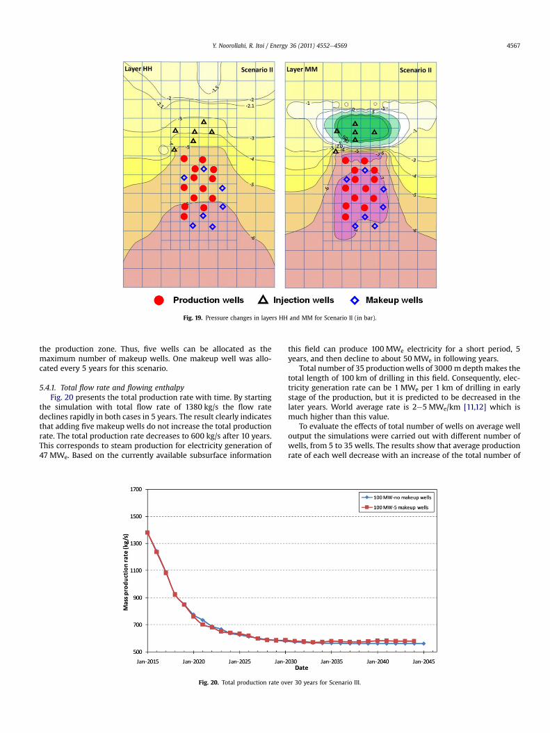
Fig. 19. Pressure changes in layers HH and MM for Scenario II (in bar).


the production zone. Thus, five wells can be allocated as themaximum number of makeup wells. One makeup well was allo-cated every 5 years for this scenario.

5.4.1. Total flow rate and flowing enthalpyFig. 20 presents the total production rate with time. By starting

the simulation with total flow rate of 1380 kg/s the flow ratedeclines rapidly in both cases in 5 years. The result clearly indicatesthat adding five makeup wells do not increase the total productionrate. The total production rate decreases to 600 kg/s after 10 years.This corresponds to steam production for electricity generation of47 MWe. Based on the currently available subsurface information

Fig. 20. Total production rate ov

this field can produce 100 MWe electricity for a short period, 5years, and then decline to about 50 MWe in following years.

Total number of 35 productionwells of 3000 m depthmakes thetotal length of 100 km of drilling in this field. Consequently, elec-tricity generation rate can be 1 MWe per 1 km of drilling in earlystage of the production, but it is predicted to be decreased in thelater years. World average rate is 2e5 MWe/km [11,12] which ismuch higher than this value.

To evaluate the effects of total number of wells on average welloutput the simulations were carried out with different number ofwells, from 5 to 35 wells. The results show that average productionrate of each well decrease with an increase of the total number of

er 30 years for Scenario III.

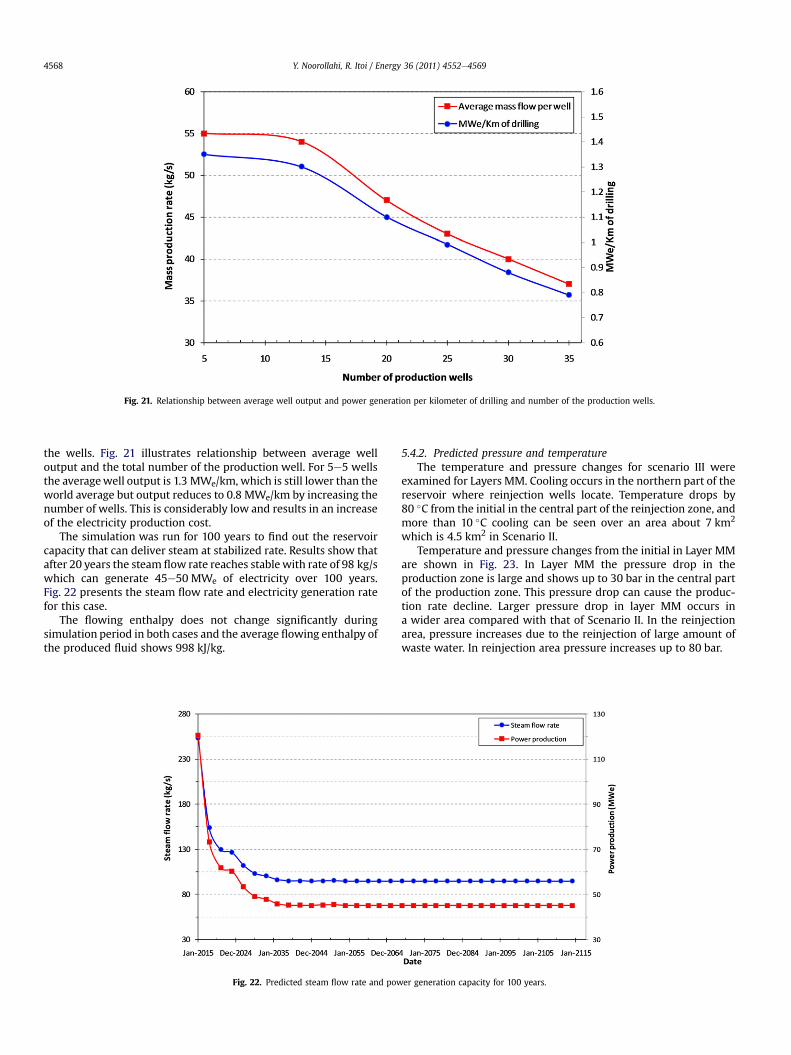
Fig. 21. Relationship between average well output and power generation per kilometer of drilling and number of the production wells.


the wells. Fig. 21 illustrates relationship between average welloutput and the total number of the production well. For 5e5 wellsthe averagewell output is 1.3 MWe/km, which is still lower than theworld average but output reduces to 0.8 MWe/km by increasing thenumber of wells. This is considerably low and results in an increaseof the electricity production cost.

The simulation was run for 100 years to find out the reservoircapacity that can deliver steam at stabilized rate. Results show thatafter 20 years the steam flow rate reaches stablewith rate of 98 kg/swhich can generate 45e50 MWe of electricity over 100 years.Fig. 22 presents the steam flow rate and electricity generation ratefor this case.

The flowing enthalpy does not change significantly duringsimulation period in both cases and the average flowing enthalpy ofthe produced fluid shows 998 kJ/kg.

Fig. 22. Predicted steam flow rate and pow

5.4.2. Predicted pressure and temperatureThe temperature and pressure changes for scenario III were

examined for Layers MM. Cooling occurs in the northern part of thereservoir where reinjection wells locate. Temperature drops by80 �C from the initial in the central part of the reinjection zone, andmore than 10 �C cooling can be seen over an area about 7 km2

which is 4.5 km2 in Scenario II.Temperature and pressure changes from the initial in Layer MM

are shown in Fig. 23. In Layer MM the pressure drop in theproduction zone is large and shows up to 30 bar in the central partof the production zone. This pressure drop can cause the produc-tion rate decline. Larger pressure drop in layer MM occurs ina wider area compared with that of Scenario II. In the reinjectionarea, pressure increases due to the reinjection of large amount ofwaste water. In reinjection area pressure increases up to 80 bar.

er generation capacity for 100 years.

Fig. 23. Temperature and pressure changes in layer MM from the initial after 30 years of production in Scenario III (in �C and bar).


6. Conclusions

A three dimensional numerical model of the NW Sabalangeothermal field was developed and calibrated by numericalsimulations. Prediction simulations of reservoir behaviors werealso carried out using the numerical model developed. Threehypothetical development scenarios were evaluated for productioncapacity assessment and reinjection effects on fluid production. Theconclusions are summarized as follows:

1. The results of natural state simulation using the AUTOUGH2simulator indicated good agreements in temperature andpressure profiles of three deep wells with measurement.

2. Reinjection of the waste water is effective for moderatingreservoir pressure drop.

3. The immediate adjacent area, north to the production area,named as Site B is recommended for locating reinjection wellsbecause of more effective on the pressure support comparedwith reinjection at further north area, Site C.

4. Based on existing data and assumptions reservoir can sustainsteam production equivalent to 50 MWe of electricity for 30years or more.

5. The reservoir can produce in maximum capacity for productionof 90e100 MWe for short period of time (5 years), but theproduction rate decreases gradually to the level of 50 MWeafter 20 years. The reservoir can sustain steam production for50 MWe over 100 years.

References

[1] Yousefi H, Noorollahi Y, Ehara S, Itoi R, Yousefi A, Fujimitsua Y, et al.Developing the geothermal resources map of Iran. Geothermics 2010;39:140e51.

[2] Noorollahi Y, Itoi R, Tanaka T. Well testing and reservoir properties analysingin Sabalan geothermal field al, north western Iran. In: 5th InternationalSymposium on Earth Science and Technology, 3e4 Dec. 2007, Fukuoka-Japan;2007. pp. 247e253.

[3] Pruess K, Oldenburg C, Moridis G. TOUGH2 user’s guide, version 2.0. ReportLBNL 43134. Berkeley, CA, USA: Lawrence Berkeley National Laboratory. 197pp. URL: , http://esd.lbl.gov/TOUGH2/LBNL_43134.pdf; 1999.

[4] Noorollahi Y, Itoi R, Fujii H, Toshiaki T. GIS integration model for geothermalexploration and well siting. Geothermics 2008;37(2):107e31.

[5] SKM (Sinclair Knight Merz). Report on completion tests and heat up surveysfor well NWS1. Sinclair Knight Merz and Renewable Energy Organization ofIran; 2004. p.26 .

[6] SKM (Sinclair Knight Merz). Well NWS3 drilling completion report. SinclairKnight Merz and Renewable Energy Organization of Iran; 2004. p.47.

[7] SKM (Sinclair Knight Merz). Well NWS4 drilling completion report.Sinclair Knight Merz and Renewable energy Organization of Iran; 2004.p.43.

[8] SKM (Sinclair Knight Merz). Sabalan Geothermal Project, stage 1 e surfaceexploration, final exploration report, report number. 2505-RPT-GE-003.Renewable Energy Organization of Iran and Kingston Morrison Limited Co.;1998. p.83.

[9] Beckman W, Klein S. Engineering equation solver professional versions usermanual, F-Chart software; 2007. p. 312.

[10] Pruess K. TOUGH2 e a general purpose numerical simulator for multiphasefluid and heat flow. Berkeley: Earth Science Division, Lawrence BerkeleyLaboratory; 1991. p.102.

[11] Stefansson V. Success in geothermal development. Geothermics 1992;21:823e34.

[12] Stefansson V. Investment cost for geothermal power plants. Geothermics2002;31:263e72.

http://esd.lbl.gov/TOUGH2/LBNL_43134.pdf

Production capacity estimation by reservoir numerical simulation of northwest (NW) Sabalan...

Documents

Transcript of Production capacity estimation by reservoir numerical simulation of northwest (NW) Sabalan...