
Processor Management for Adaptive Applications - CiteSeerX
173
Processor Management for Adaptive Applications Diss. ETH No. 14393 A dissertation submitted to the Swiss Federal Institute of Technology Zurich (ETH Zürich) for the degree of Doctor of Technical Sciences presented by Hans Domjan Dipl. Informatik-Ing. ETH born October 19, 1969 citizen of Emmen (LU), Switzerland accepted on the recommendation of Prof. Dr. Thomas R. Gross, examiner Prof. Dr. Burkhard Stiller, co-examiner 2001
-
Upload
khangminh22 -
Category
Documents
-
view
2 -
download
0
Transcript of Processor Management for Adaptive Applications - CiteSeerX

Processor Management for Adaptive Applications
Diss. ETH No. 14393
A dissertation submitted to the Swiss Federal Institute of Technology Zurich (ETH Zürich)
for the degree of Doctor of Technical Sciences
presented by Hans Domjan Dipl. Informatik-Ing. ETH born October 19, 1969 citizen of Emmen (LU), Switzerland
accepted on the recommendation of Prof. Dr. Thomas R. Gross, examiner Prof. Dr. Burkhard Stiller, co-examiner
2001

c Hans Domjan, 2001. All rights reserved

Acknowledgments
First of all, I want to thank my advisor, Prof. Thomas R. Gross, for the opportunity towork in his research group, guiding me through all aspects ofgetting a Ph.D. and provid-ing the stimulating working environment that allowed this dissertation to be carried out.His support consisted of, but was by no means limited to, granting me the freedom topursue my ideas, asking the right questions at the right timeto keep me on track, helpingme to distill my ideas into publications and turn them into effective presentations, andfacilitating contacts to other researchers.
I am also very grateful to Prof. Burkhard Stiller for being myco-examiner and pro-viding valuable feedback within an unprecedented short round trip time. His commentsgreatly helped to improve both the content as well as the presentation of my work.
Jurg Bolliger and Roger Karrer were able to squeeze the considerable amount oftime it takes to proofread a dissertation out of their busy schedules. Their eagle eyescaught many little and not so little bugs and errors, and their extensive annotations of themanuscript assisted in the noticeable enhancement of the quality of the text and further-more provided a source of some good laughs that made the revision process less painful.Special thanks deserves Jurg Bolliger for porting the Chariot Image Retrieval System toNetBSD and thus making it amenable to my work.
Thanks are owed to the past and present members of the Laboratory for SoftwareTechnology: Jurg Bolliger, Peter Brandt, Irina Chihaia, Matteo Corti, Roger Karrer, ValNaoumov, Luca Previtali, Alex Scherer, Cristian Tuduce andChristoph von Praun. All ofthem contributed to countless and interesting discussionsabout research; as well as aboutlife, the universe and everything.
I am also thankful to all colleagues of the Institute of Computer Systems and thewhole Computer Science Department at ETH Zurich, just too many to be mentioned indi-vidually. My numerous duties in departmental bodies as wellas the ACM programmingcontest I co-organized brought me in contact with a wide variety of personalities fromwhom I was able to learn a lesson or two that one does not get taught in classroom.
Last but not least, my warmest thanks go to my parents, Anna and Janos Domjan-Koppy, for enabling my education and for their continuous love, generous support andpermanent encouragement throughout my life.
iii


Table of Contents
Acknowledgments iii
Table of Contents v
Abstract ix
Kurzfassung xi
1 Introduction 11.1 Motivation . . . . . . . . . . . . . . . . . . . . . . . . . . . . . . . . . . 11.2 Thesis Statement . . . . . . . . . . . . . . . . . . . . . . . . . . . . . . 31.3 Roadmap for this Dissertation . . . . . . . . . . . . . . . . . . . . . .. 4
2 Adaptive Applications and their Processor Demands 52.1 Application Domain . . . . . . . . . . . . . . . . . . . . . . . . . . . . . 52.2 Application Examples . . . . . . . . . . . . . . . . . . . . . . . . . . . . 6
2.2.1 Resource-Aware Internet Server . . . . . . . . . . . . . . . . . .62.2.2 Networked Image Search and Retrieval System: Chariot. . . . . 82.2.3 Adaptive MPEG Decoder . . . . . . . . . . . . . . . . . . . . . 92.2.4 Comparison of the Applications . . . . . . . . . . . . . . . . . . 11
2.3 A Model of Adaptive Applications . . . . . . . . . . . . . . . . . . . .. 122.3.1 Prediction of Future Resource Needs . . . . . . . . . . . . . . .142.3.2 Prediction of Future Resource Availability . . . . . . . .. . . . . 15
2.4 Implications on CPU Management . . . . . . . . . . . . . . . . . . . . .162.4.1 Summary: Requirements . . . . . . . . . . . . . . . . . . . . . . 21
2.5 Current Practices in Processor Management . . . . . . . . . . .. . . . . 212.5.1 Best-Effort Scheduling . . . . . . . . . . . . . . . . . . . . . . . 222.5.2 Real-Time Scheduling and Resource Guarantees . . . . . .. . . 232.5.3 Scheduling for Multimedia . . . . . . . . . . . . . . . . . . . . . 262.5.4 Proportional-Share Scheduling . . . . . . . . . . . . . . . . . .. 292.5.5 Feedback-Based Scheduling . . . . . . . . . . . . . . . . . . . . 312.5.6 Split-Level Scheduling . . . . . . . . . . . . . . . . . . . . . . . 332.5.7 Resource Usage Accounting . . . . . . . . . . . . . . . . . . . . 35
2.6 Summary . . . . . . . . . . . . . . . . . . . . . . . . . . . . . . . . . . 35
v

vi Table of Contents
3 Scheduling Model and Interface 393.1 Abstractions provided by the Scheduling Model . . . . . . . .. . . . . . 39
3.1.1 Reservation Abstraction . . . . . . . . . . . . . . . . . . . . . . 403.1.2 Obtaining Reservations . . . . . . . . . . . . . . . . . . . . . . . 413.1.3 Over- and Under-Reservation . . . . . . . . . . . . . . . . . . . 433.1.4 Coexistence with Traditional Applications . . . . . . . .. . . . . 44
3.2 Application Programming Interface (API) . . . . . . . . . . . .. . . . . 463.3 Comparison to other Scheduling Approaches . . . . . . . . . . .. . . . 48
3.3.1 Best-Effort Scheduling . . . . . . . . . . . . . . . . . . . . . . . 493.3.2 Real-Time Scheduling and Resource Guarantees . . . . . .. . . 493.3.3 Scheduling for Multimedia . . . . . . . . . . . . . . . . . . . . . 493.3.4 Proportional-Share Scheduling . . . . . . . . . . . . . . . . . .. 503.3.5 Feedback-Based Scheduling . . . . . . . . . . . . . . . . . . . . 503.3.6 Split-Level Scheduling . . . . . . . . . . . . . . . . . . . . . . . 51
3.4 Summary . . . . . . . . . . . . . . . . . . . . . . . . . . . . . . . . . . 51
4 Implementation 534.1 The Reactive Scheduling Discipline . . . . . . . . . . . . . . . . .. . . 53
4.1.1 Basic Scheme . . . . . . . . . . . . . . . . . . . . . . . . . . . . 544.1.2 1! N Extension . . . . . . . . . . . . . . . . . . . . . . . . . . 57
4.2 Admission Controller and Objective Functions . . . . . . . .. . . . . . . 574.3 Admission Policy . . . . . . . . . . . . . . . . . . . . . . . . . . . . . . 614.4 Integration in NetBSD . . . . . . . . . . . . . . . . . . . . . . . . . . . 62
4.4.1 NetBSD Internals . . . . . . . . . . . . . . . . . . . . . . . . . . 624.4.2 Implementation and Integration Details . . . . . . . . . . .. . . 64
4.5 Abstract Operating System Interface . . . . . . . . . . . . . . . .. . . . 684.5.1 Differences between NetBSD and Linux . . . . . . . . . . . . . .684.5.2 Abstract OS Interface Definition . . . . . . . . . . . . . . . . . .694.5.3 Porting the RV-Scheduling System to Linux using the Abstract
Operating System Interface . . . . . . . . . . . . . . . . . . . . . 704.6 Summary . . . . . . . . . . . . . . . . . . . . . . . . . . . . . . . . . . 70
5 Evaluation 735.1 Experimental Setup . . . . . . . . . . . . . . . . . . . . . . . . . . . . . 745.2 Micro-Benchmarks . . . . . . . . . . . . . . . . . . . . . . . . . . . . . 75
5.2.1 Objective Functions and Actual Resource Consumption. . . . . 755.2.2 Scheduling and Admission Controller Overhead . . . . . .. . . 785.2.3 Vector Interface . . . . . . . . . . . . . . . . . . . . . . . . . . . 855.2.4 Immediate Reservations . . . . . . . . . . . . . . . . . . . . . . 875.2.5 Summary . . . . . . . . . . . . . . . . . . . . . . . . . . . . . . 91
5.3 Application Traces . . . . . . . . . . . . . . . . . . . . . . . . . . . . . 915.3.1 Basic Experiment . . . . . . . . . . . . . . . . . . . . . . . . . . 925.3.2 Reservation Failures as a Function ofα . . . . . . . . . . . . . . 935.3.3 Comparison to Real-Time Scheduling . . . . . . . . . . . . . . .955.3.4 Summary . . . . . . . . . . . . . . . . . . . . . . . . . . . . . . 98

Table of Contents vii
5.4 Real-Life Application 1: Resource-Aware Internet Server . . . . . . . . . 995.4.1 The Resource-Aware Internet Server and the RV-Scheduling System 995.4.2 Experiment Setup . . . . . . . . . . . . . . . . . . . . . . . . . . 1005.4.3 Experiment . . . . . . . . . . . . . . . . . . . . . . . . . . . . . 1015.4.4 Summary . . . . . . . . . . . . . . . . . . . . . . . . . . . . . . 109
5.5 Real-Life Application 2: Chariot Image Retrieval System . . . . . . . . . 1095.5.1 Chariot and the RV-Scheduling System . . . . . . . . . . . . . .1105.5.2 Experiment 1: Adaptive vs. Non-Adaptive Workload . . .. . . . 1105.5.3 General Setup for Experiments 2–4 . . . . . . . . . . . . . . . . 1135.5.4 Experiment 2: One Server, Single Image Request . . . . . .. . . 1135.5.5 Experiment 3: Multiple Servers with same Image Request . . . . 1155.5.6 Experiment 4: Multiple Servers with Multiple Random Image
Requests . . . . . . . . . . . . . . . . . . . . . . . . . . . . . . 1175.5.7 Summary . . . . . . . . . . . . . . . . . . . . . . . . . . . . . . 119
5.6 Real-Life Application 3: Adaptive MPEG Decoder . . . . . . .. . . . . 1195.6.1 The Adaptive MPEG Decoder and the RV-Scheduling System . . 1205.6.2 Experiment Setup . . . . . . . . . . . . . . . . . . . . . . . . . . 1225.6.3 Experiment 1: Various Background Loads . . . . . . . . . . . .. 1235.6.4 Experiment 2: Contention for Resources . . . . . . . . . . . .. . 1245.6.5 Experiment 3: Necessity for an Admission Policy . . . . .. . . . 1265.6.6 Experiment 4: MPEG Frame Decoding Time Predictors . . .. . 1295.6.7 Summary . . . . . . . . . . . . . . . . . . . . . . . . . . . . . . 131
5.7 Summary . . . . . . . . . . . . . . . . . . . . . . . . . . . . . . . . . . 131
6 Conclusions 1336.1 Summary and Contributions . . . . . . . . . . . . . . . . . . . . . . . . 133
6.1.1 Definition of a Model for Adaptive Applications . . . . . .. . . 1346.1.2 Specification of the Requirements of Adaptive Applications for
CPU Management . . . . . . . . . . . . . . . . . . . . . . . . . 1346.1.3 Design and Implementation of the RV-Scheduling System . . . . 1356.1.4 Evaluation of the RV-Scheduling System . . . . . . . . . . . .. 135
6.2 Future Work . . . . . . . . . . . . . . . . . . . . . . . . . . . . . . . . . 1366.2.1 Adaptive Application Model . . . . . . . . . . . . . . . . . . . . 1376.2.2 Design and Implementation of the RV-Scheduling System . . . . 1376.2.3 Evaluation of the RV-Scheduling System . . . . . . . . . . . .. 138
6.3 Concluding Remarks . . . . . . . . . . . . . . . . . . . . . . . . . . . . 139
Bibliography 141
List of Terms 155
List of Figures 157
List of Tables 159

viii Table of Contents
Curriculum Vitae 161

Abstract
Despite the ever increasing speed of hardware, today’s multimedia-rich applications ona user’s workstation and distributed computing in the Internet (Web-Servers providingdynamic content like online time tables) manage to consume the entire resources of net-works or end systems. While it is economically infeasible tosize resources for peak usage,end users nevertheless expect a predictable service from the applications, i.e., the resultshould be produced within a certain time limit. A solution tothis problem is to designapplications so that they adapt to available resources: in aresource contention situation,they lower the quality of their result and thus consume fewerresources, but produce theresult on time. If there are ample resources, they are able toproduce full-quality results,and still meet the time limit.
This dissertation investigates end system support to provide predictable service thatmatches the needs of adaptive applications with regard to the resource CPU (Central Pro-cessing Unit). It presents theRV-Scheduling System, which provides resource reservationson top of a best-effort operating system, thus combining theflexibility and versatility ofsuch OSes with resource guarantees as found in real-time systems.
Based on three example adaptive applications, we introducea model of adaptive ap-plications and derive their requirements with regard to endsystem CPU management.Subsequently we introduce the design (including the application programming interfaceAPI) and implementation of the proposed RV-Scheduling System, which fulfills theserequirements. Two key ideas of the implementation consist of an objective function forcumulative resource consumptioncombined with areactive scheduling mechanism. Athorough evaluation of the scheduler shows that the RV-Scheduling System provides—despite its integration into a best-effort operating system—resource reservations in aquality and with a predictability which is useful for adaptive applications, yet has neg-ligible additional overhead. Applications using the RV-Scheduling System experience aconsiderable increase in user-specific quality metrics compared to best-effort scheduling.Furthermore, the RV-Scheduling System enables the operating system to make more ef-ficient use of the resource CPU, and allows applications to gracefully and dynamicallydecrease their service quality without a-priori knowledgeof the available resources. Thusthe RV-Scheduling System is considered a valuable additionto today’s best-effort operat-ing systems.
ix


Kurzfassung
Trotz der standig steigenden Geschwindigkeit der Hardware sind heutige multimedia-reiche Anwendungen auf dem Arbeitsplatzrechner eines Benutzers und das verteilteRechnen im Internet (beispielsweise Web-Server, die zur Laufzeit erzeugten Inhalt wieOnline-Fahrplane bereitstellen) in der Lage, die gesamten Ressourcen der Netzwerkeoder der Endsysteme zu verbrauchen. Wahrend es okonomisch unrealistisch ist, die Res-sourcen basierend auf der Hochstauslastung auszulegen, erwarten Endbenutzer dennocheine vorhersagbare Service-Qualitat seitens der Anwendungen, d.h. das Resultat einerBerechnung sollte bis zu einer bestimmten Zeitlimite verf¨ugbar sein. Eine Losung die-ses Problems ist der Entwurf von adaptiven Anwendungen, dasheisst Anwendungen, diesich im Verhalten an die vorhandenen Ressourcen anpassen k¨onnen: Bei eingeschrankterRessourcenverfugbarkeit senken sie die Qualitat ihres Resultats und verbrauchen folglichweniger Ressourcen, sind aber andererseits in der Lage, dasResultat bis zur Zeitlimitebereitzustellen. Stehen dann wieder genugend Ressourcenzur Verfugung, konnen sie dieResultate in voller Qualitat produzieren und die Zeitlimite trotzdem einhalten.
Diese Dissertation untersucht Moglichkeiten, wie Endsysteme die Ressource CPU(Prozessor) in einer den Anspruchen von adaptiven Anwendungen genugenden Qualitatzur Verfugung stellen konnen. Wir stellen das RV-Scheduling-System vor, das Ressour-cenreservationen in ein best-effort Betriebssystem integriert und so dessen Flexibilitat mitden von Echtzeitbetriebssystemen her bekannten Ressourcenreservationen kombiniert.
Basierend auf drei Beispielen von adaptiven Anwendungen stellen wir ein Modellder adaptiven Anwendungen vor und leiten daraus die Anforderungen an ein CPU-Ressourcenmanagementsystem ab. Anschliessend wird der Entwurf (API) und Implemen-tierung des vorgeschlagenen RV-Scheduling-Systems vorgestellt, das die aufgefuhrtenAnforderungen erfullt. Zwei Hauptideen der Implementation bestehen aus einer Ziel-funktion fur den kumulativen Ressourcenverbrauch, der mit einem reaktiven Schedu-lingmechanismus kombiniert wird. Eine ausfuhrliche Evaluation zeigt, dass das RV-Scheduling-System—trotz der Tatsache, dass es auf einem best-effort Betriebssystemaufbaut—Ressourcengarantien in einer Qualitat und mit einer Zuverlassigkeit, welchesfur adaptive Anwendungen genugt, zur Verfugung zu stellen in der Lage ist, und den-noch nur unwesentliche zusatzliche Laufzeitkosten nach sich zieht. Ausserdem konnendie Anwendungen, die das RV-Scheduling-System verwenden,eine betrachtliche Zunah-me der benutzer-spezifischen Qualitatsmetrik erreichen.Zusatzlich ermoglicht das RV-Scheduling-System eine bessere Ausnutzung der RessourceCPU, und es erlaubt adapti-ven Anwendungen sich zur Laufzeit und ohne a-piori-Wissen den gerade zur Verfugungstehenden Ressourcen dynamisch anzupassen. Das RV-Scheduling-System stellt somit ei-ne wertvolle Erganzung zu den heutigen Betriebssystemen dar.
xi


1Introduction
1.1 Motivation
Today’s personal workstations are used for a wide variety oftasks like interactive editing,scientific computing, or Internet browsing. The data handled by applications used to bemainly text-oriented, but is nowadays much richer and consists of multimedia elementslike images, video and audio that require a considerable amount of CPU power to beprocessed. In addition, the exponential growth of the Internet and Web use over the pastyears has lead to the proliferation of server systems which,beside delivering staticallyprepared content like traditional Web pages, dynamically generate responses to clientrequests, often incurring significant server-side processing costs. Examples are onlineshopping systems or online timetables. Despite the ever increasing speed of hardware,new application domains are showing up, and the software is able to consume almost theentire resources of a single workstation or to impose a substantial load on server systems.
Despite advances in hardware and applications, users are often not willing to wait in-definitely long for an operation to complete: Whereas interactive systems should have aresponse time of no larger than 50�150ms to provide an acceptable service [121], usershave also quality expectations to more complex applications that may span multiple ma-chines connected by a network. As an example, a study has shown that in the context ofWeb servers, users rate a Web site’s responsiveness as “high” if the page takes 5sec or lessto load and render on the client side [19]. Within this time frame, the client’s request mustbe sent to the server (requiring network capacity), then processed by the server, whichpossibly incurs server-side computation costs (calculations, database queries), and thenthe reply is sent back to the client and has to be rendered. Beside the user’s expectationof a predictable response time, timing constraints inherent to the application can be as-sociated with the result production. For example, in a movieplayer, frames should bedecoded as closely as possible to the target frame rate specified by the movie.
One possibility to provide a timely service is to dimension the resources necessaryfor service provision based on peak usage. There are, e.g., scalable approaches to requestdistribution in a cluster of network servers [6]. Thus additional machines can easily beadded to the system to keep up with increasing usage and resource demand. However,since peak usage may be orders of magnitude larger that the average usage (as shownin, e.g., [108] for network resources, and [44] for end system resources (CPU)), over-provisioning of resources is in general not an economicallyfeasible solution to provide atimely service. Additionally, while the server-side end systems of networked applications
1

2 Chapter 1: Introduction
are under the complete control of the service provider (and therefore he could add addi-tional resources as needed), he has only limited influence onthe network capacity to theclients (especially in today’s prevailing best-effort networks where the bandwidth variesby orders of magnitude between dial-up modem lines and, e.g., Gigabit Ethernet), as wellas on each client’s processing capabilities.
Another solution for timely service provision is to design applications in such a waythat theyadaptto available resources. Intuitively, in many scenarios users prefer a servicethat is provided timely, although probably in lower quality, over a service that takes anunreasonable amount of time to eventually produce a full quality result. As a last resort ifthere are insufficient resources to run a particular service, an immediate notification thatthis service is unavailable may still be better for a user than an unpredictable waiting timefor a reply.
In a resource contention situation, i.e., when there are fewer resources available thanneeded to produce the best result, applications may adapt either by lowering the qualityof the produced result (like a frame-dropping movie player)and thus consuming less re-sources, or by trading off one type of resources for another type. An example applicationperforming resource trade off is theChariot networked image search and retrieval sys-tem [21, 153]. The image server has to deliver a number of images to the querying clientwithin a user-specified delivery time. If there are ample network resources, the imagescan be transferred in full size, whereas if there is a shortage of network resources, theapplication can transform the images to smaller versions and transmit these instead ofthe full-sized versions. To achieve a particular reductionin size, there exist a number ofconversion operations (e.g., reduction of size, reductionof color depth, change of (e.g.,JPEG) compression parameters, . . . ) with different parameters. An application such asChariot is thus able to trade off local computation (e.g., image transformation) for net-work resources (e.g., bandwidth) to meet the user-specifieddelivery time. For adaptationto work, applications must find out about the available and needed resources (network,and/or CPU) to decide which processing option to take next.
There are a lot of issues associated with adaptive applications, like finding out aboutavailable network [22] and end system resources [42], estimating end system resourceneeds [17], negotiating [96] and allocating end system [8] and network [158] resources,building resource allocation infrastructures and considering the adaptation overhead itselfwhen making decisions [117], taking the distributed [14, 56, 147] and mobile [102, 118]characteristics of certain types of adaptive applicationsinto account, and constructingadaptive applications in general [20, 30, 76] as well as finding appropriate models to cap-ture the complexity of distributed applications [137]. In this dissertation, we focus on themanagement of the end system resource CPUin the context of networked and standaloneadaptive applications. More precisely, we investigate thefeasibility of incorporating aCPU resource reservation scheme into a best-effort operating system to enable it to pro-vide predictable service that is tailored to fulfill the needs of adaptive applications.
A general purpose best-effort operating system such as Windows [124] or UNIX [115]does not offer any hard guarantees with regard to resource availability. In such a system,the amount of resources assigned to a particular application dynamically depends on theoverall usage mix and scheduling policy. Furthermore, processes may be blocked for an

1.2 Thesis Statement 3
unbounded time in a system call, or may have to wait for resources during an unboundedtime. Although in theory the delay is unbounded, theaverageresponse time for typicalusage scenarios is within acceptable bounds, and thus makesa general purpose best-effortoperating system a very attractive choice for a wide varietyof applications. Additionally,such operating systems offer a rich functionality, accommodate a wide variety of dif-ferent usage and resource demand patterns (e.g., interactive applications like editors anddrawing programs, CPU intensive applications like scientific calculations or compilations,and I/O intensive applications like data bases), and thus are very widely deployed. Fur-thermore, their functionality is relatively easy to be usedby an application programmer.We therefore consider adding resource reservations to suchan operating system a valu-able enhancement of their functionality, especially for adaptive applications [46]. As ourexperiments show, such a best-effort operating system withresource reservations can—despite the lack of hard guarantees—be a useful base for adaptive applications which areto some degree resilient with regard to the under-availability of resources anyway [45].
1.2 Thesis Statement
In this dissertation, I want to show that
“Combining the flexibility of best-effort scheduling with the resource guaran-tees of real-time scheduling in a novel scheduler integrated in a conventionalbest-effort operating system provides predictable service that best matchesthe needs of adaptive applications with regard to the resource CPU.”
The dissertation establishes this thesis statement as follows:
1. It argues that applications are faced with fluctuating resource need and availabil-ity which require adaptation from the applications to provide predictable responsetime. We claim that such adaptive applications create new challenges for operat-ing systems: they exhibit an aperiodic, highly varying processor demand changingbased on external factors (like user input); they are—to some degree—resilient withregard to under- and over-availability of resources, and they are often able to presenta (ranked) list of possible resource demands correspondingto their adaptation ca-pabilities. Furthermore, they have to switch back and forthbetween best-effort andreserved mode.
2. The dissertation claims thatreservationof the end system resource CPU is a con-venient and easily deployable way to ensure predictable resource availability; andthat none of today’s existing CPU management systems is fully able to meet therequirements of adaptive applications.
3. It presents the abstractions (i.e., scheduling model) of, an application programminginterface to and an example implementation of theRV-Scheduler, the proposed CPUmanagement system for adaptive applications.

4 Chapter 1: Introduction
4. Using various synthetic workloads as well as three, considerably different adaptiveapplications, the evaluation shows that the RV-Scheduler� can easily be integrated into an off-the-shelf operating system and works in
addition to the built-in best-effort scheduler with modestrun time overhead;� offers an application programming interface (API) that is easy to use for adap-tive applications;� provides predictable service to adaptive applications with respect to reserva-tion of CPU resources;� makes applications perform considerably better than with the default built-inbest-effort scheduler;� is able to maximize the overall CPU utilization for adaptiveapplications;� lets both adaptive, reserving as well as non-adaptive, best-effort applicationscoexist in a single system.
1.3 Roadmap for this Dissertation
Chapter 2 defines the domain of the adaptive applications considered in this dissertationand describes three different examples of them, namely a a resource-aware Internet server,a networked image search and retrieval system (Chariot) andan adaptive MPEG decoder.Based on these examples, a model of adaptive applications isderived, and the model’srequirements with regard to an end system CPU management system are listed. Theoverview of related work leads to the observation that none of the current approachescompletely satisfies these requirements.
Consequently, in Chapter 3 the reservation abstraction provided by the proposedRV-Scheduling Systemis introduced based on the requirements identified in Chapter 2. Sub-sequently the semantics of the reservation abstraction aredefined, and an appropriateapplication programming interface (API) is presented. Finally, the presented approach iscompared to current approaches in CPU management.
Chapter 4 presents a prototype implementation of the scheduling model and the APIfor the NetBSD operating system. An abstract operating system interface helps the ideasto be generalized to other operating systems. The chapter presents a Linux port as a casestudy.
Chapter 5 describes the evaluation of the implemented system using micro-bench-marks (to quantify several individual low-level parameters of the scheduling system),application traces (to quantify the extent and amount of reservation failures) and thosethree real-life applications presented in Chapter 2 (to assess the benefit of our schedulingsystem from an end user point of view).
Chapter 6 finally summarizes our work, draws conclusions andlists opportunities forfuture work.

2Adaptive Applications andtheir Processor Demands
In this chapter, first the application domain, i.e., the characteristics of the adaptive applica-tions considered in our work, is defined in Section 2.1. To illustrate the domain, three con-crete application examples—namely a resource-aware Internet server, a networked imagesearch and retrieval system (Chariot) and an adaptive MPEG decoder—are presented inSection 2.2. All of them adhere to the application domain introduced in Section 2.1, andyet they exhibit a number of significant differences that evidence the breadth of the pre-sented domain. Therefore, the domain is shown to be large enough to enclose a significantnumber of different adaptive applications. Based on these example applications and theapplication domain, we derive a general model of adaptive applications in Section 2.3,and two key problems of adaptation, namelyprediction of future resource needsandpre-diction of future resource availabilityare discussed in the context of CPU management.Based on the application model, we can extract the model’s implications to and require-ments for an end system CPU management system (Section 2.4).In Section 2.5 a widespectrum of current approaches to CPU management is reviewed and related to the statedrequirements, concluding that none of the currently existing techniques is alone able tocompletely fulfill the demands of adaptive applications.
2.1 Application Domain
The adaptive applications considered in this work can be characterized as follows:First, the application executes a task that must produce a result by a certain (tempo-
ral) deadline. This deadline is imposed either by the application’s characteristics (e.g.,because the result will be needed in a subsequent processingstep that itself has a tem-poral constraint) or by the application end user (e.g., because he is not willing to wait“forever” for the result). By introducing a temporal deadline, an application is able to re-spond to user requests within a predictable response time. The end user perceived qualityof the service provided by a particular application can be noticeably elevated if the ap-plication has a predictable response time. As examples of user expectations with regardto predictability, studies in the context of Web services have shown that users rate a Website’s responsiveness as “high” if the page takes 5sec or less to load and render on theclient side [19]. Interactive systems, however, should have a response time of no larger
5

6 Chapter 2: Adaptive Applications and their Processor Demands
than 50� 150ms to provide an acceptable service [121]. Within a certain time budget,the application must produce the best possible result usingthe available resources, thusit may has toadaptits behavior depending on the amount of resources obtainable at runtime. Other forms of adaptation not related to a temporal deadline might be the adaptationto end system capabilities (e.g., in a networked client–server scenario, adaptation to thelimited display resolution and/or color depth of the client).
Second, the application’s task can be decomposed into one ormore subtasks, whichhave their own temporal deadlines. These subtask deadlinesfollow directly from the firstassumption that the whole task must be completed by a certaindeadline.
Third, there are several (algorithmic) variants at the application’s disposal to carry outeach subtask; and the application can choose among them at run time. These variants aredistinguished by differing resource requirements, by a user-defined notion of the qualityof the result produced by that subtask variant, and by the contribution of that subtask’sresult to the overall task’s result quality. The goal of the adaptation process is thus to findthat particular algorithmic variant that on one hand can be executed with the availableresources, and on the other hand can best augment the overalltask’s quality. The detailsof the adaptation process itself are beyond the scope of our work and are discussed forexample in [20, 21].
Fourth, several adaptive and non-adaptive applications are expected to compete for re-sources. We assume that the overall resource requirements of all applications to performtheir task in the best quality exceeds the amount of available resources. In case of over-provisioning the necessary resources, adaptation could berestricted to take only user pref-erence into account and disregard resource availability, because applications could alwaysexecute that subtask that contributes most to the overall task’s result quality regardless ofthe resource needs of that subtask. But even with the increasing speed of hardware, it ishighly questionable whether one is willing to size all necessary components (end systems,network) such that they are always able to cope even with sporadic load peeks.
The following Section 2.2 gives concrete examples of applications from the sketcheddomain.
2.2 Application Examples
In this section, we present three different adaptive applications that fit the application do-main sketched in Section 2.1, namely a resource-aware Internet server (Section 2.2.1),the networked image search and retrieval systemChariot (Section 2.2.2) and an adaptivesoftware MPEG–1 decoder (Section 2.2.3). Subsequently we compare those three appli-cations and show that all of them adhere to the application domain, yet exhibit a numberof significant differences (Section 2.2.4).
2.2.1 Resource-Aware Internet Server
The first example application is a resource-aware Internet server that processes compu-tationally demanding requests. Clients submit requests tothe server and expect a replywithin a certain time limit. The time limit is the sum of a usertime limit and a time limit

2.2 Application Examples 7
Client Server
Request
Reply
Requestprocessingwindow
≈ RTT/2
≈ RTT/2
Time limit tolerance
Usertime limit
Actual requestprocessing
Wal
lclo
ck ti
me
Figure 2.1: Resource-aware Internet server time line.
tolerance to reflect the fact that the client is, to some degree, resilient to a slight delay ofthe reply (i.e., a reply later than the user time limit, but within the time limit tolerance).The time limit tolerance can also capture the jitter introduced by the network and end sys-tem. The size of both the request and the reply are assumed to be fairly small relative tothe available bandwidth, and thus the round trip time (RTT) between client and server isthe main factor dominating the request and response transmission time, and the availablebandwidth plays only a minor role. An example of such an application scenario might bea query to a Web search engine.
Given the user time limit and an estimate of the RTT between server and client1, theserver has a request processing window2 at its disposal within which it has to generate thereply, as shown in Figure 2.13. Depending on the overall end system load and the CPUrequirements of the request processing, the server may not be able to produce the reply ontime, i.e., within the user time limit plus a time limit tolerance. In this case of overload,the client may prefer an immediate request rejection notification instead of a very lateor possibly incomplete answer (note that a slight response delay that is tolerated by theclient is already captured in the model of this application by the introduction of the timelimit tolerance). If there is a cluster of servers availableto process requests received by afront-end server (such as in the scheme proposed by Aron et. al. [6]), the front-end servermay assign the processing of the request to one of the serverswith spare resources.
The adaptation to available end system resources thus consists of estimating the actualrequest processing time and the available resources withinthe request processing window(for either a single server or a cluster of servers). If not enough resources are available, the
1RTT estimation is beyond the scope of our work, see, e.g., [72] for a possible approach.2For simplicity, we assume the overall RTT to be evenly distributed between request and reply. However,
even if one path is much faster than the other, this does not affect the size of the request processing window,which is calculated as the user time limit less the RTT.
3In a more sophisticated scenario with large request/reply sizes also the bandwidth has to be takeninto account to correctly estimate the request processing window. An overview of current techniques inbandwidth estimation can be found in [20].

8 Chapter 2: Adaptive Applications and their Processor Demands
Wallclocktime
Time limit T
Monitor+reactPrepareTransmit
Imag
e 1
Imag
e 2
Imag
e 3
Figure 2.2: The four phases of Chariot, illustrated with three images to transmit.
request has to be rejected; if enough resources are available, the request can be accepted(and possibly assigned to a specific server).
2.2.2 Networked Image Search and Retrieval System: Chariot
The second example application is theChariotnetworked image search and retrieval sys-tem that attempts to adapt its behavior in response to changes in network resource avail-ability [21, 153]. Chariot allows networked clients to search a remote image data base. Itconsists of the client, a server-side search engine that finds matching images, and one ormore servers that deliver those images to the client. Using query-by-example [40, 51], auser can formulate a query for similar images. The system’s search engine subsequentlyidentifies matching images and hands the image list to one or more system-aware servers.These servers deliver the images in the best possible quality, considering network perfor-mance, system load, and a user-specified delivery timeT. The goal of the sender is thusto meet the user-specified bound on the delivery time by adapting the quality of the deliv-ered images to the available network capacity. The objective of the adaptation process isto utilize available network resources as efficiently as possible and therefore to maximizethe user-perceived quality.
Depending on available end system and network resources, images may be transcodedto less voluminous formats so that the overall amount of datacan be sent to the clientwithin the user-specified time limitT. The term “transcoding” refers to any activity ap-plicable to an image that changes its size in bytes, e.g., compression, color reduction, orresolution lowering.
The adaptation decisions are driven by a model of the expected delivery time, whichincludes estimates of future network bandwidth [22], the size of the transcoded images,and the CPU costs for transcoding steps (which depend on the size of the images, theircoding format, compression factor, and processor capabilities).
The server-initiated adaptation process is modeled with four phases:monitor, react,prepare, andtransmit. They are repeatedly executed for each image to be transmitted, asshown in Figure 2.2.
The monitor phase is responsible for obtaining information (or feedback) about theavailable network (i.e., bandwidth) and end system (i.e., host load) resources. Based onthat knowledge, it determines whether the amount of data to transmit must be reduced or

2.2 Application Examples 9
whether it may be increased, i.e., whether adaptation is needed or not. In case adaptationis needed, thereactphase decides which images to adapt, and which transcoding opera-tions will have to be applied to each image that must be adapted. Thereactphase doesnot invoke the transcoding operations directly, but deferstheir execution to forthcomingpreparephases to allow for “last-minute” adaptation. Furthermore, although thereactphase may need to change the quality state of several images at the same time, thepre-parephase makes only one image ready for transmission at a time, as shown in Figure 2.2.Once a decision on the quality of the image to be delivered hasbeen made, thepreparephase transcodes the image to the quality assigned by thereactphase. Thetransmitphasefinally delivers the prepared image to the client.
To hide the latency of the image delivery, Chariot uses threadedprepareand trans-mit phases. To maximize the utilization of the available network bandwidth, the preparethread should always have an image ready for transmission assoon as the concurrentlyrunning transmit thread has finished the image delivery. Therefore, the application asso-ciates with each prepare step a deadline for its completion.This deadline is derived fromthe model’s estimate of the duration of the concurrently running transmission step.
This scheme of adaptation is not limited to Chariot but can beapplied successfullyto many network-aware applications with request–responsecommunication and bulk datatransfer from the server to the client. Instead of images, other “objects” may be trans-ferred. The core mechanisms have in fact been factored into aframework for network-aware applications [21]; and [20] discusses the reuse potential of the framework.
2.2.3 Adaptive MPEG Decoder
The third example application is an adaptive version of the Berkeley software MPEG–1decoder [107]. MPEG, which stands for Moving Picture Experts Group, is the name offamily of standards used for coding audio-visual information (e.g., movies, video, music)in a digital compressed format. The MPEG standards cover motion video as well as audiocoding, but in the adaptive MPEG decoder only video is considered. A video is com-posed of individual images, or frames. Frames must be playedat a movie-specified framerate (i.e., 25 frames per second). The standard distinguishes the following three frametypes:I-frames(intra-coded images) are self contained, i.e., coded without any referenceto other frames. An I-frame is treated as a still image and encoded using the JPEG’sIS 10918-1 standard [152] (JPEG stands for the ‘Joint Photographic Experts Group’).P-frames(predictive-coded frames) require information from the previous I-frame and/or allprevious P-frames for encoding and decoding.B-frames(bidirectionally predictive-codedframes) require information of the previous and following I- and/or P-frame for encodingand decoding. The idea behind the P- and B-frames is that in a movie sequence, a frameis likely to be similar to its predecessor and successor. Thus a particular frame can bereconstructed from its predecessor and/or successor usingmotion compensation, whichrequires less data than to store a whole frame. Therefore, the overall movie compressionrate can noticeably be increased. The details of the encoding and decoding can be found,e.g., in [134] or [107]. The important aspects for us are thati) decoding is a computation-ally demanding task; and thatii) there is a deadline associated with each frame by whichit has to be decoded to ensure a smooth, jitter-free playbackat the target frame rate.

10 Chapter 2: Adaptive Applications and their Processor Demands
Wallclocktime
Decide+reserveDecode+bufferDisplay
GO
P 1
GO
P 2
GO
P 3
GO
P 4
...
...
...
...
Figure 2.3: The phase model of an adaptive MPEG player.
A simple way of adaptation to available end system resourcesis to decode the movieat one of the three quality levels corresponding to the decoding of all frames (IPB), IP-frames and I-frames only. The Berkeley MPEG player offers the option to indicate atstart up time which of the three quality levels to use. The choice remains in effect for thewhole movie playback duration. The disadvantage of choosing a particular quality levelthat remains in effect for the whole movie duration is obvious: If resources become scarceduring playback, the decoding process may get delayed; a toopessimistic choice at startupon the other hand may not be able to make use of resources that become available duringplayback. Additionally, for a given end system and movie, itmay be hard to decide at allat which quality level(s) the movie can be decoded on time. Furthermore, the decodingquality level can depend on dynamic user preference, i.e., his focus of interest: If the enduser’s attention turns to the movie, she would want to watch it in the best possible quality.Sometimes, on the other hand, the user may want to do other work which requires a largeamount of resources; in this case, the movie should be decoded in a low(er) quality.
Therefore a more dynamic solution is desirable. This solution, which we implementedin the modified version of the player, recurringly re-considers the quality level of thedecoding process as follows: The decoder determines the resource requirements of afuture movie sequence (whose length should be in the order ofseconds) in the threequality levels and decides, based on the available CPU resources (and possibly input fromthe user), which level can be decoded with the available resources. Subsequently, theframes are decoded into a buffer, from which they are displayed using a periodic schedulerwith the specified movie frame rate (see Figure 2.3).
The look-ahead window in the order of seconds is a compromisebetween the twopossible “extreme” solutions: On one hand, one could consider each frame individually,but this would incur a high overall adaptation overhead. On the other hand, one could tryto estimate the CPU requirements for the entire movie to minimize the adaptation over-head. The second approach, however, is questionable for a number of reasons: First, itwould need a generous buffer size to smooth out the large variability in per-frame decod-ing times. Second, in case of fluctuating end system resourceavailability, their estimatesmay be wrong; and at best the decoder may loose an opportunityto exploit additionalresources that were not available at the beginning of the movie playback, at worse it isunable to maintain the specified frame rate because of resource shortage. Third, this ap-proach is an unrealistic solution for a live broadcast with an undetermined ending time.Fourth, user input (e.g., change of focus) can not be taken into account during but only atthe beginning of the movie decoding.

2.2 Application Examples 11
Adaptivity in the realm of multimedia applications has beenaround for a few years.The main difference of our approach to existing ones [31, 50]is that it pro-actively esti-mates and matches future resource need and availability, incontrast to re-actively drop-ping frames as soon as a resource contention situation is discovered.
2.2.4 Comparison of the Applications
In this section, we describe how the three applications adhere to the application domainintroduced in Section 2.1. In particular, for each application its task is listed, and weexplain where the deadline for the completion of that task comes from, how the task issplit up into several subtasks, and what the algorithm variants for the subtasks are.
Furthermore, these three example applications are summarized and compared alongthe following criteria:
Adaptivity: Has the application been designed as an adaptive one from scratch; or hasadaptivity been added later on to an existing application?
Processing step:What does a single application processing step consist of?
Steps per task: How many times is a single processing step repeated to complete theentire application task?
Adaptation considers: What kind of resources (end system CPU, network performance)are considered by the application when it makes adaptation decisions?
Adaptation time: When does adaptation occur? Are there several adaptation steps dur-ing the processing of an application task?
Adaptation solution space: Once the application has to adapt: How large is the space ofpossible algorithm variants per adaptation step?
Adaptation view horizon: When adaptation decisions are made: How far into the futuredoes the application look?
Table 2.1 relates the three example applications to the application domain (top half), andthe findings of the comparison of the applications (bottom half). From this table we canconclude that although all three applications adhere to thedomain as stated in Section 2.1,they exhibit a number of significant differences and thus evidence the broadness of ourapplication domain. According to the classification of Steenkiste, all our applications per-form proactivemodel-based adaptation[131]. In this adaptation scheme, the applicationhas a model of its performance as a function of the various parameters characterizing itsrun time environment, e.g., network bandwidth and CPU requirements. Given this in-formation, the application uses the model to select its settings such that it will achieveoptimal performance. Steenkiste furthermore distinguishes betweenperformance-basedadaptation, where the application monitors its performance and reactively controls adap-tation based on these observations; andfeature-based adaptation, where the applicationmonitors some feature of the application and uses that to adapt. As shown by Bol-liger [20], model-based adaptation is the only scheme that is able to achieve an explicitelyquantified performance goal (that is, to meet a user-specified time-limit). Therefore werestrict the scope of our work to model-based adaptive applications.

12 Chapter 2: Adaptive Applications and their Processor Demands
Adherence to application domain (Section 2.1)
Internet Server Chariot MPEG DecoderApplicationtask
processing of request anddelivering of response
delivery of a set of images(objects)
movie decoding anddisplay
Task deadlinegiven by
user time limit plus timelimit tolerance
user time limit movie duration/frame rate
Subtasks:type
single subtask equalsapplication task
concurrent prepare /transmit of a single image
decoding of a number offrames
Algorithmvariants persubtask
single: accept or rejectrequest
numerous: severaltranscoding options withdifferent parameters;image reordering
three: decoding qualitylevels
Application comparison
Internet Server Chariot MPEG DecoderAdaptivity by design by design added later at small costProcessingstep
resource intensive requestprocessing followed byreply transmission
resource intensive preparephase with concurrenttransmit phase
resource intensive decodephase with concurrenttiming sensitive displayphase
Steps per task single several severalAdaptationconsiders
primarily end systemresources, secondarynetwork resources (RTT)
primarily networkresources (bandwidth),secondary end systemresources
end system resources only
Adaptationtime
at request arrival (single,aperiodic)
at request arrival andwhenever a prepare /transmit phase finishes(recurring, aperiodic)
at startup and in regularintervals chosen by design(recurring, periodic)
Adaptationsolution space
trivial: accept or rejectrequest
very large: severaltranscoding options withnumerous parameters;image reordering
simple: three levels
Adaptationview horizon
local: single request local: next prepare /transmit phase) global:time left for response
local: decoding of anumber of frames
Table 2.1: Comparison of the example applications.
2.3 A Model of Adaptive Applications
In this section we derive our model of adaptive applicationsbased on the applicationdomain stated in Section 2.1 and the application examples described in Section 2.2. Al-though the model is general with respect to the type of resources an application adapts to,the subsequent discussions will focus on the end system resource CPU, i.e., with “adap-tive” we understand “adaptive to the CPU”.
In the model, the application must produce its result withina certain time frame.Therefore, a known period of time is at the disposal of the application to perform its task.The task is divided into several subtasks, and upon completion of a subtask, the applica-tion determines its resource needs and the resource availability for the next subtask. Thus,

2.3 A Model of Adaptive Applications 13
Internet Server Chariot MPEG Decoder
Occurrence of firstAPi
client request arrival client request arrival decoder start
Occurrence of nextAPi+1
none (end of requestprocessing window)
estimated completion ofthe next prepare /transmit phase
design constant
Resourceavailabilitydetermined at APi
end system CPU,network RTT
network bandwidth, endsystem CPU
end system CPU
Resource needsdetermined at APi
CPU time needed toprocess request
time needed to transmitimage with availablebandwidth, and CPUtime needed totranscode next image
CPU time needed todecode next frames
Subtask options accept or reject therequest
choice of transcodingalgorithm(s) andparameters, imagechoice
quality levels ofdecoding
Table 2.2: Example applications related to the application model.
adaptation decisions are not only made once at the beginningof the task, but are maderepeatedly to take fluctuations of resource availability and demand into account. Table 2.1shows an overview of how the example applications relate to this description.
Every time the application makes an adaptation decision, ithas reached anAdapta-tion Point (AP). A new AP is triggered the first time at application startup before the firstsubtask is run, and thereafter repeatedly as soon as the previous subtask completes. For aparticular task, APs are recurring, but in general aperiodic (i.e., their spacing is irregular).Between APs, there is no adaptation. At every APi , the application must first determinethe occurrence of the next APi+1. Subsequently it must find out about the resource avail-ability and the resource needs from the current APi until the next APi+1. Finally, theapplication has to choose one of the (potentially multiple)options to complete the nextsubtask. Table 2.2 shows how the example applications relate to the APs, and Figure 2.4visualizes the model.
When the application identifies options with differing CPU requirements at an APi ,then feasible options are the ones that can actually be executed with the CPU resourcesavailable until the next APi+1. The CPU requirements can be expressed as a request for anumber of CPU cycles within a specific interval. The length ofthe interval is determinedby the estimated occurrence of the next APi+1. As long as the requested cycles are de-livered in the interval, the application requirements are satisfied. The CPU requirementsof all options are presented to the operating system in a ranked list sorted by applicationpreference, and the operating system decides which one is realistic, based on resourcerequirements and overall resource availability. The operating system’s choice is commu-nicated to the application so that it can take the necessary actions.
An application adhering to our model is faced with two problems: first, it must de-termine the resource needs of every computing option; second it must be able to find out

14 Chapter 2: Adaptive Applications and their Processor Demands
Wallclocktime
Application task start
Application task end
AP1 APi-1 APi APi+1 APi+2 APM
Time frame
Subtask1 Sti-1
...
...
"now"
? next AP
i+1
resource availability
resource need of subtask variants
...
...Sti+1 StMSti
Figure 2.4: A model of adaptive applications.
about future resource availability to choose a suitable computing option. The followingSections 2.3.1 and 2.3.2 address each of these issues.
2.3.1 Prediction of Future Resource Needs
An issue relevant in the context of adaptive applications isthe prediction of the resourceneeds of their algorithm variants. Although this is not the main focus of our work, threemethods of resource need prediction are listed to show that the problem can be tackled invarious, practical ways.
One solution is to analyze the executable and to calculate, based on the machinemodel, the maximum execution time. This approach is widely used in the domain ofreal-time systems, since they have a fixed set of processes with hard deadlines that mustnot be exceeded under any circumstances. Work started on thesource level to derive lowerand upper bounds on execution times for language statement like conditionals and repeti-tions [120]. To obtain tighter bounds, several techniques to incorporate the programmer’sknowledge about program behavior (i.e., maximum number of loop iterations, impossi-ble execution paths) by annotating source code have been proposed [32, 105, 112]. Onthe machine level, various models and calculation schemes for CISC [106] and RISCprocessors [62, 80] were suggested; current research centers around the issues relatedto instruction [5, 80, 101] and data caches [80], an integrated view of both instructioncache and pipeline [63], and issues arising in the context ofobject-oriented programminglanguages in a multitasking environment [33].
These approaches are quite complex, but give results that are on the safe side, i.e.,that are worst-case estimates exceeding the real usage. Themain drawback is that—tobe usable for adaptive applications—the analysis would have to be done for all operatingsystem functions called, and their transitive closure within the OS. The analysis to this

2.3 A Model of Adaptive Applications 15
extent would be quite complicated and would require access to the OS source code, whichis not always available.
Another solution is to run the actual code of an instrumentedversion of the applicationand to store the results for further prediction. This approach has been used in the exam-ple applications as follows: In Chariot, for all images in the database and all applicabletranscoding operations, the costs of those operations weremeasured and stored for laterresource usage prediction. In case of the MPEG decoder, the per-frame decoding timeswere measured for each movie.
This approach gives realistic “average” results that are dependent on the machine andoperating system used. The actual usage can be different from that average since theapplication run time is sensitive to factors like cache content, memory usage and busload, which vary from measurement to measurement and are beyond our control. Themain drawback of that approach is that the meta-data consumes a lot of memory (in thecase of Chariot, there are thousands of images, dozens of transcoding operations withhundreds of parameter levels. For each of the combinations the resource usage must bemeasured and stored) or cannot be established at all (in the case of the MPEG decoder thatplays a live broadcast). Furthermore, for each architecture/operating system combination,the measurements have to be re-done.
A third solution is to use indicators and a model that predictexecution time. In Char-iot, linear regression [68] is applied to predict the costs per image transformation (ex-pressed in CPU time) as a function of the image size (width� height in pixels). A similarapproach is deployed in the MPEG decoder where the frame size(in bytes) is a goodpredictor for decoding time [17]. The regression parameters can either be stored fromprevious runs or established at run time and on the fly by meansof a feedback mecha-nism (i.e., the application measures the actual resource consumption and uses the data toinitialize and then later to refine the regression parameters).
This approach may produce less accurate results than the second one; on the otherhand it is independent of a particular architecture/software combination if the regressionparameters are established at run time. The approach may also be used when a-priorimeasurements are impracticable or impossible (e.g., live broadcast).
For the MPEG decoder, the latter two approaches are discussed in more detail inSection 5.6.1.
2.3.2 Prediction of Future Resource Availability
Once an application has established the resource needs of the various computing optionsto complete the next subtask (by means of any technique discussed in Section 2.3.1), itmust discover the future resource availability to find the subtask variant(s) that can beexecuted with the available resources. In this section, we identify aprediction-basedanda reservation-basedapproach to determine future resource availability.
The first,prediction-based, approach extrapolates future resource availability based onmeasurements of the past and a prediction model. Measured values can be the Unixload(one-minute smoothed average of the run queue length, i.e.,number of processes readyto run) used in Chariot and other approaches [41, 42, 43]; or the output of thevmstatutility, which provides periodically updated readings of CPU idle time, consumed user

16 Chapter 2: Adaptive Applications and their Processor Demands
time, and consumed system time, presented as percentages [154]; or a combination of bothmetrics as in [154]. The measured values are processed with linear time series analysistechniques to obtain a forecast of future values [23].
The advantage of the prediction-based approaches is that they can be used without anychanges to the host operating system and scaled to clusters of PC’s [44]. The drawbacksare on the one hand that measurements must be obtained beforerunning the forecast,which may take some time. On the other hand, there is—depending on the quality of themeasured data and the prediction model—always an error between prediction and actualresource availability.
The second,reservation-based, approach is based on the idea that all applicationsmustcommunicate their resource needs to some (end system) central resource management au-thority that decides on the assignment of the resources to the individual applications at runtime. Based on the admitted allocations and the resource manager’s assignment policy,the amount of free resources per application is exactly known even into the future. Theprecision of this knowledge depends on the accuracy of the resource reservations: Forexample, if an application tried to “cheat” and consistently over-allocated resources, thesystem would see a smaller amount of free resources than there are effectively available.However, applications are encouraged to report theireffectiveresource needs when mak-ing reservations for two reasons: First, if they under-reserve, they hurt themselves sincethey will not be able to complete the corresponding subtask on time. Second, if theyover-reserve, the likelihood that a reservation is admitted decreases, thus the application’srequest may not be granted at all.
Reservation-based approaches have the advantage that future resource availability isknown accurately. Additionally, since resource assignment is done by a central authority,various resource management policies can easily be enforced. A disadvantage is that thisauthority is best situated in the operating system kernel toavoid its circumvention bymalicious applications. Therefore, changes to the operating system are needed.
2.4 Implications on CPU Management
In this section, we list the implications of our model of adaptive applications (Section 2.3)for an end system resource CPU management system. This system is subsequently called“scheduler”. These implications are illustrated with the example applications (presentedin Section 2.2).
Multiple Choice Resource Requests
Adaptive applications are often able to cope with reduced resource availability, since fora certain processing step, they can choose from various options with differing resourcerequirements. To select one of the options, they should knowin advance—but at least atthe APi—how much resources they have at their disposal until the next APi+1 to find asuitable subtask whose resource needs match the amount of available resources.
Example: The resource-aware Internet server accepts or rejects a request. Chariotcan choose which image to transcode next, and which transcoding operation with what

2.4 Implications on CPU Management 17
parameters to apply. The MPEG decoder must decide at which quality level to decode thenext couple of frames.
Therefore, the scheduler must provide some means for the prediction of future re-source availability (see Section 2.3.2 for details). Additionally, a suitable negotiationinterface between the application and the scheduler is needed that permits the applicationto find out which of its various options are feasible.
Flexible Resource Requirements
The main requirement of adaptive applications to the proposed scheduler is that theyreceive the once negotiated resources by the next APi+1. The details of when and howthe scheduler assigns the CPU to the application within the interval between the two APsis irrelevant to most applications, as long as the application gets its resources by the nextAPi+1. The scheduler is thus free to allocate all resources at the beginning of the interval(between the current and the next AP), to distribute them evenly over the whole interval,or to assign all resources at the very end of the interval, or to take any other alternative.
Example: The resource-aware Internet server must finish the request processingwithin the request processing window (Figure 2.1 on page 7).In Chariot, a particularprepare step (i.e., transcoding operation) must be finishedby the estimated end of theconcurrently running transmission step (Figure 2.2 on page8). The MPEG decoder mustdecode a certain number of frames until they are needed by thesubsequent display step(Figure 2.3 on page 10).
Therefore, on one hand the scheduler must make sure that it does not contract outmore resources than are available. This can be achieved by admission control [130]. Onthe other hand, the scheduler has the additional degree of freedom to decide when exactlyto assign the CPU to which application within the interval, as long as all applications getthe once granted resources. This degree of freedom can be useful to maximize the overallCPU utilization when several applications compete for resources.
Resource Reservations are Appealing
The previous two paragraphs provided a rationale for the deployment of a resource reser-vation scheme in the scheduler. On one hand, resource reservation ensures a high pre-dictability of resource availability, on the other hand it avoids—in cooperation with anadmission controller—the over-commitment of resources. The main idea is that applica-tions communicate their processing options to the scheduler, and the scheduler decides—based on “technical” feasibility and a yet to be defined policy—which of the options canbe executed.
Resource Reservations as a High-Level Abstraction
Once we advocate the deployment of a resource reservations scheme, it is desirable toprovide reservations as a high-level abstraction to the user (i.e., application programmer)instead of strongly binding a particular reservation to a single process. This separation

18 Chapter 2: Adaptive Applications and their Processor Demands
allows for a reservation to be shared among a number of processes that jointly co-operateto complete a task.
Example:To transcode images, Chariot uses the programsdjpeg to decode a JPEGimage andcjpeg to encode that image again in JPEG, but with different quality pa-rameters. Resources are allocated as a whole to this transcoding step, which is actuallyperformed by two separate programs (processes).
Application-Specific Adaptation Decisions
How an application adapts to changing resource availability is highly application-dependent. In general, an application may not be able to specify all the details of itsadaptation policies in advance, i.e., at application startup for the entire application dura-tion.
Example:The resource-aware Internet sever must decide whether to accept and pro-cess a request or immediately send back a rejection message.In Chariot, images arereordered or different transcoding algorithms may be selected; these decisions also de-pend on the estimated bandwidth and user input. The adaptiveMPEG decoder can drop acertain type of frames.
Therefore, an application programming interface (API) that is as general as possibleis needed.
Dynamic, Aperiodic Resource Requirements
The precise resource requirements of adaptive applications, as well as the number and in-terarrival spacing of the APs, are unknown at application compile time or end system buildtime. Additionally, in general, the APs are non-periodic intime. The detailed resourcerequirements (and therefore reservation parameters) depend on many factors known onlyat run time, like user input (e.g., time limit, query image, movie selection), network pa-rameters (e.g., maximum and available bandwidth) and end system parameters (e.g., endsystem load). Furthermore, the number of adaptive applications competing for resourceson an end system may vary dynamically. The application is expected to run through anumber of APs until its task is completed. Therefore, it doesnot only adapt once atstartup, but reconsiders the amount of available and neededresources several times.
Therefore, a dynamic, online scheduler4 is needed that (re-)computes its schedule atrun time based on the number of applications, their resourcerequirements and the amountof available resources.
Inaccuracy of Resource Usage Predictors
Model-based adaptive applications are driven by estimatesof future resource availabilityand a model of their resource requirements. These estimatesand models may not al-ways be completely accurate. Thus, mismatches between predicted and actual resourceconsumption can be expected.
4A dynamicscheduling algorithm determines schedules at run time as new tasks arrive; the algorithmexecutesonline, but its properties can be analyzed offline [130]

2.4 Implications on CPU Management 19
Example: In the resource-aware Internet server, the size of the request processingwindow depends on the estimates of the RTT between server andclient, and the expectedrequest processing costs. Based on that data, a decision to accept or reject a request ismade. Chariot’s adaptation mechanism relies on information about network bandwidth,and image transcoding costs. The adaptive MPEG decoder needs an estimate of the de-coding costs of a number of frames.
The scheduler should be able to handle gracefully those situations where predictedand actual resource consumption mismatches. There isunder-reservationif the predictedresource usage (and the reservation based on it) is smaller than the actual usage, andover-reservationotherwise. Over-reservation is not a problem for a particular (single)application, since it will receive the allocated resourcesanyway, but the overall end systemthroughput can severely degrade if all applications over-reserve considerably. Under-reservation, on the other hand, is more serious for an application, since it may not be ableto finish its task by the expected deadline.
Hybrid Nature of Adaptive Applications
Adaptive applications have a hybrid behavior with regard toresource usage since theyswitch back and forth between best-effort and reserving scheduling mode. In a server,administrative activities like accepting an incoming connection and forking off a childprocess to handle that request can only be scheduled in best-effort mode due to randomrequest arrival. However, once the child process has obtained the necessary information(e.g., user time limit, details of the request processing’sresource requirements), it canstart to place reservation requests.
Therefore, the scheduler must support best-effort as well as reserving mode for adap-tive applications and allow an easy and fast change between the two modes. Additionally,best-effort scheduled applications should have a reasonable response time.
Coexistence of CPU-Reserving and Best-Effort Applications
Not all applications on the end system may want to adhere to the model of adaptive appli-cations. In the case of the image retrieval server, there might be some unrelated daemonprocesses running. On a workstation, on the other hand, users can view a movie and si-multaneously run a compilation as well as a text editor. The compiler and editor can bescheduled using a default best-effort scheduler. Furthermore, it would be prohibitivelyexpensive if all applications running on the end system would have to be converted to useour model of adaptive applications (even if they were not adaptive at all), and these costswould pose a significant barrier to the deployment of the proposed scheduler.
Therefore, both best-effort processes as well as adaptive applications with reserva-tions must be supported within one single system. This single system, of course, maybe composed of two parts, one to handle the best-effort processes, and another one tohandle the processes with reservations. However, this composition should be hidden fromthe best-effort applications in the sense that they must runon the system without anymodifications.

20 Chapter 2: Adaptive Applications and their Processor Demands
Dynamic Usage Mix
In the previous paragraph we motivated the deployment of a hybrid resource manage-ment scheme that accommodates both best-effort processes as well as processes withreservations. Since the number of these two kind of processes as well as their resourcerequirements are dynamically changing, the scheduler mustcope with that variability.A fixed assignment of CPU bandwidth to these two classes (e.g., X% to best-effort and100%�X% to reservations) is hence inappropriate, since it would waste resources. Ifonly a few processes with small reservations are in the system, all the remaining CPUshould be available to best-effort processes. On the other hand, if a lot of processes wantto reserve resources, they should be able to do so up to a certain limit. Furthermore, pro-cesses with reservations should be able to use the CPU entirely if there are no best-effortprocesses.
Therefore, the scheduler should dynamically adjust the resource assignment to bothbest-effort processes and processes with reservations, giving preference to the latter class.Furthermore, an upper bound on the amount of CPU granted to processes with reserva-tions is necessary so that at least a small, non-zero fraction of the CPU remains availablefor best-effort tasks that are vital to the integrity of the end system (e.g., daemons) and for(adaptive) applications running in best-effort mode. Additionally, best-effort processesneed reasonable response time; i.e., the fraction of resources assigned to them should beavailable constantly at a fine granularity (e.g., 10ms every100ms and not in bursts, e.g.,1sec every 10sec).
Hard Guarantees vs. Flexibility
Adaptive applications are by their definition and design able to adapt themselves to fluc-tuating resource availability. Although resource reservations are highly desirable for apredictable operation as illustrated in Sections 5.4–5.6,adaptive applications do not needhard guarantees in the sense of real-time systems. In those systems, ahard deadline“means that it is vital for the safety of the system that this deadline is always met” [130].In contrast, adaptive applications havesoft deadlineswhich “means that it is desirable tofinish executing the task (job) by the deadline, but no catastrophe occurs if there is a latecompletion” [130].
Having soft deadlines instead of hard ones can increase the flexibility of the systemdesign: A simple scheme that is able to “almost always completely” fulfill reservationsmight be good enough for adaptive applications. Moreover, since those applications adaptseveral times until they complete a particular task, they can take a later completion ofa subtask into account at the next adaptation point. Additionally, due to inaccuraciesin the resource usage predictors, hard deadlines are not feasible anyway. Relaxing the‘hardness’ of resource requirements makes it furthermore practicable to use an off-the-shelf best-effort operating system as a base for our scheduler for adaptive applications,and thus get the rich set of features they offer “for free”. Incontrast to real-time operatingsystems, best-effort OSes do not provide any guarantees foran upper bound on systemcall time.

2.5 Current Practices in Processor Management 21
Unrestricted Operating System Access for Adaptive Applications
Adaptive applications should be allowed to use all featuresof a general purpose end sys-tem operating system without any restrictions. In doing so,they may block on I/O orother events. Thus they may expect delays whose duration is hardly predictable.
Example: The resource-aware Internet server sends and receives network packets(I/O), and to process a request it may access the disk. Chariot performs I/O similarly,and furthermore the transmit thread can only send an image after the previously runningprepare thread has finished the transcoding.
The scheduler should handle these cases such that the application that has blocked islater allowed to catch up the backlog in a way that does not delay other processes withreservations.
2.4.1 Summary: Requirements
From the needs and characteristics of adaptive applications as discussed above we cansummarize the requirements for a CPU management system as follows. The CPU man-agement system must provide:� Time bounded resource reservations available as an abstraction to the user;� Admission control (to prevent over-commitment of resources) with a negotiation
mechanism to choose from various resource options (to notify applications of thechoice);� Dynamic, online scheduling;� Graceful handling of special cases like blocking processes, under-reservation ofresources and over-reservation of resources;� Easy and fast switching of adaptive applications between best-effort and reservingmode;� Reasonable response times for best-effort applications;� One single, transparent scheduling system for both best-effort processes and pro-cesses with reservations;� Dynamic CPU distribution between those two classes of processes;� Maximal overall system utilization for processes with reservations.
2.5 Current Practices in Processor Management
In the following Sections 2.5.1–2.5.6, we first review previous work in the area of CPUscheduling and relate each of the described approaches to the requirements of a CPU man-agement system for adaptive applications by comparing themagainst the criteria listed inSection 2.4.1. Table 2.3 on page 36 summarizes these findings.
An important issue in the context of processor management isresource usage account-ing, because it depends on its accuracy whether the reservedamount of resources is indeeddelivered to the processes. This issue is discussed in Section 2.5.7.

22 Chapter 2: Adaptive Applications and their Processor Demands
2.5.1 Best-Effort Scheduling
Best-effort scheduling can be subdivided intonon-preemptivescheduling, where pro-cesses run either until completion or until they block; andpreemptivescheduling wherethe CPU may be taken away from a running process [37, 122, 143]. Examples for non-preemptive scheduling disciplines are “first-in first-out”(processes queued and scheduledin arrival order) and “shortest job fist” (processes queued in order of expected run time).Although simple to implement, non-preemptive scheduling does not guarantee acceptableresponse times, thus it is not well suited for interactive systems.
The classical example of a preemptive scheduling discipline is “round-robin”, whereeach process is assigned a time quantum (or interval) duringwhich it is allowed to run.If the process is still running at the end of the quantum (or the process has blocked), theCPU is preempted and given to another process. Such a scheduler is easy to implementsince it only needs to maintain a list of runnable processes.Processes to run are selectedfrom the head of the list and put back at the tail of the list.
Round-robin makes the implicit assumption that all processes are equally important,which may not be true. In this case, each process can be assigned a priority, and the sched-uler picks the process with the highest priority to run. Thisscheme is calledmultilevelqueue schedulingsince the run queue is split into separate queues corresponding to thepriorities.
Priorities can be assignedstatically or dynamically. The use of static priorities canlead to starvation when a low priority process is prevented from running by high pri-ority processes [122]. This problem can be solved by allowing priorities to vary dy-namically. One possibility called aging is to gradually increase the priority of processesthat wait in the system for a long time [122]. Another dynamicscheme is decay-usagescheduling, where for every process an exponentially-decayed average of recent proces-sor usage is kept to adjust process priorities dynamically,giving high priorities to pro-cesses that have consumed little CPU in the past. This schemegives high responsivenessfor I/O-intensive applications and prefers them over long-running CPU-bound processes;this property makes it a good choice for interactive systemslike the different flavors ofUNIX [7, 58, 87]. The dynamic priority assignment schemes are also calledmultilevelfeedback queue scheduling, since processes are allowed to move between queues. Sec-tion 4.4.1 gives some details on the implementation of this scheme in NetBSD [87].
UNIX System V Release 4 [58] introduced the notion of priority classes. The rangeof process priorities is partitioned into a number of priority classes. According to [58],initially there were three priority classes, ordered in decreasing priority/importance: real-time processes (fixed priority preemptive policy with optional maximum time quantumfor round-robin scheduling of processes with equal priorities)5, system processes (fixedpriorities for operating system processes) and time-shared processes (dynamic prioritiesbased on resource usage, as in traditional UNIX [115]). Eachclass has its own schedulingcharacteristics and class dependent routines that calculate the priority level of a processwithin the range permitted for that class. The kernel’s process selection code can then
5A process in the real-time class keeps its priority unless the user changes it. Such a process can thuseasily block the whole machine.

2.5 Current Practices in Processor Management 23
(independently of the number and the properties of the priority classes) select the processwith the highest priority to run. An example implementationof that scheme for SunOS 5.0is described in [75], and [49] reports on the addition of a newpriority class for interactiveprocesses. In IRIX, this scheme has been enhanced to supportperiodic deadline tasks [13]where each (admitted) task is guaranteed to receive its desired allocation within each(periodic) interval.
Although widely deployed in many UNIX systems, the exact behavior of the multi-level feedback queue scheduling scheme is hard to quantify,but some analytical mod-els have been developed which help to achieve service rate objectives for long-runningcompute-bound workloads by adjusting thenice-values of processes [64, 65].
There have been various approaches to augment the basic scheme with schedulingfunctionality for real-time processes [13, 75], and to define a standard for real-time ex-tensions to UNIX [54, 55]. However, it has been shown that even for a static set ofprocesses with different computational requirements (e.g., interactive editing, continuousmedia captured from a video board and rendered by an X-Server, batch compilation), it isvery hard if not impossible to find the right assignment of jobs to scheduling classes (e.g.,either time-sharing or real-time), and within each class ofjobs to priorities (real-time) ornice-values (time-sharing) [98].
Discussion
Best-effort scheduling is a dynamic, online scheduling scheme that can accommodate adynamically changing number of processes with different resource requirements but doesnot provide any resource reservations. Although static priorities can give preference ofone process over the other, they are by no means a reasonable abstraction in the handof the end user (but they can be used as a base for the implementation of higher-levelresource reservation abstractions). Lacking a resource reservation mechanism, there isalso no need to have an admission controller, or to handle over- or under-reservation.
We conclude that best-effort scheduling alone can at most cover the best-effort part ofa processor management system for adaptive applications and can thus serve as a reason-able base for such a system. However, it is not suitable to satisfy the needs of adaptiveapplications especially with regard to resource reservations. Hybrid schemes, i.e., best-effort operating systems with real-time extensions, can provide reservations and handlebest-effort processes at the same time. The suitability of real-time scheduling for adaptiveapplications is discussed in the next section.
2.5.2 Real-Time Scheduling and Resource Guarantees
Real-time systems have the inherent characteristic that their specifications include timinginformation in the form ofdeadlinesby which a certain task must be completed. Ahardreal-timesystem has to guarantee that critical tasks always completeon time to ensurecorrectness and safety of the system. Examples for hard real-time systems are systemsthat control scientific experiments, medical imaging systems, industrial control systemsor robots. Insoft real-timesystems, on the other hand, deadlines may be missed with-

24 Chapter 2: Adaptive Applications and their Processor Demands
out compromising the integrity of the system. Examples for soft real-time systems arecontinuous media applications (audio/video replay) or visualization applications.
Tasks with deadlines can be eitherperiodicor aperiodic. Periodic processes are char-acterized by their period, their deadline (which often equals the period) and their (recur-ring) required execution time per period. Aperiodic processes have also a deadline andrequired execution time, but their arrival is a “one shot” random event. If an aperiodic pro-cess has a minimum period between any two arrivals, it is saidto besporadic. Aperiodicprocesses with hard deadlines must be sporadic to be amenable to schedulability analysis.Sporadic processes can be transformed conceptually to periodic ones and thus be treatedlike periodic processes for schedulability analysis. A scheduling algorithm isstatic if itcalculates the schedule for each process in advance; whereas adynamicscheduling algo-rithm determines schedules at run time [130].
The two classical static hard real-time scheduling methodsare therate monotonic(RM)fixed priority scheduling and theearliest-deadline (EDF)dynamic priority schedul-ing [81]. Both methods make the following assumptions on thetask set (citing Liu andLayland, [81]):
1. Task requests are periodic;
2. Deadlines consist of run-ability constraints only, i.e., each task must be completedbefore the next request for it occurs;
3. Tasks are independent in that requests for a certain task do not depend on the initi-ation or the completion of requests for other tasks;
4. The run time for each task is constant and does not vary withtime;
5. Non-periodic tasks are special and do not have hard deadlines.
These assumptions imply that tasks do not suspend themselves, they do not synchronize,share resources or have other constraints with respect to other tasks. Furthermore, tasksmust be fully preemptable at any point during their execution. Both RM and EDF arepreemptive and priority-driven scheduling methods.
RM assigns (static) priorities to tasks according to their request rates (thus indepen-dently of their per-period execution times). By this policy, high-frequency tasks are im-plicitly considered more important than low-frequency ones. In EDF, on the other hand,the task with the closest deadline has the highest (dynamic)priority. For both methods,least upper bounds on processor utilization can be calculated, and additionally it can beproved that there is no other fixed [dynamic] priority assignment rule that can schedule atask set which cannot be scheduled by RM [EDF] [81]. If a taskKi has a periodTi and arun time per period ofCi , the processor utilizationU for a set ofm tasks can be defined asU = ∑m
i=1(Ci=Ti). For RM, the least upper bound isU = m(21=m�1) (= ln2= 0:69 forlargem), for EDF it isU � 1, as shown in [81]. These values can be used for admissioncontrol to deny processes that would otherwise cause systemoverload. Subsequent workhas shown thatU = 0:88 is a more realistic bound for RM [78], and can even be increasedtoU = 1 if all periods are harmonic [92].
There are various approaches to extend the fixed priority RM scheduling method tosupport soft aperiodic [35, 79], hard aperiodic [36, 145] ora mix of soft and hard aperiodic

2.5 Current Practices in Processor Management 25
tasks [126, 140]. Similar functionality extensions to the dynamic priority EDF schedulinghave also been proposed [123, 127]. All those extensions rely on the basic assumptions(listed above) as stated by Liu and Layland.
Other work relaxes these initial assumptions to allow for dependencies (i.e., synchro-nization) between real-time processes [119]. Subsequently, schemes for scheduling (non-preemptive) tasks with time and resource constraints on single [159] and multiproces-sor [114, 128] systems have been proposed, which can be used either statically or dynam-ically. These schemes work essentially by exhaustive search of the solution space, whichis represented by a search tree. The root is of that tree is theempty schedule, intermedi-ate vertices are partial schedules, and a leaf is a complete schedule. Tasks are added tothe solution space one after the other taking the resource and timing constraints into ac-count. The search finishes if a complete and feasible schedule is found; if an intermediateschedule turns out to be infeasible, that branch of the search tree is pruned. Heuristics areused to determine which task to add next to the solution space, this limits search time andincreases the likelihood that a feasible schedule is found.
Real-time applications that are deployed in dynamic environments require supportfor scheduling jobs as they arrive. If system overload is assumed to be impossible, thendynamic schedulability analysis based on EDF can be used. Unfortunately, under EDFsystem performance can rapidly degrade in case of overload [83], since the arrival of anew job may result in all the previous jobs missing their deadlines. Dynamic planning-basedscheduling approaches [113] perform a feasibility check atrun time: A dynamicallyarriving task is accepted for execution only if it is found feasible, i.e., will make its dead-line. An example of such an approach is the Robust Earliest Deadline (RED) schedulingalgorithm [28], which uses EDF in a planning mode and provides dynamic guarantees.RED adds an importance value and a deadline tolerance to eachtask, and considers twoclasses of tasks, namelycritical ones (once accepted, they are guaranteed to completewithin deadline in underload and overload condition) andhardones (once accepted, theyare guaranteed to complete within deadline in underload conditions). Thus once admittedhard tasks may be rejected later if a critical task arrives inthe system. Upon arrival of anew task, they system tries to maximize the value of all admitted tasks, and may decideto remove an already admitted task of low value in favor of a new task with high value.
Another variation is to introduceimprecise computationswhere the real-time taskis decomposed into a mandatory subtask that must be completed, and an optional partthat may be executed, depending on run time dynamics, i.e., resource availability [27,82]. Other work has shown that the strict preemptive nature of RM (and EDF) leads toinefficiencies when used to schedule protocol processing for multimedia applications, andproposes and analyzes a delayed preemption to solve that problem [59].
Burns [26] gives a good review of scheduling techniques for hard real-time systems.Stankovic et al. [129] summarize the classical scheduling results for real-time systems.
An approach to combine the flexibility of a general-purpose best-effort scheduled op-erating system with the predictability of a real-time system can be found in the implemen-tation of the Real-Time Linux operating system [11, 12]. Themain idea of this systemis to put a small and simple real-time operating system (RT OS) between Linux and theactual hardware, and have Linux run as a task only when there is no real-time task to

26 Chapter 2: Adaptive Applications and their Processor Demands
run, and to preempt Linux whenever a real-time task needs theCPU. All interrupts arecaught by that RT OS and are either processed directly or forwarded to the Linux OS.The main application domain of Real-Time Linux is the control of scientific instrumentsand robots [12]. Real-time programs should be split intoi) a small and simple part withhard real-time constraints that is executed by the real-time scheduler; andii) a larger partthat does more sophisticated processing and is running as a best-effort scheduled pro-cess under Linux. The Real-Time Linux scheduler is a periodic priority-based preemptivescheduler and assumes the applications to relinquish the CPU voluntarily upon comple-tion of their computing period. Additionally, there is no admission controller.
Discussion
Real-time scheduling provides strict resource guaranteesfor a static set of processes ad-hering to a number of restrictive assumptions. Real-time processes have one single well-defined option of resource requirement (i.e., they either run correctly if the resources aregranted, or fail otherwise), and there is a strong binding between a process and its re-source guarantee. Whereas the resource guarantees for periodic tasks typically do nothave any temporal bound (i.e., they “run forever”), those for aperiodic tasks do. Giventhe execution time of all processes, an admission controller can ensure that resources arenot over-committed; full resource utilization for a set of real-time processes is possible.Nevertheless, a transient overload (i.e., a process that executes longer than expected) orthe blocking of a process (e.g., on I/O) can cause processes other than the “faulty” oneto miss their deadlines. There are schemes that take resource constraints into account,but they assume non-preemptability of tasks, which is not feasible in the environment ofadaptive applications. Pure real-time scheduling has not been designed to handle a set ofdynamic best-effort processes. Although the Real-Time Linux approach eliminates thisinflexibility, the other drawbacks specific to real-time scheduling remain.
We conclude that although real-time scheduling approachesprovide resource reser-vations, they are not suitable in the very dynamic environment of adaptive applicationssince some of them are either targeted at a static set of periodic applications, or make toorestrictive assumptions on the task set (no interactions, non-preemptability, no resourcesharing). Additionally, none of the presented pure real-time scheduling approaches is ableto handle dynamic best-effort processes. Furthermore, it is highly questionable whetherthe behavior of dynamic, adaptive applications with regardto interaction with other pro-cesses and the OS as well as with regard to resource sharing can be characterized to theextent necessary to make them amenable to the schedulability analysis of one of the de-scribed real-time scheduling schemes.
2.5.3 Scheduling for Multimedia
Multimedia systems share some properties of real-time systems, such as the periodicity oftasks (e.g., a movie frame must be displayed at a specified rate) and their soft real-time re-quirements [133]. On the other hand, multimedia applications exhibit some degree of dy-namic behavior and unpredictability (e.g., an MPEG decoderrequires a variable amountof cycles to decode a single frame). Furthermore, in case of overload, they are expected

2.5 Current Practices in Processor Management 27
and able to scale back their processing requirements, i.e.,play back a movie with reducedframe rate (e.g., based on performance feedback). From the end system’s point of view,since real-time programs are mixed with non time-constrained programs, the schedul-ing policy must accommodate a dynamically changing mix of programs. Furthermore,computation times (i.e., resource usage) should be measured accurately [90] especially ifseveral processes contribute to the result (e.g., in a micro-kernel environment).
Mercer introduced theProcessor Capacity Reservesabstraction [88, 91, 92] specif-ically designed for a microkernel architecture for measuring and controlling processorusage of real-time and multimedia applications. The framework supports reservation andadmission control and is targeted toward multimedia applications with the goal to providethe predictability of real-time systems while retaining the flexibility of a time-sharingsystem. The abstraction and a graphical front end for its management [89] have been im-plemented under the Real-Time Mach operating system [1, 146]. The reservation strategyconsists ofi) a capacity specification mechanismby indicating the period in seconds andthe CPU utilizations as a percentage of the period, and the start time of the reserve to takeeffect; ii) anadmission control mechanismwhich employs either the RM or EDF analy-sis as in real-time systems;iii) a scheduling mechanism(either RM or EDF); andiv) anexactmeasurement of per-process consumed CPU, which is important in a micro-kernelenvironment where the running time of a server has to be charged to the client invokingthat particular server. The capacity reserves abstractionforms the basis for a more sophis-ticated management of system resources. Together with user-level protocol processing,it provides predictable network service as needed by multimedia applications [93]. Asanother application, a dynamic quality of service server has been developed which allowsapplications to dynamically adapt in real-time based on system load, user input or appli-cation requirements [77]. Clients specify their resource requirements as the minimum,maximum and most-desired levels of computation time and period. The server is free topick any value from this range, directed by the client-specified quality adjustment policy,which is selected among several predefined server-providedpolicies.
Nieh has presentedSMART, a scheduler for multimedia applications [97, 99, 100].The work is motivated by the observation that multimedia applications cannot be sched-uled reasonably well even with the real-time extensions of astandard time-sharing Unixscheduler [98].SMARTprovides two kinds of support for multimedia applications:Oneis to support the developer with three programming constructs: a time constraintthatspecifies the deadline and CPU-estimate of a block of application code; anotificationmechanismto allow the scheduler to inform the application via an upcall when its timingrequirements cannot be met; and anavailability mechanismthat allows the applicationto find out its current CPU consumption and its possible allocation (if the latter is largerthan the former, an application may increase its computing demands). To the best of ourknowledge, the time constraint has no temporal bounds, i.e., it remains into effect fromthe moment of the request until forever. The other concept isaimed at the end users andallows them to control processor allocation among a set of applications by assigning eachapplication a priority, and applications within the same priority a share. Thus,SMARTeffectively separates the notion of importance (value for user, based on weighted fairqueuing [38]) from the notion of urgency (real-time constraints, scheduled EDF). This

28 Chapter 2: Adaptive Applications and their Processor Demands
model applies uniformly to both real-time and best-effort processes. In case of overload,theSMARTalgorithm degrades conventional applications, and selectively drops slices ofreal-time applications, and notifies the applications thereof (since the basic algorithm doesnot provide admission control).
Jones et al. presented an approach to predictably and efficiently schedule multipleindependent applications with real-time characteristicsconcurrently with traditional non-real-time applications [71] in the Rialto operating system[69]. Three fundamental ab-stractions are provided in Rialto: First, anActivity object is the abstraction to whichresources are allocated and against which resource usage ischarged. Each application isassociated with a separate activity, and activities may span address spaces and machines,and may have multiple threads associated with them. Second,CPU Reservationsaremade by activities to ensure a minimum guaranteed executionrate and granularity andare in the form of “reserveX units of time out of everyY units”. This means that if anactivity A has a reservation forX units out of everyY units, then for every timeT, A willbe run for at leastX time units in the interval[T;T +Y℄. Third, aTime Constraintis adynamic request issued by a thread that the code (whose upperbound on execution timehas to be known) associated with the constraint be run to completion between a specifiedstart time and deadline. When submitting the request, a feasibility analysis is performed,and the thread is told whether its request can be satisfied or not, allowing it to take appro-priate action. Requests for Time Constraints are analyzed on a case by case basis whenemitted, thus there is no advance guarantee that a repeatingTime Constraint will be met.CPU Reservations and Time Constraints are independent in the sense that an applicationcan use either or both of them. The implementation in Rialto consists ofi) a precom-puted scheduling graph for CPU Reservations (with a periodically repeating schedule);ii) an EDF execution order for admitted Time Constraints;iii) a round-robin schedulingof multiple threads within an activity;iv) a time-shared scheduling of free (unreserved)resources among all runnable activities (thus real-time tasks can cause best-effort tasksto starve) andv) a mechanism that compensates the delay for briefly blocked activities—that mechanism is in contrast to purely EDF-based approaches (like Nemesis [66, 116] orDASH [2]), which in such a scenario have an undefined behavior.
Baker-Harvey presented theETI Resource Distributor, a multiple-choice resourcemanagement scheme targeted primarily at periodic real-time applications [9] that run on amultimedia processor emulating hardware devices. The scheduler provides absolute guar-antees in the face of a dynamic task set. Tasks are primarily periodic and have discreteresource requirements (e.g., a MPEG player may play all frames, or may drop a numberof frames. Thus the resource requirements vary in discrete steps according to the numberof frames). Additionally, tasks are able to shed load in caseof overload, i.e., an MPEGplayer can drop frames or change resolution to use fewer resources. ETI consists of threecomponents: First, theResource Managerallocates resources to competing tasks. A tasksubmits a list of ordered entries to the Resource Manager. Each entry corresponds to aparticular level of quality of service (QoS) that the application can provide and is char-acterized by the period, the amount of resources needed per period, and a handle to afunction to be called every period. The Resource Manager first determines if the new taskcan be admitted at all (a new task is admitted if and only if thesum of the minimal re-

2.5 Current Practices in Processor Management 29
source requirements for all threads in the system can be accommodated if the new threadwould be admitted), and it then determines the QoS-level perapplication. Second, theSchedulerimplements an EDF schedule. Third, thePolicy Boxis consulted if the Re-source Manager is unable to satisfy the highest quality resource needs of all applicationsand decides which application should be degraded to what extent.
Discussion
Processor Capacity Reservesprovide periodic resource reservations as a suitable user ab-straction in conjunction with an admission controller thataccepts or rejects single reserverequests. Reservations have an associated start time, but no end time. The scheduleris dynamic in the sense that the RM or EDF schedule is recalculated upon admissionof a new reserve, but it is weak in handling the special cases of blocking processes andover-/under-reservation. Resources not assigned to reserves are available for best-effortprocesses.
SMARTdoes not provide any resource reservations, and consequently there is also noadmission controller (and no need to handle the special cases of blocking processes andover-/under-reservation), but applications are at least notified by an upcall mechanism iftheir timing requirements cannot be met at the moment the violation occurs, thus dic-tating the adaptation policy and time. Resources are allocated to individual processes.The scheduler is dynamic and online and allows for a mix of real-time and best-effortprocesses, giving preference to them according to user input.
The Rialto schedulerfeatures resource reservations both in the form of a processorbandwidth (periodic CPU Reservations) as well as time bounded intervals (Time Con-straints). An admission controller deals with single reservation requests, prevents over-load, and pre-computes a scheduling graph upon admission ofa CPU Reservation or TimeConstraint. Resources are allocated to an activity object,thus to a meaningful abstractionfor the end user. The scheduler is online and dynamic, allowsfor a mix of real-time andbest-effort processes (implicitly preferring processes with reservations, i.e., real-time pro-cesses), but due to the precomputed scheduling graph lacks flexibility with regard to thehandling of under-/over-reservation.
TheETI Resource Distributorprovides absolute, periodic resource guarantees withouttime bounds, and requires applications to specify their per-period computing options inadvance. There is a strong link between a process and its reservation. The scheduler isdynamic and online, but due to its EDF nature fails to handle blocking processes or over-/under-reservation. Best-effort processes could be scheduled hierarchically by a specialreal-time task that is a sporadic server [126].
We conclude that although the described multimedia scheduling schemes come closeto or even fulfill some of our requirements, none of them aloneis fully able to completelysupport our adaptive applications.
2.5.4 Proportional-Share Scheduling
Waldspurger introducedLottery Schedulingas a novel randomized resource allocationmechanism that provides efficient, responsive control overthe relative execution rates of

30 Chapter 2: Adaptive Applications and their Processor Demands
computations [149]. Resource rights of processes are represented by lotterytickets, anda periodically held lottery grants the resources for the next period to the process winningthat lottery. Thus resources are allocated to competing clients in proportion to the numberof tickets they hold. Tickets are a first-class abstraction representing resource rights. Tick-ets are abstract (because they quantify resource rights independently of machine details),relative (since the fraction of a resource that they represent varies dynamically in propor-tion to the contention for that resource), and uniform (because rights for heterogeneousresources can be homogeneously represented as tickets) [148]. Tickets can be transferredamong clients, inflated or deflated to increase or reduce client resource rights, and groupedin currencies (backed by a base currency) to express resource rights in units local to eachgroup of mutually trusting clients. Currencies can act as asa container for ticket inflationand deflation by maintaining an exchange rate between the local (de-/inflatable) currencyand a common base currency whose amount is conserved and constant. The currencyabstraction allows applications with guaranteed resourceallocations (by assigning thema fixed amount of the base currency) as well as applications with varying allocations tocoexist. On top of the ticket and currency abstractions, more advanced resource manage-ment schemes can be built to support diverse resources and policies [151].
Due to its randomized nature, lottery scheduling is probabilistically fair but exhibitspoor throughput accuracy6 over short allocation intervals, produces high response timevariability for low-throughput clients and does not allow for user control over the gran-ularity of resource allocation. Based on lottery scheduling, Waldspurger subsequentlydeveloped the deterministicstride schedulingalgorithm [150] by cross-applying and gen-eralizing rate-based flow control algorithms used for networks [38, 104, 156, 157].
Stoica et al. [139] applied proportional share scheduling for real-time systems andintroduced an algorithm that has a (provably) bounded lag6 for all clients and showed thatthis bound is optimal in the sense that there is no other algorithm with better bounds.
Petrou et al. [109] considered incorporating into lottery scheduling the specializationspresent in current decay usage priority schedulers (that provide responsiveness for a mixedinteractive and CPU-bound workload) to improve interactive response time and reducekernel lock contention.
Sullivan et al. [141, 142] augmented lottery scheduling to securely manage multipleresources: Applications can coordinate their use of the system’s resources by barteringover resource rights with each other; e.g., a CPU-intensiveapplication could exchangesome of its disk tickets for some of the CPU tickets of an I/O-intensive application.
Bavier et al. [16] have extended proportional share scheduling to allow one task todynamically steal cycles from another. This allows a real-time task to dynamically ex-ceed its reservation by stealing cycles from best-effort applications to meet a deadline. Inoverload, their scheduler namedBERTallows performance to degrade gracefully by dif-ferentiating between important and unimportant tasks. If atask—be it either best-effortor real-time—is unimportant, cycles may be stolen from it byimportant real-time tasks.Important best-effort tasks are, however, immune to cycle stealing. BERT has been inte-grated into the Scout operating system [94].
6throughput accuracyis defined as the difference between the service time that a client shouldreceiveat timet, and the service time itactuallyreceives. In Stoica’s terms, the throughput accuracy is called lag.

2.5 Current Practices in Processor Management 31
Duda et al. [48] presentedBorrowed Virtual Time (BVT) Scheduling. BVT supportslow-latency for real-time and interactive applications, yet weighted sharing of the CPUacross applications. The main idea is that a latency sensitive thread can accelerate itselfby borrowing from its future allocations thus not disrupting long-term CPU sharing. Twoparameters (maximal amount of CPU that can be borrowed, and aminimal interarrivalbetween two borrowings) can limit the latency that a thread can add to other threads.
Based on the analysis of SMART, BERT and BVT, Bavier et al. suggested a designmethodology for producing multimedia schedulers with provable real-time behaviors us-ing virtual time [15].
Discussion
Proportional share scheduling is able to provide absolute resource reservations to appli-cations by allocating a fraction of the base, immutable tickets corresponding to a certainprocessor bandwidth. Stoica et al. noted that proportionalshare and resource reserva-tion policies can be unified [138]. Resources are granted periodically (stride scheduling)or statistically (lottery scheduling). Resource rights are abstract, but can be made con-crete by defining a relationship between the base tickets andthe processing capacity ofthe end system. Reservations do not have time bounds, and aretightly coupled with theprocess that made them. For short allocation intervals, throughput accuracy can be poor.The scheduler is dynamic in the sense that it can well accommodate arriving and leavingprocesses and execution rate changes, and is also suitable to schedule a dynamic mix ofbest-effort and real-time processes, but has an unwelcome behavior in the special cases ofblocking processes and over-/under-reservation since unused share is lost.
We conclude that proportional share scheduling does not provide the ability to maketime bounded resource reservations in advance and using a multiple choice admissioncontroller, lacks a suitable separation of reservation andprocess, and has some deficien-cies in handling special cases. Therefore, in its current form it does not completely fit theneeds of our adaptive applications.
2.5.5 Feedback-Based Scheduling
Massalin et al. [85] introduced fine-grain adaptive scheduling into their Synthesis ker-nel [84] to solve two problems, namely the dependency between jobs in a pipeline andthe low-latency requirements of multimedia type applications [111]. Jobs are scheduledas a function of a sequence of events like timer interrupts, I/O operations or queue over-/underflows. The key idea in this scheduling scheme is modeled after the hardware phaselocked loop, where an output frequency is synchronized witha reference input frequency.The input of the software feedback system is a sequence of events, and the output is a se-quence of some other events. Both event sequences are linkedby a feedback loop whichallows the adjustment of output according to measurements of the input. Filters (e.g.,low-pass, integrator, differentiator) can be used to transform measurements into adjust-ments. This scheduler has been used for sound processing, and for an interrupt generatorto generate an interrupt a few microseconds before each sector passes under the diskhead (to help the disk driver minimize rotational delay). Other applications include timer

32 Chapter 2: Adaptive Applications and their Processor Demands
synchronization, and an adaptive scheduling scheme for best-effort applications where athread’s priority is adjusted according to the length of itsinput queue, i.e., the frequencyand length of the CPU quantum of a stage is directly proportional to the length of its inputqueue and inversely proportional to the length of its outputqueue. Since the Synthesiskernel is written in assembler and uses dynamic code generation techniques, the scheduleris able to keep up with high frequencies (e.g., 44.1 kHz for sound processing). The sched-uler has been extended into a toolbox approach to address theproblems of portability andextensibility [111]. Simple components with well-defined performance and functionalitycharacteristics can be composed to support applications that need adaptive scheduling inthe multimedia and real-time domains.
Cen [30] extended Massalin’s ideas to build a software feedback toolkit. He notedthat software feedback already exists in many forms, such asnetwork flow and conges-tion control, clock synchronization, intra- and inter-stream synchronization in distributedmultimedia systems, but the existing mechanisms are implemented in an ad-hoc man-ner. In his methodology for composition of wide-range software feedback systems, thecomponents have a common interface and can thus be used to build feedback systemshierarchically out of existing building blocks and components. The toolkit’s feasibilityhas been applied in the development of several feedback systems for adaptive multimediaapplications for adaptive packet rate control, a media streaming control protocol and anadaptive distributed real-time MPEG player [8, 31, 34, 67].
Steere et al. [132] addressed the problem of estimating the period and CPU propor-tion for periodic tasks by adding a feedback mechanism to rate monotonic scheduling forthe dynamic determination of those parameters based on progress estimators (e.g., the filllevel of a buffer). Their scheduler is targeted at real-rateapplications which have spe-cific rate or throughput requirements that are driven by real-world demands (like softwaremodems, web servers, multimedia players) and aims at replacing the priority-based sched-ulers of the past with schedulers based on proportion and period. Real-rate threads have avisible metric of progress, but are without a known proportion or period, since they do nothave hard deadlines but do have throughput requirements. A suitable progress meter is thefill level of a bounded buffer for a producer–consumer scenario, the fill level of networkpacket buffer for servers, or the fill level of the keyboard buffer for interactive applica-tions. Based on the progress meter, the controller determines each application’s periodand proportion. Therefore resource allocation dynamically adjusts as the application’srequirements and the amount of available resources change.Since the system is basedon rate monotonic scheduling (RM), it can also accommodate non-real-rate applications.These applications are either real-time (if they specify both period and proportion), “ape-riodic” real-time (if they specify proportion only; in thiscase the scheduler converts thetask implicitly to a periodic one by assigning a default period) or miscellaneous (if they donot specify any of the two parameters; in this case the scheduler assigns a default periodand simulates a constant pressure from a virtual progress meter). An admission controllerrejects new real-time jobs if they would overload the system; but always admits new real-rate jobs and reduces the allocations of the existing jobs accordingly to accommodate thenew one.

2.5 Current Practices in Processor Management 33
Discussion
Feedback-based scheduling schemes are highly adaptive to changing resource needs andavailability, and are usually targeted at applications with periodic behavior. Adaptationoccurs reactivelyafter a certain condition (e.g., buffer full) has been detected, not pro-actively by estimating and reserving resource availability. The adaptation policy is thuspre-defined, and ill-suited for our type of adaptive applications. Some of the proposedschemes can accommodate a mix of best-effort and real-time tasks as well, but are basedon RM and hence implicitly require tasks to adhere to the RM/EDF task set assumptions(see page 24). However, those schemes do not support time bounded resource reserva-tions as a first-class abstraction to the user, and thereforealso lack the ability to reservein advance one of several processing options. Thus they are not appropriate for our typeof adaptive applications. However, feedback from the system about actual resource us-age vs. reservations can be useful for the application to reason about its future resourceallocations, but this topic is beyond the scope of our work.
2.5.6 Split-Level Scheduling
One of the first applications of split-level scheduling can be found in theScheduler Activa-tionsabstraction introduced by Anderson et al. [3]. They designed a kernel interface anda user-level thread package that combine the performance ofuser-level threads with thefunctionality of kernel-level threads. This abstraction is the execution context for passingcontrol from the kernel to the user-level address space on a kernel event. The addressspace thread scheduler uses this context to handle the event, e.g., to modify user-levelthread data structures, to execute user-level threads, andto make requests to the ker-nel. The allocation of processors to address spaces is done by the kernel, whereas threadscheduling (the assignment of an address space’s threads toits processors) is done by eachaddress space’s own scheduler. The kernel notifies the address space thread scheduler ofevery event affecting the address space; on the other hand the address space schedulernotifies the kernel of the subset of user-level events that can affect processor allocationdecisions.
This idea of a rich (virtual) processor interface has also been explored in the contextof the Nemesis operating system [116]. CPU is allocated to so-called scheduling domainsusing a periodic deadline scheduler. The scheduler is only entered as a result of a timerinterrupt or an event delivery. The scheduler picks the domain with the earliest deadlineto be scheduled, and sets the timer interrupt accordingly (i.e., either when the next threadwill run out of time or a waiting thread with an earlier deadline than the selected onewill become runnable because its new period starts). The interface between a domainand the scheduler provides on one hand the application with information about when andwhy it is being scheduled, the next deadline, arrival of events and feedback as to the do-main’s progress relative to the wall clock time; on the otherhand it supports user-levelmultiplexing of the CPU among distinct subtasks within the domain. Upon resumptionof a previously descheduled domain, the context is (depending on a domain-specific flag)either resumed as in conventional operating systems, or alternatively an upcall to a previ-ously specified routine is made.

34 Chapter 2: Adaptive Applications and their Processor Demands
To accommodate a variety of hard and soft real-time as well asbest-effort applica-tions in an environment like multimedia computing, a hierarchical partitioning of the CPUbandwidth can be used to enable different schedulers to be employed for different applica-tion classes and to provide protection between them [60]. The operating system partitionsthe CPU bandwidth among various application classes, and each application class parti-tions its allocation (potentially using a different scheduling algorithm for each applicationclass) among its sub-classes or applications. The hierarchical partitioning can be spec-ified by a tree: Each thread corresponds to exactly one leaf node, and each node in thetree represents either an application class or an aggregation of application classes. Whilethreads are scheduled by leaf node dependent schedulers, intermediate nodes have to bescheduled by an algorithm that achieves hierarchical partitioning. The algorithmi) mustachieve fair distribution of processor bandwidth among competing nodes;ii) should notrequire a priori knowledge of computational requirements of threads;iii) must providethroughput guarantees; andiv) should be computationally efficient. Goyal et al. presentedthe Start-Time Fair Queueing (SFQ) algorithm, which meets these requirements [60].
Another approach to hierarchical scheduling has been presented by Ford et al. in theirCPU Inheritance Schedulingframework [52]. Their basic idea is that arbitrary threadscan act as schedulers for other threads. A scheduler thread is a thread that spends most ofits time donating its CPU resources to client threads; client threads can in turn act eitherthemselves as scheduler threads or as application threads.Thus threads form a tree-likestructure with a single root scheduler thread for each CPU inthe system, and the actualCPU is passed back and forth along the nodes of the tree. A small in-kernel dispatcherimplements primitive thread management functions such as thread blocking, thread un-blocking and CPU donation. The dispatcher records events (either synchronous like theexplicit wake-up of a thread, or asynchronous like an external disk or timer interrupt) anddirects them to threads waiting on those events; but has itself no notion of thread prior-ities, CPU usage or clock and timers. The framework can be used to implement widelydifferent scheduling policies (the authors mention fixed priority, rate-monotonic real-time,background round-robin, timesharing, lottery, non-preemptive FIFO) that can coexist ona single system.
Discussion
The concept of split-level scheduling is somewhat orthogonal to our requirements for aCPU management system for our type of adaptive applications. Since an end systemfor adaptive applications indeed needs a scheduler that canaccommodate both traditionalbest-effort processes as well as reservations, a split-level scheme might be an appropriatebase. However, the presented split-level scheduling schemes deal mainly with the issuehow the CPU splitting is achieved, and less with the issue of aparticular schedulingpolicy. All of them use one or more of the already presented scheduling approaches (seeSections 2.5.1–2.5.5). Therefore, a split-level scheduling scheme alone does not meetour requirements, but the issue remains which scheduling approach to use for adaptiveapplications.

2.6 Summary 35
2.5.7 Resource Usage Accounting
Traditional implementations of the UNIX operating system provide coarse grained, sta-tistical measurements of CPU utilization [7, 18, 58, 87]. Oneach tick of the system clock(typically every 10ms), the CPU state is examined. If the processor is in user mode, thecurrently active process is charged with one sampling interval of user time. Similarly,if the processor is in system mode, the current process is charged system time. This ap-proach is problematic, as has been shown by McCanne and Torek[86], since a process canbecome synchronized with the sampling clock, resulting in large scale errors in the utiliza-tion statistics. One solution to this problem is to use a randomized sampling clock [86],or to do a precise measurement and accounting of CPU utilization at each context switch,as is done in NetBSD 1.37 (which is used as our implementation platform).
Another issue with regard to resource utilization measurement is the accounting forinterrupt processing time. On traditional UNIX implementations, the interrupt process-ing time is charged (implicitly) to the interrupted process, which is not necessarily theprocess “responsible” for the interrupt (imagine a computing application running con-currently with a busy server whose operation generates interrupts by disk and networkactivity). One solution to this problem is to move the computationally intensive networkprotocol processing [93, 144] or even whole device drivers into user-level [57]. Althoughthis solves the accounting problem, it opens up new questions with regard to securityand system safety. A different approach is to propose a network subsystem architecturethat integrates network processing into the system’s global resource management [47].With such a system, resources spent in processing network traffic are associated with andcharged to the application process that causes the traffic. Arelated, generalized approachis to introduce a new operating system abstraction called aresource container[10]. Thisabstraction separates the notion of a protection domain from that of a resource principalwhich, in current operating systems, coincide in the process abstraction. Other relatedabstractions are reservation domains in the Eclipse operating system [24, 25], paths inScout [125] or Activities in the Rialto real-time operatingsystem [70].
Discussion
For our work, we assume the availability of a precise CPU utilization accounting andignore the effects caused by interrupts since we found that for realistic usage scenarios, themeasured interrupt overhead is less than 2%. Additionally,one of the described schemescould be deployed if necessary.
2.6 Summary
In this chapter, the kind of adaptive applications we are considering in our work aresketched. The applications are expected to produce a resultby a certain temporal dead-line; the production of the result can be decomposed into a number of subtasks; and
7The subdivision of the overall CPU utilization into user andsystem time is still done statistically by thesystem clock interrupt.

36 Chapter 2: Adaptive Applications and their Processor Demands
Scheduler typeLegend:+ yes� no(+) partial/some/limited
Real-Time Multimedia
Bes
t-E
ffort
[87]
Sta
ticre
al-t
ime
(RM
/ED
F)
[81,
12
6]
Dyn
amic
real
-tim
e(R
ED
/ED
F)
[28]
Pro
cess
or
Cap
acity
Res
erve
s[8
8]
SM
AR
T[9
7]
Ria
lto[7
1]
ET
IRes
ou
rce
Dis
trib
uto
r[9]
Pro
po
rtio
nal
shar
e[1
6,4
8,1
48]
Fee
db
ack-
bas
ed[8
5,1
32]
Supported process types:- Best-effort + � � + + + � + +- Periodic � � � � + � � � +- Periodic with reservation � + + + � + + + +- Aperiodic with reservation � + + � � + � � �Adaptive applications’ requirementsTime bounded resource reservations � + + � � + � � �Reservations as an abstraction to user � � � + � + � � �Admission controller � (+) + + � + + (+) +Multiple-choice negotiation mechanism � � � � � � + � �Dynamic, online scheduler + � + + + + + + +Graceful handling of:- blocking processes (+) � � � � + � � �- over-reservation � � � � � � � (+) �- under-reservation � � � � � � � (+) �One system for BE and Res � � � + (+) + � + +Easy switching between BE and Res � � � + (+) + � + (+)Reasonable response time for BE + � � (+) (+) (+) � (+) (+)Dynamic CPU distrib. btw. BE and Res � � � + (+) + � + +Maximal overall utilization for Res � + + + (+) + + + +Table 2.3: Overview of related work and its suitability for adaptive applications.
for each subtask the application has several algorithmic variants with different resourcerequirements at its disposal to carry out the subtask. Furthermore, a mix of traditionalnon-adaptive as well as adaptive applications are expectedto compete for resources onan end system such that the overall resource requirements ofall applications exceed theavailable resources, and adaptation is indeed necessary. Subsequently we give three ex-ample adaptive applications from our domain, namely a resource-aware Internet server, anetworked image search and retrieval system (Chariot) and an adaptive MPEG decoder.Although all of them adhere to our application domain, they exhibit a number of signif-icant differences to evidence the broadness of the proposedapplication domain. Basedon the application domain and the example applications, we derive a model of adaptiveapplications and identify the two key problems of adaptation, namelyprediction of fu-

2.6 Summary 37
ture resource needsandprediction of future resource availability, and discuss analysis-,profiling-, reservation- and prediction-based approachesto solve those problems in thecontext of CPU management. Subsequently we list the model’simplications to an endsystem CPU management system, motivate a reservation basedscheme and summarizethe requirements of a CPU management scheme for our adaptiveapplications. Finally werelate a broad spectrum of current approaches to CPU management to our requirementsand conclude that none of the currently existing techniquesis alone able to completelyfulfill them. In the next two Chapters 3 and 4 we will introducethe scheduling model andimplementation of our proposed CPU management system that fulfills the requirementsof adaptive applications as listed in Table 2.3.


3Scheduling Model and
Interface
In Section 2.4.1 we summarized the requirements of adaptiveapplications for a CPUmanagement system and concluded in Section 2.5 that none of the currently existing CPUscheduling techniques is alone able to completely fulfill those requirements. Thereforethis Chapter first presents our approach to CPU management for adaptive applications inSection 3.1. This section introduces the reservation abstraction provided by our schedul-ing model and specifies its semantics, and subsequently we discuss how applications canobtain reservations and negotiate with the scheduling system about resource requirementsof their various computing options. The section then elaborates on the handling of over-and under-reservation and highlights issues in the contextof the coexistence of applica-tions with reservations and best-effort applications. After this conceptual presentation,we then introduce an application programming interface (API) to that CPU managementsystem in Section 3.2. Finally, our approach is compared with the current practices inprocessor management in Section 3.3.
3.1 Abstractions provided by the Scheduling Model
In this section, we introduce the abstractions provided by our scheduling model based onthe requirements for a CPU management system for adaptive applications (as stated inSection 2.4.1). We start with the definition of the reservation abstraction, its semantics, aswell as issues regarding the mapping of the reservation abstraction to actual processes inSection 3.1.1. Subsequently Section 3.1.2 shows how applications negotiate the resourcerequirements of their various computing options and make reservations. In Section 3.1.3,we discuss the handling of over- and under-reservation fromthe conceptual point of view(implementation details are covered in Section 4.1.1). Section 3.1.4 finally treats issuesregarding the coexistence of traditional, best-effort scheduled applications with applica-tions having reservations managed by our CPU management system, as well as how anapplication alternates between best-effort and reserved mode.
In the following sections, a number of well-defined terms (typeset inbold) in thecontext of our work will be introduced, and used in the subsequent chapters. Those termsare written in capital letters; see the list of terms (on page155) for an overview of theterminology summarizing all terms and their definitions.
39

40 Chapter 3: Scheduling Model and Interface
3.1.1 Reservation Abstraction
One of the main requirements for the CPU management system asstated in Section 2.4.1is to havetime bounded resource reservationsavailable as anabstractionto the user. Fur-thermore, the resource requirements areflexiblefrom the application’s point of view in thesense that, upon negotiation at an Adaptation Point APi , the application wants to receivea particular amount of resources by the next APi+1 (see Section 2.3 for a discussion aboutAPs). How this amount is distributed within the interval between the current APi and thenext APi+1, is essentially irrelevant to the application. Additionally, adaptive applicationsshould haveunrestricted accessto the end system operating system’s features.
Consequently we propose aReservationabstractionR(I ;C)whereI is a time boundedinterval andC indicates the amount of resources that will be delivered to the “owner”of that reservation within the intervalI . TheReservation Interval (or equivalent shortform Interval ) is specified by a start- and end-time, and written asI = [Start;End℄. Cis expressed as the overallOn-CPU-Time, i.e., the elapsed wallclock time the “owner”spends running on the processor. The time can be measured in any unit, e.g., in sec-onds. The value ofC is processor-dependent, meaning that on a fast processor, theC-value for a certain task is smaller than on a slow processor.ExpressingC in termsof elapsed wallclock time (instead of cycles) leads to the natural boundary condition ofC< α(End�Start), whereα denotes the maximal fraction of the overall CPU dedicatedto processes with reservations (0< α < 1). Recall from Section 2.4.1 that both best-effortas well as processes with reservations should co-exist on a single end system, and thusa minimal amount of CPU time must be set aside to best-effort applications, e.g., fordaemon processes.
Once a reservationR(I ;C) with I = [Start;End℄ has been granted (see next Sec-tion 3.1.2 for details on how to obtain reservations), its semantics are as follows: BetweenStartandEnd, the “owner” of the reservation will be provided withat least Ctime unitsOn-CPU-Time. How and when the CPU is actually allocated within the intervalI remainsopaque to the reservation owner. The scheduling system is thus free to, e.g., allocate allC time units at the very beginning, or at the very end of the interval or to distribute theallotment over the whole interval in an arbitrary manner. The only important point is thatthe amount of granted resourcesC be delivered no later than theEnd-time of the reserva-tion (and of course no sooner than theStart-time). To allow for this allocation flexibilitywithin the intervalI , the scheduling system must assume that the “owner” of the reser-vation is always runnable withinI . Since we do not want the applications to be limitedwith regard to the use of the end system operating system’s features, they may block onI/O or other events, or even yield the CPU voluntarily by calling sleep. In the formercase, our scheduling system does its best to allow the “owner” to catch up the delay suf-fered from being blocked (which is of course necessary only if the scheduler wanted toschedule that owner during the time it was blocked). The resources needed for the catchup may be taken away from best-effort processes, but not fromprocesses with reserva-tions so as not to violate the reservation abstraction’s semantics. Furthermore, since theblocking behavior of all reservation owners is unknown to the scheduling system, and theamount of free resources may not be sufficient to compensate all blocked reservations ontime (i.e., by their respectiveEnd-times), the scheduling system cannot guarantee that a

3.1 Abstractions provided by the Scheduling Model 41
blocked process will under any circumstances catch up its delay. Despite the lack of a“hard” guarantee, the “try its best”-approach of our scheduling system is considered asa reasonable solution that also incurs very modest implementation overhead. Addition-ally, if an “owner” has not been able to catch up its block delay by its End-time, thiscan be considered as a special case of under-reservation andhandled the same way asother under-reservations (described in Section 3.1.3). Onthe other hand, the case of vol-untary sleep is simply considered as a sort of a programming error and the schedulingsystem does not compensate for lost time. Section 4.1.1 describes how the detection ofand compensation for sleeping and blocked processes is implemented.
The discussion of the reservation abstraction omitted the relationship between reser-vations and processes (or other schedulable entities like threads) so far. A process thatholds a reservation is called anR-Process. An obvious approach to relate reservationsto R-Processes is to allow each R-Process to be associated toexactly one reservation,and each reservation to be associated to exactly one R-Process. However, this contradictsour requirement that the concept of resource rights (reservations) should not be treatedas equivalent to the concept of schedulable entities (R-Processes). Therefore a 1! Nrelationship between a (single) reservation and multiple R-Processes is allowed. This ex-tension is useful, e.g., when resources are allocated to a task that is executed by a set ofpiped processes, or where an R-Process wants a part of its task to be executed by anotherprocess that should enjoy the benefits of the reservation while it is working on behalf ofthat R-Process. In case of several R-Processes sharing a single reservation, the reserva-tion abstraction’s semantics are still preserved in the sense that theaggregateresourceallocations toall R-Processes sharing that reservation will be at leastC. Upon making ascheduling decision, the scheduler is free to pickanyof the runnable R-Processes associ-ated with that reservation. This freedom of choice is justified since in the 1!N scenario,all participating R-Processes are typically contributingcooperatively toward a commongoal. The 1! N scenario proved to be useful for the example applications, especiallythe Chariot server. For the sake of completeness, an issue yet to be explored is whetherit would make sense to associate more than one reservation with a particular R-Process.Section 3.2 lists those functions which manage the relationship between processes andreservations in detail.
3.1.2 Obtaining Reservations
After having introduced the reservation abstraction in theprevious section, we now treatthe issue of how applications obtain reservations, i.e., how they negotiate the resourceneeds of their computing variants with the scheduling system. Recall from Section 2.4.1that the detailed resource requirements of adaptive applications (and therefore the reser-vation parameters) depend on many factors known only at run time, thus the applicationsmust be able tonegotiate reservations at run time. Additionally, adaptive applicationscan often choose from various options with differing resource requirements to accom-plish a certain processing step, thus they may provide amultiple choice resource requestand let the scheduling system decide which of the choices arefeasible. The details ofadaptation to changing resource availability are highly application-dependent, thereforethe resource negotiation mechanism should beas general as possible. Last but not least,

42 Chapter 3: Scheduling Model and Interface
from the scheduling system’s point of view, it is vital that there be asingle interfaceusedby all adaptive applications to obtain reservations. Otherwise the scheduling system is notaware of all requests and cannot ensure that no more reservations are granted than thereare physical resources (i.e., CPU cycles) available.
We propose an interface where applications can submit at runtime Reservation Re-quests to the RV-Scheduling System. A reservation request consists of aReservationVector which is composed of one or moreR-RequestsRQi . A particular R-RequestRQk
out of thoseRQi is a request for a reservationRk(Ik;Ck) so thatRk represents the resourcerequirements of the application’sk-th computing option. TheRQi within the reservationvector are sorted by decreasing application preference. The RV-Scheduling System picksthe firstRQj that is “feasible”1 (given the amount of available resources, and possibly theapplication’s request history), grants the requested reservation Rj and notifies the appli-cation of its choice. The application in turn can take the appropriate actions, i.e., proceedwith the computing option corresponding toRQj . In case none of theRQi are “feasible”,the application is informed thereof, and it is completely upto the application how to han-dle this case (e.g., whether to abort or to continue in best-effort mode). The reservationvector interface thus supports multiple choice requests atrun time, notifies the applicationof the scheduling system’s choice and and is general from theapplication’s point of view.
There are two factors that determine whether an R-Request is“feasible” or not: Thefirst one is purely technical and must ensure that the aggregate resource requirements ofall granted reservations and the new R-Request under consideration do not exceed theamount of available physical resources (CPU), or a fractionα thereof. This technical fac-tor is checked by theadmission controllerof the scheduling system. The second factoris a question of policy and deals with the issue of how to allocate resources to multipleadaptive applications on a long-term basis, i.e., over the time horizon of several APs oreven the whole application run time. One policy might be to evenly distribute resourcesamongN applications such that each of them getsα� 1
N of the CPU; another policy mightassign the CPU in proportion to some resource rights (like tickets for proportional-sharescheduling [151]); yet another policy may give more resources to applications that haveconsumed few resources in the immediate past (like the multilevel-feedback queues inbest-effort scheduling [122]). This second factor is checked by theadmission policy mod-ule of our scheduling system. We’d like to emphasize that the development of admissionpolicies isnotwithin the scope of our research. In the implementation, theadmission con-troller is thus decoupled from the admission policy module.This decoupling additionallyprovides a transparent way of deciding whether the admission policy module should beconsulted or not. The application’s interface to the admission policy module consists oftwo functions: the first function serves to indicate the admission policy module a timewindow during which the application wants to allocate resources (multiple times); thesecond one is used to query the policy module about the availability of resources for thecaller during a specified time window (e.g., from the currentuntil the next AP).
Finally, two more terms are defined: ByRV-Scheduling System, we understand thewhole scheduling system for adaptive applications, including admission controller, ad-
1i.e., can be scheduled such that the requesting process is granted its reservation and other processeswith already granted reservations do not suffer.

3.1 Abstractions provided by the Scheduling Model 43
Existing,best-effort
applications
New, reserving applications
API library
System calls
built-inbest-effortscheduler
Operating system kernel (NetBSD/Linux)
ReservationRequestVector{RQ1, RQ2, ..., RQn}
Feasible option RQj
Admission Controllerand
Schedule Calculator
Kernel module
user address space
kernel address space
Admission Policy
RV-Scheduler
RV
-Sch
edul
ing
Sys
tem
Figure 3.1: Architecture overview of the RV-Scheduling System.
mission policy, and the RV-Scheduler itself. TheRV-Scheduler is our scheduler properfor R-Processes and determines, given a set of R-Processes and their associated reserva-tions, which one of them to schedule next. Figure 3.1 shows the architecture overview ofthe RV-Scheduling System, its components, and its integration with a best-effort operatingsystem (discussed in Section 3.1.4).
3.1.3 Over- and Under-Reservation
When an application submits a reservation request, the future resource demandsCk areestimates that may not always be completely accurate, i.e.,the actual resource consump-tion may differ from the predicted (and reserved) resource demands. If the predicted(and reserved) resource demandsexceedthe actual resource consumption, there isover-reservation. If the predicted (and reserved) resource demands donot exceedthe actualresource consumption, there isunder-reservation. Since both situations are expected tooccur in the context of adaptive applications due to their dynamic nature and inaccuraciesin the resource demand predictors, the RV-Scheduling System should be able to handlethem gracefully. In the following paragraph, both cases arediscussed from the perspec-tive of a particular application (that has either over- or under-reserved) as well as from theperspective of the scheduling system, which has a global view of all applications and triesto maximize the amount of resources available to the R-Processes.
From a single application’s point of view,over-reservationis not a problem worth-while being dealt with since the application will get the needed resources anyway. Ifall applications over-reserve, however, then the overall end system throughput for R-Processes can degrade considerably. This is because fewer over-reserving R-Processescan be admitted than correctly reserving ones. Despite an over-reservation, the reser-vation abstraction’s semantics still hold for all R-Processes in the system. Instead ofdevising sophisticated over-reservation detection and resource revocation schemes (that

44 Chapter 3: Scheduling Model and Interface
would possibly violate the abstraction’s semantics), we assume that the application (pro-grammer) actively and voluntarily frees unneeded resources as soon as an over-reservationis detected, i.e., upon completion of the corresponding subtask. The released resourceswill be available for the next reservation request of any application. Another, more com-plicated solution would, upon resource release, re-negotiate with the applications thosereservations that have not yet started. For reasons of implementation simplicity, we cur-rently refrain from such a solution.
Under-reservation, however, can pose a problem to the application since it may notbe able to finish its task by the next AP. Because the reservation abstraction guaranteesthat the associated R-Process(es) will receiveat leastthe requested resources, an applica-tion may still be able to finish on time, but the scheduling system cannot guarantee thatit will finish in any case. One possibility to resolve this problem is to notify the applica-tion as soon as its requested amount of resources have been granted, and to re-negotiatea new reservation. Whereas for some applications this can bea viable solution, other ap-plications may not be able to deal with such asynchronous requests from the schedulingsystem or may be unable to assess the amount of the resources yet needed to finish thatsubtask. We therefore want—beside the notification mechanism—an additional, simple,low overhead way of dealing with under-reservation withoutviolating the reservation ab-straction’s semantics. Recall from Section 2.4.1 that the RV-Scheduling System handlesboth best-effort as well as R-Processes, and in Section 3.1.1 α has been introduced asthe maximum fraction of the overall CPU resources dedicatedto R-Processes. Therefore,there is always a minimal amount of resources not contractedto R-Processes which can beassigned at run time to R-Processes suffering from under-reservation. Our solution is thusto give preference to R-Processes with under-reservation over best-effort processes. Withboth approaches (notification/renegotiation vs. preferential treatment of R-Processes), theapplication may still not be able to finish its task by the nextAP. The scheduler’s “do itsbest” approach to the handling of under-reservation is considered a reasonable solutionsince the applications in question are adaptive anyway and may be willing to accept aslight shift of the next AP. Furthermore, our system does notnot promise hard real-timeguarantees anyway.
Upon submitting a reservation request, an application can additionally indicatewhether it wants to be notified as soon as the granted resources have been delivered, andhow it wants to be scheduled thereafter. It has the option to be scheduled thereafter eitherin preference to best-effort processes, or to fall back to the default best-effort scheduling.If the application decides to be scheduled preferentially,it eventually has to notify thescheduling system that it has now indeed received the neededresources so that it can fallback to the default best-effort scheduling.
3.1.4 Coexistence with Traditional Applications
Section 2.4.1 stated the need for a single, transparent scheduling system for both best-effort processes as well as R-Processes which is able to dynamically distribute the CPUbetween those two classes of processes and to maximize the overall system utilization forR-Processes.

3.1 Abstractions provided by the Scheduling Model 45
reserved
preferential
best-effort
reserveresources
RV_Request()
resources delivered,but under-reservation
RV_FLEXIBLE
under-reservation rectified/voluntary yield
RV_Yield[All]()
resources delivered,no under-reservation
RV_STRICTor
over-reservation/voluntary yield
RV_Yield[All]()
Figure 3.2: Process scheduling modes and mode transitions.
These goals can be achieved by using a traditional operatingsystem with best-effortscheduling as the base of the CPU management system for adaptive applications. There-fore, non-adaptive, best-effort applications can run unmodified and transparently on thatsystem. The features for adaptive applications as outlinedin the previous sections areincorporated into this operating system as an additional service accessible through an ap-plication programming interface as described in Section 3.2. The dynamic distribution ofresources between best-effort and R-Processes can be attained by a split-level schedulingscheme where R-Processes are given a preferential treatment over best-effort processes,and are admitted up to a configurable boundα representing the fraction of the CPU re-sources available for R-Processes.
A process can run either in best-effort, preferential or in reserved mode, as shown inFigure 3.2. This figure additionally shows the corresponding API calls and call optionsin a non-proportional font (See Section 3.2 for further API details). The transition frombest-effort to reserved mode is achieved by obtaining a reservation as described in Sec-tion 3.1.2. After the requested resources have been delivered, the process falls back eitherto preferential mode (if it has under-reserved and needs to catch up), or to best-effortmode. The fall-back to best-effort mode can also be accomplished by voluntarily yieldingthe reservation. An adaptive application goes through possibly several state transitionsby acquiring reservations and subsequently consuming the associated resources until itfinishes its task. The problem with falling back to best-effort mode between two consec-utive reservations is that in doing so, the application may suffer unbounded delays untilit is scheduled again. To alleviate this problem, the mechanism that notifies the applica-tion that the granted resources have been delivered is allowed to run for a short time inreserved mode before falling back to preferential mode. Therefore, it can place a newreservation request during that time and avoid unwanted delays.
46 Chapter 3: Scheduling Model and Interface
3.2 Application Programming Interface (API)
In this section, the application programming interface to the abstractions provided by thescheduling model presented in Section 3.1 are described. Westart with the representationof a reservationR, followed by several functions to request, yield and otherwise managereservations and to interact with the admission policy module.
The API is specified in the C programming language [74] tailored toward a UNIXimplementation (reflected in the details of error handling and time definitions), sinceC/UNIX have been chosen for the actual implementation. However, the proposed APIcould be implemented in any other language, as well as for a wider variety of operatingsystem platforms.
Representation of a reservationR: A reservationR(I ;C) with I = [Start;End℄ is repre-sented by the followingstruct RV Res, whereRequest corresponds to theamount of requested resourcesC:
typedef struct RV_Res {struct timeval Start; /* start of interval */struct timeval End; /* end of interval */struct timeval Request; /* amount of resources */void* usrdata;
} RV_Res;
struct timeval {long tv_sec; /* seconds */long tv_usec; /* microseconds */
};
TheStart andEnd times are relative to the Epoch (00:00:00 UTC, January 1,1970), the standard time base in Unix. IfStart.tv sec == 0, the reservationinterval will start right after admission control, andEnd denotes thedurationof theinterval.Request denotes the On-CPU-Time, the time the caller wishes to spendrunning on the CPU.
Requesting reservations:To request a reservation, theRV Request() call is used:
int RV_Request(int mode, /* RV_STRICT or RV_FLEXIBLE */int is_shared, /* 0 or 1 */RV_Res** choice, /* filled in by AdmController */RV_Res* first, ... /* Reservation Vector */
);
Themode parameter specifies the behavior of the RV-Scheduling System if it hasdelivered the granted resources to the caller, and can be used to handle under-reservation: Formode == RV FLEXIBLE, the caller continues to be scheduled

3.2 Application Programming Interface (API) 47
in favor of other best-effort processes in the system and canthus finish its work un-til it calls RV Yield(). Formode == RV STRICT, the caller will be scheduledlike any other best-effort process after having consumed its granted resources.
Foris shared == 1, the granted reservation will be shared with all child pro-cesses spawned by the calling process. A process can thus request a reservation,and, for example, execute through thesystem call a (piped) shell command toperform its tasks that will enjoy the benefits of its reservation. Foris shared== 0, the child processes will run as normal best-effort processes.
The variablechoice contains a pointer to a reference to the R-Request chosen bythe admission controller, or a pointer to0 if none of the R-Requests can be satisfied.
The reservation vector, composed of one or more R-Requests,is the last parameterof the variable argument list ofRV Request(). The elements of the reservationvector are expected to be sorted in decreasing application preference.
RV Request() returns 0 for success, or�1 for failure. In the latter case,errnois set to one of the following values:
EINVAL Empty reservation vector.ERANGE Interval or Resources too large (i.e., out of implementation restriction
bounds).
EDOM Resource demand too large (more than 100% of CPU within interval), orStart > End or Start < now.
EDEADLK If the admission controller is currently processing aRV Request fromanother process.
Sharing reservations: TheRV Request() call permits the caller to indicate that thegranted reservation will be shared with all its children. Ifan R-Process wants toshare its reservation with any other process, not necessarily its child, it can use theRV AttachProc(int first, ...) call with the list of process IDs of theother processes as a parameter.RV AttachProc() returns 0 for success, or�1for failure. In the latter case,errno is set to one of the following values:
EINVAL Empty parameter list.ERANGE Too many parameters.ENOENT If the caller does not hold a reservation.ESRCH If the process benefitting from the reservation does not exist.
Yielding reservations: There can be three reasons for an R-Process to yield its reserva-tion: First, a process that has theRV FLEXIBLE flag set can indicate that it hasfinished its work and wishes no longer to be scheduled in favorof the best-effortprocesses (i.e., if it had under-reserved, but now has completed its work). Second,a process that has temporarily attached any other process toperform a subtask maywant to detach that other process from its own reservation when the subtask is fin-ished. Third, any process can yield its reservation for any reason at any time. In allcases, the freed resources will be available for the next caller of RV Request().

48 Chapter 3: Scheduling Model and Interface
RV YieldAll() indicates thatall R-Processes sharing the reservation of the call-ing R-Process should yield that reservation;RV Yield() detaches only the call-ing R-Process from its reservation, but other R-Processes sharing that reservationsare not affected.RV Yield(int first, ...) detaches the destination pro-cess(es) from the reservation of the caller. All call variants return 0 in case ofsuccess and�1 in case of failure, whereerrno is set toENOENT indicating thatthe caller does not hold any reservations at all.RV Yield(int pid) may addi-tionally seterrno to EINVAL in case of an empty parameter list, toERANGE incase of too may parameters, toESRCH if the referenced process does not hold anyreservations, or toEPERM if the referenced process has obtained its reservationnotfrom the caller.
Notification of interval Start and reservationEnd: By calling RV SetSignals(),the R-Process indicates that for all its futureRV Request() calls, it wants tobe notified of theStartof the interval, and either theEndof the interval or the com-plete delivery of the requested Resources, whatever happens first. The R-Process isnotified by having delivered a signalSIGUSR1 andSIGUSR2, respectively. A use-ful application of this notification mechanism is to place a new reservation requestupon receivingSIGUSR2 before falling back to best-effort scheduling mode.
RV CancelSignals(), on the other hand, suppresses the future delivery ofthese signals.
Admission policy: To interact with the admission policy module, the followingtwocalls are available:RV RegisterUser(Start, End) indicates that the call-ing R-Process wishes to allocate several reservations within the time interval be-tweenStart andEnd (represented in GMT asstruct timeval). This in-formation, together with the reservation request history of each R-Process, canbe used by the admission control policy to make appropriate decisions. The callRV EstimateCPU(From, To) returns to the calling R-Process adouble be-tween 0 and 1, indicating the fraction of the CPU that the caller can expect to receiveat most within the interval betweenFrom andTo (represented in GMT asstructtimeval). The return value depends on the particular admission policy.
Behind this interface, any admission policy can be implemented. Although ad-mission policies are not a focal point of this research, we have nevertheless im-plemented a simple policy which tries to allocate resourcesproportionally amongregistered R-Processes competing for resources (see Section 4.3 for details).
3.3 Comparison to other Scheduling Approaches
In this section the abstractions of our scheduling model andthe application programminginterface are compared to the current practices in processor management as described inSection 2.5.

3.3 Comparison to other Scheduling Approaches 49
3.3.1 Best-Effort Scheduling
Since a traditional, best-effort scheduled operating system is used as the base for theRV-Scheduling System, all applications automatically enjoy the benefits of best-effortscheduling. Best-effort scheduling is a dynamic, online scheduling scheme that can ac-commodate a dynamically changing number of processes with different resource require-ments. Therefore it provides acceptable response time in interactive usage scenarios. Byadding the reservation abstraction and the associated management and scheduling func-tions to this operating system, its key insufficiency for adaptive applications—namely thelack of resource reservation—is eliminated. Furthermore,the system can run an arbitrarymix of traditional, unmodified best-effort applications aswell as adaptive applicationsthat take advantage of the reservation-based scheduling scheme. Additionally, adaptiveapplications can easily switch back and forth between the two scheduling modes.
On the other hand, a best-effort operating system is unable to provide upper boundson the execution time of, e.g., system calls. Therefore, in some cases the semantics ofthe reservation abstraction (that the negotiated resources be delivered to the caller by theend of the interval) might be infringed. As our experiments in Section 5.3 show, how-ever, these cases occur infrequently; furthermore the extent of the reservation miss is wellwithin acceptable bounds for adaptive applications, so that this drawback is negligiblecompared to the advantages of using the best-effort operating system.
3.3.2 Real-Time Scheduling and Resource Guarantees
In comparison to traditional real-time operating systems,the reservation abstraction asprovided by the RV-Scheduling System is not able to deliver hard guarantees since it isimplemented on top of a best-effort operating system. Both the RV-Scheduling System aswell as (dynamic) real-time systems offer admission control and support for CPU reser-vations. On the other hand, in contrast to real-time systems, the RV-Scheduling Systemis able to handle at run time multiple-choice resource requests, separates the notion ofresource reservation from the notion of a schedulable entity, and is capable of handlingthe dynamics of over- and under-reserving as well as blocking processes in a gracefulmanner without imposing any restrictions on the processes in question or their interac-tion. Additionally, the RV-Scheduling System supports best-effort scheduling and allowsadaptive applications to switch between the two modes. Thislast observation also hold forthe combined best-effort and real-time approach of Real-Time Linux, but the drawbacksspecific to real-time scheduling still remain.
3.3.3 Scheduling for Multimedia
Comparing the RV-Scheduling System toProcessor Capacity Reserves, we see that bothprovide a suitable user abstraction for resource reservations, feature admission control,and implement a split-level scheduling scheme able to handle both best-effort processesas well as processes with reservations. The RV-Scheduling System, however, differs ina number of points from Mercer’s approach: First, it offers time bounded reservations(vs. no end time) through a multiple-choice interface to applications. Second, it refrains

50 Chapter 3: Scheduling Model and Interface
from using RM or EDF to schedule processes (that incurs problems with under-/over-reservations as well as blocking processes). Third, it leaves the issue of how to adapt tochanging resource availability completely up to the applications (in contrast to Mercer’sQoS-server, which is tailored specifically to multimedia applications requiring them tospecify different pre-defined adaptation policies in advance).
Relating the RV-Scheduling System toSMART, we observe that both of them handlea dynamic mix of processes. The RV-Scheduling System handles both best-effort as wellas processes with reservations, and implicitly gives preference to processes with reser-vations. TheSMARTscheduler handles best-effort and periodic processes, andseparatesthe concepts of importance (weight) and urgency (timing constraints) from each other.It lacks admission control and is adaptive in the sense that in case of overload, slices ofperiodic applications are dropped (notifying the applications thereof), and conventionalapplications are degraded. On the other hand, the RV-Scheduling System offers timebounded reservations and prevents overload before it occurs due to admission control; thenegotiation and adaptation process takes placebeforethe resources are used, not upondetection of a resource contention situation.
TheRialto schedulerresembles the RV-Scheduling System with regard to a number ofpoints: Both offer reservations for time bounded intervalsin conjunction with an admis-sion controller, both provide resources in terms of a meaningful abstraction to the user,feature a dynamic, online scheduler that accommodates bothbest-effort processes as wellas processes with reservations and a compensation mechanism for briefly blocked pro-cesses. Additionally, the RV-Scheduling System processesmultiple-choice resource re-quests and is much more flexible in the dynamic handling of over- and under-reservations.
TheETI Resource Distributoroffers applications a multiple-choice interface to spec-ify a set of periodic computing options, including the resource requirements per optionand a function handle to be called. In contrast, the RV-Scheduling System supports timebounded resource reservations for aperiodic tasks, and separates the notion of a reserva-tion from the notion of a process.ETI, on the other hand, is essentially a dynamic onlineEDF scheduler with all the drawbacks of such a system as described in Section 2.5.2.
3.3.4 Proportional-Share Scheduling
Like proportional-share scheduling, the RV-Scheduling System is also able to accommo-date a dynamic mix of best-effort processes and processes with guarantees in an envi-ronment of changing resource requirements. In contrast to proportional-share schedul-ing, the RV-Scheduling System offers absolute, advance reservations for time boundedintervals in a deterministic manner through a multiple-choice admission controller inter-face and is able to handle the special cases of blocking and over-/under-reserving pro-cesses. Additionally, the RV-Scheduling System offers a reservation abstraction whereasin proportional-share scheduling processes are tightly bound to their resource allocations.
3.3.5 Feedback-Based Scheduling
As already noted in Section 2.5.5, the domain of feedback-based scheduling and thedomain of adaptive applications overlap only marginally, if at all. Feedback from the

3.4 Summary 51
scheduling system about actual resource usage vs. reservations is useful information foran adaptive application to appropriately size its future resource allocations. On one hand,thegetrusage system call of UNIX provides the necessary data in conjunction withan exact resource accounting scheme as described in Section2.5.7; on the other hand weconsider the issue of reasoning about resource allocation in light of detailed informationabout past resource consumption a subject to be treated in the context of applications,not a CPU management scheme, and therefore refrain from further discussions about thistopic.
3.3.6 Split-Level Scheduling
The RV-Scheduling System can be classified as a split-level scheduling scheme since itdynamically partitions the resource CPU and assigns it to either best-effort processes orR-Processes, depending on demand. Additionally, each process class is managed by itsown scheduler. In contrast to traditional split-level approaches, however, the processes inthe RV-Scheduling System can switch dynamically between the two classes.
3.4 Summary
The RV-Scheduling System provides time bounded resource reservations available as anabstraction to the user; thus reservations can be shared by (mutually cooperating) pro-cesses. Reservations are flexible in the sense that the scheduler is free to allocate the re-sources within the specified interval (time bound) at its owndiscretion. Reservations areobtained through a multiple-choice interface that permitsthe scheduling system to selectone feasible resource option out of the list sorted by application preference, and to notifythe application of its choice. The system allows blocked processes to catch up their delayin a way that the reservations of other processes are not endangered; under-reservation ishandled in a similarly pragmatic manner by giving preference to under-reserved applica-tions over best-effort applications. In case of over-reservation, an application is expectedto behave cooperatively and yield no longer needed resources so that they are available tothe next application requesting reservations. By using a traditional, best-effort scheduledoperating system as the base of our CPU management system foradaptive applications, asingle scheduling system for best-effort programs as well as applications with reservationsis obtained. This system allows for a dynamic CPU distribution between those two appli-cation classes and permits applications to move back and forth between the two classes. Acomparison with related work reveals that our approach combines different ideas, some ofthem already existing, some of them new, in a way currently not found in any system. Infact, the RV-Scheduling System offers flexible, time bounded reservations as an abstrac-tion to the user through a multiple-choice vector negotiation interface, accepts dynamic,aperiodic resource requests, allows for a flexible assignment of processes to reservations,prevents overload due to admission control, handles over- and under-reservation in a prag-matic manner, lets reserving applications as well as traditional best-effort processes rununmodified on the same system, and allows adaptive applications to easily switch betweenthe two scheduling modes.


4Implementation
This chapter describes a prototype implementation of the scheduling model and interfacepresented in Chapter 3. The core implementation idea consists of anobjective functionfor cumulative resource consumptionfor R-Processes (see also Figure 4.1) in conjunctionwith a reactive scheduling discipline. The actual cumulative resource consumption of anR-Process is expected to follow the objective function. Thereactive scheduling disciplinetakes appropriate action whenever the actual resource consumption of any R-Process hasfallen below the objective function, but leaves the scheduling of all processes to the built-in best-effort scheduler of the operating system otherwise.
Section 4.1 details on the reactive scheduling discipline and how the special caseslike blocking and sleeping processes are handled; and in Section 4.2 we describe the Ad-mission Controller and the calculation of the objective functions. While the admissioncontroller checks only the “technical” feasibility of requests (i.e., it ensures that the sys-tem does not get overloaded), the Admission Policy Module makes long-term allocationdecisions and is able to enforce a particular resource distribution policy. Section 4.3 mo-tivates the need for an Admission Policy Module in general and outlines a possible policythat has been implemented in the RV-Scheduling System.
The core ideas of the RV-Scheduling System as presented in Sections 4.1–4.3 areindependent of a particular implementation of a best-effort operating system that servesas the base for the RV-Scheduling System. To evaluate those ideas, however, we hadto use a concrete, existing best-effort OS: in Section 4.4 wereport on the integration ofthe RV-Scheduling System into the NetBSD [87] operating system, which is a variant ofUNIX [7, 115]. In the current integration, the RV-Scheduling System and NetBSD arevery tightly coupled. To underline the generality of the ideas behind the RV-SchedulingSystem, it was subsequently decomposed into an operating system independent and anoperating system dependent part by introducing the Abstract Operating System Interface,which is presented in Section 4.5. The interface has been validated by a port of theRV-Scheduling System to a Linux version running on symmetric multiprocessing (SMP)machines.
4.1 The Reactive Scheduling Discipline
In this section, we first describe the basic reactive scheduling discipline under the assump-tion of an 1! 1 relationship between a (single) granted reservation and an R-Process.
53

54 Chapter 4: Implementation
Wallclocktime
Start End
C
Cum
ulat
ive
CP
U c
onsu
mpt
ion Objective
functionF
I
Actualconsumption
Figure 4.1: A reservation R(I, C) with continuous monotonic objectivefunction F forcumulative resource consumption.
Section 4.1.2 shows the extension of the basic discipline tosupport a 1! N relationshipbetween a single reservation and multiple R-Processes, as advocated in Section 3.1.1.
4.1.1 Basic Scheme
Recall from Section 3.1.1 that the reservation abstractionR(I ;C) guaranteesthat theholder of the reservation will receive the granted resourcesC within the intervalI . Howandwhenthe resources are actually delivered, i.e., whether at the beginning of the inter-val, evenly spaced out during the whole interval or only at the end, remains opaque tothe user. The resource delivery for each R-ProcessRPi can thus be modeled using acon-tinuous monotonic objective function Fi with the property thatFi(Endi)�Fi(Starti) =Ci ,i.e., the requested (and granted) amount of resourcesCi will be delivered to the R-ProcessRPi “somehow” within the intervalIi = [Starti ;Endi ℄, as depicted in Figure 4.1. Furtherdetails aboutF as well as how it is calculated are discussed in Section 4.2.
The task of the reactive scheduling discipline is now to ensure that the cumulative re-source consumption of every R-ProcessRPi does not fall below its objective functionsFi .The reactive scheduler is invoked from the built-in best-effort scheduler periodically1 andworks as follows: If the cumulative resource consumption ofone or more R-Processeshas fallen below their objective functionsFi (i.e., RPi has a backlog), the reactive dis-cipline arranges—in co-operation with the built-in best-effort scheduler of the operatingsystem—for the R-Process with the largest backlog to be scheduled immediately duringeither a configurable period (by choice 50ms in the current implementation) or until theselected R-Process happens to block, whatever occurs first.If there are no R-Processeswith backlog or no R-Processes at all in the system, the scheduling of the best-effort aswell as the R-Processes is left to the built-in best-effort scheduler of the operating system.
1Every 50ms in the current implementation for a good trade offbetween minimizing scheduling over-head and maximizing reservation accuracy.

4.1 The Reactive Scheduling Discipline 55
Therefore it might very well be possible that the resourcesCi are delivered toRPi wellbefore its specifiedEndi-time.
For this scheme to work properly, the R-Process selected by the scheduler must be as-sumed to be runnable from the moment of its selection and during the scheduling period.In fact, every R-ProcessRPi should be runnable during its whole intervalIi so that theRV-Scheduler is completely free in its decisions when to assign the CPU to whichRPi .While this assumption is valid for purely compute-bound processes, it becomes void ifthe application performs I/O operations such as disk or network access because the appli-cation may block waiting for data. Another, although a more exotic, way to violate therunnability assumption is for a process to voluntarily yield the CPU by callingsleep.For two reasons, the case of blocking and sleeping processesmust be handled carefully:First, we explicitly do not want to pose any restrictions on the operating system featuresapplications with reservations can use. Second, blocking and sleeping processes can posea problem if the above outlined simple scheduling discipline is applied: If, for example,an R-ProcessRPsleeps or blocks and becomes runnable thereafter, it has thelargest back-log relative to its objective functionF compared to other R-Processes (that were able torun meanwhile), and the RV-Scheduler would keep selectingRP until it has caught upits backlog. However, this decision prevents those other R-Processes from running, thuscausing them to miss their reservations and our scheduler implementation to violate thesemantics of the reservation abstraction.
To avoid this problem caused by blocking and sleeping R-Processes, we use a com-prehensive resource utilization measurement scheme, which is described in the followingparagraphs. This scheme ensures on one hand that an R-Process that voluntarily yieldsits resources has no right to reclaim them later at the cost ofother R-Processes. On theother hand, if an R-Process has been involuntarily preempted from running although ithad a backlog relative to its objective functionF , it is given the chance to catch up laterif possible. The catch up is at the expense of best-effort applications, but it must not be atthe expense of other R-Processes. This resource utilization measurement scheme keepsthree time counters per R-Process:
OnCPUTime accounts for the actual CPU usage. In terms of UNIX, this is the sumof user- and system-time obtained by thegetrusage system call and includesthe time the process is executing and when the system is running on behalf of theprocess.
BlockTime accumulates the time during which the R-Process has involuntarily been pre-vented from running. This counter is incremented either if the selected R-Processis blocked or being preempted (e.g., by another process thatunblocks from I/O andthus has a high priority) when the RV-Scheduler wanted to or has selected it forrunning.
SleepTime accumulates the time during which the R-Process has voluntarily yielded theprocessor by performing asleep system call. This counter is incremented eitherif the selected R-Process sleeps when the RV-Scheduler wanted to or has selected itfor running.

56 Chapter 4: Implementation
The RV-Scheduler is invoked periodically and first calculates for every R-ProcessRPi its∆i = Fi � (OnCPUTimei +SleepTimei)�BlockTimei . A large ∆i thus corresponds to alarge backlog ofRPi relative to its objective functionFi ; a ∆i < 0 means thatRPi has awork-ahead relative to itsFi . Sleep time is accounted for as if the process was runningduring that time2.
To select the next eligible R-Process, the list of all R-Processes is traversed in decreas-ing order based on the∆i . Each R-Process in this list is checked whether it is runnableor blocked (e.g., on I/O or waiting on other events). If the process is runnable, it is madeeligible for immediate execution and can then run until it either blocks or is preempted,or until the next invocation of the RV-Scheduler decides to schedule another R-Process.If it is blocked, itsBlockTimeis incremented by the RV-Scheduler period to reflect thefact that the RV-Scheduler would have scheduled this process, and to give it a chance tocatch up the delay suffered from being blocked. The traversal stops if a runnable processis found, or if∆i <�MaxWorkahead, wherejMaxWorkaheadj denotes the maximally al-lowed work-ahead for R-Processes to be eligible for being scheduled by the RV-Scheduler(if they have a larger work-ahead, they will be scheduled under the best-effort discipline).We allow for this work-ahead so that the actual resource consumption is slightly above theobjective function, and therefore at the end of the interval, the R-Process has been able touse the processor for at leastC cycles. The current implementation has aMaxWorkaheadequal to the invocation period of the RV-Scheduler.
If, during the first traversal of the list of all R-Processes,no eligible one is found, thenfor every R-ProcessRPi its ∆i is recalculated as∆i = Fi � (OnCPUTimei +SleepTimei),and the above outlined search step is repeated with the new∆i to find R-Processes thatwant to catch up a delay suffered from being involuntarily preempted. Due to the recal-culation, the∆i are larger than in the first iteration, thus there is a higher chance to find∆i such that∆i � �MaxWorkahead. If this second traversal finds a runnable R-ProcessRPi and schedules it, itsBlockTimei is decremented by its actual CPU usage to reflect thecatch up.
If also the second traversal does not find any R-Processes, then the scheduling ofallprocesses, i.e., both R-Processes as well as best-effort processes, is left to the built-inbest-effort operating system scheduler.
This accounting scheme ignores the processing costs for interrupts. On one hand,other researchers have already proposed solutions to this problem [10] which could beintegrated in the RV-Scheduling System. On the other hand, those costs are not severe forour example applications where we measured an overhead of less than 2% for realisticusage scenarios.
Remotely related to the objective functions for cumulativeresource consumption isthe use of value functions in real-time systems which express the value of completing ajob by its deadline as a function of elapsed system time [83].
2The calculations seem to be expensive, but as our experiments in Section 5.2.2 show, the overhead isnegligible.

4.2 Admission Controller and Objective Functions 57
4.1.2 1! N Extension
To extend the basic scheme for supporting multiple R-Processes sharing a single reserva-tion, multiple R-Processes can be grouped and considered asif they were one: There is asingle objective functionF for the reservation group, and there are the three time countersper reservation group aggregating the data for all the R-Processes belonging to that reser-vation group as explained above. The∆i are thus calculated per reservation group andnot per R-Process. To select the next schedulable R-Process, first the reservation groupsare searched in decreasing order of∆i until a group with at least one runnable processis found. Then, within that group, the next R-Process is selected in round-robin fashionamong all runnable R-Processes of that group. If there are norunnable processes in agroup, but at least one is blocked, theBlockTimeis incremented according to the rules. Incase no runnable R-Process is found in all reservation Groups, the second list traversal iscarried out as described above with the recalculated∆i .
4.2 Admission Controller and Objective Functions
The admission controller serves two purposes: First, it determines which R-Request ofthe submitted reservation vector can safely be satisfied along with the already grantedones. Second, it calculates and optimizes the objective functions for both the new andthe previously granted reservations. By “optimization” wemean that the overall CPUutilization for R-Processes should be maximized, i.e., come close to 100%. In practice,however, always some percentage (10% in the current implementation) of the CPU isleft for best-effort processes, which are not handled by theRV-Scheduling System. Thefraction of the overall CPU that can maximally be dedicated to R-Processes is denotedwith α, thus the current implementation hasα = 0:9.
Recall from Section 4.1 that the only demand we have on the continuous monotonicobjective functionFi of an R-ProcessRPi is thatFi(Endi)�Fi(Starti) = Ci , i.e., the re-quested (and granted) amount of resourcesCi will be delivered to the R-ProcessRPi
“somehow” within the intervalIi = [Starti ;Endi ℄. Conceptually, therefore arbitrary contin-uous monotonic functions could be used, but we decided to deploy compositions of linearfunctions, a decision which simplifies the implementation of both the RV-Scheduler aswell as the admission controller.
The operation of the unified admission controller, objective function calculator andrequest optimizer is best described using an example. Figure 4.2 shows the granted reser-vationsR1(I1 = [Start1;End1℄;C1) andR2(I2 = [Start2;End2℄;C2) of two R-ProcessesRP1
andRP2, together with their objective functionsF1 andF2. RP1 has already started itswork, and its actual resource consumption—as denoted by thegray line—is ahead of theobjective functionF1.
At wallclock time “now”, a new requestR3(I3 = [Start3;End3℄;C3) arrives, and the ad-mission controller has to decide whether this new request issatisfiable along the alreadygranted onesR1 andR2 (Figure 4.3). To do so, it divides the union of all intervalsI =S Iiinto segmentsalong theStarti andEndi times ofall reservations, i.e., the granted ones andthe new one under consideration, as shown by the vertical lines. The objective functions

58 Chapter 4: Implementation
Wallclocktime
Start1 End1
C1
Cum
ulat
ive
CP
U c
onsu
mpt
ion
Start2 End2
C2
F1
F2
"now"
Figure 4.2: Two granted R-Requests.
Wallclocktime
Start1 End1
C1
Cum
ulat
ive
CP
U c
onsu
mpt
ion
Start2 End2
C2
"now" Start 3 End3
C3
C'1
s11s12
s13
s21
s22s23
s31s32
s33
Figure 4.3: Newly arriving R-Request 3.

4.2 Admission Controller and Objective Functions 59
Fi for every reservationRi are composed of linear functions with individual per-segmentgradients. For each reservationRi(Ii;Ci), there are segmentsSi = hsi1;si2; : : : ;si j(i)i. IfTs(sik) denotes the start time of segmentsik andTe(sik) its end time, we have the naturalconstraints that8i : Te(sik) = Ts(sik+1);1� k < j(i) andTe(si j(i)) = Endi . If Starti < now(as is the case forRP1 in the example), we haveTs(si1) = now, andTs(si1) = Starti other-wise. Thus only segments “in the future” are considered whenrecalculating the objectivefunctions.
When processing a new request, the admission controller tries to recalculate all gradi-ents under the following boundary conditions:
1. For all segments with the same start time, the sum of the gradients of the objectivefunctions within that segment must be smaller thanα:8k; l : ∑8i; j :Ts(si j )=Ts(skl
)Gradient(si j)� α (4.1)
Equation 4.1 ensures that—at any time—we do not contract outmore CPU re-sources than are available (or we are willing to devote to R-Processes).
The number of these equations depends on how the intervals are interleaved; in caseof N reservations (granted ones and then one under consideration), there can be atmost 2N�1 such equations. Figure 4.4 visualizes these equations.
2. For each reservationRi(Ii;Ci) the following equation must hold:8i :j(i)∑k=1
Duration(sik)�Gradient(sik) = Ki (4.2)
Equation 4.2 ensures that each R-Process is granted its resource request by the endof its interval. For a reservationRi that has not yet started its interval (i.e.,Starti >now), we letKi := Ci (reservationsR2 andR3 in Figure 4.3). For a reservationRi
that has already started its interval (i.e.,Starti < now), we letKi := C0i , whereC0
iis equal to the not-yet delivered part ofCi . This is the case forR1 in our example.We thus account for a potential work-ahead ofRi when recalculating the objectivefunctions. Figure 4.5 visualizes these equations.
The above boundary conditions, applied to all reservations(i.e., the granted ones as wellas the new one under consideration), yield a set of in/equations. These in/equations maynot have a solution, and if a solution exists, it may not be unique. The Simplex LinearProgramming method [110] is able to solve such a set under theadditional condition ofmaximizing an arbitrary function. We decided to maximize the overall utilization between“now” and the next (future)End(End1 in Figure 4.3). The justification for this choice isthe reasoning that a new request may arrive at that point fromthe R-Process that heldthe just expired request, and the RV-Scheduling System should have as much freedomas possible by “using up” whatever resources it can until then. If, in our example, theR-RequestR3 has been admitted, there is the final situation where the objective functionsof all RPi have been recalculated, as shown in Figure 4.6.

60 Chapter 4: Implementation
Wallclocktime
Cum
ulat
ive
CP
U c
onsu
mpt
ion
g11
g12g13
g21
g22g23
g31g32 g33
g11 < α Σ gij
< α Σ gij < α Σ gij
< α g33 < α
Figure 4.4: Gradient boundary conditions: maximum CPU utilization for R-Processes.
Wallclocktime
C'1
Cum
ulat
ive
CP
U c
onsu
mpt
ion
C2
C3
s11s12
s13
s21
s22s23
s31s32
s33
g11
g12g13
g21 g22g23
g31g32 g33
Start1 End1Start2 End2"now" Start3 End3
Σ gij x sij
= C'1
Σ gij x sij
= C2
Σ gij x sij
= C3
Figure 4.5: Gradient boundary conditions: resource delivery to reservations.

4.3 Admission Policy 61
Wallclocktime
Start1 End1
C1
Cum
ulat
ive
CP
U c
onsu
mpt
ion
Start2 End2
C2
"now" Start3 End3
C3
F3
F2'
F1'
Figure 4.6: New R-Request admitted; all objective functions recalculated.
Since by the API definition a reservation vector can be submitted, the above algo-rithm is carried out for each of the R-Requests in the reservation vector until either asatisfiable R-Request is found (i.e., the Simplex Linear Program finds a solution to thein/equations), or all of the submitted R-Requests are foundto be unsatisfiable. Using lin-ear programming in the admission controller of an operatingsystem may raise concernsabout response time, but as we show in Chapter 5, today even low-end processors provideenough computing power to make this solution practical for realistic applications.
4.3 Admission Policy
The admission controller decides solely on a “technical” basis whether to admit a newrequest or not. If several processes are competing for reservations, one of them maymonopolize the processor and starve other processes: Assume two processesRP1 andRP2, each of them submitting a reservation request with two R-Requests with a CPUdemand ofh80%;50%i for RP1 andh60%;40%i for RP2. If RP1 manages to submit itsreservation request first,RP1 is granted by the admission controller its first request (80%);andRP2 cannot be granted any of its two requests since either of themwould overloadthe system. On the other hand, an admission policy aware of the fact that there are twoprocesses competing for resources may grant only the secondrequest ofRP1, leavingenough resources forRP2’s second request to be granted as well. It clearly depends onthe application and administrative scenario whether the first case (RP1 gets 80% andRP2
none) or the second case (RP1 gets 50% andRP2 gets 40%) is the desired behavior, so thedetails of the admission policy must be specified by the user or administrator deploying

62 Chapter 4: Implementation
the RV-Scheduling System. However, this example motivatesthe need of a policy-basedresource allocation steering mechanism in addition to the technical feasibility-based one.
To avoid the unwanted situation of processor monopolization, an admission policymodule can be consulted by the application before executingthe actual admission con-troller. The policy module has knowledge of how many processes are competing forreservations (processes can register a (long) time interval during which they will requestseveral (shorter) reservations), and possibly the requesthistory of each process. Basedon that information, it can remove those requests from the reservation vector that do notmatch the current admission policy.
In the current implementation, we use the simple admission policy that, if there areNprocesses competing for resources, each of them should get1
N of the CPU. If processes donot take advantage of their1
N share, the remaining resources are distributed evenly amongall other R-Processes. We emphasize that more sophisticated policies are possible andthus may be an area of further research.
4.4 Integration in NetBSD
The RV-Scheduling System described in Sections 4.1–4.3 hasbeen implemented forNetBSD version 1.3 on an IA32 architecture based hardware platform. NetBSD is avariant of the 4.4 BSD Operating System [87]. We have chosen NetBSD as an implemen-tation platform becausei) it is available in full source code;ii) there exists an excellentdocumentation; andiii) it incorporates the reference implementations of the TCP/IP net-working protocols [135, 136, 155] which were used in a related project [20].
In Section 4.4.1, which is summarized from [87], we give a brief overview of theNetBSD internals as far as they are needed to understand the following Section 4.4.2describing the implementation and integration details.
4.4.1 NetBSD Internals
Context Switching
The kernel switches among processes; this activity is called context switching. When aprocess executes for the duration of its time slice or when itblocks because it requires aresource that is currently unavailable, the kernel finds another process to run and contextswitches to it. Interprocess context switches are classified as voluntary or involuntary. Avoluntary context switch occurs when a process blocks because it requires a resource thatis unavailable. An involuntary context switch takes place when a process executes for theduration of its time slice or when the system identifies a higher-priority process to run.
Each type of context switching is done through a different interface: Voluntary con-text switching is initiated with a call to thesleep() routine, whereas an involuntarycontext switch is forced by direct invocation of the low-level context-switching mecha-nism embodied in themi switch() routine. Note thatsleep() will eventually callmi switch() to select the new process to run.

4.4 Integration in NetBSD 63
Process Scheduling
NetBSD uses a process-scheduling algorithm based on multilevel feedback queues [122].All processes that are runnable are assigned a scheduling priority that determines in whichrun queue they are placed. In selecting a new process to run, the system scans the runqueues from the highest to the lowest priority and chooses the first process on the firstnonempty queue. If multiple processes reside on a queue, thesystem runs them roundrobin. If a process blocks, it is not put back on any run queue.If a process uses up itsallowed time quantum (or time slice), it is placed at the end of the queue from which itcame, and a new highest priority process is selected to run. The time quantum used byNetBSD is 0:1sec.
The system adjusts the priority of a process dynamically to reflect resource require-ments (e.g., being blocked awaiting an event) and the amountof resources consumed bythe process (e.g., CPU time). Processes are moved between run queues based on changesin their scheduling priority—hence the wordfeedbackin the name “multilevel feedbackqueue”. When a process other than the currently running process attains a higher priority(by having that priority either assigned or given when it is awakened), the system switchesto that process immediately.
Calculation of Process Priority
A process’s scheduling priority is determined by the estimate of recent CPU utilizationof the process and by a user-settable weighting factornice. This scheduling priority iscalculated every four clock ticks by theresetpriority() routine, which also setsa global reschedule request flag by callingneed resched() if the newly calculatedpriority is higher than that of the currently running process. Theresetpriority()routine is called by thesoftclock() routine (see under “Clock Interrupts”).
Process Run Queues and Context Switching
The scheduling priority calculations are used to order the set of runnable processes. Thescheduling priority ranges between 0 and 127, with 0 to 49 reserved for processes exe-cuting in kernel mode, and 50 to 127 reserved for processes executing in user mode (lownumbers meanhigh priority). The system uses 32 run queues, selecting a run queue fora process by dividing the process’s priority by 4. The processes on each queue are notfurther sorted by their priorities.
The context-switch code is broken into two parts: The machine-independent coderesides inmi switch() and calls the machine-dependent part, which resides incpu switch(). Thecpu switch() routine is responsible for selecting a new pro-cess to run.
An involuntary context switch is forced by calling theneed resched() routine,which sets a global reschedule request flag and then posts an asynchronous system trap(AST) for the current process. An AST is a trap that is delivered to a process the nexttime that that process returns to user mode. ASTs can be emulated by checking the globalreschedule request flag at the end of every system call, trap and interrupt of user-mode

64 Chapter 4: Implementation
execution. If that flag is set, themi switch() routine is called instead of the currentprocess resuming execution, thus forcing a context switch.
Clock Interrupts
The system is driven by a clock that interrupts at regular intervals, typically every 10ms.Each clock interrupt is referred to as a tick. Interrupts forclock ticks are posted at highhardware-interrupt priority and processed by thehardclock() routine. Thus it is im-portant that thehardclock() routine finish its job quickly. To minimize the time spentin hardclock(), less critical time-related processing is handled by a lower-prioritysoftware-interrupt handler calledsoftclock(). Thehardclock() routine essen-tially increments the current time of day, decrements virtual or profiling timers for thecurrently running process and gathers resource usage statistics.
The softclock() routine processes timeout requests and periodically reprior-itizes ready-to-run processes by calling theresetpriority() routine. Whenhardclock() completes, if there were anysoftclock() functions to be done,hardclock() schedules a softclock interrupt, or sets a flag that will causesoftclock() to be called. As an optimization, thehardclock() may directly callsoftclock() if the state of the processor is so that thesoftclock() execution willoccur as soon as the hardclock interrupt returns. The primary task of thesoftclock()routine is to arrange for the execution of periodic events (callout queues, see next para-graph), such as to process real-time timers, to retransmit network packets, to executewatchdog timers on peripherals that require monitoring, and to recalculate the CPU pri-ority for each process in the system.
Callout Queues
The data structure that describes waiting events is called thecallout queue. When a pro-cess schedules an event, it specifies a function to be called,a pointer to be passed as anargument to the function, and the number of clock ticks untilthe event should occur. Thequeue is sorted in time order, with the events that are to occur soonest at the front, and themost distant events at the end. The time for each event is keptas a difference from thetime of the previous event in the queue, thus thehardclock() routine needs only tocheck the time to expire of the first element to determine whethersoftclock() needsto be run. Additionally, decrementing the time to expire of the first element decrementsthe time for all events. Thesoftclock() routine executes all events of the queue thathave a zero expiration time.
4.4.2 Implementation and Integration Details
RV-Scheduling System Implementation
The functionality of the RV-Scheduling System is divided intwo parts, namelyi) a user-level library that is linked to the applications that want touse the RV-Scheduling System;and ii) a loadable kernel module (LKM) that adds the RV-Scheduler functionality to the

4.4 Integration in NetBSD 65
File LoC Purpose
Timeutils.c 114 Shared utility functions for time calculationsRV Syscall.h 180
User-level libraryRV Syscall.c 996Simplex.c 278 The Simplex Linear ProgrammingRV Sched.h 272
Loadable kernel moduleRV Sched.c 2544Total 4384
Table 4.1: RV-Scheduling System: Lines of Code (LoC) per file, and their purpose.
kernel and interacts closely with the built-in best-effortscheduler. This LKM also definesa new system call that permits the interaction of the user-level library and the RV-specifickernel functions. The applications are expected to communicate only with the library, andnot directly with the LKM’s new system call.
We have chosen to use a LKM instead of a direct in-kernel implementation to speed upthe development process: The LKM can be loaded at run time in and out of the kernel; andin case of changes only the LKM needs to be recompiled and linked instead of the wholekernel. The main way of interaction between the kernel and the LKM is by means ofguarded call-backsthat were added to the kernel: upon loading the LKM, the call-backsare initialized to point to the appropriate functions within the LKM; upon unloading theLKM they are set to null (and thus not invoked), and the kernelbehaves like an unmodifiedone. The drawback of the LKM approach is the minimally largeroverhead to invoke theRV-Scheduling System’s in-kernel functions (resolving ofa function pointer instead of adirect procedure call, possibly even in-lined due to compiler optimizations). Comparedto the dramatically increased development process speedwith the LKM approach, we arewilling to take that larger overhead well into account. Additionally, the LKM approach iseasily portable to a direct in-kernel implementation for production release.
The user-level library contains all the functions as definedby the API (Section 3.2).For all but theRV Request call, it basically performs parameter checking and subse-quently invokes the new system call with the appropriate parameters. TheRV Requestcall incurs more work since the Simplex Linear Programming (SLP) to calculate the ob-jective functions is implemented in the user-level library, and not in the kernel. Therefore,two system calls into the LKM are needed, one to retrieve the in-kernel R-Process param-eters (especially actual resource usage and the∆i to the objective functionsFi), and asecond one to copy back the newly calculated objective function parameters. There aretwo reasons for the decision to keep the SLP in user space: On one hand, the SLP cantake a non-negligible time to perform its calculations, thus an in-kernel implementationwould block the kernel for an unacceptably long time. On the other hand, the kernel isprogrammed without any floating point arithmetic at all, thus adding the SLP (which usesfloating point arithmetic) to the kernel would have induced additional complexity andoverhead for saving and restoring the floating point context.
Table 4.1 shows the distribution of the RV-Scheduling System into various files andtheir size in terms of Lines of Code (including whitespace and extensive comments).

66 Chapter 4: Implementation
Reservation States and State Transitions
An admitted reservationRi takes on three different states during its lifetime:
InUse: Ri is in this state ifnow< Starti .
Active: Ri is in this state ifStarti � now, andnow� Endi andRi has not yet consumedits allocated resourcesCi .
Passive: Ri changes to this state if eitherEndi < noworRi has consumed itsCi , whicheverhappens first.
The admission controller considers all reservations in either InUseor Activestate whenmaking its decisions. The RV-Scheduler selects the next schedulable process among theprocesses associated withActivereservations. The purpose of thePassivestate is to savetheEnd time of the corresponding reservation to maintain the subdivision of the intervalsinto slices, as described in Section 4.2.
Reservations are transferred from theInUseto theActivestate by theActivate rou-tine, and from theActiveto thePassivestate by thePassivate routine3. Activateis run asynchronously to the RV-Scheduler either from the callout queue (for reservationsin the future) or directly from the LKM part of the Admission Controller (for immediatereservations). It moves the reservation from theInUse-queue to theActive-queue, ini-tializes the resource accounting information, and sends the R-Processes associated withthe reservation a signal if they haveWANT SIGNALS set. Passivate is called syn-chronously by the RV-Scheduler if one of the two passivate conditions becomes true. Itsaves theEnd-time, sends the R-Processes a signal if they have indicatedso, arranges forthem to be scheduled with a priority4 between R-Processes and best-effort processes ifthey have setRV FLEXIBLE, moves them to the right run queue if necessary and finallydeallocates all unused RV-Scheduling System specific data structures.
Run Queue Management
The built-in run queue management is modified to accommodatetwo more priority levelsabove and in addition to the best-effort priorities, namelya “very high” (Priority 47)and a “high” (Priority 48) priority. Both levels are above the best-effort priorities andcannot be reached by best-effort processes. Furthermore, the normal priority aging forthese two priority levels is disabled; thus an R-Process that attains one of the levels keepsthem until its priority is actively decreased by the RV-Scheduler. The “very high” priorityis used for R-Processes selected by the RV-Scheduler. The “high” priority is used forR-Processes that have under-reserved resources and now aregiven preference over best-effort processes. Thus, as long as there are processes with either priority, the built-in best-effort scheduler will automatically select them in favor ofthe normal best-effort processes.
3bothActivate andPassivate are new, RV-Scheduler-specific routines4Priority “high”, see next section for details.

4.4 Integration in NetBSD 67
Interaction of the RV-Scheduler with the Built-in Best-Effort Scheduler
Whenever the built-in scheduler (mi switch()) is called, it first checks whether theRV-Scheduler must be run (i.e., if a global RV-Schedule flag is set), before doing its ownwork. If the RV-Scheduler is run, it takes the following steps in its operation:
1. Calculate the amount of resources used by each reservation. This is the sum ofthe actually consumed resources, the resources consumed byexited processes (ifseveral processes share the same reservation), and theSleepTime.
2. Determine any reservations that have consumed theirCi, or have reached theirStop-time, and call thePassivate-routine for them.
3. Carry out the R-Process selection scheme as described in Section 4.1.1.
4. If the newly selected R-ProcessRPi is not the previously being scheduled one: Re-set the “very high” priority of the previous process, put it back in to the appropriatebest-effort run queue. Raise the priority ofRPi to “very high” and move it to theright run queue. This ensures that the subsequently runningcpu switch() rou-tine will select and context switch toRPi .
5. Reload the timer responsible for the periodic invocationof the RV-Scheduler byadding an entry to the callout queue. The expiring timer setsa global RV-Scheduleflag and calls theneed resched() routine, which in turn forcesmi switch()to be called, and thus the RV-Scheduler to be invoked.
6. Update statistics if logging is enabled.
Kernel Modifications
In the actual kernel, the following modifications are carried out:
Process priorities: The kernel variablePUSER, which defines the maximum user-levelpriority a process can obtain, is increased from 50 to 52. Thus the run queue withpriorities 48�51 is at the disposal of the “high” priority processes (under-reservedcatch up).
Built-in scheduler: Two guarded callbacks are added to the machine independent partof the scheduler (mi switch()) immediately before (Deschedule Handle)and after (Schedule Handle) the (machine dependent) routine that selects anew process (cpu switch()). The first callback invokes the RV-Scheduler syn-chronously to the best-effort scheduler if a RV-Scheduler period has passed. Thesecond callback adjusts theBlockTimeandSleepTimeof an R-Process if necessary.Recall from Section 4.1.1 that, if the RV-Scheduler finds an R-Process it would se-lect to be blocked, it increments itsBlockTimeby a whole scheduling period. Ifthat process now unblocks during that period, it would have been charged too muchtime, and theSchedule Handle corrects this error.

68 Chapter 4: Implementation
Process priority recalculation: The process priority recalculation for R-Processes inresetpriority() is disabled. This ensures that, if the RV-Scheduler selectsan R-ProcessRPto run and marks it accordingly,RPwill keep its priority until it isdeselected and un-marked by the RV-Scheduler again.
exit system call: A guarded callbackExit Handle is added in theexit1() rou-tine. This routine is called whenever a process exits for anyreason, i.e., eithervoluntarily or involuntarily. If the exiting process was anR-Process, the callbackupdates the accounting information and removes the data structures from the RV-Scheduling System.
fork system call: A guarded callbackFork Handle is added in thefork1() rou-tine. The callback checks whether the forking process is an R-Process, and if it hastheIS SHARED flag set (Section 3.2), adds the newly created process to the datastructures of the RV-Scheduling System.
Totally, only six new lines of code were inserted in the actual kernel, and one line modi-fied.
4.5 Abstract Operating System Interface
As reported in the previous Section 4.4, there is a tight coupling between the RV-Scheduling System and the NetBSD operating system into which it is integrated. Al-though approach is justified to get a rapid prototype implementation running and permitsboth parts to take advantage of a mutual direct access to their data structures, it has fromthe software engineering point of view the drawback that theRV-Scheduling System isdifficult to port to other UNIXoid operating systems. The desire to port the RV-SchedulingSystem to Linux lead to the definition of the Abstract Operating System Interface thatspecifies the interface between the RV-Scheduling System and an operating system intowhich the RV-Scheduling System is to be integrated. The RV-Scheduling System can thusbe implemented completely independent of a particular operating system based on the Ab-stract Operating System Interface only. This interface’s implementation then needs to betailored to the specific variant of operating system to whichthe RV-Scheduling System isto be ported to.
In Section 4.5.1, we describe the relevant differences between NetBSD and Linux.This description gives the base for the definition of the Abstract Operating System Inter-face (Section 4.5.2), and Section 4.5.3 summarizes the Linux port using the Abstract OSInterface.
4.5.1 Differences between NetBSD and Linux
There are a couple of differences between NetBSD and Linux [18] that are relevant tothe RV-Scheduling System. This comparison refers to the 1.3version of NetBSD and thekernel version 2.2.7 of Linux.

4.5 Abstract Operating System Interface 69
Symmetric multiprocessing (SMP): Linux supports SMP in contrast to NetBSD.Therefore, the Linux scheduler needs to be re-entrant sinceit may be executed onseveral CPUs at once, requiring additionally a more advanced locking scheme thanthe NetBSD scheduler.
Process data structure: The process data structure keeps track of various informationlike process identifier, scheduling parameters, process state (e.g., sleeping, runnableetc.), signal state, memory management and file descriptor information, resourceaccounting and statistics. While in both OSes roughly the same information isstored in these structures, the names of the fields differ, aswell as the memorylayout (i.e., which fields are directly in the process data structure, and which fieldshave to be reached indirectly through pointers). Additionally, in Linux it is notpossible to determine directly from the process data structure whether the processis sleeping voluntarily or being blocked involuntarily (e.g., by waiting for I/O).
Timing information: NetBSD measures resource usage in sec and updates the countersat every context switch with a granularity ofµsec; Linux accounts statistically atevery clock interrupt (10ms) in units ofticks.
Run queue management:NetBSD has 32 run queues sorted by priority; Linux has onlyone run queue, which has to be traversed by a linear search to find the next eligibleprocess.
4.5.2 Abstract OS Interface Definition
A major source of OS dependency in the RV-Scheduler stems from its direct manipulationof the run queues. If the control flow is reversed and the RV-Scheduler changed to returna pointer to the next eligible process without manipulatingthe run queues directly, we candivide the Abstract OS Interface into three parts:i) RV-Scheduler services used by thekernel; ii) kernel services used by the RV-Scheduling System; andiii) upcalls from thekernel into the RV-Scheduling System.
RV-Scheduler Services used by the Kernel
The only RV-Scheduler service used by the kernel is theRV GetNextProcHandle()routine, which returns a pointer to the next eligible R-Process as determined by the RV-Scheduling algorithm, ornull if there is no such R-Process. The built-in best-effortscheduler first callsRV GetNextProcHandle(); in case of a non-null return, it im-mediately context switches to that process; otherwise it carries out its own process selec-tion algorithm and subsequently switches to that process.
Kernel Services used by the RV-Scheduling System
The RV-Scheduling System uses the following kernel services:
Locking: Provides functions to acquire and release locks on the in-kernel data struc-tures of the RV-Scheduling System. In a uni-processor system, they may simply

70 Chapter 4: Implementation
be mapped to block and unblock interrupts, whereas on a multi-processor, wherethe RV-Scheduler may be invoked from more than one CPU simultaneously, moreadvanced schemes are needed.
Abstract process data structure: An abstract process data structureabstract procis defined, as well as functions to access the process identifier (PID), the processstate (sleeping, blocked, running), to determine whether aprocess is an R-Process,and a function returning the currently running process.
Abstract resource usage information: An abstract data typeabs time represents theCPU consumption of an R-Process. Additionally, there is a function that returns theresource consumption of an abstract process as anabs time, as well as a functionto calculate the difference of twoabs times and convert it toµsec.
Signals: There is a functionsend signal to send a signal to an abstract process.
Memory allocation: Defines functions to allocate and free kernel memory used by theRV-Scheduling System.
Upcalls from the Kernel into the RV-Scheduling System
There are the following four upcalls from the kernel into theRV-Scheduling System:
BeginSleep(), EndSleep(): Are called if a process goes to or returns from a vol-untary sleep, and allow the RV-Scheduling System to update its accounting infor-mation.
ForkHandle(): This upcall is invoked if an R-Process isforking.
ExitHandle(): This upcall is invoked if an R-Process isexiting.
4.5.3 Porting the RV-Scheduling System to Linux using the Ab stract Oper-ating System Interface
Using the previously sketched interface to port the RV-Scheduling System to Linux, wecount some 4200 LoC for the OS-independent part facing only some 360 LoC for the OS-dependent implementation of the Abstract OS Interface, as reported in [73]. These figuresprovide strong evidence that the introduction of the Abstract OS Interface considerablysimplifies the porting of the RV-Scheduling System to other operating systems.
4.6 Summary
This chapter has described a possible implementation of thescheduling model and inter-face presented in Chapter 3. The core implementation ideas are independent of a partic-ular operating system and consist of anobjective function for cumulative resource con-sumptionin conjunction with areactive scheduling discipline. The cumulative resource

4.6 Summary 71
consumption of an R-Process is expected not to fall below a pre-calculated objective func-tion, which is ensured by the reactive scheduling mechanismthat takes appropriate actionwhenever this case is about to happen, but leaves the scheduling of all processes to thebuilt-in best-effort scheduler of the operating system otherwise. The objective functionsfor all R-Processes are calculated by the Admission Controller that also makes sure that—at any time—no more than the physically available resources(or a user-defined fractionthereof) are contracted out to R-Processes, and denies R-Requests that would overloadthe system.
A detailed resource accounting scheme counting separatelythe OnCPUTime, Block-Time and SleepTime of each R-Process ensures that blocked R-Processes are allowed tocatch up their delay without endangering the reservation abstraction semantics for otherR-Processes. Several R-Processes can share a single reservation abstraction which allowsto cover a number of well-known scenarios.
The presented implementation has successfully been integrated into the NetBSD op-erating system with modest effort in terms of Lines of Code.
In the current integration, the RV-Scheduling System and NetBSD are very tightlycoupled and take advantage of each other’s implementation details like specific fields ofdata structures, which are directly accessed. To show that nevertheless it is relativelystraightforward to port the RV-Scheduling system to other “reasonable” operating sys-tems, we decomposed it into an operating system independentand and operating sys-tem dependent part by introducing an Abstract Operating System Interface. To validatethis Abstract Operating System Interface, the RV-Scheduling System has been portedto a SMP capable Linux version with a ratio of 1 : 11 LoC of OS-dependent vs. OS-independent parts.


5Evaluation
To evaluate the effectiveness of the RV-Scheduling System,we use a number of experi-ments that can be divided intoMicro-Benchmarks, Application TracesandReal-Life Ap-plications. All experiments were performed on a fully functional system. Figure 5.1shows an overview of the evaluation in relation to the architecture of the RV-SchedulingSystem.
The purpose of theMicro-Benchmarksis to obtain several low-level measurementsabout scheduling overhead (compared to the built-in best-effort scheduler), admissioncontroller overhead, and the system’s ability to keep the actual resource consumption insync with the pre-calculated objective functions. The micro-benchmarks also quantifythe advantage of the vector interface as well as the “immediate reservation” feature forapplications.
Whereas those micro-benchmarks provide useful insight into various detailed aspectsof the RV-Scheduling System, they often push the system to orbeyond a limit which willnever be reached by real applications. Thus experiments with Application Tracesare per-formed to measure the low-level costs and overhead in a more realistic environment. Theexperiments then consider the RV-Scheduling System as a black box and additionally an-swer another key question with regard to the RV-Scheduling System, namely the amountand extent of reservation failures (an R-Process receives fewer cycles than granted). Theyfurthermore show the trade-off between maximizing overallend system utilization forR-Processes and minimizing reservation failures. Finally, a comparison with an off-the-shelf real-time operating system reveals that the RV-Scheduling System is able to handlea much larger number of requests reliably.
Ultimately, the performance of the RV-Scheduling System and its effectiveness froman end user’s (or application programmer’s) point of view can only be assessed in con-junction with Real-Life Applicationsand their specific quality-metrics (which are indi-vidual for each application). Therefore experiments usingthree quite dissimilar adaptiveapplications—namely a resource-aware Internet server, the image retrieval systemChar-iot, and an adaptive MPEG decoder—were conducted. For these applications, we showthat the RV-Scheduling System is able to considerably augment the (application-specific)quality metric compared to best-effort scheduling, and seethat the RV-Scheduling Sys-tem’s performance ultimately depends on the admission policy, whose details are identi-fied as an area of future research.
This chapter is organized as follows: Section 5.1 defines thehard- and software ofthe experimental setup; Section 5.2 describes the various Micro-Benchmarks; Section 5.3
73

74 Chapter 5: Evaluation
Existing,best-effort
applications
New, reserving applications
API library
System calls
built-inbest-effortscheduler
Operating system kernel (NetBSD/Linux)
ReservationRequestVector{RQ1, RQ2, ..., RQn}
Feasible option RQj
Admission Controllerand
Schedule Calculator
Kernel module
user address space
kernel address space
Admission Policy
RV-Scheduler
RV
-Sch
edul
ing
Sys
tem
Real-Life Applications
Application Traces
Micro-Benchmarks
Figure 5.1: Evaluation overview.
describes the Application Traces experiments, and Sections 5.4, 5.5 and 5.6 report onexperiments with the Internet server, Chariot and the MPEG decoder, respectively. Theexperiment conclusions are finally summarized in Section 5.7.
5.1 Experimental Setup
All experiments were carried out on several 200 MHz Intel Pentium Pro PC, which pro-vide a hardware clock resolution in the order ofµsec1. The amount of RAM varies from64 MByte over 96 MByte to 160 MByte and is chosen such that the operating systemand all test applications fit well in RAM and the machine does not swap to disk. Logdata generated during the experiments is held either in-core until the end of the experi-ments, or directly written to a memory file system during the experiments and copied tonon-volatile storage thereafter. From the various implemented logging facilities only thatsubset is enabled for each experiment that contributes to the ascertained data.
The machines run the modified version of NetBSD 1.3. Before each experiment run,the RV-Scheduling LKM is loaded into the kernel and removed thereafter. The systems areconfigured in an out-of-the box setup running a set of standard daemons (e.g.,syslogd,nfsd, mountd, cron, inetd, lpd andsshd). Otherwise no additional load is im-posed beyond the test applications. The machines are connected to the Internet via a100MBit switched Ethernet and thus experience only marginal influence from networkpacket interrupts.
We chose what is today a low-end PC to demonstrate that the RV-Scheduling Sys-tem works also on modest platforms. For all experiments, at most 90% of the CPU ismade available for R-Processes (α = 0:9), unless otherwise stated. To show how theRV-Scheduling System’s performance keeps pace with the ever-increasing hardware per-formance, a selected subset of the experiments are run on a 933 MHz Intel Pentium IIIPC with 256 MByte of RAM.
1Therefore all measured times are given with that resolution, regardless of the fact that the RV-Scheduling System’s resolution is—in the current implementation—set to 50ms.

5.2 Micro-Benchmarks 75
Unless otherwise stated, each experiment was repeated five times, and the average(mean) and standard deviation of those five repetitions is given in the graphs and tables.
5.2 Micro-Benchmarks
The purpose of the Micro-Benchmarks is to answer the following questions:� How well is the scheduling mechanism able to keep the actual resource consump-tions of R-Processes in sync with the pre-calculated objective functions? What hap-pens if R-Processes block or go to sleep? Does the system perform as advertised inSection 3.1.1? (Section 5.2.1)� How large is the overhead of the RV-Scheduler in comparison to the best-effortscheduler? (Section 5.2.2)� How large is the admission controller overhead? (Section 5.2.2)� What is the performance gain of the vector interface compared to submitting eachrequest one after the other? (Section 5.2.3)� Does the “immediate reservations” feature work as stated inSection 3.1.4? (Sec-tion 5.2.4)
5.2.1 Objective Functions and Actual Resource Consumption
Goal
The goal of this experiment is to provide qualitative evidence that the RV-SchedulingSystem behaves as advertised in Section 4.1.1, i.e., that it. . .
. . . keeps the actual resource consumption of R-Processes along the pre-calculated ob-jective functions;
. . . allows the R-Processes to work-ahead if there are no other processes in the system;
. . . effectively shields R-Processes from best-effort scheduled processes;
. . . arranges for having-blocked R-Processes to catch up their delay without affectingother R-Processes;
. . . prevents R-Processes that have gone to sleep from catching up their delay.
Experiment Setup
For this experiment, two R-Processes and three best-effortscheduled processes are used.The parameters of the R-Processes are shown in Table 5.1.Time= 0 denotes the startof the experiment. R1 sleeps during its reservation interval, whereas R2 is blocking (byperforming aselect system call). The three best-effort processes comprise a compute-bound load, each of them starts at time 2:4sec. The parameters are chosen to show theeffects outlined in the previous paragraph. The experimenthas been repeated a few timeswithout any significant variation in the results.

76 Chapter 5: Evaluation
Workload ReservationInterval CPU Sleep Block
Start time End time Start time End time Start time End time
R1 1:439661 7:439661 4:0 5:839661 6:239500 – –R2 3:039670 8:039670 1:6 – – 3:639670 4:039670
Table 5.1: R-Process workload parameters for “Objective Function”-experiment (Timesin sec).
Results
Figure 5.2 shows the result of a single experiment run. The x-axis denotes the elapsedwallclock time since the start of the experiment, the y-axisshows the objective func-tions and actual resource consumptions. For both R-Processes, their objective func-tion F is plotted as a gray line, and the cumulative resource consumption is shownas a bold black line. For the R-Process R1, the thin black linedenotes the sum ofOnCPUTime+ SleepTime(the BlockTimeof R1 is constantly zero); for the R-ProcessR2 the thin black line shows the sum ofOnCPUTime+BlockTime(theSleepTimefor R2is constantly zero). Additionally, the aggregated cumulative resource consumption for allbest-effort processes is shown. Triangles appear on the cumulative resource consumptionline when the corresponding R-Process is chosen by the RV-Scheduler as the next processto run. In general, the RV-Scheduler always selects the R-ProcessRPi with the largest∆i = Fi � (OnCPUTimei +BlockTimei +SleepTimei).
R-Process R1 starts at time T1 and is being selected by the RV-Scheduler until T2,when its work-ahead against its objective functionF exceeds the amount of one schedul-ing period (i.e., 50ms). From T2 on, R1 is being scheduled by the built-in best-effortscheduler, and since there is no additional load on the system, R1 continues its work-ahead relative toF until T3, when the best-effort loads BE 1–3 starts to run. Since R1has already consumed a large amount of CPU relative to the newly started BE 1–3, thebest-effort scheduler reduces R1’s priority and schedulesthe BE 1–3 instead until T4,when the RV-Scheduler detects that R1 has fallen below itsF , and arranges for it to bescheduled again so that it is able to followF. At T5, R-Process R2 starts to run, and theRV-Scheduler selects among the two R-Processes the one withthe largest∆. R-Process R2blocks between T6 and T7 and itsBlockTimeis incremented each time the RV-Schedulerwould select it, because it is the R-Process with the largestbacklog relative to its objectivefunction. R1 continues to run unaffected, and the remainderof the CPU is made availablefor the best-effort processes as depicted by the gray line. When R2 unblocks at T7, it isbeing scheduled together with R1, the RV-Scheduler selectsthe process with the largest∆. At times T7.1–3, the RV-Scheduler finds that both R-Processes have a∆<�50ms (thenegative sign of∆ reflects a work-ahead), but R2 hasBlockTime> 0, so it selects R2 anddecrementsBlockTimeaccordingly to reflect the catch-up of R2. Thus R2 can catch upits delay without affecting R1, but at the cost of best-effort processes whose aggregatedresource consumption increase is zero between T7.1 and T7.3. At T8, both R-Processeshave a work-ahead, therefore the best-effort processes geta chance to run as well. R1 thengoes to sleep between T9 and T10, and itsSleepTimeis incremented by the same rules as

5.2
Micro
-Ben
chm
arks
77
0
1
2
3
4
1 2 3 4 5 6 7 8 9
Res
ourc
e C
onsu
mpt
ion/
Obj
ectiv
e F
unct
ion
[sec
]
Wallclock Time [sec]
Best-effort processes(Aggregated cumulative resource consumption)
R-Process R1
R-Process R2
T1
T2
T3
T4
T5T6 T7
T7.1 T7.2 T7.3
T8
T9 T10
T12
T11
Legend for R-Processes
Objective functionCumulative resource consumptionOnCPUTime + SleepTime + BlockTimeR-Process chosen by R-Scheduler
Figure 5.2: “Objective-Function” experiment outcome.

78 Chapter 5: Evaluation
was theBlockTimeof R2 between T6 and T7. However, when R1 unblocks at T10 (and isbeing scheduled again), itsSleepTimeis not decremented. This reflects the policy that anR-Process which has been sleeping should not be able to reclaim the slept time, not evenat the cost of best-effort processes. At T11, R1 has obtainedits requested resources (lessthe sleep duration), and is thus removed from the RV-Scheduling System. R2 continues toproceed well above its objective function, and the remaining resources are at the disposalof the best-effort processes. At T12, R2 finishes with a work-ahead of 0:038318sec, andleaves the RV-Scheduling System. From T12 on, all the resources are being managed bythe built-in best-effort scheduler again.
Summary
This experiment has shown that the RV-Scheduler keeps the actual cumulative resourceconsumption of R-Processes along the pre-calculated objective functions, allows R-Processes a work-ahead if possible and shields them from best-effort scheduled processes.Furthermore, the RV-Scheduler arranges for blocked R-Processes to make up for their de-lay without affecting other R-Processes, but prevents R-Processes that have gone to sleepfrom catching up their backlog.
5.2.2 Scheduling and Admission Controller Overhead
Goal
The first goal of this experiment is to quantify the overhead of the RV-Scheduler properand to compare it with the overhead of the built-in best-effort scheduler. For the best-effort scheduler, the measured overhead comprises the timeneeded to determine the nextprocess to run, and switching the context to that process if it is not the one that wasrunning before. For the RV-Scheduler, the measured overhead includes the time neededto determine the next R-Process to run, and to rearrange the run queues if necessary.Scheduling overhead is measured as the fraction of the timesas defined above over thewhole experiment duration.
The second goal of this experiment is to determine the cost ofthe admission controllerwhich is measured as the On-CPU-Time of the caller spent in the admission controller. Weexpect the admission controller overhead to be orders of magnitude larger than the over-head of the RV-Scheduler since a non-trivial admission controller is used, which includessolving a possibly large set of in/equations. Based on the detailed results, we should beable to mark out a “working area” of the RV-Scheduling Systemin terms of how manyprocesses it is able to admit and schedule.
Experiment Setup
For this experiment, a mix of compute-bound best-effort andR-Processes is used; theexperiment’s factors are the number of each kind of processes. Four different tests areperformed:

5.2 Micro-Benchmarks 79
1. To establish a baseline for the overhead of the built-in best-effort scheduler, an in-creasing number of best-effort processes are run concurrently on an unmodifiedNetBSD system. There are no RV-Scheduler-specific callbacks installed in the ker-nel, only a minimal logging facility has been added. We expect an increasing over-head with the growing number of processes in the system.
2. To assess the overhead incurred due to the call of the RV-Scheduler and the costsof the pragmatic integration of the RV-Scheduler in the kernel (see Section 4.4.2for details), an increasing number of best-effort processes are run in parallel, withnoadditional R-Processes. In this experiment, the modified NetBSD system with afully functional RV-Scheduling System installed is used. For the best-effort sched-uler, we expect an increasing overhead with the raising number of processes. Fur-thermore, we expect the best-effort scheduler overhead to be larger than in the firsttest because a timer forces the best-effort scheduler to be invoked at least every50ms, and it subsequently calls the RV-Scheduler. Otherwise, the best-effort sched-uler would be invoked every 100ms (if no processes block). For the RV-Scheduler,we expect a small but constant overhead, since the RV-Scheduler gets called peri-odically only to find out that there are no R-Processes in the system to be scheduledand thus immediately returns without any further work.
3. To measure the overhead of the RV-Scheduler as a function of the number of pro-cesses it must schedule, an increasing number of R-Processes is run with a sin-gle best-effort process in parallel. We expect an increasing overhead of the RV-Scheduler with the increasing number of processes. For the best-effort scheduler,we expect to have an overhead similar to the second test, since the best-effort sched-uler performs context switching and On-CPU-Time bookkeeping for best-effort aswell as R-Processes.
4. To determine the cost of the admission controller, a single R-Request is submittedto a system which has an increasing number of already grantedreservations. Wemeasure how long it takes for the admission controller to either find a feasible setof objective functions or to determine that no such set exists. We expect that themore granted reservations there are already in the system, the longer the admissioncontroller takes.
By a sensible design, both admission controller cost as wellas scheduling overhead canbe measured with the same experiment. To prevent any mutual influence of admissioncontroller and scheduler, the workload processes are started in an interleaved manner asdepicted in Figure 5.3: When an R-Process is started, it immediately makes a R-Requestfor a reservation in the future (straight line), and then sleeps for a certain time (dashedline). Upon the beginning of the reservation interval, the R-Process starts a compute-bound workload. When a best-effort process is started, it simply sleeps for the sameamount of time as the R-Process and of course does not reserveany resources. Whenmultiple workload processes are started up, a process is started only after its predecessorhas finished its admission control step, or a small time interval (0:2sec) has elapsed,whichever occurs later. A proper selection of the sleep timeensures that all processes are

80 Chapter 5: Evaluation
Wallclocktime
AdmissionControl
...
MeasurementWindow
R-Process R1
R-Process R2
R-Process R3
R-Process R4
R-Process RN
...
Best-effortprocess BE1
Best-effortprocess BE2
Best-effortprocess BEM
...
Start
sleep work
Figure 5.3: Experiment setup to determine scheduler and admission controller overhead.
started up before the first one starts to compute. As soon as all processes have begun theirworkload, the measurement window for the scheduler overhead is opened and closed justbefore the first process finishes its work. The reservation parameters for the R-Processeswere chosen such that if there are overallN R-Processes, each of them would get1
N �αof the CPU. The reservation interval duration was selected to be 40min so as to achievea steady state of the RV-Scheduling System and to have a largeenough measurementwindow. If a large number of processes is started and the reservation interval is too small,then the R-Process started first would already have finished its work before the R-Processstarted last would begin working.
Results
Figure 5.4 shows the best-effort scheduler overhead (as thepercentage of the experimentduration, i.e., measurement window) as a function of the number of concurrently runningbest-effort processes on an unmodified NetBSD system. The error bars denote�σ. Theoverhead of the best-effort scheduler is small (below 0:012% even for 100 processes)and, as expected, is proportional to the number of scheduledprocesses. At first glance,the overhead “jump” by a factor of 1:3 from one to two scheduled processes is surprising.However, the source code of the best-effort scheduler explains this observation: If, after

5.2 Micro-Benchmarks 81
0
0.02
0.04
0.06
0.08
0.1
0.12
0.14
0.16
0 10 20 30 40 50 60 70 80 90 100
Rel
ativ
e ov
erhe
ad (
% o
f exp
erim
ent d
urat
ion)
Number of best-effort processes
Figure 5.4: Best-effort scheduler overhead on an unmodified system.
determining the next process to run, the scheduler finds out that the new one is the samethat has already been running before, the context switch costs can be saved. Thus, if onlyone best-effort process is run on an otherwise unloaded system, the probability that thislow-overhead short-cut case occurs is quite high (recall that the system is measured ina standard configuration, thus some daemons are running fromtime to time). With twoor more processes, however, the scheduler will alternate between them which requires acomplete context-switch at a higher cost.
Figure 5.5 shows the best-effort and RV-Scheduler overheads (as the percentage ofthe experiment duration, i.e., measurement window) as a function of the number of con-currently running best-effort processes on a system with installed RV-Scheduling System,but no active R-Processes. The overhead of the best-effort scheduler is small (below0:03% even for 100 processes). Depending on the number of processes, a varying vari-ance is seen, for which we did not find any suitable explanation. We also make out thesame “jump” from one to two processes observed in the previous test. For the best-effortscheduler, the overhead is roughly as twice as high as in the previous test, as can be seenby comparing Figures 5.4 and 5.5: The absolute costs of a single scheduler invocation areabout the same for both tests (5:5µsec for 1 process, then linearly increasing from 7µsecfor two processes up to 9µsec for 100 processes), but in the presence of an installed RV-Scheduler, the best-effort scheduler is invoked approximately every 30ms, compared tosome 80ms without installed RV-Scheduler. The overhead forthe RV-Scheduler is con-stant (since the RV-Scheduler is called every 50ms, finds outthat there are no R-Processes

82 Chapter 5: Evaluation
0
0.02
0.04
0.06
0.08
0.1
0.12
0.14
0.16
0 10 20 30 40 50 60 70 80 90 100
Rel
ativ
e ov
erhe
ad (
% o
f exp
erim
ent d
urat
ion)
Number of best-effort processes
RV
best-effort
Figure 5.5: Scheduler overhead distribution with best-effort processes (and RV-Scheduler“idle”-call costs).
to schedule, and immediately returns) and independent of the number of concurrently run-ning best-effort processes.
Figure 5.6 shows the RV-Scheduler and best-effort scheduler overhead (as the per-centage of the experiment duration) as a function of the number of concurrently runningR-Processes. The RV-Scheduler overhead grows linearly with the increasing number ofscheduled processes. This is because to determine the next R-Process to run, all∆i haveto be calculated and the list of R-Processes is traversed in decreasing order based on the∆i as described in Section 4.1.1. For five and more processes, the RV-Scheduler overheadsurpasses the best-effort scheduler overhead, but nevertheless remains within practicalbounds (0:14% for 35 R-Processes). As far as the best-effort scheduleroverhead is con-cerned, it is of about the same order as in the previous test. The observation that theRV-Scheduler overhead grows much faster than the best-effort scheduler overhead can beattributed on one hand to the fact that the RV-Scheduler is implemented in C whereasthe best-effort scheduler is written in carefully optimized assembler, and on the otherhand to the fact that the RV-Scheduler performs much more complex operations (evalu-ating objective functions, updating accounting information, rearranging run queues) thanthe best-effort scheduler. The soundness of this explanation can be strengthened by ex-amining the absolute costs of a RV-Scheduler invocation: They start at 5µsec for one R-Process and increase linearly by roughly 2µsec per additional R-Process, thus the absoluteper-invocation costs of the RV-Scheduler are always higherthan those of the best-effort

5.2 Micro-Benchmarks 83
0
0.02
0.04
0.06
0.08
0.1
0.12
0.14
0.16
0 5 10 15 20 25 30 35 40
Rel
ativ
e ov
erhe
ad (
% o
f exp
erim
ent d
urat
ion)
Number of R-Processes
RV
best-effort
Figure 5.6: Scheduler overhead distribution with R-Processes.
scheduler (which are 5:5µsec for 1 process, then linearly increasing from 7µsec for twoprocesses up to 9µsec for 100 processes).
Figure 5.7 shows the absolute costs of the admission controller as a function of thenumber of granted reservations. The interleaving of the reservations as used in this ex-periment and depicted in Figure 5.3 represents a worst-casewith regard to the admissioncontroller, since forN reservations in the system, each reservation is cut intoN slices, thusyielding E = 3N�1 in/equations with totallyV = N2 variables for the Simplex LinearProgram to solve. According to [110], the Simplex Linear Program “finds a solution aftera number of iterations that is almost always no larger than oforderE or V, whicheveris larger”. Thus the worst-case overall admission controller overhead is in the order ofO(N4), whereN is the number of reservations in the system2. Given the fact that, de-pending on the number of granted reservations, there is a considerable cost of the order ofseveral hundred milliseconds up to several seconds to admitfurther reservations, it clearlydepends on the application behavior (i.e., its request frequency) and the overall system us-age (i.e., number of concurrently running processes competing for reservations) whetherthe RV-Scheduling system can be deployed. Additionally it should be emphasized that astandard textbook implementation of the Simplex Linear Program [110] is used, and wesuspect that there is considerable room for improvement toward a thoughtfully optimizedimplementation taking the special characteristics of the system of in/equations into ac-count. Finally, by using a state of the art microprocessor, the admission controller costsare even less, as Figure 5.7 shows.
2TotallyO(N2) iterations, withO(N2) variables

84 Chapter 5: Evaluation
0
0.2
0.4
0.6
0.8
1
1.2
1.4
1.6
1.8
2
0 5 10 15 20 25 30 35 40
Adm
issi
on c
ontr
olle
r co
st [s
ec]
Number of R-Processes (=granted Reservations)
200 MHzPentium Pro
933 MHzPentium III
Figure 5.7: Admission controller costs.
Summary
This section shows that the overhead of the straightforwardimplementation of the RV-Scheduler is higher than that of the optimized best-effort scheduler built into NetBSD,although it is of the same order of magnitude and thus negligible for practical use. TheRV-Scheduling system’s limiting factor is clearly the admission controller, which per-forms a non-trivial operation using the Simplex Linear Program to (re-)calculate the ob-jective functions. Although the admission controller could be implemented in a moreefficient way, and advances in hardware technology will speed up the admission con-troller, we speculate that it will remain the bottleneck with regard to performance. TheRV-Scheduling System is thus ill-suited for usage patternswhere a lot of processes submitreservation requests with a high frequency, i.e., with a short reservation interval. It wouldbe inappropriate to use the RV-Scheduling System, e.g., foran application that plays amovie at a constant frame rate (e.g., 30 frames/sec) and tries to place an individual reser-vation request for the decoding of each frame. On the other hand, as the evaluation withthe adaptive MPEG decoder in Section 5.6 shows, the RV-Scheduling System can wellsupport the frame decoding phase if resources are reserved for the decoding of a reason-ably large (i.e., 30 frames or more) number of frames. Additionally, our example adaptiveapplications are real applications, and they do not have a high adaptation rate.

5.2 Micro-Benchmarks 85
RV_Res InSingle, BGLoad;
for (j=0; j<30; j++) {/* set up background load and submit*/BGLoad.Start = now+4; /* sec */BGLoad.End = BGLoad.Start + 100; /* sec */BGLoad.Request = 100*(0.90-j*0.03);res = RV Request(BGLoad);
/* set up measured foreground load */InSingle.Start = now+4; /* sec */InSingle.End = InSingle.Start + 100; /* sec */
StartOverallTimer(); /* start measurement timer */for (i=0; i<30; i++) {
/* try with decreasing requests until granted */InSingle.Request=100*(0.90-i*0.03); /* sec */res = RV_Request(InSingle);if (res == granted) {break;}
}EndOverallTimer(); /* stop measurement timer */
}
Figure 5.8: Vector interface experiment source code: single R-Requests.
5.2.3 Vector Interface
Goals
Recall from Sections 3.1.2 and 3.2 that the user submits a whole reservation vector tothe RV-Scheduling System and lets it decide which of the R-Requests it is able to grant.Alternatively the user may also submit a single R-Request ata time and repeat the sub-mission until one of the R-Requests is granted. The goal of this experiment is to showthat the use of the vector interface is considerably less expensive than the single requestinterface.
Experiment Setup
This experiment measures the On-CPU-Time of a foreground R-Process in the presence ofa background R-Process. Both processes perform a compute-bound task without any I/O.The foreground process has 30 computing options with different resource requirementsthat correspond to 90;87; : : : ;9;6;3% of the CPU. The experiment factor is the amount ofCPU requested by the background R-Process, which is varied from 0;3;6; : : :;84;87%.Thus, depending on the R-Request of the background R-Process, the 1st;2nd; : : : ;Nth R-Request of the foreground R-Process is granted. Two different programs are used: Thefirst one is submitting single R-Requests until one of them isgranted (Figure 5.8); the

86 Chapter 5: Evaluation
RV_Res InVector[30];RV_Res BGLoad;
for (j=1; j<=30; j++) {/* set up background load and submit */BGLoad.Start = now+4; /* sec */BGLoad.End = BGLoad.Start + 100; /* sec */BGLoad.Request = 100*(0.90-j*0.03); /* sec */res = RV Request(BGLoad);
StartOverallTimer(); /* start measurement timer *//* set up Reservation Vector */for (i=0; i<30; i++) {InVector[i].Start = now+4; /* sec */InVector[i].End = InVector[i].Start + 100; /* sec */InVector[i].Request=100*(0.90-i*0.03); /* sec */
}/* submit whole vector */res = RV_Request(InVector);EndOverallTimer(); /* start measurement timer */
}
Figure 5.9: Vector interface experiment source code: reservation vector.
second one takes advantage of the vector interface and submits a reservation vector forall R-Requests at once (Figure 5.9). The main metric is the On-CPU-Time from thestart of the program until an R-Request is eventually granted. We expect this time toincrease with increasing numberN of the Nth granted R-Request, since the admissioncontroller has to “try out” (i.e., to perform the objective function calculation for) the1st;2nd; : : : ;N� 1th R-Requests until it finds the satisfiable,Nth one. Additionally, wepresume that the program using the reservation vector will perform better than the onewith repeated single R-Requests.
The On-CPU-Time is measured in two intervals: The first measurement interval isdenoted by the two routines that start and stop the timer (StartOverallTimer()andEndOverallTimer() in Figures 5.8 and 5.9). The time measured by those routinescomprises both the application program and the RV-Scheduling System’s costs to obtaina reservation. In the first program (Figure 5.8), this includes the costs to prepare a singleR-Request and calling (one or several times) theRV Request() routine. In the secondprogram (Figure 5.9), the time includes the costs to preparethe whole reservation vector,and callingRV Request() once.
The second measurement interval is measured upon entry and exit of theRV Request call and includes the (user-level and in-kernel) costs of the admission con-troller.
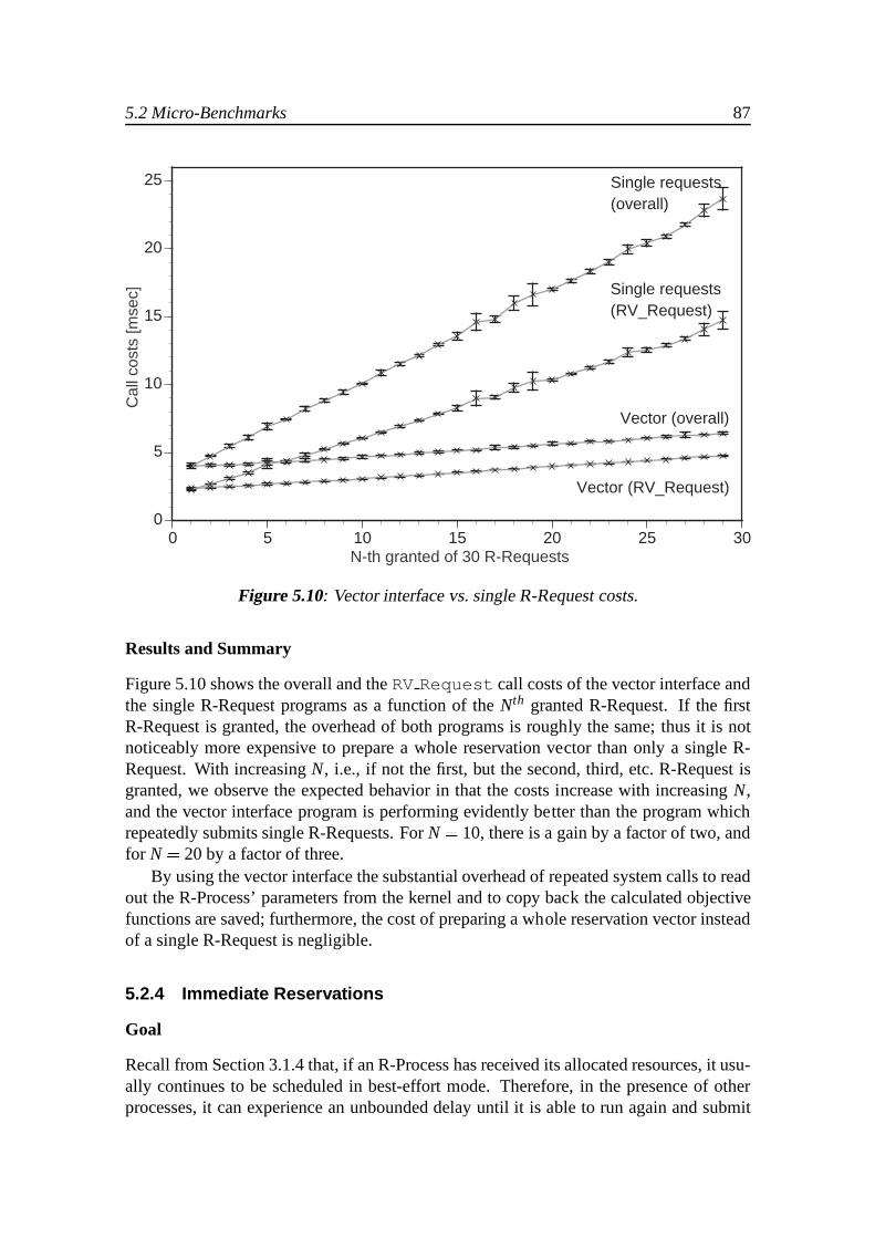
5.2 Micro-Benchmarks 87
0
5
10
15
20
25
0 5 10 15 20 25 30
Cal
l cos
ts [m
sec]
N-th granted of 30 R-Requests
Vector (overall)
Vector (RV_Request)
Single requests(overall)
Single requests(RV_Request)
Figure 5.10: Vector interface vs. single R-Request costs.
Results and Summary
Figure 5.10 shows the overall and theRV Request call costs of the vector interface andthe single R-Request programs as a function of theNth granted R-Request. If the firstR-Request is granted, the overhead of both programs is roughly the same; thus it is notnoticeably more expensive to prepare a whole reservation vector than only a single R-Request. With increasingN, i.e., if not the first, but the second, third, etc. R-Requestisgranted, we observe the expected behavior in that the costs increase with increasingN,and the vector interface program is performing evidently better than the program whichrepeatedly submits single R-Requests. ForN = 10, there is a gain by a factor of two, andfor N = 20 by a factor of three.
By using the vector interface the substantial overhead of repeated system calls to readout the R-Process’ parameters from the kernel and to copy back the calculated objectivefunctions are saved; furthermore, the cost of preparing a whole reservation vector insteadof a single R-Request is negligible.
5.2.4 Immediate Reservations
Goal
Recall from Section 3.1.4 that, if an R-Process has receivedits allocated resources, it usu-ally continues to be scheduled in best-effort mode. Therefore, in the presence of otherprocesses, it can experience an unbounded delay until it is able to run again and submit

88 Chapter 5: Evaluation
another reservation request. In Section 3.2 and 4.4.2 the design and implementation ofa signaling mechanism was described that notifies an R-Process that its reservation hasjust been fulfilled, and arranges that process to be scheduled for an additional schedulingperiod so that the signal handler can immediately be executed. If the signal handler sub-mits a reservation request to the RV-Scheduling System (andthe request is granted), theapplication can circumvent the outlined unbounded delay.
The goal of this experiment is to assess the effectiveness ofthe immediately scheduledsignal handler compared to the normal (i.e., best-effort) scheduled signal handler and toshow that, by submitting a reservation request in an immediately scheduled signal handler,the delay of R-Processes can be prevented.
Experiment Setup
For this experiment, a varying number of R-Processes and a varying number of additional,best-effort scheduled background processes are used. Bothkinds of processes perform acompute-bound task without any I/O. Every R-Process submits totally 10 reservation re-quests, each with a vector consisting of a single R-Request.Each R-Request tries toallocate 1sec of CPU time in a reservation interval of 10sec.As soon as the requestedresources of the previous reservation request have been granted to the R-Process, it im-mediately submits the next reservation request. The numberof the R-Processes is variedfrom 1;2; : : : ;9 yielding an overall CPU utilization by the R-Processes between 10% and90%. The experiment metric is the elapsed wallclock time between the submission of thefirst R-Request and the fulfillment of the last, 10th, R-Request. If the immediately sched-uled signal handler is used to place the reservation requests, the wallclock time of thatR-Process is expected to be between 10sec (in case there is noadditional load, and if therequested CPU is allocated at the very beginning of each reservation interval) and 100sec(in case there is additional load, and/or the CPU is allocated evenly distributed or only atthe very end of each reservation interval). We anticipate the wallclock time to increasewith an increasing number of additional R-Processes as wellas an increasing number ofbest-effort processes, but not to exceed the upper bound of 100sec. This is because on onehand the reservation abstraction ensures that by the end of each of the 10 R-Request inter-vals (each of them during 10sec), the process has been granted the requested resources,and on the other hand because the immediately scheduled signal handler (which is calledas soon as the requested resources have been delivered, i.e., at least at the end of the in-terval) will submit the next reservation requestbeforethe caller falls back to best-effortscheduling mode.
On the other hand, with the best-effort scheduled signal handler, we expect that upperbound to be surpassed, because the R-Process (and subsequently also the signal handler)will be scheduled in best-effort mode immediately after itsrequested resources have beengranted. If we assume that, if there are totallyN computing processes in the system,each of them gets1N of the CPU, then a process requesting an overall CPU time ofT =10� 1sec= 10sec will have a wallclock time in the order ofN� T sec, as shown inFigure 5.11.

5.2 Micro-Benchmarks 89
0
50
100
150
200
250
300
350
400
-1 0 5 10 15 20 25 30
Wal
lclo
ck ti
me
[sec
]
Number of best-effort background loads
1 RV
2 RV
3 RV
4 RV
5 RV
6 RV
7 RV
8 RV
9 RV
Figure 5.11: Expected wallclock time distribution with the best-effort scheduled signalhandler.
Results and Summary
Figure 5.12 shows the averaged wallclock time of the R-Processes as a function of thenumber of the concurrently running best-effort scheduled background and R-Processesunder the best-effort scheduled signal handler. We observethat the measured wallclocktimes are in the same order as predicted (Figure 5.11) and unbounded with increasingoverall system load. The variance between the experiment repetitions expressed in termsof the Coefficient Of Variation (C.O.V)3 is in the order of 0:01 and thus negligible.
Figure 5.13 shows the averaged wallclock time of the R-Process/es as a function of thenumber of the concurrently running best-effort scheduled background and R-Processesunder the immediately scheduled signal handler. We can see that the wallclock timeexceeds the expected upper limit of 100sec only in a few cases. This is due to the im-mediately scheduled signal handler, which submits a reservation request instantaneouslyafter the previous request has been fulfilled. The C.O.V. of the repetitions peaks at 0:1and is thus an order of magnitude larger than in the previous test, but is still acceptablylow.
This experiment has shown that by taking advantage of the immediately scheduledsignal feature to submit reservation requests, an R-Process can prevent unbounded delaysbetween two consecutive reservations.
3The C.O.V is defined as the ratio of the standard deviation to the mean.

90 Chapter 5: Evaluation
0
50
100
150
200
250
300
350
400
-1 0 5 10 15 20 25 30
Wal
lclo
ck ti
me
[sec
]
Number of best-effort background loads
1 RV
2 RV
3 RV
4 RV
5 RV
6 RV
7 RV
8 RV
9 RV
Figure 5.12: Measured wallclock time distribution with the best-effort scheduled signalhandler.
0
50
100
150
200
250
300
350
400
-1 0 5 10 15 20 25 30
Wal
lclo
ck ti
me
[sec
]
Number of best-effort background loads
1 RV
2 RV
3 RV
4 RV
5 RV
6 RV
7 RV
8 RV
9 RV
Figure 5.13: Measured wallclock time distribution with the immediately scheduled signalhandler.

5.3 Application Traces 91
5.2.5 Summary
The micro-benchmarks presented in this section show that the reactive scheduling schemedescribed in Section 4.1 is able to support the reservation abstraction with its semanticsas defined in Section 3.1.1. The scheme in fact keeps the actual cumulative resourceconsumption of the R-Processes along the objective functions, allows R-Processes a work-ahead in the order of a scheduler period in case of ample resources, and effectively isolatesthem from the influence of best-effort loads. Additionally,blocked R-Processes can catchup their delay without affecting other R-Processes.
The overhead of the RV-Scheduler is higher than that of the built-in best-effort sched-uler, but within the same order of magnitude (0:14% for 35 concurrently scheduled R-Processes) and thus acceptable for practical use. The admission controller overhead isnoticeable and thus the limiting factor of the RV-Scheduling System, although the work-ing range automatically extends with advances in hardware technology. For example, ifthe maximum tolerable admission controller overhead is limited to 200ms, 20 concurrentR-Processes can be handled on a 200 MHz Pentium Pro, comparedto 29 on a 933 MHzPentium III.
The usage of the reservation vector interface by submittinga number of R-Requestsyields a considerable performance gain (e.g., factor of three for 20 R-Requests) comparedto repeatedly submitting single R-Requests until one of them is accepted. Additionally,the overhead to prepare a whole reservation vector instead of only a single R-Requests isnot noticeable.
Finally, the immediately scheduled signal handler is an effective means for R-Processes to obtain consecutive reservations in a predictable manner without falling backto best-effort scheduling and thus experiencing possibly unbounded delays in their execu-tion.
5.3 Application Traces
While the previous section has examined the RV-Scheduling System’s various compo-nents in detail, this section takes a more global point of view and considers the RV-Scheduling System as a black box. This point of view is relevant since it representsthe application’s view of the RV-Scheduling System. Applications do not care about theinternals of the RV-Scheduling System, but are basically interested whether the system isindeed able to deliver the granted resources. Furthermore,the system’s overhead underrealistic workloads might be different from the one under the synthetic, worst-case onesconstructed in Section 5.2. This section reports on experiments with application traces.First, the experiment is run with the default configuration of α = 0:9 (i.e., at most 90%of the CPU are dedicated to R-Processes) and the results are reported in Section 5.3.1. Ina subsequent experiment, the influence ofα on the key metric “reservation failure” (anR-Process actually gets fewer cycles than originally granted) is examined and presentedin Section 5.3.2. Finally, in Section 5.3.3 the applicationtraces are submitted to a pub-licly available real-time operating system (Real-Time Linux [11, 12]), and it is shown

92 Chapter 5: Evaluation
that—while the RV-Scheduling System is able to fulfill the requests—the real-time OSfails noticeably.
5.3.1 Basic Experiment
Goal
The goal of this experiment is to show the feasibility of the RV-Scheduling System in a“realistic” environment by quantifying the amount and extent of reservation failures aswell as the the admission controller and RV-Scheduler overheads.
Experiment Setup
Two experiments with different workloads are run: The first experiment simulates alightly loaded system with few reservation requests; the second experiment simulatesa highly loaded system with an order of magnitude more reservation requests. For eachexperiment, 20 of the workload processes are run in additionto 10 best-effort compute-bound background processes. The experiment duration is setto an hour to minimize resultdistortions by possible start-up effects.
The first workload uses reservation requests with randomly generated parameters: Thereservation vector consists of five R-Requests, each of themhas the same reservationinterval length which is uniformly distributed between 0:5sec and 20sec. The requestedcycles are uniformly distributed between 0:1sec and the interval length for the first R-Request, and between 0:1sec and the cycles requested by thei�1th R-Request for theith
R-Request (i = 2; : : : ;5). The idle time between the end of an interval (for which theR-Request was granted) and the start of the new reservation interval is uniformly distributedbetween 1sec and 5sec.
The second workload (infinitely) replays a trace that has been captured from the Char-iot image retrieval system (see Section 2.2.2 for details about Chariot). A trace run con-sists of a total of 25 reservation requests. The first reservation request submits a reser-vation vector consisting of 25 R-Requests, the second one a vector of 24 R-Requests,and so on; this pattern simulates the delivery of 25 images where Chariot tries to allocateresources to one of the forthcoming preparation steps.
Results and Summary
Table 5.2 shows the results of the two experiments. In a lightly loaded system, the RV-Scheduler is able to deliver all of the granted reservationswithin �50ms of the reserva-tion; in the heavily loaded system, 99:96% are within this range. Since the RV-Scheduler’sresolution is 50ms in the current implementation, a closer match than�50ms cannot beexpected. Furthermore, in both experiments over 91% of all granted requests achieved awork-ahead which is also a good result.
For both experiments, the aggregated overhead of the admission controller and the RV-Scheduler itself is well below 0:6% of the experiment duration, and can thus be consideredas negligible. We furthermore observe that the overall delivered utilization for the R-Processes is 96:39% for experiment 1 and 94:14% for experiment 2, respectively. This

5.3 Application Traces 93
Experiment 1 Experiment 2Workload Random requests Image server trace
µ σ µ σExperiment Duration 3687sec 2:22 3608sec 0:49Reservation requests submitted 1554 72 16754 88Reservation requests granted 1452 63 15858 316
X <�50ms 0:00% 0:00 0:04% 0:01Over/under-reservation �50ms� X < 0 8:11% 0:92 8:82% 1:94(X=delivered–requested) 0� X < 50ms 91:89% 0:92 91:14% 1:93
50ms< X 0:00% 0:00 0:00% 0:00Admission controller cost 0:102% 0:014 0:574% 0:019RV-Scheduler cost 0:023% 0:001 0:026% 0:001Best-effort scheduler cost 0:026% 0:004 0:035% 0:004Overall CPU utilization 96:39% 0:16 94:14% 2:40
Table 5.2: Results of application traces.
is higher than the 90% the admission controller was configured to contract out to R-Processes, and we attribute this observation to the work-ahead mechanism of the RV-Scheduler.
To conclude, this experiment has shown that under realisticworkloads, the RV-Scheduling System is able to deliver the granted resources on time and at a negligiblecost. Additionally, the overall end system utilization is maximized up to and even beyondthe configured maximum limit of 90%.
5.3.2 Reservation Failures as a Function of α
Goal and Experiment Setup
The goal of this experiment is to examine the influence ofα on the key metric “reservationfailure”. The same experiments as described in Section 5.3.1 are repeated varying theparameterα (i.e., the fraction of the CPU granted to R-Processes) from 0:1 until 0:9 insteps of 0:1.
Results and Summary
Figures 5.14(a) and 5.14(b) show the amount of complete reservation failures (X <�50ms whereX := delivered� requested) as a percentage of the total number of ad-mitted reservations for experiment 1 and experiment 2, respectively. We note that forexperiment 1 with the lighter load, the extent of complete failures is largely independentof α, whereas for the heavier load of experiment 2, the failures increase with increasingα and thus congestion for the resource CPU. Forα = 0:3 andα = 0:8 in experiment 1andα = 0:2 in experiment 2, the averages are outliers relative to the values for the otherαs, and the standard deviation is much higher. As an example, the absolute number ofreservation failures for the five experiment repetitions are 0, 8, 1, 0, 1 (forα = 0:2 in

94 Chapter 5: Evaluation
-0.05
-0.02
0
0.02
0.04
0.06
0.08
0.1
0 0.1 0.2 0.3 0.4 0.5 0.6 0.7 0.8 0.9
Del
iver
y di
strib
utio
n (%
)
Fraction of CPU for RV-Processes (alpha)
X < –50 ms
(a) Reservation failures for experiment 1
-0.05
-0.02
0
0.02
0.04
0.06
0.08
0.1
0 0.1 0.2 0.3 0.4 0.5 0.6 0.7 0.8 0.9
Del
iver
y di
strib
utio
n (%
)
Fraction of CPU for RV-Processes (alpha)
X < –50 ms
(b) Reservation failures for experiment 2
-20
10
90
100
0 0.1 0.2 0.3 0.4 0.5 0.6 0.7 0.8 0.9
Del
iver
y di
strib
utio
n (%
)
Fraction of CPU for RV-Processes (alpha)
–50 ms ≤ X < 0
0 ≤ X < 50 ms
50 ms < X
(c) Reservation delivery distribution for experi-ment 1
-20
10
90
100
0 0.1 0.2 0.3 0.4 0.5 0.6 0.7 0.8 0.9
Del
iver
y di
strib
utio
n (%
)
Fraction of CPU for RV-Processes (alpha)
–50 ms ≤ X < 0
0 ≤ X < 50 ms
50 ms < X
(d) Reservation delivery distribution for exper-iment 2
Figure 5.14: Influence ofα on reservation failures.
experiment 2), which explains the large standard deviationdue to the one outlier value 8.Relating those figures to the average number of granted reservations (7532), however, thefailures are negligible, and thus we did not further investigate the reason for the outliers.
Figures 5.14(c) and 5.14(d) show the percentage distribution around the amount ofrequested resources for experiment 1 and experiment 2, respectively. We observe that ifample spare resources are left in the system (α < 0:5), almost all reservations are com-pletely granted, i.e., within the 0� X < 50ms range. With increasingα, the percentage ofreservations that are behind the requested amount by at least the RV-Scheduler invocationinterval (�50ms� X < 0) increases.
Because the RV-Scheduling System has been implemented under a best-effort, non-real-time operating system, it is not able to provide hard guarantees. The experimentsconfirm this assessment since independently ofα and the workload, very few (althougha non-zero number of) reservations fail to obtain their allocations. However, due to theadaptive nature of the RV-Scheduled applications, those failures are not severe since theapplication-level adaptation mechanism should be able to smooth out such infrequentdelays.

5.3 Application Traces 95
Furthermore, there is a clear trade-off between maximizingoverall end system uti-lization for the benefit of R-Processes, and maximizing the number of reservations thatare completely granted (i.e., at least the reserved amount of resources is delivered, witha possible work-ahead). Depending on the details of deployment and end user require-ments, the system may be configured either for a high overall utilization (and an increasednumber of reservation misses), or a high reservation success rate (and a lowered overallutilization). This observation suggests that the parameter α should be configurable at runtime.
5.3.3 Comparison to Real-Time Scheduling
Goal
The goal of this experiment is to compare the RV-Scheduling System with a standard real-time scheduler along the key metrics “reservation failure”and overall CPU utilization.
Experiment Setup
As the base for this experiment, a trace of the reservation requests generated in experi-ment 1 (of Section 5.3.1) is used. In addition to the reservation parameters (interval andamount of requested resources), the trace contains information about which R-Request ofeach submitted reservation vector has been admitted by the RV-Scheduling System duringexperiment 1.
As a real-time operating system, the publicly available Real-Time LinuxRTLinux V3.0 (http://www.rtlinux.org) is used (see Section 2.5.2 for a shortdescription of RTLinux). RTLinux has a pure priority-driven preemptive scheduler, inwhich the highest priority (ready) thread is always chosen to run [53]. Threads can bemade to execute periodically; they have to actively and voluntarily yield the CPU aftereach invocation (by means of a special function). RTLinux does not contain an admissioncontroller. Furthermore, it does not provide directly any of the classical real-time schedul-ing methods like RM or EDF (see Section 2.5.2). However, using the priority-driven pre-emptive scheduler, it is easy to deploy the rate monotonic fixed priority scheduling byassigning threads a priority value proportional to their request rate (thus a high-frequencytask has a higher priority than a low-frequency one). This approach is followed in thisexperiment.
The R-Requests are mapped to the periodic task model of this real-time operatingsystem as follows: Recall that each reservationRi(Ii;Ci) is denoted by a start- and anend-time (which define the time intervalIi), and the amount of resourcesCi requestedwithin that interval. Assuming that, for each invocation, the periodic task will run for atime duration ofT, it has to be invokedNi = Ci
T times to deliver the requested amountCi
of resources. This yields a period ofPi = IiNi
= Ii=CiT . In this comparative experiment, we
use a fixed time duration ofT = 50ms which corresponds to the scheduling period of theRV-Scheduler (see Section 4.1.1 for details). A reservation in the periodic task model isthus characterized by its start- and end-time, its periodPi , its priority, and the number oftimesNi it has to be invoked.

96 Chapter 5: Evaluation
Of the basic trace, three versions are generated for this experiment: Trace “RT-RV”contains, for allsubmittedreservation vectors of the basic trace, the R-Requests whichhave beenadmittedby the RV-Scheduling System. Thus this version correspondsexactlyto the workload that has successfully been processed by the RV-Scheduling System withthe performance results presented in Section 5.3.1.
Recall from Section 4.2 that in the RV-Scheduling System, the objective functionscan have any arbitrary shape, i.e., the resources may be delivered at the beginning, at theend or somehow distributed over the whole intervalI . In contrast, the presented map-ping of the R-Requests to the periodic real-time task model always evenly distributes theresource delivery over the whole interval. Therefore, someresource request scenariosthat are schedulable by the RV-Scheduling System may not be schedulable by the real-time scheduler. To ensure a fair comparison between the two schedulers, two more traces(trace “RT-AC 1” and trace “RT-AC 2”) are generated that do not contain such scenarios.
The second version—trace “RT-AC 1”—is a subset of trace “RV”. To generate thetrace “RT-AC 1”, a simple real-time scheduler admission controller as outlined in Sec-tion 2.5.2 is used. First, for every reservationRi its processor utilizationUi is calculatedasUi = Ci
Ii= T
Pi. The real-time admission controller algorithm starts withan empty set
of granted requests. In ascending start time order, it adds the next reservationRi to thegrant set. Then it checks for the whole duration between the earliest start time and thelatest end time of all requests in the grant set that the overall processor utilization doesnever exceed a certain fractionβ. If the utilization is above this value, the newly addedreservationRi contributes to the overload, and it is rejected and removed from the grantset. Otherwise, it is accepted and remains in the grant set. The above outlined algorithmis carried out for all reservationsRn. The value of the parameterβ is varied from 0:5 to0:9 in increments of 0:1, with one exception where instead of 0:7 the value of 0:69 isused. According to Liu and Layland [81], the RM algorithm is able to schedule a set ofprocesses if their utilization does not exceed an upper bound of ln2= 0:693. Therefore,for β < ln2, all processes should make it on time; whereas for largerβ, some of them maymiss their deadlines.
To generate the third version—trace “RT-AC 2”—the same admission controller al-gorithm as described above is executed, but now it considersall the R-Requests of everysubmitted reservation vector, not only ones granted by the RV-Scheduling System as fortrace “RT-AC 1”. The reason to generate this trace is that, although a particular R-Requestof a reservation vector might not have been admitted by the real-time admission controller,another R-Request of the same vector, but with lower resource demands, may be admit-ted. Thus the processor utilization of trace “RT-AC 2” is expected to be higher than thatof “RT-AC 1”.
Results and Summary
Figure 5.15 shows the experiment results, the left column for trace “RT-AC 1” and theright column for trace “RT-AC 2”. Figures 5.15(a) and 5.15(b) show the amount of suc-cessful and failed reservations as a percentage of the totalnumber of admitted requests,which are shown in Figures 5.15(c) and 5.15(d). We see that, for values ofβ < 0:69, allreservations are successful, whereas for values ofβ > 0:69 the percentage of reservation

5.3 Application Traces 97
-70
102030405060708090
100
0.45 0.5 0.6 0.7 0.8 0.9 1
Del
iver
y di
strib
utio
n (%
)
Fraction of CPU for real-time processes (beta)
success
failure
RV success
RV failure
RT-RVsuccess
RT-RVfailure
(a) Reservation delivery distribution for trace“RT-AC 1”
-50
10
20
30
40
50
60
70
80
90
100
0.45 0.5 0.6 0.7 0.8 0.9 1
Del
iver
y di
strib
utio
n (%
)
Fraction of CPU for real-time processes (beta)
success
failure
RV success
RV failure
RT-RVsuccess
RT-RVfailure
(b) Reservation delivery distribution for trace“RT-AC 2”
0
200
400
600
800
1000
1200
1400
0.45 0.5 0.6 0.7 0.8 0.9 1
Req
uest
s su
bmitt
ed
Fraction of CPU for real-time processes (beta)
RV=RT-RV
(c) Requests submitted in trace “RT-AC 1”
0
200
400
600
800
1000
1200
1400
0.45 0.5 0.6 0.7 0.8 0.9 1
Req
uest
s su
bmitt
ed
Fraction of CPU for real-time processes (beta)
RV=RT-RV
(d) Requests submitted in trace “RT-AC 2”
0
10
20
30
40
50
60
70
80
90
100
0.45 0.5 0.6 0.7 0.8 0.9 1
CP
U u
tiliz
atio
n (%
)
Fraction of CPU for real-time processes (beta)
RV
deliveredspecified
RT-RV
(e) CPU utilization for trace “RT-AC 1”
0
10
20
30
40
50
60
70
80
90
100
0.45 0.5 0.6 0.7 0.8 0.9 1
CP
U u
tiliz
atio
n (%
)
Fraction of CPU for real-time processes (beta)
RV
delivered
specifiedRT-RV
(f) CPU utilization for trace “RT-AC 2”
Figure 5.15: Comparison of the RV-Scheduling System to real-time scheduling.
failures increases with largerβ. Forβ = 0:69, some of the requests fail; the percentage islarger for the trace “RT-AC 2”, which has more requests submitted, than for “RT-AC 1”.Although from the theoretical point of view forβ = 0:69 all requests should be suc-cessful, we suspect that this small failure can be attributed to run time dynamics (i.e.,

98 Chapter 5: Evaluation
non-zero context switch costs, interrupt handling) which are not captured by the theoret-ical model. It is interesting to compare the values achievedby the real-time schedulerwith those of the RV-Scheduling System (shown as arrows labeled “RV” in the figures):The RV-Scheduling System is able to process a larger number of requests, and all of themare successful. In contrast, if the same trace, which is successfully processed by the RV-Scheduling System, is submitted unmodified to the real-timescheduling system, the latterproduces noticeably worse results, as shown by the arrows labeled “RT-RV”
Figures 5.15(e) and 5.15(f) show the percentage of requested CPU according to thetrace files and delivered to reservations (as a percentage ofthe overall experiment dura-tion) as a function ofβ. First, we see that for a certain value ofβ, the requested percentageaccording to the trace is always smaller than thatβ. This is because the described real-time admission controller limits thepeakCPU usage fraction toβ, so theaverageCPUusage is smaller. Second, we observe that forβ < 0:69, the percentage delivered to reser-vation equals the percentage requested, i.e., all requestscan successfully be satisfied. Forβ � 0:69, we see a difference between target and achieved percentage, which increasesfor largerβ and which is also more visible for the heavier load of trace “RT-AC 2”. Thearrows show again the achieved percentage by the RV-Scheduling System (“RV”), and thevalues for the unmodified trace for the real-time scheduler (“RT-RV”). In both cases, therequested CPU percentage is 95:96%; thus the RV-Scheduling System is able to deliverthis percentage completely.
Figure 5.15 contains also the standard deviationσ for five experiment repetitions plot-ted as error bars, but due to their very small values they are hardly visible.
To conclude, this experiment shows that the RV-Scheduling System is able to processa larger number of requests successfully, and thus has a noticeably higher CPU utilizationthan the real-time scheduler.
5.3.4 Summary
The experiments with the application traces show that despite the non-negligible admis-sion controller costs (as shown with the micro-benchmarks in Section 5.2.2), the RV-Scheduling System is able to deliver the granted resources in almost any cases on timeand at a negligible cost (less than 0:6% overall overhead). Furthermore, the end systemutilization for R-Processes is maximized up to and even beyond the configured values dueto the work-ahead allowed for by the RV-Scheduling mechanism. Severe reservation fail-ures (reservation miss by more than a scheduling period) areextremely rare and within atolerable range for adaptive applications. The parameterα (fraction of CPU dedicated toR-Processes) turns out to be the determining factor whetherthe RV-Scheduling Systemachieves either a low reservation failure ratio (and low overall system utilization for R-Processes) or a high overall utilization (and a higher reservation failure ratio). Finally, acomparison with a real-time OS shows that the RV-SchedulingSystem is able to processsuccessfully request streams for which a real-time scheduler fails, and thus achieves anoticeably higher CPU utilization.

5.4 Real-Life Application 1: Resource-Aware Internet Server 99
5.4 Real-Life Application 1: Resource-Aware Internet Serv er
This section describes the implementation and evaluation of the Resource-Aware Inter-net Server sketched in Section 2.2.1. Section 5.4.1 describes the implementation of theserver under both the best-effort operating system as well as its integration with the RV-Scheduling System. In Section 5.4.2 the choice of the parameters of the synthetical work-load is justified, and Section 5.4.3 compares the two server versions using that workload.
5.4.1 The Resource-Aware Internet Server and the RV-Schedu ling System
The resource-aware Internet server works as follows: Upon arrival of a new client request,the main server process immediately forks off a new child process to handle that request,and then waits for the next request to arrive. The child process behaves differently, de-pending on whether it is scheduled by the RV-Scheduler or thebest-effort scheduler.
The RV-Scheduled server tries to reserve the CPU by means of the RV Requestcall before processing the client’s request. The parameters of the submitted R-Requestare the request processing window length (calculated from the user time limit and RTT,see Figure 2.1 on page 7), and the amount of resources needed to process the request.In the experiment, all these parameters are read from a tracefile and made available tothe server at run time. The choice of the parameter values is discussed in the followingSection 5.4.2. If the reservation isnotgranted, the server immediately sends back a “fail”-message without any further attempt to process the request,otherwise the server handlesthe request and subsequently a “success”-message is sent back to the client. Therefore, incase of overload, part of the requests should be processed intime, whereas the other partshould be rejected.
For the best-effort operating system, there are three different versions of the server:The first version, which is named “Inf”, does not perform any form of admission controland thus always tries to process the request no matter how large the server load maybe. It either manages to finish before the end of the request processing window (in thiscase, a “success”-message is sent back to the client), or it fails, stops the work on thecurrent request, discards the result and sends back a “fail”-message. Therefore, in caseof overload, few requests will meet their deadline, whereasa larger number of them isexpected to fail and thus to waste server resources. The other two server versions performadmission control by using the UNIX systemload, i.e., the number of processes in therun queue4: The second version applies a fixed load limit, i.e., if the system load exceedsa configurable limit, all newly arriving client requests aredenied and a “fail”-messageis sent back. Once the load drops below that level, the serveraccepts again requests,regardless of the amount of resources each request consumes. The third version of theserver, which is named “Auto”, performs a dynamic admissioncontrol: For each newlyarriving request, it compares the current loadL (corresponding toL running processesin the system) against the averaged CPU consumption ratioR of that request (R definedas the request processing time over the request processing window). The new request isadmitted only if 1
L+1 �Runder the assumption that the currently runningL processes and
4see Section 5.5.1 for a discussion of using the UNIX system load as a resource availability predictor.

100 Chapter 5: Evaluation
Trace name request interarrival # requests CPU overbooking(ms) factor
trace-200-normal 200 1974 5.89trace-500-normal 500 1018 2.98trace-1000-normal 1000 545 1.66trace-1500-normal 1500 419 1.28trace-200-fast 200 2029 1.81trace-500-fast 500 1034 0.95trace-1000-fast 1000 568 0.50trace-1500-fast 1500 369 0.32
Table 5.3: Internet server request stream parameters.
the newly admitted one will each get about1L+1 of the CPU, and thus if the new requestconsumes less than that fraction, it should be able to finish on time.
Under the best-effort OS as well as using the RV-Scheduling System, the main serverprocess can only be scheduled in best-effort mode due to the random and thus unpre-dictable client request arrival. Within a single application, there is thus on one hand abest-effort mode to perform mainly administrative activities (accepting an incoming con-nection and forking off a child process to handle that connection), and on the other handa reserved mode to actually carry out the productive work (client request processing andreturning the result).
This application is a simulation of a productive client–server scenario. Therefore,the client’s request contains—instead of a real user query—the user time limit, the RTTand the actual request processing time; the server side processing is approximated by acounting loop; and the server’s reply merely consists of a return code corresponding toeither the “success”- or “fail”-message.
5.4.2 Experiment Setup
For the experiment, four synthetically generated request streams with a duration of 10minare used. Since the choice of a synthetic request stream may raise concerns about theexperiment’s value, the parameters are modeled as close as possible to real-world obser-vations by other researchers as follows: The interarrival time of the requests is exponen-tially distributed with a mean of 200ms, 500ms, 1000ms and 1500ms, respectively, andis modeled similar to the observations of Arlitt and Williamson [4]. The user time limitis set to 5sec with a time limit tolerance of 10%. The values are based on an empiricalstudy about user’s tolerance of QoS in the context of Web servers [19], which concludesthat for non-incremental page loading, users rate a Web site’s responsiveness as “high”if the page takes 5sec or less to load and render on the client side. The RTT’s have as abasis a Gamma distribution [68] with scale parameter 1 and shape parameter 5 (accord-ing to Mukherjee [95]) and are stretched so that the mean is around 200ms. This setupis in conformance with empirical measurements [29]. The request processing time has

5.4 Real-Life Application 1: Resource-Aware Internet Server 101
been chosen to be exponentially distributed with a mean of 3000ms to reflect typical CGIserver response times [39]. In conjunction with the other parameters, this produces thefour “trace-XX-normal” request streams as shown in Table 5.3 (whereXX stands for themean interarrival time in ms). These streams overload the server more or less heavily, asindicated by the CPU overbooking factors larger than one. The CPU overbooking factoris calculated as the sum of all requests divided by the request stream length. To obtainrequest streams that donotoverload the server, four additional traces have been generatedwith essentially the same parameters, but assuming a fastermachine and thus a mean re-quest processing time of 500ms (instead of 3000ms), yielding the “trace-XX-fast” traces.Note that an overbooking factor of less than one does not necessarily mean that all re-quests will be granted or meet their deadlines: If two requests with similar processingwindows arrive at about the same time, and each of them would,e.g., request 80% of theCPU, one of them will have to be rejected or miss its deadline.
The client, which reads the trace file with the request streamparameters and forks offa child to handle each submitted request, is run on a different machine than the server toprevent the client being affected by the server’s resource reservations. The client machinesare several 400 MHz Intel Pentium II PCs running Linux 2.2.
5.4.3 Experiment
Goal
The goal of this experiment is to compare the various best-effort scheduled servers andthe RV-Scheduled server under different degrees of (over- and under-)load.
The first metric is the relative request distribution, i.e.,which percentage of all sub-mitted requests succeed within the user time limit plus timelimit tolerance, how manyof them fail (i.e., consume resources, but are late for whatever reason), and how many ofthem are rejected right away without consuming resources. Using the percentage insteadof absolute values allows the results of different traces tobe compared directly, since theydiffer by the absolute number of submitted requests. We consider the request success rateas the most important metric. Additionally, for a certain success rate, the failure ratioshould be minimized and at the same time the rejection rate maximized. Maximizing therejection rate at the expense of the failure rate is beneficial for both the user, since he getsan immediate rejection notification instead of having to wait for an anyway incompleteanswer, as well as the the server and the end system since it frees up resources that can beused otherwise.
The second metric is the CPU usage distribution, i.e., whichpercentage of the CPU isused for the processing of requests that will eventually be successful, which percentageis “wasted”, i.e., used for the processing of requests that will eventually fail, and whichpercentage is free. The CPU percentage for successful requests should be maximized, andat the same time the “waste” percentage minimized.

102 Chapter 5: Evaluation
Experiment Setup
In the experiment, the three best-effort scheduled serversand the server under the RV-Scheduling system as described in Section 5.4.1 are run withthe two times four traces(Section 5.4.2). Further experiment factors are the maximum load limit for the secondbest-effort server, which rejects requests based on load value alone (load limit variedfrom 0:5 to 10:0 in increments of 0:5), and the maximal amount of resources granted toreservations (α) for the RV-Scheduled server (α varied from 0:05 to 0:95 in increments of0:05).
Results and Summary
Figures 5.16 and 5.17 show the relative request distribution for the “normal” and “fast”traces, respectively. The successful requests (i.e., within user time limit plus time limittolerance) are shown in black, the failed requests (i.e., they consumed resources, but didnot make it on time) in gray, and the rejected requests in white.
Figures 5.18 and 5.19 show the CPU usage distribution for the“normal” and “fast”traces, respectively. The ratio of CPU used to process successful requests is shown inblack, the CPU for the failed requests (i.e., wasted CPU) in gray, and white denotes thefree fraction of the CPU, i.e., the resources available to other applications.
For all figures, the graphs in the left column show the data forthe best-effort sched-uled servers as a function of the load limit (i.e., if the system load is greater than thelimit, the server rejects requests). There are two special cases of the load limit, namely“Auto” and “Inf”, corresponding to the third and first version as described earlier: “Auto”denotes the version of the best-effort scheduled server that performs the dynamic admis-sion control based on system load and request properties, “Inf” denotes the version of theserver that does not perform any admission control at all (i.e., would reject requests if thesystem load were greater thaninfinity). The graphs in the right columns show the datafor the RV-Scheduled servers as a function of the maximal amount of resources grantedto reservations (α).
A comparison of the three best-effort scheduled server versions shows clearly that theserver with dynamic admission control (“Auto”) dramatically outperforms the other onesboth with regard to maximizing the success rate and minimizing the failure rate (Fig-ures 5.16 and 5.17). The advantage is more pronounced for thesetups with higher endsystem load (small interarrival time, long processing time). Looking at the request distri-bution graphs for the RV-Scheduled server, we first observe that for each of thetrace-200-normal, trace-500-normalandtrace-200-fasttraces, there is an individualα-value abovewhich the amount of rejected requests does not or only minimally decrease, i.e., the sumof successful and failed requests stays more or less constant (αtrace�200�normal = 0:55,αtrace�500�normal = 0:8, αtrace�200�fast = 0:35 ). Consulting the CPU usage distributiongraphs for those traces, we note that the foundα-values denote the point where the sys-tem becomes fully loaded, i.e., the free fraction of the CPU approaches zero. Due tothe work-ahead allowance of the RV-Scheduler, the entire CPU is used anyway, and in-creasingα does not incur in any performance increase. Second, and worse yet, for allbut the two lightest loads (trace-1000-fastandtrace-1500-fastin Figures 5.16 and 5.17),

5.4
Rea
l-Life
Ap
plica
tion
1:
Reso
urce
-Aw
are
Inte
rnetS
erv
er
10
3
Auto
0.51
1.52
2.53
3.54
4.55
5.56
6.57
7.58
8.59
9.510
Inf
0
10 20 30 40 50 60 70 80 90
100
Request distribution (%)
Maxim
um load lim
it
0.050.1
0.150.2
0.250.3
0.350.4
0.450.5
0.550.6
0.650.7
0.750.8
0.850.9
0.95
0
10 20 30 40 50 60 70 80 90
100
Request distribution (%)
Fraction of C
PU
for RV
-Processes (alpha)
Figure
5.16:R
equestdistribution
forthe
“normal”
load.L:
best-effort,
R:
RV.
Traces
200,500,1000,1500from
topto
bottom.
Black:
success,gray:
failure,white:
rejection.

10
4C
ha
pte
r5
:E
valu
atio
n
Auto
0.51
1.52
2.53
3.54
4.55
5.56
6.57
7.58
8.59
9.510
Inf
0
10 20 30 40 50 60 70 80 90
100
Request distribution (%)
Maxim
um load lim
it
0.050.1
0.150.2
0.250.3
0.350.4
0.450.5
0.550.6
0.650.7
0.750.8
0.850.9
0.95
0
10 20 30 40 50 60 70 80 90
100
Request distribution (%)
Fraction of C
PU
for RV
-Processes (alpha)
Figure
5.17:R
equestdistribution
forthe
“fast”load.
L:best-effort,
R:
RV.
traces200,
500,1000,1500from
topto
bottom.
Black:
success,gray:fai
lure,white:
rejection.

5.4
Rea
l-Life
Ap
plica
tion
1:
Reso
urce
-Aw
are
Inte
rnetS
erv
er
10
5
Auto
0.51
1.52
2.53
3.54
4.55
5.56
6.57
7.58
8.59
9.510
Inf
0
10 20 30 40 50 60 70 80 90
100
CPU usage distribution (%)
Maxim
um load lim
it
0.050.1
0.150.2
0.250.3
0.350.4
0.450.5
0.550.6
0.650.7
0.750.8
0.850.9
0.95
0
10 20 30 40 50 60 70 80 90
100
CPU usage distribution (%)
Fraction of C
PU
for RV
-Processes (alpha)
Figure
5.18:C
PU
distributionfor
the“norm
al”load.
L:best-effort,
R:RV.
Traces
200,500,1000,1500
fromtop
tobottom
.B
lack:success,gray:
was
te,white:
free.

10
6C
ha
pte
r5
:E
valu
atio
n
Auto
0.51
1.52
2.53
3.54
4.55
5.56
6.57
7.58
8.59
9.510
Inf
0
10 20 30 40 50 60 70 80 90
100
CPU usage distribution (%)
Maxim
um load lim
it
0.050.1
0.150.2
0.250.3
0.350.4
0.450.5
0.550.6
0.650.7
0.750.8
0.850.9
0.95
0
10 20 30 40 50 60 70 80 90
100
CPU usage distribution (%)
Fraction of C
PU
for RV
-Processes (alpha)
Figure
5.19:C
PU
distributionfor
the“fast”
load.L:best-effort,R
:RV.T
races200,500,
1000,1500from
topto
bottom.
Black:
success,gray:w
aste,white:
free.

5.4 Real-Life Application 1: Resource-Aware Internet Server 107
0
10
20
30
40
50
60
70
80
90
100
100200 400 600 800 1000 1200 1400 1600
Req
uest
suc
cess
rat
e [%
]
Mean request interarrival time [msec]
RV
BE
BE-Auto
(a) Success rate, “normal” trace
0
10
20
30
40
50
60
70
80
90
100
100200 400 600 800 1000 1200 1400 1600
Req
uest
suc
cess
rat
e [%
]
Mean request interarrival time [msec]
BE
RV
BE-Auto
(b) Success rate, “fast” trace
Figure 5.20: Summary of the request success rate.
there is a bound above which the percentage of failed requests increases at the expenseof successful requests, a clearly unwanted behavior. This observation can be explainedby the hybrid nature of the application in question: The mainserver process, which ac-cepts the incoming connections and forks off the children tohandle that connection, canonly be scheduled in best-effort mode due to the random and thus unpredictable clientrequest arrival. If too much resources are allocated to R-Processes (highα-value), themain server process has hardly any chance to run. The tasks ofaccepting the connectionand forking off the child are delayed by an indeterminable amount of time, and subse-quently there is not enough time left to provide the reply in time, even if the child wouldbe able to reserve the needed resources. This bound where thepercentage of failed re-quests increases at the expense of successful requests varies dynamically as a function ofthe properties of the trace (e.g., between 0:45 for trace-200-fastand 0:70 for trace-1500-normal). Therefore a worthwhile addition to the user interface would be the introductionof a notification mechanism by which applications could request the RV-Scheduling Sys-tem to dynamically adjust itsα-value depending on the application perceived quality (i.e.,the appearance and/or increase of the number of failed requests in the resource-awareInternet server example would trigger a lowering ofα). However, the details of such adynamic adjustment mechanism would yet have to be explored,especially in the case ofdifferent applications with different resource consumption characteristics.
If we compare the best-effort scheduled servers with the RV-scheduled versions sub-jected to the same traces, we see that the latter performs consistently better in terms ofrequest success ratio, especially in case of resource contention. If there are ample re-sources left (e.g.,trace-1000-fastandtrace-1500-fastwith small CPU overbooking fac-tors (Table 5.3), and small overall CPU utilization ratio (Figure 5.19) in conjunction witha complete request success ratio (Figure 5.17)), all versions perform equally well. The re-quest success rates are summarized in Figure 5.20 as a function of the request interarrivaltime. Data is shown for the best-effort scheduled server without any admission control(BE), the best-effort scheduled server with dynamic admission control (BE-Auto) and theRV-Scheduled server where, for a given trace, the highest possible success ratio is shown.

108 Chapter 5: Evaluation
200 500 1000 15000
10
20
30
40
50
60
70
80
90
100
CP
U u
sage
dis
trib
utio
n [%
]
Mean request interarrival time [msec]
(a) RV, “normal” trace
200 500 1000 15000
10
20
30
40
50
60
70
80
90
100
CP
U u
sage
dis
trib
utio
n [%
]
Mean request interarrival time [msec]
(b) RV, “fast” trace
200 500 1000 15000
10
20
30
40
50
60
70
80
90
100
CP
U u
sage
dis
trib
utio
n [%
]
Mean request interarrival time [msec]
(c) Best-Effort Auto, “normal” trace
200 500 1000 15000
10
20
30
40
50
60
70
80
90
100
CP
U u
sage
dis
trib
utio
n [%
]
Mean request interarrival time [msec]
(d) Best-Effort Auto, “fast” trace
200 500 1000 15000
10
20
30
40
50
60
70
80
90
100
CP
U u
sage
dis
trib
utio
n [%
]
Mean request interarrival time [msec]
(e) Best-effort, “normal” trace
200 500 1000 15000
10
20
30
40
50
60
70
80
90
100
CP
U u
sage
dis
trib
utio
n [%
]
Mean request interarrival time [msec]
(f) Best-effort, “fast” trace
Figure 5.21: Summary of the CPU usage distribution.

5.5 Real-Life Application 2: Chariot Image Retrieval System 109
Figure 5.21 summarizes the CPU usage distribution of the different server versionsas a function of the request interarrival times. The RV-Scheduled server is indeed ableto maximize the CPU percentage for successful requests and to minimize the wastedresources in all measured usage scenarios (i.e., for all traces), although its advantageis less pronounced in case of abundant resources. Additionally, this figure is consistentwith the previous one (Figure 5.20) in that for a given interarrival time, a higher CPUpercentage for successful requests correlates with a higher request success ratio.
5.4.4 Summary
Experiments with a resource-aware Internet server have shown that the RV-Schedulingsystem can considerably increase the end user quality metric (rate of successfully, i.e.,on time, handled requests) independent of the overall (over-)load imposed on the server.The advantage of the RV-Scheduled server over any of the best-effort scheduled variantsis higher for larger overloads, and the RV-Scheduled serverdoes not perform worse inany of the trials than the best-effort scheduled servers. The run time overhead is notnoticeable, neither is the lack of hard guarantees. Together with the increase of the enduser quality metric for a given usage scenario (trace), the RV-Scheduling System is alsoable to maximize the amount of free resources and to minimizethe amount of wastedresources. Thus, the RV-Scheduling System makes efficient use of the resources in thesense that they are either allocated to useful work, or left unused, but hardly wasted foractivities that eventually fail. To conclude, both the end user quality as well as the endsystem utilization is increased by deploying the RV-Scheduling system.
In the scenario of the resource-aware Internet server, which moves back and forth be-tween two different service modes (best-effort vs. reserving), the RV-Scheduling Systemachieves optimal performance only if neither too few nor toomuch resources are availablefor reservations. Therefore, resources should be dynamically partitioned between the twoclasses depending on application behavior, and the experiments suggest the addition ofa feedback mechanism from the applications to the RV-Scheduling system to guide thisdynamic partitioning. This feedback mechanism may especially be important in an envi-ronment where a variety of applications with different resource allocation behaviors runsconcurrently.
5.5 Real-Life Application 2: Chariot Image Retrieval Syste m
This section reports on several experiments with the Chariot Image Retrieval System.Section 5.5.1 describes the integration of Chariot and the RV-Scheduling System (for de-tails on Chariot proper, please refer to Section 2.2.2). An experiment based on tracesfrom Chariot shows that an adaptive reservation-based application performs considerablybetter than the non-adaptive reservation-based one (Section 5.5.2), and thus establishesthe benefit of adaptation. Section 5.5.3 describes the experiment setup for the followingthree Sections 5.5.4–5.5.6, which report on experiments with a single server, with multi-ple servers with the same image request, and multiple servers with multiple randomizedimage requests, respectively.

110 Chapter 5: Evaluation
5.5.1 Chariot and the RV-Scheduling System
To enable the best-effort scheduled Chariot server to use the RV-Scheduling System, onlya few modifications were necessary since Chariot is by designan adaptive application:
First, the monitor phase was changed to use the Admission Policy module’sRV EstimateCPU call instead of the UNIX systemload to estimate the available endsystem resources. In the best-effort scheduled Chariot server, the UNIX systemload,i.e., the number of processes in the run queue, is used as a pragmatic predictor for futureresource availability: Under the simplifying assumptionsthat i) load does not fluctuatetoo much; andii) for a givenload level L, each application gets a share of1
L of theCPU, reasonable forecasts about future CPU availability are possible. Usingload as apredictor has two drawbacks: First,load is updated only once a second and is averagedover an interval of at least one minute and thus takes long to take the load of newly startedor stopped processes into account; consequently, bursts ofstarting and stopping programscan hardly be detected. Furthermore, the second assumptionis only valid for processeswith similar I/O behavior, since the UNIX best-effort scheduler tends to favor interactive,I/O intensive processes over long-running compute-bound ones. More advanced resourceavailability prediction schemes are available [41, 42, 43,154], but they have not beendeployed in Chariot.
Second, theRV Request call to place the reservation request was added to there-act phase. After doing the same work as for the best-effort scheduled Chariot server, thereactphase builds a reservation vector with R-Requests whose reservations have the (es-timated) length of the forthcomingtransmitphase as a reservation interval parameter, andthe resource consumption of the transcoding steps of all yet-to-be delivered images as theResource parameter. The vector is sorted by decreasing resource consumption, since theorder of the R-Requests within the reservation vector implicitly defines the application’spreference, and the application wants to make the best possible use of the forthcomingtransmitphase, i.e., to maximize the CPU consumption during that phase. Thus actu-ally the RV-Scheduling System decides which image to prepare next and reserves theresources for thatpreparestep accordingly.
5.5.2 Experiment 1: Adaptive vs. Non-Adaptive Workload
Goal
The goal of this experiment is to show that the vector interface to the admission controllercan provide better support for adaptive applications than ascheme that accepts or rejectsa single reservation request only.
Experiment Setup
Based on a trace consisting of a request for 25 images, two different programs wereconstructed: Thenon-adaptive programtries to placeonereservation request per imagetranscoding step. If the attempt fails, the process waits the estimated transcoding timeand submits after that the next reservation request. The runover all 25 transcoding stepsis counted as “full success” if all reservation requests have been granted, and “failed”

5.5 Real-Life Application 2: Chariot Image Retrieval System 111
otherwise. The overall CPU demand for the 25 transcoding steps is 4:6sec, and since ittakes 20sec to process and transmit all the images, the average CPU utilization is 23%.Since at most 90% are contracted out to R-Processes, three such programs should be ableto run concurrently and each of them should achieve a complete full success rate.
Theadaptive programsubmits a reservation vector consisting offiveR-Requests pertranscoding step. The first reservation request is the same as in the non-adaptive program,and there are four additional ones with CPU requests of�20% and�40% of the originalvalue. It is ensured that there are no requests with a CPU utilization of 90% or larger,since those would not be admitted anyway. This program’s request variation simulates anapplication that is able to adapt to varying CPU availability by doing some work eitherearlier or later than the non-adaptive application. To ensure a fair comparison, the sameamount of work should be done by the adaptive program as well as by the non-adaptiveone. Therefore we arranged that the sum of the CPU requests for all 25 transcoding stepsof the adaptive workload never exceeds 4:6sec. Adding all the minimal and maximalCPU requests per transcoding step yields values of 2:7sec and 5:8sec, corresponding toCPU utilization of 14% and 29%, respectively. Six such programs should be able to runif each of them gets the minimal resource requests granted, and three if each of them getsthe median request granted. If a run over all 25 transcoding steps gets at least 4:6sec CPUtime, it is counted as “full success”, if it gets between 2:7sec and 4:6sec, it is counted as“success”, and “failed” otherwise.
For an experiment duration of one hour, a varying number of one up to nine suchprograms (all of the same type) were run concurrently.
Results
Figure 5.22 depicts the results of this experiment. Figures5.22(a) and 5.22(b) show theamount of requested vs. granted resources in terms of CPU utilization. In Figure 5.22(a),the minimum and maximum resource requirements of the adaptive application are de-picted with bars. A larger number of adaptive workloads thannon-adaptive ones canbe run: up to 4 adaptive processes can co-exist and successfully meet their reservations,while the same number of non-adaptive ones incurs a larger number of failures, as canbe seen by the opening gap between the curves for requested and granted resources. Theadaptive workloads use the resources more effectively and therefore achieve a better enduser perceived quality.
Figures 5.22(c) and 5.22(d) show the request success rates in detail. For up to threeconcurrent workloads, the adaptive program is able to achieve a “full-success” rate of over97%, whereas the non-adaptive application misses over 85% of all requests. Looking atthe situation for four and five concurrent requests (this is where the amount of requestedresources crosses the 90% boundary), the adaptive application is still able to deliver aminimal service (“full-success” or “success”) for almost all the requests, and an idealservice (“full-success”) for 58% and 14% for four and five concurrent workloads; this incontrast to 2% and 0:2% for the non-adaptive application. Even in the case where thesum of the minimal resource requirements exceeds 100% (8 and9 concurrent requests),the adaptive application is still able to obtain the minimalservice in 45% and 30% of thecases.

112 Chapter 5: Evaluation
0
50
100
150
200
250
0.5 1 2 3 4 5 6 7 8 9
CP
U u
tiliz
atio
n [%
]
Number of concurrent workloads
requested
granted
(a) Adaptive workload, requested vs. granted
0
50
100
150
200
250
0.5 1 2 3 4 5 6 7 8 9
CP
U u
tiliz
atio
n [%
]
Number of concurrent workloads
requested
granted
(b) Non-adaptive workload, requested vs.granted
1 2 3 4 5 6 7 8 90
10
20
30
40
50
60
70
80
90
100
Dis
trib
utio
n [%
]
Number of concurrent workloads
failuresuccessfull success
(c) Adaptive workload, request success rate dis-tribution
1 2 3 4 5 6 7 8 90
10
20
30
40
50
60
70
80
90
100
Dis
trib
utio
n [%
]
Number of concurrent workloads
failuresuccessfull success
(d) Non-adaptive workload, request successrate distribution
0
10
20
30
40
50
60
70
80
90
100
0.5 1 2 3 4 5 6 7 8 9
Dis
trib
utio
n [%
]
Number of concurrent workloads
100 % 90 %
50 %
40 %
30 %
60 %70 %80 %
(e) Adaptive workload, resource request missesfor various tolerance levels
0
10
20
30
40
50
60
70
80
90
100
0.5 1 2 3 4 5 6 7 8 9
Dis
trib
utio
n [%
]
Number of concurrent workloads
100 %90 %
50 %
40 %
30 %
60 %70 %
80 %
(f) Non-adaptive workload, resource requestmisses for various tolerance levels
Figure 5.22: Adaptive vs. non-adaptive applications.

5.5 Real-Life Application 2: Chariot Image Retrieval System 113
Recall that in the case of the non-adaptive workload, the runover all 25 transcodingsteps is considered a “failure” even if one single request isnot granted, which is quite astrict position. If we assume that the application tolerates a certain percentage of under-allocation, the results for the non-adaptive application become better, but still do not reachthat of the adaptive one. For example, if at most 10% under-allocation is tolerated (i.e.,the application eventually gets 90% of the “full success” request of 4:6sec), 94% of allresources requests in the case of two concurrent non-adaptive workloads and still 62% inthe case of three workloads are within this range, compared to 100% and 98:1% for theadaptive workload. Figures 5.22(e) and 5.22(f) show the failure rate as a function of thenumber of concurrent workloads and the tolerance percentage (i.e., how many percent ofthe “full success” request of 4:6sec the application effectively receives).
5.5.3 General Setup for Experiments 2–4
For the experiments 2–4, the image server executes once withthe built-in best-effortscheduler, and once with the RV-Scheduling System. The samerequest for 25 imagesis used. Additionally, a varying number (0, 1, 2, 5, 10) of twodifferent types of back-ground loads is imposed: The aggressive load “fork-100” forks off a child every 100msand lets it run for 100ms. The lighter load “fork-invers” forks off children with a morerealistic lifetime according to [61]. Our choice of the forking background loads is mo-tivated by typical server scenarios, where new processes are frequently being created tohandle incoming client requests.
The network connection assumed for this experiment is a two channel ISDN linewith high volatility, where the bandwidth toggles between aconstant low level (64 kbit/s,corresponding to one channel available to Chariot) and a constant high level (128 kbit/s,corresponding to two available channels), staying at each level for one second beforechanging to the other level. This bandwidth is transparently emulated using a techniquecalled trace modulation [103].
5.5.4 Experiment 2: One Server, Single Image Request
Experiment Setup
For this experiment, two different time limits are used: Request 1 has a user-specifiedtime limit of 17:90sec (which yields overall image prepare costs of 4:7sec CPU time,26% average CPU usage), and Request 2 has a time limit of 45:9sec (which yields overallimage prepare costs of 5sec CPU time, 11% average CPU usage).
At a first glance, the selected time limits seem to be randomlypicked to yield simplytwo CPU usages which differ by a factor of two. From Chariot’spoint of view, however,they are chosen so that for Request 1 a high image reduction ratio is obtained which isachieved by only a few transformation combinations (thus the adapt phase has to workharder to find a suitable set of transformations), whereas for Request 2 a lower reductionratio is obtained which can be achieved by considerably moretransformation combina-tions. For more details on these aspects, see [20].

114 Chapter 5: Evaluation
0
50
100
150
200
-0.50 1 2 3 4 5 6 7 8 9 10 11
resp
onse
tim
e [s
ec]
Number of background loads (fork-100)
best-effort
RV
Request 1, time limit 17.9 sec
0
50
100
150
200
-0.50 1 2 3 4 5 6 7 8 9 10 11
resp
onse
tim
e [s
ec]
Number of background loads (fork-invers)
best-effort
RV
Request 1, time limit 17.9 sec
0
50
100
150
200
-0.50 1 2 3 4 5 6 7 8 9 10 11
resp
onse
tim
e [s
ec]
Number of background loads (fork-100)
best-effort
RV
Request 2, time limit 45.9 sec
0
50
100
150
200
-0.50 1 2 3 4 5 6 7 8 9 10 11
resp
onse
tim
e [s
ec]
Number of background loads (fork-invers)
best-effort
RV
Request 2, time limit 45.9 sec
Figure 5.23: Single requests with varying background loads.
Results and Summary
Figure 5.23 plots the response time of the image retrieval system, i.e., its ability to meetthe user-specified time limit (dotted line), as a function ofthe number of actually imposedbackground loads. Without background load, there is no significant difference betweenthe two schedulers. As the number of background loads increases, the server’s perfor-mance continually degrades under best-effort scheduling.The “fork-100” backgroundload has a considerably more severe influence than “fork-invers”. Request 2 with thetighter time limit and thus higher CPU usage is more affectedthan Request 1.
An interesting observation is that using the given configuration, it would have taken102sec to transmitall the imagesuntransformed, i.e., in their full size. The reason that ittakes considerably more than 102sec in the cases of the “fork-100” background load 5 andhigher is twofold: On one hand, the simple cost model used in Chariot does not take intoaccount that the transmission of the images consumes some CPU resources. On the otherhand, the simple CPU availability estimator (for a system load ofN processes includingitself, the image server gets1N of the CPU) fails in the case of this background loadwhich consumes a disproportionate amount of CPU compared topure compute-boundworkloads.

5.5 Real-Life Application 2: Chariot Image Retrieval System 115
If the RV-Scheduling System is used, however, the response time remains largely un-affected by both the kind and number of background loads; thus the RV-Scheduler is verywell able to shield applications from the detrimental effects of any kind of backgroundload. Additionally, the image server’s working range with the simple cost and load modelcan be extended to work also with aggressive background loads.
To quantify the advantage of the RV-Scheduler over the best-effort scheduler, we as-sume that the user is willing to tolerate an overrun of at most10% of the user-specifiedlimit (i.e., a response time of 19:69sec for Request 1 and 50:40sec for Request 2). Underthis assumption, the best-effort scheduler fails completely under the “fork-100”-load forboth requests, whereas the RV-Scheduler is able to cope with5 “fork-100” backgroundprocesses for Request 1 and at least 10 background processesfor Request 2. For the “fork-invers” type, the RV-Scheduler is able to handle at least 10 background processes for bothrequests, whereas the best-effort scheduler fails after 2 and 5 background processes forRequest 1 and Request 2, respectively.
5.5.5 Experiment 3: Multiple Servers with same Image Reques t
Experiment Setup
For this experiment, the smaller time limit of 17:90sec and a varying number of serversfrom 1 to 3 (yielding, if the time limit is met, an average CPU usage of 26%, 52% and78%, respectively) are used. The image request is sent 20 times per server with an inter-request spacing of 2sec.
Results and Summary
Figure 5.24 plots the response time of Chariot as a function of the number of actually im-posed background loads (average of three runs, error bars denoting�σ). Without back-ground load, both schedulers work equally well independentof the number of concurrentservers. Using best-effort scheduling, we note that for a given number of concurrentservers, Chariot’s performance degrades with increasing load count for both types ofbackground load. We see furthermore that with the aggressive “fork-100” backgroundload, the performance of the best-effort scheduler is largely independent of the numberof concurrent servers, whereas for the more realistic background load, the performancedegrades with increasing number of concurrent servers.
If the RV-Scheduling System is deployed, we note that performance degrades withincreasing count of background loads, number of concurrentservers, severity of back-ground load or any combination of these factors, although the absolute extent is muchless severe than in the case of the best-effort scheduler. Additionally, the more loaded thesystem is, the less influence has the kind of background load:In the case of 2 or 3 serversand a background load of 5 or more, the difference between “fork-100” and the realisticload is less pronounced that for a server count of 1 or 2.
If the user is willing to accept a deadline miss of at most 10%,the RV-Scheduler isable to fulfill this goal for both background load types and a load count of at least 10in the case of a single server. For two concurrent servers, the RV-Scheduling System

116 Chapter 5: Evaluation
0
50
100
150
200
-0.50 1 2 3 4 5 6 7 8 9 10 11
resp
onse
tim
e [s
ec]
Number of background loads (fork-100)
best-effort
RV
1 Server
0
50
100
150
200
-0.50 1 2 3 4 5 6 7 8 9 10 11
resp
onse
tim
e [s
ec]
Number of background loads (fork-invers)
best-effort
RV
1 Server
0
50
100
150
200
-0.50 1 2 3 4 5 6 7 8 9 10 11
resp
onse
tim
e [s
ec]
Number of background loads (fork-100)
best-effort
RV
2 Servers
0
50
100
150
200
-0.50 1 2 3 4 5 6 7 8 9 10 11
resp
onse
tim
e [s
ec]
Number of background loads (fork-invers)
best-effort
RV
2 Servers
0
50
100
150
200
-0.50 1 2 3 4 5 6 7 8 9 10 11
resp
onse
tim
e [s
ec]
Number of background loads (fork-100)
best-effort
RV
3 Servers
0
50
100
150
200
-0.50 1 2 3 4 5 6 7 8 9 10 11
resp
onse
tim
e [s
ec]
Number of background loads (fork-invers)
best-effort
RV
3 Servers
Figure 5.24: Multiple servers with varying background loads.
is able to cope with one “fork-100”-type background load andtwo “fork-invers”-typebackground loads, compared to zero and one, respectively, for the best-effort scheduler.Having three concurrent servers, the objective is achievedonly in the case of the moreconservative background load. We would like to point out, however, that this case repre-sents a considerable end system load (average CPU usage of 78% if deadlines are met),and nevertheless the RV-Scheduler is able to achieve much better response times than thebest-effort scheduler.

5.5 Real-Life Application 2: Chariot Image Retrieval System 117
5.5.6 Experiment 4: Multiple Servers with Multiple Random I mage Re-quests
Experiment Setup
In this experiment, the server is subjected to 50 randomly5 generated requests with anexponentially distributed interarrival time (mean 10sec). The user time limit is also ex-ponentially distributed between 8:5sec and 102sec (mean 36:6sec). For the given serverconfiguration, these two values denote the two boundary cases where all images mustbe compressed to minimal quality, or not reduced at all, respectively. This kind of re-quests produces an overall end system load with a varying number of concurrently run-ning servers (from 0 to 6) and is designed to reflect a real server situation with bursts ofrequests.
Since we do not want to report the individual metric “response time” for all 50 requestsfor reasons of brevity, we resort to two aggregate metrics for all 50 requests: First thedistribution of the aggregated ratio6 Achieved Response Time
User Imposed Time Limitis shown as a metric for howmany requests achieve a reasonable response time. Second, the percentage of all requeststhat have missed their time limits by 10%, 20% and 30% is listed.
Results and Summary
Figure 5.25 shows a box-plot of the first metricAchieved Response TimeUser Imposed Time Limitwith a log-scaled
y-axis. The top, bottom and line through the middle of the boxcorrespond to the 75thpercentile, 25th percentile and 50th percentile, respectively. The whiskers on the bottomextend from the 10th percentile and top 90th percentile. Without background load, theresponse time for the RV-Scheduled server has a slightly better distribution than the best-effort scheduled server. This is because the RV-SchedulingSystem has a more preciseknowledge about the application’s exact resource requirements due to the reservationsand negotiation interface. Therefore it is thus better ableto allocate resources at the righttime to the appropriate application than the best-effort scheduler, which merely assignsresources in a round-robin fashion. As expected, performance degrades with increasingseverity of the background loads as well as their number. With increasing backgroundload count, the advantage of the RV-Scheduled server over the best-effort scheduled serverbecomes more pronounced. For a background load count of 10, Chariot performs underthe RV-Scheduling System by almost an order of magnitude better than under the best-effort scheduler (ratio of 9:54 vs. 1:6 for “fork-100” and 9:82 vs. 1:62 for “fork-invers”,respectively).
Figure 5.26 presents the end user (i.e., application) view.The figure shows the per-centage of requests that are handled on time, i.e., within the user-specified time limit. Toput the end user view into perspective, we present data for three tolerance values of 10%,20%, and 30%. On one hand, a scheduler may not be able to meet a time limit exactly,
5For each experiment, the random number generator has been seeded with the same value to ensure thatthe same sequence of random numbers for the different scheduler and background load configurations isobtained.
6A valueX < 1 thus means that the actual delivery was finished before the user-imposed time limit.

118 Chapter 5: Evaluation
0 1 2 5 100.8
1
10
40
Rat
io r
espo
nse
time/
time
limit
Number of background loads (fork-100)
Best-effort
0 1 2 5 100.8
1
10
40
Rat
io r
espo
nse
time/
time
limit
Number of background loads (fork-invers)
Best-effort
0 1 2 5 100.8
1
10
40
Rat
io r
espo
nse
time/
time
limit
Number of background loads (fork-100)
RV
0 1 2 5 100.8
1
10
40
Rat
io r
espo
nse
time/
time
limit
Number of background loads (fork-invers)
RV
Figure 5.25: Random requests with varying background loads; distribution of ratio(Achieved Response Time=User Imposed Time Limit).but exceeds it by a few percent; if just “success” or “failure” are reported, we are likelyto present an inaccurate picture of the scheduler’s capabilities. On the other hand, the enduser might not even notice if a time limit is exceeded slightly, or is willing to tolerate acertain miss. Note that the success to meet the time limit does not depend exclusivelyon the scheduler but also on the application and its ability to adapt to changing networkconditions.
As Figure 5.26 shows, the best-effort scheduler is rarely able to allow the applicationto finish within the time limit. With the “fork-100” background load, the failure is almostcomplete; for the “fork-invers” background load we see a continuous decline as the loadincreases up to five background processes. The higher the load, the fewer requests aresuccessful in meeting the time limit. With the RV-Scheduler, however, between 43%and almost 18% (for a number of “fork-100” background loads between 1 and 10) of allrequests do not exceed their time limit by more than 10%. If the user tolerates a timelimit miss of 30%, between 61% and 35% of all requests are within this bound. For the“fork-invers” background load, the RV-Scheduled server performs better than the best-effort scheduled one, although the difference between the two is less pronounced than inthe case of the “fork-100” background load.

5.6 Real-Life Application 3: Adaptive MPEG Decoder 119
-60
20
40
60
80
100
-0.50 1 2 3 4 5 6 7 8 9 10
Req
uest
s be
low
tole
rate
d m
iss
[%]
Number of background loads (fork-100)
10% BE
10% RV
20% BE
20% RV
30% BE
30% RV
-60
20
40
60
80
100
-0.50 1 2 3 4 5 6 7 8 9 10
Req
uest
s be
low
tole
rate
d m
iss
[%]
Number of background loads (fork-invers)
10% BE
10% RV
20% BE
20% RV
30% BE
30% RV
Figure 5.26: Random requests with varying background loads; percentage of requestsbelow tolerated time limit miss.
Additionally we see that using the best-effort scheduler, the success rates are—especially for a larger number or more aggressive kind of background loads—not no-ticeably sensitive to the chosen tolerance value, whereas in the case of the RV-Scheduledserver, an increased tolerance value yields also a higher success rate (e.g., raising thetolerance value from 10% to 20% for five “fork-invers” background loads increases thesuccess rate from 31:1% to 40:7%).
5.5.7 Summary
A first experiment based on traces from the Chariot image retrieval system estab-lishes the benefit of adaptive reservation-based application behavior over a non-adaptivereservation-based one. On the same system, a larger number of adaptive applicationswhich achieve a “full-success” rate can be run. In case of resource contention, the adap-tive application allows for a much better graceful service quality degradation that thenon-adaptive one.
Subsequent experiments in various usage scenarios (singleand multiple servers, vari-ous background loads) reveal that the RV-Scheduling Systemeffectively shields applica-tions from aggressive background loads, allows for the extension of the working range ofChariot’s simple load and cost models, and is able to increase the end user quality met-ric (effective response time should match user-defined timelimit as closely as possible)compared to best-effort scheduling.
Since adaptive applications are by design resilient to resource availability fluctuationsanyway, the RV-Scheduling System is an effective means of increasing their end userquality metric despite its lack of hard guarantees.
5.6 Real-Life Application 3: Adaptive MPEG Decoder
In this section, the implementation and evaluation of an Adaptive MPEG Decoder thatuses the RV-Scheduling System is described. Section 5.6.1 describes the integration of theBerkeley MPEG–1 player [107] and the RV-Scheduling System (for details on the player

120 Chapter 5: Evaluation
and the MPEG data format, please refer to Section 2.2.3) and discusses how the per-framedecoding times, which are needed to make reservations, are calculated. Section 5.6.2specifies the setup for the following experiments. In Section 5.6.3, the superiority ofthe RV-Scheduled adaptive decoder over the best-effort scheduled one is shown undera variety of (best-effort) background loads; and in Section5.6.4 the performance of theRV-Scheduled decoder and the best-effort scheduled decoder is compared in a resourcecontention situation where multiple decoders are running in parallel. The experimentin Section 5.6.5 shows the necessity for an admission policy, and in Section 5.6.6 twodifferent ways of obtaining the per-frame decoding times—atrace-based approach and anestimator-based approach—are compared.
5.6.1 The Adaptive MPEG Decoder and the RV-Scheduling Syste m
To turn the non-adaptive Berkeley MPEG–1 player [107] into an adaptive applicationusing the RV-Scheduler System’s API, the following issues had to be addressed:
Per-Frame Decoding Time Calculation
The decoder has to assess the per-frame decoding resource needs in order to make reser-vations for the different decoding quality levels. There are two ways to obtain this data:First, one can decode the movie, store the per-frame decoding times and use that trace forreservations of subsequent decodings of the same movie. Second, one can try to predictdecoding times based on frame type and size, as has been proposed in [17]. The followingparagraphs discuss both approaches in more detail.
The first approach to obtain the per-frame decoding resourceneeds is to decode themovie using an instrumented version of an MPEG player and to store the per-frame On-CPU-Times. The acquired data can then be used in subsequent runs of the decoder tomake appropriate reservations. The advantage of this approach is that it provides veryaccurate data. Repeated runs of the instrumented decoder have shown a small variance ofthese data. The disadvantage is that the acquired data is highly specific to the hardware,operating system and version of the MPEG player used. This approach is therefore notsuited in scenarios where a video server multicasts a storedmovie to different clients withunknown capabilities, or a live video broadcast (since the live video cannot be measuredbeforehand). On the other hand, it may be used in a corporate setting where employeeshave equal machines at their disposal and, e.g., watch a company training movie.
The second approach to obtain the per-frame decoding resource needs is to look forindicators that can be used to build a regression model. Bavier et al. have found that byconsidering both frame type and frame size (in bytes), it is possible to construct a linearmodel of MPEG decoding resource usage withR2 values of 0:97 and higher [17]. Todeploy this approach in the adaptive MPEG decoder, the application first has to decodea few frames to obtain the regression parameters. While the regression parameters areconstantly being updated based on the actually measured decoding times, they can si-multaneously be used to predict the decoding resource needsand thus make appropriatereservations. Although this approach provides less accurate data than the first one and

5.6 Real-Life Application 3: Adaptive MPEG Decoder 121
additionally needs some start-up time to populate the regression model, it is independentof both hard- and software and can thus be deployed in a wide variety of settings.
For research and evaluation purposes, the modified decoder has both approaches in-cluded. One of them can be selected at start-up time by means of a command-line flag.
RV-Scheduling System Calls
The adaptive decoder allocates resources to the decoding ofone or multiple group(s) ofpictures (GOPs). A GOP consists of a movie-dependent sequence of I-, P- and B-framesthat are constant for all GOPs for that movie. The decision toallocate to multiple GOPs ismotivated by the fact that there are no frame dependencies across GOP boundaries, thusthe choice whether to decode all or only a part of the frames within a certain GOP can bemade independently of the choice applied to the preceding ornext GOP. The resource al-location granularity (i.e., the numberM of subsequent GOPs to allocate resources to witha single call to the RV-Scheduling System) is indicated at decoder startup and remains ineffect for the whole playback duration.
After start up, the decoder reads the trace file used for resource consumption esti-mation if necessary. It then indicates with theRV RegisterUser system call to theRV-Scheduling System that it will be submitting reservation requests. Then, and afterthat every time it has decoded the specified number of GOPs, itdetermines the resourceneeds of the four decoding variants (IPB, IP, I, one I) of the indicated number of GOPsusing either the trace file or the linear regression model, consults the admission policymodule to eliminate R-Requests not in accordance with the actual policy, and submitsthe reservation vector to the RV-Scheduling System. Based on the return value of thatcall, it arranges for the appropriate frames to be decoded (and/or dropped, if necessary).While this prototype implementation of the adaptive MPEG decoder uses only four levelsof adaptation, more and thus finer-grained levels may also bepossible. One possibil-ity would be to include more decoding variants: If, for example, a GOP had the framesequence IBBPBBPBBPBBPBB, one could start by dropping 1; : : : ;10 B-frames, thenadditionally 1;2;3;4 P-frames. Thus there were totally 1+ 10+ 4 = 15 (N) decodingvariants per GOP instead of the four proposed. Another possibility is to consider theNpossible levels of decoding individually for each of theM GOPs instead of all GOPs to-gether, thus yieldingN�M different resource requirement levels instead of onlyN as inour implementation.
To rule out any influence of decoder startup on the measurements in case severaldecoders are started at once, the original decoders were modified so that after start up,they are waiting for a notification (i.e., signal) before beginning to actually decode thefirst and all subsequent frames.
The effort to include the RV-Scheduling System calls in terms of programming effortis moderate: We used version 2.3 of the Berkeley MPEG Video Software Decoder, whichconsists of the totally 40 files comprising of 22333 lines of code. Three files thereofhad to be modified (addition of 402 LoC), and four newly added (totally 1537 LoC ofwhich 1185 account for the user-level library to the RV-Scheduler, and 352 for the per-frame decoding time estimator). So the total amount of new code added to the Berkeleydistribution is 754 LoC, or 3:4% of the total project size.

122 Chapter 5: Evaluation
5.6.2 Experiment Setup
For the experiments, two different movies are used:
Movie 1 takes 16:35sec to play with a frame rate of 29:97 frames per sec. The movie sizeis 352�240 pixels, and there are 15 frames per GOP, one GOP having theframesequence IBBPBBPBBPBBPBB. The average CPU bandwidth needed to decodeall frames (IPB) is 38%, to decode the IP frames is 17% and to decode only theI frames is 4%. The movie has a total number of 490 frames (34 I-frames, 130P-frames and 326 B-frames).
Movie 2 takes 116:35sec to play with a frame rate of 23:976 frames per sec. The moviesize is 384� 288 pixels, and there are 16 frames per GOP, one GOP having theframe sequence IBBBPBBBPBBBPBBB. The average CPU bandwidth needed todecode all frames (IPB) is 39%, to decode the IP frames is 11% and to decode onlythe I frames is 3%. The movie has a total number of 2797 frames (175 I-frames,525 P-frames and 2097 B-frames).
Two versions of the Berkeley MPEG–1 player are used: The firstversion is the unmodifiedone from the distribution, and decodes the movie at the target frame rate. A command lineswitch indicates whether all frames should be decoded, or whether some of them (eitherB only, or B and P) should be dropped. The choice is made at start-up and remains ineffect for the whole play duration.
The second version is the modified player and incorporates the changes necessary totake advantage of the RV-Scheduling System’s features. Thedecoder tries to reserve theresources needed to decode two consecutive GOPs by submitting a reservation requestwith a reservation vector consisting of four R-Requests with a reservation interval lengthof 1sec for Movie 1 and 1:33sec for Movie 2, respectively. The amount of requestedresources corresponds to the decoding of IPB, IP, I and one I frames within that interval.The interval between the submission of two reservation requests (i.e., APs) is constantly1sec/1:33sec; thus the decoder maintains the frame rate and does notwork ahead evenif there were ample resources in the system. We have chosen two GOPs as the reserva-tion granularity as a good trade-off between low overhead (which would suggest a largernumber of GOPs as the reservation unit) and reasonably fast adaptation.
To estimate the resource needs of the various decoding levels for the RV-Scheduler-based decoder, a trace obtained from measuring the per-frame decode time is used for ex-periments 1–3. In experiment 4, the trace-based approach iscompared with the predictor-based approach, which uses a linear regression model based on frame type and size toestimate the decoding resource needs.
In experiments 1, 2 and 4, the admission policy module (see 4.3 for details) is con-sulted before making reservations. The actual policy used is a simple one and makessure that—if there areN R-Processes competing for resources—each of them gets1
N ofthe CPU; unused portions of a process’1
N share are distributed evenly among all otherR-Processes. Experiment 3 shows the decoder’s performancedecreases if the call to theadmission policy module is omitted.

5.6 Real-Life Application 3: Adaptive MPEG Decoder 123
5.6.3 Experiment 1: Various Background Loads
Goal
The goal of this experiment is to compare the performance of the RV-Scheduled MPEGdecoder with the performance of the best-effort scheduled one in the presence of differentbackground loads. The metric is the wallclock time needed todecode the movie.
Experiment Setup
A single, either RV- or best-effort scheduled, decoder is measured using onlyMovie 1.The best-effort scheduled decoder is configured to decode all frames (i.e., IPB). The RV-Scheduled decoder makes dynamic reservations, but can decode all frames as well due toover-provisioning of resources, since the overall averageCPU bandwidth need to decodeall frames is 38%. Additionally, a varying number (0, 1, 2, 5,10) of three different typesof background loads are imposed: The first one “a.out” is a purely compute-bound processwithout any I/O or other kind of interaction with the operating system. The aggressiveload “fork-100” forks off a child every 100ms and lets it run for 100ms. The lighter load“fork-invers” forks off children with a more realistic lifetime according to [61].
Results and Summary
Figure 5.27 shows the movie decoding time as a function of thekind and number of back-ground loads, both for the RV-Scheduled and the best-effortscheduled decoder. We seethat regardless of the kind and number of background loads, the RV-Scheduled decoder isalways able to meet the desired play time of 16:35sec. Note that the graph for the “a.out”background load has a differently scaled y-axis than the other two graphs.
In case of no background load, both the best-effort scheduled as well as the RV-Scheduled decoder achieve the same play time. This shows that the additional work doneby the RV-Scheduled decoder (predicting future resource needs, making the reservation,dynamically arrange for frame dropping) is marginal relative to the actual decoding costsand thus does not influence the play time.
For up to two “a.out” background loads, also the best-effortscheduled decoderachieves the desired play time. This can be explained as follows: Assuming that the built-in best-effort scheduler assigns roughly1
N of the CPU if there areN processes competingfor it, two additional processes may run aside the decoder without too much interference,because the decoder uses about 38% of the CPU. Additionally,the decoder sleeps betweenthe decoding of two consecutive frames so as not to exceed thetarget frame rate. There-fore it is identified by the built-in scheduler as an I/O-bound process. Thus it is givenslightly preferential treatment over the compute-bound background loads if it wakes upfrom its sleep, and therefore it can compensate the fact thatit uses slightly more than13 ofthe CPU. For more than two “a.out” background loads or for anynumber of the other twobackground loads, the best-effort scheduled decoder failsnoticeably.
This experiment has shown that the RV-Scheduled MPEG decoder is able to achievethe target play time regardless of the number and kind of background loads, whereas thebest-effort scheduled decoder may be delayed by up to two orders of magnitude.

124 Chapter 5: Evaluation
0
10
20
30
40
50
60
70
-1 0 1 2 3 4 5 6 7 8 9 10 11
Dec
odin
g tim
e [s
ec]
Number of background loads (a.out)
BE
RV
0
100
200
300
400
500
600
700
-1 0 1 2 3 4 5 6 7 8 9 10 11
Dec
odin
g tim
e [s
ec]
Number of background loads (fork-100)
BE
RV 0
100
200
300
400
500
600
700
-1 0 1 2 3 4 5 6 7 8 9 10 11
Dec
odin
g tim
e [s
ec]
Number of background loads (fork-invers)
BE
RV
Figure 5.27: MPEG decoder with varying background loads; decoding time.
5.6.4 Experiment 2: Contention for Resources
Goal
The goal of this experiment is to compare the dynamically adapting RV-Scheduled MPEGdecoder with the statically configured best-effort scheduled decoder in a resource con-tention situation, i.e., when multiple decoders are running in parallel whose aggregatedresource requirements to decode the movie in full quality exceed the available resources.The metrics of interest are the wallclock time to decode the movie (averaged over all de-coders), the number of frames per type decoded (as a percentage of the sum of all framesover all decoders), and the overall CPU utilization (as a percentage of the sum of theOn-CPU-Times for all decoders vs. the wallclock time).
Experiment Setup
A varying number (2, 3, . . . , 7) of decoders running in parallel is used; all of them areeither best-effort or RV-Scheduled. For the best-effort scheduled decoders, we use—forthe given number of decoders and depending on the movie decoded—all possible staticadaptation combinations that donot overload the system. For example, recall that theaveraged CPU need forMovie 1 to decode all frames (IPB) is 38%, to decode the IP

5.6 Real-Life Application 3: Adaptive MPEG Decoder 125
Decoders % CPU wallclock time frames decoded (%)# Configuration used (16:35sec) I P B
2 BE (IPB/IPB) 77 16.30 (�0:3%) 100 100 100RV 75 16.08 (�1:7%) 100 100 100
3 BE (IPB/IPB/IPB) 100 18.45 (+12:8%) 100 100 100RV 94 16.12 (�1:4%) 99 97 72BE (IPB/IPB/IP) 94 16.33 (�0:1%) 100 100 66
4 BE (IPB/IPB/IPB/IPB) 100 24.37 (+49:1%) 100 100 100RV 79 16.03 (�2:0%) 100 99 13BE (IPB/IPB/IP/I) 98 16.75 (+2:4%) 100 75 50BE (IPB/IP/IP/IP) 91 16.30 (�0:3%) 100 100 25
5 BE (IPB/IPB/IPB/IPB/IPB) 100 30.66 (+87:5%) 100 100 100RV 86 16.02 (�2:1%) 100 99 0BE (IPB/IPB/I/I/I) 89 16.30 (�0:3%) 100 40 40BE (IPB/IP/IP/IP/I) 95 16.44 (+0:5%) 100 80 20BE (IP/IP/IP/IP/IP) 87 16.30 (�0:3%) 100 100 0
6 RV 92 16.07 (�1:8%) 97 86 1BE (IPB/IP/IP/IP/I/I) 95 16.50 (+0:9%) 100 67 17BE (IP/IP/IP/IP/IP/I) 91 16.30 (�0:3%) 100 83 0
7 RV 89 16.05 (�1:8%) 98 66 0BE (IPB/IP/IP/IP/I/I/I) 100 16.62 (+1:7%) 100 57 14BE (IPB/IP/IP/I/I/I/I) 90 16.34 (�0:1%) 100 43 14BE (IP/IP/IP/IP/IP/I/I) 96 16.54 (+1:2%) 100 71 0
Table 5.4: MPEG decoder results (Movie 1).
frames is 17% and to decode only the I frames is 4%. Therefore,if 3 decoders run inparallel, two of them can decode all frames, and one must dropthe B frames, yielding anaggregated overall average CPU bandwidth of 2�38%+17%= 93%.
Results and Summary
Table 5.4 shows the quality metrics for a varying number of parallel decoders processingMovie 1, and the configurations of the best-effort scheduled decoders. For two paralleldecoders, both schedulers perform equally well since thereis no contention for resources.Increasing the number of best-effort scheduled decoders and having all of them decodethe movie at full quality, we note that to decode all frames, more time than the targeteddecoding time of 16:35sec is needed (e.g., 18:45sec for three, and 24:37sec for fourdecoders). On the other hand, by statically configuring a particular (lower) quality level,the target decoding time is achieved, but at the cost of dropped frames. If we compare thestatically configured best-effort scheduled decoders withthe dynamically adapting RV-Scheduled one, we see that both of them achieve similar results with regard to all threequality metrics. Additionally, the RV-Scheduled decoder has the added value that it isable to gracefully and dynamically degrade the decoding quality in resource contentionsituationswithoutprior knowledge about end system resource utilization (which is needed

126 Chapter 5: Evaluation
Decoders % CPU wallclock time frames decoded (%)# Configuration used (116:65sec) I P B
2 BE (IPB/IPB) 78 116.56 (�0:1%) 100 100 100RV 76 116.30 (�0:3%) 100 100 100
3 RV 90 116.18 (�0:4%) 99 98 71BE (IPB/IPB/IP) 90 116.55 (�0:1%) 100 100 66
4 RV 52 116.00 (�0:6%) 100 100 8BE (IPB/IPB/IP/IP) 100 117.25 (+0:5%) 100 100 50
5 RV 54 115.96 (�0:6%) 100 100 0BE (IPB/IPB/IP/IP/I) 100 119.31 (+2:3%) 100 80 40BE (IPB/IP/IP/IP/IP) 88 116.49 (�0:1%) 100 100 20
6 RV 64 115.96 (�0:6%) 100 100 0BE (IPB/IPB/IP/IP/I/I) 100 120.52 (+3:3%) 100 35 33BE (IPB/IP/IP/IP/IP/IP) 99 116.49 (�0:1%) 100 100 17BE (IPB/IPB/IP/I/I/I) 100 117.31 (+0:6%) 100 50 33
7 RV 75 115.95 (�0:6%) 100 100 0BE (IPB/IPB/IP/I/I/I/I) 100 118.67 (+1:7%) 100 43 29BE (IPB/IP/IP/IP/IP/IP/IP) 100 118.51 (+1:6%) 100 100 14BE (IPB/IP/IP/IP/IP/IP/I) 100 117.13 (+0:4%) 100 86 14
Table 5.5: MPEG decoder results (Movie 2).
for a reasonable static configuration). Table 5.5 shows the quality metrics forMovie 2andconfirms these observations in a different setting.
5.6.5 Experiment 3: Necessity for an Admission Policy
Goal
Recall that in Section 4.3 we motivated the introduction of an admissionpolicy in addi-tion to the admission controller. The admission controllerdecides solely on a “technical”basis whether to admit a new R-Request or not. It prevents over-allocation of resourcesby adding up the resource requirements of all granted reservations plus the new request,rejecting the latter if the sum would exceed a certain fractionα of the CPU dedicated to R-Processes. However, if several processes are competing forresources, one of them couldstill monopolize the processor and starve other processes,as described in Section 4.3.Since admission policies are not a focal point of our research, the main goal of this exper-iment is basically to point out the need of an admission policy in a resource contentionsituation and identify this issue as a topic for further research.
Experiment Setup
The previous experiment 2 is repeated with two different versions of the RV-Scheduleddecoder: The first version consults the admission policy module before making its ac-tual reservation request (and thus discards some of the R-Requests which are marked as

5.6 Real-Life Application 3: Adaptive MPEG Decoder 127
-2
-1
0
1
2
3
4
5
6
7
0 1 2 3 4 5 6 7 8
Diff
eren
ce to
targ
et p
lay
time
[sec
]
Number of concurrent decoders
with admission policy
without admission policy
(a) Movie 1
-10
0
10
20
30
40
50
60
0 1 2 3 4 5 6 7 8
Diff
eren
ce to
targ
et p
lay
time
[sec
]
Number of concurrent decoders
with admission policy
without admission policy
(b) Movie 2
Figure 5.28: MPEG decoder with and without admission policy; difference to target playtime.
inappropriate by the admission policy). The deployed admission policy tries to ensurea proportional share resource allocation between allN R-Processes competing for re-sources, such that each of them gets1
N of the CPU (in factαN ). The policy is stateless anddoes not store the request history of the R-Processes. The second version of the decoderdirectly places its complete reservation request without consulting the admission policy.The metric of interest is the wall clock time needed to decodethe movie, more preciselythe difference to the target play time as given by the MPEG fileitself (target frame ratetimes total number of frames). A varying number (2, 3, . . . , 7)of decoders running inparallel is used; all of them are of the same version, i.e., all of them either consult theadmission policy, or none of them does so. The experiment is performed for both movies.
Results and Summary
Figure 5.28 shows the difference to the target movie play time for both movies, and bothdecoder versions. We see that on one hand, the decoders consulting the admission policyare able to meet the target movie play time irrespective of the number of concurrentlyrunning decoders. The decoders bypassing the admission policy module perform equallywell as long as there is no or only minimal contention for resources, i.e., for up to threeconcurrent decoders (the average CPU bandwidth for threeMovie 1 in full quality is3� 38%= 114%, and for threeMovie 2 is 3� 39%= 117%, respectively). In case ofresource contention, on the other hand, the decoders not consulting the admission pol-icy perform considerably worse, their difference to the target play time increases withincreasing number of concurrent decoders. Furthermore, the standard deviation of thedecoding time (denoted by the error bars) is much larger thanin the non-contention case.
To explain the increasing play time for the decoders not consulting the admission pol-icy, we analyze the distribution of the resource allocations. Recall that the RV-Scheduleddecoder submits a reservation vector consisting of four R-Requests. For each R-Request,the amount of demanded resources corresponds to the decoding of IPB, IP, I and one Iframes. The RV-Scheduling System may grant one of those requests, or may deny all of

128 Chapter 5: Evaluation
1 2 3 4 5 6 70
20
40
60
80
100
Res
ourc
e ty
pe a
lloca
tion
dist
ribut
ion
[%]
Number of concurrent decoders
NoneOneIIIPIPB
(a) Decoderwith admission policy (Movie 1)
1 2 3 4 5 6 70
20
40
60
80
100
Res
ourc
e ty
pe a
lloca
tion
dist
ribut
ion
[%]
Number of concurrent decoders
NoneOneIIIPIPB
(b) Decoder without admission policy(Movie 1)
1 2 3 4 5 6 70
20
40
60
80
100
Res
ourc
e ty
pe a
lloca
tion
dist
ribut
ion
[%]
Number of concurrent decoders
NoneOneIIIPIPB
(c) Decoderwith admission policy (Movie 2)
1 2 3 4 5 6 70
20
40
60
80
100
Res
ourc
e ty
pe a
lloca
tion
dist
ribut
ion
[%]
Number of concurrent decoders
NoneOneIIIPIPB
(d) Decoder without admission policy(Movie 2)
Figure 5.29: MPEG decoder with and without admission policy; distribution of resourceallocations.
them in case there are not enough resources left. Figure 5.29shows the relative distribu-tion of the resource allocations for the two decoder types and both movies, summarizedover all decoders for a particular experiment.
As long as there are ample resources (less than three concurrent decoders), the RV-Scheduling System is always able to grant the reservations with the largest resource re-quirement, i.e., corresponding to the decoding of all frames (IPB), regardless of whetherthe admission policy module is consulted or not. In case of resource contention, however,we see that for the decodersnot consulting the admission policy (Figures 5.29(b) and5.29(d)), there is a wide variation in the distribution of the resource allocations: Some-times the R-Request with the largest resource requirement (IPB) is granted, then alsosome of the intermediate requests (IP, I, one I) are granted;but on the other hand some of

5.6 Real-Life Application 3: Adaptive MPEG Decoder 129
the requests are denied completely, as shown by the black barlabeledNone. This resultexactly reflects the unwanted situation where some of the decoders are able to get a dis-proportionate amount of resources granted (i.e., IPB), whereas even the modest requestsof some other decoders have to be denied (non-zeroNone-percentage). If none of thereservations submitted in a process’ reservation vector can be granted, then the processhas no other choice than to run in best-effort mode, thus experiencing unbounded delaysleading to the miss of the target decoding time.
If the decoders consult the admission policy module, which removes the R-Requestswith a too large amount of resources, then the CPU is distributed in a fairer manner amongthe decoders, as shown in Figures 5.29(a) and 5.29(c). Additionally, the percentage ofrequests denied at all (None) is negligible, thus all decoders meet their target play time.
This section has thus established the need for a “reasonable” admission policy whichprevents some R-Processes from monopolizing the CPU and thus starving others. Al-though our simple policy already has proved to be effective,we believe that more ad-vanced policies should be developed, especially for cases where applications with differ-ing resource request behaviors are to be run on a single system.
5.6.6 Experiment 4: MPEG Frame Decoding Time Predictors
Goal
Recall that in Section 5.6.1 two approaches to per-frame decoding time determinationwere discussed, namely a trace-based solution (which obtains the per-frame decodingresource needs using an instrumented version of the decoder, stores the data, and uses itfor subsequent decoding runs of the same movie) and a prediction-based solution (whichconstructs a linear regression model based on frame size andtype, according to [17]). Inthe previous three experiments only the trace-based approach has been used, which maylead to concerns about the validity of the conclusions in a more realistic scenario, whereonly the prediction-based approach is deployable (e.g., heterogeneous hard- and software,live broadcasts).
The goal of this experiment is to compare the trace-based dynamically adapting RV-Scheduled MPEG decoder with the prediction-based one usingthe same metrics as in theprevious experiment 2, namely the deviation from the targetmovie play time, the numberof frames per type decoded and the overall CPU utilization.
Experiment Setup
The same setup as in experiment 2 is used. In case of the prediction-based approach, everydecoder builds its own regression model, i.e., there is no information sharing between thedecoders despite the fact that all of them decode the same movie. Furthermore, duringthe first second, the prediction-based decoders have to run in best-effort mode to initializetheir regression model parameters based on the measured decode time. During that time,they decode the movie in full quality, i.e., all the frames (IPB). After that initializationphase, they are able to reserve resources using the model andadditionally, the regressionparameters are continuously being updated.

130 Chapter 5: Evaluation
-1.5
-1
-0.5
0
0.5
1
1.5
2
2.5
0 1 2 3 4 5 6 7
Diff
eren
ce to
targ
et p
lay
time
[sec
]
Number of concurrent decoders
EST
TRA
-1.5
-1
-0.5
0
0.5
1
1.5
2
2.5
0 1 2 3 4 5 6 7
Diff
eren
ce to
targ
et p
lay
time
[sec
]
Number of concurrent decoders
EST
TRA
0
20
40
60
80
100
0 1 2 3 4 5 6 7
CP
U u
sed
[%]
Number of concurrent decoders
ESTTRA
0
20
40
60
80
100
0 1 2 3 4 5 6 7
CP
U u
sed
[%]
Number of concurrent decoders
EST
TRA
-100
20
40
60
80
100
0 1 2 3 4 5 6 7
Fra
mes
dec
oded
[%]
Number of concurrent decoders
B-EST
B-TRA
P-TRA
P-EST
I-TRA
I-EST
-100
20
40
60
80
100
0 1 2 3 4 5 6 7
Fra
mes
dec
oded
[%]
Number of concurrent decoders
B-EST
B-TRA
I/P-TRA/EST
Figure 5.30: Influence of MPEG frame decoding time predictor on quality metrics (leftcolumn: Movie 1, right column: Movie 2).
Results and Summary
Figure 5.30 depicts the quality metrics for both movies (left column forMovie 1and rightcolumn forMovie 2), error bars showing�σ of five experiment repetitions.
The trace-based decoder (TRA) is well able to meet the targetdecoding time andis even consistently ahead of it, independently of the number of concurrently runningdecoders. The prediction-based decoder (EST) experiencessome larger delay to the targetplay time, which increases with the number of decoders. The absolute delay is, however,independent of the overall movie decoding time (16:35sec forMovie 2and 116:35sec

5.7 Summary 131
form Movie 2). We suspect that the delay is mainly due to the fact that after start-up, theprediction-based decoders have to run in best-effort mode to populate the model, and thussuffer a delay which increases with increasing overall end system load, i.e., number ofconcurrently running decoders.
With regard to the overall CPU utilization, there is no largedifference between thetwo decoder versions, except in the case of four concurrently running decoders where thetrace-based one decides to drop more B-frames than the prediction-based one, resultingin less time needed to decode frames and thus less overall CPUutilization.
The percentage of decoded frames is also within the same order for both decoderversions. In case ofMovie 2the difference is indistinguishable except for the B-frames incase of four decoders; forMovie 1there is a small difference.
From this experiment we conclude that the method of MPEG frame decoding timeestimation (whether trace-based or prediction-model based) has no significant influenceon the overall quality metrics of the RV-Scheduled adaptiveMPEG decoders. The de-coder is well able to deliver reasonable quality with both estimation approaches, makingit suitable for a wide variety of usage scenarios (e.g., alsothe decoding of live broadcastsin a heterogeneous client environment).
5.6.7 Summary
This section has shown that the RV-Scheduler is able to effectively shield an adaptiveapplication from the detrimental effects of background loads. Furthermore, it allows theapplication to dynamically degrade the quality of the produced result without a-prioriknowledge of the available resources, and achieves a resultcomparable to static adapta-tion with a-priori knowledge. A reasonable admission policy, which prevents R-Processesfrom monopolizing the CPU at the expense of other R-Processes, has been shown to bevital for a good end user perceived application quality. Additionally, we have shownthat the choice of the MPEG decoding time predictor has only amarginal influence on theend user perceived quality. Finally, the efforts to turn this static application into a dynami-cally adapting one by incorporating the necessary calls to the RV-Scheduling System weremodest, adding evidence that it is both feasible and worthwhile to change applications touse the added benefits of the RV-Scheduling System.
5.7 Summary
TheMicro-Benchmarkshave shown that the RV-Scheduler’s overhead is within the sameorder of magnitude than the one for the built-in best-effortscheduler and thus well accept-able for practical use (i.e., below 0:15%). However, the admission controller costs are thelimiting factor of the RV-Scheduling System, but we have also shown that these costsdecrease with increased hardware speed. The reactive scheduling scheme is well able tosupport the reservation abstraction’s semantics and to keep the actual resource consump-tion of the R-Processes along the pre-calculated objectivefunctions even in the case ofblocking or sleeping R-Processes and to effectively shieldR-Processes from best-effortloads. Last but not least, it has been shown that using the reservation vector interface

132 Chapter 5: Evaluation
instead of submitting individual requests yields a considerable performance gain for ap-plications (up to a factor of three for 20 R-Requests).
Experiments withApplication Traceshave shown that under realistic loads, the RV-Scheduling System is able to deliver the granted resources on time (i.e., reservation missless than 0:04%) and at a negligible cost (i.e., less than 0:6% overall overhead), yet doesnot provide hard guarantees since some reservations fail. Furthermore, the parameterα(fraction of the CPU dedicated to R-Processes) is the determining factor whether the RV-Scheduling System achieves a low reservation failure rate (and low overall end systemutilization for R-Processes) for smallαs or a high overall utilization (and higher reser-vation failure ratio) for largeα. Additionally, a comparative evaluation with a periodicreal-time scheduler shows that the RV-Scheduling System isable to process a larger num-ber of requests successfully (i.e., up to 62%) and thus achieves a better CPU utilization.
Finally, various experiments withReal-Life Applicationsshow that the RV-SchedulingSystem is well able to shield wide variety of applications from various background loads.
The Resource-Aware Internet Server achieves a higher end user quality, and resourcesare efficiently allocated to either the server or left unused(and thus amenable for otherapplications), but hardly wasted. Since the application moves back and forth betweenbest-effort and reserved mode, the (dynamic) partitioningof the resources between thesetwo modes is crucial to this application’s performance and suggests the addition of afeedback mechanism from the application to the RV-Scheduling System to guide thisdynamic partitioning.
The Chariot image retrieval system establishes the benefit of adaptive reservation-based application behavior versus a non-adaptive reservation-based one. On the samesystem, a larger number of adaptive applications can run, and in case of resource con-tention they gracefully degrade service. Various usage scenarios of Chariot show that theRV-Scheduling System is able to extend Chariot’s working range with the simple load andcost model, and is able to noticeably increase the end user quality metric under a varietyof background loads.
Experiments with an adaptive MPEG decoder show that using the RV-Scheduling Sys-tem, this application is able to dynamically degrade service quality without prior knowl-edge about resource needs and availability and achieves an end user performance compa-rable to and competitive with statically configured applications that need prior knowledge.The RV-Scheduling System thus enables such applications towork in a setting where theapplication’s resource needs and available resources are not known in advance, like in abroadcast of a live movie to a group of viewers equipped with heterogeneous hardware.This experiment also establishes the need for a “reasonable” admission policy which en-ables a number of processes requesting resources to co-exist peacefully in a resourcecontention situation and which prevents some R-Processes from monopolizing the CPU.Last but not least, this application’s performance under the RV-Scheduling System hasbeen shown to be largely independent of the deployed MPEG execution time predictor.

6Conclusions
Today’s computers are deployed in a wide variety of usage scenarios: They may be usedas a personal workstation with a heterogeneous applicationmix ranging from interactiveediting to processing of multimedia data; or they may be set up as a server system acces-sible from a number of clients over the Internet and providing dynamically generated con-tent. In spite of the ever increasing hardware speed, today’s applications are often able toconsume the entire processing capacity of a single workstation or to impose a considerableload on server systems. The user, however, is not willing to wait indefinitely for an op-eration to complete; additionally, some applications may have inherent timing constraints(like, e.g., movie players with a specific frame rate). Sinceover-provisioning of resourcesto provide a timely service is hardly an economically feasible solution, applications canbe designed in such a way that they adapt to available resources, i.e., in a resource con-tention situation, they may produce a result on time—but in lowered quality—consumingless resources.
Adaptive applications are essentially faced with two problems: They must find out theamount of resources available in the future; and they must beable to predict their ownfuture resource needs. Based on this data, they can behave (i.e., choose the appropriatecomputing option) so that they will produce their result on time with the available re-sources. Limiting the scope of our work to the management of the end system resourceCPU, we find that a novel resource management system—the RV-Scheduling System—incorporated in a best-effort operating system is able to provide a predictable service thatmatches the needs of adaptive applications.
6.1 Summary and Contributions
The domain of adaptive applications considered in this workis defined as follows: Theapplications must produce a result by a certain temporal deadline, which is set eitherby the user (because he expects a predictable response time)or is application-inherent(because, e.g., the result will be needed in a subsequent processing step which itself hasa temporal constraint). The production of the result can be decomposed into a numberof subtasks. To carry out a subtask, the application has several algorithmic variants withdifferent resource requirements at its disposal. The adaptation process tries to find thevariant that—with the resources available—contributes most to the quality of the final
133

134 Chapter 6: Conclusions
result. As an additional assumption, the overall resource requirements of all applicationsmay exceed the amount of available resources, so that adaptation is indeed necessary.
To evidence the relevance and broadness of the described domain, three quite differentexample applications (a resource-aware Internet server, anetworked image search andretrieval system; and an adaptive MPEG decoder) are presented.
Within this application domain, we make the following contributions:� Definition of a model for adaptive applications;� Specification of the requirements of adaptive applicationsfor CPU management;� Design and implementation of the RV-Scheduling System, theproposed CPU man-agement system for adaptive applications;� Evaluation of the RV-Scheduling System.
Each of the following sections first summarizes the key elements of the contribution, andthen derives some direct conclusions.
6.1.1 Definition of a Model for Adaptive Applications
Based on the defined domain and the example applications, we derive a model of adap-tive applications as follows: Adaptation decisions are made at discrete, recurring andaperiodic intervals (which coincide with the subtask boundaries), at so-calledAdaptationPoints. At every Adaptation Point, the application must first determine the next adaptationpoint, and the resource availability until that point. Then, based on the resource needs ofthe various subtask variants, it must find an appropriate subtask that can be completedwith the available resources on time. In that model, the application may consider at theAdaptation Points all necessary resources (e.g., CPU, network capacity), although in thisdissertation we restrict ourselves to the resource CPU only.
Since all three–considerably different—example applications adhere to this model foradaptive applications, we can conclude that the presented model is on one hand simple tounderstand, yet sufficiently general to cover a substantialnumber of application scenarios.
6.1.2 Specification of the Requirements of Adaptive Applica tions for CPUManagement
We identify resource reservation as the key to provide predictable resource availability toadaptive applications. Based on the application domain andmodel, we find the follow-ing requirements of adaptive applications for a CPU management system: The systemneeds to offer time bounded resource reservations as an abstraction to the user througha multiple-choice negotiation interface; it needs to accept at run time dynamic, aperi-odic resource requests; and an admission controller must prevent over-commitment of re-sources. Special cases like blocking processes, and under-reservation or over-reservationof resources must be gracefully handled. There should be onesingle, transparent schedul-ing system for both best-effort processes and processes with reservations, applicationsmust be allowed to easily switch between those two modes, andthe CPU must be dy-namically distributed between the two classes, under the boundary conditions that on one

6.1 Summary and Contributions 135
hand best-effort processes need a reasonable response timewhereas the CPU utilizationfor processes with reservations is to be maximized.
An overview of related work in the area of resource management—in particular, CPUscheduling—reveals that none of the approaches presented so far are themselves able tocompletely fulfill those requirements.
6.1.3 Design and Implementation of the RV-Scheduling Syste m
We present the design and implementation of a CPU managementsystem for adaptive ap-plications that fulfills the previously specified requirements: The RV-Scheduling System.This system provides the user with a reservation abstraction that is specified by a timebounded interval and the amount of resources to be deliveredwithin that interval. TheRV-Scheduling System makes sure that the requested resources will indeed be given tothe application, although it remains opaque to the user whenand how within this intervalthe resources will be delivered. A single reservation may beshared by multiple schedu-lable entities, i.e., processes. The system separates between admission control (whichchecks, based on processor usage only, that a reservation does not overload the system)and admission policy (which determines how to allocate resources to multiple applicationson a long-term basis). A rich API enables adaptive applications to use the RV-SchedulingSystem according to their needs and to make application-specific adaptation decisions.To enforce the reservations, the RV-Scheduling System usesobjective functions for cu-mulative resource consumption (calculated by the admission controller using the SimplexLinear Program) and a reactive scheduling discipline whichensures that the resource con-sumption of a reservation does not fall below the calculatedobjective function, but leavesscheduling of all processes to the built-in best-effort scheduler of the operating system.A detailed resource accounting scheme ensures that blockedprocesses can catch up theirdelay without affecting other processes with reservations.
The RV-Scheduling System is successfully integrated in a best-effort operating system(NetBSD). The introduction of an Abstract Operating SystemInterface shows that theRV-Scheduling System can easily be ported to other operating systems as well. Thereforewe demonstrate that the concepts behind the RV-Scheduling System can successfully beimplemented with reasonable efforts.
6.1.4 Evaluation of the RV-Scheduling System
We present a thorough evaluation of the RV-Scheduling System using micro-benchmarks,application traces and real-life applications.
The micro-benchmarks show that the RV-Scheduling System has a higher overheadthan the best-effort scheduler, but the overhead is still acceptable (below 0:14% for 35concurrently running R-Processes). The admission controller performs computationallyintensive operations solving the Simplex Linear Programming, and has been identifiedas the performance bottleneck. Nevertheless, its overheadis still acceptable (e.g., with200ms overhead for the admission of a new reservation, 20 concurrent processes can behandled on a low-end computer, and 35 processes on a state-of-the-art workstation). Theimplementation is able to keep the actual resource consumptions along the recalculated

136 Chapter 6: Conclusions
objective functions, allows for a work-ahead of R-Processes if there is no resource con-tention, and manages the catch up of blocked processes correctly. The vector interfaceyields a performance gain relative to submitting single requests.
The evaluation with the application traces shows that the amount and extent of reserva-tion failures is well within acceptable bounds for adaptiveapplications (i.e., below 0:04%failures even for high loads) despite the fact that the base operating system for the RV-Scheduling System is best-effort and therefore does not provide hard guarantees. Theoverall run time overhead is also negligible (i.e., below 0:6%). The parameterα (max-imal fraction of the CPU dedicated to R-Processes) is identified as an indicator of thetrade-off between high end system utilization and high reservation success rate. In com-parison with a real-time operating system, the RV-Scheduling System is able to processnoticeably more requests successfully (i.e., up to 62%).
The three example applications, which initially were designed for a best-effort oper-ating system, are modified to use the RV-Scheduling System. The porting effort is neg-ligible even for applications which were not adaptive by design. The evaluation showsthat, compared to best-effort scheduling, the RV-Scheduling System is able to notice-ably increase the applications-specific quality metrics for all three applications. On theother hand, the run time cost of the RV-Scheduling System is not noticeable at all. Theresource-aware Internet server processes more requests successfully, especially in situa-tions of high load. The resources are efficiently allocated to either useful work or leftidle, and are thus amenable to other applications. Therefore in addition to the increaseduser quality metric, useful utilization of end system resources is also maximized. Theevaluation also motivates the need to tune the parameterα at run time based on appli-cation behavior. The networked image search and retrieval system Chariot is effectivelyshielded from a number of background loads, and the RV-Scheduling System is able toextend Chariot’s working range with the simple load and costmodel. With Chariot wealso show that an adaptive, reservation-based applicationperforms considerably betterthan a non-adaptive, reservation-based one. The adaptive MPEG decoder can gracefullyand dynamically decrease service quality in resource contention situations and achievesan end user performance comparable to and competitive with statically configured appli-cations. It shows furthermore that it is feasible to obtain both the amount of availableresources (through the RV-Scheduling System) as well as theamount of needed resources(by means of model-based prediction) at run time, and to achieve a good service qual-ity. Therefore the adaptive MPEG decoder can be deployed in situations where content isgenerated at run time (i.e., live broadcasts). The evaluation also identifies the search forreasonable admission policies as an area of future research.
6.2 Future Work
In this section, we identify a list of future work items alongthe contributions presented inthe previous Section 6.1. Most of them are conceptual issues, although some implemen-tation enhancements are listed that were not carried out mainly due to time constraints.

6.2 Future Work 137
6.2.1 Adaptive Application Model
Integrated resource management:Our work has treated the management of one endsystem resource, namely CPU, so far. One of the more sophisticated example ap-plications (Chariot) trades off local computation for network resources. An inte-grated view of all resources required by an application would also have to includeother resources like memory, bus bandwidth or disk space. While we believe thatwe cover the most important resource, CPU, a more thorough investigation shouldbe conducted to determine the importance of these other resources, and the subse-quently develop appropriate management schemes for them individually as well asan integrated system for all resources.
Extended model for adaptive applications: In the current model for adaptive applica-tions, we assume that at an adaptation point, the application is able to predict exactly(i.e., as a set of options) its future resource needs. For some applications, only aranges of resource needs instead of exact figures might be known. Some other ap-plications may be much more resilient to variations of the delivered resources, e.g.,because they work with so-called imprecise computations where a task is decom-posed into a mandatory subtask that must be completed, and anoptional part thatmay be executed to refine the result, if there are sufficient resources available [82].This idea can be carried further in hierarchical image coding schemes where data isbroken into several layers. The first layer contains the mostsignificant information,subsequent layers incrementally improve the quality of theimage. Thus the decod-ing process can stop any time after the first layer has been decoded, and the user hasnevertheless a result at hand. The current model for adaptive applications does notcompletely capture those application types; and it would beworthwhile to extendboth the model as well as the RV-Scheduling System to supportsuch applications.
6.2.2 Design and Implementation of the RV-Scheduling Syste m
Objective functions for cumulative resource consumption:The RV-Scheduling Sys-tem uses objective functions to represent the cumulative resource consumptionsof R-Processes, and calculates them according to the semantics of the reservationabstraction (i.e., the resources have to be delivered within a certain interval, thedistribution within the interval is unspecified). By introducing additional bound-ary conditions for the calculation, other scheduling paradigms (e.g., periodic re-source delivery if the gradient of the function is constant over the whole interval)can be implemented. Therefore it would be worthwhile to explore the idea of usingobjective functions for cumulative resource consumption further and to determinewhether they are suitable as a base for an “unified schedulingparadigm” where dif-ferent scheduling paradigms can be implemented on that basein a framework-likemanner.
Miscellaneous implementation enhancements:Although the RV-Scheduling Systemhas been ported to a Linux version that supports symmetric multiprocessing (SMP),the current implementation is not optimized for SMP: If a reservation is shared by

138 Chapter 6: Conclusions
more than one process, the overall fraction of CPU utilization can be larger thanone (e.g., two processes on a two processor machine, each of them consuming 0:7of its CPU), which is not taken into account in the current implementation. There-fore the API has to be extended so that applications can indicate at reservation timewhether the requested reservation will be shared by more than one process, andprobably submit additional information on the individual processes’ run time be-havior. Additionally, in the current implementation thereis one single run queuewhich has to be traversed with linear search to find the next schedulable process. Ina multiprocessor environment, this may turn out to be a performance bottleneck.
Another possible extension of the RV-Scheduling System is the support of clustersof PCs, where requests are received by a front-end system that distributes themover a cluster. Issues to be examined in this context are admission control (a singlecentralized one for all PC’s, or one individually for each PC?), and communicationlatency (which arises when, e.g., the workstations have to be queried, or the requesthas to be sent to an individual machine for processing).
The admission controller uses the Simplex Linear Program (in a standard textbookimplementation) to determine the feasibility of a new request and to calculate theobjective function for all R-Processes. The evaluation hasshown that the admissioncontroller is the performance bottleneck of the RV-Scheduling System. To enablethe deployment of the RV-Scheduling System in large servers, which process ordersof magnitude more requests than we did in our evaluation, it would be worthwhileto develop an optimized version of the SLP that takes into account the special char-acteristics of the system of in/equations used by the admission controller.
6.2.3 Evaluation of the RV-Scheduling System
Dynamics ofα: The evaluations have shown that the parameterα (the maximal fractionof the CPU assigned to reservations) is a key parameter for the performance ofthe RV-Scheduling System for two main reasons: First, it allows for a trade-offbetween reservation predictability and overall CPU utilization: For a small valueof α, there are much less reservation failures than for large values. But this comesat the expense of a reduced overall CPU utilization for R-Processes. Second, fromthe point of view of an application that switches back and forth between best-effortand reserved mode (like the resource-aware Internet server, where the main serverthread accepting incoming connections has to be scheduled in best-effort mode dueto the unpredictable request arrival process), the parameter α has to be sized suchthat the best-effort part of the application has enough resources to finish within areasonable time limit.
These observations suggest thatα should be allowed to change dynamically at runtime, depending on feedback from applications. This raisesa number of issues likehow do applications find out about their “optimal”α, the definition of a suitable in-terface between the RV-Scheduling System and the applications, and the arbitrationof possibly conflicting application requests (i.e., the determination of the “optimal”α for a certain application mix).

6.3 Concluding Remarks 139
Admission policies: The experiments have shown the need for a a suitable admissionpolicy that, in a resource contention situation, enables a number of processes re-questing resources to co-exist peacefully. In fact, it prevents some R-Processesfrom monopolizing the CPU to such an extent that the other R-Processes are un-able to do any work at all. The definition of various admissionpolicies, which dealwith the issue of how to allocate resources to multiple adaptive applications on along-term basis, needs to be further explored. One possibility would be to, e.g., ap-ply proportional-sharing of resources among processes in the long-term, and to usereservations to ensure predictable resource delivery between the adaptation points.Depending on the end system usage scenario (e.g., a dedicated server with one kindof applications vs. applications with dissimilar usage characteristics) different poli-cies might be appropriate.
6.3 Concluding Remarks
Adaptive applications need to be ensured that they have the necessary resources availableat the right time and in the right quantity to be able to provide a predictable service. Thisdissertation provides a practical solution to this problemby presenting a reservation-basedCPU scheduling scheme—the RV-Scheduling System—that is integrated into a conven-tional best-effort operating system and thus combines the flexibility of best-effort schedul-ing with the resource guarantees found in real-time systems. It provides a predictableresource availability that matches the need of adaptive applications with regard to theresource CPU.
Therefore, the RV-Scheduling System simplifies the construction of CPU-aware ap-plications considerably: It allows them to be programmed ontop of widely available andwell-known best-effort operating systems, and yet provides predictable CPU availabilitythrough a simple API. Furthermore, it is also helpful for thedesigners of more general,system-aware applications (i.e., applications that adaptto multiple resources like CPUand network capacity) in that it covers the end system part ofsuch applications. Thissupport is especially useful for applications that are deployed in environments where net-works prevail that go beyond the best-effort type and provide a certain quality of service(QoS). In this case, the notion of QoS found in the network canbe extended into the op-erating system with regard to the resource CPU, and thus the application programmer hasan end-to-end QoS notion at his disposal.
In general, the RV-Scheduling System eases the construction of adaptive applications,and provides a base for turning non-adaptive applications into adaptive ones when pre-dictable service is highly desirable (even at the cost of a reduced result quality), but over-provisioning of resources is not a possible or feasible solution. As an additional benefit,the RV-Scheduling System allows such applications to adaptthemselves dynamically andtransparently to the current end system load (i.e., number of processes competing for re-sources) as well as to the overall amount of end system resources, should that amount beincreased by the addition of, e.g., a second processor to a workstation.

140 Chapter 6: Conclusions
Furthermore, the RV-Scheduling System is a valuable addition to a framework-basedapproach to the construction of network-aware applications [20] and thus provides a basefor further research on system-aware adaptive applications.
The RV-Scheduling System provides resource reservations as an additional service toapplications, yet it does not impose any restrictions on thewide variety of usage scenariosfound on today’s workstations, since existing applications can run unmodified on an endsystem equipped with the RV-Scheduling System. Because therun-time overhead of theRV-Scheduling System is negligible, it can be considered asa valuable addition to eachof today’s best-effort operating systems.

Bibliography
[1] Mike Accetta, Robert Baron, William Bolosky, David Golub, Richard Rashid,Avadis Tevanian, and Michael Young. Mach: A new kernel foundation for UNIXdevelopment. InProceedings of the USENIX 1986 Summer Technical Conference;Atlanta GA, pages 93–112, 1986.
[2] David P. Anderson, Shin-Yuan Tzou, Robert Wahbe, RameshGovindan, and Mar-tin Andrews. Support for continuous media in the Dash system. In Internationalconference on distributed computing systems, pages 54–61, 1990.
[3] Thomas E. Anderson, Brian N. Bershad, Edward D. Lazowska, and Henry M.Levy. Scheduler activations: Effective kernel support forthe user-level manage-ment of parallelism.ACM Transactions on Computer Systems, 10(1):53–79, Febru-ary 1992.
[4] Martin F. Arlitt and Carey L. Williamson. Internet web servers: Workload charac-terization and performance implications.IEEE/ACM Transactions on Networking,5(5):631–645, October 1997.
[5] Robert Arnold, Frank Mueller, David Whalley, and MarionHarmon. Boundingworst-case instruction cache performance. InProceedings Real-Time Systems Sym-posium, pages 172–181. IEEE Computer Society Technical Committeeon Real-Time Systems, December 1994.
[6] Mohit Aron, Darren Sanders, Peter Druschel, and Willy Zwaenepoel. Scalablecontent-aware request distribution in cluster-based network servers. InProceedingsof 2000 USENIX Annual Technical Conference, San Diego, CA, USA. USENIXAssociation, June 2000.
[7] Maurice J. Bach.The Design of the UNIX Operating System. Prentice Hall, 1986.
[8] Veronica Baiceanu, Crispin Covan, Dylan McNamee, Calton Pu, and JonathanWalpole. Multimedia applications require adaptive CPU scheduling. InProceed-ings of the IEEE RTSS Workshop on Resource Allocation Problems in MultimediaSystems, Washington , DC, Department of Computer Science and Engineering,Oregon Graduate Institute of Science and Technology; Portland, Oregon, Decem-ber 1996.
[9] Miche Baker-Harvey. ETI resource distributor: Guaranteed resource allocationand scheduling in multimedia systems. InProceedings of the Third Symposiumon Operating Systems Design and Implementation (OSDI ’99), pages 131–144,February 1999.
141

142 Bibliography
[10] Gaurav Banga, Peter Druschel, and Jeffrey C. Mogul. Resource containers: Anew facility for resource management in server systems. InProceedings of theThird Symposium on Operating System Design and Implementation (ODSI), NewOrleans, LA, pages 45–58, February 1999.
[11] Michael Barabanov. A linux-based real-time operatingsystem. Master’s thesis,New Mexico Institute of Mining and Technology, June 1997.
[12] Michael Barabanov and Victor Yodaiken. Real-time linux. LINUX Journal, (34),February 1997.
[13] James M. Barton and Nawaf Bitar. A scalable multi-discipline, multi-processorscheduling framework for IRIX. In Berlin Springer-Verlag,editor,Proceedings ofWorkshop on Job Scheduling Strategies for Parallel Processing, Lecture Notes inComputer Science, Vol. 949, pages 45–69, April 1995.
[14] Daniel Bauer, Burkhard Stiller, and Bernhard Plattner. Guaranteed multipoint com-munication support for multimedia applications. InProceedings of the Symposiumon Broadband European Networks (SYBEN ’98), pages 395–404, May 1998.
[15] Andy Bavier and Larry Peterson. The power of virtual time for multimedia schedul-ing. In Kevin Jeffay and Harrick Vin, editors,Proceedings of the 10th InternationalWorkshop on Network and Operating System Support for Digital Audio and Video,June 26–28 2000; Chapel Hill, North Carolina, USA, June 2000.
[16] Andy Bavier, Larry Peterson, and David Mosberger. BERT: A scheduler for besteffort and realtime tasks. Technical Report TR 602-99, Department of ComputerScience, Princeton University, March 1999.
[17] Andy C. Bavier, A. Brady Montz, and Larry L. Peterson. Predicting MPEG exe-cution times. InProceedings of the SIGMETRICS ’98/PERFORMANCE ’98 JointInternational Conference on Measurement and modeling of Computers Systems,June 22-26, 1998; Madison WI, pages 131–140, May 1998.
[18] Michael Beck, Harald Bohme, Mirko Dziadzka, Ulrich Kunitz, Robert Magnus,Claus Schroter, and Dirk Verworrner.Linux Kernel-Programmierung (Linux Ker-nel Programming, in German). Addison-Wesley-Longman Verlag, 1999.
[19] Nina Bhatti, Anna Bouch, and Allan Kuchinsky. Integrating user-perceived qual-ity into web server design. Technical Report HPL-2000-3, Internet Systems andApplications Laboratory, HP Laboratories Palo Alto, January 2000.
[20] Jurg Bolliger. A framework for network-aware applications. PhD thesis, ETHZurich, April 2000. No. 13636.
[21] Jurg Bolliger and Thomas Gross. A framework-based approach to the develop-ment of network-aware applications.IEEE Transactions on Software Engineering(Special Issue on Mobility and Network-Aware Computing, 24(5):376–390, May1998.
[22] Jurg Bolliger, Thomas Gross, and Urs Hengartner. Bandwidth modelling fornetwork-aware applications. InProceedings of IEEE INFOCOMM 1999, pages1300–1309, March 1999.

Bibliography 143
[23] George E. P. Box, Gwilym M. Jenkins, and Gregory C. Reinsel. Time Series Anal-ysis: Forecasting and Control. Prentice Hall, third edition, 1994.
[24] John Bruno, Jose Brustoloni, Eran Gabber, BanuOzden, and Abraham Silber-schatz. Retrofitting quality of service into a time-sharingoperating system. InProceedings of the 1999 USENIX Annual Technical Conference, June 6–11, 1999,Monterey, CA USA, June 1999.
[25] John Bruno, Eran Gabber, BanuOzden, and Abraham Silberschatz. The Eclipseoperating system: Providing quality of service via reservation domains. InPro-ceedings of the 1998 USENIX Annual Technical Conference, pages 235–246, 1998.
[26] A. Burns. Scheduling hard real-time systems: a review.Software EngineeringJournal, 6(3):116–128, May 1991.
[27] Giorgio C. Buttazzo.Hard Real-Time Computing Systems: Predictable SchedulingAlgorithms and Applications. Kluwer Academic Publishers, 1997.
[28] Giorgio C. Buttazzo and John A. Stankovic. Adding robustness in dynamic pre-emptive scheduling. In Donald S. Fussell and Miroslaw Malek, editors,ResponsiveComputer Systems: Steps Toward Fault-Tolerant Real-Time Systems, pages 67–88.Kluwer Academic Publishers, Boston, 1995.
[29] Robert L. Carter and Mark E. Crovella. Dynamic server selection using bandwidthprobing in wide-area networks. Technical Report BU-CS-96-007, Computer Sci-ence Department, Boston University; 111 Cummington St., Boston MA 02215,March 1996.
[30] Shanwei Cen.A Software Feedback Toolkit and its Application in AdaptiveMulti-media Systems. PhD thesis, Oregon Graduate Institute of Science and Technology,October 1997.
[31] Shanwei Cen, Calton Pu, Richard Staehli, Crispin Cowan, and Jonathal Walpole.A distributed real-time MPEG video audio player. InProceedings of the 5th Inter-national Workshop on Network and Operating System Support for Digital Audioand Video, pages 151–162, April 1995.
[32] Roderick Chapman, Alan Burns, and Andy Wellings. Combining static worst-casetiming analysis and program proof.Real-Time Systems, 11(2):145–171, September1996.
[33] Matteo Corti, Roberto Brega, and Thomas R. Gross. Approximation of worst-caseexecution time for preemptive multitasking systems. InProceedings of the ACMSIGPLAN 2000 Workshop on Languages, Compilers, and Tools for Embedded Sys-tems (LCTES’2000), Vancouver BC, Canada, pages 95–105, June 2000.
[34] Crispin Cowan, Shanwei Cen, Jonathan Walpole, and Calton Pu. Adaptive meth-ods for distributed video presentation.ACM Computing Surveys, 27(4):580–583,December 1995.
[35] R. I. Davis, K. W. Tindell, and A. Burns. Scheduling slack time in fixed prioritypre-emptive systems. InProceedings of the IEEE Real-Time Systems Symposium;Raleigh-Durham; December 1–3, 1993, pages 222–231, December 1993.

144 Bibliography
[36] Robert Davis and Alan Burns. Optimal priority assignment for aperiodic task withfirm deadlines in fixed priority pre-emptive systems.Information Processing Let-ters, 53(5):249–254, March 1995.
[37] Harvey M. Deitel. Operating Systems, chapter 10. Addison-Wesley PublishingCompany, first edition, 1990.
[38] Alan Demers, Srinivasan Keshav, and Scott Shenker. Analysis and simulation of afair queueing algorithm.Computer Communication Review, 19(4):1–12, Septem-ber 1989. Proceedings ACM SIGCOMM 1989; Austin, TX.
[39] John Dilley. Web server workload characterization. Technical Report HPL-96-160,Hewlett-Packard Laboratories, December 1996.
[40] Alex Dimai. Invariant Scene Representation for Preattentive Similarity Assess-ment. PhD thesis, ETH Zurich, May 1999. No. 13164.
[41] Peter A. Dinda. The statistical properties of host load. In Proceedings of the 4thWorkshop on Languages, Compilers and Run-Time Systems for Scalable Comput-ers, Pittsburgh, PA, May 1998.
[42] Peter A. Dinda and David R. O’Hallaron. An evaluation oflinear models for hostload prediction. Technical Report CMU-CS-98-148, School of Computer Science,Carnegie Mellon University, November 1998. (also in SIGMETRICS 99).
[43] Peter A. Dinda and David R. O’Hallaron. The statisticalproperties of host load.Technical Report CMU-CS-98-142, School of Computer Science, Carnegie MellonUniversity, Pittsburgh, PA 15213, July 1998.
[44] Peter August Dinda.Resource Signal Prediction and Its Application to Real-timeScheduling Advisors. PhD thesis, School of Computer Science, Carnegie MellonUniversity, Pittsburgh, PA 15213, May 2000.
[45] Hans Domjan and Thomas R. Gross. Extending a best-effort operating systemto provide QoS processor management. InProceedings of the 9th InternationalWorkshop on Quality of Service (IWQoS), Karlsruhe, Germany, June 5–8 2001,pages 92–106, June 2001.
[46] Hans Domjan and Thomas R. Gross. Managing resource reservations and admis-sion control for adaptive applications. InProceedings of the International Con-ference on Parallel Processing; Valencia, Spain, September 3–7 2001, pages 499–507, September 2001.
[47] Peter Druschel and Gaurav Banga. Lazy receiver processing (LRP): A network sub-system architecture for server systems. InProceedings of the Second Symposiumon Operating System Design and Implementation, Seattle, WA, pages 261–275,October 1996.
[48] Kenneth J. Duda and David R. Cheriton. Borrowed-virtual-time (BVT) scheduling:supporting latency-sensitive threads in a general-purpose scheduler. InProceedingsof the 17th ACM Symposium on Operating Systems Principles; December 12–15;Charleston USA, pages 261–276, December 1999.

Bibliography 145
[49] Steve Evans, Kevin Clarke, Dave Singleton, and Bart Smaalders. OptimizingUNIX resource scheduling for user interaction. InUSENIX Conference Proceed-ings, pages 205–218, Cincinnati, OH, 1993. USENIX Association.
[50] Kevin Fall, Joseph Pasquale, and Steven McCanne. Workstation video playbackperformance with competitive process load. InProceedings of the 5th InternationalWorkshop on Network and Operating System Support for Digital Audio and Video,pages 179–182, April 1995.
[51] Myron Flickner, Harpreet Sawhney, Wayne Niblack, Jonathan Ashley, QuianHuang, Byron Dom, Monika Gorkani, Jim Hafner, Denis Lee, Dragutin Petkovic,David Steele, and Peter Yanker. Query by image and video content: The QBICsystem.IEEE Computer, 28(9):23–32, September 1995.
[52] Bryan Ford and Sai Susarla. CPU inheritance scheduling. Operating Systems Re-view, 30:91–105, October 1996. also Proceedings of the Second USENIX Sympo-sium on Operating Systems Design and Implementation (OSDI). 28-31 Oct. 1996;Seattle, WA, USA.
[53] FSM Labs, Inc. Getting Started with RTLinux, April 2001.
[54] Bill O. Gallmeister. POSIX.4: Programming for the Real World.O’Reilly&Associates, 1995.
[55] Bill O. Gallmeister and Chris Lanier. Early experiencewith POSIX 1003.4 andPOSIX 1003.4A. InProceedings of the 12th Real-Time Systems Symposium, pages190–198, San Antonio, TX, USA, December 1991.
[56] Jan Gecsei. Adaptation in distributed multimedia systems. IEEE Multimedia,4(2):58–66, 1997.
[57] David B. Goluib, Guy G. Sotomayor, and Freeman L. Rawson. An architecturefor device drivers executing as user-level tasks. InMACH III Symposium, pages153–171, April 1993.
[58] Berny Goodheart and James Cox.The Magic Garden explained: the Internals ofUNIX System V Release 4, an Open-Systems design. Prentice Hall, 1993.
[59] R. Gopalakrishnan and Gurudatta M. Parulkar. Bringingreal-time scheduling the-ory and practice closer for multimedia computing. InProceedings of the 1996 ACMSIGMETRICS Conference, 1996.
[60] Pawan Goyal, Xingang Guo, and Harrick M. Vin. A hierarchical CPU schedulerfor multimedia operating systems. InProceedings of the Second USENIX Sympo-sium on Operating Systems Design and Implementation (OSDI). 28-31 Oct. 1996;Seattle, WA, USA, pages 107–121, October 1996.
[61] Mor Harchol-Balter and Allen B. Downey. Exploiting process lifetime distribu-tions for dynamic load balancing. InProceedings of the 1996 ACM SIGMETRICSConference, pages 13–23, 1996.
[62] Marion G. Harmon, T. P. Baker, and David B. Whalley. A retargetable techniquefor predicting execution time of code segments.Real-Time Systems, 7(2):159–182,September 1994.

146 Bibliography
[63] Christopher A. Healy, David B. Whalley, and Marion G. Harmon. Integrating thetiming analysis of pipelining and instruction caching. InProceedings of the 16thIEEE Real-Time Systems Symposium, pages 288–297. IEEE Computer Society, De-cember 1995.
[64] Joseph L. Hellerstein. Control considerations for CPUscheduling in UNIX sys-tems. InProceedings of the Winter 1992 USENIX Conference, pages 359–374.USENIX Association, January 1991.
[65] Joseph L. Hellerstein. Achieving service rate objectives with decay usage schedul-ing. IEEE Transactions on Software Engineering, 19(8):813–825, August 1993.
[66] Eoin Andrew Hyden.Operating System Support for Quality of Service. PhD thesis,Wolfson College, University of Cambridge, February 1994.
[67] Jon Inouye, Shanwei Cen, Calton Pu, and Jonathan Walpole. System support formobile multimedia applications. InProceedings of NOSSDAV ’97, St. Louis, Mis-souri, pages 143–154, May 1997.
[68] Raj Jain.The Art of Computer Systems Performance Analysis. John Wiley & Sons,Inc., 1991.
[69] Michael B. Jones, Paul J. Leach, Richard P. Draves, and Joseph S. Barrera. Sup-port for user-centric modular real-time resource management in the Rialto oper-ating system. InProceedings of the 5th International Workshop on Network andOperating System Support for Digital Audio and Video, pages 55–66, April 1995.
[70] Michael B. Jones, Paul J. Leach, Richard P. Draves, and III Joseph S. Barrera.Modular real-time resource management in the Rialto operating system. InPro-ceedings of the Fifth Workshop on hot Topics in Operating Systems (HotOS-V),Orcas Island, WA., pages 12–17. IEEE Computer Society, May 1995.
[71] Michael B. Jones, Daniela Rosu, and Marcel-CatalinRosu. CPU reservations andtime constraints: Efficient, predictable scheduling of independent activities. InPro-ceedings of the Sixteenth ACM Symposium on Operating SystemPrinciples (SOSP-16), Saint-Malo, France, October 5–8, pages 198–211, October 1997.
[72] Phil Karn and Craig Partridge. Improving round-trip time estimates in reliabletransport protocols.Computer Communication Review, 17(5):2–7, August 1987.
[73] Nicky Kern. Portierung des RV-Schedulers auf SMP-Linux. Semesterarbeit, SwissFederal Institute of Technology Zurich, Institute for Computer Systems, February2000.
[74] Brian W. Kernighan and Dennis M. Ritchie.The C Programming Language.Prentice-Hall International, Englewood Clifss, New Jersey, 1978.
[75] Sandeep Khanna, Michael Sebree, and John Zolnowsky. Realtime scheduling inSunOS 5.0. InProceedings of the Winter 1992 USENIX Conference, pages 375–390. USENIX Association, January 1991.
[76] Krishnamurthy Lakshman.AQUA: An Adaptive Quality of Service Architecture forDistributed Multimedia Applications. PhD thesis, University of Kentucky, 1997.

Bibliography 147
[77] Chen Lee, Ragunathan Rajkumar, and Cliff Mercer. Experiences with processor-reservation and dynamic QOS in real-time mach. InProceedings of MultimediaJapan, March 1996, March 1996.
[78] John Lehoczky, Lui Sha, and Ye Ding. The rate monotonic scheduling algorithm:Exact characterization and average case behavior. InProceedings of the Tenth IEEEReal-Time Systems Symposium, pages 166–171, 1989.
[79] John P. Lehoczky and Sandra Ramos-Thuel. An optimal algorithm for schedulingsoft-aperiodic tasks in fixed-priority preemptive systems. In Proceedings of the1992 Real-Time Systems Symposium; 2.–4. Dec. 1992; Phoenix, AZ, pages 110–123, December 1992.
[80] Sung-Soo Lim, Young Hyun Bae, Gyu Tae Jang, Byung-Do Rhee, Sang Lyu Min,Chang Yun Park, Heonshik Shin, Kunsoo Park, Soo-Mook Moon, and Chong SangKim. An accurate worst case timing analysis for RISC processors. IEEE Transac-tions on Software Engineering, 21(7):593–604, July 1995.
[81] C. L. Liu and James W. Layland. Scheduling algorithms for multiprogramming ina hard-real-time environment.Journal of the Association of Computing Machinery,20(1):46–61, January 1973.
[82] Jane W. S. Liu, Kwei-Jay Lin, Wei-Kuan Shih, and Albert Chuang-shi Yu. Algo-rithms for scheduling imprecise computations.IEEE Computer, pages 58–68, May1991.
[83] Douglas Locke.Best-Effort Decision Making for Real-Time Scheduling. PhD the-sis, Computer Science Department, Carnegie Mellon University, Pittsburgh, PA,May 1986.
[84] Henry Massalin.Synthesis: An Efficient Implementation of Fundamental Operat-ing System Services. PhD thesis, Columbia University, 1992.
[85] Henry Massalin and Calton Pu. Fine-grain adaptive scheduling using feedback.Computing Systems, 3(1):139–173, 1990.
[86] Steven McCanne and Chris Torek. A randomized sampling clock for CPU utiliza-tion estimation and code profiling. InProceedings of the Winter 1993 USENIXConference. 25–29 Jan. 1993; San Diego, CA, USA, pages 387–394, January 1993.
[87] Marshall Kirk McKusick, Keith Bostic, Michael J. Karels, and John S. Quarterman.The Design and Implementation of the 4.4BSD Operating System. Addison-WesleyPublishing Company, 1996.
[88] Clifford W. Mercer. Operating System Resource Reservation for Real-Time andMultimedia Applications. PhD thesis, School of Computer Science, Carnegie Mel-lon University Pittsburgh, PA 15213-3890, June 1997.
[89] Clifford W. Mercer and Ragunathan Rajkumar. An interactive interface and RT-Mach support for monitoring and controlling resource management. Technicalreport, School of Computer Science, Software Engineering Institute, 1995.

148 Bibliography
[90] Clifford W. Mercer, Ragunathan Rajkumar, and HideyukiTokuda. Applying hardreal-time technology to multimedia systems. InProceedings of the Workshop onthe Role of Real-Time in Multimedia/Interactive ComputingSystems, November1993.
[91] Clifford W. Mercer, Stefan Savage, and Hideyuki Tokuda. Processor capacity re-serves: An abstraction for managing processor usage. InProceedings of the FourthWorkshop on Workstation Operating Systems, October 1993.
[92] Clifford W. Mercer, Stefan Savage, and Hideyuki Tokuda. Processor capacity re-serves: Operating system support for multimedia applications. InProceedings ofthe IEEE International Conference on Multimedia Computingand Systems, pages90–99, May 1994.
[93] Clifford W. Mercer, Jim Zelenka, and Ragunathan Rajkumar. On predictable op-erating system protocol processing. Technical Report CMU-CS-94-165, School ofComputer Science, Carnegie Mellon University, May 1994.
[94] David Mosberger and Larry L. Peterson. Making paths explicit in the scout op-erating system.Operating Systems Review, 30:153–167, October 1996. also Pro-ceedings of the Second USENIX Symposium on Operating Systems Design andImplementation (OSDI). 28-31 Oct. 1996; Seattle, WA, USA.
[95] Amarnath Mukherjee. On the dynamics and significance oflow frequency compo-nents of internet load.Internetworking: Practice and Experience, 5(4):163–205,December 1994.
[96] Klara Nahrstedt and Jonathan M. Smith. The QOS broker.IEEE Multimedia,1(2):53–67, 1995.
[97] Jason Nieh.The Design, Implementation and Evaluation of SMART: A Schedulerfor Multimedia Applications. PhD thesis, Stanford University, June 1999.
[98] Jason Nieh, James G. Hanko, J. Duane Northcutt, and Gerard A. Wall. SVR4 UNIXscheduler unacceptable for multimedia applications. InProceedings of the FourthInternational Workshop on Network and Operating Systems Support for DigitalAudio and Video; Lancaster U.K. Nov. 1993, pages 35–48, November 1993.
[99] Jason Nieh and Monica Lam. The design, implementation and evaluation ofSMART: A scheduler for multimedia applications. InProceedings of the 16thACM Symposium on Operating System Principles, St. Malo, October 1997, pages184–197, October 1997.
[100] Jason Nieh and Monica Lam. SMART UNIX SVR4 support for multimedia ap-plications. InProceedings of the IEEE International Conference on MultimediaComputing and Systems, Ottawa, Canada; June 1997, pages 404–414, June 1997.
[101] Kelvin D. Nilsen and Bernt Rygg. Worst-case executiontime analysis on mod-ern processors.ACM SIGPLAN Notices, 30(11):20–30, November 1995. ACMSIGPLAN 1995 Workshop on Languages, Compilers, and Tools for Real-TimeSystems. 21-22 June 1995; La Jolla, CA, USA.

Bibliography 149
[102] Brian D. Noble, M. Satyanarayanan, Sushyanth Narayanan, James Eric Tilton, Ja-son Flinn, and Kevin R. Walker. Agile application-aware adaptation for mobility.In Proceedings of the 16th ACM Symposium on Operating System Principles, St.Malo, October 1997, October 1997.
[103] Brian D. Noble, Mahadev Satyanarayanan, Giao Thanh Nguyen, and Randy H.Katz. Trace-based mobile network emulation. InProceedings of ACM SIGCOMM’97, pages 51–61, September 1997.
[104] Abhay K. Parekh and Robert G. Gallager. A generalized processor sharing ap-proach to flow control in integrated services networks: The single-node case.IEEE/ACM Transactions on Networking, 1(3):344–357, June 1993.
[105] Chang Yun Park. Predicting program execution times byanalyzing static and dy-namic program paths.Real-Time Systems, 5(1):31–62, March 1993.
[106] Chang Yun Park and Alan C. Shaw. Experiments with a program timing tool basedon scource-level timing schema.IEEE Computer, 24(5):48–56, May 1991.
[107] Ketan Patel, Brian C. Smith, and Lawrence A. Rowe. Performance of a softwareMPEG video decoder. InProceedings of the First International Conference onMultimedia; 1–6 August 1993; Anaheim, CA, USA, pages 75–82. ACM, August1993.
[108] Vern Paxson.Measurement and Analysis of End-to-End Internet Dynamics. PhDthesis, Information and Computing Sciences Division, Lawrence Berkeley Na-tional Laboratory, University of California, Berkeley, CA94720, April 1986.
[109] David Petrou, John W. Milford, and Garth A. Gibson. Implementing lotteryscheduling: Matching the specializations in traditional schedulers. InProceedingsof the 1999 USENIX Annual Technical Conference, June 6–11, 1999, Monterey, CAUSA, June 1999.
[110] William H. Press, Saul A. Teukolsky, William T. Vetterling, and Brian P. Flannery.Numerical Recipes in C. Cambridge University Press, 1991.
[111] Calton Pu and Robert M. Fuhrer. Feedback-based scheduling: A toolbox approach.In Proceedings of the 4th Workshop on Workstation Operating Systems, October1993.
[112] P. Puschner and Ch. Koza. Calculating the maximum execution time of real-timesystems.The Journal of Real-Time Systems, 1(2):159–176, September 1989.
[113] Krithi Ramamritham and John A. Stankovic. Schedulingalgorithms and operat-ing system support for real-time systems.Proceedings of the IEEE, 82(1):55–67,January 1994.
[114] Krithi Ramamritham, John A. Stankovic, and Perng-FeiShiah. Efficient schedulingalgorithms for real-time multiprocessor systems.IEEE Transactions on Paralleland Distributed Systems, 1(2):184–194, April 1990.
[115] Dennis M. Ritchie and Ken Thompson. The UNIX time-sharing system.Commu-nications of the ACM, 17(7):365–375, July 1974.

150 Bibliography
[116] Timothy Roscoe.The Structure of a Multi-Service Operating System. PhD thesis,Queens’ College, University of Cambridge, April 1995.
[117] Daniela Ivan Rosu.Dynamic Resource Allocation for Adaptive Real-Time Appli-cations. PhD thesis, Georgia Institute of Technology, September 1999.
[118] M. Satyanarayanan, Brian D. Noble, Puneet Kumar, and Morgan Price.Application-aware adaptation for mobile computing. InProceedings of the 6thACM SIGOPS European Workshop, Dagstuhl, Germany, September 1994.
[119] Lui Sha, Ragunathan Rajkumar, and John P. Lehoczky. Priority inheritance proto-cols: An approach to real-time synchronization.IEEE Transactions on Computers,39(9):1175–1185, September 1990.
[120] Alan C. Shaw. Reasoning about time in higher-level language software.IEEETransactions on Software Engineering, 15(7):875–889, July 1989.
[121] Ben Shneiderman.Designing the User Interface: Strategies for Effective Human-Computer Interaction. Addison-Wesley, second edition, 1991.
[122] Galvin Silberschatz.Operating System Concepts. Addison-Wesley PublishingCompany, fourth edition, 1994.
[123] M. Silly-Chetto. Dynamic acceptance of aperiodic tasks with periodic tasks underresource sharing constraints.IEE Proceedings Software, 146(2):120–127, April1999.
[124] David A. Solomon.Inside Windows NT. Microsoft Press, second edition, 1998.
[125] Oliver Spatscheck and Larry L. Peterson. Defending against denial of service at-tacks in Scout. InProceedings of the 3rd Symposium on Operating Systems Designand Implementation, New Orleans, LA, pages 59–73. USENIX Association, Febru-ary 1999.
[126] Brinkley Sprunt, Lui Sha, and John Lehoczky. Aperiodic task scheduling for hard-real-time systems.The Journal of Real-Time Systems, 1(1):27–60, June 1989.
[127] Marco Spuri, Giorgio Buttazzo, and Fabrizio Sensini.Robust aperiodic schedul-ing under dynamic priority systems. InProceedings of the 16th IEEE Real-TimeSystems Symposium; December 5–7, 1995; Pisa, Italy, pages 210–219, 1995.
[128] John A. Stankovic and Krithi Ramamritham. The Spring kernel: A new paradigmfor real-time operating systems.IEEE Software, 8(3):62–72, May 1991.
[129] John A. Stankovic, Marco Spuri, Marco Di Natale, and Girogio Buttazzo. Im-plications of classical scheduling results for real-time systems. IEEE Computer,28(6):16–25, June 1995.
[130] John A. Stankovic, Marco Spuri, Krithi Ramamritham, and Giorgio C. Buttazzo.Deadline Scheduling for Real-Time Systems — EDF and RelatedAlgorithms.Kluwer Academic Publishers, 1998.
[131] Peter Steenkiste. Adaptation models for network-aware distributed computations.In Proceedings of the 3rd Workshop on Communication, Architecture, and Appli-

Bibliography 151
cations for Network-based Parallel Computing (CANPC ’99),Orlando, FL, pages16–31, January 1999.
[132] David C. Steere, Ashvin Goel, Joshua Gruenberg, DylanMcNamee, Calton Pu, andJonathan Walpole. A feedback-driven proportion allocatorfor real-rate scheduling.In Proceedings of the Third Symposium on Operating Systems Design and Imple-mentation (OSDI ’99), pages 145–159, February 1999.
[133] Ralf Steinmetz. Analyzing the multimedia operating system. IEEE Multimedia,2(1):68–84, 1995.
[134] Ralf Steinmetz and Klara Nahrstedt.Multimedia: computing, communications andapplications. Prentice Hall, 1995.
[135] W. Richard Stevens.TCP/IP Illustrated, Volume 1. Professional Computing Series.Addison Welsey Publishing Company, 1994.
[136] W. Richard Stevens.TCP/IP Illustrated, Volume 3. Professional Computing Series.Addison Welsey Publishing Company, 1996.
[137] Burkhard Stiller. QoS methods for managing communication requirements of dis-tributed applications.Journal on Integrated Computer-Aided Engineering, SpecialIssue on “ICDP”, 6(2):159–169, February 1999.
[138] Ion Stoica, Hussein Abdel-Wahab, and Kevin Jeffay. Onthe duality between re-source reservation and proportional share resource allocation. In Multimedia Com-puting and Networking 1007, SPIE Proceedings Series, Volume 3020, San Jose,CA, pages 207–214, February 1997.
[139] Ion Stoica, Hussein Abdel-Wahab, Kevin Jeffay, Sanjoy K. Baruah, Johannes E.Gehrke, and C. Greg Plaxton. A proportional share resource allocation algorithmfor real-time, time-shared systems. InProceedings of the 17th IEEE Real-TimeSystems Symposium, pages 288–299, December 1996.
[140] Jay K. Strosnider, John P. Lehoczky, and Lui Sha. The deferrable server algorithmfor enhanced aperiodic responsiveness in hard real-time systems. IEEE Transac-tions on Computers, 44(1):73–91, January 1995.
[141] David G. Sullivan, Robert Haas, and Margo I. Seltzer. Tickets and currenciesrevisited: Extensions to multi-resource lottery scheduling. In Proceedings of the1999 Workshop on Hot Topics in Operating Systems (HotOS VII), March, 1999,Rio Rico, AZ, March 1999.
[142] David G. Sullivan and Margo I. Seltzer. Isolation withflexibility: A resource man-agement framework for central servers. InProceedings of 2000 USENIX AnnualTechnical Conference, San Diego, CA, pages 337–350. USENIX Association, June2000.
[143] Andrew S. Tanenbaum.Modern Operating Systems. Prentice Hall, 1992.
[144] Chandramohan A. Thekkath, Thu D. Nguyen, Evelyn Moy, and Edward D. La-zowska. Implementing network protocols at user level. InProceedings of ACMSIGCOMM, pages 64–72, September 1993.

152 Bibliography
[145] Sandra R. Thuel and John P. Lehoczky. Algorithms for scheduling hard aperiodictasks in fixed-priority systems using slack stealing. InProceedings of the IEEEReal-Time Systems Symposium, pages 22–33, 1994.
[146] Hideyuki Tokuda, Tatsuo Nakajima, and Prithvi Rao. Real-time mach: Towardsa predictable real-time system. InProceedings of the USENIX Mach Workshop,pages 73–82, October 1990.
[147] Andreas Vogel, Brigitte Kerherve, Gregor von Bochmann, and Jan Gecsei. Dis-tributed multimedia and QoS: A survey.IEEE Multimedia, 2(2):10–18, 1995.
[148] Carl A. Waldspurger.Lottery and Stride Scheduling: Flexible Proportional-ShareResource Management. PhD thesis, Massachusetts Institute of Technology, De-partment of Electrical Engineering and Computer Science, September 1995.
[149] Carl A. Waldspurger and William E. Weihl. Lottery scheduling: Flexibleproportional-share resource management. InProceedings of the First Symposiumon Operating Systems Design and Implementation, pages 1–11, 1994.
[150] Carl A. Waldspurger and William E. Weihl. Stride scheduling: Deterministicproportional-share resource management. Technical Memorandum MIT/LCS/TM-528, MIT Laboratory for Computer Science, Cambridge, MA 02139, June 1995.
[151] Carl A. Waldspurger and William E. Weihl. An object-oriented framework formodular resource management. InProceedings of the Fifth International Workshopon Object-Orientation in Operating Systems. 27-28 Oct. 1996; Seattle, WA, USA,pages 138–143, October 1996.
[152] Gregory K. Wallace. The JPEG still picture compression standard.Communica-tions of the ACM, 34(4):30–44, April 1991.
[153] Roger Weber, Jurg Bolliger, Thomas Gross, and Hans-Jorg Schek. Architectureof a networked image search and retrieval system. InProceedings of the ACMConference on Information and Knowledge Management (CIKM ’99), pages 430–441, November 1999.
[154] Rich Wolski, Neil Spring, and Jim Hayes. Predicting the CPU availability of time-shared UNIX systems. InProceedings of the Eighth IEEE Symposium on HighPerformance Distributed Computing Conference, pages 105–112. IEEE, August1999.
[155] Gary R. Wright and W. Richard Stevens.TCP/IP Illustrated, Volume 2. Profes-sional Computing Series. Addison Welsey Publishing Company, 1995.
[156] Hui Zhang and Srinivasan Keshav. Comparison of rate-based service disciplines. InProceedings of the ACM SIGCOMM ’91 Conference, pages 113–121, September1991.
[157] Lixia Zhang. Virtual clock: A new traffic control algorithm for packet switchingnetworks. InProceedings of ACM SIGCOMM ’90, pages 19–29, September 1990.
[158] Lixia Zhang, Stephen Deering, Deborah Estring, ScottShenker, and Daniel Zap-pala. RSVP: A new resource reservation protocol.IEEE Network Magazine,7(5):8–18, September 1993.

Bibliography 153
[159] Wei Zhao and Krithi Ramamritham. Simple and integrated heuristic algorithmsfor scheduling tasks with time and resource constraints.Journal of Systems andSoftware, 7(3):195–205, September 1987.


List of Terms
On-CPU-Time The elapsed time a process spends running on the CPU. In termsofUNIX, this is the sum of user- and system-time obtained by thegetrusage systemcall and includes the time the process is executing and when the system is running onbehalf of the process.
(Reservation) Interval Denoted by a Start- and End-time (expressed in GMT); writtenasI = [Start;End℄.
R-ProcessA process that holds aReservation; written asRP.
R-Request A request for aReservation, submitted as part of aReservation Vectorto thescheduler’s admission controller.
Reservation Denoted by the parametersInterval (I ) and Amount of Resources (C); writ-ten asR(I ;C).
Reservation RequestConsists of aReservation Vectorand is submitted to theRV-Scheduling System.
Reservation Vector a “vector” consisting of at least oneR-Request.
RV-Scheduler Our scheduler forR-Processes. Is part of the kernel and closely interactswith its built-in best-effort scheduler.
RV-Scheduling SystemThe whole scheduling system including admission controller,admission policy module and theRV-Scheduleritself.
155


List of Figures
2.1 Resource-aware Internet server time line. . . . . . . . . . . .. . . . . . 72.2 The four phases of Chariot, illustrated with three images to transmit. . . . 82.3 The phase model of an adaptive MPEG player. . . . . . . . . . . . .. . . 102.4 A model of adaptive applications. . . . . . . . . . . . . . . . . . . .. . 14
3.1 Architecture overview of the RV-Scheduling System. . . .. . . . . . . . 433.2 Process scheduling modes and mode transitions. . . . . . . .. . . . . . . 45
4.1 A reservation R(I, C) with continuous monotonic objective function F forcumulative resource consumption. . . . . . . . . . . . . . . . . . . . . .54
4.2 Two granted R-Requests. . . . . . . . . . . . . . . . . . . . . . . . . . . 584.3 Newly arriving R-Request 3. . . . . . . . . . . . . . . . . . . . . . . . .584.4 Gradient boundary conditions: maximum CPU utilizationfor R-Processes. 604.5 Gradient boundary conditions: resource delivery to reservations. . . . . . 604.6 New R-Request admitted; all objective functions recalculated. . . . . . . 61
5.1 Evaluation overview. . . . . . . . . . . . . . . . . . . . . . . . . . . . . 745.2 “Objective-Function” experiment outcome. . . . . . . . . . .. . . . . . 775.3 Experiment setup to determine scheduler and admission controller overhead. 805.4 Best-effort scheduler overhead on an unmodified system.. . . . . . . . . 815.5 Scheduler overhead distribution with best-effort processes (and RV-
Scheduler “idle”-call costs). . . . . . . . . . . . . . . . . . . . . . . . .825.6 Scheduler overhead distribution with R-Processes. . . .. . . . . . . . . . 835.7 Admission controller costs. . . . . . . . . . . . . . . . . . . . . . . .. . 845.8 Vector interface experiment source code: single R-Requests. . . . . . . . 855.9 Vector interface experiment source code: reservation vector. . . . . . . . 865.10 Vector interface vs. single R-Request costs. . . . . . . . .. . . . . . . . 875.11 Expected wallclock time distribution with the best-effort scheduled signal
handler. . . . . . . . . . . . . . . . . . . . . . . . . . . . . . . . . . . . 895.12 Measured wallclock time distribution with the best-effort scheduled sig-
nal handler. . . . . . . . . . . . . . . . . . . . . . . . . . . . . . . . . . 905.13 Measured wallclock time distribution with the immediately scheduled sig-
nal handler. . . . . . . . . . . . . . . . . . . . . . . . . . . . . . . . . . 905.14 Influence ofα on reservation failures. . . . . . . . . . . . . . . . . . . . 945.15 Comparison of the RV-Scheduling System to real-time scheduling. . . . . 97
157

158 List of Figures
5.16 Request distribution for the “normal” load. L: best-effort, R: RV. Traces200, 500, 1000, 1500 from top to bottom. Black: success, gray: failure,white: rejection. . . . . . . . . . . . . . . . . . . . . . . . . . . . . . . . 103
5.17 Request distribution for the “fast” load. L: best-effort, R: RV. traces 200,500, 1000, 1500 from top to bottom. Black: success, gray: failure, white:rejection. . . . . . . . . . . . . . . . . . . . . . . . . . . . . . . . . . . 104
5.18 CPU distribution for the “normal” load. L: best-effort, R: RV. Traces 200,500, 1000, 1500 from top to bottom. Black: success, gray: waste, white:free. . . . . . . . . . . . . . . . . . . . . . . . . . . . . . . . . . . . . . 105
5.19 CPU distribution for the “fast” load. L: best-effort, R: RV. Traces 200,500, 1000, 1500 from top to bottom. Black: success, gray: waste, white:free. . . . . . . . . . . . . . . . . . . . . . . . . . . . . . . . . . . . . . 106
5.20 Summary of the request success rate. . . . . . . . . . . . . . . . .. . . . 1075.21 Summary of the CPU usage distribution. . . . . . . . . . . . . . .. . . . 1085.22 Adaptive vs. non-adaptive applications. . . . . . . . . . . .. . . . . . . 1125.23 Single requests with varying background loads. . . . . . .. . . . . . . . 1145.24 Multiple servers with varying background loads. . . . . .. . . . . . . . . 1165.25 Random requests with varying background loads; distribution of ratio(Achieved Response Time=User Imposed Time Limit). . . . . . . . . . . 1185.26 Random requests with varying background loads; percentage of requests
below tolerated time limit miss. . . . . . . . . . . . . . . . . . . . . . . .1195.27 MPEG decoder with varying background loads; decoding time. . . . . . . 1245.28 MPEG decoder with and without admission policy; difference to target
play time. . . . . . . . . . . . . . . . . . . . . . . . . . . . . . . . . . . 1275.29 MPEG decoder with and without admission policy; distribution of re-
source allocations. . . . . . . . . . . . . . . . . . . . . . . . . . . . . . . 1285.30 Influence of MPEG frame decoding time predictor on quality metrics (left
column: Movie 1, right column: Movie 2). . . . . . . . . . . . . . . . . .130

List of Tables
2.1 Comparison of the example applications. . . . . . . . . . . . . .. . . . . 122.2 Example applications related to the application model.. . . . . . . . . . 132.3 Overview of related work and its suitability for adaptive applications. . . 36
4.1 RV-Scheduling System: Lines of Code (LoC) per file, and their purpose. . 65
5.1 R-Process workload parameters for “Objective Function”-experiment(Times in sec). . . . . . . . . . . . . . . . . . . . . . . . . . . . . . . . . 76
5.2 Results of application traces. . . . . . . . . . . . . . . . . . . . . .. . . 935.3 Internet server request stream parameters. . . . . . . . . . .. . . . . . . 1005.4 MPEG decoder results (Movie 1). . . . . . . . . . . . . . . . . . . . . .1255.5 MPEG decoder results (Movie 2). . . . . . . . . . . . . . . . . . . . . .126
159


Curriculum Vitae
19. October 1969 Born in Mendrisio (TI), SwitzerlandSon of Anna and Janos Domjan-Koppy
1976–1982 Primary school in Littau and Emmenbrucke
1982–1989 Secondary school: Kantonsschule ReussbuhlMatura Typus C
1990–1994 Studies in Computer ScienceSwiss Federal Institute of Technology, Zurich
1993 Internship at the UBILAB, the Information Technology Laboratoryof Union Bank of Switzerland
1995 Diploma in Computer Science, ETH Zurich(Dipl. Informatik-Ingenieur ETH)Diploma Thesis on “MetaOberon: Design and Implementation of aMeta-Data-based, persistent Oberon System”, supervised by Prof.Niklaus Wirth and Dr. Michael Franz
1995–2001 Research and teaching assistant at ETH Zurich (Institute for Com-puter Systems, Laboratory for Software Technology), in there-search group of Prof. Thomas R. Gross
161