Process monitoring with economic performance functions

Process monitoring with economic

performance functions: Feasibility

assessment for milling circuits

by

Mollin Siwella

Thesis presented in partial fulfilment

of the requirements for the Degree

of

MASTER OF ENGINEERING

(Extractive Metallurgical Engineering)

in the Faculty of Engineering

at Stellenbosch University

Supervisor:

Dr. Lidia Auret

December 2017

i

Declaration

By submitting this thesis electronically, I declare that the entirety of the work contained therein is my own,

original work, that I am the sole author thereof (save to the extent explicitly otherwise stated), that

reproduction and publication thereof by Stellenbosch University will not infringe any third party rights and

that I have not previously in its entirety or in part submitted it for obtaining any qualification.

Date: December 2017

Copyright © 2017 Stellenbosch UniversityAll rights reserved

Stellenbosch University https://scholar.sun.ac.za

ii

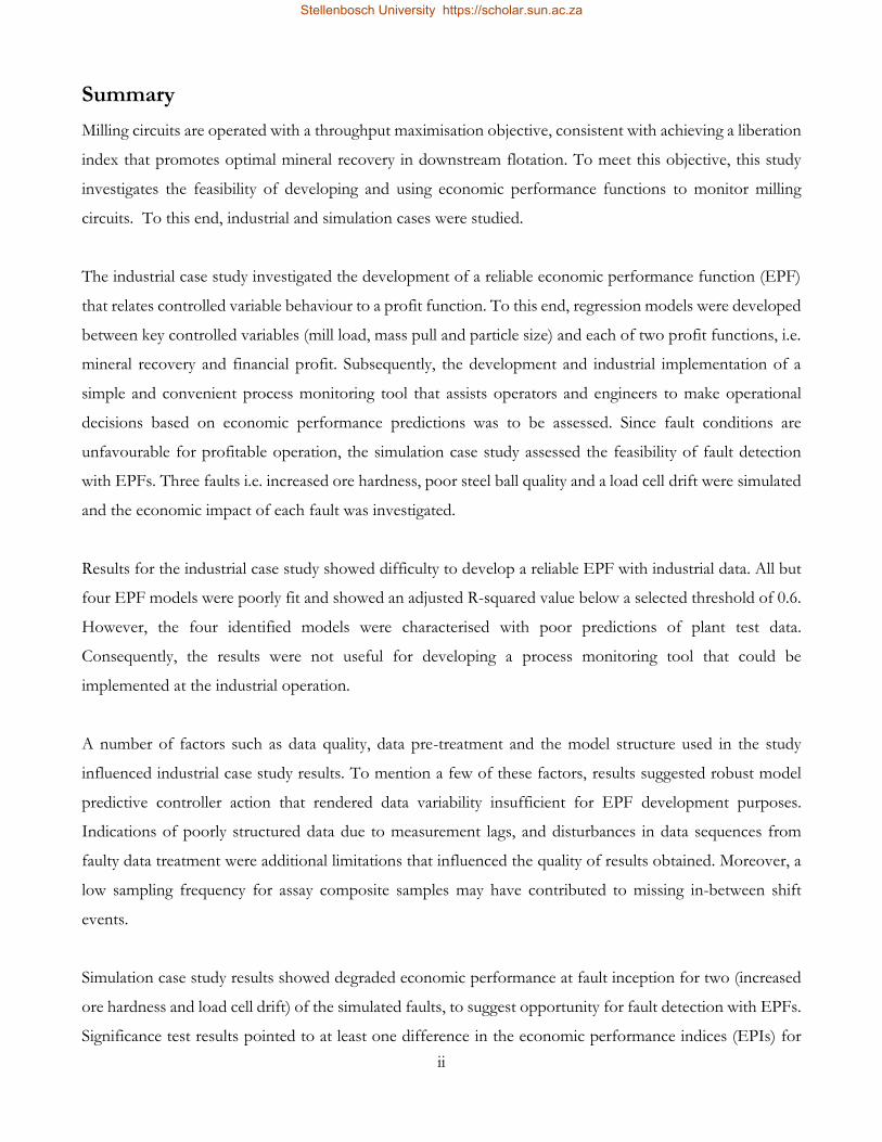
Summary

Milling circuits are operated with a throughput maximisation objective, consistent with achieving a liberation

index that promotes optimal mineral recovery in downstream flotation. To meet this objective, this study

investigates the feasibility of developing and using economic performance functions to monitor milling

circuits. To this end, industrial and simulation cases were studied.

The industrial case study investigated the development of a reliable economic performance function (EPF)

that relates controlled variable behaviour to a profit function. To this end, regression models were developed

between key controlled variables (mill load, mass pull and particle size) and each of two profit functions, i.e.

mineral recovery and financial profit. Subsequently, the development and industrial implementation of a

simple and convenient process monitoring tool that assists operators and engineers to make operational

decisions based on economic performance predictions was to be assessed. Since fault conditions are

unfavourable for profitable operation, the simulation case study assessed the feasibility of fault detection

with EPFs. Three faults i.e. increased ore hardness, poor steel ball quality and a load cell drift were simulated

and the economic impact of each fault was investigated.

Results for the industrial case study showed difficulty to develop a reliable EPF with industrial data. All but

four EPF models were poorly fit and showed an adjusted R-squared value below a selected threshold of 0.6.

However, the four identified models were characterised with poor predictions of plant test data.

Consequently, the results were not useful for developing a process monitoring tool that could be

implemented at the industrial operation.

A number of factors such as data quality, data pre-treatment and the model structure used in the study

influenced industrial case study results. To mention a few of these factors, results suggested robust model

predictive controller action that rendered data variability insufficient for EPF development purposes.

Indications of poorly structured data due to measurement lags, and disturbances in data sequences from

faulty data treatment were additional limitations that influenced the quality of results obtained. Moreover, a

low sampling frequency for assay composite samples may have contributed to missing in-between shift

events.

Simulation case study results showed degraded economic performance at fault inception for two (increased

ore hardness and load cell drift) of the simulated faults, to suggest opportunity for fault detection with EPFs.

Significance test results pointed to at least one difference in the economic performance indices (EPIs) for


iii

the simulated faults. Although not fully explored in this study, significance test results suggested opportunity

for fault prioritisation with the EPI that allows decisions about the corrective action to be made based on

the severity of the impact on economic performance.

Since reliable EPF development was the main limitation in this study, a comparative assessment in a different

operation with well-structured data is recommended. Fault prioritisation with the EPI may also be an area

of interest for future work. However, the shortcomings identified in some of the simplifying assumptions

made when deriving the EPI will need to be addressed.


iv

Opsomming

Maalkringe het deurvoermaksimalisering ten doel, gegee dat ŉ vrylatingsindeks wat optimale

mineraalwinning in stroomafflottering verkry word. Met hierdie doelwit voor oë is hierdie studie gemik

daarop om die haalbaarheid van die ontwikkeling en gebruik van ekonomiese prestasiefunksies om ŉ

maalkring te monitor. Daarom is nywerheids- en simulasiegevalle bestudeer.

Die nywerheidsgevallestudie het die ontwikkeling van ŉ betroubare ekonomiese prestasiefunksie (EPF) wat

beheerdeveranderlike-gedrag korreleer met ‘n winsfunksie ten doel. Daarom is regressiemodelle tussen

sleutel beheerdeveranderlikes (meullading, massavloei, en partikelgrootte) en elk van twee winsfunksies,

naamlik mineraalherwinning en finansiële wins, ontwikkel. Vervolgens is die ontwikkeling en

nywerheidsimplementering van ŉ eenvoudige en geskikte prosesmoniteringsinstrument wat operateurs en

ingenieurs help om operasionele besluite op grond van voorspellings van ekonomiese prestasie te neem,

geassesseer. Aangesien fouttoestande nadelig vir winsgewende werking is, het die simulasiegevallestudie die

haalbaarheid van foutspeuring deur middel van EPF’s bepaal. Drie foute, naamlik verhoogde ersthardheid,

swak staalbalkwaliteit en ŉ ladingselafwyking, is gesimuleer en die ekonomiese impak van elke fout is

ondersoek.

Die resultate van die nywerheidsgevallestudie het op ŉ paar probleme met die ontwikkeling van ŉ betroubare

EPF met nywerheidsdata gedui. Alle EPF modelle, uitgesluit vier, het swak passing getoon, met ŉ aangepaste

R-kwadraat waarde van minder as die gekose limiet van 0.6. Die vier geïdentifiseerde modelle is gekenmerk

deur die swak voorspelling van aanlegdata. Die resultate was dus nie bruikbaar vir die ontwikkeling van ŉ

prosesmoniteringsinstrument wat by die nywerheidsproses geïmplementeer kon word nie.

ŉ Aantal faktore, soos datakwaliteit, datavoorverwerking en die modelstruktuur wat gebruik is, het die

resultate van die nywerheidsgeval beïnvloed. Om ŉ paar van die faktore te noem, die resultate van die

nywerheidsgevallestudie het gedui op robuuste model-voorspellende-beheerderaksie, wat

dataveranderlikheid onvoldoende vir die doeleindes van EPF-ontwikkeling gemaak het. Aanduidings van

swak gestruktureerde data as gevolg van metingsagterstande sowel as steurings in datareekse as gevolg van

foutiewe datahantering was verdere beperkinge wat die gehalte van die verkrege resultate beïnvloed het.

Daarby kon ŉ lae steekproeffrekwensie vir saamgestelde komposisiemonsters daartoe bygedra het dat

tussenskofvoorvalle oor die hoof gesien is.


v

Resultate van die simulasiegevallestudie het verlaagde ekonomiese prestasie met die ontstaan van die fout vir

twee die gesimuleerde foute (verhoogde ersthardheid en ŉ ladingselafwyking) getoon, wat geleentheid vir

foutspeuring met EPF’s voorstel. Betekenistoetsresultate het gedui op ten minste een verskil in die

ekonomiese prestasie-indekse (EPI’s) vir die gesimuleerde foute. Alhoewel dit nie ten volle in hierdie studie

ondersoek is nie, het betekenistoetsresultate die geleentheid vir foutprioritisering met die EPI voorgestel wat

dit moontlik maak om besluite oor die nodige regstellende optrede te neem op grond van die graad van die

impak op ekonomiese prestasie.

Aangesien betroubare EPF-ontwikkeling die hoofbeperking in hierdie studie was, word ŉ vergelykende

assessering in ŉ ander proses met goed gestruktureerde data aanbeveel. Foutprioritisering met die EPI kan

ook ŉ area vir toekomstige navorsing wees. Die tekortkominge wat geïdentifiseer is in sommige van die

vereenvoudigende aannames wat met die ontwikkeling van die EPI gemaak is, sal egter steeds aandag moet

geniet.


vi


vii

Acknowledgements I would like to express my appreciation to everyone who contributed towards the completion of this thesis.

To God Almighty, for this study opportunity, guidance and protection.

To my supervisor, Dr. Lidia Auret, for the continuous guidance and kind support throughout my

Masters study.

To the sponsor, for your financial support of this project.

To the industrial contact person, for your insightful guidance.

To my husband and son, for your unquestionable support, encouragement and endurance while I was

pursuing my studies away from home.

To my dad and sister, for your prayers and emotional support.

To my research group colleagues, for your support.

To Sefakor Eunice Dogbe, for your all-weather friendship and consistent encouragement throughout

my Masters study.


viii

Table of Contents

Summary ...................................................................................................................................................................... ii

Opsomming ................................................................................................................................................................ iii

Acknowledgements ........................................................................................................................ ........................... iv

Nomenclature ............................................................................................................................................................. xi

List of Figures ........................................................................................................................................................... xiii

List of Tables ............................................................................................................................................................ xxi

Appendices ............................................................................................................................................................... xxii

CHAPTER 1: INTRODUCTION ..................................................................................................................... ….20

1.1 Introduction ................................................................................................................................................ 20

1.1.1 Process overview of the milling circuits ......................................................................................... 20

1.1.2 Overview of the economic significance of milling circuits.......................................................... 21

1.2 Motivation and significance of study ...................................................................................................... 22

1.3 Research objectives .................................................................................................................................... 23

1.4 Research design .......................................................................................................................................... 23

1.5 Thesis outline .............................................................................................................................................. 23

CHAPTER 2: ECONOMIC PERFORMANCE ASSESSMENT OF MILLING CIRCUITS ............................. 25

2.1 Factors influencing economic performance ........................................................................................... 25

2.2 Process control assessment ...................................................................................................................... 26

2.2.1 Process control hierarchy ................................................................................................................. 26

2.2.2 Economic benefits of process control ............................................................................................ 27

2.3 Background to economic performance assessment .............................................................................. 29

2.4 Economic performance functions ........................................................................................................... 32

2.4.1 Quadratic performance function ..................................................................................................... 32

2.4.2 Linear performance function ........................................................................................................... 32

2.4.3 Clifftent performance function ........................................................................................................ 33

2.5 Significance and application of economic performance functions ..................................................... 34


ix

2.6 Development of economic performance functions .............................................................................. 35

2.7 Derivation of the economic performance index ................................................................................... 36

2.8 Economic performance assessment case studies .................................................................................. 38

2.8.1 Case study of Steyn and Sandrock .................................................................................................. 39

2.8.2 Case study of Wei and Craig ............................................................................................................ 40

2.9 Faulty data handling techniques ............................................................................................................... 41

2.9.1 Incomplete data with missing values .............................................................................................. 42

2.9.2 Outlier detection ................................................................................................................................ 42

CHAPTER 3: PROCESS MONITORING AND FAULT DETECTION ........................................................... 44

3.1 The significance of process monitoring .................................................................................................. 44

3.2 Process monitoring approaches ............................................................................................................... 45

3.2.1 Process monitoring with empirical models .................................................................................... 45

3.2.2 Statistical process monitoring .......................................................................................................... 47

3.2.3 The role of control charts ................................................................................................................. 49

3.2.4 Criteria for implementing control charts ........................................................................................ 50

3.2.5 Shewhart control chart ...................................................................................................................... 50

3.3 Fault characteristics and common faults in grinding mill circuits ....................................................... 53

3.3.1 Fault characteristics ........................................................................................................................... 53

3.3.2 Fault classification.............................................................................................................................. 53

3.3.3 Rate of occurrence ............................................................................................................................. 54

3.3.4 Frequency of occurrence .................................................................................................................. 55

3.4 Common faults in milling circuits ........................................................................................................... 55

3.4.1 Drifting mill load cell ........................................................................................................................ 55

3.4.2 Steel ball overcharge .......................................................................................................................... 56

3.4.3 Poor quality steel ball charge ............................................................................................................ 56

3.4.4 Ore hardness variation ...................................................................................................................... 57


x

CHAPTER 4: INDUSTRIAL PRIMARY MILL CIRCUIT SURVEY........................................................................ 59

4.1 Introduction ................................................................................................................................................ 59

4.1.1 Concentrator plant overview............................................................................................................ 59

4.1.2 Primary mill circuit process description ......................................................................................... 60

4.2 Process control hierarchy .......................................................................................................................... 61

4.2.1 Instrumentation.................................................................................................................................. 61

4.2.2 Base control ........................................................................................................................................ 63

4.2.3 Advanced control .............................................................................................................................. 66

4.2.4 Optimization level ............................................................................................................................. 67

4.3 Variables for the primary mill and rougher flotation circuit ................................................................ 69

4.4 Operational performance at the Concentrator plant ............................................................................ 72

4.5 Process performance monitoring strategies ........................................................................................... 73

4.5.1 Offline sample analysis ..................................................................................................................... 73

4.5.2 Plant surveys ....................................................................................................................................... 73

4.5.3 Tracking key performance indicators ............................................................................................. 73

4.6 Factors influencing economic performance ........................................................................................... 74

4.6.1 Economic performance assessment of primary mill circuit ........................................................ 75

CHAPTER 5: RESEARCH METHODOLOGY ..................................................................................... 78

5.1 A background on case study research methods .................................................................................... 78

5.2 Industrial case study ................................................................................................................................... 80

5.2.1 Case study data sources and research instruments ....................................................................... 80

5.2.2 A background to EPF development ............................................................................................... 80

5.2.3 A background to the process monitoring tool .............................................................................. 81

5.2.4 Selection of economic performance scenarios .............................................................................. 81

5.2.5 Methodology for EPF development ............................................................................................... 82

5.2.6 Determining information requirements for EPF development .................................................. 82


xi

5.2.7 Identifying key controlled variables ................................................................................................ 82

5.2.8 Retrieving the required information ............................................................................................... 83

5.2.9 Pre-treating the data .......................................................................................................................... 84

5.2.10 Investigating data reduction ............................................................................................................. 84

5.2.11 Investigating data normality and correlations ................................................................................ 85

5.2.12 Simplifying assumptions ................................................................................................................... 85

5.2.13 Identifying benchmark data set........................................................................................................ 86

5.2.14 Validating the selected benchmark .................................................................................................. 86

5.2.15 Identifying approaches to EPF development ................................................................................ 86

5.2.16 Identifying EPF development strategies ........................................................................................ 88

5.2.17 EPF development with base case data ........................................................................................... 88

5.2.18 Searches for valid EPF ...................................................................................................................... 88

5.2.19 Performing sliding window iterations ............................................................................................. 90

5.2.20 Investigating measurement lags ....................................................................................................... 90

5.2.21 Developing a process monitoring tool ........................................................................................... 90

5.2.22 Determining the overall economic performance index ............................................................... 91

5.2.23 Testing the process monitoring tool for implementation feasibility .......................................... 91

5.2.24 Process monitoring post-implementation ...................................................................................... 92

5.3 Simulation case study ................................................................................................................................. 95

5.3.1 Objectives ........................................................................................................................................... 95

5.3.2 Simulation case study background .................................................................................................. 95

5.3.3 Overview of the SAG mill circuit.................................................................................................... 95

5.3.4 A background to simulation models ............................................................................................... 95

5.3.5 Le Roux’s SAG mill model .............................................................................................................. 96

5.3.6 SAG mill circuit process variables ................................................................................................... 97

5.4 Simulation case study design .................................................................................................................... 97

5.4.1 Defining experiment objectives ....................................................................................................... 98


xii

5.4.2 Stating a hypothesis to be evaluated ............................................................................................... 98

5.4.3 Identifying the significance test ....................................................................................................... 99

5.4.4 Planning an experiment to test the hypothesis ............................................................................ 100

5.5 Conducting the simulation experiments ............................................................................................... 102

5.5.1 Simulating the faults ........................................................................................................................ 102

5.5.2 Generating normal operating condition and fault data .............................................................. 104

5.6 Analysing the data .................................................................................................................................... 104

5.6.1 Data pre-processing ......................................................................................................................... 104

5.6.2 Apportioning data into training, test and fault data sets ............................................................ 105

5.6.3 Selecting bin width........................................................................................................................... 105

5.6.4 Making suitable assumptions ......................................................................................................... 105

5.7 Testing the null hypothesis ..................................................................................................................... 106

5.7.1 Deriving data averages .................................................................................................................... 106

5.7.2 Deriving the sliding window economic performance index (EPI) ........................................... 106

5.7.3 Selecting sliding window size ......................................................................................................... 106

5.7.4 Plotting sliding window EPIs for all the faults ............................................................................ 106

5.7.5 Assess scope for fault monitoring and prioritisation.................................................................. 106

CHAPTER 6: RESULTS AND DISCUSSION -INDUSTRIAL CASE STUDY ......................................... 108

6.1 Selection of base-case model data set ................................................................................................... 108

6.2 Data normality .......................................................................................................................................... 110

6.3 Data correlation ........................................................................................................................................ 111

6.4 Single-predictor EPF results ................................................................................................................... 112

6.4.1 Single-predictor PVA model .......................................................................................................... 112

6.4.2 Single-predictor FEA model .......................................................................................................... 113

6.4.3 Results summary for the single-predictor EPF models ............................................................. 113

6.5 Multi-predictor EPF results .................................................................................................................... 114


xiii

6.5.1 Multi-predictor PVA model ........................................................................................................... 114

6.5.2 FEA model with multiple predictors ............................................................................................ 115

6.5.3 Results summary for multi-predictor EPF models ..................................................................... 115

6.6 Findings for EPF model development with base-case data .............................................................. 115

6.7 EPF searches ............................................................................................................................................ 115

6.7.1 Single-predictor PVA models ........................................................................................................ 115

6.7.2 Multi-predictor PVA results ........................................................................................................... 120

6.7.3 Results summary for EPF searches ............................................................................................... 127

6.8 Summary results for EPF development strategies .............................................................................. 127

CHAPTER 7: RESULTS AND DISCUSSION -SIMULATION CASE STUDY ........................................ 129

7.1 Controlled variable –manipulated variable plots for simulated faults .............................................. 129

7.1.1 Drifting mill load cell ...................................................................................................................... 129

7.1.2 Poor steel ball quality fault ............................................................................................................. 131

7.1.3 Ore hardness increase ..................................................................................................................... 132

7.1.4 Summary for simulated faults ........................................................................................................ 134

7.2 Significance tests ...................................................................................................................................... 136

7.3 Economic performance indices for simulated faults .......................................................................... 138

CHAPTER 8: CONCLUSION AND RECOMMENDATIONS ............................................................... 140

REFERENCES ................................................................................................................................... 144

APPENDICES .................................................................................................................................... 158


xiv

Nomenclature

Acronym Description

3E Platinum (Pt), palladium (Pd), rhodium

(Rh)

ANOVA Analysis of variance

APC Advanced process control

CFF Cyclone feed flow

CV Controlled variable

CL Centre line

EPA Economic performance assessment

EPF Economic performance functions

EPI Economic performance index

FEA Financial elements analysis

IPF Individual performance function

JPF Joint performance function

KPI Key performance indicator

MF2 Mill-Float-Mill-Float

MFB Mill feed balls

MFS Mill feed solids

MSPM Multivariate statistical process monitoring

MIMO Multi-input–multi-output

MPC Model Predictive Control

MP Multi-predictors

MR Mineral recovery

MVC Minimum variance control

MV Manipulated variable

MW Megawatt

NOC Normal Operating Condition

PAR Peak Air Recovery

PID Proportional Integral Derivative

PDF Probability Density Function

PGM Platinum Group Metals


xv

PS Particle size

PVA Process variables analysis

PM Process monitoring

ROM Run-off mine

RSD Relative standard deviation

SAG Semi-autogenous grinding

SP Single-predictor

SPM Statistical process monitoring

SVOL Sump volume

LCL Lower control limit

UCL Upper control limit

XRDF X-ray diffraction and fluorescence

Symbol Description

σ standard deviation

μ mean

y controlled variable

ϑ (y) economic performance function

R metal sales revenue

F mill throughput

t time period (h)

c conversion factor (oz/g)

C operating cost (ZAR)

u unit cost

BPadj adjusted basket price

Bw bin width

R2adj adjusted R-squared


xvi

List of Figures

Figure 1-1 Simplified schematic of a milling and flotation circuit. ...................................................................... 21

Figure 2-1: Process control hierarchy ...................................................................................................................... 26

Figure 2-2: Economic benefits of variability reduction ....................................................................................... 28

Figure 2-3: Quadratic performance function .......................................................................................................... 32

Figure 2-4 : Linear performance function .............................................................................................................. 33

Figure 2-5 Clifftent function .................................................................................................................................... 33

Figure 2-6: Derivation of an EPI ............................................................................................................................. 38

Figure 3-1: Process-data based modelling procedure ........................................................................................... 46

Figure 3-2: Roles for control charts ......................................................................................................................... 49

Figure 3-3: Shewhart control chart........................................................................................................................... 51

Figure 3-4: Control chart zones ................................................................................................................................ 53

Figure 3-5: Fault classification within a process ..................................................................................................... 53

Figure 3-6: Time dependency of faults .................................................................................................................... 54

Figure 4-1: Concentrator plant flow diagram ......................................................................................................... 60

Figure 4-2: Process and instrumentation diagram ................................................................................................. 65

Figure 4-3: Relationship between froth depth, air rate and air recovery ............................................................ 68

Figure 4-4 : Primary mill control .............................................................................................................................. 71

Figure 4-5: Operational performance metrics ........................................................................................................ 72

Figure 4-6: Operating cost elements ........................................................................................................................ 76

Figure 4-7 : Distribution of operating costs .......................................................................................................... 76

Figure 5-1: Factors influencing primary mill circuit performance ....................................................................... 82

Figure 5-2 : Transient performance curve ............................................................................................................... 89

Figure 5-3: Summarized industrial case study methodology steps ...................................................................... 94

Figure 5-4: Single staged close circuit SAG mill circuit ........................................................................................ 96

Figure 5-5: SAG mill circuit control loops .............................................................................................................. 97

Figure 5-6: Model variables .................................................................................................................................... 101

Figure 5-7: Simulation experiments methodology summary steps .................................................................... 107

Figure 6-1: Profit for base-case benchmark and performance scenarios ......................................................... 109

Figure 6-2: Q-Q normality probability plots ......................................................................................................... 110

Figure 6-3: Scatter plots for filtered regression model data ............................................................................... 111

Figure 6-4: Particle size-mineral recovery EPF .................................................................................................... 112


xvii

Figure 6-5: Particle size-financial profit EPF ....................................................................................................... 113

Figure 6-6: Particle size moving window statistical data ..................................................................................... 116

Figure 6-7: Mineral recovery moving window statistical data ............................................................................ 117

Figure 6-8: Single-predictor PVA adjusted R-squared values ............................................................................ 118

Figure 6-9: Normalized actual and predicted mineral recovery for single-predictor EPF models ............... 119

Figure 6-10: Mass pull moving window statistical data ....................................................................................... 121

Figure 6-11: Mill load moving window statistical data ........................................................................................ 122

Figure 6-12: Multi-predictor PVA adjusted R-squared ....................................................................................... 123

Figure 6-13: Adjusted R-squared values for reduced EPF models ................................................................... 124

Figure 6-14: Models with above threshold R2adj and significant regression coefficients ................................ 125

Figure 6-15: Actual and predicted mineral recovery ............................................................................................ 126

Figure 7-1: CV-MV plots for drifting mill load cell ............................................................................................. 129

Figure 7-2: Revenue and cost metrics for the drifting mill load cell ................................................................. 130

Figure 7-3: CV-MV plots for poor steel ball quality ............................................................................................ 131

Figure 7-4: Revenue and cost metrics for poor steel ball quality ....................................................................... 132

Figure 7-5: CV-MV plots for increased ore hardness ......................................................................................... 133

Figure 7-6: Revenue and cost metrics for increased ore hardness .................................................................... 134

Figure 7-7: Mineral recovery box plot ................................................................................................................... 137

Figure 7-8: Mill throughput box plot ..................................................................................................................... 137

Figure 7-9: Sliding window economic performance indices ............................................................................... 138


xviii

List of Tables

Table 3-1: Control chart rules ................................................................................................................................... 52

Table 4-1: Primary mill circuit instrumentation ..................................................................................................... 62

Table 4-2: Base control for the primary mill circuit .............................................................................................. 64

Table 4-3: Controlled and manipulated variables for the primary mill circuit ................................................... 69

Table 4-4: Offline sample analysis ............................................................................................................................ 73

Table 4-5: Key performance indicators for the primary mill circuit .................................................................. 74

Table 5-1: Controlled variable ranking in terms of economic significance ........................................................ 83

Table 5-2: Economic performance indicators ........................................................................................................ 92

Table 5-3: CV-MV loop pairings .............................................................................................................................. 97

Table 5-4: Randomised simulation experiment runs ........................................................................................... 103

Table 5-5: Simulation experiment data of interest ............................................................................................... 104

Table 6-1: Key performance metrics ..................................................................................................................... 108

Table 6-2: Data for benchmark validation cases .................................................................................................. 109

Table 6-3: Single-predictor PVA ............................................................................................................................ 112

Table 6-4: Single-predictor FEA results ................................................................................................................ 113

Table 6-5: Multi-predictor PVA results ................................................................................................................. 114

Table 6-6: Multi-predictor FEA.............................................................................................................................. 115

Table 6-7: Single-predictor PVA summary results ............................................................................................... 119

Table 6-8: Missing data ............................................................................................................................................ 120

Table 6-9: Multi-predictor PVA summary results ................................................................................................ 126

Table 7-1: F-test results ............................................................................................................................................ 136

Table 7-2: Pairwise p-values .................................................................................................................................... 136


xix

Appendices

APPENDIX A: PRELIMINARY AND CRITICAL SITE SURVEYS .............................................................................. 158

APPENDIX B: MARKET FACTORS INFLUENCING ECONOMIC PERFORMANCE ............................................... 159

APPENDIX C: CALCULATION FORMULAE ............................................................................................................. 160

APPENDIX D: NORMALIZED AVERAGE ELECTRICITY AND CONSUMABLE CONSUMPTION RATES ........... 165

APPENDIX E: ANCILLARY EQUIPMENT ................................................................................................................. 168

APPENDIX F: NORMALIZED AVERAGE TONNAGE PROCESSED ....................................................................... 169

APPENDIX G: NORMALIZED KEY PERFORMANCE INDICATORS ...................................................................... 169

APPENDIX H : MONTHLY AVERAGES FOR KEY PERFORMANCE INDICATORS ............................................... 171

APPENDIX I: NORMALIZED PRIMARY MILL CIRCUIT ECONOMIC PERFORMANCE ........................................ 172

APPENDIX J: SPOT METAL PRICES (AS AT JUNE 2016) ....................................................................................... 173

APPENDIX K: DATA OF INTEREST ......................................................................................................................... 174

APPENDIX L: MATHEMATICAL MODEL FOR SAG MILL ...................................................................................... 177

APPENDIX M: STEEL BALL – POWER RELATIONSHIP ......................................................................................... 178

APPENDIX N: SIMULATION EXPERIMENT CALCULATIONS ............................................................................... 179

APPENDIX O: PLOTS FOR ACTUAL VS. PREDICTED MINERAL RECOVERY ...................................................... 181

APPENDIX P: RESULTS FOR WINDOW SIZE 21 ..................................................................................................... 181

APPENDIX Q: AVERAGE MINERAL RECOVERY FOR SIMULATED FAULTS ....................................................... 183

APPENDIX R: AVERAGE MILL THROUGHPUT FOR SIMULATED FAULTS ......................................................... 184


20

CHAPTER 1: INTRODUCTION

Chapter Overview

This chapter introduces the thesis by providing a background to the study and a description of the scope.

The research problem is highlighted through a discussion of the motivation and significance of conducting

this study. A presentation of the research objectives follows and finally, a thesis layout is provided.

1.1 Introduction

Mineral processing operations are faced with a challenge to consistently achieve satisfactory process

economic performance despite fluctuating markets, low-grade deposits with complex mineralogy, increasing

operating costs and penalties from stringent environmental regulations. An ongoing implementation of more

efficient technologies, strategies on cost minimisation and throughput improvement, as well as timely fault

detection and process recovery are some of the commonly applied interventions to meet this challenge (Rule

& DeWaal, 2011; Simonsen & Perry, 1999).

To address the challenge highlighted above, this study investigated the feasibility of industrial online primary

mill circuit monitoring with a simple and convenient tool developed using an economic performance

function (EPF) that related key production and control objectives to profit, as a possible avenue to make

operating decisions consistent with satisfactory economic performance. An objective and detailed economic

performance evaluation of a platinum group metal (PGM) primary mill circuit at a Concentrator plant

provided a reference basis to the investigation. In addition, fault detection with EPFs was investigated in a

semi-autogenous grinding (SAG) mill circuit simulation experiment that offered control over fault

occurrence and the time window for fault detection.

1.1.1 Process overview of the milling circuits

The milling process reduces ore to a size amenable to efficient mineral recovery in downstream flotation

(Matthews & Craig, 2013). Ore feed and steel ball media are charged into a mill for particle size reduction to

achieve a liberation index that promotes optimal mineral recovery. Water is added to the mill to form a slurry

mixture (also referred to as pulp) with a suitable density for optimal grinding conditions. Ground ore is


21

discharged into a sump, which also acts as a buffer for the circuit where make up water is added to achieve

flow and density control. Close control is exercised on the fraction of sub 75 microns product (also referred

to as the grind), through classification in a hydrocyclone. Therefore, slurry is pumped from the sump to a

hydrocylone where heavy particles report to the underflow stream and are recirculated into the mill for

regrinding. Lighter particles report to the overflow stream and are delivered to a froth flotation circuit for

mineral recovery. With the aid of reagents, flotation feed is conditioned to modify the surface properties of

mineral values and air is introduced into agitated flotation cells to pull/float mineral values into the

concentrate at a controlled rate subject to a trade-off between concentrate grade and mineral recovery. Figure

1-1 shows a simplified schematic of a typical milling and flotation circuit.

Figure 1-1 Simplified schematic of a milling and flotation circuit.

1.1.2 Overview of the economic significance of milling circuits

Milling is a materials and energy intensive process which drives the cost of mineral processing operations

(Powell et al., 2009; Schena et al., 1996). About 40-45% of the total milling costs are attributable to grinding

media, and an estimated 40% of mineral processing energy is used up in comminution (Ballantyne & Powell,

2014; Ebadnejad, 2016; Moema et al., 2009). Moreover, the economic performance of downstream flotation

efficiency is influenced by the particle size achieved in milling (Hodouin et al., 2001; Valery & Jankovic, 2002).

An analysis of recent plant data showed that the rougher flotation circuit typically makes a 65% contribution


22

to the overall mineral value recovered in the concentrator plant. Hence, the primary mill and rougher

flotation circuit was an economically significant scope for the investigation.

1.2 Motivation and significance of study

Process monitoring plays a critical role in the delivery of efficient and profitable process operations, through

tracking process-related variables to effect control and optimisation of that process. In recent years, the use

of simple models to derive product quality from operating conditions, optimise operating conditions and

detect faults has become more preferred in industrial operations (Kano & Nakagawa, 2008). Powell &

Morrison (2007) recommended the use of these models to monitor comminution processes. Although the

simplicity and effectiveness of these models have encouraged widespread use across industries (e.g., chemical

and food industry), reliable models are not yet available in the mineral processing industry (Powell &

Morrison, 2007; Le Roux et al., 2013). The success of these models for process control and monitoring in

other industries provides motivation for implementation in the mineral processing industry, where a large

number of process variables with complex interactions are monitored and controlled.

The economic significance of milling circuits has led to several economic performance assessment (EPA)

studies. However, most of the available EPA studies were conducted for once-off controller performance

assessment and amongst these, only a few applied economic performance functions (e.g., Steyn & Sandrock,

2013; Wei & Craig, 2009a; Zhao et al., 2009). The reported success of these few studies and a

recommendation in Bauer et al. (2007) inspired this study, which addressed process performance assessment.

Instead of a once-off performance assessment, this study rather investigated the feasibility of continuously

monitoring the economic performance of a milling circuit. Furthermore, the EPF used in this study

incorporated more controlled variables as well as key revenue and cost metrics associated with operating a

milling circuit. The simulation case study followed an approach similar to Wei & Craig (2009a) but addressed

an objective to investigate fault detection and prioritisation with EPFs.

The use of simulation and industrial data to develop EPFs is referred to in literature (Bauer et al., 2007; Wei

& Craig, 2009a). Simulation data was used in most EPA studies, with the exception of Steyn & Sandrock

(2013) who used industrial data. The rare opportunity to use industrial data in this study provided some

objective insight on the development of reliable EPFs. Consequently, study findings reduced the knowledge

gap on reliable economic performance assessment of milling circuits.


23

According to experts at the industrial operation, no EPFs were developed in the processing history of the

primary mill circuit. In addition, no previous research has been conducted on process monitoring with EPFs

to the author’s best knowledge. The availability of limited information on EPFs has contributed to the low

maturity level of demonstrated EPF industrial application and research. As such, the development of EPFs

is difficult since they are poorly understood even amongst some industrial experts (Wei & Craig, 2009b).

Therefore, this study largely referred to the sequel study by Wei & Craig (2009a,2009b; 2009c) on EPFs and

also sought to increase awareness on this promising research area.

1.3 Research objectives

The overall aim of this study is to investigate online process monitoring with EPFs. For the industrial case

study, the following objectives were identified:

1. To develop a reliable EPF with industrial primary mill and rougher flotation data;

2. To derive the circuit’s benchmark economic performance;

3. To assess the feasibility of industrially implementing an online process monitoring tool for the circuit,

using one key controlled variable; and

4. To assess the feasibility of incorporating additional key controlled variables in the process monitoring

tool.

For the simulation case study, the overall aim was to investigate the feasibility of fault detection with EPFs.

The following objectives were identified:

1. To derive the economic performance of a SAG mill circuit subject to three common industrial faults;

and

2. To assess the economic impact of the fault events and subsequently, determine fault detection

feasibility with EPFs.

1.4 Research design

A triangulation of qualitative and quantitative approaches were used to explore the two cases studies. The

research instruments used for data gathering to achieve the objectives of this study included a literature

survey, site survey at the industrial Concentrator plant and simulation experiments.

1.5 Thesis outline

This thesis progresses as follows:


24

Chapter 2 presents a literature review on assessing the economic performance of milling circuits. Chapter 3

follows with a literature discussion on the significance of fault detection in process monitoring. Model and

data based approaches are distinguished, and common faults in milling circuits are identified. In Chapter 4,

site survey findings on the process operation, control and economics of an industrial primary mill circuit are

presented. Research methodology steps for the industrial and simulation case studies are proposed in Chapter

5. Chapter 6 presents the industrial case study results and discusses findings thereof. Similarly, Chapter 7

presents the results and discussion for the simulation case study. This thesis concludes with Chapter 8

wherein the key findings of this study are summarized. The final conclusions to the study are made, and

recommendations for future work are presented.


25

CHAPTER 2: ECONOMIC PERFORMANCE ASSESSMENT

OF MILLING CIRCUITS

Chapter Overview

This chapter reviews literature on assessing the economic performance of milling circuits. The overall aim is

to provide insight on two objectives for this study i.e., EPF development with industrial data and the

derivation of an economic performance index. To this end, factors that significantly influence economic

performance are identified and the critical role of process control in delivering economic benefits is discussed

using demonstrated studies. Economic performance functions are introduced and their significance,

development, and application are highlighted. Methodology steps on economic performance assessment are

presented, and this chapter concludes with techniques for industrial data treatment prior to EPF

development. By the end of this chapter, relevant strategies for developing EPFs in this study are identified

as well as a procedure to derive the primary mill circuit’s economic performance.

2.1 Factors influencing economic performance

The economic performance of milling circuits is assessed across a number of objectives that include

profitability, efficiency, product variability and throughput (Ellis et al., 2014). A holistic consideration of these

key objectives is necessary for representative economic performance assessment. Commonly, cost

minimisation or revenue maximisation strategies are used to achieve maximum profit (Simonsen & Perry,

1999). Milling processes significantly contribute towards the overall mineral processing operating cost

structure due to energy, grinding media, and costs for replacing mill liners. For flotation processes, reagent

consumption is a major cost (Wills & Napier-Munn, 2006). Energy consumption accounts for about 50% of

the total comminution costs and in addition, grinding media constitutes of up to 40–45% and liner wear 5-

10% (Moema et al., 2009; Radziszewski, 2013). Therefore, the reduction of utility and consumable quantities

is one commonly implemented cost minimisation strategy. On the other hand, increased throughput rates

and consistent attainment of target product quality achieve profit maximisation (Matthews & Craig, 2013).

According to Cavender (2001), consistent compliance with operating conditions and standards, optimisation

of operating practices through continuous improvement research work, and equipment maintenance or

upgrades contribute towards improved economic performance. However, not all of these strategies are easy


26

to implement without applying process control to achieve economic efficiency. Therefore, process control

is used in virtually all milling circuit operations to achieve target operating and consequently, economic

objectives (King, 2001).

The highly dynamic nature of milling circuit operations makes process control necessary in order to

simultaneously maintain the large number of controlled variables at their set points (Jakhu, 1998). Additional

benefits such as process variability reduction, increased efficiency, safe operating conditions are achieved

(Contreras-Dordelly & Marlin, 2000).

The next section introduces a process control hierarchy as a basis for discussing the economic benefits

derived with process control. This discussion leads to a review of some relevant economic performance

assessment (EPA) studies.

2.2 Process control assessment

2.2.1 Process control hierarchy

Different functional levels of process control systems contribute to the overall control performance and

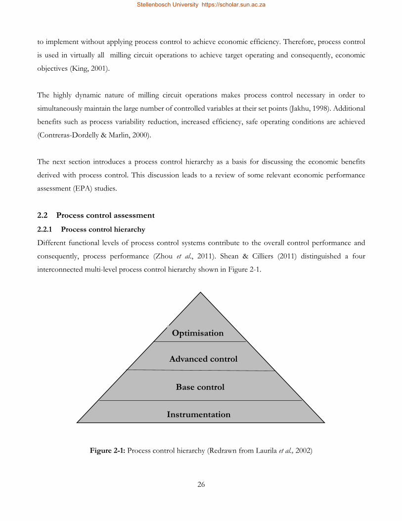
consequently, process performance (Zhou et al., 2011). Shean & Cilliers (2011) distinguished a four

interconnected multi-level process control hierarchy shown in Figure 2-1.

Figure 2-1: Process control hierarchy (Redrawn from Laurila et al., 2002)

Advanced control

Instrumentation

Base control

Optimisation


27

The effectiveness of each level is a pre-requisite for successful higher-level operation. However, lower levels

may still operate even when higher levels do not. Each process control level is discussed below:

2.2.1.1 Instrumentation

At the lowest level in the process control hierarchy, instrumentation provides process observations for

process monitoring, control and optimisation (Shean & Cilliers, 2011). Regular instrumentation maintenance

ensures measurement reliability and enables process regulation within an acceptable operating window.

2.2.1.2 Base control

Controllers implemented at base level transfer the variability introduced by disturbance variables away from

controlled variables to manipulated variables and hence, achieve stable operation (Oosthuizen et al., 2004).

This level uses interlocks and sequences to ensure safe and reliable operation (Fiske, 2006). Milling circuits

predominantly implement proportional-integral-derivative (PID) controllers for base control (Edwards et al.,

2002).

2.2.1.3 Advanced control

Advanced control improves the economic performance of a process through stabilisation, to achieve the

desirable operating window to enable process optimisation (Almond et al., 2012; Smith & Corripio, 1997).

As pointed out by process stabilisation not only. Milling circuits commonly implement fuzzy logic, rule-

based expert system, and model predictive control for advanced control (Wei & Craig, 2009b).

2.2.1.4 Optimisation control

Optimisation control is only achievable when underlying base control has established stable operation

(Laurila et al., 2002). This level typically uses mathematical modelling and simulation to determine set points

for optimum process performance, based on maximizing or minimizing an objective function (Valenta &

Mapheto, 2011). A trade-off between mill throughput and mineral recovery is dynamically optimised at this

level to maximise economic efficiency (Barker, 1989).

Optimal process performance is only maintained when process disturbances are compensated for and

process variability is reduced (Herbst et al., 1988). The economic benefits derived from variability reduction

are discussed in the next section.

2.2.2 Economic benefits of process control

Process variability in milling circuits is induced by several factors such as changes in feed ore characteristics

(hardness, grade, particle size), ore feed rate and quality, mill sump level, mill load, product particle size and


28

mill discharge viscosity (Hodouin et al., 2001; Wei & Craig, 2009b). Furthermore, non-uniform feed ore

mineralogy, grind size, flotation feed flow and pulp density as well as spillage due to malfunctioning ancillary

equipment, are sources of process variability in flotation circuits (Villeneuve et al., 1995). The frequency and

severity of these disturbances significantly influence milling circuit performance to produce off-specification

and consistently variable product quality (Brisk, 2004; Oakland, 2003).

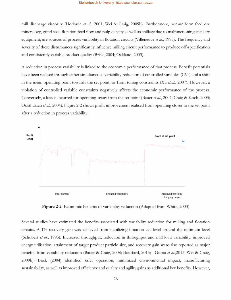
A reduction in process variability is linked to the economic performance of that process. Benefit potentials

have been realised through either simultaneous variability reduction of controlled variables (CVs) and a shift

in the mean operating point towards the set point, or from tuning constraints (Xu et.al., 2007). However, a

violation of controlled variable constraints negatively affects the economic performance of the process.

Conversely, a loss is incurred for operating away from the set point (Bauer et al., 2007; Craig & Koch, 2003;

Oosthuizen et al., 2004). Figure 2-2 shows profit improvement realised from operating closer to the set point

after a reduction in process variability.

Profit at set point

Poor control Improved profit by changing target

Reduced variability

Profit (ZAR)

Figure 2-2: Economic benefits of variability reduction (Adapted from White, 2003)

Several studies have estimated the benefits associated with variability reduction for milling and flotation

circuits. A 1% recovery gain was achieved from stabilizing flotation cell level around the optimum level

(Schubert et al., 1995). Increased throughput, reduction in throughput and mill load variability, improved

energy utilisation, attainment of target product particle size, and recovery gain were also reported as major

benefits from variability reduction (Bauer & Craig, 2008; Bouffard, 2015; Gupta et al.,2013; Wei & Craig,

2009b). Brisk (2004) identified safer operation, minimized environmental impact, manufacturing

sustainability, as well as improved efficiency and quality and agility gains as additional key benefits. However,


29

these benefits were difficult to quantify monetarily due to subjective measures with safety or legal

considerations.

The economic significance of reduced variability has resulted in a number of assessment studies that address

several controller performance objectives. Some studies assessed the economic impact of implementing

advanced control either before or after installation (e.g. Bauer et al., 2007); monitored current controller

performance (e.g. Rato & Reis, 2010); compared controllers to identify a better performing one (e.g. Craig

& Henning, 2000; Wei & Craig, 2009a); and to optimise processes (e.g. Marlin et al., 1991; Steyn & Sandrock,

2013; Zhao et al., 2009). Despite the numerous studies on controller performance assessment, only a few

(e.g., Wei & Craig, 2009a; Zhao et al., 2009) focused on deriving the economic performance monetarily.

Similar concepts from these EPA studies were applicable to this study. The next section discusses key factors

associated with economic performance assessment.

2.3 Background to economic performance assessment

The most important step to any EPA is a prior consideration of the objectivity and accuracy of a criterion

upon which performance is to be evaluated (Jämsä-Jounela et al., 2003). Therefore, the first step is to identify

a performance index that represents the assessment objective. The selected index must have a satisfactory

confidence level that is verifiable with plant data. Hence, selection methods must be realistic and achievable

under specific physical constraints (Jämsä-Jounela et al., 2003; Xia & Howell, 2003). For example, Wei &

Craig (2009a) addressed a common milling circuit objective i.e., to achieve the target particle size from which

a profitable mineral recovery can be realised to evaluate the profit realised from implementing a new

controller. Their study results were also industrially realistic.

An appropriate benchmark is selected after a performance index has been identified. Some performance

assessment studies have used minimum variance control (MVC) and the historical-data benchmarks (e.g.

Bauer et al., 2007; Jelali, 2006; Rato & Reis, 2010; Zhao et al., 2011). MVC benchmarks are derived from a

performance index which compares the minimum variance achievable to actual controller variance, as shown

in Equation 2-1(Harris et al., 1989).

𝜂𝑀𝑉𝐶 = 1 −

𝜎𝑀𝑉𝐶2

𝜎𝐴𝐶𝑇2

2-1


30

Where σ2MVC is the minimum achievable variance

σ2ACT is the actual controller variance

Preference for the MVC benchmark is associated with benefits realised from operating a process within

profitable controlled variable constraints and how variability reduction can be directly related to profit

improvement (Brisk, 2004). Furthermore, this benchmark is computationally simple and routine operating

data are used without the need for additional experiments (Muske & Finegan, 2001). However, it is more

relevant for cases in which performance on controller disturbance rejection is considered (Qin & Yu, 2007).

Although time correlations typically influence a process output, a linear time-invariant transfer functions and

additive disturbances are assumed for the process whenever the MVC benchmark is used (Jelali, 2010).

Furthermore, some researchers (e.g. Huang et al., 1997; Zhao et al., 2009), have raised concern over its

robustness and argue that it is unrealistic relative to other benchmarks since it suggests excessive controller

action. The unavailability of perfect disturbance models is yet another reliability challenge faced with this

benchmark as a disturbance model mismatch produces inaccurate performance (Eriksson & Isaksson, 1994;

Hugo, 2001). Due to these limitations, the MVC benchmark is rarely implemented in industry. Nonetheless,

most researchers (e.g. Huang et al., 1997; Hugo, 2001; Hoo et al., 2003; Stanfelj & Marlin, 1993; Yuan &

Lennox, 2009) widely acknowledged its useful application as a theoretical approach in most controller

performance assessment studies.

Bauer et al. (2007) demonstrated the MVC benchmark in a justification study for implementing a new

industrial controller. In the study, historical data was used to estimate base case performance while improved

performance was derived from simulation data. Subsequently, they derived an economic performance index

(EPI) as a function of the standard deviation (Equation 2-2). This EPI derivation method is validated in a

number of studies (Bauer & Craig, 2008; Latour et al.,1986; Oosthuizen et al., 2004; cited by Wei & Craig,

2009a).

EPI = ∫ 𝜗(𝑦)𝑓(𝑦, σ, μ)𝑑𝑦

∞

−∞

2-2

where ϑ - economic performance function

f - frequency distribution or probability density function (PDF) of the time series of a controlled variable y,

which was assumed to have a Gaussian distribution


31

σ - standard deviation of the controlled variable, y

µ - mean of the controlled variable, y

Consequently, a decision to implement the new controller was reached based on an evaluation of the

potential profit improvement (determined from the MVC benchmark) against the estimated maximum

achievable profit derived with Equation 2-2. However, the study did not consider installation costs although

doing so would have provided an insightful cost-benefit analysis.

A user-specified historical performance benchmark compares routine operating data that is representative of

past satisfactory performance against current performance (Brisk, 2004). However, an expert assessment of

comprehensive plant data over a period that is influenced by the objectives to be achieved is required

(Patwardhan et al.,2002). Commonly, this benchmark is obtained from a stable operation during which there

were no unusual conditions such as equipment outages or an out-of-control state (Latour et al., 1986; Nel et

al., 2004).

Although the historical-data benchmark is convenient, easy to apply and interpret, it has some shortcomings.

Interpretations of previously good performance may differ even with expert assessments, thus it is rather

subjective since a standard performance basis is difficult to establish (Patwardhan et al., 2002). Furthermore,

the lack of a theoretical minimum that can be used irrespective of the process or controller is an additional

concern relating to its subjectivity. Consequently, the cause of performance degradation cannot be

confidently assigned as it is not immediately obvious whether performance changes are attributable to the

controller’s core functions or to changes in process disturbances. As a result, very few studies (e.g., Rato &

Reis, 2010) demonstrated this benchmark. The historical-data benchmark is a relevant alternative for

industrial use, and is considered to be less complex relative to the MVC benchmark (Shah et al., 2005; Rato

& Reis, 2010).

A study by Rato & Reis (2010) investigated the suitability of a historical-data benchmark to monitor

controller performance and detect degradation due to factors external to the process control system. The

benchmark was derived from a reference dataset generated in a distinct time period where satisfactory

controller performance was achieved. The performance thereof was constantly assessed against current

performance using a fixed window size so that degradation in controller performance could be identified.


32

The next section gives an overview of the significance, development, and application of EPFs. Subsequently,

two case studies where EPFs were applied to economic performance are discussed.

2.4 Economic performance functions

Bauer et al. (2007) discussed the quadratic, linear and performance function types in terms of their functional

forms. These types have been referred to by Steyn & Sandrock (2013); Wei & Craig (2009a; 2009b; 2009c);

Xu et al. (2011); Yin et al. (2015) and Zhao et al. (2011). The section below discusses each type with a relevant

example for milling and flotation operations.

2.4.1 Quadratic performance function

The quadratic performance function shown in Figure 2-3, depicts maximum benefit (ϑm) when a controlled

variable lies at an optimal set point (xm). This benefit diminishes when a controlled variable deviates from

the optimal set point (xm) until beyond the points, xm±x1, where the profit is zero. A common example of

the quadratic performance function is the mill product particle-size and flotation mineral recovery

relationship. Maximum mineral recovery and hence maximum benefit is realised at the optimal grind. The

mineral recovery decreases with either finer or coarser grind (Bauer et al., 2007).

Xm-X1 Xm+X1Xm

ϑ(x)

ϑm

Xm-X1 Xm+X1Xm

ϑ(x)

ϑm

xXm-X1 Xm+X1Xm

ϑ(x)

ϑm

x

Figure 2-3: Quadratic performance function (Redrawn from Bauer et al., 2007)

2.4.2 Linear performance function

The performance function shown in Figure 2-4 increases linearly from a point x1, to an operating constraint

x2, which when exceeded results in zero profit.


33

ϑ(x)

X1 X2 X

ϑm

ϑ(x)

X1 X2 X

ϑm

Figure 2-4 : Linear performance function (Redrawn from Bauer et al., 2007)

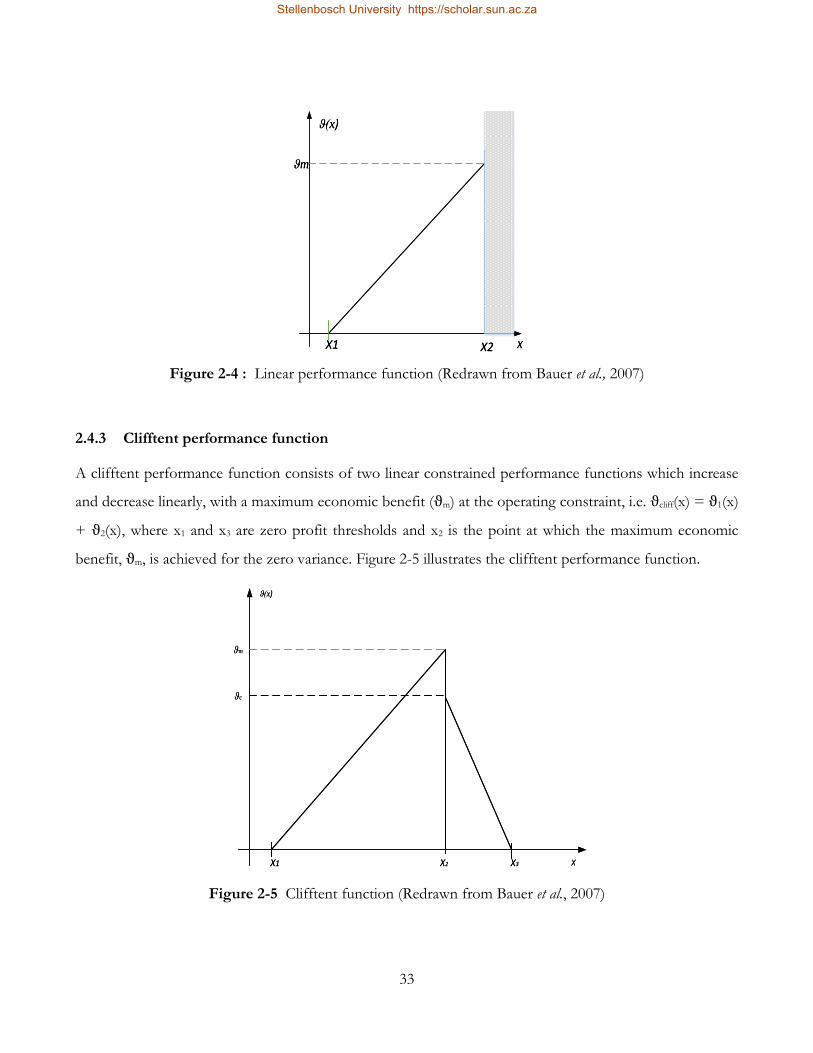
2.4.3 Clifftent performance function

A clifftent performance function consists of two linear constrained performance functions which increase

and decrease linearly, with a maximum economic benefit (ϑm) at the operating constraint, i.e. ϑcliff(x) = ϑ1(x)

+ ϑ2(x), where x1 and x3 are zero profit thresholds and x2 is the point at which the maximum economic

benefit, ϑm, is achieved for the zero variance. Figure 2-5 illustrates the clifftent performance function.

ϑ(x)

X1 X2 X

ϑm

X3

ϑc

ϑ(x)

X1 X2 X

ϑm

X3

ϑc

Figure 2-5 Clifftent function (Redrawn from Bauer et al., 2007)


34

The mill load is operated with tight control near an operating constraint to maximise throughput and hence,

maximise economic benefit. When upper and lower limits are exceeded, the economic benefit reduces albeit

to different extents to resembles a clifftent performance function (Wei & Craig, 2009a). The mass pull-

concentrate grade relationship in the flotation circuit, also characterizes this function. When mass pull

continuously increases beyond a profitable constraint, flotation selectivity diminishes and gangue material

begins to float. Consequently, the concentrate grade decreases until there is no profit.

As explained with the three performance function types, milling and flotation circuit controlled variables

produce different economic consequences due to their behaviour with respect to operating limits and

implemented control strategies. Clearly, a reduction in the variability of controlled variables can translate to

improved economic performance.

2.5 Significance and application of economic performance functions

Economic performance functions (EPFs) relate the dynamic behaviour of a controlled variable to money.

As such, they have a wide application in processes where controlled variables are controlled for economic

reasons and therefore, underlie almost every process. EPFs vary from process to process such that generic

EPFs are difficult to obtain even when the same process in different operations is considered. This

occurrence is due to different performance measures and operating strategies implemented across

operations. Furthermore, EPFs change within the same process and need to be constantly reviewed (Wei &

Craig, 2009a; 2009c).

EPFs are only applicable to process variables with an operating constraint. Therefore, benefits derived from

improved operating safety and reliability are not incorporated in economic performance functions (Bauer &

Craig, 2008). Furthermore, the control technology used in a process does not significantly influence EPFs.

Instead, factors such as process dynamics, process economics, operational specifications, and market

conditions are more relevant (Craig & Henning, 2000; Bauer et al., 2007; Wei & Craig, 2009a).

Although EPFs appear to be a significant tool for economic performance assessment, they are poorly

understood. This was observed from the results of a web-based survey conducted for mineral processing

experts in operations across the world. The experts who included process engineers, plant managers and

metallurgists, as well as mill and metallurgical superintendents could not adequately specify the relationships

that best described the economic behaviour of selected controlled variables. The poor understanding of

EPFs may be attributed to limited available information. For example, prior to the contribution by Wei &


35

Craig (2009b), there had been no clearly established methodology on developing EPFs. In addition, this

thesis also sought to address these limitations and extend the existing methodology to address the scope

considered in this study.

2.6 Development of economic performance functions

Economic performance functions are difficult to develop and therefore, rely heavily on assumptions to

simplify the highly complex economic relations in most processes. Thus, knowledge gaps are overcome since

complete knowledge on the process is often unavailable (Bauer & Craig, 2008). Credible performance

estimates are achieved through careful consideration of the assumptions made, as well as a judicious

consideration of the unique performance objectives for the process (Craig & Henning, 2000; Wei & Craig,

2009b). As an example, most EPA studies (e.g., Bauer & Craig, 2008; Wei & Craig, 2009a; Matthews & Craig,

2013) treated a process product as the final sellable product to enable the derivation of a monetary value for

economic performance. An assumption to neglect small economic consequences is made in most studies

(Steyn & Sandrock, 2013; Wei & Craig,2009a; Zhou & Forbes, 2003), and only key factors are identified

(Griesel, 2008).

The development of reliable EPFs requires an in-depth understanding of the process operation, process

control and process economics which is not obvious from process data (Bauer & Craig, 2008). Therefore,

each of these three factors must be critically analysed. Production objectives and consequently, performance

metrics must be established for the process operation. Information on the process description, utilities, and

consumables used in the process for which EPFs are to be developed, is also necessary. Process control

objectives must be well understood and aspects that include typical process disturbances, selection criteria

of controlled and manipulated variables, controlled variable operating limits, and the compensative action

required when operating limits are violated. An understanding of controlled variable interactions is also

critical. Finally, knowledge of the resultant economic impact when controlled variable specifications are

violated is necessary to understand process economics. Hence, controlled variables with the largest economic

impact must be considered since not all controlled variables are directly controlled for economic reasons.

Similarly, not all operating costs are very significant (Bauer et al., 2007; Wei & Craig, 2009a; 2009b). Clearly,

in order to develop a reliable EPF for this study, a judicious selection of key controlled variables must be

performed, as well as a careful assessment of operating cost distributions for the primary mill circuit.

EPFs can be developed by survey research, literature survey, plant tests, and from expert knowledge (Bauer

& Craig, 2008). Experienced process engineers possess an understanding of the economic impact of


36

important controlled variables (Bauer et al., 2007). Therefore, Wei & Craig (2009b) conducted a web-based

survey research in which experts were consulted to gain an in-depth process understanding of milling circuits.

In another study, Wei & Craig (2009a) applied a literature survey to develop EPFs for milling circuit variables.

Plant tests are rarely conducted as they are extremely time-consuming and may require the costly interruption

of normal operation. Despite this limitation, Steyn & Sandrock (2013) conducted a study using plant tests.

Historical data from industrial operation is a more acceptable alternative to plant tests. Although

organisational data is confidential, better process understanding is gained from empirically developing EPFs

as was done in this study. Moreover, degrading process performance is easy to detect with knowledge of past

performance. Zhou & Forbes (2003) recommend an empirical analysis of product value and production costs

for EPF development, as done in this study.

Data from laboratory experiments and simulation studies are also suitable for EPF development (Craig et

al., 1992). For example, Edwards & Vien (1999) derived a quadratic performance function between the

particle size and mineral recovery using laboratory grind and float experiments. Runge et al. (2007) also

validated the quadratic relationship between product particle size and mineral recovery with three different

flotation models that related flotation feed particle size to flotation circuit performance. In addition, some

simulation studies (e.g. Bauer et al., 2007; Craig & Henning, 2000; Wei & Craig, 2009a; Zhao et al., 2009) have

been used for EPF development.

With a good experimental design, the simulation approach is more accurate and simulation experiments can

be easily replicated (Craig & Koch, 2003). The main challenge however, is the difficulty in predicting

industrial performance with simulation models due to either model uncertainties or the numerous

disturbances that occur in industrial mineral processing operations (Contreras-Dordelly & Marlin, 2000;

Sosa-Blanco et al., 2000). In conclusion, combined approaches to EPF development are more effective as

demonstrated by Wei & Craig (2009a,2009b; 2009c).

2.7 Derivation of the economic performance index

An economic performance index (EPI) is estimated for a specified operating period based on the variability

of a controlled variable around a set point (Bauer & Craig, 2008; Jelali, 2006; Wei & Craig, 2009a). It is a

function of controlled variable set point and standard deviation of the time series. Therefore, the time

correlation does not matter as two different control conditions with the same probability density function


37

(PDF) but different autocorrelation functions will produce the same economic performance index (Jelali,

2010; Gupta et al., 2013).

Process economic performance is influenced by process variance, product quality, energy and material

consumption (Bezergianni & Georgakis, 2003). Therefore, an EPI that links a reduction in controlled

variability, revenue and production costs is more useful (Bauer & Craig, 2008; Gupta et al., 2013; Hodouin,

2011). This is especially important for milling circuit operations, where trade-offs between mill throughput,

concentrate grade, and mineral recovery are made. Furthermore, where production costs arising from

electricity and grinding media consumption are significant (Votteler & Brent, 2017; Wills & Napier-Munn,

2006).

Milling circuit variables are known to be strongly dependent on each other (Wills & Napier-Munn, 2006).

Dependencies exist between particle size -mill load, particle size-sump slurry discharge density, and mill load-

mill power (Wei & Craig, 2009c). A joint performance function (JPF) is developed for such cases to account

for resultant economic consequences, using a ratio of contribution assigned between each controlled variable

based on dependence strength.

Wei and Craig (2009b) proposed the following methodology steps (Figure 2-6) to determine the EPI using

economic performance functions.


38

Figure 2-6: Derivation of an EPI

In the next section, two EPA case studies conducted within milling circuits are reviewed.

2.8 Economic performance assessment case studies

Most EPA studies conducted for milling circuits use the crucial link between particle size and mineral

recovery to relate the performance of milling and flotation circuits. An independent assessment of milling

and flotation circuit performances is complicated (Craig & Henning, 2000). The major drawback for flotation

circuit EPA studies has been the difficulty to distinguish between flotation cell and feed properties due to

strong stream interactions and this limitation is addressed by linking milling and flotation circuits (Runge et

al., 2013). Although this is the best alternative, the lack of in-depth examination of the flotation circuit is still

a key shortcoming. Therefore, the common practice has been to derive milling circuit economic performance

Determine the overall EPI

Determine the information

required

Collect the information

Obtain suitable performance

measures

Make suitable assumptions

Develop joint performance

functions

Determine EPFs


39

with particle size, which is a measure of milling product quality and a major determinant of downstream

mineral recovery efficiency (Bauer & Craig, 2008; Matthews & Craig, 2013).

2.8.1 Case study of Steyn and Sandrock

Steyn & Sandrock (2013) assessed the economic benefit achieved by stabilising an industrial autogenous

PGM primary mill at its optimum power utilisation with a model predictive controller. A linear primary mill

and final grind relationship was modelled and subsequently, a relationship between the final grind and mineral

recovery was developed based on an assumption of perfect flotation. Fixed costs were assumed to remain

constant and mill liner cost was beyond the scope of their study. Therefore, the study only considered the

cost related to energy consumption.

Steyn & Sandrock (2013) derived the EPI as the financial profit determined between revenue (Equation 2-3)

and cost (Equation 2-4) over the period of assessment.

𝑅 = 𝐵𝑃 × 𝐹 × 𝐻𝐺 × 𝑃𝑅 × 𝑡 × 𝑐

2-3

where R – metal sales revenue

BP - PGM mineral basket price (ZAR/oz)

F - throughput rate (t/h)

HG - head grade (g/t)

PR - potential recovery (%)

t - time period (h)

c - conversion factor (oz/g)

The cost was determined as below:

𝐶 = 𝑢 × 𝑃 × 𝑡

2-4

where C - cost (ZAR)

u - unit cost of power (ZAR/kWh)

P - power consumed (kW)

t - time period (h)


40

There was some difficulty to develop a model between the primary and final grind so as to infer the final

mineral recovery. This pointed to challenges associated with developing models with real plant data, and

without a priori knowledge of the relationship between variables. Although using the final grind was more

appropriate for the assessment, the development of a reliable model was likely limited by complex

interactions between process streams because of recirculating streams. Moreover, different objectives govern

primary and downstream milling such that primary mills are typically tonnage mills with an operating

objective to maximize throughput. On the other hand, secondary or regrind mills rather focus on achieving

the target grind (Giddy, 1988; Moys et al., 1996). Despite this major limitation, the economic performance

assessment by Steyn & Sandrock (2013) represented key metrics associated with milling circuit operation..

2.8.2 Case study of Wei and Craig

Wei & Craig (2009a) assessed the economic performance of two controllers in a simulated run-off mine

(ROM) milling circuit. The assessment determined a better performing controller based on the rejection of

typical milling circuit disturbances, to achieve target particle size. Subsequently, the mineral recovery was

predicted with a-priori particle size-mineral recovery performance function.

The following assumptions were made in the EPA study:

1. the milling product was flotation circuit feed;

2. the head grade, throughput rate, and mineral price remained constant;

3. the flotation product was the final sellable product; and

4. milling circuit and downstream flotation operating costs remained constant with slightly better or

worse grinding.

The EPA relevantly considered major installation costs to give a detailed cost-benefit analysis of

implementing a new controller. However, some issues may need further investigation. A well-performing

controller takes action to restore controlled variables within an acceptable operating window when a

disturbance causes deviation. Hence, the large step disturbance applied to ore hardness and rock fraction in

the simulation experiments likely increased the amount of electricity required to achieve target particle size

since mill power draw typically increases with ore hardness and rock fraction (Coetzee et al., 2008; Rajagopal

& Iwasaki, 1992). Furthermore, an increase in ore hardness and rock fraction results in increased ore

retention time, to become throughput limiting (Wills & Napier-Munn, 2006). Therefore, assumptions of

fixed mill throughput rate and electricity consumption are only justifiable on the basis that economic


41

consequences arising from changes in throughput rate and mill power draw were not significant for

comparing controller performance.

Since it is particularly challenging to account for every factor contributing to the economic performance of

a milling circuit due to the highly complex economic relations, the role of simplifying assumptions is well

acknowledged. However, a shortcoming was identified in one of the assumptions made by Wei & Craig

(2009a). Flotation product was assumed to be the final sellable product, however, the revenue generated was

not appropriately adjusted to account for downstream beneficiation as done in Matthews & Craig (2013).

The two case studies demonstrate that economic performance functions provide a powerful tool for

evaluating the economic benefit of process control. However, an evaluation of economic performance is

impossible without simplifying assumptions. A Gaussian probability density function was assumed for the

data used in both case studies. Goodness of fit tests and visual plots may be used to test this assumption

(Hair et al., 2010). The Kolmogorov-Smirnov, Shapiro-Wilk, Cramer-vom Mises and the Anderson-Darling

are four commonly used tests (Royston & Matthews, 1991). Alternatively, normal probability and quantile

plots may be used. The probability plot shows the cumulative probability of a variable against the normal

distribution cumulative probability, and the quantile plot shows data set quantiles. Data are plotted against a

theoretical linear normal distribution and any departure from the straight line corresponds to departure from

normality. Quantile plots are more easily interpreted for large sample sizes (Ghasemi & Zahediasl, 2012).

The inclusion of key revenue and cost metrics was common in both studies i.e., Steyn & Sandrock (2013)

included throughput and mineral recovery for the revenue, and electricity as a cost element. Wei & Craig

(2009a) considered mineral recovery and controller installation costs. Although the EPA studies were

conducted once off, the success thereof may point to opportunity for implementing EPFs in process

monitoring.

Industrial data for EPF development must be reliable because any inaccuracies lead to substantial bias in

estimating economic performance. The next section discusses techniques for handling faulty data to improve

the quality of empirical EPFs with industrial data.

2.9 Faulty data handling techniques

Historical process data contain faulty data, which manifests as incomplete data with missing values,

anomalous data with impossible values and noisy data such as outliers. Accurate estimation of economic


42

performance becomes difficult when insufficient, incomplete and/or unreliable process measurements are

used (Ma et al., 2010). Therefore, appropriate data handling techniques are applied.

2.9.1 Incomplete data with missing values

Valid observations for one or more variables may be unavailable for analysis. Valuable information is lost

when large amounts of data are missing and consequently, EPF reliability is threatened (Kang, 2013). EPFs

estimated from data with a large number of missing values may be biased, particularly if the values are

systematically different from available data. To reduce bias and achieve reliable conclusions, cases with

missing data are handled with appropriate methods.

Missing data constituting less than 15% of individual variables is ignored except when missing data occurs

in a non-random fashion. Otherwise, case reweighting or multiple imputations may be considered if a large

percentage of cases are missing data (Hair et al., 2010). When a strategy to use complete vectors is considered,

observations in other variables that correspond to the missing data are deleted. This is necessary when there

is a systematic association between variable observations that directly affects the analysis (Langkamp et al.,

2010).

2.9.2 Outlier detection

Outliers are unusual observations that are considerably different from the general data trend (Chandola,

2009; Rahman et al., 2012). In this study, outliers can drastically influence the reliability of EPF predictions

and the process monitoring tool’s benchmark performance. Outlier sources in industrial data include

transmission or transcription errors. In addition, incorrect manual data entry of laboratory assays or

measurement errors from undetected sensor failures may occur. Outliers must be judiciously detected and

filtered out because some outliers may still carry important information (Herman et al., 2013; Filzmoser,

2007).

Outlier detection and filtering helps to improve the performance of predictive models. Several techniques to

detect time series outliers are proposed in literature (e.g., Tsay et al., 2000; Weng & Shen, 2008). However,

distance-based and density-based approaches are widely used (Rahman et al., 2012). A distance-based

approach determines the distance between a data point and its nearest neighbour, and compares the distances

for all of the data. On the other hand, density-based approaches compare the density of a data point’s

neighbourhood with that of its neighbour’s neighbourhood. The underlying principle is that a data point that

is far from its neighbours is likely to be an outlier (Knorr & Ng, 1997). As such, distance-based approaches

barely detect local outliers while density-based are not good at finding global outliers, where local outliers


43

are extreme relative to its neighbours and global outliers are outlying with respect to the majority of data

points (Rahman et al., 2012).

Single-step and sequential procedures are often used for outlier detection, whereby all outliers are identified

at once in single-step procedures as opposed to successive elimination or addition of datum in the sequential

procedure (Davies & Gather, 1993; Liu & Spencer, 2004). Typically, sequential procedures delete outliers

based on control charting where outliers are identified outside three data standard deviations on a normality

assumption (Woodall, 2004). Any identified outliers are removed and control chart limits are recalculated.

These two steps are performed recursively until the process is statistically stable i.e., no further outliers can

be detected. This procedure is known as ‘classical outlier analysis’ (Ben-Gal, 2005).

Chapter Summary

Chapter 2 has provided a literature review on economic performance assessment. More insight into two

objectives for this study i.e., the development of EPFs and subsequently, the derivation of the EPI were

provided. The factors that influence economic performance and the critical role of process control in

improving economic performance were discussed. In addition, EPA methodology steps proposed by Wei &

Criag (2009b) for controller performance assessment studies formed the theoretical framework for this study.

A historical-data benchmark was relevant to this study. Moreover, particle size was identified as the most

economically significant controlled variable for the milling circuits. Lastly, a strategy to consult experts at the

industrial operation and conduct a plant survey was planned for EPF development.

The next Chapter discusses the significance of process monitoring for fault detection. Criteria used to select

an appropriate process monitoring method are also presented.


44

CHAPTER 3: PROCESS MONITORING AND FAULT

DETECTION

Chapter Overview

This chapter discusses the significance of process monitoring for fault detection. To this end, model and

data-based approaches are first distinguished with more emphasis on the data-based approach. The

regression analysis technique for model development, and the Shewhart control chart are discussed to

address two aspects of this study i.e., a method for reliable EPF development and a strategy for developing

the industrial process monitoring tool. Fault identification characteristics are discussed, and common faults

in milling circuits are identified in partial fulfilment of the study objective to investigate fault detection with

EPFs.

3.1 The significance of process monitoring

Process monitoring is a continuous task of recording information, identifying and detecting process

performance anomalies or faults (Isermann & Balle, 1997). A fault is an ‘unpermitted deviation of at least

one parameter of the process or system from the acceptable condition’ (Isermann & Balle, 1997). According

to Venkatasubramanian et al. (2003b), when a detection mechanism gives a fault signal, the fault is said to be

‘detected’. By monitoring process performance over time, faults can be detected when they occur (Yin et al.,

2002). Fault detection is achieved through a comparison of operating data to the behaviour of a model system

or by applying rules to operating data. However, process performance anomalies are commonly detected

using comparisons between operating data and baseline process data. Both approaches were applicable to

simulation and industrial cases, respectively.

Timely fault detection is critical for consistently satisfactory economic performance. Moreover, fault

detection while the process is still within a controllable operating region allows for intervention to recover

the process to normal operating conditions before significant production losses are incurred. Thus, economic

benefits associated with increased uptime are delivered (Fatlin et al., 1993; Zhou & Guo, 2011). On the other

hand, undetected faults result in safety, environmental and economic impact, depending on the fault. Thus,

fault detection and identification are important to sustain satisfactory process performance as discussed in

Section 3.3.


45

Real-time process monitoring evaluates and updates process performance with changes in process conditions

(Grimshaw et al., 1998). Reliable process observations improve timely fault detection rates and corrective

action (Venkatasubramanian et al., 2003a). On the other, log-based monitoring analyses process performance

trends post-processing, in order to evaluate or monitor current performance based on these trends (Mitchell

et al., 2008). Long-term process evaluation for process optimization purposes is also supported by log-based

process monitoring. Moreover, predictive process performance models are commonly developed with

historical data (Kano & Nakagawa, 2008; Woodall et al., 2004). Although the level of detail differs, both real-

time and log based process monitoring are important and beneficial depending on the objectives that are to

be achieved (Barton, 2013).

While process monitoring methods have been classified as a function of time i.e. real-time or log-based, they

can be further classified broadly into model-based and data based approaches (Dvorak & Kuipers, 1991;

Serpas, 2012). The next sections discuss these two classes.

3.2 Process monitoring approaches

According to Tatara & Cinar (2002), data-based process monitoring is a generally predominant method used

to detect changes in an industrial process from historical process knowledge. For the purpose of this study,

process monitoring with empirical models and statistical process monitoring are further distinguished. The

first method consisted of models developed from historical data.

3.2.1 Process monitoring with empirical models

Process data is commonly used to develop empirical models of important process variables. Unlike the

model-based approach, these models are more dependent on the availability of quality historical data and

may even be developed without any insight on the physics of the process (Jearkpaporn et al., 2005; Qin, 1998;

Yin et al., 2002). Empirical models developed from historical analysis require as much process data as

possible, especially in cases where inferences are made with the models. The data must capture typical

variation in the model parameters for good predictions to be made over a wide range of operating regions

(Giddy, 1988). However, care must be taken to judiciously select model data since process data typically

contains observations that reflect process upsets and assignable causes (Jearkpaporn et al., 2005). Hence,

process data quality must achieve the objectives being assessed (Kaka,1999; Kresta et al., 1994).


46

Sliškovic et al. (2011) proposed the process-data based modelling procedure shown in Figure 3-1. Typically,

the development of a reliable model often involves several iterations with these steps. However, some

background knowledge formed from in-depth process understanding is useful to develop reliable empirical

models (Hodouin, 2011).

Data gathering from process database

Data pre-treatment

Model structure selection

Selection of criterion for model parameter

estimations

Model parameters estimation

Possible a-priori knowledge

Knowledge about process model purpose

Model validation

Theoretical knowledge about process-data

based modelling

Model aceptable End

YesNo

Data gathering from process database

Data pre-treatment

Model structure selection

Selection of criterion for model parameter

estimations

Model parameters estimation

Possible a-priori knowledge

Knowledge about process model purpose

Model validation

Theoretical knowledge about process-data

based modelling

Model aceptable End

YesNo

Figure 3-1: Process-data based modelling procedure (Redrawn from Sliškovic et al., 2011)

The validity of empirical models is a critical criterion that ensures model representativeness. It is tested based

on the significance between predicted and actual performance of an output variable of interest. When

presented to new data, a valid model must possess good data fit and predict performance corresponding to

the input(s). Model goodness of fit is evaluated with statistical indicators such as the adjusted R-squared.


47

Although predictive capability is a crucial aspect, an expert intuition is also necessary for further decision

making on model appropriateness (Hamilton, 2015; Reisinger, 1997).

Most researchers (e.g., Fan & Huang, 2001; Marto & Wolfe, 1962) support the use of regression modelling

to learn more about process performance. Moreover, quality is best assessed using a function, i.e., a

relationship between a response variable and one or more explanatory variables (Woodall, 2016). As such,

regression models have been demonstrated to account for costs associated with major grinding mill

equipment (Sayadi et al., 2014), for optimisation of milling circuits (Steyn & Sandrock, 2013) and for assessing

the performance of milling circuits (Silva & Casali, 2015). The choice of a regression model, whether linear

or non-linear largely depends on the model application. Linear regression is the most common application

of regression analysis. Although it may be argued that nonlinear models are necessary, linear models are

usually sufficient for monitoring (MacGregor & Kourti, 1995).

Data-based process monitoring has been demonstrated in a number of studies (e.g., Kazemzadeh et al., 2009;

Stover & Brill, 1998; Woodall et al., 2004; Wang & Tsung, 2005), where control charts and linear regression

models monitored product quality variability. The main objective for these studies was to maintain a linear

profile for a data series collected at regular time intervals. Any outlying profiles pointed to an out-of-control

process (Yen & Shiau, 2010). The studies applied either phases I or II, where phase I profile parameters are

estimated using historical profiles. Phase II however, detects changes in the estimated parameters (Aly et al.,

2015). The two phases are distinguished respectively as retrospective and ongoing monitoring (Mahmoud et

al., 2010). Thus, phase II and is more appropriate for statistical process monitoring (as discussed in the next

section).

Studies on linear profile monitoring were conducted mostly for chemical industries. Model-based process

monitoring in the mineral processing industry rather focuses on nonlinear models. This is because of the

challenges arising from developing linear models that are consistently representative over a wide operating

range using a limited data set (Powell & Morrison, 2007; Skogestad, 2004). Moreover, data features such as

the high dimensionality, input correlations and the presence of errors and disturbances make the

development of accurate models for complex processes difficult (Madakyaru et al., 2017).

3.2.2 Statistical process monitoring

Statistical process monitoring (SPM) is a common type of data-based process monitoring extensively applied

in industry (Coetzer & Khumalo, 2006). Key process variables representative of process performance are

monitored in order to maintain a state of statistical control by eliminating assignable causes of variation. The


48

process may be susceptible to further drift outside satisfactory process performance if no action is taken

(Besterfield, 2001; Woodall et al., 2004).

Siddiqui et al. (2014) classified variations into common and assignable causes. Common cause variations are

inherent in a process and difficult to eliminate. However, they are controllable within some range by closed

loop control. Assignable causes are unexpected random variations that influence changes in the system or

process input parameters. These variations are removed in order to sustain satisfactory process performance

(Besterfield, 2001; Woodall et al., 2004).

SPM tools identify assignable causes and detect changes in process performance. Although the basic

concepts behind these traditional tools are still valid, they are not applicable to cases where the process

dynamics are non-negligible or cases where the process variables are highly correlated. Moreover, SPM tools

are incapable of accommodating large amounts of data. In cases with dependent process variables,

multivariate statistical process monitoring (MSPM) is commonly used (e.g., Arteaga & Ferrer, 2002; Boque

& Smilde, 1999; Yoo et al., 2002).

MSPM techniques capture correlations between process variables to minimize the probability of missing an

out-of-control event due to correlation inherent in the data (Moody, 2014). These techniques have been

demonstrated in several studies with many successful industrial applications for fault detection (e.g.,

Desborough & Miller, 2002; Yuan & Lennox, 2009). Active statistical process monitoring has been applied

in other studies (e.g. Hachicha et al., 2012; Ibrahim, 1996), to complement concepts from automatic process

control with SPM techniques. However, this study focused on univariate statistical process monitoring.

The variability of a single process variable is monitored about a statistical measure of the variable in univariate

statistical process monitoring. However, selecting a single process variable may not be sufficient to monitor

a milling circuit as a large number of key process variables should be monitored to assess process

performance (McClure et al., 2014). Hence, univariate statistical process monitoring appears to be restrictive

and inappropriate for complex processes (Hachicha et al., 2012).

Interactions between process variables are common in milling circuits and information contained therein

enhances process understanding. However, each process variable is assumed to be independent and

correlation structures between process variables are disregarded. By so doing, essential multivariate qualities

in process data are deconstructed and useful information is lost. Consequently, process deviations are either


49

not detected for processes with high correlations amongst variables or false alarms may be generated.

Alternatively, monitoring multiple process variables discretely provides a poor and costly design for

univariate monitoring that results in the generation of an uncontrollable number of alarms (Yin et al., 2002).

Therefore, multi-predictor EPFs are also developed in this study to investigate the feasibility of process

monitoring with all key controlled variables for the primary mill circuit.

3.2.3 The role of control charts

Control charts are a form of time series plots that are applied in univariate statistical process monitoring.

The use of control charts is summarised in (

Figure 3-2), where trial control charting tests whether consistently predictable results are produced, in an

attempt to bring the process to stable and predictable operation (Benneyan, 2001; Steiner & Mackay, 2000).

Figure 3-2: Roles for control charts (Redrawn from Benneyan, 2001)

Understand past performance

Is the process stable or in statistical control

Conduct trial control charting

Establish consistent process

Iterative process using trial control charts

Bring process into statistical control

Remove sources of natural variability until in control

Improve stable process

Remove source of natural variability

Position the average and reduce variability until acceptable

Test and verify impact of interventions and improvements

Monitor process for variability

Maintain a state of statistical control

Identify and remove special causes


50

3.2.4 Criteria for implementing control charts

The following criteria tests the appropriateness of implementing control charts (Box & Luceno, 1997):

1. Is a control chart an appropriate tool for application? The appropriateness of applying a control chart

in process monitoring depends on whether or not a stable period exists. A process variable with

stable variance but a drifting mean requires automatic process control strategy to reduce variability.

2. Which type of control chart should be used? Control chart selection is influenced by the objective

for applying a control chart i.e., whether for real-time process monitoring, problem-solving, or

assessment of process stability. In addition, the function of control charts is also considered i.e.,

whether for variable data or quality attributes data. Attribute control charts are more useful for

attributes data (Gulbay & Kahraman, 2006).

3. Where should control limits be placed? Successful statistical process monitoring is ensured by

correctly set control chart limits, which crucially define acceptance and rejection regions for

satisfactory performance. Therefore, careful thought must be put when determining control chart

limits.

Based on this criteria, the Shewhart control chart was applied in this study to monitor economic performance.

This chart is understood by a wide range of audiences and is useful for detecting significant variability by

monitoring economic performance over time (Benneyan, 2001). Subsequently, root causes can be established

and corrective action taken (Alt & Smith, 1998).

3.2.5 Shewhart control chart

Shewhart charts are constructed with three distinctive features: a central line (CL) representing the target

economic performance for the process, an upper control limit (UCL), and a lower control limit (LCL). The

control limits are typically three standard deviations (as shown in Equation 3-1) from the economic

performance derived from a representative stable normal operating period. This period reflects all the natural

process variance when process performance specifications are met (Kresta et al., 1994).

𝐿𝐶𝐿 = 𝐶𝐿 − 3𝜎

𝑈𝐶𝐿 = 𝐶𝐿 + 3𝜎

3-1

where σ - standard deviation from target economic performance

The Shewhart chart assumes that the process subject to common cause variation will remain in a state of

statistical control, where a process variable remains close to the set point. Therefore, control chart limits will


51

reflect the variability produced by assignable causes such that out-of-control data lies outside the control

limits as shown in Figure 3-3. This chart becomes an insensitive method for diagnosing assignable causes

when these limits become wider than necessary (Wood et al., 1998). Furthermore, the use of unfiltered

process data makes this chart susceptible to noise and increases the rate of false alarms.

Time

Obs

erve

d v

aria

ble

Centre line

Lower control limit

Upper control limit

In control

Out of control

Figure 3-3: Shewhart control chart

Shewhart control chart rules for degrading performance

A Shewhart control chart provides early insight on degrading economic performance through identifying an

out-of-control process from a time series plot of process performance. Table 3-1 gives the rules for

identifying out of control signals (Duncan, 1986).


52

Table 3-1: Control chart rules

Test Criterion Number

of points

1. Points above Upper Control Limit (UCL) or below Lower

Control Limit (LCL)

1

2. Zone A n of n+1 points above/below 2 sigma 2

3. Zone B n of n+1 points above/below 1 sigma 4

4. n points in a row above or below the centre line 9

5. Trends of n points in a row increasing or decreasing 6

6. Zone C—n points in a row inside Zone C 15

7. n points in a row alternating up and down 14

8. Zone C – n points in a row outside Zone C 8

The following describes the information presented in Table 3-1.

Test 1: Extreme Points

Test 2: Two out of three points in Zone A or beyond

Test 3: Four out of five points in Zone B or beyond

Test 4: Runs above or below the centre line

Test 5: Linear Trend Identification

Test 6: Oscillatory Trend Identification

Test 7: Avoidance of Zone C

Test 8: Run in Zone C

The corresponding control chart zones are illustrated in Figure 3-4.


53

A Zone A

B Zone B

C Zone C

C Zone C

B Zone B

A Zone A

Figure 3-4: Control chart zones

In the next section, three fault identification characteristics are discussed and an overview on common faults

in milling circuits is provided.

3.3 Fault characteristics and common faults in grinding mill circuits

3.3.1 Fault characteristics

Three features that distinguish faults i.e., classification, rate and frequency of occurrence are discussed in

subsequent sections.

3.3.2 Fault classification

Faults are broadly classified into five categories based on where they occur. Controller malfunction, actuator

failures, structural failures, human intervention, sensor failures and process disturbances are illustrated in

Figure 3-5 (McClure et al., 2014; Venkatasubramanian et al., 2003b).

Figure 3-5: Fault classification within a process (Adapted from Venkatasubramanian et al., 2003a)

𝜀

Process disturbances

Controller malfunction

Actuator failures

Sensor failures

Structural failures

Final control element (FCE)

Process

Measurement

sensor

Controller SP

+ -

Measured CV

CV MV U

CL

LCL

UCL


54

The automation of industrial processes makes them vulnerable to controller, actuator, and sensor failures.

Sensors provide critical feedback signals for the control of a process. Faults may occur as a malfunctioning

sensor, a fixed failure, a drift or an out-of-range failure (Arzen, 1991; Barton, 2013). Sensor faults result in

differences between measured and actual values of process variables. As such, prompt fault detection and

timeous accomplishment of corrective actions of sensor failure are necessary to avert the deviation of plant

state variables beyond acceptable limits (Gertler, 1998). Structural failures e.g. mill failure occur in process

unit equipment. In some instances, inappropriate human intervention may result in a fault (Buchanan &

Bessant, 1985; Riascos et al., 2004). However, this is now less common especially with the growing reliance

on automated processes. Process disturbances manifest when there are difficulties to sufficiently attenuate

input variation. For example, variation in ore feed size distribution may result in high circulating loads to

produce effects such as mill overfilling and hydrocyclone spigot choking.

3.3.3 Rate of occurrence

Faults are also characterised according to the rate of occurrence. Cha & Agrawal (2014) classified the time

dependency of faults into abrupt, incipient and intermittent categories as shown in Figure 3-6 (where f is the

fault size and t is the time).

fb

a

t

fb

a

t

f

t

f

t

cf

t

cfb

a

t

f

t

cfb

a

t

f

t

cfb

a

t

f

t

cfb

a

t

f

t

c

Figure 3-6: Time dependency of faults (a) abrupt (b) incipient (c) intermittent (Adapted from Cha &

Agrawal, 2014)

Abrupt faults occur instantly and are referred to as ‘short” faults because of the sharp change between two

successive data points. However, incipient faults slowly develop with time as “long” faults with a constant

value over successive data points. Unlike abrupt faults with a sudden appearance, these faults are less easy to

detect. Intermittent faults occur abruptly in varying sizes and for varying time intervals. In simulation


55

experiments, abrupt faults are modelled as a stepwise function representing a bias in the monitored signal,

incipient faults are represented by drift-type changes and intermittent faults are modelled as a combination

of impulses with different amplitudes as cyclic, a spike (sudden increase during a short duration) or erratic

faults (Cha & Agrawal, 2014; Lees, 1973; Sharma et al., 2007; Zhang & Yan, 2011).

3.3.4 Frequency of occurrence

The frequency of fault occurrences is yet another important characteristic that provides systematic strategies

to prevent fault recurrence or propagation into total failures (El-Farra & Giridhar, 2008). This information

is useful for diagnosing the root cause of more frequently occurring faults (Himmelblau, 1978).

In the next section, common faults in milling circuits are discussed.

3.4 Common faults in milling circuits

Although myriads of faults can occur in milling circuits, only a few frequently occur. Respondents in a web-

based survey conducted by Wei & Craig (2009b) on milling circuits listed poor load cell reliability, steam and

slurry build-up on sump level sensor, and continual drift in densitometers as some of the frequently faced

instrumentation challenges. Furthermore, automated steel ball loading and mill load control were some of

the additional challenges highlighted in milling circuit control and optimisation (Wei & Craig, 2009b). Based

on these contributions, faults that could be simulated with Le Roux’s SAG mill model are introduced in the

next sections.

3.4.1 Drifting mill load cell

Mill load cells are commonly used to measure the mill weight (Wei & Craig, 2009b). Most modern mills

operate with load cells which synchronize the mill weight, power draw, and ore feed with density control

(Mular et al., 1988; Wills & Napier-Munn, 2006). Since automatic process control depends on reliable

measurements, mill load cells require accurate calibration (Marlin et al., 1991). However, measurements are

prone to variation from humidity changes, chemical seepage (of reagents dosed into the mill) or random

sensor drift. Hence, sensor measurements systematically drift away from the actual weight (Dey et al., 2014).

An unobserved load cell fault may cause mill overload due to erroneous measurements. Therefore, corrective

action such as stopping the mill to reduce the load may be required. Consequently, production and revenue

losses are incurred (Wei & Craig, 2009b).


56

3.4.2 Steel ball overcharge

Steel ball charge provides breaking mass to support the milling process. The volume of steel balls in the mill

is an important control parameter that affects breakage rates and in-mill trajectories. Moreover, mill

throughput and specific power input are affected by the amount of steel ball charge maintained in a mill.

Hence, additional steel balls are added whenever in-mill charge falls below the target volume (Gupta et al.,

2013). SAG mills normally operate with ball charge level of between 8 to 21% (Wills & Napier-Munn, 2006;

Morrell & Valery, 2001).

Accurate measurements of steel ball charge still present a challenge since mill absorbed power not only

depends on ball level but also on operating parameters that include pulp density and liner configuration

(Bartsch et al., 2008; Rupare et al., 2013). Due to this limitation, plant operators usually infer ball level from

power draw and bearing pressure measurements which may result in steel ball overcharge faults (Clermont

& De Haas, 2010) Occasionally, crash stops are performed to obtain more accurate ball load measurements

based on the volume percentage of steel balls in the mill. A crash stop involves instantaneously cutting off

all mill feed streams during steady state mill operation and completely grinding out the ore (Clermont & De

Haas, 2010). These practices seek to address lack of better online measurements of in-mill ball level.

About 40-45% of the total comminution costs are attributable to grinding media and 5-10% to linear wear,

hence the control of steel ball charging is highly important (Radziszewski, 2013; Rupare et al., 2013). Thus,

ball media overcharge is associated with direct economic impact from excessive liner wear rates, increased

steel ball consumption, as well as frequent overload trips and downtime (Pokrajcic & Morrison, 2008; Rupare

et al., 2013). Furthermore, an additional operating cost is incurred for power consumption since specific mill

power is directly proportional to the amount of steel ball added at a particular time (Williams et al.,1986;

Almond & Valderrama, 2004; Silva & Casali, 2015).

3.4.3 Poor quality steel ball charge

Milling circuits are operated with an objective to minimize steel ball consumption (Wei & Craig, 2009a).

Spero et al. (1991) and Aldrich (2013) relate steel ball wear rate to ball quality (i.e., composition and

metallurgical properties), the ore feed (i.e., particle size and hardness), mill properties (i.e., size, speed and

liner profile), milling environment (i.e., in mill conditions such as slurry density) and milling circuit parameters

(e.g., circulating load and residence time).


57

Quality issues in steel ball media induce process disturbances (Moema et al., 2009; Singh, 2003). Furthermore,

poor quality steel ball charge not only affects consumption rates but milling effectiveness and power

consumption (Morrison & Powell, 2006). Therefore, manufacturers conduct quality checks of standard

physical and mechanical specifications before supply. Steel ball chemical composition and hardness profiling

tests are two of the crucial quality control procedures followed to ensure on-specification steel balls.

Steel abrasiveness is an important hardness factor that determines the absolute wear rate of steel balls

(Aldrich, 2013). Despite quality checks, casting defects such as shrinkage and gas porosity are common in

some batches supplied to industry (Jankovic, 2003; Moema et al., 2009). Casting defects in steel balls result

in minimized steel ball wear resistance, leading to premature steel ball breakage. Consequently, rapid steel

ball wear rates are experienced and steel ball consumption is increased.

3.4.4 Ore hardness variation

Highly variable ore feed characteristics are manifested by intrinsically variable orebody composition (Hunt et

al., 2013). Ore feed hardness affects the control of grinding mills because of its effect on actual grinding

mechanics (Egbe & Abubakre, 2013). Comminution behaviour, energy requirements, the product particle

size achieved and hence mineral liberation, are directly influenced by ore hardness (Mwanga et al., 2015).

When ore hardness significantly increases by 90% for example (as cited in Coetzee et al., 2008), fault

conditions manifest. The mill build-ups from increased grinding time and recirculating coarse sized particles

to become throughput limiting. Consequently, production rate is lowered in order to stay within the rated

mill power draw constraint (Wills & Napier-Munn, 2006.; Powell et al., 2009). Typically, additional steel balls

are charged into the mill to counteract the effect of the fault. However, this takes significant time for

equilibrium to be reached and hence, it is more effective for long term circuit improvement (Forssberg &

Schonert, 2012).

Chapter Summary

Chapter 3 has provided a literature review on process monitoring methods. Model and data-based methods

were distinguished and a discussion on the significance of statistical process monitoring highlighted the

importance of timely fault detection. Regression modelling was identified as a suitable method for EPF

model development, and the Shewhart control chart for process monitoring. Five fault classes were

distinguished, and a characterisation of the rate and frequency of fault occurrence was presented. Finally,

four common faults in milling circuits were identified and their consequences, highlighted. Therefore, this


58

Chapter addressed three aspects i.e., the use of regression modelling for EPF model development with

industrial data, strategies for developing the industrial process monitoring tool and for assessing the feasibility

of fault detection with EPFs.

The next Chapter discusses a critical site survey at the industrial Concentrator plant. Insight is provided on

process operations, economics, and control as a critical step to EPF development with industrial data


59

CHAPTER 4: INDUSTRIAL PRIMARY MILL CIRCUIT

SURVEY

Chapter Overview

This chapter reports on information acquired from the industrial operation during preliminary and critical

site survey visits. A review of primary mill circuit operation, control, and economics provides a basis for

reliable EPF development, as discussed in Chapter 2. Key objectives driving operating strategies are discussed

and an overview of the control philosophy is presented. Furthermore, the factors influencing economic

performance are identified. Finally, historical data is used to assess the primary mill circuit’s economic

performance in monetary terms.

4.1 Introduction

A week long preliminary site visit was conducted at the industrial concentrator plant with an objective to

appreciate the Concentrator plant operations. The key outcome of the preliminary site visit was to identify a

suitable scope for the industrial case study. Issues that related to process operation, control and economics

(Appendix A) were studied. After identifying a suitable scope, a critical site survey was conducted to acquire

an in-depth understanding of the primary mill circuit’s operation as presented in this Chapter.

4.1.1 Concentrator plant overview

Operations at the industrial Concentrator plant consist of Dry and Wet sections. Crushing and coarse

grinding stages constitute the Dry section, while milling, flotation, and downstream thickening operations

make up the Wet section.

Minerals are liberated from the ore through a multi-staged comminution circuit to ensure sufficient liberation

since the ore is one of the hardest to beneficiate (Rule & DeWaal, 2011). Sufficient liberation of mineral

values is important for downstream flotation, which intermittently occurs after milling stages in a Mill-Float-

Mill-Float (MF2) circuit configuration. The scope of this study was limited to the primary mill circuit as

highlighted in the MF2 circuit flow diagram shown in Figure 4-1.


60

Figure 4-1: Concentrator plant flow diagram

4.1.2 Primary mill circuit process description

The primary mill circuit comprises the primary ball mill, sump, hydrocyclone cluster and rougher flotation

units. A process narrative of the circuit is presented below:

Ore with a nominal size of 100% passing 8mm is reclaimed from the primary mill feed silo and fed into a

17.5 MW grate discharge ball mill of diameter 7.92m and an effective grinding length of 11.28m. Water is

added at the mill feed end to improve in-mill rheology. Steel balls with a top size of 70mm are charged into

the mill as grinding media. During the milling process, ore pulp and some steel ball scats are discharged

through a 15x28mm slotted aperture discharge screen. Oversize scats are conveyed to the mill scats bunker,

while undersize material gravitates to the primary mill discharge sump.

Collector and promoter reagents are dosed into the primary mill discharge sump for pulp conditioning in

preparation for downstream processing. Make-up water is added to the primary mill discharge sump for

density control and diluted pulp is pumped to a duty hydrocyclone cluster. The primary ball mill is operated

in a closed circuit with a hydrocyclone cluster which separates coarse and fine particles into underflow and

overflow streams respectively. The underflow stream of coarse particles gravitates back to the ball mill for


61

additional grinding, while the overflow stream of fine particles is delivered to the flotation circuit for mineral

recovery. The overflow stream is gravity fed to a rougher flotation splitter box, where it is split into two

parallel rougher flotation banks. Reagents (frother, collector, promotor, depressant and activator) prepared

to a specified strength are dosed into rougher feed boxes with additional controlled dosing down the bank.

Rougher flotation feed typically has a target grind of between 40-55% passing 75µm. It is treated in two

flotation banks, each consisting of seven 100m3 flotation cells. The first three flotation cells in bank #1 are

Dorr-Oliver forced-air type and the last four are self-aspirating Wemco flotation cells, while bank #2 only

operates Dorr-Oliver forced-air type flotation cells. The different bank design facilitates plant-scale

optimisation test work. Despite the mechanical difference between the banks, metallurgical performance i.e.

upgrade ratio and recovery of the two banks is reported to be comparable. Each bank produces a first and

second grade concentrate stream that is delivered to respective primary cleaner flotation cells. The number

of flotation cells reporting to either the first or second concentrator grade sump is variable. Rougher tailings

from each rougher flotation bank report to the rougher flotation tailings sump before downstream

processing.

The process control hierarchy given in Chapter 2 is discussed for the primary mill circuit in the next section.

4.2 Process control hierarchy

The primary mill circuit is controlled with an objective to meet operating and economic objectives as

discussed in following process control hierarchy:

4.2.1 Instrumentation

Table 4-1 lists key instrumentation for the primary mill circuit, and a brief description for some instruments

is given.


62

Table 4-1: Primary mill circuit instrumentation

Milling

Measured variable Instrument

Primary mill feed silo level Ultrasonic level transmitter (%)

Primary mill feed rate Electromechanical weightometer (t)

Primary mill discharge particle

size

Ultrasonic particle size analyser (μm)

Mill load Load cell (t)

Inferred from bearing pressure

Mill inlet water Magnetic flowmeter (m3/h)

Sump level Ultrasonic level transmitter (%)

Sump make-up water flow rate Flowmeter (m3/h)

Hydrocyclone slurry flow rate Magnetic flowmeter(m3/h)

Hydrocyclone feed pressure Pressure transmitter (kPa)

Hydrocyclone feed density In-line densitometer (t/m3)

Flotation

Rougher feed Pd grade On-stream XRDF stream analyser

Froth velocity Froth cameras (mm/s)

Reagent dosage rate Magnetic flowmeters (m3/h)

Rougher cell pulp level Ultrasonic level transmitter (m)

Rougher cell air flow rate Air flowmeter (m3/h)

The instrumentation listed in Table 4-1 is commonly used in milling circuit operations (Wei & Craig, 2009b).

Many process variables are monitored online in order to achieve efficient process performance in response

to changes in system inputs. The ultrasonic particle size analyser obtains a running average of the particle

size distribution as an ultrasonic wave propagates through the primary mill discharge stream. Ultrasonic

spectroscopy is typically applied for particle sizes of between about 10nm and 1000 µm (Riebel & Löffler,

1989). This measurement method is preferred relative to alternative offline techniques because it minimizes

handling errors and the time taken to generate measurements.

Elemental on-stream X-ray diffraction and fluorescence (XRDF) analysers measure rougher feed stream

samples. An average of the specific gravity and palladium (Pd) content is continuously generated from 5-

minute measurements. Measurement reliability depends on the extraction of a representative sample, and it


63

is checked for consistency with offline analysis. On-stream XRDF measurements are more suitable for

rougher flotation assay-based control, rather than for metallurgical accounting purposes. The analysis of

multiple streams to provide simultaneous comparisons between feed, concentrate and tails for measured

streams is one major advantage of XRDF analysers.

Froth cameras are installed on each rougher flotation cell to capture and analyze froth surface images. Several

froth features including froth velocity, froth stability, and bubble size distribution measurements are

extracted from the froth images. Furthermore, measures of concentrate contribution from each individual

cell are determined based on the froth velocity.

4.2.2 Base control

Table 4-2 presents the controlled variables regulated with base control. The control of solids (ore and steel

ball) feed rate, circulating load, mill feed water, hydrocyclone feed flow and rougher flotation feed improves

primary mill circuit stability. Effective sump control is critical to stable operation without which, an off-

specification particle size product and poor flotation performance result.


64

Table 4-2: Base control for the primary mill circuit

Controlled variable Control objective Control used Controller type

Mill ore feed To maximise

throughput

Load control PID

Mill inlet water To achieve target in-

mill density

Ratio control PI

Steel ball grinding

media

To maintain load to

steel ball ratio

Ratio control PI

Sump level To maintain stable

operation

Level range control PID

Sump discharge

rate/Hydrocyclone

feed flow rate

To achieve consistent

rougher feed flow

To stabilise the mass

pull achieved

Cascade control PID

Hydrocyclone feed

pressure

To achieve target

particle size

Ratio control PI

Reagent flow rates into

designated reagent

dosage points

To condition the pulp

for mineral recovery

Ratio control PID

Mass pull To achieve stable

concentrate mass flow

Cascade control PID

Figure 4-2 is a process and instrumentation schematic showing manipulated variables for the primary mill

and floatation circuit. Only one rougher flotation cell is illustratively shown.


DIT

FIT

PIT

SC

FIT

LT

Make up water

Mill inlet water

FIT

Air flow

LT

WIT

WE

WST LT

WE JE

Mill feed weightometer

WST WE

WIT

Steel balls addition

weightometer

XE

Size analyser

Mill load

weight sensorMill power meter

Reagents

FIT

Figure 4-2: Process and instrumentation diagram

48



66

4.2.3 Advanced control

Model predictive and fuzzy logic controllers provide a consistency of control actions to optimize primary

mill circuit operation, based on the following objectives:

1 Liner wear reduction;

2 In-mill density control; and

3 Target mass pull attainment

Section 0 to Section 0 discusses each of the four control objectives

Liner wear reduction

The primary mill is lined with renewable wear-resistant liners to withstand the impact of in-mill charge

trajectories and grinding mechanics. Liner profiles are selected to promote the desired charge trajectories at

minimum wear rate, and prolong service life since liner replacement is a substantial maintenance cost. Despite

their cost, mill liners with longer service life are preferred such that labour costs associated with mill relining,

and production losses incurred during reline stoppages are minimized. The primary mill load is regulate

within set limits through efficient ore feed and steel ball control in order to promote desirable grinding

mechanics and yet reduce liner wear rates. Mill relining typically takes place every 4-6 months dependent on

the liner thickness profiles tracked during scheduled downtimes.

In-mill density control

Ore feed and water addition rates are two independent variables in the primary mill circuit operation that

influence milling efficiency. Ratio control regulates ore feed rate and mill inlet water flowrate to achieve

target in-mill density. Consequently, optimal milling conditions are established and mill ancillaries are

safeguarded from wet or sticky conditions that arise due to poor density control. A reduction in comminution

energy is an added benefit.

Increased mill inlet water yields wet in-mill conditions that result in metal-to-metal interactions between steel

ball and mill liner or among steel balls. These interactions cause rapid mill liner and steel ball wear rates to

consequently, increase comminution costs and flush out of the mill insufficiently ground particles. Sticky in-

mill conditions arise from high in-mill density that promotes steel ball coating. As a result, grinding impact

and attrition forces decrease such that mill throughput becomes limited (Wills & Napier-Munn, 2006).

Target mass pull attainment


67

Mass pull influences mineral value recovery into the rougher concentrate, as well as the trade-off relationship

existing between mineral recovery and concentrate grade. Fuzzy logic control aims to operate the flotation

circuit to a desired recipe in order to stabilize both individual cell and overall flotation bank mass pull. Thus,

mass pull and target aeration rates are adjusted for each defined functional unit to stabilise concentrate flow

and achieve the target overall bank mass pull.

4.2.4 Optimization level

Advanced process controllers possess functionality for online process optimisation where the following

economic objectives are to be satisfied:

1 Throughput maximisation;

2 Power utilization minimization; and

3 Target peak air recovery (PAR) attainment

Throughput maximisation

Maximum economic benefits from the low-grade Plat reef ore are achieved with throughput maximisation.

The optimization criterion for model predictive control (MPC) is to maximise throughput within design

capacity and operating limitations, while achieving target product particle size.

Power utilisation minimisation

Milling operations are energy-intensive, and in most cases energy inefficient. In conventional ball mill

technologies, only 1% of the energy is used for size reduction (Wills & Napier-Munn, 2006). To improve

power utilisation (Equation 4-1), the primary mill is operated with a gearless variable speed drive.

Furthermore, primary mill variable speed drives optimise mill speed based on mill load operating parameters.

𝐽 =

𝑃

𝐹 × 𝑃𝑆

4-1

Where J – power utilisation, kWh/t <75μm

F – throughput rate, tph

PS – particle size <75μm

Target peak air recovery attainment


68

Flotation cell airflow leaves either as bubbles in the overflowing froth or by bursting on the surface. The

fraction of air overflowing as froth is known as the air recovery, which subsequently affects the separation

performance between the gangue and mineral values. Peak air recovery (PAR) is an intermediate between

very low and very high aeration rates, where froth velocity is high enough for a substantial proportion of the

bubbles to overflow before bursting, thus recovering mineral values (Smith et al., 2010).

Figure 4-3 shows the PAR at mid froth depth, between shallow and deeper froths.

Increasing froth depth

Increasing PAR air rate

Air rate

Air

fre

quen

cy

At lower air rates: Shallow froths = Higher

air recoveries

At higher air rates: Deeper froths = Higher air

recoveries

Shallow froth

Mid froth depth

Deep froth

Increasing froth depth

Increasing PAR air rate

Air rate

Air

fre

quen

cy

At lower air rates: Shallow froths = Higher

air recoveries

At higher air rates: Deeper froths = Higher air

recoveries

Shallow froth

Mid froth depth

Deep froth

Figure 4-3: Relationship between froth depth, air rate and air recovery (Redrawn from Smith et al., 2010)

Consistently operating at the target PAR continuously optimises concentrate grade and recovery. Hence,

fuzzy logic control regulates aeration rate around the PAR to satisfy rougher flotation mass pull target.

Empirical studies are conducted periodically to establish the optimal target PAR for each rougher flotation

cell and subsequently, control limits for aeration rates.

The next section identifies and discusses key controlled variables and corresponding manipulated variables

for the primary mill circuit.


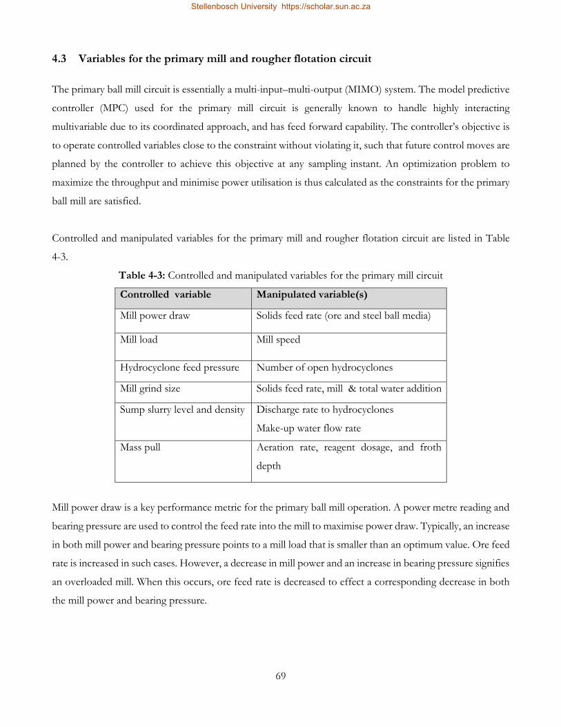
69

4.3 Variables for the primary mill and rougher flotation circuit

The primary ball mill circuit is essentially a multi-input–multi-output (MIMO) system. The model predictive

controller (MPC) used for the primary mill circuit is generally known to handle highly interacting

multivariable due to its coordinated approach, and has feed forward capability. The controller’s objective is

to operate controlled variables close to the constraint without violating it, such that future control moves are

planned by the controller to achieve this objective at any sampling instant. An optimization problem to

maximize the throughput and minimise power utilisation is thus calculated as the constraints for the primary

ball mill are satisfied.

Controlled and manipulated variables for the primary mill and rougher flotation circuit are listed in Table

4-3.

Table 4-3: Controlled and manipulated variables for the primary mill circuit

Controlled variable Manipulated variable(s)

Mill power draw Solids feed rate (ore and steel ball media)

Mill load Mill speed

Hydrocyclone feed pressure Number of open hydrocyclones

Mill grind size Solids feed rate, mill & total water addition

Sump slurry level and density Discharge rate to hydrocyclones

Make-up water flow rate

Mass pull Aeration rate, reagent dosage, and froth

depth

Mill power draw is a key performance metric for the primary ball mill operation. A power metre reading and

bearing pressure are used to control the feed rate into the mill to maximise power draw. Typically, an increase

in both mill power and bearing pressure points to a mill load that is smaller than an optimum value. Ore feed

rate is increased in such cases. However, a decrease in mill power and an increase in bearing pressure signifies

an overloaded mill. When this occurs, ore feed rate is decreased to effect a corresponding decrease in both

the mill power and bearing pressure.


70

Mill load behaviour impacts on the primary mill circuit’s efficiency. Hence, mill load volume is controlled

such that the mill operates at maximum available power through maximising ore feed rate as well as

minimising mill speed and mill inlet water, while coarse ore ratio is maintained.

The primary mill’s performance in terms of throughput, power draw and grind can be expressed as a function

of mill filling in grind curves, These are used to achieve optimal mill operation through determining

throughput, power draw, and grind peaks, relative to mill filling levels. The manipulated variables shown in

Table 4-3, as well as the feed size distribution and ore hardness also influence the grind curve. Typically, the

shape of the curves is dramatically affected by mill speed, as the mill throughput increases with mill speed,

and the grind becomes considerably coarser as mill speed increases because this promotes better impact

breakage. Hence, the mill speed, target mill filling is varied, based on the grind curves in order to satisfy the

throughput maximisation objective.

Hydrocyclone feed pressure affects the cut-point which determines whether particles report to the overflow

or underflow. A high feed pressure causes the cut point to drop and give a finer overflow. However, coarse

particles transfer to the overflow stream at even higher pressures. Hence, the feed pressure is controlled to

stabilize rougher feed particle size and density, by manipulating the number of open/closed hydrocyclones

through a valve arrangement.

The efficiency of hydrocyclone classification and rougher flotation is significantly impacted on, by the

variation in the fineness of grind. A coarse mill product results in a low liberation index, such that non-

liberated particles are not recovered during flotation. The circuit also becomes throughput limiting due to a

high circulating load to the mill. On the other hand, a very fine grind results in mineral losses during flotation

and high energy consumption rates. Typically, the amount of sub 75microns mill product particle size (grind)

lies between 40-55% for the industrial operation.

The primary mill circuit’s sump level is controlled by either increasing or decreasing sump discharge pump

speed to a hydrocyclone cluster. A dual PID cascade simultaneously controls sump density and level such

that a stable level and density is maintained. The level PID controller drives the hydrocyclone feed flow rate

set point so that the sump level is maintained at set point, while makeup water to the sump controls the

density.


71

The schematic diagram of how MPC is applied in the primary mill can be summarised as shown in Figure

4-4.

Figure 4-4 : Primary mill control

During rougher flotation, mineral recovery into the concentrate stream is achieved through mass pull control

in order to optimise grade and mineral recovery at stable concentrate flow. Mass pull and air targets set per

functional unit are achieved with fuzzy control. The rougher flotation circuit is thus operated to a desired

recipe to stabilize both individual cell and consequently, functional unit mass pulls.

A mass pull controller calculates a mass pull flowrate from the concentrate flowrate and density. The mass

pull is monitored by froth cameras, which are installed above each rougher flotation cell to perform froth

image analysis. These cameras measure the amount of bubbles present, bubble size, colour as well as their

direction and rate of movement. The mass pull controller manipulates flotation cell level (and hence froth

depth), aeration rate and reagent dosing rate. Controlling the flotation cell level minimizes long-term variation

in flotation performance due to steady-state changes in flotation feed, while airflow control assists with rapid

response to disturbances. Hence, cell level is varied over a wide range for concentrate grade control, but

within a defined acceptable operating window such that changes in operating conditions between cells,

changes in milling performance and ore type are managed. However, the level is manipulated slowly in order

to maintain setpoint tracking and achieve a stable circuit. Typically, a residence time of 30minutes is achieved

in rougher flotation.


72

4.4 Operational performance at the Concentrator plant

Operational performance at the Concentrator plant is assessed across the three metrics shown in Figure 4-5.

Figure 4-5: Operational performance metrics

Safety management is a priority for all the work conducted within the concentrator plant. All work is executed

in strict adherence to organizational safety procedures. Preventative maintenance is an essential control

implemented for employee, equipment and environmental protection amongst other key purposes. Assets

are managed through scheduled preventative and predictive equipment maintenance, to enhance equipment

reliability and increase the time between failures. As a result, the costs associated with inefficient processes

and production losses during equipment breakdowns are minimized.

Scheduled maintenance for major primary mill circuit equipment occurs once in every two months. Mill

ancillaries and peripherals that include conveyance systems (pumps, conveyor belts, as well as delivery and

transfer pipes) are attended to more often. During maintenance periods, flotation cells and respective

peripheral ancillaries are drained, cleaned and worn out flotation cell components are replaced. Similarly,

reagent tanks and lines are also flushed out and cleaned to prevent reagent delivery pipe blockages which

result in poor dosage and consequently, poor flotation performance. Instrument replacement and

recalibration in the primary mill circuit is another key scope during maintenance shutdowns.

Key performance indicators (KPIs) are tracked to assess profitability and identify any gaps between actual

performance and management objectives.

Zero harm to equipment and personnel

Safety

Profitability

Asset management

Operational performance

Plant scheduled maintenance to reduce downtime

Satisfactory key performance indicators


73

4.5 Process performance monitoring strategies

4.5.1 Offline sample analysis

Online assay analysis for the primary mill circuit is complemented by offline laboratory analysis. Composite

samples of mill feed and rougher flotation streams (Table 4-4) are taken every shift (eight hours) for

laboratory analysis. The 4E represents platinum (Pt), palladium (Pd), rhodium (Rh) and gold (Au), while 3E

consists of the first three elements. 3Es are assayed for the rougher tails, as base metals and gold appear in

comparatively smaller quantities.

Table 4-4: Offline sample analysis

Sample Quality sampled

Mill feed

Particle Size (%< specified sieve

sizes, mm)

4E Head grade (g/t)

Hydrocyclone streams

(overflow and underflow) Particle size distribution

Rougher feed

Grind (% < 75µm)

4E (g/t)

Rougher tails 3E (g/t)

4.5.2 Plant surveys

Annual plant surveys of milling and flotation streams are conducted to provide a critical assessment of the

primary mill circuit’s performance. Particle size distribution and densities for the primary mill discharge,

hydrocyclone feed, rougher flotation feed and tail streams are measured during these surveys. In addition,

mineral compositions the rougher feed and tail streams are determined from laboratory tests. Subsequently,

the data is used to identify opportunities for debottlenecking and process optimisation.

4.5.3 Tracking key performance indicators

Budget plans for operating expenditures and production targets are forecasted each year. Performance goals

are then developed from budget plans into more manageable and easily monitored performance metrics,

which are implementable at operational level. Subsequently, production and financial performances are

evaluated with key performance indicators (KPIs). Performance reports that track and assess KPIs are


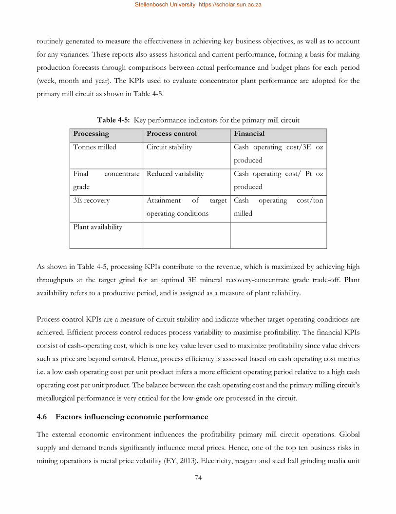
74

routinely generated to measure the effectiveness in achieving key business objectives, as well as to account

for any variances. These reports also assess historical and current performance, forming a basis for making

production forecasts through comparisons between actual performance and budget plans for each period

(week, month and year). The KPIs used to evaluate concentrator plant performance are adopted for the

primary mill circuit as shown in Table 4-5.

Table 4-5: Key performance indicators for the primary mill circuit

Processing Process control Financial

Tonnes milled Circuit stability Cash operating cost/3E oz

produced

Final concentrate

grade

Reduced variability Cash operating cost/ Pt oz

produced

3E recovery Attainment of target

operating conditions

Cash operating cost/ton

milled

Plant availability

As shown in Table 4-5, processing KPIs contribute to the revenue, which is maximized by achieving high

throughputs at the target grind for an optimal 3E mineral recovery-concentrate grade trade-off. Plant

availability refers to a productive period, and is assigned as a measure of plant reliability.

Process control KPIs are a measure of circuit stability and indicate whether target operating conditions are

achieved. Efficient process control reduces process variability to maximise profitability. The financial KPIs

consist of cash-operating cost, which is one key value lever used to maximize profitability since value drivers

such as price are beyond control. Hence, process efficiency is assessed based on cash operating cost metrics

i.e. a low cash operating cost per unit product infers a more efficient operating period relative to a high cash

operating cost per unit product. The balance between the cash operating cost and the primary milling circuit’s

metallurgical performance is very critical for the low-grade ore processed in the circuit.

4.6 Factors influencing economic performance

The external economic environment influences the profitability primary mill circuit operations. Global

supply and demand trends significantly influence metal prices. Hence, one of the top ten business risks in

mining operations is metal price volatility (EY, 2013). Electricity, reagent and steel ball grinding media unit


75

pricing, as well as 3E metal prices are subject to cost inflation and exchange rate movements. Inflation and

exchange rate trends, as well as metal price movements are presented in Appendix B.

Increased scale of production together with improved electricity and consumable utilisation are two strategies

employed to maximise profit. Efforts towards reducing the consumption of electricity and consumables,

consistent with achieving satisfactory performance is continuously made. Since maximizing profit is not

entirely dependent on minimizing operating costs, efforts are also made to achieve target production

tonnages.

Based on the discussions and derivations in this section, the following conditions improve the economic

performance of the primary milling circuit:

1. Throughput maximisation and 3E mineral recovery control

2. Efficient consumable and electricity consumption

3. Effective scheduled maintenance

4. Improved market conditions (exchange rate, metal pricing)

5. Supply conditions (consumable prices, electricity tariffs)

The first three factors are manageable within operations, while the remaining two factors are beyond the

control of the organization.

4.6.1 Economic performance assessment of primary mill circuit

The primary mill circuit’s economic performance was derived so that suitable benchmark data sets for the

process monitoring tool could be identified. Financial KPIs referred to in Section 4.5.3 were derived, as well

as the profit realised for the years 2012-2016. In order to mask confidential industrial data, normalised values

(determined as shown in Appendix C - Equation 1) were presented. Detailed cost elements for the primary mill

circuit are shown in Figure 4-6. Appendix D shows normalized consumption rates for the cost elements.


76

Discharge sump

Rougher flotation

Primary mill

Primary cyclones

Promotor Electricity Steel ballDepressantFrotherCollector

Mill motor

Conveyor belts

Pumps , agitators

pumps

Figure 4-6: Operating cost elements

The cost distribution of major elements in the primary mill circuit for the years 2012 to 2016 are presented

as percentages in Figure 4-7.

Figure 4-7 : Distribution of operating costs

62,45 67,77 64,41 64,8 60,48

35,2631,86

33,99 33,5637,93

2,29 0,37 1,59 1,64 1,59

0

20

40

60

80

100

2012 2013 2014 2015 2016

Co

ntr

ibuti

on

to

to

tal c

ost

, %

Year

Electricity Steel ball media Reagents


77

In agreement with several literature (e.g. Matthew & Craig, 2013; King, 2001), a similar trend is observed

throughout the years, where electricity costs (derived from equipment listed in Appendix E) contribute the

largest percentage towards the assessed cost structure. Steel ball costs are a significant cost that is influenced

by the amount of tonnage processed (Appendix F). Reagent cost contributed the least to overall cost

structure. The significant drop after the year 2012 was based on a management decision to lower reagent

dosage rates (depressant, collector and promotor) as a cost-cutting initiative (Appendix D). This decision

was supported by laboratory test work results, which showed satisfactory performance at the lower dosage

rates.

The financial KPIs identified in Table 4-5 were also derived for the primary mill circuit for the years 2012 to

2016 (Appendix G). To this end, cash operating costs only constituted variable costs that included

consumables (steel ball grinding media and reagents), and electricity. Maintenance materials and supplies,

other utilities i.e. water and compressed air, as well as labour for both scheduled and unscheduled

maintenance were not included in the assessment based on the same reasoning used for the cost associated

with mill liner replacement. Constant fixed costs and consumable unit prices were assumed in the

performance assessment. Although industrial electricity tariffs vary according to seasonality, time of use,

peak demand and the power factor, a flat rate was assumed for electricity unit cost.

Appendix I presents the metal sales revenue, operating cost and profit realised from operating the primary

mill circuit. Rougher flotation feed was assumed the final sellable product. However, an adjustment factor

was applied to account for downstream beneficiation. The spot metal prices and calculation formulae used

in this assessment are presented in Appendix J and Appendix C, respectively.

Chapter Summary

Chapter 4 has reported on critical site survey findings at the industrial Concentrator plant. A background to

the primary mill circuit operation, process control and economics was provided. The strategies implemented

for economic performance monitoring were presented, and factors affecting economic performance were

identified as well as illustrated. It was possible to derive historical economic performance for the primary

mill circuit in monetary terms. This was a necessary step towards developing a benchmark for the process

monitoring tool. The next Chapter presents a research methodology for developing a reliable EPF and

subsequently, a process monitoring tool for the industrial primary mill circuit. Furthermore, the economic

impact of three different simulated fault events is assessed to investigate fault detection with EPFs.


78

CHAPTER 5: RESEARCH METHODOLOGY

Chapter Overview

This Chapter first provides a background on the research design and introduces industrial and simulation

case studies. A research methodology is presented to address objectives for the industrial case study i.e., to

develop a reliable EPF with industrial data, and to derive an overall economic performance index for the

primary mill circuit. Similarly, methodology steps to assess the feasibility of fault detection with EPFs is

presented for the simulation case study.

5.1 A background on case study research methods

The application of case study research is relevant in many fields and disciplines. Case studies give an insight

into the context of the study and illustrate the main point (Fry et al, 1999). Wei & Craig (2009c) regard case

study as an appropriate research method used to examine and evaluate the relevance of existing theoretical

propositions and practice. In addition, past studies and complex issues are explored to gain an in-depth

understanding (Gulsecen & Kubat, 2006).

There are generally three types of case studies i.e., exploratory, descriptive, and explanatory (Ponelis, 2015).

Exploratory case studies critically focus on any significant observation that serves as a point of interest to

the researcher. For instance, a hypothesis can be derived or cause-and-effect relationships tested (Yoon &

Hwang, 1995). Descriptive case studies on the other hand, rather describe a significant observation and

finally, explanatory case studies examine the significant observation to the extent of explaining it (Zaidah,

2007). Jankowski et al. (2011) classified retrospective, snapshot and longitudinal case study research according

to the time dimension. In retrospective case studies, a past significant observation is studied. However,

snapshot case studies are more concerned with examining the significant observation within a particular

period. Lastly, longitudinal case studies compare a significant observation over time.

According to Baxter & Jack (2008), single or multiple case studies can be conducted. Multiple case studies

enable an understanding of the differences and similarities between cases (Stake, 1995). Furthermore, they

allow for a wider exploration of the observation and hence, are considered to be more reliable since a

significant observation can be analysed both within and across situations (Baxter & Jack, 2008; Yin et al.,

2002).


79

Case studies are conducted as qualitative and quantitative research. Qualitative research is common in

exploratory case studies where data are collected through direct encounters. Often, verbal data is acquired

using interviews, discussions, and surveys as research tools rather than measurements. The information

gathered is indicative and can only be analysed in an interpretative manner (Williams & Dame, 2015).

Quantitative research on the other hand, involves generating numerical data or information that is converted

into measurements that may be statistically analysed. Typically, experiments and surveys are used in

quantitative research (Creswell, 2003).

Quantitative research often involves finding evidence to either test predictive hypothesis or investigate

generalizability, reliability or causality. Generalizability investigates the extent to which the results of a study

can be applied beyond the sample to a larger population. A previous study is repeated to establish the

consistency of its findings when reliability is investigated. However, causality is concerned with cause and

effect relationships (Heale & Twycross, 2015). For example, static and dynamic relations among system

variables and parameters are investigated so that a system's behaviour is described in quantitative

mathematical terms (Isermann & Balle, 1997). To this end, statistical models are applied to establish and

assess relationships as well as test the relationship strength and significance, typically with correlation and

regression analysis (Bax, 2004; Chi, 1997).

Unlike quantitative research, qualitative research is not limited to rigidly defined variables. Complex

questions that are difficult to resolve or understand by quantitative research are examined further. The

findings of qualitative research are instructive and based on the sample., hence, not usually generalizable.

Consequently, it is difficult to replicate or make systematic comparisons with the qualitative approach

(Bryman & Bell, 2007; Hoepfl, 1997). The key disadvantage of a qualitative approach is the subjectivity

associated with a researcher’s perception. Hence, the interpretation of research findings is usually researcher

biased.

On the other hand, the research problem is stated in very specific terms when a quantitative approach is used

(Frankfort-Nachmias & Nachmias, 1992). The researcher remains objectively separated from the study or

investigation and only needs to appreciate the assumptions inherent within different statistical models (Wei,

2010). Thus, quantitative research possesses a high reliability level and is easily replicable when the methods

used are well explained (Creswell, 2003). However, the outcomes of quantitative research are limited to those

outlined in the research objectives, and this is unlike qualitative research. To maximise the benefits of both


80

qualitative and quantitative approaches, triangulation is used to synthesize both approaches and improve

research validity and reliability (Denzin, 1998).

The next section introduces the industrial case study and presents the research methodology.

5.2 Industrial case study

The following objectives were defined for the industrial case study:



3. To assess the feasibility of industrially implementing an online process monitoring tool for the circuit,

using one key controlled variable; and

4. To assess the feasibility of incorporating additional key controlled variables in the process monitoring

tool.

5.2.1 Case study data sources and research instruments

This study used a triangulation of literature survey of academic books, journals and electronic sources, semi-

structured interviews, a survey of the industrial operation, and simulation experiments to gather primary and

secondary data. The literature survey provided a good basis to construct interview questions and

contextualize literature findings to the objectives of this study.

5.2.2 A background to EPF development

The development of EPFs was informed by expert knowledge and literature findings. Based on the EPF

developed by Edwards & Vien (1999) at laboratory scale, operating data was empirically analysed using a

linear second-order model with first term interactions (Equation 5-1). Furthermore, model predictive control

in its common form uses a linear model to represent the dynamic process within separate time periods, and

a quadratic objective function is used to drive controlled variables back to their set points (Beigler, 2010).

Thus, the selected model is justified.

P = 𝛽𝑜 + ∑ 𝛽𝑖𝐶𝑉𝑖

𝑘

𝑖=1

+ ∑ 𝛽𝑖,𝑖𝐶𝑉𝑖2 + ∑ ∑ 𝛽𝑖,𝑗𝐶𝑉𝑖𝐶𝑉𝑗 + 𝜀

𝑘

𝑗=𝑖+1

𝑘−1

𝑖=1

𝑘

𝑖=1

5-1


81

Where βo and βi are regression coefficients

P – profit function

CV – economically significant controlled variables

i,j – ith observation of jth controlled variable

ε – residual

Single-predictor (SP) and multi-predictor (MP) linear regression EPFs were developed between CV and

mineral recovery data. Single-predictor EPFs were developed with the most economically significant CV,

and subsequently used to develop an algorithm for the process monitoring tool. On the other hand, multi-

predictor EPFs were developed using all economically significant CVs for the primary mill circuit to further

assess the feasibility of incorporating more CVs into the process monitoring tool and account for underlying

CV interactions. Key revenue and cost metrics associated with the primary mill circuit were incorporated to

improve the representativeness of the EPF.

5.2.3 A background to the process monitoring tool

Primary mill circuit monitoring was investigated with a Shewhart control chart to detect degrading economic

performance. To this end, a reliable single-predictor EPF was first developed with industrial data from a

satisfactory operating period. Subsequently, a base case EPI that represented the historical benchmark was

derived as the Shewhart control chart mean. It was anticipated that degrading economic performance could

be detected from process observations using control chart rules discussed in Section 0.

5.2.4 Selection of economic performance scenarios

The main aim for long term process monitoring is not only to track performance, but diagnose the reasons

for good and bad performance. As such, three economic performance scenarios i.e., base, best, and worst

cases were identified to firstly, validate the historical benchmark and secondly, to investigate the proposed

process monitoring tool working concept. Benchmark validation was necessary to provide a credible process

monitoring tool, and for appropriate process action to be taken.

The selection of performance scenarios was influenced by factors summarised in Figure 5-1.


82

Control system performance

Circuit stability Circuit Uptime Key performance

efficiency factors

Primary mill circuit

Process performance scenarios

Best caseBase case

Worst case

Control system performance

Circuit stability Circuit Uptime Key performance

efficiency factors


Process performance scenarios

Best caseBase case

Worst case

Figure 5-1: Factors influencing primary mill circuit performance

The base case scenario consisted of satisfactory performance from normal operating conditions. The best

case represented a good operating period with minimal performance variation. Finally, the worst case

scenario was derived from a period with unstable circuit operation and large performance variation.

5.2.5 Methodology for EPF development

The theoretical framework of Wei & Craig (2009b) presented in Section 2.7 was used to develop research

methodology steps for this study as discussed in the following sections:

5.2.6 Determining information requirements for EPF development

A thorough examination of the primary mill circuit flowsheet was conducted for an appreciation of the type

of historical production data captured. Historical data for the period January 2012 to April 2016 were

available for assessment. Consultations and semi-structured interviews with site experts provided further

information on the process (Appendix A). In addition, data logged into control room log-sheets, laboratory

assaying reports, production and financial reports were analysed. Appendix K lists data of interest, which

included key controlled variables, revenue and cost elements relevant to the primary mill circuit for EPF

development.

5.2.7 Identifying key controlled variables

An in-depth process understanding from literature survey and site expert opinion informed the selection of

key controlled variables for the circuit. Two Plant Metallurgists, a Process Control Metallurgist, and Project

Engineer were each asked to select key controlled variables in terms of economic significance, based on the


83

impact of controlled variables on the operating objective, i.e. to maximise throughput and at that throughput,

optimise mineral recovery. Table 5-1 ranks controlled variables for the primary mill and flotation circuit

based on the industrial experts’ input.

Table 5-1: Controlled variable ranking in terms of economic significance

Controlled variable Percentage agreement

amongst consulted

experts

Mill load 100

Particle size 100

Mass pull 75

Sump slurry density 50

Hydro-cyclone feed pressure 25

Sump level 25

Mill power 0

At least half of the experts selected mill product particle size, mill load, sump slurry density and mass pull

as the most economically significant CVs, and this was in agreement with most literature sources (e,g,.

Hodouin, 2011; Le Roux et al.,2013; Pomerleau et al., 2000; Ramasamy et al., 2005). None of the consultants

selected mill power as it does not influence the operating objective and hence, revenue elements. Therefore,

these four CVs were adopted as predictors for regression analysis in EPF development.

5.2.8 Retrieving the required information

The data of interest identified in Appendix K were retrieved from the plant historian, as well as archived

production, laboratory and financial reports. Online data for both standby and duty equipment (where

relevant) were retrieved from the Plant Historian in thirty-minute time stamps. The time stamp was nominal

for retrieving large amounts of data since a shorter time stamp significantly slowed down data retrieval.

Offline assay data was available from laboratory archives in eight-hour time stamps. Both online and offline

data were available in Microsoft Excel format.

The following control measures were exercised for efficient and correct data retrieval from the Plant

Historian:

1. Listing all the data to be accessed from the plant historian.

2. Accurately identifying plant historian data tags corresponding to data of interest.


84

3. Ensuring the inclusion of both standby and duty equipment, as necessary.

5.2.9 Pre-treating the data

Integrating and cleaning data

Online data were rolled up into shift averages in Microsoft Excel to correspond with the sampling frequency

for laboratory assay-data. Thereafter, the data were organized into meaningful data sets to minimize errors

associated with handling the large amounts of data. Related data were classified into separate folders as cost,

revenue and CV data. The cost folder consisted of electricity, reagent and steel ball consumption rates.

Correspondingly, the revenue folder consisted of the mineral recovery, rougher flotation feed assays, rougher

tail assays and mill throughput data. Lastly, the CV folder consisted of data identified in Section 5.2.7.

Illogical and anomalous data entries that were negative, or labelled ‘Not connected’, ‘NaN’ and ‘ERROR’

were detected in online process data. These data elements likely resulted from faulty instrumentation or

measurements taken during plant downtime periods. Furthermore, some data elements were missing in

laboratory assays and online measurements. These faulty data were handled in MATLAB as follows:

Outlier data

Outliers were identified as controlled variables and mineral recovery data elements lying outside three sigma

lower and upper control limits (LCL and UCL). The outliers as well as values corresponding to identified

outliers were deleted so that functional relationships between variables and their data were preserved. This

step was performed to twice in order to minimize outlier influence on regression modelling. Moreover, doing

this ensured that a reasonably representative amount of data was available for EPF development. In contrast,

data quality would be compromised due to loss of useful process data variation from an iterative deletion

process with classical outlier analysis.

Missing data

Efforts were initially made to recover any missing data although none of the data was recovered. The use of

complete data vectors was important in subsequent methodology steps. Hence, missing data and

corresponding elements for other variables were deleted. Data imputation was not considered to avoid the

risk of introducing bias.

5.2.10 Investigating data reduction

The amount of data available for EPF development and economic performance assessment after pre-

treatment must be representative of the period assessed. Data equivalent to one year was considered to be


85

representative and sufficient for the period being assessed (Appendix C– Calculation 2). Since too many

deletions would result in less representative EPFs due to significant loss of information, variables (CV or

mineral recovery) with too many deletions were excluded from the regression analysis.

5.2.11 Investigating data normality and correlations

The normality assumption was tested by plotting quartile-quartile (Q-Q) normality probability plots for CV

and mineral recovery data in order to assess the appropriateness of applying statistical tests. A scatterplot

matrix was plotted and corresponding bivariate correlation coefficients were determined for all CVs and

mineral recovery to determine data correlations. A correlation coefficient of at least 0.7 suggested a strong

relationship between the investigated CVs, between which a joint economic performance function would be

derived (as discussed in Section 2.7).

5.2.12 Simplifying assumptions

Simplifying assumptions were made for the process operation, process control, and process economics as

follows:

Assumptions for process operations

1 There were no significant configuration changes in the primary mill circuit during the reviewed

period.

2 Historical changes in reagent types and steel ball sizes had a negligible influence on operating

conditions.

3 There were no analytical and transcription errors in laboratory assay results.

4 The particle size-mineral recovery EPF was quadratic

Assumptions for process control

1. The MPC was performing well and hence process data fit a normal distribution.

2. There were no measurement lags in the data. Typically, plant data is appropriately time shifted to

account for time delays, and lagged to account for any autocorrelations in the data (Remes et al., 2006;

Smith et al., 2004).

3. All control loops were well maintained throughout the reviewed period.


86

Assumptions for process economics

1 In order to assess the sensitivity of process conditions (i.e. factors within the control of industrial

personnel) on economic performance, the economic environment was assumed constant. Hence,

cost element unit prices, the exchange rate, and 3E basket price were fixed.

2 Electricity unit cost was equivalent to the industrial flat rate.

3 Plant overheads and maintenance costs were constant and hence not included in the assessment.

4 Economic performance for the primary mill circuit was equivalent to the profit before fixed costs.

5 The rougher flotation concentrate was the final sellable product. However, an adjustment was made

to the metal basket price to account for downstream beneficiation.

5.2.13 Identifying benchmark data set

As previously highlighted, the benchmark data set was identified to achieve two purposes i.e., to train the

EPF model, and to derive the primary mill circuit EPI. Since EPFs change with time, the timeliness of this

data set was considered important. Hence, the benchmark data set consisting of 21 shifts was identified from

a recent processing period, through the following steps:

Five performance metrics that represented key economic objectives for the primary mill circuit (i.e. electricity

consumed per ton milled, production cost per ton milled, tonnage processed, 3E mineral recovery and profit)

were assessed to identify a representative benchmark. The profit realised from primary mill circuit operation

summarised these factors and was therefore, used as the criterion to assess economic performance.

5.2.14 Validating the selected benchmark

Three economic performance scenarios i.e., best, base and worst case performances were used to validate

the selected benchmark. Data equivalent to seven shifts was used for each economic performance scenario.

The EPI for each shift was derived and plotted onto a Shewhart control chart. It was expected that base

case EPIs would lie around the benchmark while the best case and worst case EPIs would lie above and

below, respectively.

5.2.15 Identifying approaches to EPF development

EPFs were developed using two comparative approaches referred as process variable analysis (PVA) and

financial elements analysis (FEA) in this study. The financial profit and mineral recovery were used as

respective profit functions. Subsequently, an economic performance function between the primary mill

circuit CVs and mineral recovery was modelled using both SP and MP second-order regression analysis for


87

the PVA approach. In the FEA approach, financial profit derived from the metal sales revenue and unit level

costs was used. Formulae for the following calculations are presented in Appendix C.

Process variable analysis

EPF single-predictor and multi-predictor linear regression models were developed as a function of CV and

mineral recovery data as shown in Equations 5-2 and Equation 5-3, respectively.

EPF𝑃𝑉𝐴: 𝑀𝑅 = 𝑓𝑃𝑉𝐴(𝐶𝑉𝑃𝑆)

5-2

EPF𝑃𝑉𝐴: 𝑀𝑅 = 𝑓𝑃𝑉𝐴(𝐶𝑉𝑎𝑙𝑙) 5-3

Where CVPS – particle size controlled variable

MR - mineral recovery (%)

CVall – all controlled variables

Financial elements analysis

Financial profit was derived as shown in Equation 5-4 to Equation 5-6:

P = R − C

5-4

Where P - financial profit (ZAR)

R – 3E metal sales revenue (ZAR)

C – operating cost (ZAR)

R = f(F, BP𝑎𝑑𝑗 , HG, MR)

5-5

Where F - throughput rate (tph)

BPadj - adjusted basket price (ZAR/oz).

HG - 3E head grade (g/t)

MR - mineral recovery (%)

The basket price was derived from a prill split percentage (adopted from May 2016), since platinum is mined

as part of a basket of metals with each metal priced differently. Spot metal prices and exchange rates as at 06


88

June 2016 were adopted (Appendix J), and an adjustment factor of 0.65 was used to account for downstream

beneficiation. The cost was derived as below:

C = f(ci, ui)

5-6

Where ci – cost element consumption rate (units)

ui - cost element unit price adapted from Concentrator data for April 2016 (ZAR/unit)

Subsequently, the EPF was developed using multi-predictor linear regression, as shown in Equations 5-7.

EPF𝐹𝐸𝐴: 𝑃 = 𝑓𝐹𝐸𝐴(𝐶𝑉𝑎𝑙𝑙)

5-7

Where EPFFEA - EPF derived from financial elements analysis

CVall - particle size, mill load, sump density, and mass pull

5.2.16 Identifying EPF development strategies

The following two strategies were investigated:

1 EPF development with base case data

2 Searches for EPFs throughout pre-treated historical data

In the first case, both PVA and FEA were investigated for SP and MP linear regression EPF models. Sliding

window searches were applied in the PVA approach due to computational limits and a prior knowledge on

the limited likelihood for valid EPFs with this approach. Valid EPFs possessed good model fit (with an R2adj

threshold value of at least 0.6) and reliable predictive capability.

5.2.17 EPF development with base case data

A sample size of 100 shifts was further selected for EPF model training, and 50 shifts for testing EPF validity

during the identified base case period. These sample sizes moderated the effects of very large and very small

sample sizes. Furthermore, they were representative of the amount of data available for analysis.

5.2.18 Searches for valid EPF

Based on the assertion of Hodouin (2011), steady-state changes in process disturbances induce a perpetually

transient economic performance curve (Figure 5-2). Several studies have supported these findings (e.g.,

Bauer et al., 2007; Cutler & Perry, 1983; Contreras-Dordelly, 2000; Craig & Henning, 2000; Gupta et al.,

2013; Herbst & Lo, 1996; Muske & Finegan, 2001; Oosthuizen et al., 2004). As such, it was reasonable in this


89

study to assume that different EPFs are generated each time a different steady state is attained. From this

perspective, it was likely that poor EPF accuracy would result over a large operating window. Therefore, a

reasonably sized sliding window that sufficiently captured steady states was applied to search for valid EPFs.

To this end, a window sampling scheme and window size were determined.

Figure 5-2 : Transient performance curve

Determining window sampling scheme

Sequence-based and timestamp-based sliding windows are two common window schema (Braverman et al.,

2009). Previous data elements cease to be significant and only the most recent ones (as relevantly defined)

are considered for analysis in a sequence-based window. Hence, the sequence-based window is more

appropriate for cases where data elements have regular, fixed sampling intervals for all variables. A

timestamp-based window on the other hand, analyses all data elements that lie within a specified time interval.

Data elements for the timestamp-based window may vary over time as opposed to a fixed number of data

elements when the window size is specified (Babcock et al., 2002; Wang & Tsung, 2005). In this study, a

sequence-based window of fixed size is applied. The earliest shift (based on time) expired from the window

sample at each window slide


90

Determining window sample size

Window sample size can affect statistical tests by either making them insensitive (at small sample size) or

overly sensitive at very large sample sizes. Small window sample sizes generally result in too little statistical

power to identify significant results, and data are easily over-fit to produce artificially good results. However,

effects such as variable correlations are initially found to be statistically significant until at a very large sample

size where almost any effect is significant (Hair et al., 2010).

For this study, window sample size were large enough to cover the period during which steady state was

assumed. Thus, a window size equivalent to two weeks (i.e., 42 shifts) was regarded to be sufficient.

Moreover, it constituted a representative fraction of the data amount available for analyses. For further

comparison, a window size of one week (i.e., 21 shifts) was investigated.

5.2.19 Performing sliding window iterations

Sliding window iterations were performed, and the following measures were plotted for each window slide

iteration:

1 Window sample mean, standard deviation and the relative standard deviation (RSD) for all CVs and

mineral recovery

2 R2adj for model developed with window sample data, and for model developed between mineral

recovery and CV data for a consecutive window (R2adj,pred)

3 Mineral recovery predictions for a consecutive window

Window mean, standard deviation and RSD were used to observe and compare variability across windows.

Regression coefficients for EPFs with above threshold R2adj values were evaluated based on a calculated p-

value of less than 0.05. Subsequently, a reduced regression equation consisting of significant predictors was

developed and tested for reliability. A reliable EPF exhibited valid mineral recovery predictions for test data

in a consecutive window.

5.2.20 Investigating measurement lags

EPF models between the mineral recovery in a preceding window and CV data in a subsequent window were

developed to investigate the possibility of measurement lags. Hence, test results (R2adj,test) were determined

for each window slide.

5.2.21 Developing a process monitoring tool

The process monitoring tool was developed with a valid and reliable single-predictor EPF. Predictions for

the primary mill circuit’s economic performance would be made with this EPF. It was necessary to first


91

review all the computations performed, prior to implementing the process monitoring tool in the industrial

operation.

5.2.22 Determining the overall economic performance index

The PVA approach was used to estimate the EPI for the primary mill circuit since the FEA approach had

been demonstrated in Section 4.5.3. Time fluctuations for the variables were discretized into a histogram and

the EPI was derived with Equation 5-8

𝐸𝑃𝐼𝑃𝑉𝐴,𝑜𝑣𝑒𝑟𝑎𝑙𝑙 = ∑ 𝐹𝑗(𝐸𝑃𝐹𝑉𝑎𝑙𝑖𝑑)𝑗

𝑀

𝑗=1

5-8

where

EPIPVA - average economic performance index for the PVA approach

Fj – economic performance for each bin interval

EPFvalid - valid single-predictor or multi-predictors’ EPF

j –the bin number

M – total number of bins

The optimal bin width was determined using Equation 5-9 (Scott, 1979).

B𝑤 = 3.49s × 𝑀1/3 5-9

where

Bw - bin width

s - estimated standard deviation,

M - number of bins.

Generally, 5-20 histogram bins were sufficient (He & Meeden, 1994; Knuth, 2013).

5.2.23 Testing the process monitoring tool for implementation feasibility

The process monitoring tool was tested for implementation feasibility at the Concentrator plant. The key

test criterion was the tool’s ability to derive the EPI based on a valid EPF, and plot it onto the Shewhart

chart. After successive observations, the primary mill circuit’s economic performance would be assessed

based on EPI spread around the historical benchmark, using indicators listed in Table 5-2 .


92

Table 5-2: Economic performance indicators

Indicator Criteria

Outlier economic

performance

One point exceeds UCL or LCL benchmark performance

Runs Nine points above/below the benchmark performance

Four out of five points are above/below the benchmark

performance and exceed the ±σ limit.

Fifteen points are within the ±σ limits

Good/bad trend Six consecutive points show continual rise or fall of economic

performance indices.

Eight consecutive values are beyond the ±σ limits

Periodicity Defined as economic performance indices showing fluctuating

behaviour over time.

Difference of consecutive values alternates in sign for fourteen

points

Regular re-evaluation of the EPF used to develop the process monitoring tool was important since economic

performance functions change within the same process over time (Wei & Craig, 2009c).

5.2.24 Process monitoring post-implementation

With time, good or bad economic performance must be critically reviewed for continuous performance

improvement. For example, when high profit is consistently achieved the following questions must be

investigated:

1. What changed in the primary mill circuit’s operation?

2. Is the change repeatable?

3. Can the change even be enhanced in future operation?

However, answers to the following questions are necessary in the event of a loss:

1. What went wrong or influenced the loss incurred for the primary mill circuit?


93

2. Is the cause from the preceding question avoidable?

3. What steps can be taken to prevent the loss from recurring?

Figure 5-3 provides a summary of the industrial case study methodology steps.


94

Start

End

Collect data Online data from

Plant historian Offline laboratory

assays Financial data

Perform regression analysisBase case and EPF searches

FEA analysisDerive the revenue, cost and

profitEstimate EPI

Analyze data Estimate PDFs for each CV Select suitable performance

assumptions Identify performance

scenarios Validate base case

Data storage and security Make assumptions

Estimate EPF models FEA analysis PVA analysis

Data analysis

Select window size Determine regression statistics

(Adjusted R squared, p-values Significance tests

Determine information requirements

Identify key information sources

PVA analysisDetermine the CVs of

interest

Multi-predictor All CVs vs. mineral

recovery (PVA)

Single-predictor Particle size vs profit

(FEA) Particle size vs. mineral

recovery (PVA)

Are EPF models valid

Data pre-treatment

Develop PM tool Yes No

Implement PM tool

Figure 5-3: Summarized industrial case study methodology steps


95

5.3 Simulation case study

5.3.1 Objectives

The following objectives were defined for the simulation case study:

3. To derive the economic performance of a SAG mill circuit subject to three common industrial faults;

and



5.3.2 Simulation case study background

The simulation case study uses typical production and control objectives for a SAG mill circuit, to investigate

the economic impact of extreme changes in process conditions, i.e. faults. Faults can result in variable circuit

throughput and delivery of inconsistent product particle size (Wills & Napier-Munn, 2006). A priori particle

size-mineral recovery EPF adopted from Edwards & Vien (1999) was used to evaluate the economic impact

of three simulated faults.

The simulation case study offered control over the fault type and sizes, as well as the time window for fault

detection. Process recovery in the simulation experiments was effected by PID control. This controller type

consists of proportional, integral and derivative tuning parameters that are varied for an optimal response.

Reference can be made to Khandalkar, et al. (2015) and Wu et al. (2015) for more information on this

controller.

5.3.3 Overview of the SAG mill circuit

The process description has been presented in Section 1.1.1. The SAG mill circuit is operated to produce at

reasonable throughput, a target product particle size from which good recovery can be achieved. In addition,

steel ball and electricity consumptions are minimized (Coetzee et al., 2008; Craig & Macleod, 1996; Matthews

& Craig, 2013). These objectives require certain trade-offs to be made.

5.3.4 A background to simulation models

Simulation models are widely used to analyse industrial processes, to test several scenarios and investigate

effects which are impractical or too expensive to perform on a real process (Hangos & Tuza, 2001).

Furthermore, reliable proof of concept results are made available before the investigated concept can be

implemented in a real process (Barton, 2013). Simplifying assumptions are often made when simulation


96

models are developed since not all possible situations to which a real plant process is exposed may be

simulated. Therefore, models differ in terms of the objective being investigated, which in turn influences the

derivation complexity and amount of data required for model calibration (Runge et al., 2007).

5.3.5 Le Roux’s SAG mill model

Le Roux et al. (2013) validated a nonlinear SAG mill circuit model, which used the least amount of parameters

and equations. This model is applicable over a wide operating range and model parameters were fit using

steady state data obtained from industrial surveys. Le Roux’s model consists of four system volumes in a

closed loop SAG mill circuit i.e., the feeder, SAG mill, sump and the hydrocyclone. A perfectly mixed sump

volume is assumed, and hydrocyclone dynamics are independent of changes in feed density.

Process streams exist in five states i.e., rocks, solids, fines, steel balls and water. The rocks and steel balls are

too large to exit the mill and hence, are consumed in the mill. Solids consist of coarse and out of specification

particles that are small enough to be discharged from the mill, while fines are of target specification. Figure

5-4 shows modules and variables for the SAG mill model.

Figure 5-4: Single staged close circuit SAG mill circuit (Adapted from Le Roux et al., 2013)

Cyclone feed (CFF)

Sump water (SFW)

Mill feed solids (MFS)

Mill inlet water (MIW)

Particle Size (PS)

Sump volume (SVOL)

Mill load (LOAD)

Mill feed balls (MFB)


97

5.3.6 SAG mill circuit process variables

SAG mill circuit CV-MV control loop pairings are shown in Figure 5-5.

Hydro-cyclone

SAG Mill

Sump

Feeder

Water

Ore

BallsWater

Ground ore

MFS

LOAD

SFW

SVOL

CFF

PS

scre

en

Figure 5-5: SAG mill circuit control loops (Redrawn from Wakefield, 2015)

Table 5-3 lists the CV-MV loop pairings.

Table 5-3: CV-MV loop pairings

Controlled variable Manipulated variable

Mill volume fill (LOAD) Mill feed solids (MFS)

sump volume (SVOL) Sump feed water (SFW)

particle size (PS) Cyclone feed flow (CFF)

5.4 Simulation case study design

Meaningful simulation results significantly depend on an appropriate experiment design. Poorly planned

simulation experiments can give results that provide little insight, or at worst provide misleading results


98

(Barton, 2013). Therefore, experiments must generate unbiased simulation data that capture the dynamics of

the process variables considered. Typically, costly decisions are made based on simulation experiment results.

As such, experiments are designed for appropriate data analysis with statistical methods in order to give valid

and objective conclusions (Montgomery, 1991).

One key objective for experimental design is to estimate how results are influenced by changes in input

factors (Law & Kelton, 1991). To this end, the conditions under which a simulation experiment is conducted,

must be well defined. Although simulation experiment conditions depend on the experimenter’s goals, there

are generic steps for conducting them (Sokolowski & Banks, 2010). Barton (2013) and Leal et al. (2011)

propose the following steps for experiment design:

1. Define experiment objectives.

2. State a hypothesis to be evaluated.

3. Plan an experiment to test the hypothesis.

4. Conduct the experiment.

5. Analyse experiment results.

These steps were applied in the simulation case study as discussed below. Simulation experiments were

conducted in MATLAB’s Simulink environment using the procedure proposed by Wei & Craig (2009a).

5.4.1 Defining experiment objectives

The objectives of the experiment were:

1. To derive economic performance indices for three common faults in SAG mill circuits; and

2. To assess the economic impact of each fault.

5.4.2 Stating a hypothesis to be evaluated

The null hypothesis (H0) tested whether the economic impact of each fault event as represented by the EPI,

was indistinguishable to the simulated fault. The alternative hypothesis (H1) stated that the EPIs (and hence

economic impacts) are unique to each simulated fault. The hypotheses are shown in Equation 5-10.

𝐻0 : 𝜇𝐸𝑃𝐼,1 = 𝜇𝐸𝑃𝐼,2 = 𝜇𝐸𝑃𝐼,3

𝐻1 : 𝜇𝐸𝑃𝐼,𝑖 ≠ 𝜇𝐸𝑃𝐼,𝑗

5-10

where the subscripts 1, 2, 3 refer to each of the faults investigated and i,j are fault pairs (i,j = 1,2,3).


99

A trade-off exists between mineral recovery and mill throughput, two revenue measures that significantly

influence economic performance (Bauer & Craig, 2008). As illustrated in Wei & Craig (2009a), the null

hypothesis of these two variables is tested to investigate significant differences between any two simulated

faults. Craig & Henning (2000) followed the same approach, albeit for a flotation process.

Equation 5-11 and Equation 5-12 give the null and alternative hypotheses for mineral recovery and mill

throughput, respectively.

𝐻0 : 𝜇𝑀𝑅,1 = 𝜇𝑀𝑅,2 = 𝜇𝑀𝑅,3

𝐻1 : 𝜇𝑀𝑅,𝑖 ≠ 𝜇𝑀𝑅,𝑗

5-11

𝐻0 : 𝜇𝑇𝐻𝑅,1 = 𝜇𝑇𝐻𝑅,2 = 𝜇𝑇,3

𝐻1 : 𝜇𝑇𝐻𝑅,𝑖 ≠ 𝜇𝑝𝑇𝐻𝑅,𝑗

5-12

where the subscripts 1, 2, 3 refer to each simulated fault.

5.4.3 Identifying the significance test

Simulation results were tested for significance using a one-way analysis of variance (ANOVA). Three

assumptions are made about the data when this significance test is used. Firstly, simulation experiment data

is assumed to be random and statistically independent. Secondly, samples are extracted from normally

distributed populations, and thirdly, equal population variances are assumed.

One-way ANOVA is quite robust to deviations from these assumptions (Walck, 2007). Small departures

from normality do not significantly affect the results, and for the same sample size, the assumption of equal

population variances is not strict. However, it was prudent to investigate the equal variance assumption. The

F-test, which is a ratio of sample variances was used to find out whether samples were from the same

population. It is performed only when the one-way ANOVA shows a p-value less than the significance level.

MATLAB computes F-test statistic based on a null hypothesis of equal population variances. The critical F

value (Fcvdf1, df2) is determined using F tables and degrees of freedom (df1 and df2) corresponding to a

significance level (α). The null hypothesis is rejected for Fob > Fcvdf1, df2, where Fob is the observed F statistic.

If the null hypothesis of equal population variances is rejected, further tests are investigated. However, if the

null hypothesis is accepted, then all fault events are from the same population with the same variance.

Further multiple comparison methods i.e., the Tukey-Kramer, Bonferroni and Dunn-Šidák provide pairwise

comparisons to determine which means are different. However, the Tukey-Kramer is more preferred as it


100

has greater statistical power compared to other tests and is readily available in computer packages. Moreover,

this method is considered the best available for pairwise comparisons when confidence intervals are needed

or sample sizes are not equal for. (Ostertagova & Ostertag, 2013). P-values less than 0.05 indicate with 95%

confidence that estimated means for compared faults significantly differ from each other.

Selecting the significance level

Significance levels are rather subjective, but a significance level of 𝛼 =0.05 is typically used in most

experiments. Although, a significance level of 0.01 is used in some cases, it is considered more conservative.

The choice of significance level is influenced by the probability of a type I error occurrence where a true null

hypothesis is incorrectly rejected. In such cases, a more relaxed significance level may be used as was done

by Wei & Craig (2009a) who used 𝛼 =0.15. To achieve the intended purpose, Craig & Koch (2003) suggested

either a marginal increase in the number of replications or relaxing the significance level. This study used a

significance level of 𝛼 =0.05.

5.4.4 Planning an experiment to test the hypothesis

Simulation experiment steps were planned as follows:

1. Introducing process and sensor noise into the SAG mill model

2. Identifying independent, intermediate and dependent variables

3. Identifying common faults in semi-autogenous grinding mill circuits

Introducing process and sensor noise

Process noise was introduced in the SAG mill model using random walks, where a pseudorandom value x,

was generated with random positive and negative gradients. The gradients were numerically integrated and

added to the initial value of the input variable v in v0 as shown in Equation 5-13 and Equation 5-14

(Wakefield, 2015). This non-deterministic excitation was incorporated in input disturbance variables i.e., the

ore hardness and feed size, in order to simulate the dynamic variation seen in industrial data.

𝑠𝑖 = {

+1, 𝑥𝑖 < 0.5−1, 𝑥𝑖 ≥ 0.5

5-13

𝑣𝑀 = ∑ 𝑠𝑖

𝑀

𝑖=1

∆𝑡 + 𝑣0

5-14


https://en.wikipedia.org/wiki/Confidence_interval

101

where the subscripts i and M denote a step from time 0 to M, respectively.

A fixed sensor noise of 1% was applied to all (mill load, product particle size and sump volume) controlled

variable sensors. This sensor noise size is recommended in Castle et al. (1984). Applying a fixed size not only

simplified the simulation experiments, but also eliminated the likelihood of compromising the quality of

simulation results since there was no exact knowledge on typical industrial sizes for relevant sensor noises.

To simulate the faster variation common in sensor noise, a higher frequency of 5seconds was used for sensor

noise compared to a frequency of 10seconds for process noise.

Identifying and classifying model parameters

All fixed, dependent and independent variables were first identified for the simulation experiments to allow

for easier replications. Dependent variables are measures of interest that are not controlled independently,

but are affected by independent variable settings. Figure 5-6 shows the controlled (dependent) variables,

manipulated (independent) variables, disturbances and simulated faults for the SAG mill model.

Flotation feed

Product particle size(%<75µm)SAG mill circuit

Disturbances in ore feed hardness and

size


Mill feed balls (MFB)

Mill inlet water (MIW)

Cyclone feed flow (CFF)

Sump feed water (SFW)


Process noise

Manipulated variables

SAG mill feed

Simulated faults

Sensornoise

Figure 5-6: Model variables

Selecting experiment design parameters

Appendix L represents mathematical calculations for the SAG mill model. Model parameter input values and

initial states were adopted from Wei & Craig (2009a) and Coetzee et al., (2008). Input parameter values were

changed accordingly to represent each fault.


102

Selecting the simulation run length and sampling frequency

Simulation experiments were run for 640 simulation hours to provide a sample size large enough to apportion

data into training, test, and fault data sets. This run length was longer than the one to three days

recommended by Craig & Henning (2000) for controller simulations. The amount of experiment data

generated over the simulation length was sufficient for further classification into eight-hour shifts, to match

typical industrial data. A small sampling frequency of 10seconds was used in order to sufficiently capture

process dynamics, and generate a large historical data set to satisfy the conditions discussed above.

Identifying simulation faults

Three faults i.e. drifting mill load cell, poor quality steel ball media, and increased ore hardness were

investigated for fault detection with EPFs. The faults remained unresolved, except by simulated

Proportional-Integral-Derivative (PID) control.

5.5 Conducting the simulation experiments

5.5.1 Simulating the faults

To simulate occurrence after a long processing period, the three faults were each introduced into the

simulation run at 400hours. Although the time of fault inception was arbitrarily selected, sufficient time for

PID controller action was considered. The effectiveness with which controlled variable set points were

maintained in the simulation experiments depended on the capability of corresponding manipulated variables

to counteract the faults. Hence, the variability in economic performance was assessed and the differences

were contextualised for each fault at a later stage.

A completely randomised design was used for the simulation experiments. This design is appropriate in

constant experimenting environments as was the case for this study. The three faults given in Sections 3.4.1

to 3.4.4 were replicated five times each, to give fifteen simulation experiment runs. The experiments were

performed following the sequence shown in Table 5-4.


103

Table 5-4: Randomised simulation experiment runs

1 F2 2 F1 3 F3

4 F2 5 F1 6 F2

7 F1 8 F2 9 F3

10 F3 11 F1 12 F3

13 F2 14 F3 15 F1

where Fi is the fault number for drifting mill load cell (1), poor quality steel ball charge (2), and ore hardness

increase (3). According to the resource equation method presented by Mead & Gilmour (1988), the difference

between the number of observations and the variables being investigated must typically lie between 10 and

20. The simulation experiment design satisfied this condition.

Drifting load cell

A 45% negative drift was applied over 30minutes to the load cell sensor. In the absence of industrial

information on marginal sensor drift sizes, this drift size was iteratively determined based on reaching the

mill load constraint over a reasonably short time.

Poor quality steel ball charge

A 60% negative step disturbance was applied to the abrasion factor (φ) in order to simulate poor quality

steel ball charge (Appendix M). This step size was reasonably sufficient to simulate rapid steel ball wear.

Ore hardness increase

A 80% positive step disturbance was applied to the ore bond work index to simulate increased ore hardness.

This step size was adapted from Wei & Craig (2009a), and is common in industrial operations (Coetzee et al.,

2008).


104

5.5.2 Generating normal operating condition and fault data

For each simulation experiment, normal operating condition (NOC) and fault data were generated for the

variables listed in Table 5-5. The NOC data consisted of steady state data with random walk variations, while

the fault data was generated from fault inception until the end of a simulation run.

Table 5-5: Simulation experiment data of interest

Controlled variables - product particle size (PS)

- mill load (LOAD)

- sump volume (SVOL)

Manipulated variables - cyclone feed flow (CFF)

- mill feed solids (MFS)

- sump feed water (SFW)

Other variables - ore hardness factor

- mill load sensor

- steel abrasion factor

Cost elements - mill ball charge (MFB)

- mill power draw (P)

Revenue elements - mill throughput (F)

- mineral recovery (MR)

5.6 Analysing the data

5.6.1 Data pre-processing

The PID controller seeks for steady-state conditions as circuit transients persist at simulation run initialisation

(Rajamani & Herbst, 1991). This initialisation bias can be a major source of errors when steady state values

of system performance measures are estimated (Ghorbani, 2004). Therefore, initial transient phase data is

truncated using suitable techniques discussed in literature (e.g., Law & Kelton, 1991; McKinnon & Tipper,

1995; Schruben, 1982). According to McKinnon & Tipper (1995), the Welsh algorithm generates more

accurate results for multiple replications as was the case in this study. A manual estimation of when the

transient period ends is made after ‘n’ replications each of length ‘m’ are generated and an average across the

replications is determined. Subsequently, transient phase is visually estimated using a generally conservative

approach that deletes a longer duration of the initial transient period (Ghorbani, 2004; McKinnon & Tipper,

1995). Therefore, 10% of the simulation data was deleted as the transient phase data in this study.


105

5.6.2 Apportioning data into training, test and fault data sets

The data generated from simulation experiment runs were first averaged into eight-hour shifts to resemble

typical industrial shift periods. Data were apportioned between training, test, and fault data sets, where the

training data set comprised two-thirds of the NOC data and the remaining third made up test data. Fault

data constituted of data generated from fault inception until the end of each simulation run.

5.6.3 Selecting bin width

A very large bin width results in loss of data, while a narrow bin width produces few data points in each bin.

Thus, the number of bins selected must be sufficiently large to capture major data features while ignoring

details due to random sampling fluctuations (Knuth, 2013). Several iterations were performed to determine

the most representative bin width for mineral recovery data. Thus, a bin width of 0.05 was identified based

on the small data variation and subsequently, used to derive the average potential mineral recovery as

discussed in Section 5.7. However, the bin width for processed tonnage was derived using the Freedman-

Diaconis (FD) rule for a reasonable number of bins (Equation 20). Similarly, this bin width was used to

derive the average tonnage processed.

5.6.4 Making suitable assumptions

The following assumptions were made:

1. The SAG mill product was regarded as flotation feed.

2. The flotation product was sellable product, and was relevantly adjusted to account for costs

associated with downstream beneficiation. A value of 0.75 was adopted from Matthews & Craig

(2013).

3. The SAG mill circuit was for a PGM operation and industrial unit prices were adopted.

4. A flat industrial rate was assumed for electricity consumption.

5. Only major cost elements associated with operating the SAG mill were considered i.e., steel balls and

electricity.

6. Metal basket price, exchange rate and unit cost prices were constant.

7. The costs associated with downstream beneficiation were constant.

8. The quadratic relationship given by Edwards & Vien (1999) was assumed between the product

particle size and mineral recovery.

9. All the flow streams to the mill circuit were controllable.


106

10. The simulation data was normally distributed.

The following data analysis steps were applied for each fault:

5.7 Testing the null hypothesis

5.7.1 Deriving data averages

Mineral recovery data was inferred from the mill product particle size–mineral recovery performance

function, and the average potential mineral recovery (PR) was determined using Equation 16 to Equation 19

(Appendix N). Similarly, the average processed tonnage was derived using Equation 16 to Equation 19.

5.7.2 Deriving the sliding window economic performance index (EPI)

Economic performance indices for the training, test, and fault datasets were developed as shown in Appendix

N (Equation 21 and Equation 22). A MATLAB algorithm was developed and used to derive the sliding

window EPI.

5.7.3 Selecting sliding window size

Process conditions gradually culminate into a fault. Hence, a time-based sliding window size of 10 shifts was

selected to analyse simulation data and determine the moving economic performance index. Window sample

data were updated in increments of one shift, as the earliest shift was retired.

5.7.4 Plotting sliding window EPIs for all the faults

Sliding window normalized EPIs were plotted onto a Shewhart control chart. The mean EPI derived from

normal operating conditions for all the simulation experiments was as the assigned centre line (CL) in the

Shewhart control chart. The lower control limit (LCL) and upper control limit (UCL) were determined using

three standard deviations.

A null hypotheses of equal economic performance indices, mineral recovery, and mill throughput were tested

using one-way ANOVA as discussed in Section 5.4.3 to investigate the significant differences between any

two simulated faults. In addition, box plots were constructed for a visual analysis of mineral recovery and

mill throughput data for each simulated fault.

5.7.5 Assess scope for fault monitoring and prioritisation

Finally, scope for fault monitoring was assessed based on the detection of faults after each respective fault

was introduced in the simulation experiments. Furthermore, scope for fault prioritisation was assessed based


107

on the unique economic impact of each fault, determined from the significant differences between any two

simulated faults as discussed in the previous step.

Figure 5-7 shows a summarised methodology flow sheet for the simulation case study.

Start

End

Derive the EPI for each simulted fault event

Assess the economic impact of each fault event

Test the hypothesis

Generate normal operating condition and fault data

Conduct simulation experiments

Accept null hypothesis

NoYes

Assess scope for fault monitoring and

prioritisation

Figure 5-7: Simulation experiments methodology summary steps

Chapter Summary

Chapter 5 presented a research methodology for the industrial and simulation case studies to address the

research objectives. The next Chapter presents results and a discussion for the industrial case study.


108

CHAPTER 6: RESULTS AND DISCUSSION -

INDUSTRIAL CASE STUDY

Chapter Overview

The previous Chapter outlined the objectives and methodology steps for the industrial. This Chapter presents

industrial case study results and discusses the findings thereof.

6.1 Selection of base-case model data set

Appendix H shows the monthly performance of key indicators between the years 2012 and 2016. All the

KPIs showed variability across the years, to correspond with changes in operating conditions such as feed

ore properties and management decisions on throughput targets. The annual performances are each

summarised in Table 6-1.

Table 6-1: Key performance metrics

Key: X worst performance √ best performance

In Table 6-1, the years 2014 and 2016 each show two best and two worst cases across the years reviewed.

The year 2012 shows a best and worst case for the performance metrics considered. However, the years 2013

Key performance

metric

Years

2012 2013 2014 2015 2016

Electricity per ton milled

√

X

Production cost per ton

milled

√

X

Tonnage processed

X

√

3E rougher flotation

recovery

√

X

Profit/ton

X

√


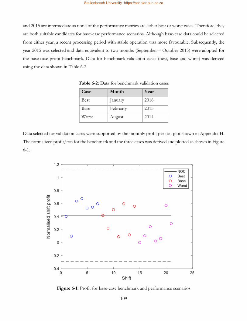
109

and 2015 are intermediate as none of the performance metrics are either best or worst cases. Therefore, they

are both suitable candidates for base-case performance scenarios. Although base-case data could be selected

from either year, a recent processing period with stable operation was more favourable. Subsequently, the

year 2015 was selected and data equivalent to two months (September – October 2015) were adopted for

the base-case profit benchmark. Data for benchmark validation cases (best, base and worst) was derived

using the data shown in Table 6-2.

Table 6-2: Data for benchmark validation cases

Case Month Year

Best January 2016

Base February 2015

Worst August 2014

Data selected for validation cases were supported by the monthly profit per ton plot shown in Appendix H.

The normalized profit/ton for the benchmark and the three cases was derived and plotted as shown in Figure

6-1.

Figure 6-1: Profit for base-case benchmark and performance scenarios


110

As expected, most of the best-case profit i.e. 71% of the 7shifts lies above the base-case benchmark, and

86% of the 7 worst case shift profit lie below the base-case benchmark. The test base-case shift profit is

evenly distributed around the selected benchmark. Thus, the selected benchmark was validated for further

use in the process monitoring tool.

6.2 Data normality

Q-Q normality probability plots for the base case model variables are shown in Figure 6-2.

Figure 6-2: Q-Q normality probability plots

With process control, distributions for CV data differ between variables controlled around a set point

(normally distributed) and as close to a set point as possible but not exceeding the set point (skewed

distribution). Rougher flotation mass pull is regulated to attain the set-point and consequently, stabilise

concentrate flow such that liberated minerals are recovered. Hence, mass pull data shows a positive skew

(Figure 6-2). However, mill load data show a negative skew since it is operated close to the maximum


111

constraint. Particle size and mineral recovery data show very little departure from normality. Therefore, the

normality assumption is valid for all the variables.

6.3 Data correlation

Correlations for filtered data were investigated with scatter plots as shown in Figure 6-3. The data is

normalised in order to mask industrial information.

Figure 6-3: Scatter plots for filtered regression model data

Primary mill circuit variables are known to have multiple and often unexplained interactions (De Haas, 2012;

Wills & Napier-Munn, 2006). However, this does not appear in any of the scatter plots. Instead, weak

correlations are shown for all variables. The likely reasons for weak correlations between the particle size and

mineral recovery are discussed in Section 6.4.3.

A well performing model predictive controller (MPC) determines the set of input variables that maintain

process variability at a minimum and as close as possible to set points, whilst satisfying manipulated variable


112

constraints. This is observed for mill load, which is tightly controlled close to the maximum constraint.

Mineral recovery improves with mass pull but a trade-off exists between the mineral recovery and

concentrate grade, should the mass pull continue to increase. However, a weak correlation is observed

between the two. Laboratory tests conducted at the Concentrator showed that an increase in mass pull

beyond 5.5% resulted in minor overall recovery increase. This may explain the erratic variability beyond the

mass pull of 10%.

The data variability observed in Figure 6-3 was initially considered as suitable for reliable EPF model

development. However, the correlation coefficients were too weak for meaningful relationships to be

developed amongst variables. The weak correlations may have been due to process interactions that are

introduced by recycle flows, resulting in measurement lags.

6.4 Single-predictor EPF results

6.4.1 Single-predictor PVA model

Figure 6-4 shows a particle size-mineral recovery (PS-MR) EPF developed with the base-case training data

set, and Table 6-3 summarises results for the model.

Single-predictor PVA model

R2adj -0.016

Missing data 0

Outlier 1 0

Outlier 2 0

Negative outliers 0

Table 6-3: Single-predictor PVA

Single-predictor PVA results

Figure 6-4: Particle size-mineral recovery

EPF


113

An R2adj value of -0.016 indicated poor model fit between particle size and mineral recovery data, such that

no significant relationship could be developed between the two. No outliers or missing data were present in

the training data set analysed (Table 6-3).

6.4.2 Single-predictor FEA model

Figure 6-5 shows the particle size-financial profit (PS-P) EPF, and Table 6-4 summarises results for the

model.

Figure 6-5: Particle size-financial profit EPF

An R2adj value of -0.001 pointed to poor mode fit between particle size and profit data. Consequently, no

good predictions could be made with this model. No missing data were identified in the training data set.

However, two outliers were present in the data (Table 6-4).

6.4.3 Results summary for the single-predictor EPF models

The results obtained using both FEA and PVA approaches contradict a priori knowledge on the particle size-

profit function relationship. Grind improvement typically improves the profit function, subject to an optimal

grind which results in a drop in grade when exceeded. Therefore, the particle size-profit function EPF was

expected to describe a quadratic function. However, this was not so, due to poor model fit.

The primary mill is operated with the key objective to maintain a constant product size at maximum

throughput. As such, the particle size was expected to normalize at a particular throughput to give a

Single-predictor FEA model

R2adj -0.001

Missing data 0

Outlier 1 1

Outlier 2 1

Negative outliers 0

Table 6-4: Single-predictor FEA results


114

consistent grind, but this is not seen in any of the plots (Figure 6-4 and Figure 6-5). Giddy (1988) attributed

this occurrence to the throughput maximisation objective of primary mills. Unlike secondary or regrind mills

which are operated to achieve the desired fineness of grind, primary mill operation is more concerned with

processing high tonnages than getting the correct particle size. Therefore, Giddy (1988) noted that erratic

grind results often characterize primary mill operation. An internal report by Johannesburg Consolidated

Investment Company Limited (1980) on the erratic behaviour between the ore grind and rougher flotation

mineral recovery for the industrial operation supported these findings

The long sampling frequency of particle size and mineral recovery assay data were likely an additional

limitation. Important in-between events may have been missed and the true dynamics not well reflected in

the shift data. Consequently, the developed single-predictor EPF models were unsuitable for making

performance predictions and for the industrial process monitoring tool.

6.5 Multi-predictor EPF results

A model between key CVs (mill load, sump density, mass pull, and particle size) and mineral recovery was

also developed. Table 6-5 and Table 6-6 summarise PVA and FEA results, respectively.

6.5.1 Multi-predictor PVA model

Table 6-5: Multi-predictor PVA results

Multi-predictor PVA

R2adj 0.0083

Missing data 0

Outlier 1 0

Outlier 2 0

Negative outliers 0

The multi-predictor EPF model had an R2adj of 0.0083 to signify poor model fit. There were no missing or

outlier data.


115

6.5.2 FEA model with multiple predictors

Table 6-6: Multi-predictor FEA

Multi-predictor FEA

R2adj -0.0524

Missing data 0

Outlier 1 1

Outlier 2 1

Negative outliers 0

The multi-predictor EPF model had an R2adj of -0.0524 to signify poor model fit. There were no missing

data, however, two outliers were identified in the base-case training data set.

6.5.3 Results summary for multi-predictor EPF models

Both multi-predictor FEA and PVA models had poor fit, and hence no performance predictions were made.

Thus incorporating more controlled variables did not improve the models as R2adj values remained below the

threshold.

6.6 Findings for EPF model development with base-case data

The EPF models developed with base-case training data gave insight into some aspects that were addressed

in the subsequent investigation. A point in case was the difficulty to identify a conventional quadratic

relationship between the particle size and profit function. Although Giddy (1988) cited the operating

objective of the primary mill as a key limitation, the likelihood of dynamic steady states was another plausible

limitation, which was overcome by searching for EPFs throughout the historical data.

6.7 EPF searches

Single-predictor and multi-predictor PVA results are presented for EPF searches with a window size of

42shifts.

6.7.1 Single-predictor PVA models

After outlier deletions were made, 43% and 54% of the particle size and mineral recovery data respectively,

were missing. Figure 6-6 shows normalized window mean particle size, standard deviation and relative

standard deviation (RSD) for the product particle size.


116

Figure 6-6: Particle size moving window statistical data

Window mean particle size shows a persistent below mean trend after 1500 window slides. Variability within

each window slide is observed for the standard deviation data, and the RSD plot shows particle size variability

across window slides. High variability is observed between 2000 to 2500 window slide shifts, relative to the

first 1500 window slides. The least variability is observed between 500 to 1000 window slides. Hence, the

observed trends show some variability which is necessary for EPF model development.

Figure 6-7 shows plots for normalized mineral recovery window mean, standard deviation, and RSD.


117

Figure 6-7: Mineral recovery moving window statistical data

The first 500 window slides show high mineral recovery means. High window data variability is observed for

the window slides 2000 to 2500 in the standard deviation plot. The RSD plot shows high variability within

the first 500 window slides.

Figure 6-8 shows window slide R2adj,actual (actual data) and R2

adj,test (test data in a consecutive window) for

single-predictor EPF models.


118

Figure 6-8: Single-predictor PVA adjusted R-squared values

All R2adj values fall below the threshold and therefore, have poor model fit for both the actual data and

investigated measurement lag. Figure 6-9 shows normalized actual and predicted mineral recovery plots for

each window slide.


119

Figure 6-9: Normalized actual and predicted mineral recovery for single-predictor EPF models

The similar trends between predicted and actual mineral recoveries in Figure 6-9 are investigated for any

significant difference. A plot of the actual vs predicted mineral recovery is shown in Appendix O.

Table 6-7 presents a summary of single-predictor PVA results.

Table 6-7: Single-predictor PVA summary results

Single-predictor PVA

Maximum R2adj,actual 0.58

Maximum R2adj,test 0.50

R2adj,actual >0.6 0

R2adj,test >0.6 0

Missing MR data 54.4%

Missing PS data 42.5%

Outlier 1 11

Outlier 2 1

Negative outliers 0


120

Although single-predictor EPF models developed with actual and test data had poor model fit, the maximum

R2adj for actual data was better. The model data had 12 outliers but no negative values. For window size

21shifts, the SP approach did not have above-threshold EPF models for both actual and test data (Appendix

P).

6.7.2 Multi-predictor PVA results

Table 6-8 presents the amount of missing data for each primary mill circuit variable.

Table 6-8: Missing data

Variable Missing data (%)

Mass pull 1.81

Mill load 0.61

Mill density 51.1

Particle size 22.9

Mineral recovery 30.4

Overall missing data 69.2

The mill load recorded the least amount of missing data, while the mill density had 51.5% missing data and

this was the highest amount recorded. As a result, data constituting of 69.2% were missing and consequently,

only 30.8% complete vectors. The overall amount of missing data reduced to 38.6% when mill density data

were excluded. Therefore, 61.4% of the data were available for reasonable EPF model development.

Window mean, standard deviation and window relative standard deviation for particle size and mineral

recovery have been highlighted in Figure 6-6 and Figure 6-7, respectively. Figure 6-10 shows mass pull

window data.


121

Figure 6-10: Mass pull moving window statistical data

Most of the mass pull mean data within the first 1000 window slide shifts lies above the overall mean. The

high mass pull suggests maximum mineral recovery, and this is observed in Figure 6-7. Therefore, the two

are well correlated. The RSD plot shows significant variability in mass pull data across the window slides.

Figure 6-11 shows a plot for the mill load window data.


122

Figure 6-11: Mill load moving window statistical data

The window means do not show any obvious distributions around the overall mean as the mill load is tightly

controlled around the set point. However, the standard deviation plot shows some variability within window

slide data. The RSD plot shows a wide variability across the window slides of between 20 and 100% as a

result of the changes in mill load set point to accommodate tonnage increments across the years.

Figure 6-12 shows the R2adj plots for the actual and test data.


123

Figure 6-12: Multi-predictor PVA adjusted R-squared

R2adj,actual values in the first plot fall below the threshold value, to indicate poor model fit. However, six R2

adj,test

values in the second plot lie above the threshold. These six models were restructured to only consist of

significant regression coefficients. As a result, only four of the six models had significant coefficients. Figure

6-13 shows the R2adj,test for each of the four EPF models, where y - mineral recovery, x1 - mass pull, x2 - mill

load, and x3 - particle size. R2adj values for all four models fall below the threshold.


124

Figure 6-13: Adjusted R-squared values for reduced EPF models


125

The four models appeared in consecutive window slides and the relative standard deviation for each model

is shown in Figure 6-14.

Figure 6-14: Models with above threshold R2adj and significant regression coefficients

In Figure 6-14, the data shows very little variability and hence, may explain the above-threshold R2adj values

obtained for the four models. Normalized actual and predicted mineral recovery values were plotted (Figure

6-15) in order to further investigate the validity of these models.


126

Figure 6-15: Actual and predicted mineral recovery

The plots show poor model predictions of actual mineral recovery and hence, the models were invalid.

Summarized results for multi-predictor PVA analysis are presented in Table 6-9.

Table 6-9: Multi-predictor PVA summary results

Multi-predictors’ PVA



R2adj,actual >0.6 0

R2adj,test >0.6 6

Outlier 1 11

Outlier 2 2

Negative outliers 199


127

Appendix P shows R2adj, train and R2

adj, test results for a window size of 21 shifts. The results show some evidence

of overfitting as 57 and 41 models had above-threshold R2adj values for actual and test data, respectively.

Therefore, a window size of 21shifts was too small to develop meaningful EPF models.

6.7.3 Results summary for EPF searches

Based on the successful development of an EPF between particle size and mineral recovery at laboratory

scale, it was expected that reliable EPF models could also be developed with industrial data. However, the

results obtained in this study demonstrated difficulty to develop EPF with industrial data. A significant

amount, i.e. 61% of the industrial data was assessed and showed good variability. Although good correlations

were expected between data, none of the variables had significant correlation coefficients. Furthermore, the

quadratic relationship between particle size and mineral recovery data remained elusive due to the limitations

highlighted in Section 6.4.3.

While no reliable EPF models could be developed, four of the models developed with the multi-predictor

approach showed R2adj,actual values above a threshold of 0.6.

6.8 Summary results for EPF development strategies

Results for base-case data and searches for EPFs strategies demonstrated better results with the latter

strategy. EPF searches were more effective relative to EPF development with base case data, based on

achieved R2ajd results. Hence, the assumption of dynamic steady states seemed to hold. However, both

strategies showed poor model fit.

Due to bias and data distortion risks associated with case reweighting or multiple imputations, either option

was not considered in this study. R2adj values for test data were better, compared to training data results. The

difference was more pronounced for the multi-predictor PVA approach where an R2ajd of 0.58 against 0.67

was obtained for actual and test models were obtained, respectively. This showed better correlation between

mineral recovery data and controlled variables for the next window, pointing to possible measurement lags

in some of the controlled variable.

The data variability observed in scatter (Figure 6-3) and RSD plots (Figure 6-6, Figure 6-7, Figure 6-10, and

Figure 6-11) appeared to be sufficient for EPF development. However, the poor results suggest inadequate

variability for EPF development, due to robust model predictive controller action. In addition, process

variable dynamics were smoothed out by using shift composite samples to analyse particle size and mineral


128

recovery. Therefore, the shift averages did not adequately capture the process dynamics. As a further

limitation, some important in-between events were lost due to deletions made during data cleaning. For

example, in cases where one variable had fault data, corresponding data in other variables was also deleted

to preserve the relationships between variables. However, doing this inevitably reordered data sequencing

and disturbed the time series effect.

Due to the highlighted limitations, it was not possible to develop a reliable EPF model with industrial data.

Consequently, the process monitoring tool could not be implemented at the industrial operation.

Chapter Summary

Chapter 6 presented industrial case study results. Two approaches i.e., FEA and PVA were investigated for

single and multi-predictor EPF model development using two strategies i.e., base case data and searches for

EPFs throughout the data. It was difficult to develop a reliable EPF for either for cases as results

characterized poor model fit. Furthermore, the quadratic relationship between particle size and mineral

recovery remained elusive throughout historical data. Some evidence of measurement lags, information loss

due to reordered data sequences and data cleaning techniques, erratic particle size data due to a throughput

maximisation objective, and robust controller action emerged as possible key limitations.

The next Chapter discusses simulation case study results.


129

CHAPTER 7: RESULTS AND DISCUSSION -

SIMULATION CASE STUDY

This Chapter reports on the economic impact of three simulated faults - drifting load cell, poor steel ball

quality, and increased ore hardness.

7.1 Controlled variable –manipulated variable plots for simulated faults

7.1.1 Drifting mill load cell

CV-MV plots are shown in Figure 7-1 for a mill load cell with negative drift. All the plots show truncated

transient-phase shifts.

Figure 7-1: CV-MV plots for drifting mill load cell


130

At fault inception, the mill load gradually increased until it reached saturation level. Mill feed solids increased

to correspond with the change in mill load, based on modelled equations. In industrial operations, mill

discharge rate typically increases at high mill loads to stabilise the mill load (Wei & Craig, 2009c). The load

cell drift was propagated to the particle size, which dropped by about 54% to give a coarse product. As a

result of poor in-mill trajectories arising from an increased mill feed solids rate, the product particle size did

not improve within the simulation run length. However, the 5% increase in hydrocyclone feed flow implied

an increase in coarse material recirculation for further grinding. The PID controller maintained the sump

volume around the set point to minimize circuit instability. Consequently, the sump feed water flow rate

reduced in order to maintain the sump volume, since the mill discharge flow had increased.

Figure 7-2 shows the revenue and cost metric for the drifting mill load cell.

Figure 7-2: Revenue and cost metrics for the drifting mill load cell

MFB

, tp

h


131

The mill throughput increased by about 33% due to an increase in mill feed solids. A 43% reduction in the

mineral recovery was observed, indicating a trade-off between mill throughput and mineral recovery. Hence,

the decrease in mineral recovery after fault inception corresponded to the coarse particle size achieved. A

31% decrease in the SAG mill electricity consumption was observed as a result of a coarser product. The

steel ball consumption remained constant, with normal variation from random walks.

7.1.2 Poor steel ball quality fault

The CV-MV plots for poor steel ball quality are shown in Figure 7-3.

Figure 7-3: CV-MV plots for poor steel ball quality

All CVs and corresponding MVs showed normal variations introduced by random walks. The particle size

was expected to coarsen due to poor grinding media impact and abrasive forces. As a result of increased steel

ball addition, the mill feed solids were expected to be limited. Figure 7-3 shows that there was no fault


132

propagation to the particle size as it remained around the target size. This showed that the only economic

consequence was the cost arising from increased steel consumption. Figure 7-4 shows corresponding revenue

and cost metrics.

Figure 7-4: Revenue and cost metrics for poor steel ball quality

The revenue and cost metrics had normal variation except for steel ball charge rate which increased by a fault

size of 60%.

7.1.3 Ore hardness increase

Figure 7-5 shows CV-MV plots for the increased ore hardness fault.

MFB

, tp

h


133

Figure 7-5: CV-MV plots for increased ore hardness

The mill load was well controlled around the set point as mill feed solids attenuated the effect of increased

ore hardness. A 35% reduction in mill feed solids suggests a control effort to compensate for ore hardness

changes, such that material discharged from the mill was recirculated for further grinding, in order to

maintain mill load around the set point. Furthermore, a 4% increase in hydrocyclone flow feed supported

the assertion on material recirculation for regrinding. Consequently, fresh ore feed was limited as shown by

a decrease in mill feed solids. Although the PID controller showed some effort to minimize the effect of

increased ore hardness, a coarser product with 65% passing 75µm was achieved. The sump volume was

maintained around the set point due to a decrease in sump feed water caused by increased mill discharge

rates into the sump. Hence, the PID controller showed effective stabilizing control of the mill load and sump

volume.

Figure 7-6 shows the corresponding revenue and cost metrics.


134

Figure 7-6: Revenue and cost metrics for increased ore hardness

The mill throughput decreased by 32% due to increased ore grinding resistance and hence, a longer ore

retention time. This decrease was similar to that observed for the mill feed solids. The mineral recovery

sharply decreased by 7% due to the low degree of liberation achieved. Although electricity consumption was

expected to increase with abrasive ore feed, a 10% decrease was observed. As a possible inference, less power

was required to regrind the recirculating material. The target particle size was not achieved despite increased

grinding time.

7.1.4 Summary for simulated faults

Stabilizing the grinding mill circuit has been key to successful industrial circuit operation, hence the use of

process control systems. As such, simulation experiment results showed economic consequences with

changes in CVs, to support literature findings on the cost implication of process variability when CVs move

away from a profitable operating mean. This was particularly observed for the particle size, which was directly

MFB

, tp

h


135

related to mineral recovery. Furthermore, changes in process conditions (for the drifting load cell and

increased ore hardness) resulted in variable flow throughout the circuit and delivery of material that is

inconsistent with the required target particle size of 80% passing 75µm.

The SAG mill is operated with an objective to liberate mineral value for downstream recovery. By

convention, mineral recovery is improved within an optimal particle size range. In all the simulation results,

the correlation between the particle size and mineral recovery was evident. Furthermore, the trade-off

relationship between the particle size and throughput was observed for poor steel ball quality and increased

ore hardness faults.

Two of the faults (drifting load cell and poor quality steel ball) showed significant changes of 32% and 60%

in the mill throughput and the steel ball charge rate, respectively. In addition, process control action to

attenuate the impact of fault conditions introduced in the model either limited the throughput, or produced

a coarse product. Either outcome affected revenue or cost elements, to emphasize the significance of these

metrics in the EPI. Moreover, industrial operations employ tonnage maximisation and cost minimisation

strategies. Therefore, the significance of these metrics justifies their inclusion when the economic

performance of milling circuits is assessed.

The increased ore hardness fault showed a decrease in both the mill throughput and the particle size. This

may have been as a result of the large fault size which limited the throughput and resulted in a coarser product

size. Typically, increased ore abrasiveness results in higher electricity and steel ball demands in order to grind

the ore to target particle size (King, 2001). However, the simulation results indicated decreased electricity

consumption and did not reflect any significant changes in the steel ball consumption. The poor steel ball

quality fault did not reflect any significant changes in the operating conditions. A decrease in the mill

throughput was expected since more steel balls would have been charged into the mill to maintain ore-steel

ball ratio. However, the particle size was then expected to coarsen since no changes were observed for the

mill feed solids. Despite the identified anomalies, the results showed that fault detection was possible with

an EPF model.


136

7.2 Significance tests

Appendix P and Appendix R list mineral recovery and mill throughput data respectively, for each of the 15

simulation experiments. Table 7-1 presents F-test and p-value results based on this data.

Table 7-1: F-test results

Mineral

recovery

Mill throughput

Fcrit - critical,

Where df1 = 2, df2 = 12

3.89 3.89

Fob - observed, 71.99 25.44

Condition Fob>Fcrit

Reject null hypothesis of equal

sample means

Reject null

hypothesis

Reject null

hypothesis

p-value

2.07E-07 4.83E-05

Condition p-value<0.05

Reject null hypothesis of equal

sample means for the three faults

Reject null

hypothesis

Reject null

hypothesis

For both the mineral recovery and mill throughput, F-test and p-value results indicate at least one significant

difference between sample means for the three faults. Hence, a Tukey-Kramer post-hoc analysis was

conducted to identify the different means. The pairwise comparisons of p-values are shown for the mineral

recovery and mill throughput in Table 7-2.

Table 7-2: Pairwise p-values

Pairs Mineral recovery Mill throughput

1,2 2.25E-07 0.001

1,3 3.99E-06 4.04E-05

2,3 0.06 0.10

Where 1,2,3 are the drifting load cell, poor steel ball quality and increased ore hardness faults

The results show p-values < 0.05 between the drifting load cell – poor steel ball quality (1,2) and the drifting

load cell – increased ore hardness (1,3) faults, pointing to a significant difference between the drifting load


137

cell fault and the other two faults. The box plots shown in Figure 7-7 and Figure 7-8 for mineral recovery

and mill throughput respectively, validate this finding.

Figure 7-7: Mineral recovery box plot

Figure 7-8: Mill throughput box plot


138

7.3 Economic performance indices for simulated faults

Sliding window normalized EPIs for all three simulated faults are shown in Figure 7-9.

Figure 7-9: Sliding window economic performance indices

All three faults show different NOC economic performances due to process noise introduced through

random walks. Minimal change is observed for the poor steel ball quality after fault inception at 50 shifts.

Although there was a cost associated with extra ball charge, the sliding EPI shows little variability around

the NOC (shown as CL) after fault inception. The EPI did not degrade and hence, this fault showed the

least economic impact. The drifting load cell and increased ore hardness faults show significant deviation

from normal operating economic performance after fault inception. In this assessment, the economic impact

of the ore hardness fault was greater compared to that for a drifting load cell.

In Figure 7-9, process noise variability does not reflect significant changes in the EPI. However, there is a

significant degradation in the EPI due to large disturbances introduced by two faults (drifting load cell and

increased ore hardness). Hence, the EPI shows potential for fault (large disturbances) detection. Moreover,

significance test results pointed to the difference between a drifting load cell and the other two faults. The

results suggest opportunity to prioritise faults and make decisions about the corrective action to be taken,


139

based on the severity of impact on economic performance. It is reasonable to allow a fault with very little

impact on the EPI to persist. However, serious corrective action such as a shutdown for maintenance may

be considered for faults with a large impact on the EPI. A similar concept is discussed in Olivier & Craig

(2017).

The simulation results show that changes in economic performance were influenced to a greater extent by

revenue metrics i.e., changes in the particle size and hence, mineral recovery as well as changes in the mill

throughput. On this merit, the study of Wei & Craig (2009a) used mineral recovery to represent economic

performance. However, there was at least one significant change in either cost element (electricity or steel

ball consumption) for two of the simulated faults (drifting load cell and poor steel ball quality) presented in

Figure 7-2.

Since grinding operations are energy intensive and require large amounts of grinding media, the EPI is more

representative when the two cost elements are incorporated. The drifting load cell fault resulted in a 31%

decrease in electricity consumption while poor steel ball quality also influenced steel ball consumption rates.

Based on these findings, revenue metrics alone may be inadequate for industrial operations since cost

minimisation strategies are employed in industrial operations. Therefore, electricity and steel ball

consumption must be considered when deriving the economic performance of a milling circuit.

Chapter Summary

Chapter 7 investigated the merit of fault detection with the economic performance index, based on deviation

from normal operating performance. To this end, three common faults in a milling circuit were simulated. A

sliding window EPI was derived for each fault, using a priori particle size-mineral recovery EPF as well as key

revenue and cost metrics. The simulation results showed scope for fault detection and prioritisation with the

EPI. Two of the faults (drifting load cell and increased ore hardness) showed significant EPI degradation

after fault inception. Moreover, a significant difference between the economic impact of the drifting load

cell fault and the other two faults (poor steel ball quality and increased ore hardness) was observed, pointing

to scope for fault prioritisation.

The next Chapter concludes this study with a summary of the findings and recommendations for future

work.


140

CHAPTER 8: CONCLUSION AND RECOMMENDATIONS

Study background and objectives summary

Milling circuit operations are driven with a profit maximisation objective, and decisions for consistent

profitability are enabled by effective process monitoring. Although it is beneficial to monitor all the variables

in milling circuits, only a few are directly controlled for economic reasons. Therefore, this study aimed to

assess the feasibility of monitoring milling circuits with economic performance functions (EPFs). These

relate the behaviour of a controlled variable about a profitable set point, to money. To achieve the aim of

the study, industrial and simulation cases were studied. The objectives of the industrial case study were:



3. To assess the feasibility of industrially implementing an online process monitoring tool for the

circuit, using one key controlled variable; and

4. To assess the feasibility of incorporating additional key controlled variables in the process

monitoring tool.

The proof of concept was tested in a simulation case study, where a priori EPF developed at laboratory scale

was used to investigate fault detection with EPFs. Fault detection is a critical aspect of process monitoring

that minimizes the occurrence of faults and their economic impact. Therefore, the following objectives were

identified for the simulation case study:

1. To derive the economic performance of a SAG mill circuit subject to three common industrial

faults; and



Industrial case study summary methodology and findings

Data for EPF and process monitoring tool development were judiciously identified based on in-depth

literature survey, a site survey at the industrial operation and consultations with expert site personnel.

Historical data for the years January 2012 till April 2016 were retrieved from the plants historian, control

room log sheets, laboratory data archives and financial reports. The data were well documented, so an


141

assessment of EPF development and economic performance evaluation for the primary mill and rougher

flotation circuit was possible.

Three key controlled variables i.e. mass pull, particle size and mill load were selected based on the expert

opinion of consulted site personnel. However, this selection can also be validated by several literature. Single

predictor regression was performed with particle size (the key controlled variable) and multi-predictor

regression was also performed to incorporate two additional controlled variables (mass pull and mill load).

For each of these regressions, financial elements analysis (FEA) and process variable analysis (PVA) were

investigated using base case data, as well as sliding window searches for EPFs throughout all the historical

data. Significant revenue (throughput and mineral recovery) and cost elements (electricity, reagents and steel

balls) were used to derive the profit realised from operating the industrial primary mill and rougher flotation

circuit. Consequently, this profit was related to CV behaviour in the FEA approach. On the other hand, the

PVA approach related CV behaviour to mineral recovery.

Results for the industrial case study showed that it was difficult to develop a reliable EPF using either FEA

or PVA approaches. This concurred with the finding in Wei & Craig (2009c) and Bauer & Craig (2008) on

the difficulty to develop EPFs with industrial data. EPF model adjusted R-squared values fell below a selected

significance threshold of 0.6, to indicate poor model fit. Furthermore, model predictions were not in

agreement with plant test data. Consequently, it was not possible to implement the process monitoring tool

at the industrial operation. In addition, incorporating two more economically significant CVs into the EPF

model did not improve the results.

Two points of interest emerged from the results in the study. Firstly, it was not possible to identify the

conventionally quadratic relationship between particle size and mineral recovery throughout all the data.

Although a wide range for particle size data may have been good for EPF model development, particle size

measurements were rather too erratic. Giddy (1988) refer to erratic particle size as a typical occurrence since

primary mills are operated as tonnage mills controlled with an objective to maximise throughput, rather than

to achieve the target particle size. The second interesting finding was that despite a priori knowledge of the

strong interactions between milling circuit controlled variables (Hodouin, 2011; Wills & Napier-Munn, 2006),

variables for the primary mill and rougher flotation circuit were characterized by weak correlation coefficients

of less than 0.2.


142

The development of EPF models is premised on having significantly variable process data. Model data

variability was possibly insufficient for EPF development, due to robust model predictive controller action.

In addition, limitations in data cleaning techniques, data quality and proposed model structure also accounted

for the poor EPF models.

A major shortcoming for reliable data analysis and subsequently, EPF model development was resolution

mismatch between offline and online data was. At the industrial operation, shift composite samples are

analysed offline for particle size and mineral recovery measurements. Hence, the true process dynamics are

insufficiently captured by these ‘averaged’ measurements. Similarly, shift averages for 30 minute time-

stamped online data were determined in order to match the offline shift data. Doing this also smoothed out

data dynamics and it was therefore difficult to identify unique process states due to loss of variability. The

data cleaning techniques applied for faulty data resulted in loss of information. Faulty data and

corresponding measurements in the other key variables were deleted, in order to preserve functional

relationships between variables. This reordered data sequences, disturbed the time series effect and important

in-between events were missed.

Both offline and online data had some anomalous and out of range entries, which had to be filtered out.

Factors related to sensor accuracy and calibration frequency, as well as differing sensor qualities across the

measured variables for the years under consideration influenced data quality. Although no correlations were

identified between the data, the proposed model structure may have been too simple for milling circuit

variables, which typically strongly interact.

While it was difficult to obtain a reliable EPF model for this case study, it was possible to derive the primary

mill circuit’s economic performance in terms of financial profit. Methodology steps to apply performance

models to process monitoring and test process monitoring tool validity were discussed in this study, although

it had not been possible to develop and implement the process monitoring tool.

Simulation case study findings Simulation results showed a dynamic EPI in response to changes in operating conditions vis-à-vis process

noise and fault conditions. After fault inception, two faults (drifting mill load cell and increased ore hardness)

showed marginal EPI degradation. Hence, fault detection was possible with the investigated EPF. One-way

ANOVA significance tests pointed to at least one difference between EPI values for drifting load cell and

the other two faults. This finding suggests opportunity for fault prioritisation with EPFs, such that decisions


143

on corrective action can be reached based on the severity of impact on economic performance. A similar

concept is discussed in Olivier & Craig (2017). However, this study associated EPI values with specific fault

types that were simulated in the SAG mill circuit, and did not fully explore this finding. Fault sizes can vary,

to result in completely different EPI values, which may even overlap with a different type of fault in industrial

operations.

Although necessary, simplifying assumptions pose certain limitations and economic consequences that are

difficult to account for adequately. To give a few examples, an unstable SAG mill circuit minimizes the

efficiency of downstream processes, to result in loss of performance. In addition, unstable hydrocyclone feed

flow rates (shown for the drifting load cell and increased ore hardness) induce variability in flotation feed, to

result in mineral losses. Furthermore, a coarse flotation feed may require more reagents, especially the

collector (Bahena et.al. 2006). Due to insufficient model information, other economically significant

consequences such as increased liner wear from operating the mill at a high load were not taken into

consideration, in order to simplify the economic performance assessment.

Recommendations for future work Some areas of interest in this study were identified for future work. In many industrial operations, focus is

mostly directed to meet and even better, surpass production targets to maximise revenue. In comparison,

less attention is paid to manage cost variation within production operations. Therefore, a recommendation

to use financial elements to monitor the primary mill circuit’s economic performance online is proposed.

Following this recommendation, process decisions that maximize profit may be reached through

manipulating revenue and cost metrics associated with the process. This provides opportunity to interrogate

any performance deviations, and to simultaneously optimise all the key economically significant metrics for

the primary mill circuit. Consequently, process decisions can be reached earlier on in the process, rather than

retrospectively after accounting reports have been generated.

Despite the challenges faced in this study, the few successful EPA studies (e.g., Bauer et al., 2007; Steyn &

Sandrock, 2013; Wei & Craig, 2009a) demonstrated for controller performance , process monitoring with

EPFs seems to be a promising avenue which requires further investigation. Since reliable EPF development

was the main limitation in this study, a comparative assessment in a different operation which addresses the

shortcomings identified in this study is recommended. Moreover, the shortcomings identified in some of the

simplifying assumptions will need to be addressed in future work.


144

REFERENCES

Aldrich, C. 2013. Consumption of steel grinding media in mills – A review. Minerals Engineering. 49:77–91.

Almond, D.G. & Valderrama, W. 2004. Performance enhancement tools for grinding mills. International

Platinum Conference “Platinum Adding Value”. 103–110.

Almond, D., Becerra, K. & Campain, D. 2012. The Minerals Plant of the Future – Leveraging Automation

and Using Intelligent Collaborative Environment. The Southern African Institute of Mining and Metallurgy

Platinum 2012.

Alt, F.B. & Smith, N.D. 1998. Multivariate process control. New York: Elsevier Science Publisher.

Aly, A.A., Mahmoud, M.A. & Woodall, W.H. 2015. A Comparison of the Performance of Phase II Simple

Linear Profile Control Charts when Parameters are Estimated. Communications in Statistics—Simulation

and Computation.

Arteaga, F. & Ferrer, A. 2002. Dealing with missing data in MSPC: Several methods, different interpretations,

some examples. Journal of Chemometrics. (16):408–418.

Arzen, K. 1991. “Knowledge based applications in the processs industry: Current state and future

directions”. In Bergen, Norway IFAC Proceedings on Computer software structures integrating AI/KBS Systems

in Process Control.

Babcock, B., Datar, M. & Motwani, R. 2002. Sampling From a Moving Window Over Streaming Data.

Proceedings of 13th Annual ACMSIAM Symposium on Discrete Algorithms. 102(2001–33):633–634. [Online],

Available: http://ilpubs.stanford.edu:8090/503/1/2001-33.pdf.

Ballantyne, G. & Powell, M. 2014. Benchmarking comminution energy consumption for the processing of

copper and gold ores. Minerals Engineering. 65:109–114.

Barton, R. 2013. Designing simulation experiments. Proceedings of the 2013 Winter Simulation Conference. 342–

353.

Bartsch, E., Comeau, G., Hardie, C. 2008. Evolution of SAG Mill Process Control at the Xstrata Nickel

Raglan Operation. In 40th Annual Meeting of the Canadian Mineral Processors. 445–464.

Bauer, M. & Craig, I.K. 2008. Economic assessment of advanced process control - A survey and framework.

Journal of Process Control. 18(1):2–18.

Bauer, M., Craig, I.K., Tolsma, E. & de Beer, H. 2007. A Profit Index for Assessing the Benefits of Process

Control. Industrial & Engineering Chemistry Research. 46(17):5614–5623.

Baxter, P., & Jack, S. 2008. Qualitative Case Study Methodology: Study Design and Implementation for

Novice Researchers. The Qualitative Report. 13(4):544–556.


145

Beigler, L. 2010. Nonlinear Programming: Concepts, Algorithms, and Applications to Chemical Processes. New York:

SIAM-Society for Industrial and Applied Mathematics.

Ben-Gal, I. 2005. Outlier detection. O. Maimon & L. Rockach (eds.). Kluwer Academic Publishers.

Benneyan J.C. 2001. Design, Use and Performance of Statistical Control Charts for Clinical Process

Improvement. International Journal for Quality Health. 69–73.

Besterfield, D. 2001. Quality control. Upper Saddle River, NJ:. Prentice Hall.

Bezergianni, S. & Georgakis, C. 2003. Evaluation of controller performance?use of models derived by

subspace identification. International Journal of Adaptive Control and Signal Processing. 17(7–9):527–552.

Boque, R., Smilde, A.K. 1999. Monitoring and diagnosing batch processes with multiway covariates

regression models. American Institute of Chemical Engineers. 30:1429–1432.

Bouffard, S.C. 2015. Benefits of process control systems in mineral processing grinding circuits. Minerals

Engineering. 79:139–142.

Box, G., and Luceno, A. 1997. Discrete proportional integral adjustment and statistical process control.

Journal of Quality Technology. 29(3):248–259.

Braverman, V., Ostrovsky, R. & Zaniolo, C. 2009. Optimal sampling from sliding windows. In ACM PODS,

Providence. 1–13.

Brisk, M.L. 2004. Process Control : Potential Benefits and Wasted Opportunities. 5th Asian Control Conference

Process. 10–16.

Bryman, A. & Bell, E. 2007. The nature of qualitative research. In: Business Research Methods. New York.

Oxford University Press.

Buchanan, D.. & Bessant, J. 1985. Failure, uncertainty and control: the role of operators in computer

integrated production systems. Journal of Management Studies. 22(3):292–308.

Castle, J. F. & Imre, U. 1984. Exploitation staretgy for complex Cu-Pb-Zn orebodies. Mineral Engineering.

12(2):473–477.

Cha, Y. & Agrawal, A. 2014. Robustness studies of sensor faults and noises for semi-active control strategies

using large-scale magnetorheological dampers. Journal of Vibration and Control. 1–16.

Chandola. 2009. Anomaly Detection for Symbolic Sequences and Time Series Data. University of Minnesota.

Doctor Of Philosophy.

Clermont, B. & De Haas, B. 2010. Optimization of mill performance by using online ball and pulp

measurements. Journal of the Southern African Institute of Mining and Metallurgy. 110(3):133–140.

Coetzee, L.C., Craig, I.K. & Kerrigan, E.C. 2008. Nonlinear model predictive control of a run-of-mine ore

milling circuit. In Proceedings of the 17th IFAC World Congress. Elsevier, Korea. 10620–10625.

Coetzer, L.P. & Khumalo, T. 2006. The use of performance monitoring techniques in detecting process


146

shifts and potential root causes in a variable speed grinding application. The Southern African Institute of

Mining and Metallurgy. 2:137–142.

Contreras-Dordelly, J. & Marlin, T.E. 2000. Control design for increased profit. Computers & Chemical


Contreras-Dordelly J.L, M.T. 2000. Control design for increased profit. Computers and Chemical Engineering.

24:267–272.

Craig, I.K. & Henning, R.G.D. 2000. Evaluation of advanced industrial control projects: a framework for

determining economic benefits. Control Engineering Practice. 8(7):769–780.

Craig, I.K. & Koch, I. 2003. Experimental design for the economic performance evaluation of industrial

controllers. Control Engineering Practice. 11(1):57–66.

Craig, I.K. & Macleod, I. 1996. Robust controller design and implementation for a run-of-mine ore milling

circuit. Control Engineering Practice. 4(1):1–12.

Creswell, J. 2003. Research design: Qualitative, quantitative and mixed methods approaches. 2nd ed. CA: Thousand

Oaks.

Cutler, C.R. & Perry, R.T. 1983. Real time optimization with multivariable control is required to maximize

profits. Computers and Chemical Engineering. 7(5):663–667.

Denzin, N. 1998. The art and politics of interpretation. CA: Thousand Oaks.

Desborough, L. & Miller, R. 2002. Increasing Customer Value of Industrial Control Performance Monitoring

— Honeywell ’ s Experience. Sixth International Conference on Chemical Process Control, AIChE Symposium

Series Number 326. 98(Figure 1):169–189.

Dey, R., Pal, A., Biswas,A., Das, A. 2014. Creeping and Drifting Correction of Sensor Using Adaptive

Method. International Journal of Advanced Research in Electrical, Electronics and Instrumentation Engineering.

3(1):6670–6672.

Duncan, A. 1986. Quality control and industrial statistics. Vol. 5th Editio. Chicago: Irwin.

Dvorak, D. & Kuipers, B. 1991. Process monitoring and diagnosis: a model-based approach. IEEE Expert.

6(3):67–74.

Edwards, R. & Vien, A. 1999. Application of a model-based size recovery methodology. Control and

Optimisation in Minerals, Metals and Materials Processing. 147–160.

Edwards, R., Vien, A. & Perry, R. 2002. Strategies for the instrumentation and control of grinding circuits.

Society for Mining Metallurgy and Exploration. 2130–2151.

Egbe, E.A.P. & Abubakre, O.K. 2013. Determination of the Bond ’ S Work Index of Baban Tsauni ( Nigeria

) Lead-Gold Ore. European Scientific Journal. 9(12):78–86.

El-Farra, N. & Giridhar, A. 2008. Detection and management of actuator faults in controlled particulate


147

processes using population balance models. Chemical Engineering Science. 63(5):1185 – 1204.

Ellis, M., Duranda, H., Panagiotis, D. & Christofides, B. 2014. A tutorial review of economic model

predictive control methods. Journal of Process Control. 24:1156–1178.

Eriksson, P.-G. & Isaksson, A.J. 1994. Some aspects of control loop performance monitoring. Control

Applications, 1994., Proceedings of the Third IEEE Conference on. (3):1029–1034 vol.2.

Fan, J. & Huang, L. 2001. Goodness-of-Fit Test for Parametric Regression Models. Journal of American

Statistical Association. 96:640–652.

Filzmoser, P., Maronna, R. & Werner, M. 2007. Outlier Identification in High Dimensions. Elsevier Science.

5(1):23–27.

Fiske, T. 2006. Advanced process control for competitive advantage. Hydrocarbon Processing. 85(2):15–16.

Frankfort-Nachmias, C. & Nachmias, D. 1992. Research Methods in the Social Sciences, Melbourne. 4th

edition.

Fry, H., Ketteridge, S. & Marshall, S. 1999. A Handbook for Teaching and Learning in Higher Education. Glasgow:

Kogan Page.

Gertler J. 1998. Fault detection and diagnosis in engineering systems. New York: Marcel Dekker.

Ghasemi, B. & Zahediasl, C. 2012. Normality Tests for Statistical Analysis: A Guide for Non-Statisticians.

Journal of Applied Statistics. 10(2):486–489.

Ghorbani, B. 2004. Initial transient phase of steady state simulation: Methods of its length detection and

their evaluation.

Giddy, M. 1988. Identification of an industrial scale semi-autogenous grinding circuit for control purposes.

University of the Witswatersand.

Griesel, H. 2008. Optimizing project value by defining and modelling key drivers in the concept phase.

Platinum in Translation. 349–354.

Gulsecen, S. & Kubat, A. 2006. Teaching ICT to teacher candidates using PBL: A qualitative and quantitative

evaluation. Educational Technology & Society. 9(2):96–106.

Gupta, A., Mathur, T., Stadler, K. & Gallestey, E. 2013. A pragmatic approach for performance assessment

of advanced process control. IEEE International Conference on Control Applications (CCA). 754–759.

Hachicha, W., Moussa, I., Kolsi, R. 2012. Integration of Statistical and Engineering Process Control in a

Batch Processes Monitoring: Case of Alkyd Polymerization Reactor. International Journal of Control and

Automation. 5:212–216.

Hamilton, C. 2015. Applied Multiple Regression and Correlation Analysis. Journal of Applied Statistics.

Hangos, K.M. & Tuza, Z. 2001. Optimal control structure selection for process systems. Computers &

Chemical Engineering. 25(11–12):1521–1536.


148

He, K. & Meeden, G. (in press). Selecting the number of bins in a histogram : A decision theoretic approach.

Journal of Statistical Planning and Inference. 61:49 59.

Heale, R. & Twycross, A. 2015. Validity and reliability in quantitative studies. Evidence Based Nursing. 18(3):15–

18.

Herbst, J.A. & Lo, Y.C. 1996. Financial implications of comminution system optimization. International Journal

of Mineral Processing. 44–45(SPEC. ISS.):209–221.

Herbst, J.A., Alba, F.J., Pate, W.T. & Oblad, A.E. 1988. Optimal control of comminution operations.

International Journal of Mineral Processing.

Herman, A., Gottfredson, R. & Joo, H. 2013. Best-Practice Recommendations for Defining, Identifying, and

Handling Outliers. Organizational Research Methods. 16(2):270–301.

Himmelblau. 1978. Fault detection and diagnosis in chemical and petrochemical processes. Elsevier:

Amsterdam.

Hodouin, D. 2011. Methods for automatic control, observation, and optimization in mineral processing

plants. Journal of Process Control. 21(2):211–225.

Hodouin, D., Jämsä-Jounela, S.L., Carvalho, M.. & Bergh, L. 2001. State of the art and challenges in mineral

processing control. Control Engineering Practice. 9(9):995–1005.

Hoepfl, M.. 1997. Choosing qualitative research: A primer for technology education researchers. Journal of

Technology Education. 1(9):11–14.

Hoo, K.A., Piovoso, M.J., Schnelle, P.D. & Rowan, D. A. 2003. Process and controller performance

monitoring: overview with industrial applications. International Journal of Adaptive Control and Signal

Processing. 17(7–9):635–662.

Horch, A. & Isaksson, A.J. 1999. A modified index for control performance assessment. Journal of Process

Control. 9(June):475–483.

Huang, B., Shah, S.L. & Kwok, E.K. 1997. Good, bad or optimal? Performance assessment of multivariable

processes. Automatica. 33(6):1175–1183.

Hugo, A. 2001. Process controller performance assessment. Hydrocarbon Processing. 80(4):85–90.

Hunt, J., Kojovic, T. & Berry, R. 2013. Estimating comminution indices from ore mineralogy, chemistry and

drill core logging. Proceedings of the Second AusIMM Geometallurgy Conference. 173–176.

Ibrahim, K.A. 1996. Active statistical process control PhD Chemical and Process Engineering. University of

Newcastle.

Irannajad, M., Farzanegan, A. & Razavian, S.M. 2006. Spreadsheet-based simulation of closed ball milling

circuits. Minerals Engineering.

Isermann, R. & Balle, P. 1997. Trends in the application of model based fault detection and diagnosis of


149

technical processes. Control engineering practice. 5(5):709–719.

Jakhu, M.. 1998. Process Control in Flotation Plants. IIME. 79–102.

James R. B, Carroll, C. & Young, G. 2007. Colorado Mineral and Energy Industry Activities.

Jämsä-Jounela, S.L., Poikonen, R., Vatanski, N. & Rantala, A. 2003. Evaluation of control performance:

Methods, monitoring tool and applications in a flotation plant. Minerals Engineering. 16(11):1069–1074.

Jankovic, A. 2003. Variables affecting the fine grinding of minerals using stirred mills. Minerals Engineering.

Jankowski, T., Davis, G., Holmes, J. & Kemper, G. 2011. Increasing data historian efficiency. IEEE Cement

Industry Technical Conference (Paper).

Jearkpaporn, D., Montgomery, D.C., Runger, G.C. & Borror, C.M. 2005. Model-based process monitoring

using robust generalized linear models. International Journal of Production Research. 43(7):1337–1354.

Jelali, M. 2006. An overview of control performance assessment technology and industrial applications.

Control Engineering Practice. 14(5):441–466.

Kaka, A.P. 1999. The development of a benchmark model that uses historical data for monitoring the

progress of current construction projects. Engineering, Construction and Architectural Management. 6(3):256–

266.

Kang, H. 2013. The prevention and handling of the missing data. Korean Journal of Anesthesiol. 64(5):402–406.

Kano, M. & Nakagawa, Y. 2008. Data-Based Process Monitoring , Process Control , and Quality

Improvement : Recent Developments and Applications in Steel. Computers and Chemical Engineering. 32(1–

2):12–34.

Kawatra, S. K., Eisele, T. C.,Weldum, T., Larsen, D., Mariani, R., P.J. 2005. Optimization of Comminution

Circuit Throughput and Product Size Distribution by Simulation and Control.

Kazemzadeh, R.B., Noorossana, R. & Amiri, A. 2009. Monitoring polynomial profiles in quality control

applications. The International Journal of Advanced Manufacturing Technology. 42(7–8):703–712.

Keet, K. & Du Plessis, F. 2010. Flotation process optimization through frequent in-line grade measurement

as an alternative to sampling surveys that deliver outdated results. In The 4th International Platinum

Conference, Platinum in transition “Boom or Bust”, The Southern African Institute of Mining and Metallurgy.

Khandalkar, B. 2015. Design and Analysis of Digital PID Controller A Review. 2(4):940–942.

King, P.. 2001. Modelling and simulation of mineral processing systems. First ed. Oxford: Butterworth-Heinemann.

Knorr, E.. & Ng, R.. 1997. A Unified Notion of Outliers: Properties and Computation. American Association

for Artificial Intelligence. 219–222. [Online], Available:

http://www.aaai.org/Papers/KDD/1997/KDD97-044.pdf.

Knuth, K.. 2013. Optimal Data-Based Binning for Histograms. ArXiv Physics e-prints.

Kourti, T. & MacGregor, J.F. 1995. Process analysis, monitoring and diagnosis, using multivariate projection


150

methods. Chemometrics and intelligent laboratory systems. 28:3–21.

Kresta, J. V., Marlin, T.E. & MacGregor, J.F. 1994. Development of Inferential Process Models Using PLS.

Computers Chenical Engineering. 18(7):597–611.

Latour, P., Sharpe, J. & Delaney, M.1986. Estimating benefits from advanced control. Instrument Society of

America. 25(4):13–21.

Laurila, H., Karesvuori, J. & Tiili, O. 2002. Strategies for Instrumentation and Control of Flotation Circuits.

Mineral Processing Plant Design, Practise and Control. 1:2174–2195.

Law, A.M. & Kelton, W.D. 1991. Simulation, Modeling, and Analysis. Journal of Modelling and Simulation. 4:36–

42.

Leal, F., da Silva CostaI, R.F., Barra MontevechiI, J., de Almeida, D. & Marins, F. 2011. A practical guide for

operational validation of discrete simulation models. Pesquisa Operacional. 31(1):57–77.

Lees, F. 1973. Some data on the failure modes of instruments in the chemical plant environment. Chemical


Le Roux, J.D., Craig, I.K., Hulbert, D.G., Hinde, A.L. 2013. Analysis and validation of a run-of-mine ore

grinding mill circuit model for process control. Minerals Engineering. 43‐44:121–134.

Liu, Y. & Spencer, S. 2004. Dynamic simulation of grinding circuits. Minerals Engineering. 17(11–12):1189–

1198.

Ma, Y., Gu, X. & Wang, Y. 2010. Histogram similarity measure using variable bin size distance. 114:981–

989.

MacGregor, J. & Kourti, T. 1995. Statistical process control of multivariate processes. Control Engineering

Practice. 95(451):403–414. [Online], Available:

http://www.jstor.org/stable/10.2307/2669484%5Cnhttp://www.sciencedirect.com/science/article/pii/0

96706619500014L.

Madakyaru, M., Harrou, F. & Sun, Y. 2017. Improved data-based fault detection strategy and application to

distillation columns. Process Safety and Environmental Protection.

Mahmoud, M.A., Morgan, J.P. & Woodall, W.H. 2010. The monitoring of simple linear regression profiles

with two observations per sample. Journal of Applied statistics. 37(8):1249–1263.

Marlin, T. E., Perkins, J. D., Barton, G. W., & Brisk, M.L. 1991. Benefits from process control: results of a

joint industry-university study. Journal of Process Control. 1(57):83–86.

Marto, M.. & Wolfe, R.. 1962. Computer control for an ore beneficiation process. Society of Mining Engineers

of AIME. 1–37.

Matthews, B. & Craig, I.K. 2013. Control Engineering Practice Demand side management of a run-of-mine

ore milling circuit. Control Engineering Practice. 21(6):759–768.


151

McClure, K.S., Gopaluni, R.B., Chmelyk, T., Marshman, D. & Shah, S.L. 2014. Nonlinear process monitoring

using supervised locally linear embedding projection. Industrial and Engineering Chemistry Research. 53(13).

McKinnon, M.. & Tipper, D. 1995. A Comparison of Transient Period Detection Algorithms Applied to Markovian

Queueing Systems.

Mcnickle, D., Pawlikowski, K. & Stacey, C. n.d. Detection and Significance of the Initial Transient Period in

Quantitative Steady-State Simulation. 1–12.

Mead, R. & Gilmour, S.G. 1988. Statistical Principles for the Design of Experiments. Cambridge.

Mitchell, J.D., Abhinava, K., Griffiths, K.., McGarvey, B., Seibert, K. & Sethuraman, S. 2008. Unit

Operations Characterization Using Historical Manufacturing Performance. Industrial & Engineering

Chemistry Research. 47(17):6612–6621.

Moema, J.S., Papo, M.J., Slabbert, G.A. & Zimba, J. 2009. Grinding media quality assurance for the

comminution of gold ores. The Southern African Institute of Mining and Metallurgy. 27–34. [Online],

Available: http://www.saimm.co.za/Conferences/WorldGold2009/027-034_MOEMA.pdf.

Montgomery, D.C. 1991. Introduction to Statistical Quality Control. 2nd ed. New York: John Wiley & Sons.

Moody, J. 2014. Process Monitoring with Restricted Boltzmann Machines. Stellenbosch University.

Morrell, S. & Valery, W. 2001. Influence of Feed Size on AG/SAG Mill Performance. Mining and mineral

process engineering. 203–214.

Moys, M.H., Souza, D.E., Tshabalala, S. & Giddy, M. 1987. Use of an Energy Balance around the Mill Sump

to Estimate Mill Discharge Density. Application of Computers and Mathematics in the Mineral Industries. 2:15–

26.

Mular, A.L., Bond, T., Kingston, J.F. & Farnell, G.D. 1988. Instrumentation and control of a Continuous

SAG mill circuit. MINPRO International Journal of Mineral Processing. 24(3):217–234.

Muske, K.R. & Finegan, C.S. 2001. Analysis of a class of statistical techniques for estimating the economic

benefit from improved process control. 408–412.

Mwanga A., Lamberg P., Rozenkranz, J. 2015. Minerals Testing of Ore Comminution Behavior in the

Geometallurgical Context—A Review. Minerals Engineering. 5:276–297.

Nel, E., Theron, J., Martin, C. & Raabe, H. 2004. PGM ore processing at Impala’s UG-2 Concentrator in Rustenburg,

South Africa.

Olivier, L.E. & Craig, I.K. 2017. Should I shut down my processing plant ? An analysis in the presence of

faults ଝ. Journal of Process Control. 56:35–47.

Oosthuizen, D.J., Craig, I.K. & Pistorius, P.C. 2004. Economic evaluation and design of an electric arc

furnace controller based on economic objectives. Control Engineering Practice. 12(3):253–265.

Ostertagova, E. & Ostertag, O. 2013. Methodology and Application of One-way ANOVA,. American Journal


152

of Mechanical Engineering. 1(7):256–261.

Patwardhan, R.S., Shah, S.L. & Q, K.Z. 2002. Assessing the Performance of Model Predictive Controllers.

The Canadian Jorunal of Chemical Engineering.

Paulonis, M.A. & Cox, J.W. 2003. A practical approach for large-scale controller performance assessment,

diagnosis, and improvement. Journal of Process Control. 13(2):155–168.

Performance, C.L., Von, I.A., Maschinenbau, A., Automatisierungstechnik, L., Jelali, M., Bouzid, S. & Lunze,

J. 2010. Control System Performance Monitoring.

Pokrajcic, Z. Morrison, R. 2008. Evaluation by Simulation of Grinding Circuit Options to Improve Eco-

Efficiency. MEI Comminution’08 Conference.

Pomerleau, A., Hodouin, D., Desbiens, A. & Gagnon, É. 2000. A survey of grinding circuit control methods:

From decentralized PID controllers to multivariable predictive controllers. Powder Technology. 108(2–

3):103–115.

Ponelis, S.. 2015. Using Interpretive Qualitative Case Studies for Exploratory Research in Doctoral Studies:

A Case of Information Systems Research in Small and Medium Enterprises. International Journal of

Doctoral Studies. 10:535–550.

Powell, M.S. & Morrison, R.D. 2007. The future of comminution modelling. International Journal of Mineral

Processing. 84(1–4):228–239.

Powell, M.S., van der Westhuizen, A.P. & Mainza, A.N. 2009. Applying grindcurves to mill operation and

optimisation. Minerals Engineering. 22(7–8):625–632.

Qin, J.S. 1998. Control performance monitoring — a review and assessment. Computers & Chemical

Engineering. 23(2):173–186.

Qin, S.. & Yu, J. 2007. Recent developments in multivariable controller performance monitoring. Journal of

Process Control. 17(3):221–227.

Radziszewski, P. 2013. Energy recovery potential in comminution processes. Minerals Engineering. 46–47:83–

88.

Rahman, S.M.A.K Sathik,M.Mohamed Kannan, K.S. 2012. Multiple Linear Regression Models in Outlier

Detection. International Journal of Research in Computer Science. 2(2):23–28.

Rajagopal, V. & Iwasaki, I. 1992. The properties and performance of cast iron. grinding media. Mineral

Processing Extractive Metallurgy. 11:75–106.

Rajamani, R. & Herbst, J. 1991. Optimal control of a ball mill grinding circuit - Grinding circuit modeling

and dynamic simulation. Chemical Engineering Science. 46(3):861–870.

Ramasamy, M., Narayanan, S.S. & Rao, C.D.P. 2005. Control of ball mill grinding circuit using model

predictive control scheme. Journal of Process Control. 15(3):273–283.


153

Rato, T.J. & Reis, M.S. 2010. Statistical monitoring of control loops performance: An improved historical-

data benchmark index. Quality and Reliability Engineering International. 26(8):831–844.

Reisinger, H. 1997. The impact of research designs on R2 in linear regression models: an exploratory meta-

analysis. Journal of Empirical Generalisations in Marketing Science. 2.

Remes, A., Karesvuori, J., Pekkarinen, H. & Jämsä-Jounela, S.-L. 2006. Integrated approach to monitoring

and control of mineral grinding processes. In IFAC Proceedings.

Riascos, L.A.M., Moscato, L.A. & Miyagi, P.E. 2004. Detection and treatment of faults in manufacturing

systems based on Petri Nets. Journal of the Brazilian Society of Mechanical Sciences and Engineering. 26(3).

Rice, R.C. & Cooper, D.J. 2005. Opening the Black Box : Demystifying Performance Assessment

Techniques. 25–27.

Riebel, U. & Löffler, F. 1989. The Fundamentals of Particle Size Analysis by Means of Ultrasonic

Spectrometry. TOC. 6(1–4):135–143.

Royston, P., Matthews, J.N. 1991. Estimation of reference ranges from normal samples. Statistics in medicine.

10(5):691–695.

Rule, C. & DeWaal, H. 2011. IsaMill design improvements and operational performance at Anglo Platinum.

In Perth, Australia MetPlant.

Runge, K., McMaster, J., Ijsselstijn, M. & Andre, V. 2007. Establishing the Relationship between Grind Size

and Flotation Recovery using Modelling Techniques.

Runge, K.C., Tabosa, E. & Jankovic, A. 2013. Particle Size Distribution Effects that Should be Considered

when Performing Flotation Geometallurgical Testing. In AUSIMM International Geometallurgy conference.

335–344.

Rupare, W. F., Nyanga, L., Van Der Merwe, A. F., Matope, S., and Mhlanga, S. 2013. Design of an automated

grinding media charging system for ball mills.

Sayadi, A.R., Khalesi, M.R. & Khosfarman, M. 2014. A parametric cost model for mineral grinding mills.

Minerals Engineering. 55:96–102.

Schena, G., Villeneuve, J. & Noël, Y. 1996. A method for a financially efficient design of cell-based flotation

circuits. International Journal of Mineral Processing. 46(1–2):1–20.

Schruben, L.W. 1982. Detecting Initialization Bias in Simulation Output. Operations Research . 30(3):569–590.

Schubert, J. H., Henning, R. G. D., Hulbert, D. G., & Craig, I.K. 1995. Flotation control—a multivariable

stabilizer. International Mineral Processing Congress. XIX.

Serpas, M. 2012. Soft sensors for process monitoring of complex processes. A&M University.

Shah, S., Mitchell, W. & Shook, D. 2005. Challenges in the detection, diagnosis and visualisation of controller

performance data. IEE Computing & Control Engineering. 31–34.


154

Shean, B.J. & Cilliers, J.J. 2011. A review of froth flotation control. International Journal of Mineral Processing.

100(3–4):57–71.

Siddiqui, Y.A., Saif, A.-W.A., Cheded, L., Elshafei, M. & Rahim, A. 2014. Integration of multivariate

statistical process control and engineering process control: a novel framework. The International Journal

of Advanced Manufacturing Technology. 78(1–4):259–268.

Silva, M. & Casali, A. 2015. Modelling SAG milling power and specific energy consumption including the

feed percentage of intermediate size particles. Minerals Engineering. 70:156–161.

Simonsen, H. & Perry, J. 1999. Risk identification, assessment and management in the mining and

metallurgical industries. The Southern African Institute of Mining and Metallurgy. 99(6):321–328. [Online],

Available: http://www.saimm.co.za/Journal/v099n06p321.pdf.

Singh, N. 2013. Factors driving entrainment in flotation systems and implications for bank management.

Masters in Engineering.

Skogestad, S. 2004. Control structure design for complete chemical plants. Computers and Chemical Engineering.

Sliškovic, D., Grbic, R. & Hocenski, Ž. 2011. Methods for Plant Data-Based Process Modeling in Soft-

Sensor Development. Automatika. 52(4):306–318.

Smith, C.A. & Corripio, A.B. 1997. Principles and practice of automatic process control Solucionario

Capitulo 13b. Simulation. 13–18.

Smith, G.C., Jordaan, L., Singh, A., Vandayar, V., Smith, V.C., Muller, B. & Hulbert, D. 2004. Innovative

process control technology for milling and flotation circuit operations. The Journal of The South African

Institute of Mining and Metallurgy. 353–366.

Smith, C.D., Hadler, K., Cilliers, J.J. 2010. Flotation bank air addition and distribution for optimal

performance. Minerals Engineering. 23:1023–1029.

Sokolowski, J. & Banks, C.. 2010. Modeling and simulation fundamentals Theoretical underpinnings and practical

domains. USA: John Wiley & Sons Inc.

Sosa-Blanco, C., Hodouin, D., Bazin, C., Lara-Valenzuela, C., Salazar, J. 2000. Economic optimisation of a

flotation plant through grinding circuit tuning. Minerals Engineering. 13(10–11):999–1018.

Spero, C., Hargreaves D.J., Kirkcaidie R.K., F.H.J. 1991. Review of test methods for abrasive wear in ore

grinding. Mineral Engineering. 146:389–408.

Stake, R.E. 1995. The art of case study research. CA: Sage: Thousand Oaks.

Steiner, S. H., & Mackay, J. 2000. Monitoring process with highly censored data. Journal of Quality Technology.

32:199–208.

Steyn, C.W. & Sandrock, C. 2013. Benefits of optimisation and model predictive control on a fully

autogenous mill with variable speed. Minerals Engineering. 53:113–123.


155

Stover, F.S. & Brill, R. V. 1998. Statistical Quality Control Applied to Ion Chromatography Calibrations.

Journal of Chromatography. 804:37–43.

Tatara, E. & Cinar, A. 2002. An Intelligent System for Multivariate Statistical Process Monitoring and

Diagnosis. ISA Transactions. 41:255–270.

Taylor, S.L. 2010. Analyzing methods of mitigating initialization bias in transporttation simulation models

Tsay, R., Peña, D. & Pankratz, A.E. 2000. Outliers in multivariate time series. Biometrika. 87:789–804.

Valenta, M.M. & Mapheto, H. 2011. Application of fundamentals in optimizing platinum concentrator

performance. Journal of the Southern African Institute of Mining and Metallurgy. 111(2):93–99.

Valery, W. & Jankovic, A. 2002. The Future of Comminution. In Bor Lake, Yugoslavia Proceedings of 34th IOC

on Mining and Metallurgy Conference,.

Venkatasubramanian, R., Hayes, J. & Murray, B. 2003. Low-cost on-line fault detection using control flow

assertions. In 9th IEEE On-Line Testing Symposium. 137 – 143.

Venkatasubramanian, V., Rengaswamy, R. & Ka, S.N. 2003a. A review of process fault detection and

diagnosis Part I: Qualitati v e models and search strategies. 27:313–326.

Venkatasubramanian, V., Rengaswamy, R. & Ka, S.N. 2003b. A review of process fault detection and

diagnosis Part II : Qualitati v e models and search strategies. 27:313–326.

Veronesi, M. & Visioli, A. 2015. Deterministic Performance Assessment and Retuning of Industrial

Controllers Based on Routine Operating Data: Applications. Processes. 3(1):113–137.

Votteler, R.G. & Brent, A.C. 2017. A mining perspective on the potential of renewable electricity sources

for operations in South Africa : Part 2 – A multi-criteria decision assessment. The South African Institute

of Mining and Metallurg. 117:299–312.

Wakefield, B.J. 2015. Process control and root-cause analysis of a run-of-mine ore mill circuit. Stellenbosch

University.

Wang, K. & Tsung, F. 2005. Using Profile Monitoring Techniques for a Data-rich Environment with Huge

Sample Size. International Quality and reliability engineering. 21:677–688.

Wei, D. 2010. Development Of Performance Functions For Economic Performance Assessment Of Process

Control Systems. (February):1–6.

Wei, D. & Craig, I.K. 2009a. Economic performance assessment of two ROM ore milling circuit controllers.

Minerals Engineering. 22(9–10):826–839.

Wei, D. & Craig, I.K. 2009b. Grinding mill circuits - A survey of control and economic concerns. International

Journal of Mineral Processing. 90(1–4):56–66.

Weng, X. & Shen, J. 2008. Detecting outlier samples in multivariate time series dataset. Knowledge-Based

Systems. 21(8):807–812.


156

White, D.C. 2003. The Economics of Advanced Automation. Process Management. 1–11.

Williams, R. & Dame, N. 2015. Interaction effects between continuous variables. 1–5.

Williams, M.C., Fuerstenau, D.W. & Meloy, T.P. 1986. Circuit analysis-General product equations for

multifeed, multistage circuits containing variable selectivity functions. International Journal of Mineral

Processing. 17(1–2):99–111.

Wills, B.A. & Napier-Munn, T. 2006. Mineral processing technology. 7th Edition:146–170.

Wood, M., Capon, N. & Kaye, M. 1998. User-friendly statistical concepts for process monitoring. Journal of

the Operational Research Society. 49(9):976–985.

Woodall, W. 2016. Bridging the Gap between Theory and Practice in Basic Statistical Process Monitoring.

In 4th STU Hunter Research Conference.

Woodall, W.H., Spitzner, D.J., Montgomery, D.C. & Gupta, S. 2004. Using control charts to monitor process

and product quality profiles. Journal of Quality Technology. 36(3):309–320.

Wu, X., Miao, R., Li, Z., Ren, J., Zhang, J. & Jiang, Z. 2015. Process monitoring research with various

estimator-based MEWMA control charts. International Journal of production research. 53(14):4337–4350.

Xia, C., & Howell, J. 2003. Loop status monitoring and fault localization. Journal of Process Control. 13:679–

691.

Xu, F., Huang, B. & Akande, S. 2007. Performance assessment of model predictive control for variability

and constraint tuning. Industrial & Engineering Chemistry Research. 46:1208–1219.

Yang, R. & Hongjian, X. 2004. Process monitoring method in Largescale Production. IEEE International

Conference on Control Applications (CCA). 342–344.

Yen, C. & Shiau, J. 2010. A multivariate control chart for detecting increases in process dispersion. Institute

of Statistical Science. 20(4):1683–1707.

Yin, K.K., Yang, H.C. & Cramer, F. 2002. On-line monitoring of papermaking processes. Chemical Engineering

Communications. 189(9):1242–1261.

Yin, L., Zhang, H., Wang, A. & Wang, H. 2015. Disturbance Observer Based Optimal Setting Control for

Complex Industrial Processes. (Cdc):1205–1209.

Yoo, C.K., Chooi, S.W., Lee, I. 2002. Dynamic monitoring method for multiscale fault detection and

diagnosis in MSPC. Ind. Eng. Chem. Res. 41(17):4303–4317.

Yoon, K. & Hwang, C.. 1995. Quantitative Applications in the Social Sciences,. CA: Sage,: Thousand Oaks.

Yuan, Q. & Lennox, B. 2009. Control performance assessment for multivariable systems based on a modified

relative variance technique. Journal of Process Control. 19(3):489–497.

Zaidah Z. 2007. Case study as a research method. Jurnal Kemanusiaan.

Zhang, J.. & Yan, Y. 2011. A wavelet-based approach to abrupt fault detection and diagnosis of sensors.


157

IEEE Transactions on Instrumentation and Measurement. 50(5):1389–1396.

Zhao, C., Zhao, Y., Su, H. & Huang, B. 2009. Economic performance assessment of advanced process

control with LQG benchmarking. Journal of Process Control. 19(4):557–569.

Zhao, C., Xu, Q., Zhang, D. & An, A. 2011. Economic performance assessment of process control: A

probability optimization approach. 2011 International Symposium on Advanced Control of Industrial Processes

(ADCONIP). 585–590.

Zhou, K. & Guo, R. 2011. Research on Process Monitoring Method Based on SPC and PCA Technology.

IEEE Process Control Theory Applications. 691–694.

Zhou, Y. & Forbes, J.F. 2003. Determining controller benefits via probabilistic optimization. International

Journal of Adaptive Control and Signal Processing. 17:553–568.

Zwetsloot, I.. & Woodall, W. 2017. A head-to-head comparative study of the conditional performance of

control charts based on estimated parameters. Journal of Quality Engineering. 29(2):244–253.


158

APPENDICES

APPENDIX A: PRELIMINARY AND CRITICAL SITE SURVEYS

Process operation

1. Current process flowsheet configuration/overview for the Concentrator plant.

2. Identification of any significant changes in flowsheet configuration implemented in the processing

history of the plant.

3. The potential impact of flowsheet configuration changes on identified reference conditions: the

operating conditions and economic performance.

4. Appreciation of captured process data.

5. Access to historical metallurgical and financial data.

6. Whether any previous work to relate key profit metrics such as the mineral recovery to corresponding

operating conditions has been previously performed.

7. Whether any grind-float tests have been done for the Concentrator plant, for which a product particle

size-mineral recovery relationship was developed as done in Edwards and Vien (1999).

Process control

1. The control variables tracked per subsection of the Concentrator plant, how they are tracked and the

tracking frequency.

2. How controlled variables can be ranked in terms of economic impact/significance.

3. How controlled variable set points and operating constraints are determined.

4. Objectives for the process control system and current methods for controller performance

assessment.

Process economics

1. The type of economic data available for the Concentrator plant.

2. How operating costs for plant operations are distributed, and frequency of operating costs are

acquisition and updating.

3. How the net concentrator revenue is determined, and profit quantified.


159

APPENDIX B: MARKET FACTORS INFLUENCING ECONOMIC PERFORMANCE

South African inflation rate

http://www.inflation.eu/inflation-rates/south-africa/historic-inflation/cpi-inflation-south-africa.aspx

Exchange rate movement

https://www.irs.gov/individuals/international-taxpayers/yearly-average-currency-exchange-rates

6

8

10

12

14

16

2012 2013 2014 2015 2016

Infl

atio

n r

ate,

%

Year

8

10

12

14

16

2012 2013 2014 2015 2016

ZAR

/USD

Year


http://www.inflation.eu/inflation-rates/south-africa/historic-inflation/cpi-inflation-south-africa.aspx

https://www.irs.gov/individuals/international-taxpayers/yearly-average-currency-exchange-rates

160

3E metal prices

http://www.infomine.com/ChartsAndData/ChartBuilder.aspx?z=f&gf=110577.USD.ozt&dr=5y&cd=1

APPENDIX C: CALCULATION FORMULAE

Normalizing

where, xnorm is the normalized variable x

xmax is the maximum variable value

xmin is the minimum variable value

Amount of data available for analysis

𝐷𝑎𝑣𝑎𝑖𝑙 =

𝐷𝑎𝑛𝑎𝑙𝑦𝑠𝑖𝑠

𝑠 × 𝑡 × 𝐶𝑎𝑣𝑎𝑖𝑙 2

where Davail - amount of data available for analysis, years

Danalysis - data to be analysed, shifts

s - conversion factor of 3shifts per day

𝑥𝑛𝑜𝑟𝑚 =𝑥 − 𝑥𝑚𝑖𝑛

𝑥𝑚𝑎𝑥 − 𝑥𝑚𝑖𝑛

1


http://www.infomine.com/ChartsAndData/ChartBuilder.aspx?z=f&gf=110577.USD.ozt&dr=5y&cd=1

161

t - time conversion factor of 365 days per year

Cavail - average primary mill circuit availability. An average circuit availability of 90% is assumed based on

historical plant availability statistics.

Sliding window size in shifts

𝑤𝑒𝑠𝑡 = 2𝑤𝑒𝑒𝑘 ×

7𝑑𝑎𝑦𝑠𝑤𝑒𝑒𝑘

× 24ℎ𝑜𝑢𝑟𝑠/𝑑𝑎𝑦

8ℎ𝑜𝑢𝑟𝑠/𝑠ℎ𝑖𝑓𝑡

3

where west is the estimated window size, shifts

An estimated window size of 2 weeks is equivalent to 42shifts.

3E rougher flotation recovery

𝑀𝑅 =

(𝐻𝐺 − 𝑇)

100𝐻𝐺

4

where MR is the 3E mineral recovery, %

HG is the 3E head grade, g/t

T is the 3E rougher tail grade, g/t

3E basket price

where BP is the basket price, ZAR/oz

Padj is the adjustment factor

ER is the exchange rate, USD/ZAR

x is each of the 3E metals

e is the prill split contribution

p is the metal price, USD/oz

𝐵𝑃 = 𝑃𝑎𝑑𝑗𝐸𝑅 ∑(𝑒𝑝)𝑥

3

𝑥=1

5


162

Metal sales revenue

where R is the 3E metal sales revenue (ZAR)

HG is the 3E head grade (g/t)

F is the throughput rate (t/h)

t is the time period (t)

MR - 3E rougher flotation mineral recovery (%)

c - oz/g conversion factor

BPadj - adjusted basket price (ZAR/oz)

Electricity consumption

The total electricity consumption was derived for the primary ball mill, conveyor belts, flotation cell agitators

and all pumps within the primary mill circuit, listed in APPENDIX E.

where Em is the primary ball mill electricity consumption, MWh

P is the average shift power, MW

R is the run time, %

t is the operating time, h

where

Ract is the actual running time, h

Ravail is the time ancillary equipment was available for operation, h

For each of the primary mill circuit ancillary equipment shown in APPENDIX E, the electricity consumption

for each ancillary equipment was given as shown in Equation 5.0.

𝑅 = 𝐻𝐺 × 𝐹 × 𝑀𝑅 × 𝑡 × 𝑐 × 𝛼 × 𝐵𝑃𝑎𝑑𝑗

6

𝐸𝑚 = 𝑃𝑅𝑡

7

𝑅 =

𝑅𝑎𝑐𝑡

𝑅𝑎𝑣𝑎𝑖𝑙∗ 100% 8


163

where, Eanc is the ancillary equipment electricity consumption

f is the number of ancillary equipment

I is the current, amps

V is the voltage, volts

R is the runtime for each ancillary equipment, %


The runtime was determined using rule based formula in MS Excel to determine the time ratio during which

the equipment was actually running, to the total time available for operation during the month. The run time

was determined as such in all of the following cases where relevant.

Electricity cost

The total electricity cost was determined as shown in Equation 6.0.

where, Celec is the total electricity cost, ZAR

Uelec is the electricity unit cost, ZAR/kWh


Em is the primary ball mill consumption, kW

Eanc is the ancillary equipment electricity consumption, kW

Reagent cost

The runtime in this case was determined for each of the respective reagent dosage pump, and the total

reagent cost was derived as below:

𝐸𝑎𝑛𝑐 = ∑(𝐼𝑉𝑅𝑡)𝑖

𝑓

𝑖=1

9

𝐶𝑒𝑙𝑒𝑐 = 𝑢𝑡(𝐸𝑚 + 𝐸𝑎𝑛𝑐)

10


164

where, Creag is the total reagent cost, ZAR

i is the reagent

creag is the reagent cost unit cost, ZAR/kg

ureag is the number of units consumed, kg

Cs is the steel ball grinding media cost, ZAR

cs is the steel ball unit cost, ZAR/t

us is the number of steel ball units consumed, t

Total production cost

where, CT is the total production cost, ZAR

𝐶𝑟𝑒𝑎𝑔 = ∑(𝑐𝑟𝑒𝑎𝑔𝑢𝑟𝑒𝑎𝑔)𝑖

3

𝑖=1

11

𝐶𝑠 = 𝑐𝑠𝑢𝑠

12

𝐶𝑇 = 𝐶𝑒𝑙𝑒𝑐 + 𝐶𝑎𝑛𝑐 + 𝐶𝑠

13


165

APPENDIX D: NORMALIZED AVERAGE ELECTRICITY AND CONSUMABLE CONSUMPTION RATES

Average electricity consumption rate

Average steel ball consumption rate

0,59

0,55

0,00

0,88

1,00

0,00 0,20 0,40 0,60 0,80 1,00

2012

2013

2014

2015

2016

Normalized electricity consumption

Yea

r

0,46

0,00

0,08

0,38

1,00

0 0,2 0,4 0,6 0,8 1

2012

2013

2014

2015

2016

Normalized steel ball consumption

Yea

r


166

Average depressant consumption rate

Average frother consumption rate

1,00

0,24

0,11

0,14

0,00

0 0,2 0,4 0,6 0,8 1

2012

2013

2014

2015

2016

Normalized depressant consumption

Yea

r

0,00

0,46

0,01

0,89

1,00

0 0,2 0,4 0,6 0,8 1

2012

2013

2014

2015

2016

Frother consumption, kg/t

Yea

r


167

Average promoter consumption rate

Average collector consumption rate

1,00

0,25

0,17

0,00

0,00

0 0,2 0,4 0,6 0,8 1

2012

2013

2014

2015

2016

Promotor consumption, kg/t

Yea

r

1,00

0,03

0,00

0,08

0,48

0 0,2 0,4 0,6 0,8 1

2012

2013

2014

2015

2016

Collector consumption, kg/t

Yea

r


168

APPENDIX E: ANCILLARY EQUIPMENT

Ancillary equipment

Flotation cells

Flotation cells 1-14 agitators

Conveyors

Primary mill feed conveyor

Primary mill scats conveyor

Pumps

Primary mill sump

1st grade rougher concentrate bank 1-2

1st grade rougher agitator bank 1

2nd grade rougher agitator bank 2

2nd grade rougher concentrate bank 1-2

Rougher bank spillage bank 1-2

Rougher tails bank 1-2

Frother dosage to rougher banks 1-2

Depressant dosage to rougher banks 1-2

Collector dosage to primary mill sump, rougher

banks 1-2

Promotor dosage to primary mill sump, rougher

banks 1-2


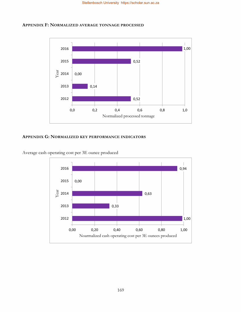
169

APPENDIX F: NORMALIZED AVERAGE TONNAGE PROCESSED

APPENDIX G: NORMALIZED KEY PERFORMANCE INDICATORS

Average cash operating cost per 3E ounce produced

0,52

0,14

0,00

0,52

1,00

0,0 0,2 0,4 0,6 0,8 1,0

2012

2013

2014

2015

2016

Normalized processed tonnage

Yea

r

1,00

0,33

0,63

0,00

0,94

0,00 0,20 0,40 0,60 0,80 1,00

2012

2013

2014

2015

2016

Noarmalized cash operating cost per 3E ounces produced

Yea

r


170

Average cash operating cost per Pt oz produced

Average cash operating cost per ton milled

1,00

0,34

0,58

0,67

0,00

0,00 0,20 0,40 0,60 0,80 1,00

2012

2013

2014

2015

2016

Noramlized cash operating cost per Pt oz produced

Yea

r

0,52

0,14

0,00

0,52

1,00

0,00 0,20 0,40 0,60 0,80 1,00

2012

2013

2014

2015

2016

Normalzed cash operating cost per ton milled

Yea

r


171

APPENDIX H : MONTHLY AVERAGES FOR KEY PERFORMANCE INDICATORS


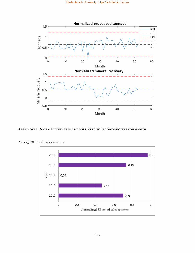
172

APPENDIX I: NORMALIZED PRIMARY MILL CIRCUIT ECONOMIC PERFORMANCE

Average 3E metal sales revenue

0,70

0,47

0,00

0,73

1,00

0 0,2 0,4 0,6 0,8 1

2012

2013

2014

2015

2016

Normalized 3E metal sales revenue

Yea

r


173

Average operating cost

Average annual profit

APPENDIX J: SPOT METAL PRICES (AS AT JUNE 2016)

Element Spot metal price

(USD/oz)

Pt 976.00

Pd 545.00

Rh 660.00

0,59

0,55

0,00

0,88

1,00

0,00 0,20 0,40 0,60 0,80 1,00

2012

2013

2014

2015

2016

Normalized operating cost

Yea

r

0,70

0,47

0,00

0,73

1,00

0,00 0,20 0,40 0,60 0,80 1,00

2012

2013

2014

2015

2016

Normalized profit

Yea

r


APPENDIX K: DATA OF INTEREST

Data item Data source Frequency of data generation Data availability

Key controlled

variables

Primary mill

product PSD

Offline Lab analysis data base Every shift (8 hours) 48hours later

Primary mill load

Online Pi historian Every second Immediately

Primary mill sump

slurry density


Rougher flotation

mass pull


Metallurgical data

Tonnes milled Online

Offline

Pi historian

Production reports

Every second

Hourly (Control room report)

Daily (Production report)

Monthly (Production report)

Monthly and yearly (Financial

report)

Immediately

Determined by report

Head grade Offline Laboratory assaying Every shift 48 hours later

Rougher tails grade Offline Laboratory assaying Every shift 48 hours later

*Rougher flotation

recovery

Offline Computationally

determined from

Based on available head and

rougher tail grade grades

Not applicable

159



available head and

rougher tails grade

Cost data

Actual motor

current for the :

Primary mill


pumps

Flotation cells

Conveyor belts

Online

and

offline

Pi historian Variable, based on

predetermined data capture

frequency

Not determined

Motor voltage

rating for the :

Primary mill


pumps

Flotation cells and

tank agitators

Conveyor belts

Offline Motor name plates Not applicable Not applicable

Primary mill

equipment running

time

Online Pi historian Variable, based on


frequency

Immediately

160



Reagent flowrate

Depressant

Collector

Promotor

Frother

Online Pi historian Variable, based on


frequency

Immediately

Reagent

concentration

Depressant

Collector

Promotor

Frother

Offline Laboratory sampling Every shift 24 hours later

Primary mill steel

ball grinding media

Offline

Control room log sheet

Financial report

Every shift

Monthly

8hours later

Every first week of the

new month

Unit prices for cost

data

Offline Unit prices from April

2016 report

Not applicable Not applicable

*Revenue data Basket price

Metal pricing

Exchange rate

Offline Computationally

determined from current

prill split and commodity

prices

www.kitco.com

www.xe.com

Calculated

161



http://www.kitco.com/

APPENDIX L: MATHEMATICAL MODEL FOR SAG MILL

Feeder module

V𝑓𝑤𝑜 = 𝑀𝐼𝑊

V𝑓𝑠𝑜 =𝑀𝐹𝑆

𝐷𝑠

(1 − 𝛼𝑠)

V𝑓𝑓𝑜 =𝑀𝐹𝑆

𝐷𝑠

𝛼𝑓

V𝑓𝑟𝑜 =𝑀𝐹𝑆

𝐷𝑠

𝛼𝑟

V𝑓𝑟𝑜 =𝑀𝐹𝐵

𝐷𝐵

Mill module

𝑑

𝑑𝑡𝑋𝑚𝑤 = 𝑉𝑚𝑤𝑖 − 𝑉𝑚𝑤𝑜

𝑑

𝑑𝑡𝑋𝑚𝑠 = 𝑉𝑚𝑠𝑖 − 𝑉𝑚𝑠𝑜 + 𝑅𝐶

𝑑

𝑑𝑡𝑋𝑚𝑓 = 𝑉𝑚𝑓𝑖 − 𝑉𝑚𝑓𝑜 + 𝐹𝑃

𝑑

𝑑𝑡𝑋𝑚𝑟 = 𝑉𝑚𝑟𝑖 − 𝑅𝐶

𝑑

𝑑𝑡𝑋𝑚𝑏 = 𝑉𝑚𝑏𝑖 − 𝐵𝐶

Hydrocyclone Overflow

𝑷𝑺𝑬 =𝑽𝒄𝒇𝒊 − 𝑉𝑐𝑓𝑢

𝑉𝑐𝑐𝑖 + 𝑽𝒄𝒄𝒖 − 𝑽𝒄𝒇𝒐

Mill Discharge

𝑽𝒎𝒘𝒐 = 𝑽𝒗 × 𝝋 × 𝑿𝒎𝒘 ×𝑿𝒎𝒘

𝑿𝒎𝒔 + 𝑿𝒎𝒘

𝑽𝒎𝒔𝒐 = 𝑽𝒗 × 𝝋 × 𝑿𝒎𝒘 ×𝑿𝒎𝒔


𝑽𝒎𝒇𝒐 = 𝑽𝒗 × 𝝋 × 𝑿𝒎𝒘 ×𝑿𝒎𝒘𝒎𝒇


𝑽𝒎𝒓𝒐 = 𝑽𝒎𝒃𝒐 = 𝟎

Hydrocyclone Underflow

V𝑐𝑤𝑢 =𝑉𝑐𝑤𝑖(𝑽𝒄𝒄𝒖 − 𝑭𝒖𝑽𝒄𝒄𝒖)

𝐹𝑢𝑉𝑐𝑤𝑖 + 𝑭𝒖𝑽𝒄𝒇𝒊 − 𝑽𝒄𝒇𝒊

V𝑐𝑓𝑢 =𝑉𝑐𝑓𝑖(𝑽𝒄𝒄𝒖 − 𝑭𝒖𝑽𝒄𝒄𝒖)

𝐹𝑢𝑉𝑐𝑤𝑖 + 𝑭𝒖𝑽𝒄𝒇𝒊 − 𝑽𝒄𝒇𝒊

Sump Discharge

V𝑠𝑤𝑜 = 𝐶𝐹𝐹 ×𝑋𝑠𝑤

𝑆𝑉𝑂𝐿

V𝑠𝑠𝑜 = 𝐶𝐹𝐹 ×𝑋𝑠𝑠

𝑆𝑉𝑂𝐿

V𝑠𝑓𝑜 = 𝐶𝐹𝐹 ×𝑋𝑠𝑓

𝑆𝑉𝑂𝐿

Sump Module

𝑑

𝑑𝑡𝑋𝑠𝑤 = 𝑉𝑠𝑤𝑖 − 𝑉𝑠𝑤𝑜 + 𝑆𝐹𝑊

𝑑

𝑑𝑡𝑋𝑠𝑠 = 𝑉𝑠𝑠𝑖 − 𝑉𝑠𝑠𝑜

𝑑

𝑑𝑡𝑋𝑠𝑓 = 𝑉𝑠𝑓𝑖 − 𝑉𝑠𝑓𝑜

Hydrocyclone module

Flotation

162



178

The mathematical descriptions are shown below:

V denotes the flowrate, m3/h

X denotes the states of the model as volumes, m3

RC is the rock consumption

BC is the ball consumption

FP is the fines production

α denotes the fraction

ϕ is the rheology factor

Subscripts

The first subscript indicates the module considered

The second subscript specifies one of the five states

The last subscript shows an inflow (i), outflow (o) or underflow (u)

The connotations are given in the Table below:

Subscripts for Le Roux’s model

Subscript Description

XΔ- f-feeder m-mill s-sump c-cyclone

X-Δ w-water s-solids c-coarse f-fines r-rocks b-balls t -total

V--Δ i-inflow o-outflow u-underflow

APPENDIX M: STEEL BALL – POWER RELATIONSHIP

𝐵𝐶 =

𝑃𝑚𝑖𝑙𝑙𝝋

𝜙 (

𝑋𝑚𝑏

𝐷𝑠(𝑋𝑚𝑟 + 𝑋𝑚𝑠) + 𝐷𝐵𝑋𝑚𝑏) 14

where, BC - steel ball grinding media consumption, t

Pmill - power draw, kW

φ - steel abrasion factor, kWh/t

ϕ - rheology factor,

Xmb - ball charge fraction


179

Ds - density of steel balls, t/m3

DB - density of feed ore, t/m3

Xmr - rock fraction

Xms - solids fraction

APPENDIX N: SIMULATION EXPERIMENT CALCULATIONS

Mineral recovery from particle size

𝑃𝑅𝑖 = −0.009776(𝑃𝑆𝑖2) + 1.705(𝑃𝑆𝑖) − 2.995

15

Average predicted mineral recovery

𝑃𝑅𝑎𝑣𝑒 = ∑ 𝑓𝑖

𝑚

𝑖=1

𝑃𝑅𝑖 16

where, PRave - shift potential mineral recovery

fi - fraction of data in the bin i

PRi - potential recovery derived from Equation 15 for bin i

m - number of intervals in the frequency distribution

The fraction of the data in bin i is derived as shown in Equation 17.

𝑓𝑖 =

𝑓

𝑓𝑡

17

Where f - number of data in bin i

ft - total number of data points

Number of bins

𝑆 = max (𝑃𝑅) − min (𝑃𝑅) 18

Where S is the range


180

𝑁 =

𝑆

𝐵𝑤

19

Where N - number of bins

Bw – bin width

Bin width calculation

𝐵𝑤 = 2 × 𝐼𝑄𝑅 (𝑇𝐻𝑅) × 𝑛−1/3 20

where IQR – interquartile range

THR – throughput

n – sample size

EPI calculation

𝐸𝑃𝐼 = (𝑘 ∑ ∑ 𝑓𝑖,𝑗

𝑠

𝑗=1

𝑚

1=1

𝑃𝑖,𝑗) − ∑(𝑐𝑢)𝑒

𝑛

𝑒=1

21

Where i - shift potential mineral recovery PDF (%)

j - mill throughput PDF (tph)

f - frequency for class widths, i,j

P - class interval median for the class i,j

m, s - the number of bins for the PDF I, j

c -number of cost element units consumed (units)

u - cost element unit price (ZAR/unit)

e - cost element

n - number of cost elements

𝑘 = 𝐻𝐺 × 𝐵𝑃𝑎𝑑𝑗 22

Where HG - head grade of 3g/t (adopted from Matthew & Craig (2013).


181

BPadj - adjusted basket price (ZAR/oz) derived as shown in Equation 23 (Appendix N)

0.032 - a conversion factor of between grams and troy ounces.

0.75 - an adjustment factor of was assigned for a PGM operation by Matthew & Craig (2013).

BP is the basket price adopted from industrial prill split data (ZAR/4E oz)

APPENDIX O: PLOTS FOR ACTUAL VS. PREDICTED MINERAL RECOVERY

Multi-predictor PVA approach

APPENDIX P: RESULTS FOR WINDOW SIZE 21

Single-predictor PVA approach – searches for EPFs


182

Results summary

Single-predictors PVA



R2adj,actual above threshold 0

R2adj,test above threshold 0

Multi-predictor PVA approach – searches for EPFs


183

Results summary

Multi-predictor PVA



R2adj,actual above threshold 57

R2adj,test above threshold 41

APPENDIX Q: AVERAGE MINERAL RECOVERY FOR SIMULATED FAULTS

Experiment Number

Drifting load cell

Steel ball quality

Ore hardness

1 58.20 70.25 68.34

2 56.70 69.15 67.23

3 54.50 72.05 66.25

4 59.40 68.15 69.01

5 55.10 71.12 64.21


184

APPENDIX R: AVERAGE MILL THROUGHPUT FOR SIMULATED FAULTS

Experiment Number

Drifting load cell

Steel ball quality

Ore hardness

1 39.13 32.53 28.86

2 37.15 31.61 27.44

3 36.00 28.79 26.51

4 34.12 33.52 30.73

5 40.01 30.25 29.14


Process monitoring with economic performance functions

Documents

Transcript of Process monitoring with economic performance functions