Appendix A Trigonometric Functions
117
Appendix A Trigonometric Functions 8 c a Fig. A.l A.l Definitions Let us consider a right-angled triangle ABC (Fig. A.l). If the side BC is of length a, AC of length b, AB of length c, andx is the angle BAC then we define sine x = sin x = f! c . b cosme x = cos x = - c tangent x = tan x = ~ Values of these functions can be obtained from tables. For a right-angled triangle, a2+b2=CZ 395 (1) (2) (3)
-
Upload
khangminh22 -
Category
Documents
-
view
0 -
download
0
Transcript of Appendix A Trigonometric Functions

Appendix A Trigonometric Functions
8
c a
Fig. A.l
A.l Definitions Let us consider a right-angled triangle ABC (Fig. A.l). If the side
BC is of length a, AC of length b, AB of length c, andx is the angle BAC then we define
sine x = sin x = f! c
. b cosme x = cos x = -
c
tangent x = tan x = ~
Values of these functions can be obtained from tables. For a right-angled triangle,
a2+b2=CZ
395
(1)
(2)
(3)

396
or, dividing by c?,
That is
or
Therefore,
Notice that
(sin xY + (cos xY = 1
sin2 x + cos2 x = 1
sin2 x = 1 - cos2 x
cos2 x = 1 - sin2 x
a ale sin x tanx = -=-=--
b b!c cosx
From (4), by dividing by cos2 x,
sin2 x cos2 x 1 --+--=--COS2 x cos2 x cos2 x
or, tan2 x + 1 = sec2 x
where sec x = secant x = 1/cos x
Appendix A
(4)
(5)
Two other trigonometric functions are the cosecant and cotangent defined by
and
1 cosecant x = cosec x = -
sin x
1 COS X cotangent x = cotan x = --= -.--
tan X SID X
A.2 Compound angles For any two angles x andy the following relationships can be shown
to be true:
sin (x + y) sin x cos y + cos x sin y
cos (x + y) = cos x cos y - sin x sin y
sin (x - y) sin x cosy- cos x sin y
cos (x - y) cos x cosy + sin x sin y
(6)
(7)
(8)
(9)

Trigonometric Functions
tan (x + y)
tan (x- y)
tanx+tany
1-tanxtany
tan x- tan y
1 + tan x tan y
Using these relationships, we have
(a) when x = y, from (6)
397
(10)
(11)
sin (x + x) = sin 2x = 2 sin x cos x (12)
(b) when x = y, from (7),
cos 2x = cos x cos x - sin x sin x
= 1 - 2 sin2 x = 2 cos2 x - 1 (13)
since cos2 x + sin2 x = 1. Hence,
2 sin2 x = 1 - cos 2x
• 2 1-cos2x sm x=----
2 (14) or
and 2 1 + cos 2x
COS X=----2
(15)
(c) When x = y, from (10)
tan 2x = 2 tan x (16)
1- tan2 x
(d) sin x + sin y = 2 sin ( x : y ) cos ( x ; Y ) (17)
. . 2 (x+y). (x-y) sm x- sm y = cos - 2- sm - 2-(18)
COS X + COS y = 2 COS (X : y) COS ( X ; y ) (19)
2 . (x+y). (x-y) cosx-cosy=- sm - 2- sm - 2-(20)

398 Appendix A
The formulae (17) to (20) can be verified by using (6) to (9) to expand the right-hand side of each statement.
A.3 Degrees and radians In elementary mathematical work it is convenient to measure
angles in degrees. In more advanced work, however, it is more convenient to use another measure of angles, known as radians. A radian is defined as the angle at the centre of a circle which contains an arc length equal to the radius of the circle (see Fig. A.2).
1 radian
Fig. A.2
If r is the radius of a circle, the circumference is of length 2nr. The angle at the centre of a circle is 360°, and so
360° = 2nr = 2lr radians r
or n radians = 180°
and n/2 radians = 90°
where n = 3.14159. Now consider the relationship between an angle measured as Do and R radians. Since 360° = 2lr radians,
and so
D R =
360 2n
D = 360 R and 2n
R =2nD 360
These convert radians to degrees and degrees to radians. For example,
if D = 30° R = 2lr(30) = 0.5236 radians ' 360

Trigonometric Functions
Also, if R = 1.30 radians, D = 360(1.30) = 74.48° 2Jr
A.4 General angles
399
From Fig. A.3 and the definitions sin x = ale, cos x = blc, tan x = alb we can see that varying x causes the point P to mark out a quadrant of a circle from A to B. At the same time the values of a and b vary.
8
A
Fig. A.3
If we allow x to become very small and approach zero, a approaches zero, and b approaches c, hence sin 0 = 0, cos 0 = 1, tan 0 = 0.
Similarly if we allow x to approach 90°, a approaches c and b approaches zero. Hence,
sin 90° = sin (nl2) = 1
cos 90° = cos (tr12) = 0
tan 90° = tan (trl2) = oo
Let us now increase x to 135° or 3nl4 radians (Fig. A.4). We know that, for example, using (6),
sin 135° = sin (90 + 45t = sin 90° cos 45° + cos 90° sin 45°
= cos 45° = 0.7071,
400 Appendix A
8
c
b A
Fig. A.4
that is, we can obtain sin x even when x is greater than 90° or n/2 radians. Similarly it can be shown that
cos 135° =-sin 45° = -0.7071
tan 135° = -tan 45° = -1.0000
Notice that cos 135° and tan 135° are both negative. This is because
b cosx =c
a tan x = b
and b is measured in the negative direction from 0, and so is a negative number. Both a and c are positive numbers.
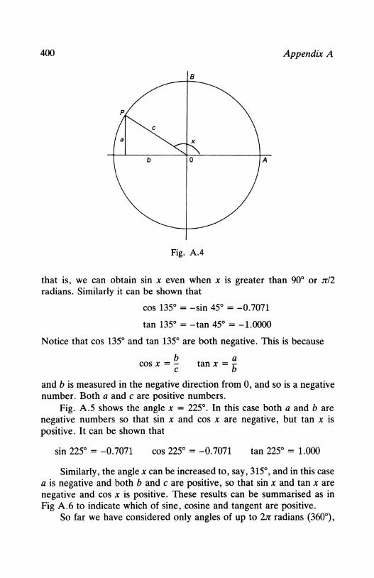
Fig. A.5 shows the angle x = 225°. In this case both a and b are negative numbers so that sin x and cos x are negative, but tan x is positive. It can be shown that
sin 225° = -0.7071 cos 225° = -0.7071 tan 225° = 1. 000
Similarly, the anglex can be increased to, say, 315°, and in this case a is negative and both b and c are positive, so that sin x and tan x are negative and cos x is positive. These results can be summarised as in Fig A.6 to indicate which of sine, cosine and tangent are positive.
So far we have considered only angles of up to 2Jr radians (360°),
Trigonometric Functions 401
Fig. A.S
Sin All
Tan Cos
Fig. A.6
but it is possible to allow an angle to exceed this by rotating the point P (Fig. A.5) around the circle. In this way, an angle of, say, 2.rr + x has the same sine, cosine, and tangent as x has.
We know that
sin 0 = 0 cos 0 = 1 tan 0 = 0
sin (.rr/2) = 1 cos (.rr/2) = 0 cos (.rr/2) = 00

402 Appendix A
Fig. A.7
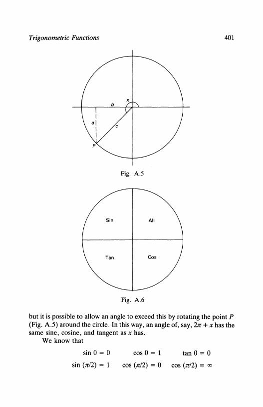
By evaluating sin x, cos x, and tan x for other values of x we can draw the graphs of these functions (Fig. A.7).
The graph of cos x is identical to the graph of sin x moved n/2 to the left. The graph of tan x has asymptotes at n/2, 3n/2, Sn/2, ... and so it consists of a series of sections.

Trigonometric Functions 403
A.5 Differentiation If y =sin x and we allow x to increase by a small amount ox, and let
the corresponding increase in y be oy, then
y + oy = sin (x + ox)
Subtracting, we have
Oy = sin (x + OX) - sin X
Using (6), we obtain
Oy = sin XCOS OX+ COS X sin OX- sin X
= sin x (cos ox - 1) + cos x sin ox
Oy . (COS OX- 1) COS X sin OX -= smx +-----ox ox ox
Hence,
Now by MacLaurin's theorem (section 5.15)
and
That is,
so that
and
Similarly,
and
Therefore,
Hence, if
x2 x4 x6 COS X = 1 -- + - - - + · · ·
2! 4! 6!
. x3 x5 X1
sm x = x--+- - - + · · · 3! 5! 7!
cos ox = 1- (6x)2 + (ox)4- (ox)6 + ... 2! 4! 6!
cos ox- 1 ox (ox)3 (ox)5 ----= --+-----+ ...
Ox 2! 4! 6!
lim(cos ox -1) = 0 /lx--.0 OX
l. (sin ox) 1m-- =1 /lx-+0 OX
lim (oy) = dy = sin x (0) + cos x (1) = cos x llx-+0 Ox dx

404
y = sin x dy =COS X
dx
Appendix A
The same method can be used to show that if y =cos x, dyldx =-sin x. If y =tan x = (sin x)/(cos x), then, using the rule for differentiating
quotients, we have
dy cos x (cos x)- sin x (-sin x)
dx (cos x)2
= cos2 x + sin2 x = _1_ = sec2 x cos2 x cos2 x
Similarly it can be shown that if
1 dy -1 - = -cosec2 x = -dx sin2 x
y = cotan x = -tan x
1 y =cosec x =-.
smx
1 y= secx =-
cos X
dy -cos x -cosec x -=---=----dx sin2 x tan x
dy sin x - = --= tan x sec x dx COS2 X
The above results can be generalised for the angle mx (where m is a constant) by use of the function of a function rule.
For example, if y = sin mx, let () = mx so that d()!dx = m.
Then y = sin () dy = cos () d()
dy dy d() -=-- = m cos mx dx d() dx
The derivatives of the trigonometric functions are listed in Table A.l.
A.6 Integration The integrals of some trigonometric functions can be deduced from
Table A.l. For example,
and
J cos x dx = sin x + c
J sin x dx =-cos x + c

Trigonometric Functions 405
TABLE A.l
Function Derivative Function Derivative
sin x COS X sin mx m cos mx
COS X -sin x cos mx -m sin mx
tan x sec2 x tan mx m sec2 mx
cotan x -cosec2 x cotan mx -m cosec2 mx
sec x tan x sec x sec mx m tan mx sec mx
-cosec x -m cosec mx cosec x cosec mx
tan x tan mx
J J sin x dx __ -J -sin x dx Now tan x dx = COS X COS X
=-log (cos x) + c
The integrals of other trigonometric functions are more difficult but some can be obtained by making the substitutions
. 2 tan (x/2) smx =
1 + tan2 (x/2) 1 - tan2 (x/2)
COS X=
or, writing t = tan (x/2),
. 2t smx=--
1 + (2
1- (2 cosx =--
1 + t 2
1 + tan2 (x/2)
These can be shown to be true by using the formulae for compound angles:
2 tan (x/2) 2[sin (x/2)]/[cos (x/2)]
1 + tan 2 (x/2) 1 + l sin2 (x/2) ]/[ cos2 (x/2)]
2 sin (x/2)
cos (x/2)[cos2 (x/2) + sin2 (x/2)]/cos2 (x/2)
2 sin (x/2) cos (x/2) = 1 = sin x, using (12) and (4)
406
Similarly,
1- tan2 (x/2) = 1- [sin2 (x/2)]/[cos2 (x/2)]
1 + tan2 (x/2) 1 + [sin2 (x/2)]/[cos2 (x/2)]
Appendix A
cos2 (x/2) - sin2 (x/2) = = cosx
cos2 (x/2) + sin2 (x/2)
using (4) and (13). These can be used to integrate some functions which cannot be integrated by other methods.
For example I _..!!:!...._
Let t = tan (x/2)
Then
Now
COS X
1- t 2
cosx =--1 + t 2
. 2t smx=--
1 + (2
dx=_l:_!!!_ 1 + t 2
I dx I (1 + t 2) 2 dt I 2dt COS X = (1 - t 2) (1 + t 2) = 1 - t 2
1 1 = J 1+t dt + J 1 - t dt
= log (1 + t)- log (1- t) + C
= log ( 1 + t) + C 1- t
I ( 1 + tan (x/2)) = og + C
1- tan (x/2)
Some standard integrals are given in Table A.2 (the constants of integration are omitted).
A. 7 Inverse functions If y = sin x then x = sin-1 y is known as the inverse sine function, or,
x is an angle whose sine is y. Similarly, x = cos-1 y and x = tan-1 y are the inverse cosine and tangent functions.
These are useful in integration when trigonometric substitutions can be made. For example,
Trigonometric Functions 407
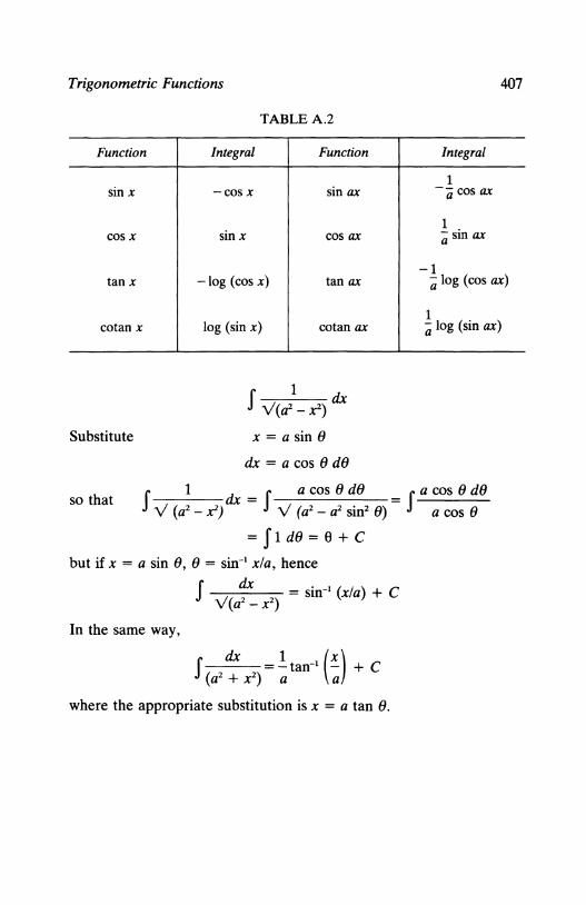
TABLEA.2
Function Integral Function Integral
1 sin x -cosx sin ax -a cos ax
1 COS X sin x cos ax a sin ax
-1 tan x -log (cos x) tan ax a log (cos ax)
1 cotan x log (sin x) cotan ax a log (sin ax)
f 1 dx V(a2 - X2 )
Substitute x=asinO
dx =a cos 8 dO
so that f 1 dx = f a cos 8 dO = f a cos e dO v (a2 - r) v (a2 - a2 sin2 8) a cos e
= f1 de= e + c but if X = a sin 8, 8 = sin-1 xfa, hence
J V dx = sin-1 (xla) + C (a2- x2)
In the same way,
J dx = .!tan-1 (~) + C (a2 + r) a a
where the appropriate substitution is X = a tan 8.

Appendix B Set Theory
B .1 Introduction A set is the name given to a group or collection of distinct objects.
Each member of a set is called an element. For example the set A might be defined as consisting of the three integers 1, 2 and 3, so that
A= {1, 2, 3},
where curly brackets or braces are used around the elements, while the set B might consist of four integers
B = {1, 3, 5, 7}.
To indicate that an element is a member of a set the special symbol E, which is read as 'belongs to' or 'is an element of', is used. Here 1 E A and 3 E B. When an element does not belong to a set the symbol fE. is used so that 4 fE. A and 2 fE. B.
The special set which has no elements is called the null set or referred to as an empty set and is represented by 0.
In these examples the sets A and B have been defined by enumerating all of the elements. This is possible when the number of elements in the set is small but in other cases it is more convenient to include a mathematical description, as in
P ={pIP> o}
where the set P is defined as containing those values of p for which p is greater than zero, and here p might be the price of a good. Here the convention of using capital letters for the set and lower case letters for the elements of the set is adopted. Another example is
Q = {q 13 < q < 30}
where Q is those values of q which are greater than 3 and less than 30.
408

Set Theory 409
More generally, the name R is commonly given to the set of all real numbers,
R = { x I x is a real number}
and the statement 'x is a real number' can be written x E R. Another useful concept is the idea of the universal set, which is all
the elements under discussion, and therefore varies with the context. For example, in discussing the properties of the set A the corresponding universal set, S, might be defined in one of the following ways
s = {1, 2, 3, 4, 5, 6, 7, 8}
or s = {-1, 0, 1, 2, 3, 9}
or S = {x I xis a real number}
B.2 Combining sets We now consider relationships between sets. First, two sets are
equal only if they contain identical elements. Thus if
A= {1, 2, 3},
and E = {2, 3, 1}
then E = A, even though the order in which the elements are written differs. Conversely, if at least one element does not occur in both sets the sets are not equal. For example, if
B = {1, 3, 5, 7}
A =I= B since 2 E A and 2 fE. B. In the special case where all the elements of one set, M say, are also elements in a larger set, N say, then M is said to be a sub-set of N, and this is written M C Nand is read 'M is a sub-set of N' or 'M is contained in N'. An example of a sub-set is where
M = {Monday, Tuesday}
N = {x I xis a day of the week}
Another example is where
A = {1, 2, 3},
and s = {1, 2, 3, 4, 5, 6, 7, 8, 9}
so that A is a sub-set of S. Notice that every set is a sub-set of its corresponding universal set.

410 Appendix B
Next, we can combine together two sets to form their union (indicated by U), which includes those elements belonging to either or both sets. For example,
A U B = {1, 2, 3} U {1, 3, 5, 7}
= {1, 2, 3, 5, 7}.
More formally, A U B = {x I x E A or x E B}
In the same way we can define the intersection (indicated by n) of two sets as being only those elements which occur in both sets. Thus,
A n B = {1, 2, 3} n {1, 3, 5, 7}
= {1, 3}
The formal definition is
A n B = {x I x E A and x E B}
As another example consider
and
then
and
F = {a, b, c, -1, 0, 6}
G = {c, d, 0, 1, 6},
F U G = {a, b, c, d, -1, 0, 1, 6}
F n G = {c, 0, 6}.
An interesting special case occurs when two sets have no elements in common, and so are said to be disjoint, and their union is the universal set. For example, consider
and
Since
A= {1, 2, 3},
p = {4, 6, 7, 9}
s = {1, 2, 3, 4, 6, 7, 9}
S=AUP
then P is called the complement of A, written A. Thus the union of a set and its complement is the universal set.
B.3 Venn diagrams The properties of combinations of sets can be illustrated by the use
of 'Venn diagrams'. In these, the universal set is represented by a
Set Theory 411
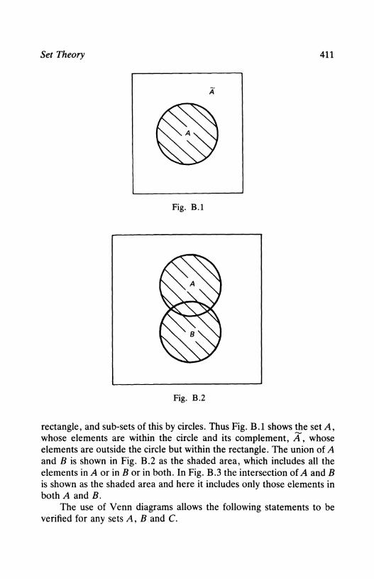
Fig. B.l
Fig. B.2
rectangle, and sub-sets of this by circles. Thus Fig. B.l shows the set A, whose elements are within the circle and its complement, A, whose elements are outside the circle but within the rectangle. The union of A and B is shown in Fig. B.2 as the shaded area, which includes all the elements in A or in Borin both. In Fig. B.3 the intersection of A and B is shown as the shaded area and here it includes only those elements in both A and B.
The use of Venn diagrams allows the following statements to be verified for any sets A, Band C.

412
Fig. B.3
(a) Commutative law of unions and intersections:
AUB=BUA
AnB=BnA
Appendix B
By considering Fig. B.2 and Fig. B.3 it can be seen that these are true and therefore the order of the sets does not matter for unions and intersections. This corresponds to addition and multiplication in algebra where a + b = b + a and ab = ba. Notice that in algebra the commutative law does not apply for substraction and division.
(b) Associative law of unions and intersections:
AU~Uq=0UmUC=AUBUC
An~nq=0nmnc=AnBnc
These are illustrated in Fig. B.4 and Fig. B.S and also correspond to addition and multiplication in algebra.
(c) Distributive law of unions and intersections:
A U (B n q = (A U B) n (A U q An (B U q =(An B) U (An q
These are shown in Fig. B.6 and Fig. B.7.

Set Theory 413
Fig. B.4
Fig. B.S
The laws of unions and intersections of sets extend to the special sets mentioned earlier, namely the universal set, the null set and the complement of any set.

414
Fig. B.6
Fig. B.7
B.4 Relations and functions
Appendix B
The concept of a set is essentially one-dimensional since only one variable is considered at a time. We now extend the ideas to combinations of sets. For example, suppose we observe the price, p, of a product

Set Theory 415
and the corresponding quantity demanded, q, where both p and q are real numbers and so are elements of the real number set R. That is, p E R and q E R. The sets of prices, P, and quantities, Q, are of course related since for each particular price there is an associated quantity and these two sets can be combined into an ordered set, say,
M = {(p, q) I pER, q E R}
Here the outer curly brackets or braces define the ordered set M, while the round brackets contain the elements of M, which are the sets P and Q. Therefore M consists of ordered pairs of prices and quantities and so while two sets, A = {1, 2, 3} and E = {2, 3, 1} are identical since they contain the same elements, the two ordered pairs from the ordered set M, (1, 5) and (5, 1) are different because the first is p = 1 and q = 5, while the second is p = 5 and q = 1.
Any ordered pair of values, say (p, q) or more generally (x, y) define what is called a relation between the variables. That is, a given value of xis associated with one or more values of y. For example, the relation defined by the ordered set {(x, y) I y = x + 2} includes the ordered pairs (0,2), ( -1,1) and (100,102). Graphically, this relation can be represented by a straight line. Another example is the relation defined by the ordered set { (x, y) I y < 2x} which includes the ordered pairs (3,0), (3,1) and (1,0). In this example it is clear that the relation between y and x is not unique since for a given value of x many different values of y can occur. The graphical representation consists of the area below the straight line y = 2x.
When there is just one value of y corresponding to each value of x the relation defines y as a function of x or y = f(x). That is, a function relating y and x is a set of ordered pairs with the property that for each value of x there is a unique value of y. Alternatively, the way in which y and x are related is said to be single valued. Notice that it is possible for a function to give the same y value for different values of x and an obvious example is y = x 2 where x = - 1 and x = 1 both give y = 1. In the converse case, for example if y2 = x, for each value of x there are two values of y and here we have a relation that is not a function.
The rule defined by a function, such as y = x 2 , can also be interpreted as a mapping or transformation, since the value of x is mapped or transformed into the value of y. The notation
f: X-> y
indicates the mapping from x toy with/representing the particular rule, y = x 2 here. Also, y is called the value of the function and x the

416 Appendix B
argument. Returning to the terminology of section 1.1, the variable xis the independent variable and y is the dependent variable. Two other terms are used in the literature: the domain of a function is the set of all permissible x values while the range is the set of all the values resulting from the mapping and so is the set of y values. For example suppose
y=5x-5
and x lies between 2 and 20. Then the domain is the set {X 12 <X< 20} and the range is the set {Y I 5 < Y < 95} .
Finally, it is sometimes convenient to find the inverse relationship for a particular relation. This can generally be found but may not be a function. For example, if
y=5x-5
the inverse relationship, which is a function, is
X= 0.2y + 1,
while if
the inverse relationship is
x= Yy which has two values of x for each y and so is not a function.

Appendix C Answers to Exercises
Exercises 1.5 1. (a) Y = 3x + 4; intercept is 4, slope is 3
(b) Y = 3x - 4; intercept is -4, slope is 3
(c) Y = 4 - 3x; intercept is 4, slope is -3
(d) Y= 3x;
(e) Y= 4;
2. Let TC = a + bq
intercept is 0, slope is 3
intercept is 4, slope is 0.
then from (a) 70 = a + lOb and (b) 120 = a + 20b
Solving these equations simultaneously gives the values a = 20, b=5
TC = 20 + 5q
Fixed cost = 20, variable cost = 5.
3. TC = 15 + 6q Total cost is £75 for an output of 10 units.
4. (b) Fixed cost is 3, variable cost is 2 (c) 33 (d) 21.
Exercises 1.8 1. y = 33 + 2x
(a) At the breakeven point Y = total revenue = 13x
13x = 33 + 2x
x=3
(b) Net revenue = pX - Y = 13(15) - 33 - 2(15) = 132
417

418 Appendix C
(d) Because the slope is 2, i.e. the variable cost is £2 per unit.
2. (a) TC = 50 + 5q
(b) At breakeven point, 50 + 5q = 10q so that q = 10
(c) Net revenue = 12p - 110
(i) p = 5, net revenue = - £50
(ii) p = 10, net revenue = £10
(iii) p = 15, net revenue = £70.
3. (a) At equilibrium q s = q d
:. 25p - 10 = 200 - 5p
:. p = 7 and q = 165
(b) 20p - 25 = 200 - 5p
:. p = 9 and q = 155.
4. (a) p = 4, q = 3
(b) p = 4, q = 0
(c) There is no unique solution (only one line)
(d) The equations are inconsistent (parallel lines).
Exercises 1.12 1. (a) In equilibrium, qd = qs or 200- 4p = -10 + 26p. Rearranging
gives 210 = 30p or p = 7, hence q = 172 and pq = 1204.
(b) Here p1 = p -5 so that qs = -10 + 26(p- 5) = 26p- 140. Equating to demand gives 26p -140 = 200 - 4p so 30p = 340 and p = 11.3, q = 154.7. Tax revenue = 5q = 773.3 and the producer's revenue is p1q = 974.6.
(c) Here p' = 0.8p so that qs = -10 + 26(0.8p) = -10 + 20.8p. Equating to demand gives -10 + 20.8p = 200- 4p so 24.8p = 210 and p = 8.47, q = 166.1. Tax revenue = 0.2(8.47)(166.1) = 281.4 Producer's revenue= p'q = 0.8(8.47)(166.1) = 1125.5.
2. Let the flat-rate tax be t per unit so that qs = -40 + 15(p - t). Equating to demand, - 40 + 15(p - t) = 300 - 6p or p = (340 +

Answer to Exercises 419
15t)/21 and if t = 1.7, p = 17.4. For a 10% tax, qs = -40 + 15(0.9)p = -40 + 13.5p In equilibrium, 300- 6p = -40 + 13.5p or p = 340/19.5 = 17.4
3. (a) Y = 20 + 0.7Y + 4 = 24 + 0.7Y or 0.3Y = 24 soY= 80 and c = 20 + 0.7(80) = 76
(b) Y = 20 + 0.7(Y - 10) + 4 = 17 + 0.7Y or 0.3Y = 17 so Y = 56.7 and C = 20 + 0.7(56.7- 10) = 52.7
(c) Y = 20 + 0.7(0.75)Y + 4 = 24 + 0.525Y or 0.475Y = 24 so Y = 50.5 and C = 20 + 0.7(0.75)50.5 = 46.5
(d) Y = 20 + 0.7(0.75Y- 10) + 4 = 17 + 0.525Yor 0.475Y = 17 so Y = 35.8 and C = 20 + 0.7[(0.75)(35.8) - 10] = 31.8.
4. (a) IS: Y = C + I = 15 + 0.8Y + 75 -100i or Y = 450 - 500i LM: 250 = 250- 160i + 0.1 Y or Y = 1600i Solution is i = 450/2100 = 0.214 oe 21.4% and Y = 342.9
(b) IS: Y = 65 + 0.8Y -100i or Y = 325 - 500i LM: Y = 1600i. Solution is i = 325/2100 = 0.155 andY= 248.
(c) IS: Y = 450 - 500i LM: 275 = 250 - 160i + 0.1 Y or Y = 250 + 1600i. Solution is i = 200/2100 = 0.095 and Y = 402.
5. (a) IS: Y = C + I + G = 15 + 0.8Yd + 75 - lOOi + 300 and Yd = 0.8Y - 5 so Y = 386 + 0.64Y - 100i and this simplifies to Y = 1072.2 - 277.8i.
(b) LM: 950 = 0.2Y + 750- 260i or Y = 1000 + 1300i Equilibrium requires 1072.2 - 277 .8i = 1000 + 1300i or i = 72.2/1577.8 = 0.046 and Y = 1059.8.
(c) IS: Y = 440 + 0.64Y- 4- 100i or Y = 1211.1 - 277.8i LM: Y = 1000 + 1300i Equilibrium has i = 211.111577.8 = 0.134 andY= 1173.9. Here both Y and i are higher than previously.
Exercises 1.14 1. 2xl + 2x2 = 2
3x1 - X2 = 1

420 Appendix C
I 2 2 1 -1 (-2 -2) -4
1 .. x, ~ I = =- =;z
2 2 (-2 -6) -8 3 -1
I 2 2 3 1 2-6 -4
and 1
x, ~I = --=- =;z 2 2 -8 -8 3 -1
2. x, = 1, X2 = 1.
3. x, - x 2 + x3 = 4
x, + X2 + 3x3 = 8
X 1 + 2x2 - X3 = 0
4 -1 1 1 3 8 3 8 1 8 1 3 4 - (-1) + 1 0 2 -1 2 -1 0 -1 0 2
.. x, = 1 -1 1 1 3 1 3 1 1 1 1 3 1 - (-1) + 1 1 2 -1 2 -1 1 -1 1 2
4(-7) + (-8) + (16) -20 = =-=2
(-7) + (-4) + (1) -10
1 4 1 1 8 3 1 0 -1 -8 + 16 -8
x2 = =0 1 -1 1 -10 1 1 3 1 2 -1

Answer to Exercises
1 -1 4 1 1 8 1 2 0 - 16- 8 + 4 -20
x3 = =-=2 1 -1 1 -10 -10 1 1 3 1 2 -1
4. x,= 1, x2 = 1, x3 = -1.
5. x, = 2, x2 = 2, x3 = 2.
6. x, = -1, x2 = -2, X3 = -3.
Exercises 1.16
1. (a) Y = C + I + G = C + I + 20
C = 20 + 0.7(Y- T) = 20 + 0.7(Y- 5- 0.3Y)
= 16.5 + 0.49Y
I= 15 + 0.1Y
Arranging in the order Y, C I: Y-C-I=20
-0.49Y + C = 16.5
-0.1 Y +I = 15
Using the notation of the text,
1 -1 -1 0.9 -1 0 IAI = -0.49 1 0 -0.49 1 0
-0.1 0 1 -0.1 0 1
= 0.9 - 0.49 = 0.41
20 -1 -1 35 -1 0 IA,I = 16.5 1 0 = 16.5 1 0
15 0 1 15 0 1
= 35 + 16.5 = 51.5
421

422
1 20 -1 -0.49 16.5 0 -0.1 15 1
= 14.85 + 17.15 = 32
1 -0.49 -0.1
-1 20 1 16.5 0 15
= 7.65 + 3.65 = 11.3
0.9 35 0 = -0.49 16.5 0
-0.1 15 1
0.51 0 36.5 -0.49 1 16.5 -0.1 0 15
Appendix C
51.5 32 11.3 Hence, Y = - = 125.6, C = -= 78.0 and I=-= 27.6
0.41 0.41 0.41
At this equilibrium, G = 20 and T = 5 + 0.3(125.6) = 42.7 and so there is a surplus of 22.7.
1. (b) If G = T = 5 + 0.3 Y the national income identity becomes Y = C +I+ 5 + 0.3¥ or 0.7¥- C- I= 5. The other two equations are unchanged: -0.49¥ + C = 16.5
-0.1 Y + I = 15
0.7 -1 -1 0.6 -1 Here, IAI = -0.49 1 0 = -0.49 1
-0.1 0 1 -0.1 0
= 0.6- 0.49 = 0.11
5 -1 -1 IA,I = 16.5 1 0
15 0 1
= 20 + 16.5 = 36.5
0.7 5 -1 IA21 = -0.49 16.5 0
-0.1 15 1
= 9.9 + 9.8 = 19.7
= 20 -1 0 16.5 1 0 15 0 1
0.6 20 0 -0.49 16.5 0 -0.1 15 1
0 0 1
Answer to Exercises
0.7 -0.49 -0.1
-1 5 1 16.5 0 15
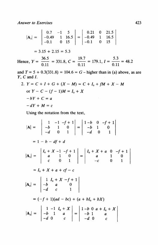
= 3.15 + 2.15 = 5.3
0.21 0 21.5 = -0.49 1 16.5
-0.1 0 15
36.5 19.7 5.3 Hence Y = - = 331.8 C = - = 179.1 I=-= 48.2
' 0.11 ' 0.11 ' 0.11
423
and T = 5 + 0.3(331.8) = 104.6 = G- higher than in (a) above, as are Y, C and I.
2. Y = C + I + G + (X - M) = C + I0 + fM + X - M
or Y - C - (f - 1 )M = I0 + X
-bY+C=a
-dY + M = c
Using the notation from the text,
1 -1 -f + 1 1-b 0 -f + 1 IAI = -b 1 0 = -b 1 0
-d 0 1 -d 0 1
= 1- b- df + d
Io +X -1 -f + 1 I0 + X + a 0 -f + 1 IA,I = a 1 0 a 1 0
c 0 1 -c 0 1
= Io + X + a + cf - c
1 I 0 +X -J + 1 IA2I = -b a 0
-d c 1
= (-f + 1)(ad- be)+ (a+ bi0 + bX)
1 -1 I 0 +X IA31 = -b 1 a
-d 0 c
1-b 0 a+ I0 +X -b 1 a -d 0 c
424 Appendix C
= (1 - b)c + d(a + /0 +X)
10 + X + a + cf - c Therefore, Y = '
1- b- df + d
C = (-f + 1)(ad - be) + (a + b/0 + bX)
1- b- df+ d
(1 - b)c + d(a + /0 +X) and M = --'----'--------'----....:.._
1- b- df + d
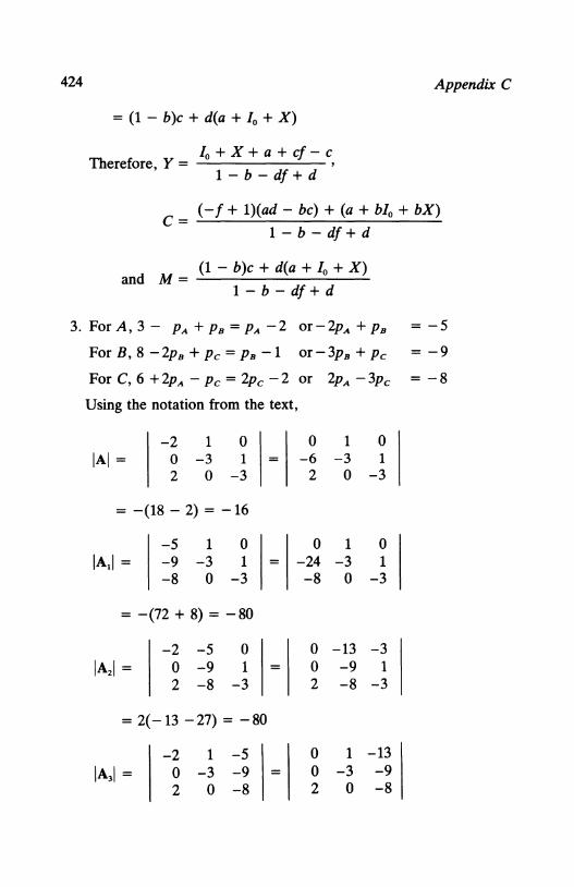
3. For A, 3- PA + p 8 = PA -2 or-2pA + p 8 = -5
ForB,8-2p8 +pc=Ps-1 or-3ps+Pc =-9
For C, 6 +2pA- Pc = 2pc -2 or 2pA -3pc = -8
Using the notation from the text,
-2 1 0 0 -3 1 2 0 -3
= -(18 - 2) = -16
-5 1 0 IA~I = -9 -3 1
-8 0 -3
= -(72 + 8) = -80
-2 -5 0 IA21 = 0 -9 1
2 -8 -3
= 2(- 13 - 27) = - 80
-2 1 -5 IA31 = 0 -3 -9
2 0 -8
=
=
=
0 1 0 -6 -3 1
2 0 -3
0 1 0 -24 -3 1 -8 0 -3
0 -13 -3 0 -9 1 2 -8 -3
0 1 -13 0 -3 -9 2 0 -8

Answer to Exercises
= 2(-9 -39) = -96
rr = 3, qB = 4, qC = 10
4. Equating supply and demand in each market,
44 - 2pl + P2 + P3 = - 10 + 3pl or 54 = 5pl - P2 - p3
25 + P1 - P2 + 3p3 = - 15 + 5p2 or 40 = -p1 + 6p2 - 3p3
40 + 2pl + P2- 3p3 = -18 + 2p3 or 58= -2pl - P2 + 5p3
Using the notation from the text,
5 -1 -1 0 -1 0 IAI = -1 6 -3 29 6 -9
-2 -1 5 -7 -1 6
= (29 X 6) - (7 X 9) = 111
54 -1 -1 -4 0 -6 IA1i = 40 6 -3 = 40 6 -3
58 -1 5 58 -1 5
= -4(30 - 3) - 6 (- 40 - 348) = 2220
5 54 -1 0 254 -16 IA21 = -1 40 -3 -1 40 -3
-2 58 5 0 -22 11
= 2794 - 352 = 2442
5 -1 54 7 0 -4 IA31 = -1 6 40 = -13 0 388
-2 -1 58 -2 -1 58
= 2716 - 52 = 2664
425

426 Appendix C
2220 2442 2664 Therefore, p1 = ill= 20, P2 =ill= 22, p3 =ill= 24
q! = 50, q2 = 95, q3 = 30.
Exercises 2.3
(a) A + B = [ 2 + 2 4 + 0 l = [ 4 4] 1 + (-1) 3 + 1 0 4
[ 2 - (2 X 2) 4 - (2 X 0) ]-- [ -2
3 41 l
(b) A- 2B = 1 - (2 X - 1) 3 - (2 X 1)
[ 2 4][ 2 0 l [(2x2) + (4x-1) (2x0) + (4x1) l
(c) AB = = 1 3 -1 1 (1x2) + (3x-1) (lxO) + (3x1)
[4-4 0+4] [ 0 4]
= 2- 3 0 + 3 = -1 3
(d)AC=[ 2 4][3]=[(2x3)+(4x1)]=[10]
1 3 1 (1 X 3) + (3 X 1) 6
(2 X 2) (2 X 1) (2 X 1)
_ [ 3] [ 2 4] It is not possible to form the product (e) CA- matrix CA
1 1 3
(2 X 1) (2 X 2)

Answer to Exercises
(f) B = [ 2 0 l -1 1
: l [ : -: l =[ (2 X 2) + (4 X 0) (2 X -1) + (4 X 1) l
(1 X 2) + (3 X 0) (1 X -1) + (3 X 1)
(g) C ~ [ : l C' ~ [3 1]
C'A =[3 1] [ 21 43]
(1 X 2) (2 X 2)
=((3 X 2) + (1 X 1) (3 X 4) + (1 X 3)) = (7 15) (1 X 2)
(h) BA = [ 2 0 l [ 2 4] -1 1 1 3
[ (2x2) + (Ox1) (2x4) + (Ox3) l [ 4 8]
= ( -1x2) + (1x1) ( -lx4) + (1x3) = -1 -1
This is not equal to AB (obtained earlier in (c)).
427
428 Appendix C
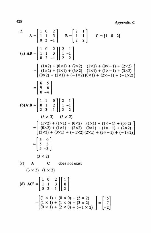
2.
A~o 0 j] B ~[ ~ -n 1 c = [1 0 2] 2
(a) AB ~ [ i 0 q[L:j 1 2 -1 2 2
[ (1x2) + (Ox1) + (2x2) (1x1) + (Ox-1) + (2x2) l
= (1x2) + (1x1) + (3x2) (1x1) + (1x-1) + (3x2) (Ox2) + (2x1) + (-1x2) (Ox1) + (2x-1) + (-1x2)
=[ ~ ~ l 0 -4
(b)A'B = [ ~ ~ ~ l [ i -~ l 2 3 -1 2 2
(3 X 3) (3 X 2)
[ (1x2) + (1x1) + (Ox2) (1x1) + (1x-1) + (Ox2) l
= (Ox2) + (1x1) + (2x2) (Ox1) + (1x-1) + (2x2) (2x2) + (3x1) + (-1x2) (2x1) + (3x-1) + (-1x2)
=[ ~ ~ l 5 -3
(3 X 2)
(c) A C does not exist
(3 X 3) (1 X 3)
(d) AC' = [ ~ ~ ; l [ ~ l 0 2 -1 2
[(1 X 1) + (0 X 0) + (2 X 2)
= (1 X 1) + (1 X 0) + (3 X 2) (0 X 1) + (2 X 0) + (-1 X 2) HJl

Answer to Exercises 429
(e) CB ~[1 0 2] [ H] (1 X 3) (3 X 2)
=[(lx2) + (Ox1) + (2x2) (1x1) + (Ox-1) + (2x2)]
=[6 5]
(1 X 2)
Exercises 2.5
LA~[::]
. . C = [ 3 -
1 ] and IAI = 5
-1 2
:. A-1 = ~ [ 3 -1 l = [ _: -: l -1 2 5 5
The solution to the equations is given by
[ ~ -~ l [ 4] X = A- 1b = -~ ~ 7
= [ a X 4) + (-~ X 7) l = [ (-~ X 4) + (~ X 7)
.". X 1 = 1, X2 = 2
2. (a) X1 = 58/23, X2 = -14/23
(b) X 1 = 0, X2 = -1, X3 = 3
(c) X 1 = 2, X2 = 0, X 3 = 1

430 Appendix C
Exercises 2. 7 1. Including the unit matrix with A gives
[ 2 -3
1 1
1
0
Subtract row 2 from row 1 to give 1 in the (1,1) position,
[ 1 -4 1 -1 l 1 1 0 1
Substract row 1 from row 2 to give 0 in the (2,1) position,
[ 1 -4
0 5
1 -1 l -1 2
Divide row 2 by 5, to give a 1 in the (2,2) position, and add four times the new row 2, to give a 0 in the (1,2) position,
[ : 0 0.2 0.6]
1 -0.2 0.4
Hence, A-'= [ 0.2 0.6 rod A-' A~ I
-0.2 0.4
For 8, [ 0 2 1 : l -1 -1 0
To get 1 in the (1,1) position, subtract row 2 from row 1,
[ _: 3 1 -: l -1 0
Add row 1 to row 2
[ 1 3 1 -: l 0 2 1
Answer to Exercises
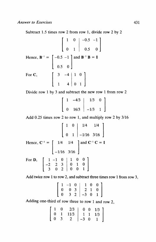
Subtract 1.5 times row 2 from row 1, divide row 2 by 2
0 -0.5 -1 l 0.5 0 1
Hence, B- 1 = [ -0.5 -1 land B- 1 B = I
0.5 0
For C,
4
-4 1 0 l 0 1
Divide row 1 by 3 and subtract the new row 1 from row 2
-4/3 113
16/3 -113
Add 0.25 times row 2 to row 1, and multiply row 2 by 3/16
[ I 0 114
114 l
0 1 -1116 3/16
Hence, c- 1 = [ 114
114 rod c-• C ~I -1116 3/16
ForD, [ I -1 0 1 0 n -2 2 3 0 1 3 0 2 0 0
431
Add twice row 1 to row 2, and subtract three times row 1 from row 3,
[ I -1 0 1 0
~ l 0 0 3 2 1 0 3 2 -3 0
Adding one-third of row three to row 1 and row 2 '
[ ~ 0 2/3 0 0 1/3] 1 1113 1 1 113 3 2 -3 0 1

432 Appendix C
Subtract three times row 2 from row 3
~ ~ ~~; l -6 -3 0
Divide row 3 by - 9 and combine with row 1 and row 2
[ 1 0 0 -4/9 -2/9 113] 0 1 0 -13/9 -2/9 1/3 0 0 1 2/3 1/3 0
Hence, o- 1 = [ -4/9 -2/9 1/3 ]"nd n-• D ~I -13/9 -2/9 1/3
2/3 113 0
For, E, u 0 1 1 0
~ l 3 -2 0 1 1 -1 0 0
Divide row 1 by 2, subtract twice the new row 1 from row 2, and add the new row 1 to row 3,
0 0.5 3 -3 1 -0.5
0.5 0 0 l -1 1 0 0.5 0 1
Divide row 2 by 3 and subtract the new row 2 from row 3,
[ ~ 0 0.5 1 -1 0 0.5
0.5 0 0 l -113 1/3 0 516 -1/3 1
Subtract row 3 from row 1, add twice row 3 to row 2, and multiply row 3 by 2,
[ ~ 0 0 -1/3 113 -1 l 1 0 4/3 -1/3 2 0 1 5/3 -2/3 2
Hence, E-• ~ [ -113 113 -1 ]"nd E-• E ~I 4/3 -113 2 5/3 -2/3 2

Answer to Exercises
For F, [
3 -2 3 -1 0 3
2 1 -1
1 0 0 l 0 1 0 0 0 1
433
Divide row 1 by 3, add the new row 1 to row 2 and subtract twice the new row 1 from row 3,
[ 1 -2/3 1 0 -2/3 4 0 7/3 -3
113 113
-2/3
0 0 l 1 0 0 1
Subtract row 2 from row 1, multiply row 2 by -3/2, and subtract 7/3 times the new row 2 from row 3
[ ~ ~ =~ 0 0 11
0 -1 0 l -0.5 -1.5 0
0.5 3.5 1
Divide row 3 by 11, add three times the new row 3 to row 1, and add six times the new row 3 to row 2
[ 1 0 0 0 1 0 0 0 1
3/22 -1122 3/11 l -5/22 9/22 6/11
1122 7/22 1111
Hence, F- 1 = [ 3/22 -1122 3/11 land F- 1 F = I -5/22 9/22 6/11
1122 7/22 1111
For G, [
-1 0 2 1 2 1 2 1 3
Add row 1 to row 2, add twice row 1 to row 3, and multiply row 1 by -1,
[ 1 0 -2 0 2 3 0 1 7
-1 0 0 l 1 1 0 2 0 1
Divide row 2 by 2 and subtract the new row 2 from row 3
-2 1.5 5.5
-1 0.5 1.5
g_ 5 ~1 l -0.5

434 Appendix C
Divide row 3 by 5.5, add twice the new row 3 to row 1 and subtract 1.5 times the new row 3 from row 2
[ 1 0 0 0 1 0 0 0 1
-5/11 1111 3/11
-2/11 7/11
-1111
4/11 l -3111 2/11
Hence G- 1 = [
-5/11 -2/11 4/11 land G- 1 G = I 1111 7/11 -3/11 3/11 -1111 2/11
2. As explained in the text it is not necessary to calculate the inverse matrix in order to get the solution but it is included in these answers for completeness.
1 0 (a) [
4 -2
2 1 0 1
Divide row 1 by 4 and subtract twice the new row 1 from row 2
[ I -0.5 0.25 0 1~5 l 0 2 -0.5 1
Divide row 2 by 2 and add 0.5 times the new row 2 to row 1
[ : 0 0.125 0.25 : rnd so x ~ 2, y ~ I
1 -0.25 0.5
(b) [ 3 -1 2 1 0 0 !] 1 3 1 0 1 0 2 1 1 0 0 1
Divide row 1 by 3, subtract the new row 1 from row 2, and subtract twice the new row 1 from row 3
[ 1 -113 2/3 0 10/3 113 0 5/3 -113
1/3 0 0 -113 1 0 -2/3 0 1
7/3 l 2/3 -2/3
Multiply row 2 by 3/10, add one-third of the new row 2 to row 1, and subtract 5/3 times the new row 2 from row 3.

Answer to Exercises
[ ~1 0 00 .. 71 0.3 0.1 0 1 -0.1 0.3 0 0 -0.5 -0.5 -0.5 1
435
2.4] 0.2 -1
Multiply row 3 by -2, subtract 0.7 times the new row 3 from row 1, and subtract 0.1 times the new row 3 from row 2
[ ~ 0 0 -0.4 -0.6 1.4 ~ l and x ~ I, y ~ 0, z ~ 2 1 0 -0.2 0.2 0.2 0 1 1 1 -2
(c) [ I I 1 1 0 0
! l 4 3 2 0 1 0 1 -1 -1 0 0 1
Subtract four times row 1 from row 2 and subtract row 1 from row 3,
[ 1 1 1 0 -1 -2 0 -2 -2
1 0 0 -4 1 0 :....1 0 1 -i l
-2
Add row 2 to row 1, multiply row 2 by -1, add twice the new row 2 to row 3,
[ ~ 0 -1 -3 1 0
i l 1 2 4 -1 0 0 2 7 -2 1
Subtract row 3 from row 2, add half of row 3 to row 1, and multiply row 3 by 0.5,
[ ~ 0 0 0.5 0 0.5 i l and x ~ I, y ~ I, z ~ 0 1 0 -3 1 -1 0 1 3.5 -1 0.5
(d) 2 1 1 1 1 0 0 0
~ l 1 -1 -1 1 0 1 0 0 1 2 3 -1 0 0 1 0 3 3 -1 2 0 0 0 1
Divide row 1 by 2, subtract the new row 1 from row 2 and from row 3, and subtract three times the new row 1 from row 4

436 Appendix C
[ ~ 0.5 0.5 0.5 0.5 0 0 0 1.5] -1.5 -1.5 0.5 -0.5 1 0 0 1.5 1.5 2.5 -1.5 -0.5 0 1 0 0.5 1.5 -2.5 0.5 -1.5 0 0 1 -0.5
Add row 2 to row 3 and row 4, divide row 2 by - 1.5 and subtract half of the new row 2 from row 1
[ ~ 0 0 2/3 1/3 1/3 0 0
-~ l 1 1 -1/3 1/3 -2/3 0 0 0 1 -1 -1 1 1 0 0 -4 1 -2 1 0 1
Subtract row 3 from row 2, add four times row 3 to row 4,
[ ~ 0 0 2/3 113 1/3 0 0 2 1 0 2/3 4/3 -5/3 -1 0 -3 0 1 -1 -1 1 1 0 2 0 0 -3 -6 5 4 1 9
Divide row 4 by- 3, add the new row 4 to row 3, subtract 2/3 times the new row 4 from row 1 and from row 2
[ ~ 0 0 0 -1 13/9 8/9 2/9 4 rdw =4 1 0 0 0 -5/9 -119 2/9 -1 X = -1 0 1 0 1 -2/3 -113 -113 -1 y = -1 0 0 1 2 -5/3 -4/3 -1/3 -3 z = -3
Exercises 2.9 1. (a) llere, li - ~ I = 2 - (- 1) = 3 and so rank = 2
By Gaussian elimination,
[i -~~~ ~] Subtract row 2 from row 1 and subtract the new row 1 from row 2
[ 1 -21 1 -1] 0 3 -1 2
Divide row 2 by 3 and add twice the new row 2 to row 1; this will give the unit matrix and so the rank is 2.

Answers to Exercises 437
(b) 1 1 3 2 1 1 1 -2 -1 =11 11-12 11 -2 -1 1 -1
+312 11=1+3-9=-5 1 -1
and so the rank is 3. By Gaussian elimination,
[ ~ ~ ~ ~ ~ ~] 1 -2 -1 0 0 1
Subtract twice row 1 from row 2 and row 1 from row 3
[1 1 3 1 0 0] 0 -1 -5 -2 1 0 0 -3 -4 -1 0 1
Add row 2 to row 1 and subtract three times row 2 from row 3, and multiply row 2 by - 1
[ 1 0 -2 0 1 5 0 0 11
-1 1 0 l 2 -1 0 5 -3 1
It can be seen that further operations will result in the unit matrix and so the rank is 3.
(c) The determinant can be simplified by adding twice column 2 to column 1, subtracting column 2 from column 3 and expanding by row 2
1 2 -4 2 -1 -1 3 1 -5
5 2 -6 0 - 1 0 = -~5 - 61 = 0 so the 5 1 - 6 5 - 6 rank < 3.
Next, try to find a non-zero (2 x 2) determinant. Here,
11 21 = - 1 - 4 = - 5 and so the rank is 2. 2 -1
By Gaussian elimination,
[ ~ 2 -4
-1 -1 1 -5

438 Appendix C
Subtract twice row 1 from row 2 and subtract three times row 1 from row 3
[1 2 -4 0 -5 7 0 -5 7
1 0 0 l -2 1 0 -3 0 1
Subtracting row 2 from row 3 will give 0, 0, 0 on row 3 and further row operations will give a (2 X 2) unit matrix and so the rank is 2.
(d) Expanding the determinant by the first row,
1 0 0 1 1 1 0 1 1
= I ~ ~ I = 0 and rank < 3
Searching for a non-zero (2 x 2) determinant, I ~ ~ I = 1
and the rank = 2 By Gaussian elimination,
[ 1 0 0 1 1 1 0 1 1
1 0 0 l 0 1 0 0 0 1
Subtract row 1 from row 2 and subtract the new row 2 from row 3,
[ 1 0 0 1 0 0] and the rank is 2. 0 1 1 -1 1 0 0 0 0 1 -1 1
(e) The determinant can be simplified by subtracting column 1 from column 2 and from column 3, and then expanding by row 1
1 1 1 1 0 0 1 0 2 = 1 -1 1 = 3 and rank = 3 2 2 -1 2 0 -3
By Gaussian elimination,
u 1 1 1 0
~ l 0 2 0 1 2 -1 0 0

Answers to Exercises 439
Subtract row 1 from row 2 and subtract twice row 1 from row 3
[1 1 1 0 -1 1 0 0 -3
1 0 0 l -1 1 0 -2 0 1
It can be seen that further row operations will result in the unit matrix and so the rank is 3.
(f) Here the matrix is (3 x 4) and so the maximum rank is 3. Taking the first 3 columns, the determinant is
1 0 0 0 2 2 =I 2 2 I = 2 and rank = 3 2 1 2 1 2
By Gaussian elimination,
[ ~ 0 0 -1 1 0 0
~ l 2 2 1 0 1 0 1 3 1 0 0 1
Subtract twice row 1 from row 3 and divide row 2 by 2
[1 0 0 -1 1 0 0 0] 0 1 1 0.5 0 0.5 0 0 0 1 3 3 -2 0 1 0
Subtracting row 2 from row 3 will give 0 0 2 on row 3 and so a unit matrix can be formed and the rank is 3.
(g) The maximum rank is 3 and taking the first three columns, adding column 1 to column 3
1 0 -1 1 0 0 1 1 -1 1 1 0 0 1 -1 0 1 -1
=i 1 0 I = -1 so rank = 3 1 -1
By Gaussian elimination,
u 0 -1 -1 1 0 0 0 l 1 -1 -1 0 1 0 0 1 -1 -1 0 0 1 0

440 Appendix C
Subtracting row 1 from row 2 and the new row 2 from row 3
[ 1 0 - 1 - 1 1 0 0 0] 0 1 0 0 -1 1 0 0 0 0 -1 -1 1 -1 1 0
and further row operations will give a (3 x 3) unit matrix and so the rank is 3.
2. In each case there is a unique solution if the determinant has a non-zero value.
(a) 1 3 -2 1 -2 1 = 2 -2 3
1 3 -2 0 -5 3 0 -8 7
=i-5 31=-11 -8 7
where row 1 was subtracted from row 2 and twice row 1 from row 3, and there is a unique solution.
(b) 1 2 1 2 -1 2 1 1 1
5 2 5 0 -1 0 3 1 3
where twice column 2 was added to column 1 and column 3, and as the determinant is zero there is no unique solution.
(c) 1 3 -1 2 1 2 -1 -3 1 -1 2 1 = 1 -2 2 -4 1 1 1 -2 1 0 1 -7 1 1 0 5 1 0 0 0
2 -1 -3 -2 2 -4
0 1 -7
where column 1 was subtracted from column 2 and five times column 1 was subtracted from column 4. Adding row 2 to row 1 gives a determinant with two identical rows and so it has a value zero. There is no unique solution.
Exercises 2.11
1. A=[2 1 1 0
2 1 1 0 2 1
r (A')'~~ i ~ i] =A

Answers to Exercises 441
A+B=[21 1 2]+[3 -1 1]=[5 0 3] 0 1 2 -2 0 3 -2 1
(BC)' = [ - 6 - 6 ] -1 -2
and
Also, C'B' = [-6 2 -1][ 3 2]=[-6 1 0 -~ -~ -1
-6]= (BC)'. -2
2. Require A2 = A for A to be idempotent
A'= [ ~ 0
~ ][ ~ 0
~ H ~ 0 ~ ] = A - idempotent 1 1 1 0 0 0
0.25 0.25 0.25 0.25 0.25 0.25 0.25 0.25 Bz= 0.25 0.25 0.25 0.25 0.25 0.25 0.25 0.25
0.25 0.25 0.25 0.25 0.25 0.25 0.25 0.25 0.25 0.25 0.25 0.25 0.25 0.25 0.25 0.25
0.25 0.25 0.25 0.25 0.25 0.25 0.25 0.25 = B - idempotent 0.25 0.25 0.25 0.25 0.25 0.25 0.25 0.25
C2 = [ a 0 ] [ a 0 ] = [ a2 0 ] = C only if a = 0 or a = 1. Oa Oa Oa2
3.A'=[ 2 1]and(A't 1 =[0.2 -0.2] -3 1 0.6 0.4
Now A -I= [ 0.2 0.6] and so (A-T = [0.2 -0.2] = (A't 1
-0.2 0.4 0.6 0.4
AB=[2 -3][ 2 2]=[7 1]and(ABt 1 =1_[ 3 -1] 1 1 -1 1 1 3 20 -1 7

442 Appendix C
B- 1 = [ 0.25 -0.5] 0.25 0.5
Also,
and so B-tA- 1 =_1_[ 3 -1]=(ABt 1 •
20 -1 7
4. Since A = [ ~ j ] then lA - rii =
= (3 - r) (3 - r) - 1
13- r 1 I
1 3- r
and setting this to zero gives 9 - 6r + r 2 - 1 = 0. Solving gives r = 4 and r = 2. For r = 4 the characteristic vector is from [A - 4I]x = 0,
Or [ 3 - 4 1 ] [ X 1 ] = [ 0 ] and -X 1 + X 2 : 0 SO X 1 = X 2
1 3 - 4 X 2 0 X 1 - X 2 - 0.
Normalising by setting xi +xi = 1 gives x 1 = 11\12 = X 2 • For r = 2 the characteristic vector is from [A - 2I]x = 0,
Or [ 3 - 2 1 ] [ X 1 ] = [ 0 ] and X 1 + X 2 = 0 SO X 1 = -X 2
1 3 - 2 X 2 0 X 1 + X 2 = 0.
Normalising by setting xi + x; = 1 gives x 1 = 11\12 and X 2 = -11\12.
Since B = [ ~ - ~] then IB - rii = 12 ~ r 1- ~ r I
= (2 - r) (1 - r)
and setting this to zero gives r = 2 and r = 1. For r = 2 the characteristic vector is from [B - 2I]x = 0,
or [ 2 - 2 - 1 ] [ x 1 ] = [ 0 ] and - x 2 = 0 0 1 - 2 X 2 0 -x 2 = 0.
Normalising by setting xi +xi = 1 gives x 1 = 1, X 2 = 0. For r = 1 the characteristic vector is from [B - ll]x = 0,
Or [ 2 - 1 - 1 ] [ X 1 ] = [ 0 ] and X 1 - X 2 = 0 SO X 1 = X 2
0 1 - 1 X 2 0
Normalising by setting x 12 + x} = 1 gives x 1 = 11\12 and x 2 = 11\12.
Answers to Exercises 443
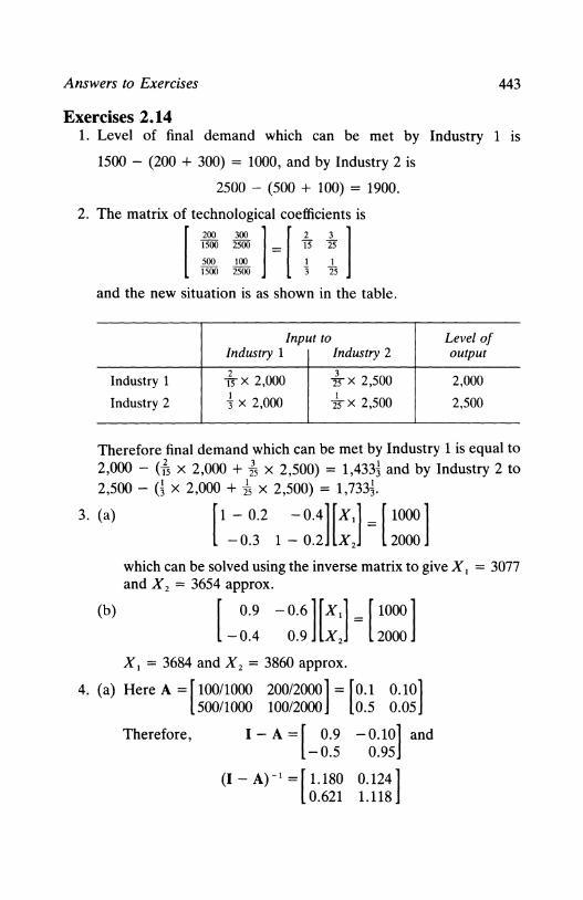
Exercises 2.14 1. Level of final demand which can be met by Industry 1 is
1500 - (200 + 300) = 1000, and by Industry 2 is
2500 - (500 + 100) = 1900.
2. The matrix of technological coefficients is
[ ~: is~]=[ fs is] 500 100 I I 1500 2500 3 25
and the new situation is as shown in the table.
Input to Level of Industry 1 Industry 2 output
Industry 1 2
J5X 2,000 3 zsx 2,500 2,000
Industry 2 I 3 X 2,000
I zsx 2,500 2,500
Therefore final demand which can be met by Industry 1 is equal to 2,000 - (fs x 2,000 + ~ x 2,500) = 1,4331 and by Industry 2 to 2,500 - (~ X 2,000 + fs X 2,500) = 1,733~.
3. (a)
(b)
[1-0.2 -o.4][x~]=[10oo] -0.3 1 - 0.2 x2 2000
which can be solved using the inverse matrix to give X 1 = 3077 and X 2 = 3654 approx.
[ 0.9 -o.6][x~]=[10oo] -0.4 0.9 x2 2000
X 1 = 3684 and X 2 = 3860 approx.
4. (a) HereA=[100/1000 200/2000]=[0.1 0.10] 500/1000 100/2000 0.5 0.05
Therefore, I- A= [ 0.9 -0.5
(I- A)- 1 =[1.180 0.621
-0.10] and 0.95
0.124] 1.118

444 Appendix C
by row operations. The multipliers are 1.180 + 0.621 = 1.801 and 0.124 + 1.118 = 1.242.
If the final demand for exports becomes 500 for agriculture and 900 for industry, the total final demands are 800 and 1500 respectively. Therefore,
X=(I-A)- 1 C=[1.180 0.124][ 800]=[1130.0] 0.621 1.118 1500 2173.8
instead of 1000 and 2000.
(b) Here [
0.1 0.10 300/900 l [0.1 0.10 0.33] A = 0.5 0.05 6001900 = 0.5 0.05 0.67
0.1 0.40 0/900 0.1 0.40 0.00
Therefore, I- A= [ 0.9 -0.10 -0.33] -0.5 0.95 -0.67 -0.1 -0.40 1.00
and (I - At 1 can be found by row operations:
[ 0.9 -0.10 -0.33 1 0 0 l
-0.5 0.95 -0.67 0 1 0 -0.1 -0.40 1.00 0 0 1
Divide row 1 by 0.9 and combine the new row 1 with rows 2 and 3:
[ 1 -0.111 -0.370 1.111 0 0] 0 0.895 -0.855 0.556 1 0 0 -0.411 0.963 0.111 0 1
Divide row 2 by 0.895 and combine the new row 2 with rows 1 and 3:
[ 1 0 -0.476 1.180 0.124 0 l 0 1 -0.955 0.621 1.117 0 0 0 0.570 0.366 0.459 1
Divide row 3 by 0.570 and combine the new row 3 with row 1 and row 2:
[ 1 0 0 1.486 0.507 0.835] 0 1 0 1.234 1.886 1.675 0 0 1 0.642 0.805 1.754
(Check that (I - A) (I- At 1 = I, apart from rounding errors)

Answers to Exercises 445
The multipliers, from adding the columns, are 3.362, 3.198 and 4.264, compared to 1.801 and 1.242 previously. If the final demand for exports becomes 500 for agriculture and 900 for industry, these are the total final demands (since households are an industry). Therefore,
X= (I- At'C =[ 1.486 0.507 0.835][500] [1199.3] 1.234 1.886 1.675 900 = 2314.4 0.642 0.805 1.754 0 1045.5
instead of the original values of 1000, 2000, 900 and the values in (a) of 1130 and 2173 (and 900 for households).
5. (a) The technology matrix is obtained by dividing each column by the gross output of the sector:
[11/41 19/240 11185] [ 0.268 0.079 0.005]
A = 5/41 89/240 40/185 = 0.122 0.371 0.216 5/41 37/240 37/185 0.122 0.154 0.200
[ 0.732 -0.079 -0.005]
Hence, I - A = - 0.122 0.629 - 0.216 -0.122 -0.154 0.800
and (I - A) multiplied by the given matrix is approximately I.
(b) Here, X= (I- At 1C =[ 1.409 0.192 0.062] [ 15] 0.372 1. 753 0.476 120 0.286 0.367 1.351 130
[ 52.2]
= 277.8 224.0
(c) Combining the industry and services sectors gives:
Input to Output from Agriculture Other
Agriculture 11 20 Other 10 203
The technology matrix is A = [ 11141 10/41
= [ 0.268 0.244
Final demand
10 212
20/425] 203/425
0.047] 0.478
Total output
41 425

446
and so
By row operations
Appendix C
I-A=[ 0.732 -0.047] -0.244 0.522
(I - At I = [ 1.408 0.127] 0.658 1.975
Hence, X= [1.408 0.127] [ 15] = [ 52.9] 0.658 1.975 250 503.6
These values compare with 52.2 and 277.8 + 224.0 = 501.8 and so, apart from rounding errors (which could be reduced by working to more places after the decimal point in both A and (I - A)- 1), the values for agriculture and the aggregate are the same. Thus, for an economist interested only in agriculture it does not matter whether we have one or two other sectors and, by implication, the results for agriculture would be the same if there were many other sectors.
Also, the multipliers for agriculture are 2.066 in both cases, while for industry the multiplier is 2.312 and for services, 1.889, and for the combined sector 2.102, the average of the two values.
Exercises 3.2 1. (a) Let x = output and TC = total cost, and since the cost func
tion is quadratic, let TC = a + bx + cx 2 •
Using the three pairs of values given:
4 = a (1)
14 = a + 2b + 4c (2)
58 = a + 6b + 36c (3)
Substituting from (1) into (2) and (3) and simplifying:
10 = 2b + 4c (4)
54 = 6b + 36c (5)
Subtract three times (4) from (5)
24 = 24c or c = 1
Putting a = 4 and c = 1 in (2) gives b = 3 and so
TC = 4 + 3x + x 2

Answers to Exercises 447
X 0 2 4 6 8 10 TC 4 14 32 58 92 134
(b) TC = 10 + 2x + 0.5x 2
X 0 2 4 6 8 10 TC 10 16 26 40 58 80
(c) TC = 25 + 0.5x + 0.25x 2
X 0 2 4 6 8 10 TC 25 27 31 37 45 55
(d) TC = 20 + 0.8x + 0.02x 2
X 0 1 3 5 7 9 10 TC 20 20.82 22.58 24.50 26.58 28.82 30.00
(e) TC = 20 + 0.5x 2
X 0 2 4 6 8 10 TC 20 22 28 38 52 70
2. X 0 1 2 3 4 5 6 7 8 9 10
(a) y 100 111 124 139 156 175 196 219 244 271 300 (b) y 100 91 84 79 76 75 76 79 84 91 100 (c) y 100 109 116 121 124 125 124 121 116 109 100 (d) y 100 89 76 61 44 25 4 -19 -44 -71 -100
Exercises 3.4 1. Formula is x = { -b ± v'(b2 - 4ac)}/2a
(a) a= 1, b = -7, c = 12 sox= 4 or 3
448
(b) a = 1, b = 1, c = - 2 so x = 1 or - 2
(c) a= 2, b = 7, c = 3 sox= -0.5 or -3
(d) a= 1, b = -2, c = 1 sox= 1 (repeated root)
(e) a = 1, b = 0, c = -1 sox = 1 or -1
(f) a = 1, b = 0, c = 1 sox = i or - i
(g) a = 1, b = - 4, c = 5 so x = 2 + i or 2 - i
(h) a = 1, b = 2, c = 2 sox = -1 + i or -1 - i.
Appendix C
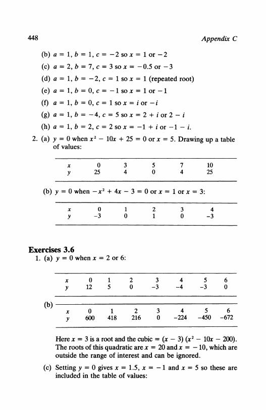
2. (a) y = 0 when x 2 - lOx + 25 = 0 or x = 5. Drawing up a table of values:
X
y 0
25 3 4
5 0
7 4
10 25
(b) y = 0 when - x 2 + 4x - 3 = 0 or x = 1 or x = 3:
X
y
Exercises 3.6
0 -3
1 0
1. (a) y = 0 when x = 2 or 6:
X 0 1 y 12 5
(b) X 0 1 y 600 418
2 0
2 216
2 1
3 -3
3 0
3 0
4 -4
4 -224
4 -3
5 -3
5 -450
6 0
6 -672
Here x = 3 is a root and the cubic= (x- 3) (x 2 - lOx - 200). The roots of this quadratic are x = 20 and x = - 10, which are outside the range of interest and can be ignored.
(c) Setting y = 0 gives x = 1.5, x = -1 and x = 5 so these are included in the table of values:

Answers to Exercises 449
X -2 -1 0 1 1.5 2 3 4 5 6 y -49 0 15 8 0 -9 -24 -25 0 63
(d) Setting y = 0 gives x = 0, and so 32 - 2x 2 = 0 resulting in x = 4 or -4.
X -4 -3 -2 -1 0 1 2 3 4 y 0 -42 -48 -30 0 30 48 42 0
(e) When y = 0, x = 0:
X 0 1 2 3 y 0 1 32 243
(f) y = 20/x so as x ~ 0, y ~ oo
X 1 5 10 20 100 y 20 4 2 1 0.2
(g) y = (20/x) + 1. Asx~ O,y~ oo, andasx~ oo,y~ 1:
X 1 5 10 20 100 y 21 5 3 2 1.2
2. Q = KL so that K = Q/L
L 10 20 50 80 100
Qt/L 2 1 0.4 0.25 0.2 QiL 5 2.5 1 0.625 0.5 QiL 10 5 2 1.25 1
3. AC = TC/x. Here x > 0 and negative values can be ignored:
X 1 10 20 50 100 200
(a) AC 100 10 5 2 1 0.5 (b) AC 105 15 10 7 6 5.5 (c) AC 106 25 30 57 106 205.5

450 Appendix C
Exercises 3.10 1. The breakeven point has TC = TR.
(a) x 2 - 6x + 9 = 0 has x = 3 as the repeated root and this is the breakeven point
(b) x 2 - 9x + 18 = 0 has x = 6 and x = 3 as the breakeven points
(c) 2x 2 - 3x + 10 = 0 has no real roots and so there is no breakeven point.
2. (a) TC = 25 - 6x + x 2
(b) 305 (d) total revenue equals total cost when
lOx + 15 = 25 - 6x + x 2
that is when x 2 - l6x + 10 = 0 The roots of this quadratic are given by
X = 16 ± Y(l62 - 4 X 10)
2
= !(16 ± V(256 - 40)) = !(16 ± V (216))
= 8 ± 7.35 = 15.35 or 0.65.
These are the two levels of output at which total revenue equals total cost.
4. The equations are satisfied by the values x = 1 and x = 15.
5.
or
y = 20 + 3x + X 2
y = 5x + b
20 + 3x + x 2 = 5x + b
x 2 - 2x + (20- b) = 0
X = 2 ± V[4- 4(20- b)]
2
= 1 ± V[ 1 - (20 - b)]
= 1 ± V'(b- 19)
when b = 20 x = 1 ± 1 = 2 or 0 (2 real solutions)

Answers to Exercises 451
6.
b = 19 x = 1 (the solutions are coincident) b = 18 x = 1 ± Y( -1) (2 complex solutions)
2p2 - 3p - 40 = 250 - 4p - p 2
3p2 + p - 290 = 0
p -1 ± Y(l + 12 X 290)
6
-1 ± \13481
6
58
6 or
-60
6
-1 ±59
6
In this example we take the positive root, p = 9§, and at this value q = 117~.
7. (a) p = 5 (c) p = 2
q = 10 q = 3
(b) p = 4 q=4
8. Net revenue NR = TR - TC and TR = pq. Since TC is expressed in terms of q rearrange demand to give p = (200 - q D)/2 so NR = qD (200 - qD)/2 - 20 - 5qD.
At the breakeven points, NR is zero when qD = 0.21 or 189.8. The corresponding prices are 99.9 and 5.1:
0 -20
10 880
20 50 100 150 200 1680 3480 4480 2980 - 1020
(maximum NR is when qD is 95 and NR = 4492.5)
Exercises 3.12 1. (a) When x = 19, TC = 72 and when x = 21, TC = 78 and extra
cost is 78 - 72 = 6 (b) When x = 29, TC = 102 and when x = 31, TC = 133 and
extra cost is 133 - 102 = 31 (c) When x = 49, TC = 187 and when x =51, TC = 223 and
extra cost is 223 - 187 = 36.
2. Let x = number of cans sold Revenue = 30x for 0 < x ::::; 100 and
= 30 (0.85)x for x > 100

452 Appendix C
If x = 99, cost = 30 (99) = 2970p If x = 101, cost = 30 (0.85) 101 = 2575.5- cheaper than for 99!
New system: Revenue = 30x for 0 < x < 101 Revenue = 100 (30) + (x - 100) (0.80) 30 for x > 100
If x = 120, old revenue = 30 (0.85) 120 = 3060, new revenue = 100 (30) + (20) (0.80) 30 = 3480.
Exercises 4.3 1. (a) 19, 225
(c) -210, -2,250
2. £300 3. £11,300, £67,900
(b) 950, 12,750 (d) 82, 1,290
4. Arithmetic progression with 20 = a + (n - 1)d = 10 + 15d. Hence d = ~and rate of interest is ~/10 = 0.067 or 6.7 per cent.
Exercises 4.5 10(1 - 310)
1. (a) 2,430; S10 = = 295240 -2
1 81[1 - Grol . (b) 3; S10 = 1 = 121.5 approxtmately
1 - 3
81 Soo = I = 243/2 = 121~
1 - (3)
2[1 - (- 2) 10] (c) -64;510 = =-682
3
(d) 32· s = -1024[1 - ( -~rol ' 10 I 1- (-2)
= - 682 approximately
-1024 2 Soo = I = -6823
1 - ( -2)
1 [1 - (0.1)10] . (e) 0.00001; S10 = 1 _ 0. 1 = 1.111 approxtmately
1 Soo = - 10
1 - 0.1 - 9

Answers to Exercises
2. (a) 300(1.05) 15 = 623.7 (b) 300(1.10f5 = 1253.2
150(1 - 1.0625) = 8229.7 (1 - 1.06)
4. 4(1 + r)4 = 5
. . (1 + rt = 1.25
1 + r = 1.06 approximately
and implied rate of compound interest is 6 per cent.
Exercises 4.7
453
1. (a) Present value of £800 received in 10 years time is given by £800/(1 + i)'0 ; this is equal to £300 .
.". (1 + i) 10 = 800/300 = ~
We therefore require the discount factors which make
1 = ~ = 0.375 (1 + i)'o 8
From Table 4.5 it can be seen that 0.386 is the factor used to discount sums of money received 10 years hence when the interest rate is equal to 10 per cent. Therefore the implied rate of compound interest is slightly greater than 10 per cent.
(b) The present value of the £800 when the interest rate is 16 per cent is given by £800 x 0.227 = £181.6
2. (a) £1,000 x 0.270 = £270
3. (a) £250 x 0.621 = £155.25
(b) £155.25/0.751 = £206.72
(b) £1,000 X 0.463 = £463
4. Present value of A = 100 x 0.909 + 200 x 0.826
+ 300 X 0.751 = 481.4
Present value of B = 150 x 0.909 + 300 x 0.826
+ 100 X 0.751 = 459.3
:. Project A has the greater present value if the discount rate is 10 per cent.
5. Let r = internal rate of return; then

454 Appendix C
(100 - 120) + (110 - 120) + (160 - 100) = 0 (1 + r) (1 + r)2 (1 + rY
- 20(1 + r)2 - 10(1 + r) + 60 = 0 (1 + r)3
2(1 + r) 2 + (1 + r) - 6 = 0
2 + 4r + 2r2 + 1 + r - 6 = 0
2r2 + 5r- 3 = 0
r = -5 ± Y(25 + 24t -5 ± 7 4 4
Taking the positive root, r = 0.5, or 50 per cent.
Exercises 4.9
1 PV = 100 [1 --1-] = 981. . 0.08 1.0820
2. PV = Ali = 25/0.04 = 625.
3. A = 2500 (1 - 1.09)/(1 - 1.09'5) = 85.15.
4· (a) PV =~ [1 --1-] = 441.6 0.06 1.0610
(b) PV = 60/0.06 = 1000 .
. (1 + ')n 5. For a mortgage, A = l l p
(1 +it- 1
where A = annual payment, i = interest rate, p = amount borrowed.
Here 0.12 (1.12)20 70000
A = (l.l2)2o _ 1 = 9371.51 per year
With n = 30, A = 8690.05. 6. Value, V = A{(1 +it- 1}/i = 300{1.09'0 - 1}/0.09 = 4557.88
With n = 20, V = 15348.04. 7. Using the same formula as in Question 6, V = 250 {1.08n- 1}/
0.08 and (a) V = 18276.49 (b) V = 43079.20.

Answers to Exercises 455
Exercises 4.13 1. (a) Simple interest of 6% per annum produces £45
Compound interest of 5% produces £41 Compound interest of 4% paid twice per
year produces £ 33 :. most profitable investment is that returning simple interest at 6%.
(b) £90, £94, £73; most profitable investment is that returning compound interest of 5% per annum.
2. 50(1.02)12 = 63.4
3. (a) 1 + 5x + 10x2 + 10x3 + 5x4 + x5
(b) 8 - 12x + 6x2 - x3
(c) 81 + 108 ( ~) + 54 ( ~ r + 12 ( ~ r + ( ~ r (d) 64 - 192x2 + 240x4 - 160x6 + 60x8 - 12x10 + x12
(0.1)2 (0.1)3 4. (a) e01 1 + 0.1 +-2-+-6-+ · · ·
(b)
1 + 0.1 + 0.005 + 0.00017 + ... 1.10517 approx. (from tables e0 ·1 = 1.1052)
1 + 0 5 + (0.5)2 + (0.5)3 + ... . 2 6
1.6458 approx. (from tables e0·5 = 1.6487)
If we include the next term in the expansion we obtain a closer approximation with e0·5 = 1.6484.
(c) ~ = 1 + 2 + ~ + ~ + ~ + ?z~ + 1~ + · · · 7.35556 approx. (from tables e2 = 7.3891)
. . in this case we need to include more terms to obtain a good approximation.
(d) e-1
0.368 approx. (from tables e-1 = 0.3679).
5. Let P, be the population in millions after t years so that P, = 2e0 ·04'.

456 Appendix C
When t = 5, P5 = 2e0 ·2 = 2(1.2214) = 2.44 million. When t = 25, P25 = 2et.o = 2(2.7183) = 5.44 million.
If growth rate is 2%, P, = 2e0 ·021 and P5 = 2e0 ·1 = 2(1.1052) = 2.21 instead of2.44, while P25 = 2e0 ·5 = 2(1.6487) = 3.30 instead of 5.44.
6. Let Y, be the value of national income in after t years so that Y, = 125e0 ·031• When t = 30, Y30 = 125e0 ·9 = 125(2.4596) = 307.5.
7. Let S, be the number of firms surviving in year t then S, = 15(}()()0e-O lSI and for ( = 4, S4 = 150000e-0·6 = 150000(0.5488) =
82320. fort= 20, S20 = 150000e-3·0 = 150000(0.04979) = 7469.
8. Let r be the required continuous rate of interest, then e' = (1 + 0.0612Y = l.OY = 1.0609. Taking natural logarithms, r = 0.0591 or 5.91%.
Exercises 4.15 (1 + x) x3 r
1. These use log.,(l _ x) = 2{ x + )+S+ · · ·}
and x = (a- 1)/(a + 1). Also, log10x = lo~xllo~lO. For a= 0.1, x = - 0. 9/1.1 = - 0.8181818 so all the terms in the series are negative. The series is 2{- 0.8181818 - 0.1825695 - 0.0733296 - 0.0350631 - 0.0182560 - 0.0099990 - 0.0056638 - 0.0032859 - 0.0019409 - ... } = 2{ -1.1482896} = -2.2965792 compared with -2.302585 in the tables. Using loge10 = 2.3025851, log100.1 = -2.2965792/2.3025851 = -0.9974 while the accurate value is - 1.0.
For a = 100, x = 991101 = 0.980198 and the series is 2{0.980198 + 0.3139209 + 0.1809669 + 0.1241934 + 0.0928072 + 0.0729557 + 0.0593111 + 0.0493874 + 0.0418684 + ... } = 2{1.915609} = 3.831218. The accurate value is 4.60517 and the error is because of the slow convergence of the series which occurs because x is close to 1. log10100 = 3.831218/2.3025851 = 1.6639 instead of the accurate value of 2.0.
2. Let P, be the population in year t. Here, P, = 2.4e0·051•
(a) Require solution of 3 = 2.4e0 ·051 or 1.25 = e0 ·051• Taking natural logarithms, log.,l.25 = 0.05t or 0.22314 = 0.05t so t = 4.46 years.
(b) Require solution of 5 = 2.4e0·051 or 2.0833 = e0 ·051• Taking natural logarithms, 0.73397 = 0.05t sot= 14.68 years.

Answers to Exercises 457
3. Let S, be the number of firms surviving in year t. Here, S, = 100000e-O 12'. Require the solution of 50000 = 100000~·121 or 0.5 = e-0121• Taking natural logarithms, -0.69315 = -0.12tsot= 5.78 years. But this is with this year taking the value 1, so it will be in 4.78 years from now.
4. Pareto's law: n = N/xu. Here N = 55000000
(a) x = 10000 son = 55000000/1000015
Taking logarithms to the base 10, log10n = 7.74036 -{1.5(4.00)} = 7.74036-6 = 1.74036 and antilog is 55.0 and 55 are expected to have incomes over £10,000. This is rather low and implies that the power to which x is raised should be smaller than 1.5.
(b) x = 100000 so n = 5500000011000001.5 Taking logarithms to the base 10, log1on = 7.74036- {1.5(5)} = 0.24036 and antilog is 1.7. Therefore 2 are expected to have incomes over £100 000. Again this suggests the power to which x is raised should be lower.
Exercises 5.3 1. y = 3x - 4, dyldx = 3
2. y = x2 - 3x + 3, dyldx = 2x - 3
3. 12x 3 - 3x2 + 2x + 25
5. (1/x - 3x + 2)(4x + 3) + (2x 2 + 3x -1)( -1/x 2 - 3)
6. (3x + 2/x 2)(2) + (2x + 4)(3 - 4/x 3)
(x2 + 3x + 2)(8x) - (4x2 + 4)(2x + 3) 7 · (x2 + 3x + 2)2
1 8. 5(2x + 3)4 • 2 9. 2x + 3 . 2
x(4x + 3) 10. log(2x2 + 3x- 5) + 2x2 + 3x _ 5
3 12. 2 cos 2x - 15 sin 5x - 2 3 COS X
458
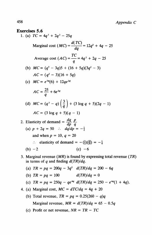
Exercises 5.6 1. (a) TC = 4q 3 + 2q 2 - 25q
d(TC) Marginal cost (MC) = dq = 12q2 + 4q- 25
TC Average cost (A C)=-= 4q 2 + 2q- 25
q
(b) MC = (q3 - 3q)5 + (16 + 5q)(3q2 - 3)
AC = (q2 - 3)(16 + Sq)
(c) MC = e2q(6) + 12qe2q
AC = 25 + 6e 2q q
(d) MC= (q 2 - q) (~) + (3log q + 5)(2q- 1)
AC = (3 log q + S)(q- 1)
2. Elasticity of demand = ddq .f!_ p q
(a) p + 2q = 50 :. dq!dp = -~
and whenp = 10, q = 20
:. elasticity of demand = - (!}(!8) = -! (b) -2 (c) -6
Appendix C
3. Marginal revenue (MR) is found by expressing total revenue (TR) in terms of q and finding d(TR)Idq.
(a) TR = pq = 200q - 3q2 d(TR)Idq = 200 - 6q
(b) TR = pq = 100 d(TR)Idq = 0
(c) TR = pq = 250q - qe4q d(TR)Idq = 250 - e4q(1 + 4q).
4. (a) Marginal cost, MC = dTC/dq = 4q + 20
(b) Total revenue, TR = pq = 0.25(260 - q)q
Marginal revenue, MR = d(TR)Idq = 65 - O.Sq
(c) Profit or net revenue, NR = TR - TC

Answers to Exercises
= (65q - Oo25q2) - (2q2 + 20q + 300)
= 45q - 2025q2 - 300
Marginal profits = d(NR)/dq = 45 - 4o5q
459
(d) MR = MC when 65- Oo5q = 4q + 20 or 45 = 4o5q so q = 100
50 Profit or net revenue is NR = TR - TC = pq - TC
= 177q- q3 - 30- 2q- 2q2 = 175q- q3 - 30- 2q2
Marginal profit is d(NR)Idq = 175- 3q2 - 4q and this is zero when 3q2 + 4q- 175 = 0 or q = 7 or -8033 and so the answer is q = 70
60 Average propensity to consume:
APC = C/Y = a/Y + b + cY
Marginal propensity to consume: dC/dY = b + 2cYo
Exercises 5.9 1. (a) y = 3x 2 - 120x + 30
dy -=6x- 120 dx
dy For a stationary value dx = 0
so 6x - 120 = 0 and x = 20
dzy 0 0 0 0 dx2 = 6 whtch IS positive
: 0 x = 20 is a minimum value andy= -1170
(b) y = 16 - Bx - x 2
dy d 2y -=-8-2x -=-2 dx dx 2
dyldx = 0 when x = -4 and there is a maximum value at this point with y = 32
(c)y=x4
dy -=4x 3
dx

460 Appendix C
There is a stationary value when 4x 3 = 0, that is x = 0. This is in fact a minimum, withy = 0, and the curve is symmetrical about the y-axis. (Draw the curve for x = - 3 to x = + 3.)
(d) y = (x - 5)3
dy -= 3(x- 5)2
dx
There is a stationary value when
3(x - 5)2 = 0 that is when x = 5
at this point d 2yldx2 is also equal to 0 and it is necessary to sketch the curve in order to show it is a point of inflexion.
2. c = 500 + 4q + 1 q2
500 q . . average cost = -- + 4 + -
q 2
d(AC). -500 1 --=--+:z
dq q2 and
There is a stationary point when 500/q2 = 1 that is q 2 = 1000 and q = ± 31.6
There is a minimum when q = 31.6 because d 2AC/dq2 > 0 for this value.
3. Demand function is given by q + 2p = 10
Total revenue = pq = p(10 - 2p)
. . d(TR) = 10 _ 4p d 2(TR) = _ 4 dp ' dp 2
This has a stationary value when p = ¥ = ~
The second-order derivative is negative and there is therefore a maximum when p = ~.
q=l0-2p=10-5=5
. . dq p <-z)<n Elasttctty of demand = --= = - 1
dp q 5

Answers to Exercises
4. Net revenue = pq- TC = q(240- q)- (q3 + 20q 2 + 20)
d(NR) .. --= 240- 2q- 3q 2 - 40q = -3q 2 - 42q + 240
dq
461
This has a stationary value when q 2 + 14q - 80 = 0, that is when q = 4.36 or - 18.35
d 2(NR) ----:---::-- = - 6q - 42
dq2
This is positive when q = - 18.35 and negative when q = 4.36.
:. net revenue is maximised when q = 4.36 and p = 235.6.
5. (a) Total revenue, TR = pq = (50 - 0.5q)q = 50q - 0.5q 2
Maximum is when d(TR)Idq =50- q = 0 so q =50, provided that the second-order derivative is negative. Here d 2(TR)Idq 2
= - 1 so q = 50 maximises total revenue. (b) Average cost, AC = TC/q = 256/q + 2 + 2q. Stationary values
occur when d(AC)Idq = - 256/q 2 + 2 = 0 so q = 11.3 or -11.3 The second-order condition for a minimum is that d 2(AC)Idq 2 is positive. Since d 2(AC)Idq 2 = 512/q 3 which is positive when q = 11.3, this is the value of q which minimises average cost.
(c) Profit or net revenue is NR = TR- TC = 50q- 0.5q 2 - (256 + 2q + 2q 2) = 48q - 2.5q 2 - 256 and the stationary value is when d(NR)Idq = 48 - 5q = 0 or q = 9.6. Here d 2(NR)Idq 2
= -5 and so q = 9.6 maximises profit. Notice that to maximise total revenue, q = 50, to mini
mise average costs, q = 11.3 and to maximise profits, q = 9.6. It is the last of these that the monopolist should adopt.
Exercises 5.13 1. With price discrimination the firm will maximise profits in each
market. For its own workers, profit or net revenue is NR 1 = total
revenue - total costs = P1Q1 - TC = (500 - 10Q1)Q1 - 1000 - 15Q1 - 15Q2 - 15Q3 and the maximum is when d(NR 1)/dQ1
= 500 - 20Q1 - 15 = 0 or Q1 = 24.25. That this maximises profit is shown by d 2(NR 1)1dQi = -20. Here P1 = 257.5.

462 Appendix C
For the domestic market, NR2 = (100000 - 5Q2)Q2 - 1000 - 15Q1 - 15Q2 - 15Q3 and d(NR2 )1dQ2 = 100000 - 10Q2 - 15 which is zero when Q2 = 9998.5. The second-order derivative is negative and so this maximises profit. Here P2 = 50007.5.
For the overseas market, NR3 = (62500 - 2.5Q3)Q3 - 1000 - 15Q1 - 15Q2 - 15Q3 and d(NR3)1dQ3 = 62500- 5Q3 - 15 which is zero when Q3 = 12497. The second-order derivative is negative and so this maximises profit. Here P3 = 31257.5.
The total profit under price discrimination is P1Q1 + P2Q2
+ P3Q3 - TC = 6244.375 + 499999988.8 + 390624977.5 - (1000 + 15(24.25 + 9998.8 + 12497) = 890292414.4. Notice the wide divergence of the prices in these three markets and that the total sales, Q = Q1 + Q2 + Q3 = 22519.75.
With no price discrimination all the prices are P, say, and the three demand functions are combined by adding Q1 + Q2 + Q3
=(50- 0.1P) + (20000- 0.2P) + (25000- 0.4P) = 45050- 0.7P = Q. The profit or net revenue is given by
NR = PQ- TC = (64357.14- 1.4286Q)Q- 1000- 15Q.
The stationary value occurs when d(NR)/dQ = 0 or 64357 2.8572Q - 15 = 0 so Q = 22519.25 and the second-order derivative is negative, indicating a maximum value. Here P = 32186.00 and NR = 724465791.8 which is lower than the pricediscrimination one of 890292414.4. Therefore it pays the monopolist to follow a policy of price discrimination. Also, notice that the value of Q is (apart from rounding errors) the same in both cases with linear demand functions. See question 2 below for a demonstration of this.
2. With price discrimination, maximising profits in the first market requires the maximisation of NR 1 = p1q1- TC = (a - bq1)q1 - f - g(q1 + q2) which occurs when d(NR 1)1dq1 = 0 or a - 2bq1 - g = 0 so q1 = (a - g)/2b. The second-order derivative is - 2b which is negative if b > 0 (which requires the demand curve to be downward sloping) and so NR 1 is maximised. From the demand function p 1 = (a + g)/2.
For the second market, NR2 = (c - eq2)q2 - f- g(q! + q2)
and when d(NR2)1dq2 = 0 then c - 2eq2 - g = 0 and q2 = (c -g)/2e. The second-order condition proves that this gives a maximum of NR2 • Here p2 = (c + g)/2.
The quantity sold with price discrimination is

Answers to Exercises 463
(a - g) (c - g) ae - eg + be - bg q = q, + qz = 2b + 2e = 2be
With a common price p, the total demand is
(a - p) (c - p) (ae + be) - (b + e)p q = q, + qz = b + e = be or
(ae + be) - beq p = (b +e)
(ae + be) A - Bq where A = (b + e) ,
B = bel(b + e) and NR = pq - TC = (A - Bq)q - f- gq
Differentiating gives
~ 0-~ dq = A - 2Bq - g which is zero when q = 28
The second-order derivative is -28 which is negative (since b and e are positive) so that the stationary value is a maximum. Here p =(A + g)/2.
Therefore the quantity sold without price discrimination will be
(A - g) ae + be - bg - eg q
2B 2be
which is the same value as with price discrimination. 3. (a) With a flat-rate tax, demand is p + 2q = 250
supply is (p - t) - 4q = 100 and tax revenue is T = tq where tis the flat-rate tax. Equilibrium is when q = 0.5(250- p) = 0.25(p- t- 100) or 500- 2p = p- t- 100 sop= (600 + t)/3 and q = 25- (t/6). Hence, T = tq = 25t - (t2/6) and so dT/dt = 25 - t/3 and this is zero when t = 75 and q = 12.5, p = 225. This is a maximum since the second-order derivative, d 2Tidt 2 = -1/3 is negative. The maximum tax revenue is T = tq = 12.5(75) = 937.5.
(b) With tax of r% the supply function is p(1 - r) - 4q = 100 and demand is p + 2q = 250. In equilibrium, q = 0.5(250 - p) = 0.25[p(1 - r) - 100] or 500 - 2p = p - rp - 100 so that p = 600/(3- r), q = 125- [300/(3- r)] = (75- 125r)/(3- r). The tax revenue is

464 Appendix C
r(600)[75 - 125r) 600[75r - 125r2]
T = rpq = (3 - r )(3 - r) = (3 - r )2
So,
dT 600{ (3 - r )2(75 - 250r)- (75r - 125r2)(2)(- 1 )(3 - r)}
dr (3-rt
Setting to zero: (3 - r )(75 - 250r) = - 2(75r - 125r2) or 225 - 75r - 750r + 250r 2 = 250r2 - 150r or 225 = 675r and r = 113. To check for a maximum the second-order derivative is required. Now, simplifying,
dT 600{225 - 75r - 750r + 250r 2 + 150r - 250r2 }
dr (3 - r)3
600{225- 675r} 135000{1- 3r}
(3 - r)3 (3 - r)3
d 2T 135000{(3 - r)3(- 3) - (1 - 3r)3( -1)(3 - r)Z
When r = 113, the sign of this is negative and so the maximum is when r = 1/3, p = 225, q = 12.5 and the tax revenue is T = rpq = 937.5. This is the same as for the flat-rate tax case in (a).
4. (a) In equilibrium, 110 - 3q 2 = 10 + q 2 or 100 = 4q 2 and q = 5 (taking the positive root), p = 35.
(b) With a flat-rate tax oft per unit supply is now p - t = 10 + q2
and demand is p = 110 - 3q2 • The new equilibrium is when 10 + t + q2 = 110- 3q2 or q2 = 25- (t/4) and p = 110- 3q2 =
35 + 3(t/4). Tax revenue is T = tq = t(25 - (t/4) )05 and so
dT t(0.5)(- 0.25) dt = (25 - (t/4) )05 + (25 - (t/4) )05
Setting to zero, (25 - (t/4)) = 0.125t and t = 66.67. For this value q = 2.89 and p = 85. To check for a maximum, the second-order derivative is needed. It is convenient here to use q 2 = 25 - (t/4)
and to note that differentiating this gives
dq -1 2q dt =4

Answers to Exercises 465
dq -1 I
-=-=q dt 8q
so that
dT 0.125t Since -=q---
dt q
d 2T dq {q - tq'} -1 1 t -=-- =-----dt2 dt 8q 2 8q 8q 64q3
which is negative. The maximum is when t = 66.67 and T = tq = 192.68.
5. Here N = 20000 = annual demand, S = 2000 =set-up cost Q = batch size (to be determined), i = 5 = inventory cost per unit per year. The number of batches per year is N/Q. The total annual cost, Cis given by the sum of total set-up costs times number of batches and the inventory cost
SN iQ 40000000 5Q dC - 40000000 5 C =-+-= +-and-= +-
Q 2 Q 2 dQ Q2 2
Setting to zero gives Q = 4000 and the second-order derivative is positive, indicating this is a minimum. The total annual cost is £20,000.
6. Let R = 50000 be the rate of production. As before, i = 5, N = 20000, S = 2000. The maximum inventory is now Q(l - NIR) (see the text, p. 204) and the total annual cost is
N SN 40000000 C = 0.5iQ(l- R) +Q= 1.5Q + Q
dC 40000000 and dQ = 1.5 - Q2 which is zero when Q = 5164.
The second-order derivative is positive and so Q = 5164 give the production run size which minimises the total annual cost. The total cost is 15492, which is below the value in question 5 since there is a saving in inventory costs when production is spread over time, rather than being instantaneous.
7. Here, annual demand, N = 3000 boxes, inventory cost i = 3, set-up cost S = 500 and the annual production rate is R = 9000 boxes. The average inventory size is 0.5Q(l - NIR) = Q/3 and so the total annual cost is
C = iQ/3 + SN/Q = Q + 1500000/Q

466
dC -=1-dQ
Appendix C
1500000 Q2 and this is zero when Q = 12240 7 0
As the second-order derivative is positive this is the minimising value and the total cost is 2449060
Exercises 5.19 10 Taylor's theorem states
xz f(a + x) = f(a) + xf'(a) + 2!f"(a) + o o o
Let f(a + x) (1 + xt
f(a) 1
f'(a + x) 4(1 + x)3 and f'(a) = 4
f"(a + x) = 12(1 + xY and f"(a) = 12
f'"(a + x) = 24(1 + x) and f"'(a) = 24
rca+ x) = 24 and r(a) = 24
X 2 x' X 4
0 0 (1 + xt = 1 + x(4) + T (12) + 6 (24) + 24 (24)
= 1 + 4x + 6x 2 + 4x 3 + x 4
and 1S = (1 + ~t = 1 + 4 X~+ 6 X~+ 4 X k + ft = 1 + 2 + 1.5 + 005 + 000625 = 500625
20 MacLaurin's theorem states
xz f(x) = f(O) + xf'(O) + 2! f"(O) + o o o
Let f(x) = (1 + x}-1
then f'(x) = - (1 + x)-2
f"(x) = 2(1 + x)-3
f"'(x) - 6(1 + x)-4
Therefore (1 + x)-1 = 1 - x + x 2 - x 3 + 0 0 0

Answers to Exercises
3. (a) f(x) = X 2 + 4.55x - 8.70
f'(x) = 2(x) + 4.55
Using as a starting point a = 1.5
/(1.5) = 2.25 + 6.825 - 8.70 = 0.375
/'(1.5) = 3.0 + 4.55 = 7.55
f(a) 0.375 · · h1 =- f'(a) =- 7.55 = -0.0497
. . new approximate root is 1.5 - 0.05 = 1.45 for which
/(1.45) = 2.1 + 6.6- 8.7 = 0
467
This result shows that 1.45 is a good approximation to one of the values of x which satisfies the equation.
(b) f(x) = X 3 - 2.34x 2 + 2x - 4.68
f'(x) = 3x 2 - 4.68x + 2
Using as a starting point a = 2.25
f(a) = 11.39 - 11.85 + 4.50- 4.68 = -0.64
f'(a) = 15.19- 10.53 + 2 = 6.66
f(a) 0.64 · · h1 = - f'(a) = 6.66 = 0.096
. . new approximate root is 2.25 + 0.096 = 2.346
for which /(2.346) = 0.045. A closer approximation can be obtained by repeating this process.
(c) x = 4.1 for whichf(4.1) = 0.
70 80 100 100 4. Pvl =If+ R2 +w+RI
60 90 80 130 PV2=R+ R2 +w+RI
these are equal when PV1 - PV2 = 0 that is
10 10 20 30 R- R2 + R3 - R4 = 0

468
or R 3 - R2 + 2R - 3 = 0
f(R) = R3 - R2 + 2R - 3
f'(R) = 3R2 - 2R + 2
Appendix C
Using Newton's method with a = 1 as a starting point, we obtain
f(a) 1-1+2-3=-1
f'(a) 3-2+2=3
f(a) 1
- f'(a) = 3 = 0.33
. . approximate root is 1 + 0.33 = 1.33; using this as a new starting point, we have
/(1.33) = 0.2437
/'(1.33) = 4.6467
/(1.33) 0.2437 hz = - /'(1.33) = - 4.6467 = -0.052
Try R = 1.33 - 0.052 = 1.278 as the next root: /(1.278) = 0.0101 and so the rate of interest is approximately 27.8 per cent. A more accurate value can be obtained by repeating the process.
5. In each case the places where the function cuts the axes are required and also where the stationary values are.
(a) y = x 2 + x + 12. This cuts they-axis when x = 0, y = 12, and the x-axis when 0 = x 2 + x + 12 or
-1 v'(1- 48) x = 2 so there are no real roots
The stationary values are when
dy -1 - = 2x + 1 = 0 or x =dx 2
d2y dx2- 2
and so there is a local minimum when x = -0.5, y = 11.75. As extra values to help to position the graph, x = -3, y = 18, x = 3, y = 24, and the table of values is:
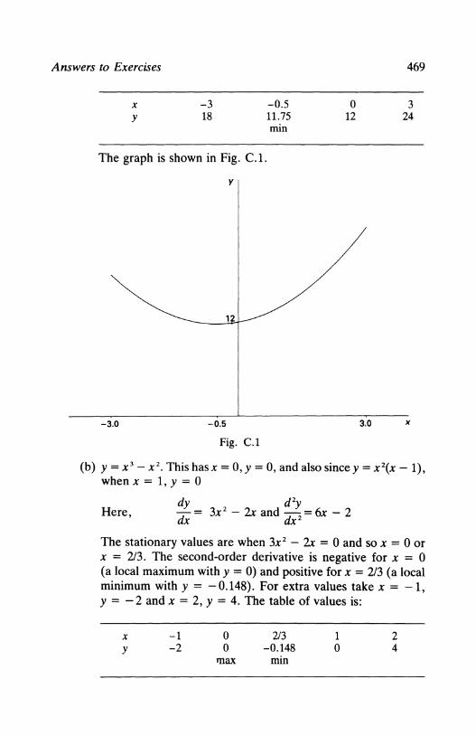
Answers to Exercises
X
y -3 18
The graph is shown in Fig. C.1.
y
-3.0 -0.5
Fig. C.1
-0.5 11.75 min
0 12
3.0
469
3 24
X
(b) y = x 3 - x 2 • This hasx = 0, y = 0, and also since y = x 2(x- 1), when x = 1, y = 0
Here, dy
dx
The stationary values are when 3x 2 - 2x = 0 and sox = 0 or x = 2/3. The second-order derivative is negative for x = 0 (a local maximum withy= 0) and positive for x = 2/3 (a local minimum withy = -0.148). For extra values take x = -1, y = - 2 and x = 2, y = 4. The table of values is:
X
y -1 -2
0 0
2/3 -0.148
max min
1 0
2 4

470 Appendix C
The graph is shown in Fig. C.2. y
4
2
-2 -1 2 X
-2
-4
Fig. C.2
(c) y = x 3 - 3x 2 - 24x + 26. This cuts they-axis when x = 0, y = 26, and the x-axis when y = 0 = x 3 - 3x 2 - 24x + 26. To find an approximate root, since the cubic has some terms with negative signs, positive values of x are worth trying. For x = 1, y = 0 so that (x - 1) is a factor and dividing into the cubic:
x 2 - 2x - 26
x- 1lx3 -3x 2 - 24x + 26
- 2x2- 24x -2x2+ 2x
-26x+26 -26x+26
and soy= (x- 1)(x 2 - 2x- 26) and if y = 0, x 2 - 2x- 26 = 0 so x = 6.2 or x = - 4.2
dy d 2y Here -= 3x 2 - 6x- 24 and-= 6x- 6
' dx dx 2

Answers to Exercises 471
The stationary values are when 3x 2 - 6x - 24 = 0 and sox = 4 and x = - 2. When x = 4 the second-order derivative is positive and so the local minimum is y = - 54 and when x = - 2 the second-order derivative is negative and so the local maximum is y = 54, The table of values is:
X
y -4.2
0 -2 54
max
0 26
The graph is shown in Fig. C.3.
y
75
50
-6 -2
-25
-50
-75
Fig. C.3
1 0
4
4 -54 min
X
6.2 0
(d) y = x 5 • This goes through the origin (x = 0, y = 0) and does not cut the axes anywhere else. In attempting to find stationary points, we get
dy d2y - = 5x 4 and-= 20x 3
dx dx 2
and when

472 Appendix C
dy - = 0 5x 4 = 0 so x = 0 dx '
but for this value the second-order derivative is also zero. This means that the general rules do not give a clear indication of whether at x = 0 there is a maximum, a minimum or a point of inflexion. We therefore work out a table of values centred on x = 0 to obtain the general shape of the curve:
X
y -3
-243 -2
-32 -1 -1
0 0
1 1
2 32
3 243
The graph is shown in Fig. C.4 and it can be seen that there is a point of inflexion at x = 0.
y
30
15
-2 -1 X
-15
-30
Fig. C.4
Exercises 6.2
dTC 1. (a) dq = 1 TC= q + C
when q = 0, TC= 600

Answers to Exercises
:. TC = 600 + q
(b) TC =50+ q
(c) TC = x 2 + 3x + C
100 = 25 + 15 + c :. c = 60 and TC = x 2 + 3x + 60.
2. Given C =a+ bY+ c¥2 then mpc = ~~ = b + 2cY
Since mpc = 0.1 + 0.02¥, b = 0.1 and c = 0.01
The consumption function is C =a+ 0.1Y + 0.01¥2
When Y = 0, C = 0 and so a= 0, giving C = 0.1Y + 0.01¥2
dK 3. Here I(t) = dt = a + 2bt + 3ct2
and K = JI(t)dt = at+ bt2 + ct3 + d
Since K = 0 when t = 0, d = 0 and K = at + bt2 + ct3
Exercises 6.4 1. (a) TC = x 2 + 3x + 10
(b) TC = ~ x 3 + x 2 + 4x + 90
2. (a) ~ x 2 - 4x + C (b) ~ x 3 - 2x 2 + 3x + C
(c) !x6 + 4/x + x 2 + C (d) -llx 2 - 4logx + C
(e) log (3x - 5) + C (f) log (2x 2 + x - 4) + C
(g) i log (x 4 - 2x 2 + 2) + C (h) 2 log (x 2 + 3x + 1)
(i) ~ e3x - e-x + c (j) 2ex - ~ e3x + c (k) - 2 cos x - 4 sin x
3. Given MR =a- 2bq, TR = JMR dq = aq- bq 2 + c
When q = 0, TR = 0 so that c = 0 and TR = aq- bq 2
473
Now TR = pq and sop= TR!q =a- bq is the demand function.
p pdq dq 4. Given ed = -0.3- and since ed =-then-= -0.3
q qdp dp

474
Integrating, q = - 0.3p + c
When p = 10, q = 100 = -30 + c and so c = 130
The demand curve is q = 130 - 0.3p
5. Given mpc = 0.5 + y-1 - Y-2 = dC!dY
Integrating, C = 0.5Y + logY + y-1 + A
Appendix C
When Y = 1, C = 1 = 0.5 + 0 + 1 +A so A = -0.5 and the consumption function is C = 0.5Y + logY+ y-1 - 0.5.
Exercises 6.6 x 2 ~ 3 3
1. (a) J y dx = J2x dx = [x 2]~ = 9 Xt = 0 0
(b) [x 2]~ = 36 - 9 = 27
(c) [x 2]g = 36
(d) [~ x 2]~ = ~ [64 - 36] = 70
(e) [2x + ~ x 2]~ = 6 + ¥ = 19!
2. Since MC = 100 - 4q + q\ TC = f30 MCdq 20
= [100q - 2q 2 + (q 3/3)]~g
= (3000 - 1800 + 9000) - (2000 - 800 + 2666.7)
= 10200 - 3866.7 = 6333.3.
3. TR = f20 MR dq = [200q - 3q 2m 15
= (4000 - 1200) - (3000 - 675) = 475.
4. pn = f~o 1000e-005t dt = 1000[e-0 ·05t/(- o.o5m0
= -20000{e-05 - 1} = -20000{0.6065- 1} = 7870.
Exercises 6.8 1. (a) y = 2x crosses the x-axis at x = 0.
1
:. area = 2 J2x dx = 2[x2]~ = 2 0
(b) y = 2 + 3x crosses the x-axis at x = - ~

Answers to Exercises 475
-V3 2
0 0 area =- J (2 + 3x)dx + J (2 + 3x)dx -3 -V3
= _ [2x + J x2]-v1 + [2x + J x2]z 2 -3 2 -V3
=- [-1 + ~- c-6 + 13o5)J + [4 + 6- c-~ + m = 8o16 + 10067 = 18083 3
(c) Area = J x 2 dx = B x 3]:2 = ~ + 9 = 11~ (as the curve -2 does not cross the x-axis)
(d) y = 1 + x + x 2 does not cross the x-axis +I
area = J (1 + x + x 2)dx -4
= [x + ~ x 2 + ! x 3]~! = 115/6
20 E(t) = 55 - 16t + t 2o This cuts the t-axis when E(t) = 0 or t = 5 or
11. The required area is evaluated in two parts: from t = 0 tot= 5 and from t = 5 to t = 10
J: E(t)dt = [SSt - 8t2 + Oo3333t3]g
= (275 - 200 + 41.67) - (0) = 116067
J:o E(t)dt = [55t - 8t2 + Oo3333t3]~0
= (550 - 800 + 333033) - (116067) = - 33o33
Total absolute error =116067 + 33o33 = 1500
Exercises 6.11 1. When p = 40, q = 100 Consumer's surplus = J~o pdq - pq
= J~o (100 - 6q)dq - 400 = [100q - 3q 2]~0 - 400
= (1000 - 300) - (0) - 400 = 300
20 Equilibrium is when 60- q- q 2 = 10 + 4q so q = 5 or q = -100 For q = 5, p = 30:
area under demand curve is J: pdq = [60q - Oo5q 2 - Oo3333q 3]g
= (300 - 1205 - 41.67) - (0) = 245083
consumer's surplus = 245083 - 150 = 95083

476 Appendix C
area under supply curve = J; (10 + 4q)dq = [lOq + 2q 2]g = 100
producer's surplus = pq - 100 = 150 - 100 = 50
With a tax of 2 per unit supply is now p - 2 = 10 + 4q or p = 12 + 4q (see section 5.11). The new equilibrium is when 12 + 4q = 60 - q - q 2 or q = 4.865, p = 31.468.
area under demand curve is
[60q - 0.5q 2 - 0.3333q 3]ri·865 = (291.9 - 11.834 - 38.382)
= 241.684
and the consumer's surplus= 241.684- (4.865)(31.468) = 88.59, which is smaller than the previous value of 95.83
area under the supply curve is now s:·865 (12 + q)dq = [12q
+ 0.5q 2]ri·865 = (58.38 + 11.834) = 70.21
producer's surplus is pq - 70.21 = 153.09 - 70.21 = 82.88, an increase on the previous value.
30
3. MR = 200 - 3q and MC = 2q so profit = f (MR-MC)dq = 30 0
f (200 - 5q)dq = [200q - 2.5q2]~0 = (6000 - 2250)- 0 = 3750 0
Maximum profit is when MR = MC or 200- 3q = 2q and q = 40 (assuming that the second-order condition is satisfied, which can easily be checked)
40
f (MR-MC)dq = [200q- 2.5q2]~ = 4000. 0 4
4. S(t)- C(t) = 10- 5t + 30t2 - 4t3 • Total net revenue= J (S(t) -4 0
C(t)) dt = f (10- 5t + 30t2 - 4t3)dt =[lOt- 2.5t2 + 10t3 - t 4]~ = 0
(40 - 40 + 640 - 256) - (0) = 384 If the campaign is extended from 6 to 8 months the extra net revenue is
8
f (S(t) - C(t))dt = [lOt- 2.5t2 + 10t3 - t4]: = (944) - (834) 6
= 110
and so it is worthwhile. But this is not optimal since S(7) - C(7) = 73 > 0 while S(8) - C(8) = - 158 < 0. That is, the optimal length is the value oft for which S(t) = C(t), and is approx. 7.4 months.
5. MR = MCwhen 600- lOt- 3t2 =50+ 15tor 3t2 + 25t- 550 = 0

Answers to Exercises 477
so t = 10 years. Total net revenue is 10 10
f (MR - MC)dt = f (550 - 25t- 3t2)dt = [550t- 12.5t2 -0 0
f]~0 = (5500 - 1250 - 1000)- (0) = 3250 T
Total return at time Tis R(T) = J (MR - MC)dt + S(T) 0
= 550T- 12.5P - P + 5000- 300T
= 250T- 12.5P- P + 5000
dR = 250- 25T- 3P which is zero when T = 5.87
dT
The maximum value is R(5.87) = 5834.53.
Exercises 6.13 3
1. (a) Exact: J 4x3 dx = [x4n = 81 - 1 = 80 1
(b) Simpson's rule: Taking n = 4 and c = 0.5 the table of values is:
X
y 1 4
1.5 13.5
2 32
2.5 62.5
3 108
The approximate area = c[y0 + 4y1 + 2y2 + 4y3 + y4]/3
= 0.5 [4 + 54 + 64 + 250 + 108]/3 = 80. 14
2. Here n = 4 and c = (b- a)/n = 1. Total cost = J MCdq 10
:::::: c[MC0 + 4MC1 + 2MC2 + 4MC3 + MC4]/3
:::::: [3 + 16 + 18 + 40 + 15]/3 = 30.67.
3. (a) n = 2, c = (b - a)/n = 4. The table of values is:
X
y 0 0
4 256
8 4096
area""' c[y0 + 4y1 + y2]3 = 4[0 + 1024 + 4096]/3 = 6826.7.
(b) n = 8, c = 1. The table of values is:
X
y 0 0
12 3 4 56 7 8 1 16 81 256 625 1296 2401 4096

478 Appendix C
area= c[yo + 4yt + 2y2 + 4y3 + 2y4 + 4y5 + 2y6 + 4y1 + Ys]/3
= [0 + 4 + 32 + 324 + 512 + 2500 + 2592 + 9604 + 4096]/3 = 6554.7.
8
(c) Exact: f X4 dx = [0.2x5]~ = 0.2(32768) = 6553.6 0
Here Simpson's rule with n = 8 is close to the exact value. 4
4. Require f x- 1dx. Here f(x) = x-t, f'(x) = -x-2 , f"(x) =2x-\ I
f'"(x) = -6x-4 and the integral of Taylor's series is:
4 (x a)2P(a) (x a)3 f f(x)dx = [f(a)x + - 1 + - f"(a) + · · ·t I 2! 3! I
(a) For a= 1,/(1) = 1,/'(1) = -1,/"(1) = 2,/"'(1) = -6
4 (X - 1 )2 (X - 1 )3 (X - 1 )4 f f(x)dx = [x- + - + · · ·t I 2 3 4 1
= ( 4 - 4.5 + 9 - 20.25) - (1)
= -12.75
This poor result occurs because the Taylor's series for a = 1 does not converge.
(b) For a = 3, /(3) = 0.3333, /'(3) = -0.1111,
!" (3) = 0.0741, /"'(3) = -0.0741 4
f f(x) = [0.3333x-0.0556 (x- 3)2 + 0.0124 (x- 3)3
I
-0.0031 (x- 3t + · · ·]~ = (1.333 - 0.0556 + 0.0124 - 0.0031)
- (0.3333 - 0.2224 - 0.0992 - 0.0496)
= 1.287 - (- 0.0379) = 1.3249.
(c) From section 6.12, the value when a = 2.5 is 1.344 and the exact value is 1.3863. For a = 1 the result -12.75 is very inaccurate, while with a = 3, 1.3249 is worse than when a = 2.5. This suggests that the value of a is important and should be in the middle of the range of x-values. Also, with Taylor's series it may be necessary to check whether the expansion

Answers to Exercises 479
converges and include more than just the first three derivatives.
4
5. (a) Exact: f exdx = [~]~ = (e4) - (e0) = 54.598 - 1 = 53.598. 0
(b) Simpson's rule with n = 4: With c = 1 the table of values is:
X
y 0 1
1 2.718
2 7.389
area = c[y0 + 4y1 + 2y2 + 4y3 + y4]/3
3 20.086
4 54.598
= [1 + 10.872 + 14.778 + 80.344 + 54.598]/3 = 53.864.
(c) By Taylor's series: f(x) = ex= f'(x) = f"(x) = f"'(x) etc. Taking a= 2,/(2) = 7.389 = ['(2) = ["(2) = f"'(2) etc. and this can be taken outside the brackets:
4 (x a)2 (x aY J f(x)dx = [f(a)x + - f'(a) + - f"(a) + · · ·]~ 0 2! 3!
(x - 2y (x - 2y (x - 2y (x - 2)5 4 = 7.389 [x + 2! + 3! + 4! + 5! ]o
= 7.389 {(4 + 2 + 1.333 + 0.6667 + 0.2667)
- (2 - 1.3333 + 0.6667 - 0.2667)}
= 7.389 (8.2667 - 1.0667) = 53.2
Here Simpson's rule gives a better approximation than does the Taylor's series result, but adding extra terms to the Taylor's series expansion will improve its accuracy.
Exercises 6.15 1. Let (5r + 4) = u and e3xdx = dv
Then 10xe1x J (5x 2 + 4)e3xdx = (5x2 + 4)je3x- J-3- dx
10e3x J 10xe1xdx = 10x(je3x) - J-3- dx and
and J 10e3xdx = 10 {j e1x)

480 Appendix C
[5x2 + 4 lOx 10] . . f (sr + 4) ~dx = ~ 3 - 9 + 27 + c. 2. Let log x = u and x2 dx = dv
Then f r log X dx = f log X X 2 dx
3. Let
Then
and
I Jl 1 = log x(Jx3) - 3r- dx X
~ X3 log X - ~ f r dx
= H X3 log X - ~ r] + c = ~ x3 [log x - ~] + C.
3 A B ----=--+--(x + 1 )(x - 1) (x + 1) (x - 1)
3 = A(x - 1) + B(x + 1)
3 =-A+ B
O=A+B
:. A=-~ B = ~ 3 3 3
:. J (x + l)(x - 1) dx = f -2 dx + f 2 dx
(x + 1) (x- 1)
4. Let
then
= -~ log (x + 1) + ~ log (x- 1) + C
Hlog (x - 1) - log (x + 1)] + C
3 (x- 1) = -log--+ C.
2 (x + 1)
x A Bx + C ----- = -- + --(x- 2)(r- 3) (x- 2) (x2 - 3)
x = A(x2 - 3) + (Bx + C)(x - 2)
= Ax2 - 3A + Bx2 + Cx - 2Bx - 2C
A+ B = 0
-2B + C = 1
-3A- 2C = 0

Answers to Exercises
and A = 2, B = - 2, C = - 3
··I X dx=J 2 dx-J2x+3dx (x - 2)(x2 - 3) (x - 2) (x2 - 3)
1 = 2 log (x- 2) -log (r- 3)- 3 J r- 3 dx
= lo [(x- 2)2] + _3_lo ( v'3 + x) + D g (x2 - 3) 2v'3 g v'3 - x
This can be further simplified if necessary.
5. Let 4x + 3 = u; then du = 4 dx
u10 u11 ( 4x + 3)11 :. J (4x + 3)10 dx = J- du =- + C = +C. 4 44 44
6. Let log x = u and dx = dv
1 Then J log xdx = (log x)x- J x- dx
X
=X log X- X+ C
=X (log X - 1) + C.
Exercises 7.4 (Jz
1. (a) - = y + 2xy + y2 (Jx
(Jz -=x+x2 +2xy (Jy
(Jz (b) - = 6xy + 4y2 + 6y ax
az -=3x2 +8xy+6x ay az
(c) - = 2x sin y - y2 sin x ax az - = x2 cos y + 2y cos x ay
481
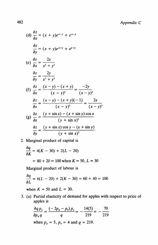
482
az (d) - = (x + y)ex+y + ex+y
ax
iJz - = (x + y)ex+y + ~+y ay
az 2x (e)-=--
ax X2 + y2
az 2y -=--ay x2 + y2
az (x-y)-(x+y) -2y (f) ax= (x - YY = (x- Y)2
az (x- y) - (x + y)(- 1) 2x
ax (x- YY (x- YY az (y + sinx)- (x + siny) cosx (g) - = ....;;._ _ __;_ _ __;_ _ __;__ ax (y + sin x)2
az (y + sinx) cosy- (x + siny)
ay (y +sin xY 2. Marginal product of capital is
aq = 4(K - 30) + 2(L - 20) aK
= 80 + 20 = 100 when K = 50, L = 30
Marginal product of labour is
aq = 6(L - 20) + 2(K- 30) = 60 + 40 = 100 aL when K =50 and L = 30.
Appendix C
3. (a) Partial elasticity of demand for apples with respect to price of apples is
aq P. (- 2pa- Po) P. 14(5) = = ---= apaq q 219
when Pa = 5, Po = 4 and q = 219.
70
219

Answers to Exercises 483
(b) Partial elasticity of demand for apples with respect to price of oranges is
iJq Po (6- p.)Po 4 --= dp0 q q 219
when Pa = 5, p0 = 4 and q = 219.
iJQ aQ iJQL 4. Since Q = AUKfl then-=- and so--= a.
iJL L iJLQ
5. Let w = a11x 1 + a,~2 and z = a21X 1 + a2~2 so that the first-order partial derivatives are
/J/ = = /A/ as required.
Exercises 7. 7
1. dq = aq dL + aq de aL ac
= (3£2- 3 + 4C)dL + (4L- 2C)dC
= 317(1) + 30(1) = 347 when L = 10 and C = 5
If dC = 0 and dL = 1, dq = 317.
aq aq 2. dq = -dpa +- dp0
dpa dpo
= (-2pa- Po) dpa + (6- Pa) dpo
= -14(1) + 1(1) = -13.
dz azdx azdy 3. -=--+--
dt ax dt ay dt
dx (a) - = e'(-sin t) + e' cost,
dt
dz
dy - = e' cos t + e' sin t dt
- = 2x(e')(cos t- sin t) + (-2y)(e')(cos t +sin t) dt

484 Appendix C
dx (b) dt = 2te' + t 2 e',
dy -=cost dt
dz = (-1-)(2t + t 2 )e' + (-1-) cost dt X+ y X+ y
dx dy 1 (c) - = e', - =-
dt dt t
dz 2 2(1) - = (2xyex )e' + (ex) -dt t
dx 1 dy 1 (d) - = 1 - _, - = 1 + -
dt t 2 dt (2
~~ = (2x+ y)( 1- t12)+ (x + 2y)( 1 + t12).
4. (a) Since Q, = Aer'L~Kf then QL = aAer'L~- 1 Kf = aQ!L and QK = f3Q!K so MRS = QL!QK = aK!f3L which is unaffected by r.
(b) From above, (K!L) = ({3/a)(MRS) and so the elasticity of substitution is
d(K!L)I(K!L) ({3/a) MRS a = = = 1 as before
d(MRS)/MRS KIL
Therefore technical progress (of the form given in the question) does not affect the elasticity of substitution with the Cobb-Douglas production function.
5. Since C =a+ bY, Cy =band as I= c- er, Ir = -e (a) Taking the total derivative of Y = C + I + G,
dY = Cy dY + Ir dr + dG
= b dY - e dr + dG
Since G is fixed, dG = 0 and (1) can be written
dY -e (1 - b)dY = - e dr and so- = which is negative.
dr (1 -b)
(b) Taking the total derivative of Ml P = fY - gr gives
(1)

Answers to Exercises 485
dM dP - - M- = f dY - g dr p p2 (2)
Now P and rare fixed and so dr = 0 = dP. Hence (1)
dM becomes (1- b)dY = dG and (2) is-p = fdY
dM fP dY fP -= =--· dG (1-b)dY (1-b)
Therefore,
Exercises 7.9
dy (iJz!iJx) 1. -= ----
dx (iJzliJy)
dy (-8xy2 + 12y + 4) (a) - = - ...;____.;._ _ __.;.__ dx 3y2 - 8x2y + 6x2
dy (2xy2 + e') (b) dx = - 2x2y - &'
dy [(3/(x + y)] + 8x (c) - = - .::..c...__;__-=--.:...;:.___
dx [(3/(x + y)]- 2y
dy [cos (x + y)- 3y- 10y2]
(d)-=- . dx cos (x + y)- 3x- 20xy
2. When p = 2, q = 12.18. By differentiating term by term
dq (2 + p)(- 2p)- (500- p 2) dq 2q dp = (2 + p y + p dp + q
dq 1 [ - 4p - 500 - p 2 ] Hence-= + q
dp (2q - p) (2 + p y and elasticity when p = 2 and q = 12.18 is
!!_dq = - 2-(-1-) [ - 512 + 12.18] = -0.15. qdp 12.18 22.36 16

486 Appendix C
3. Differentiating Q2 = BKL - 3Q + V + 2K2 with respect to L: 2QQL = BK - 3QL + 2L
and QL = (8K + 2L)/(2Q +3)
Similarly for K, 2QQK = BL - 3Qx + 4K
and Qx = (8L + 4K)/(2Q + 3)
The marginal rate of substitution is
MRS = _QL = (BK + 2L) = _4_(K_IL_)_+_1 QK (8L + 4K) 2(KIL) + 4
(1)
For the elasticity of substitution (a), we need d(K/L)/d(MRS),and so rearranging ( 1),
[2(K/L) + 4] MRS= 4(K/L) + 1
Differentiating term by term, with respect to MRS,
[2(K/L) + 4] + MRS[2d(KIL)Id(MRS)] = 4 d(KIL)/d(MRS)
. d(K/L) 2(KIL) + 4 and solvmg = -----
' d(MRS) 4 - 2MRS
Therefore, d(K/L) MRS [(KIL) + 2] MRS
a= =------d(MRS) KIL [2- MRS] KIL
[(K/L) + 2][4(K/L) + 1] =
7(KIL)
Exercises 7.12 1. Replace x andy by tx and ty and show f(tx, ty) = tkf(x, y) where k
is the degree of homogeneity: (a) k = 3; (b) k = -1; (c) k = 3. 2. Euler's theorem: xzx + yzy = kz
For (a), Zx = 3x2 - 2xy, Zy = 9y2 - x2
hence x(3x2 - 2xy) + y (9y2 - x2) = 3f(x, y)
( 4 x3)y - 12x2( xy + y2)
For (b), Zx = (4 rY ' x+2y
z =--y 4x3
hence xzx + yzy = - f(x, y). 3. Own-price elasticity is
poq P -- = - ( 4r - 4p) qop q

Amwers to Exercises 487
Cross-elasticity is
rCJq r -- =- (20r + 4p) qCJr q
Sum is 2, the degree of homogeneity. 4. Replacing L and K by tL and tK, the first gives t0 ·8q and the second
gives tuq as required. 5. The partial derivatives of q = p2Yipi are
CJq Y CJq -2p2Y dq P2 - = -·~=---and-=-CJp2 P~ CJp, Pi CJY Pi
and so the elasticities are
p2CJq p2Y p,CJq -p,2p2Y YCJq Yp2 -- = -= 1 --= ---= -2-- =- = 1
!I 2 '!I 3 '.:~y 2 qup2 qp1 q up1 q p 1 q u qp1
Notice that the sum of the elasticities is zero The degree of homogeneity is found by multiplying each variable
tpztY by t to give -- = t0q and so is zero
(tp,y
Euler's theorem states that, for q = f(P~> p 2 , Y)
pJ, + Pzfz + Yfy = kq
where k is the degree of homogeneity (zero here) and f, and f 2
indicate partial derivatives with respect to p 1 and p2
Substituting in,
(-2p2Y) + p, 3
(Y) + Y (pz) = - 2q + q + q = 0 P2 2 2 p, p, p,
as required.
6. For q = ALaKfJ, qL = aq!L and qK = {3q!K so that the slope of an isoquant at (U, K 0 ) is- qL/qK = - aK0/{3L0 , and at (kL0 , kK0) it is - ak~/{3kL0· = - aK0/L0{3. Therefore this Cobb-Douglas production function is homothetic.
Exercises 7.14
1. (a) z = x2 - xy + y2
Zx = 2x- y Zy -x + 2y

488
Zxx = 2 Zxy = -1
(b) z = (x + y)3
Zx = 3(x + Y)2
Zxx = 6(x + y) Zxy = 6(x + y)
Zyy = 2
zy = 3(x + y)2
Zyy = 6(x + y).
Appendix C
2. Find when Zx = 0 ·= Zy and check for Maximum: ZxxZyy > (ZxyY, Zxx < 0, Zyy < 0 Minimum: ZxxZyy > (ZxyY, Zxx > 0, Zyy > 0 Saddle point: ZxxZyy < (zxyY, Zxx = 0 = Zyy
(a) Zx = 0 = zy when x = 0, y = 0 and x = ~, y = -~
Zxx = 6x, Zyy = 2, Zxy = 2
For x = 0, y = 0, tests fail - further investigation needed.
2 2 • . • 4 For x =- y = -- mtmmum w1th z =- -·
3' 3' 27
(b) zx = 0 = zy when x =! andy=!. Maximum value is z = 1.
3. Method is as in Problem 2 above.
(a) Zx = 0 = Zy when x = 2 andy = 0.5. Zxy = 0, Zxx = 2, Zyy = 2 so minimum value of z = 45.75.
(b) Zx = 0 = Zy when X = ± v'(0.67), y = 1.5. Minimum is z = 196.7 when x = v'(0.67), y = 1.5
(c) Zx = 0 = Zy when x = 3, y = 4 and x = -3, y = 4. Minimum is z = 180 when x = 3, y = 4.
4. Here q = 36K + 120L- 3K2 -4£2- 10 + 2KL
and so qL = 120- 8L + 2K
qK = 36 - 6K + 2L
and setting these to zero and solving, K = 12, L = 18. Also, qKK =
-6, qLL = -8, qKL = 2 so that the conditions for a maximum are satisfied. The maximum is q = 1286.
5. Profits, :Jr = total revenue - total costs = p.q. + p2q2 - (qi + 3q.q2 + q;)
and substituting from the demand functions for p 1 and p 2 ,
:Jr = 40q. - qi + 60q2 - 2q; - qi - 3q.q2 - q;

Answers to Exercises
= 40ql - 2qi + 60q2 - 3q~ - 3qlq2
The first-order derivatives are
1r1 = 40 - 4q1 - 3q2 and lrz = 60 - 6qz - 3qt
489
Setting these to zero gives q1 = 4, q2 = 8 and the second-order derivatives are Jr11 = -4, Jr22 = -6, 1r12 = -3 and so we have a maximum value of profits of 320.
6. (a) With price discrimination, profits,
1r = Ptqt + Pzqz - TC
= 105ql - 25qi + 50q2 - 2q~ - 10 - 5qi - 2q2
= 100ql - 25qi + 48q2 - 2q~ - 10
The first-order derivatives are 1r1 = 100 - 50q1 and 1r2 = 48 - 4q2 and setting these to zero gives q1 = 2, q2 = 12 Here 1r11 = -50, 1r22 = -4, 1r12 = 0 and so we have a maximum for which 1r =378. The prices are p1 = 55 in the peak period and p2 = 26 in the off-peak period.
(b) With no price discrimination the demand functions are p = 105 - 25q1 and p = 50 - 2q2. From these we obtain q1 = 4.2 -0.04p and q2 = 25 - 0.5p Profits are given by 1r = p(q1 + q2)- TC and so it is convenient to substitute for q1 and q2 in TC to get everything in terms of p: TC = 10 + 5( 4.2 - 0.04p) + 2(25 - 0.5p) and so
1r = p(29.2- 0.54p) - 10- 21 + 0.2p- 50+ p
= 30.4p - 0.54p2 - 81
To maximise this we set d1rldp = 0, giving 0 = 30.4 - 1.08p or p = 28.15 and check that d 21rldp2 = -1.08 is negative as required. With p = 28.15 the profits are 346.9 and q1 = 3.074, q2 = 10.93. With price discrimination, 1r = 378, q1 = 2, p 1 = 55, q2 = 12 and P2 = 26.
Exercises 7.18 1. Using a Lagrangian multiplier, as in section 7.16,
z' = 100x1 - 2xi + 60x2 - ~ + A.(x1 + X2 - 41) Setting z; = 0, z~ = 0, z~ = 0 gives X 1 = 20.33 x2 = 20.67 which are the maximising values, z = 2019.3 (compare z = 2000 when the constraint was X 1 + x2 , = 40, and A. = - 20).

490 Appendix C
Alternatively, substitute X 1 = 41 - x 2 in the expression for z and maximise as in section 5.7.
2. For the unrestricted case, Zx = 0 = zy gives x = 2, y = 7 and z = 89 as the minimum value (see section 7.13 for method). For the restricted case, using a Lagrangian multiplier, the firstorder partial derivatives are zero when x = 10/7, y = 43/7, and the minimum value of z is 635/7.
3. (a) Using a Lagrangian multiplier shows that the first-order partial derivatives are zero when x = 200/41, y = 160/41, and the minimum value of z is 1600/41.
(b) Using a Lagrangian multiplier shows that the first-order partial derivatives are zero when x = 48/17, y = 36117, and the maximum value of z is 162/17.
(c) Using a Lagrangian multiplier shows that the first-order partial derivatives set equal to zero give
0 = 6xy2 + A., 0 = 6x2y + 3A., 0 = x + 3y - 18
These are satisfied by three pairs of values:
x = 0, y = 6, minimum value z = 0
x = 18, y = 0, minimum value z = 0
x = 9, y = 3, maximum value z = 2187
4. The constraint is 4/ + 5c = 28. Using a Lagrangian multiplier, we find that the first-order partial derivatives are zero when I = 93/49 and c = 200/49. The maximum value of x is 144.0.
5. The budget constraint is 100 = 5x + lOy and so let z' = 6xy + A.(lOO- 5x - lOy). The partial derivatives are z: = 6y + SA., z~ = 6x + lOA., z~ = 100- 5x- lOy and setting these to zero gives x = 2y so that x = 10, y = 5 and A = 6. To check whether this is a maximum, the Hessian is, with z = 6xy and u = -5x- lOy+ 100,
Zxx Zxy Ux
Zyx Zyy Uy
Ux Uy 0
0 6 -5 6 0 -10 = 600
-5-10 0
and as this is positive, x = 10, y = 5 gives a maximum with U = 6xy = 300.

Answers to Exercises 491
Exercises 8.8 1. The situation shown in Table 8.4 can be expressed as
2x, + 3x2 ~ 25
4x 1 + X2 ~ 35
where x, and x2 are the numbers of units of product A and B which are manufactured. x, and X 2 must both therefore be ~ 0
The contribution is given by 9x, + 7x2 •
TABLE 8.4
No. of hours Total required no. per unit of hours
of product available
A B
Machine U 2 3 25 Machine V 4 1 35
Contribution per unit of product 9 7
Slack variables x 3 and x4 are inserted in the equations in order to obtain a first feasible solution. The Simplex tableau is as shown in Tableau 1.
Tableau 1
x, Xz x3 x4 p p;la;i
x3 2 3 1 0 25 25/2
x4 4 1 0 1 35 35/4 departing ~variable
z -9 -7 0 0 0 t
entering variable

492 Appendix C
Using the method of row and column operations successive tableaux are obtained as shown in Tableaux 2 and 3.
The final tableau shows that the maximum contribution is obtained by manufacturing 8 units of product A and 3 units of product B, in which case z = 93.
Check 8 X 9 + 3 X 7 = 72 + 21 = 93.
Tableau 2
XI Xz x3 x4 p pla;j
0 5 1 I 15 3 departing x3 2 -2 2 -variable
I 0 I 35 35 XI 4 4 4
0 19 0 9 315 z 4 4 T
i entering variable
Tableau 3
XI Xz x3 x4 p
Xz 0 1 2 I 3 5 5
XI 0 I 3 8 -TO TO
z 0 0 19 26 93 TO 20
The value of increasing capacity on machine U by one unit is 19/10 and that on machine V is 26/20. These values are obtained directly from the bottom line of the final tableau. They can be verified by using the simplex method with the constraints adjusted by one unit of capacity for machines U and V separately.
2. (a) (i) A = 9i, B = 2. (ii) A = 11, B = 1 (b) A = 0, B = 8~ (c)A = 7!, B = 5
3. (a) Let x 1 = number of units of A produced x2 = number of units of B produced
then the problem is to max z = 3x1 + 2x2

Answers to Exercises 493
subject to X 1 + 4x2 ~ 60 (labour)
2x1 + X 2 ~ 40 (land)
3x1 + X 2 ~ 50 (machines)
and X 1 ~ 0, x 2 ~ 0, x 3 ~ 0 Introducing three slack variables, X3 , X4 and x 5 the constraints are
The first tableau is:
XI
x3 1 x4 2 Xs 3
z -3
X 1 + 4x2 + X3 = 60
2xl + X2 + X4 = 40
3x1 + X2 + X5 = 50
x2 x3 x4
4 1 0 1 0 1 1 0 0
-2 0 0
Xs
0 0 1
0
The first feasible solution is x3 = 60, X 4 = 40, x 5 = 50
p
60 40 50
0
The entering variable is x1 and the departing variable x 5
Dividing row 3 by 3 and combining the new row 3 with the other rows gives:
z
0 0 1
0
1113 113 113
-1
1 0 0
0
0 1 0
0
-113 -2/3
1/3
1
p
130/3 20/3 50/3
50
The entering variable is x 2 and the departing variable x 3
Dividing row 1 by 1113 and combining the new row with the other rows gives:

494 Appendix C
xi x2 x3 x4 Xs p
x2 0 1 3/11 0 -1/11 130/11 x4 0 0 -1/11 1 -21/33 90/33 xi 1 0 -1/11 0 12/33 140/11
z 0 0 3/11 0 10/11 680/11
Since all the coefficients on the bottom row are positive the solution is X 1 = 140/11, X2 = 130/11 and z = 680/11.
(b) The slack variable for land is x4 and from the bottom row of the final tableau above the shadow price is zero. Therefore there is some land not being used (check the land constraint 2x1 + x2 :::: 40). It is not worthwhile renting extra land since it would not increase profits.
4. (a) Let u1, u2 and u3 be the number of units of bread, cheese and meat consumed. The total cost is z = 2u1 + 4u1 + 5u3 which is to be minimised subject to the constraints:
energy: u1 + 2u2 + u3 ;a, 10
protein: U 1 + 3u2 + 6u3 ;a, 15
and U 1 ;a, 0, U2 ;a, 0, u3 ;a, 0. (b) The dual problem is to max z' = 10x1 + 15x2 subject to
2x1 + 3x2 :::: 4
xi + 6x2:::;; 5
and X 1 ~ 0, X2 ~ 0. Introducing three slack variables x3 , X4
and x5 , the first tableau is
xi X2 x3 x4 Xs p
x3 1 1 1 0 0 2 x4 2 3 0 1 0 4 Xs 1 6 0 0 1 5
z' -10 -15 0 0 0 0

Answers to Exercises 495
The first feasible solution is X3 = 2, X4 = 4, x 5 = 5 The entering variable is x2 and the departing variable is x 5
Dividing row 3 by 6 and combining the new row with the other rows:
x, Xz x3 x4 Xs p
x3 5/6 0 1 0 -1/6 7/6 x4 3/2 0 0 1 -112 3/2 Xz 1/6 1 0 0 1/6 516
z' -15/2 0 0 0 5/2 12.5
The entering variable is x, and the departing variable is X4
Dividing the second row by 3/2 and combining the new row with the other rows:
z'
0 1 0
0
Xz
0 0 1
0
1 0 0
0
-5/9 2/3
-1/9
5
1/9 -1/3
2/9
0
p
113 1
2/3
20
The coefficients on the bottom row are positive and so the solution is x, = 1, x2 = 2/3 and z' = 20. The only positive shadow price is for x4 , the slack variable associated with the price of cheese, and it would be advantageous to buy more cheese if the price is less than 5.
Exercises 9.4 1. Let Y = VX, so that dY = V dX + X dV
Substituting and rearranging gives
(a,V- b, - a2V 2 + b2V)dX = (a2VX- b7)dV
dX (a 2V- b2)dV or -=
X a,V- b, - a2VZ + b2V
which can be integrated given the values of a" a2 , b, and b2 •

496 Appendix C
2. Let q be the quantity demanded at price p. Then we require
pdq
or
--= -n qdp
dq -= q
dp -n
p
Integrating, we obtain
log q = - n log p +A' or q = Ap-n
Thus qp" = A is the general form required. 3. Put y = vx, dy = v dx + x dv; then, on re-arranging,
v dv dx --
24- 2v2 x
or - i log (24 - 2v2) = log x + A'
This becomes
A = (24 - 2v2)x4 = 24x4 - 2x2 y2
and using x = 2, y = 4 gives A = 256. bx2
4. Separable variables: c = ax - - + A . 2
dp 5. (a) -= kap
dt
dp or - = ka dt
p
Integrating gives
log p = kat + A' or p = Aekac
dp , (b) - = k(ap + bp-)
dt or dp = k dt
p(a + bp)
Using partial fractions (see Section 6.14), we have
dp b dp = k dt ap a(a + bp)
1 1 or -log p- -log (a+ bp) = kt + A'
a a
P = Ae"k' (a+ bp) ·

Answers to Exercises
6. Substituting gives
dY
Hence,
b- = aY or dt
b log Y = at + A'
7. (a) x dy = (x- y)dx
dY b- =a dt
y
or Yb =Ae"'.
497
Put y = vx, dy = v dx + x dv, then (-1 + 2v)dx = - x dv
dx dv or -+--=0
x 2v- 1
so log x + ! log (2v - 1) = A' or 2xy - x2 = A.
(b) Let X= y + 1 andY= 2y + x; then
dY dY/dx 2(dyldx) + 1 2(X/Y) + 1
dX dX/dx dyldx XIY
and X dY = (2X + Y)dX
Let Y = VX, dY = V dX +X dV
Hence 2 dX = X dV and 2 log X = V + A
Thus
(c) Rewriting as
(2y +X) 2 log (y + 1) = -- + A· y + 1
dy - + 2y = x(l + x) dx
we have e2x as an integrating factor and the integral of the left hand side is ye2x. The right hand side is
(x + x2)e2x e2x J e2x (x + x2)d.x = 2 - J 2(1 + 2x)dx
(x + x2)e2x (1 + 2x)e2x e2x = - + J-(2)dx
2 4 4

498 Appendix C
Hence the solution is
(d) If dy -+ 4y = x3
dx
then e4x is an integrating factor and integrating gives
[x3 3x2 3x 3 ]
ye4x = J x3e4x dx = e4x 4 -M + 32- 128 +A.
8. Since the market clears, if = qd and so
dp dp -a+ bp = e- fp +-or-= (b + f)p -(a+ e)
dt dt
or dp = dt (b + f)p - (a + e)
For convenience, multiply each side by (b + f) and integrating gives
or
and so
Exercises 9.6
log [(b + f)p - (a + e)] = (b + f)t + log A
(b + f)p - (a + e) = Ae1b+J>•
p = [(a+ e)+ Ae1b+n•]f(b +f)
In each case put y = e= etc. and form the reduced equation am2 + bm +c. The roots are m1 and m2
1. m1 = 4, m2 = -3, y = k 1e4k + k2e-3x
2. m1 = 1, m2 = 2, y = k1~ + k2e'
3. m1 = 3, m2 = 3, Y = (kl + kzX)~x
4. m1 = 1, m2 = 1, y = (k! + kzX)e'
5. m1 = 4, m2 = -4, Y = k!e4x + kze-4x
6. m1 = 4i, m2 = -4i, y = k3 cos 4x + k4 sin 4x = A cos ( 4x - E)

Answers to Exercises 499
7. m 1 = -1 + 3i, m 2 = -1 - 3i, y = e-x (k3 cos 3x + k4 sin 3x) = Ae-x cos (3x - E)
Exercises 9.8 1. (a) Complementary function: m1 = 8, m2 = 2
y = klesx + k2e2x
Particular integral: try y = K1 + K~ then y = 5/64 + x/8 Solution is
5 X Y = k esx + k e2x + - + -
I 2 64 8
The initial conditions give k1 = 0.1979, k2 = -0.3542
(b) Complementary function [from Exercise 9.5, Question 5],
y = kle4x + k2e-4x
Particular integral: try y = aeX, then y = - ex/15. Solution is
ex Y = -- + k e4x + k e-4x
15 I 2
The initial conditions give k, = t k2 = !. (c) Complementary function [from Exercise 9.5, Question 4],
Y = (k1 + k2 x)ex
Particular integral: try y = ae2x; then y = e2x Solution is y = (k1 + k2 x)ex + e2x and the initial conditions give k1 = 1, k2 = -1.
(d) Complementary function: m1 = -1 + 2i, m2 = -1 - 2i:
y = Ae-x COS (2x - f)
Particular integral: try y = ax + b; then y =:!:- 2 5 25
Solution is y = :!: - 2 + Ae-x cos (2x - f) 5 25
The initial conditions give A cos (- f) = 0 1 = - 2A sin (- f)

500 Appendix C
and hence f = - :~r/2 and A = - !. (e) Complementary function: m1 = 0, m2 = 1
y =A+ Bex
Particular integral: try y = a cos x + b sin x; then
y = -cos x - sin x.
Solution is y = A + Bex - cos x - sin x Initial conditions give A = -1, B = 3.
2. Solve homogeneous part by putting y = tt= etc; then m1 = 2, m2 = -3 and
y = Acx + Be-3x
Particular integral: try y = a + bx + cx2 ; then a= -1/6,b= -1,c= -3. Solution is y = Acx + Be-3x- {t) - x- 3r Initial conditions give A = -h\, B = fs.
Exercises 9.12 1. Differentiating (1),
and using (2) and (3),
Differentiating:
dp = be(m- p) + fk(p- p") dt
dzp = -be dp + fk dp - fk dp" dt2 dt dt dt
and using (4) to eliminate dp"ldt,
dzp =-be dp + fk dp- k{dp + b df/l dt2 dt dt dt ii f
Using (3) to remove dU/dt and simplifying,
d2p dp - + (be + k(1 - [])- + bekp = bekm dt2 dt
(4)

Answers to Exercises 501
which reduces to (6) in the text when f = 1.
d 2 d 2. (a) lf = qdgivesf_E + cJ!. +(a+ h)p = b + g
dt2 dt
For the homogeneous equation, putting p = e"'' gives fm2 + em + (a + h) = 0 and the roots are complex, giving a cyclical solution, if c2 - 4(a + h) f < 0.
(b) Putting the values into the equation,
d 2 d _p_ + 8J!. + 15p = 1800 dt2 dt
and the auxiliary equation is m2 + 8m + 15 = 0 which has the roots - 3 and - 5. The particular integral is from putting p = K and K = 1800/15 = 120 and so the solution is p = Ae- 3' + Be- 5' + 120. The condition t = 0, p = 130 gives 130 =A + B + 120 or A + B = 10. The condition t = 0, dp/dt = -2 gives -2 = - 3A - 5B. Solving, A = 24, B = -14 and p = 24e- 3'- 14e- 5' + 120. As t increases the value of p quickly approaches 120.
Exercises 10.7 1. The general solution of Y,+, = AY, + K is
K y =AA'+--' 1- A
where A is a constant
(a) A = 1.5, K = 3, Y, = A(1.5') - 6 Initial condition gives A = 8
0 2 3 4 5
2 6 12 21 34.5 54.75
(b) A= 0.9, K = 2, Y, = A(0.9') + 20 Initial condition gives A = - 17
0 1 2 3 4 5
3 4.7 6.23 7.61 8.85 9.96

502 Appendix C
(c) A= 1, K = 0, Y, =A. Initial condition gives A = 6
0 1 2 3 4 5
Y, 6 6 6 6 6 6
(d) A= 1.1, K = 4, Y, = A(l.1') - 40 Initial condition gives A = 41
0 1 2 3 4 5
Y, 1 5.1 9.61 14.57 20.03 26.03
2. Let Y, be the value of the savings after t years; then Yo = 15, Y1 = 1.05(15) + 15 and in general Y,+ 1 = 1.05 Y, + 15. The solution is Y1 = A(l.OS)' - 300 and Y0 = 15 gives A = 315. y21 = 535.8.
3. The difference equation is p, = -l.5p1_ 1 + 3 and the solution is p, = - ~(- 1.5)' + 1.2, which is 'exploding' since 1.5 > 1.
4. The difference equation is p1 = 0.5p,_ 1 + 3 with the solution p, = - (- 0.5)' + 2, which is stable since 0.5 < 1. The equilibrium price is 2.
5. The difference equation is p, = - p,_ 1 + 8/3 with the solution p 1 = [2 (- 1 )' + 4]/3 which oscillates since I-ll = 1.
6. The difference equation is 0.9Y, = 0.3Y,- 0.3¥,_ 1 or Y1 = -0.5¥,_ 1, and the solution is Y, = 100(-0.5)'.
7. Substituting into the pricing equation:
Pt+l = Pt - 0.3(0.4p, - 50 - 150 + 0.6p,)
= 0.7p, + 60
The solution is p, = A(0.7') + 60/(1 - 0.7) = A(0.7') + 200 As t ~ oo, p converges on the value 200.
8. Substituting into the first equation:
Y, = b Y,_ 1 + c + a(Y, - Y,_ 1)

Answers to Exercises 503
or Y _ (b- a) y _c_ t- t-1 +
(1 - a) (1 -a)
For stability, the coefficient on Y,_ 1 has to lie between 1 and -1 or -1 < (b - a)/(1 - a) < 1.
Exercises 10.12 1. Difference equation is Y, = (c + b) Y,_1 - bY,_2 and putting
Y, = )./gives the characteristic equation A2 = (c + b) A - b
(a) Roots are A1 = 0.7 + 0.1i, (b) Roots are A1 = 0.8, (c) Roots are A1 = 0.845,
A2 = 0.7 - O.li A2 = 0.8 A2 = 0.355.
2. Solve homogeneous part by putting Y, = A, and obtaining the roots A1 and A2 of the characteristic equation. The equilibrium or particular solution is found by trying expressions of the same form as f(t).
(a) A1 = 2, A2 = -1. Try Y, = Z as particular solution then Y, = -1.5. Solution is Y, =A(21) + B( -1Y - 1.5 and initial values give A = 7/3, B = 7/6.
(b) A1 = 2, A2 = 1. Try Y, = Z as particular solution- fails. Try Y, = Zt; Y,+ 1 = Zt + Z, Yt+2 = Zt + 2Z, then Z = -4. Solution is Y, = A(21) + B - 4t and initial conditions give A = 5, B = -4.
(c) A1 = 2, A2 = 2. Try Y, = Z(31); then Z = 1. Solution is Y, = (k1 + k2t)(21) + 31 and initial conditions give k1 = 2, k2 = -1.5.
(d) A1 = 2, A2 = 1. Try Y, = Zt(21); then Z = + 1.5. Solution is Y, = (A(21) + B + 1.5t(21) and initial conditions give A = 1, B = 0.
(e) A1 = -0.5, A2 = -0.5. Try Y, = Z0 + Z 1t; then Z0 = -~, Z1 = 1. Solution is Y, = (k1 + k2t)(- 0.5y - ~ + (t/3) and initial conditions give k 1 = -88/9, k2 = 8.
(f) A1 = -2 + i,A2 = -2- ihencea = -2,b = l,r = V5and cos () = - 2/V 5 so () = -26° 34' = -0.4636 radians. Try Y, = Z; then Z = 0.4 and the solution is
Y, = A(V 5Y cos (- 0.4636t - f) + 0.4

504 Appendix C
(g) A1 = 2 + 2i, A2 = 2- 2i, hence a= 2, b = -2, r = v'8 and cos (} = 2/V8 = 0.7071, so (} = n/4. Try Y, = k1 + k2t and k1 = 2/25, k2 = !. The solution is Y, = A(v'8)' cos [n(t/4) - f] + (2/25) + t/5).
3. Equation is (1 - a) Y, = (/3 + y) Y,_l - yY,_2 + c5
(a) A1 = 0.625 + 0.599i, A2 = 0.625 - 0.599i hence a= 0.625, b = 0.599, r = 0.8657, (} = 0.7642 radians. Try Y, = Z and Z = 5. Solution is Y, = A(0.8657)' cos (0.7642t - f) + 5.
(b) A1 = 0.4 + 0.49i, ~ = 0.4 - 0.49i; hence a = 0.4, b = 0.49, r = 0.6324, (} = 0.886 radians. Try Y, = Z and Z = 3.33. The solution is Y, = A(0.6324)' cos (0.886t - f) + 3.33.
4. The method is to use all three equations and to eliminate U and pe. Differencing ( 1),
p,- Pt-1 = - b(U, - U,_l) + f(p~ - P1-l)
Substituting from (3),
p, - Pt-1 - be(m - p,) = f(p~ - P1-l)
Using (2), p, - Pt-1 - be(m - p,) = fk(pt-t - P1-l) and since, from (1), fp~ = p, - a + bU, + c
p, - Pt-1 - be(m - p,) = fkPt-1 - k(p,_l - a + bU,_I + c)
Simplifying: (1 + be)p, + (k - kf - 1)pt-t - bern - ak + ck
= -bkU,_ 1
Differencing again to eliminate U,
(1 + be)(p,- p,_ 1) + (k- kf- 1)(Pt-t- p,_2) = - bk( U,_ 1 - U,_2)
Using (3) and simplifying,
(1 + be)p, - (kf- k + 2 + be - bke)p,_l + (1 - k + kf)p,_2
= bkem
Comparing this with the result in the text:
(1 + be)pt+1 - (2 + be[1 - k])p, + p,_ 1 = bkem
it can be seen that they are the same iff = 1, but if this is not the case then the dynamics are affected.

Answers to Exercises 505
5. Substituting in the national income identity,
Y1 = a¥1_ 1 + b(Y1 - Y1_ 1) + c¥1_ 1 + dG1_ 1
or (1 - b)Y1 = (a - b + c)YI-t + dG1_,
From the national income identity, G1 = Y1 - C, - 11 and so G1_ 1 = ¥1_ 1 - C1_ 1 - 11_ 1 = ¥1_ 1 - a¥1_ 2 - b¥1_ 1 + b¥1_ 2 and so (1 - b)Y1 = (a - b + c)Y1_ 1 + d(1 - b)¥1_ 1 + d(b - a)Y1_ 2 or (1 - b)Y1 = (a- b + c + d- bd)¥1_ 1 - (b- a)d¥1_ 2 which is the required equation.
(a) If d = 0 the equation is (1 - b)Y1 = (a - b + c)Y1_ 1 as required.
(b) With a = 0.6, b = 2, c = 0.1 and d = 0.5 the equation is - Y1 = -1.8¥1_ 1 - 0.7¥1_ 2 or Y1 - 1.8¥1_ 1 - 0.7¥1_ 2 = 0. The roots of the characteristic equation are -0.33 and 2.13 and so the general solution is Y1 =A(- 0.33Y + B(2.13y. The initial conditions Y0 = 1 and Y, = 1 give 1 = A + B and 1 = -0.33A + 2.13B. The solution is A = 0.45 and B = 0.55 so that Y1 = 0.45(- 0.33Y + 0.55(2.13Y. As t increases the first term will tend to zero and the second term approach infinity.
Further Reading
This book is intended as an introduction to the use of mathematics in economics and business. As a supplement to the material covered here, and for those who like to use a work-book with many worked problems to accompany a text, the following excellent book is recommended:
A. J. Mabbett, Work Out Mathematics for Economists (Basingstoke: Macmillan, 1986).
Once the basics have been mastered, the student should be able to benefit from the many more advanced books which are available for those wishing to study the subject seriously. Two recommended mathematics books for economists are:
A. C. Chiang, Fundamental Methods of Mathematical Economics (New York: McGraw-Hill, 1984) 3rd edn.
R. C. Read, A Mathematical Background for Economists and Social Scientists (Englewood Cliffs, N.J.: Prentice-Hall, 1972).
There are a large number of books which use mathematics as a means of developing economic theory. The following are suitable for intermediate level students:
A. Koutsoyiannis, Modern Microeconomics (Basingstoke: Macmillan, 1984).
J. M. Henderson and R. E. Quandt, Microeconomic Theory (New York: McGraw-Hill, 1980) 3rd edn.
R. Dornbusch and S. Fischer, Macroeconomics (New York: McGrawHill, 1987) 4th edn.
W. M. Scarth, Macroeconomics (Toronto: Harcourt Brace Jovanovich, 1988).
One of the major applications of mathematics in economics is in the area of economic modelling and forecasting. Introductions to these topics are given in:
506

Further Reading 507
K. Holden, D. A. Peel and J. L. Thompson, Economic Forecasting: an introduction (Cambridge: Cambridge University Press, 1990).
R. S. Pindyck and D. L. Rubinfeld, Econometric Models and Economic Forecasts (New York: McGraw-Hill, 1990) 3rd edn.
Applications of quantitative methods in marketing and marketing research are the subject of many books, and two recent ones are:
G. Oliver, Marketing Today (New York: Prentice-Hall, 1990) 3rd edn. C. McDaniel and R. Gates, Contemporary Marketing Research (St Paul,
Minnesota: West Publishing, 1991).
For details of the formulae for the solution of cubic equations, see:
J. Parry Lewis, An Introduction to Mathematics for Students of Economics (Basingstoke: Macmillan, 1969) 2nd edn.
For both cubic and quartic equations, see:
F. Gerrish, Pure Mathematics, vol. 2 (Cambridge: Cambridge University Press, 1960).
Further applications of mathematics to finance, and to the use of mortality tables, are contained in:
F. Ayres, Theory and Problems of Finance (New York: Schaum, 1963).
For a detailed treatment of the properties of matrices, see:
G. Hadley, Linear Algebra (Reading, Mass: Addison-Wesley, 1961).
For the application of matrices in econometrics, see:
J. Johnston, Econometric Methods (New York: McGraw-Hill, 1984) 3rd edn.
Introductions to the uses of input-output analysis in regional economics are provided by:
H. Armstrong and J. Taylor, Regional Economics and Policy (Deddington: Philip Allan, 1985).
P. N. Balchin and G. H. Bull, Regional and Urban Economics (London: Harper & Row, 1987).
A more general treatment of input-output analysis is given by:
R. O'Connor and E. W. Henry, Input-Output Analysis and its Applications (London: Griffen, 1975).

508 Further Reading
The inventory models discussed in Chapter 5 assume a known demand. The extension of the model to probabilistic demand is covered in books on operations research, for example:
D. R. Anderson, D. J. Sweeney and T. A. Williams, An Introduction to Management Science (St Paul, Minnesota: West Publishing, 1991).
This also discusses linear programming in detail as well as other applications of mathematics to management problems. A general treatment of difference and differential equations is provided by:
W. J. Baumol, Economic Dynamics (New York: Macmillan, 1959) 2nd edn.
Finally, since any list of books inevitably dates, the student is advised to look at the current journals in economics and business to see the latest applications. A start could be made with The American Economic Review, The Economic Journal, Management Science, The Journal of Marketing and The Journal of Marketing Research.

Index
Absolute areas, 234--6 Adjoint, 54 Annuities, 140-2 Areas, calculation of, 229-36 Arithmetic progression, 130-4 Arithmetic series, 132-4 Associative rule, 9, 412 Asymptotes, 111-13 Auxiliary equation, 338 Average cost, 111-15, 184 Average propensity to consume, 183
Binomial theorem, 148-50, 170 Boundary conditions, 322 Breakeven point, 11, 115-19
CES production function, 271 Chain rule, 173 Characteristic equation, 338, 379 Characteristic roots and vectors, 73 Chief rent, 142 Cobb-Douglas production function,
263-4, 270-1, 274, 279, 281, 282 Cobweb model, 368-74, 376 Cofactor, 51-4 Commutative rule, 9, 412 Complementary function, 345 Complex numbers, 2, 104, 341, 379 Compound interest, 134-5, 146-8,
336, 365-7 Constrained maxima and minima, 88,
289-318 Consumer's surplus, 236-8 Consumption-investment models, 23,
24--6, 384--6 Consumption model, 375 Contribution per unit, 13, 298 Convergence of a geometric series,
150
Coordinates, 5 Cosine, see Trigonometric functions Cramer's rule, 30, 34-5, 97 Cubic equations, 106, 507
Demand, 13-21, 177-80, 198-202, 236-8, 264--6, 322, 334--6, 368-74
De Moivre's theorem, 379 Dependent variable, 3, 416 Derivative, 167 Determinants, 28-36, 51-7, 79-80,
287, 301 Difference equations
first-order, 364-78 second-order, 378-91
Differential equations first-order, 319-38, 350-2 second-order, 319, 338-54
Differentials, 207-9, 267-73 Differentiation, 165-223, 257-96
exponential functions, 175--ti functions of one variable, 165-223 functions of more than one
variable, 257-96 logarithmic functions, 174-5 trigonometric functions, 176, 403-4
Discontinuous functions, 125-7 Discounting, 137-9, 154 Distributive rule, 9, 412 Domar debt model, 332-3 Dual price, 311 Dual problem, 314-5
e, 147, 151, 159 Economic order quantity, 204 Eigenvalues, see Characteristic roots Elasticity, 177-80, 182, 264--6, 281,
322 Elasticity of substitution, 270
509
510
Endogenous variable, 3 Equations
inconsistent, 64 linear, 1-42, 48, 50 linear dependence, 64-9 non-linear, 92-129 quadratic, 92-125 redundant, 64 roots, 98--105, 213--17 roots of quadratic, 98--105 simultaneous linear, 9-42, 48,
50-1, 60-9 simultaneous quadratic, 119-25
Equilibrium condition, 3 Equilibrium solution, 368, 381 Euler relations, 212, 341 Euler's theorem, 280-2 Exogenous variable, 3 Exponential series, 151, 212 Extrapolation, 8
Factorial, 149 Feasible solution, 299 Fixed costs, 3 Function of a function rule, 173--5 Functions, 2, 415
Gaussian elimination, 57 Geometric progression, 134-6 Geometric series, 135-6 Gradient, 6, 165 Graphs, 4
Harrod-Domar growth model, 374-5, 376
Hawkins-Simon conditions, 85 Hessian, 284, 287, 291 Homogeneous forms, 323--5, 338, 367 Homogeneous functions, 278--80 Homothetic functions, 282 Hyperbolic logarithms, 159
Identity, 3 Imaginary numbers, 2, 104 Implicit differentiation, 275-7 Incremental worth, 311 Independent variable, 3, 416 Indifference curves, 269
Infinity, 10, 110 Inflexion, point of, 194 Initial conditions, 322 Input-output analysis, 76--91 Integers, 1, 408 Integrating factor, 330-1 Integration, 224-55
by parts, 248--50 by substitution, 253-4
Index
of trigonometric functions, 404-6 see also Differential equations
Intercept, 6, 92 Internal rate of return, 139 Interpolation, 8 Inventory models, 202-6, 208--9 Inverse trigonometric functions,
406--7 Irrational numbers, 1-2, 147 IS/LM model, 24-8, 41, 272-3 Isoquant, 270 Iterative procedure, 214, 301
Jacobian, 262
Lagrangian multipliers, 289-94 Laplace expansion, 52 Latent roots, see Characteristic roots Leontief, 76 Life insurance policies, 145 Limit of a function, 110 Linear equation, 6 Linear expenditure system, 292-4 Linear programming, 88, 297-318 LM schedule, 25 Logarithms, 156-61
MacLaurin's theorem, 209-12, 403 Marginal analysis, 180-3, 238-42,
263-4 Marginal propensity to consume, 21,
183 Marginal rate of substitution, 269-72 Matrices, 43--91
addition, 45 cofactor, 51-2 equality, 44 identity, 48--9 idempotent, 70

Index
inverse, 5~1 multiplication, 45-8 partition, 71 rank, 65 square, 44 symmetric, 69 transpose, 49 unit, 48--9
Maximum and minimum values, 100--1, 184--94, 282-94
Minors of a matrix, 51-4 Modulus, 150, 373 Money illusion, 279 Mortgages, 142-4 Multiplier, 22, 24, 83
Napierian logarithms, 159 National income models, 21-8, 36-42 Natural logarithms, 159 Natural rate of unemployment, 359,
391 Necessary and sufficient conditions,
194 Net present value, 138 Net revenue, 122-4, 182, 195 Newton's method, 213-20 Numbers, 1
Objective function, 299 Opportunity cost, 311, 314 Optimal solution, 299
Parabola, 95, 121 Partial differentiation, 257-94 Partial fractions, 250--3 Particular integral, 345-9 Particular solution, 368, 381 Pascal's triangle, 149 Perfect competition, 10 Phase, 354 Phillips curve, 354--5, 387 Point of inflexion, 194 Polynomial, 93, 106, 189 Present value, 137-9, 154 Producer's surplus, 237 Production function, 263, 270--2, 279 Product-mix problem, 297-9 Progression, 130
Quadratic equation, 98 Quadratic form, 70 Quadratic function, 92 Quartic equation, 106, 507
Radians, 398 Rank of a matrix, 65 Rational numbers, 1 Rectangular hyperbola, 109-13 Returns to scale, 279 Riemann integral, 230 Row operations, 57-63
511
Saddle point, 283-4, 287-9 Samuelson's multiplier-accelerator
model, 377-8 Scalars, 45 Sensitivity analysis, 208 Set theory, 408--16 Shadow price, 311, 314 Simplex method, 301, 315 Simpson's rule, 243-5 Sine, see Trigonometric functions Sinking fund, 144 Slope, 6, 92, 165-6 Stone, R., 292 Supply, 13-6, 281, 368--74
Tangent to a curve, 117, 166 Taxes and demand, 17-21, 200--2 Taylor's theorem, 209-11, 213, 216,
245 Total derivatives, 273-4 Transient solution, 368, 381 Trigonometric functions, 17fr-7,
211-3, 273-4, 341-2, 347-8, 379-80, 384, 395-407
Utility function, 269, 292, 293
Variable, 2 Variable costs, 4 Vector, 44 Venn diagrams, 410--14
Walrasian adjustment, 335