Proceedings of the International Academy of Ecology and Environmental Sciences, 2014, Vol. 4, Iss. 3

Proceedings of the International Academy of
Ecology and Environmental Sciences
Vol. 4, No. 4, 1 December 2014
International Academy of Ecology and Environmental Sciences

Proceedings of the International Academy of Ecology and Environmental Sciences ISSN 2220-8860 ∣ CODEN PIAEBW Volume 4, Number 4, 1 December 2014
Editor-in-Chief WenJun Zhang Sun Yat-sen University, China International Academy of Ecology and Environmental Sciences, Hong Kong E-mail: [email protected], [email protected] Editorial Board Taicheng An (Guangzhou Institute of Geochemistry, Chinese Academy of Sciences, China) Jayanath Ananda (La Trobe University, Australia) Ronaldo Angelini (The Federal University of Rio Grande do Norte, Brazil) Nabin Baral (Virginia Polytechnic Institute and State University, USA) Andre Bianconi (Sao Paulo State University (Unesp), Brazil) Iris Bohnet (CSIRO, James Cook University, Australia) Goutam Chandra (Burdwan University, India) Daniela Cianelli (University of Naples Parthenope, Italy) Alessandro Ferrarini (University of Parma, Italy) Marcello Iriti (Milan State University, Italy) Vladimir Krivtsov (Heriot-Watt University, UK) Suyash Kumar (Govt. PG Science College, India) Frank Lemckert (Industry and Investment NSW, Australia) Bryan F. J. Manly (Western EcoSystems Technology Inc. and University of Wyoming, USA) T.N. Manohara (Rain Forest Research Institute, India) Ioannis M. Meliadis (Forest Research Institute, Greece) Lev V. Nedorezov (University of Nova Gorica, Slovenia) George P. Petropoulos (Institute of Applied and Computational Mathematics, Greece) Edoardo Puglisi (Università Cattolica del Sacro Cuore, Italy) Zeyuan Qiu (New Jersey Institute of Technology, USA) Mohammad Hossein Sayadi Anari (University of Birjand, Iran) Mohammed Rafi G. Sayyed (Poona College, India) R.N. Tiwari (Govt. P.G.Science College, India) Editorial Office: [email protected] Publisher: International Academy of Ecology and Environmental Sciences Address: Flat C, 23/F, Lucky Plaza, 315-321 Lockhart Road, Wanchai, Hong Kong Tel: 00852-6555 7188; Fax: 00852-3177 9906 Website: http://www.iaees.org/ E-mail: [email protected]

Proceedings of the International Academy of Ecology and Environmental Sciences, 2014, 4(4): 134-147
IAEES www.iaees.org
Article
Assessment of aerosol-cloud-rainfall interactions in Northern Thailand
V. Tuankrua1,2, Piyapong Tongdeenog3, Nipon Tangtham4, Prasert Aungsuratana5, Pongsak Witthawatchuetikul6
1Graduate School, Kasetsart University, 50 Phaholyothin rd., Chatuchak, Bangkok, 10900, Thailand 2Center for Advanced Studies in Tropical Natural Resources, Kasetsart University, 50 Phaholyothin rd., Chatuchak, Bangkok,
10900, Thailand 3Department of Conservation, Kasetsart University, 50 Phaholyothin rd., Chatuchak, Bangkok, 10900, Thailand 4Forestry Research Center, Kasetsart University, 50 Phaholyothin rd., Chatuchak, Bangkok, 10900, Thailand 5Bureau of Royal Rainmaking and Agricultural Aviation, BangKhen, Bangkok, 10900, Thailand 6Watershed Conservation and Management Office, Department of Natural Parks, Wildlife and Plant Conservation, BangKhen,
Bangkok, 10900, Thailand E-mail: [email protected]
Received 1 July 2014; Accepted 8 August 2014; Published online 1 December 2014
Abstract
Biomass burning in the northern Thailand probably provides strong input of aerosols into the atmosphere, with
potential effects on cloud and rainfall, over an entire burning season. This research was focus on effect of
biomass burning aerosols on clouds and rainfall using multiple regression analysis and AOT for indicating
aerosol concentrations from satellite MODIS (Terra / Aqua) and AERONET station since 2003-2012. The
results indicated that average AOT of the Northern Thailand showed the highest value in pre-monsoon season
especially in March with 0.5 unit less and decreased in June to July. It corresponded with hotspot data were
mostly occurring in pre-monsoon season. Furthermore, almost all of the aerosols that were found during
monsoon season as the big particles, caused by salt spray combine with water vapor. In the other hand, almost
all of the aerosols during pre-monsoon were the small particles which come from the black carbon caused by
biomass burning. There was high positive relationship with rainfall with cloud water content (CWC) and cloud
fraction (CF), but it was found that were negative relationship with aerosol optical thickness (AOT) and
hotspot (HP). There was moderate relationship between rainfall amount with AOT, cloud fraction (CF), cloud
water content (CWC) and hotspot (HP) in all provinces of the northern Thailand. It was noticed that in any
year there were the high biomass burning aerosols which caused rain later than usual about 1-2 months.
Keywords aerosols; AOT; cloud; rainfall; northern Thailand.
1 Introduction
Proceedings of the International Academy of Ecology and Environmental Sciences ISSN 22208860 URL: http://www.iaees.org/publications/journals/piaees/onlineversion.asp RSS: http://www.iaees.org/publications/journals/piaees/rss.xml Email: [email protected] EditorinChief: WenJun Zhang Publisher: International Academy of Ecology and Environmental Sciences

Proceedings of the International Academy of Ecology and Environmental Sciences, 2014, 4(4): 134-147
IAEES www.iaees.org
1 Introduction
Aerosols actually act as cloud condensation nuclei (CCN) for cloud water droplets. The changes in aerosol
concentrations have been observed as having significant impacts on the corresponding cloud properties
(Ackerman et al., 2000; Rosenfeld, 2000; Andreae et al., 2004; Kaufman et al., 2005). An increase in aerosol
concentration may lead to an increase in CCN, with an associated decrease in cloud droplet size for a given
cloud liquid water content (Kaufman et al., 1997; Ramanathan et al., 2001). As mentioned (Rogers and Yau,
1989), clouds that form in air containing relatively low concentrations of CCN tend to have a broader droplet
size distribution and a few large drops. Provided the latter drops are large enough (diameter ~ 40 m) they
can grow by collision-coalescence to form raindrops. It is for this reason that marine clouds tend to precipitate
more efficiently than continental clouds. This is the theoretical basis for attempts to increase precipitation by
seeding with large hygroscopic nuclei, which can provide the seeds upon which precipitable particles can grow.
Smaller droplet sizes may then lead to a reduction in precipitation efficiency and an increase in cloud lifetimes
(Rosenfeld, 1999, 2000). However, these effects are highly dependent on the aerosol concentration, aerosol
species, and the meteorological conditions.
In Thailand, there have been more aerosols emissions to atmosphere found in each region and their effects
on livelihood of people, particularly on cloud and rainfall. Hence, the different sources of aerosol such as
biomass burning, soot and salt from sea spray caused different effects on cloud and rainfall characteristics. It
is known that rainfall play essential role on agriculture and industry of Thailand. Aerosols may disperse
rainfall and caused drought in some area of Thailand. Recently, it is still needed to clarify the effects of
aerosols on clouds and rainfall. Consequently, the objectives of this paper are an attempt to particularly explain
the spatial and temporal aerosol characteristics and analyze trend of temporal change on cloud and rainfall
characteristics in Northern Thailand using observed by MODIS data. The specific objectives are following as
(1) To investigate the spatial and temporal aerosol characteristics in northern Thailand (2) To detect
observational evidence of aerosol effects on the spatial and temporal cloud and rainfall characteristics in
northern Thailand (3) To formulate numerical relationships between aerosols with cloud and rainfall
characteristics in northern Thailand.
2 Study area and Methodology
2.1 Study site
The upper northern Thailand was selected as the study area which had high the aerosol source emissions from
forest fires and biomasses burning from agriculture area leading to produce smog problem during the past 5-10
years. Forest fire in this area constantly increased, especially pre-monsoon season or summer season, a cause
of changing in the cloud physics and rainfall. This research covered 9 provinces covering Mae Hong Son,
Chiang Mai, Chiang Rai, Lamphun, Lampang, Phayao, Phrae, Nan and Uttaradit. The area has co-ordinates
with latitude, 17.5 to 20 N and longitude 98 to 101 E.
2.2 Data collection
2.2.1 Aerosol Optical Thickness (AOT) and fire count (hotspot numbers) were collected from Terra/Aqua
MODIS and fire count activity information. The collected data were used to study the variability of aerosol
loading in relation with the enhanced pre-monsoon biomass burning activity as that employed by Levy et al.
(2007). Globally gridded daily and monthly mean MODIS products, with spatial resolution of were obtained
for the period 2003-2012 from the NASA LAADS web portal.
2.2.2 Aerosol particles sizes from The Aerosol Robotic NETwork stations (AERONET) at Chiang Mai during
year 2007 to 2012.
135

Proceedings of the International Academy of Ecology and Environmental Sciences, 2014, 4(4): 134-147
IAEES www.iaees.org
2.2.3 Daily and monthly cloud fraction (CF), cloud water content (CWC) and rainfall amount (RF) from
TRMM data during year 2003 to 2012.
2.2.4 Daily particle Matter (PM10) from Air and Noise pollution monitoring stations of from Pollution Control
Department during year 2005 to 2012.
2.3 Analysis data
2.3.1 To determine temporal variation of aerosol using time series analysis. They were shown in monthly
variations and seasonal variations were winter season (Nov-Jan), pre-monsoon season (Feb-Apr) and rainy
season (May-Oct).
2.3.2 Two modes of aerosol size (< 1 micron as fine mode and > 1 micron as coarse mode) were analyzed
determining aerosol particles size distribution using data collected from AERONET station.
2.3.3 To analyzed spatial and temporal aerosols characteristics from MODIS data (Terra/Aqua) using aerosol
parameters to indicate aerosol concentration was Aerosol Optical Thickness (AOT).
Fire counts or Hotspot number from MODIS data during 2003 to 2012 were used for identifying amount and
location of forest fire or biomass burning area.
2.3.4 Seasonal variation of rainfall and cloud water content (CWC) and cloud fraction (CF) derived from
TRMM satellite data during year 2003 to 2012 were analyzed into 2 patterns, (1) Normal day (non-hazy day)
and (2) burning day (Hazy day). Normal day (non-hazy day) was no has hotspot and PM10 less than 120 µg/m3
but burning day (hazy day) was defined by Hotspot day and PM10 data (> 120 µg/m3).
2.3.5 Relationships between aerosol, cloud and rainfall for determining suitable model using multiple
correlations and multiple regression analysis as following are
R = f {AOT, APS, Hot, CF, CWC}
where AOT = Aerosol Optical Thickness (unitless)
APS = aerosol particle size (µm)
R = rainfall amount (mm)
Hot = hot spot (point)
CF = cloud fraction (unitless)
CWC = cloud water content (g/cm2)
3 Results and Discussion
3.1 Spatial and seasonal variation of aerosols in the upper Northern Thailand
This result was separated into 2 parts were 1) variation of aerosol in different areas and 2) variation of aerosol
in different seasons. The details are following;
3.1.1 Spatial variation of aerosols in the upper Northern Thailand
The spatial distribution of monthly mean AOT has been demonstrated for the period from 2003 to 2012 (Table
1, Fig. 1). The average annual AOTs of Northern Thailand were about 0.18-0.32 which implies that moderate
aerosol concentration. In March, almost all provinces in Northern Thailand are found the high AOT (0.63)
especially at Chiang Rai showed the highest AOT in Table 1 (0.79). The high AOT value (>0.4) are found
over the northern areas by caused intense anthropogenic activity and burning areas.
136

Proceedings of the International Academy of Ecology and Environmental Sciences, 2014, 4(4): 134-147
IAEES www.iaees.org
Table 1 Average monthly AOT in Northern Thailand (during year 2003 to 2012).
Provinces
Average monthly AOT (during 2003 to 2012) Average Annual Jan Feb Mar Apr May Jun Jul Aug Sep Oct Nov Dec
Mae Hong Son 0.07 0.16 0.50 0.50 0.22 0.21 0.11 0.14 0.20 0.15 0.06 0.07 0.20
Chiang Mai 0.05 0.15 0.47 0.46 0.23 0.28 0.00 0.10 0.22 0.14 0.05 0.07 0.18
Lamphun 0.12 0.23 0.52 0.51 0.25 0.30 0.08 0.12 0.22 0.18 0.10 0.13 0.23
Chiang Rai 0.14 0.36 0.79 0.65 0.25 0.10 0.21 0.06 0.17 0.21 0.11 0.14 0.27
Lampang 0.19 0.42 0.66 0.50 0.21 0.22 0.06 0.13 0.20 0.23 0.13 0.15 0.26
Phayao 0.12 0.28 0.77 0.64 0.25 0.22 0.12 0.21 0.20 0.20 0.11 0.14 0.27
Phrae 0.15 0.34 0.77 0.67 0.28 0.25 0.32 0.28 0.26 0.24 0.13 0.16 0.32
Nan 0.13 0.30 0.62 0.55 0.22 0.24 0.08 0.10 0.28 0.22 0.11 0.14 0.25
Uttaradit 0.17 0.35 0.57 0.51 0.18 0.23 0.04 0.13 0.12 0.17 0.11 0.15 0.23 Mean of Northern Thailand 0.13 0.29 0.63 0.55 0.23 0.23 0.11 0.14 0.21 0.19 0.10 0.13 0.25
NanChiangmai
Lampang
Chiangrai
Phrae
Maehongson
Phayao
Uttharadit
Lamphun
101°0'0"E
101°0'0"E
100°30'0"E
100°30'0"E
100°0'0"E
100°0'0"E
99°30'0"E
99°30'0"E
99°0'0"E
99°0'0"E
98°30'0"E
98°30'0"E
98°0'0"E
98°0'0"E
97°30'0"E
97°30'0"E
20°3
0'0"
N
20°3
0'0"
N
20°0
'0"
N
20°0
'0"
N
19°3
0'0"
N
19°3
0'0"
N
19°0
'0"N
19°0
'0"N
18°3
0'0"
N
18°3
0'0"
N
18°0
'0"
N
18°0
'0"
N
17°3
0'0"
N
17°3
0'0"
N
Average annual AOT
ValueHigh : 1
Low : 0
NanChiangmai
Lampang
Chiangrai
Phrae
Maehongson
Phayao
Uttharadit
Lamphun
101°0'0"E
101°0'0"E
100°30'0"E
100°30'0"E
100°0'0"E
100°0'0"E
99°30'0"E
99°30'0"E
99°0'0"E
99°0'0"E
98°30'0"E
98°30'0"E
98°0'0"E
98°0'0"E
97°30'0"E
97°30'0"E20
°30'
0"N
20°3
0'0"
N
20°0
'0"N
20°0
'0"N
19°3
0'0"
N
19°3
0'0"
N
19°0
'0"N
19°0
'0"N
18°3
0'0"
N
18°3
0'0"
N
18°0
'0"N
18°0
'0"N
17°3
0'0"
N
17°3
0'0"
N
AOT in pre-monsoon
ValueHigh : 1
Low : 0
(a) (b)
NanChiangmai
Lampang
Chiangrai
Phrae
Maehongson
Phayao
Uttharadit
Lamphun
101°0'0"E
101°0'0"E
100°30'0"E
100°30'0"E
100°0'0"E
100°0'0"E
99°30'0"E
99°30'0"E
99°0'0"E
99°0'0"E
98°30'0"E
98°30'0"E
98°0'0"E
98°0'0"E
97°30'0"E
97°30'0"E
20°3
0'0"
N
20°3
0'0"
N
20°0
'0"N
20°0
'0"N
19°3
0'0"
N
19°3
0'0"
N
19°0
'0"
N
19°0
'0"
N
18°3
0'0"
N
18°3
0'0"
N
18°0
'0"N
18°0
'0"N
17°3
0'0"
N
17°3
0'0"
N
AOT in monsoon
ValueHigh : 1
Low : 0
NanChiangmai
Lampang
Chiangrai
Phrae
Maehongson
Phayao
Uttharadit
Lamphun
101°0'0"E
101°0'0"E
100°30'0"E
100°30'0"E
100°0'0"E
100°0'0"E
99°30'0"E
99°30'0"E
99°0'0"E
99°0'0"E
98°30'0"E
98°30'0"E
98°0'0"E
98°0'0"E
97°30'0"E
97°30'0"E
20°3
0'0"
N
20°3
0'0"
N
20°0
'0"
N
20°0
'0"
N
19°3
0'0"
N
19°3
0'0"
N
19°0
'0"
N
19°0
'0"
N
18°3
0'0"
N
18°3
0'0"
N
18°0
'0"
N
18°0
'0"
N
17°3
0'0"
N
17°3
0'0"
N
AOT in winter
ValueHigh : 1
Low : 0
(c) (d)
Fig. 1 Distribution of average Aerosol Optical Thickness (AOT) in Northern Thailand during 2003-2012 (a) annual AOT (b) AOT in pre-monsoon (c) AOT in monsoon and (d) AOT in winter.
137

Proceedings of the International Academy of Ecology and Environmental Sciences, 2014, 4(4): 134-147
IAEES www.iaees.org
3.1.2 Seasonal variation of aerosols in the Upper Northern Thailand
Seasonal variations of AOTs were shown in Table 2. The mean, maximum and minimum AOT during 2003 to
2012 were calculated as shown in Table 1. Table 2 was showed that mean AOT was highest during pre-
monsoon season (February to April) are at about 0.5 especially in march over Chiang Rai, Phayao and Phrae. It
was noticed that during this period the low pressure over the upper northern Thailand lifted the warm air
masses above the Earth's surface. Aerosol particles were taken up in the low atmosphere causing haze. Aerosol
concentrations during the pre-monsoon season (March to April) are typically at peak associated with biomass
burning activity and contribute significantly to the regional emissions (Carmichael et al., 2003; Janjai et al.,
2009; Streets et al., 2009). The seasonal emissions peak occurs prior to the onset of the Asian summer
monsoon rains and is prevalent over the forested regions of the peninsula including Myanmar and northern
Thailand. Smoke plumes due to biomass burning, accompanied by anthropogenic emissions, result in dense
haze conditions, with episodic pollution levels at surface (e.g., PM10, Total Suspended Particulate, etc.) far
exceeding the regional air quality standards during the pre-monsoon season (Chew et al., 2008; Pengchai et al.,
2009). In addition to air quality effects, aerosols from this region, mostly fine-mode smoke plumes, have been
shown to have potential climate impacts by altering cloud microphysics (Ramanathan et al., 2001) and
perturbing regional radiation budget (Hsu et al., 2003) during pre-monsoon season. In rainy season (May to
October), mean AOT value was less at about 0.2 because it was washed out by rain (Table 2). The annual
average AOT indicated at about 0.1 in the winter (November to January).
Table 2 Seasonal average AOT in upper Northern Thailand (during 2003 to 2012).
Provinces
Pre-monsoon (Feb-Apr) Monsoon (May-Oct) Winter (Nov-Jan)
Mean Max Min Mean Max Min Mean Max Min
Mae Hong Son 0.387 0.531 0.206 0.173 0.312 0.069 0.066 0.111 0.025
Chiang Mai 0.356 0.481 0.182 0.161 0.299 0.063 0.059 0.108 0.014
Lamphun 0.421 0.612 0.211 0.193 0.364 0.044 0.119 0.201 0.045
Chiang Rai 0.604 0.790 0.297 0.167 0.340 0.059 0.129 0.197 0.068
Lampang 0.526 0.700 0.298 0.175 0.333 0.051 0.154 0.246 0.080
Phayao 0.563 0.765 0.311 0.202 0.344 0.072 0.123 0.202 0.045
Phrae 0.591 0.776 0.327 0.273 0.527 0.104 0.147 0.216 0.073
Nan 0.490 0.653 0.269 0.190 0.354 0.069 0.127 0.208 0.053
Uttaradit 0.476 0.622 0.327 0.143 0.325 0.028 0.143 0.241 0.051
Mean of Northern Thailand 0.491 0.659 0.270 0.186 0.356 0.062 0.118 0.192 0.050
3.1.3 Aerosol particle size distribution
Analysis of aerosols size distribution was used ground based data of AERONET station at Chiang Mai since
year 2007 to 2012. Fig. 2 shows that almost all of total Aerosol Optical Depth (Total AOD) in pre-monsoon
are the small size of aerosol (Fine mode) but in rainy season almost all of aerosol in the atmosphere are big
size of aerosol (Coarse Mode). So the small aerosol particles played more influence in pre-monsoon than the
big size of aerosol particles (Table 3).
138

Proceedings of the International Academy of Ecology and Environmental Sciences, 2014, 4(4): 134-147
IAEES www.iaees.org
Fig. 2 Aerosol size characteristics (a) fine mode (small size) (b) coarse mode (big size) found during year 2007 to 2012 from AERONET station at Chiang Mai.
Table 3 Fine mode and coarse mode AOT in different seasons based on AERONET station during 2007 to 2012.
Year
Fine Mode AOT Coarse Mode AOT
Pre-Monsoon Rainy season
Winter season Pre-Monsoon
Rainy season
Winter season
2008 0.666 0.153 0.293 0.097 0.329 0.051
2009 0.763 0.128 0.333 0.103 0.230 0.050
2010 0.832 0.142 0.294 0.110 0.260 0.049
2011 0.519 0.132 0.344 0.069 0.199 0.039
2012 1.088 0.178 0.211 0.074 0.184 0.035
3.1.4 Aerosol types and aerosol sources classification
In Northern Thailand, annual aerosol size distribution shows a bimodal distribution with a fine mode peak at
0.14 micron and coarse mode peak near 5 micron (Fig. 3b). This distribution agreed with Gautam et al. (2012)
who found the bimodal distribution in pre-monsoon small aerosol emission from urban and agricultural area
over Indochina zone. When compared Fig. 3a with the diagram as shown in Fig. 3a by Jaenicke (1993), it is
found that small aerosol particles were about 0.08-0.5 microns similar ranges of Black carbon size and smoke
particles. Then, big size of aerosol were about 1.3-8.7 microns could be emitted from sea spray, pollen, fly ash,
cloud droplet and rain droplet (Fig. 3a).
Pre monsoon
Pre monsoon
monsoon
monsoon
monsoonPre monsoon
Pre monsoon
Pre monsoon
Pre monsoonmonsoon
monsoonmonsoon
(a)
(b)
139

Proceedings of the International Academy of Ecology and Environmental Sciences, 2014, 4(4): 134-147
IAEES www.iaees.org
(a) Aerosol size distribution by Jaenicke (1993).
(b) Annual mean aerosol optical depths (AOD) over AERONET station from 2007 to 2012.
Fig. 3 Comparing aerosol size distribution by Jaenicke (1993) and aerosol particles size distribution observed over AERONET station during 2007 to 2012.
When considering the size distribution of the chemical composition from the study of Li et al. (2013)
described the basic elements that come from the soil such as Ca2+, Na+ and Mg2+ were found in coarse
aerosols or large aerosols particle (Fig. 4). It also found that K+ was found prominently in small aerosols
particle and were released from biomass burning. Source of Potassium in rainfall was aerosols from sea salt,
biomass burning and fertilizer production processes. O'Neill (1993) stated that in the seawater intake
Potassium 0.39 g dm-3, it ranked 4th of available cations in sea. Berner and Berner (1996) stated that the source
of Potassium in the atmosphere above the ground emitted from five sources, namely: 1) the melting of dust 2)
fertilizer containing Potassium in soil 3) pollens and seeds 4) biogenic aerosols and 5) forest fires that the
major problems in the tropics. Basing on Fig. 3b and Fig. 4 it could be assumed that small aerosols which were
in the range of 0.08 to 0.5, it may be the main component is a water-soluble K+ which comes from the burning
of biomass and may be compounds with SO42- was suspended in the atmosphere about 5-12 days and spread to
Coarse Mode/Big size Fine Mode/Small size
140

Proceedings of the International Academy of Ecology and Environmental Sciences, 2014, 4(4): 134-147
IAEES www.iaees.org
far up to 1,000 kilometers or NH4+ compounds can float in the atmosphere about 6 days and fly as far as 5,000
kilometers, mostly resulting from the burning coal or fuel.
Fig. 4 The average size distributions of different species. Source: Li et al. (2013).
3.1.5 Hotspot variation for defining burning aerosol
Mean hotspot numbers in Northern Thailand were detected by MODIS during year 2003 to 2012 appeared at
about 675 points. The highest hotspot number in year 2007 was found especially in Mae Hong Son. Table 4
shows the highest frequency of hotspot number appearing in March. The highest biomass burning was
occurred in 2004 but dramatically reduced in year 2011 because of policy about biomass burning events
reducing.
Table 4 Average monthly Hotspot (HP) during 2003 to 2012 in the different provinces (analyzed based on MODIS data).
Province
Average monthly hotspot (HP) during 2003 to 2012
Jan Feb Mar Apr May Jun Jul Aug Sep Oct Nov Dec
Mae Hong Son 14 235 1472 589 5 1 1 0 0 1 1 8
Chiang Mai 58 421 1227 356 7 1 0 1 1 1 5 46
Lamphun 49 201 136 12 2 1 1 1 1 1 1 8
Chiang Rai 81 286 797 263 6 1 1 1 2 1 5 59
Lampang 68 294 337 58 3 2 1 1 1 1 4 22
Phayao 36 108 226 79 4 1 1 0 0 1 1 18
Phrae 27 158 317 89 5 1 1 0 1 1 3 33
Nan 17 241 1352 331 5 1 0 0 1 0 3 7
Uttaradit 58 139 211 74 10 1 1 1 1 2 20 77
141

Proceedings of the International Academy of Ecology and Environmental Sciences, 2014, 4(4): 134-147
IAEES www.iaees.org
3.2 Variation of cloud and rainfall in upper Northern Thailand
3.2.1 Clouds water content (CWC)
Cloud water content (CWC) can be expressed either in g/m3 or mm. Monthly cloud water content during year
2003 to 2012 in the Northern Thailand (Table 5a) indicated the highest CWC in August with 196g/m3. There
was high fluctuation of CWC in February and Mar. Cloud water content anomalies in March and April were
subnormal at about -2.58 and -1.66 respectively. It corresponded with highest AOT in the same period.
Table 5 Average monthly Cloud Water Content (CWC), average monthly Cloud Fraction (CF) and average monthly rainfall (RF) during 2003 to 2012 analyzed based on MODIS and TRMMM data.
Province
(a) Cloud Water Content (CWC); g/cm2
Jan Feb Mar Apr May Jun Jul Aug Sep Oct Nov Dec Mae Hong Son 149.7 112.8 98.9 153.4 168.0 175.4 195.7 196.1 162.5 148.8 165.6 89.0
Chiang Mai 130.2 104.8 103.2 193.8 200.2 182.9 208.2 208.8 190.7 196.0 125.3 100.7
Lamphun 156.4 146.2 109.5 192.5 211.8 165.6 164.0 175.8 198.8 189.2 166.3 80.1
Chiang Rai 145.8 83.2 124.7 119.8 173.8 186.1 192.5 202.3 196.9 140.6 116.7 82.3
Lampang 80.5 108.4 112.5 114.5 179.6 143.7 166.7 183.6 174.2 195.6 106.5 71.9
Phayao 150.1 87.6 95.4 136.7 194.0 192.0 210.5 225.7 235.3 158.6 124.9 103.6
Phrae 101.6 98.9 161.9 105.4 172.2 168.7 207.9 220.1 212.8 165.0 147.2 86.6
Nan 115.5 135.1 95.5 125.6 191.6 156.1 168.7 178.9 186.9 190.7 118.2 113.6
Uttaradit 78.7 76.6 119.9 141.7 163.4 154.7 151.6 172.8 170.1 205.5 102.4 82.7
Province
(b) Cloud Fraction (CF)
Jan Feb Mar Apr May Jun Jul Aug Sep Oct Nov Dec Mae Hong Son 0.12 0.10 0.26 0.46 0.62 0.68 0.68 0.68 0.64 0.43 0.22 0.16
Chiang Mai 0.12 0.13 0.27 0.43 0.62 0.68 0.68 0.68 0.63 0.48 0.28 0.20
Lamphun 0.12 0.15 0.28 0.51 0.68 0.72 0.70 0.68 0.64 0.49 0.28 0.21
Chiang Rai 0.20 0.28 0.44 0.62 0.68 0.68 0.69 0.67 0.59 0.44 0.26 0.19
Lampang 0.20 0.32 0.44 0.61 0.70 0.72 0.68 0.68 0.61 0.47 0.27 0.19
Phayao 0.18 0.23 0.39 0.53 0.64 0.71 0.69 0.68 0.60 0.45 0.26 0.21
Phrae 0.23 0.25 0.40 0.59 0.68 0.68 0.70 0.68 0.61 0.49 0.29 0.24
Nan 0.16 0.20 0.32 0.50 0.65 0.73 0.69 0.67 0.64 0.49 0.29 0.21
Uttaradit 0.21 0.29 0.39 0.64 0.71 0.75 0.68 0.67 0.63 0.54 0.33 0.22 (c) Rainfall amount (RF)
Jan Feb Mar Apr May Jun Jul Aug Sep Oct Nov Dec Mae Hong Son 11.57 3.29 29.84 74.70 236.39 285.16 326.79 344.10 301.84 166.24 32.03 10.42Chiang Mai 12.70 5.17 34.68 90.73 229.83 224.41 262.00 288.77 299.22 146.65 28.87 10.97
Lamphun 9.03 5.52 35.22 82.35 228.08 208.86 204.95 253.10 290.43 137.77 27.92 8.82 Chiang Rai 16.31 12.31 53.75 145.05 226.27 222.17 281.51 351.05 302.81 98.28 24.78 11.35
Lampang 11.27 11.21 40.75 110.62 235.38 238.83 219.80 268.72 308.34 119.13 21.02 9.25
Phayao 17.60 12.59 51.80 134.63 240.76 209.55 323.12 353.51 336.08 138.51 31.85 15.05
Phrae 17.50 11.23 53.79 133.26 232.62 203.90 288.47 345.16 325.92 131.63 29.92 11.44
Nan 10.64 8.43 41.03 104.65 232.00 182.86 203.48 254.99 304.79 128.46 27.42 10.31
Uttaradit 10.96 10.27 39.84 107.64 242.38 203.21 195.71 240.92 303.30 115.50 23.99 9.68
142

Proceedings of the International Academy of Ecology and Environmental Sciences, 2014, 4(4): 134-147
IAEES www.iaees.org
3.2.2 Cloud cover or Cloud fraction
All the clouds that covered the sky visible to the eye were in the range of 0-1. It was found that cloud covered
in the upper northern Thailand were maximum in June at about 0.71 or 71% of the sky areas, especially over
Uttaradit. Minimum clouds covered were found in January at about 0.12 or 12% especially in Mae Hong Son,
Chiang Mai and Lamphun (Table 5b).
3.2.3 Rainfall amount
In the Northern Thailand, average annual rainfall amount was approximately 1,661 mm and average monthly
rainfall was highest in August about 300 mm especially in Phayao and Phrae (Table 5c).
3.3 Relationship between aerosols, cloud and rainfall
The relationship between aerosols, clouds and rainfall based on Aerosol Optical Thickness (AOT) Clouds
Water Content (CWC), Clouds Fraction (CF), Rainfall (R) and Hotspot number (HP) using multiple
correlation and multiple regression analysis are the details as follows;
3.3.1 Relationships between aerosols, cloud and rainfall using Multiple Correlation
Multiple correlation analyzed relationships between two parameters based on Correlation Coefficient (Cohen,
1988). It could be indicated that Rainfall (R) was high positive relationship with Clouds Fraction (CF) and
Clouds Water Content (CWC). In the other hand, rainfall amount was high negative relationship with Aerosol
Optical Thickness (AOT) and Hotspot (HP) (Table 6). In Chiang Mai, Mae Hong Son, Lamphun and Uttaradit,
rainfall amount was mostly related with Clouds Fraction (r=0.359 to 0.508). In Chiang Rai, Lampang, Phayao,
Phrae and Nan, it was found that the rainfall amount (R) was most closely associated with Clouds Water
Content (r = 0.284 to 0.639).
Table 6 Pearson correlation coefficient for Aerosol Optical Thickness (AOT), cloud fraction (CF), rainfall, cloud water content (CWC) and hotspot (HP) factors during 2003 to 2012.
Province Factors Cloud Fraction Rainfall CWC AOT Hotspot
Chiang Mai
Cloud Fraction 1 .474** .382** -.117 -.216*
Rainfall .474** 1 .471** -.354** -.385**
CWC .382** .471** 1 -.125 -.254**
AOT -.117 -.354** -.125 1 .724**
Hotspot -.216* -.385** -.254** .724** 1
Mae Hong Son
Cloud Fraction 1 .508** .224* -0.133 -0.152
Rainfall .508** 1 .320** -.471** -.349**
CWC .224* .320** 1 -.229* -.214*
AOT -0.133 -.471** -.229* 1 .733**
Hotspot -0.152 -.349** -.214* .733** 1
Province Factors Cloud
Fraction Rainfall CWC AOT Hotspot
Chiang Rai Cloud Fraction 1 .417** .325** .026 -.098
Rainfall .417** 1 .599** -.331** -.355**
CWC .325** .599** 1 -.266** -.296**
AOT .026 -.331** -.266** 1 .803**
Hotspot -.098 -.355** -.296** .803** 1
Lamphun
Cloud Fraction 1 .456** .183 -.061 -.317**
Rainfall .456** 1 .284** -.324** -.429**
CWC .183 .284** 1 -.058 -.235*
143

Proceedings of the International Academy of Ecology and Environmental Sciences, 2014, 4(4): 134-147
IAEES www.iaees.org
AOT -.061 -.324** -.058 1 .441**
Hotspot -.317** -.429** -.235* .441** 1
Lampang
Cloud Fraction 1 .399** .329** -.017 -.155
Rainfall .399** 1 .548** -.389** -.443**
CWC .329** .548** 1 -.174 -.244**
AOT -.017 -.389** -.174 1 .654**
Hotspot -.155 -.443** -.244** .654** 1
Phayao
Cloud Fraction 1 .463** .348** .021 -.153
Rainfall .463** 1 .639** -.261** -.402**
CWC .348** .639** 1 -.317** -.497**
AOT .021 -.261** -.317** 1 .713**
Hotspot -.153 -.402** -.497** .713** 1
Phrae
Cloud Fraction 1 .437** .286** -.152 -.157
Rainfall .437** 1 .528** -.413** -.406**
CWC .286** .528** 1 -.320** -.196*
AOT -.152 -.413** -.320** 1 .728**
Hotspot -.157 -.406** -.196* .728** 1
Nan
Cloud Fraction 1 .430** .307** -.119 -.132
Rainfall .430** 1 .454** -.362** -.284**
CWC .307** .454** 1 -.294** -.337**
AOT -.119 -.362** -.294** 1 .783**
Hotspot -.132 -.284** -.337** .783** 1
Uttaradit
Cloud Fraction 1 .359** .181 -.061 -.268**
Rainfall .359** 1 .353** -.418** -.511**
CWC .181 .353** 1 -.109 -.237*
AOT -.061 -.418** -.109 1 .731**
Hotspot -.268** -.511** -.237* .731** 1
** Correlation is significant at the 0.01 level (2-tailed).
* Correlation is significant at the 0.05 level (2-tailed).
AOT = Aerosol Optical Thickness (unitless) R = rainfall amount (mm) Hot = hotspot (point) CF = cloud fraction (unitless) CWC = cloud water content (g/cm2)
Fig. 5a showed the spatial correlation between average annual AOT and annual cloud fraction. It was
noticed that there were high correlations between AOT and cloud fraction over Chiang Rai, some area in
Phayao and Chiang Mai. In the other hand, spatial correlation between AOT and rainfall amount showed low.
144

Proceedings of the International Academy of Ecology and Environmental Sciences, 2014, 4(4): 134-147
IAEES www.iaees.org
NanChiangmai
Lampang
Chiangrai
Phrae
Maehongson
Phayao
Uttharadit
Lamphun
101°0'0"E
101°0'0"E
100°30'0"E
100°30'0"E
100°0'0"E
100°0'0"E
99°30'0"E
99°30'0"E
99°0'0"E
99°0'0"E
98°30'0"E
98°30'0"E
98°0'0"E
98°0'0"E
97°30'0"E
97°30'0"E
20°3
0'0"
N
20°3
0'0"
N
20°0
'0"N
20°0
'0"N
19°3
0'0"
N
19°3
0'0"
N
19°0
'0"N
19°0
'0"N
18°3
0'0"
N
18°3
0'0"
N
18°0
'0"N
18°0
'0"N
17°3
0'0"
N
17°3
0'0"
N
AOT vs Cloud Fraction
ValueHigh : 1
Low : 0
NanChiangmai
Lampang
Chiangrai
Phrae
Maehongson
Phayao
Uttharadit
Lamphun
101°0'0"E
101°0'0"E
100°30'0"E
100°30'0"E
100°0'0"E
100°0'0"E
99°30'0"E
99°30'0"E
99°0'0"E
99°0'0"E
98°30'0"E
98°30'0"E
98°0'0"E
98°0'0"E
97°30'0"E
97°30'0"E
20°3
0'0"
N
20°3
0'0"
N
20°0
'0"N
20°0
'0"N
19°3
0'0"
N
19°3
0'0"
N
19°0
'0"N
19°0
'0"N
18°3
0'0"
N
18°3
0'0"
N
18°0
'0"N
18°0
'0"N
17°3
0'0"
N
17°3
0'0"
N
AOT vs Rainfall
ValueHigh : 1
Low : 0
(a) (b)
Fig. 5 Spatial correlation of (a) average annual AOT and cloud fraction and (b) average annual AOT and rainfall in Northern Thailand.
3.3.2 Relationship equations between aerosols, cloud and rainfall using multiple regression analysis
The interaction between aerosol and rainfall amount is shown in Table 6. When there was less aerosol amount
(less AOT), rainfall amount would be high. In the other hand, the highest AOT in dry season would cause the
less rainfall. It was found that there were many factors influencing cloud and rainfall amount rather than
aerosol concentration. So, in order to get better relationships between aerosol with cloud and rainfall, one
should consider including the other criteria (i.e., relative humidity, polluted cloud, atmospheric stability, etc.).
Results of the stepwise multiple regression analysis to select the factors influencing the average monthly
rainfall indicated that in almost all cloud water content (CWC) and cloud cover influence on increasing rainfall
as CWC and Cloud cover are also a contributory factor to increase water droplets in clouds, including
increased reflectivity in cloud. On contrary, aerosols effect on the rainfall decline was exception in Phayao
Province where the AOT was also high. This increase may be due to other factors such as weather conditions
played more influence than the aerosol factor. In general, all relationship equations indicated variability of
aerosol and cloud could be moderately explained changing of rainfall (Table 7).
Table 7 Relationships between AOT, cloud water content, cloud fraction and rainfall amount using multiple regressions.
Province Equations (Relationships) r
Mae Hong Son R = 124.92 -297.323AOT+167.671CF 0.636
Chiang Mai R = 41.086 +0.469CWC -171.315AOT+105.994CF 0.625
Chiang Rai R = -7.269 +0.873CWC -111.503AOT+106.352CF 0.675
Phrae R = 35.112 +0.016CWC -169.391AOT+107.556CF 0.643
Phayao R = -47.78 +0.958CWC +107.89CF 0.688
Uttaradit R = 91.034 +0.325CWC -219.898AOT+86.67CF 0.578
Nan R = 33.678 +0.480CWC -108.367AOT+97.083CF 0.580
Lampang R = 24.988 +0.765CWC -185.200AOT+86.136CF 0.665
Lamphun R = 77.378 +0.100CWC -195.406AOT+117.317CF 0.537 AOT = Aerosol Optical Thickness (unitless); R = rainfall amount (mm)
CF = cloud fraction (unitless); CWC = cloud water content (g/cm2)
145

Proceedings of the International Academy of Ecology and Environmental Sciences, 2014, 4(4): 134-147
IAEES www.iaees.org
4 Conclusions
In Northern Thailand, it was found that almost all provinces showed the highest average annual AOT in March
especially over Chiang Rai with 0.79. Fine mode of aerosol (small size) could be dominated in dry period.
While the big size of aerosol was dominated in wet period. In dry season, black carbon from on-site biomass
burning were the main types of aerosol, which they actually affected on cloud and rainfall in early rainy season.
Cloud water content anomaly show that in March and April are subnormal at about -2.576 g/m3 and -1.658
g/m3 respectively. It corresponds with highest AOT in the same period in the Northern Thailand. Average
monthly rainfall amount in the Northern Thailand showed the highest amount in September with 308.08 mm
Aerosol concentration was high effect on decreasing cloud and rainfall in dry season, but it showed that the
size of aerosols play more influence than aerosol concentration in rainy season because there was high water
vapors in the atmosphere. In the Northern Thailand, there was moderate relationship between rainfall amount
with AOT and Cloud Fraction (CF). It could be said that increased aerosol loading induced to decrease rainfall
amount.
Acknowledgement
The authors are gratefully acknowledging the Center for Advanced Studies in Tropical Natural Resources for
supporting this research grant. The authors acknowledge MODIS and TRMM for providing the dataset.
References
Berner EK, Berner RA. Global Environment: Water, Air and Geochemical Cycles. Prentice Hall, New Jersey,
1996
Carmichael GR, Ferm M, Thongboonchoo N, et al. 2003. Measurements of sulfur dioxide, ozone and ammonia
concentrations in Asia, Africa, and South America using passive samplers. Atmospheric Environment,
37:1293-1308
Chew BN, Chang CW, Liew SC, et al. 2008. Remote sensing measurements of aerosol optical thickness and
correlation with in-situ air quality parameters during a biomass burning episode in Southeast Asia. In:
Proceedings of the 29th Asian Conference on Remote Sensing (ACRS2008) 10-14 November 2008,
Colombo, Sri Lanka, Paper no. TS25.4
Cohen J. 1988. Statistical Power Analysis for The Behavioral Sciences (2nd ed). Hillsdale, Lawrence Earlbaum
Associates, New Jersey, USA
Gautam R, Hsu NC, Eck TF, et al. 2012. Characterization of aerosols over the Indochina peninsula from
satellite-surface observations during biomass burning pre-monsoon season. Atmospheric Environment
(DOI:10.1016/j.atmosenv. 2012.05.038)
Hsu NC, Herman JR, Say TS. 2003. Radiative impacts from biomass burning in the presence of clouds during
boreal spring in Southeast Asia. Geophysical Research Letters, 30(5): 1224
Jaenicke R. 1993. Tropospheric aerosols in Aerosol-Cloud-Climate Interactions. P.V. Hobbs, Academic Press,
San Diego, USA
Janjai S, Suntaropas S, Nunez M, 2009. Investigation of aerosol optical properties in Bangkok and suburbs.
Theoretical and Applied Climatology, 96: 221-233
Kaufman YJ, Koren I, Remer LA, et al. 2005. The effect of smoke, dust, and pollution, aerosol on shallow
cloud development over the Atlantic Ocean. Proceedings of the National Academy of Sciences of USA,
102: 11207-11212
146

Proceedings of the International Academy of Ecology and Environmental Sciences, 2014, 4(4): 134-147
IAEES www.iaees.org
Kaufman YJ, Tanré D, Remer LA, et al. 1997. Operational remote sensing of tropospheric aerosol over land
from EOS moderate resolution imaging spectroradiometer. Journal of Geophysical Research, 102(D14):
17051-17068
Levy RC, Remer LA, Dubovik O. 2007. Global aerosol optical properties and application to Moderate
Resolution Imaging Spectroradiometer aerosol retrieval over land. Journal of Geophysical Research, 112:
D13210
Li C, Tsay SC, Hsu NV, et al. 2013. Characteristics and composition of atmospheric aerosols in Phimai,
Central Thailand during BASE-ASIA. Atmospheric Environment, 78: 60-71
O'Neill P. 1993. Environmental Chemistry (2nd ed). Chapman and Hall, London, UK
Pengchai P, Chantara S, Sopajaree K, et al. 2009. Seasonal variation, risk assessment and source estimation of
PM10 and PM10-bound PAHs in the ambient air of Chiang Mai and Lamphun, Thailand. Environmental
Monitoring and Assessment, 154: 197-218
Rogers RR, Yau MK. 1989. A Short Course in Cloud Physic (Third edition). Burlington. M.S. Thesis,
Butterworth-Heinemann, UK
Ramanathan V, Crutzen PJ, Kiehl JT, et al. 2001. Aerosols, climate, and the hydrological cycle. Science, 294
(5549): 2119-2124
Rosenfeld D. 1999. TRMM observed first direct evidence of smoke from forest fires inhibiting rainfall.
Geophysical Research Letters, 26: 3105-3108
Rosenfeld D. 2000. Suppression of rain and snow by urban and industrial air pollution. Science, 287: 1793-
1796
Rosenfeld D, Rudich Y, Lahav R. 2001. Desert dust suppressing precipitation: A possible desertification
feedback loop. Proceedings of the National Academy of Sciences of USA, 98: 5975-5980
Streets DG, Yan F, Chin M, et al. 2009. Anthropogenic and natural contributions to regional trends in aerosol
optical depth, 1980-2006. Journal of Geophysical Research, 114(D10): D00D18
147

Proceedings of the International Academy of Ecology and Environmental Sciences, 2014, 4(4): 148-161
IAEES www.iaees.org
Article
Detected foraging strategies and consequent conservation policies of
the Lesser Kestrel Falco naumanni in Southern Italy
Marco Gustin1, Alessandro Ferrarini 2, Giuseppe Giglio1, Stefania Caterina Pellegrino1, Annagrazia Frassanito3 1LIPU (Lega Italiana Protezione Uccelli) - BirdLife International, Conservation Department, Via Udine 3, I-43100 Parma, Italy 2Department of Evolutionary and Functional Biology, University of Parma, Via G. Saragat 4, I-43100 Parma, Italy 3Alta Murgia National Park, via Firenze 10, 70024, Gravina in Puglia, Bari, Italy
E-mail: [email protected], [email protected]
Received 6 June 2014; Accepted 10 July 2014; Published online 1 December 2014
Abstract
The reduction in both the extent and quality of foraging habitats is considered the primary cause of the Lesser
Kestrel Falco naumanni population decline. A proper knowledge of Lesser Kestrel’s foraging habitat selection
at local scale is necessary for its conservation. Using accurate GPS devices, we investigated the patterns of
local movements and land-cover type selection of 9 Lesser Kestrels in the main colony in Italy (Alta Murgia
National Park, Gravina in Puglia and the surrounding rural areas) during the hatching period. The goals of our
work were to individuate: 1) the preferred foraging habitats, 2) the potential sexual divergences in foraging
movements and in 3) foraging habitat selection, 4) the relationship between foraging movements and the
spatial arrangement of land codes. We detected significant sexual divergences in foraging movements and
habitat selection. Lesser Kestrels preferred pseudo-steppes and significantly avoided ligneous crops and
forested areas. While males selected positively pseudo-steppes, females used both pseudo-steppes and cereals
in proportion to their availability. Foraging selection was influenced by the interplay between the spatial
arrangement of land codes and the sexual divergences in foraging strategies. On the basis of our results, we
have been able to propose suitable local-scale conservation actions to the Alta Murgia National Park and to the
local administrations: a) the enlargements of the park’s boundaries; b) the purchasing of land parcels; c) the
provision of suitable nesting sites near the higher quality areas; d) the optimal timing for harvesting. Our study
is the first contribution to the assessment of the foraging strategies and the necessary conservation policies of
the Lesser Kestrel in Southern Italy.
Keywords Alta Murgia National Park; data-loggers; foraging movements; hatching period; sexual divergences;
special protection area.
1 Introduction
Proceedings of the International Academy of Ecology and Environmental Sciences ISSN 22208860 URL: http://www.iaees.org/publications/journals/piaees/onlineversion.asp RSS: http://www.iaees.org/publications/journals/piaees/rss.xml Email: [email protected] EditorinChief: WenJun Zhang Publisher: International Academy of Ecology and Environmental Sciences

Proceedings of the International Academy of Ecology and Environmental Sciences, 2014, 4(4): 148-161
IAEES www.iaees.org
1 Introduction
Resource selection studies are commonly conducted because it is generally assumed that if animals select
habitat disproportionately to their availability, that habitat improves their fitness, reproduction and survival
(Stephens and Krebs, 1986). From foraging theory strategy, it’s also known that if land cover change causes
impoverishment and/or loss of preferred hunting habitats, a species would obtain a lesser hunting yields, with
direct implications for its conservation.
Changes in land-use, both with concurrent aspects of global change, have a strong impact on the structure
of biological communities (Gil-Tena et al., 2009). Many species of conservation interest in Europe are
considered associated with traditional farm landscapes and the semi-natural habitats they produce and maintain
(Tucker and Evans, 1997). Land abandonment has been an important land-use change in recent decades
(Ostermann, 1998). The decrease in farming mainly affected the least productive agricultural land, and
activated the recovery of semi-natural vegetation (Sirami et al., 2008). In most of the Mediterranean region,
land abandonment has occurred during the last century, leading to the naturalization and vegetation closure of
many areas, thus favouring the spread of forests (Debussche et al., 1999). This caused a decrease of open
grassland-like habitats and an increase in shrubland and, on the long-term, woodland cover (Romero-
Calcerrada and Perry, 2004), thus determining a decline of species tied to open habitats (Suárez-Seoane et al.,
2002; Sirami et al., 2007), in particular migrant species associated with open farmland habitats (Sirami et al.,
2008). On the other hand, agricultural intensification and abandonment of traditional farming had dramatic
impacts on farmland birds (Donald et al., 2001), in particular on the quality of foraging patches and food
availability (Donázar et al., 1993), thus affecting species’ fitness components such as the number of offspring
that parents are able to raise (Tella et al., 1998).
In the past, the reduction in quality and extent of foraging habitats has been the primary cause of decline
for Lesser Kestrel (Negro, 1997; Peet and Gallo-Orsi, 2000). Extensive cereal fields, fallows, pasturelands and
field margins in agricultural areas are usually considered the main habitats used by this species for foraging
(Cramp and Simmons, 1980; Donázar et al., 1993; Tella et al., 1998). Arthropod abundance is usually higher
in these types of land-use (Martínez, 1994; Moreira, 1999). On the other hand, for hunters such as the Lesser
Kestrel, access to prey is also affected by vegetation structure (Shrubb, 1980; Toland, 1987), in particular by
land cover offering shelter to prey, and height which obstructs hunting manoeuvres. This may explain why
they usually avoid hunting in habitat patches with taller vegetation cover, such as abandoned crop fields or
shrublands (Tella et al., 1998). In addition, the species has declined markedly in the last decades also because
of agricultural intensification and pesticide use, which affected their foraging habitats and food availability
(Parr et al., 1995; Bustamante, 1997; Tella et al., 1998; BirdLife International, 2004).
Despite the urgent need for the conservation of this species, at present little is known about foraging
habitat selection of Lesser Kestrels in Italy (Sarà 2010). Due to this reason, in this paper we investigate the
patterns of land-cover type selection of Lesser Kestrels in the main colony in Italy (Alta Murgia National Park,
Gravina in Puglia and the surrounding rural areas) during the hatching period. The goals of our work were to
individuate preferred foraging habitats within and outside the Alta Murgia National Park, and explore the
hypothesis of potential foraging divergences with regard to sex. In fact, sexual differences in foraging habitat
selection can be hypothesized to arise as a consequence of two necessities for females during the hatching
period, i.e. spending as much time as possible in parental care and limiting energy requirements for foraging
movements. No studies focus on this topic for Lesser Kestrels yet, but sexual divergences in foraging selection
might have important consequences on conservation strategies for this species.
149

Proceedings of the International Academy of Ecology and Environmental Sciences, 2014, 4(4): 148-161
IAEES www.iaees.org
We also explored if the relationship between the Lesser Kestrel’s foraging movements and the spatial
arrangement of habitats may influence the foraging habitat selection. Based on our results, several
management policies are proposed for the conservation of this important species in Italy.
2 Materials and Methods
2.1 Study area
The study area (Fig. 1) corresponds to the Alta Murgia National Park and the SPA (Special Protection Area)
“Murgia Alta” IT9120007 (Apulia, Southern Italy) and is included within the IBA (Important Bird Area)
“Murge” (Heath and Evans, 2000). It comprehends the main colony of Lesser Kestrels in Italy (Bux et al. 2008,
Gustin et al., 2014), i.e. the town of Gravina in Puglia and the surrounding rural areas.
2.2 Study species
Lesser Kestrel is a migratory, colonial, small (body length 29–32 cm, wingspan 58–72 cm) falcon breeding
mainly in holes and crevices in large historic buildings within towns and villages, or often in abandoned farm
houses scattered across the countryside (Negro, 1997). The Lesser Kestrel is primarily insectivorous, feeding
mainly on beetles, myriapods and grasshoppers (Franco and Andrada, 1977; Kok et al., 2000). It inhabits
steppe-like ecosystems around the Mediterranean and central Asia. In Western Europe it is mainly a summer
visitor, migrating to Africa in winter (Rodríguez et al., 2009). Today Lesser Kestrel is considered a “least
concern” species (BirdLife International, 2013; Gustin et al., 2014).
Fig. 1 Study area (Gravina in Puglia and Alta Murgia National Park; Apulia, Italy), nests and roosts. The study area corresponds to the SPA (Special Protection Area) “Murgia Alta” IT9120007 and is included within the IBA (Important Bird Area) “Murge”.
2.3 Data sampling
Nine individuals (4 males and 5 females) were surveyed in a period of 20 days from June 20th to July 9th 2012
in the colony of Gravina in Puglia. Surveys were conducted using TechnoSmart GiPSy-4 data-loggers
(backpack harness; 23x15x6 mm; total weight: 1.8 g plus 3.2 g battery), that provided for each GPS point
information about date (dd/mm/yyyy), local time (hh:mm:ss), latitude (degrees-minutes-seconds), longitude
(degrees-minutes-seconds), altitude (meters above mean sea level) and instantaneous speed (km/h). Data
150
Proceedings of the International Academy of Ecology and Environmental Sciences, 2014, 4(4): 148-161
IAEES www.iaees.org
acquisition occurred every 5 minutes during two time periods: day (08:00-19:00 H local time) and night
(02:00-06:00 H local time). In situ surveys allowed us to locate nests and roosts used by the observed
individuals. Birds were captured at their nest boxes when they were delivering food to their nestlings and fitted
with data-loggers. To download the data from the data-loggers, birds were recaptured at their nest boxes after
batteries were exhausted three days later.
2.4 Data analyses
GPS data were imported into the GIS GRASS (Neteler and Mitasova, 2008). Layers used for the subsequent
analyses were: a) boundaries of the Alta Murgia National Park, b) land cover at 1:10,000 scale (provided by
the Apulia Region), c) digital terrain model (DTM) of the study area (digitized at 1:10,000 scale by the authors
from available topographic maps of Apulia Region), d) nest and roost locations.
We estimated home-ranges using fixed kernel estimators (Worton, 1989) at 95% isopleth, which were
calculated with least-squares cross-validation and adjusted to extreme locations (Worton, 1989). The 95%
isopleth (HR95 from now on) is most widely used in the literature and represented the full home range.
Foraging points (FP) have been individuated using two steps. First, for each GPS point we achieved flight
height above ground level (a.g.l. hereafter) by subtracting terrain elevation (indicated by DTM) from altitude
a.s.l. (provided by data-loggers). Second, among the GPS points having flight height a.g.l. equal to 0, we chose
only those ones having an instantaneous speed (provided by GPS) equal to 0. We privileged this conservative
approach rather than using also GPS points with low instantaneous speed (e.g., less than 1 or 2 km/h) because
we preferred to miss some FP rather than being at risk of including also non-foraging points. These two steps
allowed us to detect locations of the study area where Lesser Kestrels remained motionless at ground level (i.e.,
instantaneous speed and flight height a.g.l. equal to 0). Detected FP thence represented strike attempts (i.e.,
strikes in which the bird landed on the ground), not necessarily successful captures. For the purposes of this
work we considered that strike attempts were a type of foraging habitat selection.
Foraging habitat selection was investigated at the following levels:
a) FP as compared to habitat availability in HR95;
b) male FP as compared to habitat availability in HR95;
c) female FP as compared to habitat availability in HR95.
Thomas and Taylor (1990) distinguished three types of use-availability design used in the studies of habitat
and resource selection. In design I studies, the animals are not identified; the habitat use and availability are
measured at the scale of the population. In design II studies, the animals are identified and the use is measured
for each one, however, the availability is measured at the scale of population. In design III studies, the animals
are identified and both the use and the availability are measured for each one. The choice of the proper use-
availability design can be evaluated only in reference to a specific data set and a specified model (Hurlbert,
1984). In order to decide which type of design to use, we applied the pairwise test of multiple associations
(Janson and Vegelius, 1981; Ludwig and Reynolds, 1988). The pairwise test is based on a chi-squared test
between all possible pairs of point patterns selected for comparisons. Yates correction factor has been
calculated to account for bias resulting from cases of low cell frequencies. These tests were applied to both the
whole set of GPS points (for testing association in space use, and thence in resource availability) and FP (for
testing association in resource use during foraging activities).
Last, in order to evaluate forage habitat selection in relation to availability (i.e., the disproportionate use of
some foraging areas over others when compared to what was available), we used a chi-square goodness-of-fit
test with Bonferroni simultaneous confidence intervals (Neu et al., 1974; Byers et al., 1984). We avoided
compositional analysis (Aebischer et al., 1993) because it is preferable when the number of individuals is at
least equal to the number of habitat classes (Cherry, 1996).
151

Proceedings of the International Academy of Ecology and Environmental Sciences, 2014, 4(4): 148-161
IAEES www.iaees.org
All the statistical analyses were considered significant for P<0.05.
3 Results
The monitoring period amounted to 311 hours (3726 GPS locations), of which 116 hours (1389 GPS points)
for females and 195 (2337 GPS points) for males. Lesser Kestrels flew 3674.2 km in total, of which 966.5 due
to females and 2707.7 to males. A total of 329 FP were detected and considered for successive analyses, of
which 179 belonged to females (mean±SD: 35.80 ± 3.56) and 150 to males (mean ± SD: 37.50 ± 4.04).
Pairwise tests of multiple associations on space use (Table 1) suggested to measure the availability at the
scale of population. In fact, all the 36 pairwise comparisons resulted positive, and 19 out of 36 were
statistically significant (P<0.05). Instead, pairwise tests on feeding sites suggested to consider resource use
separately for each Lesser Kestrel (Table 1). In fact, only 5 significant (P<0.05) positive associations remained,
and many associations resulted negative (of which 5 were significant; P<0.05). Hence, a design II study (i.e.,
the use is measured for each animal, however the availability is measured at the scale of population) resulted
most appropriate for our case study.
HR95 (35,503.07 hectares; Fig. 2) resulted prevalently composed of non-irrigated arable lands (AL;
24,852.8 hectares, 70.00% of HR95; Table 2) and pseudo-steppes (PS; 3936.1 hectares, 11.09%). Human
settlements (1041.5 ha) cover about 3% of HR95.
The type of land-use most frequently utilized by foraging Lesser Kestrels (Table 3) was AL (214 FP;
65.05%), followed by PS (97 FP; 29.48%), NG (5 FP; 1.52%), HS (4 FP; 1.22%) and, to a lesser extent, the
remaining codes. These differences between the number of foraging attempts in relation to land-use types were
statistically significant (χ2 = 940.89, d.f. = 9, P<0.001).
Table 1 Results of the pairwise tests of multiple associations on space use (3726 GPS points) and resource use (i.e., foraging sites; 329 GPS points) for the 9 surveyed lesser kestrels. The first column indicates the sex of the 9 individuals (F: female; M: male).
Sex 1 2 3 4 5 6 7 8 9
F ++ ++ ++ ++ + + + + F ++ + ++ + + ++ + F ++ ++ + ++ + + Space use F ++ + + + ++ F + ++ ++ + M ++ ++ + M ++ ++ M ++ M F + + ++ + + - -- - F ++ + + - + - -- Resource use F + ++ - -- - + F + - - + -- F -- + + - M + ++ + M + + M ++ M
++ positive association (P<0.05); + positive association (P >0.05); - negative association (P >0.05); -- negative association (P <0.05).
152

Proceedings of the International Academy of Ecology and Environmental Sciences, 2014, 4(4): 148-161
IAEES www.iaees.org
Table 2 Description of the landcover types present in the lesser kestrel’s home-range (35,503.07 hectares). For each code, the extent and the percentage with regard to the home-range are given.
Code Description Hectares % HS continuous and discontinuous urban fabric, agricultural farms,
mineral extraction sites 1041.5 2.93
AL non-irrigated arable lands (cereals in particular, but also legumes, fodder crops, root crops, fallow land)
24,852.8 70.00
LC ligneous crops (vineyards, fruit trees, olive groves) 1824.8 5.14 PS pseudo-steppes (dry grassland grazed extensively by livestock herds) 3936.1 11.09FO broad-leaved forests, coniferous forests, mixed forests 3119.2 8.79 NG natural grasslands 333.0 0.94 SV sclerophylous vegetation 47.5 0.13 TR transitional woodland/shrubs 274.1 0.77 BR bare rocks 69.1 0.19 WA water bodies and courses (including banks) 5.0 0.01
Table 3 Resulting foraging land use (number of feeding sites in the different landcover types) separately for the 4 male and the 5 female lesser kestrels under study. See Table 2 for the explanation of landcover codes.
ID Sex HS AL LC PS FO NG SV TR BR WA 1 F 1 29 0 8 0 1 0 0 0 0 2 F 0 23 1 5 0 1 0 0 0 0 3 F 1 28 0 7 0 0 1 0 0 0 4 F 1 24 0 8 0 1 0 0 1 0 5 F 0 29 1 6 1 0 0 1 0 0 6 M 0 21 0 12 0 1 0 0 0 0 7 M 1 21 0 19 0 0 0 1 0 1 8 M 0 20 0 18 0 0 0 0 0 0 9 M 0 19 0 14 0 1 0 0 0 1
Considering all the individuals under study, 7 land codes were used in proportion to their availability (HS,
AL, NG, SV, TR, BR, WA; Table 4), while breeding kestrels positively selected PS (P < 0.001), and
significantly avoided LC (P < 0.05) and FO (P < 0.05). When considering only female Lesser Kestrels, 8 land
codes were used in proportion to their availability (HS, AL, PS, NG, SV, TR, BR, WA; Table 4), while LC (P
< 0.05) and FO (P < 0.05) were significantly avoided. When considering only male Lesser Kestrels, 5 land
codes were significantly avoided (P < 0.05; HS, AL, LC, FO, BR; Table 4), PS were positively selected (P <
0.001) while the remaining codes were used in proportion to their availability.
153

Proceedings of the International Academy of Ecology and Environmental Sciences, 2014, 4(4): 148-161
IAEES www.iaees.org
Fig. 2 The Lesser Kestrel’s home range (95% isopleth; 35,503.07 hectares) and the detected 329 foraging points are shown. A design II study (i.e., the use is measured for each animal, however the availability is measured at the scale of population) resulted most appropriate for our case study.
Table 4 Foraging land code selection measured through Bonferroni simultaneous confidence intervals for: a) all individuals, b) only females, c) only males.
All Land code Lower Upper Available Selection df Prob HS 0.000 0.034 0.029 AL 0.574 0.721 0.700 LC 0.000 0.018 0.051 avoid 9 P < 0.05 PS 0.224 0.365 0.111 prefer 9 P < 0.001 FO 0.000 0.012 0.088 avoid 9 P < 0.05 NG 0.000 0.034 0.009 SV 0.000 0.018 0.001 TR 0.000 0.018 0.008 BR 0.000 0.012 0.002 WA 0.000 0.012 0.000 Females Land code Lower Upper Available Selection df Prob HS 0.000 0.044 0.029 AL 0.651 0.835 0.700 LC 0.000 0.033 0.051 avoid 9 P < 0.05 PS 0.108 0.272 0.111 FO 0.000 0.021 0.088 avoid 9 P < 0.05 NG 0.000 0.044 0.009 SV 0.000 0.021 0.001 TR 0.000 0.021 0.008 BR 0.000 0.021 0.002 WA 0.000 0.000 0.000
154

Proceedings of the International Academy of Ecology and Environmental Sciences, 2014, 4(4): 148-161
IAEES www.iaees.org
Males Land code Lower Upper Available Selection df Prob HS 0.000 0.025 0.029 avoid 9 P < 0.05 AL 0.426 0.654 0.700 avoid 9 P < 0.05 LC 0.000 0.000 0.051 avoid 9 P < 0.05 PS 0.307 0.533 0.111 prefer 9 P < 0.001 FO 0.000 0.000 0.088 avoid 9 P < 0.05 NG 0.000 0.040 0.009 SV 0.000 0.025 0.001 TR 0.000 0.025 0.008 BR 0.000 0.000 0.002 avoid 9 P < 0.05 WA 0.000 0.025 0.000
The two most important cover types for Lesser Kestrels’ foraging requirements (PS and AL) have a
different spatial configuration within HR95 (Fig. 3). AL present fewer patches (274 vs. 346) with larger
extension (mean ± SD: 90.70 ha ± 938.56 vs. 11.37 ha ± 66.21, t = 2.160, P < 0.05) and lower distance from
the colony (mean ± SD: 7245 m ± 3200 vs. 11,278 m ± 3350, t = -15.182, P < 0.001).
Fig. 3 Boxplots of distances (in m) from Lesser Kestrels’ colony of: a) patches (GIS polygons) of non-irrigated arable land (AL), b) patches of pseudo-steppes (PS), c) male foraging points FP (M), d) female foraging points FP (F).
During the monitoring period, distance from nest (measured on 2337 GPS points for males and on 1389
GPS points for females, using a repeated measures ANOVA) resulted significantly higher for males than for
females (mean ± SD: 6.209 km ± 5.085 vs. 2.752 km ± 3.234, F = 21.674, P < 0.01). When considering only
the 329 FP (150 for males and 179 for females), using a repeated measures ANOVA distance from nest
resulted significantly higher for males than for females (mean ± SD: 6.972 km ± 6.522 vs. 2.496 km ± 3.328, F
= 7.837, P < 0.01; Fig. 3).
155

Proceedings of the International Academy of Ecology and Environmental Sciences, 2014, 4(4): 148-161
IAEES www.iaees.org
4 Discussion
4.1 Sexual divergences in Lesser Kestrels’ movements
Comparisons between home-ranges and distances travelled by female and male Lesser Kestrels are present in
other studies as well (Catry et al., 2013; Tella et al., 1998). These studies have presented contradictory findings,
in some cases females showed smaller home-ranges but not in all cases.
We have found clear sexual divergences in Lesser Kestrels’ movements during the monitoring period.
Distance from nest was about 2.25 times higher for male than for females. When considering only foraging
points, distance from nest was about 2.8 higher for males than for females. GPS data also revealed a higher
amount of total movements for males (2707.7 km vs. 966.5 km). Hence, male movements have been more
frequent and more long-range than female ones. This is likely due to the fact that we focussed our study on the
hatching period, and not on the whole nestling one.
Owing to budgetary requirements of time and energy for reproduction and parental care, an upper limit to
female flight activities during the hatching period was expected as a consequence of two necessities: a)
spending as much time as possible in parental care, b) limiting energy requirements for resource acquisition. In
fact, although among Lesser Kestrels males and females both feed the chicks along the chick rearing period
until chick emancipation, in the first days after hatching the female stays longer periods with the chicks.
During 2012, in the study area 77 nests surveyed by the authors had a clutch of 3.79 ± 0.82 eggs. We might
expect that any sex divergence in Lesser Kestrel’s foraging behaviour was the product of their respective ways
to optimize the relationship between resource acquisition and reproductive activity (Emlen and Oring, 1977).
Sexual divergences in reproductive role were expected to translate into significant divergences in movements
patterns and resource use between males and females, at least during the hatching period.
The distances travelled by Lesser Kestrels also suggest that in the study area the foraging habitat is not
good. In fact, several authors have found values of less than 3 km away from colony when agriculture in the
surround of the colony of Lesser Kestrel was non-intensive (Bustamante, 1997; Tella et al., 1998). When
favourable habitat is available in the surroundings of the colony, foraging distances are small and males and
females may probably use the same fields to hunt (Catry et al., 2013; Tella et al., 1998). If the preferred habitat
around the colony is scarce, birds are expected to move further distances, and this is the case when differences
between males and females arise.
4.2 Lesser Kestrel’s foraging habitat selection
In our study area, Lesser Kestrels seem to prefer PS for foraging activities, suggesting that preys are more
accessible or more frequent in this land-use category. In the study area, these dry grasslands with scant trees
and flat relief present extensive cereal crop cultivation with harvested field that remain uncultivated for one or
more years (short-medium fallow), and are grazed by livestock herds. Livestock produces optimal conditions
for Lesser Kestrels’ breeding activity by making vegetation shorter and less dense, hence facilitating the access
to prey for Lesser Kestrels.
We also found that AL (cereals to a great extent, but also legumes, fodder crops, root crops and fallow land)
were used in proportion to their availability by Lesser Kestrels, and avoided by males. Avoidance of cereals
was also found by Ursúa et al. (2005) in the Ebro valley (North-East Spain). Therefore, our results confirm this
behaviour as a general pattern in the species. One possible explanation is that vegetation structure of cereals
makes foraging in this habitat complex at this time of year, since AL are denser and taller than PS, and they
might offer shelter to prey and/or obstruct hunting manoeuvres (Shrubb, 1980; Toland, 1987) hence reducing
access to prey for kestrels. In addition, in our study area, the use of biocides and fertilizers within AL is
common, which could have a negative affect on the abundance of insect prey, making this habitat less suitable
as hunting grounds for kestrels (BirdLife International, 2004; BirdLife International, 2013).
156

Proceedings of the International Academy of Ecology and Environmental Sciences, 2014, 4(4): 148-161
IAEES www.iaees.org
Avoidance of LC (olive groves, vineyards and fruit trees) and FO by foraging birds could be easily
expected for an open-habitat raptor such us the Lesser Kestrel, as it has been previously shown (e.g., Tella et
al., 1998). The 4 FP detected in HS were due to agricultural farms, as we were able to control on the digital
orthophotos of the study area provided by the Apulia Region.
The spatial distribution of PS and AL around the colony of Gravina is very dissimilar, with AL patches
significantly closer that PS ones. Although PS represent about 11% of HR95, they are almost exclusively
within the boundaries of the Alta Murgia National Park (2876.7 hectares out of 3936.1; Fig. 4) that is more
than 5 km distant from the colony.
In the remaining portion of the Lesser Kestrel’s HR95, PS have been almost completely replaced by AL,
FO and LC in the recent past. Agricultural expansion, that determined the increase of AL and LC, both with
the abandonment of marginally cultivated areas, that led to the progressive colonization by natural vegetation
(NG, SV and TR firstly, and FO secondly), have strongly reduced PS in the study area.
This has influenced the foraging selection by females (Fig. 3), since PS are almost completely absent, or at
least rather rare, in the smaller area surveyed by females (Fig. 4). In fact, 50% of female FP are less than 650
m distant from the colony, and only 19 female FP have been detected at a distance greater than 5 km. This
suggests that females, because of their greater effort in hatching activities, must be content with the kind of
foraging habitat they can accomplish within a reasonable distance from the colony. Males, instead, are less
limited in their foraging efforts during the hatching period, thus they can select more distant habitats. Hence
male Lesser Kestrels reveal the kind of more suitable habitat for foraging, independently of further limitations.
Fig. 4 Spatial configuration of the pseudo-steppes in the lesser kestrel’s home range. Although pseudo-steppes represent about 11% of the home-range, they are almost exclusively within the boundaries of the Alta Murgia National Park (2876.7 hectares out of 3936.1) that is more than 5 km distant from the colony. In the remaining portion of lesser kestrel’s home-range, pseudo-steppes have been almost completely replaced by arable lands, forests and ligneous crops in the recent past.
157

Proceedings of the International Academy of Ecology and Environmental Sciences, 2014, 4(4): 148-161
IAEES www.iaees.org
4.3 Implications for conservation
The first consequence of our results for management is that, during the hatching period, females are more
vulnerable than males, due to time-consuming parental care to offspring. Thus, conservation policies in the
study area should prevalently boost females rather than males. Since 50% of the FP for females were found
within 650 meters from the colony of Gravina (hence outside the Alta Murgia National Park), it follows that
conservation measures need to be more restrictive within that radius, and must consist of two main actions: a)
preserving all the patches at PS present, b) maintain non-intensive agriculture in AL as much as possible. The
first objective can be achieved by purchasing the few land parcels at PS using funds from the Apulia Regional
Plan for Rural Development 2014-2020. The cost of land parcels at PS is very low in the study area (about
1700 EURs per hectare; source: Apulia Regional Plan for Rural Development 2007-2013), therefore this
management policy is highly feasible. The second objective is less easy to accomplish, but it can be achieved
using incentives to farmers through funds from the Apulia Regional Plan for Rural Development 2014-2020 or
from the European Union.
The second implication is that PS are the most important habitat for the maintenance of the species in the
study area. PS can be found almost exclusively within the National Park, this demonstrating the importance of
this institution for the preservation of the Lesser Kestrel. However, many other patches at PS are within a
radius of few hundred meters from the boundary of the National Park. Hence, few small enlargements of the
park’s boundaries would result in the automatic preservation of hundreds of hectares at PS included in
colony’s HR95. This management option has already been indicated by the authors to the managers of the Alta
Murgia National Park, who in turn are discussing this topic with the municipality of Gravina and the Apulia
Region. It's clear that a further action is required to fully preserve the existing PS outside the park, and in
particular in the home range of the species.
The third implication for conservation planning is that Lesser Kestrels are forced to fly even 17 km away
from the colony to find food. This reveals that in the neighbourhood of the colony, intensive agriculture is
present that makes AL less attractive for foraging, as confirmed by our field surveys. As it seems unfeasible
from an economic viewpoint the distribution of incentives to maintain traditional agriculture over all the home
range (about 35,000 ha), the only feasible solution seems to be the creation of an ecological network of small
patches at PS in the Lesser Kestrel’s home range, in order to maintain suitable areas for foraging at distances
not too prohibitive for females, and energetically favourable for males. The most suitable land codes for this
kind of conversion to PS are NG and SV, which together total around 380 hectares, and whose acquisition cost
in the study area is rather low (about 1000 EURs per hectare; source: Apulia Regional Plan for Rural
Development 2007-2013). Furthermore, about 25 hectares out of 380 are within 650 m from the colony, hence
being of particular interest for the conservation of female Lesser Kestrels. A further useful conservation action
is the provision of suitable nesting sites near the higher quality areas (i.e. PS) individuated in this study (Pérez
et al., 2011).
Last, the pattern of cereal rotation means that the landscape around the colony is modified every breeding
season, influencing individual foraging decisions and patch use. Several authors (Donázar et al., 1993; Catry et
al., 2011) have highlighted the differences in foraging opportunities presented by each of the three cereal
stages (cereal, fields being harvested and stubble) and its impact on breeding success. During harvest, cereals
become a quality foraging habitat owing to an increase in prey accessibility caused by the sudden removal of
vegetation cover. The sequence in which patches are harvested influences the total amount of food delivered to
chicks and annual breeding success. The considerable impact of the timing in which cereal patches are
harvested highlights the interacting effect of spatial and temporal resource dynamics, which are likely to affect
158
Proceedings of the International Academy of Ecology and Environmental Sciences, 2014, 4(4): 148-161
IAEES www.iaees.org
the foraging and breeding success of Lesser Kestrels. Thus, ideally the cereals in the study area should be
harvested on a rotation covering the period of chick growth to maximise food abundance.
5 Concluding Remarks
In this study, focussed on the hatching period, we detected: a) the preferred foraging habitats for the Lesser
Kestrel within and outside the Alta Murgia National Park in Italy, b) the sexual divergences in foraging
movements and in c) foraging habitat selection, d) the relationship between foraging movements and the
spatial arrangement of habitats in the study area.
Although the detected Lesser Kestrel’s behaviour resulted rather clear, it was achieved in a specific period
(i.e., 20 days of the hatching period when the species is particularly vulnerable) when female Lesser Kestrels
remain a long time brooding the chicks, thus this could not be representative of the whole nestling period. For
this reason, in accord with the Alta Murgia National park we have already planned to extend our monitoring
efforts to the whole nestling period in 2014 and 2015. In order to detect if sexual divergences in foraging
selection of Lesser Kestrels are a prerogative of the reproductive period, we are planning to extend our surveys
to the pre-reproductive period as well.
Despite these limitations, our study is the first contribution to the assessment of the foraging strategies and
the necessary conservation policies for the Lesser Kestrel in Southern Italy.
Acknowledgements
We are grateful to the Alta Murgia National Park that funded this study.
References
Aebischer NJ, Robertson PA, Kenward R.E. 1993. Compositional analysis of habitat use from animal radio-
tracking data. Ecology, 74: 1313-1325
BirdLife International 2004. Birds in Europe: Population Estimates, Trends and Conservation Status. BirdLife
International, Cambridge, UK
BirdLife International 2013. Species factsheet: Falco naumanni. <http://www.birdlife.org>
Bustamante J. 1997. Predictive models for lesser kestrel Falco naumanni distribution, abundance and
extinction in southern Spain. Biological Conservation, 80:153-160
Bux M, Giglio G, Gustin M. 2008. Nest box provision for lesser kestrel Falco naumanni populations in the
Apulia region of southern Italy. Conservation Evidence, 5: 58-61
Byers CR, Steinhorst RK, Krausman P.R. 1984. Clarification of a technique for analysis of utilization-
availability data. Journal of Wildlife Management, 48:1050-1053
Catry I, Amano T, Franco AMA, Sutherland W.J. 2012. Influence of spatial and temporal dynamics of
agricultural practices on the lesser kestrel. Journal of Applied Ecology, 49: 99-108
Catry I, Franco AMA, Rocha P, Alcazar R, Reis S, Cordeiro A, Ventim R, Teodósio J, Moreira F. 2013.
Foraging habitat quality constrains effectiveness of artificial nest site provisioning in reversing population
declines in a colonial cavity nester. PLoS ONE, 8: e58320
Cherry S. 1996. A comparison of confidence interval methods for habitat use-availability studies. Journal of
Wildlife Management, 60: 653-658
Cramp S, Simmons KEL. 1980. The Birds of the Western Palearctic. Oxford University Press, Oxford, UK
159

Proceedings of the International Academy of Ecology and Environmental Sciences, 2014, 4(4): 148-161
IAEES www.iaees.org
Debussche M, Lepart J, Dervieux A. 1999. Mediterranean landscape changes: evidence from old postcards.
Global Ecology and Biogeography, 8: 3-15
Donázar J, Negro J, Hiraldo F. 1993. Foraging habitat selection, land-use changes and population decline in
the lesser kestrel Falco naumanni. Journal of Applied Ecology, 30: 515-522
Donald PF, Green RE, Heath M. F. 2001. Agricultural intensification and the collapse of Europe’s farmland
bird populations. Proceedings of the Royal Society of London B Biology, 268: 25-29
Emlen S, Oring L. 1977. Ecology, sexual selection and the evolution of mating systems. Science, 197: 215-223
Franco A, Andrada J. 1977. Alimentación y selección de presa en Falco naumanni. Ardeola, 23: 137-187
Gil-Tena A, Brotons L, Saura S. 2009. Mediterranean forest dynamics and forest bird distribution changes in
the late 20th century. Global Change Biology, 15: 474-485
Gustin M, Ferrarini A, Giglio G, Pellegrino SC, Frassanito A. 2014. First evidences of sexual divergences in
flight behaviour and space use of lesser kestrel Falco naumanni. Environmental Skeptics and Critics, 3(1):
1-7
Heath MF, Evans MI. 2000. Important bird areas in Europe: priority sites for conservation. Cambridge:
BirdLife International, Cambridge, UK
Hurlbert S.H. 1984. Pseudoreplication and the design of ecological field experiments. Ecological Monograph
54: 187-211
Janson S, Vegelius J. 1981. Measures of ecological association. Oecologia, 49: 371-376
Kok OB, Kok AC, Van Ee C. A. 2000. Diet of the migrant lesser kestrel Falco naumanni in their winter
quarters in South Africa. Acta Ornithologica, 35:147-151
Ludwig JA, Reynolds J F. 1988. Statistical ecology. John Wiley and Sons, New York, USA
Martínez C. 1994. Habitat selection by the Little Bustard Tetrax tetrax in cultivated areas of central Spain.
Biological Conservation, 67:125-128
Moreira F. 1999. Relationships between vegetation structure and breeding bird densities in fallow cereal
steppes in Castro Verde, Portugal. Bird Study 46:309–318
Negro J. J. 1997. Falco naumanni lesser kestrel. Birds of Western Palearctic Update, 1: 49-56
Neteler M, Mitasova H. 2008. Open Source GIS: A GRASS GIS Approach. Springer, New York, USA
Neu CW, Byers CR, Peek J. M. 1974. A technique for analysis of utilization-availability data. Journal of
Wildlife Management, 38: 541-545
Ostermann O.P. 1998. The need for management of nature conservation sites designated under Natura 2000.
Journal of Applied Ecology, 35: 968-973
Parr S, Collin P, Silk S, Wilbraham J, Williams NP, Yarar M. 1995. A baseline survey of lesser kestrels Falco
naumanni in central Turkey. Biological Conservation, 72: 45-53
Peet NB, Gallo-Orsi U. 2000. Action plan for the lesser kestrel Falco naumanni. Council of Europe and
BirdLife International, Cambridge, UK
Pérez I, Noguera JC, Mínguez E. 2011. Is there enough habitat for reintroduced populations of the lesser
kestrel? A case study in eastern Spain. Bird Conservation International 21: 228-239
Rodríguez A, Negro JJ, Bustamante J, Fox JW, Afanasyev V. 2009. Geolocators map the wintering grounds of
threatened lesser kestrels in Africa. Diversity and Distribution, 15: 1010-1016
Romero-Calcerrada R, Perry G. L. W. 2004. The role of land abandonment in landscape dynamics in the SPA
‘Encinares del rio Alberche y Cofio’, Central Spain, 1984–1999. Landscape and Urban Planning, 66: 217-
232
Sarà G. 2010. Climate and land-use changes as determinants of lesser kestrel abundance in Mediterranean
cereal steppes. Ardeola, 57: 3-22
160

Proceedings of the International Academy of Ecology and Environmental Sciences, 2014, 4(4): 148-161
IAEES www.iaees.org
Shrubb M. 1980. Farming influences on the food and hunting of kestrels. Bird Study, 27: 109-115
Sirami C, Brotons L, Martin JL. 2007. Vegetation and songbird response to land abandonment: from landscape
to census plot. Diversity and Distribution, 13: 42-52
Sirami C, Brotons L, Burfield I, Fonderflick J, Martin JL. 2008. Is land abandonment having an impact on
biodiversity? A meta-analytical approach to bird distribution changes in the north-western Mediterranean.
Biological Conservation, 141: 450-459
Stephens D W, Krebs JR. 1986. Foraging Theory. Princeton University Press, London, UK
Suárez-Seoane S, Osborne PE, Baudry J. 2002. Responses of birds of different biogeographic origins and
habitat requirements to agricultural land abandonment in northern Spain. Biological Conservation, 105:
332-344
Tella JL, Forero MG, Hiraldo F, Donázar JA. 1998. Conflicts between lesser kestrel conservation and
European agricultural policies as identified by habitat use analyses. Conservation Biology, 12: 593-604
Thomas D, Taylor E. 1990. Study designs and tests for comparing resource use and availability. Journal of
Wildlife Management, 54: 322-330
Toland BR. 1987. The effect of vegetative cover on foraging strategies, hunting success and nesting
distribution of American kestrels in central Missouri. Journal of Raptor Research, 21: 14-20
Tucker GM, Evans MI. 1997. Habitats for Birds in Europe: A Conservation Strategy for the Wider
Environment. Birdlife International, Cambridge, UK
Ursúa E, Serrano D, Tella JL. 2005. Does land irrigation actually reduce foraging habitat for breeding lesser
kestrels? The role of crop types. Biological Conservation, 122: 643-648
Worton B. 1989. Kernel methods for estimating the utilization distribution in home-range studies. Ecology, 70:
164-168
161

Proceedings of the International Academy of Ecology and Environmental Sciences, 2014, 4(4): 162-175
IAEES www.iaees.org
Article
Dynamics of 35 trace elements throughout plant organs in the
subalpine broad leaf evergreen shrub Rhododendron ferrugineum
Charles Marty1,2, André Pornon1, Thierry Lamaze2, Jérome Viers3 1Laboratoire Évolution et Diversité Biologique (CNRS-UMR 5174), Université Toulouse III, Bât. 4 R3, 118 route de Narbonne,
F-31062 Toulouse cedex 04, France 2Centre d’études spatiales de la biosphère (UMR CNES-CNRS-UPS-IRD 5126), 18 Av. Ed. Belin bpi 2801, 31401 Toulouse
cedex, France 3Géosciences Environnement Toulouse, Observatoire Midi Pyrénées CNRS – IRD-Université Paul Sabatier, 14 avenue Edouard
Belin, 31400 Toulouse, France
E-mail: [email protected]
Received 14 July 2014; Accepted 20 August 2014; Published online 1 December 2014
Abstract
Increased atmospheric deposition and climate change might affect soil biogeochemical processes and release
potentially toxic trace elements in the soil solution. The dynamics and the distribution among plant organs of
many trace elements are nevertheless still poorly documented, especially in evergreen species. Here,we
measured the concentration of 35 trace elements in roots, stems, as well as in current, 1 yr-old and 2 yr-old
leaves (respectively L0, L1 and L2) of the subalpine evergreen shrub Rhododendron ferrugineum. In every
plant compartment, concentrations decreased with increasing atomic number. Based on a PCA analysis and the
distribution of elements among the different plant compartments at least two groups of elements could be
distinguished: i) elements with a high retention factor (RF) in the root compartment and accumulating in
leaves with leaf aging, resulting in concentrations decreasing in the order Roots >> Stems > L2 > L1 > L0; and
ii) elements with a low RF resulting in leaf concentrations higher or close to those in roots and stems. However,
in contrast with elements from the first group, the dynamics in the leaf compartment of elements from the
second group was erratic, with concentrations increasing, decreasing or remaining constant with leaf aging.
Keywords Rhododendron ferrugineum; trace elements; retention factor; translocation; subalpine heathland.
1 Introduction
1 Introduction
Global warming and increased nitrogen and sulphur atmospheric depositions are known to alter
biogeochemical cycles by impacting physical, chemical and biological processes occurring in soils (Campbell
et al., 2009; Zhang and Liu, 2012). Atmospheric deposition has resulted in increasing soil acidity which can
Proceedings of the International Academy of Ecology and Environmental Sciences ISSN 22208860 URL: http://www.iaees.org/publications/journals/piaees/onlineversion.asp RSS: http://www.iaees.org/publications/journals/piaees/rss.xml Email: [email protected] EditorinChief: WenJun Zhang Publisher: International Academy of Ecology and Environmental Sciences

Proceedings of the International Academy of Ecology and Environmental Sciences, 2014, 4(4): 162-175
IAEES www.iaees.org
increase the release and the mobility in the soil solution of metals potentially toxic like Al, Pb or Cd (Blake
and Goulding, 2002; Ediagbonya et al., 2013). The fate of these elements depends on several factors such as
soil properties and environmental conditions, which control their mobility in the soil and their
phytoavailability (e.g., pH, cation exchange capacity, clay and organic matter contents) (Greger, 2004). It also
depends on the ability of plants to take up and then translocate these elements from roots to the other plant
compartments (Perronnet et al., 2003; Anim et al., 2012). The uptake, translocation or accumulation of trace
elements across the different plant organs partly depend on their physicochemical properties (e.g. solubility,
mobility in the phloem) and roles in plant physiology, as well as on plant genetics and environment (Greger,
2004).
Numerous studies have focused on the uptake, translocation and storage of major elements (e.g. N, P, Ca)
in both agro- and ecosystems, but much less is known about trace elements (Watanabe et al., 2007). Yet, their
dynamics in the plants (e.g. uptake, translocation, storage) can have an impact on their cycling rate and on the
cycling of major elements representing large proportions of plant biomass (e.g., C, N, Ca). The uptake of some
key elements can actually impact the growth or the longevity of plant organs, particularly leaves and roots. For
instance, it has been shown that N plant uptake affected both the kinetics of leaf N resorption and leaf life span
in Rhododendron ferrugineum (Marty et al., 2009), that high Al accumulation in roots accelerated root
turnover in Abies amabilis (Vogt et al., 1987a, 1987b), that Cd decreased leaf longevity in wheat (Ouzounidou
et al., 1997), and that Cd and Zn inclusions in the soil stimulated root proliferation in Thlaspi caerulescens
(Schwartz et al., 2003), while other heavy metals can inhibit root elongation and growth of herbaceous species
(Baker et al., 1994; Bakkaus et al., 2005). It is therefore important to investigate element dynamics in the
plants in order to predict their cycling in the soil-plant system. Translocation of toxic elements from roots to
aboveground biomass could for instance result in their accumulation in the upper soil horizons through leaf
shedding and their dispersion through the food chain through herbivory.
Here, we measured the concentration of 35 trace elements in different plant compartments (roots, stems
and current, 1 yr-old and 2 yr-old leaves) during the growing season of a widespread evergreen plant in the
Pyrenean subalpine belt, Rhododendron ferrugineum. This species dominates most ericaceous heathlands of
European mountains and contrary to most evergreen species of high altitude habitats R. ferrugineum is
characterized by broad leaves. These oligotrophic ecosystems are particularly at risk because the parental
material is depleted in base cations and as a consequence have a low buffering power. Soils may therefore
acidify in response to even low atmospheric deposition. The aim of this study was to describe and compare the
distribution and dynamics of these 35 elements in the different plant organs and try to group them according to
their distribution patterns among plant organs.
2 Materials and Methods
2.1 Study site
The study was conducted in the central French Pyrenees in the vale of Estaragne. This valley (42° 48’ N; 0°9’ E)
is oriented North-east /South-west (opening to the north) and stretches over 3 km between 1850 and 2500 m
a.s.l. The vegetation is composed of a mosaic of meadows, shrubs and trees (Pinus uncinata Ram.) with long
heathland/meadow ecotones. Heathlands are mainly composed of Rhododendron ferrugineum L. and Vaccinium
myrtillus L. (Ericaceae). Nardus stricta L. and Festuca eskia Ram. are the main dominating species (Poaceae) of
the meadows.The subalpine climate prevailing in the site is relatively mild due to Ibero-Mediterranean
influences. Snow cover usually persists from late October till early June. The average annual precipitation
amounts to 1500 mm. The geological substrate is mainly granite, amphibole and schist. Soils are acidic (pH =
4.7 ± 0.1, SD; total N: 0.5% ± 0.044, SD; bulk density: 0.65 ± 0.099, SD). This site has been intensively studied
163

Proceedings of the International Academy of Ecology and Environmental Sciences, 2014, 4(4): 162-175
IAEES www.iaees.org
(Marty et al., 2009, 2010; Pornon and Lamaze, 2007). Soil field capacities and organic matter contents are
respectively 0.8 ± 0.1 g g-1 DW and 11.7 ± 1.3 %.
2.2 Vegetation sampling
The species studied, Rhododendron ferrugineum, is an evergreen shrub, with well-branched trailing stems that
reaches a height of 70-80 cm. It is widely distributed in the Alps and the Pyrenees between 1600 and 2200 m
a.s.l. (Ozenda, 1985)where it can dominate plant communities especially in areas where grazing pressure has
subsided. Chemical analyses were conducted on five compartments: roots (R), stems (S) and current, 1 yr-old
and 2 yr-old leaves (respectively L0, L1 and L2). Every compartment was collected three times in the
vegetation period on mature shrubs: mid-June, mid-August and end-October. These periods match with the
beginning of the vegetation period, the end of shoot growth and the end of the vegetation period respectively.
Ten sub-areas (50 m2 each) were delimited. Inside each sub-area, plant compartment samples were collected on
four shrubs and pooled together so that we obtained ten replicates of each compartment from forty individuals
three times during the whole vegetation period. Samples were immediately refrigerated before they were
meticulously rinsed with ultrapure water (Milli-Q integral system) in the laboratory. Then, they were oven-dried
for 72h at 60°C and ground in fine powder (Ø<10µm) in an agate mortar.
2.3 Multi-elementary analysis
For each plant sample, series of oxidizing acid attacks (bidistilled HNO3, HF and HCl) were conducted on 100
mg powder in Teflon reactors (Savillex®). Details about the whole procedure are elsewhere (Viers et al.,
2007). The dry residual was then weighted and diluted in bi-distilled nitric acid (2%) for multi-elementary
analyses.
Trace elements were analyzed by inductively coupled plasma mass spectrometry (ICP-MS; 7500 CE,
Agilent Technologies).
2.4 Calculations and statistics
Differences in elements concentrations among plant compartments were tested with one-way ANOVA
followed by a Turkey post hoc analysis (R core Development Core Team, 2009). A principal component
analysis (PCA) was performed to analyze data on the concentrations of 35 elements in the different plant
compartments using R package ade4 (Dray and Dufour, 2007). For each element, a retention factor (RF) was
calculated as the ratio between the concentration in roots and that in stems (R-S), 2-yr old leaves (R-L2), 1-yr
old (L1) and current-year leaves (R-L0).
Annual translocation from roots to the foliage (AT) was estimated for each element. Some elements like
barium have been shown to accumulate in R. ferrugineum’s leaves with leaf aging while others like rubidium
are partly resorbed from leaves over their life span (Marty et al., 2014). Therefore, for elements with
decreasing concentrations with leaf age (concentrations decreasing in the order L0>L1>L2), AT was estimated
as the amount of the element in the L0 cohort at the end of the growing season minus the amount of the
element resorbed from the L1 and L2 cohorts (eqn 1). In contrast, for elements with increasing concentrations
with leaf age (concentrations decreasing in the order L0<L1<L2), the amount of element accumulated in the
remaining L1 and L2 leaves must be accounted and AT was estimated as shown in eqn 2.
ATj mL0 j CL0 j mL0 CL0 j CL1 j mL1 CL1 j CL2 j (1)
ATj mL0 CL0 j mL1 CL1 j CL0 j mL2 CL2 j CL1 j (2)
164
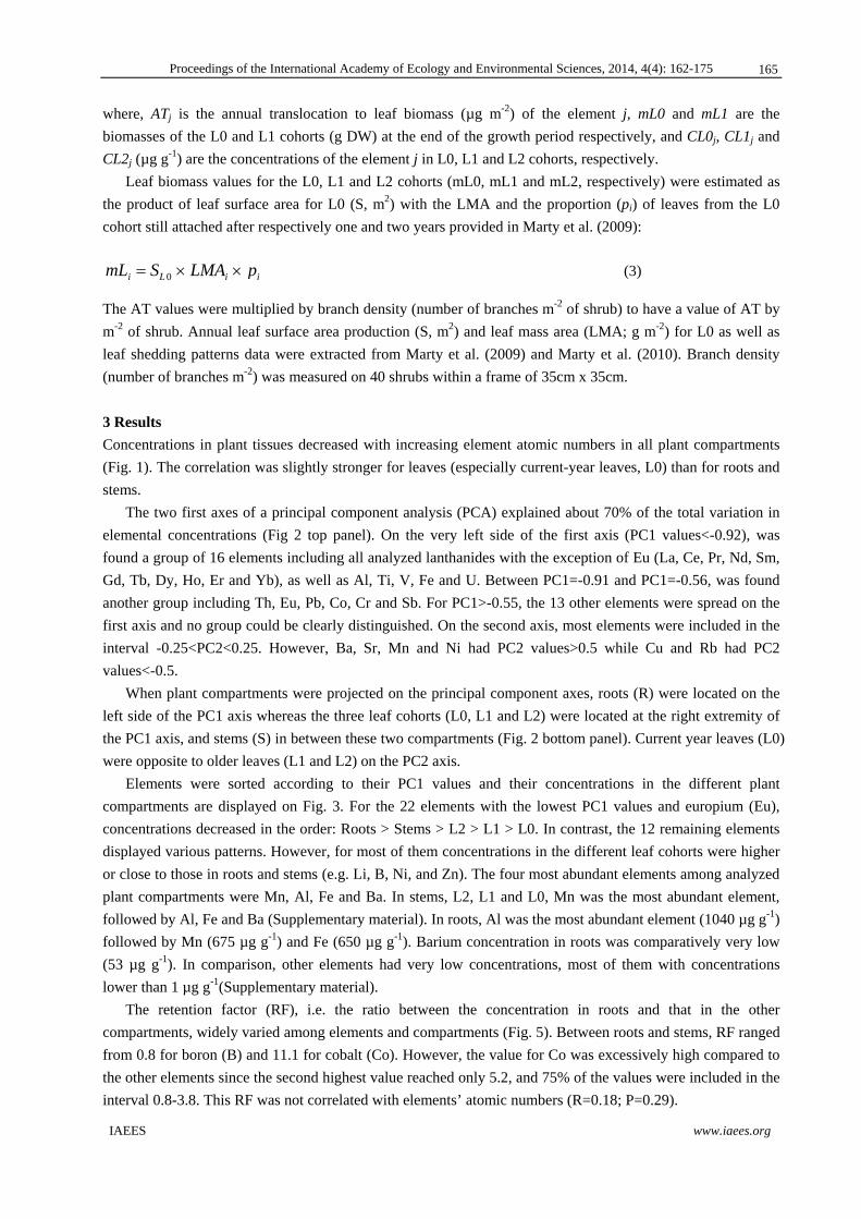
Proceedings of the International Academy of Ecology and Environmental Sciences, 2014, 4(4): 162-175
IAEES www.iaees.org
where, ATj is the annual translocation to leaf biomass (µg m-2) of the element j, mL0 and mL1 are the
biomasses of the L0 and L1 cohorts (g DW) at the end of the growth period respectively, and CL0j, CL1j and
CL2j (µg g-1) are the concentrations of the element j in L0, L1 and L2 cohorts, respectively.
Leaf biomass values for the L0, L1 and L2 cohorts (mL0, mL1 and mL2, respectively) were estimated as
the product of leaf surface area for L0 (S, m2) with the LMA and the proportion (pi) of leaves from the L0
cohort still attached after respectively one and two years provided in Marty et al. (2009):
mLi SL 0 LMAi pi (3)
The AT values were multiplied by branch density (number of branches m-2 of shrub) to have a value of AT by
m-2 of shrub. Annual leaf surface area production (S, m2) and leaf mass area (LMA; g m-2) for L0 as well as
leaf shedding patterns data were extracted from Marty et al. (2009) and Marty et al. (2010). Branch density
(number of branches m-2) was measured on 40 shrubs within a frame of 35cm x 35cm.
3 Results
Concentrations in plant tissues decreased with increasing element atomic numbers in all plant compartments
(Fig. 1). The correlation was slightly stronger for leaves (especially current-year leaves, L0) than for roots and
stems.
The two first axes of a principal component analysis (PCA) explained about 70% of the total variation in
elemental concentrations (Fig 2 top panel). On the very left side of the first axis (PC1 values<-0.92), was
found a group of 16 elements including all analyzed lanthanides with the exception of Eu (La, Ce, Pr, Nd, Sm,
Gd, Tb, Dy, Ho, Er and Yb), as well as Al, Ti, V, Fe and U. Between PC1=-0.91 and PC1=-0.56, was found
another group including Th, Eu, Pb, Co, Cr and Sb. For PC1>-0.55, the 13 other elements were spread on the
first axis and no group could be clearly distinguished. On the second axis, most elements were included in the
interval -0.25<PC2<0.25. However, Ba, Sr, Mn and Ni had PC2 values>0.5 while Cu and Rb had PC2
values<-0.5.
When plant compartments were projected on the principal component axes, roots (R) were located on the
left side of the PC1 axis whereas the three leaf cohorts (L0, L1 and L2) were located at the right extremity of
the PC1 axis, and stems (S) in between these two compartments (Fig. 2 bottom panel). Current year leaves (L0)
were opposite to older leaves (L1 and L2) on the PC2 axis.
Elements were sorted according to their PC1 values and their concentrations in the different plant
compartments are displayed on Fig. 3. For the 22 elements with the lowest PC1 values and europium (Eu),
concentrations decreased in the order: Roots > Stems > L2 > L1 > L0. In contrast, the 12 remaining elements
displayed various patterns. However, for most of them concentrations in the different leaf cohorts were higher
or close to those in roots and stems (e.g. Li, B, Ni, and Zn). The four most abundant elements among analyzed
plant compartments were Mn, Al, Fe and Ba. In stems, L2, L1 and L0, Mn was the most abundant element,
followed by Al, Fe and Ba (Supplementary material). In roots, Al was the most abundant element (1040 µg g-1)
followed by Mn (675 µg g-1) and Fe (650 µg g-1). Barium concentration in roots was comparatively very low
(53 µg g-1). In comparison, other elements had very low concentrations, most of them with concentrations
lower than 1 µg g-1(Supplementary material).
The retention factor (RF), i.e. the ratio between the concentration in roots and that in the other
compartments, widely varied among elements and compartments (Fig. 5). Between roots and stems, RF ranged
from 0.8 for boron (B) and 11.1 for cobalt (Co). However, the value for Co was excessively high compared to
the other elements since the second highest value reached only 5.2, and 75% of the values were included in the
interval 0.8-3.8. This RF was not correlated with elements’ atomic numbers (R=0.18; P=0.29).
165
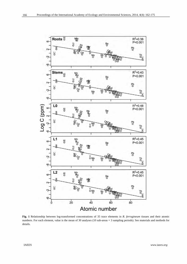
Proceedings of the International Academy of Ecology and Environmental Sciences, 2014, 4(4): 162-175
IAEES www.iaees.org
Fig. 1 Relationship between log-transformed concentrations of 35 trace elements in R. ferrugineum tissues and their atomic numbers. For each element, value is the mean of 30 analyses (10 sub-areas × 3 sampling periods). See materials and methods for details.
166

Proceedings of the International Academy of Ecology and Environmental Sciences, 2014, 4(4): 162-175
IAEES www.iaees.org
Fig. 2 Principal component analysis (PCA) of concentrations of 35 elements in plant compartments. Top: Projection of the different elements analyzed in the two principal axes space. Bottom: Projection of the different plant compartments in the two principal axes space. Each ellipse is a graphic résumé of the point cloud, the centre of which representing the gravity centre.
167

Proceedings of the International Academy of Ecology and Environmental Sciences, 2014, 4(4): 162-175
IAEES www.iaees.org
Fig. 3 Mean concentrations (µg g-1) of the 35 analyzed trace elements in R. ferrugineum’s compartments. Elements are sorted as a function of their coordinate on the first axis of the PCA presented on Fig 2. PC1 values increase from right to left and from top to bottom. Errors bars are SE.
168

Proceedings of the International Academy of Ecology and Environmental Sciences, 2014, 4(4): 162-175
IAEES www.iaees.org
Fig. 4 Mean concentrations (µg g-1) of the 35 analyzed trace elements in R. ferrugineum’s roots, stems, 2-yr old leaves (L2), 1-yr old leaves (L1) and current-yr leaves (L0). Errors bars are SE.
169

Proceedings of the International Academy of Ecology and Environmental Sciences, 2014, 4(4): 162-175
IAEES www.iaees.org
Fig. 5 Retention factor (RF) between roots and stems (R-S), 2-yr old leaves (R-L2), one yr-old leaves (R-L1) and current-year leaves (R-L0) for 35 trace elements. The retention factor is calculated as the ratio between the concentration in roots and that in the other compartments. Elements’ atomic number increases from the left to the right of the x-axis.
Fig. 6 Mean Retention Factor (+ SE) for the 35 analyzed elements. The group of elements characterized by a low PC1 value as well as by concentrations decreasing in the order R>S>L2>L1>L0 (Group 1) is shown.
170

Proceedings of the International Academy of Ecology and Environmental Sciences, 2014, 4(4): 162-175
IAEES www.iaees.org
Fig. 7 Annual translocation to the foliage (µg m-2 yr-1) for each analyzed element.
The RF between roots and all leaf cohorts was high and similar for all elements with an atomic number
higher than 57 (at the right of lanthanum on Fig. 5) with the exception of europium (Eu) for which RF for all
leaf cohorts was only slightly higher than for stems. The RF between roots and leaves was particularly high for
lead (Pb), yttrium (Y) and cobalt (Co) with RFR-L0 averaging 46, 30 and 24, respectively. For most elements,
RF decreased with leaf age (R-L0>R-L1>R-L2) with the exception of 12 elements: Li, B, Mn, Ni, Cu, Zn, Ga,
Rb, Sr, Mo, Cs and Ba. For these elements, the RF for leaves was similar, slightly higher or even lower than
for stems. The RF for L0, L1 and L2 was positively correlated with elemental atomic number (R=0.42, P<0.05;
R=0.35, P<0.05; R=0.44, P<0.01, respectively).
The amount of element annually translocated from roots to the foliage varied by several orders of
magnitude (Fig. 7), from ~0.5 µg m-2 yr-1 for homium (Ho) and terbium (Tb) to ~100 mg m-2 yr-1 for
manganese (Mn). Only ten elements had annual translocation higher than 1 mg m-2 yr-1 (Ni < Ti <Sr<Rb< B <
Zn <Ba< Fe < Al <Mn). Most elements had an annual translocation to the foliage <10 µg m-2 yr-1.
4 Discussion
4.1 Elements retention in the root compartment
As expected we found a large discrepancy in concentrations among elements and plant compartments. In every
compartment, concentrations decreased with elements’ atomic number which is in line with Watanabe et al.
(2007) who observed the same patterns on 670 species of terrestrial plants, sampled from 29 sites in four
countries. The fact that roots and the three leaf cohorts were opposite on the PC1 axis reflected the markedly
different chemical composition of these compartments. Concentrations were generally higher in roots than in
leaves, especially for the 22 elements with the lowest PC1 coordinate (Fig. 3). These elements with yttrium (Y)
could be assembled in one group (hereafter Group 1) characterized by high retention factors (RF) (Fig. 6) and
a slight accumulation in leaves as they aged which resulted in the following concentration pattern:
R>>S>L2>L1>L0 (Fig. 3). For this group of elements, concentration was on average i) 3.8 times higher in
171

Proceedings of the International Academy of Ecology and Environmental Sciences, 2014, 4(4): 162-175
IAEES www.iaees.org
roots than in stems with a range of 1.7 times for chromium (Cr) to 11.1 times for cobalt (Co); ii) 14.1times
higher in roots than in L0 with a range of 3.3 to 46.3 for europium (Eu) and lead (Pb), respectively; iii) 2.6
times higher in L2 than in L0 with a range of 1.2 to 3.4 for antimony (Sb) and lead (Pb), respectively. The 12
remaining elements (hereafter Group 2) including molybdenum (Mo), copper (Cu), manganese (Mn), cesium
(Cs), lithium (Li), gallium (Ga), zinc (Zn), barium (Ba), strontium (Sr), nickel (Ni), rubidium (Rb) and boron
(B) showed various concentration patterns but were all characterized by low RFs (Fig. 6). This generally
resulted in relatively high concentrations in leaf cohorts compared to elements from Group 1.
Although RF tended to increase with atomic number some elements with a relatively low atomic number
had a high RF (e.g., Al, V, Co) and some with a high atomic number had a low RF (e.g., Ba, Rb, Sr, Eu).
Elements like aluminum (Al) and cobalt (Co) are known to be toxic for plants. High retention of these
elements in the roots corroborates the hypothesis that in acidic soils, root biomass plays an important role in
sequestration of toxic trace elements (Vogt et al., 1987b). This accumulation followed by root senescence and
death could actually avoid the toxicity to propagate in all the biological components. However, despite its
toxicity and its high RF, Al was the second most abundant trace element in the foliage after Mn
(Supplementary material). This might result from its high concentration in the soil solution in phytoavailable
form (see below). In contrast, barium (Ba) and strontium (Sr), two alkaline earth elements, as well as rubidium
(Rb), an alkali element, had a low RF. This probably resulted from their physico-chemical properties (Aberg et
al., 1990), which are similar to those of calcium (Ca) for the two firsts and potassium (K) for the latter, and
which confer them similar dynamics in the plant-soil system (see below).
Trace elements that are known to be essential for plants are boron (B), iron (Fe), zinc (Zn), copper (Cu),
manganese (Mn), cobalt (Co), nickel (Ni) and molybdenum (Mo) (Graham and Stangoulis, 2003; Marschner,
1995). With the exception of Fe and particularly Co that had a very high RF and were characterized by the
pattern R>>S>L2>L1>L0, all these essential elements were weakly retained in the roots (RF ranging from 0.4
for B to 2.3 for Mo). However, despite its high RF, Fe concentrations in the leaves were very high compared to
the other essential elements (Fig. 3), suggesting that their high retention in the roots resulted from high element
availability compared to leaf requirements. In contrast, Co concentrations in the roots and leaves were very
low suggesting that the high retention of this element in the roots resulted from the very small amounts
required by the plants and from its toxicity at high concentrations. Cobalt concentrations in plants are actually
generally as low as 0.1–10 μgg-1 (Palit et al., 1994) although concentrations can quickly increase in some crops,
especially in roots, with increasing concentrations in the soil solution (Bakkaus et al., 2005). Concentrations of
these essential elements were generally higher in roots than in the other plant compartments, with the
exception of Zn, Ni and B (Fig. 3). In many soils, B can be taken up as a neutral molecule, which is highly
permeable across cellular membranes (Stangoulis et al., 2001). Its transport throughout the plant is facilitated
when external concentrations are low like in acidic alpine soils. Its passive uptake and its high transport ability
could explain why B concentration is significantly higher in leaves than in stems and roots, which was not the
case for most of the studied trace elements.
4.2 Elements dynamics in the leaf compartment
As mentioned above, concentration in leaves increased with leaf age for all elements from Group 1. This trend
was also observed for some elements from Group 2: Mn, Ga, Ba, Sr and Ni. In contrast, concentrations in Cu,
Zn, Cs and Rb tended to decline with leaf age. These different dynamics probably contributed to the opposite
locations of these two groups of elements on the second axis of the PCA (Fig. 2). Indeed, Mn, Na, Sr and Ni
had high positive PC2 values, while Cu, Zn and Rb had low negative PC2 values. These different patterns
might result from elements’ physico-chemical properties (e.g. lack of mobility in the phloem) and their
physiological roles in the plant. For instance, root uptake is thought to not distinguish between Rb and K
172

Proceedings of the International Academy of Ecology and Environmental Sciences, 2014, 4(4): 162-175
IAEES www.iaees.org
because of close ionic radii and similar valences (Marschner, 1995). These similarities in atomic properties
could explain Rb high concentrations in leaves since K+ optimal cytosolic concentration is in the range of 100
mM (Ashley et al., 2006), which makes K+ the most abundant cation in the cytosol (Véry and Sentenac, 2003).
In addition, K high solubility in the cytosol makes its retranslocation from senescent leaves through the
phloem possible (Véry and Sentenac, 2003). These similar physico-chemical properties might explain the very
close dynamics of these two elements in R. ferrugineum (Marty et al., 2014). The retranslocation process
might therefore explain the decrease in the concentration of Rb and other elements like Cu and Zn with leaf
age, as the latter are also known to be efficiently retranslocated from leaves, at least in crops (Marschner,
1995). As it has been shown for nitrogen, this resorption process might contribute to annual growth in R.
ferrugineum (Marty et al., 2009, 2010; Pasche et al., 2002). In contrast, Sr and Ba accumulated in leaves with
time and were shown to have the same dynamics as Ca in R. ferrugineum (Marty et al., 2014), resulting from
similar physico-chemical properties. Strontium’s ionic radius is close to that of Ca (1.00 and 1.18 Å for Ca and
Sr, respectively), which can give these elements similar dynamics in the soil-plant system (Aberg et al., 1990;
Poszwa et al., 2000). Barium, another alkaline-earth with a close ionic radius (1.35 Å), can also have a similar
dynamics in soil-plant system (Suwa et al., 2008). Although Ca is one of the most abundant elements in plant
tissues, cytosolic concentration is maintained at submicromolar levels because of a low solubility (White and
Broadley, 2003). These properties prevent Ca and hence Sr and Ba from being translocated from leaves to
other organs via the phloem and result in Ca, Sr and Ba accumulation with leaf age. Such low solubility in the
cytosol and therefore low mobility in the phloem could be responsible for the accumulation of all elements
from group 1.
Annual translocation to the foliage strongly varied among the analyzed trace elements. The four elements
with the highest concentrations in the analyzed plant compartments (Mn, Al, Fe and Ba) were also the
elements with the highest annual translocation to the foliage, which ranged from 10 to 100 mg m-2 yr-1. The
annual translocation to the foliage of Sr, Rb, B and Zn was >1 mg m-2 yr-1. With the exception of Al, all these
elements are either essential elements (B, Zn, Fe and Mn) or analogs of essential elements (Sr, Rb and Ba).
Aluminum can be abundant in the parental rock and occur in the soil solution in nonphytotoxic forms, which
might explain the high concentrations in roots (Fig 3). Nevertheless, the high translocation of Al is surprising
since Al is known to be highly toxic for plants even at low concentrations (Delhaize and Ryan, 1995). This
annual translocation to the foliage might result in the incorporation of a similar amount of element into the top
layer of the soil through litter production. The amount of Al returning to the soil annually through litter (65 mg
m-2 yr-1) is nevertheless very low compared to major elements. Indeed, using concentrations values provided in
Marty et al. (2014), we estimated that Ca and K annual translocation to the foliage was 1.9 g m-2 yr-1 and 0.9 g
m-2 yr-1, respectively. Therefore, it takes approximately 20 times longer to bring up a given amount of Al from
the mineral soil to the top layer compared to Ca through this process.
5 Conclusion
The present data allowed us to distinguish at least two groups of elements among the 35 analyzed based on
their distribution throughout the plant organs. The first group included 23 elements characterized by a high
retention in the roots and accumulation in leaves with leaf aging. There was a positive relationship between
retention in the roots and atomic number but this latter did not appear to be the only determinant factor since
some elements with low atomic number (e.g., Al, Co) were highly retained in the roots. This retention might
be an adaptation to impede the propagation of toxic elements to other plant organs. On the other hand, we
found elements, most of them being essential for plants, which were weakly retained in the root compartment
and distributed to the leaves where they either accumulated or were resorbed with leaf aging. More research
173

Proceedings of the International Academy of Ecology and Environmental Sciences, 2014, 4(4): 162-175
IAEES www.iaees.org
should be conducted to verify whether the observed patterns in R. ferrugineum are universal or related to
phylogenetic, functional or ecologic characteristics as it has been previously shown for leaf element
composition (Watanabe et al., 2007). In addition, the different dynamics of the two groups of elements may
impact element distribution throughout the soil profile. Concentrations of elements with high retention in the
roots might remain very low in the upper horizons while those of elements with low retention could
accumulate in the upper horizons through litter inputs.
References
Aberg G, Jacks G, Wickman T, Hamilton PJ. 1990. Strontium isotopes in trees as an indicator for calcium
availability. Catena, 17: 1-11
Anim AK, Laar C, Osei J, et al. 2012. Trace metals quality of some herbal medicines sold in Accra, Ghana.
Proceedings of the International Academy of Ecology and Environmental Sciences, 2(2): 111-117
Ashley MK, Grant M, Grabov A. 2006. Plant responses to potassium deficiencies: a role for potassium
transport proteins. Journal of Experimental Botany, 57(2): 425-436
Baker A, Reeves R, Hajar A. 1994. Heavy metal accumulation and tolerance in British populations of the
metallophyte Thlaspi caerulescens J .& C. Presl. New Phytologist, 127: 61-68
Bakkaus E, Gouget B, Gallien JP, et al. 2005. Concentration and distribution of cobalt in higher plants: The
use of micro-PIXE spectroscopy. Nuclear Instruments and Methods in Physics Research B, 231(1-4): 350-
356
Blake L, Goulding KWT. 2002. Effects of atmospheric deposition , soil pH and acidification on heavy metal
contents in soils and vegetation of semi-natural ecosystems at Rothamsted Experimental Station, UK. Plant
and Soil, 240: 235-251
Campbell JL, Rustad LE, Boyer EW, et al. 2009. Consequences of climate change for biogeochemical cycling
in forests of northeastern North America. Canadian Journal of Forest Research-Revue Canadienne De
Recherche Forestiere, 39: 264-284
Delhaize E, Ryan PR. 1995. Aluminum Toxicity and Tolerance in Plants. Plant Physiology, 107(2): 315-321
Dray S, Dufour AB. 2007. The ade4 package: implementing the duality diagram for ecologists. Journal of
Statistical Software, 22(4): 1-20
Ediagbonya TF, Ukpebor EE, Okieimen FE. 2013. Heavy metal in inhalable and respirable particles in urban
atmosphere. Environmental Skeptics and Critics, 2(3): 108-117
Graham RD, Stangoulis JCR. 2003. Comparative trace element nutrition -trace element uptake and distribution
in plants. Journal of Nutrition, 1502-1505
Greger M. 2004. Metal availability, uptake, transport and accumulation in plants. In: Heavy Metal Stress in
Plants-From Biomolecules to Ecosystems (Prasad M, ed). Springer-Verlag, Berlin Heidelberg, Germany
Marschner H. 1995. Mineral Nutrition of Higher Plants. Academic Press London, UK
Marty C, Lamaze T, Pornon A. 2009. Endogenous sink-source interactions and soil nitrogen regulate leaf life-
span in an evergreen shrub. New Phytologist, 183(4): 1114-1123
Marty C, Lamaze T, Pornon A. 2010. Leaf life span optimizes annual biomass production rather than plant
photosynthetic capacity in an evergreen shrub. New Phytologist, 187: 407-416
Marty C, Pornon A, Lamaze T, Viers J. 2014. Calcium and potassium dynamics and biopurification in two
populations of the subalpine evergreen shrub Rhododendron ferrugineum. Proceedings of the International
Academy of Ecology and Environmental Sciences, 4(2): 50-61
174

Proceedings of the International Academy of Ecology and Environmental Sciences, 2014, 4(4): 162-175
IAEES www.iaees.org
Ouzounidou G, Moustakas,M, Eleftheriou EP. 1997. Physiological and ultrastructural effects of cadmium on
wheat (Triticumaestivum L.) leaves. Archives of Environmental Contamination and Toxicology, 32(2):
154-160
Ozenda, P. 1985. La végétation de la chaine Alpine dansl’espacemontagnardeuropéen. Masson, Paris, France
Palit S, Sharma A, Talukder G. 1994. Effects of cobalt in plants.The Botanical Review, 60(2): 149-181
Pasche F, Pornon A, Lamaze T. 2002. Do mature leaves provide a net source of nitrogen supporting shoot
growth in Rhododendron ferrugineum? New Phytologist, 154: 99-105
Perronnet K, Schwartz C, Morel JL. 2003. Distribution of cadmium and zinc in the
hyperaccumulatorThlaspicaerulescens grown on multicontaminated soil. Plant and Soil, 249: 19-25
Pornon A, Lamaze T. 2007. Nitrogen resorption and photosynthetic activity over leaf life span in an evergreen
shrub, Rhododendron ferrugineum, in a subalpine environment. New Phytologist, 175: 301-310
Poszwa A, Dambrine E, Pollier B, Atteia O. 2000. A comparison between Ca and Sr cycling in forest
ecosystems. Plant and Soil, 225: 299-310
Schwartz C, Echevarria G, Morel JL. 2003. Phytoextraction of cadmium with Thlaspicaerulescens. Plant and
Soil, 249: 27-35
Stangoulis JCR, Reid RJ, Brown PH, Graham RD. 2001. Micronutrient nutrition of plants. Critical Reviews in
Plant Sciences, 14: 49-82
Suwa R, Jayachandran K, Nguyen NT, et al. 2008. Barium toxicity effects in soybean plants. Archives of
Environmental Contamination and Toxicology, 55: 397: 403
Véry AA, Sentenac H. 2003. Molecular mechanisms and regulation of K+ transport in higher plants. Annual
Review of Plant Biology, 54: 575-603
Viers J, Oliva P, Sonke J, et al. 2007. Evidence of Zn isotopic fractionation in a soil-plant-system of a pristine
tropical watershed (Nsimi, south Cameroon). Chemical Geology, 239: 124-137
Vogt K, Dahlgren R, Ugloni F, et al. 1987a. Aluminum, Fe, Ca, Mg, K, Mn, Cu, Zn and P in above- and
belowground biomass. I. Abiesamabilis and Tsugamertensiana. Biogeochemistry, 4: 277-294
Vogt K, Dahlgren R, Ugloni F, et al. 1987b. Aluminum, Fe, Ca, Mg, K, Mn, Cu, Zn and P in above- and
belowground biomass. II. Pools and circulation in a subalpine Abiesamabilis stand. Biogeochemistry, 4:
295-311
Watanabe T, Broadley MR, Jansen S, et al. 2007. Evolutionary control of leaf element composition in plants.
New Phytologist, 174: 516-523
White PJ, Broadley MR. 2003. Calcium in plants. Annals of Botany, 92(4): 487-511
Zhang WJ, Liu CH. 2012. Some thoughts on global climate change: will it get warmer and warmer?
Environmental Skeptics and Critics, 1(1): 1-7
175

Proceedings of the International Academy of Ecology and Environmental Sciences, 2014, 4(4): 176-184
IAEES www.iaees.org
Article
Assessment of metal bioaccumulation in Clarias batrachus and
exposure evaluation in human
Mayank Pandey1, Ashutosh Kumar Pandey1, Ashutosh Mishra1, B. D. Tripathi2 1Institute of Environment and Sustainable Development, Banaras Hindu University, Varanasi, 221005, India 2Department of Botany, Banaras Hindu University, Varanasi, 221005, India
E-mail: [email protected]
Received 27 June 2014; Accepted 1 August 2014; Published online 1 December 2014
Abstract
The present work was conducted for heavy metal (Cr, Mn, Fe, Co, Ni, Cu, Zn, Cd and Pb) quantification in the
river Ganga water and their bioaccumulation in vital organ tissues of Clarius batrachus. Heavy metal
characterization in vital organ tissues (gills, liver and muscle) and comparison with FAO permissible
guidelines revealed that Cd and Pb were hyper-accumulated which may lead to metal toxicity in fish and its
consumers. High metal pollution index (MPI) was recorded for organ tissues of exposed samples (liver 6.05;
gills 22.95; muscle 44.48) as compared to unexposed samples (liver 4.5; gills 18.8; muscle 36.76). Effective
ingestive dose (EID) was calculated to assess the exposure threat to the human which may occur through
dietary inputs. Results revealed that EID for Cr, Co, Cd and Pb was found significantly higher than the dose
concentration prescribed by USEPA.
Keywords Clarius batrachus; river Ganga; metal; bioaccumulation; ingestion dose.
1 Introduction
1 Introduction
Metals discharged from the anthropogenic sources (industries, mining, tannery etc.) have become potential
threat for aquatic ecosystem. Metals are believed to be potent toxic substances due to their slow degradation
rate and long half-life period (Chabukdhara and Nema, 2012; Jain, 2004; Kelepertzis et al., 2012; Prajapati et
al., 2012). Through various paths, metals enter the food chain/web and ultimately cause adverse physical and
physiological effects on biotic elements of earth and get accumulated in flora and fauna, which is called
bioaccumulation. Being at the top of the trophic level, human gets most affected by bioaccumulation and bio
magnification (Chi et al., 2007; Mishra and Mohanty, 2008; Alhashemi et al., 2011; Garg et al., 2014;
Goodyear and McNeill, 1999). Minamata disease (mercury), itai-itai (cadmium), lead leprosy, metal fume
fever, arsenic poisoning in South East Asia are few examples to depict the catastrophic effects of metals at
higher concentration.
Proceedings of the International Academy of Ecology and Environmental Sciences ISSN 22208860 URL: http://www.iaees.org/publications/journals/piaees/onlineversion.asp RSS: http://www.iaees.org/publications/journals/piaees/rss.xml Email: [email protected] EditorinChief: WenJun Zhang Publisher: International Academy of Ecology and Environmental Sciences

Proceedings of the International Academy of Ecology and Environmental Sciences, 2014, 4(4): 176-184
IAEES www.iaees.org
Fish is considered an excellent biomarker of metal pollution in aquatic ecosystem for many reasons; it
occupies higher trophic level in an aquatic ecosystem, metal toxicity adversely affects the physical and
physiological behavior of the fish and it is an important constituent of non-vegetarian diet of human. High
quality of protein, amino acid (lysine, sulfur containing amino acids etc.), iodine, calcium, trace elements (Mn,
Fe, Cu, Zn, Se etc.), vitamins and omega-3-polyunsaturated fatty acid are obtained from fish (Ashwani and
Ashok, 2006; Mishra and Mohanty, 2008; Rani and Sivaraj, 2010). Therefore, human consumption of fish as
dietary component may lead to severe health hazards to the mankind. Minamata disaster is an example for the
same (McCurry, 2006).
Gills are respiratory and osmo-regulatory organs having large surface area which interacts with dissolved
metal in the surrounding for maximum period. Also, the detoxification system of gills is not as strong as that of
liver. High metal concentration in gills reflects high metal concentration in dissolved phase. High absorption
rate of toxic elements by gills causes high toxic concentration in gills (Pandey et al., 2008). High metal
concentration in liver indicates dietary input of metal as liver is the storage organ. Muscle tissue is an inactive
site of metal accumulation (Alhashemi et al., 2012). Bioaccumulation Factor (BAF) and Metal Pollution Index
(MPI) are few indices for the assessment of degree of metal accumulation (Vaseem and Banerjee, 2013).
Workers have assessed effective ingestive dose (EID) for heavy metals in human by the consumption of metal
accumulated fish (Alhashemi et al., 2012).
River Ganga pollution is a challenge to the scientific community and policy makers in India.
Anthropogenic factors (discharge from agriculture, domestic and industrial sectors) are the prime cause of
river pollution. A descriptive study on metal bioaccumulation in C. batrachus in river Ganga is not been done
so far. Therefore, the main objective of the present study was to assess metal concentration in river water vis-à-
vis their accumulation in vital organ tissues of fish. Ingestion dose of metals through diet (fish) by human
beings was also determined as described elsewhere (Alhashemi et al., 2012).
2 Materials and Methods
2.1 Study region
Varanasi (25016´55ʺN 82057´23ʺE, 76m amsl) is situated at the left bank of Ganga, the national river of India.
Varanasi is known for its dense population and large number of industries (locomotive and metal works;
textile and dye industries, glass) which discharge effluent having high concentration of heavy metals.
Industrial effluents directly get mixed into city sewage and ultimately discharged into the river due to
unavailability of metal removing technologies (Tripathi et al., 1991).
2.2 Sampling and analysis
River water sampling (PTFE bottles; prewashed and acidified) was done from sixteen points between
Shooltankeshwar (S0) and Ganga-Varuna confluence (S15), following standard protocols (APHA, 2005).
Reference site (S0) was chosen at upstream while remaining sampling points (S1-S15) were along the
downstream. Length of entire river stretch was c.a. 20 km (S0-S1 10km; S1-S15 10 km). Water samples were
carried immediately after sampling to the laboratory at 40C.
Seven samples of Clarius batrachus (Mangur) were caught by using traditional net method with the help of
professional fishermen from reference and downstream stretch. It was tried to maintain homogeneity in weight
and length of samples. Fish samples were kept and transferred immediately to the laboratory in river water.
Fish were anaesthetized and dissected to get liver, gill and muscle tissue (mid abdomen region). Organ tissues
were acid digested (3HNO3:1HCl:1HClO4 v/v) in Teflon vessels for 60-120 minutes to get a clear solution was
obtained. Volume of digested samples was made up to 100 ml using Millipore water and metal analysis was
done by flame Atomic Absorption Spectrophotometer (AAS) (AAnalyst 800-Perkin Elmer). Calibration of
177

Proceedings of the International Academy of Ecology and Environmental Sciences, 2014, 4(4): 176-184
IAEES www.iaees.org
AAS was done with metal standard solutions after every 15 samples. Statistical significance of the results was
assessed by applying independent sample t test.
3 Results and Discussion
Heavy metal concentration was considerably higher from S1-S15 than at reference site (S0) (Table 2).
Anthropogenic sources (industrial, domestic and agricultural effluents) are the principal cause of high metal
concentration in downstream river water. Large drain confluence (S1 and S15), dead body cremation (S7 and
S9) and mass bathing (S8) are also chief pollutant sources to the river Ganga. There are reports suggesting that
developmental stages of fish are negatively affected by higher metal concentration in river water. It has been
established that there is a negative linear regression between metal concentration and size of fish (Canli and
Atli, 2003).
The objective of the present work was to assess the degree of metal accumulation (wet weight; mgkg-1) in
vital organ tissues of studied fish samples. Simultaneous quantification of heavy metals in river water and fish
tissues was done. Metal concentration (wet weight, mgKg-1) in tissues (Gill, Liver and Muscle) of downstream
fish samples were compared with samples of reference site and FAO permissible limit (FAO, 1983). Metal
accumulation indices like bioaccumulation factor (BAF) and metal pollution index (MPI) were calculated as
discussed below (Vaseem and Banerjee, 2013):
BAF = Cf/Cw
where, Cf is concentration of metal in fish organ (mgkg-1) and Cw is metal concentration in river water (mgl-1).
MPI = (Cf1 x Cf2 x Cf3 x… Cfn)1/n
where Cfn is concentration of metal n in the given sample
Organosomatic index (OSI) was calculated to assess the proportional size change in the gills (gill somatic
index) and liver (hepato somatic index) of exposed and unexposed fish samples. The hepato-somatic index
percentage (HSI %) was found almost same for exposed (0.48 ± 0.02 %) and reference (0.48 ± 0.01 %)
samples. However, gill somatic index (GSI %) of exposed sample was found higher in exposed sample (1.6 ±
0.02 %) as compared to reference sample (1.51 ± 0.02 %), indicating metal accumulation in gills.
Metal pollution index (MPI) for gills (22.95), liver (6.05) and muscle (44.48) of exposed sample was found
significantly higher than in gills (18.79), liver (4.5) and muscle (36.76) of unexposed samples. Highest bio-
accumulation factor (BAF) was observed in muscle tissue of exposed fish samples for all heavy metals except
Cr, Mn and Fe which were higher in gill tissues (Fig. 1).
Higher concentration of Cr was found in exposed fish samples. The order of Cr concentration in exposed
fish organ was gills (43.6 ± 1.85 mgkg-1), muscle (27.1 ± 1.63 mgkg-1) and liver (13.17 ± 3 mgkg-1). Similar
trend was observed for unexposed samples (gills 39 ± 1.68 mgkg-1; muscle 21.35 ± 0.93 mgkg-1; liver 7.4 ±
1.11 mgkg-1) (Table 1). It has been reported that higher Cr concentration may adversely affect the amino acid
content in fish (Rani and Sivaraj, 2010). Chromium concentration in exposed and unexposed samples was well
above the permissible guidelines of FAO (1 mgkg-1) (Table 1; Hong Kong FAO, 1983).
Highest concentration of Mn in exposed samples was found in gills (16.7 ± 1.35 mgkg-1), followed by
muscle (6.6 ± 1.5 mgkg-1) and least in liver (1.61 ± 0.2 mgkg-1). Also in unexposed samples, gills were highly
accumulated (14.05 ± 1.12 mgkg-1) while liver was least accumulated (1.1 ± 0.06 mgkg-1) with Mn. Similar
trend was followed by Fe in gills (334.4 ± 12.01 mgkg-1), muscle (156.2 ± 6.27 mgkg-1) and liver tissues
(79.10 ± 6.2 mgkg-1) of exposed samples. No permissible guidelines have been provided by FAO for Mn and
Fe concentration in fish tissues (Table 1; FAO, 1983).
Co and Ni accumulation showed similar behaviour in studied samples. Highest concentration of Co was
found in muscle (41.5 ± 2.78 mgkg-1) followed by gills (17.7 ± 1.16 mgkg-1) and least in liver tissues (5.0 ± 0.7
178

Proceedings of the International Academy of Ecology and Environmental Sciences, 2014, 4(4): 176-184
IAEES www.iaees.org
mgkg-1) of exposed samples. Co concentration followed similar trend in unexposed samples, but concentration
was well below the exposed samples. Co is regarded as essential nutrient required in trace concentration. It is
indispensible part of vitamin B12 but may prove itself hazardous in higher concentration which may in turn
cause physiological diseases like polycythemia (Gal et al., 2008). Highest concentration of Ni was observed in
muscle tissues of exposed (21.5 ± 2.15 mgkg-1) and unexposed (18.26 ± 0.73 mgkg-1) samples. Almost similar
concentration of Ni was found in liver tissues of exposed (1.05 ± 0.2 mgkg-1) and unexposed fish (0.9 ± 0.13
mgkg-1). Ni concentration in muscle tissues of exposed sample (10 ± 1.76 mgkg-1) was significantly higher
than in unexposed sample (7.8 ± 0.96 mgkg-1).
Table 1 Metal concentration in Clarias batrachus.
Fish Length (cm) Weight (g) HSI% GSI% Reference 24.76 ±1.39 54.81 ± 1.66 0.48 ± 0.01 1.51 ± 0.02 Exposed 22.8 ± 3.4 52.14 ± 2.17 0.48 ± 0.02 1.6 ± 0.02
Concentration of Metals in Fish (Mean ± SD wet weight mgKg-1) Liver Cr Mn Fe Co* Ni* Cu Zn* Cd* Pb
Reference 7.4 ± 1.11
1.1 ± 0.06
71.7 ± 3.42
3.5 ± 0.66
0.9 ± 0.13
3.4 ± 0.38
8.4 ± 0.74
1.3 ± 0.44
11.4 ± 0.93
Exposed 13.17 ±
3 1.61 ±
0.2 79.10 ±
6.2 5.0 ± 0.7
1.05 ± 0.2
4.86 ± 0.6
9.73 ± 1.2
1.89 ± 0.5
13.77 ± 1.3
Gill Cr* Mn Fe Co* Ni Cu Zn Cd Pb*
Reference 38.9 ± 1.68
14.05 ± 1.12
326.97 ± 3.92
15.33 ± 1.17
7.8 ± 0.96
1.62 ± 0.37
47.54 ± 1.45
3.75 ± 1.12
47.41 ± 2.78
Exposed 43.6 ± 1.85
16.7 ± 1.35
334.4 ± 12.01
17.7 ± 1.16
10 ± 1.76
2.6 ± 0.9
53.5 ± 2.26
5.9 ± 1.67
51.4 ± 2.14
Muscle Cr Mn Fe Co Ni Cu Zn* Cd Pb
Reference 21.35 ±
0.93 4.29 ± 0.43
137.26 ± 1.12
36.87 ± 0.83
18.26 ± 0.73
78.41 ± 0.79
79.41 ± 2.31
19.78 ± 0.98
117.46 ± 1.11
Exposed 27.1 ± 1.63
6.6 ± 1.5
156.2 ± 6.27
41.5 ± 2.78
21.5 ± 2.15
90.8 ± 1.83
94.0 ± 2.28
25.9 ± 1.87
122.9 ± 1.84
India (FAO, 1983)
NA NA NA NA NA 10 50 NA 5
Australia (FAO, 1983)
NA NA NA NA NA 10 150 0.2 1.5
Hong Kong (FAO, 1983)
1 NA NA NA NA NA NA 2 6
HSI-Hepatosomatic index; GSI-Gill Somatic Index; FAO- Food and Agriculture Organization; NA-Not Available. * Independent sample t test significance > 0.6
Muscle tissues of the exposed fish samples (90.8 ± 1.83 mgkg-1) were highly accumulated with Cu as
compared to the unexposed samples (78.41 ± 0.79 mgkg-1). Cu concentration in muscle was significantly
higher than that of permissible limits given by FAO (10 mgkg-1) (Table 1; FAO, 1983). Concentration of Cu in
liver in exposed and unexposed samples was found 4.86 ± 0.6 mgkg-1 and 3.4 ± 0.38 mgkg-1 respectively. Least
concentration of Cu was found in gills (Table 1). Higher concentration of Cu in liver indicates Cu ingestion in
the form of diet rather than accumulation from surrounding water. Higher concentration of Cu may lead to
digestive complications in the organism (Clearwater et al., 2002).
Order of Zn accumulation in different organ tissues of exposed and unexposed fish samples was as follows:
highest in muscle (94.0 ± 2.28 mgkg-1 and 79.41 ± 2.31 mgkg-1) followed by gills (53.5 ± 2.26 mgkg-1 and
47.54 ± 1.45 mgkg-1) and least in liver (9.73 ± 1.2 mgkg-1 and 8.4 ± 0.74 mgkg-1). Higher concentration of Zn
179

Proceedings of the International Academy of Ecology and Environmental Sciences, 2014, 4(4): 176-184
IAEES www.iaees.org
in gills indicates accumulation of metal from surrounding water. Zn concentration found in fish samples were
well under the permissible guidelines of FAO (Table 1; FAO, 1983).
Fig. 1 Bioaccumulation factor of metals in fish.
Fig. 2 Effective ingestive dose.
Highest concentration of Cd in exposed samples was found in muscle tissues (25.9 ± 1.87 mgkg-1)
followed by gill (5.9 ± 1.67 mgkg-1) and least in liver (1.89 ± 0.5 mgkg-1). Similar trend were found for
unexposed samples. Cd concentration in the present study has significantly crossed the permissible guidelines
of FAO (Table 1; FAO, 1983). Oxygen uptake efficiency is considerably affected by Cd exposure (acute and
chronic). However, it can be counterbalanced by consumption of Zn, Se or ascorbic acid (Sastry and Shukla,
1994). Cd toxicity may cause carcinogenic, mutagenic and teratogenic effects on its consumers (Bellinger et al.,
180

Proceedings of the International Academy of Ecology and Environmental Sciences, 2014, 4(4): 176-184
IAEES www.iaees.org
2004). Kumar et al. (2007) suggested the selective removal of hyper-metal accumulated tissue in the fish
before the consumption which may reduce the exposure concentration.
Pb concentration in exposed and unexposed fish samples was found in the order: muscle (122.9 ± 1.84
mgkg-1 and 117.46 ± 1.11 mgkg-1), gills (51.4 ± 2.14 mgkg-1 and 47.41 ± 2.78 mgkg-1) and liver (13.77 ± 1.3
mgkg-1 and 11.4 ± 0.93 mgkg-1) (Table 1). Hyper accumulation of Pb in gills suggested that Pb might have
introduced into the body by osmo-regulation through river water containing higher Pb concentration. However,
human population is most exposed to Pb as fish is the major constituent of human diet and fish muscle is the
chief edible part. Similar results were observed by Gupta et al., 2009. In another study, Pb concentration in
edible muscle of C. batrachus, collected from river Gomti (India), was reported 1.133 ± 0.391 µgg-1 (Agarwal
et al., 2007). Higher Pb concentration may lead to muscle degeneration in fish (Su et al., 2013).
Table 2 Heavy metal concentration in river water (µgl-1).
Site Cr Mn Fe Co Ni Cu Zn Cd Pb S0 (N25012´42.6"
E82057´13.7") 6 59 123 17 2 0 10 2 14
S1 (N25016´26.34" E83000´52.84")
23 73 191 43 5 15 21 6 43
S2 (N25016´51.09" E83000´38.45")
35 116 709 36 8 24 160 9 72
S3 (N25017´13.80" E83000´25.45")
35 70 128 40 13 15 54 4 67
S4 (N25017´27.99" E83000´24.69")
42 89 239 46 16 16 17 7 70
S5 (N25017´40.40" E83000´26.56")
43 83 739 57 21 4 14 7 90
S6 (N25017´51.39" E83000´28.93")
53 65 62 50 15 11 17 11 85
S7 (N25018´11.64" E 83000´27.9")
60 69 980 59 12 27 21 9 90
S8 (N25018´22" E83000´34.78")
86 62 775 59 28 23 24 10 132
S9 (N25018´39.4" E 83000´52")
70 63 759 58 23 30 38 11 113
S10 (N25018´51.99" E8301´01.67")
88 71 899 75 21 19 26 9 146
S11 (N25019´4.19" E 83001´15.6")
92 5 56 72 20 6 22 9 106
S12 (N25019´14.7" E 8301´36.2")
96 62 215 66 11 2 19 14 146
S13 (N25019´23.1" E 8301´51.7")
89 65 151 74 11 9 24 17 128
S14 (N25019´25.35" E83001´57.87")
106 106 146 70 16 17 60 20 185
S15 (N25019´33.6" E 8302´15.9")
118 87 1100 74 29 48 830 19 220
Maximum 118 116 1100 75 29 48 830 20 220 Minimum 6 5 56 17 2 0 10 2 14
Mean 64.78 70.33 468.22 54.89 15.67 17.44 122.06 10.33 107.83SD 32.64 24.19 376.07 16.46 7.67 12.19 201.96 5.07 52.28
SD- Standard Deviation.
181

Proceedings of the International Academy of Ecology and Environmental Sciences, 2014, 4(4): 176-184
IAEES www.iaees.org
Humans are ultimately affected by the consumption of metal-accumulated edible fish tissue (Chi et al.,
2007). The adverse effects of metal accumulation in biotic components have been widely discussed. Therefore,
it is necessary to assess the effective ingestive dose (EID) for heavy metals by fish consumption. The EID in
the present study was calculated as described by Alhashemi et al. (2012):
Em = (Cm x CR x Xm)/Bw
where, Em is effective ingestive dose (mg/Kg-d); Cm is concentration of contaminant in edible portion (mgkg-
1); CR is mean daily consumption rate [142.4 g/d (0.1424 kg/d)]; Xm is relative absorption coefficient (in most
instances, it is 1); Bw is mean human body weight (70 Kg).
EID in exposed samples were found higher than those in unexposed samples. Highest EID was observed
for Fe followed by Pb, Zn and Cu while least EID was for Mn (Fig. 2). The EID for Cr, Co, Cd and Pb was
found significantly higher than the permissible dose (Fig. 2; USEPA, 2000; Alhashemi et al., 2012). The
results in the present study revealed that continuous and long term exposure of metals may be adversely
affecting the human population.
4 Conclusion
The aim of the present work was to quantify the metal concentration in the river water and their accumulation
in the vital organ tissues of native fish species C. batrachus. Results revealed that metal concentration in the
river water increases along downstream, mainly due to anthropogenic activities. River water characterization
showed good agreement with metal bioaccumulation study as the fish samples collected from downstream
were hyper-accumulated with metals as compared to unexposed samples. MPI results indicated that highest
accumulation of metals was in fish muscle followed by gills and least in liver. Therefore, fish muscle is the
principal source of metal exposure to human as the studied fish is an important food item of non-vegetarian
diet of population living in river Ganga basin.
Acknowledgements
Authors are thankful to University Grant Commission, New Delhi for providing financial support and Institute
of Environment and Sustainable Development and Centre of Advanced Study in Botany, Banaras Hindu
University, Varanasi, India for providing necessary infrastructure.
References
Agarwal R, Kumar R, Behari JR. 2007. Mercury and lead content in fish species from the river Gomti,
Lucknow, India, as biomarkers of contamination. Bulletin of Environment Contamination and Toxicology,
78: 118-122
Alhashemi ASH, Karbassi AR, Kiabi BH, et al. 2011. Bioaccumulation of trace elements in trophic levels of
wetland plants and waterfowl birds. Biological Trace Element Research, 142: 500-516
Alhashemi AH, Sekhavatjou MS, Kiabi BH, Karbassi AR. 2012. Bioaccumulation of trace elements in water,
sediment, and six fish species from a freshwater wetland, Iran. Microchemical Journal, 104: 1-6
APHA. 2005. Standard Methods for The Examination of Water and Wastewater. APHA, AWWA
Ashwani K, Ashok KG. 2006. Acute toxicity of mercury to the fingerlings of Indian major carps (Catla, Rohu
and Mrigala) in relation to water hardness and temperature. Journal of Environmental Biology, 27: 89-92
Bellinger D, Bolger M, Goyer R, Barraj L, Baines J. 2004. WHO food additives series 46: cadmium—IPCS—
INCHEM. WHO, Switzerland
182

Proceedings of the International Academy of Ecology and Environmental Sciences, 2014, 4(4): 176-184
IAEES www.iaees.org
Canli M, Atli G. 2003. The relationships between heavy metal (Cd, Cr, Cu, Fe, Pb, Zn) levels and the size of
six Mediterranean fish species. Environmental Pollution, 121: 129-136
Chabukdhara M, Nema AK. 2012. Assessment of heavy metal contamination in Hindon River sediments: A
chemometric and geochemical approach. Chemosphere, 87: 945-953
Chi QQ, Zhu GW, Langdon A. 2007. Bioaccumulation of heavy metals in fishes from Taihu Lake, China.
Journal of Environmental Science, 19: 1500-1504
Clearwater SJ, Farag AM, Meyer JS. 2002. Bioavailability and toxicity of diet borne copper and zinc to fish.
Comparative Biochemistry Physiology C, 132: 269-313
FAO. 1983. Compilation of Legal Limits for Hazardous Substances in Fish and Fishery Products. Food and
Agriculture Organization of the United Nation, Rome, Italy
Gal J, Hursthouse A, Tatner P, et al. 2008. Cobalt and secondary poisoning in the terrestrial food chain: Data
review and research gaps to support risk assessment. Environmental International, 34: 821-838
Garg VK, Yadav P, Mor S, et al. 2014. Heavy metals bioconcentration from soil to vegetables and assessment
of health risk caused by their ingestion. Biological Trace Elements Research, 157: 256-265
Goodyear KL, McNeill S. 1999. Bioaccumulation of heavy metals by aquatic macro-invertebrates of different
feeding guilds: a review. The Science of the Total Environment, 229: 1-19
Gupta A, Rai DK, Pandey, Sharma B. 2009. Analysis of some heavy metals in the riverine water, sediments
and fish from river Ganges at Allahabad. Environment Monitoring and Assessment, 157: 449-458
Jain CK. 2004. Metal fractionation study on bed sediments of River Yamuna, India. Water Research, 38: 569-
578
Kelepertzis E, Argyraki A, Daftsis E. 2012. Geochemical signature of surface water and stream sediment of a
mineralized drainage basin at NE Chalkidiki, Greece: A pre-mining survey. Journal of Geochemical
Exploration, 114: 70-81
Kumar P, Prasad Y, Patra AK, Swarup D. 2007. Levels of cadmium and lead in tissues of freshwater fish
(Clarias batrachus L.) and chicken in Western UP (India). Bulletin of Environmental Contamination and
Toxicology, 79: 396-400
McCurry J. 2006. Japan Remembers Minamata. World Report, 367: 99-100
Mishra AK, Mohanty B. 2008. Acute toxicity impacts of hexavalent chromium on behavior and histopathology
of gill, kidney and liver of the freshwater fish, Channa punctatus (Bloch). Environmental Toxicology and
Pharmacology, 26: 136-141
Pandey S, Parvez S, Ansari RA, Ali M, et al. 2008. Effects of exposure to multiple trace metals on biochemical,
histological and ultrastructural features of gills of a freshwater fish, Channa punctata Bloch. Chemico-
Biological Interactions, 174: 183-192
Prajapati SK, Meravi N, Singh S. 2012. Phytoremediation of Chromium and Cobalt using Pistia stratiotes: A
sustainable approach. Proceedings of the International Academy of Ecology and Environmental Sciences,
2(2): 136-138
Rani AMJ, Sivaraj A. 2010. Adverse effects of chromium on amino acid levels in freshwater fish Clarias
batrachus (Linn.). Toxicological & Environmental Chemistry, 92(10): 1879-1888
Sastry KV, Shukla V. 1994. Influence of protective agents in the toxicity of cadmium to a freshwater fish
(Channa punctatus). Bulletin of Environment Contamination and Toxicology, 53: 711-717
Su SGL, Ramos GB, Su MLLS. 2013. Bioaccumulation and histopathological alteration of total lead in
selected fishes from Manila Bay, Philippines. Saudi Journal of Biological Sciences,
http://dx.doi.org/10.1016/j.sjbs.2013.03.003
183

Proceedings of the International Academy of Ecology and Environmental Sciences, 2014, 4(4): 176-184
IAEES www.iaees.org
Tripathi BD, Sikandar M, Shukla SC. 1991. Physico-chemical characterization of city sewage discharged unto
river Ganga at Varanasi, India. Environment International, 17(5): 469-478
U.S. Environmental Protection Agency. 2000. Guidance for Assessing Chemical Contaminant Data for Use in
Fish Advisories (Third Edition). Risk Assessment and Fish Consumption Limits (Volume 2). Washington
DC, USA
Vaseem H, Banerjee TK. 2013. Contamination of metals in different tissues of rohu (Labeo rohita, Cyprinidae)
collected from the Indian River Ganga. Bulletin of Environment and Contamination Toxicology, 91: 36-41
184

Proceedings of the International Academy of Ecology and Environmental Sciences, 2014, 4(4): 185-193
IAEES www.iaees.org
Article
Optimization of phytoremediation in Cd- contaminated soil by using
Taguchi method in Spinacia oleracea
Shirin Jahanbakhshi1, Mohammad Reza Rezaei1, Mohammad Hassan Sayyari-Zahan2
1University of Birjand, Faculty of Agriculture, Department of Environment, Birjand, Iran 2Assistant Prof, University of Birjand, Faculty of Agriculture, Department of Soil Science, Birjand, Iran
E-mail: [email protected]
Received 10 June 2014; Accepted 15 July 2014; Published online 1 December 2014
Abstract
Phytoremediation is an environmental friendly technique to the cleanup of polluted soils, which combines the
disciplines of plant, soil and microbiology. In this study, four factors including: cow manure, compost, urea
fertilizer and Cd-resistant bacteria with three different levels in soils contaminated with cadmium using 50 mg
kg-1 cadmium chloride (CdCl2.H2O) were used to optimize of phytoremediation by Spinacia oleracea. Taguchi
method has been used for experimental design. Results showed that significant factors in the order of
importance were: cow manure, Cd- resistant batteries, urea fertilizer and compost. The optimum conditions for
the selected levels were inoculate three types of bacteria (CC3, CC4, CC5), compost = 10 (g kg-1), urea
fertilizer = 0.05 (g kg-1) and cow manure = 40 (g kg-1). The performance of` these conditions were estimated at
257.27 (mg kg-1). Cow manure is the most contribution to efficiency of phytoremediation in Spinacia Oleracea.
Keywords optimization; Spinaceae oleracea; fertilizer; resistance bacteria; cadmium.
1 Introduction
1 Introduction
Contamination of heavy metals in soils may affect soil ecology, quality of agricultural products and water
resources, human health problem (Thawornchaisit and Polprasert, 2009; Su et al., 2014). Soil are contaminated
by heavy metals due to different sources such as agricultural activates; sewage sludge, fertilizers and pesticide
(Sayyed and Sayadi 2011; Sayadi and Rezaei 2014). One of heavy metals is cadmium. The amount of
cadmium enter into the soil through utilization of sewage sludge and agricultural activates and also as a result
of industrial activities such as dye making, rubber making, production of fertilizer from phosphate rock,
automobile fuel and metal melting industry (Moteshare-zadeh et al., 2010; Sayadi et al., 2010). Increasing
awareness of the environmental and public health hazard of toxic metals pressurizes society to develop
management strategies to remediate or restore the contaminated area (Thawornchaisit and Polprasert, 2009;
Sayadi and Torabi, 2009). The high cost of existing remediation technologies led to the search for novel
Proceedings of the International Academy of Ecology and Environmental Sciences ISSN 22208860 URL: http://www.iaees.org/publications/journals/piaees/onlineversion.asp RSS: http://www.iaees.org/publications/journals/piaees/rss.xml Email: [email protected] EditorinChief: WenJun Zhang Publisher: International Academy of Ecology and Environmental Sciences

Proceedings of the International Academy of Ecology and Environmental Sciences, 2014, 4(4): 185-193
IAEES www.iaees.org
strategies that have the potential to be low cost and impact (Chhotu et al., 2009). Phytoremediation is a
technology that plants and their associated rhizospheric microorganisms are applied to remove, degrade and
detoxify of soil, sediments, water resources and even atmosphere pollution (Ying, 2002). In this study, four
factors include: cow manure, compost, urea fertilizer and Cd-resistant bacteria (after isolation and identity) in
Cd-contaminated soil has been used to optimize of phytoremediation by Spinacia oleracea. Taguchi method
has been used for experimental design. The Taguchi method is a strong design approach to study a large
number of parameters with small number of experiments using fractional factorial design (Khosla et al., 2006).
Soil bacteria play an important role in the recovery of nutrients, development of the soil structure, removal of
toxicity resulting from soil chemical activities, control of plant’s pests and also in stimulation of the plant's
growth (Moteshare-zadeh and Savaghebi-Firoozabadi, 2010). Kuffnet et al. (2008) revealed the effects of
rhizosphere bacteria on absorption and metal concentration in willows in the contaminated soils from lead
mine. pseudomonas, agromyces, streptomyces, flavobacterium, servatia and janthinobacterium were identified.
Among strains, four strains of pseudomonas and serratia and two strains of streptomyces type have the ability
of siderophore production and also three strains of janthino bacterium and serratia have the ability of auxin
production. Tu et al. (2000) reported Fertilizers can affect the soil properties such as pH, CEC and ions in soil.
All these effects would result in the changes in the forms of heavy metals.
The objectives of the study were to:
1. Choice of appropriate experimental design.
2. Determination the optimal settings of the design parameters which would maximize uptake cadmium in
Spinacia oleracea.
3. Improving the performance of phytoremediation process.
2 Materials and Methods
This research was done to pot culture at the University of Birjand (Iran). Soil samples were collected from a
depth of 0-30 cm from the field of faculty of agriculture university of Birjand. Samples were air dried and
passed through 4-mesh sieve and mixed uniformly. Physical and chemical properties soil samples were
measured. Results are given in Table 1.
The methods for bacterial isolation and identity of resistant microorganisms to heavy metals have been
reported previous in (Jahanbakhshi et al., 2011). Isolation and purification of native resistant bacteria from soil
samples were done before the performance of pot culture experiments (Table 2). Cd- contaminated soil
samples with concentration of 50 mg kg-1 Cd were simulated. Cadmium solution was prepared from
CdCl2.H2O. Four other parameters including: compost, cow manure, urea and Cd-resistant bacteria in three
levels were also formulated. Characteristic of compost and cow manure are shown in Table 3.
The plant species Spinacia oleracea was used to remove or reduce concentrating cadmium (Jahanbakhshi,
2011). Pots were made of polyethylene material and weighed about 250 g with diameter of 14.2 cm and height
of 13 cm. In each pot 1000g of sieved soil were added. The pots were placed in a laboratory environment with
lighting of 14 hours during the mean day and night temperatures of 25°C and 18°C. Soil moisture was
maintained by weighing the pots and replenishing the water loss daily. Seedlings were fifteen plants in each
pot and grown for about four weeks. Taguchi method has been used for experimental design.
After planting period, shoot samples were harvested and washed with distilled water and placed in the
special packets and dried in oven at 70°C for 48 hours. The dry weight was recorded. The plant sample was
grinded with pestle and mortar. Sample was prepared for Cd determination by wet digestion method where
nitric acid (65%) and percholoric acid (70%) were used to chop off the organic component of the sample
(Ebrahimpour and Mushrifah, 2008). The extracts were determined for Cd using model Shimadzu 6300 AA
186

Proceedings of the International Academy of Ecology and Environmental Sciences, 2014, 4(4): 185-193
IAEES www.iaees.org
atomic absorption spectrophotometer (Japan). The optimization of the observed values was determined by
analysis of variance (ANOVA) which was based on the Taguchi method.
Table 1 Characteristic physical and chemical of used soil (sandy-loam).
FC: Field Capacity, OM: Organic matter, EC: Electrical conductivity.
Table 2 Characteristic of activate Cd- Cr resistant bacteries (Jahanbakhshi et al, 2011).
Table 3 Characteristic of compost and cow manure.
Cd Total N
Available P
Available K
Electrical conductivity extractECe
pH Type of component
mg kg-1 % mg kg-1 mg kg-1 dS m-1 -
- 2.1 6300 8100 5.85 7.7 compost
- 3.02 2600 7500 3.45 7.8 cow manure
Taguchi replaces the full factorial experiment with a lean, less expensive, faster, partial factorial
experiment. Taguchi's design for the partial factorial experiment is based on specially developed Orthogonal
Arrays (Christopher and Tpwle, 2001). The Taguchi method having a orthogonal array table to affect the
design process (Gerjan et al., 2000). OA (Orthogonal array) is a matrix of numbers arranged in rows and
columns. Each row represents the level of factors in each run and each column represents a specific level for a
factor that can be changed for each run (Khosla et al., 2006).
Cd
mg kg-1)(
Available K
mg kg-1)(
Available P
(mg kg-1)
Total N
)%(
pH
EC
(dS m-1)
OM
)%(
FC
%)(
Silt
)%(
Sand
)%(
Clay
)%(
0/02 250 10 0/04 7.5 2.21 0/4 15 32 56 12
Color colony
Size colony
Status colony
Gram reacts
Morphology Number bactery
White Point Soft Negative Coco basil CC1
White Point Soft Negative Cocsi CC2
White Point Soft Negative Cocsi CC3
White Point Soft Negative Cocsi CC4
White Point Soft Positive Coco basil CC5
187

Proceedings of the International Academy of Ecology and Environmental Sciences, 2014, 4(4): 185-193
IAEES www.iaees.org
3 Results
For our experiments, we considered four parameters. These four main factors for convenience are represented
by the letters A~D (Table 4). The levels of the parameters are listed in Table 5. For these experiments, L9(34)
OA was selected, which represents 9 experiments with four three-level factors. The selected OA is represented
in Table 6.
Table 4 Main factors to optimization of phytoremediation.
Factor Description A Compost B Resistant Bacteria C Urea Fertilizer D Cow Manure
Table 5 Factors and levels.
Factor Level 1 2 3
A 10 (gr kg-1) 20 (gr kg-1) 40 (gr kg-1) B - CC1, CC2 CC3, CC4, CC5 C 0.05 (gr kg-1) 0.1 (gr kg-1) 0.15 (gr kg-1) D 10 (gr kg-1) 20 (gr kg-1) 40 (gr kg-1)
Table 6 Matrix experiments with L9 OA.
Experiment Factors and Levels Response of shoots A B C D Concentration of Cd
( mg kg-1) 1 1 1 1 1 197.96 2 1 2 2 2 173.50 3 1 3 3 3 222.79 4 2 1 2 3 183.98 5 2 2 3 1 169.28 6 2 3 1 2 205.51 7 3 1 3 2 130.26 8 3 2 1 3 222.34 9 3 3 2 1 196.29
The data produced is analyzed for identifying optimum parameters. The response of each experiment is
shown (Table 7). The average response of each factor is calculated at each level. Response table is used for
recording the processed data and presents the calculations of the effects from the orthogonally designed
experiments.
188

Proceedings of the International Academy of Ecology and Environmental Sciences, 2014, 4(4): 185-193
IAEES www.iaees.org
Table 7 Average response of each factor at each level (for Concentration of Cd (mg kg-1)).
Factor Level 1 Level 2 Level 3 A 198.08 186.26 182.96 B 170.73 188.37 208.20 C 208.60 184.59 174.11 D 187.84 169.75 209.70
The optimum condition is defined by studying the main effects of each of the factors. The levels of the
factors are expected to produce the best results can be predicted. From the response table or the response graph,
the optimum level of each factor can be predicted as the level that has the highest value of response. Thus, the
optimal configuration for the phytoremediation parameters was identified A (1) B (3) C (1) D (3). The
corresponding parameter values are listed in Table 8.
Table 8 Predicted best strategy parameters.
Factor (Level) Value( mg kg-1) A(1) 594.25 B(3) 624.59 C(1) 625.81 D(3) 629.11
The response graph is the graphical representation for the data presented in the response table to quickly
identify the effects of different parameters (Taguchi et al., 2005). The response graphs corresponding to the
different factors are represented in Fig 1.
Fig. 1 Response graphs.
189

Proceedings of the International Academy of Ecology and Environmental Sciences, 2014, 4(4): 185-193
IAEES www.iaees.org
Since the partial experiment is only a sample of the full experiment, the analysis of the partial experiment
must include analysis of the confidence that can be placed in the results. A standard technique called Analysis
of Variance (ANOVA) is used to provide a measure of confidence. (Christopher and Tpwle, 2001). Table 9
lists the ANOVA for each operating parameter of Optimization of phytoremediation in Spinacia oleracea .
Table 9 ANOVA table.
DOF: Degree of freedom; e: error; T: Total of all results.
One of the columns of the ANOVA table is percent contribution, which reflects the portion of the total
variation observed in an experiment to each significant parameter. It signifies that the parameters with
substantial percent contributions are the most important for reducing variation. The contributions of different
of phytoremediation in Spinacia oleracea parameters are also represented in Fig 2. Cow manure parameter D
(3) is the most significant factor and compost the least impact amongst the factors considered for Optimization
of phytoremediation in Spinacia oleracea. The optimum value obtained was 257.27.
Fig. 2 Percent contribution of each parameter.
Factor (DOF)
Sum of Squares
Variance
Variance Ratio
Pure sum of Squares
Percent Contribution
f S V F S' P
A 2 379.33 189.66 37932 379.32 5.6
B 2 217.63 1053.81 210762 2107.62 31.15
C 2 1876.25 938.12 187624 1876.24 27.75
D 2 2400.72 1200.36 240072 2400.71 35.5
e 18 .09 .005 1 .13 .001
T 26 6764.02 ….. …... ….. 100
190

Proceedings of the International Academy of Ecology and Environmental Sciences, 2014, 4(4): 185-193
IAEES www.iaees.org
4 Discussion
A number of factors affect Cd bioavailability in soil, including soil pH, organic matter presence of other ions,
root exudates, types and cultivars of crop plants, and plant age. These factors influence the solubility of Cd
compounds and the release of Cd into the soil solution or affect the ability of plants to take up Cd from soil.
Some have positive effects while others have negative effects on Cd bioavailability (Sarwar et al., 2010).
Results of the analysis showed that the intended soil have suitable physical and chemical properties for
greenhouse culture.
The present study found that Application cow manure led to cadmium concentration increase in shoot of
Spinacia oleracea. There are several possible explanations for this result. Gregson and Alloway (1984)
reported, application of cow manure, the soil pH was increased slightly which may have caused the formation
of soluble Cd-organic complexes which can increase metal solubility. In 1994, Ramos et al. reported Cd may
form weak complexes with OM and can be easily removed. According to the report of Lamas and Singh
(2001), the provision of soluble organic compounds complexes causes Cd solubility. High concentrations of
dissolved organic compounds increase metal uptake to root surface (McBride, 1995). Finally, the high biomass
productivity in the plants grown in cow manure soil possibly resulted the increase of Cd accumulation in shoot
and total Cd uptake (Lamas and Singh, 2001). Narwal and Singh showed significant increase in Cd
concentration in wheat when pig manure was the OM source.
With regard to results provided in fig2 Application of inoculants (CC3, CC4 and CC5 have the positive
effects of absorbing and translocating Cd to the shoots of Spinacia oleracea. Thereby application of these
inoculants, better results will be achieved in phytoextraction. According to Yan- de et al. (2007), multiple
metal resistance (MMR) have more effects in bacteria than the resistance to one metal, thereby it is possible
that in treatments with application of these inoculants, better results will be achieved in phytoremedation.
Native and resistant bacteria, by their effective growth promoting abilities, especially providing necessary
iron for the plants by production of microbial siderophores, influencing phytopathogens, could bring out the
drought and salinity resistance and also producing indole acetic acid (IAA), and stimulating root, caused
enhancement in translocation of metal from soil to the plant and as a result increased the efficiency of
phytoremediation (Moteshare-zadeh and Savaghebi-Firoozabadi, 2010). Growth of the plant's roots could
increase as a result of production of auxin (IAA) by plant growth promoting rhizobacteria. Also, existence of
ACC deaminase enzyme with decreasing of stress ethylene stimulates the plant's growth, so assists in less
toxicity of heavy metals in plant (Yan-de et al., 2007).
In this research, Application urea fertilizers led to cadmium concentration increase in shoot of Spinacia
oleracea. Application of some fertilizers, such as NH4+ fertilizers including urea, ammonium sulfate and
monoammonium phosphate (MAP), can enhance Cd availability by lowering pH. Rhizosphere acidification
occurs as a result of NH4+ nutrition due to the release of protons (H+) by root cells or nitrification of NH4+, and
this induced acidification can promote mobilization of a localized metal in neutral to alkaline soil
contaminated with a particular heavy metal like Cd. The type of N fertilizers applied will determine whether
there would be a decrease or an increase in Cd uptake with its application. Compared to NO3− fertilizers,
NH4+containing fertilizers could result in enhanced Cd uptake due to decrease in soil pH (Sarwar et al., 2010).
The addition of organic matter to soil, especially in the form of compost, results in increased mineralization of
urea and also micronutrients (Dick and McCoy, 1993). The compost treatment causes the development of
microbial populations and influence the metal distribution, during organic matter mineralization or the metal
solubilization by decreasing of pH, metal adsorption by the microbial biomass\ metal complexion with the
freshly formed humic substances (Hsu and Lo, 2001; Zorpas et al., 2003)
191

Proceedings of the International Academy of Ecology and Environmental Sciences, 2014, 4(4): 185-193
IAEES www.iaees.org
Utilization of compost in soil improves physical properties which can helps to phytoremediation
(Zheljazkov and Warman, 2004) due to increased biomass by growing plants, suggesting that more metal can
be taken up from the contaminated soils (Tang et al., 2003).
5 Conclusions
The optimal configuration for the phytoremediation parameters was identified A (1) B (3) C (1) D (3). Cow
manure factor is the most significant factor and compost the least impact amongst the factors considered for
Optimization of phytoremediation in Spinacia oleracea.
References
Chhotu D, Jadia Fulekar MH. 2009. Phytoremediation of heavy metals: Recent techniques. African Journal of
Biotechnology, 8(6): 921-928
Christopher M, Towle BSEE. 2001. Exposure of soft defects in integrated circuits using taguchi. MSc thesis.
Texas Tech University, USA
Dick WA, McCoy EL. 1993. Science and engineering of composting: Design, environmental, microbiological
and utilization aspects. Ohio Agricultural Research and Development Center. The Ohio State University,
USA
Gerjan D, Vitronics S, Oosterhout NL. 2000. All roads lead to apex. Session P-SM4 / 1- 1. Analyzing Lead-
Free Soldering Defects in Wave Soldering Using Taguchi Methods Presented at Apex 2000 March 14-16.
IPC, California, USA
Gregson SK, Alloway BJ. 1984. Gel permeation chromatography studies on the speciation of lead in solutions
of heavily polluted soils. Journal of Soil Science, 35: 55-61
Hsu JH, Lo SL. 2001. Effect of composting on characterization and leaching of copper, manganese, and zinc
from swine manure. Environmental Pollution, 114: 119-127
Jahanbakhshi, Sh 2011. Evaluation of phytoremediation of heavy metal in contaminated soil by Spinacia
oleracea and Lepidium sativum. MSc thesis. Birjand University, India
Jahanbakhshi Sh, Rezaei MR, Sayyari-Zahan MH. 2011. Isolation and identity of resistant microorganisms to
heavy metals in order to improvement of process Phytoremediation. First Congress Technologies of
Monitoring In Environment, Tehran, Iran
Khosla A, Kumar S, Aggarwalk K. 2006. Identification of strategy parameters for particle swarm optimizer
through Taguchi method. Journal of Zhejiang University Science, 7(12): 1989-1994
Kuffner M, Puschenreiter M, Wieshammer G, Gorfer M, Sessitsch A. 2008. Rhizosphere bacteria affect
growth and metal uptake of heavy metal accumulating willows. Plant Soil, 304: 35-44
McBride MB. 1995. Toxic metal accumulation from agricultural use of sludge: Are the USEPA regulations
protective? Journal of Environmental Quality, 24: 5-18
Moteshare-zadeh B, Savaghebi-Firoozabadi GhR, Mirseyed Hosseini H, Alikhani HA. 2010. Study of the
Enhanced Phytoextraction of Cadmium in a Calcareous Soil. International Journal Environmental Research,
4(3): 525-532
Moteshare-zadeh B, Savaghebi-Firoozabadi GhR. 2010. Bioaccumulation and phyto translocation of Nickel by
Medicago sativa in a calcareous soil of Iran. Desert, 15: 61-69
Narwal RP, Singh BR. 1998. Effect of organic materials on partitioning, extractability and plant uptake of
metals in an alum shale soil. Water Air Soil Pollution, 103: 405-421
192

Proceedings of the International Academy of Ecology and Environmental Sciences, 2014, 4(4): 185-193
IAEES www.iaees.org
Ramos L, Hernandez LM, Gonzalez MJ. 1994. Sequential fractionation of copper, lead, cadmium and zinc in
soils from or near Do˜nana National Park. Journal of Environmental Quality, 23: 50-57
Sarwar N, Saifullah Malhi SS, Zia MH, et al. 2010. Role of mineral nutrition in minimizing cadmium
accumulation by plants. Journal of The Science of Food and Agriculture, 90: 925-937
Sayadi MH, Rezaei MR. 2014. Impact of land use on the distribution of toxic metals in surface soils in Birjand
city, Iran. Proceedings of the International Academy of Ecology and Environmental Sciences, 4(1): 18-29
Sayadi MH, Sayyed MRG, Kumar S. 2010. Short-term accumulative signatures of heavy metals in river bed
sediments in the industrial area, Tehran, Iran. Environmental Monitoring and Assessment, 162(1-4): 465-
473
Sayadi MH, Torabi S. 2009. Geochemistry of soil and human health: A review. Pollution Research, 28(2):
257-262
Sayyed MRG, Sayadi MH. 2011. Variations in the heavy metal accumulations within the surface soils from the
Chitgar industrial area of Tehran. Proceedings of the International Academy of Ecology and Environmental
Sciences, 1(1): 36-46
Su C, Zhang WJ, Jiang LQ. 2014. A review on heavy metal contamination in the soil worldwide: Situation,
impact and remediation techniques. Environmental Skeptics and Critics, 3(2): 24-38
Taguchi G, Chowdhury S, Wu Y. 2005. Taguchi Quality Engineering Handbook. John Wiley and Sons, USA
Tang S, Xi L, Zheng J, Li H. 2003. Response to elevated CO2 of Indian Mustard and Sunflower growing on
copper contaminated soil. Bulletin of Environmental Contamination and Toxicology, 71: 988-997
Thawornchaisit U, Polprasert C. 2009. Evaluation of phosphate fertilizers for the stabilization of cadmium in
highly contaminated soils. Journal of Hazardous Materials, 165: 1109-1113
Tu C, Zheng CR, Chen HM. 2000. Efect of applying chemical fertilizers on forms of lead and cadmium in red
soil. Chemosphere, 41: 133-138
Yan-de J, Zhen-li H, Xiao Y. 2007. Role of soil rhizobacteria in phytoremediation of heavy metal
contaminated soils. Journal of Zhejiang University Science, 8(3): 197-207
Ying O. 2002. Phytoremediation: modeling plant uptake and contaminant transport in the soil–plant–
atmosphere continuum. Journal of Hydrology, 266: 66-82
Zheljazkov VD, Warman PR. 2004. Application of high Cu compost to Dill and Peppermint. Journal of
Agricultural and Food Chemistry, 52:2615-2622
Zorpas AA, Arapoglou D, Panagiotis K. 2003. Waste paper and clinoptilolite as a bulking material with
dewatered an aerobically stabilized primary sewage sludge (DASPSS) for compost production. Waste
Management, 23: 27-35
193

Proceedings of the International Academy of Ecology and
Environmental Sciences
The Proceedings of the International Academy of Ecology and Environmental Sciences (ISSN 2220-8860) is an open access, peer-reviewed online journal that considers scientific articles in all different areas of ecology and environmental sciences. It is the flagship journal of the International Academy of Ecology and Environmental Sciences. It dedicates to the latest advances in ecology and environmental sciences. The goal of this journal is to keep a record of the state-of-the-art research and promote the research work in these fast moving areas. All manuscripts submitted to Proceedings of the International Academy of Ecology and Environmental Sciences must be previously unpublished and may not be considered for publication elsewhere at any time during review period of this journal. The topics to be covered by this journal include, but are not limited to theory, methodology, technology, innovation, activity, and project in the following areas:
Animal ecology, plant/microbe ecology, wetland ecology, farmland ecology, forest/grassland ecology, marine ecology, pollution ecology, etc.
Biological conservation & preservation, ecosystem restoration, environmental policy, environmental toxicology, environmental pollution and control, natural resource, bioenergy research, environmental technology, waste management, environmental economics, environmental management & planning, environmental education, environmental engineering, global climate change, oceanography, etc.
Authors can submit their works to the email box of this journal, [email protected].
In addition to free submissions from authors around the world, special issues are also accepted.
The organizer of a special issue can collect submissions (yielded from a research project, a
research group, etc.) on a specific topic, or submissions of a conference for publication of special
issue.
Editorial Office: [email protected]
Publisher: International Academy of Ecology and Environmental Sciences
Address: Flat C, 23/F, Lucky Plaza, 315-321 Lockhart Road, Wanchai, Hong Kong
Tel: 00852-6555 7188
Fax: 00852-3177 9906
E-mail: [email protected]
Proceedings of the International Academy of Ecology and Environmental Sciences ISSN 2220-8860 ∣ CODEN PIAEBW Volume 4, Number 4, 1 December 2014 Articles
Assessment of aerosol-cloud-rainfall interactions in Northern Thailand V. Tuankrua, Piyapong Tongdeenog, Nipon Tangtham, et al. 134-147
Detected foraging strategies and consequent conservation policies of the Lesser Kestrel Falco naumanni in Southern Italy Marco Gustin, Alessandro Ferrarini , Giuseppe Giglio, et al. 148-161
Dynamics of 35 trace elements throughout plant organs in the subalpine broad leaf evergreen shrub Rhododendron ferrugineum Charles Marty, André Pornon, Thierry Lamaze, Jérome Viers 162-175
Assessment of metal bioaccumulation in Clarias batrachus and exposure evaluation in human
Mayank Pandey, Ashutosh Kumar Pandey, Ashutosh Mishra, B. D. Tripathi 176-184
Optimization of phytoremediation in Cd- contaminated soil by using Taguchi method in Spinacia oleracea Shirin Jahanbakhshi, Mohammad Reza Rezaei, Mohammad Hassan Sayyari-Zahan 185-193
IAEES http://www.iaees.org/
Copyright © 2022 FDOKUMEN


![8 Sima review RDS Spec Iss 4 reprint[1] de2](https://static.fdokumen.com/doc/165x107/631b167a2784ca2fc00526da/8-sima-review-rds-spec-iss-4-reprint1-de2.jpg)