1

Probabilistic Modeling of Scene Dynamics forApplications in Visual Surveillance

Imran Saleemi, Khurram Shafique, and Mubarak Shah

Abstract —We propose a novel method to model and learn the scene activity, observed by a static camera. The proposed model isvery general and can be applied for solution of a variety of problems. The motion patterns of objects in the scene are modeled inthe form of a multivariate non-parametric probability density function of spatio-temporal variables (object locations and transition timesbetween them). Kernel Density Estimation is used to learn this model in a completely unsupervised fashion. Learning is accomplishedby observing the trajectories of objects by a static camera over extended periods of time. It encodes the probabilistic nature of thebehavior of moving objects in the scene and is useful for activity analysis applications, such as persistent tracking and anomalousmotion detection. In addition, the model also captures salient scene features, such as, the areas of occlusion and most likely paths.Once the model is learned, we use a unified Markov Chain Monte-Carlo (MCMC) based framework for generating the most likely pathsin the scene, improving foreground detection, persistent labelling of objects during tracking and deciding whether a given trajectoryrepresents an anomaly to the observed motion patterns. Experiments with real world videos are reported which validate the proposedapproach.

Index Terms —Vision and Scene Understanding, Machine Learning, Tracking, Markov Processes, Nonparametric statistics, KernelDensity Estimation, Metropolis Hastings, Markov Chain Monte Carlo.

1 INTRODUCTION

1.1 Problem Description

R ECENTLY, there is a major effort underway in the vi-sion community to develop fully automated surveil-

lance and monitoring systems [1], [2]. Such systems havethe advantage of providing continuous 24 hour activewarning capabilities and are especially useful in the ar-eas of law enforcement, national defence, border controland airport security. The current systems are efficientand robust in their handling of common issues, suchas illumination changes, shadows, short-term occlusions,weather conditions, and noise in the imaging process[3]. However, most of the current systems have shortor no memory in terms of the observables in the scene.Due to this memory-less behavior, these systems lack thecapability of learning the environment parameters andintelligent reasoning based on these parameters. Suchlearning, prior modeling, and reasoning is an importantcharacteristic of all cognitive systems that increases theadaptability and thus the practicality of such systems. Anumber of studies have provided strong psychophysicalevidence of the importance of prior knowledge andcontext for scene understanding in humans, such as,handling long term occlusions, detection of anomalousbehavior, and even improving the existing low-levelvision tasks of object detection and tracking [4], [5].

Recent works in the area of scene modeling are limitedto the detection of entry and exit points and finding thelikely paths in the scene [6], [7], [8], [9]. We argue that

I. Saleemi and M. Shah are with University of Central Florida, Orlando FL.Email: imran@cs.ucf.edu, shah@eecs.ucf.edu. K. Shafique is with ObjectVideoInc., Reston VA. Email: kshafique@objectvideo.com.

over the period of its operation, an intelligent trackingsystem should be able to model the scene from itsobservables and be able to improve its performancebased on this prior model. The high-level knowledgenecessary to make such inferences derives from domainknowledge, past experiences, as well as scene geometry,learned traffic and target behavior patterns in the area,etc. For example, consider a scene that contains bushesthat only allow partial or no observation while thetargets pass behind them. Most existing systems onlydetect the target when it comes out of the bushes and areunable to link the observations of the target before andafter the long term occlusion. Given that this behaviorof targets disappearing and appearing after a certaininterval at a certain place is consistently observed, anintelligent system should be able to infer the correlationbetween these observations and to use it to correctlyidentify the targets at reappearance. We believe that theidentification, modeling and analysis of target behaviorin the scene is the key to achieving autonomous intel-ligent decision making capabilities. The work presentedhere is a step forward in this direction. Specifically, wepresent a framework to automatically learn a probabilis-tic model of the traffic patterns in a scene. We showthat the proposed model can be applied towards variousvisual surveillance applications that include, behaviorprediction, detection of anomalous patterns in the scene,improvement of foreground detection, and persistenttracking.

1.2 Proposed ApproachIn this paper, we present a novel framework to learn traf-fic patterns in the form of a multivariate non-parametric

2

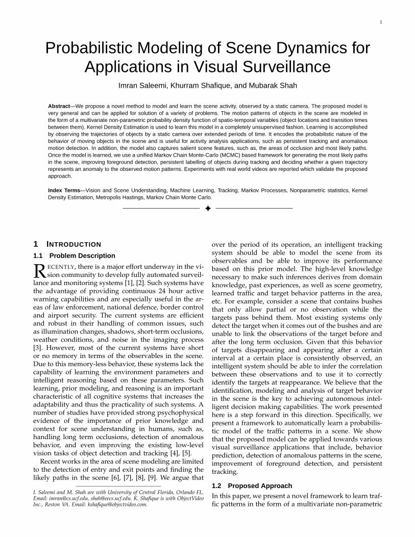
probability density function of spatio-temporal variablesthat include the locations of objects detected in thescene and their transition times from one location toanother. The model is learned in a fully unsupervisedfashion by observing the trajectories of objects by astatic camera over extended periods of time. The modelalso captures salient scene features, such as, the usuallyadapted paths, frequently visited areas, occlusion areas,entry/exit points, etc.

We learn the scene model by using the observationsof tracks over a long period of time. These tracks mayhave errors due to clutter and may also be brokendue to short term and long term occlusions, howeverby observing enough tracks, one can get a fairly goodunderstanding of the scene and infer above describedscene properties and salient features. We assume thatthe tracks of the moving objects are available for training(We use KNIGHT system for generating these tracks [3]).Two scenes and the observed tracks are shown in Fig. 1.We use these tracks in a training phase to discover thecorrelation in the observations by learning the motionpattern model in the form of a multivariate probabilitydensity function (pdf) of spatio-temporal parameters(i.e., the joint probability density of pairs of observationsof an object occurring within certain time intervals,(x, y, x′, y′, ∆t)). Instead of imposing assumptions aboutthe form of this pdf, we estimate the pdf using kerneldensity estimators. Each track on the image lattice canthen be seen as a random walk where the probabilities oftransition at each state of the walk is given by the learnedspatio-temporal kernel density estimate. Once the modelis learned, we use a unified Markov Chain Monte-Carlo(MCMC) sampling based scheme to generate the mostlikely paths in the scene, to decide whether a given pathis an anomaly to the learned model, and to estimatethe probability density of the next state of the randomwalk based on its previous states. The predictions basedon the model are then used to improve the detectionof foreground objects as well as to persistently tracktargets through short-term and long-term occlusions. Weshow quantitatively that the proposed system improvesboth the precision and recall of the foreground detectionand can handle long term occlusions that cannot behandled using constant dynamics models commonlyused in the literature. We also show that the proposedalgorithm can handle occlusions that were not observedduring training. The examples of these type of occlusionsinclude vehicles parked in the scene after training, or abug sitting on the camera lens.

2 RELATED WORK

Trajectory and path modeling is an important stepin various applications, many of which are crucial tosurveillance and monitoring systems. Such models canbe used to filter tracking algorithms, generate likelypaths, find locations of sources and sinks in the scene,and detect anomalous tracks, etc. This kind of modeling

(a) (b)

Fig. 1. Two scenes used for the testing of proposedframework, with some of the tracks observed by thetracker during training.

can be directly used as a feedback to the initial stagesof the tracking algorithm, and applied to solve shortand long term occlusions. In recent years, a number ofdifferent methods and features for trajectory and pathmodeling of traffic in the scene have been proposed.These methods differ by their choice of features, models,learning algorithms, applications, and training data. Adetailed review of these models is presented in [10]. Wenow describe some of these methods.

Neural Network based approaches for learning oftypical paths and trajectory modeling are proposed in[11], [12], [13]. Other than the computational complexityand lack of adaptability of Neural Networks, a majordisadvantage of these methods is their inability to handleincomplete and partial trajectories. Fernyhough et al.[14] use the spatial model presented in [15] as a basisfor a learning algorithm that can automatically learnobject paths by accumulating the traces of targets. Koller-Meier et al. [16] use a node-based model to representthe average of trajectory clusters. A similar technique issuggested by Lou et al. [17]. Although both methodssuccessfully identify the mean of common trajectorypatterns, no explicit information is derived regardingthe distribution of trajectories around the mean. A hi-erarchical clustering of trajectories is proposed in [18],[19], where trajectories are represented as a sequence ofstates in a quantized 6D space for trajectory classificationand the method is based on a co-occurrence matrix thatassumes that all trajectory sequences are equally long.However, this assumption is usually not true in realsequences.

Detection of sources and sinks in a scene as a pre-stepallows robust tracking. In [20], a Hidden Markov Modelbased scheme of learning sources and sinks is presented,where all sequences are two-state long. The knowledgeof sources and sinks is used to correct and stitch tracksin a closed-loop manner. Another HMM-based approachis to model trajectories as transitions between statesrepresenting Gaussian distributions on the 2D imageplane [21], [22]. Galata et al. [23] propose a mechanismthat automatically acquires stochastic models of anybehavior. Unlike HMMs, the proposed variable lengthmarkov model can capture dependencies that may havea variable time scale.

3

Another body of work for modeling motion patternsin a scene lies in the literature of multi-camera tracking[9], [24], [25], where the objective is to use these modelsto solve for hand-off between cameras. The motionpatterns are modeled only between the field of viewsof cameras. These models can be seen as special casesof the proposed model, which is richer in the sensethat it captures the motion pattern both in visible andoccluded regions. This richness of the proposed modelallows it to handle dynamic occlusions, such as person toperson occlusions as well as occlusions that occur afterthe model is learned. Tekalp[26] uses Bayesian networksfor tracking and occlusion reasoning across calibratedcameras with overlapping views, where sparse motionestimation and appearance are used as features. Tieu etal.[6] infer the topology of a network of non-overlappingcameras by computing the statistical dependence be-tween observations in different cameras.

Another interesting piece of work in this area is byEllis et al.[7] who determined the topology of a cam-era network by using a two stage algorithm. First theentry and exit zones of each camera are determinedusing an Expectation-Minimization technique to clusterthe start and end points of object tracks. The linksbetween these zones across cameras are then foundusing the co-occurrence of entry and exit events. Theproposed method assumes that correct correspondenceswill cluster in the feature space (location and time) whilethe wrong correspondences will generally be scatteredacross the feature space. Stauffer [8] proposes an im-proved linking method that tests the hypothesis that thecorrelation between exit and entry events is similar to theexpected correlation when there are no valid transitions.This allows the algorithm to handle the cases where exit-entrance events may be correlated, but the correlation isnot due to valid object transitions. Both of these methodsassume a fixed set of entry and exit locations afterinitial training and hence cannot deal with newly formedocclusions without retraining of the model.

Hoiem et. al. [27] take a step forward in image andscene understanding and proposed improvement in ob-ject recognition by modeling the correlation between ob-jects, surface geometry and camera viewpoints. Rosaleset al. [28] estimate motion trajectories using ExtendedKalman Filter to enable improved tracking before, dur-ing and after occlusions. Kaucic et al. [29] present a mod-ular framework that handles tracking through occlusionsand the blind regions between cameras by the initial-ization, tracking and linking of high-confidence smallertrack sections. Wang et al. [30] propose measures forsimilarity between tracks that take into account spatialdistribution, velocity, and object size. The trajectories arethen clustered based on object type and its spatial andvelocity distributions. Perera et. al. [31] present a methodto reliably link track segments during the linking stage.Splitting and merging of tracks is handled to achievemulti-object tracking through occlusion. Recently, Hu etal. [32] have presented an algorithm for learning motion

patterns where foreground pixels are first clustered us-ing fuzzy K-means algorithm and trajectories are thenhierarchically clustered based on the results of previousstep. Trajectory clustering is performed in two layersfor spatial and temporal based clustering. Each patternof clustered trajectories is then assumed to be a linkin a chain of gaussian distributions, the parameters forwhich are estimated using features of each clusteredtrajectory. Results of experiments on anomaly detectionand behavior prediction are reported.

As opposed to explicitly modeling trajectories orsmaller sections of trajectories of objects in the scene, wepropose modeling of joint distribution of initial and finallocations of every possible transition and the transitiontimes. Our approach is original in the following ways:• We propose a novel motion model that not only learns the

scene semantics but also the behavior of traffic througharbitrary paths. This learning is not limited like otherapproaches that work best with well defined paths likeroads and walkways.

• The learning is accomplished using a joint five dimen-sional model unlike pixel-wise models and mixture orchain models. The proposed model represents the jointprobability of a transition from any point in the imageto any other point, and the time taken to complete thattransition.

• The temporal dimension of traffic patterns is explicitlymodeled, and is included in the feature vector, thusenabling us to distinguish patterns of activity that cor-respond to the same trajectory cluster but have highdeviation in the temporal dimension. This is a moregeneralized method as compared to modeling pixel-wisevelocities.

• Instead of fitting parametric models to the data, wepropose the idea of learning tracks information usingKernel Density Estimation. It allows for a richer modeland the density retained at each point in the feature spaceaccurately reflects the training data.

• Rather than exhaustively searching for predictions in thefeature space based on their probabilities, we proposeto use stochastic methods to sample from the learneddistribution and use it as prediction with a computedprobability. Sampling is thus used as the process propa-gation function in our state estimation framework.

• Unlike most of the previous work reported in this section,which is targeted towards one or two similar applications,we apply the proposed probabilistic framework to solve avariety of problems that are commonly encountered insurveillance and scene analysis.

3 PROBABILISTIC TRAFFIC MODEL

We now propose a model that learns traffic patterns asjoint probability of the initial and final locations, andduration of object transitions and describe our methodof learning and sampling from the distribution. In thissection, we discuss the feature to be learned and explainhow it is computed. The sampling process and its use inthe state estimation framework is also explained.

4

3.1 Learning the Transition Distribution using KDE

We use the surveillance and monitoring system,KNIGHT[3] to collect tracking data. This data consistsof time stamps and object labels with locations of theircentroid for each frame of video. KNIGHT assigns aunique label to each object present in the scene andattempts to persistently track the object using a jointmotion and appearance model. A frame of video maycontain multiple objects. Given this data, we associate anobservation vector O(x, y, t, l) with each detected object.In this vector, x and y are the spatial coordinates of theobject centroid on image lattice, t is the time instant atwhich O is observed (accurate to a millisecond) and l isthe label for object in O as per tracking. We seek to builda five dimensional estimate of the transition probabilitydensity function p (X, Y, τ), where X and Y are the initialand final states representing the object centroid locationsin 2d image coordinates and τ is the time taken to makethe transition from X to Y in milliseconds.

In the proposed work, the analysis is performed on afeature space where the n transitions are represented byzi ∈ R5, i = 1, 2, . . . , n. The vector z consists of a pairof 2d locations of the centroid of object before and aftertransition, and time taken to execute the transition. Anytwo observations Oi and Oj in frames i and j respec-tively, comprise a feature point Z(xi, yi, xj , yj , tj− ti) forthe probability estimate if they satisfy the following:• 0 < tj − ti = τ < T , thus the implicit assumption

is that Oi and Oj are uncorrelated if occurringsimultaneously or beyond a time interval of T . Forour experiments, we chose T = 5000ms.

• li = lj , both Oi and Oj are the observations of thesame object as per the tracker’s labelling.

• If lj /∈ Lk, where Lk is the set of all objects (labels) inframe k, then all labels in frame k make valid datapoints with lj provided 0 < τ < T .

Kernel Density Estimation ([33], [34]) is used to esti-mate the pdf p (X,Y, τ) non-parametrically. Suppose wehave a sample consisting of n, d dimensional, data pointsz1, z2, . . . , zn from a multi-variate distribution p(z) , thenan estimate p(z) of the density at z can be computedusing

p(z) =1n|H|− 1

2

n∑

i=1

K(H− 12 (z− zi)), (1)

where the d variate kernel K(z) is a bounded functionsatisfying

∫K(z)dz = 1, K(z) = K(-z),

∫zK(z)dz = 0,∫

zzTK(z)dz = Id and H is the symmetric positivedefinite d×d bandwidth matrix. The multivariate kernelK(z) can be generated from a product of symmetricunivariate kernel Ku, i.e.,

K(z) =d∏

j=1

Ku(zj). (2)

The selection of the kernel bandwidth H is the singlemost important criterion in kernel density estimation.Asymptotically, the selected bandwidth H does not affect

the estimate but in practice sample sizes are limited.Theoretically, the ideal or optimal H that balances thebias and variance globally can be computed by minimiz-ing the mean-squared error, MSEpH(z) = E[pH(z)−pH(z)]2, where p is the estimated density, p is the truedensity, and the subscript H indicates the use of thebandwidth H in computing the density. However, thetrue density p is not known in practice. Instead, variousheuristic approaches have been proposed for finding H(See [35] for a survey of these approaches). We use theRule of Thumb method [36], which is a fast standarddeviation based method that uses the Asymptotic MeanIntegrated Squared error (AMISE) criterion,

AMISEH =1n

R(K)|H|− 12 +

∫

R5[(KH∗p)(z)−p(z)]2dz,

(3)where R(K) =

∫R5 K(z)2dz and ∗ is the convolution

operator. The data-driven bandwidth selector is then,H = arg minH

AMISEH. To reduce the complex-ity, H is assumed to be a diagonal matrix, i.e., H =diag[h2

1, h22, . . . , h

2d]. We use a product of univariate Gaus-

sian kernels to generate K(z), i.e.,

Ku(zj) =1

hj

√2π

exp

(−

z2j

2hj2

), (4)

where, hj is the jth non-zero element of H, and Ku

is centered at zj. It is emphasized here, that using aGaussian kernel does not make any assumption on thescatter of data in the feature space. The kernel functiononly defines the effective region in 5d space in whicheach data point will have an influence while computingthe probability estimate. Each time a pair of observationssatisfying the described criteria are available duringtraining, the observed feature z is added to the sample.p(X,Y, τ) then gives the probability of a transition frompoint X to point Y in τ milliseconds.

50 100 150 200 250 300 350

50

100

150

200

50 100 150 200 250 300 350

50

100

150

200

(a) (b) (c) (d)

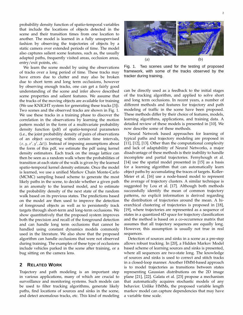
Fig. 2. These maps represent the marginal probabilityof any object, (a) reaching each point in the image, and(b) starting from each point in the image, in any arbitraryduration of time for the scene in Fig. 1a. (c) and (d) showsimilar maps for the scene in Fig. 1b.

Fig. 2 illustrates the maps of p(X, Y, τ) marginalizedover 2d vectors X and Y , i.e., Fig. 2a represents theprobability of an object reaching a point in the map from

any location, i.e.,∫

X

∫

τ

p(X, Y, τ) dτdX . It is important

to note that the areas with higher densities (brightercolors) cannot be labelled as entry or exit points. Theintensity at a point in the image only illustrates the

5

marginal probability that an observed state transitionhas, of starting or ending at that point. The dominantpoints in the maps only mean that a higher numberof object observations were made at these points. Forexample, in practice, this could possibly mean that theseareas are places where people stand or sit while ex-hibiting nominal motion but significant enough to benoticed by the tracker. Similarly, each point in Fig. 2brepresents the probability of an object starting from thatparticular point and ending anywhere in the image,

i.e.,∫

Y

∫

τ

p(X, Y, τ) dτdY . Notice that the similarity in

the two maps manifests a correlation between incomingand outgoing object transitions at the same locations. Itshould also be pointed out that since p(X,Y, τ) is a highdimensional space, the probabilities from a particularlocation to another location in a specific interval can bevery low and a high dynamic range is required to displaythese maps correctly. So the dark blue regions in thesemaps are not necessarily absolutely zero. Many darkblue regions in these maps will have relatively higherprobabilities of transition, if the pdf is marginalized overspecific time intervals or a specific starting or endingpoint, as discussed later. Figures 2c and 2d show similarmaps for the scene in Figure 1b.

The probability density function p(X, Y, τ) now repre-sents the distribution of transitions from any point X inthe scene to any other point Y given the time taken tocomplete the transition as τ . Our next step is to be ableto predict the next state of an object, given the currentstate and an approximate time duration of the jump. Thisis achieved by sampling the marginal of this distributionfunction as described in the following subsection.

3.2 Construction of Predicted Trajectories

The learned model can be used to find a likely next stategiven the current state of an object. The motivation isthat we want to construct a likely trajectory from thecurrent object position onwards, which would act asthe predicted behavior of the object. Instead of findingthe probabilities of transitions to different locations, weuse the learned distribution as a generative model andsample feature points from the model to construct asequence of tracks based on the training observations.

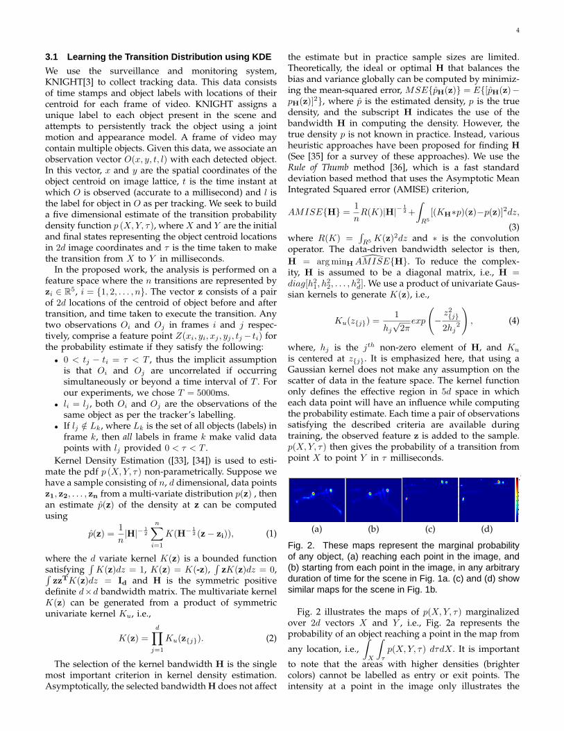
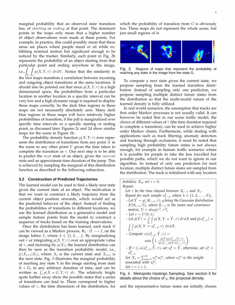
Once the distribution has been learned, each track Ωcan be viewed as a Markov process, Ψk : Ω −→ I , on theimage lattice I , where k ∈ 1, 2, . . .. By marginalizingout τ or integrating p(X, Y, τ) over an appropriate valueof τ , and factoring by p(X), the learned distribution canthen be seen as the transition probability model, i.e.,p (Xt+1|Xt), where Xt is the current state and Xt+1 isthe next state. Fig. 3 illustrates the marginal probabilityof reaching any state Y in the image starting from stateX = G, in any arbitrary duration of time, and can bewritten as

∫τ

p(X = G,Y, τ) dτ . The relatively brightspots further away show the possible states that a seriesof transitions can lead to. These correspond to highervalues of τ , the time dimension of the distribution, for

which the probability of transition from G is obviouslylow. These maps do not represent the whole scene, butjust small regions of it.

Fig. 3. Regions of maps that represent the probability ofreaching any state in the image from the state G.

To compute a next state given the current state, wepropose sampling from the learned transition distri-bution. Instead of sampling only one prediction, wepropose sampling multiple distinct future states fromthe distribution so that the multi-modal nature of thelearned density is fully utilized.

In real world scenarios, the assumption that tracks arefirst order Markov processes is not usually valid. It canhowever be noted that in our scene traffic model, thechoice of different values of τ (the time duration requiredto complete a transition), can be used to achieve higherorder Markov chains. Furthermore, while dealing withapplications such as track filtering, anomaly detectionand tracking through occlusions, it must be noted thatsampling high probability future states is not alwaysenough, for example in human traffic scenarios whereit is possible for people to take the less travelled butpossible paths, which we do not want to ignore in ouralgorithm. So instead of only one prediction for nextlocation, multiple distinct future states are sampled fromthe distribution. The track is initialized with any location

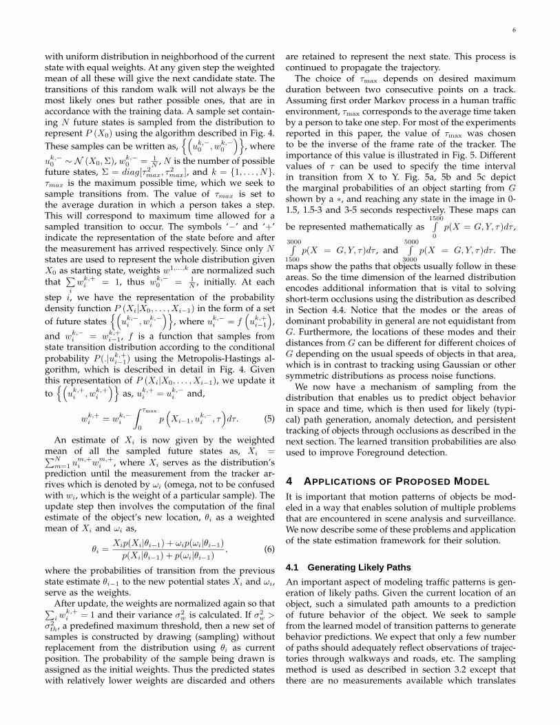
Initialize X0; set i = 0.Repeat,

Let τ be the time elapsed between Xi−1 and Xi.Repeat for each sample uk

i−1, where k ∈ 1, 2, . . . , N,- Let Y ∼ q(.|θi−1, τ), q being the Gaussian distributionN (θi−1, Σ), where θi−1 is the mean and covariancematrix, Σ = diag[τ2, τ2].

- Let r ∼ U(0, 1).- Let p(Y ) =

∫X

∫τ

p(X, Y = Y , τ) dτdX and p(uki−1) =

∫X

∫τ

p(X,Y = uki−1, τ) dτdX .

- Compute α(uki−1, Y , τ) =

min(

1,p(Y )q(uk

i−1|Y ,τ)

p(uki−1)q(Y |uk

i−1,τ)

).

- If r ≤ α(uki−1, Y , τ), set uk

i = Y , otherwise, set uki =

uki−1.

Set Xi =∑N

m=1 umi wm

i , where wmi is the weight

associated with umi .

Set i = i + 1.

Fig. 4. Metropolis Hastings Sampling. See section 6 fordetails about the choice of q, the proposal density.

and the representative future states are initially chosen

6

with uniform distribution in neighborhood of the currentstate with equal weights. At any given step the weightedmean of all these will give the next candidate state. Thetransitions of this random walk will not always be themost likely ones but rather possible ones, that are inaccordance with the training data. A sample set contain-ing N future states is sampled from the distribution torepresent P (X0) using the algorithm described in Fig. 4.These samples can be written as,

(uk,−

0 , wk,−0

), where

uk,−0 ∼ N (X0, Σ), wk,−

0 = 1N , N is the number of possible

future states, Σ = diag[τ2max, τ2

max], and k = 1, . . . , N.τmax is the maximum possible time, which we seek tosample transitions from. The value of τmax is set tothe average duration in which a person takes a step.This will correspond to maximum time allowed for asampled transition to occur. The symbols ‘−’ and ‘+’indicate the representation of the state before and afterthe measurement has arrived respectively. Since only Nstates are used to represent the whole distribution givenX0 as starting state, weights w1,...,k are normalized suchthat

∑i

wk,+i = 1, thus wk,−

0 = 1N , initially. At each

step i, we have the representation of the probabilitydensity function P (Xi|X0, . . . , Xi−1) in the form of a setof future states

(uk,−

i , wk,−i

), where uk,−

i = f(uk,+

i−1

),

and wk,−i = wk,+

i−1, f is a function that samples fromstate transition distribution according to the conditionalprobability P (.|uk,+

i−1) using the Metropolis-Hastings al-gorithm, which is described in detail in Fig. 4. Giventhis representation of P (Xi|X0, . . . , Xi−1), we update itto

(uk,+

i , wk,+i

)as, uk,+

i = uk,−i and,

wk,+i = wk,−

i

∫ τmax

0

p(Xi−1, u

k,−i , τ

)dτ. (5)

An estimate of Xi is now given by the weightedmean of all the sampled future states as, Xi =∑N

m=1 um,+i wm,+

i , where Xi serves as the distribution’sprediction until the measurement from the tracker ar-rives which is denoted by ωi (omega, not to be confusedwith wi, which is the weight of a particular sample). Theupdate step then involves the computation of the finalestimate of the object’s new location, θi as a weightedmean of Xi and ωi as,

θi =Xip(Xi|θi−1) + ωip(ωi|θi−1)

p(Xi|θi−1) + p(ωi|θi−1), (6)

where the probabilities of transition from the previousstate estimate θi−1 to the new potential states Xi and ωi,serve as the weights.

After update, the weights are normalized again so that∑i wk,+

i = 1 and their variance σ2w is calculated. If σ2

w >σ2

th, a predefined maximum threshold, then a new set ofsamples is constructed by drawing (sampling) withoutreplacement from the distribution using θi as currentposition. The probability of the sample being drawn isassigned as the initial weights. Thus the predicted stateswith relatively lower weights are discarded and others

are retained to represent the next state. This process iscontinued to propagate the trajectory.

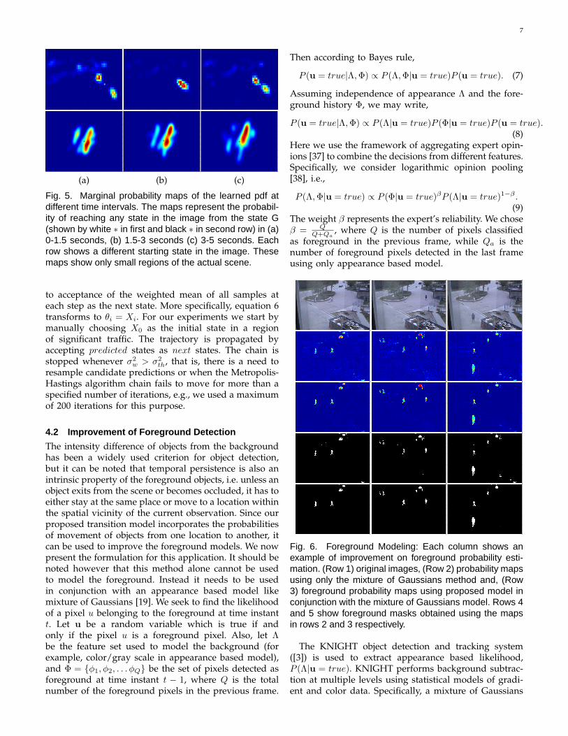
The choice of τmax depends on desired maximumduration between two consecutive points on a track.Assuming first order Markov process in a human trafficenvironment, τmax corresponds to the average time takenby a person to take one step. For most of the experimentsreported in this paper, the value of τmax was chosento be the inverse of the frame rate of the tracker. Theimportance of this value is illustrated in Fig. 5. Differentvalues of τ can be used to specify the time intervalin transition from X to Y. Fig. 5a, 5b and 5c depictthe marginal probabilities of an object starting from Gshown by a ∗, and reaching any state in the image in 0-1.5, 1.5-3 and 3-5 seconds respectively. These maps can

be represented mathematically as1500∫0

p(X = G,Y, τ)dτ ,

3000∫1500

p(X = G, Y, τ)dτ , and5000∫3000

p(X = G, Y, τ)dτ . The

maps show the paths that objects usually follow in theseareas. So the time dimension of the learned distributionencodes additional information that is vital to solvingshort-term occlusions using the distribution as describedin Section 4.4. Notice that the modes or the areas ofdominant probability in general are not equidistant fromG. Furthermore, the locations of these modes and theirdistances from G can be different for different choices ofG depending on the usual speeds of objects in that area,which is in contrast to tracking using Gaussian or othersymmetric distributions as process noise functions.

We now have a mechanism of sampling from thedistribution that enables us to predict object behaviorin space and time, which is then used for likely (typi-cal) path generation, anomaly detection, and persistenttracking of objects through occlusions as described in thenext section. The learned transition probabilities are alsoused to improve Foreground detection.

4 APPLICATIONS OF PROPOSED MODEL

It is important that motion patterns of objects be mod-eled in a way that enables solution of multiple problemsthat are encountered in scene analysis and surveillance.We now describe some of these problems and applicationof the state estimation framework for their solution.

4.1 Generating Likely Paths

An important aspect of modeling traffic patterns is gen-eration of likely paths. Given the current location of anobject, such a simulated path amounts to a predictionof future behavior of the object. We seek to samplefrom the learned model of transition patterns to generatebehavior predictions. We expect that only a few numberof paths should adequately reflect observations of trajec-tories through walkways and roads, etc. The samplingmethod is used as described in section 3.2 except thatthere are no measurements available which translates

7

180 200 220 240 260 280 300

100

110

120

130

140

150

160

170

180

190

160 180 200 220 240 260 280 300

100

110

120

130

140

150

160

170

180

190

180 200 220 240 260 280 300

100

110

120

130

140

150

160

170

180

190

(a) (b) (c)

Fig. 5. Marginal probability maps of the learned pdf atdifferent time intervals. The maps represent the probabil-ity of reaching any state in the image from the state G(shown by white ∗ in first and black ∗ in second row) in (a)0-1.5 seconds, (b) 1.5-3 seconds (c) 3-5 seconds. Eachrow shows a different starting state in the image. Thesemaps show only small regions of the actual scene.

to acceptance of the weighted mean of all samples ateach step as the next state. More specifically, equation 6transforms to θi = Xi. For our experiments we start bymanually choosing X0 as the initial state in a regionof significant traffic. The trajectory is propagated byaccepting predicted states as next states. The chain isstopped whenever σ2

w > σ2th, that is, there is a need to

resample candidate predictions or when the Metropolis-Hastings algorithm chain fails to move for more than aspecified number of iterations, e.g., we used a maximumof 200 iterations for this purpose.

4.2 Improvement of Foreground Detection

The intensity difference of objects from the backgroundhas been a widely used criterion for object detection,but it can be noted that temporal persistence is also anintrinsic property of the foreground objects, i.e. unless anobject exits from the scene or becomes occluded, it has toeither stay at the same place or move to a location withinthe spatial vicinity of the current observation. Since ourproposed transition model incorporates the probabilitiesof movement of objects from one location to another, itcan be used to improve the foreground models. We nowpresent the formulation for this application. It should benoted however that this method alone cannot be usedto model the foreground. Instead it needs to be usedin conjunction with an appearance based model likemixture of Gaussians [19]. We seek to find the likelihoodof a pixel u belonging to the foreground at time instantt. Let u be a random variable which is true if andonly if the pixel u is a foreground pixel. Also, let Λbe the feature set used to model the background (forexample, color/gray scale in appearance based model),and Φ = φ1, φ2, . . . φQ be the set of pixels detected asforeground at time instant t − 1, where Q is the totalnumber of the foreground pixels in the previous frame.

Then according to Bayes rule,

P (u = true|Λ, Φ) ∝ P (Λ, Φ|u = true)P (u = true). (7)

Assuming independence of appearance Λ and the fore-ground history Φ, we may write,

P (u = true|Λ, Φ) ∝ P (Λ|u = true)P (Φ|u = true)P (u = true).(8)

Here we use the framework of aggregating expert opin-ions [37] to combine the decisions from different features.Specifically, we consider logarithmic opinion pooling[38], i.e.,

P (Λ, Φ|u = true) ∝ P (Φ|u = true)βP (Λ|u = true)1−β .(9)

The weight β represents the expert’s reliability. We choseβ = Q

Q+Qa, where Q is the number of pixels classified

as foreground in the previous frame, while Qa is thenumber of foreground pixels detected in the last frameusing only appearance based model.

50 100 150 200 250 300 350

0

50

100

150

200

250

50 100 150 200 250 300 350

0

50

100

150

200

250

50 100 150 200 250 300 350

0

50

100

150

200

250

50 100 150 200 250 300 350

0

50

100

150

200

250

50 100 150 200 250 300 350

0

50

100

150

200

250

50 100 150 200 250 300 350

0

50

100

150

200

250

50 100 150 200 250 300 350

0

50

100

150

200

250

50 100 150 200 250 300 350

0

50

100

150

200

250

50 100 150 200 250 300 350

0

50

100

150

200

250

50 100 150 200 250 300 350

0

50

100

150

200

250

50 100 150 200 250 300 350

0

50

100

150

200

250

50 100 150 200 250 300 350

0

50

100

150

200

250

50 100 150 200 250 300 350

0

50

100

150

200

250

50 100 150 200 250 300 350

0

50

100

150

200

250

50 100 150 200 250 300 350

0

50

100

150

200

250

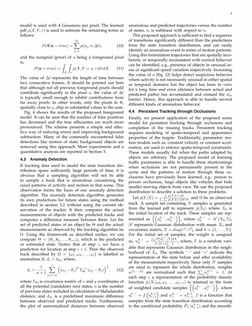
Fig. 6. Foreground Modeling: Each column shows anexample of improvement on foreground probability esti-mation. (Row 1) original images, (Row 2) probability mapsusing only the mixture of Gaussians method and, (Row3) foreground probability maps using proposed model inconjunction with the mixture of Gaussians model. Rows 4and 5 show foreground masks obtained using the mapsin rows 2 and 3 respectively.

The KNIGHT object detection and tracking system([3]) is used to extract appearance based likelihood,P (Λ|u = true). KNIGHT performs background subtrac-tion at multiple levels using statistical models of gradi-ent and color data. Specifically, a mixture of Gaussians

8

model is used with 4 Gaussians per pixel. The learnedpdf p(X, Y, τ) is used to estimate the remaining terms asfollows:

P (Φ|u = true) =Q∑

j=1

p(φj , u, ∆t), (10)

and the marginal (prior) of u being a foreground pixelis,

P (u = true) =∫

X

∫

τ

p(X, Y = u, τ)dτdX. (11)

The value of ∆t represents the length of time betweentwo consecutive frames. It should be pointed out herethat although not all previous foreground pixels shouldcontribute significantly to the pixel u, the value of ∆tis typically small enough to inhibit contributions fromfar away pixels. In other words, only the pixels in Φ,spatially close to u, chip in substantial values to the sum.

Fig. 6 shows the results of the proposed foregroundmodel. It can be seen that the number of false positiveshas decreased and the true silhouettes are much morepronounced. The scheme presents a simple and effec-tive way of reducing errors and improving backgroundsubtraction. Many of the commonly encountered falsedetections like motion of static background objects areremoved using this approach. More experiments and aquantitative analysis are reported in Section 5.

4.3 Anomaly Detection

If tracking data used to model the state transition dis-tribution spans sufficiently large periods of time, it isobvious that a sampling algorithm will not be ableto sample a track that is anomalous considering theusual patterns of activity and motion in that scene. Thisobservation forms the basis of our anomaly detectionalgorithm. The anomaly detection algorithm generatesits own predictions for future states using the methoddescribed in section 3.2 without using the current ob-servation of the tracker. It then compares the actualmeasurements of objects with the predicted tracks andcomputes a difference measure between them. Let theset of predicted states of an object be Θ and the actualmeasurements as observed by the tracking algorithm beΩ. Using the framework as described earlier, we cancompute Θ = θ1, θ2, . . . , θi+1, which is the predictedor estimated state. Notice that at step i, we have aprediction for location at step i + 1. Then the observedtrack described by Ω = ω1, ω2, . . . , ωi is labelled asanomalous if, di > dth, where,

di =1

n + 1

i∑

j=i−n

((ωj − θj)

T Σ−1Θ (ωj − θj)

) 12, (12)

where ΣΘ is covariance matrix of x and y coordinates ofall the potential (candidate) next states, n is the numberof previous states included in calculation of Mahalanobisdistance, and dth is a predefined maximum differencebetween observed and predicted tracks. Furthermore,the plot of unnormalized distances between observed

anomalous and predicted trajectories versus the numberof states, n, is sublinear with respect to n.

This proposed approach is sufficient to find a sequenceof transitions significantly different than the predictionsfrom the state transition distribution, and can easilyidentify an anomalous event in terms of motion patterns.Using this formulation trajectories that are spatially inco-herent, or temporally inconsistent with normal behaviorcan be identified, e.g., presence of objects in unusual ar-eas or significant speed variation respectively. Increasingthe value of n (Eq. 12) helps detect suspicious behaviorwhere activity is not necessarily unusual in either spatialor temporal domains but the object has been in viewfor a long time and error (distance between actual andpredicted paths) has accumulated and crossed the dth

barrier. Hence, this approach is able to handle severaldifferent kinds of anomalous behavior.

4.4 Persistent Tracking through Occlusions

Finally, we present application of the proposed scenemodel for persistent tracking through occlusions andcompletion of the missing tracks. Persistent trackingrequires modeling of spatio-temporal and appearanceproperties of the targets. Traditionally, parametric mo-tion models such as, constant velocity or constant accel-eration, are used to enforce spatio-temporal constraints.These models usually fail when the paths adapted byobjects are arbitrary. The proposed model of learningtraffic parameters is able to handle these shortcomingswhen occlusions are not permanently present in thescene and the patterns of motion through these oc-clusions have previously been learned, e.g., person toperson occlusions, large objects like vehicles that hidesmaller moving objects from view. We use the proposeddistribution to describe a solution to these problems.

Let p(Y |X) =∫

τp(X,Y,τ)dτ∫

τ

∫Y

p(X,Y,τ)dY dτand Ω be an observed

track. A sample set containing N samples is generatedfrom the learned pdf to represent p(X0) where X0 isthe initial location of the track. These samples are rep-resented as

(uk,−

0 , wk,−0

), where uk,−

0 ∼ N (X0, Σ),N represents Gaussian distribution with mean X0 andcovariance matrix, Σ = diag[τ2, τ2], and k = 1, . . . , N.For the initial set of samples, the weight is assigned

as, wk,−0 =

∫X

P(uk,−0 |X)dX

Pγ(Γ=uk,−0 ) , where, Γ is a random vari-

able that represents Gaussian distribution in the neigh-borhood of X0. The symbols ‘−’ and ‘+’ indicate therepresentation of the state before and after availabilityof the measurement respectively. Since only N samplesare used to represent the whole distribution, weightsw1,...,k are normalized such that

∑i wk,+

i = 1. Ateach step i, a representation of the probability densityfunction p (Xi|ω0, ω1, . . . , ωi−1) is retained in the formof weighted candidate samples

(uk,−

i , wk,−i

), where

uk,−i = f

(uk,+

i−1

)and wk,−

i = wk,+i−1. f is a function that

samples from the state transition distribution accordingto the conditional probability P (.|uk,+

i−1) and the smooth-

9

ness of motion constraint using the Metropolis-Hastingsalgorithm, which is described in detail in Fig. 4.

At any time, we want to be able to find correspon-dences between successive instances of objects. This taskproves to be very difficult when the color and shapedistributions of objects are very similar or when theobjects are in very close proximity of each other, includ-ing in person to person occlusion scenarios. However,in the proposed model, a hierarchical use of transitiondensity enables our scheme to assign larger weightsto more likely paths. Assume now that the observedmeasurements of m objects at time instant i are givenby Ω =

ω1

i , ω2i , . . . , ωm

i

, and the predicted states of

previously observed s objects are Θ =θ1

i , θ2i , . . . , θs

i

respectively. We must find the mapping function fromthe set Ωk

i , 1 ≤ k ≤ m to the set Θli, 1 ≤ l ≤ s. To

establish this mapping function, we use the graph basedalgorithm proposed in [39]. The weights of the edgescorresponding to the mapping Θl

i and Ωki are given by

the Mahalanobis distance between the estimated posi-tion θl

i and the observed position ωki , for each l and

k. Once the correspondences are established, for eachobject, given the representation of p (θi|θ0, . . . , θi−1), andthe corresponding new observation ωi, we update it to(

uk,+i , wk,+

i

)as uk,+

i = uk,−i and,

wk,+i = wk,−

i

N∑

k=1

P(ωi|uk,−

i

)=

i∏

j=0

N∑

k=1

P(ωj |uk,−

j

).

(13)The product of old weight with the sum of probabilitiesof reaching ωi from each sample state uk,−

i for all k,translates into a product of transition probabilities for alljumps taken by an object. This results into assignmentof larger weights for higher probability tracks and inthe next time step, this weight helps establish corre-spondences such that the probability of an object’s trackis maximized. Once updated, candidate locations arere-sampled as described in section 3.2. This approachenables simultaneous solution of short-term, and personto person occlusions, as well as persistent labeling.

5 RESULTS

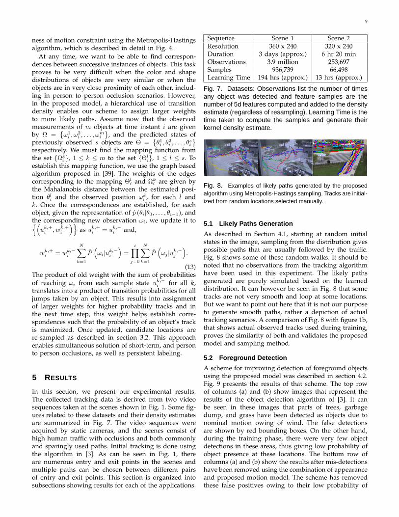
In this section, we present our experimental results.The collected tracking data is derived from two videosequences taken at the scenes shown in Fig. 1. Some fig-ures related to these datasets and their density estimatesare summarized in Fig. 7. The video sequences wereacquired by static cameras, and the scenes consist ofhigh human traffic with occlusions and both commonlyand sparingly used paths. Initial tracking is done usingthe algorithm in [3]. As can be seen in Fig. 1, thereare numerous entry and exit points in the scenes andmultiple paths can be chosen between different pairsof entry and exit points. This section is organized intosubsections showing results for each of the applications.

Sequence Scene 1 Scene 2Resolution 360 x 240 320 x 240Duration 3 days (approx.) 6 hr 20 minObservations 3.9 million 253,697Samples 936,739 66,498Learning Time 194 hrs (approx.) 13 hrs (approx.)

Fig. 7. Datasets: Observations list the number of timesany object was detected and feature samples are thenumber of 5d features computed and added to the densityestimate (regardless of resampling). Learning Time is thetime taken to compute the samples and generate theirkernel density estimate.

Fig. 8. Examples of likely paths generated by the proposedalgorithm using Metropolis-Hastings sampling. Tracks are initial-ized from random locations selected manually.

5.1 Likely Paths Generation

As described in Section 4.1, starting at random initialstates in the image, sampling from the distribution givespossible paths that are usually followed by the traffic.Fig. 8 shows some of these random walks. It should benoted that no observations from the tracking algorithmhave been used in this experiment. The likely pathsgenerated are purely simulated based on the learneddistribution. It can however be seen in Fig. 8 that sometracks are not very smooth and loop at some locations.But we want to point out here that it is not our purposeto generate smooth paths, rather a depiction of actualtracking scenarios. A comparison of Fig. 8 with figure 1b,that shows actual observed tracks used during training,proves the similarity of both and validates the proposedmodel and sampling method.

5.2 Foreground Detection

A scheme for improving detection of foreground objectsusing the proposed model was described in section 4.2.Fig. 9 presents the results of that scheme. The top rowof columns (a) and (b) show images that represent theresults of the object detection algorithm of [3]. It canbe seen in these images that parts of trees, garbagedump, and grass have been detected as objects due tonominal motion owing of wind. The false detectionsare shown by red bounding boxes. On the other hand,during the training phase, there were very few objectdetections in these areas, thus giving low probability ofobject presence at these locations. The bottom row ofcolumns (a) and (b) show the results after mis-detectionshave been removed using the combination of appearanceand proposed motion model. The scheme has removedthese false positives owing to their low probability of

10

(a) (b) (c) (d)

Fig. 9. Foreground Modeling Results: Columns (a) and(b) show results of object detection . The images in toprow are without and bottom row are with using the pro-posed model. Green and red bounding boxes show trueand false detections respectively. (c) and (d) show resultsof blob tracking. Red tracks are original broken tracks andblack ones are after improved foreground modeling.

transition or existence or both. Columns (c) and (d) showtracks from the tracking algorithm of [3] which are bro-ken in different places because of a significant numberof false negatives in foreground detection. Again thesemissed detections were corrected after incorporating themotion based foreground model.

0 100 200 300 400 5000

200

400

600

800

1000

1200

1400

1600

1800

2000

Frame Number

Num

ber

of F

oreg

roun

d P

ixel

s

Ground Truth

Mixture of Gaussians

Proposed Method

0 100 200 300 400 5000

0.1

0.2

0.3

0.4

0.5

0.6

0.7

0.8

0.9

1

Frame Number

Pre

cisi

on

Proposed Method

Mixture of Gaussians

0 100 200 300 400 5000

0.1

0.2

0.3

0.4

0.5

0.6

0.7

0.8

0.9

1

Frame Number

Rec

all

Proposed Method

Mixture of Gaussians

(a) (b) (c)

Fig. 10. Foreground Modeling Results: (a) Number offoreground pixels detected by the mixture of Gaussiansmethod, the logarithmic pooling method, and the groundtruth. The pixel-level foreground detection recall and pre-cision using the mixture of Gaussians approach only,and the proposed formulation are shown in (b) and (c)respectively.

For a quantitative analysis of the foreground modelingscheme, we manually segmented a 500 frames videosequence into foreground and background regions. Thefirst 200 frames were used to initialize the mixture ofGaussians based background model. Foreground wasestimated on the rest of the frames using, i) mixtureof Gaussians model, and ii) the proposed logarithmicpooling of appearance and motion models. Pixel levelprecision and recall were computed for both cases. Theresults of this experiment are shown in Fig. 10. It canbe seen from the plots that both the precision andrecall of the combined model are consistently better thanmixture of Gaussians approach alone. The number offalse positives for the combined model was reduced by79.65% on average. The average reduction in the numberof false negatives was 58.27%.

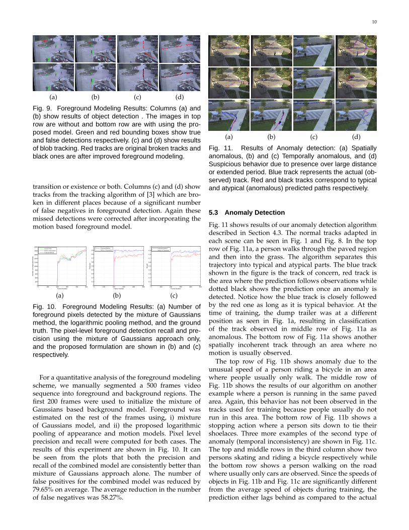
(a) (b) (c) (d)

Fig. 11. Results of Anomaly detection: (a) Spatiallyanomalous, (b) and (c) Temporally anomalous, and (d)Suspicious behavior due to presence over large distanceor extended period. Blue track represents the actual (ob-served) track. Red and black tracks correspond to typicaland atypical (anomalous) predicted paths respectively.

5.3 Anomaly Detection

Fig. 11 shows results of our anomaly detection algorithmdescribed in Section 4.3. The normal tracks adapted ineach scene can be seen in Fig. 1 and Fig. 8. In the toprow of Fig. 11a, a person walks through the paved regionand then into the grass. The algorithm separates thistrajectory into typical and atypical parts. The blue trackshown in the figure is the track of concern, red track isthe area where the prediction follows observations whiledotted black shows the prediction once an anomaly isdetected. Notice how the blue track is closely followedby the red one as long as it is typical behavior. At thetime of training, the dump trailer was at a differentposition as seen in Fig. 1a, resulting in classificationof the track observed in middle row of Fig. 11a asanomalous. The bottom row of Fig. 11a shows anotherspatially incoherent track through an area where nomotion is usually observed.

The top row of Fig. 11b shows anomaly due to theunusual speed of a person riding a bicycle in an areawhere people usually only walk. The middle row ofFig. 11b shows the results of our algorithm on anotherexample where a person is running in the same pavedarea. Again, this behavior has not been observed in thetracks used for training because people usually do notrun in this area. The bottom row of Fig. 11b shows astopping action where a person sits down to tie theirshoelaces. Three more examples of the second type ofanomaly (temporal inconsistency) are shown in Fig. 11c.The top and middle rows in the third column show twopersons skating and riding a bicycle respectively whilethe bottom row shows a person walking on the roadwhere usually only cars are observed. Since the speeds ofobjects in Fig. 11b and Fig. 11c are significantly differentfrom the average speed of objects during training, theprediction either lags behind as compared to the actual

11

measurements from the tracker, or hurries ahead result-ing in the observed trajectory being labelled anomalous.

Three examples of the third type of anomalies areshown in Fig. 11d. In the top row of Fig. 11d a personis walking slowly in a circular path for a few minutes.The motion pattern itself is not anomalous to the learneddistribution, but the presence of the object in the scenefor a relatively longer period of time results in accumu-lation of error, calculated as di using larger values ofn in Eq. 12, and eventually becomes greater than dth

resulting in classification of the sequence as an anomaly.The middle row of Fig. 11d shows a person jumpingover an area which people usually only sit on. Eventhough the person is not present in the scene for verylong, the error di quickly becomes significant due tothe incoherence of his actions relative to the trainingexamples. The bottom row shows a a zigzag pattern ofwalking, something not observed before, resulting in theclassification of the trajectory as anomalous.

Since the decision as to whether a given trajectoryis anomalous is subjective and differs from one ob-server to another, we asked three human observers toclassify 19 sequences as either normal or anomalous.The proposed method of anomaly detection was runon these 19 sequences which labelled 14 of them asanomalous. The quantitative results of these experimentsare summarized in Fig. 12.

Ground Truth Human 1 Human 2 Human 3Anomalous 13 15 11Normal 6 4 8Precision 92.86 100 78.57Recall 100 93.34 100

Fig. 12. Quantitative analysis of anomaly detection re-sults using classification by 3 human observers as theground truth.

5.4 Persistent Tracking

(a) (b) (c)

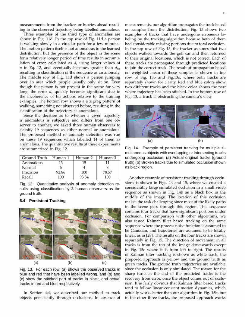
Fig. 13. For each row, (a) shows the observed tracks inblue and red that have been labelled wrong, and (b) and(c) show the stitched part of tracks in black, and actualtracks in red and blue respectively.

In Section 4.4, we described our method to trackobjects persistently through occlusions. In absence of

measurements, our algorithm propagates the track basedon samples from the distribution. Fig. 13 shows twoexamples of tracks that have undergone erroneous la-beling by the tracking algorithm because both of themhad considerable missing portions due to total occlusion.In the top row of Fig. 13, the tracker assumes that twoobjects walked towards the golf car and then returnedto their original locations, which is not correct. Each ofthese tracks are propagated through predicted locationsto join the correct track. The result of propagation basedon weighted mean of these samples is shown in toprow of Fig. 13b and Fig.13c, where both tracks areseparately shown for clarity. Red and blue colors showtwo different tracks and the black color shows the partwhere trajectory has been stitched. In the bottom row ofFig. 13, a truck is obstructing the camera’s view.

50 100 150 200 250 300 350

0

50

100

150

200

250

50 100 150 200 250 300 350

0

50

100

150

200

250

(a) (b)

Fig. 14. Example of persistent tracking for multiple si-multaneous objects with overlapping or intersecting tracksundergoing occlusion. (a) Actual original tracks (groundtruth) (b) Broken tracks due to simulated occlusion shownas black region.

Another example of persistent tracking through occlu-sions is shown in Figs. 14 and 15, where we created aconsiderably large simulated occlusion in a small videosequence as shown in Fig. 14b as a black box in themiddle of the image. The location of this occlusionmakes the task challenging since most of the likely pathsin the scene pass through this region. This sequencecontains four tracks that have significant portions underocclusion. For comparison with other algorithms, wealso tested Kalman filter based tracking on the samesequence where the process noise function is assumed tobe Gaussian, and trajectories are assumed to be locallylinear, as in [28]. The results on the four tracks are shownseparately in Fig. 15. The direction of movement in alltracks is from the top of the image downwards exceptin Fig. 15c where it is from left to right. The resultsof Kalman filter tracking is shown as white track, theproposed approach as yellow and the ground truth asgreen tracks. The ground truth trajectories are availablesince the occlusion is only simulated. The reason for thesharp turns at the end of the predicted tracks is therecovery from error, once the object comes out of occlu-sion. It is fairly obvious that Kalman filter based trackstend to follow linear constant motion dynamics, whichactually works better than our algorithm in Fig. 15b, butin the other three tracks, the proposed approach works

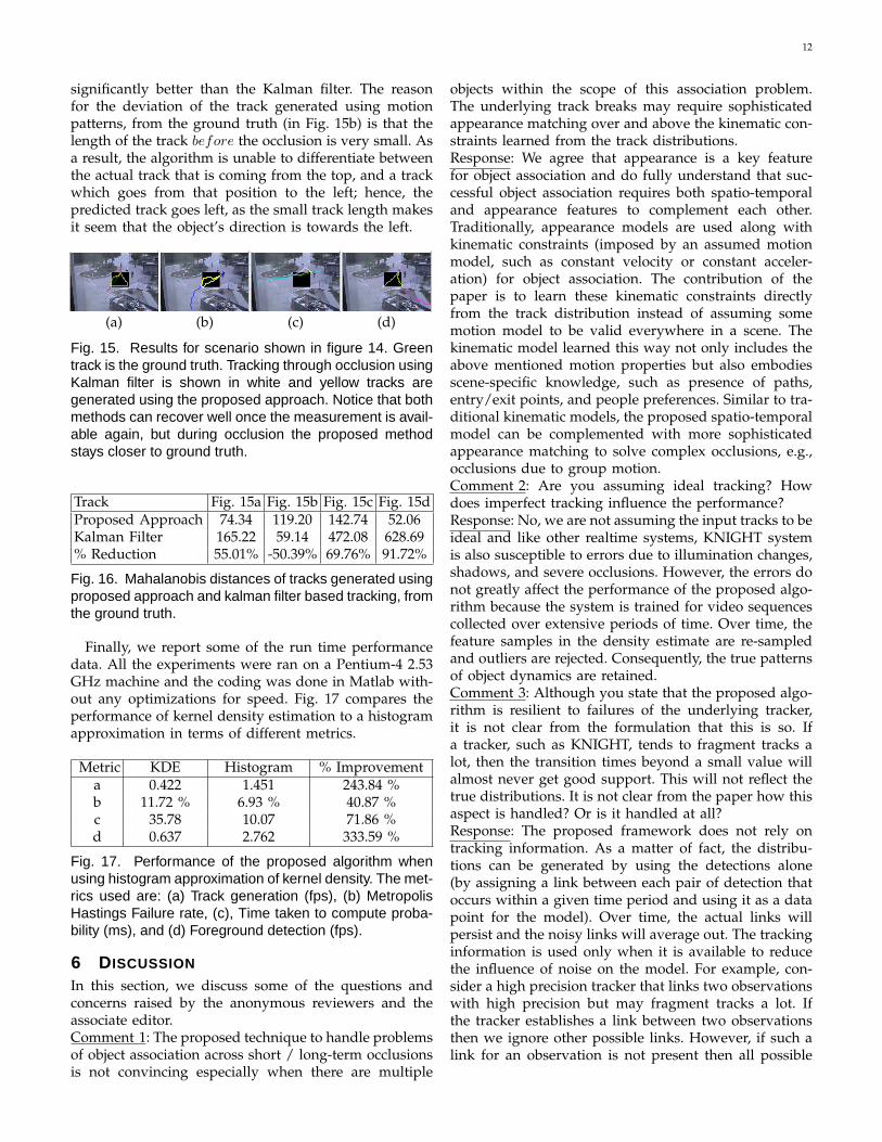
12

significantly better than the Kalman filter. The reasonfor the deviation of the track generated using motionpatterns, from the ground truth (in Fig. 15b) is that thelength of the track before the occlusion is very small. Asa result, the algorithm is unable to differentiate betweenthe actual track that is coming from the top, and a trackwhich goes from that position to the left; hence, thepredicted track goes left, as the small track length makesit seem that the object’s direction is towards the left.

50 100 150 200 250 300 350

0

50

100

150

200

250

50 100 150 200 250 300 350

0

50

100

150

200

250

50 100 150 200 250 300 350

0

50

100

150

200

250

50 100 150 200 250 300 350

0

50

100

150

200

250

(a) (b) (c) (d)

Fig. 15. Results for scenario shown in figure 14. Greentrack is the ground truth. Tracking through occlusion usingKalman filter is shown in white and yellow tracks aregenerated using the proposed approach. Notice that bothmethods can recover well once the measurement is avail-able again, but during occlusion the proposed methodstays closer to ground truth.

Track Fig. 15a Fig. 15b Fig. 15c Fig. 15dProposed Approach 74.34 119.20 142.74 52.06Kalman Filter 165.22 59.14 472.08 628.69% Reduction 55.01% -50.39% 69.76% 91.72%

Fig. 16. Mahalanobis distances of tracks generated usingproposed approach and kalman filter based tracking, fromthe ground truth.

Finally, we report some of the run time performancedata. All the experiments were ran on a Pentium-4 2.53GHz machine and the coding was done in Matlab with-out any optimizations for speed. Fig. 17 compares theperformance of kernel density estimation to a histogramapproximation in terms of different metrics.

Metric KDE Histogram % Improvementa 0.422 1.451 243.84 %b 11.72 % 6.93 % 40.87 %c 35.78 10.07 71.86 %d 0.637 2.762 333.59 %

Fig. 17. Performance of the proposed algorithm whenusing histogram approximation of kernel density. The met-rics used are: (a) Track generation (fps), (b) MetropolisHastings Failure rate, (c), Time taken to compute proba-bility (ms), and (d) Foreground detection (fps).

6 DISCUSSION

In this section, we discuss some of the questions andconcerns raised by the anonymous reviewers and theassociate editor.Comment 1: The proposed technique to handle problemsof object association across short / long-term occlusionsis not convincing especially when there are multiple

objects within the scope of this association problem.The underlying track breaks may require sophisticatedappearance matching over and above the kinematic con-straints learned from the track distributions.Response: We agree that appearance is a key featurefor object association and do fully understand that suc-cessful object association requires both spatio-temporaland appearance features to complement each other.Traditionally, appearance models are used along withkinematic constraints (imposed by an assumed motionmodel, such as constant velocity or constant acceler-ation) for object association. The contribution of thepaper is to learn these kinematic constraints directlyfrom the track distribution instead of assuming somemotion model to be valid everywhere in a scene. Thekinematic model learned this way not only includes theabove mentioned motion properties but also embodiesscene-specific knowledge, such as presence of paths,entry/exit points, and people preferences. Similar to tra-ditional kinematic models, the proposed spatio-temporalmodel can be complemented with more sophisticatedappearance matching to solve complex occlusions, e.g.,occlusions due to group motion.Comment 2: Are you assuming ideal tracking? Howdoes imperfect tracking influence the performance?Response: No, we are not assuming the input tracks to beideal and like other realtime systems, KNIGHT systemis also susceptible to errors due to illumination changes,shadows, and severe occlusions. However, the errors donot greatly affect the performance of the proposed algo-rithm because the system is trained for video sequencescollected over extensive periods of time. Over time, thefeature samples in the density estimate are re-sampledand outliers are rejected. Consequently, the true patternsof object dynamics are retained.Comment 3: Although you state that the proposed algo-rithm is resilient to failures of the underlying tracker,it is not clear from the formulation that this is so. Ifa tracker, such as KNIGHT, tends to fragment tracks alot, then the transition times beyond a small value willalmost never get good support. This will not reflect thetrue distributions. It is not clear from the paper how thisaspect is handled? Or is it handled at all?Response: The proposed framework does not rely ontracking information. As a matter of fact, the distribu-tions can be generated by using the detections alone(by assigning a link between each pair of detection thatoccurs within a given time period and using it as a datapoint for the model). Over time, the actual links willpersist and the noisy links will average out. The trackinginformation is used only when it is available to reducethe influence of noise on the model. For example, con-sider a high precision tracker that links two observationswith high precision but may fragment tracks a lot. Ifthe tracker establishes a link between two observationsthen we ignore other possible links. However, if such alink for an observation is not present then all possible

13

pairs are considered (for example, for time interval of nframes, the first and last n points in a track do not havelinks established by the tracker). This way, the algorithmis resilient to failures of the underlying tracker.Comment 4: If there is a static object, like a truck ora building, that occludes objects consistently over thecourse of their motion, how can the proposed algorithmconnect these objects especially in situations when ob-jects close to each other are moving?Response: As mentioned in response to Comment 3, thealgorithm does not fully rely on the track links andthus can connect objects across long term occlusionsdue to a static object. The algorithm however cannotsolve occlusions caused by objects moving together ingroups. Resolving such occlusions would require use ofappearance features along with the proposed model.Comment 5: Are there some anomalous trajectories inyour training dataset?Response: There are some anomalous trajectories in ourtraining sets, for example, people walking through thegrassy areas. However, by definition, the anomaloustrajectories are very sparse and hence have very lowprobability in the model as compared to normal trajec-tories or events.Comment 6: The determination of dth is tricky. How canit be determined automatically?Response: The threshold dth depends on several factorsincluding the distance of an object from the camera. Inother words, the farther the object, lesser should be thevalue of dth, especially for scenes where the sizes ofobjects vary greatly from one region to another withinthe image lattice. The threshold can be determined au-tomatically if either the camera calibration is known orif the object sizes are also used in the feature vector.Comment 7: The system has a high computational cost.Response: The system has high computational cost fortraining, but it can be performed off-line. The run-timeperformance of the system can be significantly improvedby using software optimization and using well knownapproximations of KDE, such as histograms, Fast GaussTransform [40], [41], and mixture models. In our ex-periments, the use of histogram approximation (in anun-optimized MATLAB code) greatly improved the run-time performance. (See Fig. 17).Comment 8: How to apply incremental learning to up-date the model adaptively.Response: Traditionally, the kernel density estimation ismade adaptive to the changes in the data by keepinga fixed size queue of n data points. Once k new datapoints are observed, the oldest k points in the queueare replaced with the new data points and the model isupdated. The model updates can be done on a low pri-ority thread, although online updating will not have anysignificant effect on performance. Note that the proposedsystem is based on static scenes and the availabilityof large training data, and hence does not have to beupdated very frequently.

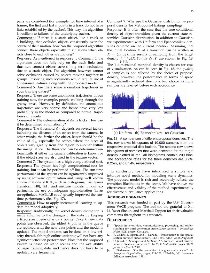
Comment 9: Why use the Gaussian distribution as pro-posal density for Metropolis-Hastings sampling?Response: It is often the case that the true conditionaldensity of object transition given the current state re-sembles Gaussian distribution. In addition to Gaussian,we experimented with Uniform and Epanechnikov den-sities centered on the current location. Assuming thatthe initial location X of a transition can be written asX = (x1, x2), the results of sampling from the targetdensity

∫Y

∫τ

∫x1

p(X, Y, τ)dx1dτdY are shown in Fig. 18.

The 1 dimensional marginal density is chosen for easeof visualization. As can be seen in Fig. 18, the qualityof samples is not affected by the choice of proposaldensity, however, the performance in terms of speedis significantly reduced due to a bad choice as moresamples are rejected before each acceptance.

0 50 100 150 2000

10

20

30

40

50

60

70

0 50 100 150 2000

20

40

60

80

100

120

0 50 100 150 2000

20

40

60

80

100

120

140

160

0 50 100 150 2000

50

100

150

Uniform samplesTarget density

0 50 100 150 2000

50

100

150

Epanechnikov samples

Target density

0 50 100 150 2000

50

100

150

Gaussian samples

Target density

(a) Uniform (b) Epanechnikov (c) Gaussian

Fig. 18. A comparison of different proposal densities. Thefirst row shows histograms of 10,000 samples from therespective proposal distributions. The second row showshistograms of samples that were accepted for the targetdensity plotted in red. All histograms contain 200 bins.The acceptance rates for the three densities are 0.2%,0.25%, and 0.54% respectively.

In conclusion, we have introduced a simple andintuitive novel method for modeling scene dynamics.The proposed model is rich and accurately reflects thetransition likelihoods in the scene. We have shown theeffectiveness and validity of the method experimentallyfor diverse surveillance applications.

ACKNOWLEDGMENTS

This research was funded in part by the U.S. Govern-ment VACE program. The authors are grateful to XinLi, Yaser Sheikh, and Marshall Tappen for their valuablecomments throughout this research.

REFERENCES

[1] “Special issue on video communications, processing, and under-standing for third generation surveillance systems”. Proceedingsof the IEEE, 89(10), Oct 2001.

[2] R. Collins, J. Lipton, and T. Kanade. “Introduction to the specialsection on video surveillance”. IEEE Trans. PAMI, 22(8), Aug 2000.

[3] O. Javed, K. Shafique, and M. Shah. “Automated Visual Surveil-lance in Realistic Scenarios ”. In IEEE Multimedia, pages 30–39,January - March 2007.

[4] I. Biederman. “On the semantics of a glance at a scene”. InPerceptual Organization, pages 213–253. Hillsdale, NJ: LawrenceErlbaum Associates, 1981.

14

[5] A. Torralba. “Contextual influences on saliency”. In Neurobiologyof Attention.

[6] K. Tieu, G. Dalley, and W.E.L. Grimson. “Inference of Non-overlapping Camera Network Topology by Measuring StatisticalDependence”. In IEEE ICCV, 2005.

[7] T.J. Ellis, D. Makris, and J.K. Black. “Learning a multi-cameratopology”. In Joint IEEE International Workshop on Visual Surveil-lance and Performance Evaluation of Tracking and Surveillance, 2003.

[8] C. Stauffer. “Learning to track objects through unobservedregions”. In Proceedings of the IEEE Workshop on Motion and VideoComputing, volume 2, pages 96–102, 2005.

[9] O. Javed, K. Shafique, Z. Rasheed, and M. Shah. “Modelinginter-camera space-time and appearance relationships for track-ing across non-overlapping views”. Computer Vision and ImageUnderstanding: CVIU, 109(2), Feb 2008.

[10] H. Buxton. “Generative models for learning and understandingdynamic scene activity”. In Generative Model Based Vision Work-shop, 2002.

[11] A. Hunter, J. Owens, and M. Carpenter. “A neural system forautomated CCTV surveillance”. In IEE Intelligent DistributedSurveillance Systems, 2003.

[12] J. Owens and A. Hunter. “Application of the self-organising mapto trajectory classification”. In 3rd IEEE International Workshop onVisual Surveillance, 2000.

[13] N. Johnson and D.C. Hogg. “Learning the distribution of objecttrajectories for event recognition”. Image and Vision Computing,14(8):609–615, August 1996.

[14] J.H. Fernyhough, A.G. Cohn, and D.C. Hogg. “Generation ofsemantic regions from image sequences”. In ECCV, 1996.

[15] R.J. Howard and H. Buxton. “Analogical representation of spatialevents, for understanding traffic behaviour”. In 10th EuropeanConference On Artificial Intelligence, 1992.

[16] E.B. Koller-Meier and L. Van Gool. “Modeling and recognition ofhuman actions using a stochastic approached”. In 2nd EuropeanWorkshop on Advanced Video-Based Surveillance Systems, 2001.

[17] J. Lou, Q. Liu, T. Tan, and W. Hu. “Semantic interpretation ofobject activities in a surveillance system”. In ICPR, 2002.

[18] W.E.L. Grimson, C. Stauffer, R. Romano, and L. Lee. “Usingadaptive tracking to classify and monitor activities in a site”. InIEEE CVPR, 1998.

[19] C. Stauffer and W.E.L. Grimson. “Learning patterns of activityusing real time tracking”. IEEE Trans. PAMI, 22(8):747–767, 2000.

[20] C. Stauffer. “Estimating tracking sources and sinks”. In SecondIEEE Event Mining Workshop, 2003.

[21] P. Remagnino and G.A. Jones. “Classifying surveillance eventsfrom attributes and behaviour”. In BMVC, 2001.

[22] M. Walter, A. Psarrou, and S. Gong. “Learning prior and obser-vation augmented density models for behaviour recognition”. InBMVC, 1999.

[23] A. Galata, N. Johnson, and D. Hogg. “Learning variable lengthmarkov models of behaviour”. Computer Vision and Image Under-standing: CVIU, 81(3):398–413, 2001.

[24] T. Huang and S. Russell. “Object identification in a bayesiancontext”. In Proceedings of IJCAI,, 1997.

[25] V. Kettnaker and R. Zabih. “Bayesian multi-camera surveillance”.In IEEE CVPR, 1999.

[26] S. Dockstader and A. Tekalp. “Multiple camera fusion for multi-object tracking”. In IEEE Workshop on Multi-Object Tracking, 2001.

[27] D. Hoiem, A. Efros, and M. Hebert. “Putting Objects in Perspec-tive”. In IEEE CVPR, 2006.

[28] R. Rosales and S. Sclaroff. “Improved tracking of multiple humanswith trajectory prediction and occlusion modeling”. In CVPRWorkshop on the Interpretation of Visual Motion, 1998.

[29] R. Kaucic, A. Perera, G. Brooksby, J. Kaufhold, and A. Hoogs.“A unified framework for tracking through occlusions and acrosssensor gaps”. In IEEE CVPR, 2005.

[30] X. Wang, K. Tieu, and E. Grimson. “Learning semantic scenemodels by trajectory analysis”. In ECCV, 2006.

[31] A. Perera, C. Srinivas, A. Hoogs, G. Brooksby, and W. Hu. “Multi-object tracking through simultaneous long occlusions and split-merge conditions”. In IEEE CVPR, 2006.

[32] W. Hu, X. Xiao, Z. Fu, D. Xie, T. Tan, and S. Maybank. “Asystem for learning statistical motion patterns”. IEEE Trans. PAMI,28(9):1450–1464, September 2006.

[33] E. Parzen. “On the estimation of a probability density functionand mode”. Ann. Math. Stati., 33:1065–1076, 1962.

[34] R. Duda, P. Hart, and D. Stork. “Pattern Classification”. WileyInterscience, 2nd edition, 2001.

[35] B. Turlach. “Bandwidth selection in kernel density estimation: Areview”. Institut de Statistique, 1993.

[36] B. W. Silverman. “Density Estimation for Statistics and Data Analy-sis”. Chapman and Hall, 1986.

[37] J. A. Benediktsson and P. H. Swain. “Consensus theoretic clas-sification methods”. In IEEE Trans. Sys. Man and Cybernetics,volume 22, pages 688–704, 1992.

[38] G. Hinton. “Products of experts”. In ICANN, pages 1–6, 1999.[39] K. Shafique and M. Shah. “A non-iterative greedy algorithm for

multi-frame point correspondence”. IEEE Trans. PAMI, Jan 2005.[40] L. Greengard and J. Strain. “The fast Gauss transform”. SIAM J.

Sci. Statist. Comput., 12(1):79–94, 1991.[41] A. Elgammal, R. Duraiswami, and L. Davis. “The fast Gauss

transform for efficient kernel density evaluation with applicationsin computer vision”. IEEE Trans. PAMI., 25, Nov 2003.

Imran Saleemi received the BS degree in Com-puter System Engineering from the GhulamIshaq Khan Institute of Engineering Sciencesand Technology, Pakistan in 2004, and MS inComputer Science from the University of Cen-tral Florida in 2008. He is currently workingtowards the PhD degree at the Computer VisionLaboratory at University of Central Florida. Hisresearch interests include visual tracking andsurveillance, probabilistic graphical models, andmultiview object detection and categorization.

Khurram Shafique received the BE degree incomputer systems engineering from NED Uni-versity of Engineering and Technology, Pakistan,in 1998 and the MS and PhD degrees, both incomputer science, from the University of Cen-tral Florida in 2001 and 2004, respectively. Heis currently a research scientist at the Cen-ter for Video Understanding Excellence at Ob-jectVideo, Reston, VA. His research interests in-clude graph theory, discrete optimization, track-ing, correspondence across multiple cameras,

and real-time surveillance systems. He was a recipient of HillmanFellowship award for excellence in research in Computer Science in2003. He is a member of the IEEE.

Mubarak Shah, Agere Chair Professor of Com-puter Science, is the founding director of theComputer Vision Lab at UCF. He is a co-authorof two books (Motion-Based Recognition (1997)and Video Registration (2003)) both by KluwerAcademic Publisher. Dr. Shah is a fellow ofIEEE, IAPR and SPIE. In 2006, he was awardedthe Pegasus Professor award, the highest facultyaward at UCF. He was an IEEE DistinguishedVisitor speaker for 1997-2000 and receivedIEEE Outstanding Engineering Educator Award

in 1997. He received the Harris Corporations Engineering AchievementAward in 1999, the TOKTEN awards from UNDP in 1995, 1997, and2000; Teaching Incentive Program award in 1995 and 2003, ResearchIncentive Award in 2003, Millionaires Club awards in 2005 and 2006,University Distinguished Researcher award in 2007, honorable mentionfor the ICCV 2005 Where Am I? Challenge Problem, and was nominatedfor the best paper award in ACM Multimedia Conference in 2005. Heis an editor of international book series on Video Computing; editor inchief of Machine Vision and Applications journal, and an associate editorof ACM Computing Surveys journal. He was an associate editor of theIEEE Transactions on PAMI, and a guest editor of the special issue ofInternational Journal of Computer Vision on Video Computing.