PRICING AND INVENTORY DECISIONS WITH UNCERTAIN SUPPLY AND STOCHASTIC DEMAND

2nd Reading

October 18, 2013 9:8 WSPC/S0217-5959 APJOR 1350030.tex

Asia-Pacific Journal of Operational ResearchVol. 30, No. 6 (2013) 1350030 (25 pages)c© World Scientific Publishing Co. & Operational Research Society of SingaporeDOI: 10.1142/S0217595913500309

PRICING AND INVENTORY DECISIONS WITH UNCERTAINSUPPLY AND STOCHASTIC DEMAND

CHIRAG SURTI∗

Faculty of Business and ITUniversity of Ontario Institute of Technology (UOIT )

2000 Simcoe Street North, Oshawa, Ontario, Canada L1H [email protected]

ELKAFI HASSINI† and PRAKASH ABAD‡

DeGroote School of Business, McMaster University1280 Main Street West, Hamilton, Ontario, Canada L8S 4L8

†[email protected]‡[email protected]

Received 7 December 2010Revised 10 March 2011Accepted 10 July 2011

Published 21 October 2013

We consider a retailer, facing uncertain supply and price-sensitive stochastic demand,who has to make stocking and pricing decisions for a given selling period. We alsoconsider the case when the demand is price-sensitive deterministic and provide a unifiedframework for the model with additive errors. For both scenarios, we look at the casewhen the price is set before receiving the supply, called simultaneous pricing and thecase when the price is set after receiving it, which is called postponed pricing. We developa procedure for finding the optimal policy for the retailer with general distributions forthe supply and the demand. To study the effect of supply uncertainty on expected profit,we conduct sensitivity analysis and develop results for both pricing scenarios and giveinsights. The results have important implications for a retailer in the supply chain, wherea portion of the inventory may be lost due to variety of factors including mishandlingand failure to meet quality standards. The findings shed light on the nature and role ofprices and their relationship to supply and demand.

Keywords: Pricing; inventory; random yield; demand uncertainty.

1. Introduction

Retailers are exposed to a variety of risks, one of which is having too much or toolittle stock to sell. This risk is usually due to uncertainty in consumer demand,which is amplified when the supply is uncertain. The uncertainty in supply can be

∗Corresponding author

1350030-1

http://dx.doi.org/10.1142/S0217595913500309

2nd Reading


C. Surti, E. Hassini & P. Abad

due to long lead times, loss, damage or theft in transit. If the demand outstrips thesupply then a mid-season recourse may not be possible, resulting in costly shortages.On the other hand, overstocking or using buffer stock is not always desirable as itcan be costly. Supply may be uncertain in many different environments, such aselectronic fabrication, chemical manufacturing, discrete parts manufacturing, foodand agricultural products, pharmaceutical products and medical supplies. Joneset al. (2001), Kazaz (2004), Bakal and Akcali (2006), Tang and Yin (2007) andHsieh and Wu (2008) are the most recent industry specific studies that have lookedat the issue of yield uncertainty.

For a risk neutral retailer, an order quantity and a price that maximize revenueand minimize salvage and shortage losses need to be determined, in order to balancethese risks. We assume the yield to be stochastically proportional, i.e., the yield doesnot depend on the order size. In our study, we develop models that support uncertainsupply with demand either being stochastic or deterministic, to yield results thatexplain the optimal price and order quantity and their relationship to the uncertainsupply. The added uncertainty in supply makes the analytical determination of theoptimal price and quantity complex. The existing body of knowledge on this issuedoes not always include pricing as one of the levers to reduce these risks.

There are two distinct cases of pricing in relation to the realization of demand.In the first instance, the price set before the supply is received. We refer to this asthe simultaneous pricing and ordering model. Such situations arise when the retailerneeds to engage in advertising of the product in advance of the selling season andbefore receipt of stock, or when a sales contract has been signed before the supplyis received. In the second case, we consider a retailer who may be able to delay thepricing decision until the receipt of the supply, but before the realization of demand.We refer to this as the postponed pricing model. In the postponed pricing case thedecision process is two-staged. In stage one, the retailer places an order, optimizingfor the anticipated unreliability of the supply as well as that of the demand.

Once the supply is received, the retailer prices and sells such that the revenueis maximized. Some specific situations in the literature where postponed pricing isapplicable include agribusinesses (Jones et al., 2001; Kazaz, 2004), re-manufacturedautomotive parts (Bakal and Akcali, 2006) and retailing (Tang and Yin, 2007). Weassume the demand to be linear in price and consider both additive and multiplica-tive demand error that can assume any general distribution.

In Sec. 2, we provide a brief review of the existing relevant literature on uncer-tain supply and demand. In Sec. 3, we develop the proposed model and analyze theproblem with stochastic and deterministic demand. Within each demand case, wefurther analyze the two cases of simultaneous and postponed pricing. For stochasticdemand case, we consider the case of additive as well as multiplicative demanderror. In Sec. 4, we conduct a sensitivity analysis to study the effects of yielddistribution parameters on the expected profit, the order quantity and the price.Finally we provide our conclusions as well as identify avenues for future research inSec. 5.

1350030-2

2nd Reading


Pricing and Inventory Decisions with Uncertain Supply and Stochastic Demand

2. Literature Review

The earliest model of random supply and demand was explored by Karlin (1958),where the amount received is independent of the order quantity. Silver (1976)explored the exact relationship between the optimal order quantity and the parame-ters of the yield distribution. He found that the optimal order quantity is a multipleof the EOQ and this multiple depends on the choice of mean and variance of the yielddistribution. Analysis of supply uncertainty in a newsvendor context is provided byRekik et al. (2007).

The most comprehensive review of the literature on random yields, in a manu-facturing context, is by Yano and Lee (1995), who broadly classify yields into twoclasses: random process yields and variable capacity yields. Examples for randomprocess yields include a discrete manufacturing system, producing one unit at atime, with a quality control process that may accept or reject the components.For a batch or a continuous type system, a stochastically proportional yield is used,where only a fraction of the whole batch is fit for consumption. For random capacity,where the actual process capacity is unknown, examples include land under agri-culture cultivation or a scarce manufacturing resource such as a highly specializedmachine that is not always available either due to breakdown, routine maintenanceor because it is processing another job.

Henig and Gerchak (1990) provide a comprehensive analysis of a periodic reviewinventory system with random yields. All the studies mentioned do not incorporateprice as a decision variable, since they are focused on production environments. Liand Zheng (2006) incorporate the simultaneous pricing decision in this model withfull backlogging of unmet demand. They show, for a general stochastic demandfunction, that the objective function is jointly concave in price and order quantity.Any unmet demand at the end of the selling cycle is fully met, with the help of aspecial order, in which all units of good quality and surplus inventory are carriedforward. Although such assumptions are normal in production/manufacturing typesettings, they are not realistic in a retail setting where the unmet demand at theend of the selling season is lost and surplus is usually salvaged.

Van Mieghem and Dada (1999), and later Gerchak (2012), analyze the bene-fits of a price-postponement strategy under demand uncertainty. Although productpostponement is well studied and understood as a means to reduce demand uncer-tainty, they propose a price-postponement strategy as a cost effective tool to reduceuncertainty in the supply chain when only demand is uncertain. Other work involv-ing postponed pricing with uncertain yield and demand includes Jones et al. (2001),Kazaz (2004) and Bakal and Akcali (2006), where they take the problem and sepa-rate it into two stages. Stage one deals with the realization of random yield and stagetwo with a recourse action in terms of either placing a second order with no yielduncertainty (Kazaz, 2004) or placing a second order with yield uncertainty (Joneset al., 2001) or setting a postponed price (Bakal and Akcali, 2006). Wang (2006)considers the problem of simultaneous pricing and ordering as well as postponed

1350030-3

2nd Reading



pricing in a decentralized supply chain setting with n manufacturers and a singleretailer with certain yield for complementary products. In our case we consider aretailer facing an uncertain supply and a price-sensitive demand and no recourse interms of placing a second order.

More recently, Rekik et al. (2007) consider random demand with additive andmultiplicative errors for the case when yield and demand are either uniform ornormal, obtain closed form expressions and provide some statistical insights for achoice of uniform distribution. Tang and Yin (2007) develop a model with uncertainsupply yield for the case when demand is deterministic and price-sensitive. Theyalso develop a model for simultaneous pricing and postponed pricing. Our modelextends that of Tang and Yin (2007) in two ways: (1) it assumes demand to bestochastic and similar to existing stochastic inventory models, includes shortageand surplus cost; (2) it assumes yield to be stochastically proportional to the lotsize and represents it by a general distribution. Hsieh and Wu (2008) consider adecentralized supply chain, consisting of a manufacturer, distributor and an originalequipment manufacturer (OEM). The source of randomness in supply comes fromcapacity at the manufacturing end and random demand at the distributors end. Therandom demand faced by the distributor is iso-elastic. They find that coordination,depending upon the scenario, may be beneficial to the manufacturer but not to theOEM. The distributor makes ordering and pricing decisions simultaneously.

Our paper assumes uncertain supply as well as stochastic demand allowing forboth the additive and multiplicative error. Given stochastic demand, we incorpo-rate shortage and salvage values in our analysis. We consider both simultaneous andpostponed pricing and show analytically that postponed pricing leads to higher prof-its and lower prices. We develop the analytical results and conditions that guaranteeoptimality, as well as provide simple yet effective solution procedures. The analyticalresults are sometimes intractable and closed form solutions are not always possible,especially when the yield and demand error distributions are complex. We providenumerical examples as well as conduct sensitivity analysis for the models using theBeta distribution for the yield.

3. Model

3.1. Notations and assumptions

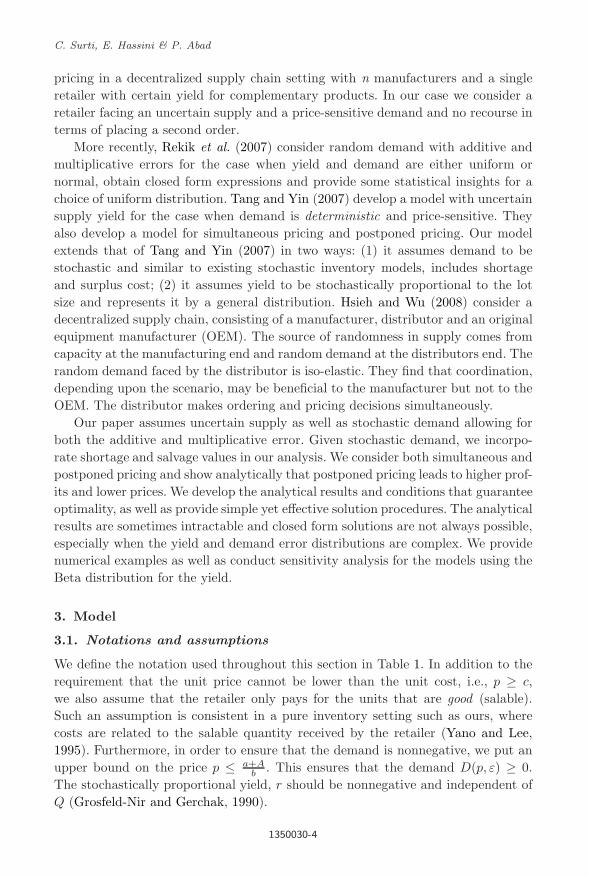
We define the notation used throughout this section in Table 1. In addition to therequirement that the unit price cannot be lower than the unit cost, i.e., p ≥ c,we also assume that the retailer only pays for the units that are good (salable).Such an assumption is consistent in a pure inventory setting such as ours, wherecosts are related to the salable quantity received by the retailer (Yano and Lee,1995). Furthermore, in order to ensure that the demand is nonnegative, we put anupper bound on the price p ≤ a+A

b . This ensures that the demand D(p, ε) ≥ 0.The stochastically proportional yield, r should be nonnegative and independent ofQ (Grosfeld-Nir and Gerchak, 1990).

1350030-4

2nd Reading



Table 1. Definition of terms.

Symbol Definitions

c unit cost, c ≥ 0.p price per unit charged, a decision variable such that p ≥ c.Q lot size, a decision variable such that Q > 0.h salvage price such that 0 ≤ h ≤ c.s shortage cost s ≥ c.r random variable representing the supply yield defined over the range [0, 1], with

mean µr and standard deviation σr . Its probability density and cumulativefunctions are denoted by f and F , respectively.

u realized value of yield r.D(p, ε) is the demand function such that D(p, ε) = y(p) + ε, where y(p) = a − bp and

a > 0 and b > 0 are known constants. a is the market size parameter and b isthe price elasticity.

ε random variable representing the uncertainty in demand defined over range[A,B], such that A > −a, with mean µε and standard deviation σε. Its prob-ability density and cumulative functions are denoted by g and G, respectively.

v realized value of the demand error ε.D(p, v) is the realized demand D(p, v) = y(p) + v.

3.2. Model with stochastic demand

3.2.1. Simultaneous pricing and ordering

In this case, the retailer determines the order size Q and price p at the same time.The retailer has no recourse and thus must mitigate the risk of shortages and riskof being left with excess inventory at the end of the selling period.

The profit function is

Π(p, Q) = p min{D(p, ε), rQ} − crQ + h(rQ − D(p, ε))+ − s(D(p, ε) − rQ)+, (1)

where x+ = max{0, x}.Upon substituting D(p, v) = y(p) + v in Π and simplifying, the expected profit

function is given as

E[Π(p, Q)] = (p − h)[y(p) + µε] − (c − h)µrQ

+ (p + s − h)∫ 1

0

∫ B

uQ−y(p)

[uQ − y(p) − v]g(v)dvf(u)du. (2)

The problem of maximizing the expected profit is thus formulated as

maxp,Q

E[Π(p, Q)]. (P1)

The optimization problem (P1) has been stated in the unconstrained form, sincewe deal with the simple bounds on the price in the solution procedure itself.

AnalysisIn the newsvendor model for a retailer facing only demand uncertainty, it is possibleto use a change of variable z = Q − y(p) in order to simplify the analysis of theproblem (without guaranteeing joint concavity) (e.g., Petruzzi and Dada (1999)).

1350030-5

2nd Reading



Unfortunately, when supply uncertainty is combined with that of demand uncer-tainly, it is no longer possible to make use of this change of variable idea. Due tothe existence of the random yield variable, a change of variable does not lead to anexpected profit that is simpler than what we currently have and, in particular, itdoes not lead to an expression that recasts the expected profit as a separable sumof expected leftovers and shortages. It will also not allow us to distinguish betweenthe riskless profit and the loss associated with uncertain supply and demand. Li andZheng (2006) and Kazaz (2004) were able to obtain analytically tractable objectivefunctions by allowing for any unmet demand to be satisfied by placing a specialorder with no supply yield uncertainty at the end of the season. Such a recoursemay be plausible in a manufacturing or production environment. However in retailoperations, lost sales are the norm and it is not reasonable to assume that we canplace a special order at the end of the season to satisfy unmet demand withoutsupply uncertainty.

The expression for the Hessian is very complicated and proving joint concav-ity analytically, even under some conditions on the problem parameters, leads tovery complex and meaningless expressions. The lack of joint concavity propertiesis in general true for all price setting newsvendor problems and requires completeenumeration (Petruzzi and Dada, 1999). In such circumstances one would seek toat least show concavity for separate decision variables (e.g., Agrawal and Nahmias(1997) and Karakul and Chan (2008)). Likewise, we show that the expected profitfunction is concave in each decision variable in Proposition 1.

Proposition 1. For any given price p, E[Π(p, Q)] is concave in Q. For any givenorder quantity Q, E[Π(p, Q)] is concave in p.

Proof. First we consider a fixed price p. From (1) we see that the terms rQ and −rQ

are concave in Q, since they are linear in Q, and so min{D(p, ε), rQ}, (rQ−D(p, ε))+

and (D(p, ε) − rQ)+ are also concave in Q, because concavity is preserved undermaximization and minimization. Finally, taking expectation preserves concavity,hence E[Π(p, Q)] is concave in Q, when p is fixed. A similar argument can be usedfor the case when Q is fixed.

Thus, we can calculate p∗(Q) by solving the first-order conditions given as

∂E(Π(p, Q))∂p

= (y(p) + µε) − (p − h)b

+∫ 1

0

∫ B

uQ−y(p)

[(uQ − y(p) − v) + b(p + s − h)]

× g(v)f(u)dvdu = 0. (3)

Solution ProcedureTo find an optimal order quantity Q∗, price p∗ and expected profit E[Π(p∗, Q∗)] wepropose a simple search procedure. From Proposition 1 and Eq. (3), we note that, for

1350030-6

2nd Reading



a given order quantity Q, we have a unique p∗(Q). To ensure that the demand takesa meaningful form, we require that the price be such that D(p, ε) ≥ 0 ⇒ p ≤ a+A

b .The lower bound on the order quantity is the natural limit: Q ≥ 1. Observation 1establishes an upper bound on the optimal quantity.

Observation 1. Let Ql = (a+µε−bh)2

4b(c−h)µr. Then E(Π(p, Q)) ≤ 0 for all p, Q such that

c ≤ p ≤ (a + A)/b, Q ≥ Ql.

Proof. The last term of (2) is negative for all p and Q. Hence,

E(Π(p, Q)) < (p − h)[y(p) + µε] − (c − h)µrQ (4)

for all p, Q such that c ≤ p ≤ (a + A)/b, Q > 0. Since

maxp

{(p − h)[y(p) + µε]} =(a + µε − bh)2

4b

it follows that

(p − h)[y(p) + µε] − (c − h)µrQl ≤ 0 (5)

for all p, Q such that c ≤ p ≤ (a + A)/b, Q > Ql. Combining (4) and (5), we get thedesired result.

With the above bounds on the decision variables, we propose the following solu-tion procedure:

(1) Initialize i = 0 and Qi = 1.

(2) Find p̂i, s.t. ∂E[Π(bpi |Qi)]∂p = 0 and set pi =

{a+A

b , if pi ≥ a+Ab ,

bpi, if c ≤ pi ≤ a+Ab ,

c, if pi ≤ c.

(3) Calculate E[Π(pi, Qi)]. Store pi, Qi and E[Π(pi, Qi)] in a table.(4) Let i = i + 1 and Qi = Qi−1 + ∆ where ∆ > 0. If Qi ≥ Ql then end else goto

Step 2.

The global maximum (or maxima) is identified by searching the table developed inStep 3.

3.2.2. Postponed pricing

In this case, the retailer first determines the optimal order quantity Q in Stage Iand after observing the value of supply yield, determines the optimal selling pricep in Stage II. Thus the problem is formulated in stages, with Stage II solved firstwhere the retailer knows the value uQ ≥ 0.

The profit function for Stage II is

ΠII (p |uQ) = p min(D(p, ε), uQ) − cuQ + h(uQ − D(p, ε))+ − s(D(p, ε) − uQ)+.

Note that in the above expression the value of the yield is already known.

1350030-7

2nd Reading



The problem of maximizing the expected profit in Stage II is

max E[ΠII (p |uQ)]. (P2)

Let p∗(uQ) be the optimal price that maximizes the expected profit in Stage II for arealized value of supply yield u and order quantity Q. The expected profit functionfor Stage I is given as

E[ΠI(Q)] =∫ 1

0

E(ΠII (p∗(uQ) |uQ))f(u)du. (6)

The problem of maximizing the expected profit in Stage I is

max E[ΠI(Q)]. (P3)

The optimization problems (P2) and (P3) have been stated in the unconstrainedform since we handle the simple bounds on the price and order quantity explicitlyin the solution procedure proposed in Sec. 3.2.2.

Using the same logic in Proposition 1 we can show that E(ΠII (p |uQ)) is aconcave function in p, for a given uQ value. Hence, there is a unique p, given asp∗(uQ), that satisfies the first-order condition

∂E(ΠII (p |uQ))∂p

= (y(p) + µε) − (p − h)b

+∫ B

uQ−y(p)

[(uQ − y(p) − v) + b(p + s − h)]g(v)dv = 0. (7)

Thus the optimal price p∗(uQ) can be determined using the first-order condition inEq. (7).

Solution ProcedureTo find the order quantity Q that maximizes E(ΠI(Q)), we propose the followingsolution procedure. To ensure that the demand takes a meaningful form, we requirethat the price be such that D(p, ε) ≥ 0 ⇒ p ≤ a+A

b . A result similar to Observation 1can be shown for E(ΠII (p |uQ)) and thus the bounds for Q are 1 and Ql. Theprocedure is described in the following two steps:

(1) We obtain a set of p̂i(uQ), s.t. ∂E[ΠII (bpi|uQ)]∂p = 0 values for a set of (uQ) values,

0 ≤ uQ ≤ Ql. Since in Stage II, the values of u and Q are numerically known,i.e., yield r takes a value u for a given order size Q, the problem simply reducesto using the corresponding price p∗(uQ) that maximizes the expected profit in(P2). This price is given as

p∗(uQ) =

a + A

b, if p̂i(uQ) ≥ a + A

b,

p̂i(uQ), if c ≤ p̂i(uQ) ≤ a + A

b,

c, if p̂i(uQ) ≤ c.

1350030-8

2nd Reading



(2) Next, we vary Q ∈ [1, Ql] by increment ∆ > 0 to find the global optimum Q.For the problem in Stage II, p(uQ) can take values depending upon the valueof Q and the realized value u. We calculate the expected profit for the value ofQ using Eq. (6) as follows

E(ΠI(Q)) =∫ 1

0

E(ΠII (p, Q))|p=p(uQ)f(u)du,

≈∑uj

E(ΠII (p, Q))|p=p(ujQ)f(uj)∆u.

We store the values of Q and the corresponding E[ΠI(Q)] in a table. The globalmaximum (or maxima) are then identified by searching the table. The averageprice, which we define as p =

∑uj

p(ujQ)|Q=Q∗f(uj)∆u, can be calculated atthis stage.

3.3. Extension to multiplicative demand error

We consider the case where demand is multiplicative, such that D(p, ε) = y(p)ε,where the random error range is [A, B] and A > 0, without loss of generality. Toemphasize the similarity to the additive demand case we use the same equationnumbers with letter ‘m’, for multiplicative, attached to them.



Π(p, Q) = p min(D(p, ε), rQ) − crQ + h(rQ − D(p, ε))+ − s(D(p, ε) − rQ)+,

and the expected profit is

E[Π(p, Q)] = (p − h)[y(p)µε] − (c − h)µrQ

+ (p + s − h)∫ 1

0

∫ B

uQ/y(p)

[uQ − y(p)v]g(v)dvf(u)du. (1m)

The problem of maximizing the expected profit is formulated as

maxp,Q

E[Π(p, Q)].

As in Proposition 1 we can show that expected profit function (1m) is concave in p

for any given Q. Thus, we can calculate the optimal p∗(Q) by solving the followingfirst-order condition

∂E(Π(p, Q))∂p

= (y(p)µε) − (p − h)bµε

+∫ 1

0

∫ B

uQ/y(p)

[(uQ − y(p)v) + bv(p + s − h)]g(v)f(u)dvdu = 0.

1350030-9

2nd Reading



The solution procedure is similar to the additive demand case, except for steps 2and 4, where we are required to change some values and limits for the decisionvariables:

(1) Initialize i = 0 and Qi = 1.

(2) Find p̂i, s.t. ∂E[Π(bpi |Qi)]∂p = 0 and set pi =

{ab , if pi ≥ a

b ,

bpi, if c ≤ pi ≤ ab ,

c, if pi ≤ c.

(3) Calculate E[Π(pi, Qi)]. Store pi, Qi and E[Π(pi, Qi)] in a table.(4) Let i = i + 1 and Qi = Qi−1 + ∆ where ∆ > 0. If Qi ≥ µε(a−bh)2

4b(c−h)µrthen end else

goto Step 2.

The global maximum (or maxima) is identified by searching the table developed inStep 3.


The profit function for Stage II is

ΠII (p |uQ) = p min(D(p, ε), uQ) − cuQ + h(uQ − D(p, ε))+ − s(D(p, ε) − uQ)+,

and the expected profit function for Stage II is

E(ΠII (p |uQ)) = (p − h)[y(p)µε] + (h − c)uQ

+ (p + s − h)∫ B

uQ/y(p)

[uQ − y(p)v]g(v)dv.

The problem of maximizing the expected profit in Stage II is

max E[ΠII (p |uQ)].

Let p∗(uQ) be the optimal price that maximizes the expected profit in Stage II for arealized value of supply yield u and order quantity Q. The expected profit functionfor Stage I is given as

E[ΠI(Q)] =∫ 1

0

E(ΠII (p∗(uQ) |uQ))f(u)du.

The problem of maximizing the expected profit in Stage I is

max E[ΠI(Q)].

In a similar way to Sec. 3.2.2 we can show that E(ΠII (p |uQ)) is a concave functionin p, for a given uQ value. Hence, there is a unique p, given as p∗(uQ), that satisfiesthe first-order condition

∂E(ΠII (p |uQ))∂p

= (y(p)µε) − (p − h)bµε

+∫ B

uQ/y(p)

[(uQ − y(p)v) + bv(p + s − h)]g(v)dv = 0. (2m)

1350030-10

2nd Reading



Thus the optimal price p∗(uQ) can be determined using the first-order conditionin Eq. (2m) and the same procedure used in Sec. 3.2.2 can be used here with somemodifications to the decision variables limits and values:

(1) We obtain a set of p̂i(uQ), s.t. ∂E[ΠII (bpi|uQ)]∂p = 0 values for a set of (uQ) values,

0 ≤ uQ ≤ Ql. The price p∗(uQ) that maximizes expected profit is given as

p∗(uQ) =

a

b, if p̂i(uQ) ≥ a

b,

p̂i(uQ), if c ≤ p̂i(uQ) ≤ a

b,

c, if p̂i(uQ) ≤ c.

(2) Next, we vary Q ∈ [1, Ql] by increment ∆ > 0 to find the global optimum Q.We calculate the expected profit for the value of Q using Eq. (3.3.2) as follows

E(ΠI(Q)) =∫ 1

0

E(ΠII (p, Q))|p=p(uQ)f(u)du,

≈∑uj

E(ΠII (p, Q))|p=p(ujQ)f(uj)∆u.

We store the values of Q and the corresponding E[ΠI(Q)] in a table. The globalmaximum (or maxima) are then identified by searching the table. The averageprice, which we define as p =

∑uj

p(ujQ)|Q=Q∗f(uj)∆u, can be calculated atthis stage.

3.4. Model with deterministic demand

We now analyze the case where the demand is deterministic (i.e., D(p) = y(p) =a− bp) and the supply is unreliable. We first develop and analyze the case when theprice p and the order quantity Q are simultaneously determined and then developand analyze the case when the price is set after realizing the supply yield r, for agiven order quantity Q.



Π(p, Q) = p min(D(p), rQ) − crQ + h(rQ − D(p))+ − s(D(p) − rQ)+.

Upon simplification the expected profit is given as

E[Π(p, Q)] = (p − h)y(p) − (c − h)µrQ + (p + s − h)

×∫ y(p)

Q

0

[uQ − y(p)]f(u)du. (8)

The problem of maximizing the expected profit can now be stated as

maxp,Q

E[Π(p, Q)].

1350030-11

2nd Reading



As in Proposition 1, we can show that for a given price p, E[Π(p, Q)], as defined in(8), is concave in Q. For any given order quantity Q, E[Π(p, Q)] is concave in p.

The first-order conditions for the expected profit are given as

∂E(Π(p, Q))∂Q

= −(c − h)µr + (p + s − h)∫ y(p)/Q

0

uf(u)du, (9)

∂E(Π(p, Q))∂p

= y(p) − (p − h)b

+∫ y(p)/Q

0

[(uQ − y(p)) + (p + s − h)b]f(u)du. (10)

By solving Eq. (9) for Q, we get the following implicit expression for Q∗ as a functionof p: ∫ y(p)/Q

0

uf(u)du =[

c − h

p + s − h

]µr. (11)

It is interesting to note that condition (11) is similar to the fractile form in Whitin(1955). The optimal price p∗(Q) can be determined using the first-order conditiongiven by Eq. (10). The solution procedure for the simultaneous pricing problemwith deterministic demand is similar to the solution procedure in Sec. 3.2.1, thuswe do not repeat it.


In this section, we consider the scenario where the price will be set after the orderquantity, Q, has been received and the outcome of the supply yield, r, is known.Unlike the model in the previous sections, in the case of postponed pricing withdeterministic demand, there is no further uncertainty left for the retailer (no demanduncertainty). The retailer, based on the available stock, must decide on the optimalprice at which his revenue is maximized. Note that the retailer will not face shortageloss in this case, i.e., D(p) ≤ uQ. However it is still possible that the retailer mayhave supply that exceeds the revenue maximizing quantity in which case the retailerwill salvage the remaining units.

Optimal PriceGiven an order quantity Q and an observed value of supply yield u, the retailercan sell, at most, uQ units at price p. The postponed pricing problem can beformulated as

maxp

{(p − h)(a − bp) + huQ | a− bp ≤ uQ, h ≤ p ≤ a/b}. (P4)

Note that the lower bound on p is set to h as the retailer can price below cost aslong as the price is higher than the salvage value. Depending on the state of thefirst constraint in (P4), the optimal price can take two values as per Proposition 2.

1350030-12

2nd Reading



Proposition 2. The optimal postponed price when demand is deterministic is

p∗(u, Q) =

p0 =

a + bh

2b, if uQ > D(p0),

p1 =a − uQ

b, otherwise.

Furthermore, p0 ≤ p1.

Proof. It is easy to show that a+bh2b = argmaxp{(p − h)(a − bp) + huQ}, i.e.,

the unconstrained solution for problem (P4). We will show that p∗(u, Q) satisifesthe constraints. We start with the bounds on the prices and show that h ≤ p0 ≤p1 ≤ a/b:

p0 − h =a − bh

2b≥ 0 ∵ D(h) ≥ 0;

p1 − p0 =(a − bh) − 2uQ

2b≥ 0 ∵ D(p0) ≥ uQ;

a

b− p1 =

uQ

b≥ 0.

Next we consider the demand (no shortage) constraint. If uQ > D(p0) then p0, theoptimal price to the unconstrained version of (P4), also solves (P4). In this case wehave ample supply and should charge a+bh

2b and salvage the remaining [uQ−D(p0)]at a salvage price h. If uQ ≤ D(p0) then the first constraint in (P4) will be bindingat optimality, i.e., the price should be p1 such that D(p1) = a − bp1 = uQ, orp1 = a−uQ

b . In this case the retailer does not have enough supply to maximizeprofit and should charge a price that will clear the supply with no quantity left forsalvage.

Optimal Order QuantityGiven the above discussion and noting when uQ ≤ D(p0), we can have eitherQ ≥ D(p0) or Q < D(p0). The profit, as a function of Q, is defined as

Π(Q) =

{p0D(p0) − cuQ + h[uQ − D(p0)] uQ ≥ D(p0),

(p1 − c)uQ uQ < D(p0).(12)

In order to calculate the expected profit we consider two cases.

Case A: Q < D(p0). Since Q < D(p0) it follows that uQ < D(p0) for all 0 < u ≤ 1.From (12), the profit for Stage I in this case is ΠA(Q) = (p1 − c)uQ and the expectedprofit is

E(ΠIA(Q)) =∫ 1

0

(p1 − c)uQf(u)du = [a − bc]µrQ

b− Q2

b[σ2

r + µ2r]. (13)

1350030-13

2nd Reading



The problem of maximizing the expected profit for Stage I can be formulated as

max0<Q≤D(p0)

E(ΠA(Q)). (P5)

From (13) we see that E(ΠIA(Q)) is quadratic and concave in Q and it follows thatthe optimal unconstrained Q is the solution to the following first-order necessarycondition

dE(ΠA(Q))dQ

=1b[(a − bc)µr − 2Q(σ2

r + µ2r)] = 0.

Taking into account the constraint in (P5), it is easy to see that the solution to(P5) is as stated in Proposition 3 without proof.

Proposition 3. Given that Q ≤ D(p0) =a−bh2 , the optimal order quantity that

solves (P5) is

Q∗A = min

[(a − bc)µr

2(σ2r + µ2

r),a − bh

2

].

Case B: Q ≥ D(p0). Since Q ≥ D(p0) =a−bh2 , we can either have uQ ≥

D(p0) =a−bh2 or uQ < D(p0) =a−bh

2 . The expected profit is

E[ΠB(Q)] =1b

[(a − bc)µrQ − Q2(σ2

r + µ2r) +

∫ 1

(a−bh)/2Q

(a − bh

2− uQ

)2

f(u)du

].

(14)

In Proposition 4, we show the concavity of the expected profit and establish anupper bound on the optimal quantity.

Proposition 4. E[ΠB(Q)] is concave. Furthermore E[ΠB(Q)] ≤ 0 ∀Q ≥ Qld

where Qld = (a−bh)2

4b(c−h)µr.

Proof. Concavity follows from the fact that

d2E(ΠB(Q))dQ2

=−2b

∫ (a−bh)/2Q

0

u2f(u)du ≤ 0.

To establish a limit for the optimal Q we note that from (14) we get

E[ΠB(Q)] ≤ 1b[(a − bc)µrQ − Q2(σ2

r + µ2r) +

∫ 1

0

(a − bh

2− uQ

)2

f(u)du]

=1b[µrb(c − h)(Qld − Q)].

Therefore, E(Π(p, Q)) ≤ 0 for all Q ≥ Qld.

1350030-14

2nd Reading



The problem of maximizing the expected profit can then be formulated asfollows:

max{

E(ΠB(Q))∣∣∣∣ a − bh

2≤ Q ≤ Qld

}. (P6)

Given the concavity result in Proposition 4, the optimal solution to (P6) is Q∗B =

min[Q0B, Q1

B], where Q1B is such that E(ΠB(Q1

B) = 0 and Q0B) solves the following

first-order optimality condition

dE(ΠIB (Q))dQ

= (a − bc)µr − 2Q(µ2r + σ2

r )

−∫ 1

(a−bh)/2Q

2u

(a − bh

2− uQ

)f(u)du = 0.

The optimal quantity Q∗ that solves the original optimization problem (P4) is statedin Theorem 1.

Theorem 1. The optimal order quantity under deterministic demand and post-poned pricing is:

Q∗ =

{Q∗

A if E(ΠA(Q∗A)) ≥ E(ΠB(Q∗

B)),

Q∗B otherwise.

4. Comparison of Simultaneous and Postponed Pricing Scenarios

In this section, we analytically compare prices and expected profits in the simulta-neous and postponed pricing models. In addition, we provide a numerical exampleand perform sensitivity analysis to further compare these scenarios with respect tothe supply uncertainty parameters.

4.1. Analytical results for prices and expected profits

In Theorem 2, we show that the optimal expected postponed profit dominates theoptimal expected simultaneous profit.

Theorem 2. Let (p∗s and Q∗s) be the optimal price and quantity found by solv-

ing (P1) corresponding to the simultaneous case. Similarly, let Q∗p be the opti-

mal quantity found by solving (P2) corresponding to the postponed case. ThenΠ∗

s = E(Π(p∗s , Q∗s)) ≤ Π∗

p = E(ΠI(Q∗p)).

Proof. Proof is in two parts.Part 1: Suppose the quantity used in the postponed case is Q∗

s and let Π′p =

E(ΠI(Q∗s)). Given the optimality of Q∗

p, Π∗p ≥ Π

′p.

Part 2: Now suppose that the quantity is Q∗s and the realized yield in the post-

poned case is u. From problem (P2) the optimal postponed price is p∗(uQ∗s) =

arg maxc≤p≤ a+Ab

E(ΠII (p |uQ∗s)). Clearly, given the optimality of p∗(uQ∗

s), we

1350030-15

2nd Reading



have

E(ΠII (p∗(uQ∗s) |uQ∗

s)) ≥ E(ΠII (p∗s |uQ∗s)).

The above applies for all realizations u, hence,∫ 1

0

E(ΠII (p∗(uQ∗s) |uQ∗

s))f(u)du ≥∫ 1

0

E(ΠII (p∗s |uQ∗s))f(u)du

or

E(ΠI(Q∗s) = Π

′p ≥ E(Π(p∗s , Q

∗s)) = Π∗

s.

Combining Part 1 and Part 2, we have Π∗p ≥ Π∗

s .

In Theorem 3, we show that when demand is deterministic, the optimal post-poned price, p∗pd, and the optimal riskless postponed price, p0 = a+bh

2b are bothlower than the optimal simultaneous price, p∗sd.

Theorem 3. Let p∗sd be the optimal price in the simultaneous case and p∗pd theexpected optimal price in the postponed case when the demand is deterministic. Asbefore, p0 = a+bh

2b is the postponed riskless price. The following is then true:

(a) p0 ≤ p∗sd.(b) If a−bh

a−bh+sb ≤ F (µr) then p∗pd ≤ p∗sd.

Proof. Let Πsd denote the expected simultaneous profit, when demand is deter-ministic, as stated in (8). Recall from Proposition 2 that Πsd is concave in p andtherefore dΠsd

dp is decreasing in p.

(a) It is easy to verify that

dΠsd

dp

∣∣∣∣p=p0

=∫ (a−bh)/2Q

0

(uQ + sb)f(u)du ≥ 0,

and therefore p0 ≤ p∗sd since dΠsd

dp

∣∣p=p∗

sd

= 0 and dΠsd

dp is decreasing in p.(b) The expected optimal price in the posponed case is

p∗pd =∫ y(p0)/Q

0

p1f(u)du +∫ 1

y(p0)/Q

p0f(u)du

=a + bh

2b+

Q

b

∫ y(p0)/Q

0

(y(p0)

Q− u

)f(u)du

≤ a − µrQ

b

= p̄1,

1350030-16

2nd Reading



where y(p0) = a−bh2 . Note that y(p̄1)/Q = µr. Now, from (10)

dΠsd

dp

∣∣∣∣p=p̄1

= F (µr)(a − hb + sb) − (a − hb)

+ 2µrQ(1 − F (µr)) +∫ µr

0

uQf(u)du

≥ 0, ifa − bh

a − bh + sb≤ F (µr).

Thus, p∗pd ≤ p̄1 ≤ p∗sd since dΠsd

dp

∣∣p=p∗

sd

= 0 and dΠsd

dp is decreasing in p.

Remark 1. The condition in Theorem 3 is only a sufficiency condition. For exam-ple, it is possible that even if the condition does not hold, the expected postponedprice may still be lower than the simultaneous price.

Remark 2. For symmetric distributions, the condition in Theorem 3 reduces toab ≤ s+h. Therefore, the sum of salvage and penalty values have to be greater thanthe price at which zero demand occurs. Alternatively, the conditions stipulate thatpricing at s + h would attract no demand.

4.2. Numerical example

We provide a numerical example to highlight the analytical results for the simulta-neous and the postponed pricing problems proposed in Secs. 3.2 and 3.4. For thedistribution of the supply yield r, we consider the Beta distribution r ∼ Beta[α, β],where α ≥ 1 and β ≥ 1 are the shape parameters. It is widely used in Bayesian statis-tics and quality control as it is a flexible distribution (Stapper, 1992; Bollapragadaand Morton, 1999). Studies that make use of the Beta distribution in the operationsmanagement and manufacturing literature include Stapper (1992) (VLSI yields),Grosfeld-Nir and Gerchak (1990) (general manufacturing yield), Lin et al. (1997)(tolerance analysis) and Kuo and Kim (1999) (semiconductor industry).

Although there are several recent studies on random yield in operations man-agement, Rekik et al. (2007) and Tang and Yin (2007) make use of the uniformdistribution to represent yield. This choice is not ideal to model stochastically pro-portional yield in a supplier and a retailer setting. The stochastically proportionalyield faced by a retailer can take different forms over the same support, dependingon the supplier’s reliability. Therefore, the choice of the Uniform distribution is notrealistic as it rules out the possibility of asymmetry or skewness in yield, somethingthat can lead the retailer to make inappropriate decisions. It is worthwhile to notethat, for a Beta distribution, with shape parameters α = β = 1, the distribution isuniform over support [0, 1]. The pdf of the Beta distribution is given as

f(u) =

Γ(α + β)Γ(α)Γ(β)

u(α−1)(1 − u)(β−1) if 0 ≤ u ≤ 1,

0 otherwise.

1350030-17

2nd Reading



The mean and the variance are given as µr = αα+β and σ2

r = αβ(α+β)2(α+β+1) ,

respectively.By varying the choice of α and β, the supply yield distribution can take a variety

of shapes, thus offering the flexibility to model different uncertain yield situations.For a complete discussion on the Beta distribution, we refer readers to Chapter25 in Johnson et al. (1995). For our numerical example, we consider the followingparameter values: a = 500, b = 20, c = 5, h = 2, s = 10, A = −50, B = 50,∆u = 0.001. Unless otherwise stated, the same values are used for all subsequentnumerical analysis. For the supply yield we assume α = 7, β = 7, µr = 0.5 andσr = 0.129 and for the demand error we have µε = 0, σε = 16.67. To accuratelyrepresent the demand error ε, we use a Normal distribution that is truncated overthe interval [A, B], i.e.,

g(v) =

g1(v)

G(B) − G(A)if A ≤ v ≤ B,

0 otherwise,

where the pdf of the Normal distribution is given as:

g1(v) =

1

σ√

2πexp

(− (v − µε)2

2σ2

)if −∞ ≤ v ≤ ∞,

0 otherwise.

For a more complete discussion on the truncated Normal distribution, we referreaders to Chapter 13 in Johnson et al. (1994). The optimal quantity and expectedprofits with corresponding prices are included in Table 2. Note that the price in thecase of the postponed pricing problem cannot be determined until the value of thesupply yield is observed. Thus, an average price p is calculated for a given value ofQ, where p =

∑uj

p(uj, Q)f(uj)∆u, j ∈ {1, 2, . . . , 1,000}.Stochastic DemandFrom Table 2, we see that for the postponed pricing, the price and the quantity arelower, whereas the expected profit is higher. There is a greater uncertainty facedby the retailer, when the pricing and ordering decisions are made simultaneously.Once the supply yield uncertainty is resolved, the subsequent pricing decision is

Table 2. Stochastic demand.

Simultaneous pricing Postponed pricing

Price 15.59 15.46Quantity 498.3 431.5Expected revenue 2832.35 2850.4Expected salvage 134.94 53.85Expected shortage 65.22 20.41Expected profit 1656.32 1805.1

1350030-18

2nd Reading



Table 3. Deterministic demand.

Simultaneous pricing Postponed pricing

Price 15.69 15.05Quantity 481.58 398.01Expected revenue 2818.40 2872.02Expected salvage 122.40 8.67Expected shortage 65.41 0.00Expected profit 1671.42 1889.05

made with regards to mitigating demand uncertainty alone. We also note that theincrease in the expected profit is due to savings in inventory costs, rather than anincrease in sales revenue.

Deterministic DemandFor the postponed pricing problem, we make use of the relationship between µr

σ2r+µ2

r

and aa−bc to identify whether Case A or Case B apply in calculating the optimal

order quantity. Pricing decision cannot be determined till the supply yield u isobserved. Thus, an average price p is calculated for a given value of Q, wherep =

∑uj

p(uj , Q)f(uj)∆u.Price and order quantity are lower and profits are higher for postponed pricing

(see Table 3). We note here that the condition of Theorem 3 does not hold, but thepostponed price is nevertheless lower than the simultaneous price. The expectedprofit is higher for the deterministic demand case as compared to the stochasticdemand case. This indicates that ignoring the demand uncertainty, as has been thecase for most of the literature on pricing with uncertain supply, could lead to anoverestimation of the expected profits.

4.3. Sensitivity analysis

We conduct sensitivity analysis by varying the shape parameters of the Beta distri-bution, α and β, such that the mean µr varies from 0.2 to 0.9, holding σr = 0.125and the standard deviation σr varies from 0.078 to 0.2886, holding mean constantat µr = 0.5. Our aim is to study the impact of supply uncertainty on the expectedprofit, order quantity and selling price. We hold all other parameters constant forour analysis.

4.3.1. Stochastic demand

From Fig. 1, we see that the expected profit in the case when the pricing decision ispostponed is always higher than the case of simultaneous pricing. The order quantityQ for the simultaneous pricing problem is always higher than the postponed pricingcase, as there is greater uncertainty faced by the retailer. The retailer, being able topostpone the pricing decision, orders less from the supplier. The retailer can set theprice after observing the supply yield and thus, is in a better position to maximize

1350030-19

2nd Reading



0.3 0.4 0.5 0.6 0.7 0.815

15.5

16

16.5

17

17.5

µr

0.1 0.15 0.2 0.2515

15.5

16

16.5

17

17.5

σr

0.3 0.4 0.5 0.6 0.7 0.8200

400

600

800

1000

1200

µr

0.1 0.15 0.2 0.25200

400

600

800

1000

1200

σr

0.3 0.4 0.5 0.6 0.7 0.81000

1200

1400

1600

1800

2000

µr

0.1 0.15 0.2 0.251000

1200

1400

1600

1800

2000

σrPostponed Pricing

Simultaneous Pricing

σr=0.125 µ

r=0.5

p p

Q Q

E(Π) E(Π)

Fig. 1. Sensitivity analysis for stochastic demand.

the expected profit with lower uncertainty. As the supply uncertainty reduces, i.e.,as µr increases, the marginal increase in the expected profit diminishes.

The expected price charged in the postponed pricing problem is always lowerthan the simultaneous pricing problem. The ability of the retailer to postpone thepricing decision yields superior performance. However, as µr increases, the expectedprofits for the postponed pricing and simultaneous pricing tend to converge alongwith the order quantities and prices charged. Thus, for a supplier who is “reliable”,the difference in the expected profit for the simultaneous and postponed pricingproblem faced by the retailer is only marginally lower. Whereas for a very “unre-liable” supplier, the retailer’s profits are significantly greater for the postponedpricing case.

As variability in supply decreases, i.e., as σr decreases, the expected profits andthe prices charged converge. However, the reduction in variability does not seem tohave a significant impact on the order quantities for the postponed pricing problem,as the retailer is able to first observe the supply yield. Similar results hold whenthe demand error distribution is assumed to be uniform, i.e., ε ∼ U [A, B].

1350030-20

2nd Reading



0.3 0.4 0.5 0.6 0.7 0.81500

2000

2500

3000

µr

Rev

enue

0.1 0.15 0.2 0.251500

2000

2500

3000

σr

Rev

enue

0.3 0.4 0.5 0.6 0.7 0.80

50

100

150

200

250

µr

Sal

vage

0.1 0.15 0.2 0.250

50

100

150

200

250

σr

Sal

vage

0.3 0.4 0.5 0.6 0.7 0.80

100

200

300

µr

Sho

rtag

e

0.1 0.15 0.2 0.250

100

200

300

σr

Sho

rtag

e

Postponed PricingSimultaneous Pricing

σr=0.125 µ

r=0.5

Fig. 2. Performance analysis for stochastic demand.

To better understand the cause of the superior performance for the postponedpricing model we next investigate the expected revenue as well as expected salvageand shortage costs.

In Fig. 2, we note that the expected revenues have similar marginal increasewhen the supply yield becomes more certain. However, the marginal decrease inthe expected inventory costs are not similar, in particular for the expected shortagecosts under postponement. For the postponed pricing problem, the shortage costsseem to be almost insensitive to supply uncertainty.

4.3.2. Deterministic demand

From Fig. 3, we see that the results for the sensitivity analysis are similar to those forstochastic demand. The problem of simultaneous pricing and ordering has a greaterlevel of uncertainty than the postponed pricing case, resulting in the retailer charg-ing a higher price, even with demand being deterministic. For the postponed pricing

1350030-21

2nd Reading



Fig. 3. Sensitivity analysis for deterministic demand.

case, the inventory costs are minimal, given that supply uncertainty is resolvedbefore setting the price and there is no demand uncertainty in the problem. Theremaining insights are consistent with those in Sec. 4.3.1. We do not repeat them.

5. Conclusion

We have studied a single period model with supply and demand uncertainty facedby a price-setting retailer. We consider stochastic demand with both additive andmultiplicative errors. The work is aimed at developing a pricing strategy that canhelp mitigate the risk of supply and demand uncertainty faced by a retailer in asupply chain. Our model for both the stochastic and deterministic demand cases aremore general than the ones previously developed in the literature. We also providesolution procedures for finding the optimal price p and order quantity Q for allscenarios under general distributions.

We analytically show that expected profit under postponed pricing is alwayshigher than the expected profit in simultaneous pricing. We unify the results forthe deterministic demand scenario and in addition, like Silver (1976), show thatthere is a relationship between the optimal order quantity Q and the parameters ofthe yield distribution µr and σr which can be explicitly observed in the postponed

1350030-22

2nd Reading



pricing case. In addition, we provide sufficient conditions under which the expectedpostponed price will be lower than the simultaneous price when demand is deter-ministic.

From our sensitivity analysis, we see that postponing the pricing decision canhelp produce more profits for the retailer even when the demand is price-sensitiveand stochastic. This is due to greater uncertainty in simultaneous pricing that leadsthe retailer to be more cautious in its pricing and ordering decisions. Thus, froma supply chain management standpoint, it is in the interest of the retailer facingunreliable supply to postpone the pricing decision until the supply uncertainty isresolved, whenever possible.

Under the deterministic framework, we can see that the postponing pricingdecision can also lead to higher profits with a lower order quantity. This is due tothe fact that once the supply uncertainty is resolved, the retailer faces no addedrisk and thus is free to price the product so that the profit is maximized. Further,we can see that in general, the expected profit when the demand is assumed to bedeterministic is higher than the expected profit when it is stochastic. This meansthat a model that does not incorporate the stochastic demand tends to producehigher projected profits; results that do not adequately represent reality where aretailer faces stochastic demand from consumers.

The sensitivity analysis helped us gain insight into the role of price and orderquantity decisions and their relationship to the supply uncertainty. As the supplyuncertainty decreases in terms of a higher expected yield (µr), the expected profitsfor both simultaneous and postponed pricing scenarios tend to converge and themarginal difference between them decreases. This implies that for a supplier whohas a stable production process overall, or when the amount lost during transit isusually low, the added benefit of postponing the pricing decision is only incrementalas measured by the expected profit.

However, when the supplier is very unreliable, the exact opposite is true. Reduc-ing the supply variability (σr) does not seem to have a significant impact on theorder quantity Q for both the simultaneous and postponed pricing case. Howeveras variability reduces, the expected profits for both simultaneous and postponedpricing tend to converge and the marginal difference between them decreases. Mostimportantly, we find that the difference in the expected profits is not due to higherexpected revenue, but due to lower expected salvage and shortage losses when thepricing decision is postponed.

The consequence of unreliable supply to the supplier are higher production andshipping costs, as well as the cost of having unsalable goods left over at the endof a selling period when the uncertainty is high. For the retailer, it means highershortage or salvage losses. Furthermore, postponement may not always be a feasibleresponse to the supply uncertainty problem as the advertising and marketing effortrequired by the retailer may have to begin well in advance of the receipt of goodsby the retailer and thus price postponement although, more profitable, may not bethe feasible response.

1350030-23

2nd Reading



Acknowledgment

The authors would like to thank the anonymous reviewers and the Associate Editorfor comments that helped improve the presentation and content of this paper. Wealso would like to acknowledge the financial support from the Natural Science andEngineering Research Council.

References

Agrawal, N and S Nahmias (1997). Rationalization of the supplier base in the presence ofyield uncertainty. Production and Operations Management, 6(3), 291–308.

Bakal, I and E Akcali (2006). Effects of random yield in reverse supply chains withprice sensitive supply and demand. Production and Operations Management, 15(3),407–420.

Bollapragada, S and TE Morton (1999). Myopic heuristics for the random yield problem.Operations Research, 47(5), 713–722.

Gerchak, Y (2012). Postponed holdback pricing, profit and consumer surplus. Asia-PacificJournal of Operational Research, 29, 1240007-1–1240007-8.

Grosfeld-Nir, A and Y Gerchak (1990). Multiple lotsizing with random common-causeyield and rigid demand. Operations Research Letters, 9(6), 383–387.

Henig, M and Y Gerchak (1990). The structure of periodic review policies in the presenceof random yield. Operations Research, 38(4), 634–643.

Hsieh, CC and CH Wu (2008). Capacity allocation, ordering, and pricing decisions in a sup-ply chain with demand and supply uncertainties. European Journal of OperationalResearch, 184(2), 667–684.

Johnson, NL, S Kotz and N Balakrishnan (1994). Continuous Univariate Distributions,Vol. 1. New Jersey: Wiley-Interscience.

Johnson, NL, S Kotz and N Balakrishnan (1995). Continuous Univariate Distributions,Vol. 2. New York: J Wiley & Sons.

Jones, PC, TJ Lowe, RD Traub and G Kegler (2001). Matching supply and demand: Thevalue of a second chance in producing hybrid seed corn. Manufacturing & ServiceOperations Management, 3(2), 122–137.

Karakul, M and LMA Chan (2008). Analytical and managerial implications of integratingproduct substitutability in the joint pricing and procurement problem. EuropeanJournal of Operational Research, 190(1), 179–204.

Karlin, S (1958). One Stage Inventory Models with Uncertainty, KJ, Arrow, S Karlin andH Scarf (Eds.). Stanford, California: Stanford University Press.

Kazaz, B (2004). Production planning under yield and demand uncertainty with yield-dependent cost and price. Manufacturing & Service Operations Management, 6(3),209–224.

Kuo, W and T Kim (1999). An overview of manufacturing yield and reliability modelingfor semiconductor products. Proceedings of the IEEE, 87(8), 1329–1344.

Li, Q and S Zheng (2006). Joint inventory replenishment and pricing control for systemswith uncertain yield and demand. Operations Research, 54(4), 696–705.

Lin, S, H Wang and C Zhang (1997). Statistical tolerance analysis based on beta distri-butions. Journal of Manufacturing Systems, 16(2), 150–158.

Petruzzi, NC and M Dada (1999). Pricing and the newsvendor problem: A review withextensions. Operations Research, 47(2), 183–194.

Rekik, Y, E Sahin and Y Dallery (2007). A comprehensive analysis of the newsvendormodel with unreliable supply. OR Spectrum, 29(2), 207–233.

1350030-24

2nd Reading



Silver, EA (1976). Establishing the order quantity when the amount received is uncertain.INFOR, 14(1), 32–39.

Stapper, CH (1992). A new statistical approach for fault-tolerant VLSI systems. Twenty-Second Int. Symp. Fault-Tolerant Computing, 1992. FTCS-22. Digest of Papers,pp. 356–365.

Tang, CS and R Yin (2007). Responsive pricing under supply uncertainty. European Jour-nal of Operational Research, 182(1), 239–255.

Van Mieghem, JA and M Dada (1999). Price versus production postponement: Capacityand competition. Management Science, 45(12), 1631–1649.

Wang, Y (2006). Joint pricing-production decisions in supply chains of complementaryproducts with uncertain demand. Operations Research, 54(6), 1110–1127.

Whitin, TM (1955). Inventory control and price theory. Management Science, 2(1), 61–68.Yano, CA and HL Lee (1995). Lot sizing with random yields: A review. Operations

Research, 43(2), 311–334.

Chirag Surti is an Assistant Professor of Logistics and Supply Chain Managementat the Faculty of Business and IT at University of Ontario Institute of Technol-ogy. He holds a Ph.D. in Management Sciences from McMaster University, M.S. inIndustrial Engineering from SUNY Buffalo and B.Eng. from Mumbai University.His research interests include operations and supply chain management, inventorymanagement.

Elkafi Hassini is an Associate Professor of Operation Management at the De-Groote School of Business, McMaster University. He holds Ph.D. and M.A.Sc.degrees in Management Sciences from the University of Waterloo and a B.Sc. fromBilkent University. Professor Hassini uses mathematical models and techniquesto solve business decision problems. He teaches supply chain management andoperations management. His current research projects include e-retailing supplychain management, joint pricing and inventory management in supply chains,supplier selection and negotiations and design and operation of e-auctions ande-marketplaces for procurement. Dr. Hassini’s work has appeared in several refereedjournals. He has been chairing the Annual International Symposium on SupplyChain Management since 2006. He is a member of the Canadian OperationalResearch Society.

Prakash Abad research interests include inventory management, statistical dataanalysis, and nonlinear and stochastic optimization. He teaches courses in opera-tions research/management science, logistics, production/operations managementand statistics both at the graduate and undergraduate level. Professor Abad’sresearch has appeared in Management Science, Decision Sciences, European Journalof Operations Research, Optimal Control and Applications, International Journalof Systems Science, Computers and Operations Research, Journal of the Opera-tional Research Society, and IIE Transactions. He has consulted on issues involvedin repeat buying theory. He has a Ph.D. in Management Science, University ofCincinnati.

1350030-25

Copyright of Asia-Pacific Journal of Operational Research is the property of World ScientificPublishing Company and its content may not be copied or emailed to multiple sites or postedto a listserv without the copyright holder's express written permission. However, users mayprint, download, or email articles for individual use.

PRICING AND INVENTORY DECISIONS WITH UNCERTAIN SUPPLY AND STOCHASTIC DEMAND

Documents

Transcript of PRICING AND INVENTORY DECISIONS WITH UNCERTAIN SUPPLY AND STOCHASTIC DEMAND