Working Paper 99-32

Economics Series 14

May 1999

Departamento de Economia

Universidad Carlos III de Madrid

Calle Madrid, 126

28903 Getafe (Spain)

Fax (341) 624-98-75

PRICES, DELAY , AND THE DYNAMICS OF TRADE *

Diego Moreno and John Wooders

Abstract ------------------------------­We characterize trading patterns and their dynamics in a market in which trade is bilateral, finding a trading partner is costly, prices are determined by bargaining, and preferences are private information. We also determine how the trading pattern depends on the market composition. Our analysis reveals that market equilibria may be inefficient and may exhibit delay. As the market becomes frictionless the welfare loss due to inefficiency vanishes; delay persists, however, and in this respect frictionless markets are not competitive.

Keywords: Trade dynamics, matching, bargaining, delay, asymmetric information, decentralized trade.

Moreno (dmoreno@eco.uc3m.es), Departamento de Economia, Universidad CarIos III de Madrid. Wooders (jwooders@bpa.arizona.edu), Department of Economics, University of Arizona.

* We gratefully acknowledge financial support from the National Science Foundation, grant SBR-9810481, and the Spanish Ministry of Education (DGES), grant PB97-0091. We thank Mark Walker and Eric Fisher for helpfulcomments, as well the seminar participants at Arizona State University, Boston University, California Institute of Technology, Institut d'Estudis Catalans (Barcelona Jocs), Universidad de Alicante, Universitat Pompeu Fabra, University of Bonn, ISER at Osaka, and the University of Tsukuba, and the participants at the 1999 Southern California Theory Conference and the 1999 Decentralization Conference.

1 Introduction

In many markets, when (or whether) an agent trades, and at what price, depends on

his own characteristics (his value, or the cost or quality of his good), as well as on

the characteristics of the other traders. In the market for new assistant professors of

economics, for example, high-quality job candidates tend to leave the market (i.e.,

to accept job offers) earlier than low-quality candidates. In the clothing market,

high-value buyers purchase the new fall fashions as soon as the clothes enter stores,

whereas low-value buyers purchase later in the season once the clothes go on sale.

The distribution of the characteristics of active traders also varies over time: In the

market for new assistant professors, for example, the proportion of active candidates

that are of high quality is larger when the market opens than when it closes. In these

markets the "trading pattern" at each date (i.e., which types of buyers and sellers

trade), and the "market composition" at each date (i.e., the characteristics of active

traders), are determined endogenously.

In this paper we introduce a simple model of a market, and we characterize the

trading patterns that arise in equilibrium as well as their dynamics (that is, when

more than one trading pattern arises, we identify the possible transitions from one

trading pattern to the next). We also determine how the trading pattern depends

on the market composition. ·With these results in hand, we establish that market

equilibria may be inefficient (and may even exhibit trading delay), and we obtain

results on the competitiveness of nearly frictionless markets.

We study a market for an indivisible good that operates over a finite number of

periods. There are two types of buyers, whose values are either "high" or "low,"

initially present in the market in given proportions. All sellers can supply a unit of

the good at equal cost. After the market opens there is no further entry. Each period,

active traders are randomly matched and bargain bilaterally. In the bargaining game

one of the traders is randomly selected to make a take-it-or-Ieave-it price proposal.

Bargaining is under incomplete information, as a seller does not know whether his

partner has a high or a low value.

A variety of trading patterns are possible in this market. A "pure" trading pattern

1

(where traders of the same type bargain the same way) specifies (i) whether sellers'

price offers are accepted by high-value buyers, (ii) whether sellers' price offers are

accepted by low-value buyers, (iii) whether low-value buyers' price offers are accepted

by sellers, and (iv) whether high-value buyers' price offers are accepted by sellers.

Hence in a given date there are 16 different "pure" trading patterns. In addition, there

are "mixed" trading patterns in which traders of the same type bargain differently.

There are two cases of interest: the "high cost" case where sellers have a cost

above the value of low-value buyers (but below the value of high-value buyers), and

the "low cost" case where the sellers' cost is below the values of both types of buyers.

For both the high cost and the low cost case, we establish that a market equilibrium

exists, and that as the discount factor approaches one and the time horizon becomes

infinite, transaction prices converge to the competitive price.

In the high cost case the market equilibrium is unique and symmetric (except

for rejected offers): high-value buyers and sellers always trade, but low-value buyers

never trade.

In the low cost case, the case of primary interest, a richer set of trading patterns

can arise. We establish that a market equilibrium exhibits at most three (pure)

trading patterns over the life of the market. An important variable in determining

which trading pattern arises at each date is the proportion of high-value buyers in the

market. In periods where high-value buyers are abundant (i.e., when their proportion

exceeds a critical threshold we identify), the trading pattern is either separating (high­

value buyers trade, but low-value buyers do not trade) or partially-separating (high­

value buyers trade, and low-value buyers trade only when they propose). In periods

where high-value buyers are scarce, the trading pattern is pooling (both types of

buyers trade). We establish that the proportion of high-value buyers in the market

is (weakly) decreasing over time, and hence the pooling trading pattern is absorbing.

Moreover, for discount factors near or equal to one, the transitions from one trading

pattern to the next are in a particular order: from separating to partially-separating

to pooling. When the market transits from one pure trading pattern to the next,

however, there may be a single intervening period in which the trading pattern is

2

mixed. (Thus, unlike in the high cost case, in this case market equilibria need not be

symmetric. )

Our analysis reveals two properties of market equilibria in the low cost case that

are in sharp contrast with Walrasian equilibria: market equilibria may be inefficient

and may exhibit delay. Since efficiency in the low cost case requires that both types

of buyers always trade when matched, the equilibrium is inefficient whenever the

separating or partially separating trading pattern arise. Market equilibria exhibit

delay when the trading pattern is either separating or partially separating at the

market open, and it is pooling by the market close; e.g., low-value buyers do not trade

at the market open, but do trade at later periods. A sufficient condition for market

equilibria to be inefficient is that high-value buyers are abundant when the market

opens. If in addition the time horizon is sufficiently long, then there is also delay.

Hence both inefficiency and delay occur for a non-negligible subset of the parameter

space. As the market becomes frictionless the welfare loss due to inefficiency vanishes;

delay persists, however, and in this respect frictionless markets are not competitive.

RELATED LITERATURE

Our results on trading patterns and their dynamics are novel and have no counter­

part in the literature. Our findings that market equilibria may be inefficient and may

exhibit delay, and that transaction prices are competitive as frictions vanish relate to

results already in the literature. We discuss these connections.

Equilibrium in a market is competitive: There is now a large literature studying

whether decentralized markets are competitive as frictions vanish (see, for example,

Rubinstein and Wolinsky (1985), and Gale (1987)). With the important exception of

Binmore and Herrero (1988), who study markets with a single type of buyer and a

single type of seller, the literature has focused on stationary equilibria. In the present

paper we study dynamic markets with heterogenous traders.

Equilibrium in markets where agents are asymmetrically informed: Wolinsky (1990)

studies convergence to rational expectations equilibrium as frictions vanish when some

traders are uninformed about the quality of the traded good. In Wolinsky's model

3

traders may bargain either "tough" or "soft." If both traders in a match bargain

tough, the outcome is no trade. Otherwise, they trade at one of three exogenously

given prices. The pair of bargaining positions determines at which of the three prices

they trade. Adopting Wolinsky's model of bargaining, in the low cost case Serrano

and Yosha (1996) show that when frictions are small every match ends with trade (in

our terminology, the trading pattern is pooling), and therefore that market equilibria

are efficient. Our results on trading patterns and their dynamics reveal that both the

separating and partially-separating trading patterns arise in equilibrium even when

frictions are small (in fact, even when frictions vanish). Therefore market equilibria

may be inefficient and exhibit delay even when frictions are small. Our results differs

from Serrano and Yosha's because we place no a priori restrictions on the prices a

trader can offer. 1

Market Efficiency and Equilibrium Delay: Samuelson (1992) models the decision

of traders to terminate bargaining. In a model of decentralized trade and Nash

bargaining, Sattinger (1995) shows that equilibrium is not efficient. Jackson and

Palfrey (1999) show that there is a robust distribution of buyer and seller values for

which equilibrium is inefficient for every bargaining game in a general class. Although

inefficiency also arises in our model, we show that as the market becomes frictionless

the welfare loss vanishes and each trader obtains his competitive equilibriuni utility.

It is an open question whether similar results on the efficiency of frictionless markets

hold in Jackson and Palfrey's general framework.

Our work also relates to a large literature studying price dispersion and sales.

Varian (1980), for example, shows that sales provide a means for sellers to price dis­

criminate between informed and uninformed consumers. In Varian's model informed

buyers pay the lowest offered price, while uninformed buyers purchase from each firm

1 Wolinsky's two bargaining position model also imposes a monotonicity restriction on bargaining

behavior as a trader's strategy is simply the number of periods in which he bargains tough (after

which he forever bargains soft). Example 2 shows that the monotonicity of bargaining strategies is

not a feature of equilibrium in our model, e.g., a seller may raise his price offer from one period to

the next.

4

with equal likelihood. In our model price discrimination arises as a consequence of

the differential willingness of high-value and low-value buyers to endure delay. When

equilibrium delay arises, low-value buyers postpone trading until sellers lower their

price offers from the high-value buyer reservation price to the low-value buyer reser­

vation price, i.e., until sellers offer a "sale" price.

The paper is organized as follows: we describe our model in Section 2. In Section

3 we establish that a market equilibrium exists. We study the properties of market

equilibria in Section 4. In Section 5 we conclude. Appendix A contains the proof of

existence of equilibrium. The remaining proofs are in Appendix B.

2 The Model

A market for a single indivisible commodity opens for T + 1 periods, which we denote

by the positive integers from 0 to T. Each seller is endowed with a single unit of the

indivisible good. Each buyer is endowed with one unit of money. Buyers and sellers

preferences are characterized by, respectively, their values and costs: All sellers (8)

have the same cost, c ~ 0, whereas there are two types of buyers, "high-value" (H) and

"low-value" (L), whose values are, respectively, uH and uL , where 1 ~ uH > uL ~ o. At period t = 0 there is a continuum of traders; no new traders enter the market

subsequently. Buyers and sellers are initially present in equal measures; high-value

and low-value buyers are present in the population of buyers in proportions b{f and

b{; = 1 - b{f, respectively. We assume throughout that u H > c and b{f E (0,1). If

a buyer whose value is UT trades with a seller at the price p in time t they obtain a

utility of ot(uT - p) and ot(p - c), respectively. Here 0 E (0,1]' the discount factor,

expresses the traders' impatience. A buyer or a seller who never trades obtains a

utility of zero.

Each period every buyer (seller) remaining in the market meets a randomly se­

lected seller (buyer) with probability a, where 0 < a < 1. A matched seller does not

observe the buyer's value. When a buyer and a seller meet, one of them is selected

randomly (with probability !) to propose a price at which to trade. If the proposed

5

price is accepted by the other party, then the agents trade at that price and both leave

the market. Otherwise, the agents remain in the market at the next date and wait

for a new match. An agent who is not matched in the current period also remains in

the market at the next date. A trader observes only the outcome of his own matches.

A strategy for a trader of type T E {H, L, S} is a vector of real numbers indicating

the trader's price offers and reservation prices at each date (Po, ···,Pr; ro, ... , rr) =

(pT, rT) E lR.2(T+1). The vector of prices specifies the price that an agent would propose

at each date if matched and selected to propose a price; the vector of reservation

prices specifies the maximum (minimum) price that a buyer (seller) would accept at

each date if responding to a price offer. A strategy distribution is a vector (p, r,..\) =

[(pHi rHi AHi)r:H (pLi rLi ALi)r:L (pSi rSi ASi)r:S] where "n'T ATk = 1 for each T E , , 2=1, , , 2=1, , , 2=1 , L...-k=l

{H, L, S}, ..\ Tk > 0 is the proportion of type T players using strategy (pTk, rTk) E

lR.2(T+1) , and nT is the (countable) number of distinct strategies used by (a positive

measure of) type T traders.

We do not restrict attention to symmetric strategy distributions (Le., different

agents of the same type T may follow different strategies). Indeed, allowing asymmet­

ric strategy distributions is necessary to guarantee existence of a market equilibrium

(see Example 3). We consider only strategies in which a trader does not condition

his actions in the current match on the history of his prior matches. This restriction

is inconsequential, since for any equilibrium in which the players' strategies depend

on histories, there is another equilibrium in history-independent strategies which is

equivalent (i.e., transaction prices, trading patterns, and market compositions are

the same). For simplicity, we restrict attention to strategy distributions where only

countably many distinct strategies are used. As we shall see, however, for discount

factors near or equal to one, in equilibrium at most two different strategies are played

by each type of trader.

2.1 Laws of Motion

Given a strategy distribution (p, r, A), for T E {H, L, S} and k ~ n T let ..\? denote

the proportion of agents following the k-th type T strategy out of the total measure

6

of agents of type T who remain in the market at time t. (Throughout, we use i, j,

and k, respectively, to index the strategies of buyers, sellers, and generic traders.)

This proportion can be computed for t E {O, ... ,T}, given )..~k = )..Tk, as

where J.l;k denotes the probability that a trader who is in the market at t and who

follows the strategy (P?, r?) remains in the market at the next period. This proba­

bility is computed as follows: For x, y E lR denote by J(x, y) the indicator junction,

whose value is 1 if x 2: y, and 0 otherwise. Writing B = {H, L} for the set of buyer

types, then for T E B we have

For sellers, this probability is given by

n T n'T

Si -1 et "'bT'" \TiJ( Ti Si) et "'bT'" \TiJ( Ti Si) J.lt - - 2" ~ t ~ At rt , Pt - 2" ~ t ~ At Pt, r t , TEE i=l TEE i=l

where b[, the proportion of the buyers of type T out of the total measure of buyers

remaining in the market at time t, can be computed for t > 0, given bo, as

Since there is a continuum of traders, the market evolves deterministic ally, even

though a trader's own market experience is stochastic.

2.2 Value Functions

Given a strategy distribution (p, r, )..), the expected utility at time t of an agent of

type T E {H, L, S} who is using strategy Tk is computed recursively, given V;~l = 0,

as

In this expression, P? (R?) is the expected utility to a trader of type T following

the k-th type T strategy who is matched at t and selected to propose (respond to) a

7

price offer. These expected utilities can be calculated for T E B as

nS nS

Pti = (UT - p;i) L )..;i I (p;i ,r;i) + (1 - L )..;i I (p;i ,r;i))8~~1' j=l j=l

and

For sellers we have

TEE i=l TEE i=l

and

n'T n'T

~i = L b;'2~ Ni (p[i - c)I(p[i, r~i) + (1 - L b[ L )..[i I (p[i ,r~i))8~~1. TEE i=l TEE i=l

Note that >.~i is the probability that a buyer matched at t is matched with a seller

following the j-th seller strategy. Similarly, b[ >,;i is the probability that a seller

matched at t is matched with a buyer of type T following the i-th type T buyer

strategy.

2.3 Equilibrium

A strategy distribution (p: r: >.) is a market equilibrium if for each t E {O, ... : T}:

each T E Band i E {I, ... ,nT}, and each j E {I, ... ,nS }

(E.1) UT - r[i _ 8~~\,

s· s· rt J - c 8~-:1'

and

(E.2)

Condition E.1 requires that at each date a trader's reservation price makes him

indifferent between accepting or rejecting an offer of his reservation price. Condition

8

E.2 ensures that price offers are optimal. Given the recursive nature of our setting,

in a market equilibrium traders' strategies are globally optimal, i.e., no trader can do

better by changing his reservation prices or price offers simultaneously at more than

one date.

In a market equilibrium, at each date traders form their expectations of the pro­

portion of buyers of each type remaining in the market (bD, and the proportion of

traders following each of the strategies being played ()..?), on the basis of the strategy

distribution being played. Moreover, each trader maximizes his expected utility at

each of his information sets. Thus, the notion of market equilibrium is in the spirit of

sequential (or Bayes perfect) equilibrium, when agents do not take their own observa­

tion of a deviation from equilibrium play as evidence that play of a positive measure

of agents has deviated from equilibrium. (See Osborne and Rubinstein (1990), pages

154-162, for a discussion of this issue for related models.)

3 Existence of Market Equilibria

In this section we establish that market equilibria exist under general conditions. It

might seem that one could calculate a market equilibrium via backward induction.

Computing a traders' reservation price and optimal price offer at a date t, however,

requires knowing the market composition (i.e., the proportion of traders of each type

present in the market) at t, as well as his expected utility if he remains in the market

at t + 1. Since the market composition at date t is determined by the trading patterns

(and the traders' strategies) prior to t, a market equilibrium cannot be computed by

backward induction.

For some parameter configurations it is easy to guess an equilibrium sequence

of trading patterns (e.g., in the high cost case, or in the low cost case if the initial

proportion of high-value buyers is small). In general, however, this is a difficult task:

although the number of "pure" trading patterns that may arise in equilibrium is small

(as we shall see in the next section), there is a continuum of mixed trading patterns,

differing in the proportions of traders following different strategies. These mixed

9

trading patterns cannot be neglected since for some parameter values the unique

market equilibrium has "mixed" trading patterns (see Example 3). Thus, guessing

equilibrium trading patterns in order to establish existence of equilibrium does not

seem viable.

Notwithstanding this difficulty, we establish in Theorem 1 that a market equilib­

rium always exists.

Theorem 1. A market equilibrium exists.

Proof: See Appendix A.

Theorem 1 is established using a fixed point argument: We construct a mapping

which for arbitrary sequences describing the trading patterns, market compositions,

and reservation prices at each date, provides

(i) the trading patterns arising when traders make optimal price offers for the given

sequence of market compositions and reservation prices, and

(ii) the sequence of market compositions and reservation prices that results from

the sequence of trading patterns obtained in (i).

As this description suggests, the "equilibrium mapping" is a composition of two

mappings. The first mapping turns out to be an upper hemicontinuous non-empty

compact convex valued correspondence. The second mapping is a continuous function.

In general, the result of this composition need not yield a convex valued correspon­

dence, a property required to use Kakutani's Fixed Point Theorem. Nevertheless, we

are able to establish existence of a fixed point using Cellina's Theorem. From a fixed

point of this mapping we construct a strategy distribution which we show is a market

equilibrium.

4 Properties of Market Equilibria

We study the properties of market equilibria for the two cases of interest: the high

cost case (i.e., uH > c > uL ), and the low cost case (i.e., uH > uL > c). We study

10

these two cases in turn.

4.1 Properties of market equilibria in the high cost case

Supply and demand schedules in this case are illustrated below in Figure 1. Beginning

with this case allows us to discuss the workings of our model in a simple environment

and facilitates understanding the subtleties that arise in the more interesting case

where there are gains to trade between sellers and both types of buyers.

Figure 1 goes here.

Market equilibria in this case have a simple structure: at every date high-value

(low-value) buyers offer a price equal to (below) the seller reservation price, and

sellers offer a price equal to the high-value-buyer reservation price. Thus, only high­

value buyers, and the sellers they are matched with, trade. We provide an informal

discussion of these results.

Let (p, r, >.) be a market equilibrium. As an agent who does not trade while the

market is open obtains a utility of zero (i.e., Vi+l = 0), by El reservation prices

at the last date are r¥ = uH, r~ = uL

, and r~ = c. Hence r¥ > r~ > r~. It

is easy to see that high-value (low-value) buyers offer at date T a price equal to

(belm'.T) the seller-reservation price: A high-value (low-value) buyer obtains a utility

of 'UH

- r~ = uH - C > 0 (1.1 L

- r~ = uL - C < 0) offering r~, the lowest price

accepted by sellers, and obtains 8V,f!+l = 0 (8Vf:+l = 0) with a lower price offer.

Thus, p!f. = r~ (p~ < r~). Sellers offer at date T the high-value-buyer reservation

price (i.e., the highest price accepted by high-value buyers): a seller who offers r¥

obtains an expected utility of b!f. (r¥ - c) = b!f. (uH - c) > 0, whereas he obtains

r~ - c = uL - C < 0 offering r¥.2 Thus, Pf = r¥- Hence the pattern of trade at

date T is separating: all matched high-value buyers trade, low-value buyers do not

trade, and sellers only trade when matched to a high-value buyer. Therefore traders'

expected utilities at T are V,f! = HuH - c), v,f = 0, and vI = ~b!f. (uH - c).

2Note that b!f. is strictly positive since a measure (1 - a.)Tb{! > 0 of high-value buyers has never

been matched before T, and therefore at least this measure of high-value buyers remains in the

market at T.

11

Now, using El again we calculate traders' reservation prices at T - 1 to obtain

r¥_l = u H - 8~(uH - c), r~_l = c + 8~b¥(uH - c), and r~_l = uL. Thus r¥_l >

r~_l > rf_l' regardless of the value of b!f., and the same pattern of trade arises at

date T - 1. In fact, it can be shown by induction that reservation prices satisfy this

inequality at every date t, independently of bP, and therefore that the pattern of trade

is separating at every date.

Given the initial proportion of high-value buyers in the market and knowing the

pattern of trade at each date, we can compute the entire evolution of the market com­

position (i.e., the sequence {bP};=o). Knowing the trading pattern and the market

composition at each date, the sequence of reservation prices is then computed re­

cursively. Transaction prices are the seller-reservation price when high-value buyers

propose, and the high-value-buyer reservation price when sellers propose. The market

equilibrium is therefore unique and symmetric, except for low-value-buyer price offers

(which are not determined).

When traders are sufficiently patient (i.e., 8 is close to one) and the time horizon is

sufficiently long, transaction prices at a given date are close to the competitive price

(the sellers' cost in this case). Intuitively this is because when the time horizon is

long, high-value buyers eventually become so scarce that the seller-reservation price

approaches their cost. Since the probability of a future match is close to one (because

the time horizon is long and the matching probabilities are constant), if high-value

buyers do not discount future utilities very much, then their cost of waiting is small,

and therefore their reservation price also approaches the sellers' cost.

These findings are summarized in Proposition 1.

Proposition 1. Assume u H > c > u L .

(P.I) Let (p, r,,x) be a market equilibrium and f E {O, ... ,T}.

Reservation Prices:

(P1.1.I) r? = rf for every T E {H,L,S} and i ~ nT•

(PI.l.2) rr > rf > rf·

Price Offers:

(PI.I.3) pPi = rf for i ~ n H, pfi < rf for i ~ n L , and pfj = rr for j ~ nS.

12

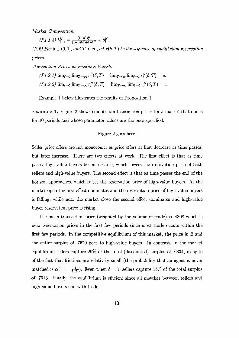
Market Composition:

( ) bH - (l-a)W bH

Pl.1.4 [+1 - (l-a)W+l-W < [. {P.2} For 8 E (0,1]' and T < 00, let r(8, T) be the sequence of equilibrium reservation

pnces.

Transaction Prices as Frictions Vanish:

{Pl.2.1} limo-> 1 limT-> 00 rf(8, T) = limT->oo limO->l rf(8, T) = c.

{Pl.2.2} limo->llimT--+oo rf (8, T) = limT--+oo limo--+l rf (8, T) = c.

Example 1 below illustrates the results of Proposition 1.

Example 1. Figure 2 shows equilibrium transaction prices for a market that opens

for 10 periods and whose parameter values are the ones specified.

Figure 2 goes here.

Seller price offers are not monotonic, as price offers at first decrease as time passes,

but later increase. There are two effects at work: The first effect is that as time

passes high-value buyers become scarce, which lowers the reservation price of both

sellers and high-value buyers. The second effect is that as time passes the end of the

horizon approaches, which raises the reservation price of high-value buyers. At the

market open the first effect dominates and the reservation price of high-value buyers

is falling, while near the market close the second effect dominates and high-value

buyer reservation price is rising.

The mean transaction price (weighted by the volume of trade) is .4308 which is

near reservation prices in the first few periods since most trade occurs within the

first few periods. In the competitive equilibrium of this market, the price is .2 and

the entire surplus of .7520 goes to high-value buyers. In contrast, in the market

equilibrium sellers capture 29% of the total (discounted) surplus of .6834, in spite

of the fact that frictions are relatively small (the probability that an agent is never

matched is aT +1 = lO~4)' Even when 8 = 1, sellers capture 15% of the total surplus

of .7513. Finally, the equilibrium is efficient since all matches between sellers and

high-value buyers end with trade.

13

4.2 Properties of market equilibria in the low cost case

Figure 3 below illustrates the supply and demand schedules for this case. We identify

the trading patterns which may arise in equilibrium and identify the transitions among

them. We also relate the trading pattern to the market composition, and describe

how the market composition evolves over time. We show that if the initial proportion

of high-value buyers in the market is above a critical threshold we identify, then in

a market equilibrium trade is inefficient. If in addition the time horizon is long

then a market equilibrium also exhibits delay. Finally, we show that as market

frictions vanish (i.e., as the discount factor approaches one and the time horizon

grows long), equilibrium transaction prices converge to a competitive equilibrium

price. We establish that in the limit equilibrium delay persists, although its cost

vanishes.

Figure 3 goes here.

In order to illustrate the difficulties that arise in the analysis of the present case,

assume, for the purpose of discussion, that in a market equilibrium (i) traders of the

same type have the same reservation price, (ii) sellers offer either the high-value-buyer

reservation price r[I, or the low-value-buyer reservation price rf, and (iii) r[I > rf·3

\-Vhen a seller offers r[I at date t, he trades only with high-value buyers and obtains

an expected utility of

bf (rf - c) + (1 - bf)(rf - c).

(Recall that 8~~1 = rf - c by El.) A seller who offers rf at date t trades with both

types of buyers, and obtains rf - c. Therefore it is optimal for a seller to offer the

high-value-buyer reservation price if

bf(rf - c) + (1- bf)(rf - c) ~ rt - c,

i.e.,

bH( H S) > L S t rt - rt _ rt - rt .

3Each of these facts is proven in Appendix B.

14

In other words, sellers offer the high-value-buyer reservation price if the probability

that the current partner is a high-value buyer times the gains to trade with high-value

buyers is greater than the gains to trade with low-value buyers. (In both cases, the

gains are calculated relative to the reservation prices, rather than the actual values

or costs.) Writing trt for the ratio (rf - rf)j(rf! - rf), which measures the relative

gains to trade of sellers with low-value buyers versus high-value buyers, the inequality

above can be written as

Hence, in contrast to the low-cost case where the pattern of trade is separating re­

gardless of the market composition, in the present case the pattern of trade at date

t depends on the market composition. Further, the market composition at date t is

determined in turn by the trading patterns prior to t. Thus, the entire sequence of

trading patterns and market compositions must be determined simultaneously.

In spite of this difficulty, we identify the basic properties of market equilibria in

propositions 2 through 4. Proposition 2 establishes some basic facts about equilibrium

price offers and reservation prices.

Proposition 2. Assume that uH > uL > c. Let (p, r, A) be a market equilibrium and

let lE {a, ... ,T}.

Reserua.tion Prices:

(P2.1.1) r? = r[ for every T E {H, L, S} and i :::; nT•

(P2.1.2) r? > max{rt, rf}.

High- Va.lue-Buyer Price Offers:

(P2.2) pPi = rf, for every i :::; nH .

Low- Value-Buyer Price Offers:

(P2.3.1) pfi :::; rf for every i :::; nL .

(P2.3.2) There is c(a, T) > 0 such that for 8> 1 - c(a, T):

(i) If pfi < rf for some i :::; nL , then pf; < rf for every t < land i :::; nL .

(ii) If pfi = rf for some i :::; nL, then pfi = rf for every t > t and i :::; nL .

Seller Price Offers:

15

(P2.4.1) pfj E {rf,rf} for every j:::; nS.

(P2·4.2) If pfj = rf for some j :::; nS, then p~j = rf for every t > f and j :::; nS.

(P2.4.3) If pfj = rf for some j :::; nS, then p~j = r{f for every t < f and j :::; nS.

Seller and Low- Value-Buyer Price Offers:

(P2.5) If pfj = rf for some j :::; nS, then pti = rf for every i :::; n L .

In a market equilibrium all traders of the same type have identical reservation

prices (P2.1.1). The high-value-buyer reservation price is above both the low-value­

buyer and seller reservation prices (P2.1.2). High-value buyers offer sellers their reser­

vation price (P2.2). If the discount factor is sufficiently large, low-value buyers may

initially offer sellers a price below their reservation price, but once a positive propor­

tion of low-value buyers offers the seller reservation price, then all low-value buyers

offer this price at every subsequent date (P2.3.2). Similarly, seller's may initially of­

fer the high-value-buyer reservation price (P2.4.3), but once a positive proportion of

sellers offers the low-value-buyer reservation price, all sellers offer this price at every

subsequent date (P2.4.2). Finally, if at date t a positive proportion of sellers offer

the low-value buyer reservation price, then at date t all low-value buyers offer sellers

their reservation price (P2.5).

TRADIXG PATTERNS

We begin by discussing which trading patterns may arise in equilibrium. A "pure"

trading pattern, in which agents of the same type make the same price offers, specifies

whether sellers' price offers are accepted by high-value buyers, whether sellers' price

offers are accepted by low-value buyers, whether low-value buyers' price offers are

accepted by sellers, and whether high-value buyers' price offers are accepted by sellers.

There are 16 possible pure trading patterns.

Proposition 2 implies that at most three of these pure trading patterns may arise

in equilibrium: Sellers' price offers are accepted by high-value buyers (P2.1.2 and

P2.4.1). High-value buyers' price offers are accepted by sellers (P2.2). Hence P2.1.2,

P2.2, and P2.4.1 rule out all but four of the feasible pure trading patterns. In

addition, P2.5 rules out the trading pattern in which sellers' price offers are accepted

16

by both types of buyers, but low-value buyers' price offers are not accepted by sellers.

Thus, only three pure trading patterns may arise in equilibrium: a separating (S)

trading pattern, where only matches between high-value buyers and sellers end with

trade; a partially-separating (PS) trading pattern, where matches between high-value

buyers and sellers end with trade and matches between low-value buyers and sellers

end with trade only if the buyer proposes; and a pooling (P) trading pattern, where

all matches end with trade. The relation between price offers and reservation prices

in each of these trading patterns are described in Table I.

Trading Patterns Price Offers

Sellers High-Value Low-Value

Separating ps _ rH t - t pH -rS t - t pL < rS t t

Partially-Separating ps _ rH t - t

pH _ rS t - t

pL _ rS t - t

Pooling ps _ rL t - t

pH _ rS t - t

pL _ rS t - t

TABLE I: Equilibrium Pure Trading Patterns when uH > uL > c.

In addition to the three "pure" trading patterns, an equilibrium may also have

"mixed" ones (i.e., ones in which traders of the same type make different price offers).

In particular, an equilibrium may have "S-PS" trading patterns and "PS-P" trading

patter!1.-S. The S-PS trading pattern is the same as S, except that low-value buyers

::mix," i.e., a positive proportion offer the seller reservation price, and a positive

proportion offer a price below the seller reservation price. The PS-P trading pattern

is the same as PS, except that sellers "mix," i.e., a positive proportion offer the

high-value-buyer reservation price and a positive proportion offer the low-value-buyer

reservation price.

Proposition 2 ensures that the PS-P trading pattern arises in at most one period

(P2.4.3). Moreover, when the discount factor is sufficiently high, the S-PS trading

pattern arises also in at most one period, since by P2.3.2 once a positive proportion of

low-value buyers offer the seller reservation price, at subsequent periods all low-value

buyers offer this price.

17

DYNAMICS OF TRADING PATTERNS

Proposition 2 also yields conclusions concerning the order in which trading pat­

terns arise in equilibrium. P2.4.2 establishes that if at date t a positive proportion

of sellers offer the low-value-buyer reservation price, then at every subsequent date

all sellers offer this price. Hence the S, S-PS, and PS trading patterns (when they

arise) precede the PS-P and P trading patterns. P2.3.2 establishes that when the

discount factor is sufficiently close to one the S trading pattern precedes all the other

trading patterns. Furthermore, P2.4.2 and P2.3.2 imply, respectively, that the S-PS

mixed trading pattern precedes PS, and the PS-P mixed trading pattern precedes

P.

It can be shown that if trading patterns Sand P are both visited, then pattern

PS must also be visited. Also, PSis always visited unless the market opens at P.

The mixed trading patterns may be skipped, although the subset of the parameter

space where all market equilibria exhibit mixed trading patterns is not negligible (see

Example 3). The dynamics of trading patterns are illustrated in Figure 4.

Figure 4 goes here.

MARKET COMPOSITION

The market composition at date t is described by bf, the proportion of high-value

buyers in t.he market.. Proposit.ion 3 below relat.es t.his proport.ion t.o the t.rading

pattern and the dynamics of the market composition. Denote by 7r* the ratio (uL -

c)j(uH - c).

Proposition 3. Assume that uH > uL > c. Let (p, r, >.) be a market equilibrium and

let t E {a, ... ,T}.

The Critical Threshold (7r*):

(P3.1.1) If bp < 7r*, then pii = rt for every j ~ nS and bP-t-l = bP.

(P3.1.2) If bp = 7r*, then pf; = rf for every i ~ nL , and either

(i) bP-t-l < bP; or

(ii) bP-t-l = bp, and p~i = rf for every j ~ n S and t 2: t.

18

{P3.1.3} If bp> 7r*, then p;j = rp for every j ~ nS, and bf-t-l < bP.

The Critical Threshold is Eventually Reached :

{P3.2} There is T = T(b/f, Q, 7r*) such that if T> T, then b{1 ~ 7r* for t 2: T.

Proposition 3 therefore establishes that trading patterns and the dynamics of

market composition are governed by the relation of the proportion of high-value

buyers in the market to the critical threshold 7r*. If the proportion of high-value

buyers in the market is below 7r*, then the trading pattern is P (P3.1.1). If the

proportion of high-value buyers in the market equals 7r*, then either the trading

pattern is PS or PS-P and the proportion of high-value buyers in the market is less

than 7r* at the next period, or the trading pattern is P (and remains at P at every

subsequent period) and the proportion of high-value buyers is 7r* at the next period

(P3.1.2). P3.1.1 and P3.1.2 imply that if the proportion of high-value buyers in the

market equals 7r* at some date, at the next date the trading pattern must be P. If

the proportion of high-value buyers in the market is greater than 7r*, then the trading

pattern is either S, S-PS, or PS (P3.1.3). Finally, P3.2 ensures that if the time

horizon is sufficiently long, then eventually the proportion of high-value buyers in the

market is less than or equal to 7r*. Hence, by P3.1.1 and P3.1.2, if the time horizon

is sufficiently long, then the trading pattern is eventually P.

DYNAMICS OF MARKET COMPOSITION

In both the S and the PS trading pattern, as well as in the mixed trading patterns

S-PS and PS-P, the proportion of high-value buyers in the market is falling: in S,

each period a fraction Q of high-value buyers exit the market, while no low-value buyer

exits; in PS a fraction Q of high-value buyers and a fraction ~ of low-value buyers

exit the market each period. In the trading pattern P the same fraction Q of each

type of buyer exits the market at each date, and hence the proportion of high-value

buyers in the market remains constant. Thus, the proportion of high-value buyers in

the market decreases (quickly in S, and more slowly in PS), but once P is reached

(i.e., once this proportion falls below 7r*), it becomes stationary.

A numerical example in which all three trading patterns arise in equilibrium is

19

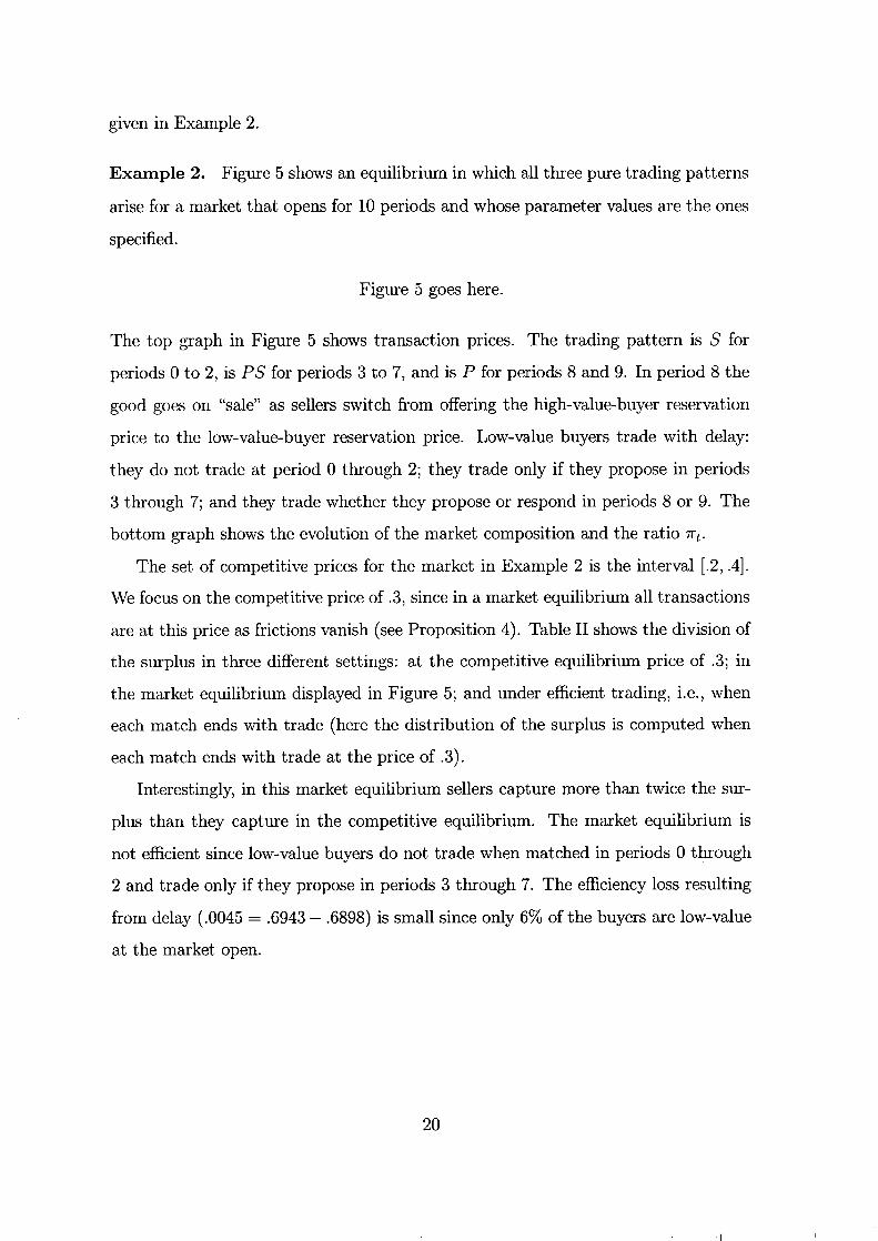
given in Example 2.

Example 2. Figure 5 shows an equilibrium in which all three pure trading patterns

arise for a market that opens for 10 periods and whose parameter values are the ones

specified.

Figure 5 goes here.

The top graph in Figure 5 shows transaction prices. The trading pattern is S for

periods 0 to 2, is PS for periods 3 to 7, and is P for periods 8 and 9. In period 8 the

good goes on "sale" as sellers switch from offering the high-value-buyer reservation

price to the low-value-buyer reservation price. Low-value buyers trade with delay:

they do not trade at period 0 through 2; they trade only if they propose in periods

3 through 7; and they trade whether they propose or respond in periods 8 or 9. The

bottom graph shows the evolution of the market composition and the ratio Kt.

The set of competitive prices for the market in Example 2 is the interval [.2, .4].

We focus on the competitive price of .3, since in a market equilibrium all transactions

are at this price as frictions vanish (see Proposition 4). Table II shows the division of

the surplus in three different settings: at the competitive equilibrium price of .3; in

the market equilibrium displayed in Figure 5; and under efficient trading, i.e., when

each match ends with trade (here the distribution of the surplus is computed when

each match ends with trade at the price of .3).

Interestingly, in this market equilibrium sellers capture more than twice the sur­

plus than they capture in the competitive equilibrium. The market equilibrium is

not efficient since low-value buyers do not trade when matched in periods 0 through

2 and trade only if they propose in periods 3 through 7. The efficiency loss resulting

from delay (.0045 = .6943 - .6898) is small since only 6% of the buyers are low-value

at the market open.

20

High-value Low-value Seller Total

Competitive Equil. .6580 (86%) .0060 (.7%) .1000 (13%) .7640 (100%)

Efficient Trading .5980 (86%) .0055 (.7%) .0909 (13%) .6943 (100%)

Market Equil. .4738 (68%) .0033 (.4%) .2128 (30%) .6898 (100%)

TABLE II: The Division of Surplus

PRICES AS FRICTION VANISH

Proposition 4 below establishes that, as frictions vanish, transaction prices con­

verge to the competitive equilibrium price that splits the gains between low-value

buyers and sellers equally, i.e., the price (uL + c)/2. For each 8 E (0,1] and integer

T, denote by r(8, T) the set of all sequences of equilibrium reservation prices, and

by V(8, T) the set of all sequences of equilibrium expected utilities. These sets are

non-empty by Theorem 1.

Proposition 4: Assume that uH > uL > c. Then jor every f and 'T E {H, L, S}

lim Hm rf(8, T) = lim Hm rf(8, T) = uL

+ c; 0-+1 T-+oo T-+oo 0-+1 2

i.e., transaction prices are competitive as jrictions vanish. Furthermore,

jor each 'T E {H, L}, and

L

Hm Hm v'l(8, T) = lim Hm v'l(8, T) = u + c - c; 0-+1 T-+oo T-+oo 0-+1 2

i. e., as jrictions vanish each agent obtains his competitive equilibrium utility.

DELAY

Although transaction prices converge to a competitive price as market frictions

vanish, delay persists in the limit and, in this sense, the market outcome is not

competitive. Consider a market in which b{f > 7r* and let (p, r, >.) be a market

21

equilibrium. By Proposition 3, so long as the proportion of buyers in the market is

above 7r* then the trading pattern is either S or PS. Define the sequence {Q~} as

ljf = b{f and, for t ~ 0

bH = (1- a)Q~ -HI (1- a)bH + 1- bH '

-t -t

The sequence {Q~} describes the evolution of the market composition as though the

trading pattern is always S. Since the proportion of high-value buyers in the market

falls more quickly in S than in the other trading patterns, then bfI ~ Q~ for all t ~ O.

Therefore, if t is smallest integer such that M! ::; 7r*, then we have bf > 7r* for t < t;

hence the trading pattern is either S or PS for periods 0 through t - 1. If the time

horizon T is sufficiently long that P is eventually reached, then low-value buyers trade

with delay: low-value buyers do not trade when responding prior to t, but do trade

if responding when P is reached. (If the market opens at the S trading pattern, then

low-value buyers do not trade at all if matched initially, but always trade if matched

once P is reached.) Since t is independent of the time horizon T and the discount

factor, equilibrium delay persists for at least t periods even as frictions vanish.

Equilibrium delay can be made to persist arbitrary long, since t can be made

arbitrarily large by choosing b{f near 1. Nonetheless, by Proposition 4 each trader

receives his competitive equilibrium utility as market frictions vanish, and therefore

delay becomes costless.

SYMMETRY

We conclude by discussing the asymmetries that may arise in equilibrium. By

Proposition 2 all high-value buyers follow the same strategy in equilibrium. Also, the

equilibrium strategies of sellers must be the same at every date, except at the PS-P

mixed trading pattern (if it arises) where both the low-value and the high-value buyer

reservation prices are offered by a positive proportion of sellers. Note, however, that

reaching this mixed trading pattern requires that the proportion of high-value buyers

exactly equal 7r* at some date (see P3.1.2).

As for low-value buyers, they all offer the same price except in the S or S-PS

trading pattern. In S, low-value buyers offer prices below the seller reservation price

22

(which sellers reject). Hence low-value buyer price offers are not determined, and

therefore there are asymmetric market equilibria in which low-value buyers make

different (rejected) price offers. Nonetheless, if a market equilibrium exhibits only

asymmetries of this kind, there is also a symmetric market equilibrium which gen­

erates the same trading pattern, market composition and transaction prices at each

date. There is a more significant asymmetry when the S-PS mixed trading pattern

arises. In this case, a positive proportion of low-value buyers offer the seller reser­

vation price, and a positive proportion offer prices below the seller reservation price.

As Example 3 shows, there are markets whose unique equilibrium exhibits the S­

PS trading pattern. Hence existence of a symmetric market equilibrium cannot be

guaranteed.

Example 3: Consider a market with parameter values as given in Example 2, except

that the initial proportion of high-value buyers is now b{f = .92. Also let the market

open only for two periods (i.e., T = 1). Note that whatever the trading pattern is at

date 0, the proportion of high-value buyers at date 1 satisfies

bH > (l-a)b{f * .4-.2 1 - ( )bH bH = .85185 > 1f = 2 = .25. I-a 0 +1- 0 1-.

Hence at date 1 sellers offer pr = rf = uH = 1. Also as rf > rr (because rf

uL > c = rf), low-value buyers offer pf = rf = c = .2. Therefore, in a market

equilibrium the trading pattern at date 1 is PS, and the traders' expected utilities

are 1I;.H = ~(UH - c) = ~(1 - .2) = ~, 1I;.L = ~(UL - c) = H.4 - .2) = io' and

VIS = ~bf(uH - c) = ibf(1- .2) = ~bf, where bf remains to be determined.

We must now determine the traders' strategies at date O. By Proposition 2, three

trading patterns are possible: S, S-PS, or PS. Suppose that the pattern of trade at

date 0 is S. Then bf = .85185, and rg = c+811;.s = .2+ .9(~)(. 85185) = .35333. Since

r{; = uL - 611;.L = .4 - .9(210) = .355, we have rg < r{;. But then low-value buyers

must offer the seller reservation price at date 0 (see Lemma 2.2), and therefore the

pattern of trade is not S.

Suppose that the pattern of trade at date 0 is PS. Then

H (1 - a)b{f b1 = (1 _ a)b{f + (1 - ~) (1 _ b{f) = .88462,

23

and rg = .2 + .9( i) (.88462) = .35923 > .355 = rt. But then low-value buyers must

offer a price below the seller reservation price at date 0 (see Lemma 2.3), and therefore

the pattern of trade is not PS.

Since a market equilibrium exists, then the trading pattern at date 0 must be

S-PS. Indeed, suppose that a proportion )..L1 = .29029 of low-value buyers offer

p~l = rg, whereas a proportion )..L2 = 1 - )..L1 of low-value buyers offer p~2 < rg. Then

(1- a)bH

bH = 0 = .86111 1 (1 - a)b{f + (1 - %)..L1) (1 - b{f) ,

and rg = .2+.9(i)(. 86111) = .355 = rt; bothp~l andp~2 are optimal offers (i.e., low­

value buyers are indifferent between trading or not trading at the sellers' reservation

price). Hence, the strategy distribution described is a market equilibrium.

5 Concluding Remarks

Previous work studying the properties of decentralized markets in which traders are

asymmetrically informed (e.g., Samuelson (1992), Serrano and Yosha (1996)) imposes

ex-ante restrictions on transaction prices (forcing each transaction to be at one of at

most three possible prices). Such restrictions seem unnatural in models whose aim

is to develop a theory of price formation. Ex-ante price restrictions may artificially

restrict the possibilities for trade: even if a buyer and a seller, when bargaining, have

gains to trade relative to continuing to search, there may be not be a feasible price

below the buyer's and above the seller's reservation prices. Price restrictions may

also qualitatively affect the results (e.g., Serrano and Yosha (1996) find that when

frictions are small equilibrium is efficient, while we find that the equilibrium may

be inefficient). Ex-ante price restrictions also seem inconsistent with decentralized

trading since an external authority must be relied upon to enforce them.

In our framework, transaction prices, the pattern of trade, and the distribution

of the characteristics of the active traders are determined endogenously. Our results

contribute to understanding how in markets these variables are interrelated and how

they evolve dynamically over time. Our findings illustrate that markets may exhibit

24

interesting dynamics, and these dynamics persist as frictions vanish even though

transaction prices become competitive. The model we introduce is useful for inves­

tigating how the institutional setting (i.e., the bargaining rules) and the nature of

uncertainty (i.e., whether it is one-sided or two-sided) influence market dynamics and

the properties of market equilibria. These are important issues which we leave for

future research.

6 Appendix A: Existence of Market Equilibria

We establish existence of a market equilibrium by means of a fixed point argument.

Market outcomes are completely described by a triple (z, (3, p) specifying, respectively,

the trading pattern, market composition, and reservation prices at each date. As we

establish in Appendix B, in equilibrium high-value buyers offer the seller reservation

price (L6.1); low value buyers offer the seller reservation price or less (L2); and sellers

offer either the high-value or low-value buyer reservation price (L3.1). Thus, we can

simplify the representation of trading patterns by focusing on the proportion zf of

low-value buyers who offer the seller reservation price and the proportion zf of sellers

who offer the low-value buyer reservation price. (Then 1 - zf is the proportion of

low-value buyers offering a price below rf and 1 - zf is the proportion of sellers

offering the price rfl.) The sequence of equilibrium trading patterns is represented as

Z = (zo, ... ,zr), where Zt = (z;, zi) E [0, IF. The market composition at each date

is described by (3 = ((30,· .. ,(3r), where (3t E [0,1] is the proportion of buyers in the

market at date t who have a high value. Reservation prices at each date are given by

P = (Po,··· ,Pr), where Pt = (pfl,Pt,pf) E [0,1]3.

The strategy of the proof of existence is as follows: we construct a mapping r.p

which for each arbitrary triple (z, (3, p) provides the trading patterns that result when

traders' price offers are optimal, and the market composition and reservation prices

resulting from these new trading patterns. As we shall see the mapping r.p is upper

hemicontinuous and non-empty valued, but it may not be convex valued. Hence we

cannot apply Kakutani's Fixed Point Theorem. Cellina (1969) has shown, however,

25

that if for each (z, j3, p), cp( z, j3, p) is the image of a convex set under a continuous

function, then cp has a fixed point. Specifically, Cellina establishes the following

theorem:4

Theorem (Cellina 1969, Theorem 2). Let K be a non-empty compact convex subset

of a Banach space. Let cp and, be two upper hemicontinuous correspondences from

K into K such that for each x E K, cp(x) is closed and ,(x) is convex. Let f

be a continuous function from the graph of , into K such that for each x E K,

cp(x) = {f(x, y) lyE ,(xn. Then cp has a fixed point in K.

With this result in hand we prove Theorem 1.

Proof of Theorem 1: Let T < 00, (uH,uL,C) E [0,1]3 with uH > max{uL,c},

b/f E (0,1),8 E (0,1]' and a E (0,1). Write Q = (1 - a)Tb/f, and denote by K the

set of triples (z,j3,p) such that z E [0, Ij2(T+1) , j3 E [Q,b/f]T+1, and pE [O,I]3(T+l)

satisfies PT = (p!j,p!;,p¥) = (uH,uL,c), and for t < T, PP - pf 2: 0, and p[I - pr 2:

(1 - a81-6~~;g::::r-t)(uH - c). Note that K c [0,1]6(T+1) is a non-empty compact

convex set.

The mapping cp : K -» K is constructed as follows: Let , : K -» K be given for

(z,j3,p) E K by ,(z,j3,p) = (,Z(z,j3,p),j3,p), where

{(I, In if j3t(p[I - pf) < pf - pr

{I} x [0,1] if j3t(p[I - pf) - pf - pr

,:(z, j3, p) = {(I, on if j3t(p[I - pr) > pf - pr> ° [0,1] x {O} if pf - pr °

{(O, on if pf - pr < 0,

for each t E {O, ... ,T}. Note that j3t(p[I - pf) > ° for t E {O, ... ,T}, whenever

(z, j3, p) E K. Hence, is well defined. Also note that, is an upper hemicontinuous

non-empty compact convex valued correspondence.

Now let D be the graph of, (i.e., the set {(z, j3, p; z, /3, p) I (z, /3, p) E ,(z, j3, pn),

and let f : D -4 K be given for (z, j3, p; z, /3, p) E D by f(z, j3, p; z, /3, p) = (z, 9(z), h(z, /3, p)),

4See also Border (1985), Theorem 15.1, page 72.

26

where 9 is defined as go(z) = b!f, and for t > ° (2) = (1 - a)gt-1(Z)

gt (1- 0:)gt-1(2) + (1- %(2t-1 + 21-1))(1- gt-1(2)) ,

and his defined as hT(z,(:J,p) = (uH,uL,C) and for t < T

(1- 8)uH + 8(%pr+1 + %Z41Pt+1 + (1 - %(1 + Zf+1))P~1) ht(z, (:J, p) = (1 - 8)uL + 8(%zt+1pr+1 + (1 - %Zt+1)Pt+1)

(1 - 8)c + 8(% (zf+1 (Pt+1 - pr+1) + (1 - Zf+1)(:Jt+1 (P~l - pf+1)) + pf+1)

The function 9 gives the market composition that results when the sequence of trad­

ing patterns is given by 2 and the initial proportion of high-value buyers is b!f.

The function h gives the reservation prices that result when the sequence of trad­

ing patterns, market compositions, and reservation prices is given by 2, (:J, and p,

respectively. We show that f is well defined, i.e., that for each (z,/3,p;z,(:J,p) E D,

f(z, /3, P; Z, (:J, p) E K.

Let (z, /3, P; Z, (:J, p) E D. We show that f(z, /3, P; Z, (:J, p) = (2, jJ, p) E K. Clearly

2 = z E 't(z, /3, p) C [0, 1j2CT +1). We prove by induction that

tH A H (1 - a) bo ::; /3t ::; bo ,

for t E {O, ... ,T}, therefore establishing that jJ E [Q, b!f]T+1. (Note that for t ::; T,

(1- a)tb!J 2:: (1- alb!J = /1.) Since ,130 = b!J, assume that the claim holds at [2:: 0.

vVe show that it holds at t + 1. By the definition of 9 we have

A (1 - a)jJl /3l+1 = A a L SA'

(1 - o:)/3l + (1 - "2(Zt + Zt ))(1 - /3l)

Since jJl+1 is increasing in both zt and zf, and zf ::; 1 and zf ::; 1, we have

A (l-o:)jJl A H /3l+1 < A A = /3l < bo . - (1 - o:)/3l + (1 - 0:)(1 - /3l) -

Also since zf 2: ° and zf 2: 0, and ° < o:jJl < 1, we have

jJl+1 2:: (1 A- o:)jJl A = (1 - o:)j3l 2:: (1 - o:)jJl2:: (1 - a)l+1bff. (1 - o:)/3l + (1 - /3l) 1 - a/3l

Finally, we show that P E [0, l]3CT+1) , and satisfies PT = (uH,uL,C), and for t < T,

H L d H S ( s:1-6T- tC1-a)T-t)( H ) B h d fi f h Pt - Pt 2:: 0, an Pt - Pt 2:: 1 - O:u 1-6(1-a) U - c. Y tee nit ion 0 ,

27

PT = (uH,uL,c). We show that 0::; P;::; 1 for t E {O, ... ,T} and T E {L,H,S},

and therefore that P E [0, Ij3(T+I). Since (z, {3, p) E K, then pr+! ::; 1, pt+I ::; 1, and

PEt-I ::; 1, and since in the expressions for p~ and pf the coefficients on pr+I' pt+! ,

and PEt-I sum to one, we have

p; ::; (1 - 8)uT + 8::; 1,

for T E {H, L}. Rewriting the expression for pr as

the same argument yields

pf ::; (1 - 8)c + 8 ::; 1.

Also (z, {3, p) E K implies that pr+I ~ 0, pt+! ~ 0, and PEt-I ~ 0, and since the

coefficients of these terms in the expressions for p~, pf, and pf are nonnegative, we

have p; ~ 0 for T E {H,L,S}.

Now for t < T, we have

p~ - pf = (1 - 8)(uH - uL) + 8[~(1 - zt+!)(pr+! - pt+I) + (1 - ~(1 + Zr+I))(p~1 - pf+I)]·

Since (1- 8)(uH - uL

) ~ 0 and (1- zf+I) (pr+I - pf+!) ~ 0 (because zf+! < 1 implies,

by the definition of 'Y~ that pt+! ::; pr+I)' and PEt-I - pt+I ~ 0 (because (z, {3, p) E K),

h AH AL > 0 we ave Pt - Pt _ .

Also for t < T, we have

p~ - pf (1 - 8)(uH - c) + 8[1 - ~(1 + Zf+l) - ~ (1 - Zf+!){3t+I)](P~l - pr+l)

> (1 - 8)(uH - c) + 8(1 - a)(p~1 - pf+!).

Since (z, {3, p) E K, we have

and therefore

1 - 8T - t - I (1 - af-t- 1

> ((1- 8) + 8(1 - a)(l - a8 1 _ 8(1 _ a) ))(uH - c)

1 - 8T - t(1- af-t H (1 - a8 8( ) )(u - c).

1- I-a

28

Hence f is well defined, and since both 9 and h are continuous functions, f is a

continuous function. Now let 'P be given for (z, (3, p) E K by

'P(z, j3, p) = {f(z, j3, p; E, /3, p) I (E, /3, p) E "((z, j3, pH·

Clearly 'P is an upper hemicontinuous closed valued correspondence. Cellina's Theo­

rem therefore implies that 'P has a fixed point.

Let (z, j3, p) be a fixed point of 'P. We construct a market equilibrium (p, r, A) as

follows: We use binary strings m = (mo, ... ,mT) E {a, I}T+l to index low-value

buyers and sellers strategies. For T E {B,L} and m = (mo, ... ,mT) E {a,I}T+l

define

T

ATm = IT (z;)mt(1 - z;)l-mt ,

t=o

and let MT = {m E {a, IV+l I ATm > a}. Note that L:mEM"T ATm = 1.

HIGH-VALUE BUYERS: All high-value buyers follow the same strategy, given by

rf = pp and pp = pr for t E {a, ... ,T}. Hence AH = 1.

LOW-VALUE BUYERS: Let x = (xo, ... ,XT) be an arbitrary vector of real numbers

such that Xt < pr for t E {a, ... ,T}. For m E ML define the low-value buyer strategy

(pLm , rLm ) as rfm = pf and

pr ifmt=1

otherwise,

for t E {a, ... ,T}.

SELLERS: For m E MS define the seller strategy (pSm, rSm ) as rfm = pr, and

{

pf pfm =

pp otherwise,

if mt = I

for t E {a, ... ,T}.

For t E {a, ... ,T} and T E {L,B}, define M; = {m E MT I mt = I}, i.e.,

MF (MtS ) contains the indexes corresponding to low-value buyer (seller) strategies

which offer sellers (low-value buyers) their reservation price at date t. Straightforward

29

calculations (which we omit) show that under the laws of motion given in Section 2.1,

the strategy distribution (p, r, >.) defined above satisfies

mEM[

for each t E {O, ... ,T} and T E {L, S}. In other words, at each date t the proportion

of low-value buyers (sellers) in the market who offer sellers (low-value buyers) their

reservation price is zf (4).

We prove that (p, r, >.) is a market equilibrium. Given (p, r, >'), let bP be computed

according to the laws of motion developed in Section 2.1. We show by induction that

bP = (3t for t E {O, ... ,T}. Clearly bt! = 90(z) = (30' Assume that bp = 9[(Z) = (3[

for f 2 0; we show that bP-t-l = (3[+1' By definition we have

b!i = bp MP HI b!i 1I!i + bI: ~ >.!:m lI!:m .

t rt t L.JmEML t rt

In this expression, MP is given by

For each m' E MS we have p!i = p§ = r~ml and p~ml < r!i (because p~ml E {pI: p!i} t tt' t - t t t't'

and (z,!3,p) E K implies pr ::; pP = rf)· Thus, I(pp,rfm/) = I(rf,pfm/) = 1 for

each rn' E lv1s , and hence

Also for Mfm we have

Note that for each m' EMs, m[ = 1 implies I (pfm , rfm/) = 1, and m[ = 0 implies

I(pfm,rfm/) = 0; also I(rfm,pfm/) = 1 whenever m' E Mf, and I(rfm,pfm/) = 0

whenever m' t/:. Mf· Therefore we have

30

Substituting in the expression for b?-t-l' and noticing that bp = f3t by the induction

hypothesis, we get

Since mt = 1 if m E Mf and mt = D if m r/:. Mf, we have

mEMf

Also as noted earlier LmEMT Ai"' = z[ for each T E {L, S}. Hence, the expression for t

b?-t-l simplifies to

H f3t(1- et) bt+1 = f3 ( ) ( f3 )( 0< L 0< S)· t 1 - et + 1 - t 1 - "2 Zt - "2Zt

Therefore b?-t-l = gt+ 1 (z) = f3 t+ 1·

Now we establish by induction that (p, r, A) satisfies Condition El for t E {D, ... ,T}.

Since VT+1 = D for T E {H,L,S}, the definition of h yields

H H H H D J;:T/"H U - r T = u - PT = = U VT+l'

and

L L", L L 0 nTL U - r T = U - PT = = U v T +1 ,

S"' S 0 nTS rT - C = PT - C = = U vT+l.

Thus, El holds at T.

Suppose that El is satisfied at t + 1 ::; Tj we show that it is satisfied at t, i.e.,

u H - rp = 0Vi-!I. For high-value buyers we have

mE MS mEMS

Since P?-t-l = P¥+1 = rf.;! for each m EMs, J(P?-t-l' rf;l) = 1 for each m EMs.

Therefore

P H H S t+l = U - Pt+l·

31

Also

R~l = L (UH

- pf+1).f+1I(r~1,pf+1) + (1 - L ).f+/(r~1,pf+1))8Vf~2· mEMs mEMs

Since Pf+1 = pr+1 :s; P~l = r~l when mt+1 = 1, and Pf+1 = P~l = r~l when

mt+1 = 0, we have I(r~1,pf+1) = 1 for each m E MS. Thus

RH -t+1 -mEMr+1 mEMS\Mr+l

- uH - (Zr+1pr+1 + (1 - Zr+1)p~l)·

>From the definition of Vf~l in Section 2.2, and as 8Vf~2 = uH - P~l by the

induction hypothesis, we have

where the last equality holds by the definition of h. Therefore El holds at t for

T=H.

\\le now establish that El holds at t for each low-value buyer strategy m E AIL,

i.e.) u L - rfTn = 811[:'1. For m E ML) we have

S· LTn - S - STn' Ch' E MS·f - - 1 d LTn _ _ < S _ STn' mce Pt+1 - Pt+1 - rt+1 lor eac m 1 mt+1 - ,an Pt+1 - Xt+1 Pt+1 - rt+1

if mt+1 = 0, and since 8Vf~2 = uL - pr+1 by the induction hypothesis, we have

We show that ptI can be written as

P LTn L [L S (1 L) L 1 t+1 = u - Zt+1Pt+1 + - Zt+1 Pt+1 .

32

If Zf+1 = 0, then mE+! = 0, and therefore

PLm _ L L _ L [L S (1 L) L 1 E+1 - U - PE+1 - u - ZE+1PE+1 + - ZE+1 PE+1 .

If zt+ 1 = 1, then mE+ 1 = 1 and therefore

PLm L S L [L S (1 L) L 1 E+! = U - PE+! = U - ZE+1PE+1 + - ZE+! PE+! .

If zt+1 E (0,1), then P¥+1 = pt+1 by the definition of ,,(, and hence

P Lm L [L S (1 L) L 1 E+! = U - ZE+!PE+1 + - ZE+1 PE+!

whether mE+1 = 1 or mE+! = 0.

For m E M L , we have

RLm E+1 =

m'EMf m'EMf

L L - U - PE+1'

where the last equality holds since, by the induction hypothesis, 8Vf~2 = uL - pr+1'

Summing up, we have

where the last equality follows from the definition of h. Since mE ML was arbitrary,

therefore El holds at t for all m E M L .

\;Ye show that El holds at f for each seller strategy m E MS, i.e., c - rfm = 8Vf~i'

For m E MS, we have

PSm E+1 =

m'EML

+(1 - b~1I(rY-t-l>pfB) - (1- b~1) L Af;; I (r;;; ,pf';1))8Vf~2' m'EAfL

33

Since pf::-1 = Pt+1 ~ PP-t-1 = rP-t-1 if mt+1 = 1, and pf::-1 = PP-t-1 = r~1 if mt+l = 0, and

since 8Vj-!'2 = pr+l - c by the induction hypothesis, we have

S { Pt+1 - c if mt+l = 1

Pt+l = f3t+l (PP-t-1 - c) + (1 - f3t+1)(pr+l - c) if mt+1 = 0,

where we have replaced bP-t-1 with f3 t+l' We show that P~l can be written as

This clearly holds if either Zr+1 = ° (and hence mt+l = 0) or zr+l = 1 (and hence

mt+1 = 1). If zr+1 E (0,1) then f3t+l (PP-t-1 - pr+l) = Pt+l - pr+1 by the definition of ,,(,

which is the same as Pt+1 = f3t+1PP-t-1 + (1 - f3t+1)pr+l' Hence

P~l - pt+1 - c = f3t+1 (PP-t-1 - c) + (1 - f3t+1)(pr+1 - c)

- Zr+1pt+1 + (1 - zf+l)(f3t+1PP-t-1 + (1 - f3t+l)p¥+l) - c.

For m E MS we have

+ (1 - bP-t-1 I (PP-t-1 , rf;1) - (1 - bP-t-1) L >..f;; I (pf;; , rf;1) ) 8Vt!'2. m'EML

U · th t H S Sm Lm' S Sm'f' 1 Lm' S smg a Pt+1 = Pt+1 = rt+1, Pt+l = Pt+l = rt+1 1 mt+l = 'Pt+1 = Xt+l < Pt+l =

rf.::'1 if m[+1 = 0, and 8Vr!'2 = pit! - c by the induction hypothesis we have

RiB = f3t+1 (p¥+l - c) + (1 - f3t+l) L >..f;; (P¥+1 - c) m'EMhl

+(1 - f3t+l - (1 - f3t+1) L >.f;;)(P¥+1 - c). m'EMhl

H RSTn - S ence t+l - Pt+l - c.

Substituting these formulas into the expression for Vj-!'1 and using that 8Vj-!'2 =

pr+l - c by the induction hypothesis, we have

8Vj-!'1 8; (Pt~l + Rf;l) + (1 - a)82Vj-!'2

8[; (zf+1Pt+l + (1 - Zr+l) (f3t+1PP-t-1 + (1 - f3t+l)pr+l) + pr+1 - 2c) + (1 - a)(pr+l - c: - 8[%(zr+l(Pt+l - pr+l) + (1- zr+l)f3t+l(PP-t-l - pr+l)) + pr+ll- Dc

S Pt - c,

34

where the last equality follows from the definition of h. Therefore El holds at [ for

all m EMs.

Finally we show that (p, r, >.) satisfies E2 for t E {O, ... ,T}. For buyers, E2

requires that pr maximize

(Note that for low value buyers P{(x) does not depend upon the particular low-value

buyer strategy being followed, since V;~1 = uL - pf by El, and so we write PP(x)

instead of ~Lm(x).) Since rfm = pf for m EMs, P{(x) is given by

If x > pr, then p{(pf) > Pt(x), as

If pr > pr, then Pt(pf) > Pt(x) for x < pr, as

PtT(pf) = UT - pf > UT - pr = Pt(x).

If pr = pr, then Pt(pr) = Pt(x) > Pt(x' ) for x < pr < x', as

Finally, if pr < P(, then Pt (x) > P{(X') for x < pr :::; x', as

For high-value buyers we have pr ~ pr and therefore pr = pr maximizes PtH(x).

For low-value buyers, let m E ML be arbitrary. If zf = 1, then pf ~ pf by the

definition of 'Y and so pfm = pr maximizes ptL (x). If ° < zf < 1, then pf = pr and

therefore pfm = pr (if mt = 1) and pfm = Xt < pr are both maximizers of PtL(x). If

zf = 0, then pf :::; pr and therefore pfm = Xt < pr maximizes PP(x).

Finally, we show that sellers strategies satisfy E2. Let m E MS. We must show

that for each t E {a, ... ,T}, pfm maximizes

m'El'vlL

+(1 - bJI I(rJI, x) + (1 - bJI) L >.~m' I(r~m', x))8V;!i. m'EML

35

As shown earlier, br = f3t . Since rf = pr, rfml = pf for each m' E M L , and since

8~!1 = pf - c by El, this expression reduces to

Note that for x < pf, since pf ~ pr we have

Also note that since pf ~ pr, then for x > pr, we have

Finally, for pf < x < pr, we have

Thus for arbitrary x, ~Sm(x) ~ max{ptSm(pf), ~Sm(pr)}.

If zf = 1, then 0 < (pr - pf)f3t ~ pf - pf and therefore

P Sm( H) _ S (H S)f3 < S L S _ pSm( L) t Pt - Pt - C + Pt - Pt t - Pt - c + Pt - Pt - t Pt·

Hence pfm = pf maximizes ptSm(x). If 0 < zf < 1 then 0 < (pfI -l/)f3t = pf - pf

and therefore

P Sm ( H) _ S (H s)f3 _ L _ pSm ( L) t Pt - Pt - c + Pt - Pt t - Pt - C - t Pt·

Hence both pfm = pf (if mt = 1) and pfm = pr (if mt = 0) maximize ptm(x). If

zf = 0, then (pr - pf)f3t ~ pf - pf and therefore

P Sm( H) _ S (H S)f3 > S L S _ pSm( L) t Pt - Pt - C + Pt - Pt t - Pt - C + Pt - Pt - t Pt·

Hence pfm = pr maximizes ptSm (x). D

7 Appendix B: Proofs of propositions 1 to 4

Before proving propositions 1 to 4, we establish a number of lemmas. Throughout

assume that (p, r,.\) is a market equilibrium.

36

Lemma 1 establishes that in a market equilibrium all type T traders have identical

reservation prices and expected utilities.

Lemma 1. For each T E {H, L, S}, each k, k' E {I, ... ,nT} and each t = 0, ... ,T :

(L1.1) r? = r;k', (L1.2) R? = R?', (L1.3) prk = pt

Tk', and

(L1.4) YtTk = YtTk'.

Proof: We show that if Vl~.\ = Vl;~ for T E {H,L,S}, and k,k' E {I, ... ,nT},

then L1.1 - L1.4 hold at t. This establishes the Lemma as V;~l = V;!'l = 0 for

T E {H,L,S}, and k,k' E {I, ... ,nT}.

Assume that Vl;l = Vl;~ for T E {H,L,S}, and k,k' E {I, ... ,nT}; then for

T E B, E.1 implies

For T = S, E.1. implies

Hence L 1.1 holds at f.

S· Tk - Tk' d T7Tk - T/Tk' th RTk - RTk' d th £ L1 2 h Id t t-mce r[ - r[ an ~f+l - Vf+l' en [ - [ ,an ere ore . 0 sa.

F B T/To V To , d Sj Sj'. 1· pTO pTo,. h·· h Or T E ,vl~I = l~l an rl = r l Imp les l' = l" smce ot erwlse elt er

p? or p?, does not satisfy E.2. An analogous argument shows P(j = ptj'; hence

L1.3 holds at f. Finally, trader Tk'S expected utility at t is

Since L1.2 and L1.3 hold at t, and since Vl;l = Vl;~, L1.4 holds at t. 0

Hereafter we write r[, R[, Pt, and YtT for the equilibrium reservation prices and

expected utilities of a trader of type T E {H, L, S} at time t ~ T. Also we denote by

Pt (x) the expected utility of a buyer of type T who is matched and proposes a price

of x at date t and follows his equilibrium strategy thereafter, i.e.,

pr(x) = (UT - x)I(x,rf) + (1- I(x,rf))8Yt~1.

37

Analogously, we denote by R[ (x) the expected utility of a buyer of type T who is

matched, employs a reservation price of x at date t, and follows his equilibrium

strategy thereafter, i.e.,

n S n S

R;(x) = 2)uT - p~j) .. ~j I(x,p~j) + (1- L)..~j I(x,p~j))8~:1'

j=l j=l

Neither P{(x) nor R[(x) depend on which equilibrium strategy a type T buyer might

be playing since by Lemma 1 buyers of the same type have identical continuation

payoff ~~1'

For sellers, we denote by pl(x) the expected utility of a matched seller who

proposes a price of x at date t and follows his equilibrium strategy thereafter, i.e.,

TEB TEB

Analogously, we denote by Rf (x) denote the expected utility of a matched seller

who employs a reservation price of x at date t and follows his equilibrium strategy

thereafter, i.e.,

TEB i=l TEB i=l

Condition E.2 can be written as p? E argma.xx P{(x) for T E {H, L, S} and

k :S nT•5 Further, if r[ satisfies E.1, then for any x we have R[(r[) ~ R[(x); i.e.,

r[ E argmaxx R[(x). This follows from r[ = UT - 8~~1' as R[(r[) - R[(x) can be

written as

i=l

which is always non-negative since I(r[,p~j) - I(x,p~j) > 0 implies r[ - p~j > 0, and

I(r[,p~j) - I(x,p~j) < 0 implies r[ - p~j < O.

Lemma 2 characterizes buyers' optimal price offers.

5Note that the sequences P?}i=o for T E {H,L,S} and k E {l, ... ,nr }, and {bni=o for

T E {H, L} are unaffected by a single trader offering a price different from his equilibrium offer.

38

Lemma 2. For each T E B, each i ::; n T and each t = 0, .. , ,T :

(L2.1) p;i ::; rf, and

(L2.2) r[ > rf implies p;i = rf, and

(L2.3) r[ < rf implies p;i < rf.

Proof: Let T E B, i ::; n T and t E {O,... ,T}. We prove L2.1. Suppose that

p;i ;::: rf. Condition E.2 implies that Pt(p;i) ;::: Pt(x) for x ;::: O. In particular,

Pt(p;i) ;::: Pt(rf), i.e.,

h To < S Th To > s, l' To s· Ti < S Th £ L2 1 h Id ence Pt' _ rt . us Pt' _ rt Imp Ies Pt' = rt ; I.e., Pt _ rt . ere ore . 0 s

We prove L2.2. Suppose p;i =I rf; then L2.1 implies p;i < rf. By E.2 we have

T T £TTT PTO( TO) > PTO( S) T S U - rt = U Vt+I = t' Pt' _ t' rt = u - rt ,

which yields r[ ::; rf.

Finally, we prove L2.3. Suppose p;i ;::: rf; then L2.1 implies p;i = rf. Let x be

such that rf > x ;::: O. By E.2 we have

T S PT( Ti) > PT() T T U - rt = t Pt _ t X = u - rt ,

, . b' l' T> S n wmc 1 llnp IeS Tt _ r t . LJ

For each t such that rf - rf > 0, we write 1ft for the ratio (rf - rf)j(rf - rf).

Lemma 3 characterizes sellers' optimal offers.

Lemma 3. For each j ::; nS and each t = 0, ... ,T, if rf > max{rf, rf} then

(L3 1) Sj {L H} . Pt E rt , rt ,

(L3.2) bP < 1ft implies p~j = rf,

(L3.3) bP = 1ft implies Pl(rf) = ptS(rf), and

(L3.4) bP > 1ft implies p~j = rf.

Proof: Let j ::; nS and t ::; T, and assume that rp > max{rf, rf}. We establish

L3.1.

39

S L H S.) L S) Ifp/ :S rt , then I(rt ,Pt] = I(rt ,Pt] = 1. By E.2 we have

S· S( s) S( L) L Pt] - c = Pt Pt J ;::: Pt rt = rt - c,

and therefore p~j = rf.

If L s· H h rt < Pt] :S rt ,t en

As bf > 0 (because bff E (0,1) and et < 1), it follows that p~j ;::: rf. Hence p~j = rf.

We show that p~j :S rf, which establishes L3.1. Suppose p~j > rf; then E.2

implies

i.e., rf;::: rf· This contradicts rf > max{rf,rf}, and proves p~j :S rf.

Now we prove L3.2 - L3.4. If rf > rf, then'Trt > O. Since rf > rf, the definitions

of ptS (x) and 'Tr t yield

ptS(r{f) = b{f (rf - c) + (1 - bf)(rf - c) = (;: - 1) (rf - rf) + pts(rf)·

If bfI < 'Trt, then Pl(rf) < Pl(rf) and therefore p~j = rf· If bfI = 'Trt, then

ptS(rf) = pp(rf)· Finally, ifbf > 7rt, then Pt (rf) > Pt(rf) and thereforep~j = rf·

If rf :S rf, then 7rt :S 0 and therefore bf > 'Trt· We must show that p~j = rf·

Since bfI > 0 and rf > rf ~ rf, we have bf rf + (1 - bfI)rf > rf, and therefore

S H hence Pt] = rt . 0

Lemmas 4 and 5 establish some inequalities between reservation prices and be­

tween expected utilities for the different types of traders.

Lemma 4. For each t = 0, ... ,T :

(L4.1) rf > rf, and

(L4.2) ~H _ ~L < uH _ uL .

40

Proof: We establish Lemma 4 by induction. As V~l = V;+l = 0, E.1 implies

rT = UT for 7 E B; hence r,f! = u H > uL = r~, and therefore L4.1 holds for t = T.

Also as rf = c, we have r!J. > max{r~,rf}, and L3.1 implies Pf E {r!J.,r~}; hence

vI! ::; ~(uH - c) + ~(uH - uL), and V; = ~(uL - c). Thus, as 0: < 1 we get

and therefore L4.2 holds for t = T.

Assume that L4.1 and L4.2 hold for t = k + 1 ::; T. We show that they hold for

t = k. By E.1 we have r'k = UT - 8V{+l' and therefore

where the strict inequality follow from the induction hypothesis. Thus L4.1 holds for

t = k.

We show that vt - VkL < uH - uL . Let i ::; n H. Since Pf: > Pf:(p-J:i) and

Rf 2: Rf(r-J:i) by El and E2, respectively, we have

Also the induction hypothesis yields

P H pL{~H;\ k - k \1'k J J(p-J:;, rZ)( uH - uL

) + (1 - J(p-J:i, re) )8(vl!1 - vl+1)

< u H _ uL ,

and

j=l j=l

Therefore

vt - VkL < ~(PkH - pf(pfi) + R-J: - Rf(rfi)) + (1 - 0:)8(Vk!1 - Vk~l)

< u H _uL .

Hence L4.2 holds for t = k. 0

41

Lemma 5. For each t = 0, ... ,T :

(L5.1) rf > rf, and

( ) H liS (H ) 1_8T - t+1(1_0)T-t+1

L5.2 ~ + v t ~ Q U - C 1-8(1-0) .

Proof: First we show that rf > rf implies p tH + Rf ~ uH - c. Suppose that rf >

rf; then p~i = rf for each i ~ nH by L2.2. Thus

and

(p~i - c)I(p~i, rf) + (1 - I(p~i, rf))(rf - c) = rf - c.

Since pfi ::; rf for i ::; nL by L2.1, we have

(pfi - c)I(pfi, rf) + (1 - I(pfi, rf))(rf - c) = rf - c.

Hence

TEE i=l TEE i=l

and therefore ~H + Rf = uH - rf + rf - c = uH - c.

Next we establish that rf > rf implies Rf + p tS ::; uH - c. Suppose rf > rf;

since rf > rf by L4.1, then rf > max{rf, rf} and therefore p~j E {rf, rf} by L3.1.

If p;j = rf, then L3.4 implies bf ::; 7rt, and since bf > 0, we have rf - rf > 0 and

£ S S If S H h H S I h s· S Th H S there ore Pt] > rt · Pt] = rt ~ t en as rt > rt we a so ave Pt] > rt . us rt > rt

implies I(rf,p~j) ~ I(rf,p~j) for j ::; nS, and therefore we have

( H s· s.) (H s· (S ) (L s.) S ) ( (L s.))( S ) I rt ,p/ )(p/ - c + (1 - I rt ,p/)) rt - c 2:: I rt ,p/ (p/ - c + 1 - I rt ,Pt] rt - c ;

( ",ns s· ) Hence recall L..Jj=l At] = 1

TEE

Thus

42

Also

Summing up we obtain RfI + pt :::; uH - c.

We establish Lemma 5 by induction. Since V;~1 = 0, E.1 implies r¥ = uH >

C = rf, and therefore L5.1 holds for t = T. Moreover, since r¥ > rf, we have

pf! + Rf :::; uH - c, and R¥ + Pf. :::; uH - c. Hence, since a < 1, for t = T we have

a 1 - 8T -t+l(1 - a)T-t+l V;S + V;H = _(pS + R S + pH + RH) < a(uH - c) = a(uH - c)-------'-----

T T 2 T T T T - 1 - 8(1 - a)

Therefore L5.2 holds for t = T. H S H S H 1_6T - k (I_0:)T-k

Assume that rH1 > rH1 , and Vk+1 + VH1 :::; a(u -c) 1-6(1-0:) for k+ 1 :::; T. H S H S H 1_6T - k+1(1_0:)T-k+l .

We show that rk > rk and Vk + Vk < a(u - c) 1-6(1-0:) . Smce 8> ° and

1 · 1· 1_6T

-k+1(1_0:)T-k+l 1 th . d t· h th· . Id v,H V,S a < Imp Ies a 1-6(1-0:) <, e m uc IOn ypo eSIs YIe s k+1 + HI <

u H - c, and therefore E.1 yields

Hence rt: > r~, and therefore PI! + R~ :::; uH - c, and Rt: + pt :::; uH

- c. Thus

which establishes the lemma. 0

Lemma 6 establishes a number of basic results that are frequently used in subse­

quent arguments.

Lemma 6. For each t = 0, ... ,T :

(L6 1) pHi = rS 'or each i < n H . . tt, JI _,

(L6.2) J.L~i = 1 - a, for each i :::; nH ;

(L6.3) p tH = uH - rf;

43

(L6.4) Rf = U L - rf;

(L6.5) Rf = rf - c.

Proof: L6.1 is a direct implication of L2.2 and L5.1. In order to prove L6.2, note

that L6.1 implies I(p~i,rf) = 1 for each j ~ nH, and since rp > max{rf,rf} by

L4.1 and L5.1, we have rf :s: pfi :s: rp, and therefore I (rp, pfi) = 1 for each j :s: n S

by L3.1. Hence

Also note that again rf ~ pfi for each j ~ nS implies I(rf,pfi)(uL - pfi)

I (rf ,pfi ) (uL - rf), and therefore using E.1 we have

j=l j=l

which establishes L6.4.

Finally, since p;i ::; rf by L2.1, we have J(p;i, rf)(p;i - c) = J(p;i, rf)(rf - c) for

each T E Band i :s: n T. Hence E.1 implies

Rs - "'bT"'( Ti )\TiJ( Ti s) + (1 "'bT'" \TiJ( Ti s))( S ) _ S t - ~ t ~ P - C At Pt, r t - ~ t ~ At Pt, r t r t - c - r t - c, TEB i=l TEB i=l

"\vhich establishes L6.5. 0

Since in a market equilibrium all high-value buyers follow the same strategy by

L1.1 and L6.1, henceforth we refer to the high-value buyer strategy as (pH, rH).

Lemma 7 establishes that the proportion of high-value buyers in the market does not

increase over time.

Lemma 7. The sequence {bP} ~:al is non-increasing.

Proof: For t E {O, ... ,T}, b~l is given by

(1 )bH bL ~nL \Li Li' - a t + t L....i=l At J-lt

44

,I

where we have used the fact that J.L{!i = 1 - Q by L6.2. Since

for each i ::; nL , we have

H (1 - Q)b[I H

bt+1 ::; (1 _ Q)b[I + (1 _ Q)bf = bt . 0

In lemmas 8 to 12 we for the low cost case which have implications for the dynamics

of trading patterns. Lemma 8 relates 1['t and 1['* when sellers offer the low-value-buyer

reservation price.

Lemma 8. Assume that uH > uL > c.

(L8.1) If p~j = rf for each j ::; nS and 1['t = 1['*, then 1['t-l = 1['*.

(L8.2) If p~j = rf for each j ::; nS and 1['t < 1['*, then 1['t-l < 1['*.

Proof: Suppose that p~j = rf for each j ::; nS. By E.1, the reservation price of a

buyer of type T E B at t - 1 is

T T 8rQ/DT. RT) '(1 )( TT)] rt - 1 =U - l2~rt --r t "t' - Q U - rt .

Also the reservation price of a seller at t - 1 is

rf-l = c + 8[~(PtS + Rf) + (1 - Q)(rf - c)].

Since p~j = rf for each j ::; nS we have Pts = rf - c and R[I = uH - rf. Furthermore,

since pl;::: Pl(rf) = rf -c by E.2, we have rf ;::: rf; hence Pl = uL-rf. (If rf > rf,

then L2 1 implies pLi = rS for every i < nL and therefore p'L = uL - rS' if rL = rS . t t - , t t, t t,

then pfi ::; rf for every i ::; nL by L2.2, and we have also ~L = uL - rf = uL - rf.)

Substituting Pt and R[ from above and noticing L6.3 - L6.5 yields for T E B,

r;_l - rf-l = (1 - 8)(uT - c) + 8(1 - Q)(r; - rf).

45

S· L * (H ) d L S - (H S) h mce u - c = 7f U - C an rt - rt - 7ft rt - rt we ave

7ft-I = (1 - 8)(uL - c) + 8(1 - a)(rf - rf) (1 - 8)(uH - c) + 8(1 - a)(rfi - rf)

* (1 - 8)(uH - c) + 8(1 - a)~(rfI - rf)

7f (1 - 8)(uH - c) + 8(1 - a)(rfi - rf)

Thus, if 7ft = 7f* then 7ft-I = 7f*; hence L8.1 holds. If 7ft < 7f*, then since rfI > rf by

L5.1, we have 7ft-I < 7f*; hence L8.2 holds. D

Lemma 9 establishes a dynamic relation between the proportion of high-value

buyers in the market and ratio 7ft.

Lemma 9. Assume that uH > uL > c.

(L9.1) If bfi ~ 7f* ~ 7ft, then 7f* ~ 7ft-I.

(L9.2) If bfI > 7f* ~ 7ft, then 7f* > 7ft-I.

(L9.3) If bfi ~ 7f* ~ 7ft and p~j = rfi for some j ::; nS, then 7f* > 7ft-I.

Proof: Suppose that bfI ~ 7f* 2: 7ft. L3.3, L3.4 and L4.1 imply

Since Rf = rf - c by L6.5, using E.1 we have

a c + 8["2(bfI (rf - c) + (1 - bf)(rf - c) + rf - c) + (1 - a)(rf - c)]

(1 - 8) c + 8[~bf (rf - rf) + rf]·

Let a E [0, 1] denote the proportion of sellers (out of the total measure of sellers

in the market at date t) who offer rfi at date t. Then by L3.1 a proportion 1 - a of

sellers offer rf. Thus, RfI = uH - arfI - (1- a)rf, and since ptH = uH -".f by L6.4,

E.1 yields

r~I uH - 8[~ (uH

- arf - (1 - a)rf) + ~ (uH - rf) + (1 - a)(uH

- rf)]

Thus

ex - (1 - 8)uH + 8{ "2[rf + arf + (1 - a)rf] + (1 - a)rf}·

r~I - rf-I - (1 - 8)(uH - c) + 8(1 - ~)(rf - rf)

-8~ [bf (rf - rf) + (1 - a)(rf - rf)]·

46

Note that if a < 1, then bfI :::; 7ft by L3.4, and since bfI ?: 7f* ?: 7ft we have bfI = 7f* =

7f t. Hence b~ (r~ - rt) = rf - rf, and therefore

b~ (r~ - rf) + (1 - a)(r~ - rf) = r~ - rf - a(r~ - rf)·

Since Rf = uL - rf by L6.4, and I(pfi,rf)(uL - pfi) = I(pfi,rf)(uL - rt} for

i :::; nL by Lemma 2, E.1 yields

rf-I - uL - 8{~[I(pfi, rf)(uL - rf) + (1 - I(pfi, rf))(uL - rf) + (uL - rf)]

+ (1 - a) (uL - rf)}

L [a (Li s)( L s) L] (1 - 8) u - 8 21 Pt ,rt rt - rt - rt .

Hence

Suppose that pfi = rf for every i ::; nL; then

rf-I - rf-I = (1- 8) (uL - c) + 8(1- ~)(rf - rf) - 8~b~(r~ - rf).

Noticing that uL - c = 7f*(uL - c) and rf - rf = 7ft(rf - rf), we have

7f t-I = 7f ( ) S . (1 - J:\ (.,H _,,\ -L" 1 _ £ ('l"H - 'l"S) - f.'£rbH(rH - r ) + (1 - a)(rH _ rL)l ,. c.:1'~ ~/'V~ 2·t 't U 2l t t t t tJ

If a = 1, then since 7ft :::; 7f* < 1, we have 7ft-1 < 7f*. Note that b~ > 7f* ;:::: 7ft implies

a = 1 by L3.4, and therefore the conclusion of L9.2 holds. If a < 1, then as shown

above bfI (rf - rf) + (1 - a)(rf - rt) = rf - rf - a(rf - rf), and therefore

* (1 - 8) (uH - c) + 8 (1 - a) ;; (rf - rf) 7ft-1 = 7f (1 _ 8) (uH - c) + 8 (1 - a) (rf - rf) + 81a(rf - rt)·

Since 7f* ;:::: 7ft and rf - rf > ° by L4.1, we have 7f* ?: 7ft-I. Hence the conclusion

of L9.1 holds. Moreover, if there is j :::; nS such that p~j = rf, then a > 0, and

since 8 > 0, we have 7f* > 7ft-I; therefore the conclusion of L9.3 holds. Hence the

conclusions of L9.1, L9.2 and L9.3 hold when pfi = rf for every i :::; nL.

47

for T E {L, S}, and V~l ~ Vk~l by the induction hypothesis.

For j ~ nS we have

TEB TEB

(rt - c) + L b,J(rLp~j)(p~j - rt)· TEB

Hence

Thus, since R~ = r~ - c by L6.5, we have

n S

pt + R~ = 2(r~ - c) + L A~j L b~J(rt,p~j)(p~j - rn· j=l TEB

For i ~ nL we have

pt J(p;i, r~)(uL - p;i) + (1 - J(p;i, r~))(uL - rt)

- (uL - rt) + J(p;i, r~)(rt - P;~l),

where the last equality follows again from Lemma 2. Hence

Pt = (uL - rt) + L A;iJ(p;i, rt)(rt - rt)· i=l

Thus, since Rt = uL - rt by L6.4, we have

n L

pt + Rt = 2(uL - rt) + LA;iJ(p;i,r~)(rt - r~). i=l

Suppose that p~j = rt: for each j ~ nS. Then we have must show

n L

2(rt - c) + b;; (rf: - rt) ~ 2(uL - rt) + (rt - r~) L AtiJ(pti, rt), i=l

which can be written using E.1 as

n L

28(Vf+1 - Vk~l) ~ (rt - rt) L Ati J(pti, rt) - b;; (r;; - rt) i=l

50

Since Vt+l ~ Vk~l by the induction hypothesis and rt: > r~ by L5.1, this inequality

holds if rf ::; r~. If rf > r~, then since 0 ::; E7~1 Ati I (pti ,rn ::; 1, it suffices to show

I.e.,

7rk - b;;_l ::; 0,

which holds as p;i = rt: implies bt: ~ 7rk by L3.2 and L3.3.

Suppose that p;i = rf, for some j ::; nS. Then

pt + Rf = (rt - rf) + 2(rf - c).

Also 7rk ~ bt: > 0 by L3.2, and since rt: > rf by L4.1, we have rf > rf. Thus

pti = rf for each i ::; nL by L2.1, and therefore

Hence we must show

I.e ..

(rt - c) - (uL - rf) ~ 0;

I.e.,

which holds by the induction hypothesis. 0

Lemma 12 establishes that if at some date there are no gains to trade between

low-value buyers and sellers, then there are no gains to trade at prior dates.

Lemma 12: Assume that uH > uL > c. There is c(a, T) > 0 such that if (j E

[1 - c(a, T), 1], then rf - rf ::; 0 implies rf-! - rf-l < O.

51

Proof: Assume rf - rf ::; 0; Lemma 2 implies I(pfi, rf)(uL - pfi) = I(pfi, rf)(uL -

rf), therefore E.1 implies

Since Rf = uL - rf by L6.4, we have

Thus, using E.1 we have

For sellers, since r[I - rf > 0 by L5.1 and rf - rf ::; 0, we have Kt ::; 0 < b[I.

Thus, p~j = r[I > rf for every j ::; nS by L3.4, and E.1 implies

pt = b[I (rfI - c) + (1 - b[I)(rf - c).

Since Rf = rf - c by L6.5, we have

aSS S "2 (Pt + Rt ) + (1 - a)8~+1

~(b[I (rfI - c) + (1 - b[I)(rf - c) + rf - c) + (1 - a)(rf - c).

(rf - c) + ~bf(rf - rf),

Thus, again by E.1

rf-l = c + 8~s = (1 - 8)c + 8rf + 8~ bf (rfI - rf).

Therefore,

rf-l - rf-l = (1- 8)(uL - c) + 8(rf - rf) - 8~bf(rfI - rf)·

Since rf - rf ::; 0, in order to prove rf-l - rf-l < 0, it suffices to show

Using E.1, this inequality can be written as

a8 H[ H H S L 2 bt (u - c) - 8(~+1 + ~+l)] > (1 - 8)(u - c).

52

Since bP > 7rt, L10.1 implies bP ~ 7r*. (For if bP < 7r*, then 7r* = 7rt < bP, a

contradiction.) Thus by L5.2 we have

0'.8 1 - 8T- t+l(1 - a)T-t+l -7r*(uH - c)[l - 80'. ] 2 1 - 6(1 - a)

> 0'.8 (uL _ c)[l _ 80'. 1 - 8T

+l(1 - a f +I

].

2 1 - 8(1 - a)

Thus, since uL - c > 0, the inequality rf-I - rf-I < 0 holds whenever

0'.8 1 - 8T +I (1 - af+l 'ljJ(a, T, 6) = 2(1 - 80'. 1- 8(1 _ a) ) - 1 + 6> O.

Note that given a E (0,1) and T, 'ljJ(a, T, 8) is continuous on 8 E [0,1]. Also 'ljJ(a, T, 1) >

O. Hence there is E(a, T) > 0 such that for 6 E [1- E(a, T), 1] we have 'ljJ(a, T, 6) > 0,

and therefore rf-I - rf-I < O. 0

We are now ready to prove propositions 1 to 4.

Proof of Proposition 1: P1.1.1 holds by L1.1. We establish P1.1.2 by induction.

At date T we have r¥ = uH > rf = C > r¥ = uL. Assume that rt:+1 > r~+1 ~ c >

rt+1 = uL for k+ 1 ::; T; we show that rt: > r~ ~ c> rt = uL. As rt:+1 > r~+1 > rt+I'

L2.1 and L2.3 imply Pt:+1 = r~+l > Pt+I' Also 7rk+1 < 0 < bt:+1 implies P;~I = rf-t1

for each j ::; n S by L3.4. Thus, using El we calculate the buyer reservation prices at

date k as

and

The seller reservation price at date k is given by

S· H d H S h mce u > c an rk+l > r k+l , we ave

53

Hence T{! > Tf 2:: C > Tf = uL.

Now, Pl.1.3 is implied by Pl.1.2, L2.1, L2.3, and L3.4. In order to prove Pl.1.4,

note that Pl.1.3 yields for i ::; n L

and since f-L~i = 1 - a for i ::; nH by L6.2, we have

bH "nH )..Hi Hi

t-l wi=l t-If-Lt-l b~ = bH "nH

)..Hi Hi bL "nL )..Li Li

t-l wi=l t-If-Lt-l + t-l wi=l t-lf-Lt-l

(1- a)b~l H

(1 - a)bH + 1 _ bH < bt-l· t-l t-l

We prove P1.2.1 and P1.2.2. All transactions are at either the high-value-buyer

or the seller reservation price. These prices are determined, for t < T, by the system

of difference equations

where rfJ = u H and rf = c. Thus, since 1 - I(l + b{!) ::; 1 - I for each k, we have

Also from above we have for each t

bH = (1 - a)b~l _ (1 - a)tb/f t (1 - a)b~l + 1 - b~l 1 - [1 - (1 - a)t]b/f·

Then, since 2:r:::~ 8k < 1~6' l-[l-CLa)kjbb" < l_lbb" , and since (1 - a)k < (1 - I)k for

k > 0, we have

Tf - (1 - 8)c + 8[Tf+l + ~b~l (T~l - rf+1)]

T

C + ~ L 8k-tb{! (T{! - r~)

k=t+l

a H bff ) < c + "2(u - c) (1 _ bff)[l _ 8(1 _ I)]1](8, T ,

54

where

",(8, T) -

Since limT->oo(T - t)(l - %f = 0, we have

lim lim ",(8, T) = lim lim ",(8, T) = o. T->oo 8->1 8->1 T->oo

Hence, since rf ~ c, we have limT->oo lim8->1 rf = lim8->llimT->oo rf = c. Therefore,

P1.2.1 holds.

Also, from above, we have

holds. 0

Proof of Proposition 2: Some of the properties listed in Proposition 2 are direct

implications of the previous lemmas: P2.1.1 has been established in Lemma 1 (L1.1);

P2.1.2 is implied by L4.1 and L5.1; P2.2 is L6.1; P2.3.1 is implied by Lemma 2;

P2.4.1 is implied by P2.1.2 and L3.1.

¥le prove P2.3.2. By Lemma 12 there is c(a, T) > 0 such that if 8> 1 - E(a, T),

then rf ::; rf implies rf-l < rf-l. Suppose that 8 E [1 - c(a, T), 1]. If pti < rf for

some i ::; nL , then L2.1 implies rf ::; rf; hence then rf-l < rf_l' and by induction

rf < rf for t < t; therefore L2.3 implies pfi < rf for every t < t and i ::; nL . Now let

t and i ::; nL be such that pti = rf, suppose by way of contradiction that p~;' = rf

for some if ::; n L , and p~;'1 < rf for some i" ::; n L and i > t; then the previous

argument implies pfi < rf for every t < i and i ::; nL ; in particular, p~;' < rf, which

is a contradiction.

We now prove P2.4.2. Assume that pij = rf for some j ::; nS. Then we have

bp ::; 7r*, for if bp > 7r* then bp > 7rt by LlO.3, and therefore we would have p;j = rp

for each j ::; nS by L3.4 and P2.1.2, which is a contradiction. Suppose that bp < 7r*;

55

then LlD.1 implies bP < 7rt for each t ;::: t, and therefore p;i = rf for every t ;::: t and j ~ nS by L3.2. Suppose that b? = 7r*; then either b~l < 7r* or bP -:- 7r* for

t ;::: t by L10.2. If b~l < 7r*, then LlD.1 again implies bfI < 7rt for each t ;::: t + 1 and

therefore p;i = rf for every t ;::: t + 1 and j ~ n S , by L3.2. If bfI = 7r* for t ;::: t,

since high-value buyers always trade when they are matched (by P2.2, P2.1.2 and

s· L P2.4.1), then low-value buyers must also trade when matched; hence Pt] = r t for

every t ;::: t + 1 and j ~ nS. S.I H

We establish P2.4.3. Suppose by way of contradiction that p:/ = r[ for some

j' ~ nS , and p?' = rt for some j" ~ nS and i < t. Then P2.4.2 implies p;i = rf for

every t > i and j ~ n s. In particular, p:il

= rf, which is a contradiction.

Finally, we prove P2.5. If pfi = rf for some j ~ nS then L3.4 implies b? ~ 7r[,

and since b? > 0 and r? - rf > 0 (by L5.1), we have rf - rf > o. Hence pf; = rf

for every i ~ n L by L2.1. D

Proof of Proposition 3: We prove P3.1.1. Assume b? < 7r*; then b? < 7r[ by

L10.1, and pfi = rf by L3.2; hence pfi rf by P2.5 for every i ~ n L . Thus

I (pfi ,rf) = I (rf , pfi) = 1, and therefore

Since J1fi = 1 - a by L5.2, we have

b!! = (1 - a)b? = bij t+1 (1 - a) b? + (1 - a) bf t .

Hence P3.1.1 holds.

We establish P3.1.2. Assume by = 7r*. Then by LlD.2 either b~l < 7r* or

b? = ... = b!J = 7r*. If b~l < 7r* = br, then b~l < 7r[+1 (by LlD.1), and pf~l = rf+l

for every j ~ nS by L3.2. Hence 7r[ = 7r* > 0 by L8.1, and therefore rf > rf (because

rp > rf by P2.1.2), and L2.1 implies pf; = rf for every i ~ nL .

If bP = ... = bfJ = 7r*, since matched high-value buyers trade (and therefore exit

the market) by P2.2, P2.1.2 and P2.4.1, then matched low-value buyers must also

trade; hence for t ;::: t, pf; = rf for every i ~ nL andp;i = rf for every j ~ nS. Thus,

P3.1.2 holds.

56

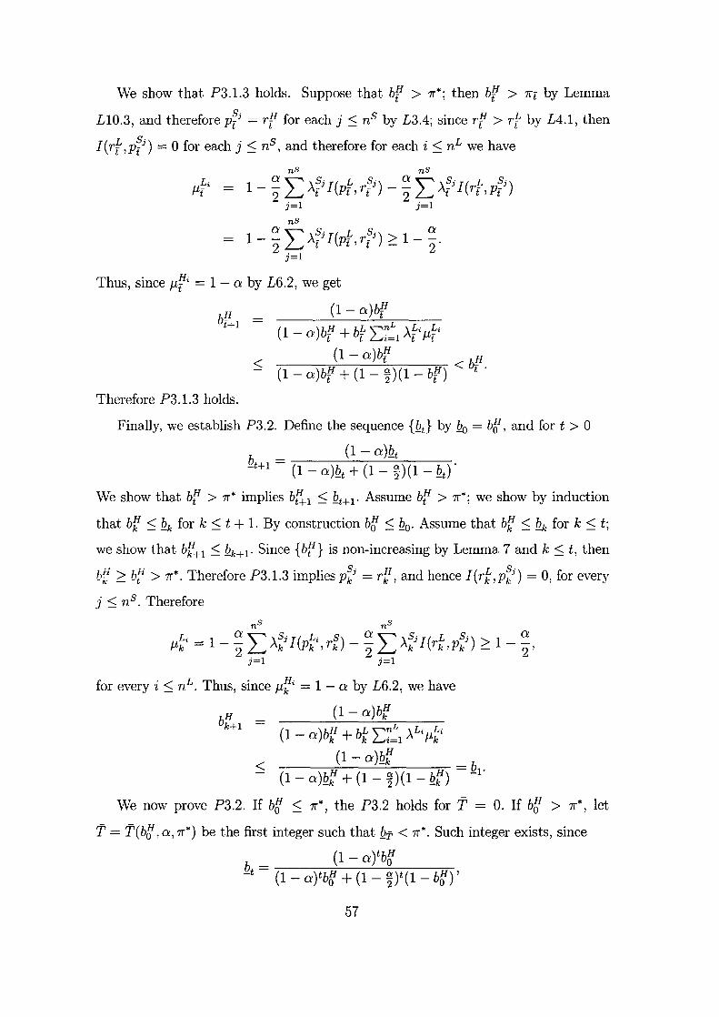
We show that P3.1.3 holds. Suppose that bp > ?r*; then bp > ?rt by Lemma

L10.3, and therefore pfj = r[! for each j ::; nS by L3.4; since r[! > rf by L4.1, then

I (rf , pfj) = 0 for each j ::; n s, and therefore for each i ::; n L we have

nS nS

L· a"", s· (L s· a"", s· L S J1t ' = 1 - 2" ~ A[ J I Pt, r [J) - 2" ~ A[ J I (r[ , p/ )

j=1 j=1

nS

Q L s· (L s.) a 1 - - A_J I Pt- r_J > 1 - -. 2 t 't - 2

j=1

Thus, since J.Lfi = 1 - Q by £6.2, we get

b?-t-l = (1 - a)b[!

(1 - a)b!l + bI:- ,,\,"}'L A!:i ,/:i t t L.n=1 t r--t (1- a)bp H

< (1 - a) bp + (1 - ~)( 1 - bP) < bt .

Therefore P3.1.3 holds.

Finally, we establish P3.2. Define the sequence {Qt} by Qo = b{f, and for t > 0

b _ (1 - a)Qt -HI - (1 - a)Qt + (1 - ~)(1 - Qt)

We show that bf > ?r* implies bEt-I::; Qt+1' Assume bf > ?r*; we show by induction

that bf: ::; Qk for k ::; t + 1. By construction bf! ::; Qo. Assume that bf: ::; Qk for k ::; t;

we show that bf:+l ::; Qk+l' Since {bf} is non-increasing by Lemma 7 and k ::; t, then

bf! 2: b~ > 7["*. Therefore P3.1.3 implies p~j = r{!, and hence I(rf,p~j) = 0, for eyery

j ::; n s. Therefore

for every i ::; nL . Thus, since J1~i = 1 - a by £6.2, we have

bH -k+l -(1 - a)bf:

(1 - Q)bH + bL ,,\,"}'L ALi IILi k k L .. n=1 r--k

< (1 - Q)Q~ _ b (1 - a)Q~ + (1 - ~)(1 _ M;) - -1'

We now prove P3.2. If bf! ::; ?r*, the P3.2 holds for T = O. If bf! > ?r*, let

T = T(b{f, a, ?r*) be the first integer such that Qi' < ?r*. Such integer exists, since

(1 - a)tbH b - 0 -t - (1 - a)tb{f + (1 - ~)t(1 - bf!)'

57

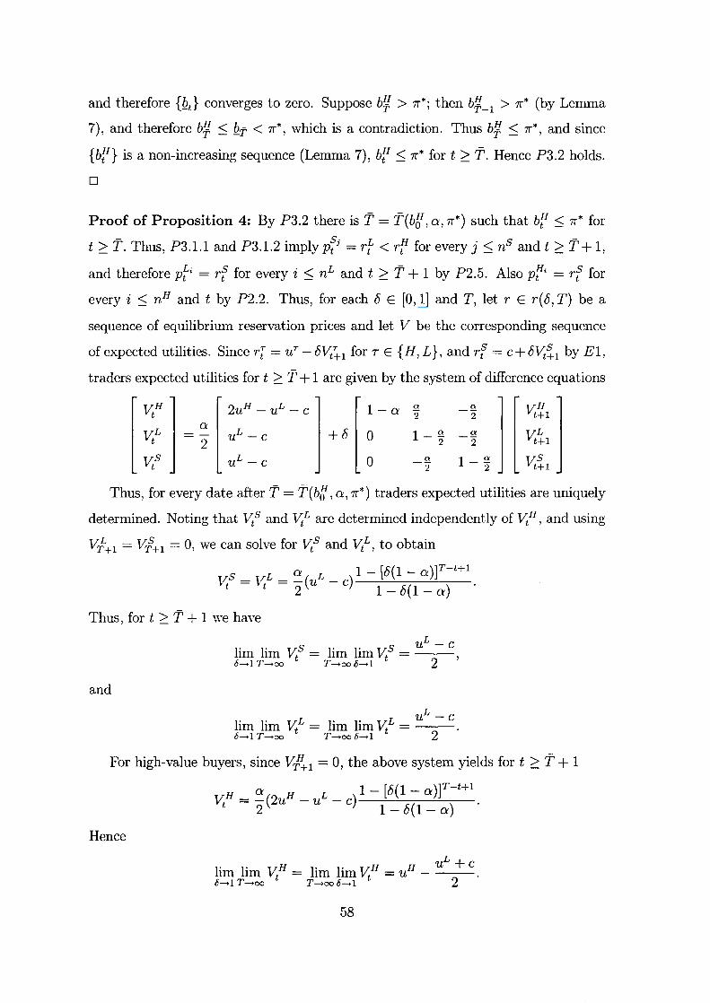
and therefore H~t} converges to zero. Suppose b¥ > 71"*; then b¥_l > 71"* (by Lemma

7), and therefore b¥ ~ Qf' < 71"*, which is a contradiction. Thus b¥ ~ 71"*, and since

{bfI} is a non-increasing sequence (Lemma 7), bfI ~ 71"* for t 2:: T. Hence P3.2 holds.

o

Proof of Proposition 4: By P3.2 there is T = T(b{f, a, 71"*) such that bfI ~ 71"* for

t 2:: T. Thus, P3.1.1 and P3.1.2 imply p~j = rf < rfI for every j ~ nS and t 2:: T + 1,

and therefore pfi = rf for every i ~ nL and t 2:: T + 1 by P2.5. Also p~i = rf for

every i ~ nH and t by P2.2. Thus, for each 8 E [0,1] and T, let r E r(8, T) be a

sequence of equilibrium reservation prices and let V be the corresponding sequence

of expected utilities. Since r[ = UT - 8~:;'-1 for T E {H, L}, and rf = C+8~~1 by El,

traders expected utilities for t 2:: T + 1 are given by the system of difference equations

v:H 2uH - uL - c I-a Q Q

~~1 t 2" 2

v:L

a uL - c +8 ~t1 ° l-Q. _Q.

t 2 2 2

~S u L - C ° Q 1-Q. ~~1 -"2 2

Thus, for every date after T = T(b{f, a, 71"*) traders expected utilities are uniquely

determined. Noting that ~s and ~L are determined independently of ~H, and using

Vf+l = VI+1 = 0, we can solve for ~s and ~L, to obtain

VS _ l!"L _ ~( L _ ) 1 - [8(1 - a)]T-t+l . t - t - 2 u c 1 _ 8(1 - a)

Thus, for t 2:: T + 1 \Ye have

L

1· 1· v:S 1· 1· v:S u - c lm lm t = lm lm t = , 6->1 T->= T->= 6->1 2

and

L

1· 1· v:L 1· 1· v:L U - C lm lm t = lm lm t = 6->1 T->= T->= 6->1 2

For high-value buyers, since Vf!.t1 = 0, the above system yields for t 2:: T + 1

v:H a( H L ) 1- [8(1- a)JT-t+l

t = - 2u - u - c ---=--'------'--"---2 1- 8(1- a)

Hence

L Hm lim ~H = Hm lim~H =uH _ u +c 6->1 T->= T->oo 6->1 2

58

Now let t < T + 1. A trader of type T who is in the market at date t obtains an

expected utility of V{ by following his equilibrium strategy; thus the expected utility

to a trader who remains in the market at t must satisfy ~T ~ 8T-tVi+1' for otherwise

he benefits from a deviation where he makes unacceptable offers and rejects any offers

until date T + 1, following his equilibrium strategy thereafter. Also ~s + ~H :S uH - c

by £5.2. Thus

and therefore

Also

hence

1· 1· Tl'S 1· 1· uS uL

- c 1m 1m v t = 1m 1m v t = 6-->1 T-->oo T-->oo 6-->1 2

1· 1· TTH 1· 1· uH _ H uL + c 1m 1m v t = 1m 1m v t - U - ---

6-->1 T-->oo T-->oo 6-->1 2

For low-value buyers we have ~s ~ ~L ~ 8T- tV#+1' where the first inequality

follows from Lemma 11 and the second ,vas established above. Thus,

L

lim lim v~ L = lim lim v~ L = U - c, 6-->1 T-->oo T-->oo 6-->1 2

Furthermore, since Tf = c + 8~! 1 and T; = UT - 8~~ 1 for T E {H, £} by El, the

above limits imply

L

1· 1· T 1· 1· T U + c 1m 1m Tt = 1m 1m Tt = , 6--> 1 T -+00 T -->00 6--> 1 2

for T E {H, £, S} and t. 0

59

References

[1] Binmore, K. and M. Rerrero (1988): "Matching and Bargaining in Dynamic

Markets," Review of Economic Studies 55, 17-31.

[2] Border, K. (1985): Fixed point theorems with applications to economics and game

theory, Cambridge Universiy Press.

[3] Cellina, A. (1969): "Approximation of set valued functions and fixed point the­

orems," Annali di Matematica Pura ed Aournal of Economic Theory 43, 20-54.

[4] Gale, D. (1987): "Limit Theorems for Markets with Sequential Bargaining,"

Journal of Economic Theory 43, 20-54.

[5] Jackson, M. and T. Palfrey. (1998): "Efficiency and Voluntary Implementation

in Markets with Repeated Parewise Bargaining," Econometrica 66, 1353-1388.

[6] Rubinstein, A. and A. Wolinsky. (1985): "Equilibrium in a Market with Sequen­

tial Bargaining," Econometrica 53, 1133-1150.

[7] Samuelson, L. (1992): "Disagreement in Markets with Matching and Bargain­

ing," Review of Economic Studies 59, 177-186.

[8] Sattinger, M. (1995): "Search and the Efficient Assignment of Workers to Jobs,"

International Economic Review 36, 283-302.

[9] Serrano, R. and O. Yosha (1996): "Decentralized Information and the Walrasian

Outcome: A Pairwise Meetings Market with Private Values," mimeo.

[10] Varian, R. (1980): "A Model of Sales," The American Economic Review 70,

651-659.

[11] Wolinsky, A. (1990): "Information Revelation in a Market with Pairwise Meet­

ings," Econometrica 58, 1-23.

60

supply uH

UL ___ ""_J

c

Figure 1

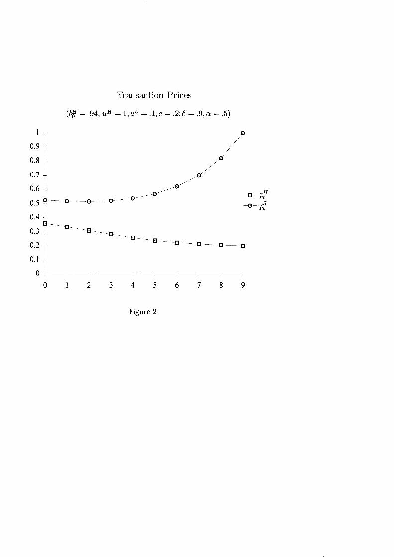
'If ansaction Prices

l:: - 9 a = .5) 1 c = .2;u -. , H -1 uL =. , (lfto = .94, u - ,

1 ,­i

0.9 ~ I I

8 I o. 7 I

0.7 ~

0.6 T

o--o-~o--0.5 -

0.4 "'------- .. _ --{J , "'-------G--_____ .. ________ "-______ El- ____ -c- _ _ .. __ 0.3 7 I

0.2 t 0.1 i

!

o o 1 2 3 4 5 6 7 8 9

Figure 2

supply

c

uL ....................................................................... demand

.. ..

Figure 3

time

Figure 4

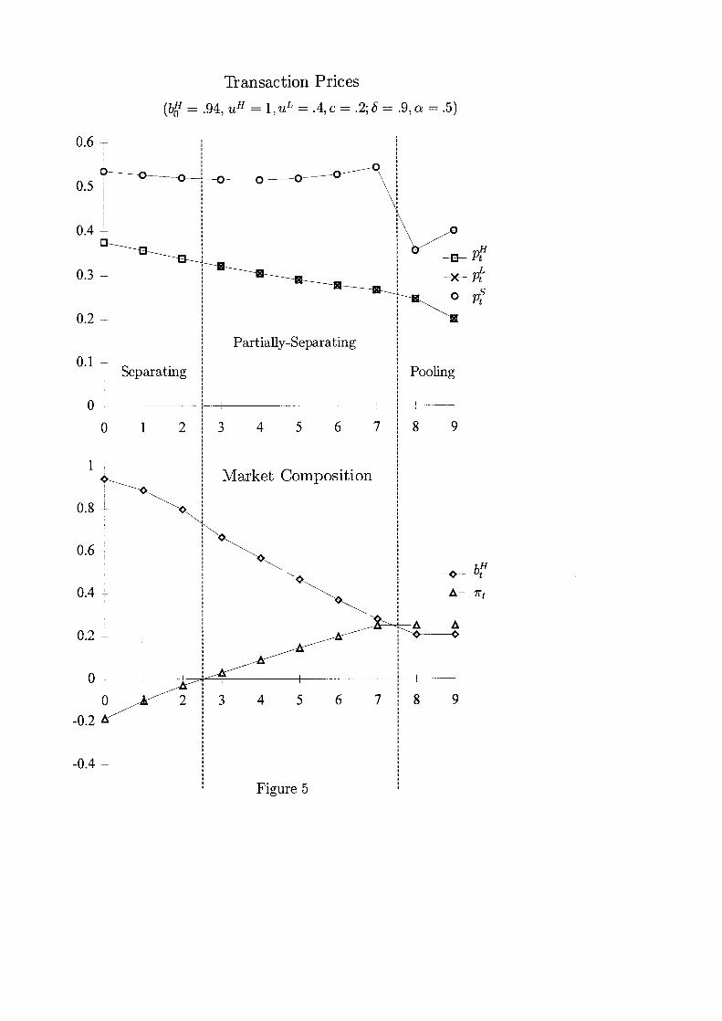
Transaction Prices

(b{f = .94, uH = 1,uL = .4,e = .2;8 = .9,0: = .5)

0.6 -

0.1 ~ Separating

o--~

o

0.8 1-

0.6 --;--

0.4 -'

0.2 ~

o -0.2

-0.4 -

1 2

2

Partially -Separating

Pooling

3 4 5 6 7 8 9

Market Composition

3 4 5 6 7 8 9

Figure 5

WORKING PAPERS 1999

Business Economics Series

99-01 (01)

99-06 (02)

99-07 (03)

99-17 (04)

99-18 (05)

99-30 (06)

Jaime Ortega "Power in the firm and managerial career concerns"

Sandro Brusco "Short-term ism as optimal experimentation policy"

A. BalMs, I.R. Longarela y 1. Lucia "How Does Financial Theory Apply to Catastrophe-Linked Derivatives? An Empirical Test of Several Pricing Models"

Ashish Arora, Andrea Fosfuri and Alfonso Gambardella "Markets for technology (why do we see them, why don't we see more of them, and why we should care"

Maria Jose Alvarez and Jaime Rivera "An integrated typology of green manufacturing profiles"

Sandro Brusco and Giuseppe Lopomo "Collusion via Signalling in Open Ascending Auctions with Multiple Objects and Complementarities"

Economics Series

99-02 (01)

99-04 (02)

99-05 (03)

99-08 (04)

99-09 (05)

99-11 (06)

99-13 (07)

99-14(08)

Carmen Arguedas "Enviromental standards and costly monitoring"

Maite Martinez-Granado "Testing Labour Supply and Hours Constraints"

Rafael Salas "Multi level Interterritorial Convergence and Additive Multidimensional Inequality Decomposition"

Ricardo Mora "Third-Generation Mexican American Workers in the South-West: A Case of Wage Discrim ination?"

Ricardo Mora "Wage Inequality and Structural Change"

Ezra Einy, Diego Moreno and Benyamin Shitovitz "The bargaining set of a large economy with differential information"

Antonio Romero-Medina and Jose Alcalde "Simple mechanisms to implement the core of college admisions problems"

Antonio Romero-Medina and Jose Alcalde "Sequential decisions in the college admisions problem"

99-16 (09)

99-20 (10)

99-21 (11)

99-22 (12)

99-25 (13)

99-32 (14)

Ezra Einy, Diego Moreno and Benyamin Shitovitz "Fine value allocations in large exchange economies with differential information"

Klaus Desmet "A Perfect Foresight Model of Regional Development and Skill Specialization"

Klaus Desmet "A Simple Dynamic Model of Uneven Development and Overtaking"

Oscar Bajo and Rafael Salas "Inequality Foundations of Concentration Measures: An Application to the Hannah­Kay Indices"

M. Angeles de Frutos and Lambros Pechlivanos "Second-Price Common-Value Auctions under Multidimensional Uncertainty"

Diego Moreno and John Wooders "Prices, Delay, and the Dynamics of Trade"

Economic History and Institutions Series

99-15 (01)

99-26 (02)

99-28 (03)

James Simpson "Cooperation and cooperatives in southern European wine production: the nature of succesful institutional innovation 1880-1950"

Joan R. Roses "Explaining the early industrialisation: a view from Catalonia (1830-1861)"

James Simpson "The Agrarian Crisis in the Late Nineteenth Century Spain: a Reconsideration"

Statistics and Econometrics Series

99-03 (01)

99-10(02)

99-12(03)

99-19 (04)

99-23 (05)

99-24 (06)

Stefan Profit and Stefan Sperlich "Non-Uniformity of Job-Matching in a Transition Economy A Nonparametric Analysis for the Czech republic"

Regina Kaiser and Agustin Maravall "Short-Term and Long-Term Trends, Seasonal Adjustment, and the Business Cycle"

Francesc Marmol, Alvaro Escribano and Felipe M. Aparicio "A New Instrumental Variable Approach for Estimation and Testing in Cointegrating Regressions"

Rosario Romera "Distributional aspects in partial least squares regression"

WaIter Kramer and Francesc Marmol "Ols-Based Asymptotic Inference in Linear Regression Models With Trending Regressors and Ar(p)-Disturbances"

WaIter Kramer and Francesc Marmol

99-27 (07)

99-29 (08)

99-31 (09)

"The Power of Residual-Based Tests for Cointegration When Residuals Are Fractionally Integrated"

Victor Aguirregabiria (University of Chicago) and Cesar Alonso Borrego (Universidad CarIos III de Madrid) "Labour Contracts and Flexibility: Evidence from a Labor Market Reform in Spain"

Juan J. Dolado, Jesus Gonzalo and Laura Mayoral "A Fractional Dickey-Fuller Test"

Lorenzo Pascual, Juan Romo and Esther Ruiz "Effects of Parameter Estimation on Prediction Densities: A Bootstrap Approach"

DOCUMENTOS DE TRABAJO 1999

Series de Economia

99-02 (01)

99-03 (02)

Jose Luis Ferreira e Ifiigo Herguera "Relaci6n entre los mercados spot y de futuros en un contexto oligopolistico"

Jose Luis Ferreira e Ifiigo Herguera "Regimen institucional del mercado spot y del mercado de futuros en distintos pafses"

Series de Economia de la Empresa

99-04 (01)

99-05 (02)

Maria Jose Alvarez GiI, Jer6nimo de Burgos Jimenez y Jose Joaquin Cespedes Lorente "(,Hay hoteles verdes en Espafia? Un amilisis exploratorio"

Ignacio Hernando y Josep A. Trib6 "Relaci6n entre contratos laborales y financieros: Un estudio te6rico y empirico para el caso espafiol"

Series de Historia Econ6mica e Instituciones

99-01 (01) Xavier Cuadras-Morat6, Angel S. Fernandez Castro y Joan R. Roses "La influencia de la productividad en la consolidaci6n de los grupos regionales de la banca privada espafiola, 1900-1914"

WORKING PAPERS 1998

Business Economics Series

98-25 (0 I)

98-27 (02)

98-31 (03)

98-32 (04)

98-35 (05)

98-40 (06)

98-43 (07)

98-44 (08)

98-59 (09)

98-65 (10)

93-66 (11)

98-67 (12)

98-70 (13)

98-72 (14)

98-77 (15)

98-78 (16)

98-90 (17)

98-92 (18)

98-93 (19)

M. Nufiez, Isabel Gutil!rrez and Salvador Carmona "Accountability and organizational survival: a study of the spanish newspaper industry (1966-1993)"

Clara Cardone, lfiaki R. Longarela and David Camino "Capital market inefficiencies, credit rationing and lending relationship in SME's"

Salvador Carmona and Isabel Gutierrez "Vogues in management accounting research"

M". Jose Alvarez-GiI and Daniel Arias-Aranda "An essay on the dimensions and components of customisation in service operations management"

Miguel A. Garcia-Cestona and Josep Trib6 "A main bank approach to financial contracting"

Elizabeth Cabrera and Jaime Bonache "A computer-based aid for the design of a strategic organizational culture"

Jose David Vicente-Lorente "The financial implications of the resource-based strategy: specificity, opacity and financial structure"

Ma. Jose Alvarez, Nora Lado and Ma. Luisa Villanueva "Innovativeness, marketing information sharing and new product success in the european insurance sector"

Alberto Maydeu Olivares and Nora Lado "Market orientation and business economic performance: a mediational model"

Maria J. A.lvarez and Pedro Gonzalez " Strategic alliances and new product development: the cases of Rover and Seat"

Ester Martinez-Ros and Vicente Salas "The effect of innovation activity on the innovating quasi-rents"

David Camino and Clara Cardone "The assessment of credit guarantee schemes for SME's: valuation and costs"

Ma. Jose Alvarez-Gil and Jaime Rivera "Environmental operations strategies: european approaches and research challenges"

Ashish Arora and Andrea Fosfuri "Licensing in the presence of competing technologies"

Marie Paule Kestemont and Jaime Rivera-Camino "The grening adaptation to European Union's environment policy: an empirical approach"

Jaime Rivera-Camino "The implementation of enviommental management systems standars in Europe: an organizational approach"

M. A. Martinez, M. Tapia, J. Yzaguirre "Information Transmission around Block Trades on the Spanish Stock Market"

Margarita Samartin "The role of demand deposits in risk sharing"

Margarita Samartin "Bank runs, suspension of convertibility versus deposit insurance"

98-95 (20)

98-97 (21)

98-98 (22)

Economics Series

98-05 (0 I)

98-06 (02)

98-10 (03)

98-11 (04)

98-13 (05)

98-24 (06)

98-26 (07)

98-28 (08)

98-2Q (1)9)

98-30 (10)

98-36 (11)

98-37 (12)

98-42 (13)

98-45 (14)

98-46 (15)

98-47 (\6)

98-48 (17)

Nora Lado Couste and Albert Maydeu-Olivares "Exploring the link between market orientation and innovation in the European and U.S. insurance markets"

Jaime Ortega "Power and the economics of organizations"

Ester Martinez-Ros "Explaining the decisions to carry out product and process innovations: The Spanish case"

Alfonso Alba "The effect of unemployment compesation on the re-employment probability in Spain"

Michael Jerison "Nonrepresentative representative consumers"

Laurence Kranich "Equality and individual responsibility"

Laurence Kranich "Altruism and the political economy of income taxation"

Jaume Garcia and Sergi Jimenez "Claim, offer and information in wage bargaining"

Michele Boldrin and Juan Manuel Martin Prieto 'Trade liberalization and private savings: the spanish experience, 1960-1995"

Antonio Romero-Medina "More on preference and freedom"

Ma. Angeles de Frutos "Asymmetric price-benefit auctions"

Helmu! Bester and Emma.!1Uel Petrakis "Wages and productivity growth in a competitive industry"

Esther Hauk "On the cultural transmission of corruption"

Emmanuel Petrakis "Diffusion of abatement technologies in a differentiated industry"

Praveen Kujal and Roland Michelitsch "Monopoly power and terms of trade"

Maite Martinez-Granado and Javier Ruiz-Castillo 'The decisions of Spanish youth: a cross-section study"

Carlos San Juan and Esther Decimavilla "Productivity comparisons: the European Union Agriculture"

Sonsoles Castillo, Juan Jose Dolado and Juan F. Jimeno "A tale of two neighbour economies: labour market dynamics in Portugal and Spain"

Sonsoles Castillo, Juan Jose Dolado and Juan F. Jimeno "The fall in consumption from being unemployed in Portugal and Spain"

Manuel Santos "Accuracy of numerical solutions using the euler equation residuals"

98-52 (18)

98-53 (19)

98-62 (20)

98-69 (21)

98-71 (22)

98-81 (23)

98-84 (24)

98-88 (25)

98-91 (26)

98-94 (27)

Antonio Romero-Medina "Stability in one-sided matching markets"

Maite Martinez-Granado "Self-employment and labour market transitions: a multiple state model"

Antonio Romero-Medina " "Sex-equal" stable matching"

Barbara Petrongolo and Maria Jesus San Segundo "Staying in at school at sixteen: The impact of labor market conditions in Spain"

Ezra Einy, Diego Moreno and Benyamin Shitovitz "Existence and equivalence of competitive and core allocations in large exchange economies with differential information"

Maia Guell Rotllan and Barbara Petrongolo "The transition from temporary to permanent employment: the spanish case"

Carlos San Juan "Capital data for productivity measurement"

Anton Garcia Diaz and Praveen Kujal "List Pricing and Pure Strategy Outcomes in a Bertrand-Edgeworth duo poly"

Ezra Einy, Diego Moreno and Benyamin Shitovitz "Rational Expectations Equilibria and the Ex-post Core of an Economy with Asymmetric Information"

Diego Moreno, Ezra Einy, Benyamin Shitovitz "On the core of an economy with differential information"

Economic History and Institutions Series

98-03 (0 I)

98-04 (02)

98-33 (03)

98-55 (04)

98-64 (05)

98-80 (06)

98-89 (07)

98-99 (08)

Pedro Fraile and Alvaro Escribano "The Spanish 1898 disaster: the drifts towards national protectionism"

Juan Carmon:! and James Simpson "The "rabassa morta" in catalan viticulture: the rise and decline of a long term sharecropping contract, 1670s-1920s"

Stefan Houpt "Location of Spanish integrated steel, 1880-1936"

Giovanni Federico and Antoni Tena "Did trade policy foster italian industrialization? Evidences from effective protection rates 1870-1930"

Leandro Prados de la Escosura "International comparisons of real product, 1820-1990: an alternative dataset"

Pablo Sanchez Leon "Markets, institutions and cultures: patterns of wine consumption in europe, 1850-1950"

Juan Roses "The choice of technology in the Mediterranean Basin: Some Evidence from the Spanish, Italian, British and U.S. Cotton Mills, 1830-1861"

Patrick Karl 0' Brien and Leandro Prados de la Escosura "Balance Sheets for the Acquisition, Retention and Loss of European Empires Overseas"

Statistics and Econometrics Series

98-01 (01) Jesus Gonzalo and Jean-Yves Pitarakis "Specification via model selection in vector error correction models"

98-02 (02)

98-07 (03)

98-08 (04)

98-09 (05)

98-12 (06)

98-14 (07)

98-15 (08)

98-16 (09)

98-17 (10)

98-18 (11)

98-19 (12)

98-20 (13)

98-21 (14)

98-22 (15)

98-23 (16)

98-34 (17)

98-38 (18)

98-39 (19)

98-41 (20)

98-49 (21)

98-50 (22)

Tom Engsted, Jesus Gonzalo and Niels Haldrup "Testing for multicointegration"

Felipe Aparicio and Alvaro Escribano "A non linear framework for the characterization of integrated and cointegrated series using induced­order statistics"

Felipe Aparicio and Alvaro Escribano "Co integration testing using first differences of ranges: an exploratory analysis"

Felipe Aparicio 'Testign linearity with information-theoretic statistics and the bootstrap"

Uwe Hassler and Francesc Marmol "Fractional co integrating regressions in the presence of linear time trends"

Clive Granger and Francesc Marmol 'The correlogram of a long memory process plus a simple noise"

Alvaro Escribano and M.A. Arranz "Detrending procedures and cointegration testing: ECM test under structural breaks"

M.A. Arranz and Alvaro Escribano "Bootstrapping cointegration test: ECM test under structural breaks"

M.A. Arranz and Alvaro Escribano "Detrending effects on error correction models: estimation biases under structural breaks"

Carlos Velasco "Non-Gaussian log-periodogram regression"

Carlos Velasco "Non-stationary log-periodogram regression"

Carlos Velasco "Gaussian semiparametric estimation of non-stationary time series"

Carlos Velasco "Local cross validation for spectrum bandwidth choice"

Ana Juste I, Daniel Pefia and Ruey S. Tasy "Detection of outlier patches in autoregressive time series"

Regina Kaiser "Detection and estimation of structural changes and outliers in unobserved components"

Antoni Espasa and Eva Senra "A nonlinear model for the investment function in Spain"

Francesc Marmol and Juan C. Reboredo "Near observationally equivalence and fractionally integrated processes"

Francesc Marmol "Searching for fractional evidence using combined unit root tests"

Juan Jose Dolado and Francescs Marmol "FM-OLS fractionally integrated processes"

Miguel A. Arranz and Francesc Marmol "Out-of-sample forecast errors in misspecified perturbed long memory time series"

Miguel A. Delgado and Javier Hidalgo

98-51 (23)

98-54 (24)

98-56 (25)

98-57 (26)

98-58 (27)

98-60 (28)

98-61 (29)

98-63 (30)

98-68 (31)

98-73 (32)

98-74 (33)

98-75 (34)

98-76 (35)

98-79 (36)

98-82 (37)

98-83 (38)

98-85 (39)

98-86 (40)

98-87 (41)

98-96 (42)

"Consistent specification testing of stationary processes with long-range dependence: asymptotic and boots trap tests"

Inmaculada Fiteni "Robust estimation of structural break points"

MigueI A. Delgado, Manuel A. Dominguez and Pascal Lavergne "Asymptotic and bootstrap specification tests of non linear in variables econometric models"

Miguel A. Delgado and Juan Mora "A nonparametric test for serial independence of errors in linear regression"

Miguel A. Delgado, Jordi Jaumandreu and Ana Martin Marcos "Input costs, capacity utilization and substitution in the short run"

Daniel Miles "The Probability of Non-purchasing Tobacco of a Smoker"

Jose Manuel Martinez and Antoni Espasa "Modelling nonlinearities in GDP. Some differences between US and Spanish data"

Ana Justel and Daniel Pena "Heterogeneity and model uncertainty in bayesian regression models"

Miguel A. Arino and Francesc Marmol "A Beveridge-Nelson decomposition for fractionally integrated time series"

Miguel A. Delgado and Wenceslao Gonzalez-Manteiga "Singnificance testing in nonparametric regression based on the bootstrap"

Olivier Nunez "Asymptotic properties for a simulated pseudo maximum likelihood estimator"

Joseph P. Romano and Michael Wolf "Subsampling confidence intervals for the autoregressive root"

Joseph P. Romano and Michael Wolf "Finite sample nonparametric inference and large sample efficiency"

M.P. Wiper, L.I. Pettit y K.D.S. Young "Bayesian inference for a Lanchester type combat model"

Miguel A. Arranz, Ana Cri ado and Alvaro Escribano "Is unit root testing on trend components robust against additive outliers?"

Miguel A. Arranz and A. Escribano "Co integration Testing under Transitory Breaks: Robust ECM Testing Procedures"

Stefan Sperlich, Oliver B.Linton, Wolfgang H1irdle " Integration and backfitting methods in additive models - finite sample properties and comparison"

Delicado, P. y Romo, J. " Constant coefficient tests for random coefficient regressions"

Pascual, L., Romo, J. Y Ruiz, E. " Predictive inference forautoregresive processes: a standard bootstrap approach"

Felipe M. Aparicio Acosta ,. Modelling adaptive complex behaviour with an application to the stock market dynamics (El Farol Problem Revisited)"

Ruey S. Tsay, Daniel Pena and Alan E. Pankratz .. Outliers in multivariate time series"

DOCUMENTOS DE TRABAJO 1998

Serie de Economia

98-01 (01) Coral del Rio y .Javier Ruiz-Castillo "El enfoque de la dominancia en el amilisis de la pobreza"

98-02 (02) Javier Ruiz-Castillo "La comparacion de distribuciones de renta en un contexto dimimico: dificultades y perspectivas"

98-12 (03) Ramon Mafia Dolores Pedrero "Asimetrias en los efectos de la politica monetaria en Espai'la (1977-1996)"

98-18 (04) .Juan Jose Dolado y Ramon Maria Dolores "Un amilisis de 105 efectos ciclicos de la politica monetaria en Espafia (1977-1996)"

98-20 (05) Jesus Zamora Bonilla "Cuestiones de sociologia y economia de la ciencia"

98-22 (06) Begofia Alvarez "La demanda atendida de consultas medicas y atencion urgente"

Serie de Economia de la Empresa

98-05 (01)

98-08 (02)

98-09 (03)

98-JI1 ~(14)

98-11(05)

98-15 (06)

98-16 (07)

98-17 (08)

Maria Jose Alvarez y Pedro Gonzalez "Las cuentas de las privatizaciones: el caso Seat"

Salvador Rayo y David Camino "La valoracion de activos mediante opciones de intercambio: aplicacion alas finanzas empresariales"

Ma . .lose Alvarez-GiI y Pedro Gonzalez de la Fe "Un analisis de los costes y beneficios de la privatizacion de Seat"

Jaime Bonache "Los estudios de casos coma estrategia de investigacion: caracteristicas, criticas y defensas"

Ma Dolores de .Iuan Vigaray y Jaime Rivera "Revision del constructo "atraccion comercial": una aproximacion tearica"

Alberto Maydeu y Jaime Rivera "La evaluacion de preferencias en marketing: comparacion de metodos pareados vs rangos"

Elizabeth F. Cabrera "(.Como valorar el impacto financiero de las intervenciones de recursos humanos? Modelos de analisis de utilidad"

Nora Lado y Ma. Luisa Villanueva "Efectos del materialismo en las decisiones del joven consumidor: un estudio exploratorio"

Serie de Estadistica y Econometria

98-03 (01)

98-04 (02)

98-06 (03)

Antoni Espasa y Jose Manuel Martinez "Caracterizacion del PIB espafiol a partir de modelos univariantes no Iineales"

.lose Manuel Martinez y Antoni Espasa "Perspectivas de la economia espaflola para 1998-1999: estabilidad en el crecimiento a niveles superiores a la media europea y con una tasa de paro muy elevada"

Jose Manuel Martinez y Antoni Espasa " La demanda de importaciones espaflolas. Un enfoque VECM desagregado"

98-13 (04)

98-14 (05)

98-21 (06)

Jose Manuel Martinez y Antoni Espasa "Evaluaci6n de asimetrias en la tasa de crecimiento trimestral del PIB usando funciones de respuesta no lineal"

Antoni Espasa y Jose Manuel Martinez 'Tendencia y ciclos en la economia espafiola: mode\os, estimaciones y perspectivas para 1998-1999"

Begofia Font "Modelizaci6n de series temporales financieras. Una recopilaci6n"

Serie de Historia Econ6mica e Instituciones

98-07 (01)

98-19 (02)

98-23 (03)

Juan Carmona y James Simpson "A vueltas con la cuesti6n agraria catalana: e\ contrato de rabassa morta y los cambios en la viticultura, 1890-1929"

Antonio Tena Junguito "Un nuevo perfil del proteccionismo espafiol durante la Restauraci6n 1875-1930"

Elena Martinez Ruiz "Las balanzas de pagos de la autarqufa. Una revision"