Entrepreneurial Capital, Inequality, and Asset Prices
102
Entrepreneurial Capital, Inequality, and Asset Prices Argyris Tsiaras ∗ February 11, 2019 Abstract This paper investigates the contribution of entrepreneurship to increasing U.S. wealth inequality. Using data from the Survey of Consumer Finances (SCF), I document that, since 2000, the increase in the wealth shares of the top 0.1% and 1% groups of households is almost exclusively driven by entrepreneurs, identi- fied empirically as private business owner-managers. Additional evidence from the SCF points to an increase in the average returns to entrepreneurial ventures as a likely driver of these patterns. I develop analytical characterizations of sum- mary measures of inequality in the context of a model of wealth accumulation featuring heterogeneity in investment returns and in labor earnings across house- holds in order to examine the restrictions that the wealth distribution imposes on the underlying return heterogeneity. To match the relative position of entrepre- neurs across the wealth distribution and the level of top concentration in the SCF data, as well as changing inequality from the 1990s to the 2010s, the model requires high persistence of entrepreneurial status across households and a sub- stantial increase in the average excess return to entrepreneurial investments. The associated slow transition dynamics of the wealth distribution in the model im- ply that, if not reversed, recent structural shifts may lead to widening inequality for many years to come. ∗ Harvard University. Email: [email protected]. I am grateful to John Campbell, Xavier Gabaix, Sam Hanson, David Laibson, and Adi Sunderam for their advice and guidance. I also thank Lisa Abraham, Chris Anderson, Chris Clayton, Robert Barro, Josh Coval, Robin Greenwood, Gita Gopinath, Greg Mankiw, Jeff Miron, Michael Reher, Jeremy Stein, Ludwig Straub, Chenzi Xu, Gabriel Zucman, and participants in the Harvard fi- nance and macro lunches for useful comments and discussions.
-
Upload
khangminh22 -
Category
Documents
-
view
0 -
download
0
Transcript of Entrepreneurial Capital, Inequality, and Asset Prices

Entrepreneurial Capital, Inequality, and Asset Prices
Argyris Tsiaras∗
February 11, 2019
Abstract
This paper investigates the contribution of entrepreneurship to increasingU.S. wealth inequality. Using data from the Survey of Consumer Finances (SCF),I document that, since 2000, the increase in the wealth shares of the top 0.1% and1% groups of households is almost exclusively driven by entrepreneurs, identi-fied empirically as private business owner-managers. Additional evidence fromthe SCF points to an increase in the average returns to entrepreneurial venturesas a likely driver of these patterns. I develop analytical characterizations of sum-mary measures of inequality in the context of a model of wealth accumulationfeaturing heterogeneity in investment returns and in labor earnings across house-holds in order to examine the restrictions that the wealth distribution imposes onthe underlying return heterogeneity. To match the relative position of entrepre-neurs across the wealth distribution and the level of top concentration in theSCF data, as well as changing inequality from the 1990s to the 2010s, the modelrequires high persistence of entrepreneurial status across households and a sub-stantial increase in the average excess return to entrepreneurial investments. Theassociated slow transition dynamics of the wealth distribution in the model im-ply that, if not reversed, recent structural shifts may lead to widening inequalityfor many years to come.
∗Harvard University. Email: [email protected]. I am grateful to John Campbell, Xavier Gabaix, SamHanson, David Laibson, and Adi Sunderam for their advice and guidance. I also thank Lisa Abraham, ChrisAnderson, Chris Clayton, Robert Barro, Josh Coval, Robin Greenwood, Gita Gopinath, Greg Mankiw, JeffMiron,Michael Reher, Jeremy Stein, Ludwig Straub, Chenzi Xu, Gabriel Zucman, and participants in the Harvard fi-nance and macro lunches for useful comments and discussions.

1 INTRODUCTION 1
1 Introduction
In recent years, the United States and many other countries around the world have experi-
enced a sustained rise in wealth inequality, particularly benefiting those at the very top of
the distribution. As I show in this paper, the notable rise in top wealth concentration in the
U.S. has been accompanied by an increase in the share of aggregate wealth held by entrepre-
neurs, both in the aggregate and at the top of the wealth distribution, especially since 2000.
I investigate the drivers and implications of these shifts in the cross-sectional structure of
inequality using a model of wealth accumulation featuring heterogeneity in investment re-
turns and in labor earnings across households. A calibration of the model to U.S. data shows
that a substantial increase in the returns to entrepreneurship is necessary to explain the
growth in wealth inequality at the top and in the relative wealth of entrepreneurs in recent
years, and it implies that wealth inequality is likely to continue to grow for decades if the
returns to entrepreneurship remain high.
Using the US Survey of Consumer Finances (SCF) from 1989 to 2016, I document that
the increase in top wealth concentration since 2000 appears to be driven almost exclusively
by entrepreneurial households, defined empirically as private business owners who actively
manage their businesses. In particular, entrepreneurs within the top 0.1% group by net
worth account for the entire 4 percentage-point increase in the aggregate net worth share of
the top 0.1% group from the 2001 survey wave to the 2016 wave. Similarly, entrepreneurs
within the top 1% group by net worth account for 85% of the 6 percentage-point increase in
the top 1% net worth share during the same period. The aggregate share of net worth held
by entrepreneurs also experienced an economically and statistically significant increase from
41% in the 1990s to 45% in the 2010s even though entrepreneurs have remained stable as a
fraction of the population, at around 12% according to my empirical definition.1
The reasons behind the growing importance of entrepreneurs in the wealth distribution
are unclear. Although changes in the return characteristics of entrepreneurial ventures are
a natural candidate and the focus of this paper, these characteristics are hard to estimate
precisely due to the lack of high-quality, representative micro-level data on private business
returns. Moreover, superior average returns to entrepreneurial ventures relative to other fi-
nancial assets are not the only reason for the prevalence of entrepreneurs at the top of the
wealth distribution. Private business owner-managers tend to receive labor earnings (wage
income declared in tax returns) almost twice as high on average as the average household,
so one would expect them to be wealthier on average even without any heterogeneity in the
1These patterns are consistent with the findings of Guvenen and Kaplan (2017) and Smith et al. (2017), whofind using administrative tax and social security data that the increase since 2000 in top U.S. income inequalityis almost entirely explained by an increase in pass-through business income. In the SCF, the increase since2000 in the aggregate income shares of the top 0.1% and 1% groups by income is also driven almost entirely byentrepreneurial households.

1 INTRODUCTION 2
returns to invested wealth across households. Entrepreneurs may also be more risk tolerant
than non-entrepreneurs on average, holding a greater fraction of their net worth in risky
assets, equities in particular (whether public or private), both across the entire population
and within top groups. For example, in 2016, entrepreneurs in the top 1% group by net
worth held 62% of their (gross) assets in equities relative to 47% for non-entrepreneurs in
the top 1% group, although the entire difference is accounted for by inside private equity,
that is, equity in private businesses actively managed by an entrepreneurial household. Ac-
cording to standard financial theory, entrepreneurs should be compensated for their greater
risk-taking via a higher average return on their wealth portfolio, even if average returns to
privately-held equity are no different from those to financial assets with similar aggregate
risk exposure.2
Although all of these factors contribute to the prevalence of entrepreneurs at the top
of the wealth distribution, my analysis, centered on a calibrated partial-equilibrium model
of wealth accumulation, points to an increase in the average return to actively-managed
privately-held equity as the most likely driver of the recent increase in the relative wealth of
entrepreneurs and in top wealth inequality.
My model features two household types: non-entrepreneurs, who receive labor earn-
ings and income from liquid financial investments, and entrepreneurs, who additionally
have access to an investment technology that is subject to undiversifiable idiosyncratic risk.
A key theoretical contribution of the paper is an analytical characterization of the long-
run level of inequality, including inequality between entrepreneurs and non-entrepreneurs
across the wealth distribution, and the speed at which inequality evolves following a transi-
tory or permanent structural shift. These analytical results highlight the distinct impact of
cross-sectional heterogeneity in labor earnings and heterogeneity in the returns on wealth.
In the model, the impact of the latter is driven by two key features of entrepreneurship
dynamics at the household level, the inside equity premium, that is, the average excess re-
turn to entrepreneurial investments per unit of idiosyncratic entrepreneurial risk exposure
(Sharpe ratio), and the cross-sectional persistence of entrepreneurial status. The model also
highlights the contribution of idiosyncratic entrepreneurial risk to wealth inequality both as
a source of cross-sectional dispersion in realized returns on wealth and also through house-
holds’ choice of the scale of their entrepreneurial investments.
The model can reproduce the structure of top wealth inequality and its recent secular
2Another theoretical possibility is that other sources of expected-return-on-wealth heterogeneity unrelatedto entrepreneurial ventures, such as the level of sophistication and diversification of the financial portfoliosof households, are cross-sectionally correlated with entrepreneurial status and contribute to the prevalence ofentrepreneurs in top wealth groups. It is, however, unlikely that this source of return heterogeneity has be-come more important in recent years, as the diversification advantage of larger portfolios has probably declinedrecently, with more investors using mutual funds and indexed exchange-traded funds to diversify even smallportfolios at low cost.

1 INTRODUCTION 3
shifts quantitatively as well as qualitatively. I use information from the cross-sectional struc-
ture of wealth inequality and its secular shifts from the 1990s to the 2010s in the SCF data
to estimate the model by the simulated method of moments and infer the structural increase
in the inside equity premium that can account for the increase in the relative wealth of en-
trepreneurs and in top wealth concentration. The calibration also takes into account the
concurrent increase in within-labor-earnings heterogeneity during this period. In the base-
line calibration, an increase in the inside equity premium (Sharpe ratio) from 0.22 to 0.27,
corresponding to a sizeable increase in the expected return-on-wealth differential between
entrepreneurs and non-entrepreneurs from 1.7% to 2.5%, is needed to match the increase
in the (top-weighted) net worth share of entrepreneurs from the 1990s to the 2010s. The
calibration accounts for the majority of the increase in the top 1% and top 0.1% net worth
shares during this period.
The increase in the return differential is essential for matching the increase in top wealth
concentration. In the SCF data, the share of aggregate labor earnings held by the group of
entrepreneurs as a whole has declined slightly from the 1990s to the 2010s. This is the case
both for the classification of total household income into wage income and capital income in
surveyed households’ tax returns, and also for an alternative factor decomposition of income
after a regression-based imputation for the labor earnings of entrepreneurs that do not re-
port regular wages in their tax returns. The model calibration takes into account this decline
in entrepreneurs’ aggregate share of labor earnings and, as a result, by itself the calibrated
increase in within-labor-earnings inequality during this period can account for only a small
fraction of the increase in top wealth inequality and cannot explain the rise in the relative
wealth of entrepreneurs.
The sizeable inferred increase in the return differential between entrepreneurs and non-
entrepreneurs is a robust feature of empirically plausible calibrations of the model. The
model requires high cross-sectional persistence of entrepreneurial status in order to jointly
match the long-run levels of both topwealth concentration (the aggregate net worth shares of
top groups of households by net worth) and the (top-weighted) net worth share of entrepre-
neurs in the data.3 In turn, the degree of entrepreneurial persistence is the key determinant
of the speed of transition of the wealth distribution following structural shifts, with high
persistence implying slow transitions. In the baseline calibration, the (asymptotic) transi-
tion half-life for the aggregate wealth share of entrepreneurs is 46 years. Given these slow
transition dynamics, the model must assume a sizeable increase in the inside equity pre-
mium in order to match the sizeable recent shifts in the structure of top inequality that have
occurred during a period of only 20 years.
3High entrepreneurial persistence, that is, the fact that entrepreneurship tends to be a life-long professionfor part of the population despite high business failure rates, has also been documented empirically in the U.S.(Quadrini, 2000).

1 INTRODUCTION 4
In support of this key implication of the model calibration, I provide micro-level evi-
dence for an increase in the average returns to private businesses, conditional on their sur-
vival in private form, relative to returns on other (passive) financial investments. Using
SCF data on the initial investment and the current estimated market value of private busi-
nesses reported by surveyed households, I construct a measure of the long-term return to a
household’s primary actively-managed private business in excess of a liquid index (the S&P
500) over the life of the business. Although this cross-section cannot capture the impact of
business failure, the most important source of risk for a private business, the analysis re-
veals a large increase in the conditional cross-sectional average excess return to private busi-
nesses since 2000, while the conditional cross-sectional volatility of returns has remained
unchanged. These results are qualitatively consistent with those of Kartashova (2014), who
uses SCF and aggregate accounting data to construct estimates of the aggregate returns to
U.S. private equity following the methodology of Moskowitz and Vissing-Jørgensen (2002),
and finds a significant increase in the aggregate premium of private equity over public eq-
uity since 2000.4
The model abstracts from changes in sources of return heterogeneity other than entre-
preneurship, such as changes in the risk characteristics of the (passively-managed) financial
portfolios of entrepreneurs and non-entrepreneurs, which could also have contributed to an
increase in the average return differential between the two groups of households. However,
measures of the differential wealth exposure to risky assets between entrepreneurs and non-
entrepreneurs in the SCF offer no evidence of an increase in the average risk taking of en-
trepreneurs relative to non-entrepreneurs. In fact, the changes from the 1990s to the 2010s
in the average equity portfolio share differentials are slightly negative and not statistically
significant, including within top net worth groups.
The slow transition dynamics of the wealth distribution in any realistic calibration of
the model, driven by the high inferred cross-sectional persistence of entrepreneurial status,
also imply that recent structural shifts may have a protracted impact on inequality in the
future. For example, if the shifts in the inside equity premium and in within-labor-earnings
heterogeneity are permanent and holding all else constant in a model simulation under the
baseline calibration, the top 1% net worth share will increase by another 2.9% over the next
20 years from the 2010s to the 2030s, almost as much as its 3.9% increase from the 1990s
to the 2010s. Even if the structural shifts are fully reversed going forward, the economy
will only slowly revert to its lower 1990s levels of inequality (the original steady state of the
model), over several decades of transition.
4The conclusions are also consistent with those of Smith et al. (2017), who use U.S. administrative tax datalinking pass-through firms to their owners. They find that more than 80% of the increase from 2001 to 2014 inthe income of S-corporations owned by individuals in the top 1% group by income is due to rising profitabilityper unit of scale (worker) rather than rising scale, a finding strongly suggestive of an increase in the returns tothese firms.

1 INTRODUCTION 5
Related Literature This paper contributes to the literature in macroeconomics and finance
on the drivers of wealth and income inequality related to cross-sectional heterogeneity in
rates of return to wealth, and in particular the part of this literature that emphasizes entre-
preneurship as a key source of this heterogeneity.
The empirical literature on inequality has documented that a rise in within-labor-earnings
inequality accounts for most of the increase in inequality in the US since the 1980s until
about the 2000s (Piketty and Saez, 2003). Using SCF data, this paper documents the im-
portant contribution of entrepreneurship to the increase in top wealth inequality, especially
since the 2000s. Guvenen and Kaplan (2017) and Smith et al. (2017) reach a similar conclu-
sion for income inequality using tax data.5
A number of papers develop models of entrepreneurship highlighting the ability of
idiosyncratic entrepreneurial risk to generate a Pareto tail in wealth and income and to
match the large observed levels of wealth concentration at the top of the wealth distribu-
tion. Quadrini (2000) and Cagetti and De Nardi (2006) emphasize the impact of financial
frictions (borrowing constraints) faced by entrepreneurs, inducing an endogenous selection
of entrepreneurs among wealthy people in the first place. Pástor and Veronesi (2016) focus
on the impact of redistributive taxation on self-selection into entrepreneurship. Jones and
Kim (2017) emphasize heterogeneity within the group of entrepreneurs and highlight cre-
ative destruction as a stabilizing force limiting the income growth of high-growth entrepre-
neurs. Aoki and Nirei (2017) develop a neoclassical growth model with entrepreneurs that
can generate both Zipf’s law of the firm size distribution as well as a Pareto tail in incomes.
Relative to these models, the key contribution of my theoretical framework, which abstracts
from the issues of entrepreneurial self-selection and within-entrepreneur heterogeneity in
expected returns, is to offer a theoretical and quantitative analysis of the relationship be-
tween key properties of the dynamics of entrepreneurship, in particular the expected excess
returns to entrepreneurial ventures and entrepreneurial persistence, and observable features
of the cross-sectional wealth distribution, especially the prevalence of entrepreneurs across
the distribution.6
The theoretical results of this paper and the insights on the important role of entrepre-
neurial persistence for the evolution of inequality are closely related to the contribution of
Gabaix et al. (2016), who introducemathematical tools from ergodic theory and the theory of
partial differential equations to characterize the transitional dynamics of the cross-sectional
income distribution in response to structural shifts in continuous-time settings. Luttmer
5See footnotes 1 and 4.6The baseline version of my model employs a reduced-form representation of entrepreneurial investment
that is symmetric to investment in a liquid financial asset. In a general-equilibrium, endogenous-productionextension of mymodel presented in Appendix E, I show that even in a setting where entrepreneurial investmentsare realistically modelled as illiquid, nontradable assets, the equilibrium implications of entrepreneurial riskand return for portfolio choice and inequality are qualitatively very similar.

1 INTRODUCTION 6
(2007) also emphasizes the slow speed of transition for aggregates in an economy with a
power law firm size distribution.
The empirical studies of Quadrini (2000) and Gentry and Hubbard (2004) on the dy-
namics of entrepreneurship findmuch larger saving rates for entrepreneurs relative to work-
ers, while Quadrini (2000) also documents a high level of entrepreneurial persistence, with
past private business owners reentering into entrepreneurial ventures at much higher rates
than households without entrepreneurial experience. The quantitative analysis of my model
replicates these two important empirical facts on the dynamics of entrepreneurship.
In an important recent empirical contribution, Fagereng et al. (2018) use panel tax data
from Norway, which administers a wealth tax and thus collects information on households’
asset holdings, to establish the presence of a large degree of persistence in the heterogeneity
of returns on wealth across households.7 Moreover, they show that entrepreneurs play an
important role in the estimated degree of persistent heterogeneity in returns and for the
correlation of returns with wealth, consistent with my model’s inference of a high degree
of cross-sectional persistence in the return differentials between entrepreneurial and non-
entrepreneurial households.
A large theoretical literature studies mechanisms that can generate the empirically ob-
served Pareto tail in the wealth distribution.8 The theoretical and quantitative analyses of
Benhabib, Bisin, and Zhu (2011, 2015, 2016), Benhabib, Bisin, and Luo (2015), and Cao and
Luo (2017) highlight that it is capital income risk and heterogeneity in returns on wealth
that drive the thickness in the right tail of the wealth distribution, rather than heterogeneity
in labor income, consistent with the results of my quantitative analysis in Section 4.9
Although the quantitative analysis of mymodel focuses on entrepreneurship as the source
of cross-sectional return heterogeneity, the key insights of the analysis regarding the pro-
tracted impact of shifts in the return differentials across different groups of the population
also apply to other sources of return heterogeneity, as long as they are cross-sectionally per-
sistent. The literature has highlighted a number of other empirically relevant drivers of
return heterogeneity, including heterogeneous financial exposures to aggregate risk (Bach,
Calvet, and Sodini, 2017), differing levels of investor sophistication and skill (Kacperczyk,
Nosal, and Stevens, 2018), under-diversification (Campbell, Ramadorai, and Ranish, 2018),
7In particular, an individual permanent component accounts for 60% of the explained variation in the returnson wealth in their sample, and this permanent component also accounts for the bulk of the cross-sectionalcorrelation between returns and the level of wealth. The authors also find that return heterogeneity is mildlypersistent across generations.
8See, e.g., Stiglitz (1969), Moll (2012), Toda (2014), Piketty and Zucman (2015), and Achdou et al. (2015)among many others, and the excellent literature surveys by Gabaix (2009) and Benhabib and Bisin (2016).
9In a similar spirit, the literature survey by Benhabib and Bisin (2016) notes that quantitative models ofinequality focusing exclusively on labor income inequality, such as Castañeda, Díaz-Giménez, and Ríos-Rull(2003) and Kindermann and Krueger (2014) need to assume a counterfactually large degree of within-labor-earnings inequality.

2 ENTREPRENEURSHIP AND U.S. WEALTH INEQUALITY: EMPIRICS 7
and limited stock market participation (Guvenen, 2009; Favilukis, 2013).
A distinct literature has focused on the challenging empirical task of estimating the aver-
age returns to entrepreneurship (Moskowitz and Vissing-Jørgensen, 2002; Hamilton, 2000;
Hall and Woodward, 2010; Kartashova, 2014). In an important contribution, Moskowitz
and Vissing-Jørgensen (2002), henceforth MV2002, estimate the time series for the aggre-
gate private equity premium, that is, the aggregate returns to private equity in excess of
publicly traded equity, using mainly SCF data and also aggregate US accounting data. I fol-
low several aspects of their methodology in my empirical analysis of the SCF data, especially
on the construction of household-level long-term private business returns. MV2002 ques-
tion the existence of a positive private equity premium but Kartashova (2014) repeats the
procedure of MV2002 to estimate the aggregate private equity premium in an updated SCF
sample and finds a substantial improvement in the aggregate performance of private equity
in the 2000s and a positive historical average premium, consistent with both the empirical
findings and the theoretical predictions of this paper.10
Paper Outline The paper is structured as follows. Section 2 presents empirical findings
regarding the role of entrepreneurs in the recent increase in top U.S. wealth inequality. Sec-
tion 3 develops a model of entrepreneurship and inequality and offers analytical character-izations of the level and transitional dynamics of top wealth inequality. Section 4 presents
the quantitative calibration of the model to U.S. data and additional evidence from the SCF
consistent with the conclusions of the model calibration. Section 5 concludes.
2 Entrepreneurship and Wealth Inequality in the United States:
An Empirical Investigation
Section 2.1 discusses the empirical definition of entrepreneurship used in this paper and
documents the prevalence of entrepreneurs at the top of the wealth distribution. Section 2.2
investigates the growing importance of entrepreneurs in recent years by studying the evolu-
tion of shares of U.S. aggregates held by entrepreneurs as a group. Section 2.3 documents the
key role of entrepreneurial households in the recent increase in top U.S. wealth inequality.
2.1 The Prevalence of Entrepreneurs at the Top
This subsection introduces and addresses concerns regarding my empirical definition of en-
trepreneurs, and documents their prevalence at the top of the wealth distribution.
10Using their tax data from Norway (2004 to 2015), Fagereng et al. (2018), discussed above, estimate a largeaverage premium of private businesses over directly held listed stocks of around 6%.

2 ENTREPRENEURSHIP AND U.S. WEALTH INEQUALITY: EMPIRICS 8
The empirical analysis of entrepreneurship in the present paper centers on micro-level
data from the Survey of Consumer Finances (SCF), conducted by the Federal Reserve Board
triennially since 1989. The survey interviews a random sample of families (households) in
the US on various aspects of their finances, including assets, sources of income, economic ex-
pectations, and other demographic characteristics. In its tenth and most recent survey wave
in 2016, 6,248 households were interviewed. The SCF does a much better job of capturing
characteristics at the top of the wealth and income distributions relative to other US surveys
because it employs a sophisticated sample selection design involving a subsample of very
wealthy individuals (see Appendix A.4.1 for more details).
Moreover, the SCF possesses two critical advantages relative to US tax return data with
regard to the study of entrepreneurship and inequality. First, it offers detailed household-
level estimates on economic stocks (assets and loans, including estimates of the value of
entrepreneurial investments) rather than just flows. In particular, the level of detail in the
survey allows for the construction of fairly comprehensive measures for the net worth, that
is, non-labor wealth (simply referred to as “wealth” in the present section), as well as the
total income of each household.11,12 Second, it contains information on key characteristics
of households’ entrepreneurial investments, including their ownership share in a business
and whether the household actively manages that business. Because the survey is conducted
independently of the US tax authority, the latter features also set this data source apart
from tax data in countries that collect information on households’ wealth for tax collection
purposes.13
I define entrepreneurs empirically as households that partly or wholly own and activelymanage a private business.14 According to this definition, entrepreneurial households con-
11In the discussion of the theoretical framework in Section 3, I distinguish between a household’s total wealth,which includes the household’s capitalized labor income stream, and net worth, which refers to the non-laborcomponents of total wealth. However, I use “wealth” and “net worth” interchangeably in the discussion of theempirical results in this section.12Throughout the analysis, I use the SCF Bulletin measures of household net worth and total income. Ap-
pendix A.4.2 offers some details on these measures.13A number of recent papers, notably Fagereng et al. (2018) and Bach, Calvet, and Sodini (2017), use datasets
derived from the tax records of Scandinavian countries, which (unlike the United States) administer a personalwealth tax in addition to a personal income tax and thus collect information on households’ (net) assets as wellas flows. Although these datasets possess distinct advantages relative to SCF data (for example, the datasetof Fagereng et al. (2018) derived from Norwegian tax data has a strong panel dimension), the value of privatebusinesses reported by households to their tax authority is very close to the book value of these firms, consistentwith tax-minimization motives. The book value is typically weakly related to their market value. In contrast,the group administering the SCF goes at great lengths to assure the individuals surveyed that the data collectedin the survey will in no way be given to the IRS for tax verification purposes (tax audits). As a result, there is noreason to believe that SCF households systematically underreport their perceived private business valuations.14More specifically, a household is classified as an entrepreneurial household if at least one adult in the house-
hold (a member of the household’s “primary economic unit”) reports owning (wholly or in part) as well asactively managing at least one private business. I exclude from the group of entrepreneurs a small number ofhouseholds that satisfy these criteria yet report zero business earnings (for the year prior to the survey year) andzero business net worth (for the survey year).

2 ENTREPRENEURSHIP AND U.S. WEALTH INEQUALITY: EMPIRICS 9
All Half Third Quarter 10% 5% 1% 0.1% 0.01%0
10
20
30
40
50
60
70
80
90
100
Top Quantile Groups by Net Worth (2010s)
Entreprene
urs’S
hare
(%)
PopulationNet Worth
Figure 1: Entrepreneurs and Top Wealth Inequality
Notes: This figure plots the shares of entrepreneurs in top quantile groups of the net worth distribution forhouseholds in the Survey of Consumer Finances (SCF). Estimates are averaged over the three latest survey waves(2010, 2013, and 2016). The colored bands represent 95% confidence intervals for the estimates (see AppendixA.4.3 on statistical inference in the SCF).
stitute about 12% of the total population of US households in the 2016 survey. Yet, as a group
they are far more important in economic terms, holding 45% of aggregate US net worth and
28% of personal income.
The prevalence of entrepreneurs at the top of the wealth distribution is striking. Figure
1 plots the population and net worth shares of entrepreneurs within top quantile groups of
the net worth distribution. Averaging estimates over the three most recent survey waves (the
“2010s”), entrepreneurs comprise less than 12% of the total population but their share in top
quantile groups in terms of net worth increases sharply as we move towards the top of the
distribution in the top panel of Figure 1.15 In particular, entrepreneurial households account
for 68% of the wealthiest 1% of households (the “top 1%”), 77% of the wealthiest 0.1%, and
15Throughout this paper SCF population weights are used to construct representative group-level andeconomy-wide totals.

2 ENTREPRENEURSHIP AND U.S. WEALTH INEQUALITY: EMPIRICS 10
85% of the wealthiest 0.01%.16,17 A similar pattern holds for the net-worth-weighted share
of entrepreneurs in top groups, that is the fraction of the total net worth of the top group that
is held by the members of that group classified as entrepreneurs. It is, therefore, evident that
any empirical or theoretical analysis of wealth inequality at the top should first and foremost
address the role of entrepreneurship.
At the same time, there is large wealth heterogeneity within the group of private busi-
ness owner-managers. Figure A.1 plots the fraction of entrepreneurs who are in each net
worth decile for the latest (2016) survey wave, where the deciles refer to the distribution of
net worth across all households, including non-entrepreneurs. Entrepreneurs can be found
in all parts of the wealth distribution. In particular, a majority of them are part of the
“middle class”, defined by Piketty (2014) to comprise households in the 50th through 90th
percentiles.
As the model of Section 3 makes clear, two key features of entrepreneurship are the fo-
cus of this paper: first, an entrepreneur’s payoff is explicitly tied to firm-level performance
and is therefore exposed to business risk; second, an entrepreneur makes firm investment
decisions, implicitly choosing his or her exposure to firm-level risk. Relative to this theo-
retical definition of an entrepreneur, the empirical definition used in this paper, common in
studies of entrepreneurship and inequality (e.g. Cagetti and De Nardi (2006)), has certain
limitations. One set of concerns relates to the fact that households owning a private busi-
ness may not be managers of businesses in a conventional sense, even if they explicitly report
actively managing one or more businesses (as they do in the SCF). First, a non-manager “su-
perstar”, such as an athlete or singer, may register a private business under his or her name
as a way to receive the stream of rents to his or her scarce skill and talent (e.g. album profits
or payments for sponsorship deals). These profit streams, the argument goes, should not
be interpreted as the payoffs to scalable capital investments but as disguised labor earnings.
Second, a wealthy household may set up a private business as a “side hobby”, that is, its
private business may not be an important source of its income and wealth. Third, a wealthy
household may set up a private company simply to manage its financial portfolio.
Even though these are valid concerns, they are unlikely to apply to a large fraction of
private business owners-managers at the top of the wealth distribution. Although the public
version of the SCF does not offer information on occupations, a comparison with the study of
Bakija, Cole, and Heim (2012) based on confidential IRS tax data suggests that most wealthy
16The uncertainty of the estimates, captured by the width of the 95% confidence intervals in the figure (theseintervals are constructed using bootstrap standard errors; see Appendix A.4.3 for details on inference in theSCF), increases as we move further along the top of the distribution towards smaller and smaller groups ofhouseholds. For example, the top 0.01% of the wealthiest families includes only 12,600 families in 2016. Still,the prevalence of entrepreneurs in the top groups is hard to dispute even under the most conservative estimates17The SCF by design excludes the members of the Forbes 400 list of wealthiest individuals, almost all of whom
would be classified as entrepreneurs under the empirical definition of this paper.

2 ENTREPRENEURSHIP AND U.S. WEALTH INEQUALITY: EMPIRICS 11
private business owner-managers identify as such when asked about their primary occu-
pation. In particular, Bakija et al. (2012) show that individuals identifying themselves in
tax returns as executives, managers, supervisors, and finance professionals (“managers”, for
short) account for 60% of the top 0.1% group by income in 2005 and for 70% of the increase
in the top 0.1% income share from 1979 to 2005.18 A comparison of the relative population
and income-weighted fractions of this group of managers within top income groups in 2004
with the ones for private business owner-managers in the 2004 SCF survey is telling. For the
top 0.1% income group, this fraction is 59.6% by population (65.7% by income) for man-
agers (see tables 3 and 7 in Bakija et al. (2012)) and 65.5% by population (66.5% by income)
for private business owner-managers in the SCF. The discrepancy is similarly small for the
top 1% income group.19
A second response to these concerns is that privately-held equity constitutes a large share
of total household assets for the majority of private business owner-managers in top wealth
groups, as can be seen in Figure A.2. This implies a large wealth exposure to firm-level risk
for these households, given that a household’s holdings of inside private equity are typically
concentrated in a very small number of businesses. Relatedly, even if the source of suc-
cess and superior investment returns for a private business is the artistic, medical, or legal
skill of its owners rather than “conventional” managerial talent, the owners still make firm
investment decisions and a large part of their wealth is exposed to the risk that business
operations and investments entail. For the same reason, to the extent that a wealth man-
agement company (“home office”) set up by a very wealth individual takes on idiosyncratic
portfolio investment risk, it can be interpreted as an entrepreneurial venture.
A distinct potential limitation of the empirical definition is that it excludes the employed
top managers of public firms, as I am unable to identify households by occupation in the
public version of the SCF. Although executive pay for large public firms is subject to a dis-
tinct set of issues, managers of public firms can be interpreted to satisfy the two key features
of entrepreneurship discussed above: their payoffs are exposed to idiosyncratic, firm-level
risk through their performance-based compensation schemes; and they implicitly decide
over the exposure of their wealth to this firm-level risk by choosing their firms’ corporate
investment policies, which in turn shape the risk of their performance-based pay.20 How-
ever, Kaplan and Rauh (2010) show that top executives of public firms are few in number,
comprising a small fraction of conventional top income groups, around 3% of the top 0.1%
income group and less than 7% of even the top 0.001% income group in 2004.
18“Arts, media, and sports” comprise only 3% of the top 0.1% income group in 2005.19For the top 1% income group, the fraction of managers is 44.0% by population (52.8% by income) (see tables
2 and 6 in Bakija et al. (2012)), while the fraction of private business owner-managers in the SCF is 54.2% bypopulation (58.1% by income).20Consistent with this interpretation, Panousi and Papanikolaou (2012) find that the sensitivity to idiosyn-
cratic risk of the investment of publicly traded firms increases when managers own a larger fraction of the firm.

2 ENTREPRENEURSHIP AND U.S. WEALTH INEQUALITY: EMPIRICS 12
2.2 Entrepreneurs and U.S. Aggregates
This subsection documents a rise since the 1990s in the aggregate shares of net worth and
total household income held by entrepreneurs, which has not been accompanied by an in-
crease in entrepreneurs’ aggregate share of labor earnings.
During the 27-year period spanned by SCF survey waves (1989-2016) there has been a
sizable and statistically significant increase in the economic importance of entrepreneurs,
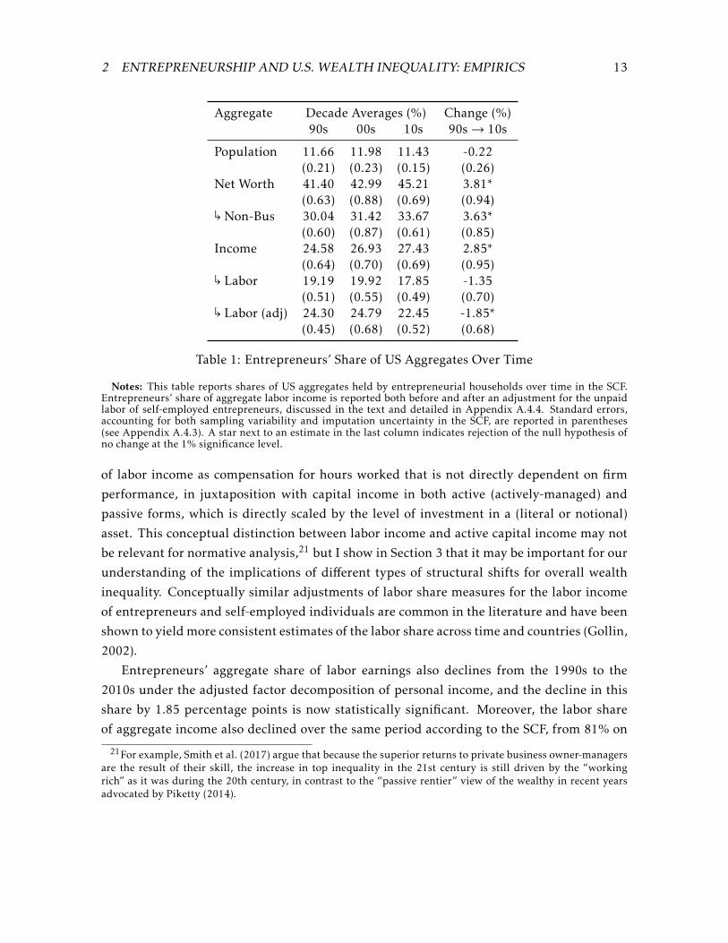
measured by their shares of key US aggregates. Table 1 reports the shares of US aggregates
held by entrepreneurial households in the SCF over the last three decades. The second,
third, and fourth columns report average estimates and corresponding standard errors from
survey waves occurring within each of the last three decades: the 1990s (waves 1989, 1992,
1995, and 1998), the 2000s (waves 2001, 2004, and 2007), and the 2010s (waves 2010, 2013,
and 2016), respectively. The last column reports the absolute change in the estimate from the
1990s average to the 2010s average. The aggregate shares of entrepreneurs for net worth and
income have both experienced a relative increase of about 10% from the 1990s to the 2000s
that is statistically significant at the 1% significance level. In particular, entrepreneurs’ share
of aggregate net worth has increased by almost 4 percentage points, from 41.4% in the 1990s
to 45.2% in the 2010s, and their share of aggregate income has increased by about 3 percent-
age points, from 24.6% to 27.4%. A similar increase has occurred for aggregate non-business
net worth, that is, all components of net worth other than inside (actively managed) private
equity (by construction, entrepreneurs own 100% of inside private business equity in all
years).
In contrast, entrepreneurs’ aggregate share of labor earnings has not increased over the
same period. The fifth row of Table 1 reports the aggregate share of labor earnings for the
group of entrepreneurs, where the measure of labor earnings for each household is its re-
ported wage income (inclusive of bonuses), extracted through survey questions that closely
follow key lines of US personal tax returns. The average labor earnings across entrepreneur-
ial households are approximately twice as high as average earnings across all households,
but the aggregate share of entrepreneurs appears to have fallen slightly from the 1990s to
the 2000s.
A limitation of this measure of labor earnings is that a substantial fraction of entrepre-
neurs, especially sole proprietors, report no wage income; this was especially true in earlier
survey waves. To address this shortcoming, I impute an estimate for the labor income of
these entrepreneurs, following a regression-based imputation method by Moskowitz and
Vissing-Jørgensen (2002) that uses information in the SCF on the hourly wages of employed
individuals and on the hours worked in a year of both employed and self-employed indi-
viduals. Appendix A.4.4 describes the method in detail. This adjustment to the “raw” fac-
tor decomposition of personal income based on tax returns is intended to capture a notion
2 ENTREPRENEURSHIP AND U.S. WEALTH INEQUALITY: EMPIRICS 13
Aggregate Decade Averages (%) Change (%)90s 00s 10s 90s→ 10s
Population 11.66 11.98 11.43 -0.22(0.21) (0.23) (0.15) (0.26)
Net Worth 41.40 42.99 45.21 3.81*(0.63) (0.88) (0.69) (0.94)↰
Non-Bus 30.04 31.42 33.67 3.63*(0.60) (0.87) (0.61) (0.85)
Income 24.58 26.93 27.43 2.85*(0.64) (0.70) (0.69) (0.95)↰
Labor 19.19 19.92 17.85 -1.35(0.51) (0.55) (0.49) (0.70)↰
Labor (adj) 24.30 24.79 22.45 -1.85*(0.45) (0.68) (0.52) (0.68)
Table 1: Entrepreneurs’ Share of US Aggregates Over Time
Notes: This table reports shares of US aggregates held by entrepreneurial households over time in the SCF.Entrepreneurs’ share of aggregate labor income is reported both before and after an adjustment for the unpaidlabor of self-employed entrepreneurs, discussed in the text and detailed in Appendix A.4.4. Standard errors,accounting for both sampling variability and imputation uncertainty in the SCF, are reported in parentheses(see Appendix A.4.3). A star next to an estimate in the last column indicates rejection of the null hypothesis ofno change at the 1% significance level.
of labor income as compensation for hours worked that is not directly dependent on firm
performance, in juxtaposition with capital income in both active (actively-managed) and
passive forms, which is directly scaled by the level of investment in a (literal or notional)
asset. This conceptual distinction between labor income and active capital income may not
be relevant for normative analysis,21 but I show in Section 3 that it may be important for our
understanding of the implications of different types of structural shifts for overall wealth
inequality. Conceptually similar adjustments of labor share measures for the labor income
of entrepreneurs and self-employed individuals are common in the literature and have been
shown to yieldmore consistent estimates of the labor share across time and countries (Gollin,
2002).
Entrepreneurs’ aggregate share of labor earnings also declines from the 1990s to the
2010s under the adjusted factor decomposition of personal income, and the decline in this
share by 1.85 percentage points is now statistically significant. Moreover, the labor share
of aggregate income also declined over the same period according to the SCF, from 81% on
21For example, Smith et al. (2017) argue that because the superior returns to private business owner-managersare the result of their skill, the increase in top inequality in the 21st century is still driven by the “workingrich” as it was during the 20th century, in contrast to the “passive rentier” view of the wealthy in recent yearsadvocated by Piketty (2014).

2 ENTREPRENEURSHIP AND U.S. WEALTH INEQUALITY: EMPIRICS 14
average in the 1990s to 73% in the 2000s to 70% in the 2010s.22,23 These trends suggest
that within-labor-earnings heterogeneity is not a likely reason for the increase in the relative
wealth of the group of entrepreneurs.
The slight decline in the relative labor earnings of entrepreneurs and the large decline
in the labor income share may partly reflect a tax-motivated reclassification of managerial
compensation from wage income to capital income in pass-through entities, S-corporations
in particular, which have grown in number in recent years. This effect is not fully accounted
for through the adjusted factor decomposition discussed above. However, the magnitude of
this effect is likely to be limited.24 In any case, a mere reclassification of managerial income
cannot by itself explain the increase in entrepreneurs’ aggregate share of total income.
2.3 Entrepreneurs and TopWealth Inequality
In this subsection, I decompose the increase in the top 0.1% and 1% net worth shares by
entrepreneurial status and find that it is driven almost exclusively by entrepreneurial house-
holds since 2000. I also show that most of the overall increase in top wealth inequality since
the 1990s took place from the 2000s to the 2010s. In Section 4.1, I confirm these trends
through two new summary measures of top inequality that play an important role in the
theoretical analysis of this paper.
Concentration of wealth at the top has increased substantially over the past three decades.
Figure A.3 plots the aggregate net worth share of top 1% group of households by net worth
from the first SCF survey wave in 1989 to the latest wave in 2016. Over this 27-year pe-
riod, the share of aggregate net worth held by the top 1% group has risen by 8.6 percentage
points, from 30.0% in 1989 to 38.6% in 2016. Similarly, the top 0.1% net worth share has
risen by 3.7 percentage points, from 11.1% in 1989 to 14.8% in 2016.25 Although there is
some disagreement on the exact magnitude of the wealth inequality increase, owing to dif-
ferent methods employed in the literature for estimating the wealth distribution in the U.S.,
the results from the SCF are on the lower end of the different estimates (Saez and Zucman,
2016; Kopczuk, 2015, 2016) and yet point to a substantial increase. This can be seen in Fig-
ure A.3, which also plots an estimate of the time series for the top 1% net worth share by
22These estimates are for the adjusted measure of labor income, that is, after the adjustment for unpaid en-trepreneurial labor income. The labor share under the tax-returns-based factor decomposition of income alsodeclines by about 10 percentage points, from 76% in the 90s to 68% in the 2000s to 66% in the 2010s.23This declining estimate for the labor share is largely consistent with other better-known estimates of labor
share dynamics from national tax and income accounting data. For example, Karabarbounis and Neiman (2014)document a 5-percentage-point decline in the labor share of the corporate sector globally using an internationaldata set compiled from country tax and income accounting data.24According to a back-of-the-envelope calculation by Smith et al. (2017), after accounting for this effect, the
true decline in the U.S. corporate sector’s labor share from 1980 to 2012 is 6.3% rather than 7.5%, which is stilla substantial decline.25The increase in these measures is slightly greater once one takes into account the increase in the wealth of
the richest 400 individuals in the Forbes 400 list, which are by design excluded from the SCF.

2 ENTREPRENEURSHIP AND U.S. WEALTH INEQUALITY: EMPIRICS 15
1989 1992 1995 1998 2001 2004 2007 2010 2013 20160
2
4
6
8
10
12
14Sh
areof
Agg
rega
teNet
Worth
Es in Top 0.1% GroupNEs in Top 0.1% Group
Figure 2: Decomposition of Top 0.1% Net Worth Share by Entrepreneurial Status over TimeNotes: This figure plots the share of aggregate net worth held by the entrepreneurs (E) and non-entrepreneurs(NE) that are part of the top 0.1% group by net worth. The colored bands represent 95% confidence intervals forthe SCF estimates based on bootstrap standard errors. Gray shaded areas denote NBER-designated recessions.
Saez and Zucman (2016), who use an income capitalization method based on tax data.
The increase in top wealth concentration has not taken place uniformly over this 27-year
period. Instead, it has mostly taken place since 2000s. The top 1% net worth share increased
by 3% on average from the 2000s to the 2010s but it increased only by 0.8% from the 1990s
to the 2000s (first column of Table A.1). The top 0.1% share in fact slightly declined on
average from the 1990s to the 2000s (Table A.2)).
Which types of households have contributed most to the increase in top wealth concen-
tration? First, consider a group decomposition of the top 1% share as T = T E + T NE , where
T E (T NE) is the aggregate value share of the entrepreneurs (non-entrepreneurs) that belong
to the top 1% group. Appendix Section A.2 discusses this decomposition for the top 1%
value share for several variables at a point in time (in the 2010s), showing that entrepre-
neurs within the top 1% groups hold a larger fraction of aggregate net worth and capital
income relative to non-entrepreneurs, while non-entrepreneurs hold a larger fraction of la-
bor income.
Figure 2 plots the net worth shares of the two groups of households within the top 0.1%
group over time, showing that the notable increase in top wealth concentration since 2000 is

3 A MODEL OF ENTREPRENEURSHIP AND INEQUALITY 16
entirely driven by entrepreneurs. In fact, the aggregate net worth share of non-entrepreneurs
within the top 0.1% group does not increase at all over the period from 2001 to 2016; the
point estimate declines from 3.7% in the 2001 survey wave to 3.5% in the 2016 wave. The
picture is similar for the evolution of the top 1% net worth share decomposition, plotted in
Figure A.4 and also summarized in terms of decade averages in the left panel of Table A.1.
Entrepreneurs within the top 1% group account for about 85% of the cumulative increase
in the top 1% share since 2000. Although these point estimates are accompanied by large
standard errors, since they correspond to a very small fraction of the population, they do
suggest that a shift occurred in the early 2000s, following a period in the 1990s where the gap
between the wealth of entrepreneurs and non-entrepreneurs in the top groups was declining.
Appendix Section A.3 presents a decomposition of the increase in top income inequal-
ity (the income share of the top 1% income group) since the 1990s both by group and by
income factor (labor and capital). This decomposition shows that the increase in the labor
income of the top 1% income group mainly occurred during the 1990s and almost exclu-
sively through non-entrepreneurs. In contrast, the increase in capital income is exclusively
due to entrepreneurs and has mostly taken place since 2000.
An analysis of US tax data also suggests that an important shift in the composition of
top income inequality and its increase occurred around the early 2000s, as emphasized by
Guvenen and Kaplan (2017). Figure A.5 plots the components of the income of the top 0.1%
and the top 1% groups by income over time, using the classification of pre-tax income into
wage income (wages, salaries, and bonuses, including exercised employee stock options),
financial income (interest income, dividends, and rents) and business income (referred to as
“entrepreneurial income” in Piketty and Saez (2003)), the latter category defined to include
the profits of partnerships, sole proprietorships, and type-S (pass-through) corporations,
and royalties. Although part of the increase in the business income of top groups since the
1980s is due to the U.S. tax reform of 1986, which created incentives for firms to register as
pass-through entities, the figure shows that the growth in the wage income for the top groups
has stopped or, for the top 0.1% group, reversed since 2000, while business income has
experienced a sustained increase until the end of the data series in 2015, with a significant
uptick in the early 2000s.26
3 A Model of Entrepreneurship and Inequality
This section introduces a parsimonious partial-equilibrium model of wealth accumulation
in order to examine the drivers and implications of the recent observed shifts in the cross-
sectional structure of inequality. Section 3.1 introduces the model setting and discusses key
26Income classified as financial income also experienced a similar uptick in the 2000s, but that was reversedin large part during the Great Recession of 2007-2009.

3 A MODEL OF ENTREPRENEURSHIP AND INEQUALITY 17
features of agents’ optimal policies. Section 3.2 introduces two analytically tractable sum-
mary measures of top wealth concentration and of the prevalence of entrepreneurs at the
top of the wealth distribution. Section 3.3 offers analytical characterizations of the level andtransitional dynamics of these inequality measures and other key aspects of the equilibrium
cross-sectional wealth distribution in themodel. Section 3.4 discusses a general-equilibrium,
endogenous-production extension of the model, presented in detail in Appendix E. Ap-
pendix B.2 contains additional details on the model and generalizations of the propositions
of this section. The quantitative calibration and analysis of the model is presented in Section
4.
3.1 Setting and Optimal Policies
Overlapping generations There is a unit mass of households. All households die randomly
at an exponential rate ω and a mass ωdt of offspring households, one for each deceased
household, is born every instant.
Preferences Households have identical scale-independent, recursive-utility preferences over
their consumption stream as well as the wealth bequeathed to their offspring, formally de-
scribed in Appendix C. This is a new specification of preferences that extends the continuous-
time version of Epstein-Zin utility, the Kreps-Porteus case of the stochastic differential util-ity class of Duffie and Epstein (1992), to allow for utility from bequests. Appendix C is
dedicated to their derivation and characterization. As with the standard Epstein-Zin speci-
fication, household preferences are characterized by the pure rate of time preference ρ, the
elasticity of intertemporal substitution (EIS) of consumption ψ, and the coefficient of rela-
tive risk aversion γ . The new specification features two additional parameters: parameter
VD that controls the strength of the bequest motive (the marginal value from bequeathed
wealth), and parameter ψ that can be interpreted as the elasticity of intergenerational sub-
stitution (EGS) of consumption.
Financial markets All households can frictionlessly invest in an instantaneously riskfree
asset at rate rf , and a risky financial asset with excess return over the riskfree rate dReBt =
πBdt + dBt, where Bt is a Brownian motion representing aggregate risk. This risky asset is
only exposed to aggregate risk, and its Sharpe ratio πB corresponds the price of aggregate
risk, that is, the risk premium (expected excess return) per unit of exposure to the aggregate
source of risk Bt.
Households can also invest in an annuity asset. A household with wealth Wit pledges a
fraction θDt of its wealth at its random time of death to the annuity fund in exchange for a

3 A MODEL OF ENTREPRENEURSHIP AND INEQUALITY 18
flow of income equal to ωθDtWitdt while alive.27 A negative position θD < 0 in this market
can be interpreted as holding a life insurance policy. Bequeathed wealth at the time of death
equalsWDit = (1− τD ) (1−θDt)Wit, where τD is the estate (bequest) tax rate.
All household income (including labor) is taxed at a proportional tax rate τ .
Entrepreneurial investment At any given point in time, an exogenous mass mE of house-
holds are entrepreneurs (Es) and amass 1−mE are non-entrepreneurs (NEs). Entrepreneurial
households have access to inside (entrepreneurial) equity, an asset with excess return over
the riskfree asset dReZit = πZdt + dZit, where household-specific Brownian motion Zit is a
source of purely idiosyncratic risk that cancels out on average across entrepreneurs. πZ is
the price of risk (Sharpe ratio) of inside equity or risk premium per unit of idiosyncratic
risk exposure, a key model parameter that is taken as exogenous in the partial-equilibrium
setting of the present section.
Type switching NE households become Es at an exponential rate νNE and E households
become NEs at a rate νE . The offspring of deceased households retain the entrepreneurial
type of their parents. The inflow-outflow balance condition for the mass of the two types,
ensuring that the mass of each type remains constant over time, is
(1−mE)νNE =mEνE . (1)
Labor earnings and newborn wealth At the time of birth, household i is endowed with a
flow of Lit = Lt exp(l˜i) units of permanent labor earnings, interpreted to include any govern-
ment transfer income, which they receive continuously until their death. Newborn house-
hold i’s draw of log relative earnings, l˜i ≡ log(Lit/Lt), is from a (scaled) distribution f sl˜ ,
for s ∈ {E,NE}, which may depend on entrepreneurial status at the time of birth.28 Let
α˜E ≡ L˜Et /Lt denote the ratio of average earnings across newborn E households over average
earnings across all households.29 Average earnings Lt evolve at a rate gLt and have propor-
tional exposure σLt to aggregate risk Bt. I consider equilibria featuring balanced growth in
the long-run, so that, in the model’s steady state, gL coincides with the growth rate of ag-
gregate income and wealth g, and σL coincides with the proportional exposure of aggregate
wealth to aggregate risk, σ .30
27This expression assumes that the annuity market is perfectly competitive, as in Blanchard (1985).28Distributions f El˜ and f NEl˜ sum tomE and 1−mE , respectively, so that f El˜ +f NEl˜ = fl˜, the (proper) distribution
of log labor earnings across all newborn households.29I assume that average earnings across newborn households equal average earnings across the population.30The endogenous-production model extension discussed in Section 3.4 and Appendix E offers a microfoun-
dation of this balanced-growth assumption.

3 A MODEL OF ENTREPRENEURSHIP AND INEQUALITY 19
Labor earning streams of living households are assumed to be fully pledgeable, so that, at
the time of their birth, newborn households pledge their future earning streams in exchange
for a capitalized stock of “labor wealth” WLit. In steady state, WLit = (1 − τ)Lt exp(li)/(rf +πBσL − (gL −ω)). Hence, the initial wealth of a newborn household is the sum of the wealth
inherited from his parent household and his own stock of labor wealth:
W newbornit =WDjt +WLit , (2)
where j refers to the parent of household i.
The assumption of fully pledgeable labor income streams ismade for the sake of tractabil-
ity, as it drastically simplifies the characterization of optimal policies under scale-independent
preferences, while still retaining the additive nature of labor earnings in the wealth accumu-
lation process across generations. Note that, under the perfect pledgeability assumption,
any transitory labor earnings risk over the life of a household would be diversified away. A
number of empirical studies have noted the importance of inequality in the permanent com-
ponent of labor earnings for overall inequality in labor incomes relative to heterogeneity
driven by transitory earnings shocks.31
The evolution of household wealth The wealth of surviving households evolves as
dWit
Wit= µWitdt + (1− τ)θBitdBt + (1− τ)θZitdZit , (3)
where τ is the income tax rate and
µWit = (1− τ)rWit − cit (4)
is the expected growth rate of wealth. Here, cit = Cit/Wit is the consumption-wealth ratio of
the household, and
rWit ≡ rf +ωθDit +πBθBit +πZθZit (5)
is the expected (pre-tax) rate of return on the wealth of household i, and θBit, and θZit denote
the optimally chosen proportional exposures of household wealth to the (pre-tax) returns of
the risky financial asset and inside entrepreneurial equity, respectively, with θZit = 0 if the
household is a non-entrepreneur.
31Guvenen et al. (2017) offer direct empirical evidence on the importance of lifetime labor earnings inequalityin the US, and Kopczuk, Saez, and Song (2010) show that almost all of the increase in the variance in annual(log) earnings in the US since 1970 is due to an increase in the variance of permanent earnings (as opposed totransitory earnings).

3 A MODEL OF ENTREPRENEURSHIP AND INEQUALITY 20
Net worth and labor wealth Total household wealth Wit is the theoretically appropriate
concept of household wealth, capturing all resources over which a household has a claim
that can be used to finance present and future consumption, but it is not directly observable.
The empirical measure of household net worth (net assets) is best interpreted in this model
as the non-labor component of total household wealth, or total wealth less the measureWLit
of the capitalized future labor income stream of the household:
Nit =Wit −WLit =Wit −WLt exp(lit), (6)
whereWLt denotes aggregate labor wealth.32
In steady state,
WLt =(1− τ)Lt
rf +πBσ − (g −ω), (7)
and the share of aggregate labor income in total expected income, a proxy for the aggregate
labor income share, is
ly =Lt
rWWt= wL
rf +πBσ − (g −ω)(1− τ)rW
, (8)
where
wL ≡WLt
Wt(9)
is the ratio of aggregate labor wealth to total wealth.
Household portfolio choice and saving Themodel features tractable household-level poli-
cies, given in appendix Proposition B.1, which only depend on the household’s type (E or NE)
after scaling by the household’s total wealth. In particular, households choose consumption-
wealth ratios c(s) ≡ Cit/Wit, bequeathed-to-surviving wealth ratios wD(s) ≡ WDit/Wit = (1 −τD )(1 − θD(s)), and proportional wealth exposures θB and θEZ to the risky asset returns that
are independent of the level of wealth and are only a function of household type s ∈ {E,NE}.Under unit elasticity of intertemporal substitution of consumption, ψ = 1, all households
choose the same consumption-wealth ratio; similarly, under unit elasticity of intergenera-
tional substitution of consumption, all households choose the same bequeathed-to-surviving
wealth ratio.
Because all households have identical preferences, and in particular the same risk aver-
sion coefficient γ , they always choose the same proportional exposure to aggregate risk
32In a version of the model with finite lifetimes, the capitalized stock of future labor income approaches zeroas the household nears the end of its (working) life. In the present setting, the capitalized value of future laborearnings only depends on a household’s initial permanent earnings draw and not on the household’s age, animplication of the perpetual-youth structure of the setting. An age-dependent profile of labor earnings couldeasily be added to the present model to generate more realistic age-labor income dynamics with minimal impacton the key model predictions.

3 A MODEL OF ENTREPRENEURSHIP AND INEQUALITY 21
θB = πB/((1 − τ)γ) regardless of type, as shown in Proposition B.1. The inclusion of the
risky asset in the model simply serves to disentangle the average return to wealth from the
riskfree rate in the quantitative calibration of the model.
Entrepreneurs choose to invest a fraction
θEZ =πZ
(1− τ)γ(10)
of their wealth in inside equity, which is proportional to the inside equity premium πZ and
inversely proportional to risk aversion γ . As a result, the expected excess pre-tax return
earned by the average entrepreneur on inside equity is given by
ΠZ = πZθEZ =
π2Z
(1− τ)γ. (11)
The expected excess return on inside equity ΠZ is the key determinant of the expected-
return-on-wealth differential between entrepreneurs and non-entrepreneurs, rEW − rNEW . In
the benchmark case where households have unit elasticities of intertemporal and intergener-
ational substitution, ψ = ψ = 1, households have the same consumption and bequest policies
regardless of type and, as a result, equations (3)–(5) imply rEW − rNEW =ΠZ .
Defining the saving rate of an agent as the expected change in total wealth as a fraction
of expected (after-tax) income,
sys ≡µsW
(1− τ)rsW= 1− cws
(1− τ)rsW, (12)
for s = {E,NE}, the model reproduces the strong empirical regularity that entrepreneurial
households have much higher saving rates than non-entrepreneurs (Gentry and Hubbard,
2004; Quadrini, 2000), as a result of the superior average return on wealth earned by entre-
preneurial households.33
3.2 Top-Weighted Inequality Measures
In this subsection, I introduce two summarymeasures of top wealth inequality, top-weighted
average wealth and the top-weighted wealth share of entrepreneurs, which I characterize
33This result holds for empirically plausible levels of consumption elasticities not too close to zero. In thesimple case with unit elasticities of intertemporal and intergenerational substitution of consumption, ψ = ψ = 1,the saving rate differential is directly proportional to the return differential:
syE − syNE =ρ(rEW − r
NEW
)(1− τ)rEW r
NEW
=ρΠZ
(1− τ)rEW rNEW
. (13)
More generally, the saving rate differential is increasing in the elasticities ψ and ψ, all else equal.

3 A MODEL OF ENTREPRENEURSHIP AND INEQUALITY 22
analytically in the next subsection and investigate empirically in Section 4.1.
I define top-weighted average wealth as the cross-sectional expectation (average) of indi-
vidual wealth relative to average wealth raised to a power ζ ≥ 1:34
Ft(ζ) ≡ E∗(Wit
Wt
)ζ , (14)
where E∗ denotes the cross-sectional expectation operator.
By definition, Ft(1) = 1. In the case of perfect equality (a degenerate wealth distribution),
this function would be constant and equal to unity for all ζ, but, for any non-degenerate
distribution of wealth, Ft(ζ) is a strictly increasing function for ζ > 1. When ζ > 1, the
expectation overweighs richer households, so that Ft(ζ) can be interpreted as a measure of
top inequality, for a given exponent ζ, with higher ζ implying further overweighting of the
top of the distribution. When the wealth distribution has a right Pareto tail, as is the case
empirically, with Pareto exponent ζ∗, it can be shown that top-weighted average wealth is
finite for 1 ≤ ζ < ζ∗, and diverges to infinity as ζ→ ζ∗.35
Figure B.1 plots the schedule of top-weighted average wealth as a function of ζ when the
wealth distribution is exactly Pareto.36 Because a lower Pareto exponent ζ∗ corresponds to
a more unequal distribution, top-weighted average wealth for a fixed ζ > 1 can be used to
compare the degree of top inequality across different distributions.An additive group decomposition of the schedule of top-weighted average wealth can be
used to study the prevalence of entrepreneurs across the wealth distribution. In particular,
decompose top-weighted average wealth as Ft(ζ) = F Et (ζ) +F NEt (ζ), where
F Et (ζ) =mEE∗(Wit
Wt
)ζ ∣∣∣∣i ∈ E (16)
F NEt (ζ) =(1−mE
)E∗
(Wit
Wt
)ζ ∣∣∣∣i ∈NE
, (17)
andmE is the population share of entrepreneurs. Define the top-weighted average wealth share
34When the empirical measure of wealth can take negative values, as in the case of net worth, I restrict atten-tion to households with strictly positive wealth when taking the average.35Of course, in any finite sample, this cross-sectional expectation is finite for any ζ > 1.36That is, log relative wealth w = log(Wit/Wt) has an exponential distribution, f (w) = cexp(−ζ∗w) for w ≥ w
(f (w) = 0 otherwise) for some constant c > 0. In this case, top-weighted average wealth is given by
F (ζ) =ζ∗
(ζ∗−1ζ∗
)ζζ∗ − ζ
. (15)

3 A MODEL OF ENTREPRENEURSHIP AND INEQUALITY 23
of entrepreneurs as
φEt (ζ) ≡F Et (ζ)Ft(ζ)
, (18)
for ζ ≥ 1. When ζ = 1, φE(1) = φE is simply the aggregate wealth share of entrepreneurs.
For ζ > 1, we can interpret φE(ζ) as a tractable indicator for the prevalence of entrepreneurs
in top wealth groups. If the wealth distribution within the two groups was identical, up
to scaling, ϕE(ζ) would be flat as a function of ζ and equal to the population fraction of
entrepreneurs.
These measures can be used to study the cross-sectional structure of inequality in any
variable, not just wealth. In particular, I define top-weighted average labor earnings and
entrepreneurs’ top-weighted share of labor earnings as:
Flt(ζ) ≡ E∗(LitLt
)ζ (19)
φELt(ζ) ≡F Elt (ζ)Flt(ζ)
, (20)
respectively, where F Elt (ζ) and FNElt (ζ) are defined as in equations (16) and (17).
3.3 The Structure of Inequality
In this subsection, I present some key analytical results regarding the implications of the
model for inequality, both in the long-run and during transitions following structural changes
in the economy. For expositional simplicity, I consider the simple case of no bequests, VD = 0
in this section. Appendix B.2 extends these results to the general case with bequests.
To examine analytically the implications of this framework for inequality, it is useful to
characterize the evolution of log relative household wealth wit ≡ log(Wit/Wt), that is, the log
of the ratio of individual wealth to average wealth. The log relative wealth of surviving E
and NE households evolves, respectively, as37,38
dwEit =(µEt +ω(1−wL)−
(θE
)2/2
)dt +θEdZit (21)
dwNEit =(µNEt +ω(1−wL)
)dt, (22)
where µEt ≡ µEW − gt = (µEW −µNEW )(1−φE) is the mean excess wealth growth rate of surviving
Es relative to the average growth rate of all surviving households, gt, and θE ≡ (1 − τ)θEZ is
37These expressions follow from the law of motion of household wealth (3) and Ito’s Lemma.38For ease of exposition, I omit the time subscript from variables that I take to be constant both in steady
state and during the transition following a structural shift (except possibly for an instantaneous jump). Theassumptions regarding the transition are discussed in Section 4.

3 A MODEL OF ENTREPRENEURSHIP AND INEQUALITY 24
the proportional wealth exposure of E households to the after-tax return to inside equity.
Similarly, µNEt ≡ µNEW − gt = −µEφE/(1 − φE) is the excess wealth growth of surviving NEs.
µE (µNE) is increasing (decreasing) in the return differential rEW − rNEW , and thus the inside
equity premium πZ , all else equal. By the law of large numbers, the proportional wealth
exposure of E households to entrepreneurial risk Z, θE , is also the cross-sectional volatility
of the instantaneous, after-tax returns to wealth across entrepreneurs. By the optimal choice
of the entrepreneurial investment scale, θE = πZ /γ is also increasing in the inside equity
premium πZ .
Inequality in the long-run Lemma 1 below characterizes the aggregate total wealth and
net worth shares of Es in terms of structural parameters in the steady state of the model.
Lemma 1 (Entrepreneurs’ Share of Aggregates). In steady state, the aggregate share of totalwealth held by Es is
φE =mEα˜EωwL + νNE/mEωwL + νNE/mE −µE
. (23)
The aggregate share of net worth held by Es is
φEN =φE −φELwL
1−wL, (24)
and their aggregate labor earnings share is
φEL =mEα˜Eω+ νNE/mE
ω+ νNE/mE. (25)
Equations (23) and (24) capture the two key distinct sources of heterogeneity affectingthe aggregate wealth and net worth shares of Es and NEs. First, if Es receive higher labor
earnings on average than NEs, α˜E > 1 and thus φEL > mE , their aggregate total wealth and
net worth shares, ϕE and ϕEN , will both be greater than their population share mE even
if they have identical returns on wealth, µE = 0.39 In the data, φEL /mE ≈ 2 (see Table 1).
Second, if Es receive superior returns on average, µE > 0, their wealth and net worth shares
will also exceed their population shares even if they receive the same earnings on average,
α˜E = 1 and thus φEL = mE . Moreover, under µE > 0, their aggregate total wealth and net
worth shares are increasing both in the level of return differential through µE and in the
cross-sectional persistence of entrepreneurial status (decreasing in the type-switching rate,
νNE), since high persistence implies that a given entrepreneurial household has access to the
superior-average-return entrepreneurial technology for a longer period of time on average.
39This is true for the net worth share under the empirically relevant case of positive aggregate net worth.

3 A MODEL OF ENTREPRENEURSHIP AND INEQUALITY 25
Next, I characterize inequality throughout the wealth distribution. Denote the cross-
sectional distribution (probability density function) of log relative wealth by ft(w), and the
(scaled) distributions for E and NE households by f Et (w) and f NEt (w), respectively, which
satisfy ft(w) = fEt (w) + f NEt (w). The dynamics of the cross-sectional distributions f Et (w) and
f NEt (w) obey a system of partial differential equations known as the Forward Kolmogorov
Equations, given by appendix equations (55) and (56). The steady-state distributions f E(w)
and f NE(w) for the model under the baseline calibration, discussed in the next subsection,
are plotted in appendix Figure B.2.
Similarly, denote the cross-sectional distribution of log relative labor earnings by flt(w),
and the corresponding (scaled) distributions for E and NE households by f Elt (w) and fNElt (w).
These distributions also obey a system of Forward Kolmogorov Equations, given by appendix
equations (59) and (60).
The measure of top-weighted average wealth, introduced in the previous subsection, cor-
responds mathematically to the moment-generating function of the distribution of log rela-
tive wealth f (w),40
Ft(ζ) =∫ ∞−∞
exp(ζw)ft(w)dw, (26)
and similarly for the (scaled) top-weighted average wealth across Es and NEs, F E(ζ) andF NE(ζ), respectively. Similarly, top-weighted average labor earnings correspond to themoment-
generating function of the distribution of log relative earnings fl(l):41
Flt(ζ) =∫ ∞−∞
exp(ζl)flt(l)dl. (27)
Proposition 1 offers analytical characterizations for the long-run levels of the top-weighted
wealth inequality measures.
Proposition 1 (Top-Weighted Moments). In steady state, the top-weighted aggregate wealthshare of entrepreneurs φE(ζ) and top-weighted average wealth F (ζ) satisfy
φE(ζ) =mEwζL(Fl(ζ)/F (ζ))(ω+ νNE/mE)φEL (ζ)/m
E +(1−wζL(Fl(ζ)/F (ζ))
)νNE/mE
λE(ζ)(28)
40Gabaix et al. (2016) use essentially the same measure to derive theoretical results regarding the speed ofconvergence for cross-sectional distributions in continuous-time settings like the present one. They state theirresults in terms of the Laplacian transform of the log relative wealth (income) distribution, which is simply thehorizontal reflection of the moment-generating function around the y-axis.41As shown in Appendix Lemma B.1, in the steady state of the model, the cross-sectional distribution of
labor earnings across all households fl (l) coincides with the (exogenous) earnings distribution across newbornhouseholds, fl˜(l). For this reason, it is also the case that Fl (ζ) = Fl˜(ζ) in steady state. However, because of typeswitching, f sl (l) , f
sl˜ (l), for s ∈ {E,NE}, that is, the equilibrium earnings distribution for each type does not
coincide with the earnings distribution across newborn households of that type.

3 A MODEL OF ENTREPRENEURSHIP AND INEQUALITY 26
and
F (ζ) =ωwζLλ(ζ)
Fl(ζ), (29)
where
λE(ζ) ≡ω (1− ζ(1−wL)) + νNE/mE −µEζ − (θE)2ζ(ζ − 1)/2 (30)
λNE(ζ) ≡ω (1− ζ(1−wL)) + νNE/mE −µNEζ, (31)
and
λ(ζ) ≡ λE(ζ)φE(ζ) +λNE(ζ)(1−φE(ζ))− νNE/mE
=ω (1− ζ(1−wL))−µEφE(ζ)−φE
1−φEζ −φE(ζ)
(θE
)2ζ(ζ − 1)/2. (32)
For given ζ and for µE > 0, both wealth inequality measures are increasing in the mean ex-cess wealth growth rate of entrepreneurs µE and, when φE(ζ) > φEL (ζ), in entrepreneurial typepersistence (decreasing in the type-switching rate νNE). For ζ > 1, they are also increasing in thevolatility of entrepreneurial returns θE .
The prevalence of entrepreneurs at the top of the wealth distribution, captured by φE(ζ)
for high ζ > 1, is increasing in the return differential between Es and NEs and in the cross-
sectional persistence of this differential, as in the special case of the aggregate wealth share,
φE = φE(1), presented in Lemma 1.The fraction of Es at the top is, however, also increasing
directly in the volatility of returns across Es, θE . Even in a world with no labor earnings het-
erogeneity between Es and NEs, φE =mE , and no superior average returns to entrepreneur-
ship, µE = µNE = 0, if there is, for unmodeled reasons, dispersion in realized entrepreneurial
returns, θE > 0, successful entrepreneurs will tend to dominate the top of the distribution
merely as a consequence of the idiosyncratic risk that they take. This highlights the impor-
tance of explaining the entire schedule of the top-weighted entrepreneurial wealth share,
including both its intercept at ζ = 1 and its slope.
Overall topwealth inequality, as captured by themeasure of top-weighted average wealth
F (ζ) for ζ > 1, is increasing in top concentration within the labor earnings distribution, as
captured by top-weighted average earnings Fl(ζ). By equation (32), it is also increasing in
the expected return differential between Es and NEs, and the magnitude of this effect isincreasing with the slope of Es’ top-weighted share schedule.
A key insight from equations (29) and (32) is that, after controlling for the schedule of
the top-weighted wealth share of Es, the long-run level of top-weighted average wealth does
not depend directly on the churning rate νNE . As I discuss in Section 4.5, this implies that

3 A MODEL OF ENTREPRENEURSHIP AND INEQUALITY 27
entrepreneurial persistence can be separately identified from the average return differentialbetween entrepreneurs and non-entrepreneurs by imposing the joint restrictions of observed
top wealth concentration (the schedule Ft(ζ) or top group wealth shares) and the observed
relative wealth of entrepreneurs across the distribution (the schedule ϕE(ζ)).
Even in a world with homogeneous investment returns, entrepreneurs will be prevalent
at the top of the wealth distribution, φE(ζ) > mE , as long as they are prevalent at the top
of the labor earnings distribution, φEL (ζ) > mE . However, in realistic model calibrations, the
impact of Es’ top-weighted labor earnings share ϕEL (ζ) on their top-weighted wealth share
φE(ζ) declines as one moves along the top of the wealth distribution by considering increas-
ing values of ζ. The reason is that, empirically, the Pareto tail of wealth is thicker than the
Pareto tail of labor earnings. As a result, Fl(ζ)/F (ζ) declines to zero as ζ approaches the
wealth Pareto tail exponent ζ∗ from below.42 As ζ ↗ ζ∗, the top-weighted wealth share of
entrepreneurs becomes independent of labor-earnings heterogeneity. The next proposition,
which characterizes the asymptotic right Pareto tail of the wealth distribution, further illus-
trates this point.
Proposition 2 (Pareto Tail in Steady State). Wealth and net worth exhibit a right Pareto tail. Inparticular, f E(w)→ cE exp(−ζ∗w) and f NE(w)→ cNE exp(−ζ∗w) as w→∞, where ζ∗ > 1 is thePareto exponent of the tail and cE , cNE > 0 are constants.
In any equilibrium where the Pareto tail of wealth is thicker than the Pareto tail of laborearnings (the empirically relevant case), the Pareto tail exponent solves the equation
λE(ζ∗)λNE(ζ∗)− νEλE(ζ∗)− νNEλNE(ζ∗) = 0, (33)
where λE(ζ) and λNE(ζ) are given by equations (30) and (31), respectively.43
The (population and wealth-weighted) share of Es in the asymptotic top wealth (and net worth)group is
cE
cE + cNE=
νNE
λE(ζ∗). (34)
Inequality at the very top of the distribution as captured by the Pareto tail exponent,
with a lower exponent corresponding to higher inequality (thicker tail), is determined ex-
clusively by the process of wealth accumulation and is independent of the distribution of
labor earnings.44 These asymptotic expressions hinge on the empirically realistic assump-
42Recall from the discussion of Section 3.2 that top-weighted average wealth diverges to infinity as ζ ↗ ζ∗.The same is true for top-weighted average earnings as ζ ↗ ζ∗L, where ζ∗L is the Pareto tail exponent of earn-ings. However, the fact that the Pareto tail of wealth is thicker than that of earnings implies ζ∗ < ζ∗L, so thatFl (ζ)/F (ζ)↘ 0 as ζ↗ ζ∗.43Note that equation (33) is equivalent to λ(ζ∗) = 0, where λ(ζ) is given by equation (32).44The result that the Pareto tail of wealth is either dominated by the Pareto tail of labor earnings or completely
independent of labor earnings inequality is a celebrated result in formal theories of top inequality that goes backat least to Grey (1994).

3 A MODEL OF ENTREPRENEURSHIP AND INEQUALITY 28
tion that labor earnings become a negligible fraction of the total income of extremely rich
individuals (e.g. the individuals in the Forbes 400). In themodel, non-entrepreneurs in these
very small groups of individuals at the very top are part of these groups solely because they
used to be extremely rich entrepreneurs in the recent past and not due to high labor earn-
ings.45 Although empirically labor earnings is a non-negligible part of the total income of
conventionally studied top groups, such as the top 0.1% and 1% groups, expression (34) for
entrepreneurs’ share in the asymptotic top wealth group offers a useful analytical approx-
imation for the fraction of entrepreneurs, which turns out to be quite accurate in realistic
model calibrations.
Inequality dynamics The final analytical result offers important insights into the predic-
tions of this theoretical framework regarding the transitional dynamics of inequality.
Proposition 3 (Speed of Transition). In response to permanent and unanticipated structuralshifts, the top-weighted wealth share of Es evolves according to
dφE(ζ)dt
= −sEt (ζ)φEt (ζ) + νNE +ωwζLF
El˜ (ζ)/Ft(ζ), (35)
with speed of transitionsEt (ζ) = λ
Et (ζ) +ωw
ζLFl˜(ζ)/Ft(ζ)−λt(ζ), (36)
where λE(ζ) and λ(ζ) are given in equations (30) and (32). For µEt ≥ 0, the asymptotic speed ofthe transition in Es’ top-weighted wealth share,46
sE(ζ) = limt→∞
sEt (ζ) = λE(ζ), (37)
for ζ ≥ 1, is bounded above by the speed of transition of Es’ aggregate wealth share:
λE ≡ λE(1) = ωwL + νNE/mE −µE , (38)
which is decreasing in entrepreneurial persistence and in the mean excess wealth growth rate ofentrepreneurs, µE .
45Formally, the fact that E type is not an “absorbing” state at the household level (i.e. νE > 0), so that thePareto tail of wealth is not comprised solely of Es, gives rise to the third-degree polynomial equation (33) for thePareto exponent. If νE = 0, equation (33) simplifies to λE(ζ∗) = νNE , a quadratic polynomial equation in ζ∗ ofthe type commonly found in single-type random growth models (see e.g. Gabaix (2009)).46The asymptotic exponential rate of convergence is formally defined as
sE(ζ) ≡ − limt→∞
d log(|φEt (ζ)−φEss(ζ)|
)dt
,
where φEss denotes the (new) steady-state value of φEt (ζ).

3 A MODEL OF ENTREPRENEURSHIP AND INEQUALITY 29
Expression (38) for the exponential rate of convergence of the aggregate wealth share
of entrepreneurs illustrates that type persistence, as captured by the churning rate νNE ,
and the mean excess wealth growth rate of entrepreneurs µE are the key determinants of
the speed of convergence following structural shifts in the economy, such as an increase in
the inside equity premium. Intuitively, a lower rate of churning and higher wealth growth
differential imply slower reversal of existing wealth differences between entrepreneurs and
non-entrepreneurs and between richer and poorer households. Importantly, the convergence
rate of the aggregate wealth share ϕE is an upper bound for the speed of transition of top
inequality, as captured by the top-weighted wealth shares of entrepreneurs. In particular,
top inequality evolves more slowly when there is large heterogeneity within entrepreneurs,
as captured by the cross-sectional volatility of their realized returns, θEZ .
Appendix B.2 shows that these results and intuitions readily extend to the case with
bequests, although the closed-form expressions for the top-weighted inequality measures
hold only as approximations around ζ = 1. The intergenerational transmission of wealth in
the presence of bequest motives generally amplifies the level of top inequality, all else equal.
3.4 General-EquilibriumModel Extension
The present theoretical analysis does not endogenize the level of the inside entrepreneurial
equity premium, the key determinant of cross-sectional heterogeneity in returns on wealth
in the model. In Appendix E, I present and analyze a general-equilibrium, endogenous-
production extension of the model this section, which endogenizes the inside equity pre-
mium and shows that the key implications for wealth inequality of the partial-equilibrium
model of Section 3 carry over to a setting where entrepreneurial investments are more real-
istically modeled as long-term, illiquid investments.
The model interprets the capital of a real-world firm as a combination of liquid (pledge-
able) capital (e.g. machinery, equipment, buildings) and entrepreneurial capital. Investment
in entrepreneurial capital captures investment in processes and methods tied to the skills of
the individual in charge of the firm. Because the payoff of such investments is tied to the
skills and effort exerted by the entrepreneur or manager, he or she must personally retain
exposure to this payoff for incentive reasons. In reality, this exposure may come in the form
of partial or whole equity ownership of the firm, or long-term performance-based schemes
in managerial compensation.
The key long-term determinant of the inside equity premium in the model is the relative
productivity of entrepreneurial capital relative to liquid capital. An increase in the rela-
tive productivity of entrepreneurial capital can generate the key predictions of the partial-
equilibrium model regarding the evolution of wealth inequality.
The general-equilibriummodel alsomakes additional predictions regarding the response

4 QUANTITATIVE MODEL ANALYSIS 30
of the equilibrium riskfree rate in response to an increase in the relative productivity of en-
trepreneurial capital via the precautionary saving channel. I study the impact of idiosyn-
cratic entrepreneurial risk on the dynamics of the U.S. riskfree rate both empirically and an-
alytically in the context of a related endogenous-production asset pricing model in Tsiaras
(2018).
4 TheDrivers of the U.S.Wealth Inequality Increase: Quantitative
Model Analysis
In this section I investigate the drivers of changing U.S. wealth inequality documented in
Section 2 through a calibration and quantitative analysis of the model of Section 3. In par-
ticular, I use the restrictions imposed by the structure of top inequality in the US data to
infer the increase in the inside equity premium that, together with the observed increase in
within-earnings heterogeneity, can account for the increase in top inequality and the relative
wealth of entrepreneurs from the 1990s to the 2010s. I also examine the implications of this
increase for future inequality.
Section 4.1 investigates the top-weighted inequality measures introduced in Section 3 in
the SCF data. Section 4.2 describes the transition experiment at the center of the quantitative
analysis of the model and Section 4.3 discusses the calibration of the labor earnings distri-
bution in the model. Section 4.4 presents the details and conclusions from the simulated
method of moments (SMM) estimation of the model. Section 4.5 discusses the intuition for
and evidence consistent with the inference of high cross-sectional persistence of entrepre-
neurial status. Finally, Section 4.6 discusses micro-level evidence from the SCF pointing to
an increase in the returns to privately-held equity as the main driver of the apparent increase
in the average return differential between entrepreneurs and non-entrepreneurs.
4.1 Top-Weighted Inequality Measures in the SCF
This subsection investigates in the SCF data the top-weighted inequality measures intro-
duced and characterized analytically in Section 3, for the empirically observable wealth
concept of net worth. Matching the schedule of the top-weighted net worth share of en-
trepreneurs is a key goal of the model calibration, as a way to capture the relative position
of entrepreneurs across the net worth distribution.
The top panel of Figure 3 plots decade averages of the schedule of top-weighted average
net worth in the SCF data for different values of ζ. As is visually evident from the figure,
almost all of the increase in top concentration has taken place from the 2000 to the 2010s
according to this measure, with top concentration barely changing from the 1990s to 2000s.
This conclusion is consistent with the evolution of top group shares, as discussed in Section

4 QUANTITATIVE MODEL ANALYSIS 31
2.3.
The bottom panel of Figure 3 plots decade averages for the top-weighted net worth share
of entrepreneurs in the SCF data. The figure highlights an increase in the value-weighted
share of entrepreneurs throughout the net worth distribution, including at the top, from the
1990s to the 2010s, as the gap between the two schedules is roughly constant across differentζ’s (in fact, the average slope is slightly higher in the 2010s). Interestingly, the increase in
the intercept (at ζ = 1) and the decline in the slope of the measure from the 1990s to the
2000s is consistent with the increase in the aggregate net worth share of entrepreneurs as
well as the decline in their share within the top 1% group over this period (which can be
seen in Tables 1 and A.1, respectively), highlighting the ability of this measure to capture
the relative importance of the two groups at different parts of the distribution.
4.2 Transition Experiment
The quantitative analysis of the model centers on a parsimonious calibration exercise on
transitional dynamics. Starting from the steady state of the model, which I calibrate to
moments from the 1990s, I consider the impact of three permanent, concurrent structural
shifts: a change in the level of the inside equity premium, a change in the cross-sectional
distribution of relative permanent labor earnings (within-labor-earnings heterogeneity), and
a change in the aggregate share of labor earnings in personal income (labor income share).
Starting from the old steady state, at a point in time t0 the economy experiences an in-
stantaneous jump in the inside equity premium of ∆πZ and an instantaneous jump in the
ratio of aggregate labor wealth to total wealth ∆wL. Both πZ and wL remain constant at their
new values throughout the transition. Holding constant the ratio wL during the transition
implies that the aggregate labor share of income remains roughly constant throughout the
transition at its new steady state level. At the same time t0, while the cross-sectional dis-
tribution of net worth across households is held constant (does not jump), all households
receive draws from a new distribution of relative labor earnings, retaining their relative
ranking from the old distribution. Accordingly, households’ labor wealth, and hence their
total wealth, experiences a jump at time t0. All other structural parameters are held constant.
These shifts are not anticipated ex ante by agents.
First, I calibrate a simple specification for the labor earnings distribution using data on
the labor income shares of top groups by labor income in the SCF, both in the 1990s and in
the 2010s. Second, I apply the simulated method of moments (SMM) procedure to estimate
several model parameters in the original (1990s) steady state of the model jointly with the
long-run change in the inside equity premium ∆πZ and the long-run change in the ratio of
aggregate labor wealth to total wealth ∆wL, targeting wealth inequality moments from the
1990s and 2010s together with some aggregate moments.

4 QUANTITATIVE MODEL ANALYSIS 32
1 1.1 1.2 1.3 1.41
1.2
1.4
1.6
1.8
2
2.2
2.4
2.6
2.8
3
ζ
Top-W
eigh
tedAverage
Net
Worth
1990s2000s2010s
1 1.1 1.2 1.3 1.440
42
44
46
48
50
52
54
56
58
60
62
64
ζ
Top-W
eigh
tedAgg
rega
teNet
Worth
Shareof
Es(%
),ϕE N(ζ)
1990s2000s2010s
Figure 3: Top-Weighted Inequality Moments in the SCFNotes: The top and bottom panels of this figure plot decade averages of the schedules of top-weighted averagenet worth and entrepreneurs’ top-weighted net worth share, respectively, as a function of the exponent ζ in theSCF data. These measures (applied to net worth) are defined in equations (14) and (18), respectively. Onlyhouseholds with strictly positive net worth are considered when computing the measures.

4 QUANTITATIVE MODEL ANALYSIS 33
4.3 Labor Earnings Calibration
I choose a simple specification for the cross-sectional distribution of permanent labor earn-
ings across all newborn households, fl˜, that captures well the top of the U.S. labor income
distribution as it reproduces its empirically observed Pareto tail. A fraction µL = 10% of
newborn households receive draws from an exponential distribution for log earnings with
Pareto exponent ζ∗L and threshold l, while the remaining households receive draws from a
truncated normal distribution with mean mL, standard deviation sL, truncated at l. Because
this is the distribution of log earnings relative to average earnings, there are three free pa-
rameters to be calibrated.
I calibrate these parameters using information on the aggregate labor income shares of
top groups by labor income in the SCF, separately for the 1990s and for the 2010s (using
averages of survey waves from each decade).47,48 First, I set ζ∗L to the value that reproduces
the observed ratio of the top 1% group share to the top 10% group share.49 Second, I set the
cutoff l to match the level of the top 10% labor income share. Although not directly targeted,
the implied 5% top share is within one percentage point of the actual shares, owing to the
fact that the Pareto distribution offers a remarkably good fit to the entire top end of the labor
income distribution. Finally, I calibrate the remaining free parameter, which controls the
truncated normal distribution, to match the labor income share of the top one-third of the
population. The calibrated distributions are reported in Figure 4. The Pareto exponent ζ∗Ldeclines from 2.09 in the 1990s to 1.85 in the 2010s, corresponding to a significant increase
in within-labor-earnings inequality.
I further allow for distinct average labor earnings for each type, E and NE, while assum-
ing for simplicity that the distribution of earnings relative to type-specific average earnings
is the same for the two types. In the SCF data, the estimate for ratio of average labor earn-
ings across Es to average labor earnings across all households, φEL /mE , is 2.08 in the 1990s
and declines slightly to 1.96 in the 2010s. These estimates use the factor decomposition of
income after an adjustment for the imputed labor earnings of entrepreneurs who report no
wage income in their tax returns, discussed in Section 2.2. The estimates are similar under
47Themeasure of household labor income used in the computation of the top group shares incorporates the ad-justment for the imputed labor income of self-report entrepreneurs who reported no regular salaries, discussedin Section 2.2.48This procedure ignores the impact of transitory labor income shocks to the cross-sectional distribution of
annual labor earnings. However, the estimates from the calibration (for the evolution of the Pareto exponent,in particular) are very similar quantitatively to calibrations that allow for both transitory and persistent compo-nents in individual labor earnings (see, e.g., Hubmer, Krusell, and Smith (2016)).49This computation uses the fact that, when a variable is distributed according to an exact Pareto distribution,
the ratio of the top x% group share to the top y% group share, Tx/Ty , satisfies
log(Tx/Ty ) =(1− 1/ζ∗L
)log(x/y). (39)

4 QUANTITATIVE MODEL ANALYSIS 34
−5 −4 −3 −2 −1 0 1 2 3 4 50
0.2
0.4
0.6
0.8
1
1.2
1.4
1.6
1.8
2
2.2
2.4
Log Relative Permanent Labor Earnings, l
Proba
bility
Den
sity
Func
tion
,fl(l)
1990s2010s
Figure 4: Calibration of Labor Earnings Distribution
Notes: This figure plots the calibrated cross-sectional distributions for relative labor earnings using SCF datafrom the 1990s and the 2010s. Calibrated parameters for the 1990s: ζ∗L = 2.092, l = 0.737,mL = 2.012, sL = 2.761.Calibrated parameters for the 2010s: ζ∗L = 1.846, l = 0.740, mL = −0.060, sL = 1.889.
the unadjusted decomposition of income (see Table 1).
4.4 SMMModel Estimation
Taking as given the calibration labor earnings distribution across households before and
after the structural shift (time t0), I estimate themodel by the simulatedmethod of moments,
using simulations of one million households.
Fixed parameters I fix several parameters that are directly observable and some preference
parameters, reported in the left panel of Table 2. Given the focus of the model on inequality
at the top, I choose a (capital) income tax rate τ = 28% close to the effective (and marginal)
tax rates for top groups in the US (Piketty and Saez, 2007; Auerbach and Hassett, 2015) and
an effective estate tax rate τD = 19%, following Carlitz and Friedman (2005). The assumed
death rateω = 4% corresponds to an average working life of 25 years.50 The real riskfree rate
is set to 2.2%, the average over the years from 1989 to 1998.51 I assume unit elasticities of
50Although the implied working life duration is a bit lower than conventional working life estimates of around30 to 40 years, I choose this value because in this model the parameterω also controls the degree of pledgeabilityof the future labor income stream of a household “dynasty”, with lower average generation duration (higher ω)implying lower pledgeability.51I compute the time series of the annual real rate using inflation expectations from the Survey of Professional
Forecasters.

4 QUANTITATIVE MODEL ANALYSIS 35
Parameter Description Value Parameter Description Estimate, % (SE)
Fixed Estimatedτ Income tax rate 28% πZ Inside equity premium 22.2 (0.3)τD Estate tax rate 19% νNE Type switching rate 0.1 (0.0)ψ EIS 1 πB Price of aggregate risk 33.2 (2.4)ψ EGS 1 ρ Time discount rate 1.8 (1.3)γ Risk aversion coeff 4 VD Bequest motive 6.4 (1.1)ω Death rate 4.0% wL Aggr labor-total wealth ratio 51.7 (3.5)mE E pop fraction 11.7% ∆πZ Change in πZ 4.6 (0.5)rf Riskfree rate 2.2% ∆wL Change in wL -7.5 (0.9)
Table 2: Parameters in Baseline Model Calibration
Notes: The left panel of this table reports the model parameters directly calibrated (fixed), while the rightpanel reports the parameters (all in percentage-point format) estimated by the simulated method of moments(SMM). SMM standard errors for the parameter estimates using the covariance matrix of the data moments fromthe SCF are reported in parentheses.
intertemporal and intergenerational substitution of consumption and a coefficient of relative
risk aversion equal to 4.
Targeted moments 8 model parameters are left to be calibrated: the inside equity pre-
mium, πz; the transition rate from NE to E status, νNE ; the price of aggregate risk πB; two
preference parameters (ρ and VD ); the old steady-state labor-total-wealth ratio wL; and the
changes in the inside equity premium and the labor-total-wealth ratio, ∆πZ and ∆wL. I es-
timate these parameters via simulated method of moments to match 14 moments. Ten of
these moments, overweighted in the SMM estimation, are the levels of five key net worth
inequality moments in the 1990s, as well as changes in these moments from the 1990s to
the 2010s. The changes in these moments are compared against the corresponding cross-
sectional moments in the model simulation 19.5 years after the start of the transition.52 The
moments are the aggregate net worth share of entrepreneurs, the top-weighted net worth
share of entrepreneurs evaluated a high value of ζ = 1.3, and the aggregate net worth shares
of the top 0.1%, 1%, and 10% groups of households by net worth. The first two moments
capture crucial information on the relative position of entrepreneurs along the wealth distri-
bution. These moment targets, estimated using SCF data, are reported in the first and third
rows of Table 3, together with their corresponding bootstrap standard errors.
The four remaining targets, reported in table 4 are aggregate moments: the share of ag-
gregate labor income in total income in the SCF data from the 1990s, the observed decline in
this share from the 1990s to the 2010s (assumed to be permanent in the model), an estimate
5219.5 years is the difference between the midpoint of the four SCF survey waves before 2000 (year 1993.5)and the three survey waves in the 2010s (year 2013).

4 QUANTITATIVE MODEL ANALYSIS 36
1990s 1990s→ 2010s
Data Model Data Model Model, ∆πZ = 0E share, ϕEN 41.4 (0.9) 39.1 +3.8 (1.2) +2.8 -0.6Top-wgt E share, ϕEN (1.3) 54.2 (1.3) 52.6 +3.5 (1.7) +3.6 -0.6Top 1% share 32.2 (0.6) 34.6 +3.9 (0.7) +3.4 +0.5Top 0.1% share 12.0 (0.4) 15.4 +1.4 (0.6) +1.8 +0.2Top 10% share 67.7 (0.5) 67.7 +7.9 (0.6) +3.7 +0.5
Table 3: Key Inequality Moments in the Data and in the Model
Notes: This table reports the 1990s levels and changes from the 1990s to the 2010s in key inequalitymeasures in the data (columns 1 and 3) and in the baseline calibration of the model (columns 2 ad 4). The dataestimates are from the SCF and are part of the targeted moments in the SMM estimation of the model. Numbersin parentheses denote bootstrap SCF standard errors. The last column reports the model-implied change in theinequality moments if the only structrural shift is the increase in within-labor-earnings inequality, that is,assuming no change in the inside equity premium or the labor income share (∆πZ = ∆wL = 0).
Moment Data Model
Labor income share, 1990s 82.0 (1.1) 79.7Labor income share change, 1990s→ 2010s -11.4 (1.2) -15.1Income-net worth ratio 17.8 (0.4) 13.2Bequests-income ratio 5.0 5.4
Table 4: Aggregate Moments in the Model Calibration
Notes: This table reports aggregate data moments targeted in the SMM estimation of the model. The remain-ingmoment targets (net worth inequality moments) are reported in Table 3. All values reported are percentages.
of the ratio of income to net worth, and an estimate of the ratio of annual bequests to income.
The estimate of the income-net worth ratio is the average value of this statistic across all SCF
waves from 1989 to 2016. I use this average value because my transition experiment does not
incorporate secular shifts that account for the declining trend in this ratio since the 1990s,
notably the large decline in the U.S. real riskfree rate.53,54 For the ratio of annual bequests
to income I use a target of 5% that is in the range of existing estimates for annual bequests
as a share of GDP, inclusive of inter-vivos transfers (Wang, 2016; Luo, 2017).
Estimated parameters The resulting estimates of the model parameters are reported in
the right panel of Table 2. The original-steady-state level of the inside equity premium,
estimated at 22.2%, is lower than the price of aggregate risk πB = 33.2%, that is, the Sharpe
53In the transition experiment, the riskfree rate and premium on the risky financial asset, πB, are held constantat their old steady state levels. This assumption is made for parsimony given that these asset prices do not affectinequality directly due to households’ symmetric portfolio choice (proportional wealth exposures) with respectto financial assets. As a result, the income-net worth ratio in the model remains essentially unchanged followingthe structural shifts.54The simulated value of the income-net worth ratio in the model (at the old steady state) takes into account
the adjustment in the factor decomposition of income for the imputed earnings of entrepreneurs who do notreport regular wage income.

4 QUANTITATIVE MODEL ANALYSIS 37
ratio on the risky financial asset to which all households have access (proxying for non-
business assets, such as public equity and real estate). The corresponding average excess
pre-tax returns (risk price times exposure) on the two assets are ΠZ = πZθEZ = 1.7% and
ΠB = πBθB = 3.8%, highlighting the ability of a relatively small return differential, capturedbyΠZ , to generate large average wealth differences between the groups of entrepreneurs and
non-entrepreneurs. The estimated entry and exit rates to and from entrepreneurship are
νNE = 0.1% and νE = 0.8%, respectively, corresponding to a large degree of cross-sectional
persistence of entrepreneurial status.
The calibration provides a good fit for the long-run levels of top inequality, as captured
by the 1990s values of the moment targets reported in the first column of Table 3, which is
no small feat given the parsimonious nature of the model with only a single source of ex-ante
rate-of-return heterogeneity and only two free parameters controlling this heterogeneity (πZand νNE).55 Importantly, the model matches well the entire schedule of the top-weighted
net worth share of entrepreneurs, including its average slope, as can be seen in Figure 5. By
implication, it matches well the net worth shares of entrepreneurs within top groups; for
example, the fraction of top 1% group net worth that is held by entrepreneurs within those
groups is 68% in the 1990s SCF data and 63% in the original steady state of the model.
The calibration infers a 20% relative increase in the inside equity premium, from 0.22 to
0.27, corresponding to a sizeable increase in the average excess pre-tax return to entrepre-
neurial investments from 1.7% to 2.5%, in order to account for the observed increase in the
value shares of entrepreneurs throughout the net worth distribution and the increase in top
net worth inequality. The model can easily account for the magnitude of the changes in the
inequality moments from the 1990s to the 2010s, with the exception of the increase in the
top 10% net worth share. The estimated shifts in the return and earnings heterogeneity can
together account for about half of the large increase in the top 10% share; in other words,
the inequality increase is more concentrated at the very top of the distribution in the model
relative to the data.
The calibrated model also generates a quantitatively realistic level for the saving rate
differential between entrepreneurial and non-entrepreneurial households. The saving rates
of Es and NEs, computed according to equation (12), are 29% and 17%, respectively, in the
original steady state implying a saving rate differential of 13%. This is close to the range of
saving rate differentials (16% to 35%) estimated in median regressions on entrepreneurial
status by Gentry and Hubbard (2004) using a panel dimension in the 1982 and 1989 SCF
surveys.56 In turn, given the prevalence of entrepreneurs at the top of the income and wealth
55For comparison, the calibrated wealth inequality model of Benhabib, Bisin, and Luo (2015), which offers asimilarly good fit for the top of the wealth distribution, features a 5-state Markov chain for the rate of return ofwealth, with 10 free parameters allowing for much greater freedom in the model estimation.56Gentry and Hubbard (2004) use an empirical definition of the saving rate as the change in net worth divided
by an average of the (pre-tax) incomes in the two survey years, which is comparable to the definition used here,

4 QUANTITATIVE MODEL ANALYSIS 38
1 1.1 1.2 1.3 1.40.3
0.35
0.4
0.45
0.5
0.55
0.6
0.65
0.7
0.75
0.8
ζ
Top-W
eigh
tedAgg
rega
teNet
Worth
Shareof
Es,ϕE N(ζ)
Data, 1990sModel, 1990sData, 2010sModel, 2010s
Figure 5: Top-Weighted Net Worth Share of Entrepreneurs, Data and Model
Notes: This figure plots the top-weighted net worth share of entrepreneurs as a function of the exponent ζ in theSCF data (the average schedule across the survey waves in the 1990s and in the 2010s) and in the model, both inthe original steady state (1990s) and after a 19.5-year transition (2010s). This measure is defined as in equation(18). Only households with strictly positive net worth are considered when computing the measure, both in thedata and in the model simulation.
distributions, saving rates are positively correlated with wealth in the model as they are in
the data. The level of entrepreneurs’ saving rates in the model is also close to estimates
for the saving rates of households at the top of the net worth distribution.57 In the model
calibration, these large saving rate differentials are entirely driven by the superior average
returns earned by entrepreneurs.58
The increase in the average returns to entrepreneurship, is essential for matching the
increase in top wealth concentration. The fifth column of Table 3 plots the changes in in-
equality moments following 19.5 years of transition in a model simulation assuming that
the only structural change is the increase in the cross-sectional dispersion of permanent la-
bor earnings, that is ∆πZ = ∆wL = 0. This shift by itself can generate increases in the net
worth shares of top groups that are only a fraction of the observed increases. And it is com-
equation (12). In particular, the closest model analog would be syGH = (1−τ)sy. The authors also emphasize thatstarting entrepreneurs have higher saving rates than continuing entrepreneurs, suggesting an important role forconstraints that entrepreneurs face in the external financing of new entrepreneurial ventures.57For example, using 2000-2009 data, Saez and Zucman (2016) estimate “synthetic” saving rates (constructed
by grouping everyone within a certain wealth fractile and calculating the ratio between changes in total wealthand total income for this group) of 35% for the top 1% wealth group, 9% for the group of individuals betweenthe 90th and 99th percentiles and -4% for the group of individuals below the 90th percentile.58The calibration assumes unit elasticities of consumption substitution, so that saving rates are given by equa-
tion (13). The differentials would be amplified if these elasticities are greater than unity, as entrepreneurs reducetheir consumption-wealth ratios in order to take greater advantage of their superior returns to saving.

4 QUANTITATIVE MODEL ANALYSIS 39
pletely unable to account for the notable increases in the (top-weighted) net worth shares of
entrepreneurs, which decline under this transition experiment.59
Implications for the dynamics of inequality The sizeable inferred increase in the return
differential between entrepreneurs and non-entrepreneurs is a robust feature of empirically
plausible calibrations of the model. The model requires high cross-sectional persistence
of entrepreneurial status. I discuss the intuition for the inference of high entrepreneurial
persistence in Section 4.5. In turn, the degree of entrepreneurial persistence is the key de-
terminant of the speed of transition of the wealth distribution following structural shifts,
as highlighted by equation (38) for the speed of transition of entrepreneurs’ aggregate net
worth share, with high persistence implying slow transitions. In the baseline calibration,
the (asymptotic) transition half-life for the aggregate wealth share of entrepreneurs is 46
years.60 Given these slow transition dynamics, the model must assume a sizeable increase
in the inside equity premium in order to match the sizeable recent shifts in the structure of
top inequality that have occurred during a period of only 20 years.
The slow transition dynamics of the wealth distribution in any realistic calibration of the
model, driven by the high inferred cross-sectional persistence of entrepreneurial status, also
imply that recent structural shifts may have a protracted impact on inequality in the future.
If the shifts persist in the future, the model predicts a long period of widening inequality
in the future as the wealth distribution slowly converges to its new steady state over several
decades of transition. The solid lines in Figure 6 plot the time paths of the aggregate net
worth share of entrepreneurs and of the top 1% net worth group in a model simulation
under the baseline calibration that assumes that the shifts in the inside equity premium and
in within-labor-earnings heterogeneity are permanent and holding all else constant. The
cumulative changes in the inequality moments from the 1990s to the 2030s (39 years after
time t0 = 1993.5) under this scenario are also reported in the second column of Table B.1. For
example, the top 1% net worth share will increase by another 2.9% over the next 19.5 years
from the 2010s to the 2030s, almost as much as its 3.9% increase over the 19.5 years from
the 1990s to the 2010s. Even if the structural shifts are fully reversed going forward, the
economy will only slowly revert to its lower 1990s levels of inequality (the original steady
state of the model), over several decades of transition. The dashed lines in Figure 6 and the
third column in Table B.1 depict a scenario under which the structural shifts that took place
59This version of the transition experiment assumes no change occurs in the aggregate share of labor income,which has recently experienced a significant decline in the data of 11% from the 1990s to the 2010s. Accountingfor the latter change would further diminish the implied contribution of the increase in labor earnings inequalityto the overall increase in net worth inequality.60The half-life estimate is computed using the formula half-life = log(2)/λEss, where λEss is the speed of transi-
tion λEt from equation (69) evaluated at the new-steady-state level of the excess wealth growth rate of entrepre-neurs, µE .

4 QUANTITATIVE MODEL ANALYSIS 40
1990 1995 2000 2005 2010 2015 2020 2025 2030 2035 2040 2045 20500.34
0.35
0.36
0.37
0.38
0.39
0.4
0.41
0.42
0.43
0.44
0.45
0.46
Shareof
Agg
rega
teNet
Worth
byEsan
dby
Top1%
Group
E net worth share, ϕENShare of top 1% net worth group
Figure 6: Evolution of Net Worth Share Held by Entrepreneurs and by the Top 1% Group inthe Model Simulation
Notes: This figure plots the time paths of the aggregate net worth share of entrepreneurs and of the top 1%group by net worth in model simulations under the baseline calibration. The solid lines plot the time paths ifthe structural shifts are permanent, while the dashed lines plot the time paths if the structural shifts are fullyreversed in the 2010s (after 19.5 years of transition following time t0 = 1993.5).
at time t0 = 1993.5 are fully reversed in t1 = 2013 following 19.5 years of transition, so that
inequality converges to its old steady state in the future. The simulation estimates show that
it will take far more than 20 years for inequality to return to its lower 1990s levels.
4.5 The Robustness of High Entrepreneurial Persistence
The inference of a sizeable increase in the inside equity premium and of slow transition
dynamics for the wealth distribution in the model calibration hinge critically on the high
inferred cross-sectional persistence of entrepreneurial status, captured (inversely) by the
type-switching rate νNE in the analytical results of Section 3.3. High entrepreneurial persis-
tence is a robust feature of any empirically plausible calibration of the model, because the
model can jointly match both top inequality (the top group net worth shares) and the (top-
weighted) net worth share of entrepreneurs only under high persistence of entrepreneurial
status across households (low νNE).
It is not immediately clear how the level of the return differential between entrepreneurs
and non-entrepreneurs and the cross-sectional persistence of this differential can be disen-
tangled using information from cross-sectional inequality moments, since both of these pa-
rameters directly affect the relative wealth of the two groups. To understand why the model
identifies high entrepreneurial persistence, note from formula (29) that top-weighted aver-

4 QUANTITATIVE MODEL ANALYSIS 41
age wealth, a measure capturing the degree of top wealth concentration, depends directly on
the inside equity premium (through the terms µE-µNE and θE) but not on the churning rate
νNE , after controlling for the schedule of entrepreneurs’ top-weighted wealth share φE(ζ).
Because this schedule is (approximately) observable, the degree of top concentration in the
data can help identify the return differential separately from the degree of cross-sectional
persistence.
If one imposes a low level of type persistence (high churning between types), the model
can match the observed long-run level of top inequality or the observed long-run aggregate
net worth share of the group of entrepreneurs, but not both. On one hand, a calibration
that matches top inequality under low type persistence severely under-predicts the entre-
preneurs’ aggregate net worth share (and the entire top-weighted net worth share schedule,
ϕEN (ζ)). On the other hand, a calibration that matches the observed aggregate net worth share
of entrepreneurs under low type persistence needs to assume an implausibly high level for
the expected return differential between Es and NEs, implying counterfactually large levels
of top inequality.
To better understand this important point, I conduct a simple comparative-statics anal-
ysis at the original (1990s) steady state of the model. Starting from the parametrization of
the old steady state under the baseline calibration, I increase νNE while at the same time
varying the inside premium πZ so as to hold entrepreneurs’ steady-state aggregate share of
wealth ϕE (and of net worth, ϕEN ) constant. All other model parameters are held constant
at their calibrated values for the 1990s. Figure 7 plots key variables as a function of the
rate of entry into entrepreneurship, νNE . This entry rate varies from 0.01% to 1%, implying
a corresponding variation in the exit rate from entrepreneurship, νE from 0.8% to 7.6%.61
The bottom-left panel shows how the decline in type persistence translates into faster tran-
sitions, that is, a decline in the half-life implied by the asymptotic rate of convergence of
the aggregate wealth share of entrepreneurs, λE . This half-life is 33 years in the old steady-
state of the model, and it falls to under 20 years only for values of νNE greater than 0.5%
(exit rates above 3.5%). Accounting for any increase in the inside equity premium relative
to its 1990s level, as in the transition experiment of the baseline calibration, will imply even
longer half-lifes for a given level of persistence.62
As can be seen in the top-right panel of Figure 7, such low levels of persistence (high
churning) require implausibly high average excess returns ΠZ on entrepreneurial invest-
ments in order to hold the aggregate net worth share of entrepreneurs close its empirically
observed level. In turn, these extreme return differentials imply counterfactually large levels
61The two churning rates are linked by the inflow-outflow balance condition (1).62The relevant half-life for the transition experiment is the one computed under the new steady state dynamics
and is significantly larger at 46 years, due to the fact that the convergence rate (half-life) is directly decreasing(increasing) in the excess wealth growth rate of entrepreneurs µE , and hence in the inside equity premium, forany given level of persistence, as can be seen in equation (38).

4 QUANTITATIVE MODEL ANALYSIS 42
0 0.2 0.4 0.6 0.8 10
1
2
3
4
5
6
7
8
0 0.2 0.4 0.6 0.8 10
2
4
6
8
10
12
0 0.2 0.4 0.6 0.8 110
15
20
25
30
35
40
0 0.2 0.4 0.6 0.8 120
30
40
50
60
70
80
90
100
Figure 7: Comparative Statics Analysis of the Impact of Entrepreneurial Persistence
Notes: This figures plots key equilibrium objects in the steady state of the model as a function of the entryrate νNE , while also varying the inside equity premium πZ starting from the original steady state of the base-line calibration (vertical dash line) in order to keep entrepreneurs’ aggregate total wealth and net worth sharesconstant.

4 QUANTITATIVE MODEL ANALYSIS 43
of top inequality when compared to their empirical counterparts from the 1990s, as can be
seen in the bottom-right panel of Figure 7 plotting the steady-state level of the top 1% net
worth share. For example, a value of νNE = 0.5% implies a top 1% net worth share of 58%,
compared to an estimate of 32% from the SCF data for the 1990s.
Multiple types A natural question that emerges from this analysis is whether the parsimo-
nious nature of this two-type model is the reason behind its inability to generate fast tran-
sitions in response to changes in expected-rate-of-return heterogeneity while still matching
quantitatively the key features of the structure of wealth inequality emphasized in this study.
Would the introduction of more household types, for example in the form of heterogeneity
in expected returns within the group of entrepreneurs, alter these predictions? Although I
cannot provide a definitive answer to this question, the answer is negative in the case of a
straightforward extension of this framework with multiple entrepreneurial types. The rea-
son is that the rate of convergence of the aggregate wealth share of entrepreneurs depends
on the average return on wealth across entrepreneurs (relative to non-entrepreneurs) but is
independent of heterogeneity within the group of entrepreneurs. For the same fundamental
reason, the convergence rate in equation (38) does not directly depend on the cross-sectional
volatility of entrepreneurial returns θEZ . Although high churning between different entre-preneurial types will likely speed up the convergence of the tail of the distribution in a
model with multiple types relative to the two-type model of this paper, Proposition 3 shows
that the convergence rate of the aggregate wealth share is an upper bound for the speed of
convergence of the upper tail of the wealth distribution, as captured by the speed of con-
vergence of the top-weighted wealth shares. Thus, the key prediction of slow transitional
dynamics for wealth inequality survives in a multiple-type framework.
Evidence on entrepreneurial persistence Finally, existing empirical evidence lends sup-
port to the model’s prediction of high persistence of entrepreneurial status (“entrepreneurs
for life”). Low entry and exit rates to and from entrepreneurship have been documented
empirically in the US. Using the 1984, 1989, and 1994 PSID surveys, Quadrini (2000) finds
much higher rates of re-entry into entrepreneurial ventures by previous business owners
relative to the general population, despite the high failure rates associated with private busi-
nesses. Moreover, recent empirical work by Fagereng et al. (2016) using panel tax data from
Norway documents a high degree of persistence in the heterogeneity of rates of return on
wealth across households. Although they do not directly address the persistence of entre-
preneurial status, they show that their estimates of the cross-sectional persistence in return
heterogeneity fall substantially when entrepreneurs are excluded from the sample.

4 QUANTITATIVE MODEL ANALYSIS 44
4.6 The Drivers of the Increase in Return Heterogeneity
In this subsection, I investigate the drivers of the apparent increase in the average return
differential between entrepreneurs and non-entrepreneurs. Section 4.6.1 offers micro-level
evidence of an increase in the average returns to private businesses, conditional on their sur-
vival in private form, relative to returns on passive financial investments using SCF. Section
4.6.2 shows that there is no evidence of an increase in the aggregate risk taking of entre-
preneurs relative to non-entrepreneurs, as captured by households’ portfolio exposure in
risky assets, which could account for the increase in the return differential between entre-
preneurs and non-entrepreneurs. These results point to an increase in the average returns to
entrepreneurial ventures as the most likely driver of the recent increase in entrepreneurial
wealth.
4.6.1 Estimates of the average returns to private equity
This subsection offers an analysis of a cross-section of excess returns to entrepreneurial in-
vestments using SCF data at the household level. For each entrepreneurial household in
the SCF (about 1,200 observations in the 2016 wave) I construct the long-term return to
its business with the largest inflation-adjusted initial investment (cost basis) as the sum of
a measure of annualized capital gains over the life of the business and an estimate of the
average dividend yield of the business.63 The construction of the capital gains component
uses survey data on a household’s initial investment on their business, the current market
valuation of the business as estimated by the respondent, and business age. Because the SCF
does not offer reliable information on the average dividend yield (distributed earnings as a
share of firm value) of an individual business and to facilitate transparent comparisons over
time, I use the time average (over all SCF waves) of an estimate of the aggregate dividend
yield on inside private equity (8.9%) as an estimate of the dividend yield component of the
return of each business. I subtract the geometric-average annual return of the S&P500 index
over the life of the business to obtain an estimate of the annualized long-term return of the
business in excess of the return to a liquid investment over the same period. The details of
the construction and further analysis of this cross-section is presented in Appendix A.4.5.
Figure A.6 plots an estimate of the probability density function for the cross-sectional
distribution of simple excess business returns from the 2016 SCF wave. The distribution
displays extreme skewness and kurtosis, with a long right tail of extremely high return re-
alizations (only partly displayed in the figure). The key limitation of this cross-sectional
sample is that it only contains information on private businesses that are still in operation as
63The overwhelmingmajority of entrepreneurial households have a single business. For households with morethan one business, I construct alternative measures that combine the returns to all businesses at the householdlevel. The results from an analysis based on this alternative construction are very similar quantitatively.

4 QUANTITATIVE MODEL ANALYSIS 45
Before 2000 After 20000
10
20
30
40
50
60
70
80
90
100
Figure 8: Cross-sectional Moments of Private Business Returns in the SCF, Conditional onSurvival in Private Form
Notes: This figure plots averages across SCF waves before and after the year 2000 for the cross-sectional meanof the annualized excess simple returns and the cross-sectional standard deviation of the annualized excess logreturns on private businesses, and for the ratio of these measures (Sharpe ratio). Annualized returns areadjusted by a factor of
√T , where T denotes business age, when computing the standard deviation. The
errorbars denote 95% confidence intervals. SCF population weights are used through the analysis.
private businesses at the time of each survey. It excludes businesses of surveyed households
that have failed or have been liquidated, that have been acquired by other businesses, or that
have gone public in the past. Accounting for firm failure, the most important source of risk
for entrepreneurial ventures, would push down estimates of the average return and push up
estimates of the volatility of returns,while accounting for firms that have been acquired or
gone public would likely go in the other direction.A second limitation is that by construc-
tion the cross-sectional distribution of returns captures variation only in the capital gains
component of returns but not in the dividend yield component.
Figure 8 reports the average levels of the cross-sectional mean of excess simple returns,
the cross-sectional standard deviation of excess log returns across survey waves before and

4 QUANTITATIVE MODEL ANALYSIS 46
after the year 2000. For a comparable estimate of the volatility of returns across firms of
different ages (investment horizons), annualized business returns are multiplied by a factor
of√T , where T denotes business age in years, to compute an estimate of the standard devi-
ation of one-year-ahead log returns. This is an appropriate benchmark because, in a model
where one-period-ahead (excess) returns are identically and independently distributed con-
ditional on survival, the standard deviation of the cumulative return grows with the square
root of the horizon, so one would expect the term structure of the standard deviation of log
returns constructed as such to be flat under that benchmark.Figure 8 also reports averages
of the ratio of the cross-sectional mean over the adjusted cross-sectional standard deviation,
which is an estimate of the Sharpe ratio of private business returns conditional on survival
in private form.
The conditional cross-sectional mean of the excess simple returns has experienced a large
increase in post-2000 surveys relative to pre-2000 survey waves, although the uncertainty in
the estimates of average returns is large. In contrast, the conditional cross-sectional volatility
of one-period-ahead log returns has not experienced a significant change since the 1990s. As
a result, the ratio of these two cross-sectional measures (conditional Sharpe ratio) more than
doubled from an average level of 27% in pre-2000 surveys to 68% in post-2000 surveys,
a large and statistically significant increase of 41.0% (standard error 15.7%).64 Although
the magnitudes of these estimates are sensitive to details of the construction of returns,
the qualitative conclusion of a substantial increase in conditional average returns and the
conditional Sharpe ratio is robust across different constructions.This analysis does not provide a definitive answer on the trends in the corresponding
unconditional moments, after accounting for the full range of possible firm outcomes, in-
cluding business failure, transition to public status, and acquisitions. For example, a possi-
bility is that an increase in firm failure rates has occurred since the 1990s, biasing upward
the reported estimates of average returns conditional on survival. However, recent empirical
studies using panel data show a post-2000 decline in the (unconditional) firm-level idiosyn-
cratic volatility of publicly traded stock returns relative to their level in the 1990s.65 It would
be surprising if the volatility of private firms followed an increasing trend since the 2000s,
especially in light of the fact that it did not even share the increasing trend of public stocks
64Appendix Figure A.7 reports survey wave averages of the same measures for each decade (1990s, 2000s,and 2010s), and shows that the increase in average returns and the conditional Sharpe ratio is particularlypronounced during the 2000s.65Brandt et al. (2010) show that the increasing trend in the firm-level idiosyncratic volatility of public stocks
up until the late 1990s, emphasized by Campbell et al. (2001), was reversed by the early 2000s. In particular, theequally-weighted annualized idiosyncratic standard deviation of the simple returns to public stocks, estimatedusing daily data and the variance decomposition of Campbell et al. (2001) rose to 80% on average in the 1991-2000 period but came back down to around 60% in the 2000s, and remained in low pre-1990s level in the early2010s, notwithstanding the temporary spike of the measure during the recent financial crisis. (Brandt et al.,2010; Lebedinsky and Wilmes, 2018).

4 QUANTITATIVE MODEL ANALYSIS 47
during the 1980s and 1990s (Davis et al., 2006).66
The conclusions from the analysis above are consistent with estimates of the time vari-
ation in the aggregate returns to private equity in recent years. Kartashova (2014) repeats
in an updated sample the methodology of MV2002 for estimating the premium earned by
private equity over an index of publicly traded stocks using aggregate data from the SCF
(aggregate dividend yield and change in the aggregate market value of private businesses).
This methodology makes several adjustments at the aggregate level, including adjustments
for firm births and for firm exits due to initial public offerings and mergers and acquisi-
tions.67 Kartashova (2014) finds that the aggregate returns to private equity in excess of
the returns to public equity (the CRSP index of publicly traded stocks) were substantially
higher in the 2000s relative to the 1990s. The conclusions are also consistent with those of
Smith et al. (2017), who use U.S. administrative tax data linking pass-through firms to their
owners and find that more than 80% of the increase from 2001 to 2014 in the income of
S-corporations owned by individuals in the top 1% group by income is due to rising prof-
itability per unit of scale (worker) rather than rising scale, strongly suggestive of an increase
in the returns to these firms.
4.6.2 Aggregate risk taking by entrepreneurs and non-entrepreneurs
The model abstracts from sources of return heterogeneity other than entrepreneurship. In
particular, agents in the model, which assumes homogeneous preferences across households
and complete financial markets with respect to aggregate risk, choose an identical propor-
tional wealth exposure θB to aggregate risk. In reality, there is large heterogeneity in the
degree to which households take on aggregate risk implicitly or explicitly through their fi-
nancial portfolios and nontradable assets (e.g. their labor income streams), with wealthier
households being significantly more exposed to aggregate fluctuations than poorer house-
holds (see e.g. Parker and Vissing-Jorgensen (2009)). In light of the sizeable risk premia in
financial assets (such as the U.S. stock market) in recent decades, this asymmetry is likely
to be an important source of cross-sectional return heterogeneity. This begs the question of
whether an increase in the aggregate risk exposure of entrepreneurs (i.e. private business
owner-managers) relative to non-entrepreneurs since the 1990s has contributed to the ap-
parent increase in the expected return differential between the two groups of households in
66 Davis et al. (2006) show that the volatility of employment growth rates declined for private firms by about50 percent between the early 1980s and the late 1990s, in contrast to the increasing trend for public firms overthis period. They also estimate a ratio for the employment-weighted volatility of private firms relative to that ofpublic firms of 1.6 in 2001.67This measure of the private equity premium based on aggregate data has two important limitations. First,
the return to the average single private business may be very different from the aggregate return on privateequity, as pointed out by MV2002. Second, the time series for aggregate private equity returns is silent onchanges in the riskiness of entrepreneurial investments.

4 QUANTITATIVE MODEL ANALYSIS 48
recent years.68
To investigate this possibility, I examine some aspects of the portfolio allocation of en-
trepreneurs and non-entrepreneurs in the SCF data. Table A.5 reports the cross-sectional
average share of household gross assets (net worth plus debt) invested in different typesof assets across entrepreneurs and non-entrepreneurs, including within top groups by net
worth. The asset categories are: inside private equity (“private equity” in the table), public
equity, all equity, and all risky assets. Public equity includes all financial investments in
publicly traded stocks, whether held directly, through mutual funds, through IRA accounts,
or other accounts.69 “All equity” is the sum of inside private equity, public equity, and out-
side (not actively managed) private equity. The measure of “all risky assets” adds housing,
vehicles and “other non-financial” assets to equity.70
Table A.5 shows that entrepreneurs have significantly larger shares of their wealth in-
vested in equity and risky assets in general than entrepreneurs on average, both across the
population and within top groups. However, inside private equity accounts entirely for
the larger total equity shares of entrepreneurs and, for top groups, there is a significant
crowding-out of public equity by inside private equity in entrepreneurs’ portfolios relative
to those of non-entrepreneurs in a given wealth group. This crowding-out effect is consistentwith the presence of a premium for inside private equity relative to public equity and need
not imply differences in the risk tolerance between entrepreneurs and non-entrepreneurs.
For example, the model of this paper makes this prediction, under the realistic assumption
that private firms have comparable aggregate risk exposures to those of public firms.71
Examining the evolution of the portfolio share differentials between entrepreneurs and
non-entrepreneurs, I do not find consistent evidence of an increase in the (aggregate) risk
taking of entrepreneurs relative to non-entrepreneurs across SCF survey waves. In fact,
the estimates of Table A.6 show that the positive difference between entrepreneurs’ and
non-entrepreneurs’ portfolio share of equity (public plus private) appears to have declined
slightly from the 1990s to the 2010s, including within top groups, although the changes are
not statistically significant. There appears to be a meaningful increase in the risky asset
share differential between the two groups within the top 1% group, which is completely
due to housing and takes place from the 2000s to the 2010s. However, the increase is not
68An interesting possibility is that asymmetric aggregate risk taking can amplify the impact of an increase inthe returns to entrepreneurial activity. For example, if privately-held equity has similar aggregate risk exposureto that of public equity and if there are frictions making it hard to short public equity, entrepreneurs may have toindirectly increase their aggregate risk exposure when scaling up their investments to private equity in responseto an increase in the expected returns of the latter.69I use the SCF Bulletin measure for household-level public equity throughout this analysis, but the conclu-
sions are unchanged under other (narrower or broader) definitions.70The remaining (non-risky) assets are mainly cash-like assets, bonds (directly and indirectly held), and re-
tirement accounts.71Recall that inside equity in the model should be interpreted as inside privately-held equity stripped of its
systematic risk exposure.

5 CONCLUSION 49
statistically significant and is not reflected in the estimates for other top groups.
5 Conclusion
This paper has presented survey-based evidence pointing to an important contribution of the
returns to entrepreneurs, identified empirically as owner-managers of private businesses, to
the increase in U.S. wealth inequality and concentration at the top over the last three decades.
Moreover, an analysis of a calibrated model of entrepreneurship and inequality shows that
an increase in the average return premium to entrepreneurial investments can account for
most of the recent increase in top wealth inequality and is likely to have a protracted impact
on inequality in the future.
An open question for future empirical and theoretical work relates to the structural
forces that have led to the apparent increase in the returns to entrepreneurial and man-
agerial capital and whether these forces will remain relevant in the future. A conjecture is
that these developments are related to the rising importance of intangible investments in the
modern economy. Intangible investments, defined to include software development, R&D,
and investments in process engineering, have overtaken tangible investments as a share of
aggregate firm investment in most developed countries over the last three decades (Corrado,
Hulten, and Sichel, 2006; Haskel and Westlake, 2018). These types of investment are by
their nature less pledgeable and tied to performance of the entrepreneur or manager who
undertakes them. Another possibility is that some entrepreneurs have been able to enjoy a
lower effective tax rate on their business income by exploiting the differential tax treatment
of pass-through legal forms of business organization in the U.S. since the 1980s.
References
Achdou, Yves, Jean-Michel Lasry, Pierre-Louis Lions, and Benjamin Moll. 2015. “Heteroge-
neous Agent Models in Continuous Time.” http://www.princeton.edu/~moll/HACT.pdf.
Aoki, Shuhei and Makoto Nirei. 2017. “Zipf’s Law, Pareto’s Law, and the Evolution of Top
Incomes in the United States.” American Economic Journal: Macroeconomics 9 (3):36–71.
Auerbach, Alan J. and Kevin Hassett. 2015. “Capital Taxation in the Twenty-First Century.”
American Economic Review 105 (5):38–42.
Bach, Laurent, Laurent E. Calvet, and Paolo Sodini. 2017. “Rich Pickings? Risk, Return, and
Skill in the Portfolios of the Wealthy.” SSRN Scholarly Paper ID 2706207, Social Science
Research Network, Rochester, NY.

REFERENCES 50
Bakija, Jon, AdamCole, and Bradley T. Heim. 2012. “Jobs and Income Growth of Top Earners
and the Causes of Changing Income Inequality: Evidence from U.S. Tax Return Data.”
Benhabib, Jess and Alberto Bisin. 2016. “Skewed Wealth Distributions: Theory and Empir-
ics.” Working Paper 21924, National Bureau of Economic Research.
Benhabib, Jess, Alberto Bisin, and Mi Luo. 2015. “Wealth Distribution and Social Mobility
in the US: A Quantitative Approach.”
Benhabib, Jess, Alberto Bisin, and Shenghao Zhu. 2011. “The Distribution of Wealth and
Fiscal Policy in Economies With Finitely Lived Agents.” Econometrica 79 (1):123–157.
———. 2015. “The Wealth Distribution in Bewley Economies with Capital Income Risk.”
Journal of Economic Theory 159:489–515.
———. 2016. “The Distribution of Wealth in the Blanchard-Yaari Model.” MacroeconomicDynamics; Cambridge 20 (2):466–481.
Bewley, Truman F. 1987. “Stationary Monetary Equilibrium with a Continuum of Indepen-
dently Fluctuating Consumers.” In Contributions to Mathematical Economics in Honor ofGerard Debreu, edited by W. Hildenbrand and A. Mas-Colell. North Holland, 79–102.
Blanchard, Olivier J. 1985. “Debt, Deficits, and Finite Horizons.” Journal of Political Economy93 (2):223–247.
Brandt, Michael W., Alon Brav, John R. Graham, and Alok Kumar. 2010. “The Idiosyncratic
Volatility Puzzle: Time Trend or Speculative Episodes?” The Review of Financial Studies23 (2):863–899.
Bricker, Jesse, Alice Henriques, Jacob Krimmel, and John Sabelhaus. 2016. “Measuring In-
come and Wealth at the Top Using Administrative and Survey Data.” Brookings Papers onEconomic Activity :261–321.
Bricker, Jesse, Alice Henriques, and Kevin Moore. 2017. “Updates to the Sampling of
Wealthy Families in the Survey of Consumer Finances.” Finance and Economics Discus-
sion Series 2017-114, Board of Governors of the Federal Reserve System, Washington.
Brunnermeier, Markus K. and Yuliy Sannikov. 2016. “The I Theory of Money.”
Cagetti, Marco and Mariacristina De Nardi. 2006. “Entrepreneurship, Frictions, and
Wealth.” Journal of Political Economy 114 (5):835–870.
Campbell, John Y., Martin Lettau, Burton G. Malkiel, and Yexiao Xu. 2001. “Have Individual
Stocks BecomeMore Volatile? An Empirical Exploration of Idiosyncratic Risk.” The Journalof Finance 56 (1):1–43.

REFERENCES 51
Campbell, John Y, Tarun Ramadorai, and Benjamin Ranish. 2018. “Do the Rich Get Richer
in the Stock Market? Evidence from India.” Working Paper 24898, National Bureau of
Economic Research.
Cao, Dan and Wenlan Luo. 2017. “Persistent Heterogeneous Returns and Top End Wealth
Inequality.” Review of Economic Dynamics 26:301–326.
Castañeda, Ana, Javier Díaz-Giménez, and José-Víctor Ríos-Rull. 2003. “Accounting for the
U.S. Earnings and Wealth Inequality.” Journal of Political Economy 111 (4):818–857.
Corrado, Carol A, Charles R Hulten, and Daniel E Sichel. 2006. “Intangible Capital and
Economic Growth.” NBER Working Paper 11948.
Davis, Steven J., John Haltiwanger, Ron Jarmin, and Javier Miranda. 2006. “Volatility and
Dispersion in Business Growth Rates: Publicly Traded versus Privately Held Firms.” NBERMacroeconomics Annual :107–156.
Demarzo, Peter M. and Yuliy Sannikov. 2006. “Optimal Security Design and Dynamic Cap-
ital Structure in a Continuous-Time Agency Model.” The Journal of Finance 61 (6):2681–
2724.
Duffie, Darrell and Larry G. Epstein. 1992. “Stochastic Differential Utility.” Econometrica60 (2):353–394.
Fagereng, Andreas, Luigi Guiso, Davide Malacrino, and Luigi Pistaferri. 2016. “Hetero-
geneity and Persistence in Returns to Wealth.” Working Paper 22822, National Bureau of
Economic Research.
———. 2018. “Heterogeneity and Persistence in Returns to Wealth.” IMF Working Paper
18/171.
Favilukis, Jack. 2013. “Inequality, Stock Market Participation, and the Equity Premium.”
Journal of Financial Economics 107 (3):740–759.
Gabaix, Xavier. 2009. “Power Laws in Economics and Finance.” Annual Review of Economics1 (1):255–294.
Gabaix, Xavier, Jean-Michel Lasry, Pierre-Louis Lions, and Benjamin Moll. 2016. “The Dy-
namics of Inequality.” Econometrica 84 (6):2071–2111.
Gentry, William M. and Glenn R. Hubbard. 2004. “Entrepreneurship and Household Sav-
ing.” Advances in Economic Analysis & Policy 4 (1).

REFERENCES 52
Gollin, Douglas. 2002. “Getting Income Shares Right.” Journal of Political Economy110 (2):458–474.
Grey, D. R. 1994. “Regular Variation in the Tail Behaviour of Solutions of RandomDifferenceEquations.” The Annals of Applied Probability 4 (1):169–183.
Guvenen, Fatih. 2009. “A Parsimonious Macroeconomic Model for Asset Pricing.” Economet-rica 77 (6):1711–1750.
Guvenen, Fatih and Greg Kaplan. 2017. “Top Income Inequality in the 21st Century: Some
Cautionary Notes.”
Guvenen, Fatih, Greg Kaplan, Jae Song, and Justin Weidner. 2017. “Lifetime Incomes in the
United States over Six Decades.”
Hall, Robert E. and Susan E. Woodward. 2010. “The Burden of the Nondiversifiable Risk of
Entrepreneurship.” American Economic Review 100 (3):1163–94.
Hamilton, Barton H. 2000. “Does Entrepreneurship Pay? An Empirical Analysis of the
Returns to Self-Employment.” Journal of Political Economy 108 (3):604–631.
Hanson, Floyd B. 2007. Applied Stochastic Processes and Control for Jump-Diffusions: Modeling,Analysis, and Computation.
Haskel, Jonathan and Stian Westlake. 2018. Capitalism without Capital. Princeton University
Press.
Hayashi, Fumio. 1982. “Tobin’s Marginal q and Average q: A Neoclassical Interpretation.”
Econometrica 50 (1):213–224.
He, Zhiguo and Arvind Krishnamurthy. 2013. “Intermediary Asset Pricing.” The AmericanEconomic Review 103 (2):732–770.
Hubmer, Joachim, Per Krusell, and Anthony A. Smith. 2016. “The Historical Evolution of
the Wealth Distribution: A Quantitative-Theoretic Investigation.” Working Paper 23011,
National Bureau of Economic Research.
Jones, Charles I. and Jihee Kim. 2017. “A Schumpeterian Model of Top Income Inequality.”
Journal of Political Economy (forth) .
Kacperczyk, Marcin, Jaromir Nosal, and Luminita Stevens. 2018. “Investor Sophistication
and Capital Income Inequality.”
Kaplan, Steven N. and Joshua Rauh. 2010. “Wall Street and Main Street: What Contributes
to the Rise in the Highest Incomes?” The Review of Financial Studies 23 (3):1004–1050.

REFERENCES 53
Karabarbounis, Loukas and Brent Neiman. 2014. “The Global Decline of the Labor Share.”
The Quarterly Journal of Economics 129 (1):61–103.
Kartashova, Katya. 2014. “Private Equity Premium Puzzle Revisited.” American EconomicReview 104 (10):3297–3334.
Kindermann, Fabian and Dirk Krueger. 2014. “High Marginal Tax Rates on the Top 1%?
Lessons from a Life Cycle Model with Idiosyncratic Income Risk.” Working Paper 20601,
National Bureau of Economic Research.
Kopczuk, Wojciech. 2015. “What Do We Know about the Evolution of Top Wealth Shares in
the United States?” Journal of Economic Perspectives 29 (1):47–66.
———. 2016. “Comment on "Measuring Income andWealth at the TopUsing Administrative
and Survey Data".” Brookings Papers on Economic Activity :321–327.
Kopczuk, Wojciech, Emmanuel Saez, and Jae Song. 2010. “Earnings Inequality and Mobility
in the United States: Evidence from Social Security Data Since 1937.” The Quarterly Journalof Economics 125 (1):91–128.
Lebedinsky, Alex and Nicholas Wilmes. 2018. “A Re-Examination of Firm, Industry and
Market Volatilities.” The Quarterly Review of Economics and Finance 67:113–120.
Luttmer, Erzo G. J. 2007. “Selection, Growth, and the Size Distribution of Firms.” TheQuarterly Journal of Economics 122 (3):1103–1144.
Mimica, Ante. 2016. “Exponential Decay of Measures and Tauberian Theorems.” Journal ofMathematical Analysis and Applications 440 (1):266–285.
Moll, Benjamin. 2012. “Inequality and Financial Development: A Power-Law Kuznets
Curve.”
Montalto, Catherine and Jaimie Sung. 1996. “Multiple Imputation in the 1992 Survey of
Consumer Finances.” Financial Counseling and Planning 7:133–146.
Moskowitz, Tobias J and Annette Vissing-Jørgensen. 2002. “The Returns to Entrepreneurial
Investment: A Private Equity Premium Puzzle?” American Economic Review 92 (4):745–
778.
Panousi, Vasia and Dimitris Papanikolaou. 2012. “Investment, Idiosyncratic Risk, and Own-
ership.” The Journal of Finance 67 (3):1113–1148.
Parker, Jonathan A. and Annette Vissing-Jorgensen. 2009. “Who Bears Aggregate Fluctua-
tions and How?” American Economic Review: Papers and Proceedings 99 (2):399–405.

REFERENCES 54
Pástor, Luboš and Pietro Veronesi. 2016. “Income Inequality and Asset Prices under Redis-
tributive Taxation.” Journal of Monetary Economics 81:1–20.
Piketty, Thomas. 2014. Capital in the Twenty-First Century. Cambridge, MA: Harvard Uni-
versity Press.
Piketty, Thomas and Emmanuel Saez. 2003. “Income Inequality in the United States,
1913–1998.” The Quarterly Journal of Economics 118 (1):1–41.
———. 2007. “How Progressive Is the U.S. Federal Tax System? A Historical and Interna-
tional Perspective.” Journal of Economic Perspectives 21 (1):3–24.
Piketty, Thomas and Gabriel Zucman. 2015. “Wealth and Inheritance in the Long Run.”
Handbook of Income Distribution 2:1303–1368.
Quadrini, Vincenzo. 2000. “Entrepreneurship, Saving, and Social Mobility.” Review of Eco-nomic Dynamics 3 (1):1–40.
Romer, Paul M. 1986. “Increasing Returns and Long-Run Growth.” Journal of Political Econ-omy 94 (5):1002–1037.
Rubin, Donald B. 1987. Multiple Imputation for Nonresponse in Surveys. New York: John
Wiley & Sons, Inc.
Saez, Emmanuel and Gabriel Zucman. 2016. “Wealth Inequality in the United States since
1913: Evidence from Capitalized Income Tax Data.” The Quarterly Journal of Economics131 (2):519–578.
Sannikov, Yuliy. 2013. “Chapter 2: Dynamic Security Design and Corporate Financing.” In
Handbook of the Economics of Finance, vol. 2, Part A, edited by Milton Harris and Rene
M. Stulz George M. Constantinides. Elsevier, 71–122.
Smith, Matthew, Danny Yagan, Owen Zidar, and Eric Zwick. 2017. “Capitalists in the 21st
Century.”
Stiglitz, J. E. 1969. “Distribution of Income and Wealth Among Individuals.” Econometrica37 (3):382–397.
Toda, Alexis Akira. 2014. “IncompleteMarket Dynamics and Cross-Sectional Distributions.”
Journal of Economic Theory 154:310–348.
Tsiaras, Argyris. 2018. “Entrepreneurial Risk, Precautionary Savings, and Riskfree Rate
Fluctuations.”
Uhlig, Harald. 1996. “A Law of Large Numbers for Large Economies.” Economic Theory8 (1):41–50.

A EMPIRICS SUPPLEMENT 55
A Empirics Supplement
A.1 Additional Figures and Tables
Figure A.1: Entrepreneurs Across the Net Worth Distribution
Notes: This figure plots the fraction of entrepreneurs who are in each decile of the net worth distribution acrossall households, using the 2016 SCF survey wave.
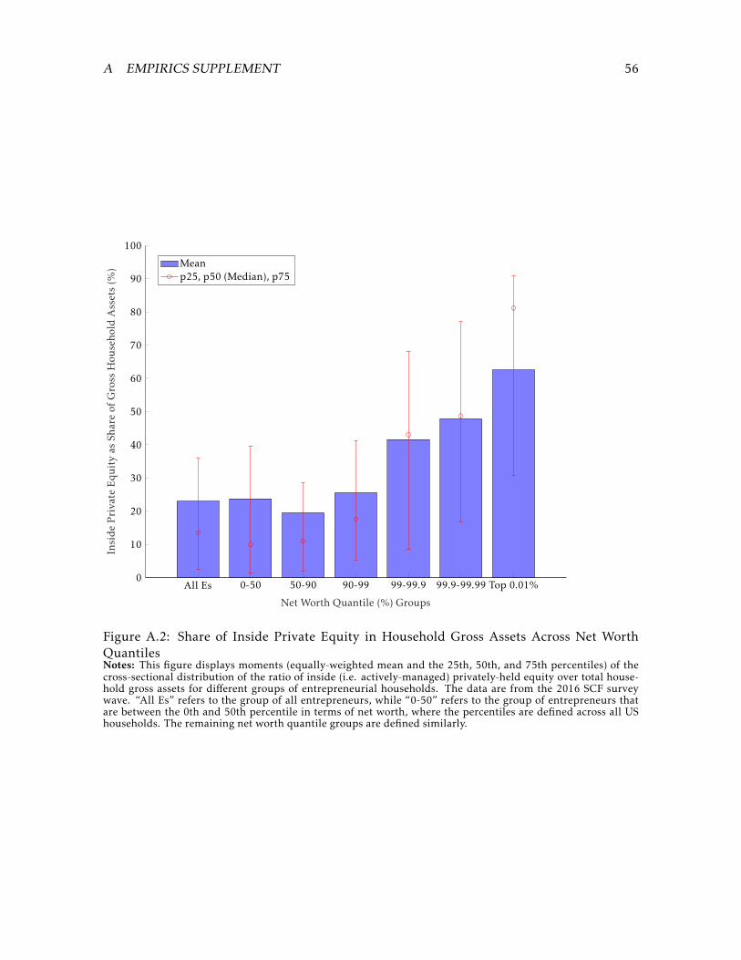
A EMPIRICS SUPPLEMENT 56
All Es 0-50 50-90 90-99 99-99.9 99.9-99.99 Top 0.01%0
10
20
30
40
50
60
70
80
90
100
Net Worth Quantile (%) Groups
InsidePriva
teEqu
ityas
Shareof
Gross
Hou
seho
ldAssets(%
) Meanp25, p50 (Median), p75
Figure A.2: Share of Inside Private Equity in Household Gross Assets Across Net WorthQuantilesNotes: This figure displays moments (equally-weighted mean and the 25th, 50th, and 75th percentiles) of thecross-sectional distribution of the ratio of inside (i.e. actively-managed) privately-held equity over total house-hold gross assets for different groups of entrepreneurial households. The data are from the 2016 SCF surveywave. “All Es” refers to the group of all entrepreneurs, while “0-50” refers to the group of entrepreneurs thatare between the 0th and 50th percentile in terms of net worth, where the percentiles are defined across all UShouseholds. The remaining net worth quantile groups are defined similarly.

A EMPIRICS SUPPLEMENT 57
1989 1992 1995 1998 2001 2004 2007 2010 2013 201626
28
30
32
34
36
38
40
42
Shareof
Top1%
byNet
Worth
(%)
Survey of Consumer FinancesSaez and Zucman (2016)
Figure A.3: Wealth and Income Top Inequality in the SCFNotes: This figure plots the net worth share of the top 1% group by net worth over time, as measured in theSCF and also by the income-capitalization method of Saez and Zucman (2016). The colored bands represent95% confidence intervals for the SCF estimates based on bootstrap standard errors (see Appendix A.4.3). Grayshaded areas denote NBER-designated recessions.

A EMPIRICS SUPPLEMENT 58
1989 1992 1995 1998 2001 2004 2007 2010 2013 2016
6
8
10
12
14
16
18
20
22
24
26
28
30
Shareof
Agg
rega
teNet
Worth
Es in Top 1% GroupNEs in Top 1% Group
Figure A.4: Decomposition of Top 0.1% Net Worth Share by Entrepreneurial Status overTimeNotes: This figure plots the share of aggregate net worth held by the entrepreneurs (E) and non-entrepreneurs(NE) that are part of the top 0.1% group by net worth. The colored bands represent 95% confidence intervals forthe SCF estimates based on bootstrap standard errors. Gray shaded areas denote NBER-designated recessions..

A EMPIRICS SUPPLEMENT 59
1977 1980 1982 1985 1987 1990 1992 1995 1997 2000 2002 2005 2007 2010 2012 20150%
0.5%
1%
1.5%
2%
2.5%
3%
3.5%
4%
4.5%
5%
Shareof
Agg
rega
teIncome
Top 0.1% Income Group
1977 1980 1982 1985 1987 1990 1992 1995 1997 2000 2002 2005 2007 2010 2012 20150%
2%
4%
6%
8%
10%
12%
Shareof
Agg
rega
teIncome
Top 1% Income Group
Wage IncomeFinancial IncomeBusiness Income
Figure A.5: Income Factor Decomposition for Top 0.1% and 1% Shares Over Time (Tax Data)Notes: This figure plots components of the aggregate income of the top 0.1% income group (top panel) and thetop 1% income group (bottom panel) since the 1970s. The data, based on IRS administrative tax data, and theclassification of income based on categories (lines) in US tax returns are from an updated version of the dataset ofPiketty and Saez (2003). The plotted categories do not include realized capital gains. Gray shaded areas denoteNBER-designated recessions.

A EMPIRICS SUPPLEMENT 60
−100 −80 −60 −40 −20 0 20 40 60 80 100 120 140 160 180 2000
0.5
1
1.5
2
2.5
3
3.5
4
4.5
5·10−2
Long-Term Excess Simple Business Return (Annualized, %)
Proba
bility
Den
sity
Func
tion
Figure A.6: Cross-Sectional Distribution of Annualized Long-Run Excess Simple BusinessReturns, 2016 SCF WaveNotes: This figure plots the probability density function for annualized long-run excess simple private businessreturns, conditional on no firm exit (due to business failure, acquistion by another firm, or transition to a publicfirm), from the 2016 survey wave. The plot of the probability density estimate uses the unified dataset acrossall implicates and a normal kernel function (with bandwidth equal to 3).Only businesses with aninflation-adjusted cost basis of at least $5,000 and survey-year market value of at least $1,000 are considered.See Appendix A.4.5 for details on the construction of business-level returns.

A EMPIRICS SUPPLEMENT 61
1990s 2000s 2010s0
10
20
30
40
50
60
70
80
90
100
110
Lon
g-Te
rmPriva
teBusine
ssReturn
(%)
Mean Excess Simple ReturnAdj. St. Dev. of Excess Log ReturnSharpe Ratio
Figure A.7: Cross-sectional Moments of Excess Private Business Returns in the SCF AcrossDecades, Conditional on Survival in Private Form
Notes: This figure plots decade averages for the cross-sectional mean of the annualized excess simple returnsand the cross-sectional standard deviation of the annualized excess log returns on private businesses in SCF,and for the ratio of these measures (Sharpe ratio). Annualized returns are adjusted by a factor of
√T , where T
denotes business age, when computing the standard deviation. The errorbars denote 95% confidence intervals.

A EMPIRICS SUPPLEMENT 62
1-5 6-10 11-15 16-20 21-25 26-30 31-35 36-40 41-45 >45−20
0
20
40
60
80
100
120
Business Age (Years)
Lon
g-Te
rmExcessSimple
Return
(%)
Meanp25, p50 (Median), p75
1-5 6-10 11-15 16-20 21-25 26-30 31-35 36-40 41-45 >450
10
20
30
40
50
60
70
Business Age (Years)
Stan
dardDev
iation
ofOne
-Period-A
head
ExcessLog
Return
(%)
Figure A.8: Mean and Standard Deviation of Long-Run Excess Private Business ReturnAgainst Business Age, Conditional on SurvivalNotes: This figure plots cross-sectional moments of annualized long-run excess private business returns fordifferent business age groups at the time of the survey. The top panel plots the equally-weighted mean and the25th, 50th, and 75th percentiles of excess simple returns, and the bottom panel plots the standard deviationof excess log returns. The reported moments are averages across the three SCF survey waves in the 2010s.Annualized returns are adjusted by a factor of
√T , where T denotes business age, when computing the standard
deviation. See Appendix A.4.5 for details on the construction of the long-run entrepreneurial business returnsat the household level.

A EMPIRICS SUPPLEMENT 63
1-5 6-10 11-15 16-20 21-25 26-30 31-35 36-40 41-45 >45−10
0
10
20
30
40
50
60
Business Age (Years)
Cha
ngein
MeanLon
g-Te
rmExcessSimple
Return
(%)
1-5 6-10 11-15 16-20 21-25 26-30 31-35 36-40 41-45 >45−20
−15
−10
−5
0
5
10
15
Business Age (Years)
Cha
ngein
St.D
ev.o
fOne
-Period-A
head
ExcessLog
Return
(%)
Figure A.9: Change in Mean and Standard Deviation of Long-Run Excess Private BusinessReturn Against Business Age, Conditional on Survival (1990s to 2010s)Notes: This figure plots the change from the 1990s to the 2010s in cross-sectional moments of annualized long-run excess private business returns for different business age groups at the time of the survey. The top panelplots the change in the cross-sectional mean of excess simple returns and the bottom panel plots the standarddeviation of excess log returns. Annualized returns are adjusted by a factor of
√T , where T denotes business
age, when computing the standard deviation.

A EMPIRICS SUPPLEMENT 64
Net Worth Income
Top 1% Share By Es By NEs Top 1% Share By Es By NEs
Level, 32.23 21.98 10.25 14.97 9.25 5.7290s (0.60) (0.80) (0.66) (0.64) (0.69) (0.42)Change, 0.86 -0.43 1.29 4.54 1.24 3.3090s→ 00s (0.71) (1.06) (0.92) (0.94) (0.85) (0.89)Change, 3.02 3.13 -0.11 0.61 1.21 -0.6000s→ 10s (0.56) (1.03) (0.90) (0.89) (0.74) (0.98)Change, 3.88 2.70 1.18 5.15 2.45 2.7090s→ 10s (0.73) (1.10) (0.92) (0.85) (0.88) (0.73)
Table A.1: Decomposition of the Increase in the Top 1% Net Worth and Income Shares ByGroupNotes: This table reports the decomposition of the top 1% share (in percentage point format) and its increase
by group, entrepreneurs (E) and non-entrepreneurs (NE), for net worth and income from the 1990s to the 2010s.The top 1% group is defined using household rankings with respect to net worth and income, respectively.“Shareby Es” refers to the share of aggregate net worth or income held by the entrepreneurs that are part of the top1% group. For all rows, the components of each decomposition sum to the total inequality level or change. SCFstandard errors are reported in parentheses.
Net Worth Income
Top 0.1% Share By Es By NEs Top 1% Share By Es By NEs
Level, 12.02 8.79 3.24 6.03 4.17 1.8690s (0.41) (0.48) (0.35) (0.58) (0.57) (0.28)Change, -0.47 -0.55 0.08 1.40 -0.47 1.8790s→ 00s (0.50) (0.61) (0.49) (0.78) (0.67) (0.67)Change, 1.91 2.15 -0.24 0.23 1.09 -0.8500s→ 10s (0.51) (0.63) (0.47) (0.69) (0.56) (0.78)Change, 1.44 1.60 -0.16 1.64 0.62 1.0290s→ 10s (0.59) (0.70) (0.48) (0.74) (0.72) (0.57)
Table A.2: Decomposition of the Increase in the Top 0.1% Net worth and Income Shares ByGroupNotes: This table reports the decomposition of the top 0.1% share (in percentage point format) and its in-
crease by group, entrepreneurs (E) and non-entrepreneurs (NE), for net worth and income from the 1990s to the2010s. The top 0.1% group is defined using household rankings with respect to net worth and income, respec-tively.“Share by Es” refers to the share of aggregate net worth or income held by the entrepreneurs that are partof the top 0.1% group. For all rows, the components of each decomposition sum to the total inequality level orchange. SCF standard errors are reported in parentheses.

A EMPIRICS SUPPLEMENT 65
T T E T NE ϕE T Ein T NEin
Net Worth 36.11 24.69 11.43 45.21 54.61 20.84Non-Bus 30.30 16.44 13.85 33.67 48.82 20.84
Bus 63.72 63.72 0.00 100.00 63.72Income 20.12 11.70 8.42 27.43 42.55 11.62
Labor 13.55 5.30 8.26 22.45 23.62 10.67Capital 35.63 27.33 8.30 40.36 67.68 13.93
Population 1.00 0.63 0.38 11.43 5.53 0.43
Table A.3: Top 1% Share Decomposition by GroupNotes: This table reports the decomposition of the value share of the top 1% by group, entrepreneurs (E) and
non-entrepreneurs (NE), for several key variables, where the top 1% group is defined with respect to total networth for rows 1-3 and 7 (net worth and its components, and population) and with respect to total income forrows 4-6 (income and its components). Business net worth refers to inside (actively-managed) private equityand non-business net worth refers to all other components of net worth. The decompositions for labor andcapital income are reported after an adjustment for the unpaid labor of self-employed entrepreneurs, detailedin Appendix A.4.4. All estimates are averaged over the three latest survey waves (2010, 2013, 2016) and arereported in percentage point format.
Top 1% Income Share
Total Labor Capital Other
by Es by NEs by Es by NEs
Level, 14.97 6.24 3.57 2.67 8.55 5.56 2.99 0.1990s (0.64) (0.34) (0.29) (0.30) (0.66) (0.64) (0.31) (0.05)Change, 4.54 2.44 0.42 2.02 2.19 0.89 1.29 -0.0890s→ 00s (0.94) (0.57) (0.45) (0.52) (0.93) (0.73) (0.70) (0.07)Change, 0.61 0.36 -0.47 0.83 -0.21 1.60 -1.81 0.4600s→ 10s (0.89) (0.67) (0.45) (0.67) (0.82) (0.57) (0.69) (0.24)Change, 5.15 2.80 -0.04 2.84 1.97 2.49 -0.52 0.3890s→ 10s (0.85) (0.60) (0.41) (0.59) (0.83) (0.78) (0.42) (0.24)
Table A.4: Decomposition of the Increase in the Top 1% Income Share by Factor and GroupNotes: This table reports the decomposition of the top 1% share and its increase by group, entrepreneurs
(E) and non-entrepreneurs (NE), for both labor and capital income from the 1990s to the 2010s. Household-level estimates of labor and capital income are adjusted for the unpaid labor if self-employed entrepreneurs, asdiscussed in the text and detailed in Appendix A.4.4. The top 1% group is defined using household rankingswith respect to total income.

A EMPIRICS SUPPLEMENT 66
Entrepreneurs Non-Entrepreneurs
Equity Risky Assets All Equity Risky Assets
Private Public All
All 23.2 10.2 34.0 83.6 9.4 75.5(0.4) (0.3) (0.5) (0.3) (0.1) (0.2)
Top 1% 38.3 17.7 59.5 84.3 42.7 68.5(1.8) (1.2) (1.5) (1.0) (2.0) (1.9)
Top 0.1% 47.4 16.6 69.5 85.9 48.8 74.6(2.7) (1.6) (2.2) (1.2) (3.9) (2.9)
Top 0.01% 53.6 18.3 75.2 86.2 70.6 82.8(4.8) (3.5) (3.2) (2.9) (6.2) (4.6)
Table A.5: The Portfolio Allocation of Entrepreneurs and Non-Entrepreneurs, 2010sNotes: This table reports the cross-sectional average of the fraction of household gross assets held in different
types of risky assets for different groups of households. See the text (Section 4.6.2) for details on the assetcategories. Top groups are defined using household rankings with respect to household net worth. All estimatesare averaged over the three latest survey waves (2010, 2013, 2016) and are reported in percentage point format.SCF standard errors are reported in parentheses.
Equity Risky Assets
1990s 1990s→ 2010s 1990s 1990s→ 2010s
All 25.6 -1.1 6.9 1.3(0.6) (0.7) (0.6) (0.7)
Top 1% 18.3 -1.5 11.3 4.6(3.2) (4.0) (2.5) (3.3)
Top 0.1% 23.7 -2.9 12.4 -1.1(4.8) (6.6) (5.7) (6.5)
Top 0.01% 22.0 -17.5 13.2 -9.8(7.3) (10.2) (7.8) (9.6)
Table A.6: Change in Portfolio Share Differentials Between Entrepreneurs and Non-EntrepreneursNotes: This table reports the level in the 1990s and the change from the 1990s to the 2000s in the difference
between entrepreneurs’ and non-entrepreneurs’ cross-sectional average of the fraction of household gross assetsheld in equity (“All Equity” in Table A.5) and in risky assets, for different groups of households by net worth.All estimates are reported in percentage point format. SCF standard errors are reported in parentheses.
A EMPIRICS SUPPLEMENT 67
A.2 Group Decomposition of the Top 1% Group for Several Variables
Table A.3 shows a decomposition of the top 1% share for several variables by entrepreneurial
status:
T = T E + T NE
= ϕET Ein + (1−ϕE)T NEin , (40)
where T is the aggregate value share of the top 1% group, T E (T NE) is the aggregate value
share of the entrepreneurs (non-entrepreneurs) that belong to the top 1% group, ϕE is the
aggregate value share of entrepreneurs (reported in Table 1), and T Ein (T NEin ) is the aggre-
gate value held by entrepreneurs (non-entrepreneurs) in the top 1% group expressed as a
share of the aggregate value of all entrepreneurs (non-entrepreneurs). The latter measure
can be interpreted as a measure of concentration at the top within each subpopulation of
households.72
The group decomposition for the 2010s, reported in Table A.3, offers several insights ontop inequality. First, net worth and capital income are more concentrated at the top relative
to labor income (and thus total income); the top 1% net worth (income) groups own 36%
of aggregate net worth (capital income), while the top 1% income group owns only 14%
of aggregate labor income. Inside private equity in particular is extremely concentrated at
top with the entrepreneurs in the top 1% group by net worth holding 64% of aggregate
inside private equity. (By definition, only entrepreneurs hold inside private equity.) Second,
entrepreneurs within the top 1% groups hold a larger fraction of aggregate net worth and
capital income relative to non-entrepreneurs (25% for Es relative to 11% for NEs), while
non-entrepreneurs hold a larger fraction of labor income (8% for NEs relative to 5% for Es).
Third, the degree of within-group top inequality as proxied by the measures T Ein and T NEin
is larger for the group of entrepreneurs for all variables. The results are quantitatively very
similar for the unadjusted factor decomposition of income (see the discussion of Section and
Appendix A.4.4).
A.3 Group and Factor Decomposition of Household Income
The trends in top income inequality are more complex relative to those for net worth in-
equality discussed in Section 2.3 due to the importance of labor income. An appropriately
capitalized version of the total current and future labor income stream of households is a key
component of the total economic wealth of households that is missing from the conventional
measure of net worth (net assets). Table A.4 decomposes the top 1% income share by factor
72For all variables, the top 1% group is constructed using the rankings of households with respect to total networth or income, not the rankings with respect to the corresponding wealth or income components.

A EMPIRICS SUPPLEMENT 68
and, additionally, by group within each factor. It shows that labor and capital income each
account for roughly half (60% for labor and 40% for capital, excluding the “other income”
category) of the increase in top income inequality since the 1990s.73
Further, Table A.4 shows that the increase in the labor income of the top 1% income
groupmainly occurred during the 1990s and almost exclusively through non-entrepreneurs.
In contrast, the increase in capital income is exclusively due to entrepreneurs and has mostly
taken place since 2000. Another important development is the collapse of the capital in-
come of non-entrepreneurs following the Great Recession of 2007-2009, which resulted in
an overall decline of the total income of non-entrepreneurs from the 2000s to 2010s (see the
last column of Table A.1) and a slight decline in the total capital income of the top 1% group
(see the fifth column of Table A.4). The capital income of entrepreneurs in the top group in
fact fell by the same amount (2.3 percentage points of aggregate total income from the 2007
survey to the 2010 survey), but the decline was not enough to reverse the sustained increase
in the capital income of this subgroup over all other three-year time periods from 2001 to
2013.
An analysis of US tax data also suggests that an important shift in the composition of
top income inequality and its increase occurred around the early 2000s, as emphasized by
Guvenen and Kaplan (2017). Figure A.5 plots the components of the income of the top
1% and 0.1% groups by income over time, using the classification of pre-tax income into
wage income (wages, salaries, and bonuses, including exercised employee stock options),
financial income (interest income, dividends, and rents) and business income (referred to as
“entrepreneurial income” in Piketty and Saez (2003)), the latter category defined to include
the profits of partnerships, sole proprietorships, and type-S (pass-through) corporations,
and royalties. The secular trends based on tax data are qualitatively consistent with the
results of the analysis based on the SCF. Figure A.5 shows that the growth in the wage income
for the top groups has stopped or even reversed since 2000 (certainly so for the top 0.1%
group), while business income has experienced an unabated and sustained increase since
the 1980s up until the end of the data series in 2015, with a significant uptick in the early
2000s. Income classified as financial income also experienced a similar uptick in the 2000s,
but that was reversed in large part during the Great Recession of 2007-2009, consistent with
the decline in the capital incomes of both entrepreneurs and non-entrepreneurs in the SCF
data discussed above.73Table A.4 shows that the contributions of labor and capital income to overall income inequality are of com-
parable magnitudes, both in levels and in changes over time. This is perhaps surprising both for the level decom-position, given the much larger share of labor income in total income (70% in the 2010s), as well as the changedecomposition, given the decline in the labor share. The explanation for the former observation is that capitalincome is in general much more unequally distributed than labor income, and the reason for the latter is thatthe decline in the labor share over the last 30 years was accompanied by a large increase in within-labor-incomeinequality.

A EMPIRICS SUPPLEMENT 69
Taking stock, the present analysis based on SCF data suggests a compositional change
in top income inequality and its increasing trend, from within-labor-income inequality in
the 1990s to within-capital-income inequality since the early 2000s, a change confirmed by
existing analyses based on tax data. Moreover, the group decomposition of top income and
net worth inequality strongly suggests that the increase in capital income and net worth
inequality at the top is primarily due to entrepreneurs and thus due to increasing returns
to actively-managed forms of capital investments, as opposed to “passive” financial invest-
ments, to which all households have access regardless of entrepreneurial status.
A.4 Additional Details on SCF Data Analysis
A.4.1 Sample Selection Design
The SCF employs a dual-frame sample selection design incorporating an area-probability
sample, which provides good information on financial variables that are broadly distributed
in the population, and a special list sample selected from a sample of recent tax records.
The list sample oversamples households that are more likely to be wealthy, thus providing
superior information on financial variables that are highly correlated with wealth, such as
business assets, ownership of stocks, and real estate investments. As with other surveys, re-
sponse rates for the SCF have fallen in recent years, a problem affecting the wealthy oversam-
ple in particular. Changes in the survey design have been implemented recently to address
this issue (Bricker, Henriques, and Moore, 2017).
A.4.2 Bulletin Measures of Household Assets and Income
The SCF Bulletin measure of household gross assets is the sum of all financial assets owned
by the households, including directly-held stocks and bonds, transaction accounts, mutual
funds, life insurance, annuities, trusts, and quasi-liquid retirement (IRA and Keogh) ac-
counts, and of the household’s non-financial assets, which include real estate, vehicles, and
actively and non-actively managed private business equity (including net loans from the
household to its business). The net worth measure subtracts from the gross assets measure a
measure of the value of the household’s total debt, including mortgages, collateralized and
non-collateralized loans, and credit card debt.
The net worth measure, constructed using all available information in the survey, misses
two important components of US household wealth relative to the economically preferable
concept of total non-labor wealth that includes all assets, net of liabilities, over which a
family has a legal claim that can be used to finance its present and future consumption:
defined-benefit (DB) pension wealth (which has grown in importance in recent years) and
the wealth of the members of the Forbes 400 list of wealthiest individuals, which are by de-
sign excluded from the survey. Bricker et al. (2016) argue that accounting for these missing

A EMPIRICS SUPPLEMENT 70
components via macro-level imputations leaves the usual measures of wealth concentration
at the top of the distribution largely unchanged, with the addition of DB pension wealth
pushing them down and that of the Forbes 400 wealth pushing them up.
SCF total income largely corresponds to the IRS measure of income, but also contains
certain non-taxable sources of income.
A.4.3 Statistical Inference in the SCF
The SCF employs a multiple imputation technique to deal with the issue of missing or in-
complete information in households’ responses. In particular, five distinct observations
called implicates are provided in the data for each household surveyed. Any missing val-
ues for the household are replaced with five values generated to simulate the conditional
sampling distribution of the missing values.
To properly analyze the data, one must use repeated-imputation inference (RII) tech-
niques (Rubin, 1987; Montalto and Sung, 1996). RII requires that separate analyses be per-
formed on each of the five data sets corresponding to the five implicates. Specifically, the
best point estimate for a statistic is constructed as the average of the five separate point esti-
mates computed in each of the five data sets. An estimate of the total variance of the overall
point estimate is given by the formula:
σ2 = σ2within +
(1+
1m
)σ2between, (41)
where σ2within is an estimate of within-imputation variance, or an estimate of the sampling
variance of the point estimate within an implicate dataset, and σ2between is between-imputation
variance defined as the sample variance of the set of the five point estimates. 1+1/m, where
m = 5 is the number of implicates, is an adjustment factor for using a finite number of im-
plicates.
To obtain good estimates of within-imputation variance, capturing uncertainty due to
sampling variability and taking into account the survey sample design, the SCF group at the
Fed makes available a set of 999 bootstrap replicate weights for the first implicate of each
raw observation. These weights are produced using the same sample selection techniques
used to choose the actual survey sample.74 The sampling variance of the point estimates
across these replicates is then an estimate of σ2within.
Confidence intervals at the 100 ·α significance level are constructed as
x ± tν (α/2)σ, (42)
74These techniques are not fully disclosed publicly, which is why the SCF group directly provides these repli-cate weights.

A EMPIRICS SUPPLEMENT 71
where x denotes the point estimates and tν (α/2) is the 100 · α/2 percentile of the student t
distribution with ν = (m− 1)(1 + 1/rm)2 degrees of freedom, where
rm =(1+1/m)σ2
between
σ2within
(43)
is the relative increase in variance due to non-response.75
To compute statistics involving estimates from different survey waves, such as decade
averages or relative changes over time, I use the standard Gaussian rules for the propagation
of uncertainty, which assume that sampling errors are uncorrelated across survey waves.
A.4.4 Imputation of Labor Income for Self-Employed Entrepreneurs in the SCF
The starting point for the factor decomposition of pre-tax income at the household level
are the reported components of pre-tax household income through a series of survey ques-
tions that closely follow key lines in the IRS personal tax return, Form 1040. In particular,
my pre-adjustment measure of labor income is reported wage and salary income (which in-
cludes bonuses). My pre-adjustment capital income consists of the following categories: sole
proprietorship and farm income; rental real estate, royalties, partnerships, S corporations,
trusts etc.; realized net capital gains; tax-exempt and taxable interest income; dividend in-
come, ordinary and qualified; Social Security, pensions, annuities etc. A third category of
“other income” includes the remaining categories, mainly transfer income: unemployment
and worker’s compensation; child support, alimony; welfare transfers (TANF, SNAP tec.);
any other sources.
I perform a regression-based imputation of the labor income of self-employed entrepre-
neurs who report that they are not paid regular wages. The method follows Moskowitz and
Vissing-Jørgensen (2002) and is similar in spirit to the methodology of the Bureau of Labor
Statistics for calculating its estimate of the labor share. It makes use of the work hours in a
year reported for all households in the SCF, including the unpaid entrepreneurs, and a pre-
dicted estimate of the hourly wage of the unpaid entrepreneurs based on a regression of the
log hourly wage of employed households (separately for the household head and partner) on
demographic characteristics (age, education, and gender).
My post-adjustment measure of labor (capital) income is wage (capital) income plus (mi-
nus) the imputed labor income of self-employed entrepreneurs reporting zero wage income.
My estimate of the labor share (pre- or post-adjustment) is aggregate labor income di-
vided by the sum of aggregate labor income and aggregate capital income, that is, I ignore
the “other income” category.
75For most statistics in the SCF the degrees of freedom are large enough that the corresponding t distributionessentially coincides with the standard normal.

A EMPIRICS SUPPLEMENT 72
A.4.5 Construction and Further Analysis of Long-Term Private Business Returns in the
SCF
For each household, I consider its primary business with the largest inflation-adjusted cost
basis. I construct the annualized long-term return to this business as the sum of a measure
of annualized capital gains over the life of the business and an estimate for the average
dividend yield of the business.
For the latter return component, I use the time average (across survey waves) of the aggre-
gate dividend yield of inside private equity, which is 8.9%. The aggregate dividend of inside
private equity for a given survey year is constructed as the aggregate net income (profit) of
all private businesses, adjusted for the share of each business owned by a managing house-
hold, for corporate taxation,76 for retained earnings (a uniform 30% earnings retention rate
for all businesses), and for the imputed labor income of self-employed entrepreneurs who
do not report regular wages (see Appendix A.4.4).77
To construct a measure of the capital gains component of the return I take the reported
cost basis as the value of the original investment and the reported current market value of
the business (multiplied the share owned by the household) as the current price. I then
compute the geometric-average annualized capital gains rate taking into account the age of
the business. Businesses with an inflation-adjusted cost basis of less than $5,000 or survey-
year market value of less than $1,000, in 2016-equivalent US dollars, are excluded from
the sample throughout the analysis in order to avoid data outliers due to artificially large
capital gains or extremely negative log returns (for businesses with near-zero survey-year
market value), respectively.
Appendix Figures A.8 and A.9 display levels and changes in conditional cross-sectional
moments for different age groups of firms. Figure A.8 displays the term (firm age) structure
of estimate moments of one-year-ahead private business returns for 5-year age groups, while
Figure A.9 plots changes in these moments from their average levels in the 1990s to their
average levels in the 2010s. The top panel of Figure A.9 shows that the increase in average
returns is mainly driven by the youngest firms (up to 20 years old), confirming that the
increase is a relatively recent phenomenon.78 The bottom panel of Figure A.9 shows that the
change in the estimated standard deviation from the 1990s to the 2010s is not statistically
significant at the 5% level for almost all age groups and the estimate of the change is negative
76I assume a uniform 30% corporate tax rate if the business is a non-S corporation. I impute the legal classi-fication of non-primary businesses (in the SCF the legal form is reported only for the first two or, prior to 2010,the first three businesses) based on the legal classification of the primary businesses. If the legal classification ofthe primary businesses is “mixed”, that is, if at least one business is pass-through and at least another one is anon-S corporation, I assume all remaining businesses are non-S corporations.77All income data in the survey are in fact for the year preceding the survey year.78On average across the three survey waves in the 2010s, about 29% of firms in the sample are of age 1-5 years,
19% are of age 6-10, 15% are of age 11-15, 10% are of age 16-20, 8% are of age 21-25, and the remaining 19%are older than 25 years.

B MODEL SUPPLEMENT 73
for most age groups. Similar conclusions follow when looking at other indicators of the
riskiness of the return distribution, such as higher cross-sectional moments.
B Model Supplement
This appendix contains supplemental material on the model of Sections 3 and 4. Section B.1
contains additional figures and tables related to the analysis of Sections 3 and 4. Section B.2
contains additional exposition, details, and results on the model of Section 3. The proofs of
the lemmas and propositions of Sections 3 and B.2 are located in a separate appendix, D.
B.1 Additional Figures and Tables
1 1.05 1.1 1.15 1.2 1.25 1.3 1.35 1.4 1.45 1.5 1.55
1
5
10
15
20
25
30
ζ
Top-W
eigh
tedAverage
Wealth,F(ζ)
ζ∗ = 1.45ζ∗ = 1.5ζ∗ = 1.55
Figure B.1: Top-Weighted Average Wealth When Wealth Follows An Exact Pareto Distribu-tion

B MODEL SUPPLEMENT 74
−6 −5 −4 −3 −2 −1 0 1 2 3 4 5 60
5 · 10−2
0.1
0.15
0.2
0.25
0.3
0.35
0.4
Log Relative Wealth, x
Proba
bility
Den
sity
Func
tion
f E(x)f NE(x)
Figure B.2: The Cross-sectional Distribution of Log Relative Wealth in the Model
Notes: This figure plots the scaled cross-sectional distributions (probability density functions) for the log relativewealth of Es and NEs in the original steady state of the model, calibrated to fit inequality moments from the1990s (see Section 4).
1990s→ 2010s 1990s→ 2030s 1990s→ 2030sno reversal reversal
E share, ϕEN +2.8 +4.7 +1.7Top-wgt E share, ϕEN (1.3) +3.6 +6.4 +1.8Top 1% share +3.4 +6.3 +2.8Top 0.1% share +1.8 +3.7 +1.5Top 10% share +3.7 +5.8 +2.3
Table B.1: Future Change in Inequality Under the Baseline Model Calibration
Notes: This table reports the cumulative change in the top inequality moments targeted in the calibration fromthe 1990s to the 2030s (39 years of transition) under two scenarios: fully permanent structural shifts (column2); and full reversal of the shifts at time t1 = 2013.

B MODEL SUPPLEMENT 75
B.2 Supplement for Section 3
B.2.1 Optimal Agent Policies
Proposition B.1 (Optimal Policies). Let U s = (exp(vs)W )1−γ /(1 − γ) denote the equilibriumlifetime utility of an agent of type s ∈ {E,NE} with wealthW .
Then the optimal consumption and bequest (annuity) policies are characterized by consumption-wealth ratios cs ≡ Cit/Wit and bequeathed-to-surviving-wealth ratios wsD ≡ WDit/Wit = (1 −τD )(1−θsD ) given by: ,
cs = (ρ+ω)ψ exp((1−ψ)vs)) , (44)
wsD =(1− τD1− τ
VD
)ψexp
((1− ψ)vs
). (45)
The optimal wealth exposure to the (after-tax) liquid financial asset return is the same for allagents,
(1− τ)θB =πBγ, (46)
and the optimal wealth exposure of entrepreneurs to the (after-tax) inside equity return is
θE =(1− τ)θEZ =πZγ. (47)
B.2.2 Wealth Dynamics
This section states the results for the general case with bequests, VD > 0 and thus wD(s) > 0
for s ∈ {E,NE}.The aggregate wealth growth rate gt and the average wealth growth rate across surviving
households gt satisfy:
gt =φEt µ
EW + (1−φEt )µNEW (48)
gt =gt −ω (1−wL −wDt) , (49)
where wDt ≡ φEt wED + (1−φEt )wNED .
The log relative wealth of surviving E and NE households evolves according to
dwEit =(µEt −
(θE
)2/2
)dt +θEdZit (50)
dwNEit = µNEt dt, (51)

B MODEL SUPPLEMENT 76
where
µEt = µEW − gt = µEt +ω (1−wL −wDt) (52)
µNEt = µNEW − gt = µNEt +ω (1−wL −wDt) . (53)
As in the main text, µEt = µEW − gt and µNEt = µNEW − gt are the mean excess wealth growth rates
of surviving Es and NEs, respectively, relative to the average growth rate of all surviving
households.
The log relative wealth of a newborn household i of type si with permanent log relative
labor earnings draw l˜i whose parent household j has log relative wealth wj at the time of its
death, is given by
w˜it = h(wj , l˜i , si) ≡ log(wD(si)exp(wjt) +wL exp(l˜i)) . (54)
Standard arguments imply that the dynamics of the cross-sectional distributions of log
relative wealth across E and NE households, f E(w) and f NE(w), satisfy the following ForwardKolmogorov equations:
df E(w)dt
=− (µEt −12(θE)2)f E′(w) +
12(θE)2f E′′(w) + νNEf NE(w)−
(νE +ω
)f E(w) +ωBE{f E}(w)
(55)
df NE(w)dt
=− (µNEt )f NE′(w) + νEf E(w)− (νNE +ω)f NE(w) +ωBNE{f NE}(w), (56)
where the functional operator Bs for s ∈ {E,NE} is defined as
Bs{f s}(w) =
fsl˜ (w − log(wL)) if wD(s) = 0∫l<w−log(wL)
exp(w−h(w,l,s))mswD (s)
f s(h(w,l, s)
)f sl˜ (l)dl if wD(s) > 0.
(57)
Here, mNE = 1−mE , and function h(w,l, s) is the inverse function of h(w,l, s) (with respect to
the argument w),
h(w,l, s) ≡ log(exp(w)−wL exp(l))− log(wD(s)). (58)
The Forward Kolmogorov equations for the equilibrium labor earnings distributions are:
df El (l)dt
= νNEf NEl (l)− (νE +ω)f El (l) +ωf El˜ (l) (59)
df NEl (l)dt
= νEf El (l)− (νNE +ω)f NEl (l) +ωf NEl˜ (l). (60)

B MODEL SUPPLEMENT 77
For notational simplicity, I omit the dependence of the cross-sectional distributions on
time in equations (55)–(57) and (59)–(60), as I also do in equations (90)–(91) describing the
law of motion for top-weighted average wealth.
Lemma B.1 (Labor Earnings Inequality in Steady State). In steady state, the equilibrium dis-tribution of log relative labor earnings across all surviving households, fl(l), coincides with that oflog relative labor earnings across newborn households, fl˜(l).
The steady-state top-weighted labor earnings share of Es is given by
φEL (ζ) =mEωφEL˜ (ζ)/mE + νNE/mE
ω+ νNE/mE, (61)
where φEL˜ (ζ) ≡∫exp(ζl)f El˜ (l)dl/
∫exp(ζl)fl˜(l)dl is the top-weighted labor earnings share of new-
born Es relative to all newborn households.
Although distributions fl(l) and fl˜(l) coincide in steady state, this is not true in general
for the type-specific distributions, f sl (l) , fsl˜ (l) for s ∈ {E,NE}, because of churning between
the two types.
Proposition B.2 (Top-Weighted Moments). Consider the general case with bequests. In steadystate, the top-weighted aggregate wealth share of entrepreneurs φE(ζ) and top-weighted averagewealth F (ζ) satisfy
φE(ζ) ≈mEwζL(Fl(ζ)/F (ζ))(ω+ νNE/mE)φEL (ζ)/m
E +(1−wζL(Fl(ζ)/F (ζ))
)νNE/mE
λE(ζ)(62)
and
F (ζ) ≈ωwζLλ(ζ)
Fl(ζ), (63)
where
λE(ζ) ≡ω(1− ζ(1−wL −wDt)− (wED )
ζ)+ νNE/mE −µEζ − (θE)2ζ(ζ − 1)/2 (64)
λNE(ζ) ≡ω(1− ζ(1−wL −wDt)− (wNED )ζ
)+ νNE/mE −µNEζ, (65)
and
λ(ζ) ≡ λE(ζ)φE(ζ) +λNE(ζ)(1−φE(ζ))− νNE/mE
=ω(1− ζ(1−wL −wDt)−φE(ζ)(wED )
ζ − (1−φE(ζ))(wNED )ζ)
−µEφE(ζ)−φE
1−φEζ −φE(ζ)
(θE
)2ζ(ζ − 1)/2. (66)

C EPSTEIN-ZIN PREFERENCES WITH BEQUESTS 78
Equations (62) and (63) hold exactly for ζ = 1 and approximately so for ζ close to 1.
Proposition B.3 (Pareto Tail in Steady State). Consider the general case with bequests. Theresults of Proposition 2 still hold, but with functions λE(ζ) and λNE(ζ) defined as in equations(64) and (65).
Proposition B.4 (Speed of Transition). Consider the general case with bequests. In responseto permanent and unanticipated structural shifts, the top-weighted wealth share of Es evolvesapproximately as
dφE(ζ)dt
≈ −sEt (ζ)φEt (ζ) + νNE +ωwζLF
El˜ (ζ)/Ft(ζ), (67)
with approximate speed of transition
sEt (ζ) = λEt (ζ) +ωw
ζLFl˜(ζ)/Ft(ζ)−λt(ζ), (68)
where λE(ζ) and λ(ζ) are given in equations (64) and (66).The convergence rate for Es’ aggregate wealth share is:
λEt ≡ λEt (1) = ω(wL − (1−φEt )(wED −w
NED )
)+ νNE/mE −µEt , (69)
which is decreasing in entrepreneurial persistence and in the mean excess wealth growth rate ofentrepreneurs, µEt .
C Epstein-Zin Preferences with Bequests: Characterization and
Derivation
This appendix introduces an extension to the continuous-time version of Epstein-Zin (EZ)
preferences (the Kreps-Porteus case of the stochastic differential utility class of Duffie and
Epstein (1992)) that allows for utility from bequests in settings where agents are subject to
random times of death. Section C.1 introduces the specification, Section C.2 formally derives
it as the continuous-time limit of a natural extension of discrete-time EZ preferences. The
optimal policies implied by this specification for the setting of the model of Section 3 are
given in Proposition B.1.
C.1 Preference Specification
Households die stochastically at a Poisson rate ω. They derive utility from their own con-
sumption stream as well as from the level of wealth bequeathed to their offspring.The lifetime utility Uit of household i over its consumption in case of survival [Ciτ ]τ≥t

C EPSTEIN-ZIN PREFERENCES WITH BEQUESTS 79
and its bequeathed wealth in case of death [WDiτ ]τ≥t is defined recursively through
Uit = Et
[∫ ∞tf (Ciτ ,UDiτ ,Uiτ )dτ + lim
τ→∞Uiτ
], (70)
where felicity function f is given by (under γ , ψ, ψ , 1)
f (C,UD ,U ) =1
1− 1/ψ
[(ρ+ω)C1−1/ψ ((1−γ)U )1−ϑ +ω
ϑ
ϑ((1−γ)UD )ϑ ((1−γ)U )1−ϑ
−(ρ+ω
(1+VD
ϑ
ϑ
))(1−γ)U
]. (71)
Here, the utility from bequeathed wealth and the composite parameters are defined, respec-
tively, as
UDt ≡ V 1/ϑD
W1−γDt
1−γ, (72)
and
ϑ ≡1− 1/ψ1−γ
, (73)
ϑ ≡1− 1/ψ1−γ
. (74)
Parameters ρ, γ , and ψ denote the rate of pure time preference, the coefficient of rela-
tive risk aversion, and the elasticity of intertemporal substitution (EIS), respectively, as in
the standard EZ preference specification. Specification (70)– (74) introduces two additional
exogenous parameters: the marginal value from bequeathed wealth VD ≥ 0 (with VD = 0
corresponding to no bequest motive), and the elasticity of intergenerational substitution of
consumption ψ.
In equation (70), consumption Ciτ denotes the household’s consumption flow at time τ
conditional on survival up to time τ , while UDiτ is the level of wealth bequeathed to the
agent’s offspring conditional on death taking place exactly at time τ .79
Section C.2 shows that specification (70)– (74) is the continuous-time limit of a contin-
uum of discrete-time optimization settings, indexed by period duration ∆ > 0, in which the
agent’s utility Ut(∆) is defined recursively through
Ut(∆) =
(1− β(∆))C1−1/ψt + β(∆)Et
((1−πD(∆)VD )Ut+∆(∆)1−1/ψ +πD(∆)VDW1−1/ψD,t+∆
) 1−γ1−1/ψ
1−1/ψ1−γ
1
1−1/ψ
,
(75)
79Formally, the expectation in (70) is taken with respect to all events other than the household’s random timeof death.

C EPSTEIN-ZIN PREFERENCES WITH BEQUESTS 80
where
β(∆) ≡ exp(−(ρ+ω)∆) (76)
πD(∆) ≡ 1− exp(−ω∆). (77)
The utility of specification (70)– (74) corresponds to the limit
Ut = lim∆→0
Ut(∆)1−γ
1−γ. (78)
C.1.1 Special Cases
When ψ = 1, ψ , 1, the felicity function is given by
f (C,UD ,U ) =(ρ+ω) log(C)(1−γ)U +ωVD
1− 1/ψW
1−1/ψD ((1−γ)U )1−ϑ
−(ρ+ω1−γ
log((1−γ)U ) +ωVD
1− 1/ψ
)(1−γ)U. (79)
When ψ , 1, ψ = 1 and VD > 0,
f (C,UD ,U ) =ρ+ω1− 1/ψ
C1−1/ψ ((1−γ)U )1−ϑ +ωVD log(WD )(1−γ)U
−(ρ+ω1− 1/ψ
+ωVD log((1−γ)U )U). (80)
When ψ = 1, ψ = 1, and VD > 0,
f (C,UD ,U ) =(ρ+ω) log(C)(1−γ)U +ωVD log(WD )(1−γ)U
− (ρ+ω(1 +VD )) log((1−γ)U )U. (81)
Finally, the simple case γ = 1/ψ = 1/ψ corresponds to time-separable power utility with
bequests:
Ut =∫ ∞t
exp(−(ρ+ω)(s − t))
C1−γs
1−γ+ωVD
W1−γDs
1−γ
. (82)

C EPSTEIN-ZIN PREFERENCES WITH BEQUESTS 81
C.1.2 Transversality Condition
A transversality condition must hold in any equilibrium to ensure that the agent’s lifetime
utility and policy functions are well-defined (finite):80
limτ→∞
exp(− (ρ+ω) (τ − t)))Et [Uiτ ] = 0, (83)
where Uit is the household’s utility under the optimal consumption stream (the value func-
tion), Uit =maxUit.
C.2 Derivation
Proposition C.1. Assume that the continuum of discrete-time optimization settings given byequations (75)–(77) and indexed by period duration ∆ > 0 satisfies the following condition:
lim∆↘0
Et[Ut+∆(∆)1−γ ]− Ut(∆)1−γ
∆
exists and is finite.Then,
lim∆→0
Ut(∆)1−γ
1−γ=Ut , (84)
where Ut satisfies the recursive definition of equations (70)– (74).
Proof. To Be Added.
80The limit in (70) is zero only under the stronger transversality condition limτ→∞Et[Uiτ
∣∣∣tiD =∞]= 0. See
the appendix to Duffie and Epstein (1992) written by Duffie, Epstein, and Skiadas on this point. However, aweaker transversality condition of the form of (83) suffices for the validity of the equilibrium.

D PROOFS 82
D Proofs of the Analytical Results of Sections 3 and Appendix B.2
Proof of Proposition B.1. Applying Ito’s Lemma on the conjecture for the value function U =
(exp(vs)W )1−γ /(1−γ) when the agent is of type s ∈ {E,NE}, we have
dU(1−γ)U
=dWW− 12γ(1− τ)2
(θ2B +θ
2Z
)dt +
W 1−γ
γ[exp((1−γ)v−s)− exp((1−γ)vs)]dFst , (85)
where −s refers to the other type and Fst is a Poisson counting process governing the transi-
tion from type s to type −s.The Hamilton-Jacobi-Bellman (HJB) equation is
0 = maxf (C,UD ,U ) +Et−[dU ], (86)
where the felicity function f is given by (71). Dividing (86) by (1−γ)U and rearranging, we
obtain the HJB for type s as
ρ+ω(1 +VDϑϑ)
1− 1/ψ= maxcw,θD ,θB,θZ
ρ+ω1− 1/ψ
cw1−1/ψ exp(−(1− 1/ψ)vs)
+ω
1− 1/ψVD [(1− τD )(1−θD )]1−1/ψ exp(−(1− 1/ψ)vs)
+ (1− τ)(rf +ωθD +πBθB +1s=EπZθZ
)− cw
− 12γ(1− τ)2(θ2
B +θ2Z ) +
νs
1−γ [exp((1−γ)(v−s − vs))− 1] (87)
The first-order condition (FOC) with respect to the consumption-wealth ratio cw is
(ρ+ω)cw−1/ψ exp(−(1− 1/ψ)vs) = 1, (88)
which yields (44).
Using wD = (1 − τD )(1 − θD ), the FOC with respect to the fraction of wealth invested in
the annuity asset θD can be written as
ωVD(1− τD )w−1/ψD exp(−(1− 1/ψ)vs) = (1− τ)ω, (89)
which yields (45).
Optimal policies (46) and (47) follow immediately as the FOCs with respect to θB and
θZ , respectively.
The proofs of the propositions regarding the long-run level and dynamics of inequality

D PROOFS 83
use the following lemma:
Lemma D.1 (Law of Motion for Top-Weighted Average Wealth). Top-weighted average wealthacross E and NE households, F E(ζ) and F NE(ζ), evolves over time according to
dF E(ζ)dt
= −(λEt (ζ)− νNE
)F E(ζ) + νNEF NE(ζ) +ωBE(ζ) (90)
dF NE(ζ)dt
= −(λNEt (ζ)− νE
)F NE(ζ) + νEF E(ζ) +ωBNE(ζ), (91)
where
λEt (ζ) = ω+ νNE/mE − µEt ζ − (θE)2ζ(ζ − 1)/2 (92)
λNEt (ζ) = ω+ νNE/mE − µNEt ζ, (93)
and
Bs(ζ) = Bs{f s}(ζ) ≡
wζLF
sl˜ (ζ) if wD(s) = 0
1ms
∫l
∫wexp(ζh(w,l, s))f s(w)f sl˜ (l)dwdl if wD(s) > 0,
(94)
for s ∈ {E,NE}.
Proof of Lemma D.1. The proof uses the following assumption on the equilibrium probability
density functions f Et (w) and f NEt (w):81 Let v(w) be an arbitrary bounded and twice differen-tiable function; then the integrated conjuncts vanish,[((
µE − 12(θE)2
)f E(w)− 1
2(θE)2f E′(w)
)v(w) +
12(θE)2f E(w)v′(w)
]+∞−∞
= 0 (95)[f NE(w)v(w)
]+∞−∞
= 0. (96)
Multiplying the FK equations (55) and (56) by exp(ζw) and integration from −∞ to +∞,
81This integrated conjunct assumption is in fact necessary for the Forward Kolmogorov equations to hold, asit ensures that the backward and forward Kolmogorov operators are formal adjoint operators. See any text onstochastic processes, e.g. Hanson (2007). It essentially requires that the density functions decline to zero fastenough as w→ +∞ and as w→−∞ so that the cross-sectional distributions are convergent.

D PROOFS 84
we get
dF E(ζ)dt
=−(µEt −
12(θE)2
)∫ +∞
−∞exp(ζw)f E′(w)dw+
12(θE)2
∫ +∞
−∞exp(ζw)f E′′(w)dw
+ νNEF NE(ζ)− (νE +ω)F E(ζ) +ω∫
exp(ζw)BE{f E(w)}dw (97)
dF NE(ζ)dt
=− µNEt∫ +∞
−∞exp(ζw)f NE′(w)dw+ νEF E(ζ)− (νNE +ω)F NE(ζ)
+ω∫
exp(ζw)BNE{f NE(w)}dw (98)
Using integration parts and condition (95) with v(w) = exp(ζw), the first two terms on
the right-hand side (RHS) of (97) equal(µEt −
12(θE)2
)ζF E(ζ) + 1
2(θE)2ζ2F E(ζ). (99)
Similarly, using integration parts and condition (96), the first term on the RHS of (98) equals
µNEt ζF NE(ζ). (100)
In the case of no bequests wD(s) = 0 for s ∈ {E,NE},
Bs{f s}(ζ) ≡∫
exp(ζw)sl˜(w − log(wL))dw=wζL
∫exp(ζl)fl˜(l)dl
=wζLFl˜(ζ). (101)
With bequests, wD(s) > 0,
Bs{f s}(ζ) ≡ 1ms
∫ ∫l<w−log(wL)
exp(ζw)∂h(w,l, s)∂w
f s (h(w,l, s))f sl˜ (l)dldw
=1ms
∫ ∫exp(ζh(w, l, s))f s(w)f sl˜ (l)dldw, (102)
where the first line changes the order of integration, and the second line uses a change of
variables (l,w)→ (l, w = h(w,l, s)).
Collecting the results above and using νE+νNE = νNE/mE , which follows from the inflow-
outflow balance condition, (1), we obtain equations (90) and (91).
Proof of Lemma 1. Equations (23) and (25) follow by evaluating equations (103) and (61) at

D PROOFS 85
ζ = 1 and using the fact that φEL˜ (1)/mE = a˜E .Equation (24) follows from the definition of net worth Nit =Wit −WLit and the linearity
of the expectation operator.
Proof of Proposition 1. Under no bequests, λE(ζ) and λNE(ζ), given in equations (92) and
(93), are equal to λE(ζ) and λNE(ζ), given in equations (30) and (31), respectively.
Using the fact that, in steady state, dF E(ζ)/dt = 0, and dividing both sides of equation
(90) by F (ζ), we get
φE(ζ) =ωwζLF
El˜ (ζ)/F (ζ) + νNE
λE(ζ). (103)
Equations (103) and (61) imply equation (28).
Adding equations (90) and (91), we obtain the law of motion of top-weighted average
wealth,
dF (ζ)dt
= −λt(ζ)F (ζ) +ωwζLFl˜(ζ). (104)
Using the fact from Lemma B.1 that, in steady state, Fl˜(ζ) = Fl(ζ) and imposing dF (ζ)/dt = 0,
we obtain equation (29) for the steady-state level of top-weighted average wealth.
The positive dependence of the steady-state levels of both top-weighted inequality mea-
sures on µE and, for ζ > 1, on θE is obvious. For the impact of the level of type persistence,
inversely related to the churning rate νNE , note that
∂φE(ζ)∂νNE
=1
λE(ζ)
[−(φE(ζ)mE
− 1)+wζL
Fl(ζ)F (ζ)
(φEL (ζ)
mE− 1
)](105)
Given that wζLFl(ζ)/F (ζ) = λ(ζ)/ω < 1 from equation (29), a sufficient condition for
∂φE(ζ)/∂νNE < 0 is ϕE(ζ) > ϕEL (ζ), which is the empirically relevant case.
Proof of Proposition 2. I offer two proofs for the proposition characterizing the Pareto tail of
wealth.
The first proof proceeds by substituting the conjecture f E(w)→ cE exp(−ζ∗w) and f NE(w)→cNE exp(−ζ∗w) as w → ∞ into the system of FK equations (55) and (56). We use the result
that, when the Pareto tail of wealth is thicker than that of labor earnings, ζ∗L(s) > ζ∗, for
s ∈ {E,NE}, where f sl˜ (l)→ csL exp(−ζ∗L(s)l),
82
limw→∞
f sl˜ (w − log(wL))
f s(w)= limw→∞
csLwζ∗L(s)L
csLexp(−(ζ∗L(s)− ζ
∗)w) = 0. (106)
82The Pareto tail exponent of the distribution of equilibrium relative earnings, fl (l), is min{ζ∗L(E),ζ∗L(NE)}.

D PROOFS 86
Note that this result also implies that wealth and net worth have the same Pareto tail expo-
nent. Substituting the conjectures into equations (55) and (56), dividing by exp(ζ∗w), and
using (106), we get a system of two equations in two unknowns, the ratio cE/cNE and ζ∗:
cE(λE(ζ∗)− νNE
)= cNEνNE (107)
cNE(λNE(ζ∗)− νE
)= cEνE . (108)
This system yields expressions (33) and (34).
A secondmethod of proof uses a “Tauberian” result fromMimica (2016), also included as
Proposition 7 in the Appendix of Gabaix et al. (2016). From equation (29), a number −ζ ≥ 0
that satisfies λ(ζ) = 0 constitutes a negative abscissa of convergence for the Laplace trans-
form of f (w), that is, F (ζ) converges for 0 < ζ < ζ, diverges for ζ > ζ, and has a singularity at
ζ. The Tauberian result then implies that this number ζ is the Pareto tail exponent of f (w).
Finally, note that equation (33) defining ζ∗ is equivalent to λ(ζ∗) = 0. Therefore, ζ∗ = ζ is the
Pareto tail exponent of wealth.
Proof of Proposition 3. Using the laws of motion (90), (91), and (104) for F E(ζ), F NE(ζ), andF (ζ), respectively, we have
φE(ζ) =F E(ζ)F (ζ)
−φE(ζ) F (ζ)F (ζ)
= −λEt (ζ) +ωwζL Fl˜(ζ)F (ζ)
−λt(ζ)φE(ζ) + νNE +ωwζL F El˜ (ζ)
F (ζ)(109)
Using equation (104) and the fact that, as t→∞, dF (ζ)/dt→ 0, we obtain
sE(ζ) = limt→∞
sEt (ζ) = λE(ζ). (110)
Finally, using wL < 1 and µE > 0, it follows that λE(ζ) is a decreasing function of ζ, so that
λE(1) is an upper bound for the asymptotic speed of transition.
Also note that an analytical upper bound for the speed of transition of φEt (ζ) at any time
t is given by λE(1) + Ft(ζ)/Ft(ζ).
Proof of Lemma B.1. Adding the FK equations for relative labor earnings, equations (59)–
(60), and using the fact that fl(l) = fEl (l) + f NEl (l) and fl˜(l) = f El˜ (l) + f NEl˜ (l) yields
dfl(l)dt
=ω(fl˜(l)− fl(l)
). (111)

D PROOFS 87
In steady state, the cross-sectional distribution is time-invariant, dfl(l)/dt = 0, for all
l ∈R, so fl(l) = fl˜(l). This also implies Fl(l) = Fl˜(l).Multiplying equation (59) by exp(ζl) and integrating over l, we obtain
dF El (ζ)dt
= νNEF NEl (ζ)− (νE +ω)F El (ζ) +ωF El˜ (ζ). (112)
Imposing time invariance of the earnings distribution in steady state, dividing both sides by
Fl(l) and using F NEl (ζ)/Fl(ζ) = 1−φEL (ζ), we get
0 = νNE(1−φEL (ζ)
)− (νE +ω)φEL (ζ) +ωφ
EL˜ (ζ). (113)
Solving for φEL (ζ), we have
φEL (ζ) =ωφEL˜ (ζ) + νNEω+ νE + νNE
=ωφEL˜ (ζ) + νNEω+ νNE/mE
, (114)
where the second equality follows from the inflow-outflow condition, (1).
Proof of Propositions B.2 and B.4. Consider a first-order approximation of exp(ζh(w,l, s)) as a
function of ζ around ζ = 1:
exp(ζh(w,l, s)) = [wD(s)exp(w) +wL exp(l)]ζ
≈(wsD
)ζexp(ζw) +wζL exp(ζl). (115)
Using this approximation in the case of bequests, we obtain
Bs{f s}(ζ) = 1ms
∫ ∫exp(ζh(w,l, s))f s(w)f sl˜ (l)dldw
≈(wsD
)ζF s(w) +wζLF
sl˜ (l) (116)
It follows that the type-specific top-weighted average wealth measures approximately follow
the laws of motion:
dF E(ζ)dt
≈ −(λE(ζ)−ω
(wED
)ζ− νNE
)F E(ζ) + νNEF NE(ζ) +ωwζLF
El˜ (ζ) (117)
dF NE(ζ)dt
≈ −(λNE(ζ)−ω
(wNED
)ζ− νE
)F NE(ζ) + νEF E(ζ) +ωwζLF
NEl˜ (ζ), (118)

D PROOFS 88
These laws of motion have the same form as those for the case of no bequests, but with
λE(ζ) = λE(ζ)−ω(wED
)ζ(119)
λNE(ζ) = λNE(ζ)−ω(wNED
)ζ. (120)
Equations (62)–(63) and (67)–(69) then follow by repeating the steps in the proofs of
Propositions 1 and 3.
Proof of Proposition B.3. Performing a change of variables,
Bs{f s}(ζ) =∫l<w−log(wL)
exp(w − h(w,l, s))mswD(s)
f s(h(w,l, s)
)f sl˜ (l)dl
= − 1ms
∫ +∞
−∞
exp(w)
exp(w)−wD(s)exp(h)f s (h)f sl˜
(log(exp(w)−wD(s)exp(h))− log(wL))
)dh.
(121)
Dividing this by f s(w) and taking the limit as w→∞,
limw→∞
Bs{f s}(ζ)f s(w)
= − 1ms
∫ +∞
−∞f s (h)
limw→∞
exp(w)
exp(w)−wD(s)exp(h)·
f sl˜(log(exp(w)−wD(s)exp(h))− log(wL)
)f s(w)
dh= − 1
ms
∫ +∞
−∞f s (h)
limw→∞
wζ∗L(s)L
[1−wD(s)exp(h−w)
]−(1+ζ∗L(s)) exp(−(ζ∗L(s)− ζ∗)w)dh= 0 (122)
where the first line follows by changing the order of the limit and the integration, the second
line uses the fact that
liml→∞
f sl˜ (l) = exp(−ζ∗L(s)l) (123)
and the third line uses the fact that wealth has a thicker tail than earnings ζ∗ <min{ζ∗L(E),ζ∗L(NE)}.

E A GENERAL-EQUILIBRIUM MODEL OF ENTREPRENEURIAL CAPITAL 89
E A General-EquilibriumModel of Entrepreneurial Capital
This section introduces and analyzes a general-equilibrium (GE), endogenous-production
extension of the model of Section 3. Sections E.1–E.3 introduce the different components of
the model. Section E.4 characterizes the inside equity premium in terms of fundamentals.
Section E.5 briefly addresses the equilibrium determinants of the riskfree rate.
To ease the reader’s introduction to the key features of the model, I delegate many tech-
nical details, including generalizations of propositions and additional results, to Online Ap-
pendix F. The proofs of all formal results are located in Online Appendix G.
E.1 Setting
The overlapping-generations and labor earnings structure and household preferences are as
in the model of Section 3. As I only analyze the GE model qualitatively, for expositional
simplicity I assume no taxes, τ = τD = 0, and no bequests, VD = 0.
Production of the final good requires as inputs labor and two types of capital, liquid
capital K and entrepreneurial capital KE . A stock of liquid capital can be operated by any
agent and traded frictionlessly in financial markets. In contrast, entrepreneurial capital is
tied to an entrepreneur and subject to a financial (skin-in-the-game) friction: only he can
operate his stock of entrepreneurial capital and expand it via investment; its future income
stream cannot be pledged to outsiders. The rest of this subsection presents the details of the
setup.
E.1.1 Production
There are three types of firms: entrepreneurial firms, liquid firms, and final-good producers.
Intermediate goods An entrepreneurial firm, operated by an entrepreneurial household,
holds and accumulates entrepreneurial capital, which produces a good that serves as an
intermediate input to final good production. Denoting the quantity of the capital stock of
firm i by KEit, the firm’s cumulative flow of the entrepreneurial good SEit follows83
dSEit = KEitdJ
Eit , (124)
where
KEit ≡ AEitK
Eit (125)
83Unless otherwise indicated, all equations describing the evolution of household- or firm-level variables instochastic differential equation form are conditional on the survival of the household or firm over the timeincrement.

E A GENERAL-EQUILIBRIUM MODEL OF ENTREPRENEURIAL CAPITAL 90
denotes the quality-adjusted stock of firm i’s capital, accounting for firm-specific productivity
AEit. The dynamics of firm-level productivity are discussed in Section E.1.3.
JEit is a scaled Poisson process,84
dJEit =1λEdΥ E
it , (126)
where Υ Eit is a Poisson counting process with intensity λE . Note that Et−[dJ
Eit] = dt. J
Eit cap-
tures a firm-specific production risk with a purely transitory effect on the firm’s income
stream.Applying a law of large numbers across the continuum of entrepreneurial firms, the
aggregate quantity of the entrepreneurial good produced at time t equals E∗t[dSEit] = K
Et dt
where E∗t[·] is the cross-sectional expectation operator and KEt is the aggregate (quality-
adjusted) stock of entrepreneurial capital.85
The entrepreneurial good is traded on a Walrasian market at price pEt in units of the final
good (the numeraire). The cumulative business income flow YEit to entrepreneur i thus fol-
lows dYEit = pEt dS
Eit and the corresponding aggregate entrepreneurial income flow is simply
pEt KEt dt.
The production function of liquid firms, which produce a different intermediate input, is
defined symmetrically. The cumulative flow Sit of the intermediate good of liquid firm i with
capital stockKit follows dSit = KitdJit where Kit ≡ AitKit is the quality-adjusted stock of firm
i’s capital and Jit again captures a source of idiosyncratic income risk withEt−[dJit] = dt. The
intermediate good produced by liquid capital is traded at a unit price pt.
Final-good producers Final-good producer j combines GEjt and Gjt units of intermediate in-
puts from entrepreneurial and liquid capital, respectively, with Ljt units of labor to produce
Yjt units of the final good according to the production function
Yjt =(Gcjt
)ς (ALt Ljt
)1−ς, (127)
where ALt denotes the productivity of labor, and the composite intermediate input from cap-
ital is defined as
Gcjt ≡[Ξ(GEjt
)1− 1ε + (1−Ξ)
(Gjt
)1− 1ε
] 11− 1ε
(128)
84More generally, JEit can be any Lévy subordinator process, that is, a stochastic process with non-negativeincrements that are stationary and identically and independently distributed (iid) over time, which is also iidacross firms and satisfies Et− [dJ
Eit] = dt.
85All exogenous sources of idiosyncratic risk in the model, such as the process JEit , are distributed indepen-dently across households and independently from each other and from the aggregate source of risk Bt . SeeAppendix F.2 on the application of the law of large numbers.

E A GENERAL-EQUILIBRIUM MODEL OF ENTREPRENEURIAL CAPITAL 91
where ε > 1 is the elasticity of intratemporal substitution between entrepreneurial and liquid
capital intermediate goods, andΞ ∈ (0,1) controls the productivity of entrepreneurial capitalrelative to liquid capital.
Factor income shares The equilibrium policies of final-good producers (see appendix F.3)
imply the following distribution of aggregate income among the three factors of production:
pEt KEt = ξtςYt (129)
ptKt = (1− ξt)ςYt (130)
Lt = pLt A
Lt = (1− ς)Yt , (131)
where Yt is aggregate output and pLt is the wage (i.e. aggregate earnings Lt) normalized by
the level of aggregate productivity. (Equation (131) assumes a unit aggregate labor supply.)
Thus, parameter ς equals the capital income share, and
ξt = ξ (ηt ;Ξ, ε) ≡[1+
1−ΞΞ
η−(1− 1
ε )t
]−1=
Ξ(KEt )1−1/ε
Ξ(KEt )1−1/ε + (1−Ξ)(Kt)1−1/ε, (132)
is the share of entrepreneurial income in total capital income. Here,
ηt ≡KEtKt
(133)
is the entrepreneurial capital ratio, that is, the ratio of the two aggregate (productivity-
adjusted) stocks of capital. Under the assumption that entrepreneurial and liquid capital
are substitutes in production in the Pareto-Edgeworth sense, ε > 1, the share of entrepre-
neurial capital is increasing in the entrepreneurial capital ratio. In particular, an increase in
the relative productivity of entrepreneurial capital leads to a higher capital ratio and hence
to a higher share of capital income accruing to entrepreneurial firms.
Labor productivity I assume that labor productivity is proportional to the composite ag-
gregate capital stock, possibly due to knowledge spillovers from capital accumulation as in
Romer’s (1986) endogenous growth model with capital externalities:
ALt ≡ b1/(1−ς)Kct , (134)
where
Kct ≡[Ξ(KEt
)1− 1ε + (1−Ξ) (Kt)1−
1ε
] 11− 1ε
(135)

E A GENERAL-EQUILIBRIUM MODEL OF ENTREPRENEURIAL CAPITAL 92
and b > 0 is a constant. An implication of this assumption, and its raison d’être, is that
equilibrium aggregate output is proportional to the composite capital stock,
Yt = bKct . (136)
E.1.2 Households
Every household is characterized by its type (E or NE), the level of its liquid (i.e. non-
business) wealth Wit and, in the case of entrepreneurial households, its stock of entrepre-
neurial capital KEit .
E.1.3 Entrepreneurial firms
The cumulative entrepreneurial income flow and the idiosyncratic component of the pro-
ductivity of entrepreneurial firm (household) i evolve according to
dYEit = pEt K
EitdJ
Eit (137)
dAEitAEit−
= σdBt + dJEP it − dF
Eit − dF
Eit , (138)
where the diffusion Bt captured aggregate, total factor productivity shocks, process JEit , in-
troduced in section E.1.1, captures purely transient income shocks, process JEP it captures
permanent income shocks, and FEit and FEit are Poisson counting process with intensities νE
and νE , capturing business failure shocks as discussed below.
I assume that transient and permanent income shocks are driven by the same idiosyn-
cratic underlying shocks,
dJEP it = sKtdJEit , (139)
where sKt may depend on the aggregate state of the economy.
The inclusion of both transient and permanent income shocks and the specification of
their relationship in (139) are made for tractability reasons, as I discuss in Section E.3.
Failure risk Entrepreneurial firms of surviving households fail at a rate νE+νE losing all of
their capital (their capital becomes completely unproductive, hence worthless), a risk cap-
tured by the counting processes FEit and FEit. If failure is driven by an FEit shock, dF
Eit = 1,
the household operating the firm becomes a non-entrepreneur. If failure is driven by an FEit
shock, dFEit = 1, the household receives an idea (blueprint) for a new entrepreneurial ven-
ture immediately upon failure of its existing firm, retaining its status as an entrepreneurial
household. This structure serves to disentangle the persistence of entrepreneurial status,

E A GENERAL-EQUILIBRIUM MODEL OF ENTREPRENEURIAL CAPITAL 93
governed by the churning rate νE as in the model of Section 3, from the business failure rate,
governed by νE + νE .
If the household dies, its stock of entrepreneurial capital is similarly lost.86
Capital investment Entrepreneurial firms accumulate capital via an investment technol-
ogy subject to convex adjustment costs, as in the q-theory of Hayashi (1982). In particular,
the quantity of the capital stock of an entrepreneurial firm i evolves as
dKEitdt
=(χ(ιEit)− δ
E)KEit , (140)
where χ(·) is a concave function, ιEit ≡ IEit /K
Eit is the ratio of the firm’s investment expenditure
flow IEit to its productivity-adjusted capital stock KEit , and δE is the rate of depreciation of
entrepreneurial capital.
Combining equations (138) and (140), a household’s quality-adjusted capital stock KEit ≡AEitK
Eit evolves according to
dKEitKEit−
=(χ(ιEit)− δ
E)dt + σdBt + dJ
EP it − dF
Eit − dF
Eit . (141)
E.1.4 Entrepreneurial firm creation
At every point in time a mass νNEdt of non-entrepreneurial households become entre-
preneurs and establish new entrepreneurial firms, an event that occurs according to the
household-specific Poisson counting processGNEit capturing the arrival of an idea (blueprint)
for a new entrepreneurial venture. Additionally, a mass νEdt of entrepreneurial households
(whose businesses have just failed) also establish new entrepreneurial firms.
Founders of new entrepreneurial firms decide on their initial investment in the firm,
I˜Eit.87 (A tilde below a variable indicates that the variable is associated with entrepreneurial
firm creation.) The process of new firm creation is subject to convex costs at the aggregate
level, capturing diminishing returns to the implementability of new ideas and methods. In
particular, the initial (productivity-adjusted) capital stock of an entrepreneurial firm is given
by
K˜Eit = χ˜t(I˜EtKEt
)I˜Eit , (142)
86An alternative assumption with the same qualitative implications is that, upon the household’s death, itsstock of entrepreneurial capital is converted into liquid capital. As I abstract from bequests and do not calibratethe model in this section, I choose the simpler assumption that the household’s stock of entrepreneurial capitalis fully destroyed upon death.87Capital investment expenditures at the time of firm creation are discrete (lumpy) at the household level, in
contrast to the smooth flow of capital investment expenditures by existing entrepreneurial firms.

E A GENERAL-EQUILIBRIUM MODEL OF ENTREPRENEURIAL CAPITAL 94
where χ˜t(·) is a concave function and
I˜Et dt ≡∫i∈I˜E[t,t+dt)
I˜Eitdi (143)
is aggregate investment by founders of new entrepreneurial ventures.88,89
E.1.5 Liquid firms
Liquid firms face no financial frictions. As discussed in the next subsection, ownership
claims to liquid firms are pooled together, so that all idiosyncratic risks to their income and
productivity are fully diversified away. Hence, the structure of their idiosyncratic risks is
irrelevant for the determination of aggregate equilibrium prices and quantities. Therefore,
without loss of generality for the present purposes, I assume a time-invariant set of liquid
firms IK and that firm-level productivity is only affected by aggregate risk (TFP shocks):
dAitAit
= σdBt , (144)
for all i ∈ IK .Liquid firms accumulate capital via the same investment technology as entrepreneurial
firms,dKitdt
= (χ(ιit)− δ)Kit , (145)
where ιit ≡ Iit/Kit and δ is the rate of depreciation of liquid capital.
Combining equations (145) and , the productivity-adjusted stock of liquid capital Kit ≡AitKit evolves as
dKitKit
= (χ (ιit)− δ)dt + σdBt . (146)
E.1.6 Financial markets
Financial markets are formally complete with respect to all risks, aggregate as well as id-
iosyncratic. However, entrepreneurs are not able to issue claims against the future income
streams of their entrepreneurial firms for moral hazard (skin-in-the-game) reasons.90 More-
88Function χ˜(ι˜E ) is defined on ι˜E ≥ 0, satisfies χ˜(0) = 0 and χ˜′(0) =∞, and may be a function of the aggregatestate vector Σt defined in Section E.3.89I˜E[t,t+dt) denotes the set of households who become entrepreneurs over the infinitesimal time interval [t, t +
dt).90The framework can easily be extended (without loss of tractability) to allow for partial outside financing
of entrepreneurial capital investments, by assuming that entrepreneurs must at all times retain ownership of aminimum fraction Φ ∈ (0,1] of the future income stream of its entrepreneurial firm.

E A GENERAL-EQUILIBRIUM MODEL OF ENTREPRENEURIAL CAPITAL 95
over, the arrival of an idea (blueprint) for a new entrepreneurial firm is not contractible ex-
ante. Appendix F.5 discusses related microfoundations for the assumed form of the financial
friction.
The market value of a liquid firm can be written as QitKit, where Qit equals the market
price of the claim to a unit of firm i’s capital stock.91 By absence of arbitrage, liquid capital
price Qit equals the present discounted value of the future stream of net profits to the firm
normalized by its current capital stock:
Qit = max[ιiτ ]∞τ=t
Et
[∫ ∞t
Mτ
Mt(pτ − ιiτ )
KiτKit
dτ
], (147)
whereMt denotes the pricing kernel for financial assets.92 Liquid firms choose their invest-
ment policy to maximize market value as in the neoclassical theory of the firm.
Taking into account all types of traded assets, aggregate liquid (non-business) wealth in
the economy is the sum of aggregate financial wealth and aggregate capitalized labor wealth:
Wt =QtKt +WLt =QtKt +QLt A
Lt , (149)
where
QLt = Et
[∫ ∞t
Mτ
Mtexp(−ω(τ − t))pLτ
ALτALtdτ
](150)
denotes aggregate labor wealth normalized by the level of labor productivity.
E.2 Equilibrium
In this subsection I discuss the optimization problem of households and market clearing for
final output. The formal statement of equilibrium is given in Definition 1 in the appendix.
Households solve the following maximization problem for all t ∈ [ti0, tiD ), where ti0 is
household i’s time of birth and tiD its random time of death:
Uit ≡ maxCi ,Θi ,I
Ei ,I˜Ei
Uit , (151)
91In this model, average or Tobin’s q equals marginal q in q-theory terms due to the proportional specificationof investment adjustment costs in (145).92The (unique) pricing kernel in this economy follows
dMt
Mt= −rf tdt −πBtdBt , (148)
where rf t and πBt denote the riskfree rate and the price of aggregate risk, respectively. To the extent that theycan be traded, idiosyncratic risks have a zeromarket price because they are fully diversified away by risk pooling.

E A GENERAL-EQUILIBRIUM MODEL OF ENTREPRENEURIAL CAPITAL 96
subject to
Wit′ ≥ 0 ∀t′ ∈ [t, tiD ), (152)
where the utility function Uit is given by (70) and the households’ liquid or tradable wealth
at time t is
Wit = Witi0 +∫ t
ti0
WiτdRΘiτ︸ ︷︷ ︸
financial & labor income
+YEit −∫ t
ti0
IEiτdτ −∑t˜I˜Eit˜︸ ︷︷ ︸
entrepreneurial income
−∫ t
ti0
Ciτdτ, (153)
and Witi0 =QLti0ALti0 .
93 Θi summarizes the household’s financial portfolio policy, which affectsthe returns to its liquid portfolio dRΘ
it , and t˜ denotes a stopping time associated with the
creation of a new entrepreneurial firm.
The solvency constraint takes the form of (152) because I have defined initial wealth
Witi0 to include the present discounted value of all pledgeable sources of future wealth,
in particular future labor income. In other words, the constraint still allows for real-world
borrowing. However, liquid wealth does not account for households’ future business income,
which is non-pledgeable.94
Non-entrepreneurs Non-entrepreneurs face a simple consumption and financial portfolio
choice problem as in standard financial portfolio choice theory, and their (non-business)
wealth Wit evolves according to equations (3)– (5).
Due to the scale independence of preferences, non-entrepreneurs’ value function can be
written as
UNEit = Ut(WNEit ) =
11−γ
(WNEit exp
(V NEt
))1−γ, (154)
where the normalized value function V NEt is the same across non-entrepreneurs, since they
face the same investment opportunities going forward. For notational simplicity, I omit the
dependence of V NE on the aggregate state of the economy, as I also do below for V E .
Entrepreneurs The problem of an entrepreneur is more complicated because of his ad-
ditional decision over the capital investment policy of his entrepreneurial firm. A key
93If i is part of the initial cohort, ti0 = 0, its initial wealth is as described in Section F.6.94This constraint never binds strictly in the model. The reason is that if it did, that is if entrepreneurs at any
point chose to hold only illiquid wealth (E capital) and zero liquid wealth, they would be left with no wealthat all and be forced to choose zero consumption in the event that a business failure shock occurred in the nextinstant, an event with strictly positive probability. Under Epstein-Zin preferences, zero consumption at anypoint implies infinite disutility so it cannot be part of the optimal consumption policy.

E A GENERAL-EQUILIBRIUM MODEL OF ENTREPRENEURIAL CAPITAL 97
household-level state variable for entrepreneurs is their liquidity ratio
κit ≡KEitW Eit
, (155)
that is, the ratio of their entrepreneurial (productivity-adjusted) capital stock to their liquid
wealth. Using this definition, an entrepreneur’s liquid wealth follows
dW Eit
W Eit
=(rf t +ω − cwEit
)dt +θBit (πBtdt + dBt) +κit
(pEt dJ
Eit − ι
Eitdt
)(156)
where, as in Section 3, cwEit ≡ CEit/W
Eit , and θBit captures the entrepreneur’s financial portfolio
choice. The law of motion (156) shows that the effective proportional exposure of liquid
wealth to income risk,
sW it ≡ pEt κit , (157)
is endogenously increasing in the price of the entrepreneurial good pEt and in the entrepre-
neur’s liquidity ratio κit. Forces such as an increase in aggregate entrepreneurial productiv-
ity that increase the equilibrium price of the entrepreneurial good and lead entrepreneurs
to invest more of their wealth into entrepreneurial capital will lead to an increase in the
quantity of idiosyncratic income risk borne by entrepreneurs.
The scale independence of preferences again implies a simplified form for the value func-
tion:
UEit = Ut(WEit ,K
Eit) =
11−γ
(W Eit exp
(V Et (κit)
))1−γ, (158)
where now the normalized value function V Et (κit) depends not only on the aggregate state
of the economy but also on the entrepreneur’s allocation of his wealth between liquid and
illiquid forms, captured by the liquidity ratio.
Founders of new entrepreneurial firms When a household receives an idea for a new
business venture, it faces a one-off choice over the initial capital investment I˜Eit in its new
entrepreneurial firm. It solves
maxI˜Eit ,Wit≥0
Ut(W Eit ,K˜Eit) , (159)
subject to the budget constraint
I˜Eit + W Eit ≤ Wit− , (160)

E A GENERAL-EQUILIBRIUM MODEL OF ENTREPRENEURIAL CAPITAL 98
where the initial capital stock K˜Eit is given by (142) as a function of I˜Eit, and Wit− (WEit ) is the
household’s level of liquid wealth right before (after) it establishes the entrepreneurial firm.
The dynamic programming formulation of the optimization problems for each house-
hold type and their optimality conditions are presented in appendix F.7.
Final good market clearing Final output is used for consumption and capital investment:
Yt = CEt +CNEt + IEt + I˜Et + It , (161)
where CEt and CNEt are the aggregate consumption levels of the groups of entrepreneurs and
non-entrepreneurs, IEt and I˜Et are aggregate investment expenditures by existing and new
entrepreneurial firms, respectively, and It is aggregate investment by liquid firms.
E.3 Aggregation
The aggregate state of the economy Σ is essentially described by the following variables:
the aggregate capital ratio η ≡ KE/K , the aggregate liquid wealth share of entrepreneurs
φE ≡ W E/W , and the joint cross-sectional distribution of relative liquid wealth and liquidity
ratios across households, f (w,κ, s), where s ∈ {E,NE}. As the in the model of Section 3, the
aggregate state is unaffected by fully symmetric (total factor productivity) shocks driven by
Brownian motion Bt, as all agents choose the same proportional exposures to aggregate risk.
In general, the model features a non-degenerate cross-sectional distribution of liquidity
ratios across entrepreneurs. Heterogeneity in liquidity ratios translates into heterogeneity
across entrepreneurs in the exposure of total household wealth to inside entrepreneurial
equity, which is realistic (see Figure A.2). However, for tractability purposes, I make a set of
ad-hoc functional form assumptions implying that all entrepreneurs optimally choose the
same liquidity ratio, which coincides with the aggregate liquidity ratio, κt ≡ KEt /W Et . These
assumptions result in a parsimonious two-type model, directly comparable to the two-type
model of Section 3. In particular, the cross-sectional distribution of relative wealth and
liquidity ratios is not needed as part of the aggregate state vector Σ, resulting in a finite-
dimensional aggregate state space for the model.95
Proposition E.1 (Tractable Aggregation Assumptions, TAA). Assume that, at all times,
1. the exposure of entrepreneurial capital productivity to idiosyncratic income shocks satisfies
sKt = pEt κt , (162)
95This implies in particular that, starting from the model’s steady state, the transition paths of aggregates inresponse to structural shifts are independent of the cross-sectional distributions.

E A GENERAL-EQUILIBRIUM MODEL OF ENTREPRENEURIAL CAPITAL 99
2. function χ˜(·) in equation (142), controlling the efficiency of investment in new entrepreneur-ial firms, satisfies
χ˜t I˜EtKEt
= 1−V Eκ (κt)κt
V Eκ (κt)
, (163)
where κt is the aggregate liquidity ratio of entrepreneurs.Then, the economy converges in the long-run to a degenerate cross-sectional distribution for
liquidity ratios, equal to κt for all entrepreneurs.
E.4 The Valuation of Inside Equity
Proposition E.2 (Shadow Prices). Assume the Tractable Aggregation Assumptions of PropositionE.1 hold, and κit = κt for all i ∈ E.
Define the shadow capital price of inside equity
QEt ≡V Eκ (κt)
1−V Eκ (κt)κt
, (164)
total household wealthWit ≡ Wit + QEt K
Eit︸︷︷︸
inside equity
, (165)
and the shadow risk prices
πJt ≡ 1−(1+
pEt κtλE
)−γ> 0 (166)
πFt ≡ 1−(1+QEt κt
)exp
((1−γ)
(V NEt −V E
t (κt)))< 0 (167)
πFt ≡ 1−(1+QEt κt
)γ< 0. (168)
Then, the equilibrium consumption and portfolio policies of agents coincide with those in asetting (the dual economy) without illiquid investments in entrepreneurial capital but where eachentrepreneur i perceives his wealth to be given by (165) and can frictionlessly trade on the sourcesof risk JEit , F
Eit, and F
Eit at risk prices πJ , πF , and πF , respectively.
The shadow capital price of inside equity QE does not satisfy a pricing equation analo-
gous to equation (147) for the liquid capital price Q; it implies a higher discount rate on the
future cash flows of the entrepreneurial firm because undiversifiable idiosyncratic firm-level
risk is priced in equilibrium.96
96One can define the price of outside entrepreneurial equity, as the normalized present discounted value ofthe future stream of net profits of the entrepreneurial firm, discounted using the pricing kernel from financial

E A GENERAL-EQUILIBRIUM MODEL OF ENTREPRENEURIAL CAPITAL 100
The proportional exposures of total entrepreneurial household wealth, given by equation
(165), to firm-level risks JEit , FEit, and F
Eit are given by:
θEJt = pEt κt > 0 (170)
θEFt = θEFt
= − QE(κt)κt1+QE(κt)κt
< 0. (171)
To relate the expected returns on inside equity in this setting, which features jump risks
at the firm level, to the expected returns on inside equity in the diffusion setting of the
partial-equilibrium model of Section 3, it is useful to define the process Zit through
dZit =1
θEt
(θEJt
(dJEit − dt
)+θEFt
(dFEit − ν
Edt)+θE
Ft
(dF
Eit − νEdt
)), (172)
where
θEt ≡√(
θEJt)2/λE +
(θEFt
)2νE +
(θEFt
)2νE (173)
is a measure of the overall proportional exposure of total household wealth to firm-level
risks. By the properties of Poisson processes, the increment of the Zit process has zero mean
and variance equal to dt, just like the Brownian motion assumed in the setting of Section 3.
Proposition E.3 (The Inside Equity Premium in Equilibrium). The excess return earned by theaverage entrepreneur on entrepreneurial investments is
ΠZt = πJtθEJt + ν
EπEFtθEFt + ν
EπEFtθEFt. (174)
The inside equity premium (Sharpe ratio) can be defined as
πZt ≡ΠZt
θEt, (175)
and is increasing in the relative productivity of entrepreneurial capital, Ξ, all else equal.
Wealth inequality Once expressed using the formulation of Proposition E.2 in terms of
shadow prices, the dynamics of log relative total household wealth wit ≡ log(Wit/Wt) sat-
isfy a set of Forward Kolmogorov equations, given in Appendix F.8, which are very similar
markets (which assigns a zero price to idiosyncratic risk):
QEit = Et
∫ ∞t
Mτ
Mt
(pEτ − ιEiτ
) KEiτKEit
dτ
, (169)
Then, in equilibrium the shadow price of inside equity is always lower than the price of outside equity,QEit < QEit .
(There is a zero gross supply of outside equity in this setting.)

E A GENERAL-EQUILIBRIUM MODEL OF ENTREPRENEURIAL CAPITAL 101
qualitatively to the Forward Kolmogorov equations (55)–(56) in the partial-equilibrium set-
ting of Section 3. Hence, the key implications of the partial-equilibrium model regarding
the impact of entrepreneurship dynamics on the evolution of inequality also apply in this
setting.
E.5 Precautionary Savings and the Riskfree Rate
Proposition E.4 (The Riskfree Rate in Equilibrium). In the case of a unit elasticity of intertem-poral substitution, ψ = 1, the riskfree rate is given by
rf t = ρ+ gt +ω(1−wLt)− (γσ2 +φEt ΠZt). (176)
where gt is the aggregate wealth growth rate, wLt ≡WLt/Wt, and φE is the aggregate (total) wealthshare of entrepreneurs.
In steady state, the riskfree rate is decreasing in the relative productivity of entrepreneurialcapital, Ξ, all else equal.
The expression for the riskfree rate is similar to the standard expression in a representa-
tive agent economy. The riskfree rate is increasing in the time discount rate ρ, increasing in
the aggregate wealth growth rate (with an adjustment ofω(1−wL) for the wedge between the
average wealth growth rate of surviving households and the aggregate wealth growth rate),
and decreasing in precautionary saving demand, an effect captured by the last two terms in
equation (176). An increase in the inside equity premium, which may be due to an increase
in the relative productivity of entrepreneurial capital Ξ, raises the quantity of idiosyncratic
risk borne by entrepreneurs on average in equilibrium, since entrepreneurs increase their
wealth exposure to inside equity in order to take advantage of its higher return. In turn, this
makes their future consumption stream riskier, increasing their demand for precautionary
savings. As a result, the riskfree rate as well as discount rates on all liquid financial assets
decline in equilibrium.
Thus, besides its effects on the evolution of US wealth inequality in recent years, an
increase in the inside equity premium may also help to account for part of the long-term
decline in the US real riskfree rate since the 1980s.