Preference simulation and preference programming: robustness issues in priority derivation

200 European Journal of Operational Research 69 (1993) 200-209 North-Holland

Theory and Methodology

Preference simulation and preference programming: robustness issues in priority derivation

A m i A r b e l

School of Engineering, Tel-Aviv University, Tel-Aviv 69978, Israel

Luis G. Va rgas

Joseph M. Katz Graduate School of Business, University of Pittsburgh, Pittsburgh, PA 15260, USA

Received October 1990; revised December 1990

Abstract: Decision makers often resist having to make what appears to them as precise numerical judgments in fuzzy situations. Pairwise verbal comparisons used in the AHP are fuzzy in the sense that decision maker(s) need not relate verbal judgment to precise numbers; because of the redundancy inherent in each set of judgments, accurate priorities can be derived from such fuzzy verbal judgments. Another way of making fuzzy judgments is to express each judgment as a numerical interval. This paper explores two new approaches for priority derivation when preferences are expressed as interval judgments, one based on a simulation approach and the other based on mathematical programming. The first approach assumes that the interval judgments are uniformly distributed and proceeds to derive the priority vectors and their underlying rank order by randomly sampling from these distribution. This approach provides, in addition to the priority vectors, a measure of robustness given by the probability of rank reversal. The second approach generates a region (if one exists) that encloses all priority vectors derived from inequalities representing the original interval judgments. The two approaches are described and illustrated through a numerical example.

Keywords: Analytic Hierarchy Process (AHP); Preference programming

I. Introduction

A method that is used for priority derivation in multicriteria decision making is the Analytic Hierarchy Process (AHP) (Saaty, 1986, 1990). It is based on three principles: Decomposition, Measurement of preferences and Synthesis. Decomposition breaks down the problem into manageable elements that are treated individually. This process starts from the implicit descriptors of the problem (e.g., general objectives) and proceeds in a logical manner to identify more explicit and detailed (measurable) descriptors according to which, one later compares the alternatives under consideration. The result of this phase is a hierarchic structure consisting of levels grouping together issues of a homogeneous nature. Measurement is used in comparing elements in a level of the hierarchy with respect to an element in a

037%2217/93/$06.00 © 1993 - Elsevier Science Publishers B.V. All rights reserved

A. Arbel, L.G. Vargas / Preference programming: robustness issues 201

level immediately above them. The comparison is done in a pairwise manner with judgments provided as numerical or verbal statements utilizing an established comparison scale. These judgments are summarized in a comparison matrix and used to derive a priority vector as an estimate of the underlying preference associated with the elements being compared. Finally, when comparisons are done for all elements of the hierarchy, one proceeds to synthesize the local priorities derived for each one of them into a global measure of priority used in making the final decision. These global priorities are obtained by applying the principle of hierarchic composition.

This paper explores two new approaches for priority derivation when preference is expressed as an interval judgment. An interval judgment is a natural way for a decision maker (DM) to express his views when he is uncertain about his exact level of preference. This uncertainty may be the result of a number of factors such as unfamiliarity with the elicitation process and the scale used in its implementation, incomplete information or knowledge, and uncertainty about outcome of events or levels of intensity associated with his preference.

Using intervals to express preference poses technical problems in processing these judgments to arrive at a representative preference structure. To cope with this difficulty this paper presents two ways of processing interval judgments. One is based on Simulation (Saaty and Vargas, 1987) and another is based on Mathematical Programming (Arbel, 1989). The first approach assumes that the interval judgments are uniformly distributed and yields the priority vectors and the underlying rank order, by randomly sampling from these distribution. This approach provides, in addition to the priority vectors, a probability distribution defined on the intervals of the components of the eigenvector. The second approach generates a region (if one exists) that encloses all priority vectors derived from inequalities representing the original interval judgments. This approach has already been generalized to the non-linear constraint case (see Arbel and Vargas, 1991). The main goal of this paper is to establish a connection between the two approaches as a point of departure for the development of a more general approach.

Interval judgements are not new in the literature. Earlier in the 1980's Saaty proposed and studied them; Vargas (1982) assumed the judgments to be random variables; Laarhoven and Pedrycz (1983) assumed the judgments to be fuzzy numbers with triangular membership functions; Buckley (1985) extended fuzzy sets to hierarchical analysis; Saaty and Vargas (1987) assumed interval judgments without any probabilistic or fuzzy properties; Boender, de Graan and Lootsma (1989) extended Laarhoven and Pedrycz's approach; Arbel (1989) introduced the concept of preference programming after formulating the prioritization process as a linear programming model; Salo and Hamalainen (1990) extended Arbel's approach to hierarchic structures; and Arbel and Vargas (1990) formulated the hierarchic problem as a nonlinear model.

This paper is organized as follows: Section 2 provides background information on the basic ideas of the AHP and the use of interval judgments. Section 3 describes the preference simulation approach. Section 4 describes the mathematical programming approach (preference programming). Sections 5 and 6 illustrate both approaches through a numerical example, and Section 7 provides a summary and concluding remarks.

2. Preliminary discussions

A major component of the AHP methodology is concerned with deriving a priority structure associated with a hierarchy whose elements represent issues relevant to a specific decision problem. In deriving these priorities, a distinction is made between local and global priorities. A local priority reflects the importance (priority) of an element in a certain level with respect to an element in a level immediately above it. A global priority reflects the importance of an element with respect to the focus of the problem. Since this paper is concerned with the derivation of local priorities, the basic steps followed in this process are described briefly below.

The derivation of local priorities is carried out through the use of a comparison scale and a pairwise comparison matrix. A comparison matrix for deriving the priority vector w T = [Wl, w 2 . . . . . w n] is associ-

202 A. Arbe~ L.G. Vargas / Preference programming: robustness issues

ated with n elements in a specific level with respect to a single element in a level immediately above it. Such a matrix, denoted by A, is shown in (2.1):

W2//W1 W2//W 2 . . . W2//W n A = . . (2.1)

L Wn/W1 Wn/W2 . . . Wn/W n

In this matrix every element, aij, is an answer to a pairwise comparison question inquiring as to the relative dominance (importance) of element i relative to element j. Answers to this question can be provided in a numerical or verbal mode using the 1-9 comparison scale. Obviously, if one compares the i-th element with the j-th element, a comparison is being made also of the j-th element with the i-th element. This causes the comparison matrix to be a reciprocal matrix satisfying aij = 1 /a~. The answers to the pairwise comparison questions are provided by using the 1-9 comparison scale suggested by Saaty (1987).

Note that for the matrix given in (2.1) the following relation holds: A w --- nw, where w is the priority vector and n is the number of elements being compared. This is the case for a consistent comparison matrix whose elements satisfy aij = ai~akj for all i, j, k. In this special case every column of this consistent matrix provides the solution to the eigenvalue problem A w = nw. Since the consistent case is the exception rather than the rule, we have in general A w = Am~,W, where Ar, ax is the largest eigenvalue of the comparison matrix which satisfies Amax >-n with equality holding only in the consistent case. A consistency index (CI) is defined as CI = (Area x - n ) / ( n - 1). This index assumes the value zero in the consistent case, and it is positive otherwise.

In the decision science literature one encounters the concept of transitivity while in the AHP one encounters the issue of consistency. Transitivity implies that if A is preferred to B, and B is preferred to C, then A is preferred to C. Consistency on the other hand, implies that if A is preferred to B by a ratio of, say, 2 : 1, and if B is preferred to C by a ratio of, say, 3 : 1, then one expects A to be preferred to C by a ratio of 6 : 1. The decision science literature does not provide ways to check directly for transitivity and, therefore, this concept can only be explored, and its importance appreciated, through the use of various behavioral paradoxes. In contrast, the AHP provides a direct proxy measure of consistency and an indirect measure for transitivity. The first measure is offered when the largest eigenvalue, Amax is equal to the dimension of the comparison matrix (or the number of elements being compared), n, only in the case when one is consistent. Weak transitivity is answered, indirectly, through the consistency index that is required to remain within tight bounds for acceptable results. For a more detailed discussion of this and other related issues, the reader is referred to Saaty (1986, 1988). We address intransitivity and its relation to feasible solutions of preference programs in Section 4.

The results shown above are applicable when the decision maker can articulate his preference by a single scale value that serves as an element in a comparison matrix from which one derives the priority vector. This paper is concerned with the case where one has to resort to approximate articulations of preference that still permit exposing the decision maker's underlying preference and priority structure. In this case, an interval of numerical values is associated with each judgment and we refer to the pairwise comparison as an interval pairwise comparison or simply interval judgment (Saaty and Vargas, 1987; Arbel, 1989).

A reciprocal matrix of interval pairwise comparisons is given in (2.2) where l~j and u,. i represent the lower and upper bounds, respectively, of his preference in comparing element i versus element j taken as values from the 1-9 comparison scale:

1 [112' u12] "'" [lln' nan] ]

[lzl, U21 ] 1 [12,, uz , ]

1 A = . (2.2)

[lnl, Unl] [In2, Un2] . . . ]


How does one process such preference statements? This topic is discussed in the next sections where we present two approaches.

3. Stability of the eigenvactor: Preference simulation

Let A 1 , A 2 . . . . . A , be a set of alternatives compared according to a given criterion. Let /,t be the interval judgment provided by the decision maker when comparing alternatives Z i and A t, i.e., Iij = [l~t, u~t]. Let I ( w i) = [WLi , Wui] be the interval of variation of the i - t h component of the eigenvector associated with the pairwise comparison process. The problem is the computation of wL~ and wv~. One way of doing this is to randomly sample values from the interval lit = [l~t, uit], compute the eigenvector of the resulting matrices, and construct a confidence interval for each of the components. This approach will lead to estimating the probability that an alternative exchanges rank with another. These probabili- ties can then be used to answer the question: What is the probability that component i is greater than or equal to component j?

Let us assume that a sample of size N is selected and let {Xi, i = 1, 2 . . . . . n} be the random variable representing the principal right eigenvector components of the sample. For N sufficiently large, the variables {Xi, i = 1, 2 . . . . , n} can be assumed to be normally distributed. This is a consequence of the following:

Theorem 3.1. The principal right eigenvector w o f a positive reciprocal matrix A is given by

1 ~ A~e w = l i m - . (3.1)

r n ~ m k = l eTAke

Proof: See Saaty and Vargas (1984).

Thus, the principal eigenvector of A is the limiting average of the powers of the matrix, and hence by the Central Limit Theorem must converge to a normal distribution. The probability of rank reversals can be easily found by computing the common areas of the probability distributions of the independent components of the eigenvector.

It is clear that given i and j, if l ( w i) and I ( w t) do not have any element in common, then either P [ X i > X t] = 1 or P [ X i > X t] = 1 and the two components will never reverse rank. On the other hand, if the intersection of I (w i) and I ( w t) is non-empty, then the probability that {X/> X t} is a function of the intersection of I ( w ) and I (wj) . If there are n - 1 independent components whose intervals I (w i) do not intersect, then P[X, > X t] = 1 or 0. When the intervals intersect, there is not a unique ranking of the alternatives. If judgments were given at random from the intervals [lit, uit], which ranking is more likely to be expressed by the decision maker?

In the next section we present an approach which yields a region of the hyperplane Y'./xi = 1 in which all the points reveal the same ranking. However, the ranking generated is not unique. The size of the regions with different rankings could be thought of as a measure of the likelihood of a ranking being chosen.

4. Stability of choice: Preference programming

This section presents another approach for dealing with interval judgments. We would like to find the wi's such that

lij <_ Wi//W j <_ Uij , 1 < i , j <_ n. (4.1)

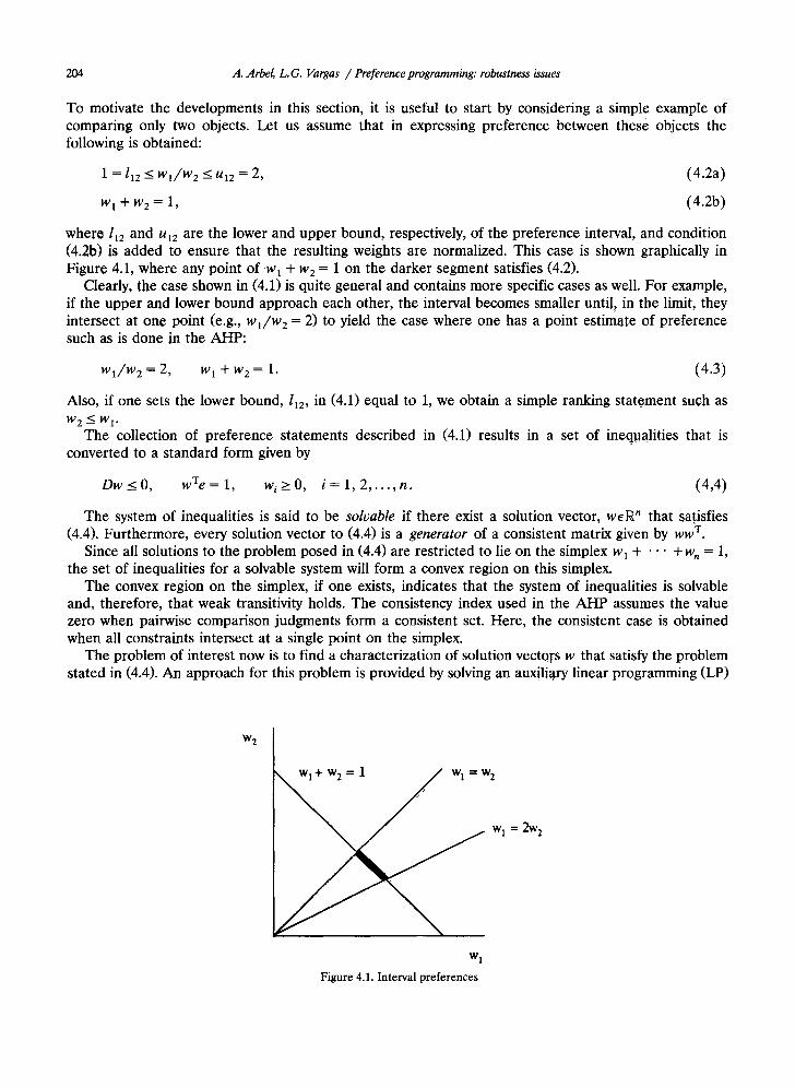
204 A. Arbel, L.G. Vargas / Preference programming." robustness issues

To motivate the developments in this section, it is useful to start by considering a simple example of comparing only two objects. Let us assume that in expressing preference between these objects the following is obtained:

1 = 112 _< W l / W 2 <_ U12 = 2, (4.2a)

w 1 + w 2 = 1, (4.2b)

where 112 and u12 are the lower and upper bound, respectively, of the preference interval, and condition (4.2b) is added to ensure that the resulting weights are normalized. This case is shown graphically in Figure 4.1, where any point of w 1 + w 2 = 1 on the darker segment satisfies (4.2).

Clearly, the case shown in (4.1) is quite general and contains more specific cases as well. For example, if the upper and lower bound approach each other, the interval becomes smaller until; in the limit, they intersect at one point (e.g., wa/ /w 2 = 2) to yield the case where one has a point estimote of preference such as is done in the AHP:

W 1 / W 2 = 2, w 1 + w 2 = 1. (4.3)

Also, if one sets the lower bound, l~2, in (4.1) equal to 1, we obtain a simple ranking statement such as W 2 -~< W 1.

The collection of preference statements described in (4.1) results in a set of inequalities that is converted to a standard form given by

D w < O , wTe = 1, w i > O , i = 1 , 2 . . . . ,n . (4,4)

The system of inequalities is said to be solvable if there exist a solution vector, w e ~ n that satisfies (4.4). Furthermore, every solution vector to (4.4) is a generator of a consistent matrix given by w w T.

Since all solutions to the problem posed in (4.4) are restricted to lie on the simplex w I + • • • + w n = 1,

the set of inequalities for a solvable system will form a convex region on this simplex. The convex region on the simplex, if one exists, indicates that the system of inequalities is solvable

and, therefore, that weak transitivity holds. The consistency index used in the AHP assumes the value zero when pairwise comparison judgments form a consistent set. Here, the consistent case is obtained when all constraints intersect at a single point on the simplex.

The problem of interest now is to find a characterization of solution vectors w that satisfy the problem stated in (4.4). An approach for this problem is provided by solving an auxiliary linear programming (LP)

W 2

= 1 ~ w I = w 2

Wl = 2W 2

w 1

Figure 4.1. In te rva l p re fe rences


problem given by

Minimize

subject to

w 0

D w <O,

wTe = 1,

w>_O,

where w 0 is an artificial variable used to identify the existence of a feasible solution.

(4.5)

Theorem 4.1. The vertices o f the feasible region for a solvable system o f inequalities given by (4.4) are generators o f consistent comparison matrices.

Proof. The vertices for the feasible region are found at unique intersection points of constraints that are active at that vertex. Since other inequalities do not intersect at this particular vertex they are inactive and, therefore, redundant for the solution obtained at this vertex.

A related question is what happens to a solvable system when the ranges of preference shrink until inequalities of the type shown in (4.1) become equality constraints. Can we expect any relation to the eigenvector solution proposed by the AHP? It is clear that when the upper and lower bounds of a solvable system of inequalities approach each other the unique solution to (4.4) is the vector w that is the eigenvector to a consistent matrix.

In many decision-making situations, priorities are derived for establishing a rank ordering among the elements being compared. Can one expect a definitive rank order when preference is stated approximately as in (4.1)? This is answered next.

Theorem 4,2 (Rank order). I f all q vertices o f the solution subspace for a solvable system exhibit the same rank order, then any interior point will exhibit the same rank order, too.

Proof. The solution subspace, W, for the problem posed in (4.4) is defined by W = {weRe: D w < 0, wTe = 1}. Since the subspace forms a convex region, any convex combination of points in this region belongs also to the region. Specifically, let the convex region describing the solution subspace of (4.4) have q vertices denoted by w 1, w 2 , . . . , Wq. Then for any collection of weights, a,, where 0 < a~ < 1 and 0/1 q'- 0/2 + " " " qt_ 0 / q = 1 , the vector v, given by v = a lw I + 0/2w2 + • • • +0/qWq, belongs also to the solution subspace of (4.4). Let w i = (wi[1],. . . , wi[n]), i = 1, 2 . . . . . q. If the vertices of the solution subspace satisfy wi[k] > wj[l], for all vertices 1 < ij < n, and for some given components k and l, then any point given by v = 0/lwl + 0/2w2 + • • • +aqwq satisfies v[k] > [l], where

v [ k ] =0/1wl[k] +0/2w2[k] + . . . +0/qwq[k] and v[ l ] = a l W l [ l ] +0/2w2[1] + " " +0/qwq[l].

Any point in the feasible region for a solvable system is represented as a convex combination of the vertices forming this region. Since the coefficients a i used to form these combinations satisfy 0 _< ai -< 1 and 0/1 -{'- ol2 + " " " " [ - 0 / q = 1, a question of interest is whether there is a way of choosing these coefficients. We present two interpretations: one is based on preference assessment among the vertices, and the other represents a limit case when these coefficients are considered random partitions of the interval [0.1]. We state without proof the following:

Corollary 4.2.1. I f all q vertices { W 1 , W 2 . . . . . Wq} are equally preferred (i f equal weights are assigned to them), then the interior point o f the feasible region generated as the normalized relative priorities is the arithmetic mean o f the vertices.

The second result is less obvious and considers the coefficients used in generating interior points to be the result of a limiting process.

206 A. Arbel, L.G. Vargas / Preference programming: robustness issues

Theorem 4.3. Consider a solvable system of inequalities having q vertices {Wl, w 2 . . . . , wq}. I f { a l k , Ol2k , . . . . aqk} is the k-th random partition of the interval [0, 1], then the point generated with these coefficients

given by OtlkW l + OZ2kW 2 + " '" +OlqkW q converges to the arithmetic mean of the vertices as k tends to infinity.

Proof. Let U,, i = 1, 2 , . . . , q - 1, be uniformly dis tr ibuted random variables U(0, 1). Let

U(k) = min{Uj : Uj > U(k_ 1)}, k = l , 2 . . . . , q ,

where Urn) = 0 and U~q) = 1. The probabil i ty distr ibution of U~k ) is given by

e [ u ~ ) <_ul = l - {e[Uj > u]} q-k

and its expected value is given by

E[U(k)] = u de[U(k)_< u ] = 1 / ( q - k + 1).

Let a i = U(i ) -U(i.1 ). We have E[oq] = 1/q. For i = 2 we have E[oe 21 = E [ ( 1 - U(1))U(2 )] because by defini t ion U{2 ) is the p ropor t ion of l - U(I ) which U¢2 ) is above U m. In addition, since U¢1) and U¢2 ) are independent , we have

1 - l / q E[a2]=E[1-U(1)]E[U(2)] =E[1-Ctl]E[U(2)] = q - 1 l / q .

Similarly, E [ a 3] = E[1 - a 1 - tez]E[U(3 )] = 1/q. By induction, if this is t rue for i = 1, 2 , . . . , k - 1, then for i = k we have

E[ak] = E [ 1 - a , - a 2 . . . . . Olk_l]E[U(k)] = 1 /q

and the result follows. []

This t heo rem states that if in the simulation approach we restrict the sample to those matrices whose principal right e igenvector w satisfies (4.1), then the average of the sample is given by the ar i thmetic mean of the vert ices of the simplex def ined by (4.1). T he examples that follow illustrate this point.

5. A numerical example: Preference simulation

Let us illustrate the results p resen ted in Section 3 with an example. Consider the following (reciprocal) matr ix of interval jedgments:

A =

1 [2, 5] [2, 4] [1, 3] ] [½,½] 1 [ 1 , 3 ] [ 1 , 2 ]

1 [¼, ½] [1, 1] 1 [1, 11 "

[ 1 , 1 ] [½,1] [ 1 , 2 ] 1

(5.1)

Table 1

IF/ Minimum Average Maximum St. Dev.

w 1 0.3694 0.4704 0.5517 0.0366 w 2 0.1501 0.2138 0.2895 0.0255 w 3 0.0929 0.1318 0.1891 0.0159 w 4 0.1332 0.1842 0.2600 0.0231

A. Arbel, L.G. Vargas / Preference programming." robustness issues 207

Table 2

W/ Minimum Average Maximum

w I 0.4347 0.4694 0.5034 W 2 0.1845 0.2109 0.2350 W 3 0.1158 0.1373 0.1560 w 4 0.1631 0.1823 0.2092

The results of the simulation for a sample of size n = 1000 are given in Table 1. A 99-percent confidence interval of the components if given by

0.3758 < w~ < 0.5646, 0.1480 < w z < 0.2796, 0.0908 < w 3 < 0.1728, 0.1245 < w 4 < 0.2439.

(5.2)

Restricting the simulation to the principal eigenvectors which yield wi/w: between the upper and lower bounds we arrive at the results displayed in Table 2.

The interval of variation of the wpi = 1, 2, 3, 4, given by Table 2 defines a region in which all the points reveal the same ranking of the alternatives. Note that the fourth component w 4 does not need to be considered because there are only three degrees of freedom. Thus, we only need to consider Wl, w z

and w 3. Note that if there are n - 1 independent components whose intervals of variation do not intersect, then there is no possibility of rank reversal.

6. A numerical example: Preference programming

Consider an assessment process that yields the following statements of relative importance (preference) among four objects of comparisons:

2 < w1//w 2 _~< 5, (6.1)

2 < w t / w 3 < 4, (6.2)

1 < w l / w 4 < 3, (6.3)

1 < w 2 / w 3 _< 3, (6.4)

1 ~_~ Wz//W 4 _~ 2, (6.5)

1 < W3//W4 < 1. (6.6)

The comparison matrix having these ranges as its elements is shown in (5.1). Since the priorities satisfying (6.1)-(6.6) represent components of a normalized priority vector, we have an additional equality constraint given by

W 1 + W 2 + W 3 + W 4 = 1. (6.7)

If the system of inequalities shown in (6.1)-(6.6) is solvable, the inequalities are consistent and their intersections define a region in the 4-dimensional priority space (contradictory inequalities result from

Table 3

Vertex# 1 Vertex#2 Vertex#3 Vertex#4 Vertex#5

0.522 0.500 0.400 0.444 0.489 0.174 0.167 0.200 0.222 0.240 0.130 0.167 0.200 0.111 0.120 0.174 0.174 0.200 0.222 0.160

208 A. Arbel, L.G. Vargas / Preference programming: robustness issues

violation of transitivity). The solvability of this system of inequalities is explored by formulating the problem as a Linear Programmng (LP) problem:

Minimize w o

subject to

W 0 - - W 1 + 2w 2 < O,

W 0 + W 1 - - 5 W 2 _~ O,

w 0 -- w 1 + 2w 3 _< 0,

w 0 + w I -- 4w 3 _< 0,

W 0 - - W 1 -~- W 4 -~< 0 ,

w 0 + w 1 - 3w 4 < 0,

W 0 - - W 2 "1- W 3 <~ 0 ,

w 0 + w 2 -- 3w 3 _< 0,

W 0 - - W 2 + W 4 _~< 0 ,

w 0 + w 2 - 2w 4 < 0,

w 0 - 2w 3 + w 4 < 0,

W 0 + W 3 - - W 4 _~< 0 ,

W 1 -~- W 2 -Je W 3 + W 4 = 1 ,

WO, W1, W 2 , W 3 , W 4 >___ O.

(6.8)

The solution to this LP problem (for a solvable system) identifies a vertex of the feasible region. To find the other vertices of the feasible region, one pivots in - one at time - the variables not currently in the basis. These vertices are summarized in Table 3.

Note that the vertices of the feasible region exhibit a distinct rank order among themselves given by Wi[1] :> Wi[2] ~> wi[4] > wi[3], i = 1, 2 . . . . ,5, and therefore, by Theorem 4.2, every internal feasible point maintains the same rank order. Therefore, in this case, one concludes that even though preference was articulated only approximately using interval judgments, the resulting rank order is robust and unchang- ing throughout the range of possible priority vectors satisfying this articulation of preference.

These vertices can be used to generate any point of the feasible region satisfying the system of inequalities. In particular, the arithmetic mean, v, of the vertices of the feasible region is given by

v T = [0.469237, 0.200560, 0.14564, 0.184560]. (6.9)

Note that the average point obtained in the preference simulation example of Section 5, [0.4694, 0.2109, 0.1373, 0.1823], is fairly close to the vector given by (6.9).

7. Summary and concluding remarks

We presented two ways of dealing with approximate articulation of preferences. These approaches allow decision makers to express their preference in an approximate way through interval judgments rather than by stating it as a single number taken from the 1-9 comparison scale. These procedures may prove particularly useful at the initial phase of an elicitation process where difficulties in articulating preference could arise. Thus, the decision maker is made aware of his preference structure and its underlying priorities without providing point estimates. After this is done, one may use a comparison matrix to either obtain the required priority vector or, using the information contained in the vertices of the solution subspace, find a set of priorities that will identify an interior point through a convex combination of the vertices. Future research in this area should a t tempt to integrate the approach given


here to the established AHP approach, explore the sensitivity of rank order to the range of preference, and provide flexible ways for dealing with articulation of non-transitive preference structures.

References

Arbel, A. (1989), "Approximate articulation of preference and priority derivation", European Journal of Operational Research 43, 317-326.

Arbel, A., and Vargas, L.G. (1990), "The Analytic Hierarchy Process with interval judgments", in: Proceedings of the IXth International Symposium on Multicriteria Decision Making, Fairfax, VA, August 5-8, 1990.

Boender, C.G.E., de Graan, J.G., and Lootsma, F.A. (1989), "Multi-criteria decision analysis with fuzzy pairwise comparisons", Fuzz)' Sets and Systems 29, 133-143.

Buckley, J.J. (1985), "Fuzzy hierarchical analysis", Fuzzy Sets and Systems 17, 233-247. Saaty, T.L. (1990), Multicriteria Decision Making: The Analytic Hierarchy Process, RSW Publications, 1990. Saaty, T.L (1986), "Axiomatic foundation of the Analytic Hierarchy Process", Management Science 32/7 841-855. Saaty, T.L., and Vargas, L.G. (1984), "Inconsistency and rank preservation", Journal of Mathematical Psychology 28/3, 205-214. Saaty, T.L., and Vargas, L.G. (1987), "Uncertainty and rank order in the Analytic Hierarchy Process", European Journal of

Operational Research 32 107-117. Salo, A., and Hamalainen, R.P. (1990), "Processing interval judgments in the Analytic Hierarchy Process", in: Proceedings of the

IXth International Symposium on Multicriteria Decision Making, August 5-8, 1990. Van Laarhoven, P.J.M., and Pedrycz, W. (1983), "A Fuzzy extension of Saaty's priority theory", Fuzzy Sets and Systems 11,

229-241. Vargas, L.G. (1982), "Reciprocal matrices with random coefficients", Mathematical Modelling3, 39-81.

Preference simulation and preference programming: robustness issues in priority derivation

Documents

Transcript of Preference simulation and preference programming: robustness issues in priority derivation