MARINE ECOLOGY PROGRESS SERIESMar Ecol Prog Ser

Vol. 481: 121–132, 2013doi: 10.3354/meps10252

Published May 7

INTRODUCTION

Coral reefs are an ecosystem in transition (Dubin-sky & Stambler 2011). As reefs transform over thenext century, the ability to understand the magnitudeand composition of coral community changes de -pends upon the accuracy and resolution of the bio-logical characterization of reef ecosystems. Sclerac-tinian corals are the foundation species of tropicaland subtropical reefs, yet information to evaluatetheir status is deficient. For example, only 5 of 845coral species had sufficient species-specific popula-tion trend data to recently evaluate their extinctionrisk using the associated IUCN Red List criteria (Car-penter et al. 2008). Remote sensing technology has

enabled global- and regional-scale mapping of shal-low coral reefs (Spalding et al. 2001, Mumby et al.2004), yet the sensors only allow interpretation ofhabitats (e.g. patch reef, fore reef) or functionalgroups (e.g. coral, algae, sand) and cannot differenti-ate be tween individual species (Mumby et al. 2004,Good man & Ustin 2007). Field surveys can provideinformation at a species level, but are often limited toa small set of geographic locations. As a method tointegrate the strengths of the different approaches toimprove the biological characterization of reefs, spe-cies distribution models (SDMs) can incorporate fieldobservations and environmental covariates from ob -servational, remotely sensed, or model data into sta-tistical models that predict macroecological-scale,

© Inter-Research 2013 · www.int-res.com*Email: erik.franklin@hawaii.edu

Predictive modeling of coral distribution and abundance in the Hawaiian Islands

Erik C. Franklin*, Paul L. Jokiel, Megan J. Donahue

Hawaii Institute of Marine Biology, School of Ocean and Earth Science and Technology, University of Hawaii, Kaneohe, Hawaii 96744, USA

ABSTRACT: This study developed species distribution models (SDMs) of the 6 dominant Hawai-ian coral species (Montipora capitata, Montipora flabellata, Montipora patula, Pocillopora meand-rina, Porites compressa, and Porites lobata) around the main Hawaiian Islands (MHI). To constructthe SDMs, we used boosted regression tree (BRT) models to investigate relationships between theabundance (i.e. benthic cover) of each species with a set of environmental variables for the timeperiod from 2000 to 2009. Mean significant wave height and maximum significant wave heightwere the most influential variables explaining coral abundance in the Hawaiian Islands. The BRTmodels also identified relationships between coral cover and island age, depth, downwelled irra-diance, rugosity, slope, and aspect. The rank order of coral abundance (from highest to lowest) forthe MHI was Porites lobata, M. patula, Pocillopora meandrina, M. capitata, Porites compressa, andM. flabellata. Mean coral cover predicted for each species was relatively low (≤5%) at each islandand for the entire MHI except for Porites lobata around Hawaii (11%). The areas of highest pre-dicted coral cover summed for the 6 species were Kaneohe Bay on Oahu; the wave-sheltered reefsof Molokai, Lanai, Maui, and Kahoolawe; and the Kohala coast of Hawaii. Regional-scale charac-terizations of coral species from these SDMs provide a framework for spatially explicit populationmodeling and ecological inputs to marine spatial planning of Hawaiian coral reef ecosystems.

KEY WORDS: Coral · Species distribution · Modeling · Benthic cover · Boosted regression trees ·Hawaiian Islands

Resale or republication not permitted without written consent of the publisher

This authors' personal copy may not be publicly or systematically copied or distributed, or posted on the Open Web, except with written permission of the copyright holder(s). It may be distributed to interested individuals on request.

Mar Ecol Prog Ser 481: 121–132, 2013

spatially continuous distributions of coral species(Guisan & Thuiller 2005, Austin 2007, Elith & Leath-wick 2009).

Widely utilized for modeling species in many eco-systems (Elith & Leathwick 2009, Ready et al. 2010,Robinson et al. 2011), SDMs have less frequentlybeen applied to coral reef species but have been usedto predict distributions of biological functional groupsand habitat types (Garza-Pérez et al. 2004, Guinotteet al. 2006, Chollett & Mumby 2012) and coral reefcommunity metrics (Harborne et al. 2006, Pittman etal. 2009, Knudby et al. 2010). SDMs are constructedby building a representation of the realized speciesniche and extrapolating the niche requirements intogeographical space (Guisan et al. 2007, Elith & Leath-wick 2009, Peterson et al. 2011). Comparative ana -lysis of population condition and geographic distribu-tion across a range of temporal and spatial scales arepossible with SDMs (Guisan et al. 2007, Elith &Leath wick 2009, Peterson et al. 2011).

Coral species distributions are influenced by anumber of environmental factors such as waveenergy, benthic geomorphology, and turbidity. In theHawaiian Islands, disturbance from waves is the primary factor that structures coral communities(Dollar 1982, Grigg 1983, Engels et al. 2004, Jokiel etal. 2004, Storlazzi et al. 2005). Dollar (1982) found avertical zonation of coral species dominance, fromshallow to deep, of a Pocillopora meandrina boulderzone, Porites lobata reef bench zone, and Poritescom pressa structured by wave energy and storm fre-quency. In addition to wave height and direction,Jokiel et al. (2004) identified depth, rugosity, geolog-ical island age, and organic sediment content (anindicator of turbid, low light environments) as signif-icant factors that structure Hawaiian coral communi-ties. Although these studies identified significantenvironmental factors for Hawaiian reefs, no priorstudies have systematically examined the influenceof these factors on the distribution and abundance ofcoral species across the entire seascape of shallowreefs in the main Hawaiian Islands (MHI).

In order to evaluate the contribution of environ-mental drivers to Hawaiian corals, we developedspecies distribution models for the benthic cover ofthe 6 most common coral species (Montipora capitata,M. flabellata, M. patula, Porites compressa, P. lobata,Pocillopora meandrina) around the MHI. To constructthe SDMs, we use boosted regression trees (BRT), anefficient, ensemble method for fitting statistical mod-els of species response variables (e.g. benthic cover)from environmental predictor variables (Elith et al.2006, Elith et al. 2008). We integrate field surveys for

corals with environmental data of wave exposure,benthic geomorphology, and downwelled irradiancefrom 2000 to 2009 to predict species distribution andabundance. Using the BRTs, we identify optimal mo -dels for each species from a set of model runs thatexplore the best model parameters to minimize pre-dictive deviance (Elith et al. 2008). We discuss thegeographic distributions and benthic cover patternsof the coral species and the set of environmental fac-tors most prominently used by the models to con-struct the distributions.

MATERIALS AND METHODS

Study area

The study area included the shallow seafloor (0 to30 m depth) around the 8 MHI. The Hawaiian archi-pelago en compasses a group of volcanic islands andatolls that span 2500 km in the central north PacificOcean (Fig. 1, Fletcher et al. 2008). The geography ofthese volcanic islands is characterized by prominentcoastal capes and headlands that demarcate coastalexposures to different climate and ocean conditions(Fig. 1). The north coasts of Kauai, Oahu, and Mauiare ex posed to large northern hemisphere winterswells (≥7 m), while southern hemisphere stormsproduce waves (3 to 5 m) along Hawaiian southshores in summer (Fletcher et al. 2008). The easternor windward side of the islands experience consistenteasterly trade winds (10 to 20 knots) that generatesteady wind-driven waves (1 m; Fletcher et al. 2008).There are only 2 large, natural semi-enclosed watersbodies in the MHI, Pearl Harbor and Kaneohe Bay onOahu (Fig. 1). Coral reefs are found around the coastsand embayments of all islands (Battista et al. 2007).

Coral species benthic cover observations

We compiled a benthic cover database of 6 Hawai-ian coral species (Montipora capitata, M. flabellata,M. patula, Pocillopora meandrina, Porites compressa,Porites lobata) from scientific research and monitoringprograms of the University of Hawaii (Brown et al.2004, Jokiel et al. 2004), National Park Service (Brownet al. 2007) and NOAA Coral Reef Ecosystem Division(www.pifsc.noaa.gov/cred) as well as research projectdata archived in the National Oceanographic DataCenter (www.nodc.noaa.gov). Our database in cluded37 710 total benthic cover observations from 2000 to2009, of the 6 coral species around the MHI (Fig. 1,

122A

utho

r cop

y

Franklin et al.: Modeling coral abundance in Hawaiian Islands 123

Table 1). Survey methods included insitu diver observations and interpretedphoto-quadrats for survey areas rang-ing from 0.25 to 25 m2. Using the loca-tion information provided with eachsurvey, we mapped benthic cover ob-servations for each coral species asvector point features. Vector pointswere converted to raster grids using asurvey area-weighted mean of coralcover for each grid cell in ArcGIS (v.9.3.1, ESRI). The number of grid cellswith data on benthic cover rangedfrom 1190 to 5611 (Table 1). Each gridwas georectified and matched to theextent of a 50 m resolution base analy-sis grid. No significant correlationswere observed between sampled areawithin a grid cell and species cover.

Environmental data layers

We utilized 9 environmental covari-ate data layers for the statistical mod-eling (Table 2). Digital files for all environmental data layers were geo -rec tified to a base analysis grid of 477

Species Field observations Model grid cells N Cover range (%) N Cover range (%)

Montipora capitata 4580 0−80.7 1190 0−58.0Montipora flabellata 4555 0−54.2 1192 0−29.9Montipora patula 4555 0−72.0 1193 0−72.0Pocillopora meandrina 4580 0−39.7 1190 0−32.9Porites compressa 14 860 0−100.0 5611 0−94.0Porites lobata 4580 0−85.7 1190 0−73.6

Table 1. Number and range of benthic cover (%) from observations and modelgrid cells for 6 coral species around the main Hawaiian Islands (MHI). Gridcell cover values were computed from a survey area-weighted mean average

of observations within that cell

Fig. 1. Location of the Hawaiian Archipelago in the central North Pacific Ocean (inset) and the 8 main Hawaiian Islands (MHI)with benthic cover field observations for coral species (open circles) compiled from 2000 to 2009. The study area (orange)

extends throughout the shallow, coastal waters (0 to 30 m depth)

Variable Mean SD Range Unit

Aspect 182.4 107.0 0.0−360.0 °Depth −13.3 8.8 −30.0−0.0 mIsland age na na <0.5−5.0 myaMax. significant wave height 3.0 1.5 0.00−8.3 mMean significant wave height 1.1 0.4 0.00−4.3 mDownwelled irradiance 0.4 0.2 0.0−1.0 ProportionRugosity 1.002 0.013 1.0−2.5 RatioSandbottom 0.21 0.38 0.0−1.0 ProportionSlope 1.7 1.7 0−14.4 °

Table 2. Summary statistics of environmental covariates. na = not available, mya = million years ago

Aut

hor c

opy

Mar Ecol Prog Ser 481: 121–132, 2013

795 cells (approximately 1194 km2) that covered theextent of the study do main in ArcGIS (v. 9.3.1, ESRI)and geoprocessed using scripts in Python (www.python.org). Data manipulation for coral surveys andenvironmental variables was performed using basefunctions in R (v. 2.14, R Development Core Team).Detailed figures (Figs. S1–S32) of the environmentaldata layers for the Hawaiian Islands are in the Sup -plement at www.int-res. com/ articles/ suppl/ m481 p121_ supp. pdf.

A bathymetry synthesis for the MHI (Hawaii Map-ping Research Group 2011) provided depth data forthe majority of the study domain. The horizontal res-olution of the bathy metry synthesis was approxi-mately 50 m (~0.0005°). For cells that contained nobathymetric data, depths recorded from NOAANatio nal Geodetic Survey soundings and coral reefsurvey observations were used to fill gaps wherepossible. After gap filling with empirical depth ob -servations, we used an iterative nearest neighbormethod, in an 8-cell neighborhood, to calculatedepth for no data cells using the average depth of theneighborhood to create a no gaps bathymetry file.This method was used for approximately 2.7% of thestudy grid cells.

We derived 3 measures of benthic geomorphology(slope, aspect, and rugosity) from the bathymetrydata layer. Bathymetric slope was the steepest angle,measured in degrees, of a plane defined for a depthgrid cell and its surrounding 8 neighbors. Bathymet-ric aspect was the steepest downslope direction,measured in compass degrees (0° to 360°) of a planedefined by the slope grid cell and its 8 surroundingneighbors. Bathymetric rugosity was the ratio be -tween the surface area and the planimetric area ofthe depth grid cell and its 8 surrounding neighbors.

Sandbottom habitat areas were converted fromdigital polygon features delineated from interpretedsatellite imagery (Battista et al. 2007) to 5 m resolu-tion raster grids. Sandbottom included sand, mud,and silt habitats. Sandbottom habitat raster cells (at5 m resolution) were summed within the cells of thebasemap grid (at ~50 m resolution) to derive a sand-bottom proportion (scale of 0 to 1) data layer. Sand-bottom cells with a value of 1 were not included inthe analysis.

From a SWAN hindcast model (v40.51, SWANTeam 2006) forced with spectral wave data fromWAVEWATCH III (WW3 v3.14, Tolman 2009) forevery 6 h during January 2000 to December 2009, weobtained parametric wave data for the Hawaiian Is-lands. Maximum significant wave height, max. Hs,and mean significant wave height, mean Hs, were es-

timated for the 10 yr period at a grid resolution of0.005 degrees (for Oahu and Kauai) or 0.01 degrees(for Maui Nui and Hawaii) which was resampled to0.0005 degrees using an 8-cell nearest neighbor in-terpolation algorithm on mean values. Results werevalidated from a comparison of computed and meas-ured Hs values at NOAA/NDBC Buoys 51201 and51202 which demonstrated good overall correlation (r= 0.9) with a slight underestimate in modeled Hs val-ues (Arinaga & Cheung 2012). Interpolated max. Hs

values also corresponded well with an independentstudy of modeled wave heights (at grid resolutions of40 m) for large NW storms around Hanalei Bay alongthe north coast of Kauai (Hoeke et al. 2011).

Downwelled irradiance was modeled using theBeer-Lambert law in the form: Ed(Z) = Ed(0−)e−KdZ,where Ed(Z) is the downwelled irradiance at depth Zdetermined from the bathymetry data layer, Ed(0−) isthe irradiance just below the sea surface, and Kd isthe diffuse attenuation coefficient (Kirk 1994). Dif-fuse attenuation coefficient (Kd) for PAR (photosyn-thetically active radiation, 400 to 700 nm) valueswere 0.054 for coastal waters greater than 10 mdepth, 0.212 for coastal waters shallower than 10 m,and 0.273 for waters of semi-enclosed embaymentsin cluding Kaneohe Bay, Pearl Harbor, and KeehiLagoon on Oahu (Connolly et al. 1999, Isoun et al.2003, Jacobson 2005). A digital file of downwelledirradiance [Ed(Z) / Ed(0−)] was calculated as the pro-portion of downwelled irradiance at depth Z from thebathymetry data file to the irradiance just below thesurface (Grigg 2006).

We assigned a categorical variable called ‘islandage’ to each 50 m grid cell that represented the geo-logical age of the nearest island group estimatedusing the K-Ar radiometric dating method (Clague &Dalrymple 1994). The 8 islands (and associated ageranges) were represented by 4 categories: Kauai(5 mya), Oahu (2.5 to 3.5 mya), Maui Nui (1 to 2 mya),and Hawaii (<0.5 mya). The Kauai category includedKauai and Niihau while the Maui category repre-sented Maui, Molokai, Lanai, and Kahoolawe. Forconvenience, the Maui category is referred to as‘Maui Nui’ throughout the study which reflects theshared geological origin of the group of 4 islands(Fletcher et al. 2008). Oahu and Hawaii categoriesdid not include additional islands.

Statistical modeling

BRT models were constructed for each coral speciescover using the routines gbm (generalized boosted

124A

utho

r cop

y

Franklin et al.: Modeling coral abundance in Hawaiian Islands 125

regression models) v1.6−32 (Ridgeway 2012) andgbm.step (Elith et al. 2008) in the R statistical programv2.14 (R Development Core Team, www.r-project.org). BRT models combine re gression trees that fit en-vironmental predictors to response variables with aboosting algorithm that assembles an ensemble oftrees in an additive, stage-wise fashion (Hastie et al.2001, Elith et al. 2008). Within the BRT models, 3terms were used to optimize predictive performance:tree complexity, learning rate, and bag-fraction. Treecomplexity (tc) determined the number of nodes in atree that should reflect the true interaction order onthe response being modeled, although this is oftenun known, and learning rate (lr) was used to shrink thecontribution of each tree as it is added to the model(Elith et al. 2008). The bag-fraction determined theproportion of data to be selected at each step and,therefore, the model stochasticity (Elith et al. 2008).For each species, the BRT model training dataset wasa one-time random selection of 70% of the original to-tal dataset of model grid cells (Table 1). The re -maining 30% was held out for independent validationof each optimal BRT model. We determined optimalsettings for these parameters by examining the cross-validation de viance over tc values 1−5, lr values of0.05, 0.01 and 0.005, and bag fractions of 0.5 and 0.75.All possible combinations were run, with the optimalnumber of trees in each case being determined bygbm.step (Elith et al. 2008). Each model run included10-fold cross-validation using training data sets. Thecombination of the 3 parameter settings with the low-est cross-validation deviance was then selected toproduce the optimal BRT model for each species fitwith the entire training dataset (Elith et al. 2008). Finally, the deviance of the optimal model was evalu-ated on the test (30%) dataset. All models were runwith arc-sine transformed measures of cover whichwere treated as a Gaussian (normal) response distri-bution (Read et al. 2008, 2011). For the final BRT mod-els, the relative contribution of each predictor wasbased on the number of times the variable was se-lected for splitting, weighted by the squared improve-ment to the model as a result of each split, and aver-aged over all trees (Friedman & Meulman 2003, Elithet al. 2008). Partial dependency plots were used for in-terpretation and to quantify the relationship betweeneach predictor variable and res ponse variable, afteraccounting for the average ef fect of all other predictorvariables in the model. We used gbm.interactions(Elith et al. 2008) to quantify interaction effects be-tween predictors. The relative strength of interactionfitted by BRT was quantified by the residual variancefrom a linear model, and the value indicates the rela-

tive degree of departure from a purely additive effect,with zero indicating no interaction effects fitted (Elithet al. 2008). We de fined a threshold inter action valueand reported the inter actions with values ≥0.1.

RESULTS

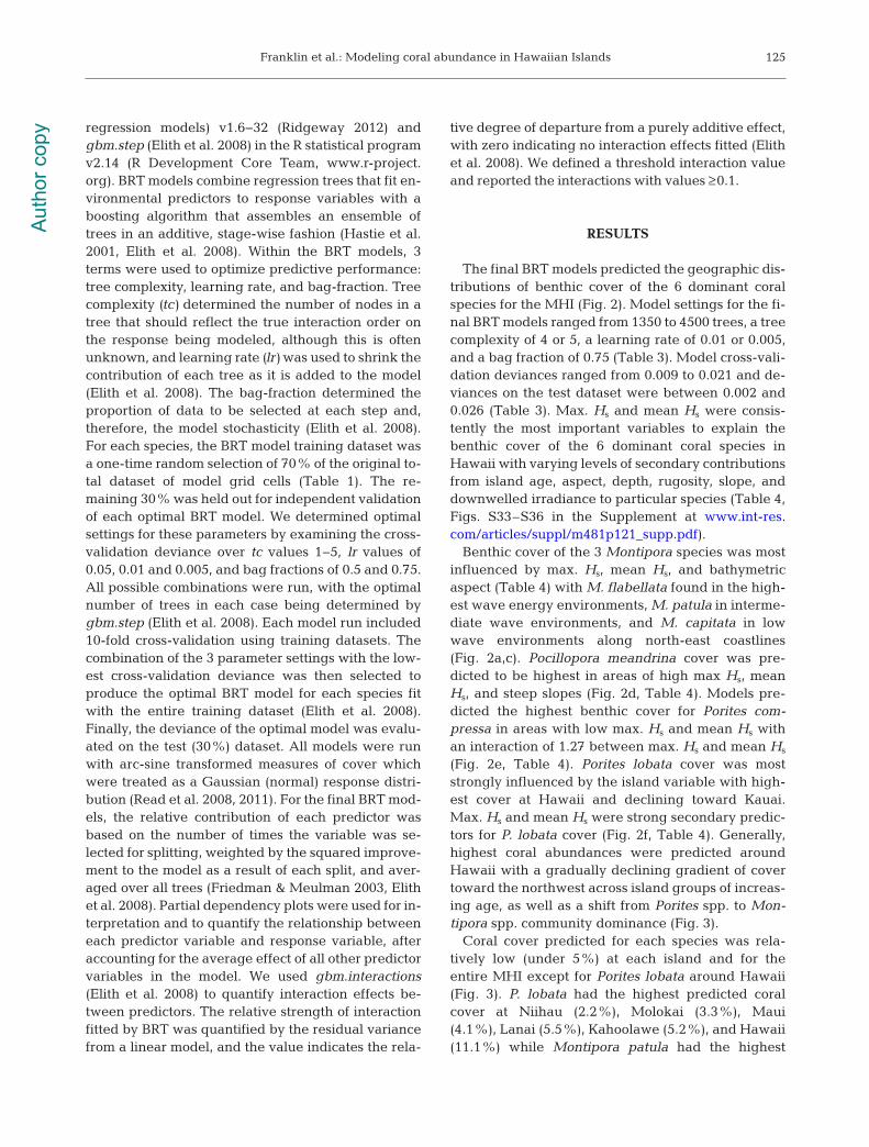
The final BRT models predicted the geographic dis-tributions of benthic cover of the 6 dominant coralspecies for the MHI (Fig. 2). Model settings for the fi-nal BRT models ranged from 1350 to 4500 trees, a treecomplexity of 4 or 5, a learning rate of 0.01 or 0.005,and a bag fraction of 0.75 (Table 3). Model cross-vali-dation deviances ranged from 0.009 to 0.021 and de-viances on the test dataset were be tween 0.002 and0.026 (Table 3). Max. Hs and mean Hs were consis-tently the most important variables to explain thebenthic cover of the 6 dominant coral species inHawaii with varying levels of secondary contributionsfrom island age, aspect, depth, rugosity, slope, anddownwelled irradiance to particular species (Table 4,Figs. S33–S36 in the Supplement at www.int-res.com/ articles/ suppl/ m481p121_ supp. pdf).

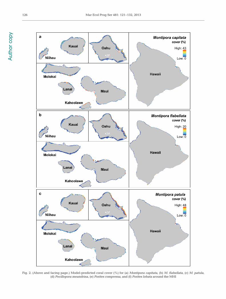
Benthic cover of the 3 Montipora species was mostinfluenced by max. Hs, mean Hs, and bathymetricaspect (Table 4) with M. flabellata found in the high-est wave energy environments, M. patula in interme-diate wave environments, and M. capitata in lowwave environments along north-east coastlines(Fig. 2a,c). Pocillopora meandrina cover was pre-dicted to be highest in areas of high max Hs, meanHs, and steep slopes (Fig. 2d, Table 4). Models pre-dicted the highest benthic cover for Porites com-pressa in areas with low max. Hs and mean Hs withan interaction of 1.27 between max. Hs and mean Hs

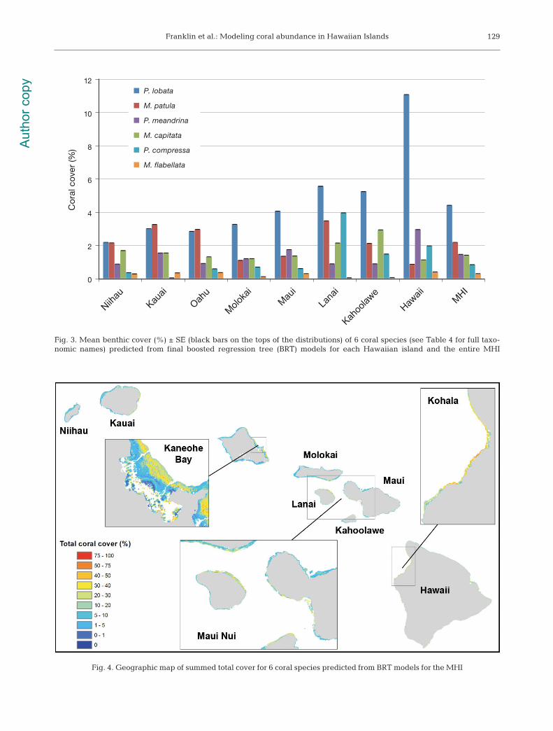
(Fig. 2e, Table 4). Porites lobata cover was moststrongly influenced by the island variable with high-est cover at Hawaii and declining toward Kauai.Max. Hs and mean Hs were strong secondary predic-tors for P. lobata cover (Fig. 2f, Table 4). Generally,highest coral abundances were predicted aroundHawaii with a gradually declining gradient of covertoward the northwest across island groups of increas-ing age, as well as a shift from Porites spp. to Mon-tipora spp. community dominance (Fig. 3).

Coral cover predicted for each species was rela-tively low (under 5%) at each island and for theentire MHI except for Porites lobata around Hawaii(Fig. 3). P. lobata had the highest predicted coralcover at Niihau (2.2%), Molokai (3.3%), Maui(4.1%), Lanai (5.5%), Kahoolawe (5.2%), and Hawaii(11.1%) while Montipora patula had the highest

Aut

hor c

opy

Mar Ecol Prog Ser 481: 121–132, 2013126

Fig. 2. (Above and facing page.) Model-predicted coral cover (%) for (a) Montipora capitata, (b) M. flabellata, (c) M. patula, (d) Pocillopora meandrina, (e) Porites compressa, and (f) Porites lobata around the MHI

Aut

hor c

opy

Franklin et al.: Modeling coral abundance in Hawaiian Islands 127

Fig. 2 (continued)

Aut

hor c

opy

Mar Ecol Prog Ser 481: 121–132, 2013

cover around Kauai (3.3%) and Oahu (3.0%) (Fig. 3).The rank order of abundance (from highest to lowestwith coral cover in parenthesis) for the entire MHIwas P. lobata (4.4%), M. patula (2.2%), Pocilloporameandrina (1.44%), M. capitata (1.40%), Poritescompressa (0.8%), and M. flabellata (0.3%). Noisland had the same rank order of abundance as theoverall MHI order, but Molokai and Maui were mostsimilar to the MHI. Notable divergences from theMHI rank order were Porites compressa with the 2ndand 3rd highest cover at Lanai and Hawaii, respec-tively, and Pocillopora meandrina with the secondhighest cover around Maui and Hawaii (Fig. 3).

Predicted total coral cover from a summation of the6 species varied between a low of 7.5% (Niihau and

Molokai) to 18.4% with an overall mean of 10.5% forthe MHI. Kaneohe Bay on Oahu; the wave-shelteredarea of Maui Nui that includes reefs of Molokai,Lanai, Maui, and Kahoolawe; and the Kohala coast ofHawaii were predicted as areas of the highest totalcoral cover summed for the 6 species (Fig. 4). Meanisland coral cover ranged between 2 and 26% withthe highest cover around Lanai and Hawaii and thelowest at Niihau and Kauai.

DISCUSSION

Using BRT models, we developed continuous spatialdistribution maps of the benthic cover for the dominant6 Hawaiian coral species around the MHI. The BRTmodels identified the most important sets of environ-mental variables for each species (Table 4). Mean co -ral cover for each species and species rank abundanceby island and the entire MHI were calculated fromfinal BRT model predicted coral covers (Figs. 3 & 4).

Wave exposure or wave energy has been identifiedas the primary factor influencing the distribution,zonation, and composition of Hawaiian coral reefs(Dollar 1982, Grigg 1983, Engels et al. 2004, Jokiel etal. 2004, Storlazzi et al. 2005). In the present study,both max. Hs and mean Hs were consistently the mostimportant variables to explain the benthic cover ofHawaiian coral species (Table 4). This result suggestsa synergistic effect between the typical, daily waveconditions and periodic high energy wave eventsfrom storms in structuring coral communities aroundthe Hawaiian Islands (Dollar 1982, Grigg 1983).Other environmental variables contributing greaterthan 10% relative importance to BRT models wereisland age, aspect, depth, rugosity, slope, and down-welled irradiance, relationships which were alsoreported by Jokiel et al. (2004).

Predicted cover for Pocillopora meandrina washighest in shallow, high-wave energy environmentsalong the north coasts and headlands of Kauai, Oahu,and Maui and the entire coastline of Hawaii (Fig. 2d).These areas are commonly characterized by shallow,basalt boulder habitats with steep slope, high rugos-ity, and high wave-energy (Jokiel et al. 2004, Battistaet al. 2007). Although significant wave height is asurface observation, its predictive capacity for coralspecies abundance seems promising, and appears toperform similarly to other wave-related metrics suchas near-bottom shear stress (Storlazzi et al. 2005) orwave exposure (Chollett & Mumby 2012).

Of the 3 Montipora species, M. capitata appearsthe most broadly adaptable to a range of habitats

128

Mcap Mfla Mpat Pmea Pcom Plob

Mean Hs 25.5 26.7 18.7 21.2 33.5 14.5Max. Hs 17.4 22.2 16.4 17.8 20.7 14.7Island age 2.7 3.8 11.3 3.5 6.8 28.6Aspect 14.7 17.1 14.4 11.5 3.2 9.0Depth (m) 9.8 8.6 10.3 8.6 10.8 9.6Rugosity 6.9 11.4 7.4 13.7 8.5 6.1Slope 7.0 4.3 8.2 11.4 4.0 8.0Downwelled 10.4 4.8 9.6 3.1 6.5 6.9irradiance

Sandbottom 5.5 1.2 3.7 3.1 6.1 2.6

Table 4. Relative contribution of environmental variables toBRT models of Montipora capitata (Mcap), M. flabellata(Mfla), M. patula (Mpat), Pocillopora meandrina (Pmea),Porites compressa (Pcom), and Porites. lobata (Plob). Envi-ronmental variables: Hs : mean and maximum significantwave height (m); Island age (mya); aspect (°); depth (m); ru-gosity (surface/ planar area); slope (°); downwelled irradiance

[Ed(Z)/Ed(0−)]; sandbottom (proportion)

nt tc lr cv dev eval cv

Montipora 2550 5 0.01 0.011 ± 0.001 0.012capitata

M. flabellata 1450 4 0.01 0.002 ± 0 0.002M. patula 4050 5 0.005 0.011 ± 0.001 0.010Pocillopora 3400 4 0.005 0.009 ± 0.001 0.011meandrina

Porites compressa 2550 5 0.01 0.010 ± 0.001 0.010Porites lobata 1350 5 0.01 0.021 ± 0.001 0.026

Table 3. Model settings and cross-validation deviance of final BRT models for benthic cover of Montipora capitata,M. flabellata, M. patula, Pocillopora mean drina, Poritescompressa, and Porites lobata around the MHI. Model set-tings include the number of trees (nt), tree complexity (tc),and learning rate (lr). Bag fraction was 0.75 for each model.Cross-validation deviance (cv dev) with ±SE, and deviance

of evaluation observations (eval cv)Aut

hor c

opy

Franklin et al.: Modeling coral abundance in Hawaiian Islands 129

Fig. 4. Geographic map of summed total cover for 6 coral species predicted from BRT models for the MHI

0

2

4

6

8

10

12C

ora

l cov

er (%

)

P. lobata

M. patula

P. meandrina

M. capitata

P. compressa

M. flabellata

Fig. 3. Mean benthic cover (%) ± SE (black bars on the tops of the distributions) of 6 coral species (see Table 4 for full taxo-nomic names) predicted from final boosted regression tree (BRT) models for each Hawaiian island and the entire MHI

Aut

hor c

opy

Mar Ecol Prog Ser 481: 121–132, 2013

since it is predicted to occur both along fore reefs aswell as in quiescent environments such as KaneoheBay on Oahu (Fig. 2a). The ability of M. capitata tooccupy such diverse habitats may be due to the ex -treme phenotypic plasticity that the species exhibits(Forsman et al. 2010). For example, a single colony ofM. capitata may possess sections that are laminar,encrusting, or branching (Forsman et al. 2010). M.patula and M. flabellata were predicted to occur inhigher wave environments than M. capitata. Highestpredicted cover for M. patula and M. flabellata wasalong the east coasts of Kauai and Oahu and wave-sheltered areas of Maui Nui (Fig. 2b,c). Both speciesare endemic to Hawaii and currently under reviewfor listing as threatened or endangered species underthe US Endangered Species Act (Brainard et al.2011). The present study represents the most com -pre hensive distribution and abundance informationavailable for these 2 species and should be used toinform ongoing conservation ef forts.

Porites compressa cover dominated low wave-energy environments that are typically shallow,nearshore habitats with turbid waters from sedimentresuspension and watershed inputs (Hunter & Evans1995, Coles et al. 1997, Jokiel 2006). High P. com-pressa cover was also predicted for wave-shelteredcoasts of Maui Nui and deeper waters (>10 m)around Hawaii, an observation reported by Dollar(1982, our Fig. 2e). At intermediate wave energies (1to 3 m max Hs), Porites lobata was predicted to be thedominant coral (Fig. 2f) and was the most abundantcoral species in the MHI (Fig. 3). Island age was alsoa strong positive factor for P. lobata with high benthiccover occurring around the youngest island, Hawaii(<0.5 mya).

In general, coral cover was predicted to be highestin primarily wave-sheltered coastlines and embay-ments. High coral cover locations were predictedthroughout the islands, but reefs with highest coverwere concentrated in Kaneohe Bay on Oahu, thewave-sheltered areas of Maui Nui, and along thewest coast of Hawaii (Fig. 4). These areas have vary-ing benthic geomorphology and levels of down-welled irradiance but share similar low wave energycharacteristics. Previously, the Engels et al. (2004)model of modern coral zonation for the HawaiianIslands related the occurrence of highest total coralcover to low wave-energy environments. Storlazzi etal. (2005) also observed the highest total coral coveralong sections of the Molokai coastline with the low-est wave-induced near bed shear stress. These stud-ies correspond well with the predicted results fromour BRT models.

Rank order of coral species abundance differedslightly from prior studies. We found the rank order(from highest to lowest) to be Porites lobata, Mon-tipora patula, Pocillopora meandrina, M. capitata,Porites compressa, and M. flabellata. From a surveyof the southwest coasts of Kauai, Oahu, Maui, andHawaii, Grigg (1983) found the rank order of abun-dance for the 6 coral species in the present study asPorites lobata, P. compressa, M. capitata, Pocilloporameandrina, M. patula, and M. flabellata. Jokiel et al.(2004) surveyed 60 monitoring locations throughoutthe MHI and ob served a similar rank order of abun-dance (and coral cover) of Porites lobata (6.1%), P.compressa (4.5%), M. capitata (3.9%), M. patula(2.7%), Pocillopora mean drina (2.4%), and M. flabel-lata (0.7%). Compared to Grigg (1983) and Jokiel etal. (2004), our study found Porites compressa to berelatively less abundant overall and M. patula moreabundant than M. capitata.

The BRT models provided strong results for the pre-dicted cover of the 6 coral species (Table 3), but the in-clusion of additional environmental variables and amore comprehensive geographic distribution of fieldsamples should lead to better model performance andmore accurate cover predictions. For example, finergrain bathymetry data (<10 m cell size) could improvethe predictive power of modeled bottom complexity(such as found in Jokiel et al. 2004), but were notavailable for the entire study domain. Furthermore,significant wave heights are a surface measurement.Wave environments at the sea floor are more accu-rately characterized by bottom water velocity (Loweet al. 2009) or near bed shear stress (Storlazzi et al.2005), which may be 2 potential variables for futurestudy. A better representation of downwelled irradi-ance would incorporate the absolute surface irradi-ance instead of a relative metric which assumessimilar surface levels throughout the study domain.

Species observations compiled for this study werecollected throughout the MHI (Fig. 1). Although mostareas were well sampled, several locations had highsample clusters which may bias model results to -wards the characteristics of those areas. In addition,Kahoolawe, south Molokai, north Lanai, and north-east Oahu were undersampled and we suggest futurecoral surveys to focus on these areas. In the absenceof acquiring additional samples, future studies couldinclude a spatially explicit term to address potentialspatial autocorrelation in the models (Latimer et al.2006) or select subsets of the existing datasets by geo-graphic location to achieve area proportional sam-pling between islands (Jiménez-Valverde et al. 2009)to mitigate spatial sampling bias.

130A

utho

r cop

y

Franklin et al.: Modeling coral abundance in Hawaiian Islands

Regional-scale characterizations of coral speciesfrom SDMs provide the framework for spatially ex -plicit ecosystem modeling and marine spatial plan-ning of coral reefs (Franklin et al. 2003, Crowder &Norse 2008, Klein et al. 2010). SDMs of coral speciesare critically useful since species respond differen-tially to thermal stressors (Guest et al. 2012) and coraldiseases (Williams et al. 2010, Aeby et al. 2011),while studies of total coral cover alone overlookchanges in reef composition and species dominance.Data from coral SDMs can be incorporated into spa-tial optimization exercises for marine conservation(Leathwick et al. 2008) or for geographically explicitthreat assessments to reefs (Selkoe et al. 2009, Burkeet al. 2011). The geographic characterization of coralreefs would benefit greatly from the improved coraldistribution and abundance information generatedfrom SDMs.

Acknowledgements. Coral species observation data wereprovided by the US National Park Service and US NationalOceanic and Atmospheric Administration. Wave model datawere provided by K. F. Cheung and R. A. Arinaga (Univ. ofHawaii, Dept. of Ocean and Resources Engineering). TheNational Marine Sanctuary Program (memorandum ofagreement 2005-008 ⁄ 66882), the US Environmental Protec-tion Agency Science To Achieve Results PhD Fellowship(FP917096), and the US National Science Foundation(OCE1041673) provided financial support for this research.This is HIMB contribution #1532 and SOEST contribution#8797.

LITERATURE CITED

Aeby GS, Williams GJ, Franklin EC, Kenyon J, Cox EF,Coles S, Work TM (2011) Patterns of coral disease acrossthe Hawaiian Archipelago: relating disease to environ-ment. PLoS ONE 6: e20370

Arinaga RA, Cheung KF (2012) Atlas of global wave energyfrom 10 years of reanalysis and hindcast data. RenewEnergy 39: 49−64

Austin M (2007) Species distribution models and ecologicaltheory: a critical assessment and some possible newapproaches Ecol Model 200: 1−19

Battista TA, Costa BM, Anderson SM (2007) Shallow-waterbenthic habitats of the main eight Hawaiian Islands(DVD). NOAA Technical Memorandum NOS NCCOS61, Biogeography Branch. Silver Spring, MD

Brainard RE, Birkeland C, Eakin CM, McElhany P, MillerMW, Patterson M, Piniak GA (2011) Status review reportof 82 candidate coral species petitioned under the USEndangered Species Act. US Dept of Commerce, NOAATech Memo, NMFS-PIFSC-27, Pacific Islands FisheriesScience Center, Honolulu, HI

Brown E, Cox E, Jokiel P, Rodgers K and others (2004)Development of benthic sampling methods for the coralreef assessment and monitoring program (CRAMP) inHawai‘i. Pac Sci 58: 145−158

Brown E, Minton D, Daniel R, Klasner F and others (2007)Benthic marine community monitoring protocol — Pacific

island network. Natural Resource Report NPS/ PACN/NRTR — 2007/002. National Park Service, Fort Collins,CO

Burke L, Reytar K, Spalding M, Perry A (2011) Reefs at riskrevisited. World Resources Institute, Washington, DC

Carpenter KE, Abrar M, Aeby G, Aronson RB and others(2008) One-third of reef-building corals face elevatedextinction risk from climate change and local impacts.Science 321: 560−563

Chollett I, Mumby PJ (2012) Predicting the distribution ofMontastrea reefs using wave exposure. Coral Reefs 31: 493−503

Clague DA, Dalrymple GB (1994) Tectonics, geochronology,and origin of the Hawaiian Emperor volcano chain. In: Kay EA (ed) A natural history of the Hawaiian Islands.University of Hawaii Press, Honolulu, HI

Coles SL, DeFelice RC, Eldredge LG, Carlton JT, Pyle RL,Suzumoto A (1997) Biodiversity of marine communitiesin Pearl Harbor, Oahu, Hawaii with observations onintroduced exotic species. Bishop Mus Tech Report 10.Honolulu, HI

Connolly JP, Blumberg AF, Quadrini JD (1999) Modelingfate of pathogenic organisms in coastal waters of Oahu,Hawaii. J Environ Eng 125: 398−406

Crowder L, Norse E (2008) Essential ecological insights formarine ecosystem-based management and marine spa-tial planning. Mar Policy 32: 772−778

Dollar SJ (1982) Wave stress and coral community structurein Hawaii. Coral Reefs 1: 71−81

Dubinsky Z, Stambler N (2011) Coral reefs: an ecosystem intransition. Springer, New York, NY

Elith J, Leathwick JR (2009) Species distribution models: ecological explanation and prediction across space andtime. Annu Rev Ecol Evol Sys 40: 677−697

Elith J, Graham CH, Anderson RP, Dudik M and others(2006) Novel methods improve prediction of species’ dis-tributions from occurrence data. Ecography 29: 129−151

Elith J, Leathwick JR, Hastie T (2008) A working guide toboosted regression trees. J Anim Ecol 77: 802−813

Engels MS, Fletcher CH, Field ME, Storlazzi CD and others(2004) Holocene reef accretion: southwest Molokai,Hawaii, USA. J Sed Res 74: 255−269

Fletcher CH, Bochicchio C, Conger CL, Engels MS andothers (2008) Geology of Hawaii reefs. In: Riegl BM,Dodge RE (eds) Coral reefs of the USA. Springer, NewYork, NY

Forsman ZH, Concepcion GT, Haverkort RD, Shaw RW,Maragos JE, Toonen RJ (2010) Ecomorph or endangeredcoral? DNA and microstructure reveal Hawaiian speciescomplexes: Montipora dilatata/flabellata/turgescens &M. patula/verrilli. PLoS ONE 5: e15021

Franklin EC, Ault JS, Smith SG, Luo J and others (2003)Benthic habitat mapping in the Tortugas region, Florida.Mar Geodesy 26:19–34

Friedman JH, Meulman JJ (2003) Multiple additive regres-sion trees with application in epidemiology. Stat Med 22: 1365−1381

Garza-Pérez JR, Lehmann A, Arias-González JE (2004) Spa-tial prediction of coral reef habitats: integrating ecologywith spatial modeling and remote sensing. Mar Ecol ProgSer 269: 141−152

Goodman J, Ustin SL (2007) Classification of benthic compo-sition in a coral reef environment using spectral unmix-ing. J Appl Remote Sens 1: 011501

Grigg RW (1983) Community structure, succession, and

131A

utho

r cop

y

Mar Ecol Prog Ser 481: 121–132, 2013

development of coral reefs in Hawaii. Mar Ecol Prog Ser11: 1−14

Grigg RW (2006) Depth limit for reef building corals in theAu'au Channel, S.E. Hawaii. Coral Reefs 25:77–84

Guest JR, Baird AH, Maynard JA, Muttaqin E and others(2012) Contrasting patterns of coral bleaching suscepti-bility in 2010 suggest an adaptive response to thermalstress. PLoS ONE 7: e33353

Guinotte JM, Bartley JD, Iqbal A, Fautin DG, BuddemeierRW (2006) Modeling habitat distribution from organismoccurrences and environmental data: case study usinganemonefishes and their sea anemone hosts. Mar EcolProg Ser 316: 269−283

Guisan A, Thuiller W (2005) Predicting species distribution: offering more than simple habitat models. Ecol Lett 8: 993−1009

Guisan A, Zimmermann NE, Elith J, Graham CH, Phillips S,Peterson AT (2007) What matters for predicting theoccurrences of trees: techniques, data, or species charac-teristics? Ecol Monogr 77: 615−630

Harborne AR, Mumby PJ, Zychaluk K, Hedley JD, Black-well PG (2006) Modeling the beta diversity of coral reefs.Ecology 87: 2871−2881

Hastie T, Tibshirani R, Friedman JH (2001) The elements ofstatistical learning: data mining, inference and predic-tion. Springer-Verlag, New York, NY

Hawaii Mapping Research Group (2011) Main HawaiianIslands multibeam bathymetry synthesis. www.soest.hawaii. edu/hmrg/Multibeam/grids.php

Hoeke R, Storlazzi C, Ridd P (2011) Hydrodynamics of abathymetrically complex fringing coral reef embayment: wave climate, in situ observations, and wave prediction.J Geophys Res 116: C04018, doi:10. 1029/ 2010 JC 006170

Hunter CL, Evans CW (1995) Coral reefs in Kaneohe Bay,Hawaii: two centuries of western influence and twodecades of data. Bull Mar Sci 57: 501−515

Isoun E, Fletcher C, Frazier N, Gradie J (2003) Multi- spectral mapping of reef bathymetry and coral cover;Kailua Bay, Hawaii. Coral Reefs 22: 68−82

Jacobson EC (2005) Light attenuation in a nearshore coralreef ecosystem. MS thesis, University of Hawaii, Hon-olulu, HI

Jiménez-Valverde A, Lobo JM, Hortal J (2009) The effect ofprevalence and its interaction with sample size on thereliability of species distribution models. CommunityEcol 10: 196−205

Jokiel PL (2006) Impact of storm waves and storm floods onHawaiian reefs. Proc 10th Int Coral Reef Symp, Okinawa1: 390−398

Jokiel PL, Brown EK, Friedlander A, Rodgers SK, Smith WR(2004) Hawai‘i coral reef assessment and monitoring pro-gram: spatial patterns and temporal dynamics in reefcoral communities. Pac Sci 58: 159−174

Kirk JTO (1994) Light and photosynthesis in aquatic ecosys-tems. Cambridge University Press, Cambridge

Klein CJ, Steinback C, Watts M, Scholz AJ, Possingham HP(2010) Spatial marine zoning for fisheries and conserva-tion. Front Ecol Environ 8: 349−353

Knudby A, LeDrew E, Brenning A (2010) Predictive mappingof reef fish species richness, diversity and biomass in

Zanzibar using IKONOS imagery and machine- learningtechniques. Remote Sens Environ 114: 1230−1241

Latimer AM, Wu S, Gelfand AE, Silander JA (2006) Buildingstatistical models to analyze species distributions. EcolAppl 16: 33−50

Leathwick J, Moilanen A, Francis M, Elith J and others(2008) Novel methods for the design and evaluation ofmarine protected areas in offshore waters. Conserv Lett1: 91−102

Lowe RJ, Falter JL, Monismith SG, Atkinson MJ (2009)Wave-driven circulation of a coastal reef-lagoon system.J Phys Oceanogr 39: 873−893

Mumby PJ, Skirving W, Strong AE, Hardy JT and others(2004) Remote sensing of coral reefs and their physicalenvironment. Mar Pollut Bull 48: 219−228

Peterson AT, Soberón J, Pearson RG, Anderson RP, Mar-tinez-Meyer E, Nakamura M, Araújo MB (2011) Ecologi-cal niches and geographic distributions. Princeton Uni-versity Press, Princeton, NJ

Pittman SJ, Costa BM, Battista TA (2009) Using lidarbathymetry and boosted regression trees to predict thediversity and abundance of fish and corals. J Coast ResSpec Issue 53: 27−38

Read CF, Duncan DH, Vesk PA, Elith J (2008) Biological soilcrust distribution is related to patterns of fragmentationand landuse in a dryland agricultural landscape of south-ern Australia. Landsc Ecol 23: 1093−1105

Read CF, Duncan DH, Vesk PA, Elith J (2011) Surprisinglyfast recovery of biological soil crusts following livestockremoval in southern Australia. J Veg Sci 22: 905−916

Ready J, Kaschner K, South AB, Eastwood PD and others(2010) Predicting the distribution of marine organisms atthe global scale. Ecol Model 221: 467−478

Ridgeway G (2012) Generalized boosted regression models.Documentation on the R package ‘gbm’, version 1.6−32,www. r-project.org/

Robinson LM, Elith J, Hobday AJ, Pearson RG, Kendall BE,Possingham HP, Richardson AJ (2011) Pushing the limitsin marine species distribution modelling: lessons fromthe land present challenges and opportunities. Glob EcolBiogeogr 20: 789−802

Selkoe KA, Halpern BS, Ebert CM, Franklin EC and others(2009) A map of human impacts to a ‘pristine’ coral reefecosystem, the Papahanaumokuakea Marine NationalMonument. Coral Reefs 28: 635−650

Spalding MD, Ravilious C, Green EP (2001) World atlas ofcoral reefs. University of California Press, Berkeley, CA

Storlazzi CD, Brown EK, Field ME, Rodgers K, Jokiel PL(2005) A model for wave control on coral breakage andspecies distribution in the Hawaiian Islands. Coral Reefs24: 43−55

SWAN Team (2006) SWAN User Manual: SWAN Cycle IIIversion 40.51. Delft University of Technology, Delft

Tolman HL (2009) User manual and system documentationof WAVEWATCH III version 3.14. NOAA / NWS / NCEP/ MMAB Technical Note 276, US Dept of Commerce,NOAA, Camp Springs, MD

Williams GJ, Aeby GS, Cowie ROM, Davy SK (2010) Predic-tive modeling of coral disease distribution within a reefsystem. PLoS ONE 5: e9264

132

Editorial responsibility: Brian Helmuth, Nahant, Massachusetts, USA

Submitted: July 26, 2012; Accepted: January 6, 2013Proofs received from author(s): April 19, 2013

Aut

hor c

opy