Prediction of the Discharge Coefficient for a Cipolletti Weir with Rectangular Bottom Opening

Rafa H. Al-Suhili et al Int. Journal of Engineering Research and Applications www.ijera.com

ISSN : 2248-9622, Vol. 4, Issue 1( Version 4), January 2014, pp.80-89

www.ijera.com 80 | P a g e

Prediction of the Discharge Coefficient for a Cipolletti Weir with

Rectangular Bottom Opening

Rafa H. Al-Suhili1 and Alan Jalal Shwana

2

1Senior Professor of the civil engineering Dept., College of Engineering, University of Baghdad, Baghdad, Iraq.

Visiting professor at the City College of New York. New York, USA 2M.Sc.Water Resources and Dam Engineering Dept, College of Engineering, .University of Sulaimania, Sulaimania,

Iraq.

Abstract The hydraulic characteristics of a Cipolletti weir with rectangular bottom opening were investigated in this study.

The work was carried out using an existing experimental setup of a flume with storage and re-circulating tanks, a

pump, a flow meter and a piping system with valves. Thirty nine physical models were made for the Cipolletti weir

with rectangular bottom opening with different geometrical dimensions called hereafter as configurations.

Experimental measurements were taken for each configuration for different flow values to find the actual discharge,

the head over the weir and the head of the approaching flow. For each configuration the data set were analyzed in

order to find the discharge coefficient using equation, derived for the combined flow over the weir and from the

bottom rectangular opening. All the flow cases tested were for free flow over the weir and sub-critical flows.

Dimensional analysis was made to relate the discharge coefficient with different geometrical and flow variables

using artificial neural networks modeling. The correlation coefficient found for the predicted values of the discharge

coefficient is (r=0.88).

Key words: Cipolletti weir, Bottom opening, Discharge Coefficient, Artificial Neural Networks, Physical

modeling.

I. Introduction Weirs are built as a standing wall across the

flow section with opening at the top. Sediments are

often accumulated at the upstream side of the weir.

These sediments will affect the weir function. This

problem is exaggerated when the approaching channel

has a high suspended load causing large changes in the

upstream channel section. This results in many

problems, such as high measuring errors and flow

diversion problems. Many solutions were adopted

before, such as the use of sediment excluder structure,

sloping weirs, and continuous periodical removal of

sediments. Sediments excluding structures are an

alternative solution for sediment removal upstream

hydraulic structures. Al-Suhaili and Auda(2001), had

conducted a physical model study for Adhaim dam

diversion weir located in Iraq. This weir was designed

with sediment excluder that has two openings with

gates. The main problem faced by hydraulic engineers

is the difficulty in the design and operation of such

structure, since it needs physical modeling to find the

real ability of removal. Moreover many operation

problems were also found.

Periodical removal of sediments is the other

solution. However, this solution is rather expensive and

difficult, especially for large weirs and for those rivers

and channels that have high suspended loads, which

usually settled and accumulated at the upstream side of

the wier.

Other solutions have been adopted by Al-

Hamid, et. al., (1996) for triangular weirs and

Negm,(1998) for rectangular weirs with unequal

contractions. That is to provide an opening at the

bottom of the weirs. It was found that sediments are

partially removed through this opening.

In this research an attempt has been made to

study the flow conditions and discharge coefficient for

a Cipolletti weir with rectangle opening at the bottom

for sediments removal. There is no equation available

in the literature for calculating the discharge coefficient

of such structure. The study is conducted using

experimental physical modeling to calculate the

discharge coefficient as a function of both geometrical

and flow variables.

Al-Hamid, et.al., (1996-a) had investigated a

discharge equation for simultaneous flow over

rectangular contracted weir with bottom triangular

opening. The .In this paper one generalized equation

including all the important variables was obtained from

an experimental investigation. The predictions of the

equation agreed well with the experimental

observations.

Al-Hamid, et.al. (1996-b) had investigated the

hydraulics of a triangular weir with bottom rectangular

RESEARCH ARTICLE OPEN ACCESS




opening. Different models with different geometric

combinations were tested. These geometries include,

gate opening, gate length and V-notch angle.

Experiments were conducted for free gate flow (un-

submerged) conditions on horizontal and sloping

channels. Results showed that flow passes through the

weir is affected by the weir and opening geometry and

the flow parameters. Semi-empirical discharge equation

was developed. This equation represents the collected

experimental data well with an absolute error less than

4%.

Negm,(1998) had investigated the

characteristics of combined flow over contracted weir

and below submerged rectangular opening with unequal

contractions. This paper presents the results of an

experimental study on the characteristics of

simultaneous flow over the contracted weir and below

the contracted submerged opening with unequal

contractions. A prediction equation relating the non-

dimensional combined discharge to both flow and

geometry parameters was developed. The predicted

combined discharges agreed well with the

experimentally measured ones.

Negm,et.al.,( 2002) had investigated the

combined –free flow over weirs and below rectangular

opening of equal contraction. The experiments were

carried out in a laboratory flume using various

geometrical dimensions under different flow conditions.

The experimental data were then used to develop a

general non-dimensional equation for predicting the

discharge through the combined system knowing its

geometry and the head of water over the weir.

Negm, (2002) had investigated the modeling

of submerged simultaneous flow through combined

weirs and rectangular opening of unequal contractions.

In this study, a generalized discharge model was

proposed based on the known equations of weirs and

openings. The proposed equation was calibrated using

large series of experimental data for weirs having

opening of unequal contractions under both free and

submerged flow conditions. The predictions of the

proposed model agree well with the observations with a

deviation of less than ± 5 for about 90% of the data.

Hayawiet.al,(2008) had investigated free

combined flow over a triangular weir and under

rectangular opening. The main objective of this

investigation is to find the characteristics of free flow

through the combined triangular weir and a rectangular

opening. Nine combined weirs were constructed and

tested for three different triangular angles (30o, 45

oand

60o). The vertical distance between the weir crest and

the top level of the opening was changed three times for

each angle(5,10 and15) cm. A general expression was

obtained for the discharge coefficient as a function of

Froude number, angle of the weir, and different

geometrical non dimensional terms. The estimated

values of the discharge coefficient were compared well

with the experimental results.

Saman and Mazaheri, (2009) had investigated

combined flow over weir and under rectangular

opening. Models of sharp-edged weirs and openings

with no lateral contraction were combined. To calibrate

and validate the proposed model, experiments have

been carried out in a laboratory flume applying

different submergence conditions. It was found that the

model is able to predict the stage–discharge relationship

with reasonable accuracy. The researchers had

concluded that the results of the proposed model show

good agreement between calculated and measured

discharges implying reasonable precision.

II. Experimental work For conducting the experiments on the

proposed Cipolletti weir models with a rectangular

opening at the bottom, a flume of conventional size was

used. The conventional size is the size that can allow

easy measurements of flow depth and permit good

visualization of the flow pattern over the weir and at the

downstream side from the bottom opening. This flume

has other facilities, such as: storage tank, recirculation

tank, pump, ultrasonic flow meter, point gauges and

valves. The flume section is rectangular with 60cm

width which is considered acceptable in accordance to

(USBR, 2001) specifications. Along its length the

flume has two different heights, 135cm height at the

inlet (upstream) side with a length of 2.5m, and 70cm

height at the downstream side with a length of 5.5m.

In order to investigate the hydraulics of

Cipolletti weir with bottom rectangular opening,

different configurations were used in this experimental

work. Table (1) shows the details of these

configurations. Figure (1) shows a general setup of the

proposed weir model that covers all the configurations

stated in table (1) with different dimensions.

Where:

hw: Height of the Cipolletti weir.

Bw: Bed width of the Cipolletti weir.

ho: Height of the rectangular bottom opening.

bo: Width of the rectangular bottom opening.

P : Vertical distance between the bottom of the

weir and its crest (ho+d).

For each configuration from those mentioned

in table (1), the number of flow values for which

experimental measurements was conducted is different,

according to what the experimental setup allows. For

each configuration from those mentioned above and for

each flow value, the following variables were

measured:

1. Actual flow values (Qact) using the flow meter.

2. The head over the crest (h1’) using point gage

no.1




3. The total head (H) at a distance (3 h1’)

upstream of the weir crest using point gage

no.2

Using these data the discharge coefficient was

calculated for each configuration and flow value.

To compute the discharge coefficient for the

proposed hydraulic structure, the following equation

may be obtained by adding the discharge over the weir

and the discharge through the opening as follows:

Qtheo= Qgtheo+ Qwtheo ………… (1)

Where; Qgtheo= is the theoretical discharge through the

opening which can be expressed as follows:

Qgtheo= 2gHbo ho ……… (2)

Where; (H: Total head, bo: opening width, ho:

opening height, g: gravitational

acceleration.)

And Qw theo=

2

3 2gBw h1

1.5 …………… (3)

Where; (h1=H-P, P: is the crest height, P=d+ho).

The actual discharges are: Qgact, and Qwact

for the

opening and the weir respectively:

Qgact= Cdg . Qgtheo

…………… (4)

Qwact= Cdw .Qw theo

……… (5)

Where;Cdg and Cdw are the discharge coefficients for

the opening and the weir respectively.

For the flow condition of both from opening and over

weir the theoretical flow is Qtheo ;

Qtheo = 2gHbo ho +2

3 2gBw h1

1.5

…… (6), and

Qact = Cdg . 2gHbo ho + Cdw .2

3 2gBw h1

1.5 …… (7)

Simplifying equations (7):

Qact = Cdc . 2g Hbo ho +2

3Bw h1

1.5 …. (8)

Where; Cdc: is the combined discharge coefficient.

Hence this combined discharge coefficient will

be estimated using equation (8). It is expected that the

combined discharge coefficient is dependent on the

geometry of the model as well as the flow conditions

and properties , i.e. ( ho , bo , d ,hw , Bw , H, g, ρ , µ ,

Ɵ,So,σ)

g: gravitational acceleration.

ρ: water mass density.

µ: water viscosity.

Ɵ: weir angle.

So: slope of channel.

σ: surface tension.

For water at specific temperature (ρ,µ and σ)

are constant, hence, can be excluded, Ackers,(1978) as

mentioned in Al-Hamed et. al. (1996-a).This is

evidence herein since the water temperature measured

during the experimental work was ranged between (18,

25). Moreover, since the standard side slope is (1:4) for

Cipolletti weir USBR, (2001), hence Ɵ is constant. The

available flume has no facility to change the bed slope

of the channel, which is nearly horizontal, then (So) was

also considered constant as well as (g). Then, the

discharge coefficient can be expressed as:

Cdc = Φ( ho / H , bo /H , d/H , hw /H , Bw/ H ) ……..(10)

Or can be expressed using h1= H – P, i.e.:

Cdc = Φ ( ho / h1 , bo /h1, d/h1 , hw /h1 , Bw/h1 )……..(11)

Table (2) shows the calculations of the

discharge coefficient for configuration (1.a.1), for a

Cipolletti weir of a crest height “P=0.31m”and a crest

length “Bw=0.22m” with a bottom opening of width “bo

= 0.15m” and height “ho = 0.05m”. This table Shows

that the discharge coefficient range is (0.6227-0.6458)

with average value of (0.6346). The Froude number

range is (0.0447-0.0526) which indicates a subcritical

flow.

For the other configurations similar results

were obtained as for configuration (1.a.1) above. Table

(3) shows the summary of results for all of these other

configurations.

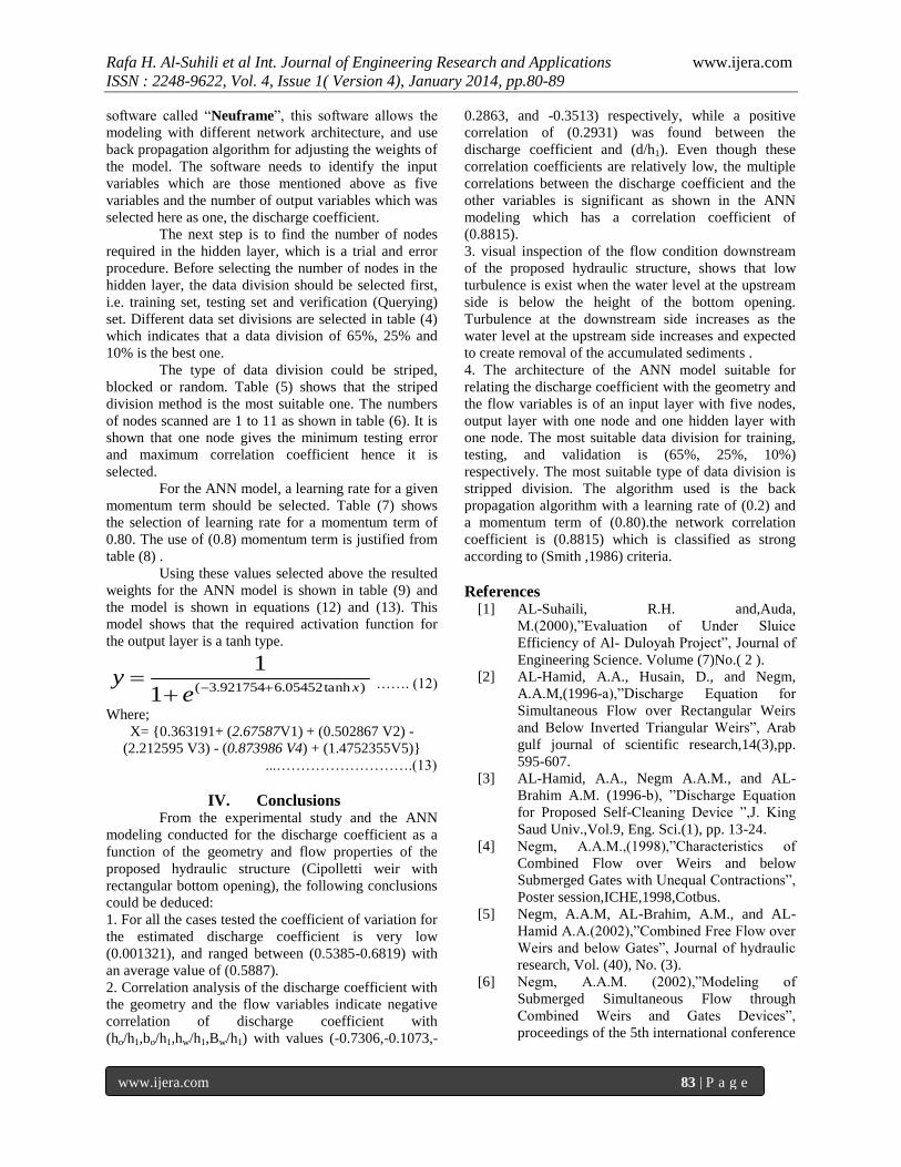
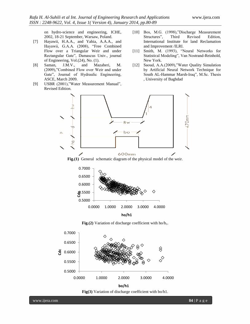
The variation of Cdc with each of the variables

(ho / h1 , bo /h1, d/h1 , hw /h1 , Bw/h1) are shown in

figures (2 to 6) respectively. Even though single

correlation between Cdc and each variable is low, it is

expected that its multiple correlation with these

variables will be significant, this will be shown later

among the application of the ANN model.

III. Artificial Neural Network Model for the

Discharge Coefficient Artificial neural network models (ANN) had

proved nowadays it's efficiency against nonlinear

regression models. The calculations of the discharge

coefficient presented above depend on equation

(8).This equation requires the value of measured actual

discharge. In practice, in order to use a Cipolletti weir

with bottom rectangular opening, the actual discharge

value should be calculated using equation (8) with the

knowledge of discharge coefficient and by measuring

the head value (h1).Hence, a model is required to find

the discharge coefficient as a function of ( ho / h1 , bo

/h1, d/h1 , hw /h1 ,and Bw/h1 ). This model could be a

regression model or an (ANN)model. Since the

experiments conducted covers different cases with

different crest height, crest length and bottom opening

dimensions the regression models are rather difficult ,

and may need classification ,i.e. different regression

equations for different cases. In such situation the

(ANN) models proved its superiority against regression

models (Saoud, 2009). Moreover the use of one model

in practice is much easier than using different

equations. Therefore an (ANN) model was developed

here including all the cases investigated to be used as a

one applicable model for all cases rather than different

models.

The artificial neural network model for

estimating the discharge coefficient as a function of (ho

/ h1, bo /h1, d/h1, hw/h1, Bw/ h1) , was developed using a




software called “Neuframe”, this software allows the

modeling with different network architecture, and use

back propagation algorithm for adjusting the weights of

the model. The software needs to identify the input

variables which are those mentioned above as five

variables and the number of output variables which was

selected here as one, the discharge coefficient.

The next step is to find the number of nodes

required in the hidden layer, which is a trial and error

procedure. Before selecting the number of nodes in the

hidden layer, the data division should be selected first,

i.e. training set, testing set and verification (Querying)

set. Different data set divisions are selected in table (4)

which indicates that a data division of 65%, 25% and

10% is the best one.

The type of data division could be striped,

blocked or random. Table (5) shows that the striped

division method is the most suitable one. The numbers

of nodes scanned are 1 to 11 as shown in table (6). It is

shown that one node gives the minimum testing error

and maximum correlation coefficient hence it is

selected.

For the ANN model, a learning rate for a given

momentum term should be selected. Table (7) shows

the selection of learning rate for a momentum term of

0.80. The use of (0.8) momentum term is justified from

table (8) .

Using these values selected above the resulted

weights for the ANN model is shown in table (9) and

the model is shown in equations (12) and (13). This

model shows that the required activation function for

the output layer is a tanh type.

)tanh05452.6921754.3(1

1xe

y

……. (12)

Where;

X= {0.363191+ (2.67587V1) + (0.502867 V2) -

(2.212595 V3) - (0.873986 V4) + (1.4752355V5)}

...……………………….(13)

IV. Conclusions From the experimental study and the ANN

modeling conducted for the discharge coefficient as a

function of the geometry and flow properties of the

proposed hydraulic structure (Cipolletti weir with

rectangular bottom opening), the following conclusions

could be deduced:

1. For all the cases tested the coefficient of variation for

the estimated discharge coefficient is very low

(0.001321), and ranged between (0.5385-0.6819) with

an average value of (0.5887).

2. Correlation analysis of the discharge coefficient with

the geometry and the flow variables indicate negative

correlation of discharge coefficient with

(ho/h1,bo/h1,hw/h1,Bw/h1) with values (-0.7306,-0.1073,-

0.2863, and -0.3513) respectively, while a positive

correlation of (0.2931) was found between the

discharge coefficient and (d/h1). Even though these

correlation coefficients are relatively low, the multiple

correlations between the discharge coefficient and the

other variables is significant as shown in the ANN

modeling which has a correlation coefficient of

(0.8815).

3. visual inspection of the flow condition downstream

of the proposed hydraulic structure, shows that low

turbulence is exist when the water level at the upstream

side is below the height of the bottom opening.

Turbulence at the downstream side increases as the

water level at the upstream side increases and expected

to create removal of the accumulated sediments .

4. The architecture of the ANN model suitable for

relating the discharge coefficient with the geometry and

the flow variables is of an input layer with five nodes,

output layer with one node and one hidden layer with

one node. The most suitable data division for training,

testing, and validation is (65%, 25%, 10%)

respectively. The most suitable type of data division is

stripped division. The algorithm used is the back

propagation algorithm with a learning rate of (0.2) and

a momentum term of (0.80).the network correlation

coefficient is (0.8815) which is classified as strong

according to (Smith ,1986) criteria.

References

[1] AL-Suhaili, R.H. and,Auda,

M.(2000),”Evaluation of Under Sluice

Efficiency of Al- Duloyah Project”, Journal of

Engineering Science. Volume (7)No.( 2 ).

[2] AL-Hamid, A.A., Husain, D., and Negm,

A.A.M,(1996-a),”Discharge Equation for

Simultaneous Flow over Rectangular Weirs

and Below Inverted Triangular Weirs”, Arab

gulf journal of scientific research,14(3),pp.

595-607.

[3] AL-Hamid, A.A., Negm A.A.M., and AL-

Brahim A.M. (1996-b), ”Discharge Equation

for Proposed Self-Cleaning Device ”,J. King

Saud Univ.,Vol.9, Eng. Sci.(1), pp. 13-24.

[4] Negm, A.A.M.,(1998),”Characteristics of

Combined Flow over Weirs and below

Submerged Gates with Unequal Contractions”,

Poster session,ICHE,1998,Cotbus.

[5] Negm, A.A.M, AL-Brahim, A.M., and AL-

Hamid A.A.(2002),”Combined Free Flow over

Weirs and below Gates”, Journal of hydraulic

research, Vol. (40), No. (3).

[6] Negm, A.A.M. (2002),”Modeling of

Submerged Simultaneous Flow through

Combined Weirs and Gates Devices”,

proceedings of the 5th international conference




on hydro-science and engineering, ICHE,

2002, 18-21 September, Warsaw, Poland.

[7] Hayawii, H.A.A., and Yahia, A.A.A., and

Hayawii, G.A.A. (2008), “Free Combined

Flow over a Triangular Weir and under

Rectangular Gate”, Damascus Univ., journal

of Engineering, Vol.(24), No. (1).

[8] Saman, J.M.V., and Mazaheri, M.

(2009),”Combined Flow over Weir and under

Gate”, Journal of Hydraulic Engineering,

ASCE, March 2009.

[9] USBR (2001),”Water Measurement Manual”,

Revised Edition.

[10] Bos, M.G. (1998),”Discharge Measurement

Structures”, Third Revised Edition,

International Institute for land Reclamation

and Improvement /ILRI.

[11] Smith, M. (1993), “Neural Networks for

Statistical Modeling”, Van Nostrand-Reinhold,

New York.

[12] Saoud, A.A.(2009),”Water Quality Simulation

by Artificial Neural Network Technique for

South AL-Hammar Marsh-Iraq”, M.Sc. Thesis

, University of Baghdad

Fig.(1) General schematic diagram of the physical model of the weir.

Fig.(2) Variation of discharge coefficient with ho/h1.

Fig(3) Variation of discharge coefficient with bo/h1.

0.5000

0.5500

0.6000

0.6500

0.7000

0.0000 1.0000 2.0000 3.0000 4.0000

Cdc

ho/h1

0.5000

0.5500

0.6000

0.6500

0.7000

0.0000 1.0000 2.0000 3.0000 4.0000

Cdc

bo/h1




0.5000

0.5500

0.6000

0.6500

0.7000

0.0000 2.0000 4.0000 6.0000 8.0000

Cdc

hw/h1

Fig.(4) Variation of discharge coefficient with d/h1.

Fig.(5) Variation of discharge coefficient with hw/h1.

Fig.(6) Variation of discharge coefficient with Bw/h1.

Table (1) Different configurations used in the experimental work.

Configurations Crest height

(P=ho +d) cm Crest length (Bw) cm

Bottom Opening

(bo x ho) cm

1.a

1.a.1

31 22

15 x 5

1.a.2 15 x 10

1.a.3 15 x 15

1.a.4 10 x 10

1.a.5 10 x 15

0.5000

0.5500

0.6000

0.6500

0.7000

0.0000 2.0000 4.0000 6.0000 8.0000Cdc

d/h1

0.5000

0.5500

0.6000

0.6500

0.7000

0.0000 5.0000 10.0000

Cdc

Bw/h1




1.b

1.b.1

31 32

15 x 5

1.b.2 15 x 10

1.b.3 10 x 10

1.b.4 10 x 15

2.a

2.a.1

27 40

15 x 5

2.a.2 15 x 10

2.a.3 15 x 15

2.a.4 10 x 10

2.a.5 10 x 15

Table 2 Test results and calculations for Configuration1.a.1),(P=0.31m,BW=0.22m,bo = 0.15m,ho = 0.05m).

Variables Test 1 Test 2 Test 3 Test 4 Test 5

Q act (m3/s) 0.0192 0.0210 0.0222 0.0238 0.0251

H(m) 0.3740 0.3830 0.3890 0.3950 0.4010

h1(m) 0.0640 0.0730 0.0790 0.0850 0.0910

h1'(m) 0.0530 0.0620 0.0680 0.0730 0.0800

V (m/S) 0.0856 0.0914 0.0951 0.1004 0.1043

Fr1 0.0447 0.0471 0.0487 0.0510 0.0526

Cdc 0.6227 0.6293 0.6317 0.6437 0.6458

ho/h1 0.7813 0.6849 0.6329 0.5882 0.5495

bo/h1 2.3438 2.0548 1.8987 1.7647 1.6484

d/h1 4.0625 3.5616 3.2911 3.0588 2.8571

hw/h1 2.5000 2.1918 2.0253 1.8824 1.7582

Bw/h1 3.4375 3.0137 2.7848 2.5882 2.4176

Note :( h1 is the calculated water height above the crest which found by (h1=H-P), but h1/ is the measured water

height above the crest and V is the approach flow velocity upstream the weir which is found by continuity equation).

2.b

2.b.1

27 30

15 x 5

2.b.2 15 x 10

2.b.3 15 x 15

2.b.4 10 x 10

2.b.5 10 x 15

2.c

2.c.1

27 20

15 x 5

2.c.2 15 x 10

2.c.3 15 x 15

2.c.4 10 x 10

2.c.5 10 x 15

3.a

3.a.1

23 28

15 x 5

3.a.2 15 x 10

3.a.3 15 x 15

3.a.4 10 x 10

3.a.5 10 x 15

3.b

3.b.1

23 23

15 x 5

3.b.2 15 x 10

3.b.3 15 x 15

3.b.4 10 x 10

3.b.5 10 x 15

3.c

3.c.1

23 23

15 x 5

3.c.2 15 x 10

3.c.3 15 x 15

3.c.4 10 x 10

3.c.5 10 x 15




Table (3) Summary of analysis results for all of the configurations.

Table (4) Data sets selection for the ANN model.

Data Division training

error

%

testing

error

%

coefficient

correlation(r)

% % Training

% Testing % Querying

80 10 10 7.38% 8.55% 70.05%

75 15 10 9.30% 8.45% 73.73%

70 15 15 7.51% 7.82% 80.50%

70 10 20 8.96% 7.24% 84.35%

70 20 10 8.80% 7.08% 80.85%

65 20 10 6.60% 7.88% 81.08%

65 25 10 6.15% 7.02% 88.15%

Config. No.

P (m)

Bw (m)

bo (m)

ho (m)

Cdc Range

Cdc Avg.

Cdc coeff.

Of

Froud No. Range

1.a.1 0.31 0.22 0.15 0.05 0.6227-0.6458 0.6346 0.000152 0.0447-0.0526 1.a.2 0.31 0.22 0.15 0.1 0.5949-0.6087 0.6025 0.000040 0.0695-0.0759 1.a.3 0.31 0.22 0.15 0.15 0.5676-0.5784 0.5729 0.000036 0.0939-0.0970 1.a.4 0.31 0.22 0.1 0.1 0.6093-0.6222 0.6150 0.000040 0.0540-0.0604 1.a.5 0.31 0.22 0.1 0.15 0.5801-0.5982 0.5913 0.000104 0.0697-0.0751 1.b.1 0.31 0.32 0.15 0.05 0.6106-0.6393 0.6278 0.000237 0.0430-0.0581 1.b.2 0.31 0.32 0.15 0.1 0.5866-0.5925 0.5902 0.000009 0.0741-0.0828 1.b.3 0.31 0.32 0.1 0.1 0.5999-0.6055 0.6021 0.000008 0.0582-0.0657 1.b.4 0.31 0.32 0.1 0.15 0.5770-0.5924 0.5847 0.000050 0.0731-0.0825 2.a.1 0.27 0.4 0.15 0.05 0.5674-0.5835 0.5736 0.000084 0.0548-0.0914 2.a.2 0.27 0.4 0.15 0.1 0.5426-0.5812 0.5642 0.000444 0.0817-0.1073 2.a.3 0.27 0.4 0.15 0.15 0.5482-0.5557 0.5520 0.000051 0.1143-0.1205 2.a.4 0.27 0.4 0.1 0.1 0.5462-0.5680 0.5573 0.000124 0.0639-0.0979 2.a.5 0.27 0.4 0.1 0.15 0.5421-0.5712 0.5561 0.000267 0.0813-0.1066 2.b.1 0.27 0.3 0.15 0.05 0.6363-0.6819 0.6618 0.000541 0.0548-0.0897 2.b.2 0.27 0.3 0.15 0.1 0.5387-0.5845 0.5661 0.000525 0.0776-0.0989 2.b.3 0.27 0.3 0.15 0.15 0.5444-0.5569 0.5506 0.000050 0.1071-0.1141 2.b.4 0.27 0.3 0.1 0.1 0.5576-0.5972 0.5761 0.000408 0.0629-0.0876 2.b.5 0.27 0.3 0.1 0.15 0.5385-0.5822 0.5640 0.000607 0.0785-0.0991 2.c.1 0.27 0.2 0.15 0.05 0.6027-0.6333 0.6158 0.000185 0.0648-0.0482 2.c.2 0.27 0.2 0.15 0.1 0.5626-0.5996 0.5844 0.000340 0.0755-0.0862 2.c.3 0.27 0.2 0.15 0.15 0.5558-0.5780 0.5671 0.000152 0.1031-0.1084 2.c.4 0.27 0.2 0.1 0.1 0.5414-0.6204 0.5831 0.001079 0.0496-0.0740 2.c.5 0.27 0.2 0.1 0.15 0.5533-0.5830 0.5699 0.000271 0.0755-0.0863 3.a.1 0.23 0.28 0.15 0.05 0.6210-0.6438 0.6292 0.000096 0.0566-0.0879 3.a.2 0.23 0.28 0.15 0.1 0.5706-0.5955 0.5840 0.000148 0.0890-0.1067 3.a.3 0.23 0.28 0.15 0.15 0.5579-0.5746 0.5656 0.000073 0.124-0.1323 3.a.4 0.23 0.28 0.1 0.1 0.5899-0.6085 0.6009 0.000079 0.0717-0.0881 3.a.5 0.23 0.28 0.1 0.15 0.5618-0.5642 0.5625 0.000002 0.0913-0.0974 3.b.1 0.23 0.23 0.15 0.05 0.6350-0.6383 0.6363 0.000005 0.0609-0.0733 3.b.2 0.23 0.23 0.15 0.1 0.5886-0.5914 0.5903 0.000003 0.0913-0.0975 3.b.3 0.23 0.23 0.15 0.15 0.5490-0.5681 0.5586 0.000104 0.1189-0.1247 3.b.4 0.23 0.23 0.1 0.1 0.5979-0.6117 0.6070 0.000048 0.0701-0.0793 3.b.5 0.23 0.23 0.1 0.15 0.5607-0.5737 0.5653 0.000056 0.0870-0.0940 3.c.1 0.23 0.18 0.15 0.05 0.6161-0.6370 0.6271 0.000092 0.0553-0.0650 3.c.2 0.23 0.18 0.15 0.1 0.5872-0.5944 0.5901 0.000013 0.0870-0.0913 3.c.3 0.23 0.18 0.15 0.15 0.5424-0.5695 0.5559 0.000201 0.1136-0.1184 3.c.4 0.23 0.18 0.1 0.1 0.5986-0.6023 0.5998 0.000003 0.0652-0.0723 3.c.5 0.23 0.18 0.1 0.15 0.5770-0.5880 0.5807 0.000038 0.0860-0.0911




max

88.15%

min 6.15% 7.02%

Table (5) Data sets Division type selection for the ANN model.

Data Division choices

of division

training

error

testing

error

coefficient

correlation % Training % Testing % Querying

65 25 10 Striped 6.15% 7.02% 88.15%

65 25 10 Blocked 7.90% 6.67% 82.60%

65 25 10 Random 7.34% 6.34% 81.38%

max

88.15%

min

6.15% 6.34%

Table (6) Number of nodes in the hidden layer selection for a stripped data division of (65%, 25%, and 10%)

No. of

Nodes training

error

testing

error

coefficient

correlation

1 6.15% 7.02% 88.15%

2 6.02% 7.93% 84.55%

3 6.13% 7.95% 83.49%

4 6.85% 7.77% 83.84%

5 6.68% 7.79% 83.09%

6 6.90% 7.00% 84.61%

7 6.80% 7.52% 84.97%

8 6.86% 7.71% 84.52%

9 6.70% 7.77% 84.25%

10 6.75% 8.60% 84.85%

11 7.10% 8.00% 85.29%

Table (7) learning rate selection for the ANN model.

momentum

term

learning

rate

training

error

testing

error

coefficient

correlation®

0.8 0.2 6.15% 7.02% 88.15%

0.1 6.65% 7.15% 86.78%

0.2 6.15% 7.02% 88.15%

0.3 6.65% 7.33% 84.95%

0.4 6.84% 7.35% 84.92%

0.5 6.65% 7.50% 84.77%

0.6 6.23% 7.55% 75.20%

0.7 6.33% 7.50% 77.58%

0.8 6.45% 7.84% 76.89%




Table (8) Selection of the momentum term for the ANN model.

momentum

term

training

error

testing

error

coefficient

correlation®

0.8 6.15% 7.02% 88.15%

0.1 6.65% 7.64% 84.11%

0.2 6.92% 7.50% 84.75%

0.3 6.98% 7.50% 85.73%

0.4 6.92% 7.55% 84.00%

0.5 6.93% 7.87% 83.02%

0.6 6.92% 7.85% 83.33%

0.7 6.88% 8.58% 83.59%

0.8 6.15% 7.02% 88.15%

0.9 6.69% 7.08% 84.99%

0.95 6.69% 7.88% 84.89%

Table (9) Weights and Threshold Levels for the ANN Optimal Model .

Hidden

layer

nodes

wji(weight from node i in the input layer to node j in the hidden layer) Hidden

layer

threshold θj

i=1 i=2 i=3 i=4 i=5

j=6 2.675870 0.502867 -2.212595 -0.873986 1.4752355 0.363191

Output

layer

nodes

wji(weight from node i in the hidden layer to node j in the output layer) Output

layer

threshold θj i=6 - - - - -

j=7 -

6.0545213 - - -

- - 3.921754

Prediction of the Discharge Coefficient for a Cipolletti Weir with Rectangular Bottom Opening

Documents

Transcript of Prediction of the Discharge Coefficient for a Cipolletti Weir with Rectangular Bottom Opening