Prediction of Interface Residues in Protein–Protein Hetero Complexes

Sonkamble K.V et al, International Journal of Computer Science and Mobile Computing, Vol.3 Issue.7, July- 2014, pg. 980-989

© 2014, IJCSMC All Rights Reserved 980

Available Online at www.ijcsmc.com

International Journal of Computer Science and Mobile Computing

A Monthly Journal of Computer Science and Information Technology

ISSN 2320–088X

IJCSMC, Vol. 3, Issue. 7, July 2014, pg.980 – 989

RESEARCH ARTICLE

Prediction of Interface Residues in

Protein–Protein Hetero Complexes

Sonkamble K.V Department of Computer Science and IT

Dr. Babasaheb Ambedkar Marathwada University

Aurangabad

[email protected]

Dr. S.N.Deshmukh Department of Computer Science and IT

Dr. Babasaheb Ambedkar Marathwada University

Aurangabad

[email protected]

Abstract- Many data mining technique have been proposed for fulfilling various knowledge discover task in order

to achieve the goal of retrieving useful information for user. Sequence based protein is understanding and

identification of protein binding interface is a challenging task, in this protein system imbalanced distribution

between positive sample (interface) and negative sample (non-interface).This paper proposed method that can be

predict protein interaction sites in hereto-complexes. Mahalanobis distance measure (namely, a pseudo distance)

termed as locally centered Mahalanobis distance, derived by centering the covariance matrix at each data sample

rather than at the data centroid as in the classical covariance matrix. The probability of the class label of the

residue instance (PCL), and the importance of within-class and between-class (IWB) residue instances. That is,

an SVM classifier trained on an imbalanced dataset the data sets without outliers are taken as input for a support

vector machine (SVM) ensemble. The proposed SVM ensemble trained on input data without outliers performs

better than that with outliers.

Keywords:- Outlier detection, protein-protein interaction, SVM ensemble



I. INTRODUCTION

Outlier is a data point that does not conform to the normal points characterizing the data. Detecting outliers

has important applications in data cleaning as well as in the mining of abnormal points for fraud detection, stock

market analysis, intrusion detection, marketing, network sensors, and email spam detection. Finding anomalous

points among the data points is the basic idea to findout an outlier. Outlier detection signals out the objects mostly

deviating from a given data set. Typically, the user has to model the data points using a statistical distribution, and

points are determined to be outliers depending on how they appear in relation to the postulated model. The main

problem with these techniques is that in many situations, user might not have the enough knowledge about the

understanding data distribution.[1] [2]

Based on the extent to which the labels are available, outlier detection techniques can operate in one of the

following three categories

Supervised outlier detection techniques trained in supervised mode assume the availability of a training

data set which has labeled instances for normal or anomaly class. [3]

There are two major issues that arise in supervised anomaly detection. First, the anomalous instances are far fewer

compared to the normal instances in the training data. Issues that arise due to imbalanced class distributions have

been addressed in the data mining and machine learning. Second, obtaining accurate and representative labels,

especially for the outliers is usually challenging. A number of techniques have been proposed that inject artificial

anomalies in a normal data set to obtain a labeled training data set. Other than these two issues, the supervised

anomaly detection problem is similar to building predictive models. Hence we will not address this category of

techniques.[2]

Semi-Supervised outlier detection techniques that operate in a semi- supervised mode, assume that the

training data has labeled instances for only the normal class. Since they do not require labels for the anomaly class,

they are more widely applicable than supervised techniques [4].

Unsupervised outlier detection Techniques that operate in unsupervised mode do not require training

data, and thus are most widely applicable. The techniques in this category make the implicit assumption that normal

instances are far more frequent than anomalies in the test data. If this assumption is not true then such techniques

super from high false alarm rate.[5,6]

II. RELATED WORK

First, the HFV residues are compared with structurally conserved residues of the clusters‟ representatives.

Ninety monomers out of the 100 representatives that contain conserved residues are used. A few cases with only

helices are excluded, to avoid ambiguity in the multiple alignments. There are 10% outliers in the analyzed

structures. To assess the significance of the correlation, the conserved residues are also analyzed with respect to the

randomly sampled peaks. The HFV residues are further compared with hot spots from the alanine-scanning database

in six complexes, where both monomers were alanine scanned. No outliers are detected Second, we compare the

trends in the interfaces versus the remainder of the surface. Here, 100 monomers are analyzed, because no

conservation is needed. Again, we find ,10% outliers. We could identify interfaces for .90% of the cases. Third, we



compare the monomers in the isolated and complexed states. We observe a similar dynamical behavior between the

isolated and the complexed states. [8]

In the present study, a systematic method for identifying the k cally hot residues in folded proteins, is

presented, based on the proteins. These are generally tightly packed residues. Thus, the coordination number of

individual residues is an improperly dominating the fluctuation behavior. In addition to relatively high local packing

density, residues presently identified as hot spots experience an extremely strong coupling to all other residues

within the particular network topology of native nonbonded contacts are distinguished after decomposition of the

protein dynamics into a set of collective modes, and examination of the residue fluctuations driven by the highest

frequency/smallest amplitude modes.

The occurrence of high frequency modes is associated with the steepness of the energy landscape in the

neighborhood of the local minima corresponding to the equilibrium (native) positions of residues Any departure

from these mean positions is strongly opposed due to the steepness of the surrounding energy walls. Such cannot

efficiently exchange energy with their surroundings, and thus preserve their state despite changes in other parts of

which suggests their possible involvement at the condensation stage of folding. Our recent study of hydrogen

exchange behavior also showed that residues subject to small amplitude/high frequency fluctuations cannot

efficiently exchange with the solvent (Bahar et al., 1998b).[9]

III. MATERIALS AND METHODS

A) Data Set

The complexes used in this work were extracted from the 3dComplex database [10], which is an database

for automatically generating non-redundant sets of complexes. Only those proteins in hetero-complexes with

sequence identity ≤ 30% were selected in this work. Mean while, proteins and molecules with fewer than 30

residues were excluded from our dataset. Protein chains which are not available in HSSP database [11] were also

removed. As a result, our dataset contains protein chains in complexes. There are mainly two definitions for protein

interface residues. The first one is based on differences in ASA of the residues before and after complexation, and

the second is based on distance between interacting residues. In this work, the ASA change is used to extract

interface residues. We applied the PSAIA software to the extraction [7]. In our case, a residue is considered to be an

interface residue if the difference of its ASA in unbound and bound form is > 1Å. As a result, we obtained interface

residues (positive samples) and non-interface residues (negative samples), where the ratio of the number of positive

samples.

B) Feature Vector Representing a Residue

Determination of sliding windows length

A sliding window technique is used to represent each target residue in this study, where the most

challenging issue is to represent each residue by a feature vector and further to construct a predictor. Our first step is



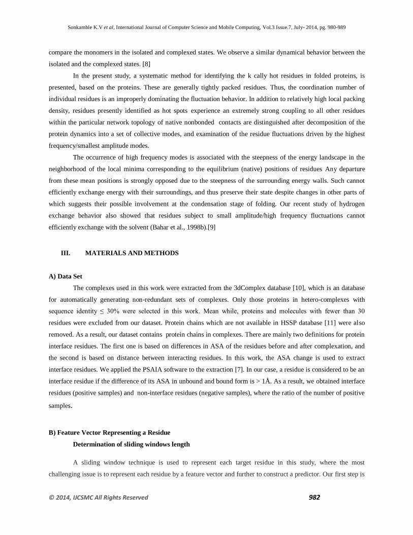
the determination of a good sliding window length since prediction performance is usually varied with window

length.[12]

A sliding window technique is used here in order to involve the association among neighboring residues. It

should be noted that the target residue centered on the sliding window plays important role compared to its

neighboring ones in the window. Within a sliding window, it is assumed that the influence of residues on the target

one fits a normal distribution. Therefore, a series of factors for residues in the window are taken into account to

explain how residues affect the probability of the target one being interface residue by using

= – , i=1L (1)

Where i is residue separation between residue xi and the target residue in sequence, pi denotes an

influencing coefficient of residue xi on the target residue, and L is the length of window. μ and s are parameters for

each residue. In this work, μ is regarded as the position of the central target residue and the value is (L + 1)/2, and

the standard deviation s2 of residue position is calculated by the following formula:

=

∑

–𝞵 (2)

Then Equation (1) can be rewritten as:

= – , i=1L (3)

C) Generation of residue profile

It is well known that hydrophobic force is often a major driver to binding affinity. Moreover, interfaces

bury a large extent of non-polar surface area and many of them have a hydrophobic core surrounded by a ring of

polar residues. The hydrophobic force plays a significant role in protein-protein interactions; however, the

hydrophobic effect alone does not represent the whole behavior of amino acids. Therefore, we integrate a

hydrophobic scale and sequence profile in the identification of protein-protein interaction residues. In this work,

Kyte-Doolittle (KD) hydropathy scale of 20 common types of amino acids is used.

Therefore, two vector types are ready for representing residue i, one is the KD hydropathy scale vector

and the other one is the corresponding sequence profile , which is a 1-by-20 vector evaluated from multiple

sequence alignment and the potential structural homologs. Multiplying the two vectors can achieve another 1 × 20

vector for residue i. However, representing each residue as a 1 × 20 vector is not always a good idea in residue

profiling schema. Here we use a standard deviation of the multiplication to measure the fluctuation of residue i in its

evolutionary context with respect to hydrophobicity. Then standard deviation value for residue i in a protein is

shown as the following form:

=(

∑

X

- (4)



where and

denote the k-th value of and

for residue i, respectively, and denotes the

mean value of vector SP × KD. Note that Equation (4) is an unbiased estimation of X

. In addition

and k represent the same amino acid type. For instance,

1 and all represent residue „ALA‟.

Furthermore, with a sliding window whose length is an odd number L, each residue i can be represented as a 1 × L

vector. The final profile vector for residue i in the protein is shown as,

= [ ………….., ………….., ] = [ X

(5)

Where vector for residue i is the multiplication of the standard deviation value by its influencing coefficient

. More details of generating the profile vectors can be referred to an example in. For each residue in protein

chains, in summary, the input of our model is an array , while the corresponding target is another state value 1 or

0 that denotes whether the residue is located at interface or non-interface region. Similar to most other machine

learning methods, our method aims to learn the mapping from the input array V onto the corresponding target array

T. Suppose that O is the output from our method, it is trained to make the output O as close as possible to the target

T.

D) Mahalanobis distance.

The Mahalanobis distance of an observation x= ( , , from a group of observations

with mean .The Mahalanobis distance of an observation X=( from a group of

observations with mean

…………… and covariance matrix S is defined as:

(x)=√ (6)

Mahalanobis distance (or "generalized squared interpoint distance" for its squared value) can also be defined as a

dissimilarity measure between two random vectors and of the same distribution with the covariance matrix S:

d( )=√ (7)

If the covariance matrix is the identity matrix[13] the Mahalanobis distance reduces to the Euclidean distance. If the

covariance matrix is diagonal, then the resulting distance measure is called

d( , )= √∑

(8)

where si is the standard deviation of the xi and yi over the sample set

E) Probability of the Class Label (PCL) of a Residue

The second measure, PCL, is related to the probability of the class label of an instance in terms of its KNN

nearest neighbors. For example, the PCL of the instance I (the green one within the circle in Fig), denoted by



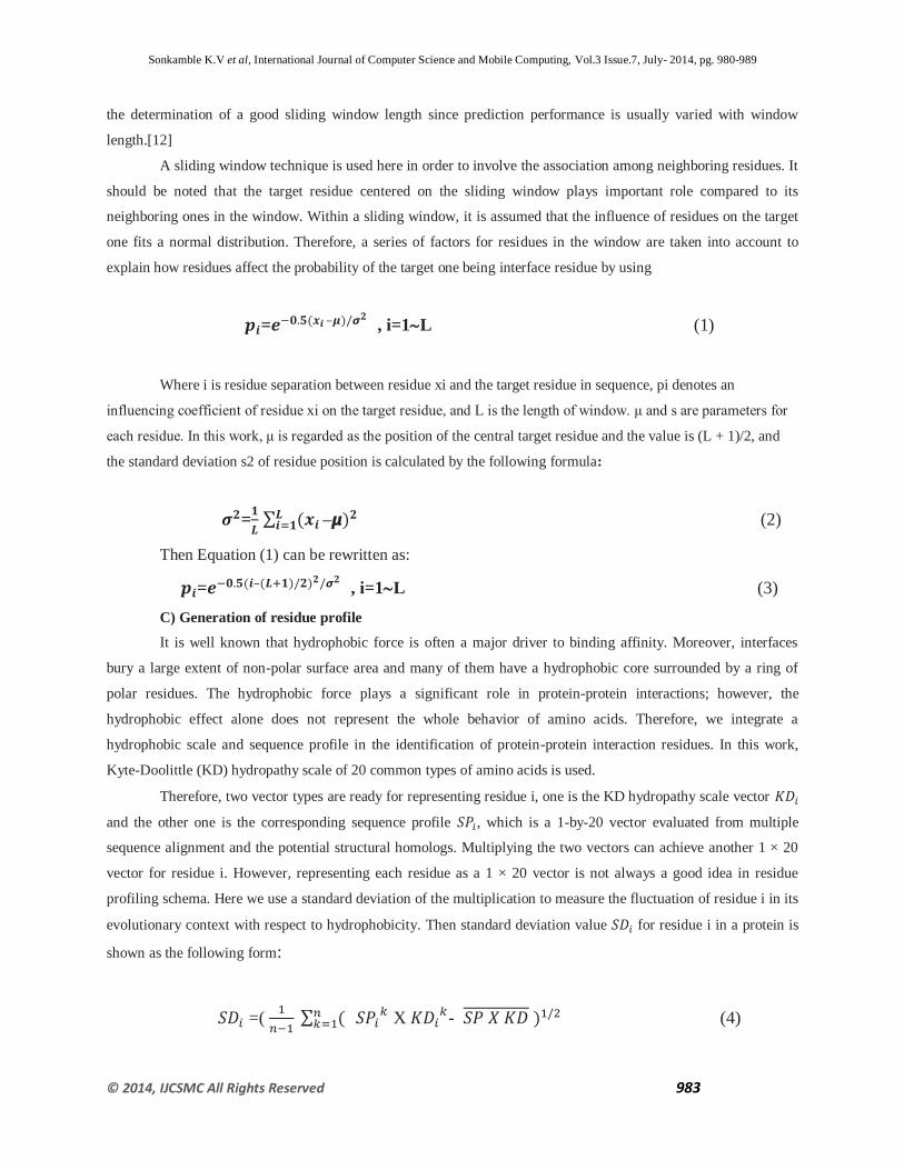
PCL(I), is defined as the ratio of the number of instances with class label 1 to the total number of instances in the

green circle in terms of its nearest neighbors, including the instance itself[1]

F) Importance of Within-Class and Between-Class (IWB)

In a concept learning problem, imbalances in the distribution of the data can occur either between the two

classes or within a single class. Yet, although both types of imbalances are known to act negatively the performance

of standard classier, methods for dealing with the class imbalance problem usually focus on rectifying the between-

class imbalance problem, neglecting to address the imbalance occurring within each class. The purpose of this paper

is to extend the simplest proposed approach for dealing with the between-class imbalance problem random re-

sampling in order to deal simultaneously with the two problems. Although re-sampling is not necessarily the best

way to deal with problems of imbalance, the results reported in this paper suggest that addressing both problems

simultaneously is beneficial and should be done by more sophisticated techniques as well. [

IWB measures the importance of within-class and between-class changes for an instance. The IWB of

instance I, denoted by IWB(I), is defined as the change in the ratio of between-class scatter to within-class

scatter before and after excluding instance I. In the two-class case, stands for the subtraction of the mean

values of the classes from each other. In contrast, denotes the summation of the two scatters calculated within the

same class. In general, a within-class scatter is equivalent to the variance in the same class computed as

=(∑ -

Where j =1 or 2, and is the residue set of class j. In particular, and enote between-class scatter and

within-class scatter after excluding the instance I, respectively

IWB (I) =

-

=

=

∑

∑

∑

∑ (9)

Where and are sample means for particular classes, and and are sample means for the two

corresponding classes excluding the instance I.

G) Class Outlier Score (COS)

The class outlier score of an instance I stands for the degree of an instance being outlier with respect to a

particular class



Where α, β,& are parameters to trade off the probability of class label, M-distance, and IWB, respectively. In this

work, α, β,& are all normalized in the range [-1, 1]. The outlier detection was performed by a grid search. An

instance I is assigned as an outlier residue if

Where c is a threshold according to experimental results From the definitions above, the larger the values

of the three measures, the more likely the instance I could be an outlier. Residues with the top scores are treated as

outliers, where the exact number of outliers depends on a specific data set.

Since each set of parameters makes different results of the protein-protein interface (PPI) prediction, we aim to

find the optimal set of parameters. The most common and reliable approach to parameter selection is to determine

parameter ranges, and then to conduct an exhaustive grid search over the parameter space to find the best setting,

which is what we have done in this work. A implicit reason is in that the performance is varied in terms of the set of

parameters

IV. SVM Classifier

Support vector machines (SVM) are supervised learning models with associated learning algorithms that analyze

data and recognize patterns, used for classification and regression analysis. Given a set of training examples, each

marked as belonging to one of two categories, an SVM training algorithm builds a model that assigns new examples

into one category or the other, making it a non-probabilistic binary linear classifier. An SVM model is a

representation of the examples as points in space, mapped so that the examples of the separate categories are divided

by a clear gap that is as wide as possible. New examples are then mapped into that same space and predicted to

belong to a category based on which side of the gap they fall on. Ensemble learning has also been applied as a

solution for training SVMs with imbalanced datasets .Generally, in these methods, the majority class dataset is

separated into multiple sub datasets such that each of these sub-datasets has a similar number of examples as the

minority class. This can be done by random sampling with or without replacement, or through clustering methods.

Then a set of SVM classifier developed so that each one is trained with the same positive dataset and a different

negative sub-dataset. Finally, the decisions made by the classifier ensemble are combined by using a method.

Performance Evaluation Measures Since the data set contains imbalanced positive samples and negative

samples, only 27.56 percent negative ones in the data set, in this work six evaluation measures are used to show the

performance of our model: sensitivity (Sen), specificity (Spec), accuracy (Acc), precision (Prec), F measure (F1),

and Matthews correlation coefficient (MCC).

Their definitions are as follows:



MCC=

√ (11)

Where True Positive (TP) is the number of interface residues; False Positive (FP) is the number of false

positives; True Negative (TN) is the number of non interface residues; and False Negative (FN) is the number false

negatives. In this work, MCC ranges from -1 to 1 and all others are represented by percentage values

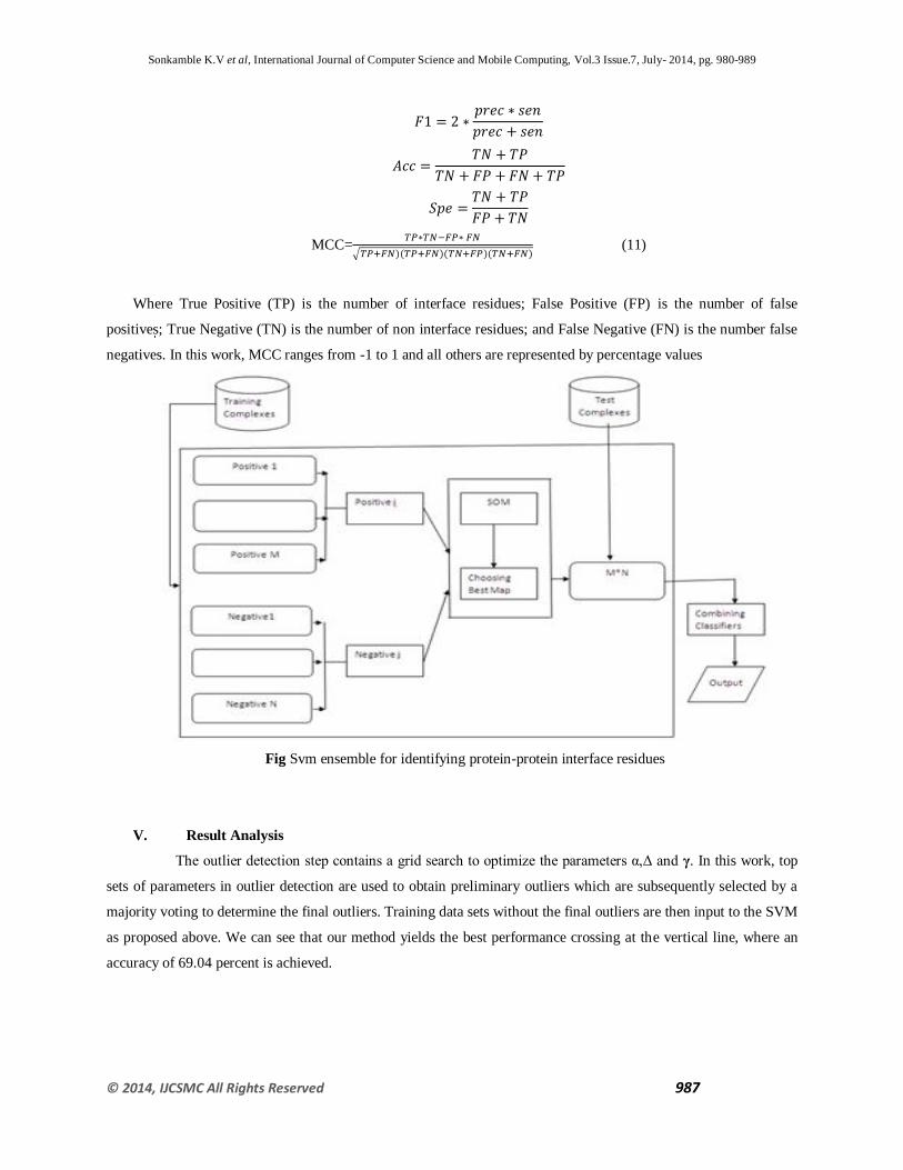
Fig Svm ensemble for identifying protein-protein interface residues

V. Result Analysis

The outlier detection step contains a grid search to optimize the parameters α,Δ and γ. In this work, top

sets of parameters in outlier detection are used to obtain preliminary outliers which are subsequently selected by a

majority voting to determine the final outliers. Training data sets without the final outliers are then input to the SVM

as proposed above. We can see that our method yields the best performance crossing at the vertical line, where an

accuracy of 69.04 percent is achieved.



VI. Conclusion

In this work, we adopted three outlier detection measures to evaluate the extent a residue becomes an

outlier. It may be results show that the three measures are effective to detect outliers in the training data and make

the identification of interface residues more accurate.

First, a residue in our work is represented as a 1-by-19 vector by using a sliding window of length 19. This

dimensionality is much smaller than most of the other methods. Therefore, our model is simple and space efficient

more importantly, earlier works reported that using larger number of features for input vectors does not always lead

to an improved performance [3]. A machine learning algorithm adopting a simple yet more discriminative

representation of a sequence space could be much more powerful and effective than using the original data

containing all details.

Second, the vector for each residue contains evolutionary context with hydrophobicity. Only two features,

namely sequence profile and hydrophobicity for residues used in this work, make our model simpler. Actually,

biological properties which may be responsible for protein protein interactions are not fully understood. Therefore

how to find feasible features or feature transformations in protein interaction prediction remains a challenging

problem. Finally, unbalanced data between interface and non-interface residues is also a very challenging issue,

which always causes a classifier over fitting. Results in this paper do indicate that developing a classifier ensemble

may be a feasible pathway to deal with this unbalance nature.

Acknowledgements

I wish to thank Dr S.N.Deshmukh (Dept of computer science and IT.Dr.B.A.M.University Aurangabad) for

suggesting this area of investigation to me and guiding me throughout this work. I am indebted for many helpful

suggestions.

References

[1] P.Chen, Limsoon Wong, and Jinyan Li Vol 9 No 4 July/ Aug 2012, Detection of outlier residues for improving

interface prediction in Protein Heterocomplexes

[2] V. Chandola, A. Banerjee, and V. Kumar, “Anomaly Detection: A Survey,” ACM Computing Surveys, vol. 41,

no. 3, pp. 1-58, 2009

[3] P. Rousseeuw and A. Leroy, Robust Regression and Outlier Detection, third ed. John Wiley and Sons. 1996

[4] S. Marsland, “On-Line Novelty Detection through Self-Organization, with Application to Inspection Robotics,”

PhD thesis, Faculty of Science and Eng., Univ. of Manchester, United Kingdom, 2001

[5] T. Fawcett and F.J. Provost, “Activity Monitoring: Noticing Interesting Changes in Behavior,” Proc. Fifth ACM

SIGKDD Int‟l Conf. Knowledge Discovery and Data Mining, pp. 53-62, 1999



[6] N. Japkowicz, C. Myers, and M.A. Gluck, “A Novelty Detection Approach to Classification,” Proc. 14th Int‟l

Conf. Artificial Intelligence (IJCAI ‟95), pp. 518-523, 1995

[7] Mihel J, Sikic M, Tomic S, Jeren B, Vlahovicek K: PSAIA-Protein Structure and Interaction Analyzer. BMC

Struct Biol 2008, 8:21

[8] M.C. Demirel, A.R. Atilgan, R.L. Jernigan, B. Erman, and I. Bahar, “Identification of Kinetically Hot Residues

in Proteins,” Protein Science, vol. 7, pp. 2522-2532, 1998.

[9] T. Haliloglu, O. Keskin, B. Ma, and R. Nussinov, “How Similar Are Protein Folding and Protein Binding

Nuclei? Examination of Vibrational Motions of Energy Hot Spots and Conserved Residues,” Biophysical J.,

vol. 88, no. 3 pp. 1552-1559, 2005.

[10] Levy ED, Pereira-Leal JB, Chothia C: Teichmann SA 3D complex: a structural classification of protein

complexes. PLoS Comput Biol 2006, 2(11):e155.

[11] C. Sander and R. Schneider, “Database of Homology Derived Protein Structures and the Structural Meaning of

Sequence Alignment,” Proteins, vol. 9, pp. 56-68, 1991.

[12] Pazos F, Valencia A: In silico two hybrid system for the selection of physically interacting protein pairs.

Proteins 2002, 47:219-227.

[13] Roberto Todeschinia,, Davide Ballabioa, Viviana Consonnia, Faizan Sahigaraa, Peter Filzmoserb locally

centred Mahalanobis distance: A new distance measure with salient features towards outlier detection.

Prediction of Interface Residues in Protein–Protein Hetero Complexes

Documents

Transcript of Prediction of Interface Residues in Protein–Protein Hetero Complexes