PREDICTION OF FATIGUE LIFE AND CRACK PATH IN GENERIC 2D STRUCTURAL COMPONENTS UNDER COMPLEX LOADING Marco Antonio Meggiolaro, Jaime Tupiassú Pinho de Castro Pontifical Catholic University of Rio de Janeiro (PUC-Rio) - Dept. Mechanical Eng. Rua Marquês de São Vicente, 225 Gávea, Rio de Janeiro, RJ 22453-900 meggi@mec.puc-rio.br, jtcastro@mec.puc-rio.br Antonio Carlos de Oliveira Miranda, Luiz Fernando Martha Pontifical Catholic University of Rio de Janeiro (PUC-Rio) - Dept. Civil Eng. Rua Marquês de São Vicente, 225 Gávea, Rio de Janeiro, RJ 22453-900 amiranda@tecgraf.puc-rio.br, lfm@civ.puc-rio.br Tulio N. Bittencourt Polytechnic School at the University of São Paulo (USP) - Dept. Structural and Foundation Eng. 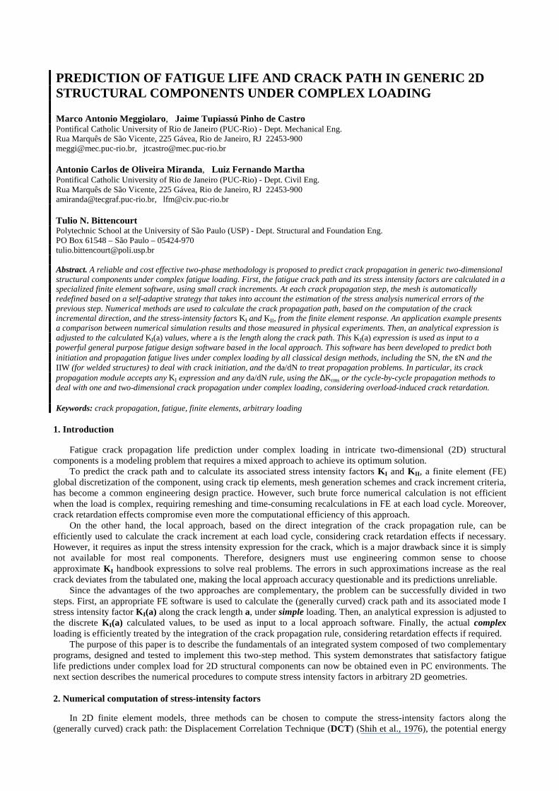PO Box 61548 – São Paulo – 05424-970 tulio.bittencourt@poli.usp.br Abstract. A reliable and cost effective two-phase methodology is proposed to predict crack propagation in generic two-dimensional structural components under complex fatigue loading. First, the fatigue crack path and its stress intensity factors are calculated in a specialized finite element software, using small crack increments. At each crack propagation step, the mesh is automatically redefined based on a self-adaptive strategy that takes into account the estimation of the stress analysis numerical errors of the previous step. Numerical methods are used to calculate the crack propagation path, based on the computation of the crack incremental direction, and the stress-intensity factors KI and KII, from the finite element response. An application example presents a comparison between numerical simulation results and those measured in physical experiments. Then, an analytical expression is adjusted to the calculated KI(a) values, where a is the length along the crack path. This KI(a) expression is used as input to a powerful general purpose fatigue design software based in the local approach. This software has been developed to predict both initiation and propagation fatigue lives under complex loading by all classical design methods, including the SN, the εN and the IIW (for welded structures) to deal with crack initiation, and the da/dN to treat propagation problems. In particular, its crack propagation module accepts any KI expression and any da/dN rule, using the ∆Krms or the cycle-by-cycle propagation methods to deal with one and two-dimensional crack propagation under complex loading, considering overload-induced crack retardation. Keywords: crack propagation, fatigue, finite elements, arbitrary loading

1. Introduction

Fatigue crack propagation life prediction under complex loading in intricate two-dimensional (2D) structural components is a modeling problem that requires a mixed approach to achieve its optimum solution.

To predict the crack path and to calculate its associated stress intensity factors KI and KII, a finite element (FE) global discretization of the component, using crack tip elements, mesh generation schemes and crack increment criteria, has become a common engineering design practice. However, such brute force numerical calculation is not efficient when the load is complex, requiring remeshing and time-consuming recalculations in FE at each load cycle. Moreover, crack retardation effects compromise even more the computational efficiency of this approach.

On the other hand, the local approach, based on the direct integration of the crack propagation rule, can be efficiently used to calculate the crack increment at each load cycle, considering crack retardation effects if necessary. However, it requires as input the stress intensity expression for the crack, which is a major drawback since it is simply not available for most real components. Therefore, designers must use engineering common sense to choose approximate KI handbook expressions to solve real problems. The errors in such approximations increase as the real crack deviates from the tabulated one, making the local approach accuracy questionable and its predictions unreliable.

Since the advantages of the two approaches are complementary, the problem can be successfully divided in two steps. First, an appropriate FE software is used to calculate the (generally curved) crack path and its associated mode I stress intensity factor KI(a) along the crack length a, under simple loading. Then, an analytical expression is adjusted to the discrete KI(a) calculated values, to be used as input to a local approach software. Finally, the actual complex loading is efficiently treated by the integration of the crack propagation rule, considering retardation effects if required.

The purpose of this paper is to describe the fundamentals of an integrated system composed of two complementary programs, designed and tested to implement this two-step method. This system demonstrates that satisfactory fatigue life predictions under complex load for 2D structural components can now be obtained even in PC environments. The next section describes the numerical procedures to compute stress intensity factors in arbitrary 2D geometries.

2. Numerical computation of stress-intensity factors

In 2D finite element models, three methods can be chosen to compute the stress-intensity factors along the

(generally curved) crack path: the Displacement Correlation Technique (DCT) (Shih et al., 1976), the potential energy

release rate computed by means of a Modified Crack-Closure (MCC) integral technique (Rybicki et al., 1977; Raju, 1987), and the J-integral computed by means of the Equivalent Domain Integral (EDI) together with a mode decomposition scheme (Nikishkov et al., 1987; Dodds et al., 1988).

2.1. Displacement Correlation Technique (DCT)

In this method, the displacements obtained from the finite element analysis at specific locations are correlated with

the analytic solutions expressed in terms of the stress-intensity factors. For quarter-point singular elements (Shih et al., 1976), the crack opening displacement δδδδ is given by:

(((( )))) (((( ))))ππππ

µµµµ++++κκκκ====−−−−====δδδδ −−−−−−−− 2

r1KLrvv4r I2j1j (1)

where vj−−−−1 and vj−−−−2 are the relative displacements in the y direction at the j−−−−1 and j−−−−2 nodes (see Fig. (1-a)), L is the element size, κκκκ = 3 − 4νννν in plane strain, κκκκ = (3 − νννν) / (1 + νννν) in plane stress, νννν is the Poisson ratio, and µµµµ is the shear modulus. From Eq. (1), the Mode I (and analogously the Mode II) stress-intensity factor can be evaluated by:

(((( ))))2j1jI vv4L2

1K −−−−−−−− −−−−ππππ

++++κκκκµµµµ==== and (((( ))))2j1jII uu4

L2

1K −−−−−−−− −−−−

ππππ

++++κκκκµµµµ==== (2)

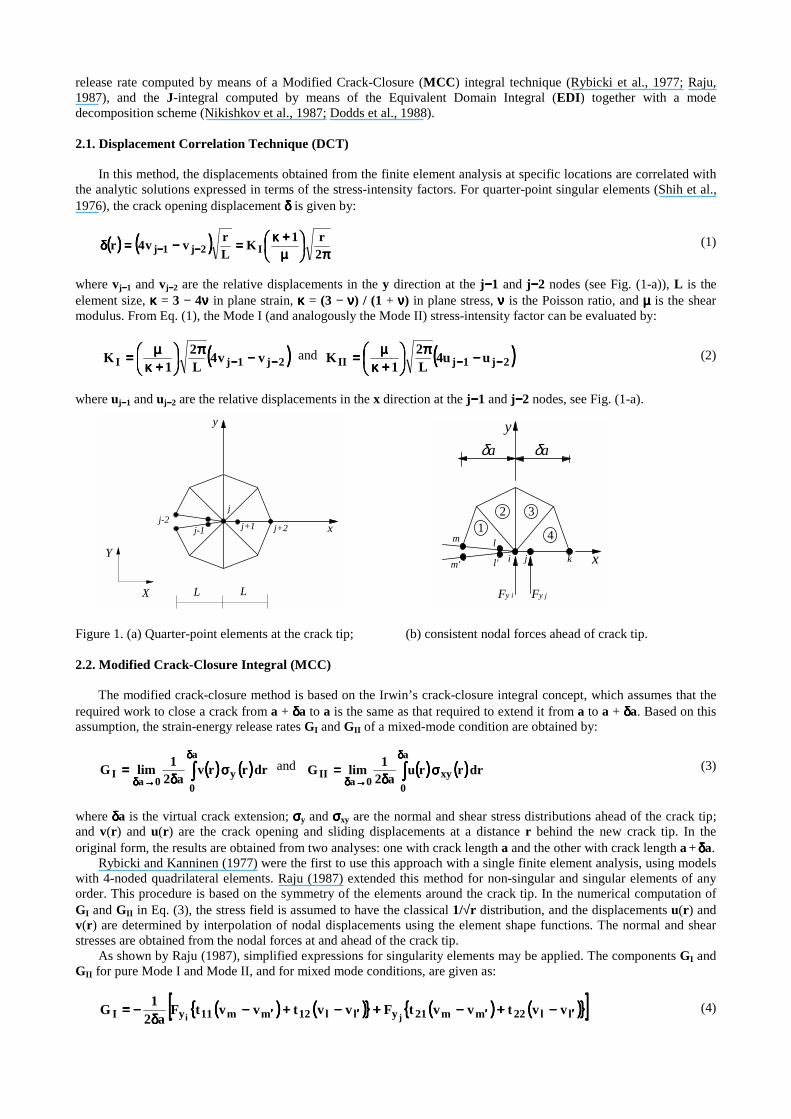
where uj−−−−1 and uj−−−−2 are the relative displacements in the x direction at the j−−−−1 and j−−−−2 nodes, see Fig. (1-a).

L L

j-2j+2

j

j+1j-1 x

y

X

Y

δaδa

m

m'

l

l' i j k x

y

Fy i Fy j

2 31 4

Figure 1. (a) Quarter-point elements at the crack tip; (b) consistent nodal forces ahead of crack tip. 2.2. Modified Crack-Closure Integral (MCC)

The modified crack-closure method is based on the Irwin’s crack-closure integral concept, which assumes that the required work to close a crack from a + δδδδa to a is the same as that required to extend it from a to a + δδδδa. Based on this assumption, the strain-energy release rates GI and GII of a mixed-mode condition are obtained by:

(((( )))) (((( ))))dr r rva2

1limG y

a

00aI σσσσ

δδδδ==== ∫∫∫∫

δδδδ

→→→→δδδδ and (((( )))) (((( ))))dr r ru

a21limG xy

a

00aII σσσσ

δδδδ==== ∫∫∫∫

δδδδ

→→→→δδδδ (3)

where δδδδa is the virtual crack extension; σσσσy and σσσσxy are the normal and shear stress distributions ahead of the crack tip; and v(r) and u(r) are the crack opening and sliding displacements at a distance r behind the new crack tip. In the original form, the results are obtained from two analyses: one with crack length a and the other with crack length a + δδδδa.

Rybicki and Kanninen (1977) were the first to use this approach with a single finite element analysis, using models with 4-noded quadrilateral elements. Raju (1987) extended this method for non-singular and singular elements of any order. This procedure is based on the symmetry of the elements around the crack tip. In the numerical computation of GI and GII in Eq. (3), the stress field is assumed to have the classical 1/√r distribution, and the displacements u(r) and v(r) are determined by interpolation of nodal displacements using the element shape functions. The normal and shear stresses are obtained from the nodal forces at and ahead of the crack tip.

As shown by Raju (1987), simplified expressions for singularity elements may be applied. The components GI and GII for pure Mode I and Mode II, and for mixed mode conditions, are given as:

(((( )))) (((( )))){{{{ }}}} (((( )))) (((( )))){{{{ }}}}[[[[ ]]]] vvtvvtFvvtvvtFa2

1G ll22mm21yll12mm11yI ji ′′′′′′′′′′′′′′′′ −−−−++++−−−−++++−−−−++++−−−−δδδδ

−−−−==== (4)

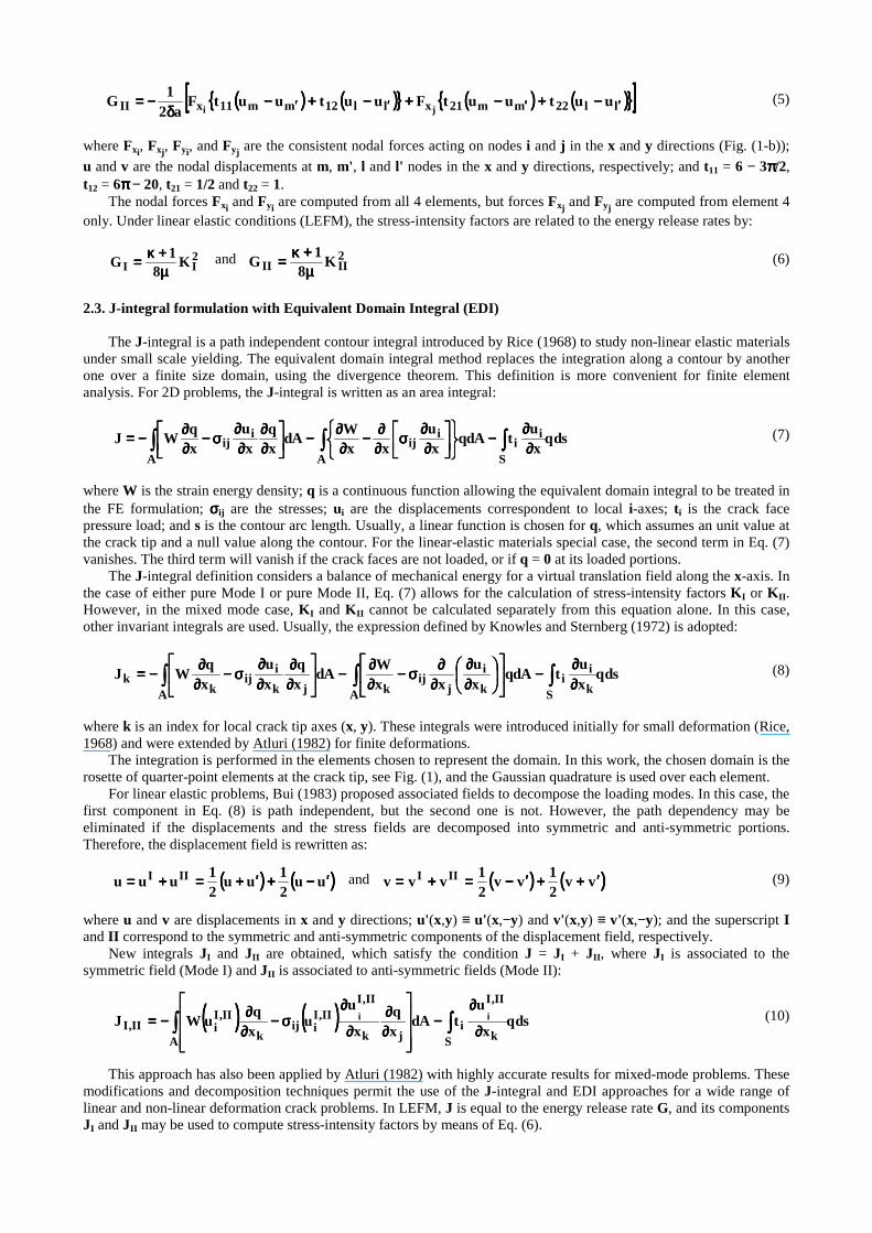
(((( )))) (((( )))){{{{ }}}} (((( )))) (((( )))){{{{ }}}}[[[[ ]]]] uutuutFuutuutFa2

1G ll22mm21xll12mm11xII ji ′′′′′′′′′′′′′′′′ −−−−++++−−−−++++−−−−++++−−−−δδδδ

−−−−==== (5)

where Fxi, Fxj, Fyi, and Fyj are the consistent nodal forces acting on nodes i and j in the x and y directions (Fig. (1-b)); u and v are the nodal displacements at m, m', l and l' nodes in the x and y directions, respectively; and t11 = 6 − 3ππππ/2, t12 = 6ππππ − 20, t21 = 1/2 and t22 = 1.

The nodal forces Fxi and Fyi are computed from all 4 elements, but forces Fxj and Fyj are computed from element 4 only. Under linear elastic conditions (LEFM), the stress-intensity factors are related to the energy release rates by:

2II K8

1G µµµµ++++κκκκ==== and 2

IIII K81G

µµµµ++++κκκκ==== (6)

2.3. J-integral formulation with Equivalent Domain Integral (EDI)

The J-integral is a path independent contour integral introduced by Rice (1968) to study non-linear elastic materials

under small scale yielding. The equivalent domain integral method replaces the integration along a contour by another one over a finite size domain, using the divergence theorem. This definition is more convenient for finite element analysis. For 2D problems, the J-integral is written as an area integral:

sdqxutAdq

xu

xxWAd

xq

xu

xqWJ

S

ii

A

iij

A

iij ∫∫∫∫∫∫∫∫∫∫∫∫ ∂∂∂∂

∂∂∂∂−−−−

∂∂∂∂∂∂∂∂σσσσ

∂∂∂∂∂∂∂∂−−−−

∂∂∂∂∂∂∂∂−−−−

∂∂∂∂∂∂∂∂

∂∂∂∂∂∂∂∂σσσσ−−−−

∂∂∂∂∂∂∂∂−−−−==== (7)

where W is the strain energy density; q is a continuous function allowing the equivalent domain integral to be treated in the FE formulation; σσσσij are the stresses; ui are the displacements correspondent to local i-axes; ti is the crack face pressure load; and s is the contour arc length. Usually, a linear function is chosen for q, which assumes an unit value at the crack tip and a null value along the contour. For the linear-elastic materials special case, the second term in Eq. (7) vanishes. The third term will vanish if the crack faces are not loaded, or if q = 0 at its loaded portions.

The J-integral definition considers a balance of mechanical energy for a virtual translation field along the x-axis. In the case of either pure Mode I or pure Mode II, Eq. (7) allows for the calculation of stress-intensity factors KI or KII. However, in the mixed mode case, KI and KII cannot be calculated separately from this equation alone. In this case, other invariant integrals are used. Usually, the expression defined by Knowles and Sternberg (1972) is adopted:

sdqxutAdq

xu

xxWAd

xq

xu

xqWJ

S ki

iA k

ij

ijkA jk

iij

kk ∫∫∫∫∫∫∫∫∫∫∫∫ ∂∂∂∂

∂∂∂∂−−−−

∂∂∂∂∂∂∂∂

∂∂∂∂∂∂∂∂σσσσ−−−−

∂∂∂∂∂∂∂∂−−−−

∂∂∂∂∂∂∂∂

∂∂∂∂∂∂∂∂σσσσ−−−−

∂∂∂∂∂∂∂∂−−−−==== (8)

where k is an index for local crack tip axes (x, y). These integrals were introduced initially for small deformation (Rice, 1968) and were extended by Atluri (1982) for finite deformations.

The integration is performed in the elements chosen to represent the domain. In this work, the chosen domain is the rosette of quarter-point elements at the crack tip, see Fig. (1), and the Gaussian quadrature is used over each element.

For linear elastic problems, Bui (1983) proposed associated fields to decompose the loading modes. In this case, the first component in Eq. (8) is path independent, but the second one is not. However, the path dependency may be eliminated if the displacements and the stress fields are decomposed into symmetric and anti-symmetric portions. Therefore, the displacement field is rewritten as:

(((( )))) (((( ))))uu21uu

21uuu III ′′′′−−−−++++′′′′++++====++++==== and (((( )))) (((( ))))vv

21vv

21vvv III ′′′′++++++++′′′′−−−−====++++==== (9)

where u and v are displacements in x and y directions; u'(x,y) ≡ u'(x,−y) and v'(x,y) ≡ v'(x,−y); and the superscript I and II correspond to the symmetric and anti-symmetric components of the displacement field, respectively.

New integrals JI and JII are obtained, which satisfy the condition J = JI + JII, where JI is associated to the symmetric field (Mode I) and JII is associated to anti-symmetric fields (Mode II):

(((( )))) (((( )))) sdqx

utAd

xq

x

uu

xquWJ

S k

II,I

iA jk

II,III,I

iijk

II,IiII,I

ii∫∫∫∫∫∫∫∫ ∂∂∂∂

∂∂∂∂−−−−

∂∂∂∂∂∂∂∂

∂∂∂∂

∂∂∂∂σσσσ−−−−

∂∂∂∂∂∂∂∂−−−−==== (10)

This approach has also been applied by Atluri (1982) with highly accurate results for mixed-mode problems. These modifications and decomposition techniques permit the use of the J-integral and EDI approaches for a wide range of linear and non-linear deformation crack problems. In LEFM, J is equal to the energy release rate G, and its components JI and JII may be used to compute stress-intensity factors by means of Eq. (6).

3. Numerical computation of the crack increment direction In 2D finite element analysis, the three most used criteria for numerical computation of crack (incremental) growth

in the linear-elastic regime are: (a) the Maximum Circumferential Stress (σσσσθθθθmax), (b) the Maximum Potential Energy Release Rate (Gθθθθmax), and (c) the Minimum Strain Energy Density (Sθθθθmin).

In the first criterion, Erdogan and Sih (1963) considered that the crack extension should occur in the direction that maximizes the circumferential stress in the region close to the crack tip. In the second, Hussain et al. (1974) have suggested that the crack extension occurs in the direction that causes the maximum fracturing energy release rate. And in the last criterion, Sih (1974) assumed that the crack growth direction is determined by the minimum strain energy density value near the crack tip. Bittencourt et al. (1996) have shown that if the crack orientation is allowed to change in automatic fracture simulation, the three criteria furnish basically the same results. Since the Maximum Circumferential Stress criterion is the simplest, even presenting a closed form solution, it is the criterion described below.

The stresses at the crack tip for Modes I and II are given by summing up the stresses obtained separately for each mode. As a result, the following equations are obtained in polar coordinates:

θθθθ−−−−θθθθ++++θθθθ++++θθθθ

ππππ====σσσσ /2)(tanK2sinK2

3]/2)(sin1[K/2)(cosr2

1IIII

2Ir (11)

θθθθ−−−−θθθθθθθθππππ

====σσσσθθθθ sinK23/2)(cosK/2)(cos

r21

II2

I (12)

(((( ))))[[[[ ]]]]1sco3KinsK/2)(cosr2

1IIIr −−−−θθθθ++++θθθθθθθθ

ππππ====ττττ θθθθ (13)

These expressions are valid both for plane stress and plane strain. The Maximum Circumferential Stress criterion

determines that crack extension begins on a plane perpendicular to the direction in which σσσσθθθθ is maximum, thus ττττrθθθθ = 0, and that monotonic (non-fatigued) extension shall occur when σσσσθθθθmax reaches a critical value corresponding to a property of the material (KIC for Mode I). From Eqs. (12-13) and using that ττττrθθθθ = 0, it is found a trivial solution θθθθ = ππππ±±±± for cos(θθθθ/2) = 0, and a non-trivial solution:

KI sinθθθθ + KII (3cosθ−θ−θ−θ−1) = 0 (14)

Analyzing Eq. (14) for the two pure modes, it is found for pure Mode I that KII = 0, KI sinθθθθ = 0 and θθθθ = 0o, and for pure Mode II that KI = 0, KII (3cosθ−θ−θ−θ−1) = 0 and θθθθ = ± 70.5o. These θθθθ values are the extreme values of the crack propagation angles. The intermediary values are found solving Eq. (14) for θθθθ considering the mixed mode, resulting in:

++++

±±±±====θθθθ 8KK

41

KK

41arctan2

2

III

III (15)

where the sign of θθθθ is the opposite of the sign of KII. 4. Finite element crack propagation simulation

The computational models described above were implemented in a software called QUEBRA2D (meaning 2D

fracture in Portuguese) (Araújo et al., 1997; Carvalho 1999), which is an interactive graphical software for simulating two-dimensional fracture processes based on a finite element adaptive mesh generation strategy (Paulino et al., 1999). The adaptive process first requires the results from the analysis of an initial finite element mesh, usually rough, with the geometric descriptions, boundary conditions, and their attributes. Then a discretization of the domain’s region boundary is performed based on the geometric properties and on the characteristic sizes of the boundary elements (adjacent to the boundary curves), determined from the error estimate resulting from the previous step of the finite element analysis.

One advantage of this strategy is that the boundary curve is discretized independently of the model’s domain, thus resulting in a more regular boundary discretization. From this discretization, the new mesh is generated (Araújo et al., 1997), based on quadtree and Delaunay triangulation techniques. The quadtree generates the mesh in the interior of the model, leaving a band near the boundary to be discretized by the Delaunay triangulation. This process is repeated until the estimate discretization error reaches a predefined value (Paulino et al., 1999).

Some other QUEBRA2D highlights are: (i) visualization of iso-strips and iso-lines from scalar results at the nodes and at the Gauss points; (ii) stress-intensity factor and crack propagation direction computation by means of all methods presented above; (iii) vectorial or scalar plotting for visualizing the principal stress results; (iv) visualization of the model's deformed configuration, with zoom, distortion, and translation specification; (v) visualization of the model’s animation along the several steps; and (vi) option of the interface language, with automatic portability to several platforms, including Unix-based workstations and PCs running under Windows 98/2000 or NT.

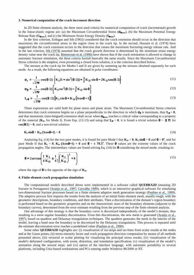
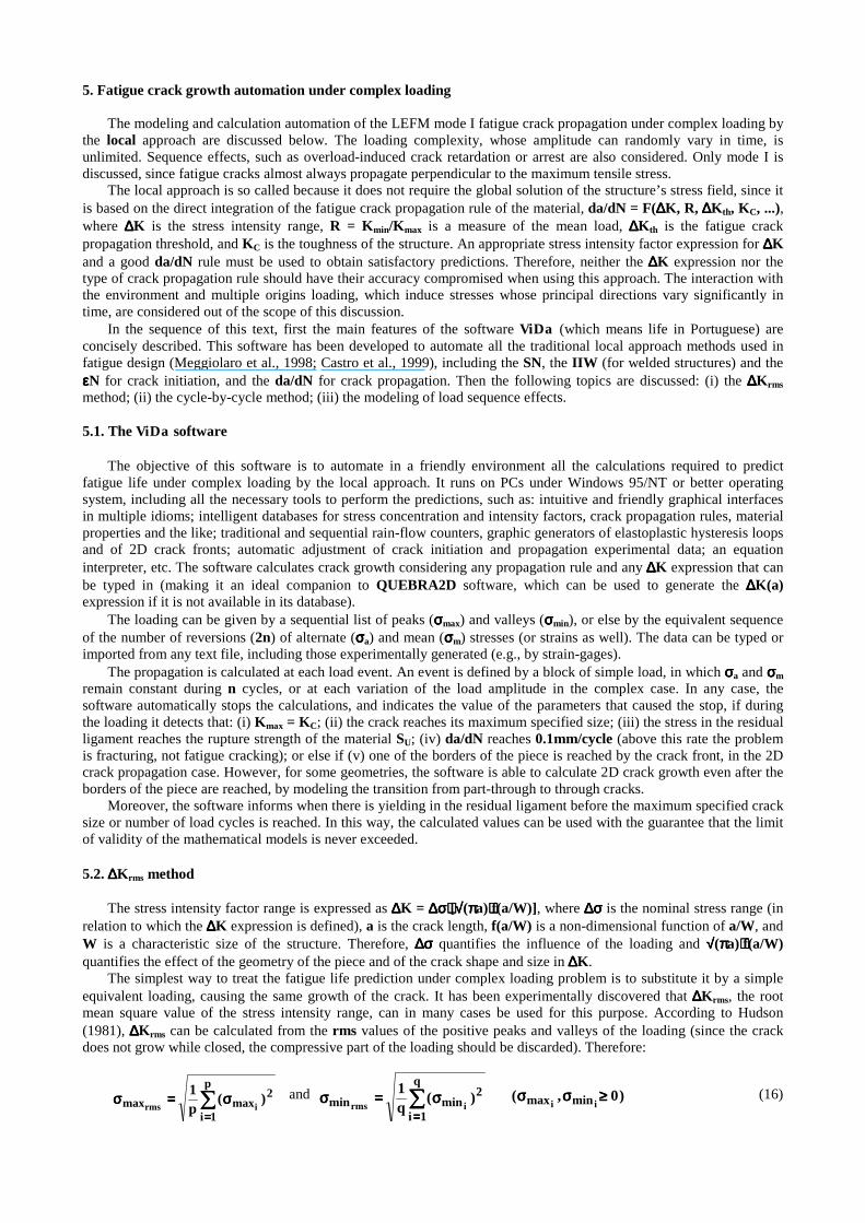
A simple test was performed to verify the crack path predicted by the QUEBRA2D software and to demonstrate its capabilities. A crack was fatigue propagated in an SEN specimen with a hole slightly to the left of the starting notch, loaded in 4-point bending, see Fig. (2). Due to the hole, the crack does not follow a straight line path, but curves toward the hole. Fig. (3) compares the FE predicted crack path with the actual one. The FE software then calculated the mode I stress intensity factor along the crack path, KI(a), see Fig. (4). This is the information that the local approach uses for calculating the fatigue life under complex loading.

Figure 2. SEN specimen with a hole to the left of the starting notch (dimensions in mm).

35 40 45 50

0

55

5

10

15

20

x in mm

y in mm

FEMEXPER.

25

Figure 3. Predicted and measured crack path in the tested SEN specimen.

1

1.1

1.2

1.3

1.4

1.5

1.6

1.7

1.8

1.9

2

0 0.1 0.2 0.3 0.4 0.5a/w

f(a/w

)

( ) arsP6

wtKwaf

2I

π−=

Figure 4. Calculated KI(a) along the crack path.

5. Fatigue crack growth automation under complex loading The modeling and calculation automation of the LEFM mode I fatigue crack propagation under complex loading by

the local approach are discussed below. The loading complexity, whose amplitude can randomly vary in time, is unlimited. Sequence effects, such as overload-induced crack retardation or arrest are also considered. Only mode I is discussed, since fatigue cracks almost always propagate perpendicular to the maximum tensile stress.

The local approach is so called because it does not require the global solution of the structure’s stress field, since it is based on the direct integration of the fatigue crack propagation rule of the material, da/dN = F(∆∆∆∆K, R, ∆∆∆∆Kth, KC, ...), where ∆∆∆∆K is the stress intensity range, R = Kmin/Kmax is a measure of the mean load, ∆∆∆∆Kth is the fatigue crack propagation threshold, and KC is the toughness of the structure. An appropriate stress intensity factor expression for ∆∆∆∆K and a good da/dN rule must be used to obtain satisfactory predictions. Therefore, neither the ∆∆∆∆K expression nor the type of crack propagation rule should have their accuracy compromised when using this approach. The interaction with the environment and multiple origins loading, which induce stresses whose principal directions vary significantly in time, are considered out of the scope of this discussion.

In the sequence of this text, first the main features of the software ViDa (which means life in Portuguese) are concisely described. This software has been developed to automate all the traditional local approach methods used in fatigue design (Meggiolaro et al., 1998; Castro et al., 1999), including the SN, the IIW (for welded structures) and the εεεεN for crack initiation, and the da/dN for crack propagation. Then the following topics are discussed: (i) the ∆∆∆∆Krms method; (ii) the cycle-by-cycle method; (iii) the modeling of load sequence effects.

5.1. The ViDa software

The objective of this software is to automate in a friendly environment all the calculations required to predict

fatigue life under complex loading by the local approach. It runs on PCs under Windows 95/NT or better operating system, including all the necessary tools to perform the predictions, such as: intuitive and friendly graphical interfaces in multiple idioms; intelligent databases for stress concentration and intensity factors, crack propagation rules, material properties and the like; traditional and sequential rain-flow counters, graphic generators of elastoplastic hysteresis loops and of 2D crack fronts; automatic adjustment of crack initiation and propagation experimental data; an equation interpreter, etc. The software calculates crack growth considering any propagation rule and any ∆∆∆∆K expression that can be typed in (making it an ideal companion to QUEBRA2D software, which can be used to generate the ∆∆∆∆K(a) expression if it is not available in its database).

The loading can be given by a sequential list of peaks (σσσσmax) and valleys (σσσσmin), or else by the equivalent sequence of the number of reversions (2n) of alternate (σσσσa) and mean (σσσσm) stresses (or strains as well). The data can be typed or imported from any text file, including those experimentally generated (e.g., by strain-gages).

The propagation is calculated at each load event. An event is defined by a block of simple load, in which σσσσa and σσσσm remain constant during n cycles, or at each variation of the load amplitude in the complex case. In any case, the software automatically stops the calculations, and indicates the value of the parameters that caused the stop, if during the loading it detects that: (i) Kmax = KC; (ii) the crack reaches its maximum specified size; (iii) the stress in the residual ligament reaches the rupture strength of the material SU; (iv) da/dN reaches 0.1mm/cycle (above this rate the problem is fracturing, not fatigue cracking); or else if (v) one of the borders of the piece is reached by the crack front, in the 2D crack propagation case. However, for some geometries, the software is able to calculate 2D crack growth even after the borders of the piece are reached, by modeling the transition from part-through to through cracks.

Moreover, the software informs when there is yielding in the residual ligament before the maximum specified crack size or number of load cycles is reached. In this way, the calculated values can be used with the guarantee that the limit of validity of the mathematical models is never exceeded.

5.2. ∆∆∆∆Krms method

The stress intensity factor range is expressed as ∆∆∆∆K = ∆∆∆∆σσσσ⋅⋅⋅⋅[√√√√(ππππa)⋅⋅⋅⋅f(a/W)], where ∆∆∆∆σσσσ is the nominal stress range (in

relation to which the ∆∆∆∆K expression is defined), a is the crack length, f(a/W) is a non-dimensional function of a/W, and W is a characteristic size of the structure. Therefore, ∆∆∆∆σσσσ quantifies the influence of the loading and √√√√(ππππa)⋅⋅⋅⋅f(a/W) quantifies the effect of the geometry of the piece and of the crack shape and size in ∆∆∆∆K.

The simplest way to treat the fatigue life prediction under complex loading problem is to substitute it by a simple equivalent loading, causing the same growth of the crack. It has been experimentally discovered that ∆∆∆∆Krms, the root mean square value of the stress intensity range, can in many cases be used for this purpose. According to Hudson (1981), ∆∆∆∆Krms can be calculated from the rms values of the positive peaks and valleys of the loading (since the crack does not grow while closed, the compressive part of the loading should be discarded). Therefore:

∑∑∑∑====

σσσσ====σσσσp

1i

2maxmax )(

p1

irms and ∑∑∑∑

====σσσσ====σσσσ

q

1i

2minmin )(q

1irms

)0,(ii minmax ≥≥≥≥σσσσσσσσ (16)

rmsrms minmaxrms σσσσ−−−−σσσσ====σσσσ∆∆∆∆ and rms

rms

max

minrmsR

σσσσσσσσ

==== (17)

As ∆∆∆∆Krms = ∆∆∆∆σσσσrms⋅⋅⋅⋅[√√√√(ππππa)⋅⋅⋅⋅f(a/W)], the number of cycles the crack takes to grow from the initial length a0 to the final

one af is given by:

∫∫∫∫ ∆∆∆∆∆∆∆∆====

f

0

a

a cthrmsrms ,...)K,K,R,K(FdaN (18)

In the ViDa software, a variation of the Simpson's algorithm can be used for the numeric integration of the simple

loading case and, consequently, also for the ∆∆∆∆Krms method. Crack increments δδδδa > 0.1µµµµm for the discretization of the integral can be specified by the user, who can also choose an integration method based on adjustable steps depending on the variation of the crack length, as it will be discussed later on the study of the cycle-by-cycle method.

It should be mentioned that the ∆∆∆∆Krms value of a complex loading is similar but not identical to the ∆∆∆∆K of a simple loading. As any statistics, ∆∆∆∆Krms does not recognize temporal order, and cannot detect important problems such as:

• Sudden fracture caused by a single big peak during the complex loading (in order to start the fracture process, it is enough that in just one event Kmax = KC).

• Any interaction among the loading cycles (e.g., the crack retardation or arrest phenomena after an overload). • It is not possible to guarantee the inactivity of the crack if ∆∆∆∆Krms(a0) < ∆∆∆∆Kth(Rrms). In complex loading, this latter problem can be caused by all the (∆∆∆∆σσσσi, Ri) events that induce ∆∆∆∆Ki > ∆∆∆∆Kth(Ri), which

can make the crack grow even if ∆∆∆∆Krms < ∆∆∆∆Kth(Rrms). Therefore, as ∆∆∆∆Ki depends both on the stress range ∆∆∆∆σσσσi and on the crack size ai in that event, even if the value of ∆∆∆∆σσσσrms stays constant, the same cannot be guaranteed for ∆∆∆∆Krms.

To conclude, it is worthwhile to remind that the ∆∆∆∆Krms method is the simplest way to treat a complex loading problem, but it should only be used, as with any model, with the due appreciation of its limitations.

5.3. Cycle-by-cycle method

The basic idea of this method is to associate to each load reversion the growth that the crack would have if that 1/2

cycle was the only one to load the piece. Using this assumption, it is easy to write a general expression for the cycle-by-cycle crack growth, by any crack propagation rule: if da/dN = F(∆∆∆∆K, R, ∆∆∆∆Kth, KC,...), and if in the i-th 1/2 cycle of the loading the length of the crack is ai, the stress range is ∆∆∆∆σσσσi and the mean load causes Ri, then the crack grows by a δδδδai given by:

...)K,K),,(R),a,(K(F21a cthmaxiiii i

∆∆∆∆σσσσσσσσ∆∆∆∆σσσσ∆∆∆∆∆∆∆∆⋅⋅⋅⋅====δδδδ (19)

The total growth of the crack is quantified by ΣΣΣΣ(δδδδai). Therefore, the cycle-by-cycle rule is similar in concept to the

linear damage accumulation used in the SN and εεεεN fatigue design methods. And, as in Miner’s rule, it requests that all the events that cause fatigue damage be recognized before the calculation, by rain-flow counting the loading.

However, this counting algorithm alters the order of the loading, as shown in Fig. (5). This can cause serious problems in the predictions, because the loading order effects in crack propagation are of two different natures:

• Delayed effects, that can retard or stop the subsequent growth of the crack due, e.g., to plasticity-induced Elber-type crack closure (Suresh, 1998) or to crack tip bifurcation. These interaction effects among the loading cycles normally increase the crack life and, if neglected, may induce excessively conservative predictions.

• Instantaneous fracture, that occurs when Kmax = KC in one event, which must be precisely predicted. As already mentioned above, the loading input in the ViDa software is sequential, and preserves the time order

information that is lost when histograms or any other loading statistics are generated. To take advantage of this feature, a sequential rain-flow counting option was introduced in that software. With this technique, the effect of each large loading event is counted when it happens (and not before its occurrence, as in the traditional rain-flow method), see Fig. (5).

The main advantage of the sequential rain-flow counting algorithm is to avoid the premature calculation of the overload effects, which can cause non-conservative crack propagation life predictions (as K(σσσσ, a) in general grows with the crack, a given overload applied when the crack is large can be much more harmful than applied when the crack is small). The sequential rain-flow does not eliminate all sequencing problems caused by the traditional method, but it is certainly an advisable option since it presents advantages over the original algorithm, without increasing its difficulty.

As discussed in the ∆∆∆∆Krms method, the compressive part of the loading can be discarded in the calculations, that is, the negative peaks and valleys can be zeroed before the computations to decrease the numerical effort of the cycle-by-cycle method. And, in the same way, a range filtering option can be very useful to discard the small loads that cause no damage inducing ∆∆∆∆Ki < ∆∆∆∆Kth(Ri), following the ideas of the race-track method (Nelson at al., 1977).

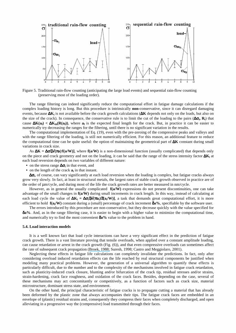
Figure 5. Traditional rain-flow counting (anticipating the large load events) and sequential rain-flow counting

(preserving most of the loading order). The range filtering can indeed significantly reduce the computational effort in fatigue damage calculations if the

complex loading history is long. But this procedure is intrinsically non-conservative, since it can disregard damaging events, because ∆∆∆∆Ki is not available before the crack growth calculations (∆∆∆∆K depends not only on the loads, but also on the size of the crack). In consequence, the conservative rule is to limit the cut of the loading to the pairs (∆∆∆∆σσσσi, Ri) that cause ∆∆∆∆K(af) < ∆∆∆∆Kth(R(af)), where af is the expected final length for the crack. But, in practice it can be easier to numerically try decreasing the ranges for the filtering, until there is no significant variation in the results.

The computational implementation of Eq. (19), even with the pre-zeroing of the compressive peaks and valleys and with the range filtering of the loading, is still not numerically efficient. For this reason, an additional feature to reduce the computational time can be quite useful: the option of maintaining the geometrical part of ∆∆∆∆K constant during small variations in crack size.

As ∆∆∆∆K = ∆∆∆∆σσσσ⋅⋅⋅⋅[√√√√(ππππa).f(a/W)], where f(a/W) is a non-dimensional function (usually complicated) that depends only on the piece and crack geometry and not on the loading, it can be said that the range of the stress intensity factor ∆∆∆∆Ki at each load reversion depends on two variables of different nature:

• on the stress range ∆∆∆∆σσσσi in that event, and • on the length of the crack ai in that instant.

∆∆∆∆σσσσi, of course, can vary significantly at each load reversion when the loading is complex, but fatigue cracks always grow very slowly. In fact, at least in structural metals, the largest rates of stable crack growth observed in practice are of the order of µm/cycle, and during most of the life the crack growth rates are better measured in nm/cycle.

However, as in general the usually complicated f(a/W) expressions do not present discontinuities, one can take advantage of the small changes in f(a/W) during small increments in crack length. In this way, instead of calculating at each load cycle the value of ∆∆∆∆Ki = ∆∆∆∆σσσσi⋅⋅⋅⋅[√√√√(ππππai)⋅⋅⋅⋅f(ai/W)], a task that demands great computational effort, it is more efficient to hold f(ai/W) constant during a (small) percentage of crack increment δδδδa%, specifiable by the software user.

The errors introduced by this procedure are non-conservative, but they decrease quickly with the value specified for δδδδa%. And, as in the range filtering case, it is easier to begin with a higher value to minimize the computational time, and numerically try to find the most convenient δδδδa% value to the problem in hand.

5.4. Load interaction models

It is a well known fact that load cycle interactions can have a very significant effect in the prediction of fatigue

crack growth. There is a vast literature proving that tensile overloads, when applied over a constant amplitude loading, can cause retardation or arrest in the crack growth (Fig. (6)), and that even compressive overloads can sometimes affect the rate of subsequent crack propagation (Broek, 1988; Suresh, 1998; Castro and Meggiolaro, 2001).

Neglecting these effects in fatigue life calculations can completely invalidate the predictions. In fact, only after considering overload induced retardation effects can the life reached by real structural components be justified when modeling many practical problems. However, the generation of a universal algorithm to quantify these effects is particularly difficult, due to the number and to the complexity of the mechanisms involved in fatigue crack retardation, such as plasticity-induced crack closure, blunting and/or bifurcation of the crack tip, residual stresses and/or strains, strain-hardening, crack face roughness, and oxidation of the crack faces. Besides, depending on the case, several of these mechanisms may act concomitantly or competitively, as a function of factors such as crack size, material microstructure, dominant stress state, and environment.

On the other hand, the principal characteristic of fatigue cracks is to propagate cutting a material that has already been deformed by the plastic zone that always accompanies their tips. The fatigue crack faces are embedded in an envelope of (plastic) residual strains and, consequently they compress their faces when completely discharged, and open alleviating in a progressive way the (compressive) load transmitted through their faces.

Figure 6. Fatigue crack growth retardation induced by tensile overloads.

According to Elber (1971), only after completely opening the crack at a load Kop, would the crack tip be stressed.

Therefore, the bigger the Kop, the less would be the effective stress intensity range ∆∆∆∆Keff = Kmax − Kop, and this ∆∆∆∆Keff instead of ∆∆∆∆K would be the crack propagation rate controlling parameter. Most load interaction models are, although indirectly, based in this idea. This implicates in the supposition that the principal retardation mechanism is caused by plasticity induced crack closure: in these cases, the opening load should increase when the crack penetrates into the plastic zone inflated by the overload, reducing the ∆∆∆∆Keff and stopping or delaying the crack, while the plastic zones associated with the loading are contained in the overload induced plastic zone.

Several mathematical models have been developed to account for load interaction in crack propagation based on Elber’s crack closure idea. In these methods, the retardation mechanism is only considered within the plastic zone situated in front of the crack tip. According to these procedures, a larger plastic zone Zol is created by means of an overload, see Fig. (7). When the overload is removed, an increased compressive stress state is set up in the volume of its plastic zone, reducing crack propagation under a smaller succeeding load cycle.

Figure 7. Yield zone crack growth retardation region used by the Wheeler and Willenborg load interaction models.

The detailed discussion of this complex phenomenology is considered beyond the scope of this work, but a revision of the phenomenological problem can be found in (Suresh, 1998). A taxonomy of the load interaction models has been introduced by Meggiolaro and Castro (2001), including proposed modifications to better model such effects as crack arrest, crack acceleration due to compressive underloads, and the effect of small cracks. Meggiolaro and Castro (2001) classified these models in 4 categories: (i) da/dN models, such as the Wheeler model, which use retardation functions to directly reduce the calculated crack propagation rate da/dN; (ii) ∆∆∆∆K models, such as the Modified Wheeler model, which use retardation functions to reduce the value of the stress intensity factor range ∆∆∆∆K; (iii) Reff models, such as the Willenborg model, which introduce an effective stress ratio Reff, calculated by reducing the maximum and minimum stress intensity factors acting on the crack tip, however not necessarily changing the value of ∆∆∆∆K; and (iv) Kop models, such as the strip yield model, which use estimates of the opening stress intensity factor Kop to directly account for Elber-type crack closure.

There are several other retardation models (Suresh, 1998), but none of those that can be implemented in a local approach code has definitive advantages over the models discussed in (Meggiolaro and Castro, 2001). This is no surprise, since single equations are too simplistic to model all the several mechanisms that can induce retardation effects. Therefore, in the same way that a curve da/dN vs. ∆∆∆∆K is experimentally measured, a propagation model should be adjusted to experimental data to calibrate the retardation models, as recommended by Broek (1988).

The numerical implementation of these retardation models in a cycle-by-cycle algorithm is not conceptually difficult, but it requires a considerable programming effort. All load interaction models presented in (Meggiolaro and Castro, 2001) have been implemented in the ViDa software.

6. Conclusions In this paper, a two-phase methodology was presented to predict fatigue crack propagation in generic 2D structures

under complex loading. First, self-adaptive finite elements were used to calculate, by three different methods, the fatigue crack path and the stress intensity factors along the crack length KI(a) and KII(a), at each propagation step. The calculated KI(a) was then used to predict the propagation fatigue life of the structure by the local approach, using the root mean square or the cycle-by-cycle integration methods, even considering overload-induced crack retardation effects in this latter one. Two complementary software were developed to implement this methodology. The first software is an interactive graphical program for simulating two-dimensional fracture processes based on a finite element adaptive mesh generation strategy. The second is a general purpose fatigue design software developed to predict both initiation and propagation fatigue lives under complex loading by all classical design methods. In particular, its crack propagation module accepts any stress intensity factor expression, including the ones generated by the finite element software. Experimental results showed that the presented methodology and its software implementation could effectively predict the crack propagation path and fatigue life of an arbitrary two-dimensional structural component.

7. References

Araújo, T.D.P., Cavalcante, J.B., Carvalho, M.T.M., Bittencourt, T.N., Martha, L.F., 1997, “Adaptive Simulation of

Fracture Processes Based on Spatial Enumeration Techniques,” Int. J. Rock Mech. Mining Sciences, Vol.34, p. 551. Atluri, S.N., 1982, “Path-Independent Integrals in Finite Elasticity and Inelasticity, with Body Forces, Inertia, and

Arbitrary Crack-Face Conditions,” Engineering Fracture Mechanics, Vol.16, pp. 341-364. Bittencourt, T.N., Wawrzynek, P.A., Ingraffea, A.R., Sousa, J.L.A., 1996, “Quasi-Automatic Simulation of Crack

Propagation for 2D LEFM Problems,” Engineering Fracture Mechanics, Vol.55, pp. 321-334. Broek, D., 1988, The Practical Use of Fracture Mechanics," Kluwer. Carvalho, C.V.A., Araújo, T.D.P., Cavalcante Neto, J.B., Martha, L.F., and Bittencourt, T.N., 1999, “Automatic Fatigue

Crack Propagation using a Self-adaptive Strategy,” PACAM VI - Sixth Pan-American Congress of Applied Mechanics, Rio de Janeiro, Vol.6, pp. 377-380.

Castro, J.T.P., Meggiolaro, M.A., 1999, “Some Comments on the εN Method Automation for Fatigue Dimensioning under Complex Loading,” (in Portuguese), Revista Brasileira de Ciências Mecânicas, Vol.21, pp.294-312.

Castro, J.T.P., Meggiolaro, M.A., 2001, "Fatigue Design under Complex Loading" (in Portuguese), PUC-Rio. Dodds, R.H. Jr., Vargas, P.M., 1988, “Numerical Evaluation of Domain and Contour Integrals for Nonlinear Fracture

Mechanics,” Report, Dept. of Civil Engineering, U. of Illinois, Urbana-Champaign. Elber, W., 1971, “The Significance of Fatigue Crack Closure,” ASTM STP 486. Erdogan, F., Sih, G.C., 1963, “On the Crack Extension in Plates under Plane Loading and Transverse Shear,” Journal of

Basic Engineering, Vol.85, pp. 519-527. Hudson, C.M., 1981, “A Root-Mean-Square Approach for Predicting Fatigue Crack Growth under Random Loading,”

ASTM STP 748, pp. 41-52. Hussain, M.A., Pu, S.U., Underwood, J., 1974, “Strain Energy Release Rate for a Crack under Combined Mode I and

II,” ASTM STP 560, pp. 2-28. Knowles, J.K., Sternberg, E., 1972, “On a Class of Conservation Laws in Linearized and Finite Elastostatics,” Archives

for Rational Mechanics & Analysis, Vol.44, pp. 187-211. Meggiolaro, M.A., Castro, J.T.P., 1998, “ViDa 98 - a Visual Damagemeter to Automatize the Fatigue Design under

Complex Loading,” (in Portuguese), Revista Brasileira de Ciências Mecânicas, Vol.20, pp. 666-685. Meggiolaro, M.A., Castro, J.T.P., 2001, “Comparison of Load Interaction Models in Fatigue Crack Propagation,” XVI

Congresso Brasileiro de Eng. Mecânica (COBEM), ABCM, Uberlândia, MG. Nelson, D.V., Fuchs, H.O., 1977, “Predictions of Cumulative Fatigue Damage Using Condensed Load Histories,” in

Fatigue Under Complex Loading, SAE. Nikishkov, G.P., Atluri,S.N., 1987, “Calculation of Fracture Mechanics Parameters for an Arbitrary Three-Dimensional

Crack by the Equivalent Domain Integral Method,” Int. J. for Numerical Methods in Eng., Vol.24, pp.1801-1821. Paulino, G.H., Menezes,I.F.M., Cavalcante Neto,J.B., Martha,L.F., 1999, “A Methodology for Adaptive Finite Element

Analysis: Towards an Integrated Computational Environment,” Computational Mechanics, Vol.23, pp. 361-388. Raju, I.S., 1987, “Calculation of Strain-Energy Release Rates with Higher Order and Singular Finite Elements,”

Engineering Fracture Mechanics, Vol.28, pp. 251-274. Rice, J.R., 1968, “A Path Independent Integral and the Approximate Analysis of Strain Concentration by Notches and

Cracks,” Journal of Applied Mechanics, Vol.35, pp. 379-386. Rybicki, E.F., Kanninen, M.F., 1977, “A Finite Element Calculation of Stress-Intensity Factors by a Modified Crack

Closure Integral,” Engineering Fracture Mechanics, Vol.9, pp. 931-938. Shih, C.F., de Lorenzi, H.G., German, M.D., 1976, “Crack Extension Modeling with Singular Quadratic Isoparametric

Elements,” International Journal of Fracture, Vol.12, pp. 647-651. Sih, G.C., 1974, “Strain-Energy-Density Factor Applied to Mixed Mode Crack Problems,” International Journal of

Fracture Mechanics, Vol.10, pp. 305-321. Suresh, S., 1998, "Fatigue of Materials," Cambridge.