Predicting transport by Lagrangian coherent structures with a high-order method
21
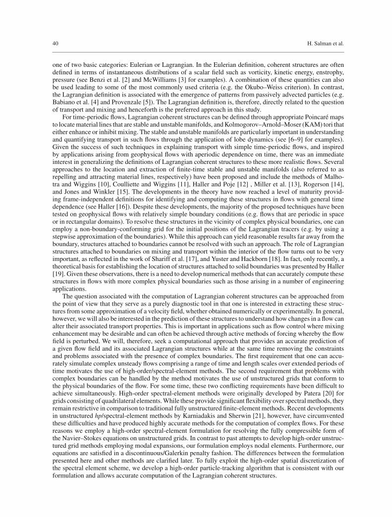
Theor. Comput. Fluid Dyn. (2007) 21: 39–58 DOI 10.1007/s00162-006-0031-0 ORIGINAL ARTICLE Hayder Salman · Jan S. Hesthaven · Tim Warburton George Haller Predicting transport by Lagrangian coherent structures with a high-order method Received: 22 February 2005 / Accepted: 23 May 2006 / Published online: 8 September 2006 © Springer-Verlag 2006 Abstract Recent developments in identifying Lagrangian coherent structures from finite-time velocity data have provided a theoretical basis for understanding chaotic transport in general flows with aperiodic depen- dence on time. As these theoretical developments are extended and applied to more complex flows, an accurate and general numerical method for computing these structures is needed to exploit these ideas for engineering applications. We present an unstructured high-order hp/spectral-element method for solving the two-dimen- sional compressible form of the Navier–Stokes equations. A corresponding high-order particle tracking method is also developed for extracting the Lagrangian coherent structures from the numerically computed velocity fields. Two different techniques are used; the first computes the direct Lyapunov exponent from an unstruc- tured initial particle distribution, providing easier resolution of structures located close to physical boundaries, whereas the second advects a small material line initialized close to a Lagrangian saddle point to delineate these structures. We demonstrate our algorithm on simulations of a bluff-body flow at a Reynolds number of Re = 150 and a Mach number of M = 0.2 with and without flow forcing. We show that, in the unforced flow, periodic vortex shedding is predicted by our numerical simulations that is in stark contrast to the aperiodic flow field in the case with forcing. An analysis of the Lagrangian structures reveals a transport barrier that inhibits cross-wake transport in the unforced flow. The transport barrier is broken with forcing, producing enhanced transport properties by chaotic advection and consequently improved mixing of advected scalars within the wake. 1 Introduction It has become well established that coherent structures, which arise in many engineering and geophysical flows, play an important role in characterizing transport and mixing of passively advected quantities [1]. Despite the abundant evidence of their presence, a unique definition of a coherent structure does not exist and identifying them has been for some time a subjective topic. In general, we can separate the contrasting definitions into Communicated by M. Y. Hussaini H. Salman (B ) · J. S. Hesthaven Division of Applied Mathematics, Brown University, Providence, RI 02912, USA Present address: H. Salman, Department of Mathematics, CB #3250, Phillips Hall, UNC-Chapel Hill, Chapel Hill, NC 27599, USA E-mail: [email protected] T. Warburton Department of Computational and Applied Mathematics, Rice University, Houston, TX 77005, USA H. Salman · G. Haller Department of Mechanical Engineering, MIT, Cambridge, MA 02139, USA
-
Upload
eastanglia -
Category
Documents
-
view
2 -
download
0
Transcript of Predicting transport by Lagrangian coherent structures with a high-order method
Theor. Comput. Fluid Dyn. (2007) 21: 39–58DOI 10.1007/s00162-006-0031-0
ORIGINAL ARTICLE
Hayder Salman · Jan S. Hesthaven · Tim WarburtonGeorge Haller
Predicting transport by Lagrangian coherent structureswith a high-order method
Received: 22 February 2005 / Accepted: 23 May 2006 / Published online: 8 September 2006© Springer-Verlag 2006
Abstract Recent developments in identifying Lagrangian coherent structures from finite-time velocity datahave provided a theoretical basis for understanding chaotic transport in general flows with aperiodic depen-dence on time. As these theoretical developments are extended and applied to more complex flows, an accurateand general numerical method for computing these structures is needed to exploit these ideas for engineeringapplications. We present an unstructured high-order hp/spectral-element method for solving the two-dimen-sional compressible form of the Navier–Stokes equations. A corresponding high-order particle tracking methodis also developed for extracting the Lagrangian coherent structures from the numerically computed velocityfields. Two different techniques are used; the first computes the direct Lyapunov exponent from an unstruc-tured initial particle distribution, providing easier resolution of structures located close to physical boundaries,whereas the second advects a small material line initialized close to a Lagrangian saddle point to delineatethese structures. We demonstrate our algorithm on simulations of a bluff-body flow at a Reynolds number ofRe = 150 and a Mach number of M = 0.2 with and without flow forcing. We show that, in the unforced flow,periodic vortex shedding is predicted by our numerical simulations that is in stark contrast to the aperiodic flowfield in the case with forcing. An analysis of the Lagrangian structures reveals a transport barrier that inhibitscross-wake transport in the unforced flow. The transport barrier is broken with forcing, producing enhancedtransport properties by chaotic advection and consequently improved mixing of advected scalars within thewake.
1 Introduction
It has become well established that coherent structures, which arise in many engineering and geophysical flows,play an important role in characterizing transport and mixing of passively advected quantities [1]. Despite theabundant evidence of their presence, a unique definition of a coherent structure does not exist and identifyingthem has been for some time a subjective topic. In general, we can separate the contrasting definitions into
Communicated by M. Y. Hussaini
H. Salman (B) · J. S. HesthavenDivision of Applied Mathematics, Brown University, Providence, RI 02912, USA
Present address: H. Salman, Department of Mathematics, CB #3250, Phillips Hall, UNC-Chapel Hill,Chapel Hill, NC 27599, USAE-mail: [email protected]
T. WarburtonDepartment of Computational and Applied Mathematics, Rice University, Houston, TX 77005, USA
H. Salman · G. HallerDepartment of Mechanical Engineering, MIT, Cambridge, MA 02139, USA
40 H. Salman et al.
one of two basic categories: Eulerian or Lagrangian. In the Eulerian definition, coherent structures are oftendefined in terms of instantaneous distributions of a scalar field such as vorticity, kinetic energy, enstrophy,pressure (see Benzi et al. [2] and McWilliams [3] for examples). A combination of these quantities can alsobe used leading to some of the most commonly used criteria (e.g. the Okubo–Weiss criterion). In contrast,the Lagrangian definition is associated with the emergence of patterns from passively advected particles (e.g.Babiano et al. [4] and Provenzale [5]). The Lagrangian definition is, therefore, directly related to the questionof transport and mixing and henceforth is the preferred approach in this study.
For time-periodic flows, Lagrangian coherent structures can be defined through appropriate Poincaré mapsto locate material lines that are stable and unstable manifolds, and Kolmogorov–Arnold–Moser (KAM) tori thateither enhance or inhibit mixing. The stable and unstable manifolds are particularly important in understandingand quantifying transport in such flows through the application of lobe dynamics (see [6–9] for examples).Given the success of such techniques in explaining transport with simple time-periodic flows, and inspiredby applications arising from geophysical flows with aperiodic dependence on time, there was an immediateinterest in generalizing the definitions of Lagrangian coherent structures to these more realistic flows. Severalapproaches to the location and extraction of finite-time stable and unstable manifolds (also referred to asrepelling and attracting material lines, respectively) have been proposed and include the methods of Malho-tra and Wiggins [10], Coulliette and Wiggins [11], Haller and Poje [12] , Miller et al. [13], Rogerson [14],and Jones and Winkler [15]. The developments in the theory have now reached a level of maturity provid-ing frame-independent definitions for identifying and computing these structures in flows with general timedependence (see Haller [16]). Despite these developments, the majority of the proposed techniques have beentested on geophysical flows with relatively simple boundary conditions (e.g. flows that are periodic in spaceor in rectangular domains). To resolve these structures in the vicinity of complex physical boundaries, one canemploy a non-boundary-conforming grid for the initial positions of the Lagrangian tracers (e.g. by using astepwise approximation of the boundaries). While this approach can yield reasonable results far away from theboundary, structures attached to boundaries cannot be resolved with such an approach. The role of Lagrangianstructures attached to boundaries on mixing and transport within the interior of the flow turns out to be veryimportant, as reflected in the work of Shariff et al. [17], and Yuster and Hackborn [18]. In fact, only recently, atheoretical basis for establishing the location of structures attached to solid boundaries was presented by Haller[19]. Given these observations, there is a need to develop numerical methods that can accurately compute thesestructures in flows with more complex physical boundaries such as those arising in a number of engineeringapplications.
The question associated with the computation of Lagrangian coherent structures can be approached fromthe point of view that they serve as a purely diagnostic tool in that one is interested in extracting these struc-tures from some approximation of a velocity field, whether obtained numerically or experimentally. In general,however, we will also be interested in the prediction of these structures to understand how changes in a flow canalter their associated transport properties. This is important in applications such as flow control where mixingenhancement may be desirable and can often be achieved through active methods of forcing whereby the flowfield is perturbed. We will, therefore, seek a computational approach that provides an accurate prediction ofa given flow field and its associated Lagrangian structures while at the same time removing the constraintsand problems associated with the presence of complex boundaries. The first requirement that one can accu-rately simulate complex unsteady flows comprising a range of time and length scales over extended periods oftime motivates the use of high-order/spectral-element methods. The second requirement that problems withcomplex boundaries can be handled by the method motivates the use of unstructured grids that conform tothe physical boundaries of the flow. For some time, these two conflicting requirements have been difficult toachieve simultaneously. High-order spectral-element methods were originally developed by Patera [20] forgrids consisting of quadrilateral elements. While these provide significant flexibility over spectral methods, theyremain restrictive in comparison to traditional fully unstructured finite-element methods. Recent developmentsin unstructured hp/spectral-element methods by Karniadakis and Sherwin [21], however, have circumventedthese difficulties and have produced highly accurate methods for the computation of complex flows. For thesereasons we employ a high-order spectral-element formulation for resolving the fully compressible form ofthe Navier–Stokes equations on unstructured grids. In contrast to past attempts to develop high-order unstruc-tured grid methods employing modal expansions, our formulation employs nodal elements. Furthermore, ourequations are satisfied in a discontinuous/Galerkin penalty fashion. The differences between the formulationpresented here and other methods are clarified later. To fully exploit the high-order spatial discretization ofthe spectral element scheme, we develop a high-order particle-tracking algorithm that is consistent with ourformulation and allows accurate computation of the Lagrangian coherent structures.
Predicting transport by Lagrangian coherent structures with a high-order method 41
We begin by describing the high-order unstructured hp/spectral-element numerical scheme that we employin our study. The high-order particle-tracking method developed for extracting the Lagrangian structures isalso described. Results are then presented for three different flows. The first is a simulation of the temporalinstability in a compressible plane Poiseuille flow that occurs above a critical Reynolds number. This flowserves as a test case to verify the high-order spectral-element method used in this work. The second is a baselinesimulation of the flow around a bluff body without forcing that is used to demonstrate the method and to verifythe Lagrangian coherent structures are in agreement with previous results of Shariff et al. [17], and Duan andWiggins [22]. The third simulation is carried out under the same flow conditions but with forcing providedby four wall-mounted actuators. This form of forcing was motivated by the recent work of Wang et al. [23]who used a point vortex reduced-order model to demonstrate how this form of forcing can excite Lagrangiancoherent structures within the flow. Using our more refined spectral element simulations, we present a moredetailed study of the transport mechanisms associated with these Lagrangian structures. A striking feature ofthe result is the breaking of a transport barrier within the wake cavity providing a means for the upper andlower streams to mix together more effectively in comparison to the unforced flow. We end with a summaryof the key results and conclusions.
2 Governing equations
We are interested in resolving the compressible form of the Navier–Stokes equations in two spatial dimensions.After writing these equations in conservation form, we have
∂
∂t
∫
�
qdA +∮
∂�
F(q,∇q) · nds = 0, (1)
where q = (ρ, ρu, ρv, ρE)� is the conservative state vector, q = (p, u, v, T )� is the primitive state vector,and n is an outward unit normal vector to the surface ∂�. The flux tensor F(q,∇q) = FI(q)− FV(q,∇q) isgiven by
FI =
ρu ρv
ρu2 + p ρuvρuv ρv2 + pρu H ρvH
, FV =
0 0τxx τxyτyx τyy
τxx u + τxyv − Qx τyx u + τyyv − Qy
. (2)
In the above expressions, ρ(x, t) denotes the density of the fluid, p(x, t) is the static pressure, u(x, t) =(u(x, t), v(x, t)) is the local velocity vector, E(x, t) is the total energy per unit volume, and H(x, t) is thespecific total enthalpy of the fluid. Assuming air as the working fluid, the perfect gas law relation is given by
p = ρRT = (γ − 1)ρ
[E − 1
2(u2 + v2)
], (3)
where T (x, t) is the static temperature, R is the gas constant, and γ is the ratio of specific enthalpies. For aNewtonian fluid such as air, the viscous stress tensor can be expressed in terms of the local velocity gradientsby
τ = µ(∇u + (∇u)T
) − 2µ
3I (∇ · u) . (4)
For air, the dependence of the molecular viscosity µ on temperature is described by Sutherland’s law whichcan be written as
µ = 1.461 × 10⁻⁶T 3/2
T + 110.3. (5)
The heat flux vector Q = (Qx , Qy) is assumed to obey Fourier’s law such that
Q = −κ∇T, (6)
where κ is the thermal conductivity. It is common to relate κ to µ through the Prandtl number
Pr = µC p
κ, (7)
which we take as 0.72. In (7), C p is the specific heat for air at constant pressure.
42 H. Salman et al.
3 Numerical scheme
3.1 Basic discretization
Our computational domain� is now represented by the union of the non-overlapping triangular elements Dk .To formulate our scheme, we approximate the state vector in each element by
q(x, t) ≈ qN (x, t) =N∑
i=1
qi (t)ψi (x) : ∀x ∈ Dk (8)
where N denotes the number of unknowns in each element. We assume a similar polynomial representa-tion of the flux FN . We denote the minimal polynomial space for approximating these quantities by PN (i.e.PN = span{xα1 yα2}|α|≤n = span{ψi }N
i=1 with α = (α1, α2) being a multi-index). The number of unknownsin each element is, therefore, given by
dim PN = N = (n + 1)(n + 2)
2. (9)
We construct equations for these N unknowns in each element Dk by requiring our solution to satisfy thediscontinuous Galerkin formulation
∫
Dk
(∂qN
∂t+ ∇ · FN
)ψi (x)dx =
∮
∂Dk
ψi (x)n · [FN − F∗]dx. (10)
The numerical flux F∗ is used to pass information between adjacent elements and to impose the boundary con-ditions. We note that our formulation imposes the boundary/interface conditions weakly through the surfaceintegral and leads to an inherently discontinuous scheme. To proceed, we introduce the local operators
Mi j =∫
Dk
ψ jψi dx, Si j =∫
Dk
∇ψ jψi dx, (11)
Fi j =∮
∂Dk
ψiψ j dx, (12)
thus transforming (10) into
Mdqdt
+ S · F = Fn ·[F(q−,∇q−)− F∗(q+,∇q+,q−,∇q−)
](13)
In this form, q represents the 4N vector of coefficients for qN , and similarly for F and F∗. The superscript ‘−’refers to values local to the element whereas the superscript ‘+’ refers to values from the neighboring element.
To complete the formulation, we must define the numerical flux F∗. To ensure consistency of the numericalscheme, a consistent flux must be selected with the desired properties for numerical stability. In this work, wehave chosen to model the inviscid contribution using a Lax–Friedrichs flux to produce
n ·[FI − FI,∗] = 1
2n ·
[FI,− − FI,+]
+ 1
2||(q+ − q−), (14)
where || is the largest eigenvalue of the linearized system of equations. In this work we have computed ||by evaluating |(u2 + v2)1/2 + cair| locally for every point in each element Dk , where cair is the local speedof sound, and then taking the global maximum. This results in a slightly higher numerical dissipation than aRiemann solver in which the eigenvalue is computed using |u · n + cair| but produces a more stable numericalscheme. Given the high-order discretization we employ in this work, this particular choice of the numerical
Predicting transport by Lagrangian coherent structures with a high-order method 43
flux has little impact on the accuracy of the results to be presented later. The discretization of the viscous fluxesis based on the work of Bassi and Rebay [24] so that
n ·[FV − FV,∗] = 1
2n ·
[FV,−(q−,∇q− + r−
e )− FV,+(q+,∇q+ + r+e )
], (15)
r−e = ∂lk,e
2Akn · [
q+ − q−], (16)
r+e = ∂lk,e
2Akn · [
q− − q+]. (17)
∂lk,e corresponds to the length of edge e in element k, and Ak is the area of the element. To compute the spatialderivatives ∇q appearing in the viscous fluxes, we directly differentiate the basis functions used in (8).
When imposing the boundary conditions, the numerical flux FI,∗ is modified to obtain the desired state atthe boundary. For no-slip boundaries, we set the local velocity vector to zero and impose a constant wall tem-perature equal to the free-stream value at the inlet. At inflow and outflow, we impose characteristic boundaryconditions for FI,∗ by linearizing the equations around the computed flow state. At the same time, we set thecontribution from the viscous flux to zero. Although this introduces some errors, the effect on the computationswill be extremely small given that the inflow and outflow boundaries are located far away from the regionsof interest. The exact procedure of how this is accomplished can be found in Hesthaven [25]. In addition,a notoriously common problem is the reflection of waves that occurs near the outflow boundary. While thecharacteristic boundary conditions tend to minimize these effects, reflected waves continue to occur. In ourhigh-order numerical simulations, these reflected waves take longer to dissipate as a result of the lower dissi-pative properties of the scheme. To prevent our numerical solution further upstream from being contaminatedby these reflecting waves, a sponge layer is introduced near the outflow boundary that essentially absorbs thesewaves. The sponge layer introduces spurious results in the region in which it is employed and we will thereforenot present any results in this part of the flow.
3.2 The nodal element
In discretizing our flow equations, we have introduced a set of unspecified basis functionsψi (x). In this secondpart of our numerical scheme, we present a set of basis functions ψi (x) that allow us to construct well-con-ditioned operators. With the basis functions appropriately chosen, we can define the expansion coefficientsq as required. In this work, we will define q such that qN is an interpolating polynomial. Our coefficients,therefore, directly correspond to the state vector evaluated at a set of predefined nodes producing the nodalelement method which forms the distinguishable aspect of our scheme from other hp/spectral-element methods(e.g. Karniadakis and Sherwin [21]).
We will begin by defining a smooth mapping from any given triangular element Dk in our domain to astandard triangular element I . We define this standard element in (ξ, η) space by
I = {(ξ, η) ∈ R2|(ξ, η) ≥ −1; ξ + η ≤ 1}. (18)
In this work, we will only consider straight-sided triangles, for which the transformation Jacobian (J ) willbe constant. This provides a significant simplification for the construction of all operators since we need toconstruct them for only the standard element I and then subsequent operators for all other physical elementsDk can be computed through simple linear rescaling. This assumption can affect the accuracy near curvedboundaries. However, since we are interested in regions of the flow that are remote from such curved surfaces,this assumption will have very little impact on our results. We now seek a basis ψi (ξ, η) for our standardelement to allow us to construct well-conditioned operators. Such a basis can be obtained from Proriol [26],and Koornwinder [27] and is given by
ψi = P(0,0)α1(r)
(1 − s
2
)α1
P(2α1+1,0)α2
(s),
γi =(
2
2α1 + 1
)(2
α1 + α2 + 1
), (19)
ψi (ξ) = ψ(ξ)√γi, (20)
44 H. Salman et al.
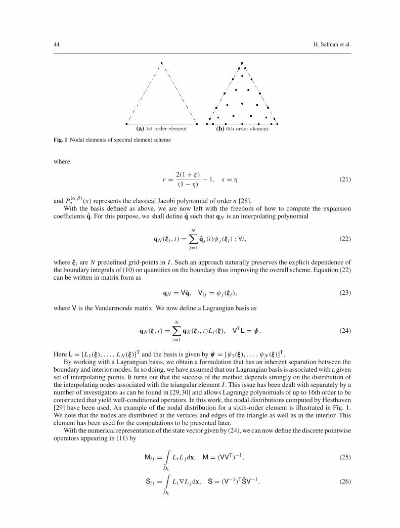
(a) 1st order element (b) 6th order element
Fig. 1 Nodal elements of spectral element scheme
where
r = 2(1 + ξ)
(1 − η)− 1, s = η (21)
and P(α,β)n (x) represents the classical Jacobi polynomial of order n [28].With the basis defined as above, we are now left with the freedom of how to compute the expansion
coefficients q. For this purpose, we shall define q such that qN is an interpolating polynomial
qN (ξ i , t) =N∑
j=1
q j (t)ψ j (ξ i ) : ∀i, (22)
where ξ i are N predefined grid-points in I . Such an approach naturally preserves the explicit dependence ofthe boundary integrals of (10) on quantities on the boundary thus improving the overall scheme. Equation (22)can be written in matrix form as
qN = Vq, Vi j = ψ j (ξ i ), (23)
where V is the Vandermonde matrix. We now define a Lagrangian basis as
qN (ξ , t) =N∑
i=1
qN (ξ i , t)Li (ξ), VTL = ψ . (24)
Here L = [L1(ξ), . . . , L N (ξ)]T and the basis is given by ψ = [ψ1(ξ), . . . , ψN (ξ)]T.By working with a Lagrangian basis, we obtain a formulation that has an inherent separation between the
boundary and interior modes. In so doing, we have assumed that our Lagrangian basis is associated with a givenset of interpolating points. It turns out that the success of the method depends strongly on the distribution ofthe interpolating nodes associated with the triangular element I . This issue has been dealt with separately by anumber of investigators as can be found in [29,30] and allows Lagrange polynomials of up to 16th order to beconstructed that yield well-conditioned operators. In this work, the nodal distributions computed by Hesthaven[29] have been used. An example of the nodal distribution for a sixth-order element is illustrated in Fig. 1.We note that the nodes are distributed at the vertices and edges of the triangle as well as in the interior. Thiselement has been used for the computations to be presented later.
With the numerical representation of the state vector given by (24), we can now define the discrete pointwiseoperators appearing in (11) by
Mi j =∫
Dk
Li L j dx, M = (VVT)−1, (25)
Si j =∫
Dk
Li∇L j dx, S = (V−1)TSV−1. (26)
Predicting transport by Lagrangian coherent structures with a high-order method 45
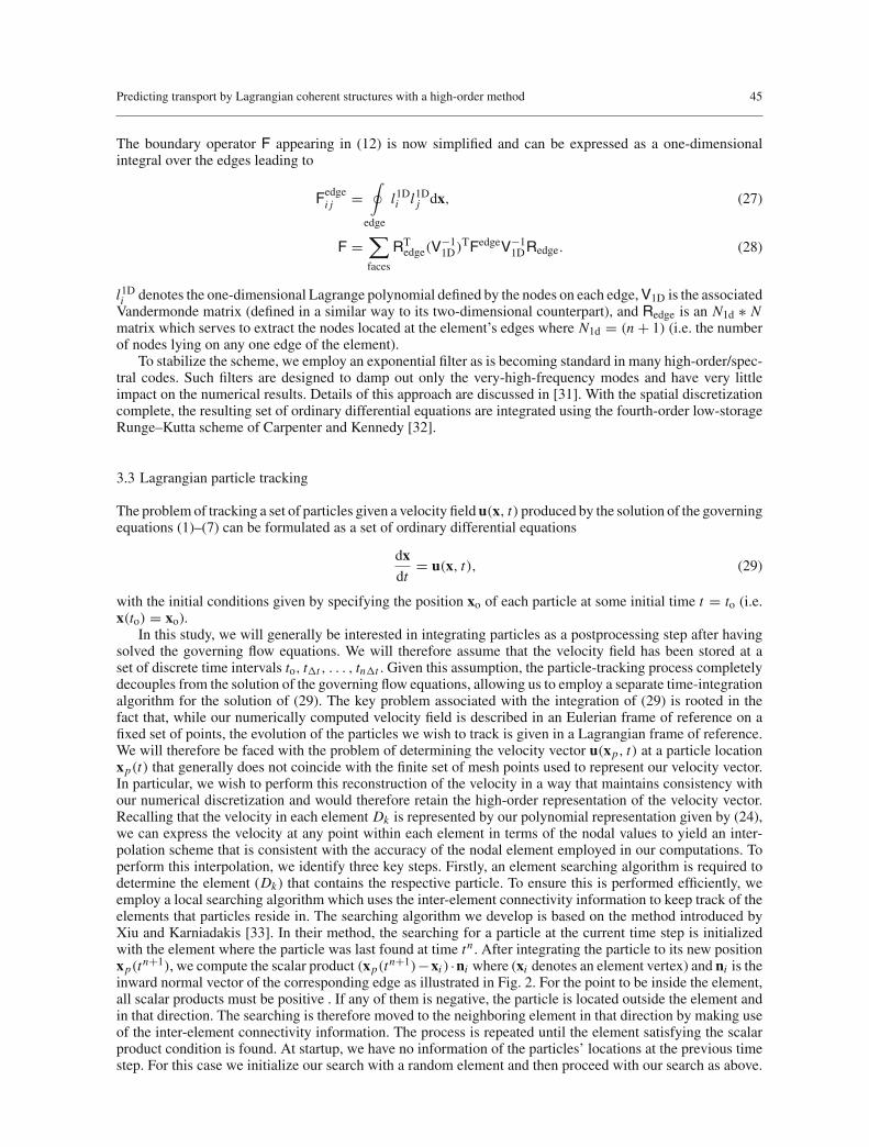
The boundary operator F appearing in (12) is now simplified and can be expressed as a one-dimensionalintegral over the edges leading to
Fedgei j =
∮
edge
l1Di l1D
j dx, (27)
F =∑faces
RTedge(V
−11D)
TFedgeV−11DRedge. (28)
l1Di denotes the one-dimensional Lagrange polynomial defined by the nodes on each edge, V1D is the associated
Vandermonde matrix (defined in a similar way to its two-dimensional counterpart), and Redge is an N1d ∗ Nmatrix which serves to extract the nodes located at the element’s edges where N1d = (n + 1) (i.e. the numberof nodes lying on any one edge of the element).
To stabilize the scheme, we employ an exponential filter as is becoming standard in many high-order/spec-tral codes. Such filters are designed to damp out only the very-high-frequency modes and have very littleimpact on the numerical results. Details of this approach are discussed in [31]. With the spatial discretizationcomplete, the resulting set of ordinary differential equations are integrated using the fourth-order low-storageRunge–Kutta scheme of Carpenter and Kennedy [32].
3.3 Lagrangian particle tracking
The problem of tracking a set of particles given a velocity field u(x, t) produced by the solution of the governingequations (1)–(7) can be formulated as a set of ordinary differential equations
dxdt
= u(x, t), (29)
with the initial conditions given by specifying the position xo of each particle at some initial time t = to (i.e.x(to) = xo).
In this study, we will generally be interested in integrating particles as a postprocessing step after havingsolved the governing flow equations. We will therefore assume that the velocity field has been stored at aset of discrete time intervals to, t t , . . . , tn t . Given this assumption, the particle-tracking process completelydecouples from the solution of the governing flow equations, allowing us to employ a separate time-integrationalgorithm for the solution of (29). The key problem associated with the integration of (29) is rooted in thefact that, while our numerically computed velocity field is described in an Eulerian frame of reference on afixed set of points, the evolution of the particles we wish to track is given in a Lagrangian frame of reference.We will therefore be faced with the problem of determining the velocity vector u(xp, t) at a particle locationxp(t) that generally does not coincide with the finite set of mesh points used to represent our velocity vector.In particular, we wish to perform this reconstruction of the velocity in a way that maintains consistency withour numerical discretization and would therefore retain the high-order representation of the velocity vector.Recalling that the velocity in each element Dk is represented by our polynomial representation given by (24),we can express the velocity at any point within each element in terms of the nodal values to yield an inter-polation scheme that is consistent with the accuracy of the nodal element employed in our computations. Toperform this interpolation, we identify three key steps. Firstly, an element searching algorithm is required todetermine the element (Dk) that contains the respective particle. To ensure this is performed efficiently, weemploy a local searching algorithm which uses the inter-element connectivity information to keep track of theelements that particles reside in. The searching algorithm we develop is based on the method introduced byXiu and Karniadakis [33]. In their method, the searching for a particle at the current time step is initializedwith the element where the particle was last found at time tn . After integrating the particle to its new positionxp(tn+1), we compute the scalar product (xp(tn+1)−xi ) ·ni where (xi denotes an element vertex) and ni is theinward normal vector of the corresponding edge as illustrated in Fig. 2. For the point to be inside the element,all scalar products must be positive . If any of them is negative, the particle is located outside the element andin that direction. The searching is therefore moved to the neighboring element in that direction by making useof the inter-element connectivity information. The process is repeated until the element satisfying the scalarproduct condition is found. At startup, we have no information of the particles’ locations at the previous timestep. For this case we initialize our search with a random element and then proceed with our search as above.

46 H. Salman et al.
x1 x2
x3
n1
n2n3
Fig. 2 Definition of normals used in the element-searching routine
In a worst-case scenario, we might have to search all the elements but this would be performed only once atstartup. The algorithm is, therefore, efficient and allows us to search for a large number of particles. After wehave identified all the elements containing the particles to be advected, our second step involves the mappingof the particles’ positions from physical space (x, y) to the parametric space (ξ, η) of the parent element. Asnoted by Coppola et al. [34], while the mapping from parametric to physical space is generally analytic, thecorresponding inverse for nonlinear elements with curved edges is typically nonanalytic. In this study, however,we will only use straight-sided elements, thus alleviating the problems associated with the computation of theinverse mapping. For a particle located at xpi , we denote the corresponding position in parametric space byξ pi
. The third and final step requires the interpolation of the velocity to the mapped particle position ξ pi. Given
that we have the state vector at the nodal points denoted by qN (ξ i , t), the state vector at ξ pican be written as
q(ξ pi) =
N∑j=1
V−1qN (ξ j , t)ψ j (ξ pi) (30)
where we have used (23) to express the coefficients of the orthonormal basis in terms of our solution. Withthe velocity u(ξ p, t) known, we can now integrate (29) using a standard fourth-order Runge–Kutta scheme.In the results to be presented later, we have employed a time step of t = 0.005 corresponding to the intervalsize at which our data is stored. To obtain the state vector field at intermediate times, we perform a third-orderLagrangian interpolation in time. In general, one has the freedom to choose the order in which to performthe temporal–spatial interpolation of the flow field. Given that the spatial interpolation is generally far moreexpensive, we perform the temporal interpolation initially, followed by the spatial interpolation.
4 Results
4.1 Plane Poiseuille flow
Before we present results for Lagrangian coherent structures in a bluff-body flow, we will first verify ourhigh-order spectral-element method. To do this, we have chosen to test the numerical scheme on the planePoiseuille flow. The hydrodynamic instability of the incompressible plane Poiseuille flow is a much-studiedand well-documented problem (see Drazin and Reid [35], and Drazin [36] for further details). These studieshave shown that the flow is stable to all small disturbances below a critical Reynolds number Rec of 5,779based on the center-line velocity and half the channel height. Above this critical value of Rec, the flow becomeslinearly unstable due to an unstable eigenmode that can be computed from the Orr–Sommerfeld equation [35].The linear stability analysis can be used to determine both the onset of instability as well as its growth rate.We will, therefore, use analytical results of the linearized stability analysis to verify that we can correctlycompute the growth and decay of a perturbation superimposed on a background mean flow. However, giventhat we are interested in verifying our compressible Navier–Stokes numerical scheme, we will use results forthe linearized form of the compressible Navier–Stokes equations. The corresponding linearized equations canbe found in [37] and have already been used by other investigators to study the stability of several compressibleflows (e.g. Hanifi et al. [38]).
Predicting transport by Lagrangian coherent structures with a high-order method 47
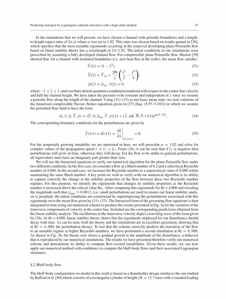
In the simulations that we will present, we have chosen a channel with periodic boundaries and a length-to-height aspect ratio of 2π/α where α was set to 1.02. This ratio was chosen based on results quoted in [36],which specifies that the most unstable eigenmode occurring in the temporal developing plane Poiseuille flowbased on linear stability theory has a wavelength of 2π/1.02. The initial conditions in our simulations wereprescribed by assuming a fully developed channel flow. For compressible plane Poiseuille flow, Maslen [39]showed that, for a channel with insulated boundaries (i.e. zero heat flux at the walls), the mean flow satisfies
U (y) = (1 − y2), (31)
T (y) = T ∞ + 2Pr
γ
(y2
2− y4
4
), (32)
p(y) = p∞, v(y) = 0, (33)
where −1 ≤ y ≤ 1, and overlines denote quantities nondimensionalized with respect to the center-line velocityand half the channel height. We have taken the pressure to be constant and independent of x since we assumea periodic flow along the length of the channel. Using (31)–(33) as our basic mean state, we seek solutions ofthe linearized compressible Navier–Stokes equations given in [37] (Eqs. (5.97–5.102)) in which we assumethe perturbed flow field to have the form
(u, v, p, T , ρ) = (U , 0, p∞, T , ρ)(y)+ ( f , αφ,�, θ, r)(y)eiα(x−ct). (34)
The corresponding boundary conditions for the perturbations are given by
f (±1) = φ(±1) = ∂θ
∂ y
∣∣∣∣∣(y=±1)
= 0. (35)
For the temporally growing instability we are interested in here, we will prescribe α = 1.02 and solve forcomplex values of the propagation speed c = cr + ici . From (34), it can be seen that if ci is negative thenperturbations will grow in time, otherwise they will decay. For the flow to be stable to general perturbations,all eigenvalues must have an imaginary part greater than zero.
We will use the linearized equations to verify our numerical algorithm for the plane Poiseuille flow undertwo different conditions. In the first case, we consider a flow at a Mach number of 0.2 and a subcritical Reynoldsnumber of 4,000. In the second case, we increase the Reynolds number to a supercritical value of 8,000 whilstmaintaining the same Mach number. A key point we wish to verify with our numerical algorithm is its abilityto capture correctly the change in the stability properties of the flow between these two Reynolds numberregimes. For this purpose, we identify the eigenmode that changes its stability properties as the Reynoldsnumber is increased above the critical value Rec. After computing this eigenmode for Re = 4,000 and rescalingthe magnitude such that v′
max ≈ 0.0012, (i.e. small perturbations are used to ensure our linear stability analy-sis is justified), the initial conditions are constructed by superimposing the perturbations associated with thiseigenmode on to the mean flow given by (31)–(33). The linearized form of the governing flow equations is thenintegrated in time using our numerical scheme to produce the results presented in Fig. 3a for the variation of thetransverse components of velocity at the center line. Included are the corresponding predictions obtained fromthe linear stability analysis. The oscillations in the transverse velocity depict a traveling wave of the form givenby (34). At Re = 4,000, linear stability theory shows that the eigenmode employed for our disturbance shoulddecay with time. As can be seen, both the theory and the simulations are in excellent agreement, showing thatat Re = 4, 000, the perturbation decays. To test that the scheme correctly predicts the transition of the flowto an unstable regime at higher Reynolds numbers, we have performed a second simulation at Re = 8, 000.As shown in Fig. 3b, the theory now shows a gradual growth in the amplitude of the disturbance, a behaviorthat is reproduced by our numerical simulations. The results we have presented therefore verify our numericalscheme and demonstrate its ability to compute flow-excited instabilities. Given these results, we can nowapply our numerical method with confidence to compute the bluff-body flows and their associated Lagrangianstructures.
4.2 Bluff-body flow
The bluff-body configuration we model in this work is based on a flameholder design similar to the one studiedby Raffoul et al. [40] which consists of a rectangular cylinder of height (H = 12.7 mm) with a rounded leading

48 H. Salman et al.
time
v’m
ax
0 20 40 60 80-0.0015
-0.001
-0.0005
0
0.0005
0.001
0.0015
0.002NumericalLinear stability analysis
(a) Reynolds number = 4000.
time
v’m
ax
0 20 40 60 80-0.0015
-0.001
-0.0005
0
0.0005
0.001
0.0015
0.002NumericalLinear stability analysis
(b) Reynolds number = 8000.
Fig. 3 Time trace of transverse velocity in plane Poiseuille flow
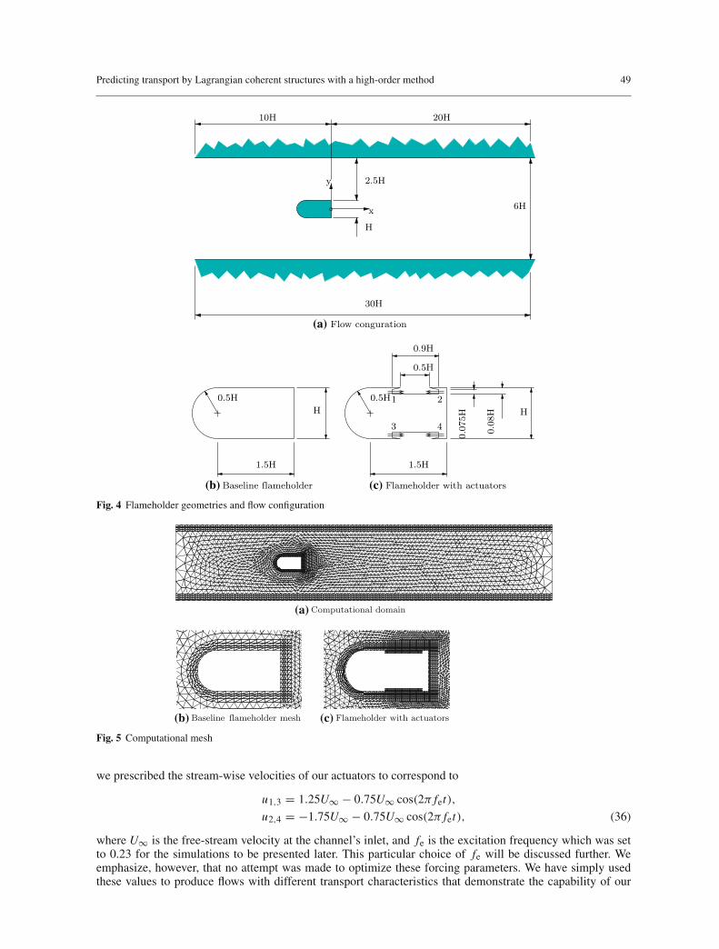
edge. The bluff body is positioned symmetrically within a channel of height (h) and length (L) as shown inFig. 4. To model the flow with forcing, we employ active actuation by means of blowing on the surface of thebluff body. This form of forcing is similar to the approaches employed in the work of Min and Choi [41], Parket al. [42], and Gunzburger and Lee [43]. Alternative forms of forcing have been discussed by Karniadakisand Triantafyllou [44] who used a vibrating wire located in the vicinity of the cylinder (modeled as a potentialflow), by He et al. [45] and Homescu et al. [46] who used cylinder rotations, and by Blackburn and Henderson[47] who used transverse motion of the cylinder. Our motivation for using flow forcing by blowing on thesurface of the bluff body was to extend the recent work of Wang et al. [23] using a reduced-order point vortexmodel to a numerical simulation of the Navier–Stokes equations. The blowing is provided by four actuators,two of which are located on the upper surface and two on the lower surface of the bluff body. To model theseactuators, a recess is introduced on the upper and lower surfaces. The recess is extended in both directionsforming channels that restrict the local flow in the tangential direction as illustrated in Fig. 4c.
The flow domain which we denote by � consists of the region bounded by the bluff-body geometry, theupper and the lower walls of the channel, and the inlet and outlet flow boundaries used in our simulations.This flow region was discretized into a finite number of non-overlapping body conforming triangular elementsDI as shown in Fig. 5. These computational grids were generated using the commercial software GAMBIT.In our computations, we have modeled all physical boundaries as no-slip walls. To allow efficient resolutionof the boundary layers around these surfaces, we have generated stretched anisotropic triangular elements asillustrated in Fig. 5a. A magnified portion of the grid generated for the flameholder with the actuators in placeis shown in Fig. 5b and illustrates the mesh used in the vicinity of the wall jets. The total number of elementsgenerated for the case without forcing was 5,534 elements and for the case with forcing was 10,509 elements.We point out that the area ratio of the largest to smallest computational element that arises with the forced flow(Amax/Amin = 1.2 × 10³) makes this case a particularly challenging problem.
The flow conditions that we used for our simulations correspond to a Reynolds number of Re = 150 basedon the bluff-body height and a Mach number of M = 0.2. Both quantities are evaluated with respect to flowconditions at inlet where we have assumed a parabolic inlet velocity profile. For the simulation with forcing,
Predicting transport by Lagrangian coherent structures with a high-order method 49
x
y
10H 20H
30H
2.5H
H
6H
(a) Flow conguration
0.5H
1.5H
H
(b) Baseline flameholder
1 2
3 4
0.5H
1.5H
H
0.07
5H
0.08
H
0.5H
0.9H
(c) Flameholder with actuators
Fig. 4 Flameholder geometries and flow configuration
(a) Computational domain
(b) Baseline flameholder mesh (c) Flameholder with actuators
Fig. 5 Computational mesh
we prescribed the stream-wise velocities of our actuators to correspond to
u1,3 = 1.25U∞ − 0.75U∞ cos(2π fet),
u2,4 = −1.75U∞ − 0.75U∞ cos(2π fet), (36)
where U∞ is the free-stream velocity at the channel’s inlet, and fe is the excitation frequency which was setto 0.23 for the simulations to be presented later. This particular choice of fe will be discussed further. Weemphasize, however, that no attempt was made to optimize these forcing parameters. We have simply usedthese values to produce flows with different transport characteristics that demonstrate the capability of our
50 H. Salman et al.
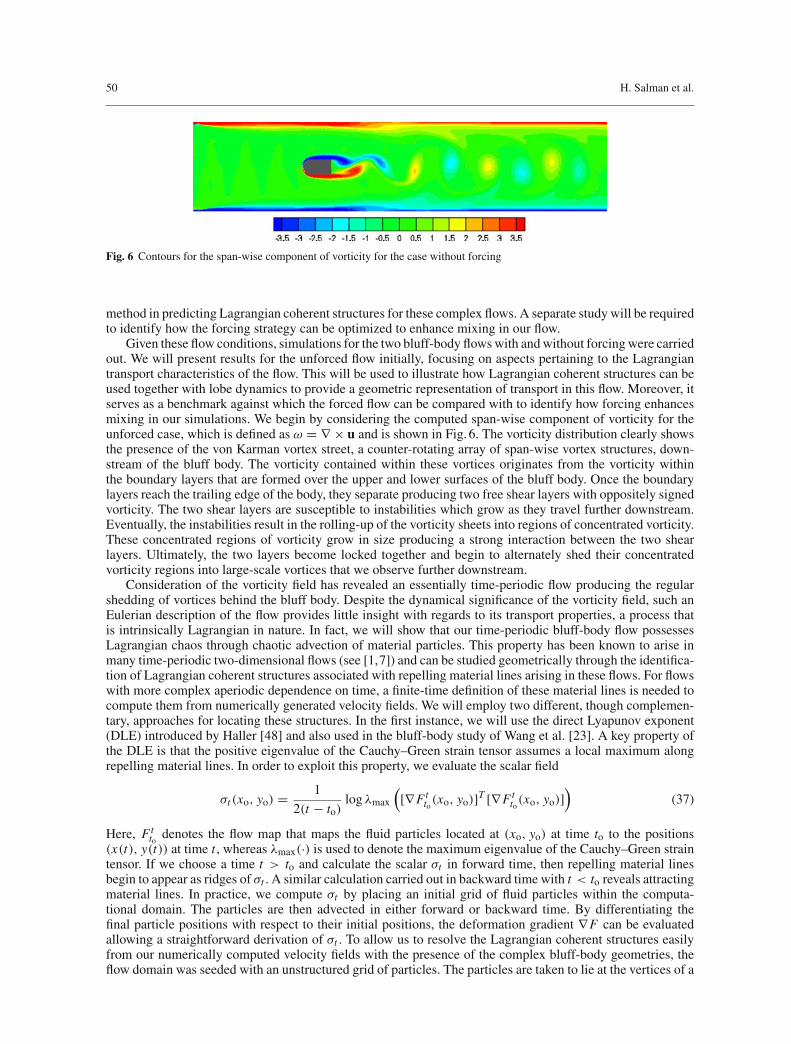
Fig. 6 Contours for the span-wise component of vorticity for the case without forcing
method in predicting Lagrangian coherent structures for these complex flows. A separate study will be requiredto identify how the forcing strategy can be optimized to enhance mixing in our flow.
Given these flow conditions, simulations for the two bluff-body flows with and without forcing were carriedout. We will present results for the unforced flow initially, focusing on aspects pertaining to the Lagrangiantransport characteristics of the flow. This will be used to illustrate how Lagrangian coherent structures can beused together with lobe dynamics to provide a geometric representation of transport in this flow. Moreover, itserves as a benchmark against which the forced flow can be compared with to identify how forcing enhancesmixing in our simulations. We begin by considering the computed span-wise component of vorticity for theunforced case, which is defined as ω = ∇ × u and is shown in Fig. 6. The vorticity distribution clearly showsthe presence of the von Karman vortex street, a counter-rotating array of span-wise vortex structures, down-stream of the bluff body. The vorticity contained within these vortices originates from the vorticity withinthe boundary layers that are formed over the upper and lower surfaces of the bluff body. Once the boundarylayers reach the trailing edge of the body, they separate producing two free shear layers with oppositely signedvorticity. The two shear layers are susceptible to instabilities which grow as they travel further downstream.Eventually, the instabilities result in the rolling-up of the vorticity sheets into regions of concentrated vorticity.These concentrated regions of vorticity grow in size producing a strong interaction between the two shearlayers. Ultimately, the two layers become locked together and begin to alternately shed their concentratedvorticity regions into large-scale vortices that we observe further downstream.
Consideration of the vorticity field has revealed an essentially time-periodic flow producing the regularshedding of vortices behind the bluff body. Despite the dynamical significance of the vorticity field, such anEulerian description of the flow provides little insight with regards to its transport properties, a process thatis intrinsically Lagrangian in nature. In fact, we will show that our time-periodic bluff-body flow possessesLagrangian chaos through chaotic advection of material particles. This property has been known to arise inmany time-periodic two-dimensional flows (see [1,7]) and can be studied geometrically through the identifica-tion of Lagrangian coherent structures associated with repelling material lines arising in these flows. For flowswith more complex aperiodic dependence on time, a finite-time definition of these material lines is needed tocompute them from numerically generated velocity fields. We will employ two different, though complemen-tary, approaches for locating these structures. In the first instance, we will use the direct Lyapunov exponent(DLE) introduced by Haller [48] and also used in the bluff-body study of Wang et al. [23]. A key property ofthe DLE is that the positive eigenvalue of the Cauchy–Green strain tensor assumes a local maximum alongrepelling material lines. In order to exploit this property, we evaluate the scalar field
σt (xo, yo) = 1
2(t − to)log λmax
([∇Ft
to(xo, yo)]T [∇Ftto(xo, yo)]
)(37)
Here, Ftto denotes the flow map that maps the fluid particles located at (xo, yo) at time to to the positions
(x(t), y(t)) at time t , whereas λmax(·) is used to denote the maximum eigenvalue of the Cauchy–Green straintensor. If we choose a time t > to and calculate the scalar σt in forward time, then repelling material linesbegin to appear as ridges of σt . A similar calculation carried out in backward time with t < to reveals attractingmaterial lines. In practice, we compute σt by placing an initial grid of fluid particles within the computa-tional domain. The particles are then advected in either forward or backward time. By differentiating thefinal particle positions with respect to their initial positions, the deformation gradient ∇F can be evaluatedallowing a straightforward derivation of σt . To allow us to resolve the Lagrangian coherent structures easilyfrom our numerically computed velocity fields with the presence of the complex bluff-body geometries, theflow domain was seeded with an unstructured grid of particles. The particles are taken to lie at the vertices of a
Predicting transport by Lagrangian coherent structures with a high-order method 51
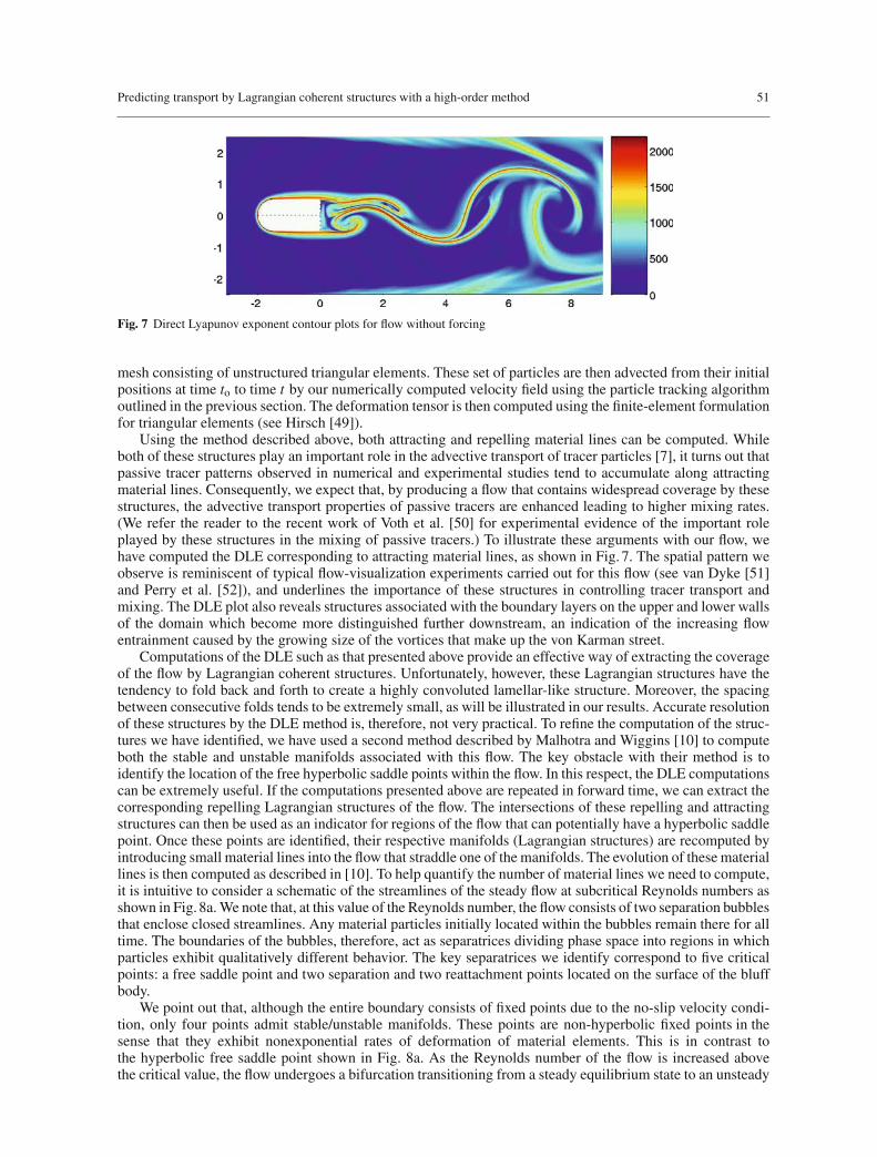
Fig. 7 Direct Lyapunov exponent contour plots for flow without forcing
mesh consisting of unstructured triangular elements. These set of particles are then advected from their initialpositions at time to to time t by our numerically computed velocity field using the particle tracking algorithmoutlined in the previous section. The deformation tensor is then computed using the finite-element formulationfor triangular elements (see Hirsch [49]).
Using the method described above, both attracting and repelling material lines can be computed. Whileboth of these structures play an important role in the advective transport of tracer particles [7], it turns out thatpassive tracer patterns observed in numerical and experimental studies tend to accumulate along attractingmaterial lines. Consequently, we expect that, by producing a flow that contains widespread coverage by thesestructures, the advective transport properties of passive tracers are enhanced leading to higher mixing rates.(We refer the reader to the recent work of Voth et al. [50] for experimental evidence of the important roleplayed by these structures in the mixing of passive tracers.) To illustrate these arguments with our flow, wehave computed the DLE corresponding to attracting material lines, as shown in Fig. 7. The spatial pattern weobserve is reminiscent of typical flow-visualization experiments carried out for this flow (see van Dyke [51]and Perry et al. [52]), and underlines the importance of these structures in controlling tracer transport andmixing. The DLE plot also reveals structures associated with the boundary layers on the upper and lower wallsof the domain which become more distinguished further downstream, an indication of the increasing flowentrainment caused by the growing size of the vortices that make up the von Karman street.
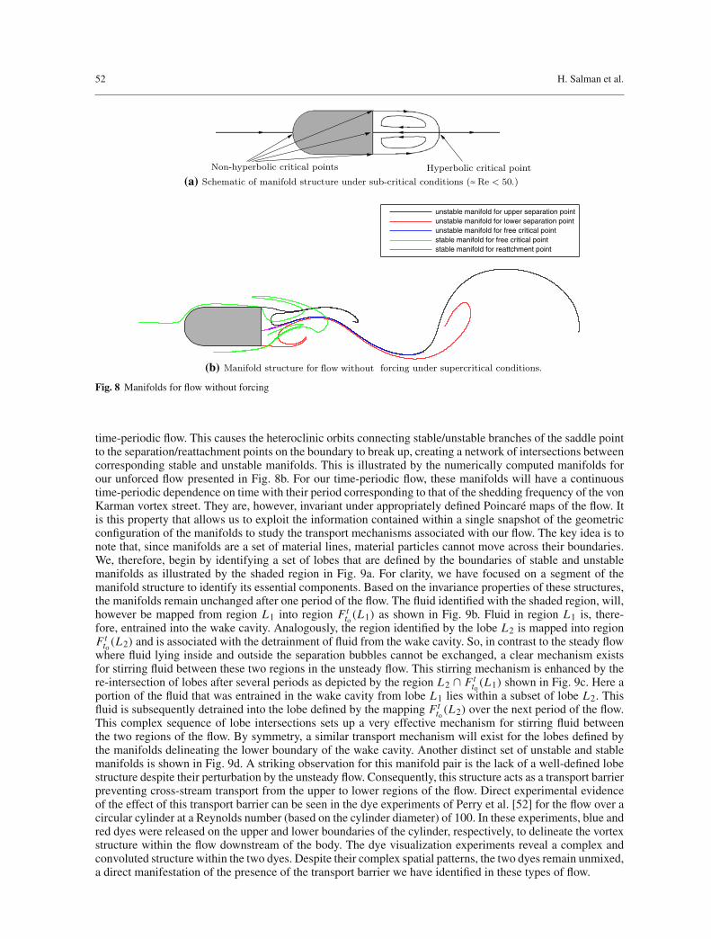
Computations of the DLE such as that presented above provide an effective way of extracting the coverageof the flow by Lagrangian coherent structures. Unfortunately, however, these Lagrangian structures have thetendency to fold back and forth to create a highly convoluted lamellar-like structure. Moreover, the spacingbetween consecutive folds tends to be extremely small, as will be illustrated in our results. Accurate resolutionof these structures by the DLE method is, therefore, not very practical. To refine the computation of the struc-tures we have identified, we have used a second method described by Malhotra and Wiggins [10] to computeboth the stable and unstable manifolds associated with this flow. The key obstacle with their method is toidentify the location of the free hyperbolic saddle points within the flow. In this respect, the DLE computationscan be extremely useful. If the computations presented above are repeated in forward time, we can extract thecorresponding repelling Lagrangian structures of the flow. The intersections of these repelling and attractingstructures can then be used as an indicator for regions of the flow that can potentially have a hyperbolic saddlepoint. Once these points are identified, their respective manifolds (Lagrangian structures) are recomputed byintroducing small material lines into the flow that straddle one of the manifolds. The evolution of these materiallines is then computed as described in [10]. To help quantify the number of material lines we need to compute,it is intuitive to consider a schematic of the streamlines of the steady flow at subcritical Reynolds numbers asshown in Fig. 8a. We note that, at this value of the Reynolds number, the flow consists of two separation bubblesthat enclose closed streamlines. Any material particles initially located within the bubbles remain there for alltime. The boundaries of the bubbles, therefore, act as separatrices dividing phase space into regions in whichparticles exhibit qualitatively different behavior. The key separatrices we identify correspond to five criticalpoints: a free saddle point and two separation and two reattachment points located on the surface of the bluffbody.
We point out that, although the entire boundary consists of fixed points due to the no-slip velocity condi-tion, only four points admit stable/unstable manifolds. These points are non-hyperbolic fixed points in thesense that they exhibit nonexponential rates of deformation of material elements. This is in contrast tothe hyperbolic free saddle point shown in Fig. 8a. As the Reynolds number of the flow is increased abovethe critical value, the flow undergoes a bifurcation transitioning from a steady equilibrium state to an unsteady
52 H. Salman et al.
Non-hyperbolic critical points Hyperbolic critical point
(a) Schematic of manifold structure under sub-critical conditions (≈ Re < 50.)
unstable manifold for upper separation pointunstable manifold for lower separation pointunstable manifold for free critical pointstable manifold for free critical pointstable manifold for reattchment point
(b) Manifold structure for without forcing under supercritical conditions.flow
Fig. 8 Manifolds for flow without forcing
time-periodic flow. This causes the heteroclinic orbits connecting stable/unstable branches of the saddle pointto the separation/reattachment points on the boundary to break up, creating a network of intersections betweencorresponding stable and unstable manifolds. This is illustrated by the numerically computed manifolds forour unforced flow presented in Fig. 8b. For our time-periodic flow, these manifolds will have a continuoustime-periodic dependence on time with their period corresponding to that of the shedding frequency of the vonKarman vortex street. They are, however, invariant under appropriately defined Poincaré maps of the flow. Itis this property that allows us to exploit the information contained within a single snapshot of the geometricconfiguration of the manifolds to study the transport mechanisms associated with our flow. The key idea is tonote that, since manifolds are a set of material lines, material particles cannot move across their boundaries.We, therefore, begin by identifying a set of lobes that are defined by the boundaries of stable and unstablemanifolds as illustrated by the shaded region in Fig. 9a. For clarity, we have focused on a segment of themanifold structure to identify its essential components. Based on the invariance properties of these structures,the manifolds remain unchanged after one period of the flow. The fluid identified with the shaded region, will,however be mapped from region L1 into region Ft
to(L1) as shown in Fig. 9b. Fluid in region L1 is, there-fore, entrained into the wake cavity. Analogously, the region identified by the lobe L2 is mapped into regionFt
to(L2) and is associated with the detrainment of fluid from the wake cavity. So, in contrast to the steady flowwhere fluid lying inside and outside the separation bubbles cannot be exchanged, a clear mechanism existsfor stirring fluid between these two regions in the unsteady flow. This stirring mechanism is enhanced by there-intersection of lobes after several periods as depicted by the region L2 ∩ Ft
to(L1) shown in Fig. 9c. Here aportion of the fluid that was entrained in the wake cavity from lobe L1 lies within a subset of lobe L2. Thisfluid is subsequently detrained into the lobe defined by the mapping Ft
to(L2) over the next period of the flow.This complex sequence of lobe intersections sets up a very effective mechanism for stirring fluid betweenthe two regions of the flow. By symmetry, a similar transport mechanism will exist for the lobes defined bythe manifolds delineating the lower boundary of the wake cavity. Another distinct set of unstable and stablemanifolds is shown in Fig. 9d. A striking observation for this manifold pair is the lack of a well-defined lobestructure despite their perturbation by the unsteady flow. Consequently, this structure acts as a transport barrierpreventing cross-stream transport from the upper to lower regions of the flow. Direct experimental evidenceof the effect of this transport barrier can be seen in the dye experiments of Perry et al. [52] for the flow over acircular cylinder at a Reynolds number (based on the cylinder diameter) of 100. In these experiments, blue andred dyes were released on the upper and lower boundaries of the cylinder, respectively, to delineate the vortexstructure within the flow downstream of the body. The dye visualization experiments reveal a complex andconvoluted structure within the two dyes. Despite their complex spatial patterns, the two dyes remain unmixed,a direct manifestation of the presence of the transport barrier we have identified in these types of flow.

Predicting transport by Lagrangian coherent structures with a high-order method 53
(d) Identication of cross-stream transport barrier.
L2 F tto
(L1)
(c) Chaotic transport produced by complex lobe geometry.
F tto
(L1)
F tto
(L2)
(b) Lobe evolution under one period of the flow.
L1
L2
(a) Denition of lobe by intersection of stablunstable
e andmanifolds.
Fig. 9 Transport mechanism by manifolds for flow without forcing
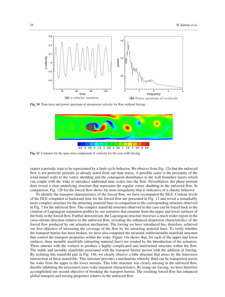
The presence of the transport barrier within the flow is undesirable for applications requiring effective mix-ing of passively advected tracers. We will, therefore, explore the possibility of using flow forcing to break thetransport barrier identified above. Having recognized that attracting material lines are the organizing structureswithin a flow, a desirable objective of our forcing would be to break the transport barrier whilst at the sametime increasing the coverage of the flow by these structures. This would consequently result in the effectivestretching and rapid stirring of passively advected quantities. This reasoning is in part what motivated theconfiguration of four wall mounted actuators illustrated in Fig. 4c. By opting for two actuators on each of theupper and lower boundaries, a separation profile can be created by appropriate setting of the wall jet velocities(see (36)). An additional parameter is the forcing frequency ( fe) which we set in such a way as to excite thelarge-scale structures observed in our unforced flow. Based on the work of Karniadakis and Triantafyllou [44],we have chosen a value of fe ≈ 1.05 fs, where fs is the natural shedding frequency of the large-scale vortices.To determine fs, we have extracted the variation of the streamwise component of velocity (u) as a function oftime for a point located within the wake. For the results presented here, we have chosen the coordinates of ourpoint to lie at (x p, yp) = (1.0, 0.25). The corresponding time history is shown in Fig. 10a. The plot reveals thesignal to be made up of a higher-frequency harmonic superimposed with a low-frequency modulation of theamplitude. Decomposing this signal into its constituent Fourier modes, as shown in Fig. 10b, we observe that alarge percentage of the energy in the power spectrum is confined to a narrow range located around a frequencyof 0.22. This corresponds to the natural shedding frequency (Strouhal frequency) of the large-scale vorticesin the unforced flow and is well documented in the literature on bluff-body flows (e.g. Williamson [53]). Itis natural to consider what implication does the lack of strict periodicity have on the lobe dynamic analysispresented in Fig. 9. Since the large-scale coherent vortices shed alternately from the body in a regular manneras depicted in Fig. 6, we can conclude that the qualitative description of the transport mechanisms presentedin Fig. 9 will not be impacted by the low-frequency modulation. The lack of strict periodicity can, however,alter the areas of the lobes shown in the figure so that a different mass of fluid is entrained and detrained intoand out of the wake cavity on each shedding cycle of the vortices.
Using the above parameters, we have simulated the forced flow to produce the span-wise component ofthe vorticity field shown in Fig. 11. As can be seen, the forcing introduced by our actuators results in theproduction of stronger vortical structures that shed off in a more irregular fashion. This irregular shedding is adirect result of the intrinsic forcing frequency we have used to excite the flow. A consequence of the irregularand stronger vortex structure produced within the wake is the broader cross-stream migration that the vorticesshow in the forced flow producing strong interactions with the boundary layers of the tunnel walls. This causesfluid to be detrained from the viscous boundary layers, as can be seen from the undulations in the vorticityfield. In stark contrast, such interactions are much weaker in the unforced flow (Fig. 6).
In order to obtain a clearer geometrical picture of the system’s response and to identify the temporal devel-opment of the flow, we conducted a phase-plane analysis by projecting the trajectory of the system onto atwo-dimensional space defined by two arbitrary independent state variables. Motivated by a similar analysisconducted by Karniadakis and Triantafyllou [44], we have chosen the stream-wise and transverse componentsof the velocity vector as our two independent state vector variables with measurements taken at the point(x p, yp) = (1.0, 0.25). This point coincides with the point used to extract our time traces. On such a plot, we
54 H. Salman et al.
time
u-ve
loci
ty
70 80 90 100
-0.4
-0.2
0
0.2
0.4
0.6
(a) u-velocity variationfrequency
pow
er
0 1 2 3 4
100
101
102
(b) Power spectrum of u-velocity
Fig. 10 Time trace and power spectrum of streamwise velocity for flow without forcing
Fig. 11 Contours for the span-wise component of vorticity for the case with forcing
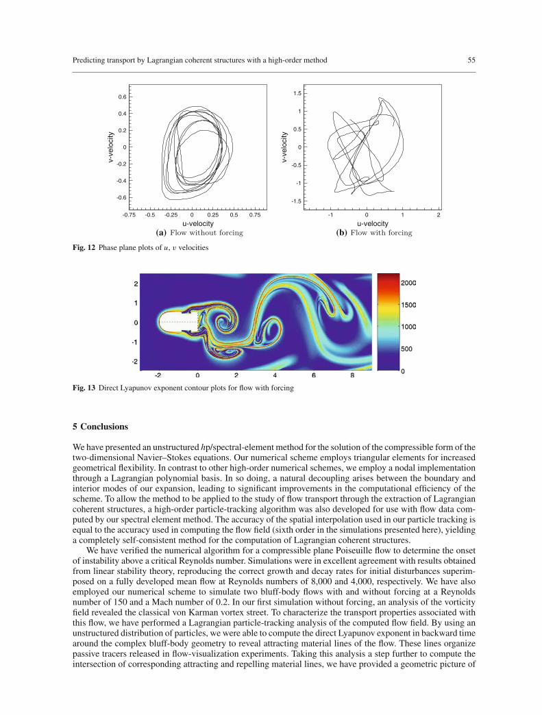
expect a periodic state to be represented by a limit-cycle behavior. We observe from Fig. 12a that the unforcedflow is not perfectly periodic as already noted from our time traces. A possible cause is the proximity of thewind-tunnel walls to the vortex shedding and the consequent disturbance to the wall boundary layers whichcan couple with the wake to introduce additional time scales into the flow. Nevertheless, the phase portraitdoes reveal a clear underlying structure that represents the regular vortex shedding in the unforced flow. Incomparison, Fig. 12b for the forced flow shows far more irregularity that is indicative of a chaotic behavior.
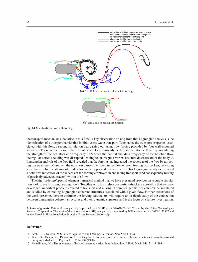
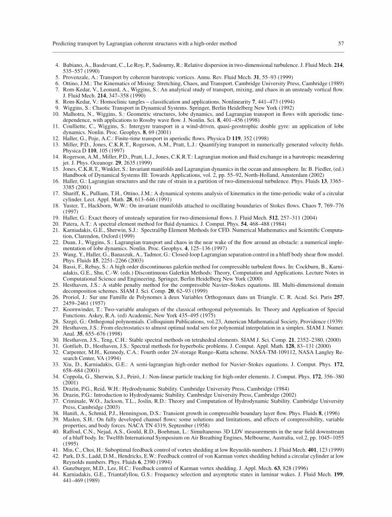
To identify the transport characteristics of the forced flow, we have recomputed the DLE. Contour levelsof the DLE computed in backward time for the forced flow are presented in Fig. 13 and reveal a remarkablymore complex structure for the attracting material lines in comparison to the corresponding structure observedin Fig. 7 for the unforced flow. The complex manifold structure observed in this case can be traced back to thecreation of Lagrangian separation profiles by our actuators that emanate from the upper and lower surfaces ofthe body in the forced flow. Further downstream, the Lagrangian structure traverses a much wider region in thecross-stream direction relative to the unforced flow, revealing the enhanced dispersion characteristics of theforced flow produced by our actuation mechanism. The forcing we have introduced has, therefore, achievedour first objective of increasing the coverage of the flow by the attracting material lines. To verify whetherthe transport barrier has been broken, we have also computed the invariant stable/unstable manifold structurethat control the transport properties within the wake. Figure 14a shows that, for each of the upper and lowersurfaces, three unstable manifolds (attracting material lines) are created by the introduction of the actuators.These interact with the vortices to produce a highly complicated and intertwined structure within the flow.The stable and unstable manifolds associated with the transport barrier persist with the addition of forcing.By isolating this manifold pair in Fig. 14b, we clearly observe a lobe structure that arises by the transverseintersection of these manifolds. This structure provides a mechanism whereby fluid can be transported acrossthe wake from the upper to the lower streams. This lobe structure was clearly missing in the unforced flow,thereby inhibiting the associated cross-wake transport characteristics. By using our forcing, we have thereforeaccomplished our second objective of breaking the transport barrier. The resulting forced flow has enhancedglobal transport and mixing properties relative to the unforced flow.
Predicting transport by Lagrangian coherent structures with a high-order method 55
u-velocity
v-ve
loci
ty
-0.75 -0.5 -0.25 0 0.25 0.5 0.75
-0.6
-0.4
-0.2
0
0.2
0.4
0.6
(a) Flow without forcingu-velocity
v-ve
loci
ty
-1 0 1 2
-1.5
-1
-0.5
0
0.5
1
1.5
(b) Flow with forcing
Fig. 12 Phase plane plots of u, v velocities
Fig. 13 Direct Lyapunov exponent contour plots for flow with forcing
5 Conclusions
We have presented an unstructured hp/spectral-element method for the solution of the compressible form of thetwo-dimensional Navier–Stokes equations. Our numerical scheme employs triangular elements for increasedgeometrical flexibility. In contrast to other high-order numerical schemes, we employ a nodal implementationthrough a Lagrangian polynomial basis. In so doing, a natural decoupling arises between the boundary andinterior modes of our expansion, leading to significant improvements in the computational efficiency of thescheme. To allow the method to be applied to the study of flow transport through the extraction of Lagrangiancoherent structures, a high-order particle-tracking algorithm was also developed for use with flow data com-puted by our spectral element method. The accuracy of the spatial interpolation used in our particle tracking isequal to the accuracy used in computing the flow field (sixth order in the simulations presented here), yieldinga completely self-consistent method for the computation of Lagrangian coherent structures.
We have verified the numerical algorithm for a compressible plane Poiseuille flow to determine the onsetof instability above a critical Reynolds number. Simulations were in excellent agreement with results obtainedfrom linear stability theory, reproducing the correct growth and decay rates for initial disturbances superim-posed on a fully developed mean flow at Reynolds numbers of 8,000 and 4,000, respectively. We have alsoemployed our numerical scheme to simulate two bluff-body flows with and without forcing at a Reynoldsnumber of 150 and a Mach number of 0.2. In our first simulation without forcing, an analysis of the vorticityfield revealed the classical von Karman vortex street. To characterize the transport properties associated withthis flow, we have performed a Lagrangian particle-tracking analysis of the computed flow field. By using anunstructured distribution of particles, we were able to compute the direct Lyapunov exponent in backward timearound the complex bluff-body geometry to reveal attracting material lines of the flow. These lines organizepassive tracers released in flow-visualization experiments. Taking this analysis a step further to compute theintersection of corresponding attracting and repelling material lines, we have provided a geometric picture of
56 H. Salman et al.
unstable manifolds for upper separation pointsunstable manifolds for lower separation pointsunstable manifold for free critical pointstable manifold for free critical pointstable manifold for reattchment point
(a) Manifold structure for flow with forcing.
(b) Breaking of transport barrier.
Fig. 14 Manifolds for flow with forcing
the transport mechanisms that arise in this flow. A key observation arising from this Lagrangian analysis is theidentification of a transport barrier that inhibits cross-wake transport. To enhance the transport properties asso-ciated with this flow, a second simulation was carried out using flow forcing provided by four wall-mountedactuators. These actuators were used to introduce local unsteady perturbations into the flow. By modulatingthe strength of the actuators at a frequency 1.05 times the natural shedding frequency of the baseline flow,the regular vortex shedding was disrupted, leading to an irregular vortex structure downstream of the body. ALagrangian analysis of the flow field revealed that the forcing had increased the coverage of the flow by attract-ing material lines. Moreover, the transport barrier identified in the flow without forcing was broken, providinga mechanism for the stirring of fluid between the upper and lower streams. This Lagrangian analysis provideda definitive indication of the success of the forcing employed in enhancing transport (and consequently mixingof passively advected tracers) within the flow.
The high-order hp/spectral-element numerical method that we have presented provides an accurate simula-tion tool for realistic engineering flows. Together with the high-order particle-tracking algorithm that we havedeveloped, important problems related to transport and mixing in complex geometries can now be simulatedand studied by extracting Lagrangian coherent structures associated with a given flow. Further extensions ofthe work presented here to optimize the forcing parameters will require an in-depth study of the connectionbetween Lagrangian coherent structures and their dynamic signature and is the focus of a future investigation.
Acknowledgments This work was partially supported by AFOSR grant F49620-00-1-0133, and by the United TechnologiesResearch Corporation. The work of the second author (JSH) was partially supported by NSF under contract DMS-0132967 andby the Alfred P. Sloan Foundation through a Sloan Research Fellowship.
References
1. Aref, H., El Naschie, M.S.: Chaos Applied to Fluid Mixing. Pergamon, New York (1995)2. Benzi, R., Paladin, G., Patarnello, S., Santangelo, P., Vulpiani, A.: Self-similar coherent structures in two-dimensional
decaying turbulence. J. Phys. A 21, 1221–1237 (1988)3. McWilliams, J.C.: The emergence of isolated coherent vortices in turbulent flow. J. Fluid Mech. 146, 21–43 (1984)
Predicting transport by Lagrangian coherent structures with a high-order method 57
4. Babiano, A., Basdevant, C., Le Roy, P., Sadourny, R.: Relative dispersion in two-dimensional turbulence. J. Fluid Mech. 214,535–557 (1990)
5. Provenzale, A.: Transport by coherent barotropic vortices. Annu. Rev. Fluid Mech. 31, 55–93 (1999)6. Ottino, J.M.: The Kinematics of Mixing: Stretching, Chaos, and Transport. Cambridge University Press, Cambridge (1989)7. Rom-Kedar, V., Leonard, A., Wiggins, S.: An analytical study of transport, mixing, and chaos in an unsteady vortical flow.
J. Fluid Mech. 214, 347–358 (1990)8. Rom-Kedar, V.: Homoclinic tangles – classification and applications. Nonlinearity 7, 441–473 (1994)9. Wiggins, S.: Chaotic Transport in Dynamical Systems. Springer, Berlin Heidelberg New York (1992)
10. Malhotra, N., Wiggins, S.: Geometric structures, lobe dynamics, and Lagrangian transport in flows with aperiodic time-dependence, with applications to Rossby wave flow. J. Nonlin. Sci. 8, 401–456 (1998)
11. Coulliette, C., Wiggins, S.: Intergyre transport in a wind-driven, quasi-geostrophic double gyre: an application of lobedynamics. Nonlin. Proc. Geophys. 8, 69 (2001)
12. Haller, G., Poje, A.C.: Finite-time transport in aperiodic flows. Physica D 119, 352 (1998)13. Miller, P.D., Jones, C.K.R.T., Rogerson, A.M., Pratt, L.J.: Quantifying transport in numerically generated velocity fields.
Physica D 110, 105 (1997)14. Rogerson, A.M., Miller, P.D., Pratt, L.J., Jones, C.K.R.T.: Lagrangian motion and fluid exchange in a barotropic meandering
jet. J. Phys. Oceanogr. 29, 2635 (1999)15. Jones, C.K.R.T., Winkler, S.: Invariant manifolds and Lagrangian dynamics in the ocean and atmosphere. In: B. Fiedler, (ed.)
Handbook of Dynamical Systems III: Towards Applications, vol. 2, pp. 55–92, North-Holland, Amsterdam (2002)16. Haller, G.: Lagrangian structures and the rate of strain in a partition of two-dimensional turbulence. Phys. Fluids 13, 3365–
3385 (2001)17. Shariff, K., Pulliam, T.H., Ottino, J.M.: A dynamical systems analysis of kinematics in the time-periodic wake of a circular
cylinder. Lect. Appl. Math. 28, 613–646 (1991)18. Yuster, T., Hackborn, W.W.: On invariant manifolds attached to oscillating boundaries of Stokes flows. Chaos 7, 769–776
(1997)19. Haller, G.: Exact theory of unsteady separation for two-dimensional flows. J. Fluid Mech. 512, 257–311 (2004)20. Patera, A.T.: A spectral element method for fluid dynamics. J. Comput. Phys. 54, 468–488 (1984)21. Karniadakis, G.E., Sherwin, S.J.: Spectral/hp Element Methods for CFD. Numerical Mathematics and Scientific Computa-
tion, Clarendon, Oxford (1999)22. Duan, J., Wiggins, S.: Lagrangian transport and chaos in the near wake of the flow around an obstacle: a numerical imple-
mentation of lobe dynamics. Nonlin. Proc. Geophys. 4, 125–136 (1997)23. Wang, Y., Haller, G., Banaszuk, A., Tadmor, G.: Closed-loop Lagrangian separation control in a bluff body shear flow model.
Phys. Fluids 15, 2251–2266 (2003)24. Bassi, F., Rebay, S.: A high order discontinuous galerkin method for compressible turbulent flows. In: Cockburn, B., Karni-
adakis, G.E., Shu, C.-W. (eds.) Discontinuous Galerkin Methods: Theory, Computation and Applications. Lecture Notes inComputational Science and Engineering. Springer, Berlin Heidelberg New York (2000)
25. Hesthaven, J.S.: A stable penalty method for the compressible Navier–Stokes equations. III. Multi-dimensional domaindecomposition schemes. SIAM J. Sci. Comp. 20, 62–93 (1999)
26. Proriol, J.: Sur une Famille de Polynomes à deux Variables Orthogonaux dans un Triangle. C. R. Acad. Sci. Paris 257,2459–2461 (1957)
27. Koornwinder, T.: Two-variable analogues of the classical orthogonal polynomials. In: Theory and Application of SpecialFunctions. Askey, R.A. (ed) Academic, New York 435–495 (1975)
28. Szegö, G.: Orthogonal polynomials. Colloquium Publications, vol.23, American Mathematical Society, Providence (1939)29. Hesthaven, J.S.: From electrostatics to almost optimal nodal sets for polynomial interpolation in a simplex. SIAM J. Numer.
Anal. 35, 655–676 (1998)30. Hesthaven, J.S., Teng, C.H.: Stable spectral methods on tetrahedral elements. SIAM J. Sci. Comp. 21, 2352–2380, (2000)31. Gottlieb, D., Hesthaven, J.S.: Spectral methods for hyperbolic problems. J. Comput. Appl. Math. 128, 83–131 (2000)32. Carpenter, M.H., Kennedy, C.A.: Fourth order 2N-storage Runge–Kutta scheme. NASA-TM-109112, NASA Langley Re-
search Center, VA (1994)33. Xiu, D., Karniadakis, G.E.: A semi-lagrangian high-order method for Navier–Stokes equations. J. Comput. Phys. 172,
658–684 (2001)34. Coppola, G., Sherwin, S.J., Peiró, J.: Non-linear particle tracking for high-order elements. J. Comput. Phys. 172, 356–380
(2001)35. Drazin, P.G., Reid, W.H.: Hydrodynamic Stability. Cambridge University Press, Cambridge (1984)36. Drazin, P.G.: Introduction to Hydrodynamic Stability. Cambridge University Press, Cambridge (2002)37. Criminale, W.O., Jackson, T.L., Joslin, R.D.: Theory and Computation of Hydrodynamic Stability. Cambridge University
Press, Cambridge (2003)38. Hanifi, A., Schmid, P.J., Henningson, D.S.: Transient growth in compressible boundary layer flow. Phys. Fluids 8, (1996)39. Maslen, S.H.: On fully developed channel flows: some solutions and limitations, and effects of compressibility, variable
properties, and body forces. NACA TN 4319, September (1958)40. Raffoul, C.N., Nejad, A.S., Gould, R.D., Boehman, L.: Simultaneous 3D LDV measurements in the near field downstream
of a bluff body. In: Twelfth International Symposium on Air Breathing Engines, Melbourne, Australia, vol.2, pp. 1045–1055(1995)
41. Min, C., Choi, H.: Suboptimal feedback control of vortex shedding at low Reynolds numbers. J. Fluid Mech. 401, 123 (1999)42. Park, D.S., Ladd, D.M., Hendricks, E.W.: Feedback control of von Karman vortex shedding behind a circular cylinder at low
Reynolds numbers. Phys. Fluids 6, 2390 (1994)43. Gunzburger, M.D., Lee, H.C.: Feedback control of Karman vortex shedding. J. Appl. Mech. 63, 828 (1996)44. Karniadakis, G.E., Triantafyllou, G.S.: Frequency selection and asymptotic states in laminar wakes. J. Fluid Mech. 199,
441–469 (1989)
58 H. Salman et al.
45. He, J.W., Glowinski, R., Metcalfe, R., Nordlander, A., Periaux, J.: Active control and drag optimization for flow past acircular cylinder. J. Comput. Phys. 163, 83 (2000)
46. Homescu, C., Navon, I.M., Li, Z.: Suppression of vortex shedding for flow around a circular cylinder using optimal control.Int. J. Numer. Methods. Fluids 38, 43 (2002)
47. Blackburn, H.M., Henderson, R.D.: A study of two-dimensional flow past an oscillating cylinder. J. Fluid Mech. 385, 255(1999)
48. Haller, G.: Distinguished material surfaces and coherent structures in 3D fluid flows. Physica D 149, 248–277 (2001)49. Hirsch, C.: Numerical Computation of Internal and External Flows: Volume 1 – Fundamentals of Numerical Discretisation.
Wiley, New York (1990)50. Voth, G.A., Haller, G., Gollub, J.: Experimental measurements of stretching fields in fluid mixing. Phys. Rev. Lett. 88, 254501
(2002)51. van Dyke, M.: Album of Fluid Motion. Parabolic Press, (1982)52. Perry, A.E., Chong, M.S., Lim, T.T.: The vortex shedding process behind two-dimensional bluff bodies. J. Fluid Mech. 116,
77–90 (1982)53. Williamson, C.H.K.: Vortex dynamics in the cylinder wake. Annu. Rev. Fluid Mech. 28, 477 (1996)

Reproduced with permission of the copyright owner. Further reproduction prohibited without permission.