J. theor. Biol. (2000) 207, 37}56doi:10.1006/jtbi.2000.2154, available online at http://www.idealibrary.com on

Predicting Response to Selection on a Quantitative Trait:A Comparison between Models for Mixed-mating Populations

JOHN K. KELLY* AND SCOTT WILLIAMSON

Department of Ecology and Evolutionary Biology, ;niversity of Kansas, ¸awrence, KS 66045, ;.S.A.

(Received on 21 April 2000, Accepted in revised form on 19 July 2000)

Two di!erent theoretical frameworks have been developed to predict response to selection ina mixed mating population (in which reproduction occurs by a mixture of outcrossing andself-fertilization). The genotypic covariance model (GCM) and the structured linear model(SLM) rely on the same assumptions regarding quantitative trait inheritance, but use di!erentgenetic summary statistics. Here, we demonstrate the algebraic relationships between thevarious genetic metrics used in each theory. This is accomplished by reformulating the GCMin terms of the Wright}Kempthorne equation. We use stochastic simulations to investigate therelative accuracy of each theory for a range of sel"ng rates. The SLM is generally moreaccurate than the GCM, the most pronounced di!erences emerging in simulations withinbreeding depression for "tness. In fact, with strong inbreeding depression and high sel"ngrates, evolution can occur opposite the direction predicted by the GCM. The simulations alsoindicate that direct application of random mating models to partially sel"ng populations canproduce very inaccurate predictions if quantitative trait loci exhibit dominance.

( 2000 Academic Press

Introduction

Most phenotypes of economic or ecologicalimportance vary continuously and exhibit multi-locus genetic variation (Wright, 1978). For thisreason, both agricultural breeding programs andevolutionary studies of natural populationsroutinely employ quantitative genetic models(Lush, 1937; Lande & Arnold, 1983; Grant &Grant, 1995). While generally not exact, thesemodels can provide accurate predictions ofshort-term changes in the mean and variance ofa quantitative trait under a broad range of condi-tions (Bulmer, 1985; Turelli & Barton, 1994).Perhaps most importantly, the parameters of

*Author to whom correspondence should be addressed.E-mail: jkk@eagle.cc.ukans.edu

0022}5193/00/210037#20 $35.00/0

quantitative genetic models can be estimatedusing established experimental methods (Lynch& Walsh, 1998).

The quantitative genetic approach is statisticalin nature. Let z denote the value for a quantitat-ive trait. If selection acts only on this character,the predicted change in the mean (ZM ) from onegeneration to the next, DZM , is

DZM "RS, (1)

where S is the selection di!erential and R is thelinear regression of o!spring phenotype onto theaverage phenotypic value of parents (Falconer,1989, p. 153). The selection di!erential measuresthe change in mean phenotype within a genera-tion due to selection, and R determines the pro-portion of that change transmitted to progeny. In

( 2000 Academic Press

38 J. K. KELLY AND S. WILLIAMSON

this regard, eqn (1) is an example of simple linearprediction. With random mating, the regressioncoe$cient is directly related to an underlyinggenetic model. In the absence of other complicat-ing factors (such as epistasis, genotype-by-envi-ronment interaction or correlation, or maternale!ects), R is equal to the &&narrow sense heritabil-ity'': the ratio of the additive genetic variance (<

a)

to the phenotypic variance (<z). The numerator

of this ratio, <a, is equal to the covariance be-

tween the average genotypic value of parentsand the genotypic value of o!spring (Falconer,1989, Chapter 9). We will refer to this form ofeqn (1), in which DZM "S<

a/<

z, as the Breeder's

equation.Inbreeding changes the joint distribution of

genotypic and phenotypic variation in a popula-tion (Wright, 1951; Kempthorne, 1957; Crow& Kimura, 1970; Jacquard, 1974). The Breeder'sequation is thus not directly applicable to self-fertilizing species. However, Pederson (1969a, b)did extend eqn (1) to one important situationinvolving non-random mating: an outbred basepopulation subjected to repeated cycles of selec-tion and self-fertilization. Like eqn (1), the pre-dicted change in mean phenotype involves theproduct of the selection di!erential and a herita-bility term. The relevant heritability is basedon the phenotypic linear regression of inbreddescendants onto ancestors [see Hayashi & Ukai(1994) for an important generalization of thismodel]. Cockerham & Matzinger (1985) de-veloped a similar model for a slightly di!erentsituation in which an outbred base population isself-fertilized for an arbitrary number of gene-rations followed by a generation of selection.Finally, Wright & Cockerham (1985) considera partially sel"ng population subjected to a singlegeneration of selection. In each of these models,inbreeding changes heritability through its e!ecton the genotypic covariance of ancestors anddescendants. For this reason, we refer to thisapproach as the genotypic covariance model(GCM).

Unfortunately, there are a number of di$cul-ties with the genotypic covariance approach.First, existing models are limited to a very speci-"c set of conditions. For example, the models ofWright & Cockerham (1985) and Cockerham& Matzinger (1985) provide valid predictions for

only a single generation of selection. A secondkind of di$culty emerges for GCM when a popu-lation contains individuals that vary in the extentto which they are inbred. This may causelinearity assumptions necessary to the GCM tobreak down (Wright & Cockerham, 1985; Kelly,1999a). Such variation in individual inbreedingcoe$cients is inevitable in a partially sel"ngpopulation, but not under certain experimentallycontrolled inbreeding schemes (such as the situ-ation consider by Pederson, 1969a, b). Finally,inbreeding depression for "tness can cause sub-stantial di!erences between the actual selectionregime on a trait and the observed selectiondi!erential (Willis, 1996; Kelly, 1999b). Theseconcerns motivated an alternative quantitativegenetic model for partially sel"ng populations,the structured linear model or (SLM) (Kelly,1999a, b).

In this paper, we demonstrate the algebraicrelationship between the GCM and SLM byusing the Wright}Kempthorne equation forthe mean phenotype of a population. We then usestochastic simulations to investigate the relativeaccuracy of each theory in predicting response toselection for a range of sel"ng rates. Two othermodels are tested in these simulations, theBreeder's equation used for randomly matingpopulations (here denoted BE) and a simpli"edversion of the SLM (denoted RSLM). The simu-lations also consider the e!ect of inbreedingdepression for "tness on the relative performanceof the models.

The Wright+Kempthorne Equation

Consider the standard model of quantitativetrait inheritance in which the trait value of anindividual is determined by the sum of statist-ically independent genetic and environmentalcomponents (Falconer, 1989, Chapters 7 and 8).The environmental e!ect has an expected valueof zero and a variance of<

e. The genetic compon-

ent is due to the cumulative contribution of mul-tiple loci. Each locus may have multiple alleleswith arbitrary dominance relations, but there isno epistasis. Under these assumptions, the meanphenotype of an inbreeding population is

ZM "kO#F(k

I!k

O) (2a)

SELECTION WITH INBREEDING 39

orZM "k

O#FB, (2b)

where kO

is the outbred mean of population (themean phenotype when all loci exhibit Hardy}Weinberg genotype frequencies), k

Iis the inbred

mean of population (the mean phenotype withcomplete homozygosity), B is the directionaldominance of the trait (the di!erence betweenkIand k

O), and F is the mean inbreeding coe$-

cient of the population. Equation (2) indicatesthat the mean phenotype is a linear function of F,assuming that genotype frequencies conform totheir expectations given allele frequencies and F(Crow & Kimura, 1970).

We will refer to eqn (2) as the Wright}Kempthorne equation. Sewall Wright obtainedeqn (2) with a single-locus model (see AppendixC of Wright, 1951), but he certainly realized thatit could be extended to multiple loci in the ab-sence of epistasis (James Crow, pers. comm.).Oscar Kempthorne provided an explicit multi-locus derivation demonstrating that only certainkinds of epistasis will generate a nonlinear rela-tionship between ZM and F (summarized in Chap-ter 20 of Kempthorne, 1957; see also Crow& Kimura, 1970, pp. 77}81; Weir & Cockerham,1977). Nonlinearity results only from domi-nance-by-dominance interactions. Additive-by-additive and additive-by-dominance epistatice!ects will not generate nonlinearity.

The SLM is based on the decomposition of themean phenotype given in eqn (2) (Kelly, 1999a, b).The change in the mean phenotype is predictedfrom changes in k

O, k

I, and F (or, equivalently,

from changes in kO, B, and F). One advantage of

using eqn (2) is that kO

and kI

are functions ofpopulation allele frequencies and do not dependon genotype frequencies. As a consequence,changes in k

Oand k

Icaused by selection within

a generation are directly transmitted to progeny.The recursive equations in the SLM predict im-mediate changes in k

Oand k

Iand the relevant

genetic metrics are based on statistical relation-ship between genotype and phenotype withina generation (e.g. Hill, 1971, 1974). [The originalderivation of the SLM was based on eqn (2b)(Kelly, 1999a, b). Here, we use the form given byeqn (2a) in order to facilitate comparison of theGCM and SLM.]

While previous GCM have focused on predic-ting changes in the mean directly, genotypiccovariances can also be used to predict changesin k

Oand k

I. The predicted change in the outbred

mean is

DkO"

2CgO<z

S, (3)

where CgO

is the genotypic covariance betweenparents and outbred progeny, and <

zis the

phenotypic variance in the parental generation (afactor of 2 is included because two separate par-ents contribute). Similarly,

DkI"

CgI<z

S, (4)

where CgI

is the genotypic covariance betweenindividuals in the current generation and com-pletely inbred descendants. As in eqn (3),<

zrefers

to the phenotypic variance in the current (ances-tral) generation.

In the SLM, the recursions for kO

and kI

arespeci"c to a particular &&inbreeding cohort''.All individuals within a cohort have the sameinbreeding coe$cient. For a particular cohort,

DkO"

Caz<z

S (5)

and

DkI"Dk

O#DB"

Caz#C

bz<z

S, (6)

where Caz

is the covariance between the additivegenetic value of individuals (a) and their pheno-typic values (z) within a generation. C

bzis the

covariance between the &&homozygous dominancedeviations'' of individuals (b) and their pheno-typic values (z).

Like the additive genetic value, the homo-zygous dominance deviation is a sum of genetice!ects associated with each quantitative trait lo-cus. The contribution of each locus is determinedby the dominance deviation associated with eachallele when that allele occurs in homozygous form.When the two alleles are identical, the contribu-tion of that locus to b is just equal to the standarddominance deviation (Falconer, 1989, Chapter 7)

a az

40 J. K. KELLY AND S. WILLIAMSON

for that genotype. If a locus is heterozygous, thecontribution to b is the average of the dominancedeviations for each alternative homozygote[Kelly (1999a) gives a more detailed explanationof b]. The population average (or expected value)for b is the directional dominance of the trait, B.It is for this reason that we can use C

bzto predict

changes in B caused by selection.Equations (5) and (6) are cohort-speci"c

predictions and the elements in each are likelyto di!er among cohorts. C

azand C

bzwill di!er

among cohorts because inbreeding changes thestatistical relationship between genotype andphenotype. The quantity S/<

z, which character-

izes selection, is also likely to di!er among co-horts except in special case of linear selection.The changes in k

Oor k

Ifor the entire population

are determined by a weighted average of cohort-speci"c values (Kelly, 1999a).

The Relationships Between Genetic Statistics

There are two apparent di!erences between theGCM and SLM. The "rst is that the recursionsfor k

Oand k

Iin each theory contain di!erent

genetic summary statistics [eqns (3)}(6)]. Thesecond di!erence is that there are actually a seriesof predicted changes for k

Oand k

Iin the SLM

(corresponding to di!erent inbreeding cohorts),whereas the GCM has only one recursion foreach quantity. In this section, we show that the"rst di!erence is semantic. The right-hand side(r.h.s.) of eqn (3) is equivalent to the r.h.s. ofeqn (5) because C

az"2C

gO. The r.h.s. of eqn (4)

is equivalent to the r.h.s. of eqn (6) becauseC

gI"C

az#C

bz. These identities are demon-

strated for a single bi-allelic locus in the followingsection, and for two loci with arbitrary geneticassociations in the appendix.

Result 1: Caz"2C

gO

It is useful to decompose Caz

into components:

Caz"CovMa, a#d#eN

"CovMa, aN#CovMa, dN, (7)

where d and e are the standard dominanceand environmental deviations (Falconer, 1989,

Chapter 7). The "rst term on the r.h.s. of eqn (7),CovMa, aN, is the additive genetic variance (<

a).

Consider a single locus with two alleles, A0

andA

1. We can express the variance and covariance

in eqn (7) in more familiar terms:

<a"x

00(2a

0)2#x

01(a

0#a

1)2#x

11(2a

1)2

(8)and

CovMa, dN"x00

(2a0d00

)#x01

(a0#a

1)d

01

#x11

(2a1d11

), (9)

where x00

denotes the frequency of genotypeA

0A

0, x

01denotes the frequency of genotype

A0A

1, and x

11denotes the frequency of geno-

type A1A

1. The additive e!ects of A

0and A

1are

a0

and a1, respectively. The dominance devi-

ations for A0A

0, A

0A

1, and A

1A

1are d

00, d

01,

and d11

. Here, the Greek symbols refer to valuesfor speci"c alleles and genotypes as de"ned inFalconer (1989, Chapter 7). In contrast, a andd are random variables (whose distributionsdepend on these values in addition to allelefrequencies).

The genotypic covariance between individualsand their outbred progeny, C

gO, can be cal-

culated by determining the expected genotypicvalue of progeny for each particular genotype.For example, the outbred progeny of an A

0A

0individual will be A

0A

0with probability q and

A0A

1with probability p. Here, p denotes the

frequency of the A1

allele (q"1!p). Thus,the expected genotypic value of outbred o!springfor an A

0A

0individual is q(2a

0#d

00)#

p(a0#a

1#d

01). The genotypic covariance is

obtained by taking the product of parental andaverage o!spring values and then averagingacross parental genotypes. After some simpli"ca-tion,

CgO"x

00(2a

0#d

00)a

0

#x01

(a0#a

1#d

01) (1/2)

](a0#a

1#qd

00#d

01#pd

11)

#x11

(2a1#d

11)a

1

"(<#CovMa, dN)/2"C /2. (10)

SELECTION WITH INBREEDING 41

This demonstrates Result 1 for the case of a singlelocus. This directly generalizes to any number ofloci under linkage equilibrium because the result-ing covariance is the sum of covariances at indi-vidual loci [e.g. eqn (10)]. A more complicatedderivation is necessary when there are inter-locusassociations. In the appendix, we show that Re-sult 1 holds for a two-locus model with arbitrarylinkage disequilibrium and identity disequilib-rium (sensu Cockerham & Weir, 1984).

Result 2: Caz#C

bz"C

gI.

As previously, it is useful to decompose the geno-typic value into components:

Cbz"CovMb, a#d#eN"CovMb, aN#CovMb, dN.

(11)

For a single locus,

CovMa, bN"x00

(2a0d00

)#x01

(a0#a

1)

](1/2) (d00#d

11)#x

11(2a

1d11

)

(12)

and

CovMb, dN"x00

d00

(d00!B)#x

01d01

](1/2) (d00#d

11!2B)

#x11

d11

(d11!B). (13)

The directional dominance, B, appears in eqn (13)because it is the expected value of b. For a singlelocus with two alleles, B"qd

00#pd

11.

We obtain an expression for CgI

by determin-ing the expected genotypic values of completelyinbred descendants for each parental genotypeand then take a weighted average of cross-products:

CgI"x

00(2a

0#d

00) (2a

0#d

00!B)

#x01

(a0#a

1#d

01)

](1/2) (2a0#d

00#2a

1#d

11!2B)

#x11

(2a1#d

11)(2a

1#d

11!B). (14)

Collecting appropriate terms, this equation sim-pli"es to

CgI"<

a#CovMa, dN#CovMb, dN#CovMa, bN

"Caz#C

bz, (15)

which demonstrates Result 2 for the case ofa single locus. The extension of the derivation totwo loci with arbitrary associations is given in theappendix.

Results 1 and 2 imply that the GCM and SLMare equivalent for populations that can be de-scribed by a single inbreeding coe$cient (at anyone time). In such circumstances, a single valuefor C

azand a single value for C

bzfully specify the

SLM. Uniformity of the inbreeding coe$cientemerges in several important situations includingthe agricultural breeding scenario considered byPederson (1969a, b) and Hayashi & Ukai (1994).We do not expect that the GCM and SLM willbe equivalent when individuals vary in theirinbreeding coe$cients. The SLM characterizessuch a population with a vector of values for bothC

azand C

bz. None of these cohort speci"c values

are generally equal to their respective values forthe entire population.

Stochastic Simulations

The primary purpose of the following simula-tion study is to compare the accuracy of theGCM and SLM in predicting response to selec-tion with intermediate sel"ng rates. However, wecan also use these simulations to test other mod-els. As a practical matter, we wish to knowwhether a model as complicated as either theGCM or SLM is really necessary. Can we obtainaccurate predictions with the Breeder's equation,at least for changes in the outbred mean? We willalso consider a reduced version of the SLM inwhich there are only two cohorts, outbred and&&inbred''. In the reduced structured linear model(RSLM), all inbred individuals (with inbreedingcoe$cients ranging from 0.5 to 1) are collectedinto the same cohort. For this reason, the RSLMwith two inbreeding cohorts is an intermediatebetween the GCM (one cohort) and SLM (mul-tiple cohorts).

42 J. K. KELLY AND S. WILLIAMSON

The simulation model assumes that 50 locidistributed across 10 chromosomes ("ve on each)determine the genotypic value of an individual.The recombination rate between adjacent loci ona chromosome is 0.2. Each locus has two alleles,a high allele (A

1) that increases the trait value

and a low allele (A0) that reduces the trait value.

At locus i, the three genotypes (A0A

0, A

0A

1, and

A1A

1) contribute 0, (1#k

i)a

i, and 2a

i, respec-

tively, to the genotypic value of an individual.Here, a

iis the genotypic &&e!ect'' of locus i and

kiis the dominance parameter for this locus (this

follows the parameterization of Lynch & Walsh,1998). We assume that loci contribute additivelyto determine the genotypic value of an individual(there is no epistasis at the phenotypic scale). Thephenotype of an individual is the sum of itsgenotypic value plus a random environmentalerror (a normally distributed random variancewith mean zero and a speci"ed variance).

The initial population for a simulation is ob-tained by randomly sampling 1000 individualsfrom the &&base population''. The genotype ofeach individual is determined by randomly samp-ling alleles given their respective frequencies inthe base population. Thus, the population in gen-eration 0 should be close to Hardy}Weinbergequilibrium and linkage equilibrium across loci.Allele frequencies in the base population maydi!er among loci. In most of the simulations, thefrequency of the high allele (A

1) is uniformly

distributed between 0 and 1 (initial frequencies0.01 at locus 1, 0.03 at locus 2, 0.05 at locus3,2, 0.97 at locus 49, and 0.99 at locus 50).

The population reproduces in discrete, non-overlapping generations and has constant size(1000 individuals prior to selection). At the begin-ning of each generation, individuals are rankedby their phenotypic value. Selection is then im-posed by truncation such that individuals withhigher ranks survive to reproduce. The propor-tion surviving to reproduce is either 500/1000 or200/1000 depending on the parameter set. Onethousand progeny are produced from these sur-viving adults to form the next generation. Toproduce an o!spring, one adult is randomly se-lected. This adult reproduces by sel"ng (withprobability j) or accepts a male gamete fromanother random adult to produce an outcrossedo!spring (with probability 1!j). For each

parameter set, evolution is repeated 100 timesand the results averaged to obtain expected ratesof evolutionary change.

We simulate evolution with di!ering sel"ngrates (j"0, 0.02, 0.1, 0.2, 0.3, 0.4, 0.5, 0.6, 0.7, 0.8,0.9, 0.98, and 1.0), environmental variances anddominance schemes. The duration of selection(number of generations per simulation) is varieddepending on the intensity of selection and theheritability. Two di!erent &&initial conditions'' areconsidered. In the "rst series of simulations, selec-tion is initiated immediately after the populationis founded, i.e. on the set of genotypes randomlyselected from the base population. In the secondseries of simulations, the population experiences"ve generations of mating/sel"ng prior to theinitiation of selection. These pre-selection genera-tions allow the population to approach &&breedingsystem equilibrium'' (sensu Wright & Cocker-ham, 1985) in which the population containsa mixture of individuals with di!erent inbreedingcoe$cients. Five generations are su$cient be-cause equilibrium is approached rapidly withsel"ng.

The models are tested by comparing observedcumulative changes in k

Oand k

Ito predicted

changes. The predicted change for a speci"cmodel is obtained by summing per generationpredictions. The relevant predictions for theGCM are given by eqns (3) and (4). A numericalvalue is obtained by measuring C

gO, C

gI, <

z, and

S directly from the observed array of genotypesand phenotypes in the population. Cohort-speci"c predictions for the SLM are derived fromeqns (5) and (6) (the program tracks the inbreed-ing history of individuals which allows us todetermine inbreeding cohorts). The predictedchange in k

Oand k

Ifor the entire population is

a weighted average of cohort speci"c predictions[see eqn (8) of Kelly, 1999a]. A similar procedureis used to obtain predictions for the RSLM, ex-cept that all inbred individuals are collected intothe same cohort. Finally, we test the adequacy ofthe Breeder's equation (abbreviated BE), to pre-dict changes in k

Owith inbreeding. Thus, each

simulation of evolution produces one &&observed''and four &&expected'' values for k

O, and one ob-

served and three expected values for kI(since the

Breeder's equation produces no prediction forthis quantity).

SELECTION WITH INBREEDING 43

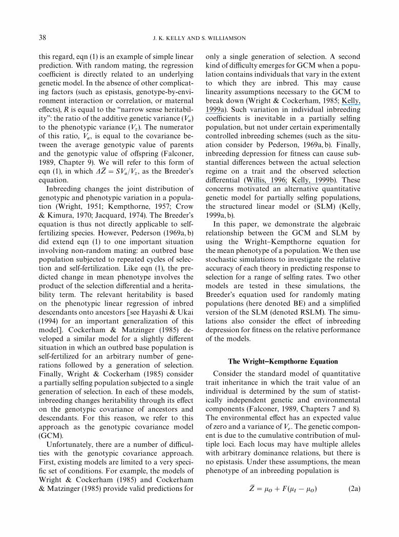
A summary of results for simulations in whichselection is imposed immediately after popula-tion founding is given in Table 1. Each line of thetable summarizes 100 replicate simulations fora particular parameter set. The average observedcumulative changes in k

Oand k

Iare given in

absolute units. The predicted changes in kO

orkI

for each model are expressed as proportionaldeviations: (predicted!observed)/observed. Aproportional deviation of !0.06 implies that theaverage predicted cumulative change is 6% lower(in magnitude) than the average observed change.A value of 2.50 implies that the predictedchange is 2.5 times greater than the observedchange. To highlight larger deviations, we have&&boxed'' all deviations that are greater than 5%in Tables 1}3.

In the simulations of Table 1, the genotypice!ect (a

i) and the dominance parameter (k

i) are

the same across loci (ai"1 and k

i"k for all i),

but the dominance parameter is varied in di!er-ent sets of simulations. The sel"ng rate (j) is alsovaried. The cases denote di!erent values for therelative magnitude of the environmental variance(<

e/<

g), the intensity of selection, and the dura-

tion of selection. In case 1, the environmentalvariance is equal to the initial genetic variance inthe population (<

e/<

g"1). This ratio will gener-

ally change over the course of a simulation be-cause<

gchanges but<

edoes not. In case 1, half of

the measured individuals are selected to repro-duce (500 of 1000) and selection is maintained for10 generations (t"10). Case 2 is the same ascase 1 except that <

e/<

g"5 and t"30. In cases

3 and 4, selection is more intense (200 of 1000 areselected). In case 3,<

e/<

g"1 and t"5. In case 4,

<e/<

g"5 and t"15.

Inspection of Table 1 con"rms the analyticalresults of the previous section. The GCM, SLM,and RSLM yield equivalent predictions whenj"0 or 1 (small di!erences occur due to samp-ling error). With complete sel"ng or completeoutcrossing, there is no variation in individualinbreeding coe$cients (within a generation) andthe models become equivalent. A second notableresult is that all of the models, including theBreeder's equation, yield accurate predictions inthe absence of dominance (when k"0). Whenthere is dominance, the Breeder's equation oftengives highly inaccurate predictions with sel"ng

(for j"0.5, 0.9, or 1). The GCM performs sub-stantially better than the Breeder's equation inthese situations, but not quite as well as either theSLM or RSLM. The di!erence between the lattertwo models is negligible in this set of simulations.

Table 2 describes simulation results for thesame set of conditions in Table 1 except thatpopulations were allowed to approach breedingsystem equilibrium prior to the initiation of selec-tion. This should make relatively little di!erencewith random mating and the results in Tables1 and 2 are nearly equivalent for j"0. However,there are some di!erences between Tables 1 and2 for both observed and predicted values in simu-lations with sel"ng. The performance of theBreeder's equation when there is inbreeding anddominance is substantially worse. With completesel"ng, the predicted change may be 4 or 5 timesgreater than the actual change. The GCM, SLM,and RSLM remain reasonably accurate, al-though there is greater error in the predictedchange in k

Owith j"1. As in Table 1, the GCM

is less accurate than the either the SLM or RSLMand the latter two models are nearly equivalent.

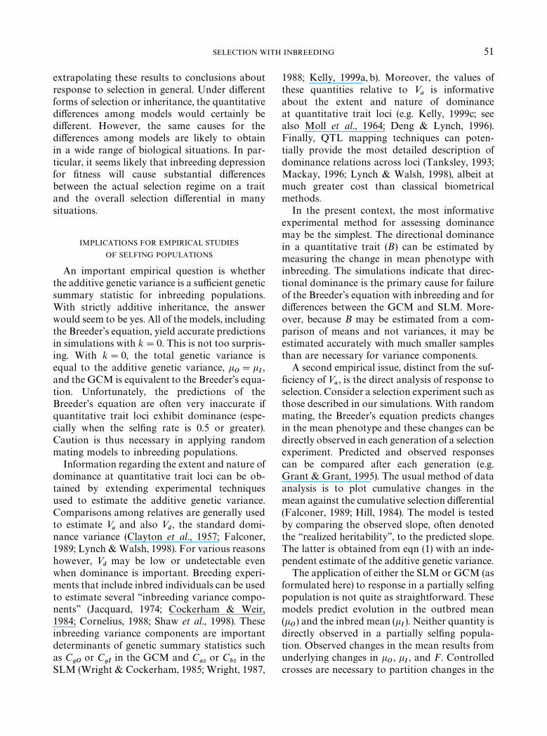
Table 3 describes results from a series of simu-lations in which there is inbreeding depression for"tness. In previous simulations, the survival andreproduction of an individual was determined bytheir phenotypic value. Inbreeding in#uenced "t-ness indirectly through its e!ect on the jointdistribution of genotypic and phenotypic vari-ation. In many natural and agricultural situ-ations, however, we expect that inbreeding willhave a direct negative e!ect on "tness. In mostcases, this inbreeding depression is probablycaused by the expression of partially recessivedeleterious alleles (Moll et al., 1964; Charles-worth & Charlesworth, 1987).

We consider a simple model of inbreeding de-pression for "tness in which inbreeding can causesterility. As in the previous simulation models,1000 individuals are ranked by phenotype at thebeginning of each generation. Each individual isthen determined to be either fertile or sterile byassignment of a random number. The probabilitythat an individual is fertile is ExpM!b f N, wheref is the inbreeding coe$cient of an individual andb is the &&inbreeding load'' (b*0). The probabil-ity function corresponds to the standard &&multi-plicative model'', in which log-transformed

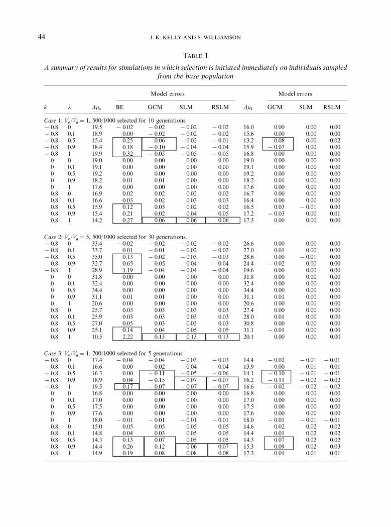
TABLE 1

A summary of results for simulations in which selection is initiated immediately on individuals sampledfrom the base population

Model errors Model errors

k j Dko

BE GCM SLM RSLM DkI

GCM SLM RSLM

Case 1: <e/<

g"1, 500/1000 selected for 10 generations

!0.8 0 19.5 !0.02 !0.02 !0.02 !0.02 16.0 0.00 0.00 0.00!0.8 0.1 18.9 0.00 !0.02 !0.02 !0.02 15.6 0.00 0.00 0.00!0.8 0.5 15.4 0.25 0.06 !0.02 !0.01 13.2 0.08 0.00 0.02!0.8 0.9 18.4 0.18 !0.10 !0.04 !0.04 15.9 !0.07 0.00 0.00!0.8 1 19.9 0.32 !0.05 !0.05 !0.05 16.8 0.00 0.00 0.00

0 0 19.0 0.00 0.00 0.00 0.00 19.0 0.00 0.00 0.000 0.1 19.1 0.00 0.00 0.00 0.00 19.1 0.00 0.00 0.000 0.5 19.2 0.00 0.00 0.00 0.00 19.2 0.00 0.00 0.000 0.9 18.2 0.01 0.01 0.00 0.00 18.2 0.01 0.00 0.000 1 17.6 0.00 0.00 0.00 0.00 17.6 0.00 0.00 0.000.8 0 16.9 0.02 0.02 0.02 0.02 16.7 0.00 0.00 0.000.8 0.1 16.6 0.03 0.02 0.03 0.03 16.4 0.00 0.00 0.000.8 0.5 15.9 0.12 0.05 0.02 0.02 16.5 0.03 !0.01 0.000.8 0.9 15.4 0.21 0.02 0.04 0.05 17.2 !0.03 0.00 0.010.8 1 14.2 0.27 0.06 0.06 0.06 17.3 0.00 0.00 0.00

Case 2: <e/<

g"5, 500/1000 selected for 30 generations.

!0.8 0 33.4 !0.02 !0.02 !0.02 !0.02 26.6 0.00 0.00 0.00!0.8 0.1 33.7 0.01 !0.01 !0.02 !0.02 27.0 0.01 0.00 0.00!0.8 0.5 35.0 0.13 !0.02 !0.03 !0.03 28.6 0.00 !0.01 0.00!0.8 0.9 32.7 0.65 !0.05 !0.04 !0.04 24.4 !0.02 0.00 0.00!0.8 1 28.9 1.19 !0.04 !0.04 !0.04 19.6 0.00 0.00 0.00

0 0 31.8 0.00 0.00 0.00 0.00 31.8 0.00 0.00 0.000 0.1 32.4 0.00 0.00 0.00 0.00 32.4 0.00 0.00 0.000 0.5 34.4 0.00 0.00 0.00 0.00 34.4 0.00 0.00 0.000 0.9 31.1 0.01 0.01 0.00 0.00 31.1 0.01 0.00 0.000 1 20.6 0.00 0.00 0.00 0.00 20.6 0.00 0.00 0.000.8 0 25.7 0.03 0.03 0.03 0.03 27.4 0.00 0.00 0.000.8 0.1 25.9 0.03 0.03 0.03 0.03 28.0 0.01 0.00 0.000.8 0.5 27.0 0.05 0.03 0.03 0.03 30.8 0.00 0.00 0.000.8 0.9 25.1 0.14 0.04 0.05 0.05 31.1 !0.01 0.00 0.000.8 1 10.5 2.22 0.13 0.13 0.13 20.1 0.00 0.00 0.00

Case 3: <e/<

g"1, 200/1000 selected for 5 generations

!0.8 0 17.4 !0.04 !0.04 !0.03 !0.03 14.4 !0.02 !0.01 !0.01!0.8 0.1 16.6 0.00 !0.02 !0.04 !0.04 13.9 0.00 !0.01 !0.01!0.8 0.5 16.3 0.00 !0.11 !0.05 !0.06 14.1 !0.10 !0.01 !0.01!0.8 0.9 18.9 0.04 !0.15 !0.07 !0.07 16.2 !0.11 !0.02 !0.02!0.8 1 19.5 0.17 !0.07 !0.07 !0.07 16.6 !0.02 !0.02 !0.02

0 0 16.8 0.00 0.00 0.00 0.00 16.8 0.00 0.00 0.000 0.1 17.0 0.00 0.00 0.00 0.00 17.0 0.00 0.00 0.000 0.5 17.5 0.00 0.00 0.00 0.00 17.5 0.00 0.00 0.000 0.9 17.6 0.00 0.00 0.00 0.00 17.6 0.00 0.00 0.000 1 18.0 !0.01 !0.01 !0.01 !0.01 18.0 !0.01 !0.01 !0.010.8 0 15.0 0.05 0.05 0.05 0.05 14.6 0.02 0.02 0.020.8 0.1 14.8 0.04 0.03 0.05 0.05 14.4 0.01 0.02 0.020.8 0.5 14.3 0.13 0.07 0.05 0.05 14.3 0.07 0.02 0.020.8 0.9 14.4 0.26 0.12 0.06 0.07 15.3 0.09 0.02 0.030.8 1 14.9 0.19 0.08 0.08 0.08 17.3 0.01 0.01 0.01

44 J. K. KELLY AND S. WILLIAMSON

TABLE 1

Model errors Model errors

k j Dko

BE GCM SLM RSLM DkI

GCM SLM RSLM

Case 4: <e/<

g"5, 200/1000 selected for 15 generations

!0.8 0 30.3 !0.03 !0.03 !0.03 !0.03 24.2 !0.01 !0.01 !0.01!0.8 0.1 30.4 !0.01 !0.03 !0.02 !0.03 24.5 !0.01 0.00 0.00!0.8 0.5 31.1 0.14 !0.07 !0.04 !0.05 23.8 !0.05 0.00 !0.01!0.8 0.9 29.8 0.67 !0.06 !0.04 !0.04 21.0 !0.02 0.01 0.01!0.8 1 29.9 0.88 !0.04 !0.03 !0.03 20.8 0.01 0.02 0.02

0 0 28.4 0.00 0.00 0.00 0.00 28.4 0.00 0.00 0.000 0.1 28.7 0.01 0.01 0.01 0.01 28.7 0.01 0.01 0.010 0.5 30.2 0.01 0.01 0.01 0.00 30.2 0.01 0.01 0.000 0.9 27.3 0.01 0.01 0.01 0.01 27.3 0.01 0.01 0.010 1 21.8 0.02 0.02 0.02 0.02 21.8 0.02 0.02 0.020.8 0 23.2 0.05 0.05 0.05 0.05 24.3 0.01 0.02 0.020.8 0.1 23.3 0.06 0.06 0.05 0.05 24.6 0.03 0.02 0.020.8 0.5 23.6 0.13 0.11 0.07 0.07 26.0 0.09 0.03 0.030.8 0.9 22.5 0.21 0.11 0.08 0.08 27.2 0.06 0.03 0.030.8 1 12.8 1.15 0.18 0.17 0.17 21.4 0.03 0.03 0.03

Each line represents the mean of 100 replicate simulations of the same parameter set. The case numbers refer to speci"cvalues for the environmental variance, intensity of selection, and duration of selection (see text). The "rst two columns ofthe table give the particular values for the dominance parameter (k) and the sel"ng rate (j) in that set of simulations. Thethird and eighth columns, labeled Observed Dk

Oand Observed Dk

I, respectively, give the average changes in k

Oand k

I.

Columns 4}7 give the proportional error associated with the predicted cumulative change in kO

for each model:(predicted!observed)/observed. Columns 9}11 give the proportional errors of model prediction for Dk

I. Model

predictions in error of greater than 5% are boxed.

SELECTION WITH INBREEDING 45

"tness declines linearly with inbreeding coe$-cient (Morton et al., 1956; Charlesworth &Charlesworth, 1987; Deng & Lynch, 1996). Thismodel for inbreeding depression is not explicitlygenetic in that we do not directly monitor the lociresponsible for sterility. However, this relativelysimple treatment of inbreeding depression for"tness has proven useful in previous theoreticalstudies (Charlesworth & Charlesworth, 1987;Deng & Lynch, 1996) and we expect that thee!ects identi"ed here will also emerge in morecomplicated and realistic models.

The inbreeding load, b, is a model parameterthat determines the magnitude of inbreedingdepression for "tness (with higher valuescorresponding to stronger inbreeding depress-ion). Empirical studies of both Drosophilamelanogaster and Mimulus guttatus suggest thatb may be close to 1 (Simmons & Crow, 1977;Willis, 1999). With b"1 and all else equal, the"tness of completely inbred individuals is 37% ofthe "tness of outbred individuals.

Following assignment of sterility, selectionis imposed on the population. Only fertile

individuals are included among those selectedto reproduce. If the intensity of selection is500/1000, the 500 fertile individuals with highestcharacter values are selected. An important con-sequence is that these individuals may not be thetop 500 individuals in the total population. In-breeding depression for "tness can thus reducethe magnitude of the selection di!erential. Thelatter is calculated by comparing the mean ofselected individual to mean of all individualsprior to selection. The selection di!erential thusdepends on both inbreeding induced sterility andphenotypic selection.

The results from simulations with inbreedingdepression for "tness (Table 3) are very di!erentfrom the results without inbreeding depressionfor "tness (Tables 1 and 2). Like the previoussimulations, all the models perform well if allelesare additive in their e!ects. With dominancehowever, the GCM and BE are often very inac-curate. In some cases, the proportional error issubstantially negative (less than !1.00). This im-plies that evolution occurs in the opposite direc-tion of that predicted by the GCM. Predicted and

TABLE 2

¹he simulation results with selection imposed after breeding system equilibrium has been established.All conventions are the same as ¹able 1

Model errors Model errors

k j Dko

BE GCM SLM RSLM DkI

GCM SLM RSLM

Case 1: <e/<

g"1, 500/1000 selected for 10 generations

!0.8 0 19.8 !0.03 !0.03 !0.03 !0.03 16.2 0.00 0.00 0.00!0.8 0.1 19.2 0.00 !0.03 !0.02 !0.02 15.8 0.00 0.00 0.00!0.8 0.5 15.2 0.32 0.08 !0.03 !0.01 13.0 0.12 0.00 0.02!0.8 0.9 20.2 0.31 !0.16 !0.08 !0.07 15.5 !0.11 !0.01 0.00!0.8 1 21.5 0.69 !0.08 !0.08 !0.08 15.7 !0.01 !0.01 !0.01

0 0 19.2 0.00 0.00 0.00 0.00 19.2 0.00 0.00 0.000 0.1 19.3 0.00 0.00 0.00 0.00 19.3 0.00 0.00 0.000 0.5 19.5 0.01 0.01 0.00 0.00 19.5 0.01 0.00 0.000 0.9 18.0 0.01 0.01 0.00 0.01 18.0 0.01 0.00 0.010 1 15.8 0.00 0.00 0.00 0.00 15.8 0.00 0.00 0.000.8 0 17.0 0.03 0.03 0.03 0.03 16.9 0.00 0.00 0.000.8 0.1 16.7 0.03 0.02 0.03 0.03 16.6 0.00 0.00 0.000.8 0.5 15.9 0.15 0.06 0.02 0.03 16.6 0.03 !0.01 0.000.8 0.9 14.8 0.29 0.01 0.05 0.06 17.1 !0.04 0.00 0.010.8 1 10.0 0.92 0.15 0.15 0.15 15.8 0.00 0.00 0.00

Case 2: <e/<

g"5, 500/1000 selected for 30 generations

!0.8 0 33.9 !0.02 !0.02 !0.02 !0.02 26.9 0.00 0.00 0.00!0.8 0.1 34.5 0.01 !0.01 !0.01 !0.02 27.6 0.01 0.00 0.00!0.8 0.5 35.1 0.14 !0.02 !0.03 !0.03 28.6 0.01 0.00 0.00!0.8 0.9 32.5 0.86 !0.06 !0.06 !0.06 23.3 !0.03 !0.02 !0.01!0.8 1 27.9 1.55 !0.06 !0.06 !0.06 17.4 !0.01 !0.01 !0.01

0 0 32.2 0.00 0.00 0.00 0.00 32.2 0.00 0.00 0.000 0.1 32.8 0.00 0.00 0.00 0.00 32.8 0.00 0.00 0.000 0.5 34.9 0.00 0.00 0.00 0.00 34.9 0.00 0.00 0.000 0.9 30.8 0.00 0.00 !0.01 0.00 30.8 0.00 !0.01 0.000 1 17.3 !0.01 !0.01 0.00 0.00 17.3 !0.01 0.00 0.000.8 0 25.7 0.03 0.03 0.03 0.03 27.5 0.00 0.00 0.000.8 0.1 25.8 0.03 0.04 0.03 0.03 28.0 0.01 0.00 0.000.8 0.5 26.9 0.06 0.04 0.03 0.03 31.0 0.01 0.00 0.000.8 0.9 25.0 0.17 0.03 0.04 0.04 31.2 !0.01 !0.01 0.000.8 1 6.5 4.89 0.21 0.22 0.22 16.6 !0.01 !0.01 !0.01

Case 3: <e/<

g"1, 200/1000 selected for 5 generations

!0.8 0 17.9 !0.05 !0.05 !0.05 !0.05 14.8 !0.02 !0.02 !0.02!0.8 0.1 16.9 0.02 !0.01 !0.04 !0.04 14.1 0.01 !0.01 !0.01!0.8 0.5 16.3 !0.02 !0.18 !0.07 !0.07 13.7 !0.16 !0.01 !0.01!0.8 0.9 21.5 0.18 !0.24 !0.09 !0.10 16.0 !0.17 0.01 0.00!0.8 1 22.8 0.53 !0.10 !0.10 !0.10 16.3 0.00 0.00 0.00

0 0 17.0 0.00 0.00 0.00 0.00 17.0 0.00 0.00 0.000 0.1 17.2 0.00 0.00 0.00 0.00 17.2 0.00 0.00 0.000 0.5 17.6 0.01 0.01 0.00 0.00 17.6 0.01 0.00 0.000 0.9 17.4 0.00 0.00 0.00 0.00 17.4 0.00 0.00 0.000 1 16.3 0.00 0.00 0.00 0.00 16.3 0.00 0.00 0.000.8 0 15.0 0.05 0.05 0.05 0.05 14.7 0.02 0.02 0.020.8 0.1 14.9 0.04 0.03 0.05 0.05 14.7 0.00 0.02 0.020.8 0.5 14.3 0.17 0.09 0.05 0.05 14.5 0.08 0.01 0.020.8 0.9 13.6 0.54 0.21 0.08 0.11 15.5 0.16 0.02 0.060.8 1 10.1 0.81 0.24 0.24 0.24 15.9 0.01 0.01 0.01

46 J. K. KELLY AND S. WILLIAMSON

TABLE 2

Model errors Model errors

k j Dko

BE GCM SLM RSLM DkI

GCM SLM RSLM

Case 4: <e/<

g"5, 200/1000 selected for 15 generations

!0.8 0 30.6 !0.03 !0.03 !0.02 !0.02 24.4 !0.01 0.00 0.00!0.8 0.1 31.3 !0.01 !0.04 !0.03 !0.03 25.2 !0.01 0.00 0.00!0.8 0.5 31.0 0.18 !0.09 !0.05 !0.06 23.1 !0.07 0.00 !0.01!0.8 0.9 29.4 1.05 !0.07 !0.04 !0.04 19.0 !0.03 0.03 0.02!0.8 1 27.0 1.43 !0.05 !0.04 !0.04 17.1 0.03 0.03 0.03

0 0 28.6 0.01 0.01 0.01 0.01 28.6 0.01 0.01 0.010 0.1 29.3 0.00 0.00 0.00 0.00 29.3 0.00 0.00 0.000 0.5 31.0 0.00 0.00 0.00 0.00 31.0 0.00 0.00 0.000 0.9 26.6 0.00 0.00 0.01 0.00 26.6 0.00 0.01 0.000 1 17.4 0.03 0.03 0.03 0.03 17.4 0.03 0.03 0.030.8 0 23.3 0.05 0.05 0.05 0.05 24.5 0.02 0.01 0.010.8 0.1 23.2 0.07 0.07 0.06 0.06 24.6 0.04 0.02 0.020.8 0.5 24.0 0.14 0.11 0.06 0.06 26.7 0.08 0.02 0.020.8 0.9 22.1 0.27 0.12 0.09 0.09 27.4 0.07 0.03 0.040.8 1 6.7 4.10 0.33 0.33 0.33 17.2 0.03 0.03 0.03

SELECTION WITH INBREEDING 47

observed changes in kO

and kIfor one parameter

set are given as a function of the inbreeding loadin Fig. 1. A second notable departure from pre-vious simulations is that the SLM often performssigni"cantly better than the RSLM (although theRSLM is consistently superior to the GCM).

Considering the body of simulation results to-gether, one striking observation is that cumulat-ive changes in k

Oand k

Iare often substantially

lower with complete sel"ng (j"1) than with anyother mating system (Tables 1}3). ConsiderCase 2 of Table 3. If k"!0.8, the observedcumulative change in k

Ois 10 times greater in an

outcrossing population (j"0) than in a sel"ngpopulation (j"1). If k"0.8, Dk

Ois 25 times

greater for j"0 than for j"1. These examplesillustrate the importance of the &&Bulmer e!ect'' insel"ng populations (Kelly, 1999a). Favorablealleles become negatively associated due toselection and the genetic variance is reduced asa consequence. Recombination would restorethis variation in a randomly mating population.However, inbreeding reduces the rate that recom-bination restores variation, especially with com-plete sel"ng (Allard, 1975; Hedrick, 1980). Thesmall observed values for Dk

Oare the primary

reason for the high proportional errors of allmodels in some simulations with j"1 (e.g.Table 3, case 2, k"0.8). The absolute di!erencebetween observed and predicted is not large,

but because the denominator of the ratio ismuch smaller, a substantial proportional error isobserved.

Finally, we have also performed a large numberof simulations varying other characteristics of themodel (the numerical results are not presented inorder to save space). For example, the dominancecoe$cient (k

i) for each locus was the same (k

i"k

for all i ) in all of the simulations described above.In one series of additional simulations, we re-laxed this assumption by allowing k

ito vary

among loci. An important special case is wheredominance is present, but the direction of domi-nance (whether the high allele is partially reces-sive or dominant) #uctuates across loci. With thiskind of genetic architecture, there is a substantialamount of dominance variance but little direc-tional dominance (B is close 0, at least initially).The GCM, SLM, and RSLM all yield accuratepredictions for the cases we have considered. TheBreeder's equation does reasonably well if thesel"ng rate is below 0.5, but not with highersel"ng rates, although the magnitude of the er-rors is typically smaller than in comparable simu-lations with directional dominance (e.g. Table 1).

Discussion

Self-fertilization increases the likelihood thatan allele will occur in homozygous form and, as

TABLE 3

A summary of results for simulations with inbreeding depression for ,tness (b"1). All conventions arethe same as ¹able 1

Model errors Model errors

k j Dko

BE GCM SLM RSLM DkI

GCM SLM RSLM

Case 1: <e/<

g"1, 500/1000 selected for 10 generations

!0.8 0 19.4 !0.02 !0.02 !0.02 !0.02 16.0 0.00 0.00 0.00!0.8 0.1 18.6 !0.07 !0.09 !0.02 !0.02 15.3 !0.06 0.00 0.00!0.8 0.5 13.8 !0.20 !0.28 !0.02 !0.07 11.6 !0.23 0.01 !0.04!0.8 0.9 4.4 !0.96 !0.88 !0.03 !0.30 3.7 !0.92 0.04 !0.26!0.8 1 3.4 !0.02 !0.06 !0.05 !0.05 2.8 0.04 0.04 0.04

0 0 18.9 0.00 0.00 0.00 0.00 18.9 0.00 0.00 0.000 0.1 18.4 0.01 0.01 0.00 0.00 18.4 0.01 0.00 0.000 0.5 15.2 0.03 0.03 0.00 0.00 15.2 0.03 0.00 0.000 0.9 5.0 0.03 0.03 0.02 0.02 5.0 0.03 0.02 0.020 1 3.4 !0.02 !0.02 !0.02 !0.02 3.4 !0.02 !0.02 !0.020.8 0 16.9 0.02 0.02 0.02 0.02 16.7 0.00 0.00 0.000.8 0.1 16.2 0.05 0.05 0.03 0.02 16.0 0.03 0.00 0.000.8 0.5 12.9 0.32 0.25 0.03 0.03 13.0 0.24 0.00 0.010.8 0.9 4.3 1.11 0.95 0.10 0.33 4.4 0.88 0.03 0.270.8 1 2.9 0.14 0.11 0.11 0.11 3.0 !0.03 !0.03 !0.03

Case 2: <e/<

g"5, 500/1000 selected for 30 generations

!0.8 0 33.4 !0.02 !0.02 !0.02 !0.02 26.6 0.00 0.00 0.00!0.8 0.1 32.5 !0.02 !0.04 !0.02 !0.02 26.0 !0.01 0.00 0.00!0.8 0.5 26.6 !0.06 !0.15 !0.02 !0.05 21.8 !0.10 0.01 !0.01!0.8 0.9 4.8 !1.48 !1.39 !0.13 !0.50 3.8 !1.50 0.03 !0.43!0.8 1 3.1 !0.36 !0.38 !0.38 !0.38 2.0 !0.11 !0.11 !0.11

0 0 31.7 0.00 0.00 0.00 0.00 31.7 0.00 0.00 0.000 0.1 31.2 0.01 0.01 0.00 0.00 31.2 0.01 0.00 0.000 0.5 27.0 0.06 0.06 0.00 0.01 27.0 0.06 0.00 0.010 0.9 5.0 0.03 0.03 !0.03 0.01 5.0 0.03 !0.03 0.010 1 2.1 !0.02 !0.02 !0.01 !0.01 2.1 !0.02 !0.01 !0.010.8 0 25.6 0.02 0.02 0.03 0.03 27.4 !0.01 0.00 0.000.8 0.1 25.2 0.06 0.06 0.02 0.02 27.0 0.04 0.00 0.000.8 0.5 22.0 0.24 0.22 0.03 0.04 23.7 0.19 !0.01 0.010.8 0.9 3.9 2.01 1.79 0.21 0.67 4.6 1.40 0.00 0.430.8 1 0.9 1.11 1.05 1.07 1.07 1.8 !0.06 !0.05 !0.05

Case 3: <e/V

g"1, 200/1000 selected for 5 generations

!0.8 0 17.5 !0.04 !0.04 !0.04 !0.04 14.4 !0.02 !0.02 !0.02!0.8 0.1 17.0 !0.06 !0.08 !0.04 !0.04 14.1 !0.05 !0.02 !0.02!0.8 0.5 14.3 !0.03 !0.14 !0.04 !0.06 12.3 !0.11 !0.01 !0.03!0.8 0.9 13.9 0.05 !0.10 !0.05 !0.05 12.1 !0.06 0.00 !0.01!0.8 1 14.2 0.14 !0.04 !0.04 !0.04 12.6 0.00 0.00 0.00

0 0 16.9 0.00 0.00 0.00 0.00 16.9 0.00 0.00 0.000 0.1 16.6 0.01 0.01 0.00 0.00 16.6 0.01 0.00 0.000 0.5 15.9 0.03 0.03 0.01 0.01 15.9 0.03 0.01 0.010 0.9 14.5 0.01 0.01 0.00 0.00 14.5 0.01 0.00 0.000 1 13.5 0.00 0.00 0.00 0.00 13.5 0.00 0.00 0.000.8 0 15.0 0.04 0.04 0.05 0.05 14.6 0.01 0.02 0.020.8 0.1 14.8 0.04 0.04 0.04 0.04 14.4 0.02 0.02 0.020.8 0.5 13.6 0.17 0.13 0.05 0.05 13.4 0.13 0.02 0.020.8 0.9 12.1 0.37 0.22 0.04 0.08 12.6 0.20 0.00 0.050.8 1 12.0 0.14 0.05 0.05 0.05 13.0 0.00 0.00 0.00

48 J. K. KELLY AND S. WILLIAMSON

TABLE 3

Model errors Model errors

k j Dko

BE GCM SLM RSLM DkI

GCM SLM RSLM

Case 4: <e/<

g"5, 200/1000 selected for 15 generations

!0.8 0 30.2 !0.03 !0.03 !0.03 !0.03 24.0 !0.01 !0.01 !0.01!0.8 0.1 29.9 !0.02 !0.04 !0.02 !0.03 24.0 !0.01 0.00 0.00!0.8 0.5 28.7 0.01 !0.10 !0.04 !0.05 23.3 !0.06 0.00 !0.02!0.8 0.9 24.9 0.20 !0.12 !0.06 !0.08 19.6 !0.06 !0.01 !0.03!0.8 1 22.3 0.41 !0.08 !0.07 !0.07 17.0 !0.01 !0.01 !0.01

0 0 28.6 0.00 0.00 0.00 0.00 28.6 0.00 0.00 0.000 0.1 28.3 0.02 0.02 0.01 0.01 28.3 0.02 0.01 0.010 0.5 27.8 0.06 0.06 0.00 0.01 27.8 0.06 0.00 0.010 0.9 23.7 0.05 0.05 0.00 0.02 23.7 0.05 0.00 0.020 1 18.4 0.00 0.00 0.00 0.00 18.4 0.00 0.00 0.000.8 0 23.3 0.05 0.05 0.05 0.05 24.4 0.01 0.02 0.020.8 0.1 23.2 0.07 0.07 0.05 0.05 24.3 0.05 0.02 0.020.8 0.5 22.1 0.21 0.19 0.06 0.06 23.7 0.18 0.02 0.030.8 0.9 19.3 0.34 0.25 0.06 0.12 21.9 0.22 0.01 0.080.8 1 12.1 0.44 0.13 0.14 0.14 17.4 0.00 0.01 0.01

FIG. 1. The predicted and simulated changes in DkO

asa function of the inbreeding load (b). Observed values forDk

Oare given by solid symbols while "lled symbols denote

predicted values. The sel"ng rate is 0.9 and the favored alleleat each QTL is either partially recessive [k"!0.8 in (a)] orpartially dominant [k"0.8 in (b)]: ( ) GCM; ( )SLM; ( ) RSLM; ( ) observed.

SELECTION WITH INBREEDING 49

a consequence, has a range of important geneticand evolutionary consequences (Crow & Kimura,1970; Felsenstein, 1971; Allard, 1975; Lande& Schemske, 1985; Charlesworth & Charles-worth, 1987; Levin, 1988; Caballero & Hill,1992a, b; Charlesworth, 1992; Pollak & Sabran,1992). In this paper, we have focused on howsel"ng a!ects quantitative genetic predictions.The Breeder's equation predicts response toselection on a single trait in a randomly matingpopulation (Falconer, 1989): DZM "S<

a/<

z. The

additive genetic variance, <a, characterizes the

relationship between genotype and phenotype.The selection di!erential characterizes the rela-tionship between phenotype and "tness. Eitherquantity may be &&standardized'' by dividing bythe phenotypic variance (Falconer, 1989; Brodieet al., 1995). This very simple model has beenwidely applied in evolutionary studies of naturalpopulations (Lande, 2000).

The genotypic covariance model (GCM) andthe structured linear model (SLM) representdirect extensions of eqn (1) to non-randomlymating populations. However, each theory issubstantially more complicated than theBreeder's equation. The increased complexity isdue, in part, to the fact that inbreeding has bothdirect and indirect e!ects on the evolution of themean phenotype. The direct e!ect is a function ofthe directional dominance (B) of the trait. If

50 J. K. KELLY AND S. WILLIAMSON

BO0, then changes in the mean inbreeding coef-"cient will cause changes in the mean phenotypewithout any evolution of allele frequencies.The indirect e!ect of inbreeding is that it changesthe joint distribution of genotypic and pheno-typic variation. This joint distribution, which ischaracterized by covariance terms in the GCMand SLM, determines how phenotypic selectionchanges allele frequencies.

One objective of this paper is to demonstratethe relationships between the various covarianceterms in the GCM and SLM. When formulatedin terms of the Wright}Kempthorne equation[eqn (2)], there are two covariance terms inthe GCM: the genetic covariance of individualswith outbred progeny (C

gO), and the genetic

covariance of individuals with completely inbreddescendants (C

gI). In the SLM, there are two

covariance terms for each &&inbreeding cohort'':the covariance of additive genetic with pheno-typic values (C

az), and the covariance of homo-

zygous dominance deviations with phenotypicvalues (C

bz). Here, we show that for the popula-

tion as a whole, Caz"2 C

gOand C

gI"C

az#C

bz[eqns (7)}(15) and the appendix].

These relationships indicate that the mostsubstantive di!erence between the models is thatthe SLM includes structure. While C

az"2C

gOand C

gI"C

az#C

bzwithin the population as

a whole, the cohort speci"c values of Caz

andC

bzwill generally not equal their respective

values for the whole population. As a conse-quence, the GCM and SLM yield equivalent pre-dictions for populations in which all individualshave the same inbreeding coe$cient (where thereis only one cohort), but not when there is vari-ation in individual inbreeding coe$cients. Vari-ation in inbreeding coe$cients is inevitable ina partially sel"ng population and, for such popu-lations, the predictions of the GCM and SLMcan be very di!erent.

Does incorporating structure into a model sig-ni"cantly improve predictions for partially self-ing populations? The stochastic simulations ofselection indicate that the answer to this questiondepends on whether the trait under selectionexhibits directional dominance. In the absence ofdirectional dominance, di!erences in the predic-tions of the SLM, RSLM, and GCM are gener-ally slight (and each model is quite accurate). This

conclusion is supported by simulations withadditive inheritance (k"0 in Tables 1}3) andsimulations with the dominance coe$cient vary-ing across loci (such that the high allele is notgenerally either recessive or dominant). Withdirectional dominance, the performance of struc-tured models (SLM and RSLM) is consistentlysuperior to the performance of the unstructuredGCM (Tables 1}3, Fig. 1).

The inclusion of structure is most importantwhen there is inbreeding depression for "tness.With inbreeding depression for "tness, the di!er-ences between models are most pronounced andthe SLM is the only model that gives consistentlyaccurate predictions. With strong inbreeding de-pression and high sel"ng rates, evolution canoccur opposite the direction predicted by theGCM (Fig. 1). In this example, inbred individualstend to have both increased sterility (due to theexpression of deleterious mutations) and highertrait values (because of directional dominance,e.g. k"!0.8). Because phenotypic selection isfavoring higher trait values, these two e!ects arecon#icting. If inbreeding depression for "tnessis su$ciently strong (b is large enough), thenet selection di!erential on the population asa whole can be negative. As a consequence, theBreeder's equation and the GCM predict thatlower trait values will evolve (because the predic-tions of each model are directly proportional tothe selection di!erential). This is not what occurshowever.

This example illustrates that the selection dif-ferential on the whole population can be mislead-ing in a partially sel"ng population (see alsoWillis, 1996; Kelly, 1999b). In cases such as Fig. 1,the primary determinant of allele frequencyevolution is the relationship between phenotypeand "tness among individuals with the same in-breeding coe.cient (Kelly, 1999a). It is for thisreason that the SLM characterizes selection with-in inbreeding cohorts. The selection di!erentialwithin cohorts can be positive even when theselection di!erential on the entire population isnegative and vice versa. As a consequence, theSLM correctly predicts the direction of selectionin Fig. 1.

The results in Tables 1}3 are based on stochas-tic simulations of a speci"c genetic modeland form of selection. Caution is necessary in

SELECTION WITH INBREEDING 51

extrapolating these results to conclusions aboutresponse to selection in general. Under di!erentforms of selection or inheritance, the quantitativedi!erences among models would certainly bedi!erent. However, the same causes for thedi!erences among models are likely to obtainin a wide range of biological situations. In par-ticular, it seems likely that inbreeding depressionfor "tness will cause substantial di!erencesbetween the actual selection regime on a traitand the overall selection di!erential in manysituations.

IMPLICATIONS FOR EMPIRICAL STUDIES

OF SELFING POPULATIONS

An important empirical question is whetherthe additive genetic variance is a su$cient geneticsummary statistic for inbreeding populations.With strictly additive inheritance, the answerwould seem to be yes. All of the models, includingthe Breeder's equation, yield accurate predictionsin simulations with k"0. This is not too surpris-ing. With k"0, the total genetic variance isequal to the additive genetic variance, k

O"k

I,

and the GCM is equivalent to the Breeder's equa-tion. Unfortunately, the predictions of theBreeder's equation are often very inaccurate ifquantitative trait loci exhibit dominance (espe-cially when the sel"ng rate is 0.5 or greater).Caution is thus necessary in applying randommating models to inbreeding populations.

Information regarding the extent and nature ofdominance at quantitative trait loci can be ob-tained by extending experimental techniquesused to estimate the additive genetic variance.Comparisons among relatives are generally usedto estimate <

aand also <

d, the standard domi-

nance variance (Clayton et al., 1957; Falconer,1989; Lynch & Walsh, 1998). For various reasonshowever, <

dmay be low or undetectable even

when dominance is important. Breeding experi-ments that include inbred individuals can be usedto estimate several &&inbreeding variance compo-nents'' (Jacquard, 1974; Cockerham & Weir,1984; Cornelius, 1988; Shaw et al., 1998). Theseinbreeding variance components are importantdeterminants of genetic summary statistics suchas C

gOor C

gIin the GCM and C

azor C

bzin the

SLM (Wright & Cockerham, 1985; Wright, 1987,

1988; Kelly, 1999a, b). Moreover, the values ofthese quantities relative to <

ais informative

about the extent and nature of dominanceat quantitative trait loci (e.g. Kelly, 1999c; seealso Moll et al., 1964; Deng & Lynch, 1996).Finally, QTL mapping techniques can poten-tially provide the most detailed description ofdominance relations across loci (Tanksley, 1993;Mackay, 1996; Lynch & Walsh, 1998), albeit atmuch greater cost than classical biometricalmethods.

In the present context, the most informativeexperimental method for assessing dominancemay be the simplest. The directional dominancein a quantitative trait (B) can be estimated bymeasuring the change in mean phenotype withinbreeding. The simulations indicate that direc-tional dominance is the primary cause for failureof the Breeder's equation with inbreeding and fordi!erences between the GCM and SLM. More-over, because B may be estimated from a com-parison of means and not variances, it may beestimated accurately with much smaller samplesthan are necessary for variance components.

A second empirical issue, distinct from the suf-"ciency of <

a, is the direct analysis of response to

selection. Consider a selection experiment such asthose described in our simulations. With randommating, the Breeder's equation predicts changesin the mean phenotype and these changes can bedirectly observed in each generation of a selectionexperiment. Predicted and observed responsescan be compared after each generation (e.g.Grant & Grant, 1995). The usual method of dataanalysis is to plot cumulative changes in themean against the cumulative selection di!erential(Falconer, 1989; Hill, 1984). The model is testedby comparing the observed slope, often denotedthe &&realized heritability'', to the predicted slope.The latter is obtained from eqn (1) with an inde-pendent estimate of the additive genetic variance.

The application of either the SLM or GCM (asformulated here) to response in a partially sel"ngpopulation is not quite as straightforward. Thesemodels predict evolution in the outbred mean(k

O) and the inbred mean (k

I). Neither quantity is

directly observed in a partially sel"ng popula-tion. Observed changes in the mean results fromunderlying changes in k

O, k

I, and F. Controlled

crosses are necessary to partition changes in the

52 J. K. KELLY AND S. WILLIAMSON

phenotypic mean of an inbreeding populationinto changes in k

Oand k

I. To obtain empirical

measurements of cumulative changes in kO

andkI

(such as those described in Tables 1}3), onecould impose a generation of random matingafter the "nal generation of selection. The meanphenotype among the outbred progeny wouldprovide a direct estimate of k

O(and hence the

cumulative change in kO

caused by selection).These outbred individuals would subsequently beself-fertilized. The di!erence between the meanphenotype of these selfed progeny (who shouldhave an inbreeding coe$cient of 0.5) and theoutbred mean could then be used to estimate thedirectional dominance (a more detailed descrip-tion is given in Kelly, 1999c).

An important assumption in most experi-mental tests of the Breeder's equation is that theadditive genetic variance remains approximatelyconstant over the course of the selection experi-ment. However, substantial changes in the addi-tive genetic variance can result from linkagedisequilibria generated by both selection andgenetic drift (Avery & Hill, 1977; Bulmer, 1985).As a consequence, observed changes in the meanmay deviate from expected even if eqn (1) iswholly correct. Such transitory changes in <

aare

likely to be especially important in a partiallysel"ng population because inbreeding allowslinkage disequilibria to persist (Allard, 1975;Hayashi & Ukai, 1984; Kelly, 1999a).

Changes in genetic variance components arenot a cause for model inaccuracies in the simula-tion study described here. The purpose of ourstudy is to determine the accuracy of predictedchanges in k

Oand k

Igiven the values of the

relevant genetic summary statistics. To this end,the latter are directly measured in each genera-tion of a simulation and then substituted into therelevant recursions. While this procedure is justi-"ed to address theoretical questions (such as thevalidity of various simplifying assumptions), itcannot be done in most experimental situations.Thus, to generate quantitative predictions forsustained response to selection from either theGCM or SLM, we would need a complimentaryset of recursions to predict changes in the geneticstatistics (C

gOand C

gIor C

azand C

bz).

Bulmer (1971) developed a recursion for thechange in the additive genetic variance of a

randomly mating population under sustained se-lection. This methodology has been extended toinbreeding populations. Hayashi & Ukai (1994)obtained a recursion for the genetic covariance ofancestors and descendants for an outbred basepopulation subjected to an arbitrary numberof cycles of selection and self-fertilization. Wederived a complementary series of equations topredict changes in C

azand C

bzin a partially

sel"ng population (Kelly, 1999a, b). In each case,change(s) in the genetic variance(s) is predictedfrom measurable changes in the phenotypic dis-tribution (such as the observed reduction inphenotypic variance caused by selection) and thecoupling of recursions for means and variancesyields a closed-form dynamical system.

Each of the models described above predictingchanges in the genetic variance (or componentsof the variance) is based on the in"nitesimalmodel. Under the in"nitesimal assumption, cha-nges in the genetic variance are due entirely tolinkage disequilibria (Bulmer, 1971). Whilea good approximation in the short term, allelefrequency changes are likely to have an impor-tant e!ect on the genetic variance over longertime-scales (Barton & Turelli, 1989). At present,no quantitative genetic theory can predict theconsequences of allele frequency evolution exceptunder highly restrictive assumptions (e.g. Zeng,1987).

In summary, we have compared di!erent the-oretical approaches for predicting response toselection in a mixed mating population. Theanalytic comparison is based on the Wright}Kempthorne equation [eqn (2)]. In some situ-ations, the GCM and SLM yield equivalent ornearly equivalent predictions. However, substan-tial di!erences emerge when the trait under selec-tion exhibits directional dominance. WhenBO0, the SLM is usually more accurate than theGCM, particularly if there is inbreeding depress-ion for "tness. More generally, our analyses indi-cate that the magnitude of direction dominance(and whether it is positive or negative) is a criticalfactor determining the consequences of selectionand whether inbreeding accelerates or retardsresponse. For this reason, we suggest that experi-mental estimates of B might substantially in-crease our understanding of evolution in partiallysel"ng species.

SELECTION WITH INBREEDING 53

We would like to thank James Crow for helpfulcomments on the &&ancestry'' of eqn (2). Maria Oriveprovided useful criticism of a preliminary draft. Wealso acknowledge the support of a NSF predoctoralfellowship (to S. W.) and NSF grant DEB-9903758(to J. K.).

REFERENCES

ALLARD, R. W. (1975). The mating system and microevolu-tion. Genetics 79, S115}S126.

AVERY, P. J. & HILL, W. G. (1977). Variability in geneticparameters among small populations. Genet. Res. 29,193}213.

BARTON, N. H. & TURELLI, M. (1989). Evolutionary quant-itative genetics: how little do we know? Ann. Rev. Ecol.Systemat. 23, 337}370.

BRODIE, E. D., MOORE, A. J. & JANZEN, F. J. (1995). Visual-izing and quantifying natural selection. ¹rends Ecol. Evol.10, 313}318.

BULMER, M. G. (1971). The e!ect of selection on geneticvariability. Am. Nat. 105, 201}211.

BULMER, M. G. (1985). ¹he Mathematical ¹heory of Quant-itative Genetics. Oxford: Clarendon press.

CABALLERO, A. & HILL, W. G. (1992a). E!ects of partialinbreeding on "xation rates and variation of mutant genes.Genetics 131, 493}507.

CABALLERO, A. & HILL, W. G. (1992b). E!ectivesize of nonrandom mating populations. Genetics 130,909}916.

CHARLESWORTH, B. (1992). Evolutionary rates in partiallyself-fertilizing species. Am. Nat. 140, 126}148.

CHARLESWORTH, D. & CHARLESWORTH, B. (1987). Inbreed-ing depression and its evolutionary consequences. Ann.Rev. Ecol. Systemat. 18, 237}268.

CLAYTON, G. A., MORRIS, J. A. & ROBERTSON, A. (1957).An experimental check on quantitative genetic theory.I. Short term responses to selection. J. Genet. 5,131}151.

COCKERHAM, C. C., & MATZINGER, D. F. (1985).Selection response based on selfed progenies. Crop Sci. 25,483}488.

COCKERHAM, C. C. & WEIR, B. S. (1984). Covariancesof relatives stemming from a population undergoingmixed self and random mating. Biometrics 40,157}164.

CORNELIUS, P. L. (1988). Properties of components ofcovariance of inbred relatives and their estimates ina maize population. ¹heor. Appl. Genet. 75, 701}711.

CROW, J. F. & KIMURA, M. (1970). An Introduction toPopulation Genetics ¹heory. Minneapolis, MN: BurgessPublishing Company.

DENG, H.-W. & LYNCH, M. (1996). Estimation of genomicmutation parameters in natural populations. Genetics 144,349}360.

FALCONER, D. S. (1989). An Introduction to QuantitativeGenetics. New York: John Wiley and Sons Co.

FELSENSTEIN, J. (1971). Inbreeding and variance e!ectivenumbers in populations with overlapping generations.Genetics 68, 581}597.

GRANT, P. R. & GRANT, B. R. (1995). Predicting micro-evolutionary responses to directional selection on heri-table variation. Evolution 49, 241}251.

HAYASHI, T. & UKAI, Y. (1994). Change in genetic varianceunder selection in a self- fertilizing population. Genetics136, 693}704.

HEDRICK, P. W. (1980). Hitchhiking: a comparison of link-age and partial sel"ng. Genetics 94, 791}808.

HILL, W. G. (1971). Design and e$ciency of selection experi-ments for estimating genetic parameters. Biometrics 28,293}311.

HILL, W. G. (1974). Variability of response to selection ingenetic experiments. Biometrics 30, 363}366.

HILL, W. G. (1984). Quantitative Genetics, Part II: Selection.New York: Van Nostrand Reinhold Co.

JACQUARD, A. (1974). ¹he Genetic Structure of Populations.New York: Springer-Verlag.

KELLY, J. K. (1999a). Response to selection in partially selffertilizing populations. I. Selection on a single trait. Evolu-tion 53, 336}349.

KELLY, J. K. (1999b). Response to selection in partially selffertilizing populations. II. Selection on multiple traits.Evolution 53, 350}357.

KELLY, J. K. (1999c). An experimental method for evaluat-ing the contribution of deleterious mutations to quantitat-ive trait variation. Genetic Res. 73, 263}273.

KEMPTHORNE, O. (1957). An Introduction to Genetic Statis-tics. New York: Wiley.

LANDE, R. (2000). Quantitative genetics and phenotypicevolution. Evolutionary Genetics: from Molecules toMorphology, (Singh, R. S. & Krimbas, C. B., eds),pp. 335}350. Cambridge, U.K.: Cambridge UniversityPress.

LANDE, R. & ARNOLD, S. (1983). The measurement of selec-tion on correlated characters. Evolution 37, 1210}1226.

LANDE, R. & SCHEMSKE, D. W. (1985). The evolution ofself-fertilization and inbreeding depression in plants.I. Genetic models. Evolution 39, 24}40.

LEVIN, D. A. (1988). Local di!erentiation and the breedingstructure of plant populations. In: Plant EvolutionaryBiology (Gottleib, L. D. & Jain, S. K., eds). New York:Chapman & Hall.

LUSH, J. L. (1937). Animal Breeding Plans. Ames, IA: IowaState Press,.

LYNCH, M. & WALSH, B. (1998). Genetics and Analysisof Quantitative Characters. Sunderland, MA: Sinauerassociates.

MACKAY, T. F. C. (1996). The nature of quantitative geneticvariation revisited: lessons from Drosophila bristles. Bio-Essays 18, 113}121.

MOLL, R. H., LINDSEY, M. F. & ROBINSON, H. F. (1964).Estimates of genetic variances and level of dominance inMaize. Genetics 49, 411}423.

MORTON, N. E., CROW, J. F. & MULLER, H. J. (1956). Anestimate of the mutational damage in man from data onconsanguineous marriages. Proc. Natl Acad. Sci.;.S.A. 42,855}863.

PEDERSON, D. G. (1969a). The prediction of selection re-sponse in a self-fertilizing species I. Individual selection.Australian J. Biol. Sci. 22, 117}129.

PEDERSON, D. G. (1969b). The prediction of selection re-sponse in a self-fertilizing species II. Family selection. Aust.J. Biol. Sci. 22, 1245}1257.

POLLACK, E. & SABRAN, M. (1992). On the theory ofpartially inbreeding "nite populations III. Fixation prob-abilities under partial sel"ng when heterozygotes are inter-mediate in viability. Genetics 131, 979}985.

54 J. K. KELLY AND S. WILLIAMSON

SHAW, R. G., BYERS, D. L. & SHAW, F. H. (1998). Geneticcomponents of variation in Nemophila menziesii undergo-ing inbreeding: morphology and #owering time. Genetics150, 1649}1661.

SIMMONS, M. J. & CROW, J. F. (1977). Mutations a!ecting"tness in Drosophila populations. Ann. Rev. Genet. 11,49}78.

TANKSLEY, S. D. (1993). Mapping polygenes. Ann. Rev.Genet. 27, 205}233.

TURELLI, M., & BARTON, N. H. (1994). Genetic and statist-ical analyses of strong selection on polygenic traits: what,me normal? Genetics 138, 913}941.

WEIR, B. S. & COCKERHAM, C. C. (1977). Two-locus theoryin quantitative genetics. In: Proc. Int. Conf. QuantitativeGenetics (Pollack, E., Kempthorne, O. & Bailey, T. B., eds).Ames, IA: Iowa State University Press.

WILLIS, J. H. (1996). Measures of phenotypic selection arebiased by partial inbreeding. Evolution 50, 1501}1511.

WILLIS, J. H. (1999). Inbreeding load, average dominance,and the mutation rate for mildy deleterious alleles inMimulus guttatus. Genetics 153, 1885}1898.

WRIGHT, A. J. (1987). Additive variance and average e!ectwith partial sel"ng. Genet. Res. 50, 63}68.

WRIGHT, A. J. (1988). Some applications of the covariancesof relatives with inbreeding. In: Proc. Sec. Int. Conf. onQuantitative Genetics (Weir, B. S., Eisen, E. J., Goodman,M. M. & Namkoong, G., eds). Sunderland, MA: SinauerAssociates, Inc.

WRIGHT, A. J. & COCKERHAM, C. C. (1985). Selectionwith partial sel"ng I. Mass selection. Genetics 109,585}597.

WRIGHT, S. (1951). The genetical structure of populations.Ann. Eugenics 15, 323}354.

WRIGHT, S. (1978). Evolution and the Genetics of Populations,<ol. 4. <ariability within and among Natural Populations.Chicago: University of Chicago Press.

ZENG, Z.-B. (1987). Genotypic distribution at the limits tonatural and arti"cial selection with mutation. ¹heor.Popul. Biol. 32, 90}113.

APPENDIX

In this appendix, we demonstrate that Results1 and 2 remain valid with a two-locus geneticmodel. We assume that there is no epistasis, butallow arbitrary association among loci. Twodi!erent kinds of genetic association emergewith partial sel"ng in a two-locus model, linkagedisequilibria and identity disequilibria (Weir& Cockerham, 1977). We demonstrate Results1 and 2 by expressing the di!erent genetic metricsused in each in terms of additive e!ects anddominance deviations at individuals loci.

Consider two loci, X and >. Let aX

denote theadditive value of a genotype at the X locus andaY

denote the additive value at the > locus. LetdX

and dY

denote the respective dominance devi-ations associated with each locus (additive e!ectsand dominance deviations are de"ned in the

usual way, e.g. Falconer, 1989). The covariance ofadditive genetic and phenotypic values, C

az, can

be expressed as the expectation of a product thatincludes these terms:

Caz"E[(a

X#a

Y) (a

X#a

Y#d

X#d

Y)]. (A.1)

The "rst term in the product is simply the addi-tive genetic value of an individual (the sum ofadditive values for each locus). The second factoris the genotypic value. We do not need to includethe environmental e!ect in the second termbecause it is uncorrelated with the additive value(by assumption). The overall product can bedecomposed into a sum of products involvinge!ects at individual loci:

Caz"E[a2

X]#2E[a

XaY]#E[a2

Y]#E[a

XdX]

#E[aXdY]#E[a

YdX]#E[a

YdY]. (A.2)

The "rst and third terms in this sum are theadditive variance at each locus. The second termis the covariance of additive values at the X and> loci. It will be non-zero if there is linkagedisequilibrium. The remaining terms are prod-ucts of additive and dominance e!ects within andbetween loci. The expectation of these products iszero in a randomly mating population, but maybe non-zero with inbreeding.

The covariance of the genotypic values of indi-viduals with their outbred descendants, C

gO, can

also be written as the expectation of a product:

CgO"E[(a

X#a

Y#d

X#d

Y)

](a@X#a@

Y#d@

X#d@

Y)]. (A.3)

The "rst term in the product is the genotypicvalue of a randomly selected individual in thecurrent generation. The second term representsthe genotypic value of an outbred descendant(the primes denote the respective value for thequantity in an outbred descendant). In orderto relate C

gO}C

az, we need to relate primed

and unprimed variables in eqn (A.3). FollowingBulmer (1985, Chapter 8 and 9),

a@X"1

2aX#e

X(A.4)

SELECTION WITH INBREEDING 55

and

a@Y"1

2aY#e

Y, (A.5)

where eX

and eY

are residual &&error terms'' (ran-dom variables with expectation 0). Using theserelationships, it follows that

E[aXa@X]"E[a

X(12aX#e

X)]

"12E[(a

X)2] (A.6)

and

E[aYa@Y]"E[a

Y(12aY#e

Y)]

"12E[(a

Y)2]. (A.7)

In addition,

E[aXa@Y]"E[a

X(12aY#e

Y)]

"12E[a

XaY] (A.8)

and

E[aYa@X]"E[a

Y(12aX#e

X)]

"12E[a

XaY]. (A.9)

These equations follow from the fact thatE[a

XeY]"E[a

YeX]"0. In other words, the

change in the additive genetic value (from parentto o!spring) at locus X, e

X, is uncorrelated with

the additive value at locus >, aY, and vice versa.

This is noteworthy because aX

will not generallybe independent of e

Yand a

Ywill not generally be

independent of eX. The non-independence emer-

ges from the fact that the likely parental genotypeat locus X may depend on the genotype at locus> and vice versa (a

Xand a

Ymay be correlated).

They key for eqns (A.6)}(A.9) is to focus on thechange in additive value from parent to o!spring.

We apply a similar approach when consideringthe dominance deviations,

E[dXa@X]"E[d

X(12aX#e

X)]

"12E[a

XdX], (A.10)

E[dXa@Y]"E[d

X(12aY#e

Y)]

"12E[a

YdX], (A.11)

E[dYa@Y]"E[d

Y(12aY#e

Y)]

"12E[a

YdY], (A.12)

and

E[dYa@X]"E[d

Y(12aX#e

X)]

"12E[a

XdY]. (A.13)

As with the previous series of equations, theresidual errors (e

Xand e

Y) have an expected value

of zero regardless of parental genotype, althoughthe distribution of e will depend on parentalgenotype.

Finally, we need to consider cross products ofdominance terms. The expected value of a domi-nance deviation in outbred progeny (d@

Xor d@

Y)

given the parental genotype is zero for any par-ticular parental genotype. This implies that allproducts involving these terms have expectationzero:

E[aXd@X]"E[a

Xd@Y]"E[a

Yd@X]

"E[aYd@Y]"0 (A.14)

and

E[dXd@X]"E[d

Xd@Y]"E[d

Yd@X]

"E[dYd@Y]"0. (A.15)

Summing all the component terms of CgO

[eqns(A.4)}(A.15)], we "nd that they are equal to 1

2C

az[eqn (A.2)]. This generalizes Result 1 to the caseof two loci with arbitrary linkage and/or identitydisequilibrium.

The two-loci derivation corresponding toResult 2 is similar in form. The covariance ofhomozygous dominance deviations with pheno-typic values, C

bz, can be decomposed into the

following equation:

Cbz"E[(b

X#b

Y!B)(a

X#a

Y#d

X#d

Y)].

(A.16)

B in the "rst term denotes the directionaldominance. In this model, B"E[b

X#b

Y]. To

demonstrate Result 2, we need to show that

56 J. K. KELLY AND S. WILLIAMSON

Caz

[eqn (A.2)] plus Cbz

[eqn (A.16)] is equal to

CgI"E[(a

X#d

X#a

Y#d

Y)

](a@X#a@

Y#d@

X#d@

Y!B)]. (A.17)

Here, the primed variables refer to genetic valuesof completely inbred descendants [and not out-bred progeny as in eqns (A.4) and (A.5)]. Giventhat the expected additive genetic value of aninbred descendant is equal to the additive geneticvalue of the ancestor, it follows that

a@X"a

X#e

X(A.18)

anda@Y"a

Y#e

Y. (A.19)

As previously, eX

and eY

are residual error termswith expectation zero. These errors will havea di!erent distribution than those de"ned in eqns(A.4) and (A.5). Applying eqns (A.18) and (A.19),the expected values for cross-products in C

gIthat

involve only additive values are

E[a@XaX]"E[a2

X], (A.20)

E[a@YaY]"E[a2

Y] (A.21)

and

E[a@XaY]"E[a@

YaX]"E[a

XaY], (A.22)

which are components of Caz

. Using the sameequations for additive values in inbred des-cendants,

E[dXa@X]"E[d

X(a

X#e

X)]"E[a

XdX], (A.23)

E[dXa@Y]"E[a

YdX], (A.24)

E[dYa@X]"E[a

XdY], (A.25)

andE[d

Ya@Y]"E[a

YdY]. (A.26)

The key to equating terms in Cbz

and CgI

is therelationship between homozygous dominance

deviations (b) and dominance deviations in com-pletely inbred descendents (d@). For any particu-lar genotype (in the current generation), theexpected dominance deviation of completelyinbred progeny is equal to the homozygousdominance deviation of that genotype. We canthus write equations similar to eqns (A.18) and(A.19) for the genetic quantities associated withdominance:

d@X"b

X#c

X(A.27)

andd@Y"b

Y#c

Y, (A.28)

where cX

and cY

are residual error terms withexpectation zero.

Applying these equations, it follows that

E[aXd@X]"E[a

X(b

X#c

X)]

"E[aXbX], (A.29)

E[aXd@Y]"E[a

XbY], (A.30)

E[aYd@X]"E[a

YbX] (A.31)

andE[a

Yd@Y]"E[a

YbY]. (A.32)

The same rational can be applied to cross-products of dominance terms in ancestor anddescendants:

E[dXd@X]"E[d

X(b

X#c

X)]

"E[dXbX], (A.33)

E[dXd@Y]"E[d

XbY], (A.34)

E[dYd@X]"E[d

YbX] (A.35)

and

E[dYd@Y]"E[d

YbY]. (A.36)

Finally, we just need to note that both Cbz

andC

gIcontain the term M!BE[a

X#d

X#a

Y#

d ]N to demonstrate Result 2.

Y