Predicting Preference Judgments of Individual Normal and Hearing-Impaired Listeners With Gaussian...

IEEE TRANSACTIONS ON AUDIO, SPEECH, AND LANGUAGE PROCESSING, VOL. ?, NO. ??, ???? 2010 1

Predicting Preference Judgments of IndividualNormal and Hearing-Impaired Listeners With

Gaussian ProcessesPerry Groot, Tom Heskes, Tjeerd M.H. Dijkstra, and James M. Kates

Abstract—A probabilistic kernel approach to pairwise prefer-ence learning based on Gaussian processes is applied to predictpreference judgments for sound quality degradation mechanismsthat might be present in a hearing aid. Subjective sound qualitycomparisons for 14 normal-hearing and 18 hearing-impairedsubjects were used for evaluating the predictive performance.Stimuli were sentences subjected to three kinds of distortion(additive noise, peak clipping, and center clipping) with eightlevels of degradation for each distortion type. The kernel ap-proach gives a significant improvement in preference predictionsof hearing-impaired subjects by individualizing the learningprocess. A significant difference is shown between normal-hearingand hearing-impaired subjects, because of nonlinearities in theperception of hearing-impaired subjects. In particular, hearing-impaired subjects have significant nonlinear preference judg-ments when making pairwise comparisons between peak clippedsentences with different clipping thresholds. The probabilistickernel approach is shown to be robust when generalizing overdistortions and over subjects.

Index Terms—Bayes procedures, Gaussian process (GP), Pair-wise comparisons, Subjective quality measures.

I. INTRODUCTION

A central issue in the development of hearing aids orother communicating devices is the sound quality that

is perceived by their users. The perceived quality is affectedby noise present in the input signal as well as linear andnonlinear distortions that result from signal processing withinthe device itself. A number of methods have been developed inthe last decades for measuring the perception of sound quality,including a multitone test signal with logarithmically spacedcomponents [1], [2], vowel sounds [3], comb-filtered noise[4], psycho-acoustic and cognitive models combined with atime alignment algorithm [5], [6], audiory perception models[7], and coherence based methods [8], [9]. Tan and Moore [10]wrote several papers on the topic focusing on linear distortion,

Copyright (c) 2010 IEEE. Personal use of this material is permitted.However, permission to use this material for any other purposes must beobtained from IEEE by sending a request to pubs-permissionsieee.org.

Manuscript received January 13, 2010. The current research was funded bySTW project 07605 and NWO VICI grant 639.023.604.

P.C. Groot, T. Heskes, and T.M.H. Dijkstra are with the Machine LearningGroup, Intelligent Systems, Institute for Computing and Information Sciences(iCIS), Faculty of Science, Radboud University, Nijmegen, 6525 AJ Nijmegen,the Netherlands; (phone: (+31) - 24 - 3652354; e-mail: [email protected]).T.M.H. Dijkstra is also affiliated at Signal Processing Systems Group, De-partment of Electrical Engineering, Technical University of Eindhoven, 5600MB Eindhoven, the Netherlands

J.M. Kates is with the Department of Speech Language and HearingSciences, University of Colorado, Boulder, Colorado. He is also affiliatedat GN ReSound, Algorithm R&D department, Eindhoven, the Netherlands.

nonlinear distortion, and their combination. Although someof these models have been developed using normal-hearingsubjects only, prediction of sound quality perception was alsofound to be reasonable for hearing-impaired subjects, but somesystematic errors remained [9] and some model extensionshave been surprisingly ineffective possibly because of randomvariability in the judgments of subjects [10].

Arehart et al. [9] collected pairwise comparisons of 14normal-hearing and 18 hearing-impaired subjects for severalsound distortions (additive noise, peak clipping, and centerclipping). They analyzed their data by (1) pooling responsesover all normal-hearing listeners and second stimulus presenta-tions, which resulted in a preference probability (0 ≤ p ≤ 1)for each of the 24 distortions (3 types and 8 levels each);(2) by regressing the preference probability on a three-levelcoherence based speech intelligibility index (CSII) measure,they obtained three regression coefficients (plus constant);(3) with a log-sigmoid function they transformed the fittedregression model into a quality metric termed Q3.

The aim of this article is to develop a principled modelingapproach that can reproduce or predict with a maximumaccuracy the observed preference judgments of an individuallistener. Towards this end, we extend the analysis of Arehartet al. [9] by (1) fitting a model to individual listeners; (2)directly fitting the binary response data; (3) using a flexiblenonparametric regression model based on Gaussian processes[11]; (4) devising model-independent measures for responsebias and consistency. We model preferences with Gaussianprocesses because these can implement nonparametric nonlin-ear functions. This allows us to find evidence for nonlinearbehaviour without assuming a specific form of nonlinearity.In [12], nonlinear and nonparametric techniques are shown toprovide higher correlations with subjective speech quality andspeech/noise distortions than conventional measures.

The contribution of this article is a significant improvementin the predictive performance for hearing-impaired individuals.Reasons for this improvement include (1) the use of individualpreferences; (2) taking into account a response bias and incon-sistencies in user preferences; (3) allowing for nonlinearitiesin the preference judgments of hearing-impaired subjects (i.e.,preference judgments are modeled using nonlinear functions).As no such improvements could be made for normal-hearingsubjects, this also demonstrates significant differences betweenthe groups of normal-hearing and hearing-impaired subjects.We show that the methodology proposed is robust whengeneralizing over distortions and over subjects. We believe


to be the first to develop a robust individualized sound qualitymodel.

A. The structure of this article

The next three sections describes the techniques used.Section II describes Bayesian probability theory for plausiblereasoning. Section III introduces the concept of Gaussianprocesses. Readers familiar with Bayesian probability theoryand Gaussian processes may skip these sections. Section IVdescribes the Bayesian framework for preference learning withGaussian processes from pairwise listening experiments. Sec-tion V describes empirical results obtained with our frameworkapplied to data collected by Arehart et al. [9]. Section VI givesconclusions.

II. BAYESIAN PROBABILITY THEORY

In this section we briefly introduce notation and imple-mentation issues related to Bayesian inference [13]. For atutorial application of Bayesian theory to hearing aid fittingsee Dijkstra et al. [14]. Bayes’ theorem gives rules for howprobabilities can be manipulated:

p(M|D,H) =p(D|M,H)p(M|H)

p(D|H)(Bayes’ rule) (1)

Here, H,D,M are propositions, where H can be interpretedas a hypothesis, D as the observed data, andM a model. Theevidence is computed by integrating over all possible outcomesfor the model parameters M

p(D|H) =∫Mp(D|M,H)p(M|H) dM (2)

One of the central tasks in science is to develop and comparehypotheses to account for observed data. Typically, thesehypotheses include free parameters (called hyperparameters),representing, for example, some physical quantities. In a so-called type II maximum likelihood approach we choose thehyperparameters that maximize the evidence in Equation (2).In practice, there are, however, only a few cases that can becarried out analytically and one has to resort to approximationtechniques for computing this integral. In our research we haveused the Laplace method [15], [16], which approximates aposterior distribution over model parameters as a Gaussian.This is a reasonable choice when, as in our case, the posteriordistribution is obtained by multiplying a sigmoid function witha Gaussian prior distribution [17], [18].

III. GAUSSIAN PROCESSES

Several good introductions to the topic of Gaussian pro-cesses (GPs) are available [19], [20]. We denote vectors xand matricesK with bold-face type and their components withregular type, i.e., xi, Kij . With xT we denote the transposeof the vector x. A GP is a collection of random variables,any finite number of which have a joint Gaussian distribution.A GP is completely specified by its mean function and kernelfunction. In our case the random variables represent the valuesof a function f(x) indexed by the set of sound samples X ,

where we represent a sound x as a N -dimensional vector ofreal-valued features (x ∈ RN ).

A GP is in fact equivalent to a Bayesian interpretation oflinear regression. Let

f(x) = wTφ(x) =N∑

n=1

wnφn(x) (3)

be a linear combination of basis functions φn(·) where wis a weight vector. If the weight vector w is drawn from aGaussian distribution, this induces a probability distributionover functions f(·) = wTφ(·). This distribution is a GP.

0 0.2 0.4 0.6 0.8 1−2.5

−2

−1.5

−1

−0.5

0

0.5

1

1.5

x

f

fa

fb

fc

fd

+

+

Fig. 1. Space of four functions fa(x), fb(x), fc(x), and fd(x) togetherwith two data points (represented with +).

Consider, for example, the function space illustrated inFig. 1, which consists of four different curves fa(x), fb(x),fc(x), and fd(x). If there is no reason a priori to prefer onecurve over another, then each curve has an a priori probabilityof 1/4. On observing one data point (the left-most + inFig. 1), the likelihood (or data fit) is much higher for curvesfa, fc, and fd than for curve fb and their probability would beupdated correspondingly. After observing a second data point(the right-most + in Fig. 1), only curve fd fits both data pointswell, and thus the posterior probability will have most of itsmass concentrated on this curve.

We only consider GPs with a mean function equal to zero.The kernel function k (also called (co)variance function) isa function mapping two arguments into R that is symmetric,i.e., k(x,x′) = k(x′,x), and positive definite, i.e., zTKz > 0for all nonzero vectors z with real entries (zn ∈ R) and K asdefined below. Intuitively, the kernel function can be viewedas a closeness or similarity measure between sounds x and x′

[21], [22]. If two sounds x,x′ are similar, the function valuesf(x) and f(x′) should also be similar. The kernel functioncan be used to construct a covariance matrix K with respectto a set X = {x1, . . . ,xI} by defining Kpq = k(xp,xq). Anoften used kernel is the Gaussian kernel:

kG(x,x′) = exp

(− `

2

N∑n=1

(xn − x′n)2)

(4)

where ` ≥ 0 is a length-scale hyperparameter, specifying howmuch the function can vary. A kernel function k leads to a


multivariate Gaussian prior distribution on any finite subsetf ⊆ {f(xi)}xi∈X of function values

p(f) =1

(2π)N2 |K| 12

exp(−1

2fTK−1f

)(5)

where Kpq = k(xp,xq).Note that we represent a function—in principle infinite

dimensional—as a finite vector of function values on (a subsetof) the I distinct instances in X , i.e., f = [f(x1), . . . , f(xI)]T .This can be done, because in the GP framework, predictingfunction values is computationally only dependent on theobserved values, which are usually finite in number.

Furthermore, a GP is a nonparametric regression method.This means that one does not have to specify the form ofthe function f that one tries to model in advance givingmore flexibility than, for example, the work of Pourmandet al. [23], which assumes a linear combination of radialbasis functions. Empirical evidence has shown that GPs dowell regardless of the input dimensionality, the degree ofnonlinearity, the noise-level, and the identity of the data-family [24]. Prior assumptions about f can be specified inthe kernel function k leading to different prior distributionsover f . The Gaussian kernel kG allows f to be nonlinear inx. The amount of smoothness, related to the length-scale `of the Gaussian kernel, can be fitted automatically to the dataobserved (corresponding, in our case, to individual subjects).

IV. BAYESIAN FRAMEWORK

In this section we discuss our Bayesian framework, whichfollows the work of Chu and Ghahramani [11], for learningsubject preferences given observations from pairwise listeningexperiments, i.e., given two sounds, the user states his prefer-ence with respect to sound quality. In terms of Section II, ourBayesian framework consists of models M = {f : X → R}and hypothesesH = {`, σ, b} explained below. The underlyingidea, from economics, is that the preferences for a subjectfollow from an objective function (utility function) f : X → Revaluating sounds. Basically, this means x is preferred over x′

whenever f(x) > f(x′). The hypotheses H = {`, σ, b} are aset of hyperparameters that influence the models, which wesometimes omit from formulas for the sake of readability (cf.Sections III and IV-C).

Current approaches for predicting sound quality preferencesoften use an absolute numeric scale (e.g., ITU-T P.835 method-ology [25]) using trained individuals for rating sound quality.Our framework is motivated by the fact that in practice it isdifficult to get consistent responses from naive users whenthey are asked to rate sounds numerically [12], [25]. Becausehumans do excel at comparing alternatives and expressinga qualitative preference for one over the other [26], [27]we use qualitative preferences to make inferences about theunobserved utility function f . However, our framework canbe extended to accomodate other forms of data such as, forexample, the commonly used subjective mean opinion scores(MOS) [28], [29] as shown in [30].

A. Data set

Let X = {x1, . . . ,xI} be a set of I distinct sound sampleswith xi ∈ RN , i.e., sounds are represented as a N -dimensionalvector of real-valued features. Let D be a set of M observedpairwise preference comparisons over instances in X , i.e.,

D = {〈xi1(m),xi2(m), dm〉 | 1 ≤ m ≤M,dm ∈ {−1, 1}}

with i1, i2 : {1, . . . ,M} → {1, . . . , I} index functions suchthat xi1(m),xi2(m) denote, respectively, the first and secondsound sample presented in the mth listening experiment, anddm represents the subject’s preference with respect to listeningexperiment m. We use dm = 1 when xi1(m) is preferred overxi2(m) and dm = −1 otherwise.

B. Gaussian process prior p(f)

As explained in Section III, we define a prior over functionsby assuming that function values {f(xi)} are a realization ofrandom variables in a zero-mean Gaussian process, specifiedby a covariance matrix or kernel function. Here we use theGaussian kernel (4) and the linear kernel [11], defined as

kL(x,x′) =N∑

n=1

xnx′n (6)

The Gaussian kernel is a common choice, whereas the linearkernel corresponds to Bayesian linear regression.

C. Likelihood function p(D|f)

The likelihood function is a mapping denoting how likelythe preference data D are given function f . We make thestandard independence assumption that the likelihood can beevaluated on individual observations

p(D|f) =M∏

m=1

p(〈xi1(m),xi2(m), dm〉|f(xi1(m)), f(xi2(m)))

Under ideal circumstances, i.e., when subjects can make per-fect statements about their preferences, the likelihood functioncould be defined as

pideal(〈xi1(m),xi2(m), dm〉|f(xi1(m)), f(xi2(m))) = 1 if f(xi1(m)) > f(xi2(m)) and dm = 11 if f(xi1(m)) ≤ f(xi2(m)) and dm = −10 otherwise

(7)

In practice, however, subjects are sometimes inconsistentand could be influenced by the order in which we presentsound samples. In order to deal with this less than idealsituation we augment the likelihood function with additionalvariables. Analogously to Chu and Ghahramani [11], weassume that for each sound sample presented, its evaluationis contaminated with Gaussian noise δ1, δ2 ∼ N (0, σ2). Fur-thermore, because subjects are forced to choose a preferenceover sounds even though they may not hear any difference insound quality, we assume that subjects have a response biasb that depends on the order of sound samples presented. Wenoticed that adding a response bias in the context of listening


experiments, significantly improves upon the likelihood func-tion proposed by Chu and Ghahramani [11]. The augmentedlikelihood function then becomes

p(〈xi1(m),xi2(m), 1〉|f(xi1(m)), f(xi2(m)))= p(f(xi1(m)) + δ1 > f(xi2(m)) + b+ δ2)

(8)

with b < 0 denoting a response bias for the first sample, b > 0denoting a response bias for the second sample, and b = 0denoting no response bias for both samples.

Equation (8) can be rewritten in terms of a cumulativeGaussian [31]

p(〈xi1(m),xi2(m), dm〉|f(xi1(m)), f(xi2(m))) = Φ(zm) (9)

with Φ(z) =∫ z

−∞N (x; 0, 1) dx, dm ∈ {−1, 1}, and

zm =dm(f(xi1(m))− f(xi2(m))− b)√

2σ, (10)

which is a common choice of response function in discretechoice methods and is also known as the probit function[32]. Other response functions, such as the Bradley-Terry-Luce (BTL) model [33], [34], can also be incorporated as alikelihood function in the current framework. As the bias andvariability in judgment of a subject are explicitly written asa parameter of the likelihood function they can be optimizedwith respect to the data.

D. Posterior probability p(f |D) and model selection

The posterior probability can now be computed by applyingBayes’ rule (1)

p(f |D,H) =p(f |H)p(D|f ,H)

p(D|H)

=p(f |H)p(D|H)

M∏m=1

Φ(zm)(11)

with H = {`, σ, b} the hyperparameters of the model.As a Gaussian prior multiplied by a cumulative Gaussian

(the likelihood function) does not lead to a closed formformula, approximations are needed to compute the posteriorprobability. We use the Laplace approximation [16]. Modelselection is done by maximum likelihood estimation of thehyperparameters H = {`, σ, b}, which we compute using gra-dient descent. For details see our technical report [31].

V. EMPIRICAL RESULTS

A. Methodology

1) Data set: We use data from Arehart et al. [9], whocollected pairwise preference data using listener experiments.In this study, participants include 14 subjects with normal-hearing and 18 subjects with hearing loss of presumed cochlearorigin as cochlear impairment was consistent with the resultsof an audiometric evaluation during their initial visit. Thestimulus presented were two sets (one male, one femaletalker) of concatenated sentences from the hearing-in-noise-test (HINT) [35]. The sentences were subjected to three typesof degradation: symmetric peak-clipping, symmetric center-clipping, and additive stationary speech-shaped noise. The

clipping conditions were included as they are related todistortion mechanisms found in hearing aids. Peak clippingis related to arithmetic, amplifier, and transducer saturation.Center clipping is related to numeric underflow and to theeffects of noise-suppression signal processing in reducing theintensity of low-level signal components. Each stimulus wassubjected to I = 24 distortion conditions, i.e., to 8 levels ofeach type of degradation.

Each subject participated in 3 one-hour sessions. Duringeach session three blocks of 72 paired comparisons werepresented, of which the first block in the first session was a trialblock—a full orthogonal design. In total J = (2+3+3)·72 =576 paired comparisons were collected for each subject.

In our approach to model and predict the preference judg-ment of listeners with respect to speech quality for arbitrarydegradation mechanisms we need to make assumptions aboutwhat factors are dominant in forming quality judgments. Here,we follow Arehart et al. [9] and assume that audibility maybe an important factor in the perceptual judgment of qualityby subjects. The coherence speech intelligibility index (CSII)approach of Kates and Arehart gives a procedure to take intoaccount audibility factors [36]. Each degraded test sentencewas divided into three amplitude regions, at or above theroot-mean squared sentence level (RMS), 0-10 dB below theRMS level, and 10-30 dB below the RMS level. The signalenvelope was computed using a Hamming-windowed segmentsize of 16 ms. The procedure results for each sound samplein three features, namely CSIILow, CSIIMid, and CSIIHigh, forthe low-, mid-, and high-level portions of the speech. Weuse the CSII approach to represent the pairwise preferencedata of Arehart et al. [9], i.e., the data consists of pairwiseexperiments 〈x,x′, d〉 of two sound samples x,x′ ∈ X andsubject decision d ∈ {1,−1} denoting whether x is preferredover x′ or x′ is preferred over x, respectively. Each soundsample is represented by three features CSIILow, CSIIMid, andCSIIHigh, which can take values in [0, 1]3.

2) K-fold cross-validation: When learning a model fromdata, the goal is to make good predictions for data not yetobserved. Therefore, one has to take care that the modelgeneralizes well to situations not yet presented and does notoverfit the gathered data. Here we use cross-validation, whichsplits the data into disjoint subsets used for training andtesting of the model, to validate that there is no overfittingto the training data. Note that we do not use cross-validationto search for optimal hyperparameters as this is done bymaximizing the evidence (cf. Section IV-D).

In K-fold cross-validation [37], a data set D is partitionedinto K mutually exclusive subsets D1, . . . ,DK of approxi-mately equal size. The classifier is trained K folds (10-foldcross-validation is a common choice and is also used here).For each fold k ∈ {1, . . . ,K} the classifier is trained on thedata set D \ Dk and tested on the data set Dk. Each sampleis thus used for training and used exactly once for testing.

The K results from the folds are combined to produce a sin-gle cross-validation estimate of accuracy. This is the numberof correct classifications, divided by the number of instances|D| = J = 576. Formally, let C(D, 〈x,x′〉) be the classifierthat returns a label for samples 〈x,x′〉 when trained on D. Let


D(j) be the test set that contains instance 〈xi1(j),xi2(j), dj〉,then the cross-validation estimate of accuracy is defined as

accCV =1J

J∑j=1

δ(C(D \ D(j), 〈xi1(j),xi2(j)〉), dj) (12)

where δ(p, q) = 1 iff p = q and δ(p, q) = 0 iff p 6= q. Theprediction error (PE) is 1− accCV .

In order to determine whether one classifier fA significantlyimproves upon another classifier fB when training with K-fold cross-validation, one can use McNemar’s test [38]–[40].McNemar’s test only focuses on the outcomes of the classifiersthat are different, i.e., outcomes that are classified both cor-rectly or incorrectly by both classifiers are disregarded. In ourcase, many comparisons are very easy to classify, e.g., no noiseversus a lot of peak clipping and will be classified correctly byany reasonable classifier. McNemar’s test disregards the easyto classify cases and focuses on the hard to classify cases.McNemar’s test was also found to be one of the best statisticaltests for comparing supervised classification algorithms in anempirical evaluation by Dietterich [39].K-fold cross-validation results in a classification for each

sample, as each sample is used exactly once for testing, fromwhich we can construct the following contingency table [39]

J00: Number of examples J01: Number of examplesmisclassified by misclassified byboth fA and fB fA but not by fB

J10: Number of examples J11: Number of examplesmisclassified by misclassified byfB but not by fA neither fA nor fB .

where J = J00+J01+J10+J11 is the total number of samples(pairwise comparisons).

Under the null hypothesis that both algorithms performequally well, the two algorithms should have the same errorrate, which means that J01 = J10. McNemar’s test is basedon a χ2 test for goodness of fit that compares the distributionof counts expected under the null hypothesis to the observedcounts. The expected counts under the null hypothesis are

J00 (J01 + J10)/2(J01 + J10)/2 J11

The following statistic is distributed (approximately) asχ2 with 1 degree of freedom; it incorporates a “continuitycorrection” term (of -1 in the numerator) to account for thefact that the statistic is discrete while the χ2 distribution iscontinuous:

(|J01 − J10| − 1)2

J01 + J10(13)

If the null hypothesis is correct, then the probability thatthis quantity is greater than χ2

1,0.95 = 3.841459 is less than0.05. Then we may reject the null hypothesis in favor of thehypothesis that the two algorithms have different performance.

B. Classifier comparison results

In this section we compare three classifiers for the pairwisecomparison data of Arehart et al. [9]. The first classifier is theQ3 metric reported by Arehart et al. [9], which is a minimum

mean-squared error fit to the normal-hearing subjects’ qualityratings and is given by

Q3 =1

1 + e−c(14)

with

c = −4.56 + 2.41 · CSIILow + 2.16 · CSIIMid + 1.73 · CSIIHigh

The same Q3 metric was used for the normal-hearing andthe hearing-impaired subjects. The metric is therefore basedon the assumptions that the same low, mid, and high-levelweights are appropriate for both subject populations, and thatthe audiogram embedded in the CSII calculations is sufficientto explain the group differences. Note, that the Q3 measuredoes not incorporate a response bias and that the constant -4.56is irrelevant as two Q3 values are subtracted when determiningthe preference between two samples.

Using the Bayesian framework discussed in Section IV wetrained two other classifiers. A Gaussian process with a linearkernel (LK) and a Gaussian process with a Gaussian kernel(GK). We use GK0 to denote a GK model where the biashyperparameter b = 0 is fixed, i.e., no bias. The linear kernelcorresponds to probit regression for each individual subject.The Gaussian process with linear kernel would give similarresults to the Q3 metric if we would apply it on the pooled dataset consisting of all the normal-hearing subject data. The orderof the pairwise comparisons in each data file was randomizedbefore the data file was split into 10 equal sized blocks in orderto train both kernels using 10-fold cross-validation, i.e., bothkernels used the same splits of the data files. The classifierresults were compared to each other using the McNemar test(cf. Section V-A2) and are shown in Table I.

The first column is an identifier indicating the subject. Thetop half (from ‘nh1’ to ‘nh14’) are the 14 normal-hearingsubjects. The bottom half (from ‘hi1’ to ‘hi18’) are the 18hearing-impaired subjects. The second and third column reporton the response bias and the level of inconsistency of thelistener (discussed in the next paragraph). Columns 4, 5, and6 report the prediction error (PE) as well as the correlationcoefficient r for the three classifiers on each data set corre-sponding to a single subject. For the correlation coefficientwe follow [9] by computing individual preference scores(the proportion of the times a signal degradation conditionwas preferred to all the other conditions) based on the dataand the model predictions. The last four columns report thecomparison results between the classifiers using McNemar’stest. Here, ‘p’ is the reported p-value, ‘J10’ is the numberof examples correctly predicted by the first named classifier,but wrongly predicted by the second named classifier, and‘J01’ is the number of examples wrongly predicted by thefirst named classifier, but correctly predicted by the secondnamed classifier. Finally, the results for all normal-hearingand the results for all hearing-impaired subjects are collectedand shown in the rows ‘overall’, i.e., average percentages andprediction errors, and overall McNemar test results (i.e., thep-value is based on the sum of J10 and J01 scores).

The second column reports the percentage of biased pairsof examples, i.e., with x 6= x′ the percentage of pairs such


TABLE ICLASSIFIER COMPARISON RESULTS FOR NORMAL-HEARING SUBJECTS (FROM ‘NH1’ TO ‘NH14’) AND HEARING-IMPAIRED SUBJECTS (FROM ‘HI1’ TO

‘HI18’). COLUMNS 2 AND 3 REPORT DATA STATISTICS. COLUMNS 4, 5, AND 6 REPORT THE PREDICTION ERROR (PE) AND CORRELATION COEFFICIENT rOF THE THREE CLASSIFIERS COLUMNS 7, 8, 9, AND 10 REPORT COMPARISONS BETWEEN CLASSIFIERS USING MCNEMAR’S TEST WITH ‘P’ THE

P-VALUE, ‘J10’ THE NUMBER OF EXAMPLES CORRECTLY CLASSIFIED BY THE FIRST BUT NOT BY THE SECOND NAMED CLASSIFIER, AND ‘J01’ THENUMBER OF EXAMPLES CORRECTLY CLASSIFIED BY THE SECOND BUT NOT BY THE FIRST NAMED CLASSIFIER.

Subj. % % Q3 LK GK Q3 vs LK Q3 vs GK LK vs GK GK0 vs GKname bias incons. PE r PE r PE r p J10 J01 p J10 J01 p J10 J01 p J10 J01

nh1 21.7 0.11 0.15 0.94 0.14 0.94 0.15 0.95 0.81 8 10 0.68 13 10 0.23 8 3 1.00 8 7nh2 14.5 0.21 0.13 0.97 0.11 0.97 0.11 0.97 0.14 14 24 0.07 15 28 0.58 5 8 0.44 18 24nh3 13.4 0.27 0.12 0.95 0.12 0.94 0.12 0.96 0.86 16 14 0.88 22 20 0.86 16 16 0.18 18 10nh4 10.1 0.14 0.12 0.94 0.12 0.94 0.12 0.95 1.00 20 19 0.55 25 20 0.39 8 4 0.31 28 20nh5 15.9 0.21 0.14 0.93 0.15 0.93 0.14 0.94 0.15 16 8 0.86 15 15 0.17 9 17 0.65 11 8nh6 17.4 0.20 0.14 0.92 0.14 0.93 0.13 0.94 0.86 14 16 0.57 22 27 0.74 16 19 0.45 19 25nh7 18.5 0.61 0.18 0.86 0.18 0.86 0.16 0.92 1.00 27 28 0.42 34 42 0.42 24 31 0.44 34 27nh8 22.8 1.28 0.21 0.89 0.21 0.89 0.19 0.92 0.88 22 22 0.19 24 35 0.14 17 28 1.00 22 23nh9 14.1 0.32 0.16 0.90 0.16 0.89 0.17 0.91 0.87 19 21 1.00 19 18 0.78 26 23 0.23 8 3

nh10 15.9 0.33 0.14 0.95 0.14 0.95 0.13 0.96 1.00 11 10 0.58 13 17 0.40 9 14 0.45 6 10nh11 18.1 0.68 0.16 0.94 0.18 0.93 0.17 0.95 0.05 22 10 0.17 27 17 0.84 11 13 0.06 17 7nh12 19.9 0.74 0.15 0.91 0.15 0.92 0.13 0.96 1.00 19 18 0.20 25 36 0.10 17 29 0.29 18 26nh13 22.5 0.27 0.15 0.95 0.15 0.95 0.16 0.94 0.87 19 19 1.00 20 19 1.00 5 4 0.85 12 14nh14 18.5 0.33 0.14 0.98 0.12 0.98 0.12 0.98 0.16 12 21 0.26 15 23 1.00 6 5 0.23 9 16

overall 17.4 0.41 0.15 0.93 0.15 0.93 0.14 0.95 1.00 239 240 0.14 289 327 0.07 177 214 0.78 227 220hi1 37.7 0.82 0.26 0.81 0.19 0.84 0.11 0.98 0.00 56 94 0.00 29 115 0.00 17 65 0.00 24 54hi2 21.7 0.57 0.16 0.95 0.11 0.98 0.11 0.99 0.01 22 46 0.00 20 45 1.00 13 14 0.05 13 26hi3 18.8 0.82 0.18 0.87 0.16 0.89 0.16 0.93 0.27 28 38 0.28 37 48 1.00 24 25 0.69 30 26hi4 22.8 0.43 0.18 0.94 0.15 0.95 0.14 0.96 0.03 30 51 0.00 24 52 0.32 15 22 0.01 20 41hi5 32.2 0.84 0.20 0.96 0.14 0.96 0.14 0.97 0.00 33 64 0.00 33 64 0.80 8 8 0.01 33 58hi6 27.9 1.43 0.24 0.78 0.23 0.82 0.21 0.90 0.34 31 40 0.06 37 56 0.22 22 32 0.49 41 34hi7 18.1 0.44 0.14 0.96 0.11 0.97 0.11 0.98 0.04 20 36 0.02 17 35 0.79 6 8 0.07 10 21hi8 21.7 1.23 0.18 0.92 0.17 0.93 0.15 0.98 0.88 22 24 0.11 22 35 0.14 17 28 0.11 18 30hi9 18.1 0.59 0.15 0.92 0.12 0.96 0.12 0.98 0.03 15 31 0.01 15 35 0.62 16 20 0.00 3 17hi10 15.6 0.26 0.14 0.96 0.12 0.97 0.11 0.99 0.01 7 21 0.01 12 31 0.42 10 15 0.54 10 14hi11 29.3 0.22 0.16 0.95 0.12 0.96 0.10 0.98 0.01 22 44 0.00 18 53 0.03 9 22 0.00 16 48hi12 35.5 0.31 0.19 0.88 0.14 0.91 0.09 0.99 0.00 28 56 0.00 18 79 0.00 15 48 0.00 17 56hi13 35.9 2.00 0.24 0.94 0.22 0.94 0.18 0.97 0.27 44 56 0.00 45 78 0.00 15 36 0.37 36 45hi14 25.0 0.66 0.18 0.90 0.13 0.96 0.11 0.97 0.00 21 52 0.00 16 58 0.03 6 17 0.07 15 28hi15 14.1 0.22 0.13 0.98 0.14 0.98 0.12 0.98 0.80 32 29 0.72 33 37 0.19 7 14 0.64 23 19hi16 30.1 2.05 0.31 0.64 0.23 0.89 0.20 0.96 0.00 63 109 0.00 45 108 0.06 27 44 0.45 6 10hi17 31.9 3.04 0.24 0.88 0.22 0.96 0.22 0.96 0.28 37 48 0.19 36 49 0.75 4 6 0.77 22 25hi18 30.4 0.49 0.18 0.97 0.15 0.97 0.15 0.97 0.05 19 34 0.04 24 42 0.69 11 14 0.19 23 34

overall 25.9 0.91 0.19 0.90 0.16 0.94 0.14 0.97 0.00 530 873 0.00 481 1020 0.00 242 438 0.00 360 586

that 〈x,x′, d〉 and 〈x′,x, d〉 holds for d ∈ {1,−1}, givinga base rate of 50%. The third column reports a consistencycheck independent from the response bias. For this, we countedfor all quadruples A,B,C,D ∈ X distinct whether thesubject’s preferences dm ∈ {−1, 1} in 〈A,B, d1〉, 〈C,B, d2〉,〈A,D, d3〉, 〈C,D, d4〉 are consistent with some total order-ing over 〈A,B,C,D〉. Note, that only 〈d1, d2, d3, d4〉 ∈{〈−1, 1, 1,−1〉, 〈1,−1,−1, 1〉} does not lead to a total orderover 〈A,B,C,D〉 giving a base rate of 12.5%.

The second column shows that normal-hearing subjects havea lower response bias than hearing-impaired subjects (mean17.4% versus 25.9%) and there is less variability within thegroup (standard deviation 0.95% versus 1.69%). Analogously,normal-hearing subjects are more consistent in their responses(mean 0.41% versus 0.91% with standard deviations 0.08%and 0.18% respectively). The low percentage of inconsistencycomes from the large number of obvious preference relationsand a low base rate of 12.5% for a random guesser.

The tenth column shows the effect of incorporating a biasparameter in the likelihood function using a GK classifier (i.e.,GK0 stands for a GK model with fixed b = 0 meaning nobias). Incorporating a response bias significantly improved the

GK model for hearing-impaired subjects, i.e., for each of the18 hearing-impaired subjects the McNemar test showed sixsignificant differences (p < 0.05) in favour of a GK modelwith a response bias when compared with a GK model withouta response bias.

Looking at the results for the normal-hearing subjects, wesee that the classification performances of the three classifiersQ3, LK, and GK are very similar. Sometimes one classifierperforms better than another, sometimes worse. The classifi-cation performance of one classifier, however, is never signifi-cantly better than another classifier as all reported p-values aregreater than 0.05. This changes, however, when we considerthe classification performance on the data corresponding tothe hearing-impaired subjects. The Q3 metric is significantlyoutperformed by the LK and GK classifiers on 11 and 13subjects respectively. The LK classifier is again significantlyoutperformed by the GK classifier on 5 subjects. Note that theQ3 metric uses a linear model fitted to the group of normal-hearing subjects for the group of hearing-impaired subjects,whereas the GK and LK models are fitted for each subjectindividually. Furthermore, for normal-hearing data the LKclassifier is basically the same as the Q3 classifier except


applied to individual subjects instead of pooled data.It follows from these results that the prediction of preference

judgments for hearing-impaired subjects with respect to speechand arbitrary degradation mechanisms can be significantlyimproved by (1) personalization (i.e., using individual pref-erences as well as modeling a response bias significantlyimproved the model; This follows from the ‘Q3 vs LK’ col-umn which compares a linear model on pooled data with alinear model on individual data), and by (2) allowing nonlinearrelationships in the decision model (the latter follows from the‘LK vs GK’ column which compares a linear model with anonlinear model). For normal-hearing subjects simple logisticregression techniques can be used as no significant improve-ments could be obtained when using a more complex model.This shows that there are significant differences between thegroups of normal-hearing and hearing-impaired subjects andone should be careful generalizing models learned from/fittedon normal-hearing subjects to hearing-impaired subjects.

C. Validation of coherence speech intelligibility index

One of the questions that may arise from the results re-ported in Table I and Fig. 2 is that the nonlinear behaviorin perception of hearing-impaired subjects is a result of theuse of the CSII measure that transforms the sound featuresbased on the audiogram of the subject. In order to validatethe CSII based approach we compared a Gaussian processhaving a Gaussian kernel on the hearing-impaired subjects’data using (1) the sound features present in the data set (i.e.,the CSII which incorporates the audiogram), with (2) thesound features following from the coherence measure withoutincorporating the audiogram (i.e., the same features used fornormal-hearing subjects). The comparison results are shownin Table II, which shows that the CSII, which incorporates theaudiogram, significantly improved the overall results as well asthe individual results of three hearing-impaired subjects. Thisvalidates the approach followed of using the CSII measurewhich incorporates the audiogram of the subject. Note thatthis approach differs from related work of Tan and Moore [10]who do not subject their distorted signals to the frequency-dependent amplification prescribed by the Cambridge-formula.

D. Nonlinearity

To demonstrate the nonlinear perception in hearing-impairedsubjects we show in Fig. 2 middle panel the elicited utilityfunction of a typical normal-hearing subject (top row) and ahearing-impaired subject (bottom row) for which we obtaineda significant improvement in predicting preference judgmentsbecause of a nonlinear utility function. As the CSIIMid featureswere highly correlated with the CSIILow and CSIIHigh featureswe used linear regression for each subject to effectively reduceour graph to 3-dimensions. For example, for subject ‘hi12’ weobtained the following linear regression relation (R2 = 0.68):

CSIIMid′ = −0.0134 + 0.6555 · CSIILow + 0.5351 · CSIIHigh

Fig. 2 shows the hyperplane in terms of CSIILow, CSIIHigh, andCSIIMid

′ features, and the samples projected on the contourplot of the utility function.

TABLE IIPREDICTION ERROR (PE) OF A GAUSSIAN PROCESS WITH GAUSSIAN

KERNEL FOR HEARING-IMPAIRED SUBJECTS USING COHERENCE BASEDFEATURES (GK) AND FEATURES USED BY NORMAL-HEARING SUBJECTS(GK-NH). COMPARISONS ARE MADE USING MCNEMAR’S TEST WITH ‘P’

THE P-VALUE, ‘J10’ THE NUMBER OF EXAMPLES CORRECTLY CLASSIFIEDBY THE FIRST BUT NOT BY THE SECOND NAMED CLASSIFIER, AND ‘J01’

THE NUMBER OF EXAMPLES CORRECTLY CLASSIFIED BY THE SECONDBUT NOT BY THE FIRST NAMED CLASSIFIER.

Subj. GK GK-nh GK vs GK-nhname PE PE p J10 J01

hi1 0.11 0.13 0.04 27 13hi2 0.11 0.12 0.65 11 8hi3 0.16 0.16 0.71 13 16hi4 0.14 0.12 0.11 2 8hi5 0.14 0.15 0.58 8 5hi6 0.21 0.21 1.00 7 6hi7 0.11 0.11 0.62 3 1hi8 0.15 0.16 0.38 13 8hi9 0.12 0.14 0.07 25 13hi10 0.11 0.11 1.00 12 11hi11 0.10 0.11 0.54 14 10hi12 0.09 0.14 0.00 40 11hi13 0.18 0.21 0.08 30 17hi14 0.11 0.12 0.61 19 15hi15 0.12 0.13 0.71 34 30hi16 0.20 0.21 0.28 40 30hi17 0.22 0.21 0.71 30 34hi18 0.15 0.17 0.04 30 15

overall 0.14 0.15 0.00 358 251

0.20.4

0.60.8

0.5

1

0.4

0.6

0.8

1

low

Subject nh1

high

mid

0.2 0.4 0.6 0.8

0.4

0.5

0.6

0.7

0.8

0.9

1

low

high

noisepeak clippingcenter clipping

−0.8 −0.6 −0.4 −0.2

00.2

0.4

0.2

0.4

0.2

0.3

0.4

0.5

low

Subject hi12

high

mid

0 0.2 0.40.2

0.3

0.4

0.5

low

high

noisepeak clippingcenter clipping

−1 −0.5 0 0.5 1

Fig. 2. Utility function elicited for a normal-hearing subject ‘nh1’ (top)and hearing-impaired subject ‘hi12’ (bottom). Left: hyperplane formed bylinear regression of CSIIMid in terms of CSIILow and CSIIHigh features.Right: contour plot with sound samples distorted with noise (circle), peakclipping (triangle), and center clipping (cross). The noise levels of the soundsamples are lowest in the upper right corner and increase when moving intothe direction of the lower left corner.


Perc

enta

gepr

efer

red

0

50

100

0.00140 60 80 90 95 98 100

nh3

0

50

100

0.00140 60 80 90 95 98 100

nh13

0

50

100

0.00140 60 80 90 95 98 100

nh14

0

50

100

0.00140 60 80 90 95 98 100

hi2

0

50

100

0.00140 60 80 90 95 98 100

hi3Pe

rcen

tage

pref

erre

d

0

50

100

0.00140 60 80 90 95 98 100

hi1

0

50

100

0.00140 60 80 90 95 98 100

hi11

0

50

100

0.00140 60 80 90 95 98 100

hi12

0

50

100

0.00140 60 80 90 95 98 100

hi13

0

50

100

0.00140 60 80 90 95 98 100

hi14

Clipping thresholds in percentage of the cumulative level histogram of each sentence

Fig. 3. Comparison within the peak clipping degradation for ten subjects. The solid line is calculated from the data whereas the dashed line is the modelprediction using a Gaussian process with a nonlinear Gaussian kernel (by summing up predictive probabilities). The y-axis represents the fraction (percentage)of times that a particular distortion level is preferred over all other distortion levels. The x-axis denotes the clipping threshold used in terms of the percentageof the cumulative level histogram of each sentence. The effect of peak clipping is reduced as the clipping threshold is increased. With respect to improvedperformance in preference prediction when comparing a linear and nonlinear model, the top row shows the least significant results and the bottom row showsthe most significant results (cf. Table I).

To get more insight into the observed nonlinear behaviourwe went back to the original data set and counted for each ofthe three distortion types per level how often it was preferredwhen compared to the same distortion type, i.e., comparisonsare within a distortion type. The results for peak clipping areshown in Fig. 3. The top row corresponds to the five leastsignificant differences and the bottom row to the five mostsignificant differences in Table I, which reports the comparisonbetween a linear and nonlinear model. Results for centerclipping and noise are not shown, because preferences forall normal-hearing and hearing-impaired listeners were quitelinear. From Fig. 3 it can be observed that the preferencesfor peak clipping are not always linear with respect to thedistortion level. The preferences for peak clipping show a dropat the end of our range. The Q3 metric of Arehart et al. [9]would predict a line from the left bottom corner to the rightupper corner for each individual, whereas the GP clearly fitsa nonlinear smooth curve to the data of each individual.

Note that in Fig. 3 the least significant results (top row)contain both normal-hearing and hearing-impaired subjects,whereas the most significant results (bottom row) containonly hearing-impaired subjects. From these results, it seemsthat some hearing-impaired subjects have difficulty in hearingdifferences between peak clipped speech at the end of ourrange, which leads to nonlinear behaviour in their preferencedecisions. We also noted some drop in the middle ofour range for center clipped sentences, but did not note anyclear differences between the least and most significant results.

E. Generalization over distortions and over subjects

So far, we have shown a significant improvement in pre-dictive performance of sound quality perception of hearing-impaired subjects. Here, we take a look at the generalizationbehaviour of the GP model over distortions and over subjects.

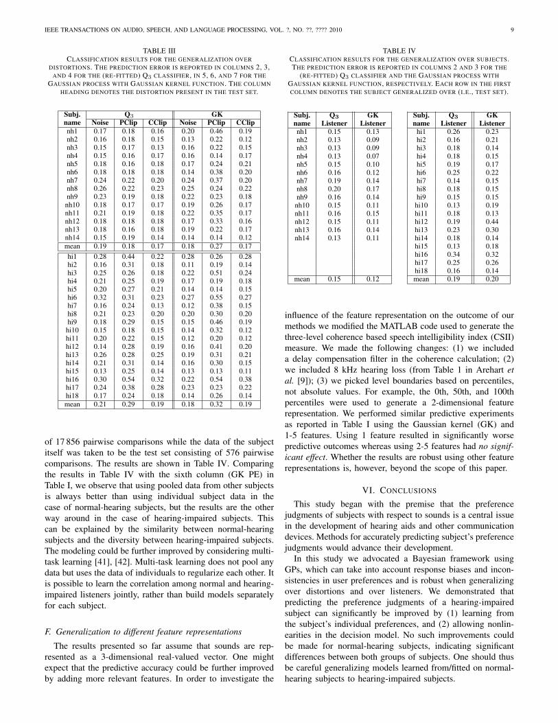
In the case of generalizing over distortions we split the dataper subject in a training set (256 comparisons) and test set(320 comparisons). The training set consisted of all pairwisecomparisons of two distortions (e.g., noise and peak-clipping)and the test set of all pairwise comparisons containing the leftout distortion (e.g., center-clipping). Per subject, this resultedin three experiments for each possible division of distortionsin training and test set. The results are shown in Table III.Each column heading shows the distortion put in the test setand the prediction error on this set per subject. Per subject,the coefficients in the Q3 metric were re-fitted using the256 comparisons in the training data. For the normal-hearingsubjects both the Q3 metric and the GP model perform equallywell, except that the GP model tends to overfit to the trainingdata when the peak clipping distortion is left out of the trainingset. This is exactly what one should expect when taking Fig. 2into account as the features of the signals distorted with noiseare similar to the features of the signals distorted with center-clipping, but quite different from the features of the signalsdistorted with peak-clipping. The same remarks hold for thehearing-impaired subjects, except that the GP model performsbetter than Q3 when the comparisons involving noise are leftout of the training data.

In the case of generalizing over subjects, per subject wepooled all data of all other subjects into one big training set


TABLE IIICLASSIFICATION RESULTS FOR THE GENERALIZATION OVER

DISTORTIONS. THE PREDICTION ERROR IS REPORTED IN COLUMNS 2, 3,AND 4 FOR THE (RE-FITTED) Q3 CLASSIFIER, IN 5, 6, AND 7 FOR THE

GAUSSIAN PROCESS WITH GAUSSIAN KERNEL FUNCTION. THE COLUMNHEADING DENOTES THE DISTORTION PRESENT IN THE TEST SET.

Subj. Q3 GKname Noise PClip CClip Noise PClip CClipnh1 0.17 0.18 0.16 0.20 0.46 0.19nh2 0.16 0.18 0.15 0.13 0.22 0.12nh3 0.15 0.17 0.13 0.16 0.22 0.15nh4 0.15 0.16 0.17 0.16 0.14 0.17nh5 0.18 0.16 0.18 0.17 0.24 0.21nh6 0.18 0.18 0.18 0.14 0.38 0.20nh7 0.24 0.22 0.20 0.24 0.37 0.20nh8 0.26 0.22 0.23 0.25 0.24 0.22nh9 0.23 0.19 0.18 0.22 0.23 0.18nh10 0.18 0.17 0.17 0.19 0.26 0.17nh11 0.21 0.19 0.18 0.22 0.35 0.17nh12 0.18 0.18 0.18 0.17 0.33 0.16nh13 0.18 0.16 0.18 0.19 0.22 0.17nh14 0.15 0.19 0.14 0.14 0.14 0.12mean 0.19 0.18 0.17 0.18 0.27 0.17hi1 0.28 0.44 0.22 0.28 0.26 0.28hi2 0.16 0.31 0.18 0.11 0.19 0.14hi3 0.25 0.26 0.18 0.22 0.51 0.24hi4 0.21 0.25 0.19 0.17 0.19 0.18hi5 0.20 0.27 0.21 0.14 0.14 0.15hi6 0.32 0.31 0.23 0.27 0.55 0.27hi7 0.16 0.24 0.13 0.12 0.38 0.15hi8 0.21 0.23 0.20 0.20 0.30 0.20hi9 0.18 0.29 0.15 0.15 0.46 0.19hi10 0.15 0.18 0.15 0.14 0.32 0.12hi11 0.20 0.22 0.15 0.12 0.20 0.12hi12 0.14 0.28 0.19 0.16 0.41 0.20hi13 0.26 0.28 0.25 0.19 0.31 0.21hi14 0.21 0.31 0.14 0.16 0.30 0.15hi15 0.13 0.25 0.14 0.13 0.13 0.11hi16 0.30 0.54 0.32 0.22 0.54 0.38hi17 0.24 0.38 0.28 0.23 0.23 0.22hi18 0.17 0.24 0.18 0.14 0.26 0.14mean 0.21 0.29 0.19 0.18 0.32 0.19

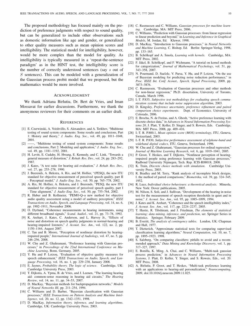
of 17 856 pairwise comparisons while the data of the subjectitself was taken to be the test set consisting of 576 pairwisecomparisons. The results are shown in Table IV. Comparingthe results in Table IV with the sixth column (GK PE) inTable I, we observe that using pooled data from other subjectsis always better than using individual subject data in thecase of normal-hearing subjects, but the results are the otherway around in the case of hearing-impaired subjects. Thiscan be explained by the similarity between normal-hearingsubjects and the diversity between hearing-impaired subjects.The modeling could be further improved by considering multi-task learning [41], [42]. Multi-task learning does not pool anydata but uses the data of individuals to regularize each other. Itis possible to learn the correlation among normal and hearing-impaired listeners jointly, rather than build models separatelyfor each subject.

F. Generalization to different feature representations

The results presented so far assume that sounds are rep-resented as a 3-dimensional real-valued vector. One mightexpect that the predictive accuracy could be further improvedby adding more relevant features. In order to investigate the

TABLE IVCLASSIFICATION RESULTS FOR THE GENERALIZATION OVER SUBJECTS.THE PREDICTION ERROR IS REPORTED IN COLUMNS 2 AND 3 FOR THE

(RE-FITTED) Q3 CLASSIFIER AND THE GAUSSIAN PROCESS WITHGAUSSIAN KERNEL FUNCTION, RESPECTIVELY. EACH ROW IN THE FIRSTCOLUMN DENOTES THE SUBJECT GENERALIZED OVER (I.E., TEST SET).

Subj. Q3 GK Subj. Q3 GKname Listener Listener name Listener Listenernh1 0.15 0.13 hi1 0.26 0.23nh2 0.13 0.09 hi2 0.16 0.21nh3 0.13 0.09 hi3 0.18 0.14nh4 0.13 0.07 hi4 0.18 0.15nh5 0.15 0.10 hi5 0.19 0.17nh6 0.16 0.12 hi6 0.25 0.22nh7 0.19 0.14 hi7 0.14 0.15nh8 0.20 0.17 hi8 0.18 0.15nh9 0.16 0.14 hi9 0.15 0.15

nh10 0.15 0.11 hi10 0.13 0.19nh11 0.16 0.15 hi11 0.18 0.13nh12 0.15 0.11 hi12 0.19 0.44nh13 0.16 0.14 hi13 0.23 0.30nh14 0.13 0.11 hi14 0.18 0.14

hi15 0.13 0.18hi16 0.34 0.32hi17 0.25 0.26hi18 0.16 0.14

mean 0.15 0.12 mean 0.19 0.20

influence of the feature representation on the outcome of ourmethods we modified the MATLAB code used to generate thethree-level coherence based speech intelligibility index (CSII)measure. We made the following changes: (1) we includeda delay compensation filter in the coherence calculation; (2)we included 8 kHz hearing loss (from Table 1 in Arehart etal. [9]); (3) we picked level boundaries based on percentiles,not absolute values. For example, the 0th, 50th, and 100thpercentiles were used to generate a 2-dimensional featurerepresentation. We performed similar predictive experimentsas reported in Table I using the Gaussian kernel (GK) and1-5 features. Using 1 feature resulted in significantly worsepredictive outcomes whereas using 2-5 features had no signif-icant effect. Whether the results are robust using other featurerepresentations is, however, beyond the scope of this paper.

VI. CONCLUSIONS

This study began with the premise that the preferencejudgments of subjects with respect to sounds is a central issuein the development of hearing aids and other communicationdevices. Methods for accurately predicting subject’s preferencejudgments would advance their development.

In this study we advocated a Bayesian framework usingGPs, which can take into account response biases and incon-sistencies in user preferences and is robust when generalizingover distortions and over listeners. We demonstrated thatpredicting the preference judgments of a hearing-impairedsubject can significantly be improved by (1) learning fromthe subject’s individual preferences, and (2) allowing nonlin-earities in the decision model. No such improvements couldbe made for normal-hearing subjects, indicating significantdifferences between both groups of subjects. One should thusbe careful generalizing models learned from/fitted on normal-hearing subjects to hearing-impaired subjects.


The proposed methodology has focused mainly on the pre-diction of preference judgments with respect to sound quality,but can be generalized to include other observations suchas domestic information like age and gender, or generalizedto other quality measures such as mean opinion scores andintelligibility. The statistical model for intelligibility, however,would be more complex than the model for quality. Asintelligibility is typically measured in a ‘repeat-the-sentenceparadigm’ as in the HINT test, the intelligibility score isthe number of correctly understood sentences (say s out ofS sentences). This can be modeled with a generalization ofthe Gaussian process probit model that we proposed, but themathematics would be more involved.

ACKNOWLEDGMENT

We thank Adriana Birlutiu, Dr. Bert de Vries, and ImanMossavat for earlier discussions. Furthermore, we thank theanonymous reviewers for their comments on an earlier draft.

REFERENCES

[1] E. Czerwinski, A. Voishvillo, S. Alexandrov, and A. Terkhov, “Multitonetesting of sound system components: Some results and conclusions, Part1: History and theory,” J. Audio. Eng. Soc., vol. 49, pp. 1011–1048,2001.

[2] ——, “Multitone testing of sound system components: Some resultsand conclusions, Part 2: Modeling and application,” J. Audio. Eng. Soc.,vol. 49, pp. 1181–1192, 2001.

[3] H. Levitt, E. Cudahy, H. Hwang, E. Kennedy, and C. Link, “Towards ageneral measure of distortion,” J. Rehab. Res. Dev., vol. 24, pp. 283–292,1987.

[4] J. Kates, “A test suite for hearing aid evaluation,” J. Rehab. Res. Dev.,vol. 27, pp. 255–278, 1990.

[5] J. Beerends, A. Hekstra, A. Rix, and M. Hollier, “(PESQ), the new ITUstandard for objective measurement of perceived speech quality, part II- Perceptual model,” J. Audio Eng. Soc., vol. 50, pp. 765–778, 2002.

[6] A. Rix, M. Hollier, A. Hekstra, and J. Beerends, “PESQ, the new ITUstandard for objective measurement of perceived speech quality, part I- Time alignment,” J. Audio Eng. Soc., vol. 50, pp. 755–764, 2002.

[7] R. Huber and B. Kollmeier, “PEMO-Q–a new method for objectiveaudio quality assessment using a model of auditory perception,” IEEETransactions on Audio, Speech, and Language Processing, vol. 14, no. 6,pp. 1902–1911, November 2006.

[8] O. Dyrlund, “Coherence measurements in hearing instruments, usingdifferent broadband signals,” Scand. Audiol., vol. 21, pp. 73–78, 1992.

[9] K. Arehart, J. Kates, C. Anderson, and L. Harvey Jr., “Effects ofnoise and distortion on speech quality judgments in normal-hearing andhearing-impaired listeners,” J. Acoust. Soc. Am., vol. 122, no. 2, pp.1150–1164, August 2007.

[10] C. Tan and B. Moore, “Perception of nonlinear distortion by hearing-impaired people,” International Journal of Audiology, vol. 47, no. 5, pp.246–256, 2008.

[11] W. Chu and Z. Ghahramani, “Preference learning with Gaussian pro-cesses,” in Proceedings of the 22nd International Conference on Ma-chine Learning, Bonn, Germany, 2005.

[12] Y. Hu and P. Loizou, “Evaluation of objective quality measures forspeech enhancement,” IEEE Transactions on Audio, Speech, and Lan-guage Processing, vol. 16, no. 1, pp. 229–238, January 2008.

[13] E. Jaynes, Probability theory. The logic of science. Cambridge, UK:Cambridge University Press, 2003.

[14] T. Dijkstra, A. Ypma, B. de Vries, and J. Leenen, “The learning hearingaid: common-sense reasoning in hearing aid circuits,” The HearingReview, vol. 14, no. 11, pp. 34–53, 2007.

[15] D. MacKay, “Bayesian methods for backpropagation networks,” Modelsof Neural Networks III, pp. 211–254, 1994.

[16] C. Williams and D. Barber, “Bayesian classification with Gaussianprocesses,” IEEE Transactions on Pattern Analysis and Machine Intel-ligence, vol. 20, no. 12, pp. 1342–1351, 1998.

[17] D. MacKay, Information theory, inference, and learning algorithms.Cambridge, UK: Cambridge University Press, 2003.

[18] C. Rasmussen and C. Williams, Gaussian processes for machine learn-ing. Cambridge, MA: MIT Press, 2006.

[19] C. Williams, “Prediction with Gaussian processes: from linear regressionto linear prediction and beyond,” in Learning and Inference in GraphicalModels, M. Jordan, Ed. Kluwer, 1998.

[20] D. MacKay, “Introduction to Gaussian processes,” in Neural Networksand Machine Learning, C. Bishop, Ed. Berlin: Springer-Verlag, 1998,pp. 133–165.

[21] B. Scholkopf and A. Smola, Learning with kernels. Cambridge, MA:MIT Press, 2002.

[22] F. Jakel, B. Scholkopf, and F. Wichmann, “A tutorial on kernel methodsfor categorization,” Journal of Mathematical Psychology, vol. 51, pp.343–358, 2007.

[23] N. Pourmand, D. Suelzle, V. Parsa, Y. Hu, and P. Loizou, “On the useof Bayesian modeling for predicting noise reduction performance,” inProc. IEEE Int. Conf. Acoust., Speech, Signal Processing, 2009, pp.3873–3876.

[24] C. Rasmussen, “Evaluation of Gaussian processes and other methodsfor non-linear regression,” Ph.D. dissertation, University of Toronto,Canada, March 1996.

[25] I.-T. P.835, Subjective test methodology for evaluating speech commu-nication systems that include noise suppression algorithm, 2003.

[26] D. Kingsley, Preference uncertainty, preference refinement and pairedcomparison choice experiments. Dept. of Economics. University ofColorado, 2006.

[27] E. Brochu, N. de Freitas, and A. Ghosh, “Active preference learning withdiscrete choice data,” in Advances in Neural Information Processing Sys-tems 20, J. Platt, Y. Koller, D. Singer, and S. Roweis, Eds. Cambridge,MA: MIT Press, 2008, pp. 409–416.

[28] I.-T. R. P.800.1, Mean opinion score (MOS) terminology, ITU, Geneva,Switzerland, 2003.

[29] I.-T. R. P.830, Subjective performance assessment of telphone-band andwideband digital codecs, ITU, Geneva, Switzerland, 1996.

[30] W. Chu and Z. Ghahramani, “Gaussian processes for ordinal regression,”Journal of Machine Learning Research, vol. 6, pp. 1019–1041, 2005.

[31] P. Groot, T. Heskes, and T. Dijkstra, “Nonlinear perception of hearing-impaired people using preference learning with Gaussian processes,”Radboud University Nijmegen, Tech. Rep. ICIS-R08018, 2008.

[32] K. Train, Discrete choice methods with simulation. Cambridge Uni-versity Press, 2003.

[33] R. Bradley and M. Terry, “Rank analysis of incomplete block designs,I. the method of paired comparisons,” Biometrika, vol. 39, pp. 324–345,1952.

[34] R. Luce, Individual choice behaviours: a theoretical analysis. Mineola,New York: Dover publications, 2005.

[35] M. Nilson, S. Soli, and J. Sullivan, “Development of the hearing in noisetest for the measurement of speech reception thresholds in quiet and innoise,” J. Acoust. Soc. Am., vol. 95, pp. 1085–1099, 1994.

[36] J. Kates and K. Arehart, “Coherence and the speech intelligibility index,”J. Acoust. Soc. Am., vol. 117, pp. 2224–2237, 2005.

[37] T. Hastie, R. Tibshirani, and J. Friedman, The elements of statisticallearning: data mining, inference, and prediction, ser. Springer Series inStatistics. Springer, February 2009.

[38] B. Everitt, The analysis of contingency tables. London, UK: Chapmanand Hall, 1977.

[39] T. Dietterich, “Approximate statistical tests for comparing supervisedclassification learning algorithms,” Neural Computation, vol. 10, no. 7,pp. 1895–1923, 1998.

[40] S. Salzberg, “On comparing classifiers: pitfalls to avoid and a recom-mended approach,” Data Mining and Knowledge Discovery, vol. 1, pp.317–327, 1997.

[41] E. Bonilla, K. Ming, A. Chai, and C. Williams, “Multi-task gaussianprocess prediction,” in Advances in Neural Information ProcessingSystems, J. Platt, D. Koller, Y. Singer, and S. Roweis, Eds., vol. 20.MIT Press, 2008.

[42] A. Birlutiu, P. Groot, and T. Heskes, “Multi-task preference learningwith an applications to hearing-aid personalization,” Neurocomputing,2009, doi:10.1016/j.neucom.2009.11.025.


Perry Groot received the M.Sc degrees in Com-puter Science (artificial intelligence) and Mathemat-ics (topology) in 1998 and a Ph.D. degree from theDepartment of Artificial Intelligence, Vrije Univer-sity Amsterdam in 2003. Currently, he is a researcherat the Institute for Computing and Information Sci-ences at the Radboud University Nijmegen, theNetherlands. His research interests include Bayesianreasoning applications, particularly the use of Gaus-sian processes for preference learning and functionoptimization.

Tom Heskes received both the M.Sc and Ph.Ddegrees in Physics from the University of Nijmegen,The Netherlands, in 1989 and 1993, respectively.After a year of postdoctoral work at the BeckmanInstitute in Urbana-Champaign, Illinois, he workedfrom 1994 to 2004 as a researcher for SNN, Nijme-gen. Between 1997 and 2004 he headed the companySMART Research BV, specialized in applicationsof neural networks and related techniques. Since2004 he works at the Institute for Computing andInformation Sciences at the Faculty of Science,

Radboud University Nijmegen, where he is now a full professor in artificialintelligence. Prof. Heskes is Editor-in-Chief of Neurocomputing. His researchinterests include theoretical and practical aspects of neural networks, machinelearning, and probabilistic graphical models.

Tjeerd M.H. Dijkstra received his M.Sc degreein Physics from the University of Utrecht in 1988and his Ph.D. in Biophysics from the University ofNijmegen in 1994. After a post-doc in Psychologyat the University of Pennsylvania, he held a facultyposition in Psychology at The Ohio State University.From 2005 until 2009 he worked at the hearing-aidcompany GN ReSound in Eindhoven. His researchinterests include human perception, both visual andauditory, human motor control, bioinformatics andsystems biology.

James M. Kates was born in Brookline, Mas-sachusetts, in 1948. He received the Bachelor ofScience and Master of Science degrees in electri-cal engineering from the Massachusetts Institute ofTechnology in 1971, and the professional degreeof Electrical Engineer from M.I.T. in 1972. Hecurrently holds the position of Research Fellow withGN ReSound. He has an office in Boulder, Colorado,where he is involved in research in digital signalprocessing for hearing aids. He is also an adjunctprofessor in the Department of Speech Language

and Hearing Sciences at University of Colorado in Boulder, where heteaches courses in hearing-aid technology and conducts research in auditoryperception, hearing loss, and signal processing for hearing aids. Prior positionsinclude Senior Research Scientist and adjunct faculty at the Center forResearch in Speech and Hearing Sciences of the City University of NewYork, Director of Basic Research for Siemens Hearing Aids in Piscataway,NJ, and work in radio direction finding, speech coding and enhancement,digital audio, and loudspeaker design and evaluation. He is a Fellow of theAcoustical Society of America and a Fellow of the Audio Engineering Society,and is the author or co-author of 50 technical papers, seven book chapters,and holds 20 US patents. His book Digital Hearing Aids was published in2008 by Plural Publishing, San Diego.

Predicting Preference Judgments of Individual Normal and Hearing-Impaired Listeners With Gaussian...

Documents

Transcript of Predicting Preference Judgments of Individual Normal and Hearing-Impaired Listeners With Gaussian...