REVISTA DE METODOS CUANTITATIVOS PARA LA

ECONOMIA Y LA EMPRESA (26). Paginas 294–314.Diciembre de 2018. ISSN: 1886-516X. D.L: SE-2927-06.www.upo.es/revistas/index.php/RevMetCuant/article/view/2810

Predicting Corporate Failure: TheGRASP-LOGIT Model

Casado Yusta, SilviaDepartamento de Economıa Aplicada

Universidad de Burgos (Espana)

E-mail: scasado@ubu.es

Nunez Letamendıa, LauraDepartamento de Finanzas

IE Business School, IE University (Espana)

E-mail: laura.nunez@ie.edu

Pacheco Bonrostro, Joaquın AntonioDepartamento de Economıa Aplicada

Universidad de Burgos (Espana)

E-mail: jpacheco@ubu.es

ABSTRACT

Predicting corporate failure is an important problem in management sci-ence. This study tests a new method for predicting corporate failure on asample of Spanish firms. A GRASP (Greedy Randomized Adaptive SearchProcedure) strategy is proposed to use a feature selection algorithm to selecta subset of available financial ratios, as a preliminary step in estimating amodel of logistic regression for predicting corporate failure. Selecting onlya subset of variables (financial ratios) reduces the costs of data acquisition,increases prediction accuracy by excluding irrelevant variables, and providesinsight into the nature of the prediction problem allowing a better under-standing of the final classification model. The proposed algorithm, that itis named GRASP-LOGIT algorithm, performs better than a simple logisticregression in that it reaches the same level of forecasting ability with feweraccounting ratios, leading to a better interpretation of the model and there-fore to a better understanding of the failure process.

Keywords: Financial distress; accounting ratios; feature selection; GRASPmetaheuristic; logistic regression.JEL classification: C39; C44; G33.MSC2010: 62P20; 62J05; 68T20; 90C59; 91G50.

Artıculo recibido el 31 de octubre de 2017 y aceptado el 21 de abril de 2018.

294

Prediccion de la quiebra empresarial:el modelo GRASP-LOGIT

RESUMEN

La prediccion de la quiebra empresarial es un problema que goza de unagran relevancia en las ciencias empresariales. En este trabajo se proponeun nuevo metodo para predecir la quiebra empresarial en una muestra deempresas espanolas. Concretamente se trata de un algoritmo de seleccionde variables basado en la estrategia metaheurıstica GRASP (procedimientode busqueda adaptativa aleatoria y voraz) para seleccionar un subconjuntode ratios financieros, como un paso preliminar para estimar un modelo deregresion logıstica que prediga la quiebra empresarial. La seleccion de unsubconjunto de ratios financieros, de entre todos los disponibles, reduce loscostes de adquisicion de datos, aumenta la precision de la prediccion al ex-cluir las variables irrelevantes y proporciona informacion sobre la naturalezadel problema de prediccion. Todo lo anterior permite una mejor comprensiondel modelo de clasificacion final. Nuestro nuevo modelo, al que llamamosmodelo GRASP-LOGIT, funciona mejor que una simple regresion logısticaen el sentido de que alcanza el mismo nivel de capacidad de prediccion conmenos ratios contables, lo que lleva a una mejor interpretacion del modeloy, por lo tanto, a una mejor comprension del proceso de quiebra empresarial.

Palabras claves: dificultades financieras; ratios contables; seleccion decaracterısticas; metaheurıstico GRASP; regresion logıstica.Clasificacion JEL: C39; C44; G33.MSC2010: 62P20; 62J05; 68T20; 90C59; 91G50.

295

296

1. INTRODUCTION

Since the pioneering works of Beaver (1966) and Altman (1968), many studies have been devoted to

predicting financial distress (throughout this paper, we use the terms “corporate failure” and

“financial distress” to refer to both bankruptcy and temporary receivership) using accounting-based

variables; however, theoretical approaches to corporate failure are rare. Some papers have based

bankruptcy prediction models on the glamber’s ruin model of probability theory. There has been also

some other attempts of building a bankruptcy theory as Scott (1977), who proposes a model that,

contrary to the glamber’s ruin model, allows the firm to access external capital. For a survey of these

theoretical papers, see Scott (1981). But, as Laitinen and Laitinen (2000) pointed out, these

theoretical grounds are too simplified or too indefinite to give advice for the selection of the

functional form of the model; yet there is not a general accepted economic theory about corporate

failure. The lack of a unified theory makes difficult to use an economically grounded approach by

stating theoretical a priori reasons for using one variable or another and then testing whether the

theoretical hypotheses can be supported by the empirical evidence. But, as Jones (1987) has argued,

the lack of a theory is not necessarily a serious impediment to studying corporate failure, if we can

apply an economic interpretation to an empirically derived model. In fact, empirical findings that can

be interpreted via economic reasoning can help to build a corporate failure theory.

Existing empirical studies reflect a lack of consensus on what constitutes the best

methodological approach to analyze financial distress. Preliminary studies on insolvency used

univariate techniques (Beaver, 1966). Two years later, discriminant multivariate analysis, which

became the predominant technique during the 1970s, was introduced by Altman (1968).

Subsequently, in the 1980s, discriminant analysis, whose principle of normality for predictors and

equality for variance-covariance matrices is usually violated by the distributions of financial ratios,

was complemented by a logit and probit analysis; see Ohlson (1980), Zmijewski (1984) and Lennox

(1999), among others. Despite the drawbacks of discriminant analysis, it produces classification

results very similar to those of the logit models. Nonparametric models were also applied; e.g. the

recursive partitioning algorithm (Frydman et al., 1985) and the ID3 (Messier et al., 1988). Researchers

have used other approaches to address the problem of predicting failure, namely: Neural networks

(Altman et al., 1994; Etheridge et al., 1996; Baesens et al., 2003a; Iturriaga and Sanz, 2015), genetic

algorithms (Varetto, 1998; Sexton et al., 2003), decision trees (Curran and Mingers, 1994), Bayesian

analysis (Sarkar and Sriram, 2001), multidimensional scaling (Neophytou and Molinero, 2004), hazard

models (Shumway, 2001; Lee and Urrutia, 1996), support vector machine (Wu et al., 2007; Hua et al.,

2007) or more sophisticated logit models (Laitinen and Laitinen, 2000; Jones and Hensher, 2004; Li et

al., 2011). In Balcaen and Ooghe (2006), an overview of classic statistical methodologies that analyze

business failure prediction and their related problems is shown. More recent works about

bankruptcy prediction were published by Yang et al. (2011), Jeong et al. (2012), Lu et al. (2015) and

Liang et al. (2016).

This study uses a new methodological approach based on the idea that a model performs

better when it uses a subset of superior variables from a set of candidate variables. There can be

many reasons for selecting only a subset of the variables instead of the whole set of candidate

variables –see Liu and Motoda (1998) and Reunanen, 2003–: (1) It is cheaper to measure only a

reduced set of variables; (2) prediction accuracy may be improved through exclusion of redundant

and irrelevant variables; (3) the predictor to be built is usually simpler and potentially faster when

fewer input variables are used; and (4) knowing which variables are relevant can give insight into the

nature of the prediction problem and allows a better understanding of the final classification model.

This last point is important in this field, where it is necessary to know not only whether a company is

likely to fail, but why. As pointed out by Baesens et al. (2003b, p.312), “[m]ost of these studies

297

[credit-risk studies] focus primarily on developing classification models with high predictive accuracy

without paying any attention to explaining how the classifications are being made. Clearly, this plays

a pivotal role in credit-risk evaluation, as the evaluator may be required to give a justification for why

a certain credit application is approved or rejected”.

How to choose this superior subset of variables is the problem known in the literature as

feature selection. Research in feature selection started in the early 1960s (Lewis, 1962; Sebestyen,

1962). Over the past four decades, extensive research into feature selection has been conducted.

Some of these works are Ganster et al. (2001), Lee et al. (2003), Crone and Finlay (2012) and

Mangalova and Agafonov (2014). Besides, the problem of selecting variables from a large candidate

pool abounds in areas such as discriminant analysis (Pacheco et al., 2006), linear regression (Wang et

al., 2007, Arslan, 2012) and logistic regression (Pacheco et al., 2009; Matsui, 2014). The selection of

the best subset of variables for building the predictor is not a trivial question, because the number of

subsets to be considered grows exponentially with the number of candidate variables. Even with a

moderate number of candidate variables, not all the possible subsets can be evaluated, which means

that feature selection is a NP-hard problem –non-deterministic polynomial-time hard in

computational complexity theory, see Kohavi (1995) and Cotta et al. (2004– and therefore, there is

no guarantee of finding the solution.

For feature selection problems, two different methodological approaches have been

developed: Exact techniques (enumerative techniques), which guarantee an optimal solution, but are

applicable only in small instances; and approximate techniques, which can find good solutions

(although they cannot guarantee the optimum) in a reasonable amount of time. Among the latter,

the Narendra-Fukunaga algorithm (Narendra and Fukunaga, 1977) is one of the best known, but as

Jain and Zongker (1997) pointed out, this algorithm is impractical for problems with a large number

of features. Among the heuristic techniques, there are for example those based on genetic

algorithms (Bala et al., 1996; Jourdan et al., 2001; Oliveira et al., 2003; Meiri and Zahavi, 2006; Zhang

et al., 2015).

A feature selection algorithm based on the heuristic approach is proposed as a preliminary

step in estimating a logit model for predicting corporate failure. In this paper, only quantitative

variables (accounting ratios) are used to classify firms as healthy or financially distressed. Using only

quantitative variables allows a better measurement and comparison of their classificatory capacity.

Thus, a variable selection method especially adapted to these kinds of variables can be developed,

which will therefore be more efficient. Specifically, GRASP (Greedy Randomized Adaptive Search

Procedure) is designed to solve the feature subset selection problem. The GRASP algorithm (Feo and

Resende, 1995) is used to select accounting ratios, for a sample of 198 Spanish companies, which are

then used in a logit model that is called the GRASP-LOGIT model. The results obtained by the GRASP-

LOGIT model are superior to those from the traditional logit in the sense that the GRASP-LOGIT

model reaches the same level of forecasting ability with fewer variables (accounting ratios), leading

to a better interpretation of the model and therefore to a better understanding of the failure

process. As far as we know, this is the first study that has combined both methodologies, the GRASP

and the logistic regression, logit.

The remainder of this paper is organized as follows. Section 2 describes the sample, and

Section 3 describes the GRASP procedure. Section 4 presents data from the estimation of the GRASP-

LOGIT model. Section 5 reports the main conclusions.

298

2. SAMPLE SELECTION AND ACCOUNTING RATIOS

2.1 COMPANIES

The data have been obtained from the SABI database from Bureau Van Dijk (BVD), one of Europe's

leading publishers of electronic business information databases and one of the providers of the

Wharton Research Data Services. SABI comprises all the companies whose accounts are placed on

the Spanish Mercantile Registry. BVD databases have been used in previous failure studies on

companies from European countries (e.g. Ooghe and and Balcaen, 2002). The sample consists of 198

Spanish companies, of which approximately one-third (67) are failed companies placed under

temporary receivership (18, or 27%) or declare bankrupt (49, or 73%). The remaining 131 companies

are healthy or, at least, “active,” firms. We use also an additional testing sample of 61 companies, of

which 40 are healthy and 21 are failed firms. All these companies have complete data available for

three consecutive years. Thus, our sample selection method does not pair failed/healthy firms by

sector and size. Although the paired sample method is usual, not all authors follow it, because of its

arbitrariness and the lack of empirical evidence to support or disconfirm its superiority (see Ohlson,

1980: p. 112). It might actually be more interesting to include the variables “size” and “sector” as

predictors than their use for matching (see Lennox, 1999).

CNAE Failed Healthy

01 Farming 0 3

02 Forestry 0 1

15 Food and beverage sector 5 6

17 Textile industry 3 1

18 Clothing industry 1 1

19 Shoemaking 0 1

20 Wood and cork industry 1 2

21 Paper industry 0 1

22 Publishing and graphic arts 2 3

24 Chemical industry 0 4

25 Manufacturing of plastic and rubber products 1 2

26 Manufacturing of other mineral products 0 1

27 Metalwork 2 1

28 Manufacturing of metal products 4 3

29 Building machinery 5 3

31 Manufacturing of electric equipment 2 0

33 Manufacturing of medical equipment 0 1

34 Manufacturing of motorized vehicles 0 1

35 Manufacturing of other transport material 1 0

36 Manufacturing of furniture; other industries 4 3

41 Water collecting, purifying, and distribution 0 1

45 Building 10 16

50 Sales and repair of. motorized vehicles 0 5

51 Wholesale sales 12 16

52 Retail sales 7 11

55 Hospitality sector 0 4

60 Land transport 0 2

61 Sea transport 0 1

63 Transport-related activities 1 1

65 Finance trading (except insurance) 0 1

70 Real estate agents 2 16

74 Other business activities 2 12

80 Education 2 0

85 Hospital and veterinary activities 0 2

92 Cultural, recreational, and sport activities 0 4

93 Personal services activities 0 1

Total 67 131

Table 1: Failed/healthy firms by CNAE classification

299

Table 1 shows the distribution of failed and healthy firms by sector. We can observe that 55

of the 67 failed firms do have healthy counterparts in the same sector (as defined by the two-digit

CNAE [Spanish Classification of Economic Activities] code). The extra 12 failed companies are

distributed over 8 sectors, where failed firms outnumber healthy ones.

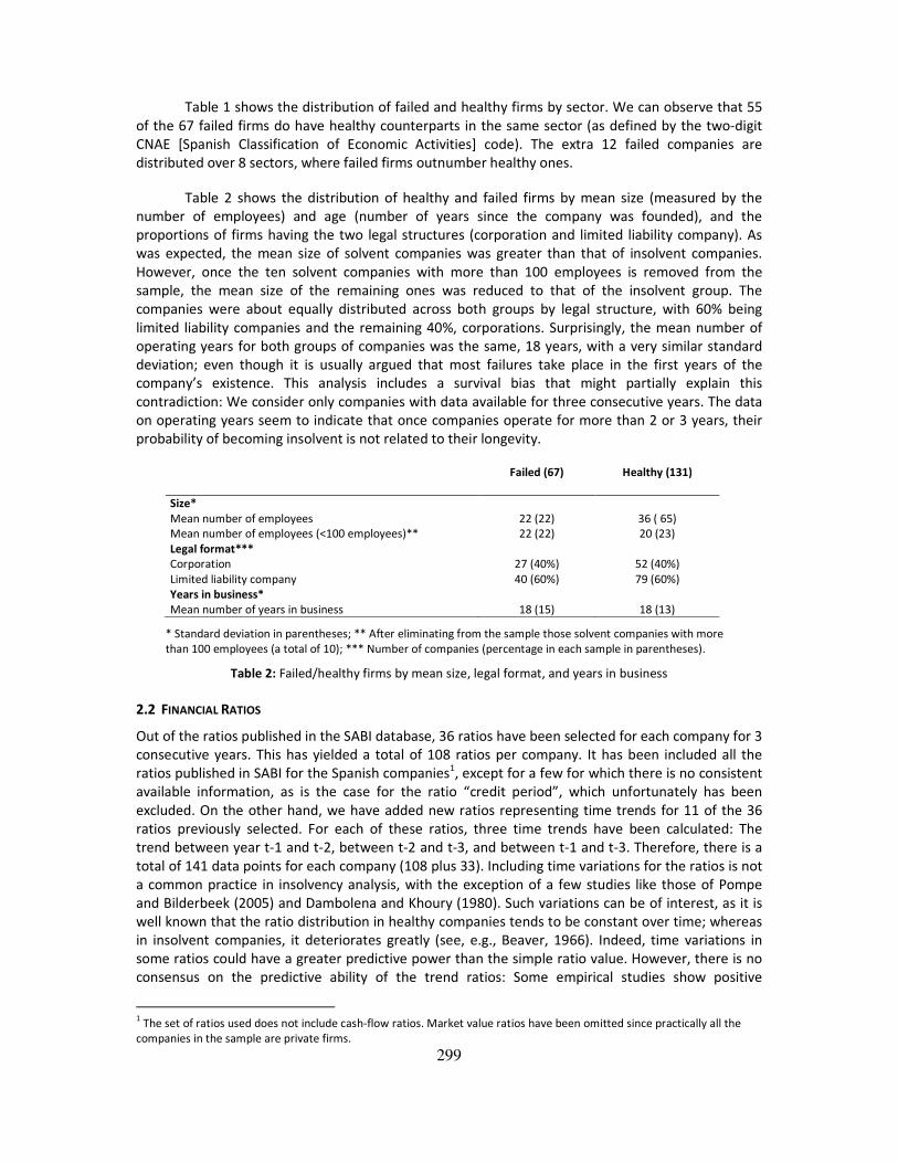
Table 2 shows the distribution of healthy and failed firms by mean size (measured by the

number of employees) and age (number of years since the company was founded), and the

proportions of firms having the two legal structures (corporation and limited liability company). As

was expected, the mean size of solvent companies was greater than that of insolvent companies.

However, once the ten solvent companies with more than 100 employees is removed from the

sample, the mean size of the remaining ones was reduced to that of the insolvent group. The

companies were about equally distributed across both groups by legal structure, with 60% being

limited liability companies and the remaining 40%, corporations. Surprisingly, the mean number of

operating years for both groups of companies was the same, 18 years, with a very similar standard

deviation; even though it is usually argued that most failures take place in the first years of the

company’s existence. This analysis includes a survival bias that might partially explain this

contradiction: We consider only companies with data available for three consecutive years. The data

on operating years seem to indicate that once companies operate for more than 2 or 3 years, their

probability of becoming insolvent is not related to their longevity.

Failed (67) Healthy (131)

Size*

Mean number of employees 22 (22) 36 ( 65)

Mean number of employees (<100 employees)** 22 (22) 20 (23)

Legal format***

Corporation 27 (40%) 52 (40%)

Limited liability company 40 (60%) 79 (60%)

Years in business*

Mean number of years in business 18 (15) 18 (13)

* Standard deviation in parentheses; ** After eliminating from the sample those solvent companies with more

than 100 employees (a total of 10); *** Number of companies (percentage in each sample in parentheses).

Table 2: Failed/healthy firms by mean size, legal format, and years in business

2.2 FINANCIAL RATIOS

Out of the ratios published in the SABI database, 36 ratios have been selected for each company for 3

consecutive years. This has yielded a total of 108 ratios per company. It has been included all the

ratios published in SABI for the Spanish companies1, except for a few for which there is no consistent

available information, as is the case for the ratio “credit period”, which unfortunately has been

excluded. On the other hand, we have added new ratios representing time trends for 11 of the 36

ratios previously selected. For each of these ratios, three time trends have been calculated: The

trend between year t-1 and t-2, between t-2 and t-3, and between t-1 and t-3. Therefore, there is a

total of 141 data points for each company (108 plus 33). Including time variations for the ratios is not

a common practice in insolvency analysis, with the exception of a few studies like those of Pompe

and Bilderbeek (2005) and Dambolena and Khoury (1980). Such variations can be of interest, as it is

well known that the ratio distribution in healthy companies tends to be constant over time; whereas

in insolvent companies, it deteriorates greatly (see, e.g., Beaver, 1966). Indeed, time variations in

some ratios could have a greater predictive power than the simple ratio value. However, there is no

consensus on the predictive ability of the trend ratios: Some empirical studies show positive

1 The set of ratios used does not include cash-flow ratios. Market value ratios have been omitted since practically all the

companies in the sample are private firms.

300

evidence (i.e., Dambolena and Khoury, 1980), whereas others find negative evidence (i.e., Pompe

and Bilderbeek, 2005). As an additional advantage, it seems a priori that such variations might have

greater independence from the activity sector and the company size than from the simple ratio.

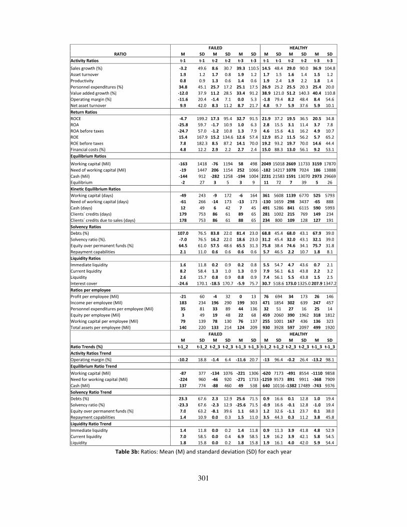
Tables 3a and 3b show the definitions of the financial ratios and their main descriptors respectively

(M=mean and SD= Standard Deviation).

Activity Ratios

Sales growth (%) [[Sales_t – Sales_t-1] / Sales_t-1] x 100%

Asset turnover Sales / Total assets

Productivity [Operating revenues – Consumption and oper. expenditures] / Personnel expend.

Personnel expenditures (%) [Personnel expenditures / Operating revenues] x 100%

Value added growth (%) [[Value added_t – Value added_t-1] / Value added_t-1] x 100%

Operating margin (%) [Earnings before taxes / Operating revenues] x 100%

Net asset turnover Operating revenues / Permanent funds

Return Ratios

ROCE [Earnings before taxes + Financial expenses] / Permanent funds] x 100%

ROA [Earnings / Total assets] x 100%

ROA before taxes [Earnings before taxes / Total assets] x 100%

ROE [Earnings / Equity] x 100%

ROE before taxes [Earnings before taxes / Equity] x 100%

Financing costs (%) [Financing costs / Sales] x 100%

Equilibrium Ratios

Working capital (€) Equity + Provisions for C & E+ LT creditors – Fixed assets

Need for working capital (€) [EHNDP + Accrued expenses + (Inventory + Accounts receivable)] –

[Accrued incomes + Accounts payable]

Cash (€) ST financial investments + Cash – ST debt

Equilibrium Equity + provisions for C & E+ LT debt] / Fixed assets

Kinetic Equilibrium Ratios

Working capital (days) [Working capital / sales] x 360

Need for working capital (days) [Need for working capital / Sales] x 360

Cash (days) [Cash / Sales] x 360

Clients´ credits (days) [Accounts receivable / Operating incomes] x 360

Clients´ credits due to sales (days) [Accounts receivable / Sales] x 360

Solvency Ratios

Debt (%) [Total liabilities / Total liabilities and owners’ equity ] x 100%

Solvency ratio (%) [Equity / Total assets] x 100%

Equity over permanent funds (%) [[Equity / [ Equity + LT creditors + Provisions for C & E]] x 100%

Repayment capabilities [LT and ST creditors / [Sales + Depreciations + Provisions + Equity]

Liquidity Ratios

Immediate liquidity [ST Financial investments + Cash] / Accounts payable]

Current liquidity [Cash + ST financial investments + Accounts receivable+ Inventory] / ST Liabilities

Liquidity [Cash + ST financial investments + accounts receivable] / ST liabilities

Interest cover Operating profit / Financial expenses

Ratios per employee

Profit per employee Earnings before taxes / Number of employees

Income per employee Operating incomes / Number of employees

Personnel costs per employee Personnel expenses / Number of employees

Equity per employee Equity / Number of employees

Working capital per employee Working capital / Number of employees

Total assets per employee Total assets / Number of employees

*Abbreviations: EHNDP (Equity Holders by Non-Demanded Payments); ST (Short Term); LT (Long Term); C&E (Contingencies and Expenses).

Table 3a: Definitions of ratios

301

FAILED HEALTHY

RATIO M SD M SD M SD M SD M SD M SD

Activity Ratios t-1 t-1 t-2 t-2 t-3 t-3 t-1 t-1 t-2 t-2 t-3 t-3

Sales growth (%) -3.2 49.6 8.6 30.7 39.3 110.5 14.5 48.4 29.0 90.0 36.9 104.8

Asset turnover 1.9 1.2 1.7 0.8 1.9 1.2 1.7 1.5 1.6 1.4 1.5 1.2

Productivity 0.8 0.9 1.3 0.6 1.4 0.6 1.9 2.4 1.9 2.2 1.8 1.4

Personnel expenditures (%) 34.8 45.1 25.7 17.2 25.1 17.5 26.9 25.2 25.5 20.3 25.4 20.0

Value added growth (%) -12.0 37.9 11.2 28.5 33.4 91.2 38.9 121.0 51.2 140.3 40.4 110.8

Operating margin (%) -11.6 20.4 -1.4 7.1 0.0 5.3 -1.8 79.4 8.2 48.4 8.4 54.6

Net asset turnover 9.9 42.0 8.3 11.2 8.7 21.7 4.8 9.7 5.9 37.6 5.9 10.1

Return Ratios

ROCE -4.7 199.2 17.3 95.4 32.7 91.5 21.9 37.2 19.5 36.5 20.5 34.8

ROA -25.8 59.7 -1.7 10.9 1.0 6.3 2.8 15.5 3.1 11.4 3.7 7.8

ROA before taxes -24.7 57.0 -1.2 10.8 1.3 7.9 4.6 15.6 4.1 16.2 4.9 10.7

ROE 15.4 167.9 15.2 134.6 12.6 57.4 12.9 85.2 11.5 56.2 5.7 65.2

ROE before taxes 7.8 182.3 8.5 87.2 14.1 70.0 19.2 93.2 19.7 70.0 14.6 44.4

Financial costs (%) 4.8 12.2 2.9 2.2 2.7 2.4 15.0 88.3 13.0 56.1 9.2 53.1

Equilibrium Ratios

Working capital (Mil) -163 1418 -76 1194 58 498 2049 15018 2669 11733 3159 17870

Need of working capital (Mil) -19 1447 206 1154 252 1066 -182 14217 1078 7024 186 13888

Cash (Mil) -144 912 -282 1258 -194 1004 2231 21583 1591 13070 2973 29669

Equilibrium -2 27 3 5 3 9 11 72 7 39 5 26

Kinetic Equilibrium Ratios

Working capital (days) -49 243 -9 172 -6 164 361 5608 1139 6770 525 5793

Need of working capital (days) -61 266 -14 173 -13 173 -130 1659 298 3437 -65 888

Cash (days) 12 49 6 42 7 45 491 5286 841 6115 590 5993

Clients´ credits (days) 179 753 86 61 89 65 281 1002 215 769 149 234

Clients´ credits due to sales (days) 178 753 86 61 88 65 234 800 109 128 127 191

Solvency Ratios

Debts (%) 107.0 76.5 83.8 22.0 81.4 23.0 68.8 45.4 68.0 43.1 67.9 39.0

Solvency ratio (%). -7.0 76.5 16.2 22.0 18.6 23.0 31.2 45.4 32.0 43.1 32.1 39.0

Equity over permanent funds (%) 64.5 61.0 57.5 48.6 65.5 31.3 75.8 38.4 74.6 34.1 75.7 31.8

Repayment capabilities 2.1 11.0 0.6 0.6 0.6 0.6 5.7 46.5 2.2 10.7 1.8 8.1

Liquidity Ratios

Immediate liquidity 1.6 11.8 0.2 0.9 0.2 0.8 5.5 54.7 4.7 43.6 0.7 2.1

Current liquidity 8.2 58.4 1.3 1.0 1.3 0.9 7.9 56.1 6.1 43.8 2.2 3.2

Liquidity 2.6 15.7 0.8 0.9 0.8 0.9 7.4 56.1 5.5 43.8 1.5 2.5

Interest cover -24.6 170.1 -18.5 170.7 -5.9 75.7 30.7 518.6 173.0 1325.0 207.9 1347.2

Ratios per employee

Profit per employee (Mil) -21 60 -4 32 0 13 76 694 34 173 26 146

Income per employee (Mil) 183 234 196 290 199 303 471 1854 302 639 247 457

Personnel expenditures per employee (Mil) 35 81 33 89 44 136 32 51 27 16 25 14

Equity per employee (Mil) 3 49 19 48 22 68 459 2060 390 1962 318 1812

Working capital per employee (Mil) 79 139 78 130 76 137 255 1001 167 436 136 323

Total assets per employee (Mil) 140 220 133 214 124 209 930 3928 597 2097 499 1920

FAILED HEALTHY

M SD M SD M SD M SD M SD M SD

Ratio Trends (%) t-1_2 t-1_2 t-2_3 t-2_3 t-1_3 t-1_3 t-1_2 t-1_2 t-2_3 t-2_3 t-1_3 t-1_3

Activity Ratios Trend

Operating margin (%) -10.2 18.8 -1.4 6.4 -11.6 20.7 -13 96.4 -0.2 26.4 -13.2 98.1

Equilibrium Ratio Trend

Working capital (Mil) -87 377 -134 1076 -221 1306 -620 7173 -491 8554 -1110 9858

Need for working capital (Mil) -224 960 -46 920 -271 1733 -1259 9573 891 9911 -368 7909

Cash (Mil) 137 774 -88 460 49 538 640 10116 -1382 17489 -743 9376

Solvency Ratio Trend

Debts (%) 23.3 67.6 2.3 12.9 25.6 71.5 0.9 16.6 0.1 12.8 1.0 19.4

Solvency ratio (%) -23.3 67.6 -2.3 12.9 -25.6 71.5 -0.9 16.6 -0.1 12.8 -1.0 19.4

Equity over permanent funds (%) 7.0 63.2 -8.1 39.6 1.1 68.3 1.2 32.6 -1.1 23.7 0.1 38.0

Repayment capabilities 1.4 10.9 0.0 0.3 1.5 11.0 3.5 44.3 0.3 11.2 3.8 45.8

Liquidity Ratio Trend

Immediate liquidity 1.4 11.8 0.0 0.2 1.4 11.8 0.9 11.3 3.9 41.8 4.8 52.9

Current liquidity 7.0 58.5 0.0 0.4 6.9 58.5 1.9 16.2 3.9 42.1 5.8 54.5

Liquidity 1.8 15.8 0.0 0.2 1.8 15.8 1.9 16.1 4.0 42.0 5.9 54.4

Table 3b: Ratios: Mean (M) and standard deviation (SD) for each year

302

The relationship between the mean values of the ratios in both groups (healthy and failed)

generally is the expected one, with some exceptions (e.g. financial costs % and liquidity ratios).

However, when such exceptions are examined in detail, it can be seen that they are due to extreme

values in the ratios of some of the companies.

3. THE GRASP ALGORITHM FOR FEATURE SELECTION

3.1 THE FEATURE SELECTION PROBLEM

The problem of selecting the subset of financial ratios with superior classificatory performance can

be formulated as follows: Let V be a set of m variables (financial ratios) such that V = {1, 2,..., m}, and

let A be a set of cases (firms). For each case (firm), the class to which it belongs (“healthy” or “failed”)

is known. Given a predefined value p ∈ N, p < m, we have to find a subset S ⊂ V, with a size p, with

the greatest classificatory capacity. The classificatory capacity for each subset S ⊂ V is estimated by

the function f(S), which is computed as follows: The partition A = A1 ∪ A2 is made in A. For each case

(firm) in A2, the Euclidean distance with every case in A1 is computed and the class (healthy or failed)

of the closest case is assigned. The value of f(S) is the percentage of hits in the assigned classes

(healthy or failed), namely the number of times that the assigned class is the same as the real class.

The partitions A1 and A2 have approximately the same size (number of firms) and the same

proportions of firms in both classes, healthy and failed.

3.2 THE GRASP ALGORITHM

GRASP constructs solutions with controlled randomization and a greedy function. Most GRASP

implementations also include a local search that is used to improve upon the solutions generated

with the randomized greedy function. GRASP was originally proposed in the context of a set covering

problem (Feo and Resende, 1989). Details of the methodology and a survey of applications can be

found in Feo and Resende (1995) and Pitsoulis and Resende (2002).

In each iteration, a solution that is improved with a local search procedure is built. The final

solution is the best solution from all the iterations. The stop criterion is executed when no exchange

provides a better solution or when a maximum number of iterations or a maximum computational

time is reached.

The remainder of Subsection 3.2 is organized as follows: Subsections 3.2.1 and 3.2.2 describe

both procedures of the proposed GRASP algorithm, the greedy random procedure and the local

search procedure, respectively; and, in Subsection 3.2.3, the performance of the GRASP method is

evaluated carrying out some preliminary tests.

3.2.1. The greedy random procedure

The functioning of the greedy random procedure is as follows: Starting from an empty initial solution

(S = Ø), a variable (financial ratio) is added in each iteration until the solution S reaches p variables

(|S| = p). A fitness function is used to decide which variable (financial ratio) is added to the solution

in each iteration. In contrast with deterministic techniques, the GRASP algorithm does not take the

variable with the best fitness value, but makes a “candidate list” denoted by L, comprising the subset

of variables (financial ratios) with the highest fitness values and takes randomly one variable from L.

The pseudo-code for the greedy random procedure is summarized in Algorithm 1.

303

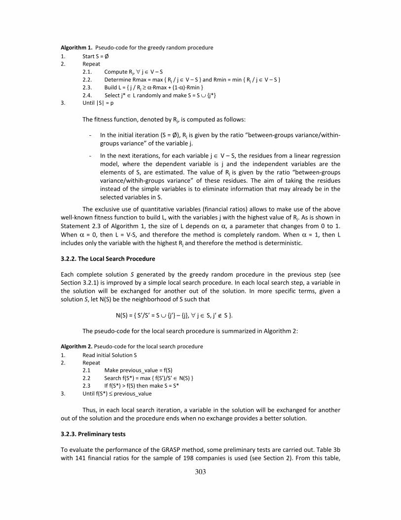
Algorithm 1. Pseudo-code for the greedy random procedure

1. Start S = Ø

2. Repeat

2.1. Compute Rj, ∀ j ∈ V – S

2.2. Determine Rmax = max { Rj / j ∈ V – S } and Rmin = min { Rj / j ∈ V – S }

2.3. Build L = { j / Rj ≥ α·Rmax + (1-α)·Rmin }

2.4. Select j* ∈ L randomly and make S = S ∪ {j*}

3. Until |S| = p

The fitness function, denoted by Rj, is computed as follows:

- In the initial iteration (S = Ø), Rj is given by the ratio “between-groups variance/within-

groups variance” of the variable j.

- In the next iterations, for each variable j ∈ V – S, the residues from a linear regression

model, where the dependent variable is j and the independent variables are the

elements of S, are estimated. The value of Rj is given by the ratio “between-groups

variance/withih-groups variance” of these residues. The aim of taking the residues

instead of the simple variables is to eliminate information that may already be in the

selected variables in S.

The exclusive use of quantitative variables (financial ratios) allows to make use of the above

well-known fitness function to build L, with the variables j with the highest value of Rj. As is shown in

Statement 2.3 of Algorithm 1, the size of L depends on α, a parameter that changes from 0 to 1.

When α = 0, then L = V-S, and therefore the method is completely random. When α = 1, then L

includes only the variable with the highest Rj and therefore the method is deterministic.

3.2.2. The Local Search Procedure

Each complete solution S generated by the greedy random procedure in the previous step (see

Section 3.2.1) is improved by a simple local search procedure. In each local search step, a variable in

the solution will be exchanged for another out of the solution. In more specific terms, given a

solution S, let N(S) be the neighborhood of S such that

N(S) = { S’/S’ = S ∪ {j’} – {j}, ∀ j ∈ S, j’ ∉ S }.

The pseudo-code for the local search procedure is summarized in Algorithm 2:

Algorithm 2. Pseudo-code for the local search procedure

1. Read initial Solution S

2. Repeat

2.1 Make previous_value = f(S)

2.2 Search f(S*) = max { f(S’)/S’ ∈ N(S) }

2.3 If f(S*) > f(S) then make S = S*

3. Until f(S*) ≤ previous_value

Thus, in each local search iteration, a variable in the solution will be exchanged for another

out of the solution and the procedure ends when no exchange provides a better solution.

3.2.3. Preliminary tests

To evaluate the performance of the GRASP method, some preliminary tests are carried out. Table 3b

with 141 financial ratios for the sample of 198 companies is used (see Section 2). From this table,

304

smaller tables with m financial ratios are obtained. The following values of m are considered: m = 40

(corresponding to the first 40 financial ratios), 65, 90, 105, and 120. Solutions S of size p (number of

financial ratios selected for classification), where p ranged from 4 to 16, are used. For each value of

m, the algorithm is run one time for the deterministic method (α = 1) and 20 times for both

algorithms, the greedy random method (α=0.85) and the GRASP (α=0.85). Previously, different

values for α were tested and the best results were obtained for α = 0.85. The number of cases (firms)

under consideration is 198, divided into classes “healthy” and “failed”, with 131 and 67 members

respectively. A partition such that A = A1 ∪ A2, where A1 consists of 100 items (66 solvent and 34

insolvent) and A2 consists of 98 (65 solvent and 33 insolvent), are considered. In Table 4, Columns 1

and 2 show the values of m and p respectively. Column 3 shows the classificatory power –values of

f(S)– for the deterministic algorithm. Finally, Columns 4 and 5 show the values of f(S) for 20 iterations

of both algorithms, the greedy random method and the GRASP (the greedy random method plus the

local search).

m P

Deterministic:

αααα=1

Greedy random:

αααα=0.85

GRASP:

αααα=0.85

40

4 0.67346939 0.70408163 0.7755102

5 0.69387755 0.69387755 0.7755102

6 0.68367347 0.68367347 0.7755102

7 0.68367347 0.68367347 0.79591837

8 0.71428571 0.71428571 0.80612245

65

6 0.67346939 0.71428571 0.80612245

7 0.69387755 0.69387755 0.81632653

8 0.70408163 0.70408163 0.82653061

9 0.70408163 0.70408163 0.84693878

10 0.73469388 0.68367347 0.85714286

90

8 0.65306122 0.75510204 0.85714286

9 0.68367347 0.75510204 0.85714286

10 0.69387755 0.74489796 0.86734694

11 0.69387755 0.70408163 0.86734694

12 0.67346939 0.75510204 0.86734694

105

10 0.64285714 0.74489796 0.87755102

11 0.60204082 0.75510204 0.87755102

12 0.60204082 0.71428571 0.87755102

13 0.60204082 0.7244898 0.8877551

14 0.59183673 0.69387755 0.87755102

120

12 0.66326531 0.78571429 0.90816327

13 0.65306122 0.78571429 0.8877551

14 0.68367347 0.7244898 0.90816327

15 0.70408163 0.73469388 0.8877551

16 0.68367347 0.7244898 0.8877551

Table 4: Results from computational tests for the deterministic, the greedy random and the GRASP algorithm

Table 4 shows that the greedy random method gives higher values for f(S) than the

deterministic method: In 17 cases, it is better (in bold); in seven, it is the same: and only in one case,

it is worse. In addition, it can be observed that the GRASP method strongly improves the results of

the greedy random method on its own. Therefore, the local search is very efficient for improving the

quality of the solutions obtained by both the deterministic constructive algorithm and the random

constructive algorithm. It should be highlighted that the best result of the GRASP strategy is not

always obtained with the highest values of p. For instance, for m=105, the best result is obtained

when p=13; and for m=120, the best result is obtained when p=14. This situation is not strange due

to the use of approximate heuristic methods for both, the variable selection (deterministic, greedy

random and GRASP) and the parameter fine-tuning methods that use logistic regression methods.

305

4. THE GRASP-LOGIT MODEL

4.1. APPLYING GRASP AS A RATIO PRESELECTION PROCEDURE

Now that the efficiency of the GRASP algorithm has been demonstrated, we proceed to solve the

problem of variable selection for the considered sample. As it is stated above, we deal with 198 cases

(firms), divided into two classes (healthy and failed), with 131 and 67 members respectively. The

same partition as in previous tests –A = A1 ∪ A2, where A1 has 100 items (66 healthy and 34 failed)

and A2 has 98 (65 solvent and 33 insolvent)– is considered. In this case, the total number of variables

or ratios (m=141) is used.

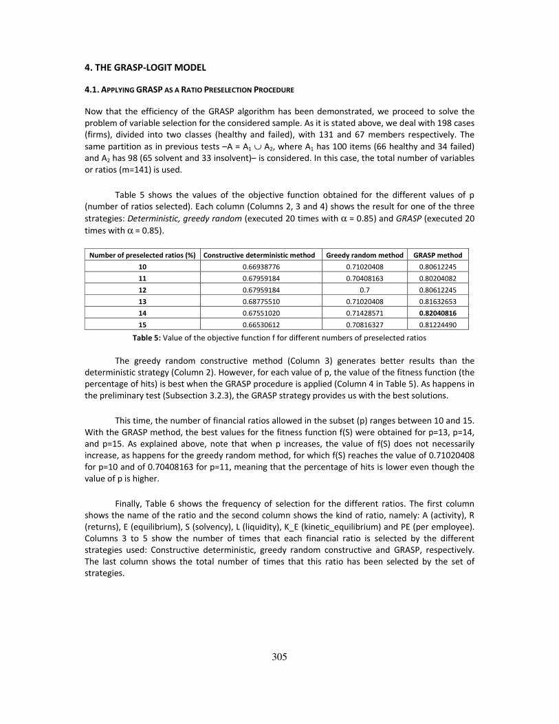
Table 5 shows the values of the objective function obtained for the different values of p

(number of ratios selected). Each column (Columns 2, 3 and 4) shows the result for one of the three

strategies: Deterministic, greedy random (executed 20 times with α = 0.85) and GRASP (executed 20

times with α = 0.85).

Number of preselected ratios (%) Constructive deterministic method Greedy random method GRASP method

10 0.66938776 0.71020408 0.80612245

11 0.67959184 0.70408163 0.80204082

12 0.67959184 0.7 0.80612245

13 0.68775510 0.71020408 0.81632653

14 0.67551020 0.71428571 0.82040816

15 0.66530612 0.70816327 0.81224490

Table 5: Value of the objective function f for different numbers of preselected ratios

The greedy random constructive method (Column 3) generates better results than the

deterministic strategy (Column 2). However, for each value of p, the value of the fitness function (the

percentage of hits) is best when the GRASP procedure is applied (Column 4 in Table 5). As happens in

the preliminary test (Subsection 3.2.3), the GRASP strategy provides us with the best solutions.

This time, the number of financial ratios allowed in the subset (p) ranges between 10 and 15.

With the GRASP method, the best values for the fitness function f(S) were obtained for p=13, p=14,

and p=15. As explained above, note that when p increases, the value of f(S) does not necessarily

increase, as happens for the greedy random method, for which f(S) reaches the value of 0.71020408

for p=10 and of 0.70408163 for p=11, meaning that the percentage of hits is lower even though the

value of p is higher.

Finally, Table 6 shows the frequency of selection for the different ratios. The first column

shows the name of the ratio and the second column shows the kind of ratio, namely: A (activity), R

(returns), E (equilibrium), S (solvency), L (liquidity), K_E (kinetic_equilibrium) and PE (per employee).

Columns 3 to 5 show the number of times that each financial ratio is selected by the different

strategies used: Constructive deterministic, greedy random constructive and GRASP, respectively.

The last column shows the total number of times that this ratio has been selected by the set of

strategies.

306

Non-Selected Ratios Deterministic

constructive Random constructive GRASP TOTAL

Financial costs % R 0 0 0 0

Working capital (days) E_C 0 0 0 0

Need of working capital (days) E_C 0 0 0 0

Cash (days) E_C 0 0 0 0

Clients´credit (days) E_C 0 0 0 0

Repayment capability S 0 0 0 0

Current liquidity L 0 0 0 0

Liquidity L 0 0 0 0

Interest cover L 0 0 0 0

Profit per employee PE 0 0 0 0

Equity per employee PE 0 0 0 0

Working capital per employee PE 0 0 0 0

Total assets per employee PE 0 0 0 0

Selected Ratios * Deterministic

constructive Random constructive GRASP TOTAL

Value added growth A 12 12 7 31

Sales growth A 1 0 0 1

Productivity A 12 12 2 26

Personnel expenditures (%) A 6 6 3 15

Operating margin (%) A 0 1 3 4

Asset turnover A 2 2 3 7

Net asset turnover A 3 3 4 10

ROA R 0 0 3 3

ROA before taxes R 12 6 5 23

ROE R 0 1 0 1

ROE before taxes R 0 3 3 6

ROCE R 2 3 5 10

Solvency ratio S 9 7 15 31

Equity over permanent funds S 12 7 3 22

Debt ratio S 4 6 7 17

Equilibrium E 0 0 4 4

Working capital (€) E 0 0 1 1

Need of working capital (€) E 0 0 2 2

Clients’ credits due to sales (days) E_C 0 2 0 2

Income per employee PE 0 2 1 3

Personnel expenditures per employee PE 0 2 1 3

Immediate liquidity L 0 0 2 2

Cash E 0 0 1 1

* A: activity; R: returns; E: equilibrium; S: solvency; L: liquidity; K_E: kinetic_equilibrium; and PE: per employee.

Table 6: Number of times that each financial ratio is selected by the different algorithms

If we focus on the selected financial ratios (that is, those ratios that predict better corporate

failure), the following conclusions can be drawn:

TOTAL 75 75 75 225

307

- The ratios more often selected are those referring to activity, solvency and, to a lesser

degree, return. In more specific terms, the most relevant ratios are value-added growth,

solvency ratio, productivity, ROA before taxes, and equity over permanent funds. As a

group, these financial ratios encapsulate good information regarding the solvency of the

company. Interestingly, however, as Table 6 shows, the “leading” ratios are not always

the same in each selection procedure. Liquidity, per employee, and kinetic equilibrium

ratios are rejected by all three selection procedures. It was unexpected that liquidity

ratios were selected only by GRASP and only in fewer than 3% of the cases. Economic

sense suggests that liquidity ratios could be important to anticipate the financial distress

of a company. However, some other studies converge with our findings; Beaver (1966)

and Pompe and Bilderbeek (2005) did not find liquidity ratios having a predictive value

for failure forecasting. A possible explanation might be that the “right” value of liquidity

ratios depends on sector and firm characteristics (i.e., healthy big companies in the retail

sector, like Wal-mart or Carrefour, present liquidity ratios below those of small

manufacturing firms with financial problems), so that they are seldom useful except

where failure forecast is focused on a specific sector or type of firms.

- On the other hand, ratios referring to trends (time variations) are the most prominent

type within the selected ratios. Eighteen models have been tested: 6 models (with

values of p ranging from 10 to 15) for each of the three strategies under consideration

(constructive deterministic, greedy random constructive and GRASP). In 16 out of the 18

models, at least one trend ratio was always selected. Therefore, although trend ratios

are not usually included in this kind of analysis, they are important. The relevance of

time variability in financial ratios dealing with solvency and debts, which are the ones

with the highest frequency in all the models tested, makes sense because the worsening

of these ratios over time might suggest that the company is close to insolvency. From

the beginning, the literature on financial distress (see Beaver, 1966) has suggested that

the ratio distribution of healthy companies is steady over time, whereas it changes in a

significant way for unsound companies.

4.2. APPLYING THE LOGISTIC REGRESSION

After solving the problem of variable selection, logistic regression is used to fine-tune the ratios that

best predict insolvency.

Logistic regression models belong to the generalized linear models. Basically, logistic

regression models estimate the probability that an individual belongs to a class by transforming a

linear function of explanatory variables through the logistic function. Specifically, they calculate the

value of a linear function of the explanatory variables and, from this value through the logistic

function, they transform it into the probability of belonging to a certain class. To estimate the

coefficients of this linear function, the maximum likelihood criterion is used.

To apply logistic regression, we take the selected ratios with the best value for the objective

function, which corresponds to the GRASP metaheuristic strategy when p=14 and f(S)= 0.82040816

(shown in bold in Table 5). In this case, we apply logistic regression to the 14 variables selected,

which are shown in Table 7. Note that 5 out of 14 are trend ratios. Furthermore, 5 of them are

solvency ratios, 3 are return ratios, 3 are activity ratios, and the remaining 3 are equilibrium ratios.

Table 8 shows the financial ratios that best predict corporate failure (out of the 14 ratios in

Table 7) after performing the logistic regression. Specifically, Column 1 is devoted to the name of the

ratios, Columns 2 and 3 show the coefficients of the ratios and their standard error, respectively, and

finally, Column 4 shows the signification level of the coefficients.

308

ROA before taxes_t-1 Working capital_t-1_vs_t-2

ROA_t-1 Need for working capital_t-1_vs_t-2

Equity over permanent funds _t-2 Debts_t-1_vs_t-2

Solvency ratio_t-2 Net asset turnover_t-2

Value added growth _t-2 Solvency ratio_t-1_vs _t-2

Equilibrium_t-2 ROCE_t-3

Debts_t-2_vs_t-3 Operating ratio_t-1

Table 7: Variables preselected by GRASP

B S.E. Sig.

Step 1 ROA bt_t-1 0.066 0.015 0.000

Constant 0.881 0.173 0.000

Step 2 VAG t-2 0.008 0.003 0.001

ROA bt_t-1 0.077 0.016 0.000

Constant 0.705 0.182 0.000

Step 3 VAG t-2 0.009 0.003 0.001

ROA bt_t-1 0.077 0.016 0.000

Solv_ t-2 0.012 0.005 0.008

Constant 0.395 0.213 0.063

Table 8: Results from the GRASP-LOGIT (78.9% of hits for in-sample data – 77.04% for out-of-sample data)

As can be seen in Table 8, the financial ratios that best predict corporate failure are: ROA

before taxes_t-1; Solvency ratio_t-2 and Value added growth _t-2.

We have introduced, into the GRASP-LOGIT model, control variables for the size of the

company (measured by number of employees), for its age and for the sector that it belongs to (using

the CNAE 2-digit code. However, these variables had no effect in the final results of the model.

Neither the size of the company, nor its age2 nor the sector that it belongs to, seems to have any

predictive value regarding insolvency.

Given a cut-off probability of 0.5, the global percentage of hits in this analysis is 78.9%.

Although we cannot state this analysis in terms of the hits in each group (healthy/failed), because

type I and type II errors have not been taken into account in the ratio preselection process using

GRASP, we have tried several different cut-off points in order to balance both types of errors while

getting a global fitness similar to the total given above. For instance, a cut-off probability of 0.67

results in a global fitness of 77.8%, with fitness for type I and type II errors of 76.2% and 78.6%,

respectively.

The result obtained makes economic sense because it uses three of the key variables in the

financial analysis of a company. These include, on one hand, the business return (ROA before taxes t-

1) and a variable that represents in some way the company’s recent evolution (value added growth t-

2); and, on the other hand, its leverage (solvency ratio t-2). Besides, these ratios are not biased by

the activity sector that the firm belongs to. Interestingly, our final model (the GRASP-LOGIT) does not

include any trend ratio, in spite of the results obtained in the preliminary step, when we applied the

GRASP metaheuristic method.

- ROA shows the company’s capacity to obtain returns from its assets and, to some

extent, this variable is immune to which sector the company belongs to. In the well-

known “DuPont” analysis, ROA is decomposed into sales margin and total turnover of

assets, as follows:

ROA_ before_taxes= Pr _ _

_

ofit before taxes SalesX

Sales Total Asset

2 Recall that there is an important bias in the analysis of age, as the sample included only firms with at least three years of

life.

309

Normally, capital-intensive sectors have a greater sales margin than those that are

less capital-intensive. However, capital-intensive sectors have a lower asset turnover

(because they have greater fixed assets) than those that have smaller fixed assets and

thus less need for capital. Because the two differences tend to cancel each other out, by

including both variables, ROA palliates, to a great extent, the effect of belonging to one

sector or another.

- The solvency ratio represents the equity-debt level of the company and, by combining

this with ROA before taxes using DuPont analysis decomposition ratios, we obtain ROE

before taxes as shown in the following expressions:

ROE_before_taxes=ROA_before_taxes X leverage

ROE_before_taxes.=Pr _ _ 1

__

_

ofit before taxes SalesX X

Total EquitySales Total Asset

Total Asset

- Finally, value-added growth shows the evolution of the company’s operating profit over

time. Thus, given an original level of solvency in the firm, a positive value of this rate

would involve, initially, an improvement in the financial situation and in the return of

the company; and a negative value, the worsening of its financial situation and its

return.

To make sure that the forecasting ability of the model is not the result of overfitting, we have

tested our GRASP-LOGIT model with out-of-sample data by using 61 companies (of which 40 are

healthy and 21 failed firms) selected randomly from each group. The global fitness obtained with

out-of-sample data is 77.04% (compared with a fitness of 78.9% for in-sample data), which confirms

the forecasting ability of the model. We check again that type I and type II errors may be balanced by

changing the cut-off point but maintaining the same level of global fitness.

Finally, in order to analyze the advantages of the GRASP method for solving the problem of

variable selection before applying logistic regression, we have also carried out a logistic regression on

the 141 original variables so that we can make comparisons. These are the results:

- Despite the much greater number of variables included in this new model, its

percentage of global hits is very similar to the one obtained for the 14 variables

preselected by GRASP and reduced in GRASP-LOGIT to 3 (79.3%, compared to 78.9% for

GRASP-LOGIT). Obviously, this is due to the good performance of the GRASP algorithm.

- The variables selected in the logit with 141 variables are the following: Value added

growth _t-1 (%), Value added growth _t-2 (%), Productivity_t-3, Equity over permanent

funds _t-1(%), Debts _t-3 (%), ROA before taxes_t-1 (%) and Personnel expenditures_t-2

(%).

Within the seven variables selected in this case –or six if we do not take into account the

time factor–, the three variables that were previously selected by the GRASP-LOGIT model (ROA

before taxes_t-1, value added growth_t-2, and debts_t-3) are found. The variable debts is equivalent

to the solvency ratio that appeared in the GRASP-LOGIT model (although its reading is the opposite),

because Solvency ratio = 100 – Debts. This latter variable now appears in the t-3 period, while in the

first GRASP- LOGIT model, the solvency ratio appeared in the t-2 period. The remaining variables

selected for this model are personnel expenditures (%), productivity (gross operating margin per

monetary unit used in labor) and equity over permanent funds. The meaning of these variables as

predictors of failure is not as clear as for the three variables obtained with the GRASP-LOGIT model.

Personnel expenditures (measured as a percentage of the firm’s income) show great dependency on

310

sector, because the more labor-intensive sectors are the higher values are for this variable. The

opposite happens with productivity; i.e. the sector that is more labor intensive has lower figures for

this indicator. Finally, the variable equity over permanent funds or long-term funds does not seem to

be a good predictor of insolvency, because it does not take into account short-term debts, which in

many cases can be decisive for assessing the payment capacities of the company.

Therefore, it seems that the results obtained by the GRASP-LOGIT model are more

transparent to interpretation than the ones from the logit with 141 ratios, whereas the predictive

capacity of both models is the same.

4.3. APPLYING THE GRASP STRATEGY TO OTHER CLASSIFICATION MODELS

GRASP strategy can be applied to other well-known classification models to improve them (similar to

that has been done in the paper with logistic regression). In this way, in Pacheco et al. (2012), GRASP

is combined with decision-tree models, specifically with the variant of the model C4.5 proposed by

Fayyad and Irani (1992). A set of experiments with 17 databases belong to the well-known UCI

Repository of Machine Learning at the University of California, Irvine (see Murphy and Aha, 1994),

and the financial database used in this paper is performed. These experiments show that the GRASP

strategy improves the performance of the C4.5 model.

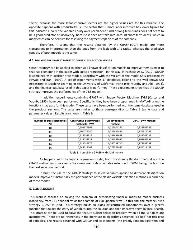
In addition, experiments combining GRASP with Suppor Vector Machine, SVM (Cortes and

Vapnik, 1995), have been performed. Specifically, they have been programmed in MATLAB using the

functions that exist for this model. These tests have been performed with the same database used in

the previous sections. The tests are similar to those corresponding to Table 5 (same data and

parameter values). Results are shown in Table 9.

Number of preselected ratios

(%)

Constructive deterministic

method for SVM

Greedy random

method

GRASP-SVM method

10 0,691375963 0,729004251 0,828801363

11 0,700075040 0,739926856 0,836319241

12 0,717251325 0,747999498 0,837509731

13 0,718058322 0,756363947 0,867865397

14 0,731584376 0,766728715 0,879347788

15 0,747119069 0,772571942 0,885211169

Table 9: Combining GRASP with SVM models

As happens with the logistic regression model, both the Greedy Random method and the

GRASP method improve clearly the classic methods of variable selection for SVM, being this last one

the best selection method.

In brief, the use of the GRASP strategy to select variables applied to different classification

models improved substantially the performance of the classic variable selection methods in each one

of these models.

5. CONCLUSIONS

This work is focused on solving the problem of preselecting financial ratios to model business

insolvency, from 141 financial ratios for a sample of 198 Spanish firms. To this end, the metaheuristic

strategy GRASP is used. This strategy builds solutions by controlled randomness over a greedy

function that guides the entry of variables into the solution and then improves them by local search.

This strategy can be used to solve the feature subset selection problem when all the variables are

quantitative. There are no references in the literature to algorithms designed “ad hoc” for this type

of variables. The results obtained with GRASP and its elements (the greedy random algorithm and

311

the local search algorithm) are compared to those obtained by applying a deterministic algorithm.

The systematic superiority of GRASP means that the quality of the solutions so found can be

improved either by introducing randomness into the selection procedure or by using local search.

GRASP strategy is also applied successfully to other models (as can be seen in Subsection 4.3).

In addition, business insolvency is modeled by applying a logistic regression model to the

results from the GRASP procedure. GRASP is used to preselect 14 financial ratios from which the logit

is built. We called this model GRASP-LOGIT and the results obtained with it are compared to those

obtained by applying a logit directly to the original 141 financial ratios. Although the classificatory

capacity of the GRASP-LOGIT is the same as that of the logit model with 141 ratios, the former has

more explanatory capacity and greater simplicity, and thus improves our understanding of business

insolvency. It also reduces the cost of data acquisition.

The GRASP-LOGIT model shows that the best combination of ratios to explain corporate

failure is ROA before taxes, solvency ratio, and value-added growth. The first two ratios are the

components of ROE identified by DuPont analysis. In contrast with our initial expectations, none of

the trend ratios had predictive value in the final model (GRASP-LOGIT). Liquidity ratios are also

rejected by the model. Our results also reveal that neither the size of the company (measured by the

number of employees), nor its age nor the sector that it belongs to, seems to have any value in

predicting insolvency.

Acknowledgments

This work has been partially supported by FEDER funds and the Spanish Ministry of Economy and

Competitiveness (Projects ECO2013-47129-C4-3-R and ECO2016-76567-C4-2-R), the Regional

Government of “Castilla y León”, Spain (Project BU329U14) and the Regional Government of “Castilla

y León” and FEDER funds (Project BU062U16); all of whom are gratefully acknowledged.

REFERENCES

Altman, E. (1968). Financial ratios, discriminant analysis and the prediction of corporate bankruptcy.

Journal of Finance, 23, 589-609.

Altman, E.; Marco, G. and Varetto F. (1994). Corporate distress diagnosis: Comparisons using linear

discriminant analysis and neural networks. Journal of Banking and Finance, 18, 505-529.

Arslan, O. (2012). Weighted LAD–LASSO method for robust parameter estimation and variable

selection in regression. Computational Statistics & Data Analysis, 56 (6), 1952-1965.

Baesens, B.; Setiono, R.; Mues, C. and Vanthienen, J. (2003a). Using neural networks rule extaction

and decision tables for credit-risk evaluation. Management Science, 49(3), 312-329.

Baesens, B.; Van Gestel, T.; Viaene, S.; Stepanova, M.; Suykens, J. and Vanthienen J. (2003b).

Benchmarking state-of-the-art classification algorithms for credit scoring. Journal of the

Operational Research Society, 54(6), 627-635.

Bala, J.; Dejong, K., Huang, J.; Vafaie, H. and Wechsler, H. (1996). Using learning to facilitate the

evolution of features for recognizing visual concepts. Evolutionary Computation, 4 (3), 297-311.

Balcaen, S. and Ooghe, H. (2006). 35 years of studies on business failure: An overview of the classic

statistical methodologies and their related problems. The British Accounting Review, 38 (1),

63-93.

Beaver, W. (1966). Financial ratios as predictors of failures. In: S. Davidson (ed.), Empirical Research in

Accounting: Selected Studies (pp. 71-111), Chicago: Institute of Professional Accounting.

312

Cortes, C. and Vapnik, V. N. (1995). Support-vector networks. Machine Learning, 20 (3). 273-297.

Cotta C.; Sloper, C. and Moscato, P. (2004). Evolutionary search of thresholds for robust feature set

selection: Application to the analysis of microarray data. Lecture Notes in Computer Science,

3005, 21-30.

Crone, S. F. and Finlay, S. (2012). Instance sampling in credit scoring: An empirical study of sample

size and balancing. International Journal of Forecasting, 28(1), 224-238.

Curran, S. and Mingers J. (1994). Neural networks, decision tree induction and discriminant analysis:

An empirical comparison. Journal of the Operational Research Society, 45 (4), 440-450.

Dambolena, I. G. and Khoury, S. J. (1980). Ratio stability and corporate failure. Journal of Finance, 35,

1017-1026.

Etheridge, H. L. and Sriram, R. S. (1996). A Neural Network Approach to Financial Distress Analysis. In:

S. G. Sutton (ed.), Advances in Accounting Information Systems, Volume 4 (pp.201-222), Bingley:

Emerald Group Publishing.

Fayyad, U. M. and Irani, K. B. (1992). On the handling of continuous-valued attributes in decision tree

generation. Machine Learning, 8, 87-102.

Feo, T. A. and Resende M. G. C. (1989). A probabilistic heuristic for a computationally difficult set

covering problem. Operations Research Letters, 8 (2), 67-71.

Feo, T. A. and Resende M. G. C. (1995). Greedy randomized adaptive search procedures. Journal of

Global Optimization, 2, 1-27.

Frydman, H.; Altman, E. I. and Kao, D. (1985). Introducing recursive partitioning for financial

classification: the case of financial distress. Journal of Finance, 40(1), 269-291.

Ganster, H.; Pinz, A.; Rohrer, R.; Wildling, E.; Binder, M. and Kittler, H. (2001). Automated melanoma

recognition. IEEE Transactions on Medical Imaging, 20 (3), 233-239.

Hua, Z.; Wang, Y.; Xu, X.; Zhang, B. and Liang, L. (2007). Predicting corporate financial distress on

integration of support vector machine and logistic regression. Expert Systems with Applications,

33(2), 434-440.

Iturriaga, F. J. L. and Sanz, I. P. (2015). Bankruptcy visualization and prediction using neural networks:

A study of US commercial banks. Expert Systems with Applications, 42(6), 2857-2869.

Jain, A. and Zongker, D. (1997). Feature selection: Evaluation, application, and small sample

performance. IEEE Transactions on Pattern Analysis and Machine Intelligence, 19(2), 153-158.

Jeong C.; Min, J. N. and Kim, M. S. (2012). A tuning method for the architecture of neural network

models incorporating GAM and GA as applied to bankruptcy prediction. Expert Systems with

Applications, 39(3), 3650-3658.

Jones, F. L. (1987). Current techniques in bankruptcy prediction. Journal of Accounting Literature, 6,

131-164.

Jones, S. and Hensher, D. A. (2004). Predicting firm financial distress: a mixed logit model. The

Accounting Review, 79 (4), 1011-1038.

Jourdan, L.; Dhaenens, C. and Talbi, E. (2001). A genetic algorithm for feature subset selection in data-

mining for genetics. In: J. P. de Sousa (ed.), Proceedings of the 4th

Metaheuristics International

Conference (pp. 29-34), Porto: MIC.

Kohavi, R. (1995). Wrappers for performance enhancement and oblivious decision graphs. Ph. D.

Thesis, Computer Science Department, Stanford University.

313

Laitinen, E. K. and Laitinen, T. (2000). Bankruptcy prediction. Application of the Taylor’s expansion in

logistic regression. International Review of Financial Analysis, 9, 327-349.

Lee, S. H. and Urrutia, J. L. (1996). Analysis and prediction of insolvency in the property-liability

insurance industry: A comparison of logit and hazard models. The Journal of Risk and Insurance,

63(1), 121-130.

Lee, S.; Yang, J. and Oh, K. W. (2003). Prediction of molecular bioactivity for drug design using a

decision tree algorithm. Lecture Notes in Artificial Intelligence, 2843, 344-351.

Lennox, C. (1999). Identifying failing companies: A reevaluation of the logit, probit and DA approaches.

Journal of Economics and Business, 51, 347-364.

Lewis, P. M. (1962). The characteristic selection problem in recognition systems. IEEE Transactions on

Information Theory, 8, 171-178.

Li, H.; Lee, Y. C.; Zhou, Y. C. and Sun, J. (2011). The random subspace binary logit (RSBL) model for

bankruptcy prediction. Knowledge-Based Systems, 24 (8), 1380-1388.

Liang, D.; Lu, C. C.; Tsai, C. F. and Shih, G. A. (2016). Financial ratios and corporate governance

indicators in bankruptcy prediction: A comprehensive study. European Journal of Operational

Research, 252(2), 561-572.

Liu, H. and Motoda, H. (1998). Feature selection for knowledge discovery and data mining. Boston:

Kluwer Academic.

Lu, Y.; Zeng, N.; Liu, X. & Yi, S. (2015). A new hybrid algorithm for bankruptcy prediction using

switching particle swarm optimization and support vector machines. Discrete Dynamics in

Nature and Society, 2015, Article ID 294930, 7 pp.

Mangalova, E. and Agafonov, E. (2014). Wind power forecasting using the k-nearest neighbors

algorithm. International Journal of Forecasting, 30(2), 402-406.

Matsui, H. (2014). Variable and boundary selection for functional data via multiclass logistic regression

modeling. Computational Statistics & Data Analysis, 78, 176-185.

Meiri, R. and Zahavi, J. (2006). Using simulated annealing to optimize the feature selection problem

in marketing applications. European Journal of Operational Research, 171, 842-858.

Messier Jr., W. F. and Hansen, J. V. (1988). Inducing rules for expert system development: An example

using default and bankruptcy data. Management Science, 34 (12), 1403-1415.

Murphy, P. M. and Aha, D. W. (1994). UCI Repository of Machine Learning. Department of Information

and Computer Science, University of California.

Narendra, P. M. and Fukunaga, K. (1977). A Branch and Bound algorithm for feature subset selection.

IEEE Transactions on Computers, 26(9), 917-922.

Neophytou, E. and Molinero, C. M. (2004). Predicting corporate failure in the UK: a multidimensional

scaling approach. Journal of Business Finance and Accounting, 31(5-6), 677-710.

Ohlson, J. A. (1980). Financial ratios and the probabilistic prediction of bankruptcy. Journal of

Accounting Research, 18(1), 109-111.

Oliveira, L. S.; Sabourin, R.; Bortolozzi, F. and Suen, C. Y. (2003). A methodology for feature selection

using multiobjective genetic algorithms for handwritten digit string recognition. International

Journal of Pattern Recognition and Artificial Intelligence, 17(6), 903-929.

Ooghe, H. and Balcaen, S. (2002). Are failure prediction models transferable from one country to

another? An empirical study using Belgian financial statements. Vlerick Leuven Gent Management

School Working Paper, 2002-3, 42 pp.

314

Pacheco, J.; Alfaro, E.; Casado, S.; Gámez, M. and García, N. (2012). A GRASP Method for Building

Classification Trees. Expert Systems with Applications, 39(3), 3241-3248.

Pacheco, J.; Casado, S. and Núñez, L. (2009). A variable selection method based on tabu search for

logistic regression models. European Journal of Operational Research, 199, 506-511.

Pacheco, J.; Casado, S.; Núñez, L. and Gómez, O. (2006). Analysis of new variable selection methods

for discriminant analysis. Computational Statistics & Data Analysis, 51, 1463-1478.

Pitsoulis, L. S. and Resende, M. G. C. (2002). Greedy randomized adaptive search procedures. In: P. M.

Pardalos and M. G. C. Resende (eds.), Handbook of Applied Optimization, Oxford: Oxford

University Press.

Pompe, P. P. M. and Bilderbeek, J. (2005). The prediction of small- and medium-sized industrial firms.

Journal of Business Venturing, 20(6), 847-868.

Reunanen, J. (2003). Overfitting in making comparisons between variable selection methods. Journal

of Machine Learning Research, 3, 1371-1382.

Sarkar, S. and Sriram, R. S. (2001). Bayesian models for early warning of bank failures. Management

Science, 47(11), 1457-1475.

Scott, J. (1977). Bankruptcy, secured debt and optimal capital structure. Journal of Finance, 33, 1-19.

Scott, J. (1981). The probability of bankruptcy. A comparison of empirical predictions and theoretical

models. Journal of Banking and Finance, 5, 317-344.

Sebestyen, G. (1962). Decision-making processes in pattern recognition. New York: Macmillan.

Sexton, R. S.; Sriram, R.S. and Etheridge, H. (2003). Improving Decision Effectiveness of Artificial Neural

Networks: A Modified Genetic Algorithm Approach. Decision Sciences, 34(3) 421-442.

Shumway, T. (2001). Forecasting bankruptcy more accurately: A simple hazard model. Journal of

Business, 74(1), 101-124.

Varetto, F. (1998). Genetic algorithms applications in the analysis of insolvency risk. Journal of Banking

and Finance, 22, 1421-1439.

Wang, H.; Li, G. and Jiang, G. (2007). Robust regression shrinkage and consistent variable selection

through the LAD-Lasso. Journal of Business and Economic Statistics, 25(3), 347-355.

Wu, C. H.; Tzeng, G. H.; Goo, Y. J. and Fang, W. C. ( 2007). A real-valued genetic algorithm to optimize

the parameters of support vector machine for predicting bankruptcy. Expert Systems with

Applications, 32(2), 397-408.

Yang, Z.; You, W. and Ji, G. (2011). Using partial least squares and support vector machines for

bankruptcy prediction. Expert Systems with Applications, 38(7), 8336-8342.

Zhang, C. X.; Wang, G. W. and Liu, J. M. (2015). RandGA: Injecting randomness into parallel genetic

algorithm for variable selection. Journal of Applied Statistics, 42(3), 630-647.

Zmijewski, M. E. (1984). Methodological issues related to the estimation of financial distress

prediction models. Journal of Accounting Research, 22(Supplement), 59-82.