Guidelines for Predicting Crop Water Requirements.

•

lrrigation and Drainage Paper

Guidelines for predicting

crop water requirements

by

J. Doorenbos Water Management Specialist Land and Water Development Division FAO, Rome

W. 0. Pruitt FAO Consultant lrrigation Engineer University of California Davis, California, U.S.A.

24

Prepared in consuttation with Messrs. A. Aboukhaled (Lebanon), J. Damagnez (France), N.G. Dastane (lndia), C. van den Berg and P.E. Rijtema (Netherlands), O.M. Ashford IWMO), M. Frere IFAOI and FAO field staff.

FOOD AND AGRICULTURE ORGANIZATION

OF THE UNITED NATIONS Rome, 1975

- iii -

FOREWORD

~ 'And with water we have made all whic.h is living'' ..•

Man, throughout history, has been able to develop skills to deal with his environment~ He has developed plants and improved crop varieties adapted to his ne.eds. He has developed suitable practices to use water, fertilizers and pesticides mast effec.tively to increase crop production. But he has not been able to maste~ climate and has remained under the threat of drought. With limited water and with the increase in population and the need for more and better food production, water has become the most precious natural resource in mast regions of the world; so there is now an imperative need for really effective planning of water utilization in crop production.

Methodologies have been developed to predict the correct amounts of water needed to obtain optimal production of crops. Such methods are developed for climatic, agronomic and soil conditions prevailing in a given areao The transfer of methodologies from one area to another far different from t.hat in which they were developed remains problematic; time and

, labour-consuming field experiments, sometimes also costly, are frequently required to test and calibrate the methods in a new set of conditions.

The quantitative prediction of irrigation needs in respect to crop production must be accurately known for identification and feasibility analysis of proposed irrigation projects. Guidance is needed on the mast promising prediction methods to be applied in determining the mast effective use of available water for irrigation~ In this paper four widely knmm pre"' diction methods have been calibrated for different climatic conditions. There are descriptions of the extent to which local conditions, including variations in weather, advection, soil and soil-water, agronomic and irrigation practices and production potential, may affect crop water requirernents. The application of derived crop water requirements <lata to deter"' mine irrigation requirements and supply schedules for planned irrigation development project is summarized. For the actual operation of schemes and for water application at the field level still more detailed field research <lata will be required.

The approach presented in this paper was formulated by the FAO Consultative Group on Crop Water Requirements held in Lebanon 1971 and Rome 1972. It is a pleasure to record our appreciation for the continuing advice and assistance received from Drs A. Aboukhaled of Lebanon, C. van den Berg and P.E. Rijtema of the Netherlands:, N.G. Dastane of īndia and J. Damagnez of France. Guidance in outlining the document was received from Dr. O.M. Ashford (WMO) and Mr. M. Frere (FAO). Much help was obtained from an intensive use made of published aud unpublished resea!'ch results collected by leading research institutes located in differ„ ent geographic and climatic zones; direct contact was established with prominent researchers in Denmark, Ethiopia, France, Haiti, India~ Israel, Kenya, Lebanon~ Nigeria, the Netherlands, Philippines, Senegal, Sudan, Syrian Arab Republic, Thailand:, Tunisia, UeK., U.S.A~, Zaire, Venezuela, and with WMO, IAEA and regional FAO offices in the Near East and Asia and the Far East. Within FAO, the preparation of the paper has been the responsihility of the Water Resources, Developrnent and Management Service of the Land and Water Development Division. An impressive contribution in developing the methodologies for determination of crop water requirements was made during his six-month stay in Rome asa FAO Consultant, by Mr. W.O. Pruitt, University of California, Davis, California, U.SeA~ and we gratefully acknowledge his invaluable help. Mr. Jo Doorenbos acted as coordinator and editor in all stages of the preparation and contributed the chapters dealing with the effect of local conditions and the application of crop water requirements <lata in planning irrigation projects.

~ iv "'

In this pa-per the main aim has been to gather togeiher from many sources guidance for the field e.xpert. The methodoLogies presented are considered adequate for preliminary project planning and can be applied to determine average and peak irrigation requirements for project design purposes. Caution and a critical attitude should be adopted and aware~ ness maintained of the extent to which the presented approach is likely to fit local condi„ tions and experience and, conversely, the influence they may exert on the chosen method. It follows that the methods given should never be used on a purely routine basis.

We would welcorne conunents and suggestions for improvement of the paper and ultimately we hope that a revised and more complete edition may meet the ambitious goal of presenting rnethods covering all possible conditions where planning the optimum utilization of water in crop production is most essential.

Edouard Saouma Director

Land aud Water Development Division

,,. V "'

TABLE OF CONTENTS

FOREWORD

LIST OF TABLES

11ST OF FIGURES

CONVERSION FACTORS

CLIMATOLOGICAL NOMENCLATURE

SUMMARY

PART I -

CHAPTER I. 1

CHAPTER I. 2

CALCULATION OF CROP EVAPOTRANSPIRATION, ET(crop)

Introduction

Calculation Procedures

CALCULATION OF REFERENCE CROP EVAPOTRANSPIRATION, ETo

Method I - Blaney-Criddle

Recommended relationships

Additional considerations

Sample calculations

Method II - Radiation


Prediction of reference crop evapotranspiration, ETo


Sample calculations

Method III - Modified Penman



Description of variables involved and method of calculation

Method IV - Pan Evaporation


Description of pans


Sample calculations

SELECTION OF CROP COEFFICIENT, kc

General considerations

Recommended values

a. Field aud vegetable crops b. Rice c. Sugarcane d. Alfalfa, clover, grass-legumes, pastures e. Deciduous fruits and nuts f „ Citrus g. Grapes h~ Bananas i. Aquatic weeds and open water j. Coffee k. Tea 1. Non-cropped or bare soils

Page

iii

vii

xi

xii

xiii

4

4

5

7

7

7

8

9

15

15

18

18

19

28

29

29

30

50

50

51

51

54

57

57

61

61 70 72 73 76 78 79 80 81 82 82 82

1~

CBAPTER I. 3

CHAPTER I. 4

PART II -

CHAPT ER II, 1

CHAPTER II, 2

CHAPTER II.3

- vi -

CALCULATION OF ET(crop)

CONSIDERATION OF FACTORS AFFECTING ET(crop) UNDER PREVAILING LOCAL CONDITIONS

1. Climate

a. Variation with time b. Variation with distance c. Variation with size of irrigation

development (advection) d. Variation with altitude

2. Soil water

a~ Level of available soil water

b. Soil water uptake c~ Groundwater tables d. Salinity

3. Method of irrigation

a. Surface b. Sp rinkle r c. Drip or trickle d. Subsurface

4. Cultural practices

a~ Fertilizers b. Plant population c. Tillage d. Mulching e. Windbreaks f. Anti-transpirants

5 ~ Crop yields

CALCULATION OF FIELD IRRIGATIDN REQUIREMENTS, If

Introduction Calculation procedures

FIELD WATER BALANCE

1. Crop evapotranspiration, ET(crop)

2. Effective precipitation, Pe

a. Rainfall b. Dew c. Snow

3. Groundwater contribution~ Ge

4. Surface and snbsurface in and outflow, N and R

5. Deep percolation below root zone i F

6. Changes in s tored soil water, L1 W

NET FIELD IRRIGATION REQUIREMENTS, In

1. Seasonal and monthly data

2. Peak period irrigation requirements

GROSS FIELD IRRIGATION REQUIREMENTS, If

1. Irrigation application efficiency, Ea

2. Other water needs including leaching requirements

83

84

84

84 86

87 90

90

90 96 97 98

99

99 99

100 100

100

100 101 102 102 102 103

103

109

109 110

111

111

11 2

11 2 11 7 117

118

118

118

120

1 21

121

122

124

124

126

i•

l

CHAPTER II , 4

PART III -

- vii

FIELD IRRIGATION SCHEDULING

1. Depth of irrigation

2. īrrigation interval

3. Irrigation frequency

CALCULATION OF IRRIGATION SUPPLY, Vs

Introduction

Calculation procedures

CHAPTER III.1 PRELIMINARY ESTIMATES OF SEASONAL AND PEAK PROJECT IRRIGATION SUPPLY

1. Cropping pattern and cropping intensity

2. Level of supply

3. Distribution efficiency

4. Calculation of seasonal project supply

5. Calculation of peak project supply

6. Project operation aud field supply scheduling

CHAPTER III,2 FIELD IRRIGATION SUPPLY

128

129

129

130

132

132

133

135

135

136

137

138

139

140

143

1. Relation between depth of soil water replenishrnent and supply 143

2. Relation between soil intake rate and supply J43

3. Relation between method of irrigation and stream size j44

a. Surface irrigation b. Sprinkler irrigation c. Drip irrigation

4. Relation between field size, field layout and supply

CHAPTER III.3 REFINEMENT OF FIELD IRRIGATION SCHEDULING;

APPENDIX I

APPENDIX II

APPENDIX III

APPENDIX IV

DEVELOPMENT OF DATA ON SOIL, WATER, CROP AND CLIMATE

·1. Refinement of field irrigation <lata

a. Agro-meteorological stations be Soil survey c. Water requirement studies d. Monitoring water supply scheduling for

projects in progress

2. Application of field irri.gation <lata

GLOSSARY

PERSONS AND INSTITUTES CONSULTED

REFERENCES

EXPERIMENTALLY DETERMINED CONSTANTS FOR THE RADIATION EQUATION

144 144 149

151

153

153

l 53 1~4 154

155

157

1 61

167

169

179

1.

2.

2a.

3.

4.

5.

6.

7.

Sa.

8b.

Sc.

9.

·10.

11 •

12.

14.

15.

16.

17.

18.

19.

20.

"' viii =

LIST OF TABLES

Formulae to estimate crop water requirements

Mean daily percentage (p) of annual daytime hours for different latitudes

Value of Blaney-Criddle f value for different temperatures and daily percentage of annual daylight hours

Extra-terrestrial radiation Ra expressed in equivalent evaporation in mm/day

Mean daily maximurn duration of bright sunshine hours N for different months and latitudes

Conversion factor for extra~terrestrial radiation Ra to solar radiation Rs for different ratios of actual to maximum possible sunshine hours (0~25+0.50 n/N)

Values of weighting factor W for the effect of radiation on ETo at different temperatures and altitudes

Saturation vapour pressure ea in mbar as function of . . 0

mean air temperature t,in C

Vapour pressure ed in mbar from dry and wet bulb temperature <lata in °c (aspirated psychrometer)

Vapour pressure ed in rnbar from dry and wet bulb temperature <lata in °c (non„ventilated psychrometer)

Vapour pressure ed from dewpoint temperature

Values of wind function f (u) fo:r ,vind run at a 2 m height in km/day

Values of weighting factor (1-W) for the effect of wind and humidity oī.1 ETo at different temperatures and altitudes

Values of weighting factor W for the effect of radiation on ETo at different temperatures and altitudes

Extra=terre.strial radiation Ra expressed in equivalent evaporation in mm/day

Mean daily maximum duration of bright sunshine hours N for different months and latitudes

Conversion factor for e.xtra=terrestrial radiation to net solar radiation Rns fo:r a given reflection a of 2510 and different ratios of actua.l to ma:ximum sunshine hours (1-a)(0.25 + 0„50 n/N)

Correction for temperature f(t) on net long wave radiation Rnl

Correction for vapour pressure f(ed) on long wave radiation Rnl

Correction for the ratio actual and maximum bright sunshine hours f(n/N) on long wave radiation Rnl

Relation be.t.1.veen evaporation from sunken pans mentioned and from Colorado sunken pan for different climatic conditions and pan environments

Pan coefficie.nt Kp for c.lass A pan for different ground cover and levels of mean relative humidity and 24-hour wind

Pan coefficient Kp for Colorado sunken pan for different ground cover and levels of mean relative humidity and 24-hour wind

2

11

1 2

22

23

24

24

39

1,0

41

41

42

43

43

44

45

46

46

46

46

53

55

56

'

•

'lP""'" ·l

21.

22;

23.

24.

25.

26.

27.

28.

29.

30.

31.

32.

33.

34.

35.

36.

37.

38.

39.

40.

41.

42.

43.

44.

45.

46.

47.

ix

Approximate range of seasonal ET(crop) in mm and i:i comparison with ET(grass)

Crop coefficient kc for field and vegetable crops for different stages of crop growth and prevailing climatic conditions

Length of growing season aud crop development stages of selected field crops: sorne indications

kc values for rice

kc values for sugarcane

Crop coefficient kc(mean) for alfalfaj grass for hay) clover aud grass-legume mixture aud pasture, and kc(peak) just before harvesting and kc(low) just following harvesting

kc values for full grown deciduous trees aud nut trees

kc values for citrus

kc values for grapes

kc values for bananas

kc values for aquatic weeds and coefficients for open water

Depth of soil water available in mm for different soil textures and Ievels of ET(crop) at which ET(crop) is maintained at its predicted maximum level

Effective rooting depth for various crops at mature growing stage grown in homogeneous deep soils

Tolerance levels of crops to high groundwater tables and waterlogging

Critical periods for soil~water stress for different crops

Soil water depletion levels~ expressed in soil water tensions, tolerated by different crous for which ET(crop) remains at predicted level and maximum yields are obtained

Average monthly effective rainfall as related to average monthly ET(crop) and mean monthly rainfall

Field application efficiency for method of irrigation

Irrigation application losses ~a.....fractiop. of water applied and fļeld application efficiencY for different soil conditions

Approximate values of salinity levels for different crops assOO"ling. 50%.decrease in yield

Leaahing requirements in pe_rce_ntage_ for different salini tv · levels .of _irrigation (EC/irr) ānd dra:Cnage·water ·cECĪ<lw).·Iī</JIJmhos/cm

Qualitative norms on frequency and depth of irrigation application in relation to cropi soil, climate, type of harvested yield and level of management

Phases of project planning and type of wate.r supply data needed

Dist_ribution efficiency in existing projects

Average field and conveyance efficiency in existing irrigation projects subdivided into method of field delivery

Approximate relation between soil texture~ intake rate and stream size

Suggested size of basins and stream stze for dif'ferent soils

60

65

6ī

71

72

75

77

78

79

80

81

94

96

97

107

108

116

125

12S

126

127

128

134

137

141

14<\

146

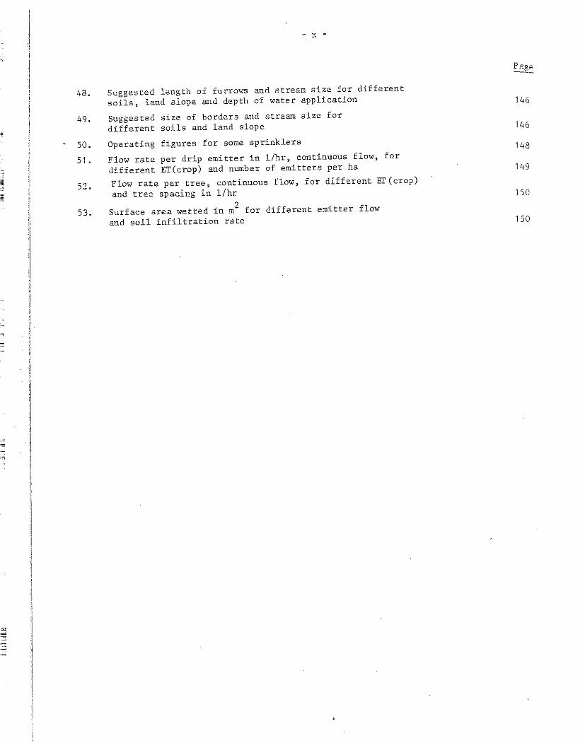
48.

49.

50.

51.

52.

Suggested length of furrows and stream size for different

soils, land slope and depth of water application

Suggested size of borders and stream size for

different soils and land slope

Operating figures for some sprinklers

Flow rate per drip emitter in 1/hrj continuous flow, for

different ET(crop) and number of emitters per ha

Flow rate per tree, continuous flow, for different EI'(crop)

and tree spacing in 1/hr

53. Surface area wetted in m2 for different emitter flow

and soil infiltration rate

146

146

148

149

150

150

'

'

'

1.

2,

3.

4.

5.

6.

7.

s.

9.

10.

11.

12.

1 3.

14.

15.

16.

17.

1 8.

19.

20.

21.

22,

23.

„ xi

LIST OF FIGURES

Prediction of ETo from Blaney-Criddle factor for different conditions of minimum re.lative humidity, daily sunshine hours and daytime wind

Relationships for obtaining ETo from calculated values of W.Rs and general knowledge of' mean relative humidity and daytime wind

Illustration of the radiation balance

Correction on calculated ETo(Penman)* for day and nighttime wind and humidity condition

Magnitudes of ET(crop) as compared to ET(grass)

Sugarbeets: kc for different sowing dates and irrigation and rainfall frequency

Example of crop coefficient curve (maize)~ Cairo

Average kc for initial stage asa function of average ETo Ievel (during initial stage) and frequency of irrigation or of significant

kc values for alfalfa grown in dry climate with light to moderate wind with cuttings every 4 weeks

Frequency distribution of mean daily ET(rye grass); frequency distribution of 1 to 30 day mean ET(irrigated rye grass) during peak period

Determination of peak period ET(crop) from·mean monthly ET(crop) <lata and depth of available soil.water

Change in ETo with distance from ocean, California

Value of pan coefficient Kp under arid windy conditions at various distances frorn upwind edge of the field

Correction factor for ET(crop) determined from climatic <lata collected outside or prior to irrigation developrnent for different size irrigated fi.elds under arid, hot, moderate wind conditions

Changes in Epan (Hudson) <lata for cross-section over irrigated cotton and fallow fields

RatļO ET(crop) actual to ET(crop) maximum for different levels of available soil water for a heavy and a light textured soil

Mean ET(cotton) and length of irrigation interval for a fine textured soil

Effect of water supply on response of wheat to nitrogen

Relation between ET(crop) and kernel yield of maize at 5 nitrogen fertilizer levels

Relation between ET(grass) and dry matter production frorn pastures at different latitudes

Relationships between relative yield and relative ET(crop) for non-forage crops, maize and virgin cane

Example of rainfall probability calculation

Contribution of groundwater to rootzone in mrn/day for different depth of groundwater and soil texture under moist conditions

rain

14

25

34

47

58

59

63

64

74

85

86

87

88

89

90

93

95

101

101

104

105

114

11 9

!;:ength

foot = 30.48 cm

foot = 0.305 m

inch 2.54 cm

yard 91. 44 cm

statu te rnile = 1. 61 km

US naut. mile 1.85 km

Int. naut. mile = 1. 85 km

Area

acre

sq. stat. mi

Volume ---in 3

ft3

ft3

gallon (US)

gallon (Imp)

acre foot

Tempera tur,=.

OF

= 6. 45 cm2

2 929.03 cm

= 0.835 m2

0.405 ha

= 2.59 km 2

16.39 cm

= 28316.8

= 28.32 1

3.79 1

= 4.55 1

3

cm

3 = 1 233.5 m

3

= xii ~

CONVERSION FACTORS

Velocitl

1 knot

1 foot/sec

1 foot/min

1 mile/min

m/ sec (24 hr)

=0.515 m/sec

= 1. 85 km/hr

=0.305 m/sec

= 1. 095 km/hr

=0.51 cm/sec

=O, 18 km/hr

= 2 682 cm/sec

= 1 • 61 km/ min

= 86,4 km/day

foot/sec (24 hr) =26.33 km/day

mile /hour (24 hr) =38.6 km/day

Pressure

atrnosphere

bar

inch Hg

inch -H2

0

m bar ?

lb/in-

Radiation

inch/day

cal/cm2/min

2 cal/cm / day

mW/cm2

0

Joule/cm"/min

=76 cm Hg

=1 013 atm

= 0. 0334 atm

=2.49 m bar

=O. 75 mm Hg

=51.72 mm Hg

= 25. 4 mm/ day

=i: 1 mm/hou r ( equ i v al.en t evaporation)

=59 mm/day

=0.083 mm/day

= 14. 2 mm/ day

ī

l

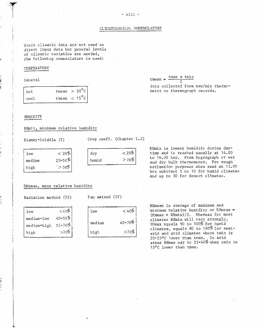
= xiii -

CLIMATOLOGICAL NOMENCLATURE

Wbere climatic data are not used as direct input data but general levels of climatic variables are needed, the following nomenclature is used:

TEMPERATURE ----General

hot

cool

HUMIDITY

> 300~1 < 15°c

·-----

tmean

tmean

RHmin, minimum relative humidity

Blaney-Criddle (I) Crop

low < 201, dry

coeff.

medium 20-50% humid

high > 50%

RHmean, mean relative hurnidity

(Chapter I. 2)

< 201, > 70%

Radiation method (II) Pan method (IV)

low <40%

medium·low 40-55}

medium-high 55·70%

high >7o1,

low

medium

high

<40"/,

40·70'1o

>70"/,

trnax + tmin tmean =

2 <lata collected from max/min thermometer or thermograph records~

RHmin is lowest humidity during daytime and is reached usually at 14e00 to 16.00 hrs. From hygrograph or wet and dry bulb thermometer. For rough estimation purposes when read at 12.00 hrs subtract 5 to 10 for humid clirnates and up to 30 for desert climate~~

RHmean is average of maximum and minimum relative humidity or RHrnean (Rllmax + RHmin)/2. Whereas for most climates RHmin will vary strongly, RHmax equals 90 to 100% for humid climates~ equals 80 to 10010 for semi= arid and arid climates where tmin is 20-25oc lower than tmax. In arid areas RHmax may be z5„4ofo when tmin is 1s0 c lower than tmax.

WIND

Ge11eral

light moderate strong v. strong

Radiation

< 2 m/ sec 2·5 m/sec 5·8 m/sec > 8 m/sec

Blaney-Criddle (I)

sunshine n/N

low medium high

or

< .6 .6-. 8

>.8

Blaney-Criddle (I)

< 175 175-425 425-700

>700

cloudiness tenth '"] low >5 >4 medium 2-5 1 • 5-4 high < 2 < 1.5

km/da~ km/day km/day km/ day

xiv -

For rough estimation purposes sum of several windspeed observations divided by number of readings in m/sec or multiplied by 86.4 to give wind run in km/day.

With 2 m/sec; wind is felt on face aud leaves start to rustle

With 5 m/sec; twigs move, paper blows away ~ flags fly

With 8 m/sec; dust rises~ small branches move

With > 8 m/sec; small trees start to move, waves form on inland waters etc~

Ratio between daily actual (n) and daily maximum possible (N) sunshine duration.

n/N > 0.8; near bright sunshine all day;

n/N = 0. 6 to O. 8; some 40°fo of daytime hours full cloudiness or partially clouded for 7010 of daytime hours.

Mean of several cloudiness observations per

day on percentage or segments of sky covered by clouds.

4- oktas: 501, of the sky covered all daytime hours by clouds or half of daytime hours the sky is fully clouded.

1. 5 oktas: less than 20'1/o of the sky covered all daytime hours by clouds or each. day the sky has a full cloud cover for some 2 hours.

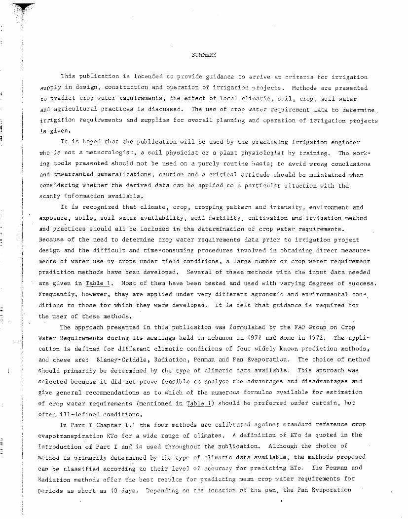
sm!MARY

This publication is intended to provi.de guidance to arrive at criteria for irrigation

supply in design~ construction and operation of irrigation projects. Methods are presented

to predict crop water requirements; the effect of local climatic, soil ~ crop, soil water

and agricultural practices is discussed. The use of crop water requirement data to determine

irrigation requirements and supplies for overall planning and operation of irrigation projects

is given.

It is hoped that the publication will be used by the practising irrigation engineer

who is nota meteorologist, a soil physicist or a plant physiologist by training. The work~

ing tools presented should not be used on a purely routine basis; to avoid wrong conclusions

and unwarranted generalizations~ caution and a critical attitude should be maintained when

considering whether the derived <lata can be applied to a particular situ2tion with the

scanty inforrnation available~

It is recognized that climate, crop, cropping pattern and intensity~ environment and

exposure~ soils, soil water availability) soil fertility) cultivation and irrigation method

and practices should all be included in the determination of crcp water requirements~

Because of the need to determine crop water requirernents <lata prior to irrigation project

design and the difficult and time""consuming procedures involved in obtaining direct measure"'

ments bf water use by crops under field conditions, a large number of crop water requirement

prediction methods have been developed. Several of the.se methods with the input <lata needed

are given in Table 1& Most of them have been tested and used with varying degrees of success.

Frequently, however, they are applied under very different agronomic and environmental con""

ditions to those for which they were developed. It is felt that guidance is required for

the user of these methods.

The approach pres_ented in this publication was formulated by the FAO Group on Crop

Water Requirements during its meetings held in Lebanon in 1971 and Rome in '1972. The appli"'

cation is defined for different climatic conditions of four widely known prediction methods~

and these are: Blaney~Criddlej Radiation 1 Penman and Pan Evaporation~ The choice of method

should primarily be determined by the type of clirnatic data available3 This approach was

selected beca.use it did not prove feasible to analyse the advantages and disadvantages and

give general recommendations as to which of the numerous formulae available for estimation

of crop water requirements (mentioned in Table 1) should be preferred under certain, but

often ill~defined conditions~

In Part I Chapter 1~1 the four methods are calibrated against standard reference crop

evapotranspiration ETo for a wide range of climates. A definition of ETo is quoted in the

Introduction of Part I and is used throughout the publication~ Although the choice of

method is primarily determined by the type of clirnatic data available 9 the methods proposed

can be classified according to their level of accuracy for predicting ETo. The Penman and

Radiation methods offer the best results f'.Jr pre<licting mean crop water requirements for

periods as short as 10 days. Dependtng on the loca::ion of. the pan~ the Pan Evaporation

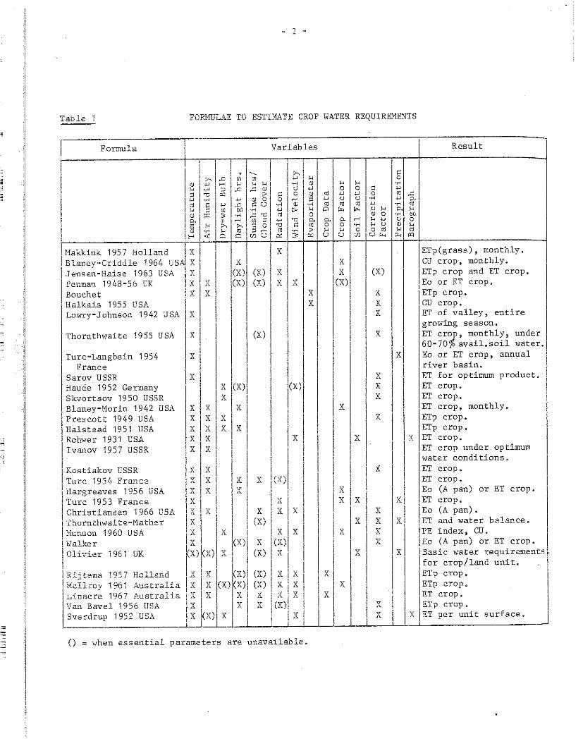
Table FOP.MULAE TO ESTIMATE CROP WATER REQUIREMENTS

Formula Result

1

IMakkink 1957 Holland , X I ļ X !j X I IETp(grass), monthly. Blaney"Criddle 1964 USA X ļ I X CU crop, monthly. ļJensen-Haise 1963 USA X j I j(X)j (X) 1 X 1 1 X (X) IETp crop and ET crop. J Penman 1948-56 UK I X I X j(X)I (X) ļ X X 1

1

ļ<x) 11 Eo or ET crop.

Bouchet X X I j Xl[ 1 1 X ļ ETp crop. Halkais 1955 USA 1 1 1 1 1

11 X CU crop.

Lowry-Johnson 1942 USA I X II I 1

1 1

1 X IET of valley, entire

1

1 1 lgrowing season. Thornthwaite 19 55 U SA I X I ļ 1 (X) 1 X ET crop, monthly, under

IIXļj 1 ,

1

, II 11

1 I 1 1 j60-7ü%avail.soilwater.l Turc-Langbein 1954 ~ X IEo or ET crop, annual 1

France 1 1 1 , 1 1 1 river basin. Sarov USSR jx 1 1 1 X ET for optimum product,

Haude 1952 Germany 'I I X '1(X)I 1 (X)II X I ET crop. Skvortsov 1950 USSR j X I X I IET crop, Blaney-Morin 1942 USA X ļ X ļ I X I X

I ET crop, monthly.

Prescott 1949 USA X I v X 1 1 X jETp crop. Halstead 1951 USA X i j ~ X j

11 .,, 1 ETp crop.

Rohwer 1931 USA IX X 1 1 .. X X ET crop. īvanov 1957 USSR X I X 1 1 1 1 ET crop under optimum

1 • 1 i , t j 1 1 f EwTater conditions.

1 Kostiakov USSR I X X 1 1 i ļ 1 1 X I crop ļ Turc 1954 France i XX ~ II ;; 1, X [ ()01 1 X j . 1 EE•T

0 c(Aroppa:n)

1 Hargreaves 1956 USA , H , 1 1 1 or ET crop. 'ITurc '1953 France '1~ i" 'I 11 ļ J X 1 1 X X I X ET crop. Christiansen 1966 USA X I X I 1 1 X I

v I X 11 1 1 X I Eo (A pan).

Thornthwaite•Mather I X j \ ! (~) 1 " , II X I X X ET and water balance.

IMun.son 1960 USA 1X X 1 1 X X ļ X X ļ IPE index 9 CU, 1

Walker lx 1 1 (x)ļ X 1(X) i I X X I IEo (A pan) or ET crop.

1

Olivier 1 961 UK pO kx) t X , 1 (X) X 1

1

X Basie water requirements , ļ ! , lļ 1 1 1 for crop/land unit, ,

1 r~~i~::; ; !~; !~!!:~fia ~ 1 ~ (X) 11,)~; ~~; 1 ~ 1 : l 1 ' : 'I 1 1 !~~ ~;:~:

Linacre 1967 Australia X l X X X ! X X X 1 ! ! ET crop. Van Bavel 1956 USA X 1 1 X X ļcx)I 1 1 X i I IIETp crop. Sverdrup 1952 USA X 1(X)I X , X _1___L'.'.__lj X ET per unit surface. _J

() = when essential parameters are unavailable~

J

·~.·.··.·.· •• · ''::i,:,l

1 ....

method may be graded next~ a1though this method c.ould be superivr for pans with excellent

siting and for light windsQ In many climates the Blaney""C:riddle method :Ls best for periods

of one month or more. To reach the relationships presented, use was made of data obtained

from many research stations and publications listed in the Appendices. In Chapter Ia2 the

relationship between crop evapotranspiration ET(crop) and the reference crop ETo is given

by crop coefficients kc for the different crops, stages of growth) length of growing season

and prevailing climatic conditions. Since ETo is used as the standard reference for the

four methods presented, one set of kc values applies to all methods~ To arrive at the kc

values presented, the sources mentioned in Appendix II were consulted and extensive use was

made of published material& Once ETo and kc have been determined for a given period ET(crop)

can be found as shown in Chapter I.3~ In Chapter I.4) the extent to which local conditions

can have an appreciable effect on crop water requirements is given; these include local

variations in climate, advection, soil water availability~ irrigation methods and practices,

agronomic practices and production levela

In Part II, the use of crop water requirement <lata in determining field irrigation

requirements is discussed. Methods are suggested to calculate the variables composing the

field water balance, which in turn fonns the basis for predicting seasonal and peak field

irrigation requirements, and field irrigation schedules. Attention is given to water

required to compensate for inefficiency in field application, and for cultural practices

and leaching of salts.

In Part III discussions are centred around the use of crop water requirement <lata to

determine seasonal and peak project water supply for the purpose of project planning~

Methods are suggested for evaluating field supply schedules while considering different

methods of water delivery. Suggestions are also mad'e for applied research which may be

necessary and for the refinement of field supply schedules once the project is in operation.

The methods proposed in this publication for determining crop water requirements,

field irrigation requirements and irrigation supply are cons~dered adequate for preliminary

project planning~ It should be realized that local practical~ technical, social and econo=

mic considerations may have a great effect on the final planning criteria selected.

It will be noted that certain information or calculation procedures are repeated under

different headings; this has been done intentionally to maintain continuity or sequence.

Throughout the text or in tables and figures an asterisk indicates the example or

calculation being discussed. Abbreviations such as RHmax, ETo and Vs are given on the same

line for ease of presentation (i~e. not Pu~ax~ ET0

or V8

which is the common practice).

PART L CALCULATION OF CROP EVAPOTRAl\lSPīRATION, ET, (Crop)

INTRODUCTION

It is generally r2cognized that climate is one of the most important factors determin

ing the amount of water loss by evapotranspiration frDm the crop. Apart from the climatic

factors, evapotranspiration for a given crop is also determined by the crop itself and so

are growth characteristics~ Local environment, soil and soil water conditions, fertilizers,

insect and dise.ase infestations, agricultural and itrigation practices and other factors

may also influence growth rates and resulting evapotranspiration.

Methods are. used to predict evapotranspiration from climatic variables owing to the

diffic.ulty of obtaining accurat.e. direct measurements under field conditions. Mast predic„

tion formulae use a differentiation between the components of climate and crop. Such

formulae often have to be applied under climatic aud agronomic conditions very different to

those for which they were originally developedD It is therefore important to test the

accuracy of the formulae before using them under a new set of conrl.itions~ Not only the

degree of accuracy required for predicting evapotranspirationj but also the choice of

formula is conditioned by the climatic variables obtaining which must have been measured

with sufficient accuracy over a certain number of yearsG

Testing prediction formulae in a new set of conditions is laborious, time consuming

and costlyD Yet crop water requirement <lata are frequently needed at short notice for

regional and preliminary project planning and to determine average aud peak water require

ments for overall irrigation project design. In order to overcome the limitations that

different climatic conditions have on the accuracy of the prediction fonnulae and to dis

seminate the wealth of infonnation available on the growth characteristics of the crop in

relation to crop evapotranspiration, four widely used prediction formulae have been tested

against measured evapotranspiration <lata for different geographic areas and climatic

conditions.

The approach followed was to relate magnitude aud variation of evapotranspiration to

one ar more climatic factors (day length, temperature, hUL-nidity 9 wind, sunshine)o For this,

measured evapotranspiration data from a grass cover were used, assuming that evapotranspira„

tion of grass occurs largely in response to clirnatic conditions. A reference value, ETo,

was introduced and defined as ~ ~the rate of evapotranspiration from an extended surface of

8 to 15 cm tall green grass cover of unifonn height, actively growingj completely shading

the ground and not short of water'~. Four prediction fonnulae are presented to calculate

ETo, viz~! adaptations of the Blaney=Criddle, the Radiation~ the Penman and the Pan Evapora„

tion method. Each method was calibrated against measured ETo <lata collected from different

locations and climates, Choice of method to be used to calculate ETo is primarily based on

the type of climatic data available for the area of investigation. Applying one of the

four formulae described ~ ETo can be compu.ted fo:r each 30 or 10 day period using the rnean

climatic data for the pe:.ciod cons::Lder2d, ETo is expre.ssed in mm per day and represents the

T l - s

mean value over that period, Since for a given climate ETo will vary from year to year, an

analysis should be made of m~gni tude and frequency of extreme values of ETo for which a

frequency distribution analysis on ETo may be required 0

To know the evapotranspiration of the crop~ ET(crop)~ the relation between ETo and

ET(crop) was studied using data from different locations and climates. For the selected

crop, its stage of development and prevailini climatic conditions is given by the crop

coefficients~ kc. ET(crop) is found for a given 30 or 10 day period by ET(crop) = kc. ETo.

Since the four prediction formulae to calculate ETo have been calibrated against the same

reference crop evapotranspiration~ the presented crop coefficients apply to each method 0

ET(crop) thus detennined refers to evapotranspiration of a disease-free crop, growing

in a large field (one ar more hectares) unde:r optimal soil conditions including sufficient

water and fertility and achieving full production potential of that crop under the given

growing environment. Local conditions and agricultural practices may have a substantial

effect on ET(crop) which might require some correctione

CALCULATION PROCEDURES

Before calculating ET(crop), a review should be made of completed climatological and

agricultural surveys aud of specific studies and research carried out on crop water require„

ments in the area of investigation~ Available measured climatic <lata should be reviewed;

if possible, meteorological and research stations should be visited and environmentJ siting~

type of instruments and observation and recording practices appraised to evaluate accuracy

of available data. Data relevant to types of crops grown, cropping pattern, and agricultural

and irrigation practices should be collectedo

After this reviewj the procedure is to determine ET(crop) from available meteorological

and crop <lata.

1. Calculation of reference crop evapotranspirationj ETo

Based on meteorological <lata available 1 select prediction method to calculate

reference crop evapotranspiration, ETo~ If a complete set of meteorological

<lata is available, the choice of method should be based on the required level

of accuracy in predicting ETo. The Penman and Radiation method offer the best

results for periods as short as 10 days. Depending on the location of the pan,

the Pan method may be graded next, although for pans with excellent siting and

for light winds ~ pan <lata may be superior. In rnany climates the Blaney-Criddle

method is best applied for periods of one month ar moreo Minimum input <lata

for each method are given below~ indicating measured data required and general

knowledge of weather needed for each method:

1

:1

1 'I '1

C 1

' ,,

.. 6 -

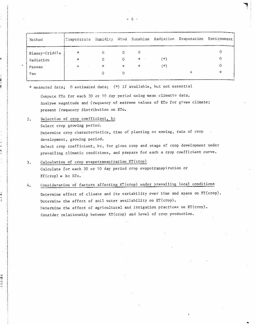
Method j Temperature hurnidity Wind Sunshine Radiation Evaporation Envi r_onmen t

Blaney-Criddle * 0 0 0

Radiation * 0 0 * (*)

Penman * * * * (*)

Pan 0 0 *

* measured <lata; 0 estimated <lata; (*) if available, but not essential

Compute ETo for each 30 or 10 day period using mean climatic dataG

2.

3.

Analyse magnitude and frequency of extreme values of ETo for given climate;

present frequency distribution on ETo~

Selection of crop coefficient, kc

Select crop growing period.

Determine crop characteristics, time of planting ar sowing, rate of crop

development, growing period.

Select crop coefficient, kc, for given crop and stage of crop development under

prevailing climatic conditions, and prepare for each a crop coefficient curve.

Calculation of crop evapotranspiration ET(crop)

Calculate for each 30 or 10 day period crop evapotranspiration ar

ET(crop) = kc ETo.

0

0

0

*

4. Consideration of factors affecting ET(crop) under prevailing local conditions

Determine effect of climate and its variability over time and space on ET(crop).

Detennine the effect of soil water availability on ET(crop).

Determine the effect of agricultural and irrigation practices on ET(crop)~

Consider relationship between ET(crop) and level of crop production~

[

"

l

- 7 =

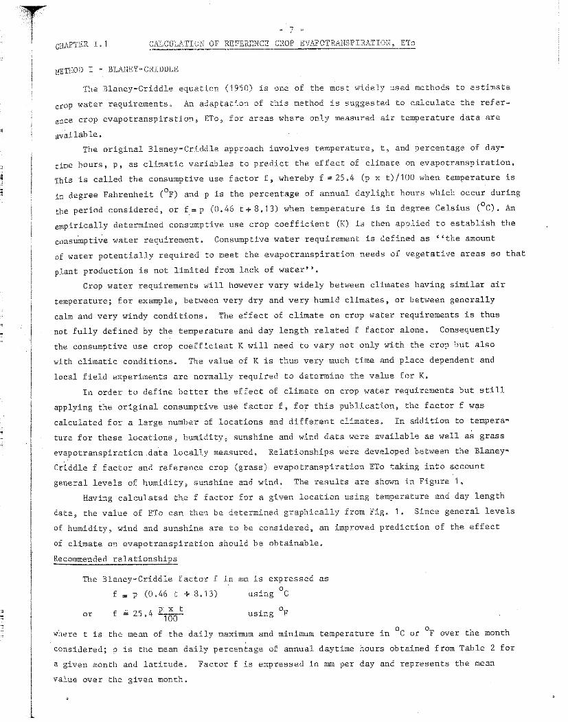
cHAPTER I, 1 CALCDLATION OF REFERENCE CROP EVAPCTR..'lHSPIRATIOH, ETo

METl!OD I - BLA!lEY-CRIDDLE

The Blaney„Criddle equation CI 950) is one of the mast widely used methods to estimate

crop water requirements" An adaptation of this method is suggested to c.alculate the refer=

ence crop evapotranspiration, ETo~ for areas where only measured air temperature data are

available.

The original Blaney~Criddle approach involves temperature, t, and percentage of day

time hours, p, as climatic variables to predict the effect of climate on evapotranspiration~

This is called the consumptive use factor f, whereby f = 25.4 (p x t)/100 when temperature is

in degree Fahrenheit (°F) and p is the percentage of annual daylight hours which occur during

the period considered~ or f.=P (0.46 t+8.13) when temperature is in degree Celsius (0c). An

empirically determined consumptive use crop coefficient (K) is then applied to establish the

consumptive water re.quirement. Consumptive water requirement is defined as ''the amount

of water potentially required to meet the evapotranspiration needs of vegetative areas so that

plant production is not limited frorn lnck of water''.

Crop water requirements will however vary widely between climates having similar air

temperature; for example, between very dry and very humid clirnates, ar between generally

calm and very windy conditions. The effect of climate on crop water requirements is thus

not fully defined by the ternperature aud day length related f factor alone. Consequently

the consumptive use crop coefficient K will need to vary not only wi.th the crop but also

with climatic conditions. The value of K is thus very much time and place dependent and

local field experiments are normally required to determine the value for K.

In order to define better the effect of climate on crop water requirements but still

applying the original consumptive use factor f, foŗ this publication, the factor f was

calculated for a large number of locations and different climates~ In addition to tempera•

ture for these locations ~ humidity J sunshine and wind <lata were available as well aS grass

evapotranspiration.data locally measuredo Relationships were developed between the Blaney„

Criddle f factor and reference crop (grass) evapotranspiration ETo taking into account

general levels of humidity 3 sunshine and wind3 The results are shown in Figure 1~

Having calculated the f factor for a given location using temperature and day length

<lata~ the value of ETo can then be determiwed graphically from Fig. 1. Since general levels

of humidity, wind and sunshine are to be consideredt an improved prediction of the effect

of climate on evapotranspiration should be obtainable.


The Blaney·Criddle factor f in mm is expressed as

f = p (0.46 t + 8.13) using oc

f 25. 4 p X t using OF or = -100-

where t is the mean of the daily maximum and minimum temperature in °c or °F over the roonth

considered; p is the rnean daily percentage of annual daytime hours obtained from Table 2 for

a given month and latitude. Factor f is expressed in mm per day aud represents the mean

value over the given month.

~ 8 "'

For the Blaney„Criddle f values thus detennined~ Figure ·1 depicts recommended relationm

ships to determine ETo estimates. The value of f is given on the X-axis and the value of

ETo can be read from the Y=axis. Relationships are presented in Fig. 1 for three levels of

daytime minimum humidity (RHmin) and three levels of the ratio actual to maximum possible

sunshine hours (n/N). Additionally, relationships are given for three ranges of daytime wind

conditions (U) at 2 metre height. Information on general weather conditions, including

RHmin, n/N and Uz may be obtained from published weather descriptions or from local sources.

The nomenclature used to depict general levels of humidity, sunshine and wind is given

under Climatological Nomenclature in the introductory pages of this publication.

Several selected relationships would norrnally. be required for the same location since

one or more of the three climatic variables considered would probably show major changes

according to season. Also the combination of weather conditions selected for Fig. 1 may

require interpolation bet.ween the :r:elationships given~ For example, the dotted line in

Fig. 1, Block II involves light to moderate wind~

Since factor f is expressed in mm per day ETo is also expressed in nnn per day and

represents the mean daily value of the period considered~ which is usually one rnonth. To

find monthly ETo in w.m, the value needs to·be multiplied by the number of days of each month.

After deterrnining ETo. from Fig. 1 ~ ET(crop) can be. pre.dicted using the appropriate

crop coefficient kc, or ET(crop):::: kc x ETo. Crop coefficients are given l.n Chapter I~Z.


The adaptation of the Blaney=Criddle method presented should only be used when tempera"'

ture data are the only specific weather <lata available~ The empiricism invoJ.ved in any ET

prediction method using a single weather factor is inevitably high. Only for weather conM

ditions similar in nature does a generally positive correlation seem to exist between

Blaney-Criddle f values and ETo~ As shown in Fig. 1, the relation between factor f and ETo

therefore varies widely between climates, for example, very dry as compared to very humid

climates, or between light and strong winds.

In this publication the use of crop coefficients (K) normally employed in the original

Blaney-Criddle approach is rejected because: (i) the original crop coefficients (K) are

heavily dependent on local conditions, and the wide variety of K values reported in literature

makes the selection of this value rather difficult; (ii) the relationship between Blaney"'

Criddle f values and ETo can be adequately described for a wide range of temperatures for

areas having only minor variations in RHmini n/N and U; and (iii) once ETo has been deter

mined by each of the methods proposed, one set of crop factors (kc) can be used to determine

ET(crop).

The use of the Blaney~Criddle method to calculate mean daily ETo should norrnally be

applied for periods no shorter than one month~ Unless verification of the general prevail

ing weather conditions (RH(min), n/N, and Uz) can be obtained, predictions are obviously

highly questionable, Considerable care is thus needed in the use of this method since for

.,

- 9 -

a particular month n/N may vary greatly from year to year and consequently ETo. Hence., it

iS suggested that ETo should be calculated .for each calendar month for each year of record

rather than by using mean temperatures based on several years' records.

This method should not be used in equatorial regions where temperatures remain fairly

constant hut other weather parameters wi~l changee It should not be used either for small

islands where air ternperature is generally a function of the surrounding sea temperature

showing little response to seasonal change in radiation. At high altitudes the approach

becomes uncertain due to the fairly low mean daily temperature (cold nights) even though

daytime radiation levels are high. Also in climat.es with a high variability in sunshine

hours during transition months (e.g. monsoon climates, mid 00 latitude climates during spring

and autumn) the method could be misleading.

~ple calculations

First using mean daily temperature and daylength <lata for one month only, an example

provides the necessary simple calculation procedure to obtain the mean daily value of

f = p(0.46 t + 8.13) in mm for the given month. Then mean daily <lata for each month and for

the whole year are given to illustrate the selection of relationships between prevailing

weather conditions and of the value of ETo for each month using Fig. 1. ETO can be deter·

mined graphically or by machine calculations using coefficients indicated for each relation

ship shown. A format for the necessary calculation procedures is given at the end of this

sub-chapter.

Figures and tables to be used:

~:' Prediction of ETo from Blaney-Criddle f factor for different conditions of relative humidity, daily sunshine hours and daytime wind.

Mean daily percentage of annual daytime hours for different latitudes. '--------------------------

EXAMPLE:

given: Cairo, Arab Republic of Egypt;

latitude: 30° N

altitude: 95 m

month July

tmax

tmin

tdaily mean

p

=

f = p(0,46 t + 8, 13)

RH(min)

n/N

u2 daytime

1 ETo

2:: tmax daily values/31

1: tmin daily Values/31

2:: tmean [2:: tmax . 2:: tminl ~ 2 3-1-- or -:ŗr- ,. 31 J ·

select from Table 2 for 30°N

0,31 (0,46 X 28,5 + 8, 13)

from Climates of Africa, Griffith (1972) Table XXVIII

from Rijtema and Aboukhaled (1973)

Fig. 1 - Block II

35°C

22°c

28,5°C

0.31

6.6 mm/day

35 'f, (medium)

>0.8 (high)

3 m/sec (moderate)

8, 1 mm/day

'

'"l

Based on general in:formation and re.ferences (Climates of Africa~ Griffith 1972) the f,Jllowing breakdovv'11 for Cairo can be made:

!

~"'~"' n/N u2

daytime Block Line

1

Jan • March Medium Medium Light to V 2 moderate

April - May Low to High to Moderate (IV, V, 2 mediurn rnedium I & II) 1 /

June - July Medium High Moderate II 2

Aug - Sept Medium High Light to II - 2 moderate

Oct - Dec Medium Medium Light to V 1 - 2 moderate

1 ) Jan Feb Mar Apr May June July Aug Sept Oct Nav

tmean oc 15 17. 5 21 25.5 27.5 28.5 28.5 26 24 20

pmean 0.24 0.25 0.27 0.29 o. 31 0.32 0.31 o. 30 0.28 0.26 0.24

p(0.46t+8.13) 3.5 3,8 4.4 5, 1 6. 1 6.6 6.6 6.3 5.6 5.0 4.2

ETo mm/day 2.3 2.6 3.4 5. 8.!_I 1.3Y 8. 1 8. 1 6.9 5.9 4.2 3.2

Dec

15.5

0.23

3.5 --2.3

1/ Borderline RH(min) aud n/N conditions suggest a compromise between Blocks IV r V using curve 2 for moderate wind in all cases. """ī"TĪĪ'

April (f = 5.1 mm) 5.8 l_Li.8 ET 6.T"T's:-'J ar 0

= 5. 8 mm/day

May (f = 6. 1 mm) --7:ĪĪ=r 6. 2 -

1ī:')" 7

_3

ar ETo = 7.4 mm/day

If machine calculation is used, expressions are presented which directly predict reference evapotranspiration ETo for mean dail percentage of annual daytime hours (p) and mean daily temperature (t).

or ETo = ~ + ~ {p (0.46 t + 8.13)]

Values of g and Q for different combinations of RH(min) n/N and u2 are given in Fig. 1 ,

EXAMPLE:

given: Cairo;

latitude: 30°N

altitude: 95 m

1 Jan - Mar

Apr ""May

June - July

E' - Sept .

t Dec

ETo „2 ~ 17 + 1. 29

ETo = -2.25 + 1 .59

ETo = -2.50 + 1.61

ETo = -2.50 + 1, 61

ETo = -2.45 + 1.49

ETo = -2, 17 + 1 .29

{p (0, 46 t + 8.13)] 1/

[p (0.46 t+8.13)] 2/

[p (0.46 t + 8.13)]

[0.31 (0.46 X 28 0 5 + 8.13)] = 8. 1

{p (0.46 t + 8.13)] 1 / -[!J.46 t+8.13)] 1/

1/ interpolation for wind speed of around 2 rn/sec (light to moderate)

mm/day

2/ average of constants in 4 equations, curve 2 in Blocks I, II, IV and V

. -~

' . ·11 .

Table 2 MEAN DAILY PERCENTAGE(p) OF ANNUAL DAYTIME HOURS

FOR DIFFERENT LATITUDES

Latitude North Jan Feb Mar Apr May June July Aug Sept Oct Nov Dec 1

' South-!_/ Junej July Aug Sept Oct Nov Dec Jan Feb Mar Apr May

1 60° . 15 .20 • 26 .32 .38 .41 .40 .34 .28 .22 . 17 • 13 1

58 • 16 • 21 .26 .32 .37 .40 .39 .34 .28 .23 • 18 . 15 1

56 • 17 • 21 .26 .32 .36 .39 .38 .33 .28 .23 • 18 • 16 1

54 • 18 ,22 .26 , 31 .36 .38 .3 7 .33 .28 .23 • 1 9 • 17

52 • 19 .22 .27 • 31 .35 .37 .36 .33 .28 .24 .20 • 17

50 • 19 .23 .27 • 31 .34 .36 .35 .32 .28 .24 .20 .18

48 ,20 .23 .27 • 31 .34 .36 .35 .32 .28 .24 • 21 • 19

46 .20 .23 .27 .30 .34 .35 .34 .32 ,28 .24 , 21 ,20

44 .21 .24 ,27 .30 .33 .35 .34 , 31 .28 .25 ,22 • 20

42 , 21 .24 .27 .30 .33 .34 .33 . 31 .28 .25 • 22 • 21

40 .22 .24 ,27 .30 .32 .34 .33 • 31 .28 .25 • 22 .21

' 35 • 23 .25 .27 .29 • 31 .32 .32 .30 .28 ,25 • 23 ,22

30 .24 .25 .27 .29 , 31 .32 . 31,, .30 .28 .26 • 24 .23

25 ,24 .26 • 27 .29 .30 • 31 • 31 .29 ,28 , 26 , 25 • 24

20 .25 .26 .27 .28 .29 .30 .30 • 29 .28 .26 • 25 ,25

15 .26 .26 .27 .28 .29 .29 , 29 .28 .28 .27 .26 .25

10 .26 .27 .27 .28 .28 .29 • 29 .28 .28 .27 • 26 • 26

5 .27 .27 .27 .28 .28 .28 .28 .28 .28 .27 .27 .27

0 .27 .27 .27 .27 .27 • 27 .27 .27 ,27 .27 .27 ·:J 1 / Southern latitudes: apply 6 month difference as shown~

;J,ld JJi LI

Table 2a

t 0 c 0 2

P"i" , 14 1 • 1 1,3

• 16 1 • 3 1.4

.18 1,5 1 • 6

.20 1.6 1.8

,22 1.8 2.0

,24 2.0 2.2

.26 2.1 2,4

,28 2,3 2,5

, 30 2,4 2,7

,32 2.6 2,9

.34 2,8 3, 1

,36 2,9 3,3

,38 3.1 3,4

,40 3,3 3,6

,42 3,4 3,8

1 ,i.;, li ,1 ,IĪ JI,• ,,Hit,,,,,,

VALUE OF BLANEY-CRIDDLE f VALUE FOR DIFFERENT TEMPERA'lURES AND DAILI PERCENTAGE OF ANNUAL DAYLIGHT HCURS

4 6 8 10 12 14 16 18 20 22 24 26 28 30 32

1,4 1.5 1 • 7 1.8 1.9 2.0 2.2 2,3 2,4 2.6 2„7 2,8 2,9 3,0 3,2

1 • 6 1 , 7 1.9 2,0 2.2 2.3 2.5 2.6 2.8 2.9 3. 1 3,2 3,4 3,5 3,7

LS 2.0 2.1 2.3 2,5 2.6 2.8 3.0 3, 1 3.3 3,5 3,6 3,8 3,9 4,1

2.0 2o2 2,4 2.5 2,7 2,9 3, 1 3,3 3.5 3,7 3,8 4,0 4,2 4~4 4,6

2.2 2.4 2.6 2.8 3,0 3,2 3,4 3,6 3,8 4.0 4„2 4,4 4,6 4,8 5.0

2,4 2,6 2.8 3, 1 3,3 3,5 3~7 3,9 4,2 4,4 4,6 4,8 5.0 5,3 5,5

2,6 2.8 3. 1 3,3 3,5 3,8 4,0 4,3 4,5 4,7 5.0 5,2 5,5 5,7 5,9

2.8 3,0 3,J 3,6 3,8 4,1 4,3 4,6 4,9 5.1 5,4 5,6 5,9 6. 1 6,4

3,0 3,3 3o5 3,8 4, 1 4,4 4,6 4,9 5.2 5,5 5,8 6.0 6.3 6.6 6,9

3,2 3,5 3,8 4, 1 4,4 4,7 5,0 5,3 5.5 5.8 6,1 6,4 6,7* 7.0 7,3

3,4 3,7 4,0 4,3 4.6 5,0 'i. 3 5.6 5,9 6.2 6.5 6,8 7,1 7,5 7,8

3,6 3,9 4.3 4,6 4,9 5,2 5.6 5,9 6.2 6.6 6,9 7.2 7,6 7,9 8,2

3,8 4.1 4,5 4,8 5.2 5,5 5.9 6~2 6.6 6,9 7,3 7,6 8.o 8,3 8,7

4,0 4,4 4,7 5,1 5.5 5.8 6.2 6,6 6.9 7,3 7,7 8,0 8,4 8,8 9, 1

4,2 4,6 5.0 5,3 5,7 6,1 6.5 6.9 7,3 7,7 8.1 8,4 8.8 9.2 9,6 ,.

34

3,3

3,8

4,3

4.8

5.2 5,7

6.2

6,7

7. 1 7,6

8.1

8,6

9,0

9,5

10.0

"''

36 38 40

3,5 3,6 3,7

4,0 4,1 4,2

4,4 4,6 4,8

4,9 5.1 5,3

5.4 5,6 5,8

5.9 6. 1 6,4 -· ,~ 6.4 6.7 6,9

6,9 7,2 7,4

7,4 7,7 8.o

7.9 8,2 8,5

8,4 8,7 9,0

8,9 9.2 9,6

9,4 9,7 10.1

9,9 10,2 10.6

10.4 10.8 11 „ 1

'

•

i:'s

i . .J..

DATA

t mean =J2,/'c

. 0 latitude =;?;, tl

Rl! (min) {~;j %

u2 daytime •(3) m/sec

DATA

t mean

latitude •

Rl! (min)•

n/N :

u2 daytime.: m/sec

oc

0

t mean

p

f

Country: Period :

t mean

p

f

data

Ta.ble 2

Ta.ble 2a

estima.te

eatimate

eetimate

Fig~ 1

Fig. 1

• 13 •

Place2&1/tJ

.26, 6-

1 ,:}, ?,/

Block/line

ETo

Lati tude t Jo e)/ Longi tude: ;to~

Altitudei C/:) m

'

~-J-, -/~! mm/day

FORMAT FOR CALaJLATIO!T OF BLANEY-GRIDDLE l!ETHOD

data

Table 2

Table 2a

estimate

estimate

estimate

Fig~

Fig~ 1

Places

l.____,1-

lllock/line

Latitude i Longi tudet

Al tituclet

-

" ~ -

H--;-6-H l ---T

ļ . :~ :t 5

• 3

11

10

9

8

7

• 5

4

3

2

13 ~ 12

11

10

9 ~

.g. ' E 7 E

cS 1-

'" 5

4

3

2

(3)- - !.:50

{21 - i .8d

(!} -2.00

• 3

0

(3) - l.80

12l -2.05

11) -2..30

2 • 0

(3}-2..00"

(21 -2.:SO

111 -2.SO

= • 5 š 7 8

3

b --

2 L73.

L:3.5.: l·

1

~ s • , t „ a P·(0.46-t-8)13Hlln°CJ.: or ~5,4 :P,:.t Cit itt 0 F°]

_j~--1 iī ___ -----··fu-

~ i:-JJ.--~ C. 70 .-1„t.5

i te) - ,.JJS ___ LllL /7: ŗrl [U -e.oc l.lliL __ -7/ 1

7'/ --· ŗ_- - -o/' r --- if-_ [ ff~ •·····:-~

2 ' 4 :5 S 7 •

b

l.5..2. - -- 7 3_ t a

Ll!8 2 __

! IJ -2...._2.Q: ,t.20:

2 3 • • 1

- ---]-

·-· ii -.-:

{3l -2-5.5:---·. 1.82:. _

(2J -2.5.0: 11.~_1_[_

ŗ tJ.l ... eeitA~ 'l.37 , ļ. _

f -{'J •Lfil>-, --0.SO

~,. ___ UJ - Ul5 0.3"3

l [Ü -HO O.SO

2 3 4 5 6 7

0 b

_____ ļ3..J .-.L10 l. !6

t~_L75 LOG

_____ {l) - 1.80 0+97

• • • 7

--~-- [!_ l3L..;.L1.n~ ____ 1. 31

bi.ta5[ LiL 1

_ ~--lu~.,.k_iJiL LL4L_ __ 0)

oi\ 1 J-____________ -, ' /

1 / 1/• ----r+- • ~ ~ /VAI i~-1---~+ 2 ei

: - ~-) __

r 1 ·1~_: ~il li 1 '" 1 ŗ ' ·• . . i 1 ...•. , .. , .. : 1 .• _i 1 ļf :i. U : :r:rf ·1 . f i ••• l. 1 ~_'. J t'f ~1 ;J_ ;_J.ļ.[ ;'.,il,,:....j .... L •. ic-. c--1K + • ' o 1 • r 1 1 f' '·l ' ' r i ij

1 l !'.---1~-- ___ L...._ ___ .i.,.__ ! j__

Fig. l Prediction of ETo friom Bloney - Criddle 1ac1or humidity, doily sunshine hours, and doytime wind.

for different! eonditions of minimu!m r lotive

•

M.ETHOD II '" RADIATION

For are.as where available climatic <lata include measured air tempe:cature and sunshine

or cloud.i:1ess or radiation .. 1 but not: ,,1ind and numidity) the radiation metlwd is suggested

to predict the effect of clima;:e oŗi crop water requirements. Direct measurement of the duration

of bright sunshine hours or if not available, cloud observations can be used to obtain a

measure of solar radiation, In addition, only general levels of humidity and wind are required

and such information may be obtained from published weathe.r descriptions or from local

sources,

The method predicts the effect of climate on crop water requirements. For this

publication the radiation formula was calculated for a large number of locations and different

climates. For these locations~ apart from measured data on temperature and solar radiation,

wind and humidi ty data were also available ~ as well as locally measured grass evapotrans

piration <lata, Relationships were developed between the radiation term and reference crop

(grass) evapotranspiration, ETo~ taking into account humidity and wind conditions. The result

is shown in Figure 2.

Results from the Radiation Method should be more reliable than those from the Blaney'"

Criddle approach outlined earlier. ln fact, in equatorial zones, on small islands, or at

high elevations, the radiation method should be more reliable even if measured bright

sunshine or cloudiness data are not available. 1 in which case <lata from solar radiation maps

prepared for mos t locations in the world would provi de the nec.essary solar radiation d.ata. 1 /

Recommended _ relationships

The relationship suggested to calculate referenc.e crop evaporation ETo from temperature

and radiation <lata is:

ETo = a y b.W. Rs

wher,e ETo is reference crop evapotranspire..tion in mm/ da.y and represents the mean value over

the period considered~ i.e. 30 or 10 days~ Rs is tne solar radiation expressed in equivalent

evaporation in mrn/day) and' W a weighting factor which depends on temperature and altutude;

a and b are coefficients for wflich the values are given in Fig. 2. The ·relationships presented

in Fig. 2 between the radiation terms W.Rs and ETo tak:: into account general weather

conditions, notably mean relative humidity and daytime wind. From available measured data on

temperature and radiation the radiation term W. Rs is calculated first, For the prevailing

conditions of mean relative hurnidity and daytirne wind the value of the radiation term if

given in Fig. 2 on the x~axis and the value of. ETo can be read from the Y-axis. Both are

exp:ressed in mm/day and represent the mean value for the period concerned.

1 / See for instance Solar Radiation aud Radiation Balance Data; routine observations for the

whole world published un der WMO auspices in Leningrad, U. S. S. R.

Wl10~ Data of the Intern. Geoph. Year, Forms E1 9 E2 and E3.

J.N. Black (1956). Distribution of solar radiation over the earth's surface.

J.F. Griffith (1971), World Survey of Climatology~ Elsevier.

• ·16 •

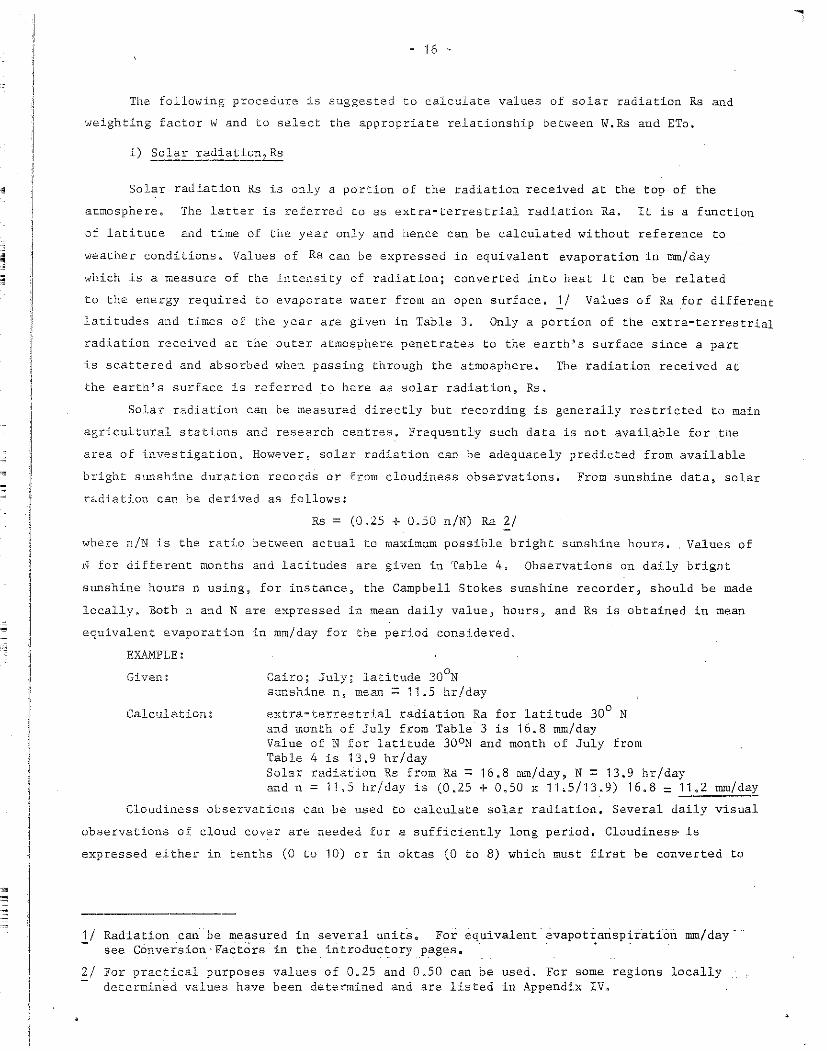
The following procedure is suggested to calculate values of solar radiation Rs and

weighting factor W and to select the appropriate relationship between W.Rs aud ETo.

Solar radiation Rs is only a portion of the radiation received at the top of the

atmosphere. The latter is referred to as extra-terrestrial radiation Ra. It is a function

of latitute and time of the year only and hence can be calculated without reference to

weather conditions. Values of Ra can be expressed in equivalent evaporation in nun/day

which is a measure of the intensity of radiation; converted into heat it can be related

to the energy required to evaporate water from an open surface, 1/ Values of Ra for different

latitudes and times of the year are given in Table 3, Only a portion of the extra•terrestrial

radiation received at the outer atmosphere penetrates to the earth's surface since apart

is scattered and absorbed when passing through the atmosphere. The radiation received at

tbe earth' s surface is referred .to here as sol ar radiation, Rs.

Solar radiation can be measured directly but recording is generally restricted to main

agricultural stations and research centres. Frequently such <lata is not available for tne

area of investigation. However~ solar radiation can be adequately predicte.d from available

bright sunshine duration records or from cloudiness observations. From sunshine data, solar

rc:~diation can be derived as follows:

Rs = (0.25 + 0.50 n/N) Ra 2/

where n/N is the ratio between actual to maximum possible bright sunshiue hours. Values of

1~ for different months and latitudes are given in Table 4, Observations on daily brignt

sunshine hours n using, for instance 3 the Campbell Stokes suushine recorder, should be made

locally~ Both n and N are expressed in mean daily value, hours, and Rs is obtained in mean

equivaleut evaporation iu mm/day for the period considered.

EXAMPLE:

Given:

Calculation:

Cairo; July; latitude 30°N sunshine n~ mean = 11„5 hr/day

extra~terrestrial radiation Ra for latitude 30° N aud month of July from Table 3 is 16.8 mm/day Value of N for latitude 30°N and month of July from Table 4 is 13.9 hr/day Solar radiation Rs from Ra = 16.8 mrn/day, N = 13.9 hr/day and n = 11.5 hr/day is (0.25 + 0.50 X 11.5/13.9) 16.8 = ~.!.2 rnrn/da)'.

Cloudiness observatious can be used to calculate solar radiationc Several daily visual

observations of cloud cover are needed for a sufficiently long period. Cloudines& is

expressed either in tenths (Oto 10) or in oktas (0 to 8) which must first be converted to

.:!./ Radiation can be measured in several unitS„ Fo:C equivalent · ~vapot~arisp~i"a.tiOīi mm/day -see Conversion · Factors in the. iritroduc~.ory .P.ag~s a - •

2/ For practical purposes values of 0.25 and 0~50 can be used~ For some regions locally determined values have been determined aud are listed in Appendix IV.

-

l

- 17 -

the n/N ratio~ To shorten correlations between cloudiness and solar radiation~ for some

areas the direct relationship between cloudiness aud the ratio Rs/Ra has been established

(frere and Rijks, 1974):

---;;loudiness _ oktas P--1 _2 __ 3 4 ___ 5 _6 ___ 7 _s _

Humid equatorial highlands, Rs/Ra

1

,66 ,62 ,59 ,56 ,52 ,49 ,46 ,42 ,39 semi•arid climate, Rs/Ra ,70 .67 ,64 ,61 ,58 ,56 ,53 .50 .46

Values of Ra for a given latitude and time of the year can be obtained from Table 3.

However, it is preferable to use locally derived <lata on the relationship between cloudiness

and sunshine. Sometimes sky observations are made which are expressed in four classes;

conversion is approximately: clear day akta, partial cloud = 3 ok~as~ clouds = 6 oktas,

0vercast = 8 oktas. The conVersion of the visual observations of cloudiness into equivalent

values of n/N can be obtained from the following table& Scatter in conversion factors from

location to location has been noted which indicates a degree of inaccuracy when using

cloudiness <lata for obtaining daily bright su.1shine hours.

"'""'"es'-i. o ., ., ·' . 't '''""'"'' 1 lo ,2 (tenths) (oktas) * ----- ---------------

0 .95 ,9 .9 .9 .9 0 . .9 .9 1 ,85 • 85 , 85 • 85 ,8 1 ,85 ,85

2 .8 ,8 .8 , 75 ,75 2 • 75 .75

3 ,75 '7 '7 • 7 .65 3 ,65 , 65

4 ,65 ,65 ,6 ,6 ,6 4 ,55 .55

5 ,55 .55 .5 .5 .5 5 .45 ,4

6 .5 .45 ,45 .4 .4 6 • 3 ,3

7 .4 .35 • 35 .3 .3 7 , 15 , 1 5

8 .3 ,25 ,25 . 2 • 2 9 , 15 , 15 , 15 * oktas: a scale where 8,0

10 _j__ - cloudiness ------

EXAMPLE:

Given: Latitude 34° S, month of June Cloudiness, oktas = 1.4

.4 .6 ,8 l

.9 ,85 .85 ,8* ,8 • 8 ,75 ,7 • 7 ,65 • 6 ,6 .5 ,5 , 45 .4 , 35 ,35 , 25 ,25 ,2

is full 1

_J

Calculation: Extra„terrestrial radiation Ra for latitude 34° S for month of June from Table 3 is 6 • .8 mm/ day Value of n/N for cloudiness equal to 1.4 oktas from table above or locally determined conversion factor is 0.8 Solar radiation Rs for Ra = 6.8 mm/day and ratio n/N = 0.8 is (0,25 + 0,50 X 0,8) 6,8 = ~mm/daz

ii) Weighting factor,W

The weighting factor W includes the effect of temperature and elevation in the.relation

between the radiation received on the earth surface, Rsj and reference crop evapotranspiration,

E'Io '! /~ -Values -of W as .::el2t::-:;d to ·:e:.1.1pe:rature. -8.nd altii:.ude are gi·,ren in Table 6. Temperature

re:flects the mean temperature i:;:i 0 c :!:or the period considered. Where temperature is given

as tmax and tmin, the temperature to be used equals (tmax + -tmin) /2.

EXA11PLE~ ----Given:

Calculaticn:

CaLro; altitude 95 m tmean 28~5°c :Erorn Table: 6 for altitude = 95 m and tmean = 28,5°c the value of W is equal 0.77

Pre~~ctio~~! reference crop_evapotranspiration,ETo

As shown in Fig, 2 i the :relationship between the radiation term W. Rs and referenc.e

crop evapotranspiration~ ETo, depe.nds greatly on climate. The relationship between W. Rs

and ETo is given in Fig. 2 for four general levels of mean relative humidity and four

levels of daytime wind (Oī,00 ~ 19.00 hr).

The nomenclature used co depict general levels of mean humidity and daytime wind

is given in the Table of Climatic Nomenclature at the beginning of the publication.

After calculating the radiation term W,Rs and selecting the appropriate humidity and

wind conditions~ the value of ETo c9n be determined graphically using Fig. 2. The value

of W,Rs is given on the X=axis and the value of ETo is given in the Y~axis~ They are

expressed in mm/day and represent the mean daily value for the period considered.

EXAMPLE:

Given~

Ca.lculation;

Cairo; July; latitude 30°N; altitude 9.5 m:1 tmean: 28.5°c Sunshine n mean: 11.5 hr Wind daytime~ moderate (some 3'm/sec) ReL humidity mean: medium (some 55%)

For given condition solaI· radiation Rs = 11~2 mm/day_and weighting factor W = 0„ ī7 oT W„Rs :Ls equal 8~6 mm/day With mean relative humidity equal to ss1o Blocks II and III of Fig, 2 should be used., For 1LRs equal 8"6 mrn/day on X=axis~ from y„axis the ETo value read is respectively 8"0 and 7n3 mm/day or average is 7, 7 1Tu.ī1/ day 2/,,


Speci:fic. conditions of wind and humidity are not included and only general levels of

these two climatic variables are considered. Except for equatorial regions ~ the amount of

radiation received at the earth~s surface, Rs) varies c.onsiderably from se.ason to seasan and

for each season from year to year. The radiation method suggested must of necessity remain

empirical in nature. One distinct advantage of this approach to the Blaney„Criddle is

that.~ with the inclusion of calculated or me2.sured radiation and with a partial conside:ration

of temperature~ only general levels of daytime wind aud mean relative humidity need to

selected.

1 / W = tJ/ (d + Y) where L\ is the rate of change of the saturation vapour pressure with temperature aud y is the psychrometric constant.

3_/ Instead of obtaining the value of ETo ~y graphical means~ machine calculation can also Ue use<l. ETo can be calculated selecting the appropiate b value from general knowledge of RH mean and daytime wind or ETo = a + b,W,Rs. The value of a is in all cases - 0„3, In the above example ETo :: - 0, 3 -r 2..:i8 -!. 0 .:.98 x 8 ,, 6 = 2..:,2_:'.m/ ~2-•

'

' ::,

1

19

The anal7sis oi <lats from a wide rangs 0:f cJ.imates hc:ts shoi:,m tb.at no additional breakdc'NE

into general levels of tempe::-atu:r2 :Ls needed as lorrg as mean re1ative humidit:y is used :rather

than the minimum relative humidity as in the Blaney=Crici.dle :Eormulao The inclusion cf the

weighting factor W appears furthermore to remove the seasonal cycling effect that normally

exists between ETo and sola-c radiation Rs. For similar conditions of daytime wind and

mean relative humidity) a good correlation was shown to exist between measured ETo and W~Rs

for a wide range of temperature conditions.

Since climatic conditions foi' each month or shorter period vary from year to year

and consequently ETo, it is suggested that ETo be calculated for each month or period for

each year of record rather than use mean radiation and mean temperature data based on several

years of record~ A higher value of ETo than is obtained by using mean <lata may have to be

selected to ensure that water requirements will be met with a high degree of certainty~

As mentioned before~ the method is considered more reliable than the Blaney-Criddle

approach, particularly in equatorial regions, on small islands and at high elevationsj

Even if measured radiation~ sunshine <lata or cloudines.s observations are not available, the

radiation data should be obtainable from sol ar radiation maps.

Sample calculations

An example provides the necessary calculation procedure to obtain the mean daily value

of ETo = a + b W ~ Rs in mm for the whole rnonth by using rnean daily temperature aud sunshine

hour <lata. Then mean daily <lata for each month for the whole year are given to illustrate

the selection of relationships between prevailing humidity and wind conditions and of the

value of ETo for each month using Fig. 2. In the latter case measured solar radiation and

temperature <lata are available. Asis shown, ETo can be determined graphically or by

machine calculations using a and b coefficients indicated for each relationship shown~

A format for the necessary calculation procedures is g.iven at the end of this sub=chapter,

Figures and tables to be used:

Number Variable Descripi:ion

Fig. 2 ETo

Tab ~ 3 Ra

Tab, 1, N

Tab, 5 Rs

Tab. 6 w

Relationship for -Jbtaining ETo from ealcuļated values of ·w$Rs and ge.neral knowle.dge of mean r,=lative humidity and daytime wi.nd

füŗtra„terrest:rial radiation Ra in equivaleni'.: evaporation in mm/ day for di:fferent months of the yea:r and latit·ade

Maximum possible sunshine du:ration :Ln hou:rs (N) for different months of the year and latitude.

Conversion factor for extra ... terre.striaJ.. radiation Ra to solar radiat.ion Rs for different ratios of actual to maximum possible. sunshine hours (O, 25 + 50 n/N)

Values o.t weight:.tng facto:c W fo:r the e:tf-ec.c of radiation on ETo at different te:mperatu.-res and altitude.s

Input data

\aLRs humidity wind sunshine

Latitude month

Latitude month

n/N

0,., t. ,..,

altitude

-----------··--------------------------------------------------------l

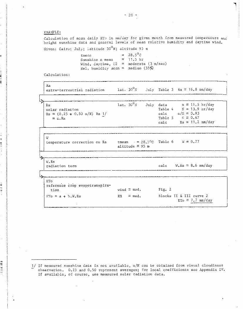
= 20 =

EXAMPLE:

Calculation of mean daily ETo in mm/day for given month from measured temperature anct bright sunshine <lata and general levels of mean re.lative humidity and daytime wind.

Given: Cairo; July; la'titude 30°N; altitude 95 m

Calculation:

tmean Sunshine n mean Wind, daytime, U2 Rel~ humidity mean

= =

2s. s0 c 11.5 hr moderate (3 m/sec) medium (55fo)

~:ra-t::restria:-radiati=----lat~-:::N -July -~:bl~~~:-~:~:~m/da~--1

~-----------------------------------------=~ ļ Rs lat. 30°N July data n = 11. 5 hr/day ll

solar radiation Table 4 N = 13,9 hr/day Rs = (0.25 + 0.50 n/N) Ra 1/ calc n/N 0,83 j

= c.Ra Table 5 c 0,67 calc Rs = 11.2 mm/day

--------~---------------------------~-~-~-~-----~~~~-

w temperature correction on Rs tmean

altitude 2s. soc 95 to

Table 6 W = o. 77 ] >~------------------------------------------

W. Rs radiation term calc W$Rs - 8.6 mm/day

Cr-------------------------------------· ! ETo

referen·ce CrOp evap.otranspira-tion wind

ETo = a + b.W.Rs RH

mod.

med.

Fig, 2

Blocks II & III curve 2 ETo = 7.7 mm/day ------

1/ If measured sunshine <lata is not available, n/N can be obtained from visual cloudiness observation3 0.25 and 0.50 represent averages; for local coefficients see Appendix IV, If available, of coursej use measured solar radiation data.

l i

i

- 21 -

EXAMPLE:

Calculation of mean monthly ETo data based ori rneasured temperature and solar radiation <lata and approximate levels of daytime wind and rnean relative humidity.

Jan. Feb. Mar, Apr. May June July Aug, Sept. Oct~ Nav. Dec.

14 15 17,5 21 25.5 27,5 28.5 28,5 26 24 20 15,5

Rs, mm/ day

w

4.96 6.41 8.52 9.85 10,86 11.41 11.24 10.43 9,11 7.12 5,45 4,55

,61 ,62 ,65 .70 .74 .76 .77 .77 .75 .73 ,68 ,63

W.Rs

Approx.

3.02 3.97 5.54 6.89 8,04 8.67 8,65 8.03 6,83 5,24 3.71 2.87

RH mean

Approx, wind

ETo mm/day

III III

av a av. 1&21&2

2. 1 2,9

III II II

2 2 2

4.6 6.4 7.5

II

2

8.2

a_v „ II & TU

7.7

av„II & III

III III av.III av.111 & IV & IV 1

av. av. av. av* av. 1&2 1&21&21&21&2

6,6 5,3 4.0 2,5 1. 9

.If rnachine calculation is used, expressions are presented which directly predict ETo from W.Rs. Values of b for different ranges of RH mean and wind are given- in Fig~ 2. In all cases a = -0.3.

Cairo

June, ETo = -0,3 + 0.98 W.Rs = 8.2 mm/day

July, ETo = -0,3 + 0.93 W,Rs = 7.7

August, ETo = -0.3 + 0,86 W,Rs = 6.6 " "

1 /

2/

ll 0,93 = average b for curve 2, Blocks II & III

~/ 0.86 average b for curves 1 & 2, Blocks II & III

ii,Jd JUI tl

Table }

1 ,i,;, 1,d J!

EXTRA-TERRESTRIAL RADIATION Ra EXPRESSED 1N EQUIVALENT EVAPORATION 1N mm/DAY

,,l,t ,,,iJlit,, ·~

Northern Hemisphere . ··-··~='·'="""-""''='~'"-·-·---<·--,;.,.____ So u t he rn __ Hemis p he re

Jan .• Feb" 1'-far 0 Apl." 0 Hay June. 3uly Aug" Sept. Oct. Nov. Dec~ Jau~ Feb~ Mar~ Apr. Hay June July Augc Sept. Oct~ Nav~ De,e:.

Lat -· ------ .--·--------·----··-·---·--·------·-·-----·-··-·-·--·-·--·

3.8 Li"' 3

1

. 1,. 9

j! ~::

6.4 . 6, 9

7.4 7~9 il, 3

6.1 9.~ 12.7 15.8 11.1 16.~ 14.1 10.9 7.4 6~6 9GB LLQ 15.9 l}a2 16,.S !fŗ~j l"J.2 J.8 7.1 10,2 13.3 16.0 17.2 16.6 14.5 11.5 8.3 7.6 10,6 13.7 16.1 17.2 16.6 14.7 11.9 8,7 801 11.0 14.() f6.2 !7.3 "[6~7 15.0 12.2 9~1

Ba6 11~4 14~3 16.4 17.J 16.7 15~2 12~5 9~6 9.0 11.8 14.5 16.4 17.2 16.7 15a3 12.B 10.0 9.4 12.1 14.7 16.4 17.2 16.7 15.4 13.1 10.6 9,812.4 14,8 16.5 17.1 16,8 15.5 13.4 10.8

10,2 12.8 15,0 16.5 17.0 16.8 15.6 13.6 11.2

4.5 5a{)

5.5 6,0 6a5

7.0 7o5 8.0 8.5 9.0

3.2 ,.., ""/ ..)" i

Li-.3

50° 48 46

4. 7 1 44

5. 2 1 42

5. 7--J 40 6. 1 , 38

36 6.6 7.2 708

31, 32

8.8 10,7 13,1 9.3 11.1 13.4 9.8 11.5 1_3.7

10,2 '11,9 13,9 "i0~7 -12.3 11~,,2

15,2 16.5 17,0 16.8*15.7 13.9 11,6 9.5 8.3 15.J 16.5 16.8 16.7 15.7 14.1 12,0 9.9 8.8 15.3 16.4 16.7 16.6 15.7 14.3 12.3 10.3 9.3 JS.4 16.4 16.6 16~5 15Q8 14.5 12,6 10.J 9a7 15.5 16.J 16.4 16.4 15.8 14.6 13aÜ 11.1 10.2

30 28 26 24 22

17. 5 17,6 17.7 17. 8 17.8

17.9 17.9 17. 9 17.8 17.8

17. 8 17,7 17.6 17 .5 17.4

14.7 14.9 15, 1 ·15. 3 15,5

15.7 15.8 16.0 16, 1 16,2

16.4 16,4 16~4 16.5 16,5

10.9 11 • 2 11. 5 11. 9 12,2

12.5 12.8 13. 2 13. 5 13.8

14.0 14,3 14, L,

14.6 14,8

7.0 7.5 7.9 8.4 8.8

9.2 9.6

10. "i 10,5 10.9

11. 3 11. 6 12.0 12.3 12,6

4.2 li- .. 7 5,2 5.7 6. 1

6.6 7. 1 7.5 8,0 8,5

8,9 9.3 9.7

10. 2 10.6

3.1 3.5 3.5 4~ü 4,0 4.4 L,,4 4,9 4.9 5.4

5,3 5.9 5.8 6.3 6,3 6,8 6,8* 7,2 7.3 7.7

5,5 B. 9 6,0 9,3 6.5 9.7 6,9 10.2

·12.9 H)"S 18,~:. LL2 'l6~6 ·rn~:i 13.Li- 16ol HL:!. 13~7 16.7HLJ

7.4 10.6 14.Q 16.8 "fBwJ

7.9 11.0 14.2 16,9 lb,3 8.3 11.4 14.4 17~0 1Bw3 e.s 11.7 14,6 11.0 1c.• 9.2 12.0 14,9 17.1 18." 9.6 12.4 15.1 17.2 18.'

7.8 8.2 8.7 9. 1 9.6

8,1 10,1 ·12,7 8.6 10.4 13.0 9. ·1 10.9 "13.2 9.5 1L2 ·tJ.4

15,3 17,3 IS,1 15.4 17.2 17.9 15.5 17~2 15.6 17.1 15,7 17,0

17. g 'l7" 7

10.0 11.6 13.7 '/ 7 c; 'I .,,,

11.2 12.7 14.4 15.6 16.3 16.4 16.J 15.9 14.B 13.3 11.6 10.7 11.6 13.0 14.6 15.6 16,1 16.1 16.1 15.8 14.9 13.6 12.0 11.1 12.0 13.3 14.7 15,6 16.0 15.9 15.9 i5.I 15,0 13.9 12,4 11.6 12.4 13,6 14.9 15.7 15.8 15.7 15.7 15.7 15.1 14.1 12.8 12.0 12.8 13.9 15.1 15.7 15~7 15~5 15~5 15.6 15Q2 14~~ i3$3 12.5

20 117.3 16.5 15.0 13.0 11.0 10,0 10.4 12,0 13.9 15,8 17.0 1/.~ 18 17.1 16.5 15,1 13,2 11.4 10.4 10.8 12.3 14.1 15,8 16.8 17.1 16 116.9 16.4 15.2 13.5 11.7 10.~ 11.2 12.6 1~-~ 15.8 16.7 16.~.J 14 16.7 16.4 15.3 13.7 12.1 11.2 11.6 12.9 1-1.0 15.8 lb.5 16,0

12 , 16.6 16.3 15.4 14,0 12,5 11.6 12.0 13.2 14.7 15.8 16.4 16.5

13.2 14.2 15,315.7 15.5 15 3 15.3 15.5 15.3 14.7 13.6 12.9 10 16,416.3 15.5 14.2 12.8 12.0 12.4 13.5 14.8 15.9 16,2 i6.? 13.6 14,5 15,3 15.6 15.3 15.0 15.1 15.4 15.3 14.8 13.9 13.3 8 16.1 16,1 15.5 14.4 13.1 12,4 12.7 13.7 14,9 15,8 16,0 IG.O 13.9 14,8 15.4 15.4 15.1 14.7 14.9 15,2 15.3 15.0 14.2 13.7 6 15.8 16.0 15,6 14.7 13,4 12.8 13.1 14.0 15,0 15,7 15,H 15,J 14.3 15.0 15.5 15.5 14.9 14.4 14.6 15.1 15.3 15.1 14,5 14.1 4 15,5 15,8 15.6 14,9 13,8 13.2 13.4 14.3 15,1 15,6 15.5 15,4 14.7 15.3 15.6 15.3 14.6 14.2 14.3 14.Y 15.3 15.3 14.8 14.4 2 15.3 15,7 15,7 15.1 14,1 13,5 13.7 14.5 15,2 15,5 15.3 15.1 15 0 0 15~5 \5 0 7 15~3 14.4 13.9 \4,1 14.8 15.J 15.4 15.1 14.8 Ü 15oÜ 15.5 15.7 15~3 14~4 13.9 14.1 14.8 15.3 15$4 15~1 14~8

l°'s.J

1-..J

-----"

1,1 1.11

Ta.ble 4

,,, •

HEAN DAILY MAXUillH DURATION OF BRIGHT SUNSHINE HOURS N FOR DIFFERENT MONTHS AND LATITUDES

r- •" ,,,___c ___ , _____ ' "'"'""'-"""'''""'""''"""--·----,,,____________ ' --------·-----\ Northern . Lats Jan~ .Feb~ Marc.h Apri.l May June July Aug~ Sept~

Southern Lats. July Au.g, Sept., Oc t ~ Nov. Dec. JP-n~ Feb. Mar~

50° 8.5 10 ~ ·J 1LB 13,8 15.4 "16. 3 15.9 H.5 12.7 48° 8.8 10, 2 ·1LB 13,6 ·is .2 16.0 15.6 14.3 12.6 Li-6° 9. 1 -! 0., L1 "j •j -, 9 U~5 11,, 9 "i 5, 7 15.4 14.2 12.6 !+Lf o 9.3 10,5 ·1 ·1 a

1 ' ~ J 13, 1, 1 L,. 7 15.4 15.2 14.0 12.6

42° 9. ,, ·w „ 6 1L9 ·u ~ t\. 14~6 ·1 s O 2 14.9 13.9 12.9 40° 9.6 10~7 iL9 13„ 3 11,. 4 15.0 14~7 13.7 12.5

35° "I O. 1 -1 ·1 „0 1L9 13, 1 14~0 1 Lf „5 14.3 13.5 12.4 30° 10, 1, "! 1 • 'j ·12.0 12~9 1 .3" 6 "jlj .• 0 13. 9• '13. 2 12, 4 zs0 10. 7 n.3 ~12. ~ ü 12 ~ 7 '[ 3~3 13.7 13. 5 13.0 12.3 20°

l 11. 0 ·11,,s 12,0 12.6 1 3. 1 13. 3 13. 2 12.8 12.3

15° 11. 3 11.6 ·i:LO 12.5 12,, 8 13.0 12.9 12,6 12. 2 rno '11. 6 1L8 -u.o LL3 -: 2. 6 12.7 12. 6 12.4 12. 1

50 l 11. 8 11.9 1:Lü 12.2 12.3 12.4 12.3 ·12. 3 12. 1

QÜ 1 12. 1 12. 1 12 ~ ·i -12" 1 12. 'I '12. 1 12. 1 12. 1 12. 1

,__ ________ _j_ _____ , ___________ •. ~-·------·-···----·----·-··-·-------·-

--1 ' '

---·--·---~-·-"··-··-··-. . . 1

1 Oct. Nov. Dec.~ !

Apr. May June

10,8 9, 1 8. ·1 10.9 9.3 8,, 3 10.9 9.5 8. 7 11. 0 9,7 8.9 11. 1 9.8 9 ~ 1 N

11. 2 10.0 9.3 LJ

11. 3 10.3 9.8 11, 5 10,6 10. 2 11. 6 IO. 9 ·10. 6 11. 7 'J 1.2 10.9 11. 8 1L4 1L2 11. 8 1 1 • 6 1L5 12.0 '11. 9 '11. 8

12. 1 12,1 12. 1 1

--·---·-··----,-/

iJ,id JJI tl 1 ''"

,id ,li .. 1.1 '"jjļjj,d,X<

Table 5 CONVERSION FACTOR FOR EXTRA•TERRESTRIAL RADIATION Ra TO SOLAR RAllIATION Rs FOR DIFFERENT RATIOS OF ACTUAL TO MAXIMUM POSSIBLE SUNSHINE HOURS (0.25 +'0.50 n/N)

"~" 0.05 • 1 . 15 .2 • 25 .3 .35 .4 .45 .5 ~55 .6 .65 .7 .75 .8 .85 .9 .95 1.0

n.25 + 0.50 n/N .25 .28 .30 .33 .35 .38 .40 ,L,3 .45 .48 .50 .53 .55 .58 ,60 .63 .65 ;, .68 . 70 .73 .75

Table 6 VALUES OF WEIGHTING FACTOR W FOR THE EFFECT OF RADIATION ON ETo AT DIFFERENT TEMPERATURES AND ALTITUDES

,--0

Temperature C 1 2 4 6 8 10 12 14 16 18 20 22 24 26 28 30 32 34 36 38 40 1 '

N

" W at altitude m

0 0.43 .46 .49 .52 .55 .58 .61 .64 .66 .68 . 71 . 73 .75 * • 77 . 78 .80 .82 .83 .84 .85 500 .45 .48 . 51 .54 .57 .60 .62 .65 . 6 7 .70 .72 • 74 .76 .78 .79 • 81 .82 .84 .85 .86 000 .46 .49 .52 .55 .58 .61 .64 .66 .69 . 71 .73 .75 • 77 .79 .80 .82 .83 .85 • 86 .87

2 000 .49 .52 .55 .58 • 61 .64 .66 .69 . 71 .73 .75 • 77 .79 .81 .82 ,84 .85 .86 .87 .88 3 000 .5,2 .55 .58 • 61 ,64 .66 .69 • 71 . 73 . 75 • 77 .79 • 81 .82 • 84 .85 • 86 .88 .88 .89 4 000 .55 .58 • 61 .64 .66 .69 • 71 • 73 .76 .78 .79 • 81 • 83 .84 .85 • 86 .88 • 89 .90 .90

'

T

' 1

L

Reiationships -forr obta!ning ETo mean r,alative humidity and d;;iJdimij minci.

fH1 ~~~ ,> ?'1:i% ----t~---- ·--'-~~

!

.... ··J .!41 '.Ullt. -------·--

• C I• __ :... ----+--'-_;__J.3 L- -JJ _92..__ --

'

.. DL

l<J

oi

...

;~--~untry, 1 llATA

' ~

eriod t

"I .. ·/®> l 1atitude

i r n ma~ ~ n

l!

njN or cloudinesa or

'l oi. • ..i....d 1 /il.1-1,::l. aY. e:;: lll

t. mea.n !jļl 0 c

w

1 ļ fü'ī mer.m

1

1

1:1,, daytime: j 4

m/oec

1 1

., .26 •n

Placei

Table 3

dota

Table 4

oale 'l'abl. text

calc

'l'a.ble 6

eeHruate l }-i · __ JH,1 eiatimata -·--

Lart i tu.de ~

Lo:ngi tu.de~

X

j

R.J.!

iltitude;

W„ Ra b . 1

1

[ r-··~~i Fig. 2 lllook/li.-.,o L _____________ ,., i L.

i...,_.l,,.__J 1 ,., .. .,.

E'.~) mm /i,J\"'17 ,,J_ . . . J i, ,, '1n;o,,; __ ==

1

1 ·------"'---------------·-----· ' I . ..JJ or from eolar radiation mape

.;

Table 4 /3.

n/N ca.lc or oloudinasa or Table tert

1

0.25+0,50 n/N Table 5

1 calc //,1

alti tude >!j'ļ'S" m

1· (J. 7

w„ R.a

1

PJ! """" ~ .f,f %1

u 2 cla7time ~-.J ! m/••c 1

'

,-. -.-71 i /7/,ü·

1 n 1

ŗ--1 1 ' 1 . mvd. H

,____, 1

j I"'~"!'' --,1 :Block/1.ine L.--------------~UL· 1ll'! ,,2 '

] Fig„ 2

_____ _,_ ___________ , ________________________ .., ]./ or from mol&r radiation mmps

l

- 28 -

!YlETHOD īII .~ MODIFIED PENMAl.\"f

For areas where measured data on temperature) humidity 1 wind and bright sunshine hours

or radiation are available, the rnodified Penman method is suggested since it is likely to

provide the mast satisfactory results to predict the effect of clirnate on crop water

requirements.

The original Penman (1948) equation predicted the loss of water by evaporatio.n from

an open water surface, Eo. Experimentally determined crop coefficients ranging from 0.6

in winter rnonths to 0.8 in summer rnonths were suggested to relate Eo to crop evapotranspira

tion for the climate in England. The Penman equation consists of two terms, namely the

.....

energy (radiation) term and aerodynarnic (wind and humidity) term. The relative importance of

the two terms varies with climatic conditions. Under calm weather conditions the aerodynamic

term is usually much smaller than the energy term. In such conditions the Penman Eo equation

using a crop coefficient of 0.8 has been shown to predict ET(grass) closely, not only in cool

humid regions as in England but also in very hot, and semi-arid regions. It is under windy

c.onditions and particularly in the more arid regions that the aerodynamic term becomes relative

ly more important and thus serious errors can result in predicting ET(grass) when using 0.8 Eo.

An adaptation of the Penman equation can be used for direct prediction of ET(crop) by

the use of appropriate reflection coefficients for incoming solar radiation, the effect of

plant resistance to trasnpiration and by inclusion of appropriate wind functions which take

into account the change in aerodynamic roughness with growth of crop. This would require

additional input <lata and involve a level of complexity considered beyond the intended scope

of this publication.

That approach has not been used here, but in this publication a slightly modified

Penman method is suggested to predict the effec.t of climate on crop water requirements. The

formula presented and procedure to follow will enable prediction of the effect of climate

on reference crop evapotranspiration ETo" The only variation to the original Penman method

(1948) proposed herein involves a revised wind function term and an additional correction

for day and night~time \.ve.ather conditions not representative of climates for which the wind

func-cion was de.termined. To arrive at the relationship presented, use was made of climatic,

and measured grass evapotranspiration <lata from research stations mentioned in Appendix II

and frorn references in Appendix III.

To predict the effect of the crop characteristics on crop water requirements 1 the crop

coefficients 1 kc, presented in Chapter 1 .2 can be applied. The crop evapotranspiration,

ET(crop) is found by ET(crop) ::: kc ETo. A two-step approach by first calculating ETo followed

by the selection of the appropriate crop coefficient kc to predic.t ET(crop) is presented

rather than suggesting the use of the Penman method for a direct prediction of ET (crop),

Some compromise in accuracy may be accepted for the sake of simplicity.

~ 1

o.

d

1

l

- 29 -

The. calculation procedure.s to P.stimate ETo may seem rather complicated. This is

caused by the fact that the formula contains components which can be derived previously from

recorded and related climatic <lata when no direct measuremencs are available. For instance,

the essential radiation component can be o~tained from measured solar radiation from bright

sunshine duration or cloudiness observations7

and from measured humidity and temperature

dA.ta for placPs when": no direc.t rneasurements of net radiation are available. Computation

techniques and tables are given here to facilitate the necessary calculation. A fonnat for

calculation is given at the end of this sub-chapter.

Recommended relationships ---------------The form of the equation used in this method is:

ETo* = W. Rn + (1·11). f(u). (ea-ed)

radiation term

aerodynamic term

(not adjusted)

where: ETo:l', is the reference crop evapotranspiration in mm/day (not adjusted)

W is temperature•related weighting factor

Rn is net radiation in equivalent evaporation in mm/day

f(u) is the wind-related function

(ea-ed) is the difference between the saturation vapour pressure at mean air temperature and the mean actu~l vapour pressure of the air, both in mbar.

To find ETo, the reference crop evapotranspiration, ETo* needs to be adjusted for day and

night„time weather conditions.

Brief notes on the variables involved and examples of calculations are given below.

The <lata used daily in calculating ETo are applied as the mean daily value and represent

the mean of such data over the period considered usually one month or ten days.


Due to the interdependence of the variables composing the equation, the correct use of

units in which variables need to be expressed is important. Of particular significance is

the use of the wind function which is to be expressed in total wind run in km/day. Use of

the correct units for each variable is shown in the calculation examples presented below.

Normally, total wind run per day is the only wind <lata available. If 24-hour wind

totals are used in the original Penman equation there will be a serious overprediction of ETo

under conditions of strong day-time winds accompanied by strong night„time winds especially

if humidity remains low; conversely, for areas experiencing moderate to strong day-time wind

but calm nignts the equation will tend to underpredict ETo, especially in dry climates with

RHmax of n2ar 100 percent. The separation of day and night computations by matching mean

day-time wind r,.rith day-time humidity and mean night-time wind with mean night-time humidity

would provide an improvement. The procedure is however rather complicated and is not

1·ecommended because of the frequent limited availatiility of the necessary data. Rather,

a graphic adjustment of LTo*to obtain ETo is recommended, as shown at the end of this

· chapter in Fig, 4, for conditions where total wind nm during the day-time (07 .00··19.00 hr)

is twice that of the total wind run at night.

30

Description of variables involved and methods of calculation

A brief description of the variables involved and units to be used in the equatic-n is

given, together with the method of calculatioi:i when direct measuremem:s are not available.

This is followed by an example to calculate ETo using mean daily data for a one-month period

for which a special form has been prepared, Again usiug mean daily data, ETo is calculat2d

for each month during a year showing examples for adjusting ETo* for day and night"' time

weather conditions.

Figures and Tables to be used~

r ---------------------------------------------1 l :Number Variable Descripti.on Input <lata 1

1 -------------------------------------·-------------j j Table 7 ea Saturation vapour pressure ea in mbar as I ! function of mean air temperature tOC 1

1 Table Sa ed Vapour pressure ed from dry and wet bulb t°C and tOC 1

1 temperature <lata (aspirated psychrometer) wet bulb ļ

Table 8b ed Vapour pressure ed from dry and wet bulb tOC and t 0 c

Table Sc

1

Table 9

1 ::::: ::

1 Table 12

1

1 Table 13

1 Table 14

1

Table 15

Table 16

1 Table 1 7

1 Figure 4 1

L

ed

f (u)

(1 ·W)

w

Ra

N

Rns

f(t)

f(ed)

f(n/N)

ETo

temperature data (_not ventilated psychrometer)_ wet bulb 1

Vapour pressure from detvpoint temperature t oc . . d.ewpoint

Values of wind function f(u) for wind run at a 2 m height in km/day Uz

Values of weighting factor (1-W) for the t°C effect of wind and humidity on ETo at different altitude temperatures and altitudes

Values of weighting factor W for the effect of radiation on ETo at different temperatures t°C and altitudes altitude

Extra-terrestrial radiation Ra expressed i.n equivalent evaporation in mm/day for different month months and latitudes latitude

Mean daily rnaximum duration of bright sunshine month hours for different months and latitudes latitude

Conversion factor for extra ... terrestrial radia·· tion Ra to net solar radiation Rns for a given n/N reflection of 25 percent and different ratios a:: 0.25 of actual to maximum Sunshine hours ļ-(1 • a) (0.25 + 0.50 n/N))

Correction for temperature on net lcng wave radiation Rnl

Correction for vapour pressure on long wave radiation Rnl

Corre.ction fo:::- the ratio actual and maximum sunshine hours on long wave radiation Rnl

Adjustment on calculated ETo* for day and night„time wind and humidity conditions

ed

n/N

ratio day/nighttime wind and humid:Lty

-·-------------------------·---~

'

e

T -~ 3 1 ,~

a) Va-pour :pressure (2a-ed) ----~~-~ ~-~ ~-~

ETo is a function of air humidity. In preference to relative humidity values~ the water

vapour pressure is use.d here in terms of the difference between the mean saturation water

vapour pressure, ea, and the mean actual water vapour pressure, ed.

Air humidity <lata are reported in various ways ~ mostly as relative humi<lity (RHmax and

RHmin in percentage), as psychrometric readings (t°C of dry and wet bulb)' from either ventilated

or non-ventilated wet and dry bulb thermometers~ or as dewpoint temperature (tdewpoint OC).

Time of measurement is important but is often not given. Fortunately, actual vapour pressure

is a fairly constant element and even one rneasurement per day may suffice for the type of

application envisaged. Depending on the available humidity dataj cases Ij II or III will

apply. Vapour pressure must be exļ)ressed in mbar; if ed is given in mm Hg, multiply

by 1013 : 1.33 to find mbar. 766

EXAMPLES:

for all cases altitude is Om;

I Given:

Calculation:

tmax = 35°c; tmin =

tmean Rl--Imean ea at tmean ~ 28. s0 c ed s:: ea x RHmean

-100 -(ea-ed)

0 22 C; RHmax

= 28.5°c = 55 % • 38.9 mbar

=21,4mbar

= 17. 5 mbar

(35 + 22) /2 (80 + 30) /2 from Table 7

38,9 X Ü.55

38.9 - 21.4

II Given o o o " 20oC 1 / tmax m: 35 C; tmin ,,i;: 22 C; tdrybulb • 25 C; twetbulb ·

Calculation: tmean ea at 28,5°c ed (ea=ed)

~ 28.5°c ll!I 38. 9 mbar m 20 mbar =18.9mbar

from Table 7 from Table 8a (aspirated psychrometer)

III Given: tma:r ,=, 35°c; tmin :.... 22°c; tdew-point s,; ·17 ~5°c

Calculation: t:m.ean ea at 28.5°c ed

~2a.s 0 c = 38. 9 mbar

20. 0 mbar

18~9mbar

from Table 7 from Table 8c at dewpofat of 17.5°c

1/ Conversion of readings to humidity data from dry and wet bulb thermometers changes when they are force-ventilated (Assmann type) or non-ventilated; Tables Sa and 8b to be used respectively.

•

DO NOT USE

IV Given:

Calculation:

- 32 -

tmax = 35°C; tmin = 22°C; RHmax = soi; Rllri.in = 30%;

ea at tmax = 56. 2 mbar from Table 7 ed at tmax = 16. 9 mbar 56.2 X RH s 56. 2 X 0.3

100 (ea-ed) at tmax • 39. 3 mbar ea at tmin = 26.4 mbar from Table 7 ed at tmin = 21. 1 mbar 26.4 X RH = 26.4 X O.G

īoo (ea-ed) at tmin = 5.3 mbar (ea-ed) mean = 22. 3 mbar 39.3+5.3 ---z--

because recommended wind functioa f (u) was derived using (e.a-ed) as obtained in case I, II and III and does not correspcnd to example in case IV, much greater divergence will occur in mean (ea 00 ed) between the first cases and the 4th for situations other than evident here and errors could result if case IV was used.

b) Wind function f(u)

The term f(u) is a wind related function; the effect of wind on ETo using the modified

Penman method has been defined in this publication as: īJ"

f(u) = 0.27 (1+ 10

~)

where U2 is total wind run in km/day at 2 m height. This expression is valid when (ea-ed)

is expressed in mbar and is calculated according to the methods shown in cases I, II or III

in the last paragraph.

Where wind <lata are not collected at 2 m height the appropriate corrections for wind

measurements taken at different heights are given below:

Factors for correcting wind speed at heights other than_2 met~E

----------------------------------------------------------Measurement height, rn 0.5 1.0 1.5 2.0 3.0 4.0 5.0 6.0 10.0

-------------- -------------------------------------------Correction factor 1. 35 1 . 15 1 .06 1. 00 0.93* 0.88

-------------- ____ " ______________ _ EXAMPLE

Given:

Calculation:

wind

UZ f(u)

speed at 3 m height is 250 km/day

= 0.93 X 250 ~ 232 km/day • 0.27 (1 + 232) 0.90 (from Table 9)

100

0.85 0.83 0. 77

•

= 33 -

The given wind ::Eunction appJ..ies to mest commonly found conditions where average wind

speed during the day~time period,, ioe. from Oī .00 till 19.00 hr local standard time1

for mid

summer midlatitude .climates is double the average speed during the remaining or night-time

hours; in other words, where some two thirds of the total windrun occurs during day-time

hours, Under some conditions where strong winds or __ exC.e_ptionally calm conditions prevail

at nighttime;,-with abnormal high :Jr low relative humidity values, corrections in predicted

ETo* must be applied as given at the end of the subchapter on calculation procedures.

c) Weighting factor (1-W)

(1-W) is a weighting factor for the effect of wind and humidity on ETo~/ Values of (1 ~w)

8.s related to temperature and elevation are given in Table 10. For temperature use

tmax + tmin ----z--EXA!1PLE

Given: elevation 95 m; tmax = 35°c and tmin = 22°c

d)

Calculation: tmean ~ 28. 5 %

Weighting factor,W

(1-W) = b.23 from Table 10

W is weighting factor for the effect of radiation on ETo*. Values for W as related to

temperature and elevation are given in Table 11. For temperature use tmax + tmin

e)

EXAMPLE:

Given: elevation 95 m; trnax = 35°c aud tmin = 22°c

Calculation: tmean = 28.5°c W =. 0. 77 frorn Table 11

Net_radiation, Rn

---z--

Rn, net radiation, or difference between all incoming aud outgoing radiation, can be

measured, but such <lata. are seldom available. Rn can be calculated if measured sunshine

hours (or degree of cloud cover), temperature and humidity <lata are avaiblable. Calculations

will be simplified and more reliable if solar radiation is known.

In Figure 3 different portions Üf the radiation balance are shown. The amoUnt of

radiation received at the top of the atmosphere is equal to extra-terrestrial radiationj Ra.

Ra is dependei1t on latitude and the time of the year only; its values are given in Table 12.

Part of Ra is absorbed and scattered when passing through the atmosphere. The remainder,

including some that is scattered but reaches the earth's surface, is identified as solar

radiation, (Rs). Rs is dependent on cloud cover and length of day. Part of Rs is reflected

back directly by the soil and crop and is lost to the atmosphere. Reflection (a) depends

on the nature-of the surface cover and is approximately 5 percent for water and around

20=25 percent for mast crops. That which remains is net shortwave solar radiation (Rns).

1/ W , !J/ (.1 + J') where temperature aud y

Ll is the rate of change of the saturation vapour pressure in the µsychromet:ric const.ant.

with

' uira lerreslriol Ra

shorhwove

solar R5

Nel shortwove

- 3Li- =

Jongwave

Net longwove Rn 1

'

net net

radio tion solor Rn5

Rn = - ne! longwave Rn 1 = ( 1-0() Rs - Rn1

Fig& 3 Illustration of the radiation balance

Additional loss at the earth's surface normally exists since the earth radiates part

of the absorbed energy into the atmosphere as longwave radiation. This is normally greater

than the downcoming longwave atmospheric radiation. The difference between outgoing aud

incoming longwave radiation is called net longwave radiation, Rnl. Since outgoing is greater

than incoming longwave radiation, Rnl represents an energy loss~

Total net radiation Rn is equal to the difference between net shortwave solar

radiation Rns, and net longwave radiation Rnl) or Rn Rns - Rnl. It is expressed in mm/day~

To calculate Rn the different steps involved are:

i. If solar radiation Rs is not available select Ra value from Table 12 for given month

aud latitude in mm/day.

ii. To obtain solar radiation Rs, correct Ra value for ratio of actual (n) to maximum

possible (N) bright sunshine hours; Rs = (0.25 + 0.50 n/N) Ra ·1;. Values for N for

a given month and latitude are given in Table 13. Both n and N are expressed in mean

daily values for the period considered.

Wlle.n only visual cloud observations are available, they can be used to calculate Rs.

Several daily visual observations of cloudiness over a sufficiently long period are

needed. Cloudiness is expressed in oktas (0 to 8) or tenths (0 to 10) which must first

be converted into equivalent values of n/N. ~he following table can be used:

1/ For practical purposes 0.25 and 0.50 can be used. For some regions loc.al values have been determined and are listed in Appendix IV.

~ l

1

- 35 -

------- . ----------------------ŗ----- - --- ----------------~--- , 1

(t·2nths) i · . (oktas) * 0 . 2 .4 '6 '8 i Lloudiness ļ O , 2 . 4 . 6 . 8 1 Clotidiness

------t---------------- ----- ---------------i .9 .9 .85 3, 0 1 • 95 . 9 . 9 . 9 . 9 0

I; .85 .85 .85 .85 .8 1

2 .8 .8 .8 .75 .75 2

.0

.85

.75

.65 4 .65 .65 .6 .6 .6 4 .55 3 1· .75 .7 .7 .7 .65 3

5 .55 .55 .5 .5 .5 5 .45

.85 .8 .8 .8

.75 .75 .7 .7

.65 .65 .6 .6

.55 .5 .5* .45

.4 .4 .35 .35 6 . 5 . 45 . 45 . 4 . 4 6 . 3 . 3 .25 .25 .2 7 . 4 . 35 . 35 . 3 . 3 7 . 15 . 15 1

8 . 3 . 25 . 25 • 2 . 2 8 9 .15 .15 .15 ------ - ' 1

1 O * oktas: a scale where 8. 0 is full -cloudiness

-------------------EXAl1PLE: Cloudiness is 4.6 oktas; equivalent value of n/N is 0.5 1/

iii. To obtain net shortwave radiation, Rns, the solar radiation must be corrected for

reflectivity of the crop surface, a,or Rns = (1- a) Rs = (1-0.25) Rs, in equivalent

evaporation in mm/ day. Table 14 can be used to calculate Rns from the ratio n/N and

the reflection coefficient a = 0.25 multiplied by the extra terrestrial radiation Ra~

iv. Net longwave radiation Rnl can be determined from available temperature t, vapour

pressure ed~ and ratio n/N <lata. Values for the function f(t), f(ed), and f(n/N)

are given in Tables 15, 16 and 17, respectively.

v. To obtain total net radiation, Rn, the algebraic sum of net shortwave radiation Rns,

and net longwave radiation is calculated. Rns always constitutes a net loss so

Rn : Rns - Rnl .

1/ Variations in conversion factors from location to location have been noted when using cloudiness data for obtaining the ratio n/N. Where available locally derived conversion factors should be used. Sometimes sky observations are made which are expressed in four classes; conversion is approximately: clear day: 1 akta, partial cloud: 3 oktas, cloud = 6 oktas, overcast: 8 oktas.

;

-

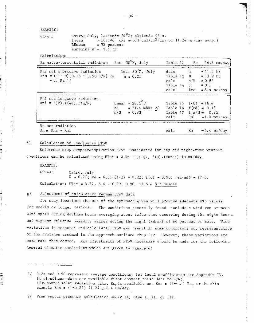
EXAMPLE:

Given:

Calculation·

Cairo; tmean

- 36 -

July~ latitude 30°N; altitude 95 m. = 28.50C (Rs = 633 cal/cm2/day

RHmean = 55 percent sunshine n = 11 .5 hr

or 11.24 mm/day evap.)

Ra extra-terrestrial radiation lat. 30°N, July Table 12 Ra 16.8 mm/dayl 1

Rns net shortwave radiation lat. 30°N, July <lata n = 11. 5 hr Rns = (1 - a)(0.25 + 0.50 n/N) Ra a = O. 25 Table 13 N = 13. 9 hr

• C, Ra 1 / calc n/N = 0.83 - Table 14 C = 0.5 calc Rns =8.4 mm/day

01.nl net longwave radiation 28.5°C Rnl = f(t).f(ed).f(n/N) tmean = Table 15 f(t) = 16. 4

ed = 21.I+ mbar 2/ Table 16 f (ed) = 0. 13 n/N = 0.83 - Table 17 f(n/N)= 0.35

calc Rnl =1.3 mm/day

Rn net radiation l

= 6. 6 mm/daz 1 !Rn a:: Rns - Rnl calc Rn

f) Calculation of unadjusted ETo~'.:

Reference crop evapotranspiration ETo~'.: unadjusted for day and night-time weather

conditions can be calculated using ETo* = W.Rn + (1-W). f(u). (ea-ed) in mm/day.

EXAMPLE:

Given: Cairo, July ll = 0.77; Rn = 6.6; (1-W) = 0.23; f(u) = 0.90; (ea-ed) = 17.5;

Calculation: ETo•> = 0.77. 6.6 + 0.23. 0.90. 17.5 = §..:_2__~/day

g) ~dj~stment of_calculation_~enma~~To* ~~!~

For many locations the use of the approach given will provide adequate ETo values

for weekly or longer periods. The conditions generally found include a wind run or mean

wind speed during daytime hours averaging about twice that occurring during the night hours,

and highest relative humidity values during the night (fuqmax) of 60 percent or more. Wide

variations in measured and calculated ETo* may result in some conditions not representative

of the averages assumed in the approach outlined thus far. However, these variations are

rnore rare than common, Any adjustments of ETo:.'• necessary should be made for the following

general climatic conditions which are given in Figure 4:

1/ 0.25 and 0.50 represent average conditions; for local coefficients see Appendix IV. If cloudiness <lata are available first convert these <lata to n/N; if measured solar radiation <lata~ Rs„ is available use Rns :: (1- a) Rs, or in this example Rns = (1-0.25) 11 .24: 8.4 mm/day.

2/ From vapour pressure calculation under (a) case I, II, ar III.

1 l

~ "i'. 1

" = 37 =

Impor'.:ant in areas with moderate to high radiation (> 8 mm/day) during summer months ~

which consis-cently have low=humidity winds during much of the day () 4 m/sec) and

calm night~time conditions with high night hurnidity values approac.hing 100%, Curve

in Fig" 4 applies for day-night wind ratios of about 3 to 4 with very high RHmax.

ETo-. 1.05 to 1.10 ETot;

Applies in areas where daytime winds are < 4 m/ sec:. and nights are very c.alm and humid,

i.e. RHmax>75%. The daily wind distribution should give a day-night ratio of 3 or

more, To adjust ETo*~ curve 2 in Fig. 4 should be used.

ETo = ETo'~

Daytime wind speeds of about twice those during the nightMtime are generally found and

maximum relative humidity )60fo. No adjustment of Penman ETo* is required.

ETo"' 0.75 to 0.95 ETo*

ETo will be slightly over predicted in areas with moderate to high radiation and with

wind speeds <4 m/sec but about equal du:ting the day and night@ When relative humidity

during n.ight=time is ):60% curve 4 in Fig. 4 applies.

ETo - 0.65 to 0,80 ETo* 1/

Re1atively rare but applies for spring~ summer and autumn conditions with moderate to

high radiation- and when wind speeds during the day and night are between 5 and 8 m/sec

with maximum relative humidity<40lijo, Curve 5 in Fig. 4 should be used.

ETo - 0.55 to 0.65 ETo* 1/

Also rare, but applies dU"ring spring~ surruner and autumn with moderate to high radiation

and when wind speeds during day and night are >8 m/sec and with relative humidity day

and night <~.o1o. See curve 6 in Fig. 4.

ETo ,.,., 0,30 to 0.35 ETo* 1/

Very rare~ but will apply under very strong i:,vinds of >8 m/sec during both day and

night, while. relative humidi ty ~ day and night, is low and <4010. Curve 7 in Fig. 4

will apply but only when radiation is low) i.e. during late autumn and winter

(Rns < 4 mm/ day).

1/ These cases seldom occ.ur; -very windy c.onditions accompanied by low relative humidity necessitating dra~~tic corrections would pers-ist fo-r only a few days in mast climates.

•

= ~ ::s

a

"'!'!!

~ 33 =

Using mean daily <lata :Eor e.ac.h month a surnrnary of c.alculation o:f ETo is given indicating for each month of the year the mean daily ETo value in mm/day.

EXAMPLE: Cairo 197-; latitude 30°N; altitude 95 m.

1 1

Jan Feb Mar April May June July Aug Sept Oct Nov De~ 1 --- -J

1

t mean oc 14 15 17 0 5 21 25.5 27.5 28.5 28.5 26 24 20 15 0 s 1

FJl rnean 65 65 63 50 45 50 55 57 60 64 68 68 "'I

n hr 9,4 8.0 8.9 9.7 10.8 11. 4 11 , 5 11 • 1 10 ,4 9.6 8.6 7. si u

2 km/d 173 181 207 207 232 251 232 1 81 164 190 164 155 1

i

! ETo* 1 mm/day 3.0 4.0 5.7 7.0 8,9 9,4 8.7 7 C 6.0 5.0 3.4 ',J 2,6j

ETo*

-...J

Adjusted ETo

Based on available weather <lata and general clirnatic descriptions for Cairo, adjust= ments of calculated ETo* are to be made using the correction relationship indicated by curve 4 in Fig. 4~ Corrections to ETo* values are needed because of the day=night wind ratio of- around 1.0 to ·1 .3 produced by rather calm morning and mid-day conditions with the onset of breezes in late afternoon and evening hours; an exception wnuld be the ''Khamaseen'' winds of April and May which blow day and night but still have. a ratio of about 1~0 to 1.5

1

Jan Feb Mar April May June July Aug Sept Oct Nov Dec 1

1

mm/day 3.0 4.0 5.7 7.0 8,9 9.4 8.7 7.5 6.0 5. 1 3.4 2.6 1

1 1 ETo

mm/day 2.4 3.3 4~8 6.0 8. 1 8.6 7.9 6.6 5. 1 4.3 2,8 2, 1 ' -'

i

L,1 J„l ,SS i ,i„ " ..IJ , .. ,llii.,

~

~ . iI~ ,_.. - --- --_,,,,.,,_, -""-=-----~,,,,_

Table 7 SATURATION VAPOUR PRESSURE ea IN mbar AS FUNCTION OF MEAN AIR TEMPERATURE t IN °c

----·---------,--------------------------------------1

Ternper= ļ at:ure o0 c I 0 2 3 L,, 5 6 7 8 9

-----------t-- --------· ---------------------------~-"--_mb_a_r _ j 6. 1 6 ·_6. _____ ~~~---~:_6. ____ s_._1 ___ s_._1____ 9. 4

10.0 10.7 11. 5

Temper„

~:· ;:"],~----,: :-9.-__ -___ -,j: ~~:_;_ -~--;:_:~-, __ :_~_1 __ 3_3_. 6-

26 27 28 29

35.7 37.8* 40.1

10

12 .3

30

42.4

-------------------·-1· 1

11 12 13 14 15 16 17 18 191

-------------- ---------------------1 13. 1 14.0

31 32

44.9 47.6

15.0 16 • 1 1

17.0 18.2 19.4 20.6 22.01 _________________________________________ !

-- - 1

33 34 35 36 37 38 39 !

-------- --- ------------1 50.3 53.2 56.2 59.4 62.8 66.3 69.9 i

- ___________________ __J

w '-D

il 'J ll jJI ilil i ,i.i 1, 11 ,li d• '<.lilil.a, •.

'fable aa VAPOUR PRESSURE ed 1N mbar FROM DRY AND WET BULB TEMPERATURE DATA IN °c (ASPIRATED PSYCHROMETER)

1 Depressi-0n wet bulb t

0c, altitude 0~1 000 m --- ----------------------------------~-~

dry bulb Depression wet bulb t 0c, altitude 1 000~2 000 m

20 ~ ! 0 2 4 6 3 10 12 14 16 18 20 22 t 0 c 0 2 4 6 8 10 12 14 16 18

113.S M.9 56„8 49„2 42.2 35.8 29.8 24.3 19. 2 14.4 10.1 6.0 40 73.8 65.2 5 7 ~ 1 49.8 43.0 41.8 31.0 25.6 20.7 16.2 12.0 a. 1 1 1 ~-'i.~ 58. 1 50.:i 43.6 37.1 31. 'J 25.6 20.5 15.8 11. 4 7.3 38 66.3 58.2 50.9 44.1 37.9 36.7 26.S 21.8 17 .3 13.2 9.2 5, 71 ! .'.i9a 4 51.9 44.9 3i:!.4 32.5 26.9 21.8 17. 1 12, 7 B.6 4.9 36 59.4 52.1 45.2 39.0 33.3 32.1 23.0 18.4 14.3 10.4 6.8 3.51 S3.2 46.2 39.8 :n.a 28.3 23.2 18.4 14.0 10.0 6.2 34 53.2 46.4 40. 1 3lr. 4 29.1 24. i 19.6 15.4 11. 5 8.0 4.6 1.5.

:1 O<i7 ~5 41.1 35.~ 19,0 24.5 19.8 15.4 11.3 7 .5 4.0 32 47.5 41.3 35.5 30.2 25.3 20.7 16,6 12.6 9. 1 5.8 2.6 1

1 !:;:2.4 36.5 30.9 2:).G 2L·t 16 • .7 n.6 8.8 5.3 30 42.4 36. 7 31.3 26.4 21. 9 17. 7 13.8 10.2 6.9 3.8 0.9 1 Yi.U 32..3 2·L2. 2.:L.!~ rn.o 14.0 iü.2 6.7 3.4 28 37.8 32.5 27.5 23.0 18, 9 14. 9 11.4 8.0 4.9 2. 1 1-, ... 23.S 23.8 ü 9. 4 U.3 11.5 8.0 4. 7 1.6 26 33.6 28. 7 24. 1 20,0 16. 1 12. 5 9.2 6.0 3.2 0 ' 1 .~ • .," 'O ,, 11 ?!) '<'; 25. 1 20. 7* 16.6 12.8 9.3 6.0 2.9 24 29.8 25.3 21. 1 17 .2 13. 9 10.3 7.2 4.3 1.6 1 Ļ• 1 ·: • G :±>1~. 4 22„0 HLO 16-,2 10.6 7„4 4 ' 1. 4 22 26.4 22.3 18.3 14.3 11.5 B.3 5.5 2." ī' 0,2 C,

1 12:1,4 19.3 15.5 12.G īL7 5,6 ·2. 7 20 23.4 19. 5 15.9 12.6 9.5 6.6 3,9 1.3 f! 1i.L6 ü6.0 0~3 UÜoÜ 6.9 4o 1 1-. i1 18 20.6 17. 1 i 3. 7 10.6 7.8 5.0 .2.5 ü.1 j 'W/!~ '14~6 ·iL4 11.J 5.4 2.7 16 18.2 14. 9 11. 7 8.9 6.2 3.6 1.3 ļ'l'GJJ 1:L 7 9.6 _ .. -, o„ 4.0 1.5 14 16.0 12. 9 10,0 7.3 4.8 2.4 0.3 i 1iiJi 1

rn.9 l:L 1 5, ~1 2.B 12 14.0 11, 2 8.4 5.9 3.6 1. 4

1 ' -, 9.Jl 0~ }' t,." ·1 Ll 10 12.3 9.6 7 .o 4. 7 2.6 0.4 ' -- 0 .. ~

1 iü. 7 e.o 5~5 J.I 0"8 B 10. 7 8.2 5.8 3.7 1.6

1 ~: ;'

6,8 t,' i, 2. ·i 6 9.3 7 .o 4.8 2.7 0.7 5.7 3" t, L6 4 8. 1 6.0 3.8 1.8

j O -i (08 Z.ü lLB 2 7. 1 5.0 2.9 1.0 ! 6" 1 ti.() .Ln

I _________ ··------·-··-··---------.---···--------0 6. 1 4. 1 2. 1

···--------------------- - __ I

ld J,:l ,"1 i ,i,, 1, ,1 ,,ja "'' Īi>" '"' ~

',-<_,~,-=-=-w- ~ . . .

'

Ta.ble 8b

! l ,) 2. ,_ ' ]173.8 61 •• 7 !,-66,3 57.8 l!j9.4 51.6 ) :1'.:Li 45.9 j.41.5 40.8

i ' .. ' " . 1. '",L.<i, _:io 0 l.. ī 3)' .8 ]2.0 j D,O 28.2 ) 29.8 14.8 (20.4 2·1.a

i il 23.4 19 .0 1 :2.0.6 116,6 ! rn.i 14.4 J 16.0 i2J-i l 14.0 10. 7 1

-U.3 9.-1 rn.1 1.1 9.3 6.5 a. ·1 s.s 7 0 ·1 4.5, :~. [ J. 7

VAPOUR PRESSURE ed IN mbar FROM DRY AND WET BULB TEHPERATURE DATA IN °c (NON-VENTILATED PSYCHROMETF.R)

Depression wet bulb, t°C altitude 0~1 000 m

4 6 3 10

56.2 48.4 41.2 34.4 50~0 42~6 36.0 29.B 44~4 37~6 J1.4 25.6 39 0 2 11 0 0 27 0 2 21.8 34.6 28,8 23.4 18a4

30.4 26.6 23,2 20. 2 1L4

25.0 20.0 2L6 n.o '18.6 14.2 1s.2 n .3 13.4 9 .6

15. Li

i2.6 10.2

lLO 6.0

'12

28.2 24.0 20.2 16. 8 13.8

1LO 8.6 6,4 4.4 2.7

15.0 !1.2 7,6 4.3 1.1 12.8 9.Z 5.9 2.7 10.8 7.5 4.3 1.4 9.1 5.9 3.0 !L1 7.5 4.6 1.7

6. 1 0. 7 4.9 3.9 2.9 0.9 2.3 LS:

14

22.4 18.6 15.2 12.2 9.4

7 .o 4.3 2.8 1. 1

16

17 .0 "13. 6 10.6

7 .8 5.4

3.2 1.2

18

12.0 9.0 6.2 3.8 1. 6

20

7 .4 li. 6 2.2

dry bulb

22 1 t°C

3.01 40 0.6 38

36 34 32

30 28 26 24 22

20 18 16 14 12

10 8 6 4 2 0

0

73.8 66.3 59.4 53.2 47.5

42.4 37 .8 33.6 29.8 26.4

23.4 20.6 18.2 16.0 14.0

12. 3 10. 7 9.3 8. 1 7. 1 6.1

2

64.9 58.0 51.8 46.1 41.0

36.4 32.2 28.4 25.0 22.0

19.2 16.8 14.6 12 .6 10.9

9.3 7.9 6.7 5. 7 4.7 3.8

Depression wet bulb t°C altitude 1 000-2 000 n -il

4 6 s 10 12 ·14 16 1 a 20 a . -··----~ --~-- - -

56.7 50.5 44.8 39.7 35.1

30.9 2 7. 1 23.7 20. 7 17 .9

15.5 13. 3 11. 3 19.6 8.0

6.7 5.4 4.4 3.4 2. 5 1. 7

49.1 43.4 38.3 33.7 29.5

25.7 22.3 19. 3 16.5 14. !

11. 9 9.9 8.2 6.6 5.2

4.0 3.0 2.0 1. 1 0.3

42.0 36.9 32.3 28. 1 24.3

20.9 17 .9 15. 1 12, 7 10.5

8.5 6.8 5.2 3.8 2.6

1.6 0.6

35.6 31.0 26.8 23.0 19.6

16.6 13.8 11 • lf 9.2 7.2

5.5 3.9 2.5 1. 3 0.3

29.6 25.4 21.2 18.2 15.2

12.4 10.0 7.8 5.8 4.1

2.5 1.1

34.1 18,9 H.1 9,3 S.& 1 ... " • ·1 ,-, •.• " LÜ.3 15,J 1 ļ,, J.Ü 5.L

:6.9 12.s ~·~ ~"~ -1 "o j !~.9 9.7 h~ ~-~ 1 11.1 7.3 J.7 1L-; ,:

3. 7 6,5 4.5 2.3 1.2

5. ·1 3. ·1 Lii

Lī 1

1

1

1 1

i !

:_,_ .. __ , __ ·-----------·---···----·---- ---~-----·--~-... ----------------..L-----L------------·-------------·---- ···-·---··-·-·-'

']:'Qble 8c \l"AJ'otrn PmšSSU:WJ: ed FRCK DEWPOllT TEMPERA'!URE

6

~-=-~-"1

8 10 12 14 16 18 20 22 24 26 28 30 32 34 36 38 40 i 10.7 12.3 14.0 16.0 18.2•20.6°23.4 26.4 29.8 33.6 37.8 42.4 47.5 °53,2 59.·;·66.;··;;:;1

--·-~,----= -~'" .J

r o*· · -· J teM!ip C o 11. 4

~~~~2 9~3

s>

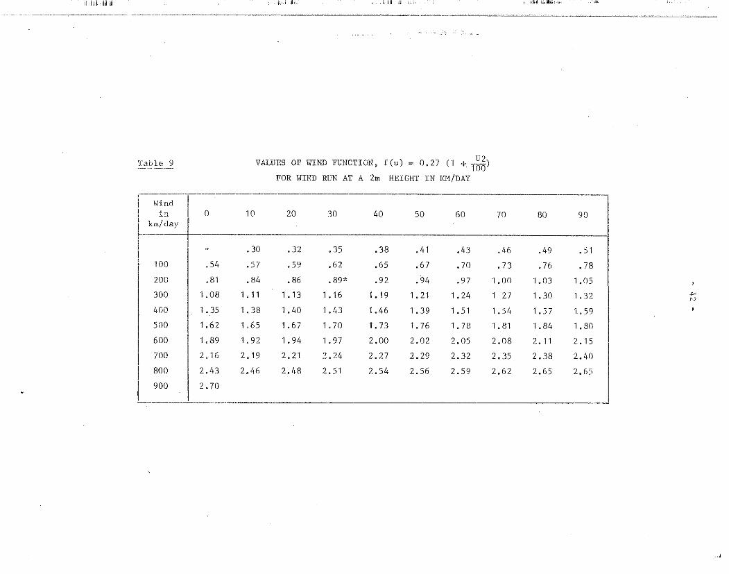
ii, J ll JJI llii .i ,i,1 i, 11 ,11 "i,l ldllii.,,"

Taule 9 VALUES OF WIND FUNCTION, f(u) = 0,27 ("I + 1~-8) ~--,,_~,·-·---

FOR WIND RUN AT A 2m HEIGHT IN KM/DAY

1------------ --, , Wind 1 1

in i () 10 20 30 40 50 60 70 80 90 km/day

------~----·-- ----. 30 .32 .35 .38 • 41 .43 .46 ,L,9 . 51

rno .54 „ 57 .59 .62 .65 . 6 7 .70 . 73 .76 .78

200 • 81 • 84 • 86 .89* .92 . 94 .97 1. 00 1.03 1.05

300 1.08 1 • 11 1. 13 1. 16 1. 19 1 . 21 1. 24 1 27 1. 30 1.32 1

+' CJ

400 1. 35 1. 38 1.40 1.43 1.46 1. 39 1. 51 1.54 1. 5 7 l. 59

500 1.62 1.65 1. 67 1. 70 T. 73 1. 76 1. 78 1. 81 1. 84 1. 80

600 1.89 1. 92 1. 94 1. 97 2.00 2.02 2.05 2.08 2. 11 2. 15

700 2. 16 2. 19 2. 21 2.24 2.27 2. 29 2.32 2. 35 2.38 2.40

800 2.43 2.46 2.48 2.51 2.54 2.56 2.59 2.62 2.65 2,65

900 2.70 1

_J

1 ,1 ü "' 'j .i,, i, d ·" dJ ,,.,11,., ...

~------- ----··· ---···------ ----·-""'''····~-- •"O•W, ___ _.,_,,, ,,,,_ 00 ... ,,m.~•--•« ·-----·

•

Table 10

0 Temperature C

(1-W) at altitude m 0

Table 11

500

000

2 000

3 000

4 000

f Temperature 0 c

1 m

VALUES OF WEIGHTING FACTOR (1 •W) FOR THE EFFECT OF WIND A..c"lD HUMIDITY ON ETo AT DIFFERENT TEMPERATURES AND ALTITUDES

-------·---·---------------i 2 4 6 8 10 12 14 16 18 20 22 24 26 28 l----··----------···

lo.5ī .54 • 51 .48 .t,5 .42 • 39 1

. 36 .34 .32 . 29 • 27 . 25 .23*

1 .56 . 52 . 49 .46 .43 .45 .38 .35 .33 .30 .28 . 26 .24 . 22 1 .54 . 51 .48 .L}5 • 42 .39 .36 .34 • 31 .29 • 27 . 25 .23 • 21 1 . 51 .48 .45 .42 .39 . 36 .34 . 31 . 29 . 27 • 25 . 23 . 21 . 19

1 .48 .t,5 .42 .39 • 36 • 34 • 31 .29 . 27 .25 .23 . 21 . 19 .18

L~~6 .42 .39 • 36 .34 .31 • 29 • 27 . 25 .23 . 21 . 19 • 18 • 16

VALUES OF WEIGl!TING FACTOR W FOR THE EFFECT OF RADIATION ON ETo AT DIFFERENT TEMPERATURES AND ALTITUDES

2 t, 6 810 12 14 16 18 20 22 24 26 28

30 32 34 ·-·--:-::-,

36 1~ t, 0 1

.22 .20 • 1 8 .17 • 16 ~~i

. 21 . 19 . 18 . 16 • 15 • 14

• 20 • 1 8 . 1 7 . 15 • 14 • 13

• 18 • 16 . 15 . 14 . 13 . 12

. 16 . 15 . 14 . 13 . 12 . 11

• 15 • 14 • 13 . 12 . 11 • 10 . 1

30 32 34 36 38 --t,o -··1

J W at altitude ! o lo.43 .46 .49 .52 .ss .58 .64

.65

.66

.69

-----~---- -------, .66 .68 .71 .73 .75 .77- .78 .80 .82 .83 .84 .851

.67 .70 .72 .74 .76 .78 .79 .81 .82 .84 .85 .86

.69 .71 .73 .75 .77 .79 .80 .82 .83 .85 .86 .871

.71 .73 .75 .77 .79 .81 .82 .84 .85 .86 .87 .88

.73 .75 .77 .79 .81 .82 .84 .85 .86 .87 .88 .891 1

500

,100

2 000

3 000

.44 .48 .51 .54 .57

.46 .49 .52 .55 .58

~ L+9 .52 .55 .58 • 61

.52 .55 .58 • 61 .64

• 60

• 61

• 71

l 4 000 1 • 54 .58 .61 .64 .66

·-------------- -·--·--·----·-·--··--

• 61,

.66

.69

.61

.62

.64

.66

.69

• 71 • 73 • 1 5 • 17 • 7 9 • 81 . _s_2 -~s-4 ___ :~~--·-s_6_~~7--. s_g _:_~:--~-~j

-~ .,.,,-, ·-.,,

-"· t,_;

li ļ ;l J.il :il! i .lai 1, 11 .11 dt l<,!lliiJ,,1' ~

Table 12 EXTRA-TERRESTRIAL RADIATION Ra EXPRESSED IN EQUIV ALENT EVAPORATION IN MM/DAY

-----

.-------------·-···-··-----------·---·-· -~J Jan Feb Mar Api:- Hay June July Aug Sept Oct Nov Dec [ Lat Jan Feb Mar Apr May June July Aug Sept Oct Nov

··- ---· ' 3.8 6. l · 9.4 12. 7 15.8 17. 1 16.4 14.1 10.9 7.4 4.5 J.2 so0

"17. 5 14. 7 10.9 7 .o 4.2 3. 1 3. 5 5.5 8.9 12.9 16. 5 18.2

4.3 6.6 9.8 13a0 15.9 17 .2 16. 5 14.3 11. 2 7.8 s.o 3.7 48 17 .6 14. 9 11.2 LS 4. 7 3.5 l1 ,0 6.0 9.3 13.2 16.6 18.2

l,. 9 7. 1 10..,2 13~3 16.0 17. 2 16.6 14.5 11 . 5 8.3 5.S 4.3 1,6 17. 7 15.1 11.5 7. 9 5.2 4.0 4.4 6.5 9.7 13,4 16. 7 18.3

5.3 7.6 10J, 1 ~. 7 16. 1 17 .2 16.6 14.7 11.9 B.7 6.0 4,. 7 44 17 .8 15.3 11.9 8.4 5. 7 4.4 4.9 6.9 10.2 13.7 16. 7 18.J

5.9 8.1 11.0 14.0 16 .2 17 .3 16. 7 15.0 12.2: 9 .1 6.5 5.2 42 17 ,8 15. 5 12. 2 8.B 6. 1 4.9 5, lf 7.4 10.6 14.0 16.8 18.3

6.4 8.6 11. 4, 14.3 16. lf 17 .3 16, 7 15. 2 12.5 9.6 7.0 5.7 40 17 .9 15. 7 12.5 9.2 6.6 5.3 5.9 7.9 11.0 14.2 16,9 18.3

6.9 9.0 11 .8 14.5 16.4 17 .2 16.7 15.3 12.8 10.0 7.5 6. 1 38 17 .9 15.8. 12. 8 9.6 7. 1 5.8 6.3 8.3 11.4 14.4 17 .o 18.3

7.4 9.4 12. 1 14.7 16 .4 17 .2 "16. 7 15.4 n.1 10.6 8.0 6.6 36 17 .9 16.0 13. 2 10. 1 7. 5 6.3 6,8 8.8 11.7 14.6 1 7. 0 18. 2

7.9 9.8 12.4 14.8 16 .5 ! 7. 1 16.8 15.5 H.4 10.8 8.5 7.2 34 17.8 ·15. 1 13. 5 10.S 8.0 6.8 7.2 9.2 12.0 14.9 17. 1 18. 2

8.3 10.2 1L8 15.0 16. 5 17.0 16.8 15.6 13.6 11 • 2 9.0 7.8 32 17 .s 16.2 13.8 10.9 8.5 7.3 7. 7 9.6 12.4 15. 1 17 .2 180 i

6.8 10.7 13. 1 15.2 16.5 17.0 16. 8* 15. 7 13, 9 11.6 9.5 8.3 30 17. 8 16 .4 14.0 11. 3 8.9 7.8 8. 1 10, 1 12. 7 15.3 17. 3 18, 1

9.3 11. 1 13.4 15. 3 16.5 16.8 16.7 15. 7 14. 1 12.0 9.9 8.8 28 17. 7 16.4 14.3 11.6 9.3 8.2 8.6 10,4 13.0 1'>. 4 17 .2 17 .9 1 +· +'

9.8 1 i. 5 13. 7 15. 3 16.4 16.7 16.6 15.7 14.3 12. .3 10.3 9.3 26 17.6 16.4 ·14_4 12,0 9,7 8.7 9.1 10.9 13. 2 15. 5 17. 2 17 .8

10.2 11.9 13.9 15.4 16.4 16.6 16.5 15. 8 1405 12.6 10. 7 9.7 24 17 .5 16. 5 14.6 12. 3 10.2 9. 1 9.5 1L2 13.4 15,6 17. 1 17. 7

10. 7 12 .J 14.2 15. 5 16.3 16. 4 "l 6, 11 15.8 14.6 u.o 11. 1 10.2 22 17 .4 16.5 14.8 12.6 10.6 9.6 10.0 11. 6 13. 7 15. 7 17 .0 17 .5

11.2 12. 7 14.4 15. 6 16.3 16.4 "16.3 !5.9 14 .8 13 .3 11.6 10. 7 20 17. 3 ·16.5 15,[) 13.0 11. 0 10.0 10.4 12.0 13.9 15,8 17 ,0 !7 o4

1"I • 6 13 .0 14.6 15"6 16. 1 16. 1 16, ·1 15.8 1 tf. 9 13. 6 12.0 11.1 18 17, 1 16.5 15, 1 13 ,2 11. 4 11) .lf 10.8 12. 3 14.1 15.8 16.8 17. 'i

12.0 13. 3 14.7 1So6 16.0 15. 9 15.9 15 0 7 15.0 13.9 12.4 11.6 16 16. 9 16.4 15,2 13.5 11. 7 10.8 1L2 12.6 14,3 15.8 16. 7 16.8

12.<"l 13.6 14.9 15. 7 15.8 15. 7 15. 7 15 e 7 15.1 14. 1 12.B 12.0 14 16. 7 16.4 15, 3 13. 7 12.1 11. 2 11. 6 12. 9 14. 5 15.8 16. 5 16,6

12.8 13.9 15, 1 15,1 15. 7 15. 5 15. 5 15.6 15. 2 14.4 13. 3 12.5 12 16.6 16.3 15.4 1l,. 0 12. 5 11. 6 12.0 13. 2 14, 7 15,8 16.4 16.5

13,2 14.2 15. 3 15.7 15. 5 15, 3 15. 3 15.5 15.3 14. 7 13.6 12.9 10 16.li 16.3 15, 5 14. 2 12. 8 12.0 12,4 13 .5 14. 8 15.9 16.2 16 0 2

13. 6 14.5 15. 3 15.6 ·1 s. 3 15.0 15. '\ 15. 4 15. 3 14. 8 13. 9 13. 3 8 16. 1 16. 1 ·15, 5 14. 4 13. 1 12. 4 12. 7 13. 7 14.9 15.8 16.0 16.0

13.9 14.8 15.4 15. 4 15. 1 14, 7 H.9 15.2 ·i 5. 3 l5.0 14.2 13. 7 6 15.8 16.0 15,6 14.7 1 3. l1 12. 8 11.1 14.0 15.0 15. 7 15.8 15. 7

1 L1, 3 15.0 15.5 15 .5 1Lf. 9 1 lf O l1 14.6 15. 1 15.3 15.1 14. 5 14. 1 4 15 .5 15.8 15, 6 14.9 13.8 13.2 13.4 14. 3 15. 1 15,6 15. 5 15.4

14. 7 15.3 15 .G 15,3 14,6 14, 2 14.3 ilf.9 15.3 15 ,3 14.8 14.4 2 15.3 15. 7 15, 7 15. 1 14. 1 13.5 13. 7 14.5 15,2 15,5 15. 3 15. 1

15.0 15.5 15. 7 15.3 l 4. Lf 13.9 14. ·1 1Li .• 8 15. 3 15.4 15. 1 14.8 0 15.0 15, 2 15. 7 15.3 14. 4 13. 9 14. 1 14.8 15,3 15.4 15. 1 14.8

-J

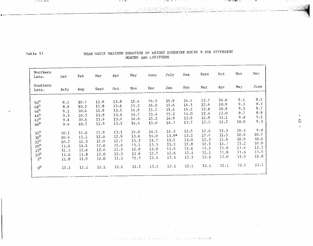
I, J J,,I ~, ; ,1., " ..i, ,.,,liii

--------- -•s·--•-=•-"" -·-----••-""' • .-4.·.···

·.·-~

Table 13 MEAN DAILY l'.AXIMUM DURATION OF BRIGHT SUNS!HNE HOURS N FOR DIFFERENT

MONTHS AND LATITUDES

Northern Lats. Jan Feb Mar Apr May June July Aug Sept Oct Nov Dec

Southern Lats. July Aug Sept Oct Nov Dec Jan Feb Mar Apr May J'une

50° 8.5 10.1 n.8 13.8 15 .4 16.3 15.9 14.5 12.7 10.8 9.1 8.1

48° 8.8 10.2 ll.8 13.6 15. 2 16.0 15 .6 H.3 12.6 10.9 9.3 8.3

46° 9.1 10.4 11.9 13.5 14.9 15.7 15 .4 11,.2 12.6 10.9 9.5 8.7

44° 9.3 10.5 11.9 13.4 14.7 15. 4 15. 2 14.0 12.6 11.0 9.7 8.9

42° 9.4 10.6 ll.9 13.4 14 .6 15 .2 14.9 13.9 12.9 11.1 9.8 9.1

40° ". 6 10.7 11.9 13.3 14.4 15.0 14.7 13.7 12 .5 11.2 10.0 9. 3 1 +• v,

35° 10.1 11.0 11.9 13.1 14.0 14.5 14. 3 13.5 12.4 11.3 10.3 9.8

30° 10.4 11.1 12.0 12.9 13.6 14.0 13.9* 13.2 12.4 11.5 10.6 10.2

25° 10.7 11. 3 12.0 12. 7 13.3 13.7 13.5 13.0 12.3 11.6 10.9 10.6

20° ll.O 11.5 12.0 12. 6 13.1 13.3 13.2 12.8 12. 3 11.7 11.2 10.9

15° 11. 3 11.6 12.0 12.5 12. 8 13.0 12.9 12.6 12.2 11. 8 11.4 11. 2

100 11. 6 11.8 12.0 12.3 12.6 12 .. 7 12.6 12.4 12.1 11.8 11.6 11.5

50 11.8 11.9 12.0 12. 2 12.3 12.4 12 .3 12.3 12.l 12.0 11.9 11.8

00 12.1 12.1 12.1 12.1 12 .1 12.1 12.1 12.1 12.1 12.1 12.l 12.1 l ··----~--------·--------~----~-··~-·

J1LJ:,1 ~l , i .Ī;1 i, 11 ,iÜ 1,iJ 1,,iīlii,;.u, "'

Table 14 CONVERSION FACTOR F'OR EXTRA-TEFRESTIAL RADIATION TO NET SOLAR RADIATION Rns FOR A GIVEN REF'LECTION a OF 25%AND DIFFERENT RATIOS OF ACTUAL TO MAXIMUM SUNSHINE HOURS (1-a) (0.25 + 0.50 n/N)

~

----------···"------------------ .. , N 0.0 05 .10 .15 .20 .25 .30 .35 .40 .45 .50 .55 .60 .65 .70 .75 .80 .85 .90 .95 1.00

-a)(0.25 + 0.50 n/N) . 0.19 .21 .22 .24 .26 .28 .30 .32 .34 .36 .37 .39 .41 .43 .45 .47 .49*.51 .52 ,51, .56 , 1 ------------- -. -----------------------------·--- ---------------------------

Table 15 ----- CORRECTION FOR TEMPERATURE f(t) ON LONGWAVE RADIATION Rnl

r·-----·-··-t . -·-. _, ........... _,, ____ ,, ____ , .. , ... __________________________ ,, ... ___________ , _______ ,, _________ .., ___ .. _____________ .,,., 1 t

0 c O 2 L, 6 8 10 12 14 16 18 20 22 24 26 28 30 32 34 36 1

l L, • __ ........... - ... ,·-.•. -·. ·--- , .. ·.?·· .. --.---------------.--.·-·~· -·---,,-----.. ·-···---j f(t)~aTk 11.0 H. 01 Ll.7 12.0 12.o+ L./ 13.1 B.5 13.8 14.2 14.6 15.0 15.1, 15.9 16.3-16.7 17.s 1L7 18.l ·--------·-·-· ----------·-----------------.. -----------------------------------------.. -- ......... 1

Ta~le ļiL CORRilGTION FOR VAPOUR PRESSURE f (ed) ON LONGWAVE RADIATION Rnl f'.·

· .. - .... -----·-··--- ........................... ,........................ ........... _______ ------------ -- ______________________ , ___ ............. !

::m1::a:limates t0,:7 .:1, ~:l ~:9 ~:6 ~:4 ~:3 ~:1 ~:9 ~:7 ~:6 ~:4 ~:3 ~:l ~:O ~:9 ~:7 ~:61

f(ed) ~ 0.56 „ 0.079 Ved j 1

d,·1 climaces l ,2'J .22 .20 .19 .18 .16 .15 .14* .13 .12 .12 .ll .10 .09 .08 .08 .07 .06 1! 1 . r-f(e.i)~ ü.34 • 0.044ved 1

1 .. - ··-· __ ,.. _____ ·----·--··-·-· _ ...... ··----.. ------------------------·-.. ··--·---------------" .. ,

Tat)_ļ!, .. J} CORRECTION FOR THE RATIO ACTUAL AND MAXIMUM BRIGHT SUNSHINE HOURS f (n/N) ON LONGWAVE RADIATION Rnl

1 n/N O .05 .1 .b .2 .. 5 ._; .35 .4 .1,5 .5 .55 .6 .oS .7 ./5 .~ .85 .9 .95 LO ŗ .. -·---- ____ ] ___ ., ...... ----- ___ ,, __ ? ___ ---_ ---·------.----_ ·-.. ·-·--· _-·-_ ·-· ....... ..

Lf(n/N)_~o.l„0.9.n/N____ .10_.15. .19 .. 24 .28 .33 .37 .4-2 .46 .51 .55 .60 .69 .73 .78 .82*.87 .91 .96 1.00 ___ _/

'

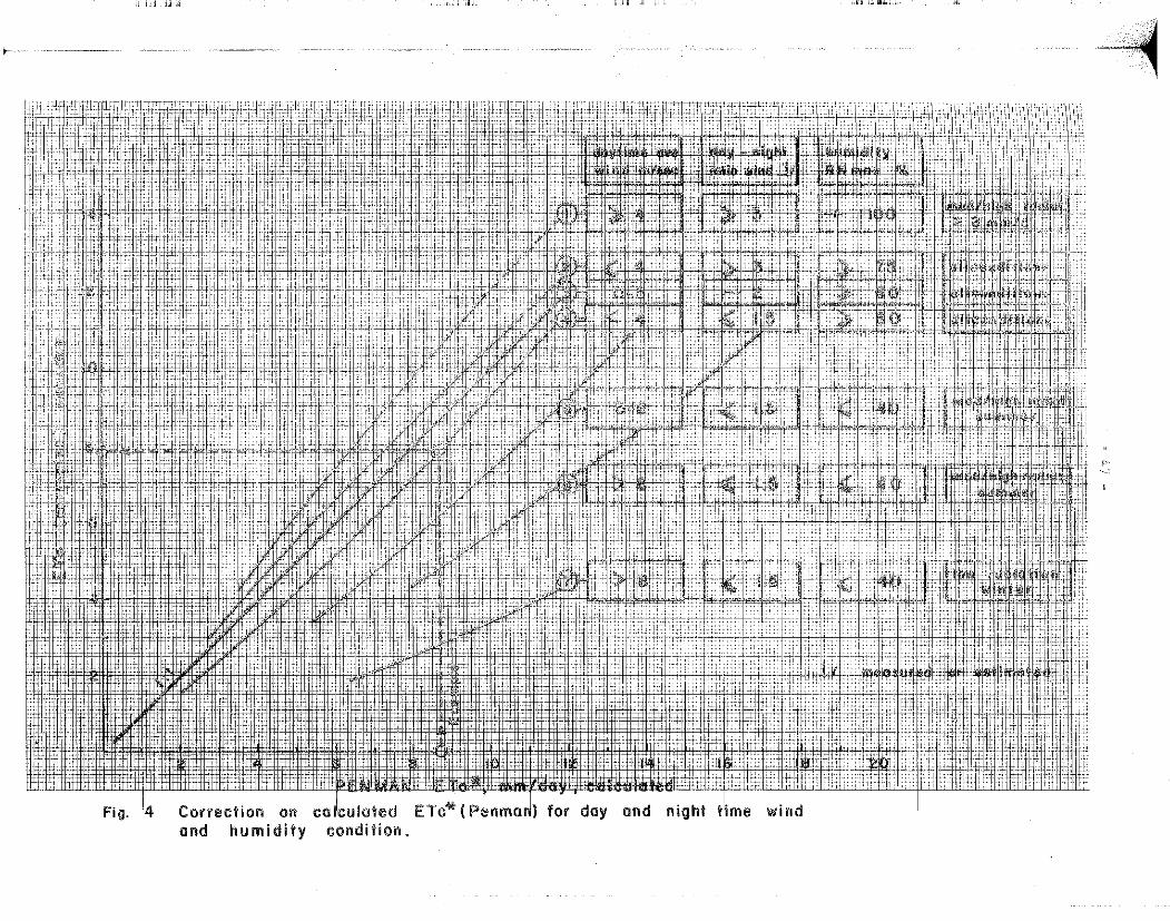
"i,i J,1,,1 ; ,i,1 i, ,1

fT'ITT'riuīJJJll. füBI .. ''tffllhljlll'iilHJJ\ll!\HWlrJUll\filTilll:lHfjliH'ftlTilffllilli'Jil;!J"jpm 1 ,1 ··l·n 'Hfü- _· t ~.t:-_W '!·I •t1-H- t .;_ __ t-:_Wtttf1-h-tt:::it~~f1HH :.,.;~:-,.· :-.--' ' ,--n---n .. !'

L"

ii

ffijī Jiü

It!,

'

,. tiit

'·1·1111!1 f . hrl:rrmrr

··+li

mtt1tmt1#f1J±>1

Lll jj \ļlltJill,Utl« iillHHll!IļlE

·"

nīīl1 +.ttt-rri. 1-+:r

iilf1.ļ.nfrrī<-I

Fig, '4 Correction 011 col'culoted Eīo* ! PenmonJ for doy and night tlme wind and humidity condilion.

d; ,.,,ia;,,,,, >,

~ ,

DATA

- 48 -

FCRJIIAT FOR CALCULATION 01' l'ElfflAll METHOD

Penma:n reference crop ETo • W, Rn + (1-W) f(u) (ea.-ed)

I 1AR Country: v Period 1 ~ 1972

Pla.ce: č'cuw La.titude : 30"/V Longi tude: ~0°

t mea.n .,,.28.)c ea m'ba.r (7) 11 36'9

05j-Rl! mea.n •55 Rll/100

or t wet bulb 1 depress.

or t dewpoint

u2• 232 Jcm/d t • 2.f!.6 °c alt • c/5 m

month • 2 .... &, lat. .. 3cf-;N

n .11.5 month • .J::!:t, lat~ • 30 N

ed mbar

Ra nun/day

n hr/day

N hr/day

n/N

data.

calc

ar (8a)(8b)

ar ( 8c)

( 12)

data.

( 13)

oalc

:l. / 4-

(ea,-ed) mbar calc

f(u)

( 1-W)

( 1-W) f( u)

({,,J

(9)

(10) . _)3

(ea-ed) nun/dazy- calc

~. o< . 0.25 (1-c<)(o,25-0,50 n/N)

H .fj 1

(14) 50

t • 28 S 0 c

ed =21.L/ mbar

nfe.Oi3

t -2~5°c alt •'/5 m

Rna mm/day calc

f(t) ( 15)

f(ed) (16)

f(n/N) ( 17)

Rnl. f(t). f( ed). f(n/N)

8.4 y

1 i0. !/ h

~ 1 ~ ' mm/day ca.lc /' ii

Rn • Rna-Rnl calc

l1 (11) · 77 w. Rn calo

Al titude1 '1_"/ m

3 (,

;.- -1 :7'

day/night U2,Rl!

ETc• • WR.~ + (1-W) f(u)(e,...ed) rnm/ā.ay calc

correotian on ETo* for d.ay and night time Fig. 4 ,ind and humidity ETc

1/ Numbera in bracketa indica.te Ta.ble of reference„

EJ When Rs d.ata are available Rno • 0,75 Rs.

§

::;;

-

·~·\.· .... ··•·.··

1 '

i .l

~ 49 ,~

Penma.n referenoe orop ETo a Wo Rn + (1-~) f(u) (e1Ji-scl)

DATA Countr:,ī

Periods

t mean "" 0 c ea mbar

RR mea.n „ j Rll/100

or t wet bulb depres11„

or t dewpoint

"2" t • alt •

lclll/d oc m

ed mba.r

(7) 11

da.ta

calc

or (8a)(8b) or ( 8c)

Places La.tituāe g

LlllD.gitude~

(eo,-ed) mb.,.r co.1:-~ h ·:===:::::@ ±"(u) (9) ! µ

il ti tudeg

(1-ll) (10) 1-_J~ (1-ll) f(u) (e,....od) ,m//J.o;;ŗ calc q

month „ lat. •

n • month • lat. ...

c< • 0.25

t "c

ed . abar

n/H •

t oc alt • "

iiq/night 112.u:

1

1

1

Ra 11m/d'17 ( 12)

n hr/dt&y data

ll' hr/do.y ( 13)

n/J oalo

( 1-"' )(0.25-0.50 n;il)

Rn• ,m/da.:, colc

f( t) ( 15)

!(od) (16)

f(nfe) ( 17)

Rnl" f( t)' r( ed). f(n;\'I)

j/ iuala?'ll'I in bro.akllltm in.diaa.t.s ''l'abl0 @'! :r~f1lr'1!lnco5i„

Y Vhz b Uia m.r1t &vta.ila.bl0 Ima m O„ 75 Ra„

( 1i)

i

i

1 1

$ 1

1

lll

"' 50 ~

MllTHOD IV • PAN EVAPOFu'.TION

Evaporation pa~s provide a measurement of the integrated effect of radiation~ wind 1

temperature and humidity on evaporation from an open water surface. Ina similar fashion

the plant responds to the same climatic variables but several major factors may produce

significant differences in loss of water. Reflectivity of radiation from a water surface is

only 5~8%, while that from mast vegetative surfaces is 20-251o of solar radiation received,

Daytime storage of heat within the pan can be appreciable and may cause alrnost equal distri

bution of evaporation between night and day, while mast crops lose 95% or more of their

24-hour loss during daytime hours. Also a great difference in water losses from pans and

from crop covers can be caused by the variance in air turbulence just above the surfaces

and in the temperature and humidity of the air immediately adjacent to these· surfaces~ For

both above~ground and sunken pans heat transfer through the sides of the pan can occur; this

may be severe for sunken pans in fallow grounda Also the colour of the pan and use of

screens to protect it against birds will affect the measurement. The si ting of the pan and

the pan environment influence the measured results, especially when the pan is placed in

cropped rather than fallow fieldsa The importance of siting and environment of the pans will

be shown later. 1 /

Notwi ths tanding these deficiencies ~ wi th proper siting, maintenance of a standardized

environment and condition of pans 3 their use to predict crop water requirements for periods

of 10 days or longer is still warranted. To relate pan evaporation to reference crop

evapotranspiration ETo empirically derived coefficients are suggested which take into account

climate, type of pan and pan environment. Of the many different types of pans, the

U.S. Class A pan and the Colorado sunken pan have been selected~ A description of these

pans is given below~

The pan coefficj_ents ŗ, Kp, presented together wi th measured pan evaporation data, Epan,

reflec.t the effect of climate on reference crop evapotranspiration ETo which was defined in

Part I. To arrive at this relationship use has been made of detailed climatic and grass

evapotranspiration <lata from research stations and literature mentioned in the Appendicesa

Similar to the previous methods ~ the effect of crop characteristics on crop water

requirements is represented by the crop coefficients given in Chapter I.2.


Reference crop evapotranspiration (ETo) can be predicted by:

ETo := Kp Epan

where ETo is in mm/day~ Epan is pan evaporation in mm/day and represents the mean daily

value of the period considered; Kp is the pan coefficienL

1/ For comparison between pan and lake 2vaporat:ton see C.E. Hounam (1973) WMO Note 1263

'T'.'.,,····''·.·.··.· . '''! '· l

,,

•

-

l

Values for Kp are given in Tables 19 and 20 for di:f:fe.rent cond,itions of humidi ty and

vind, pan environment and type of ·pan and should be applied to pans located in an open

environment with no crops taller than ·i m ·wi thin some 50 m of the pan. Except fffr the bare

so-il conditions (case B) ~ irnmediate surroundings, within 10 m, are covered by a green~

frequently mowed, grass cover~ The pan station is placed in an agricultural area with a

Cropping density of some 5ü%G No screens are mounted over the pan~

Nomenclature used to describe general levels of mean temperature, mean relative

humidity and wind are given in the Table on Climatic Nomenclature in the introductory pages •

Description of pans

The class A evaporation pan is circula-r) 121 cm ( 4 7. 5 in) in diameter and 25. 5 cm

(10 in) deep. It is made of galvanized iron (22 gage) ar monel metal (0.8 lllIIl). The pan is

mounted on a wooden open frarne platforrn with its bottom 15 cm above groundlevel~ The soil

is built up to within 5 cm of the bottom of the pan. The pan must be level. It is filled

with water 5 cm below the rim~ and water level should not drap to more than 7 .5 cm

below the rim. Water is regularly renewed to eliminate extreme turbidity. The pan if

galvanized is painted annually with alluminium paint.

Sunken Colorado pans are sometimes preferred in crop water requirement studies, since

these pans have a water level 5 cm bel.ow the rim at soil level height and give a better

direct prediction of potential evapotranspiration of grass than does the class A pane The

pan is 92 cm (36 in) square and 46 cm (18 in) deep. It is made of galvanized iron, set in

the ground with the rim 5 cm (2 in) above the groundlevel~ The water level inside the pan

is maintained at or slightly below groundlevel.


In selecting the appropriate value of Kp to relate Class A and Colorado sunken pan

<lata to ETo, the ground cover of the weather station itself, that of the surroundings

outside the station, the effect of day and night weather conditions and the pan conditions

need to be consideredo

a) īn the case of pans located at a weather station with vecy poor grass cover or dry

bare scil or~ undesirably~ a concrete or asphalt apron~ air temperatures at pan level may

be 2 to s0 c higher and relative humidity 20 to 30% lower~ Under these rather too commonly

found condi tions ~ Epan greatly exceeds EToo This wiJ.l be most pronounced in arid and semi„

arid climates during all but the rainy periodso This effect has been accounted for in the

figures of Tables 19 and 20. However in cases wi th no agricultural de,1elopment and extensive

areas of bare soils = as are found~ for instance, under desert or semi„desert conditions ~

the values of Kp given in case B for arid windy areas may need to be reduced by up to 205"°;

for areas with moderate levels of wind, temperature and relative humidity by 5 to 10%,; no or

little reduction in Kp is needed in humid cool conditions~ It follows that, particularly

for truly desert areas~ the radiation method of predicting ETO is preferable, since the

errors involved may be less severe_,

'

-

= 52 =

b) \"l'here. pans are plac2-.::.!. in a smaJ.l e!1closure but surrounded

2.5 m high maize) the coe.fficients in Tables 19 and 20 may nee.d

by tall crops, for example

increasing by up to 30% for

dry windy climates, when.:as only a 5 to 10% increase is required for calm humid conditions.

Epan decreases a::-1 pans arr~ placed w:i. thin increasingly large cropped areas 1 mos t of

the decrease occuring w:lchin the f:i.rst few tens of metres of upwind cropped fields. This is

clearly evident from d.-:c::a in Tables 19 and 2G whe-re a separation is made for pans loc.ated

within c.ropped plo-c.s surrounct2d Jy or do•,,mw:Lnd frorn dry surface areas (case A) and for pans

locat.ed w::i. thi:1 a dry or f al:ow fie.ld but surrourrded by irrigated ar rainf ed upw ind cropped

are.as (case B),

Cose A

Wind '1ii 7

50mo o, mor@

-• pan

grtsrn crop \lll)Vii\l!/lļf!l)IYJU\IUJHISHE:J=?

Case 8

Wind

pan grHn crop dry 1urfoce

1\l l llli!ltllSVtll\1/1 UP/UIIU fl l(llftW

50mo o, more vories

c) Since pans lose a significant portion of total evaporation at nigh t, the inclusion of

night~t.ime humidity appears Jesirable. Hence the relative humidity referred to is hased on

(RHmax + RHmin) /2. The ranges showu for < 40fo relative humidity thus relate to very dry

night-time as well as very dry daytime conditions. The range from 40 to 70°/o is typic.al for

summertime conditions in drier semi"'arid climates although some Mediterranean areas would

tend to fall between the 40 to 70 and > 70% relative humidity range~ Wind is reflected as

total daily wind run. Levels of radiation for similar conditions of humidity and wind will

affect somewhat the relationship between Epan and ETo, particularly in very dry and windy

conditions. The coefficients presented for such conditions reflect a linear relationship

as the possible error involved in mast cases would be little more than 5%.

d) The pan coefficients listed below apply to galvanized pans annually painted with

aluminium„ -Wllile little difference in Epan will show when inside and outside surfaces of

the pan are painted white 9 an inc.rease in Epan of up to 10% may occur when they are painted

black. The material from which the pan is made may account for variations of only a few

percent. Turbidity of the water in the pan does not affect Epan <lata by more than 5%.

Overa.11 variation in Epan is not constant with time because of ageing, deterioration and

repainting. The level at which the water is maintained in the pan is very important;

resulting errors may be up to ·15,fo when water levels in Class A pans fall 10 cm below the

accepted standard of between 5 aud 7 .5 cm below the rim~ Sc.reens mounted over pans will

reduce Epan by up to 1 o~0. In an endeavour to avoid pans being used by birds for drinking,

a pan filled to the rim with water can be plac.ed near the Class A pan; birds may prefer to

use the fully filled pan~

-

~ 1 l

- 53 -

e) The various types of evaporation pans in use differ in sizei shape. a.nd installation

method. Even for the same crop environments the relationship between evaporation from any

two types of pan is acutely dependent upon weather conditions; no constant ratio in measure

ment can be expected. Caution should therefore be exercised in applying the ratios shown

in Table 18 between evaporation for the unscreened sunken pans mentioned and Colorado sunken

pans if the two pans are placed in similar environments. The pan area of the Colorado sunken 2

pans is 3 ft square or 0.84 m

Table 18 RELATION BETWEEN EVAPORATION FROM SUNKEN PANS HENTIONED AND FROM COLORADO SUN',ZEN PAN FOR DIFFERENT CLIHATIC CONDITIONS AND PAN ENVIRONMENTS. COEFFICIENTS GIVEN CAN SERVE AS MULTIPLYING FACTOR TO OBTAIN ESTIMATED COLORADO PAN EVAPORATION,

Climate ·~~~~~~-~mid-temperate climate

Arid to semi~arid 1

(dry season) ~

Groundcover surrounding pan I Short green (50 m or more) cover Dry fallow

Short gree:-Ī~~llow cover I y

___ _,_P_a_n_ m~-r-e-a-+-------l-------+------ŗ

CGI 20 dia. 5 m, depth 2 m 20 1.0 1.1 1.05 1 1.25* (USSR)

Sunken pan, dia. 12 ft, depth 3.3 ft (Israel)

2 Symmons pan 6 ft , depth 2 ft (UK)

BPI dia. 6 ft, depth 2 ft (USA)

Kenya pan dia. 4 ft, depth 14 in

Australian pan, dia. 3 ft, depth 3 ft

2 Aslyng pan, 0.33 m, depth 1 m (Denmark)

CGI 3000 dia. 61.8 cm, depth 60-80 cm

Sunken pan dia. 50 cm, depth 25 cm (Netherlands)

1 0 .5

3.3

2.6

1 • 2

0.7

0.3

0.3

1 0.2 1.0

EXAMPLE: CGI 20 in semi-arid climatei dry season, for given month Epan CGI 20 = 8 mm/ day. Colorado is 1.25 x 8 = 10 mm/day.

1 .o 1 • 0

1 , 0

l .95 1.0

placed in dry fallow land; Corresponding E pan sunken

, 95

'

-

• 54 •

Sample calculations

First, using mean daily Epan <lata, an example shows the procedure to obtain the mean

daily value of ETo in mm for a given month. Then mean daily <lata for each month for the

whole year are given to illustrate the selection of relationships between prevailing climatic

and environmental conditions and Kp for each month using Tables 19 and 20.

EXAMPLE:

Given: Cairo, July; Epan = 11.1 mm/day from class A pan. RH mean = medium; wind = moderate Pan is located in 20 x 20 m bare soil plet with surrounding crops of berseem or wheat in autumn and winter, and cotton in spring and summer; the pan is not screened.

Calculation: Monthly data: since pan is surrounded by 10 m of dry fallow land case B applies.

Wind

RH mean

Surrounding

[{p

Epan mm/day

ETo mm/day

From Table 19 for moderate wind and medium humidity while upwind distance of dry fallow is 10 m, value of Kp = 0.65.

Reference crop evapotranspiration ETo in July = Kp x Epan 0. 65 x 11. 1 = 7. 2 mm/ day

Yearly <lata: class A pan;

Jan Feb Mar Apr May June July Aug Sept OcE Dec

Light to moderate _ light to moderate _

-moderate-

Medium medium medium

- high - - to high-to

bare fallow .land, 20 X 20 m, surrounded by irrigated crop; Case B with 10 m upwind distance applies for all months,

• 7 • 7 .65 .65 .65 .65 .65 .65 .65 • 65 • 7 • 7

3.3 4.5 6.4 8.5 11. 2 12.8 11. 1 9.7 8.9 6.9 4.5 3.3

2.3 3. 1 4.2 5.5 7.3 8.3 7.2 6.3 5.8 4.5 3.2 2.3

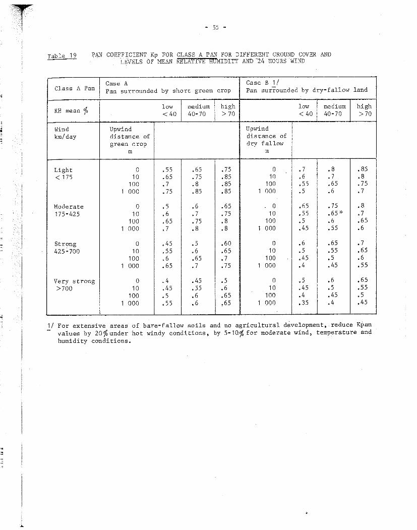
T l l - 55 -

Table 19 PAN COEFFICIENT Kp FOR CLASS A PAN FOR DIFFERENT GROUND COVER Al'ID LEVELS OF MEAN RELATIVE HUMIDITY AND --24 HOURS WIND

Case A Case B 1/ Class A Pan Pan surrounded by short green crop Pan sur"rounded by dry-fallow land

RH mean °fo low medium high low medium~h <40 40-70 > 70 < 40 40-70 > 70

--Wind Upwind Upwind km/day distance of distance of

green crop dry fallow m m

Light 0 .55 .65 .75 0 • 7 • 8 , 85 < 175 10 .65 .75 .85 10 • 6 • 7 .8

100 • 7 .8 .85 100 .55 .65 .75 1 000 .75 , 85 , 85 1 000 .5 .6 .7

Moderate 0 .5 .6 .65 0 .65 , 75 .8 175-425 10 .6 • 7 .75 10 .55 , 65" .7

100 .65 , 75 .8 100 .5 .6 .65 1 000 .7 • 8 .8 1 000 .45 .55 .6

Strong 0 • 45 .5 .60 0 .6 .65 • 7 425-700 10 .55 .6 .65 10 . 5 .55 .65

100 .6 .65 .7 100 .45 .5 .6 1 000 .65 . 7 , 75 1 000 .4 , 45 .55

Very strong 0 .4 , 45 .5 0 .5 .6 .65 >700 10 .45 .55 ,6 10 • 45 .5 .55

100 .5 .6 .65 100 .4 , 45 .5 1 000 .55 .6 ,65 1 000 .35 .4 .45

1 / For extensive areas of bare„fallow soils and no agricultural development, re·duce KI)an values by 2ü%under hot windy conditions~ by 5-10% for moderate wind, temperature and humidity -conditions~

•

Table 20

• 56 -

PAN COEFFICIENT Kp FOR COLORADO SUNKEN PAN FOR DIFFERENT GROUND COVER AND LEVELS OF MEAN RELATIVE HUMIDITY AND 24 HOURS WIND

Sunken Case A I Case B 1 / l ļ Colorado ļ Pan surrounded by short green crop Pan sur'rounded by dry-fallow land 1

'f-------l--------------------+-i_____ -.j

r T low ļl medium high 11 low I medium '

RH mean % 1 1 f--------1'e--_______ <_4_o-"-_4_0_-_10 _ _,__>_7_o--i--------<--4-0_L_'.'.0-7o

Wind krn/day

1 Light < 175

1 Moderate 17 5-425

Strong 425-700

Very strong >700

'I Upwind I Upwindl I distance of I distance of greenm crop I dry-!allow

1

0 10

) 1 00

0 10

)100

0 10

)100

0 10

)100

1 ; :f5111

.65 • 85 .95

.55

.75

.8

.5

.65 • 7

• 7 5 11

1. 0

1 • 1 11

.7

.85

.95

.6

.75

.8

.55 • 7 .75

.8 1.0 1 • 1

• 7 .9 .95

.65

. 75

.8

.6 • 7 .75

0 10

100 1 000

0 10

100 000

0 10

100 000

0 10

100 000

1

1.1 ŗl , 85

.75 1 • 7

.95

. 75

.65

.6

.8

.65 • 55 .5

• 7 .55 .5 .45

1

1 • 1 , 85 .75 • 7

.95 , 75 .65 .6

.8

.65

.6

.55

.75

.6

.55

.5

high > 70

1 • 1 , 85 .8 , 75

, 95 • 75 • 70 .65

.8

.65

.65

.6

, 75 .65 .6

.55J

1 / For extensive areas of bare-fallow soils and no agricultural development, reduce Kpan by 2ü%under hot, windy conditions; by 5 to 10% for moderate wind, temperature and humidity conditions3

-~

• 57 •

cHAPTER I. 2 : SELECTION OF CROP COEFFī CIENT, kc

The four methods described in Chapter I. 1 predict the effec.t of cJ.imate on c.rop wa-cer

requirements. Each method is calibrated against reference crop evapotranspiration ETo.

To account for the effect of the crop characteristics on crop water requirements~ crop

coef ficients, kc, are presented to relate ETo to c:rop evapotranspiration ET ( c-rop) The kc.

value represents evapotranspiration of a crop grown under optimum eonditions producing

optimum yields. ET(crop) can be found by kc.ET(crop)., As each of the four methods

predicts ETo only one set of crop coefficients kc is required.

Procedures for selection of appropriate kc values are presented, which take into

account the crop characteristics, time of planting or sowing ~ a.nd stages of crop development,

General climatic conditions~ especially wind and humidity, still need to be considered~

particularly as after temperature, it is the wind conditions which wil1 affe.c.t the rate of

transpiration due to the degree of air turbulence above the rough crop canopy. Furthermore,

rate of transpiration is higher under conditions with dry a.ir winds as r.ompared to humid

air winds.

Crop coefficients published elsewhere relating ET(crop) directly to the ori.ginal

prediction formulae should not be used if the apprca.ch presented in this publication is

followed because the kc values relate to ETo~ The crop coefficients sugg~sted here m2y still

contain inaccuracies due to the many factors involved and the problems that plague p:resent

day applied research on crop water use, such as sa.mpling errors) deep percolation loss~s

or supply from groundwater, size of experimental plotj lysimeter and other problerns. Much

<lata from many sources representing experience covering many climatic.~ crop and grow:tng

conditions had to be considered and may account for some of the autho:r.'s bias in the

selecti.on or rejection of the assembled data~

Local conditions, including agricultural and irriga.tion practices tha.t affect E'I'(c:rop)

are discussed in Chapter I.4.

General considerations

Factors affect:i.ng the value of the crop coefficient kc are mainly the crop charac=

teristics, crop planting or sowing <lata, rate of crop development and length of growing

season, climatic conditions and~ particularly during the earJ .. y growth stage 3 the frequency

of rain or irrigation.

The effect of crop characteristics on the relationship between ET(crop) and ETo .is

shown in the conceptual diagram in Fig. 5. The wide var:i..ations between mA.jor groups of crops

are largely due to the difference in plant mechanisms for resisting transpiration, such as

closed stomata during the daytime (pineapple) and waxy leaves (citrus). Also difference in

crop height, crop roughness, reflection and ground cover produce the illustrated variation

in ET(crop). For high evaporative c.ondit:i.ons; i.e. hot, st:rong winds and low humidity,

' • -

~

-

• 58 •

ETo values of up te 12 to 14 mm/day and ET(crop) values of up to 15 to 17 mm/day may be

realistic, partJ.cul.arly for small fields reacting in somewhat similar fashion as laundry on

a clothesline. However, wilting of crops often occurs under such conditions asis shown for

sugarbeets in Fig. 5.

Sugorbeets Maize

15 CoUon Tomotoes

14 Apples (with cover crop)

>, 0 12 Grou ,::, ..... E

10 ~Sugorbeel, severely willed E on extremely hol - Citrus windy doy Q. 8 e "' - 6 1- Pineopple w

4 Agave

2

2 10 12 14 ET{groH) mm/doy

Fig. 5 Mognitudes of ET(crop) 011 compored to ET (gross)

The crop planting or sowing date will affect the length of the growing season, the

rate of crop development to full ground cover and onset of maturity. For instance, depending on

clirnate~sugarbeets c.a1: be sown in autumn, spring and surnmer with a total growiI__lg season ranging

from 230 to 160 days 3 For soybeans~ the growing season 1 ranges from 100 days in warm, low altitude

areas~ to 190 days .at 2 500 m altitudes in Equatorial Africa .and for maize 80 to 240 days

respectively. Crop development will also be at a different pace; as shown in Fig. 6 for

surgarbeets the time needed to reach full development or maximum water demand varies from

up to 60 percent to the total growing season for an autumn sown crop to about 35 percent for

an early summer sowing ~}_/. īn selecting the appropriate crop coefficient, kc~ for a given crop

for each month in the growing season 1 the rate of crop development must be considered.

1/ This indicates that, when calculating water requirements, the commonly used presentation of k.c values asa function of percentage of total growing season (USDA ... SCS Release No. 21, 1967) will not suffice when attempting to include all possible variations of growing seasons.

-

e

.6

.4

.2 aulumn

20 40 60 80 100°/c

i 1 .,

· 59 •

s pring

20 40 60 80 100%

Growfng s.eason - 2!0 dayll - 200 days

Fig. 6 Sugorbeets ~ kc ond rainfoll

for different frequency.

sowing dotes ond

dry

20 40 60 30 100%

,..,, 160 doym

irrigotion

For the same crop, fully developed, the ratio ET(crop) and ETo or the value of kc

is not constant but changes with climatic conditions. In relation to ETo, crop evapotrans

piration is higher in hot, windy and dry climates as compared to cool, calm and humid

climates. This is clearly reflected in the kc values presented for different climatic

conditions.

The nomenclature used in describing generai levels of the climatic variables involved

has been 'given in the introductory pages.

ET(crop) is the sum of transpiration by the crop and evaporation from the soil surface.

Whereas "during full ground cover J_/ evaporation is negligibly small, during the early growing

period evaporation from the· soil surface may be considerable, particularly when the soil

surface is wet for mast of the time from irrigation and rain3 Hence the great range of kc

values during early season_ growth as shown in Fig, 6 for dry aud wet soil surface conditionsa

The smooth curves are obviously idealized since each irrigation or rain would produce a

sharp increase in kc with a less sharp but mark.ed dropping off afterwards, until the next

irrigation or rain. The practical significance in terms of field irrigation water management

are described in Chapter I.4.

1/ Ground cover is expressed in percentage of soil surface shaded by the crop when

the sun is directly overhe.ad; fu.11 g:round cover is frequeintly assumed whe.n ground cover

as defined in some 80 perc.ent.

-

= 60 =

Fo:r ease oz: c.~pf,::,·,~ep,-.a „ a.pp-roximate ranges of seasonal ET(crop) for different crops are

given in Table 7.. ·j Th2 magn.:i.tudes shown will c.hange according to the factors discussed, i.e.

mainly crop characte.:ris tics J cllrnat.-e 9 leng th of growing season) time of planting; other

factors includ2: size of fields 1 soil water 1.evels and agricultural practices. Also,

approximate comparative valuee ar<;: given where 100 is for grass with a 12 month growing

sea.son in frost free are,g_s,

Table 21 APPROXI1"'1ATE RANGE OF SEASONAL ET(CROP) IN MM AND IN

- -COMPARTSON WITH ET(GRASS) ŗ-- 1 1

1 % 1 mm % IETC(crop) seasonal mm

' ------------- -=r- --

1

Alfalfa 600 .• 1 500 90 • 1 051 Onions 350 - 600 25 - 40 Avocado 650 - ·1 000 65 - 75 Orange 600 - 950 60 - 75 Bananas 700 - 1 700

1

90 - 105 Potatoes 350 - 625 25 - 40 Beans 250 • 400 20 - 25 Rice 500 - 800 45 - 65 Cocoa 800 - 1 200 95 - 110 Sisal 550 - 800 65 - 75 Coffee 800 - 1 200

1

95 - 110 Sorghum 300 - 650 30 - 45 Cotton 550 - 950

1

50 - 65 Soybeans 450 - 825 30 • 45 Datcs 900 - 1 300 85 - 110 Sugarbeets 450 - 850 50 - 65 Deciduous Sugarcane 1 000 - 1 500 105 - 120 trees 700 .• 1 050 60 - 70 Sweet potatoes 400 - 675 30 • 45

Flax 450 - 900 55 - 70 Tobacco 300 - 500 30 - 35 Grains (small) 300 - 450 25 - 30 Tomatoes 300 - 600 30 - 45 Grapefruit 650 - 1 000 70 - 85 Vegetables 250 - 500 15 - 30 Maize 400 - 700

1

30 - 45 Vineyards 450 - 900 30 - 55 Oil seeds 300 - 600 25 • 40 Walnuts 700 - 1 000 65 - 75

-

'

Recommended values -~ 61 =

a) Field and vegetable crops

Values of kc for the different stages of crop devel.opment are given below. Ths crop

growing season is divided into four stages. For each stage, c-rop c.oef:ficients k.c for

different climatic conditions are presented in Table 22. For refe.rence ~ length of crop

development stages and total growing season for selected crops and climate are g:iven in

Table 23~ The need to collect data locally on growing season and rate of crop dev,=:lopment

cannot be overstressed~

The four stages in crop development· ar.e:

- initial stage germination and early growth when the sDil surü-1ce: is not or hardly covered by the crop;

~ crop development stage : from end of initial stage to attairrment of effective full ground cover ~/;

- mid-season stage from attainment of effective full ground cover to tim.e of start of maturing as indicated by discolouring of leaves (be.ans) or leav~'.!s falling off (cotton). For some crops this may extend to very near harvest (sugarbeets) unless irrigation is not applied at late season and reduction in ET(cro~) is induced to increase yield and/or quality (sugarcane, cotton, some grains);

.. late season stage : from end of mid~season stage until full maturity or harvest.

The steps needed to arrive at the kc values for the different stages to be plotted

for simplification as straight lines are indicated in Fig. 7:

(1) establish planting or sowing date from local information or from practice.s in similar climatic zones;

(2) determine total growing season and length of crop development stages from 1ocal information (for approximations see Table 23);

(3) initial stage: predict irrigation and/or rainfall frequency; for predete.rmined ETo value, obtain kc from Fig. 8 and plot kc value as shown in Fig. 7;

(4) mid„season stage: for given climate (humidity and wind), select kc value from Table 22 and plot as straight line;

(5) late-season stage: for time of full maturity or harvest, select kc value from Table 22 for given climate (humidity and wind) and plot value at end of growing season or full maturity. Assume straight line between kc values at end of midseason period and at end of growing season;

(6) development stage: assume straight line between kc value at end of initial stage to start of rnid-season stage.

1/ Start of mid-season stage can be recognized in the field when crop has attained 70 to 80 percent ground cover which, hm.vever; does not mean that the crop has reached its mature height. Effective full ground cover refers to cover when kc is approaching a maximum.

•

- 62 -

For each 10 or 30 day period the kc values can be obtained from the prepared graph,

A smoothed curve might first be. drawn as inUicated in Fig. 7 althou:gh this may have little

effect in terms of accuracy added.

EXAMPLE:

Given: Cairo; corn pla~ted mid-May; for total growing season winds are light to moderate (Om5 m/sec), and mid.summer FHroin in 30-35 percent; ETo initial stage is 8.4 nuu/day; irrigation frequency initial period assumed to be 7 days .

. -----------·-----------------------------------------··------(1) Planting date

(2) Length of growth stages

initial crop development mid„season

local information (ar Table 23)

Late spring, early summer

20 days 35 days 40 days

late season _30 dal'..§.

(3) Plot periods as indicated

(4) kc initial stage ETo: 8.4 mm/day irrig. frequency: 7 days

kc mid-season stage wind = J.ight/moderate humidi ty = low

kc late season stage (end) wind = light/moderate humidity: low

Fig. 7

Fig. 8

Table 22

Table 22

(5) P lot kc vaJ.ue a.1d connect values Fig. 7 with straight lines

(6) Read kc value from prep·ared graph for each selected period at mid point of 10 to 30 day period.

125 days

kc initial: 0.35

kc mid-season: 1.15

kc end of season: 0.6

kc developmeht stage • 0.35-1.15 kc late season stage • 1.15-0.6

~ - --

J il 1"1 iill i ,id i, 11 di 1!.IILI,, . .,, "'

1 '

1 - i -, 1 - . 1.. 1 . - 1 •I -.,1,g, 1 rW 1B.1,m1m\lij\C1~ __ \_ H-,-~

i"Ltt -, T 1 , t ,

'l,bl4io

-·-·.;_·_-_._._- • .,,_- , - ··_-""- __________ , __ ·_ 1 - ŗ r -1-1 ' . .. . . .. ---- ... . .. ' .. .. . " . ' ' - .. . - ' . .... '., i> 1 . --1 i : ·j. ; 1 j 1 ' ŗ--j-j---cŗc0.--f-j---j-'--1--,--, - 1 -1 1 ' - 1- 1 . 1 ., ,-, ' !. . -,_ ·-· !---c·---1 ., ,,,, ', .. --___ - - - . --,-, ------;·-------,- --- ----1-f- - _, ---

'-1- - 1·-r··- ŗ:·-,-T , --~---.- --- ' -

' '"', .• ,,,.,,.,,,,,,c+.~~1r.~~*'~- '++1

·•cc-j--c-, - - ~-'-';,-"L - _j __ .J_~-l-•-- JJ_,__ .·l::::1 ,: : ' ; ; 1 ;le;. o. 1 1 1

.. _ .. _ .. _ _ _ -··· ., _ ... _ .. ·- __ .. _ _ _ _ _ .. __ Lfl]-+-if: '---,ifT~t=- r -·-1-+--r-! : !! : 1 ,--- ---- .... c-7-'+4-I \ 1 :11 :1 1 1 1 J' : 1 l-+-.-'-'-J"+-A----v-f-T-1- Li ! 1 -1 J....+__n_ --L: - 1 -:1·'-:fhl,--

• '"'"' ,.;i.,=.c4 c.c' "' ,,_,_c,c-• ,_,ceicc ... i.,. ',_ ,... • _, - ,, _· --L ...•• --.: '_-._--: .•• -1 T 1 1

- .ep ~T4'bl 2::1 • ! +· J .1 ---1----,-=f .. ~i----1,-'1----,- --1---lH-- -ll'-1----,-+'-' =f · , 1 11 1 i ŗ-_-J--! T • - i -1

~ -t,, ; 1--- .~\:l +·r , _, ·-• • - 1 , -_ t· _-, 1 J.,_·f ,, 1 n -+c-1----!----: -- t-.. -:cf---" ' -- - . -----,-----r-+•" -.. '-i . Ļ,l.J-1~+fl-

' mWl]•••• .... ... ·r·u··· b··•f ; .. •1. • ..• 1 ••.. :····

1

·.• 1 .•• 1 •.••..• J 1 •.•. bl···:bl L

-~ "' - c-c-" T~ -c, , · t:~;1~ ,------ +--f---t-·f--'-'• -----:ļ •[ ... 1 1 r 1 ··~±#1 ' 1~· r· 1 ~ 'i 1 ., r . r:,,--, ------ _!.~:' 1 1 ,, 1 -,- 1 -, 1--- ,,--t--,, -- -, ' : , .: , -L~J%!ij1l,. 7 -- t'- ., !lrj. -· 'i»f.-,,_1 ='-J,~ , , ____ :_iQ ____ , '~~--' :_,_-+--,Ļ_ļ_j.cc: ___ ): ,. __

, , - ·--- ---· - , ---- ---- ---- ---- , - -- - ,- , -- - i , - Lc;_,ŗ 1- ; 1 r l:t j1 i ++

·-•ir •r +- l . : J:1 !t; i ·,, ..i , - ; , 1··- r' -~-!-_:_:.:_~~j:__l:d____~~: -- : .\ ___ ~_-:+:__.c__:____J____;_._J_ ___ J: .. _.

~ -""

°' w

1 d ,LI ,.it

Fig. 8

i .i,i

'.Average kc for initi'al stage as initial stage) and frequency of

;. ,, , " ,,, ILi,, fu

-~;L:...;__;_:...:...:...:..~ ____ 1 ____ .L.:.__ __ ; .. _L~· · ~-:.i--· ·--t~--·-

a function of averaoe (during irrigation or of significant rain.

°' -1'·

. . .i

- 65 -

Table 22 CROP COEFFICIENT kc FOR FIELD AND VEGETABLE CROPS FOR DIFFEREN1'

STAGES OF CROP GROWTll AND PREVAILING CLI'.'IATIC CONDITIOI,JS

~ \ H 'd'~ Crop um11. ... v

Wind m/sec

All field crops initial

" crop dev. 2

Artichokes mid-season 3

(perennial-clean at harvest 4

cultivated)

Badey

Beans (green)

Beans (dry) Pulses

Beets ( tab le)

Carrots

Castorbeans

Celery

Corn (sweet) (maize)

Corn (grain) (maize)

Cotton

Crucifers (cabba e, cauliflower, broccoli,

Brussels .sprout)

Cucumber Fresh market Machine harves

Egg plant (aubergine)

3 4

3 4

3 4

3 4

3 4

3 4

3 4

3 4

3 4

3 4

3 4

3 4 4

3 4

Flax mid-season 3 at harvest 4

Grain

Lentil

Lettuce

3 4

3 4

3 4

RH min >706/, RH min

o-5 s-a I o-5 T--1-----1 .95 .9

1.05 .25

.95

.85

1 ,05 • .3

i.O .9

1.0 . 7

1.05 .5

1.0 0

o C

1 .05 . 95 1

1 .05 .55

·1.os ,65

.95 ,80

.9 • 7 .85

• 95 .8

1.0 .25

1.05 .3

1.05 .3

.95

.9

Use Fig. 8 by interpolation

.95

.9

1 • 1 .25

.95

.85

·1. 1

'3

1.0 ,9

1.05 ,75

1. 1 .5

1.05 .95

1. 1 1 .o 1. l

.55

1 . 15 .65

1 ,0 .85

.9

.7

.85

1 .o .85

1.05 .25

\ . " ' .3

1 • 1 .3

.95

.9

ļ 1 l ļ

·1.0 ,95

1 „ 15 .2

·1 .o .9

1. 15 .25

1.05 .95

1. 1 .8

1. 15 .5

i . 1 1.0

·1. 15 1.05

1. ·15 .6

L2 .65

1.05 . 9

.75

.95

1.05 .85

1, 15 .25

! • 15 .25

, ·1.0 .9

1 .05 . 10

1.2 • 2

1 .05 • 9

L .2 .25

1 • 1 1 .o

1. 15 .85

1 . 2 .5

1. 15 1 ,05

1.2 1. 1

1. 2 .6

1 .25 • 7

1.0 .8

1.0

1 • 1 .9

1.15

1 .2 ~25

1.2 .25

1.05 1.0

'

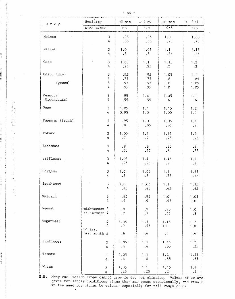
L_c_r_o __ .P ______ _

Melons

Millet

Oats

Onion (dry)

(green)

Peanuts (Groundnuts)

Peas

1 Peppers (fresh)

.Potato

Radishes

Safflower

Sorghum

Soyabeans

Spinach

Squash

Sugarbeet

Sunflower

Tomato

= 66 =

1 Humidity ! - 1

ļ RH min > 7 0 % ! __ RI __ " __ m_i.n _______ < __ 2_0_"'_~--J 1 0·5 LS-8 t 0·5 1 5·8

!----·-·----+------! ----, ----------------1 .95 1 .95 1 LO 3

4

3 4

3 4

3 4 3 4

3 4

3 4

3 4

3 4

3 4

3 4

3 4

3 4

3 4

mid-season 3 at harvest 4

no irr.

3 4

last month 4

3 4

3 4

1 .65 11: .65 . .75

1.0 1.05 1.1 .3 ! .3 .25

1.05 .25

.95

.75

.95

.95

.95

.55

1.05 0.95

.95

.8

1.05 • 7

.8

. 75

1.05 .25

1 .o .5

1.0 .45

.95

.9

• 9 • 7

1 .05 .9

.6

1.05 .4

1.05 .6

1

1. 1 .25

.95

.75

.95

.95

1 .o .55

1 . 1 1.0

1.0 .85

1 • 1 .7

.8

.75

1. 1 .25

1 .05 .5

1.05 .45

.95

.9

.9

.7

1. 1 .95

.6

1. 1 .4

1. 1 .6

1 . 15 .2

1.05 .8

1.0 1.0

1.05 .6

1. 15 1.05

1 .05 .85

1. 15 .75

.85

.8

1. 15 .2

1. 1 .55

1. 1 .45

1.0 .95

.95

.75

1. 15 1.0

.6

1 . 15 .35

1.2 .65

1.05 .75

1. 15 ,25

1.2 • 2

1. 1 .85

1.05 1.05

1. 1 .6

1.2 1 • 1

1. 1 .9

1 • 2 .75

.9

.85

1.2 .2

1 • 15 .55

1. 15 .45

1.05 1.0

1 .o .8

1.2 1.0

.6

1.2 .35

1. 25 .65

IWheat 3 1.05 1.1 1.15 1.2 4 .25 ,25 .2 .2

N.B. Many cool season crops cannot grow in dry hot climates, Values of kc are given for latter conditions since they may occur occasionally, and result in the need for higher k.c valuesJ especially for tall rough crops.

·~'.·"_·-_---_-._··· <.i;1.,;;

--

'

1

Table 23

Beans (green)

Beans (dry) Pulses

Beets (table)

Carrots

Cas torbeans

Corn (maize) \sweet)

Corn (maize) Tgrains)

.~ 6 7 ,.~

LENGTH OF GROWING SEASON AND CROP DEVELOPMENT STAGES OF SELECTED FIELD CROPS; SOME INDICATIONS

Perennial, replanted ~y_e,_rs; 4=7 years; example Coastal Califomia with planting in April, ·40/40/250/30 and (360) 1 /; subsequent crops with crop growth cutback to groundlevel iÜ late spring each year at end of harvest or 20/40/220/30 and (310).

Also wheat and oats; varies strongly with variety; wheat Centra.l India November planting 15/25/50/30 and (120); semi-arid, 35°-45° latitudes early spring sowing aud South Korea November planting 20/25/60/30 and (135); wheat in East African highlands at 2 500 m altitude sown in July and South Korea 15/30/65/40 and (150),

1

February and March planting California desert and Mediterranean 20/30/30/10 and (90); August-September planting California desert,1 Egypt, Coastal Lebanon 15/25/25/10 and (75).

Continental climates late spring planting 20/30/40/20 and (110); June planting Central California and West Pakistan 15/25/35/20 and (95); longer season varieties 15/25/50/20 and (110).

Spring planting Mediterranean 15/25/20/10 and (70); early spring planting Mediterranean climates and pre-cool season in desert climates 25/30/25/10 and (90).

Warm season of semi-arid to arid climates 20/30/30/20 and (100) 1

for cool season up to 20/30/80/20 and (160); early spring planting Mediterranean 25/35/40/20 and (120) up to 30/40/60/20 and (150) for late winter planting.

Semi-arid and arid climates, spring planting 25/40/65/50 and (180).

_Pre-cool season planting semi-arid 25/40/95/20 and (180), cool season 30/55/105/20 and (210); humid mediterranean mid-season 30/40/45/15 and (125).

Philippines, early March planting (late dry season) 20/20/30/10 and (70); late-spring planting Mediterranean 20/25/25/10 and (80); late cool season planting desert cHmates 20/30/30/10 and (90); early cool season planting desert cli.mates 20/30/50/10 and ( 110).

Spring planting East African highlands 30/50/60/40 and (180); late cool season planting~ wann desert climates 25/40/45/30 ! and (140); June planting sub-humid Nigeria~ early October 1

India 20/35/40/30 and (125); early April planting Sevilla Spain_J 30/40/50/30 and (150).

1 / 40/40/250/30 and (360) St.ands for respectively initial~ crop development, mid-season and late season crop develcpment stages in days and (360) for total growing period from planting to harvest in days.

•

Cotton

Crucifers

Cucumber

Fla.x

Grain

Lentil

Lettuce

Melons

Millet

Oats

Onion (dry)

Peanuts \groundnuts)

Peas

Marc.h. planting Egypt, April ... May planting Pakistan, September planting South Arabia 30/50/60/55 and (195); spring planting, machi.ne harvested Texas 30/50/55/1,5 and (180).

Wj_de ra:i1ge in. length of season due to varietal differences; spr:L:1g planting Hediterranean and continental climates 2G/3C/2.0/10 and (80); late winter planting Mediterranean 25/35/25(10 and (95); autumn pla:nting Coastal Mediterranean 30/3.5/90/40 and (19.5),

..Iune p1anting Egypt) August„October California desert 20/30/f;0/15 and (105); spring planti.ng semi„arid and cool sen.san arid climat.es, low desertj 25/35/50/20 and (130).

\·,īann winte.r desert climates 30/40/L-.0/20 and (130); late sp:ring=early sumrner plant:i.ng Mediterranean 30/45/40/25 and (140),

Spring planting cold winter climates 25/35/50/40 and (150); pr::=~cool season planting Arizona low desert 30/40/100/50 and (220),

Spring planting Hediterranean 20/30/60/40 and (150); OctoberNovember planting warm winter climates; Pakistan and low deserts 25/35/65/40 and (165).

Spring planting in cold winter climates 20/30/60/40 and (150); pre-cool season planting wann winter climates 25/35/70/40 and (170),

Spring planting Hediterranean climates 20/30/15/10 and (75) and late winter planting 30/40/25/10 and (105); early cool season low desert climates from 25/35/30/10 and (100); late cool season planting, low deserts 35/50/45/10 and (140).

Late spring planting Hediterranean climates 25/35/40/20 and (110); mid-winter planting low desert climates 30/45/65/20 and ( 160) .

June planting Pakistan 15/25/40/25 and (105); central plains U,S.A, spring planting 20/30/55/35 and (140).

See Barley,

Spring planting Hediterranean climates 15/25/70/40 and (150); pre~warm winter planting semi""arid and arid desert climates 20/35/110/45 and (210).

Green - Re.sp, 25/30/10/5 and (ĪO) and 20/45/20/10 and (95).

Dry season planting West Africa 25/35/45/25 and (130); late spring planting Coastal plains of Lebanon and Israel 35/45/35/25 and (140).

Cool ma·.ritime climates early summer planting 15/25/35/15 and (90); Me.diterranean early spring aud warm winter desert climat-cs planting 20/25/35/15 and (95); late winter Mediterranean planting 25/30/30/15 and (100)~

l

.

l

Potato (Īrish)

Radishes

Safflower

Squash (wiuter) pumpkin

Squash (zucchiui) crookneck

Sunflower

Tomato

Wheat !---

Fresh - Mediterranean early spring and continental early summer planting 30/35/40/20 and (125); cool coastal continental climates mid-spring planting 2.5/35/~-0/20 and (120); pre-warmwinter planting desert climat:2.s .30/40/)H)/30 aud (210).

Full planting warrn winter desert climates 25/30/30/20 anč (105); late winter planting arid and semi=arid r.::.limates and late spring-early summer planting continental climate 25/30/45/30 and (130); early-mid spring plan-ring central Europe 30/35/.50/30 and (145); slow emergence may inc·.rease length of initial period by 15 days during cold spring.

Mediterranean early spring and contin.ental summer pl2.ntj_ng 5/10/15/5 and (35); coastal Hediterranean late winter and warm wiuter desert climates planting 10/10/15/5 aud (40).

Central Cali:fornia early·mid spring planting 20/35/45/25 aud (125) aud late wiuter planting 25/35/55/30 and ("145); warrn wiuter desert climates 35/55/60/40 and (190).

Warm seasou desert climates 20/30/40/30 and (120); mid-June planting Pakistan, May in niid-West U~S.A. and Mediterranean 20/35/40/30 aud (125); early spring plautiug warm ari.d climates 20/35/45/30 and (130).

May plautiug Ceutral U.S.A. 20/35/60/25 an<l (140); May-.June plautiug California desert 20/30/60/25 and (135); Philippines

1 late December plauting, early dry season - dry: 15/15/40/15 1

aud (85) vegetables: 15/15/30/- and (60). 1

Spriug plautiug Mediterraueau, 20/20/15/5 and (60), Sept-Oct. and late winter planting Mediterranean 20/20/25/5 aud (70); warm winter desert climates 20/30/40/10 and (100) .

Late winter planting Mediterranean and warm winter desert climates 20/30/30/15 and (95); August plautiug California desert 20/35/30/25 and (110); early June planting maritime Europe 25/35/35/25 aud (120).

Spring plautiug Mediterraueau 25/35/25/15 and (100+); early summer Mediterranean and maritime Europe. 20/30/25/15 and (9o+);winter planting warm desert 25/35/25/15 and (110).

1

Coastal Lebauou, mid·uovember plautiug 45/75/80/30 aud (230), early summer plautiug 25/35/50/50 and (160); early spring plautiug Uruguay 30/45/60/45 and (180); late wiuter plauting

1

warm winter desert 35/60/70/40 aud (205).

Spriug plantiug Mediterranean 25/35/45/25 and (130); early summer planting California desert 20/35/45/25 aud (125).

Warm wiuter desert climates 30/40/40/25 and (135) and late autumu 35/45/70/30 and (150); spring plauting Mediterraueau climates 30/40/45/30 and (145).

See Barley.

-

- 70 -

b) Rice

For submerged rice kc values are given in Table 24 for different geographical locations

and for different seasons includ~ng wind conditions •. Relative humidity during dry season may

be important; where minimum relative humidity is more than 70 foduring the dry season, kc values

given for the wet season should be used.

No difference is assumed in kc values between broadcast or sown and transplanted rice

since percentage cover during first month after transplantation is little different from that of

broadcast rice.

As the plant cover spreads with time, the average reflectivity of the surface increases

from low values for free water surface (5 "/o) to high values for vegetative surface (25 % ) , For humid areas with light to moderate wind this may tend to produce slightly lower kc values

in the succeeding months. For dry conditions with light to moderate wind this trend is reversed

due to the increased influence of the roughness of the surface. This is even more marked under

very strong winds. Therefore, little difference in kc value between the first aud second months

can be noted.

There are differences in growing season according to variety, therefore the length of

mid·season growth period will need adjustment; local inforrnation on length of growing season will

need to be collected.

For upland rice, the same coefficients given for submerged rice will apply since recommended

practices involve the maintaining of top soil layers very close to saturation. Only during initial

crop stage will kc need to be reduced by 15 to 20 % .

It should be added that efforts to predict accurately the kc and ET(crop) values needed

to determine irrigation water requirements,are wasted when water loss through deep percolation

is not determined with equal accuracy.

•

-

. "'·'{,,,: ·~··· .. ·.· ........ ·.··'

,d

,1

i - 71 -

Table 24 kc VALUES FOR_RICE

~·

ŗ 1

1 1

:Planting Harvest First Second period period month month

Humid Asia ----Wet season (monsoon) June·July Nov"'Dec

light to moderate wind 1. 1 1 , 1 strong wind 1 , 15 1. 15

Dry season 1/ Dec-Jan rnid·May light to moderate wind 1 • 1 1. 1 strong wind

1

1. 15 1. 15

Humid Australia

Wet season Dec"'Jan Apr•May light to moderate wind 1. 1 1. 1 strong wind

1 1. 15 1. 15

Humid S. America ---------Wet season Nov"'Dec Apr·May

light to moderate wind 1. 1 1. 1 strong wind 1. 15 1 • 15

Europe ( Spain~ southern 1

France and northern Italy)

Dry season May·June Sept to

' early Oct

light to moderate wind· 1 , 1 1. 1 strong wind 1 , 15 1. 15

U.S.Ae ---Wet summer (southern

states) May Sept·Oct light to moderate ·wind 1. 1 1. 1 strong win"d 1 1 , 15 1. 15

' ' Dry summer (Calif.) 1 late Apr late Sept

to to early May early Oct

light to rnoderate wind 1

1. 1 1. 1 strong wind

1 1

1 , 15 1, 15

' 1

')__/ Only when Rhmin > 701, 9 kc values for wet season are to be used

T ' 1

1

1 Mid• Last

i season 3·4 weeks

1 1

1

1 1 . 0 5 .95 1. 1 1 • 0 1

1.25 1.0 !_/ 1, 35 1.05

1

1.05 . 95 1 • 1 1.0

1, 05 . 95 1. 1 1. 0

1.2 .95 1.3 1.0

L1 ,95 1. 15 1.00

1 , 25 1.0 1.35 1.05

•

•

- 72 -

c)

Crop coefficients kc for sugarcane may vary considerably depending on climate and canE! variety particularly for initial and crop/development stages. Also early crop development varies according to whether it is virgin or a ratoon crop. Total length of growing season varies with clirnate aud ac.cording to whether the crop is virgin or ratoona Total growing season for virgin plantings may range from 13 to 14 months in hot Iran, to 16 months in Mauritius and up to 20 to 24 months in some cases in Hawaii. Ratoon crop season varies from as short as 9 months in Iran to 12 months in Mauritius and up to 14 months in other areas,

T,"') determine kc values use of local dat.a or information or normal rate of development under similar climatic conditions is.essential. Also, attention must be given to cane Variety, Data provided refer to a ratoon crop for the 12-mont:r. crop and to a virgin cane for the 24 month peri.od 0 Irrigation application usually ceases 4 to 6 weeks before harvest.

Table ? 5 kc VALUES FOR SUGARCANE

light to r--~~::g . light to=+-~;::ng -moderat~ . d moderate i d . win . w n wind w1nd ----

1 0-1 ļ 0·2.5 [ planting to 0.25 .55 .6 .4 .45

1

1 1 I fuU canopy 1-2 1 2.5-J.5 1 0.25-0.5 full

1

i ! canopy 0 ? s 1 3 - , 5 10 5 0 -- f 11 L- •• " 1 ,)-q, ·1 • • ,/:, U.

I canopy

2,5~4 1 4.5 ... 6 1o.75 to full

1

j I canopy 1

1,·10 1 6·17 lpeak use 1.05 1.15

l:~-11 117·22 !earlysenescencel .8 ,85

[_1 z __ ..Ļl _22_-_24 1

ripening _____ L_ . 6 _J ____ ~_l

.8 .75 .8

• 95 1. 0

1 • 1 1. 2

1. 25 1. 3

.95 1. 05

• 7 ,75

• 85

• 9 .95

1.0 1. 1

"

" ,-a

~ ·· f . - 73 -i

'

,.

d) Alfalfa~ clover, grass-leguffies,pastures

Alfalfa =---The kc values vary similarly to those for field crops except ti.1at the initial stage to

harvest is repeated 2 to 8 times a year. Fig~ 9 shows expected variation of kc values for

alfalfa for the total growing season under, dry, an·d light to moderate wind condi tions. To

obtain mean ET (alfalfa) for design purposes, kc(mean\ shown as the smoothed curve in Fig. 9,

would generally suffice. This value should be selected rather than the higher kc values of

the 3 to 4 week period before cutting. Only for irrigation depth and frequency determinations

will the variation of kc over the irrigation interval need to be considered, that is from

kc (low) to kc(peak). During full cover until the middle of full bloomjalfalfa grown for seed

production will have a kc value equal to kc(peak) just before cutting. Values of kc are

given in Table 26,

Grasses '

Grasses grown for hay reach kc(peak) values within 6 to 8 days after cutting. The kc(low)

values are 10 to 20 % higher than the kc(low) values shown for alfalfa since considerable

vegetation is left on the ground after cutting~

Clover and grass~legume mixture ~

Due to some cover left after cutting, kc(low) for clover and grass"'legume mixture will be

close to that of grass, while kc (peak) will be closer to alfalfa.

PastuE.! (5rass, grass-legumes and alfalfa)

Depending on pasturing practices kc values for pastures will show a wide varlation. Tt:.e

values presented -assume excellent plant population density ~ high fe.rtility aud good irrigation.

For pastures kc(low) may need to be taken close to kc(low) alfalfa unde~ pcor pasturing

practices when all ground cover is destroyed.

:, 1 ;! j,J ;.)

i . : ·1·.:. •j'"'l' . .., 1 :ŗ- - cc- "" ,pfHl'!IDL"' h~ ( n,,, m#i'' •"'

:<i+-fur l,Jrn~fl : : ' ;_:_ . ~ :_;':

1-:t; ,!!: " : :~:.L:: .. •·I'

i i

1 ' ,.

t,' .t_J

fi)füillj' ,1ffiHTilll,

1;;

Hr:

1·,1j1

,illtl

F

n·:

~

" ,. Ifill..W ill wUill l ! --,- .,., ., ...

1~-1:

- ·:: .iJJ.~ e+~; .,Wi:_-1< .. ··I.L ·····-1,a;īn'.:

lcra! !l; jļ 1H , 1µ,I, •. -F---1-,-:-rr: ... i i; F:1 F

'H -r:± {_: iij r!-f1 j i.:J.

r1 : · · 'tt[JtftlŗĻ.'1-īļ:"~.~r ···r· ··r' ·11'' illllīJün

fi;:f!"'.-J-lfi11n:::~11:

l"'l'<:'l!1''l '' ·1 ~· ~lli+')l·'t

1wf j l" jl .. ,_'.' t U HJt#mITf i+ 1rli ;jjiU j,,j : l ' i •· J::1 r, .-r·,11:ŗ

fr:)

::1E

1:-

i ,i,i

H, 1ilii un

W-! -:-1"7:

i, 11

•1F ""TI

·'!·!:

l

,ij ,,,111!1a,i. w

·:;1 : i lf {; W1m1 dn tm :·!lL: .... ' ··i-

t:!'.:J1•- :l ;r i:

!:'!:: 1

1

~' 1

r ,.

--

r..:-· .,,, .,l~I, IJ .. ,!ll ., 1 •. ,_+: '"c'. :b"liiiil"rrn . olfolfc L_,i,a·""""··" kc volues for

Fig. 9

1 -s+i±!Ei+t!Sli'+ 1trit ;1:: l~j~~l1f '.B_llil-~[.1 ~ i~t-ill,1-• :1 _-~sJ1tt~ :~ŗ=~~d:t= :.

grown in dry climote with liglh to moderbte irrigation per growth period, o week befon!

wind with cuttings every culling, is assumed. 4 weeks. One heovy

"" .ŗ::..

1-'"-·

i, i il 11-1 ml „i ,id 1, 11 ,,l ,.j,j ,,,ia,I,,.,, "'

--------- '"" ____ _

Table 26 CROP COEFFICIENT kc(mean) FOR ALF ALFA, GRASS FOR HAY, CLOVER AND GRASS•LEGUME MIXTURE AND PASTURE, AND kc(peak) JUST BEFORE HARVESTING AND kc(low) JUST FOLLOWING HARVESTING

r~~:-~~::~~-= L kc(me:~--- -- - kc(peak) ==i------~~(~=~?ī~~:~~~~~~~-: _____ JI-

Humid, light Dry 9 light Dry, strong Humid~ light DJiy; light Dry, _stronģHumid,light Dry»l1ght Dry~st1-(1ng to mod,wind to mod,wind winds to mod,wind to mod,wind w,.nd~,wind to mod,wl.nd winds 1

--- ---------+-------------------------- . 1. 25 1 . 3 -----------·--·. 4---------------- • 3-- -1

- 1

AI:talf:a

1

• 85 .95 1. 05

1

1.05 1. 15

Grass for hay 1 .s .9 1,0

Clover ~ grass= legume mixture 1.0 1.05 1. 1

Pasture ,95 1.0 1.05

·--~--·----,----··---"-,-...~---"~--.. =----··--

1 1.05 1 , 1

1 1.05 1 , 15

_L 1.05 1. 1

- -----

1 • 15 .6

1, 2 .55

5,• 0

.55

.5 !

,55

1.15 1 .55 .5 .5 1

___ ___,__ ___________________________________ I

1/ Under dry soil surface conditions; under wet conditions increase values by 25 d/o or more.

-~,. -----,

•,.j

U1

· 76 ·

e) Deciduous fruits and nuts

Va.lues of kc for deciduous fruit and nut crops for clean cultivated and for cover„ crop

condition.s are pre.sented in T.č.i.ble 27. Coefficients given relate to full-grown trees with

spacings that provide about 70 % ground cover~ Examples are given for higher latitudes (e.g,

aorther-a Europe, no:rthern U" S .A .. ) with cold winters and growing seasons extending from around

1 }fay (blossom) to 1 Novembe.r (kil.ling frosts) and others involve lower latitude and warm

winter c.onditions (e,g~ Me.diterranean)~ In the former case and at altitudes of >1 200 min

lower L1ti tude areas, trees haYe leaves for some 5 1 /2 to 6 months, with the time of harvest

varying from rnid ... July for cberries to mid„October for late varieties of apples~ For lower

latitude.s near sea level, b.losso;r, occ.:urs a month or more earlier with a wide range of harvest

dates~ starting and ending several weeks earlier for respective species and varieties than at

the higher latitude, However, trees generally have leaves longer ~ e. g. well into November.

Months mentioned refer to northe~n hemisphere; for southern hemisphere add 6 months.

Also indicate.d in Table 27 is a variation of crop coefficients with climatic variables

in particular ~- humidity aud wind.

~-

Jd J,.1,lli i ,i.i i, LI iJ '" lld,s "'

_,, _____ ,,, ··-----·

T:ib.le 27 kc VALUES FOR FULL GROWN DECIDUOUS TREES AND NUT 'ļ'ļl_];_E__s_

Wi th ground cover crop 1 / Without g~ound cover crop 2/ - (clean c.ultivated> weed free) 1!,,.r Apr May June July Aug Sept Oct Nov Mar Apr May June July Aug Sept O~t Nov

COLD WINTKR WITH KILLING FROST : GROUND COVER STARTING IN APRIL

Apples, cherries

humid, light-to•mod. wind - .5 .75 1.0 1 • 1 1. 1 1. 1 .85 -humid, strong wind - .5 • 75 1.1 1.2 1. 2 1. 15 • 9 -dry, light to mod. wind - .45 .85 1.15 1.25 1.25 1.2 .95 -dry, strong wind - .45 .85 1.2 1.35 1.35 1 .25 1.0 -Peaches, apricots, pears, plum

humid, lig~t to mod. wind . • 5 .7 .9 1.0 1. 0 .95 • 75 . humid~ strong wind - .5 • 7 1.0 1.05 1.1 1.0 .8 -dry, light to mod. wind - .45 .8 1.05 1.15 1.15 1.1 .85 -dry :11 strong wind - .45 .8 1. 1 1.2 1.2 1 • 15 .9 -

COLD WINTER WITH LIGHT FROST : NO DORMANCY IN GRASS COVER CROPS

Apples, cherries, wal.Jiuts

humid, light _to mod~ wind .8 • 9 1, 0 1.1 1. 1 1 , 1 1.05 .85 .8

humid~ strong wind .8 .95 1 • 1 1.15.1.2 1, 2 1.15 .9 .8

dryp light to mod. wind • 85 1 .o 1.15 1.25 1.25 1.25 1.2 .95 .85

dry, strong wind .85 1.05 1.2 1.35 1.35 1.35 1.25 1.0 .85

Peaches, apricots 1 pears 9 plum: , almonds, pecans

humid, light to mod~ wind

humid, strong wind

dry, light to mod. wi.nd

dry ~ strong wind

.8 • 85 • 9 1,0 1.0 1.0 .95 .s .8

.8 .9 • 95 1. 0 1. 1 1.1 1, 0 .85 .8

• 85 ,95 1.05 1.15 1.15 1.15 1,1 .9 .85

.85 1.0 1 , 1 1.2 1.2 1.2 1.15 .95 .85

1/ kc values need to be increased if frequent rain occura (see Fig., 8 for adjustment).

For young orchards with tree ground cover of 20 and 50 ri/o, reduee mi.d„seaaon kc values by 10 to 151, and 5 tQ 10% respectively.

. .45 .55 .75 .85 .85 .8 .6 -- ,45 .55 • 8 .9 .9 ,85 .65 -- .4 .6 .85 1.0 1 .o .95 • 7 -- .4 ,65 • 9 1.05 1,05 1.0 .75 -

- .45 .5 .65 .75 .75 .7 .55 -- .45 .55 • 7 • 8 .s .75 .6 . - .4 .55 .75 ,9 .9 ,7 .65 -. .4 • 6 .8 .95 .95 ,9 .65 ----

.6 .7 .8 .85 , 85 .8 .8 .75 .65

.6 .75 .85 .9 .9 .85 .8 .8 .7

.5 .75 • 95 1.0 1.0 .95 .9 .85 . 7

.5 .8 1 .o 1.05 1.05 1.0 .95 .9 .75 -

.55 .7 .75 .8 .8 . 7 .7 .65 ,55

.55 .7 ,75 .3 .8 .8 .75 .7 .6

.5 .7 .85 • 9 .9 • 9 .8 .75 ,6S

.5 .75 .9 .95 ,95 , 95 • 85 .8 • 7 -··------- ·--2/ kc values assume infrequent wetting by

irrigacion or rain (every 2 to 4 weeks). In case of freque11t irr:l.gation for i1arch » April and November adjust ·using Fig. 8; for May to October 1.1se kc values of t.able ''with ground cover crop''•

For young orchards with tree ground cover of 20 and 50% reduce mid ... :?:ieason kc values by 25 to 35cfaand 10.to 1sā/0 respectively,

~ --'

~ ,,

•

f) Citrus

The kc value for citrus, large mature trees; include different tree ground cove.r

conditions with clean cultivation and no weed control programme. Since citrus is grown

primarily in dry Mediterranean-type climates, only this condition is considered. The effect

of wind stronger than moderate is negligible since citrus has good transpiration control.

For young orchards with a low percentage of tree ground cover~ kc values given for 201° and

soi tree ground cover may be assumed. For frequent rain or irrigation, kc values for clean

cultivation will approach those for no weed control programme. It should be added that certain

studies have indicated somewhat higher kc values~ up to 10·15 i for grapefr.uit and lemons

compared with those given. Months mentioned refer to northern hemisphere; for southern

hemisphere add 6 months.

Table 28 kc VALDES FOR CITRUS (GROWN IN PREDOMINANTLY DRY AREAS WITH LIGHT TO MODERATE WIND)

Jan Feb Mar Apr May June July Aug Sept Oct Nov Dec

~se aae,rr, e,~, viding > 701o tree

ground cover Clean cultivated .5 .5 .55 .55 .55 .6 .6 .6 .6 .6 .55 .55

No we.ed control prQgramme .75 ,75 .8 ,8 .8 .85 , 85 .R5 , 85 , 85 .8 .8

Trees providing ,..,,, 50 0

tree ground cover Clean cultivated • 45 .45 .5 .5 .5 .55 ,55 .55 .55 ,55 ,5 .5

No weed control prograrnme .75 • 75 .8 • 8 .8 • 85 • 85 , 85 • 85 • 85 • 8 .8

--Trees providing < 20

:, ' tree ground cover

Clean cultivated .4 .4 ,4 ,4 .4 .45 , 45 • 45 .45 .45 .4 .4

No weed contrOl progranuue , 85 , 85 .9 ,9 ,9 • 95 • 95 ,95 .95 .95 • 9 ,9

r--

•

··~.····.· ....... ·.·'

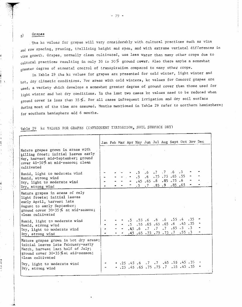
r - 79 -

g) Grapes

The kc values for grapes will vary considerably with cultural practices such as vine

and row spacing, pruning~ trellicing height and span, and with extreme varietal differences in

vine growth. Grapes ~ normally clean cultivated, use less Water than many other crops due to

cultural practices resulting in only 30 to 50 % ground cover. Also there maybe a somewhat

greater degree of stomatal control of transpiration compared to many other crops.

In Table 29 the kc values for grapes are presented for cold winter, light winter and

hot, dry climatic conditions. For areas with cold winters, kc values for Concord grapes are

used, a variety which develops a somewhat greater degree of ground cover than those used for

light winter and hot dry conditions. In the last two cases kc values need to be reduced when

ground cover is less than 35 % • For all cases infrequent irrigation and dry soil surface

during most of the time are assumed. Months mentioned in Table 29 refer to northern hemisphere;

for southern hemisphere add 6 months.

Table 29 kc VALDES FOR GRAPES (INFREQUENT IRRIGATION.,. ,SOIL_ SURFACE DRY)

Jau Feb Mar Apr May Jun Jul Aug Sept Oct Nov Dec

Mature grapes grown in areas wi th ķilling frost; initial leaves early

May, harvest mid~September; ground cover 40„50% at mid ... season; clean cultivated

Humid~ ligbt to moderate wind - . - - .5 ,6 • 7 . 7 .6 .5 . -Humid, strong wind . - . - .5 .6 .75 • 7 5 .65 .55 - -Dry, light to moderate wind - - - - • 45 ,65 ,8 .85 .75 .6 - -Dry, strong wind - - - - ,5 • 7 .85 .9 .85 .65 . .

.

Mature grapes in areas of only light frosts; initial leaves early April, harvest late August to early September; ground cover 30-35 % at mid"'season; clean cultivated

HumidD light to moderate wind - - - .5 .55 .6 .6 .6 .55 .4 ,35 -Humid, strong wind - - . ,5 .55 .65 .65 .65 .6 • 45 .35 -Dry, light to moderate wind . - - ,45 ,

,O .7 . 7 • 7 . 65 .5 • 3 -Dry ~ strong wind - . - ,45 .65 .75 , 75 .75 • 7 .55 ,3 -Mature grapes grown in hot dry areas; 1 initial leaves late February""early Marchj harvest last half of July;

ground cover 30-35 % at mid-season; clean cultivated

Dry, light to moderate wind - - ,25 .45 ,6 • 7 • 7 .65 .55 • 45 ,35 . Dry ~ strong wind - . .25 .45 .65 , 75 .75 .7 .55 • 45 ,35 -

•

-

.. 30 -

h) Bananas

Values of kc fo:r bananas are given in Table 30 for different climates, for both first

y~.ar with p1.anting in mid-March anC. for se-con<l y,:'!ar with remc,val of original plants in early

}'ebruary. For the e2r.ly sta.ges c,f development, espec-Lally in thE' first year, kc values refle.ct

a considerable lack of grocnU cover anJ a climate where rainfall is presumed to occur at

5-7 day intervals, For less frequent rain, lūwer kc values should be used; in humid tropical

zones with more frequent raint coefficients close to 1.0 would be likely even during the crop

developrnent stage. Fig 8 can l::e used for estimating kc during the first 2 months after planting,

taking into account rainfall frequency and level of ETo.

The drap in kc in Febrm:i..ry reflects the removal of origi.nal large plants at that time,

Local practices should be taken into account in timing the drop of kc, with subsequent recovery

to ldgh levels 4-5 months later~ or as ground cover again approaches 70-80%. Recovery time may

be cc,nsi.de-rably shorter than 4 ... 5 rocnths in warm or hot humid climates. Figures given in Table

30 reflect the effect of the climate on the eastern coast of the Mediterranean Sea. Months

me:ntioned in Table 30 refer to the northern hemisphere; for the southern hemisphere add 6 months,

Table 30

First-year crop, based on March planting with c.rop height 3.5 m by August:

Humid, li3ht to mod. wind

Humid, strong wind

Dry, li gh t to mod. wind

Dry, strong wind

Second season with removal of original plants in Feb. and 8010 ground cover by

August:

Humid, ligh t to mod. ivind

Huroid~ strong wind

kc VALUES FOR EANANAS

-----------------------------·-------·---~

Jau Feb Mar Apr May June July Aug Sept Oct Nov Dec --·-- ··----------------------·---------

.65 ,6 .55 .6

.65 .6 .55 .6

.6

,7 .85 .95 1.0 1.0 1.0

.75 .9 1.0 1,05 1.05 1.05

,75 .95 1,1 1.15 1.1 1.1 .5

.5

• 45 . 5

.45 .5 • 65 , 8 1. 0 1. 15 1. 2 1. 15 1. 15

---~--~---------------------------~---

1.0 .8 .75 .7 .7 .75 .9 1,051.05 1.05 1.0 1.0

1.05 .8 .75 .7 .7 .8 ,95 1.1 1.1 1.1 1.05 1.05

ļ Dry, light to mod, wind 1.1 , 7 , 75 . 7 , 75 .85 1,05 1.2 1.2 1.2 1.15 1.15

Lry, str~:~-~~:~ ________ _L 1.15 -~:-~~~-~~~~~~-~~~~~~~~~~~~~-~~

!

'

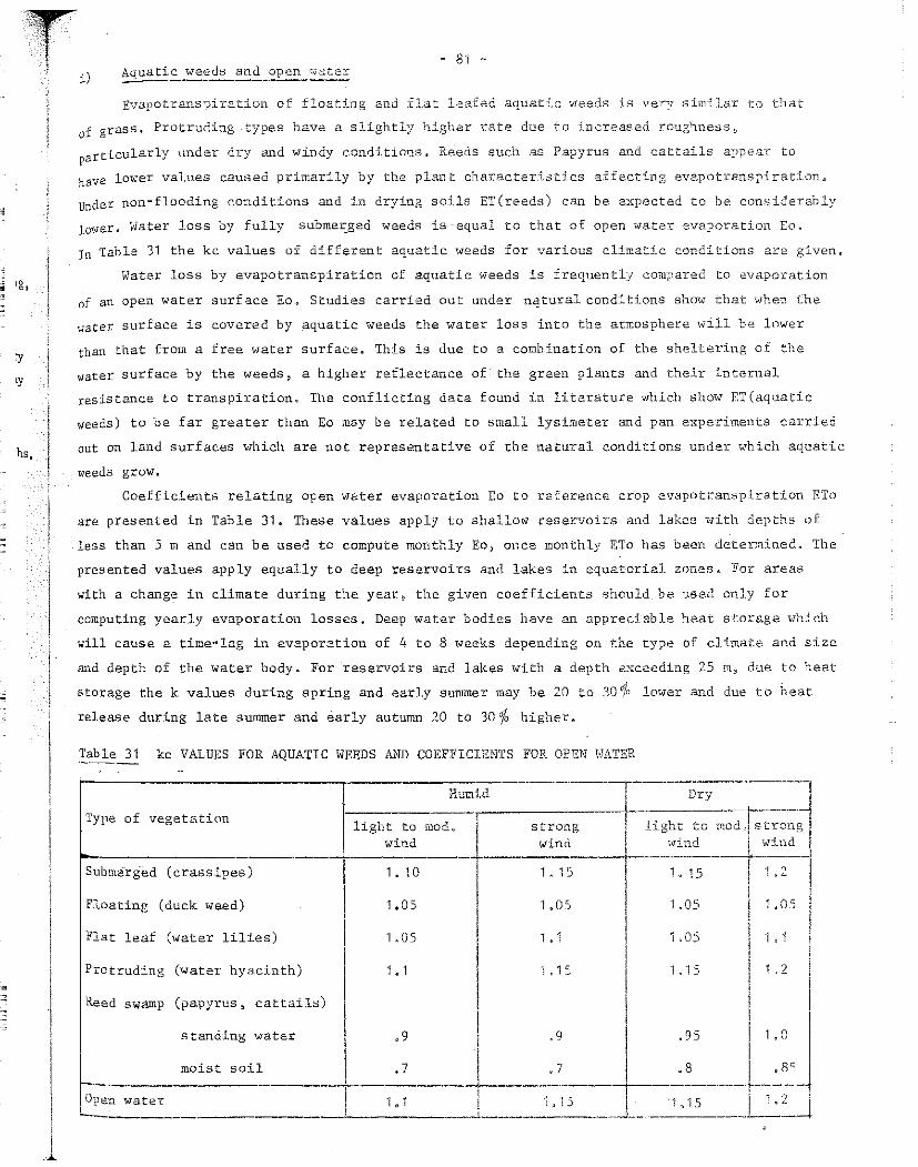
·ŗ-··, -fr.· .. ·.1.·.-r.·.·.·.· ;"' ·.

- 81 -l

,g,

1y

hs,

l

i.) Aauatic we.eds aud op,rn. ~,..·.·:1.ter - - --------------Evapotrans-piration of floating and fl.at le.afe.d aquatic weeds is very simiJ.ar to that

of grass, Protruding types have a slightly higher rate due to increased roug<-mess ~

particularly under dry and windy conditions, Reeds such as Papyrus and cattails appear to

have lower values cauRed primarily by the plan t characteristics affecting evapotranspiration.

Under non-flooding conditions and in drying soils ET(reeds) can be expected to be considerably

1ov1er. Water loss by fully submer_ged weeds is equal to that of open water evaporation Eo.

In Table 31 the kc values of different aquatic weeds for various climad.c conditicns are given.

Water loss by evapotranepiration of aquatic weeds is frequently compared to evaporation

of an open water surface Eo. Studies c.arried out under n~tural.conditions show that when the

water surface is cove.red by aquatic weeds the water loss into the atmosphere will be lnwer

than that from a free water surface. This is due to a combination of the sheltering of the

water surface by the weeds, a higher reflectance of the green plants and their internal

resistance to transpiration, The conflicting data found i.n literature which show ET(aquatic

weeds) to be far greater than Eo may be related to small lysimete.r and pan experiments carrie.cl

aut on land surfaces which are not representative of the natural condj_tions unde.r which aqnatic:

weeds grow.

Coefficients relating oŗ:en water evaporation Eo to re-ference crop evapotransp:i.ration ETo

are presented in Table 31. These values apply to shallow reservoirs and lakes with depths of

less than 5 m and can be used to cornpute monthly Eo, once monthly ETo has been determine.d. The

presented values apply equally to deep reservoirs a.nd lakes in cqu2.torial zones ~ For ar.eas

with a change in clirnate during the ye.ar ~ the given coefficients should be used only for

computing yearly evaporation losses. Deep water bodies have an appreciable heat storage whi_ch

will cause a time„lag in evaporation of 4 to 8 weeks depending on the type of climate and size

and depth of the water body ~ For ·reservoirs and lakes with a depth exceeding 25 m, due to heat

storage the k values during spring and early sunune.r may be 20 to 30 o/o lower and due to he.at

release during late summer and early autumn 20 to 301/o highe-r.'.

Table 31 kc VALDES FOR AQUATIC WEEDS AND COEFT!'īCIENTS FOR OPEN WATER

r-----------~---~---~-~------------r-· 'l Humid ! Dry i

Type of vegetation

Subme·rg"ed (crassipes)

Floatini (duck weed)

Flat leaf (water lilies)

Protruding (water hyacinth)

Reed swarnp (papyrus, cattail~)

s tanding water

moist soil

1 -l l------·---~----------1----------4------,! j strong 1

1

light te mod.! strong 1 light to mod~ ·wind wind wind j wind 1

-+---------4----...j 1 1.,15 J 1.2 1

1

1 1.05 1 LOS 1

! ! 1,05 1 1,1 1

1.15 1 L2 f

1. 10 1. 15

1.05 1 .05

L 05 1 , 1

1. 1 1 , 15

1

:: _j' :: ___ :.:s __ 11 1 :::_

~~en w._a_t_e·-r--------------·-·--1---1-,-1----- ļ_-_-_--_-,-:-1-_s==---1 __ _1_:~ ____ I _'._:_2

•

- 82 -

j) Coffee

Two species of c.offee provide the bulk of the world's supply, Coffea arabica and

Coffea robusta. The former only is irrigated on a limited scale; much of it is grown at

higher altitudes (1 000-2 000 m),

For mature coffee grown without shade and where cultural practices involve clean

cultivation with heavy cut grass mulching, crop coefficients of around 0~9 are recommended

throughout the year~ If significant weed growth is allowed~ coefficients close to 1.05„1.1

would be more appropriate.

k) Tea

No direct comparison of evapotranspiration by tea with that by grass could be found in

literature. The water requirement of tea bushes in full production can he assumed to be

close to ETo. Hence, crop coefficients kc of around .95 to 1~0 are suggested for non-shaded

plantations where more than 70% ground cover exists. Where grown under shade trees 1 kc

values of 1.5-1~10 would be more appropriate for more humid periods, and perhaps 1.10-1.15

for dry periods.

1) Non-cropped or bare soils

To determine the water balance, particularly after winter rains~ estimation of

evaporation 1osses from the soil surface E(soil) are needed~ This will assist, for instance,

in the determination of the first irrigation application on a wheat crop sown in March .. _April

following winter rains. E(soil) will be greatly affected by the water content of the soil

surface, and frequency and depth of rain, type of soil and level of evaporative demanda

To determine kc Fig. 8 should be used; the prediction of E(soil) follows closely the method

shown for field crops, initial stage. Data presented in Fig. 8 assume a medium-textured

soil. For light aud heavy-textured soils kc values may need a downward adjustment by some

30 %and upward by some 15 % respectively. Only a short period following the rain should be

considered since top soil may soon dry out and~ particularly for sandy soil, soil evapora~

tion will be severely restricted.

1

EXJ\MPLE:

Estimation of E(soil) from fallowJ essentially weed„free soil.

Given~ Cairo; ETo as given aud obtained from Method III of Chapter I.1; ficticious rainfall <lata on frequeucy.

Calculation: from ETb in mm/day and <lata on frequency of raiufall, select kc value from Fig. 8.

Nav, Dec. Jan. Feb, March --

ETo, mm/day 2.8 2. 1 2.4 3.3 4.8 Method

Frequency of raiu, days 7 7 5 7 10 Data

kc factor .6 .65 • 75 .ss .35 Fig. 8

E (soil) mm/day = kc x ETo 1. 7 L4 1.8 1. 8 1. 7 Calc.

III

•

•

- 83 -

CBAP':'ER I -, 3 CALCTJLATīON OF ET ( c~rop)

As stated in the introduction ET(crop) reflects the rate of evapotranspiration of a

disease~free crop, growing in a large field (one ar more hectares) under optimal soil

conditions including sufficient water and fertility and achieving full production potential

of that crop under the given growing erivironment~

The methods of calculating crop evapotranspiration have been detailed and include the

effect. of climate on crop water re.quirements as the mean daily value of ETo in mm for the

period considered9 The effect of crop characteristics on water requirernents is represented

by the crop coefficient kc and its values can be obtained from the information outlined in

Chapter I.2. For a given cropi planting date, growing season and length of crop development,

ET(crop) can be determined by ET(crop) = kc. ET(crop) for each 30 to 10 day period.

EXAMPLE:

Given:

Calculation:

Cairo; maize; sown in mid May total length of growing season initial stage crop development stage mid-season stage late season stage

May

ETo, mm/day 8. 1

kc 0.35

ET(crop) nnn/day 2.8

June

8.6

0.60

5.2

125 days 20 " 35 " 40 '' 30 ''

July

ī.9

1 • 12

8.8

Aug

6.6

1. 08

7. 1

.

Sept

5. 1 Method

0.75 Fig. 7

3.8 Calc.

Mean 10 daily ET(crop) can be obtained from reading kc from Fig, 7 for each 10 day period.

--īII

"

ii

·~

is'l!

'~

CRI\PT ER I • ,,~

- % •

fON SIDERl.\.TION _Q'F F ACTORS ļd?FECTING ET ( cro.:e.2_ UNDER PREVAILING LOCAL CONDITIONS

Act.uaJ. ET (crop) depends t-o a marked degree on local conditions including variation in

climate~ size of fields and nature of surrounds, advection, altitude, soil„water ava1' l b' l a i i ty,

salinity, method of i:rrigat:Lon, methods of cultivation and sorne of these factors are in turn

part::Lal1y dependent '..m the farming and irrigation practices followed. The prediction methods

described so far do not co-:.rer all possible factors prevailing under local conditions which

mny h.ave a d:1-stinct effect oü ET(crop) ~ Some additional considerations are therefore given

in order to alert and oric,mt the user of <lata when particular conditions occur. Where

possible., :Eact.ors and proce.sses are formula.ted in quantita.tive terms; others are formulated

in quaJ.it:ative terms only since the present lack of data hinders adequate quantification af

the complex phenomena involved4

I. 4, 1 CLIHATE

a) Variation with time

For a given location ET(crop) will vary from year to year and for each period within

the year.

Total annual ET(crop) on the other hand, will vary little from year to year for many

climates since it is largely dependent on the input of solar energy which, outside the

atrnosphere~ may be considered asa constant on a yearly basis$ The variation in annual

total ET(crop) may be as low as about 10% for the humid tropics, and as high as about 2So/o

for midcontinental climates, depending mostly on the degree of cloudinesse

Compared with the annual variation, monthly ET(crop) values for a given month and

location will tend to be larger, the nature of distribution being close.ly related to typical

variations in weather conditions. For mid-latitude continental climates the variability in

ne.t radiation can be extreme for a given calendar month. Normal transition months for areas

having distinct dry and wet seasons also show significant changes for the same month from

year to year; when rains arrive. ei ther exceptionally early or exceptionally late the monthly

ET(crop) values of that month may vary from one year to the next by SOrJjo or more~

Daily ET(crop) may vary drasticallyj with low ET(crop) values registered on days that

are rainy, humid~ cloudy and calm and with high values on dry, sunny, windy days.

As shown in Fig. 10~ the wide range of·daily, 10-day or mollthly ET(crop) values

clearly demonstrates that ET(crop) for a given period should be calculated for each year of

record rather than using mean climatic <lata to derive mean values for ET(crop). , Not only

are extre.mes of high and low ET(crop) <lata revealed~ but also the expected variation in it

allows a better selection of th.e level of ET(crop) for design purposes. When sufficiently

long climatic records are available a frequency distribution analysis should preferably be

made. The methodology for making such an analysis is similar to that presented for

rainfall (Chapter II.1.2).

i

• '

-

' ..

6

~5 0 ~

'

Frequency, p<!rcan'f

95

90

- 35 -

l 1 1 ~. 1 6.01-

F,~q~ency,

e 95 ____ _

~ ----------7~ E 4.5( ...____ - 90

' 54.0 -- ~~ -------~I Či, t . 2s - j "' 35 _,,,,--

E -----==.- i~

[;j 3.0 / .,,,----- ~ 12+ ----0 J F M A M J J A s 0

20t I.S'------:,4,-------;!;e,---,1"~-.>16.----,:Ž,\,b.---2c.4-n--,rl N D

Mon!h Llllnglh of period, Days

Fig. 10 - Frequency distribution of mean daily ET (ryegrass) for each month in coastal California Valley (Source: Nixon et al. 1972)

Frequency distribution of 1·30 day mean ET (irrigated ryegrass) during peak period June·July (Source: Nixon et a~G 1972)

Long ET(crop) records will be needed when analysing the magnitude and frequency of

ET(crop) extremes but these are often not available. An irrigation system should have the

eapaci ty to meet the adopted Ievels of peak ET ( crop) of the crops it is to serve. Peak

ET(crop) will vary with the length of time considered or for any given month or

Peak ET(crop) daily 1 >

Peak ET(crop) 10-daily 10 >

Peak ET(crop) monthlz 30

To allow a first estimate of maximum crop water requirements from mean monthly ET(crop)

<lata, consideration must be given to the degree to which ET(crop) may vary during that

period~ the possible duration of peak ET(crop) within that period and the length of time for

which peak ET(crop) can be met from available soil water. In Fig. 11 generalized curves are

given for two clirnatic extrernes showing the ratio of average daily peak ET(crop) to average

daily ET(crop) for the month of rnaxirnurn ET(crop) and level of soil water availability.

From Fig. 11 a first approximation can be made of average peak ET(crop) when only

mean monthly ET(crop) data are available. Especially when soils are shallow and light~ a

correction is thus made which allows full water supply to the crop during peak dernand.

EXAMPLE: for rnid-continental climate with variable cloudiness~ mean monthly ET(crop) is 6 mm/day; depth of available soil water or irrigation per applic.ation is 60 mm; peak period ET(crop) is 6 x 1.175 = 7.1 mm/day.

•

-

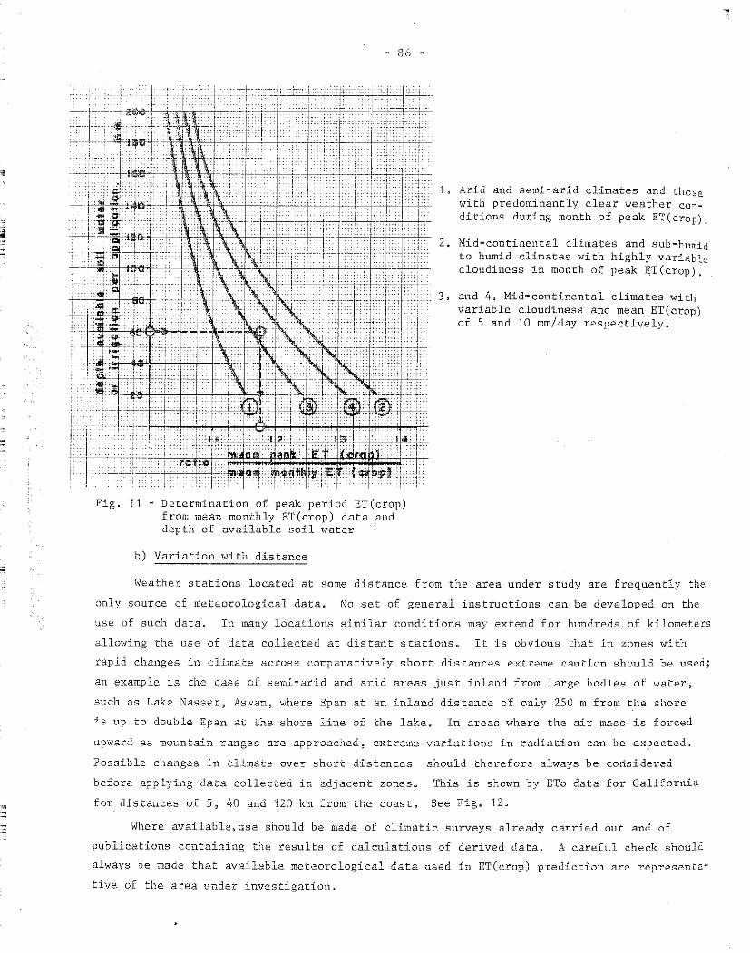
Fig. 11 - Determination of peak period ET(crop) from mean monthly ET(crop) <lata and depth of available soil water

b) Variation with distance

1~ Arid and semi•arid climates and those with predominantly clear weather con~ ditions during month of peak ET(crop),

2. Mid-continental climates and sub·humid to humid climates with highly variable cloudiness in month of peak ET(crop),

3. and 4. Mid-continental climates with variable cloudiness and mean ET(crop) of 5 and 10 rnrn/day respectively.

Weather stations located at some distance from the area under study are frequently the

only source of meteorological <lata. No set of general instructions can be developed on the

use of such <lata. In many locations similar conditions may extend for hundreds of kilometers

allowing the use of data collected at distant stations. It is obvious that in zones with

rapid changes in climate across comparatively short distances extreme caution should be used;

an example is the case of semi=arid and arid areas just inland from large bodies of water~

such as Lake Nasser, Aswan~ where Epan at an inland distance of only 250 m from the shore

is up to double Epan at the shore line of the lake. In areas where the air mass is forced

upward as mountain ranges are approached, extreme variations in radiation can be expected.

Possible changes in climate over short distances should therefore always be corisidered

before applying <lata collected in adjacent zones. This is shown by ETo <lata for California

for distances of 5~ 40 and '!20 km from the coast. See Figo 12.

Where available,use should be made of climatic surveys already carried out and of

publications containing the results of calculations of derived <lata. A careful check should

always be made that available meteorological <lata used in ET(crop) prediction are representa~

tive of the area under investigation.

• ' :::

-

s

'~ I:,,, 1

mm

,001

150 l "' :i:: 100 -,:: 0

E

0 1-

50 l.lJ

, ,,. Apr/Oct Nov/Mar tota l • ., . • ., ' 5} .. ., .. coosl 740 290 1030 • ., .

cooslol valley 880 270 1150 40 Km •, •• • centra! valley 1100 230 1330 120 from ocean

J F M A M J J A s 0 N D

Fig. 12 Change in ETo with d~stance from ocean, California (Source: State of California, (1967) Bulletin 113·2)

c) Variation with size of irrigation development: advection

Most of the raw <lata used in predicting ET(crop) are collected on sites located in

rainfed or uncultivated areas, or even on rooftops arat airports. Irrigated fields will

produce a different microclimate aud ET(crop) may not be equal to predicted values based on

meteorological <lata from sites outside of or collected prior to the development of large

irrigation projects. The different microclimate induced by irrigated agriculture will

depend mostly on the aridity of the surroundings, wind~ size of the irrigated area and

distribution and density of irrigated cropped and fallow fields.

Crops grown in arid and semi~arid climates but surrounded by large dry fallow areas

are subject to advection by which air masses greatly warmed while passing over such areas

will give up heat as they pass over the irrigated fields. Advective energy resolves into

the G~clothesline'' effect at the edge of the field and into the ŗ~oasis~' effect inside the

large irrigated field. Appreciably higher ET(crop) can be expected on the upwind edge of

the field and can be as much as double the predicted value for large fields. With increasing

distances downwind from the upwind border the air becomes cooler and more humid.

Asis shown in Fig. 13, the high ET(crop) values near the edge will fall off sharply

followed by a more gradual general decrease. The ''clothesline'' effect may become negligible

with distance from the border where the change of temperature, humidity and wind profiles is

complete and a near~equilibriurn of air temperature, and humidity is reached. This distance will

depend on initial temperature, humidity and wind speed, and may extend in dry hot climates for

100 to 400 m from the leading edge for wind speeds greater than 5 m/sec, 50 to 100 m for speeds

of 2 to 5 m/sec and 10 to 25 m for speeds of O to 2 m/sec. This aspect is of considerably less

importance in humid areas.

'

•

1.1

1.0

.,

.8

25 50 100 200 500 m

from edge of field

- 83 -

Fig, 13 Value of pan coefficient Kp under arid windy conditions at various distances from upwind edge of the field; A-pan is located in upwind dry fallow field,

It follows that caution should be applied when extrapolating measured ET(crop) <lata

from irrigation experiments carried out on small plats and located in dry surroundings to

large irrigation projects. The ''clothesline'' effect on the patchwork of different crops

and treatments within small irrigation experimental plats of 0.01 to OoS ha can be

considerable. With such small plats, especially when surrounded by several hectares of dry

surface area, measured experimental results rnay predict up to double irrigation requirements

of a future large irrigati0n development.

The ''oasis'' effect per~= will result in higher ET(crop) values for irrigated fields

surrounded by large dry fallow areas compared to irrigated fields in extensive vegetated

areas. However~ in arid and semi-arid climates, inside the irrigated fields temperatures

are generally lower and humidity higher compared to out.side the scheme. Therefore, when

ET(crop) is predicted frorn <lata collected before irrigation development, ET(crop) could be

over-predicted by 5 to 1 Sd/a for fields of 5 to 20 ha and 10 to 25'{o for large irrigation

schemes wi th a cropping densi ty close to 100%.

In Fig. 14 approximate values for the effect on ET(crop) o:f size of the irrigated area

located in dry fallow surrounds is given for arid hot conditions with moderate winds. Values

shown are coefficients for correcting ET(crop) values determined from climatic dµta from

non-i rrigated areas.

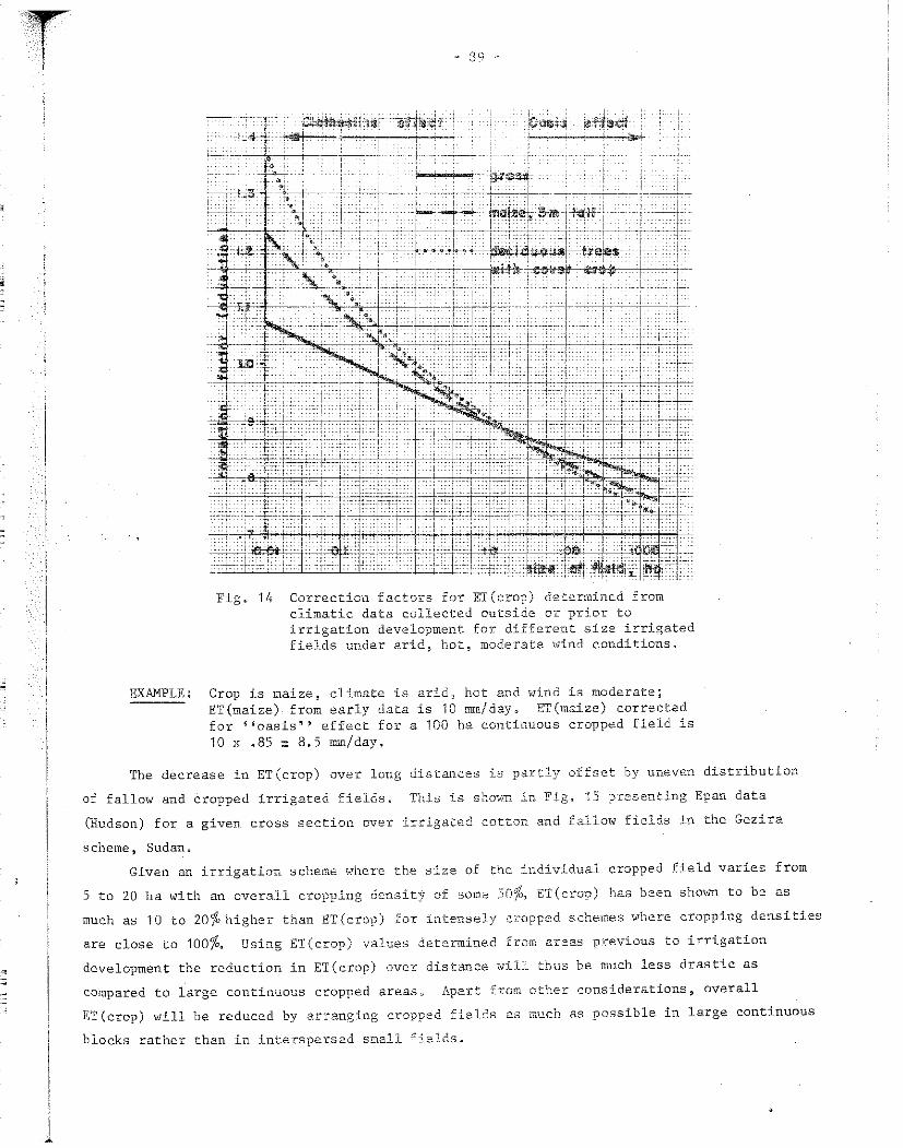
·r'f . 1

1

EXAMPLE:

· 39 -

Fig. 14 Correction factors for ET(crop) de.termined from climatic <lata collected outside or pr:i.or to irrigation development for differe.nt size irrigated fields under arid, hot, moderate wind conditions.

Crop is maize, climate is arid, hot and wind is moderate; ET (maize) from early <lata is 10 IT>J.n/ day ~ ET (maize) corrected for ~'oasis'' effect for a 100 ha continuous cropped field is 10 x .85: 8.5 rnin/day.

The decrease in ET(crop) over long distances is partly offset by uneven distribution

of fallow aud cropped irrigated fields. This is shown in Fig. 15 presenting Epan <lata

(Hudson) for a given cross section over irrigated cotton and fallow fields in the Gezira

scheme, Sudan.

Given an irrigation scheme where the size of the individual cropped field varies from

5 to 20 ha with an overa.11 cropping densitj of some. 50%, ET(crop) has been shown to be as

much as 10 to 20% higher than ET(crop) for intensely cropped sc.hemes where cropping densities

are close to 100%. Using ET(crop) values determine.d from areas previous to irrigation

development the reduction in ET(crop) over distance wil:L thus be much less drastic as

compared to large continuous cropped areas .• Apart h .. ·om other c.onsiderations, overall

ET(crop) will be reduced by arranging cropped fields as much as possible in large continuous

blocks rather than in interspe.rsed small f~c.e.lds.

•

-

'" -

20

E 10 E

C 0 a.

w

- 90 -

----GEi\lERAL WiND DIRECTiON

dry

dry dry dry follow fallow fallow

dry stubble

600 900 1200 2100 2400

DISTANCE FROM WINDWARD EDGE ( m)

Fig. 15 Cbanges in Epan (Hudson) data for cross-section over irrigated cotton and fallow fields (Source: Hudson, 1964)

dry stubble

6300

Only approximate values for the effect of advection are presented and these only for

arid, hot, moderate wind conditions. Advection is much less important under cool, humid

conditions. There is no simple way of evaluating the effect of advection on ET(crop).

d) Variation with altitude

ET(crop) changes significantly with altitude in a given climatic zone. These

differences are not caused by variations in altitude as such but mainly by changes in

temperature~ humidity and in the day'"night distribution of wind from areas near the coast

to high mountain valleys„ Also radiation at high altitudes may be rather different than in

low-lying areas. The use of the ET(crop) prediction methods presented will remain

problematic for high altitude areas with the possible exception of the Penman and Pan

method„

I. 4, 2 S01L WATER

a) Level of available soil water

ET(crop) prediction me.thods pre.se.nte.d in Chapter I.1 and I.2 take into account climatic

conditions and crop characte.ristics and assume soil water in ample supply. In the. absence of

appreciable drainage losses, after irrigation ar rain~ the soil water content will be reduced

primarily by evapotranspiration. As the soil dries aut, the rate of water transmitted

through the soil and supplied to the. roots will reduce and consequently the rate of water

uptake by the plant will be affected„ ET(crop) will fall at some stage below its predicted

level or p = ETa(crop) / ET(crop)

where p ,s;;; 1 and ETa(crop) and ET(crop) are respec.tively actual and predicted evapotranspirati011 •

T '

. on,

The. value c::" p is dependent on the le.vel of available water in the soil te -::he crop

and cn the le.vel oi the 2vaporati ve demand of the air and will vary wi th type of c.rcip and

soiL The level of available water in the soil can be described as the force or tension at

which water is held by the soil at a given soil water content; in common usage soil water

tension is expressed in atmospheres (1 atm ::::: 1 bar ::::: 100 ce.ntibars :::::::: 1000 cm of water).

For ease of reference~ soil water tension and corresponding available water content in

volume percentage are given below. Available water is defined here as the difference in

soil water content at field capacity (soil water tension of some 0.2 to 0.3 atm) and at

wilting point (16 atm)1/,

Soil water tension 0.2 0.5 2.5 16 , 0.2 0.5 2.5 16,

Heavy clay 18 15 8 0 0 17 55 100

Silty clay 19 17 10 0 0 10 45 100

Loam 20 15 7 0 0 25 65 100

Silt loam 25 19 5 0 0 25 80 100

Silty clay loam 16 12 7 0 0 25 55 100

Sandy clay 1.oam 14 11 6 0 0 20 55 100

Sandy loam 13 8 3 0 0 40 75 100

Loamy fine sand 14 11 5 0 0 20 65 100

Medium fine sand 6 3 2 0 0 50 65 100

Available soil water in Available soil water volume % depletion in volume %

For condi tions where evaporative dernand by the air is high, the point · at which soil

water supply to the roots becomes insufficient to meet predicted ET(crop) is reached at a

lower soil water tensi'on compared to conditions where evaporative demands by the air are

low. This will be even more pronounced in heavy textured soils compared to light textured

ones since water can be transmitted more rapidly and removed more easily from a light

textured soil than a heavy one. Due to differences in plant characteristics, the value of

P will vary with crop species. Also the value of p is not constant over the entire irriga

tion period; p will be e.qual to unity during days just following irrigation aud will

gradually decrease until next irrigation.

1 / The concepts of field capacity and wilting poim: assume static soil water conditions and represent an equilibrium value on soil water content; in fact, soil water through continuous redistribution in the soil profi1e under both saturated and unsaturated conditions is a dynamic process and in a physical senseno static levels can be assumed. Despite this, the mentioned concept.s are, for practical reasoris herei still considered as useful criteria for determining the soil water available •

•

= 92

Idealized curves are pr2.sented in Fig. 16 ind:i.cating the relative decrease in ET(crop)

which occurs 'in a drying soil f or both a heavy and a light textured soil at a given soil

water tension" The effect of evaporative c.onditions on the decrease in E'I'(crop) in a drying

soil is shown for ET(grass) J a.dapte.d from Rijtema~ ·196.5. For well established grass~ gro-wn

on a deep clay or loamy sand~ under low e.vaporative demand - 2 to 4 mm/day - ET(grass)

starts to decre.ase at .soil ws.te:r te.nsions of 5 and 8 atmospheres respectively or, correspond

ingly, available soil water depletion of some 70% for clay and about 99% for loamy sand~

Un.der conditions of high evaporat.ive demand = 8 to 10 mm/day - ET(grass) starts to decrease

at. a soil ·wm:er tension of 1. 5 and 3 atillospheres or at available soil water depletion levels

of 35 and 75°/o respectively.

Timing and magnitude of ET(crop) reduction are important criteria for predicting crop

yield and for reconnnending irrigation practices~ In Table 32,, adapted from Rijtema (1965),

<lata are presented on the amount of soil water available since last irrigation for a number

of soil types aud climatic conditions; soil water depletion in excess of the indicated arnount

will result in a decrease in predicted ET(crop) ~ Data in Table 32 assurne a rooting depth of

of 1 m; interpolation can be used to de.rive estimates for different rooting depths for crops

given. i".vith ET(crop) known, a first approximation can be made on the length of time after

irrigation that ET(crop) will be maintained at the predicted level. Since higher levels of

soil water are found during infiltration and water distribution in the soil profile during

and irnmediately following irrigation, one or two days can be added. Table 32 clearly

indicates that under conditions of high evaporative demand the predicted ET(crop) is main

tained for a relatively short period following irrigation. Also~ total arnount of soil

water available until ET(crop) begins to reduce varies with the type of crop and type of

soil.

EXAMPLE: Alfalfa grown in a mediurn textured soil; ET (alfalfa) is 9 mm/ day; rooting depth is 1. 50 m. Available soil water after irrigation before ET(alfalfa) will start to reduce is 1.5 x 50 = 75 mm; E'"!:.'(crop) will start to reduce (75--;-- 9) + 2 = 10 to 11 days following the last irrigation.

The rate of decrease in ET (crop) is shown in Fig. 17 for cotton grown in Egypt- on a

fine textured soil (Rijtema and Aboukhaled, in press). Different levels of ET(crop) are

assumed. When ET ( cotton) is 8 and '! 2 mm/ day, it will rernain at this level for some 12 and

8 days respect-Lvelyo For longer periods since the last irrigation, ET(cotton) is shown to

decrease more rapidly lmder high evapotranspJration conditions compared to lower ones~

The value of p will decrease with time; the mean value of p over a period exceeding 24 days

si.nce the last irrigation becomes more or less independent of the evaporative conditions~

Whether the reduction in ET (cotton) is pennissible during part or all of the grm-ring season

can only be determined if sufficient <lata on the effect of soil wate.r stress on yield during

the various stages of growth are available. This is discussed in the chapter on crop yields.

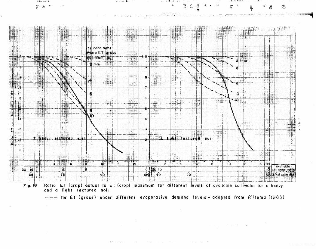
. 1 d Jel ,1)

m OQ ,_

··+·L---10-:

j! '' ' ' ··i i~i--l-fc-ļ~W~• ... ,~Jl,Wļ

. .... ·• •·•·• •• 1 '

i ,i,I 1, 11

H,

1 ,i , •. ; ILi,,

-OOC:ri"''"d cn ,-,, "

>-' ro cn

rt " p.

'

&

" " ""

--~. •.· •. --. •.·1'1,

::::: : . · :· : .. · ·.. ·:· · ·:_ .. .. · :· :·60 _::· .: · ..... : ·::: ·: _·: ·:_ ·: __ ·:· .. _.· :· ::· ' . · ._ . - .. ·i : . · ·: . ::·. · _: · .. · . :· · ... '·. '.::·i· .- - ·:·; .. - :· .· · -L- : ,. '~ll'il IH 11· tl ·1 ~l'i ,ļ li:~~i j vri .. 1 ·1 ' I'' ' ·I . '' r . -· .. , ;':Jij:i'~L ··"' ', ' , ",·,, .. c · ', .. ···· ·,· · · ··, ···· ··· · · · · ·· 1 ·Lc . ,

1LJJITtt·rrr1 tl J;I~ f'"l 1 1 r+ 1 j"·j I] t1 f ! lccf""P-:"!f i . ; 1"~

t)

Rotio ET (crop) clctuol to ET (crop) moximum for different Ievels of available soil •water far o heavy and a light teKtured

--- for ET (gross) under differenl evoporo!ive demond Ievels - odopied from Rijlema !1965)

=,,__,

'° w

,i,IJĪ iri ilil

Table 32

1 Soil texture

1 Fine Uoām - clay)

Medium (sandy loam ~

sandy clay loam)

1 Coarse (loamy sand -sand)

1

1

!..._ ___ _

j _ _,' i ;[J IL 11 „b jj „111iīJJ,dl·

DEPTH OF SOIL WATER AVAILABLE IN mm FOR DIFFERENT SOIL TEXTURES AND LEVELS OF ET(crop) AT WHICH ET (crop) IS MAINTAINED AT ITS PREDICTED MAXIMUM LEVEL; SOIL DEPTH 1 m

1 1 Predicted 1 2 3 4 5 6 7 8 9 10 11 12 13 14 15 ET(crop)

1

Cotton 200 190 170 155 140 125 110 100 95 90 80 75 70 65 60

Cereals, alfalfa clover, grass 190 165 150 135 115 100 90 80 75 70 65 60 60 55 55

Sunflower 170 145 125 110 95 80 75 65 60 55 55 50 50 45 40

Pepper, potatoes 125 95 75 60 55 45 +--------·

Cotton 130 125 1"I 0 100 90 80 70 65 60 55 50 50 45 40 40

, Cereals, alfalfa clover, grass 125 110 100 85 75 65 60 55 50 ,, 45 40 40 35 35 35

Sunflower 110 95 85 70 60 55 50 40 40 35 35 30 30 30 25

Pepperj potatoes 80 60 50 40 35 30

Cotton 60 55 50 45 40 35 30 30 25 25 25 20 20 20 20

Cereals, alfalfa c.lover, grass 55 50 45 40 35 30 25 25 20 20 20 15 15 15 15

Sunflower 50 1,5 35 30 25 25 20 20 15 15 15 15 15 10 10

Pepper, potatoes 35 25 20 15 15 10

16

60

50

35

30

15

15

,.

1 7 -------1 18 19 20 1

5 5 =-50-::1 5 0 45 45

1

--·--·-

C - 5 30 30 30

C - 0 30 25

--··--------·-··-- "i

5 15 15 1s l 5 15 rn

\.'.)

·"

.. J

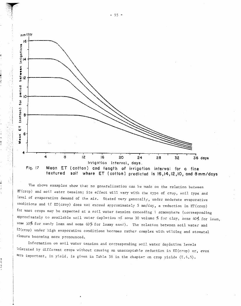
;j

~ 1 - 95 -l

rnrn/dcy

16 -C 0 .:. 0

"' ·: 14 " C • • ' .Īl2 ,,

" 0 ·~ G

" 10 " 0 ~

C 0 ~ 8 ~

0 u -t-w C 6 0 G ::t

4

,111. 11

4

Meo11 ET !exlured

12 16 20 24 28 32 36 doys lrrig"!ion in!erool, dayi.

( co!lon) cmd lenglh of irrigotion il'lter11ol for o fine soil where ET (cotton) predicted i:. 16,14,12,10, and 8mm/doys

The above examples show that no generalization can be made on the relation between ET(crop) and soil water tension; its effect will vary with the type of crop, soil type and level of evaporative demand of the air ~ Stated very generally" under moderate evaporative conditions and if ET (crop) does not exceed approximately 5 mm/day ~ a reduction in ET (crop) for most crops may be expected at a soil water tension exceeding 1 atmosphere (corresponding approximately to available soil water depletion of some 30 volume %, for clay, some 4D1o for .loam, some Süc% for sandy loam and some 6D·1o for loamy sand). The relation between soil water and ET(crop) under high evaporative conditions becomes rather complex with wilting and stomatal closure becoming more pronounced.

Information on soil water tension and corresponding soil water depletion levels tolerated by different crops without causing an unacceptable reduction in ET(crop) or, even more important ~ i.n yield, is given in Table 36 in the chapter on c.rop yields (I. 4. 5).

'

•

"' " "

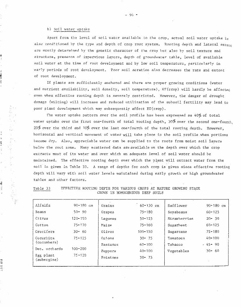
- 96 -

b) Soil water uptake

Apart from the level of soil water available to the crop, ac.tual soil water uptake is

also conditioned by the type and depth of crop root system. Rooting depth and lateral extent

are mostly determined by the genetic character of the crop but also by soil texture and

structure, presence of impervious layers, depth of groundwater table, level of available

soil wate.r at the time of root development and by low soil temperature, particularly in

early periods of root development. Poor soil aeration also decreases the rate and extent

of root developrnent.

If plants are sufficiently anchored and there are proper growing conditions (water

and nutrient availability, soil density, soil temperature)jl ET(crop) will hardly be affected

even when effective rooting depth is severely restricted. However, the danger of drought

damage (wilting) will increase and reduced utilization of the subsoil fertility rnay lead to

poor plant development which may subsequently affect ET(crop).

The water uptake pattem .over the soil profile has been expressed as 40% of total

water uptake over the first one-fourth of total rooting depthjl 30% over the second one-fourth)

20% over the third and 10% over the last one. 00 fourth of the total rooting depth. However,

horizontal and vertical rnovement of water will take place in the soil profile when portions

become dry. Also, appreciable water can be supplied to the roots from moist soil layers

below the root zone. Many scattered <lata are available on the depth over which the crop

extracts most of its water and over which an adequate level of soil water should be

maintained. The effective rooting depth over which the p~ant will extract water from the

soil is given in Table 33. A range of depths for each crop is given since effective rooting

clepth will vary with soil water levels maintained during early growth or high groundwater

tables and other factors.

Table 33 EFFECTIVE ROOTING DEPTH FOR VARIOUS CROPS AT MATURE GROWING STA,GE GROWN IN HOMOGENEOUS DEEP SOILS

r--

cm l 1

Alf alfa 90-180 cm Grains 60-150 cm Safflower 90-180

1

Beans 50- 90 Grapes 75 .. '/80 Soyabeans 60-125

1

Citrus 120-150 Legumes 50-125 Strawberries 20· 30

Cotton 75-170 Maize 75-160 Sugarbeet 60-125

Crucifers 30· 60 Olives 100-150 Sugarcane 75-180

Cu.curbits 75-125 ünions 30· 75 Tomatoes 40-100 (cucumbers)

Pastures 60-100 Tobacco 45· 90 Dece orchards 100-200

Peppers 40-100 Vegetables 30- 60 Egg plant 75-120

Potatoes 30- 75 (aubergine)

,,~ '.,·;···.·.· .·· ">·'

!

t

h,

.. 97 =

c) Groundwater tab les

Soils which are too wet can be just as harmful to plant growth as soils which have

little water in the root zone. When groundwater tables are high and soils saturated, the

growth and consequent ET(crop) of mast crops will be reduced. Wet soils in cooler climates

are slow to warm in spring thus causing delays to seed germination and plant development.

Alsog land preparation and use of farm machinery may have to be restricted resulting in

later planting aud consequently different ET(crop) rates during the remainder of the

season.

The relative tolerance of some crops to oxygen deficits in the root zone, to high

groundwater levels and to waterlogging is summarized in Table 34.

Table 34 TOLERANCE LEVELS OF CROPS TO HIGH GROUNDWATER TABLES AND WATERLOGGING

ŗ o2

deficit

High conc. 02 o-1'1o tolerance

rice willow sugarcane various grasses

Medium conc. 02 2-5% tolerance

oats barley onions cotton citrus

1 soyabeans apples

1

- 1 Sensitive conc. 02'>10 %

maize peas beans tobacco

Groundwater tables t 50 a cm

yield 80-100 %

sugarcane potatoes broad beans

-yield 60-80 %

sugarbeet wheat barley oats peas cotton

yield < 60%

maize

Waterlogging

strawberries various grasses plums

citrus

1

banana apples

1 pears 1 blackberries

1

1 1 peach

1

cherry date palm

1

olives

Source: International Sourcebook on Irrigation and Drainage of Arid Land's, F AO/Unesco, 1973~

Higher groundwater tables are generally permitted in sandy soils than in loam and clay

soils since the latter have verJ limited air„filled pores in the capillary fringe above t.he

groundwater table~ In sandy soils, more pore space will contain air in comparable conditions.

This effect of soil type has been expressed as minimum depth of groundwater table required

for maximum yields for most crops as follows:

s:a.nd, rooting depth + 20 c.m

clay 9

roo ting de.pth + ,40 cm

loam ~ rooting depth + 80 cm

= 98 ,,,

d) Salinitv

ET(crop) c:an be aff2.cted by soil salinity whic.h is partly caused by reduction in

water availability J.ue to salinity~ by reduced growth due ro nutritional imbalances and by

toxic effects of spe.cific ions in solution. Uptake of soil water by the plant can be

drastically reduced due to the higher osmotic pressure of the saline soil water 1/. An

additional factor causing poor plant growth rnay be the poor physical charac.teristics of

some soils due to sodium associated with soluble salts which causes low water transmission

and lack of aeratione It is impossible to distinguish the relative extent to which each of

these factors affects ET(crop)~ The composition of salts contained in the soil water has

an effect on plant growth (specific ion toxicity); crops like citrus and mast fruit trees

are very sensitive to sodium and/or chloride. Chlorides may cause a sharper drop in ET(crop)

than an equivalent amount of sulphate.

Reduced water uptake by the plant under sa.line condi tions is shown by symptoms similar

in appearance to those of drought such as early wilting, leaf burning, a bluish-green colour

in some plants, reduced growth and small leaves, Certain shallow rooted crops require high

soil water levels for best production, e.g. potatoes and onions, may be partic.ularly

sensitive to reduc.ed availability of free wat.erG It follows that high evaporative conditions

accentuate the effect of salinity on water uptake by the plants and consequently the effect

on ET(c:rop) is evidenced more rapidly, The same level of soil salinity can be expected to

cause more dama.ge under hot conditions than under cool weather unless water management c.an

be adjusted to meet the added ET dernand. The detrimental effect of soil salinity on the

water uptake by the crop can be partly off=set by maintaining a high Ievel of soil water in

the root zone.

1 / High salt c.oncentz·ation ,,vill inc.:rease tctal soil water tension as exerted by both the soil and the. salt solution. The apprmdmate relation between salt content or the soil solution and osmotic pressure is~

Conduc.tivity 1

Salt content Osmotic pressure rrnnhos ppm meq/1 atm

1: 1 650 1 10 0.3 2,5 600

1

30 0,9

!

5 300 60 1. 9 7.5

1 ~ 000 90 2.9 1 10 600 125 3.9

1

20

1

13 000 270 8.2

i

The osmotic effect (atmospheres) can be added to usual soil water tension (atmospheres) to obtain approximate net eftect on. wate.r availability,

~ !

'

•

I,4,3 :tvrETHGD OF IRRIGATIO}ī

ET(crcp) ia l:U:tl2 aff.ected by the rnethod of s.tion if the sys tem is ~Jropčrly

designed~ installed and ope:ra'c2d~ The. advantages of one method. over another are therefore

not determined by diffe:rences in total i:?::"rigation wate:::- supplied but by the adequacy and

effect:Lvene.ss wi th which etap require.ments are met, Selection of the method is generally

determined by the cost of water application, water use efficiency, simplicity of the system,

soil erosion and deterioration, salinity of irrigation water and perhaps other factors •

Different methods of irrigation generally imply different rates of water application~

In experiments to evaluate and compare the various methods in tenns of water efficiency,

such differences should be recognized; the apparent superiority of one method over another

may be merely the result of too much or too little water being applied. There may be no

fault in the actual method of irrigation 9 only in the management. There are several sources

of information for practical considerations on irrigation methods and practices !/. A number of practices which may directly affect ET(crop) are mentioned briefly below.

a) Surface irrigation

The practice of reducing the area wetted by alternate furrow irrigation for row crops

gellerally has little effect on the total quantity of irrigation water needed. The positive

effect on crop growth of alternating furrow irrigatiou which has sometimes been noticed

should therefore be ascribed to other factors such as better soil aeration~ Only in the

case of incomplete crop cover - less than 60% ~ and of a relatively small wetted area - less

than 3010 - will there be a noticeable reduction in evaporation from the soil surface& This

practice is often followed in orchards and vineyards by means of irrigating furrows and

basins near the stems of fruit trees and vines; the net reduction in seasonal ET(crop)

generally will not be more than 5 % •

b) Sprinkler irrigation

ET(crop), including the direct evaporation of water from wet leaves, of recently

sprinkled crops with full crop cover does not greatly exceed predicted ET(crop) rates.

Transpiration by the crop may be greatly reduced during application but will be compensated

by increased evaporation from the wet leaves and soil surface~ However~ the higher evapora~

tion from wet leaves does not lead to a significant increase in water loss~ The effects of

under-tree sprinkling on water savings are unlikely to be very great. With above»tree.

canopy sprinkling the micro"'climate can change considerably under severe hot dry condi tions;

a temperature d:rop of up to 10°c and a humidity increase of up to 30% has been noted~ The

effect of irrigation on micro"'climatic modific.ation is howe.ver relatively short lived and

little effect on ET(crop) will be observed.

1 / For surface irrigation Booher ( (1971); sprinkler irrigation Pi and D:rainage Paper No. 14 ('1973

974) an<l Merriam (1968); for basin irrigation S1abbe:rs lsbury (1968) 9 and trickle irrigation in FAO Irrigation

and Keller and Karmeli Trickle Ir::r:Lgation Design (1974).

j

- 100 •

Evaporation losses occur from the spray, their magni tude depe.nding on climate (wind ~

tempera tu.re~ humidity) ar.d spra.y characteristics such as radius of spray and size of draps.

Such losses have been estimated to range from 2 to possibly 8% of the water discharged by

the sprinklers. Strong winds will result in poor water distributi.on~ Depending on sprinkler

system design~ sprinkler irrigation should not be used when windspeeds are over 5 m/sec.

c) Drip or trickle irrigation

Drip irrigation systems allow frequent application of small quantities of water which

closely follow the rate of soil water uptake by the crop ., A well operated drip system c.an

provide a nearly constant lmv tens:i.on soil water condition in major portion of the plant

root zone. The high wate:- use efficiency can be attributed to improved water conveyance

and water distribution to the root zone. Evapotranspiration of a crop with near or full

ground cover such as vegetables and closely spaced mature tree crops should be affected

little by this method of irrigation unless under-irrigation is practised. It is only with

widely spaced crops and young orchards that ET(crop) will be reduced since a small proportion

of the soil surface will be wetted and evaporation from it will be restricted to that area

kept moist near the individual plant or tree. For young orchards with 20 to 30% groundcover

on light sandy soils and under conditions of high evaporation requiring very frequent

irrigations, a reduction in ET(crop) of up to possibly 60% as compared to surface and sprinkler

irrigation has been observed. This reduction in ET(crop) would be considerably lower for

medium to heavy textured soils or for conditions with low evaporative demands requiring much

less frequent irrigation applicationso For closely spaced crops the crop water requirements

under drip irrigation can be predicted using the methods described without applying any

reduction factor.

d) Subsurface irrigation

When meeting crop water demands with a subsurface water distribution system, depending

on the adequacy of the water supply through upward water movement to the root zone~ ET(crop)

should be affected little except for the early stage of growth of some crops which require

frequent irrigation.

1,4.4 CULTURAL PRACTICES

a) Fertilizers --------The use of fertilizers to promote maximum plant growth and crop yields gives only a

slight affect on seasonal ET(crop)~ if any, unless crop growth was previously severely

affected by low soil nutrition. Lower water uptake is experienced during early stages

of crop growth as poor fertilization will retard vegetative growth and full crop cover is

attained at a later date. In well=fertilized soil the crop may be somewhat less suscepti=

ble to drought,:, due to a better developed root system. Irrigation imposes a greater demand

on fertilizer nu trients; adequately fertilized soils produce much higher yields per unit o.E

irrigation water than do poor soils~ provided the fertilizer is at the level in the soil

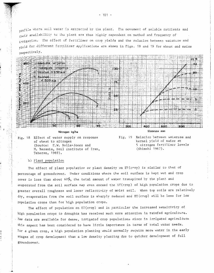
r

profile wher2 soil warer is ext::act2d by the. p1.anL The movement of soluble. nutrients and

their avai.lability to the plant are thus highly depe.ndent on method and frequency of

irrigation. The effe.c.t of fertilizer on crop yields aud the relation between wateruse and

yield for different fertilizer applications are shown in Figs. 18 and 19 for wheat and maize

respectively.

y~ :"o~r±~ ":; '" ., . . .. .., .... ..

:~: :: :t !::: :!;:;; :: ::· ---:-:- :._ .:: < ::·· ..... :· : ··_: ,_

... ŗ;{: :,-;.; ±±'"C ,.; : " :·

~1~ft • 1 •• :'" .. :._,_;_ ... : :: ':_ ::: :::.' ::

; :.~ : ; ' : : .. :: ::: ..

' ... ::

:

~:[ifj·~T: .L,

ļ-:-f'"' .:~--, 0 ::·H-~,~ .w

ta,j -f-•H ·,• ::h- ,,c; ~::•

~::-, .;~~r::i~~-::J~ - .:-1;:n -·-··

Nitrogen kg/ha

Fig. 18 Effect of water supply on response of wheat to nitrogen (Source: E.W. Bolle-Jones and M. Rezania, Soil Institute of Iran, Teheran, 1969).

b) Plant population

.. :: ..

Wateruse mm

Fig. 19 Relation between wateruse and k.ernel yield of maize at 5 nitrogen fertilizer levels ( Shimshi 196 7).

The effect of plant population or plant density on ET(crop) is similar to that of

percentage of groundcover. Under conditions where the soil surface is kept wet and crop

cover is less than about 6010, the total amount of water transpired by the plant and

evaporated from the soil surface may even exceed the ET(crop) of high population crops due to

greater overall roughness and lower reflectivity of moist soil. When top soils are relatively

dry, evaporation from the soil surface is sharply reduced and ET (crop) will be less for low

population crops than for high population crops.

The effect of population on ET(crop) and in particular the increased sensitivity of

high population crops to droughts has received much more attention in rainfed agriculturee

Few data are available for dense9

irrigated crop poplllations since in irrigated agriculture

this aspect has been considered to have little importance in terms of total water needs.

For a given crop, a high population planting would normally require more water in the early

stages of crop development than a low density planting due to quicker development of full

groundcover ~

.

....

- 102 -

c) Tillage

Except for soil:S which tend to form deep cracks, tillage produces little if any effect

on ET(crop) unless a significan.t quantity of weeds is eliminated„ Rough tillage will

accelerate evaporation from the plough layer; deep tillage may increase ET(crop) when the

land is fallow or when the crop cover is sparse. However other factors such as higher

infiltration rates may decide in favour of tillage. On some soils tillage may be required

to break up sealed furrow surfaces in order to achieve adequate infiltration. Soil ripping

between crop rows may result in temporarily higher infiltration rates but the crop could be

slightly set back due to root pruning.

d) Mulching

Except for specific purposes such asa reduction in erosion by wind and in water

runoff, the use of a mulch of crop residues in irrigated agriculture to reduce ET(crop) is

often considered of little net benefit. Crop residues may even be a disadvantage where

soils are intennittently wetted; the water-absorbing organic matter remains wet much longer

thus increasing evaporation. Asa barrier to evaporation it is rather ineffective. The

lower temperature of the covered soil and the higl_1er reflective capacity of the organic

matter are easily outweighed by evaporation of the often rewetted crop residue layerv There

may be additional disadvantages such as the increased danger of pests and diseases, possible

slower plant development due to lower soil temperatures, and problematic water distribution

from surface irrigation.

However, a major advantage of mulching using organic plant material is the protection

of the soil surface, preventing soil capping or sealing and it may produce a higher infiltration

rate which results in greater storage of rainfall in the soil.

Polyethylene and perhaps also asphalt mulches are the most effective. A net reduction

in ET(crop) using waterproof covers is however largely dependent on the percentage of land

covered as well as on the percentage of crop cover. The method is mast effective when mulch

covers more than 8o% of the soil surface and crop cover is less than 50 % of the total cultivated

area. For instance, positive results have been obtained in Tunisia on strawberries where plants

grow through boles in plastic sheets and the soil is kept relatively wet. Wead control and

little rotting of the fruit added to the successful use of plastic.

e) Windb reaks

Due to a reduction in wind velocities produced by artificial and vegetative windbreaks~

ET(crop) may be reduced under windy, wann, dry conditions by about si at a horizontal distance

equal to 25 times the height of the barrier downwind from it, increasing to 10 and sometimes

up to 30%at a distance of 10 times this heighte However, ET(crop) as detennined by the

overall climatic conditions is not altered~ In mast cases shrubs and trees are used and

thus~ due to the transpiration of the vegetative windbreak, overall ET may be more"

f • 103 •

Regardless of the benefits of reduc.ed ET(crop) ~ wind damage to crops~ such as by the mistral

in southern France, may be far more serious than the increase in total water loss. A pro'"

ductive, low water consuming windbreak~ for example citrus, or an artificiai wind barri.er

might be considered in order to eliminate even this last negative effect. Recent studies

have shown in Nebraska (U. S~A.) that due to the protective physical effect of artificial

tvind barriers, crop yields of maize can be increased by from 10 up to 30'5p wi thou t an

increase in ET(crop).

f) Anti~transpirants

The use of anti~transpirantj natural or artificially induced variations in plant

foliage properties and soil conditioners to reduce ET(crop), continues to interest many

investigatorsj but so far is still in the. experirnental stage.

I. 4. 5 CROP YIELDS

Knowledge of the relationship between crop water requirements and crop yields is

ueeded to predict levels of production that can be achieved by varying the allocation and

use of available water for irrigation. Whether or not ET(crop) is to be fully met by

adequate irrigation water supply depends on set objec_tives such as maximum production in

relation to investment~ greatest yield per unit of water when water is short, greatest

yield per unit of land when land is short, in assuring the greatest nurnber of farmers to

benefit from irrigation when socio~economic factors are mast pressing, ar in assuring a high

net income for the fanners. Also ~ in project operations, particularly during periods o.f

water shortages decisions need to be made on the best use of available water and how to

minimize reduction in crop Jields due to droughte Much of the information required concerns

the relation between periods when the crop is most sensitive to reduced water uptake

associated with soil water stresseso

The relation between crop yields and water seems confusing due to the many factors

involved. Earlier investigations suggested that for most crops a linear relationship exists

between seasonal ET(crop) and dry matter production~ The slope of the linear relationship

varies with each crop species 0 For instance, to obtain the same dry matter yield, total

seasonal ET(alfalfa) may be four times that of sorghum~ and twice that of wheat. ET(rice)

of high~yielĢing varieties is similar to that of traditional rice varieties but yields can

be fourfold provided good water management is practised and other agricultural inputs are

supplied at the correct time. In addition~ climate also affects the relationships as shown

in Fig. 20 for dry matter production of grass.

The linear relationshp between dry matter production and seasonal ET(crop) seems to

be valid only when other growth factors such as fertilizers, temperature, sunshine and soil

depth are not limiting. However, for mast crops dry matter production does not determine

the actual yield as this depends on the harvested part of tpe plant which can be either a

chemical constituent (e.g. sugar, oil) ar reproductive (apples, grain). Additional considera

tion will be neede.d to express the relationship between harvested yield and ET(crop)~

;j

C

0 g

' C

J1

" ;; 2 "' 8

" ~ , • C • E

$

-~ 4 .!! , e , <}

200 400 SC-0 600 1000

Cumul!::ifi'lf(ļ ET (;rau) mm.

- 104 •

Fig. 20 Relation between ET(grass) and dry rnatter production from pastures at different latitudes (Stanhill 1960)

Recently deve1oped concepts seem to show that for harvested yields the ratio of

relative yield to relative ET(crop) may be assumed to be constant or nearly constant for a

given variety provided specific crop characteristics and growth stage effects are controlled,

and growth factors other than water are not limiting. If this is so, knowledge of the slope

of the two parameters considered, that is actual ET (crop) /maximum ET (crop) versus. actual

yield/maximum yield, combined with the quantitative prediction of rnaximurn yield and maximum

ET(crop), would enable a quantitative prediction to be made of yields to be obtained with

the selected water supply for any given location with a suitable climate (Stewart and

Hagan, 1973, 1974). This assumption seems to be supported by Downey (1972) who provides

<lata on 14 non=forage crops including wheat~ potatoes, cotton, beans, maize9

drawing these

<lata from a variety of sources. Figure 21(1) shows that for dotted envelope curves repre·

senting 86% of the results analysed, yields decrease by 80% when actual ET (crop) is allowed

to drop to 0.5 ET(crop) maximum; yields decrease by 50% when actual ET(crop) is O. 7 ET(crop)

maxirnum. These <lata apply for conditions where soil water is available at a fairly constant

reduced rate for most of the growing season~ It should be noted that the curve does not

begin at the origin; there a threshold value below which production is negligible.

The effect of water shortage on yield is very pronounced during periods when the plant

is particularly susceptible to water stress. This is shown for maize in Fig. 21 (2) for which

yields are negligible when li.mited soil water sharply reduces ET(crop) during the tasselling

stage. Figure 21(3) shows a generalized relationship between yield and actual ET(sugar

cane) in Hawaii~ Prolonged reduction in ET(cane) during the period of active growth from

; . J; j t, .~ i ,i,J

>--·-------· .

.i --1

____ _)_ __

--· .. F"l!· -. . , ti ·=-- -~,4' r~~ ~f J,._ t ,-- J %,

100.i

i, ,1 d,i 1,111,l,i""

.. ,. j i

----1-: __; --~- -- . ' ' ' : 1 : ! - ' :,,•,,+- ,..,$ .... h~.t·: ... ~:.-.!i .. ..j .. ,· •. ··.· .. '·.··.· 't~ .. :: " i +

-- '' .. :

f ~v r=4-: r-::---~r:-,' -~~- 1 i-'1--1 1 -:- ji'::; ~~~~~1g~ ; ,., . , --r::j-+--: J.1-:-· .... -, : - -ŗ-- --,- r·--1-: .,_,._'"-'Jlf.

C TT i l ··:·. ··. •. t. . . . 6,:> 1 1 1

i ~ . . ~t ~~--: :_L.L -l--. ·Y.: fJ _. ~-~.·. -4~ - T ~ŗ-_; ~-1 ~-. ++ 1. 1 1/, ,1 1 ·[ 1 1 ti1 .l·-1·- •11

J:.l+.·· ·. .. . . , .. \. cc.=~=.·~., -i.· •. ·· ... i-.ld···· .. · ... · . C.,j·. •. -,·.·. a~š • ~~~ŗ, _J.~(___µU:~+~;-~14 ___ : .•• l- 1·:~

! ~:::·:rc~a~~::·h:~•prbi:~1:!·:ij•J::,11~~7~ie{: a!; 1::~~tf e virgin cone ( Downey (1972), Chang {1963!}.

4

-~ ·--~

0 V,

•

- 106 -

12 to 14 rnonths after planting virgin cane will have a much greate.r negative effect on yields

than if the reduction in ET(cane) is experienced during the late growth period„

Reducing ĶT(crop) by decreasing the irrigation supply or by extending the irrigation

interval beyond the period during which soil water is freely available to the crop is thus

particularly critical during times when the crop is sensitive to soil water stress; at that

time any soil water stress may have a lasting effect and could drastically reduce yields.

Critical stages of crop growth for mast field crops can be considered as any changes from

vegetative to reproductive growth~heading aud flowering to fruit setting. However some

crops have no specific critical stage, for example such vegetables as potatoes, bananas and

other crops grown for fresh weight production~ but they are sensitive in any period to

prolonged water stress conditions~ Critical stages for soil water of some crops are given

in Table 35,

In order to produce high yields, crops have different requirements as to maximum soil

water tension or degree of depletion between irrigations. Some crops will only produce an

acceptable yield when soil water· is kept at a high level, usually well above 50ti/o of available

soil water. Crops requiring relatively wet soils include mast vegetables, potatoes, bananas,

etc. Yields from other crops including deciduous fruits, barley and sugarbeet, nonnally do

not respond when water is applied above the 50% depletion level. Moreover, soil water

deficits can sometimes have a positive effect on the quality of yields; slight deficits may

improve the quality of apples~ peaches and plums, and increase the aromatic quality of

tobacco and the oil content of olives. An induced reduction in ET(crop) before harvesting

may also increase the sugar content of sugarcane~ Irrigations should therefore be scheduled

to bring about the specific soil water levels required by the crops.

Infonnation on soil water tension tolerated by different crops without causing ari

unacceptable reduction in ET(crop) ar, even more important~ an unacceptable reduction in

yield, is given in Table 36. The corresponding level of available soil water depletion

should not be exceeded, particularly during critical periods~ Lower values apply to high

and higher-values apply to low evaporative conditions; values given in the table represent

mostly vegetative periods and may not apply during critical periods where plants are sensitive

to soil water stress& A comprehensive review of the subject of crop responses to soil water

deficits at different stages of crop growth including the critical stage for soil water

stress can be obtained from the references given 1/

1/ R.O. Slatyer~ Plant-Water Relationships, Academic Press, 1967. R.M. Hagan~ H.R. Haise and T.W. Edrninster, Irrigation of Agricultural Lands~ ASA No. 11~

196 7. T.T. Kozlowski, Water Deficits and Plant Growth I~ II and III~ Academic Press, 1968. P.J. Salter and J.E. Goode, Crop Responses to Water at Different Stages of Growth,

CoTIIlllonwealth Agricultural Bureau~ 1967. Y.F. Vaadia et al, Plant Water Deficits and Physiological Processes~ American Review of

Plant Physiology, 12: 265·292, 1961.

T ·.

rable 35

Alf alfa

Apricots

Barley

Beans

Broccoli

Cabbage

Castor bean

Cauliflower

Cherries

Citrus

Cotton

Groundnuts

Lettuce

Maize

Oats

Olives

Peaches

Peas

Potatoes

Radish

Sunflower

Small grains

Sorghum

Soybeans

Strawberries

Sugarbeet

Sugarcane

Tobacco

Tomatoes

Turnips

Water melon

Wheat

B 107 =

CRITICAL PERIODS l<'OR so::::L W'f,_'L:!:R STRESS FOR DIF?ERENT CRO:PS

i~~~u~~~~: cutting for hay and at the start of flowering for seed ll period of flower and bud development

early hoot stage stage

> soft dough stage > onset of tillering ar ripening ļ

flowering and pod setting period > earlier > ripening period. However ripening period > earlier if not prior water stress.

during head formation aud enlargement

during head fonnation and enlargement

requires relatively high soil water Ievel during full growing period

requires frequent irrigation from planting to harvesting

period of rapid growth of fruit prior to maturing

flowering and fruit setting stages; heavy flowering may he induced by withholding irrigation just before flowering stage (lemon); ''June drop'' of weaker fruits may be controlled by high soil water Ievels

flowering and boll formation > early stages of growth > after boll formation

flowering and seed development stages > between germination and flowering and end of growing season

requires wet soil particularly before harvest

pollination period from tasselling to blister kernel stages > prior to tasselling > grain filling periods; pollination period very critical if no prior water stress

beginning of ear emergence possibly up to heading

just before flowering and during fruit enlargement

period of rapid fruit growth. prior to maturity

at start of flowering and when pods are swelling

high soil water Ievels; after formation of tubers, blossom to harvest

during period of root enlargement

possibly during seeding aud flowering ~ seed development stage

boot to heading Stage

.secondary rooting and tillering to boot stage > grain formation > grain filling period

flowering and fruiting stage and possibly period growth

heading, flowering and 1

of maximum vegetative

fruit development to ripening

3 to 4 weeks after emergence

period of maximum vegetative growth

knee high to blossoming

when flowers are formed and fruits are rapidly enlarging

when size of edible root increases rapidly up to harvesting

blossom to harvesting

possibly during booting and heading and two weeks before pollination. _J

Tab1e 36

Alf alfa

Banana

Beans

Cabbage

Carrots

Citrus

Clover

Cotton

Cucumber

Deciduous

Flowers &

Grapes

Grass

Lettuce

Maize

Melons

SOIL ·wATER DEPL:S'1'ION LEVEL.S~ E:CPRESSED IN SOIL WATER TENSIONS ~ TOLER.,l,.TED BY DIFFSRENT CROPS FOR WHICH ET(crop) REMAINS AT

PREDICTED LEVEL AND MAJ{IM1JM YIELDS .ARE OBTAINED

0,8 - LS atm 1 / Onions 0.4

0.3 - LS Peas 0.3

0.6 - 1.0 1 / Potatoes () ~ 3

---

0.6 1.0 Rice at or near

(' t; , . - - !L 7 Safflower 1. 0

o.s - LO Small grains 0.4 -() ' 3 - 0.6 Sorghum 0.6 -LO - 3.0 Soybeans 0.5 -1.0 - 3.0 Strawberries 0.2 -

fruits 0.6 - 1.0 Sugarbeet 0.6 -o·rnamen tals 0. 1 - 0.5 Sugarcane 0.8 -

0.4 - 1, 0 Tobacco, early 0.3 -0 .Lr - 1. 0 " late 0.8 -0.4 - 0.6 Tomatoes o . .s -0.5 - 1.5 1 / Wheat 0.8 -0.3 - o.s " ripening 3.0

"J_/ Higher values than t.hose shown apply during ripening period,

-1 0.7

0.8

0.7

saturation

2,0 1 /

1, 0 1 / -1. 3 1 /

1 . 5

0.5

0.8

1. 5 1 /

0.8

2.5

1. 5

1 . 5

4.0

Source: Taylor 1965, Hagan and Stewart 1972, Salter and Goode 1967, and others.

~ ·. f i '

p/lRT II CALCULATION OF _FIELD_ IRRIGATION REQUIREMENTS ,_If

INTRODUCTION

Field irrigation requirement is J;h,~_jWlount ~f ~ater and timing of

itS application needed to compensate soil water deficits during the growing season of a

given crop. Irrigation requirements are determined by crop evapotranspiration minus the

water contributed from precipitation, groundwater, carryover of soil \.'ater from earlier

precipitation or flooding, and surface and subsurface in flow. It is expressed in mm per

growing period (season or one month or less) for the purpose of overall planning and

evaluation of the field~ project or basin water balance. Summarized over the entire

cultivated area, it forms the basis for determining the necessary supply and the adequacy

of available water resources. It is expressed in the form of an irrigation schedule in

depth of an interval between irrigation for the purpose of project operations (mm and days).

Irrigation is never 100 percent effective and allowance must be made for unavoidable

and avoidable losses including deep percolation, surface runoff and other managerial or

technical faults. Irrigation application efficiency Ea is normally expressed in fraction

or percentage of In or field irrigation requirement If : In/Ea where In is the net irrigation

requirement and If is the gross field irrigation requirement.

In is based on the field water balance which for a given crop and period can be

exµressed as:

In {ET(crop) + F + R7 - /Pe + Ge + N + L!W7

loss es gains

where Pe and Ge are the effective contribution to the rootzone by rainfall and groundwater

respectively; surface and subsurface in and outflow, N and R can be of local significance;

deep percolation F whieē:h tak.es place after the soil has attained field capacity following

irrigation is generally but incorrectly accounted for in the correction of Ea~ the field

application efficiency; Ll W is the change in soil water content in the effective root zone

which, under irrigation, should 1.,1ary between field capacity and maximum available soil water

depletion for a given soil and c.rop, All variables can be expressed in units of depth of

water (mm). Depending on <lata available and accuracy required, In can be predicted for

seasonal, monthly or 10 day periods.

Of importance is the period or time interval over which the field water balance is

made, Too long periods may obscure the occurrence of short duration water shortages. For

instance 1 when using monthly data~ monthly e.ffective rainfall may be shown to meet monthly

ET(c,:-op) but .since rainfall is norrnally not distributed evenly over the month, short duration

Water deficits may occur" Too short periods may be impractical. It should be realized that

when using a monthly rather than a daily balance thi!3 may produce results acceptable for

overall planning purposes but these r.esults may be far from realistic for use in detailed

design and operation of irrigation works 1 and in schedu.ling field application.

•

-

' l - ' f -h - · ld · ba' -n-e ~··-i-11 ha-ve to be mad,3 for In mos t cases, ca cu1..at1on o t e rie waI:er .La.1 '-- w-~--

alternative cropping patterns in order to find the optimum solution between irrigs.tion

requirements and water supply available at source.


When determining field i:::-rigation requirements for a selected c.rop and cropping pa.ttern

for overall planning purposes certain data are required and to obtain it procedures are

suggested. Determine:

1. for alternativ2. crops, cropping patterns and intensities the variables composing the

2.

3.

4.

fielü. water balance for the growing season and for shorter periods:

crop evapotranspiration, ET(crop)

effective preciritation, Pe

groundwa.ter contribution, Ge

surface and subsurface in and outflow, N and R

deep percolation from rootzone~ F

changes in stored soil water, L1_W

from field v:ater baldnce the seasonal aud monthly net irrigation requirements In;

for the month of maximum net irrigation requirements, the peak period net

irrigation requirements Inpeak;

after selecting field irrigation application efficiency, the gross field irrigation

requirements If;

5. the water requirements for cultural practices and leaching of salts;

6. the irrigation schedules from field water balance, taking also into account

water storage capacity of the soil and level of soil water required by the crop,

1 1

'

:::

"' 111 =

cHAPTER I I, 1 FIELD WATER BALA.t\lCE

To calculate net irrigation requirements for seasonal, monthly or shorter periods the

variables composing the field water balance must be determined first.

II,1,1 Crop evapotranspiration,ET(crOp)'

Crop evapotranspiration, ET(crop) can be determined using one of the four prediction

methods given in Chapter I. 1 and selecting an appropriate crop coefficient kc from

Chapter I.2. At this point of investigations <lata on ET(crop) for different crops and

cropping periods should be availahle, taking into account also the considerations given in

Chapter 1.4. Expected crops yields~ agricultural inputs~ soil improvements and sometimes

other opposite facets should have been investigated.

Depending on local weather conditions ~ ET(crop) will vary from year to yea-r and for

each period therein; ET(crop) should then preferably be calculated for each y.ear for which

climatic records are available. A probability analysis may be made from which ET(crop)

value can be selected.

When mean climatic <lata from available years of record are used to predict ET(crop)~

a correction factor on ET(crop) to account for the year to year variation in it for the

given period will be required, For overall planning this correction is normally applied

only for the month of maximum irrigation requirements in order to derive peak water

requirements, Deta:tls are described in Chapter I, 4. 1 ,

When climatic data have been used collected outside or prior to large scale irrigation

development~ a correction of the effect of advection rnay be required ... as given in

Chapter I,4.1,

To reduce the risk of crop failure due to water shortages or drought, in overall

planning an ample supply of soil water to the crop is norrnally assumed. Orily in the case

tha1: detailed data on the relation be.tween ET(crop) and level of production have been

loca.lly determinedp r-md whe:n water is short ].n supp.ly or expensive) should a reduction in

the prcdicted ~T(crop) and -St leve.1 of production below maximu.m be c.onsidered. This is

dis cussed in Chapter 1 . 4, 5 ,

EXAl.\fPLE : semi"'arid~ hot and moderate winds during July and August; crop is maize. soī.m mid May ~ harvested end September; size of fields is ·10 ha and cropping intensity :Ls 50%; surrounds are dry fa11ow lands; iŗrigation d~pth oi applicatio11 is 80 mm? c;l,imatic <lata are c;11ected before '±rrigatTGln d~ve!:!.Optll~n.t :Ln non-::agx-±cultura1 area,

ī--------------ļ Ma;---June ---:;:;-----;:;-, -~;-. ---------~

ET(maize) mm 2,8 5.2 8.8 /.1 3,8 (Chap. I.1 and 2)ļ Correction factor

advec tiem

ICorrection peak 1 month 1,09 (Chap. I, 4~'!)

JE:~:aize) ~----ļ 2 ~ ~-----~-· 9 _____ _!_~~---: j 4 ------3 ., 6 (~~~~------J.

0,95 0,95 0,9 0,9 0,95(Chap, L 4,1)

•

• i i 2

a) Rainfall

Vital to irrigation planning is knowledge of the frequency and amount of rainfall,

Since rainfall for a given period can be expected to vary considerably from year to year,

mean rainfall based on short records crm at best be considered a very gross approximation

and subject to large errors. Also~ not all rainfall is effective; part is lost by runoff,

by deep percoļation or by evaporation, Methods are given below to estimate the percentage

of effective rainfall which will be available to the crop~

Future rainfall can be projected through statistical analysis of past rainfall

records. Rainfall probabilities derived from historical <lata will show the amount which

can be expected in any percentage of time and from this a dependable level of rainfall can

then be selected. A practical and realistic value of dependable rainfall frequently used

is mean monthly rainfall that occurs on a probability basis three years aut of four;

however, this also means a shortage one year out of four, To allow proper evaluation of

dependable rainfall the degree of shortage and the expectable frequency during the. driest

years should preferably also be given, The resulting loss in yields during driest years

may be of significant importance in the economic viability of the project,

Furthermore, the time of deficient rainfall periods is important. Some crops, as

indicated in Table 34~ are particularly sensitive during certain stages of crop growth and

all crops are during germination. Water shortage during these periods may well have a marked

negative effect on crop yields; a higher level of dependable rain should be selected for

these periods.

For large sc.ale irrigation development or where mountains or other physiograpic

features greatly influence rainfall and the occurrence of storms, the spatial distribution

of rainfall must be evaluated, Methods Lor interpreting areal rainfall are described in

detail in mast textbooks on hydrology ]_/.

i) Method for _ computing rainfal1 probabilities

There are several methods for determining the .Ereguency distribution of rainfall;

mast will produce similar results at cr near the middle of the distribution, but different

values for high End low extremes. The selection of method should thus depend on the purpose.

for which the data are going to be used ., For detai_1e.d. an2lysts the references g:tven .should

be consulted. Computer calculation rn.2.y often be required for detailed analys:i..an

1 / Ven Te Chow, Handbook of Applied Hydrology, lYkG:caw""Hill? ·1964, Linsley ~ Kohler and Paulus. Hidrology for Engineers ~ f'IcGraw"'Hill ~ ·1953, WHO, Guide to Hydromete.orological Practices ~ ·1965. USDA (SCS). Engineering Handbook Hydrology, Section 4

1 suppl, A~ 1957,

Ramlrez, L~E„ Development of a p:1:ocedure for determtni:ng spacia.l and t1.me vEriations a:f precipi"ta"fiOn in Venezuela~ PRWG 59,,,3, Utah~ ·usA~ -.1971.

·?

A simple method to provide rainfaJ.l probability data .Ls g::'.5en below. From the results

a selection of the probability le.·,1el and coT_"responding likely depth of rai'i:1fall can be made;

the probability level must be based on the crop to be grow"TI in the area and on the crop growing

stage,

ine

EXi\.MPLE:

Computing rainfall_probabilities

1) Point rainfall frequency:

Steps involved:

tabulate rainfall totals for given period/line 2 for number of records ar items (N) arrange rainfall in order of magnitude and give rank number (m)/lines 3 and 4

- tabulate plotting position (Fa) using for instance Weilbull formula 1 Oüm/(N -1:' 1) Q

(N is total number of items, mis number of items arranged in descendiilg magnitude, thus m:1 is the largest item)/line 5

• prepare vertical scale and plot rainfall according to Fa position on log-normal probability paper/Fig. 22

(1) year 9 56 57

75 85

58

50

59

65

60

45

61

30

62

20

63

65

64

35

65

80

66

45

67

25

68

60

69

75

70

40

71

55 (2) mm/given

month

(4) nurnber m 2 3 4 5 6 7 8 9 10 11 1 2 13 14 15 16

(5) plotting

--~osition~j5.9 11.8 17.6 23.5 29.4 35.3 41.2 47.0 52.9 58.8 64.7 70.6 76.4 82.3 88.2 94.1

From Fig. 22: dependable rainf all 3 out of 4 years ~ or 7 5 % probability, for given month is 36 mm~

A skewed frequency distribution, where p,oints on the probability paper do not fall in a reasonable alignment, may mean either too few data are available, <lata are affected by sorne physical occurrence causing consistent bias, or, more often, rainfall is not distributed in such a way as to allow simple statistical analysis. This last factor can be overcome to some extent by either:

plotting on probability paper the square root of the same rainfall <lata or

particularly for periods with spells of no rainfall, use Ga .!: P + (1 „ P) Fa, where Ga is probability of occurrence and P is the portion in which no rainfall occurred. Sample: if no rainfall is recorded in 6 out of 30 years in the period considered then P ::: 0.20. Then Fa is determined on a /-4 ... year basis following the step method given.

2) Rainfall duration frequency:

Rainfall values over consecutive days are found by moving totals, i.e. for a period of say 5 consecutive days the totals of rainfall from 1-5 May, 2=6 May, 3=7 May ... 27=31 May are computed. In this way 27 values of 5 day-totals of rainfall for the month of May are obtained. Then aut of the 27 values the highest is selected. Fora recording period of say 30 years, this gives 30 values of highest rainfall on 5 consecutive days in May. Frequency distribution of these values is made following the step method given before. The same procedure can be .repeated for different numbers of consecutive days. Rainfall duration curves are obtained by plotting, for a given frequency of rainfall occurrence~ the number of days against d2pth of rainfall. Curves of equal probability are drawn t:hrough the points.

•

;,:;,.

-~ c,--,-__ 11r_1, =t1, 1'_l.,.,,1i ,11.: •. =·t..,..,.I I, CTT! 111 =i '. l"'tl ,-ml ,,.,.,! '1 i-n-. - ·cn-n-,-,-,-11 !"_n-l mlrn HJ-rr.J±I L"'Mf 1·1n-r' . -=ll [!.,..,..,,ļ ļl'TT'.H. 1 1==11.ļ,,..,_ ļ 1=11_1=11.::1 i :_11·H~ltt11:-,-,-11,~111 =L1~=1 l~ll ~ 5 1 · · . 1 t_ Li'. __ i 1 _ . J .. 1 . _,,J . ~ ·-i--,', .. ,1 ), !,' ... j-1+'. 1 J 1.1, 1 i 1··f T; l I r 1

: ,jJ~ ,, 1~:~tfl-t ī - - ,· ---j 1 '- -1-~-ri-if-- -Hi-+ .. ···t-+ļ -1· , ,:·--.. ··:rJTl~-~t+:,_ ;---~t o ,c:+:+-+ j .. , +!_-f--ljj'··J_--+-- i:ti_·+: .. 1·-t ··lJ· +- u. -1 1 i-i- l -- -~1-'·'::1:::t:jjl ''·+---+ -Hti- ~-::}+_ ++ ~- .. , _ _-t-; ŗ- -i_ - T -r .- - j- - :=t:--- ---:p:-_[_ '·+b-=r ·· +, .. :: -:=~ ·1 ~-

; + u t -! .. :f H- HH --! 1 ! -1 1„.1 1 1 1

: -1- . + --H-L, 1 1 i. ,_

111JH ; ~ ~ ' ' ' ' 1 ' ' ,,.... .....

"' 1 ' 1 ' 11 i i ' ' 1 " 1· i ' 1 1 1 ' , , ! ·+ 1 ! : '· ļ j. .l ' 1 i 1 1 ! ' .. ., i -H+f Hn ŗt++L'; i+f-l+ H 1 +l i,. +cr, +i 1 1 1, ,+ +r. ti+' -HI +H++++++I

MJ i ----- i -, ·!· 1- --r-1 tt'" ,-ŗ 1-t -r -r- 1 + __ · ___ --- ++ · T- -H-1-i· .. , ... ·+· 1 ·t+:f-1 f--H+++++++t++- --· - ,+ -,+h ~ 0 ! 1 ~--

c ~+.-i -J-+ L. -!+·J-·t ·.. -+ .-,.L !.. +.-\.. + .Ļ - , __ ;T-f -t"t +--1 ti Tt +J.+ · a-+H·t cl=, ct..;-t-t ± ± ... :

10,f_:_,,·:_1_: ___ ~ ... t ___ ŗ,_._bH'_,ti,r,I .r:·+ '· ·--1 ···H ·

=tt_:~--i . 1- 1 .f. -•· •. 1-1 --... !--+- 4 .i: -~ · ··+- -'- -x:r-_ _ ;t,, 'ē""O

- Lt::~ Hf1 tJ+,._+ -++ r(i !+i±t1+ + 1, 1 , " • 1 +_·,.··_, 1.•- .·j l-_ "~~

-+-~---(:l T1:+:_: --l- i tt +i= 'i-l j .t.tl}~+-- ::t". -t- ... i- ---l ~- -f----;t~ , -+ • E~ .. ! ! ! ' ! i 1 1 ' 1 ,'-· 'i .. 1' 1 1 • l I i i 11 ! 1 1 ' i 1 ! ! 11 ! ' .. -0

111 ,1: fftt 1[1

+' · - rH-'.+1,~'=++-+1. -t+i+J+++,,-H-+1-+++J.+,t! + :1• ':i, f1f1r !h1ļŗi ie

-·r- -- -+•-,-H ,,. , 1,··1,·' 1 -t--/-t -C-i-:~ t-1--H·++++1tr --f-1. ++-,. f++,+1++, ++-,H,+ - -rr:-- -1-!Tt· -i- 1 ·- ~ --w 1-t-++rn-++++t+r-rn,,++-++++-++t-H+t++++++-++m+t+t++++-,++t-H+t+++, ++++tt-t-H+t++tt+t-t-1,1.H+t++++++-t+rnH·-t+H .. ,:; -m-- ) ,~ j : ++·eH·H++++++-+++J++++++++-J_-ļ<,++>-+:-J+1_+1'._HJ-1. ļt'- _ . j. '-~ ± ___ t_l- . -•4·1:l. _.. <>:::,

1-H++++·H:U·H·+Jrrr-rdirl ++-4-H-+1 __ J.... -t- f; 1----i-r __ E;? - ,,· 1~,. ,.,.--yT'-H+++++t 1 1 tL. . +:· t-+,_j_i -, -- ' - _1_ 1 c - ,--~ ~- ' ŗ ' --ļ t·f--LJ-h-i-- - . :-0 -jj:J-~fil~~t~{i"ļfĻ_~;-t-~~--f_1_-· -t~

4Jf_· r~t· ~\~F; ,---+ f-H. -tt·- ;-H_ Oc c }fj~ ,., ..... +++t··itF}JJt~ :1· ·- + l ---It .. ~~11~--+.1 r-_.: +·-~--li::-=kn-- -·1 o @J:S N l ;-rl;-- _;trt --=--h -ii'r' 'm-l,·,--~_,+,i'·,·,.'r-tl+ i-·--.. ""t·· -:-- -- -·+ H',unnm+~t_ ;· + ·-m_. _+'-+-±+-1=~-'HH.:r.:rtt+'·-t-+T. ntt-t1t+f-hf-H .. !:c"'·

- r f- - ' rĻ' "1 i. ' +-i +i- 'i- L.--'-, i-f1-+. ) ' __ L; ĻĻ, -C ~ + 'l ~+ -+---4+ 1 : -+ - i-1-, +-+ J ·!·H-- "' 1 --~-1 .. ,,_ ~ #) q;

ffl tttl·-+-~--+ --· --ī-R+-1_-+--~ t~ntt1-rt-+- ffi.j .. ·,·--·+++di=l - t+t· ___ +t ... Lt ""'f:Č Q rt ++--+:lļ~--- ' 1 ·_ 1· " . . . -~-+-r; t-- :·:a-iill::J:.~-:r .. ~L ' . -: ! ' fj -L-tL l l- -· 1 , lT-t . + ~ ~ ~

q, -"· ' ---+-t±i 1· 1--1- - ' .t .L: .. :r:- : :1~1::it :i: 1t ._ -+ ~-tt ~ :H·l+H 1 .,ilī :J - H- P. ~- ··T ·.··-H+ , ~ +-~ -1-' c+ ±1-1-i• : · +Lf-·-- tJ c :ttr:ļ:. :.P:~i:1~ :: !--- : .. ,t c.,. tT. 'll. t. ____ µ..

+:-f:1t·_,, .. :ļ_. l ";- -.. + 1-l : C H- · ·'i" 1--~I ' : ;

""-41-+t+-r- .i~t:----c l .:!-., 1ļŗJ .. :_ + L!+-CH-H .. "' •

.. .. "' .. 1

+t,. '

ļjj"'( ! 1: 1 ! 1' !

0 0 m Jll)

,. t++ f +t 't·.

-, .. i..

t ·+L +i

~QJJ-~i:fErt:"" +1J:-j-+;+I··

• 1 '. '

.•. ,. t:tl+ l.f:t·.+ ·++, +_,-.. --~ -t 1.,.. :_ ,_;,_ .l_ .. ..1,.. C i" 1 r-1-- • 1· , 1

-+ --t- -1 }-lH=- -u- - ' -h -,- ' ,++-++++++++t+i:c++-:- "t-i :t: '. · j+ 1--- j„4 -·t' r-t ļ ·1+l·i H+-tt-·+: 1

~-~ · :;r ifl~: jJ~J~ ,. H· ·+--i-

:q:.. ··1.

1 1 1 ' 1 + i. '

' ·r l 1 '.1 t

1 IT 1 1 11 'i

11 0 ,o 0 .,

'1#" O'I

Tt · -t :t±t-~"i @

··- ŗ

1 i 1

0

""

1 1

11, ,

1

,1,

1

, '

,, 1

3) Drough-c dura-cion irequency;

Here only the lowest values of rainfall of the moving totals of rain for a given number of consecutive days, say 15 9 30 and 40 days, are selecte.d„ The drought duration frequency is obtained by plotting values for each selected period of consecutive days according to the given method.

,, ·:1 :.: ', :11 'I

i:: 1 "I '.] ''11

2 and 3 machine calculation will be required .

1

1

.!-il 1

':i

.. ,~ iv2 rainfall '-------·-------------

T:3.infa.ll i.s only a portion of total rainfall. Part of the rain may be lost

by d.1~~E~p percolation below the rootzone ar by evaporation of the rain

:,

,, !

i'

1

1

1

r, 1 \-: ,i'i\ ~; 1 /'• , 1

i:: "i

'.{

·1J 1 H H

·"!

i1 i,,; ļ,

·,./ 1· 11 : l ļ:

'".;\ il :, 1,

'·' 1

'I ,:, ,

11'· 1·!

!!i

fql:i..age .. .ln .regions with heavy and high intensity rains only a

t:n:i:·:::d :i.n l:J:r: rootzone and the effectiveness of rain is consequently

n::e ::+t: ::.on by the plant foliage can be important; wet plants

:+: :t.::'.h t:::. o:i::l:°"·:::,et by increased evaporation of the rain water inter""

, ;.1 1

Iri prac.t:Lce, for full ground cover conditions it can be safely

r,:d.n:l:a:Ll is close to 100 %effective. Where a high percentage

(

i1: )( ,

f; 1' ·ii / lii \ .. ,

d

1 !'· ·,· , ·:' ·'C

\i ::i, {

•'r'1 ,.,1 a:nd t:.he soil surface has been dry for some timi=: before )J JI! :tfac·:'~ can be considerable. Rainfall of 6 to 8 mm per

:.1

il ,;.\ ,j',1

·,.i 1,

:L :;n, Even rains of 25 to 30 mm during initial

·,.1 JH:i·c-.::y::·1tage of ground cover may result in a net

,,,

• 1 ... :r~ .. os to e2.tiriate effective rainfall as a

of the average seasonal rainfall

1c mean rainfall but. excluding

,,;:-s of 75 mm in day and

:~i:i:· ·,:i f: ":-1: .1owing irrigation is con-

't:L:rr: ·12 um. considered ineffective, while

,·: ·y!c.:·,x:•mber and 90% of December

::ice, rainfall is

(',

n.d. u

,,

' 1

'ii;n is disregarded;

:

1

'.) mm, the surplus

50 mm is

5.s ?neffect}.ve;

r·

tl 11

'J."

•

A more detailed evapotranspiration/prec.ipitation ratio method to de.termine effective

rainfall is given in Table 37 (USDA 1969). It shows the re~~tionship between average monthly

effective rainfall and mean monthly rainfall fo~ different values of average monthly ET(crop),

The soil water storage capacity, d S, is assumed equal to 75 mm at the time of irrigation,, but

correction factors are presented where L1 S is either srnaller or greater than 75 mm at the

time of irrigation. The data presented do not account for variations in soil infiltration

rates and rainfall intensity; where infiltration is low and rainfall intensities are high,

a considerable percentage of water may be lost by runoff which is not accounted for

in this method. The effect of scheduling irrigation or the net depth of irrigation

application on the amount of rainfall predicted to be effective, should be considered in

relation to the amount of water stored in the soil and available at the time of irrigation.

For a more detailed prediction of effective rainfall from available rain <lata

reference is made to FAO Irrigation and Drainage Paper No~ 25 by Dastane (in press)~

Table 37 AVERAGE MONTHLY EFFECTIVE RAINFALL AS RELATED TO AVERAGE MONTHLY ------ ET(crop) AND MEAN MONTHLY RAINFALL (ADAPTED FROM USDA, SOIL CONS.SERV., 1969)

~onthly me~------lrainf al!_:__rtun_l:_=.:_5 25 37.5 50 62.5 75 87.5 100 112.5 125 137.5 150 162.5 175 187.5 200

I_ Average monthly effective rainfall 1·1

25

50

75

100

125

150

175

200

[ _____ ~:-~-'-.

---·---· 8 16 24

8 17 25 32 39 46

9 18 27 34 41 48 56 62

9 19 28 35 43 52 59 66

10 20 30 37 46 54 62 70

69

73

76

10 21 31 39 49 57 66 74 * 81

11 23 32 42 52 61 69 78 86

80

85

89

87

92

94

98

97 104

95 103 111

11 24 33 44 54 64 73 82 91 rno rn9 111

12 25 35 47 57 68 78 87 96 106 115 124

12 2s 37 so 61 72 84 92 rn2 112 121 132

100

1 07 11 6 1 20

112 119 127 133

118 126 134 141

125 134 142 150

132 141 150 159

140 150 158 167

i/ Where soil water storage at time of irrigation (AS) is greater or smaller than 75 mm. 1

the correction factor to be used is:

J r-----~----------· .,1S, mm 20 25 37.5 50 -----+-----------·-----actor . 73 • 77 .86 .93

62.5 75

.97 1.00

100

1.02

125

1.04

150

1 . 06

_n_5 __ -. 200 l 1.07 * 1.08 .

EXAMPLE: monthly mean rainfall is 100 mm; ET(crop) is 150 mm and~S is 175 mm, the average monthly effective ·rainfall is 1 .07 x 74: 79 mm.

T l

b) Dew

The contribution of dew to crop water needs is often considered very small. Sometimes

various types of dew formation are distinguished, the main ones being atmospheric moisture

condensing on c.ooler surfacE'.s, or the trapping of fog or cloud droplets by vegetation. For

irrigated crops much of the moisture condensed on crops by early morning comes from the

re-condensing on leaves of water evaporated frorn the soilj hence no real change in water

budget results.

Measured <lata from India and Israel show that annually measured dew accumulation is

below 30 mm, with possibly a monthly maximum rate of 3 to 7 mm. California <lata i.ndicate

monthly maximum values of only O. 5 mm. Data from Australia show that only about 3 % of

monthly ET(crop) is met by dew during summer. In arid and semi=arid regions.dew deposition

is often too small to make any contribution to soil water. In Canada the highest quantity

of observed dew on tobacco leaves was only 1 .25 mm per night. It is sometimes claimed that

dew on leaves is much greater than that actually measured. Examples are found on high mountain

ranges and volcanoes (Canary Island) of crop water requirements being met by the interception

of fog, but these are very rare. Benefits from dew include delayed warming of leaves and

reduction in wilting symptoms in the early morning. Detrimental effects include the spreading

of piant diseases (fungi). It should be noted that there has been a strong tendency to

over""estimate average dew; impossible amounts have been claimed as researchers overlooked

absolute physical limitations involved in the pto"č.eS:s.

c) Snow

Snow remaining on the soil surface provides a considerable source for storage of water.

Normally 10 cm of snow hold approximately 1 cm of water and may hold as much as 1 .5 cm but

both the amount of snow and the percentage of water content are difficult to measure. The

amount of runoff and infiltration into the soil is very dependent upon the rate of snow melt.

The contribution of sno~ toward future crop water requirements should be seen asa contribution

of water to the soil~water reservoir similar to winter ra.ins.

d) ~arry=ove~ of soil water: winte.r rains and melting snow may cause the soil profile to

be near or at field cap2.city at the start of the growing season, The contribution of winter

rain, which may be equivalent to one full irrigation~ is generally deducted when determining

seasonal irrig'ation requirements. An additional benefit of excess winter rain is the leaching

of salts accumulated in the root zone in the summer season. Carry~over of soil water is of

great importance in rainfed farming in water=short areas.

The amount of winter rain stored in the root zone does not necessarily have to be

100 % effective. Soil water can be lost at appreciable rates from the wet soil surface equal

to open~water evaporation, but this decreases as the soil dries. Evaporation losses may remain

fairly high due to the rnovement of soil water by capillary action toward the soil surface.

Attempts to control soil surface evaporation include the use of various mulches, but unless

complete scil cover is attained, such as by the use of plastic, the reduction in evaporation

1s often sina11.

•

In addition water is lost from the root zone by deep percolation where g:r:oun.dwater

tEbl2s are low. Deep percolation can persist at an apprec.iable ·cate following the attainrnent

cf fie.ld c.apacity. Depending on weather~. type of soil and ti:.12 span consideTr3d, ef:Zectiveness

of stored soil water may be as high as 90% or as low as 40'% .

II.1 .3 Groundwater contribution~ Ge

The contribution frorn the groundwater table is determined by the depth of groundwater

below the root zone~ the capillary and conductive properties cf the soil and the soil wat2r

content or soil wa.ter tension in the root zone. Both rate and distance. of water movement are

importa.nt criteria; for heavy soils distance of movement is high and the rate 1ow) while for

light textured soils distance of movement is low and the rate high, Very detailed experiments

will often be require.d to determine the groundwater contribution under field conditions.

In the absence of impervious 19-yet~, the depth of groundwater below the root zone~ at which

the contribution to the moist root zone is reduced to less than 1 mm/day 1 may be taken approxi~

mately at some 50 to 90 cm for coarse and heavy textured soils and about 120 to 200 cm for

mast medium textured soils. In Fig. 23 some examples of the contribution of water are given

in mm/day for different depths of groundwater below the root zone and various soil types; the

soil in the root zone is assu.med to be relatively moist or soil water tension equal to about

0. 5 atm. īt should be added that to obtain lasting benefit from relatively high groundwater

table.s, their level and fluctuations must be controlled.

II.1.4 Surface and subsurface_in and outflow, N and R

Calculation of surface inflow normally does not apply, exce.pt for areas subject to

occasional flooding. Under good irrigation practices surface outflow should be small; management

losses and waste of water due to technical faults should normally be 2ccounted for in irri=

gation efficiency,

Subsurface inflow is only of local significance in areas where. there is upward movement

of water from deepe:;:- subsoil causecl by seepage from reservoirs and canals. Subsurface inflow

may also occur locally on or near the toe of sloping lands. Detailed fie1.d investigat:Lons will

be requ::Lred to determ:1.ne total depth of water involved.

IL ·1,5 De·2p_percolation below_root zone~ F

Deep percolatioī:;_ or drainag.e out of th2 root zon2 can continue for a long time .a:ft2T

fie.ld capacity has bec~n reached following irrigation or heavy ra.in, The rate of deep percolation

decreases with time, Total water loss by deep perc:.olation :Ln ir:i:·ii,l;ate.d ,:.onditionS c.an account

for 20 % or more of the tctal amount of water applied (Hille.l ·i 97 2), However ~ sDil wate:r ·;:novement

in and below the root zone, after an initially net do~mward outflow~ can later be reversed to

a net upward inflow from the wet sub=soil to the drying root zone above .. Detailed field in

vestigation will be required to deterrnine the net rate of downward flow of water, In calculating

monthly irrigation requirements dee.p percolation is often~ but incorrectly, accounted for in

irrigation application efficiency.

•

.,, ! 20

It should be u.oi:2:d tüat d,e.ep perco:Lation ·will .B.ffec.t the amount of soil water availab:Le

to the c.rop betweea two irr:Lgations, Whe.Le the. dee.p drainage. compon- ,_ is appreciably high~

more frequent irr:Lgation may be required _than is indicated by simply divid.ing the depth of soil

wat2r available to the crop bet·ween irrig.ation (mm) by the rate of evapotranspiration (mm/day)

under give.n climatic and crop c·onditions,

II. 1. 6 Changes in stored _ soil ,;,mterL d W

Changes in store.d soilwater L.\W rnay vary between absolute dry soil or W .:: 0 and field

capac.ity or l'J '"" Sfc. The water storage c.apac.ity of the soil feflec.ts the balancing between

water outflow (losses) and water inflow (gains). Soil water storage capacity will change with

type of soil and depth of root zone. Since soils are rarely homogeneous over the entire root

zone, their storage capacity is the sum of the storage capacity of the different layers

composing the soil.

For irrigation purposes the water storage c.apacity of the soil is frequently expressed

as total available storage capacity .ds taking into acc.ount only the water that is available to

the c.rop between field capacity Sfc and wilting point Sw. Approximate <lata on total available

soil water are given for different soil textures in Chapter I.4.2.

To calculate available soil water storage at given soil water tension ar soil water

content the fcllowing <lata should be available:

soil and rooting depth, D

soil texture and struc.ture of soil layers and their depth, Dl

soil water content in volume percent at field capacity, Sfc.

soil water content in volume perc.ent at given soil water tension, Si

When soil water c.ontent is given in weight percentage, the apparent. specific. gravity of

the soil As (ranging from 1.1 to 1.6) should be known to calculate soil water content in

volume perc.ent or S in vol% = As x S in weight % . The available storage capac.ity of the soil at given soil water tension is the summation

of storage capacity of each soil 1ayer ar:

D is frequently taken as effec.tive rooting depth of the given c.rop.

EXAMPLE:

Soil depth is>140 cm; c.rop rooting depth is 140 cm. Soil te:xture is sandy loam over first 60 c.m and sandy c.lay loam over next 80 cm; Fr.om measured data or from the table in Chapter I.4.2a, Sfc is respectively 13 and 14 vol 6/o and Si at a selected soi1 water tension of 1„5 atm. is respectivel.y 5 and 8 · vol Available storage capac.ity at tim.2 of irrigation is:

., 51. ~ (13 - s)6o "' ··roo- + (14-8)80 TOO- ""' 9.6 c.m cr 96 mm.

Soil data should inc.1ude a real distribution of the soil type for which a soil su-rvey

of the area under investigation will be required" For eac.h soil type the physical soil data

need to be determined including fieLl capacity and wilting point ~ soi.1 apparent spec.ifj_c

gravity~ infiltrat:Lon rate and hydraultc conductivity. Suc.h data are essentJa.l fm:: selsc.t:iug

the method of irrigation and for determini.ng irrigaticn sched-u.les,

:

'

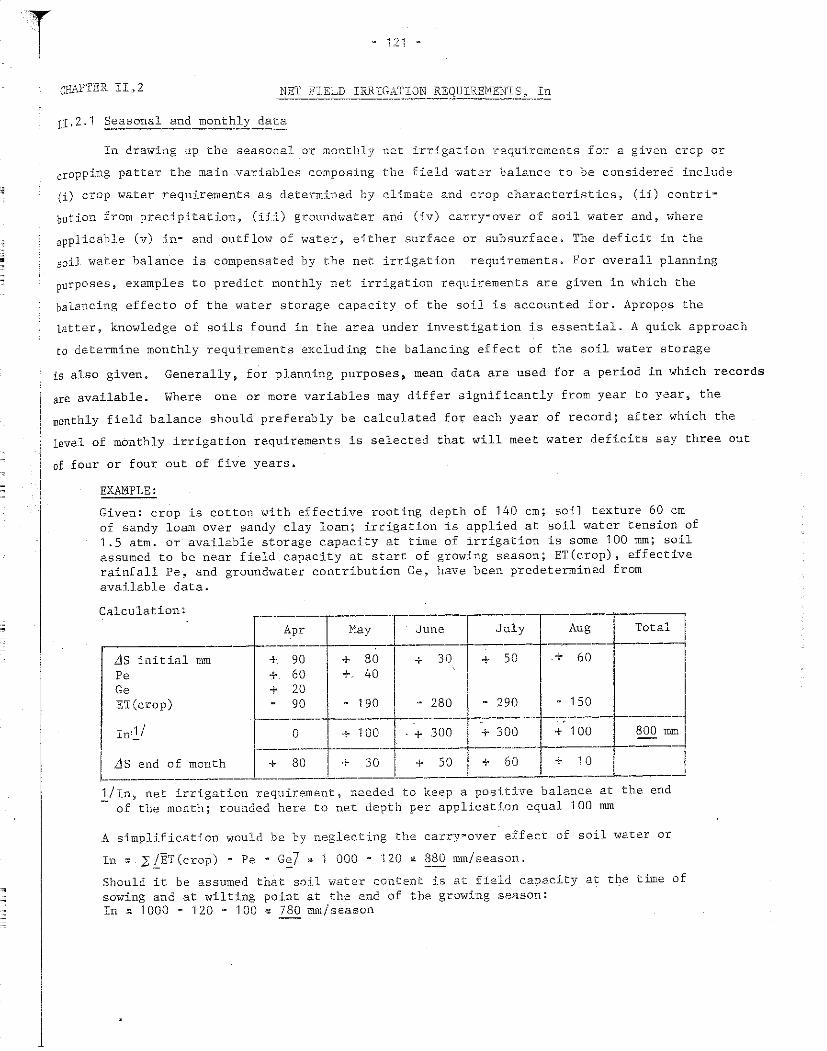
T i

cHAP'I'ER II" 2 _NET FIELD __ IRRIGA'I'ION REQUIREMEŅTS ..:~-~~

īn drawing up the seasonal or monthly ne1: irrigation re.quirements for a given crop or

cropping patter the main variables composing the field water balance to be considered include

(i) crop water requirements as determined by climate and c.rop characteristics ~ (ii) contri

bution from precipitation, (iii) groundwater and (iv) carry-over of soil water and, where

applicable (v) in- and outflow of water, either surface or subsurface. The deficit in the

soil water balance is compensated by the net irrigation requirements, For overall planning

purposes, examples to predict monthly net irrigation requirements are given in which the

balancing effecto of the water storage capacity of the soil is accounted for. Apropos the

latter, knowledge of soils found in the area under investigation is essential. A quick approach

to deterrnine monthly requirements excluding the balancing effect of the soil water storage

is a1so given. Generally, for planning purposes~ mean data are used for a period in which records

are available. Where one or more variable.s may differ significantly from year to ycar, the

monthly field balance should preferably be calculated for each ycar of record; after which the

i level of monthly irrigation requirements is selected that will meet water deficits say three aut

of follr or four out of five years.

EXAMPLE:

Given: crop is cotton with effective rooting depth of 140 cm; soil texture 60 cm of sandy loam over sandy clay loam; irrigation is applied at soil water tension of 1 .5 atm. or available storage capacity at time of irrigation is some 100 mm; soil assumed to be near field capacity at start of growing season; ET(crop), effective rainfall Pe, aud groundwater contribution Ge, have been predetermined from available <lata.

Calculation:

Lls initial mm Pe Ge ET(crop)

Apr

+ 90 + 60 + 20

90

~ Ma;~:0une ~ + 80 + 30 +. 40

- 190 - 280

July

+ 50

- 290

Aug

.+ 60

- 150 ---·---·. _____ T _____ --------- ...,..---

Total

800 mm In 1 / 0 1 - 100 + 300 + + 300 + 100 -------r-------l------- -------- ---·

l_:~--~~~~~-:~nt~---~-80 __ L_~_ 30 _L_::_:_o_l _~-~~--1-~~~-2_/In, net irrigation requirement~ needed to keep a positive balance

of the month; rounded here to net de-pth per applicat1on equal 100

at the end mm

A simplification would be by neglecting the car-.ry"'over effect of soil water ar

In , 1: ļĪĪT (crop) - Pe • Ge7 " 1 000 - 120 • 880 mm/ season.

Should it be assumed that soil ·water conte.nt is at field capacity at the tirne of sowing and at wilting point at the end of the growing season: In a 1000 - 120 • 100 , 780 mm/season

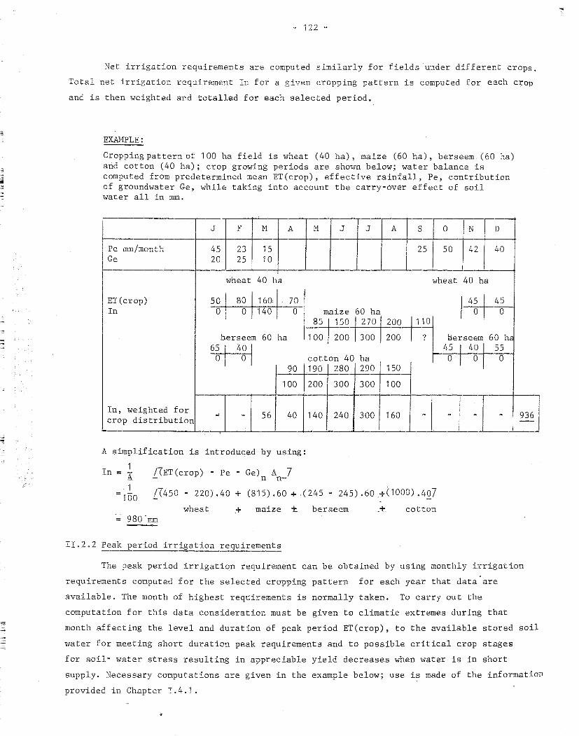
- 'i 22 ~

Net irrigation requirements are computed similarly for fields under different crops,

Total net irrigation requirernent In for a given cropping pattern is computed for each crop

and is then weighted aud totalled for each selected period.

EXAMPLE:

Cropping pattern of 100 ha field is wheat (40 ha), maize (60 ha), berseem (60 ha) aud cotton (40 ha); crop growing periods are shown below; water balance is computed from predetermined mean ET(crop), effective rainfall, Pe, contribution of groundwater Ge, while taking into account the carry-over effect of soil water all in mm.

Pe mm/month Ge

ET (crop) In

wheat 40 ha

:?.2 1 80 1 160 1 7 Q_ o!ofīZi°!o

.berseem

~~~ 60 ha

90

100

wheat 40 ha

1

4.u_ 45 maize 60 ha -0 1 0

8 :?..ļ.1_ 5 0 -Uz.QD_Q_Q__V_ ,, 100 / 200 1 300 1 200 / ? lJerseem 60 h

1,5 f 4.;Ll_ 55 cotton 40 ha O -0 / 0 190 280 29tl!50

200 300 3001100

!~~-Pw_~_~_!_~!-~_~_u_!_~--~-n~J -I5_:~_.4_0_,__1_4_o~.240 30~ 160 ~ī- : -I~:2] A simplification is introduced by using:

1 In = -

A ļ(ET(crop) - Pe - Ge) A 7 n n-1

100 /(450 - 220) .40 + (815) .60 ... (245 • 245) .60 +(1000) .4_Q7

wheat _+ maize t berseem cotton = 980 ·mm

II.2.2 Peak period irrigation requirements

The peak period irrigation requirement can be obtained by using monthly irrigation

requirements computed for the selected cropping pattern for each year that data0

are

available. The month of highest requirements is normally taken. To carry aut the

computation for this <lata consideration must be given to climatic extremes during that

month affecting the level and duration of peak period ET(crop), to the available stored soil

water for meeting short duration peak requirements and to possible critical crop stages

for soilwater stress resulting in appreciable yield decreases when water is in short

supply. Necessary computations are given in the example below; use i~ made of the information

provided in Chapter I. 4. 1 .

~.~ ..•. · .... ·.• •. ····

~ - 123 -

EXAMPLE:

Given: crops include maize) mid May to end September, and cotton, early April to half September; acreages are respectively 60 and 40 ha. Maximum mean monthly ET(crop) in July is 280 and 288 mm ar 9.0 and 9.3 mm/day; available soil water storage is 100 mm for both crops; climate is semi·arid with predominantly clear weather conditions.

Calculation: using Fig. 11 of Chapter I.4.1 for given climate and depth of available soil water the ratio between mean peak ET(crop) and mean monthly ET(crop)is 1 .075 or ET(maize) 9.7 mm/day and ET(cotton) = 10 mm/day. Weighted peak period ET(crop) = (9.7 x 0.6) + (10 x 0.4) = 9.8 mm/day

"

~ 124 "'

CHAPTER II.3 GROSS FIELD _ IRRIGATION REQUIREMENTS, If

II.3,1 Irrigation application_efficiency,_Ea

To account for avoidable and unavoidable inefficiencies in water application, net

irrigation requirement_'l In, needs to be increased by the irrigation application efficiency Ea, or

1 If = In x -

Ea (or = In x 2.1212 )

Ea

·where If is the gross field irrigation requirement; Ea is commorily expressed in fraction

(Or percentage) and is the ratio between the amount of water actually stored in the root zone

directly available to the crop and the total amount of water applied to the field.

EXAi.'!PLE:

Given: single crop, cotton; <lata are derived according to Chapter II.2.

-------ŗ---- i -------

--l'" May June July Aug ' Total ----- ---- --- -------

In mm 0 100 300 300 100

Ea fraction .55 .65 .60 .55

l __ -__ : --- ---- ------

If 180 460 500 180 1 320 mm _____ 1 ____ ---- ---- ------

A simplification is by using:

If = 1:/ET(crop) - Pe - Ge7 = 880 Ea

100 X -60 1 470 mm/season

Gross field irrigation requirement is directly related to irrigation application

efficiency Ea which is the fraction of applied irrigation water that is stored in the soil

and available to the crop. Low efficiencies will occur when depth of wateŗ applied is in

excess of the amount that can be stored in the root zone at time of irrigation and the

excess water is lost by deep drainage. When the rate of application is in excess of the soil

infiltration rate, appreciable run""off and tail"'losses will retmlt. Uneven distribution of

water applied will normally cause drainage losses in one part and possible under-irrigation

in the remaining part of the field.

Apart from avoidable losses due to field layciut and water application incfficiencies·,

there are unavoidable losses. These include deep percolation of stored soil water after

attainment of field capacity, losses by evaporation from the soil surface and, for sprinkler

irrigation, evaporation losses from the spray. Complete uniformity of water application over

a field is hard to obtain. -Also ~ sudden ·cain may upset pre-determined irrigation s~hedules and

will result in a lower percentage of water being applied that is stored in the root zone.

Attairnnent of 100 percent irrigation efficiency can therefore never be reached.

However, on average, in mast schemes irrigation application efficiency does not exceed

0.60 particularly in the early years of the project; much lower efficiencies are frequently

found. Some variation over season may be noted with higher efficiencies during peak

requirement periods and lower efficiency in the early and late crop seasons.

1 l

or

• :

c, 125 -

Data on field irrigation application efficiency is of the utmost importance but is at

the same time difficult to estimate. When estimations are too high it results in water

deficiencies during average rainfall years and during peak water use periods in mast years,

and in too low irrigation system capacities. When estimated too low~ the result is a reduction

in size of the area that c.an be iŗrigated~ overcapacity of the irrigation system and probably

wasteful irrigation practices. However, the former is more commonly the case.

Some indicative <lata on field irrigation efficiencies are given as they could be

considered to apply to a well designed layout, well levelled fields aud to optimum irrigation

practices achieved after the scherne has been in operation for many years. (See tables 38 and 39)

Table 38 FIELD APPLICATION EFFICIENCY FOR METHOD OF IRRIGATION -----

Graded borders Basin and level borders Contour ditch Furrows Corrugations Subsurface Sprinkler~ hot dry climate

moderate climate humid and cool

Rice

r US(SCS)

0.60-75 .60 80 ,50 - 55 .55 - 70 .50 • 70 up to .80 .60

.80

---- 1/ ---ICID o."58

,53

,57

.67

.32 l .70

-----------------·-------Sou_~ 1 / M.G. Bos and J. Nugteren Ir-rigation efficency in small,farm areas.

ICID 1974 or Publication No,. 'i 9, International Institute ·for Land Reclamation and Improvement, Wageningen 1974

Table 39 IRRIGATīON APPLICATION LOSSES AS FRACTION OF WATER APPLIED AND FIELD APPLICATION EFFICIENCY FOR DIFFERENT SOIL CONDITIONS

1-- _ ~--. -------··---·-·---light-T medium -- heavy text:;-e---1

'I Farrn late~al losses, unUned ltl O. 15 , 10 · 05 1 Surface runoff loss .05 .10 .25 Deep percolai:ion loss , 35 1 • 15 ° 10 ' --- -------------·-·----- -------r--------- ----------

!' Field irrigation efficiency .45 l .65 .60 L-----------------·--------'------ ----- 1 ----------

.Sou rce : U SDA

Evaporation losses from the soil Surface run~aff losses Drainage losEes, except porous soils Field ditch lcsses Field application efficiency, common

1 farm c.rops

ļ---;;-:m-per irrigation--1.

1 0. 1 1 o-o .s

0.03-0,3 per km

!_ Field application efficiency, fruit crops·I 1 Average field application efficiencyj

L:~rg~proje~ts --------------

0.2-0,5 0.35•0„7

0.3-0.5

Source: Houk (1951)

•

II, 3, 2 Othe·r t.vater.~.".needs including lea_c.iing :.::"squir 2ments

Some conside.ration should be given to t:he nesd for water applications for purposes

other than just crop water requirements. Water is needed fm: cultural practices 1:.vhich are

1:Lnked to specific requirements of certain crcps. The fulfilling of these water needs can

often be considered asa bonus feature. of irrigation; but they are also mast desirable even

if no irrigation is required for crop g:rowth. To improve the yield and its quality water may

be needed for such specific reasons as an aid to germination, land preparation~ frost

protection, maintenance of crispness of some fresh vegetables, control of certain insects

and pe.sts, control of te.mperature and humidity ~ and for dissolving fertilizers, Post harvest

irrigation is sometimes practised; for example after harvesting groundnuts co induce

germination of any nuts left behind so that they can be removed easily from the fields. One

other important aspect is the leaching of salts from the root zone.

Except for the last reason, generally no allowance is made during planning for these

extra water needs~ which may have important local significance in certain cases. Except

for salt leaching, which should always be considered in total irrigation requirements, sorne of

these specific demands may also be taken into account when determining irrigation schedules

in existing projects.

The level of soil salinity is affected mainly by irrigation, effective rainfall and

leaching practices. Salinity varies during the growing season; salts accumulate in the soil

profile as the season advances. Leaching of the accumulated salts can be programmed to take

place during, before or after the g:rowing season depending on available water~ the efficiency

of irrigation 1 leaching practices and the yield reduction the grower will accept due to the

accumula.tion of salts. The effect of salts can be appreciably decreased by maintaining soil

water in the root zone in the upper range of availability. Approximate data on upper limits

of soil salinity levels for different crops are given in Table 4-0 3 whe.re salinity is

expressed in electrical conductivity (rnmhos/cm) of the soil saturation extract.

Table 40 APPROXIMATE VALDES OF SALINITY LEVELS FOR DIFFERENT CROPS

ASSUMING so% DECREASE IN "'tIELD

~ ECe - _'' mmhos _____ 1 ________ 4 - 10 ---·-·---- i ___ 1 0------~

1 Pear Peas ! Fig Corn (maiz.e) ! Date j : ' . l ! ! 1 Apple Beans ) Oats Flax Barley l 1 Orange Sugarcane I Grape Potato Sugarbeet

1

' 1

::::e _111 Apricot

L

'fri/heat

Tomato

Alfalfa

Source: Handbook 60~ US salinity Laboratory

Ca.rrot Cotton

Onion ! 1

Sp:tnach

' ' L _________ J Cucumber

l

:

l

The yearly leac„hing ·cequircment can; in a first approximation~ be rs:~2.t2d

quality of the irrigation water to be used and the quality of the drainage ,.-vat.2.r tc.lerat:ed

by the crop at the bottom of the root zone. Using the quality of the drainage water to be

tolerated as 4~ 8, 12 and 16 mmhos~ the leaching requirement (LR) is then given

asa percentage of the total amount for the various qualities of irrigation water, using

the formula:

LR: :~!:r X 100

quality of irrigation and drainage water is given as electrical conductivity in mmhos/cm.

Examples are given in Table 41.

Table 41 LEACHING REQUIREMENTS IN PERCENTAGE FOR DIFFERENT SALINITY LEVELS

OF IRRIGATION (ECirr) AND DRAINAGE WATER (ECdw) IN mmhos/cm

0.75

2.25

s.o

20

60

_______ _J__ __

1 0

30

60

6

20

40

5

15

3g

For preliminary planning, the prediction of yearly water demand (If) including need

for leaching water can be made by:

If ·..; ET(crop) - Pe --1--=-ī:R___ Ea

where LR is the annual leaching requirement in fraction and Pe is effective rainfall.

The above predict::Lon method fo:r annual leaching requirements does not account for

the effect of the type of salts on plant growth, type of soil~ and restrictive drainage

conditions., Also~ the va·.;::-iat:l..on :i..n salinity l2ve.l of the soil during the growing season is

not. ·re:flecte.d., ·No consideration is given to the. method of leaching ~ i, e. inte.rmittent or

continuous, In addition~ the leaching r2quirement3 are relate.d to the entire root zone

although crops can perform well 1..mde.r ccnditions ,;,.-;here. part of the root zone only has a

high salt content,

For detailed evaluations 1 incJ..uding monthly leaching requirements as related to

salt tolerance levels during various stages of crop growth and appropriate leaching practices

to be followed~ there are many sources of reference.J/

ļTFAO/Unesco International Sourcebook on .Irri.gation and Drainage of Arid Lands. FAO/Unesco 1973; Hagan et al., Irrigation of Agri::ultural Lands, 196 7; Salinity Laboratory Handbook No.-60; FAO Irrigation and Drainage Paper No, 7 ~ Salinity Seminar, Baghdad (1972); Unesco~ Final Report of the GRUESI Project, 'I\misia~ 1971~

-; .28 "

CHAPTER II. l} FIELD IRRIGATION SCHEDULING

Depth and frequency of irrigation should conform to the soil replenishment (~r:i.teria

for a given crop 1 soil and climate. Water scheduling, in depth and time~ must be carefully

determined throughout the crop season to avoid any decrease in crop yield due to soil water

shortage. At the planning stage only approximate rules on irrigation application scheduling

can be given. Refinements to water application scheduling will be required after projects have

been constructed and been in operation for some time.

Depth and frequency of irrigation will vary with crop, soil, ET(crop), type of harvested

yield and level of manag~ment and these are shown in qualitative terms in the next Table.

Table 42 QUALITATIVE NORMS ON FREQUENCY AND DEPTH OF IRRIGATION APPLICATION IN RELATION TO

CROP, SOIL, CLIMATE, TYPE OF HARVESTED YIELD, AND LEVEL OF MANAGEMENT

1 Long in terval and great depth Factor Short interval and small depth

rneep rooted, dense --------1--;la:-t- Slow growing and shallow rooted 1 ~hick, hairy, waxy leaves Complete ground cover

Low crop factor (kc) Broad flat leaves Low percentage of ground cover Main growth during hot dry periods Early closing of stornata and wilting Drought sensitive period Main growth during winter periods High crop factor (kc) Accept high soil water depletion rates Requiring high level of soil water Srnooth crop surface throughout

Medium to heavy textured Deep, wellstructured High water holding capacity Non-saline High groundwater table of good quality

Soil

High--yielding variety High population density Rough crop surface

Light textured Shallow, poor structure Impervious layers, hardpans Low water holding capacity Poor aeration Saline-alkaline Slow infiltration rate 1 soil crust Root pests and disease Poor soil fertility

-- '--·--··.-=-=~·-··=-- =-·-=-,=~=--·-··- .. =,.·--·-=-=•- ··--Low ETo I Weather I High Eto

~~~~~;n~a~:!nfall, well distribut,::d

1

1 :!!:c~~~~y vari.ation in ETo

Closed smooth crop su-rface I No rainfall

__ .-~- _ .. ----~----------·-· _-,==,,~!ŗ -- .. ----·--t Low so:i.l._ t .. emperatu,. __ ·es d~ring·-~earl:·,··· g:rowth

Optimum_ yields I

P:::·'.Jduct High wate:i:- use/cro-p proctuction I"ē1.·t:.1.u 1 Dry weight yields j Maximum vegetative yields !

, ~ Fresh weight yield 1 J High quality of harvested y:lelcl .J1

Large contin':-ous fields ------ [Ifu'!.1agem12.n.t ~mal1. int:rspersed fields __ .. ---.--,.,~·-···

Dormancy periods 1 - - · ! Planting Just before hot d:ry season 1

Good land preparation Foo-:r irr:Lg:;:1:t:ion methcds 2nd. prCH'r-,"c"' il

Well designed field ir:dgsrtion I f

L dist r ibut io~- sys tem --~"- ~, ______ [ ·-_____ ___ j_~----·-------~ ,~-·-",,--"···-.. -·------~-----·--·c

~ . l 1

Dep t.h_ o f irrigation

Depth cf irr:i_gati_on .is the amount of soil water that san be stored between so-~called

field capacity .s.n.d, for the. given c:cop ~ the selected maximum soil water tension or avai1able

soil water depJ.etion. Data on type of soil and its available soil water storage capac.ity

should be collected at site. An approximation of the water content at field capacity can be

made using the data given in Chapter I.4.2~ Selection of the maximum allowable soil water

tension aud corresponding level of available soil water depletion should be based on crop and

soil <lata discussed in Chapter I.4.5. Depth of application (d) will vary over the growing

season and for a given crop and crop phase can be determined by d: (Sfc - Si)D where Sfc and

Si are soil water content in volume percentage at field capacity and just before irrigation

and D is rooting depth. To find gross depth of application the irrigation application

efficiency should be accounted for.

EXAMPLE:

Cotton, 4th growing month, effective rooting 140 cm soil is sandy clay loam, Sfc = 14 volw~, Si = 7 vol foJapplication efficiency is 0.65„ d = (0.14 • 0.07) 140 = 9.8cm = 98 mm Gross depth of application is d./EA • 98/0 .65 = 150 mm

If too little water is applied and the rooting depth is not kept pennanently moistj

the soil volume from which plants can draw water and nutrients will be reduced. When water

applications are too light the risk of depressing yields is greatly increased. Under-irri

gation will result in the onset of soil water stress sooner particularly when the subsoil

layers are dry. The detrimental effect on crop growth and yields cannot be overcome by

increasi.ng the depth of water in later applications. Water applied in excess of the amount

that can be stored in the root zone will be lost through deep percolation aud ruņ.-off.

II.4.2 Irrigation interval

Correct timing and regularity of water application are quite as important as the total

seasonal amount of water applied to the field. Too frequent irrigation even though the

amount applied correctly equals soil water depletion, will re.duce water use efficiency mainly

by increasing conveyance and app.lication losses. Delayed irr:Ļgation~ particularly during

the periods when the plant is sensitive to soil water stress 0 can have a considerable

negat:Lve. effect on crop yie.lds~ even though the tota1 arnount of seasonal water application

is about the same.

By e~~c1uding the car1::-y=over effect of the so:Ll water ,:·r.:oservoir, first estimates on

irrigation interval (i) ca.n be. obtained fot· n given crop ahd growing phase by:

i ""

EXAMPLE:

cotton, 4th growing month~ effe.ctive ;::-ooting depth 140 cm, Sfc :t:i"14 vold/o ~ Si ~ 7 vol1o ~ ET(c.rop) is 280 mm/month~ Pe is 30 mm/month i (0.14 • 0.07) 1 400. 12 days

(280 = 30)/30

•

-

.. i JO .-~

ET(crop) varies considerably during the growing season even if climatic conditions do

not change; also the depth of soil from which water is abstracted by the crop will vary

particularly during the early growth stages. Mast crops have specific requirements during

different stages of growth. Also, the amount of soil water available to maintain ET(crop) at

the predicted valu_e will vary with evaporative demand of the air (Chapter I.4.2). Therefore,

rather than basing irrigation applications on the calendar or on fixed schedules, considerable

flexibility in time and depth of irrigation applications should be maintained to accommodate

distinct differences in crop water needs over a period of time. These considerations are

often omitted in overall planning. Such <lata, however, must be available before a detailed

field design and preliminary field irrigation schedules for a new scheme are developed.

II.4.3 Ir:::igation frequency

Irrigation application schedules can be predicted at the planning stage from the

monthly field water balance an~ by selecting from available crop and soil date maximum

level of available soil water depletion. An example to develop the necessary data from

available information is given below for a barley crop followed by potatoes9 The example

clearly reflects differences in both frequency and depth of irrigation application and is

mostly due to var:lations in rooting depth and maximum level of availabl~ soil water depletion

for the two crops.

EXAMPLE:

Soil: Soil depth ),-130 cm; soil texture is loam; available soil water at soil water tension of 0.2 atm (field capacity) is 20 vol%, at 0.5 atm is 14 vol 'fo, at 1.2 atm is 9 vol1o; at 16 atm (wilting point) is O volaJo.

Crops: barley, sown in February, harvested in June followed by potatoes from July to October. Barley:effective rooting depth at mature ģrowth 120 cm; irrigation is applied at soil water tension of 1.2 atm; depth of available water between field capacity and 1 . 2 atm is 1200 x 11 = 130 mm. Potatoes: effective rooting depth 60 cm; irrigation at 0.5 atm; available soil water 35 mm.

Climate: winter rains with residua1 so11. water available at beginning of season; little rain during crop season; ET(crop) is predicted from available climate records. Effective rainfall is calculated with selected reliability of 3 years out of 4.

Groundwate.r: groundwater table is at 2 m early in the year; surface and subsur'face in and outflow is negligibly small; dee.p -percolation is assumed to be balanced by difference. between net and gross irrigation requirements.

T

'

--

= 1 31 ~·

-------------------F A l1 J

ŗ----~----~~

1 Pre-irriga tion

1 Lls ini tial

rainfall

groundwater

ET(crop)

--- --

+ 70 + 50 - 5 -125 - 260· __ ,

Pe +_20 ;, 10

Ge + 20 -+_ 10

-60 -75 -120 -135 - 70

}', -! ~:.:: ;:{·,:.J? ~: : .. . ....... , .... . '> C t :: C ,:: '--'

"'., - - - " ---

::.;~ :'. :: ·;::: .. , ----

.. ,... -·-·-·-· ''": .. ::-;::·---

. :: ::. ::::: --- --------

-

,.:; ::: ;:::: ....

: - -

net depth of irr. 130 100 130

1 1

1 irr.fficiency .60 .60 .60

ļ eross irr.req, 215 165 215

L ____________ "-+----------------......1

"

1

J A S O 1

-------------~-i --~~-- -55 -175 "310 1

+ 30 + 45 1

-90 -120 -165 -120

'

•

?.:1,RT III CALCULATION OF IRRIGATION SUPPLY, Vs

:čNTRODUCTION

Calculation of project irrigation supply is needed to quantifv project acreage and to

Jetermine diversion requirements from river flow, abstraction from groundwater aquifers and

to establish reservoir op~ration. For preliminary planning, irrigation supply frorn available

:,rater resources is determined primarily by project area, cropping pattern and intensity and

:trrigation requirernents over time. Supply is expressed in flow per time unit (m3 /month or

)r 1/sec or a given period).

Calculation of irrigation supply to the individual field is needed to plan field irriga~

~:ion schedules and operation of conveyance and distribution systems. Main variables deter ..

<'.Üning the irrigation supply to the field are depth and frequency of soil"'water replenish

E1ent for a given soil and crop 1 soil intake rate~ method of irrigation and size of field.

Field supply is expressed in flow per time unit (1/sec),

The calculation of irrigation supply should be preceded by a detailed study on cropping

pattern and intensity for the proposed project. Apart from ~ater required and water avail~

able at source, pertinent social~ financial and economic aspects need evaluation before the

final selection of crops to be grown can be made. This should include economic returns per

unit of water in terms of production and the economic viability as well as secondary and

intangible benefits of the proposed project.

The procedure generally followed in quantifying project and field supplies is first, ·to

prepare a preliminary layout of the scheme and next to deterrnine the area distribution of

crops to be grown and the cropping intensity. This will also include consideration of the

si.ze and shape of cornrnanded areas, water level and flow control and the spec.ific provisions

to be made such as location and size of main canals and number, type and size of structures

n0:eded, Preliminary estimates of total project supply can be based on monthly irrigation

requirement <lata for the cropping pattern and intensity selected.

The next step is more detailed field layout an·d for this consideration mu.st be giv.en

to such aspects as land ownership and natural boundaries~ land slope~ need for land prepara=

tion including leve.lling~ crops to be. grmm and method of irrigatiori. Once the size of fields,

c.ropping pattern and method of irrigation have been selecte.d~ the field irrigation supply in

,11.1antity over time can be determined, After selecting the method of water deliverY ~ continuousi

T'Otation~ demand = the developed <lata are in turn incorporated in the supply schedules of

the project. When determining the necessary suppl.y 9 the project efficiency in meeting field

irrigation requirements must be predicted"

•

us,

- 133 -

Each phasc <)f projec,: planning will require a specific type and accuracy of · data on

irrigāt-iofl supply. - This :ts sho,,vn in Table 43,, :ī.;: is obvious that~ at the planning stage,

no accurate evaluation of futur2 p'!'oject cperation and water scheduling can be given unless

pilot proj ects have been started previously and have been in operation for a number of yea!'s.

Even then~ an allowance should be incorporated in the supply to account for any- changes in

cropping pattern and intensity but at the same time avoiding any quantity in excess of

realistic requirements.

Data for detailed water schedul.ing will still be required after projects have been

constructed and been in operation for smņe time~ Field studies should still be continued

after the project ·has been completed to ensure an acc~ptable level of water use efficiency

at the field level and to arrive at irrigation supply schedules which adequately meet the

irrigation requirements of the crops grown. An effective organizational framework is

essential to im.p·lement irrigation scheduling and to opera te schemes.

A large number of approaches have been developed for the planning of optimum water use

in crop production. Although discussions here are centered around the development of basie

<lata on crop i;vater requirements and the necessary irrigation supplies only, it is apparent

that for planning irrigated agricultural production numerous additional parameters will

need consideration.


To determine Scheme and field supplies for the planning and operation of irrigationJ

projects require the following data and to obtain it a procedure is suggesteda Determine:

1. The preliminary seasonal project supply for the selected cropping pattern,

cropping intensity, level of supply efficiency of the distribution systems

and project size;

2. f"or the month of highest demand, the preliminary peak project supply for the

selected cropping pattern and intensity~ level of supply and flexibility

f ac tor ~ ef f iciency of the distribu tion sys tem and proj ec t siz.a;

3. following preparation of the project systern layout, preliminary project

supply schedules; assess reJ..ation between supply and area served; select

method of water delivery - continuous ~ rotation~ demand;

4" the field irrigation supply for the given soil and crop, depth and me.thod of

irrigation; evaluate field supply schedules in quantity over time; prepare

5"

water supply schedules;

following project implementation~ the detailed supply schedules through

field monitoring and applied research; revL2w projec.t organizational

framework.

•

?H.ASES OF PROJECT PL.A.1.'\/NING AND TYPE OF WATER SUPPLY DATA NEEDED

Data required ---,

1

' --J r~ase 1 --------- Data applicati.on -·

! Reconnaissance j ~ present hydrologic budget Average seasonal wace.r 1

11 1,,. identification of i.rrigab:::..e areas supply ' 1

l -!--------------------·--·-·-------- :-------------------.! 1

! Proje.ct ! .. 1ocation _of project ! Seasonal supply of i

! identification 1 ! m~in crops ' i ! ... se.lection o:f irrigabl2. a.rea~ project size, 1

1 preliminary dr::termination of main works j

f i ~ predictcd water demand j

' 1 1 L_______ ! .. predic~-~~~uture hyd:r.~ol~gic budget--------+- _j

I., "'l' ' ct' ' ' ,. f ' ' • i M ·b1 10 cl. t t J ! ..:easiui ity 1 ~ e;..ermirraLJ.on o~· pro.1ecc size I onr .~y or =- ay ·o· a _ s tudv 11

1 .supoly

. 1- ~~~~~~:~!:e a~:o~;:~!: for water supply j Mo~~hly peak supply

11!

1 : ::::::::: :;•:::::fo, seCCssss 1

1 1

_ optimization of scherne water distribut:Lon

sizing and costi.ng of main engineering

ļ I works f f

1- phasing of proj ect development j __ J Detailed project design

Project implementation

l - final design of distribution system 11

. 5,- to 10-day peaK. ---jl i j supply '1 network and hydraulic. structure

de:tailed cropping pattern 1 1

... detailed delivery schedules ! J

j - irrigation methods and practices -------k . --·----' review of scheme w.s.ter scheduling i 5 ... to 1 O··day peak

1

l '· t neec's I supply ī - c 1.e.c". on crop wa er 1

ļ ... evaluation of wate.r application methods i 5- to 1 O„day water 1 1' · 1 1 1

- · "f, · -, · oa ance . ·· water use e.1. ·1c1ency stuc.ies l ! L- 1 -- .t-------------1 / Project l = monitoring of field wate.r balances Water budget in farmer's j'

I! operation · field l "' detai1ed operation scheduling J

11 - l training of farmers in water application ! 1 i and scheduling _I 1 i

L-------' --------------·----

•

cBAPTER III. PRELLV1HīARY ESTIY1A1;'ES or SEAS~ AtD E'BAK PROSSCT IR8.I\;AT ION ------ SU?P'LY

In c:alculating seasonal and peak proj2ct irrigat:Lon supply, the main var:Lables include

the cropping pattern~ cropping intensity) project size., irrigation r,:=q1..dr12.ments9 level

of supply in terms of crop production and efficiency of the di.s-::::ribution system.

nr.1, 1 Cropping pattern and cropping_!ntensit.Y

For the proposed project 9 the selection of the cropping pattern and intensities is in

fluenced by many factors including suitability of climate and soil for various crops, the

return to the farmers, the preference and experience of the farmers} size and type of farms~

and such outside factors as market demands and market prices. :)2ta.iled studies w:Lll be

required to deterrnine the cropping pattern and intensities, Pertinent social, financial

and economic aspects will also Ileed studying and this should include economic returns per

unit of water in terms of production and economic viability and thr~ secondary and intangiblP

b~nefits of the proposed project.

When establishing a cropping pattern and intensities in tenns of an ensured water

supply the main aspec ts include:

a) In terms of water availability = meeting seasona1 and short duration peak period

irrigation requirernents by selecting cropping patterns that follow approximately the

same pattern as river flow, aquifer discharge by pu.mping 9 opera_tion of reservoir~ etc;

b) minimizing total irrigation requirements through optimum use of seasonal rainfall

and water stored in the soil from winter rains.Jby sele.cting crops with low seasonal

irrigation requirements, c.hoosing crop varieties with the possibility of shifting

sowing dates and shcrtening the growing season, applying special field practices,

such as transplanting rice, weeding~ using Ii1lptimurn field irrigation methods and

prac·cices,1 app1yin.g water needed fo:ŗ leaching salts at the end of the growing season,

and lining canals to reduce seepage losses~ etc;

c) in terms of supply capacities = reducing peak wa.ter deman.ds by avoiding peak r.equire

ments with periods o:E rainfall or lcw e.vaporative demand~ including dormancy periods

during times of high evaporativ,~ demand (alfalfa dm:ing hot summer months in North

AĪrica)~ avoiding double c.roppin.g prac.tic-es 1 etc.

D2cisions on c.ropping pa.tt,srn.s and intens::!.ties nrust be made at an early stage in project

planning. Cropping patterns and intensities for individual field.s will differ from those

proje.cts as a whole, In general cropping intensities o:f 100 percent are seldom ac.hieved over

an 2ntire project area and are often considerably lower.

Weighted figur.e.s on crop acreages can be. used when deriving total project supply

or irrigation mod1:-1-le..,,_

•

•

-

'0 136 -

III .1. 2 Level of supply

The criteria most commonly applied in determining project supply on irrigation

module are based on the principle of maximum supply to prevent the crop from suffering

water shortages. An acceptable level of supply to meet crop irrigation requirements is

normally established; this level is met in at .least x years out of 10, or in other words~

the probability that a water deficit will occur during a particular period is never greater

than (10 „ x) years. Planning is thus based on the risk approach whereby a set water sup~

ply or irrigation norm:. and the corresponding project size~ are linked to an ac.c.eptable level of

production. In most cases this approach is consistent with the achievement of maximum averall

productian during years of adequate water supply.

The risk approach has been commonly used until now for a number of reasons~ Not only

has the concept of risk become -qi.ore familiar to the irrigation engineer but also,usually few

factual <lata on crop production are available upon which to base the selection af optimum

use of the water resources. Furthermore 1 in methods and programmes developed in connection

with designs for operations and system engineering the risk approach can rnore easily be

applied because fewer variables are involvedĢ

The use o{ the risk approach in rnany irrigation projec.ts has resultecl in on„field

delivery being based on criteria in which the increase in product:ion asa result of an ad

ditional water supply is zeroj i.e. the amount of water supplied per ha will maximize yields

per ha irrigated. This standard might be acceptable where the water supply is abundant and

land is the limiting resource; but this is seldom the case. When water is limited in supply

and land resources are abundant the concept of optimization of production per unit area

versus water supplied may need to be pursued~ that is the amount of water supplied per ha

will have to maximize the yield per volume of water.

An engineer may be reluctant to follow the latter approach because a certain over=

supply is a safety valve against the unexpected. Slight chauges in giowing seasons or the

introduction of new varieties of different crops, which ar2 both determined mainly by outside

factors such as market demand, may upset carefully selected supply criteria, Moreover~ de~

tailed <lata on the level of supply and crop production are seldom available locally and the

transfer of <lata and supply criteria developed elsewhere will, in most cases, lead to erroneous

conclus ions.

No irrigation scheme functions fully and perfectly the day it becomes operational.

Water supply anct schectuling may need altering to match unexpected changes in production pat~

terns. Until any particular significant new facts or data on the optimum utilization of

water in the everchanging agricultural pattern become available~ the supply of the irrigation

project rnay need to be organized with the possibility of acconnnodating any future extension

of the irrigated area or the cultivation of profitable high water demanding crops should new

water resources beco~e available and economic aspects permit.

'

~ . 1

1

- D7 •

nr.1.J Distribution efficiency

'"!'o quantify the supply needed to rneet irrigation requirements at the field~ the effi

ciency of the distribution system must be determined. Distribution effic.iency, Ed, is de

fined as that portion of water released at the headworks and that received at the field inlet.

The main factors deciding distribution efficiency are method of wai:er deJ.ivery (continuous,

rotatior,_, demand), size of project area and effectiveness of management organization, Distri~

bution efficiency can be subdivided into conveyance efficiency 1 Fc, between headworks and

the inlet to a block of fields, and field ditch efficiency, Eb, between main canal and inlet

of an individual field. The supply in the main canal is continuous ar intermittent; the sup

ply in the field ditches within the block of fields served by the same canal is mostly on a

rotational basis. Distribution efficiency is obtained from Ed = Ec x Eb.

A recent study on irrigation efficiency in some 90 pro.iects in progress carried out by

ICIDļ/ provides the <lata in Table 44:

Table 44 DISTRIBUTION EFFICIENCY IN EXISTING PROJECTS

.--·------------------------------------------,

Conveyance Efficiency ~ Ec

Continoussupply with no substantial change in flow

Intermittent supply in projects of 3 000 ~ 7 000 ha and rotation areas of 70 = 300 ha~ with effective management

Large schemes ( > 10 000 ha) and small schemes ( < 1 000 ha) with respective pŗoblematic c.ommunication and less effect"" ive management

Field Ditch Efficiency 1 Eb

Blocks of 20 ha or more 1 unlined lin.ed or piped

Blocks of 1 = 20 ha„ unlined lined or piped

Source: ICID

Func.tion

0,9

0.8 0,85

0,5 0, 7

0.8 0.9 0.95

0.6 0.7

0.75 0.9

The distribution efficiency Ed of a rotational supply system under optimum conditions

including adequate project organization and C8mmunication was shown to average some 0.65.

Corrections to adjust distribution efficieny to quality of management and c.ornmunication pro„

posed were 1 "O for adequate, 0.85 for sufficient~ 0.60 for insufficient aud 0,50 for poor

management and c9mmunications and which need to be incorporated in estimating Ec and Eba

1/ M.G. Bos and J. Nugteren. Irrigation efficümcy in small farm areas, ICID, 1974, ar Publication No. 19~ Internationa].. Institut-e for Land Reclamation and Improvement

9 Wageningen, 1974.

•

-

~

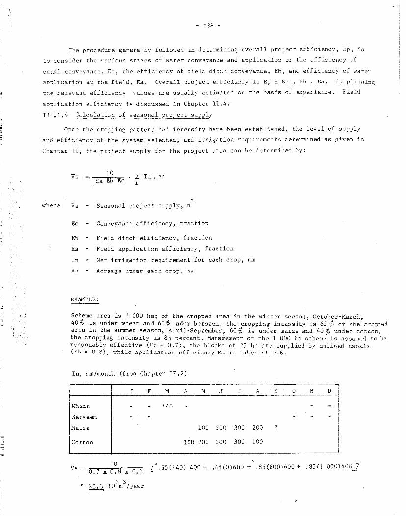
:::a

-

- 138 -

The procedure generally followed in determining overall project efficiency~ Ep, is

to consider the various stages of water conveyance and application ar the efficiency vf

canal conveyance, Ec, the efficiency of field ditch conveyance, Eb 3 and efficiency of water

application at the field, Ea. Overall project efficiency is Ep = Ec • Eb . Ea. In planning

the relevant efficiency values are usually estimated on the basis of experience. Field

application efficiency is discussed in Chapter II.4.

II1.1a4 Calculation of seasonal project supply

Once the cropping pattern and intensity have been established, the level of supply

and efficiency of the system selected, and irrigation requirements deterrnined as given in

Chapter II, the project supply for the project area can be <letermined by:

where

Vs

Vs

Ec

Eb

Ea

In

An

10 Ea Eb Ec

l:In.An i

3 Seasonal project supply, m

Conveyance efficiency, fraction

Field ditch efficiencyj fraction

Field application efficiency, fraction

Net irrigation requirement for each crop, mm

Acreage undEr each crop, ha

EXAMPLE:

Scheme area is 1 000 ha; of the cropped area in the winter season, October~March 40 '% is under wheat and 60 o/o under berseem, the cropping intensity is 65 rfo of the ~ c.rcrpps:::d area in the summer season, April„September, 60% is under maize and 40 % under cotto~~ the cropping intensity is 85 percent. Manaģement of the ·i 000 ha scheme. is assumed to be reasonably effective (Ec • 0.7), the blocks of 25 ha are supplied by unlined canals (Eb • 0.8), while application efficiency Ea is taken at 0.6.

īn~ mm/month (from Chapter II, 2)

J F M A M J J A s 0 N D l Wheat 140

f Berseem ! Maize 100 200 300 200 ?

Cotton 100 200 300 300 100

10 L ,65(140) 400 + ,65(0)600 + .85(800)600 + , 85 (1 000)400_7 Vs = 0,7 X o.s X 0,6

23,3 6 3

10 m /year

~ .·.1 ' - 1 39 -

Using weighted <lata for crop distributlon, weightecl irrigation requirement is multiplied by the project area taking into consideration the cropping intensity~ ar the scheme seasonal water supply (using <lata from Chapter II,2) is :

Vs= JO ( 56 l{ 0,65 + 880 X 0,85 J 1 000 0.7x0.8x0.6

23.3 106m3/year =

III„1 ~5. Calculation of peak project ~upply

The project supply should meet irrigation requirements throughout the whole growing

season. Preliminary peak project supply can be based on field irrigation re.quirements of

the month of highest demand or

where

Vsmax

Vsm@t

In peak

10 C. Ed Eb Ea Z In peak month An

Average daily peak supply, 3

m

Net irrigation requirements for each crop during month of highest demands, mm/day !1

An = Acreage under each crop~ ha

C = Flexibility factor

To incorporate flexibility of the delivery capacity, the derived value

of Vsma:x is normally increased by 10 %when the project area is greater than 2 000 ha.

This may be increased progressively wi th a decrease in acreage served and can be as high

as 100 %,when the projec t area is 50 ha or smaller,

EXAMPLE:

Same as before; ET(maiza) , July) is 280 mm and ET(cotton), July, is 288 mm or respectively 9,0 and 9.3 mm/da.y; depth of irrigation is 80 mm per application; peak periods ET(maize) and ET(cotton), Using Figure 11 Chapter I.4.1, at'e respectively 1.08 x 9,0 and 1.08 x 9.3 or 9.7 and 10.0 mm/day; area is 1 000 ha, cropping intensitv is 85 % , The correction factor assumed for the area of 1 000 ha ·1s 1~2; conveyance efficiencyj Ec, is 0.7j field ditch efficiency, Eb, is 098 and aDnlication efficiencv, Ea = 0.6.

Vsmax 10 1·

2 ' 0.7 . 0.8 . 0.6

[O .35 (9, 7) 600 + 0 .85 (1 O. O) 400] ~ JJO 000 m3/day

1/ Here ET(crop) and effective rainfall should ref1ect the peak period ir:. che month of highest demand; calculation of peak period ET(crop) and selection of dependable level of rainfall are given in Chapters I.4.1 an.d II.1.1i and in Chapter II.1.2 respectively.

•

= 140 =

III.1 .6 Project operational field: supply scheduling

An evalua tion of supply over a period of time v,1i.ll he ne(~ded for preliminary proj ec t

design. The classic method of deriving the supply for projects greater than 2 000 ha is to

co!lsider the layout of the main canal syst::.:m an<l ac:reages it is to serveo Each area served

will, for the given cropping pattern and intensity~ have its irrigation requirement (mm/month/ 3

ha) which will give an ļ ;acreage figure'' for the necessary supply (m /day) ~ The graphical

presentation of such a function - supply versus area serv1::od for eac.h lateral canal and totalled

for the main canal - is called the supply or capacity line. Many capacity lines are empirical.

For large irrigation projects 3 with irrigation hJ.ocks of 200 to 500 ha, a fixed flow is

normally delivered to the irrigation blocks, the size of flow being proportional to the acreage

irrigated, crops grown and cropping intensity. The water supply is then rotated amon)2: the

different fields or sections composing the irrigation block,

With any increase in crop diversification the scheduling of the supply to differ2nt

fields and blocks might become rather irregular; peak supplies for the crops grown might ocm

c.ur at different times for individual areas. An example is rice, where peak supply is mast

frequently determined by the water required for initial flooding, and

may need spreading over longer periods to avoid excessively h:Lgh peak

flooding of rice fields 1/ supply - , Ac tual

maximum scheme water supply, Vsmax, can thus diverge considerably from maximum supply figures

derived from weighted irrigation requirements of the month of highest demand. A detailed

evaluation of supply scheduling will need to be made fairly frequently and should be started

at the lowest irrigation unit or for an additional field and subsequently worked aut for

blocks of fields, for areas served by lateral canals and for total project area served by the

main canal.

Variations in irrigation requirements caused by acreage~ climate and time are difficul t

to meet if project scheduling up to the field inlet has been based on continuous supp1y as

is done in some rice schemes. Greater flexibility is obtained by rotating the supply among

individual fields and blocks of fields, provided rotation schedules are adjusted from time

to time to account for differences in crops and cropping i.ntensity and metereological condi=

tions. However~ in periods of low demand the supply may be interrupte.d~ i,e, the can.al may

be in oper:ation for only part of the time. This may have severe c"Ons2quences for instan.ce

in case of shallow rooted _crops grown on part of the project area requiring frequent light

irrigation, Large and frequent variations in supply can be attained by pr,"Jgrammed delivery,

In this case the cost of construction and opīer:ation of the sup1)1Y system may be high while

at the same time there should be adeq_uate control at the he.adworks and throughout the system

to regulate the flow.

ļj See for instance L.T. Chin, Ir:rigation 2.nd Drainage. Paper Nc„l'.'.\ F'AO, Rome, 1972.

•

,~ ·141 =

Variations in frequency and depth of irrigation are most easily met if supply is based

on a demand system. An efficient organizational framework and highly qualified project staff

are required to operate these costly systems which consist of many regulating and check

structures for the control of fluctuating disc·_1arges ļ/.

When preparing preliminary operation sch~dules for the canal system, the irrigation

blocks served by the same c-anal are frequently used as a uni t. To detennine the necessary

supply, the efficiency of the t:otal system, Ep: is then subdivided into conveyance efficiency,

Ec, and field efficiency, Ef. For a block of fields Ef is the product of field ditch effim

ciency, Eb, and field application efficiency, Ia. As discussed in Chapter III.2, Eb is

determined mainly by field size and field supp~Y with either a long or short delivery period

for the intermittent field supply; and similar]y, Ea is determined by the method of irriga•

ation and the soil type (Chapter II.4), Field supply and field application are very much

interrelated, i.e. by stream size per unit of erea and delivery period or by the method of

distribution within the block ~ continuous, ro1ational or on demand.

In Table 45 average field and conveyance =fficiencies are given for different methods

of water delivery, and their product is overallproject efficiency~ Ep. The <lata are obtained

from a recent ICID study on irrigation efficien:ies,

Table 45 AVERAGE FIELD AND CONVE'ANCE EFFICIENCY IN EXISTING īRRIGATION PROJECTS SUBlIVIDED INTO METHOD OF FIELD

DJLIVERY

ethod Ef Ec -~ ----Continuous block supply with small changes in steam size; paddy fields

Rotational supply based on predetermined schedub

Rotational supply based on advance request by fa"1Ilers

Supply on demand, supply by pipeline system unde pressure, sprinkler irrigation

Source: ICID

0.27 0.90

0.41 0.70

0.53 0.53

0. 70 0.73

1/ For a detailed description of methods of waer delivery including design criteria, reference is made to I. Nugteren, Irrigatiorand Drainage Paper No.13, FAO~ Rome, 1972.

0.25

0 .29

0.28

0.51

•

.:;

0·:o the i:rrig2.tic-n bloc.Iz fo1·

::\·om ,_,,eighted data on fre.q_u2ncy

an.d d-epe:h of i:::::·igE:.t:.tori. of the. m.ost importal!.t czops g:ro-.:,Ju i-n ·<:hat block, or from detailed

wat;.2;r schedulL1g flrog:ranmes fo·.r the differe;:.1.t crops) inclading the soil intake rate and

method of irrigation, The latter is discusseci in Chapter īII,2.

In the case of the former~ the sup-:;üy or :tr:t:Lga.tion module to the irrigation b.lock

can be obtained frmn

where: qf

A

d

A.d 3:ĪĪlI-

1

Supply to irrigation block 1 1/sr:c.

Mean ,.,alue of net depth of application~ mm

I Number of days allowed for compLstion of one irriga tion, or

so··called rotation int2rval

Ef Fie.ld efficiencyJ f1.'.'action

To increase the. flex.ibility and to accorn.t for higher water requirements, a flexibi"'

lit7 factor C) gr,2.ateT' than unity is sometime3 applied~ similar to the peak project supply.

In the case o:f a fixed sup-ply qf ,, the v::tlue of I will depend on whether the irrigation

block is supplied contim.wusly o:r intermittertly. In the latter case, the supply from the

lateral serving the irrigation block is rotared among the various irrigation blocks,,; This

is mainly determined by the layout of the caral system.,

Va.lues of A~ d~ and I wil1 vary throug1out the season. For each period qf can be det

t2rmined provided the va:ŗiables A, d and I a·e pred2termi0.ed for the different periods

within the growing season,

EX.iü"tPLE:

Irr:i.gatj_on block is īO ha; for a giveri period the net i::·.;:-igation interval (mean)

main erops c.n~ IILc:-üze and cotton deūtl• of i:cigation (mean) is 100 nim is 12 days; E:2 (L5D,

Supp1y to ir:ri;saticn block is continuorn; I 2.2 days

qf

qf

]Q X 100 X 1 s;-z;rx12 o:-;o

70 ~, 100

8, 41 X 4

X l

0,50

140 11sec

irriga ticn: blcck.s ~ /~,

.420 ./s2c -·----

(40f,); and

Aft:2r calculating qf for differ12.nt perods with1n ·i::he growing season, the necessary

supply over a period o:f ti:m.e to the ir'!:'iga ti·g block can be dete.rmined, The supply over a

time to r:he :Lndiv:i.dua1 blocks is totalled frn e.-s.ch :Later-9.l serving a number of blocks; sub„

sequently the sup-ply ove.r a time f:rom each lH:2·:-,ro'.l J.8 1-.:,,:~,;il':e,,; to obtain the project supply

over a time, This is of ten do·.t1.2 gTaphic.';!lly Tl".\2 operating rules for the canal

dist:ribn t:lon syst2m ean ti1.en be: dra.:tvn, up .,

'

CH.APTER IIL 2

mined by the depth of wa ter need;=!d tD

at whic.h wate.r can be applied or soil int:a,ke rate~ Tne:thod c:f i:::cigation~ and method cf

delivery.

III, 2, 1 Relation between '"_depth __ ·~,?i~., ·w:, t2T~~ rspļe·nishment and r3l!'.1?P~Z.

Water supply at the time of :Lrrig;:ttian for a given soi.l an.d c:rop~ expressed

in stream size qa (1/sec) and de1iv,';1r~, tim.e L".:!. Csec) 9 :.Cs ~

where

qata 10 Ea (Sfc = Si) . D • A

Ea = Field application 2ffi,:::i2ncy~ fraction

Sfc >::: Soil water c~;:ntent a.t iield capacity, volurne fraction

Si

D

Soil water cont8nt at time of irrlgation~ volurne fraction

Rooting depth ~ min

A = Area, ha

EXA1'1PLE:

Cottonj 4th month~ Sfc :Ls 14~Ji~ Si is 7%~ D

Ea =0,65%

140 cm~ A ~ 5 ha~

qata 10 o.'65

(0.14 „ 0~07) 1 400 ~ 5 ~ 3

7 .540 m

The rooting depth~ -Oi and the soJ_J_ wate.::r cont,~nt at the tirne of ir:r:tgaticn vary for

di:Efe:rent c.rops and fot each cr0p dc:.::':Lng th2 growing se.asOTL, Details about the selection of

D and Si va1ues are given in Cht1.pte·.r ! , 4, 2. and

To quantity str.e.am size, q.a) 1:;:.,.1d.

will enter the soil rnust be det.e:rm:Ln.:~:'.1 -. Int..'..".tk\8 r.e.ta.s: ,:,y:LLl ,_rary ·-:v'ith a30J.l texture and 3tx..·ucturc-:".

1/ s,ec. for an area of 1 ha ar.e. giv2-r1 i:t '.\'e'.:1-bl-e LH1

1 / Tl1e soil intake rats is not c.onstant .:rcr.e't' 2. v, .. _,_·-Jmr h-i:r;- dec.T.:eases as th.e crnil pro:tJ.1~ beccmes wet. The figures quoted l'e.:Ee:::· i:.;J ,;rve.·.E'flg© i:a.tm,k@ :rat:P-s ::::.s opposeci to initial and basie intake rate.Bp i,e. rBspectiv~:l] ,::'.t: -tJ,.,,.,,. ,J:ta:·;,; o:: 9.nd ·wh-2n t.he. :intak:2; ra.te h.ill.3 become more 0r less constant.

• :

~ 144 '"'

Table 46 APPROXIMATE RELATION BETWEEN SOII. TEXTURE, īNTAKE RATE AND STREAM SIZE

Soil Texture Int2ke Rate Stream Size mm/hr qa 1/sec/ha

1 Sand 50 140

(25 - 250)

Sandy loam 25 70

(15 - 7 5)

Loam 12.5 35 (8 - 20)

Clay Loam 8 22 (2, 5 - 15)

Silty clay 2„5 7 (0. 03 - 5)

Clay 5 14 (1 - 15)

EXAMPLE:

Cotton, 5 ha field, soil texture is loam, net depth of application is 100 mm, irrigation application e-fficiency is O. 65.

· qata = 7 540 3

m ; ta = 7 540

soooo xo:oITs 12 hr and qa = 7 540 ----12

625 3

m /hr or 175 1/sec

The stream size and deiivery time given in the example may be impractical.

Us~ally irrigction is spread over one or more days; other conditional aspects prevail

such as the quantity of water that can be handled by the irrigator, the number of plats

irrigated simultaneously, the method of irrigation and the capacity of the suppiy channel.

Basing the irrigation supply only on the intake rate of soils may lead to erronous supply

schedules.

III.2.3 RelaĻion between method of irrigation and stream size

a) Surface !E.E.igatio~

The stream size, qa in 1/sec, for a given field or block of fields will, apart from

the intake rate of the soil, depend on the method of irrigation, the stream size that can

be handled by the irrigator or irrigation crew and the number and size of furrows, borders

or basins irrigated siinultaneously. For spinkler :Lrrigation the stream size is furthermore

determinelf by the available. irrigation equipmenL

...... '

.. ·145 ·~

To attain uniform wate.r distribution over the field the rate of application will var:,

with the method of irrigation. In th2 c.ase of the basitl" (ar level border) method~ the stream

size to each border should be at least twice that required for the average soil intake rate;

0 r the water should be applied between 0.2 and 0.4 of the time necessary for the required

depth of water to enter the soil. In the case of furrow and border irrigation on sloping

landsJ the soil takes the wat.er when the soil surface is covered with flowing water. The

stream size per furrow and border should be large enough to reach the end of the run in the

desired time and small enough to be non=erosive, and· should not cause extensive flooding

or tai.l losses. The size of the stream must be adjusted to the length of the run, land slope,

erosion hazards, shape of the flow channel, soil infiltration rate and the water depth to

be applied.

Field trials on layout and irrigation practices are required to determine optimum

values of stream size qa and delivery time ta. Such physical <lata must be available at

the design stage of the project.

For easy reference, the strearn size in 11sec for a suggested size ar le.ngth of fieJ.d

under basin, border and furrow irrigation is given in Tables 47, 48 and 49. The size and

length of the field is primarily determined by the soil type and land slope. Stream size

is based on the intake rate of the soil and erosion control. Since, during irrigation ap·

plication, the intake rate of the soil changes with time, the stream size into the border

ar furrow is often reduced after an initial period of wetting. The stream size in the

supply canal is normally constant; sufficient flexibility can be maintained by regulating

the depth of application through controlling the inflow to each border or furrow, varying

the nurnber of borders and basins served simultaneously and by lengthening or shortening the

delivery time, ta. In the case of sprinkler irrigation, the strearn size is Pased on the

minimum intake rate of the soil over the total tim"e of application and on the type of

sprinkler equipment used ļj

Furrow irrigation; soil is medium texture, infiltration rate is _13 mm/hr; land slope is 0.5%. Crop is cotton, depth of water application fS 100 mm; irrigation application efficiency Ea is 0.65; number of furrows served simultaneously as determined by slope of supply lateral is 50; furrows are spaced at 0.8 m. Field distribution efficiency Eb = 0.8.

From table or field data: furrow length = 370 m. From table or field data: maximum flow per furrow is 1.2 1/sec*

3 600 x L 2 u;1,··x··370-· . 14.6 mm/hr. Depth of aŗ,plication per hour is

Stream size per furrow adjusted 13 x 1.2 °" 1.05 1/ sec 11,, 6 ·-

Depth of application is d[Ea _= 100/ .. 65 c,c 150 mm.

ta d[i = 150/13 ~ 11.5 hrs.

~ 65 1/sec ---~------

l/ For the evaluation of irrigation methods ~ reference :ts made to Merriam (1968}, S1abbers (19.71) ~ Boohrer (J.973); for spr:ü1.kL-;r irrigation Pillshury (1968).

•

•

-

j f,+·b ~,

----· --- --------- -------------·----------------------------·--. Size of Basin (ha) 1 -----,

/ - - 1 ·...,...----------,· ,rt .,.., , '~ ' , , , r. ..LOW t~.a-ce \ .L/ 3 (~,'. \ l Sand l ~~:!y ~!:: i Cl.ay Ī - .. · :---------r----------t i--------i-----------------, o-, 1 0" 1 1 ° 1 ? 1 °. ļ : o; 1 : 1 ~ 1 : 3~ : Š 1 ;~

1 °11~ 1 °4

3~

0

96

0° 1 '., ·.~ 1 2-10

2-~ ' 1 • 0 - 1 • ''.> • ' - J 1 ~ _j 1

1 , 1-0 l • 60 1 . 20 1 L • 0 1 JÜÜ : _____ . __________ !_________ ' ________ ., __________ l _________________ .J

Tab12 48 "" 3UGGZSTED LENGTH OF FURROWS AND STREAM SIZE FOR DIFFERENT SOILS, LAilD SLOPE AND DEPTH OF WATER APPLICATION 1 /

1 --------1------------------------------------r-------l Length of Furrow (m) 1 ·1 clon"" 1'~/"· ----------· -.----------------! "r•fax F'ow l 0.'h ;;,-= ,;;,J l " ; - • ..L

ļ __________ ..J ___ heavy texture - rnedium texture t- light teocture ! ___ c~=:.:2.-

! o.os 1 300 400 400 400 120 270 400 400

1

. 60 90 1so ;go J 1 2

1 • 1 340 1,40 470 500 180 340 41'0 470 90 120 190 220 ļ 6

1

.2 370 470 530 620 220 370 470 530 120 190 250 300 1 3

. 3 400 500 620 800 280 400 500 600 1· 150 220 280 4011 2

l O 5 400 500 560 750 1280 3 70* 4 70 530 120 190 250 300 ' 1. 2''

1.0 280 400 500 600 250 300 370 470 90 150 220 250 1 .6 , , 5 250 340 ~ 30 500 1 220 280 340 400 1 80 120 19C 220 1 . "

___ 2. o _____ 220 _270 340 _ 40~ 1 so _ z5o 300 340 !_ so _ 90 _ 1 so __ ·190 j__ __ . 3-- --1

ļAppJ.ication n ļ s 1 1 1

ldepth (mm) ________ L75--1-50 _22s __ 30~0-100 __ 150 2001 50 75 100 __ 125 L _______ J Tab1e 49 SUGGESTED SIZE OF BORDERS AND STREAM SīZE FOR DIFFERENT SOILS

AND Li\.i."\fD SLOPE 1 / (DEEP ROOTED CROPS)

1~:::'-"Eči2r~ 1 :t·;;,, t ';t·· :; 1"°·I·":; :';;, =~ 'j l , 6 "' 1.0 6 9 ! 75 ! 5 8 j Los.my sc,nd i ,,_,;. ,4 "12 30 1 75 "" 150 j 7 '"" 10 '_li, ., 6 9 ~ 1 2 1 ī 5 -= '/ 50 1 5 8

.6·-0 ·1.o 6""9 ' 75 l 3 6 1 Sandy le::;1.m . 2 = , 4 i 2 „ 30 90 = 250 l 5 = 7 ,! • 4 "' 0 6 6 1 2 90 = '! 80 ' lt = f,

I ''"' ,,,,, 1 l: j < ;: i , ( ::: 1 L l l.:1ay _________ J_ .z ___ .3 __ _j_ __ 12 - 30 _____ 1 ··--· 350+ _ ! __ ·-··-·----··_:_ ___ :~:. ________ ., ... ~-J

1: Und,er couditfons cf pe;:-fect land levelling.

•

... -~re r-.::o.,~ ha

:.: ~1:ight Si~Cl"-Sg.,;; :::..;3 !_...'- .,-,,_.:_...:..-:;._i :C.C/U2j_ t8 :L2 X 50 X 60 65 or sorne l 000 __ _

' 2 800 m :, the ar~a irrigated ovBr a two-day period is 3, 2 ha ·(vhen suppJ_y raceived is 65 1/sec for 24 hours.

b} Sprink1er ~-·:L:rrigation

The. supply foi.:' sprinkler ir:rigaticn)1 .is determine.d similarly to srn:.·fac.e irrig.:s.

the main diffe.rence being in i:he deta.il of information required to ope.rate t:he syGt.:;m at

lowest cost c,q. t:o minimi--ze the ,2;quipm2nt requi:r,;:od,

The stream size is determined by the app1ication rate as governed by the basi[~ :Cntake.

of the, soil and the numbe.r o:f spri:n.klers opi:;rating simultaneously. Thia latter is condition.ed

by the system .layout and number o:f latera1s which in turn is largely dic tated by si.ze and

shape of the f ield, frequency of irriga tion applica tion and the f armer' s preference -on the

number of hours per day and numbe:r o.f days pe:c ŗveek that the system will operate. These

factors have a distinct effect on wat2r supply in terms of total stream size, qa, and deli=

very time ~ ta.

F'tE a given system, the depth and frequenc.y of irrigation can be changed by vary:Lng

the appl:L~ation time and number of days between irrigation. Any alte:ration in the numl:ier

of late:rals and sprinklers operating at any time~ other than laid down in the design; may

negatively affe-ct th2 operation and uniformity of water application1

unless flow am1

pressu:re regulators are used, The total stream size~ therefore~ should = as far as possible··

conform to the discharge rate used in the design,

EXAHPLE:

Crop is cotton; net depth of applic.ation at peak period :T(crop) is 8L1. mn. B~sic soil intake,rate (i) is 11 mm/hr~ Gross depth of application is equa.l to net depth plus a1.10wance for losses, Assnming irrigation effici2ncy equal to 7.5 'fo gross depth of application is 84 -;;- 0. 75 ,:; 112 mm per apµlicat:ion, Application time ta :;;:; 112 7 11 "" 10 hrs ·with an applic:ation rate of 11 mm/hr and selected spacing along a 1.ateral 12 m and spar·ing between J.a.te~::-2.ls (E:i 2) ,J:.E 18 m~ the required stre.am size pe!."

J_:tom tables equipme.nt: far sp2cL.1g '"'

I.2 --:c 18 m an.d q 2,38 ,;,7:ith -;1ozz'l,.:i size L: ... '5/4,8 mm., p1:.-2ssur,:. :2 at:m~ spray length 14 m~ capacity 2"3 m··· (Tab:L2 50) ,,

Fo·i~ a gi-\Jen field (shap,e ,;:1,:1d si.22.),, numbe:r of hour~ of applica.tio;.1 per day a.nd pe·r ļ1T(~e,!{. and i.rrigation ft·equency J thce sy.stem field layout, the. number of sprink.lers pe-i: la.tara:L (usually a ms.xinmm of 15) and number of laterals operating simultane.ously can be fou.nd; .strcam s:f.z2 for the syst2.m i:1 equ.a1 to the number cf s;:>rinklers operating at 01:e. tiroe mult:::!.plied by the sp:rinkler discharg:~.

TtH:: tvtal p::-sssu:ce. req1.c.ir(~d c.2n "be determined from height of pump lift:,the f:ricti?n losses L;. the -pump~ the plpe fricticn loss es~ sprinkler height

1 and the pressure a.t

the Bprinkle-r nozzle, Ccnsequently, for a given stL:am siz.e and total pressure req_11i.red the. tyŗ,e. and sJ_ze of pump car, b.2 s2lected

0

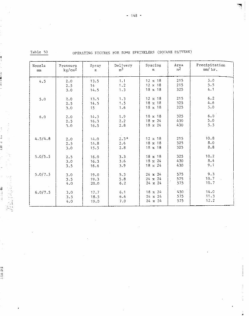
·~ 148 -

Table 50 OPERATING FIGURES FOR S0'1E SPRINKLERS (SOUARE PATTERN)

Nozzle mm

4.5

s.o

6.0

4.5/4.8

5.0/5.5

Pressure kg/cm2

2.0 2.5 3.0

2.0 2.5 3.0

2.0 2.5 3.0

2.0 2.5 3.0

2.5 3.0 3.5

5.0/7.5 3.0 3.5 4.0

6.0/7.5 3.0 3.5 4.0

Spray m

r;f~-14. 5

1 13.5 1 14.5

1 15

1

14.5

1

16. 3 16. 5

14.0 14. 8 15. 5

16.0 16.3 16.6

19.0 19.3 20.0

17. 7 18. 5 19.0

-------~·---- --

Delivery m3

1 • 1 1. 2 1. 3

1. 3 1. 5 1.6

1. 9 2.2 2.8

2.3 * 2.6 2.8

3.3 3.6 3.9

5.3 5.8 6.2

6. 1 6.6 7.0

Spac:in~-Area-r Precipitation 1

m m2 j mm/ hr . i

~-1-2-x 18 ~-215~~~~~1 12x18 12151 5.5 1

1 8 X 1 8 3 25 1 4, 1 1

11 :: ~ 11

12 X 18 18 X 18

18 18 X

18 X 18 18 X 24

24 18 X

12 X 18 18 X 18 18 X 18

18 X 18 18 X 24 18 X 24

24 X 24 24 X 24 24 X 24

18 X 24 24 X 24 24 X 24

1

1

215 325 325

325 430 430

215 325 325

325 430 430

5.0

6.0 5.0 5.5

10.8 8.0 8.8

10.2 8.4 9. 1

575 9.3 575 10. 7 575 10. 7

430 14.0 575 11.3 575 1 12.2

-~- -"--------

1

'

'

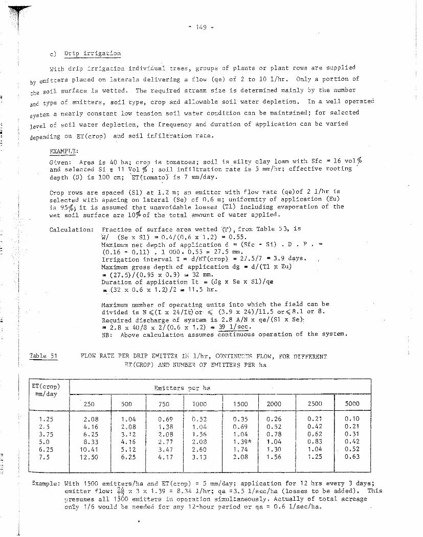
~ '"1 ! - 149 -

c)

With drip irrigation individual trees 9 groups of plants or plant rows are supplied

by emitters placed on laterals delivering a flow (qe) of 2 to 10 1/hr, Only a portion of

the soil surface is wetted. The required stream size is determined mainly by the number

and type of emitters, soil type~ crop and allowable soil water depletion. Ina well operated

system a nearly constant low tension soil water condition can be maintained; for selected

ievel of soil water depletion, the frequency and duration of application can be varied

depending on ET(crop) and soil infiltration rate.

EXAMPLE:

Given: Area is 40 ha; crop is tomatoes; soil is silty clay loam with Sfc = 16 vel% and selected Si: 11 Vol % ; soil infiltration rate is 5 mm/hr; effective rooting depth (D) is 100 cm; 'ET(tomatoj is 7 mm/day.

Crop rows are spaced (Sl) at 1.2 m; an emitter with flow rate (qe)of 2 1/hr is selected with spacing on lateral (Se) of 0.6 m; uniformity of application (Eu) is 95%:i it is assumed that unavoidable 1.osses (Tl) including evaporation of the wet soil surface are 10%of the total amount of water applied.

Calculation: Fraction of surface area wetted TP) j from Table 5 3, is W/ (Se x Sl) = 0.4/(0,6 X 1.2) = 0.55, Maximum net depth of application d = (Sfc ~ Si) . D • P = (0.16 - 0,11) , 1 000, 0.55 = 27 .5 mm. Irrigation interval I = d/ET(crop) = 27 .5/7 = 3.9 days. Maximum gross depth of application dg = d/(Tl x Eu) = (27,5)/(0.95 X 0,9) m 32 ITIIll,

Duration of application It = (dg x Se x Sl) /qe = (32 X 0,6 X 1.2)/2 = 11.5 hr,

Maximum number of operating units into which the field can be divided is N ((I x 24/Ii:)or <: (3.9 x 24)/11.5 or( 8.1 or 8. Required discharge of system is 2, 8 A/N x qe/ (Sl x Se} ~ 2.8 x 40/3 x 2/(0,6 x 1.2) = 39 1/sec. NB: Above calculation assumes contiūü"Ous operation of the system.

Table 51 FLOW RATE PER DRIP E"!ITTER IN 1/hr, CONTINFS'.TS FLOW, FOR DIFFERENT

ET(CROP) AND NUMBER OF E'iITTERS PER ha

Emitters per ha ET(crop)F mm/day --~-·

---i---250 _ļ___so_o __ !--_75_.o _,._1_0_0_0. _l~_5_o_o_ .... 0.52 1.04 1.56

1. 25 2.5 3.75 5.0 6.25 7.5

2.08 11 1.0I. 4.16

1 2.08

6.25 1 3.12 8.33 1 4.16

12.50 6.25

0.69 1. 38 2.08 2,77 3.47 4. 17

2.08 2.60 3. 13

0.35 0.69 1.04 1 • 39* 1. 74 2.08

2000

0.26 0.52 0.78 1. 04 1. 30 1.56

10~.41 5.12

-------'---· _ _L_ ___ _,_ _____ .1._ ____ ..L._.

2500 ----

0.21 0.42 0.62 0.83 1, 04

J 1. 25

5000

0. 10 0. 21 0, 31 0.42 0.52 0.63

Example: With 1500 emitters/ha and ET(crop) = 5 mm./day; application for 12 hrs every 3 days; emitter flow: 24 x 3 x 1.39 = 8.34 1/hr; qa =3.5 1/sec/ha (losses to be added). This presumes all 1ļ3o emitters in operation simultaneously. Actually of total acreage only 1/6 would be needed for any 12~hour period or qa = 0.6 1/sec/ha.

- 150 -

Tab.le 52 FLOW RATE PER I'REE, CONTINUOUS FLOW:i FOR DIFFERENT ET(CROP) AND --- TREE SPACING, 1/hr.

Tree spacing ~ ET(orchard), mm/day

--:3 m 1 5 6.25 7.5 r-· +--ļ.

1 ii

1 1 6 X 6 7.5 9.5 11

-; 1

. 1 9 X 9 17 21 25 1 1 12 X 12 30 37 45

1

15 X 15 47 59 70

J 1 18 X 18 67 84 101 1

1 ' I_ ___ _J

Table 53 • SURFACE AREA WETTED IN m2 FOR DIFFERENT EMITTER FLOW AND SOIL INFILTRATION --- INFILTRATION RATE 1 /

1

Emitter flow F- Soil infiltration rate, mm/hr 1/hr cont.

ŗ·---2.5 5 t- 7.5

1 2 0.8 0.4* 0.25

~

1 4 1. 6 0.8 0.5 -

1

i 6 2.4 1. 2 0.75

1

1

8 3.2 1.6 1. 0 1 I _______

----------'· _J

i/ Source: Personal communication Duffinll UC, Davis.

:

- 151 ..

III.2,4 Relation between field size, field layout and supply

Individual fields within an irrigation block are normally supplied in rotation. \.'Jhen

a shallow rooted cash crop is also grown, requiring frequent and light irrigation applica·~

tions, a double rotation is often practised Within the interval, I.

For surface irrigation schemes in mast cases, a fixed supply for large i·rrigation

blocks (50 ha or more) is preferable; this system is the easiest to operate and can be

controlled from ,1eadworks. Any varfation in the supply required by the block during the

growing season results either in interrupted deliveries or in reduced flow in the supply

chan_nel. The latter requires a higher degree of sophistication, both technical~ structural

and organizational. In the case of interrupted delivery, the canal serving the irrigation

block is in operation for only a portion of the interval, I 1 in periods when crop water

requirements are low. The interruption can be either randam or according to a pre„arr~n.ge~d

schedule and if the latter, then it can be cornpletely rigid - fixed supply and fixed period

of supply - or, preferably, have a certain flexibility and be adjusted from time to time

to allow for changes in crop water requirements due to variations in cropping pattern and

climatic conditions (ĶT(crop), rainfall) during the season. A more sophisticated type of

pŗoject ope:r·a.tion is required for this compared to the rigid schedule. The degree of flexim

bili.ty necessary in supply and subsequent operation of the field canals can normally only

be determined after the project has been in operation for some time·.

If detailed water scheduling prograrnmes are required for final design purposes, the

prediction of stream size and delivery time including their variations during the growing

season should start at the lowest field unit, As shown in the previous sub=chapter:. the

criteria for field supply of the lowest unit are based on acreage and type of crops grown!

i.rrigation water needs, irrigation interval, soil and method of irrigation, Timetables

for irrigation supply are prepared for the irrigation season and plotted on a weekly or

lüwday basis. The water supply schedules derived for individual fields can be totalled

for the irrigation blocks served by the same canal.

A similar approach can be used to determine supply schedules for the irrigation

blocks and these schedules for blocks of fields are then totalled to find the total pro 0

•

ject supply schedules. The following example applies to a surface irrigation scheme.

EXAMPLE:

Irrigation block is 70 ha. cropping intensity is 85%;

Crops are cotton (60%) and potatoes (40%); the acreage of cotton is thus 36 ha~ potatoes is 24 ha.

For a given period the irrigation interval for cotton is 12 days and for potatoes 6 days, The net depth of application is 100 mm for cotton and 40 mm for potatoes. Field efficiency for both crops is 0.5. From Chapter III.2.3, field supply for cotton is 65 1/sec to irrigate 1.5 ha. or 36 ha in 12 d.ays. Similarly, the field supply for potatoes can be determined as 35 1/sec to irrigate 4,0 ha/day or 24 ha in some 6 days. Within the rota"t:ion o{ the supply to the cotton fiel<ls a sub•rotation among potato fields is deerned necessary.

ii

-

1J

-

= -: 52 =

For a given period and selected project and field layout„ t summary can be pre.pared assuming a 12---day supply to the irr for simplicity the cropping pattern and cropping intensity be the same for the total project.

Section Acre.age Deliv·ery Time (ha) (days)

Field (cotton) 1.5 0.5

Field (pata to) 1 o. 25

Block 70 12

Sub-lateral 560 12

Lateral 2 240 12

Main 11 500 12

e following ga tion block; s assume.d to

Supply (1/sec)

65

35

100

800 ļ/

3 200 ļ/

16 000 ļj

If required an additional supply should be added for inefficiency of the conveyance system and for flexibility.

Similar calculations can be made for different periods of the growing season and for supply over a certain time or the supply schedules thus determined.

:

~ '1 1 ,~ ·153 '"

cHAPTER īII. 3 REFINE'fENT OF FIELD IRRIGATION SCHEDULING DEVELOPMENT -- ----------

AND USE OF DATA ON SOIL ~ WATER) CROP AND CLIMATE ---------"--" ----

In most projects, field delivery is based on fixed quantities and periods of delivery.

Thi:3 type of operation, where timing and quantity are based on the calendar regardless of

variation in irrigation neecls du_e to chapges in cr_ops and ~.ļimate~ still prevails in many

irrigated are.as in the world. Efficient water utilization can only be achieved by concen„

trating operation of the system on the primary purpose, that is to provide optimum soil

water conditions for plant growth. Crops have shown that over a period of time they require

different amounts of water; in the operation of the irrigation system, sufficient flexibility

must therefore be maintained to meet adequately these changing demands, but at the same time

excess quantities must not be given. At the planning stage, only approximate rules of ope_ra"'

tion for projects can be given. Any refinements to water scheduling that may be required

can be done after projects have been constructed and in operation for some time.

Apart from their improvement of managerial and technical aspects of operating the

distribution network, refined <lata at the field level are required on crop irrigation needs

(ET(crop), effective rainfall), soil physical qualities and depth and frequency of irriga

tion for a given crop, soil and climate, This <lata is necessary to improve irrigation

scheduling already in progress and project operations. The collection and applic.ation of

such refined <lata is briefly discussed below.

III.3.1 Refinement of field irrigation <lata.

Irrigation requirements for planning purposes c.an be predicted by using concepts and

methodologies developed elsewhere but prevailing local condit'ions must be taken into account.

Such an approach is followed in this publication.

Input <lata and methodologies used should be correlated to local conditions through

field studies. Lines of action may :Lnclude the following:

a) Agro~meteorological stations

Meteorologic.al stations for the collection of esser1tial climatic variables should be

established early.

VJhere possible, new agro"'meteorologicaJ. stations should conform to agricultural re~

quJ.rements. The lccation of stations with respect to e.nvi.ronme:nt is of the utmost irµport

ance.; meteorological inforrna.tion used on many prejects is base.d upon date. obtained from

stations located in non-agricu1tural areas~ such as airports} bare ground or roof tops.

The real value of agro""meteorological stations can only be rea1i~ed. when they are located

in similar conditions to those found in agricultural areas. Where possible the 10 x 10 m

Station should be place.d within an ir.rigated area and short grass should be provided as

station ccver. This wilJ_ have a substantial effect on the acc1J.r2cy of the <lata obtained;

•

•

J 54 ~

for- instzmce~ a Class A evaporation pan surrounded by an irrigated a}'.'ea will give results

more than 20f,~ lower than whe.n surrounded by dryl.s.nd .::rops. The buff e.r a:rea ·.vith planted

crops should be as large as possible~ but a minimum of 100 x 1nn m.

A simple.~ standardi:z:ed ag:co=meteoro;l..ogical. station should L1clude minimum observe.tions

Dn (a) ternpe.I'ature (maxirnum and minimum); (b) relative humidity (wet and drybulb thermometer);

(c) pre~iptation (Ta:Lngauge) (d) wind (totalizer); (e) sunshine hours (Ce.mpbell Stokes);

(f) evapo:cation (Class A or sunken pan) .

Refe·rence. stations} which are usually established in collaboration with meteorological

or agricultural r,::.searc:h institutes~ should be provided with the following equipment in

addition to the m:tn:Lmum instrumentation listed above: (a) th~graph (weekly charts); (b)

hygŗ0graph (weekly charts); (c) anemograph (hourly, wind directions and velocity); (d) ·--··---·~~-- ------'--pluviog;aph (weekly c.ha.:rts); (e) solar radiation i;-.īfth recorder and/or integrator; (f) barqgraph

(weekly -::ha:rts); (:;:) ne.t radiometer with integrators; (h) Class A pan; (i) _ soil thermometers,

minimum a:o.d m,:.m-Lnmm, Elt 10 cm; U) standard shel ters for the foregoing where necessary.

It sbou.ld he ensured that properly trained meteorological observers are emploved,

Particular1y wi·th respect to radiation measurements~ the services of an experienced consultant

shou1d be secu'.i'_'ed to s-elect the equipment and sites~ to train personnel~ to advise on observa~

tion programmes to be c.arrie<l out and on the analyses of the <lata obtained,

b) Soil survev --~,--m,~-Preferably s de.tailed soil survey (scale,1.:5 000 to 10,000) should have been completed

before p1amüng, design and implementation of the pro.iect. Additiona1 investigations will

be requi.redJ in p.č?,rtic.ular on physical and chemic:al properties of the soil and their changes

under prclonged irrigation 1/,

c) Water requirement studies

To e.scertain crop water requirernentsJ the following field studies should be irnplemented

depending on facilities, qua:Lity of staff and the budget available ?,/.

i) Experiments to dete.rmine seasona.l crop water require.ments:

pre.dictive approach~ based on preselected fre:quency and amount

of irrigation, crop factors aūd climatic indices;

p-cedic:tive··direc.'t approae:h~ monitoring soil water levels to

v2rify predicted soil water regimes and to post~evaluate net

i:crigation requirements,

,ļ./ For d,=.tail.s s,~e Soil Survey in Irr.igation Investigations" Sotl.ls Bulletin (draft), Land an.<l Wc1.t2.~~· Ih~v,;;.~l.Gpment Di-'lision~ ""iAO, Rom12~ 1974.

l !

d)

soil watEr :cegtmes for various stages of crcp and evapor.2.d. 72

demand.

i:Li) Expe-r.-iments on i:rrigation practices (fr.:::quency an~ amou:nt stud:Les)

base.d on

soil wat2.r tension o-;:- soil wate.r deplction;

crop appearance;

standard references ~ lysimeter, reference field, ET(crop)

estimates from formule.e~ evaporation pans.

iv) Experiments on water/yield relationships) as part of the. above

mentioned fie.ld trials to determine effect of se.asonal~ periodi,:

and diurnal water deficits on yield.

v) Experiments on field irrigation methods which should include fičüd

trials on layout, length of run, permissible stream size for method

selected - furiOw, bord-e::r ~ basin~ sprinkler, drip and sprinkle:r

irrigation 1/.

vi)

vii)

Experiments on fertilizers, irrigation/ferti.lizer interactions.

Additional experiments on cultural aspects and land preparation

Monitoring water supply scheduling for projects in progress

The following points should be considered under this heading~

Evaluation cf method of delivery and supply scheduling practiced

including de termina tion of pro j ec t ~ conveyance ~ f ield dis tribu tion and

field application efficiency by direct measurement of separate componentsy

or of water balance and budget or of a combined method.

Evaluation of scherne management including institutional aspects, p'l;.rsonnel,

communication facilities.

Water use studies in the farmer)s field by te.sting O"r' monitoring watet·

use aspects including irrigation methods and ī:.ractices for tradit:Lonal

or new crops and cropping patterns.

Appliad in:igation research should be car:-ied out in fi2.lds

ar2a. Field trial plots laid out on r2:Jresentativf~ .sci1 types ahou.ld b>2 as

sible and placed ;:.;;·ithin an existing agricultural ar2.a te avoid t:h2 ef:fect knoc,n.J. 21.s 1 0 c.1othe.s

line'' whic.h occurs in a patchwo-rk of small experü1ental plots,

Applied researcI-I on a continuous basis is nec2:ssa;:y to eval.uat:~ th<S of d

p:roject and .the ccntrol of water application for both traditional and ne.1,;r c.:::::ps, Sp{::cific

problems will need stud.ying such .-s.s the. use cf brac.kish irriga tion water, }_2.2.chL11g of salts)

applicatioī:1 of fe:ctilizers~ e.te O The type e.rrd detail of re.s2.s.rch pn:grammes will

depend greatly on the purpose oi the research and avail.a"ble financ.:La.l re:sou1~:.::2s) existing

1/ See for instance references quoted 1n Chepter I.4.,.

'

:

governmental organizations and institute.s, and the experience of the staff. The time

needed for collection of necessary <lata should form an integral and essential part of the

total duration of project planning~ design and execution, Ideally, applied research should

start as early as possible and) if possible, well before the stages of detailed project

design and project execution. Different approaches can be use<l:

Experimental stations. Many permanent experimental stations engaged in basie and applied

research have been established on a national basis (see for instance, for the Near East,

Raffiq, 1971). Optimum use should be made of knowledge and experience gained within any

one country and applied research programmes should be carried aut in close collaboration

with established institutes. Studies should be selected carefully and refJ.ect the mast

critical problems met in project design and operatian. The cost of running such stations

is high and, depending on the size of the project, they can normally be maintained only

if they forrn part of government-sponsored research institutes or universities.

Field sub-stations and field plats. Instead af conducting extensive and detailed applied

programmes, normally sub~stations are equipped to apply the results from research stations

to local conditions on a practical scale. They are mostly found in connexion with planned

or established large scale projects. Apart from agronomic and fertilizer trials~ their

type of activity should include simple studies on water requirements, crop/water response

and irrigation methods and practices. The operation of a secondwdegree weather station

should be included if possible and the value of such stations for demonstration purposes

should not be overlooked. Not many personnel may be required, but supervisory assistance

should be available.

Field experiments in the fannerjs field~ Practical studies can be carried out in the farmer's

field as part of project operations because they provide results whose value is often greatly

under„estimated. The value of such experirnents for demonstration and traip.ing is inestimable

if f.ull ccoperation with ~he. f~.rmers is achļl:?.~?., although th€: survival_ rate of such experiD

īņents may be lower than 50 percent because of uncont:rollable. factors and the difficulty of

maintaining the farmer ~ s :f.nterest and getting hi.m· to k~ēp -appr~priate· reCOrds, · CTOse· col„

laboration should be maintained with the local extension service especially as they may be

of help in convincing partners of the benefits of their field exp·eriments,

Pilot projects. The need to set up pilot projects before e.mbarking on large""scale project

development cannot be over~emphasized, The area should cover be.tween 100 and 500 ha to allow

for a detailed analysis of futur.e: project operations. Apart from water requirernent and

application experiments, problems concerning the distribution of water, use of surface

and/or groundwater, water and salt balance, and water losses can be considered and many

atber studies carried aut at project level. The scheme should be located with an eye to

its inclusion in the anticipated large project.

ŗ 1

"" 157

III. 3. 2 Application of field i:r:r_i.;~c,tion dsta

Once basie <lata on depth and· crop ,. soi}. and cliroa te

are available, various ways can iJe useci to put th2se. <lata into practice,

In irrigation p~cojects ·~iher2 wai:2.:: is suppli:::.d on demand~ the supply to indiv::tduEl

fields can be scheduled on the bas:Ls ·:Jf ciirect measureme.nt of the soil wats:r by soil water

indicators,by plant indicato:rs and by ·2vs.porat::Lon measuring devices such as pans. A11 these

methods require substantial insight into th.e effect and importance of the factors fr1volve.d

p.nd can only be successfully appLled 1,vhen~ fo:t the. given condition, the essentia1 dat:e. on

crop „soil ~wa ter-a tmosphere rela tions ar:2 ava::Llab le" Numerous techn:f.cal pub:Lica.t.ions-> manua.ls

and irrigation guides provide instruct:Lo~s on--- the application of ditect ruemsurements a.1;1d, the

use of soil wate.r indicators for irrigaticn @che<lul:Lng 1/. However:"? :r,2sults frcm the use

of these devices by farmers is often d:Lsappointi-:t.g simply because they have not the required

technical knowledge or understanding to- extract fu.11 bene:Eit from the indicat:Lons obtain.ed~

Therefore it is often preferable :!:o-z a<lvice and assi.;tance to be given by central i:-riga""

tion authorities or extension se.rv:Lc.,2s r2ther than to leave all the work o:f colle.cting neces„

sary <lata to the farmers. The data :;."H:!eded can be collected :from small e:xperim.en.tal field

plots which mirror the local agricultural p1:actices (PhiLlppines). When ex:te.nsiva -research

has already been carried out, evapo:ration pans (Class A) can be used for sche.dul:!.:ng irriga„

tion and will give a sufficie.ntly high degree of accu.racy (Israel~ Hawaii)., An example is

cit.ed of the use of the evaporation pan in scheduling of ir:rigation, A simple method is

sometimes followed in India; within an i:rriga ted field of medium o:r heavy=te:xtured soi1 ~ a 3 soil block of 1 m is mixed with abou.t 10'.;l sand; ea:rly wilting of plants growri in the scil„

sand mixture is noticed indicating tha·:: i:r:rigaticn of the crcpped field should follow soone

Other metbods are based on meteorological <lata combined with known soiJ. and crcp <lata

and supplemented by sufficient fte.1d c.h2cks. For development and testing of such prediction

methods adequate exper:imental data on t:hese. and related subjects must be available for the

given conditions. These methods can be applied more rea<lily if water delivery is based on

controlled or free demand. -1 /

Efficient extension se.rv:.l.ce.s c.e.~,. 1,;::. of much assistance. not only in collect:Lng

information frorn field experimentaJ. ·work but S.LSG in. applying its resultant dat& for the.

improvernent .of irrigation efficj_ency,

1/ B...agan, Haise _ and Ed~i:q.s ter J I.rrig21,tion oi Agr.icn1 Lands ~ {,1.9~7 l'.FAO/Un.iscO ·J·

Interna tional SourceboOk cn Irr:Lgation 2nd Drain.age .of .Aīrirl L.ands 9 'Unesco "': Pa.ris -- (·197'3) ~ .:Stanhill_, PraCtical soil moisture ·p~cofi":i'8t:r.G-.i° in-ii:giicul"faii'e~ .'īfrJD'"-(1968) ;-

1 /See f or instance J-ensen ~l'L E, Sc.hedulJ.ni,~ i2~Tigati::m;;; - ASCE~ J., Irrigaŗio!ļ __ _?..P_<t _:Qraj,nage. _ 23..<00,';t8 __ .,.-1910~-

using climate=c.!."Op""soil data

--

1S3

EXM1PLE: Irrigation sc:heduling by soil ,:,7at.2.r account:i.ng proc2dur-2 using Class A evaporation pan.

Required: standard rain gauge and Class A pan on grassed site sur,~ounded by short crop; daily observation (08.00 hours), estimated or measured wind and humidity Ievels oi previous day. soil data on water holding characteristics; crop rooting depth and level of maximurn soil water depletion. crop coefficient kc for different stages of crop growth.

Procedure: At 08.00 hours pan evaporation is measured. For humidity and wind values of previous day and for given upwind distance of gree.n crop, kpan is determined ('!'able 19). For given stage of crop growth kc is selected (Tables 2·1 ~JO). ET(crop) = kpan x kc x Epan. From soil water balance, subtract ET(crop) and add daily rainfall and irrigation application. Irrigation is applied when soil water depletion has reached soil water tension of 0.5 for mast vegetable crops, onions and potatoes, and 1.0 to 1.5 for most-field crops. Depth of application equals /Soil water content at field capacity minus soil water content at Iirne of irrigation in volume percentag~7 times rooting depth.

1 SOIL WATER BALANC;-;EET .. •

i Scheme: f ..q. .l.c;J'J,~ Soil type 4'~;;-: .. Total available soil .. Jc,; v1, O· 30 cm

v1, 30· 60 cm

water ..•

Field : ... /f .............. . ci.6: Farmer: .. --(c:r{G.c-:(c~ .. , . . . . . . . o2 6- v% 60- 90 cm

Months: ,(1.,f,;/,c.-:*-.ļ2l.·.... v% 90-120 cm

l . /(![, --n-i A:L;bll'i~{- "°') I I (oO Pan ocation: ....... · 1,· •• ·: .•.•• Crop:. ,:...r.."':1C4~,0(;iS'. Rooting depth:, .•... ,., .... cm

Date

jz: 2!/)±_

Days after plant~ ing

0 J_

2

l,.,cl~d.- .·'.·; · ~ .I //.:C ! ; 1--Ut:..a__ Irrigate when balance is: ..... ,;...: .•.. , . mm ~--,~~" ·-~--~--~~~~-Epan Wind

nun

Humidity

kpan kcrop ETcrop

mm

Rain Irr. Bal~ Remarks ance

mm mm mm

T ~ \ 59 "'

The following is an example of t:he se.quence of soil 1 water, crop and climatic <lata

which should be avail2.ble on which to base recommendations for irrigation scheduling:

Action

1. Estimate ET for reference crop (grass, alfalfa)

2. Apply crop coefficient for given crop depending on stage of grcwth and soil water level

3. Determine effective contribution of rain since last irrigation

4. Determine soil water depletion level in irrigated fields (calculated, and by making field checks)

5. Predict future rainfall contribution

6. Predict with computed ET(crop) when day of maximum allowable soil water will be reached

7. Calculate total amount of water to be delivered to the field at predicted tirne

Field plot or adequately tested radiation/ energy method

Adequate experimental and field <lata on given crop, soil and production potential (crop and field surveys)

Rainfall observationsj determination of effectiveness, field checks

Date of last irrigation, water retention capacity of soil, soil survey

Rainfall frequency distribution analysis of long-term daily <lata

Detailed soil and crop data, water use/ production function

Irrigation efficiency, groundwater contributed to root zone

Information centre

Optimum timing of irrigation is even more essential when there is a short supply of

water at the source. Decisions must be made early regarding the times at which water can

be saved and when its allocation is most essential. The amount of irrigation water needed

during the growing season may be reduced appreciably by the optimum utilization of soil

water stored from winter rains or pre~irrigation. Additional savings may be made by

allowing the soil to dry to the maximum pe:rmissible degree at the end of the growing season,

rather than by leaving a high level of available soil water at harvest time; possibly one

or two irrigations may be saved by this practice. Mini:nizing the total depth of water and

the number of irrigations on the basis of a better understanding and use of the soil water

reservoir should receive particular attention in water scheduling programmes where water

is scarce and expensive.

When water is in short supply decisions must be made early in project operations for

the allocation of water when mast needed in terms of attaining acceptable yields. Water

distribution to the fields should be planned to avoid the water supply to the crop being

restricted during its critical period for water stress; for mest crops this is from

flowering and early fruit deve.lopment onward. Thus during periods of water shortage,

irrigation delivery should be programmeci on preselected ET(crop) deficits, with the least

deficit allowed during the most sens:Ltive gLowth stage. It is obvious that to avoid the plant

drying out during th1.:: vegetative. growth periods, some water must still to be applied.

l60

Refine.meffts in kno'w.ledg::: m: c~op ·v.r2t=-;:: ::equi':ce-rne·;:1ts a.::.;.d fi.-;:;ld applications can only be

o:f val1;te if th-2 d,~sign and operaticn of ir:rigation <':Jystems r:1-:·e gea:red to meeting actu.al field

del:l3ering the p:roper quantities to ·:::b.2 farm at the right time.

Time is :r2quired fo1~ t:h,s int1.:oductton of mode:":n i:r:;:::?.5.:<.ted farming technology and for

the eve.ntual acc.eptanc1:; of new prac.tices by the farmer in ?la.:rmed irrigation developments.

New t,:=chniques eannot be applied who1esaL:: hut rimst be c:..sa.:.rn..:..L„Led according to capacity;

the t.ransfe.1· crf knowledge on the most effe.ctive ;Jse of J.rn.ter at the level of the farmers

fi.elds ·wi.11 nct be achieved overnight ~ but must graduallf seep in and be accepted as benefits

a:c.e. demonst:::-ated, A Tihc.le range of long=term ac-::iviti':c~G r,.T:Ll.1 be required such as the

set.ī.:J.ng np of ext;~nsicn services~ the establishment o:E der,_1o~stration plots a.nd the

provision of training faciliti.2s" It is cnly ·~v'hen. this r,:.s.:m2work has been established and

is functioning \' that ca:zefully develop2d techniques can čro tested and applied once their

validity has bee.n proved,

:

APPENDIX I

GLOSSARY

ACTUAL CROP EVAPOTR.I'l.NSPIRATION~ ETa(c.rop): rate of evapotranspiration equal to or smaller than predicted ET(c.rop) dependi!1g on the level of available soil water, wilting phenomena, salinity, field size, or other causes; mm per day.

ACTUAL VAPOUR PRESSURE, ed: pressure exerted by water vapour c.ontained in the air; millibar.

ADVECTīON: transport by air movement of sensible heat from large dry fallow surrounds into irrigated areasa

AVAILABLE SOIL WATER STORAGE, L1Si: amount of water storable in the raot zone at tL'Tle of irrigation; weight or volume percentage ar mm over rooting depth.

AVERAGE INTAKE RA.TE: rate of infiltration of water into the soil by dividing the total depth of water infiltrated by the total time from start of irrigation to the moment when infiltration rate is equal to the basie infiltration rate; mm/hour.

BASIC INTAKE RATE: rate at which water will enter the soil after a period when the change in rate becomes very slow; rnm/hour.

CANOPY INTERCEPTION: depth of precipitation caught and held by plant foliage and lost by evaporation without reaching the ground surface; percentage ar mm.

CARRY~OVER SOIL WATER: amount of water stored in the soil from earlier rains, snow ar irrigation applications whic.h meets water defic.iencies in following periods; volume or weight percentage.

CLOTHESLINE EFFECT: horizontal heat transfer from warm upwind area to a relatively cooler crop field resulting in increased ET(crop) particularly at the field border or patchwork of small interspersed fields.

CLOUDINESS: degree of cloud cover as mean of several observations per day; expressed in oktas ~ in eights of sky covered; or tenths - in tenths af sky covered.

CONTINUOUS SUPPLY: continuous and constant discharge to inlet af the individual farms ar fields; 1/sec.

CONVEYANCE EFFICIENCY Ec: ratio between quantity supplied to a block of fields or rotation unit and total quantity supplied to the irrigated project area; fraction.

CRITICAL PERIOD: period during crop growth when the crop is most sensitive to soil water stress which will have a lasting effect on crop growth and will reduce yields.

CROP COEFFICIENT~ kc: ratio between crop evapotranspiratian ET(crop) and reference crop evapotranspiration ETo when both are in large fields, under optimum growing conditions.

CROP DEVELOPMENT STAGE: for given crop time between end of initial stage and when crop reaches 70 to 80%full ground cover; days.

CROP EVAPOTRANSPIRATION 1 ET(crop): rate of evapotranspiration of a disease-free crop growing in a large field (one or more ha) under optimal soil conditions, including sufficient water and fertility and achieving full production potential of that crop under the given growing environment; mm/dayo

•

- 162 •

CROPPING INTENSITY: at a given time the percentage of the total scheme area which can be supplied·by the irrigation system and is fully equipped for water distribution that is under an irrigated crop; at a ~iven time, the percentage of the cultivated area that is under a crop; percentage.

CROPPING PATTERN: sequence of different crops grown in regular order on any particular field or fields,

CROP WATER REQUIREMENTS, ET(crop): depth of water, regardless of its source, required by a crop or a diversified pattern of crops for evapotranspiration; mm and period; mm/day .

DAYLENGTH, p: number of hours between sunrise and sunset; hours or in percentage of total annual daylight hours for each day.

DEEP PERCOLATION, F: rate of downward movement of soil water from the root zone prior to and following attainment of field capacity after ample irrigation or heavy rains; mm/day.

DELIVERY TIME, ta: field or

length of time during »7hich a given streamsize is delivered to the block of ,fields; hour or dayo

DEWPOINT TEMPERATURE: temperature to which the air needs to be cooled down in o·.rder to become saturated and at which water vapour starts to condense,. degree Celsius . .,

DEPTH OF IRRIGATION, d: depth of irrigation applied to the soil in one irrigation, or volume of water delivered to a given area in one irrigation divided by the acreage and which is needed to bring the water content of root zone to field capacity; mm.

DRAINAGE: removal of excess surface and groundwater from the soil; mm/day.

EFFECTIVE FULL GROUNDCOVER: percentage of groundcover by the crop when ET(cropj is approaching maximum „ generally 70 to 80 % ~

EFFECTīVE PRECIPITATION: that fraction of total precipitation useful for meeting crop water requirements; it excludes deep drainage, run·off,and evaporation from the soil surface; fraction.

EFFECTIVE ROOTING DEPTH, D: soil depth from which the crop extracts most of the water needed for evapotranspiration (also called design rooting depth); cm.

ELECTRICAL CONDUCTIVITY, DRAINAGE WATER, ECdr: measure of salt content of excess soil water that is removed by downward flow through the soil; mmhos/cm.

ELECTRICAL CONDUCTIVITY„ IRRIGATION WATER, ECirr: measure of salt content of irrigation water; in mmhos/cm; salts in part per million = 0"64 x EC x 103 for irrigation water up to 5 mmhos/cm; mmhos/cm.

ELECTRICAL CONDUCTIVITY, SATURATION EXTRACTS~ ECe: measure of salt content of soil water extracted from the soil, when saturated with water; mmhos/cm.

EVAPORATION, E: rate of transformation of water from liquid to vaµour phase through purely physical processes, mm/day.

EVAPOTRANSPIRATION, ET(crop): rate of transpiration from a vegetal cover, evaporation frorn the soil and from the wet surface of the vegetation; mm/day.

~ !

EXTRA·TERRESTRIAL Ri\DIATION, Ra: equivalent evaporation

• 163 ""

amount: of radiation received at the top of mm/day.

the atmosphere;

FIELD APPLICATION EFFICIENCY, Ea: ratio between water placed in the root zone and directly available to the crop versus total quantity applied to the field; percentage or fraction.

:FIELD CAPACITY~ Sfc: amount of water held in the soil after ample irrigation or heavy rain when the rate of downward movement has substantially decreased, usually 1 to 3 days after irrigation or rain; also called effective water holding capacity or soil water content at soil water tension of 0.2 to 0.3 atmoshpere; volume or weight perc~ntage.

FIELD DITCH EFFICIENCY, Eb: ratio between the quantity supplied to the individual fields and the total quantity supplied to a group of fields or rotation unit; percentage or fraction.

FIELD EFFICIENCY, Ef: supplied to fraction.

ratio between quantity of water placed in the root zone and quantity a group of fields or rotation unit;Ef = Ea x Eb; percentage or

FIELD SCHEDULE: quantity and timing of water delivered to the individual field or block of fields; volume and interval.

FIELD SUPPLY, Vs: quantity of water delivered during a certain length of time to an individual field or block of fields; volume.

FIELD WATER BALANCE: sum of all gains and losses of water over a given period in the root zone.

FLEXIBILITY FACTOR, C: coefficient greater than unity to account for fluctuations in water supply in excess of those determined for an assumed cropping pattern and cropping intensity; fraction.

FULL GROUND COVER: amount of soil covered by crops approaching 100 percent when looking downwards.

GROSS IRRIGATION REQUIREMENT, If: depth of water, excluding contribution by precipitation, groundwater, stored soilwater, or surface or subsurface inflow, required for normal crop production plus water losses and operational wastes; mm and period.

GROUNDWATER TABLE: upper boundary of groundwater where water pressure is equal to atmosphere, i. e·. depth of water level in borehole when groundwater can freely enter the borehole; cm below soil surface.

GROUNDCOVER: percentage of soil surface shaded by the crop when sun is directly overhead; percentage.

GROWING SEASON: for a given crop the time·between planting or sowing and harvest; days.

INITIAL DEVELOPMENT STAGE: for a given crop the time during germination or early growth when groundcover is less than 10 percent; days,

INITTAL INTAKE RATE: rate at which water will enter the soil when water is first applied; nmi/hour.

IRRIGATION INTERVAL OR FREQUENCY OF IRRIGATION, I: time between the starting of one irrigat:ton and the. starting of the next on the same field; d2.ys.

'

•

-

,··~-

,. 161, -

IRRIGATION MODULE: flow of water designed for or used in irrigating a unit of land.

LATE=SEASON STAGE: for a given crop the time hetween the end of the midseason stage and harvest; days.

LEACHING; removal of soluble salts by passage of water through soil.

LEVEL OF SUPPLY: quantity of water selected on the basis of probability to meet crop irrigation requirements .

MAXIMUM NUMBER OF BRIGHT SUNSHINE HOURS, N: number of bright sunshine hours for a 24·hour day with no cloud cover; hours.

MAXIMUM RELATIVE HUMIDITY, RHmax: maximum or mean of maximum of each day over the period considered of actual amount of water vapour in the air relative to the amount of water vapour the air would hold when saturated at the same temperature; percentage.

MAXIMUM TEMPERATURE, tmax: maximum temperature during the day or mean of rnaximum temperature for each day for the period considered; degree Celsiuse

METHOD OF WATER DELIVERY: way of making an irrigation system function to convey water from the source of supply to each field served by the system.

MIDSEASON STAGE: for a given crop the time between effective full ground cover and the onset of maturity (i.e. leaves start to discolour ar fall off); days.

MINIMUM RELATIVE HUMIDITY, RHmin: minimum or mean of each day over the period considered actual amount of water vapour in the air relative to the amount of water vapour the air would hold when saturate.d at the same temperature; percentage.

MINIMUM TEMPERATURE, tmin: of each day for

lowest temperature during the day ar mean of lowest temperatures the period considered; degree Celsius .

NET IRRIGATION REQUīREMENT, In: depth of water, excluding contribution by precipitation, groundwater, stored soilwater, surface or subsurface inflow.; ~ required for normal crop production; mm and period.

NET LONGWAWE RADIATION, Rnl: balance between all outgoing and incoming longwave radiation; equivalent evaporation mm/day.

NET RADIATION, Rn: balance between all incoming and outgoing short and longwawe radiation; Rn: Rns + Rnl; equivalent evaporation mm/day.

NET SOLAR RADIATION,Rns: difference between shortwave radiation received on the earth surface and that reflected by the soil~ crop and water surface; equivalent evaporation mm/day.

OASIS EFFECT: vertical energy transfer from air to the crop; effect of dry fallow surrounds on the microclimate of a relatively small acreage of land where an ai.r mass moving into an irrigated area will give up much sensible heat. For small fields this may result in a higher ET(crop) as compared to predicted ET(crop) using climatic <lata colJ.ected inside the irrigated area; conversely ET(crop) predictions based on weather <lata collected outside the irrigated fields may over-predict actual evapotranspiration losses.

OSMOTIC PRESSURE: equivalent negative pressure to which water must be subjected to bring the saline soil-water through a semi-permeable membrane into static equilibrium with pure water; atmosphere.

•

"' 16S -

PAN COEFFICIENT, kp: ratio between crop evaporation from an open water

evapotranspiration ET(crop) and water loss by surface of a pan.

PAN EVAPORATION, Epan: rate of water loss by evaporation from an open water surface of pan; mm/day .

pEAIZ PERIOD CROP WATER REQUIREMENTS, ET(crop) peak: for a given crop the peak crop water requirements during the month of highest water requi.rements; mm/day.

PLANT POPULATION: number of plants per unit of area.

PRECIPITATION: total amount of precipitation (rain, drizzle, s.now, hail, fog condensation, hoar frost and rime) expressed in depth of water which would cover a horizontal plane if there is no run-off, infiltration or evapotranspiration; mm/days

PROJECT EFFICIENCY, OR OVERALL EFFICIENCY, Ep zone and total quantity supplied to the Ep = Ec x Ef = Ec x Eb x Ea; percentage

ratio between water placed irrigated project area; or fraction.

in the root

PSYCHROMETER: device to measure air humidity; generally cansisting af a normal thermometer and a thermometer whose bulb is surrounded by a wet muslin bag; the latter, called wet-bulb thermameter, should normally be force ventilated (Assmann type).

REFERENCE CROP EVAPOTRANSPIRATION, ETo: rate of evapotranspiratian from an extended surface of 8 to 15 cm tall green grass cover of uniform height, actively _growing, completely shading the ground and not short of water; mm per day.

REFLECTION COEFFICIENT, a: ratio between the amount of shortwave radiation received at the earth surface aud that reflected back by the soil, crap ar water surface; f-ŗactian.

ROTATION INTERVAL, I: time between the start of supply to a given field or block of fields belonging to the rotatian unit and the start af the next supply; days.

ROTATIONAL SUPPLY: supply of water on a rotational basis within a d.istribution system amant laterals, sub~laterals ar field inlets at a regular ar varied interval; larger streamsize and shortened time of delivery far a number of days to each section, with no supply during those days to the ather sections belonging to the ratation unit; 1/sec and delivery time.

SATURATION VAPOUR PRESSURE, ea: upper limit of vapaur pressure at a given temperature or vapour pressure which the air would have if saturated at that air temperature; millibaro

SEASONAL IRRIGATION REQUIREMENTS: depth of water, exlcluding contribution by precipitation groundwater, stored soil-water surface or subsurface inflow, required f0r narmal crop growth during the crop growing seasan; mm and period.

SOIL HYDRAULIC CONDUCTIVITY, k: rate of water flow through a unit cross-section of the soil under a unit hydraulic gradient; alsa called permeability or transmission; mm/day.

SOIL INTAKE (INFILTRATION) RATE: rate at which water will enter the soil under given conditions including sail water cantent; mm/hr.

SOIL SPECIFIC GRAVITY, As: ratio of the weight of water-free soil to its volume; grammes per cubic centimeter; g/cm3,

SOīL STRUCTURE: arrangement of soil particles into aggregates which occur in a variety af recognized shapes 3 sizes and strengtha

•

~ 166 ~

SOIL TEXTURE: characteristization of soil in respect to its particle sizes and dist:ribut::Lon.

SOIL WATER STRESS: sum of soil water tension and osmotic pressur-e. to which water rnust be. subjected to be in equilibrium with soil water; atmoshperes.

SOIL WATER CONTENT, Si: at a given time the amount of water held in the soil; weight or volume percentage.

SOIL WATER TENSION: force at which water is held by the soil or negative pressuZ'e or suc.tion that must be applied to bring the water in a porous cup into static equilibrium with the water in the soil; soil water tension does not include osmotic pr2ssure; atmosphere or bar.

30Lfu-q_ RADIATION, Rs: amount of shortwave radiation received at the earth surface; equivalent evaporation mm/day.

STREAJ.'\fSIZE, qa: flow selected for delivery to field inlet or irrigation block; 1/sec~

SUNSHINE HOURS, n: number of hours of bright sunshine per day, also sometimes defined as the duration of traces or burns made on a chart by Campbell Stokes recorder; not to be confused with sun brightness; hours.

SUPPLY ON DEMAND: supply in size and duration of flow to satisfy request for water at any time during the growing season without advanced notice; 1/sec and time of delive·ry;

TENSIOMETER: a device for measuring the tension of soil water in the soil consisting of a porous, penneable ceramie cup connected through a tube to a manometer.

TOTAL AVAILABLE SOIL WATER STORAGE, .1S: amount of soil water available in the root zone to the crop; difference between water content at field capacity and at wilting point; weight or volume percentage or mm over rooting depth.

TOTAL SOIL WATER STORAGE, LlW: total amount of water that can be stored in the root zone between a cornpletely dry state and water content at field capacity; volume or weight percentage or mm over soil depth.

TRA..~SPIRATION: rate of waterloss frorn the plant through the fonnation of water vapour in living cells which is regulated by physical and physiological processes; mm/day.

WET BULB TEMPERATURE, t wetbulb: temperature recorded on a thermometer with the bulb surrounded by a wet muslin bag, thus lowering the temperature by loss of latent heat through evaporation; degrees Celsius.

\.IJET BULB DEPRESSION: difference between readings of wet aud dry bulb thermometers at given temperature; degree Celsius.

WILTING POINT~ Sw: water content of the soil below which the plant cannot effectively obtain water from the soil; water content at 16 atmosphere soil water tension; available soil water is nil; volurne ar weight percentage,

WINDSPEED, U2: speed of air movement at 2 m above. ground surface. in unobstructed sur:er.::;uw<liT~gs; mean in m/sec over the period considered or total wind run in km/day.

l 1

:

- 16 7 -

APPENDIX II

PERSONS A1'1D INSTITUTES CONSULTED

Denmark ~ Hydrotechn. Lab. and Climate Stat., Royal Veterinary and Agrie. UniV. Copenhagen: S.E. Jensen, K.J. Kristensen, H.C. Aslyng.

Ethiopia ... Inst, Agr. Res., Holletta, Addis Ababa; A. Retta, C.R.K. Prashar„

France"' Station de Bioclimatologie, Sta. de Rech. Agron. du Sud-est, Inst. Nat. de la Rech. Agron., Cantarel~84 Montfavet: J. Damagnez, C. Samie, O. de Villele.

Haiti"" Service 1'1eteorologique National, Port au Prince, D.A.R.N.D.R.;'A.Goutier, M. Frere,

Joirrt FAO/IAEA Div, of Atomic Energy in Food and Agriculture, Vienna: Y. Barrada.

India ~ Indian Agrie. Res. Inst, New Delhi 12: N.G. Dastane, A.M. Michael.

Israel Dept. of Soil Science~ Hebrew Univ., Rehovot: D. Hillel, E. Rawitz.

Israel =Min.Agrie., Agrie. Res. Org. The Volcani Center, Bet Dagan: Y. Vaadia, G. Stanhill~ M, Fuchs, F. Shmueli, J .D. Kalma.

Israel ~ Dept. of Irrig., Hebrew Univ. Rehovot: S.D. Goldberg.

IC~nya "" East African Agrie. and Forestry Res. Org. Nairobi: C.W.O. Eeles

Lcbanon Dept. of Irrig, Agron, Tal Amara: S. Sarraf, A. Aboukhaled, S, Chebli.

Lebanon ""UNDF(SF) LEB/13 Project: A. Marasovic.

N:tgeria Inst. for Agrie. Res., Ahmadu Bello Univ. Samaru, Zaria: J.M. Kowal, A.H. Kassan.

Netherlands = Inst" for Land and Water Management Res., Wageningen: C. van den Berg~ P,E.Rijtcma, R.A. Feddes.

Philippines - Intern. Rice Research Inst. Los Banos: T. Wickham, S.K. de Datta.

senega1 "Projet pour le di?.veloppement de la recherche agronomique et de ses applications, Sain.t=Louisi D.A. Rijks.

Soutb. AfrJ.ca ·"' South African Sugar Association Exp. Stat., Mount Edgecombe, Natal: G. 'l'hompson, J.G. Lover.

Sudan = Dept. of Agron., Fac. o.f Agr., Khartoum Univ.: A.M.H. El Nadi.

Syrian Arab Ŗepublic "'Res. Stat, Billaneh, Min. Agr. UNDP Project SYR/22, Aleppo: Salah Sa.msam 1 J. Petrasovic. Univ. of Aleppo, Faculty of Agr.: A.N. Zein El„Abdin, A. Farrat Y. Kattan.

Thailand ~ Asian Inst. of Technology, Bangkok: A. Hossain, E.F. Schulz.

Tunis:La = UNDP/SF Project TUN/ī0/529t Tunis: B. Said, R.R. Combremont.

United Kingdom ~ Inst. of Hydrology, Wallingford, Berks: J.S.G. McCulloch

U.S.A. - US Water Cons. Lab. USDA (ARS), Phoenix, Arizona: C.H.M. van Bavel.

• :

-

• 168 •

U.S.A, - Imperial Valley Cons. Res. Center, USDA (ARS) Brawley, California: R. Le !fort L. Willardson, A.J. MacKenzie.

North Appalachian Exp.Watershed, USDA (ARS) Coshocton, Ohio: L.L. Harrold, J.L. McGuinness.

Irrig. Agrie. Res. and Ext. Center, Prosserj Washington: J.E. Middleton, M.C. Jensen, E.S. Degrnan

Agrie. Res. Serv. USDA Lompoc, California: P.R. Nixon, G.P. Lawless .

State of California, The Resources Agencyj Dept. of Water Resources, Sacramento: J.W. Shannon, N.A. MacGillivray, R.E. Merrill, J. Lawrence, C. Muir.

Agrie. Res. Serv. USDA, Colorado State Univ., Ft Gollins Colorado: G. Kruse. H.R. Haise.

Univ. of California, Davis, California: F.J. Lourence, S. von Oettingen, R.M. Hagan, J. Ian Stewart, D.W. Henderson, F.J. Veihmeyer, W.L. Sirns, V.E. Rubatzky, R.B. Duffin, R.E. Voss.

Dept. of Geography, Univ. of Hawaii, Honolulu, Hawaii: Jen-hu Chang.

Soils Dept., Univ. of Hawaii and Hawaiian Sugar Planters Experirnent Stat., Honolulu, P. Ekern.

Snake River Conserv. Lab. USDA (ARS), Kirnberly, Idaho: M.E. Jensen, J. Wright, R.D. Burrnan.

C. Brewer and Company Ltd. Honolulņ, Hawaii: K. Shoji.

Dept. of Agrie. and Irr. Eng., Utah State Univ., Logan,Utah: J,E, Christiansen, G. Hargreaves.

Zaire - Institut National pour l'Etude Agronomique: E.A, Bernard, M. Frere.

Venezuela - Servicio Shell para el Agricultor, en collaboraci6n conjunta con la Facultad de Agronomla de la Univ. Central de Venezuela. Cagua~Aragua: J,E, L6pez, K. Mathisen, 0. Padilla.

FAO Regional Office for Asia and the Far East, Bangkok, Thailand: Q, van't Woudt.

FAO Regional Office for the Near East, Cairo, Arab Republic of Egypt: A. Aboukhaled, A. Arar.

...

l

"' 169 ~

APPENDIX III

REFERENCES

Aboukhaled, A. Crop water require.ments. In: Water Use Seminar, Damascus. Irrigation and 1972 Drainage Paper ·13 5 FAO, RomeJ p. L+2=60

Aboukhaled 1 A.~ Sarraf,S. and Chebli,S. Evaluation de la fonnule de Penman au Liban; 1971 Inst. Rech. Agron., Liban. Magon Ser. Sci. 39: 21 p,

Aboukhaled, A. and Sarraf, S. A comparison of water use for a hybrid corn in the Bekaa and 1970 the Coastal Plain. Inst. Rech. Agron. Liban. Magon Ser. Tech. 12: 14 p.

Aboukhaled, A., Sarraf, S, and Vink, N, Evapotranspiration in the central Bekaa of Lebanon 1969 with reference to the irrigation of potatoes aud onions. Inst. Rech. Agron.

Lebanon, Magon Set'. Sci. 26

Asghar, A.G. Progress of land reclamation in West Pakistan. Fourtb Irr. Practices Seminar, 1962 Ankara, Turkey, p. 224-243.

Aslyng, H.C. Evaporation 1 evapotranspiration and water balance investigations at Copenbagen, 1965 1955·64. Acta Agrie. Scand. XV: 3/4: 284·300.

Black, J .N. The distribution of solar radiation over thf'. earth' s surface. Proc. New Delhi 1956 Symposium on Wind and Solar Energy. Arid Zane Research, Unesco, p. 138-140.

Blaney, H.F. and Hanson, J. Consumptiveuse and water requirements in New Mexico. 1965 Tecb. Rep, 32, New Mexico State Engineer. Santa Fe, N. Mexico, 82 p.

Blaney, 1950

H.F. and Criddle, W.D. Determining water requirements in irrigated areas from climatological and irrigation <lata. USDA(SCS)TP·96, 48 p.

Blaney, H.F. and Criddle, W.D. Determining consumptive use and irrigation water 1962 requirements. USDA (ARS) Tech. Bull. 1275, 59 p.

Booher, L. Surface Irrigation, -FAO, Rome 160 p. 1974

Bouchet, 1963

R.J. Evapotranspiration reelle. Evapotranspiration potentielle et production agricole. L'eau et la production vegetale, INRA, Paris, p, 151-232· et Ann, Agron., 14(5): 743-824.

Braun, L.H. and Cocheme, J. A study of the agroclimatology of the highlands of Eastern 1969 Africa. FAO/Unesco/lvMO. Rome, 330 p.

Brutsaert, W. Evaluation of some practical methods of estimating evapotranspiration in 1965 arid climates at low latitudes. Wate.r Resources Research, 1(2): 187„191.

Chang, Jen"'hu. MicrocJ.imate of Sugarcane, Hawaiian Planters ~ Record J 56 (2) : 195=225, 1963

Chang, Jen'"hu. Climate and agriculture .. Aldine 1 Chicago, 296 p. 1968

Chapas, 1964

L.C. and Rees, A.R. Evaporation and evapotranspiration in Southern Nigeria. Quart. J. Ro~ Met. Soc. 90: 313·319.

Childs, E.C. An introduction to the physic.al basis of soil water phenomena. Wiley 1969

Christiansen, J.E, Estimating pan evaporation and e.vapotranspiration from climatic data" 1966 ASCE;, Irrigation and Drainage Div. Symp, "JD Methods for E;:, timat i2:1.g Evapot1-.s„nspi_:ŗatie:n,

Nov" 1966.

Christiansen, J.E. and Hargreaves, J.H. 1 969 Proc. VIī Congr. īCID, Mexico

Irrigation r2quirements City~ 23:570=596.

from evaporation.

Combremont, R. Crop water requirements in Tunisia (Summary). In ; Water U.se S2.mina-r 1,

1972 Damascus, Irrigation and Drainage Paper 13, FAO, Rome~ p. 138,~14-1.

Dagg, 11. 1965

A rational approach to the selection of crops for areas of marginal rainfall in East Africa. E.A. Ag. and For. J, XXX(3): 296-300.

Damagnez? 1963

J. , Riou, C, H. , de Villele ~ 0" and el Armnani :i S. Es t:i.mat ion e:T: mesure de 1'2vapotranspiration potentielle en Tunisie. Pu"bl. Int. Assoc, Sc.ient. Hydrology} 62:98-113.

Dastane~ N.G. Effective .rainfall in agriculture. FAO. Irrigation and D-::ainage Paper (in pre-p.) 1974

Dastane~ 1970

N.G" et al,~ Review o:E ·work done on water requtrements of Prakashā~ Poona~ India, 106 p.

crops in India, Na-vabharat

Davenport 1 D.C. and Hudson, J.Po Met. observations and Peri.man estimates along a 17 lan transsect. 1967 in the Sudan Gezira. Agr, Met. 4:405=414,

Decker, W.L. The total energy budget of corn in Missouri, Missouri. Agr. Exp, 3ta., R2s ., BuJ.1., 1963

De Vries, D.A. The influence of irrigation on the energy and climate. near the grourn:L 1959 J. Applied Meteorol. 16(3): 256-270.

Dieleman~ P.J. ed. Reclamation of salt affected soils in Iraq, Internat. Inst. for Land 1963 Reclamation and Improvement, Wageningenj 175 p.

Dilly, A.C. and Shepherd~ w. Potential evaporation f:rom pa.S:...c..u.c and -potatoes A..spendale, 1972 Agrie. 11eteorol.,10:283-300.

Downey, C.A. Water·Yield relationships for non~~forage crops" ASCE. 1972 Drainage Div. Proc. Harch~ p. 107ra·115.

Ekern, 1970

P.C. Ci:Jnsumptive use of water by sugarcane ::Ln Hawaii.. Uni7, Research Center~ Tech. Rep. 3ī: 93 p.

T Irri;aticn and

o:r: iiawaii 0 ["/atzr Rcsource.s

Ekeru~ P.C. Evapotranspiration by Bermuda grass sod, Hawaii, Ag:ron., J, ~ 58::387--~390„ 1966

Ekeru~ P.C. Evapotranspiration of pin-eapple in Hawaii. Plant: Fhysiol., 40:736=ī,~-O,

1965

El Nadi~ A.H. and Hudson~ .J .P., Effects of crop height on evaporation from lucr::.rne and 1965 wheat grown in lysirneters under advective conditions ir:. the Sudan. ExpJ.. Agrie.,

Instit. p, 289~298.

El Rayah, A,D, and El Nacli~ A.IL Water requirement ir1vestigations in Sudan (Sun:mary) 1972 In: Water Use Seminar, Darnascus. Irrigation and Drainage Paper '(3 ~ FAO, Rome;,

p. 136"'137.

Erie~ 1973

L.J,, Bucks~ D.,A. and French~ F. Consumptive use and irrig.ation management -Eor higi1··yielding TN·heats in Central Arizona. P:rogr. AgT.i::., in Arizona) 25(:f·. ·:14·~15

T !

'

l

Er·."'...:o, i 96.5

1972

,3.nQ :~,ei.,..,~-; s .. :c Consumptive use of water by ;·h!.:iJ .. ,...,.,:· Jl.·:--izc-c.:, Ag:-:ic, Ex9, Stat, T:e;ch, Bullo '!69, 44 p,

crops in Arizona.

FAO. Trickl,"::. EC.A Working Party on Water Resources and Irrigation, Bucha.res L 1973 Ir·.;::-igs.t=tDn anc. Drain.age Paper No. 14, FAO, 153 p.

FAü. Scil Survey in I:c:;:::-igation Investigations, Soils Bulletin (draft). Land and Water 197!+ Development Division) F.AO, Rome 1 207 p.

FAO /TJn,::sco., International Sourcebook on Irrigation and Drainage of Arid Lands" Unesco, 197:3 Paris, Hut:chinson, London 1 510 p,

Feddes~ R,A, "f,Jater~ heat and crcip growth. (Ph.D. Thesis) Veenrnang, Wageningen. i97"1

Fr2.·.c2, 1.'L and Rijks, J, Estudio agroclimatol6gico de las regiones altas del .America del Sur. Proyectc īnter~·institutional FAO/Unesco/0:Ml:1. Agroclimatologla (en preparaci6n)

Fritschen~ L,J., and Nixon P.R. Microclimate before and after irrigation, Am. Soc. for 1965 Advancement of Science, Ann. Mtg. 27-30 Dec., Berkeley, Cal.

F.<-i.L-:::i,-hen, L.J. and Sha:,,v, R.H. Evapotranspiration for corn as related to pan evaporation. 1961 Agron. J. 53:149-150.

Fuchs~ M. and Stanhill, G, The use of c.lass A evaporation pan <lata to estimate the irri~ 1963 gati.on wat.er requirements of the cotton crop. Israel J. Agrie. Res. 13(2):63-78.

Fuku<la~ H. and Tsutsui~ H. Rice irrigation in Japan·. OTCA~ Tokyo. 88 p. 1973

Glover, J. Water demands by maize and sorghum. E.A. Ag. and For. J. XIII(3):171 P~ 1948

Goldberg~ 1967

Goldbe-rg 1

196 7

S.D. ~ Gor:natJ E„ and Sadan, D. Relation between water consumption of peanuts and class A pan evaporation during the growing season. Soil Sci. 104(4):289-296.

S,D.,~ Gornat 1 G, and Sadans D~ beets during autunm and winter „

Fubl,: Pamphle.t No. 123„ Israel

Estimating the Nat. and Univ.

14 p,

consumptive water use of sugar Inst, Agr. Div. of Science

Gr3.:f,ari:1~ W.:J, e.ri.d King) ,r ,'vl„ Fre_cticn of net radiation utilized in evapotranspiration 196'! f~L·om a co:r-n c.·r:>9, Soil Sci. Soc, ~_mer. Proc, 25:158-160.

l\.,H, and St.~,:.,ra:cd~ -J~J-~ Wat.er defic.its ~ irrigation design and programming, ASCE .J :i_t:,n and Dra:Lnage, June 1972.

R.IL, }iaiS'--3., l"LR., .s.nd Ed:ninst2:c~ T.W. L:.·Tigation cf agricultu:ral lands„ \ '}S7 Amer. Soc: ., Ag·.r:on. , 1 ·i 80 p,

Ff,,<!,4.-,.s. N.A.,~ iit:o·i'-srn·"'Y'-"'"'·. F.,,J, and Hendrickson, A.1-L Det-ermining water needs of crops from 195_:, c.l:~m.ati.c. da.ta. ~ 24;9~ Univ, cf Callfornia.

Hanks, R.J, ~ bd:CC1r„2r~ B:,R" and Flo-cian, R.L. Evapotranspiration ~ climate relations fo·r 1 S(,g :,;e.0·.,c;:2·.ē" . .:.. ·:::i:'G~~s .... ;.,. tt:e Cent·:::--?,~. G·~·ear: :elains, Ag:;:oon. J. 60; 538=542 ~

• :

-

- 172 -

Hargreaves, G.H. and Christiansen, J.E. Water use~ ERTS readout and climate. Dept. of 1973 Agriculture and Irrigation Engineering 1 Utah State Univ., Logan, Utah.

Harris, K.j Erie, L.J. and Peterson, B. Cotton irrigation in the southwest. USDA(ARS) 1959 41(26):13 p.

Harza 1965

Engineering Company International. Indus Basin irrigation and power systems operation studies - Irrigation water requirements. Report prepared for Water and Power Development Auth. of West Pakistan, Lahore.

Henderson, D.W. Sugar, oil and fibre crops. Part III - Oil crops. In Irrigation of 1967 Agricultural Lands, Amer. Soc. Agron. Monogr. No. 11, p 655 - 660.

Hilgeman, R.H. and Reuther, W. Evergreen tree fruits. In : Irrigation of Agricultural 1967 Lands. Amer. Soc. Agron. Monogr. No. 11, p. 704-718.

Hillel, D. Soil and Water, Physical Principles and Processes. Academic Press. 1971

Hillel, D. et al. The application of radiation techniques in water use efficiency studies. 1971 RēPort to IAEA, Dept. of Soil Sci., Hebrew Univ. of Jerusalem, 87 pages + reprint.

Hobbs, E.H. and Krogman, K.K. Evapotranspiration from alfalfa as related to evaporation and 1966 other meteorological variables .. Can. J. Plant Sci. 46:271-277.

Hounam, C.E. Comparison between pan and lake evaporation. WMO Tech. Note 126, 52 p. 1973 Ŗeport as Rapporteur on Lake Evaporation of the Cornmission for Hydralogy.

Hudson, J.P. Evaporation under hot dry conditions. Ernpire Cotton Growing Review. 1964 XLI(4):241-254

Indian Ministry of Agriculture, A guide for estirnating irrigation water requirements. 1971 Tech. Ser. No. 2, Water Management Division, New Delhi, 50 p.

Institut 1959

National pour l'Etude Agronomique du Congo Belge. Rapport annuel pour l'exercice, 146 p.

James, L.D. and Lee, R.R. Economics of water resources planning. McGraw„Hill, 605 p. 1974

Jensen, 1 952

M.C.and Blaney W.D. Estimated irrigation water requirernent for Idaho. Idaho Agr. Exper. Sta., Bull. 291

Jensen~ M.C., Middleton, J.E. and Pruitt~ W.O. 1961 Washington Agr. Exp. Sta. Circ. 386,

Scheduling irrigation from pan evaporation. 14 p.

Jensen, M.C., Degrnan, E.S. and Middleton. J.E. Apple orchard irrigation. 1962 Washington Agr. Exp. Sta. Circ. 402, 11 p.

Jensen, M.C. Irrigation system design capacity. Functions for Washington. 1970 Washington Agr. Exp. Stat. Circ. 525.

Jensen, M.E. Empirical methods for estimating ar predicting evapotranspiration using 1966 radiation. In: Evapotranspiration and its Role in Water Resources Management.

ASAE, St. Joseph Michigan, p. 49.

Jensen, M.E. Consurnptive use of water and irrigation water requirernents. Techn. Committee 1973 on Irrigation Water Requirements, Irrigation and Drainage Div. ASCE, 215 p~

T 1

Kalma, J .D. Some aspects of the ·water balance af an irrigated orange plantation. 1970 (Ph.D.Thesis) Nat. and Univ. Inst. of Agrie. The Volcani Inst. of Agrie. Res. 152 p.

Kato, S. et al. Studies on the characteristic features of water consumption of various crops. 1970 --V:-!Jn the transpiration and evapotranspiration of soyabean plants.

Bull. Tokai-Kiuki Agr. Exp. Stat., Japan, p. 24-54.

Keller, J. and Karmeli~ D. Trickle irrigation design. Rainbird Sprinkler Manufacturing 1974 Corp., Glendora, California 182 P~

Khafagi, 1966

A., et al. Consumptive use and irrigation water requirement Egypt.-Bull. Faculty of Engineering, Cairo Univ., 29 p.

for cotton plant in

Kozlowski, T.T. Water deficits and plant growth. Vols. I, II and III. Academic Press. 1973

Kruse, E.G. and Haise, H.R. Water use by native grasses in high altitude Colorado meadows, 1973 USDA (ARS)W-6.

Linacre, E.T. Climate and the evaporation from crops. ASCE. Irrigation and Drainage Div. 1967 93:61-79.

Linacre, E.T. Net radiation to various services~ J. Appl. Ecol. 6:61-75. 1969

Linacre, E.T. The water requirements of grass. Proc. VII Congr. ICID, Mexico City, 1969 23:173-186,

Lopez, J. 1968

Resultados comparativos de mediciones y c6rnputos de evaporaci6n y uso consuntivo. V Seminario Latinoamericano de Irrigaci6n III Jornadas Venezolanas de Riego. Fundaci6n Shell. 28 p.

Lourenc·e, F.J. and Pruitt, W.O. 1971 Valley of California.

Energy balance and water use of rice gro'Wil in the Central Agron. J, 63:827-832

Marasovic, A. Determination of water requirements in irrigation projects. In: Water Use 1972 Seminar, Damascus. Irrigation and Drainage Paper 13, FAO, Rome, p. 75-89.

Marsh, A, Applied Irrigation Research, FAO, Rorne, 54 p. 1967

Mather, J.R. The climatic water balance. Climatology XIV(3). 1964

McFarlane, N.L.~ Ayers, R.S. and Winright~ G.L. California desert agriculture, Calif, 1957 Agr. Exp. Sta. Ext. Serv. Circ. 464, 66 p.

McGuinness, J.L. and Bordne, E. 1972 with computed values.

A comparison of lysimeter - derived potential evapotranspiration USDA(ARS) Tech. Bull. 1452, 71 p.

Mcilroy, I.C. and Angus~ D.E. Grass~ water and soil evaporation at Aspendale. 1964 Agr. Meteorol. 1(3):201·224.

~ Merriam, J.L. Irrigation system evaluation and improvement. Blake Printer, San Louis Obispo, 1968 California.

Middleton, J.E., et al. Central and Western Washington consumptive use and evaporation data, 1967 1954·62-::-Washington, Agr. Exp. Sta. Bull. 681, 7 p.

-

HilLs:;:,, B.D, Effect of local. d.dv2c:'::l.cn ,Ti.1. evaporation rat-e aud plaut water status.

r:.litche.".L" Do.S, (2d1.tor) Aquatic veg2>1t:ion a,nd its use aud control 1 Unesco, ·135 p. ·19/6c

Mo1.enaar 9 A. Irrigat ion by Sprink.LLrig, F AO Agr. Dev. Paper 65) 90 p. '! 960

Ho:nte.ith, J.,L, and Sze:tcz~ G" 'T'},,:, ~-,,,,J"JatLm balance of bare soil aud vegetation. 1961 Quart. J.R. Met. Soc. 37:"159='170.

Nixon, P.R. and. Lawless~ G.?. .. Advective influenca.s on the reduction of evapotranspiration ·1953 in a coastal envL:·onrnent. Water Resources Research ~ 4 (1) 39-46.

Nixon~ '1972

P.R. et al. Costal Califo".t'nia e.vapotranspiration frequencies. ASCE. J, of IrrĪgat'Ion Drainage Div, ~ Proc, 98: 185-·! 91 ~

Pair} 1969

C, e.t al. Sprinkler īrrigation. Sprinkler Irrigation Assoc., Washington D.C. -3rdEd.

Penman~ 1948

H.L, Natural evaporation from open water, bare soil and grass. Royal Soc. London Prec. Ser. A, 193:120~146.

Pereira~H.C. Fieldmeasurements of water use for irrigation control in Kenya coffee. 1957 J, Agr. Sci 59:459·1;66.

Pereira) 1967

H.C. Coff2e, tea~ caea.o and tobacco. In ! Irrigation of Agricu1-tural Lands. Amer. Soe. Agron. Honogr, 11, p. 738„752.

Petrasovits 9 P"'T" The Euphrates pilot irrigation project. Interim ·1972 of Practtces Irrigation, FAO, .AGS/SF/SYR-67 /522, Aleppo:,

Report on the Main Basis Syria, 60 p.

Pet:casovitsJP"-':c, Study of wat.er consu.mption of cotton in the Euphrates Valley. In: Water ·1972 Use Seminar:1 Dat'1lasc.us~ Ir:cigation and Drainage Paper 13, FAO, Rome p. 111-122.

Pillsbury-s Aol''., Compton 1 O,C. and Pick.er, W,E. Irrigation water requ:irements of citrus ·194L1- in the South Coastal Basin of California. California Agr. Exp. Sta. Bull. 686. 19 p,

Pi.llsbury~ A ī7 Sprinkle:r Irrigation 1 FAO Agr. Dev, Paper 88., 179 p. (2nd print 1972). '!968

Pruitt 0 A.O, Re.lat1on oT. eonsumpt:lve use of water to cliinate.Trans. ASAE 3:·1, 9~13. 1960

:i?-;:'uitt„ W.O„ Empir:f.ca.1 method of estimating evapotranspiration using primarily evaporation ·J 966 pans, I1!) e:.ra.pott·anspirat.ion and its role in Water Resources Management, ASAE,

St. Joseph Mic.higan.~ po 57"'61.,

2rui"i:t~ 'iiLO" 2.11.d Jensen: lLC, Determ:tning when to irrigate. Agrie" Eng. 36:389·393. 1955

Pruitt~ W,O,, 1oul'ence.~ 2 ,J, e:rrd vo·c. Oettingen~ S. Water use by crops as affected by 1972 climate and plant fa,:i:ors„ California Agrie. 26:10~ pp. 10-·14.

Pruitt 9 TiLO, l von Oettin.gen 1 s. and Morgan, D.L. Central California evapotranspiration 1972 f::squ2nc.L::s, ASCE Ir:ci.gaticn and Drainage Div. Vol. 98: 177=184.

~ ,,,,,, 1

:

Rafiq, M. 1971

An evaluation of the present situation and propc32ls for s.L::..Ltn..,,. and Water Use Regional Applied Research Progra.nll'E2. fo1:· t.he l'īea:r Ea.s·c, Agl:MISC/71 /11, FAO, Rorne. 75 p.

Ravelli, A. et al, Preliminary re port on hydrometeorological baJ_ances of t:rrigated c:1.,ops 1969 iĪĪ SoĪĪ'thern Italy. Proc. VII Congr. ICID, Mexico C:U:y, 2..3; 28 p,

Research 1967

Richards, 1963

Rifai, ~'1. 1972

Group on Evapotranspiration. Evapotranspiration from Paddy Fie1d, Div, of Meteor., Nat. Inst. Agr. Sci., Nishigahara, Tokyo, J, nf Agrie, Meteorol., 22(4):149·157.

S.J. and Weeks, L.V. Evapotranspiration for turf measured with automatic. irrigation equipment. Calif. Agrie. 17:12~13.

Water use in irrigation projects in the Syrian Arab Republic. īn: Water Use Seminar" Damascus. Irrigation and Drainage Paper 13, FAO~ Rome~ p, 22=35"

Rijks, D.A. The use of Water by cotton crops in Aby_an South Arabia. J, of Appl- Ecol. 1965 2:317-343.

Rijks, D.A. Water use by cotton in Sudan. J. Appl. Ecol. 8:6Ld,.,663" 1971

Rijks, D.A. Donnees meteorologiques recueillies a Richard'"Toll:i Guede~ Kaedi et Sam8., 1971 ,1972 (AFR·REG/114), Senegal. FAO, Rome.

Rij tema, 1965

P.E. An analysis of actual evapotranspiration. Agrie. Res. Rep. 689, p, 107. Pudoc, Wageningen.

Tokyo,

Rijterna, P.E. and Aboukhaled, A. A review of some ex.perimental work on crop water use in the Arab Republic of Egypt (1973) FAO Reģional Office, Cairo (in press)

Robins, 1953

J ,S, and Domingo, C.E. Some effects of severe soil moisture deficits at specif:l..c growth stages in corn. Agron. J. 45: 618-621.

Rosenberg, N.J. Microclimate, air mixing and physiological regulation of transpirat}.on 1966 as influenced by wind sl{elter in an irrigated bean' fieldo Agr.ic. Meteorol: 3:19Ī'"221~,

Rosenberg, N.J. Advective contribution of energy utiJ.ized in evapotranspiration by 1969 alfalfa in the East Central Great Plains (USA). Agrie. Meteorol. 6:179,,.,'!84~

Rosenberg, N.J. Seasonal patterns in evapotranspiration by irrigated alfalfa 1969 in the Central Great Plains. Agron. J, 61 :879-886

Salter, P.J. and Goode, J.E. Crop response to water at different stages of growth. 1967 Res. Rev. 2. Commonwealth Agr. Bur, Fa~cnham Royal, Bu.cks.~ 246 p,,

Samie, C. 1971

and de Villele) O. Evapotranspiration sous cli"ma:t mediterraneeno Validit.8 <les formules d'estimation pour la region d~Avignon" Centre de Recherches Agron. du Sud-Est~ Montfavet, France. 25 p.

Sarraf, S. and Aboukhaled~ A. Rayonnement solaire, rayonneme.nt net ;.;:t §cJ.aire.ment au Liban.. 1970 Deuxieme Rl2.union Scientifique. Be)7routhJ 7 p.

Sarraf, S. 1973

and Bovee, A.C.J. Liban. Magon, Ser.

Evapotranspiration du bananier. Tech. 20:18 p.

īnst. Rech. Agron. Tal "'.Amara~

•

--

• 176 ·

Sarraf, 1969

S, 3 Vink, N. and Aboukhaled 5 A. Liban et coefficient du Piche Sei. 32: 29 p.

Evaporation, corrige. Inst.

evapotranspiration potentielle au Rech. Agron. Liban, Magon Ser.

Schultz, 1970

E.F. and Hossain, A. Evapotranspiration in the tropics. Paper 51 at Annual Meeting, AGU, Washington,D.C., 20-24 April, 40 p.

Shahin, M. and El-Shal, M.I. Consumptive use of water for some major crops in U.A.R. 1967 (Egypt). Aun. Bull. ICID, p. 72-83,

Shimshi. Ph. Da thesis~ Hebrew University, Israel~ 196 7

Shmuēli,

1973 E. -et al., Citrus water requirement experiments 196os-:-īn: Ecological Studies 4. Verlag,Berlin.

Shoekley, 1962

Siadat, H. 1972

D.G. and Woodward, H.J. Peak period consumptive Consumptive Use 1 Phoenix, Arizona,_6-8 March.

Water requirements of crops (Iran). In : Water and Drainage Paper ·13, FAO, Rome, p. 123-130~

conducted in Israel during the

use. Paper:ARS~SCS Workshop on

Use Seminar, Damascus. Irrigation

Sins, W.L., Sciaroni, R.H. and Lange, W. Growing globe artichokes in California. Univ. of 1968 Calif. Agrie. Ext. Serv., Art. 52 revised. 15 p.

Slabbers, P.J. Design criteria for basin irrigation systems. Irrigation and Drainage Paper 3, 1971 FAO, Rome, 13 p.

Slabbers, P.J. and Doorenbos, J. Determination of crop water requirements for field projects. 1972 In Water Use Seminar, Damascus. Irrigation and Drainage Paper 13, FAO, Rome,

~ 61-74.

Stanberry, C.O. Alfalfa irrigation, Progres. Agrie. in Arizona. 6(2):9. 1954

Stanberry, C.O. et al. Effect of moisture and phosphate variables on alfalfa hay production 1955 on the'l~iiīā Mesa. Soil Sei. Soe. Amer. Proe. 19:303-310.

Stanhill 1 G. The relationship between climate and the transpiration and growth of pastures. 1960 Proc. Eights Int. Grassland Congress.

Starthill, G. A comparison of methods of calculating potential evapotranspiration from 1961 elimatie data. Israel J, Agrie. Res. 11 (3/4):159-171.

Stanhill, G. The control of field irrigation practice from measurements of evaporation. ·1962 Israel J, Agrie. Res. 12:51-62.

Stanhill, G. Potential evapotranspiration of Caesarea. Israel J. Agrie. Res. 14(4):129-135. 1964

Stanhill, G. The concept of potential evapotransp.iration in arid zone agriculture. Proc. 1965 Montpellier, Symposium, Uneseo.

State of California, Dept. of Water Resources~ Vegetative water use. DWF Bull. 113-2j 78 p. 1967

State of 1972

California, Dept. of Water Resources, Sumrnary of agroclimatic <lata collected on the San Joaquin Valley floor, 1959-1970. DWR San Joaquin District Memorandum Report. 36 p.

.• 177 -

state of California) Dept. o:E ·water Resour:::es. V2getative 1..tate:r use, DWR Bul1. 113-3 1974 (in press) ~

stephens, J.C. and Stewart~ E.H. A comparison of procedures for computing evaporation and 1963 evapotranspiraticn, Publ. 62 of ī.A.S,H., Com. for Evaporation, Trans, IUGG,

p. 123-133.

Stewart, J.I. et al. 1973 economy in

,;vatei use.

Water production functions and irrigation progranuning for greater project and irrigation system design and for increased efficiency in USBR contract No. 14·~Q6~D ... 7324. Univ. California, Davis, Calif, 166 p.

Ste.wart 3

1973 J.I. and Hagan, R.M. Functions to predict effects of crop water deficits.ASCE J. Irrigation and D~ainage Division. Vol. 99:421-439.

Stewart, J.J., Hagan R.M. and Pruitt, W.O. 19ī4 ASCE, JG Irrigation and Drainage

Function to predict optimal Div., Voļ100:179·199,

irrigation programs,

Talsma~ T. 1963

The control of saline groundwater. Med. Landbouwhogeschool 63.10, Wageningen, Netherlands.

Tanner, C.B. Measurements of evapotranspiration. In: Irrigation of Agricultural lands. 1967 Amer. Soc. Agron. Monogr. 11, p. 534-574-;-

Tanner, C.B. and Peiton, W.L. Potential evapotranspiration estimates by the approximate 1960 energy balance method of Penman. J, Geophys. Res. 65:3391·3413.

tayior, S,A. 1952 in

A use of mean soil moisture tension to evaluate the ef.fect of sOil rnoisture ~rop yields. Soil Sci. 74:217·226.

Taylor, S.A. 1961

Water relations of field crops. In: Plant-Water Relations, Unesco, Paris.

Taylor, S .A. 1965

Managing Irrigation water on the farm. ASAE 8: 433-436.

Thompson, G.D. The relationship of potential evapotranspiration of sugarcane to environmental 1967 factors. Proc. XII ISSCT Congr., Puerto Rico 1965, p. 3·9.

Thompson, 1972

G.D. aud Boyce 9 J.P. Estimating watBr use by sugarcane from meteorological and crop parameters. Proc. XIV ISSCT, Puerto Rico p. 813-826.

Thornthwaite C.W. and Mather, J.R. The water balance. Publ. in Climatology 8(1)Lab.of 1955 Climatology. Centerton,N.J.

Till~ M.R. 1969

Timing and design criteria for irrigation of citrus. Proc. First Intern. Citrus Sympos. 3, p. 1731·1747.

Timmons, 1967

D.R.~ Holt, R.F. and Thompson, R.L. Effect of plant population and row spacing on evapotranspiration and water use efficiency by soyabeans, Agron. J. 59:262-265.

Tschannerl. Decision framework .for the efficient use of data sources. HarVard Univ, Center 1970 for Population Studies.

Uchijina, 1961

On cha.racteristics of heat balance of water layer un_der paddy plant cover. Bull. Nat. Inst. Agrie. Sci. Japan, A:8, p. 243·265.

U.S. Department of Agriculture. Soil Conservation Service. Irrigation Water Requirement. 1967 Technkal Release No. 21. Engineering Div. SCS 83 p.

•

- 178 -

U. S. Department s:f Agriculture. Growing table beets. DSDA (ARS) Leaf let No. 360 (revised) 1972 6 p.

U.S. Salin:Lty Laboratory Staff. Diagnosis and improvement of 1954 USDA Agriculture Handbook No. 60. Washington1 D.C.

saline and alkaline soils. 160 p.

Vaadia, Y.F. and Kasimatisj A.N. Vineyard irrigation trials. Amer. J. Enol. and Viticulture . 1961 12(2): 88-98,

Van Bavel, C.H.M. Changes in canopy resistance to water loss from alfalfa induced by 1967 soil water depletion. Agr. Meteorol. 4:165-176.

Van Bavel, C.H.M. and Fritschen, L.J. Evaporation and energy balance of alfalfa. 1966 Res. Rep. No. 381 ~ US Water Conserv. Lab., USDA (ARS) Phoenix, Arizona.

Van Bavel, C.H.M., Newman, J.E., and Hilgeman, R.H. Climate and estimated water use by an 1965 orange orchard. Agr. Meteorol. 4: 27-3 7.

Van't Woudt, B.D. On the estimation of irrigation needs in New Zealand. N.Z. Dep. Sci. ·1966 Industr. Res. Inf. Ser.12:109-149.

Van't Woudt, B.D. Review of techniques for estimating the water re.quirements 1966 o:f the rice crop. Meeting of the Working Party on Rice Soils, Water and

Fertiiizer Practices, -J'.Rc·., Lake Charles, July, 36 p.

Viehmeyer ~ F. J" The availability of soil moisture to plants; results of empirical expe.ri-1972 ments with fruit trees. Soil Sci. 114(4):268-294.

Vink 9 N., Aboukhaled ~ A. aud Sarraf, S. Evapotranspiration and yield of corn in the Central 1969 Bekaa of Lebanon with references to the effect of advection. Inst. Rech.

Agron. Lebanon. Magon Ser. Sci. 29: 29 p.

Vink, N., Aboukhaled, A.and Sarraf, S. Measured and estimated water use by a citrus and an 19ī0 apple orchard. Inst. Rech. Agron. Lebanon. Magon Ser.Tecb. 11 :18 p.

Vittum, M.T. and Flocher, W.J. Vegetable crops, In: Irrigation of Agricultural Lands. 1967 Amer. Soc. Agron. Monogr. 11 :674-685.

Voth, V. 196ī

Grapes and berries; Part II: Strawberries. In Amer. Soc. Agron. Monogr. 11 :734-737.

Irrigation of Agricultural Lands.

Wallis~ J ,A,N, v-Jater use by irrigated Arabica coffee in Kenya. J. Agrie. Sci. 60:381-388. 1963

Wind, G.P. '! 955

A f ie.ld e.xperiment concerning capillary ri.se Meth, of Agr. Sci, 3:60"'69„

of moisture in a heavy clay soil.

Zein El."Abdiri~ A,N., Farra A., KattanJ Y., Results of experimenr:s on irrigation water 1972 requireme.nts of cotton and different irrigation methods, Syria (Summary).

,f,EJ:,: \fater Use Seminar, Damascus. Irrigation and Drainage Paper 13, FAO, Rcme ~ p, 1 3 -1 -137 .

Zein El-Abed.ine~ A., Abdalla M.M. and Abdel=alJ S.L Evapotranspiration studies on maize in 196ī Giza, UAR, ln: Isotope and Radiation Techniques in Soil Physics and Irrigation

Studies. L4.EA/FAO Symposium, Istanbul, June 1967.

..:

U i I ll. il

,-·- ~ Source -- LoC.ii ion or R~pf locationa

As listed by Linacre ( ·967)

Black et aL ( 1954) Stockholm and Fairbanks Montoith\1966) Lerwickj U GK. Perona,, ( 1948) Rotļ:J.amBted, U.K. Baiel" et ~. ( 1965~ Canada B] ack et al. { 1954 Kew, U.K. 'iUn \·JiJkĪĪ963) Gembloux, Eelgium von Wijk { 1963 Versailles, France

l\'lean

•roo-mer et al. ( 1960) Wisconsin 1 U.S~A. de VilleĪe\1965) El .Amm.ia de Vries ( 1958) Deniliquin, AUBtralia :Oemagnez et al. ( 1963) Tunisia Preacott ( 1940) Canberra. 1 Auatralia Black et al,(1954) Dry Greek, s. Africa Page (1961) Gapetow.n~ s. Af'rica

Mean

Glover- et al. ( 1958) Thu•ban. 1 S. Africa. Yadov ( 1965) New Delhi, India Glover et a.l. ( 1958a) Pretoria1 s. Africa Glov·er et al.. ( 1958a) W:i.rulhoek, s~w~ Africa

"'"" ( 1 §l'iT 'l'ananari ve, Madagaacar Srni th ( 1959) Jamaica

Me.n

Fitzpatrick ( 1965) Kimberleyī S~ Africa Cockett et al. ( 1964) Cei'.1.tral Af:dca P""" ( -1961) llaltal', Senegal Yadov ( 1965) (9' Jifadr-dB1 India Daviea ( 1965) Kn.no;i Nigeria. Smith ( 1960) Trmidad Stanhill (1963) Benin City.1/~ Nigeria

Wean

fu.·1ri!i!<ill { 1965) .&.cc:r·a~ Gh;Si(.La Bla~k ~i._RL (1954) Ba,tavia (Djakarla) Paga ! 196T} :iLfarnhatHii Zaire p~,,., 1961) S:lngapdit·<S Glov6r et al. ( '19581,) übatei R~zy·a Pago ( 1961T' E:iaanguni 1 Zair0 Rijklil! et; al.(1964) ll:2&pala~ Ug.,;nda

:ue.w.

k„i ,IJ 1, .. 11 d

EXPERIMENTALLY DETERi"!lNED CONSTANTS FOR TlJE RADJ.ATION H)PATJON

RS ~ (a + b n/N) RA

, 1 l ,ij 11,[; 1, rn '"

,--,-~

APPENDIX TV

Conatanta Lati-S _ Lo-cat'ion or ~siants Lati--1 • Ji ____ ~7:b tugeo

0.22 0.52 o. 74 59+65 N 0.23 0.56 0.79 60 N 0.18 0.55 o. 73 52 N 0.25 0.62 0.87 52 N 0.19 0.57 0.76 51 N 0.15 0.54 0.69 51 J! 0.23 0.50 0.7] 12.1! 0~2Ī 0.55 o. 76 540

0.18 0.55 o. 7J 43 N 0.28 0.43 0.71 37 ll 0.27 0.54 0.81 36 s 0.16 0.59 o. 75 35 N 0.25 0.54 o. 79 35 s 0.30 0.50 o.Bo 35 s 0.20 Q.:.22 ~ 34 s 0,23 0.53 ,7 360

0.25 0.50 o. 75 30 S 0.31 0;46_ 0.77 29 N 0.25 0.50 0.75 26 S 0.26 0.52 0.78 23 s 0,30 0.48 0.78 19 S 0.31 Q.d2 o.so 18 N 0.28 0,49 0.77 240 0.33 0,43 0,76 16 S 0.32 0.47 0.79 15 s 0.10 0.70 0.80 15 N 0.31 0.49 0.80 13 N 0.26 0,54 0.80 12 N 0.27 0,49 o. 76 11 N OQ26 0.38 0,64 -1.lc ā.26 0.50 0,76 130

0.30 0.37 p,67 6 N 0.29 o.59~ o.88 6 s 0.21 0.52 0""{3 4 s 0~21 0.48 Oo69 1 N 0.24 0.59 o~83 1 S 0~28 0.40 0~68 1 n' 0~24 QdiMJill! _Q,__. 0.25 0,49 0.74 30

t-- ource Range of locations a ~---~b--~~~·

Constanta developed from atudies involving rnultiple locations

Fritz and McDonald (1949) Black et al. ( 1954) Mateer -09'55) Glover and McCulloch ( 1958) Hounam ( 1963j Davies ( 1965 Page (1961)

As listed by Chidley et al. (1970) --

Drurrunond aud Kirsten ( 1951) Stanhill ( 1961) Chidley et al. (1970) Kimball ( 1914) Black et al, (1954)

'Others

. Stanhill ( 1965l Stanhill ( 1965 Stanhill ( 1965 Scholte Ubing (1959) Robertson (1971) Idso ( 1969)

All in u„s„A~ Tropics to polar Canada 0-600 Australia1 12-43°S West Africa, 5-150N° 400N-40°S

Capeto\fil. 1 S„ Africa Eastern Mediterranean Saudi Arabia Virginiat u.s~A~ Salt Lake CHy~ u.s~A„

Israel 1 daily) Iarael weekly) Israel monthly) Netherlanda Los BRnos, Philippinea Phoenix. 1 Ariz~ 1 UQS~A„

0.35 0.61 0.23 0.48 0.355 0.68

0.29 cos ļlli/ 0.52 0.26 0.50 o„ 19 0.60 o. 23 0~52

0.29 0.50 0~32 0.47 0~36 0,47 0.22 0.54 0~20 0.47

0.96 0.71 1.035

0.76 0.79 (L, 75

0.79 0.79 0.83 0.76 0.67

0.36 0,39 0.41 0.18 0.24

0.43 0.79 0.38 o.n o.36 o.n l).54 o. 72 0.54 0.79

0.78 ~~----~-,.~.,

J/ Davies ( 1965) gave 0~28 and 0, 33 for a and b reapectivtily

)4 S 31 U -37 ll 41 n 1 :;

31 l! 31 lī 31 U 52 n ·15 N 33 N

Y Table by Linacre ( 1967) indica.ted 0.29 :for Ba:tavia1 a likely en-·01· oin~!i> Chidley and Pike ( 1970) give 0.59 for Djakartai the Si:ill!.e locatfon

::J Based on reviaed figure for Batavi.a.

!fl ~ is the latitude in degrees

.

~

Guidelines for Predicting Crop Water Requirements.

Documents

Transcript of Guidelines for Predicting Crop Water Requirements.