LOGIT MODEL OF WORK TRIP MODE CHOICE FOR BOLE SUB

Logit Model of Work Trip Mode Choice

for Bole Sub-City Residents Addis Ababa University

Chapter Three-Model Specification 1

Addis Ababa University

School of Graduate Studies

Faculty of Technology

LOGIT MODEL OF WORK TRIP MODE

CHOICE

FOR

BOLE SUB- CITY RESIDENTS

BY MEKDIM TESHOME

A THESIS PRESENTED TO THE SCHOOL OF GRADUATE STUDIES OF

ADDIS ABABA UNIVERSITY IN PARTIAL FULFILLMENT OF THE

REQUIREMENTS FOR THE DEGREE OF MASTER OF SCIENCE IN CIVIL

ENGINEERING (ROAD AND TRANSPORT ENGINEERING)

February 2007

Addis Ababa

Addis Ababa University




School of Graduate Studies

Faculty of Technology

LOGIT MODEL OF WORK TRIP MODE

CHOICE

FOR

BOLE SUB- CITY RESIDENTS

BY MEKDIM TESHOME

Approved By Board of Examiners

__________________

__________________

Advisor Signature

__________________

__________________

Examiner Signature

__________________

__________________

Examiner Signature




DECLARATION

I, the undersigned, declared that this thesis is my own work and has not been presented in any

other university. All sources of material used for this thesis have been dully acknowledged.

Declared by:

Name: Mekdim Teshome

Signature:

Date:

Confirmed By:

Name: Girma Birhanu (Dr Ing)

Signature:

Date:

Place and date of submission: Addis Ababa University, February 2007




ACKNOWLEDGMENT

First and foremost I would like to thank God for giving me the inspiration, ability and

discipline to make it through.

I would also like to extend my heartfelt appreciation and gratitude to my advisors Tore

Knudsen (Dr Ing, Ph D), Tor Nicolaisen (M Sc Eng) and Girma Birhanu (Dr Ing) for the

constructive comments and cautious following of this study.

My special thanks go to Fisum Teklu, who has contributed immeasurable assistance

throughout this research, and to The Planning Division staff members of ERA Beteseb Feleke

and Beza W/Aregay for their warm welcome and willingness to give me all up to date and

relevant data.

I would also like to thank my family, where it is not for their prayers, support, love and

investment I would have failed long ago.

Had it been possible, I would be more pleased listing all those who lent their hands during my

study. However, I extend my gratitude for all who were on my side without whom this effort

would have been a rough road.




ABSTRACT

The issue of mode choice is probably the single most important element in transport planning

and policy making. It affects the general efficiency with which we can travel in urban areas,

the amount of urban space devoted to transport functions, and whether a range of choices is

available to travelers (Juan De Dios Ortuzar, Luis G. Willumsen, 2004).

There are two transport studies undertaken for Addis Ababa which are part of the

development and revision efforts of the Addis Ababa master plan. In both studies, the four

stage travel demand model was adopted. However, the mode choice models developed in both

studies are direct demand models which are basically based on aggregate data.

However, with present knowledge and computer technology, it is possible to model the mode

choice for more than two alternatives by considering both the travel maker’s and the travel

mode’s characteristics. Moreover, considering both socio-economic and travel mode variables

will lead to a better understanding and simulation of the people’s behavior in choosing among

the competing modes. Therefore, in this research a Multinomial Logit model is developed,

which is based on disaggregate socio economic, mode and trip related data, for work purpose

trips made by Bole Sub-City residents.

The different modes of road passenger transport considered in the model are Walking, Small

Taxis, Mini-Buses, Anbessa City Bus, Lonchina, Private vehicle as driver, Private vehicle as

passenger and Company provided transport.

Among the various methods of revealed preference surveys, Household or Home Interview

Survey was used as a data source in addition to secondary data obtained from different

agencies of the city and this has been exploited to create the level of service data for the

competing modes.

Finally different specifications of multinomial Logit models have been tested and it has been

observed that the mode choice model has shown continuous improvement as explanatory

power as it was enhanced from being restricted to mode related variables to incorporating the

socio economic and trip related variables.




TABLE OF CONTENT

ACKNOWLEDGMENT ............................................................................................................... 4

ABSTRACT.................................................................................................................................... 5

TABLE OF CONTENT................................................................................................................. 6

LIST OF TABLES......................................................................................................................... 8

LIST OF FIGURES....................................................................................................................... 9

LIST OF APPENDICES ............................................................................................................. 11

1.

INTRODUCTION……………....………………...…………………………………………1

1.1 General Overview................................................................................................................ 1

1.2 Back Ground of the Problem ............................................................................................... 2

1.3 Statement of the Problem..................................................................................................... 3

1.4 Research Objectives............................................................................................................. 4

1.5 Significance of the Research................................................................................................ 4

1.6 Scope and Organization of the Thesis ................................................................................. 5

2. REVIEW OF RELATED

LITERATURE…..……………………………………………...6

2.1 General Overview................................................................................................................ 6

2.2 Factors Influencing the Choice of Transport Mode............................................................. 6

2.3 Direct Demand Models........................................................................................................ 7

2.3.1 Trip-End Modal-Split

Models……………………………………………………….8

2.3.2 Trip Interchange Modal-Split

Models……………………………………………….8

2.4 Discrete choice models ........................................................................................................ 9

2.4.1 Random Utility

Theory………………………………………………………….......11

2.4.2 Logistic Probability Unit or Logit

Model…………………………………………...13

2.4.3 Derivation of Logit Probabilities (Kenneth Train,

2003)…………………………...17

2.4.4 Multinomial Logit

model.………………………………………………………......18

2.5 Mode Split Models Developed For Addis Ababa.............................................................. 18

2.5.1 Mode Split Model Developed By Torrieri, Vincenzo

(1985)…………………….....19

2.5.2 Modal Split Model Used in urban Transport Study for Addis Ababa

(2005)……......22

3. MODEL

SPECIFICATION………………..………………………………………………30

3.1 General Overview.............................................................................................................. 30

3.2 The Decision-Maker .......................................................................................................... 30

3.3 The Alternatives:................................................................................................................ 31




3.4 The Attributes: ................................................................................................................... 32

3.5 The Decision Rule ............................................................................................................. 34

3.6 Limitations of the Multinomial Logit ................................................................................ 38

3.7 Estimation of the Multinomial Logit ................................................................................. 39

4. SURVEY DESIGN AND DATA

COLLECTION………….……………………………..41

4.1 Survey Objectives .............................................................................................................. 41

4.2 The Population to Be Surveyed ......................................................................................... 41

4.3 Data Requirements............................................................................................................. 42

4.4 Required Precision............................................................................................................. 43

4.5 Survey Instrument.............................................................................................................. 43

4.6 Sampling Unit .................................................................................................................... 43

4.7 Sampling Frame................................................................................................................. 44

4.8 Sampling Strategy.............................................................................................................. 44

4.9 Pre-testing the Survey........................................................................................................ 47

4.10 The survey management process ..................................................................................... 47

4.11 Analysis method .............................................................................................................. 48

4.12 Data Source...................................................................................................................... 48

4.12.1 Level of service Data for Anbessa Bus.................................................................... 48

4.12.2 Level of Service Data for Mini-Bus Taxis............................................................... 51

4.12.3 Level of Service Data for Small Taxis..................................................................... 55

4.12.4 Level of Service Data for Lonchina......................................................................... 55

4.12.5 Level of Service Data for Non-Motorized Transport .............................................. 57

4.12.6 Level of Service Data for Car Drive and Car Passenger Modes of Transport......... 57

4.12.7 Level of Service Data for Company Provided Mode of Transport.......................... 58

4.13 Sample Characteristics..................................................................................................... 58

5. RESEARCH

RESULTS…………………………………………………………………….60

5.1 Introduction........................................................................................................................ 60

5.2 Informal Tests .................................................................................................................... 66

5.3 Overall Goodness-of-Fit Measures.................................................................................... 68

5.4 Statistical Tests .................................................................................................................. 69

5.5 Test of the model Structure................................................................................................ 78

5.6 Demonstration of the optimal model ................................................................................. 81

5.5 Value of time .................................................................................................................... 82

6. CONCLUSION AND RECOMMENDATION…………………………………………....84

8.1 Conclusion.......................................................................................................................................84

8.2 Recommendation.............................................................................................................................85




REFERENCES …………………………………………...……………………………..…...…86

APPENDICES………………………………………………………………….……………….88

LIST OF TABLES

2.1 Modal Split General Figure……………………………………………….…………….21

2.2 Model Calibration Parameters………………………………………………………….29

4.1 Distribution of Employed Population Aged 10 Years And Over By Sex

and Kebele in Bole Sub-City for the Year (2006/07G.C)/1999E.C……………...………42

4.2 Distribution of Employed Population Aged 10 Years And Over

By Sex and Kebele in Bole Sub-City for the Year (2006/07G.C)/1999E.C

And The Sample Size for Each Kebele…………………………...……………………...45

4.3 Distribution of Registered Households with House Ownership

For Each Kebele in Bole Sub-City for the Year (2006/07G.C)/1999E.C……….……….46

4.4 Distribution of Registered Households for Each Kebele in Bole Sub-City

for the Year (2006/07G.C)/1999E.C and corresponding size of randomly

selected houses……………………………………………………………………...……47

4.5 Anbessa - Key Operational Characteristics……………………………………...……….49

4.6 Mini Bus - Key Operational Characteristics……………………………….……………..52

4.7 Sample Statistics of Work Trips Modal Data for Bole Sub City Residents……...………59

4.8 Mean Distance and Mean Monthly Individual Income of Trip

Makers With Respect To Their Chosen Mode………………………...…………………59




5.1 Estimation Results for Zero Coefficients, Constants Only,

Base Models and Additional Three Models……………………...………………………64

5.2 Overall Goodness-Of-Fit Measures………………………………………………………69

5.3 Critical T-Values for Selected Confidence Levels and Large Samples……….…………71

5.4 Likelihood Ratio Test for the Null Hypothesis That

All the Coefficients Are Zero…………………………………...………………………..73

5.5 Likelihood Ratio Test for the Null Hypothesis That All the Coefficients,

Except For the Alternative Specific Constants, Are Zero…………..……………………74

5.6 Likelihood Ratio Test the Null Hypothesis That Base Model Is the True

Model Compared With Model-1…………………………………………..…………….75

5.7 Likelihood Ratio Test the Null Hypothesis That Model-1 Is the True Model

Compared With Model-2…………………………………………………...…………….75

5.8 Non-Nested Hypothesis Test for the Null Hypothesis That Model-2

Is the True Model Compared With Model-3………………………………….………….77

5.9 Likelihood Ratio Test the Null Hypothesis That Model-1 Is the

True Model Compared With Model-2………………………………………..…………..77

5.10 The Optimal Logit Model for Work Trips of Mode Choice for

Bole Sub City Residents………………………………………………………………… 79

LIST OF FIGURES




1.1 Sequential Travel Demand Modeling…………………………...…………………………2

2.1 Gumbel Distribution………………………………………………...……………………14

2.2 Comparison between Normal and Gumbel Distribution…………………………………15

2.3 Frequency Distribution of Normal and Weibull Distribution……..……………………..15

2.4 Share of Work Purpose Walk Trips with the Increase in Monthly Household

Income…………………………………………………..……………………………….24

2.5 Share of Education Purpose Walk Trips with the Increase in Monthly Household

Income……………………………………………………………………………………24

2.6 Share of Other Purpose Walk Trips with the Increase in Monthly Household

Income…………………………………………………………………………………..25

2.7 Share of Non Home Based All Purpose Walk Trips with the Increase

In Monthly Household Income………………………………………………..………….25

2.8 Scatter Diagram and the Best Fit Curve between the Household

Income and Share of Private Modes for Work Purposes Trip………………..…………..26


Income and Share of Private Modes for Education Purposes Trip……………...………..27


Income and Share of Private Modes for Other Purposes Trip………………...………….27

2.11 Scatter Diagram and the Best Fit Curve between the Household Income

and Share of Private Modes for Non Home Base All Purposes Trip………...…………..28




3.1 Multinomial Logit Model Structure of Transport Mode Choice for

Work Purpose Trips of Bole Sub-City Residents…………………..…………………….36

4.1 Addis Ababa City Anbessa Bus Network…………………………………...……………50

4.2 Addis Ababa City Anbessa Bus Cost In Relation To Travel Distance…………………..51

4.3 The Addis Ababa Mini-Bus Taxi Routes……………………………………..………….53

4.4 Addis Ababa City Minibus Cost In Relation To Travel Distance………………………..54

4.5 Addis Ababa City Lonchina Cost In Relation To Travel Distance……………...……….56

LIST OF APPENDICES

Appendix A……………………………………………………………………………………….88

Appendix B………………………………………………………………….……………………94

Appendix C…………………………………...…………………………………………………101

Appendix D………………………………...……………………………………………………106

Appendix E…………………………………………………...…………………………………117




Chapter 1

1. INTRODUCTION

1.1 General Overview

Transport Modeling is a simplified mathematical representation of a small part of the real

world, aiming at describing and explaining travel behavior and visualizing the amount and

patterns of transport. (Michel Bierlaire, 1997)

Traffic on road network can be calculated for the current situation and reliable estimation of

traffic demand can be made for the future years using travel demand models taking as input

land use, transport system, socio-economic characteristics of the population together with a

mathematical approximation of human behavior.

The four stage demand model, popularly known as sequential travel demand model is one of

the travel demand models in which the distribution of land use is represented in terms of

population and employment allocation (urban transport study for Addis Ababa, 2005). This

model is organized in four basic steps as shown in figure 1.1and described below:

TRIP PRODUCTION AND ATTRACTION MODELS: This is the first stage in transport

modeling and it converts the land use into trip production. In other words, based on data for

land use, it calculates the number of trips produced and attracted to each zone in the study

area.

TRIP DISTRIBUTION MODELS: These are used to relate the trip origins and destinations in

the study area. At this stage we calculate the Origin–Destination (O-D) matrixes by using a

measure of the spatial separation between origin and destination and our knowledge of how

people react to this separation (distance, time, cost etc).

MODE CHOICE MODELS: Trips from an origin to a destination are distributed to the

different modes of transport by using these models. This is the third step of the four stage

transport modeling process and it simulates how people choose one mode of transport for

their travel by using the characteristics of each mode and socio-economic variables.




ASSIGNMENT MODELS: are used to distribute car trips to the road network and public

transport trips to the public transport network.

Figure 1.1: Sequential Travel Demand Modeling

1.2 Background of the Problem

The choice of transport mode is probably one of the most important classic models in

transport planning. This is because of the key role played by public transport in policy

making. Almost without exception public transport modes make use of road space more

efficiently than the private car. Moreover, if some drivers could be persuaded to use public

transport instead of cars, the rest of the car users would benefit from improved levels of

service. It is unlikely that all car owners wishing to use their cars could be accommodated in

urban areas without sacrificing large parts of the fabric to roads and parking space (Juan De

Dios Ortuzar, Luis G. Willumsen, 2004).

MODE CHOICE MODEL

TRIP

DISTRIBUTION MODEL

TRIP

PRODUCTION MODEL

TRAFFIC ASSIGNMENT

Land use, Zonal Population,

Zonal jobs, Car ownership

Trip production, spatial separation

(Distance, time, cost…)

Transport Standard (Travel time,

Travel cost, parking), Socio-

Economic Data (age, sex,

income)

Roads: link distance, speed,

traffic volume, delay-functions

Public transport: Scheduled time,

frequency

Steps Inputs

Out puts

Trip Ends

Trip Metrics

Trip Metrics by

Mode

Link Flows




The issue of mode choice, therefore, is probably the singlemost important element in transport

planning and policy making. It affects the general efficiency with which we can travel in

urban areas, the amount of urban space devoted to transport functions, and whether a range of

choices is available to travelers. It is important then to develop and use models which are

sensitive to those attributes of travel that influence individual choices of mode (Juan De Dios

Ortuzar, Luis G. Willumsen, 2004).

1.3 Statement of the Problem

There are two transport studies undertaken for Addis Ababa which are part of the

development and revision efforts of the Addis Ababa Master Plan. In both transport studies,

the four stage travel demand model was adopted. However, the mode choice models

developed in both studies are direct demand models which are basically based on aggregate

data.

The first mode split model, which was developed by Torrieri Vincenzo, has first spited the

pedestrian and motorized trips taking only travel distance as decision variable. Then the

modal split within the private cars and the public transport was purely dependant on the traffic

survey data.

With the assistance from the World Bank, The Ethiopian Roads Authority (ERA), Federal

Democratic Republic of Ethiopia (FDRE), then undertook a second urban transport study for

Addis Ababa city. In this study, the study team adopted a unique procedure of Modal Split.

First a trip end model was developed to find the split between Walk and Vehicular trips which

is completely dependent on use of the socio-economic characteristics of the traveler and trip

purpose. Then within vehicular trips, modal split between private and public modes was also

achieved using only income and purpose of trip variables. Finally, trip interchange model was

used to arrive at modal split among the two competing modes in public transport (Anbessa

Bus and Mini Bus). But, this trip interchange modeling approach facilitates the inclusion of

characteristics of journey and the alternate modes available for making that journey but

excludes the characteristics of trip maker.

However, with present knowledge and computer technology it is possible to model the mode

choice for more than two alternatives by considering both the travel maker’s and the travel




mode’s characteristics. Besides, considering both socio-economic and travel mode variables

will lead to a better understanding and simulation of the people’s behavior in choosing among

the competing modes. Therefore, the goal of this research is to develop a discrete choice

model, which is based on disaggregate data, for work trips made by Bole Sub-City residents.

1.4 Research Objectives

The need to understand the travel behavior of people and to be able to model this behavior is

increasingly important in order to ensure the adoption of the right policy for the benefit of the

society and the economy of the country. The transport sector is one of the major consumers

of the country’s resources, but on the other hand the transport sector is also a very important

base for stimulation of the economic development of a country.

This research will employ the Multinomial Logit Model to develop a mode choice model of work trips for Bole Sub-City residents. So this

research has the objective of developing a complete mode choice model (specify, estimate and use) for Bole Sub-City residents. Although this thesis addresses problems in just one part of the city (i.e. Bole Sub-city), it is equally important to make the correct policy decisions with

respect to the development of the city’s transport system.

1.5 Significance of the Research

The main objective of this thesis is to develop mode choice model for work trips of Bole Sub-

City residents. In addition to its application in transport modeling process as a travel demand

forecasting tool, this mode choice model can be used in:

I. the analysis of the probable market share of taxi and Anbessa Bus from Bole Sub-City

area;

II. the computation of modal choice elasticities; and

III. the determination of time value for the Bole Sub-City residents

Thinking in a broader sense, since the attributes in the utility functions of each alternative must be policy relevant, the variables in the utility functions can be used as policy variables. Moreover, the model also gives information on the competition between the different modes. Thus,

we can calculate the effect of different measures to improve the transport system.

Therefore, the developed mode choice model can be used as an input in the effort to predict

future patronage levels for different scenarios; to understand passengers’ preference to the

different attributes of a public transport mode which could indicate how a new or improved

mode would perform and to analyze policy variables relevant to the development of the

transport system.

1.6 Scope and Organization of the Thesis




From ten Sub-Cities of Addis Ababa regional administration, only Bole Sub-City is Chosen

randomly for this research. The major reason for this are limitation of time and financial

constraint. Besides, out of the different purposes of travel, the research is delimited to the

work purpose trips (Home to work trips). This is attributable to the share of work purpose

trips among the different purpose trips in Addis Ababa. The urban transport and preparation

of pilot project for Addis Ababa has predicted that the work purpose trips will constitute

36.19% out of all person trips in Addis Ababa by 2020 G.C (Urban Transport Study And

Preparation Of Pilot Project For Addis Ababa, Final Report, 2005).

The first chapter of this paper gave a brief introduction of transport modeling and continued

with the objectives and limitations of the research. Then, chapter two undertakes review of

relevant literature. Chapter three discusses the specification of the model and chapter four

gives a detailed description of the household survey and secondary data utilised for model

development. Chapter five deals with the comparison of different alternative mode choice

models developed and the selection of the optimal model. Finally, conclusions and

recommendations are provided in chapter six.




Chapter 2

2. REVIEW OF RELATED LITERATURE


A model, as a simplified description of the reality, provides a better understanding of

complex systems. Moreover, it allows for obtaining prediction of future states of the

considered system, controlling or influencing its behavior and optimizing its performances

(Michel Bierlaire, 1997).

The complex system under consideration here is a specific aspect of human behavior

dedicated to transport mode choice decisions. The complexity of this ``system'' clearly

requires many simplifying assumptions in order to obtain operational models. A specific

model will correspond to a specific set of assumptions, and it is important from a practical

point of view to be aware of these assumptions when prediction, control or optimization is

performed (Michel Bierlaire, 1997).

2.2 Factors Influencing the Choice of Transport Mode

The factors influencing mode choice may be classified into three groups and a good mode

choice model should include the most important of these factors. These factors are presented

in Juan De Dios Ortuzar, Luis G. Willumsen, (2004) as follows:

a) Characteristics of the trip maker.

The following features are generally believed to be important:

• Car availability and/or ownership;

• Possession of a driving license;

• Household structure (young couple, couple with children, retired, singles, etc.),

• Income;

• Decisions made elsewhere, for example the need to use a car at work, take children

to school, etc;

• Residential density

b) Characteristics of the journey.




Mode choice is strongly influenced by:

• The trip purpose; for example, the journey to work is normally easier to undertake

by public transport than other journeys because of its regularity and the adjustment

possible in the long run;

• Time of the day when the journey is undertaken. Late trips are more difficult to

accommodate by public transport.

c) Characteristics of the transport facility.

These can be divided into two categories. Firstly, quantitative factors such as:

• Relative travel time: in-vehicle, waiting and walking times by each mode;

• Relative monetary costs (fares, fuel and direct costs);

• Availability and cost of parking.

Secondly, qualitative factors which are less easy to measure, such as:

• Comfort and convenience;

• Reliability and regularity;

• Protection, security.

2.3 Direct Demand Models

There are quite a number of direct demand models but only trip end modal split model and

trip interchange modal split model are included since they have been used in the development

of mode choice models for Addis Ababa.

A trip end model allocates total person movements to alternate modes of travel before the trip

distribution stage, whilst trip interchange models allocate movements to the alternate modes

after the total movements have been distributed between zones of origin and destination (M.J

Burton).

2.3.1 Trip-End Modal-Split Models

The application of mode choice models over the whole of the population results in trips split

by mode. In the past, in particular in the, USA, personal characteristics were thought to be the




most important determinants of mode choice and therefore attempts were made to apply

modal-split models immediately after trip generation. In this way, the different characteristics

of the individuals could be preserved and used to estimate modal split: for example, the

different groups after a category analysis model. As that level, there was no indication to

where those trips might go, the characteristics of the journey and modes were omitted from

these models (Juan De Dios Ortuzar, Luis G. Willumsen, 2004).

This was consistent with a general planning view that as income grew; most people would

acquire cars and would want to use them. The objective of transport planning was to forecast

this growth in demand for car trips so that investment could be planned to satisfy it. The

modal-split models of this time related the choice of mode only to features like income,

residential density and car ownership. In some cases the availability of reasonable public

transport was included in the form of an accessibility index (Juan De Dios Ortuzar, Luis G.

Willumsen, 2004).

In the short run, these models could be very accurate, in particular if public transport was

available in a similar way throughout the study area and there was little congestion. However,

this type of model is, to a large extent, defeatist in the sense of being insensitive to policy

decisions; it appears that there is nothing the decision maker can do to influence the choice of

mode. Improving public transport, restricting parking, charging for the use of roads, none of

these would have any effect on modal split according to these trip-end models (Juan De Dios


2.3.2 Trip Interchange Modal-Split Models

Modal-split modeling in Europe was dominated, almost from the beginning, by post

distribution models; that is, models applied after the gravity or other distribution model. This

has the advantage of facilitating inclusion of the characteristics of the journey and that of the

alternative modes available to undertake them. However, they make it more difficult to

include the characteristics of the trip maker as they may have already been aggregated in the

trip matrix (or matrices) (Juan De Dios Ortuzar, Luis G. Willumsen, 2004).

One important limitation of these models is that they can only be used for trip matrices of

travelers who have a choice available to them. This often means the matrices of car-available

persons, although modal split can also be applied to the choice between different public




transport modes (Juan De Dios Ortuzar, Luis G. Willumsen, 2004).

The models have little theoretical basis and therefore their forecasting ability must be in

doubt. They also ignore a number of policy sensitive variables like fares, parking charges and

so on. Further, as the models are aggregate they are unlikely to model correctly the constraints

and the characteristics of the modes available to individual households (Juan De Dios Ortuzar,

Luis G. Willumsen, 2004).

2.4 Discrete choice models

Aggregate demand (first-generation) transport models, such as trip-end and trip–interchange

modal slit models, are either based on observed relations for groups of travelers or on average

relations at a zonal level. On the other hand, disaggregate demand (second-generation) models

are based on observed choices made by individual travelers. It is expected that the use of this

framework will enable more realistic models to be developed (Juan De Dios Ortuzar, Luis G.

Willumsen, 2004).

In general discrete choice models postulate that:

The probability of individuals choosing a given option is a function of their socioeconomic

characteristics and the relative attractiveness of the option (Michel Bierlaire, 1997).

Some useful properties of these models have been conveniently summarized by Juan De Dios

Ortuzar, Luis G. Willumsen, (2004) as follows:

i. Disaggregate demand models (DM) are based on theories of individual behavior and do

not constitute physical analogies of any kind. Therefore, as an attempt is made to explain

individual behavior, an important potential advantage over conventional models is that it

is more likely that DM models are stable (or transferable) in time and space.

ii. DM models are estimated using individual data and this has the following implications:

• DM models may be more efficient than conventional models in terms of information

usage; fewer data points are required as each individual choice is used as an

observation. In aggregate modeling one observation is the average of (sometimes)

hundreds of individual observations.

• As individual data are used, all the inherent variability in the information can be




utilized.

• DM models may be applied, in principle, at any aggregation level; however,

although this appears obvious, the aggregation processes are not trivial.

• DM models are less likely to suffer from biases due to correlation between aggregate

units. A serious problem when aggregating information is that individual behavior

may be hidden by unidentified characteristics associated to the zones; this is known

as ecological correlation.

iii. Disaggregate models are probabilistic; furthermore, as they yield the probability of

choosing each alternative and do not indicate which one is selected, use must be made of

basic probability concepts such as:

• The expected number of people using a certain travel option equals the sum over

each individual of the probabilities of choosing that alternative:

∑=n

inpN

• An independent set of decisions may be modeled separately considering each one as

a conditional choice; then the resulting probabilities can be multiplied to yield joint

probabilities for the set, such as in:

),,/(),/()/()(),,,( fdmrPfdmPfdPfPrmdfP =

Where f = frequency; d = destination; m = mode; r = route.

iv. The explanatory variables included in the model can have explicitly estimated coeffi-

cients. In principle, the utility function allows any number and specification of the

explanatory variables, as opposed to the case of the generalized cost function in

conventional models which is generally limited and has several fixed parameters.

This has implications such as the following:

• DM models allow for a more flexible representation of the policy variables

considered relevant for the study.

• The coefficients of the explanatory variables have a direct marginal utility inter-

pretation (i.e. they reflect the relative importance of each attribute).




2.4.1 Random Utility Theory

The most common theoretical base framework or paradigm for generating discrete choice

models is the random utility theory (Juan De Dios Ortuzar, Luis G. Willumsen, 2004), which

basically postulates that:

i. Individuals belong to a given homogeneous population Q, act rationally and possess

perfect information, i.e. they always select that option which maximizes their net personal

utility (the species has even been identified as 'Homo economicus') subject to legal, social,

physical and/or budgetary (both in time and money terms) constraints.

ii. There is a certain set },...,...,{ 1 Nj AAAA = of available alternatives and a set X of vectors

of measured attributes of the individuals and their alternatives. A given individual q is

endowed with a set of attributes Xx ∈ and in general will face a choice set AqA ∈)( .

iii. Each option AA j ∈ has associated a net utility jqU for individual q. The modeler, who is

an observer of the system, does not possess complete information about all the elements

considered by the individual making a choice; therefore, the modeler assumes that jqU can

be represented by two components:

• A measurable, systematic or representative part jqV which is a function of the

measured attributes x; and

• A random part jqε which reflects the idiosyncrasies and particular tastes of each

individual, together with any measurement or observational errors made by the

modeler.

Thus, the modeler postulates that:

jqjqjq VU ε+=

Where: U =Utility;V =Measurable Part of Utility; ε = Random Part of Utility; j =

alternative; and q = Individual

Which allows two apparent 'irrationalities' to be explained: that, two individuals with the

same attributes and facing the same choice set may select different options, and that, some

individuals may not always select the best alternative (from the point of view of the




attributes considered by the modeler).

For the decomposition jqU to be correct we need certain homogeneity in the population

under study. In principle we require that all individuals share the same set of alternatives

and face the same constraints, and to achieve this we may need to segment the market.

Although, we have termed V representative it carries the subscript q because it is a

function of the attributes x and this may vary from individual to individual. Also, without

loss of generality it can be assumed that the residuals ε are random variables with mean 0

and a certain probability distribution to be specified.

∑=k

jkqkjjqV χθ

Where the observed utility jqV for individual q from altrnative j is the sum of K

parametersθ which are observed variables relating to alternative j (assumed to be

constant for all individuals (fixed-coefficients model) but may vary across alternatives)

and a vector of observed variables jqx relating to individual q for each alternative j .

iv. the individual q selects the alternative with maximum-utility jqU , that is the individual

selects the alternative jA if and only if :

)(, qUU iiqjq AA ∈∀≥

In order to predict if an alternative will be chosen, according to the model, the value of its

utility must be constrained with those of alternative options and transformed into a probability

value between 0 and 1. For this, a variety of mathematical transformations exist which are

typically characterized for having an S-shaped plot, such as: Logit and Probit (Juan De Dios


2.4.2 Logistic Probability Unit or Logit Model

The most widely used model in practical applications is probably the Logistic Probability

Unit, or Logit, model (Michel Bierlaire, 1997). Its popularity is due to the fact that the




formula for the choice probabilities takes a closed form and is readily interpretable (Kenneth

Train, 2003).

The Logit model is obtained by assuming that each njε is independently identically distributed

extreme value. The distribution is also called Gumbel and Type I extreme value (and

sometimes, mistakenly, Weibull) (Kenneth Train, 2003).

The density for each unobserved component of utility is

njnj e

nj eefεε

ε−

−−=)( ,

And the cumulative distribution is

nje

nj eFε

ε−

−=)(

Where: ε = Random Part of Utility; j = alternative; and n = Individual

The variance of this distribution is 6/2π . The mean of the extreme value distribution is not

zero; however, the mean is immaterial, since only differences in utility matter, and the

difference between two random terms that have the same mean has itself a mean of zero

(Kenneth Train, 2003).

The Gumbel distribution is an approximation of the Normal law, as shown in Figures 2.2,

where the plain line represents the Normal distribution, and the dotted line the Gumbel

distribution (Michel Bierlaire, 1997).




Figure 2.1: Gumbel distribution (Michel Bierlaire, 1997).

Figure 2.2: Comparison between Normal and Gumbel distribution (Michel Bierlaire, 1997).




Figure 2.3: Frequency distribution of normal and Weibull distribution (Tom Domencich

and Daniel L. Mcfadden, 1975)

Using the extreme value distribution for the errors (and hence the logistic distribution for the

error differences) is nearly the same as assuming that the errors are independently normal.

The extreme value distribution gives slightly fatter tails than a normal, which means that it

allows for slightly more aberrant behavior than the normal. Usually, however, the difference

between extreme value and independent normal errors is indistinguishable empirically


The difference between two extreme value variables is distributed logistic. i.e, if njε andniε are

independently identically distributed extreme value, then ninjnji εεε −=* follows the logistic

distribution

*

*

1

)( *

nji

nji

e

eF nji ε

ε

ε+

=

Where: ε = Random Part of Utility; ij & = alternatives; and n = Individual




This formula is sometimes used in describing binary Logit models, that is, models with two

alternatives (Kenneth Train, 2003).

The key assumption is not so much the shape of the distribution as that the errors are

independent of each other. This independence means that the unobserved portion of utility for

one alternative is unrelated to the unobserved portion of utility for another alternative. It is a

fairly restrictive assumption, and the development of other models such as Nested Logit and

Probit has arisen largely for the purpose of avoiding this assumption and allowing for

correlated errors (Kenneth Train, 2003).

It is important to realize that the independence assumption is not as restrictive as it might at

first seem, and in fact can be interpreted as a natural outcome of a well-specified model. njε is

defined as the difference between the utility that the decision maker actually obtains, njU and

the representation of utility that the researcher has developed using observed variables, njV .

As such, njε and its distribution depend on the researcher’s specification of representative

utility; it is not defined by the choice situation per se. In this light, the assumption of

independence attains a different stature. Under independence, the error for one alternative

provides no information to the researcher about the error for another alternative. Stated

equivalently, the researcher has specified njV sufficiently that the remaining, unobserved

portion of utility is essentially “white noise.” In a deep sense, the ultimate goal of the

researcher is to represent utility so well that the only remaining aspects constitute simply

white noise; that is, the goal is to specify utility well enough that a Logit model is appropriate.

Seen in this way, the Logit model is the ideal rather than a restriction (Kenneth Train, 2003).

2.4.3 Derivation of Logit Probabilities

The probability that decision maker n chooses alternative i is

ijVVprob

ijVVprobP

njnininj

njnjninini

≠∀−>−=

≠∀+>+=

)(

)(

εε

εε

Where:V =Measurable Part of Utility; ε = Random Part of Utility; ij & = alternative; and

n = Individual




If niε is considered given, this expression is the cumulative distribution for each njε evaluated

at njnini VV −+ε , which is )))(exp(exp( njnini VV −+−− ε since s'ε are independent, this

cumulative distribution over all ij ≠ is the product of the individual cumulative distributions:

∏≠

−−+−

=ij

e

nini

njVniVni

eP)(

\ε

ε

Of course, niε is not given, and so the choice probability is the integral of niniP ε\ over all

values of niε weighted by its density:

ni

e

ij

e

ni deeePni

njnjVniVni

εεε ε −−+−

−−

≠

−

∫ ∏= )()(

Some algebraic manipulation of this integral result in a succinct, closed form expression:

∑=

j

V

V

ninj

ni

e

ep

Which is the Logit choice probability

Representative utility is usually specified to be linear in parameters:, njnj xV 'β= where njx is a

vector of observed variables relating to alternative j and 'β is a vector of constants for

each njx . With this specification, the Logit probabilities become

∑=

j

x

x

ninj

ni

e

ep '

'

β

β

Under fairly general conditions, any function can be approximated arbitrarily closely by one

that is linear in parameters. The assumption is therefore fairly benign. Importantly the log-

likelihood function with these choice probabilities is globally concave in parameters β, which




helps in the numerical maximization procedures. Numerous computer packages contain

routines for estimation of Logit models with linear-in-parameters representative utility


2.4.4 Multinomial Logit model

As introduced in the previous section, the Logit model is derived from the assumption that the

error terms of the utility functions are independent and identically Gumbel distributed. These

models were first introduced in the context of binary choice models, where the logistic

distribution is used to derive the probability. Their generalization to more than two

alternatives is referred to as multinomial Logit models (Michel Bierlaire, 1997).

∑∑==

j

x

x

j

V

V

ninj

ni

nj

ni

e

e

e

ep

'

'

β

β

2.5 Mode Split Models Developed For Addis Ababa

There are two mode choice models developed for Addis Ababa, which are part of the

development of the master plan for the city. The first model is developed in March 1985 by

Torrieri Vincenzo under the study mobility and traffic forecasting and the second model was

developed in 2005 in the urban transport study for Addis Ababa under the study Urban

Transport Study and Preparation of Pilot Project for Addis Ababa.

In both models walking was first splited from Vehicular travel modes by using first

generation mode split models taking distance as a determining factor in the first model and

income in the second model. The splitting of the motorized trips into motor car and public

transport modes was purely dependant on the availability of traffic survey data in the model of

Torrieri while the recent model assumed the only determining factor in the choice between

private and public transport modes is the economy and they have developed a model depicting

the relation between household income and the share of private vehicle modes for various trip

purposes. The fist model ended by dividing the motorized trips into motorized car and public

transport but the second model has gone further developing a logit model for the two

competing modes of public transport Minibus taxi and Anbessa bus by considering the




relative cost and service properties of trip and ignoring the socio-economic characteristics of

the riders.

2.5.1 Mode Split Model Developed By Torrieri, Vincenzo (1985)

The transport demand forecasting model developed for Addis Ababa by Torrieri, Vincenzo

had four sub models (Generation model, Distribution model, model split model and

Assignment model).

The model split model, at first, splits between pedestrian and motorized mobility, by the

following relation;

bdaY += ln*

Where:

• Y is percentage of pedestrian for each trip from a certain origin to a certain

destination and

• a, b are constant variable with trip purpose.

To perform the evaluation of constants a and b from survey data, the variable d was divided

into 1d and 2d distances so that:

• If ijd ≤ 1d all trips are pedestrian

• If ijd ≥ 2d all trips are motorized

Where i and j are the origin and destination of trip respectivelly.

The model is then represented as

)/ln(

ln*100

)/ln(

ln*100

21

2

21 dd

d

dd

dY

ij−=

Where:

)/ln(

100

21 dda = And

)/ln(

ln*100

21

2

dd

db −=

Generally, the constants were reported to have the following values under different trip

purposes:

• Home to Work a = -95, b = + 56




• Home to General a = -95, b = + 56

• Not Home Based a = -84, b = + 41

• Over All Mobility a = -89, b = +52

All motorized trips are then splited between transport modes, according to the following

table:-

Table 2.1: Modal split general figure

TRANSPORT MODE TRIP KIND PURPOSE

MOTOR CAR PUBLIC TRANSPORT

A Work

General

SS

% HTW

% HTG

% HTSS

% PTW

% PTG

% PTSS

B Work

General

SS

identical identical

C Work

General

SS

identical identical

D Work

General

SS

identical identical

The trip kind is correlated to Public Transport Accessibility (P.T.A) at the origin/destination

zone so:

Kind-A: - Refers to trips between zones with low P.T.A at both trip ends.

Kind-B: - Refers to trips between zones with high P.T.A at one trip end.

Kind-C: -Refers to trips between zones with medium P.T.A at both trip ends.

Kind-D: -Refers to other trips

Where:

%HTW is persentage of Home to Work trips by motor car

%HTG is persentage of Home to General trips by motor car

%HTSS is persentage of Non Home Based trips by motor car

%PTW is persentage of Home to Work trips by public transport

%PTG is persentage of Home to General trips by public transport




%PTSS is persentage of Non Home Based trips by public transport

2.5.2 Modal Split Model Used In the Urban Transport Study for Addis

Ababa, 2005

The Ethiopian Roads Authority (ERA), under assistance from the World Bank, has

undertaken an urban transport study as a project entitled, “Urban Transport Study &

Preparation of Pilot Project for Addis Ababa”. The study adopted a unique procedure of

Modal Split. First mode split between walk and vehicle trips was determined using income

levels. For this, the projected income levels for each of the traffic analysis zones in the city

were used and the zone-wise trips by walk mode and by purpose were also estimated. The trip

that ends by vehicular modes have been obtained by deducting the walk trip share from the

total trip ends. Then modal split between private and public modes within the vehicular trips

was determined by using the private mode share model, which uses income levels as the

criteria for assessing the share of private modes in the total vehicular trips. The zone wise

share of trips by private modes was estimated for work, education, other purpose and for non-

home based trips separately by using this model. Finally, the choice of modes among Public

Transport Modes was calculated using Logit Model approach. The two competing modes

considered were Minibus and the Anbessa City-Bus. The following assumptions were used

when appling the Logit Model:

• Average Access distance is 500m for both Minibus and Anbessa City-Bus

• Average Waiting time is 5minites for both Minibus and Anbessa City-Bus and

• No change in fare system.

Using the procedure described above the study estimated the travel demand by different

modes as:

• Walk Mode - 45% (this does not include Access walk trips)

• Vehicular Modes -55% i.e. 9% private modes and 46% pubic transport.




Taking a detailed look, study carried out modal split analysis in two stages:

i. Pre-Distribution Stage (Trip End Modal Split Modeling) and

ii. Post-Distribution Stage (Trip Interchange Modal Split Model).

At Pre-Distribution Stage, trip ends are modeled or obtained for each of the modes. At this

stage, it is assumed that the major determinants of mode choice are socio-economic

characteristics of trip makers. Trip characteristics of each trip maker, that influence the mode

choice decisions at this stage are household income or vehicle ownership, family size &

constitution, trip-purpose etc (Urban Transport Study And Preparation of Pilot Project For

Addis Ababa, Final Report, December 2005).

At Post Distribution Stage, the trip matrix is split into different modes, based upon the

generalized cost of using a particular mode. Here the model assumes that the major

determinants of public transport patronage are the relative cost and service properties of trip

by private and public transport. This emphasizes on the choice of riders and does not directly

consider socio-economic characteristics of riders (Urban Transport Study And Preparation of

Pilot Project For Addis Ababa, Final Report, December 2005).

In general, the study assumes that the first choice between walk and vehicular modes is

influenced by the economic status of the household. Moreover, mathematical models were

developed inorder to assess the relationship between the choice of vehicular modes/walk and

the economic status (i.e. income) of households. Figure 2.4-2.7 shows the variation of share of

walk trips in relation to increases in monthly household income for various purposes of trips.

These Figures show that with the increase in income, the tendency towards vehicular modes

increases. Which, they have found to be more prominent in the case of work purpose trips.

(Urban Transport Study And Preparation of Pilot Project For Addis Ababa, Final Report,

December 2005).




Fig 2.4 Share of Work Purpose Walk Trips with the Increase in Monthly Household Income

Fig 2.5 Share of Education Purpose Walk Trips with the Increase in Monthly Household

Income




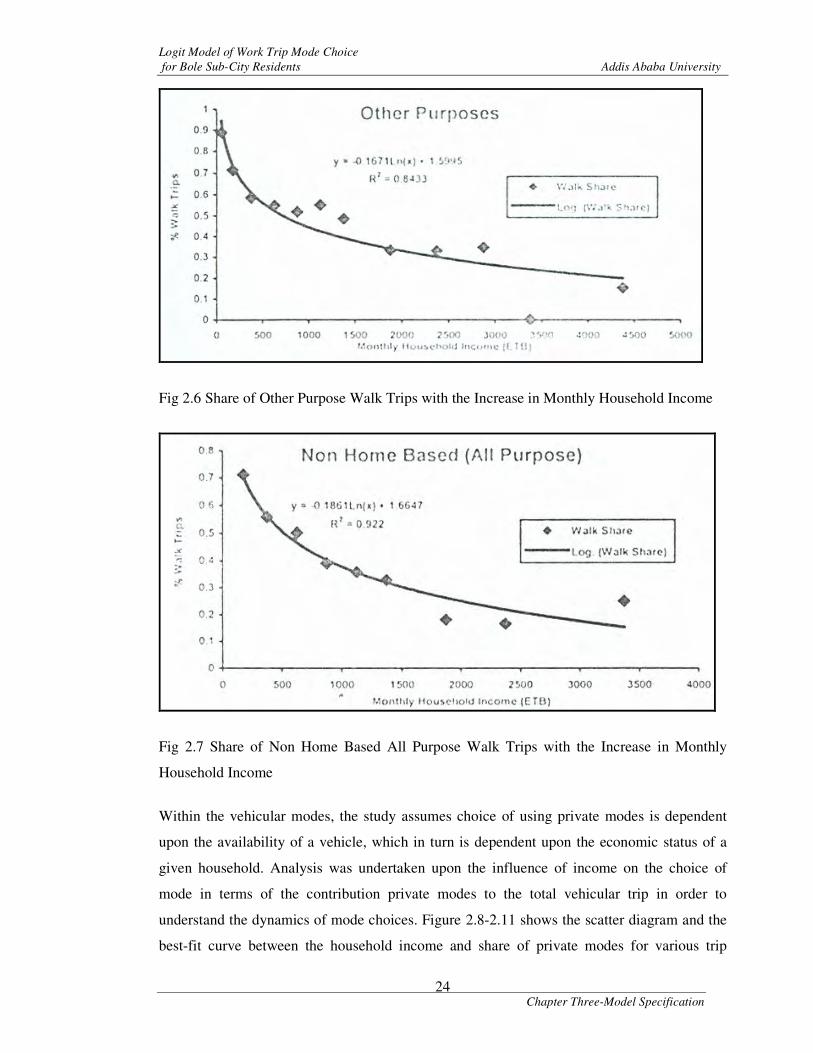
Fig 2.6 Share of Other Purpose Walk Trips with the Increase in Monthly Household Income

Fig 2.7 Share of Non Home Based All Purpose Walk Trips with the Increase in Monthly

Household Income

Within the vehicular modes, the study assumes choice of using private modes is dependent

upon the availability of a vehicle, which in turn is dependent upon the economic status of a

given household. Analysis was undertaken upon the influence of income on the choice of

mode in terms of the contribution private modes to the total vehicular trip in order to

understand the dynamics of mode choices. Figure 2.8-2.11 shows the scatter diagram and the

best-fit curve between the household income and share of private modes for various trip




purposes. It can be seen that as income increases the share of private vehicle trips increases.

Also, the rate of change per unit change in income decreases. The relation that esplains the

share of private vehicle trips for work purpose has a power function. A linear relation has also

been observed to explain the variation in the share of private vehicle trips with respect to

income in case of education and other purpose trips and a power function in case of non-home

based trips. (Urban Transport Study And Preparation of Pilot Project For Addis Ababa, Final

Report, December 2005).

Fig 2.8 Scatter Diagram and the Best-Fit Curve Between Household Income and Share of

Private Modes for Work Purposes Trip




Fig 2.9 Scatter Diagram and the Best-Fit Curve between Household Income and Share of

Private Modes for Education Purposes Trip

Fig 2.10 Scatter Diagram and the Best-Fit Curve Between Household Income and Share of

Private Modes for Other Purposes Trip




Fig 2.11 Scatter Diagram and the Best-Fit Curve between Household Income and Share of

Private Modes For Non Home Based All Purposes Trip

For public transport users, the study considered two facilities, Namely, Anbessa Bus service

and Minibus as available competing modes and a Logit model was developed in order to

assess the choice behavior between Anbessa City Bus service and Minibus service based on

the generalized cost of travel by these services. The generalized cost component includes in

vehicle travel time, access time, waiting time, out-of-pocket cost, reliability, comfort and

convenience etc. (Urban Transport Study And Preparation of Pilot Project For Addis Ababa,

Final Report, December 2005).

The functional form of the Logit model developed by Consulting Engineers Services (India)

in Association with Saba Engineering is as follows:

)}12(exp{1

11

CCP

−−+=

λ

Where,

P1 - Probability of choosing Mode 1

C1 - Cost of Travel by Mode 1 (incl. access time, waiting time, cost of travel etc)




C2 - Cost of Travel by Mode 2 (incl. access time, waiting time, cost of travel etc)

λ - Calibration Parameter

The model was calibrated for the observed data for two competing modes i.e Minibus and

Anbessa City Bus for work, education and other purpose trips.

The calibrated model parameters are provided in Table 2.2 as below:

Table 2.2: Model Calibration parameters

No Purpose Calibration Parameter, λ Goodness of fit R2

1 Work 0.3074 0.82

2 Education 0.3929 0.74

3 Other 0.0627 0.5




Chapter 3

3. MODEL SPECIFICATION


The search for a suitable model specification involves selecting the structure of the model

(MNL, HL, Probit, etc) the explanatory variables to consider, and the form in which they inter

the utility function (linear, non-linear) and the identification of the individual’s choice set

(alternatives available) (Juan De Dios Ortuzar, Luis G. Willumsen, 2004).

This means that in the search for model specification, the following four assumptions must be

addressed:

i. The Decision Maker

ii. The Alternatives

iii. The Attributes

iv. The Decision Rule

In broad terms the objectives of specification search include realism, economy, theoretical

consistency and policy sensitivity. In other words, we search for a realistic model which does

not require too much data and computer resources, does not produce pathological results and

is appropriate to the decision context where we want to use it (Juan De Dios Ortuzar, Luis G.

Willumsen, 2004)

3.2 The Decision-Maker

In this study, the individual or the decision making unit is a randomly selected working

individual living in Bole Sub-City of Addis Ababa. To ensure that the person is a resident of

Bole Sub-City, households in the Sub-City were selected randomly and workers in each

household were questioned. Moreover, the person must be employed since the model aims to

find out what variariables influence the work trip mode choice behavior of residents in Bole

Sub-City.




3.3 The Alternatives

Choice-set determination is a key problem as we estimate Disaggregate Model by means of

the (generally) observed individual choices between alternatives. These should be the

alternatives actually considered consciously or unconsciously by the individual. The omission

of seemingly unimportant options simply on the grounds of costs, may bias results. In the

same vein, the inclusion of alternatives which are actually ignored by certain groups would

also bias model estimation (Juan De Dios Ortuzar, Luis G. Willumsen, 2004).

One of the first problems an analyst has to solve, given a typical revealed preferences cross-

sectional data set, is that of deciding which alternatives are available to each individual in the

sample. It has been noted that this is one of the most difficult of all the issues to resolve,

because it reflects the dilemma the modeler has to tackle in arriving at a suitable trade-off

between modeling relevance and modeling complexity (Juan De Dios Ortuzar, Luis G.

Willumsen, 2004).

In choice set determination, one should follow two steps. The first step is to determine the

universal choice Set C for the problem under study. This step may require some judgment

about which alternatives can be ignored. The next step is to define the choice set for each

individual. This is also generally done by applying reasonable judgments about what

constituents the feasibility of an alternative in any particular situation (Moshe Ben-akiva and

Steven R. Lerman, 1985).

A study on the urban transport and road network of Addis Ababa by the Office for the

Revision of the Addis Ababa City, disclosed that the different modes of road passenger

transport in the city are walking, Anbessa City Bus, Minibus, Taxi, Private cars and service

cars. Since Bole Sub-City is one part of the city, these modes can be assumed to be available

to residents for their work purpose trips. Therefore, the modes of transport considered in the

universal choice set C for the model are:

• Walking

• Small taxis (giving a contract taxi service): - these include only the blue and white

painted small taxies with a capacity of five or less seats.




• Minibuses and Small taxis giving regular taxi service: - these are the blue and white

painted minibuses and some other minibuses painted other colors but providing the

same service in the city. Their seat capacity is between five and twelve.

• Anbessa City Bus: - the only company providing bus transport service in Addis Ababa

is the Anbessa Bus Company and its buses are the predominant service givers in the

city.

• “Lon Chinas”:- there are privately owned buses in the city providing transport service

to the public especially in the peak hour times. Therefore, this alternative includes all

privately owned buses providing public transport service.

• Private vehicle as driver and Private vehicle as passenger: - these include all privately

owned vehicles.

• Company provided transport: - this includes all company cars, which are not directly

given to the individual. A person using this mode of transport should be waiting for

the company car at a certain designated place to be picked up and travel to his/her

working place.

The rules used for determining which subset of the alternatives is feasible for each individual

are entirely judgmental. The following three rules were used to determine the availability of

an alternative to an individual

i. Any worker without a driver’s license cannot drive to work

ii. Any worker in a household without an automobile cannot drive to work

iii. Any worker who has not reported company provided transport as available cannot use

company provided transport.

3.4 The Attributes

As described in Juan De Dios Ortuzar, Luis G. Willumsen (2004), the choice of mode is

affected by the characteristics of the trip maker, the characteristics of the journey and the

characteristics of the transport facility. Here we will define the variables considered under

each category.




Exogenous Variables

To specify the utility functions for each of the alternatives in this research the following

exogenous variables are included in the econometric choice model along with their respective

symbols in {} and units in ().

Characteristics of the Trip Maker (Socioeconomic Variables)

Socioeconomic attributes of workers need to be considered in specifying utility functions of

travel choice alternatives. For this reason, it is assumed that work travel choices are formed in

response to mobility needs, which vary with individual and household socioeconomic

characteristics. Therefore the following variables are considered as candidate variables:

• Age {Age}: - the age of the worker

• Sex{Male}:- 1 if male; 0 if female

• License{L}: - 1 if worker posseses driver's license; 0 otherwise

• Car ownership group1{CG1}: - 1 if the household owns a car, 0 if not

• Car ownership group2{CG2}: - 1 if the household owns ≥ 2 cars, 0 if otherwise

• Monthly individual income {MII}:- the monthly income of the individual in Birr

• Household type {HHT}: - 1 if household has child (or children) of age 0-14;0 if

otherwise

Characteristics of the Journey

In this research, the jorney characterstics like work purpopose, start time of travel and jorney destination are considered as outlined below:

� Trip Purpose :- Only work purpose trips of Bole Sub-City residents are under

consideration.

� Start Time of Travel {PH}: - this variable checks whether the starting time of travel to

work is in the morning peak hour or not by taking the morning peak hour to be from 7:30am

to 8:30am in the morning.

� Central Business District {CBD}:- 1 if the destination of the jorny is located in Addis

Ketema Sub-City; 0 if otherwise




Characteristics of the Transport Facility

� Total Travel Time (in minutes) {TT}: - The specification for total travel time is different

for motorized and non motorized modes based upon the assumption that the utility value of

time is not equal for motorized and non-motorized modes of transport. We expect travelers in

non-motorized modes to be more sensitive to travel time than travelers in motorized modes

(since walking or biking is physically more demanding than traveling in a car).

� Out-Of-Vehicle Time Divided by Distance (min/km) {OVTBd}:- this variable is included

assuming that the sensitivity of travelers to OVT diminishes with the trip distance. In other

words, travelers are more willing to tolerate higher out-of-vehicle time for a long trip rather

than for a short trip. Out of vehicle time is determined as the summation of Access, Waiting

and Egress Times.

� Access Time (in minutes) {AT}- The time required for an individual to travel from

his/her home to a place where public transport is available.

� Waiting Time (in minutes) {WT}: - The time spent waiting for the transport mode to be

available.

� Egress Time (in minutes) {ET}:- The time required for an individual to travel from

his/her last public transport to the workplace.

� Cost by income (unit less) {CostBii}:- To take account of the expectation that low-

income travelers will be more sensitive to travel cost than high-income travelers the cost

divided by income is used in place of cost as an explanatory variable. Such a specification

implies that the importance of cost in mode choice diminishes with increasing individual

income.

3.5 The Decision Rule

The transport mode choice model for the work purpose trips of Bole Sub-City residents is

specified as a Multinomial Logit Model (MNL) with linear in parameters utility assuming

that the random component of a utility functions are independently and identically

distributed, having a double exponential distribution (sometimes called the Weibull or

Gumbel distribution). This is the simplest and most popular and practical discrete choice

model and the probability can be expressed as




∑=

j

j

ii

X

XP

)exp(

)exp(

β

β

Where iX refers to the vector of explanatory variables specific to each alternative and the

parameters β are estimated coefficients. These coefficients are assumed to be constant for all

individuals but may vary across alternatives.

The following figure shows the Logit model structure for work purpose trips of Bole Sub-

City residents.



Chapter Three-Model Specification - 35 -

Figure 3.1- Multinomial Logit Model Structure of Transport Mode Choice for Work Purpose Trips of Bole Sub-City Residents

(1)

Walk

/Cycle

(2)

Private

Vehicle

Driving (5)

Minibus

Taxi

(4)

Contract

Small

Taxi

(6)

Anbessa

City Bus

(8)

Company

Provided

Transport

(Service) (3)

Private

Vehicle

Passenger

(7)

Lonchina



XXXVI

McFadden (1974) showed that a model closely related to the Multinomial Logit Model can be

obtained from an underlying utility comparison. Suppose that, for a random draw i from the

underlying population (usually, but not necessarily, individuals), the utility from choosing

alternative j is

JjaXY ijijij ,...,0,* =+= β

Where aij; j = 0, 1, 2,…, J are unobservables affecting tastes. Here, Xij is a 1x K vector that

differs across alternatives and possibly across individuals as well.

Let Yi denote the choice of individual i that maximizes utility:

),...,,max(arg **

2

*

0 iJiii yyyY =

so that Yi takes on a value in {0; 1; . . . ; J}. As shown by McFadden (1974), if the aij,

j = 0; . . . ; J are independently distributed with cumulative distribution function

)]exp(exp[)( aaF −−= - the typeI extreme value distribution - then

Jj

x

xxjyP

J

oh

ih

ij

ii ,...,0,

)exp(

)exp()/( ===

∑=

β

β

where: P is the probability and h is total number of alternatives.

This response probabilities constitute what is usually called the Conditional Logit Model

(Jeffrey M. Wooldridge,).

The Conditional Logit Model is intended specifically for problems where consumer or firm

choices are at least partly made based on observable attributes of each alternative. The utility

level of each choice is assumed to be a linear function in choice attributes, ijX , with common

parameter vector β . This turns out to actually contain the Multinomial Logit Model as a special

case by appropriately choosing ijX . Suppose that iW is a vector of individual characteristics and



XXXVII

that )/( ii wjyP = follows the Multinomial Logit Model with parameters Jjj ,...,1, =δ . We can

cast this model as the conditional Logit model by defining ),....,2,1( ijijijij wdJwdwdx = , where

djh is a dummy variable equal to unity when hj = and ),.....,( ''

1 Jδδβ = . Consequently, some

authors refer to the conditional Logit model as the Multinomial Logit Model, with the

understanding that alternative-specific characteristics are allowed in the response probability.

Empirical applications of the Conditional Logit Model often include individual specific variables

by allowing them to have separate effects on the latent utilities. A general model is

Jjawzy ijjiijij ,....,1,0,* =++= δγ

With 00 =δ as a normalization, where zij varies across j and possibly i. if δδ =j for all j, then

δiw drops out of all response probabilities (Jeffrey M. Wooldridge,).

3.6 Limitations of the Multinomial Logit Model

The Conditional Logit Model is very convenient for modeling probabilistic choice, but it has

some limitations. An important restriction is the independence from irrelevant alternatives

(IIA) assumption because it implies that adding another alternative or changing the

characteristics of a third alternative does not affect the relative odds between alternatives. This

implication is implausible for applications with similar alternatives (Jeffrey M. Wooldridge,).

For our case, there exists clear similarity among some modes than the others in the choice set.

For example there is more similarity between private buses(Lonchinas) and Anbessa City Bus

since they are widely used mass transportation facilities, available almost every were in the city

and charge standard fees for specified distances.

Hausman and McFadden (1984) offer tests of the IIA assumption based on the observation that, if

the Conditional Logit Model is true, β can be consistently estimated by conditional Logit by

focusing on any subset of alternatives. They apply the Hausman principle, which compares the

estimate of β using all alternatives to the estimate using a subset of alternatives (Jeffrey M.

Wooldridge,).



XXXVIII

3.7 Estimation of the Multinomial Logit

We assume that the sample is exogenously drawn, that is, either random or stratified random with

the strata defined on factors that are exogenous to the choice being analyzed and the explanatory

variables are exogenous to the choice situation. In short, the variables entering representative

utility are independent of the unobserved component of utility.

If an exogenous sample of N decision makers is obtained for the purpose of estimation, since the

Logit probabilities take a closed form, the traditional maximum-likelihood procedures can be

applied. And, the probability of a person n choosing the alternative that he/she was actually

observed to choose can be expressed as

∏i

y

niniP )(

Where 1=niy

if person n chose i and zero otherwise

Assuming that each decision maker’s choice is independent of that of the other decision maker, the probability of each person in the sample

choosing the alternative that he was observed actually to choose is

∏∏=

=N

n i

y

niniPL

1

)()(β

Where β is a vector containing the parameters of the model

The log likelihood function is then

∑∑=

=N

n i

nini PyLL1

ln)(β

and the estimator is the value of β that maximizes this function. McFadden (1974) shows that LL

(β) is globally concave for linear-in parameters utility and many statistical packages are available

for estimation of these models.



XXXIX

At the maximum of the likelihood function, its derivative with respect to each of the parameters

is zero:

0)(

)(=

β

β

d

dLL

The maximum-likelihood estimates are therefore the values of β that satisfy this first-order

condition (Kenneth Train, 2003).



XL

Chapter 4

4. SURVEY DESIGN AND DATA COLLECTON

4.1 Survey Objectives

Revealed preference survey was undertaken for this research. Among the various methods of

revealed preference surveys, Household or Home Interview Survey was used as a data source to

meet the following objectives:

• Establish the socio-economic characteristics of the people of Bole Sub-City

• Obtain the work trip travel characteristics of the Bole Sub-City residents.

• Establish connection between socio-economic characteristics of a trip maker and his work

trip characteristics. This would be carried out on a disaggregated basis of gender, age and

income etc. correlating with mode, trip length and other related variables.

4.2 The Population to be Surveyed

Working population of Bole Sub-City is considered as the focus of the survey, which in turn

limits the survey population to employed residents of the Sub-City. The estimated total employed

population of the Sub-City for the year (2006/07G.C)/1999E.C is 100,664 among which 59,628

are males and the remaing 40,986 are expected to be females. Table 4.1 shows the distribution of

employed population of Bole Sub-Cirty aged 10 years and above by Kebele and gender for the

year (2006/07G.c)/1999E.C



XLI

Table 4.1: Distribution of Employed Population Aged 10 Years and above by Kebele and Gender in Bole Sub-City For the Year

(2006/07G.C)/1999E.C

Estimated Total Employed

Population

No Name Of The Kebele

In Bole Sub-City Total Male Female

1 Kebele 01 9,197 5,451 3,746

2 Kebele 02 8,409 4,984 3,425

3 Kebele 03/05 11,918 6,957 4,961

4 Kebele 04/06/07 12,160 7,196 4,964

5 Kebele 08/09 12,857 7,640 5,217

6 Kebele 10 8,788 5,090 3,698

7 Kebele 11 8,349 4,835 3,514

8 Kebele 12/13 12,975 7,595 5,380

9 Kebele 14/15 11,360 6,980 4,380

10 Kebele 16/18/21/22 2,223 1,404 819

11 Kebele 17/19/20 2,378 1,496 882

Total 100,614 59,628 40,986

Source: - Analytical Report of the 1994 Population and Housing Census of Addis Ababa

(C.S.A)

- Addis Ababa City Administration, Policy Study and Planning Commotion

4.3 Data Requirements

The data required is the socio economic characteristics of travelers interviewed and the

characteristics of available mode of transport for work purpose trip. In other words, the traveler’s

choice of mode, travel times, fares, waiting/transfer times, walking distances etc and traveler’s

socioeconomic data (gender, age, car ownership status, income, etc) related to the mode choice is

collected.

The choice of mode is required only for the work purpose trips, i.e. trips form an origin (home or

other place) to work. Trips made while they are working, i.e. for the accomplishment of any kind

of task in their working period during the day, are not required. As for the pre-work trips the

survey will address its presence and since the purpose of pre-work trips affect the mode choice it

is included in the survey. However, the trips made from work to different places like back to



XLII

home, visit friend, shopping etc are not included since most of these trips are not directly related

to the stress of reaching on time for work.

4.4 Required Precision

There is no single sample design for discrete choice analysis that is unambiguously optimal for

all values of the parameters. Rather, whether a sample design is good or bad (in the classical

sense) depends on the unknown parameter values (Ben-AKiva and Leman, 1985). Moreover, the

size of the sample needed to develop a Logit mode choice model usually is in the range 1000-

3000 individuals, not counting non-respondents and unusable response. Although the upper end

of this range is preferable to the lower, a mode choice model usually can be developed

satisfactorily from a sample of 1000 observations if cost or other considerations prohibit

acquisition of larger data set (Joel L. Horowitz, Frank S. Koppelman, Steven R. Lerman, 1986).

Therefore, considering the economic constraint and time limitation for this research, we have

used 1% of the estimated employed population for the year (2006/07G.c)/1999E.c of Bole Sub-

City as appropriate sample. In other words we have interviewed 1007 working residents of Bole

Sub City.

4.5 Survey Instrument

Questionnaire was used as a major survey instrument in the collection of primary data using

household interview. Observation of secondary data was also used to assess the socio economic

characteristics and the level of service and availability of transport service for the Sub-City.

4.6 Sampling Unit

The sampling units must be defined to be mutually exclusive and must collectively exhaust the

population. In the analysis of urban passenger travel the household has often been used as the

sampling unit (Ben-AKiva and Leman, 1985). Therefore, households in Bole Sub-City are taken

to be the sampling unit.



XLIII

4.7 Sampling Frame

Taken collectively, an implicit or explicit list of all the sampling units constitutes the sampling

frame. Such lists are often derived from utility records, telephone listings, motor vehicle registry

lists, or private directories of firms. Very often the creation of an appropriate sampling frame

may be extremely difficult. For example, in many developing countries there are no complete

listings of residents or addresses, and it may be necessary actually to visit every residence in an

area to establish a reliable sampling frame (Ben-AKiva and Leman, 1985). This is the primary

reason for using "deterministic rules" of sampling. In systematic sampling, sample units are

drawn by deterministic rather than random rules. For example, rather than drawing a random

sample of 5 percent of all households in a region from a published directory, a systematic

sampling plan may pick out every 20th household in the directory. As long as there is no inherent

bias in setting up the deterministic rule, the systematic sampling plan is essentially equivalent to

random sampling, and the choice of one over the other may be a matter of operational

convenience (Frank S. Koppelman and Chandra Bhat, 2006)

For this research, Kebeles address lists were taken to be the sampling frame. However, these lists

do not include the squatters within each Kebele. To include these households one may visit these

residences in the Kebele as recommended in Ben-AKiva and Leman, 1985. But, due to time and

budget limitations, they have not been included. To this end, only Kebeles address lists were used

as a sampling frame.

4.8 Sampling Strategy

Our sample is very small compared to the estimated total employed population of the Bole Sub-

City for the year (2006/07G.c)/1999E.C. Therefore, the employed population of Bole Sub-City is

treated as having infinite number of members. This justifies our without replacement sampling

strategy; since for an infinite population the distribution of characteristics within the pool of

sampling units is unaffected by the removal of any finite number of them (Ben-AKiva and

Leman, 1985).

Exogenous sampling is taken as the appropriate strategy of sampling. Bole Sub-City is divided

into 11 Kebeles; this is used as a yardstick to classify the residents into 11 geographical strata.



XLIV

Then 0.25% of the households from each stratum (Kebele) are selected randomly from the

respective Kebele’s Address list and their location is identified using Nortake. After that, every

tenth household is identified and all of available working residents in the household are

interviewed until 1% of the estimated employed population in each Kebele is interviewed. Table

4.2, 4.3 and 4.4 show the distribution of employed population aged 10 years and over by sex and

Kebele with the respective sample size, distribution of registered households with house

ownership and distribution of registered households for each Kebele with the corresponding size

of randomly selected houses respectively.

Table 4.2: Distribution of Employed Population Aged 10 Years and over by Sex And Kebele In Bole Sub-City for the Year

(2006/07G.C)/1999E.C and the Sample Size for each Kebele

Name of the Kebele

in Bole Sub-City

Estimated Total Employed

Population

1% of the Employed Population to be

Interviewed

Total Male Female Total Male Female

Kebele 01 9,203 5,451 3,746 92 55 37

Kebele 02 8,412 4,984 3,425 84 50 34

Kebele 03/05 11,981 6,957 4,961 120 70 50

Kebele 04/06/07 12,171 7,196 4,964 122 72 50

Kebele 08/09 12,853 7,640 5,217 129 76 52

Kebele 10 8,854 5,090 3,698 89 51 37

Kebele 11 8,412 4,835 3,514 84 48 35

Kebele 12/13 13,031 7,595 5,380 130 76 54

Kebele 14/15 11,235 6,980 4,380 112 70 44

Kebele 16/18/21/22 2,178 1,404 819 22 14 8

Kebele 17/19/20 2,334 1,496 882 23 15 9

Total 100,664 59,628 40,986 1,007 596 410


(C.S.A)




XLV

Table 4.3: Distribution of Registered Households with House Ownership for each Kebele in Bole Sub-City for the Year (2006/07G.C)/1999E.C

Name of The Kebele

In Bole Sub-City

Total Registered

Households in each

Kebele

Registered Kebele

Owned Houses

% Registered

Rent Houses

% Registered Privately

Owned Houses

%

Kebele 01 3,154 388 12 145 5 2,621 83

Kebele 02 1,475 162 11 145 10 1,168 79

Kebele 03/05 6,454 499 8 355 5 5,600 87

Kebele 04/06/07 4,105 1,642 40 142 3 2,321 57

Kebele 08/09 2,283 97 4 690 30 1,496 66

Kebele 10 3,376 623 18 472 14 2,281 68

Kebele 11 3,325 0 0 324 10 3,001 90

Kebele 12/13 3,013 246 8 368 12 2,399 80

Kebele 14/15 5,650 1,602 28 15 1 4,033 71

Kebele16/18/21/22 3,813 0 0 0 0 3,813 100

Kebele 17/19/20 2,851 10 1 128 4 2,713 95

Total 39499 5269 13 2784 7 31446 80

Source: - Kebeles of Bole Sub-City.

Table 4.4: Distribution of Registered Households for each Kebele in Bole Sub-City for the Year (2006/07G.C)/1999E.C and Corresponding Size

of Randomly Selected Houses



XLVI

Name of The Kebele in Bole Sub-City Total Registered Households in Each Kebele 0.25% of Total Registered Households in Each Kebele

Kebele 01 3,154 8

Kebele 02 1,475 4

Kebele03/05 6,454 16

Kebele04/06/07 4,105 10

Kebele 08/09 2,283 6

Kebele 10 3,376 8

Kebele 11 3,325 8

Kebele 12/13 3,013 8

Kebele 14/15 5,650 14

Kebele16/18/21/22 3,813 10

Kebele 17/19/20 2,851 7

Total 39499 99

Source: - Kebeles of Bole Sub-City.

4.9 Pre-Testing the Survey

To test the questionnaires, a pilot survey was undertaken on 30 individuals.

4.10 The Survey Management Process

Enumerators were trained on how they will perform the interview and they were provided with

support letters from the University to facilitate the response rate and to make the respondents

understand the purpose of the research and encourage them to give accurate information.

The heads of households and other working members of the households were visited at their

homes, and interviewed by enumerators using the structured questionnaire for recording

socioeconomic and work trip characteristics on an average working day.

4.11 Analysis method



XLVII

Statistical software, Stata v8, was used to develop the required Multinomial Logit Model.

4.12 Data Source

The data used for the research was primary data, which was generated from the household survey

conducted for the purpose of accomplishing this research and secondary data obtained from

different authorities of the Addis Ababa City Adminstration.

A total of 1,007 working residents of Bole Sub-City were interviewed. From these interviews

relevant data on the one-way work trip characteristics for each employed member and detailed

individual and household socio-economic information were obtained. In addition, the distance

traveled by each working resident was measured using NORTAKE map based on the reported

route of travel. Level of service data for each mode was determined in the following manner.

4.12.1 Level of Service Data for Anbessa Bus

Operational Aspects

Anbessa-Bus Service Enterprise is owned by the Federal Government and is controlled by the

Addis Ababa City Administration. Anbessa operates 92 routes in Addis Ababa with an average

route length of approximately 10 kilometers. Most operate within the city boundary but there are

several longer ones serving outlying areas: the longest is Route 60 (47 kilometers) to Debre Zeit

(LEA international, 2004).

Anbessa has two types of operations in Addis Ababa and these are urban bus services that

constitute the major part of the operation and contract services, which is primarily for employers

in the city for staff transport. The total number of buses assigned to the two types of operations is

349 and 50 respectively with approximate daily kilometers of 73,440 and 1,200 respectively.

There are three major Anbessa City Bus terminals (Addis Ketema, Leghar, Menelik Square) and

six minor terminals (Megenagna, Lideta, Sidest Kilo, Arat Kilo, Ayer Tena, Shero Meda).

Additionally, a total of 860 stops are used for loading and off-loading passengers in the city.

Curbside bus stops are spaced between 300 and 500 meters apart (LEA international, 2004). And,

Table 4.5 shows key operational characterstics of the enterprise.



XLVIII

Table 4.5: Anbessa - Key Operational Characteristics

No. Item Statistic

1. Days of operation Mon – Sun

2. Times of operation 06:00-20:30

3. Number of routes 93

4. Number of kilometers operated per month 2 120 000

5. Number of bus trips per month 200 000

6. Average bus trip length 10.4 km

7. Passengers transported per month 20 million

8. Passenger kilometers per month 208 million

9. Average kilometers per bus per day 178 km

10. Passenger trips per weekday 600 000

11. Average number of passengers per trip 96

12. Fleet Composition:

DAF buses used to provide commuter services

Mercedes Benz buses used as replacement and

for private hire services and contracts

Fiat buses used to provide a service in Jima

town

463

±65

7

13. Vehicle capacity 100 passengers

14. Seated - standing ratio per vehicle 30:70

15. Fleet availability on any given day 90%

Source: Improving Urban Transport through Private Participation in Addis Ababa,

status Quo analysis, LEA international (Ltd), 2004



XLIX

Figure 4.1: Addis Ababa city Anbessa City Bus Network (Anbessa-Bus Service

Enterprise)

Financial aspects

The fare structure is flat fare but varies amongst routes based on route length. The minimum fare is ETB0.25 (with some exceptions). Nearly, 40%

of passengers pay a fare of ETB 0.25, and 95% of passengers pay a fare of ETB 0.50 or less (LEA international, 2004). For determination of cost

in this research, we have developed the following correlation of distance and cost for Anbessa City Bus based on data obtained from Anbessa City

Bus Enterprise.

1237.00255.00007.0 2 ++= XXY 9169.02 =R

Where: X is distance (km) and Y is Anbessa Travel Cost (birr)



L

correlation of cost and distasnce for Anbessa bus

y = 0.0007x2 + 0.0255x + 0.1237

R2 = 0.9169

0.00

0.50

1.00

1.50

2.00

2.50

3.00

3.50

0.0 5.0 10.0 15.0 20.0 25.0 30.0 35.0 40.0 45.0 50.0

Distance

Co

st Series1

Poly. (Series1)

Figure 4.2: Addis Ababa City Anbessa City Bus Cost In Relation To Travel Distance

Travel Time Aspects

Based on data obtained from the Anbessa City Bus Enterprise, it was determined that average

speed of Anbessa City Bus is 16km/h, which was used to determine the in-vehicle time of

Anbessa City Bus. The average waiting time was also found to be 32 minites. The average access

time for Anbessa City Bus is determined by calculating the average access time for persons who

have actually used walking for their travel to work from our survey and it is found to be 12

minutes.

4.12.2 Level of Service Data for Minibus Taxis

Operational Aspects

No formal economic regulation of taxi operations per route or area exists and no restrictions exist in terms of the routes or areas where a taxi may

operate. The legal requirements related to taxi operation are: (i) to obtain business license from the Department of Trade and Industry;(ii)



LI

Vehicles to be licensed and inspected annually; (iii) Drivers to be licensed and are in possession of a Class 3 driving license (LEA international,

2004).

According to the urban transport study and preparation of pilot project for Addis Ababa (2005),

Minibuses are mainly Toyota Hi-Ace or converted pick-up vehicles (Toyota Hi-Lux and old

Peugeot vehicles). The capacity is 11 passengers. There are 105 Minibus taxi routes in Addis

Ababa, with the longest close to 25km and an average round trip length of 15km. The Minibuses

on an average do, 6 to 8 round trips per day.

Table 4.6: Mini Bus - Key Operational Characteristics

No. Item Statistic

1. Days of operation Mon – Sun

2. Times of operation 06:00 – 22:00 Hrs

3. Number of routes 105

4. Passengers per day 1,200,000

5. Fleet size 12,500

6. Average Route Length 15 Km

7. Average Trip Length 5.44 Km

8. No of Trips per Minibus per Day 6 to 8 Round Trips

9. Fleet Utilization 75 %

10. Vehicle Utilization 180 Km

11. Vehicle capacity 11

12. Operational staff per Minibus trip Driver & conductor

13. Ownership 88 % Single Vehicle

Source: Urban Transport Study for Addis Ababa, 2005.



LII

Figure 4.3: The Addis Ababa Minibus taxi routes

(Urban transport study for Addis Ababa, 2005)

Financial Aspects

As per, the Urban Transport Study for Addis Ababa in 2005, the fares of Minibus taxies are

regulated by the Government. However, there is malpractice and passengers are charged more,

particularly in peak hours. Current tariff for Minibuses are 0.65 Birr for a trip less than 2.5km in

length, 1.20 Birr from 2.5 km to 7.0 km, 1.60 Birr from 7.0 km to 10.0 km, 1.75 Birr from 10.0

km to 12.0 km and 2.20 Birr from 12.0 km to 15.0 km (Addis Ababa Transport Branch Office).

F et aw ra ri H ab te G io rg is S t.

De

j . Be

lay Z

ele

ke S

t.

I nto

to

A

ve

nu

e

Rus sia n S t.

F .Maria m

Ab a Te chan S t.

To

go

S

t.

H aile G eb re S e las ie Road

So

uth

Afirc

a S

t.

Nam

ibia

St.

Rin

g R

oa

d

Bo

le R

oa

d

Eth

io- C

hin

a Road

De

br e

Ze

it R

oa

dAle xa nd e r Pus hk in S t.

Ro

se

ve

l t S

t .

S m ut snd S t.R as M ek on ne n Avenue

Me

nili k

II

Av

en

ueC

hu

rch

il R

oa

d

She

h O

jet e

St.

Old

A

irp

ort

Ro

ad

Mic

ke

y Le

y La

nd

St.

Tit o

St.

D.W

.Ga

brie

l St.

Arb en yo ch S t.



LIII

Based upon the information obtained from the Addis Ababa Transport Branch Office on Minibus

route, we have developed the following correlation of travel distance and cost for Minibus taxi.

5903.01202.0 += XY 7787.02 =R

Where: X is distance (km) and Y is Minibus taxi Cost (birr)

correlation of cost and distance for Mini bus taxi

y = 0.1202x + 0.5903

R2 = 0.7787

0

0.5

1

1.5

2

2.5

3

0 2 4 6 8 10 12 14 16 18 20

Distance

Co

st Series1

Linear (Series1)

Figure 4.4: Addis Ababa City Minibus Cost In Relation To Travel Distance

Travel Time Aspects

The average access time, average waiting time and average speed for taxi service is determined

by calculating the respective averages for the persons who have actually used taxi for their travel

to work in our survey. Based on this calculation; the access time, average waiting time and

average speed are found to be 9 minutes, 12 minutes and 19Km/h respectively.



LIV

4.12.3 Level of Service Data for Small Taxis

The Urban Transport Study for Addis Ababa in 2005 has revealed that Short distance or small

taxis provide more personalized services (door-to-door) on contract basis. However, during peak

periods they also act as “Minibuses” and transport commuters, but at a higher fare than the

Minibuses. Mainly old vehicles, Fiat 124 or Ladas, are used as small taxis. Small taxis are not

legally allowed to work at hotels and airports. These services are provided by “yellow taxis”,

which have different licenses/ permits (LEA international, 2004).

Financial Aspects

Fares of short-distance taxis are “negotiable” on time and distance basis. A typical fare is in the

order of 30 Birr per hour (more is charged if luggage is included) (LEA international, 2004). But

this is small for the current market since fuel cost has nearly doubled. Therefore, based on this

charge of 30birr per hour, on interviews with different small taxi operators and the vehicle

operating cost for small cars which is currently 2.537 birr per km (Kocks Consult Gmbh, 2006)

the charge was estimated at 3.3 birr per km for contact taxi service, Which is basically an

addition of a 30% profit over the vehicle operating costs.

Travel Time Aspects

The average access time, average waiting time and average speed for small taxi contact service is

determined by calculating the respective averages for the persons who have actually used contract

taxi for their travel to work in our survey. Based on this calculation, the average access time,

average waiting time and average speed are found to be 6 minutes, 0 minutes and 22 Km/h

respectively.

4.12.4 Level of Service Data for Lonchina

Lonchina (medium size and small Buses) operate on 95 routes in the city. Their tariff is cheaper

than taxi but more expensive than Anbessa City Bus.



LV

Financial Aspects

Base on the information obtained from Addis Ababa Transport Branch Office, we have

developed the following correlation of travel distance and cost for Lonchina.

1859.00944.0 += XY 6884.02 =R

Where: X is distance (km) and Y is Minibus taxi Cost (km)

correlation of Cost and Distance for Lonchina

y = 0.0944x + 0.1859

R2 = 0.6884

0

0.5

1

1.5

2

2.5

0 2 4 6 8 10 12 14 16 18

Diatance

Co

st Series1

Linear (Series1)

Figure 4.5 Addis Ababa City Lonchina Cost in Relation To Travel Distance

Travel Time Aspects

The average access time, average waiting time and average speed for Lonchina service is

determined by calculating the respective averages for the persons who have actually used

Lonchina for their travel to work in our survey. Based on this calculation, the average access



LVI

time, average waiting time and average speed were found to be 10 minutes, 10 minutes and 20

Km/h respectively.

4.12.5 Level of Service Data for Non-Motorized Transport

Pedestrians and animals form a component of urban mobility for the city of Addis Ababa. The

urban mobility study states that over 4.9 million trips are generated daily. Out of this around 4%

were made using private cars, 26% using public transport and 70% on foot. Of the 70 percent of

the home to work trips that are made on foot, over 50 percent are beyond half hour walking time

(Urban Transport Study for Addis Ababa, 2005). In this research, an average travel speed of 2

km/h was taken for walking. This was determined by calculating the average walking speed for

the persons who have actually used walking for their travel to work from our survey.

4.12.6 Level of Service Data for Car Drive and Car Passenger Modes of Transport

Financial Aspects

Based on the data found in the feasibility study for Gonder- Debalk Road project undertaken by

Kock Consult Gmbh June 2006, a vehicle operating cost of 2.537 birr/km for driving car and zero

cost for Car Passenger were adopted in the study.

Travel Time Aspects

The average access time, average waiting time and average speed for Car Drive and Car

Passenger modes of transport are determined by calculating the respective averages for the

persons who have actually used Car Drive and Car Passenger modes of transport during their

travels to work in the survey. Based on this calculation, average access time and average waiting

time were found to be zero in both cases and average speeds are was found to be 22 Km/h and

48Km/h for Car Drive and Car Passenger modes of transport respectively.



LVII

4.12.7 Level of Service Data for Company Provided Mode of Transport

Financial Aspects

There is no cost incurred by the company provided mode transport user for his work trip.

Travel Time Aspects

The average access time, average waiting time and average speed for company provided transport

service is determined by calculating the respective averages for the persons who have actually

used company provided transport services during their travel to work in the survey. Based on this

calculation, the average access time, average waiting time and average speed are found to be 5

minutes, 8 minutes and 24 Km/h respectively.

4.13 Sample Characteristics

Table 4.7 provides information about the availability and usage of each alternative in the sample.

Taxi is available to all workers in the Bole Sub-City and is the most frequently chosen

alternative. The Anbessa City Bus mode is also available for all trips and account for the next

largest share of chosen alternatives. The combined total of taxi and Anbessa City Bus trips

represent a bit more than 70% of all work trips. Company provided mode of transport (service),

Lonchina, Car passenger, Car Drive and Lada contract constitute 4.6%, 4%, 2.1%, 10.1% and

1.2% respectively. The fraction of trips using non-motorized modes (walk) constitutes 5.6%.



LVIII

Table 4.7: Sample Statistics of Work Trips Modal Data For Bole Sub-City Residents

NO Mode Fraction of Sample

with Mode

Available (%)

Sample

Frequencies of

the Chosen Mode

Sample Market

Share (%)

1 Walk 100 56 5.6

2 Car Drive 14.1 102 10.1

3 Car Passenger 100 21 2.1

4 Lada Contract 100 12 1.2

5 Taxi 100 608 60.5

6 Anbessa Bus 100 120 11.9

7 Lonchina 100 40 4

8 Service 6.6 46 4.6

Table 4.8: Mean Distance, Total Travel Time, Cost and Monthly Individual Income of Trip Makers With Respect to their Chosen Mode

Mean Distance Mean Monthly Individual

Income

NO Chosen

Mode

Km Ratio Birr Ratio

1 Walk 2.4 1 334 1

2 Car Drive 7.3 3.04 3560 10.66

3 Car Passenger 6.8 2.83 1715 5.13

4 Lada Contract 7.8 3.25 3475 10.4

5 Taxi 6.4 2.67 1150 3.44

6 Anbessa Bus 8.3 3.46 611 1.83

7 Lonchina 7.7 3.21 693 2.07

8 Service 7.6 3.17 1293 3.87



LIX

Chapter 5

5. RESEARCH RESULTS

5.1 Introduction

In this research we have estimated five different Models for the work trips of Bole Sub City

residents as shown table 5.1. These Models are:

i. The Base Model: - having only the mode related variables (total travel time and cost) in

addition to the alternative specific constants.

ii. Model 1: - having the socioeconomic variable (income) in addition to the alternative

specific constants and the mode related variables (total travel time and cost).

iii. Model 2: - which is an upgrading of Model 1 by adding the trip related variable (peak

hour)

iv. Model 3 and Model 4: - which have different specifications of total travel time and cost

including socioeconomic variables i.e gender, age, Car and child ownership and trip

related variable CBD to Model 2.

In this chapter we will compare and evaluate these Models by using informal judgment based on tests, goodness of fit measures and statistical

tests and as a final task we will choose the optimal Model.

Utility functions for alternative modes of travel under each Model have been expressed. The

following Model labels were used in the equations: TT is total travel time, TC is total travel cost,

MII is monthly individual income, PH is peak hour dummy variable equal to one if the individual

started his trip to work between 7:30am to 8:30am and 0 otherwise, AGE is age in years, CostBii

is cost divided by income, OVTBd is out of vehicle time divided by distance, Car is dummy

variable equal to one if the household owns car(s) and 0 other wise, 2Car is dummy variable

equal to one if the household owns two or more cars and 0 other wise, CHILD is a dummy

variable equal to one if the household has child(ren) aged less than fourteen years,

Base Model



LX

)(2)()( walkwalkwalk TTV ββ +=

)(2)(1)()( cardrivecardrivecardrivecardrive TTTCV βββ ++=

)(2)()( ercarpassengercarpassengercarpasseng TTV ββ +=

)(2)(1)()( ctLadacontractLadacontractLadacontractLadacontra TTTCV βββ ++=

)(2)(1)( TaxiTaxiTaxi TTTCV ββ +=

)(2)(1)()( AnbessaAnbessaAnbessaAnbessa TTTCV βββ ++=

)(2)(1)()( LonchinaLonchinaLonchinaLonchina TTTCV βββ ++=

)(2)()( ServiceServiceService TTV ββ +=

Model 1

MIITTV walkwalkwalkwalk )()(2)()( γββ ++=

MIITTTCV cardrivecardrivecardrivecardrivecardrive )()(2)(1)()( γβββ +++=

MIITTV ercarpassengercarpassengercarpassengercarpasseng )()(2)()( γββ ++=

MIITTTCV ctLadacontractLadacontractLadacontractLadacontractLadacontra )()(2)(1)()( γβββ +++=

MIITTTCV TaxiTaxiTaxiTaxi )()(2)(1)( γββ ++=

MIITTTCV AnbessaAnbessaAnbessaAnbessaAnbessa )()(2)(1)()( γβββ +++=

MIITTTCV LonchinaLonchinaLonchinaLonchinaLonchina )()(2)(1)()( γβββ +++=

MIITTV ServiceServiceServiceService )()(2)()( γββ ++=



LXI

Model 2

PHMIITTV walkwalkwalkwalkwalk )()()(2)()( αγββ +++=

MIITTTCV cardrivecardrivecardrivecardrivecardrive )()(2)(1)()( γβββ +++=

MIITTV ercarpassengercarpassengercarpassengercarpasseng )()(2)()( γββ ++=

MIITTTCV ctLadacontractLadacontractLadacontractLadacontractLadacontra )()(2)(1)()( γβββ +++=

MIITTTCV TaxiTaxiTaxiTaxi )()(2)(1)( γββ ++=

PHMIITTTCV AnbessaAnbessaAnbessaAnbessaAnbessaAnbessa )()()(2)(1)()( αγβββ ++++=

MIITTTCV LonchinaLonchinaLonchinaLonchinaLonchina )()(2)(1)()( γβββ +++=

MIITTV ServiceServiceServiceService )()(2)()( γββ ++=

Model 3

AGEMALEMIITTVwalkwalkwalkwalkwalkwalk )(3)(2)(1)(4)()( γγγββ ++++=

CARAGE

MIIOVTBdTTCostBiiV

cardrivecardrive

cardrivecardrivecardrivecardrivecardrivecardrive

2)(5)(3

)(1)(6)(5)(3)()(

γγ

γββββ

+

+++++=

CAROVTBdTTVercarpassengercarpassengercarpassengercarpassengercarpasseng )(4)(6)(5)()( γβββ +++=

MIIOVTBdTTCostBiiV ctLadacontractLadacontractLadacontractLadacontractLadacontractLadacontra )()(6)(5)(3)()( γββββ ++++=

MIIOVTBdTTCostBiiV TaxiTaxiTaxiTaxiTaxi )()(6)(5)(3)( γβββ +++=



LXII

CBDPHCHILDMALE

MIIOVTBdTTCostBiiV

AnbessaAnbessaAnbessaAnbessa

AnbessaAnbessaAnbessaAnbessaAnbessaAnbessa

)(2)(1)(6)(2

)(1)(6)(5)(3)()(

ααγγ

γββββ

+++

+++++=

MIIOVTBdTTCostBiiV LonchinaLonchinaLonchinaLonchinaLonchinaLonchina )()(6)(5)(3)()( γββββ ++++=

MIIOVTBdTTV ServiceServiceServiceServiceService )()(6)(5)()( γβββ +++=

Model 4

AGEMALEMIITTVwalkwalkwalkwalkwalkwalk )(3)(2)(1)(2)()( γγγββ ++++=

CARAGE

MIIOVTBdTTCostBiiV

cardrivecardrive

cardrivecardrivecardrivecardrivecardrivecardrive

2)(5)(3

)(1)(6)(2)(3)()(

γγ

γββββ

+

+++++=

CAROVTBdTTVercarpassengercarpassengercarpassengercarpassengercarpasseng )(4)(6)(2)()( γβββ +++=

MIIOVTBdTTCostBiiV ctLadacontractLadacontractLadacontractLadacontractLadacontractLadacontra )()(6)(2)(3)()( γββββ ++++=

MIIOVTBdTTCostBiiV TaxiTaxiTaxiTaxiTaxi )()(6)(2)(3)( γβββ +++=

CBDPHCHILDMALE

MIIOVTBdTTCostBiiV

AnbessaAnbessaAnbessaAnbessa

AnbessaAnbessaAnbessaAnbessaAnbessaAnbessa

)(2)(1)(6)(2

)(1)(6)(2)(3)()(

ααγγ

γββββ

+++

+++++=

MIIOVTBdTTCostBiiV LonchinaLonchinaLonchinaLonchinaLonchinaLonchina )()(6)(2)(3)()( γββββ ++++=

MIIOVTBdTTV ServiceServiceServiceServiceService )()(6)(2)()( γβββ +++=



LXIII

Table 5.1 Research Results

Table 5.1.1 Research Results for Zero Coefficients, Constants Only and Base Models

Variables Zero

Coefficients

Model

Constants Only

Model

Base Model Model 1

Travel Cost (Birr) -.0092061(-0.59) -0.0165833(-0.98)

Total Travel Time (Min) -.0249704(-7.07) -0.0242011(-6.51)

Monthly Individual

Income (Birr) Walk

Car Drive

Car Passenger

Lada Contract

Taxi(Base) Anbessa

Lonchina

Service

-0.0054253 (-6.85)

0.0005778 (3.88)

0.0003615 (2.55)

0.0005789 (4.30)

0.0

-0.0016163 (-6.23)

-0.0011339 (-3.13)

-0.0005888(-2.51)

Alternative Specific

Constants Walk

Car Drive

Car Passenger

Lada Contract

Taxi (Base) Anbessa

Lonchina

Service

-2.384823(-17.08)

1.449281(7.45)

-3.365652(-15.16)

-3.925268(-13.47)

0.0

-1.622683(-16.24)

-2.721295(-16.67)

1.520255(5.38)

-0.5244118 (-2.50)

0.8962151 (2.63)

-4.261089 (-16.49)

-4.234801 (-9.83)

0.0

-0.9205077 (-6.48)

-2.657552 (-16.23)

1.096012(3.78)

2.405236 (5.78)

-0.3950503(-0.88)

-4.743031(-13.52)

-5.068401(-9.53)

0.0

0.3450086(1.54)

-1.681623(-5.53)

2.130865(4.06)

Log - Likelihood At Zero -1832.4929 -1832.4929 -1832.4929

Log - Likelihood At

Constants

-963.22434 -963.22434

Log - Likelihood At

Convergence

-1832.4929 -963.22434 -914.73224 -809.52729

Rho–Squared W.R.T

Zero

NA 0.4744 0.5008 0.5582

Rho-Squared W.R.T

Constants

NA NA 0.05034 0.1596

Number Of Parameters 0 7 9 16



LXIV

Table 5.1.2 Research Results or Additional Three Models

Variables Model 2 Model 3 Model 4

Travel Cost (Birr) -0.0155124(-0.91)

Cost By Monthly Individual Income -41.69661(-1.93) -41.2782(-1.93)

Total Travel Time (Min) -0.0250796(-6.60) -0.014314(-3.57)

Total Travel Time Non-Motorized Modes Only

(Min)

Total Travel Time Motorized Modes Only

(Min)

OVT By Distance Motorized Modes Only

(Min/Km)

-0.0140908(-3.28)

-0.0100045(-0.35)

-0.0881094(-3.76)

-0.0900883(-4.59)

Monthly Individual Income (Birr) Walk

Car Drive

Car Passenger

Lada Contract

Taxi(Base) Anbessa

Lonchina

Service

-0.0053327(-6.69)

0.0005729(3.90)

0.0003603(2.54)

0.0005774(4.32)

0.0

-0.0014608(-5.62)

-0.0011378(-3.14)

-0.0005829(-2.48)

-0.0060429(-6.54)

0.0005425(2.61)

0.0

0.0004357(2.75)

0.0

-0.0014693(-5.47)

-0.0010771(-3.02)

-0.0005732(-2.44)

-0.0060517(-6.55)

0.0005458(2.63)

0.0

0.0004371(2.75)

0.0

-0.0014695(-5.47)

-0.001078(-3.02)

-0.0005726(-2.44)

Sex Dummy(1= In Male ; 0= Female) Walk

Anbessa

1.369157(3.09)

0.9085835(3.56)

1.369401(3.09)

0.9086398(3.56)

Age (Years) Walk

Car Drive

0.0662878(3.06)

-0.0619296(-2.37)

0.0663425(3.07)

-0.0619398(-2.37)

Car Ownership Dummy(1= If The Household

Owns Car; 0= Otherwise) Car Passenger

3.573028(7.33)

3.56354(7.38)

2Cars Ownership Dummy(1= If The

Household Owns ≥2car; 0= Otherwise) Car Driver

0.9000716(1.79)

0.9013805(1.79)

Child Dummy(1= If The Household Has

Child(Ren) With Age Form 0-14 Years ; 0= If

They Don’t Anbessa

0.7073651 (3.28)

0.7079533(3.28)

Peak Hour Dummy (1= Start Of Trip B/N

7:30am To 8:30am;0 =Otherwise ) Walk

Anbessa

-0.7344271(-1.97)

-1.605033(-5.20)

0.0

-1.370143(-4.37)

0.0

-1.372834(-4.39)

CBD Dummy(1= In CBD ; 0= Not In CBD) Anbessa

-0.6962555(-1.35)

-0.6921062(-1.34)

Alternative Specific Constants Walk

Car Drive

Car Passenger

Lada Contract

Taxi (Base) Anbessa

Lon China

2.649331(6.00)

-0.4218159(-0.95)

-4.768124(-13.56)

-5.105458(-9.63)

0.0

0.631877(2.74)

-1.675012(-5.49)

-1.885082(-1.46)

2.073739(1.47)

-5.238223(-4.89)

-4.685202(-5.31)

0.0

-0.4444644(-0.47)

-1.721955(-5.38)

-2.03729( -2.50 )

1.932846(1.80)

-5.391247(-14.15)

-4.787428(-8.33)

0.0

-0.3090763(-0.97)

-1.707166(-5.60)



LXV

Variables Model 2 Model 3 Model 4

Service 2.098929(3.99) 2.074617(2.86) 1.999398 (3.76)

Log - Likelihood At Zero -1832.4929 -1832.4929 -1832.4929

Log - Likelihood At Constants -963.22434 -963.22434 -963.22434

Log - Likelihood At Convergence -790.52946 -727.25811 -727.26979

Rho–Squared W.R.T Zero 0.5686 0.6031 0.6031

Rho-Squared W.R.T Constants 0.1793 0.2450 0.2450

Number Of Parameters 18 26 25

Adjusted Rho–Squared W.R.T Zero 0.558782 0.588944 0.589483

Adjusted Rho-Squared W.R.T Constants 0.166657 0.223625 0.224643

5.2 Informal Tests

A variety of informal tests can be applied to an estimated Model. These tests are designed to

assess the reasonableness of the implications of estimated parameters. The most common tests of

concern are: the sign of parameters (do the associated variables have a positive or negative effect

on the alternatives with which they are associated?), and the difference (positive or negative)

within sets of alternative specific variables (does the inclusion of this variable have a more or less

positive effect on one alternative relative to another?) (Frank S. Koppelman and Chandra Bhat,

2006).

Signs of Parameters

The most basic test of the estimation results is to examine the signs of the estimated parameters

with theory, intuition and judgment regarding the expected impact of the corresponding variables.

The estimated coefficients on the travel time and cost variables are expected to be negative,

implying that the utility of a mode decreases as the mode becomes slower and/or more expensive.

This, in turn, will reduce the choice probability of the corresponding mode (Frank S. Koppelman

and Chandra Bhat, 2006). The travel time and cost variables in all four Models have negative

sign, which is consistent with the expectation.

Differences in Alternative Specific Variable Parameters Across Alternatives

When analyzing mode choice, we expect a number of variables to be more positive for

automobile alternatives, especially Drive Alone, than for other alternatives. These include

income, automobile ownership, and home ownership, single-family dwelling unit, etc (Frank S.

Koppelman and Chandra, 2006). In our estimation of Model 3, we have found a consistent result



LXVI

with this argument. That is, car drive mode of transport is found to have a positive parameter for

belonging to a household owning more than one car and car passenger mode of transport is

associated positively with car ownership.

In the reseach, Taxi was the reference alternative, and we have found positive parameters for car

drive and Lada contract modes of transport and negative parameters for walk, Anbessa and

Lonchina alternative specific income variables in all estimated Models reflecting that with

increasing income, taxi is the most preferred transport mode next to car drive and Lada contract.

It was also found that negative income specific parameter for service (company provided

transport), which is a free mass transport service to employees. This shows that increasing

income will be associated with decreased preference for public transport.

With respect to gender, males were found to have more positive attitude towards walking and

usage of Anbessa City Bus than females. Walking is found to have a positive parameter and car

drive is found to have a negative sign parameter with respect to age. This may be due to the

health concern of the elderly and lesser income of the pensioners.

In Model 3, Anbessa City Bus has positive parameter for the dummy variable indicating the

presence of a child aged 0-14 years in the household. This may be attributable to its low cost.

Moreover, Anbessa City Bus has negative parameter for peak hour and CBD dummy variables,

which can be related to the higher waiting time. Additional informal tests involve comparisons

among the estimated income parameters.

The differences in the magnitude of these alternative-specific income parameters indicate the

relative impact of increasing income on the utility and, hence, the choice probability of each

mode (Frank S. Koppelman and Chandra Bhat, 2006). The results in Table 5-1 show that an

increase in income will have a larger negative effect on the utilities of the non-motorized modes

(walk) than on those of Anbessa City Bus and Lonchina modes.



LXVII

5.3 Overall Goodness-of-Fit Measures

The first Model estimation outputs to be examined are the signs and relative values of the

coefficients estimates and the significance of individual coefficients. With the estimation of more

than one specification it is also useful to compare goodness-of-fit measures. Everything else

being equal, a specification with a higher maximum value of likelihood function is considered to

be better. It is more convenient to compare the value of likelihood ratio index (rho-squared) that

is used in a fashion similar to 2R in regression analysis. And, there are no general guidelines for

when a 2ρ is sufficiently high (Ben-Akiva and Lerman, 1985).

If the reference Model is the equally likely Model, the rho-square with respect to zero, 2

0ρ is:

)0(

)(12

0LL

LL βρ

)

−=

Similarly, the rho-square with respect to the constants-only Model is:

)(

)(12

0CLL

LL βρ

)

−=

Where )0(LL represents the log-likelihood with respect to zero coefficients Model,

)(CLL represents the log-likelihood for the constants only Model, and )(β)

LL represents the log-

likelihood for the estimated Model (Frank S. Koppelman and Chandra Bhat, 2006).

For the same data set, the 2ρ of a Model will always increase or at least stay the same when ever

new variables are added to the utility functions, a shortcoming it shares with the regression

statistic 2R . For this reason, the adjusted likelihood ratio index (rho-squared bar) is used (Ben-

Akiva and Lerman, 1985).

The adjusted rho-squared for the zero Model is given by:

)0(

)(12

0LL

KLL −−=

βρ

)



LXVIII

Where K is the number of degrees of freedom (parameters) used in the Model

The corresponding adjusted rho-squared for the constants only Model is given by:

msKCLL

KLL

−

−−=

)(

)(12

0

βρ

)

Where msK is the number of degrees of freedom (parameters) used in the constants only Model

(Frank S. Koppelman and Chandra Bhat, 2006)

Research results in Table 5.2 reveals that as we increase the number of explanatory variables

from only mode related variables to incorporating the socioeconomic and trip related variables in

addition to the mode related variables there is a continuous increase in both goodness of fit

statistics rho-squared and adjusted rho-squared. But, Model 4 and Model 3 are found to have the

same rho-squared values associated with an increase in the adjusted rho-squared statistics for

Model 4. From this observation, we can conclude that Model 4, which includes mode related,

socioeconomic and trip related variables, is the best fit for our data.

Table 5.2 Overall Goodness-of-Fit Measures

Base

Model

Model 1 Model 2 Model 3 Model 4

Rho–Squared w.r.t Zero 0.5008 0.5582 0.5686 0.6031 0.6031

Rho-Squared w.r.t Constants 0.05034 0.1596 0.1793 0.2450 0.2450

Adjusted Rho–Squared w.r.t Zero 0.495915 0.549506 0.558782 0.588944 0.589483

Adjusted Rho-Squared w.r.t Constants 0.047919 0.149138 0.166657 0.223625 0.224643

5.4 Statistical Tests

Statistical tests may be used to evaluate formal hypotheses about individual parameters or groups

of parameters taken together.



LXIX

Test of Individual Parameters (the Asymptotic t Test)

There is sampling error associated with the Model parameters because the Models were

developed based upon only a sample of the relevant population. The magnitude of the sampling

error in a parameter is provided by the standard error associated with that parameter; the larger

the standard error, the lower the precision with which the corresponding parameter is estimated.

The standard error plays an important role in testing whether a particular parameter is equal to

some hypothesized value (Frank S. Koppelman and Chandra Bhat, 2006).

The statistic used for testing the null hypothesis that a parameter Kβ̂ is equal to some

hypothesized value, *

Kβ is the asymptotic t-statistic, which takes the following form:

k

kk

Sstatistict

*ˆ ββ −=−

Where kβ̂ is the estimate for the kth

parameter

*

kβ is the hypothesized value for the kth

parameter and

kS is the standard error of the estimate.

Sufficiently large absolute values of the t-statistic lead to the rejection of the null hypothesis that

the parameter is equal to the hypothesized value. When the hypothesized value, *

kβ , is zero, the t-

statistic becomes the ratio of the estimated parameter to the standard error. The default estimation

output from most software packages includes the t-statistic for the test of the hypothesis that the

true value is zero. The rejection of this null hypothesis implies that the corresponding variable

has a significant impact on the modal utilities and suggests that the variable should be retained in

the Model. Low absolute values of the t-statistic imply that the variable does not contribute

significantly to the explanatory power of the Model and can be considered for exclusion (Frank

S. Koppelman and Chandra Bhat, 2006).



LXX

The selection of a critical value for the t-statistic test is a matter of judgment and depends on the

level of confidence with which the analyst wants to test his/her hypotheses. Critical t-values for

different levels of confidences for sample sizes those are larger than 150 (which is the norm in

mode choice analysis) are shown in Table 5-3. It should be apparent that the critical t-value

increases with the desired level of confidence. Thus, one can conclude that a particular variable

has no influence on choice (or equivalently that the true parameter associated with the variable is

zero) can be rejected at 90% level of confidence if the absolute value of the t-statistic is greater

than 1.645 and at 95% level of confidence if the t-statistic is greater than 1.960 (Frank S.

Koppelman and Chandra Bhat, 2006).

Table 5-3 Critical t-Values for Selected Confidence Levels and Large Samples

Confidence Level

Critical t-value

(Two-tailed test)

90% 1.645

95% 1.960

99% 2.576

99.5% 2.810

99.9% 3.290

In our estimation (Table 5.1), travel cost has not been found significant at 0.1 level in the base

Model, Model 1 and Model 2 but when we change the cost specification to cost divided by

monthly individual income in Model 3 and Model 4 we able to preserve an absolute t-statistic

value of 1.93 which leads us to reject the hypothesis that this variable has no effect on modal

utilities at a confidence level higher than 90%.

Total travel time has large absolute t-statistic values; 3.57, 6.6, 6.51, 7.07 for Model 4, Model 2,

Model1 and base Model. In Model 3, and Model 4, out of vehicle time by distance specific to

motorized modes has also recorded high absolute t-statistic of 3.76 and 4.59 respectively. In all

these cases we can reject the null hypothesis that this variable has no effect on modal utilities at a

confidence level higher than 99.9%. Thus, this variable should be retained in the Model.

However, the splitting of the total travel time into motorized and non-motorized specific

variables made the total travel time for the motorized modes insignificant even at 0.1 level of



LXXI

significance. All of the other t-statistics, except for CBD dummy specific to Anbessa are greater

than 1.645 (90% confidence) supporting the inclusion of the corresponding variables.

The lack of significance of the alternative specific constant is immaterial since the constants

represent the average effect of all the variables not included in the Model and should always be

retained despite the fact that they do not have a well-understood behavioral interpretation (Frank

S. Koppelman and Chandra Bhat, 2006).

Tests of Entire Models

The Likelihood Ratio Test

If we wish to test multiple hypotheses simultaneously, we can continue by formulating a test

statistic which can be used to compare two Models provided that one is a restricted version of the

other; that is, the restricted Model can be obtained by imposing restrictions (setting some

parameters to zero, setting pairs of parameters equal to one another and so on) on parameters in

the unrestricted Model. This test statistic can then be used for any case when one or more

restrictions are imposed on a Model to obtain another Model (Frank S. Koppelman and Chandra

Bhat, 2006).

Let LLu and LLr denote the values of the log likelihood function at its maximum for the

unrestricted and restricted Models, respectively. Again let r denote the number of independent

restrictions imposed on the parameters in computing LLr. The test statistic for the null hypothesis

that the restrictions are true is )(2 Ur LLLL −− , which is asymptotically distributed as

2χ (chi

squared) with r degrees of freedom. Thus, if )(2 Ur LLLL −−is “large” in the statistical sense, we

reject the null hypothesis that the restrictions are true (Ben-Akiva and Lerman, 1985).

Under the null hypothesis that all the coefficients are zero, the statistic ))()0((2 βLLLL −− is

2χ distributed with K (number of parameters of the unrestricted Model) degrees of freedom. This

statistic is given as one of the summary measures in the Estimation Results Table of STATA.

However, it is not a very useful test because almost always we can reject this null hypothesis at a

very low level of significance. It is more informative to test the null hypothesis that all the



LXXII

coefficients, except for the alternative specific constants, are zero (Frank S. Koppelman and

Chandra Bhat, 2006).

Table 5.4 Likelihood Ratio Test for the Null Hypothesis that all the Coefficients are Zero

Base

Model

Model 1 Model 2 Model 3 Model 4

Log - Likelihood at Zero LL (0) -1832.4929 -1832.4929 -1832.4929 -1832.4929 -1832.4929

Log - Likelihood at Convergence LL ( β̂ ) -914.73224 -809.52729 -790.52946 -727.25811 -727.26979

Test Statistics

[-2(LL(0)-LL( β̂ )]

1835.52132

2045.93122

2083.92688

2210.46958

2210.44622

Number of Restrictions 9 16 18 26 25

Critical Chi-Squared Value at 99.9%

Confidence

27.88

39.25

42.31

54.05

52.62

Rejection Confidence 99.9% 99.9% 99.9% 99.9% 99.9%

Rejection Significance 0.001 0.001 0.001 0.001 0.001

Table 5.5 Likelihood Ratio Test for the Null Hypothesis that all the Coefficients, Except for the Alternative Specific Constants, are Zero



LXXIII

Base Model Model 1 Model 2 Model 3 Model 4

Log - Likelihood at Constants LL(c) -963.22434 -963.22434 -963.22434 -963.22434 -963.22434

Log - Likelihood at Convergence LL ( β̂ ) -914.73224 -809.52729 -790.52946 -727.25811 -727.26979

Test Statistics

[-2(LL(C)-LL ( β̂ )]

96.9842

307.3941

345.38976

471.93246

471.9091

Number of Restrictions 2 9 11 19 18

Critical Chi-Squared Value at 99.9%

Confidence

13.82

27.88

31.26

43.82

42.31

Rejection Confidence 99.9% 99.9% 99.9% 99.9% 99.9%

Rejection Significance 0.001 0.001 0.001 0.001 0.001

Table 5.4 and 5.5 are application of the log likelihood ratio test where the null hypothesis leads to

the zero coefficients Model and the alternative specific constants only Model respectively. In

both tests, the null hypothesis is rejected at a very high level of significance (0.001) for all

Models. The log-likelihood test can also be applied to test the null hypothesis that the inclusion

of certain groups of variables does not add to the explanatory power of the Model. Here, we

apply such hypothesis to compare the Base Model with Model-1 and Model-1 with Model-2. In

the first case, the null hypothesis is that the inclusion of the alternative specific monthly

individual income variable has no effect on the mode choice decision. This null hypothesis is

rejected by 99.9% confidence, as shown in table 5.6. The second null hypothesis is Peak hour

dummy variables specific to walk and Anbessa have no effect on travel mode choice. This

hypothesis is also rejected at significance level of 0.001, as can be observed in the likelihood test

in Table 5.7.

Table 5.6 Likelihood Ratio Test The Null Hypothesis That Base Model Is The True Model Compared With Model-1

Variables Test for Hypothesis



LXXIV

Base Model is Better Compared to Model-1

Log-Likelihood of Unrestricted

Model (LLU)

-809.52729

Log-Likelihood of Restricted

Model (LLR)

-914.73224

Test Statistics [-2(LLR-LLU)] 210.4099

Number of Restrictions 7

Critical Chi-Squared Value at

99.9% Confidence

24.32

Rejection Confidence 99.9%

Rejection Significance 0.001

Table 5.7 Likelihood Ratio Test the null hypothesis that Model-1 is the true Model compared with Model-2


Model-1 is Better Compared to Model-2


Model (LLU)

-790.52946


Model (LLR)

-809.52729




99.9% Confidence

13.82

Rejection Confidence 99.9%

Rejection Significance 0.001

Non-Nested Hypothesis Tests

The likelihood ratio test can only be applied to compare Models, which differ due to the

application of restrictions to one of the Models. Such cases are referred to as nested hypothesis

tests. However, there are important cases when the rival Models do not have this type of



LXXV

restricted – unrestricted relationship. For example, we might like to compare the base Model to

an alternative specification in which the variable cost divided by income is used to replace cost.

This reflects the expectation that the importance of cost diminishes with increasing income. This

analysis can be performed by using the non-nested hypothesis test proposed by Horowitz (1982).

The non-nested hypothesis test uses the adjusted likelihood ratio index,2ρ , to test the hypothesis

that the Model with the lower 2ρ value is the true Model. In this test, the null hypothesis that the

Model with the lower value is the true Model is rejected at the significance level determined by

the following equation (Frank S. Koppelman and Chandra Bhat, 2006):

ceSignifican ]))()0(*)(2([ 2/122

LHLH KKLLLevel −+−−−= ρρφ

Where

2

Lρ : is the adjusted likelihood ratio index for the Model with the lower value,

2

Hρ : is the adjusted likelihood ratio index for the Model with the higher value,

LH KK , : are the numbers of parameters in Models H and L, respectively, and

φ : is the standard normal cumulative distribution function.

We have used the non-nested hypothesis test to compare the Model-2 with Model-3 that replaces

the cost variable in Model-2 with cost divided by income. Since the Model-3 using cost adjusted

for income has the best goodness of fit (highest2ρ ), the null hypotheses for these tests is that

Model-2 having the cost not adjusted by income variable is the true Model.

The result in table 5.8 implies that the null hypotheses that the Models with cost not adjusted by

income variable is true is rejected at a significance level greater than 0.001.

Table 5.8 Non-Nested Hypothesis Test for the Null Hypothesis that Model-2 is the True

Model Compared With Model-3



LXXVI

Variables Model 2 Model 3

Log - Likelihood at Zero -1832.4929 -1832.4929

Number of parameters 18 26

Adjusted Rho–Squared w.r.t Zero 0.558782 0.588944

Significance Level

]))()0(*)(2([ 2/122

LHLH KKLL −+−−− ρρφ

φ [-10.8877593]<<0.001

The comparison of Model-3 with Model-4 can be conducted using the Likelihood Ratio Test. The

null hypothesis in this case is that Model-4 is the true Model compared with Model-3. And, the

result in Table 5.9 indicates that we cannot reject the null hypothesis that Model-4 is better than

Model-3 even at 90% confidence interval.

Table 5.9 Likelihood Ratio Test the Null Hypothesis that Model-1 is the True Model

Compared With Model-2


Model-4 is Better Compared to Model-3


Model (LLU)

-727.25811


Model (LLR)

-727.26979




90% Confidence

2.71

Significance 0.01

5.5 Test of The Model Structure

Test of The IIA Assumption



LXXVII

This test involves comparison of Logit Models estimated with subsets of alternatives from the

universal choice set. If the IIA Assumption holds for the full choice set, then the Logit Model

also applies to a choice from any subset of alternatives.

The linear in parameters Logit Model for the full choice set is

∑ ∈

=

n

jn

in

Cj

x

x

n

e

eCiP

'

'

)/(β

β

And for a restricted choice set nn CC ⊆~

we obtain the following Logit Model

∑ ∈

=

n

jn

in

Cj

x

x

n

e

eCiP

~

'

'

)/(~

β

β

nn CCi ⊆∈~

With the absence of certain alternatives from~

nC , it is in general possible to identify only a sub

vector of β . This sub vector does not include the alternative specific parameters of alternatives

not included in the restricted choice set~

nC . The estimation data used for the Model with a

restricted set of alternatives not included in the restricted choice set, omitting observations with

chosen alternatives not in the restricted choice set.

Thus, if the Logit Model is correctly specified, we can obtain consistent coefficient estimates of

the same sub vector of parameters from a Logit Model estimated with the full choice set and from

a Logit Model estimated from a restricted choice set. i.e denote the estimated coefficients from

the restricted set of alternatives as ~

C

β)

and the estimated values or the same sub vector of

coefficients from a Model with Model with a full choice set asC

β)

. Denote analogously the

covariance matrices ∑~C

βand∑

C

β, where the latter matrix is the appropriate sub matrix from



LXXVIII

the estimation with a full choice set. Hausman and MaFadden (1984) developed a test for the null

hypothesis that ~

CC ββ = . The following test Statistic

)()()'( ~~

~

1

CC

CC C

C

ββββββ

)))))) −−− −∑∑

Is asymptotically 2χ distributed with ~

K degrees of freedom, where ~

K is the number of

elements in the sub vector of coefficients that is identifiable from the restricted choice set Model

(Moshe Ben-akiva and Steven R. Lerman, 1985).

We have undertaken Hausman specification test for our last two Models using STATA and the

test results showed that Model-3 and Model-4 do not violate the IIA assumption at a significance

level of 0.01. (See appendix A (STATA Out put))

Therefore based on the above analysis and personal judgment Model-3 is selected as the optimal

Model.

Table 5.10: The Optimal Logit Model for Work Trips of Mode Choice for Bole Sub City

Residents

Variables Optimal Model

Cost By Monthly Individual Income -41.69661(-1.93)*

Total Travel Time Non-Motorized Modes Only (Min)

Total Travel Time Motorized Modes Only (Min)

OVT By Distance Motorized Modes Only (Min/Km)

-0.0140908(-3.28)***

-0.0100045(-0.35)

-0.0881094(-3.76)***

Monthly Individual Income (Birr) Walk

Car Drive

Car Passenger

Lada Contract

Taxi(Base) Anbessa

Lonchina

Service

-0.0060429(-6.54)***

0.0005425(2.61)***

0.0

0.0004357(2.75)***

0.0

-0.0014693(-5.47)***

-0.0010771(-3.02)***

-0.0005732(-2.44)**

Sex Dummy(1= In Male ; 0= Female) Walk

Anbessa

1.369157(3.09)***

0.9085835(3.56)***

Age (Years) Walk

0.0662878(3.06)***



LXXIX

Variables Optimal Model

Car Drive -0.0619296(-2.37)**

Car Ownership Dummy(1= If The Household Owns Car;

0= Otherwise) Car Passenger

3.573028(7.33)***

2Cars Ownership Dummy(1= If The Household Owns

≥2car; 0= Otherwise) Car Driver

0.9000716(1.79)*

Child Dummy(1= If The Household Has Child(Ren) With

Age Form 0-14 Years ; 0= If They Don’t Anbessa

0.7073651 (3.28)***

Peak Hour Dummy (1= Start Of Trip B/N 7:30am To

8:30am;0 =Otherwise ) Walk

Anbessa

0.0

-1.370143(-4.37)***

CBD Dummy(1= In CBD ; 0= Not In CBD) Anbessa

-0.6962555(-1.35)

Alternative Specific Constants Walk

Car Drive

Car Passenger

Lada Contract

Taxi (Base) Anbessa

Lon China

Service

-1.885082(-1.46)

2.073739(1.47)

-5.238223(-4.89)***

-4.685202(-5.31)***

0.0

-0.4444644(-0.47)

-1.721955(-5.38)***

2.074617(2.86)***

Log - Likelihood At Zero -1832.4929

Log - Likelihood At Constants -963.22434

Log - Likelihood At Convergence -727.25811

Rho–Squared W.R.T Zero 0.6031

Rho-Squared W.R.T Constants 0.2450

Number Of Parameters 26

Adjusted Rho–Squared W.R.T Zero 0.588944

Adjusted Rho-Squared W.R.T Constants 0.223625

*, **, *** means significant at 90%, 95% and 99% confidence respectively

Utility functions in the Optimal Model

AGEMALEMIITTV walkwalk 0.06628781.3691570.0060429-0.0140908--1.885082 )()( ++=



LXXX

CARAGE

MIIOVTBdTTCostBiiV cardrive

2 0.90007160.0619296

0.08810940.0881094-0.010004541.69661-2.073739)(

+

−−−=

CAROVTBdTTV ercarpasseng 3.5730280881094.00.0100045--5.238223)( +−=

MIIOVTBdTTCostBiiV ctLadacontra 0.0004357 0.0881094-0.0100045-69661.41-4.685202)( +−=

OVTBdTTCostBiiV Taxi 0881094.00100045.06966.41)( −−−=

CBDPHCHILDMALE

MIIOVTBdTTCostBiiV Anbessa

0.6962555-1.370143- 0.70736510.9085835

-0.00146930881094.00100045.041.69661--0.4444644)(

+

++−−=

MIIVTBdTTCostBiiV Lonchina 0.00107710881094.00100045.041.69661--1.721955)( −−−=

MIIOVTBdTTV Service 0.0005732-0881094.00100045.02.074617)( −−=

5.6 Demonstration of the Optimal Model

The following table is dedicated to demonstrating the Models ability to explain the mode choices

made by the people we have interviewed. This is sort of a self-explanatory procedure since we

would try to explain the choices we used to develop the Model. This helps to show that the

Model is working properly. The ideal case for the demonstration would be to apply the Model on

another data but this is out of reach for our case.

In table 5.11 the probability of choice for the available alternatives to individuals in the survey is

calculated and it was found that the calculated probability of the chosen altrnatves using the

Optimal Model is the highest in all individual choice cases.

Table 5.11: The Optimal Logit Model Demonstration on the Servey Data

Demonstration of How Well The Model Works

Model_Chioce_Probability Trip maker Mode Choice

0.0094045 1 Walk 0



LXXXI

0.0012392 1 Car Passenger 0

0.0010833 1 Lada Contract 0

0.0876269 1 Taxi 0

0.0236508 1 Bus 0

0.0075215 1 Lonchina 0

0.8694737 1 Service 1

0 2 Walk 0

0.9998479 2 Car Drive 1

1.36e-12 2 Car Passenger 0


3.91e-12 2 Taxi 0

0 2 Bus 0

2.66e-36 2 Lonchina 0

0.0100443 3 Walk 0



0.6984236 3 Taxi 1

0.2141404 3 Bus 0

0.0650527 3 Lonchina 0

0.2001511 4 Walk 0



0.4965132 4 Taxi 1

0.2254727 4 Bus 0

0.0690116 4 Lonchina 0

5.7 Value of Time

The value of time is equal to the ratio between the derivative of utility with respect to time and

the derivative of utility with respect to cost (Frank S. Koppelman and Chandra Bhat, 2006). That

is

i

i

i

i

Cost

V

Time

V

VofT

∂

∂

∂

∂

=

The application of this definition to Model 3 where the part of utility function can be expressed

as



LXXXII

................ 23 +++= i

i

i TTMII

CostV ββ

The value of time becomes

MII

Cost

V

Time

V

VofT

i

i

i

i

*3

2

β

β=

∂

∂

∂

∂

=

Using this formula the value of time for different individuals having different monthly individual income can be calculated as Shown in table 5.12

Table 5.12: Value of Time Calculation Using the Optimal Logit Model

Coefficient Of Total

Travel Time

Motorized Modes

Only

Coefficient Of Cost

Divided By Monthly

Individual Income

Coefficient

Case Monthly

Individual

Income

Individual

Income Per

Hour

Value Of

Time

-0.0100045 -41.69661 300 1.704545455 4.31884031

-0.0100045 -41.69661 500 2.840909091 7.19806718

-0.0100045 -41.69661 700 3.977272727 10.0772941

-0.0100045 -41.69661 900 5.113636364 12.9565209

-0.0100045 -41.69661 1100 6.25 15.8357478

-0.0100045 -41.69661 1300 7.386363636 18.7149747



LXXXIII

Chapter 6

6. CONCLUSIONS AND RECOMMENDATIONs

6.1 Conclusions

It has been observed in the previous chapter that the mode choice model has shown continuous

improvement in its explanatory power as the model got improved from being restricted to mode

related variables to incorporating the socio economic and trip related variables.

Moreover, cost and travel time variables are found to be negatively related to the utility of a

mode choice. In addition, it is found that total travel time by non-motorized modes has a more

negative effect on the mode choice than total travel time using motorized modes. This shows that

traveling on foot is less preferred than traveling using motorized modes.

The effect of increasing monthly individual income on mode choice is found to be positive for

the car drive and using contact taxi and negative for traveling on foot, using Anbessa bus,

Lonchina and service relative to using taxi. In addition, driving is found to have a more positive

parameter than contract taxi indicating that people choose to drive more than to use contract taxi

as their incomes grows. Walking on the other hand is associated most negatively with increasing

income followed by utilizing Anbessa bus and Lonchina. Comparing the parameters of Anbessa

bus and Lonchina indicates that as income grows Lonchina is more preferred to Anbessa bus. The

negative sign associated with company provided transport shows that people tend to prefer a

more private transport as their income grows even when the service is free.

Regarding the effect of sex on the mode choice, it is found that males have more positive attitude

towards walking and using Anbessa bus.

The car ownership variables have shown that the utility of driving will have an additional value

of 0.9 units if the person is belonging to a household owning greater than one car and there is an

increase of about 3.6 units in the utility of car passenger if the trip maker is belonging to a

household owning car.



LXXXIV

The utility of Anbessa bus is found to decrease if the person is traveling to the city center, Addis-

Ketema Sub-City in which the city’s biggest market, Merkato is located, and for peak hour travel.

However, an increase in its utility is observed if the person is belonging to a household having a

child less than 14 years of age.

6.2 Recommendations

In this research, we have shown that with present knowledge and computer technology, it is

possible to model the mode choice for more than two alternatives by considering both the travel

maker’s and the travel mode’s characteristics. Moreover, we have also illustrated that considering

both socio-economic and travel mode variables will lead to a better understanding and simulation

of the people’s behavior in choosing among the competing modes. But from the ten sub-cities of

Addis Ababa regional Administration only Bole sub-city is considered in this research. Besides,

out of the different purposes of travel, the research only focused on the work purpose trips (Home

to work trips). Therefore, we would like to recommend the use of discrete choice models

incorporating both the travel maker’s and the travel mode’s characteristics in future urban

transport studies after further research is undertaken to check its effectiveness for other trip

purposes and its applicability in other areas. Furthermore, determination of level of service data

for different modes of transport on the road networks of Addis Ababa is also another required

area for future research.



LXXXV

REFERENCES

1. Charles F. Manski And Daniel L. Mcfadden,1981,Structural Analysis Of Discrete Data

And Econometric Applications Editors Cambridge: The Mit Press

2. City Government Of Addis Ababa, Works And Urban Development Bureau, Office For

The Revision Of The Addis Ababa Master Plan (ORAAMP),2002, Administrative

Restructuring And Service Decentralization In Addis Ababa Executive Summary.

3. Consulting Engineers Services (India) Private Limited 57 In Association With Saba

Engineering Plc, 2005, Urban Transport Study And Preparation Of Pilot Project For

Addis Ababa, Final Report.

4. F.S. Koppelman, And Chandra Bhart With Technical Support From Vaneet Sethi,

Sriram Subramanian, Vincent Bernardin And Jian Zhang, 2006, A Self Instructing

Course In Disaggregate Mode Choice Modeling: Multinomial And Nested Logit.

5. Green, William H., 1993, Econometric Analysis 2nd Edition, Prentice-Hall, Inc.

6. J.L Horowitz, F.S. Koppelman, S.R. Lerman, 1986, A Self Instructing Course In

Disaggregate Mode Choice Modeling.

7. Jeffrey M. Wooldridge, Econometric Analysis Of Cross Section And Panel Data

8. Juan De Dios Ortuzar, Luis G. Willumsen, 2004, Modeling Transport Third Edition,

John Wiley & Sons, Ltd

9. Kenneth Train, Cambridge University Press, 2003, Discrete Choice Methods With

Simulation URL: Http://Elsa.Berkeley.Edu/~Train/Index.Html

10. Kocks Consult Gmbh ,2006, Feasibility Study for Gonder-Debalk Road Project, ERA

11. Lea International (Ltd), 2004 Improving Urban Transport through Private Participation

in Addis Ababa, Status Quo Analysis, Third Draft.

12. M.G.H.Bell, P.W.Bonsall, G.R.Leake, A.D.May, C.A.Nash, C.A.O’flaherty, 1997,

Transport Planning And Traffic Engineering, Elsevier Butterworth Heinemann

13. M.J Bruton, 1968, Introduction to transport planning, Hutchinson Technical Education

Publishers.

14. Marno Verbeek,2002, A Guide To Modern Econometrics, John Wiley & Sons, Ltd

15. Michel Bierlaire, Intelligent Transportation Systems Program Massachusetts Institute Of

Technology May 22, 1997, Discrete Choice Models URL:

http://Web.Mit.Edu/Mbi/Www/Michel.Html



LXXXVI

16. Moshe Ben-Akiva And Steven R. Lerman ,1985, Discrete Choice Analysis: Theory And

Application To Travel Demand

17. Policy Study and Plan Commission, Population Unit of Finance and Economy

Development Bureau, 2006, Addis Ababa City Administration Population Profile.

18. Theodros Tadesse, Dr. Mesfin Bantyehu, Lia G. Mariam, 2000, ORAAMP, the Urban

Transport and Road Network Of Addis Ababa.

19. Tom Domencich and Daniel L. Mcfadden, 1996, Urban Travel Demand: A Behavioral

Analysis, North-Holland Publishing Co.,

URL:http://emlab.berkeley.edu/users/mcfadden/index.html

20. Torrieri, Vincenzo, 1985, Mobility and Traffic Forecasting, Urban Transportation Sector

in AAMP, People’s Democratic Republic of Ethiopia, National Urban Planning

Institute.

21. Transitional Government Of Ethiopia, Office Of Population And Housing Census

Commotion, Central Statistical Authority, The 1994 Population And Housing Census Of

Ethiopia, Results For Addis Ababa, Volume-1 Statistical Report.

22. Transitional Government Of Ethiopia, Office Of Population And Housing Census

Commotion, Central Statistical Authority, The 1994 Population And Housing Census Of

Ethiopia, Results For Addis Ababa, Volume-2 Analytical Report.



LXXXVII

Appendix A

STATA Output

IIA Test for model 3 . clogit choice walk_asc card_asc carp_asc ladac_asc anbassa_asc lonchina_asc

service_asc costBii total_W_travel_t total_V_travel_t total_outVm_travel_t

walk_male anbassa_male walk_age card_age carp_car card__2car walk_income

card_income ladac_income anbassa_income lonchina_income service_income

anbassa_14child anbassa_ph anbassa_cbd ,group( trip)

Iteration 0: log likelihood = -1508.5699









Conditional (fixed-effects) logistic regression Number of obs = 6238

LR chi2(26) = 2210.47

Prob > chi2 = 0.0000

Log likelihood = -727.25811 Pseudo R2 = 0.6031

------------------------------------------------------------------------------

choice | Coef. Std. Err. z P>|z| [95% Conf. Interval]

-------------+----------------------------------------------------------------

walk_asc | -1.885082 1.287782 -1.46 0.143 -4.409087 .6389241

card_asc | 2.073739 1.413813 1.47 0.142 -.697283 4.84476

carp_asc | -5.238223 1.070854 -4.89 0.000 -7.337058 -3.139388

ladac_asc | -4.685202 .8817735 -5.31 0.000 -6.413446 -2.956958

anbassa_asc | -.4444644 .9430953 -0.47 0.637 -2.292897 1.403968

lonchina_asc | -1.721955 .3199201 -5.38 0.000 -2.348987 -1.094923

service_asc | 2.074617 .7254892 2.86 0.004 .6526838 3.496549

costBii | -41.69661 21.55521 -1.93 0.053 -83.94404 .5508178

total_W_tr~t | -.0140908 .0042955 -3.28 0.001 -.0225099 -.0056717

total_V_tr~t | -.0100045 .0285403 -0.35 0.726 -.0659425 .0459336

t~m_travel_t | -.0881094 .0234323 -3.76 0.000 -.1340358 -.042183

walk_male | 1.369157 .4424056 3.09 0.002 .5020582 2.236256

anbassa_male | .9085835 .2555614 3.56 0.000 .4076923 1.409475

walk_age | .0662878 .0216594 3.06 0.002 .0238362 .1087395

card_age | -.0619296 .0261612 -2.37 0.018 -.1132045 -.0106546

carp_car | 3.573028 .4874766 7.33 0.000 2.617592 4.528465

card__2car | .9000716 .5033347 1.79 0.074 -.0864462 1.886589

walk_income | -.0060429 .0009239 -6.54 0.000 -.0078538 -.004232

card_income | .0005425 .0002079 2.61 0.009 .0001351 .0009499

ladac_income | .0004357 .0001587 2.75 0.006 .0001248 .0007467

anbassa_in~e | -.0014693 .0002685 -5.47 0.000 -.0019956 -.000943

lonchina_i~e | -.0010771 .000357 -3.02 0.003 -.0017768 -.0003775

service_in~e | -.0005732 .0002347 -2.44 0.015 -.0010332 -.0001131

anbassa_14~d | .7073651 .2158803 3.28 0.001 .2842474 1.130483

anbassa_ph | -1.370143 .3135791 -4.37 0.000 -1.984747 -.7555397

anbassa_cbd | -.6962555 .5157104 -1.35 0.177 -1.707029 .3145183



LXXXVIII

------------------------------------------------------------------------------

. estimates stor modelA

. clogit choice walk_asc card_asc carp_asc ladac_asc lonchina_asc service_asc

costBii total_W_travel_t total_V_travel_t total_outVm_travel_t walk_male

walk_age card_age carp_car card__2car walk_income card_income ladac_income

lonchina_income service_income if mode_code !=6 ,group( trip)

note: 120 groups (600 obs) dropped due to all positive or

all negative outcomes.











LR chi2(20) = 2026.88

Prob > chi2 = 0.0000


------------------------------------------------------------------------------


-------------+----------------------------------------------------------------

walk_asc | -2.411866 1.370889 -1.76 0.079 -5.098758 .275027

card_asc | 1.252366 1.488773 0.84 0.400 -1.665576 4.170308

carp_asc | -6.023841 1.196242 -5.04 0.000 -8.368433 -3.67925

ladac_asc | -5.122258 .9444763 -5.42 0.000 -6.973397 -3.271118

lonchina_asc | -1.653448 .3242345 -5.10 0.000 -2.288936 -1.01796

service_asc | 1.519103 .7542869 2.01 0.044 .0407275 2.997478

costBii | -41.26489 22.01199 -1.87 0.061 -84.4076 1.877815

total_W_tr~t | -.0181276 .0049493 -3.66 0.000 -.027828 -.0084273

total_V_tr~t | -.0356738 .0317116 -1.12 0.261 -.0978274 .0264797

t~m_travel_t | -.078407 .0272654 -2.88 0.004 -.1318463 -.0249678

walk_male | 1.362742 .4469665 3.05 0.002 .486704 2.23878

walk_age | .0667847 .0231155 2.89 0.004 .0214791 .1120903

card_age | -.0611891 .0260356 -2.35 0.019 -.1122179 -.0101604

carp_car | 3.421085 .4862324 7.04 0.000 2.468087 4.374083

card__2car | .8777603 .5010538 1.75 0.080 -.1042871 1.859808

walk_income | -.0058691 .0009306 -6.31 0.000 -.007693 -.0040452

card_income | .0005724 .0002126 2.69 0.007 .0001557 .0009891

ladac_income | .0004294 .00016 2.68 0.007 .0001157 .000743

lonchina_i~e | -.0010806 .0003567 -3.03 0.002 -.0017798 -.0003815

service_in~e | -.0005288 .0002326 -2.27 0.023 -.0009847 -.000073

------------------------------------------------------------------------------

. estimates stor modelA1

. hausman modelA1 modelA

---- Coefficients ----

| (b) (B) (b-B) sqrt(diag(V_b-V_B))



LXXXIX

| modelA1 modelA Difference S.E.

-------------+----------------------------------------------------------------

walk_asc | -2.411866 -1.885082 -.526784 .4700579

card_asc | 1.252366 2.073739 -.821373 .4664546

carp_asc | -6.023841 -5.238223 -.7856183 .5331675

ladac_asc | -5.122258 -4.685202 -.4370558 .3383946

lonchina_asc | -1.653448 -1.721955 .0685068 .0527174

service_asc | 1.519103 2.074617 -.5555139 .206432

costBii | -41.26489 -41.69661 .431721 4.461022

total_W_tr~t | -.0181276 -.0140908 -.0040368 .0024584

total_V_tr~t | -.0356738 -.0100045 -.0256693 .0138229

t~m_travel_t | -.078407 -.0881094 .0097024 .0139403

walk_male | 1.362742 1.369157 -.0064151 .0636891

walk_age | .0667847 .0662878 .0004969 .0080745

card_age | -.0611891 -.0619296 .0007404 .

carp_car | 3.421085 3.573028 -.1519429 .

card__2car | .8777603 .9000716 -.0223113 .

walk_income | -.0058691 -.0060429 .0001738 .000111

card_income | .0005724 .0005425 .0000299 .0000446

ladac_income | .0004294 .0004357 -6.36e-06 .0000208

lonchina_i~e | -.0010806 -.0010771 -3.50e-06 .

service_in~e | -.0005288 -.0005732 .0000444 .

------------------------------------------------------------------------------

b = consistent under Ho and Ha; obtained from clogit

B = inconsistent under Ha, efficient under Ho; obtained from clogit

Test: Ho: difference in coefficients not systematic

chi2(14) = (b-B)'[(V_b-V_B)^(-1)](b-B)

= 61.73

Prob>chi2 = 0.0000



XC

IIA Test for model 4

. clogit choice walk_asc card_asc carp_asc ladac_asc anbassa_asc lonchina_asc

service_asc costBii total_travel_t total_outVm_travel_t walk_male

anbassa_male walk_age card_age carp_car card__2car walk_income card_income

ladac_income anbassa_income lonchina_income service_income anbassa_14child

anbassa_ph anbassa_cbd ,group( trip)











LR chi2(25) = 2210.45

Prob > chi2 = 0.0000


------------------------------------------------------------------------------


-------------+----------------------------------------------------------------

walk_asc | -2.03729 .8150682 -2.50 0.012 -3.634795 -.4397859

card_asc | 1.932846 1.071072 1.80 0.071 -.1664158 4.032108

carp_asc | -5.391247 .3809338 -14.15 0.000 -6.137863 -4.64463

ladac_asc | -4.787428 .5746008 -8.33 0.000 -5.913625 -3.661232

anbassa_asc | -.3090763 .3194662 -0.97 0.333 -.9352184 .3170659

lonchina_asc | -1.707166 .3049336 -5.60 0.000 -2.304825 -1.109507

service_asc | 1.999398 .5318707 3.76 0.000 .9569505 3.041845

costBii | -41.2782 21.34223 -1.93 0.053 -83.10821 .5518124

total_trav~t | -.014314 .0040146 -3.57 0.000 -.0221823 -.0064456

t~m_travel_t | -.0900883 .0196311 -4.59 0.000 -.1285645 -.0516121

walk_male | 1.369401 .4427072 3.09 0.002 .5017111 2.237091

anbassa_male | .9086398 .2555515 3.56 0.000 .4077681 1.409512

walk_age | .0663425 .0216451 3.07 0.002 .0239188 .1087661

card_age | -.0619398 .0261735 -2.37 0.018 -.1132389 -.0106406

carp_car | 3.56354 .483112 7.38 0.000 2.616658 4.510422

card__2car | .9013805 .5033405 1.79 0.073 -.0851487 1.88791

walk_income | -.0060517 .0009232 -6.55 0.000 -.0078612 -.0042421

card_income | .0005458 .0002071 2.63 0.008 .0001398 .0009517

ladac_income | .0004371 .0001587 2.75 0.006 .0001261 .0007481

anbassa_in~e | -.0014695 .0002684 -5.47 0.000 -.0019957 -.0009434

lonchina_i~e | -.001078 .000357 -3.02 0.003 -.0017777 -.0003783

service_in~e | -.0005726 .0002347 -2.44 0.015 -.0010325 -.0001127

anbassa_14~d | .7079533 .2158017 3.28 0.001 .2849897 1.130917

anbassa_ph | -1.372834 .3130625 -4.39 0.000 -1.986425 -.7592429

anbassa_cbd | -.6921062 .5149372 -1.34 0.179 -1.701365 .3171522

------------------------------------------------------------------------------

. estimates stor modelA

. clogit choice walk_asc card_asc carp_asc ladac_asc anbassa_asc lonchina_asc

service_asc costBii total_travel_t total_outVm_travel_t walk_male



XCI

anbassa_male walk_age card_age carp_car card__2car walk_income card_income

ladac_income anbassa_income lonchina_income service_income anbassa_14child

anbassa_ph anbassa_cbd if mode_code!=6 ,group( trip)

note: anbassa_asc dropped due to collinearity

note: anbassa_male dropped due to collinearity

note: anbassa_income dropped due to collinearity

note: anbassa_14child dropped due to collinearity

note: anbassa_ph dropped due to collinearity

note: anbassa_cbd dropped due to collinearity

note: 120 groups (600 obs) dropped due to all positive or

all negative outcomes.











LR chi2(19) = 2026.53

Prob > chi2 = 0.0000


------------------------------------------------------------------------------


-------------+----------------------------------------------------------------

walk_asc | -1.791121 .8803868 -2.03 0.042 -3.516647 -.0655944

card_asc | 1.862274 1.075122 1.73 0.083 -.2449266 3.969474

carp_asc | -5.360115 .3848166 -13.93 0.000 -6.114342 -4.605888

ladac_asc | -4.686178 .5856262 -8.00 0.000 -5.833985 -3.538372

lonchina_asc | -1.717569 .3054035 -5.62 0.000 -2.316148 -1.118989

service_asc | 1.836343 .5328284 3.45 0.001 .7920191 2.880668

costBii | -43.49292 21.92286 -1.98 0.047 -86.46094 -.5248971

total_trav~t | -.0170618 .0047128 -3.62 0.000 -.0262986 -.007825

t~m_travel_t | -.0715442 .0242518 -2.95 0.003 -.119077 -.0240115

walk_male | 1.36665 .4464217 3.06 0.002 .4916794 2.24162

walk_age | .0667912 .0231542 2.88 0.004 .0214099 .1121725

card_age | -.0612281 .0260025 -2.35 0.019 -.1121921 -.0102642

carp_car | 3.4588 .483844 7.15 0.000 2.510484 4.407117

card__2car | .8735464 .5008518 1.74 0.081 -.1081052 1.855198

walk_income | -.0058405 .000926 -6.31 0.000 -.0076554 -.0040256

card_income | .0005571 .0002098 2.65 0.008 .0001458 .0009683

ladac_income | .0004237 .0001586 2.67 0.008 .0001129 .0007344

lonchina_i~e | -.0010762 .0003562 -3.02 0.003 -.0017744 -.000378

service_in~e | -.0005305 .0002326 -2.28 0.023 -.0009864 -.0000746

------------------------------------------------------------------------------

. estimates stor modelA1

. hausman modelA1 modelA

---- Coefficients ----

| (b) (B) (b-B) sqrt(diag(V_b-V_B))



XCII

| modelA1 modelA Difference S.E.

-------------+----------------------------------------------------------------

walk_asc | -1.791121 -2.03729 .2461694 .3327833

card_asc | 1.862274 1.932846 -.0705726 .093233

carp_asc | -5.360115 -5.391247 .0311321 .0545276

ladac_asc | -4.686178 -4.787428 .1012499 .1131017

lonchina_asc | -1.717569 -1.707166 -.0104026 .0169347

service_asc | 1.836343 1.999398 -.1630545 .0319316

costBii | -43.49292 -41.2782 -2.214723 5.012087

total_trav~t | -.0170618 -.014314 -.0027478 .0024685

t~m_travel_t | -.0715442 -.0900883 .0185441 .0142398

walk_male | 1.36665 1.369401 -.0027514 .0574693

walk_age | .0667912 .0663425 .0004487 .0082222

card_age | -.0612281 -.0619398 .0007116 .

carp_car | 3.4588 3.56354 -.1047395 .0266048

card__2car | .8735464 .9013805 -.0278342 .

walk_income | -.0058405 -.0060517 .0002112 .0000713

card_income | .0005571 .0005458 .0000113 .0000336

ladac_income | .0004237 .0004371 -.0000134 .

lonchina_i~e | -.0010762 -.001078 1.76e-06 .

service_in~e | -.0005305 -.0005726 .0000421 .

------------------------------------------------------------------------------

b = consistent under Ho and Ha; obtained from clogit

B = inconsistent under Ha, efficient under Ho; obtained from clogit

Test: Ho: difference in coefficients not systematic

chi2(14) = (b-B)'[(V_b-V_B)^(-1)](b-B)

= 22.38

Prob>chi2 = 0.0712



XCIII

APPENDIX B

BOLE SUB-CITY

Background of the Sub-City

According to the recent (Aug 2004) administration rearrangement, Addis Ababa has been

restructured into 10 sub cities each empowered with municipal authority in managing its Sub-

City municipal tasks. Bole Sub-City is one of the newly organized sub-cities and is found in the

southeastern part of Addis with a total Area 120.93 km2 (Bole Sub-City eco-city project). It is

relatively well developed and planed. In the previous administration, the present Bole Sub-City

was incorporated in Zone 3 that incorporated four Weredas under it (Wereda, 17, 18, 19 and 28).

According to the recent administration the previous Wereda 17 is approximately equal in area to

Bole Sub-city. It was composed of 12 Kebeles (Kebele 15, 13, 14, 16, 17, 18, 19, 20, 21, 23, 24

and 25). Now, Bole Sub-City is organized into 11 Kebeles, (Kebele 01, 02, 03/05, 04/05/07,

08/09, 10, 11, 12/13, 14/15, 16/18/21/22 and 17/19/20).

The Sub-City has a variety of physical characteristics ranging from semi-urban character, through

suburb residential zone to rural land as we move towards the outskirts of the area. This is because

of its peripheral location to what is considered as an expansion zone. The Ring Road also splits

the Sub-City into two while Addis Ababa International Airport is the major landmark for the

Sub-City.



XCIV

Table A: Description of Kebeles of Bole Sub-City According to the New Organization

No Newly Established Kebeles Replaced Kebeles

1 Kebele 01 Wereda 17 Kebele 20B

2 Kebele 02 Wereda 17 Kebele 20A

3 Kebele 03/05 Wereda 17 Kebele 17,18,19,23

4 Kebele 04/06/07 Wereda 17 Kebele 13,14,15,16

Wereda 15 Kebele 35,36

5 Kebele 08/09 Wereda 17 Kebele 24A,24B

6 Kebele 10 Wereda 17 Kebele 25B

7 Kebele 11 Wereda 17 Kebele 25A



10 Kebele 16/18/21/22 Wereda 28 Kebele 28

Wereda 28 Kebele Yeka Farmers Association

Wereda 17 Kebele Bole-Lemi Farmers Association

Wereda 17 Kebele Bole-Arbsa Farmers Association

11 Kebele 17/19/20 Wereda 28 Kebele 28

Wereda 17 Kebele Bole-Kotebe Farmers Association

Wereda 17 Kebele Bole-Weregenu Farmers Association

Source: Bole Sub-City

Kebele Boundaries of the Bole Sub-city



XCV

Demographic Features

In assessing the demographic features of Bole Sub-City, The National Population and Housing

Census conducted in year 1994 and latest population prediction data obtained from Addis Ababa

Policy Study and Planning Commission have been intensively exploited. Moreover, some

relevant data drawn from the household survey, conducted as part of the Urban Transport Study

for Addis Ababa (2005) were also utilized.

Population Size

According to the 1994 census, which was carried out nation wide, Wereda 17 recently Bole Sub-

city had a total population size of 124,639 (male 53,310, Female 66,329). In Zonal context,

Wereda 17 stood 1st

in population size. Earlier, during the 1984 National Census the same

Wereda, which was then called Kefitegna 17, had a population of 57,448 (Male = 26,977, Female

= 30,471).

According to the population unit of the Finance and Economy Development Bureau, the

population of Bole Sub-City is estimated to be 325,022 in year 2006/07 G.C (1999E.c). Within

the Sub-City the highest population is found in Kebele 12/13 and the lowest in Kebele

16/18/21/22.



XCVI

Table B: The Bole Sub-City Administration Population by on Age and Sex (2006/07G.c)/1999E.c

Bole Sub-City Population

Age group Total Male female

0-4 20598 10063 10535

5-9 33347 16043 17304

10-14 43985 20413 23572

15-19 52490 22514 29976

20-24 43487 19869 23618

25-29 33125 15362 17763

30-34 21969 10710 11259

35-39 21426 9710 11716

40-44 14477 7781 6696

45-49 11651 6446 5205

50-54 8835 4574 4261

55-59 5853 3061 2792

60-64 4956 2378 2578

65-69 3183 1560 1623

70-74 2416 1064 1352

75-79 1366 634 732

≥80 1858 732 1126

total 325022 152914 172108

Source: Addis Ababa City Administration, Policy Study and Planning Commotion

Table C: Bole Sub-City Administration Population Size by Kebele (2006/07G.C)/1999E.C

Sub-City Population

No

Kebele Total Male Female

1 01 29,712 13,982 15,730

2 02 27,159 12,781 14,378

3 03/05 38,683 17,844 20,839

4 04/06/07 39,298 18,453 20,845

5 08/09 41,500 19,591 21,909

6 10 28,588 13,051 15,537

7 11 27,159 12,398 14,761

8 12/13 42,074 19,475 22,599

9 14/15 36,277 17,899 18,378

10 16/18/21/22 7,035 3,601 3,434

11 17/19/20 7,537 3,839 3,698

Total 325,022 152,914 172,108


Sex Distribution



XCVII

The sex distribution in Bole Sub-city according to the prediction of the population unit of finance

and economy development bureau for the year 2006/07 G.C (1999E.c) is 152,914 male and

172,108 female residents. Based on this prediction the sex ratio of Bole Sub-city is 89 males per

100 females. This means the number of males in Bole Sub-City is less by 11% compared to that

of females.

The sex distribution of all Kebeles for the year 1999 E.C (2006/07 G.C) has shown that there are

more females than males in all Kebeles except Kebele14/15, 16/18/21/22 and 17/19/20 with

respective sex ratio of 97, 95, 96 females per 100 males. The sex ratio of Kebele 01, 02, 04/06/07

and 08/09 is found to be 89 males to 100 females, for Kebele 03/05 and 12/13 it is 86 males to

100 females and for Kebele 10 and 11 it is 84 males to 100 females.

Population Density

According to data obtained from Addis Ababa Policy Study and Planning Commission, the

population density of Addis Ababa Administrative city and Bole Sub-city is estimated to be about

6228 and 2688 persons per km2 in the year 2006/07 G.C (1999E.c). Out of ten sub cities of Addis

Ababa, Addis Ketema and Bole sub cities are the most densely and second sparsely populated

parts of the city respectively. Furthermore, the most densely and sparsely populated Kebeles

within bole Sub-City are Kebele 08/09 and Kebele 16/18/21/22 respectively.

Table D: Population Density (2006/07G.C)/1999E.C

Community Population Total Area

(km2)

Population

density

(person/km2)

Rremark

Bole sub city 325,022 120.93 2688 Second separsely

populated settlement

Addis Ababa 3,363,104 540.01 6228


Table E: Population Density (2006/07G.c)/1999E.c



XCVIII

Community Total

Population

Total

Area

(Km2)

Total Area

Population Density

(Person/Km2)

Kebele 01 29,712 8.71 3,411

Kebele 02 27,159 1.23 22,080

Kebele 03/05 38,683 5.66 6,834

Kebele 04/06/07 39,298 2.04 19,264

Kebele 08/09 41,500 1.61 25,776

Kebele 10 28,588 2.98 9,593

Kebele 11 27,159 1.89 14,370

Kebele 12/13 42,074 3.2 13,148

Kebele 14/15 36,277 15.82 2,293

Kebele 16/18/21/22 7,035 51.13 138

Kebele 17/19/20 7,537 30.98 243

Total 325,022 125 2,595


Urban Transport Study and Preparation of Pilot Project for Addis Ababa (2005).

Employed and Unemployed Population

As per the analytical report of the 1994 population and housing census of Addis Ababa, in zone

three out of the total active population 69.8% were employed and 30.2% were unemployed. The

sex distribution of employment in Zone 3 shows that 72.9% of males and 65.8% of females are

employed.

Adopting these rates for the 1999 E.C estimated population; in this economically active

population of Bole Sub-City, the total employed and unemployed populations are estimated to be

103,154 and 44,543 respectively. Moreover, from the economically active population 61,290

males and 41,864 females are estimated to be employed, while 22,784 males and 21,759 females

are estimated to be unemployed.

Table F: Distribution of Employed and Unemployed Population Aged 10 Years and Over by Sex

and Place of Residence for The Year (2006/07g.C)/1999e.C



XCIX

Pop Aged >10

Years

Active Pop Employed Unemployed

Region Male Female Male Female Male Female Male Female

Bole Sub-

City

123,371 141,244 81,795 62,289 59,628 40,986 22,166 21,303

Total 264,620 144,219 100,664 43,555

Source: - Analytical Report Of The 1994 Population and Housing Census of Addis Ababa

(C.S.A)


Table G: Distribution of Employed and Unemployed Population Aged 10 Years and Over by Sex

and Place of Residence for the Year (2006/07G.C)/1999E.C

Pop Aged >10 Years Active Pop Employed Unemployed

Kebele

Total Male Female Total Male Female Total Male Female Total Male Female

01 24,192 11,279 12,909 13,185 7,478 5,693 9,203 5,451 3,746 3,982 2,027 1,947

02 22,113 10,312 11,802 12,052 6,837 5,205 8,412 4,984 3,425 3,640 1,853 1,780

03/05 31,494 14,395 17,098 17,164 9,544 7,540 11,981 6,957 4,961 5,184 2,586 2,579

04/06/07 31,995 14,889 17,107 17,437 9,871 7,544 12,171 7,196 4,964 5,266 2,675 2,580

08/09 33,787 15,808 17,980 18,414 10,481 7,929 12,853 7,640 5,217 5,561 2,840 2,712

10 23,274 10,531 12,743 12,684 6,982 5,620 8,854 5,090 3,698 3,831 1,892 1,922

11 22,113 10,003 12,109 12,052 6,632 5,340 8,412 4,835 3,514 3,640 1,797 1,826

12/13 34,256 15,713 18,540 18,670 10,418 8,176 13,031 7,595 5,380 5,638 2,823 2,796

14/15 29,534 14,441 15,094 16,096 9,574 6,656 11,235 6,980 4,380 4,861 2,595 2,277

16/18/21/22 5,726 2,905 2,822 3,121 1,926 1,245 2,178 1,404 819 942 522 426

17/19/20 6,136 3,095 3,040 3,344 2,052 1,341 2,334 1,496 882 1,010 556 458

Total 264,620 123,371 141,244 144,219 81,795 62,289 100,664 59,628 40,986 43,555 22,166 21,303


(C.S.A)




C

APPENDIX C

ANBESSA BUS ROUTE INFORMATION

ROUTE

ORIGIN-

DESTINATION

NO OF

BUSES

ASIGNED

DAILY

TRIP

PER

BUS

TRAVEL

DISTANCE

(KM)

TRAVEL

TIME

(MIN)

WAITING

TIME

(MIN)

TARIF

(BIRR)

1

Kasances-

Adisketema 2 22 8.1 37 37 0.50

2

Kore Mekanisa-

Addis Ketema 5 17 11.1 48 19 0.50

3

Ayer Tena-

Minilik Square 10 19 10.8 44 9 0.50

4

Kaliti-Addis

Ketema 6 12 19.4 69 23 0.75

5

Kore Mekanisa-

Minilik Square 4 17 12.7 48 24 0.50

6

Kera-Semen

Addisu Gebeya 10 20 9.9 41 8 0.35

7

Megenag --

Legtafo 2 17 15.5 50 50 0.50

8

Semen Gebeya-

Addis Ketema 3 22 9.4 37 25 0.50

9

Bras Cilinic Bole

School-Piassa 4 22 10.5 40 20 0.50

10

Kotebe Teacher

Training-Piassa 6 17 12.7 49 16 0.50

11

Mesalemia-

Minilik Hospital

Kolfe Efoyta 4 20 10.0 40 20 0.50

12

Ferencay Film

Center-Addis

Ketema 8 20 9.9 41 10 0.35

13

Bella-Addis

Ketema 4 20 9.9 41 21 0.50

14 Saris Abo-Piassa 4 18 12.3 48 24 0.50

15

Megenag-

Adisketema 2 18 10.4 46 46 0.50

16

Kidane Mihiret-

Addis Ketema 6 20 7.9 40 13 0.25

17

Kuskuam-Addis

Ketema 6 18 9.1 45 15 0.35

18

Keraniyo-Addis

Ketema 6 18 7.3 45 15 0.35

19 Asko-Piassa 6 18 12.2 50 17 0.50

20

Dil Ber-Addis

Ketema 3 26 8.6 31 21 0.50



CI

ROUTE

ORIGIN-

DESTINATION

NO OF

BUSES

ASIGNED

DAILY

TRIP

PER

BUS

TRAVEL

DISTANCE

(KM)

TRAVEL

TIME

(MIN)

WAITING

TIME

(MIN)

TARIF

(BIRR)

21

Fetno Derash-

Addis Ketema

Piassa 3 27 8.6 30 20 0.50

22

Samit

Leghare 2 19 12.3 43 43 0.50

23

Lamberet-Addis

Ketema 4 16 12.4 50 25 0.50

24

Burayu-Degol

Square 3 11 17.7 75 50 0.75

25 Legehar-Akaki 6 12 19.0 73 24 0.75

26

Addis Ketema-

Sebeta 4 13 25.5 62 31 1.25

27

Legehar-Saris

Abo Korki F 8 17 11.4 50 13 0.50

28

Asko Sansuz-

Addis Ketema 4 20 11.1 42 21 0.50

29

Addisu Sefer-

Addis Ketema 6 16 12.7 55 18 0.50

30

Sululta-Addis

Ketema 2 10 25.8 60 60 1.25

31

Legehar-Shiro

Meda 8 26 7.4 30 8 0.25

32

Hana Mariam-

Legehar 6 19 10.6 43 14 0.35

33

Kotebe Gebriel-

Arat Killo 5 19 11.4 44 18 0.50

34

Gofa Camp-Addis

Ketema 4 18 9.8 45 23 0.35

35

Cherkos-Addis

Ketema

Mesalemia Kolfe

Efoyta 3 16 9.8 50 33 0.50

36

Kara Kore-

Legehar 4 16 11.7 52 26 0.50

37

Keraniyo-Minilik

Square 4 16 12.0 52 26 0.50

38

Gofa Camp-Sidist

Killo 4 18 11.0 45 23 0.50

39

Bole School-

Addis Ketema 4 22 9.6 40 20 0.50

40

Kara Alo-Addis

Ketema 3 12 17.9 65 43 0.75

41 Eyesus-Merkato 4 20 8.5 40 20 0.25

42

Megenagna-Bole

Legehar 4 24 9.8 35 18 0.35



CII

ROUTE

ORIGIN-

DESTINATION

NO OF

BUSES

ASIGNED

DAILY

TRIP

PER

BUS

TRAVEL

DISTANCE

(KM)

TRAVEL

TIME

(MIN)

WAITING

TIME

(MIN)

TARIF

(BIRR)

43

Menagesha-

Merkato 2 8 30.2 90 90 1.50

44

Legedadi-

Merkato 2 8 30.4 90 90 1.50

45 Legehar-Dil Ber 3 24 8.6 35 23 0.50

46 Gergi-Arat Killo 6 17 11.2 50 17 0.50

47

Yenegew Fire

School-Merkato 2 24 8.3 35 35 0.35

48

Bole Michael

Square-Minilik

Square 3 20 10.9 42 28 0.50

49

Meri Cmc-

Megenagna 3 36 6.8 23 15 0.25

50

Total No. 3

Roundabout-

Megenagna 3 18 12.1 45 30 0.50

51

Behere Tsige-

Lagehar Balcha 3 18 10.1 45 30 0.50

52 Gergi-Merkato 6 15 14.1 59 20 0.50

53 Bole-Shiro Meda 3 21 11.5 40 27 0.50

54 Lafto-Lagehar 4 19 9.5 42 21 0.50

55

Legehar-Ferencay

Kella 2 22 9.5 38 38 0.50

56

Saris Abo-Shiro

Meda 3 15 14.2 50 33 0.50

57 Kara-Lagehar 4 15 14.4 55 28 0.50

58

Legehar-World

Bank 2 18 12.0 45 45 0.65

59

Belet Hospital-

Minilik Square 4 22 11.5 38 19 0.50

60

Debre Zeit-

Lagehar 6 9 47.2 90 30 2.25

61

Meri Cmc-

Legehar Through

Kasanchis 3 18 13.8 48 32 0.50

62 Sebeta-Lagehar 2 12 23.8 63 63 1.25

63

Bole Michael-

Wello Sefer 3 23 9.1 35 23 0.35

64

Sidist Killo-

Megenagna Gorf

Aswgaj 4 26 9.5 40 20 0.50

65

Merkato-World

Bank 2 20 11.0 43 43 0.65



CIII

ROUTE

ORIGIN-

DESTINATION

NO OF

BUSES

ASIGNED

DAILY

TRIP

PER

BUS

TRAVEL

DISTANCE

(KM)

TRAVEL

TIME

(MIN)

WAITING

TIME

(MIN)

TARIF

(BIRR)

66

Addis Ketema-

Kara Kore 4 17 10.5 47 24 0.50

67

Mekanisa Square

Through Ring

Road-Lagehar 4 19 10.2 37 19 0.50

68

Minilik Hospital

--Torehailoch

Hospital 4 18 10.2 48 24 0.50

70

Kasanchis-Ayer

Tena 4 20 11.0 40 20 0.50

71

Bole Gumruke

Brass Clinic-

Balcha Hospital 3 17 10.6 50 33 0.50

72

Addisu Serer

Saris-Legehar 2 31 9.6 40 40 0.35

73

Legehar-Winget

School 4 20 10.2 42 21 0.50

74

Gurd Sholla

Michael-Merkato

Through Ghion

Hotel 4 17 13.3 54 27 0.50

75 Sidest Killo-Kera 4 20 10.4 40 20 0.50

76

Megemagma

Zerihun Building-

Saris Abo 3 16 12.1 50 33 0.50

77

Ayer Tena-Saris

Abo 4 18 13.0 48 24 0.50

79

Megenagna-

Galcha Hospital 4 18 11.4 48 24 0.50

80

Semen Gebeya-

Megenagna 5 18 12.4 48 19 0.50

81

Arat Killo-

Yenegew Fire

School 2 24 10.7 35 35 0.50

82

Yerer Ber-Balcha

Hospital 3 16 11.3 52 35 0.50

83 Cmc-Sidist Killo 3 12 13.8 47 31 0.50

84

Kolfe Efoyta

Mesalemia-

Lagehar 3 15 9.5 53 35 0.50

85

Addis Ketema-

Holeta 2 8 45.0 99 99 2.25

87

Kolfe Square

Ring Road-Ayer

Tena 2 24 10.5 35 35 0.50



CIV

ROUTE

ORIGIN-

DESTINATION

NO OF

BUSES

ASIGNED

DAILY

TRIP

PER

BUS

TRAVEL

DISTANCE

(KM)

TRAVEL

TIME

(MIN)

WAITING

TIME

(MIN)

TARIF

(BIRR)

88

Addis Ketema-

Chancho 1 2 40.0 100 200 3.00

89

Addis Ketema-

Sendafa 1 2 44.0 90 180 3.00

90

Betel Hospital-

Legehar 3 20 10.0 40 27 0.50

92

Hana Mariam

Bridhe Through

Ring Road-Balcha

Hospital 3 13 9.6 43 29 0.50

93

Bole Bulbulasaris

Abo Through

Ring Road-

Megenagna 2 10 12.3 37 37 0.75

Source: Anbassa Bus service enterprise



CV

APPENDIX C

ANBESSA BUS ROUTE INFORMATION

ROUTE

ORIGIN-

DESTINATION

NO OF

BUSES

ASIGNED

DAILY

TRIP

PER

BUS

TRAVEL

DISTANCE

(KM)

TRAVEL

TIME

(MIN)

WAITING

TIME

(MIN)

TARIF

(BIRR)

1

Kasances-

Adisketema 2 22 8.1 37 37 0.50

2

Kore Mekanisa-

Addis Ketema 5 17 11.1 48 19 0.50

3

Ayer Tena-

Minilik Square 10 19 10.8 44 9 0.50

4

Kaliti-Addis

Ketema 6 12 19.4 69 23 0.75

5

Kore Mekanisa-

Minilik Square 4 17 12.7 48 24 0.50

6

Kera-Semen

Addisu Gebeya 10 20 9.9 41 8 0.35

7

Megenag --

Legtafo 2 17 15.5 50 50 0.50

8

Semen Gebeya-

Addis Ketema 3 22 9.4 37 25 0.50

9

Bras Cilinic Bole

School-Piassa 4 22 10.5 40 20 0.50

10

Kotebe Teacher

Training-Piassa 6 17 12.7 49 16 0.50

11

Mesalemia-

Minilik Hospital

Kolfe Efoyta 4 20 10.0 40 20 0.50

12

Ferencay Film

Center-Addis

Ketema 8 20 9.9 41 10 0.35

13

Bella-Addis

Ketema 4 20 9.9 41 21 0.50

14 Saris Abo-Piassa 4 18 12.3 48 24 0.50

15

Megenag-

Adisketema 2 18 10.4 46 46 0.50

16

Kidane Mihiret-

Addis Ketema 6 20 7.9 40 13 0.25

17

Kuskuam-Addis

Ketema 6 18 9.1 45 15 0.35

18

Keraniyo-Addis

Ketema 6 18 7.3 45 15 0.35

19 Asko-Piassa 6 18 12.2 50 17 0.50

20 Dil Ber-Addis 3 26 8.6 31 21 0.50



CVI

ROUTE

ORIGIN-

DESTINATION

NO OF

BUSES

ASIGNED

DAILY

TRIP

PER

BUS

TRAVEL

DISTANCE

(KM)

TRAVEL

TIME

(MIN)

WAITING

TIME

(MIN)

TARIF

(BIRR)

Ketema

21

Fetno Derash-

Addis Ketema

Piassa 3 27 8.6 30 20 0.50

22

Samit

Leghare 2 19 12.3 43 43 0.50

23

Lamberet-Addis

Ketema 4 16 12.4 50 25 0.50

24

Burayu-Degol

Square 3 11 17.7 75 50 0.75

25 Legehar-Akaki 6 12 19.0 73 24 0.75

26

Addis Ketema-

Sebeta 4 13 25.5 62 31 1.25

27

Legehar-Saris

Abo Korki F 8 17 11.4 50 13 0.50

28

Asko Sansuz-

Addis Ketema 4 20 11.1 42 21 0.50

29

Addisu Sefer-

Addis Ketema 6 16 12.7 55 18 0.50

30

Sululta-Addis

Ketema 2 10 25.8 60 60 1.25

31

Legehar-Shiro

Meda 8 26 7.4 30 8 0.25

32

Hana Mariam-

Legehar 6 19 10.6 43 14 0.35

33

Kotebe Gebriel-

Arat Killo 5 19 11.4 44 18 0.50

34

Gofa Camp-Addis

Ketema 4 18 9.8 45 23 0.35

35

Cherkos-Addis

Ketema

Mesalemia Kolfe

Efoyta 3 16 9.8 50 33 0.50

36

Kara Kore-

Legehar 4 16 11.7 52 26 0.50

37

Keraniyo-Minilik

Square 4 16 12.0 52 26 0.50

38

Gofa Camp-Sidist

Killo 4 18 11.0 45 23 0.50

39

Bole School-

Addis Ketema 4 22 9.6 40 20 0.50

40

Kara Alo-Addis

Ketema 3 12 17.9 65 43 0.75

41 Eyesus-Merkato 4 20 8.5 40 20 0.25

42 Megenagna-Bole 4 24 9.8 35 18 0.35



CVII

ROUTE

ORIGIN-

DESTINATION

NO OF

BUSES

ASIGNED

DAILY

TRIP

PER

BUS

TRAVEL

DISTANCE

(KM)

TRAVEL

TIME

(MIN)

WAITING

TIME

(MIN)

TARIF

(BIRR)

Legehar

43

Menagesha-

Merkato 2 8 30.2 90 90 1.50

44

Legedadi-

Merkato 2 8 30.4 90 90 1.50

45 Legehar-Dil Ber 3 24 8.6 35 23 0.50

46 Gergi-Arat Killo 6 17 11.2 50 17 0.50

47

Yenegew Fire

School-Merkato 2 24 8.3 35 35 0.35

48

Bole Michael

Square-Minilik

Square 3 20 10.9 42 28 0.50

49

Meri Cmc-

Megenagna 3 36 6.8 23 15 0.25

50

Total No. 3

Roundabout-

Megenagna 3 18 12.1 45 30 0.50

51

Behere Tsige-

Lagehar Balcha 3 18 10.1 45 30 0.50

52 Gergi-Merkato 6 15 14.1 59 20 0.50

53 Bole-Shiro Meda 3 21 11.5 40 27 0.50

54 Lafto-Lagehar 4 19 9.5 42 21 0.50

55

Legehar-Ferencay

Kella 2 22 9.5 38 38 0.50

56

Saris Abo-Shiro

Meda 3 15 14.2 50 33 0.50

57 Kara-Lagehar 4 15 14.4 55 28 0.50

58

Legehar-World

Bank 2 18 12.0 45 45 0.65

59

Belet Hospital-

Minilik Square 4 22 11.5 38 19 0.50

60

Debre Zeit-

Lagehar 6 9 47.2 90 30 2.25

61

Meri Cmc-

Legehar Through

Kasanchis 3 18 13.8 48 32 0.50

62 Sebeta-Lagehar 2 12 23.8 63 63 1.25

63

Bole Michael-

Wello Sefer 3 23 9.1 35 23 0.35

64

Sidist Killo-

Megenagna Gorf

Aswgaj 4 26 9.5 40 20 0.50



CVIII

ROUTE

ORIGIN-

DESTINATION

NO OF

BUSES

ASIGNED

DAILY

TRIP

PER

BUS

TRAVEL

DISTANCE

(KM)

TRAVEL

TIME

(MIN)

WAITING

TIME

(MIN)

TARIF

(BIRR)

65

Merkato-World

Bank 2 20 11.0 43 43 0.65

66

Addis Ketema-

Kara Kore 4 17 10.5 47 24 0.50

67

Mekanisa Square

Through Ring

Road-Lagehar 4 19 10.2 37 19 0.50

68

Minilik Hospital

--Torehailoch

Hospital 4 18 10.2 48 24 0.50

70

Kasanchis-Ayer

Tena 4 20 11.0 40 20 0.50

71

Bole Gumruke

Brass Clinic-

Balcha Hospital 3 17 10.6 50 33 0.50

72

Addisu Serer

Saris-Legehar 2 31 9.6 40 40 0.35

73

Legehar-Winget

School 4 20 10.2 42 21 0.50

74

Gurd Sholla

Michael-Merkato

Through Ghion

Hotel 4 17 13.3 54 27 0.50

75 Sidest Killo-Kera 4 20 10.4 40 20 0.50

76

Megemagma

Zerihun Building-

Saris Abo 3 16 12.1 50 33 0.50

77

Ayer Tena-Saris

Abo 4 18 13.0 48 24 0.50

79

Megenagna-

Galcha Hospital 4 18 11.4 48 24 0.50

80

Semen Gebeya-

Megenagna 5 18 12.4 48 19 0.50

81

Arat Killo-

Yenegew Fire

School 2 24 10.7 35 35 0.50

82

Yerer Ber-Balcha

Hospital 3 16 11.3 52 35 0.50

83 Cmc-Sidist Killo 3 12 13.8 47 31 0.50

84

Kolfe Efoyta

Mesalemia-

Lagehar 3 15 9.5 53 35 0.50

85

Addis Ketema-

Holeta 2 8 45.0 99 99 2.25

87

Kolfe Square

Ring Road-Ayer 2 24 10.5 35 35 0.50



CIX

ROUTE

ORIGIN-

DESTINATION

NO OF

BUSES

ASIGNED

DAILY

TRIP

PER

BUS

TRAVEL

DISTANCE

(KM)

TRAVEL

TIME

(MIN)

WAITING

TIME

(MIN)

TARIF

(BIRR)

Tena

88

Addis Ketema-

Chancho 1 2 40.0 100 200 3.00

89

Addis Ketema-

Sendafa 1 2 44.0 90 180 3.00

90

Betel Hospital-

Legehar 3 20 10.0 40 27 0.50

92

Hana Mariam

Bridhe Through

Ring Road-Balcha

Hospital 3 13 9.6 43 29 0.50

93

Bole Bulbulasaris

Abo Through

Ring Road-

Megenagna 2 10 12.3 37 37 0.75

Source: Anbassa Bus service enterprise



CX

APPENDIX D

MINI BUS ROUTE INFORMATION

Route

No Start of Route End of Route Km Tariff

1 Merkato Autobus Tera Abinet 1.1 0.65

2 Merkato Autobus Tera Kefitegna Fird 1.9 0.65

3 Merkato Autobus Tera Meksiko 3.1 1.2

4 Merkato Autobus Tera Genet Hotel 4.1 1.2

5 Merkato Autobus Tera Bulgria 5.2 1.2

6 Merkato Autobus Tera Kera 6.2 1.2

7 Merkato Autobus Tera Gofa Mazoria 7.4 1.6

8 Merkato Autobus Tera Gofa 9.5 1.6

9 Merkato Sebategna Abinet 1.1 0.65

10 Merkato Sebategna Kefitegna Fird 1.9 0.65

11 Merkato Sebategna Meksiko 3.1 1.2

12 Merkato Sebategna Genet Hotel 4.1 1.2

13 Merkato Sebategna Bulgria 5.2 1.2

14 Merkato Sebategna Kera 6.2 1.2

15 Merkato Sebategna Gotera 7.6 1.6

16 Merkato Sebategna Sibsite Negasi School 8.6 1.6

17 Merkato Sebategna Race Enginnering 10.6 1.75

18 Merkato Sebategna Chimad 11.8 1.75

19 Merkato Sebategna Menged Transport Study Center 13.3 2.2

20 Merkato Sebategna Kality 18.1 2.5

21 Merkato Raguel Habite Giorgis Dildiy 0.6 0.65

22 Merkato Raguel Degol Adebabay 1.7 0.65

23 Merkato Raguel Arat Kolo 3.11 1.2

24 Merkato Raguel Sidist Kilo 4.21 1.2

25 Merkato Raguel Sositgna Shialeka 4.91 1.2

26 Merkato Raguel Bela(Torhailoch) 7.21 1.45

27 Merkato Behined Sinimaras Teklehaimanot 0.6 0.65

28 Merkato Behined Sinimaras Guma Kuteba 2 0.65

29 Merkato Behined Sinimaras Meksiko 2.8 1.2

30 Merkato Behined Sinimaras Showa Dabo 3.5 1.2

31 Merkato Behined Sinimaras Cherkos 4.5 1.2

32 Merkato Tana Teklehaimanot 0.8 0.65

33 Merkato Tana Mortgage Bank 2.9 1.2

34 Merkato Tana Sport Commition 3.4 1.2

35 Merkato Tana 4th Kifletor 4.6 1.2

36 Merkato Tana Hawi Hotel 6.3 1.2

37 Merkato Tana Gotra 7.5 1.6



CXI

Route


38 Merkato Tana Tikur Anbessa 1.8 0.65

39 Merkato Tana Legehar 3.4 1.2

40 Merkato Tana Filamingo 4.6 1.2

41 Merkato Tana Bole Matemia Bet 6.2 1.2

42 Merkato Tana Ruwanda 7.3 1.6

43 Merkato Tana Bole 8.7 1.6

44 Merkato Tana Teklehaimanot 0.8 0.65

45 Merkato Tana Ambasader 2.5 0.65

46 Merkato Tana Meskel Adebaby 3.3 1.2

47 Merkato Tana Filamingo 4.2 1.2

48 Merkato Tana Bole Matemia Bet 5.8 1.2

49 Merkato Tana Ruwanda 6.9 1.2

50 Merkato Tana Bole 8.3 1.6


52 Merkato Raguel Giorgis Church 1.3 0.65

53 Merkato Raguel Afincho Ber 3 1.2

54 Merkato Raguel Menen School 3.7 1.2

55 Merkato Raguel Shiro Meda 5.5 1.2

56 Merkato Raguel Saniba Nekersa 6.9 1.2

57 Merkato Raguel Qusquam 7.5 1.6

58 Merkato Mierab Hotel Shawel Dema School 0.8 0.65

59 Merkato Mierab Hotel Amanuel Church 1.6 0.65

60 Merkato Mierab Hotel Koka Kola Adisu 3.6 1.2

61 Merkato Mierab Hotel Amanuel 1.6 0.65

62 Merkato Mierab Hotel Mesalemia 2.3 0.65

63 Merkato Raguel Teklehaimanot 0.7 0.65

64 Merkato Raguel Teyodros Adebabay 2.5 0.65

65 Merkato Raguel Fit Ber 3.6 1.2

66 Merkato Raguel Tiyit Bet 4.6 1.2

67 Merkato Raguel Aware 5.4 1.2

68 Merkato Sinimaras Teklehaymanot 0.7 0.65

69 Merkato Sinimaras Tikur Anbessa Hopital 1.7 0.65

70 Merkato Sinimaras Meksiko 3 1.2

71 Merkato Sinimaras Tinbaho Monopl 3.9 1.2

72 Merkato Sinimaras Mekanisa 7.5 1.6

73 Merkato Tana Teklehamanot 0.7 0.65

74 Merkato Tana Tikur Anbessa Hopital 1.7 0.65

75 Merkato Tana Fil Wuha 2.9 1.2

76 Merkato Tana Super Mrarket 4 1.2

77 Merkato Tana Urael Church 5.4 1.2

78 Merkato Tana Tele Medihanialem 7.3 1.6

79 Merkato Amede Menahria 0.6 0.65

80 Merkato Amede Kuas Meda 1.2 0.65



CXII

Route


81 Merkato Amede Pasteur 2.5 0.65

82 Merkato Amede Paulos Hospital 3 1.2

83 Merkato Ertirea Hotel Gojam Berenda 0.6 0.65

84 Merkato Ertirea Hotel Yohanis Church 1.8 0.65

85 Merkato Ertirea Hotel Kelemework School 2.9 1.2

86 Merkato Ertirea Hotel Kechene Medihanialem School 5.1 1.2

87 Merkato Ertirea Hotel 8 Kutir Mazoria 5.1 1.2


89 Merkato Raguel Sidist Kilo 3.6 1.2

90 Merkato Raguel Sostegna Shialeka 4.5 1.2

91 Merkato Raguel Ferensay Enbasi 5.9 1.2

92 Merkato Tana Chew Bernda 1.8 0.65

93 Merkato Tana Pater Metatefia 2.7 1.2

94 Merkato Tana Enkulal Fabrika 3.1 1.2

95 Merkato Tana Polis Megenagna 3.7 1.2

96 Merkato Tana Rufael Chruch 4.7 1.2

97 Mekato Mierab Abinet 1.5 0.65

98 Mekato Mierab Kefitegna Fird Bet 2.4 0.65

99 Mekato Mierab Balcha Hospital 3.1 1.2

100 Mekato Mierab Bnanna Shai Minister 4.1 1.2

101 Mekato Mierab Sport Commition 4.9 1.2

102 Mekato Mierab Abinet 1.5 0.65

103 Mekato Mierab Adisu Koka Kola 2.5 0.65

104 Mekato Mierab Torhayloch 3.3 1.2

105 Mekato Mierab Keta Hulat Shel 3.7 1.2

106 Mekato Mierab 3 Kutir Mazoria 5.7 1.2

107 Mekato Mierab Zenebe Work Hospital 6.9 1.2

108 Mekato Mierab Ayer Tena 8.2 1.6

109 Mekato Mierab Samuna Factory 9.9 1.6

110 Mekato Mierab Kara Kore 10.3 1.75

111 Merkato Amede Menheria 0.8 0.65

112 Merkato Amede Mesalemia 1.6 0.65

113 Merkato Amede Kalef Dildiy 2.7 1.2

114 Merkato Amede Atari Tera 3.8 1.2

115 Merkato Amede Winget School 8.4 1.6

116 Merkato Amede Adisu Micail 1.5 0.65

117 Merkato Amede Pasteur 2.3 0.65

118 Merkato Amede Medihanialem School 3.3 1.2

119 Merkato Amede Birchiko Fabirika 6.4 1.2

120 Merkato Amede Asko 7.9 1.6

121 Merkato Mierab Habite Giorgis Dildiy 0.6 0.65

122 Merkato Mierab Kulibi Medihanit Bet 1.5 0.65

123 Merkato Mierab Degol Adebabay 2.1 0.65



CXIII

Route





127 Merkato Raguel Yekatit 12 Hospital 3.6 1.2

128 Merkato Raguel Minilik Hospital 5.3 1.2

129 Merkato Mierab Habite Giorgis Dildiy 0.9 0.65

130 Merkato Mierab Kulibi Medihanit Bet 1.5 0.65

131 Merkato Mierab Degol Adebabay 2.1 0.65




135 Merkato Raguel Yekatit 12 Hospital 3.6 1.2

136 Merkato Sebtegna 0.5 0.65

137 Merkato Abinet 1.5 0.65

138 Merkato Kefitegna Firdbet 2.4 0.65

139 Merkato Lieta 3 1.2

140 Merkato Meksiko 3.6 1.2

141 Merkato Awra Godana 3.8 1.2

142 Merkato Mamo Cacha Garaje 4.6 1.2

143 Merkato Raguel Minilik Hospital 5.3 1.2

144 Merkato Kera 6.3 1.2

145 Kolfe Atena Tera Chimad 1.4 0.65

146 Kolfe Atena Tera Menahria 3.2 1.2

147 Kolfe Atena Tera Abinet 4.8 1.2

148 Kolfe Atena Tera Kefitegna Firdbet 5.7 1.2

149 Kolfe Atena Tera Chimad 1.4 0.65

150 Kolfe Atena Tera Menaheria 3.2 1.2

151 Kolfe Atena Tera Abinet 4.8 1.2

152 Kolfe Atena Tera Kefitegna Firdbet 5.7 1.2

153 Kolfe Atena Tera Meksiko 6.8 1.2

154 Meksiko Awragodana 0.2 0.65

155 Meksiko Mamo Cacha Garaje 1 0.65

156 Meksiko Kera 2.7 1.2

157 Meksiko Ehil Gotera 3.9 1.2

158 Meksiko Yosef Betekiristian 5.3 1.2

159 Meksiko Adis Goma 7.7 1.6

160 Meksiko Timbao 1.1 0.65

161 Meksiko Ediget Tit Fabrica 2 0.65

162 Meksiko Dil Gebeya 3.7 1.2

163 Meksiko Kefitegna 23 Clinic 4.3 1.2

164 Meksiko Biherawi Teatre 0.6 0.65

165 Meksiko Filwiha 1.4 0.65

166 Meksiko Super Mrarket 2.3 0.65



CXIV

Route


167 Meksiko Kazanchis Total 2.9 1.2

168 Meksiko Kefitegna Firdbet 1.1 0.65

169 Meksiko Torhayloch 2.5 0.65

170 Meksiko Holand 3.4 1.2

171 Meksiko 18 Kutir Autobis Mazoria 2.7 1.2

172 Meksiko Atena Tera 7.7 1.6

173 Kera Awragodana 2.5 0.65

174 Kera Wabishebele 3 1.2

175 Kera Biherawi Teiter 3.7 1.2

176 Kera Tikur Anbesa School 4.4 1.2

177 Kera Piassa 5.9 1.2

178 Mebrat Hail Gofa Kera 2.8 1.2

179 Mebrat Hail Gofa Mamo Cacha Garaje 4.5 1.2

180 Mebrat Hail Gofa Fiat 4.9 1.2

181 Mebrat Hail Gofa Awragodana 5.3 1.2

182 Mebrat Hail Gofa Meksiko 5.5 1.2

183 Mekanisa Tinbaho 3.6 1.2

184 Mekanisa Meksiko 4.5 1.2

185 Mekanisa Lideta 5.1 1.2

186 Mekanisa Kefitegna Firdbet 5.7 1.2

187 Mekanisa Abinet 6.6 1.2

188 Mekanisa Merkato Mierab Hotel 8.1 1.6

189 Legehar Meskel Adebaby 0.8 0.65

190 Legehar Urael 2.4 0.65

191 Legehar Wiha Limat 3.3 1.2

192 Legehar 22 Mazoria 4.1 1.2

193 Legehar Megengna 5.6 1.2

194 Legehar Lamberet 7.2 1.6

195 Legehar Yerer Hotel 9.6 1.6

196 Legehar Kotebe 10.9 1.75

197 Legehar Kara 13.9 2.2

198 Biherwi Teater Senga Tera 0.4 0.65

199 Biherwi Teater Mecsico 1.2 0.65

200 Biherwi Teater Lideta 1.8 0.65

201 Biherwi Teater Kefitegna Firdbet 2.3 0.65

202 Biherwi Teater Hinsta College 2.5 0.65

203 Biherwi Teater Torhayloch 3.7 1.2

204 Biherwi Teater Mecsico 1.2 0.65

205 Biherwi Teater Kefitegna Fird Bet 2.5 0.65

206 Biherwi Teater Torhayloch 3.9 1.2

207 Meskel Adebaby Banbis 0.4 0.65

208 Meskel Adebaby Urael 1.6 0.65

209 Meskel Adebaby Tele 3.4 1.2



CXV

Route


210 Meskel Adebaby Gion Tikur Anbessa School 1.3 0.65

211 Meskel Adebaby Gion Degol Adebabay 2.7 1.2

212 Awtobis Tera Mesgid 0.8 0.65

213 Awtobis Tera Teklehaimanot 1.6 0.65

214 Awtobis Tera Ager Astedaer 2.7 1.2

215 Awtobis Tera Ambasader Teater 3.3 1.2

216 Awtobis Tera Arategna Kifle Tor 4.6 1.2

217 Awtobis Tera Hawi Hotel 6.3 1.2

218 Awtobis Tera Gotera 7.5 1.6

219 Minilic Hospital Ginfile Dildiy 1.2 0.65

220 Minilic Hospital Arat Kolo 2 0.65

221 Minilic Hospital Gebriel Mesalemia 3.4 1.2

222 Minilic Hospital Kaznchis Total 4.5 1.2

223 Minilic Hospital Sidist Kilo 1.5 0.65

224 Minilic Hospital Dagimawiminilic School 2.6 1.2

225 Minilic Hospital Birhaninaselam Matemia Bet 3.1 1.2

226 Minilic Hospital Piassa 4.7 1.2

227 Minilic Hospital Habiegiorgis Dildiy 6.2 1.2

228 Minilic Hospital Gojam Berenda 6.7 1.2

229 Minilic Hospital Autobis 7.2 1.6

230 Arat Kilo Mismar Fabrika 1.2 0.65

231 Arat Kilo Kenia Embasy 2.5 0.65

232 Arat Kilo Woreda 16 4.2 1.2

233 Arat Kilo Megengna Metatefia 4.9 1.2

234 Arat Kilo Shola 6.6 1.2

235 Arat Kilo Yerer Hotel 8.8 1.6

236 Arat Kilo Kotebe 10 1.6

237 Arat Kilo Piassa 2 0.65

238 Arat Kilo Habite Giorgis Dildiy 3.2 1.2

239 Arat Kilo Merkato Mierab Hotel 4.1 1.2

240 Bole Ruwanda 2 0.65

241 Bole Bole Matemia Bet 3 1.2

242 Bole Flamingo 4.7 1.2

243 Bole Africa Adarash 5.3 1.2

244 Bole Gebriel Mesalemia 7 1.2

245 Bole Arat Kolo 7.8 1.6

246 Bole Sidist Kilo 9.3 1.6

247 Bole Teferi Mokonnen 10.1 1.75

248 Bole Shiro Meda 10.2 1.75

249 Wanaw Posta Bet Meskel Adebaby 1.5 0.65

250 Wanaw Posta Bet Bole Matemia Bet 3.6 1.2

251 Wanaw Posta Bet Japan Embassy 5 1.2

252 Wanaw Posta Bet Bole 6.8 1.2



CXVI

Route


253 Stadium Nazret Mekina Tera 0.7 0.65

254 Stadium Tikur Anbessa Hopital 2 0.65

255 Stadium Teklehaymanot Hospital 3 1.2

256 Stadium Eslam Meskid 3.6 1.2

257 Stadium Meksico 1.5 0.65

258 Stadium Kiflehager Awtobis Tera 4.7 1.2

259 Gion Hotel Ager Astedaer 1.3 0.65

260 Gion Hotel Teklehamanot 2.5 0.65

261 Gion Hotel Merkato Mierab Hotel 3.3 1.1

262 Legehar Tena Tibeka 1.2 0.65

263 Legehar Teklehaymanot 2.6 1.2

264 Legehar Meskid 3.3 1.2

265 Legehar Awtobistera 4.4 1.2

266 Sport Commition Meskerem Buna Bet 1.6 0.65

267 Sport Commition Hawi Hotel 2.9 1.2

268 Sport Commition Ehil Gotera 4 1.2

269 Sport Commition Adey Abeba Tit Fabrica 6.9 1.2

270 Sport Commition Saris 7.2 1.6

271 Meslemia Shewa Dabo 1.5 0.65

272 Meslemia Habtegiogis Dildiy 2.1 0.65

273 Damo Hotel Kebele 58(Hana Mariam) 1.7 0.65

274 Total Megenteya Adisu Meoria Sefer 1.2 0.65

275 Welo Sefer Ehil Gotera 2.2 0.65

276 Abinet Teklehaymanot 1.3 0.65

277 Abinet Piassa 2.8 1.2

278 Piassa Torhayloch 6.2 1.2

279 Piassa Tewodros Debabay 0.9 0.65

280 Piassa Posta Bet 1.5 0.65

281 Piassa Biherawi Theater 2.2 0.65

282 Piassa Meksico 3.5 1.2

283 Piassa Lideta 4 1.2

284 Piassa Kefitegna Fird Bet 4.6 1.2

285 Piassa Habtegiogis Dildiy 1.2 0.65

286 Piassa Menaheria 2.4 0.65

287 Piassa Msalemia 2.6 1.2

288 Piassa Yohanis Church 1.6 0.65

289 Piassa Meonnenoch Kibeb(Polis) 2.5 0.65

290 Piassa Addis Ababa School 3.1 1.2

291 Piassa Pasteur 3.8 1.2

292 Piassa Semen Hotel 1.4 0.65

293 Piassa Kechene Mazoria 1.6 0.65

294 Piassa Wereda 10 Pois Tabia 2.5 0.65

295 Piassa Adissu Gebeya 3 1.2



CXVII

Route


296 Piassa Total 3.8 1.2

297 Piassa Dil Ber Hotel 4.8 1.2

298 Piassa Arat Kilo Wewekima 2.4 0.65

299 Piassa Mismar Fabrika 4.1 1.2

300 Piassa Kokebe Tsibah School 4.9 1.2

301 Piassa Engliz Embassy 5.8 1.2

302 Piassa Wereda 16 Tsihifet Bet 7 1.2

303 Piassa Megenagna 7.8 1.6

304 Piassa Teyodros Adebabay 1 0.65

305 Piassa Posta Bet 1.4 0.65

306 Piassa Biherawi Teiter 2.1 0.65

307 Piassa Arat Kilo Timihirt Minister 2 0.65

308 Piassa Fit Ber 3.4 1.2

309 Piassa Kazanchis 4.7 1.2

310 Piassa Urael 5.4 1.2

311 Piassa Legehar 2.8 1.2

312 Arat Kilo Gebriel Mesalemia 1.2 0.65

313 Arat Kilo Wtchi Gudy Minister 1.5 0.65

314

Arat Kilo Timihirt Minister

Biro Tyit Bet 0.8 0.65

315


Biro Tegibreed School 3.7 1.2

316


Biro Cazanchis 1.6 0.65

317 Arat Kilo Estifanos Chruch 2.4 0.65

318 Arat Kilo Sport Commition 3.2 1.2

319 Arat Kilo Mecsico 4.4 1.2

320 Megegna Emperial Hotel 2 0.65

321 Megegna Moinco 3 1.2

322 Megegna Bole 3.9 1.2

323 Megegna

Anbssa Ketma Awtobis

Metatefia 1.2 0.65

324 Megegna Mebrat Hail Gergi 2.3 0.65

325 Megegna Emperial Hotel 2 0.65

326 Megegna Gergi Bole 3.5 1.2

327 Megegna Elca Metatefia 1.4 0.65

328 Megegna Gurdi Shola 2.2 0.65

329 Megegna Altad 4.4 1.2

330 Megegna Behind Amiche 0.9 0.65

331 Megegna Egziabher Ab Betecristian 1.3 0.65

332 Megegna Kebele 24 Tshifet Bet 1.3 0.65

333 Megegna 22 Mazoria 1.4 0.65

334 Megegna Urael Church 2.8 1.2



CXVIII

Route


335 Megegna Gibrina Minister 3.3 1.2

336 Megegna Fil Wuha 5 1.2

337 Megegna Tikur Anbesa Hospital 6.3 1.2

338 Megegna Teklehaymanot 7.2 1.6

339 Megegna Merkato Mierab Hotel 8.1 1.6

340 Torhailoch Keraniyo Dildiy 1.9 0.65

341 Torhailoch Keraniyo Church 2.5 0.65

342 Torhailoch Weybul Mariam 4.4 1.2

343 Ambassader Teater Nigd Matemia Bet 1.2 0.65

344 Ambassader Teater Arat Kilo Turist Hotel 2.3 0.65

345 Shiro Meda Kidane Mihret Dildiy 1.1 0.65

346 Shiro Meda Kidane Mihret Church 2.5 0.65

347 Asko Sansli 1.4 0.65

348 Asko Shekla Fabrica 2 0.65

349 Asko Burayu 4.4 1.2

350 Asko Burayu Mariam 6.4 1.2

351 Kara Kore Welte Suk 1.7 0.65

352 Kara Kore Polis Elma Maseltegna 4.6 1.2

353 Kara Kore Alem Gena 6.6 1.2

354 Kara Kore Alem Gena Michael 7.9 1.6

355 Kara Kore Asa Erbata 10.4 1.75

356 Kara Kore Sebeta 11.7 1.75

357 Kality Akaki Cherkachek 2.4 0.65

358 Kality Akaki Dildiy 3 1.2

359 Kality Dventist Mishin 3.4 1.2

360 Kality Nigd Bank 4 1.2

361 Ruwanda Ayer Amba Hotel 0.8 0.65

362 Ruwanda Bole Michail 1.4 0.65

363 Kazanchis Gebriel Mesalemia 1.1 0.65

364 Kazanchis Minilik School 1.8 0.65

365 Megenagna Wefcho Bet 2.8 1.2

366 Megenagna Gergi Giorgis Mesalemia 3.4 1.2

367 Megenagna Gergi Diborah School 2.5 0.65

368 Megenagna Gergi Taxi Tra 3.3 1.2

369 Megenagna Shlite Mihret 2.5 0.6

370 Megenagna Cmc 4.5 1.2

371 Cmc Meri 2.1 0.65

372 Cmc Gurdi Shola 2.5 0.65

373 Megenagna Taxi Tera Wered 16 Polis Tabia 1.5 0.65

374 Megenagna Chaf Wered 16 Polis Tabia 0.7 0.65

375 Megenagna Taxi Tera Engliz Embassy 2.5 0.65

376 Megenagna Chaf Engliz Embassy 1.7 0.65

377 Megenagna Taxi Tera Kenia Embasy 3 1.2



CXIX

Route


378 Megenagna Chaf Kenia Embasy 2.2 0.65

379 Megenagna Taxi Tera Kokebe Tsibah School 3.4 1.2

380 Megenagna Chaf Kokebe Tsibah School 2.6 1.2

381 Megenagna Taxi Tera Kebena Didldiy 3.5 1.2

382 Megenagna Chaf Kebena Didldiy 2.7 1.2

383 Megenagna Taxi Tera Kebena Shell 3.7 1.2

384 Megenagna Chaf Kebena Shell 2.9 1.2

385 Megenagna Taxi Tera Mismar Fabrika 4.1 1.2

386 Megenagna Chaf Mismar Fabrika 3.3 1.2

387 Megenagna Taxi Tera Rasamba Hotel 4.4 1.2

388 Megenagna Chaf Rasamba Hotel 3.6 1.2

389 Megenagna Taxi Tera Ginfile 5 1.2

390 Megenagna Chaf Ginfile 4.2 1.2

391 Megenagna Taxi Tera Mahiberawi Wstina 5.2 1.2

392 Megenagna Chaf Mahiberawi Wstina 4.4 1.2

393 Megenagna Taxi Tera Arat Kila University 5.4 1.2

394 Megenagna Chaf Arat Kila University 4.6 1.2

395 Megenagna Taxi Tera Turist Hotel 5.7 1.2

396 Megenagna Chaf Turist Hotel 4.9 1.2

397 Megenagna Taxi Tera Ras Mekonnen Dildiy 6.5 1.2

398 Megenagna Chaf Ras Mekonnen Dildiy 5.7 1.2

399 Megenagna Taxi Tera Grick Church 7 1.2

400 Megenagna Chaf Grick Church 6.2 1.2

401 Megenagna Taxi Tera Sinima Empayer 7.4 1.2

402 Megenagna Chaf Sinima Empayer 6.6 1.2

403 Urael Church 22 Mazoria 1.4 0.65

404 Urael Church Lem Hotel 2.2 0.65

405 Urael Church Megenagna Mizan Tabia 2.6 1.2

406 Urael Church Megenagna Taxi Tera 3.2 1.2

407 Megenagna Taxi Tera Zerfeshiwal Txi Mechagnia 0.7 0.65

408 Megenagna Taxi Tera Gurdi Shola 2.5 0.65

409 Zerfeshiwal Txi Mechagnia Gurdi Shola 1.8 0.65

410 Megenagna Taxi Tera Ethiopia Management Institute 3.3 1.2

411 Zerfeshiwal Txi Mechagnia Ethiopia Management Institute 2.6 1.2

412 Megenagna Taxi Tera Civil Sevice 3.8 1.2

413 Zerfeshiwal Txi Mechagnia Civil Sevice 3.1 1.2

414 Megenagna Taxi Tera Michael 4.6 1.2

415 Zerfeshiwal Txi Mechagnia Michael 3.9 1.2

416 Megenagna Taxi Tera Cmc 5.4 1.2

417 Zerfeshiwal Txi Mechagnia Cmc 4.7 1.2

418 Megenagna Taxi Tera Semit Megenteya 5.9 1.2

419 Zerfeshiwal Txi Mechagnia Semit Megenteya 5.2 1.2

420 Megenagna Taxi Tera Semit Fabrica Taxi Mazoria 7.9 1.6



CXX

Route


421 Zerfeshiwal Txi Mechagnia Semit Fabrica Taxi Mazoria 7.2 1.6

422 Semit Megenteya Semit Fabrica Taxi Mazoria 2 0.65

423 Megenagna Taxi Tera Meri 6.8 1.2

424 Zerfeshiwal Txi Mechagnia Meri 6.1 1.2

425 Megenagna Taxi Tera Ayat 7.9 1.6

426 Zerfeshiwal Txi Mechagnia Ayat 7.1 1.6

427 Ayat Taxi Mazoria Semit Megenteya 2 0.65

428 Ayat Taxi Mazoria Michael 3.3 1.3

429 Ayat Taxi Mazoria Civil Sevice 4 1.2

430 Ayat Taxi Mazoria Ethiopia Management Institute 4.5 1.2

431 Ayat Taxi Mazoria Gurdi Shola 5.3 1.2

432 Ayat Taxi Mazoria Zerfeshiwal School 7.2 1.6

Source: Addis Ababa transport Branch office.



CXXI

APPENDIX E

LONCHINA ROUTE INFORMATION

Route

No Start Via Terminal

No Of

Buss On

The

Route

Tari

ff Km

1 Piassa Nifas Silk Saris Abo 6 1.5 10.5

2 Piassa Ambasader Bole Airport 4 1.1 8.6

3 Piassa

Sport

Commition Bole Airport 4 1.1 8.8

4 Piassa Mexico Gofa Mebrat Hail 5 1.5 10.6

5 Piassa Asko 8 1.1 9.8

6 Piassa

Total 3 Kutir

Mazoria 4 1.1 8.8

7 Piassa Karakore 8 1.5 13.4

8 Piassa Kebena Kotebe 6 1.1 13.4

9 Piassa Dilber/Gogam Ber 6 0.75 8.6

10 Piassa Kazanchis Megenagna 5 0.75 8.7

11 Biherawi Teater Ayertena Karakore 6 1.5 13.3

12 Bihrawi Teater Kera Gofa Mebrat Hail 7 0.75 8.1

13 Bihrawi Teater Mexico Saris Abo Mazoria 4 1.1 9.5

14 Bihrawi Teater Mexico

Kelem Fabrica(

3kutir Mazoia) 4 0.75 7.5

15 Bihrawi Teater Mexico Mekanisa 4 0.75 7.5

16 Ayer Tena Bisrate Gebriel Saris Abo 8 1.5 13.4

17 Merkato Abinet Saris Abo Mazoria 4 1.5 12.8

18 Merkato Ferensay Legasion 4 1.1 6.5

19 Merkato Arat Kilo Bela 6 1.1 9.1

20 Merkato Giorgis Minilik Hospital 4 0.75 5.6

21 Merkato Adisu Michael Asko 6 1.1 9.3

22 Merkato Sefere Selam Asko 6 1.1 9.1

23 Merkato

Koka Kola

Febrica Alem Bank 8 1.1 11.2

24 Merkato Sebategna Betel Hospital 4 1.1 10.2

25 Merkato Teklehaymanot Saris Adisu Sefer 4 1.5 13.2

26 Merkato Mexico Lafto 4 1.5 10.3

27 Merkato Kuskaum 6 1.5 11.5

28 Merkato Eyesus 6 1.1 12.5

29 Merkato Gergi 4 1.5 13.4

30 Merkato Gurd Shola 4 1.5 11.8

31 Merkato Kidane Mihret 6 0.5 6.1



CXXII

Route


No Of

Buss On

The

Route

Tari

ff Km

32 Merkato Abinet Hotel 3 Kutir Mazoria 6 1.1 9.1

33 Merkato 3 Kutir Mazoria Ayer Tena 8 1.1 10.2

34 Merkato 3 Kutir Mazoria Kara Kore 16 1.5 13.2

35 Merkato Sebeta 4 2 14.5

36 Adis Ketema Merkato Atena Tera 10 0.75 6.5

37 Sidist Kilo

Arat Kilo,

Megengna Cmc 4 1.1 11.6

38 Shiro Meda

Sidist Kilo,

Meskel Adebaby Bole 4 1.1 8.6

39 Sidist Kilo Megenagna Kotebe 6 1.1 12.7

40 Legehar Megenagna Gergi 4 1.1 9.5

41 Legehar Mexico Mekanisa 5 0.75 7

42 Legehar Saris Kality 5 1.5 12.5

43 Legehar Megenagna Kara 5 1.1 14.3

44 Legehar Ruwanda Bole Michael 4 0.75 5.8

45 Legehar Mexico Alembank 4 1.1 8.1

46 Legehar

Arategna Kifle

Tor

Saris Abo Adisu

Sefer 4 1.1 9.1

47 Legehar Mexico Betel Hospital 4 1.1 10.2

48 Legehar Mexico Gofa Lafto 4 1.1 7.9

49 Legehar Shiro Meda 4 1.1 7.2

51 Shiro Meda Kolfe Fetnoderash 4 1.1 14.1

52 Arat Kilo Megenagna Gergi 4 1.1 9.2

53 Arat Kilo Megenagna Yerer Ber 4 1.1 11.1

54 Arat Kilo Megenagna Kara 6 1.5 13.5

55 Arat Kilo Megenagna Cmc 4 1 12.8

56 Kazanchis

Kiray Betoh-

Megenagna Gergi 4 1.1 8.5

57 Kazanchis

Urael-

Megenagna-

Amiche Gergi 4 1.1 8.2

58 Kazanchis Mexico Ayer Tena 4 1.5 11.1

59 Kolfe Kelebet Menged Ayer Tena 4 1.75 13.2

60

Kefitegna Fird

Bet

Sport

Commition Megenagna 4 1.1 7.9

61 Balcha Minilik Adebabay 4 1.1 7.8

62 Adisu Gebeya Mexico Kera 4 1.1 9.7

63 Megenagna

Bole-Welosefer-

Gotera Saris Abo 4 1.65 12.8

64 Merkato Sululta 6 2 15.4

65 Adisu Gebeya Sululta 6 2 16.2



CXXIII

Route


No Of

Buss On

The

Route

Tari

ff Km

66 Megenagna Kelebet Menged Saris Abo 14 1 11.1

67 Mebrat Hail

Gegi 46 Kutir

Mazoria Bole-Mexico 4 1.1 11.5

68 Mebrat Hail Gergi-Sefera 4 0.5 5.2

69

Samit Leslasa

Fabrica Cmc-Megenagna Legehar 6 1.25 13.9

70 Ayat Mazoria Megenagna 6 1.1 8.1

71 Kara Megenagna Arat Kilo 6 1.1 13.8

72 Mexico

Kazanchis-Bel

Air Shola Gebeya 4 1.1 9.4

73 Shola Gebeya Urael-Kazanchis Piassa 4 1.1 8.3

74 Mebrat Hail Bole Mexico 4 1.1 11.5

75 Megenagna Mebrat Hail 6 0.5 4.4

76 Arat Kilo Stadium Legehar 4 0.5 3.9

77 Kazanchis 22 Mazoria Tele 4 0.5 4.5

78 Kazanchis Urael Tele 4 0.5 3.2

79 Megenagna

22 Mazoria-

Filwuha Merkato 6 1.1 8.8

80 Megenagna Stadium 10 0.5 5.3

81 Shola Gebeya 22 Mazoria Stadium 4 0.5 5.5

82 Arat Kilo Stadium 4 0.5 3.9

83 Megenagna

Kazanchis-Posta

Bet Merkato 6 1.1 6.5

84 Megenagna

Shola Gebeya-

Arat Kilo Piassa 6 1.1 7.1

85 Piassa Afincho Ber Minilik Hospital 6 0.5 3.8

86 Fetno Derash Adis Ketama 10 0.75 8.1

87 Semen Gebeya Adis Ketema 6 0.5 6.2

88

Ferensay Film

Meakel Adis Ketema 6 0.5 5.8

89 Cherkos Stadium

Adis Ketama

Meslemia 6 1.1 9.7

90 Legehar Piassa Dilber 6 1.1 10.1

91 Legehar Sidist Kilo Ferensay Kela 6 1.1 9.2

92 Legehar Piassa Winget School 4 0.75 8.8

93 Sidist Kilo Mexico Kera 6 1.25 12.3

94

Semen

Gebeya/Adisu

Gebeya Piassa Megenagna 6 1.25 10.9

95 Megenagna

Mebrat Hail-

Yerer Ber Sefera 6 1.1 10.4



CXXIV

Source: Addis Ababa transport Branch office.

LOGIT MODEL OF WORK TRIP MODE CHOICE FOR BOLE SUB

Documents

Transcript of LOGIT MODEL OF WORK TRIP MODE CHOICE FOR BOLE SUB