Precision spectroscopy with 40Ca+

ions in a Paul trap

Dissertation

zur Erlangung des Doktorgrades an der

Fakultat fur Mathematik, Informatik und Physik

der Leopold-Franzens-Universitat Innsbruck

vorgelegt von

Mag. Michael Chwalla

durchgefuhrt am Institut fur Experimentalphysik

unter der Leitung von

Univ.-Prof. Dr. Rainer Blatt

April 2009

Abstract

This thesis reports on experiments with trapped 40Ca+ ions related to the field of precisionspectroscopy and quantum information processing.

For the absolute frequency measurement of the 4s 2S1/2 − 3d 2D5/2 clock transition ofa single, laser-cooled 40Ca+ ion, an optical frequency comb was referenced to the trans-portable Cs atomic fountain clock of LNE-SYRTE and the frequency of an ultra-stablelaser exciting this transition was measured with a statistical uncertainty of 0.5 Hz. The cor-rection for systematic shifts of 2.4(0.9) Hz including the uncertainty in the realization of theSI second yields an absolute transition frequency of νCa+ = 411 042 129 776 393.2(1.0) Hz.This is the first report on a ion transition frequency measurement employing Ramsey’smethod of separated fields at the 10−15 level. Furthermore, an analysis of the spectroscopicdata obtained the Lande g-factor of the 3d 2D5/2 level as g5/2=1.2003340(3).

The main research field of our group is quantum information processing, therefore it isobvious to use the tools and techniques related to this topic like generating multi-particleentanglement or processing quantum information in decoherence-free sub-spaces and ap-ply them to high-resolution spectroscopy. As a first realization, the quadrupole momentθ(3d, 5/2) of the 40Ca+ 3d 2D5/2 state was measured with especially designed states thatare sensitive to electric field gradients but insensitive to the linear Zeeman effect and re-lated noise. Measurements with Ramsey-type experiments could be performed at the sub-Hertz level despite the presence of strong technical noise, yielding θ(3d, 5/2) =1.82(1) ea2

0.In addition, the measurement technique was also used in preliminary experiments to de-termine the linewidth of the narrowband interrogation laser.

While entanglement leads to enhanced signal-to-noise ratios, it is not an essential ingre-dient for this kind of method. The measurement result obtained with classically correlatedbut un-entangled states confirms the measured value previously obtained with maximallyentangled states. This might be interesting for experiments suffering from short single-atom coherences where experiments with correlated atoms could substantially enhance thecoherence time and thus allow for precision spectroscopy with high resolution.

i

ii

Zusammenfassung

In dieser Arbeit werden Messungen auf dem Gebiet der Prazisionsspektroskopie und Quan-teninformationsverarbeitung an gefangenen und Laser-gekuhlten 40Ca+ Ionen vorgestellt.

Zur Messung der Absolutfrequenz des 4s 2S1/2− 3d 2D5/2-Ubergangs von 40Ca+ wurdeein optischer Frequenzkamm auf eine transportable Atomuhr in Form einer Cs-Fontanestabilisiert und die Frequenz des hochstabilen Anregungslasers relativ zur SI-Definitionder Sekunde mit einer statistischen Unsicherheit von 0.5 Hz gemessen. Eine genaue Ana-lyse der systematischen Verschiebungen ergab eine Frequenzkorrektur von 2.4(0.9) Hz, so-daß die absolute Ubergangsfrequenz mit νCa+ =411 042 129 776 393.2 (1.0) Hz angegebenwerden kann. Das entspricht einer relativen Unsicherheit von 2.4 × 10−15 und liegt in-nerhalb eines Faktors 3 bezuglich der Ungenauigkeit der verwendeten Realisation derSI-Sekunde. Zusatzlich konnten die Spektroskopie-Daten zur Bestimmung des Lande g-Faktors des D5/2 Zustandes zu g5/2 = 1.2003340(3) genutzt werden.

Zur Demonstration der Anwendbarkeit von Methoden der Quanteninformations-Verar-beitung in der Spektroskopie konnte das Quadrupolmoment des 3d 2D5/2-Niveaus mit Hilfevon speziell fur diesen Zweck konstruierten, verschrankten Zustanden bestimmt werden.Dabei wurde ein Bell-Zustand aus magnetischen Unterzustanden des metastabilen D5/2-Niveaus erzeugt und die Oszillationsfrequenz unter Verwendung von verallgemeinertenRamsey-Experimenten als Funktion des elektischen Feldgradienten prazise vermessen.Nach Berucksichtigung von systematischen Effekten ergab sich ein elektrisches Quadrupol-moment von θ(3d, 5/2) =1.82(1) ea2

0. Weiters konnte die Linienbreite des Spektroskopie-Lasers mit Hilfe dieser Technik ermittelt werden und demonstriert somit eine weitereAnwendungsmoglichkeit.

Wahrend verschrankte Zustande Messungen bei maximalem Kontrast erlauben, ist dieseEigenschaft fur die Meßmethode an sich nicht zwingend erforderlich. Man kann alternativauch Produktzustande mit klassischen Korrelationen verwenden, allerdings unter einemKontrastverlust von mindestens 50%. Die Messung des Quadrupolmomentes liefert, wiezu erwarten, ein ahnliches Resultat wie die Messung mit Bell-Zustanden. Damit eroffnenMessungen mit korrelierten Atomen die Moglichkeit von Prazissionsmessungen auch unterungunstigen Bedingungen mit ansonsten (zu) kurzen Koharenzzeiten einzelner Atome.

iii

iv

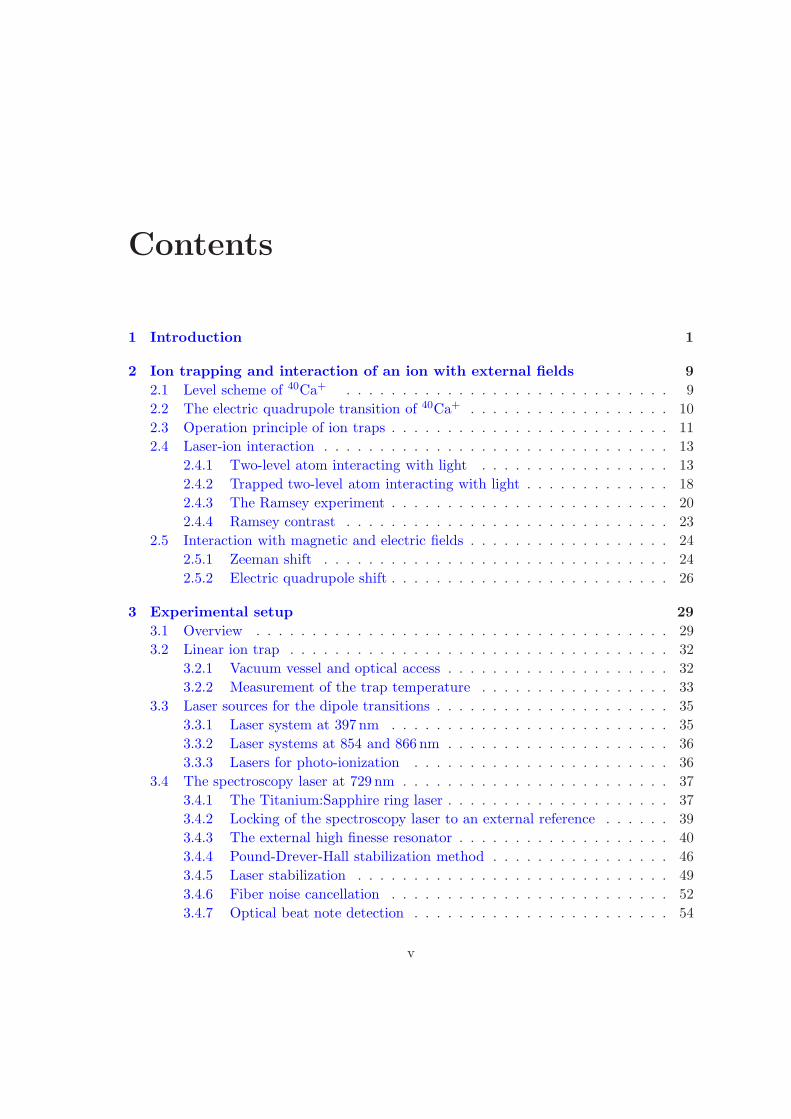
Contents

1 Introduction 1

2 Ion trapping and interaction of an ion with external fields 9

2.1 Level scheme of 40Ca+ . . . . . . . . . . . . . . . . . . . . . . . . . . . . . 9

2.2 The electric quadrupole transition of 40Ca+ . . . . . . . . . . . . . . . . . . 10

2.3 Operation principle of ion traps . . . . . . . . . . . . . . . . . . . . . . . . . 11

2.4 Laser-ion interaction . . . . . . . . . . . . . . . . . . . . . . . . . . . . . . . 13

2.4.1 Two-level atom interacting with light . . . . . . . . . . . . . . . . . 13

2.4.2 Trapped two-level atom interacting with light . . . . . . . . . . . . . 18

2.4.3 The Ramsey experiment . . . . . . . . . . . . . . . . . . . . . . . . . 20

2.4.4 Ramsey contrast . . . . . . . . . . . . . . . . . . . . . . . . . . . . . 23

2.5 Interaction with magnetic and electric fields . . . . . . . . . . . . . . . . . . 24

2.5.1 Zeeman shift . . . . . . . . . . . . . . . . . . . . . . . . . . . . . . . 24

2.5.2 Electric quadrupole shift . . . . . . . . . . . . . . . . . . . . . . . . . 26

3 Experimental setup 29

3.1 Overview . . . . . . . . . . . . . . . . . . . . . . . . . . . . . . . . . . . . . 29

3.2 Linear ion trap . . . . . . . . . . . . . . . . . . . . . . . . . . . . . . . . . . 32

3.2.1 Vacuum vessel and optical access . . . . . . . . . . . . . . . . . . . . 32

3.2.2 Measurement of the trap temperature . . . . . . . . . . . . . . . . . 33

3.3 Laser sources for the dipole transitions . . . . . . . . . . . . . . . . . . . . . 35

3.3.1 Laser system at 397 nm . . . . . . . . . . . . . . . . . . . . . . . . . 35

3.3.2 Laser systems at 854 and 866 nm . . . . . . . . . . . . . . . . . . . . 36

3.3.3 Lasers for photo-ionization . . . . . . . . . . . . . . . . . . . . . . . 36

3.4 The spectroscopy laser at 729 nm . . . . . . . . . . . . . . . . . . . . . . . . 37

3.4.1 The Titanium:Sapphire ring laser . . . . . . . . . . . . . . . . . . . . 37

3.4.2 Locking of the spectroscopy laser to an external reference . . . . . . 39

3.4.3 The external high finesse resonator . . . . . . . . . . . . . . . . . . . 40

3.4.4 Pound-Drever-Hall stabilization method . . . . . . . . . . . . . . . . 46

3.4.5 Laser stabilization . . . . . . . . . . . . . . . . . . . . . . . . . . . . 49

3.4.6 Fiber noise cancellation . . . . . . . . . . . . . . . . . . . . . . . . . 52

3.4.7 Optical beat note detection . . . . . . . . . . . . . . . . . . . . . . . 54

v

4 The frequency comb 61

4.1 Principle of operation . . . . . . . . . . . . . . . . . . . . . . . . . . . . . . 61

4.2 The fs oscillator: a Kerr lens mode-locked (KLM) laser . . . . . . . . . . . . 63

4.2.1 The stabilization of the carrier offset frequency . . . . . . . . . . . . 66

4.2.2 Stabilization of the repetition rate . . . . . . . . . . . . . . . . . . . 67

4.3 Optical beat note detection for the absolute frequency measurement . . . . 70

5 Experimental prerequisites and techniques 73

5.1 Compensation of excess micromotion . . . . . . . . . . . . . . . . . . . . . . 73

5.2 Frequency resolved optical pumping using the laser at 729 nm . . . . . . . . 75

5.3 Calibration of magnetic field coils . . . . . . . . . . . . . . . . . . . . . . . . 76

5.4 Ramsey experiments . . . . . . . . . . . . . . . . . . . . . . . . . . . . . . . 80

5.4.1 Locking the laser to the 4s 2S1/2 − 3d 2D5/2 transition . . . . . . . . 82

5.5 Frequency and phase control of the 729 nm light . . . . . . . . . . . . . . . 84

6 Absolute frequency measurement 89

6.1 Spectroscopy on the 4s 2S1/2 − 3d 2D5/2 transition . . . . . . . . . . . . . . 89

6.2 Systematic shifts . . . . . . . . . . . . . . . . . . . . . . . . . . . . . . . . . 94

6.2.1 The Zeeman effect . . . . . . . . . . . . . . . . . . . . . . . . . . . . 94

6.2.2 Electric quadupole shift . . . . . . . . . . . . . . . . . . . . . . . . . 97

6.2.3 AC Stark shifts . . . . . . . . . . . . . . . . . . . . . . . . . . . . . . 98

6.2.4 Gravitational shift . . . . . . . . . . . . . . . . . . . . . . . . . . . . 103

6.2.5 2nd-order Doppler shift . . . . . . . . . . . . . . . . . . . . . . . . . . 103

6.2.6 Errors related to the Ramsey phase experiments . . . . . . . . . . . 104

6.2.7 Uncertainty of the Cs fountain clock . . . . . . . . . . . . . . . . . . 104

6.2.8 Total error budget and result . . . . . . . . . . . . . . . . . . . . . . 105

6.3 The measurement of the 43Ca+ 4s 2S1/2 − 3d 2D5/2 transition . . . . . . . . 105

7 Precision spectroscopy with correlated atoms 109

7.1 Spectroscopy with entangled states . . . . . . . . . . . . . . . . . . . . . . . 109

7.1.1 Measurement of the quadrupole moment . . . . . . . . . . . . . . . . 110

7.1.2 Measurement of the magnetic field gradient . . . . . . . . . . . . . . 114

7.1.3 Measurement of the linewidth of the laser exciting the quadrupoletransition . . . . . . . . . . . . . . . . . . . . . . . . . . . . . . . . . 115

7.2 Spectroscopy with correlated but unentangled states . . . . . . . . . . . . . 118

7.2.1 Measurement of the quadrupole moment . . . . . . . . . . . . . . . . 118

7.2.2 Measurement of the laser linewidth . . . . . . . . . . . . . . . . . . . 120

8 Summary and outlook 125

A 129

A.1 Fundamental constants . . . . . . . . . . . . . . . . . . . . . . . . . . . . . . 129

A.2 Reduced matrix elements . . . . . . . . . . . . . . . . . . . . . . . . . . . . 129

A.3 Effective Ramsey time . . . . . . . . . . . . . . . . . . . . . . . . . . . . . . 130

vi

B Journal publications 131

© 2009 tiris, BEV

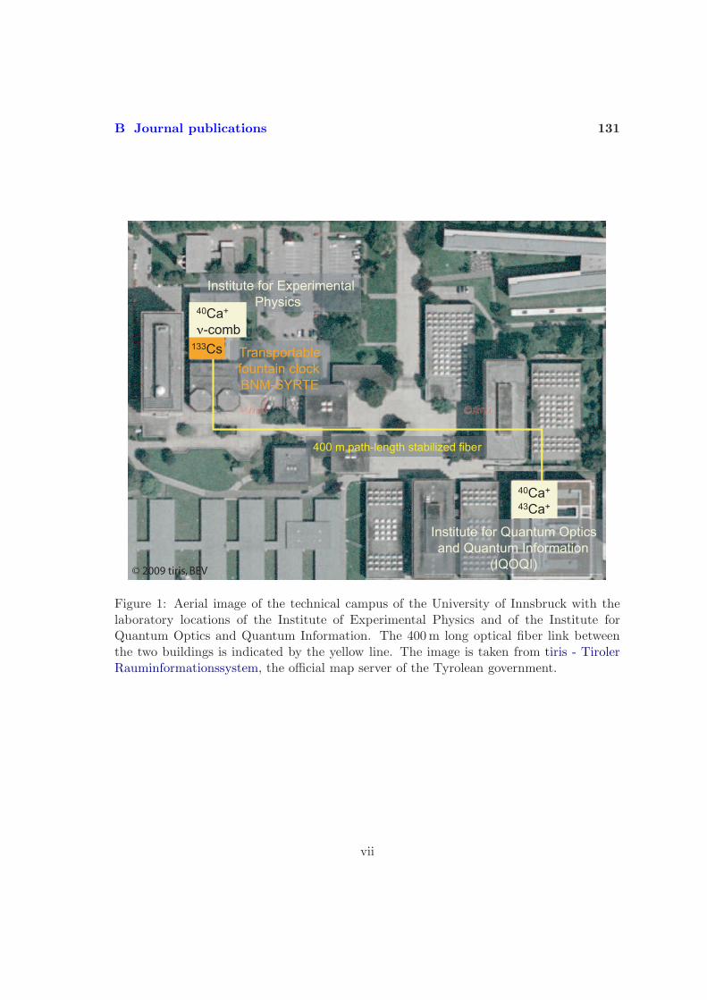
Figure 1: Aerial image of the technical campus of the University of Innsbruck with thelaboratory locations of the Institute of Experimental Physics and of the Institute forQuantum Optics and Quantum Information. The 400 m long optical fiber link betweenthe two buildings is indicated by the yellow line. The image is taken from tiris - TirolerRauminformationssystem, the official map server of the Tyrolean government.

vii

Chapter 1

Introduction

From its very beginning until today, mankind was concerned with the measurement of time.Periodic astronomical events fascinated people more than 5000 years ago and incited themto build stone rings like in Stonehenge or to make the artful sky disk of Nebra which isthe oldest depiction of the sky worldwide. With these devices people were able to directlyobserve solstices, equinoxes, and other astronomical phenomena. The first civilizationsused periodic astronomical events to predict the times for planting and harvest which wasvital for their survival. Therefore, the keeping of time was actually reserved to priests andclosely related to religion. Even today we find remnants of the Neolithic or Bronze Agecalendar in some of our festival days, although in a christianized form.

As early civilizations developed, the need for joint efforts in many parts of every daylife became more important concerning not only farming but also construction work likebuilding of cities, fortresses, or temples just to name a few. This required a division ofthe day into smaller units. A natural choice was the division of the daylight into twelvehours. Twelve, because this is approximately the ratio between the frequency of themoon’s phases and the Earth’s orbit. The measurement device for this task: a simplestick where the movement of its shadow cast by the sun can be observed on a clear day- the sundial was invented. However, it has some practical limitations: the most obviousone the fact that it doesn’t work at night or on a cloudy day. Another one is that thelength of the hour strongly depends on the latitude of the observing site and is additionallysubjected to seasonal changes, i. e. hours in summer are longer than in winter. By applyingthese corrections, modern sundials are able to reach an impressive relative (in-)accuracyof 7× 10−4.

Among the oldest and commonly used timekeeping devices for millennia were waterclocks and sandglasses. With these devices, time was measured as a function of wateror sand flow, respectively. Remarkably, the underlying principle does not depend on theobservation of celestial bodies and would also work at night or inside rooms. Furthermore,the length of an hour did not depend on the season in contrast to the case for sundials.The accuracy could be fine-tuned by controlling the water pressure including complexgearing, and some of them became quite sophisticated. The water clocks were calibratedby sundials. Through the centuries, these clocks were used for timing speeches and other

1

events, times for prayers and masses in church, though never reaching the accuracy ofmodern clocks.

The first clock which incorporates an oscillatory device depending on its natural reso-nance frequency, was the pendulum clock. The original concept had been developed byGalileo Galilei when he discovered that a pendulum’s oscillation period depends on itslength only. Christiaan Huygens, however, was credited as the inventor of the pendulumclock for his design described in 1658. Later refinements reduced the clock errors to below10 s per day enabling the discovery of variations in sundial time depending on the timeof the year and time of the day. Figure 1.1 shows the artful clock-face of a pendulumclock donated to the Institute of Experimental Physics of the university of Innnsbruck byempress Maria Theresia in the year 1798. It is kept in the institute’s inventory catalog asitem number 4.

As mankind began to travel across the seas, the need for more accurate clocks becameapparent. Precise time-keeping is the starting basis for an exact calculation of a ship’slongitude. John Harrison built a marine chronometer with a spring and balance wheelescapement in 1761 which would only loose a few seconds on transatlantic passage ofmany days on board a rolling ship.

The discovery of the piezoelectric effect by the end of the 19th century led to the arevolution in the development of clocks without gears or escapements which disturb theirregular frequency. Time is measured here by observing induced electrical vibrations ofa quartz crystal and displaying them through appropriate electronic circuits. A typicalquartz wristwatch generates a signal which is an order of magnitude more accurate thangood mechanical clocks. The best of the early crystal oscillators were already accurate towithin 1 ms a day (10−8/day) [1]. With this level of accuracy, variations of the earth’srotational frequency caused by melting ice caps, changes of the Earth’s internal structure,or on its surface could be measured.

The dramatic improvement of quartz clocks over pendulum clocks can be explained bytwo fundamental principles in frequency metrology: the first being that a clock operatingat a higher frequency has the advantage of higher precision because of a larger number ofclock ”ticks” for a given measurement time (stability), the second principle being that aclock oscillator should be chosen for a low sensitivity to external perturbations and shouldbe well isolated from the environment (accuracy). Unfortunately, the long-term behaviorof crystal oscillators is less exciting and it is impossible to reproduce two crystals withexactly the same properties. There is also a third principle which applies to any kind ofstandard, that is, a practical realization of a base unit should be possible anywhere, atany time, and as close as possible to the definition (reproducibility).

Atomic systems are close to an ideal realization of these three requirements. The ideaof an atomic clock was first conceived in 1945 by I. I. Rabi [2] using his technique ofmeasuring nuclear magnetic moments [3]. The pendulum for such a clock consists of theelectromagnetic signal associated with a quantum transition between two energy levels ofan atom. The narrow transitions typically used require fairly low excitation energies inthe microwave or optical domain, thus fulfilling the criterion of stability. The immunityagainst a perturbing environment provides for high accuracy and since atoms of the same

2

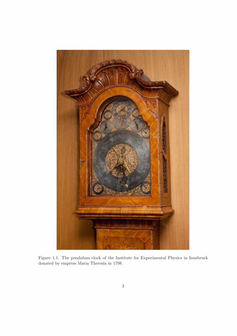
Figure 1.1: The pendulum clock of the Institute for Experimental Physics in Innsbruckdonated by empress Maria Theresia in 1798.

3

species have the same properties all across the universe - at least according to the StandardModel - it is possible to have many identical copies.

The great success of thermal cesium beam clocks employing Ramsey’s method of sepa-rated fields [4] has led to the following definition of the SI base unit of one second [5]:

The second is the duration of 9,192,631,770 periods of radiation correspondingto the transition between the two hyperfine levels of the ground state of thecesium 133 atom.

The advent of laser cooling techniques [6] significantly reduced errors due to Doppler shiftsby reducing the thermal velocities from hundreds of m/s to the cm/s scale [7] and led to therealization of Zacharias’ idea of a fountain clock [8]. Currently, the best cesium fountainclocks [9–11] have uncertainties of 5×10−16 or even better. The instability of a shot-noiselimited clock in terms of the Allan deviation is given by [12, 13]

σy(τ) ∼1

πQ

√

Tc

τ

(

1

N

)1/2

, (1.1)

where Q = ν0/∆νFWHM is the line quality factor, Tc the cycle time, N the number ofatoms (shot noise), and τ the measurement time. From this equation it is clear, that onewould prefer to operate at the highest possible atomic frequency ν0 at a given linewidth∆νFWHM . Therefore, optical clocks are the logical extension of microwave-based atomicclocks but it requires means to count optical frequencies.

Fostered by the invention of the optical frequency comb technology [14], complicatedfrequency chains [15] needed to compare optical frequencies to primary Cs standards be-came obsolete, which only existed at a few places worldwide and would only work for alimited time due to their complexity and number of stabilization loops. An optical fre-quency comb generator representing the analogue of a mechanical ”clockwork” allows forthe direct conversion of the very fast optical oscillations at frequencies of a few 100 THzdown to frequencies in the radio frequency domain on the order of 1GHz where they canbe handled by conventional electronics.

Currently, there is a lot of effort put into the development of optical frequency standardsthat are expected to replace the current microwave standard in cesium as the basis of thedefinition of the SI second in a few years from now. Recently, evaluations of systematicshifts of the best optical frequency standards, based on single trapped ions and neutralatoms held in optical lattices respectively [16, 17], have demonstrated a relative frequencyuncertainty of 10−16 or even better, thus surpassing the systematic error budgets of thebest cesium fountain clocks. But nevertheless, there is no clear indication for the optimalchoice of atom or ion. For an optical ion clock, several candidates have been thoroughlyinvestigated such as Hg+, Al+, Yb+, In+, Sr+ [18–23]. Ca+ has been proposed andtheoretically analyzed as well [24, 25], but no serious measurement had been accomplished.

Confinement of single atoms or ions in electro-magnetic fields opens up the possibilityof studying single or a few charged particles in a very well defined environment. WolfgangPaul invented a radio frequency (RF) mass filter for mass-selecting charged particles in1953 [26]. A modified design of his experimental setup [27] makes it possible to confine

4

ions in all three dimensions. Such traps have become widely used in many fields of physics,contradicting Erwin Schrodinger’s famous statement from 1952 [28]:

. . . we never experiment with just one electron or atom or (small) molecule. Inthought experiments we sometimes do; this invariably entails ridiculous conse-quences. . .

In 1980, the first trapping and laser cooling of a single ion was reported by Neuhauser etal. [29]. Since then, Paul traps have played an important role not only in mass spectro-metry but also in atomic physics, because these systems allow for trapping and controlledmanipulation of single or a few ions and extensive studies of their properties [30]. Thepossibility for laser cooling [31] in an ion trap offers the perspective of developing an op-tical frequency standard [32] because Doppler effects due to thermal motion are almosteliminated when operating in the Lamb-Dicke regime [33]. Together with efficient statepreparation [34, 35] by optical pumping and the readout of the quantum state by the obser-vation of quantum jumps (electron shelving technique) [36–38] with a detection efficiencyclose to 100%, the signal-to-noise ratio is greatly enhanced.

For precision spectroscopy and atomic clocks, an advantage of using an ion trap liesin the decoupling of the particle to a large extent from a disturbing environment leadingunperturbed transition frequencies and therefore to high accuracies. Thereby, the dis-advantage of a small atom number (see Eq. (1.1)) can be overcome due to practicallyunlimited interaction times and the observation of narrow atomic transition lines, almostfree of external energy shifts caused by unwanted interactions. As the trapping potentialnear the trap center is close to zero, systematic frequency shifts caused by electric fieldsare small. On the other hand interaction with magnetic fields can be well characterizedin a reproducible way, minimizing the associated systematic effects as well. Finally, iontraps are usually operated in an ultra-high vacuum environment, causing collision rateswith background atoms or neighboring particles (if more than one ion is in the trap) tobe very low in contrast to the case of neutral atoms. In summary, optical clocks based onsingle, trapped ions have the potential to reach an uncertainty limit of 10−18 and maybebeyond [32].

With the potential of optical clocks reaching uncertainties of 10−18, the question natu-rally arises: What is it actually good for? The obvious reason is of course that anyrealization of a standard unit should be performed at its ultimate limit. The fact thatfrequencies are the quantities which can be measured most precisely, makes it appealingto find ways to turn measurements of other fundamental base units (volt, ampere, ohm,meter) into frequency measurements [39]. Furthermore, clocks play an important role interrestrial navigation. Satellite navigation systems like GPS, Glonass, or the EuropeanGALILEO system, rely on the precision and accuracy of atomic clocks [40]. Therefore,these systems would greatly benefit from improved clocks. Also extra-terrestrial navigationof deep space probes would not be possible without the existence of high-performanceclocks. Another important aspect of atomic clocks is the test of fundamental theorieslike special and general relativity or extensions of the standard model. Time dilation andgravitational redshift effects have already been observed by comparing clocks subjected

5

to high altitude or velocity differences [41, 42], yet the direct detection of gravitationalwaves is a task still to be done, where clocks could be helpful [43]. At the same time,geodesy applications and probing Earth’s gravitational potential are expected to benefitgreatly from clocks at the 10−17 level [43]. Another important task for atomic clocks is thedetection of a possible time variation of fundamental constants [44–46] predicted by sometheories beyond the Standard Model and suggested by astronomical observations [47–50]with partially contradicting results or investigations of fission products of the Oklo reactor[51–54]. Atomic transition frequencies depend on various parameters [55] like the Rydbergconstant, the electron-to-proton mass ratio, or the fine structure constant α. Of course,the dependency is specific to the particular atom under examination. Therefore, by themeasurement of many atomic transition frequencies, the different contributions can beseparated. Finally, there is a less exotic application of clocks, namely the synchronizationof networks reaching from data synchronization in computer networks and synchronizationof different power plants for electricity, to astronomical telescopes. Here, a syntheticaperture of the size of their separation is created by linking two telescopes to increase thespatial resolution. In principle, this would also work for telescopes in space where atomicclocks could be used for maintaining their relative positions [56].

The main research focus within our group lies on quantum information processing withCa+ ions and one can use methods and techniques from that field in order to improve theperformance of optical clocks [57] and other types of precision spectroscopy. The abilityof deterministically generating entanglement is generally accepted as a key element forquantum computation [58] and quantum cryptography [59]. For the purpose of quantummetrology, the use of entangled states for an enhanced signal-to-noise ratio due to spin-squeezing [60] has been discussed [61–63] and demonstrated [64, 65] thereby beating thestandard shot noise limit [66]. In addition, entangled states of two ions of different specieshave been used in the context of atomic clocks for efficient quantum state detection [67, 68]where electron shelving wouldn’t work for technical reasons and for the measurement ofscattering lengths [69].

Quantum information processing allows for the tailored design of specific states by themanipulation of individual quantum bits. Such states can be insensitive to the detrimen-tal influences of an environment [70]. The existence of decoherence-free subspaces [71],which protect the delicate quantum information with respect to specific sources of noise,yield significantly enhanced coherence times [72] in the presence of strong technical noisewhich would render experiments with single or uncorrelated particles impossible on thesame time scale. Therefore, entangled states with long lifetimes become very useful forhigh-precision spectroscopy. In this work, the use of a decoherence-free subspace withspecifically designed entangled states [73] for precision spectroscopy is demonstrated. Theelectric quadrupole moment of Ca+ in its metastable D5/2 state is obtained, which is ofuse for frequency standard applications and for refined theoretical calculations of atomicproperties. The technique makes explicit use of multi-particle entanglement and providesan approach for designed quantum metrology. Furthermore, it can be shown that entan-glement is not a necessary ingredient for these measurements and classically correlatedstates can be used instead, although at a 50% loss of contrast.

6

This thesis is structured as follows. In chapter 2 the basic spectroscopic properties of40Ca+ are presented with a theoretical description of the ion’s interaction with externalfields and main focus on Ramsey experiments. The experimental setup including the iontrap and the laser sources is described in chapter 3, followed by the optical frequency combused for the absolute frequency measurement in chapter 4. Basic experimental procedureslike state preparation are listed in chapter 5. Chapter 6 is dedicated to the absolutefrequency measurement of the 4s 2S1/2 − 3d 2D5/2 transition. Finally, spectroscopy withcorrelated states are used in chapter 7 to determine the quadrupole moment of the D5/2

level. At the end, a brief summary and an outlook of future plans are given in chapter 8.

7

8

Chapter 2

Ion trapping and interaction of anion with external fields

In this chapter the basic theory of ion trapping and interaction of an ion with externalfields is described. First, the general atomic structure of 40Ca+ is given with a moredetailed view on the 4s 2S1/2 − 3d 2D5/2 clock transition. Then, a short review on iontraps and their operation principle is presented. Basic laser-ion interaction with focus onRamsey experiments is followed by an overview on the interaction of the ion with externalfields.

2.1 Level scheme of 40Ca+

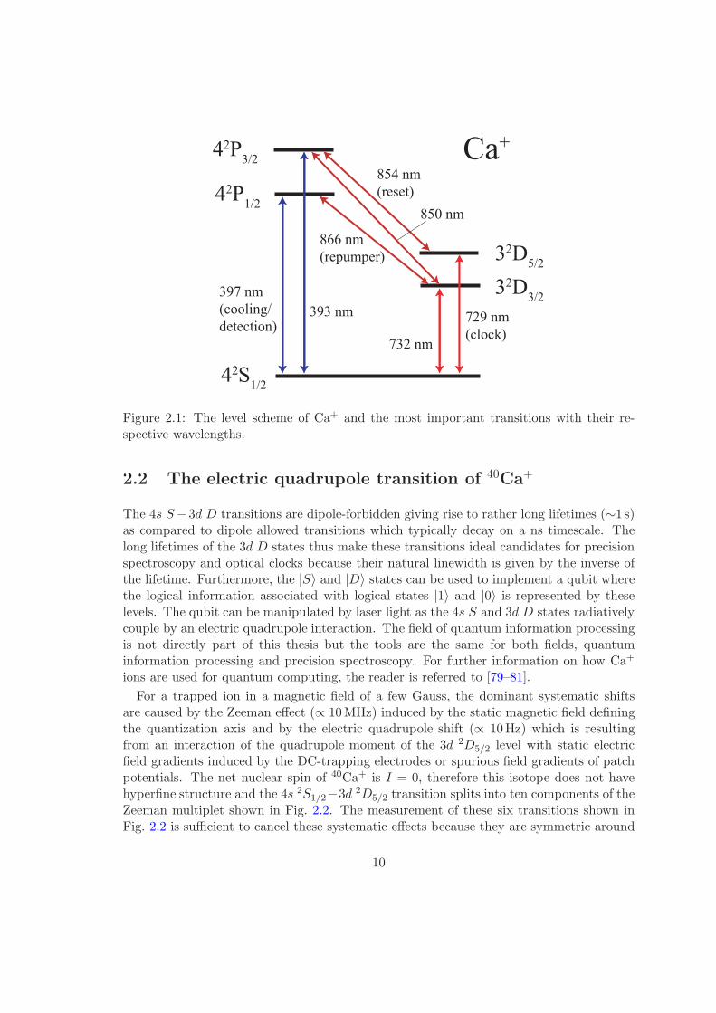
The level structure of 40Ca+, like for all singly ionized earth-alkali atoms, is similar tothe energy level scheme of neutral alkali atoms, in particular to atomic hydrogen. Thediagram in Fig. 2.1 shows the three lowest energy levels for the single valence electron.The ground state is formed by the 4S state, the lowest excited state by the metastable3D level, which has a lifetime of ∼1 s [74]. This corresponds to a natural linewidth of<0.16 Hz. Spin-orbit coupling splits the D-state into two fine structure components withtotal angular momentum J = 3/2 and J = 5/2 and a frequency difference of 1.8 THz.The narrow S −D transitions can be excited by electric quadrupole radiation at 732 nmand 729 nm, respectively. The next-higher lying excited state is the 4P level with a finestructure splitting of 6.7 THz. Lifetimes of ∼7 ns [75] for both J = 1/2 and J = 3/2 statesand corresponding linewidths of 20 MHz make these levels well suited for laser cooling.In our case, we use the S1/2 − P1/2 electric dipole transition at 397 nm. There is a smallprobability - one out of 17 - for a decay of the P into the D-levels with branching ratiosgiven in [76, 77]. The transition wavelengths are 854 nm from P3/2 − D5/2 and 866 nmfor the P1/2 − D3/2 transition. Additionally, there is an allowed transition from P3/2 tothe D3/2 level with a wavelength of 850 nm which has a transition probability of aboutone tenth of the other two. More precise wavelengths for the transitions mentioned above,transition probabilities, oscillator strengths, and more are given in [78].

9

42P3/2

42P1/2

42S1/2

32D5/2

32D3/2

Ca+

397 nm

(cooling/

detection)729 nm

(clock)

854 nm

(reset)

866 nm

(repumper)

393 nm

732 nm

850 nm

Figure 2.1: The level scheme of Ca+ and the most important transitions with their re-spective wavelengths.

2.2 The electric quadrupole transition of 40Ca+

The 4s S−3d D transitions are dipole-forbidden giving rise to rather long lifetimes (∼1 s)as compared to dipole allowed transitions which typically decay on a ns timescale. Thelong lifetimes of the 3d D states thus make these transitions ideal candidates for precisionspectroscopy and optical clocks because their natural linewidth is given by the inverse ofthe lifetime. Furthermore, the |S〉 and |D〉 states can be used to implement a qubit wherethe logical information associated with logical states |1〉 and |0〉 is represented by theselevels. The qubit can be manipulated by laser light as the 4s S and 3d D states radiativelycouple by an electric quadrupole interaction. The field of quantum information processingis not directly part of this thesis but the tools are the same for both fields, quantuminformation processing and precision spectroscopy. For further information on how Ca+

ions are used for quantum computing, the reader is referred to [79–81].

For a trapped ion in a magnetic field of a few Gauss, the dominant systematic shiftsare caused by the Zeeman effect (∝ 10MHz) induced by the static magnetic field definingthe quantization axis and by the electric quadrupole shift (∝ 10Hz) which is resultingfrom an interaction of the quadrupole moment of the 3d 2D5/2 level with static electricfield gradients induced by the DC-trapping electrodes or spurious field gradients of patchpotentials. The net nuclear spin of 40Ca+ is I = 0, therefore this isotope does not havehyperfine structure and the 4s 2S1/2−3d 2D5/2 transition splits into ten components of theZeeman multiplet shown in Fig. 2.2. The measurement of these six transitions shown inFig. 2.2 is sufficient to cancel these systematic effects because they are symmetric around

10

+5/2+3/2+1/2-1/2-3/2-5/2

+1/2

-1/2

mD

mS

1

2

34

5

6

S1/2

D5/2

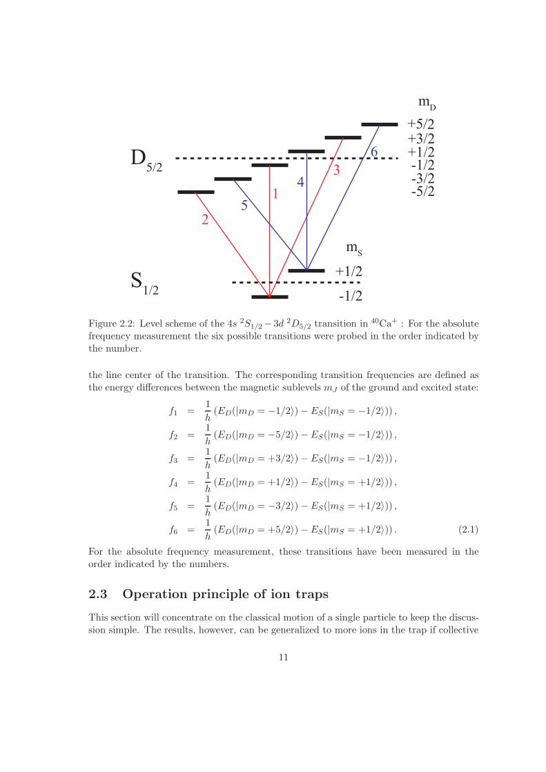
Figure 2.2: Level scheme of the 4s 2S1/2− 3d 2D5/2 transition in 40Ca+ : For the absolutefrequency measurement the six possible transitions were probed in the order indicated bythe number.

the line center of the transition. The corresponding transition frequencies are defined asthe energy differences between the magnetic sublevels mJ of the ground and excited state:

f1 =1

h(ED(|mD = −1/2〉)− ES(|mS = −1/2〉)) ,

f2 =1

h(ED(|mD = −5/2〉)− ES(|mS = −1/2〉)) ,

f3 =1

h(ED(|mD = +3/2〉)− ES(|mS = −1/2〉)) ,

f4 =1

h(ED(|mD = +1/2〉)− ES(|mS = +1/2〉)) ,

f5 =1

h(ED(|mD = −3/2〉)− ES(|mS = +1/2〉)) ,

f6 =1

h(ED(|mD = +5/2〉)− ES(|mS = +1/2〉)) . (2.1)

For the absolute frequency measurement, these transitions have been measured in theorder indicated by the numbers.

2.3 Operation principle of ion traps

This section will concentrate on the classical motion of a single particle to keep the discus-sion simple. The results, however, can be generalized to more ions in the trap if collective

11

motion of the ions is included in the equations of motion. More detailed information canbe found in a multitude of Refs. [80, 82–85], just to name a few.

y

x

2R

GND

V V

GND

(a)

y

z

x

2Z

endcaps

(b)

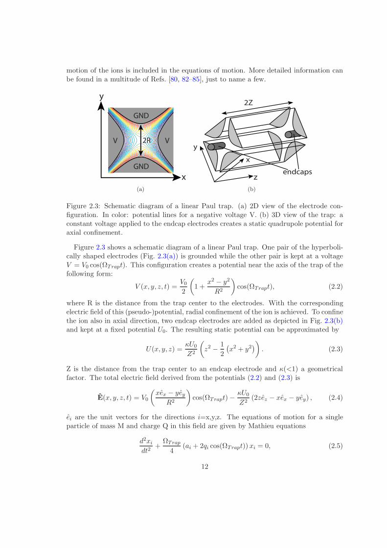
Figure 2.3: Schematic diagram of a linear Paul trap. (a) 2D view of the electrode con-figuration. In color: potential lines for a negative voltage V. (b) 3D view of the trap: aconstant voltage applied to the endcap electrodes creates a static quadrupole potential foraxial confinement.

Figure 2.3 shows a schematic diagram of a linear Paul trap. One pair of the hyperboli-cally shaped electrodes (Fig. 2.3(a)) is grounded while the other pair is kept at a voltageV = V0 cos(ΩTrapt). This configuration creates a potential near the axis of the trap of thefollowing form:

V (x, y, z, t) =V0

2

(

1 +x2 − y2

R2

)

cos(ΩTrapt), (2.2)

where R is the distance from the trap center to the electrodes. With the correspondingelectric field of this (pseudo-)potential, radial confinement of the ion is achieved. To confinethe ion also in axial direction, two endcap electrodes are added as depicted in Fig. 2.3(b)and kept at a fixed potential U0. The resulting static potential can be approximated by

U(x, y, z) =κU0

Z2

(

z2 − 1

2

(

x2 + y2)

)

. (2.3)

Z is the distance from the trap center to an endcap electrode and κ(<1) a geometricalfactor. The total electric field derived from the potentials (2.2) and (2.3) is

E(x, y, z, t) = V0

(

xex − yeyR2

)

cos(ΩTrapt)−κU0

Z2(2zez − xex − yey) , (2.4)

ei are the unit vectors for the directions i=x,y,z. The equations of motion for a singleparticle of mass M and charge Q in this field are given by Mathieu equations

d2xi

dt2+

ΩTrap

4(ai + 2qi cos(ΩTrapt)) xi = 0, (2.5)

12

where ai and qi are defined as

ax = ay = −1

2az = − 4QκU0

MZ2Ω2Trap

, (2.6)

qx = −qy =2QV0

MR2Ω2Trap

, qz = 0. (2.7)

For |qi| ≪ 1 and |ai| ≪ 1, stable solutions to Eqs. (2.5) exist and can be approximated by

xi(t) ≈ x1i cos(ωit+ ϕi)(

1 +qi2

cos(ΩTrapt))

, (2.8)

where x1i is the amplitude of the harmonic oscillation of frequency

ωi = βiΩTrap

2and βi =

√

ai +1

2q2i , (2.9)

and ϕi is a phase determined by the initial position and velocity of the ion. The motionof the particle can be decomposed into two components:

• secular motion: harmonic oscillation with frequency ωi about the trap center,

• micromotion: fast oscillation driven by the cos(ΩTrapt) term corresponding to thetrapping RF field.

Additional electric fields may exist the shift the ions out of the node of the trappingfield, causing excess micromotion. If an ion in the trap is illuminated by a light field, thisadditional micromotion creates sidebands in the excitation spectrum. The upper statepopulation Pe in this case is proportional to:

Pe ∼∞∑

n=−∞

J2n(βmicro)

(ωA − ωL + nΩT )2 + (12γ)

2. (2.10)

Here, the atomic transition frequency is given by ωA, the frequency of the light field byωL and the transition linewidth by γ. The n-th sideband power is described by the Besselfunction J2

n(βmicro) with a modulation index βmicro.

2.4 Laser-ion interaction

2.4.1 Two-level atom interacting with light

For the description of a complicated atom interacting with a light field, certain approx-imations are necessary. Let’s consider the hypothetical case of an atom having only aground |S〉 and an excited state |D〉 separated by an energy difference of

~ωA = ~(ωD − ωS). (2.11)

13

This system is called two-level atom (2LA) and is an ideal test bed for quantum mechanics.In many cases, this a very good approximation to real systems and therefore widely used.The laser is described as a classical electro-magnetic field with

E(r, t) = E(r)e−i(ωLt+ϕ) + c.c., (2.12)

where E(r) is the spatial dependence of the electric field, ωL the frequency of the light,and ϕ the phase of the traveling light wave. The frequency difference between the laserand the atomic transition is defined as

∆ = ωL − ωA. (2.13)

The undisturbed Hamiltonian for the two-level atom without the presence of light is simply

H0 =

(

~ωS 00 ~ωD

)

. (2.14)

The state |ψ〉 = cS |S〉 + cD |D〉 of an atom interacting with the classical light field ofEq. (2.12) obeys the Schrodinger equation

i~d

dt|ψ〉 = H |ψ〉 (2.15)

with the Hamiltonian H = H0 +H(i) where H(i) contains the details of the interaction.Generally, the time evolution of the state |ψ(t)〉 is given by [86]

|ψ(t)〉 = U(t) |ψ(0)〉 = e−i~

Ht |ψ(0)〉 , (2.16)

yielding a system of equations for the coefficients ci(t):

cS = − i~〈S| |H(i)| |D〉 e−i(ωAt+ϕ)cD,

˙cD = − i~〈D| |H(i)| |S〉 ei(ωAt+ϕ)cD. (2.17)

The coupling strength is proportional to the matrix element 〈S| |H(i)| |D〉 ≡ ~ΩR2 and ΩR

is usually referred to as the Rabi frequency.

To transform into a rotating frame, the Hamiltonian H is replaced by UHU †, where Uhas the form

U =

(

e−iωLt 00 1

)

. (2.18)

By neglecting terms oscillating at e−i2ωLt and a redefinition of the ground state energy,the Hamiltonian in rotating wave approximation (RWA) [87] is transformed to

HRWA = ~

(

0 ΩR2

ΩR2 ∆

)

. (2.19)

14

If the excited state can decay, or in order to take decoherence effects like a finite linewidthof the laser into account, one has to use the density matrix formalism. The Schrodingerequation is then replaced by

d

dtρ =

i

~[H, ρ] + L(ρ), (2.20)

where L(ρ) contains the relaxation terms.

The dynamics of the two-level atom with a spontaneous decay rate γ is described bythe optical Bloch equations:

ρDD = −ΩR Im(ρDS)− γρDD

ρSD = −iΩR

2(ρDD − ρSS) + (i∆ − γ

2)ρSD

ρDD = 1− ρSS

ρDS = ρ∗SD. (2.21)

The steady state solution for ρSS(t = 0) = 1 for the excited state population is

ρDD(t→∞) =(ΩR/2)

2

∆2 + (γ/2)2 + 2(ΩR/2)2. (2.22)

For low saturation (ΩR ≪ γ), the excitation probability is ρDD ≪ 1 and yields a Lorentzianline shape

ρDD(∞) =

(

ΩR

γ

)2 1

1 + 4(∆/γ)2. (2.23)

In the coherent regime, i. e. ΩR ≫ γ, the solution exhibits damped oscillations of the

population between the ground and excited state with a frequency of Ω =√

Ω2R + ∆2.

This is known as Rabi oscillations. It can be interpreted as a rotation of the Bloch vectordefined as

UVW

=

2Re(ρSD)2 Im(ρSD)ρDD − ρSS

. (2.24)

The evolution of the system for a laser pulse of length θ, given the initial conditionsU(0), V (0), and W (0), has the following matrix representation [86]:

U(θ)V (θ)W (θ)

= R(ΩR, φ,∆, θ)

U(0)V (0)W (0)

, (2.25)

15

where the transformation matrix is given by

R(ΩR, φ,∆, θ) =

cos(Ωθ) +Ω2

RΩ2 (1− cos(Ωθ)) cos2 φ

∆Ω sin(Ωθ)− Ω2

RΩ2 (1− cos(Ωθ)) cosφ sinφ

−ΩR∆Ω2 (1− cos(Ωθ)) cosφ− ΩR

Ω sin(Ωθ) sinφ

−∆Ω sin(Ωθ)− Ω2

RΩ2 (1− cos(Ωθ)) sinφ cosφ

cos(Ωθ) +Ω2

RΩ2 (1− cos(Ωθ)) sin2 φ

−ΩRΩ sin(Ωθ) cosφ+ ΩR∆

Ω2 (1− cos(Ωθ)) sinφ

−ΩR∆Ω2 (1− cos(Ωθ)) cosφ+ ΩR

Ω sin(Ωθ) sinφΩRΩ sin(Ωθ) cosφ+ ΩR∆

Ω2 (1− cos(Ωθ)) sinφ

1− Ω2R

Ω2 (1− cos(Ωθ))

(2.26)

with the generalized Rabi frequency Ω2 = Ω2R + ∆2. Equation (2.25) represents nothing

else than Rabi oscillations. The time θ describes how long the atom is exposed to theinteraction. An atomic oscillator is usually interrogated near the resonance, for which∆≪ Ω. In this case, R simplifies to

R(ΩR, φ, 0, θ) =

cos(Ωθ) + (1− cos(ΩRθ)) cos2 φ −(1− cos(ΩRθ) sinφ cosφ sin(ΩRθ) sinφ−(1− cos(ΩRθ) sinφ cosφ cos(ΩRθ) + (1− cos(ΩRθ) sin2 φ sin(ΩRθ) cosφ

− sin(ΩRθ) sinφ − sin(ΩRθ) cosφ cos(ΩRθ)

.

(2.27)

The rotation angle is given by ΩRθ. An angle of ΩRθ = π corresponds to a population ex-change from |S〉 → |D〉 and is called ”π-pulse”, a ”π

2 -pulse” creates an equal superpositionof the ground and excited state of the form |ψ〉 = 1√

2(|S〉+ eiφ |D〉).

The effect of far-detuned laser light on the transition frequency can be treated by per-turbation theory in second-order of the electric field. For non-degenerate states, the inter-action Hamiltonian of Eq. (2.19) leads to a frequency shift often referred to as AC Starkshift, that is [88]

∆νStark(|i〉) =∑

i6=j

| 〈j|HRWA |i〉 |2ωi − ωj

. (2.28)

Considering real atoms again, two types of atomic transitions are considered in thisthesis: electric dipole and quadrupole transitions.

Electric dipole transition

For an electric dipole-allowed transition like the S − P transition, the Rabi frequency isdefined via the dipole matrix element

〈S| ~d · ~E |P 〉 = ~ΩR

2, (2.29)

16

where ~d = e~r is the induced dipole moment and ~E the electric field of the light at the po-sition of the atom. The spontaneous decay rate Γ is related to the Einstein A21 coefficientand the dipole matrix element by

Γ =1

τ= A21 =

ω3A| 〈S| ~d · ~E |P 〉 |2

3πǫ0~c3(2.30)

with the speed of light c, and ǫ0 the permittivity of vacuum. Therefore, the Stark shift byfar detuned light can be calculated by using Eq. (2.28) and becomes

∆νStark(|i〉) = ±| 〈S|~d · ~E |P 〉 |2

∆= ±Ω2

R

4∆= ±3πc2

2ω3A

Γ

∆I, (2.31)

with the optical intensity I = 12µ0c |E|2.

Electric quadrupole transition

The reason for using dipole-forbidden transitions in experiments is the long lifetime ofthe metastable states and the fact that decoherence due to spontaneous emission willgreatly be suppressed. The transition for the absolute frequency measurement consideredhere is the electric quadrupole-allowed 4s 2S1/2 − 3d 2D5/2 transition. Details about theusing quadrupole transitions for quantum computation are discussed in detail in [89]. Thetransition can be excited by a coupling of the induced quadrupole moment Q1 and thegradient of the electro-magnetic field ∇E(t). The corresponding Hamiltonian to this typeof interaction is

HQ = ∇E(t)Q. (2.32)

For a more specific derivation of this interaction Hamiltonian the reader is referred to[90, 91]. The interaction strength is given by the Rabi frequency defined as

ΩR =

∣

∣

∣

∣

eE0

2~〈S,mS | (ǫ · r)(k · r) |D,mD〉

∣

∣

∣

∣

, (2.33)

where ǫ is the polarization of the light with a propagation vector k and an electric fieldamplitude E0, r is the position operator of the valence electron relative to the atomiccenter of mass. The coupling strength can be estimated by using 〈S,mS | r2 |D,mD〉 ≈ a2

0

and one obtains [84]

ΩR ≈kE0

2~ea2

0. (2.34)

As a consequence, an electric field of 40 kV/m is required for a Rabi frequency on the orderof ΩR/(2π) ∼100 kHz. To achieve field strengths like this, the laser needs to be tightlyfocused onto the ion. In our experiment, the beam waist at the focal point is less than2.5µm thus the required optical power is 40µW only.

1The individual components of the quadrupole tensor are Q(2)k = r2C

(2)k (θ, ϕ) with renormalized spher-

ical harmonics of the form C(l)m =

q

4π2l+1

Yl,m(θ, ϕ).

17

The Einstein coefficient A12 describing the decay rate of the excited state is related tothe reduced matrix element

⟨

S1/2

∥

∥r2C(2)∥

∥D5/2

⟩

by [89]

A12 =cαk5

90

∣

∣

∣

⟨

S1/2

∥

∥

∥r2C(2)

∥

∥

∥D5/2

⟩∣

∣

∣

2. (2.35)

The reduced matrix element can be calculated using the Wigner-Eckart theorem [92](see also Sec. A.2). Substituting the matrix element in Eq. (2.33) by the expressionin Eq. (2.35), the coupling strength can be further evaluated in terms of the ”specific”Clebsch-Gordan coefficients ΛJ,J ′(m,m′) for the particular total angular momenta J, J ′

of the states and a part containing the geometrical dependence g(∆m)(φ, γ). The Rabifrequency therefore is expressed as:

ΩR =e

2~

√

15

cαE0

√

A12

k3ΛJ,J ′(m,m′)g(∆m)(φ, γ), (2.36)

where α denotes the fine structure constant, φ the angle between the laser’s k-vector andthe magnetic field, and γ is the angle between the laser polarization and the projection ofthe magnetic field onto the incident plane. Explicit expressions for these functions can befound in [79]. For the specific geometry of our trap, i. e. φ = 45 and γ = 0, the valuesof the prefactors Λ(m,m′)g(∆m)(φ, γ) for ∆m = 0 and ∆m = 2 are given in Tab. 2.1.Transitions with ∆m = 1 do not couple to the laser in the configuration above, leading tothe six possible transitions mentioned in Eq. (2.1) and Fig. 2.2.

Table 2.1: The transition factors and relative coupling strengths according to the definitionof the individual transitions given in Eq. (2.1).

# Transition |S,m〉 ↔ |D,m′〉 Λ1/2,5/2(m,m′)g(∆m)(φ, γ) Rel. strength

1,4 ±1/2↔ ±1/2√

35

12 1

3,5 ±1/2↔ ∓3/2 1√5

1√24

0.24

2,6 ±1/2↔ ±5/2 1 1√24

0.53

2.4.2 Trapped two-level atom interacting with light

For a trapped atom laser-cooled to near the motional ground state, the motion of theparticle has to be treated quantum mechanically. According to [93] the Hamiltonian for atwo-level atom of mass m in a one-dimensional, harmonic trap of frequency ω interactingwith a traveling light field of a single mode laser near the atomic resonance is given by

H = H(m) +H(e) +H(i), (2.37)

H(m) =p2

2m+

1

2mω2x2, (2.38)

H(e) =1

2~ωAσz, (2.39)

18

where p and x are the momentum and position operators for the particle, and σ+, σ−, σz

are the Pauli spin matrices. H(m) and H(e) describe the atomic motion and the electronicstate of the atom. The interaction term with the classical light field of frequency ωL andwave vector k can be expressed as

H(i) =~

2Ω(σ+ + σ−)

(

ei(kx−ωLt) + e−i(kx−ωLt))

. (2.40)

The interaction strength is given by the Rabi frequency Ω. The model has a similar formto the Jaynes-Cummings model [94, 95] describing the interaction of a two-level systemwith a single cavity mode except that the role of the quantized radiation field is replacedby the quantized motion of the atom in the trap.

Because the trap is harmonic, the position and momentum operators can be replacedby the creation and annihilation operators a† and a for the trap quanta. Introducing theLamb-Dicke parameter2

η = k

√

~

2mω(2.41)

which relates the classical recoil energy of the photon to that of one trap quantum, theinteraction Hamiltonian is given by

H(i) =1

2~Ω

(

eiη(a+a†)σ+e−iωLt + e−iη(a+a†)σ+eiωLt)

. (2.42)

In the interaction picture,

HI =1

2~Ω

(

eiη(a+a†)σ+e−i∆t + e−iη(a+a†)σ+ei∆t)

. (2.43)

Here, the rotating-wave approximation [87] was applied and terms oscillating at twice theoptical frequency were neglected. Depending on the detuning ∆, this Hamiltonian willcouple certain electronic |g, e〉 and motional states |n, n′〉.

In the Lamb-Dicke limit, i. e. for the condition η2(2n + 1) ≪ 1, the exponential inEq. (2.43) can be expanded in terms of η

HI =~

2Ωσ+

(

1 + iη(ae−iωt + a†eiωt)e−i∆t +O(η2))

+H.c. (2.44)

As a consequence, transitions which change the vibrational quantum number by morethan one are greatly suppressed. Transitions |S〉 |n〉 − |D〉 |n〉, which do not change themotional state (∆ = 0) are called carrier transitions and have a coupling strength Ω. Adetuning of ∆ = −ω gives rise to red sideband transitions of the type |S〉 |n〉 − |D〉 |n− 1〉with a Rabi frequency of η

√nΩ. On the blue sideband for ∆ = ω the coupling strength is

η√n+ 1Ω.

2In case of an angle ϑ between the oscillation and the laser: η = k cos ϑp

~/2mω.

19

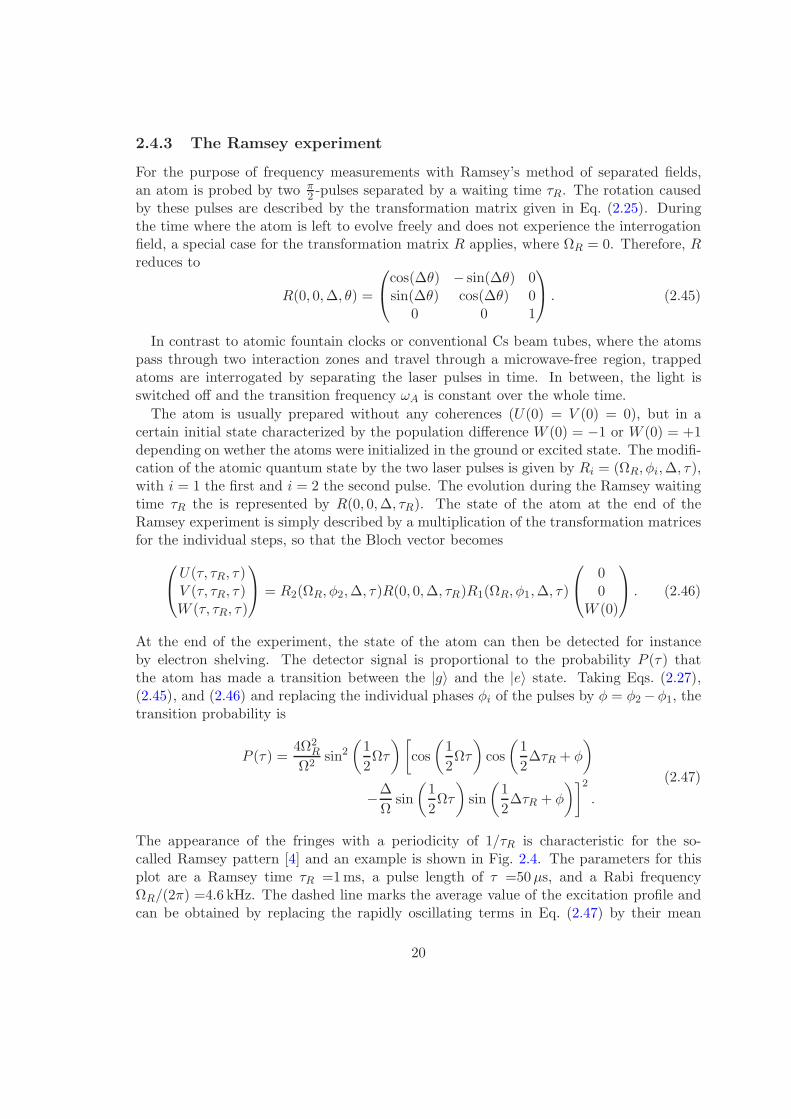
2.4.3 The Ramsey experiment

For the purpose of frequency measurements with Ramsey’s method of separated fields,an atom is probed by two π

2 -pulses separated by a waiting time τR. The rotation causedby these pulses are described by the transformation matrix given in Eq. (2.25). Duringthe time where the atom is left to evolve freely and does not experience the interrogationfield, a special case for the transformation matrix R applies, where ΩR = 0. Therefore, Rreduces to

R(0, 0,∆, θ) =

cos(∆θ) − sin(∆θ) 0sin(∆θ) cos(∆θ) 0

0 0 1

. (2.45)

In contrast to atomic fountain clocks or conventional Cs beam tubes, where the atomspass through two interaction zones and travel through a microwave-free region, trappedatoms are interrogated by separating the laser pulses in time. In between, the light isswitched off and the transition frequency ωA is constant over the whole time.

The atom is usually prepared without any coherences (U(0) = V (0) = 0), but in acertain initial state characterized by the population difference W (0) = −1 or W (0) = +1depending on wether the atoms were initialized in the ground or excited state. The modifi-cation of the atomic quantum state by the two laser pulses is given by Ri = (ΩR, φi,∆, τ),with i = 1 the first and i = 2 the second pulse. The evolution during the Ramsey waitingtime τR the is represented by R(0, 0,∆, τR). The state of the atom at the end of theRamsey experiment is simply described by a multiplication of the transformation matricesfor the individual steps, so that the Bloch vector becomes

U(τ, τR, τ)V (τ, τR, τ)W (τ, τR, τ)

= R2(ΩR, φ2,∆, τ)R(0, 0,∆, τR)R1(ΩR, φ1,∆, τ)

00

W (0)

. (2.46)

At the end of the experiment, the state of the atom can then be detected for instanceby electron shelving. The detector signal is proportional to the probability P (τ) thatthe atom has made a transition between the |g〉 and the |e〉 state. Taking Eqs. (2.27),(2.45), and (2.46) and replacing the individual phases φi of the pulses by φ = φ2−φ1, thetransition probability is

P (τ) =4Ω2

R

Ω2sin2

(

1

2Ωτ

)[

cos

(

1

2Ωτ

)

cos

(

1

2∆τR + φ

)

−∆

Ωsin

(

1

2Ωτ

)

sin

(

1

2∆τR + φ

)]2

.

(2.47)

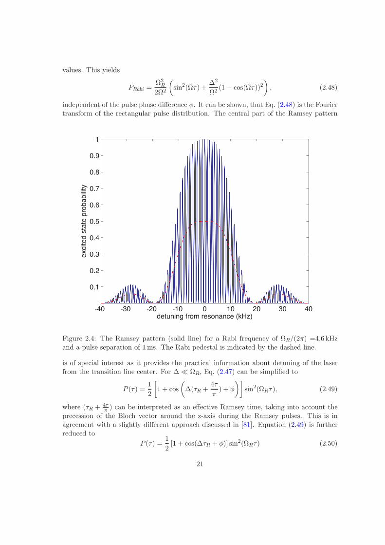
The appearance of the fringes with a periodicity of 1/τR is characteristic for the so-called Ramsey pattern [4] and an example is shown in Fig. 2.4. The parameters for thisplot are a Ramsey time τR =1 ms, a pulse length of τ =50µs, and a Rabi frequencyΩR/(2π) =4.6 kHz. The dashed line marks the average value of the excitation profile andcan be obtained by replacing the rapidly oscillating terms in Eq. (2.47) by their mean

20

values. This yields

PRabi =Ω2

R

2Ω2

(

sin2(Ωτ) +∆2

Ω2(1− cos(Ωτ))2

)

, (2.48)

independent of the pulse phase difference φ. It can be shown, that Eq. (2.48) is the Fouriertransform of the rectangular pulse distribution. The central part of the Ramsey pattern

-40 -30 -20 -10 0 10 20 30 40

0.1

0.2

0.3

0.4

0.5

0.6

0.7

0.8

0.9

1

detuning from resonance (kHz)

excited s

tate

pro

babili

ty

Figure 2.4: The Ramsey pattern (solid line) for a Rabi frequency of ΩR/(2π) =4.6 kHzand a pulse separation of 1 ms. The Rabi pedestal is indicated by the dashed line.

is of special interest as it provides the practical information about detuning of the laserfrom the transition line center. For ∆≪ ΩR, Eq. (2.47) can be simplified to

P (τ) =1

2

[

1 + cos

(

∆(τR +4τ

π) + φ

)]

sin2(ΩRτ), (2.49)

where (τR + 4τπ ) can be interpreted as an effective Ramsey time, taking into account the

precession of the Bloch vector around the z-axis during the Ramsey pulses. This is inagreement with a slightly different approach discussed in [81]. Equation (2.49) is furtherreduced to

P (τ) =1

2[1 + cos(∆τR + φ)] sin2(ΩRτ) (2.50)

21

under the condition τ ≪ τR, which is typically used in the context of text book examplesof Ramsey experiments. The error for an insufficient near-resonance condition is given bya first order expansion of

∆P (τ) = −2∆

ΩRtan(

1

2ΩRτ) sin(∆τR + φ) sin2(ΩRτ). (2.51)

For φ = 0 there is a maximum of Eq. (2.47) at ∆ = 0, when the frequency of the laserequals the atomic transition frequency. The value for the maximum also depends on theRabi frequency and reaches the upper limit of unity at ΩRτ = π

2 . If we have φ = ±π2

the pattern is shifted by half a fringe and the excitation probability reaches 50%. At thispoint, the pattern has the steepest slope with respect to the detuning, the ideal case for afrequency discriminator. The two excitation probabilities Pi obtained for the two differentphase settings φ = π

2 for i = 1 and φ = −π2 for i = 2 can be combined to calculate the

detuning to the laser with respect to the atomic resonance in the following way:

∆/(2π) = arcsin

(

P2 − P1

(P1 + P2)C

)

/

(

2π(τR +4τ

π)

)

, (2.52)

where C is introduced to describe a loss of the fringe contrast caused by decoherenceeffects or insufficient state preparation.

Please note, that the crossing point for the two cases φ = ±π2 lies at a detuning of

∆ = 0 and - for a fixed pulse time τ - does not depend on the actual Rabi frequency ΩR.Errors due to a change of the excitation strength caused by a drift in the laser intensity,are relevant only if the transition is probed at a non-zero detuning. As an example, fora pulse length of τ =54µs necessary to realize a π

2 -pulse at ΩR/(2π) =4.63 kHz and aRamsey time of τR =1ms, an offset in Rabi frequency of 6% leads to a frequency errorthat can be approximated by

∆νintensity ≈ 2.2× 10−3∆/(2π). (2.53)

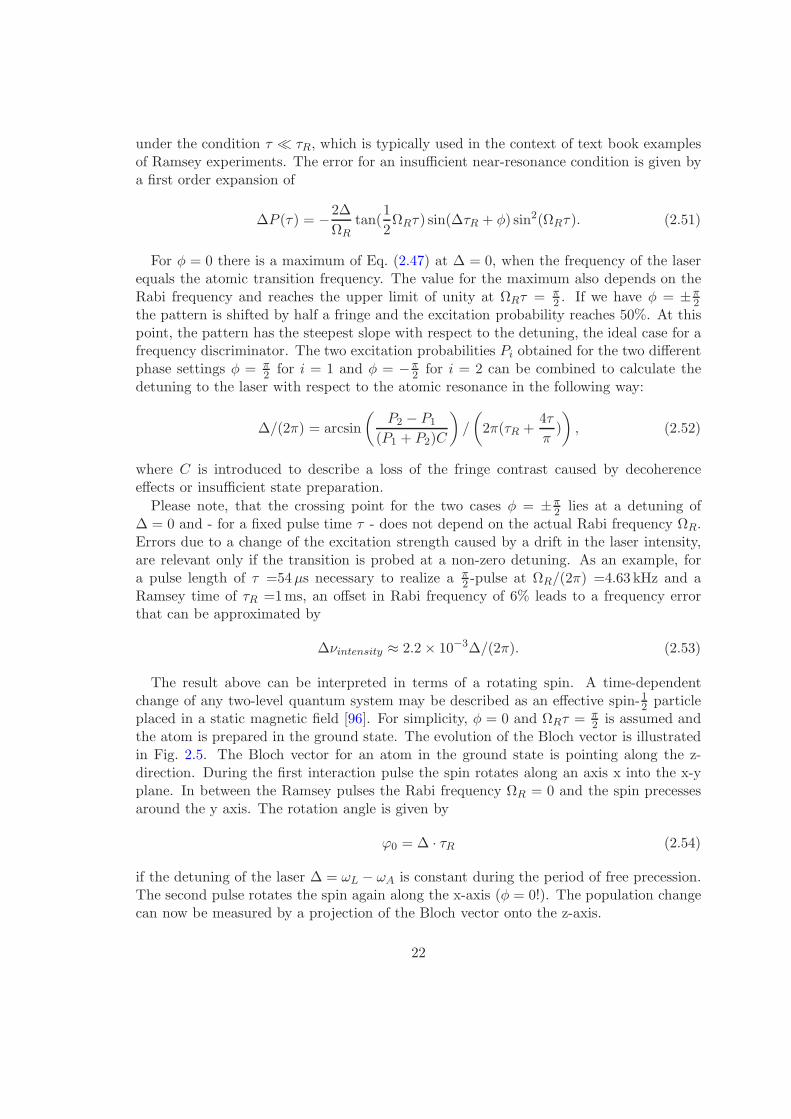
The result above can be interpreted in terms of a rotating spin. A time-dependentchange of any two-level quantum system may be described as an effective spin-1

2 particleplaced in a static magnetic field [96]. For simplicity, φ = 0 and ΩRτ = π

2 is assumed andthe atom is prepared in the ground state. The evolution of the Bloch vector is illustratedin Fig. 2.5. The Bloch vector for an atom in the ground state is pointing along the z-direction. During the first interaction pulse the spin rotates along an axis x into the x-yplane. In between the Ramsey pulses the Rabi frequency ΩR = 0 and the spin precessesaround the y axis. The rotation angle is given by

ϕ0 = ∆ · τR (2.54)

if the detuning of the laser ∆ = ωL − ωA is constant during the period of free precession.The second pulse rotates the spin again along the x-axis (φ = 0!). The population changecan now be measured by a projection of the Bloch vector onto the z-axis.

22

(a) (b) (c)

Figure 2.5: Bloch sphere pictures for a Ramsey experiment. First, the spin is rotated intothe equatorial plane by the π

2 pulse (a), then the system can evolve freely for a time τRwhere the precession angle determined by the frequency detuning (b), and the second π

2pulse rotates out of the xy-plane again (c). The precession angle can now be measured bya projection onto the z direction.

2.4.4 Ramsey contrast

The Ramsey experiment was treated so far without taking decoherence effects into accountwhich occur for real experiments. In Eq. (2.52) the contrast C was introduced withoutgiving a more detailed explanation. In 40Ca+, two effects can lead to a loss of contrastdue to decoherence, when probing the 4s 2S1/2 − 3d 2D5/2 transition. One effect is ofcourse related to frequency fluctuations of the interrogation laser, the other one is causedby magnetic field fluctuations which affect the different transitions according to theirmagnetic quantum numbers. Mathematically, these effects can be treated identically asthey both lead to a fluctuating detuning ∆ of the transition. In order to calculate thecontrast as a function of the waiting time τR, we have to assume a certain noise model.

First a Gaussian ”shot-to-shot” noise is considered with the following distribution offrequency fluctuations

P (∆) =1

σ√π

exp

(

−∆2

σ2

)

, (2.55)

where σ is the half width at the 1/e-point. Therefore, each individual Ramsey experimentwill accumulate a different phase factor exp(i∆τR). The contrast can be calculated by theaverage of the phase fluctuations, that is

C(τR) = |〈exp(i∆τR)〉| =∣

∣

∣

∣

∫ +∞

−∞d∆P (∆) exp(i∆τR)

∣

∣

∣

∣

= exp

(

−σ2τ2

R

4

)

. (2.56)

The FWHM of the frequency fluctuations for the above definition of σ is

2π∆νFWHM = 2√

ln 2 σ. (2.57)

Taking this into account, C(τR) can be expressed as

C(τR) = exp

(

−π2∆ν2

FWHMτ2R

4 ln 2

)

. (2.58)

23

Let τ1/2 be the time for which the contrast reaches 50% of the initial value, the corre-sponding FWHM of the laser frequency is given by

∆νFWHM =2 ln 2

π

1

τ1/2. (2.59)

Analogous to Gaussian frequency fluctuations, the contrast can be calculated in case ofa Lorentzian distribution

P (∆) =1

π

γ

γ2 + ∆2(2.60)

with a half width at half maximum of γ. The contrast then decays exponentially with thewaiting time given by

C(τR) = exp (−γτR) . (2.61)

The laser linewidth is related to the time τ1/2 where the contrast has decayed to 50% by

∆νFWHM =γ

π=

ln 2

π

1

τ1/2. (2.62)

Measurements of the Ramsey decay are therefore a valuable means for an investigationof the laser linewidth of an ultra-stable laser, particularly interesting for experiments whereno second ultra-stable laser system for an optical beat measurement is available.

2.5 Interaction with magnetic and electric fields

2.5.1 Zeeman shift

The total angular momentum J of the valence electron is given by

J = L+ S. (2.63)

Each of the fine structure levels J consists of (2J + 1) sublevels which are related to theangular distribution of the electron wave function. They are labeled by the magneticquantum number mJ = −|L+S| ≤ J ≤ L+S. The degeneracy of the magnetic sublevelsis lifted in the presence of a non-zero magnetic field B. The Hamiltonian describing theinteraction of the magnetic moment µ of the atom with the magnetic field in first orderperturbation theory is

HZeeman = −µB. (2.64)

If the energy shift of the magnetic field is small compared with the fine structure splitting,the magnetic moment can be written in terms of the total angular momentum of Eq. (2.63)and the interaction Hamiltonian becomes

HZeeman = −µBgJJB, (2.65)

24

where µB is the Bohr magneton and gJ the Lande g-factor, which is given by [97]

gJ = gLJ(J + 1)− S(S + 1) + L(L+ 1)

2J(J + 1)+ gS

J(J + 1) + S(S + 1)− L(L+ 1)

2J(J + 1)

≃ 1 +J(J + 1) + S(S + 1)− L(L+ 1)

2J(J + 1).

(2.66)

Here, gL and gS are the g-factors for the orbital and spin magnetic moments and the secondexpression is an approximation for gL ≃ 1 and gS ≃ 2. Equation (2.66) does not containQED effects and corrections for the complicated multi-electron structure of 40Ca+ . Theg-factor in the ground state of 40Ca+ has been precisely measured by Tommaseo et al.[98] to be gJ(4s 2S1/2) = 2.002 256 64(9) while gJ (3d 2D5/2) ≃ 1.2.

For B = Bez and J = mJez, where ez is the unit vector in the quantization direction,the frequency shift of a magnetic sublevel can be calculated as

∆νlinZ = mJgJµBB

~(2.67)

to lowest order in B. This is called the anomalous Zeeman effect. The higher ordercontribution to the Zeeman effect has a quadratic component which shifts the levels whichcouple to the sublevels of the 3d 2D3/2 state. By using second order perturbation theory[99], the quadratic Zeeman shift is

∆νquadZ = K(µBB)2

h2νFS, (2.68)

where νFS is the fine structure splitting and h the Planck constant and K a constantdepending on the magnetic sublevel given by

K =6

25for mD = ±1

2 ,

K =4

25for mD = ±3

2 ,

K = 0 for mD = ±52 . (2.69)

In most cases this correction of a few Hz is negligible compared to the linear contributionwhich is on the order of MHz but for the clock measurement it represents the largest shiftin the error budget after the cancellation of the linear Zeeman effect and the quadrupoleshift.

There is also a non-zero mean-square magnitude of the magnetic field caused by black-body radiation. According to [100], it can be expressed as

〈B2(t)〉 = (28 mG)2(

T

300 K

)4

. (2.70)

At room temperature, the estimated shifts for the individual transitions would be wellbelow 1mHz and therefore completely masked by other magnetic fields.

25

2.5.2 Electric quadrupole shift

The non-spherical charge distribution of the upper D level gives rise to an electric quadru-pole moment that can interact with any electric field gradient present in the trap, forexample those gradients generated by the DC electrodes of a linear Paul trap or by patchpotentials on the trap electrode structure. According to [91], the electric quadrupole mo-ment Θ(γ, J) of an atom in the electronic state |γ, J〉 having a the total angular momentumJ in the magnetic sublevel with maximum magnetic quantum number mJ is defined as

Θ(γ, J) = −e⟨

γ, J,mJ = J

∥

∥

∥

∥

∥

N∑

i=1

r2iC20(θi, φi)

∥

∥

∥

∥

∥

γ, J,mJ = J

⟩

, (2.71)

where the sum is taken over all electrons i with the radial coordinate ri and angular

coordinates θi, φi and the renormalized spherical harmonic C(2)0 (θi, φi) =

√

4π5 Y2,0(θi, φi).

The interaction Hamiltonian for the atomic quadrupole moment coupled to an electricfield gradient is given by Eq. (2.32). Here, the components of the tensor describing thegradient of the external field ∇E for a electric trapping potential given in Eq. (2.3) is

∇E(2)0 = −A,

∇E(2)±1 = 0,

∇E(2)±2 =

√

1

6ǫA, (2.72)

where the term proportional to ǫ takes into account a possible field gradient which is notoriented along the trap axis, e. g. created by a patch potential. The trapping potentialtherefore is modified by an extra component U ′(x, y, z) = ǫA(x2 − y2). The Hamiltonianthen takes the form

HQ = −AQ(2)0 +

√

1

6ǫA(Q

(2)2 +Q

(2)−2). (2.73)

The magnitude of the electric field gradient in z-direction can be calibrated by the trapfrequency ωz and is given by

A = ∇E =Mω2

z

e(2.74)

using the gradient of the electric field from Eq. (2.4) and inserting Eqs. (2.6) and (2.9).Comparing the results obtained by [101] for the quadrupole shift in Sr+, the shift for

the 3d 2D5/2 levels in 40Ca+ can be calculated as

∆νQuad =eA

h〈3d| r2 |3d〉

(

1

4− 3

35m2

)

[(3 cos2 β − 1)− ǫ sin2 β(cos2 α− sin2 α)], (2.75)

where the orientation of the quantization axis and the electric field gradient has beenparameterized by a set of Euler angles α, β, γ.

Theoretical calculations for the 3d 2D5/2 levels in 40Ca+ predicted a quadrupole momentof 1.89 ea2

0 and 1.92(1) ea20 [24, 102, 103], recent calculations with 1.85(2) ea2

0 [104] and

26

1.82 ea20 [105] lie closer to the experimentally obtained result described in Chp. 7. For

typical field gradients in our linear Paul trap of 25 V/mm2 at a tip voltage of 1000 V andassuming that the gradient direction is along the trap axis, but at an angle of 30 withrespect to the quantization axis, the expected shifts are on the order of ∆νQuad=10 Hz.Taking the sum over the factor

(

14 − 3

35m2)

for all possible values of m, the shift adds tozero. This means, that for an absolute frequency measurement of the 4s 2S1/2− 3d 2D5/2

transition, averaging of transitions involving all sublevels of the 3d 2D5/2 state completelycancels the quadrupole shift [23]. The same can be achieved by averaging over threemutually orthogonal directions of the quantization axis which was proposed in [91].

27

28

Chapter 3

Experimental setup

In this chapter a description of the experimental setup is given. After a complete overviewa part is dedicated to the ion trap setup followed by a brief review of the laser systemsused for cooling and repumping which have recently been remodeled. The setup for thelaser at 729 nm and the fiber noise cancellation are explained in more detail. And finally,the detection of optical beat notes for the analysis of the laser’s spectral properties ispresented.

3.1 Overview

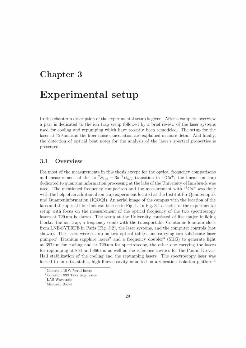
For most of the measurements in this thesis except for the optical frequency comparisonsand measurement of the 4s 2S1/2 − 3d 2D5/2 transition in 43Ca+, the linear ion trapdedicated to quantum information processing at the labs of the University of Innsbruck wasused. The mentioned frequency comparison and the measurement with 43Ca+ was donewith the help of an additional ion trap experiment located at the Institut fur Quantenoptikund Quanteninformation (IQOQI). An aerial image of the campus with the location of thelabs and the optical fiber link can be seen in Fig. 1. In Fig. 3.1 a sketch of the experimentalsetup with focus on the measurement of the optical frequency of the two spectroscopylasers at 729 nm is shown. The setup at the University consisted of five major buildingblocks: the ion trap, a frequency comb with the transportable Cs atomic fountain clockfrom LNE-SYTRTE in Paris (Fig. 3.2), the laser systems, and the computer controls (notshown). The lasers were set up on two optical tables, one carrying two solid-state laserpumped1 Titanium:sapphire lasers2 and a frequency doubler3 (SHG) to generate lightat 397 nm for cooling and at 729 nm for spectroscopy, the other one carrying the lasersfor repumping at 854 and 866 nm as well as the reference cavities for the Pound-Drever-Hall stabilization of the cooling and the repumping lasers. The spectroscopy laser waslocked to an ultra-stable, high finesse cavity mounted on a vibration isolation platform4

1Coherent 10 W Verdi lasers2Coherent 899 Ti:sa ring lasers3LAS Wavetrain4Minus-K BM-4

29

-80 MHz

University main lab

IQOQI

Ti:Sa

729 nm

Ti:Sa

729 nm

AO2

AO1

AO5

AO3

AO4

frequency

comb

Cs

fountain

RF

counter

optical

beat note

detection

optical

beat note

detection

AO6

-80 MHz

-77.76 MHz

~ 540

MHz

~1.1 GHz

40Ca+

ion trap

Ti:Sa

794 nm

SHG

397 nm

diode lasers

854 &

866 nm

PI lasers

fs lab

AO8

AO7

40Ca+/43Ca+

ion trapAO9

AO

10

AO

11

RF

counter80 MHz80 MHz

500 m

500 m

~ 487 MHz

~1.3 GHz

IQOQI lab

Figure 3.1: Overview of the frequency measurement setup: Two similar ion experimentscan be compared via 500 m long polarization maintaining fibers. A single experimentsetup consists of a linear Ca+ ion trap and Ti:Sa lasers stabilized to an ultrastable highfinesse cavity. The numbers show the AOM (yellow blocks) frequencies in MHz.

30

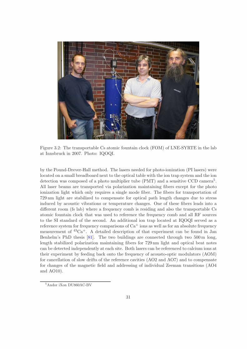
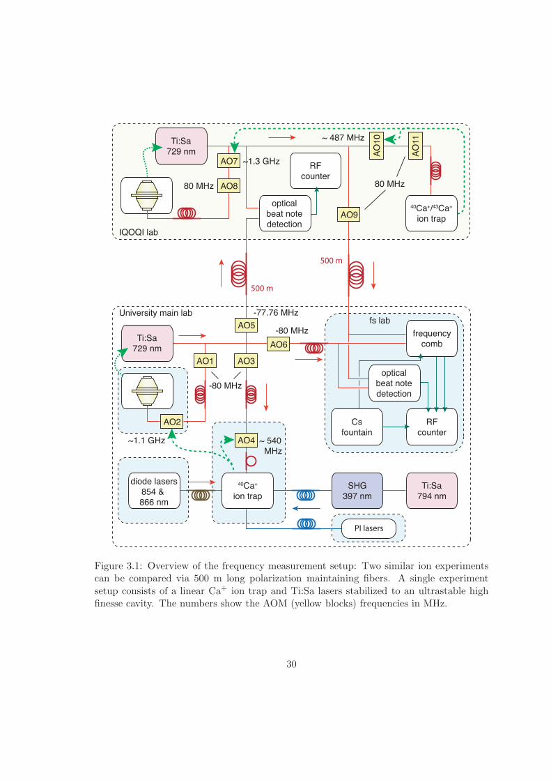
Figure 3.2: The transportable Cs atomic fountain clock (FOM) of LNE-SYRTE in the labat Innsbruck in 2007. Photo: IQOQI.

by the Pound-Drever-Hall method. The lasers needed for photo-ionization (PI lasers) werelocated on a small breadboard next to the optical table with the ion trap system and the iondetection was composed of a photo multiplier tube (PMT) and a sensitive CCD camera5.All laser beams are transported via polarization maintaining fibers except for the photoionization light which only requires a single mode fiber. The fibers for transportation of729 nm light are stabilized to compensate for optical path length changes due to stressinduced by acoustic vibrations or temperature changes. One of these fibers leads into adifferent room (fs lab) where a frequency comb is residing and also the transportable Csatomic fountain clock that was used to reference the frequency comb and all RF sourcesto the SI standard of the second. An additional ion trap located at IQOQI served as areference system for frequency comparisons of Ca+ ions as well as for an absolute frequencymeasurement of 43Ca+. A detailed description of that experiment can be found in JanBenhelm’s PhD thesis [81]. The two buildings are connected through two 500 m long,length stabilized polarization maintaining fibers for 729 nm light and optical beat notescan be detected independently at each site. Both lasers can be referenced to calcium ions attheir experiment by feeding back onto the frequency of acousto-optic modulators (AOM)for cancellation of slow drifts of the reference cavities (AO2 and AO7) and to compensatefor changes of the magnetic field and addressing of individual Zeeman transitions (AO4and AO10).

5Andor iXon DU860AC-BV

31

3.2 Linear ion trap

The linear ion trap at the University lab consists of four blade-shaped electrodes for radialand two endcaps for axial confinement. A picture and a sketch with the exact dimensionsare given in Fig. 3.3. This trap has been designed by Stephan Gulde and a more thoroughdescription can be found in his PhD thesis [79]. The details about the ion trap at IQOQIare discussed in [81]. For typical operation conditions of the University trap, a radiofrequency ΩTrap/2π =23.5 MHz from a (up to) 50 W power amplifier is coupled into ahelical resonator with a quality factor Q = 250 to boost the voltage V=V0 cos(ΩTrapt) atone of the blade pairs to V0 ∼1 kV while the other pair is connected to ground. The staticpotential applied to the end caps is provided by a stable high voltage supply6 with 10−6

stability. For a radio frequency power of 9 W and a tip voltage of 1000 V we typically get

(a) Picture of the trap.

5.0

1.6

6.0

30.0

11.2

30°

45°

3.0

18.7

RF blades

end-cap tips

compensationelectrodes

horiz.

vert.

(b) Dimensions of the trap.

Figure 3.3: The ion trap of the University of Innsbruck. The dimensions are given in mm.

secular trap frequencies of ωa/2π = 1.2MHz in the axial and ωa/2π = 3.4MHz in theradial directions.

3.2.1 Vacuum vessel and optical access

The ion trap is mounted in a vacuum vessel shown in Fig. 3.4. The trap axis is tiltedwith an angle of β0=28 with respect to the magnetic field defining the quantization axisproduced by the main coil pair Cσ. The tilt of the field is necessary since the opticalaccess along the trap axis is blocked by the end-cap tips. This is also the direction of abeam of σ-polarized light at 397 nm for optical pumping into the desired |S,ms〉 state.To control the field in horizontal direction there is another pair of coils CD along thedirection of the Doppler cooling beam which also contains the repumping lasers at 854and 866 nm. The magnetic field gradient can be changed by a single coil at the viewport

6ISEG EHQ F020p

32

O O

CD

CD Cσ

Cσ

Cg

to PMT397 nm

addressed beam729 nm

to CCD397 nm

opticalpumping397 σ

Dopplercooling/detection397 nm866 nm854 nm

photo-ionizationlasers

aux.729 nm

B

β0

(a) Top view.

O

Cz

Cz

Cg

auxiliary beam729 nm

39

7D

op

ple

r

397

σ

(b) Side view.

Figure 3.4: The optical access and magnetic field coils. The dashed lines indicate thequantization magnetic field and the trap axis.

between the Doppler and σ ports. Also shown are the two objectives (O) for imaging ofthe ion’s fluorescence at 397 nm onto a photo-multiplier (PMT) or onto the CCD camera.The latter objective’s main purpose though is to focus the 729 nm spectroscopy lighttightly onto the ions with a spot-size of less than 3µm [80]. The beam can be steeredalong the ion string for individual addressing with the help of an electro-optic deflector.Along the vertical direction the magnetic field can be controlled by a third pair of coils Cz.Additionally, there is an auxiliary port for light at 729 nm at an angle of 45 to the verticalaxis and the horizontal plane. It is used for micromotion compensation and simultaneouscoherent operations on all ions of the ion string. The whole apparatus is covered by aµ-metal box for shielding of surrounding magnetic stray fields, for example produced inthe lab by power supplies or a BEC experiment next door. The damping factor at theline frequency of 50 Hz which is the dominant contribution to the magnetic field noise is∼ 200. A magnetic field sensor sensitive in all three spatial directions placed inside thisshielding box shows an RMS magnetic field of 37µG. An estimation using Eq. (2.58) andthe obtained Ramsey contrasts in Sec. 6.1 confirms a residual magnetic field amplitude atthe position of the ion of 25µG.

3.2.2 Measurement of the trap temperature

For the error budget of the 4s 2S1/2 − 3d 2D5/2 transition frequency measurement it isnecessary to measure the trap temperature because of the AC Stark shift induced byblack body radiation. Unfortunately, with the current setup it is not possible to havedirect access to the temperature since there are no sensors built in and the viewports areopaque for light with a wavelength larger than 2µm so a thermal camera could not beused. Therefore, a test trap with unused leftover-parts had to be built including two PT100

33

0 2 4 6 8 100

20

40

60

80

100

120

140

160

RF power (W)

trap tem

pera

ture

(°C

)

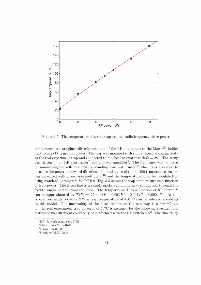
Figure 3.5: The temperature of a test trap vs. the radio frequency drive power.

temperature sensors glued directly onto one of the RF blades and to the Macor R© holdernext to one of the ground blades. The trap was mounted with similar thermal conductivityas the real experiment trap and connected to a helical resonator with Q = 280. The setupwas driven by an RF synthesizer7 and a power amplifier8. The frequency was adjustedby minimizing the reflection with a standing wave ratio meter9 which was also used tomeasure the power in forward direction. The resistance of the PT100 temperature sensorswas measured with a precision multimeter10 and the temperature could be calculated byusing standard parameters for PT100. Fig. 3.5 shows the trap temperature as a functionof trap power. The fitted line is a simple model combining heat conduction through thefeed-throughs and thermal radiation. The temperature T as a function of RF power Pcan be approximated by T (P ) = 25 + 14P − 0.003P 2 − 0.002P 3 − 0.0004P 4. At thetypical operating power of 9 W a trap temperature of 150 C can be inferred accordingto this model. The uncertainty of the measurement on the test trap is a few C butfor the real experiment trap an error of 50C is assumed for the following reasons: Theresistance measurement could only be performed with the RF switched off. The time delay

7HP Network Analyser 3577B8Minicircuits ZHL-10W9Daiwa CN-801HP

10Keithley DMM 2000

34

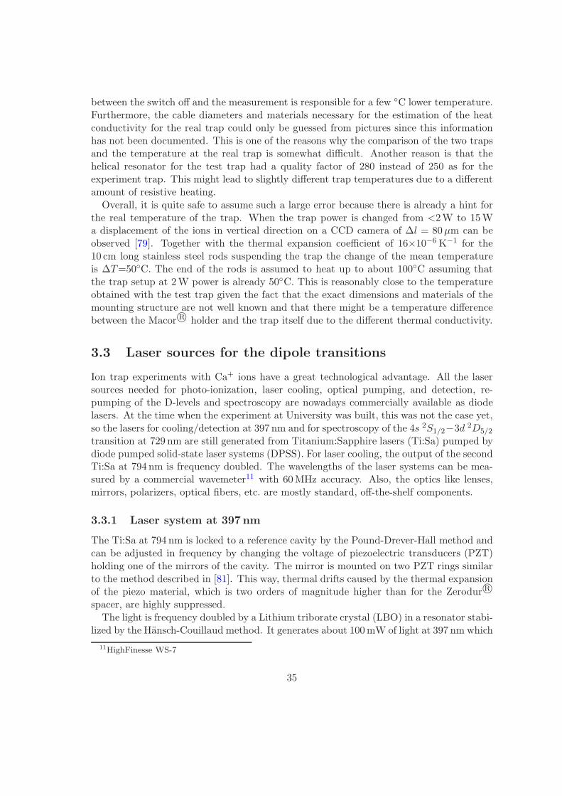
between the switch off and the measurement is responsible for a few C lower temperature.Furthermore, the cable diameters and materials necessary for the estimation of the heatconductivity for the real trap could only be guessed from pictures since this informationhas not been documented. This is one of the reasons why the comparison of the two trapsand the temperature at the real trap is somewhat difficult. Another reason is that thehelical resonator for the test trap had a quality factor of 280 instead of 250 as for theexperiment trap. This might lead to slightly different trap temperatures due to a differentamount of resistive heating.

Overall, it is quite safe to assume such a large error because there is already a hint forthe real temperature of the trap. When the trap power is changed from <2W to 15 Wa displacement of the ions in vertical direction on a CCD camera of ∆l = 80µm can beobserved [79]. Together with the thermal expansion coefficient of 16×10−6 K−1 for the10 cm long stainless steel rods suspending the trap the change of the mean temperatureis ∆T=50C. The end of the rods is assumed to heat up to about 100C assuming thatthe trap setup at 2 W power is already 50C. This is reasonably close to the temperatureobtained with the test trap given the fact that the exact dimensions and materials of themounting structure are not well known and that there might be a temperature differencebetween the Macor R© holder and the trap itself due to the different thermal conductivity.

3.3 Laser sources for the dipole transitions

Ion trap experiments with Ca+ ions have a great technological advantage. All the lasersources needed for photo-ionization, laser cooling, optical pumping, and detection, re-pumping of the D-levels and spectroscopy are nowadays commercially available as diodelasers. At the time when the experiment at University was built, this was not the case yet,so the lasers for cooling/detection at 397 nm and for spectroscopy of the 4s 2S1/2−3d 2D5/2

transition at 729 nm are still generated from Titanium:Sapphire lasers (Ti:Sa) pumped bydiode pumped solid-state laser systems (DPSS). For laser cooling, the output of the secondTi:Sa at 794 nm is frequency doubled. The wavelengths of the laser systems can be mea-sured by a commercial wavemeter11 with 60 MHz accuracy. Also, the optics like lenses,mirrors, polarizers, optical fibers, etc. are mostly standard, off-the-shelf components.

3.3.1 Laser system at 397 nm

The Ti:Sa at 794 nm is locked to a reference cavity by the Pound-Drever-Hall method andcan be adjusted in frequency by changing the voltage of piezoelectric transducers (PZT)holding one of the mirrors of the cavity. The mirror is mounted on two PZT rings similarto the method described in [81]. This way, thermal drifts caused by the thermal expansionof the piezo material, which is two orders of magnitude higher than for the Zerodur R©spacer, are highly suppressed.

The light is frequency doubled by a Lithium triborate crystal (LBO) in a resonator stabi-lized by the Hansch-Couillaud method. It generates about 100 mW of light at 397 nm which

11HighFinesse WS-7

35

is distributed to three independent 40Ca+ experiments by polarizing beam splitters (PBS)and half-waveplates. Each experiment has its own AOM12 in double pass configurationwith separate amplitude and frequency control (center frequency 80 MHz). In front of thecat’s eye prism for retro-reflection of the beam a mechanical shutter is placed to blockthe zeroth order from the AOM. If needed like in the event the ion crystal has melted orfor easier loading of the trap, the far red-detuned (160 MHz) light from the zeroth orderhelps in (re-)crystallizing. The light is then focused into a polarization maintaining opticalfiber13 and transported to the vacuum vessel housing with the ion trap. The light can beswitched off by a factor of <10−5 with two RF switches14 and a mechanical shutter forthe zeroth order.

At the experiment table the light gets split into two parts: one part for optical pumpingand one for cooling and detection of the ion. Each branch includes an AOM in single passconfiguration (center frequency 80 MHz) for individual amplitude and frequency control.The light can be switched off with more than 60 dB in each branch. The light is finallymade overlapping with the repumping light at 854 and 866 nm and transmitted to theviewports via photonic crystal fibers15 and focused onto the ion string.

3.3.2 Laser systems at 854 and 866 nm

The light at 854 nm for resetting the D5/2 level and 866 nm for repumping the D3/2 level isgenerated by two commercially available, grating stabilized diode lasers16. Both lasers arestabilized to separate reference cavities by the Pound-Drever-Hall method. The resonatorsshare the same Zerodur R© spacer together with the cavity for the stabilization of the 794 nmlaser and the same temperature stabilized vacuum vessel. The frequency of the lasers canbe tuned by changing the cavity length with mirrors mounted on PZTs the same way asmentioned above. Again, these laser sources are shared by all 40Ca+ experiments at theUniversity and each beam line has it’s own double-pass AOM17 for individual amplitudeand frequency control. When the lasers are switched off, the light levels of both lasersafter the polarization maintaining fibers18 on the experiment table are less than 0.1 nWeach.

3.3.3 Lasers for photo-ionization

In order to load ions into our trap a beam of neutral calcium atoms is ionized near thetrap center. In the past, this was achieved by electron bombardment causing a bunch ofproblems like creating stray charges on the trap electrodes and the supporting structure,the necessity of a high calcium flux, or the ionization of impurities like background atoms.This can be avoided by photo-ionizing the calcium atoms using two laser sources at 423 nm

12Brimrose QZF80-20-39713Schafter & Kirchhoff OXF-SM-400-125-P14Minicircuits ZYSW-2-50DR15Crystal Fibre PM-916Toptica DL-10017Crystal Technologies 3200-12118Schafter & Kirchhoff PMC-850-5,5-NA011-3-APC

36

for driving the 4s 1S1 − 4p 1P1− transition and 390 nm for transferring the electron intothe continuum as described in [106]. Both are grating stabilized diode lasers19 without anyfurther stabilization. The frequency of the 423 nm laser can be tuned by a PZT changingthe grating position or the diode temperature.

3.4 The spectroscopy laser at 729 nm

At the heart of the experiment is the ultra-stable laser at 729 nm used for spectroscopy ofthe 4s 2S1/2 − 3d 2D5/2 transition. In addition, the laser is used for:

• frequency resolved optical pumping,

• sideband cooling to the motional ground state,

• coherent manipulation of qubits for quantum information processing,

• precision spectroscopy on the 4s 2S1/2 − 3d 2D5/2 transition.

Since the natural linewidth of the transition is ∆ν0 =140 mHz, it requires a narrow-bandlaser for optimal state manipulation. The laser system is based on a Ti:Sa ring laserpumped by a DPSS laser at 532 nm. The standard Coherent 899 ring laser provides highoutput power (600 mW at 7W pump power) with a linewidth of roughly 500 kHz. In orderto improve the performance the system had to be upgraded by an intra-cavity electro-opticmodulator (EOM) [107] and stabilized to an external reference. More details about thestabilization of a Ti:Sa at 729 nm and the setup at IQOQI can be found in [108].

3.4.1 The Titanium:Sapphire ring laser

In the following, the system used for the absolute frequency measurement of the 4s 2S1/2−3d 2D5/2 transition is explained in more detail. Figure 3.6 shows a sketch of the Coherent899 ring laser with the intra-cavity elements. The three elements used for the external fre-quency stabilization are highlighted with dashed circles. To increase the servo bandwidthan EOM20 was inserted into the upper beam which led to a boost of the bandwidth froma few kHz to more than one MHz.

Though the Ti:Sa crystal has a very broad gain profile (650 to 1100 nm), the geometryof the laser cavity ensures single transverse mode operation. To ensure single-mode oper-ation also in longitudinal direction and to provide for frequency tuning, several frequency-selective intra-cavity elements are required. The birefringent filter (BF) consists of threebirefringent plates with a thickness ratio of 1:4:16. Only those modes survive for which theoptical path length for the ordinary as well for the extraordinary direction match integermultiples of the wavelength. By tuning the angle of the BF this optical path length can beadjusted but the transmission peak is very broad and the resulting frequency selectivityis still insufficient. In order to fully achieve longitudinal single mode operation two prisms

19Toptica DL-10020Linos PM25

37

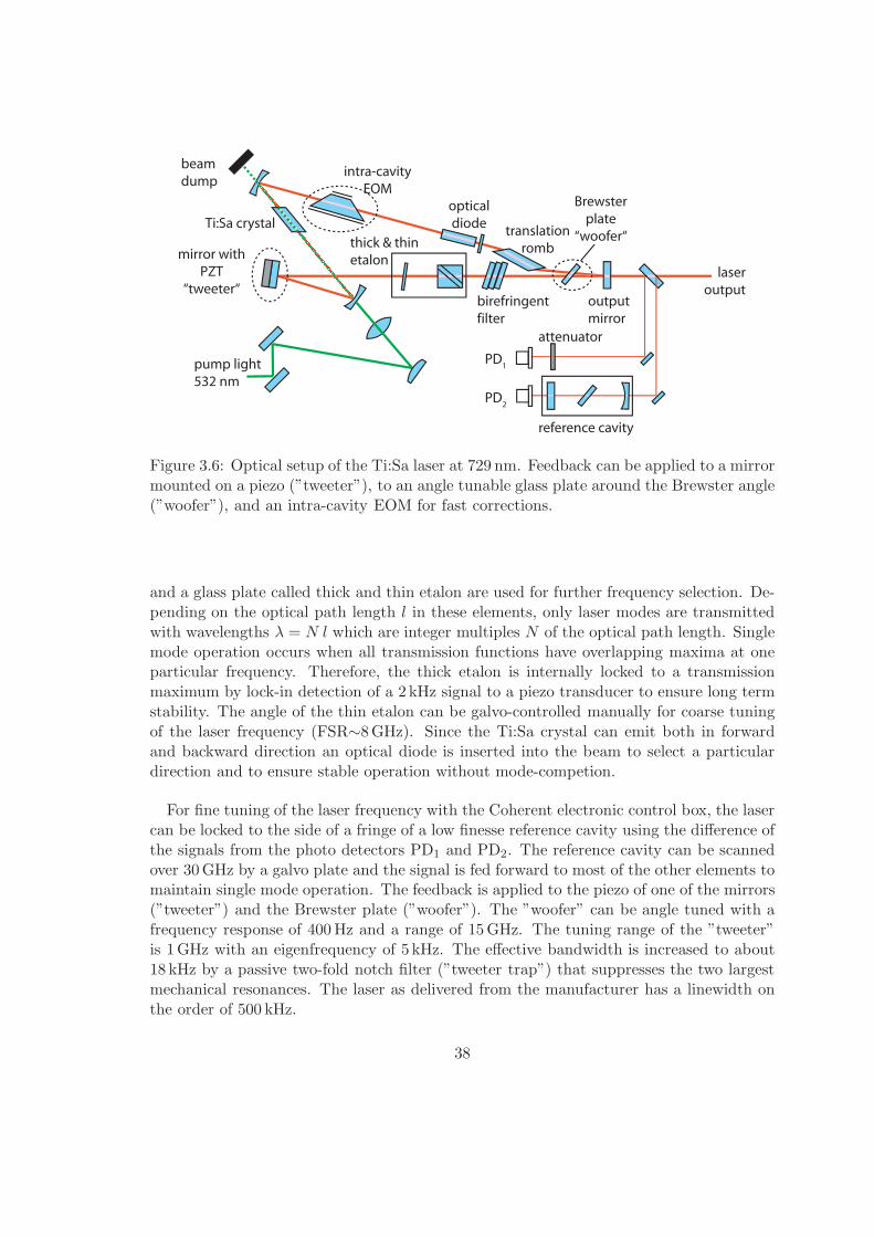
beam dump

intra-cavityEOM

opticaldiode

thick & thinetalon

translationromb

birefringentfilter

PD1

PD2

mirror withPZT

“tweeter“

pump light532 nm

outputmirror

Brewsterplate

“woofer“

reference cavity

attenuator

Ti:Sa crystal

laseroutput

Figure 3.6: Optical setup of the Ti:Sa laser at 729 nm. Feedback can be applied to a mirrormounted on a piezo (”tweeter”), to an angle tunable glass plate around the Brewster angle(”woofer”), and an intra-cavity EOM for fast corrections.

and a glass plate called thick and thin etalon are used for further frequency selection. De-pending on the optical path length l in these elements, only laser modes are transmittedwith wavelengths λ = N l which are integer multiples N of the optical path length. Singlemode operation occurs when all transmission functions have overlapping maxima at oneparticular frequency. Therefore, the thick etalon is internally locked to a transmissionmaximum by lock-in detection of a 2 kHz signal to a piezo transducer to ensure long termstability. The angle of the thin etalon can be galvo-controlled manually for coarse tuningof the laser frequency (FSR∼8GHz). Since the Ti:Sa crystal can emit both in forwardand backward direction an optical diode is inserted into the beam to select a particulardirection and to ensure stable operation without mode-competion.

For fine tuning of the laser frequency with the Coherent electronic control box, the lasercan be locked to the side of a fringe of a low finesse reference cavity using the difference ofthe signals from the photo detectors PD1 and PD2. The reference cavity can be scannedover 30 GHz by a galvo plate and the signal is fed forward to most of the other elements tomaintain single mode operation. The feedback is applied to the piezo of one of the mirrors(”tweeter”) and the Brewster plate (”woofer”). The ”woofer” can be angle tuned with afrequency response of 400 Hz and a range of 15 GHz. The tuning range of the ”tweeter”is 1GHz with an eigenfrequency of 5 kHz. The effective bandwidth is increased to about18 kHz by a passive two-fold notch filter (”tweeter trap”) that suppresses the two largestmechanical resonances. The laser as delivered from the manufacturer has a linewidth onthe order of 500 kHz.

38

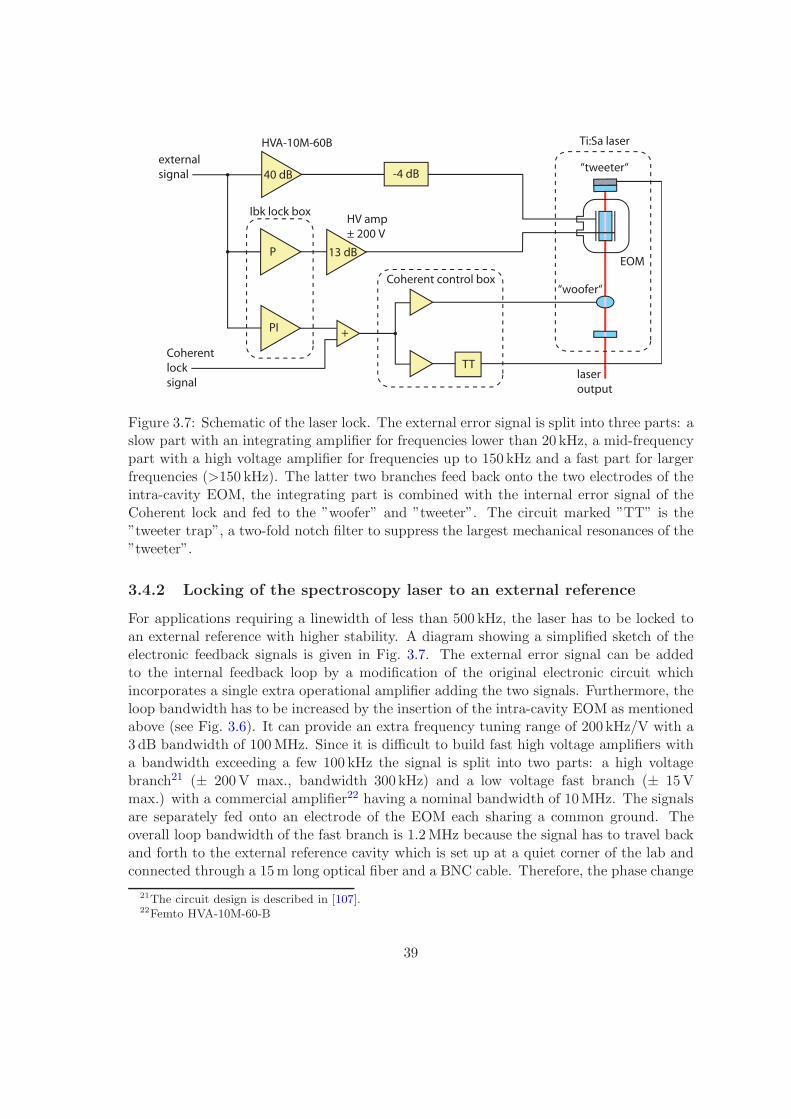
Ti:Sa laserHVA-10M-60B

40 dB -4 dB

PI

P

HV amp± 200 V

+

Coherent control box

EOM

“woofer“

“tweeter“

Ibk lock box

external signal

Coherentlock signal

laseroutput

13 dB

TT

Figure 3.7: Schematic of the laser lock. The external error signal is split into three parts: aslow part with an integrating amplifier for frequencies lower than 20 kHz, a mid-frequencypart with a high voltage amplifier for frequencies up to 150 kHz and a fast part for largerfrequencies (>150 kHz). The latter two branches feed back onto the two electrodes of theintra-cavity EOM, the integrating part is combined with the internal error signal of theCoherent lock and fed to the ”woofer” and ”tweeter”. The circuit marked ”TT” is the”tweeter trap”, a two-fold notch filter to suppress the largest mechanical resonances of the”tweeter”.

3.4.2 Locking of the spectroscopy laser to an external reference

For applications requiring a linewidth of less than 500 kHz, the laser has to be locked toan external reference with higher stability. A diagram showing a simplified sketch of theelectronic feedback signals is given in Fig. 3.7. The external error signal can be addedto the internal feedback loop by a modification of the original electronic circuit whichincorporates a single extra operational amplifier adding the two signals. Furthermore, theloop bandwidth has to be increased by the insertion of the intra-cavity EOM as mentionedabove (see Fig. 3.6). It can provide an extra frequency tuning range of 200 kHz/V with a3 dB bandwidth of 100 MHz. Since it is difficult to build fast high voltage amplifiers witha bandwidth exceeding a few 100 kHz the signal is split into two parts: a high voltagebranch21 (± 200 V max., bandwidth 300 kHz) and a low voltage fast branch (± 15 Vmax.) with a commercial amplifier22 having a nominal bandwidth of 10 MHz. The signalsare separately fed onto an electrode of the EOM each sharing a common ground. Theoverall loop bandwidth of the fast branch is 1.2 MHz because the signal has to travel backand forth to the external reference cavity which is set up at a quiet corner of the lab andconnected through a 15 m long optical fiber and a BNC cable. Therefore, the phase change

21The circuit design is described in [107].22Femto HVA-10M-60-B

39

due to the time delay reaches π already for a frequency of 3.3 MHz. The high voltage parthas a loop bandwidth of 140 kHz. With this setup it is possible to substantially narrowthe linewidth of the laser to much less than 100 Hz. The necessary parts to achieve thisgoal are explained in the following.

3.4.3 The external high finesse resonator

The construction of an ultra-stable laser necessitates an ultra-stable frequency reference.For laser stabilization an optical reference cavity formed by two mirrors attached to a rigidspacer is a good choice because of the exceptionally good short term stability that is onthe order of 10−15 and even better over time intervals ranging from 1 to 100 s for some ofthese systems. The most stable lasers have been achieved with stabilization schemes tohigh finesse cavities [109–114].

The vertical cavity design and setup

The crucial point for a stable reference is its sensitivity to external perturbations. For anoptical cavity the frequency stability is determined by the stability of the mirror distance.Vibrations caused by acoustics in the vicinity of the cavity or seismic vibrations causedby a shaking building can change the mirror distance. The goal therefore is to build areference cavity with low sensitivity to external accelerations and to shield the system asmuch as possible from the environment. The cavity design developed by Notcutt et al. [110]at JILA realizes this principle by mounting the cavity vertically exactly at the mid planebetween the mirrors. This way, length changes due to vertical acceleration which aremost likely in a typical lab environment cancel to first order. Fig. 3.8 shows a pictureof the cavity used for the laser stabilization of the laser at the University incorporatingthis design. If the cavity is accelerated upwards the upper part gets compressed and thelower part sags so that the net length change is zero and vice versa. The cavity spaceras well as the mirror substrates are made out of ultra-low expansion glass (ULE R©) witha thermal expansion coefficient of below 10−8 K−1. The mirrors are optically contactedto the spacer of 7.75 cm length. The upper mirror has a curvature of r =50 cm while thelower is planar. To avoid standing waves within the mirror substrates or etalon effectswith any parallel optical surface, the back sides of the mirrors were antireflection coatedto less than 0.1%. The cavity is mounted at the mid-plane by three PTFE rods whichare themselves resting in a Zerodur R© base plate. Since the cavity stability is determinedby the mirror distance, also length changes due to thermal fluctuations or changes of theindex of refraction have to be avoided. The cavity needs to be placed into a temperature-stabilized vacuum system as sketched in Fig. 3.9. The vacuum vessel is mounted in abox of 5 mm thick aluminum which is covered by heating mats23 and thermal insulationmaterial. Six temperature sensors are placed at each side of the box and the temperaturecan be stabilized at temperatures between 25C to 30C where the ULE R© was specified tohave a minimum of the thermal expansion coefficient. Unfortunately, some part of the ion

23available at RS components

40

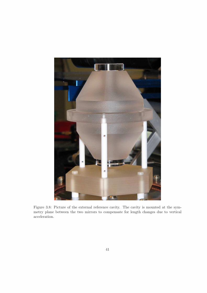
Figure 3.8: Picture of the external reference cavity. The cavity is mounted at the sym-metry plane between the two mirrors to compensate for length changes due to verticalacceleration.

41

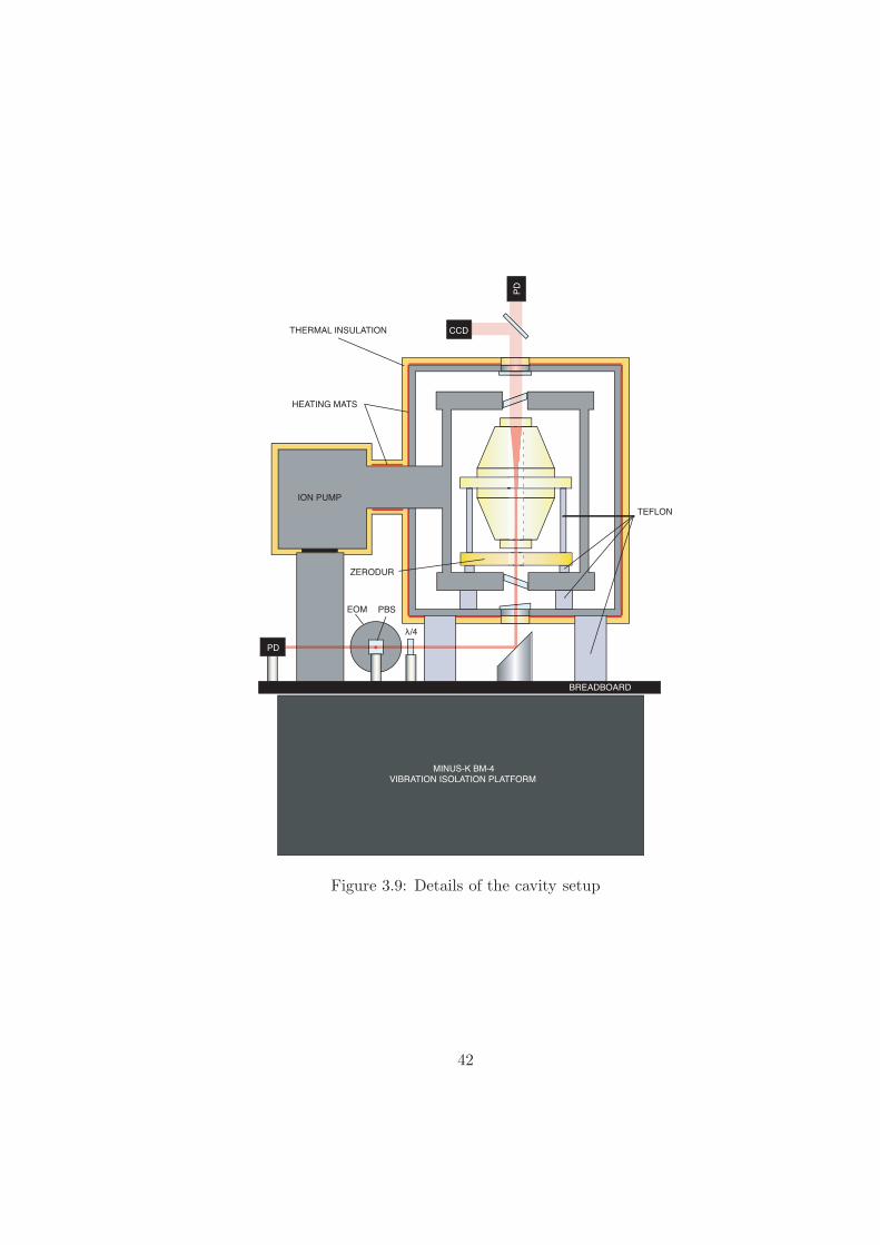
PD

CCD

PD

EOM

λ/4

PBS

ION PUMP

THERMAL INSULATION

ZERODUR

TEFLON

HEATING MATS

BREADBOARD

MINUS-K BM-4

VIBRATION ISOLATION PLATFORM

Figure 3.9: Details of the cavity setup

42

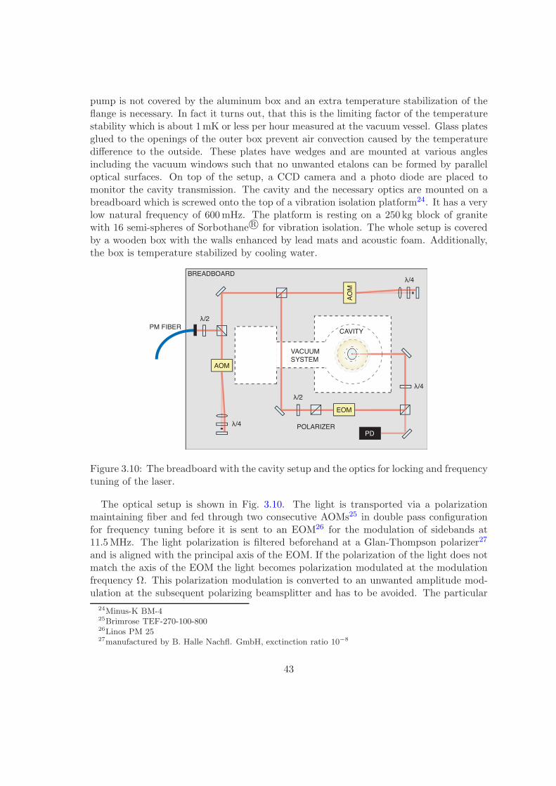
pump is not covered by the aluminum box and an extra temperature stabilization of theflange is necessary. In fact it turns out, that this is the limiting factor of the temperaturestability which is about 1 mK or less per hour measured at the vacuum vessel. Glass platesglued to the openings of the outer box prevent air convection caused by the temperaturedifference to the outside. These plates have wedges and are mounted at various anglesincluding the vacuum windows such that no unwanted etalons can be formed by paralleloptical surfaces. On top of the setup, a CCD camera and a photo diode are placed tomonitor the cavity transmission. The cavity and the necessary optics are mounted on abreadboard which is screwed onto the top of a vibration isolation platform24. It has a verylow natural frequency of 600 mHz. The platform is resting on a 250 kg block of granitewith 16 semi-spheres of Sorbothane R© for vibration isolation. The whole setup is coveredby a wooden box with the walls enhanced by lead mats and acoustic foam. Additionally,the box is temperature stabilized by cooling water.

AOM

AOM

EOM

PD

λ/2

λ/2

λ/4

λ/4

λ/4

PM FIBER

BREADBOARD

POLARIZER

CAVITY

VACUUM

SYSTEM

Figure 3.10: The breadboard with the cavity setup and the optics for locking and frequencytuning of the laser.

The optical setup is shown in Fig. 3.10. The light is transported via a polarizationmaintaining fiber and fed through two consecutive AOMs25 in double pass configurationfor frequency tuning before it is sent to an EOM26 for the modulation of sidebands at11.5 MHz. The light polarization is filtered beforehand at a Glan-Thompson polarizer27

and is aligned with the principal axis of the EOM. If the polarization of the light does notmatch the axis of the EOM the light becomes polarization modulated at the modulationfrequency Ω. This polarization modulation is converted to an unwanted amplitude mod-ulation at the subsequent polarizing beamsplitter and has to be avoided. The particular

24Minus-K BM-425Brimrose TEF-270-100-80026Linos PM 2527manufactured by B. Halle Nachfl. GmbH, exctinction ratio 10−8

43

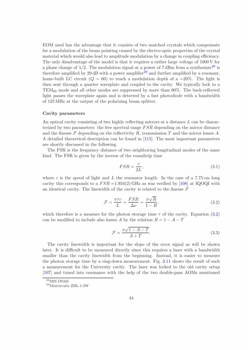
EOM used has the advantage that it consists of two matched crystals which compensatefor a modulation of the beam pointing caused by the electro-optic properties of the crystalmaterial which would also lead to amplitude modulation by a change in coupling efficiency.The only disadvantage of the model is that it requires a rather large voltage of 1000 V fora phase change of λ/2. The modulation signal at a power of 7 dBm from a synthesizer28 istherefore amplified by 29 dB with a power amplifier29 and further amplified by a resonant,home-built LC circuit (Q ∼ 60) to reach a modulation depth of a ∼20%. The light isthen sent through a quarter waveplate and coupled to the cavity. We typically lock to aTEM00 mode and all other modes are suppressed by more than 90%. The back-reflectedlight passes the waveplate again and is detected by a fast photodiode with a bandwidthof 125 MHz at the output of the polarizing beam splitter.

Cavity parameters

An optical cavity consisting of two highly reflecting mirrors at a distance L can be charac-terized by two parameters: the free spectral range FSR depending on the mirror distanceand the finesse F depending on the reflectivity R, transmission T and the mirror losses A.A detailed theoretical description can be found in [115]. The most important parametersare shortly discussed in the following.

The FSR is the frequency distance of two neighboring longitudinal modes of the samekind. The FSR is given by the inverse of the roundtrip time

FSR =c

2L, (3.1)

where c is the speed of light and L the resonator length. In the case of a 7.75 cm longcavity this corresponds to a FSR =1.934(2) GHz as was verified by [108] at IQOQI withan identical cavity. The linewidth of the cavity is related to the finesse F

F =πτc

L=FSR

∆ν=

π√R

1−R, (3.2)

which therefore is a measure for the photon storage time τ of the cavity. Equation (3.2)can be modified to include also losses A by the relation R = 1−A− T

F =π√

1−A− TA+ T

. (3.3)

The cavity linewidth is important for the slope of the error signal as will be shownlater. It is difficult to be measured directly since this requires a laser with a bandwidthsmaller than the cavity linewidth from the beginning. Instead, it is easier to measurethe photon storage time by a ring-down measurement. Fig. 3.11 shows the result of sucha measurement for the University cavity. The laser was locked to the old cavity setup[107] and tuned into resonance with the help of the two double-pass AOMs mentioned

28SRS DS34529Minicircuits ZHL-1-2W

44

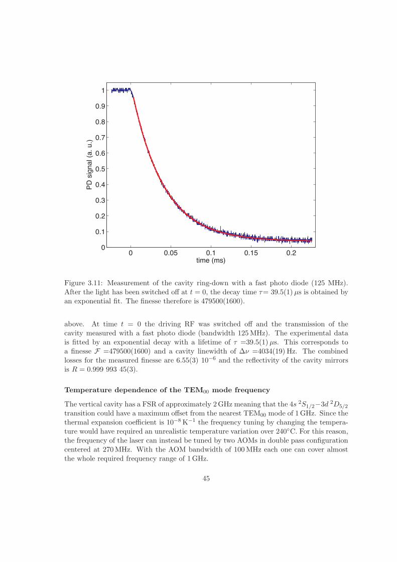
0 0.05 0.1 0.15 0.20

0.1

0.2

0.3

0.4

0.5

0.6

0.7

0.8

0.9

1

time (ms)

PD

sig

na

l (a

. u

.)

Figure 3.11: Measurement of the cavity ring-down with a fast photo diode (125 MHz).After the light has been switched off at t = 0, the decay time τ= 39.5(1) µs is obtained byan exponential fit. The finesse therefore is 479500(1600).

above. At time t = 0 the driving RF was switched off and the transmission of thecavity measured with a fast photo diode (bandwidth 125 MHz). The experimental datais fitted by an exponential decay with a lifetime of τ =39.5(1) µs. This corresponds toa finesse F =479500(1600) and a cavity linewidth of ∆ν =4034(19) Hz. The combinedlosses for the measured finesse are 6.55(3) 10−6 and the reflectivity of the cavity mirrorsis R = 0.999 993 45(3).

Temperature dependence of the TEM00 mode frequency

The vertical cavity has a FSR of approximately 2GHz meaning that the 4s 2S1/2−3d 2D5/2

transition could have a maximum offset from the nearest TEM00 mode of 1 GHz. Since thethermal expansion coefficient is 10−8 K−1 the frequency tuning by changing the tempera-ture would have required an unrealistic temperature variation over 240C. For this reason,the frequency of the laser can instead be tuned by two AOMs in double pass configurationcentered at 270 MHz. With the AOM bandwidth of 100 MHz each one can cover almostthe whole required frequency range of 1 GHz.

45

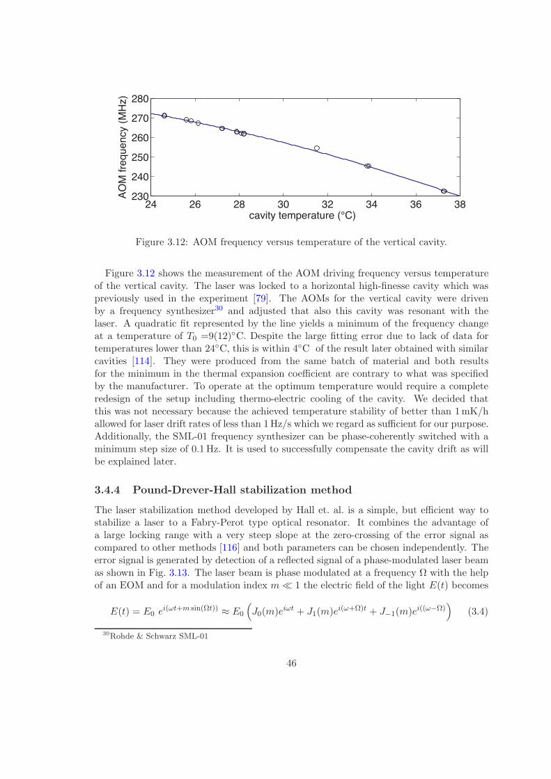
24 26 28 30 32 34 36 38230

240

250

260

270

280

cavity temperature (°C)

AO

M f

req

ue

ncy (

MH

z)

Figure 3.12: AOM frequency versus temperature of the vertical cavity.

Figure 3.12 shows the measurement of the AOM driving frequency versus temperatureof the vertical cavity. The laser was locked to a horizontal high-finesse cavity which waspreviously used in the experiment [79]. The AOMs for the vertical cavity were drivenby a frequency synthesizer30 and adjusted that also this cavity was resonant with thelaser. A quadratic fit represented by the line yields a minimum of the frequency changeat a temperature of T0 =9(12)C. Despite the large fitting error due to lack of data fortemperatures lower than 24C, this is within 4C of the result later obtained with similarcavities [114]. They were produced from the same batch of material and both resultsfor the minimum in the thermal expansion coefficient are contrary to what was specifiedby the manufacturer. To operate at the optimum temperature would require a completeredesign of the setup including thermo-electric cooling of the cavity. We decided thatthis was not necessary because the achieved temperature stability of better than 1mK/hallowed for laser drift rates of less than 1Hz/s which we regard as sufficient for our purpose.Additionally, the SML-01 frequency synthesizer can be phase-coherently switched with aminimum step size of 0.1 Hz. It is used to successfully compensate the cavity drift as willbe explained later.

3.4.4 Pound-Drever-Hall stabilization method

The laser stabilization method developed by Hall et. al. is a simple, but efficient way tostabilize a laser to a Fabry-Perot type optical resonator. It combines the advantage ofa large locking range with a very steep slope at the zero-crossing of the error signal ascompared to other methods [116] and both parameters can be chosen independently. Theerror signal is generated by detection of a reflected signal of a phase-modulated laser beamas shown in Fig. 3.13. The laser beam is phase modulated at a frequency Ω with the helpof an EOM and for a modulation index m≪ 1 the electric field of the light E(t) becomes

E(t) = E0 ei(ωt+m sin(Ωt)) ≈ E0

(

J0(m)eiωt + J1(m)ei(ω+Ω)t + J−1(m)ei((ω−Ω))

(3.4)

30Rohde & Schwarz SML-01

46

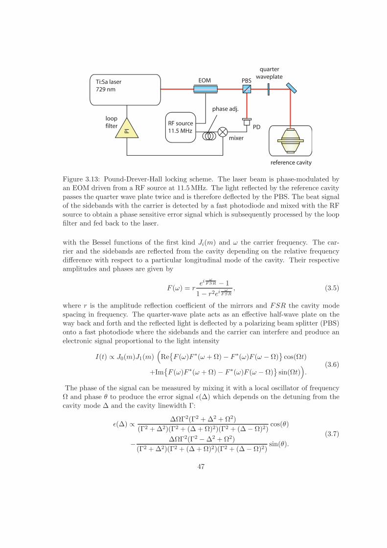
Ti:Sa laser729 nm

RF source11.5 MHzP

I

EOM

PD

quarterwaveplate

phase adj.

reference cavity

loopfilter

mixer

PBS

Figure 3.13: Pound-Drever-Hall locking scheme. The laser beam is phase-modulated byan EOM driven from a RF source at 11.5 MHz. The light reflected by the reference cavitypasses the quarter wave plate twice and is therefore deflected by the PBS. The beat signalof the sidebands with the carrier is detected by a fast photodiode and mixed with the RFsource to obtain a phase sensitive error signal which is subsequently processed by the loopfilter and fed back to the laser.

with the Bessel functions of the first kind Ji(m) and ω the carrier frequency. The car-rier and the sidebands are reflected from the cavity depending on the relative frequencydifference with respect to a particular longitudinal mode of the cavity. Their respectiveamplitudes and phases are given by

F (ω) = rei

ωF SR − 1

1− r2ei ωF SR

, (3.5)

where r is the amplitude reflection coefficient of the mirrors and FSR the cavity modespacing in frequency. The quarter-wave plate acts as an effective half-wave plate on theway back and forth and the reflected light is deflected by a polarizing beam splitter (PBS)onto a fast photodiode where the sidebands and the carrier can interfere and produce anelectronic signal proportional to the light intensity

I(t) ∝ J0(m)J1(m)(

Re

F (ω)F ∗(ω + Ω)− F ∗(ω)F (ω − Ω)

cos(Ωt)

+Im

F (ω)F ∗(ω + Ω)− F ∗(ω)F (ω − Ω)

sin(Ωt))

.(3.6)

The phase of the signal can be measured by mixing it with a local oscillator of frequencyΩ and phase θ to produce the error signal ǫ(∆) which depends on the detuning from thecavity mode ∆ and the cavity linewidth Γ:

ǫ(∆) ∝ ∆ΩΓ2(Γ2 + ∆2 + Ω2)

(Γ2 + ∆2)(Γ2 + (∆ + Ω)2)(Γ2 + (∆− Ω)2)cos(θ)

− ∆ΩΓ2(Γ2 −∆2 + Ω2)

(Γ2 + ∆2)(Γ2 + (∆ + Ω)2)(Γ2 + (∆− Ω)2)sin(θ).

(3.7)

47

-15 -10 -5 0 5 10 15-1

-0.8

-0.6

-0.4

-0.2

0

0.2

0.4

0.6

0.8

1

frequency detuning ∆/(2π) (MHz)

PDH

erro

r sig

nal (a

. u

.)

Figure 3.14: Pound-Drever-Hall error signal calculated for two different phases of the localoscillator with a cavity linewidth of 100 kHz and a modulation frequency of 10 MHz. Thesolid line corresponds to a phase θ = 0, the dashed line to θ = 90.

48

The phase of the local oscillator can be adjusted by building an electronic phase shifter orsimply by changing the cables to the right length and therefore the appropriate timedelay. The resulting shape of the error signal is displayed in Fig. 3.14 for a cavitylinewidth of Γ/(2π) =100 kHz and a modulation frequency Ω/(2π) =10 MHz at a phaseof θ =0(solid line) and θ =90 phase (dashed line). The interesting case for laser stabi-lization is θ =0 where the slope of the error signal at the center is inversely proportionalto the linewidth. Therefore, in order to increase the slope one has to decrease the cav-ity linewidth and the need for a high finesse cavity becomes apparent. Furthermore, thecapture range of the signal, i. e. the range of frequency excursions that produce an errorsignal with correct sign only depends on the modulation frequency and can be chosenindependently. Finally, the feedback loop is closed by passing the error signal through anappropriate loop filter with integrating characteristics (PI controller) to keep track of longterm drifts. Thereby, feedback is provided onto the frequency sensitive elements describedabove.

3.4.5 Laser stabilization

In this section the stabilization of the spectroscopy laser to the high finesse cavity bythe method of Pound-Drever-Hall (see Sec. 3.4.4) is discussed and the performance ofthe system is analyzed. Additionally, minor improvements concerning the laser lock arementioned. Since a huge number of sidebands were created at multiples of the thick etalonmodulation frequency in the Coherent setup, they had to be eliminated by building anexternal lock. Finally, fluctuations of the laser intensity were be reduced by intensitystabilization.

Frequency stabilization

The optical setup for the frequency stabilization has already been discussed in Sec. 3.4.3.The signal modulated at Ω/(2π) =11.5 MHz is detected by a fast photodiode, amplifiedwith a gain of 20 dB31 and mixed32 with part of the radio frequency signal as mentionedabove to generate the error signal. It is split up into three different branches as describedin Sec. 3.4.2 with an individual loop filter each to increase the total servo bandwidthto about 1MHz. The relative performance of the lock can be investigated by analyzingthe residual error signal. Figure 3.15 shows a combination of spectrum analyzer tracesof different span normalized by the square-root of the filter bandwidth so that they canbe combined independent of the spectrum analyzer settings. It clearly shows that thenoise between 200 Hz and 5 kHz is dominating the spectrum where the lock is not able tocompletely eliminate the perturbations.

The maximum peak to peak amplitude of the error signal is 490(10) mV when scanningover the resonance. Using the calibration of the Minicircuits ZAD-1 mixer in [108], thiscorresponds to a true amplitude of 1000(260) mV due to non-linearities of the mixer. Theslope of the error signal at the line center therefore is D =2.0(5) mV/Hz. The residual

31Minicircuits ZFL-1000LN32Minicircuits ZAD-1

49

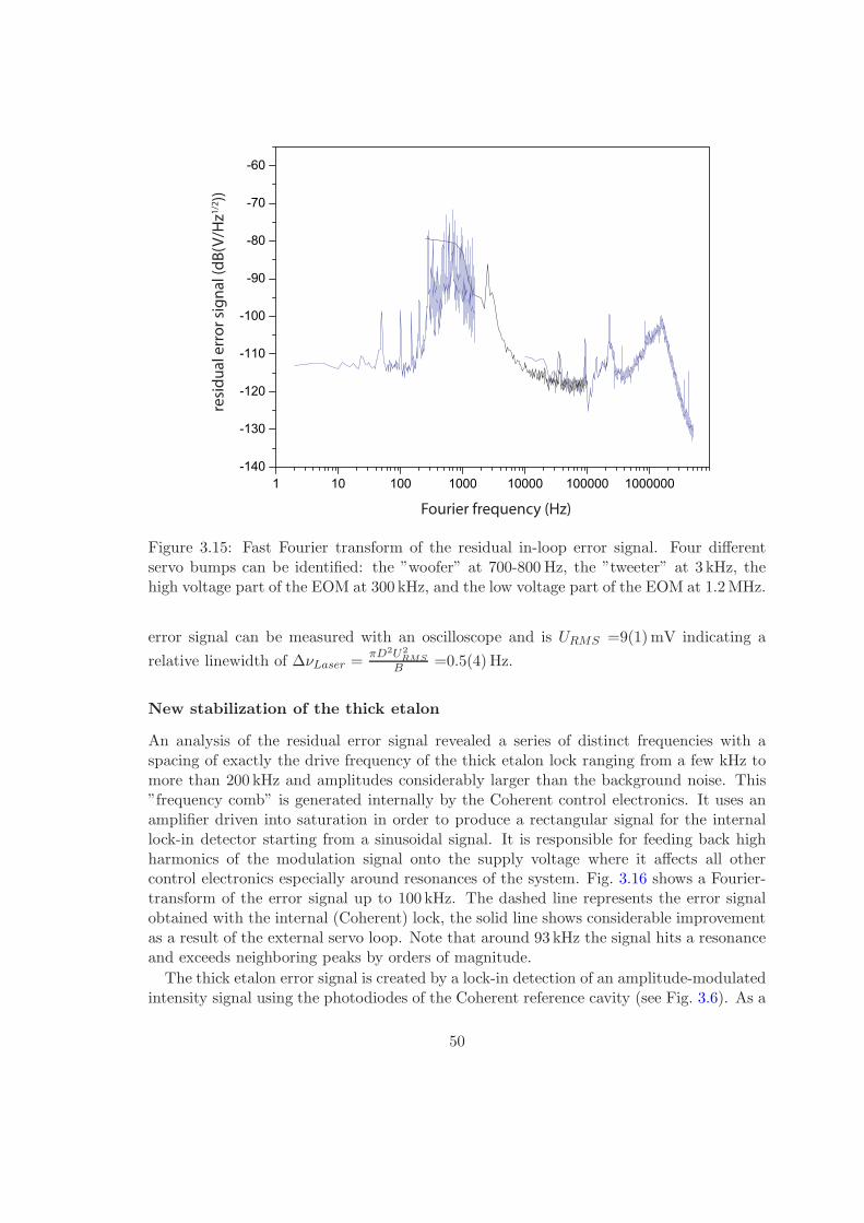
Fourier frequency (Hz)

resi

du

al e

rro

r si

gn

al (d

B(V

/Hz1

/2))

Figure 3.15: Fast Fourier transform of the residual in-loop error signal. Four differentservo bumps can be identified: the ”woofer” at 700-800 Hz, the ”tweeter” at 3 kHz, thehigh voltage part of the EOM at 300 kHz, and the low voltage part of the EOM at 1.2 MHz.

error signal can be measured with an oscilloscope and is URMS =9(1) mV indicating a

relative linewidth of ∆νLaser =πD2U2

RMSB =0.5(4) Hz.

New stabilization of the thick etalon

An analysis of the residual error signal revealed a series of distinct frequencies with aspacing of exactly the drive frequency of the thick etalon lock ranging from a few kHz tomore than 200 kHz and amplitudes considerably larger than the background noise. This”frequency comb” is generated internally by the Coherent control electronics. It uses anamplifier driven into saturation in order to produce a rectangular signal for the internallock-in detector starting from a sinusoidal signal. It is responsible for feeding back highharmonics of the modulation signal onto the supply voltage where it affects all othercontrol electronics especially around resonances of the system. Fig. 3.16 shows a Fourier-transform of the error signal up to 100 kHz. The dashed line represents the error signalobtained with the internal (Coherent) lock, the solid line shows considerable improvementas a result of the external servo loop. Note that around 93 kHz the signal hits a resonanceand exceeds neighboring peaks by orders of magnitude.

The thick etalon error signal is created by a lock-in detection of an amplitude-modulatedintensity signal using the photodiodes of the Coherent reference cavity (see Fig. 3.6). As a

50

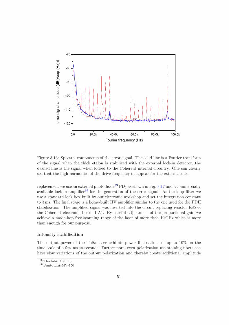
0.0 20.0k 40.0k 60.0k 80.0k 100.0k

-120

-110

-100

-90

-80

-70

erro

r sig

nal a

mpl

itude

(dB

(V/s

qrt(H

z)))

Fourier frequency (Hz)

Figure 3.16: Spectral components of the error signal. The solid line is a Fourier transformof the signal when the thick etalon is stabilized with the external lock-in detector, thedashed line is the signal when locked to the Coherent internal circuitry. One can clearlysee that the high harmonics of the drive frequency disappear for the external lock.

replacement we use an external photodiode33 PD1 as shown in Fig. 3.17 and a commerciallyavailable lock-in amplifier34 for the generation of the error signal. As the loop filter weuse a standard lock box built by our electronic workshop and set the integration constantto 3 ms. The final stage is a home-built HV amplifier similar to the one used for the PDHstabilization. The amplified signal was inserted into the circuit replacing resistor R85 ofthe Coherent electronic board 1-A1. By careful adjustment of the proportional gain weachieve a mode-hop free scanning range of the laser of more than 10 GHz which is morethan enough for our purpose.

Intensity stabilization

The output power of the Ti:Sa laser exhibits power fluctuations of up to 10% on thetime-scale of a few ms to seconds. Furthermore, even polarization maintaining fibers canhave slow variations of the output polarization and thereby create additional amplitude

33Thorlabs DET11034Femto LIA-MV-150

51

modulation when polarization sensitive optics is used. Amplitude modulation can causetwo main problems: First, it causes a variation of the Rabi frequency at the position of theion and second, amplitude noise is converted into frequency noise at the PDH stabilizationby a fluctuating error signal amplitude.

The solution to this problem is rather simple. For the intensity and polarization sta-bilization of the fiber guiding light from the laser to the experiment table (see Fig. 3.1)we take a reflex of a wedge used for the fiber noise cancellation (see section below) placedafter a polarizing beam splitter. The light intensity is monitored with a fast photodiode(bandwidth 120 MHz). The error signal is created by subtracting a constant offset voltagefrom the PD signal with a PID controller35 and fed to a variable attenuator36 controllingthe radio frequency power of the fiber noise cancellation AOM. The attainable servo band-width is 92(1) kHz. The intensity stabilization for the reference cavity light is set up in aslightly different way. Here, the transmission of the cavity is used for stabilization withthe same kind of equipment but the servo bandwidth is of course limited by the cavitybandwidth. Both systems are capable of reducing the amplitude noise to below 1%.

3.4.6 Fiber noise cancellation

The optical setup for the distribution of the 729 nm light is outlined in Fig. 3.17. The mainpart of the light (300 mW) is sent to the experiment table by a polarization maintainingfiber after passing a 2:1 telescope for adjusting the beam size to the fiber collimator37 andAO1 for stabilizing the optical path length described below. A few mW are sent to thehigh finesse cavity and the frequency comb, the rest of the light is guided through the500 m long fiber to IQOQI (see Fig. 1) for the beat note detection. All these beams passAOMs and the -1st diffraction order is sent to the fiber couplers. The AOM frequenciesare indicated in the figure by the numbers in MHz.

The light transported by optical fibers is affected by acoustic vibrations, thermally orair pressure induced stress. These effects cause changes in the index of refraction andtherefore the optical path length. The resulting broadening of the laser spectrum canbe quite severe and leads to an increased linewidth of about 1 kHz in case of the 500 mlong polarization maintaining fibers. This is not tolerable for precision spectroscopy andespecially bad if the light is sent to the stabilization cavity because the fiber-induced noisewould be transferred onto the laser. It is therefore necessary to interferometrically stabilizethe optical path length. We used the approach developed by Ma and coworkers [117].

The setup consists of a beamsplitter, an AOM and a fast photodiode (PD) as shown foreach beam in Fig. 3.17. The (minus-)first diffraction order of the AOM is sent throughthe fiber and is affected by fiber noise. Part of the light (typical 4% glass reflection) isback-reflected at the 0 angle-polished fiber end and sent back through the fiber therebypicking up the noise twice. In case of the at both ends angle-polished fiber guiding lightto the experiment, we use a glass wedge after a polarizing beam splitter to retro-reflectthe light. The beamsplitter is used for polarization cleaning. After passing the AOM the

35SRS SIM96036Minicircuits TFAS-2SM37Schafter & Kirchhoff 60FC

52

Ti:Sa laser729 nm500 mW

waveplate

PD1

toexperiment

AO1

tohigh finesse

cavityAO2

PD2

PD3

waveplate

waveplate

toIQOQI

AO4

PD4

waveplate

tofrequency

comb

AO3

PD5

waveplate

waveplate

waveplate

2 : 1

-80 MHz

-80 MHz

-80 MHz

-77.76 MHz

reflected lightfrom end facet

reference beam

Figure 3.17: The distribution of the 729 nm light with the elements for fiber noise cancel-lation. The light paths for the fiber stabilization of the reference cavity fiber are indicatedby the dashed arrows.

53

second time the light is combined with part of the unmodulated light at the beamsplitterin front of the AOM. A beat note at twice the AOM frequency can be detected with afast photodiode. The electronic beat signal is mixed down with a reference signal from astable RF synthesizer38 to produce an error signal at DC. The phase difference betweenthe beat signal and the reference is fed to a voltage-controlled oscillator (VCO) drivingthe AOM after passing an integrating loop filter. This closes the loop and the fiber noiseis compensated by a phase-locked loop (PLL). The servo bandwidth depends on the VCObandwidth (typically 300 kHz) and on the signal delay by the optical path length. Evenfor the 500 m long fiber a loop bandwidth of 35 kHz was achieved.

The effect of fiber noise broadening the light used for the laser stabilization is shownin Fig. 3.18. The fiber39 to the high finesse cavity is 15 m long. At typical noise con-ditions in our lab the spectrum broadens to a full width at half maximum (FWHM)∆νFWHM=557(7) Hz indicated by the Gaussian fit in Fig. 3.18(a). When the stabiliza-tion is active the noise gets significantly reduced to below 1Hz as it has been demonstratedin [108]. A comparison of the unstabilized to the stabilized case is shown in Fig. 3.18(b).The central peak has a linewidth of 0.9 Hz and is limited by the resolution bandwidth ofthe spectrum analyzer40. The loop bandwidth of the stabilization is 170 kHz.

3.4.7 Optical beat note detection

In the previous sections the frequency stability of the laser was only analyzed with respectto the reference cavity. The analysis of the residual error signal provides a means toevaluate the quality of the laser lock relative to the resonator. The true spectral propertiesof a laser cannot be investigated this way. Instead, comparison to an independent systemis necessary, like for instance by detecting a beat note with a second laser system. Analternative could also be to compare the laser frequency with the transition frequency of anarrow atomic transition as described in Sec. 7.2, or at the side of a fringe from an opticalresonator.

For a beat note detection, the spectroscopy laser of the 40Ca+ experiment at the uni-versity was compared against the laser system of the 40/43Ca+ experiment at IQOQI. Thelight of the two lasers can be transported to both sites by two 500 m long, polarizationmaintaining fibers equipped with fiber noise cancellation. The two lasers are overlappingon a non-polarizing beam splitter (BS) and sent to a photodetector, that measures theinterference of the two light fields. The resulting photo-current is proportional to theoptical intensity:

I(t) ∼ |E1(t) + E2(t)|2 = |E1(t)|2 + |E2(t)|2 + 2ReE∗1(t)E2(t). (3.8)

The power spectrum of the beat signal is a convolution of the power spectra of the twolasers, that is

SE∗1E2(f) = SE1(f)⊗ SE2(f). (3.9)

38Marconi 2023A39Oz Optics PMJ-3A3-633-4/125-3-10-140Rohde & Schwarz FSP-13

54

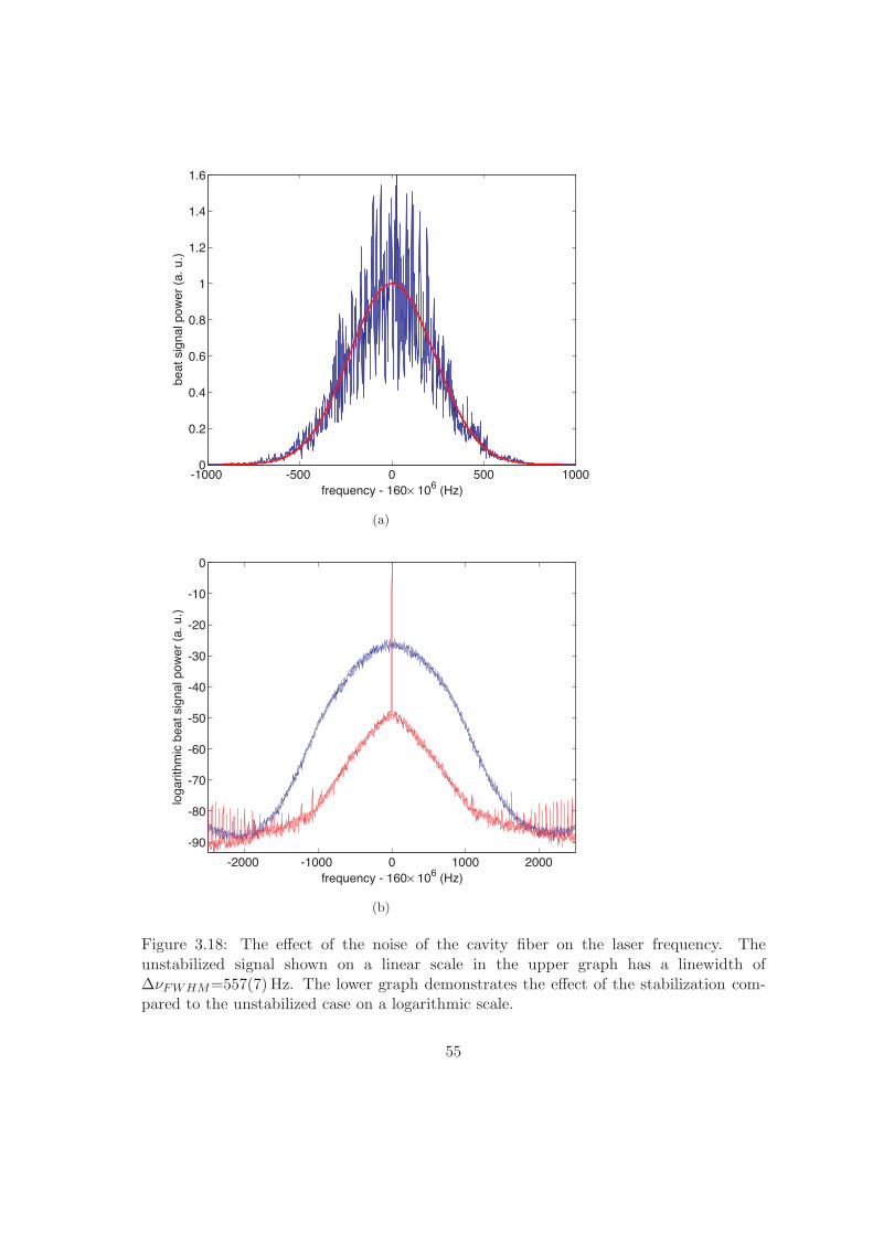
-1000 -500 0 500 10000

0.2

0.4

0.6

0.8

1

1.2

1.4

1.6

frequency - 160× 106 (Hz)

beat sig

nal pow

er (a

. u

.)

(a)

-2000 -1000 0 1000 2000

-90

-80

-70

-60

-50

-40

-30

-20

-10

0

frequency - 160× 106 (Hz)

loga

rithmic

beat sig

nal pow

er (a.

u.)

(b)

Figure 3.18: The effect of the noise of the cavity fiber on the laser frequency. Theunstabilized signal shown on a linear scale in the upper graph has a linewidth of∆νFWHM=557(7) Hz. The lower graph demonstrates the effect of the stabilization com-pared to the unstabilized case on a logarithmic scale.

55

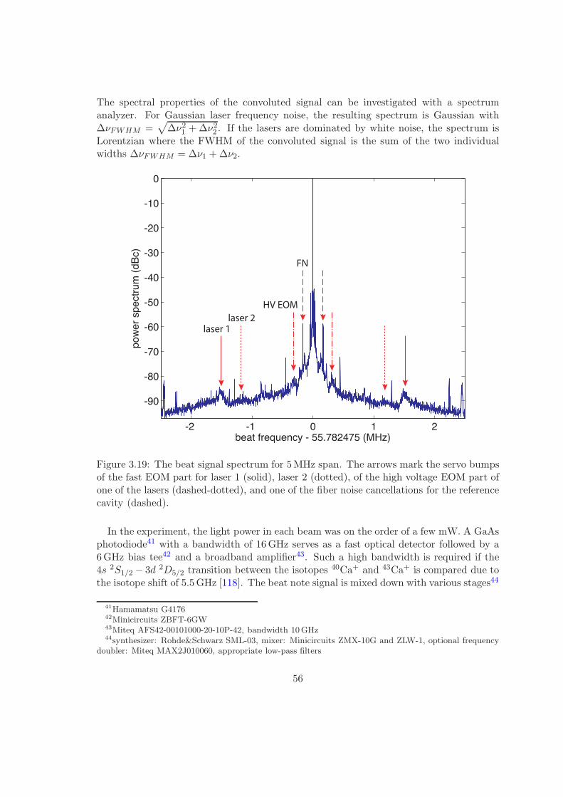
The spectral properties of the convoluted signal can be investigated with a spectrumanalyzer. For Gaussian laser frequency noise, the resulting spectrum is Gaussian with∆νFWHM =

√

∆ν21 + ∆ν2

2 . If the lasers are dominated by white noise, the spectrum isLorentzian where the FWHM of the convoluted signal is the sum of the two individualwidths ∆νFWHM = ∆ν1 + ∆ν2.

-2 -1 0 1 2

-90

-80

-70

-60

-50

-40

-30

-20

-10

0

beat frequency - 55.782475 (MHz)

pow

er

spectr

um

(dB

c)

laser 1laser 2

FN

HV EOM

Figure 3.19: The beat signal spectrum for 5 MHz span. The arrows mark the servo bumpsof the fast EOM part for laser 1 (solid), laser 2 (dotted), of the high voltage EOM part ofone of the lasers (dashed-dotted), and one of the fiber noise cancellations for the referencecavity (dashed).

In the experiment, the light power in each beam was on the order of a few mW. A GaAsphotodiode41 with a bandwidth of 16 GHz serves as a fast optical detector followed by a6 GHz bias tee42 and a broadband amplifier43. Such a high bandwidth is required if the4s 2S1/2 − 3d 2D5/2 transition between the isotopes 40Ca+ and 43Ca+ is compared due tothe isotope shift of 5.5 GHz [118]. The beat note signal is mixed down with various stages44

41Hamamatsu G417642Minicircuits ZBFT-6GW43Miteq AFS42-00101000-20-10P-42, bandwidth 10GHz44synthesizer: Rohde&Schwarz SML-03, mixer: Minicircuits ZMX-10G and ZLW-1, optional frequency

doubler: Miteq MAX2J010060, appropriate low-pass filters

56

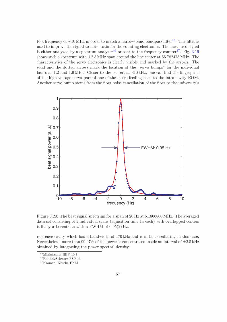
to a frequency of ∼10MHz in order to match a narrow-band bandpass filter45. The filter isused to improve the signal-to-noise ratio for the counting electronics. The measured signalis either analyzed by a spectrum analyzer46 or sent to the frequency counter47. Fig. 3.19shows such a spectrum with ±2.5 MHz span around the line center at 55.782475 MHz. Thecharacteristics of the servo electronics is clearly visible and marked by the arrows. Thesolid and the dotted arrows mark the location of the ”servo bumps” for the individuallasers at 1.2 and 1.6 MHz. Closer to the center, at 310 kHz, one can find the fingerprintof the high voltage servo part of one of the lasers feeding back to the intra-cavity EOM.Another servo bump stems from the fiber noise cancellation of the fiber to the university’s

-10 -8 -6 -4 -2 0 2 4 6 8 100

0.1

0.2

0.3

0.4

0.5

0.6

0.7

0.8

0.9

1

frequency (Hz)

beat sig

nal pow

er

(a. u.)

FWHM: 0.95 Hz

Figure 3.20: The beat signal spectrum for a span of 20 Hz at 51.806800 MHz. The averageddata set consisting of 5 individual scans (aquisition time 1 s each) with overlapped centersis fit by a Lorentzian with a FWHM of 0.95(2) Hz.

reference cavity which has a bandwidth of 170 kHz and is in fact oscillating in this case.Nevertheless, more than 99.97% of the power is concentrated inside an interval of ±2.5 kHzobtained by integrating the power spectral density.

45Minicircuits BBP-10.746Rohde&Schwarz FSP-1347Kramer+Klische FXM

57

In order to measure the linewidth of the lasers, both of them were referenced to a40Ca+ ion to cancel slow drifts. The beat signal was analyzed on the spectrum analyzerwith an integration time of 4 s to achieve a resolution bandwidth of 1Hz. For Fig. 3.20 fivescans were combined by overlapping the individual centers and taking the average. Thedata (dots) is fitted by a Lorentzian with a FWHM of ∆νFWHM =0.95(2) Hz. Neglectingthe contribution of the spectrum analyzer, an individual linewidth of ∆νFWHM/2 can beattributed to each laser, if both contribute equally to the signal. Please note, that thismeasurement represents a collection of the best shots.

0 1000 2000 3000 4000 5000 6000 7000 8000-100

-50

0

50

100

beat fr

equency

- 28962046 (

Hz)

time (s)

100

101

102

103

104

10-15

10-14

10-13

σy(τ

)

τ (s)

Figure 3.21: Beat signal analysis. The upper graph shows the frequency of the optical beatsignal measured with an RF counter for more than two hours. The lower graph representsthe Allan standard deviation for this data set.

On the time scale of less than a second, the linewidth is typically limited by the spectrumanalyzer’s bandwidth. For durations of a few seconds, the linewidth is most of the timeclose to 10-20 Hz and on the order of 50 Hz FWHM when observed over the course ofmore than two hours. The frequency counter results for a measurement with a similarsetup as described above at IQOQI [81] are shown in Fig. 3.21 in the upper graph. TheAllan deviation [119] in the lower graph has a pedestal at a few 10−14 before decreasingwith τ−1/2. This indicates that after 120 s, the lock of the lasers to the atomic transitioncomes into effect and is able to dominate frequency jitter most likely caused by seismicnoise of the reference cavities. The solid line is a fit with σy(τ) = 1.8(2) × 10−13τ−1/2.

58

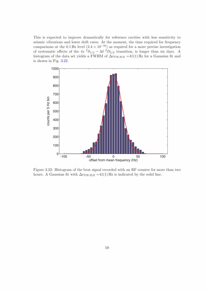
This is expected to improve dramatically for reference cavities with less sensitivity toseismic vibrations and lower drift rates. At the moment, the time required for frequencycomparisons at the 0.1 Hz level (2.4 × 10−16) as required for a more precise investigationof systematic effects of the 4s 2S1/2 − 3d 2D5/2 transition, is longer than six days. Ahistogram of the data set yields a FWHM of ∆νFWHM =41(1) Hz for a Gaussian fit andis shown in Fig. 3.22.

-100 -50 0 50 1000

100

200

300

400

500

600

700

800

900

1000

offset from mean frequency (Hz)

counts

per

5 H

z b

in

Figure 3.22: Histogram of the beat signal recorded with an RF counter for more than twohours. A Gaussian fit with ∆νFWHM =41(1) Hz is indicated by the solid line.

59

60

Chapter 4

The frequency comb

The development of self-referenced frequency combs in 1999 [120, 121] opened a new era inoptical metrology and ultra-fast physics. It allows for a direct link of optical frequency andmicrowave standards [14, 22, 122, 123] as well as for the production of ultra-short, phasestable light pulses of a few cycles [124–127] of the electric field. This opens up a new field inthe direction of optical waveform synthesis [128] and investigation of ultra-fast processeslike in semiconductor physics [129]. Frequency combs can be also used for wavelengthcalibration of astronomical spectrographs [130]. On the frequency metrology side, themost striking feature is the simplicity of the system as compared to the complicated andunreliable frequency chains [131] previously used for absolute frequency measurements.Instead of trying to keep many different oscillators and phase-locked loops (PLL) undercontrol, it suffices to stabilize the fs oscillator with two PLL’s which stands for a majorsimplification of optical frequency metrology.

This chapter contains a short review of the operation principle of frequency combs, adetailed description of the setup and the stabilization scheme, and the tools for a mea-surement of an optical frequency.

4.1 Principle of operation

The workhorse for the optical frequency metrology are mode-locked laser which emit atrain of ultra-short pulses. Upon first glance, it seems rather counter-intuitive that apulsed laser can be used to measure the frequency of a continuous wave laser. But acloser look at the spectrum reveals that a pulse is formed as a coherent superposition ofnumerous, equally spaced optical frequencies. The pulses emitted by a mode-locked laser,which are separated in time by one cavity round-trip time trt, are illustrated in Fig. 4.1.As a consequence, the Fourier spectrum consists of a series of delta functions in frequencywith each spectral component separated by frep ≡= 1/trt = c

L , with the speed of light cand the length of the cavity L.

Modelocking of the laser spectrum, which is required for the formation of an ultra-shortlight pulse, is forcing each longitudinal mode fn = n frep of the laser cavity to have acommon phase relationship. This carrier-envelope phase φCE defines the phase of the

61

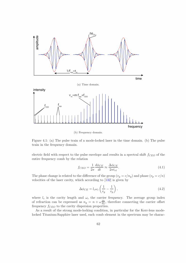
time

amplitude

1/frep

=trt

∆φCE

(a) Time domain.

frequency

intensity

frepf

CEO

νm

=m frep

+fCEO

(b) Frequency domain.

Figure 4.1: (a) The pulse train of a mode-locked laser in the time domain. (b) The pulsetrain in the frequency domain.

electric field with respect to the pulse envelope and results in a spectral shift fCEO of theentire frequency comb by the relation

fCEO =1

2π

dφCE

dt≈ ∆φCE

2πtrt. (4.1)

The phase change is related to the difference of the group (vg = c/ng) and phase (vp = c/n)velocities of the laser cavity, which according to [132] is given by

∆φCE = lcωc

(

1

vg− 1

vp

)

, (4.2)

where lc is the cavity length and ωc the carrier frequency. The average group indexof refraction can be expressed as ng = n + ω dn

dω , therefore connecting the carrier offsetfrequency fCEO to the cavity dispersion properties.

As a result of the strong mode-locking condition, in particular for the Kerr-lens mode-locked Titanium:Sapphire laser used, each comb element in the spectrum may be charac-

62

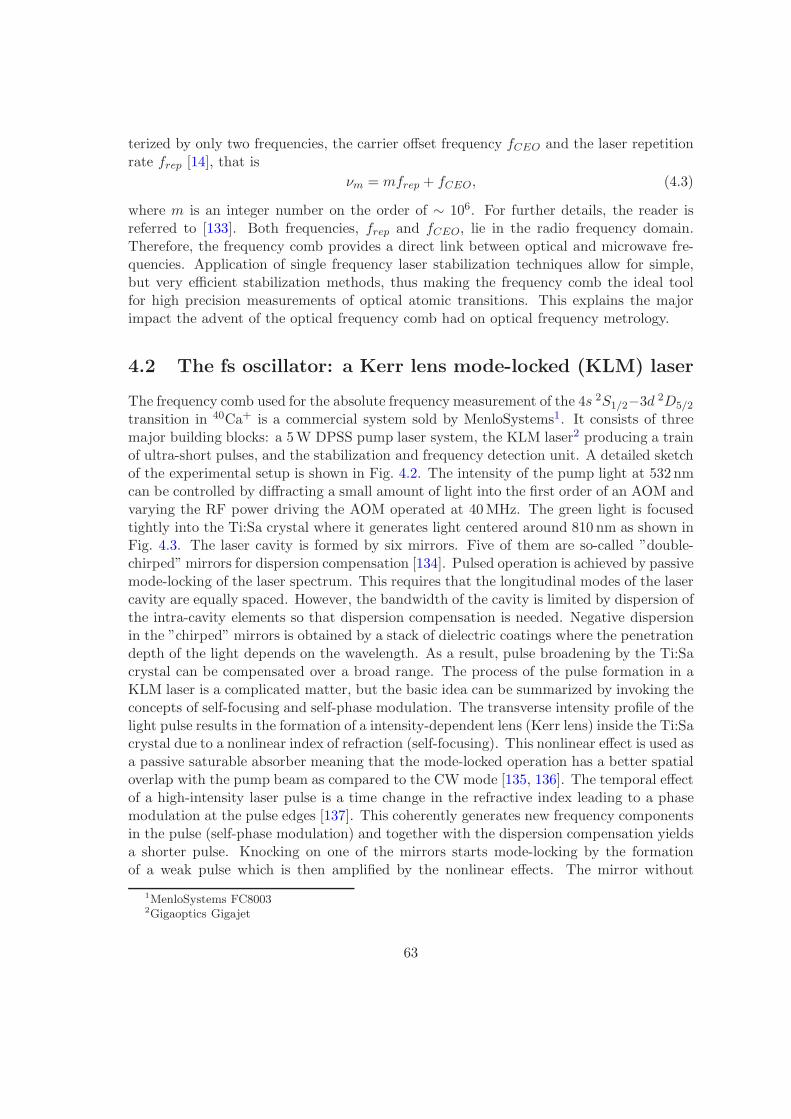
terized by only two frequencies, the carrier offset frequency fCEO and the laser repetitionrate frep [14], that is

νm = mfrep + fCEO, (4.3)

where m is an integer number on the order of ∼ 106. For further details, the reader isreferred to [133]. Both frequencies, frep and fCEO, lie in the radio frequency domain.Therefore, the frequency comb provides a direct link between optical and microwave fre-quencies. Application of single frequency laser stabilization techniques allow for simple,but very efficient stabilization methods, thus making the frequency comb the ideal toolfor high precision measurements of optical atomic transitions. This explains the majorimpact the advent of the optical frequency comb had on optical frequency metrology.

4.2 The fs oscillator: a Kerr lens mode-locked (KLM) laser

The frequency comb used for the absolute frequency measurement of the 4s 2S1/2−3d 2D5/2

transition in 40Ca+ is a commercial system sold by MenloSystems1. It consists of threemajor building blocks: a 5 W DPSS pump laser system, the KLM laser2 producing a trainof ultra-short pulses, and the stabilization and frequency detection unit. A detailed sketchof the experimental setup is shown in Fig. 4.2. The intensity of the pump light at 532 nmcan be controlled by diffracting a small amount of light into the first order of an AOM andvarying the RF power driving the AOM operated at 40 MHz. The green light is focusedtightly into the Ti:Sa crystal where it generates light centered around 810 nm as shown inFig. 4.3. The laser cavity is formed by six mirrors. Five of them are so-called ”double-chirped” mirrors for dispersion compensation [134]. Pulsed operation is achieved by passivemode-locking of the laser spectrum. This requires that the longitudinal modes of the lasercavity are equally spaced. However, the bandwidth of the cavity is limited by dispersion ofthe intra-cavity elements so that dispersion compensation is needed. Negative dispersionin the ”chirped” mirrors is obtained by a stack of dielectric coatings where the penetrationdepth of the light depends on the wavelength. As a result, pulse broadening by the Ti:Sacrystal can be compensated over a broad range. The process of the pulse formation in aKLM laser is a complicated matter, but the basic idea can be summarized by invoking theconcepts of self-focusing and self-phase modulation. The transverse intensity profile of thelight pulse results in the formation of a intensity-dependent lens (Kerr lens) inside the Ti:Sacrystal due to a nonlinear index of refraction (self-focusing). This nonlinear effect is used asa passive saturable absorber meaning that the mode-locked operation has a better spatialoverlap with the pump beam as compared to the CW mode [135, 136]. The temporal effectof a high-intensity laser pulse is a time change in the refractive index leading to a phasemodulation at the pulse edges [137]. This coherently generates new frequency componentsin the pulse (self-phase modulation) and together with the dispersion compensation yieldsa shorter pulse. Knocking on one of the mirrors starts mode-locking by the formationof a weak pulse which is then amplified by the nonlinear effects. The mirror without

1MenloSystems FC80032Gigaoptics Gigajet

63

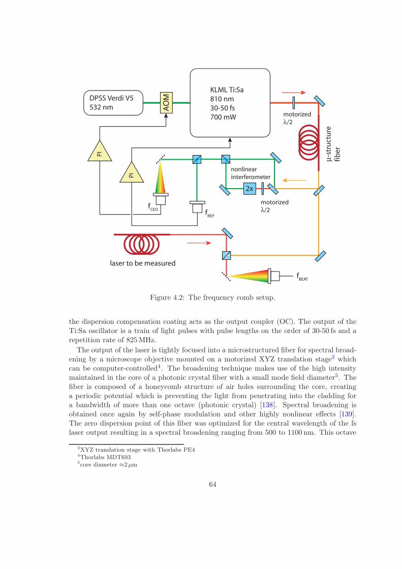
DPSS Verdi V5532 nm A

OM

KLML Ti:Sa810 nm30-50 fs700 mW

2x

µ-s

tru

ctu

refi

be

r

laser to be measured

fBEAT

PI

fCEO

fREP

PI

motorizedλ/2

motorizedλ/2

nonlinearinterferometer

Figure 4.2: The frequency comb setup.

the dispersion compensation coating acts as the output coupler (OC). The output of theTi:Sa oscillator is a train of light pulses with pulse lengths on the order of 30-50 fs and arepetition rate of 825 MHz.

The output of the laser is tightly focused into a microstructured fiber for spectral broad-ening by a microscope objective mounted on a motorized XYZ translation stage3 whichcan be computer-controlled4. The broadening technique makes use of the high intensitymaintained in the core of a photonic crystal fiber with a small mode field diameter5. Thefiber is composed of a honeycomb structure of air holes surrounding the core, creatinga periodic potential which is preventing the light from penetrating into the cladding fora bandwidth of more than one octave (photonic crystal) [138]. Spectral broadening isobtained once again by self-phase modulation and other highly nonlinear effects [139].The zero dispersion point of this fiber was optimized for the central wavelength of the fslaser output resulting in a spectral broadening ranging from 500 to 1100 nm. This octave

3XYZ translation stage with Thorlabs PE44Thorlabs MDT6935core diameter ≈2µm

64

beam dump

pump input

output810 nm30-50 fs

mirror with PZT

motorized wedge

crystalholder

cooling water in/out

Ti:Sa crystal

OC

Figure 4.3: The femto-second laser.

spanning frequency comb allows for self-referencing of the offset frequency fCEO as will beexplained in the next section. Geometrical imperfections of the fiber during its productionprocess lead to a preferred polarization direction for optimal broadening. The 20 cm fiberpiece is glued into a holder, which makes it susceptible to changes of its birefringence in-duced by thermal stress. The slow degradation of the efficiency due to polarization driftscan be compensated by a motorized half-wave plate at the fiber input.

At the output of the microstructure fiber the light is split into two parts by a dichroicmirror. The ”red” part ranging from 650 to 850 nm is used for the absolute frequencydetection with external lasers, while the infrared and green light enters the nonlinearinterferometer for the fCEO and frep detection and stabilization. The beat note signalsfor fCEO and with the external lasers are detected by avalanche photodetectors6, therepetition rate detection uses a fast Ga:As photodiode7 on a bias tee8 followed by an20 dB amplifier9. For better signal-to-noise of the weak beat signals the correspondingbeams are spectrally separated by diffraction gratings with 1200 gr/mm. Details of thestabilization schemes and the optical beat note detection are presented in the followingsections.

6MenloSystems APD2107Hamamatsu G41768Minicircuits SFBT-4R2GW-FT9Minicircuits ZEL-0812LN

65

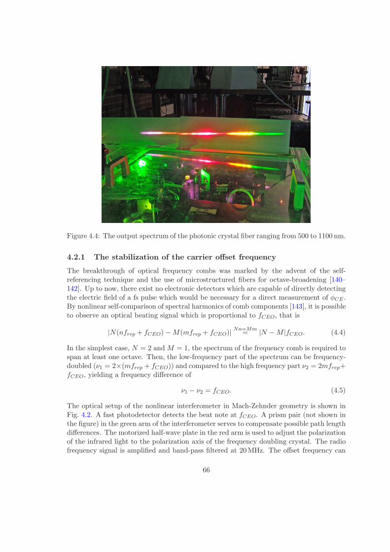
Figure 4.4: The output spectrum of the photonic crystal fiber ranging from 500 to 1100 nm.

4.2.1 The stabilization of the carrier offset frequency

The breakthrough of optical frequency combs was marked by the advent of the self-referencing technique and the use of microstructured fibers for octave-broadening [140–142]. Up to now, there exist no electronic detectors which are capable of directly detectingthe electric field of a fs pulse which would be necessary for a direct measurement of φCE.By nonlinear self-comparison of spectral harmonics of comb components [143], it is possibleto observe an optical beating signal which is proportional to fCEO, that is

|N(nfrep + fCEO)−M(mfrep + fCEO)| Nn=Mm= |N −M |fCEO. (4.4)

In the simplest case, N = 2 and M = 1, the spectrum of the frequency comb is required tospan at least one octave. Then, the low-frequency part of the spectrum can be frequency-doubled (ν1 = 2×(mfrep + fCEO)) and compared to the high frequency part ν2 = 2mfrep+fCEO, yielding a frequency difference of

ν1 − ν2 = fCEO. (4.5)

The optical setup of the nonlinear interferometer in Mach-Zehnder geometry is shown inFig. 4.2. A fast photodetector detects the beat note at fCEO. A prism pair (not shown inthe figure) in the green arm of the interferometer serves to compensate possible path lengthdifferences. The motorized half-wave plate in the red arm is used to adjust the polarizationof the infrared light to the polarization axis of the frequency doubling crystal. The radiofrequency signal is amplified and band-pass filtered at 20 MHz. The offset frequency can

66

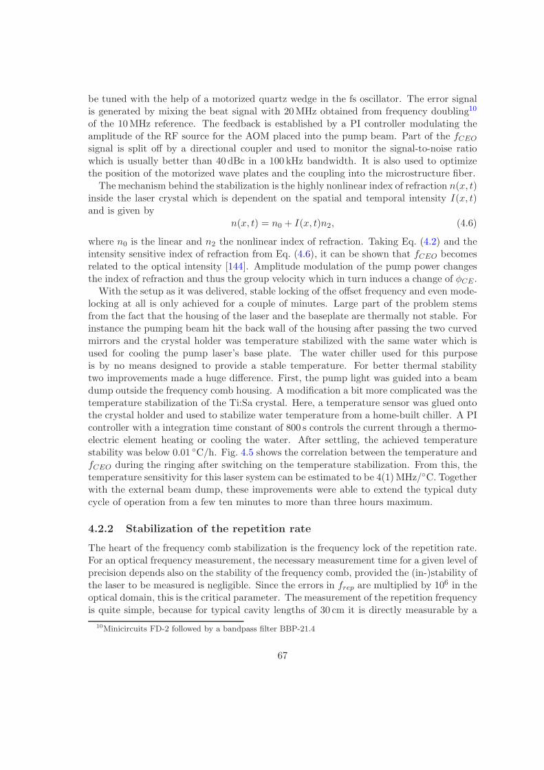
be tuned with the help of a motorized quartz wedge in the fs oscillator. The error signalis generated by mixing the beat signal with 20 MHz obtained from frequency doubling10

of the 10 MHz reference. The feedback is established by a PI controller modulating theamplitude of the RF source for the AOM placed into the pump beam. Part of the fCEO

signal is split off by a directional coupler and used to monitor the signal-to-noise ratiowhich is usually better than 40 dBc in a 100 kHz bandwidth. It is also used to optimizethe position of the motorized wave plates and the coupling into the microstructure fiber.

The mechanism behind the stabilization is the highly nonlinear index of refraction n(x, t)inside the laser crystal which is dependent on the spatial and temporal intensity I(x, t)and is given by

n(x, t) = n0 + I(x, t)n2, (4.6)

where n0 is the linear and n2 the nonlinear index of refraction. Taking Eq. (4.2) and theintensity sensitive index of refraction from Eq. (4.6), it can be shown that fCEO becomesrelated to the optical intensity [144]. Amplitude modulation of the pump power changesthe index of refraction and thus the group velocity which in turn induces a change of φCE .

With the setup as it was delivered, stable locking of the offset frequency and even mode-locking at all is only achieved for a couple of minutes. Large part of the problem stemsfrom the fact that the housing of the laser and the baseplate are thermally not stable. Forinstance the pumping beam hit the back wall of the housing after passing the two curvedmirrors and the crystal holder was temperature stabilized with the same water which isused for cooling the pump laser’s base plate. The water chiller used for this purposeis by no means designed to provide a stable temperature. For better thermal stabilitytwo improvements made a huge difference. First, the pump light was guided into a beamdump outside the frequency comb housing. A modification a bit more complicated was thetemperature stabilization of the Ti:Sa crystal. Here, a temperature sensor was glued ontothe crystal holder and used to stabilize water temperature from a home-built chiller. A PIcontroller with a integration time constant of 800 s controls the current through a thermo-electric element heating or cooling the water. After settling, the achieved temperaturestability was below 0.01 C/h. Fig. 4.5 shows the correlation between the temperature andfCEO during the ringing after switching on the temperature stabilization. From this, thetemperature sensitivity for this laser system can be estimated to be 4(1) MHz/C. Togetherwith the external beam dump, these improvements were able to extend the typical dutycycle of operation from a few ten minutes to more than three hours maximum.

4.2.2 Stabilization of the repetition rate

The heart of the frequency comb stabilization is the frequency lock of the repetition rate.For an optical frequency measurement, the necessary measurement time for a given level ofprecision depends also on the stability of the frequency comb, provided the (in-)stability ofthe laser to be measured is negligible. Since the errors in frep are multiplied by 106 in theoptical domain, this is the critical parameter. The measurement of the repetition frequencyis quite simple, because for typical cavity lengths of 30 cm it is directly measurable by a

10Minicircuits FD-2 followed by a bandpass filter BBP-21.4

67

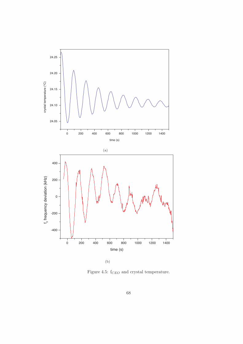
0 200 400 600 800 1000 1200 1400

24.05

24.10

24.15

24.20

24.25

cry

sta

l te

mp

era

ture

(°C

)

time (s)

(a)

0 200 400 600 800 1000 1200 1400

-400

-200

0

200

400

f 0 f

requen

cy d

evia

tio

n (

kH

z)

time (s)

(b)

Figure 4.5: fCEO and crystal temperature.

68

10 MHz

100 MHz 2x BP 15dB 2x BP 15dB 2x BP 15dB 800 MHz

800 MHz4x 4x 5x

Method 1:

Method 2:

Figure 4.6: The frequency reference for the repetition rate stabilization.

fast photodiode. Neighboring modes produce a strong heterodyne signal when shining partof the comb light onto a detector with excellent signal-to-noise as many modes contributeto the signal. The stabilization scheme is similar to the one used for fCEO. The RFsignal is amplified and compared with a synthesized frequency reference. The error signalis shaped by a loop filter and corrections of frep are applied to one of the laser cavitymirrors mounted on a PZT to stabilize the cavity length. Thereby, the repetition rate isphase-locked to the reference.

During the absolute frequency measurement of 40Ca+ the frequency comb was locked toa transportable Cs atomic fountain clock. The clock had two outputs with 10 and 100 MHzderived from an ultra-stable quartz crystal with an amazing short term stability of 8×10−14

in 1 s. This offered two possibilities to generate a frequency reference at 800 MHz for thestabilization of frep. A schematic diagram of the two methods is displayed in Fig. 4.6. Thefirst method uses the 10 MHz signal isolated from other ports by a distribution amplifier11.The multiplication chain consists of two low noise frequency quadruplers12 and a low noiseodd-order multiplier13 with internal amplifiers. For the second method, simple frequencydoublers14, bandpass filters made of lowpass and highpass filters15 and amplifiers16 werecombined to generate the 800 MHz from the 100 MHz reference. The photodiode signalat 825 MHz was mixed17 with the reference to produce an intermediate signal at 25 MHzwhich was compared to the signal from a tunable synthesizer18 with a second mixer19 tofinally generate the error signal. In case of method 2, the intermediate frequency was firstmixed with the 10 MHz reference before mixing it with the synthesizer signal.

Fig. 4.7 presents a comparison of the two different methods to generate a frequencyreference for the frep stabilization. The signals are optical beat notes at 35 MHz of thefrequency comb with a laser stabilized to a 40Ca+ ion. Details of how these signals areobtained are discussed in the next section. For the moment, the important thing to noticeis that the two methods have significantly different widths, for method 1(dark blue) the

11TimeTech 1027412Wenzel Assoc. LNHQ13Wenzel Assoc. LNOM-514Minicircuits FD-215Minicircuits BLP and BHP16Minicircuits ZFL-500HLN and ZFL-1000LN17Minicircuits ZEM-2B18SRS DS34519Minicircuits ZAD-1

69

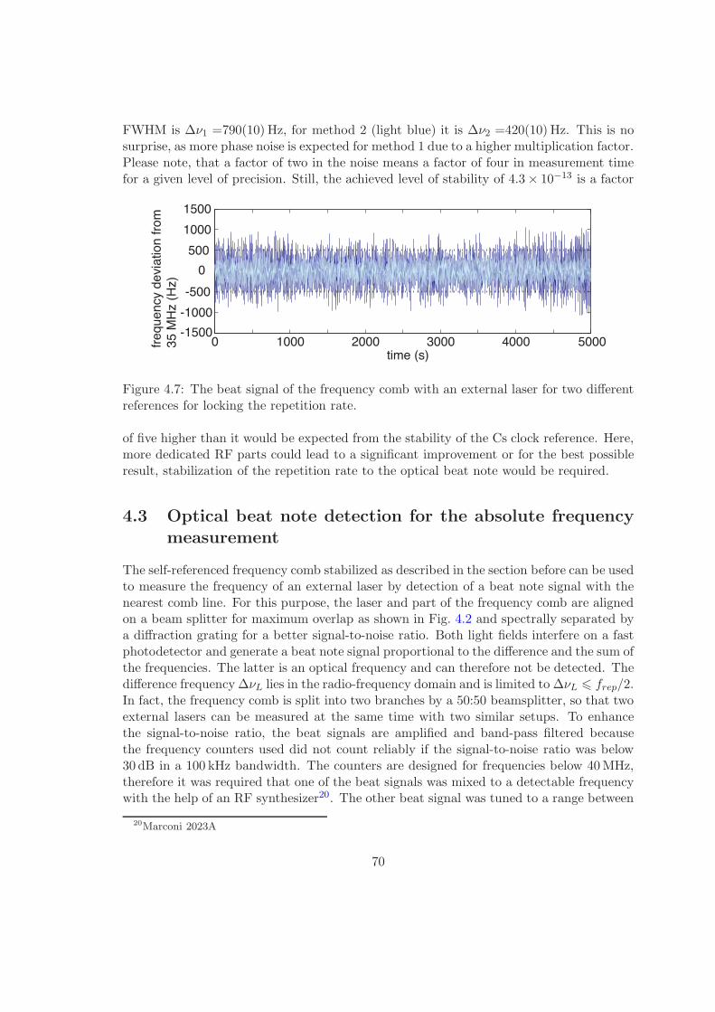
FWHM is ∆ν1 =790(10) Hz, for method 2 (light blue) it is ∆ν2 =420(10) Hz. This is nosurprise, as more phase noise is expected for method 1 due to a higher multiplication factor.Please note, that a factor of two in the noise means a factor of four in measurement timefor a given level of precision. Still, the achieved level of stability of 4.3× 10−13 is a factor

0 1000 2000 3000 4000 5000-1500

-1000

-500

0

500

1000

1500

time (s)

fre

qu

en

cy d

evia

tio

n f

rom

35

MH

z (

Hz)

Figure 4.7: The beat signal of the frequency comb with an external laser for two differentreferences for locking the repetition rate.

of five higher than it would be expected from the stability of the Cs clock reference. Here,more dedicated RF parts could lead to a significant improvement or for the best possibleresult, stabilization of the repetition rate to the optical beat note would be required.

4.3 Optical beat note detection for the absolute frequencymeasurement

The self-referenced frequency comb stabilized as described in the section before can be usedto measure the frequency of an external laser by detection of a beat note signal with thenearest comb line. For this purpose, the laser and part of the frequency comb are alignedon a beam splitter for maximum overlap as shown in Fig. 4.2 and spectrally separated bya diffraction grating for a better signal-to-noise ratio. Both light fields interfere on a fastphotodetector and generate a beat note signal proportional to the difference and the sum ofthe frequencies. The latter is an optical frequency and can therefore not be detected. Thedifference frequency ∆νL lies in the radio-frequency domain and is limited to ∆νL 6 frep/2.In fact, the frequency comb is split into two branches by a 50:50 beamsplitter, so that twoexternal lasers can be measured at the same time with two similar setups. To enhancethe signal-to-noise ratio, the beat signals are amplified and band-pass filtered becausethe frequency counters used did not count reliably if the signal-to-noise ratio was below30 dB in a 100 kHz bandwidth. The counters are designed for frequencies below 40 MHz,therefore it was required that one of the beat signals was mixed to a detectable frequencywith the help of an RF synthesizer20. The other beat signal was tuned to a range between

20Marconi 2023A

70

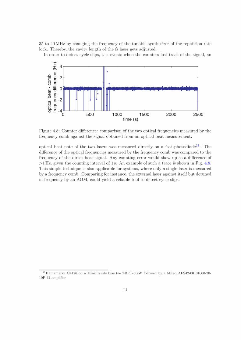
35 to 40 MHz by changing the frequency of the tunable synthesizer of the repetition ratelock. Thereby, the cavity length of the fs laser gets adjusted.

In order to detect cycle slips, i. e. events when the counters lost track of the signal, an

0 500 1000 1500 2000 2500-4

-2

0

2

4

time (s)

op

tica

l b

ea

t -

co

mb

fre

qu

en

cy d

iffe

ren

ce

(H

z)

Figure 4.8: Counter difference: comparison of the two optical frequencies measured by thefrequency comb against the signal obtained from an optical beat measurement.

optical beat note of the two lasers was measured directly on a fast photodiode21. Thedifference of the optical frequencies measured by the frequency comb was compared to thefrequency of the direct beat signal. Any counting error would show up as a difference of>1Hz, given the counting interval of 1 s. An example of such a trace is shown in Fig. 4.8.This simple technique is also applicable for systems, where only a single laser is measuredby a frequency comb. Comparing for instance, the external laser against itself but detunedin frequency by an AOM, could yield a reliable tool to detect cycle slips.

21Hamamatsu G4176 on a Minicircuits bias tee ZBFT-6GW followed by a Miteq AFS42-00101000-20-10P-42 amplifier

71

72

Chapter 5

Experimental prerequisites andtechniques

In this chapter a few experimental techniques and requirements are described which arenecessary for the absolute frequency measurement of the 4s 2S1/2− 3d 2D5/2 transition in40Ca+ and for the measurement of the electric quadrupole moment of the 3d 2D5/2 level. Itcontains information about micromotion compensation, calibration of the magnetic field,an alternative method for optical pumping, and the prerequisites for Ramsey spectroscopylike frequency and phase control of the laser exciting the quadrupole transition, Ramseyexperiments with switched phase, and the stabilization of the laser to the ion.

5.1 Compensation of excess micromotion

Electric stray fields may exist which shift the ion from the zero-point of the RF field toa region where the ion motion is driven by the trapping field in contrast to unavoidablemicromotion caused by secular motion (see Eq. (2.8)). These fields can be generatedby localized surface charges (patch potentials) on the trap structure or by geometricalimperfections of the trap like misalignment of the DC end caps. As a result, enhancedmicromotion modulates the coupling strength of the ion to laser fields. The resulting first-order Doppler shift can significantly broaden the line of an atomic transition leading to anincreased cooling limit. The final temperature TD for Doppler cooling is determined by

the effective linewidth γeff of a transition (TD ≈ ~γeff

2kB). It is even possible that heating

occurs for a laser which is detuned near, but above a micromotion sideband [82]. Therefore,compensation of excess micromotion is an essential ingredient for efficient laser cooling andimportant for experiments with cold ions, for example experiments in quantum informationprocessing. From a high-accuracy spectroscopy point of view, excessive micromotion isresponsible for large AC Stark as well as for second-order Doppler shifts [82]. In our case,the compensation is achieved by applying voltages to additional electrodes placed in thevicinity of the trap as shown in Fig. 3.3 (b). Please note that a voltage applied to thevertical electrode shifts the ion vertically but affects the horizontal micromotion and vice

73

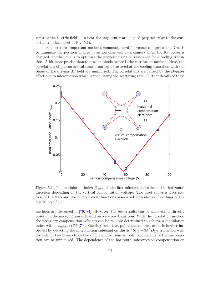
versa as the electric field lines near the trap center are aligned perpendicular to the axesof the trap (see inset of Fig. 5.1).

There exist three important methods commonly used for coarse compensation. One isto minimize the position change of an ion observed by a camera when the RF power ischanged, another one is to optimize the scattering rate on resonance for a cooling transi-tion. A bit more precise than the two methods before is the correlation method. Here, thecorrelations of photon arrival times from light scattered at the cooling transition with thephase of the driving RF field are minimized. The correlations are caused by the Dopplereffect due to micromotion which is modulating the scattering rate. Further details of these

0 20 40 60 80 1000

0.05

0.1

0.15

0.2

0.25

vertical compensation voltage (V)

horizonta

l m

odula

tion index β

mic

ro

+

+

-

-

vertical compensationelectrode

horizontalcompensationelectrodes

Figure 5.1: The modulation index βmicro of the first micromotion sideband in horizontaldirection depending on the vertical compensation voltage. The inset shows a cross sec-tion of the trap and the micromotion directions associated with electric field lines of thequadrupole field.

methods are discussed in [79, 84]. However, the best results can be achieved by directlyobserving the micromotion sideband on a narrow transition. With the correlation methodthe necessary compensation voltages can be reliably determined to achieve a modulationindex within βmicro ≈1% [79]. Starting from that point, the compensation is further im-proved by detecting the micromotion sideband on the 4s 2S1/2− 3d 2D5/2 transition withthe help of two beams from two different directions so both components of the micromo-tion can be minimized. The dependence of the horizontal micromotion compensation on

74

the applied voltage with respect to the vertical electrode is shown in Fig. 5.1. For thismeasurement the Rabi frequency on the micromotion sideband was measured at differentcompensation voltages and compared to the value on the carrier. In the case of optimalcompensation we can achieve a modulation index as low as βmicro =0.004(1), but the de-termination of the Rabi frequency becomes more and more difficult. The decoherence dueto fluctuations of the magnetic field and the laser frequency limits the contrast of the Rabiflops after a few milliseconds. Experience shows that with the photoionization techniqueto create ions in the trap we do have to check the micromotion compensation every fewmonths only and the applied voltage corrections are usually a few volts. Therefore, theuncertainty of the micromotion modulation index for the absolute frequency measurementof the 4s 2S1/2 − 3d 2D5/2 transition can conservatively be assumed to be well below∆βmicro < 0.1.

5.2 Frequency resolved optical pumping using the laser at729 nm

For most of the experiments in quantum information processing or for spectroscopy withour setup it is necessary to initialize the ion(s) in a well defined electronic state. Some-times there is even need for a defined state of the motional degrees of freedom for whichnormal Doppler cooling is not sufficient (e. g. Bell state creation). Optical pumping withσ−polarized light at 397 nm along the quantization axis is used to initialize the electronicstate of the ion into

∣

∣S1/2,mS = −1/2⟩

. Given the geometry and the optical access ofour trap, this is a simple and efficient solution as the state population ends up in theright state with an efficiency of better than 99% after 60µs of pumping with σ− light.Unfortunately, the particular method of optical pumping leads to restrictions related tothe freedom of choosing the orientation for the quantization axis. It would be very incon-venient and sometimes even impossible to realign the σ beam path each time the angleof the magnetic field is changed which was necessary for the measurement of the electricquadrupole moment described in chapter 7.

Therefore, we investigated whether initialization of the ion in a particular Zeemanground state can be achieved using the laser at 729 nm. Instead of relying on selectionrules related to the polarization of the laser exciting the broad S1/2−P1/2 transition, wecan make use of the frequency-selective pumping on the narrow quadrupole transition.The main advantages are:

• The pumping should be insensitive against imperfect polarization.

• The optical pumping beam does not need to be aligned with the B-field defining thequantization axis.

For testing the optical pumping, we first prepared the ion in themS=-1/2 state by standardoptical pumping using a beam of σ− polarized light at 397 nm (dashed lines in Fig. 5.2).Then, we switched on the laser at 729 nm with a Rabi frequency of Ω/(2π) =18(1) kHzresonant with the mS=-1/2 to mD=+1/2 transition as well as the resetting laser at 854 nm

75

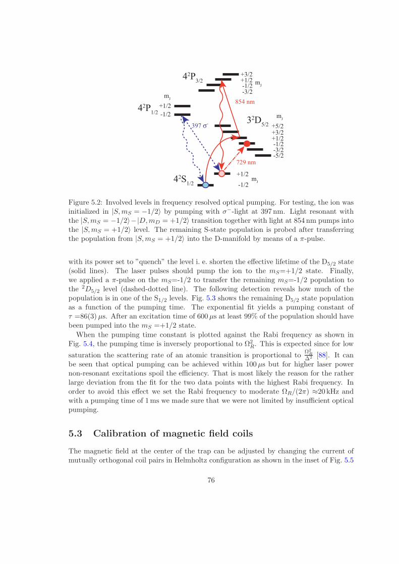
42P3/2

42P1/2

42S1/2

32D5/2397 σ-

729 nm

854 nm

+5/2+3/2+1/2-1/2-3/2-5/2

+1/2

-1/2

mJ

mJ

+3/2+1/2-1/2-3/2

mJ

+1/2

-1/2

mJ

Figure 5.2: Involved levels in frequency resolved optical pumping. For testing, the ion wasinitialized in |S,mS = −1/2〉 by pumping with σ−-light at 397 nm. Light resonant withthe |S,mS = −1/2〉−|D,mD = +1/2〉 transition together with light at 854 nm pumps intothe |S,mS = +1/2〉 level. The remaining S-state population is probed after transferringthe population from |S,mS = +1/2〉 into the D-manifold by means of a π-pulse.

with its power set to ”quench” the level i. e. shorten the effective lifetime of the D5/2 state(solid lines). The laser pulses should pump the ion to the mS=+1/2 state. Finally,we applied a π-pulse on the mS=-1/2 to transfer the remaining mS=-1/2 population tothe 2D5/2 level (dashed-dotted line). The following detection reveals how much of thepopulation is in one of the S1/2 levels. Fig. 5.3 shows the remaining D5/2 state populationas a function of the pumping time. The exponential fit yields a pumping constant ofτ =86(3) µs. After an excitation time of 600µs at least 99% of the population should havebeen pumped into the mS =+1/2 state.

When the pumping time constant is plotted against the Rabi frequency as shown inFig. 5.4, the pumping time is inversely proportional to Ω2

R. This is expected since for low

saturation the scattering rate of an atomic transition is proportional toΩ2

R∆2 [88]. It can

be seen that optical pumping can be achieved within 100µs but for higher laser powernon-resonant excitations spoil the efficiency. That is most likely the reason for the ratherlarge deviation from the fit for the two data points with the highest Rabi frequency. Inorder to avoid this effect we set the Rabi frequency to moderate ΩR/(2π) ≈20 kHz andwith a pumping time of 1 ms we made sure that we were not limited by insufficient opticalpumping.

5.3 Calibration of magnetic field coils

The magnetic field at the center of the trap can be adjusted by changing the current ofmutually orthogonal coil pairs in Helmholtz configuration as shown in the inset of Fig. 5.5

76

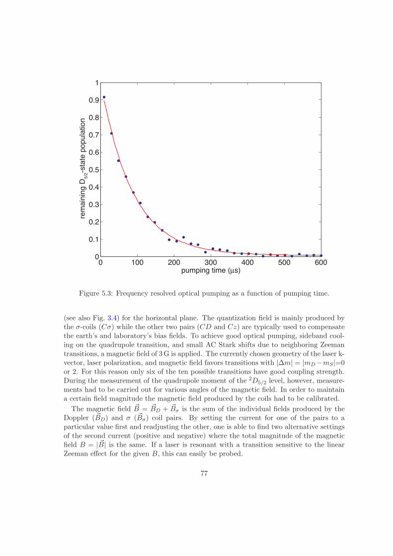
0 100 200 300 400 500 6000

0.1

0.2

0.3

0.4

0.5

0.6

0.7

0.8

0.9

1

pumping time (µs)

rema

inin

g D

5/2-s

tate

po

pula

tio

n

Figure 5.3: Frequency resolved optical pumping as a function of pumping time.

(see also Fig. 3.4) for the horizontal plane. The quantization field is mainly produced bythe σ-coils (Cσ) while the other two pairs (CD and Cz) are typically used to compensatethe earth’s and laboratory’s bias fields. To achieve good optical pumping, sideband cool-ing on the quadrupole transition, and small AC Stark shifts due to neighboring Zeemantransitions, a magnetic field of 3 G is applied. The currently chosen geometry of the laser k-vector, laser polarization, and magnetic field favors transitions with |∆m| = |mD−mS|=0or 2. For this reason only six of the ten possible transitions have good coupling strength.During the measurement of the quadrupole moment of the 2D5/2 level, however, measure-ments had to be carried out for various angles of the magnetic field. In order to maintaina certain field magnitude the magnetic field produced by the coils had to be calibrated.

The magnetic field ~B = ~BD + ~Bσ is the sum of the individual fields produced by theDoppler ( ~BD) and σ ( ~Bσ) coil pairs. By setting the current for one of the pairs to aparticular value first and readjusting the other, one is able to find two alternative settingsof the second current (positive and negative) where the total magnitude of the magneticfield B = | ~B| is the same. If a laser is resonant with a transition sensitive to the linearZeeman effect for the given B, this can easily be probed.

77

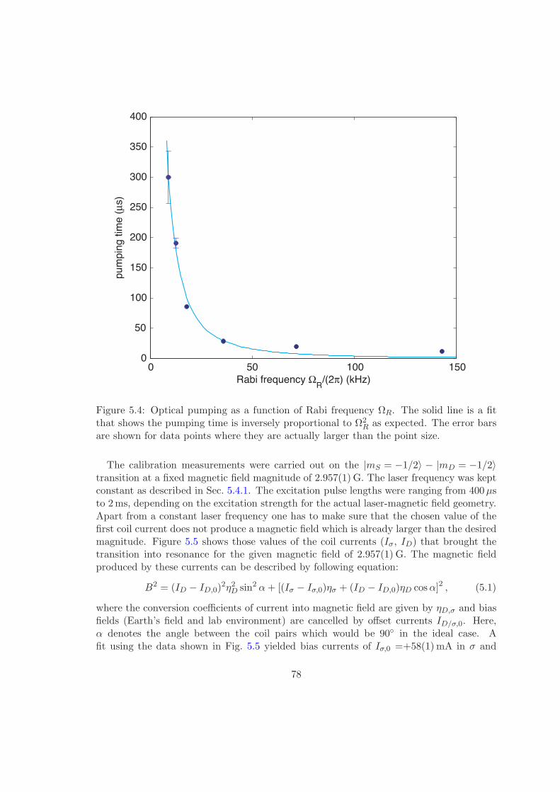
0 50 100 1500

50

100

150

200

250

300

350

400

Rabi frequency ΩR/(2π) (kHz)

pump

ing

tim

e (

µs)

Figure 5.4: Optical pumping as a function of Rabi frequency ΩR. The solid line is a fitthat shows the pumping time is inversely proportional to Ω2

R as expected. The error barsare shown for data points where they are actually larger than the point size.

The calibration measurements were carried out on the |mS = −1/2〉 − |mD = −1/2〉transition at a fixed magnetic field magnitude of 2.957(1) G. The laser frequency was keptconstant as described in Sec. 5.4.1. The excitation pulse lengths were ranging from 400µsto 2 ms, depending on the excitation strength for the actual laser-magnetic field geometry.Apart from a constant laser frequency one has to make sure that the chosen value of thefirst coil current does not produce a magnetic field which is already larger than the desiredmagnitude. Figure 5.5 shows those values of the coil currents (Iσ, ID) that brought thetransition into resonance for the given magnetic field of 2.957(1) G. The magnetic fieldproduced by these currents can be described by following equation:

B2 = (ID − ID,0)2η2

D sin2 α+ [(Iσ − Iσ,0)ησ + (ID − ID,0)ηD cosα]2 , (5.1)

where the conversion coefficients of current into magnetic field are given by ηD,σ and biasfields (Earth’s field and lab environment) are cancelled by offset currents ID/σ,0. Here,α denotes the angle between the coil pairs which would be 90 in the ideal case. Afit using the data shown in Fig. 5.5 yielded bias currents of Iσ,0 =+58(1) mA in σ and

78

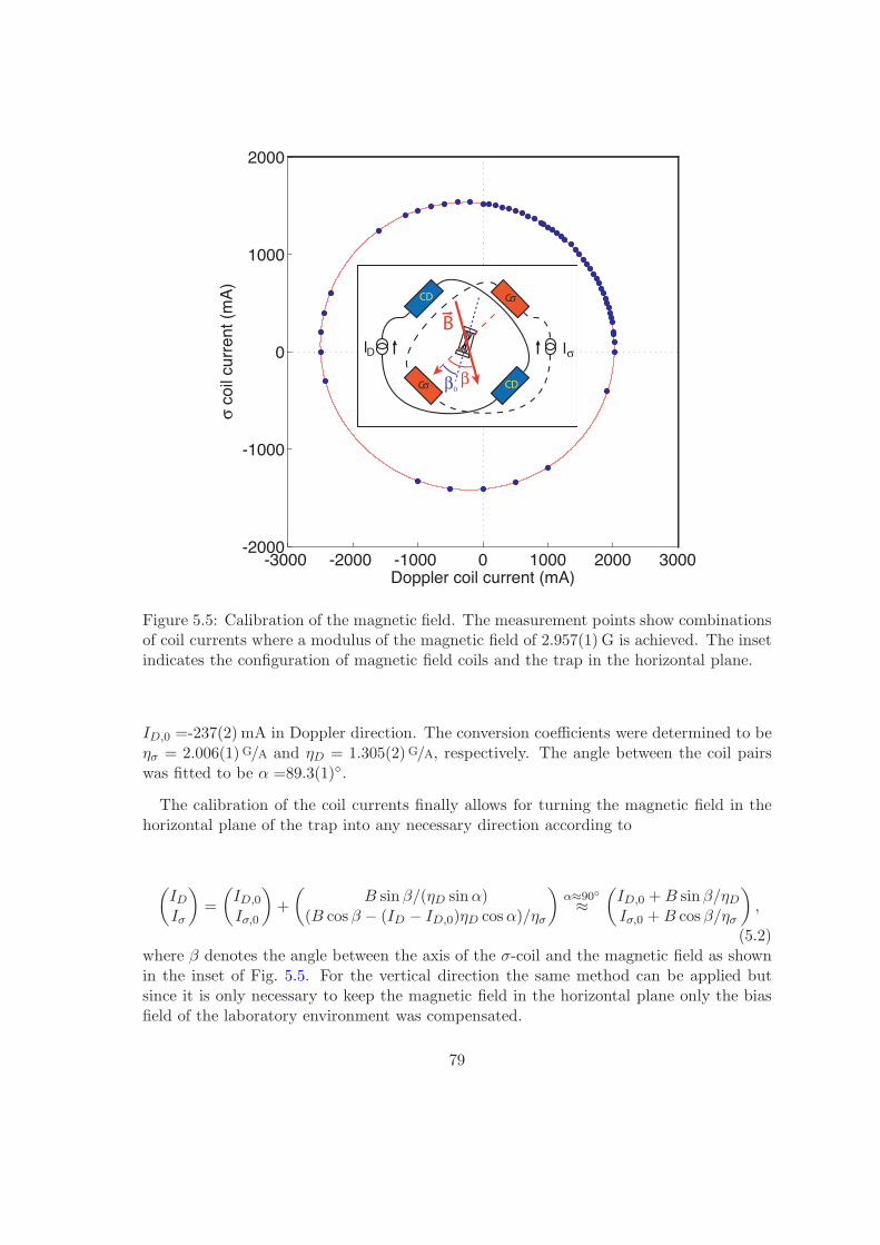
-3000 -2000 -1000 0 1000 2000 3000-2000

-1000

0

1000

2000

Doppler coil current (mA)

σ c

oil

cu

rre

nt

(mA

)

CD

CD Cσ

Cσ β0β

IσID

B

Cσ

Figure 5.5: Calibration of the magnetic field. The measurement points show combinationsof coil currents where a modulus of the magnetic field of 2.957(1) G is achieved. The insetindicates the configuration of magnetic field coils and the trap in the horizontal plane.

ID,0 =-237(2) mA in Doppler direction. The conversion coefficients were determined to beησ = 2.006(1) G/A and ηD = 1.305(2) G/A, respectively. The angle between the coil pairswas fitted to be α =89.3(1).

The calibration of the coil currents finally allows for turning the magnetic field in thehorizontal plane of the trap into any necessary direction according to

(

IDIσ

)

=

(

ID,0

Iσ,0

)

+

(

B sin β/(ηD sinα)(B cos β − (ID − ID,0)ηD cosα)/ησ

)

α≈90≈(

ID,0 +B sin β/ηD

Iσ,0 +B cos β/ησ

)

,

(5.2)where β denotes the angle between the axis of the σ-coil and the magnetic field as shownin the inset of Fig. 5.5. For the vertical direction the same method can be applied butsince it is only necessary to keep the magnetic field in the horizontal plane only the biasfield of the laboratory environment was compensated.

79

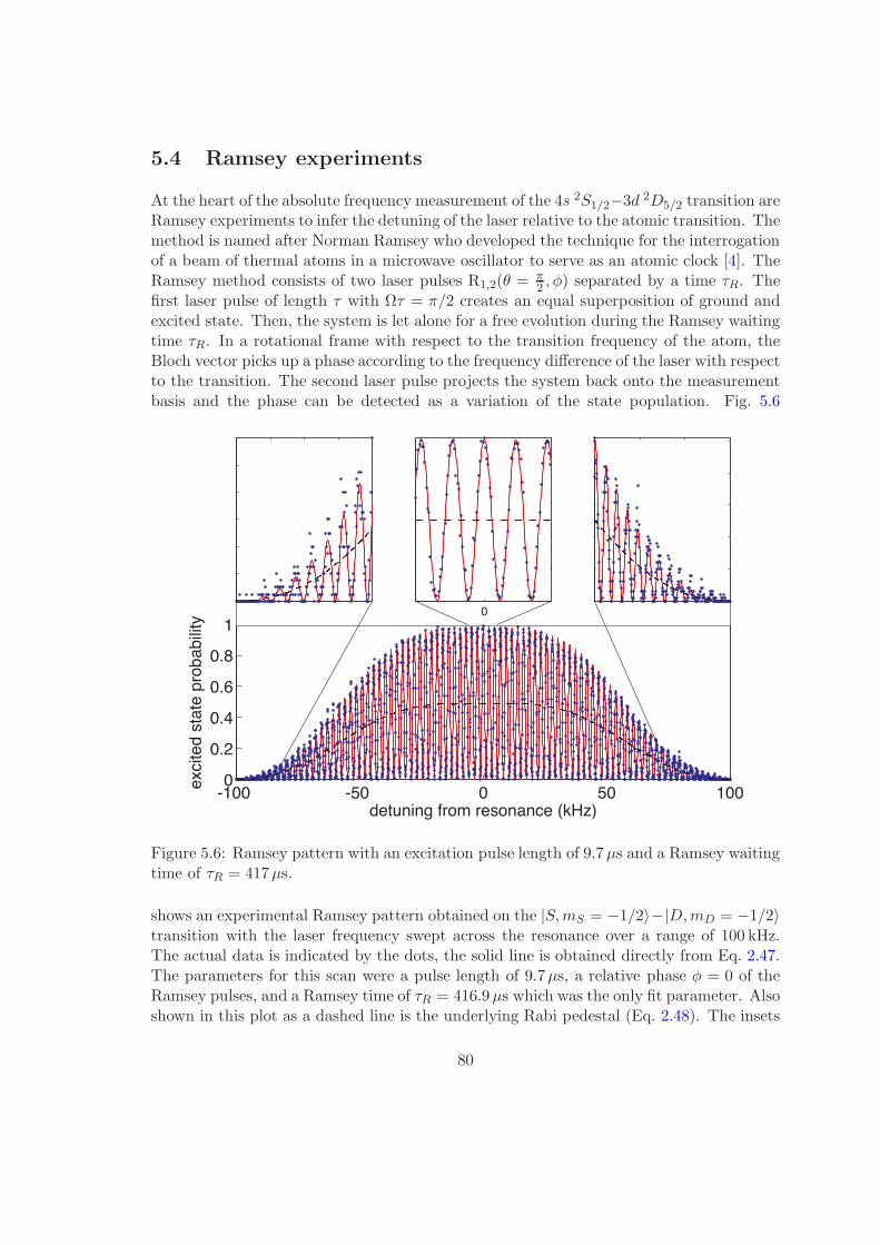
5.4 Ramsey experiments

At the heart of the absolute frequency measurement of the 4s 2S1/2−3d 2D5/2 transition areRamsey experiments to infer the detuning of the laser relative to the atomic transition. Themethod is named after Norman Ramsey who developed the technique for the interrogationof a beam of thermal atoms in a microwave oscillator to serve as an atomic clock [4]. TheRamsey method consists of two laser pulses R1,2(θ = π

2 , φ) separated by a time τR. Thefirst laser pulse of length τ with Ωτ = π/2 creates an equal superposition of ground andexcited state. Then, the system is let alone for a free evolution during the Ramsey waitingtime τR. In a rotational frame with respect to the transition frequency of the atom, theBloch vector picks up a phase according to the frequency difference of the laser with respectto the transition. The second laser pulse projects the system back onto the measurementbasis and the phase can be detected as a variation of the state population. Fig. 5.6

-100 -50 0 50 1000

0.2

0.4

0.6

0.8

detuning from resonance (kHz)

excite

d s

tate

pro

ba

bili

ty

0

1

Figure 5.6: Ramsey pattern with an excitation pulse length of 9.7µs and a Ramsey waitingtime of τR = 417µs.

shows an experimental Ramsey pattern obtained on the |S,mS = −1/2〉−|D,mD = −1/2〉transition with the laser frequency swept across the resonance over a range of 100 kHz.The actual data is indicated by the dots, the solid line is obtained directly from Eq. 2.47.The parameters for this scan were a pulse length of 9.7µs, a relative phase φ = 0 of theRamsey pulses, and a Ramsey time of τR = 416.9µs which was the only fit parameter. Alsoshown in this plot as a dashed line is the underlying Rabi pedestal (Eq. 2.48). The insets

80

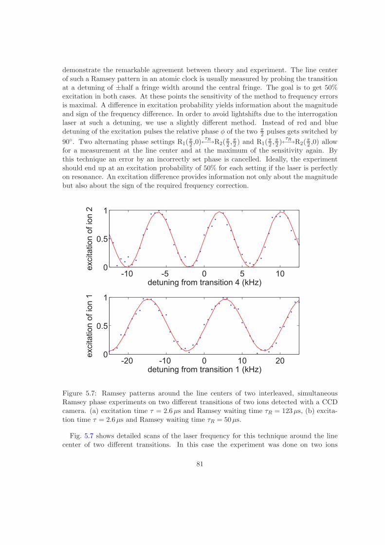
demonstrate the remarkable agreement between theory and experiment. The line centerof such a Ramsey pattern in an atomic clock is usually measured by probing the transitionat a detuning of ±half a fringe width around the central fringe. The goal is to get 50%excitation in both cases. At these points the sensitivity of the method to frequency errorsis maximal. A difference in excitation probability yields information about the magnitudeand sign of the frequency difference. In order to avoid lightshifts due to the interrogationlaser at such a detuning, we use a slightly different method. Instead of red and bluedetuning of the excitation pulses the relative phase φ of the two π

2 pulses gets switched by

90. Two alternating phase settings R1(π2 ,0)

τR←→R2(π2 ,π2 ) and R1(

π2 ,π2 )

τR←→R2(π2 ,0) allow

for a measurement at the line center and at the maximum of the sensitivity again. Bythis technique an error by an incorrectly set phase is cancelled. Ideally, the experimentshould end up at an excitation probability of 50% for each setting if the laser is perfectlyon resonance. An excitation difference provides information not only about the magnitudebut also about the sign of the required frequency correction.

-10 -5 0 5 100

0.5

1

excitation o

f io

n 2

detuning from transition 4 (kHz)

-20 -10 0 10 200

0.5

1

excitation o

f io

n 1

detuning from transition 1 (kHz)

Figure 5.7: Ramsey patterns around the line centers of two interleaved, simultaneousRamsey phase experiments on two different transitions of two ions detected with a CCDcamera. (a) excitation time τ = 2.6µs and Ramsey waiting time τR = 123µs, (b) excita-tion time τ = 2.6µs and Ramsey waiting time τR = 50µs.

Fig. 5.7 shows detailed scans of the laser frequency for this technique around the linecenter of two different transitions. In this case the experiment was done on two ions

81

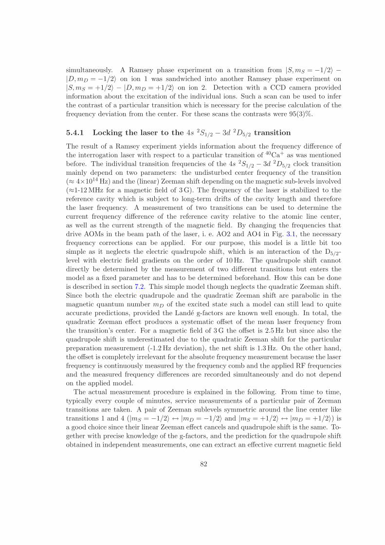
simultaneously. A Ramsey phase experiment on a transition from |S,mS = −1/2〉 −|D,mD = −1/2〉 on ion 1 was sandwiched into another Ramsey phase experiment on|S,mS = +1/2〉 − |D,mD = +1/2〉 on ion 2. Detection with a CCD camera providedinformation about the excitation of the individual ions. Such a scan can be used to inferthe contrast of a particular transition which is necessary for the precise calculation of thefrequency deviation from the center. For these scans the contrasts were 95(3)%.

5.4.1 Locking the laser to the 4s 2S1/2 − 3d 2D5/2 transition

The result of a Ramsey experiment yields information about the frequency difference ofthe interrogation laser with respect to a particular transition of 40Ca+ as was mentionedbefore. The individual transition frequencies of the 4s 2S1/2 − 3d 2D5/2 clock transitionmainly depend on two parameters: the undisturbed center frequency of the transition(≈ 4×1014 Hz) and the (linear) Zeeman shift depending on the magnetic sub-levels involved(≈1-12 MHz for a magnetic field of 3 G). The frequency of the laser is stabilized to thereference cavity which is subject to long-term drifts of the cavity length and thereforethe laser frequency. A measurement of two transitions can be used to determine thecurrent frequency difference of the reference cavity relative to the atomic line center,as well as the current strength of the magnetic field. By changing the frequencies thatdrive AOMs in the beam path of the laser, i. e. AO2 and AO4 in Fig. 3.1, the necessaryfrequency corrections can be applied. For our purpose, this model is a little bit toosimple as it neglects the electric quadrupole shift, which is an interaction of the D5/2-level with electric field gradients on the order of 10 Hz. The quadrupole shift cannotdirectly be determined by the measurement of two different transitions but enters themodel as a fixed parameter and has to be determined beforehand. How this can be doneis described in section 7.2. This simple model though neglects the quadratic Zeeman shift.Since both the electric quadrupole and the quadratic Zeeman shift are parabolic in themagnetic quantum number mD of the excited state such a model can still lead to quiteaccurate predictions, provided the Lande g-factors are known well enough. In total, thequadratic Zeeman effect produces a systematic offset of the mean laser frequency fromthe transition’s center. For a magnetic field of 3 G the offset is 2.5 Hz but since also thequadrupole shift is underestimated due to the quadratic Zeeman shift for the particularpreparation measurement (-1.2 Hz deviation), the net shift is 1.3 Hz. On the other hand,the offset is completely irrelevant for the absolute frequency measurement because the laserfrequency is continuously measured by the frequency comb and the applied RF frequenciesand the measured frequency differences are recorded simultaneously and do not dependon the applied model.

The actual measurement procedure is explained in the following. From time to time,typically every couple of minutes, service measurements of a particular pair of Zeemantransitions are taken. A pair of Zeeman sublevels symmetric around the line center liketransitions 1 and 4 (|mS = −1/2〉 ↔ |mD = −1/2〉 and |mS = +1/2〉 ↔ |mD = +1/2〉) isa good choice since their linear Zeeman effect cancels and quadrupole shift is the same. To-gether with precise knowledge of the g-factors, and the prediction for the quadrupole shiftobtained in independent measurements, one can extract an effective current magnetic field

82

100

101

102

103

104

10-15

10-14

10-13

10-12

τ (s)

All

an d

evia

tion

Figure 5.8: Allan standard deviation of the total frequency comb measurements.

and the current frequency difference between the reference cavity and the clock transition.Additionally, a quadratic fit to the history of these service measurements is used to predictthe laser and magnetic field drift until the next service measurement. The laser frequencycorrection is applied to the radiofrequency synthesizer (Rohde & Schwarz SML01) drivingthe two double pass AOMs going to the reference cavity, while the magnetic field correc-tions are applied by adjusting the various transition frequencies for the AOM in the beampath to the ion trap. Additionally, the frequency synthesizer for the reference cavity canbe phase continuously stepped in 0.1 Hz steps to compensate the cavity drift according tothe fitted drift rate. Typical parameters for the absolute frequency measurement were atime interval of 23 s between the measurements and a history length of 10 minutes. Thislocking method is good enough to get rid of long term drifts as shown in Fig. 5.8 by theoverlapping Allan deviation [119] of the laser frequency measured by the frequency combover the whole measurement time. The red line is a fit with 3.1(1) × 10−13τ−1/2. It isclear that the method is not optimized in any way to achieve the best lock of the laser tothe ion as it would be necessary for an optical clock, but we regard the residual laser driftwith −2± 600 × 10−8 Hz/s still remarkable.

This simple model together with the measured contrasts, the quadrupole shift, and theLande g-factors was good enough to probe the transitions near the line centers within theirrespective statistical errors. Histograms of the deviations from the predicted line centersfor 455600 individual measurements are shown in fig. 5.9. The mean deviations from thepredicted line centers were 0.1(3) Hz and 0.2(3) Hz for transitions 1 & 2, 0.3(3) Hz and-0.4(3) Hz for transitions 2 & 6, and -0.4(3) Hz and 0.4(4) Hz for transitions 3 & 5, wherea large part of the error can be attributed to quantum projection noise (0.2 Hz). The restis assumed to be due to fluctuations of the magnetic field and laser frequency noise.

83

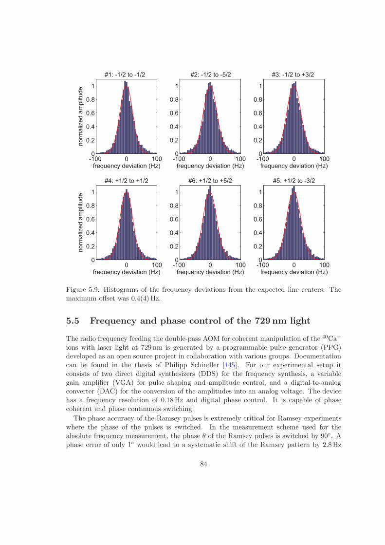
-100 0 1000

0.2

0.4

0.6

0.8

1

#1: -1/2 to -1/2

frequency deviation (Hz)

norm

aliz

ed a

mplit

ude

-100 0 1000

0.2

0.4

0.6

0.8

1

#2: -1/2 to -5/2

frequency deviation (Hz)-100 0 1000

0.2

0.4

0.6

0.8

1

#3: -1/2 to +3/2

frequency deviation (Hz)

0 1000

0.2

0.4

0.6

0.8

1

#4: +1/2 to +1/2

norm

aliz

ed a

mplit

ude

frequency deviation (Hz)-100 0 1000

0.2

0.4

0.6

0.8

1

#6: +1/2 to +5/2

frequency deviation (Hz)-100 0 1000

0.2

0.4

0.6

0.8

1

#5: +1/2 to -3/2

frequency deviation (Hz)

Figure 5.9: Histograms of the frequency deviations from the expected line centers. Themaximum offset was 0.4(4) Hz.

5.5 Frequency and phase control of the 729 nm light

The radio frequency feeding the double-pass AOM for coherent manipulation of the 40Ca+

ions with laser light at 729 nm is generated by a programmable pulse generator (PPG)developed as an open source project in collaboration with various groups. Documentationcan be found in the thesis of Philipp Schindler [145]. For our experimental setup itconsists of two direct digital synthesizers (DDS) for the frequency synthesis, a variablegain amplifier (VGA) for pulse shaping and amplitude control, and a digital-to-analogconverter (DAC) for the conversion of the amplitudes into an analog voltage. The devicehas a frequency resolution of 0.18 Hz and digital phase control. It is capable of phasecoherent and phase continuous switching.

The phase accuracy of the Ramsey pulses is extremely critical for Ramsey experimentswhere the phase of the pulses is switched. In the measurement scheme used for theabsolute frequency measurement, the phase θ of the Ramsey pulses is switched by 90. Aphase error of only 1 would lead to a systematic shift of the Ramsey pattern by 2.8 Hz

84

pulse box

f1

f2=f

1+∆f/2

f3=∆f

RF synthesizer oscilloscope

AOM

laser

2x LP

Figure 5.10: The setup for the investigation of a possible phase shift of the AOM due tothe RF pulses.

for a pulse separation time of 1 ms. By repeating the Ramsey experiment with reversedpulse order, an error by a systematically incorrect setting is cancelled though. What’sstill important is the phase reproducibility because timing jitter of the PPG can leadto phase errors in spite of the fact that the phase register has 12 bit resolution. Tofully profit from such a high resolution, this jitter would have to be smaller than 1 psat typical operation frequencies around 270 MHz. In order to investigate this effect, atrain of RF pulses with relative phase 0 and 90 was created, centered at 270 MHz andvaried about the frequency range which was necessary to probe the individual Zeemantransitions for the absolute frequency measurement. The RF was mixed down1 to 5 kHzwith the second, phase stable output of the PPG. The output of the mixer was recordedwith a fast oscilloscope2 and sinusoidal functions were fitted to each pulse with variableamplitude, frequency, and phase. The phase reproducibility for 13,668 sets of pulses as itwas used for the absolute frequency measurement of the 4s 2S1/2 − 3d 2D5/2 transition inthis case was 0.003 which corresponds to a frequency uncertainty of 8 mHz at a Ramseytime τR =1ms or 2× 10−17 relative uncertainty for the absolute frequency measurement.The corresponding timing jitter is <3 ps.

There is another effect that could cause a systematic frequency shift if the AOM usedfor frequency and phase shifting of the laser beam would introduce phase shifts that areunequal for the first and the second laser pulse. Errors of this kind might arise because

1Minicircuits ZAD-12LeCroy WP7300A

85

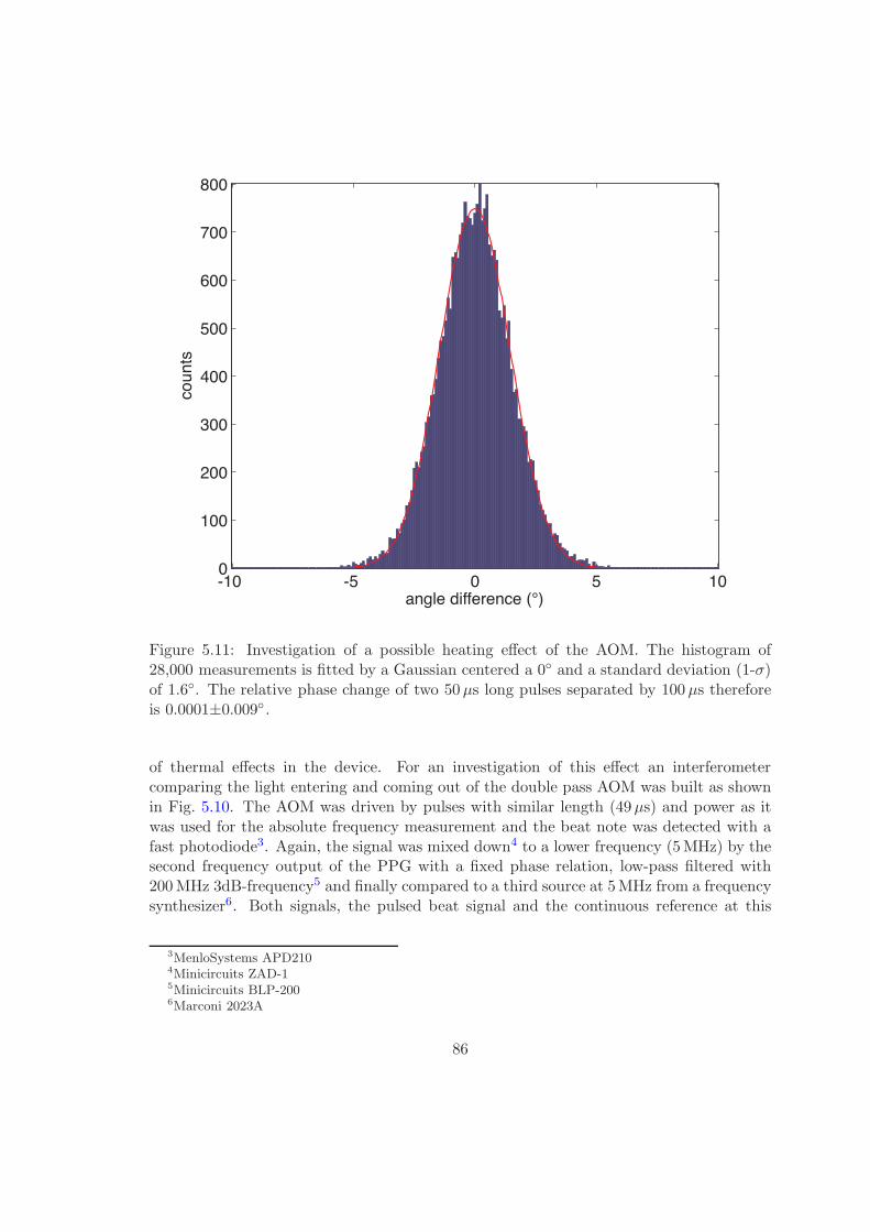
-10 -5 0 5 100

100

200

300

400

500

600

700

800

angle difference (°)

co

un

ts

Figure 5.11: Investigation of a possible heating effect of the AOM. The histogram of28,000 measurements is fitted by a Gaussian centered a 0 and a standard deviation (1-σ)of 1.6. The relative phase change of two 50µs long pulses separated by 100 µs thereforeis 0.0001±0.009 .

of thermal effects in the device. For an investigation of this effect an interferometercomparing the light entering and coming out of the double pass AOM was built as shownin Fig. 5.10. The AOM was driven by pulses with similar length (49µs) and power as itwas used for the absolute frequency measurement and the beat note was detected with afast photodiode3. Again, the signal was mixed down4 to a lower frequency (5 MHz) by thesecond frequency output of the PPG with a fixed phase relation, low-pass filtered with200 MHz 3dB-frequency5 and finally compared to a third source at 5 MHz from a frequencysynthesizer6. Both signals, the pulsed beat signal and the continuous reference at this

3MenloSystems APD2104Minicircuits ZAD-15Minicircuits BLP-2006Marconi 2023A

86

frequency were recorded with a fast oscilloscope7 and multiplied on a computer. The meanvalues for the obtained beat signal frequencies and the fitted amplitudes of the originalsignals were used to calculate the corresponding phase. For 28000 experiments with apulse length of 50µs and a pulse separation of 100µs the relative phase change was only∆θ =0.0001±0.009. The phase change was also measured for pulse separations of 50µs,250 µs, 500µs, and 1000 µs but for a smaller number of repetitions. The average phasechange and the corresponding standard deviations were -0.05(7), 0.002(66), -0.14(12), and0.14(8). This measurement was done to make sure that a possible phase change doesnot depend on the Ramsey time, at least not starting from a pulse separation of 50µs.Especially for the longer Ramsey times the amount of collected data for the fixed resolutionof 1 GS/s started to become large, and also interferometric stability was beginning to playa role, noticable in an increased standard deviation. For this reason the measurementstatistics is worse than for the 100µs data. Nevertheless, the thorough investigation of therelative phase shift at 100µs allows for a reliable interpolation of the phase error to 1 msand was reassured by the additional measurements at different waiting times. Moreover,the effect of differential heating - which is the most likely cause for a change in the opticalpath length - of the Ramsey pulses should be much worse at shorter pulse separation thanis actually used in the experiment.

7LeCroy WP7300A

87

88

Chapter 6

Absolute frequency measurementof the 4s 2S1/2 − 3d 2D5/2 clocktransition

Building an ion clock based on Ca+ has the technological advantage that all necessarywavelengths for laser cooling and state manipulation including lasers for photo-ionizationcan nowadays be generated by commercially available diode lasers. In order to show thatclocks based on Ca+ ions are a suitable candidate for an optical ion clock, Ca+ has tobe compared against the Cs frequency standard on which the current definition of the SIsecond is based. In the first part of this chapter the absolute frequency measurement on40Ca+ ions will be presented which was performed when a transportable Cs fountain clockwith an accuracy of < 10−15 was present in our lab. The interrogation lasers probing40Ca+ and 43Ca+ ions were compared against Cs through a frequency comb. The nextpart contains an analysis of the expected frequency shifts and presents the final result for40Ca+ with a detailed error budget. It represents the first absolute frequency measurementon Ca+ at the level of 10−15. Finally, a comparison of the 40Ca+ results for different trappowers and a preliminary measurement of the isotope shift of 43Ca+ are quickly discussed.

6.1 Spectroscopy on the 4s 2S1/2 − 3d 2D5/2 transition

There are two commonly used techniques of measuring the line center of an atomic tran-sition:

• simple Rabi excitations, or

• Ramsey’s method of separated fields.

In terms of frequency determination both schemes - Ramsey and Rabi excitation - arealmost equivalent. Peik et al. [146] have investigated both schemes in consideration ofbuilding an optical clock with a single ion as reference and concluded that the Ramseyscheme can be slightly better (30% for optimal parameters) regarding the highest possible

89

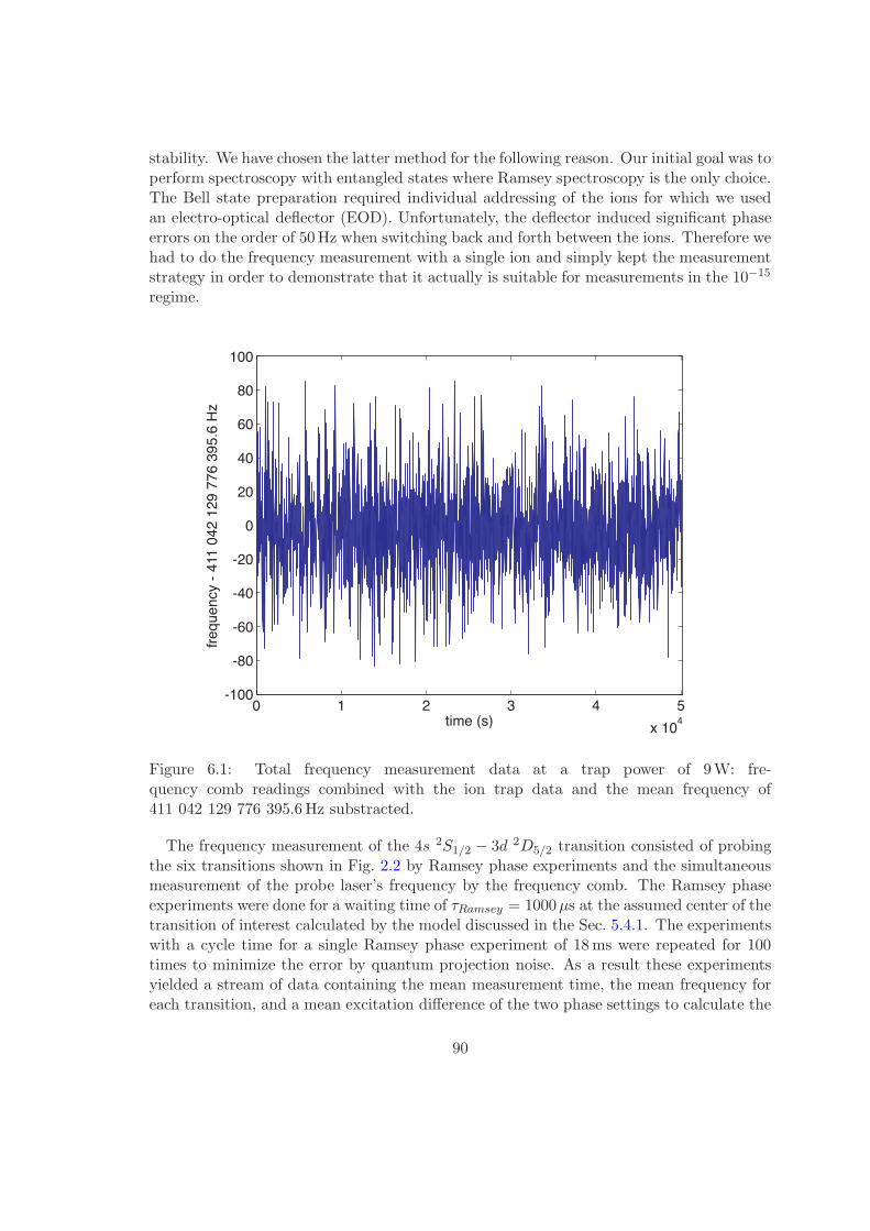
stability. We have chosen the latter method for the following reason. Our initial goal was toperform spectroscopy with entangled states where Ramsey spectroscopy is the only choice.The Bell state preparation required individual addressing of the ions for which we usedan electro-optical deflector (EOD). Unfortunately, the deflector induced significant phaseerrors on the order of 50 Hz when switching back and forth between the ions. Therefore wehad to do the frequency measurement with a single ion and simply kept the measurementstrategy in order to demonstrate that it actually is suitable for measurements in the 10−15

regime.

0 1 2 3 4 5

x 104

-100

-80

-60

-40

-20

0

20

40

60

80

100

time (s)

frequency -

411

042 1

29 7

76 3

95.6

Hz

Figure 6.1: Total frequency measurement data at a trap power of 9W: fre-quency comb readings combined with the ion trap data and the mean frequency of411 042 129 776 395.6 Hz substracted.

The frequency measurement of the 4s 2S1/2 − 3d 2D5/2 transition consisted of probingthe six transitions shown in Fig. 2.2 by Ramsey phase experiments and the simultaneousmeasurement of the probe laser’s frequency by the frequency comb. The Ramsey phaseexperiments were done for a waiting time of τRamsey = 1000µs at the assumed center of thetransition of interest calculated by the model discussed in the Sec. 5.4.1. The experimentswith a cycle time for a single Ramsey phase experiment of 18 ms were repeated for 100times to minimize the error by quantum projection noise. As a result these experimentsyielded a stream of data containing the mean measurement time, the mean frequency foreach transition, and a mean excitation difference of the two phase settings to calculate the

90

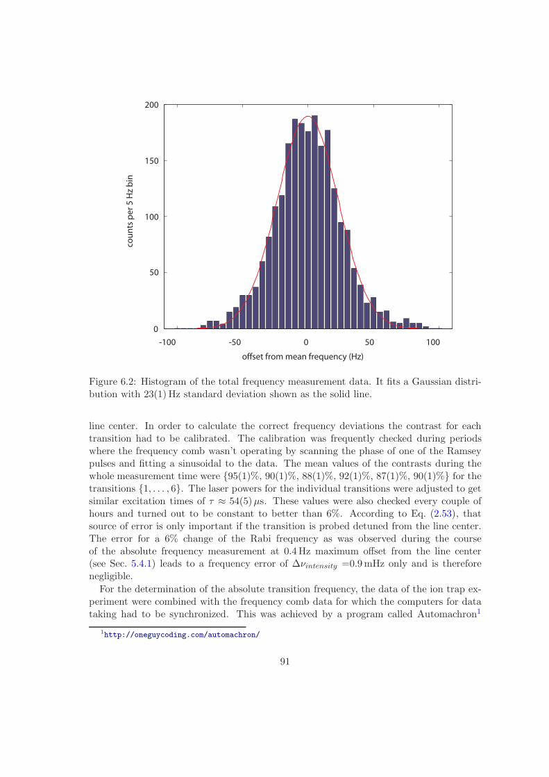
-100 -50 0 50 100

0

50

100

150

200

offset from mean frequency (Hz)

cou

nts

pe

r 5

Hz

bin

Figure 6.2: Histogram of the total frequency measurement data. It fits a Gaussian distri-bution with 23(1) Hz standard deviation shown as the solid line.

line center. In order to calculate the correct frequency deviations the contrast for eachtransition had to be calibrated. The calibration was frequently checked during periodswhere the frequency comb wasn’t operating by scanning the phase of one of the Ramseypulses and fitting a sinusoidal to the data. The mean values of the contrasts during thewhole measurement time were 95(1)%, 90(1)%, 88(1)%, 92(1)%, 87(1)%, 90(1)% for thetransitions 1, . . . , 6. The laser powers for the individual transitions were adjusted to getsimilar excitation times of τ ≈ 54(5)µs. These values were also checked every couple ofhours and turned out to be constant to better than 6%. According to Eq. (2.53), thatsource of error is only important if the transition is probed detuned from the line center.The error for a 6% change of the Rabi frequency as was observed during the courseof the absolute frequency measurement at 0.4 Hz maximum offset from the line center(see Sec. 5.4.1) leads to a frequency error of ∆νintensity =0.9 mHz only and is thereforenegligible.

For the determination of the absolute transition frequency, the data of the ion trap ex-periment were combined with the frequency comb data for which the computers for datataking had to be synchronized. This was achieved by a program called Automachron1

1http://oneguycoding.com/automachron/

91

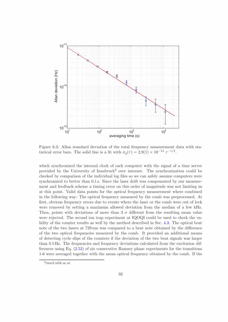
101

102

103

104

10-15

10-14

10-13

averaging time (s)

Alla

n d

evia

tion (

Hz)

Figure 6.3: Allan standard deviation of the total frequency measurement data with sta-tistical error bars. The solid line is a fit with σy(τ) = 2.9(1) × 10−13 τ−1/2.

which synchronized the internal clock of each computer with the signal of a time serverprovided by the University of Innsbruck2 over internet. The synchronization could bechecked by comparison of the individual log files so we can safely assume computers weresynchronized to better than 0.1 s. Since the laser drift was compensated by our measure-ment and feedback scheme a timing error on this order of magnitude was not limiting usat this point. Valid data points for the optical frequency measurement where combinedin the following way: The optical frequency measured by the comb was preprocessed. Atfirst, obvious frequency errors due to events where the laser or the comb were out of lockwere removed by setting a maximum allowed deviation from the median of a few kHz.Then, points with deviations of more than 3 σ different from the resulting mean valuewere rejected. The second ion trap experiment at IQOQI could be used to check the va-lidity of the counter results as well by the method described in Sec. 4.3. The optical beatnote of the two lasers at 729 nm was compared to a beat note obtained by the differenceof the two optical frequencies measured by the comb. It provided an additional meansof detecting cycle slips of the counters if the deviation of the two beat signals was largerthan 0.5 Hz. The frequencies and frequency deviations calculated from the excitation dif-ferences using Eq. (2.52) of six consecutive Ramsey phase experiments for the transitions1-6 were averaged together with the mean optical frequency obtained by the comb. If the

2time2.uibk.ac.at

92

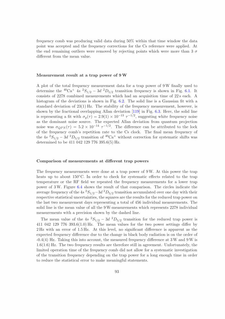
frequency comb was producing valid data during 50% within that time window the datapoint was accepted and the frequency corrections for the Cs reference were applied. Atthe end remaining outliers were removed by rejecting points which were more than 3 σdifferent from the mean value.

Measurement result at a trap power of 9 W

A plot of the total frequency measurement data for a trap power of 9W finally used todetermine the 40Ca+ 4s 2S1/2 − 3d 2D5/2 transition frequency is shown in Fig. 6.1. Itconsists of 2278 combined measurements which had an acquisition time of 22 s each. Ahistogram of the deviations is shown in Fig. 6.2. The solid line is a Gaussian fit with astandard deviation of 23(1) Hz. The stability of the frequency measurement, however, isshown by the fractional overlapping Allan deviation [119] in Fig. 6.3. Here, the solid lineis representing a fit with σy(τ) = 2.9(1) × 10−13 τ−1/2, suggesting white frequency noiseas the dominant noise source. The expected Allan deviation from quantum projectionnoise was σQPN (τ) = 5.2 × 10−14 τ−1/2. The difference can be attributed to the lockof the frequency comb’s repetition rate to the Cs clock. The final mean frequency ofthe 4s 2S1/2 − 3d 2D5/2 transition of 40Ca+ without correction for systematic shifts wasdetermined to be 411 042 129 776 395.6(5) Hz.

Comparison of measurements at different trap powers

The frequency measurements were done at a trap power of 9W. At this power the trapheats up to about 150C. In order to check for systematic effects related to the traptemperature or the RF field we repeated the frequency measurements for a lower trappower of 3 W. Figure 6.4 shows the result of that comparison. The circles indicate theaverage frequency of the 4s 2S1/2−3d 2D5/2 transition accumulated over one day with theirrespective statistical uncertainties, the squares are the results for the reduced trap power onthe last two measurement days representing a total of 456 individual measurements. Thesolid line is the mean value of all the 9W-measurements which represents 2278 individualmeasurements with a precision shown by the dashed line.

The mean value of the 4s 2S1/2 − 3d 2D5/2 transition for the reduced trap power is411 042 129 776 393.6(1.0) Hz. The mean values for the two power settings differ by2 Hz with an error of 1.5 Hz. At this level, no significant difference is apparent as theexpected frequency difference due to the change in black body radiation is on the order of-0.4(4) Hz. Taking this into account, the measured frequency difference at 3W and 9W is1.6(1.6) Hz. The two frequency results are therefore still in agreement. Unfortunately, thelimited operation time of the frequency comb did not allow for a systematic investigationof the transition frequency depending on the trap power for a long enough time in orderto reduce the statistical error to make meaningful statements.

93

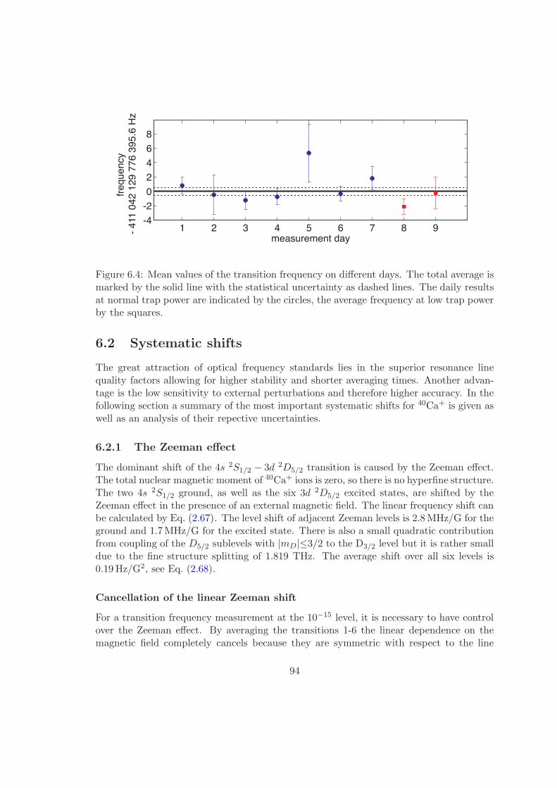
1 2 3 4 5 6 7 8 9-4

-2

0

2

4

6

8

measurement day

fre

qu

en

cy

- 4

11

04

2 1

29

77

6 3

95

.6 H

z

Figure 6.4: Mean values of the transition frequency on different days. The total average ismarked by the solid line with the statistical uncertainty as dashed lines. The daily resultsat normal trap power are indicated by the circles, the average frequency at low trap powerby the squares.

6.2 Systematic shifts

The great attraction of optical frequency standards lies in the superior resonance linequality factors allowing for higher stability and shorter averaging times. Another advan-tage is the low sensitivity to external perturbations and therefore higher accuracy. In thefollowing section a summary of the most important systematic shifts for 40Ca+ is given aswell as an analysis of their repective uncertainties.

6.2.1 The Zeeman effect

The dominant shift of the 4s 2S1/2 − 3d 2D5/2 transition is caused by the Zeeman effect.The total nuclear magnetic moment of 40Ca+ ions is zero, so there is no hyperfine structure.The two 4s 2S1/2 ground, as well as the six 3d 2D5/2 excited states, are shifted by theZeeman effect in the presence of an external magnetic field. The linear frequency shift canbe calculated by Eq. (2.67). The level shift of adjacent Zeeman levels is 2.8 MHz/G for theground and 1.7 MHz/G for the excited state. There is also a small quadratic contributionfrom coupling of the D5/2 sublevels with |mD|≤3/2 to the D3/2 level but it is rather smalldue to the fine structure splitting of 1.819 THz. The average shift over all six levels is0.19 Hz/G2, see Eq. (2.68).

Cancellation of the linear Zeeman shift

For a transition frequency measurement at the 10−15 level, it is necessary to have controlover the Zeeman effect. By averaging the transitions 1-6 the linear dependence on themagnetic field completely cancels because they are symmetric with respect to the line

94

center. The error is limited by the number of measurements only. In order to calculate thestatistical error for the data the individual AOM frequencies and the respective frequencydeviations were used. The laser was locked to the ion by the method described aboveand its frequency can be regarded as constant over time. This is a valid assumption asdemonstrated by the Allan standard deviation in Fig. 6.3. For the actual data we obtaineda statistical error of ±0.2 Hz for the averaged line center. The shot noise limit for an atomicclock using Ramsey’s method the frequency error is given by [66]

∆νQPN =√

p(1− p) 1√N

fR

π, (6.1)

where p is the excitation probability, fR the Ramsey fringe spacing, and N the numberof measurements. The total amount of data finally used for the absolute frequency deter-mination was 2278 sets of measurements of all six transitions. For each set we repeateda single Ramsey phase experiment for 100 times and probed the transition twice withreversed phase to get rid of phase errors as mentioned before. This corresponds to a totalnumber of measurements Ntot = 2278×100×2×6 =2,733,600 at an excitation probabilityp = 0.5. The expected error from quantum projection noise therefore is ∆νQPN ≈ 0.1Hz.The experimental excess noise can be explained by line frequency noise of the magneticfield and laser frequency fluctuations.

Unfortunately, the magnetic field was not always constant. Probably due to temperaturechanges in the lab, the current for the magnetic field coils was slowly changing, resultingin an average magnetic field drift of 2(1) 10−8 G/s. This led to a measurement offset of28(14) mHz because this effect is not completely canceled by averaging of the six transitionswithout changing their order.

Measurement of the g5/2-factor

The measured transition frequencies 1-6 and the frequency deviations can be used tocalculate the Lande g5/2-factor of the D5/2 level, provided the g-factor of the S1/2 level isprecisely known. For a prediction of the transition frequencies with sub-Hertz precisionin the presence of a magnetic field of a few Gauss, the g-factors have to be known tobetter than 10−7. Also, here it was sufficient to use the spectroscopic data only becausethe laser frequency was constant as the laser was locked to the ion. Three transitionsstarting from one Zeeman ground state and one from the other ground state form asystem of equations with three free parameters that can be determined unambiguously:the magnitude of the magnetic field B, the quadrupole shift q, and the g-factor g5/2. Thenecessary g-factor of the S1/2 ground state has been measured by Tommaseo et. al. [98] with10−8 accuracy. Using two different combinations of transitions increases the measurementstatistics. Transition frequency differences are defined as

fij = fi − fj. (6.2)

95

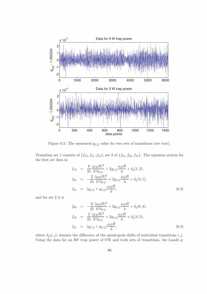
0 1000 2000 3000 4000 5000 6000

-2

-1

0

1

2

x 10-5

g5

/2 -

1.2

00334

Data for 9 W trap power

0 200 400 600 800 1000 1200 1400

-2

-1

0

1

2

x 10-5 Data for 3 W trap power

g5

/2 -

1.2

00334

data points

Figure 6.5: The measured g5/2 value for two sets of transitions (see text).

Transition set 1 consists of f12, f31, f41, set 2 of f45, f64, f41. The equation system forthe first set then is:

f12 =6

25

(µBB)2

h2δFS+ 2g5/2

µBB

h+ δq(1, 2),

f31 = − 2

25

(µBB)2

h2δFS+ 2g5/2

µBB

h+ δq(3, 1),

f41 = (g1/2 + g5/2)µBB

h, (6.3)

and for set 2 it is

f64 = − 6

25

(µBB)2

h2δFS+ 2g5/2

µBB

h+ δq(6, 4),

f45 =2

25

(µBB)2

h2δFS+ 2g5/2

µBB

h+ δq(4, 5),

f41 = (g1/2 + g5/2)µBB

h, (6.4)

where δq(i, j) denotes the difference of the quadrupole shifts of individual transitions i, j.Using the data for an RF trap power of 9 W and both sets of transitions, the Lande g-

96

factor of the D5/2 level is then g5/2 = 1.2003340± 2.5× 10−7, where the error comes froman assumed frequency error on the transitions of 1Hz while the statistical error is on theorder of 10−8. The result for the data taken at a RF trap power of 3 W yields a consistentresult of g5/2 = 1.2003342 ± 2.8 × 10−7. A plot of the deviations from 1.200334 of themeasured g-factors for the 9W and 3W data is shown in Fig. 6.5.

2nd-order Zeeman shift

Coupling of the inner Zeeman levels of D5/2 to the D3/2 levels is responsible for a smallquadratic frequency correction on the order of a few Hz. It can be calculated by us-ing second-order perturbation theory. The average magnetic field during the frequencymeasurement was 3.087(2) G. The |mD = 3/2| levels were shifted by 1.642(2) Hz, the|mD = 1/2| levels by 2.462(3) Hz while the outer levels were unaffected. These shifts arenot symmetric around the baseline at zero magnetic field and therefore are not cancelledby our measurement technique. The total shift averaged over transitions 1-6 is 1.368(2) Hzwhich is actually the largest shift in the whole error budget. But for the given uncertaintyof the magnetic field and the large fine structure splitting (1.8196 THz) the error is only2 mHz or 5× 10−18 in relative uncertainty.

There is also a contribution from the non-zero mean-square magnitude of the magneticfield from black body radiation (see Eq. (2.70)) but this effect is small compared to theshift by the quantization field. The magnetic black body shift, which is maximum forthe mD = ±1/2 levels, is 1 mHz only at a temperature of 150C. Taking into accountthat most of the surrounding environment (∼ 2/3) of the ion is at room temperature, therelative shift and the relative uncertainty are on the order of 10−18 and below.

6.2.2 Electric quadupole shift

The electric quadrupole moment of the D5/2 levels couples to static electric field gra-dients caused by either the DC-trapping fields and possible spurious field gradients ofpatch potentials. For axial confinement we applied a voltage of 1000 V to the tips ofour trap creating a static electric field gradient of 25 V/mm2. This led to shifts of∆νQ = Q (3 m2

J − J(J + 1)) where Q ≈ 1.15(3)Hz was the shift at this particularfield gradient and orientation of the quantization axis. But the effect completely can-cels when averaging over all transitions [23] because the shift for mD = ±5/2 is equal tothe combined shifts of mD = ±3/2 and mD = ±1/2 which have opposite sign. Similarto the linear Zeeman effect the error is determined by the statistical error of the sumof the measurements. Therefore, the electric quadrupole shift cancels with ±0.2 Hz anda relative uncertainty of 5 × 10−16. The individual measured shifts were 10.1(3) Hz forthe |mD = ±5/2〉 states, -2.0(3) Hz for the |mD = ±3/2〉 states, and -8.2(2) Hz for the|mD = ±1/2〉 states.

In order to take the effect into account when predicting the individual transition fre-quencies, the quadrupole shift parameter Q had to be measured beforehand. The methoddesigned to extract the quadrupole shift will be described in the next chapter. As a re-sult it led to Q = 0.98(1)Hz. The result does not take the quadratic Zeeman effect into

97

account. At a mean magnetic field of 3.100(1) G, the corrected value was Q = 1.05(1)Hz.Alternatively, the transition frequency data can be used to calculate the quadrupole shift.It is one of the three parameters determined by the set of Eqs. (6.3). The result wasQ = 1.15(3)Hz and is in reasonable agreement with the shift obtained from the previousmeasurement.

6.2.3 AC Stark shifts

All laser beams have to be switched off during the waiting times of a Ramsey experimentin order to avoid AC Stark shifts caused by laser light. In our experiment, this can be doneby switching off the RF sources of AOMs used for detuning the individual lasers. Since thiscannot be done perfectly, the residual light fields coming from stray light and incompletelyswitched off RF are expected to cause AC Stark shifts. Additionally, micromotion andblack body radiation from the environment can also be responsible for frequency shifts.

Light at 729 nm

The AC Stark shift caused by the probe laser has been thoroughly studied in our experi-ment [147]. The result of this investigation is summarized by the following equation:

∆νAC729 =

Ω2R

8π

(

2b−a±5/2

∆±5/2−a±1/2

∆±1/2−a∓3/2

∆∓3/2

)

, (6.5)

where ∆i denotes the detuning from the transition |mS〉 = ±1/2 − |mD = i〉 and b thecoupling to far detuned dipole transitions. Please note, that Eq. (6.5) is only valid forthe chosen geometry of magnetic field, laser polarization, and k-vector and also othertransitions of the Zeeman mulitplet have to be taken into account. The coefficients ai arethe squared relative coupling strengths from Tab. 2.1 and the dipole contribution has beenmeasured to be b =0.112(5)/(2π) MHz−1.

There are two contributions of probe light to the Stark shift during the probe time of aRamsey experiment. The first is simply the leakage of 729 nm light when the double passAOM is switched off. This light has a detuning of ∆/(2π) =540 MHz with respect to theS−D transition. In the case of the absolute frequency measurement, a residual backgroundlight of 0.7(1) nW was measured. Compared to the light level of 7.4µW necessary for aRabi frequency of ΩR/(2π) =8.3 kHz on the |mS〉 − |mD = −1/2〉 transition, a shift of34(1) mHz can be expected. The second part of the Stark shift stems from the fact, thatthe condition τ ≪ τR is not fulfilled well for our parameters. This means, the phasepicked up during the Ramsey experiment (see Eq. (2.54)) is modified by an additionalcomponent equal to the product of the effective pulse time τ 4

π from Eq. (2.49) and thecorresponding Stark shift calculated from Eq. (6.5). Taking Eq. (2.54) and using a pulsetime of 54(5) µ, the shift amounts to 80(4) mHz. The total shift by light at 729 nm then is∆νAC

729 =0.11(4) Hz which corresponds to 2.7× 10−16 relative uncertainty for the absolutefrequency measurement.

98

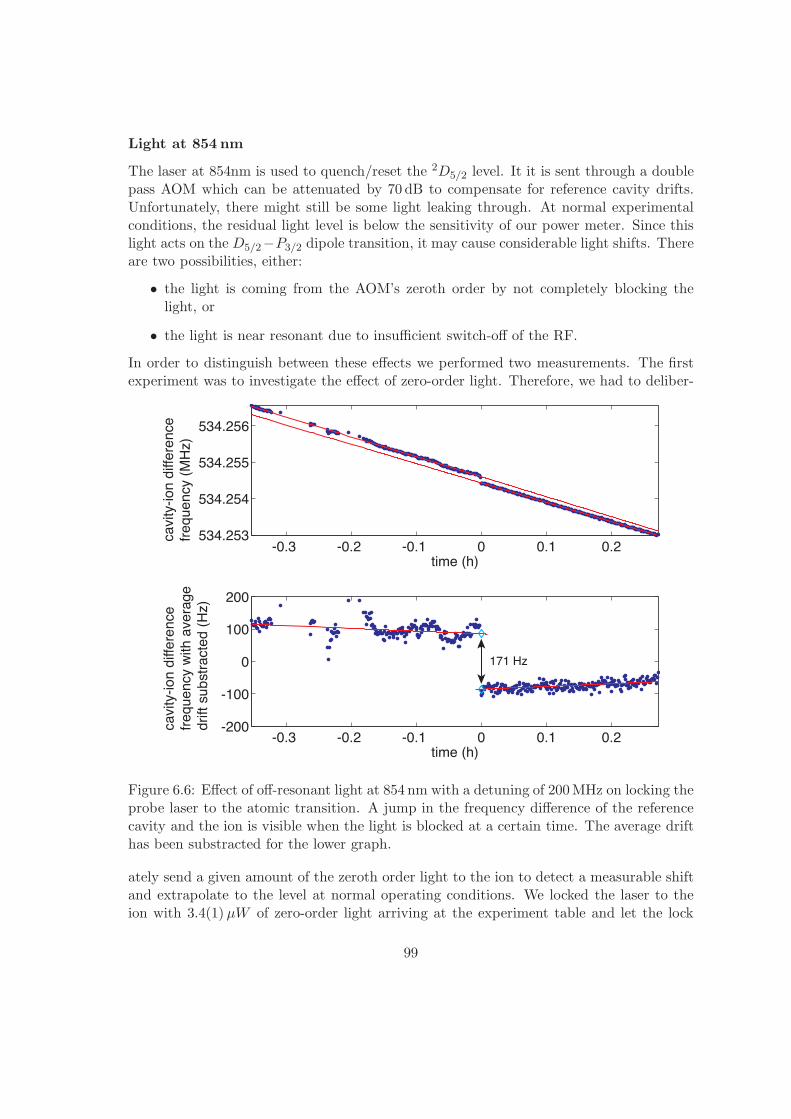
Light at 854 nm

The laser at 854nm is used to quench/reset the 2D5/2 level. It it is sent through a doublepass AOM which can be attenuated by 70 dB to compensate for reference cavity drifts.Unfortunately, there might still be some light leaking through. At normal experimentalconditions, the residual light level is below the sensitivity of our power meter. Since thislight acts on the D5/2−P3/2 dipole transition, it may cause considerable light shifts. Thereare two possibilities, either:

• the light is coming from the AOM’s zeroth order by not completely blocking thelight, or

• the light is near resonant due to insufficient switch-off of the RF.

In order to distinguish between these effects we performed two measurements. The firstexperiment was to investigate the effect of zero-order light. Therefore, we had to deliber-

-0.3 -0.2 -0.1 0 0.1 0.2534.253

534.254

534.255

534.256

time (h)

ca

vity-io

n d

iffe

ren

ce

fre

qu

en

cy (

MH

z)

-0.3 -0.2 -0.1 0 0.1 0.2-200

-100

0

100

200

time (h)

ca

vity-io

n d

iffe

ren

ce

fre

qu

en

cy w

ith

ave

rag

e

drift

su

bstr

acte

d (

Hz)

171 Hz

Figure 6.6: Effect of off-resonant light at 854 nm with a detuning of 200 MHz on locking theprobe laser to the atomic transition. A jump in the frequency difference of the referencecavity and the ion is visible when the light is blocked at a certain time. The average drifthas been substracted for the lower graph.

ately send a given amount of the zeroth order light to the ion to detect a measurable shiftand extrapolate to the level at normal operating conditions. We locked the laser to theion with 3.4(1) µW of zero-order light arriving at the experiment table and let the lock

99

settle down for about 20 minutes to get a reliable signal of the cavity drift due to slowlychanging Stark shifts. We then blocked the light and observed a jump of the cavity-iondifference frequency. Again, we then continued measuring for 15 minutes to measure thefrequency drift. We used linear fits for each data set to measure a shift of -170(40) Hzwhen the light was blocked as shown in Fig. 6.6. The power meter reading at normaloperation was 0.1 nW, which was limited by background light. Therefore, the expectedshift for zero-order light is -5(2) mHz.

The second experiment was a measurement of the lifetime of the 2D5/2 state. Thepresence of near-resonant light would result in a reduction of the lifetime due to scatter-ing events. The ion was initialized in the |S,mS = −1/2〉 state and transferred into the

0 0.5 1 1.5 20

0.1

0.2

0.3

0.4

0.5

0.6

0.7

0.8

0.9

1

waiting time (s)

D5

/2-s

tate

pro

pa

bili

ty

measured excitation

exponential fit

Figure 6.7: A lifetime measurement of the metastable D5/2-state yields a decay constantof 1.16(4) s.

|D,mD = −1/2〉 level by a π-pulse resonant with this transition. After a variable wait-ing time the remaining D-state population was detected as shown in Fig. 6.7 (points).An exponential fit (solid line) yielded a lifetime of 1.16(4) s which is within the errorbarsidentical to the lifetime measured by [148, 149]. In other words, there is no observablereduction of the D-state lifetime. The error of the lifetime can be used to set a limit onthe possible scattering rate of 0.03(1) /s caused by the unwanted light. The corresponding

100

shift according to Eq. (2.31) would be 2 mHz so that the total shift for light at 854 nm is∆ν854 =5(4) mHz with 1× 10−17 relative uncertainty.

Light at 866 nm

The shift by the repumping laser at 866 nm is estimated by making the following as-sumptions: the residual amount of light which could be detected by the power meter(0.1(1) nW) is tightly focused onto the ion. We assume a beam waist of 15µm which isprobably much tighter than in reality. The corresponding shift on the D5/2 − P3/2 transi-tion using Eq. (2.31) and the decay rate from [75] is below 10 mHz. For light intensitiessimilar to the light level at 854 nm we expect a shift of much less than 20µHz. The shiftcan safely be estimated to be ∆ν866 =0(10) mHz with 2.4×10−17 fractional uncertainty.

Light at 397 nm

The shift by the laser at 397 nm on the cooling transition can be estimated by a worst-case scenario: the residual amount of light is assumed to be focused onto the ion witha detuning of half a linewidth where the shift would be maximum. The light from thelaser can be switched off in two ways. First, there is a double-pass AOM on the lasertable and single-pass AOMs on the experiment table for each branch (optical pumpingand cooling). The maximum amount of light detected in front of the vacuum windowwas 0.3 nW and the attenuation factor of the double-pass AOM could be measured to bebetter than 105. At a beam waist of 15 µm the worst case shift would be 0.1 Hz. Sincethe residual light is probably scattered light from all kinds of surfaces like AOM crystals,lenses, beam cubes, etc. while the RF sources are switched off pretty well (>80 dB) it islikely to be detuned by 3×80 MHz. This would cause a shift of only 4 mHz. The total shiftfor light at 397 nm is then ∆ν397 =0.004(0.1) Hz and a relative uncertainty of 2.4×10−16.Furthermore, extremely long coherence times exceeding 30 s of a Bell-state consisting ofthe two ground states

∣

∣S1/2,mS = −1/2⟩

and∣

∣S1/2,mS = −1/2⟩

could be demonstratedwith this apparatus [150]. From that measurement an average photon scattering rate ofone in 8 minutes could be estimated, indicating that the error mentioned above can beconsidered as a conservative estimate.

Black body radiation

The largest uncertainty in the error budget however, stems from the AC Stark shift in-duced by black body radiation. The ion is exposed to thermal fields emanating from thesurrounding vacuum vessel at room temperature and the ion trap which gets heated up bythe applied RF power. The mean-square of the frequency-dependent electric field emittedby a black body at temperature T is given by [151]

〈E2(t)〉 = (831.9 V/m)2(

T

300 K

)4

. (6.6)

The total black body radiation shift can be calculated as the difference between the shiftsof the individual levels involved. The static scalar polarizabilities of the S1/2 and D5/2

101

states are taken from [152], that is α0(4S1/2) = 76.1(1.1)4πǫ0a30/h and α0(3D5/2) =

32.0(1.1)4πǫ0a30/h, respectively. There is also a tensorial part [24, 91] for the D level,

but this contribution is averaged out if the thermal radiation field is isotropic, or as inour case, if all sublevels with the tensorial contribution are measured similar to the can-cellation of the electric quadrupole shift. Therefore, the blackbody radiation shift can bewritten as

∆νBBR = − 1

2h〈E2(t)〉(α0(3D5/2)− α0(4S1/2)). (6.7)

The actual trap temperature as a function of the applied RF power can only be roughlyestimated with the help of the test setup mentioned in Sec. 3.2.2. At the input power of 9Wthat was applied for the frequency measurement, the trap heats up to about 150±50 C.The trap only covers about one third of the total solid angle while the rest is covered bythe surrounding vacuum vessel at a temperature of 25±2 C. Using Eqs. (6.6) and (6.7)and taking into account both contributions and their respective solid angles, we estimatethe black body shift to be ∆νBBR =0.9(7) Hz with a fractional uncertainty of 1.7×10−15.The uncertainty has two main contributions, the first being the 50% uncertainty in thesolid angle and the already discussed estimation of the temperature.

Micromotion and thermal motion

Thermal secular motion and excess micromotion cause the ion to be exposed to non-zeromean-square electric fields from the trap. The resulting Stark shift for excess micromotioncan be calculated by [82]

(∆νS)micro ≃ 2α0

(

2MΩT

ek cosφk

)2 R1

R0, (6.8)

with the ratio of the micromotion sideband powers R1R0

=J21 (βmicro)

J20 (βmicro)

, the angle between the

micromotion and the incident light φk, the mass of the ion M , and the Stark shift rateα0 [152] from the section above. Typically, we achieve micromotion compensation withmodulation indices βmicro < 0.004 in both directions. In the limit βmicro ≪ 1, the powerin the micromotion sidebands can be expanded in terms of the modulation index

R1

R0≈

(

1

2βmicro

)2

. (6.9)

Using Eqs. (6.8) and (6.9) and assuming βmicro = 0.004(±0.1), the expected Stark shift dueto micromotion therefore becomes (∆νS)micro =0.2 mHz. Again, the tensorial contributionis averaged to zero by the measurement of all 3D5/2 levels.

We hardly have to correct the compensation voltages on a time scale of months. There-fore it is safe to assume an error of well below 0.1 for the modulation index. An estimateof the expected uncertainty is then <125 mHz, given that the direction is not well known(73±10). The relative uncertainty of this contribution to the error budget is 3× 10−16.

102

The Stark shift contribution of the thermal motion can be calculated by [101]. For aDoppler cooled 40Ca+ ion (T ≈0.5 mK), the expected shift

(∆νS)thermal = α03MΩ2

TkBT

e2, (6.10)

is on the order of 1 mHz so that the total Stark shift due to motion is clearly dominatedby the micromotion contribution.

6.2.4 Gravitational shift

A gravitational potential difference between two clocks gives rise to a frequency differencedue to general relativity. For earth-based clocks, the relative frequency shift is approx-imately given by the height difference ∆h and the gravitational acceleration g providedthe clocks are almost at the same height [40]

(

∆ν

ν

)

g

=g∆h

c2, (6.11)

leading to a sensitivity of 1.1 × 10−16 m−1. The vertical distance between the Cs foun-tain and the 40Ca+ trap could be estimated to be less than 0.5(1) m. The gravitationalfrequency shift is therefore estimated by ∆νg =0.023(5) Hz.

The difference between the lab levels at the university and IQOQI has been measured bythe university’s civil engineering department to 4.41 m with a precision of 1 cm [153]. Theion trap difference is 4.5(5) m. Therefore, the expected shift between the two experimentsshould be 0.20(2) Hz. This can be important for future experiments at the 10−17 leveldedicated to a more detailed analysis of systematic shifts, e. g. a comparison of the twoexperiments at different trap powers to investigate the blackbody radiation shift.

6.2.5 2nd-order Doppler shift

Another relativistic effect is caused by excess micromotion or the thermal motion. It canshift the transition line center by the relativistic Doppler effect. This shift is produceddue to the ion motion relative to the laboratory frame. For a Doppler cooled 40Ca+ ion(T ≈0.5 mK), the shift can be estimated by

(

∆ν

ν

)

therm

= −3kBT

2Mc2(6.12)

and is -0.7(7) mHz. The contribution to the relativistic Doppler shift of the micromotiongiven by [82] is

(

∆ν

ν

)

micro

= −(

ΩT

ck cosφk

)2 (

1

2β

)2

(6.13)

and depends on the micromotion modulation index. In our case, the expected shift ismuch smaller than -1(3) mHz so the total effect of the 2nd-order Doppler shift is -1(4) mHzwith 1× 10−17 relative uncertainty.

103

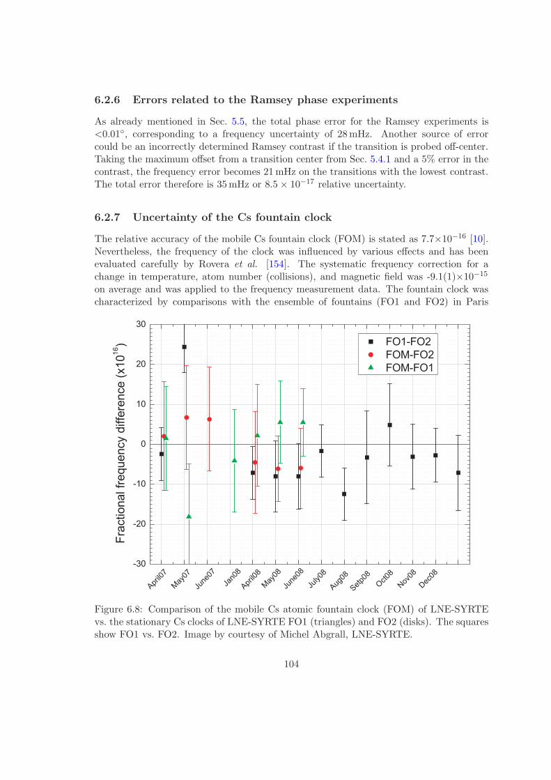
6.2.6 Errors related to the Ramsey phase experiments

As already mentioned in Sec. 5.5, the total phase error for the Ramsey experiments is<0.01, corresponding to a frequency uncertainty of 28 mHz. Another source of errorcould be an incorrectly determined Ramsey contrast if the transition is probed off-center.Taking the maximum offset from a transition center from Sec. 5.4.1 and a 5% error in thecontrast, the frequency error becomes 21 mHz on the transitions with the lowest contrast.The total error therefore is 35 mHz or 8.5× 10−17 relative uncertainty.

6.2.7 Uncertainty of the Cs fountain clock

The relative accuracy of the mobile Cs fountain clock (FOM) is stated as 7.7×10−16 [10].Nevertheless, the frequency of the clock was influenced by various effects and has beenevaluated carefully by Rovera et al. [154]. The systematic frequency correction for achange in temperature, atom number (collisions), and magnetic field was -9.1(1)×10−15

on average and was applied to the frequency measurement data. The fountain clock wascharacterized by comparisons with the ensemble of fountains (FO1 and FO2) in Paris

Figure 6.8: Comparison of the mobile Cs atomic fountain clock (FOM) of LNE-SYRTEvs. the stationary Cs clocks of LNE-SYRTE FO1 (triangles) and FO2 (disks). The squaresshow FO1 vs. FO2. Image by courtesy of Michel Abgrall, LNE-SYRTE.

104

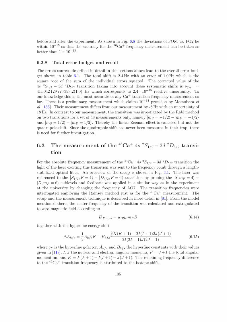
before and after the experiment. As shown in Fig. 6.8 the deviations of FOM vs. FO2 liewithin 10−15 so that the accuracy for the 40Ca+ frequency measurement can be taken asbetter than 1× 10−15.

6.2.8 Total error budget and result

The errors sources described in detail in the sections above lead to the overall error bud-get shown in table 6.1. The total shift is 2.4 Hz with an error of 1.0 Hz which is thesquare root of the sum of the individual errors squared. The corrected value of the4s 2S1/2 − 3d 2D5/2 transition taking into account these systematic shifts is νCa+ =411 042 129 776 393.2(1.0) Hz which corresponds to 2.4 · 10−15 relative uncertainty. Toour knowledge this is the most accurate of any Ca+ transition frequency measurement sofar. There is a preliminary measurement which claims 10−14 precision by Matsubara etal. [155]. Their measurement differs from our measurement by -8 Hz with an uncertainty of18 Hz. In contrast to our measurement, the transition was investigated by the Rabi methodon two transitions for a set of 48 measurements only, namely |mS = −1/2〉−|mD = −1/2〉and |mS = 1/2〉 − |mD = 1/2〉. Thereby the linear Zeeman effect is canceled but not thequadrupole shift. Since the quadrupole shift has never been measured in their trap, thereis need for further investigation.

6.3 The measurement of the 43Ca+ 4s 2S1/2− 3d 2D5/2 transi-tion

For the absolute frequency measurement of the 43Ca+ 4s 2S1/2 − 3d 2D5/2 transition thelight of the laser exciting this transition was sent to the frequency comb through a length-stabilized optical fiber. An overview of the setup is shown in Fig. 3.1. The laser wasreferenced to the

∣

∣S1/2, F = 4⟩

−∣

∣D5/2, F = 6⟩

transition by probing the |S,mF = 4〉 −|D,mF = 6〉 sublevels and feedback was applied in a similar way as in the experimentat the university by changing the frequency of AO7. The transition frequencies wereinterrogated employing the Ramsey method just as for the 40Ca+ measurement. Thesetup and the measurement technique is described in more detail in [81]. From the modelmentioned there, the center frequency of the transition was calculated and extrapolatedto zero magnetic field according to

E|F,mF 〉 = µBgFmFB (6.14)

together with the hyperfine energy shift

∆Ehfs =1

2AhfsK +Bhfs

32K(K + 1)− 2I(I + 1)2J(J + 1)

2I(2I − 1)J(2J − 1), (6.15)

where gF is the hyperfine g-factor, Ahfs and Bhfs the hyperfine constants with their valuesgiven in [118], I, J the nuclear and electron angular momenta, F = J+I the total angularmomentum, and K = F (F + 1)− I(I + 1)− J(J + 1). The remaining frequency differenceto the 40Ca+ transition frequency is attributed to the isotope shift.

105

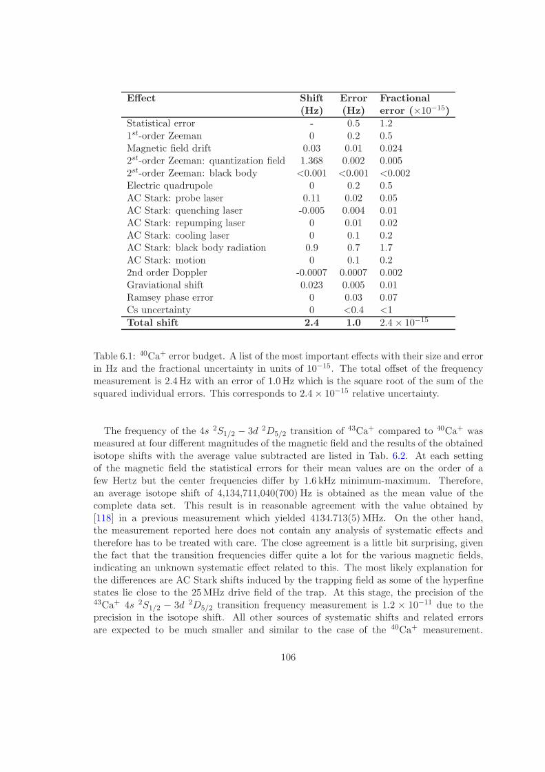
Effect Shift Error Fractional(Hz) (Hz) error (×10−15)

Statistical error - 0.5 1.21st-order Zeeman 0 0.2 0.5Magnetic field drift 0.03 0.01 0.0242st-order Zeeman: quantization field 1.368 0.002 0.0052st-order Zeeman: black body <0.001 <0.001 <0.002Electric quadrupole 0 0.2 0.5AC Stark: probe laser 0.11 0.02 0.05AC Stark: quenching laser -0.005 0.004 0.01AC Stark: repumping laser 0 0.01 0.02AC Stark: cooling laser 0 0.1 0.2AC Stark: black body radiation 0.9 0.7 1.7AC Stark: motion 0 0.1 0.22nd order Doppler -0.0007 0.0007 0.002Graviational shift 0.023 0.005 0.01Ramsey phase error 0 0.03 0.07Cs uncertainty 0 <0.4 <1

Total shift 2.4 1.0 2.4 × 10−15

Table 6.1: 40Ca+ error budget. A list of the most important effects with their size and errorin Hz and the fractional uncertainty in units of 10−15. The total offset of the frequencymeasurement is 2.4 Hz with an error of 1.0 Hz which is the square root of the sum of thesquared individual errors. This corresponds to 2.4× 10−15 relative uncertainty.

The frequency of the 4s 2S1/2 − 3d 2D5/2 transition of 43Ca+ compared to 40Ca+ wasmeasured at four different magnitudes of the magnetic field and the results of the obtainedisotope shifts with the average value subtracted are listed in Tab. 6.2. At each settingof the magnetic field the statistical errors for their mean values are on the order of afew Hertz but the center frequencies differ by 1.6 kHz minimum-maximum. Therefore,an average isotope shift of 4,134,711,040(700) Hz is obtained as the mean value of thecomplete data set. This result is in reasonable agreement with the value obtained by[118] in a previous measurement which yielded 4134.713(5) MHz. On the other hand,the measurement reported here does not contain any analysis of systematic effects andtherefore has to be treated with care. The close agreement is a little bit surprising, giventhe fact that the transition frequencies differ quite a lot for the various magnetic fields,indicating an unknown systematic effect related to this. The most likely explanation forthe differences are AC Stark shifts induced by the trapping field as some of the hyperfinestates lie close to the 25 MHz drive field of the trap. At this stage, the precision of the43Ca+ 4s 2S1/2 − 3d 2D5/2 transition frequency measurement is 1.2 × 10−11 due to theprecision in the isotope shift. All other sources of systematic shifts and related errorsare expected to be much smaller and similar to the case of the 40Ca+ measurement.

106

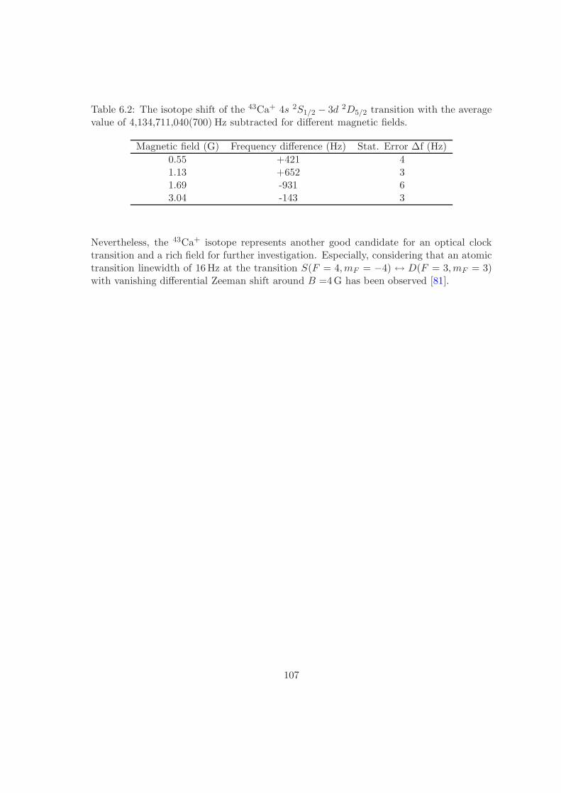
Table 6.2: The isotope shift of the 43Ca+ 4s 2S1/2 − 3d 2D5/2 transition with the averagevalue of 4,134,711,040(700) Hz subtracted for different magnetic fields.

Magnetic field (G) Frequency difference (Hz) Stat. Error ∆f (Hz)

0.55 +421 41.13 +652 31.69 -931 63.04 -143 3

Nevertheless, the 43Ca+ isotope represents another good candidate for an optical clocktransition and a rich field for further investigation. Especially, considering that an atomictransition linewidth of 16 Hz at the transition S(F = 4,mF = −4) ↔ D(F = 3,mF = 3)with vanishing differential Zeeman shift around B =4G has been observed [81].

107

108

Chapter 7

Precision spectroscopy withcorrelated atoms

The creation of entangled atoms is recognized as a key resource for quantum cryptographyand quantum computation. In this field, ion trap experiments have enabled spectacular re-sults in processing quantum information [156–158] or the creation of entanglement of up to8 ions [159, 160]. But entanglement is also of interest in the context of metrology and laserspectroscopy. Maximally entangled states can be used for efficient quantum state detec-tion by entangling an atom which is difficult to detect with another atom that is easier todetect [67] and it has been demonstrated that entangled states provide a means of improv-ing the signal-to-noise ratio in precision spectroscopy experiments [60, 65, 66, 161, 162].In addition, it is sometimes possible to identify specific states in the state space of many-particle quantum systems that are immune to decoherence [71] with respect to noise sourcesotherwise dominating single-atom systems [70]. Such decoherence-free subspaces protectquantum information and yield enhanced coherence times. Therefore these subspaces of-fer the prospect of high resolution spectroscopy even in the presence of strong technicalnoise. The question arises whether entanglement is a mandatory ingredient for this kindof measurement. As will be shown later it turns out that measurements with classicallycorrelated atoms can be used in a similar way even if the atoms are not entangled.

In this chapter, experiments with two entangled 40Ca+ ions will be presented, whichwere used to determine the electric quadrupole moment and the magnetic field gradientat the position of the ions. It will be shown how entangled states can be used to measurethe linewidth of a narrow-band laser. The second part of this chapter is dedicated tomeasurements with a pair of correlated, but not maximally entangled 40Ca+ ions used toverify the measurement results with entangled ions.

7.1 Spectroscopy with entangled states

In a Ramsey experiment, information about an atomic transition frequency is obtainedfrom a measurement of the relative phase ϕ = ϕL + ∆τ (determined by the phase ϕL ofthe exciting laser and the detuning ∆ from the transition) of a superposition of the ground

109

and excited state 1√2(|g〉+eiϕ |e〉) by mapping the states 1√

2(|g〉± |e〉) to the measurement

basis |g〉 , |e〉. This is done by the application of the second π/2-pulse.

Spectroscopy with entangled states can be realized by a generalized Ramsey experimentwhere the relative phase of a Bell state Ψϕ = 1√

2(|g〉1 |e〉2 + eiϕ |e〉1 |g〉2) is measured in

analogy to a single-ion Ramsey experiment. Here, the phase ϕ = ϕ1 − ϕ2 is measured byapplying the π/2-pulses to both atoms followed by state detection. For π/2-pulses withthe same phase the singlet state 1√

2(|g〉 |e〉 − |e〉 |g〉) is mapped onto itself, whereas the

triplet state 1√2(|g〉 |e〉+ |e〉 |g〉) is mapped onto a state 1√

2(|g〉 |g〉 + eiϕ |e〉 |e〉).

A measurement of the parity operator σ(1)z σ

(2)z yields information about the relative

phase ϕ of the Bell state’s constituents by

〈σ(1)z σ(2)

z 〉 = cosϕ. (7.1)

If the atomic transition frequencies for both ions are not exactly the same, the phasewill evolve according to ϕ(τ) = ϕ0 + ∆τ , where ∆ = ∆1 ±∆2 and ∆i are the frequencydifferences of the laser from the individual transitions. The + sign applies if the Bell stateis a superposition of both atoms in the excited and both atoms in the ground state, the −sign is for the state where an atom in the ground state is associated with the other atombeing in an excited state and vice versa. Thus, a measurement of the phase evolution ratedirectly yields information about the difference frequency ∆ of the constituents of the Bellstate. If the atomic transition frequency is the same for both ions, the phase evolutionwill be twice as sensitive to the phase ϕ(τ) = 2ϕ0 + 2∆τ as compared to a single ionmeasurement.

7.1.1 Measurement of the quadrupole moment

Ramsey experiments with a two-ion Bell-state Ψ = 1√2

(|m1〉 |m2〉+ |m3〉 |m4〉), where

the magnetic quantum numbers mi of the state |mi〉 ≡∣

∣D5/2,mi

⟩

fulfill m1 + m2 =m3 + m4 are to first order insensitive to fluctuations of the magnetic field. Both partsof the Bell-state are shifted by the same amount due to the linear Zeeman effect. Thismeans, that a state like Ψ is suitable for spectroscopy in a decoherence free subspacewith respect to the magnetic field if the inter-ion distance d is much smaller than thescale on which the magnetic field varies, i. e. the magnetic field is the same for both ions.The measurement strategy is especially useful where magnetic field noise would otherwiserender a measurement scheme with single ions difficult. Also, frequency noise of the probelaser is only relevant during the relatively short preparation of the Bell-state and theread-out analysis but not during the long Ramsey interrogation period making sub-Hertzspectroscopy feasible even with a laser that has a linewidth on the order of a few ten Hz.Since the states |mi〉 are sensitive to the electric quadrupole shifts these Bell-states canbe designed to measure the electric quadrupole moment of the 3d 2D5/2 level.

The Bell state ΨQ = 1√2

(|−5/2〉 |+3/2〉 + |−1/2〉 |−1/2〉) is used for the measure-

ment of the quadrupole shift. The level diagram with respect to the two most im-portant energy shifts for this state (linear Zeeman and electric quadrupole effect) is

110

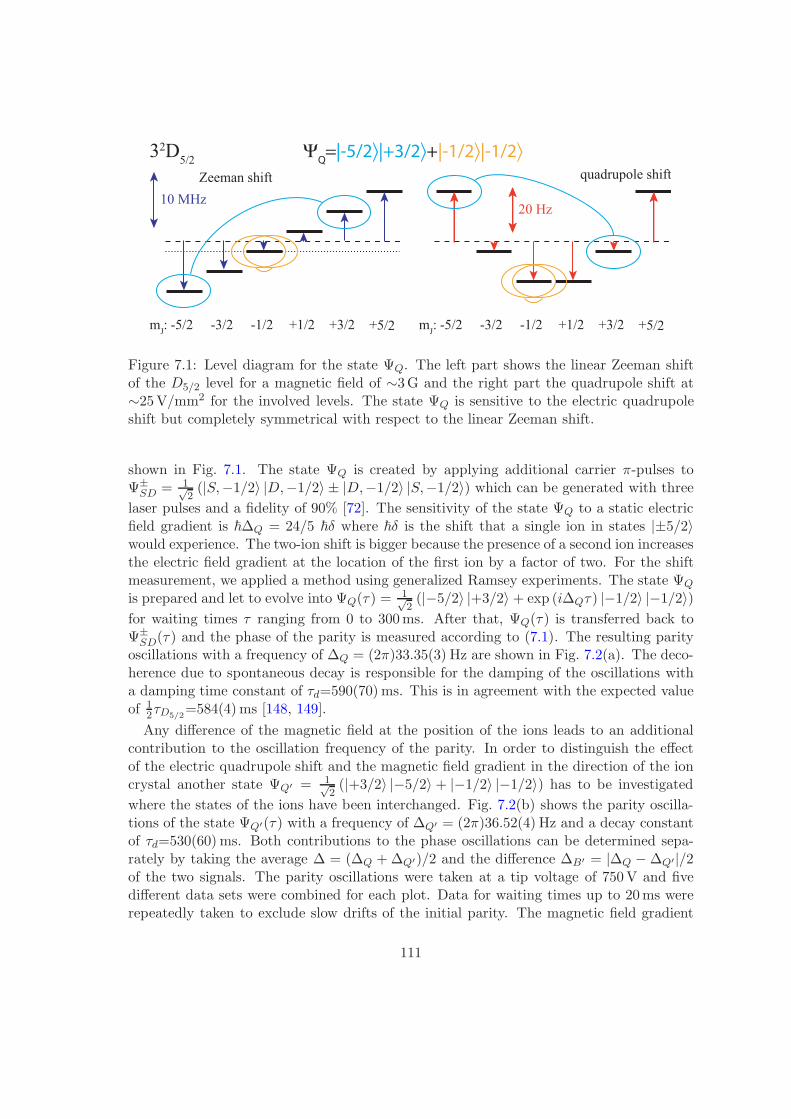
32D5/2

+5/2+3/2+1/2-1/2-3/2-5/2mJ: +5/2+3/2+1/2-1/2-3/2-5/2m

J:

10 MHz20 Hz

ΨQ=|-5/2⟩|+3/2⟩+|-1/2⟩|-1/2⟩

Zeeman shift quadrupole shift

Figure 7.1: Level diagram for the state ΨQ. The left part shows the linear Zeeman shiftof the D5/2 level for a magnetic field of ∼3G and the right part the quadrupole shift at∼25 V/mm2 for the involved levels. The state ΨQ is sensitive to the electric quadrupoleshift but completely symmetrical with respect to the linear Zeeman shift.

shown in Fig. 7.1. The state ΨQ is created by applying additional carrier π-pulses toΨ±

SD = 1√2

(|S,−1/2〉 |D,−1/2〉 ± |D,−1/2〉 |S,−1/2〉) which can be generated with three

laser pulses and a fidelity of 90% [72]. The sensitivity of the state ΨQ to a static electricfield gradient is ~∆Q = 24/5 ~δ where ~δ is the shift that a single ion in states |±5/2〉would experience. The two-ion shift is bigger because the presence of a second ion increasesthe electric field gradient at the location of the first ion by a factor of two. For the shiftmeasurement, we applied a method using generalized Ramsey experiments. The state ΨQ

is prepared and let to evolve into ΨQ(τ) = 1√2(|−5/2〉 |+3/2〉 + exp (i∆Qτ) |−1/2〉 |−1/2〉)

for waiting times τ ranging from 0 to 300 ms. After that, ΨQ(τ) is transferred back toΨ±

SD(τ) and the phase of the parity is measured according to (7.1). The resulting parityoscillations with a frequency of ∆Q = (2π)33.35(3) Hz are shown in Fig. 7.2(a). The deco-herence due to spontaneous decay is responsible for the damping of the oscillations witha damping time constant of τd=590(70) ms. This is in agreement with the expected valueof 1

2τD5/2=584(4) ms [148, 149].

Any difference of the magnetic field at the position of the ions leads to an additionalcontribution to the oscillation frequency of the parity. In order to distinguish the effectof the electric quadrupole shift and the magnetic field gradient in the direction of the ioncrystal another state ΨQ′ = 1√

2(|+3/2〉 |−5/2〉 + |−1/2〉 |−1/2〉) has to be investigated

where the states of the ions have been interchanged. Fig. 7.2(b) shows the parity oscilla-tions of the state ΨQ′(τ) with a frequency of ∆Q′ = (2π)36.52(4) Hz and a decay constantof τd=530(60) ms. Both contributions to the phase oscillations can be determined sepa-rately by taking the average ∆ = (∆Q + ∆Q′)/2 and the difference ∆B′ = |∆Q −∆Q′|/2of the two signals. The parity oscillations were taken at a tip voltage of 750 V and fivedifferent data sets were combined for each plot. Data for waiting times up to 20 ms wererepeatedly taken to exclude slow drifts of the initial parity. The magnetic field gradient

111

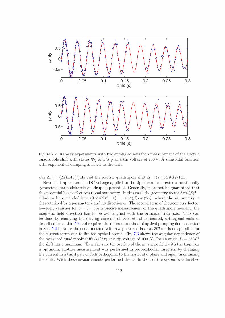
0 0.05 0.1 0.15 0.2 0.25 0.3

-0.5

0

0.5parity

time (s)

0 0.05 0.1 0.15 0.2 0.25 0.3

-0.5

0

0.5

pa

rity

time (s)

Figure 7.2: Ramsey experiments with two entangled ions for a measurement of the electricquadrupole shift with states ΨQ and ΨQ′ at a tip voltage of 750 V. A sinusoidal functionwith exponential damping is fitted to the data.

was ∆B′ = (2π)1.41(7) Hz and the electric quadrupole shift ∆ = (2π)34.94(7) Hz.

Near the trap center, the DC voltage applied to the tip electrodes creates a rotationallysymmetric static elelectric quadrupole potential. Generally, it cannot be guaranteed thatthis potential has perfect rotational symmetry. In this case, the geometry factor 3 cos(β)2−1 has to be expanded into

(

3 cos(β)2 − 1)

− ǫ sin2(β) cos(2α), where the asymmetry ischaracterized by a parameter ǫ and its direction α. The second term of the geometry factor,however, vanishes for β = 0. For a precise measurement of the quadrupole moment, themagnetic field direction has to be well aligned with the principal trap axis. This canbe done by changing the driving currents of two sets of horizontal, orthogonal coils asdescribed in section 5.3 and requires the different method of optical pumping demonstratedin Sec. 5.2 because the usual method with a σ-polarized laser at 397 nm is not possible forthe current setup due to limited optical access. Fig. 7.3 shows the angular dependence ofthe measured quadrupole shift ∆/(2π) at a tip voltage of 1000 V. For an angle β0 = 28(3)

the shift has a maximum. To make sure the overlap of the magnetic field with the trap axisis optimum, another measurement was performed in perpendicular direction by changingthe current in a third pair of coils orthogonal to the horizontal plane and again maximizingthe shift. With these measurements performed the calibration of the system was finished

112

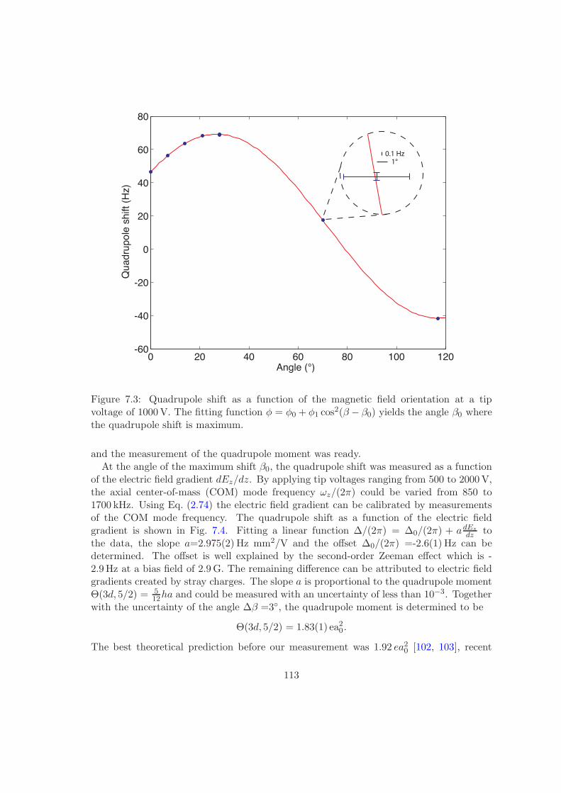
0 20 40 60 80 100 120-60

-40

-20

0

20

40

60

80

Angle (°)

Qu

ad

rup

ole

sh

ift

(Hz)

0.1 Hz1°

Figure 7.3: Quadrupole shift as a function of the magnetic field orientation at a tipvoltage of 1000 V. The fitting function φ = φ0 + φ1 cos2(β − β0) yields the angle β0 wherethe quadrupole shift is maximum.

and the measurement of the quadrupole moment was ready.At the angle of the maximum shift β0, the quadrupole shift was measured as a function

of the electric field gradient dEz/dz. By applying tip voltages ranging from 500 to 2000 V,the axial center-of-mass (COM) mode frequency ωz/(2π) could be varied from 850 to1700 kHz. Using Eq. (2.74) the electric field gradient can be calibrated by measurementsof the COM mode frequency. The quadrupole shift as a function of the electric fieldgradient is shown in Fig. 7.4. Fitting a linear function ∆/(2π) = ∆0/(2π) + adEz

dz tothe data, the slope a=2.975(2) Hz mm2/V and the offset ∆0/(2π) =-2.6(1) Hz can bedetermined. The offset is well explained by the second-order Zeeman effect which is -2.9 Hz at a bias field of 2.9 G. The remaining difference can be attributed to electric fieldgradients created by stray charges. The slope a is proportional to the quadrupole momentΘ(3d, 5/2) = 5

12ha and could be measured with an uncertainty of less than 10−3. Togetherwith the uncertainty of the angle ∆β =3, the quadrupole moment is determined to be

Θ(3d, 5/2) = 1.83(1) ea20 .

The best theoretical prediction before our measurement was 1.92 ea20 [102, 103], recent

113

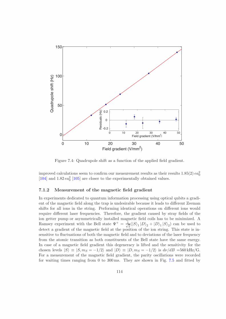
0 10 20 30 40 50

0

50

100

150

Field gradient (V/mm2)

Qu

ad

rup

ole

sh

ift

(Hz)

-0.2

0

0.2

Field gradient (V/mm2

)

Re

sid

ua

ls (

Hz)

0 10 20 30 40 50)

Figure 7.4: Quadrupole shift as a function of the applied field gradient.

improved calculations seem to confirm our measurement results as their results 1.85(2) ea20

[104] and 1.82 ea20 [105] are closer to the experimentally obtained values.

7.1.2 Measurement of the magnetic field gradient

In experiments dedicated to quantum information processing using optical qubits a gradi-ent of the magnetic field along the trap is undesirable because it leads to different Zeemanshifts for all ions in the string. Performing identical operations on different ions wouldrequire different laser frequencies. Therefore, the gradient caused by stray fields of theion getter pump or asymmetrically installed magnetic field coils has to be minimized. ARamsey experiment with the Bell state Ψ+ = 1√

2(|S〉1 |D〉2 + |D〉1 |S〉2) can be used to

detect a gradient of the magnetic field at the position of the ion string. This state is in-sensitive to fluctuations of both the magnetic field and to deviations of the laser frequencyfrom the atomic transition as both constituents of the Bell state have the same energy.In case of a magnetic field gradient this degeneracy is lifted and the sensitivity for thechosen levels |S〉 ≡ |S,mS = −1/2〉 and |D〉 ≡ |D,mS = −1/2〉 is dν/dB =560 kHz/G.For a measurement of the magnetic field gradient, the parity oscillations were recordedfor waiting times ranging from 0 to 300 ms. They are shown in Fig. 7.5 and fitted by

114

0 0.1 0.2 0.3

0

1

-1

time (s)

parity

Figure 7.5: Ramsey experiment of an entangled state |SD〉 − |SD〉 for a measurementof the magnetic field gradient. The phase evolution rate is 7.2(1) Hz and the decay time550(50) ms.

an exponentially damped sinusoidal with a frequency of 7.2(1) Hz and a damping time of550(50) ms. This indicates that the coherence of the state Ψ+ is mainly limited by the life-time of the excited state τD5/2

=1.168(7) s [148, 149]. With the help of an additional coilon one of the main magnetic field coils the parity oscillation frequency could be reducedto below 1 Hz. This corresponds to a magnetic field difference of 1.8 µG at the position ofthe ions and to a residual gradient of below 0.4 G/m. The precision of this method can beincreased by using a transition more sensitive to the linear Zeeman effect and operatingthe trap at lower axial confinement in order to increase the distance between the ions.

As already mentioned, the difference frequency of the frequencies ∆Q and ∆Q′ usedfor the quadrupole shift measurement is proportional to the magnetic field gradient. Itrepresents another possibility to gather information about the magnetic field gradient butslightly complicates the measurement procedure as it takes two measurements of the parityoscillation frequency. The frequency difference caused by a magnetic field gradient ∆B′ isdisplayed in Fig. 7.6. Since the inter-ion distance d decreases from 6.2 to 3.9µm for highertip voltages applied ranging from 500 to 2000 V, the magnetic field gradient B′ decreasesas well, because B′ ∝ d ∝ (dEz/dz)

−1/3.

7.1.3 Measurement of the linewidth of the laser exciting the quadrupoletransition

For frequency standard applications, measurements with entangled states can provide ameans which is insensitive to otherwise dominant sources of noise like fluctuations of themagnetic field for atomic transitions with even isotopes. By using a state like Ψmetro =

115

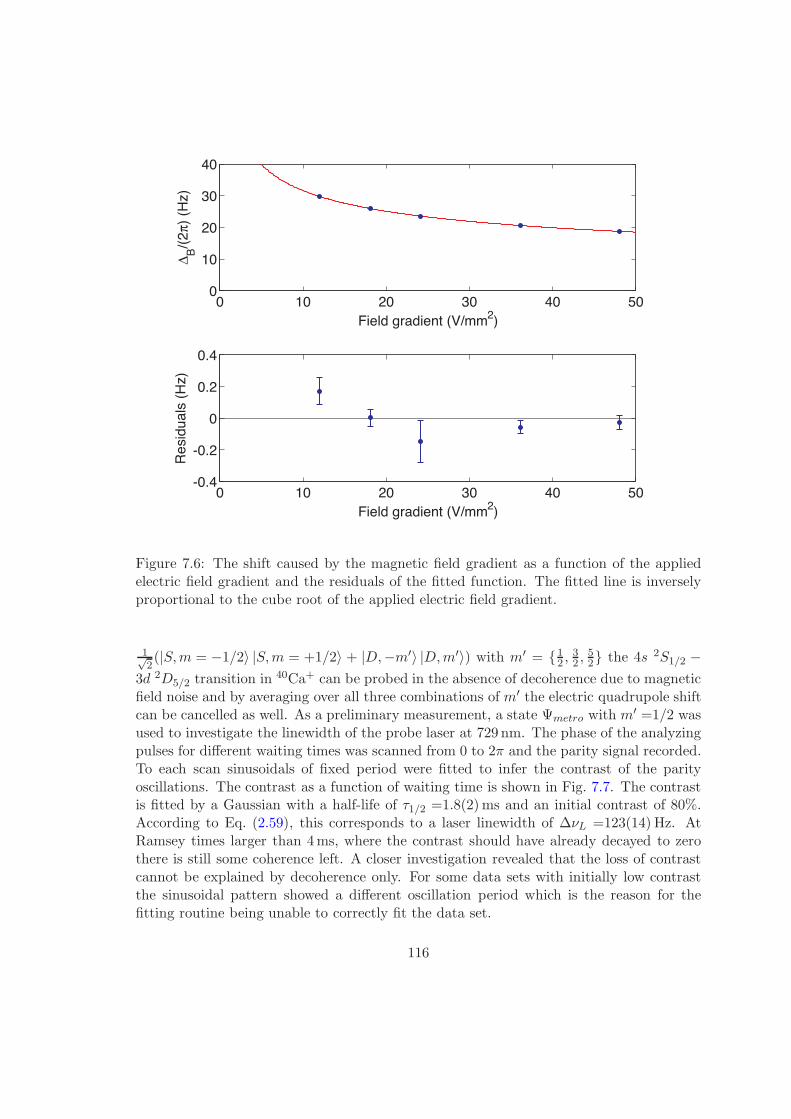
0 10 20 30 40 500

10

20

30

40

Field gradient (V/mm2)

∆B/(

2π)

(Hz)

0 10 20 30 40 50-0.4

-0.2

0

0.2

0.4

Field gradient (V/mm2)

Residu

als

(Hz)

Figure 7.6: The shift caused by the magnetic field gradient as a function of the appliedelectric field gradient and the residuals of the fitted function. The fitted line is inverselyproportional to the cube root of the applied electric field gradient.

1√2(|S,m = −1/2〉 |S,m = +1/2〉 + |D,−m′〉 |D,m′〉) with m′ = 1

2 ,32 ,

52 the 4s 2S1/2 −

3d 2D5/2 transition in 40Ca+ can be probed in the absence of decoherence due to magneticfield noise and by averaging over all three combinations of m′ the electric quadrupole shiftcan be cancelled as well. As a preliminary measurement, a state Ψmetro with m′ =1/2 wasused to investigate the linewidth of the probe laser at 729 nm. The phase of the analyzingpulses for different waiting times was scanned from 0 to 2π and the parity signal recorded.To each scan sinusoidals of fixed period were fitted to infer the contrast of the parityoscillations. The contrast as a function of waiting time is shown in Fig. 7.7. The contrastis fitted by a Gaussian with a half-life of τ1/2 =1.8(2) ms and an initial contrast of 80%.According to Eq. (2.59), this corresponds to a laser linewidth of ∆νL =123(14) Hz. AtRamsey times larger than 4 ms, where the contrast should have already decayed to zerothere is still some coherence left. A closer investigation revealed that the loss of contrastcannot be explained by decoherence only. For some data sets with initially low contrastthe sinusoidal pattern showed a different oscillation period which is the reason for thefitting routine being unable to correctly fit the data set.

116

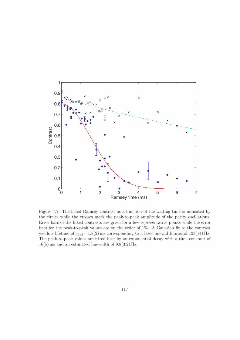
0 1 2 3 4 5 6 70

0.1

0.2

0.3

0.4

0.5

0.6

0.7

0.8

0.9

1

Ramsey time (ms)

Co

ntr

ast

Figure 7.7: The fitted Ramsey contrast as a function of the waiting time is indicated bythe circles while the crosses mark the peak-to-peak amplitude of the parity oscillations.Error bars of the fitted contrasts are given for a few representative points while the errorbars for the peak-to-peak values are on the order of 1%. A Gaussian fit to the contrastyields a lifetime of τ1/2 =1.8(2) ms corresponding to a laser linewidth around 123(14) Hz.The peak-to-peak values are fitted best by an exponential decay with a time constant of16(5) ms and an estimated linewidth of 9.8(3.2) Hz.

117

Especially for longer Ramsey times, the phase pattern gets distorted by slow frequencyfluctuations of the interrogation laser which happen on the same time scale it takes torecord a phase scan. Since it is difficult to adjust the fitting routine by a frequency chirp,the peak-to-peak amplitude ∼ (max−min)/(max + min) of the parity signal is also shownin Fig. 7.7. This way, sometimes even for Ramsey times as large as 10-15 ms, a clearsinusoidal variation of the parity signals is recognizable with contrasts larger than 50%.

The peak-to-peak amplitude is best fit by an exponential decay with a time constant of16(5) ms. Using Eq. (2.62), this would indicate a laser linewidth of ∆νFWHM =9.8(3.2) Hz.It should be pointed out that this result is rather preliminary. The peak-to-peak amplitudeis probably not the best measure for the contrast because it does not distinguish betweenperiodic and non-periodic behaviour. But still, it produces a reasonable result whencompared to the beat measurement or the measurement with unentangled states (seeSec. 7.2.2). Particularly the Allan variance of the beat measurement (see Fig. 3.21) showsthat the laser frequency is fluctuating by ∆νFWHM =40 Hz on time scales of a few secondsto hours which agrees with the change of the oscillation period during the phase scans.

7.2 Spectroscopy with correlated but unentangled states

The question is, whether entanglement is really necessary for the measurement techniquedescribed in the section above. In fact, it can be even applied to completely unentangledions because the product state

Ψp =1

2(|S〉+ |D〉)1 ⊗ (|S〉+ |D〉)2 =

1√2|Ψ+〉+

1

2|S1〉 |S2〉+

1

2|D1〉 |D2〉 (7.2)

contains the Bell state Ψ+. This state will quickly decay into the mixed state describedby the density operator

ρp =1

2|Ψ+〉 〈Ψ+|+

1

4|SS〉 〈SS|+ 1

4|DD〉 〈DD| (7.3)

under the influence of collective phase noise like fluctuating magnetic fields. A measure-ment of the parity operator will produce the same result as for a maximally entangledstate given in Eq. (7.1) apart from a reduced contrast of 50%. This is a very promisingresult because the creation of entangled states in the presence of strong decoherence mightbe difficult, but the question still remains if both methods yield the same result.

7.2.1 Measurement of the quadrupole moment

In order to check the validity of the quadrupole moment measurement and to prove that themeasurement can be done with classically correlated, but unentangled ions, we preparedthe state

Ψp =1

2(|D,−5/2〉+ |D,−1/2〉)1 ⊗ (|D,+3/2〉 + |D,−1/2〉)2 (7.4)

which contains the Bell state ΨQ as it was used for the measurement of the quadrupolemoment with entangled ions. This state quickly turned into a mixed state by fluctuations

118

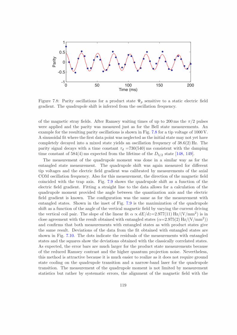
0 50 100 150 200-1

-0.5

0

0.5

1

Time (ms)

Pa

rity

Figure 7.8: Parity oscillations for a product state Ψp sensitive to a static electric fieldgradient. The quadrupole shift is inferred from the oscillation frequency.

of the magnetic stray fields. After Ramsey waiting times of up to 200 ms the π/2 pulseswere applied and the parity was measured just as for the Bell state measurements. Anexample for the resulting parity oscillations is shown in Fig. 7.8 for a tip voltage of 1000 V.A sinusoidal fit where the first data point was neglected as the initial state may not yet havecompletely decayed into a mixed state yields an oscillation frequency of 38.6(2) Hz. Theparity signal decays with a time constant τd =730(540) ms consistent with the dampingtime constant of 584(4) ms expected from the lifetime of the D5/2 state [148, 149].

The measurement of the quadrupole moment was done in a similar way as for theentangled state measurement. The quadrupole shift was again measured for differenttip voltages and the electric field gradient was calibrated by measurements of the axialCOM oscillation frequency. Also for this measurement, the direction of the magnetic fieldcoincided with the trap axis. Fig. 7.9 shows the quadrupole shift as a function of theelectric field gradient. Fitting a straight line to the data allows for a calculation of thequadrupole moment provided the angle between the quantization axis and the electricfield gradient is known. The configuration was the same as for the measurement withentangled states. Shown in the inset of Fig. 7.9 is the maximization of the quadrupoleshift as a function of the angle of the vertical magnetic field by varying the current drivingthe vertical coil pair. The slope of the linear fit α ∝ dE/dz=2.977(11) Hz/(V/mm2) is inclose agreement with the result obtained with entangled states (α=2.975(2) Hz/(V/mm2))and confirms that both measurements with entangled states as with product states givethe same result. Deviations of the data from the fit obtained with entangled states areshown in Fig. 7.10. The dots indicate the residuals of the measurements with entangledstates and the squares show the deviations obtained with the classically correlated states.As expected, the error bars are much larger for the product state measurements becauseof the reduced Ramsey contrast and the higher quantum projection noise. Nevertheless,this method is attractive because it is much easier to realize as it does not require groundstate cooling on the quadrupole transition and a narrow-band laser for the quadrupoletransition. The measurement of the quadrupole moment is not limited by measurementstatistics but rather by systematic errors, the alignment of the magnetic field with the

119

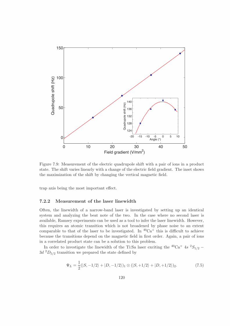
0 10 20 30 40 50

0

50

100

150

Field gradient (V/mm2)

Qu

ad

rup

ole

sh

ift

(Hz)

-20 -15 -10 -5 10

124

128

132

136

140

Angle (°)

Qu

adru

pole

shift

(Hz)

0 5

Figure 7.9: Measurement of the electric quadrupole shift with a pair of ions in a productstate. The shift varies linearly with a change of the electric field gradient. The inset showsthe maximization of the shift by changing the vertical magnetic field.

trap axis being the most important effect.

7.2.2 Measurement of the laser linewidth

Often, the linewidth of a narrow-band laser is investigated by setting up an identicalsystem and analyzing the beat note of the two. In the case where no second laser isavailable, Ramsey experiments can be used as a tool to infer the laser linewidth. However,this requires an atomic transition which is not broadened by phase noise to an extentcomparable to that of the laser to be investigated. In 40Ca+ this is difficult to achievebecause the transitions depend on the magnetic field in first order. Again, a pair of ionsin a correlated product state can be a solution to this problem.

In order to investigate the linewidth of the Ti:Sa laser exciting the 40Ca+ 4s 2S1/2 −3d 2D5/2 transition we prepared the state defined by

ΨL =1

2(|S,−1/2〉 + |D,−1/2〉)1 ⊗ (|S,+1/2〉 + |D,+1/2〉)2. (7.5)

120

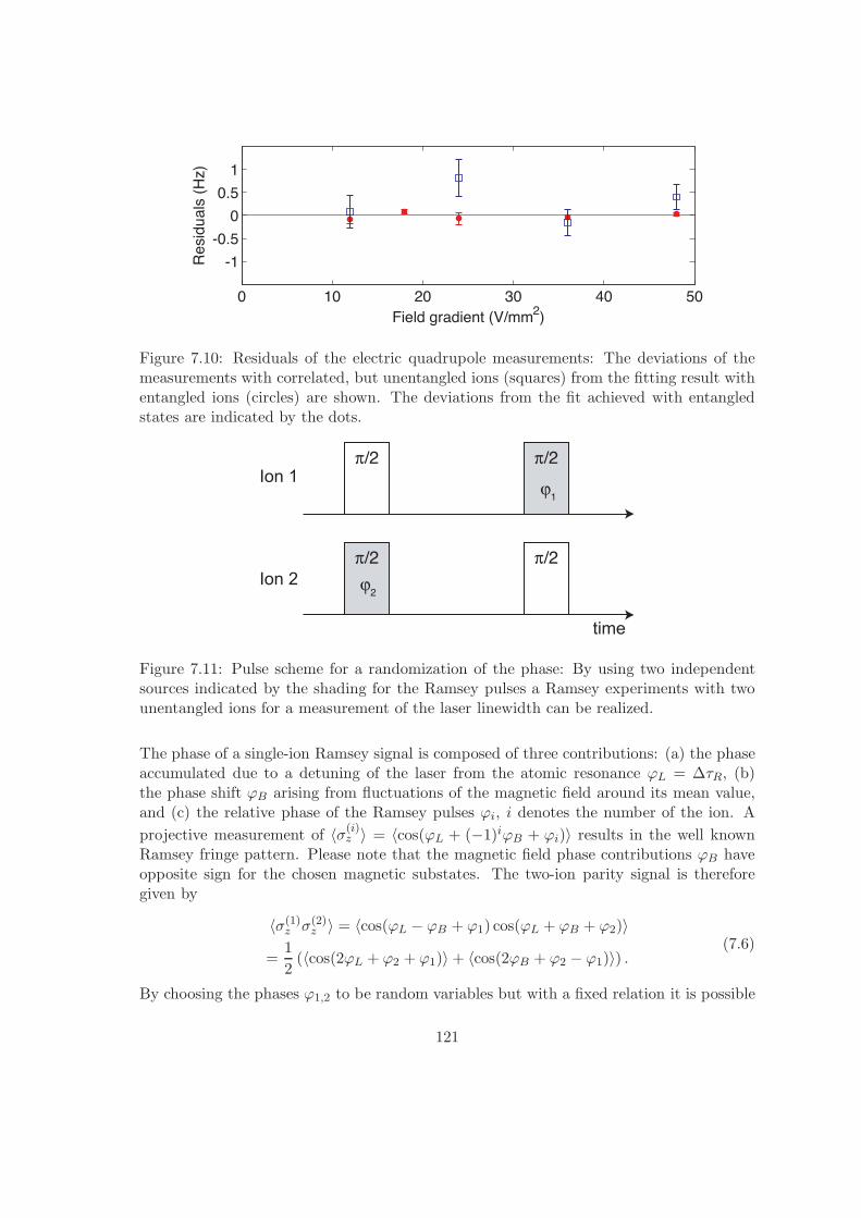
0 10 20 30 40 50

-1

-0.5

0

0.5

1

Field gradient (V/mm2)

Re

sid

ua

ls (

Hz)

Figure 7.10: Residuals of the electric quadrupole measurements: The deviations of themeasurements with correlated, but unentangled ions (squares) from the fitting result withentangled ions (circles) are shown. The deviations from the fit achieved with entangledstates are indicated by the dots.

π/2 π/2

π/2 π/2

ϕ1

time

Ion 1

Ion 2 ϕ2

Figure 7.11: Pulse scheme for a randomization of the phase: By using two independentsources indicated by the shading for the Ramsey pulses a Ramsey experiments with twounentangled ions for a measurement of the laser linewidth can be realized.

The phase of a single-ion Ramsey signal is composed of three contributions: (a) the phaseaccumulated due to a detuning of the laser from the atomic resonance ϕL = ∆τR, (b)the phase shift ϕB arising from fluctuations of the magnetic field around its mean value,and (c) the relative phase of the Ramsey pulses ϕi, i denotes the number of the ion. A

projective measurement of 〈σ(i)z 〉 = 〈cos(ϕL + (−1)iϕB + ϕi)〉 results in the well known

Ramsey fringe pattern. Please note that the magnetic field phase contributions ϕB haveopposite sign for the chosen magnetic substates. The two-ion parity signal is thereforegiven by

〈σ(1)z σ(2)

z 〉 = 〈cos(ϕL − ϕB + ϕ1) cos(ϕL + ϕB + ϕ2)〉

=1

2(〈cos(2ϕL + ϕ2 + ϕ1)〉+ 〈cos(2ϕB + ϕ2 − ϕ1)〉) .

(7.6)

By choosing the phases ϕ1,2 to be random variables but with a fixed relation it is possible

121

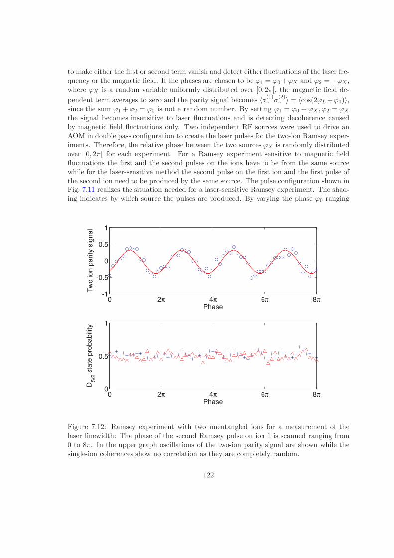
to make either the first or second term vanish and detect either fluctuations of the laser fre-quency or the magnetic field. If the phases are chosen to be ϕ1 = ϕ0 +ϕX and ϕ2 = −ϕX ,where ϕX is a random variable uniformly distributed over [0, 2π[, the magnetic field de-

pendent term averages to zero and the parity signal becomes 〈σ(1)z σ

(2)z 〉 = 〈cos(2ϕL +ϕ0)〉,

since the sum ϕ1 + ϕ2 = ϕ0 is not a random number. By setting ϕ1 = ϕ0 + ϕX , ϕ2 = ϕX

the signal becomes insensitive to laser fluctuations and is detecting decoherence causedby magnetic field fluctuations only. Two independent RF sources were used to drive anAOM in double pass configuration to create the laser pulses for the two-ion Ramsey exper-iments. Therefore, the relative phase between the two sources ϕX is randomly distributedover [0, 2π[ for each experiment. For a Ramsey experiment sensitive to magnetic fieldfluctuations the first and the second pulses on the ions have to be from the same sourcewhile for the laser-sensitive method the second pulse on the first ion and the first pulse ofthe second ion need to be produced by the same source. The pulse configuration shown inFig. 7.11 realizes the situation needed for a laser-sensitive Ramsey experiment. The shad-ing indicates by which source the pulses are produced. By varying the phase ϕ0 ranging

0 2π 4π 6π 8π-1

-0.5

0

0.5

1

Phase

Two

io

n p

arity

sig

na

l

0 2π 4π 6π 8π0

0.5

1

D5

/2 s

tate

pro

ba

bili

ty

Phase

Figure 7.12: Ramsey experiment with two unentangled ions for a measurement of thelaser linewidth: The phase of the second Ramsey pulse on ion 1 is scanned ranging from0 to 8π. In the upper graph oscillations of the two-ion parity signal are shown while thesingle-ion coherences show no correlation as they are completely random.

122

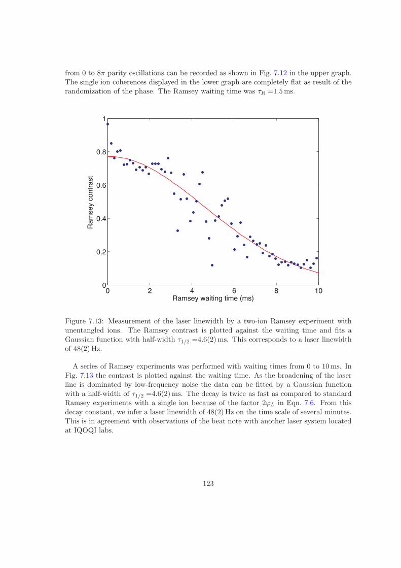
from 0 to 8π parity oscillations can be recorded as shown in Fig. 7.12 in the upper graph.The single ion coherences displayed in the lower graph are completely flat as result of therandomization of the phase. The Ramsey waiting time was τR =1.5 ms.

0 2 4 6 8 100

0.2

0.4

0.6

0.8

1

Ramsey waiting time (ms)

Ra

mse

y c

on

tra

st

Figure 7.13: Measurement of the laser linewidth by a two-ion Ramsey experiment withunentangled ions. The Ramsey contrast is plotted against the waiting time and fits aGaussian function with half-width τ1/2 =4.6(2) ms. This corresponds to a laser linewidthof 48(2) Hz.

A series of Ramsey experiments was performed with waiting times from 0 to 10 ms. InFig. 7.13 the contrast is plotted against the waiting time. As the broadening of the laserline is dominated by low-frequency noise the data can be fitted by a Gaussian functionwith a half-width of τ1/2 =4.6(2) ms. The decay is twice as fast as compared to standardRamsey experiments with a single ion because of the factor 2ϕL in Eqn. 7.6. From thisdecay constant, we infer a laser linewidth of 48(2) Hz on the time scale of several minutes.This is in agreement with observations of the beat note with another laser system locatedat IQOQI labs.

123

124

Chapter 8

Summary and outlook

In this thesis, precision spectroscopy with trapped 40Ca+ ions could be demonstrated.The absolute frequency of the 4s 2S1/2 − 3d 2D5/2 transition was measured to 1 Hz to-tal uncertainty with the help of a frequency comb referenced to a transportable cesiumfountain clock. It was clearly shown that correlated states, maximally entangled or evenclassically correlated, are suitable for high-resolution spectroscopy in the presence of anoisy environment if these states are designed such that they are immune against theseperturbations.

First, before starting spectroscopy experiments, an ultra-stable laser system had to beconstructed in order to be able to perform Hz-level measurements. The Ti:Sa laser usedfor this purpose was locked to a vertical reference cavity and short-term linewidths of wellbelow 10 Hz and a ∆νFWHM=40 Hz over more than one hour could be observed. Thefrequency drift of the reference cavity can be compensated by phase-contiuously switchingthe frequency applied to two double pass AOMs between the laser and the resonator.

The optical frequency was measured by a commercial frequency comb which was en-hanced for better operating stability. The repetition frequency and the carrier-envelope-offset frequency were stabilized to a radio frequency signal obtained from the mobile Csfountain clock FOM of LNE-SYRTE from Paris with an accuracy of better than 10−15. Bysimultaneous detection of the optical beat note from two independent lasers and compar-ison to the frequency comb readings of the two, cycle slips can be efficiently be detected.

The absolute frequency of the 40Ca+ 4s 2S1/2 − 3d 2D5/2 transition was measured toνCa+ =411 042 129 776 393.2 (1.0) Hz including a statistical uncertainty of the measurementof 0.5 Hz and the five largest systematic uncertainties of the Stark shift by black bodyradiation (0.7 Hz), the Cs uncertainty (<0.4 Hz), the cancellation of the linear Zeemaneffect and the quadrupole shift (0.2 Hz each), and the Stark shift by the cooling laser(0.1 Hz). A total systematic shift of 2.4 Hz was taken into account. This represents thefirst absolute frequency measurement of an optical transition applying Ramsey’s methodof separated fields at the 10−15 level. In addition, the spectroscopy data could be used for aprecise determination of the Lande g-factor of the D5/2 level g5/2 = 1.2003340±2.5×10−7 .

Processing quantum information is a field of research closely related to metrology: Byhigh-resolution spectroscopy with two 40Ca+ ions we have shown how Bell states can

125

be used for difference frequency measurements with sub-Hertz precision. Thereby, thequadrupole moment of the D5/2 level was determined to be Θ(3d, 5/2) =1.83(1) ea2

0 bydesigning a state insensitive to magnetic field noise. These experiments show that measure-ments with correlated ions prepared in decoherence-free subspaces allow for substantiallylonger coherence times than experiments limited by single-ion coherences. While the use ofentangled states achieves the optimum signal-to-noise ratio, substantial improvements canalready be obtained by experimenting with classically correlated but not entangled ions.Additional measurements of magnetic field gradients and the linewidth of the narrow-bandspectroscopy laser demonstrated the versatility of this method.

Possible improvements and further experiments

One of the goals of this thesis was the application of quantum information processingtechniques to precision metrology other than increasing signal-to-noise [60] or quantumstate readout [67]. For the development of an optical clock it appears realistic that anexperiment with Ca+ especially designed for metrology could lead to an accuracy of 10−17

or even better. Ca+ represents a technological alternative for an optical frequency standardbecause all required lasers including those for photo ionization can be generated by diodelasers and no deep-UV light with all its technical complications of the optical setup isnecessary.

Nevertheless, there are some improvements necessary to reach this level. As a firststep improved light attenuation with fast mechanical shutters would completely eliminateAC Stark shifts caused by the cooling and repumping lasers. Only the AC Stark shift ofthe probe laser during the Ramsey pulses would still exist but could be avoided by lowerexcitation power. Another minor improvement which could be immediately implementedconcerns the magnetic field drift. In order to eliminate a systematic frequency offsetcaused by a linear drift in the magnetic field, the transition frequencies would have to bemeasured in a different order.

Part of the largest errors of the error budget are statistical errors due to limited averagingtime. This has two reasons: one is the stability of the frequency comb and the otherthe stability of the clock laser itself. Improvement on both systems could substantiallyshorten the required measurement time. For the current stability of the frequency combit would take 84 (!) days to get down to < 10−16. The lock of the comb’s repetitionrate to the external reference needs improvement. This could be realized by choosinga higher harmonic of the repetition rate to increase the sensitivity and a more carefulway of generating the reference. On the probe laser side an improved cavity setup couldmake investigating systematic effects a lot more efficient by comparison of the two ion trapexperiments. At the moment it would take 5 days of averaging to reach the 0.1 Hz level. Alaser with 1Hz stability can get to 0.01 Hz in 10 000 s. Additionally, better laser stabilitywould allow for longer Ramsey waiting times and reduced averaging times due to quantumprojection noise. At the same time, lower power of the excitation pulses affordable due tolonger waiting time could improve on the Stark shift by the probe laser.

The most difficult improvement is related to the Stark shift by black body radiation. Adirect measurement of the trap temperature with the current setup is not possible. The

126

only possibility for a reduced error would require a frequency comparison of the two iontrap experiments at different trap RF powers but needs a laser with improved stabilityin order to keep the measurement time at a reasonable scale. An alternative would be acompletely new trap design with the possibility to measure the trap temperature exactly.Additionally, operating the trap in a cryogenic environment [45, 91] would dramaticallyreduce the frequency uncertainty due to the black body shift.

Employing entangled states for frequency measurements has been considered yet as ameans to improve the signal-to-noise ratio [61] and for read-out of the clock ion’s quantumstate [67]. States like Ψ =

∣

∣S1/2,mS

⟩ ∣

∣S1/2,−mS

⟩

+∣

∣D5/2,mD

⟩ ∣

∣D5/2,−mD

⟩

are to firstorder immune against magnetic field fluctuations and represent a kind of ”super-atom”especially designed for cancellation of the largest systematic effect in this system. Theycould be used for generalized Ramsey experiments with probe times limited only by theprobe laser stability and spontaneous decay of the metastable state and by averaging overall combinations of possible transitions, the electric quadrupole shift is cancelled as well.First tests with these states, however, revealed significant phase errors caused by changesin the optical path length when our electro-optical deflector is used to steer the beamfor addressing of individual ions. To overcome this problem, beam steering of a stronglyfocused laser could be avoided by generating high-fidelity entanglement [158] with a laserbeam collectively interacting with the ions, and combining this wide beam with a secondstrongly focused laser beam inducing phase shifts to make the ions distinguishable forcarrying out coherent operations on a single ion.

The same measurement principle could be applied for a measurement of the isotope shiftin an ion crystal consisting of different isotopes. Another possible application would be ameasurement of the tensor polarizability of theD levels by exposing the ions to a transversestatic field and a measurement of the quadratic Stark effect as presented in [163, 164]. Ithas been shown that Bell pairs of ions can be separated in a segmented trap withoutloss of coherence [165]. Then, one ion could be transported close to a surface/object andexperience a frequency shift induced by local electromagnetic fields acting as a microscopicsensor. Finally, a Bell state consisting of two ions with similar transition frequencies butdifferent dependence on fundamental constants might be interesting in the search for apossible time variation of fundamental constants.

127

128

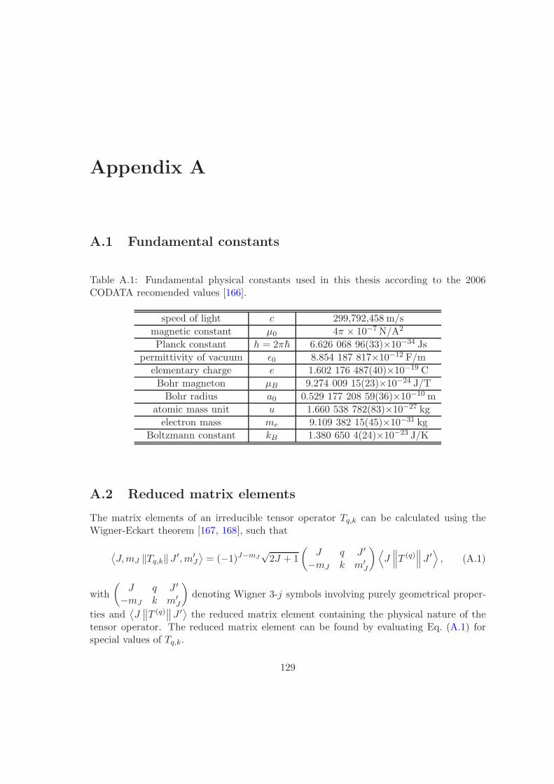
Appendix A

A.1 Fundamental constants

Table A.1: Fundamental physical constants used in this thesis according to the 2006CODATA recomended values [166].

speed of light c 299,792,458 m/s

magnetic constant µ0 4π × 10−7 N/A2

Planck constant h = 2π~ 6.626 068 96(33)×10−34 Js

permittivity of vacuum ǫ0 8.854 187 817×10−12 F/m

elementary charge e 1.602 176 487(40)×10−19 C

Bohr magneton µB 9.274 009 15(23)×10−24 J/T

Bohr radius a0 0.529 177 208 59(36)×10−10 m

atomic mass unit u 1.660 538 782(83)×10−27 kg

electron mass me 9.109 382 15(45)×10−31 kg

Boltzmann constant kB 1.380 650 4(24)×10−23 J/K

A.2 Reduced matrix elements

The matrix elements of an irreducible tensor operator Tq,k can be calculated using theWigner-Eckart theorem [167, 168], such that

⟨

J,mJ ‖Tq,k‖J ′,m′J

⟩

= (−1)J−mJ√

2J + 1

(

J q J ′

−mJ k m′J

)

⟨

J∥

∥

∥T (q)∥

∥

∥ J ′⟩

, (A.1)

with

(

J q J ′

−mJ k m′J

)

denoting Wigner 3-j symbols involving purely geometrical proper-

ties and⟨

J∥

∥T (q)∥

∥ J ′⟩ the reduced matrix element containing the physical nature of thetensor operator. The reduced matrix element can be found by evaluating Eq. (A.1) forspecial values of Tq,k.

129

In the case of the quadrupole operator Q2,k = r2C(2)k (θ, ϕ) with renormalized spherical

harmonics of the form C(l)m =

√

4π2l+1Yl,m(θ, ϕ), the reduced matrix element can be found

as

⟨

J,mJ

∥

∥

∥r2C(2)0

∥

∥

∥J ′,m′J

⟩

=

⟨

J,mJ

∥

∥

∥

∥

r23 cos2 θ − 1

2

∥

∥

∥

∥

J ′,m′J

⟩

= (−1)J−mJ√

2J + 1

(

J 2 J ′

−mJ 0 m′J

)

⟨

J∥

∥

∥r2C(2)

∥

∥

∥J ′

⟩

.

(A.2)

A.3 Effective Ramsey time

For ∆≪ ΩR and φ = 0 Eq. 2.47 can be expanded yielding

P (τ) = sin2(ΩRτ) +∆2

4Ω2R

sin(ΩRτ) [4(τ + τR)ΩR cos(ΩRτ)

−4τRΩR − (4 + τ2RΩ2

R sin(ΩRτ))]

+O(∆3)

=1

sin2(ΩRτ)

1 +∆2

4Ω2R

csc(ΩRτ) [4(τ + τR)ΩR cos(ΩRτ)

−4τRΩR − (4 + τ2RΩ2

R sin(ΩRτ))]

+O(∆3)

.

(A.3)

Under the condition ΩRτ ≈ π2 , this is reduced to

P (τ) = 1 +∆2

4Ω2R

(τ2R + 4τRΩR + 4) = 1 +

1

4

(

2∆

ΩR+ ∆τR

)2

. (A.4)

Because ∆→ 0, this can be further simplified to

P (τ) =1

2

[

1 + cos(∆(τR +2

ΩR))

]

=1

2

[

1 + cos(∆(τR +4τ

π))

]

, (A.5)

since ΩRτ = π2 .

130

Appendix B

Journal publications

The work of this thesis resulted in a number of publications:

1. ”Absolute frequency measurement of the 40Ca+ 4s 2S1/2−3d 2D5/2 clock transition”,M. Chwalla, J. Benhelm, K. Kim, G. Kirchmair, T. Monz, M. Riebe, P. Schindler,A. S. Villar, W. Hansel, C. F. Roos, R. Blatt, M. Abgrall, G. Santarelli, G. D.Rovera, Ph. Laurent, Phys. Rev. Lett. 102, 023002 (2009).

2. ”Precision spectroscopy with two correlated atoms”, M. Chwalla, K. Kim, T. Monz,P. Schindler, M. Riebe, C. F. Roos, R. Blatt, Appl. Phys. B 89, 483 (2007).

3. ”’Designer atoms’ for quantum metrology”, C. F. Roos, M. Chwalla, K. Kim, M.Riebe, and R. Blatt, Nature 443, 316 (2006).

Additional articles have been published related to the general context of this thesis:

4. ”Realization of the quantum Toffoli gate with trapped ions”, T. Monz, K. Kim, W.Hansel, M. Riebe, A. S. Villar, P. Schindler, M. Chwalla, M. Hennrich, R. Blatt,Phys. Rev. Lett. 102, 040501 (2009).

5. ”Deterministic entanglement swapping with an ion trap quantum computer”, M.Riebe, T. Monz, A. S. Villar, P. Schindler, M. Chwalla, M. Hennrich, R. Blatt,Nature Physics 4, 839 (2008).

6. ”Teleportation with atoms: quantum process tomography”, M. Riebe, M. Chwalla,J. Benhelm, H. Haffner, W. Hansel, C. F. Roos and R. Blatt, New J. Phys. 9, 211(2007).

7. ”Scalable multiparticle entanglement of trapped ions”, H. Haffner, W. Hansel, C. F.Roos, J. Benhelm, D. Chek-al-kar, M. Chwalla, T. Korber, U. D. Rapol, M. Riebe,P. O. Schmidt, C. Becher, O. Guhne, W. Dur and R. Blatt, Nature 438, 643 (2005).

8. ”Robust Entanglement”, H. Haffner, F. Schmidt-Kaler, W. Hansel, C.F. Roos, T.Korber, M. Chwalla, M. Riebe, J. Benhelm, U. D. Rapol, C. Becher, R. Blatt,Appl. Phys. B 81, 151 (2005).

131

132

Bibliography

[1] W. A. Marrison, The crystal clock, Proceedings of the National Academy of Sciencesof the United States of America 16, 496 (1930).

[2] N. F. Ramsey, History of atomic clocks, J. Res. Natl. Inst. Stand. Technol. 88, 301(1983).

[3] I. I. Rabi, J. R. Zacharias, S. Millman, and P. Kusch, A new method of measuringnuclear magnetic moments, Phys. Rev. 53, 318 (1938).

[4] N. F. Ramsey, A molecular beam resonance method with separated oscillating fields,Phys. Rev. 78, 695 (1950).

[5] J. Levine, Introduction to time and frequency metrology, Rev. Sci. Inst. 70, 2567(1999).

[6] H. J. Metcalf and P. van der Straten, Laser cooling and trapping, Springer, NewYork, 1999.

[7] W. D. Phillips, Nobel lecture: Laser cooling and trapping of neutral atoms,Rev. Mod. Phys. 70, 721 (1998).

[8] A. Clairon, C. Salomon, S. Guellati, and W. D. Phillips, Ramsey resonance in aZacharias fountain, Europhys. Lett. 16, 165 (1991).

[9] S. R. Jefferts, J. Shirley, T. E. Parker, T. P. Heavner, D. M. Meekhof, C. Nelson,F. Levi, G. Costanzo, A. D. Marchi, R. Drullinger, L. Hollberg, W. D. Lee, and F. L.Walls, Accuracy evaluation of NIST-F1, Metrologia 39, 321 (2002).

[10] S. Bize, P. Laurent, M. Abgrall, H. Marion, I. Maksimovic, L. Cacciapuoti,J. Grunert, C. Vian, F. dos Santos, P. Rosenbusch, P. Lemonde, G. Santarelli,P. Wolf, A. Clairon, A. Luiten, M. Tobar, and C. Salomon, Cold atom clocks andapplications, J. Phys. B 38, 449 (2005).

[11] R. Wynands and S. Weyers, Atomic fountain clocks, Metrologia 42, 64 (2005).

[12] A. Bauch, Caesium atomic clocks: function, performance and applications, Measure-ment Science and Technology 14, 1159 (2003).

133

[13] G. Santarelli, P. Laurent, P. Lemonde, A. Clairon, A. G. Mann, S. Chang, A. N.Luiten, and C. Salomon, Quantum projection noise in an atomic fountain: A highstability cesium frequency standard, Phys. Rev. Lett. 82, 4619 (1999).

[14] T. Udem, R. Holzwarth, and T. W. Hansch, Optical frequency metrology, Nature416, 233 (2002).

[15] J. L. Hall, Optical frequency measurement: 40 years of technology revolutions, IEEEJ. of Quant. Electron. 6, 1136 (2000).

[16] T. Rosenband, D. B. Hume, P. O. Schmidt, C. W. Chou, A. Brusch, L. Lorini, W. H.Oskay, R. E. Drullinger, T. M. Fortier, J. E. Stalnaker, S. A. Diddams, W. C. Swann,N. R. Newbury, W. M. Itano, D. J. Wineland, and J. C. Bergquist, Frequency ratioof Al+ and Hg+ single-ion optical clocks; Metrology at the 17th decimal place, Science319, 1808 (2008).

[17] A. D. Ludlow, T. Zelevinsky, G. K. Campbell, S. Blatt, M. M. Boyd, M. H. G.de Miranda, M. J. Martin, J. W. Thomsen, S. M. Foreman, J. Ye, T. M. Fortier,J. E. Stalnaker, S. A. Diddams, Y. Le Coq, Z. W. Barber, N. Poli, N. D. Lemke,K. M. Beck, and C. W. Oates, Sr lattice clock at 1× 10−16 fractional uncertainty byremote optical evaluation with a Ca clock, Science 319, 1805 (2008).

[18] W. H. Oskay, S. A. Diddams, E. A. Donley, T. M. Fortier, T. P. Heavner, L. Hollberg,W. M. Itano, S. R. Jefferts, M. J. Delaney, K. Kim, F. Levi, T. E. Parker, and J. C.Bergquist, Single-atom optical clock with high accuracy, Phys. Rev. Lett. 97, 020801(2006).

[19] T. Rosenband, P. Schmidt, D. Hume, W. Itano, T. Fortier, J. Stalnaker, K. Kim,S. Diddams, J. Koelemeij, J. Bergquist, and D. Wineland, Observation of the 1S0 −→3P0 clock transition in 27Al+, Phys. Rev. Lett. 98, 220801 (2007).

[20] J. Stenger, C. Tamm, N. Haverkamp, S. Weyers, and H. R. Telle, Absolute frequencymeasurement of the 435.5-nm 171Yb+ -clock transition with a Kerr-lens mode-lockedfemtosecond laser, Opt. Lett. 26, 1589 (2001).

[21] P. J. Blythe, S. A. Webster, H. S. Margolis, S. N. Lea, G. Huang, S.-K. Choi, W. R. C.Rowley, P. Gill, and R. S. Windeler, Sub-kilohertz absolute-frequency measurement ofthe 467-nm electric octupole transition in 171Yb+, Phys. Rev. A 67, 020501 (2003).

[22] J. von Zanthier, T. Becker, M. Eichenseer, A. Y. Nevsky, C. Schwedes, E. Peik,H. Walther, R. Holzwarth, J. Reichert, T. Udem, T. W. Hansch, P. V. Pokasov,M. N. Skvortsov, and S. N. Bagayev, Absolute frequency measurement of the In+

clock transition with a mode-locked laser, Opt. Lett. 25, 1729 (2000).

[23] H. S. Margolis, G. P. Barwood, G. Huang, H. A. Klein, S. N. Lea, K. Szymaniec, andP. Gill, Hertz-Level Measurement of the Optical Clock Frequency in a Single 88Sr+

Ion, Science 306, 1355 (2004).

134

[24] C. Champenois, M. Houssin, C. Lisowski, A. Knoop, G. Hagel, A. Vedel, andF. Vedel, Evaluation of the ultimate performances of a Ca+ single-ion frequencystandard, Phys. Lett. A 331, 298 (2004).

[25] M. Kajita, Y. Li, K. Matsubara, K. Hayasaka, and M. Hosokawa, Prospect of opticalfrequency standard based on a 43Ca+ ion, Phys. Rev. A 72, 3404 (2005).

[26] W. Paul and H. Steinwedel, Ein neues Massenspektrometer ohne Magnetfeld,Zeitschrift f. Naturforschung A 8, 448 (1953).

[27] R. F. Wuerker, H. Shelton, and R. V. Langmuir, Electrodynamic containment ofcharged particles, Journal of Applied Physics 30, 342 (1959).

[28] E. Schrodinger, Are there quantum jumps?: PART I*, Br J Philos Sci III, 109(1952).

[29] W. Neuhauser, M. Hohenstatt, P. E. Toschek, and H. Dehmelt, Localized visible Ba+

mono-ion oscillator, Phys. Rev. A 22, 1137 (1980).

[30] A. A. Madej and J. E. Bernard, Frequency measurement and control, chapter”Single-ion optical frequency standards and measurement of their absolute opticalfrequency”, pages 153–195, Springer, Berlin, 2001.

[31] D. J. Wineland and W. M. Itano, Laser cooling of atoms, Phys. Rev. A 21, 1521(1979).

[32] H. G. Dehmelt, Mono-ion oscillator as potential ultimate laser frequency standard,IEEE Trans. Instr. Meas. 31, 83 (1982).

[33] R. H. Dicke, The effect of collisions upon the doppler width of spectral lines,Phys. Rev. 89, 472 (1953).

[34] J. A. Abate, Preparation of atomic sodium as a two-level atom, Opt. Comm. 10,269 (1974).

[35] D. J. Wineland, J. C. Bergquist, W. M. Itano, and R. E. Drullinger, Double-resonance and optical-pumping experiments on electromagnetically confined, laser-cooled ions, Opt. Lett. 5, 254 (1980).

[36] W. Nagourney, J. Sandberg, and H. Dehmelt, Shelved optical electron amplifier:Observation of quantum jumps., Phys. Rev. Lett. 56, 2797 (1986).

[37] T. Sauter, W. Neuhauser, R. Blatt, and P. E. Toschek, Observation of quantumjumps, Phys. Rev. Lett. 57, 1696 (1986).

[38] J. C. Bergquist, R. G. Hulet, W. M. Itano, and D. J. Wineland, Observation ofquantum jumps in a single atom, Phys. Rev. Lett. 57, 1699 (1986).

135

[39] S. A. Diddams, J. C. Bergquist, S. R. Jefferts, and C. W. Oates, Standards of Timeand Frequency at the Outset of the 21st Century, Science 306, 1318 (2004).

[40] D. W. Allan, N. Ashby, and C. Hodge, The science of timekeeping, Hewlett-PackardApplication Note 1289 (1997).

[41] R. F. C. Vessot, M. W. Levine, E. M. Mattison, E. L. Blomberg, T. E. Hoffman,G. U. Nystrom, B. F. Farrel, R. Decher, P. B. Eby, C. R. Baugher, J. W. Watts,D. L. Teuber, and F. D. Wills, Test of relativistic gravitation with a space-bornehydrogen maser, Phys. Rev. Lett. 45, 2081 (1980).

[42] J. P. Turneaure, C. M. Will, B. F. Farrell, E. M. Mattison, and R. F. C. Vessot,Test of the principle of equivalence by a null gravitational red-shift experiment, Phys.Rev. D 27, 1705 (1983).

[43] S. Schiller, A. Gorlitz, A. Nevsky, J. C. J. Koelemeij, A. Wicht, P. Gill, H. A.Klein, H. S. Margolis, G. Mileti, U. Sterr, F. Riehle, E. Peik, C. Tamm, W. Ert-mer, E. Rasel, V. Klein, C. Salomon, G. M. Tino, P. Lemonde, R. Holzwarth, andT. Hansch, Optical clocks in space, Nuclear Physics B - Proceedings Supplements166, 300 (2007).

[44] H. Marion, F. P. D. Santos, M. Abgrall, S. Zhang, Y. Sortais, S. Bize, I. Maksimovic,D. Calonico, J. Grunert, C. Mandache, P. Lemonde, G. Santarelli, P. Laurent, andA. Clairon, Search for variations of fundamental constants using atomic fountainclocks, Phys. Rev. Lett. 90, 150801 (2003).

[45] S. Bize, S. Diddams, U. Tanaka, C. Tanner, W. H. Oskay, R. E. Drullinger,T. Parker, T. Heavner, S. R. Jefferts, L. Hollberg, W. Itano, and J. Bergquist, Test-ing the stability of fundamental constants with the 199Hg+ single-ion optical clock,Phys. Rev. Lett. 90, 150802 (2003).

[46] E. Peik, B. Lipphardt, H. Schnatz, T. Schneider, C. Tamm, and S. G. Karshen-boim, Limit on the present temporal variation of the fine structure constant,Phys. Rev. Lett. 93, 170801 (2004).

[47] J. Webb, M. Murphy, V. Flambaum, V. Dzuba, J. D. Barrow, C. Churchill,J. Prochaska, and A. Wolfe, Further evidence for cosmological evolution of the finestructure constant, Phys. Rev. Lett. 87, 091301 (2001).

[48] R. Srianand, H. Chand, P. Petitjean, and B. Aracil, Limits on the time variation ofthe electromagnetic fine-structure constant in the low energy limit from absorptionlines in the spectra of distant quasars, Phys. Rev. Lett. 92, 121302 (2004).

[49] R. Quast, D. Reimers, and S. A. Levshakov, Probing the variability of the fine-structure constant with the VLT/UVES, Astron. Astrophys. 415, L7 (2004).

136

[50] H. Chand, R. Srianand, P. Petitjean, B. Aracil, R. Quast, and D. Reimers, Variationof the fine-structure constant: very high resolution spectrum of QSO HE 0515-4414,Astron. Astrophys. 451, 45 (2006).

[51] A. Shlyakhter, Direct test of the constancy of fundamental nuclear constants, Nature264, 340 (1976).

[52] T. Damour and F. Dyson, The Oklo bound on the time variation of the fine-structureconstant revisited, Nucl. Phys. B 480, 37 (1996).

[53] Y. Fujii, A. Iwamoto, T. Fukahori, T. Ohnuki, M. Nakagawa, H. Hidaka, Y. Oura,and P. Moller, The nuclear interaction at Oklo 2 billion years ago, Nucl. Phys. B573, 377 (2000).

[54] S. K. Lamoreaux and J. R. Torgerson, Neutron moderation in the Oklo naturalreactor and the time variation of α, Phys. Rev. D 69, 121701 (2004).

[55] S. G. Karshenboim, Fundamental physical constants: Looking from different angles,Can. J. of Phys. 83, 767 (2005).

[56] P. Lemonde, P. Laurent, G. Santarelli, M. Abgrall, Y. Sortais, S. Bize, C. Nicolas,S. Zhang, A. Clairon, N. Dimareq, P. Petit, A. G. Mann, A. Luiten, S. Cheng, andC. Salomon, Frequency Measurement And Control Advanced Techniques And FutureTrends, chapter ”Cold-atom clocks on Earth and in space”, pages 131–152, Springer,Berlin, 2001.

[57] D. J. Wineland, J. C. Bergquist, T. Rosenband, P. O. Schmidt, W. M. Itano, J. J.Bollinger, D. Leibfried, and W. H. Oskay, Ion optical clocks and quantum informa-tion processing, in Proceedings of the 2003 IEEE International Frequency ControlSympposium and PDA Exhibition Jointly with the 17th European Frequency andTime Forum, pages 68–71, 2003.

[58] M. A. Nielsen and I. L. Chuang, Quantum Computation and Quantum Information,Cambridge Univ. Press, Cambridge, 2000.

[59] N. Gisin, G. Ribordy, W. Tittel, and H. Zbinden, Quantum cryptography, Rev. Mod.Phys. 74, 145 (2002).

[60] D. J. Wineland, J. J. Bollinger, W. M. Itano, and D. J. Heinzen, Squeezed atomicstates and projection noise in spectroscopy, Phys. Rev. A 50, 67 (1994).

[61] J. J. Bollinger, W. M. Itano, D. J. Wineland, and D. J. Heinzen, Optimal frequencymeasurements with maximally correlated states, Phys. Rev. A 54, R4649 (1996).

[62] V. Giovannetti, S. Lloyd, and L. Maccone, Quantum-Enhanced Measurements: Beat-ing the Standard Quantum Limit, Science 306, 1330 (2004).

[63] V. Giovannetti, S. Lloyd, and L. Maccone, Quantum metrology, Phys. Rev. Lett. 96,010401 (2006).

137

[64] V. Meyer, M. A. Rowe, D. Kielpinski, C. A. Sackett, W. M. Itano, C. Monroe,and D. J. Wineland, Experimental demonstration of entanglement-enhanced rotationangle estimation using trapped ions, Phys. Rev. Lett. 86, 5870 (2001).

[65] D. Leibfried, M. D. Barrett, T. Schatz, J. Britton, J. Chiaverini, W. M. Itano, J. D.Jost, C. Langer, and D. J. Wineland, Toward Heisenberg-limited spectroscopy withmultiparticle entangled states, Science 304, 1476 (2004).

[66] W. M. Itano, J. C. Bergquist, J. J. Bollinger, J. M. Gilligan, D. J. Heinzen, F. L.Moore, M. G. Raizen, and D. J. Wineland, Quantum projection noise: Populationfluctuations in two-level systems, Phys. Rev. A 47, 3554 (1993).

[67] P. O. Schmidt, T. Rosenband, C. Langer, W. M. Itano, J. C. Bergquist, and D. J.Wineland, Spectroscopy using quantum logic, Science 309, 749 (2005).

[68] T. Schatz, M. D. Barrett, D. Leibfried, J. Britton, J. Chiaverini, W. M. Itano, J. D.Jost, E. Knill, C. Langer, and D. J. Wineland, Enhanced quantum state detectionefficiency through quantum information processing, Phys. Rev. Lett. 94, 010501(2005).

[69] A. Widera, O. Mandel, M. Greiner, S. Kreim, T. W. Hansch, and I. Bloch, Entan-glement interferometry for precision measurement of atomic scattering properties,Phys Rev Lett 92, 160406 (2004).

[70] D. Kielpinski, V. Meyer, M. A. Rowe, C. A. Sackett, W. M. Itano, C. Monroe, andD. J. Wineland, A decoherence-free quantum memory using trapped ions, Science291, 1013 (2001).

[71] D. A. Lidar, I. L. Chuang, and K. B. Whaley., Decoherence-free subspaces for quan-tum computation, Phys. Rev. Lett. 81, 2594 (1998).

[72] C. F. Roos, G. P. T. Lancaster, M. Riebe, H. Haffner, W. Hansel, S. Gulde,C. Becher, J. Eschner, F. Schmidt-Kaler, and R. Blatt, Bell states of atoms withultralong lifetimes and their tomographic state analysis, Phys. Rev. Lett. 92, 220402(2004).

[73] C. F. Roos, Precision frequency measurements with entangled states,arXiv:quant-ph/0508148 (2005).

[74] B. K. Sahoo, M. R. Islam, B. P. Das, R. K. Chaudhuri, and D. Mukherjee, Lifetimesof the metastable 2D3/2,5/2 states in Ca+, Sr+, and Ba+, Phys. Rev. A 74, 062504(2006).

[75] J. Jin and D. A. Church, Precision lifetimes for the Ca+ 4p 2P levels: Experimentchallenges theory at the 1% level, Phys. Rev. Lett. 70, 3213 (1993).

[76] S.-S. Liaw, Ab initio calculation of the lifetimes of 4p and 3d levels of Ca+, Phys.Rev. A 51, R1723 (1995).

138

[77] R. Gerritsma, G. Kirchmair, F. Zahringer, J. Benhelm, R. Blatt, and C. F. Roos,Precision measurement of the branching fractions of the 4p 2P3/2 decay of Ca II,Eur. Phys. J. D 50, 13 (2008).

[78] Y. Ralchenko, A. E. Kramida, J. Reader, and N. A. Team, NIST atomic spectradatabase (version 3.1.5), http://physics.nist.gov/asd3, 2008.

[79] S. Gulde, Experimental realization of quantum gates and the Deutsch-Josza algo-rithm with trapped 40Ca+–ions, PhD thesis, Universitat Innsbruck, 2003.

[80] M. Riebe, Preparation of entangled states and quantum teleportation with atomicqubits, PhD thesis, Universitat Innsbruck, 2005.

[81] J. Benhelm, Experimental quantum-information processing with 43Ca+ ions, PhDthesis, University of Innsbruck, 2008.

[82] D. J. Berkeland, J. D. Miller, J. C. Bergquist, W. M. Itano, and D. J. Wineland,Minimization of ion micromotion in a Paul trap, J. App. Phys. 83, 5025 (1998).

[83] D. Leibfried, R. Blatt, C. Monroe, and D. Wineland, Quantum dynamics of singletrapped ions, Rev. Mod. Phys. 75, 281 (2003).

[84] C. F. Roos, Controlling the quantum state of trapped ions, PhD thesis, UniversitatInnsbruck, 2000.

[85] P. K. Ghosh, Ion traps, Oxford University Press, 1995.

[86] J. Vanier and C. Audoin, The Quantum Physics of Atomic Frequency Standards,IOP Publishing Ltd, 1989.

[87] R. Loudon, The Quantum Theory of Light, Oxford University Press, 3rd edition,2000.

[88] R. Grimm, M. Weidemuller, and Y. B. Ovchinnikov, Optical dipole traps for neutralatoms, Molecular and Optical Physics 42, 95 (2000).

[89] D. F. V. James, Quantum dynamics of cold trapped ions with application to quantumcomputation, Appl. Phys. B 66, 181 (1998).

[90] H. S. Freedhoff, Master equation for electric quadrupole transitions, Journal ofPhysics B Atomic Molecular Physics 22, 435 (1989).

[91] W. M. Itano, External-field shifts of the 199Hg+ optical frequency standard,J. Res. Natl. Inst. Stand. Technol. 105, 829 (2000).

[92] I. I. Sobelman, Atomic Spectra and Radiative Transitions, pages 74–88, Springer-Verlag, 1992.

[93] C. A. Blockley, D. F. Walls, and H. Risken, Quantum collapses and revivals in aquantized trap, Europhys. Lett. 17, 509 (1992).

139

[94] E. T. Jaynes and F. W. Cummings, Comparison of quantum and semiclassical ra-diation theories with application to the beam maser, Proceedings of IEEE 51, 89(1963).

[95] B. W. Shor and P. L. Knight, The Jaynes-Cummings model, J. Mod. Opt. 40, 1195(1993).

[96] R. P. Feynman, F. L. Vernon, and R. W. Hellwarth, Geometrical representation ofthe Schrodinger equation for solving the maser problem, J. App. Phys. 28, 65 (1957).

[97] T. Mayer-Kuckuk, Atomphysik: Eine Einfuhrung, page 123, Teubner-Verlag, 1994.

[98] G. Tommaseo, T. Pfeil, G. Revalde, G. Werth, P. Indelicato, and J. Desclaux, ThegJ-factor in the ground state of Ca+, Eur. Phys. J. D 25, 113 (2003).

[99] I. I. Sobelman, Atomic Spectra and Radiative Transitions, pages 189–199, Springer-Verlag, 1992.

[100] A. Bauch and R. Schroder, Experimental verification of the shift of the cesium hy-perfine transition frequency due to blackbody radiation, Phys. Rev. Lett. 78, 622(1997).

[101] A. A. Madej, J. E. Bernard, P. Dube, L. Marmet, and R. S. Windeler, Absolutefrequency of the 88Sr+5s 2S1/2 − 4d 2D5/2 reference transition at 445 THz and eval-uation of systematic shifts, Phys. Rev. A 70, 012507 (2004).

[102] W. M. Itano, Quadrupole moments and hyperfine constants of metastable states ofCa+, Sr+, Ba+, Yb+, Hg+, and Au, Phys. Rev. A 73, 022510 (2006).

[103] C. Sur, K. V. P. Latha, B. K. Sahoo, R. K. Chaudhuri, B. P. Das, and D. Mukher-jee, Electric quadrupole moments of the d states of alkaline-earth-metal ions,Phys. Rev. Lett. 96, 193001 (2006).

[104] D. Jiang, B. Arora, and M. S. Safronova, Electric quadrupole moments of metastablestates of Ca+, Sr+, and Ba+, Phys. Rev. A 78, 022514 (2008).

[105] J. Mitroy and J. Y. Zhang, Long range interactions of the Mg+ and Ca+ ions,Eur. Phys. J. D 46, 415 (2008).

[106] D. Rotter, Photoionisation von Kalzium, Diploma thesis, Universitat Innsbruck,2003.

[107] H. Rohde, Experimente zur Quanteninformationsverarbeitung in einer linearenPaulfalle, PhD thesis, Universitat Innsbruck, 2001.

[108] G. Kirchmair, Frequency stabilization of a Titanium-Sapphire laser for precisionspectroscopy on Calcium ions, Diploma thesis, Universitat Innsbruck, 2007.

140

[109] B. Young, F. Cruz, W. Itano, and J. Bergquist, Visible lasers with subhertzlinewidths, Phys. Rev. Lett. 82, 3799 (1999).

[110] M. Notcutt, L.-S. Ma, J. Ye, and J. L. Hall, Simple and compact 1-Hz laser systemvia an improved mounting configuration of a reference cavity, Opt. Lett. 30, 1815(2005).

[111] H. Stoehr, F. Mensing, J. Helmcke, and U. Sterr, Diode laser with 1 Hz linewidth,Opt. Lett. 31, 736 (2006).

[112] A. D. Ludlow, X. Huang, M. Notcutt, T. Zanon-Willette, S. M. Foreman, M. M.Boyd, S. Blatt, and J. Ye, Compact, thermal-noise-limited optical cavity for diodelaser stabilization at 1× 10−15, Opt. Lett. 32, 641 (2007).

[113] G. P. Barwood, P. Gill, G. Huang, and H. A. Klein, Observation of a sub-10-Hzlinewidth 88Sr+ 2S1/2-

2D5/2 clock transition at 674 nm, IEEE Trans. Instr. Meas.56, 226 (2007).

[114] J. Alnis, A. Matveev, N. Kolachevsky, T. Udem, and T. W. Hansch, Sub-Hertzlinewidth with diode lasers by stabilization to vibrationally and thermally compen-sated ULE Fabry-Perot cavities, Phys. Rev. A 77, 053809 (2008).

[115] B. E. A. Saleh and M. C. Teich, Fundamentals of Photonics, Wiley, New York,1991.

[116] T. W. Hansch and B. Couillaud, Laser frequency stabilization by polarization spec-troscopy of a reflecting reference cavity, Opt. Comm. 35, 441 (1980).

[117] L.-S. Ma, P. Jungner, J. Ye, and J. L. Hall, Delivering the same optical frequencyat two places: accurate cancellation of phase noise introduced by an optical fiber orother time-varying path, Opt. Lett. 19, 1777 (1994).

[118] J. Benhelm, G. Kirchmair, U. Rapol, T. Korber, C. F. Roos, and R. Blatt, Measure-ment of the hyperfine structure of the S1/2-D5/2 transition in 43Ca+, Phys. Rev. A75, 032506 (2007).

[119] F. Riehle, Frequency Standards, pages 50–54, Wiley-VCH,Weinheim, 2004.

[120] J. Reichert, M. Niering, R. Holzwarth, M. Weitz, T. Udem, and T. Hansch, Phasecoherent vacuum-ultraviolet to radio frequency comparison with a mode-locked laser,Phys. Rev. Lett. 84, 3232 (1999).

[121] S. A. Diddams, D. J. Jones, J. Ye, S. T. Cundiff, J. L. Hall, J. K. Ranka, R. S.Windeler, R. Holzwarth, T. Udem, and T. W. Hansch, Direct link between microwaveand optical frequencies with a 300 thz femtosecond laser comb, Phys. Rev. Lett. 84,5102 (2000).

141

[122] T. Udem, J. Reichert, R. Holzwarth, and T. W. Hansch, Absolute optical frequencymeasurement of the cesium D1 line with a mode-locked laser, Phys. Rev. Lett. 82,3568 (1999).

[123] M. Niering, R. Holzwarth, J. Reichert, P. Pokasov, T. Udem, M. Weitz, T. W.Hansch, P. Lemonde, G. Santarelli, M. Abgrall, P. Laurent, C. Salomon, and A. Cla-iron, Measurement of the hydrogen 1S-2S transition frequency by phase coherent com-parison with a microwave cesium fountain clock, Phys. Rev. Lett. 84, 5496 (2000).

[124] M. Hentschel, R. Kienberger, C. Spielmann, G. A. Reider, N. Milosevic, T. Brabec,P. Corkum, U. Heinzmann, M. Drescher, and F. Krausz, Attosecond metrology, Na-ture 414, 509 (2001).

[125] A. Baltuska, T. Udem, M. Uiberacker, M. Hentschel, E. Goulielmakis, C. Gohle,R. Holzwarth, V. S. Yakovlev, A. Scrinzi, T. W. Hansch, and F. Krausz, Attosecondcontrol of electronic processes by intense light fields, Nature 421, 611 (2003).

[126] R. Kienberger, E. Goulielmakis, M. Uiberacker, A. Baltuska, V. Yakovlev, F. Bam-mer, A. Scrinzi, T. Westerwalbesloh, U. Kleineberg, U. Heinzmann, M. Drescher,and F. Krausz, Atomic transient recorder, Nature 427, 817 (2004).

[127] G. Sansone, E. Benedetti, F. Calegari, C. Vozzi, L. Avaldi, R. Flammini, L. Poletto,P. Villoresi, C. Altucci, R. Velotta, S. Stagira, S. De Silvestri, and M. Nisoli, IsolatedSingle-Cycle Attosecond Pulses, Science 314, 443 (2006).

[128] T. Fuji, J. Rauschenberger, C. Gohle, A. Apolonski, T. Udem, V. S. Yakovlev,G. Tempea, T. W. Hansch, and F. Krausz, Attosecond control of optical waveforms,New J. Phys. 7, 116 (2005).

[129] A. L. Cavalieri, N. Muller, T. Uphues, V. S. Yakovlev, A. Baltuska, B. Horvath,B. Schmidt, L. Blumel, R. Holzwarth, S. Hendel, M. Drescher, U. Kleineberg, P. M.Echenique, R. Kienberger, F. Krausz, and U. Heinzmann, Attosecond spectroscopyin condensed matter, Nature 449, 1029 (2007).

[130] T. Steinmetz, T. Wilken, C. Araujo-Hauck, R. Holzwarth, T. W. Hansch,L. Pasquini, A. Manescau, S. D’Odorico, M. T. Murphy, T. Kentischer, W. Schmidt,and T. Udem, Laser Frequency Combs for Astronomical Observations, Science 321,1335 (2008).

[131] H. Schnatz, B. Lipphardt, J. Helmcke, F. Riehle, and G. Zinner, First phase-coherentfrequency measurement of visible radiation, Phys. Rev. Lett. 76, 18 (1996).

[132] S. T. Cundiff and J. Ye, Colloquium: Femtosecond optical frequency combs,Rev. Mod. Phys. 75, 325 (2003).

[133] T. Udem and F. Riehle, Frequency combs applications and optical frequency stan-dards, in Metrology and Fundamental Constants, edited by T. W. Hansch, S. Leschi-utta, A. J. Wallard, and M. L. Rastello, Proceedings of the International School

142

of Physics “Enrico Fermi”, Course CLXVI, pages 317–365, Amsterdam, 2007, IOSPress.

[134] R. Szipocs, K. Ferencz, C. Spielmann, and F. Krausz, Chirped multilayer coatingsfor broadband dispersion control in femtosecond lasers, Opt. Lett. 19, 201 (1994).

[135] F. Salin, J. Squier, and M. Piche, Mode locking of Ti:Ai2O3 lasers and self-focusing:a Gaussian approximation, Opt. Lett. 16, 1674 (1991).

[136] T. Brabec, C. Spielmann, P. F. Curley, and F. Krausz, Kerr lens mode locking, Opt.Lett. 17, 1292 (1992).

[137] F. X. Kartner and U. Keller, Stabilization of solitonlike pulses with a slow saturableabsorber, Opt. Lett. 20, 16 (1995).

[138] P. Russell, Photonic Crystal Fibers, Science 299, 358 (2003).

[139] G. P. Agrawal, Nonlinear Fiber Optics, Academic Press, New York, 2006.

[140] H. R. Telle, G. Steinmeyer, A. E. Dunlop, J. Stenger, D. H. Sutter, and U. Keller,Carrier-envelope offset phase control: A novel concept for absolute optical frequencymeasurement and ultrashort pulse generation, Appl. Phys. B 69, 327 (1999).

[141] R. Holzwarth, T. Udem, T. W. Hansch, J. C. Knight, W. J. Wadsworth, and P. S. J.Russell, Optical frequency synthesizer for precision spectroscopy, Phys. Rev. Lett.85, 2264 (2000).

[142] J. K. Ranka, R. S. Windeler, and A. J. Stentz, Visible continuum generation in air-silica microstructure optical fibers with anomalous dispersion at 800 nm, Opt. Lett.25, 25 (2000).

[143] D. J. Jones, S. A. Diddams, J. K. Ranka, A. Stentz, R. S. Windeler, J. L. Hall, andS. T. Cundiff, Carrier-envelope phase control of femtosecond mode-locked lasers anddirect optical frequency synthesis, Science 288, 635 (2000).

[144] K. W. Holman, R. J. Jones, A. Marian, S. T. Cundiff, and J. Ye, Intensity-relateddynamics of femtosecond frequency combs, Opt. Lett. 28, 851 (2003).

[145] P. Schindler, Frequency synthesis and pulse shaping for quantum information pro-cessing with trapped ions, Diploma thesis, Universitat Innsbruck, 2008.

[146] E. Peik, T. Schneiderl, and C. Tamm, Laser frequency stabilization to a single ion,J. Phys. B: At. Mol. Opt. Phys. 39, 145 (2006).

[147] H. Haffner, S. Gulde, M. Riebe, G. Lancaster, C. Becher, J. Eschner, F. Schmidt-Kaler, and R. Blatt, Precision measurement and compensation of optical Stark shiftsfor an ion-trap quantum processor, Phys. Rev. Lett. 90, 143602 (2003).

143

[148] P. A. Barton, C. J. S. Donald, D. M. Lucas, D. A. Stevens, A. M. Steane, and D. N.Stacey, Measurement of the lifetime of the 3d 2D5/2 state in 40Ca+, Phys. Rev. A62, 032503 (2000).

[149] A. Kreuter, C. Becher, G. P. T. Lancaster, A. B. Mundt, C. Russo, H. Haffner,C. Roos, W. Hansel, F. Schmidt-Kaler, R. Blatt, and M. S. Safronova, Experimentaland theoretical study of the 3d 2D–level lifetimes of 40Ca+, Phys. Rev. A 71, 032504(2005).

[150] H. Haffner, F. Schmidt-Kaler, W. Hansel, C. F. Roos, T. Korber, M. Chwalla,M. Riebe, J. Benhelm, U. D. Rapol, C. Becher, and R. Blatt, Robust entanglement,Appl. Phys. B 81, 151 (2005).

[151] W. M. Itano, L. L. Lewis, and D. J. Wineland, Shift of 2S1/2 hyperfine splittings dueto blackbody radiation, Phys. Rev. A 25, 1233 (1982).

[152] B. Arora, M. S. Safronova, and C. W. Clark, Blackbody-radiation shift in a 43Ca+

ion optical frequency standard, Phys. Rev. A 76, 064501 (2007).

[153] T. Weinold, private communication, Institut fur Geodasie, Universitat Innsbruck,2007.

[154] G. D. Rovera, M. Abgrall, and P. Laurent, private communication.

[155] K. Matsubara, K. Hayasaka, Y. Li, H. Ito, S. Nagano, M. Kajita, and M. Hosokawa,Frequency measurement of the optical clock transition of 40Ca+ ions with an uncer-tainty of 10−14 level, Appl. Phys. Express 1, 067011 (2008).

[156] D. Leibfried, B. DeMarco, V. Meyer, D. Lucas, M. Barrett, J. Britton, W. M.Itano, B. Jelenkovic, C. Langer, T. Rosenband, and D. J. Wineland, Experimentaldemonstration of a robust, high-fidelity geometric two ion-qubit phase gate, Nature422, 412 (2003).

[157] F. Schmidt-Kaler, H. Haffner, M. Riebe, S. Gulde, G. P. T. Lancaster, T. Deuschle,C. Becher, C. F. Roos, J. Eschner, and R. Blatt, Realization of the Cirac-Zollercontrolled-NOT quantum gate, Nature 422, 408 (2003).

[158] J. Benhelm, G. Kirchmair, C. F. Roos, and R. Blatt, Towards fault-tolerant quantumcomputing with trapped ions, Nat. Phys. 4, 463 (2008).

[159] D. Leibfried, E. Knill, S. Seidelin, J. Britton, R. B. Blakestad, J. Chiaverini, D. B.Hume, W. M. Itano, J. D. Jost, C. Langer, R. Ozeri, R. Reichle, and D. J. Wineland,Creation of a six–atom ’Schrodinger cat’ state, Nature 438, 639 (2005).

[160] H. Haffner, W. Hansel, C. F. Roos, J. Benhelm, D. Chek-al-Kar, M. Chwalla,T. Korber, U. D. Rapol, M. Riebe, P. O. Schmidt, C. Becher, O. Guhne, W. Dur,and R. Blatt, Scalable multiparticle entanglement of trapped ions, Nature 438, 643(2005).

144

[161] J. J. . Bollinger, W. M. Itano, D. J. Wineland, and D. J. Heinzen, Optimal frequencymeasurements with maximally correlated states, Phys. Rev. A 54, R4649 (1996).

[162] D. J. Wineland, J. J. Bollinger, W. M. Itano, F. L. Moore, and D. J. Heinzen,Spin squeezing and reduced quantum noise in spectroscopy, Phys. Rev. A 46, R6797(1992).

[163] T. Schneider, E. Peik, and C. Tamm, Sub-Hertz optical frequency comparisons be-tween two trapped 171Y b+ ions, Phys. Rev. Lett. 94, 230801 (2005).

[164] N. Yu, X. Zhao, H. Dehmelt, and W. Nagourney, Stark shift of a single barium ionand potential application to zero-point confinement in a rf trap, Phys. Rev. A 50,2738 (1994).

[165] M. D. Barrett, J. Chiaverini, T. Schatz, J. Britton, W. M. Itano, J. D. Jost, E. Knill,C. Langer, D. Leibfried, R. Ozeri, and D. J. Wineland, Deterministic quantum tele-portation of atomic qubits, Nature 429, 737 (2004).

[166] P. J. Mohr, B. N. Taylor, and D. B. Newell, CODATA recommended values forfundamental physical constants, Rev. Mod. Phys. 80, 633 (2008).

[167] E. Wigner, Einige Folgerungen aus der Schrodingerschen Theorie fur die Termstruk-turen, Z. Phys. 43, 624 (1927).

[168] C. Eckart, The application of group theory to the quantum dynamics of monatomicsystems, Rev. Mod. Phys. 2, 305 (1930).

145

146

Danksagung

Die Erstellung dieser Arbeit ware ohne die Unterstutzung und Hilfe zahlreicher Kollegennicht moglich gewesen, weshalb ich mich bei allen Beteiligten recht herzlich bedankenmochte.

An erster Stelle steht naturlich Prof. Rainer Blatt, der mir die Moglichkeit gegebenhat, nach der Diplomarbeit auch meine Dissertation in seiner Arbeitsgruppe und demwunderbaren Umfeld fur Quantenoptik an der Universitat Innsbruck anfertigen zu konnen.

For the measurement involving the Cs fountain clock from LNE-SYRTE, I’d especiallylike to thank Michel Abgrall, Daniele Rovera and Philippe Laurent for their phenomenaleffort in the realization of the absolute frequency measurement even though Hertz carrental and a hungry beech marten made the journey with the Cs clock from Paris toInnsbruck and back a lot more exciting than expected.

Bei Christian Roos mochte ich mich sowohl fur die erfolgreiche Zusammenarbeit amExperiment, als auch fur seine Hilfe bei theoretischen Problemen bedanken, allem voranseine Korrekturen zu meiner Doktorarbeit. Wolfgang Hansel danke ich fur unermudliches,nachtelanges Programmieren an unserer Experiment-Steuerung und seine Hartnackigkeit,ohne die so manche wichtige Messung unter den Tisch gefallen ware. Ebenso danke ichHartmut Haffner fur erfolgreiche Messungen, aufregende Skitouren und kritische Kom-mentare sowie Piet Schmidt fur zahlreiche Tips bei Frequenzmessung bzw. Laserstabili-sierung, und fur wertvolle Kommentare bei der Erstellung des PRL-Artikels.

Besonders großer Dank gilt den tapferen und unerschutterlichen Mit-Meßknechten am40Ca+-Experiment Kihwan Kim, Thomas Monz, Mark Riebe, Philipp Schindler, Alessan-dro Villar sowie der 43Ca+ Crew mit Gerhard Kirchmair und Jan Benhelm, ohne derenEinsatz zu jeder Tages- und Nachtzeit der Arbeitsaufwand nicht zu bewaltigen gewesenware. Die heiteren Gesprache, mit Tommy, Philipp und Mark weit nach Mitternacht amLaborrechner lummelnd, werden mir in lebhafter Erinnerung bleiben. Mein erfurchtigerRespekt gebuhrt selbstverstandlich auch Daniel Rotter, einem stolzen Trager der silbernenMensa-Nadel mit Band.

Naturlich braucht eine erfolgreiche Arbeit ein entsprechendes privates Umfeld. Des-halb mochte ich mich an dieser Stelle bei meiner Familie und ganz besonders bei meinerFreundin Evi bedanken, die mir - nicht nur - in schwierigen Zeiten und wahrend der zweiWochen Marathonmessung fur die 40Ca+ Absolutfrequenz immer zur Seite gestanden sind.

Schließlich ist auch die lastige Frage beantwortet, wann ich denn nun endlich fertigsei. . .

147