Precipitation variability and changes in the greater Alpine region over the 1800–2003 period

Precipitation variability and changes in the greater Alpine region over

the 1800–2003 period

Michele Brunetti,1 Maurizio Maugeri,2 Teresa Nanni,1 Ingeborg Auer,3 Reinhard Bohm,3

and Wolfgang Schoner3

Received 14 September 2005; revised 17 January 2006; accepted 15 February 2006; published 7 June 2006.

[1] The paper investigates precipitation variability in the greater Alpine region (GAR)(4–19�E, 43–49�N) based on 192 instrumental series of homogenized and outlier checkedmonthly precipitation and on the 1� gridded version of the same data set. Compared to theprevious data sets, the one used in this paper adds a full century of data (earliest seriesstarting in 1800) by exploiting the early instrumental period as much as possible in termsof series length and spatial density. The records were clustered into climaticallyhomogeneous subregions, by means of a principal component analysis, and averagesubregional series were calculated. The principal component analysis was applied also inT-mode to investigate the most recursive precipitation patterns that characterize theexamined area. Yearly and seasonal trend analysis was performed both on subregionalaverage series and on the mean GAR series. It was also applied to moving windows, ofvariable width ranging from 2 decades to 2 centuries, in order to investigate any trendsover decadal to secular timescales. Beside trends in total precipitation, precipitationseasonality was also analyzed as an important indicator of climate changes. Links betweenprecipitation variability in the Alpine region and atmospheric circulation, and the NorthAtlantic Oscillation in particular, were also studied.

Citation: Brunetti, M., M. Maugeri, T. Nanni, I. Auer, R. Bohm, and W. Schoner (2006), Precipitation variability and changes in the

greater Alpine region over the 1800–2003 period, J. Geophys. Res., 111, D11107, doi:10.1029/2005JD006674.

1. Introduction

[2] The European Alps and their surroundings constitutean important and interesting study region for climate vari-ability, because of their unique data availability, and becauseof their geographical position at the transition among someprincipal continental-scale climate regimes. The instrumen-tal data potential is specifically unique here, in particular asfar as the coverage of the early instrumental period (pre1850) is concerned. Past years’ activities under the umbrellaof ‘‘HISTALP’’ [Auer et al., 2006] have considerablyimproved the availability and quality of long-term climatedata and metadata. This database covers the Alps and theirwider surroundings (4–19�E, 43–49�N), which will bereferred to as GAR (greater Alpine region). The Alpsconstitute the most relevant topographic ridge of Europe,and influence atmospheric circulation on a wide range ofscales. As a consequence of its complex geography, theregion exhibits a variety of different climates, ranging frommaritime influences (both from the Mediterranean Sea andthe Atlantic Ocean) to continental features (such as theplains of eastern Europe and the inner Alpine valleys), and

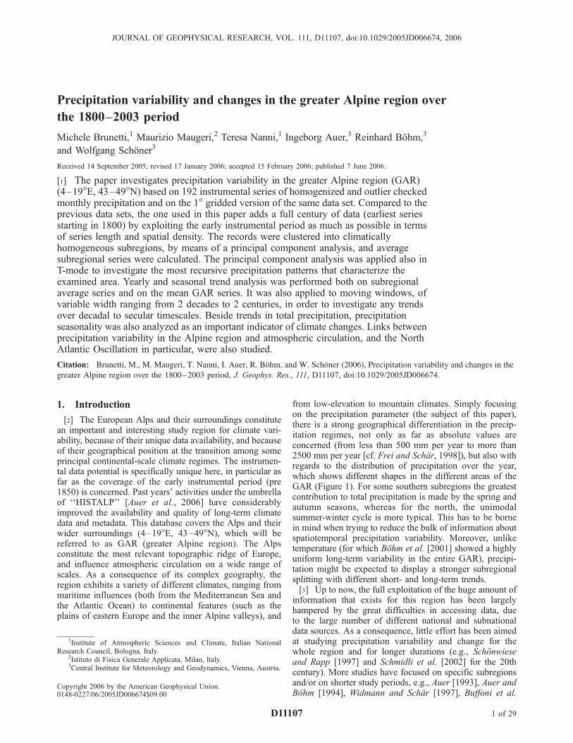
from low-elevation to mountain climates. Simply focusingon the precipitation parameter (the subject of this paper),there is a strong geographical differentiation in the precip-itation regimes, not only as far as absolute values areconcerned (from less than 500 mm per year to more than2500 mm per year [cf. Frei and Schar, 1998]), but also withregards to the distribution of precipitation over the year,which shows different shapes in the different areas of theGAR (Figure 1). For some southern subregions the greatestcontribution to total precipitation is made by the spring andautumn seasons, whereas for the north, the unimodalsummer-winter cycle is more typical. This has to be bornein mind when trying to reduce the bulk of information aboutspatiotemporal precipitation variability. Moreover, unliketemperature (for which Bohm et al. [2001] showed a highlyuniform long-term variability in the entire GAR), precipi-tation might be expected to display a stronger subregionalsplitting with different short- and long-term trends.[3] Up to now, the full exploitation of the huge amount of

information that exists for this region has been largelyhampered by the great difficulties in accessing data, dueto the large number of different national and subnationaldata sources. As a consequence, little effort has been aimedat studying precipitation variability and change for thewhole region and for longer durations (e.g., Schonwieseand Rapp [1997] and Schmidli et al. [2002] for the 20thcentury). More studies have focused on specific subregionsand/or on shorter study periods, e.g., Auer [1993], Auer andBohm [1994], Widmann and Schar [1997], Buffoni et al.

JOURNAL OF GEOPHYSICAL RESEARCH, VOL. 111, D11107, doi:10.1029/2005JD006674, 2006

1Institute of Atmospheric Sciences and Climate, Italian NationalResearch Council, Bologna, Italy.

2Istituto di Fisica Generale Applicata, Milan, Italy.3Central Institute for Meteorology and Geodynamics, Vienna, Austria.

Copyright 2006 by the American Geophysical Union.0148-0227/06/2005JD006674$09.00

D11107 1 of 29

[1999], Auer et al. [2001], Moisselin et al. [2002], Brunettiet al. [2004, 2006], Begert et al. [2005], and others. Theiranalyses provided different results for the different subre-gions, in particular when yearly and seasonal precipitationtrends were considered. In many cases the comparison ofthe results is complicated by differences in methodologiesand temporal extent of the analyzed period.[4] Within this context, the aim of our research was to

analyze the recently finished HISTALP data set of in situsecular GAR precipitation records. This is the firstcomprehensive data set for the region that allows aconsistent reconstruction of the evolution of precipitationover the last 2 centuries. The technical points of itsconstruction stages (homogeneity, outliers detection andadjustment, gap-filling, metadata, general quality, evolu-tion of network density) were described in detail by Aueret al. [2005]. It may be regarded as the logical ‘‘part 1’’of our paper, which presents the principal results of theanalysis of the Auer et al. [2005] data set, which is onlybriefly presented in section 2. Sections 3 and 4 giveinformation on the clustering of the series into homoge-neous subregions, and show the results of principalcomponent analysis, performed both in S and in T-mode.The evolution of yearly and seasonal subregional averageprecipitation records is then presented in section 5, wheretrend analysis is also discussed. Section 6 presents somedetails on the differences between the northern and thesouthern parts of the GAR and between its western andeastern parts, whereas section 7 gives some details on thetime evolution of the precipitation seasonality. Finally,

section 8 presents the correlation between GAR precipi-tation and the well-known North Atlantic OscillationIndex.

2. Data

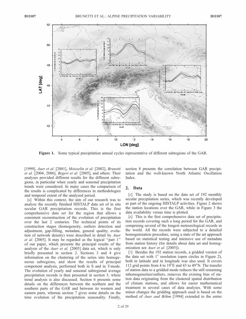
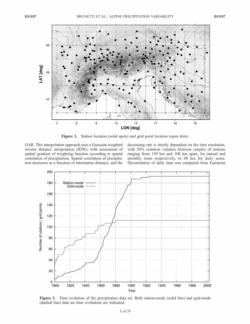
[5] The study is based on the data set of 192 monthlysecular precipitation series, which was recently developedas part of the ongoing HISTALP activities. Figure 2 showsthe station locations over the GAR, while in Figure 3 thedata availability versus time is plotted.[6] This is the first comprehensive data set of precipita-

tion records covering such a long period for the GAR, andcomprising several of the longest meteorological records inthe world. All the records were subjected to a detailedhomogenization procedure, using a state of the art approachbased on statistical testing and intensive use of metadatafrom station history (for details about data set and homog-enization see Auer et al. [2005]).[7] Besides the 192 station records, a gridded version of

the data set with 1� resolution (open circles in Figure 2),both in latitude and in longitude was also used. It covers112 grid points from 4 to 19�E and 43 to 49�N. The transferof station data to a gridded mode reduces the still remaininginhomogeneities/outliers, removes the existing bias of sta-tion data originating from the clustered spatial distributionof climate stations, and allows for easier mathematicaltreatment in several cases of data analyses. With someminor changes the gridding approach used is based on themethod of Auer and Bohm [1994] extended to the entire

Figure 1. Some typical precipitation annual cycles representative of different subregions of the GAR.

D11107 BRUNETTI ET AL.: ALPINE PRECIPITATION VARIABILITY

2 of 29

D11107

GAR. This interpolation approach uses a Gaussian weightedinverse distance interpolation (IDW), with assessment ofspatial gradient of weighting function according to spatialcorrelation of precipitation. Spatial correlation of precipita-tion decreases as a function of interstation distance, and the

decreasing rate is strictly dependent on the time resolution,with 50% common variance between couples of stationsranging from 150 km and 100 km apart, for annual andmonthly sums respectively, to 40 km for daily sums.Decorrelation of daily data was computed from European

Figure 2. Station location (solid spots) and grid point location (open dots).

Figure 3. Time evolution of the precipitation data set. Both station-mode (solid line) and grid-mode(dashed line) data set time evolutions are indicated.


3 of 29

D11107

synop data (4 years of 633 stations from 18 countriescovering the study region); while monthly and annualdecorrelations were computed from the HISTALP data set(for detail see Auer et al. [2005]).[8] To account for the steep precipitation gradients at the

Alpine and Dinaric main chains [see, e.g., Auer et al., 2006]interpolation was limited to subregions by introducing abarrier at the Alpine and Dinaric main chains. Besides thespatial gradient of weighting function, the choice of searchradius of interpolation (cutting off information from adistance larger than 100 km) was also based on the resultsof the spatial correlation study of precipitation. As HISTALPstations are homogenously distributed over the GAR, anangular weighting procedure was not used for the gridding.Moreover, it has to be emphasized that gridding is done forrelative values of precipitation with a much smoother spatialstructure of the precipitation field. This means (1) thatinterpolation needs a much lower spatial density of stationnetwork (as it would be necessary for absolute values ofprecipitation) and (2) that interpolation is much less affectedby elevation-dependent structures of precipitation. Unlike theHISTALP air temperature grid [Bohm et al., 2001], theprecipitation grid was not calculated separately for high andlow elevations. As described and referenced more in detail byAuer et al. [2005], wind exposed high summit sites, with ahigh solid precipitation share, were already excluded from thehomogenized version of the HISTALP stations data set.Førland [1996] describe the problem in general, Førlandand Hanssen-Bauer [2000] describe that it has not onlyinfluences on measuring single values and deducing climaticnormals, but it biases also long-term precipitation trends incold regions because of the observed reduction of snow ontotal precipitation. Below we will refer to the two data sets asthe station-mode and grid-mode data sets.

3. Regionalization

[9] The first step of data analysis was the study of thespatial coherence of the precipitation series. It was per-formed by means of principal component analysis (PCA)and was addressed to cluster the records into subregionswith similar precipitation variability. This technique allowsthe identification of a small number of variables, known asprincipal components (PCs), which are linear functions ofthe original data, and which maximize the amount of theirexplained variance [Wilks, 1995].[10] PCAwas applied starting from the correlation matrix

R, calculated from the monthly series that were normalizedby the monthly averages over the 1961–1990 standardperiod, in order to avoid the results being influenced bythe typical annual precipitation cycle of the different areasof the region. R was calculated both by considering all the12 months of the year and only the months of each season(winter: DJF; spring: MAM; summer: JJA; autumn: SON).The analysis was applied to the subperiod 1927–2002, forwhich all 192 series are available (see Figure 3).[11] As far as all the months are concerned, the results

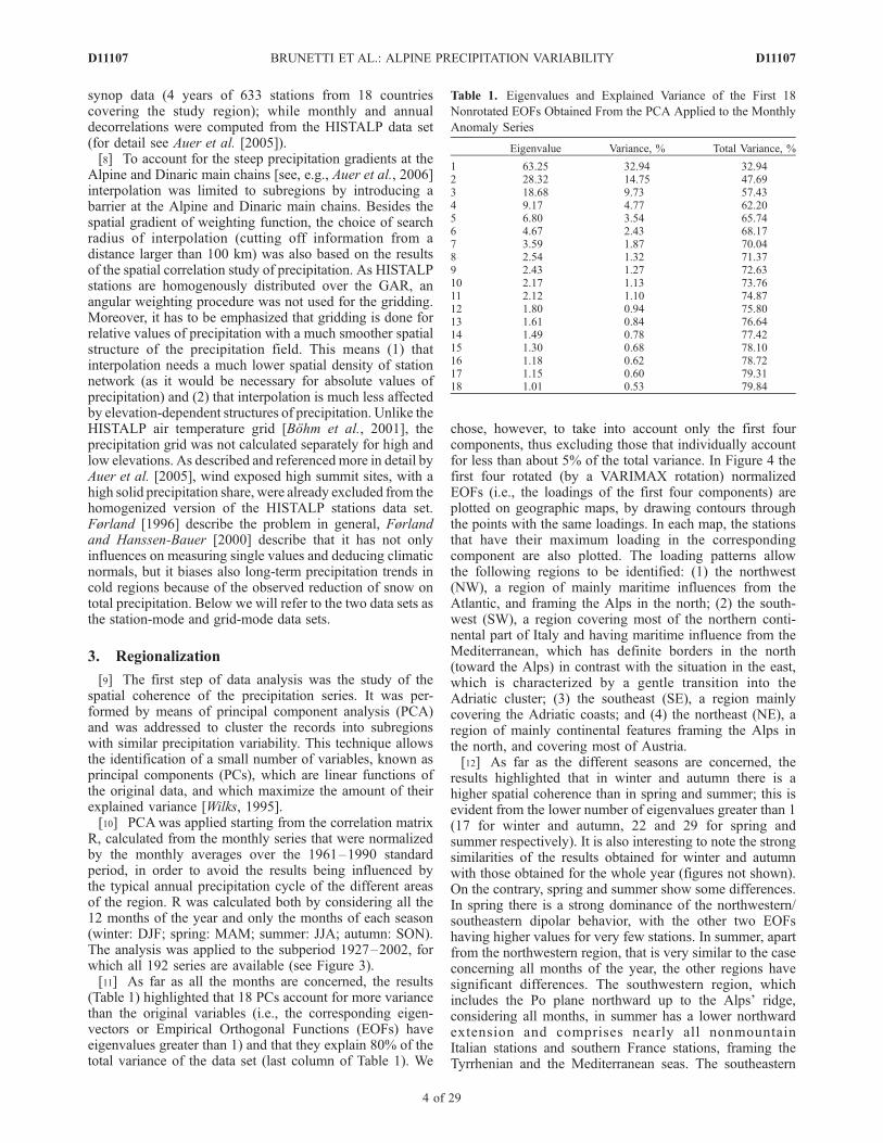
(Table 1) highlighted that 18 PCs account for more variancethan the original variables (i.e., the corresponding eigen-vectors or Empirical Orthogonal Functions (EOFs) haveeigenvalues greater than 1) and that they explain 80% of thetotal variance of the data set (last column of Table 1). We

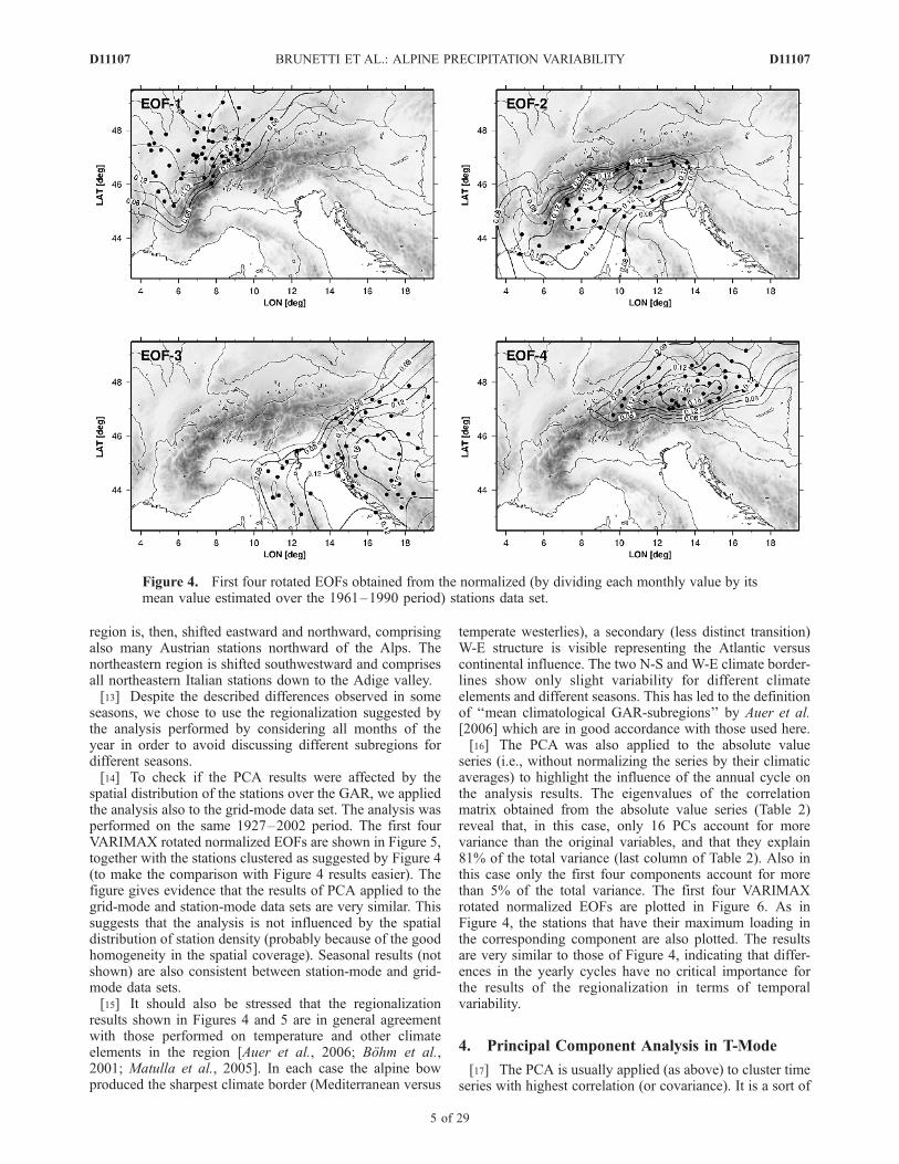
chose, however, to take into account only the first fourcomponents, thus excluding those that individually accountfor less than about 5% of the total variance. In Figure 4 thefirst four rotated (by a VARIMAX rotation) normalizedEOFs (i.e., the loadings of the first four components) areplotted on geographic maps, by drawing contours throughthe points with the same loadings. In each map, the stationsthat have their maximum loading in the correspondingcomponent are also plotted. The loading patterns allowthe following regions to be identified: (1) the northwest(NW), a region of mainly maritime influences from theAtlantic, and framing the Alps in the north; (2) the south-west (SW), a region covering most of the northern conti-nental part of Italy and having maritime influence from theMediterranean, which has definite borders in the north(toward the Alps) in contrast with the situation in the east,which is characterized by a gentle transition into theAdriatic cluster; (3) the southeast (SE), a region mainlycovering the Adriatic coasts; and (4) the northeast (NE), aregion of mainly continental features framing the Alps inthe north, and covering most of Austria.[12] As far as the different seasons are concerned, the

results highlighted that in winter and autumn there is ahigher spatial coherence than in spring and summer; this isevident from the lower number of eigenvalues greater than 1(17 for winter and autumn, 22 and 29 for spring andsummer respectively). It is also interesting to note the strongsimilarities of the results obtained for winter and autumnwith those obtained for the whole year (figures not shown).On the contrary, spring and summer show some differences.In spring there is a strong dominance of the northwestern/southeastern dipolar behavior, with the other two EOFshaving higher values for very few stations. In summer, apartfrom the northwestern region, that is very similar to the caseconcerning all months of the year, the other regions havesignificant differences. The southwestern region, whichincludes the Po plane northward up to the Alps’ ridge,considering all months, in summer has a lower northwardextension and comprises nearly all nonmountainItalian stations and southern France stations, framing theTyrrhenian and the Mediterranean seas. The southeastern

Table 1. Eigenvalues and Explained Variance of the First 18

Nonrotated EOFs Obtained From the PCA Applied to the Monthly

Anomaly Series

Eigenvalue Variance, % Total Variance, %

1 63.25 32.94 32.942 28.32 14.75 47.693 18.68 9.73 57.434 9.17 4.77 62.205 6.80 3.54 65.746 4.67 2.43 68.177 3.59 1.87 70.048 2.54 1.32 71.379 2.43 1.27 72.6310 2.17 1.13 73.7611 2.12 1.10 74.8712 1.80 0.94 75.8013 1.61 0.84 76.6414 1.49 0.78 77.4215 1.30 0.68 78.1016 1.18 0.62 78.7217 1.15 0.60 79.3118 1.01 0.53 79.84


4 of 29

D11107

region is, then, shifted eastward and northward, comprisingalso many Austrian stations northward of the Alps. Thenortheastern region is shifted southwestward and comprisesall northeastern Italian stations down to the Adige valley.[13] Despite the described differences observed in some

seasons, we chose to use the regionalization suggested bythe analysis performed by considering all months of theyear in order to avoid discussing different subregions fordifferent seasons.[14] To check if the PCA results were affected by the

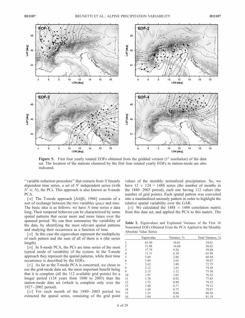
spatial distribution of the stations over the GAR, we appliedthe analysis also to the grid-mode data set. The analysis wasperformed on the same 1927–2002 period. The first fourVARIMAX rotated normalized EOFs are shown in Figure 5,together with the stations clustered as suggested by Figure 4(to make the comparison with Figure 4 results easier). Thefigure gives evidence that the results of PCA applied to thegrid-mode and station-mode data sets are very similar. Thissuggests that the analysis is not influenced by the spatialdistribution of station density (probably because of the goodhomogeneity in the spatial coverage). Seasonal results (notshown) are also consistent between station-mode and grid-mode data sets.[15] It should also be stressed that the regionalization

results shown in Figures 4 and 5 are in general agreementwith those performed on temperature and other climateelements in the region [Auer et al., 2006; Bohm et al.,2001; Matulla et al., 2005]. In each case the alpine bowproduced the sharpest climate border (Mediterranean versus

temperate westerlies), a secondary (less distinct transition)W-E structure is visible representing the Atlantic versuscontinental influence. The two N-S and W-E climate border-lines show only slight variability for different climateelements and different seasons. This has led to the definitionof ‘‘mean climatological GAR-subregions’’ by Auer et al.[2006] which are in good accordance with those used here.[16] The PCA was also applied to the absolute value

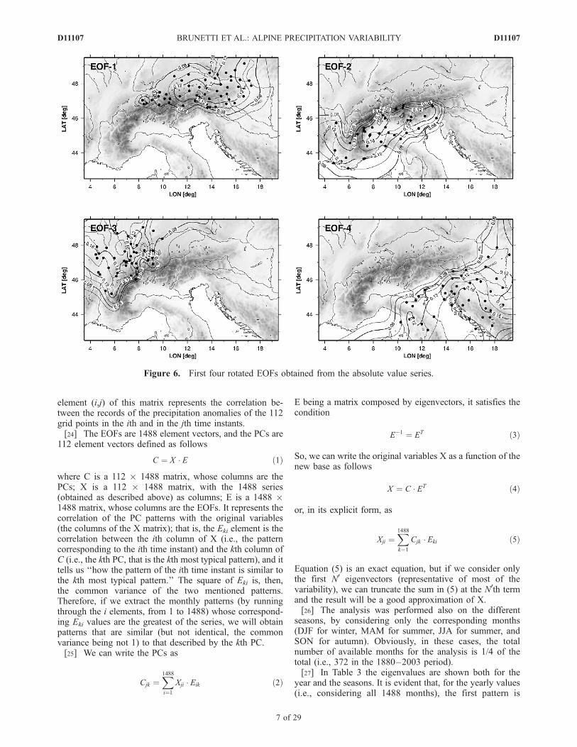
series (i.e., without normalizing the series by their climaticaverages) to highlight the influence of the annual cycle onthe analysis results. The eigenvalues of the correlationmatrix obtained from the absolute value series (Table 2)reveal that, in this case, only 16 PCs account for morevariance than the original variables, and that they explain81% of the total variance (last column of Table 2). Also inthis case only the first four components account for morethan 5% of the total variance. The first four VARIMAXrotated normalized EOFs are plotted in Figure 6. As inFigure 4, the stations that have their maximum loading inthe corresponding component are also plotted. The resultsare very similar to those of Figure 4, indicating that differ-ences in the yearly cycles have no critical importance forthe results of the regionalization in terms of temporalvariability.

4. Principal Component Analysis in T-Mode

[17] The PCA is usually applied (as above) to cluster timeseries with highest correlation (or covariance). It is a sort of

Figure 4. First four rotated EOFs obtained from the normalized (by dividing each monthly value by itsmean value estimated over the 1961–1990 period) stations data set.


5 of 29

D11107

‘‘variable reduction procedure’’ that extracts from N linearlydependent time series, a set of N0 independent series (withN0 � N), the PCs. This approach is also known as S-modePCA.[18] The T-mode approach [Joliffe, 1986] consists of a

sort of exchange between the two variables space and time.The basic idea is as follows: we have N time series n datalong. Their temporal behavior can be characterized by somespatial patterns that occur more and more times over thespanned period. We can then summarize the variability ofthe data, by identifying the most relevant spatial patternsand studying their occurrence as a function of time.[19] In this case the eigenvalues represent the multiplicity

of each pattern and the sum of all of them is n (the serieslength).[20] In S-mode PCA, the PCs are time series of the most

typical mode of variability of the system. In the T-modeapproach they represent the spatial patterns, while their timeoccurrence is described by the EOFs.[21] As far as the T-mode PCA is concerned, we chose to

use the grid-mode data set, the most important benefit beingthat it is complete (all the 112 available grid points) for alonger period (124 years from 1880 to 2003) than thestation-mode data set (which is complete only over the1927–2002 period).[22] For each month of the 1880–2003 period we

extracted the spatial series, consisting of the grid point

values of the monthly normalized precipitation. So, wehave 12 � 124 = 1488 series (the number of months inthe 1880–2003 period), each one having 112 values (thenumber of grid points). Each spatial pattern was convertedinto a standardized anomaly pattern in order to highlight therelative spatial variability over the GAR.[23] We calculated the 1488 � 1488 correlation matrix

from this data set, and applied the PCA to this matrix. The

Figure 5. First four yearly rotated EOFs obtained from the gridded version (1� resolution) of the dataset. The location of the stations clustered by the first four rotated yearly EOFs in station-mode are alsoindicated.

Table 2. Eigenvalues and Explained Variance of the First 16

Nonrotated EOFs Obtained From the PCA Applied to the Monthly

Absolute Value Series

Eigenvalue Variance, % Total Variance, %

1 65.30 34.01 34.012 31.88 16.60 50.623 17.79 9.26 59.884 11.71 6.10 65.985 5.49 2.86 68.846 3.89 2.03 70.877 3.62 1.88 72.758 3.12 1.63 74.389 2.15 1.12 75.5010 1.97 1.03 76.5211 1.78 0.92 77.4512 1.73 0.90 78.3513 1.48 0.77 79.1214 1.44 0.75 79.8715 1.31 0.68 80.5616 1.04 0.54 81.10


6 of 29

D11107

element (i,j) of this matrix represents the correlation be-tween the records of the precipitation anomalies of the 112grid points in the ith and in the jth time instants.[24] The EOFs are 1488 element vectors, and the PCs are

112 element vectors defined as follows

C ¼ X � E ð1Þ

where C is a 112 � 1488 matrix, whose columns are thePCs; X is a 112 � 1488 matrix, with the 1488 series(obtained as described above) as columns; E is a 1488 �1488 matrix, whose columns are the EOFs. It represents thecorrelation of the PC patterns with the original variables(the columns of the X matrix); that is, the Eki element is thecorrelation between the ith column of X (i.e., the patterncorresponding to the ith time instant) and the kth column ofC (i.e., the kth PC, that is the kth most typical pattern), and ittells us ‘‘how the pattern of the ith time instant is similar tothe kth most typical pattern.’’ The square of Eki is, then,the common variance of the two mentioned patterns.Therefore, if we extract the monthly patterns (by runningthrough the i elements, from 1 to 1488) whose correspond-ing Eki values are the greatest of the series, we will obtainpatterns that are similar (but not identical, the commonvariance being not 1) to that described by the kth PC.[25] We can write the PCs as

Cjk ¼X1488

i¼1

Xji � Eik ð2Þ

E being a matrix composed by eigenvectors, it satisfies thecondition

E�1 ¼ ET ð3Þ

So, we can write the original variables X as a function of thenew base as follows

X ¼ C � ET ð4Þ

or, in its explicit form, as

Xji ¼X1488

k¼1

Cjk � Eki ð5Þ

Equation (5) is an exact equation, but if we consider onlythe first N0 eigenvectors (representative of most of thevariability), we can truncate the sum in (5) at the N0th termand the result will be a good approximation of X.[26] The analysis was performed also on the different

seasons, by considering only the corresponding months(DJF for winter, MAM for summer, JJA for summer, andSON for autumn). Obviously, in these cases, the totalnumber of available months for the analysis is 1/4 of thetotal (i.e., 372 in the 1880–2003 period).[27] In Table 3 the eigenvalues are shown both for the

year and the seasons. It is evident that, for the yearly values(i.e., considering all 1488 months), the first pattern is

Figure 6. First four rotated EOFs obtained from the absolute value series.


7 of 29

D11107

representative of about 31% of the variability over the1880–2003 period, the second one is representative of22%, the third one of about 10%, and so on.[28] The PCs corresponding to the two highest eigenval-

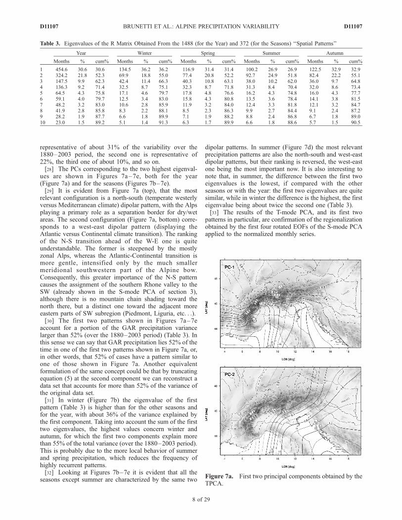
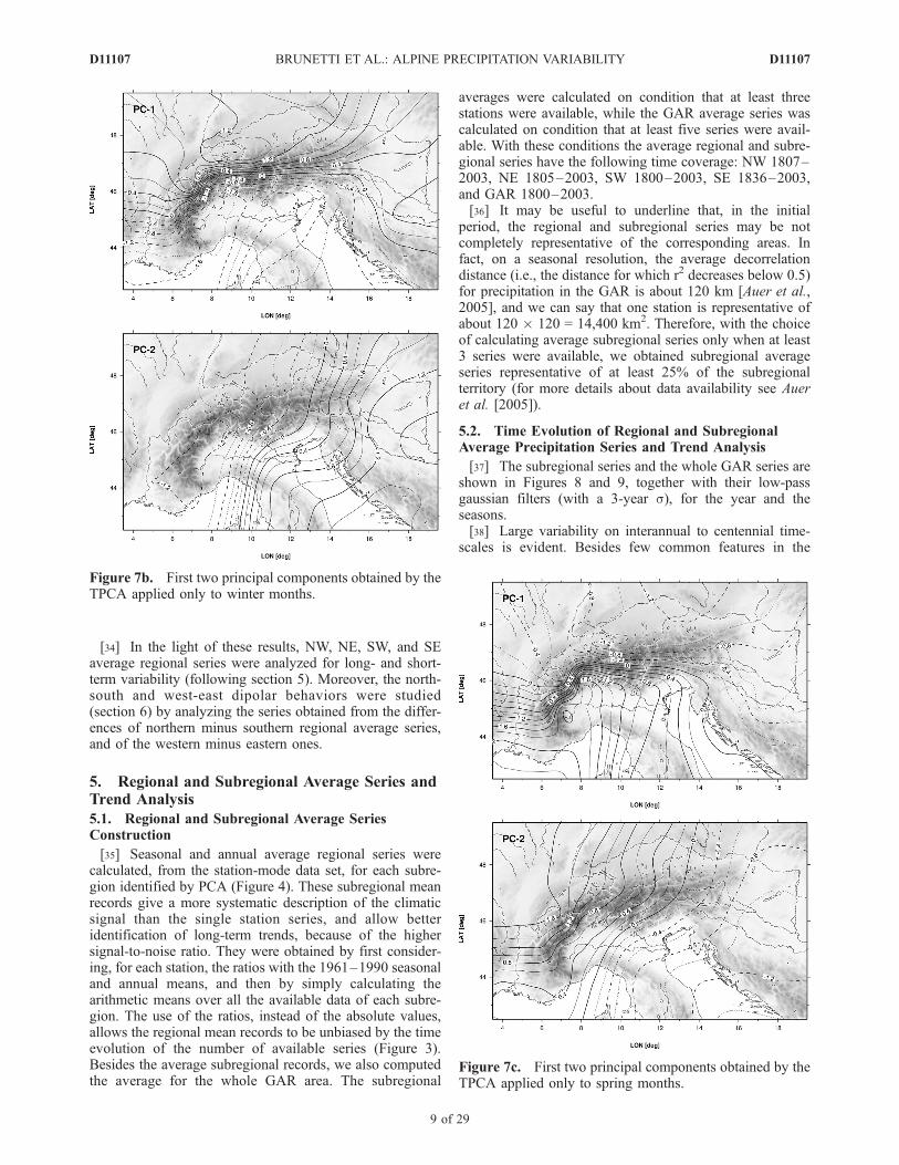
ues are shown in Figures 7a–7e, both for the year(Figure 7a) and for the seasons (Figures 7b–7e).[29] It is evident from Figure 7a (top), that the most

relevant configuration is a north-south (temperate westerlyversus Mediterranean climate) dipolar pattern, with the Alpsplaying a primary role as a separation border for dry/wetareas. The second configuration (Figure 7a, bottom) corre-sponds to a west-east dipolar pattern (displaying theAtlantic versus Continental climate transition). The rankingof the N-S transition ahead of the W-E one is quiteunderstandable. The former is steepened by the mostlyzonal Alps, whereas the Atlantic-Continental transition ismore gentle, intensified only by the much smallermeridional southwestern part of the Alpine bow.Consequently, this greater importance of the N-S patterncauses the assignment of the southern Rhone valley to theSW (already shown in the S-mode PCA of section 3),although there is no mountain chain shading toward thenorth there, but a distinct one toward the adjacent moreeastern parts of SW subregion (Piedmont, Liguria, etc. . .).[30] The first two patterns shown in Figures 7a–7e

account for a portion of the GAR precipitation variancelarger than 52% (over the 1880–2003 period) (Table 3). Inthis sense we can say that GAR precipitation lies 52% of thetime in one of the first two patterns shown in Figure 7a, or,in other words, that 52% of cases have a pattern similar toone of those shown in Figure 7a. Another equivalentformulation of the same concept could be that by truncatingequation (5) at the second component we can reconstruct adata set that accounts for more than 52% of the variance ofthe original data set.[31] In winter (Figure 7b) the eigenvalue of the first

pattern (Table 3) is higher than for the other seasons andfor the year, with about 36% of the variance explained bythe first component. Taking into account the sum of the firsttwo eigenvalues, the highest values concern winter andautumn, for which the first two components explain morethan 55% of the total variance (over the 1880–2003 period).This is probably due to the more local behavior of summerand spring precipitation, which reduces the frequency ofhighly recurrent patterns.[32] Looking at Figures 7b–7e it is evident that all the

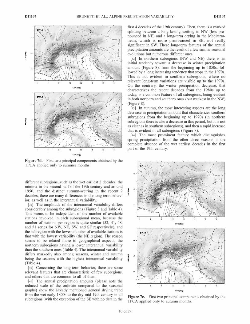
seasons except summer are characterized by the same two

dipolar patterns. In summer (Figure 7d) the most relevantprecipitation patterns are also the north-south and west-eastdipolar patterns, but their ranking is reversed, the west-eastone being the most important now. It is also interesting tonote that, in summer, the difference between the first twoeigenvalues is the lowest, if compared with the otherseasons or with the year: the first two eigenvalues are quitesimilar, while in winter the difference is the highest, the firsteigenvalue being about twice the second one (Table 3).[33] The results of the T-mode PCA, and its first two

patterns in particular, are confirmation of the regionalizationobtained by the first four rotated EOFs of the S-mode PCAapplied to the normalized monthly series.

Table 3. Eigenvalues of the R Matrix Obtained From the 1488 (for the Year) and 372 (for the Seasons) ‘‘Spatial Patterns’’

Year Winter Spring Summer Autumn

Months % cum% Months % cum% Months % cum% Months % cum% Months % cum%

1 454.6 30.6 30.6 134.5 36.2 36.2 116.9 31.4 31.4 100.2 26.9 26.9 122.5 32.9 32.92 324.2 21.8 52.3 69.9 18.8 55.0 77.4 20.8 52.2 92.7 24.9 51.8 82.4 22.2 55.13 147.5 9.9 62.3 42.4 11.4 66.3 40.3 10.8 63.1 38.0 10.2 62.0 36.0 9.7 64.84 136.3 9.2 71.4 32.5 8.7 75.1 32.3 8.7 71.8 31.3 8.4 70.4 32.0 8.6 73.45 64.5 4.3 75.8 17.1 4.6 79.7 17.8 4.8 76.6 16.2 4.3 74.8 16.0 4.3 77.76 59.1 4.0 79.7 12.5 3.4 83.0 15.8 4.3 80.8 13.5 3.6 78.4 14.1 3.8 81.57 48.2 3.2 83.0 10.6 2.8 85.9 11.9 3.2 84.0 12.4 3.3 81.8 12.1 3.2 84.78 41.9 2.8 85.8 8.3 2.2 88.1 8.5 2.3 86.3 9.9 2.7 84.4 9.1 2.4 87.29 28.2 1.9 87.7 6.6 1.8 89.9 7.1 1.9 88.2 8.8 2.4 86.8 6.7 1.8 89.010 23.0 1.5 89.2 5.1 1.4 91.3 6.3 1.7 89.9 6.6 1.8 88.6 5.7 1.5 90.5

Figure 7a. First two principal components obtained by theTPCA.


8 of 29

D11107

[34] In the light of these results, NW, NE, SW, and SEaverage regional series were analyzed for long- and short-term variability (following section 5). Moreover, the north-south and west-east dipolar behaviors were studied(section 6) by analyzing the series obtained from the differ-ences of northern minus southern regional average series,and of the western minus eastern ones.

5. Regional and Subregional Average Series andTrend Analysis

5.1. Regional and Subregional Average SeriesConstruction

[35] Seasonal and annual average regional series werecalculated, from the station-mode data set, for each subre-gion identified by PCA (Figure 4). These subregional meanrecords give a more systematic description of the climaticsignal than the single station series, and allow betteridentification of long-term trends, because of the highersignal-to-noise ratio. They were obtained by first consider-ing, for each station, the ratios with the 1961–1990 seasonaland annual means, and then by simply calculating thearithmetic means over all the available data of each subre-gion. The use of the ratios, instead of the absolute values,allows the regional mean records to be unbiased by the timeevolution of the number of available series (Figure 3).Besides the average subregional records, we also computedthe average for the whole GAR area. The subregional

averages were calculated on condition that at least threestations were available, while the GAR average series wascalculated on condition that at least five series were avail-able. With these conditions the average regional and subre-gional series have the following time coverage: NW 1807–2003, NE 1805–2003, SW 1800–2003, SE 1836–2003,and GAR 1800–2003.[36] It may be useful to underline that, in the initial

period, the regional and subregional series may be notcompletely representative of the corresponding areas. Infact, on a seasonal resolution, the average decorrelationdistance (i.e., the distance for which r2 decreases below 0.5)for precipitation in the GAR is about 120 km [Auer et al.,2005], and we can say that one station is representative ofabout 120 � 120 = 14,400 km2. Therefore, with the choiceof calculating average subregional series only when at least3 series were available, we obtained subregional averageseries representative of at least 25% of the subregionalterritory (for more details about data availability see Aueret al. [2005]).

5.2. Time Evolution of Regional and SubregionalAverage Precipitation Series and Trend Analysis

[37] The subregional series and the whole GAR series areshown in Figures 8 and 9, together with their low-passgaussian filters (with a 3-year s), for the year and theseasons.[38] Large variability on interannual to centennial time-

scales is evident. Besides few common features in the

Figure 7b. First two principal components obtained by theTPCA applied only to winter months.

Figure 7c. First two principal components obtained by theTPCA applied only to spring months.


9 of 29

D11107

different subregions, such as the wet earliest 2 decades, theminima in the second half of the 19th century and around1950, and the distinct autumn-wetting in the recent 2decades, there are many differences in the long-term behav-ior, as well as in the interannual variability.[39] The amplitude of the interannual variability differs

considerably among the subregions (Figure 8 and Table 4).This seems to be independent of the number of availablestations involved in each subregional mean, because thenumber of stations per region is quite similar (52, 41, 48,and 51 series for NW, NE, SW, and SE respectively), andthe subregion with the lowest number of available stations isthat with the lowest variability (the NE region). The reasonseems to be related more to geographical aspects, thenorthern subregions having a lower interannual variabilitythan the southern ones (Table 4). The interannual variabilitydiffers markedly also among seasons, winter and autumnbeing the seasons with the highest interannual variability(Table 4).[40] Concerning the long-term behavior, there are some

relevant features that are characteristic of few subregions,and others that are common to all of them.[41] The annual precipitation amounts (please note the

reduced scale of the ordinate compared to the seasonalgraphs) show the already mentioned general drying trendfrom the wet early 1800s to the dry mid 19th century in allsubregions (with the exception of the SE with no data in the

first 4 decades of the 19th century). Then, there is a markedsplitting between a long-lasting wetting in NW (less pro-nounced in NE) and a long-term drying in the Mediterra-nean, which is more pronounced in SE, not reallysignificant in SW. These long-term features of the annualprecipitation amounts are the result of a few similar seasonalevolutions but numerous different ones.[42] In northern subregions (NW and NE) there is an

initial tendency toward a decrease in winter precipitationamount (Figure 8), from the beginning up to 1850s, fol-lowed by a long increasing tendency that stops in the 1970s.This is not evident in southern subregions, where norelevant long-term variations are visible up to the 1970s.On the contrary, the winter precipitation decrease, thatcharacterizes the recent decades from the 1980s up totoday, is a common feature of all subregions, being evidentin both northern and southern ones (but weakest in the NW)(Figure 8).[43] In autumn, the most interesting aspects are the long

decrease in precipitation amount that characterizes southernsubregions from the beginning up to 1970s (in northernsubregions there is also a decrease in this period, but it is notas clear as in southern subregions), and then a rapid increasethat is evident in all subregions (Figure 8).[44] The most prominent feature which distinguishes

spring precipitation from the other three seasons is thecomplete absence of the wet earliest decades in the firstpart of the 19th century.

Figure 7d. First two principal components obtained by theTPCA applied only to summer months.

Figure 7e. First two principal components obtained by theTPCA applied only to autumn months.


10 of 29

D11107

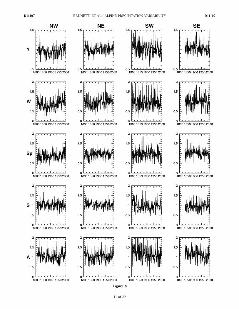
Figure 8


11 of 29

D11107

[45] As already mentioned, summer precipitation does notshow prominent and long-lasting trends. They are morecharacterized by ups and downs on a decadal scale, morepronounced in SW.

[46] According to the described subregional differences,the all GAR-average analysis is not really representative ofthe entire area, when for example, inverse subregional long-term trends lead to a no-trend result for the average over the

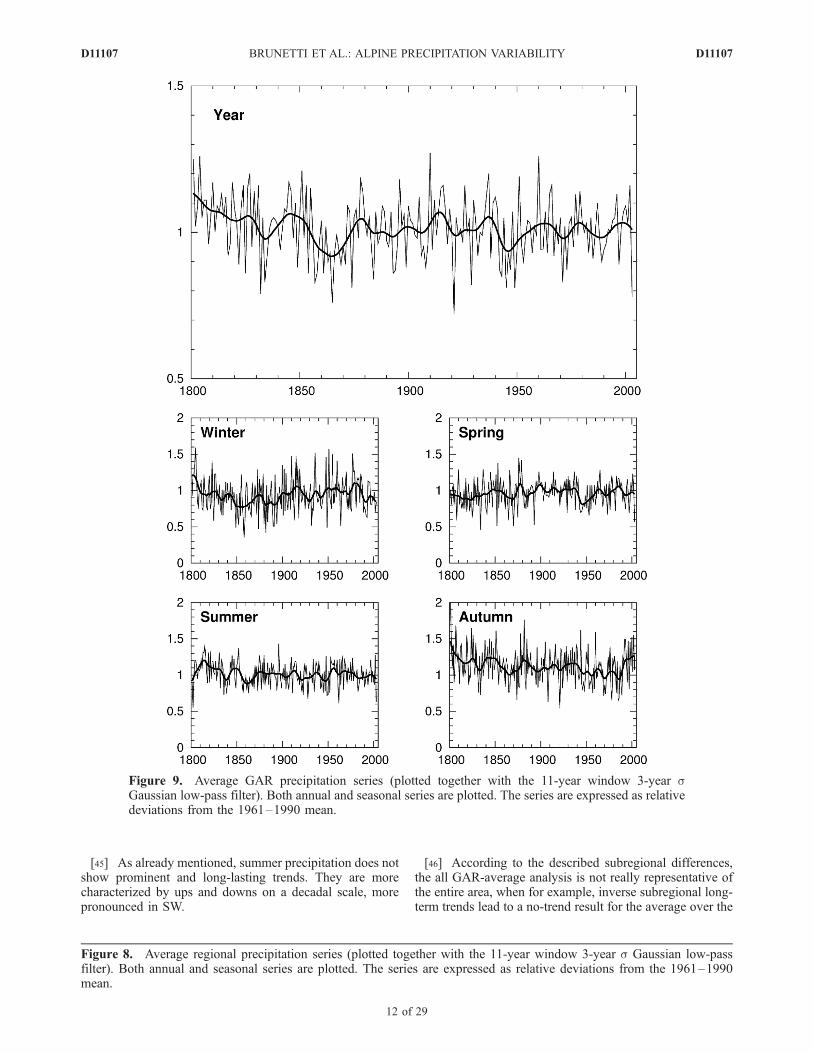
Figure 9. Average GAR precipitation series (plotted together with the 11-year window 3-year sGaussian low-pass filter). Both annual and seasonal series are plotted. The series are expressed as relativedeviations from the 1961–1990 mean.

Figure 8. Average regional precipitation series (plotted together with the 11-year window 3-year s Gaussian low-passfilter). Both annual and seasonal series are plotted. The series are expressed as relative deviations from the 1961–1990mean.


12 of 29

D11107

entire region. On the other hand, the few already mentioned‘‘all-GAR-features’’ may well reflect the continental-to-global-scale background (after the elimination of the topo-graphically forced enhancements/reductions explainablethrough the existence of the Alpine chain).[47] Figure 9 shows the annual and seasonal time series

averaged over all four subregions of the GAR. As aconsequence of the already described subregionalsimilarities/discrepancies the strongest visible feature inthe annual mean GAR-precipitation series is the dryingtrends from the wet first 3 decades (1800 to 1830 and theyears around 1850) to the leading minimum centeredaround the 1860s. Afterward, the splitting into differentsubregional evolutions leads to general deletion of signif-icant all-GAR long-term trends. Only the wet 1910s shouldbe mentioned, mainly because of their importance for thelast general glacier advance during this most maritimedecade of the entire instrumental period in the Alps.[48] This feature, together with the similar effect of the

synchronicity of the wet early instrumental period, with themost pronounced Alpine glacier advances before 1820 and1850, highlights the great application potential of the newHISTALP precipitation data set for climate impact studies.Attempts to understand the pre-1850 glacier advances withmodels based on temperature alone have not really beensuccessful so far.[49] The possibility to also use precipitation as an addi-

tional quantitative predictor may reduce the uncertaintiesthat now exist.[50] More pronounced long-term evolutions, also in the

post-1850 period, are visible in seasonal all-GAR meanseries. In particular, the winter decrease in recent decades,and the strong increase from the 1980s up to today inautumn precipitation, together with their respectiveearlier long-term counterparts, might be reflections of largerEuropean-scale features. The GAR series also highlights thewinter decrease in the first 50 years and the autumndecrease from the beginning up to 1970, even if they arenot as evident as the ones in the single subregions, becausethey characterize only some subregions, and do not affectthe whole area.[51] On a longer timescale, i.e., by considering the long-

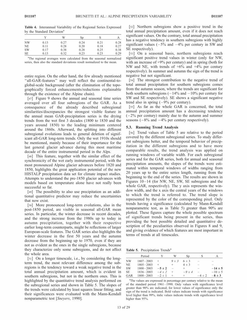
term trend, the most relevant difference among the sub-regions is the tendency toward a weak negative trend in thetotal annual precipitation amount, which is evident insouthern subregions, but not in the northern ones. This ishighlighted by the quantitative trend analysis performed onthe subregional series and shown in Table 5. The slopes ofthe trends were calculated by least squares linear fitting, andtheir significances were evaluated with the Mann-Kendallnonparametric test [Sneyers, 1990].

[52] Northern subregions show a positive trend in thetotal annual precipitation amount, even if it does not reachsignificant values. On the contrary, total annual precipitationhas a negative tendency in southern subregions with highlysignificant values (�5% and �4% per century in SW andSE respectively).[53] On a seasonal basis, northern subregions reach

significant positive trend values in winter (only for NW,with an increase of +9% per century) and in spring (both forNW and NE, with trends of +6% and +4% per centuryrespectively). In summer and autumn the sign of the trend isnegative but not significant.[54] The strongest contribution to the negative trend of

total annual precipitation for southern subregions comesfrom the autumn season, where the trends are significant forboth southern subregions (�14% and �10% per century forSW and SE respectively). SE shows a significant negativetrend also in spring (�9% per century).[55] As far as the whole GAR is concerned, the total

annual precipitation amount has a decreasing tendency(�2% per century) mainly due to the autumn and summerseasons (�8% and �4% per century respectively).

5.3. Running Trend Analysis

[56] Trend values of Table 5 are relative to the periodcovered by the different subregional series. To study differ-ent subregions better, and the temporal behavior of precip-itation in the different subregions and to have morecomparable results, the trend analysis was applied onrunning windows of variable width. For each subregionalseries and for the GAR series, both for annual and seasonalprecipitation amounts, the slopes of the trends were esti-mated within temporal windows of widths ranging from20 years up to the entire series length, running from thebeginning to the end of the series. The results are shown inFigures 10–14 (for NW, NE, SW, SE subregions and thewhole GAR, respectively). The y axis represents the win-dow width, and the x axis the central years of the windowsto which the trend is referred to. The trend slope isrepresented by the color of the corresponding pixel. Onlytrends having a significance (calculated by Mann-Kendallnonparametric test, as in Table 5) greater than 90% areplotted. These figures capture the whole possible spectrumof significant trends being present in the series, thusproviding the best possible detailed and quantitative de-scription of the peculiarities observed in Figures 8 and 9,and giving evidence of which features are most important interms of trends at all timescales.

Table 4. Interannual Variability of the Regional Series Expressed

by the Standard Deviationa

Y W Sp S A

NW 0.13 0.27 0.24 0.21 0.28NE 0.11 0.28 0.20 0.18 0.27SW 0.17 0.38 0.28 0.25 0.38SE 0.13 0.32 0.23 0.23 0.29

aThe regional averages were calculated from the seasonal normalizedseries, then also the standard deviations result normalized to the mean.

Table 5. Precipitation Trendsa

Period Y W Sp S A

NW 1807–2003 + 9 ± 3 6 ± 3 – –NE 1805–2003 + + 4 ± 3 – –SW 1800–2003 �5 ± 2 – + – �14 ± 5SE 1836–2003 �4 ± 2 + �9 ± 4 – �10 ± 5GAR 1800–2003 �2 ± 1 + + �4 ± 2 �8 ± 3

aThe values are expressed in percentage per century relative to the meanof the standard period 1961–1990. Only values with significance levelgreater than 90% are indicated; for lower values of significance only thesign of the trend is indicated. Bold values indicate trends with significancelevel higher than 99%, italic values indicate trends with significance levelhigher than 95%.


13 of 29

D11107

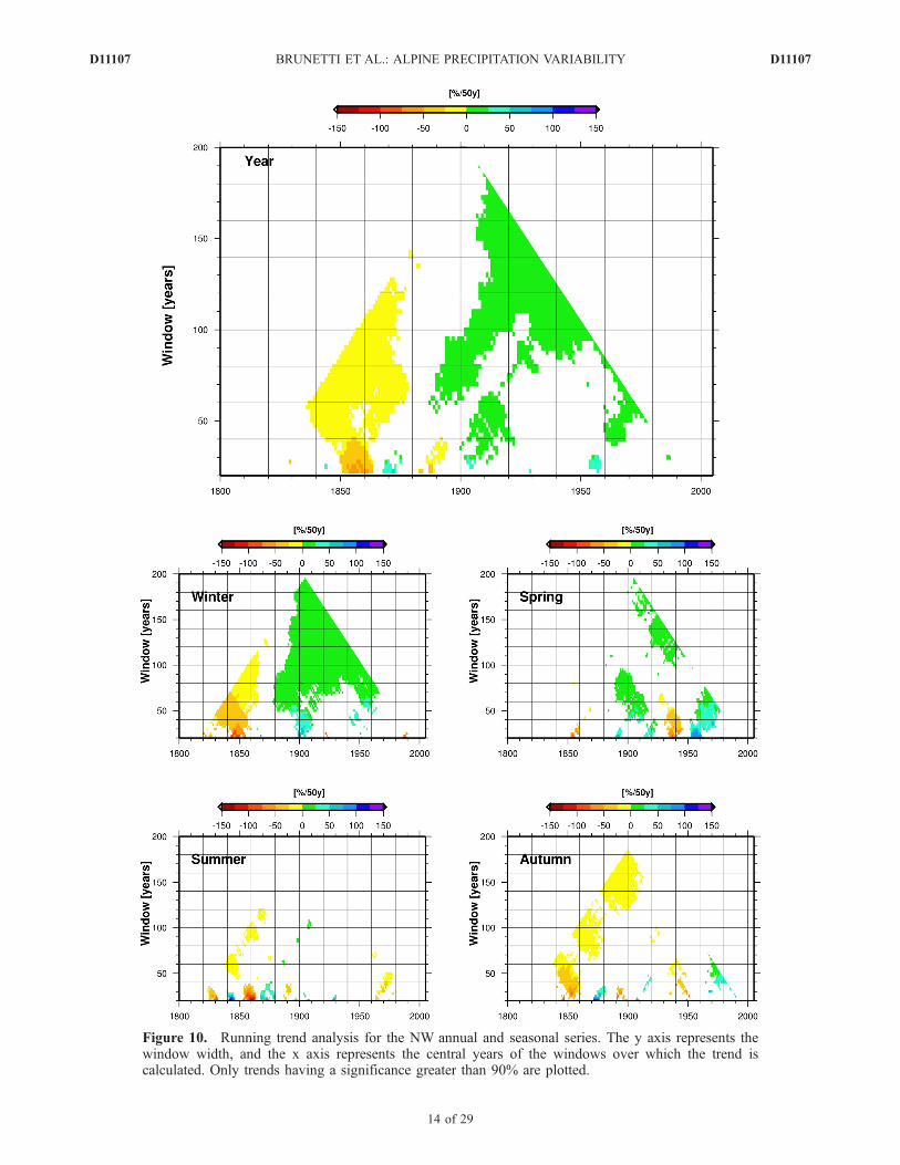
Figure 10. Running trend analysis for the NW annual and seasonal series. The y axis represents thewindow width, and the x axis represents the central years of the windows over which the trend iscalculated. Only trends having a significance greater than 90% are plotted.


14 of 29

D11107

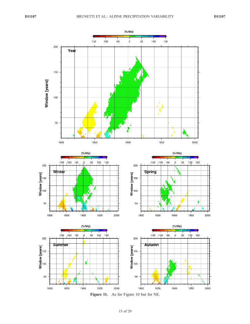
Figure 11. As for Figure 10 but for NE.


15 of 29

D11107

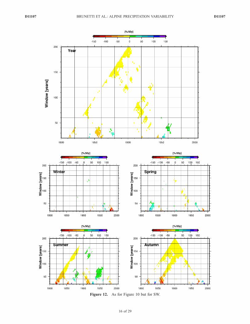
Figure 12. As for Figure 10 but for SW.


16 of 29

D11107

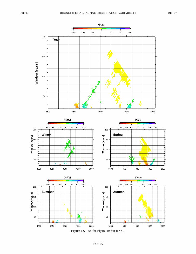
Figure 13. As for Figure 10 but for SE.


17 of 29

D11107

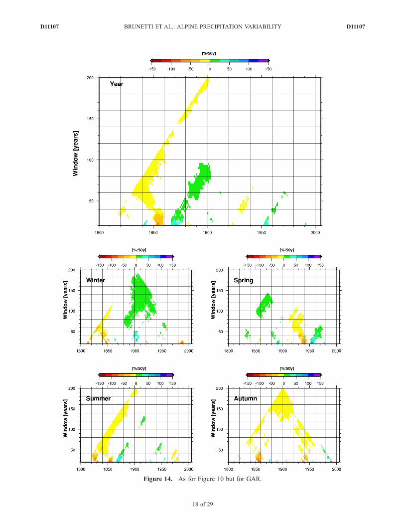
Figure 14. As for Figure 10 but for GAR.


18 of 29

D11107

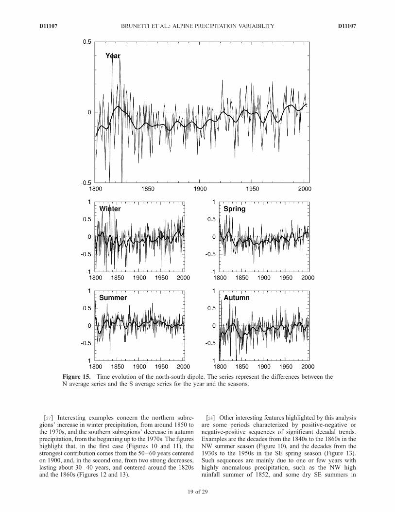
[57] Interesting examples concern the northern subre-gions’ increase in winter precipitation, from around 1850 tothe 1970s, and the southern subregions’ decrease in autumnprecipitation, from the beginning up to the 1970s. The figureshighlight that, in the first case (Figures 10 and 11), thestrongest contribution comes from the 50–60 years centeredon 1900, and, in the second one, from two strong decreases,lasting about 30–40 years, and centered around the 1820sand the 1860s (Figures 12 and 13).

[58] Other interesting features highlighted by this analysisare some periods characterized by positive-negative ornegative-positive sequences of significant decadal trends.Examples are the decades from the 1840s to the 1860s in theNW summer season (Figure 10), and the decades from the1930s to the 1950s in the SE spring season (Figure 13).Such sequences are mainly due to one or few years withhighly anomalous precipitation, such as the NW highrainfall summer of 1852, and some dry SE summers in

Figure 15. Time evolution of the north-south dipole. The series represent the differences between theN average series and the S average series for the year and the seasons.


19 of 29

D11107

the 1940s. These anomalous precipitation data can affect thetrend values for a wide range of window periods, backwardand forward to the period in which they happen.[59] The running trend analysis also helps us to compare

the results with other findings for the same study area,despite of the different time periods, even if the differentanalysis procedures (e.g., station versus grid points versusregional series trend) complicate a direct quantitative com-parison. Our results agree qualitatively with previous stud-ies: Auer and Bohm [1994], Widmann and Schar [1997],

Table 6. Interannual Variability of N-S and W-E Series Expressed

in Terms of Standard Deviationa

W Sp S A Y

N-S 0.36 0.24 0.23 0.33 0.15W-E 0.20 0.19 0.19 0.26 0.11ratio 1.8 1.3 1.2 1.2 1.3

aThe regional averages were calculated from the seasonal normalizedseries, then also the standard deviations result normalized to the mean.

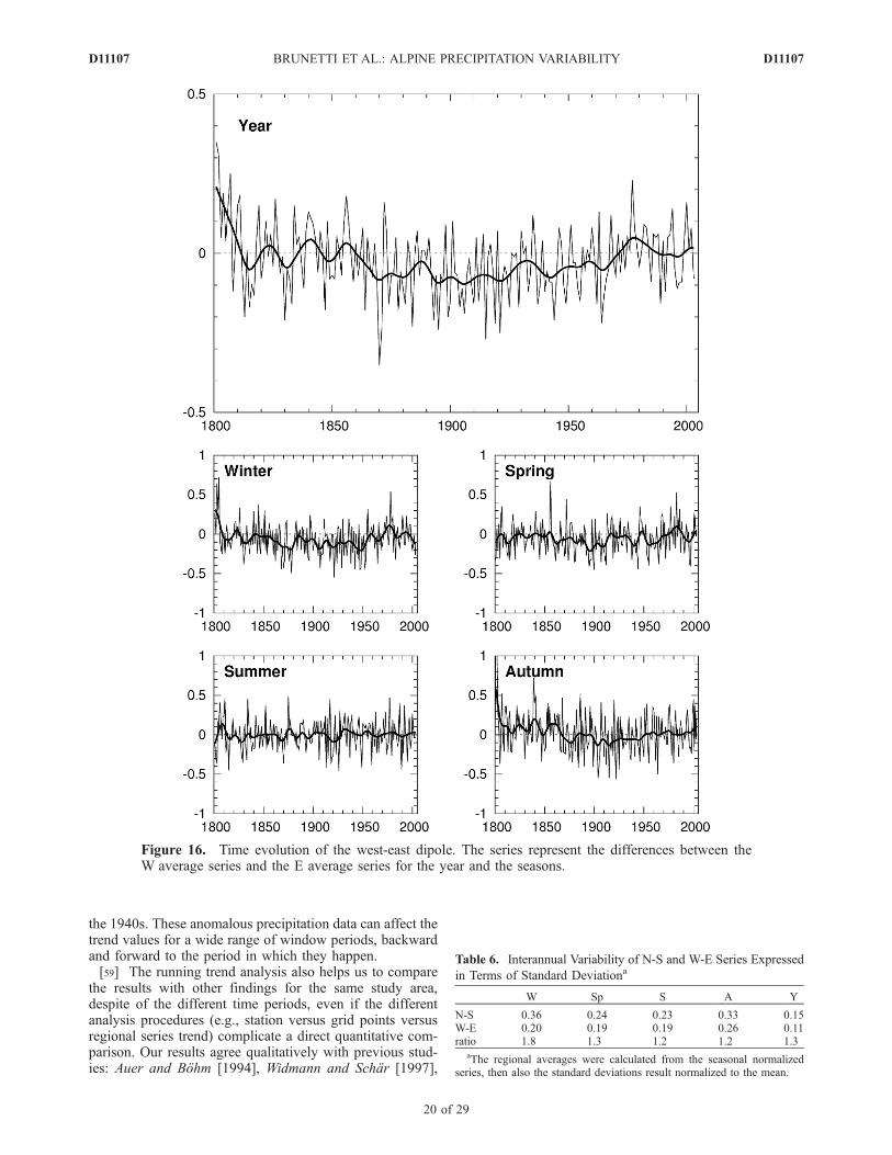
Figure 16. Time evolution of the west-east dipole. The series represent the differences between theW average series and the E average series for the year and the seasons.


20 of 29

D11107

Schmidli et al. [2002], Brunetti et al. [2004, 2006], andBegert et al. [2005]. In particular, Schmidli et al. [2002]analyzed precipitation over about the same area, but for ashorter period. They observed, for the 1901–1990 period, asignificant precipitation increase in northwestern Alps in thewinter season, and a decrease in autumn precipitation southof the Alps. This result is consistent with our findings, as itis evident from the pixel having coordinates year = 1945and window width = 90 in Figure 10 (for the winter), and inFigures 12 and 13 (for the autumn season).[60] The results of the studies performed on different

subareas of the GAR also agree with the present studyresults. Begert et al. [2005] homogenized and analyzed nineSwiss precipitation series for the 1864–2000 period. Theyobserved a significant positive trend in the winter season, inmost of Switzerland, whereas on a yearly basis the trendwas significant only for some stations. This result isconsistent with the pixel having coordinates year = 1932and window width = 137 in Figure 10 (winter and yearplots).[61] Brunetti et al. [2006] performed rigorous homogeni-

zation work on a new large (more than 100 stations)precipitation data set for Italy, covering the last 2 centuries.Their results (a decrease in precipitation amount over allItaly) are consistent with the present ones obtained for SWand SE subregions. They performed a progressive trendanalysis too, by studying the trend for the subseries endingin the last year of the series and starting in the ith one (with irunning through the time period covered by the data). Theresults are qualitatively (the regions are not the same)consistent with ours; in particular, it is interesting to notethe trend inversion in recent decades of the autumn precip-itation (from negative to positive) highlighted by bothstudies (autumn plot of Figures 12 and 13 of this workand Figure 19e of Brunetti et al. [2006]).[62] Auer and Bohm [1994] and Auer et al. [2001]

observed for Austria an increase in wet conditions in winterover the last 150 years, and no uniform behavior in the otherseasons. On a yearly basis, they observed two separatetendencies in western and eastern parts of Austria, theformer being characterized by an increase in wet conditions,while the latter being characterized by an increase in dryconditions. This behavior is consistent with our results,since Austrian stations are split into both northern (NE)and southern (SW, and SE) regions, which have oppositeprecipitation tendencies.[63] To summarize the results of comparisons with pre-

vious studies, the following points show how the newanalysis on the HISTALP-data set stands out. Comparedto the studies performed on subareas of the GAR it provides

a much better understanding of the regional structure whichdoes not obey national borders but natural ones. It hasadded another complete century of early instrumental data,compared to those studies analyzing the whole GAR, withsome highly interesting 19th century evolutions. Last butnot least, the update to the end of 2003 provides a betterview of some recent evolutions, such as the definitetermination of the long-term autumn drying, which becamecompletely compensated by a sharp precipitation increase inthe region in recent time.

6. Dipoles Analysis

[64] During the final stage of the construction of theHISTALP precipitation data set, some initial test analysespointed to the existence of dipolar variability structures inthe GAR [Bohm et al., 2003]. This made us aware that itwould be worthwhile having a second closer and moresystematic look at it. The two dipolar patterns, identified bythe T-mode PCA, were studied in detail by analyzing theseries obtained by calculating the differences betweennorthern and southern average seasonal and yearly series,and between western and eastern average seasonal andyearly series.[65] Northern average series were obtained by averaging

all the stations belonging to NW and NE subregions(hereinafter N subregion), and southern average series wereobtained by averaging all the stations belonging to SW andSE subregions (hereinafter S subregion). Similarly, westernand eastern average series were obtained by averaging allthe stations belonging to NW and SW subregions(W subregion) and those belonging to NE and SE subre-gions (E subregion) respectively. North-south (N minus S)and west-east (W minus E) dipole series are shown inFigures 15 and 16, both for the seasons and the year,together with their 3-year s Gaussian low-pass filters.[66] The N-S and W-E difference series were constructed

to be representative of two different orthogonal functionsand, as a consequence, they can be expected to be almostcompletely uncorrelated: in fact, their common variance isonly 3% on a yearly basis, and range from 0.1% to about5% in 3 of the 4 seasons. An exception is autumn, where thecommon variance is 20%.[67] For this reason the year-to-year variability of the two

series are different. This is true not only in terms oftemporal evolution of the two dipoles, but also with regardsto the amplitude of the variability: N-S shows a highervariability than W-E, highlighted by the highest standarddeviation of N-S (Table 6). This is particularly evident inwinter, where the ratio between N-S and W-E standarddeviations is 1.8 (last row of Table 6). This is consistentwith the ratios between the portion of variance explained bythe first and the second component of the T-mode PCA(Table 3), these being very similar to the standard deviationratios of Table 6.[68] The additional information provided by the two

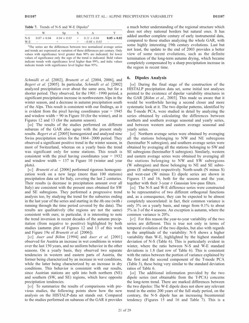
dipole series (not obtainable from the T-PCA) concernsthe long-term trend. There are marked differences betweenthe two dipoles: The W-E dipole does not show any relevanttrend in the entire 200 years of the full study period, on thecontrary, the N-S dipole has an increasing bicentennialtendency (Figures 15 and 16 and Table 7). This is a

Table 7. Trends of N-S and W-E Dipolesa

W Sp S A Y

N-S 0.07 ± 0.04 0.04 ± 0.03 + 0.11 ± 0.04 0.05 ± 0.02W-E – + + �0.08 ± 0.03 –

aThe series are the differences between two normalized average seriesand trends are expressed as variation of these differences per century. Onlyvalues with significance level greater than 90% are indicated; for lowervalues of significance only the sign of the trend is indicated. Bold valuesindicate trends with significance level higher than 99%, and italic valuesindicate trends with significance level higher than 95%.


21 of 29

D11107

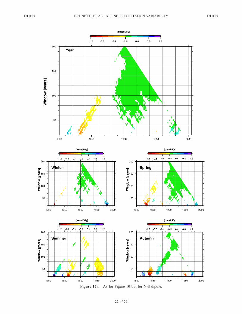
Figure 17a. As for Figure 10 but for N-S dipole.


22 of 29

D11107

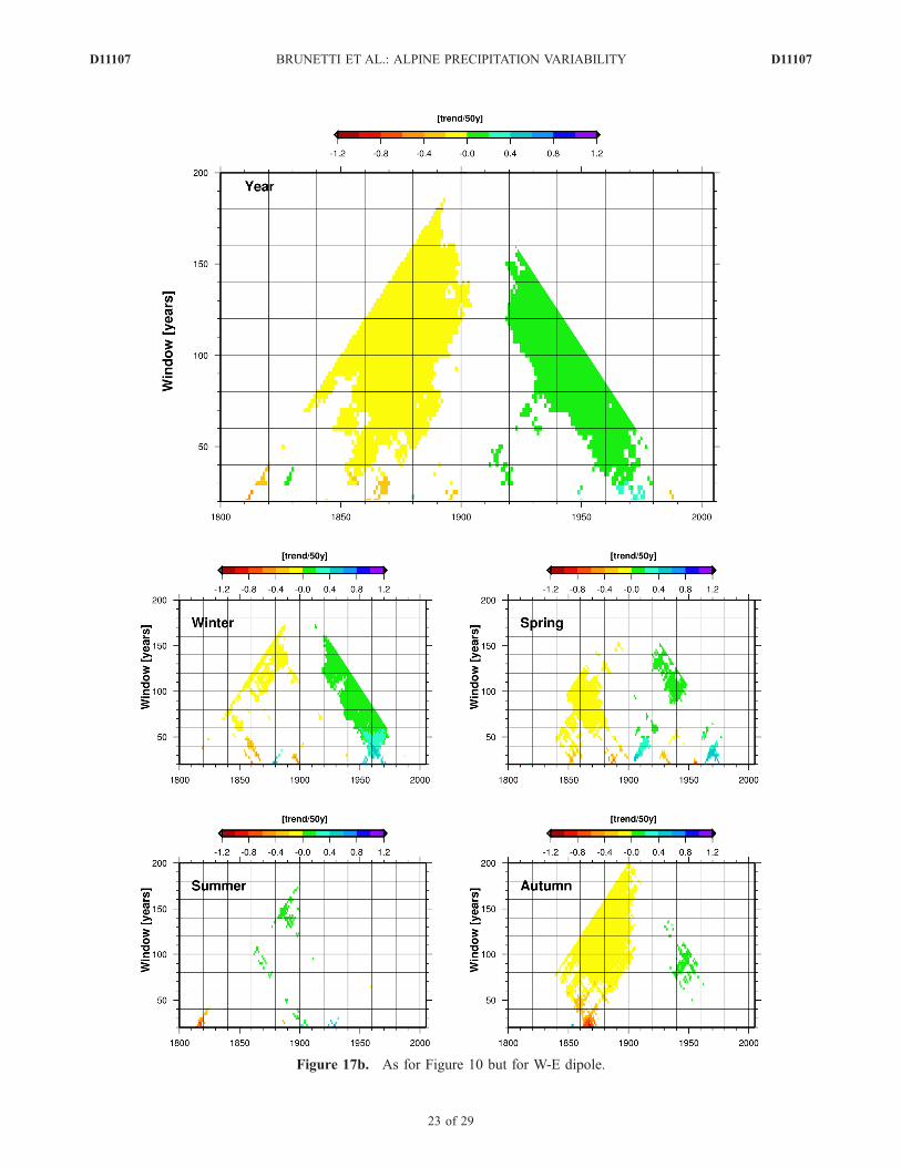
Figure 17b. As for Figure 10 but for W-E dipole.


23 of 29

D11107

consequence of the significant decrease in precipitationamount south of the Alps and the increase (not alwayssignificant) north of the Alps. The positive trend in N-S ishighly significant on a yearly basis, most of the signalcoming from autumn and winter seasons, but with animportant contribution coming also from spring (Table 7).The difference between the bicentennial trends of the N-Sand the W-E dipoles (significant increase in the former, notrend in the latter over the 2 centuries) originates mainlyfrom the higher values of the W-E difference series in theearly instrumental period, which damps the long-term trend.The dipole series were also subjected to running trendanalysis (Figures 17a and 17b). When starting later (near1870) both dipoles show increasing tendencies, the N-Sdipole’s 130-years trend being only slightly stronger thanthe W-E one (this difference is mainly caused by theongoing increase of the N-S dipole series in the recent2 decades compared to a stagnation of the respectiveevolution of the W-E dipole). In some aspects the dipoleseries show a greater regularity than those referring tothe NW-NE-SW-SE quadrupole. The clear bicentennialdecreasing-increasing scheme visible in the W-E annualdipole and the steady long-term increase of the N-S annualdipole, which is significant at all timescales from 60 to200 years, are two examples of a great number of interestingfeatures in the running trend Figures 17a and 17b.

7. Changes in Precipitation Seasonality

[69] Besides changes in total precipitation amount, pre-cipitation distribution over the year is also a very importantindicator of climate changes. Moreover, its alteration has animportant impact on many aspects of human life, such asagriculture and water management, but also on the envi-ronment. Of particular relevance for the Alpine region is itsinfluence on the glacier mass balance, as the influence ofprecipitation comes from not only total amount, but also thedistribution over the year. Precipitation influences glacier

mass balance not only directly (via direct snow accumula-tion in the cold season) but also indirectly via albedoincrease (snow episodes in the warm season) and viaadditional melting (liquid precipitation). This highlights aninteresting field of application, no further details will begiven.[70] As far as Europe is concerned, the few available

results on seasonality changes for Sweden and southern andeastern Spain [Busuic et al., 2001; Sumner et al., 2001] donot show a homogeneous behavior.[71] In order to highlight any change in the seasonality of

precipitation, we investigated the evolution of precipitationdistribution over the year.[72] The first step was to convert all the monthly precip-

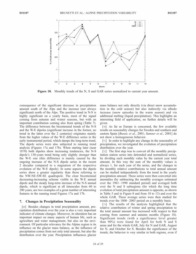
itation station series into detrended and normalized series,by dividing each monthly value by the current year totalamount. In this way the sum of the monthly values isalways 1, for each year of the series, and the changes inthe monthly relative contributions to total annual amountcan be studied independently from the trend in the yearlyprecipitation amount. These series were then converted intoanomalies (by subtracting the monthly averages estimatedover the 1961–1990 standard period) and averaged bothover the N and S subregions (for which the long timeevolution of total precipitation amount is opposite, as shownin Table 5 and in Figure 8 and from 10 to 13) and over thewhole GAR. These average series were then studied fortrends over the 1800–2003 period on a monthly basis.[73] The results of the analysis highlighted that the

relative contribution of winter and spring precipitation tothe total annual amount has increased with respect to thatcoming from summer and autumn months (Figure 18).Significant trends (with a significance level greaterthan 90%) were found for April for both N and Sareas and for the whole GAR, July for N and GAR, Augustfor N, and October for S. Besides the significance of thetrends, the behavior is very similar in both regions, even if

Figure 18. Monthly trends of the N, S and GAR series normalized to current year amount.


24 of 29

D11107

the time evolutions of precipitation in the two areas are verydifferent.[74] The regularity and smoothness of this signal, even if

it is not strong, can be interpreted as a really existingtendency toward a more Mediterranean-like precipitationseasonality, i.e., characterized by a summer minimum and awinter maximum in the precipitation cycle. It must bestressed that we are talking of a slow effect over 2 centuries,not a recent development. Because of the nonexistence ofadequate bicentennial data sets before HISTALP, this effecthas been hidden so far, and therefore not yet analyzed.Therefore we do not claim the explanation above to be theultimate cause. Specifically, one fact raises doubts on the‘‘northward shifting of Mediterranean climate’’ hypothesis:It is not really a pure winter-summer feature (but more acycle with its maximum in April (with wetting trends fromDecember to June) and its negative phase (drying) from July

to November). Thus it seems to be more an increase in amore ‘‘symmetric Mediterranean precipitation regime’’through a relative increase of the Spring against the Autumnmaximum (which has dominated so far in the region, visiblein Figure 1). However, it is an interesting effect because ofits existence north of the Alps as well. The Alpine chain isusually a strong barrier against climatic influence from thesouth, but the described effect has crossed it quite easily.The apparent ‘‘weakness’’ of the rearrangement of theseasonal cycle can be put into perspective: Compared tothe single month’s share of 8.3% (in the case of a ‘‘flat’’annual course), the typical ‘‘seasonal rearrangement magni-tude’’ of 0.5% (with peaks of up to 1%) is in fact not thatsmall.[75] There is a chance that at least parts of the bicenten-

nial seasonality shift may also be attributed to the fact thatthe precipitation series have not been adjusted systemati-

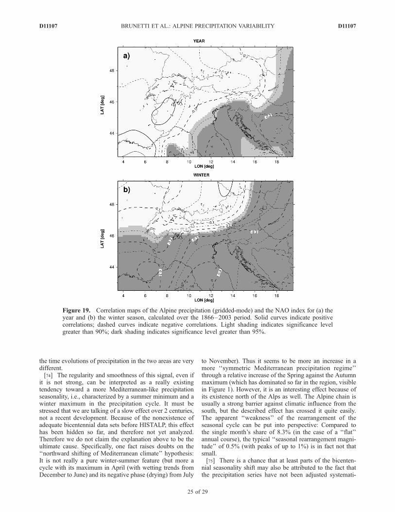
Figure 19. Correlation maps of the Alpine precipitation (gridded-mode) and the NAO index for (a) theyear and (b) the winter season, calculated over the 1866–2003 period. Solid curves indicate positivecorrelations; dashed curves indicate negative correlations. Light shading indicates significance levelgreater than 90%; dark shading indicates significance level greater than 95%.


25 of 29

D11107

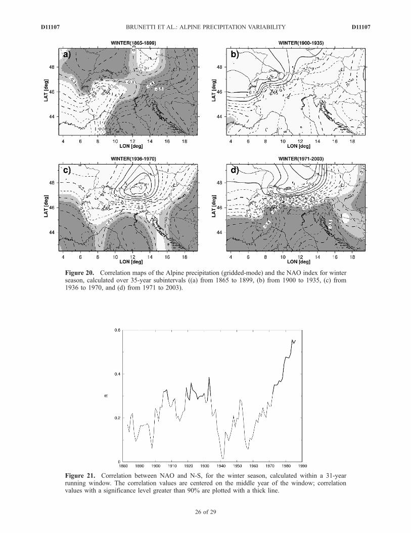
Figure 20. Correlation maps of the Alpine precipitation (gridded-mode) and the NAO index for winterseason, calculated over 35-year subintervals ((a) from 1865 to 1899, (b) from 1900 to 1935, (c) from1936 to 1970, and (d) from 1971 to 2003).

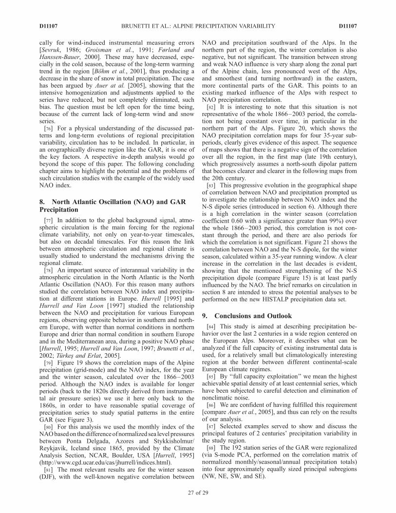
Figure 21. Correlation between NAO and N-S, for the winter season, calculated within a 31-yearrunning window. The correlation values are centered on the middle year of the window; correlationvalues with a significance level greater than 90% are plotted with a thick line.


26 of 29

D11107

cally for wind-induced instrumental measuring errors[Sevruk, 1986; Groisman et al., 1991; Førland andHanssen-Bauer, 2000]. These may have decreased, espe-cially in the cold season, because of the long-term warmingtrend in the region [Bohm et al., 2001], thus producing adecrease in the share of snow in total precipitation. The casehas been argued by Auer at al. [2005], showing that theintensive homogenization and adjustments applied to theseries have reduced, but not completely eliminated, suchbias. The question must be left open for the time being,because of the current lack of long-term wind and snowseries.[76] For a physical understanding of the discussed pat-

terns and long-term evolutions of regional precipitationvariability, circulation has to be included. In particular, inan orographically diverse region like the GAR, it is one ofthe key factors. A respective in-depth analysis would gobeyond the scope of this paper. The following concludingchapter aims to highlight the potential and the problems ofsuch circulation studies with the example of the widely usedNAO index.

8. North Atlantic Oscillation (NAO) and GARPrecipitation

[77] In addition to the global background signal, atmo-spheric circulation is the main forcing for the regionalclimate variability, not only on year-to-year timescales,but also on decadal timescales. For this reason the linkbetween atmospheric circulation and regional climate isusually studied to understand the mechanisms driving theregional climate.[78] An important source of interannual variability in the

atmospheric circulation in the North Atlantic is the NorthAtlantic Oscillation (NAO). For this reason many authorsstudied the correlation between NAO index and precipita-tion at different stations in Europe. Hurrell [1995] andHurrell and Van Loon [1997] studied the relationshipbetween the NAO and precipitation for various Europeanregions, observing opposite behavior in southern and north-ern Europe, with wetter than normal conditions in northernEurope and drier than normal condition in southern Europeand in the Mediterranean area, during a positive NAO phase[Hurrell, 1995; Hurrell and Van Loon, 1997; Brunetti et al.,2002; Turkes and Erlat, 2005].[79] Figure 19 shows the correlation maps of the Alpine

precipitation (grid-mode) and the NAO index, for the yearand the winter season, calculated over the 1866–2003period. Although the NAO index is available for longerperiods (back to the 1820s directly derived from instrumen-tal air pressure series) we use it here only back to the1860s, in order to have reasonable spatial coverage ofprecipitation series to study spatial patterns in the entireGAR (see Figure 3).[80] For this analysis we used the monthly index of the

NAObasedon thedifferenceofnormalized sea level pressuresbetween Ponta Delgada, Azores and Stykkisholmur/Reykjavik, Iceland since 1865, provided by the ClimateAnalysis Section, NCAR, Boulder, USA [Hurrell, 1995](http://www.cgd.ucar.edu/cas/jhurrell/indices.html).[81] The most relevant results are for the winter season

(DJF), with the well-known negative correlation between

NAO and precipitation southward of the Alps. In thenorthern part of the region, the winter correlation is alsonegative, but not significant. The transition between strongand weak NAO influence is very sharp along the zonal partof the Alpine chain, less pronounced west of the Alps,and smoothest (and turning northward) in the eastern,more continental parts of the GAR. This points to anexisting marked influence of the Alps with respect toNAO precipitation correlation.[82] It is interesting to note that this situation is not

representative of the whole 1866–2003 period, the correla-tion not being constant over time, in particular in thenorthern part of the Alps. Figure 20, which shows theNAO precipitation correlation maps for four 35-year sub-periods, clearly gives evidence of this aspect. The sequenceof maps shows that there is a negative sign of the correlationover all the region, in the first map (late 19th century),which progressively assumes a north-south dipolar patternthat becomes clearer and clearer in the following maps fromthe 20th century.[83] This progressive evolution in the geographical shape

of correlation between NAO and precipitation prompted usto investigate the relationship between NAO index and theN-S dipole series (introduced in section 6). Although thereis a high correlation in the winter season (correlationcoefficient 0.60 with a significance greater than 99%) overthe whole 1866–2003 period, this correlation is not con-stant through the period, and there are also periods forwhich the correlation is not significant. Figure 21 shows thecorrelation between NAO and the N-S dipole, for the winterseason, calculated within a 35-year running window. A clearincrease in the correlation in the last decades is evident,showing that the mentioned strengthening of the N-Sprecipitation dipole (compare Figure 15) is at least partlyinfluenced by the NAO. The brief remarks on circulation insection 8 are intended to stress the potential analyses to beperformed on the new HISTALP precipitation data set.

9. Conclusions and Outlook

[84] This study is aimed at describing precipitation be-havior over the last 2 centuries in a wide region centered onthe European Alps. Moreover, it describes what can beanalyzed if the full capacity of existing instrumental data isused, for a relatively small but climatologically interestingregion at the border between different continental-scaleEuropean climate regimes.[85] By ‘‘full capacity exploitation’’ we mean the highest

achievable spatial density of at least centennial series, whichhave been subjected to careful detection and elimination ofnonclimatic noise.[86] We are confident of having fulfilled this requirement

[compare Auer et al., 2005], and thus can rely on the resultsof our analysis.[87] Selected examples served to show and discuss the

principal features of 2 centuries’ precipitation variability inthe study region.[88] The 192 station series of the GAR were regionalized

(via S-mode PCA, performed on the correlation matrix ofnormalized monthly/seasonal/annual precipitation totals)into four approximately equally sized principal subregions(NW, NE, SW, and SE).


27 of 29

D11107

[89] Precipitation average series of these subregions notonly evolved through different interannual variability, butare also characterized by significantly different long-termtrends: the most relevant one being an increase in the totalprecipitation amount north of the Alpine chain, and a highlysignificant decrease south of the Alps.[90] The precipitation evolution of the different subre-

gions was stressed by means of a moving window technique(called running trend analysis here), with variable windowwidth, that allowed the identification of some relevanttendencies on a wide range of timescales (from 2 decadesto 2 centuries) involving the whole GAR, in some cases, ora few subregions, in many others.[91] The different time evolution of precipitation in the

various subregions was also highlighted by a T-modePCA. This technique highlighted the existence of twoleading general and long-term dipole structures, throughoutnorth-south and west-east main directions. Series, represen-tative of these two patterns, were constructed from thedifferences between northern and southern regional averageseries, and western and eastern ones. The N-S dipole showsthe most stable and significant 2-century trend in thestudy region: a general strengthening of the mentioneddipole structure, due to a relative wetting of the northernGAR (temperate westerly), versus the southern GAR(Mediterranean parts).[92] Besides changes in total precipitation amount, pre-

cipitation distribution over the year was also analyzed toidentify changes in precipitation seasonality. A regular andsmooth signal toward an increase in the relative contributionof winter and spring precipitation to the total annualamount, with respect to that coming from summer andautumn months, was observed. This tendency, however,must be interpreted with caution, because it could be partlyattributed to wind-induced instrumental measuring errors, abias that the intensive homogenization and adjustmentsapplied on the series have reduced but not completelyeliminated. This possibility must be investigated in the lightof a wider availability of long-term wind and snow series.[93] The final section of this work was aimed at making

an initial step into the ‘‘understanding business’’ whichhas to rely strongly on forcing via circulation – especiallyin a region with such prominent orographic features likethe Alps. The long-term correlative comparison with theNAO index showed existing spatial patterns, as well asan interesting variability of the NAO correlation overtime.[94] Our future study objectives will concentrate on

increasing our understanding of the multiple climate vari-ability structure in the GAR. This will be based on com-bined analyses of the existing climate elements in HISTALP(temperature, precipitation, air pressure with full spatialcoverage, sunshine and cloudiness with nearly full spatialcoverage, and humidity for parts of the GAR, compare Aueret al. [2006]) in relation to larger-scale (continental toglobal) background features, and finding dependencies ofthe local (GAR or smaller) climate variability residuals oncirculation.

[95] Acknowledgments. This study was carried out in the frameworkof the ALP-IMP project supported by the European Commission (EVK2-CT-2002-00148). The HISTALP-system was initially developed within the

Austrian research project CLIVALP (FWF P15076-N06). Data acquisitionwas greatly facilitated through the well-established formal and informalexchange practice among the national and subnational data providers of thestudy region.

ReferencesAuer, I. (1993), Niederschlagsschwankungen in Osterreich, OsterreichischeBeitr. Meteorol. Geophys., 7, 1–73.

Auer, I., and R. Bohm (1994), Combined temperature-precipitation varia-tions in Austria during the instrumental period, Theor. Appl. Climatol.,49, 161–174.

Auer, I., R. Bohm, and W. Schoner (2001), Austrian long-term climate1767 – 2000, multiple climate time series from central Europe,Osterreichische Beitr. Meteorol. Geophys., 25, 1–147.

Auer, I., et al. (2005), A new instrumental precipitation dataset for thegreater Alpine region for the period 1800–2002, Int. J. Climatol., 25,139–166.

Auer, I., et al. (2006), HISTALP—Historical Instrumental SurfaceClimatological Time Series of the Alpine region, Int. J. Climatol., inpress.

Begert, M., T. Schlegel, and W. Kirchhofer (2005), Homogeneous tempera-ture and precipitation series of Switzerland from 1864 to 2000, Int.J. Climatol., 25, 65–80.

Bohm, R., I. Auer, M. Brunetti, M. Maugeri, T. Nanni, and W. Schoner(2001), Regional temperature variability in the European Alps 1760–1998 from homogenized instrumental time series, Int. J. Climatol., 21,1779–1801.

Bohm, R., et al. (2003), Der Alpine Niederschlagsdipol—ein dominierendesSchwankungsmuster der Klimavariabilitat in den Scales 100 km – 100Jahre, Terra Nostra, 2003/6, 61–65.

Brunetti, M., M. Maugeri, and T. Nanni (2002), Atmospheric circulationand precipitation in Italy for the last 50 years, Int. J. Climatol., 22, 1455–1471.

Brunetti, M., M. Maugeri, F. Monti, and T. Nanni (2004), Changes in dailyprecipitation frequency and distribution in Italy over the last 120 years,J. Geophys. Res., 109, D05102, doi:10.1029/2003JD004296.

Brunetti, M., M. Maugeri, F. Monti, and T. Nanni (2006), Temperature andprecipitation variability in Italy in the last two centuries from homoge-nized instrumental time series, Int. J. Climatol., 26, 345–381.

Buffoni, L., M. Maugeri, and T. Nanni (1999), Precipitation in Italy from1833 to 1996, Theor. Appl. Climatol., 63, 33–40.

Busuic, A., D. Chen, and C. Hellstrom (2001), Temporal and spatialvariability of precipitation in Sweden and its link with the large-scaleatmospheric circulation, Tellus, Ser. A, 53, 348–367.

Førland, E. J. (Ed.) (1996), Manual for operational correction ofnordic precipitation data, Rep. 24/96, 66 pp., Norw. Meteorol. Inst.,Oslo.

Førland, E. J., and I. Hanssen-Bauer (2000), Increased precipitation in theNorwegian Arctic: True or false?, Clim. Change, 46, 485–509.

Frei, C., and C. Schar (1998), A precipitation climatology of the Alpsfrom high-resolution rain-gauge observations, Int. J. Climatol., 18,873–900.

Groisman, P. Y., V. V. Koknaeva, T. A. Belokrylova, and T. R. Karl (1991),Overcoming biases of precipitation measurement: A history of USSRexperience, Bull. Am. Meteorol. Soc., 72, 1725–1732.

Hurrell, J. W. (1995), Decadal trends in the North Atlantic Oscillation:Regional temperature and precipitaion, Science, 269, 676–679.

Hurrell, J. W., and H. Van Loon (1997), Decadal variation in climateassociated with the north atlantic oscillation, Clim. Change, 36, 301–326.

Joliffe, I. T. (1986), Principal Component Analyses, 271 pp., Springer, NewYork.

Matulla, C., I. Auer, R. Bohm, M. Ungersbock, W. Schoner, S. Wagner, andE. Zorita (2005), Outstanding past decadal-scale climate events in thegreater Alpine region analysed by 250 years data and model runs, GKSS-Rep., 2005/4, pp. 1–113, GKSS-Forschungszentrum Geesthacht GmbH,Hamburg, Germany.

Moisselin, J.-M., M. Schneider, C. Canellas, and O. Mestre (2002),Changements climatiques en France au 20eme siecle. Etude des longuesseries de donnees homogeneisees francaises de precipitations et tempera-tures, Meteorologie, 38, 45–56.

Schmidli, J., C. Schmutz, C. Frei, H. Wanner, and C. Schar (2002), Me-soscale precipitation variability in the region of the European Alps duringthe 20th century, Int. J. Climatol., 22, 1049–1074.

Schonwiese, C. D., and J. Rapp (1997), Climate Trend Atlas of Europe.Based on Observations 1901–1990, 228 pp., Springer, New York.

Sevruk, B. (Ed.) (1986), Corrections of precipitation measurements, paperpresented at WMO/IAHS/ETH Workshop, World Meteorol. Organ.,Zurich, Switzerland, 1–3 Apr.


28 of 29

D11107

Sneyers, R. (1990), On the statistical analysis of series of observation, Tech.Note 143, 192 pp., World Meteorol. Organ., Geneva, Switerland.

Sumner, G., V. Homar, and C. Ramis (2001), Precipitation seasonalityin eastern and southern coastal Spain, Int. J. Climatol., 21, 219–247.

Turkes, M., and E. Erlat (2005), Climatological responses of winter pre-cipitation in Turkey to variability of the North Atlantic Oscillation duringthe period 1930–2001, Theor. Appl. Climatol., 81, 45–69.

Widmann, M. L., and C. Schar (1997), A principal component and long-term trend analysis of daily precipitation in Switzerland, Int. J. Climatol.,17, 1333–1356.

Wilks, D. S. (1995), Statistical Methods in the Atmospheric Sciences,Elsevier, New York.

��I. Auer, R. Bohm, and W. Schoner, Central Institute for Meteorology and

Geodynamics, Hohe Warte 38, A-1190 Vienna, Austria.M. Brunetti and T. Nanni, Institute of Atmospheric Sciences and Climate,

Italian National Research Council, via Gobetti, 101, I-40129 Bologna, Italy.([email protected])M. Maugeri, Istituto di Fisica Generale Applicata, via Brera, 28, I-20121

Milan, Italy.


29 of 29

D11107

Precipitation variability and changes in the greater Alpine region over the 1800–2003 period

Documents

Transcript of Precipitation variability and changes in the greater Alpine region over the 1800–2003 period