�����������������

Citation: Cheng, M.; Wang, Y.; Zhu,

J.; Pan, Y. Precipitation Dominates the

Relative Contributions of Climate

Factors to Grasslands Spring

Phenology on the Tibetan Plateau.

Remote Sens. 2022, 14, 517.

https://doi.org/10.3390/rs14030517

Academic Editors: Ruyin Cao,

Miaogen Shen and Bin Fu

Received: 8 December 2021

Accepted: 20 January 2022

Published: 21 January 2022

Publisher’s Note: MDPI stays neutral

with regard to jurisdictional claims in

published maps and institutional affil-

iations.

Copyright: © 2022 by the authors.

Licensee MDPI, Basel, Switzerland.

This article is an open access article

distributed under the terms and

conditions of the Creative Commons

Attribution (CC BY) license (https://

creativecommons.org/licenses/by/

4.0/).

remote sensing

Article

Precipitation Dominates the Relative Contributions of ClimateFactors to Grasslands Spring Phenology on the Tibetan PlateauMin Cheng 1,2 , Ying Wang 3,* , Jinxia Zhu 1,2 and Yi Pan 1,2

1 Institute of Land and Urban-Rural Development, Zhejiang University of Finance and Economics,Hangzhou 310018, China; chengmin@zufe.edu.cn (M.C.); jxzhu@zufe.edu.cn (J.Z.);ypangis@zufe.edu.cn (Y.P.)

2 Zhejiang Institute of “Eight-Eight” Strategies, Hangzhou 310018, China3 School of Culture Industry and Tourism Management, Sanjiang University, Nanjing 210012, China* Correspondence: wang_ying@sju.edu.cn

Abstract: Temperature and precipitation are the primary regulators of vegetation phenology intemperate zones. However, the relative contributions of each factor and their underlying combinedeffect on vegetation phenology are much less clear, especially for the grassland of the Tibetan PlateauTo quantify the contribution of each factor and the potential interactions, we conducted redundancyanalysis for grasslands spring phenology on the Tibetan Plateau during 2000–2017. Generally, theindividual contribution of temperature and precipitation to grasslands spring phenology (the startof growing season (SOS)) was lower, despite a higher correlation coefficient, which further impliedthat these factors interact to affect the SOS. The contributions of temperature and precipitationto the grasslands spring phenology varied across space on the Tibetan Plateau, and these spatialheterogeneities can be mainly explained by the spatial gradient of long-term average precipitationduring spring over 2000–2017. Specifically, the SOS for meadow was dominated by the meantemperature in spring (Tspring) in the eastern wetter ecoregion, with an individual contribution of24.16% (p < 0.05), while it was strongly negatively correlated with the accumulated precipitationin spring (Pspring) in the western drier ecoregion. Spatially, a 10 mm increase in long-term averageprecipitation in spring resulted in an increase in the contribution of Tspring of 2.0% (p < 0.1) for meadow,while it caused a decrease in the contribution of Pspring of −0.3% (p < 0.05). Similarly, a highercontribution of Pspring for steppe was found in drier ecoregions. A spatial decrease in precipitationof 10 mm increased the contribution of Pspring of 1.4% (p < 0.05). Considering these impacts ofprecipitation on the relative contribution of warming and precipitation to the SOS, projected climatechange would have a stronger impact on advancing SOS in a relatively moist environment comparedto that of drier areas. Hence, these quantitative interactions and contributions must be includedin current ecosystem models, mostly driven by indicators with the direct and the overall effect inresponse to projected climate warming.

Keywords: climate change; spring phenology; individual contribution; interacting effects; TibetanPlateau

1. Introduction

Climate change was now documented in all major regions of the world and affectedvegetation structure and function as well as public health [1–4]. As the dominant vegetationtype on the Tibetan Plateau, grassland plays important roles in ecological balance andprovides an important buffer against climate change [5,6], and the grassland phenologywas identified as a key indicator of climate–vegetation interactions and reflects the responseof living systems to climate change [7,8]. In particular, the spring phenology of grasslandcan provide insight into higher level dynamics of plant functioning and feedback to climatechange through exchange of energy, the hydrological cycle, and carbon uptake, which ismore relevant to global climate and regional natural environmental changes [9–13].

Remote Sens. 2022, 14, 517. https://doi.org/10.3390/rs14030517 https://www.mdpi.com/journal/remotesensing

Remote Sens. 2022, 14, 517 2 of 18

Temperature and precipitation are regarded as the primary regulators of plant phe-nology in the temperate zone. Highly credible evidence shows that global warming andregional changes in precipitation strongly affected vegetation phenology [12,14–17]. Al-though there were many studies focused on understanding the mechanisms and influencesof climate warming and regional precipitation on vegetation phenology, there are still alot of uncertainties in the responses of the start of growing season (SOS) to these factors.As proof, Lucht et al. [18] and Xu et al. [19] showed that the growth of vegetation wouldbe facilitated, because global warming eased climatic constraints. However, according toJeong et al. [20], the vegetation spring phenology and preseason mean temperature arecorrelated across the Northern Hemisphere with a correlation coefficient varying from −0.3to −0.7, suggesting that global warming would not necessarily induce greater advance inSOS. In addition, Yu et al. [13] showed that winter warming could delay vegetation springphenology due to the adaptive ability of chilling requirements, while Suonan et al. [21]showed that winter warming increased the soil temperature, and then advanced springleaf out and flowering phenology. Some studies also showed that the daylength couldcoregulate the SOS through its interaction with temperature or its influence on the stomataaperture and photosynthetic active radiation [22,23]. Furthermore, water is also necessaryfor plant growth, which indicates that changes in regional precipitation should be an-other main driving factor that regulate vegetation phenology, particularly in water-limitedareas [9,12,16,24]. However, the SOS’s responses to preseason precipitation were alsodiverse. Dai et al. [25] found that precipitation and the first leafing date do not show asignificant negative correlation. Other studies, on the other hand, reported that, in aridor semiarid regions, preseason precipitation indeed advanced vegetation SOS because itdetermines spring water availability [5,9,26]. Moreover, some studies argued that presea-son precipitation would increase the heat demand and then influence the sensitivity ofSOS to precipitation and temperature [16,27]. That is, along with direct impact, precipita-tion may exert indirect impacts on SOS. These direct and indirect impacts indicated thattemperature and precipitation would complicatedly interact to affect vegetation SOS. Itis difficult to quantify the individual contributions of temperature and precipitation tothe interannual variation of vegetation phenology because of the nonlinear impacts andunderlying interactions of climate factors.

As the world’s largest plateau, the Tibetan Plateau is considered as one of the mostvulnerable ecosystems because of its typical alpine climate and its strong sensitivity toclimate change [5,9–13]. Although numerous recent studies reported the interannual varia-tion of SOS and its responses to warming and precipitation [10–13,28], large uncertaintiesstill exist about the advanced (i.e., earlier) or delayed (i.e., later) pattern of the vegetationspring phenology and their responses to different factors. For instance, Piao et al. [29]showed that the spring phenology of alpine meadow would be delayed by the increasedaccumulated preseason precipitation occurring in five months before the vegetation onset,while Shen et al. [30] found that declines in spring precipitation would delay SOS ratherthan increase preseason precipitation. Moreover, Yu et al. [13] showed that winter warmingcould delay grassland spring phenology on the Tibetan Plateau, while Suonan et al. [21]showed that asymmetric winter warming advanced plant phenology in alpine meadow.Furthermore, these explanations were later questioned by some studies that argued that thevegetation spring phenology was more strongly affected by the interaction of warming andprecipitation than the unitary effect of driving factors [5,9,11,16]. Even so, the interactioneffects of climate factors on vegetation phenology remain poorly understood, and theindividual contribution of each factor to grassland SOS across the Tibetan Plateau is notyet well understood. Thus, quantitative estimation of the relative contribution of criticalclimate factors and their interaction effects on grassland SOS on the Tibetan Plateau iscritical and valuable. In this study, we first analyze how SOS changed in the grassland indifferent ecoregions of the Tibetan Plateau. We untangle the individual contribution andinteraction of the mean temperature in winter (Twinter), mean temperature in spring (Tspring),and the accumulated precipitation in spring (Pspring) for interannual variations in SOS based

Remote Sens. 2022, 14, 517 3 of 18

on redundancy analysis and identify temporal-spatial pattern of SOS responses to criticalclimate factors on the Tibetan Plateau. This is an important step toward understanding themechanistic effects and underlying causes of climate change on vegetation phenology.

2. Materials and Methods2.1. Study Area

The Tibetan Plateau lies at an average altitude of over 4000 m in southwest China(Figure 1), with a typical alpine climate environment and unique composition and dis-tribution of alpine grassland, along with a low level of human interference. Across theentire plateau, the annual mean temperature varies from −15 ◦C to 10 ◦C, and the an-nual cumulative precipitation decreases from more than 1000 mm to 50 mm. Recently,the Tibetan plateau experienced substantial climate change characterized by significantwarming [9–12]. Meanwhile, numerous studies showed that vegetation was highly sensi-tive to climate changes on the Tibetan Plateau [9,12,15,27]. Hence, climate change and itsincreasingly pronounced effects on Tibetan Plateau grassland phenology are becoming anissue of global concern.

Remote Sens. 2022, 14, 517 3 of 19

contribution and interaction of the mean temperature in winter (Twinter), mean temperature in spring (Tspring), and the accumulated precipitation in spring (Pspring) for interannual vari-ations in SOS based on redundancy analysis and identify temporal-spatial pattern of SOS responses to critical climate factors on the Tibetan Plateau. This is an important step to-ward understanding the mechanistic effects and underlying causes of climate change on vegetation phenology.

2. Materials and Methods 2.1. Study Area

The Tibetan Plateau lies at an average altitude of over 4000 m in southwest China (Figure 1), with a typical alpine climate environment and unique composition and distri-bution of alpine grassland, along with a low level of human interference. Across the entire plateau, the annual mean temperature varies from −15 °C to 10 °C, and the annual cumu-lative precipitation decreases from more than 1000 mm to 50 mm. Recently, the Tibetan plateau experienced substantial climate change characterized by significant warming [9–12]. Meanwhile, numerous studies showed that vegetation was highly sensitive to climate changes on the Tibetan Plateau [9,12,15,27]. Hence, climate change and its increasingly pronounced effects on Tibetan Plateau grassland phenology are becoming an issue of global concern.

Figure 1. Location, ecoregions, and vegetation distribution for Tibetan Plateau. (I) Indicates Eastern Qinghai–Qilian montane steppe ecoregions; (II) indicates Golog–Nagqu high-cold shrub-meadow ecoregions; (III) indicates southern Qinghai high cold meadow steppe ecoregions; (IV) indicates Qi-angtang high-cold steppe ecoregions; and (V) indicates Southern Xizang montane shrub-steppe ecoregions [31]. Pixels with annual maximum normalized difference vegetation index (NDVI) greater than 0.15 and mean NDVI of July to August larger than 1.35 × NDVI during November to February are shown.

2.2. Datasets During the past two decades, the monitoring of vegetation phenology at large-scale

regional units was widely achieved using satellite remote sensing. In this study, we first produced an NDVI (normalized difference vegetation index) dataset by using MODIS (moderate resolution imaging spectroradiometer) surface reflectance products with a spa-tial resolution of 500 m and a compositional period of 8 days from 2000 to 2017 [32], ob-tained from the LPDAAC (land processes distributed active archive center,

Figure 1. Location, ecoregions, and vegetation distribution for Tibetan Plateau. (I) Indicates EasternQinghai–Qilian montane steppe ecoregions; (II) indicates Golog–Nagqu high-cold shrub-meadowecoregions; (III) indicates southern Qinghai high cold meadow steppe ecoregions; (IV) indicatesQiangtang high-cold steppe ecoregions; and (V) indicates Southern Xizang montane shrub-steppeecoregions [31]. Pixels with annual maximum normalized difference vegetation index (NDVI) greaterthan 0.15 and mean NDVI of July to August larger than 1.35 × NDVI during November to Februaryare shown.

2.2. Datasets

During the past two decades, the monitoring of vegetation phenology at large-scaleregional units was widely achieved using satellite remote sensing. In this study, wefirst produced an NDVI (normalized difference vegetation index) dataset by using MODIS(moderate resolution imaging spectroradiometer) surface reflectance products with a spatialresolution of 500 m and a compositional period of 8 days from 2000 to 2017 [32], obtainedfrom the LPDAAC (land processes distributed active archive center, https://lpdaacsvc.cr.usgs.gov/appeears/. Accessed 21 April 2021). To match the spatial resolution of theclimatic factors, we then resampled these NDVI datasets to a resolution of 1 km and usedthem to determine vegetation SOS.

Information about the meadow and steppe distribution on the Plateau was obtainedfrom the 1:1,000,000 vegetation map of China [33], created by the Chinese Academy of Sci-

Remote Sens. 2022, 14, 517 4 of 18

ences, using datasets from field observations, aerial photos, TM (landsat thematic mapper)and ETM (enhanced thematic mapper) satellite images [34,35]. Climate factors at meteoro-logical stations, including the mean air temperature (◦C), accumulative precipitation (mm)in spring (March–May), and the mean air temperature (◦C) in winter (December–February)were obtained from the China Meteorological Data Service Center. Based on the DEM(digital elevation model) data with 1 km spatial resolution produced by United StatesGeological Survey (USGS) and the 71 meteorological stations with complete records onthe Tibetan Plateau (Figure 1), we calculated the spatial grid distribution of accumulatedprecipitation and mean temperature in spring using ANUSPLIN interpolation. Specifically,considering there were fewer than 2000 meteorological stations, we first employed theSPLNEA module to calculate the surface fitting parameters and their error covariance.Based on the latitude, longitude, and elevation information in a grid cell provided by DEM,the fitted climatic values and corresponding predicted standard error in the grid were thencalculated by using the LAPGRD module [36–38].

2.3. Preprocessing of NDVI Data

Due to the inevitable impact of bare soils, sparsely vegetated grids, atmosphericcontamination, etc., there were still many spurious changes in the NDVI time series [9,34,39].Hence, to improve the quality of annual NDVI time series, the Savitzky–Golay filter forNDVI time series was conducted first. Additionally, we only selected pixels that met thefollowing principles simultaneously to analyze the relative contributions of climate factorsand their underlying combined effect on grassland spring phenology. First, the annualmaximum NDVI must be greater than 0.15, and then the mean NDVI of July to Augustmust be larger than 1.35 × NDVI during November to February. The spatial distribution ofvalid pixels is displayed in Figure 1.

2.4. Estimation of Grassland Spring Phenology

In this section, the 18-year averaged NDVI value with a compositional period of 8 dayswas calculated from the entire data set during 2000–2017. Based on this long-term averagedNDVI time series data, subsequent analysis and calculation were conducted. Specifically,two different methods were employed to detect the grassland spring phenology on theTibetan Plateau.

2.4.1. Calculating the NDVI Thresholds Based on the Relative Rates of Changes

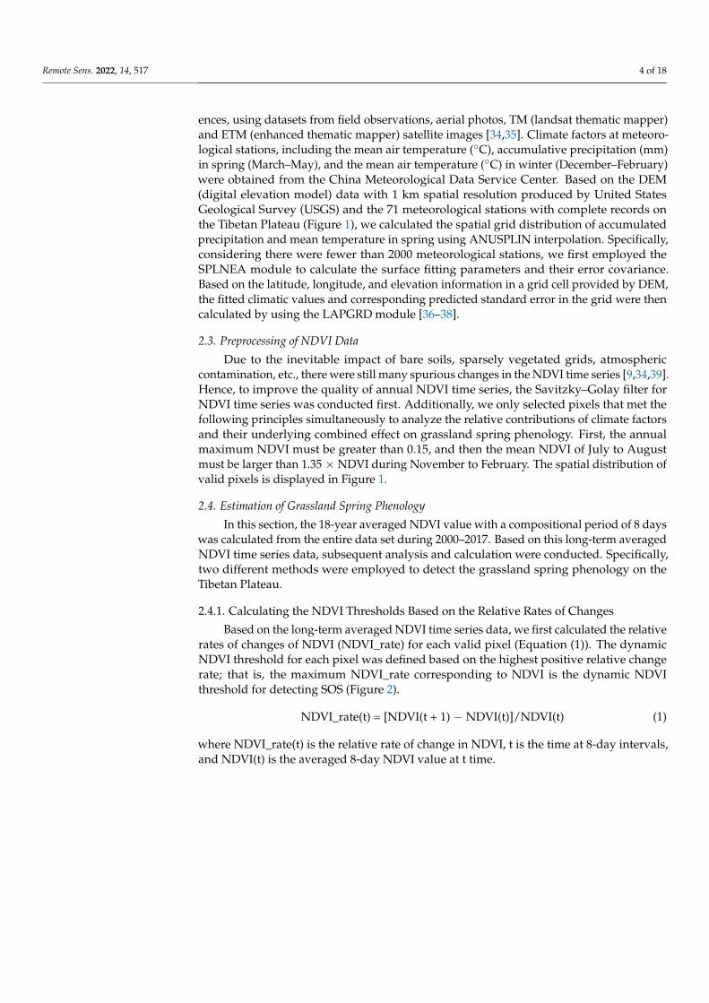
Based on the long-term averaged NDVI time series data, we first calculated the relativerates of changes of NDVI (NDVI_rate) for each valid pixel (Equation (1)). The dynamicNDVI threshold for each pixel was defined based on the highest positive relative changerate; that is, the maximum NDVI_rate corresponding to NDVI is the dynamic NDVIthreshold for detecting SOS (Figure 2).

NDVI_rate(t) = [NDVI(t + 1) − NDVI(t)]/NDVI(t) (1)

where NDVI_rate(t) is the relative rate of change in NDVI, t is the time at 8-day intervals,and NDVI(t) is the averaged 8-day NDVI value at t time.

Remote Sens. 2022, 14, 517 5 of 18Remote Sens. 2022, 14, 517 5 of 19

Figure 2. Schematic figures for calculating NDVI thresholds based on relative rates of change for NDVI time series. NDVI value of each point is mean value of grassland on Tibetan Plateau.

2.4.2. Polyfit Method

The polyfit method was initially applied to determine the vegetation spring phenol-ogy by Piao et al. [29]. Polyfit was widely shown to be one of the most efficient methods for the extraction of the vegetation phenology [8,29]. In general, the growing season of the grassland ranges from April to October in most areas of the Tibetan Plateau; that is, the NDVI value of grassland increased first, and then decreased with the increasing num-bered day of the year during the growing season. Therefore, a 6-degree polynomial with a least-square analysis can be performed to reconstruct the daily NDVI time series from the original 8-day NDVI data during January to September. The polynomial function is shown in Equation (2):

NDVI(t) = a0 + a1 × t + a2 × t2 + a3 × t3 + a4 × t4 + a5 × t5 + a6 × t6 (2)

where NDVI(t) is the NDVI at t time fitted by the polynomial equation. t is the numbered day of the year. a0, a1, a2, a3, a4, a5, a6 are the fitted coefficient derived from least-square regression analysis. The multiple linear regression function in MATLAB R2019b was used to estimate these fitted coefficients.

2.4.3. Harmonic Analysis of Time Series (HANTS) Method

The HANTS method was also used to reconstruct the daily NDVI time series from the original 8-day NDVI data. HANTS is regarded as an improved algorithm of the fast Fourier transform (FFT), which was proved to be one of the most efficient methods for the reconstruction of NDVI time series and the extraction of vegetation phenology [8,40,41]. The points with lower values than the neighbors are filtered during HANTS processing, and they are then reconstructed following Equation (3):

n

0 i i ii 1

NDVI(t)=a + a cos(ω t φ )=

− (3)

where NDVI(t) is the NDVI fitted by the HANTS model, t is the numbered day of the year. a0 and ai are the fitted coefficient of the HANTS model. n is the frequency, which is set to 1 for the grassland on the Tibetan Plateau. φi is the phase of the NDVI time series. ωi is set

Figure 2. Schematic figures for calculating NDVI thresholds based on relative rates of change forNDVI time series. NDVI value of each point is mean value of grassland on Tibetan Plateau.

2.4.2. Polyfit Method

The polyfit method was initially applied to determine the vegetation spring phenologyby Piao et al. [29]. Polyfit was widely shown to be one of the most efficient methods forthe extraction of the vegetation phenology [8,29]. In general, the growing season of thegrassland ranges from April to October in most areas of the Tibetan Plateau; that is, theNDVI value of grassland increased first, and then decreased with the increasing numberedday of the year during the growing season. Therefore, a 6-degree polynomial with aleast-square analysis can be performed to reconstruct the daily NDVI time series from theoriginal 8-day NDVI data during January to September. The polynomial function is shownin Equation (2):

NDVI(t) = a0 + a1 × t + a2 × t2 + a3 × t3 + a4 × t4 + a5 × t5 + a6 × t6 (2)

where NDVI(t) is the NDVI at t time fitted by the polynomial equation. t is the numberedday of the year. a0, a1, a2, a3, a4, a5, a6 are the fitted coefficient derived from least-squareregression analysis. The multiple linear regression function in MATLAB R2019b was usedto estimate these fitted coefficients.

2.4.3. Harmonic Analysis of Time Series (HANTS) Method

The HANTS method was also used to reconstruct the daily NDVI time series fromthe original 8-day NDVI data. HANTS is regarded as an improved algorithm of the fastFourier transform (FFT), which was proved to be one of the most efficient methods for thereconstruction of NDVI time series and the extraction of vegetation phenology [8,40,41].The points with lower values than the neighbors are filtered during HANTS processing,and they are then reconstructed following Equation (3):

NDVI(t)= a0 +n

∑i=1

ai cos(ωit−ϕi) (3)

where NDVI(t) is the NDVI fitted by the HANTS model, t is the numbered day of the year.a0 and ai are the fitted coefficient of the HANTS model. n is the frequency, which is set to 1for the grassland on the Tibetan Plateau. ϕi is the phase of the NDVI time series. ωi is set to2π in our study because the grassland on the Tibetan Plateau has a unique seasonal cycle.

Remote Sens. 2022, 14, 517 6 of 18

Based on the NDVI threshold and the fitted NDVI time series, the grassland SOS wasdetermined for each pixel and each year. Specifically, the numbered day of the year whenthe pixel’s NDVI value was first larger than the calculated NDVI threshold during thegrowing season was regarded as the grassland SOS.

2.5. Relationships between SOS and Climate

Generally, it is difficult to quantitatively estimate the individual contributions of tem-perature and precipitation for the interannual variation in vegetation phenology becauseof the nonlinear impacts and underlying interactions of climate factors. In this research,the redundancy analysis (RDA) was utilized to calculate the independent contribution ofTwinter, Tspring and Pspring to interannual variations in SOS [42,43]. The RDA is regarded as adirect extension of multiple linear regression and principal component analysis based oncanonical multivariate analyses. Based on this method, multiple response variables couldbe regressed on multiple explanatory variables, and the explanation proportion of eachexplanatory variable to response variables can be estimated and summarized [44–46]. Thisprocessing of RDA was demonstrated by Eigen analysis in the following equation:

(SyxS−1xx S′yx − λk I)uk = 0 (4)

where Syx is the covariance matrix among response variables and explanatory variables,S−1

xx is the standardized explanatory variables’ inverse covariance matrix, λk representsthe eigenvalue of the corresponding axis k, I is unit matrix, and uk is normalized canoni-cal eigenvectors.

In our study, a detrended correspondence analysis with the turnover units smallerthan three was first conducted to confirm the suitability of an RDA. The adjusted coefficientof determination obtained from the Hierarchical Partitioning algorithm was regarded asthe independent contribution of Twinter, Tspring and Pspring to interannual variations in SOS(https://github.com/laijiangshan/rdacca.hp/, Accessed 27 July 2020). Specifically, we firstconducted RDA for each ecoregion and the entire plateau to estimate the contribution ofeach factor at the ecoregional scale. Furthermore, the RDA was conducted for each validpixel to analyze spatial patterns of relative contribution of each factor and determine thedominant factor and the proportion of corresponding dominating factors. The Bonferronitest and Monte Carlo permutation methods (Permutations = 499) were used to analyze thestatistical significance [44,46,47]. In addition, to understand the spatial heterogeneity ofthe independent contribution of each factor, we performed linear regression in which theindividual contribution of each climate factor was set to the dependent variable against thelong-term average Pspring and Tspring across the Tibetan Plateau.

3. Results3.1. Interannual Variations in SOS

Across the Tibetan Plateau, most pixels’ SOS showed an advanced trend (a negativelinear trend) during 2000–2017, despite the spatial heterogeneity of trends in SOS revealedby the two different methods (Figure 3). That is, the timing of first and mean springlife history events advanced in time due to climate change. The average SOS of bothmethods advanced over about 72.42% of all the study areas, and most pixels advancedbetween 0–0.50 days per year−1 during the entire 18-year period (Figure 3c). Spatially, bothmethods showed widespread advancing trends over the central and eastern Plateau, whilea slight delayed trend in spring phenology was found in a few areas of the central andwestern Plateau. More specifically, 19.80% of pixels advanced significantly (p < 0.05), whichwere mainly located in the eastern ecoregions. While the pixels with delayed trend werediscretely distributed across the midwestern region of the Plateau, only 2.25% of pixelswere statistically significant (p < 0.05). These similar proportions and spatial patterns werealso revealed by the two different methods, and the results revealed an advanced trend ofSOS from Polyfit and HANTS at 74.26% of pixels (pixels with a significant advanced trend

Remote Sens. 2022, 14, 517 7 of 18

correspond to 24.58%, p < 0.05, Figure 3a) and 71.81% of pixels (22.03% with a significantadvanced trend, p < 0.05, Figure 3b), respectively.

Remote Sens. 2022, 14, 517 7 of 19

mainly located in the eastern ecoregions. While the pixels with delayed trend were dis-cretely distributed across the midwestern region of the Plateau, only 2.25% of pixels were statistically significant (p < 0.05). These similar proportions and spatial patterns were also revealed by the two different methods, and the results revealed an advanced trend of SOS from Polyfit and HANTS at 74.26% of pixels (pixels with a significant advanced trend correspond to 24.58%, p < 0.05, Figure 3a) and 71.81% of pixels (22.03% with a significant advanced trend, p < 0.05, Figure 3b), respectively.

Figure 3. Spatial distribution and frequency statistics of linear trends of grassland spring phenology (SOS) from Polyfit (a); HANTS (b) and average of two methods (c) during 2000–2017 and frequency distribution of different trend types for steppe and meadow across different ecoregions (d). A neg-ative value indicates an advance, and a positive value indicates a delay. Bottom-right and bottom-left insets in (a–c) show proportion of corresponding trends, indicated by map legend and spatial distribution of pixels with significantly negative (blue) and positive (red) trends (p < 0.05), respec-tively. SigD indicates significantly delayed SOS (p < 0.05). NSigD indicates delayed SOS but not significant (p > 0.05). NSigA indicates advanced SOS but not significant (p > 0.05). SigA indicates significantly advanced SOS (p < 0.05). All indicates entire plateau. I, II, III, IV, and V indicate differ-ent ecoregions following Figure 1.

With respect to meadows and steppe in different ecoregions, all methods agreed on an advanced trend (negative) over the entire study period but without consistent signifi-cance (Table 1). Specifically, the trends in the multimethod averaged SOS were −0.30 (p < 0.01) and −0.20 (p < 0.01) days per year−1 for steppe and meadow in the entire plateau, respectively. Regarding the two different models’ results, the trend of SOS for meadow across the entire plateau estimated from Polyfit was −0.21 (p < 0.01), while the result

Figure 3. Spatial distribution and frequency statistics of linear trends of grassland spring phenology(SOS) from Polyfit (a); HANTS (b) and average of two methods (c) during 2000–2017 and frequencydistribution of different trend types for steppe and meadow across different ecoregions (d). A negativevalue indicates an advance, and a positive value indicates a delay. Bottom-right and bottom-left insetsin (a–c) show proportion of corresponding trends, indicated by map legend and spatial distributionof pixels with significantly negative (blue) and positive (red) trends (p < 0.05), respectively. SigDindicates significantly delayed SOS (p < 0.05). NSigD indicates delayed SOS but not significant(p > 0.05). NSigA indicates advanced SOS but not significant (p > 0.05). SigA indicates significantlyadvanced SOS (p < 0.05). All indicates entire plateau. I, II, III, IV, and V indicate different ecoregionsfollowing Figure 1.

With respect to meadows and steppe in different ecoregions, all methods agreed on anadvanced trend (negative) over the entire study period but without consistent significance(Table 1). Specifically, the trends in the multimethod averaged SOS were−0.30 (p < 0.01) and−0.20 (p < 0.01) days per year−1 for steppe and meadow in the entire plateau, respectively.Regarding the two different models’ results, the trend of SOS for meadow across the entireplateau estimated from Polyfit was−0.21 (p < 0.01), while the result estimated from HANTSwas slightly lower (Slope = −0.19, p < 0.01). Regarding steppe across the entire plateau,a similar pattern can be found: the advanced trend of SOS from Polyfit and HANTS was−0.32 (p < 0.01) and −0.27 (p < 0.01), respectively.

Remote Sens. 2022, 14, 517 8 of 18

Table 1. Linear trends in multimethod averaged spring phenology (SOS) for steppe and meadow indifferent ecoregions from 2000–2017.

Ecoregions Meadow Steppe

ALL (Entire plateau) −0.20 ** −0.30 **I (Eastern Qinghai–Qilian montane steppe ecoregion) −0.30 ** −0.82 **II (Golog–Nagqu high-cold shrub-meadow ecoregion) −0.15 −0.07III (Southern Qinghai high-cold meadow steppe ecoregion) −0.17 −0.37 **IV (Qiangtang high-cold steppe ecoregion) −0.02 −0.16V (Southern Xizang montane shrub-steppe ecoregion) −0.11 −0.11

Bold and symbols ** indicate significance levels at p < 0.05. Trends with no asterisk are not significant (p > 0.10).

Concerning the different ecoregions, 42.88% of meadow and 77.53% of steppe showeda significant advanced trend (p < 0.05) (Figure 3d), with the mean linear trends of −0.30(p < 0.01) and −0.82 (p < 0.01) days per year−1 in the I ecoregion in the eastern TibetanPlateau. Moreover, the SOS for steppe in the III ecoregion also significantly advancedby −0.37 days year−1 (p < 0.01) according to the ensemble method, while no statisticallysignificant trend for meadow in this ecoregion was observed at the p > 0.05 level. Nostatistically significant trend in SOS for meadow or steppe was found in IV and V ecoregions,which resulted from the substantial spatial heterogeneity of the trends in SOS, with awidespread delayed trend in these ecoregions.

3.2. Responses of SOS to Climate Factors

Across the Plateau, the interannual variations in SOS for meadow were dominated byTspring, with an individual contribution of 19.90% (p < 0.05) and partial correlation coefficient(PCC) of −0.48 (p < 0.05). By contrast, the steppe’s SOS was more strongly affected by theinteractions of precipitation and temperature, with an individual contribution of Pspring andTspring of 15.90% (p < 0.1) and 13.30% (p < 0.1), respectively (Table 2). Although higher PCCvalues were found between the SOS of steppe and Pspring and Tspring, with a PCC of −0.47(p < 0.1) and −0.43 (p < 0.1), respectively, the individual contribution of Pspring and Tspringwas still lower.

Table 2. Responses of SOS to Twinter, Tspring, and Pspring for steppe and meadow in different ecoregions.

Meadow Steppe

Twinter Tspring Pspring Twinter Tspring Pspring

Partial correlation coefficient betweenSOS and each factor

ALL −0.33 −0.48 ** −0.10 −0.08 −0.47 * −0.43 *I −0.33 −0.57 ** −0.13 −0.22 −0.37 −0.41 *II −0.25 −0.35 0.24 −0.60 ** −0.14 −0.15III −0.31 −0.10 −0.12 −0.38 −0.29 −0.39IV 0.19 −0.30 −0.58 ** 0.04 −0.53 ** −0.61 **V 0.28 0.07 −0.13 0.15 −0.06 −0.37

Individual contribution of each factorfrom RDA (%)

ALL 6.13 19.90 ** 0.00 0.00 13.30 * 15.90 *I 2.13 24.16 ** 1.08 0.00 5.52 14.16 *II 6.55 15.04 * 3.22 31.32 ** 2.09 0.00III 10.8 0.00 0.00 11.4 * 6.66 5.00IV 0.00 1.82 18.47 ** 0.00 12.78 * 20.98 **V 0.89 0.00 0.00 0.00 0.00 5.08

Bold and symbols ** and * indicate significance levels at p < 0.05 and at p < 0.1, respectively. All indicates entireplateau. I, II, III, IV, and V indicate different ecoregions following Figure 1. Twinter indicates mean temperature inwinter; Tspring indicates mean temperature in spring. Pspring indicates accumulated precipitation in spring. MeanTwinter, Tspring, and Pspring and SOS were first calculated for each ecoregion and entire plateau. RDA was thenconducted at ecoregional scale.

Spatially, the individual contribution of Twinter, Tspring and Pspring to interannual vari-ations in SOS revealed a distinct east west disparity (Figure 4). The results showed thatPspring most strongly dominated vegetation SOS over 18.44% of pixels, which were mainly

Remote Sens. 2022, 14, 517 9 of 18

located in the IV ecoregion (Qiangtang high-cold steppe ecoregion) in the western regionof the Plateau. However, Tspring dominated over 12.85%, mainly located in the I ecoregion(eastern Qinghai–Qilian montane steppe ecoregion) in the eastern part of the Plateau. Inaddition, the statistical analysis showed that Twinter has the highest individual contributionin the central Plateau, with a proportion of 18.94% and 22.78% in the II (Golog–Nagquhigh-cold shrub-meadow ecoregion) and III (southern Qinghai high-cold meadow steppeecoregion) ecoregions in the central Plateau, respectively (Figure 4a).

Remote Sens. 2022, 14, 517 10 of 19

Figure 4. Spatial patterns of individual contribution of Twinter (a), Tspring (b), and Pspring (c) to interan-nual variation in SOS and cumulative contribution of all factors (d). Inset in (a–c) shows spatial distribution of pixels with significant trend (p < 0.05), and inset in (d) shows proportion of corre-sponding accumulated contribution indicated by map legend. I, II, III, IV, and V indicate different ecoregions following Figure 1.

Across the Tibetan Plateau, the responses of SOS to the interactions of temperature and precipitation were more prominent for steppe and meadow in the different ecore-gions (Table 2 and Figure 5). Across the I ecoregion, 26.62% of the pixels for meadow were dominated by Tspring, with an individual contribution of 24.16% (p < 0.05) and PCC of −0.57 (p < 0.05). By contrast, the SOS of meadow in the IV ecoregion in the western part of the Plateau was dominated by Pspring, with an individual contribution of 18.47% (p < 0.05) and PCC of −0.58 (p < 0.05). With respect to the steppe on the Tibetan Plateau, 27.72% of the pixels for steppe in the I ecoregion were dominated by Pspring. The individual contribution of Pspring to the interannual variations in SOS in this ecoregion was 14.16% (p < 0.1), and the PCC was −0.41 (p < 0.1). While the interannual variations in SOS for steppe in the IV ecore-gion in the western part of Tibetan Plateau were significantly affected by the underlying interactions of cumulative precipitation and mean temperature in spring. The individual contribution of Pspring and Tspring to the interannual variations in SOS was 20.98% (p < 0.05) and 12.78% (p < 0. 1), respectively. The PCC between SOS and Pspring and Tspring was −0.61 (p < 0.05) and −0.53 (p < 0.05), respectively. These significant individual contribution and higher PCC indicated that interannual variations in SOS for steppe exhibited a close rela-tionship with changes in climate conditions, illustrating the dependence of spring phenol-ogy on temperature and precipitation. In other words, an increase in preseason air

Figure 4. Spatial patterns of individual contribution of Twinter (a), Tspring (b), and Pspring (c) tointerannual variation in SOS and cumulative contribution of all factors (d). Inset in (a–c) showsspatial distribution of pixels with significant trend (p < 0.05), and inset in (d) shows proportionof corresponding accumulated contribution indicated by map legend. I, II, III, IV, and V indicatedifferent ecoregions following Figure 1.

Across the Tibetan Plateau, the responses of SOS to the interactions of temperatureand precipitation were more prominent for steppe and meadow in the different ecoregions(Table 2 and Figure 5). Across the I ecoregion, 26.62% of the pixels for meadow weredominated by Tspring, with an individual contribution of 24.16% (p < 0.05) and PCC of−0.57 (p < 0.05). By contrast, the SOS of meadow in the IV ecoregion in the westernpart of the Plateau was dominated by Pspring, with an individual contribution of 18.47%(p < 0.05) and PCC of −0.58 (p < 0.05). With respect to the steppe on the Tibetan Plateau,27.72% of the pixels for steppe in the I ecoregion were dominated by Pspring. The individualcontribution of Pspring to the interannual variations in SOS in this ecoregion was 14.16%(p < 0.1), and the PCC was −0.41 (p < 0.1). While the interannual variations in SOSfor steppe in the IV ecoregion in the western part of Tibetan Plateau were significantly

Remote Sens. 2022, 14, 517 10 of 18

affected by the underlying interactions of cumulative precipitation and mean temperaturein spring. The individual contribution of Pspring and Tspring to the interannual variations inSOS was 20.98% (p < 0.05) and 12.78% (p < 0. 1), respectively. The PCC between SOS andPspring and Tspring was −0.61 (p < 0.05) and −0.53 (p < 0.05), respectively. These significantindividual contribution and higher PCC indicated that interannual variations in SOS forsteppe exhibited a close relationship with changes in climate conditions, illustrating thedependence of spring phenology on temperature and precipitation. In other words, anincrease in preseason air temperature or cumulative precipitation would both correspondto a trend toward an earlier date of SOS. Our study also found that Twinter was the mostsignificant factor for steppe in the II and III ecoregions in the central Plateau, with anindividual contribution of 31.32% (p < 0.05) and 11.40% (p < 0.1), respectively.

Remote Sens. 2022, 14, 517 11 of 19

temperature or cumulative precipitation would both correspond to a trend toward an ear-lier date of SOS. Our study also found that Twinter was the most significant factor for steppe in the II and III ecoregions in the central Plateau, with an individual contribution of 31.32% (p < 0.05) and 11.40% (p < 0.1), respectively.

Figure 5. Spatial distribution of dominant drivers (a) and frequency of each dominating factor (b) in different ecoregions. Bottom-left inset in (a) shows proportion of corresponding dominating fac-tors. Dominant drivers were determined by maximum individual contribution at p < 0.05 level. NoSig indicates that none of these factors was significant (p > 0.05). All indicates entire plateau. I, II, III, IV, and V indicate different ecoregions following Figure 1.

3.3. Relationship between Individual Contribution and Climate Gradient The spatial heterogeneities of responses of SOS to each factor can be fully explained

by the long-term average precipitation gradient across the Tibetan Plateau (Figure 6). Spa-tially, the SOS of grassland in the Tibetan Plateau was more strongly affected by mean temperature in the wetter areas (I and II ecoregions), while it was dominated by the accu-mulated precipitation during spring in drier areas (IV ecoregion). Considering the values averaged from the pixels with significant individual contribution at p < 0.05 level in dif-ferent ecoregions in the Tibetan Plateau, a 10 mm increase in long-term average precipi-tation in spring responded to an increase in the individual contribution of Tspring of 1.70% (p < 0.05), while it caused a decrease in an individual contribution of Pspring of −0.70% (p < 0.1) (Figure 6a). In contrast, among different ecoregions on the Tibetan Plateau, this pat-tern linking the relative contribution of each climate factor to long-term average mean temperature in spring was not found in our study (Figure 6b).

Figure 5. Spatial distribution of dominant drivers (a) and frequency of each dominating factor (b) indifferent ecoregions. Bottom-left inset in (a) shows proportion of corresponding dominating factors.Dominant drivers were determined by maximum individual contribution at p < 0.05 level. NoSigindicates that none of these factors was significant (p > 0.05). All indicates entire plateau. I, II, III, IV,and V indicate different ecoregions following Figure 1.

3.3. Relationship between Individual Contribution and Climate Gradient

The spatial heterogeneities of responses of SOS to each factor can be fully explainedby the long-term average precipitation gradient across the Tibetan Plateau (Figure 6).Spatially, the SOS of grassland in the Tibetan Plateau was more strongly affected by meantemperature in the wetter areas (I and II ecoregions), while it was dominated by theaccumulated precipitation during spring in drier areas (IV ecoregion). Considering thevalues averaged from the pixels with significant individual contribution at p < 0.05 levelin different ecoregions in the Tibetan Plateau, a 10 mm increase in long-term average

Remote Sens. 2022, 14, 517 11 of 18

precipitation in spring responded to an increase in the individual contribution of Tspringof 1.70% (p < 0.05), while it caused a decrease in an individual contribution of Pspring of−0.70% (p < 0.1) (Figure 6a). In contrast, among different ecoregions on the Tibetan Plateau,this pattern linking the relative contribution of each climate factor to long-term averagemean temperature in spring was not found in our study (Figure 6b).

Remote Sens. 2022, 14, 517 12 of 19

Figure 6. Variations in individual contribution of each climate factor for grassland spring phenology to long-term average cumulative precipitation (a) and mean temperature (b) in spring in different ecoregions across Tibetan Plateau. Bars indicate mean long-term average precipitation or tempera-ture in spring for each ecoregion. Point and dashed curves represent averaged value of pixels with significant individual contribution at p < 0.05 level for each ecoregion listed in right y-axis labels. Solid line represents linear regression of individual contribution of each climate factor to long-term average precipitation or temperature. p value denotes significance. NoSig indicates that slope is not significant at p ≥ 0.05 level. I, II, III, IV, and V indicate different ecoregions following Figure 1.

Furthermore, this similar pattern of the impacts of long-term average cumulative pre-cipitation on the contribution of each climate factor to the SOS among the different vege-tation types was found (Figure 7). Specifically, a 10 mm increase in long-term average precipitation in spring resulted in an increase in the individual contribution of Tspring of 2.0% (p < 0.05) to the SOS of meadow, while it caused a decrease in the individual contri-bution of Pspring of −0.30% (p < 0.1) (Figure 7a). Regarding steppe across the different ecore-gions of the Tibetan plateau, these similar spatial variations were also found, with the sensitivity of individual contribution of Tspring and Pspring to the long-term average precipi-tation in spring of 0.07% mm−1 and −0.14% mm−1, respectively (Figure 7c).

Figure 6. Variations in individual contribution of each climate factor for grassland spring phenologyto long-term average cumulative precipitation (a) and mean temperature (b) in spring in differentecoregions across Tibetan Plateau. Bars indicate mean long-term average precipitation or temperaturein spring for each ecoregion. Point and dashed curves represent averaged value of pixels withsignificant individual contribution at p < 0.05 level for each ecoregion listed in right y-axis labels.Solid line represents linear regression of individual contribution of each climate factor to long-termaverage precipitation or temperature. p value denotes significance. NoSig indicates that slope is notsignificant at p ≥ 0.05 level. I, II, III, IV, and V indicate different ecoregions following Figure 1.

Furthermore, this similar pattern of the impacts of long-term average cumulativeprecipitation on the contribution of each climate factor to the SOS among the differentvegetation types was found (Figure 7). Specifically, a 10 mm increase in long-term averageprecipitation in spring resulted in an increase in the individual contribution of Tspring of 2.0%(p < 0.05) to the SOS of meadow, while it caused a decrease in the individual contributionof Pspring of −0.30% (p < 0.1) (Figure 7a). Regarding steppe across the different ecoregionsof the Tibetan plateau, these similar spatial variations were also found, with the sensitivity

Remote Sens. 2022, 14, 517 12 of 18

of individual contribution of Tspring and Pspring to the long-term average precipitation inspring of 0.07% mm−1 and −0.14% mm−1, respectively (Figure 7c).

Remote Sens. 2022, 14, 517 13 of 19

Figure 7. Variations in individual contribution of each climate factors for meadow (a,b) and steppe (c,d) to long-term average cumulative precipitation and mean temperature in spring in different ecore-gions across Tibetan Plateau. Each point shows averaged values of pixels with significant individual contribution at p < 0.05 level for meadow and steppe in different ecoregion. Error bar is SEM (standard error of mean). Line represents linear regression, and shaded area represents 95% confidence interval. p value denotes significance. NoSig indicates that slope is not significant (p ≥ 0.05).

4. Discussion 4.1. Interacting Effects of Temperature and Precipitation on Spring Phenology

Variability, particularly variability in temperature and precipitation, unequivocally affected the vegetation phenology on the Tibetan Plateau [5,9,12,15,27,28]. However, the relative contribution of each factor and the underlying combined effect on vegetation phe-nology received much less attention. In this study, we found that the individual contribu-tion of temperature and precipitation to spring phenology was lower, despite the higher correlation coefficient consistently shown by most previous studies. More importantly, individual contribution of temperature and precipitation to interannual variations in SOS revealed a distinct east west disparity across the Tibetan Plateau, which can be fully ex-plained by long-term average precipitation gradient over the entire study period. This spatial pattern of the quantitative contribution of temperature and precipitation to inter-annual variations in spring phenology further confirmed the stronger interactions of pre-cipitation and temperature and indicated underlying mechanisms of the responses of eco-logical functions of vegetation to climate change.

With increasing temperature and precipitation [28,48], all methods in our study agreed on an advanced trend in SOS for meadow and steppe on the Tibetan Plateau dur-ing 2000–2017 despite the spatial heterogeneity, with an advanced SOS across most of the Plateau and a discretely distributed and delayed SOS in the midwestern region of the Ti-betan Plateau. These complex trends in grassland spring phenology are generally sup-ported by recent studies [28,30,49–51]. Most previous studies consistently showed that the

Figure 7. Variations in individual contribution of each climate factors for meadow (a,b) and steppe(c,d) to long-term average cumulative precipitation and mean temperature in spring in differentecoregions across Tibetan Plateau. Each point shows averaged values of pixels with significantindividual contribution at p < 0.05 level for meadow and steppe in different ecoregion. Error baris SEM (standard error of mean). Line represents linear regression, and shaded area represents95% confidence interval. p value denotes significance. NoSig indicates that slope is not significant(p ≥ 0.05).

4. Discussion4.1. Interacting Effects of Temperature and Precipitation on Spring Phenology

Variability, particularly variability in temperature and precipitation, unequivocallyaffected the vegetation phenology on the Tibetan Plateau [5,9,12,15,27,28]. However, therelative contribution of each factor and the underlying combined effect on vegetationphenology received much less attention. In this study, we found that the individual con-tribution of temperature and precipitation to spring phenology was lower, despite thehigher correlation coefficient consistently shown by most previous studies. More impor-tantly, individual contribution of temperature and precipitation to interannual variationsin SOS revealed a distinct east west disparity across the Tibetan Plateau, which can befully explained by long-term average precipitation gradient over the entire study period.This spatial pattern of the quantitative contribution of temperature and precipitation tointerannual variations in spring phenology further confirmed the stronger interactions ofprecipitation and temperature and indicated underlying mechanisms of the responses ofecological functions of vegetation to climate change.

Remote Sens. 2022, 14, 517 13 of 18

With increasing temperature and precipitation [28,48], all methods in our study agreedon an advanced trend in SOS for meadow and steppe on the Tibetan Plateau during2000–2017 despite the spatial heterogeneity, with an advanced SOS across most of thePlateau and a discretely distributed and delayed SOS in the midwestern region of the Ti-betan Plateau. These complex trends in grassland spring phenology are generally supportedby recent studies [28,30,49–51]. Most previous studies consistently showed that the increas-ing spring temperature was the major dominant driver of SOS advances [11,15,17,27,28,52].However, the individual contribution of temperature and precipitation was lower, de-spite a higher correlation coefficient, which implied that these factors interact to affectthe SOS across the Tibetan Plateau. The contributions of temperature and precipitationto the grassland spring phenology varied across space on the Tibetan Plateau, and thesespatial heterogeneities can be mainly explained by the spatial gradient of long-term averageprecipitation over 2000–2017.

For meadow, the interannual variations in SOS were dominated by Tspring in theeastern I ecoregion with relatively mild climate. In these wetter areas, the soil moistureconstraints were released. Without limitation of water resources, vegetation tended tomaximize the thermal benefit and showed higher sensitivity to temperature than to pre-cipitation [12,28,53]. In other words, better thermal-hydraulic conditions would acceleratethe rates of chemical reactions because of the effect on Rubisco enzymatic activity andthen speed up development processes in photosynthetic organisms [54,55]. Consequently,the individual contribution of temperature to SOS would be significant and largest, thatis, the increasing preseason temperature would significantly stimulate plant growth andadvance the SOS under this better thermal-hydraulic conditions. Similarly, Shen et al. [12]showed that the sensitivity of SOS to temperature was negative and significant in east-ern and northeastern part of the Plateau, and Piao et al. [28] showed that the SOS couldadvance by an extra 4.5 days with an increase in spring temperature of 1 ◦C. In contrast,the interannual variations in SOS were strongly negatively correlated with Pspring in thewestern IV ecoregion with less precipitation. In those relatively dry ecoregions with springprecipitation of less than 100 mm [50], vegetation growth initiation after winters with lowrainfall would be limited by water availability [56]. Limited water potential would inhibitplant growth and photosynthesis activities, increase the risk of chlorophyll degradationand plant mortality [57], and consequently delay the SOS. In addition, the soil moisturewould be suboptimal because of the high evapotranspiration caused by increasing temper-ature [58]. Hence, the preseason precipitation would determine the water availability, andrevealed a high individual contribution to the interannual variation in SOS.

Previous studies showed that meadow and steppe responded differently to climatechange [50,53,59]. The different habitat conditions were primarily responsible for thesevarious responsive characteristics. The steppe adapted to the long period of colder anddrier weather with a shorter growth cycle. Thus, the steppe’s ecological functions showedincreased sensitivity to climate change [39,40,60–63]. Moreover, although the warmingaccelerates plant growth, it can also cause the decline of soil moisture, and then increase thesensitivity of vegetation phenology to precipitation [5,27,53], which indicated that warmingand precipitation would additionally interact to affect plant spring phenology in the drierarea. Hence, changes and interaction between temperature and precipitation would affectthe SOS for steppe significantly. Nonetheless, the long-term average precipitation gradientalso dominated the spatial disparity of the individual contribution of precipitation andtemperature; that is, the vegetation SOS would be less sensitive to temperature changes dueto the lower long-term average precipitation, while the relative contribution of preseasonprecipitation would increase. These dynamic response patterns can be well explained bythe vegetation adaptation strategy, which would maximize the benefit from the limitingclimate factors and reduce the risk imposed by other factors [12].

Generally, precipitation and temperature were considered as two main regulatorsof vegetation activity on the Tibetan Plateau [24]. Their underlying combined effect onvegetation phenology suggested a vegetation adaptation strategy that achieves a balance

Remote Sens. 2022, 14, 517 14 of 18

between maximizing benefit and minimizing risk; that is, the vegetation would makethe most of limiting climate factors and reduce the risks from other factors [12]. In thenortheastern Tibetan Plateau, the vegetation spring phenology was strongly advanced byincreasing temperature and slightly advanced by precipitation. The plant photosyntheticrate would be directly accelerated due to the effect of Rubisco enzymatic activity in thesebetter thermal-hydraulic conditions [54]. In contrast, in the drier area, the higher springtemperature would cause the decline of soil moisture, and then increase the sensitivityof vegetation phenology to precipitation [5,27,53], which indicated that warming andprecipitation would additionally interact to affect plant spring phenology. Alternatively,the higher individual contribution of preseason precipitation to SOS in more arid areasindicated that plant would intensify spring drought because bulk canopy water needs tobe increased with an advanced SOS under future climate warming. Overall, our analysishighlighted stronger interactions between warming and precipitation and quantified therelative contribution of each factor, which would benefit to gain an accurate mechanismand a better understanding of terrestrial ecosystem processes and their responses to futureclimate change.

4.2. Uncertainties and Further Studies

To account for the potential interactions and the individual contribution of eachfactor, we employed two different methods to detect SOS and conducted redundancyanalysis. Although a similar spatial pattern of the SOS trend was revealed by these twomethods, distinct values in the interannual variations still existed. The proportion ofdelayed trend of SOS from Polyfit was 25.74% (Figure 3a), which was slightly less than thatfrom HANTS, which was 28.19% (Figure 3b). This distinction maybe caused by the spuriousoscillations of the NDVI time series conducted in the HANTS and Polyfit methods [8,64–67].Therefore, the results need to be further tested with more models to characterize more exactinterannual variation in the SOS. In addition, previous studies showed that many otherfactors would also affect the vegetation phenology, for example, large diurnal temperaturerange [14,17,68,69], soil moisture [24,70–72], and some vegetation functions [73–75]. Inaddition, some studies also showed that the photoperiod could coregulate the vegetationspring phenology through its interaction with temperature or its influence on the stomataaperture and photosynthetic active radiation [22,23,56]. However, Fan et al. [76] showedthat sunshine duration in the mountain plateau zone displayed an insignificantly negativetrend (p > 0.05) at the rates of−0.001 h year−1 during 1986–2015. Thus, the photoperiod wasroughly assumed to be a valid constant without the effect of cloudiness during the studyperiod. Our study also found that Twinter was the most significant factor for the interannualvariation of the steppe in the central Plateau, which could be attributed to warming-induced changes in soil moisture. Moreover, the vegetation would require adequatechilling conditions (vernalization) during endodormancy; therefore, grassland phenologyis expected to be sensitive to winter warming [13,21]. Clearly, further analysis with morefactors should be conducted to estimate more robust contribution of each factor, andthen support these inferences and their role in the control over phenology. Nevertheless,our present work highlighted a stronger interaction between warming and precipitation,quantified the relative contribution of each factor, and identified temporal-spatial aspectsof grassland SOS responses to critical climate factors on the Tibetan Plateau, which wouldprovide a helpful reference and establish a better understanding for further studies onclimate plant interactions.

5. Conclusions

This study quantified the individual contribution of warming and precipitation forthe interannual variations in start of growing season (SOS) in the world’s largest coldand arid/semiarid regions. Our results further confirmed the strong impacts of preseasonprecipitation on satellite-derived estimates of spring phenology of grassland across theTibetan Plateau. First, the relative contribution of the accumulated precipitation in spring

Remote Sens. 2022, 14, 517 15 of 18

to interannual variations in SOS was higher in more arid than wetter areas. Alternatively,Pspring (the accumulated precipitation in spring) strongly dominated vegetation SOS overmost pixels located in the western part of the Plateau. Second, although the responses ofSOS to each factor were complex and fragmented across the Tibetan Plateau, these spatialheterogeneities can be mainly explained by the long-term average precipitation duringspring. Specifically, the increase in long-term average precipitation during spring resultedin an increase in the individual contribution of Tspring to the SOS of grassland, while theindividual contribution of the accumulated precipitation in spring would increase with thedecrease in long-term average precipitation during spring. Alternatively, climate warmingwould have less impact on SOS than precipitation, which would lead to complex responsesto climates change in these arid or semiarid regions. In addition, temperature in wintermade a larger contribution, which would change soil moisture and strongly affect the SOSin the central Plateau. For the Tibetan plateau dominated by the arid/semiarid climate, con-sidering the interactions of preseason temperature and precipitation and their stronger andmore complex effect on SOS, vegetation would experience greater SOS advancement, withsubstantial warming in relatively wetter regions than in drier areas. Instead, substantialwarming would slightly advance vegetation SOS and might delay SOS in the arid/semiaridregions because of the increase in evapotranspiration. Thus, the combined impacts andthe quantitative contribution of warming and precipitation on SOS should be considered,while assessing the responses of vegetation to climates change rather than the unitary effectof one or more factors directly.

Author Contributions: Conceptualization, Y.W. and M.C.; methodology, software, and formal anal-ysis, M.C.; data curation and validation, J.Z. and Y.P.; writing—original draft preparation, M.C.;writing—review and editing, Y.W. All authors have read and agreed to the published version ofthe manuscript.

Funding: This research was funded by National Natural Science Foundation of China (41807173,41901233); National Science-Technology Support Plan Project, China (41501190); the MOE Projectof Humanities and Social Sciences (19YJC630127) and the Natural Science Foundation of ZhejiangProvince (LY20D010007, LQ18D010005).

Institutional Review Board Statement: Not applicable.

Informed Consent Statement: Not applicable.

Data Availability Statement: Not applicable.

Acknowledgments: We thank the Land Processes Distributed Active Archive Center for providingMODIS satellite data. We also thank the China Meteorological Data Service Center for providingmeteorological data. We would like to thank Jiangshan Lai for providing the R package of rdacca.hp:Hierarchical Partitioning for Canonical Analysis. We thank the editors and the reviewers for theirvaluable suggestions which improved this paper.

Conflicts of Interest: The authors declare no conflict of interest.

References1. Walther, G.R.; Post, E.; Convey, P.; Menzel, A.; Parmesan, C.; Beebee, T.; Fromentin, J.M.; Hoegh-Guldberg, O.; Bairlein, F.

Ecological responses to recent climate change. Nature 2002, 416, 389–395. [CrossRef] [PubMed]2. Chen, L.; Hänninen, H.; Rossi, S.; Smith, N.G.; Pau, S.; Liu, Z.; Feng, G.; Gao, J.; Liu, J. Leaf senescence exhibits stronger climatic

responses during warm than during cold autumns. Nat. Clim. Chang. 2020, 10, 777–780. [CrossRef]3. Hansen, G.; Cramer, W. Global distribution of observed climate change impacts. Nat. Clim. Chang. 2015, 5, 182–185. [CrossRef]4. Franklin, J.; Serra-Diaz, J.M.; Syphard, A.D.; Regan, H.M. Global change and terrestrial plant community dynamics. Proc. Natl.

Acad. Sci. USA 2016, 113, 3725–3734. [CrossRef] [PubMed]5. Ganjurjav, H.; Gornish, E.S.; Hu, G.Z.; Schwartz, M.W.; Wan, Y.; Li, Y.; Gao, Q. Warming and precipitation addition interact to

affect plant spring phenology in alpine meadows on the central Qinghai-Tibetan Plateau. Agric. For. Meteorol. 2020, 287, 107943.[CrossRef]

6. Wang, H.; Liu, H.; Cao, G.; Ma, Z.; Li, Y.; Zhang, F.; Zhao, X.; Zhao, X.; Jiang, L.; Sanders, N.J.; et al. Alpine grassland plants growearlier and faster but biomass remains unchanged over 35 years of climate change. Ecol. Lett. 2020, 23, 701–710. [CrossRef]

Remote Sens. 2022, 14, 517 16 of 18

7. Piao, S.; Liu, Q.; Chen, A.; Janssens, I.A.; Fu, Y.; Dai, J.; Liu, L.; Lian, X.; Shen, M.; Zhu, X. Plant phenology and global climatechange: Current progresses and challenges. Glob. Chang. Biol. 2019, 25, 1922–1940. [CrossRef]

8. Zeng, L.; Wardlow, B.D.; Xiang, D.; Hu, S.; Li, D. A review of vegetation phenological metrics extraction using time-series,multispectral satellite data. Remote Sens. Environ. 2020, 237, 111511. [CrossRef]

9. Shen, M.; Tang, Y.; Chen, J.; Zhu, X.; Zheng, Y. Influences of temperature and precipitation before the growing season on springphenology in grasslands of the central and eastern Qinghai-Tibetan Plateau. Agric. For. Meteorol. 2011, 151, 1711–1722. [CrossRef]

10. Zheng, Z.; Zhu, W.; Chen, G.; Jiang, N.; Fan, D.; Zhang, D. Continuous but diverse advancement of spring-summer phenology inresponse to climate warming across the Qinghai-Tibetan Plateau. Agric. For. Meteorol. 2016, 194–202. [CrossRef]

11. Chen, H.; Zhu, Q.; Wu, N.; Wang, Y.; Peng, C. Delayed spring phenology on the Tibetan Plateau may also be attributable to otherfactors than winter and spring warming. Proc. Natl. Acad. Sci. USA 2011, 108, E93. [CrossRef] [PubMed]

12. Shen, M.; Piao, S.; Cong, N.; Zhang, G.; Jassens, I.A. Precipitation impacts on vegetation spring phenology on the Tibetan Plateau.Glob. Chang. Biol. 2015, 21, 3647–3656. [CrossRef] [PubMed]

13. Yu, H.; Luedeling, E.; Xu, J. Winter and spring warming result in delayed spring phenology on the Tibetan Plateau. Proc. Natl.Acad. Sci. USA 2010, 107, 22151–22156. [CrossRef] [PubMed]

14. Peng, S.; Piao, S.; Ciais, P.; Myneni, R.; Chen, A.; Chevallier, F.; Dolman, H.; Janssens, I.; Penuelas, J.; Zhang, G.; et al. Asymmetriceffects of daytime and night-time warming on Northern Hemisphere vegetation. Nature 2013, 501, 88–92. [CrossRef] [PubMed]

15. Shen, M.; Piao, S.; Chen, X.; An, S.; Fu, Y.; Wang, S.; Cong, N.; Janssens, I. Strong impacts of daily minimum temperature on thegreen-up date and summer greenness of the Tibetan Plateau. Glob. Chang. Biol. 2016, 22, 3057–3066. [CrossRef] [PubMed]

16. Fu, Y.; Piao, S.; Zhao, H.; Jeong, S.J.; Wang, X.H.; Vitasse, Y.; Ciais, P.; Janssens, I. Unexpected role of winter precipitation indetermining heat requirement for spring vegetation green-up at northern middle and high latitude. Glob. Chang. Biol. 2014,20, 3743–3755. [CrossRef] [PubMed]

17. Huang, Y.; Jiang, N.; Shen, M.; Guo, L. Effect of preseason diurnal temperature range on the start of vegetation growing season inthe Northern Hemisphere. Ecol. Indic. 2020, 112, 106–161. [CrossRef]

18. Lucht, W.; Prentice, I.C.; Myneni, R.B.; Sitch, S.; Friedlingstein, P.; Cramer, W.; Bousquet, P.; Buermann, W.; Smith, B. ClimaticControl of the High-Latitude Vegetation Greening Trend and Pinatubo Effect. Science 2002, 296, 1687. [CrossRef]

19. Xu, L.; Myneni, R.B.; Chapin Iii, F.S.; Callaghan, T.V.; Pinzon, J.E.; Tucker, C.J.; Zhu, Z.; Bi, J.; Ciais, P.; Tømmervik, H.; et al.Temperature and vegetation seasonality diminishment over northern lands. Nat. Clim. Chang. 2013, 3, 581–586. [CrossRef]

20. Jeong, S.J.; Ho, C.H.; Gim, H.J.; Brown, M. Phenology shifts at start vs. end of growing season in temperate vegetation over theNorthern Hemisphere for the period 1982–2008. Glob. Chang. Biol. 2011, 17, 2385–2399. [CrossRef]

21. Suonan, J.; Classen, A.T.; Zhang, Z.; He, J. Asymmetric winter warming advanced plant phenology to a greater extent thansymmetric warming in an alpine meadow. Funct. Ecol. 2017, 31, 2147–2156. [CrossRef]

22. Way, D.A.; Montgomery, R.A. Photoperiod constraints on tree phenology, performance and migration in a warming world. PlantCell Environ. 2015, 38, 1725–1736. [CrossRef] [PubMed]

23. Flynn, D.F.B.; Wolkovich, E.M. Temperature and photoperiod drive spring phenology across all species in a temperate forestcommunity. New Phytol. 2018, 219, 1353–1362. [CrossRef] [PubMed]

24. Piao, S.; Wang, X.; Park, T.; Chen, C.; Lian, X.; He, Y.; Bjerke, J.W.; Chen, A.; Ciais, P.; Tømmervik, H.; et al. Characteristics, driversand feedbacks of global greening. Nat. Rev. Earth Environ. 2020, 1, 14–27. [CrossRef]

25. Dai, J.; Wang, H.; Ge, Q. Multiple phenological responses to climate change among 42 plant species in Xi’an, China. Int. J.Biometeorol. 2013, 57, 749–758. [CrossRef]

26. Liu, H.; Tian, F.; Hu, H.C.; Hu, H.P.; Sivapalan, M. Soil moisture controls on patterns of grass green-up in Inner Mongolia: Anindex based approach. Hydrol. Earth Syst. Sci. 2013, 17, 805–815. [CrossRef]

27. Cong, N.; Wang, T.; Nan, H.; Ma, Y.; Wang, X.; Myneni, R.B.; Piao, S. Changes in satellite-derived spring vegetation green-up dateand its linkage to climate in China from 1982 to 2010: A multimethod analysis. Glob. Chang. Biol. 2013, 19, 881–891. [CrossRef]

28. Piao, S.; Cui, M.; Chen, A.; Wang, X.; Ciais, P.; Liu, J.; Tang, Y. Altitude and temperature dependence of change in the springvegetation green-up date from 1982 to 2006 in the Qinghai-Xizang Plateau. Agric. For. Meteorol. 2011, 151, 1599–1608. [CrossRef]

29. Piao, S.L.; Fang, J.J.Y.; Zhou, L.M.; Ciais, P.; Zhu, B.Y. Variations in Satellite-Derived Phenology in China’s Temperate Vegetation.Glob. Chang. Biol. 2006, 12, 672–685. [CrossRef]

30. Shen, M.; Zhangf, G.; Cong, N.; Wang, S.; Kong, W.; Piao, S. Increasing altitudinal gradient of spring vegetation phenology duringthe last decade on the Qinghai–Tibetan Plateau. Agric. For. Meteorol. 2014, 189, 71–80. [CrossRef]

31. Zheng, D. The system of physico-geographical regions of the Qinghai-Xizang (Tibet) Plateau. Sci. China Ser. D Earth Sci. 1996,39, 410–417.

32. Vermote, E. MOD09A1 MODIS/Terra Surface Reflectance 8-Day L3 Global 500m SIN Grid V006; NASA Land Processes DistributedActive Archive Center User Services and USGS Earth Resources Observation and Science (EROS) Center: Washington, DC,USA, 2015. [CrossRef]

33. Zhang, X.; Sun, S.; Yong, S.; Zhou, Z.; Wang, R. Vegetation Map of the People’s Republic of China (1:1000000); Geology PublishingHouse: Beijing, China, 2007.

34. Cheng, M.; Jin, J.; Jiang, H. Strong impacts of autumn phenology on grassland ecosystem water use efficiency on the TibetanPlateau. Ecol. Indic. 2021, 126, 107682. [CrossRef]

Remote Sens. 2022, 14, 517 17 of 18

35. Li, P.; Peng, C.; Wang, M.; Luo, Y.; Li, M.; Zhang, K.; Zhang, D.; Zhu, Q. Dynamics of vegetation autumn phenology and itsresponse to multiple environmental factors from 1982 to 2012 on Qinghai-Tibetan Plateau in China. Sci. Total Environ. 2018,637–638, 855–864. [CrossRef]

36. Hutchinson, M.F.; Xu, T. Anusplin Version 4.4 User Guide; Fenner School of Environment and Society, The Australian NationalUniversity: Canberra, Australia, 2013.

37. Zhao, H.; Huang, W.; Xie, T.T.; Wu, X.; Xie, Y.W.; Feng, S.; Chen, F.H. Optimization and evaluation of a monthly air temperatureand precipitation gridded dataset with a 0.025 degrees spatial resolution in China during 1951-2011. Theor. Appl. Climatol. 2019,138, 491–507. [CrossRef]

38. Guo, B.B.; Zhang, J.; Meng, X.Y.; Xu, T.B.; Song, Y.Y. Long-term spatio-temporal precipitation variations in China with precipitationsurface interpolated by ANUSPLIN. Sci. Rep. 2020, 10, 81. [CrossRef] [PubMed]

39. Ge, Q.; Dai, J.; Cui, H.; Wang, H. Spatiotemporal Variability in Start and End of Growing Season in China Related to ClimateVariability. Remote Sens. 2016, 8, 433. [CrossRef]

40. Jin, J.; Ying, W.; Zhen, Z.; Magliulo, V.; Min, C. Phenology Plays an Important Role in the Regulation of Terrestrial EcosystemWater-Use Efficiency in the Northern Hemisphere. Remote Sens. 2017, 9, 664. [CrossRef]

41. Zhou, J.; Jia, L.; Menenti, M. Reconstruction of global MODIS NDVI time series: Performance of Harmonic Analysis of TimeSeries (HANTS). Remote Sens. Environ. 2015, 163, 217–228. [CrossRef]

42. Oksanen, J.; Blanchet, F.G.; Friendly, M.; Kindt, R.; Legendre, P.; McGlinn, D.; Minchin, P.; O’Hara, R.B.; Simpson, G.; Solymos,P. Vegan: Community Ecology Package (CRAN). R Package Version. 2015. Available online: https://CRAN.R-project.org/package=vegan (accessed on 27 July 2020).

43. R Core Team. R: A Language and Environment for Statistical Computing; R Foundation for Statistical Computing: Vienna,Austria, 2019.

44. Buttigieg, P.L.; Ramette, A. A guide to statistical analysis in microbial ecology: A community-focused, living review of multivariatedata analyses. FEMS Microbiol. Ecol. 2014, 90, 543–550. [CrossRef]

45. Legendre, P.; Legendre, L. Canonical analysis. In Developments in Environmental Modelling; Legendre, P., Legendre, L., Eds.;Elsevier: Amsterdam, The Netherlands, 2012; Volume 24, pp. 625–710.

46. Tsai, H.P.; Lin, Y.-H.; Yang, M.-D. Exploring Long Term Spatial Vegetation Trends in Taiwan from AVHRR NDVI3g Dataset UsingRDA and HCA Analyses. Remote Sens. 2016, 8, 290. [CrossRef]

47. Lepš, J.; Šmilauer, P. (Eds.) Basics of Gradient Analysis. In Multivariate Analysis of Ecological Data Using CANOCO 5, 2nd ed.;Cambridge University Press: Cambridge, UK, 2014; pp. 50–70.

48. Center, N.C. Blue Book on Climate Change in China; National Climate Center: Beijing, China, 2019.49. Chen, X.; An, S.; Inouye, D.W.; Schwartz, M.D. Temperature and snowfall trigger alpine vegetation green-up on the world’s roof.

Glob. Chang. Biol. 2015, 21, 3635–3646. [CrossRef] [PubMed]50. Liu, L.; Zhang, X.; Donnelly, A.; Liu, X. Interannual variations in spring phenology and their response to climate change across

the Tibetan Plateau from 1982 to 2013. Int. J. Biometeorol. 2016, 60, 1563–1575. [CrossRef] [PubMed]51. Cheng, M.; Jin, J.; Zhang, J.; Jiang, H.; Wang, R. Effect of climate change on vegetation phenology of different land-cover types on

the Tibetan Plateau. Int. J. Remote Sens. 2018, 39, 470–487. [CrossRef]52. Zhang, G.; Zhang, Y.; Dong, J.; Xiao, X. Green-up dates in the Tibetan Plateau have continuously advanced from 1982 to 2011.

Proc. Natl. Acad. Sci. USA 2013, 110, 4309–4314. [CrossRef]53. Ganjurjav, H.; Gao, Q.; Schwartz, M.W.; Zhu, W.; Liang, Y.; Li, Y.; Wan, Y.; Cao, X.; Williamson, M.A.; Jiangcun, W.; et al. Complex

responses of spring vegetation growth to climate in a moisture-limited alpine meadow. Sci. Rep. 2016, 6, 23356. [CrossRef]54. Flanagan, L.B.; Syed, K.H. Stimulation of both photosynthesis and respiration in response to warmer and drier conditions in a

boreal peatland ecosystem. Glob. Chang. Biol. 2011, 17, 2271–2287. [CrossRef]55. Wu, X.; Liu, H. Consistent shifts in spring vegetation green-up date across temperate biomes in China, 1982–2006. Glob. Chang.

Biol. 2013, 19, 870–880. [CrossRef]56. Shen, M.; Tang, Y.; Jin, C.; Xi, Y.; Cong, W.; Cui, X.; Yang, Y.; Han, L.; Le, L.; Du, J. Earlier-Season Vegetation Has Greater

Temperature Sensitivity of Spring Phenology in Northern Hemisphere. PLoS ONE 2014, 9, e88178. [CrossRef]57. Liu, Q.; Fu, Y.H.; Zeng, Z.; Huang, M.; Li, X.; Piao, S. Temperature, precipitation, and insolation effects on autumn vegetation

phenology in temperate China. Glob. Chang. Biol. 2016, 22, 644–655. [CrossRef]58. Yu, F.; Price, K.P.; Ellis, J.; Shi, P. Response of seasonal vegetation development to climatic variations in eastern central Asia.

Remote Sens. Environ. 2003, 87, 42–54. [CrossRef]59. Ren, S.; Yi, S.; Peichl, M.; Wang, X. Diverse Responses of Vegetation Phenology to Climate Change in Different Grasslands in

Inner Mongolia during 2000–2016. Remote Sens. 2018, 10, 17. [CrossRef]60. Piao, S.; Friedlingstein, P.; Ciais, P.; Viovy, N.; Demarty, J. Growing season extension and its impact on terrestrial carbon cycle in

the Northern Hemisphere over the past 2 decades. Glob. Biogeochem. Cycles 2007, 21, GB3018. [CrossRef]61. Wang, C.; Guo, H.; Zhang, L.; Liu, S.; Qiu, Y.; Sun, Z. Assessing phenological change and climatic control of alpine grasslands in

the Tibetan Plateau with MODIS time series. Int. J. Biometeorol. 2015, 59, 11–23. [CrossRef] [PubMed]62. Seddon, A.W.R.; Macias-Fauria, M.; Long, P.R.; Benz, D.; Willis, K.J. Sensitivity of global terrestrial ecosystems to climate

variability. Nature 2016, 531, 229–232. [CrossRef]

Remote Sens. 2022, 14, 517 18 of 18

63. Jin, J.J.; Ma, X.; Chen, H.; Wang, H.; Kang, X.; Wang, X.; Wang, Y.; Yong, B.; Guo, F. Grassland production in response to changesin biological metrics over the Tibetan Plateau. Sci. Total Environ. 2019, 666, 641–651. [CrossRef]

64. Cong, N.; Piao, S.; Chen, A.; Wang, X.; Lin, X.; Chen, S.; Han, S.; Zhou, G.; Zhang, X. Spring vegetation green-up date in Chinainferred from SPOT NDVI data: A multiple model analysis. Agric. For. Meteorol. 2012, 165, 104–113. [CrossRef]

65. Chen, J.; Jönsson, P.; Tamura, M.; Gu, Z.; Matsushita, B.; Eklundh, L. A simple method for reconstructing a high-quality NDVItime-series data set based on the Savitzky–Golay filter. Remote Sens. Environ. 2004, 91, 332–344. [CrossRef]

66. Tian, J.; Zhu, X.; Chen, J.; Wang, C.; Shen, M.; Yang, W.; Tan, X.; Xu, S.; Li, Z. Improving the accuracy of spring phenologydetection by optimally smoothing satellite vegetation index time series based on local cloud frequency. ISPRS J. Photogramm.Remote Sens. 2021, 180, 29–44. [CrossRef]

67. Peng, D.; Wang, Y.; Xian, G.; Huete, A.R.; Huang, W.; Shen, M.; Wang, F.; Yu, L.; Liu, L.; Xie, Q.; et al. Investigation of land surfacephenology detections in shrublands using multiple scale satellite data. Remote Sens. Environ. 2021, 252, 112133. [CrossRef]

68. Wang, Y.; Luo, Y.; Shafeeque, M. Interpretation of vegetation phenology changes using daytime and night-time temperaturesacross the Yellow River Basin, China. Sci. Total Environ. 2019, 693, 133553. [CrossRef]

69. Piao, S.; Tan, J.; Chen, A.; Fu, Y.H.; Ciais, P.; Liu, Q.; Janssens, I.A.; Vicca, S.; Zeng, Z.; Jeong, S.-J.; et al. Leaf onset in the northernhemisphere triggered by daytime temperature. Nat. Commun. 2015, 6, 6911. [CrossRef] [PubMed]

70. Chai, X.; Shi, P.; Song, M.; Zong, N.; He, Y.; Li, Y.; Zhang, X.; Liu, Y. The relative controls of temperature and soil moisture on thestart of carbon flux phenology and net ecosystem production in two alpine meadows on the Qinghai-Tibetan Plateau. J. PlantEcol. 2020, 13, 247–255. [CrossRef]

71. Luo, M.; Meng, F.H.; Sa, C.L.; Duan, Y.C.; Bao, Y.H.; Liu, T.; De Maeyer, P. Response of vegetation phenology to soil moisturedynamics in the Mongolian Plateau. CATENA 2021, 206, 105505. [CrossRef]

72. Cleverly, J.; Eamus, D.; Coupe, N.R.; Chen, C.; Maes, W.H.; Li, L.H.; Faux, R.; Santini, N.S.; Rumman, R.; Yu, Q.; et al. Soilmoisture controls on phenology and productivity in a semi-arid critical zone. Sci. Total Environ. 2016, 568, 1227–1237. [CrossRef][PubMed]

73. Yang, Z.; Du, Y.; Shen, M.; Jiang, N.; Liang, E.; Zhu, W.; Wang, Y.; Zhao, W. Phylogenetic conservatism in heat requirement ofleaf-out phenology, rather than temperature sensitivity, in Tibetan Plateau. Agric. For. Meteorol. 2021, 304–305, 108413. [CrossRef]

74. Cong, N.; Shen, M.; Piao, S.; Chen, X.; An, S.; Yang, W.; Fu, Y.H.; Meng, F.; Wang, T. Little change in heat requirement forvegetation green-up on the Tibetan Plateau over the warming period of 1998–2012. Agric. For. Meteorol. 2017, 232, 650–658.[CrossRef]

75. Shen, M.; Jiang, N.; Peng, D.; Rao, Y.; Huang, Y.; Fu, Y.H.; Yang, W.; Zhu, X.; Cao, R.; Chen, X.; et al. Can changes in autumnphenology facilitate earlier green-up date of northern vegetation? Agric. For. Meteorol. 2020, 291, 108077. [CrossRef]

76. Fan, J.L.; Wu, L.F.; Zhang, F.C.; Xiang, Y.Z.; Zheng, J. Climate change effects on reference crop evapotranspiration across differentclimatic zones of China during 1956–2015. J. Hydrol. 2016, 542, 923–937. [CrossRef]