PRE-PROCESSING DONNA ROSE ADDIS - Psychology ...

Donna Rose Addis, TWRI, May 2004 1

ANALYSIS OF FUNCTIONAL MAGNETIC RESONANCE IMAGING DATA USING SPM99:

PRE-PROCESSING

DONNA ROSE ADDIS

DEPT. OF PSYCHOLOGY, UNIVERSITY OF TORONTO TORONTO WESTERN RESEARCH INSTITUTE


ACKNOWLEDGEMENTS

Information contained herein has been compiled from my own SPM99 experience at Toronto Western Research Institute, that of others in the Functional Imaging Research and Evaluation (FIRE) group at the University Health Network, the SPM email list (http://www.fil.ion.ucl.ac.uk/spm/) and helpful websites (such as that of Kalina Christoff, http://www-psych.stanford.edu/~kalina/SPM99/). Also, thanks to our over-worked physicist, Adrian Crawley, for all of his help.


BASIC UNIX COMMANDS Command Operation performed Example cd Change directory cd spm/subject1 cd .. Change directory, one back cd ../subject2 pwd Gives you the present working directory ls List contents of current directory ls –l Lists contents with details of all files ls | more List contents at a user specified rate cp Copy file to another directory cp input_file new_location

cp f001.img ../subject2 Copy but give another name cp input_file output_file

cp f001.img func.img cp –r Copy whole directory cp –r input_dir output_dir

cp –r subject2 subject2_backup mv “Move” a file (i.e., change its name) mv input_file output_file

mv f001.img func.img “Move” file to another dir (change its path) mv input_file new_location

mv f001.img ../subject2/f001.img more Inspect contents of a file more timings.txt rm Remove file (delete) rm f001.img rm –r Remove directory rm –r subject1 cat Create a file (e.g., a text file) cat < output_file

cat < timings.txt 1 2 3 ^d (to end the file)

* Wild card *.* = all files, e.g., rm *.* *.img = all files with suffix .img

top Lists current users and activity on server df –k . Gives memory capacity remaining on your dir


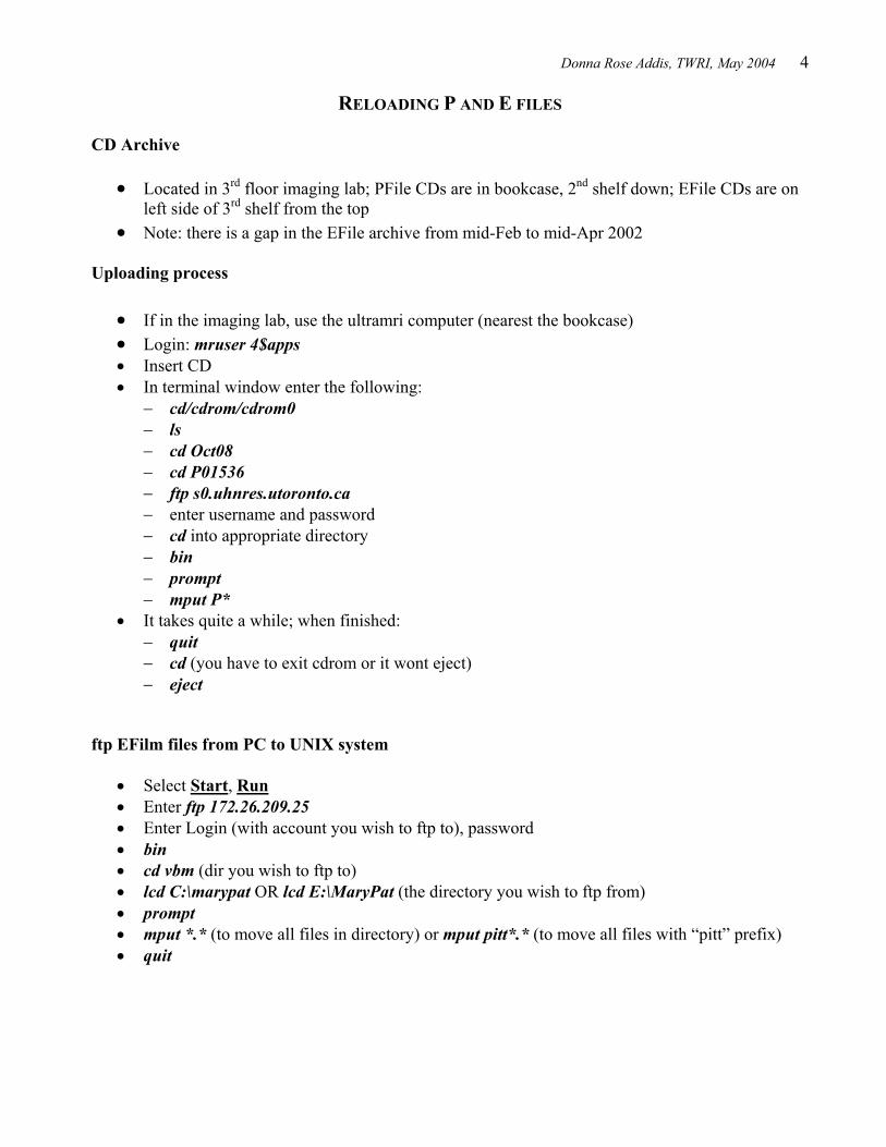
RELOADING P AND E FILES CD Archive

• Located in 3rd floor imaging lab; PFile CDs are in bookcase, 2nd shelf down; EFile CDs are on left side of 3rd shelf from the top

• Note: there is a gap in the EFile archive from mid-Feb to mid-Apr 2002 Uploading process

• If in the imaging lab, use the ultramri computer (nearest the bookcase) • Login: mruser 4$apps • Insert CD • In terminal window enter the following:

− cd/cdrom/cdrom0 − ls − cd Oct08 − cd P01536 − ftp s0.uhnres.utoronto.ca − enter username and password − cd into appropriate directory − bin − prompt − mput P*

• It takes quite a while; when finished: − quit − cd (you have to exit cdrom or it wont eject) − eject

ftp EFilm files from PC to UNIX system

• Select Start, Run • Enter ftp 172.26.209.25 • Enter Login (with account you wish to ftp to), password • bin • cd vbm (dir you wish to ftp to) • lcd C:\marypat OR lcd E:\MaryPat (the directory you wish to ftp from) • prompt • mput *.* (to move all files in directory) or mput pitt*.* (to move all files with “pitt” prefix) • quit


SPM: GETTING STARTED i. Converting EFiles to Analyze format (readable by SPM)

• In terminal window, type anattoSPM • Enter Exam number: • Enter Series number: • Enter number of slices: (e.g., 124) • Output: Creates an a.img file

ii. Converting PFiles to Analyze format (readable by SPM)

• In terminal window, type: PtoSPM Date Pnumber Output_directory • e.g., PtoSPM Apr12 P61440 subj1 • e.g., PtoSPM Apr12 P61440 ../spm/subj1 (if the output directory is located elsewhere) • e.g., PtoSPM P61440 subj1 (Date isn’t required if the P files are already in the pwd, e.g., if

you uploaded old PFiles from the CD archive) • e.g., PtoSPM Apr12 P61440 . (if you are already in the output directory) • Creates f*.img (functional images) in the specified output directory

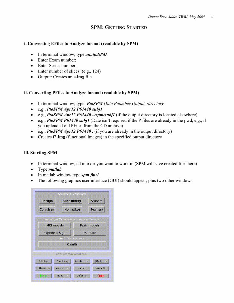
iii. Starting SPM

• In terminal window, cd into dir you want to work in (SPM will save created files here) • Type matlab • In matlab window type spm fmri • The following graphics user interface (GUI) should appear, plus two other windows.


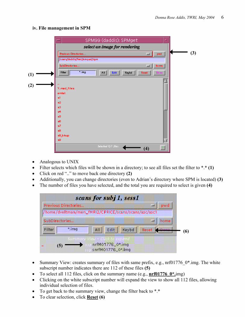
iv. File management in SPM

• Analogous to UNIX • Filter selects which files will be shown in a directory; to see all files set the filter to *.* (1) • Click on red “..” to move back one directory (2) • Additionally, you can change directories (even to Adrian’s directory where SPM is located) (3) • The number of files you have selected, and the total you are required to select is given (4)

• Summary View: creates summary of files with same prefix, e.g., nrf01776_0*.img. The white subscript number indicates there are 112 of these files (5)

• To select all 112 files, click on the summary name (e.g., nrf01776_0*.img) • Clicking on the white subscript number will expand the view to show all 112 files, allowing

individual selection of files. • To get back to the summary view, change the filter back to *.* • To clear selection, click Reset (6)

(2)

(1)

(3)

(5)

(6)

(4)


v. Files in SPM:

• a.img – anatomical image • a.hdr – header file containing information about anatomical image • f*.img – functional image (one for every TR) • f*.hdr – header file for functional image • *.mat – matrix files that contain information about transformations during pre-processing, and

later about models and contrasts etc.

vi. File Prefixes:

• Prefixes indicate the preprocessing performed on files, and the order in which they were applied

• a,img – raw anatomical image • na.img – normalized anatomical image • f*.img – raw functional image • rf*.img – realigned functional image (note, you may delay the application of realignment

transformations until the normalization stage; this info will be kept in the *.mat files for the images, and thus your images will remain as f*.img files)

• arf*.img (or af*.img) – slice-timing corrected functional image • narf*.img (or naf*.img) – normalized functional image • snarf*.img (or snarf*.img) – smoothed functional image

vii. Directories to create:

• Create a directory for every subject, and later, for each analysis/model you wish to perform • SPM uses generic naming for the files it creates and unless you create separate directories, files

will be overwritten • Note that at the model estimation stage, it is easiest if your subjects directories are numbered

(as SPM always asks you to select images for subj 1 etc and when entering many, it can be helpful)

viii. Important Note:

• This protocol assumes that you are starting the analysis for this subject "from scratch", i.e., you have never analysed this subject before.

• If you have already analysed this subject, and you are restarting the analysis from the beginning (e.g., because you're not happy with the previous analysis), please make sure there are no *.mat files in the same directory as the *.img and *.hdr files.

• The *.mat files from the previous analysis may contain information about tranformations


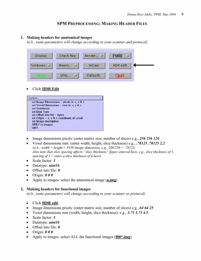
SPM PREPROCESSING: MAKING HEADER FILES 1. Making headers for anatomical images

(n.b., some parameters will change according to your scanner and protocol)

• Click HDR Edit

• Image dimensions pixels: (enter matrix size, number of slices) e.g., 256 256 124 • Voxel dimensions mm: (enter width, height, slice thickness) e.g., .78125 .78125 2.2

(n.b.: width = height = FOV/image dimension, e.g., 200/256 = .78125; Also note that slice spacing affects “slice thickness” figure entered here, e.g., slice thickness of 5, spacing of 1 = enter a slice thickness of 6 here)

• Scale factor: 1 • Datatype: uint16 • Offset into file: 0 • Origin: 0 0 0 • Apply to images: select the anatomical image (a.img)

2. Making headers for functional images

(n.b., some parameters will change according to your scanner or protocol) • Click HDR edit • Image dimensions pixels: (enter matrix size, number of slices) e.g., 64 64 25 • Voxel dimensions mm (width, height, slice thickness): e.g., 3.75 3.75 4.5 • Scale factor: 1 • Datatype: uint16 • Offset into file: 0 • Origin: 0 0 0 • Apply to images: select ALL the functional images (f00*.img)


SPM PREPROCESSING: REORIENTING ANATOMICALS AND FUNCTIONALS

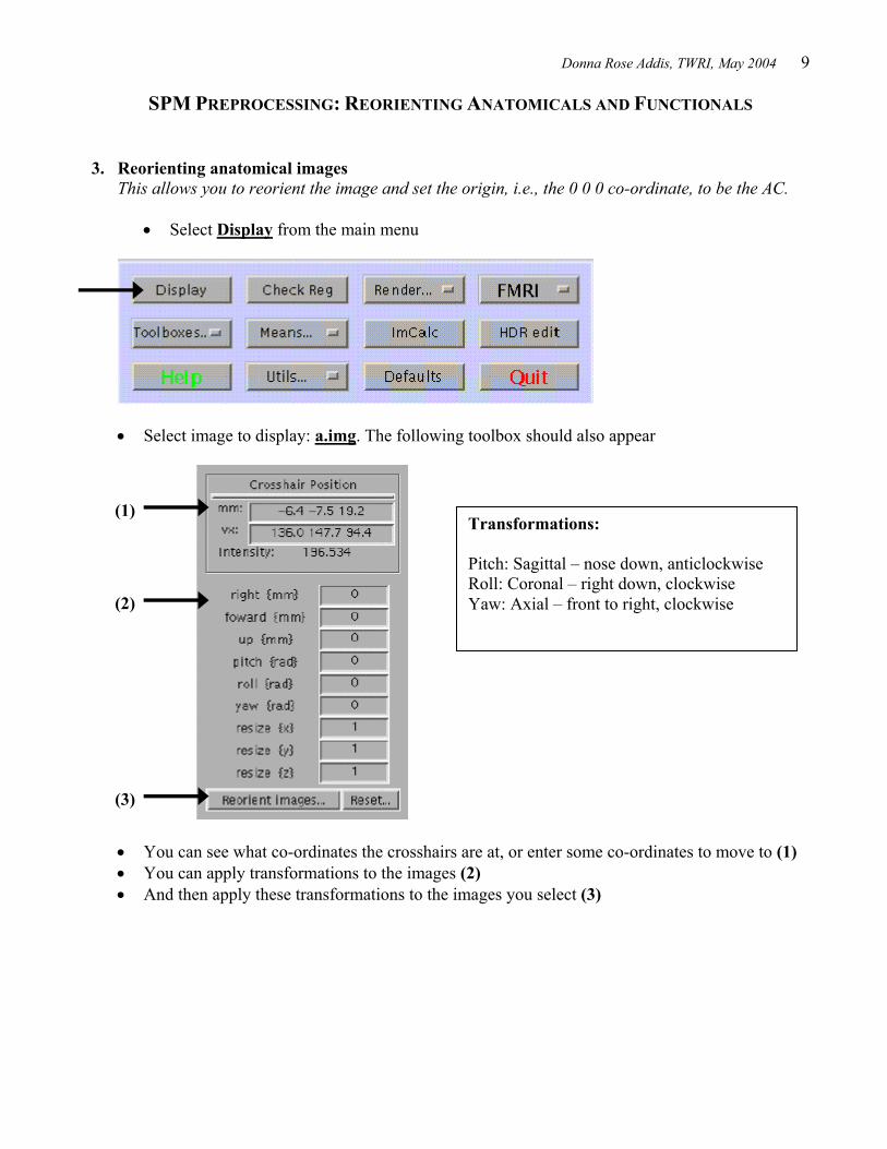
3. Reorienting anatomical images

This allows you to reorient the image and set the origin, i.e., the 0 0 0 co-ordinate, to be the AC.

• Select Display from the main menu

• Select image to display: a.img. The following toolbox should also appear

• You can see what co-ordinates the crosshairs are at, or enter some co-ordinates to move to (1) • You can apply transformations to the images (2) • And then apply these transformations to the images you select (3)

(1)

(2)

(3)

Transformations: Pitch: Sagittal – nose down, anticlockwise Roll: Coronal – right down, clockwise Yaw: Axial – front to right, clockwise


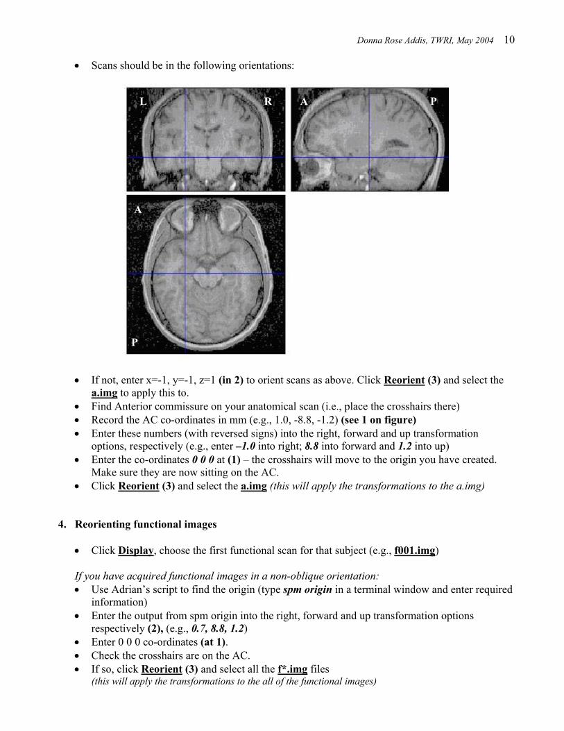
• Scans should be in the following orientations:

• If not, enter x=-1, y=-1, z=1 (in 2) to orient scans as above. Click Reorient (3) and select the

a.img to apply this to. • Find Anterior commissure on your anatomical scan (i.e., place the crosshairs there) • Record the AC co-ordinates in mm (e.g., 1.0, -8.8, -1.2) (see 1 on figure) • Enter these numbers (with reversed signs) into the right, forward and up transformation

options, respectively (e.g., enter –1.0 into right; 8.8 into forward and 1.2 into up) • Enter the co-ordinates 0 0 0 at (1) – the crosshairs will move to the origin you have created.

Make sure they are now sitting on the AC. • Click Reorient (3) and select the a.img (this will apply the transformations to the a.img)

4. Reorienting functional images

• Click Display, choose the first functional scan for that subject (e.g., f001.img) If you have acquired functional images in a non-oblique orientation: • Use Adrian’s script to find the origin (type spm origin in a terminal window and enter required

information) • Enter the output from spm origin into the right, forward and up transformation options

respectively (2), (e.g., 0.7, 8.8, 1.2) • Enter 0 0 0 co-ordinates (at 1). • Check the crosshairs are on the AC. • If so, click Reorient (3) and select all the f*.img files

(this will apply the transformations to the all of the functional images)

AL P R

P

A


If you have acquired functional scans in an oblique orientation: • Enter the following transformations (at 2): x=1, y=1, z=1, pitch=1.7, roll=0, yaw=0 • Check that images are oriented approximately correctly. • Find the AC on the functional images (Look for a bright white spot at end of fornix) • Note down the co-ordinate in (at 1) • Enter these numbers with opposite signs in right, forward and up transformation options (at 2) • Enter 0 0 0 co-ordinates (at 1). • Check the crosshairs are on the AC. If so, click Reorient (3) and select all the f*.img files

(this will apply the transformations to the all of the functional images)

5. SPM Origin scripts: spm_origin_axial This script gives you the transformations for setting your AC on axial functional images. • Type spm_origin_axial in the terminal window. The following instructions will appear: • In SPM, click Display, choose the anatomic image (a.img) • Enter the following transformations (at 2): y=1 • Find the AC on the anatomical image, enter these co-ordinate (with changed signs) as

transformations (at 2) (see above instructions on re-orienting anatomical images) • Enter 0 0 0 co-ordinates (at 1). Check the crosshairs are on the AC. • If so, click Reorient (3) and select all the a*.img file • Click Display, choose one of the functional image (e.g., f001.img) • If not already in the standard orientation, enter appropriate transformations (e.g., y = -1) • Enter the spiral (functional) image slice spacing (i.e., slice thickness plus any spacing) • Enter the number of spiral slices • Enter the anatomical slice spacing (i.e., slice thickness plus any spacing) • Enter the number of anatomical slices • Enter the centre of FOV co-ordinates for the functional images: • These are the IS, AP, LR co-ordinates. If you have R, A or S co-ordinates they should be

entered as positive numbers, and L, P or I coordinates should be entered as negative numbers. Enter the spiral ‘R’ co-ordinate (i.e., +R or -L) Enter the spiral ‘A’ co-ordinate (i.e., +A or -P) Enter the spiral ‘S’ co-ordinate (i.e., +S or -I)

• Enter the centre of FOV co-ordinates for the anatomical image: Enter the 3D ‘R’ co-ordinate (i.e., +R or -L) Enter the 3D ‘A’ co-ordinate (i.e., +A or -P) Enter the 3D ‘S’ co-ordinate (i.e., +S or -I)

• Enter the co-ordinates of the AC you obtained when re-orienting your anatomical image: (n.b. Do not switch signs when entering the AC co-ordinates here). Enter the AC “right” co-ordinate Enter the AC “forward” co-ordinate Enter the AC “up” co-ordinate

• The script will output a right, forward and up shift for you to enter in SPM at (2) to set the AC on the functional images.

• Set crosshair position to 0 0 0 mm (i.e., Enter 0 0 0 co-ordinates at 1). Check this is the AC. • Click Reorient images, and select all raf#### files (i.e., select all f*.img files)


6. SPM Origin scripts: spm_origin_axial This script gives you the transformations for setting your AC on oblique functional images. • Type spm_oblique in the MATLAB terminal window. The following instructions will appear: • Enter all R, A, S co-ordinates as positive numbers and L P I co-ordinates as negative numbers

(as in spm_origin_axial) • Axial anatomical images:

First slice of IS co-ordinate (i.e., +S or -I) Last slice of IS co-ordinate (i.e., +S or -I) LR co-ordinate (i.e., +R or -L) PA co-ordinate (i.e., +A or -P)

• Oblique coronal images: First slice of PA co-ordinate (i.e., +A or -P) First slice of IS co-ordinate (i.e., +S or -I) Last slice of PA co-ordinate (i.e., +A or -P) Last slice of IS co-ordinate (i.e., +S or -I) LR co-ordinate (i.e., +R or -L)

• In SPM, click Display, choose the anatomic image (a.img) • Enter the following transformations (at 2): x= -1, y= -1 • Set pitch = **** (at 2) (this figure will be outputted by the script) • Click Reorient (3) and select all the a*.img file • Find the AC on the anatomical image, enter these co-ordinates separated by spaces

(n.b., enter them into the script in the order they appear in SPM, and do not change signs) • The script will output a right, forward and up shift for you to enter at (2) to set the AC. • Enter 0 0 0 co-ordinates (at 1). Check the crosshairs are on the AC. • If so, click Reorient (3) and select all the a*.img file • Click Display, choose one functional image • Enter the following transformations at (2): x = -1, pitch = **** (script will output a figure) • The script will output a right, forward and up shift for you to enter at (2) to set the AC. • Enter 0 0 0 co-ordinates (at 1). Check the crosshairs are on the AC. • If so, click Reorient (3) and select all the f*.img file • Click Check Reg (lower panel of main SPM menu). • Select a.img and f001.img. These will be displayed in a locked manner. • Click crosshairs on the outer edges of anatomical image and check that this corresponds to

outer edges of functional images.


SPM PREPROCESSING: COREGSITRATION 7. Co-registration of anatomical and functional images: Method A

This step involves a segmentation and works to line up the AC of the a.img and f*.img, essentially overlaying them. This is the method I found worked best when for functional images were acquired in an oblique orientation. • Select Coregister from main menu

• Number of subjects: 1 • Select Coregister alone • Modality of first target image: T1 MRI (as it is an anatomical; see later) • Modality of first object image: EPI (as it is a functional; Select if echo-planar or spiral) • Select Target image: select a.img

This is the image the others will be coregistered to; we choose a.img as the AC is correct for sure on this image

• Select Object image: select f001.img (this is the image that will be coregistered to the a.img) • Select Other images: select f002.img to last f*.img

This will coregister these other images to a.img; note to select f002.img to f099.img, you have to expand the first summary of files f0*.img and select each image separately; then press reset to get back to a summary view and select other summaries, e.g., f1*.img etc.

• Segmented images will be displayed (and written in a spm99.ps file created in PWD) 8. Co-registration of anatomical and functional images: Method B

Another way of coregistering, useful when functional images are acquired at a standard orientation. • Select Coregister from main menu • Number of subjects: 1 • Select Coregister alone • Modality of first target image: EPI • Modality of first object image: T1 MRI • Select Target image: select f001.img • Select Object image: select a.img • Select Other images: do not select any other images


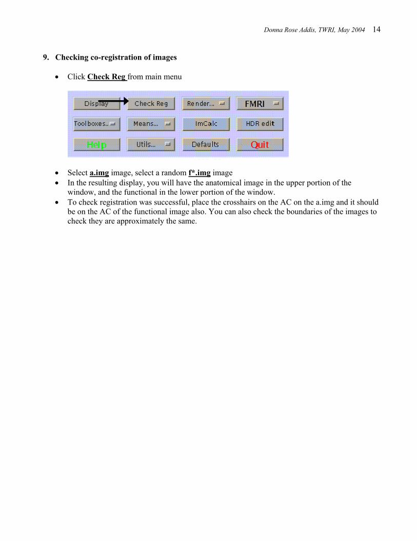
9. Checking co-registration of images

• Click Check Reg from main menu

• Select a.img image, select a random f*.img image • In the resulting display, you will have the anatomical image in the upper portion of the

window, and the functional in the lower portion of the window. • To check registration was successful, place the crosshairs on the AC on the a.img and it should

be on the AC of the functional image also. You can also check the boundaries of the images to check they are approximately the same.


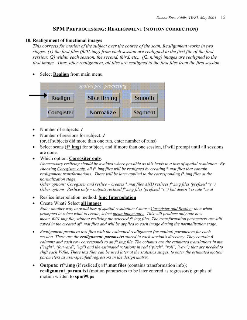
SPM PREPROCESSING: REALIGNMENT (MOTION CORRECTION) 10. Realignment of functional images

This corrects for motion of the subject over the course of the scan. Realignment works in two stages: (1) the first files (f001.img) from each session are realigned to the first file of the first session; (2) within each session, the second, third, etc... (f2..n.img) images are realigned to the first image. Thus, after realignment, all files are realigned to the first files from the first session. • Select Realign from main menu

• Number of subjects: 1 • Number of sessions for subject: 1

(or, if subjects did more than one run, enter number of runs) • Select scans (f*.img) for subject, and if more than one session, if will prompt until all sessions

are done. • Which option: Coregsiter only.

Unnecessary reslicing should be avoided where possible as this leads to a loss of spatial resolution. By choosing Coregister only, all f*.img files will be realigned by creating *.mat files that contain realignment transformations. These will be later applied to the corresponding f*.img files at the normalization stage. Other options: Coregister and reslice – creates *.mat files AND reslices f*.img files (prefixed “r”) Other options: Reslice only – outputs resliced f*.img files (prefixed “r”) but doesn’t create *.mat

• Reslice interpolation method: Sinc Interpolation • Create What? Select all images

Note: another way to avoid loss of spatial resolution: Choose Coregister and Reslice; then when prompted to select what to create, select mean image only. This will produce only one new mean_f001.img file, without reslicing the selected f*.img files. The transformation parameters are still saved in the created af*.mat files and will be applied to each image during the normalization stage.

• Realignment produces text files with the estimated realignment (or motion) parameters for each session. These are the realignment_params.txt stored in each session's directory. They contain 6 columns and each row corresponds to an f*.img file. The columns are the estimated translations in mm ("right", "forward", "up") and the estimated rotations in rad ("pitch", "roll", "yaw") that are needed to shift each V-file. These text files can be used later at the statistics stages, to enter the estimated motion parameters as user-specified regressors in the design matrix.

• Outputs: rf*.img (if resliced); rf*.mat files (contains transformation info); realignment_param.txt (motion parameters to be later entered as regressors); graphs of motion written to spm99.ps


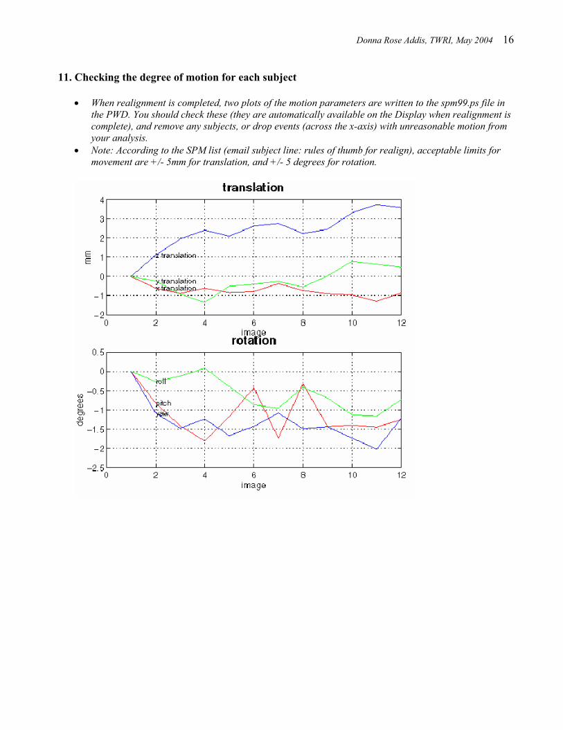
11. Checking the degree of motion for each subject

• When realignment is completed, two plots of the motion parameters are written to the spm99.ps file in

the PWD. You should check these (they are automatically available on the Display when realignment is complete), and remove any subjects, or drop events (across the x-axis) with unreasonable motion from your analysis.

• Note: According to the SPM list (email subject line: rules of thumb for realign), acceptable limits for movement are +/- 5mm for translation, and +/- 5 degrees for rotation.


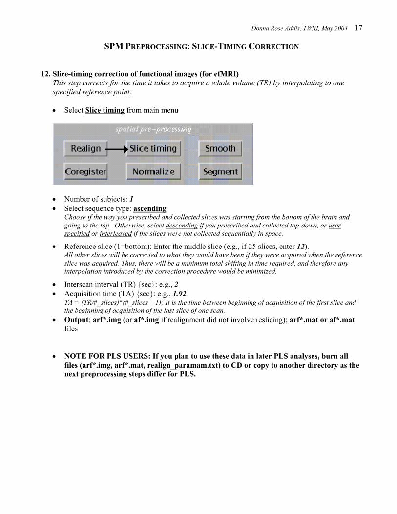
SPM PREPROCESSING: SLICE-TIMING CORRECTION 12. Slice-timing correction of functional images (for efMRI)

This step corrects for the time it takes to acquire a whole volume (TR) by interpolating to one specified reference point. • Select Slice timing from main menu

• Number of subjects: 1 • Select sequence type: ascending

Choose if the way you prescribed and collected slices was starting from the bottom of the brain and going to the top. Otherwise, select descending if you prescribed and collected top-down, or user specified or interleaved if the slices were not collected sequentially in space.

• Reference slice (1=bottom): Enter the middle slice (e.g., if 25 slices, enter 12). All other slices will be corrected to what they would have been if they were acquired when the reference slice was acquired. Thus, there will be a minimum total shifting in time required, and therefore any interpolation introduced by the correction procedure would be minimized.

• Interscan interval (TR) {sec}: e.g., 2 • Acquisition time (TA) {sec}: e.g., 1.92

TA = (TR/#_slices)*(#_slices – 1); It is the time between beginning of acquisition of the first slice and the beginning of acquisition of the last slice of one scan.

• Output: arf*.img (or af*.img if realignment did not involve reslicing); arf*.mat or af*.mat files

• NOTE FOR PLS USERS: If you plan to use these data in later PLS analyses, burn all files (arf*.img, arf*.mat, realign_paramam.txt) to CD or copy to another directory as the next preprocessing steps differ for PLS.


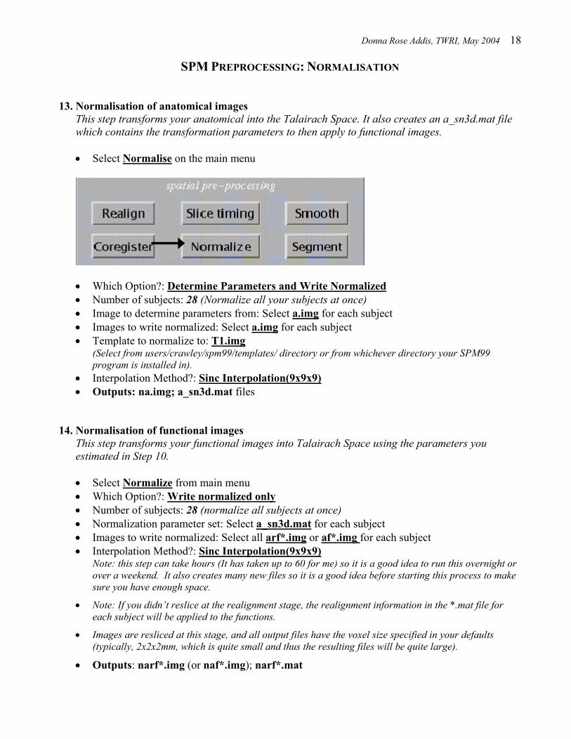
SPM PREPROCESSING: NORMALISATION 13. Normalisation of anatomical images

This step transforms your anatomical into the Talairach Space. It also creates an a_sn3d.mat file which contains the transformation parameters to then apply to functional images.

• Select Normalise on the main menu

• Which Option?: Determine Parameters and Write Normalized • Number of subjects: 28 (Normalize all your subjects at once) • Image to determine parameters from: Select a.img for each subject • Images to write normalized: Select a.img for each subject • Template to normalize to: T1.img

(Select from users/crawley/spm99/templates/ directory or from whichever directory your SPM99 program is installed in).

• Interpolation Method?: Sinc Interpolation(9x9x9) • Outputs: na.img; a_sn3d.mat files

14. Normalisation of functional images

This step transforms your functional images into Talairach Space using the parameters you estimated in Step 10. • Select Normalize from main menu • Which Option?: Write normalized only • Number of subjects: 28 (normalize all subjects at once) • Normalization parameter set: Select a_sn3d.mat for each subject • Images to write normalized: Select all arf*.img or af*.img for each subject • Interpolation Method?: Sinc Interpolation(9x9x9)

Note: this step can take hours (It has taken up to 60 for me) so it is a good idea to run this overnight or over a weekend. It also creates many new files so it is a good idea before starting this process to make sure you have enough space.

• Note: If you didn’t reslice at the realignment stage, the realignment information in the *.mat file for each subject will be applied to the functions.

• Images are resliced at this stage, and all output files have the voxel size specified in your defaults (typically, 2x2x2mm, which is quite small and thus the resulting files will be quite large).

• Outputs: narf*.img (or naf*.img); narf*.mat


SPM PREPROCESSING: NORMALISATION FOR PLS

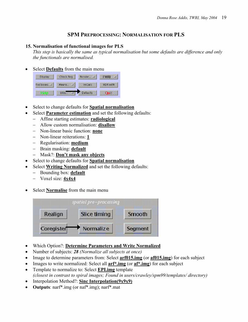
15. Normalisation of functional images for PLS

This step is basically the same as typical normalisation but some defaults are difference and only the functionals are normalised.

• Select Defaults from the main menu

• Select to change defaults for Spatial normalisation • Select Parameter estimation and set the following defaults:

− Affine starting estimates: radiological − Allow custom normalisation: disallow − Non-linear basic function: none − Non-linear reiterations: 1 − Regularisation: medium − Brain masking: default − Mask?: Don’t mask any objects

• Select to change defaults for Spatial normalisation • Select Writing Normalized and set the following defaults:

− Bounding box: default − Voxel size: 4x4x4

• Select Normalise from the main menu

• Which Option?: Determine Parameters and Write Normalized • Number of subjects: 28 (Normalize all subjects at once) • Image to determine parameters from: Select arf015.img (or af015.img) for each subject • Images to write normalized: Select all arf*.img (or af*.img) for each subject • Template to normalize to: Select EPI.img template

(closest in contrast to spiral images; Found in users/crawley/spm99/templates/ directory) • Interpolation Method?: Sinc Interpolation(9x9x9) • Outputs: narf*.img (or naf*.img); narf*.mat


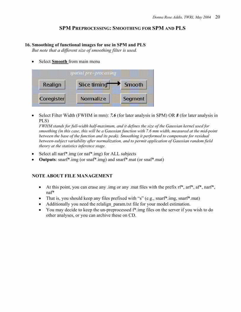
SPM PREPROCESSING: SMOOTHING FOR SPM AND PLS 16. Smoothing of functional images for use in SPM and PLS

But note that a different size of smoothing filter is used. • Select Smooth from main menu

• Select Filter Width (FWHM in mm): 7.6 (for later analysis in SPM) OR 8 (for later analysis in

PLS) FWHM stands for full-width half-maximum, and it defines the size of the Gaussian kernel used for smoothing (in this case, this will be a Gaussian function with 7.6 mm width, measured at the mid-point between the base of the function and its peak). Smoothing it performed to compensate for residual between-subject variability after normalization, and to permit application of Gaussian random field theory at the statistics inference stage.

• Select all narf*.img (or naf*.img) for ALL subjects • Outputs: snarf*.img (or snaf*.img) and snarf*.mat (or snaf*.mat) NOTE ABOUT FILE MANAGEMENT

• At this point, you can erase any .img or any .mat files with the prefix rf*, arf*, af*, narf*,

naf* • That is, you should keep any files prefixed with “s” (e.g., snarf*.img, snarf*.mat) • Additionally you need the relalign_param.txt file for your model estimation. • You may decide to keep the un-preprocessed f*.img files on the server if you wish to do

other analyses, or you can archive these on CD.

PRE-PROCESSING DONNA ROSE ADDIS - Psychology ...

Documents

Transcript of PRE-PROCESSING DONNA ROSE ADDIS - Psychology ...