processes

Article

Practice-Oriented Validation of Embedded Beam Formulationsin Geotechnical Engineering

Andreas-Nizar Granitzer * and Franz Tschuchnigg

Citation: Granitzer, A.-N.;

Tschuchnigg, F. Practice-Oriented

Validation of Embedded Beam

Formulations in Geotechnical

Engineering. Processes 2021, 9, 1739.

https://doi.org/10.3390/pr9101739

Academic Editor: Li Li

Received: 26 August 2021

Accepted: 26 September 2021

Published: 28 September 2021

Publisher’s Note: MDPI stays neutral

with regard to jurisdictional claims in

published maps and institutional affil-

iations.

Copyright: © 2021 by the authors.

Licensee MDPI, Basel, Switzerland.

This article is an open access article

distributed under the terms and

conditions of the Creative Commons

Attribution (CC BY) license (https://

creativecommons.org/licenses/by/

4.0/).

Institute of Soil Mechanics, Foundation Engineering and Computational Geotechnics,Graz University of Technology, 8010 Graz, Austria; franz.tschuchnigg@tugraz.at* Correspondence: andreas-nizar.granitzer@tugraz.at

Abstract: The numerical analysis of many geotechnical problems involves a high number of structuralelements, leading to extensive modelling and computational effort. Due to its exceptional ability tocircumvent these obstacles, the embedded beam element (EB), though originally intended for themodelling of micropiles, has become increasingly popular in computational geotechnics. Recentresearch effort has paved the way to the embedded beam element with interaction surface (EB-I),an extension of the EB. The EB-I renders soil–structure interaction along an interaction surfacerather than the centreline, making it theoretically applicable to any engineering application wherebeam-type elements interact with solid elements. At present, in-depth knowledge about relativemerits, compared to the EB, is still in demand. Subsequently, numerical analysis are carried out usingboth embedded beam formulations to model deep foundation elements. The credibility of predictedresults is assessed based on a comprehensive comparison with the well-established standard FEapproach. In all cases considered, the EB-I proves clearly superior in terms of mesh sensitivity,mobilization of skin-resistance, and predicted soil displacements. Special care must be taken whenusing embedded beam formulations for the modelling of composite structures.

Keywords: embedded beam elements; finite element; mesh sensitivity; soil-structure interaction;deep foundation; 3D modelling

1. Introduction

The dimensioning of deep foundation elements, such as single piles, pile groups, andpiled rafts represents a standard task in geotechnical engineering. Broadly, the behaviour ofthese structural elements is characterized by two complex effects: (1) non-linear behaviourof the soil surrounding the piles and (2) separation between soil and pile as a result oflarge inertial forces, generated in the soil, around the pile heads [1]. In order to accountfor the extended-continuum nature of the embedding soil around piles, the finite elementmethod (FEM), amongst other numerical techniques, has evolved as a widely accepted toolin academia and practice [2,3].

In this context, deep foundation elements are frequently considered as combinations ofsolid elements, conforming to linear elastic material of the pile, and zero-thickness interfaceelements allowing for realistic soil-structure interaction (SSI), including possible occurrenceof detachment or interface sliding between pile and soil [4–7]. The so-called standard FEapproach (SFEA) represents a very good approximation of related physical problems, espe-cially regarding the simulation of ideal non-displacement piles experiencing subordinateinstallation effects (in the literature, they are also referred to as “wished-in-place” piles ordrilled shafts [8,9]); thus, the SFEA is commonly used as a numerical benchmark solutionto assess the credibility of novel pile formulations [10,11]. Nonetheless, the SFEA hasdeficiencies concerning the analysis of large-scale geotechnical entities comprising a highnumber of piles [12]. Most significantly, the SFEA requires the application of considerablysmall elements, implicitly induced by the slenderness inherent to piles; as a consequence,

Processes 2021, 9, 1739. https://doi.org/10.3390/pr9101739 https://www.mdpi.com/journal/processes

Processes 2021, 9, 1739 2 of 27

the number of degrees of freedom (DOFs) increases disproportionately, resulting in com-putational costs that must be regarded as unbearable for most practical purposes [13]. Inaddition, the SFEA requires an a priori consideration of the orientation and location ofthe piles during the geometrical setup-up of the model, which makes design optimizationcumbersome in engineering practice [14].

To overcome these limitations, Sadek and Shahrour [15] proposed the so-called em-bedded beam (EB) formulation, which was further enhanced through the contributions ofEngin et al. [16], as well as Tschuchnigg and Schweiger [12]; in more recent publications, theEB is also referred to as embedded pile [13,17]. In its actual configuration, EBs constituteline elements composed of beams and non-linear embedded interface elements, allowingfor relative beam-soil displacements. Unlike the SFEA, the EB formulation defines pilesindependent from the solid mesh connectivity; consequently, EBs do not influence thespatial discretization of the soil domain, leading to a significant decrease in DOFs closeto the thin geometrical entities, higher calculation efficiency, and lower modelling effortcompared to the SFEA. In addition, the EB simplifies the structural analysis with respect tothe evaluation of stress resultants [13].

Since the EB modelling technique considers SSI along the centreline only, it wasoriginally intended for the analysis of axially-loaded small diameter piles installed invertical direction [18]. Due to its deficiency to capture the effect of pile installation in thesurrounding soil, it is further recommended to apply the EB framework for the modellingof piles undergoing inconsiderable installation effects, such as non-displacement pilesor, more specifically, piles which are constructed using casings [12]. Applications of EBsare reported for single piles under compression [19] and tension [20], pile rows [21], pilegroups [22,23], rigid inclusions [24], connected [25–29] and disconnected piled rafts [13].Despite aforementioned recommendations regarding its field of application, and dueto its exceptional ability to simplify the modelling process, EBs were found eligible forthe modelling of almost any type of geotechnical reinforcement interacting with solidelements: Abbas et al. investigated both the lateral load behaviour [30] and the uplift load-carrying mechanism [31] of inclined micropiles modelled by means of EBs. El-Sherbinyet al. [32] applied EBs to study the ability of jet-grout columns to stabilize berms in softsoil formations. EBs found also use in the modelling of piles subjected to different modesof loading, namely lateral [33], passive [34,35], and dynamic loading [36]. More recently,use cases suggest the incorporation of EBs to capture the response of tension members,including tunnel front fiberglass reinforcements [37], rock bolts [38], ground anchors [39],and soil nails [40].

However, as relevant as it is poorly considered, the existing EB formulation suffersfrom severe limitations compared to the SFEA. Most significantly, this modelling approachintroduces a mechanical incompatibility, resulting in stress singularities near the pilebase [41]. This effect is mesh-dependent and becomes more determinant with increasingmesh refinement in the vicinity of an EB; accordingly, EBs require the employment ofsufficiently coarse mesh discretizations in order to accurately predict their system response.Otherwise, increasing the mesh coarseness of the solid domain gives rise to inaccuratesolutions and inconvenient convergence to the sought exact solution [13]; from a practicalpoint of view, this may lead to an underestimation of foundation settlements. Hence,engineering judgment, in conjunction with mesh studies, are in demand to evaluate reliablemesh discretizations. Another important limiting factor concerns the SSI principle: as thelatter is established along the centreline rather than the physical circumference, EBs cannotdistinguish between lateral shear and normal stress components acting on the interface,which are therefore unlimited [18]. In this way, lateral plasticity is solely controlled by theevolution of failure points in the surrounding soil; this obstacle may give rise to inaccuratepredictions in the case of complex loading situations [42].

To solve aforementioned problems, Turello et al. [41,43] developed the so-calledembedded beam with interaction surface (EB-I). The novelty of this approach concernedthe integration of an explicit interaction surface to the existing EB formulation, which allows

Processes 2021, 9, 1739 3 of 27

the spread of non-linear SSI effects over the physical skin, instead of over the centreline. Inthis way, spurious stress singularities induced by the line element are markedly reduced.More recently, the improved embedded beam framework was further generalized in orderto allow for inclined pile configurations as well as non-circular cross-section shapes [10,42].Aforementioned publications found that the EB-I poses a significant enhancement, in termsof mesh sensitivity and global pile response, in comparison with the original EB. However,it should be noted that these papers were primarily devoted to the theoretical presentationof the EB-I concept, hence little attention was paid to its validation. For example, Turelloet al. [44] investigated its ability to resemble pile group members considering linear elasticsoil conditions, which must be regarded as considerable simplification with respect to themechanical soil behaviour. Moreover, Smulders et al. [42] evaluated the EB-I performancesolely based on the load-settlement behaviour of single piles, which is mainly controlledby the stiffness of the surrounding soil [11].

The present paper aims at assessing the relative merits of the improved embeddedbeam formulation, compared to the existing one, in more detail. To this end, the remainderof this paper is organized as follows: Section 2 reconsiders the theoretical frameworkof both embedded beam formulations and highlights important differences. Section 3presents the numerical modelling approach applied in the numerical studies. Section 4investigates the credibility of results computed with both embedded beam formulationsbased on a single-pile engineering case. In view of their intended use (i.e., to capture thebehaviour of SFEA piles; see [11]), the performance of both embedded beam formulationsis analysed based on a comparison with the results obtained using the SFEA, which servesas a benchmark model for numerical validation [45]. In this context, it is noted that the(numerical) validation approach applied differs from the traditional validation strategy [46],which generally uses experimental data as a benchmark. To the authors’ knowledge, theunderlying studies represent the first attempt to compare the structural performance ofembedded beam formulations with respect to the mobilization of skin tractions, loadseparation between pile shaft and pile base, as well as displacements induced in thesurrounding soil. In Section 5, both embedded beam models are utilized to approximatedeep foundation elements of a recently constructed railway station, but emphasis is givento practical implications. Section 6 closes with the main conclusions of this work. Inthe course of this document, boldface uppercase and lowercase letters denote vectors ormatrices, respectively. Italic element symbols are defined in the list of symbols.

2. Background2.1. Embedded Beam Formulation

EBs combine the efficient use of defining beam elements independent of the solid meshconnectivity, with slip between the structural element and the solid mesh defined along theelement axis. Over the last decade, many commercial software codes have incorporated anEB-type element; see Table 1. Though the latter differs in terms of element type name andrecommended application, the working principle is broadly the same.

Processes 2021, 9, 1739 4 of 27

Table 1. Overview of EB-type elements employed in numerical software codes.

Numerical Code(Version)

Simulation Method

Diana 3D(V10.4) [47]

FEM

ZSoil 3D(V20.07) [48]

FEM

RS3(V4.014) [49]

FEM

FLAC 3D(V7.0) [50]

FDM

PLAXIS 3D(V21.00) [51]

FEM

EB-type name Pile foundations Compositeelement

Embeddedelement

Pile structuralelement

Embeddedbeam element

Soil-structure interaction Line interface along shaft, point interface at base

Skin resistance in axial direction Soil-dependent or pre-defined traction (kN/m)

Base resistance in axial direction Pre-defined force (kN)

Application Piles, groundanchors

Piles, soil nails,fixed endanchors

Piles, forepoles,beams

Structuralsupport

members

Piles, rockbolts,anchors

From a numerical point of view, EBs implemented in Plaxis 3D represent compositestructural elements comprising three components:

1. Three-noded beam element with quadratic interpolation scheme and six DOFs (i.e.,three translational DOFs, ux, uy, uz; three rotational DOFs, ϕx, ϕy, ϕz). As Timo-shenko’s theory is adopted, shear deformations are explicitly taken into account. Inorder to improve the numerical stability in case of particularly fine mesh discretiza-tions, an elastic zone is automatically generated in the surrounding soil. In this zone,all Gaussian points of the solid mesh are forced to remain elastic. As the zone size iscontrolled by the pile radius, the geometrical properties of the beam element influencethe stress state in the surrounding soil [16].

2. Three-noded line interfaces with the quadratic interpolation scheme and three pairsof nodes instead of single nodes, one belonging to the beam and one to the solidelement in which the beam is located. This component accounts for the SSI along theshaft based on a material law that links the skin traction vector tskin

EB (kN/m) to therelative displacement vector urel (m):

urel = ub − us = Nb·ab −Ns·as (1)

tskinEB = De·urel (2)

where ub and us (m) denote the beam and solid displacement vector, while matricesNb and Ns represent the interpolation matrix, including standard Lagrangian elementfunctions of the corresponding beam and solid elements. The elastic constitutivematrix De (kN/m2) is composed of the embedded interface stiffnesses in normal andtangential directions. Unlike the beam component, interface stiffness matrices areevaluated employing the Newton–Cotes integration scheme, hence element functionvalues at the nodes are either one or zero. While skin traction components in radialdirection are defined as unlimited, peak values in axial direction taxial,max (kN/m)may be linked to the actual soil stress state using a Coulomb criterion:

taxial, max ≤(

c′ − σavg′n · tan ϕ′

)·2·π·R (3)

where c′ (kPa) and ϕ′ () represent the effective soil strength parameters, σavg′n (kPa)

the averaged effective normal stress along the line interface and R (m) the radius.3. Point interface with one integration point at the beam end. In its initial configuration,

the latter coincides with a solid node. Similar to the line interface, SSI effects obey amaterial law defined in terms of urel (m) and the embedded foot interface stiffnessKbase (kN/m) in an axial direction. On the contrary, the ultimate tip force is limitedthrough a user-defined tip force Fmax (kN), hence independent of the surroundingsoil. Tensile stresses are internally suppressed through a tension cut-off criterion.

Processes 2021, 9, 1739 5 of 27

For details concerning virtual work considerations and the iteration procedure, theinterested reader can refer to [47–51].

2.2. Improved Embedded Beam Formulation with Interaction Surface

To the best of found knowledge, the EB-I is yet to feature in commercial software codes.However, recent developments have been tested and incorporated in Plaxis 3D [18,42].In order to get a better understanding of the enhancements compared to the EB, a fewremarks on the implementation are noteworthy:

• Unlike EBs, which consider shaft SSI effects along the beam axis, the EB-I spreads theshaft resistance over a number of integration points located at the physical interac-tion surface; the same applies for SSI at the base, where the resistance is distributedover several points at the base, instead of a single point. In this way, singular stressconcentrations, leading to local accumulations of plastic behaviour and large displace-ments along the axis, are avoided. In analogy to the EB, the skin traction vector tskin

EB−I(kN/m2) is expressed in terms of the relative displacement vector at the interactionsurface urel (m) and the elastic stiffness matrix De (kN/m3):

urel = ub − us = H·ab −Ns·as (4)

tskinEB−I =

De

2πR·urel (5)

where ub (m) denotes the mapped beam displacement at the interaction surfaceexpressed in terms of the mapping matrix H and beam nodal DOFs ab. us (m) is thesolid displacement vector at the interaction surface obtained by means of interpolation,within solid elements, located at the interaction surface. The latter is calculated basedon vector as containing solid nodal DOFs and the interpolation matrix Ns includingstandard Lagrangian element functions of the corresponding solid elements. R (m)represents the beam radius and De (kN/m2) represents the elastic stiffness matrixcontaining the interface stiffnesses. Since each interface element no longer poses aline, but a surface, the latter is divided by the shaft circumference. A similar approachis applied to resemble SSI at the base.

• In contrast to EBs, EB-Is are able to distinguish between two shear stress directionsperpendicular to the beam axis. This allows them to enrich the slip criterion such thatit accounts for any possible direction of slip failure occurring at the interaction surface:

τmax =√

τ2s + τ2

t ≤ c′ − σ′n· tan ϕ′ (6)

where τmax (kN/m2) is the max. local shear stress, controlled by the (perpendicularlyoriented) local shear stress components τs and τt (kN/m2) acting on the interactionsurface. σ′n (kN/m2) denotes the actual normal stress developing in the surroundingsoil, c′ (kN/m2) and ϕ′ () the effective soil strength parameters. Accordingly, theintrinsic slip criterion is not restricted to the axial direction, as is the case for the EB.

• Depending on the discretization and the number of integration points at the interactionsurface, the EB-I connects multiple continuum elements to one beam element. From anumerical point of view, the embedded beam stiffness is spread over a higher numberof nodes, leading to relative merits in terms of global stiffness matrix conditioning(i.e., smaller difference between max. and min. diagonal terms). As a consequence,the robustness of the numerical procedure is improved compared to the EB.

For the sake of clarity, Figure 1 compares the global response of a vertically loadedsingle pile, modelled by means of both embedded beam formulations, namely the existingembedded beam (EB) and the improved embedded beam with interaction surface (EB-I).

Processes 2021, 9, 1739 6 of 27

Figure 1. Global response of an axially loaded pile, considered by means of different modelling approaches: (a) embeddedbeam (EB); (b) embedded beam with interaction surface (EB-I). In both cases, the mobilization of skin tractions is primarilycontrolled by the relative displacement vector urel (“spring”) and the slip criterion (“friction element”).

3. Finite Element Modelling3.1. Investigated Scenario and Model Description

Although single piles are rarely constructed in isolation, it is useful to consider theiranalysis for the numerical validation of new pile modelling methods [4]. Accordingly, theAlzey Bridge pile load test [52] serves as a reference scenario to compare the performance ofthe EB with the EB-I. The test program was originally intended to optimize the foundationdesign of a highway bridge in slightly overconsolidated Frankfurt clay. Recently, it hasgained increasing popularity for the performance assessment of novel pile formulations;for example, see [16,42].

The numerical simulations, carried out in the present study, consider different pilemodelling approaches and mesh discretizations. All simulations are carried out with Plaxis3D [51]. For the sake of numerical consistency, in terms of solid element type and domaindimensions, all results are obtained using full 3D models, instead of axisymmetric 2Dmodels or reduced 3D models for the SFEA. In view of the number of elements and DOFsrequired to discretize the domain, this allows for a direct comparison between SFEA andEB/EB-I models. Following the results of trial simulations, the model domain has beendefined such that boundary effects are reduced to an acceptable limit; see Appendix A.Consequently, the model dimensions Bm = Lm/Dm are set to 26/19 m, which is equal to20 and 2 times the pile diameter and length, respectively; see Figure 2a. With regard tothe boundary conditions, conventional kinematic conditions are considered: a fully fixedsupport, with blocking of the displacements in all directions, at the lower horizontal modelboundary and a horizontally fixed support with freedom of vertical displacements alonglateral model boundaries. Moreover, mesh sensitivity analyses, concerning the (numerical)benchmark solution, ensure that the reference model is stable and reliable; see Appendix B.

Processes 2021, 9, 1739 7 of 27

Figure 2. (a) Model geometry, boundary conditions, and (b) characteristic load-displacement regionsafter [53].

Regardless of the pile modelling approach, the majority of the performed finite ele-ment analyses (FEA) consist of five phases. All simulations start with the definition of theinitial conditions, where the initial stress field is generated by means of the K0 procedure;this is reasonable given a horizontal ground surface and homogeneous soil. The next phaseconcerns the pile installation; depending on the considered pile configuration, this includesthe assignment of hardened concrete properties and the activation of interface elementsbetween the pile and the surrounding soil (SFEA), or the activation of the respective embed-ded beam element (EB, EB-I). Hence, the piles are assumed to be homogenous in strength,stiffness, and weight, thereby ignoring effects of improper concreting [6]. According tothe reference scenario, the soil around the pile is assumed to be in its initial state, whichmay be regarded as reasonable for non-displacement piles, where installation effects are ofsubordinate importance with respect to the pile behaviour [8]. Unless otherwise stated, thepile is finally subjected to displacement-driven head-down loading.

In the course of the evaluation of results, the mesh size effect on derived quantities (forexample, the mobilization of skin and base resistance) is compared at different displacementlevels. To satisfy practical relations on the one hand, and reduce bias on the other hand,the prescribed displacements are specified beforehand, following the L1-L2 method [53];see Figure 2b.

Assuming drained conditions, the following prescribed displacements are determinedas a function of the pile diameter DPile:

• uL1 = uPile/DPile = 0.34%, approximating the end of the initial linear region [54].• uL2 = uPile/DPile = 4%, indicating the initiation of the final linear region [55].• uult = uPile/DPile = 10%, complying with the ultimate pile resistance defined in [56].

As shown in Figure 2b, uL1 and uL2 correspond to the pile head displacement uPile atthe end of the initial linear region, as well as at the initiation of the final linear region. uultmarks the pile head displacement at the end of loading.

3.2. Pile Modelling Approach

As suggested by [10,38,41], the numerical behaviour of embedded beam formulationsis numerically validated against SFEA results (i.e., full 3D FE model). In the latter case,

Processes 2021, 9, 1739 8 of 27

the swept meshing technique [57] is applied to discretize the domain with 84,148 10-noded tetrahedral elements. In this way, the solid elements representing the SFEA pileare discretized with a structured swept mesh, allowing for both a faster mesh generationprocess, as well as a considerable mesh size reduction compared to the default solid mesh.

In order to minimize the interpolation error associated with the mesh discretization ofthe model, the mesh is refined inside the pile structure, and within a zone of 3·DPile belowthe tip and beside the shaft, respectively; see Figure 3. To address possible occurrence ofrelative displacements and plastic slip parallel to the soil-structure contacts, standard zero-thickness interface elements are considered at soil-structure contacts [58,59]. The interfaceelements are extended beyond the physical pile boundary in order to reduce the effect ofsingular plasticity points developing close to the pile edge [11,60]. The interface strength isspecified with a Coulomb criterion that limits the max. shear stress τ max (kN/m2) by

τ max =(c′ − σ′n· tan ϕ′

)·Rinter (7)

where σ′n (kN/m2), ϕ′ (), and c′ (kN/m2) are the effective interface normal stress, interfacefriction angle, and interface cohesion. In accordance with recommendations given in [61],an interface reduction factor Rinter = 0.9 is adopted in the analyses, which represents atypical value to account for SSI between concrete piles and fine grained soils.

Figure 3. (a) 3D view of global SFEA mesh; (b) cross-sectional view of SFEA mesh detail.

Contrary to SFEA interfaces, embedded interface elements are not explicitly modelled,but they are internally defined after the global mesh discretization; thus, assigning interfaceparameters reduces the definition of the ultimate skin and base resistance. For the sake ofnumerical consistency, the skin resistance is defined as layer-dependent (i.e., dependentof the stress state in the surrounding soil; see Equation (3)). In this way, the embeddedinterface elements are defined similarly to the interface elements used in the SFEA [12]. Inan attempt to capture the SFEA pile capacity with sufficient accuracy, the base resistanceis limited by the SFEA normal force developing at the pile base after the final loadingstep. The mesh sensitivity of both embedded beam formulations is investigated withfive different mesh refinements, which are referred to as very fine, fine, medium, coarse,and very coarse (Figure 4). The model boundary conditions are specified equal to theSFEA case.

Processes 2021, 9, 1739 9 of 27

Figure 4. Mesh discretizations considered for EB/EB-I models.

It is noted that both embedded beam formulations are analysed with the same meshdiscretizations and considerably less DOFs compared to the SFEA. Since beam elements aresuperimposed on the solid domain, and therefore overlap the soil, the beam unit weightrepresents a delta unit weight to the surrounding soil [11]. Noteworthy, this differs fromprevious interpretations of the embedded beam unit weight documented in [27,30,31,62],where the unit weight is assigned with the actual unit weight of the volume pile; as aconsequence, this approach leads to an overestimation of the soil-structure unit weight.To realistically approximate the kinematics at the pile head, the uppermost connectionpoint is considered as free to move and rotate, relative to the surrounding soil. Additionalmodelling parameters summarized in Table 2 are taken from [16] and resemble on-siteconditions as described in [52].

Table 2. Overview of pile parameters applied in the Alzey Bridge model.

Parameter Symbol Unit SFEA EB/EB-I 1

Pile Interface Pile Interface

Unit weight γ kN/m3 25.0 5.0Young’s modulus E GPa 10.0 10.0

Poisson’s ratio ν - 0.2Pile diameter D m 1.3 1.3

Pile length L m 9.5 9.5Base resistance Fmax kN 2300.0

Interface reduction factor Rinter - 0.9 0.9Effective friction angle ϕ′ deg 20.0 20.0

Effective cohesion c′ kN/m2 20.0 20.01 Calibrated numerical model documented in [18].

3.3. Constitutive Model and Parameter Determination

Regardless of the pile modelling approach, the use of a proper constitutive modelis crucial to cover the complex stress-strain behaviour of soils. Specific to this study, thisincludes a realistic evolution of potential slip planes along the pile-soil contacts, which isfundamental in the analysis of the pile behaviour. Since piles may undergo a wide rangeof deformations, leading to considerable strains in the soil, the constitutive model should

Processes 2021, 9, 1739 10 of 27

also be capable of effectively simulating the shear modulus degradation with the evolutionof shear strain [63]. Lastly, the constitutive model is supposed to account for the stressdependency of soil stiffness in order to capture the gradual mobilization of skin frictionwith sufficient accuracy [11].

Concerning these critical modelling aspects, the Hardening Soil Small (HSS) with non-associated flow rule and small-strain stiffness overlay [64], an extension of the HardeningSoil (HS) model [65], is used in this study. While HS parameters and drainage conditions areadopted from [16], HSS-specific model parameters, namely the threshold shear strain forstiffness degradation, γ0.7, and the initial shear modulus, G0, are defined using empiricalcorrelations documented in [66] and [67], respectively. The groundwater table is located3.5 m below ground surface. Soil parameters adopted in the analyses are listed in Table 3.

Table 3. Overview of soil parameters applied in Alzey Bridge model.

Parameter Symbol Unit Value

Drainage conditions - - drainedDepth of groundwater table - m 3.5

Unit weight γsat,γunsat kN/m3 20.0Reference deviatoric hardening modulus at pref Ere f

50 kN/m2 45,000Reference oedometer stiffness at pref Ere f

oedkN/m2 27,150

Reference un-/reloading stiffness at pref Ere fur kN/m2 90,000

Power index m - 1.0Isotropic Poisson’s ratio ν′ur - 0.2Effective friction angle ϕ′ deg 20.0

Effective cohesion c′ kN/m2 20.0Pre-overburden pressure POP kN/m2 50.0

Reference pressure pre f kN/m2 100.0Initial shear modulus at pref Gre f

0 kN/m2 116,000Threshold shear strain γ0.7 - 0.00015

4. Numerical Validation

A series of finite element analyses has been performed to assess the performance of theimproved embedded beam with interaction surface. Therefore, the latter is compared to theexisting embedded beam formulation, as well as the SFEA, which serves as the benchmark.The simulations focus on two specific points: mesh sensitivity studies and displacementsinduced in the surrounding soil. In addition, practical implications are drawn based onthe results.

4.1. Influence of Mesh Size on Global Pile Behaviour

The most critical issue in the design of pile supported structures is a reliable predic-tion of the pile behaviour, in terms of bearing capacity and settlement, under workingload conditions [68]. Consequently, the first series of calculations has been performed toinvestigate the mesh size effect on the mobilization of compressive pile resistance Rc (kN).

As it can be observed in Figure 5, all pile models show a similar behaviour in the firststage of loading, regardless of spatial discretization level and pile modelling approach.However, as the load increases beyond 2000 kN, the results reveal considerable limitationsof the EB, including a significant scatter of results and overestimation of bearing capacity,compared to the reference solution. Although it is generally known that coarser meshesyield a stiffer pile response, the wide scatter of load-displacement curves must be regardedas considerable obstacles to produce consistent results. In contrast, a more realistic pileresponse is obtained when employing the EB-I, thereby transforming the pile-soil line in-terface to an explicit interaction surface. Up to a relative displacement of 2%, the mobilizedpile resistance magnitudes are almost independent of the domain discretization. Even athigher displacement levels, the mesh size effect remains insignificant compared to the EB.

Processes 2021, 9, 1739 11 of 27

Figure 5. Influence of spatial discretization on mobilization of compressive pile resistance.

In view of the load-displacement behaviour, the EB-I gives a softer global responsecompared to the EB after reaching the ultimate skin resistance, which is mainly attributedto the different mobilization of base resistance Rb (kN); see Figure 6. The base–resistancecurves, deduced from both embedded beam formulations, may be well approximatedthrough bi-linear functions bounded by the max. base resistance Fmax, which is a directinput to the analysis. However, the EB shows considerably steeper gradients in comparisonwith the EB-I, which is a direct consequence of the modified embedded base interfacestiffness considered in the actual EB-I configuration. As a by-product, EB-I curves are inremarkable agreement with the reference solution. Moreover, the results confirm that theEB-I is less mesh-size dependent; for example, at a relative displacement of 2%, the rangeof Rc-values obtained with the EB-I (<100 kN) is considerably smaller when comparedwith the EB (>1000 kN). Nevertheless, both formulations have deficiencies regarding theinitial mobilization of base resistance in the first part of loading (see Figure 6); in allcases considered, the base resistance is considerably underestimated and shows a lowermobilization rate compared to the SFEA. This must be regarded as a considerable limitationof the actual embedded beam configurations.

Figure 6. Influence of spatial discretization on the mobilization of base resistance.

Figure 7 provides more insight into the effect of different mesh discretizations onthe mobilization of Rc at different pile displacement levels, namely uL1, uL2, and uult; seeFigure 2b. The obtained Rc-values are normalized with respect to the benchmark solution:

Rc,norm =Rc,EB|EB−I

Rc,SFEA·100 % (8)

Processes 2021, 9, 1739 12 of 27

where Rc,norm (%) is the normalized compressive pile resistance. Rc,EB|EB−I (kN) andRc,SFEA (kN) represent the mobilized compressive pile resistance, either obtained with theEB, EB-I, or SFEA at a given pile head displacement. To quantify the refinement level ofthe considered mesh, independent of the model dimensions, the results are plotted versusthe average element size Lavg (m), which is internally controlled by the mesh coarsenessfactor and the model dimensions [57].

Figure 7. Influence of spatial discretization on the mobilization of pile resistance at different displacement levels, namely(a) uL1, (b) uL2, (c) urel .

In compliance with the previous results, the EB-I achieves a satisfactory agreementwith the reference solution, with the max. deviation being as little as 12%. On the contrary,Rc-magnitudes obtained with the EB are highly mesh-dependent. In all cases considered,the EB yields the highest Rc-values. In particular, for coarse mesh discretizations, thebenchmark value is considerably overestimated with a peak deviation of 58%.

In order to describe the mesh size effect by means of a quantitative measure, the meshdependency ratio MDR is introduced:

MDR =Rc,max

Rc,min≥ 1.0 (9)

where Rc,max and Rc,min (kN) represent the max. and min. compressive pile resistancevalues obtained at a given pile head displacement, either using the EB or the EB-I. Obviously,a MDR of 1.0 indicates mesh-independency, even though the results may differ from thereference solution. As expected, MDR-values listed in Table 4 are remarkably smallerfor the EB-I, thus underlining that the EB-I is clearly superior in the elimination of themesh-size effect for all cases considered. For example, at the pile head displacement of uL1,the MDR reduces to 1.02 for the EB-I; at the other extreme, the MDR gives 1.22 for the EB.

Table 4. Summary of pile resistance values obtained at different displacement levels.

Mesh ConfigurationLavg EB EB-I

Unitm Rc, uL1 Rc, uL2 Rc, uult Rc, uL1 Rc, uL2 Rc, uult

Very coarse 4.15 2355 4642 4667 1867 3284 3855 kNCoarse 3.44 2363 4386 4385 1877 3208 3876 kN

Medium 2.48 2045 4224 4208 1887 3017 3863 kNFine 1.81 1974 3723 3975 1891 3283 3916 kN

Very Fine 1.32 1940 3603 4228 1906 3071 3796 kN

MDR 1.22 1.29 1.17 1.02 1.09 1.03 -

Processes 2021, 9, 1739 13 of 27

4.2. Influence of Mesh Size on Pile Load Transfer Mechanism

A realistic representation of the load sharing between pile shaft and pile base is criticalin the analysis of geotechnical structures, including deep foundation elements. For example,Zhou et al. [69] have reported that the development of differential settlements, developingbetween the pile and surrounding soil, is more pronounced for end-bearing piles, incomparison with floating piles. In addition, the load-carrying mechanism influences thedevelopment of skin tractions along the pile length, hence, this is of paramount importancein the analysis of composite foundations such as piled rafts [70]. As discussed in Section 1,these structures are often modelled using EB, although the load transfer mechanism hasbeen rarely validated in literature.

To close this knowledge gap, a closer inspection of the load separation is given inFigure 8, where relative pile head displacements are plotted versus skin resistance ratios(i.e., percentage of total load resisted by skin friction). This approach is often utilized tocharacterize the load-bearing behaviour of piles, whereas admissible values range from 0%(end-bearing pile) to 100% (floating pile). In all cases considered, the results infer that theskin resistance ratio decreases with increasing pile displacement, albeit underestimated, ataround 20%, in the initial stage of loading. While all curves obtained with the EB-I convergeto the reference solution at approximately 40%, the EB indicates mesh sensitive values thatvary within higher bounds. This observation complies with previous findings concerningRc [42]; as the ultimate base resistance is limited by Fmax, the scatter of magnitudes must becaused by an overestimation of the skin resistance. This tendency, in turn, is presumablytriggered by singular skin traction values developing near the pile base, which are likely tooccur due to a combination of very high stress gradients in the soil elements around the pilebase and constitutive models concerning stress-dependent soil stiffness; a comprehensivediscussion on this limitation inherent to EBs is provided in [11].

Figure 8. Influence of spatial discretization on load separation plotted by means of skin resistance ratio.

4.3. Influence of Mesh Size on Pile Stiffness Coefficient

In traditional serviceability analysis of pile-plate systems, SSI effects are numericallyconsidered as spring constants acting on bending plates [56]. In this context, the pilestiffness coefficient ks (MN/m), representing the pile stiffness, is expressed by the formula:

ks =Rc,i

ui(10)

where Rc,i (kN) is the compressive pile resistance, mobilized at the pile head displacementui (mm). The current engineering approach assumes ks from the secant on the resistance-settlement curve of pile load tests working in the initial linear region, commonly adoptingempirical data with respect to allowable settlements [69]. Following engineering practice,ks is calculated as the slope of the secant line connecting the origin to the curve at uL2; see

Processes 2021, 9, 1739 14 of 27

Figure 3b. Figure 9a presents ks-values as a function of Lavg; in analogy to Equation (8),derived quantities are normalized with respect to the benchmark solution. As one canobserve, all EB-I results are in remarkable agreement with the benchmark solution; on thecontrary, the EB overestimates ks up to 26%. With regard to the mesh dependency ratio,the EB-I yields values that are too small to warrant differentiation, while the EB, again,indicates a notable mesh sensitivity; see Figure 9b. From a practical point of view, the EB-Iincreases the confidence with which ks may be estimated by reducing the influence of themesh size.

Figure 9. Mesh size effect on (a) normalized pile stiffness factor and (b) respective mesh dependency ratio.

4.4. Influence of Mesh Size on Mobilization of Skin Traction

Many researchers have focused on the evaluation of normal forces to study the load-transfer mechanism of EB along the pile length (for example, see [13,24,37]). Skin tractionprofiles, in contrast, have received only subordinate attention. The underlying causebecomes apparent from Figure 10, which compares both approaches at typical workingload conditions. Regardless of the pile modelling approach, the normal force distributionindicates a smooth distribution of skin tractions along the pile length. In comparison withthe reference solution, increasing deviations towards the pile base are attributed to thespurious mobilization of base resistance, which is underestimated with the EB and EB-I inthe initial stage of loading; see Section 4.1.

In contrast, the EB yields numerical oscillations in the predicted skin traction responsefor all mesh discretizations considered, even though the mean values are almost identicalto the benchmark results. To explain the origin for this abnormality, the following pointsdeserve attention:

• EB results of the beam and the line interface are presented at the nodes [71]. Therefore,the normal forces are internally extrapolated from Gaussian beam stress points tothe node of interest, leading to smooth profiles. In contrast, Equation (2) is usedto work out nodal skin tractions, which are consequently a function of the relativedisplacement vector field and the embedded stiffness matrix. An additional parametricstudy (not shown) has revealed that skin traction oscillations also occur with linearelastic soil behaviour, ensuring identical (stress-independent) embedded stiffnessvalues along the pile length. Consequently, the apparent reasoning of the oscillationsmust be attributed to the relative displacement vector field, which is interpolatedusing displacement vector fields of different continuity at the element boundaries (C0for soil displacements; C1 for beam displacements).

• The spurious tendency to produce oscillations is amplified by high stress and straingradients, predominantly occurring at the EB axis. Since the EB-I evaluates the relativedisplacements at multiple points over the real pile perimeter, instead of one pointlocated at the pile axis, local effects are significantly reduced. As a consequence, skintraction profiles are considerably smoothened.

Processes 2021, 9, 1739 15 of 27

• Oscillations of integration point stresses, observed with the SFEA, are caused by steepstress gradients at the pile ends. This was already explained in [58].

In view of skin traction analysis, previous observations demonstrate that the EB-Iposes a significant enhancement compared to the EB, as it significantly reduces numericalinconsistencies leading to unrealistic oscillations in skin traction.

Figure 10. Influence of mesh size on development of skin traction and normal force distribution in an axial direction at avertical load of 1500 kN: (a) EB, (b) EB-I.

4.5. Displacements Induced in Surronding Soil

In design situations, where the cost-effectiveness of pile caps are of primary interest,pile spacings should be kept as close as possible [68]. The optimal pile layout, however,should also ensure the effectiveness of resisting piles, which is primarily achieved throughsufficiently large pile spacings [72]. The assessment of optimal pile spacings may bebased on the evaluation of settlement profiles at different pile depths [52]. Moreover,mixed foundations, involving deep foundation elements, must satisfy serviceability limits,defined in terms of admissible differential settlements [73]. In any of these cases, it isimportant to realistically capture spatial soil displacements induced by external loads. Aninsight into the predicted displacement behaviour can be gained by looking at Figure 11,where the final distribution of soil settlements, induced by a vertical load of 1500 kN, areillustrated. At a first glance, it can be observed that:

• Except for the displacement field in close proximity to the pile base, all calculationsyield similar results within the soil domain (i.e., zone Ω1).

• Apparently, the pile domain (i.e., zone Ω2) experiences settlement concentrations,which are particularly pronounced for the EB. This is a direct consequence of theSSI considered along a line, thereby introducing high displacement gradients in aradial direction. In contrast, the EB-I finds homogenous displacement regions of lowermagnitude enclosed by the explicit interaction surface; although vertical displacementsare slightly underestimated compared to the SFEA, the EB-I is obviously superior tothe EB with regard to the prediction of the general deformation pattern inside Ω2.

A closer inspection of the settlement profiles, at different pile depths, reveals theapparent origin of previous observations (see Figure 12): With the SFEA, an explicitinterface (i.e., series of linked pairs of nodes) is inserted at the physical pile-soil contact. This

Processes 2021, 9, 1739 16 of 27

interface fulfils the role of a kinematic discontinuity, capable of accounting for extremelyhigh strain gradients [74]. Concerning both embedded beam formulations, the fallacyto account for the displacement jump at the pile skin becomes obvious. This is due tothe implicit nature of the embedded interface, where displacement jumps are internallyconsidered to describe the nodal connectivity of beam and soil nodes, but do not evolve inthe physical mesh.

Figure 11. Settlement contour plots at a vertical load of 1500 kN: (a) SFEA, (b) EB, (c) EB-I. The latter models are obtainedwith the fine mesh configuration. The real pile skin is indicated by dashed lines.

Figure 12. (a) Settlement profiles and (b) vertical settlements at the pile axis, obtained with a vertical load of 1500 kN atdifferent pile depths.

Processes 2021, 9, 1739 17 of 27

From an engineering perspective, the settlement curves evolving outside the piledomain vary within acceptable bounds; at a distance greater than two times the pilediameter, the settlement profiles of all pile modelling approaches practically coincide. Onthe contrary, increasing deviations are observed towards the pile axis. While the EB tendsto overestimate the settlements, the EB-I gives lower values. In all cases considered, peakdeviations are observed at the lowermost settlement profile (EB: −54%, EB-I: 54%). Furtherimprovements of the spatial deformation behaviour are mainly related to the stiffnessdefinition of the embedded interface, which is at the forefront of ongoing research.

5. Case Study

As part of the restructuring of the Vienna rail node, Tschuchnigg [11] has describedthe application of 3D finite element simulations to the foundation design of central station“Wien Mitte”; see Figure 13. Due to serviceability requirements, critical zones of theexisting slab are supported by jet-grout columns to satisfy serviceability criterions, mainlyconcerning differential settlements.

Figure 13. Project overview “Wien Mitte”.

The performance of previously described embedded beam formulations is assessed byperforming the same numerical simulations. In absence of measurement data, the resultsare, again, numerically validated against a full 3D representation of the problem includingSFEA, which is widely recognized as convenient for the numerical analysis of similarproblems; for example, see [75,76]. By taking advantage of the symmetry, the model size isdefined as 50 × 4 × 48 m; see Figure 14a. The soil layering is similar to the real project. Theraft of the simplified model is supported by nine jet-grout columns, which are symmetri-cally arranged on the foundation axis; see Figure 14b. SSI between soil and raft boundariesare addressed by means of zero-thickness interface elements [58,59] (not shown). The basemodel boundary condition is defined as fully fixed, whereas the vertical boundaries are setto allow vertical movement of soil layers (i.e., roller supports). Depending on the columnmodelling approach, the domain is discretized with 102,811 (SFEA) and 41,205 (EB, EB-I)10-noded tetrahedral elements with quadratic element function.

Table 5 gives the HSS soil parameters adopted in the analyses; in analogy to Section 3.3,HSS-specific soil parameters are obtained using profound empirical correlations [66,67].Additional material parameters related to the column-raft system, as well as the calculationphase sequence, are described in [11].

Processes 2021, 9, 1739 18 of 27

Figure 14. Description of the FE analysis model “Wien Mitte”: (a) Model configuration and (b) side/3D view ofpile-raft system.

Table 5. Overview of HSS soil parameters used in the analyses (Wien Mitte).

Parameter Symbol Unit Gravel SandySilt I|II Sand Stiff Silt

Depth of groundwater table - m 6.0 - - -Layer thickness t m 8.0 3.0|11.0 14.0|2.0 10.0

Unit weight γsat, γunsat kN/m3 21.5|21.0 20.0 21.0|20.0 20.0Reference deviatoric hardening modulus at pref Ere f

50 kN/m2 40,000 20,000 25,000 30,000Reference oedometer stiffness at pref Ere f

oedkN/m2 40,000 20,000 25,000 30,000

Reference un-/reloading stiffness at pref Ere fur kN/m2 120,000 50,000 62,500 90,000

Power index m - 0.0 0.8 0.65 0.6Isotropic Poisson’s ratio ν′ur - 0.2 0.2 0.2 0.2Effective friction angle ϕ′ deg 35.0 27.5 32.5 27.5

Effective cohesion c′ kN/m2 0.1 20.0|30.0 5.0 30.0Ultimate dilatancy angle Ψ deg 5.0 0.0 2.5 0.0Pre-overburden pressure POP kN/m2 600 600 600 600

Reference pressure pre f kN/m2 100 100 100 100Initial shear modulus at pref Gre f

0 kN/m2 138,000 81,000 93,000 116,000Threshold shear strain γ0.7 - 0.00015 0.00015 0.00015 0.00015

Figure 15a compares the load-settlement curves, obtained with the embedded beammodels, against the benchmark solution. It is interesting to note that settlements occurringat the central point (see Figure 14) are practically coincident (<1 mm) up to an applied loadof around 40%. Beyond this value, one can observe slightly higher settlements for bothembedded beam models, presumably due to lower base resistance mobilization rates inthe initial stage of loading; see Section 4.1. The settlement profiles, illustrated in Figure 15b,indicate that this tendency is further amplified towards edge columns 8 and 9, which areexposed to a higher surface load. At final load, corresponding edge settlements are 35 mm(SFEA), 41 mm (EB), and 42 mm (EB-I).

Figure 16a indicates the displacements of the foundation at the final loading stage.Following the definition documented in [73], the displacements along the foundation axisare expressed as the tangent rotation θ (i.e., negative when the tangent of successive nodespoints downwards). Again, almost identical results are calculated for both embedded beamformulations. Ignoring the presence of successive peak values, the derived foundationmovements appear to be in reasonable agreement with the reference solution. Successivepeak values, however, are an important aspect in structural analysis (especially for the

Processes 2021, 9, 1739 19 of 27

design of the raft) and thus, require discussion. In the simulations, all column-raft contactsare imposed with a rigid connection. While the reference solution spreads the column-raftinteraction over multiple nodes, both embedded beam formulations consider the column-raft connection at one node only. As the raft is discretized with solid elements occupyingno rotational DOFs, the connection type reduces to a hinge for single-node connections,which has a remarkable influence on the magnitude of the tangent rotation developing indirection of the foundation axis.

Figure 15. (a) Central point settlement plotted as a function of total load applied and (b) settlement curve along thefoundation axis at final load, obtained with SFEA, EB, and EB-I.

Figure 16. (a) Foundation movement at peak load and (b) schematic illustration of deformation patterns obtained withdifferent column modelling approaches.

Figure 16b illustrates the observed deformation patterns schematically. In the referencemodel, the tangent rotation achieves max. values outside the column-raft contacts, indicat-ing offsets between the columns. Since the tangent rotations are purely negative in sign, thetangent between successive nodes (in direction of the axial coordinate) points strictly down-wards. In contrast, tangent rotation peak values evolve at the column-raft contacts withthe EB and EB-I. In addition, the tangent rotations vary in sign at the column-raft contacts,indicating relatively high curvatures. Taking into account the bending moment–curvaturerelationship, this is likely to result in the spurious prediction of internal forces and aninconvenient raft design. To circumvent these obstacles, a more realistic representation offoundation movement could be realized by using alternative modelling techniques suchas the hybrid modelling approach described by Lodör and Balázs [24], where embeddedbeams are circumscribed by volume elements at connection areas.

Processes 2021, 9, 1739 20 of 27

The last section is devoted to examining the load sharing between members of thecomposite geotechnical structure. In this context, the column raft coefficient αcr at differentloading stages is calculated as:

αcr =∑ Rcolumn

Rtotal(11)

where ∑ Rcolumn (kN) defines the sum of loads carried by the columns and Rtotal (kN)the total load applied. Figure 17a depicts αcr as a function of relative load applied. Allmodels show higher αcr-values with increasing load level, indicating that additional loadportions are predominantly carried by the columns. On the one hand, both embeddedbeam formulations show almost identical results and converge to αcr = 0.46 after the finalstage of loading. On the other hand, deviations compared to the benchmark are striking(αcr = 0.71) and require discussion.

Figure 17. (a) Column raft coefficient and (b) normal force distribution developing along column 5,plotted as a function of total load applied.

To study the load transfer characteristics in more detail, Figure 17b shows the normalforce distribution along (central) column 5. Obviously, arising differences with regard toαcr can be attributed to a combination of remaining issues associated with both embeddedbeam configurations, namely:

• At load levels, fairly below the ultimate skin resistance, the load carried by the baseresistance is significantly underestimated; see Section 4.1. As a consequence, thegeneral column response is too soft.

• The single-node connection causes a combination of unrealistic settlement concentra-tions and spurious stress path evolutions in the vicinity of column-raft contacts. Asa result, column 5 experiences negative skin friction along the upper portion of theshaft (normal force increases up to a depth of around 1.0 m), instead of a direct pilehead load. As a consequence, lower αcr-values are obtained.

More research, with the aim of analysing complex boundary value problems, is partof ongoing research.

Processes 2021, 9, 1739 21 of 27

6. Discussion and Conclusions

Two different embedded beam formulations for finite element modelling of deep foun-dation elements have been extensively compared in terms of geotechnical and structuralperformance, namely the embedded beam element (EB) and the recently developed em-bedded beam element with interaction surface (EB-I). Derived quantities are numericallyvalidated against the widely accepted standard FE approach (SFEA), a full 3D representa-tion of respective structures. To the authors’ knowledge, this work poses the first attemptto assess the suitability of the EB-I for practical use. In this respect, a number of criticalaspects have been tackled, such as load sharing between base and shaft, evolution of soildisplacements in the surrounding soil, and mobilization of skin resistance. In this context,particular emphasis has been given to the influence of the mesh sensitivity of results. Thefollowing conclusions are drawn from the FEA of deep foundation elements:

• In the initial phase of loading, both embedded beam formulations yield load-displacementresponses which are in remarkable agreement with the SFEA. At load levels beyond theshaft capacity, load-displacement curves obtained with the EB are considerably meshsensitive, whereas the pile behaves stiffer with increasing mesh-coarseness. The EB-I,in contrast, reduces the mesh size effect tremendously. Moreover, the EB-I achieves asatisfactory agreement with the SFEA.

• Concerning the predicted pile capacity, the EB produces a wide scatter of results whichmust be regarded as unsatisfactory. This shortcoming is effectively eliminated bythe EB-I; in all cases considered, the pile capacity varies, within acceptable bounds,slightly higher than the SFEA target value. Reducing the mesh size effect also allowsengineers to deduce pile stiffness coefficients with more confidence.

• At typical working load conditions, skin traction profiles obtained with both embed-ded beam formulations fit SFEA results qualitatively well. However, the EB producesnumerical oscillations about the mean that are significantly reduced with the EB-I.

• Although both embedded beam formulations appear to capture the evolution ofspatial soil displacements with sufficient accuracy, major differences occur inside thepile domain. While the EB calculates the highest soil displacement at the pile axis, theEB-I computes almost constant displacement profiles within the pile boundaries, as isthe case with the SFEA. However, reproducing displacement jumps at the pile skinlies beyond the capabilities of the actual EB-I configuration.

• When modelling deep foundation elements of composite structures, by means ofembedded beams, the connection of the individual structures needs to be consideredcarefully: specifically, if embedded beams are imposed with a rigid connection. Oth-erwise, the prediction of structural forces, shaft-base load sharing, and differentialsettlements may lack physical meaning.

Considering the above findings, the EB-I proves superior to the EB. Nevertheless,several limitation of the current version have been observed which require further researcheffort. This includes the development of a generally applicable concept capable of pre-dicting SSI effects at the base with sufficient accuracy; in addition, guidelines concerningthe definition of the ultimate base resistance are still in demand. Further, future studiesshould explore whether the elastic zone approach is still required with the EB-I. In thecourse of this paper, the application of EB-Is was limited to axial loading cases, neglectingpassive, as well as lateral, loading; therefore, future studies should focus on more complexloading situations, whereas the credibility of results should be carefully validated usingmeasurement data. Research to resolve remaining issues is ongoing with promising resultsso far.

Author Contributions: A.-N.G. focused on the conceptualization, methodology, software, investiga-tion, writing of the original draft preparation, formal analysis, and the visualization. F.T. pursued thesupervision, editing of the original draft and the project administration. All authors have read andagreed to the published version of the manuscript.

Processes 2021, 9, 1739 22 of 27

Funding: Open Access Funding by the Graz University of Technology. This research received noexternal funding.

Institutional Review Board Statement: Not applicable.

Informed Consent Statement: Not applicable.

Acknowledgments: Special thanks should be given to Sandro Brasile and Saman Hosseini for theirvaluable technical support on this research.

Conflicts of Interest: The authors declare no conflict of interest.

Abbreviations

ux,uy,uz Translational DOFsϕx,ϕy,ϕz Rotational DOFstskinEB|EB − I Skin traction vector

urel Relative displacement vectorub, us Beam (b) and soil (s) displacement vectorNb, Ns Beam (b) and (s) soil interpolation matrixDe Elastic stiffness matrix of interfacetaxial,max Ultimate shear traction at line interfacec′, ϕ′ Effective shear strength parametersσ

avg′n , σ′n Effective normal stress at interface

R, D Pile radius (R) and diameter (D)Kbase Interface stiffness at baseFmax Ultimate base resistanceH Interpolation matrix for interaction surfaceab, ab Nodal beam (b) and soil (s) DOFsuL1, uL2, uult Empirical pile head displacementsτmax, τs, τt (Max.) shear stress (component) at interfaceRinter Interface reduction factorRc,norm, Rc (Normalized) compressive pile resistanceRc,min, Rc,max Min./max. compressive pile resistanceRb, Rs Base (b) and skin (s) resistanceLavg Average element sizeMDR Mesh dependency ratioks Pile stiffness coefficientΩ1 Soil domainΩ2 Column domainθ Tangent rotationRcolumn Load carried by columnsRtotal Total load appliedαcr Column raft coefficient

Appendix A

For the investigation of boundary effects, it is proposed to use the stiffness multiplierGm (i.e., state parameter of the HSS model) [77]:

Gm =G

Gur≥ 0.8

G0

Gur(A1)

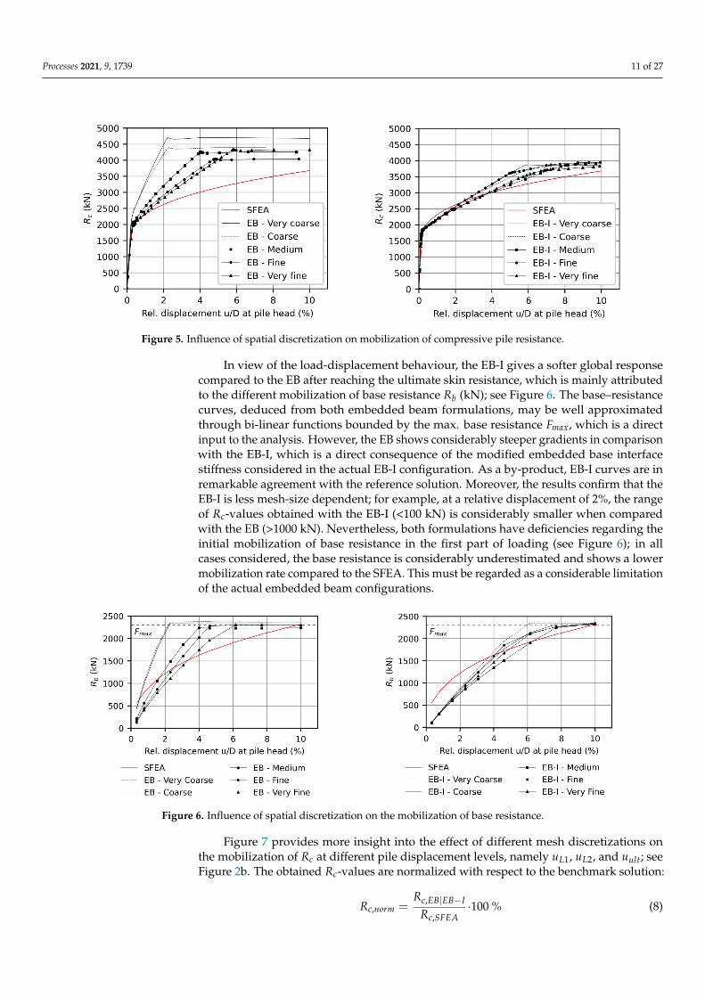
in the outermost stress points (i.e., at kinematically constrained model boundaries). InEquation (A1), G denotes the elastic tangent shear modulus, G0 the initial shear modulus,and Gur the unloading-reloading shear modulus. In this respect, Figure A1 shows theGm-contour plot obtained with the SFEA, which is considered as a benchmark model inSection 4. The minimum Gm-value (at the kinematically constrained model boundaries) atthe end of loading is 2.7, which satisfies the criterion specified in Equation (A1). Hence, itcan be concluded that the application domain is large enough in both the horizontal and

Processes 2021, 9, 1739 23 of 27

vertical directions to avoid any boundary cut-off effects (or at least that such effects arereduced to an acceptable limit). The same conclusion holds for all FE models where thepiles are idealised with EBs/EB-Is (minimum Gm-value = 2.7, not shown).

Figure A1. Alzey Bridge pile load test: factorized increase in unloading/reloading stiffness at the end of loading (SFEA).

Appendix B

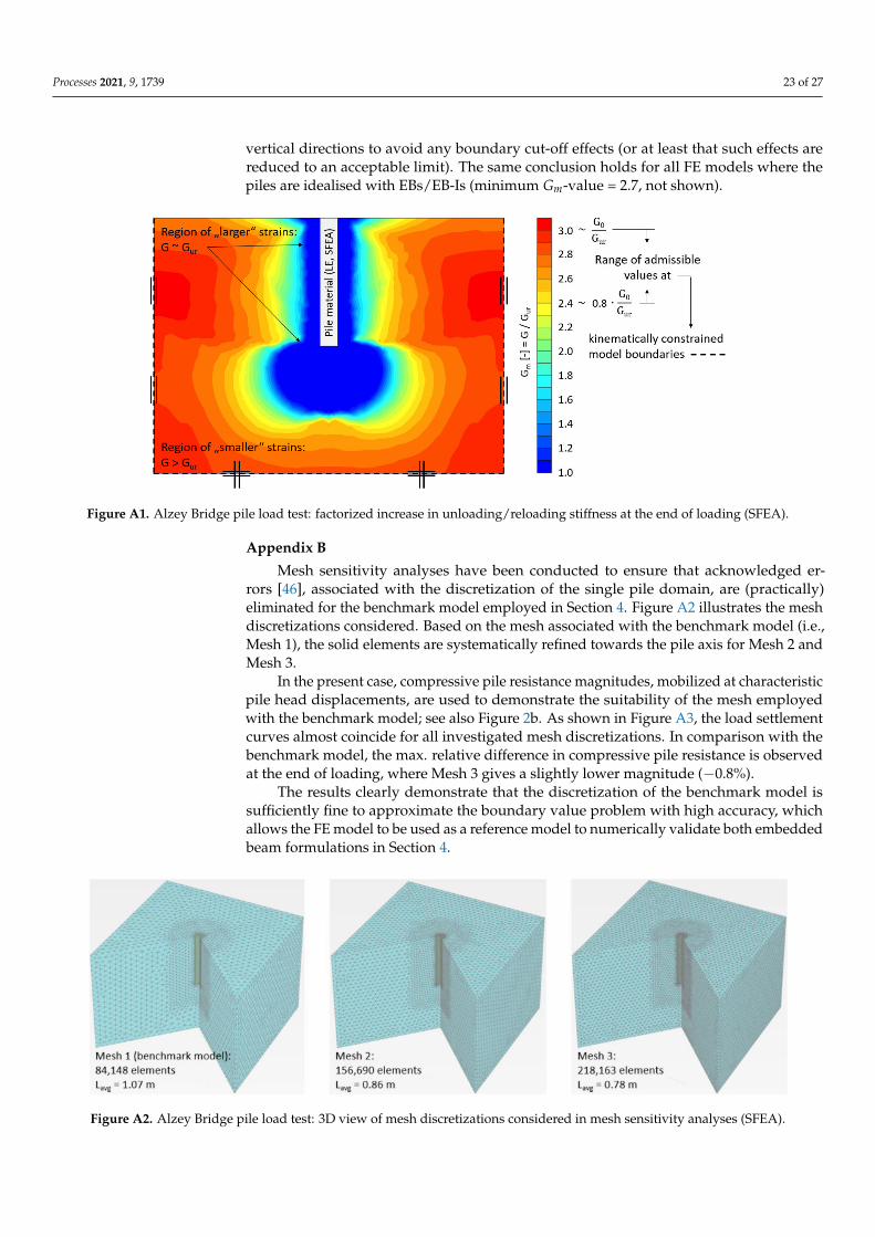
Mesh sensitivity analyses have been conducted to ensure that acknowledged er-rors [46], associated with the discretization of the single pile domain, are (practically)eliminated for the benchmark model employed in Section 4. Figure A2 illustrates the meshdiscretizations considered. Based on the mesh associated with the benchmark model (i.e.,Mesh 1), the solid elements are systematically refined towards the pile axis for Mesh 2 andMesh 3.

In the present case, compressive pile resistance magnitudes, mobilized at characteristicpile head displacements, are used to demonstrate the suitability of the mesh employedwith the benchmark model; see also Figure 2b. As shown in Figure A3, the load settlementcurves almost coincide for all investigated mesh discretizations. In comparison with thebenchmark model, the max. relative difference in compressive pile resistance is observedat the end of loading, where Mesh 3 gives a slightly lower magnitude (−0.8%).

The results clearly demonstrate that the discretization of the benchmark model issufficiently fine to approximate the boundary value problem with high accuracy, whichallows the FE model to be used as a reference model to numerically validate both embeddedbeam formulations in Section 4.

Figure A2. Alzey Bridge pile load test: 3D view of mesh discretizations considered in mesh sensitivity analyses (SFEA).

Processes 2021, 9, 1739 24 of 27

Figure A3. Alzey Bridge pile load test: influence of spatial discretization on (a) vertical pile head settlements at the pile axisand (b) mobilization of compressive pile resistance at different pile head settlements.

References1. Maheshwari, B.K.; Watanabe, H. Nonlinear Dynamic Behavior of Pile Foundations: Effects of Separation at the Soil-Pile Interface.

Soils Found 2006, 46, 437–448. [CrossRef]2. Poulos, H.G.; Davis, E.H. Pile Foundation Analysis and Design, 1st ed.; Poulos, H.G., Davis, E.H., Eds.; Wiley: New York, NY, USA,

1980; ISBN 0471020842.3. von Wolffersdorff, P.-A.; Henke, S. Möglichkeiten und Grenzen numerischer Methoden in der Geotechnik. Bautechnik 2021, 98,

1–17. [CrossRef]4. Potts, D.M.; Zdravkovic, L. Finite Element Analysis in Geotechnical Engineering: Application, 1st ed.; Thomas Telford Ltd.: London,

UK, 2001; ISBN 0727728121.5. Engin, H.K. Modelling of Installation Effects: A Numerical Approach. Ph.D. Thesis, Delft University of Technology, Delft, The

Netherlands, 2013.6. Schmüdderich, C.; Shahrabi, M.M.; Taiebat, M.; Lavasan, A.A. Strategies for numerical simulation of cast-in-place piles under

axial loading. Comput. Geotech. 2020, 125, 1–19. [CrossRef]7. Wehnert, M.; Vermeer, P.A. Numerische Simulation von Probebelastungen an Großbohrpfählen. In Proceedings of the Bauen

in Boden und Fels: 4. Kolloquium, Ostfildern, Germany, 20–21 January 2004; TAE: Esslingen, Germany, 2004; pp. 555–565,ISBN 3924813558.

8. Han, F.; Salgado, R.; Prezzi, M.; Lim, J. Shaft and base resistance of non-displacement piles in sand. Comput. Geotech. 2017, 83,184–197. [CrossRef]

9. Chen, Y.-J.; Lin, S.-S.; Chang, H.-W.; Marcos, M.C. Evaluation of side resistance capacity for drilled shafts. J. Mar. Sci. Technol.2011, 19, 210–221. [CrossRef]

10. Turello, D.F.; Sánchez, P.J.; Blanco, P.J.; Pinto, F. A variational approach to embed 1D beam models into 3D solid continua. Comput.Struct. 2018, 206, 145–168. [CrossRef]

11. Tschuchnigg, F. 3D Finite Element Modelling of Deep Foundations Employing an Embedded Pile Formulation. Ph.D. Thesis,Graz University of Technology, Graz, Austria, 2013.

12. Tschuchnigg, F.; Schweiger, H.F. The embedded pile concept—Verification of an efficient tool for modelling complex deepfoundations. Comput. Geotech. 2015, 63, 244–254. [CrossRef]

13. Tradigo, F.; Pisanò, F.; Di Prisco, C. On the use of embedded pile elements for the numerical analysis of disconnected piled rafts.Comput. Geotech. 2016, 72, 89–99. [CrossRef]

14. Ninic, J.; Stascheit, J.; Meschke, G. Beam-solid contact formulation for finite element analysis of pile-soil interaction with arbitrarydiscretization. Int. J. Numer. Anal. Meth. Geomech. 2014, 38, 1453–1476. [CrossRef]

15. Sadek, M.; Shahrour, I. A three dimensional embedded beam element for reinforced geomaterials. Int. J. Numer. Anal. Meth.Geomech. 2004, 28, 931–946. [CrossRef]

16. Engin, H.; Brinkgreve, R.; Septanika, E. Improved embedded beam elements for the modelling of piles. In Numerical Models inGeomechanics, Proceedings of the 10th International Symposium on Numerical Models in Geomechanics, Rhodes, Greece, 25–27 April 2007;Pande, G.N., Ed.; Taylor & Francis: London, UK, 2007; ISBN 978-0-415-44027-1.

17. Oliveria, D.; Wong, P.K. Use of embedded pile elements in 3D modelling of piled-raft foundations. Aust. Geomech. J. 2011, 46,9–19.

Processes 2021, 9, 1739 25 of 27

18. Smulders, C.M. An Improved 3D Embedded Beam Element with Explicit Interaction Surface. Master’s Thesis, Delft University ofTechnology, Delft, The Netherlands, 2018.

19. Ukritchon, B.; Faustino, J.C.; Keawsawasvong, S. Numerical investigations of pile load distribution in pile group foundationsubjected to vertical load and large moment. Geomech. Eng. 2016, 10, 577–598. [CrossRef]

20. Engin, H.K.; Brinkgreve, R.B.J. Investigation of Pile Behaviour Using Embedded Piles. In Proceedings of the 17th InternationalConference on Soil Mechanics and Geotechnical Engineering, Alexandria, Egypt, 5–9 October 2009; Hamza, M., Shahien, M.,El-Mossallamy, Y., Eds.; IOS Press: Amsterdam, The Netherlands, 2009; pp. 1189–1192.

21. Jongpradist, P.; Haema, N.; Lueprasert, P. Influence of pile row under loading on existing tunnel. In Tunnels and UndergroundCities: Engineering and Innovation Meet Archaeology, Architecture and Art; Peila, D., Viggiani, G., Celestino, T., Eds.; CRC Press:London, UK, 2019; pp. 5711–5719, ISBN 9781003031857.

22. Engin, H.; Septanika, E.; Brinkgreve, R. Estimation of Pile Group Behavior using Embedded Piles. In Proceedings of the 12thInternational Conference on Computer Methods and Advances in Geomechanics, Goa, India, 1–6 October 2008; Jadhav, M.N.,Ed.; Curran: New York, NY, USA, 2008, ISBN 9781622761760.

23. Engin, H.; Brinkgreve, R.; Bonnier, P.; Septanika, E. Modelling piled foundation by means of embedded piles. In Geotechnics of SoftSoils: Focus on Ground Improvement, Proceedings of the 2nd International Workshop, Glasgow, Scotland, 3–5 September 2008; Karstunen,M., Leoni, M., Eds.; Taylor & Francis: London, UK, 2008; pp. 131–136, ISBN 978-0-415-47591-4.

24. Lodör, K.; Balázs, M. Finite element modelling of rigid inclusion ground improvement. In Numerical Methods in GeotechnicalEngineering, Proceedings of the 9th European Conference on Numerical Methods in Geotechnical Engineering, Porto, Portugal, 25–27 June2018; Cardoso, A.S., Borges, J.L., Costa, P.A., Gomes, A.T., Marques, J.C., Vieira, C.S., Eds.; CRC Press: London, UK, 2018; pp. 1–8,ISBN 9781138544468.

25. Tschuchnigg, F.; Schweiger, H.F. Numerical study of simplified piled raft foundations employing an embedded pile formula-tion. In Proceedings of the 1st International Symposium on Computational Geomechanics. ComGeo I, Juan-les-Pins, France,29 April–1 May 2009; IC2E: Rhodes, Greece, 2009; pp. 743–752.

26. Lee, S.W.; Cheang, W.; Swolfs, W.M.; Brinkgreve, R. Modelling of piled rafts with different pile models. In Numerical Methods inGeotechnical Engineering, Proceedings of 7th European Conference on Numerical Methods in Geotechnical Engineering, Trondheim, Norway,2–4 June 2010; Benz, T., Nordal, S., Eds.; CRC Press: London, UK, 2010; pp. 1–6, ISBN 9780429206191.

27. Elshehahwy, E.R.; Eltahrany, A.; Dif, A. Numerical Analysis Validation Using Embedded Pile. In Advances in Numerical Methodsin Geotechnical Engineering, Proceedings of 2nd GeoMEast International Congress and Exhibition on Sustainable Civil Infrastructures,Cairo, Egypt, 10–15 November 2019; Shehata, H., Desai, C.S., Eds.; Springer: Berlin/Heidelberg, Germany, 2019; pp. 199–208,ISBN 978-3-030-01925-9.

28. Watcharasawe, K.; Jongpradist, P.; Kitiyodom, P.; Matsumoto, T. Measurements and analysis of load sharing between piles andraft in a pile foundation in clay. Geomech. Eng. 2021, 24, 559–572. [CrossRef]

29. Banerjee, R.; Bandyopadhyay, S.; Sengupta, A.; Reddy, G.R. Settlement behaviour of a pile raft subjected to vertical loadings inmultilayered soil. Geomech. Geoengin. 2020, 1–15. [CrossRef]

30. Abbas, Q.; Kim, G.; Kim, I.; Kyung, D.; Lee, J. Lateral Load Behavior of Inclined Micropiles Installed in Soil and Rock Layers.Int. J. Geomech. 2021, 21, 1–13. [CrossRef]

31. Abbas, Q.; Choi, W.; Kim, G.; Kim, I.; Lee, J. Characterizing uplift load capacity of micropiles embedded in soil and rockconsidering inclined installation conditions. Comput. Geotech. 2021, 132, 1–12. [CrossRef]

32. El-Sherbiny, M.M.; El-Sherbiny, R.M.; El-Mamlouk, H. Three Dimensional Effect of Grouted Discontinuous Berms for PassiveSupport of Diaphragm Walls. In Proceedings of the Grouting 2017: Jet Grouting, Diaphragm Walls, and Deep Mixing, Honolulu,HI, USA, 9–12 July 2017; Gazzarrini, P., Richards, J.T.D., Bruce, D.A., Byle, M.J., El Mohtar, C.S., Johnsen, L.F., Eds.; AmericanSociety of Civil Engineers: Reston, VA, USA, 2017; pp. 571–583, ISBN 9780784480809.

33. Marjanovic, M.; Vukicevic, M.; König, D.; Schanz, T.; Schäfer, R. Modeling of laterally loaded piles using embedded beam elements.In Contemporary Achievements in Civil Engineering, Proceedings of 4th International Conference, Subotica, Serbia, 22–23 April 2016;Faculty of Civil Engineering: Novi Sad, Serbia, 2016; pp. 349–358.

34. Abo-Youssef, A.; Morsy, M.S.; El Ashaal, A.; El Mossallamy, Y.M. Numerical modelling of passive loaded pile group inmultilayered soil. Innov. Infrastruct. Solut. 2021, 6, 1–13. [CrossRef]

35. Al-abboodi, I.; Sabbagh, T.T. Numerical Modelling of Passively Loaded Pile Groups. Geotech. Geol. Eng. 2019, 37, 2747–2761.[CrossRef]

36. Scarfone, R.; Morigi, M.; Conti, R. Assessment of dynamic soil-structure interaction effects for tall buildings: A 3D numericalapproach. Soil Dyn. Earthq. Eng. 2020, 128, 1–14. [CrossRef]

37. Di Prisco, C.; Flessati, L.; Porta, D. Deep tunnel fronts in cohesive soils under undrained conditions: A displacement-basedapproach for the design of fibreglass reinforcements. Acta Geotech. 2020, 15, 1013–1030. [CrossRef]

38. Ninic, J. Computational Strategies for Predictions of the Soil-Structure Interaction during Mechanized Tunneling. Ph.D. Thesis,Ruhr University Bochum, Bochum, Germany, 2015.

39. Granitzer, A.; Tschuchnigg, F.; Summerer, W.; Galler, R.; Stoxreiter, T. Construction of a railway tunnel above the main drainagetunnel of Stuttgart using the cut-and-cover method. Bauingenieur 2021, 96, 156–164. [CrossRef]

Processes 2021, 9, 1739 26 of 27

40. Lo, S. A study in an attempt to use embedded pile structure elements to simulate soil nail structures in PLAXIS 2D 2012 and3D 2012. In Numerical Methods in Geotechnical Engineering, Proceedings of the 8th European Conference on Numerical Methods inGeotechnical Engineering, Delft, The Netherlands, 18–20 June 2014; Hicks, M., Brinkgreve, R., Rohe, A., Eds.; CRC Press: London, UK,2014; pp. 765–769, ISBN 978-1-138-00146-6.

41. Turello, D.F.; Pinto, F.; Sánchez, P.J. Embedded beam element with interaction surface for lateral loading of piles. Int. J. Numer.Anal. Meth. Geomech. 2016, 40, 568–582. [CrossRef]

42. Smulders, C.M.; Hosseini, S.; Brinkgreve, R. Improved embedded beam with interaction surface. In Proceedings of the 17thEuropean Conference on Soil Mechanics and Geotechnical Engineering, Reykjavík, Iceland, 1–6 September 2019; Sigursteinsson,H., Erlingsson, S., Bessason, B., Eds.; COC: Reykjavík, Iceland, 2019; pp. 1048–1055.

43. Turello, D.F.; Pinto, F.; Sánchez, P.J. Three dimensional elasto-plastic interface for embedded beam elements with interactionsurface for the analysis of lateral loading of piles. Int. J. Numer. Anal. Meth. Geomech. 2017, 41, 859–879. [CrossRef]

44. Turello, D.F.; Pinto, F.; Sánchez, P.J. Analysis of lateral loading of pile groups using embedded beam elements with interactionsurface. Int. J. Numer. Anal. Meth. Geomech. 2019, 43, 272–292. [CrossRef]

45. Jauregui, R.; Silva, F. Numerical Validation Methods. In Numerical Analysis—Theory and Application; Awrejcewicz, J., Ed.; InTech:Toyama, Japan, 2011; ISBN 978-953-307-389-7.

46. Oberkampf, W.L.; Trucano, T.G.; Hirsch, C. Verification, validation, and predictive capability in computational engineering andphysics. Appl. Mech. Rev. 2004, 57, 345–384. [CrossRef]

47. Ferreira, D.; Manie, J. DIANA—Finite Element Analysis: DIANA Documentation—Release 10.4. Available online: https://dianafea.com/manuals/d104/Diana.html (accessed on 25 February 2021).

48. Truty, A.; Zimmermann, T.; Podles, K.; Obrzud, R. ZSOIL.PC 2020: User Manual—Theory. Available online: https://www.zsoil.com/zsoil_manual/TM-Man.pdf (accessed on 26 July 2021).

49. Rocscience Online Help: Online Documentation. Available online: https://www.rocscience.com/about (accessed on25 February 2021).

50. FLAC3D 7.0 Documentation. Available online: http://docs.itascacg.com/flac3d700/common/sel/doc/manual/sel_manual/piles/piles.html?node903 (accessed on 26 February 2021).

51. PLAXIS Scientific Manual: 3D—Connect Edition V21. Available online: https://communities.bentley.com/cfs-file/__key/communityserver-wikis-components-files/00-00-00-05-58/PLAXIS3DCE_2D00_V21.01_2D00_04_2D00_Scientific.pdf (accessedon 26 July 2021).

52. Sommer, H.; Hambach, P. Großpfahlversuche im Ton für die Talbrücke Alzey. Bauingenieur 1974, 49, 310–317.53. Hirany, A.; Kulhawy, F.H. Interpretation of Load Tests on Drilled Shafts—Part 1: Axial Compression. In Proceedings of the

Foundation Engineering—Current Principles and Practices, Evanston, IL, USA, 25–29 June 1989; Kulhawy, F.H., Ed.; AmericanSociety of Civil Engineers: New York, NY, USA, 1989; pp. 1132–1149, ISBN 0872627047.

54. Chen, Y.-J.; Fang, Y.-C. Critical Evaluation of Compression Interpretation Criteria for Drilled Shafts. J. Geotech. GeoenvironmentalEng. 2009, 135, 1056–1069. [CrossRef]

55. Hirany, A.; Kulhawy, F.H. On the Interpretation of Drilled Foundation Load Test Results. In International Deep FoundationsCongress, Proceedings of the Deep Foundations: An International Perspective on Theory, Design, Construction, and Performance, Orlando,FL, USA, 14–16 February 2002; O’Neill, M.W., Townsend, F.C., Eds.; American Society of Civil Engineers: New York, NY, USA,2002; pp. 1018–1028, ISBN 9780784406014.

56. German Geotechnical Society. Recommendations on Piling (EA-Pfähle), 2nd ed.; Wilhelm Ernst & Sohn: Berlin, Germany, 2014; ISBN9783433030189.

57. PLAXIS Reference Manual: 3D—Connect Edition V21. Available online: https://communities.bentley.com/cfs-file/__key/communityserver-wikis-components-files/00-00-00-05-58/PLAXIS3DCE_2D00_V21.01_2D00_02_2D00_Reference.pdf (accessedon 16 August 2021).

58. Day, R.A.; Potts, D.M. Zero thickness interface elements—Numerical stability and application. Int. J. Numer. Anal. Meth. Geomech.1994, 18, 689–708. [CrossRef]

59. Goodman, R.; Taylor, R.; Brekke, T. A Model for the Mechanics of Jointed Rock. J. Soil Mech. Found. Div. 1968, 94, 637–659.[CrossRef]

60. van Langen, H.; Vermeer, P.A. Interface elements for singular plasticity points. Int. J. Numer. Anal. Meth. Geomech. 1991, 15,301–315. [CrossRef]

61. Kulhawy, F.H. Limiting tip and side resistance: Fact or Fallacy? In Proceedings of the Analysis and Design of Pile Foundations,San Francisco, CA, USA, 1–5 October 1984; Meyer, J.R., Ed.; American Society of Civil Engineers: New York, NY, USA, 1984;pp. 80–98.

62. Sheil, B.; McCabe, B.A. Predictions of friction pile group response using embedded piles in PLAXIS. In Proceedings of the 3rd In-ternational Conference on New Developments in Soil Mechanics and Geotechnical Engineering, Nicosia, Turkey, 28–30 June 2012;Near East University: Nicosia, Turkey, 2012; pp. 679–686.

63. Fleming, W.G.K.; Weltman, A.; Randolph, M.F.; Elson, K. Piling Engineering, 3rd ed.; Taylor & Francis: London, UK, 2020;ISBN 9780367659387.

64. Benz, T.; Schwab, R.; Vermeer, P. Small-strain stiffness in geotechnical analyses. Bautechnik 2009, 86, 16–27. [CrossRef]

Processes 2021, 9, 1739 27 of 27

65. Schanz, T.; Vermeer, P.A.; Bonnier, P.G. The hardening soil model: Formulation and verification. In Beyond 2000 in ComputationalGeotechnics, 1st ed.; Brinkgreve, R.B.J., Ed.; Routledge: London, UK, 2019; pp. 281–296, ISBN 9781315138206.

66. Vucetic, M.; Dobry, R. Effect of Soil Plasticity on Cyclic Response. J. Geotech. Eng. 1991, 117, 89–107. [CrossRef]67. Alpan, I. The geotechnical properties of soils. Earth-Sci. Rev. 1970, 6, 5–49. [CrossRef]68. Viggiani, C.; Mandolini, A.; Russo, G. Piles and Pile Foundations, 1st ed.; Taylor & Francis: London, UK, 2012; ISBN 978-0-415-

49066-5.69. Urbonas, K.; Slizyte, D.; Mackevicius, R. Influence of the pile stiffness on the ground slab behaviour. J. Civ. Eng. Manag. 2016, 22,

690–698. [CrossRef]70. Hanisch, J.; Katzenbach, R.; König, G. (Eds.) Kombinierte Pfahl-Plattengründungen; Ernst & Sohn: Berlin, Germany, 2001;

ISBN 3433016062.71. Schreppers, G.-J. Bond-slip Reinforcements and Pile Foundations. Available online: https://dianafea.com/sites/default/files/20

18-04/Bondslip_reinforcements_and_Pile_foundations.pdf (accessed on 26 July 2021).72. Schmidt, H.-H.; Buchmaier, R.F.; Vogt-Breyer, C. Grundlagen der Geotechnik, 5th ed.; Springer Fachmedien Wiesbaden: Wiesbaden,

Germany, 2017; ISBN 978-3-658-14930-7.73. British Standards Institution. BS EN 1997-1:2004: Eurocode 7: Geotechnical Design—Part 1: General Rules; BSI: London, UK, 2004.74. de Gennaro, V.; Frank, R.; Said, I. Finite element analysis of model piles axially loaded in sands. Riv. Ital. Geotec. 2008, 2, 44–62.75. Cho, J.; Lee, J.-H.; Jeong, S.; Lee, J. The settlement behavior of piled raft in clay soils. Ocean Eng. 2012, 53, 153–163. [CrossRef]76. Poulos, H.G. Piled raft foundations: Design and applications. Géotechnique 2001, 51, 95–113. [CrossRef]77. Benz, T. Small-Strain Stiffness of Soils and Its Numerical Consequences. Ph.D. Thesis, University of Stuttgart, Stuttgart,

Germany, 2007.