1

EEL 5771-001

Introduction to Computer Graphics

PPT2: Graphics Output Primitives

TEAM - ELECTRA

Team members

Member 1 : Sidharth Sribhashyam (U02410812)

Member 2: Syam Adarsh Adusumilli (U97004410)

Member 3: Naga Sindhuri Bollineni(U27394206)

Introduction to Graphics Output Primitives

• Definition of Output Primitives : These are geometric functions or algorithms which assist user in generating basic computer graphics.

• Examples : Points, Line segments, circles, hyperbola, parabola, ellipses, quadratic and curved surfaces, polygon areas.

• We can generate more complex structures from these simple attributes.

• Each primitive is specified with input coordinates data and other information which describe the object well

• These primitives are defined in OpenGL.

• Open GL stands for Open Graphics Library which is a cross platform, cross language API which renders 2D and 3D vector graphics.

Coordinate Frames

• To setup a scene or space in the system, we need to define a frame of reference using coordinate systems

• For a 2D space, X and Y coordinates are enough. But for 3D space, 3 Axes namely X axis which is horizontal axis, Y axis which is the vertical axis and Z axis which is the Depth axis.

• One of the most used coordinate system is World Coordinate System which is the base reference system for 3D models.

• The system used here is Right Hand Coordinate system where if the thumb of right hand faces positive Z axis, the curl of rest of fingers curl in positive X and Y axes.

An illustration of 3D frame of reference where a 3D object is shown and the corresponding axes are also depicted

Coordinate Frames

• Scan Conversion Process : This process holds the information regarding the scene such as locations of different attributes, color values and the objects within.

• Locations of the pixels within the screen are represented with integer screen coordinates.

• The coordinate values are converted to integer pixel positions within a frame buffer using a process known as Rasterization

• Some functions used for these manipulations are as follows• setPixel(x,y) sets pixel color at coordinates (x,y)• getPixel(x,y,color) returns the color value for given coordinates (x,y)

An illustration of 3D frame of reference where a 3D object is shown and the corresponding axes are also depicted

An Introduction to point functions in OpenGL

• OpenGL stands for Open Graphics Library which is used to deal with both 2D and 3D coordinate spaces.

• As OpenGL deals with rendering graphics, it needs a high computational power and parallel processing to speed up the process and render well.

• This demands the usage of dedicated GPU for OpenGL which helps accelerating the process of rendering.

• Few examples of point functions with arbitrary pixel values are as follows

glBegin(GL_POINTS):glVertex2iv(p1);glVertex2iv(p2);glVertex2iv(p3);

glEnd()

7

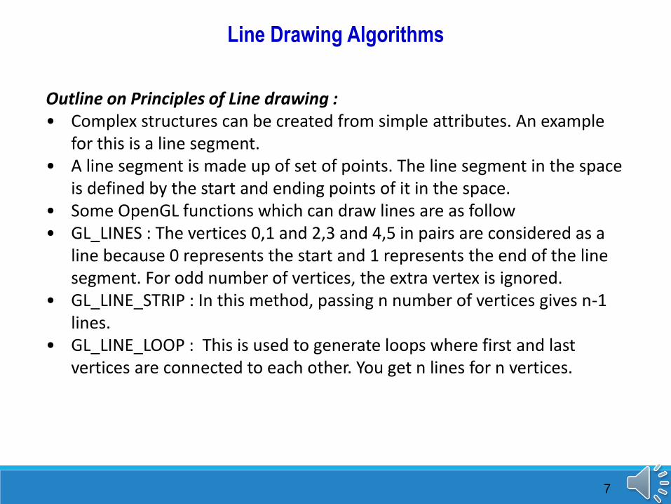
Line Drawing Algorithms

Outline on Principles of Line drawing : • Complex structures can be created from simple attributes. An example

for this is a line segment. • A line segment is made up of set of points. The line segment in the space

is defined by the start and ending points of it in the space.• Some OpenGL functions which can draw lines are as follow • GL_LINES : The vertices 0,1 and 2,3 and 4,5 in pairs are considered as a

line because 0 represents the start and 1 represents the end of the line segment. For odd number of vertices, the extra vertex is ignored.

• GL_LINE_STRIP : In this method, passing n number of vertices gives n-1 lines.

• GL_LINE_LOOP : This is used to generate loops where first and last vertices are connected to each other. You get n lines for n vertices.

8

Line Drawing Algorithms

Line drawing principles continued :• Starting and ending points determine the position of the line in the vector

space.• To project a line on the monitor, the start and end points are chosen and the

nearest pixels and the shortest distance between both the start and end point is calculated and then projected. The color information of the line is loaded into the frame buffer of those pixels.

• Reading from the frame buffer, the video controller plots the screen pixels.• This process digitizes the line into a set of discrete integer positions that, in

general, only approximates the actual line path.• A computed line position of (20.42, 30.69), for example, is translated the to

pixel position (20,31). This rounding of coordinate values to integers causes all but horizontal and vertical lines to be displayed with a stair-step appearance.

• Due to which, a line displayed in a monitor is not always a perfect line but a stair-step arrangement of points as shown

9

Line Drawing Algorithms

The math required to plot the lines: • A straight line in a vector space can be represented by a mathematical

equation which carries information about the inclination of the line in X-Y plane and also the point at which it crosses Y axis.

• The equation can be given as y = mx+c where m is the slope or inclination of the line with respect to the X axis and c is the Y intercept.

• The slope of a line is calculated using the starting and ending points of the line.

• Assume (x0,y0) represent starting points and (x1,y1 ) represent end points, the slope of the line is given by the equation (y1-y0)/(x1-x0).

• If the angle of the line is known, Tan function of the angle also gives the slope of the line.

• These equations help determining variations in voltage in analog displays well.

10

Line Drawing Algorithms

DDA(Digital differential Analyzer) Algorithm :• The DDA algorithm is a faster method for calculating pixel positions than

one directly implements y = m *x+c.• The accumulation of round-off error in successive additions ofthe floating-

point increment, however, can cause the calculated pixel positions to drift away from the true path for long line segments.

• The rounding operations and floating-point arithmetic in this procedure are still time consuming.

Steps in DDA Algorithm : • Walk through the line, starting at (x0,y0)• Constrain x, y increments to values in [0,1] range• Case a: x is incrementing faster (m < 1)• Step in x=1 increment, compute and round y• Case b: y is incrementing faster (m > 1)• Step in y=1 increment, compute and round x

11

Line Drawing Algorithms

DDA Algorithm Pseudo Code :Step1: Start AlgorithmStep2: Declare x1,y1,x2,y2,dx,dy,x,y as integer variables.Step3: Enter value of x1,y1,x2,y2.Step4: Calculate dx = x2-x1

Step5: Calculate dy = y2-y1

Step6: If ABS (dx) > ABS (dy)Then step = abs (dx)

ElseStep7: xinc=dx/step yinc=dy/step

assign x = x1 assign y = y1

Step8: Set pixel (x, y)Step9: x = x + xinc y = y + yinc

Set pixels (Round (x), Round (y))Step10: Repeat step 9 until x = x2

Source for the pseudo code : https://www.javatpoint.com/computer-graphics-dda-algorithm

12

Line Drawing Algorithms

Bresenham Line Drawing Algorithm•Starting coordinates = (X0, Y0)•Ending coordinates = (Xn, Yn)Step-01:Calculate ΔX and ΔY from the given input.These parameters are calculated as-•ΔX = Xn – X0

•ΔY =Yn – Y0

Step-02:Calculate the decision parameter Pk.It is calculated as- Pk = 2ΔY – ΔXStep-03: Step 3 has 2 cases as shown.Keep repeating the steps until endpoint is reached.

13

Line Drawing Algorithms: Line Clipping

• Line clipping:• Process of removing lines or portions of lines outside an area of interest. Typically,

any line or part there of which is outside of the viewing area is removed.• The two common algorithms for line clipping: Cohen-Sutherland and Liang-Barsky• Aline-clipping method consists of various parts. Tests are conducted on a given line

segment to find out whether it lies outside the view volume.• Afterwards, intersection calculations are carried out with one or more clipping

boundaries.• To minimize the intersection calculations and to increase the efficiency of the

clipping algorithm, initially, completely visible and invisible lines are identified and then the intersection points are calculated for remaining lines.

• Determining which portion of the line is inside or outside of the clipping volume is done by processing the endpoints of the line with regards to the intersection.

14

Line Drawing Algorithms

Cohen-Sutherland Algorithm• The Cohen-Sutherland Line-Clipping Algorithm performs initial tests on a line

to determine whether intersection calculations can be avoided.• First, end-point pairs are checked for trivial acceptance.• If the line cannot be trivially accepted, region checks are done for Trivial

rejection.• If the line segment can be neither trivially accepted or rejected, it is divided

into two segments at a clip edge, so that one segment can be trivially rejected.

• These three steps are performed iteratively until what remains can be trivially accepted or rejected.

Circle Algorithms

Introduction

A Circle is set of points which are all at distance of r from the center point. This

can be expressed in cartesian coordinates as follows.

(x − xc)2 + (y − yc)2 = r2

The points on the circumference can be calculated by stepping along the x axis. The

circle has a property called eight way symmetry, which means if we knew the point

coordinates in any one of the octant, we can determine the corresponding points in the

remaining seven octants.

15

Steps

1. Determine the radius of circle.

2. The center is assumed to be at origin (0,0).

3. The first pixel of the octant is assumed to be at (0,r).

4. The initial decision parameter d0 = 3-2r is calculated.

5. This is repeated until x<=y.

6. If dk > 0

• dk+1 = dk+4(xk-yk)+10

• xk+1 = xk+1

• yk+1 = yk-1

7. If dk < 0

• dk+1 = dk+4xk+6

• xk+1 = xk+1

• yk+1 = yk

16

17

8. Plot all (xk+1,yk+1).

9. Plot all the points in all the octants remaining.

10. Add the center coordinates to all the obtained points.

Example

The radius of circle is 10

Iteration X Y Decision parameter

0 0 10 d0 = 3-2(10) = -17

1 1 10 d1 = d0+4x0+6 = -17+0+6 = -11

2 2 10 d2 = d1+4x1+6 = -11+4+6 = -1

3 3 10 d3 = d2+4x2+6 = -1+8+6 = 13

4 4 9 d4 = d3+4(x3-y3)+10 = 13-28+10 = -5

5 5 9 d5 = d4+4x4+6 = -5+16+6 = 17

6 6 8 d6 = d5+4(x5-y5)+10 = 17-16+10 = 11

7 7 7 d7 = d6+4(x6-y6)+10 = 11+10 = 21

Midpoint Circle Drawing Algorithm

Introduction

In this algorithm we consider a circle, origin as centre, the equation of that circle

will be

f(x,y) = x2+y2-r2. We can deduce that

So we use the circle equation as the decision parameter and setup incremental or

decremental calculations accordingly. The steps for the midpoint circle drawing

algorithm are as follows

18

Steps

1. Determine the radius of circle.

2. The center is assumed to be at origin (0,0).

3. The first pixel of the octant is assumed to be at (0,r).

4. The initial decision parameter d0 = (5/4)-r is calculated.

5. This is repeated until x<=y.

6. If dk > 0

• dk+1 = dk+2(xk-yk)+5

• xk+1 = xk+1

• yk+1 = yk-1

7. If dk < 0

• dk+1 = dk+2xk+3

• xk+1 = xk+1

• yk+1 = yk

19

20

8. Plot all (xk+1,yk+1).

9. Plot all the points in all the octants remaining.

10. Add the center coordinates to all the obtained points.

Ellipse Algorithms

Introduction

An Ellipse can be defined as a set of points whose sum of distance from the foci of

the ellipse constant. If F1 and F2 are the foci of the ellipse, and d1 and d2 are distance

between the foci and a point P, then d1+d2 = Constant

Ellipse has two diameters, one is maximum and the other is minimum in the

perpendicular direction of the other. Ellipse doesn’t have 8 way symmetry. The slope is

given by dy/dx

x2r2y+y2r2

x = r2xr

2y

21

• The slope in the first octant is always less than 1, we start with point on y axis

m<1

yk+1 = yk/yk-1

if yk+1 = yk => (xk+1,yk)

if yk+1 = yk-1 => (xk+1,yk-1)

• Go to octant 2 when slope equals -1

• The endpoint of first octant will be the start of second octant, the slope in

second octant is always greater than 1

m>1

xk+1 = xk/xk-1

if xk+1 = xk => (xk,yk-1)

if xk+1 = xk-1 => (xk+1,yk-1)

22

Steps

Region1

• Initial decision parameter d0=r2y+r2

x/4-r2yr

2x

• Repeated until 2r2yxk+1>=2r2

xyk+1

• dk+1=dk+r2y+2(xk+1)r

2y+r2

x(y2k+1-y

2k)-r

2x(yk+1-yk)

• If dk>=0 => (xk+1,yK-1)

• If dk<0 => (xk+1,yk)

Region2

• Initial decision parameter d0=(xk+1/2)2r2x+(yk-1/2)2r2

y-r2yr

2x

• Repeated until we get (x,0)

• dk+1=dk+r2x-2(yk-1)r

2x+r2

y(x2k+1-x

2k)+r2

y(Xk+1-Xk)

• If dk>=0 => (xk,yK-1)

• If dk<0 => (xk+1,yk+1)

23

24

Example

K (xk,yk) dk (xk+1,Yk+1) 2r2yxk+1 2r2

xyk+1 dk+1

0 (0,6) -332 (1,6) 72 768 -224

1 (1,6) -224 (2,6) 144 768 -44

2 (2,6) -44 (3,6) 216 768 208

3 (3,6) 208 (4,5) 288 640 -108

4 (4,5) -108 (5,5) 360 640 288

5 (5,5) 288 (6,4) 432 512 244

6 (6,4) 244 (7,3) 504 384 -23

7 (7,3) -23 (8,2) 361

8 (8,2) 361 (8,1) 297

9 (8,1) 297 (8,0)

Pixel Addressing

Introduction

The coordinate positions which are given as input to graphics program, as

description of object are very small points. So it is necessary to preserve the geometry of

the object when converting them to pixel coordinates. That can be done in the following

ways.

1. Adjust the pixel dimensions of displayed objects so as to correspond to the

dimensions given in the original mathematical description of the scene.

2. Map world coordinates onto screen positions between pixels, so that we align object

boundaries with pixel boundaries instead of pixel centers.

25

Screen Grid Coordinates

• In this method the screen is divided by grid line and pixels are located one unit apart.

• The position of pixel on the screen is given by a pair of integer values.

• Using this method, the area occupied by pixel which is at (x,y) can be seen as the

square with (x,y) and (x+1,y+1) as the diagonally opposite corners.

• The advantages of this method of pixel addressing is it eliminates half integer pixel

boundaries.

• It also gives precise object representation and simplifies the processing

26

Pixel Addressing for Lines

• Consider a line plotted in bresenham algorithm with (20,10) and (30,18) as its end

points.

• So in mathematical terms the line has a magnitude of 10 units horizontally and 8

units vertically.

• So we should not pot the pixel in (30,18) because then the magnitude of the line will

be 11 units horizontally and 9 units vertically.

• Therefore inorder to preserve the geometry, we plot the points which are interior to

the line path, which means we only plot until (29,17).

27

Pixel Addressing for Rectangles

• Consider a rectangle plotted between the coordinates (0,0) , (0,3) , (4,3) and (4,0).

• In order to preserve the geometry we need to plot the pixels which are within the

boundaries of the object.

• For example figure (a) is the actual rectangle, when we convert into pixel

coordinates, we should consider the coordinates outside the boundary like figure (b).

• The pixels only interior to the boundary are to be considered same as in figure (c).

28

Pixel Addressing for Circle

• Consider a circle with radius 5 and center at (10,10).

• Generally the circle plotted using midpoint algorithm would like in figure to left, but

then the diameter of circle would be 11 instead of 10.

• So to preserve the geometry we can change the algorithm to shorten each pixel scan

line and each pixel column, then we will get a circle similar to one in right figure.

29

Area Fill Methods

There are two methods

Scan Line Approach

This method first determines the overlap intervals along the scan lines that cross

area, and the pixel positions along these intervals are set to the desired fill color. This is

used for simple shapes.

Fill Approach

In this method, the filling starts at a interior position and paints outward until it

reaches the boundary. This is used for complex shapes. A reference point can be set at

any convenient position.

30

Concave and Convex Polygons

• The angle inside the polygon boundary which is formed by two adjacent edges is

called an interior angle.

• If all the interior angles are <=180o , then it is a convex polygon.

• Anything other than convex polygon is a concave polygon.

• Often concave polygons are split into set of convex polygons because concave

polygons preset problems to algorithms.

31

Concave Polygon Split

• A concave polygon can be split by using rotational method.

• The polygon is rotated counterclockwise, and the position is shifted so that each

vertex vk is at origin.

• Then the polygon is rotated about origin in clockwise direction, so that the next

vertex vk+1 is on x axis.

• If the vertex vk+2 is below the x axis, the polygon is concave and we split it along x

axis.

• We repeat this until all the polygons and all the vertices are tested.

32

Convex Polygon Split

• A convex polygon is split into set of triangles.

• Any sequence of three vertices are defined to be a new triangle.

• The middle triangle vertex is then deleted from the main polygon and the remaining

polygon is further splitted using the same process.

• This goes on until the last polygon is a triangle.

• Concave polygons can also be splitted using this method.

33

Area Fill Using Boolean Operations

• Sometimes we need to determine interior region of objects to fill the area.

• Booleans are used to specify fill area as a combination of two regions.

• Variation of basic winding rule is a way to implement boolean operations.

• First a non intersecting boundary for two regions is defined, then the direction of the

two regions is considered to be counterclockwise.

• The union of two regions consists of points whose winding number is positive, and

similarly the intersection of two regions will be whose winding number is greater

than 1.

• To get the difference of two regions one is enclosed countercolckwise and the other

in clockwise, and the difference with set of all values positive.

34

35

Data Structure for Polygonal Objects

• The data is stored in two tables

• Geometric tables

• Attribute tables.

• Geometric tables contain data about vertex coordinates and spatial orientation.

• Attribute table contain degree of transparency, surface and texture characteristics.

• The data in the geometric tables are displayed in three different tables for

convenience.

• Coordinates for vertices are stored in vertex table, edge table contains edges between

the vertices, surface facet table has pointers back to edge table to identify edges of

each polygon

36

Plane Equations - General implicit form

• For some of the processes like transformation of the modeling and world-

coordinate descriptions through the viewing pipeline, application of

rendering routines to the individual surface facets etc, we do require the

information about the spatial orientation of the surface components of

objects.

• This information can be obtained from the vertex coordinate values and

the equations that describe the polygon surfaces.

• The general equation of a plane is A x + B y + C z + D = 0 → (1)

-where (x, y, z) is any point on the plane,

-the coefficients A, B, C, and D (called plane parameters) are constants

which describe spatial properties of the plane.

37

Plane Equations- Three-point form

• There is another way of representing the plane equation, if we know any

three points on the plane, we can easily find the equation of it.

• For example, we have three successive convex-polygon vertices, (x1, y1,

z1), (x2, y2, z2), and (x3, y3, z3), in a counterclockwise order.

• The solution to this set of equations can be obtained in determinant form,

using Cramer’s rule.

• Expanding the determinants, we get the below equations to solve.

A = y1(z2 − z3) + y2(z3 − z1) + y3(z1 − z2)

B = z1(x2 − x3) + z2(x3 − x1) + z3(x1 − x2)

C = x1(y2 − y3) + x2(y3 − y1) + x3(y1 − y2)

D = −x1(y2z3 − y3z2) − x2(y3z1 − y1z3) − x3(y1z2 − y2z1) → (2)

After solving this, we can find the values of A, B, C, D and hence the plane

equation is Ax + By + Cz + D = 0.

38

Plane Equations- eigen-vector method

• Plane equations are used to find the position of spatial points.

• For any point (x, y, z) not on a plane with parameters A, B, C, D, we have

A x + B y + C z + D ≠ 0.

if A x + B y + C z + D < 0, the point (x, y, z) is behind the plane .

if A x + B y + C z + D > 0, the point (x, y, z) is in front of the plane.

• The elements of a normal vector can also be obtained using a vector cross-product

calculation. For example, select any three vertex positions, V1, V2, and V3, taken in

counterclockwise . From V1 to V2 , form the first vector and the second from V1 to V3,

we calculate N as the vector cross-product:

N = (V2 − V1) × (V3 − V1).

• This generates values for the plane parameters A, B, and C. We can then obtain the value

for parameter D by substituting these values into Equation 1 and solving for D.

• The plane equation can be expressed in vector form using the normal N and the position P

of any point in the plane as N · P = −D to get the correct normal vector direction for the

polygon surface.

39

OpenGL Polygon Fill Area Functions

• The OpenGL Polygon Fill Area Functions are used to draw the polygons.

• There are many functions described for drawing the Polygon, some of

them are as follows.

glVertex – This function is used for a single polygon vertex to input the

coordinates for that vertex.

glBegin/glEnd pair – All the vertices to the polygon must be present in

between these two functions.

• The least number of vertices that a polygon contains is atleast 3. So, this

glVertex function should be called 3 times minimum so that a complete

triangle can be formed.

• For the glBegin function, there are like 6 different symbolic constants that

can be passed as an argument to describe the polygon fill areas.

• Every polygon has two faces, front and back face. We can fill different

colors for each face separately.

40

41

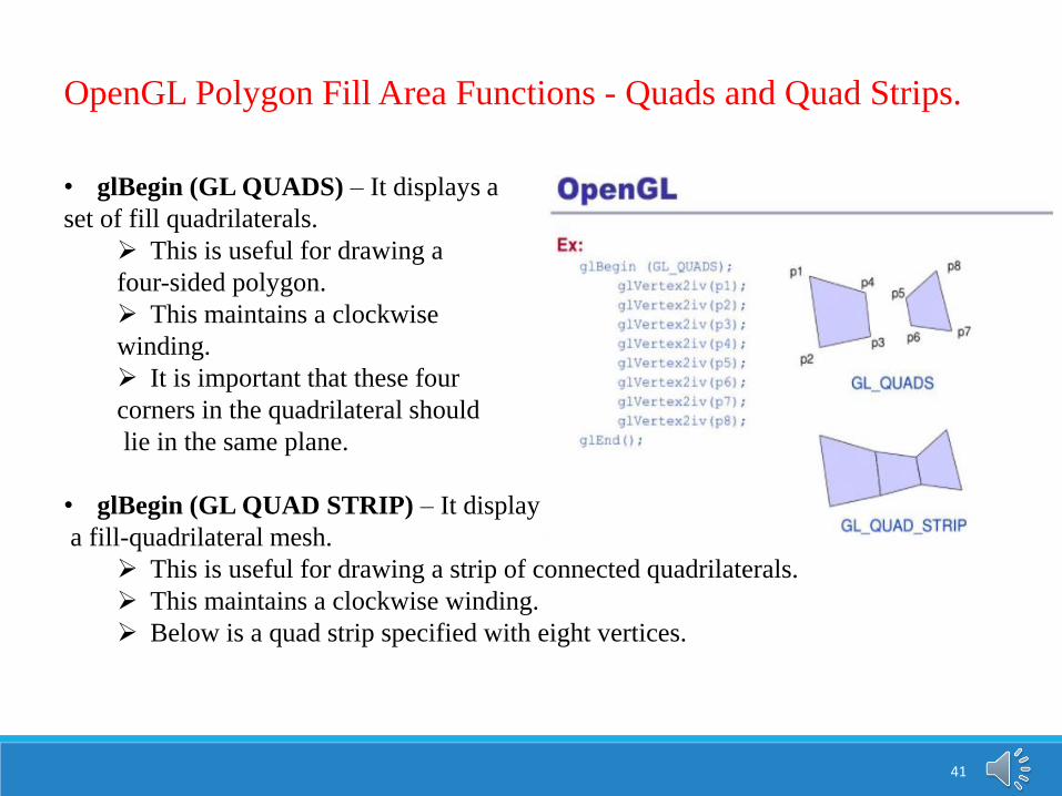
OpenGL Polygon Fill Area Functions - Quads and Quad Strips.

• glBegin (GL QUADS) – It displays a

set of fill quadrilaterals.

➢ This is useful for drawing a

four-sided polygon.

➢ This maintains a clockwise

winding.

➢ It is important that these four

corners in the quadrilateral should

lie in the same plane.

• glBegin (GL QUAD STRIP) – It display

a fill-quadrilateral mesh.

➢ This is useful for drawing a strip of connected quadrilaterals.

➢ This maintains a clockwise winding.

➢ Below is a quad strip specified with eight vertices.

42

OpenGL Polygon Fill Area Functions- Polygon, Triangle and Strips.

• glBegin (GL POLYGON)– It displays a fill polygon, whose vertices are given in

glVertex functions and terminated with a glEnd statement.

➢ This primitive is useful for drawing a polygon that has any number of sides.

➢ Any polygon must follow the convex rule – Any two edges of the polygon

must not intersect with each other.

➢ Also all the vertices of the polygon must lie

in the same plane always.

• glBegin (GL TRIANGLES)– Displays a set of

fill triangles.

➢ This primitive is useful for drawing a

polygon that has 3 sides.

• glBegin (GL TRIANGLE STRIP) - Displays a fill-triangle mesh.

43

Vertex Arrays

• To reduce the number of calls required to process the coordinate information, OpenGl

provides a very good mechanism which is called as Vertex Arrays. Using this, it is just

enough if we need only a few function calls for describing any scene. To enable this we

have some few steps that we need to follow which are as follows.

1. Firstly, call the glEnableClientState (GL VERTEX ARRAY) to activate the vertex-array

feature of OpenGL.

2. By using glVertexPointer , we can specify the location and data format for the vertex

coordinates.

3. By using routines such as glDrawElements, we can process multiple primitives with very

few function calls for displaying the scene.

• glDisableClientState (GL_VERTEX_ARRAY)- To deactivate the vertex- array feature of

OpenGL. Also, we can supply additional information such as color etc, to process the

scene description.

Sample code for polygonal objects

44

Pixel Array Primitives- Bitmaps and Pixmaps

• For displaying the structures that are described using the rectangular arrays, graphics

library uses a lot of routines. Two type of arrays namely Bitmaps and Pixelmaps are

formed and provided as inputs which are defined as follows.

Pixmaps :

➢ Every data point in the array displays some color in this array.

➢ It is mostly used to describe the actual array of pixels. The values(data points) within the

array sometimes have more locations within the scene, it may be one more.

➢ Pixmaps have many properties such as bits-per-pixel, colors, height, name etc.

➢ The function with this pixmap can be defined as.

glDrawPixels(width, height, dataFormat, dataType, PixMap);

Bitmaps :

➢ If the pixmap uses only a single bit to denote the color of each pixel, then it is called as

a bitmap. Sometimes, this is as well used to refer to any pixmap.

➢ Here every pixel is mapped to either 0 or 1.

➢ It simply defines if that pixel is to be mapped to a default color.

45

Pixel Array Primitives- Storage Buffers and code segments

• OpenGl provides many buffers to store the pixel data, colors and other information.

• Depth Buffer- It is useful for storing the object’s depth from the viewing position

• Stencil Buffer- It is useful for storing the boundary patterns for the scenes.

glDrawPixels (width, height, dataFormat, dataType, pixMap);

• We can set one of these buffers by setting the dataFormat in glDrawPixels routine to

either GL DEPTH COMPONENT or GL STENCIL INDEX.

• The pixel data can be copied from one location to the other using the following

openGL function.

glCopyPixels (xmin, ymin, width, height, pixelValues};

-PixelValues can be asssigned to GL COLOR, GL DEPTH, or GL STENCIL to

indicate the kind of data we want to copy – can be either color values, depth values, or

stencil values.

46

Pixel Array Primitives-Pixel Drawing

• glDrawPixels (width, height, dataFormat, dataType, pixMap) –

This function is used for drawing pixels on the display where width, height indicates the

row and columns of the pixel map.

-Format – It specifies the format of the pixel data.

-Type- It specifies the data type for the data. Symbolic constants

GL_UNSIGNED_BYTE, GL_BYTE, GL_BITMAP etc, are used.

• If the raster position is valid, then this glDrawPixels routines reads pixel data from

memory and writes back into the frame buffer with respect to the current raster

position.

47

Pixel Array Primitives-Double Buffering

Double Buffering:

• For generating a real-time animation with a rater system, it is good method to employ

two refresh buffers.

• In one buffer, we create the animation frame while this screen is refreshed in one

buffer, the next frame can be generated in the other buffer. When finally the two

frames gets completed, we can switch the role between the two.

• There are like two functions supported by the graphic library – one to activate the

double-buffering routines and the other to interchange the roles of the two buffers.

• The interchange can happen at various times. Mostly it is good to switch the two

buffers at the end of the current refresh cycle.

• When the frame construction time is very nearly equal to an integer multiple of the

screen refresh time, Irregular animation frame rates may take place.

48

Pixel Array Primitives-Buffers for stereo imaging

• In OpenGL, we have like four color buffers which is used for screen refreshing. Out

of which, two of those represents a left-right scene pair for displaying stereoscopic

views. Each of the stereoscopic buffers has a front-back pair for double-buffered

animation displays.

• A default refresh buffer(single refresh buffer) is used when double buffering or

stereoscopic effects is not available or not in effect.

• glDrawBuffer (buffer) is used to select single color or auxiliary buffer or a

combination of color buffers for storing the pixmap.

• We can assign a lot of openGL symbolic constants for a parameter buffer to one or

more “draw” buffers. For instance, a singe buffer can be picked using GL FRONT

LEFT, GL FRONT RIGHT, GL BACK LEFT, or GL BACK RIGHT. Both front

buffers can be selected using GL FRONT, and we can select both back buffers with

GL BACK. This is assuming that stereoscopic viewing is in effect.

Character Handling- Bitmap characters

• Character handling routines which are provided by the graphics library, helps to generate

textural information of the scene, such as labels on graphs and charts, signs on buildings

or vehicles etc.

• Typeface – It is the overall design style for a group of characters linked like a family.

• There are like two different representations to save the computer fonts.

a) Bitmap Characters b) Stroke Characters

Bitmap Characters:

➢ A pattern of binary values are defined on a rectangular grid for representing the character

shapes and so it is called as Bitmap characters.

➢ The set of characters is then referred to as a bitmap font whereas every bit corresponds to

some pixel on the display. We can use method glutBitmapCharacter(font, character) for

displaying the bitmap character.

➢ Scaling is an issue with the bitmap characters whereas the size of the character bitmap can

be either increased or decreased. If at all, we prefer doubling the size, then we need to

double the number of pixels as well. Also, this type of characters requires more storage

space.

49

50

Character Handling – Stroke Characters

• Here the character shapes are defined using straight-line and curve sections.

• Unlike bitmap fonts, without disturbing the character shapes, outline fonts can be

increased in size.

• These fonts require less storage when compare to the bitmap characters whereas

scaling is not an issue here as they support it with variable line length which are used

to form them.

• Method called

glutStrokeCharacter(font,

character) is used to display the

stroke character.

• It takes more time

to process the outline fonts

because they must be scan-

converted into the frame buffer

• Figure illustrates the two methods for character representation.