Powersim: Power Estimation with SystemC - iris univpm

Chapter 20Powersim: Power Estimationwith SystemC

Computational Complexity Estimate of a DSRFront-End Compliant to ETSI StandardES 202 212

Marco Giammarini, Simone Orcioni and Massimo Conti

20.1 Introduction

The International Technology Roadmap for Semiconductors (ITRS) [1] andMEDEA ? Roadmap [2] evidence that power and performance analysis arebecoming challenging task in current System-on-Chip (SoC) design. In recentyears, portable devices has largely spread out implementing more and morecomplex applications that require a large energy amount from battery. Thisincreasing interest in energy and power consumption of hardware has driven tosearch new design methodologies and tools to analyze and lower power con-sumption just in the early stages of the design. To facilitate this analysis, researchhas focused efforts in developing tools to be used when project is still in system-level phase; this fact gives an estimation of power dissipated before going intoother planning levels and then optimize the system to decrease consumption.

SystemC [3, 4], now in its version 2.2.0, add a new library of C++ classes inorder to create a language for description of hardware at system-level. In 2005,IEEE has approved a standard, named ‘‘IEEE Std. 1666-2005’’ [5], for SystemC.Although SystemC is now considered one of the more promising languages forsystem-level design, it does not encompass any functionality for power estimation.However, the object oriented nature of SystemC, can easily be extended to coverthis lack.

This chapter extends the work presented in [6] proposing a new framework,called Powersim, that consist of a C++ library added to SystemC, in order toestimate the power consumption of a system described at system-level. Powersimcan estimate the power of a system interacting with arithmetic operations, logicalfunctions and mathematical functions of the various modules constituting the

M. Giammarini � S. Orcioni (&) � M. ContiDIBET, Università Politecnica delle Marche, Ancona, Italye-mail: [email protected]

M. Conti et al. (eds.), Solutions on Embedded Systems,Lecture Notes in Electrical Engineering, 81, DOI: 10.1007/978-94-007-0638-5_20,� Springer Science+Business Media B.V. 2011

285

system. Also, thanks to the fact that the Powersim monitors operator and mathe-matical functions it is able to provide a computational complexity estimate of thesystem. This feature, combined with accurate power models leads also to a goodpower consumption estimate.

At the end of this chapter, we presents, an application example of the proposedtool, the computational complexity estimate of a DSR front-end, compliant toETSI Standard ES 202 212 [7] and implemented at system-level in SystemC.

20.2 Powersim

Powersim [8] is a C++ class library developed to be used inside a SystemCimplementation. Its main purpose its the simulation of computational complexityand power consumption of digital system described at system-level. Its maincharacteristics are:

1. no need to change the source code describing the system;2. easy configuration via file described in Extended BNF [9] grammar;3. possibility to assign a different power model for each operation performed on

each data type;4. possibility to add, in a simple way, new power models;5. possibility to extend, in a simple way, its functionality through a fully object

oriented implementation based on C++.

Development of Powersim requested the change of some SystemC classes andthe addition of Powersim classes to SystemC library.

The next paragraphs will show in detail the Powersim classes, the changes toSystemC, the creation and use of power models and of the configuration file.

Powersim library consists basically of four classes, in addition to power modelsand error report classes. Figure 20.1 shows the structure of Powersim and how itinteracts with SystemC.

The main class of this library is ps_kernel: an object of this class isinstantiated inside the sc_main function before the modules are created. Thisclass, using the static methods of ps_configure, parses the configuration file andstores the read data in a static map. The map contains an object of ps_moduleclass for each SystemC module used in the source code. Each object takes care tomaintain and update data on computational cost and power dissipation estimationof the module to which it is associated. This is done using the map that each objectof ps_module class has within. The map contains ps_power_model typepointers that point classes derived from ps_power_model. Indeed the classps_power_model is an interface which generalises all functions necessary tocreate a new power model. So the user can implement its own power model byextending ps_power_model and implementing all its methods.

Regarding changes to SystemC, we have acted on two types of classes: (i) sc_module class and (ii) data-type classes. Changes to the class sc_module,

286 M. Giammarini et al.

the class that let to create a new SystemC module, consist of providing a newmethod called ps_init(). This method, during simulation, calles a staticfunction of ps_kernel class. The static method adds the current module undercontrol of the Powersim kernel. Changes to data-type classes consist of providingthe necessary code to maintain in each operation the previous value of eachvariable. Furthermore, the definition of each operator function has been modifiedto allow the call to ps_call(). This function, during simulation, tells to thePowersim kernel that was performed a new operation.

The power models are the instrument through which Powesim estimate thepower associated with on operator run on a SystemC data type. As mentioned, thepower models are represented by classes that extend ps_power_model classand implement also the methods necessary to interact with Powersim kernel. Thesemethods have different purposes: (i) to define the model of the power dissipated byarithmetic or logic operation and mathematical function, (ii) to set the parametersof the power model, using the values that users provide in the configuration file,(iii) to return the total power consumption, (iv) to manage the variables that will beprinted in the result tracing file.

Through the configuration file, the user can choose of which modules tomonitor the power dissipation. In particular, the user can decide which operatorsto control the power consumption of and which power model to bind. In order towrite a configuration file, the user must follow a grammar defined in Extended

Fig. 20.1 Block scheme of Powersim

20 Powersim: Power Estimation with SystemC 287

Backus-Naur Form [9], a syntactic meta-language used to describe formal lan-guages syntax. The rules imposed by the grammar are used by ps_configureclass to parse the input file.

20.3 Case Study

Thanks to the continuous improvement in computer performances and to thedevelopment in Digital Signal Processing (DSP), Automatic Speech Recognition(ASR) is spreading in many aspects of everyday life. The application fields ofspeech recognition go from the help in editing by means of dictation, to commandrecognition and execution in the automotive or other fields. In general, a voicerecognizer can be applied in all situations where the voice may replace hands,including applications to provide support for people with disabilities.

Another area of application of voice recognition is the Distributed SpeechRecognition (DSR). Through a client–server based approach in combination with aspeech recognizer, DSR can offer a new chance in the field of home automation ormobile communications, for instance, the ability to dictate the notes of a confer-ence directly to your phone immediately after the end of the meeting and to returnto office with the text file stored on your PC ready to be edited. This new approachrevolutionizes the way of speech recognizing, allowing to replace the communi-cation of the signal samples with a parameterized and compressed representation,which is suitable for the recognition and for the communication over a noisy orlimited-capacity channel. In this section we presents a computational complexityestimate, computed by Powersim, of a DSR front-end, compliant to ETSI StandardES 202 212 [7] and implemented at system-level in SystemC.

20.3.1 The ETSI Front-End

Accordingly to ETSI Standard ES 202 212 a DSR system is composed by a mobileterminal, or front-end, and a server or back-end. The Front-end extracts the fea-tures of the voice, implementing signal denoising and cepstrum coefficientcalculation. Then this features must be compressed and packaged, as show inFig. 20.2, before being sent to the server, where the recognition take place.

Fig. 20.2 Block scheme theterminal side of ETSI ES 202212


In this work we have estimated the computational cost of the FeatureExtraction part, as defined in [7]. Figure 20.3 shows our SystemC implementationof the Feature Extraction, divided into five main blocks: the first two blocks makesignal denoising, the third makes waveform processing, the fourth performs cep-strum calculation, and the last executes blind equalization of cepstrum coefficients.Before Feature Extraction, in Input Stream the signal is divided into frames of 80samples each.

20.3.1.1 First Noise Reduction

The noise reduction consists of two cascaded stages, which, as can be seen in [7],are almost identical. Figure 20.4 shows First Noise Reduction SystemC imple-mentation, which consists of eight modules.

In Buffering module a four-frame long FIFO (320 samples) is used in order toobtain in each iteration, a 200-sample frame, used to obtain the Wiener-filtercoefficients be applied to a single 80-sample long frame. To this end the moduleapplies a 200-sample wide window from the 260th sample to the 61th sample ofthe buffer, and takes the frame to be denoised from the last but one frame of theFIFO. The Spectrum Estimation module performs a power spectrum estimate of its200-sample long input frame. First the input frame is windowed by Hanningwindow sWðnÞ ¼ sinðnÞ � wHannðnÞ where 0 B n B Nin - 1, Nin = 200, and theHanning window is

wHannðnÞ ¼ 0:5� 0:5 cos2p � ðnþ 0:5Þ

Nin

� �: ð20:1Þ

Fig. 20.3 SystemCschematic representation ofETSI ES 202 212 FeatureExtraction


Then zeros are padded, in order to apply a 256-sample wide Fast FourierTransform (FFT). The power spectrum is calculated by squaring the module of

FFT representation, X(bin), PðbinÞ ¼ jXðbinÞj2; 0� bin�NFFT=2:Then the power spectrum is smoothed, as shown in the following PinðbinÞ ¼

ðPð2 � binÞ þ Pð2 � binþ 1ÞÞ=2, where 0� bin\NFFT=4 and PinðNFFT=4Þ ¼PðNFFT=2Þ. By means of this last operation, the length of Pin is reduced toNSPEC ¼ NFFT=4.

In the PSD Mean module, the mean of power spectral density is performed overthe last TPSD frames

Pin PSD bin; tð Þ ¼ 1TPSD

XTPSD�1

i¼0

Pin bin; t � ið Þ ð20:2Þ

for 0� bin�NSPEC � 1, where bin is the frequency index ant t is the current frameindex. VADNest module is used to decide if the current frame is speech or not bymeans of two variables. The former is the logarithmic energy of the last frame ofthe input signal

frameEn ¼ 0:5þ 16ln 2� ln 64þ

PM�1n¼0 sinðnÞ2

64

!: ð20:3Þ

This parameter is used to update the second variable meanEn. The output of thismodule is the Boolean variable flagVADNest that indicates if the current frame isspeech or not.

Wiener Filter module computes the Wiener filter coefficients that are used toreduce the amount of noise present in a signal by comparison with an estimation ofthe desired noiseless signal. In the Wiener Filter First Stage the noise spectrumestimate Pnoise

1/2 (bin, t) is calculated according to the flagVADNest. Then the

Fig. 20.4 SystemCschematic representation ofSystemC First NoiseReduction Module


noiseless signal spectrum Pden1/2 (bin, t) is estimated using a ‘‘decision-directed’’

approach and the a priori SNR g(bin, t) is computed as gðbin; tÞ ¼ Pdenðbin; tÞ=Pnoiseðbin; tÞ.

The Wiener filter transfer function H(bin, t) is obtained according to the fol-

lowing equation Hðbin; tÞ ¼ffiffiffiffiffiffiffiffiffiffiffiffiffiffiffiffigðbin; tÞ

p=1þ

ffiffiffiffiffiffiffiffiffiffiffiffiffiffiffiffigðbin; tÞ

pand it is used to improve

the estimation of the noiseless signal spectrum Pden21/2 (bin, t). By the new noiseless

signal spectrum an improved a priori SNR g2(bin, t) is obtained like

g2 bin; tð Þ ¼ maxPden2 bin; tð ÞPnoise bin; tð Þ; g

2TH

� �ð20:4Þ

where gTH corresponds to a SNR of -22 dB. Then the improved transferfunction H2(bin, t), that is the module output, is obtained as H2 bin; tð Þ ¼ffiffiffiffiffiffiffiffiffiffiffiffiffiffiffiffiffiffi

g2 bin; tð Þp �

1þffiffiffiffiffiffiffiffiffiffiffiffiffiffiffiffiffiffig2 bin; tð Þ

p, for 0 B bin B NSPEC - 1. This function is utilized

to calculate the new improved noiseless signal spectrum Pden31/2 (bin, t), that will be

used to calculate Pden1/2 (bin, t) of the next frame. The difference between the Wiener

Filter First Stage and Wiener Filter Second Stage is the method of computation ofthe noise spectrum estimate Pnoise(bin, t), that in the second case does not dependon the VADNest module.

The Wiener filter coefficients H2(bin) are smoothed and transformed to theMel-frequency scale by Mel Filter module. The new coefficients H2_mel(k) arecalculated by using triangular-shaped, half-overlapped frequency window appliedon H2(bin) as

H2 mel kð Þ ¼ 1PNSPEC�1i¼0 W k; ið Þ

XNSPEC�1

i¼0

W k; ið ÞH2 ið Þ ð20:5Þ

where k are the transformed frequency, 0 B k B KFB ? 1, with KFB = 23, andW(k, i) is the frequency window.

In the Mel IDCT module the time-domain impulse response of Wiener filter iscomputed from the Mel Wiener filter coefficient H2_mel(k) by using Mel-warpedinverse DCT.

hWF nð Þ ¼XKFBþ1

k¼0

H2 mel kð Þ � IDCTmel k; nð Þ ð20:6Þ

for 0 B n B KFB ? 1, where IDCTmel(k, n) are Mel-warped inverse DCT, that areobtained as

IDCTmel k; nð Þ ¼ cos2pn � fcentr kð Þ

fsamp

� �� df kð Þ ð20:7Þ

for 0 B k, n B KFB ? 1, where fsamp = 8,000 is the sampling frequency and fcentr

is the central frequency of each Mel band. The central frequency is computed likefcentr kð Þ ¼ 700 � 10fmel kð Þ=2;595 � 1

� �, 0 B k B KFB where


fmel kð Þ ¼ k �Mel flin samp=2

� KFB þ 1

ð20:8Þ

where flin_samp is the linear sampling frequency and Mel{�} is the function thattransform a linear frequency to a Mel scale frequency as

Mel flinf g ¼ 2; 595 � log10 1þ flin=700

�: ð20:9Þ

The output of this module is the mirrored impulse response of Wiener filterhWF_mirr(k).

In the last module (Apply Filter) the noise-reduced signal is produced by meansof tree steps. In the former step the causal impulse response is obtained fromprevious module output. In the second the impulse response is truncated andweighted by a Hanning window. In the latter stage the input signal is filtered like

snr nð Þ ¼XðFL�1Þ=2

i¼� FL�1ð Þ=2

hWF w iþ FL� 1ð Þ=2ð Þsin n� ið Þ ð20:10Þ

for 0 B n B M - 1, where hWF_w is the filter impulse response, the filter lengthFL equals 17 and the frame shift interval M equals 80.

20.3.1.2 Second Noise Reduction

The Second Noise Reduction, as show in Fig. 20.5, differs from the former becauseVADNest is not present, instead Gain Factorization and Offset Compensation havebeen added.

Fig. 20.5 SystemCschematic representation ofSystemC Second NoiseReduction Module


Gain Factorization module aims to apply a more aggressive noise reduction topurely noisy frames and less aggressive noise reduction to frames also containingspeech. To decide the degree of aggression, SNR value, based on energy valuescalculated in Wiener filter stages are used. In particular in the Wiener Filter FirstStage, denoised frame signal energy is calculated by using the denoised powerspectrum Pden3(bin, t)

Eden tð Þ ¼XNSPEC�1

bin¼0

P1=2den3 bin; tð Þ ð20:11Þ

where t is the current frame index, instead in the Wiener Filter Second Stage, thenoise energy is computed by using the noise spectrum Pnoise(bin, t)

Enoise tð Þ ¼XNSPEC�1

bin¼0

P1=2noise bin; tð Þ: ð20:12Þ

Smoothed SNR SNRaver(t), is evaluated by using tree value of Eden(t) andEnoise(t). At this point, the current SNR estimation is compared to the low SNRtracked value, and the aggression of the second stage Wiener filter is reduced to10% for speech and noise frames and to 80% for noise frames.

Offset Compensation module removes the DC offset by a notch filtering oper-ation that is applied to the noise-reduced signal like snr of nð Þ ¼ snr nð Þ � snr

n� 1ð Þ þ 1� 1=1; 024ð Þ � snr of n� 1ð Þ, 0 B n B M - 1, where snr(- 1) andsnr_of(- 1) correspond to the last sample of the previous frame.

20.3.1.3 Waveform Processing

After denoising, the Waveform Processing part of the standard begins. In thisblock emphasis on higher energy parts of the signal occurs by means of the actionof four blocks, as shown in Fig. 20.6.

Fig. 20.6 SystemCschematic representation ofSystemC WaveformProcessing Module


The first block, Buffer, stores in a 240-sample buffer the 80-sample long framesgiven in output by the Second Noise Reduction. In this module a 200 (fromposition 1 to position 200) samples wide window is applied to the buffer.

The second one, Smoothed Energy Contour, calculates the Teager-Kaiserenergy of the signal and smooth it by means of a FIR filter. The Teager-Kaiserenergy is computed for each input frame ETeag ¼ s2

nr of nð Þ � s2nr of n� 1ð Þ�

��snr of2 nþ1ð Þj where 0 B n B Nin - 1.

Peak Picking block finds the global maximum in the smoothed energy contourand the maxima on the left and right side of the global maximum, so that maximarelated to the fundamental frequency are found.

Such values are used in Waveform SNR Weighting block to realize a windowfunction to be applied to the input signal. Indeed having the number of maxima NMAX

of the smoothed energy contour and their position posMAX, a weighting function oflength Nin is constructed and applied to the input noise-reduced frame like

sswp nð Þ ¼ 1:2 � wswp nð Þ � snr of nð Þ þ 0:8 � 1� wswp nð Þ� �

� snr of nð Þ ð20:13Þ

where 0 B n B Nin – 1 and wswp is a weighting function that equals 1.0 forn belonging to the following interval

posMAX nMAXð Þ � 4ð Þ; posMAX nMAXð Þ � 4ð Þ½þ0:8 � posMAX nMAX þ 1ð Þ � posMAX nMAXð Þð Þ� ð20:14Þ

and 0 otherwise.

20.3.1.4 Cepstrum Calculation

The Cepstrum Calculation part performs the calculation of cepstrum coefficientsand the natural logarithm of the energy of the signal. The our SystemC imple-mentation consist of seven modules, as shown in Fig. 20.7.

First a Pre-emphasis filter is applied to the output of Waveform Processingblock sswp pe nð Þ ¼ sswp nð Þ � 0:9 � sswp n� 1ð Þ followed by a Windowing, wherethe following Hamming window of length Nin = 200

wswp w nð Þ ¼ 0:54� 0:46 � cos2p � nþ 0:5ð Þ

Nin

� �ð20:15Þ

for 0 B n B Nin - 1, is applied to the output of the previous module.Then a Fast Fourier Transform (FFT) is applied. Each frame of Nin samples is

zero padded to create an extended frame of 256 samples. An FFT is applied tocompute the complex spectrum of the denoised signal, then a corresponding powerspectrum Pswp is calculated.

The next module, MEL-FB, recombines the information contained in the FFTaccording to the Mel band representation. The FFT elements are linearly recom-bined for each Mel Band. The useful frequency band lies between fstart and fsample/


2. This band is divided into KFB equidistant channels in the Mel frequency domain.Each channel has a triangular-shaped frequency window and consecutive channelsare half-overlapping. To perform an equidistant distribution of the band in the Meldomain, the central frequency of each filter are calculated from the Mel-functionlike

fcentr kð Þ ¼ Mel�1 Mel fstartf g þ k �Mel fsample=2

� �Mel fstartf g

KFB þ 1

�ð20:16Þ

for 0 B k B KFB, where Mel{�} is the Mel-function and it is the operator whichrescales the frequency domain, likewise Eq. 20.9. Indeed the inverse Mel-functionis Mel�1 yf g ¼ 700 � ey=1;127 � 1

� �.

In terms of FFT index, the central frequency of the band correspond to

bincentr kð Þ ¼ index fcentr kð Þf g ¼ roundfcentr kð Þ

fsamp

NFFT

�ð20:17Þ

for 0 B k B KFB. For the kth Mel Band, the frequency window W(i, k) is con-structed and divided into two parts. The former part accounts for increasingweights, whereas the latter part accounts for decreasing weights. Each frequencywindow is applied to the denoised power spectrum Pswp(bin) computed in theprevious module. The output of each Mel filter is

EFB kð Þ ¼Xbincentr kð Þ

i¼bincentr k�1ð ÞWleft i; kð Þ � Pswp ið Þþ

Xbincentr kþ1ð Þ

i¼bincentr kð Þþ1

Wright i; kð Þ � Pswp ið Þ

ð20:18Þ

for 0 B k B KFB.

Fig. 20.7 SystemCschematic representation ofSystemC CepstrumCalculation Module


The Log module carries out the logarithmic function on the output ofMel-filtering and finally the thirteen cepstral coefficients are obtained by applyingthe DCT on the nonlinear transformed FFT by means DCT module. The followingequation shows how cepstrum coefficients are obtained

c ið Þ ¼XKFB

k¼1

SFB kð Þ � cosi � pKFB

� k � 0:5ð Þ� �

ð20:19Þ

where 0 B i B 12. The last module (LogE) perform a natural logarithm of theenergy of the denoised signal as

log E ¼ ln Eswp

� �if Eswp�ETHRESH;

ln ETHRESHð Þ otherwise,

ð20:20Þ

where ETHRESH = e-50 and Eswp is calculated as Eswp ¼PNin�1

n¼0 sswp nð Þ � sswp nð Þ.

20.3.1.5 Blind Equalization

In the last module of ETSI 202 212 Feature Extraction named Blind Equalization,twelve cepstral coefficients (c(1), …, c(12)) are equalized according to LMSalgorithm. The final feature vector consists of thirteen cepstral coefficient and thelog-energy coefficient.

20.3.2 Computational Complexity Estimate

The aim of this section is to show the results of the estimate of the computationalcomplexity of the Feature Extraction as computed by Powersim. They will beprovided by means of the number values of different mathematical operationsperformed by each block and by means of the total computational complexityestimate of each block.

Table 20.1 shows the number of operations executed by each SystemC moduleduring a simulation with a registered voice as input. The input signal was sampledat 8 kHz and was 6 s long for a total of 48,000 samples.

To see the computational load of each block, the relative computational com-plexity of each operation must be estimated. The computational complexity ofeach operation clearly depends on the hardware where they are executed. As areference for the relative complexity of operations the Intel� AtomTM N270 [10],largely used in many netbook or embedded systems, has been chosen. The relativecost of each operation has been estimated by simulating ad-hoc programs andcalculating the CPU time needed by the execution of each arithmetic operation andmathematical function as implemented in the C ++ cmath library [11]. Table 20.2reports these relative costs.


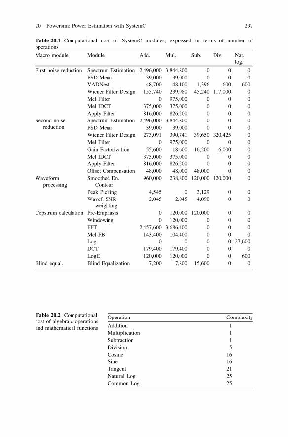
Table 20.1 Computational cost of SystemC modules, expressed in terms of number ofoperations

Macro module Module Add. Mul. Sub. Div. Nat.log.

First noise reduction Spectrum Estimation 2,496,000 3,844,800 0 0 0PSD Mean 39,000 39,000 0 0 0VADNest 48,700 48,100 1,396 600 600Wiener Filter Design 155,740 239,980 45,240 117,000 0Mel Filter 0 975,000 0 0 0Mel IDCT 375,000 375,000 0 0 0Apply Filter 816,000 826,200 0 0 0

Second noisereduction

Spectrum Estimation 2,496,000 3,844,800 0 0 0PSD Mean 39,000 39,000 0 0 0Wiener Filter Design 273,091 390,741 39,650 320,425 0Mel Filter 0 975,000 0 0 0Gain Factorization 55,600 18,600 16,200 6,000 0Mel IDCT 375,000 375,000 0 0 0Apply Filter 816,000 826,200 0 0 0Offset Compensation 48,000 48,000 48,000 0 0

Waveformprocessing

Smoothed En.Contour

960,000 238,800 120,000 120,000 0

Peak Picking 4,545 0 3,129 0 0Wavef. SNR

weighting2,045 2,045 4,090 0 0

Cepstrum calculation Pre-Emphasis 0 120,000 120,000 0 0Windowing 0 120,000 0 0 0FFT 2,457,600 3,686,400 0 0 0Mel-FB 143,400 104,400 0 0 0Log 0 0 0 0 27,600DCT 179,400 179,400 0 0 0LogE 120,000 120,000 0 0 600

Blind equal. Blind Equalization 7,200 7,800 15,600 0 0

Table 20.2 Computationalcost of algebraic operationsand mathematical functions

Operation Complexity

Addition 1Multiplication 1Subtraction 1Division 5Cosine 16Sine 16Tangent 21Natural Log 25Common Log 25


By applying the relative costs shown in Table 20.2 at Table 20.1 the datashown in Table 20.3 has been obtained. The first data column shows the absolutecost of each block while the second one the relative cost. The horizontal linesgroup together SystemC block belonging to the same ETSI block, respectively,First Noise Reduction, Second Noise Reduction, Waveform Processing, CepstrumCalculation and Blind Equalization. Furthermore, since analyzing the algorithmsperformed the front-end, spectrum calculations performed by means of FFT, wererecurrent, the FFT cost has been extracted and shown in last two column of

Table 20.3 Computational cost of single SystemC modules of the ‘‘Terminal Front-End’’

Macro Module Module Comp.Cost

Comp.Cost(% Total)

Comp.Costof FFT

Comp. CostFFT (% row)

First NoiseReduction

SpectrumEstimation

6,340,800 19.05 6,144,000 96.90

PSD Mean 78,000 0.23 0 0.00VADNest 116,196 0.35 0 0.00Wiener Filter

Design1,025,960 3.08 0 0.00

Mel Filter 975,000 2.93 0 0.00Mel IDCT 750,000 2.25 0 0.00Apply Filter 1,642,200 4.93 0 0.00

Second NoiseReduction

SpectrumEstimation

6,340,800 19.05 6,144,000 96.90

PSD Mean 78,000 0.23 0 0.00Wiener Filter

Design2,305,607 6.93 0 0.00

Mel Filter 975,000 2.93 0 0.00Gain

Factorization93,400 0.28 0 0.00

Mel IDCT 750,000 2.25 0 0.00Apply Filter 1,642,200 4.93 0 0.00Offset

Compensation144,000 0.43 0 0.00

WaveformProcessing

Smoot. En.Contour

1,918,800 5.77 0 0.00

Peak Picking 7,674 0.02 0 0.00Wavef. SNR

weight.8,180 0.02 0 0.00

CepstrumCalculation

Pre-Emphasis 240,000 0.72 0 0.00Windowing 120,000 0.36 0 0.00FFT 6,144,000 18.46 6,144,000 100.00Mel-FB 247,800 0.74 0 0.00Log 690,000 2.07 0 0.00DCT 358,800 1.08 0 0.00LogE 255,000 0.77 0 0.00

Blind Equal. BlindEqualization

30,600 0.09 0 0.00

Total 33,278,017 100.00 18,432,000 55.39


Table 20.3, in absolute and relative values. While the relative computational costof each block is calculated with respect to the total operations performed by thefront-end, the FFT relative cost is relative to each block where it is executed, i.e.relative to each row of the table. So in the last row the cost of FFT is relative to thetotal cost and it can be noticed that it amounts to the 55.39% of the total. This cansuggest the use of specialized hardware for the FFT in a low-power implemen-tation of the front-end because of the relevance of FFT computational cost. InTable 20.4 the computational costs of the main four blocks of the front-end areshown.

The data shown in Table 20.1 can be seen also under another view, grouped byoperations performed instead of functional block. Table 20.5 shows this view thatreveals that the more expensive operation are respectively multiplication andaddition. Table 20.6 shows the same view, but with the FFT cost excluded. In thiscase also the cost of division becomes relevant.

Table 20.4 Computational cost of the ETSI ‘‘Front-End’’

Module Computational cost Computational cost (%)

First Noise Reduction 10,928,156 32.84Second Noise Reduction 12,329,007 37.05Waveform Processing 1,934,654 5.81Cepstrum Calculation 8,055,600 24.21Blind Equalization 30,600 0.09Total 33,278,017 100.00

Table 20.5 Computational cost by operations

Operations Number of operation Computational cost Comput. cost % total

Addition 11,907,321 11,907,321 35.78Multiplication 17,444,266 17,444,266 52.43Subtraction 413,305 413,305 1.24Division 558,625 2,793,125 8.39Natural log. 28,800 720,000 2.16Total 30,352,317 33,278,017 100.00

Table 20.6 Computational cost by operation, FFT excluded

Operations Number of operation Computational cost Comput. cost % total

Addition 4,534,521 4,534,521 30.54Multiplication 6,385,066 6,385,066 43.02Subtraction 413,305 413,305 2.78Division 558,625 2,793,125 18.81Natural Log. 28,800 720,000 4.85Total 11,920,317 14,846,017 100.00


20.4 Conclusions

In this chapter we presented the Powersim, a new framework for the computationalcost and power consumption estimate of a system described in SystemC.Furthermore, we presented, as an application example of Powersim, a computa-tional cost estimation of standard ETSI ES 202 212. This analysis has been carriedout at system level by means of a SystemC implementation.

The analysis of computational cost of ETSI 202 212 ‘‘Front-End’’ reveals thatthe major cost, with more than 55% of the total, can be assigned to the FFTcomputations performed in the First Noise Reduction, Second Noise Reduction andCepstrum Calculation functional blocks. So particular care must be taken of thisfunction in a hardware implementation. If a specialized hardware for FFT is notchosen, the more computational expensive operation are multiplication andaddition with respectively a 52.43% and 35.78% of the total cost.

References

1. ITRS, International Technology Roadmap for Semiconductors (2005) 2005 edn. Design,December. http://public.itrs.net

2. MEDEA+ (2005) MEDEA Electronic Design Automation (EDA) Roadmap, 5th release,September. http://www.medea.org

3. The Open SystemC Initiative—OSCI, SystemC documentation. http://www.systemc.org4. Grötker T, Liao S, Martin G, Swan S (2002) System design with SystemC. Kluwer Academic

Publishers, New York5. SystemC Language Reference Manual (2006) IEEE-Std 1666-2005, March6. Giammarini M, Orcioni S, Conti M (2009) Computational complexity estimate of a DSR

front-end compliant to ETSI Standard ES 202 212. In: 2009 seventh workshop on intelligentsolutions in embedded systems, WISES09, June, pp 171–177

7. Speech Processing, Transmission and Quality Aspects (STQ); Distributed speechrecognition; Extended advanced front-end feature extraction algorithm; Compressionalgorithms; Back-end speech reconstruction algorithm, ETSI Std. ES 202 212, Rev. 1.1.2,November 2005

8. Powersim 0.1.0—WebSite, Documentation and Source Code. http://sourceforge.net/projects/powersim

9. Information technology—syntactic metalanguage—extended BNF, ISO/IEC Std.14977,December 1996

10. Intel� AtomTM Processor—WebSite and Documentation. http://www.intel.com/products/processor/atom/index.htm

11. CMATH—C numerics library—math.h


http://public.itrs.net

http://www.medea.org

http://www.systemc.org

http://sourceforge.net/projects/powersim

http://sourceforge.net/projects/powersim

http://www.intel.com/products/

Powersim: Power Estimation with SystemC - iris univpm

Documents

Transcript of Powersim: Power Estimation with SystemC - iris univpm