POVERTY IMPACT OF ECONOMIC POLICIES IN ARGENTINA: A DYNAMIC CGE-MICROSIMULATION ANALYSIS

-1-

POVERTY IMPACT OF ECONOMIC POLICIES IN ARGENTINA: A DYNAMIC CGE-MICROSIMULATION

ANALYSIS

Martín Cicowiez, Javier Alejo, Luciano Di Gresia, Sergio Olivieri and Ana Pacheco

Centro de Estudios Distributivos, Laborales y Sociales (CEDLAS)Universidad Nacional de La Plata

ARGENTINA

DRAFT

November 10, 2008

1. INTRODUCTION

Since the 1970s Argentina has experienced several major macroeconomic crisis and episodes

of structural changes. A severe macroeconomic crisis in mid 1970s under the Peronist

administration was followed by some structural reforms carried out by the military regime.

The debt crisis of the early 1980s hit the Argentina’s economy, which entered a phase of deep

recession. The lost decade of the 1980s, characterized by poor economic performance,

finished with a major macroeconomic crisis, including two episodes of hyperinflation in 1989

and 1990. The Peronist administration that took power in 1989 introduced in the early 1990s a

wide range of macro and market-based reforms. Despite an impressive macroeconomic

record, the social situation significantly deteriorated. The 1990s ended with another recession,

which was followed by a major breakdown; the 2001/02 crisis implied a fall in the GDP of

more than 15%, 200% devaluation of the exchange rate, public debt default, restrictions on

bank deposits withdrawal, 40.5% inflation during 2002, an increase in the unemployment rate

-2-

to 24%, and an increase in the poverty rate to 54.3 in 2003. The economy has strongly

recovered since then, reaching levels of activity similar to those in the 1990s (see Table A.1 in

the Appendix) and a poverty rate of 27% in 2006.

In the year 2002, after the devaluation of the exchange rate, the government established an

export tax to all products, with heterogeneous tax rates – higher for the main agri-food export

products (Cereals, Oil seeds, and Vegetable oils and fats) and Oil, and lower for processed

products such as heavy manufactures. The export tax was introduced in order to keep

bounded the domestic price level and to strength the governmental fiscal position. The

increase in the world price of food during 2002-2008 also contributed to increase the fiscal

revenue coming from the export tax.

Nowadays, more than 10% of the tax revenue collected by the national government comes

from the export tax, which is considered by many observers as academics (Sturzenegger,

2006; Llach and Harriague, 2005), businessmen (Foro de la Cadena Agroindustrial Argentina,

2005), private organizations (CIPPEC, 2002a; CIPPEC, 2002b; Castro and Díaz Frers, 2008),

and policy makers (Redrado, 2005; Ambito Financiero, 2006-9-13; Clarín, 2004-5-3) to have

a negative impact on investment and, consequently, on growth and employment. Therefore,

we consider relevant to ask what would be the impact of (1) gradually eliminating the export

tax, and (2) a decrease in the world prices of food.

In this study we assess (1) the short and long run economic impacts of a gradual reduction in

the export tax that was introduced during the economic crisis that hit Argentina at the end of

2001, and (2) the impact of a decrease in the world prices of food and oil, two of the main

export products of Argentina. To this aim we built a sequential dynamic computable general

equilibrium (CGE) model linked to a microsimulation model that allows us to capture the

“macro-micro” links. We analyze the effects of the proposed policy changes and external

shocks on aggregate output, sectoral output, employment, government budget, poverty, and

inequality.

We consider the dynamic macro-micro framework particularly well-suited for the questions at

hand. The CGE model captures some of the main features of structural change and the relative

price changes accompanying them. The microsimulation model, in turn, allows for a detailed

empirical assessment of the household income response to those changes.

-3-

This document is organized as follows. The next section describes the method and data used

for this project. Section 3 presents and discusses our results. Finally, conclusions are

presented in Sector 4. We also provide an Appendix with a mathematical statement of our

CGE model and additional simulation results.

2. METHODOLOGY AND DATA

The CGE methodology is not intensively used in Argentina. In a recent paper, Mercado

(2003) surveys only two “institutional” CGE models. We are aware of only a few papers that

have applied the CGE-Microsimulation methodology to Argentina.

Díaz-Bonilla et al. (2004) used the IFPRI (static) Standard Model (Lofgren et al., 2002)

linked to a microsimulation model that follows the non-parametric methodology proposed by

Ganuza et al. (2002). Our analysis differs from Díaz-Bonilla et al. (2004) in several aspects.

The IFPRI team used a 1993 SAM while we built a 2005 SAM. This is especially important

taking into account the economic changes that Argentina experienced during the last years.

The IFPRI paper simulates some shocks that Argentina experienced during the 1990s (e.g.,

unilateral trade liberalization). We conduct a prospective analysis trying to identify the

outcome of different counterfactual scenarios (especially) on poverty.

Cicowiez et al. (2008) used the MAMS (Lofgren and Diaz-Bonilla, 2006) model linked to a

non-parametric microsimulation model to evaluate different strategies to achieve some of the

MDGs in the year 2015. Our analysis will differ from this previous work in several aspects.

For example, we develop a new dynamic CGE-Microsimulation model not related to the

MDG achievement calibrated with a new (recent) SAM.

In a recent paper, Cicowiez et al. (2008) used a static CGE-Microsimulation model linked to

the World Bank LINKAGE model to study the impact of global agricultural liberalization in

Argentina; they used legal (higher) instead of effective export tax rates. Accordingly, the

analysis here differs in many aspects.

CGE models have long been used for poverty analysis. The representative household

approach to CGE modeling can not capture the impact of a shock over the whole distribution

of income. For this reason, we will link our CGE model to a microsimulation model that

allows us to map the aggregate results to the individual level using microdata.

-4-

Our CGE-Microsimulation methodology is implemented in two steps. First, we run

counterfactual scenarios using a sequential dynamic CGE model of the Argentine economy

calibrated with a 2005 SAM. Second, we use a layered top-down approach to implement a

microsimulation model in order to capture the distributional effects of the simulated shocks.

THE DATA

The data requirements are the usual for this type of methodology: i) a Social Accounting

Matrix (SAM) and complementary data to calibrate the CGE model, and ii) microdata from a

household survey to conduct the microsimulations.

ARGENTINA SAM

Since the December 2001 crisis, the Argentine economy experienced important structural

changes (see above). Taking this into account, we constructed a SAM for Argentina using the

most recent data. In this section we describe the building process of the 2005 Argentina. As

our starting point we used the 1997 (latest available) input-ouput tables constructed by the

National Institute of Statistics and Censuses (INDEC, 2001). In order to reflect the changes in

the economic structure caused by the 2001/02 economic crisis we used to following sources

of information for the years 1997 and 2005: national accounts statistics, external trade data

(imports and exports), government budget data (expenditures and revenues), and balance of

payments data. The SAM building process followed the approach proposed by Reinert and

Roland-Holst (1997) that involved five steps:

1. Construction of a detailed (i.e., with full disaggregation of activities and commodities)

SAM for the year 1997.

2. Construction of macroeconomic (i.e., with only one activity and one commodity) SAM

for the years 1997 and 2005.

3. Computation of ratios between corresponding cells in the 1997 and 2005 macroeconomic

SAM.

4. Construction of a first detailed 2005 SAM by applying the ratios computed in the last step

to the detailed 1997 SAM. As expected, the resulting SAM was unbalanced.

-5-

5. We used the cross-entropy estimation technique described in Fofana et al. (2005) and

Robinson et al. (2001) to balance the resulting SAM from the previous step. In order to

correctly reflect the 2005 economic structure of Argentina we imposed many constraints

to the balancing process based on known data as GDP value, exports and imports by

commodity, aggregate private and government consumption and investment, value added

by activity, total tax revenue collected by tax instrument, among others.

Table 2.1 shows the accounts in the fully disaggregated SAM. The productive sector is split in

22 activities and 23 commodities: 8 primary, 16 manufactures, and services. This sectoral

disaggregation allow us to identify the commodities that bear relatively high export tax rates,

which, at the same time, are some of the main export products of Argentina. The highest

export tax rates are faced by such commodities as Oil, Oil seeds, Vegetable oils and fats,

Cereals, and Meat; the corresponding effective export tax rates are 33, 20, 17, 15, and 11

percent.1 The SAM identifies three types of labor: those with less than completed secondary

education (unskilled), with completed secondary education but incomplete tertiary (semi-

skilled), and with complete tertiary (skilled). The remaining productive factors are the capital

stock, land used in agricultural activities, and a natural resource factor used in the oil

extraction sector. The institutional accounts include the government, a household (i.e, the

private domestic institution), and the rest of the world. The tax accounts have been

disaggregated into nine taxes showed in Table 2.1. Lastly, there is one consolidated savings-

investment account.

1 Notice that we found that the CGE results were sensible to the sectoral dissagregation in the SAM.

-6-

Table 2.1: Argentina SAM 2005 accountsSectors (23) Sectors (23) -- (cont) Institutions (3)

Primary Other manuctures Household

Cereals Textiles and apparel Government

Vegetables and fruits Petroleum refinery Rest of World

Oil seeds Chemical products

Other crops Mineral products Taxes (9)

Livestock, milk and wool Metal products Value added tax

Other non-agr primary Machinery and equipment Fuel tax

Mining Vehicles Financial services tax

Oil Other manufacturing Export taxes

Services Tariffs

Processed food Turnover tax

Meat Factors (6) Taxes on products

Vegetable oils and fats Unskilled labor Income tax

Dairy products Semi-skilled labor Factor tax

Sugar Skilled labor

Other proc food Capital, short run specific Savings-Investment (1)

Beverages and tobacco Land, mobile bt agric sectors

Natural resources, specific

Table 2.2 shows a macroeconomic SAM that is an aggregation of the detailed SAM.

Argentina GDP reached 535,108 million pesos in 2005 (see Table 2.3). In 2005 the

government current surplus was around 5% of GDP and remained in similar values until

2007, the last available information.

Table 2.2: Argentina MACROSAM 2005(x100 = million pesos)

act com fac hhd gov row s-i tax total

act 10,508 10,508

com 5,980 3,263 657 1,365 1,114 12,379

fac 4,434 4,434

hhd 4,260 523 -95 4,687

gov -55 1,500 1,445

row 1,041 1,041

s-i 1,022 265 -173 1,114

tax 94 830 174 402 1,500

total 10,508 12,379 4,434 4,687 1,445 1,041 1,114 1,500

Source: Argentina SAM 2005.

-7-

Table 2.3: Argentina GDP 2005(x100 = million pesos)

indicator LCU shr GDP

household consumption 3,263 60.9

fixed investment 1,114 20.8

government consumption 657 12.3

exports 1,365 25.5

imports -1,041 -19.4

GDP market price 5,358 100.0

net indirect taxes 963 18.0

GDP at factor cost 4,395 82.0


The production and trade structure of Argentina is reflected in tables 2.3 and 2.4, respectively.

Columns (i) and (ii) of Table 2.4 show the share of each sector in total exports and imports,

respectively. Columns (iii) and (iv) of Table 2.4 present, for each sector, the share of exports

in production and the share of imports in consumption, respectively. While the agro-food

products represent a significant share of export revenue (around 44%), their share in the

economy value added is less than 14%. The Argentine SAM 2005 reports taxes paid by

institutions, commodity sales, and factors. The different tax instruments and their share in

total revenue are summarized in Table 2.5.

-8-

Table 2.3: production structure Argentina 2005(%)

VA f-labn f-labs f-labt f-cap f-land f-natres

Grains 3.7 1.2 1.0 0.9 4.9 44.5 0.0

Vegetables and fruits 1.0 1.2 1.0 0.9 0.4 12.0 0.0

Other crops 0.8 1.1 1.0 0.9 0.1 9.9 0.0

Livestock, milk and wool 2.8 3.0 2.6 2.3 1.3 33.6 0.0

Other non-agr primary 0.4 0.7 0.6 0.5 0.3 0.0 0.0

Oil 4.1 1.0 1.1 1.6 4.1 0.0 100.0

Mining 0.7 0.4 0.4 0.6 1.1 0.0 0.0

Meat 0.8 1.3 0.9 0.4 0.9 0.0 0.0

Other proc food 2.4 3.9 2.6 1.2 2.2 0.0 0.0

Vegetable oils and fats 0.3 0.6 0.4 0.2 0.3 0.0 0.0

Dairy products 0.4 0.9 0.6 0.3 0.2 0.0 0.0

Sugar 0.2 0.2 0.1 0.1 0.2 0.0 0.0

Beverages and tobbaco 1.3 1.7 1.5 0.7 1.4 0.0 0.0

Textil and apparel 1.6 2.4 1.5 0.7 1.8 0.0 0.0

Other manufacturing 3.6 4.7 4.5 1.9 3.7 0.0 0.0

Petroleum refinery 0.7 0.4 0.8 0.7 0.8 0.0 0.0

Chemical products 2.9 2.4 4.1 4.0 2.5 0.0 0.0

Mineral products 0.6 1.1 0.7 0.6 0.5 0.0 0.0

Metal products 2.5 3.5 2.7 1.2 2.6 0.0 0.0

Machinery and equipment 1.6 1.9 2.5 1.5 1.4 0.0 0.0

Vehicles 1.4 1.6 1.8 1.3 1.2 0.0 0.0

Services 66.2 64.8 67.6 77.7 68.1 0.0 0.0

total 100.0 100.0 100.0 100.0 100.0 100.0 100.0

shr VA = share value added

shr f-labn, f-labs, f-labt = share unskill, semi-skilled, and skilled labor payments

shr f-cap = share capital payments

shr f-land = share land payments

shr f-natres = share natural resource payments


sectorshare

-9-

Table 2.4: trade structure of Argentina 2005(%)

exports% imports% ex intensity im intensity

(ii) (iv) (i) (iii)

Primary

Cereals 6.5 0.0 59.2 0.5

Vegetables and fruits 2.3 0.3 29.8 4.7

Oil seeds 5.4 0.5 34.0 4.2

Other crops 0.8 0.5 9.4 4.6

Livestock, milk and wool 0.5 0.1 1.8 0.2

Other non-agr primary 0.1 0.2 8.3 9.2

Mining 3.3 3.0 28.9 23.6

Oil 5.8 0.8 25.2 3.6

Processed food

Meat 3.8 0.2 18.0 1.1

Other proc food 5.3 1.4 15.8 4.0

Vegetable oils and fats 16.7 0.1 87.8 4.6

Dairy products 1.5 0.1 14.0 0.7

Sugar 0.3 0.0 19.4 0.2

Beverages and tobbaco 1.2 0.2 7.5 1.0

Other manuctures

Textil and apparel 3.6 4.2 17.9 17.7

Other manufacturing 5.8 9.0 13.8 17.5

Petroleum refinery 8.6 2.7 38.9 14.6

Chemical products 8.9 18.9 25.7 38.3

Mineral products 0.5 0.9 6.1 9.6

Metal products 7.0 7.0 21.0 18.3

Machinery and equipment 4.1 33.6 18.6 61.3

Vehicles 7.9 16.3 41.3 55.1

Total 100.0 100.0 11.8 10.4

References:

Exports% = share of each sector in total exports

Imports% = share of each sector in total imports

EX intensity = share of exports in production

IM intensity = share of imports in consumption


sector

-10-

Table 2.5: taxes included in the CGE modelShare (%)

tax instrument (*) trev$ shr-trev shr-GDP

export tax 123 8.2 2.3

tariffs 40 2.7 0.7

value added tax 369 24.6 6.9

other indirect taxes 392 26.1 7.3

direct taxes 576 38.4 10.8

total 1,500 100.0 28.0

(*) includes national and local taxes.


Apart from the SAM, our CGE model database includes data related to the stocks of labor by

skill level (source: census data combined with microdata from household survey), data on

initial unemployment rates by skill level (source: microdata from household survey), data on

the labor force growth rate by skill level (source: census data); data on the capital depreciation

rate (source: CEP (2003); Coremberg (2004); Bulacio (2005)), and various elasticities that

include those in production, trade, and consumption (source: Annabi et al. (2006) and own

literature review).

ARGENTINA HOUSEHOLD SURVEY

In building the microsimulation model we used the Encuesta Permanente de Hogares (EPH),

the main household survey in Argentina. The EPH is carried out by the INDEC, covering 31

urban areas (all the urban areas with more than 100,000 inhabitants) which are home of 71%

of the Argentine urban population. Since the share of urban areas in Argentina is 87.1%, the

sample of the EPH represents around 62% of the total population of the country. The EPH

gathers information on individual sociodemographic characteristics, employment status, hours

of work, wages, incomes, type of job, education, and migration status. The microdata of the

EPH is available for the Greater Buenos Aires (GBA) since 1974. The rest of the urban areas

have been added during the last three decades. There is no alternative to the use of the (urban)

EPH. The EPH for the period 1999-2005 was also used to split by skill level the total labor

payment by each activity in the SAM building process.

-11-

THE MODEL

In this section we provide a description of the CGE and Microsimulation models constructed

for this project.

CGE MODEL

We built a perfectly competitive sequential dynamic CGE model in order to capture the

economy-wide and growth effects of policy-induced and external shocks. The economic

agents in the model are assumed to have a myopic behavior (i.e., their decisions depend on

the past and the present, but not on the future). In what follows we present a description of the

CGE model structure. A complete mathematical statement of the CGE model can be found in

the Appendix. The model can be solved one period at a time from the base year and moving

forward or simultaneously for all time periods.2 The model structure can be divided in two

modules: i) within period, and ii) between period.

WITHIN-PERIOD MODULE

As usual in the CGE literature, our model decomposes the production structure into a series of

nested decisions that allow for a wide range of substitution possibilities between inputs. A

picture of the production side of the model is presented in Figure 2.1. We use standard

functional forms to model substitution and transformation possibilities (i.e., LF=Leontief,

CES=Constant Elasticity of Substitution, and CET=Constant Elasticity of Transformation).

2 The second alternative offers the possibility of adding some forward looking behavior to the model. On the

other hand, for some complex experiments, it is easier for GAMS to find a solution if the model is solved one

period at a time.

-12-

Figure 2.1: The production side

INTERMEDIATE INPUT c

LABOR CAPITALINTERMEDIATE

INPUT 1...

VALUE ADDEDINTERMEDIATE

INPUTS

CES LF

LF

PRODUCTION GOOD c

PRODUCTION GOOD 1

LF

PRODUCTION ACTIVITY

DOMESTIC SALES

EXPORT SALES

CET

For the private consumption we assume that there is a single representative household who

allocates his disposable income across the various commodities according to a Stone-Geary

utility function. This functional form has the advantage of allowing for commodity-specific

income elasticities. The government collects taxes, makes and receives transfers, and

purchases commodities. The behavior of the government receipts and spending depends on

the selected macroeconomic closure rule (see below).

The model incorporates a value added tax with rebates for intermediate input and investment

purchases as in Go et al. (2005). With this treatment, there is no cascading effect on prices of

taxes on intermediate goods. We assume the VAT is administered using the “invoice

method.” All transactions are taxed at a fixed proportional rate regardless of whether they are

final or intermediate transactions. Firms can deduct taxes paid on intermediate inputs and that

tax amount is reported on the invoices for intermediates. Import sales are subject to a VAT,

export sales are not.

Argentina is modeled as a small open economy that takes the prices of exports and imports as

given. By following the Armington assumption (Armington, 1969; de Melo and Robinson,

1989), products are differentiated according to their country of origin (domestic versus

imports) and destination (domestic versus exports). As usual, a sectoral CES and a sectoral

CET are used for consumption and production, respectively.

The labor market is the main channel of interaction between the CGE model and the

microsimulation model. We built a model with endogenous labor supply and unemployment.

-13-

We assume the existence of a downward rigid real wage for each type of labor. The minimum

real wage for each skill level varies with the following determinants: the unemployment rate

as in a wage curve, real living standards captured by the household consumption per capita,

average real factor returns (price of value added), and the consumer price index.3 The labor-

leisure choice is modeled according to a Stone-Geary utility function as in de Melo and Tarr

(1992). We assume a minimal level of leisure in the utility function along with a minimal

level consumption of each good. Figure 2.2 shows the representative household decision tree.

Figure 2.2: The consumption side

UTILITY

LEISURE (LSUPPLY)

CONSUMPTION

STONE-GEARY

COMMODITY 1 COMMODITY c...

BETWEEN-PERIOD MODULE

The model is formulated as a static model that is solved sequentially over time. In each period

the following variables are updated: physical sectoral capital stocks, population, labor force

disaggregated by skill level, LES (linear expenditure system) minimal consumption, and

technological change.

The process of physical capital accumulation is endogenous with previous-period investment

generating new capital stock for the subsequent period. The allocation of new capital across

sectors is influenced by two factors: i) each sector’s initial share of aggregate capital income,

and ii) sectoral profit-rate differentials from the previous period. Sectors with above (below)

average capital returns will receive a larger (smaller) share of total investment than their share

in capital income. A similar approach is followed by Dervis et al. (1982) and more recently by

Thurlow (2004) in his extension of the IFPRI Standard Model.

3 Our formulation for the downward rigid real wage can be derived from the efficiency wage literature as in

Thierfelder and Shiells (1997), Maechler and Roland-Holst (1997), and Annabi (2003).

-14-

The population growth is exogenously imposed on the model based on separately calculated

growth projections. We make a distinction between total population and the labor force. We

assume, based on past trends, an exogenous growth path for the labor supply with skilled

labor growing faster than unskilled labor. The transfers between different institutions are

assumed to change at the same (exogenous) base GDP growth rate.

MACROECONOMIC CLOSURE

As usual (Robinson, 2003), we need to specify the three macroeconomic balances that are

usually present in a CGE model: i) external balance, ii) savings-investment, and iii)

government budget. The model allows for alternative closure rules for these balances. In the

following section we explain the macroeconomic closure rules used for each simulation.

MICROSIMULATION

The microsimulation model generates a counterfactual household income distribution for each

time period of the simulation. Let tY be the household income distribution in year t, which

can be written as a function F of the labor income ( LtY ), the non-labor income ( NL

tY ), and

the population structure ( tpop ). Then,

tNL

tL

tt popYYFY ,, (1)

We can simulate the income distribution in a given year t by changing the arguments in

equation (1).

In what follows we describe the microsimulation methodology that was developed for this

project. The Encuesta Permanente de Hogares (EPH) corresponding to the year 2005 was

used as our main data base for the microsimulation model. The microsimulation model

consists of the following nine effects that are simulated accumulatively one after the other and

individually.

POPULATION GROWTH. The first effect consists in individual re-weighting in order to

reflect the population growth over time. First, we change the individual weights based on

population forecasts by age brackets and gender from INDEC; the new weights are computed

taking into account that individuals in the same household should have the same weights.

Second, we rescale all individual weights in order to replicate the total population growth

-15-

from INDEC; this last adjustment is implemented because the age and gender structure in the

household survey is not necessarily identical to that in the population projections.

EDUCATIONAL STRUCTURE. This effect takes into account that part of the workforce

may change its skill level (unskilled, semi-skilled, skilled) from one period to the next, given

the population growth. We impose the change in the skill structure of employment that comes

from the CGE by randomly selecting workers, taking into account that they can only move

one skill level between year t-1 and t, or stay in the same level.

PARTICIPATION RATE. In this step the participation rate (i.e., the size of the labor force) of

each labor category is changed. The participation rate is defined as the ratio between the labor

force and the total population in each labor category. The individuals that change their labor

status are randomly selected. The counterfactual labor income of the newly active individuals

is assigned after the unemployment rate and the sectoral structure of employment effects are

introduced.

UNEMPLOYMENT RATE. This effect moves individuals between employment and

unemployment such that the change in the unemployment rate from the CGE model is

replicated. The individuals that change their labour status are randomly selected. The

counterfactual employment level (e) results from the combination of the participation rate (a)

and the unemployment rate (u), according to the formula e=(1-u)a. The counterfactual labor

income of those individuals that move from unemployment to employment is assigned in the

next step of the microsimulation model, once they are assigned a counterfactual sector of

employment.

SECTORAL STRUCTURE OF EMPLOYMENT. This effect replicates the change in the

sectoral structure of employment that results from the CGE model. In each period, depending

on the previous effects, the employed individuals can be classified in three groups: (1) those

that were working in the previous period, (2) those that moved from unemployment to

employment, and (3) those that moved from inactivity to being employed. The new workers

are the first in being assigned to the expanding sectors. Among each group, the individuals

that change their sector of employment are randomly selected. For those individuals that

change their sector of employment a counterfactual labor income is estimated using the

-16-

coefficients from a Mincerian wage equation, plus a random shock.4 Finally, for those

individuals that move from employment to inactivity or unemployment a counterfactual labor

income of zero is assigned.

RELATIVE WAGES. This simulation refers to the change in relative wages. First, we modify

individual wages according to the results generated by the CGE model for each labor

category. We then rescale individual wages so as to keep the average wage constant.

AVERAGE WAGE. This effect refers to the change in the average wage. We simply multiply

all individual wages that result from the previous effect by the same scalar to reflect the

change in the average wage generated by the CGE model.

NON-LABOR FACTOR INCOME. This simulation considers the change in the non-labor

factor income; we increase the non-labor factor income of t-1 by applying the change in the

rate of return to non-labor factors (capital, land, natural resources) from the CGE model. 5

POVERTY LINE. The value of the extreme (food) poverty line is determined endogenously

within the CGE model as in Decalawé et al. (1999). This is possible because all the

commodity prices are endogenous in the CGE model. The counterfactual value for the

moderate poverty line is computed by applying the inverse of the Engel coefficient to the

value of the extreme poverty line.

This sequence for introducing changes in the selected labor market parameters is similar to

that of Vos et al. (2002). However, our approach is different in that we use econometric

estimations to assign counterfactual wages to those individuals that change their

characteristics in a counterfactual scenario and the last step involves a change in the poverty

line that reflects the price movement of different goods. The microsimulation model is solved

several times, due to the use of random numbers at different steps of the process. This allows

us to construct confidence intervals for the poverty and inequality results.

4 The explanatory variables included in the equation are experience and experience squared, dummies per sector,

regional dummies, and marital status. The individuals included in the regression are those that were employed in

t-1 and still are in t.

5 However, notice that the underreporting of non-labor factor income is very important in the Argentinean

household survey (Gasparini, 1999). See also Deaton (1997).

-17-

At every step of the microsimulation a counterfactual labor income for each individual in the

workerforce is generated. This new labor income distribution is used to compute a

counterfactual household income. Additionally, at the last step a new poverty line is also

computed. We then calculate several standard inequality and poverty indicators such as the

Gini coefficient and the poverty headcount ratio.

MACRO-MICRO INTERACTION

The two methodologies are used in a sequential top-down fashion. The (macro) CGE model

communicates with the microsimulation model by generating a vector of prices, wages, and

aggregate employment variables such as labor supply and unemployment. The functioning of

the labor market thus plays an important role. The dynamic nature of our macro-micro model

allows us to track the effect of economic policies and external shocks on poverty and

inequality on a period by period basis.

Only the percentage deviations from the baseline are transmitted from the CGE model to the

microsimulation model. Consequently, we do not need to assure complete consistency (i.e.,

that absolute aggregate magnitudes are equal) between the data sets used at the two modeling

stages.

3. SIMULATIONS

SCENARIOS

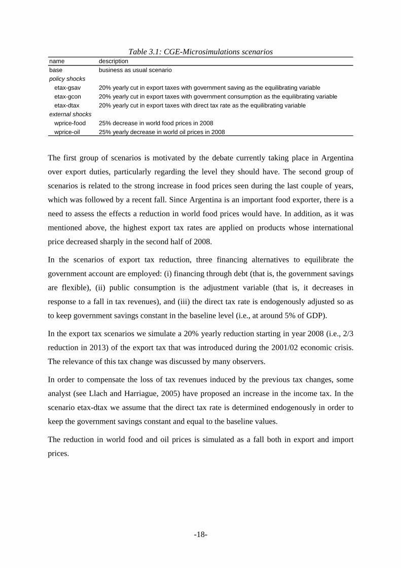
The scenarios that we consider can be divided into two groups (see Table 3.1). On the one

hand, there are simulations of the elimination of the export duties introduced during the 2001-

2002 crisis. On the other hand, there are simulations of changes in world food and oil prices.

In both cases, special emphasis is placed on the effects on the fiscal situation. As was

mentioned, both short and long run effects are analyzed.

-18-

Table 3.1: CGE-Microsimulations scenariosname description

base business as usual scenario

policy shocks

etax-gsav 20% yearly cut in export taxes with government saving as the equilibrating variable

etax-gcon 20% yearly cut in export taxes with government consumption as the equilibrating variable

etax-dtax 20% yearly cut in export taxes with direct tax rate as the equilibrating variable

external shocks

wprice-food 25% decrease in world food prices in 2008

wprice-oil 25% yearly decrease in world oil prices in 2008

The first group of scenarios is motivated by the debate currently taking place in Argentina

over export duties, particularly regarding the level they should have. The second group of

scenarios is related to the strong increase in food prices seen during the last couple of years,

which was followed by a recent fall. Since Argentina is an important food exporter, there is a

need to assess the effects a reduction in world food prices would have. In addition, as it was

mentioned above, the highest export tax rates are applied on products whose international

price decreased sharply in the second half of 2008.

In the scenarios of export tax reduction, three financing alternatives to equilibrate the

government account are employed: (i) financing through debt (that is, the government savings

are flexible), (ii) public consumption is the adjustment variable (that is, it decreases in

response to a fall in tax revenues), and (iii) the direct tax rate is endogenously adjusted so as

to keep government savings constant in the baseline level (i.e., at around 5% of GDP).

In the export tax scenarios we simulate a 20% yearly reduction starting in year 2008 (i.e., 2/3

reduction in 2013) of the export tax that was introduced during the 2001/02 economic crisis.

The relevance of this tax change was discussed by many observers.

In order to compensate the loss of tax revenues induced by the previous tax changes, some

analyst (see Llach and Harriague, 2005) have proposed an increase in the income tax. In the

scenario etax-dtax we assume that the direct tax rate is determined endogenously in order to

keep the government savings constant and equal to the baseline values.

The reduction in world food and oil prices is simulated as a fall both in export and import

prices.

-19-

RESULTS

We show results in terms of aggregate welfare, sectoral output, sectoral trade, unemployment,

terms of trade, commodities prices, and wages from the CGE model. Using the

microsimulation model we compute results in terms of inequality and poverty. The

differences between the counterfactual scenarios and the baseline scenario are interpreted as

the economy-wide impact of the simulated shocks.

BASELINE SCENARIO

The first (base) scenario is a business-as-usual scenario. Accoringly, this scenario reflects the

evolution of the economy in the absence of shocks. In order to produce a baseline scenario

(i.e., a business-as-usual scenario), the exogenous part of the TFP (see variable CALTFP in

the model’s mathematical statement) is adjusted to generate an annual growth rate for real

GDP at factor cost that replicates the behavior of the Argentine economy for the period 2005-

2007 and decreases thereafter reaching an annual growth rate of 3.5% in year 2015.6

As said before, the model has three balances at the macro level. The shares in absorption of

government consumption, investment, and household consumption are kept constant in order

to produce a “balance” closure. This closure mimics the Argentine past experience with

simultaneous adjustments in the three components of absorption. The value of private savings

is determined endogenously to maintain the balance between investment and total savings.7

The real exchange rate varies in order to equilibrate the total inflows and outflows of foreign

exchange, keeping foreign savings fixed as a share of GDP. The transfers from the rest of the

world to the domestic institutions are set to grow exogenously at the same rate as real GDP,

expressed in foreign currency. The transfers between the government and households grow

exogenously at the same rate as real GDP. The model numeraire is the consumer price index.

Finally, all tax rates are fixed over time. The model also considers the quantitative restrictions

on exports of agri-food products that were introduced for the period 2006-2008.

6 The 3.5% growth rate was obtained using data on factor endowments for the period 1990-2001 to compute the

potential GDP for Argentina.

7 In order to generate savings that equal the cost of investment, the savings rate of the representative household is

endogenously adjusted.

-20-

The poverty rate in the baseline scenario diminishes from 33.8% observed in 2005 to around

20% in 2015, mainly as a consequence of an increase in the average wage (see Table A.3).

The implicit growth elasticity of poverty for the period 2005-2015 is approximately 0.48. The

Gini coefficient does not show any significan change throughout the whole simulation period.

COUNTERFACTUAL SCENARIOS

The rules for keeping the government account balanced are changed across the simulations.

Specifically, we consider three closure rules in the policy-induced simulations (see above),

and assume that government saving flexible in the external shocks simulations. The real

investment is endogenous and follows the available savings (i.e., savings driven). The foreign

savings are fixed in the baseline scenario values, being the real exchange rate the variable that

equilibrates the inflows and outflows of foreign currency.

POLICY SHOCKS

In aggregated terms, the reduction in the export tax has different effects in the short and in the

long run when the government budget is equilibrated through direct taxes (see etax-dtax

scenario) or government consumption (see etax-gcon scenario) (see Table 3.2 and Table A.2

in the Appendix). In the short run, a fall in GDP is obtained, which can be accounted for by

several factors. When the export tax is eliminated, the sectors with the highest tax rates

expand their production level (see below). As was shown, these sectors are, in relation to the

rest of the economy, relatively capital intensive (particularly, in land). Consequently, when

expanded, they can not to absorb all the labor -- particularly semi-skilled and skilled labor --

that is expelled by the sectors that are contracting, for which reason unemployment increases

(see Table 3.3).8 Additionally, a fall in labor supply is observed, especially when government

savings and public consumption are used as variables for the adjustment of the government

budget. The decrease in the participation rate combined with the increase in the

unemployment rate impact negatively on poverty (see Table A.3).

In the long run, the reallocation of resources generates an increase in the returns to capital,

land and natural resource factors that enable higher private savings, even after facing a higher

8 When the model is run with full employment and with no leisure-consumption choice, a fall in wages is

obtained.

-21-

direct tax in the etax-dtax scenario. Then, investment is higher than in the baseline scenario,

and as a consequence the capital stock increases, which results in a growth rate slightly higher

than that of the baseline scenario (see Table 3.2). However, when government financing is

through debt, there is a fall in investment that reduces the economy’s growth rate throughout

the whole simulation period. That is to say, the need for public financing reduces the savings

available for investment.

Table 3.2: real macro indicators by simulation (annual growth rate 2007-2015)

etax-gsav etax-gcon etax-dtax pw-food pw-oil

absorption 5,033 6.2 6.0 6.3 6.3 5.6 6.0

household consumption 3,263 6.1 6.1 6.4 6.1 5.7 6.0

government consumption 657 6.5 6.5 5.2 6.5 6.5 6.5

fixed investment 1,114 6.2 5.4 6.7 6.5 4.7 5.7

exports 1,365 6.0 6.3 6.6 6.5 6.0 6.0

imports -1,041 6.0 6.3 6.8 6.7 5.0 5.8

GDP market price 5,358 6.2 6.0 6.3 6.3 5.8 6.1

GDP factor cost 4,434 6.2 6.0 6.3 6.3 5.9 6.1

real exchane rate 1 0.1 -0.4 -0.4 -0.4 0.9 0.3

Source: Author's estimates.

indicatorbase

(LCU$)base

(chg%)policy shocks external shocks

Table 3.3: Unemployment rate by labor type in base year and final year by simulation (%)

2005 base etax-gsav etax-gcon etax-dtax wp-food wp-oil

unskilled labor 19.1 11.4 11.8 11.5 11.5 11.8 11.4

semi-skilled labor 14.6 8.1 8.5 8.2 8.3 8.4 8.1

skilled labor 5.5 2.5 2.5 2.5 2.5 2.5 2.5

total 15.7 8.8 9.1 8.9 8.9 9.1 8.8


2015 (final year)labor category

The loss of tax revenues due to the elimination of export duties is not automatically

compensated by an increase in revenues from other tax instruments (see Table 3.4). As a

consequence, it generates: (1) a reduction in public savings (etax-gsav scenario) by 1.6 points

of the GDP by 2015, or (2) a reduction in public consumption (etax-gcon scenario) by 1.2

points of the GDP. In the first case, a crowding-out effect that reduces investment takes place.

As a consequence, a reduction in the growth rate is obtained; in the 2007-2015 period, the

annual growth rate falls from 6.2% in the base scenario to 6% in the etax-gsav scenario (see

Table 3.2). However, when the elimination of export duties is compensated with a reduction

-22-

in government consumption, the average annual growth rate for 2007-2015 slightly increases

to reach 6.3%.

Table 3.4: fiscal indicators

2005 base etax-gsav etax-gcon etax-dtax wp-food wp-oil

gov. consumption (share GDP) 12.3 12.3 12.4 11.0 12.2 12.8 12.4

gov. savings (share GDP) 4.9 4.8 3.2 4.8 4.8 3.6 4.3

tax revenue (share GDP) 28.0 28.0 26.7 26.7 27.9 27.9 27.8

export tax 2.3 2.0 0.4 0.4 0.4 1.6 1.9

tariffs 0.7 0.8 0.8 0.8 0.8 0.8 0.8

value added tax 6.9 6.9 6.9 6.9 6.9 6.9 6.8

other indirect taxes 7.3 7.5 7.6 7.6 7.6 7.6 7.3

direct taxes 10.8 10.9 11.0 11.0 12.2 11.0 11.0


2015 (final year)indicator

The price that Argentine merchandise exporters are paid increases by a (weighted) average

annual growth rate around 0.54 percentage points higher than in the baseline (average across

all export tax scenarios). As expected, export volumes increase as a result of the elimination

of the export tax. As a result, an appreciation of the real exchange rate takes place in order to

re-equilibrate the current account of the balance of payments (see Table 3.2).

There is an (expected) increase in the domestic prices of food items (see Table A.3). In fact,

one of the reasons mentioned in the literature for the existence of export duties is to

“decouple” the domestic prices from the world prices (Devarajan et al., 1996; Piermartini,

2004). This increase in domestic food prices has a negative effect on the poverty rate, trough

the poverty line effect (see Table A.3).

As expected, after the elimination of export duties, the sectors that show the highest increase

in their production level are those that, at the beginning, faced the highest export tax rates.

Therefore, the effect of rising primary exports is an appreciation of the real exchange rate,

which undermines the competitiveness of other agricultural and manufacturing exports (see

Table 3.5).

A significant change in the sectoral composition of Argentina’s economic structure can be

observed. In particular, both production and exports turn towards primary products (see Table

3.5). At the same time, imports of manufactures increase, replacing domestic production.

Argentina’s productive structure is thus modified with primary products such us Cereals, Oil

seeds, Oil, and Vegetable oils and fats gaining importance.

-23-

Table 3.4: sectoral results by simulation (annual growth rate 2007-2015)

etax-gsav etax-gcon etax-dtax pw-food pw-oil

GDP primary 596 4.6 4.8 5.0 5.0 3.8 4.5

GDP non-primary 3,837 6.5 6.2 6.5 6.5 6.2 6.4

exports primary 320 3.6 6.0 6.1 6.1 2.8 3.8

imports primary 47 6.9 8.8 9.3 9.2 6.2 6.4

exports non-primary 1,045 6.6 6.4 6.8 6.7 6.8 6.6

imports non-primary 994 5.9 6.2 6.7 6.6 5.0 5.8


base (LCU$)

base (chg%)

policy shocks external shocks

The production of Oil seeds aimed at the domestic market increases considerable since it

constitutes the most important individual intermediate input in the production of Vegetable

oils and fats – the main Argentine export product.

The reduction in the export tax increases the price of the intermediate inputs used by the

sectors that process raw products such as Dairy products, Beverages and tobacco, among

others, due to the fact that higher export tax rate are imposed on primary products. This effect

also contributes to the expansion of primary sectors vis-à-vis manufacturing sectors.

EXTERNAL SHOCKS

In this section the impact of changes in the world price of food products and oil is analyzed.9

In this case, it is assumed that the adjustment variable for the government is public savings.

Then, it is expected that a reduction in the world price of the products exported by Argentina

will increase government deficit as a result of a decrease in tax revenue, particularly from

export duties. Following, the growth rate of the economy will be reduced as a result of a

crowding-out effect of investment.

In fact, the fiscal situation deteriorates, mainly as a consequence of a reduction in the tax

collection from the export tax. The government surplus as a share of GDP is 1.2 percentage

points lower in 2015 in the food price reduction scenario (pw-food) than in the baseline

scenario, generating a crowding out effect of investment, which reduces GDP growth and

increases unemployment (see Table 3.2, 3.3, and 3.4).

9 Notice, however, that we focus our attention in the results from the wprice-food scenario.

-24-

When the world food prices falls, there is a negative effect both in the short and in the long

run (see Table A.2). As was previously described, Argentina is a net agri-food exporter.

Consequently, this shock constitutes a worsening in the Argentina’s terms of trade in; the

economic indicators as a whole worsen. The growth rate of the GDP at factor cost for the

2007-2015 period falls by 0.3 percentage points (see scenario pw-food), while the

unemployment rate increases by 3.4% in 2015 with respect to the baseline scenario.10

On the other hand, the domestic price of food products decreases with a positive impact on

poverty. In fact, the poverty headcount diminishes due to the poverty line effect but increases

due to the unemployment and the average wage effects (see Table A.3).

The decrease in the world price of food generates a depreciation of the real exchange rate that,

ceteris paribus, increases exports and decreases imports, necessary to keep the (fixed) ratio

between foreign savings and GDP imposed as part of the model macro closure rule for the

external sector (see above).

The decrease in the growth rate is higher for primary than for non-primary activities (see

Table 3.5).

4. CONCLUDING REMARKS

This study has analyzed the economy-wide impact of (1) a gradual elimination of the export

tax that was introduced after the 2001/2002 economic crisis, and (2) a decrease in the world

price of Argentina’s main export products. We found that the elimination of the export tax

would have different long run effects depending on the fiscal instrument that is used by the

government to compensate for the loss in tax revenue. On the one hand, when the government

budget is equilibrated by an increased deficit, the average annual growth rate for 2008-2015 is

lower than in the baseline scenario. On the other hand, when the government budget is

equilibrated by an increased direct tax rate, there is a long run positive effect on growth. In

any case, the employment level is lower (i.e., participation rate decreases at the same time that

10 Notice that we are not considering the negative growth effect that a reduced public spending in infrastructure

may have.

-25-

unemployment rate increases) and the price of food items is higher.11 Therefore, the poverty

headcount ratio increases.

As expected, a reduction in the world price of food items (i.e., a worsening in Argentina’s

terms of trade) would impact negatively on Argentina’s GDP growth rate.

11 As shown in Section 3, the employment level is lower than in the baseline scenario due to the change in the

sectoral composition of Argentina’s productive structure.

-26-

REFERENCES

Annabi, Nabil (2003). Modeling Labor Markets in CGE Models Endogenous Labor Supply, Unions and Efficiency Wages. PEP.

Annabi, Nabil; Cockburn, John and Decaluwé, Bernard (2006). Functional Forms and Parametrization of CGE Models . PEP MPIA Working Paper 2006-04.

Armington, Paul S. (1969). A Theory of Demand for Products Distinguished by Place of Production. International Monetary Fund Staff Papers 16: 159-178.

Bulacio, José Marcos (2005). El Stock de Capital del Gobierno en Argentina. Anales XL Reunión Anual de la AAEP. Universidad Nacional de La Plata.

Castro, Lucio and Díaz Frers, Luciana (2008). Las Retenciones sobre la Mesa: Del Conflictoa una Estrategia de Desarrollo. Documento de Trabajo 14. CIPPEC.

CEP (2003). Antigüedad del Equipo Durable de Producción. Centro de Estudios para la Producción. Secretaría de Industria, Comercio y Minería. Ministerio de Economía.

Cetrángolo, O. and Gomez Sabaini, J.C. (2007) Política tributaria en Argentina. Entre la Solvencia y la Emergencia. Serie Estudios y Perspectivas 38. Oficina de la CEPAL en Buenos Aires.

Cicowiez, Martín; Díaz-Bonilla, Carolina and Díaz-Bonilla, Eugenio (2008). The Impact of Global and Domestic Trade Liberalization on Poverty and Inequality in Argentina. GTAP Conference Paper.

CIPPEC (2002a). Boletín Fiscal #5. Centro de Implementación de Políticas Públicas para la Equidad y El Crecimiento.

CIPPEC (2002b). Boletín Fiscal #7. Centro de Implementación de Políticas Públicas para la Equidad y El Crecimiento.

Cockburn, John (2001). Trade Liberalisation and Poverty in Nepal: A Computable General Equilibrium Micro Simulation Analysis. Centre de Recherche en Économie et Finance Appliquées (Université Laval) Discussion Paper 01-18.

Coremberg, Ariel (2004). Estimación del Stock de Capital Fijo de la República Argentina 1990-2003: Ministerio de Economía.

Decaluwé, B.; Patry, A.; Savard, L. and Thorbecke, E. (1999). Poverty Analysis Within a General Equilibrium Framework. CRÉFA Working Paper 99-09.

Díaz-Bonilla, Carolina; Díaz-Bonilla, Eugenio; Piñeiro, Valeria and Robinson, Sherman. (2004). El Plan de Convertibilidad, Apertura de la Economía y Empleo en Argentina: Una Simulación Macro-Micro de Pobreza y Desigualdad. In Ganuza; Morley; Robinson and Vos (eds.). ¿Quién se Beneficia del Libre Comercio?UNDP/CEPAL/ISS/IFPRI.

Foro de la Cadena Agroindustrial Argentina (2005). Lineamientos de Política Tributaria. Documento de Trabajo.

Ganuza, Enrique; Paes de Barros, Ricardo and Vos, Rob (2002). Labour Market Adjustment, Poverty and Inequality During Liberalization. In Vos, Taylor and Paes de Barros

-27-

(eds.). Economic Liberalization, Distribution and Poverty: Latina America in the 1990s. UNDP.

Gasparini, L. (1999). Incidencia Distributiva del Gasto Público Social y de la Política Tributaria en Argentina. En FIEL. La Distribución del Ingreso en Argentina. Buenos Aires.

Go, Delfin S.; Kearney, Marna; Robinson, Sherman and Thierfelder, Karen (2005). An Analysis of South Africa's Value Added Tax. World Bank Policy Research Wroking Paper 3671.

Harrison, Glen W. and Vinod, H. D. (1992). The Sensitivity Analysis of Applied General Equilibrium Models: Completely Randomized Factorial Designs. The Review of Economics and Statistics.

INDEC (2001). Matriz Insumo Producto Argentina 1997. Instituto Nacional de Estadística y Censos.

Llach, Juan J. and Harriague, María Marcela (2005). Un Sistema Impositivo para elDesarrollo y la Equidad. Fundación Producir Conservando.

Lofgren, H.; Lee Harris, R. and Robinson, S. (2002). A Standard Computable General Equilibrium (CGE) Model in GAMS. International Food Policy Research Institute Microcomputers in Policy Research 5.

Lofgren, Hans and Diaz-Bonilla, Carolina (2006). MAMS: An Economy Wide Model for Analysis of MDG Country Strategies: Technical Documentation. DECPG World Bank.

Maechler, Andréa M and Roland-Holst, David W. (1997). Labor Market Structure and Conduct. In Francois, Joseph F. and Reinert, Kenneth A. (eds.). Applied Methods for Trade Policy Analysis: A Handbook. Cambridge: Cambridge University Press.

Melo de, Jaime and Robinson, Sherman (1989). Product Differentiation and The Treatment of Foreign Trade in Computable General Equilibrium Models of Small Economies. Journal of International Economics 27: 47-67.

Melo de, Jaime and Tarr, David (1992). A General Equilibrium Analysis of US Foreign Trade Policy. The MIT Press.

Mercado, P. R. (2003). Empirical Economywide Modeling in Argentina. Lozano-Long Institute of Latin American Studies. The University of Texas at Austin.

Mincer, J. (1974). Schooling, Experience and Earnings. New York. Columbia University Press for NBER.

Redrado, Martín (2005). Exposición en el 41 Coloquio de Idea. Presidente del Banco Central de la República Argentina.

Reinert, K. A. and Roland-Holst, D. W. (1997). Social Accounting Matrices. In Francois, J. F. and Reinert, K. A. (eds.). Applied Methods for Trade Policy Analysis: A Handbook. Cambridge University Press.

Robinson, S.; Cattaneo, A. and El-Said, M. (2001). Updating and Estimating a Social Accountig Matrix Using Cross Entropy Methods. Economic System Research 13 (1): 47-64.

-28-

Robinson, Sherman (2003). Macro Models and Multipliers: Leontief, Stone, Keynes, and CGE Models. International Food Policy Research Institute.

Sturzenegger, Federico (2006). Justificando una Estructura Impositiva “Distorsiva”.Colaboraciones. Indicadores de Coyuntura 464. FIEL.

Thierfelder, Karen E. and Shiells, Clinton R. (1997). Trade and Labor Market Behavior. In Francois, Joseph F. and Reinert, Kenneth A. (eds.). Applied Methods for Trade Policy Analysis: A Handbook. Cambridge: Cambridge University Press.

Thurlow, James (2004). A Dynamic Computable General Equilibrium (CGE) Model for South Africa: Extending the Static IFPRI Model. Trade and Industrial Policy Strategies (TIPS) Working Paper 1-2004.

Vos, Rob; Taylor, Lance and Paes de Barros, Ricardo (eds.) (2002). Economic Liberalization, Distribution and Poverty: Latin America in the 1990s. UNDP.

-29-

APPENDIX

ADDITIONAL TABLES

Table A.1: Argentina 1993-2007

yearreal GDP

(mill. LCU)unemp rate

(%)extreme pov (%)

moderate pov (%)

1993 236,505 9.3 4.4 16.8

1994 250,308 12.1 3.5 19.0

1995 243,186 16.6 6.3 24.8

1996 256,626 17.3 7.5 27.9

1997 277,441 13.7 6.4 26.0

1998 288,123 12.4 6.9 25.9

1999 278,369 13.8 6.7 26.7

2000 276,173 14.7 7.7 28.9

2001 263,997 18.3 12.2 35.4

2002 235,236 23.6 24.7 54.3

2003 256,023 20.6 20.5 47.8

2004 279,141 16.9 15.0 40.2

2005 304,764 13.4 12.2 33.8

2006 330,565 11.1 8.7 26.9

2007 359,170 8.5 8.2 23.4

Source: Ministerio de Economía and INDEC.

-30-

Table A.2: real macro indicators by simulation and year (growth rate)indicator scenario 2005 2006 2007 2008 2009 2010 2011 2012 2013 2014 2015

absorption base 5,033 8.5 8.4 8.0 7.5 7.0 6.4 5.9 5.4 4.9 4.4

household consumption base 3,263 8.5 8.5 7.8 7.4 6.9 6.4 5.9 5.4 4.8 4.3

government consumption base 657 8.6 8.3 8.5 7.7 7.2 6.7 6.2 5.7 5.2 4.7

fixed investment base 1,114 8.4 8.3 8.1 7.5 7.0 6.5 6.0 5.5 4.9 4.4

exports base 1,365 8.3 8.1 7.9 7.3 6.8 6.3 5.7 5.2 4.7 4.2

imports base -1,041 8.3 8.1 7.9 7.3 6.8 6.2 5.7 5.2 4.7 4.2

GDP market price base 5,358 8.5 8.4 8.0 7.5 6.9 6.4 5.9 5.4 4.9 4.4

GDP factor cost base 4,434 8.5 8.5 8.0 7.5 7.0 6.5 6.0 5.5 5.0 4.5

real exchane rate base 1 0.3 0.6 -0.2 0.2 0.2 0.2 0.2 0.2 0.2 0.2

absorption etax-gsav 5,033 8.5 8.4 8.0 7.4 6.8 6.3 5.7 5.2 4.6 4.1

household consumption etax-gsav 3,263 8.5 8.5 8.2 7.7 7.0 6.4 5.8 5.2 4.7 4.1

government consumption etax-gsav 657 8.6 8.3 8.5 7.7 7.2 6.7 6.2 5.7 5.2 4.7

fixed investment etax-gsav 1,114 8.4 8.3 7.2 6.5 6.0 5.5 5.1 4.6 4.2 3.7

exports etax-gsav 1,365 8.3 8.1 8.6 7.8 7.2 6.5 5.9 5.3 4.8 4.2

imports etax-gsav -1,041 8.3 8.1 8.8 7.9 7.3 6.6 6.0 5.3 4.8 4.2

GDP market price etax-gsav 5,358 8.5 8.4 8.0 7.4 6.8 6.3 5.7 5.2 4.7 4.1

GDP factor cost etax-gsav 4,434 8.5 8.5 7.9 7.4 6.8 6.3 5.7 5.2 4.7 4.2

real exchane rate etax-gsav 1 0.3 0.6 -1.1 -0.6 -0.5 -0.4 -0.3 -0.2 -0.2 -0.1

absorption etax-gcon 5,033 8.5 8.4 8.0 7.6 7.1 6.6 6.1 5.6 5.0 4.5

household consumption etax-gcon 3,263 8.5 8.5 8.2 7.8 7.2 6.7 6.1 5.6 5.0 4.5

government consumption etax-gcon 657 8.6 8.3 5.9 5.6 5.5 5.4 5.3 5.1 4.8 4.5

fixed investment etax-gcon 1,114 8.4 8.3 8.8 8.1 7.5 6.9 6.4 5.8 5.3 4.7

exports etax-gcon 1,365 8.3 8.1 8.8 8.1 7.5 6.9 6.3 5.7 5.2 4.6

imports etax-gcon -1,041 8.3 8.1 9.0 8.3 7.7 7.1 6.5 5.9 5.3 4.7

GDP market price etax-gcon 5,358 8.5 8.4 8.0 7.5 7.1 6.6 6.1 5.5 5.0 4.5

GDP factor cost etax-gcon 4,434 8.5 8.5 7.9 7.5 7.1 6.6 6.1 5.6 5.1 4.6

real exchane rate etax-gcon 1 0.3 0.6 -1.0 -0.5 -0.4 -0.4 -0.3 -0.3 -0.2 -0.2

absorption etax-dtax 5,033 8.5 8.4 8.1 7.5 7.0 6.5 6.0 5.5 5.0 4.5

household consumption etax-dtax 3,263 8.5 8.5 7.9 7.4 6.9 6.4 5.9 5.4 4.9 4.4

government consumption etax-dtax 657 8.6 8.3 8.5 7.7 7.2 6.7 6.2 5.7 5.2 4.7

fixed investment etax-dtax 1,114 8.4 8.3 8.5 7.8 7.3 6.7 6.2 5.7 5.1 4.6

exports etax-dtax 1,365 8.3 8.1 8.7 8.0 7.4 6.8 6.2 5.7 5.1 4.5

imports etax-dtax -1,041 8.3 8.1 8.9 8.2 7.6 7.0 6.4 5.8 5.2 4.6

GDP market price etax-dtax 5,358 8.5 8.4 8.1 7.5 7.0 6.5 6.0 5.5 5.0 4.5

GDP factor cost etax-dtax 4,434 8.5 8.5 8.0 7.5 7.0 6.5 6.0 5.5 5.0 4.5

real exchane rate etax-dtax 1 0.3 0.6 -1.0 -0.5 -0.5 -0.4 -0.3 -0.3 -0.2 -0.2

absorption pw-food 5,033 8.5 8.4 5.8 7.0 6.5 6.0 5.6 5.1 4.6 4.1

household consumption pw-food 3,263 8.5 8.5 6.7 7.0 6.6 6.1 5.6 5.1 4.6 4.1

government consumption pw-food 657 8.6 8.3 8.5 7.7 7.2 6.7 6.2 5.7 5.2 4.7

fixed investment pw-food 1,114 8.4 8.3 1.4 6.5 6.1 5.6 5.1 4.7 4.2 3.8

exports pw-food 1,365 8.3 8.1 11.5 6.6 6.2 5.7 5.2 4.7 4.3 3.8

imports pw-food -1,041 8.3 8.1 2.6 6.8 6.3 5.9 5.4 4.9 4.5 4.0

GDP market price pw-food 5,358 8.5 8.4 7.8 6.9 6.5 6.0 5.5 5.0 4.5 4.1

GDP factor cost pw-food 4,434 8.5 8.5 8.4 7.0 6.6 6.1 5.6 5.1 4.6 4.2

real exchane rate pw-food 1 0.3 0.6 7.1 0.0 0.0 0.0 0.0 0.0 0.0 0.0

absorption pw-oil 5,033 8.5 8.4 7.5 7.3 6.8 6.3 5.8 5.3 4.8 4.3

household consumption pw-oil 3,263 8.5 8.5 7.9 7.3 6.8 6.3 5.8 5.3 4.8 4.3

government consumption pw-oil 657 8.6 8.3 8.5 7.7 7.2 6.7 6.2 5.7 5.2 4.7

fixed investment pw-oil 1,114 8.4 8.3 5.6 7.1 6.7 6.2 5.7 5.3 4.8 4.3

exports pw-oil 1,365 8.3 8.1 9.5 7.0 6.5 6.0 5.5 5.0 4.5 4.1

imports pw-oil -1,041 8.3 8.1 6.7 7.1 6.7 6.2 5.7 5.2 4.7 4.2

GDP market price pw-oil 5,358 8.5 8.4 8.1 7.2 6.8 6.3 5.8 5.3 4.8 4.3

GDP factor cost pw-oil 4,434 8.5 8.5 8.1 7.3 6.8 6.3 5.9 5.4 4.9 4.4

real exchane rate pw-oil 1 0.3 0.6 1.7 0.1 0.1 0.1 0.1 0.1 0.1 0.1


-31-

CGE MODEL MATHEMATICAL STATEMENT

The CGE model mathematical statement uses the following notation: uppercase letters for

endogenous variables; lowercase letters for exogenous variables; greek letters for behavioral

parameters; quantity start with Q; and prices start with P.12 The model has the following sets:

t time period; a activities; c commodities; f factors; h households; ins institutions; insd

domestic institutions; and insng domestic non-government institutions.

The model can be split in two modules. The within-period module defines a single country

static CGE model. The equations in this module are grouped in blocs covering production,

trade, institutions, investment, equilibrium conditions, and macro variables. The within-period

module presents some similarities to Lofgren et al. (2002).

The equations in the between-period module update population, labor force by skill level,

institutional stocks of assets, and total factor productivity. Naturally, the equations in this

module include lagged variables and do not apply to the first period. We assume that the

capital stock is sector-specific. As a consequence, sectoral profit rates will be different across

activities. In fact, that difference in the capital returns determines how the new capital (i.e.,

investment) is assigned across sectors.13 In the model, flows are measured at the end of each

period and stocks are measured at the beginning of each period.

VARIABLES

tCALTFP TFP for calibration run

tCPI consumer price index

tDPI producer domestic price index

tEG government expenditure

htEH consumption expenditure hhd h

12 The notation used is similar to Lofgren et al. (2002).

13 For alternative approaches see Abbink et al. (1995), Annabi et al. (2004), Bourguignon et al. (1989), among

others.

-32-

tEXR exchange rate (domestic currency per unit of foreign currency)

tFSAV rest of the world savings (expressed in foreign currency)

tGDAJ adjustment factor government consumption

tGDPREALFC real GDP at factor cost

tGDPMP GDP at market prices

tGOVSHR government consumption share in absorption

tGSAV government savings

tIADJ adjustment factor investment

tINVSHR investment share in absorption

tflabinsMAXHOUR ,, endowment factor flab institution ins

tinsdngMPS , marginal propensity to save institution insdng

tMPSADJ adjustment factor marginal propensity to save

atPA price of activity a

tPCAP price of capital

ctPD price of commodity c domestic

ctPE domestic price of commodity c exports

atPINTA price of intermediate inputs aggregate activity a

ctPM domestic price of commodity c imports

ctPQD demand price composite commodity c

ctPQS supply price composite commodity c

atPVA value added price activity a

tPVAAVG average price value added

-33-

ctPWE export price commodity c (foreign currency)

ctPWM import price commodity c (foreign currency)

ctPX producer price commodity c

atQA level of activity a

atQCAPNEW new capital in activity a

ctQD sales and purchases domestic commodity c

ctQE exports commodity c

tfinsQFACINS ,, factor f supply institution ins

ftQFStotal employment factor f

ctQG government consumption commodity c

chtQH consumption of commodity c by hhd h

tQHPCREAL per capital real consumption

catQINT intermediate demand of commodity c by activity a

atQINTA intermediate inputs aggregate activity a

ctQINV investment commodity c

ctQM imports commodity c

ctQQ domestic demand composite commodity (D+M)

atQVA value added activity a

ctQX domestic supply composite commodity c (D+E)

tGDPMPFSAVRAT __ ratio between foreign savings and GDP at market prices

tGDPMPGDSAVRAT __ ratio between government savings and GDP at market

prices

-34-

atREBATE value added rebate for intermediate consumption activity a

atSHRCAPNEW share of activity a in the new capital

atTA tax rate activity a

tTAADJ adjustment factor TA

tTABS total absorption

ctTE tax rate exports commodity c

tTEADJ adjustment factor TE

ftTF tax rate factor f income

tTFADJ adjustment factor TF

atTFINSER tax rate use of financial services

tTFINSERADJ adjustment factor TFINSER

ctTFUEL tax rate fuel (c=fuel)

tTFUELADJ adjustment factor TFUEL

ctTM tariff rate imports commodity c

tTMADJ adjustment factor TM

ctTPRODUCTS tax rate product c

tDJTPRODUCTSA adjustment factor TPRODUCTS

tTREV tax revenue

tiiTRII ' transfer from institution insdngp to institution insdng

ctTTURNONVER tax rate turnover tax commodity c

tADJTTURNONVER adjustment factor TTURNOVER

ctTVAT tax rate value added commodity c

-35-

tTVATADJ adjustment factor TVAT

tinsdngTY , tax rate income institution insdng

tTYADJ adjustment factor TY

ftUERAT unemployment rate

ctURNTQEMAX unitary rent due to export quota commodity c

tWALRAS to check ley walras

tWCAPAVG average profit rate

ftWF price of factor f

fatWFDIST distortion factor price of factor f in activity a

ftWFREAL real wage

ftWFREALMIN minimum real wage

ftYF income of factor f

tYG government income

tinsdngYI , income of institution insdng

EXOGENOUS VARIABLES

ifshif share institution i in factor f income

cqinv initial investment commodity c

insdngmps initial marginal propensity to save institution insdng

cqg initial government consumption commodity c

atabar initial tax rate activity a

cte initial tax rate exports commodity c

-36-

ctf initial tax rate factor f income

ctfinser initial tax rate financial transactions (c=financ)

ctfuel initial tax rate fuel (c=fuel)

ctm initial tariff rate imports commodity c

ctproducts initial tax rate product c

ctturnover initial tax rate turnover tax commodity c

ctvatbar initial tax rate value added commodity c

ity initial tax rate income institution insdng

tiitrnsfr ' transfers from institution i' to institution i

'iishii share in ins i income of transfers from ins i’ to ins i

netprfrat capital net rate of return

fueratmin minimum unemployment rate factor f

cqemax maximum exports commodity c

tpop population

flabqlabgrwrat labor endowment growth rate

popgrwrat population growth rate

landgrwrat land growth rate

PARAMETERS

vafa share factor f activity a value added

a shift parameter activity a value added

vaa substitution elasticity activity a value added

vaa exponent activity a value added

-37-

ac yield commodity c per unit activity a

caica intermediate consumption commodity c per unit of intermediate

inputs aggregate activity a

aiva value added per unit activity a

ainta intermediate inputs aggregate per unit activity a

ych income elasticity demand commodity c household h

lhflab, income elasticity labor supply

ch share commodity c consumption household h

hflab , share leisure utility household h

htminv _ minimum total consumption value household h

chtminc _ minimum consumption value commodity c household h

Mcq share imports commodity c armington q

Dcq share domestic commodity c armington q

cq shift parameter armington q

cq substitution elasticity armington q

cq exponent armington q

Ect share exports commodity c CET x

Dct share domestic commodity c CET x

ct shift parameter CET x

ct transformation elasticity CET x

-38-

ct exponent CET x

ccwts weight commodity c in CPI

cdwts weight commodity c in DPI

fwfqh min wage elasticity w.r.t. per capita household consumption

fwfpva min wage elasticity w.r.t. average value added price

fwfuerat min wage elasticity w.r.t. (1-unemployment rate)

fwfcpi min wage elasticity w.r.t. consumer price index

deprcap capital depreciation rate

speed capital mobility between activities

EQUATIONS

WITHIN-PERIOD MODULE

LEVEL 1: VALUE-ADDED

Equation (1) shows that value-added is a fixed proportion of the activity production level. The

value added price is obtained, implicitly, from equation (2). The rest of the variables in

equation (2) are determined elsewhere in the model.

ataat QAivaQVA (1)

atatatatatatatat QINTAPINTAQVAPVAQATFINSERTAPA 1 (2)

LEVEL 1: INTERMEDIATE INPUTS

The aggregate intermediate input used by each activity is a fixed share of their production

level (equation (3)). The price of the aggregate intermediate input is obtained as a weighted

average of the prices of every commodity demanded as intermediate input (equation (4)). The

coefficient caica refers to the quantity of intermediate input c used in activity a per unit of

-39-

aggregate intermediate inputs atQINTA . The last term on the right-hand side is the VAT

rebate per unit of aggregate intermediate inputs purchased by the representative firm in

activity a.

ataai QAintaQINTA (3)

at

at

ccactat QINTA

REBATEicaPQDPINTA (4)

LEVEL 2: VALUE ADDED

Equations (5) and (6) are the first order conditions of the firm optimization problem. Value

added production is modeled using a CES technology (constant elasticity substitution). Factor

f remuneration in activity a in time period t is calculated as fatftWFDISTWF . Hence, factor f

remuneration may differ across activities. The variable tCALTFP is used in the calibration run

to impose a growth rate to the real GDP at factor cost in the baseline scenario.

aa

va

f

vafat

vafataat QFCALTFPQVA

1

(5)

atva

ta

vavafa

va

fatft

atfat QVACALTFP

WFDISTWF

PVAQF

a

1

(6)

LEVEL 2: INTERMEDIATE INPUTS

Intermediate inputs are also a fixed share of the activity production level. However, in

equation (7), intermediate inputs appear as a fixed proportion of aggregate intermediate

inputs. These, in turn, are a fixed proportion of the activity production (equation (3)). In

equation (8), the production of every commodity is computed using the ac parameter, which

refers to the production level of commodity c per unit of activity a production. The price of

activity a is a weighted average of the prices of the commodities produced by this activity

(equation (9)).

atcacat QINTAicaQINT (7)

a

atacct QAQX (8)

-40-

c

ctacat PXPA (9)

INTERNATIONAL TRADE PRICES

Equations (10) and (11) define export and import domestic prices. Based on the small country

assumption, tradable commodity international prices are considered as given. Government

collects import tariffs and export duties. Equations (12), (13), and (14) are used to impose

restrictions on the volume of exports for commodities in the set cqemax. Equation (15) can be

used for commodities that face a constant-elasticity export demand function.

cttctct PWMEXRTMPM 1 (10)

cttctctct PWEEXRURNTQEMAXTEPE 1 (11)

ctct qemaxQE cqemaxc (12)

0ctURNTQEMAX cqemaxc (13)

0 ctctct URNTQEMAXqemaxQE cqemaxc (14)

ct

ctctct pwse

PWEqeQE cedc (15)

CONSUMPTION COMPOSITE COMMODITY

On the consumption side, under the Armington assumption (1969), commodities are

differentiated by their country of origin. A CES function is used to model imperfect

substitutability between imports and domestic commodities (equation (16)).14 Equation (17)

shows the tangency condition that determines the quantities of domestic commodity and

imports consumed. Equation (18) computes the supply price of the composite commodity QQ

as a weighted average of the domestic and imported varieties of the same good. Taxes on

commodities are levied on the composite commodity QQ (equation (19)). The GAMS code

includes additional equations for the cases of non-imported goods and non-produced imports.

ccc qq

ctDc

qct

Mccct QDqQMqqQQ

1 (16)

14 The substitution elasticity between domestic commodities and imports is 11 cc q .

-41-

cq

Dc

Mc

ct

ct

ct

ct

q

q

PM

PD

QD

QM

1

1

(17)

ctctctctctct QMPMQDPDQQPQS (18)

ctctctctct

ct

TTURNOVERTVATTPRODUCTSTFUELPQS

PQD

1

(19)

PRODUCTION COMPOSITY COMMODITY

Production can be destined either to domestic or to export markets. This possibility is

modeled using a CET function (equation (20)).15 Equation (21) is derived from the profit

maximization first order conditions. Equation (22) is the zero profit condition for the producer

of commodity c. From this equation, the price PX is derived. The GAMS code includes

additional equations for the cases of domestically sold outputs without exports and exports

without domestic sales.

ttct

Dc

tct

Eccct QDtQEttQX

1

(20)

1

1

ct

Ec

Dc

ct

ct

ct

ct

t

t

PD

PE

QD

QE

(21)

ctctctctctct QEPEQDPDQXPX (22)

NON-GOVERNMENT DOMESTIC INSTITUTIONS INCOME

Equation (23) computes factor f total income. Remuneration paid to the factor f in activity a is

WF(f)*WFDIST(f,a). This modeling strategy allows alternative closure rules (i.e., ways to

equilibrate demand and supply) in factor markets. The income of institution i is obtained by

adding four components: i) income from all factors; ii) government (real) transfers; iii)

transfers received from the rest of the world expressed in local currency; and iv) transfers

from other domestic non-government institutions (equation (24)).

a

fatfatftft QFWFDISTWFYF (23)

15 The transformation elasticity between domestic sales and exports 11 cc t .

-42-

cqemaxctcttcti

itii

ttrowi

ttgovi

fftftifit

QEPWEEXRURNTQEMAXaxshrentquem

TRII

EXRtrnsfr

CPItrnsfr

YFTFshifYI

''

,,

,,

)1(

insdngii ' (24)

TRANSFERS BETWEEN NON-GOVERNMENT DOMESTIC INSTITUTIONS

The model allows for a detailed treatment of transfers between domestic non-government

institutions (e.g., households and firms). In particular, transfers from institution i’ to

institution i are modeled as a fixed proportion of institution i’ income net of savings and direct

taxes (equation (25)). Firms can save, pay direct taxes, but not consume goods. In general,

firms received most part of the capital factor income in order to distribute it between the other

institutions (e.g., households and rest of the world). Notice, however, that the Argentina SAM

2005 used to calibrate the model only identifies one private domestic institution (i.e.,

household).

tititiiitii YITYMPSshiiTRII ''''' 11 insdngii ' (25)

NON-GOVERNMENT DOMESTIC INSTITUTIONS MARGINAL PROPENSITY TO SAVE

The non-government domestic institutions marginal propensity to save is calculated in

equation (26).

tiit MPSADJmpsMPS insdngi (26)

HOUSEHOLDS

Equation (27) calculates the household consumption expenditure as the household h income

net of transfers to other domestic institutions, savings, and direct taxes. Household

consumption expenditure is distributed between the different commodities and leisure from

the (flab) different labor categories according to a Stone-Geary utility function (equation

(28)). Equation (29) refers to the labor supply of household h.

hththti

iht YITYMPSshiiEH

111 (27)

-43-

c

tcchtht

flabhflab

chtcchttccht PQDmincEHPQDmincPQDQH _

1

_

,

(28)

c

tcchtth

flabtflabflab

hflab

hflabtflabh

tflabh

PQDmincEH

UERATWF

MAXHOUR

QFACINS

,,

,,

,,,

,,

_

11

(29)

INVESTMENT

Equation (30) calculates the quantity of commodity c for investment demand. It is assumed

that the commodity composition of investment is constant at the initial values. If the

investment increases, the investment demand of every commodity is increased by the same

proportion.

tcct IADJqinvQINV (30)

GOVERNMENT

Equation (31) calculates the government consumption of commodity c, defined as the base-

year quantity multiplied by an adjustment factor. Equations (32) to (41) compute all the tax

rates as the product between the initial rate and an adjustment factor. This formulation allows

for great flexibility when simulating counterfactual scenarios. The (net) tax revenue is

computed in equation (42). Equation (43) shows the two government’s income sources: i) tax

revenue; and ii) transfers from the rest of the world (multiplied by the exchange rate in order

to express them in domestic currency). Equation (44) calculates the VAT rebate given by the

government to the firms because of their intermediate inputs purchases. Government uses its

income to buy commodities and make transfers to the households and firms (equation (45)).

Equation (46) defines government saving as the difference between government revenues and

expenditures.

tcct GADJqgQG (31)

tatat TAADJtabarTA (32)

tctct TVATADJtvatbarTVAT (33)

-44-

tctct DJTPRODUCTSAtproductsTPRODUCTS (34)

tctct TFUELADJtfuelTFUEL (35)

tctct DJTTURNOVERAtturnoverTTURNOVER (36)

tatat TFINSERADJtfinserTFINSER (37)

ttinsdngtinsdng TYADJtyTY ,, (38)

tctct TEADJteTE (39)

tctct TMADJtmTM (40)

tctft TFADJtfTF (41)

aat

aatatat

aatatat

cctctct

cctctct

cctctct

cctctct

cctctct

cctctct

insdngiititt

REBATE

QAPATA

QAPATFINSER

QEpweEXRTE

QMpwmEXRTM

QQPQSTTURNOVER

QQPQSTVAT

QQPQSTPRODUCTS

QQPQSTFUEL

YITYTREV

(42)

cqemaxctcttctgov

trowgovttt

QEPWEEXRURNTQEMAXaxshrentquem

trnsfrEXRTREVYG ,,

(43)

c

catctctat QINTPQSTVATREBATE (44)

ti

tgovic

ctctt CPItrnsfrQGPQDEG ,, (45)

-45-

ttt EGYGGSAV (46)

FACTOR MARKET EQUILIBRIUM

Equation (47) shows the equilibrium condition in the factor f market. Total employment of

each productive factor is calculated in this equation.

a

fatft QFQFS (47)

COMMODITY MARKET EQUILIBRIUM

Equation (48) is the equilibrium condition in the market of the composite commodity QQ.

The commodity demand is given by household consumption, intermediate consumption,

investment, and government consumption.

ctctcta

cath

cht QQQGQINVQINTQH (48)

CURRENT ACCOUNT OF BALANCE OF PAYMENTS

Equation (49) is the current account of the balance of payments. It is expressed in foreign

currency. The left hand-side (right hand-side) shows the foreign currency earning (spending).

insdi c

ctcttrowic

ctc QMPWMFSAVtrnsfrQEPWE ,, (49)

SAVINGS-INVESTMENT BALANCE

Equation (50) shows the savings-investment balance. Households, government, and the rest of

the world are the institutions which contribute to the total saving. The variable WALRAS

must be zero in equilibrium.

tttinsdngi

ititit

tc

ctct

FSAVEXRGSAVYITYMPS

WALRASQINVPQD

1(50)

CONSUMER PRICE INDEX

Equation (51) defines the consumer price index. The weights are given by each commodity

share in the household consumption.

-46-

tc

cct CPIcwtsPQD (51)

PRODUCER DOMESTIC PRICE INDEX

Equation (52) defines the producer domestic price index as a weighted average of the prices

of domestically produced and domestically marketed output.

tc

cct DPIdwtsPD (52)

UNEMPLOYMENT

In this group of equations, the existence of unemployment with minimum real wage (i.e., rigid

downward) is modeled. Equation (53) defines the real wage. Equation (54) assumes that the

minimum wage varies with household consumption per capita, employment rate, consumer

price index, and the average price of value added. Equation (55) imposes a lower bound for

the real wage. Equation (56) fixes the lower bound for the unemployment rate. Equation (57)

establishes a complementarity relationship between the real wage and the unemployment rate.

This relationship shows the two possible situations in the factor market with unemployment:

i) the real wage is equal to its minimum, and the unemployment rate is above the minimum;

or ii) the real wage is above the minimum, and the unemployment rate is equal to its

minimum. Equation (58) computes the total employment of each factor. Finally, equations

(59) and (60) compute the household consumption per capita and the average price of value

added, respectively.

t

ftft CPI

WFWFREAL (53)

ff

ff

wfpva

t

wfcpi

t

wfuerat

f

ft

wfqh

tfft

PVAAVG

PVAAVG

CPI

CPI

UERAT

UERAT

QHPCREAL

QHPCREAL

CPI

WFWFREALMIN

00

000

0

1

1

(54)

ftft WFREALMINWFREAL fuendogf (55)

fft ueratminUERAT fuendogf (56)

0 fftftft ueratminUERATWFREALMINWFREAL (57)

-47-

fti

iftft UERATQFACINSQFS 1 insi (58)

t

chchtc

t pop

QHPQDQHPCREAL

0

(59)

aat

aatat

t QVA

QVAPVAPVAAVG (60)

GDP

Equation (61) defines the real Gross Domestic Product (GDP) at factor cost. This equation is

used in the calibration run to impose a real GDP at factor cost growth rate in the baseline

scenario. Equation (62) defines the nominal GDP at market prices.

a

atat QVAPVAGDPREALFC 0 (61)

ccttct

ccttct

cctct

cctct

chchtctt

QMEXRPWMQEEXRPWE

QGPQD

QINVPQD

QHPQDGDPMP

(62)

RATIO BETWEEN GOVERNMENT SAVINGS AND GDP AT MARKET PRICES

Equation (63) defines the ratio between government savings and GDP at market prices. This

equation is used to impose a closure rule.

t

tt GDPMP

GSAVGDPMPGDSAVRAT __ (63)

RATIO BETWEEN FOREIGN SAVINGS AND GDP AT MARKET PRICES

Equation (64) defines the ratio between foreign savings and GDP at market prices. This

equation is used to impose a closure rule.

t

tt GDPMP

FSAVGDPMPFSAVRAT __ (64)

-48-

ABSORPTION

Equation (65) defines absorption as the sum of three components: i) household consumption;

ii) government consumption; and iii) investment demand. The ratio of investment to

absorption is computed in equation (66). The ratio of government consumption to absorption

is computed in equation (67).

c

ctctc

ctctch

chtctt QINVPQDQGPQDQHPQDTABS (65)

t

cctct

t TABS

QINVPQDINVSHR

(66)

t

cctct

t TABS

QGPQDGOVSHR

(67)

BETWEEN-PERIOD MODULE

Between periods we need to decide how to distribute the investment across the different

productive sectors in order to increase their (specific) capital stock. Sectors with above

(below) average capital returns will receive a larger (smaller) share of total investment than

their share in the capital stock in the previous period. The average profit rate is computed in

period t as shown in equation (68). Equation (69) defines each sector share in the new capital

stock. The value of kappa varies between zero and one and measures the degree of capital

mobility between sectors. When kappa is zero, investment is assigned across sectors only

based in the initial share of each sector in the total capital stock. When kappa is positive,

investment is assign across sectors by also following differences in sectoral profit rates. The

price of one unit of the capital good is computed in equation (70). The quantity of new capital

that each sector receives is calculated at the end of period t as shown in equation (71). This

new capital increases the capital available at the beginning of the next period (equation (72)).

Equations (73) and (74) update the capital and labor stocks owned by each institution.16

16 Notice that we also exogenously impose growth rates for population, minimum consumption, and transfers

trnsfr.

-49-

'',

,,

aacapf

aacapfcapfacapf

t QF

WFDISTWFQFWCAPAVG (68)

11 ,,,

',',

,,

t

tacapftcapf

atacapf

tacapfat WCAPAVG

WFDISTWF

QF

QFSHRCAPNEW (69)

cct

cctct

t QINV

QINVPQDPCAP (70)

t

cctct

atat PCAP

QINVPQDSHRCAPNEWQCAPNEW

(71)

11,,,, 1 attacapftacapf QCAPNEWdeprcapQFQF (72)

a

tacapfinstcapfinstcapfins QCAPNEWshifQFACINSQFACINS 1,,1,,,, (73)

flabtflabtflab qlabgrwratMAXHOURMAXHOUR 11,, (74)

MACROECONOMIC CLOSURE RULE

The number of variables in each time period is

10 a + 20 c + 7 f + h + 2 (f x a) + (c x a) + (c x h) + 3 insdng + (ins x f) + (ins x ins) + 32

The number of equations in each time period is

11 a + 20 c + 7 f + h + (f x a) + (c x a) + (c x h) + 3 insdng + (ins x f) + (ins x ins) + 17

As a consequence, we need to specify as exogenous (f x a) +15 variables.

The macroeconomic behavior depends on which variables are kept fixed. Specifically, we

need to specify the ways in which following components reach an equilibrium situation: the

factors markets; the government; the external sector; and the savings-investment balance.

As an example, we chose the following: WFDIST(flab,a); QF(fcap,a); GADJ; FSAV;

MPSADJ; CPI; TAADJ; TVATADJ; TPRODCTSADJ; TFUELADJ; TTURNOVERADJ;

TFINSERADJ; TYADJ; TMADJ; TEADJ; TFADJ; and CALTFP. This selection implies the

following for each time period: labor is unemployed and perfectly mobile across sectors;

-50-

capital is fully employed and sector specific; government savings are flexible and government

real consumption is fixed; the real exchange rates varies in order to equilibrate the current

account of the balance of payments; real investment is endogenous and follows the available

savings; the model numeraire is the consumer price index; all tax rates are exogenous; and the

TFP variable used in the calibration run is exogenous.

POVERTY IMPACT OF ECONOMIC POLICIES IN ARGENTINA: A DYNAMIC CGE-MICROSIMULATION ANALYSIS

Documents

Transcript of POVERTY IMPACT OF ECONOMIC POLICIES IN ARGENTINA: A DYNAMIC CGE-MICROSIMULATION ANALYSIS