Dominican Republic: A CGE Analysis

Dominican Republic: A CGE Analysis

Jaime Aristy-Escudera

aPontificia Universidad Catolica, Av. Bolivar Esq. Abraham Lincoln, Santo Domingo, Dominican Republic

Abstract

The paper commences with a description of the performance of the Dominican economy duringthe last three decades, including economic reforms in the early nineties. Next there is a briefdescription of the methodology used in the construction of the Social Accounting Matrix (SAM)for the Dominican Republic. There are comments on the CGE’s general characteristics and theresults of calibrating its parameters. Results of different simulations are presented and someeconomic policy suggestions made concerning trade liberalization, exchange rate depreciation andtax reform. © 1999 Elsevier Science Inc. All rights reserved.

JEL classifications:C68; F14; O54

Keywords:Tariff reform; Poverty; Income distribution

1. Introduction

The Dominican Republic has a small, open economy. In 1995, its per capita income wasU.S. $1, 500. Social indicators show that in 1992, 9% of the national population was indestitute conditions (Dauhajre, A. et al., 1994). In rural areas, 12.3% of the population werein this situation, whereas the urban indigents numbered 5%. By gender, we find that 7.4% ofhouseholds with a male head of the family and 8.5% of households with a female head of thefamily were in conditions of extreme poverty. The depth of this poverty in households runby women was almost twice that of those with a male head.

The results of the survey reported by Dauhajre et al. (op. cit) reveal that 20.6% of theDominican population lived under the poverty line in 1992. Of these, a great percentage

* Corresponding author. Tel.:11(809) 508-6263; fax:11(809) 508-6266.E-mail address:[email protected] (J. Aristy)

North American Journal ofEconomics and Finance 10 (1999) 207–233

1062-9408/99/$ – see front matter © 1999 Elsevier Science Inc. All rights reserved.PII: S1062-9408(99)00022-4

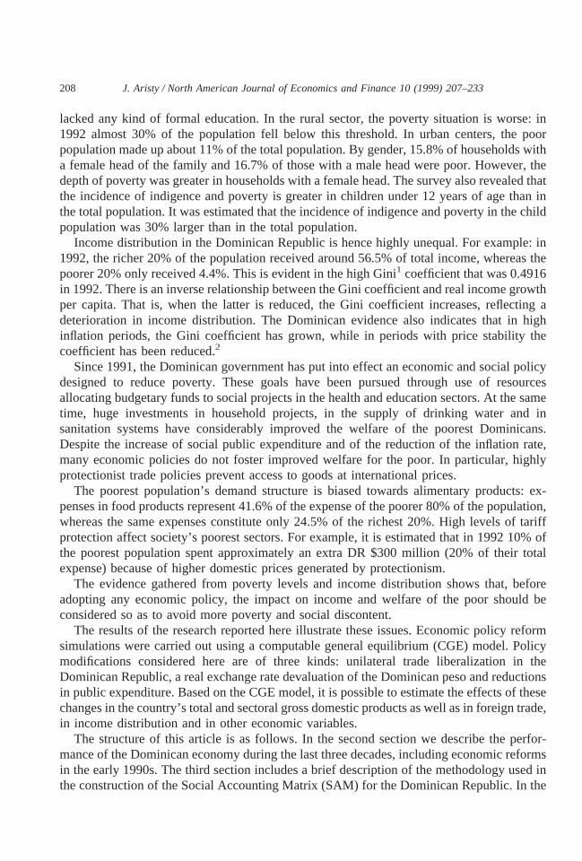
lacked any kind of formal education. In the rural sector, the poverty situation is worse: in1992 almost 30% of the population fell below this threshold. In urban centers, the poorpopulation made up about 11% of the total population. By gender, 15.8% of households witha female head of the family and 16.7% of those with a male head were poor. However, thedepth of poverty was greater in households with a female head. The survey also revealed thatthe incidence of indigence and poverty is greater in children under 12 years of age than inthe total population. It was estimated that the incidence of indigence and poverty in the childpopulation was 30% larger than in the total population.

Income distribution in the Dominican Republic is hence highly unequal. For example: in1992, the richer 20% of the population received around 56.5% of total income, whereas thepoorer 20% only received 4.4%. This is evident in the high Gini1 coefficient that was 0.4916in 1992. There is an inverse relationship between the Gini coefficient and real income growthper capita. That is, when the latter is reduced, the Gini coefficient increases, reflecting adeterioration in income distribution. The Dominican evidence also indicates that in highinflation periods, the Gini coefficient has grown, while in periods with price stability thecoefficient has been reduced.2

Since 1991, the Dominican government has put into effect an economic and social policydesigned to reduce poverty. These goals have been pursued through use of resourcesallocating budgetary funds to social projects in the health and education sectors. At the sametime, huge investments in household projects, in the supply of drinking water and insanitation systems have considerably improved the welfare of the poorest Dominicans.Despite the increase of social public expenditure and of the reduction of the inflation rate,many economic policies do not foster improved welfare for the poor. In particular, highlyprotectionist trade policies prevent access to goods at international prices.

The poorest population’s demand structure is biased towards alimentary products: ex-penses in food products represent 41.6% of the expense of the poorer 80% of the population,whereas the same expenses constitute only 24.5% of the richest 20%. High levels of tariffprotection affect society’s poorest sectors. For example, it is estimated that in 1992 10% ofthe poorest population spent approximately an extra DR $300 million (20% of their totalexpense) because of higher domestic prices generated by protectionism.

The evidence gathered from poverty levels and income distribution shows that, beforeadopting any economic policy, the impact on income and welfare of the poor should beconsidered so as to avoid more poverty and social discontent.

The results of the research reported here illustrate these issues. Economic policy reformsimulations were carried out using a computable general equilibrium (CGE) model. Policymodifications considered here are of three kinds: unilateral trade liberalization in theDominican Republic, a real exchange rate devaluation of the Dominican peso and reductionsin public expenditure. Based on the CGE model, it is possible to estimate the effects of thesechanges in the country’s total and sectoral gross domestic products as well as in foreign trade,in income distribution and in other economic variables.

The structure of this article is as follows. In the second section we describe the perfor-mance of the Dominican economy during the last three decades, including economic reformsin the early 1990s. The third section includes a brief description of the methodology used inthe construction of the Social Accounting Matrix (SAM) for the Dominican Republic. In the

208 J. Aristy / North American Journal of Economics and Finance 10 (1999) 207–233

fourth, we comment on the CGE’s general characteristics and the results of calibrating itsparameters. In the fifth, we present the results of the different simulations. Finally, thisdocument concludes with some economic policy suggestions.

2. Macroeconomic framework

2.1. Economic performance

Between 1970 and 1990, the Dominican economy experienced slow and unsteady growth.Inflation and foreign debt were rampant and social conditions deteriorated. From 1970 to1978, the country experienced rapid economic expansion, based up increased exports and bya growth in public investment. Despite the increase in public capital spending, publicfinances were balanced, making it easier for the Central Bank to control monetary aggre-gates. In fact, in these years, authorities kept a sensible monetary policy, coherent with priceand exchange rate stability.

In 1978 there was a change of government and of economic policy. Public expenditureexpanded, creating a public deficit that was unsustainable within a few years. It was easy forthe government to acquire foreign resources from petro-dollars recycled in the Europeanmarket. Authorities financed the public deficit by acquiring foreign debts. After 1980,however, because foreign borrowing has limits, authorities addressed the external accountsdeficit through import duties and quotas. The Central Bank expanded the money supply andstrong pressures on prices and the exchange rate began to be felt.

In 1982 there was a change in the government and in economic policy. Because macro-economic imbalances passed on by the previous administration could no longer be sustained,the new government turned to the International Monetary Fund (IMF). Between 1983 and1986, several IMF agreements were signed and carried out to achieve macroeconomicstability. After the 1983 Agreement, economic policy was inconsistent with price stabilityobjectives and the government’s economic team changed. After 1985, a new stabilizingprogram commenced in which a contractionary fiscal policy and restrictive monetary poli-cies, and devaluation of the official exchange rate were implemented. The effects of thesemeasures were notable: inflation rates fell, the free market exchange rate significantlyappreciated and net international reserves grew.

After 1986, the Dominican government launched a large public investment program,increasing domestic gross investment from 20.1% of the GDP in 1986 to 26.4% in 1987.Authorities executed fiscal policies to increase current savings to finance the public invest-ment program. The savings rate 3.4% of the GDP in 1986 rose to 7.0% in 1987. However,the amount of public investments was so great that a fiscal deficit of 5% of the GDP appearedin 1987. It was financed with resources from the Central Bank, from the Reserve Bank, andfrom foreign resources. The result was an increase in prices and significant exchange ratedepreciation. The average annual inflation rate rose to 22% in 1987 and reached a maximumof almost 80% in 1990. The free market exchange rate went from 2.90 peso per U.S. dollarin 1986 to 11.13 in 1990 and the official rate was devalued from 2.71 pesos per U.S. dollarto 12.50 during that same period. The rate of economic growth which accelerated between

209J. Aristy / North American Journal of Economics and Finance 10 (1999) 207–233

1986 and 1988 (for example, it had reached a rate of 7% in 1987), turned negative in 1990.In short, Dominican economy collapsed in 1990, when a 5% contraction of the real GDP wascombined with an inflation rate of 80%.

In September 1990, Dominican authorities started a new economic program. It includeda stabilizing structural adjustment package with the support of the United Nations Devel-opment Program (UNDP), and a 19-month “stand-by” agreement with the IMF, approved inAugust 1991. Stabilizing policies focused on monetary contraction and elimination of thefiscal deficit, subsidies and public price control.3 The effects were significant: inflation ratedropped to 4%, the rate of exchange of the local currency was stabilized in 12.50 pesos perdollar, and the real GDP revived with growth rate of approximately 7% in 1992 (the IMFrecognized that all its goals were satisfactorily achieved).

However, by the end of 1993 and at the beginning of 1994, Dominican authorities decidedto increase government expenditure. As a consequence, the total financial position of thepublic sector went from a 1.3% surplus of the GDP in 1992 to a 0.2% and 2.9% deficit in1993 and 1994, respectively.4 The requirements of this fiscal expansion provoked an increasein credits from the Central Bank to the public sector and in reduced international reserves(between 1993 and 1994, gross reserves decreased approximately by U.S. $350 million).Financial program goals became unattainable, there were pressures on the exchange rateleading to an expected devaluation, and there was an increase in interest rates. The currentaccount went from a deficit of 0.9% of the GDP in 1993 to a deficit of 1.4% in the followingyear. There was a massive outflow of capital and inflation rates rose to 14% in 1994. The realGDP in that year grew by 4.3% compared with 1993, the result of a boom in construction(mainly in the public sector), in tourism, mining, and communications.

In September 1994, after the presidential elections, the new Central Bank governorinstituted another stabilizing program that eliminated Central Bank financing of the budgetdeficit, thus forcing a fiscal deficit reduction. The official exchange rate was devalued by 3%,the interest rate of financial certificates issued by the Central Bank was increased and themonetary growth rate was reduced. The results of these measures were positive: price growthwas reduced, the exchange rate was stabilized and net international reserves started to grow.In 1995, the inflation rate was stabilized in 9.2%, real GDP growth was 4.8%, the currentaccount closed with a small deficit of U.S. $15.2 million, and short term capital outflow wasconsiderably reduced.

2.2. Economic reforms

Since 1990, the Dominican government has put a package of structural reforms into effect.Its main objective is to achieve a sustainable real annual growth of approximately 7% (thisgrowth must be noninflationary and compatible with a current account balance sustainable inthe long term).

In 1990, the government issued a Presidential Decree that contained the tariff reform. TheNational Congress approved it in 1993. Before September 1990, the trade regimen wascharacterized by high tariffs, fees, and import prohibitions. Tariff rates fluctuated between0% and 200%, creating very high protection levels for sectors catering to the domesticmarket. Also, many exemptions, incentive laws, administrative regulations, and special


decrees were included; this exacerbated the discriminatory characteristics of this traderegime.

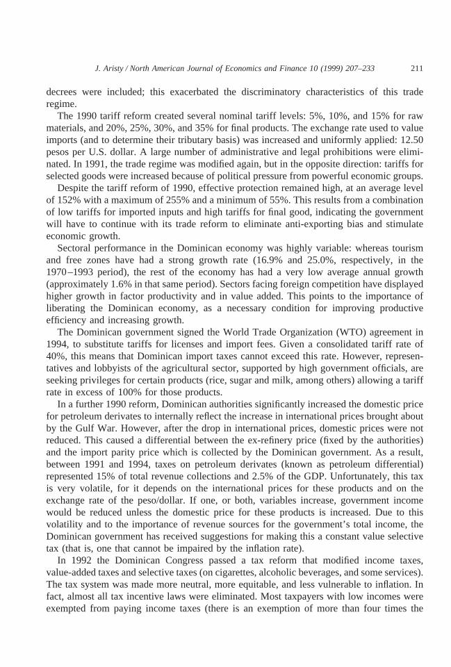
The 1990 tariff reform created several nominal tariff levels: 5%, 10%, and 15% for rawmaterials, and 20%, 25%, 30%, and 35% for final products. The exchange rate used to valueimports (and to determine their tributary basis) was increased and uniformly applied: 12.50pesos per U.S. dollar. A large number of administrative and legal prohibitions were elimi-nated. In 1991, the trade regime was modified again, but in the opposite direction: tariffs forselected goods were increased because of political pressure from powerful economic groups.

Despite the tariff reform of 1990, effective protection remained high, at an average levelof 152% with a maximum of 255% and a minimum of 55%. This results from a combinationof low tariffs for imported inputs and high tariffs for final good, indicating the governmentwill have to continue with its trade reform to eliminate anti-exporting bias and stimulateeconomic growth.

Sectoral performance in the Dominican economy was highly variable: whereas tourismand free zones have had a strong growth rate (16.9% and 25.0%, respectively, in the1970–1993 period), the rest of the economy has had a very low average annual growth(approximately 1.6% in that same period). Sectors facing foreign competition have displayedhigher growth in factor productivity and in value added. This points to the importance ofliberating the Dominican economy, as a necessary condition for improving productiveefficiency and increasing growth.

The Dominican government signed the World Trade Organization (WTO) agreement in1994, to substitute tariffs for licenses and import fees. Given a consolidated tariff rate of40%, this means that Dominican import taxes cannot exceed this rate. However, represen-tatives and lobbyists of the agricultural sector, supported by high government officials, areseeking privileges for certain products (rice, sugar and milk, among others) allowing a tariffrate in excess of 100% for those products.

In a further 1990 reform, Dominican authorities significantly increased the domestic pricefor petroleum derivates to internally reflect the increase in international prices brought aboutby the Gulf War. However, after the drop in international prices, domestic prices were notreduced. This caused a differential between the ex-refinery price (fixed by the authorities)and the import parity price which is collected by the Dominican government. As a result,between 1991 and 1994, taxes on petroleum derivates (known as petroleum differential)represented 15% of total revenue collections and 2.5% of the GDP. Unfortunately, this taxis very volatile, for it depends on the international prices for these products and on theexchange rate of the peso/dollar. If one, or both, variables increase, government incomewould be reduced unless the domestic price for these products is increased. Due to thisvolatility and to the importance of revenue sources for the government’s total income, theDominican government has received suggestions for making this a constant value selectivetax (that is, one that cannot be impaired by the inflation rate).

In 1992 the Dominican Congress passed a tax reform that modified income taxes,value-added taxes and selective taxes (on cigarettes, alcoholic beverages, and some services).The tax system was made more neutral, more equitable, and less vulnerable to inflation. Infact, almost all tax incentive laws were eliminated. Most taxpayers with low incomes wereexempted from paying income taxes (there is an exemption of more than four times the


minimum wage), income tax maximum rates were substantially reduced (from 73% to 25%)and excise taxes with a fixed basis were modified by ad-valorem based taxes. The value-added tax rate was increased from 6% to 8%.5

Despite internal tax reforms, the government still depends on 60% of foreign trade taxesand on the petroleum differential. Trade liberalization will require collections from domestictaxes to increase to compensate for reduced tariff revenues. Several tax rates will have toincrease (such as value-added tax rates and excise taxes on alcoholic beverages and tobaccorelated products). Simultaneously, it will be necessary to carry out a major reform to improvetax administration and domestic tax collection. (Evidence in this respect points to the needof strong political will to carry out reforms in the Dominican tributary administration).

Another important 1991 economic reform was monetary and financial. At the beginningof 1991, the Monetary Commission (Junta Monetaria) freed interest rates and new prudentialstandards were introduced to guarantee bank solvency and to reduce the probabilities of bankcrisis. Since the beginning of 1996, the discussion of the Monetary and Financial Codeproject was initiated in Congress; it would legalize many measures adopted by the MonetaryCommission between 1991 and 1996, and it would grant greater autonomy to the CentralBank.

The Dominican government recognizes a need to hasten the implementation of theeconomic reform package and it is expected that the new administration (in power sinceAugust 1996) will continue macroeconomic reforms started in this decade and put in practicethe pending ones. There is also need for a series of microeconomic reforms such as thoseinvolving capital markets, the pension system and social security, the promotion of com-petitiveness and the hydrocarbon market.

3. A SAM for the Dominican Republic

3.1. Introduction

The SAM for the Dominican Republic was constructed using information from the“supply and utilization” table (that includes an input/output table of 28 by 28 accounts)recently calculated by the Central Bank taking 1991 as the base year (Dominican RepublicCentral Bank: 1996). This information was grouped in thirteen sectors or economic activities.From this table we obtained intermediate consumption, value added by activity, indirecttaxes and final demand.

The supply and utilization table also provided information on international trade byactivity. In spite of this, it was necessary to use additional information to estimate tradeparticipation for each activity and region of the world. This information proceeded from theCentral Bank, National Statistics Office (NSO) and the IMF. The regions that were identifiedwere: the members of NAFTA, the Caribbean, the Central American Common Market,Europe, and the rest of the world.

On the other hand, data from institutional sectors (corporations, households, government,and the rest of the world) were used as they were estimated for that same year by the nationalaccounts department from the Central Bank. This information includes income and expense


accounts for each institutional sector. Given that the information provided by the CentralBank on income and expense by sector was not sufficiently detailed, information from someincome and expense surveys was used. The income and expense survey carried out by theFundacio´n Economı´a y Desarrollo in 1992 was used to estimate adequate participation thatallowed us to divide consumption and income by type of household (wage earner andcapitalist).

3.2. Description of the Dominican economy

In the Dominican SAM, we distinguish 13 activities or productive sectors, 3 productionfactors, and two kinds of households. The 13 productive sectors are: rice; crops for expor-tation; rest of the agricultural and stock-raising activities; mine and quarry exploitation; foodproduction; beverage production and tobacco; textiles; leather and shoes; petroleum; chem-icals and plastics; other industries; construction; hotels; and services. The three productivefactors are capital, urban labor, and rural labor. The types of households are: capitalists (thericher 20%) and wage earners (the poorer 80%).

The matrix exhibits basic characteristics of the Dominican economy; some of thisinformation is summarized in Table 1. The gross production demand originates mainly in thedomestic market (78.0%) whereas exports represent 22.0% of the gross product. Demand for

Table 1Dominican Republic economic structure 1991 thousands of millions of 1991 Dominican pesos

Sector ExportsE

DomesticgoodsDG

DomesticactivityDA

GrossproductX

ImportsM

Total supplyDC1MQ

Exports/grossproductE/X

Imports/total supplyM/Q

Rice 0.0 2.226 2.246 2.2457 0.0 2.226 0% 0%Farm exports 0.5731 3.699 3.513 4.0859 0.0252 3.724 14.03% 0.68%Rest of agriculture 0.4605 15.83 12.789 13.2491 1.2653 17.095 3.48% 7.40%Mining 0.0158 0.604 5.784 5.8002 0.2223 0.826 0.27% 26.90%Food production 3.8235 27.211 20.799 24.6225 3.0898 30.301 15.53% 10.20%Produc. of beverages

and cigars1.3294 6.908 5.617 6.9467 1.1508 8.059 19.14% 14.28%

Textiles, leather, andfootwear

19.9262 6.075 3.043 22.9694 15.2475 21.323 86.75% 71.51%

Petroleum 0.4677 6.756 5.479 5.9463 6.604 13.36 7.87% 49.43%Chemicals and

plastics0.0905 10.554 5.959 6.0496 6.2756 16.83 1.50% 37.29%

Other industries 12.0140 13.816 6.624 18.6385 16.1539 29.97 64.46% 53.90%Construction 0.0 12.810 12.808 12.8082 0.0 12.81 0% 0%Hotels 6.4257 4.159 4.373 10.7986 0.7229 4.882 59.50% 14.81%Services 2.2297 56.895 78.536 80.7387 2.3476 59.243 2.76% 3.96%

Source: Author’s estimates using data from the Social Accounting Matrix. Central Bank of the DominicanRepublic.


imports is higher than demand for exports by more than DR $5.7 thousand billion (1991pesos).

The weightiest sectors in the total gross product are: services (with a 37.6% participation),food production (11.5%), textiles, leather, and shoes (10.7%), other industries (8.7%), therest of the agricultural and stock-raising activities (6.2%), construction (6.0%), and hotels(5.0%). Capital value added is basically created by the service sector (53.4%), the rest of theagricultural and stock-raising activities (12.3%), food production (5.4%), and construction(5.1%). The value added of the work force—including rural and urban—is mainly created byservices (50.9%), textiles,leather, and shoes (8.8%), construction (8.7%), and food produc-tion (7.0%).

Regarding foreign trade, the sectors that have the most important participation in totalexports are: textiles, leather, and shoes (42.1%), other industries (25.4%), and hotels(13.6%). It is important to highlight the fact that textile and other industry exports arebasically related with free zone operation. This export structure reveals the deterioration oftraditionally exporting sectors whose importance as foreign currency sources has beengreatly diminished. For example, crops for exportation only represent 1.2% of total Domin-ican exports and the food producing sector—which includes sugar—8.1% (in 1995, Domin-ican sugar exports were drastically reduced as a result of the collapse of state sugarcorporations).

On the other hand, textile, leather, and shoe sectors, as well as other industries, areamong the activities with most imports. In fact, imports into the textile sector represent28.7% of total imports and imports in other industries represent 30.4%. Petroleumimports represent 12.4% and chemicals (including plastics) are equal to 11.8% of thetotal.

The structure of tributary collection is biased towards indirect taxes. In fact, tariffcollection represents 35.7% of total government income, whereas indirect domestic taxesrepresent 39.6%. Goods constituting the greater part of tariff collection are included in theother industries sector (57.0%), food production (13.6%), and chemicals (11.6%). Thissuggests that these products’ effective protection must be placed among the highest oneswithin Dominican economy. Concerning indirect domestic taxes, income originated bygoods in the petroleum sector represents 42.7% of this income (as expected from thepetroleum differential), other industries (31.2%), and alcoholic beverages and tobacco(12.9%). On the other hand, income taxes represent 23.6% of government income, fromwhich 56.1% is contributed by corporations and the remaining 43.9% by households(capitalist households pay 80% of income taxes and wage earners 20%).

The SAM also shows the structure of savings. Total savings in the Dominican economyduring 1991 were dominated by the public finance current account surplus originated by astabilizing policy implemented that year. Total domestic savings—including family remit-tances, which represent an important amount—were of DR $21.9 thousand billion. Theywere distributed in the following way: government, 36.7%, households, 33.9% and corpo-rations, 29.4% (capitalist households saved 75% of total domestic savings, whereas wageearner households saved 25%).


4. The general equilibrium model

The CGE model used in the Dominican case is based on models built by ShermanRobinson and associates for Cameroon and for the United States. (Robinson et. al). Adaptingthis model for the Dominican required adding some inter-institutional relationships that didnot exist in the base models. The CGE model assumes fixed capital, perfect competition,fixed factor supply, and full employment.

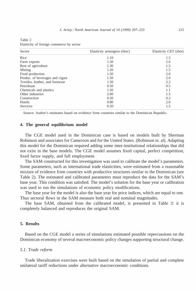
The SAM constructed for this investigation was used to calibrate the model’s parameters.Some parameters, such as international trade elasticities, were estimated from a reasonablemixture of evidence from countries with productive structures similar to the Dominican (seeTable 2). The estimated and calibrated parameters must reproduce the data for the SAM’sbase year. This condition was satisfied. The model’s solution for the base year or calibrationwas used to run the simulations of economic policy modifications.

The base year for the model is also the base year for price indices, which are equal to one.Thus sectoral flows in the SAM measure both real and nominal magnitudes.

The base SAM, obtained from the calibrated model, is presented in Table 3: it iscompletely balanced and reproduces the original SAM.

5. Results

Based on the CGE model a series of simulations estimated possible repercussions on theDominican economy of several macroeconomic policy changes supporting structural change.

5.1. Trade reform

Trade liberalization exercises were built based on the simulation of partial and completeunilateral tariff reductions under alternative macroeconomic conditions.

Table 2Elasticity of foreign commerce by sector

Sector Elasticity armington (rhoc) Elasticity CET (rhot)

Rice 1.10 1.5Farm exports 1.50 2.0Rest of agriculture 1.30 1.5Mining 1.20 1.5Food production 1.50 2.0Produc. of beverages and cigars 1.50 2.0Textiles, leather, and footwear 1.50 2.2Petroleum 0.50 0.5Chemicals and plastics 1.50 1.1Other industries 2.00 1.5Construction 0.20 0.2Hotels 0.80 2.0Services 0.50 1.5

Source: Author’s estimates based on evidence from countries similar to the Dominican Republic.

215J. Aristy / North American Journal of 10 (1999) 207–233

5.1.1. First case

The first closure to study the effects of trade liberalization assumes that governmentincome is flexible, that exchange rate and aggregate investment are fixed and that foreignsavings are flexible (results are shown in Tables 4 to 8).

Tariff reduction leads to an increment of the Dominican GDP (Table 4). Results show thatthe GDP growth rate increases with greater trade liberalization. The growth in GDP amounts0.58% at a zero tariff rate. This is not large and shows the short-term effect of trade reforms.

Table 3MCS base (in DR billions)

Goods Activity Valueadded

Institutions Families Government Capitalaccount

World Total

Goods 100.82 99.55 3.74 20.71 224.82Activity 167.53 47.34 214.87Value added 109.39 109.39Institutions 109.39 0.03 109.42Families 98.25 9.97 108.22Government 4.2 4.66 0.00 1.60 1.25 0.14 11.85Capital account 6.38 7.42 8.11 21.20 20.71World 53.09 3.18 56.28Total 224.82 214.87 109.39 109.41 108.22 11.85 20.71 56.28

Source: Calculated by the calibrated model.

Table 4Macroeconomic implications of a tariff reduction—fixed exchange rate and floating government revenue—(percentage change relative to the base)

Variable Tariff elimination100%

Tariff reduction60%

Tariff reduction40%

Tariff reduction20%

Exchange rate (EXR) 0.00 0.00 0.00 0.00GDP deflator (PINDEX) 0.00 0.00 0.00 0.00Current public consumption (GDTOT) 0.00 0.00 0.00 0.00Enterprise taxes (ENTTAX) 4.59 2.58 1.66 0.81Household taxes (HHTAX) 7.29 4.05 2.60 1.25Tariff revenue (TARIFF) 2100.00 256.44 236.58 217.80Indirect taxes (INDTAX) 0.44 0.18 0.10 0.04Government revenue (GR) 233.89 219.16 212.43 26.05Government savings (GOVSAV) 251.11 228.88 218.73 29.12Household savings (HHSAV) 7.27 4.03 2.59 1.25Enterprise savings (ENTSAV) 246.65 225.22 215.59 27.62Foreign savings (FSAV)a 5.97 3.28 2.10 1.45Total savings (SAVING) 22.99 21.83 21.23 20.62Total nominal investment (INVEST) 22.99 21.83 21.23 20.62Real GDP (RGDP) 0.58 0.33 0.21 0.10Total real exports (ESUM) 21.22 20.55 20.31 20.13Total real imports (MSUM) 10.59 5.92 3.82 1.85Total production (XTOT) 20.23 20.11 20.07 20.03Total private consumption (CDTOT) 6.38 3.58 2.31 1.12

* Total change (thousands millions of pesos)


It is well known that the most important effects are long term ones, through improvementsin efficiency and productivity due to greater competition. Because the model assumes fixedproduction factors, this impact of liberalization is a lower bound.

In general, trade reforms through tariff reduction (or tariff elimination) would increaseincome levels for both kinds of households: the wage earner household (the poorer 80%) andthe capitalist household (the richer 20%). One of the results of this reduction is that, withlower tariffs, income would be greater. However, the increment in capitalist income is greaterthan the one in wage earner income; in fact, a 100% reduction in tariffs would increase theformer’s income by 7.37% and the latter’s by 6.98% (Table 5). This means that in thisscenario—keeping a fixed exchange rate—income distribution will get worse after tariffreduction. At the same time, welfare—measured by level of consumption—for both kinds ofhouseholds will increase after tariff reduction. Again, the improvement in welfare will begreater for capitalist families (6.72%) than for wage earner families (5.83%, Table 6).

Reform brings about a trade deficit increase. This is caused by the strong increase inimports and the reduction of exports. The constant exchange rate along with tariff reductionwould cause a significant reduction in import prices (Table 7) promoting an increase in thelatters’ aggregate demand (10.59%). Imports growing the most are processed foods(37.27%), crops for exportation (33.31%), alcoholic beverages and cigarettes (15.05%), andother industries (15.03%). At the same time, exports for almost all activities decrease,reducing total exports by 1.22%. This is due to export price deterioration compared withdomestic prices. These actions explain the reduction in total production (Table 4). Thegreatest trade deficit is financed through foreign savings, which reveals that a fixed exchangerate policy is the same as using foreign capital to subsidize consumption, mainly that of thecapitalists.

Regarding employment and sectoral production, a reduction in tariffs has differentiatedeffects (Table 8): negative in the mining sector (employment is reduced by 7.47% and its

Table 5Impact of a tariff reduction on income—fixed exchange rate and floating government revenue—(percentagechange relative to the base)

Type of Household Tariff elimination100%

Tariff reduction60%

Tariff reduction40%

Tariff reduction20%

Wage earners 6.98 3.87 2.49 1.20Capitalist 7.37 4.09 2.63 1.27

Table 6Impact of a tariff reduction on households’ welfare—fixed exchange rate and floating government revenue—(percentage change relative to the base)

Type ofHousehold

Tariff elimination100%

Tariff reduction60%

Tariff reduction40%

Tariff reduction20%



GDP by 3.44%), in the textile sector (3.99% and 2.48%, respectively), in the hotel sector(3.72% and 1.59%), in chemicals (6.41% and 1.51%), and in crops for exportation (2.22%and 0.67%), and it has positive effects for other industries (their employment grows by1.56% and their GDP by 0.53%), for services (1.43% and 0.47%) and for the rest of theagricultural and stock-raising activities (1.22% and 0.19%).

Given that tariff income represents 30% of total public income, tariff reforms wouldsignificantly reduce this income. This—if government expenditure is assumed constant—would increase the fiscal deficit (or a reduction in public savings), which could not becompensated by an increase in indirect taxes (related with greater consumption) nor with

Table 7Sector implications of a tariff elimination—fixed exchange rate and floating governmentrevenue—(percentage change relative to the base)

Sector Grossproduction prices

Domesticactivity prices

Export prices Import prices

Rice 2.61 2.61 0.00 0.00Farm exports 1.54 1.79 0.00 215.95Rest of agriculture 4.04 4.18 0.00 23.61Mining 0.96 0.97 0.00 24.22Food production 2.71 3.19 0.00 215.64Produc. of beverages and cigars 2.43 2.99 0.00 25.15Textiles, leather, and footwear 20.07 20.51 0.00 21.97Petroleum 0.84 0.91 0.00 21.65Chemicals and plastics 21.29 21.30 0.00 27.22Other industries 22.91 28.56 0.00 212.92Construction 20.44 20.44 0.00 0.00Hotels 1.61 3.88 0.00 0.00Services 4.01 4.12 0.00 27.97

Table 8Sector implications of a tariff reduction—fixed exchange rate and floating government revenue—(percentagechange relative to the base)

Sector Employment Gross productX

Domestic supply(DA)

ExportsE

ImportsM

Rice 0.34 0.10 0.10 0.00 0.00Farm exports 22.22 20.67 20.18 23.67 33.31Rest of agriculture 1.22 0.19 0.40 25.59 11.15Mining 27.47 23.44 23.44 24.82 4.86Food production 20.04 20.02 0.92 25.22 37.27Produc. of beverages and cigar 0.73 0.18 1.28 24.22 15.05Textiles, leather, and footwear 23.99 22.48 23.42 22.34 2.20Petroleum 4.84 0.96 1.00 0.54 2.48Chemicals and plastics 26.41 21.51 21.53 20.10 11.94Other industries 1.56 0.53 28.11 5.08 15.03Construction 0.05 0.03 0.03 0.00 0.00Hotels 23.72 21.59 2.87 24.67 6.12Services 1.43 0.47 0.63 25.29 8.05


income taxes on households and corporations (both associated with higher income, Table 4).Both corporate savings and public savings suffer a reduction. This is not compensated by anincrease in foreign and household savings. This means that, since real investment is fixed, theeffect of trade liberalization in savings and in total nominal investment is negative.

5.1.2. Second case

In this simulation, public income is assumed fixed, the exchange rate is assumed flexibleand real aggregate investment fixed, as well as fixed foreign savings and total governmentexpenses (see results in Tables 9 to 13).

With tariff reduction or elimination, public income would be dramatically reduced. Toachieve fixed public income it is necessary for some other tax rate to increase: in this case,corporate taxes, which are the fiscal adjustment variable. This macroeconomic closure is not

Table 9Macroeconomic implications of a tariff reduction—floating exchange rate and fixed government revenue—(percentage change relative to the base)

Variable Tariff elimination100%

Tariff reduction60%

Tariff reduction40%

Tariff reduction20%

Exchange rate (EXR) 4.5 2.5 1.6 0.8GDP deflator (PINDEX) 0.0 0.0 0.0 0.0Current public consumption (GDTOT) 0.0 0.0 0.0 0.0Enterprise taxes (ENTTAX) 264.2 149.9 97.3 47.4Household taxes (HHTAX) 0.8 0.5 0.3 0.2Tariff revenue (TARIFF) 2100.0 256.7 236.8 217.9Indirect taxes (INDTAX) 2.8 1.6 1.0 0.5Government revenue (GR) 0.0 0.0 0.0 0.0Government savings (GOVSAV) 21.1 20.6 20.4 20.2Household savings (HHSAV) 0.8 0.5 0.3 0.2Enterprise savings (ENTSAV) 22.6 21.8 21.3 20.7Foreign savings (FSAV)* 0.0 0.0 0.0 0.0Total savings (SAVING) 21.2 20.8 20.5 20.3Total nominal investment (INVEST) 21.2 20.8 20.5 20.3Real GDP (RGDP) 0.36 0.21 0.14 0.07Total real exports (ESUM) 7.4 4.3 2.8 1.4Total real imports (MSUM) 6.9 4.0 2.6 1.3Total production (XTOT) 0.72 0.42 0.28 0.14Total private consumption (CDTOT) 0.3 0.2 0.1 0.1

* Total change (thousands of millions of pesos).

Table 10Impact of a tariff reduction on income—floating exchange rate and fixed government revenue—(percentagechange relative to the base)

Type of household Tariff elimination100%

Tariff reduction60%

Tariff reduction40%

Tariff reduction20%



feasible, since corporation owners would not be willing to face 50% to 250% increments intheir payments to the government (Table 9). Nevertheless, fixing foreign savings andgovernment income allows us to isolate their effects on welfare and, as a consequence, tostudy more rigorously the effects of trade liberalization on this important variable.

One of the model’s results is that the impact of tariff reductions on the real GDP is positiveand that it grows as the reduction deepens (by 0.36% when free trade means elimination ofimport taxes). The same happens with total gross production, though in this case, the impactis greater (e.g., it increases by 0.72% with total liberalization, Table 9). This last variable’sbehavior is the opposite of what resulted from fixing the exchange rate (first case). Thisshows that it is extremely important to choose an exchange rate policy that is consistent withincrements in economic activity.

The impact of trade reforms on wage earner and capitalist household incomes is positive.However, in this case the income increase for wage earners is greater (0.91%) than that ofthe capitalists (0.79%). This reveals that tariff reduction improves income distribution whenit includes a liberal exchange rate policy (Table 10). More so, results show that economicwelfare for both capitalist and wage earner households improves, but the latters’ do so at agreater rate (Table 11), which means that there is improvement in rent distribution while atthe same time there is a reduction in the level of poverty.

Table 11Impact of a tariff reduction on the households’ welfare—floating exchange rate and fixed governmentrevenue—(percentage change relative to the base)

Type of household Tariff elimination100%

Tariff reduction60%

Tariff reduction40%

Tariff reduction20%


Table 12Sectoral implications of a tariff reduction—floating exchange rate and fixed government revenue—(percentagechange relative to the base)

Sector Gross productionprices

Domestic activityprices

Exportprices

Importprices



In macroeconomic terms, a 100% tariff reduction would depreciate the Dominican pesoby 4.5% (Table 9). That depreciation would increase export prices (in domestic currency,Table 12) by the same percentage and it would tend to compensate the negative impact oftariff reduction on import prices (in domestic currency). Results show that a reduction inimport prices after tariff reforms would be much lower than the one observed in the first casewhen the exchange rate was kept constant. In this case, total imports would increase by6.85% (3.7 percentile points less than in the first case) and exports would increase by 7.41%(8.6 percentile points more than in the first case, Tables 8 and 13, respectively).

Due to the fact that public income is fixed, tariff reduction would imply a considerableincrease in corporate taxes (for example, by 264.23% with total liberalization) to compensatethe reduction in tributary income caused by trade reform. This extraordinary increment couldbe more realistically distributed by an increase in indirect tax rates and in household incometaxes. A tributary policy with fixed real government income and a fiscal policy that does notincrease its expenses, would cause a reduction in public savings of only 1.06% (Table 9). Ifthe adjustment were carried out only by increasing corporate taxes, the latter’s level ofsavings would deteriorate by 2.57%, in the case of total tariff elimination. This reductioncould not be compensated by an increase in household savings, so total savings would dropby about 1.18%, also reducing nominal investment by the same percentage. It is importantto note that the model assumes that real investment is fixed, so if this assumption wereeliminated, a greater contraction in investment could be expected because of the reduction indomestic savings.

Sectoral implications of tariff elimination are shown in Tables 12 and 13. Gross produc-tion and employment would increase in the textile sector (8.91% and 14.83%, respectively),other industries (3.91% and 11.89%), hotels (1.03% and 2.45%), and crops for exportation(0.36% and 1.21%); this is mainly caused by the increase in their exports. In general,increments in gross production and in employment will be greater with greater tariffreductions and, therefore, with a greater depreciation of the real exchange rate.

Table 13Sector implications of a tariff reduction—floating exchange rate and fixed government revenue—(percentagechange relative to the base)


Domestic supply(DA)

ExportsE

ImportsM

Rice 21.9 20.6 20.6 0.0 0.0Farm exports 1.2 0.4 20.7 6.9 22.1Rest of agriculture 20.3 20.1 20.3 6.1 0.1Mining 27.2 23.3 23.3 0.7 2.8Food production 21.5 20.6 21.7 5.2 21.4Produc. of beverages and cigars20.8 20.2 21.1 3.7 3.5Textiles, leather, and footwear 14.8 8.9 5.4 9.4 5.8Petroleum 24.7 21.0 21.1 0.1 21.3Chemicals and plastics 25.2 21.2 21.3 3.0 5.4Other industries 11.9 3.9 26.2 9.2 10.1Construction 20.1 0.0 0.0 0.0 0.0Hotels 2.5 1.0 21.4 2.7 23.0Services 23.2 21.0 21.1 1.5 2.2


5.2. Devaluation

In this section the results of devaluing the Dominican peso by 10%, 5%, and 2% aredescribed under two closing scenarios for the model. In the first, real aggregate investmentis fixed, foreign savings are flexible (therefore the exchange rate is fixed and it only movesexogenously through the devaluation policy), corporate savings rates are flexible, publicincome is endogenously determined and government expenses are fixed (results are shownin Tables 14 to 18). In the second scenario, real aggregate investment is allowed to bedetermined endogenously and, to achieve macroeconomic balance, corporate savings ratesare fixed (Tables 19 to 23).

5.2.1. First case

Devaluation causes a depression of the GDP, which emerges mostly from the reduction ofimports caused by this measure (Table 14). In fact, the depreciation of the exchange rate will

Table 14Macroeconomic implications of a devaluation—real investment fixed—(percentage change relative to thebase)

Variable Devaluation15%

Devaluation10%

Devaluation5%

Devaluation2%

Exchange rate (EXR) 15.00 10.00 5.00 2.00GDP deflator (PINDEX) 0.00 0.00 0.00 0.00Current public consumption (GDTOT) 0.00 0.00 0.00 0.00Enterprise taxes (ENTTAX) 23.95 22.37 21.07 20.41Household taxes (HHTAX) 225.06 215.60 27.32 22.82Tariff revenue (TARIFF) 24.19 22.34 20.98 20.35Indirect taxes (INDTAX) 7.60 5.30 2.75 1.12Government revenue (GR) 21.50 20.59 20.13 20.01Government savings (GOVSAV) 0.32 0.53 0.40 0.19Household savings (HHSAV) 224.97 215.54 27.29 22.81Enterprise savings (ENTSAV) 410.11 256.92 121.25 46.90Foreign savings (FSAV)* 219.99 213.04 26.42 22.55Total savings (SAVING) 6.11 4.23 2.17 0.88Total nominal investment (INVEST) 6.11 4.23 2.17 0.88Real GDP (RGDP) 21.10 20.59 20.24 20.08Total real exports (ESUM) 31.94 20.56 9.97 3.92Total real imports (MSUM) 29.71 26.59 23.38 21.38Total production (XTOT) 3.06 2.09 1.07 0.43Total private consumption (CDTOT) 222.38 214.21 26.83 22.68


Table 15Impact of a devaluation on income—real investment fixed—(percentage change relative to the base)

Type of household Devaluation15%

Devaluation10%

Devaluation5%

Devaluation2%

Wage earner 223.61 214.66 26.86 22.64Capitalist 225.43 215.83 27.43 22.87


cause a comparable increase in domestic prices for imports (Table 17); therefore, importswill undergo a reduction. On the other hand, exports grow as their domestic prices do thesame because of the peso depreciation. The net result these movements have on foreign tradeis a trade deficit reduction.

Sectors with the higher growth rates of exports are: textiles, rest of the agricultural andstock-raising activities, crops for exportation, food production, alcoholic beverages andtobacco, hotels and other industries. On the other hand, sectors with the most drastic dropsin imports include hotels, rest of the agricultural and stock-raising activities, food production,services and other industries (Table 18).

The pronounced effects of a devaluation can be seen even for the case of a 5% devalu-ation. In fact, in this case, the balance of trade would go from a DR $9.9 thousand billiondeficit to a DR $6.3 thousand billion surplus. Because of this reduction, foreign savingswould decrease (there would be an outflow of capital from the country or an accumulationof international reserves of more than DR $6 thousand billion).

Because the closure assumes that real investment is constant, corporate savings wouldhave to increase dramatically to compensate the reduction in foreign savings, for otherwiseit would be impossible to keep real investment constant. In the 5% devaluation scenario,corporate savings would increase by 121.25%. This means that less transferences towards

Table 17Sector implications of a 10% devaluation—real investment fixed—(percentage change relative to the base)

Sector Grossproduction prices

Domesticactivity prices

Export prices Import prices


Table 16Impact of a devaluation on households’ welfare—real investment fixed—(percentage change relative to thebase)

Type of household Devaluation15%

Devaluation10%

Devaluation5%

Devaluation2%

Wage earner 220.83 213.15 26.29 22.45Capitalist 223.96 215.22 27.32 22.87


households would be made, both for capitalist and for wage earner households, which meansa reduction in household income and consumption. In fact, in this case, wage earner incomewould be reduced by 6.86% and capitalist income by 7.43% (Table 15). Simultaneously,economic welfare—measured as real consumption—of wage earner and capitalist familieswould drop by 6.29% and by 7.32%, respectively (Table 16).

In macroeconomic terms, total private consumption would be reduced by 6.83% with a

Table 18Sector implications of a 10% devaluation—fixed real investment—(percentage change relative to the base)


Domestic supply(DA)

ExportsE

ImportsM

Rice 25.27 21.63 21.63 0.00 0.00Farm exports 9.31 2.69 21.32 25.79 217.86Rest of agriculture 24.26 20.69 21.97 31.47 222.21Mining 0.29 0.13 0.09 13.13 24.52Food production 23.49 21.42 27.05 26.81 225.96Produc. of beverages and cigars 23.63 20.91 26.27 20.16 222.45Textiles, leather, and footwear 47.73 27.23 22.30 27.98 9.18Petroleum 221.50 24.78 25.05 21.72 28.59Chemicals and plastics 2.07 0.47 0.37 6.90 212.89Other industries 23.52 7.48 4.62 9.03 29.43Construction 20.31 20.15 20.15 0.00 0.00Hotels 16.09 6.48 210.69 17.40 220.12Services 211.45 23.91 24.53 16.73 212.93

Table 19Macroeconomic implications of a devaluation—floating real investment—(percentage change relative to thebase)

Variable 10% 5% 2%

Exchange rate (EXR) 10.00 5.00 2.00GDP deflator (PINDEX) 0.00 0.00 0.00Current public consumption (GDTOT) 0.00 0.00 0.00Enterprise taxes (ENTTAX) 22.17 20.92 20.34Household taxes (HHTAX) 20.10 0.01 0.02Tariff revenue (TARIFF) 211.20 25.68 22.31Indirect taxes (INDTAX) 2.31 1.05 0.40Government revenue (GR) 23.25 21.67 20.68Government savings (GOVSAV) 22.44 21.53 20.68Household savings (HHSAV) 20.07 0.03 0.02Enterprise savings (ENTSAV) 22.17 20.92 20.34Foreign savings (FSAV)* 219.24 29.50 23.79Total savings (SAVING) 2100.00 248.59 218.86Total nominal investment (INVEST) 2100.00 248.59 218.86Real GDP (RGDP) 21.00 20.44 20.17Total real exports (ESUM) 23.03 10.87 4.22Total real imports (MSUM) 215.95 28.34 23.44Total production (XTOT) 2.53 1.20 0.47Total private consumption (CDTOT) 0.83 0.17 0.02



devaluation of only 5%. Due to the high percentage of private consumption in the GDP, thisbehavior would cause a reduction in the real GDP. Total production would expand due to anextraordinary increase in exports (Table 14). Textiles, hotels and other industries would bethe sectors with greater growth in total production. Sectoral demand for work would movein the same direction (Table 18).

Tributary income would decrease because of the drop in household and corporate incometaxes and because of a slight reduction in income proceeding from tariffs. Due to grossproduction increments, indirect taxes would increase, but their growth would not be enoughto compensate a reduction in other public income sources, so their total level would bereduced. Because expenditure is kept constant, the situation would result in a deteriorationof public savings (Table 14).

5.2.2. Second case

In a case where aggregate real investment is endogenously determined and corporatesavings rates are fixed, devaluation, again would tend to reduce the trade deficit, increasingwith exports and diminishing with imports (Table 19). In the 5% devaluation scenario, thebalance of trade would go from a deficit of DR $9.5 thousand billion to a zero balance. Thisis mainly explained because of the increase in exports of: textiles, food production, crops forexportation, services, hotels, alcoholic beverages and tobacco, and the rest of agricultural andstock-raising activities. Total exports would increase by 10.87%. On the other hand, totalimports would be reduced by 8.34% due to the contraction in import demand in the rest ofthe agricultural and stock–raising activities, in other industries and in alcoholic beveragesand tobacco (Table 23). The new balance of the balance of trade would reduce foreignsavings demand by more than DR $9.50 thousand billion. This result, along with the drop inpublic savings, would reduce the level of total savings, as well as the level of totalinvestment, by almost 50%. The real GDP would be reduced by 0.44%, but future growth canalso be expected to drop due to contractions in investment. This shows that this scenario isworse than the first in terms of growth capability evolution (Table 19). From another point

Table 20Impact of a devaluation on income—floating real investment—(percentage change relative to the base)

Type ofhousehold

10% 5% 2%

Wage earner 0.38 0.25 0.11Capitalist 20.22 20.05 20.01

Table 21Impact of a devaluation on households’ welfare—floating real investment—(percentage change relative to thebase)

Type of household 10% 5% 2%

Wage earner 1.27 0.41 0.12Capitalist 0.34 20.06 20.07


of view, impact on income and economic welfare is better for wage earner families than forcapitalist ones. In fact, income for wage earners would increase by 0.25% whereas incomefor capitalist households would be reduced by almost 0.05%. Simultaneously, economicwelfare would improve for most of the wage earner households (0.41%) and would deteri-orate for capitalist ones (Tables 20 and 21).

On the other hand, the contraction in imports resulting from devaluation would decreaseincome through tariffs. Increments in indirect and household taxes could not compensate areduction in tariff income, so total public income would contract. Given that total govern-ment expenditure is fixed, this latter’s savings would be reduced (Table 19).

Table 22Sector implications of a 10% devaluation—floating real investment—(percentage change relative to the base)



Exportprices

Importprices

Domestic goodsprices

Rice 0.00 0.00 0.00 0.00 0.00Farm exports 1.52 0.00 10.00 10.00 20.37Rest of agriculture 0.37 0.00 10.00 10.00 21.66Mining 0.03 0.00 10.00 10.00 0.00Food production 1.68 0.00 10.00 10.00 21.48Produc. of beverages and cigars 2.07 0.00 10.00 10.0021.33Textiles, leather, and footwear 8.79 0.00 10.00 10.0022.99Petroleum 0.80 0.00 10.00 10.00 20.75Chemicals and plastics 0.16 0.00 10.00 10.0022.14Other industries 6.61 0.00 10.00 10.00 21.88Construction 0.00 0.00 0.00 0.00 20.00Hotels 6.18 0.00 10.00 10.00 0.00Services 25.49 25.99 10.00 10.00 25.64

Table 23Sector implications of a 10% devaluation—floating real investment—(percentage change relative to the base)


Domestic supply(DA)

ExportsE

ImportsM



5.3. Fiscal restriction

The impact of reductions in public spending of 5% to 25% on the Dominican Republic isevaluated under two macroeconomic frameworks. In the first one, we assume a flexibleexchange rate, flexible foreign savings, an unchanging real investment, flexible publicsavings and fixed income, but income tax rates on corporations are flexible (results are inTables 24 to 28). The second case can be distinguished from the first because its closure isbased on the fact that exchange rate is the adjustment variable and foreign savings are fixed(Tables 29 to 33).

5.3.1. First case

A reduction in government spending would cause an increase in the country’s totalproduction, though a very slight one (Table 24). Given that public income levels remain

Table 24Macroeconomic implications of a government spending reduction—fixed exchange rate—(percentage changerelative to the base)

Variable 25% 20% 15% 10% 5%

Exchange rate (EXR) 0.00 0.00 0.00 0.00 0.00GDP deflator (PINDEX) 0.00 0.00 0.00 0.00 0.00Current public consumption (GDTOT) 225.00 220.00 215.00 210.00 25.00Enterprise taxes (ENTTAX) 23.76 23.01 22.26 21.51 20.76Household taxes (HHTAX) 1.20 0.96 0.72 0.48 0.24Tariff revenue (TARIFF) 0.52 0.41 0.31 0.21 0.10Indirect taxes (INDTAX) 0.45 0.36 0.27 0.18 0.09Government revenue (GR) 0.00 0.00 0.00 0.00 0.00Government savings (GOVSAV) 11.82 9.47 7.11 4.74 2.37Household savings (HHSAV) 1.19 0.96 0.72 0.48 0.24Enterprise savings (ENTSAV) 219.05 215.27 211.47 27.66 23.84Foreign savings (FSAV)* 0.18 0.15 0.11 0.08 0.04Total savings (SAVING) 20.07 20.06 20.04 20.03 20.01Total nominal investment (INVEST) 20.07 20.06 20.04 20.03 20.01Real GDP (RGDP) 0.03 0.02 0.02 0.01 0.01Total real exports (ESUM) 0.29 0.23 0.17 0.11 0.06Total real imports (MSUM) 0.59 0.47 0.35 0.24 0.12Total production (XTOT) 0.13 0.10 0.08 0.05 0.03Total private consumption (CDTOT) 1.16 0.93 0.69 0.46 0.23


Table 25Impact of a government spending reduction on income—fixed exchange rate—(percentage change relative tothe base)

Type ofhousehold

25% 20% 15% 10% 5%

Wage earner 1.16 0.93 0.70 0.47 0.23Capitalist 1.21 0.97 0.73 0.48 0.24


fixed, a reduction in its expense would increase its current savings. In the scenario of a 25%reduction in expenditure, public savings would increase by around 11.82%. This incrementwould mean that the economy would have more resources to invest, but since it has beenassumed that real investment is fixed, corporate savings would have to be reduced (througha reduction in corporate savings rates). In fact, in this scenario, corporate savings woulddecrease by 19.05%, which would mean that a greater amount of resources would betransferred to families.

With a 25% reduction in public expenditure, wage earner, and capitalist households wouldexperiment an increase in their income: for the first group it would increase by 1.16% andin the second group by 1.21% (Table 25). This would allow an increase in household incometax collection of 1.20%. However, economic welfare—measured based on real consump-tion—would improve by 1.07% and by 1.22% in wage earner and capitalist households,respectively (Table 26). The final result is an increase in total private consumption of 1.16%and in gross production of 0.13%. Domestic production and employment would increase inall sectors except in services and construction because in both these sectors, there is a greatinfluence of government current expenditure. Despite this, the real GDP remains relativelyconstant (0.03%).

Increments in consumption would promote import demand, which would rise by 0.59%.Given the increase in exports (0.29%), a deterioration in the balance of the balance of trade

Table 26Impact of a government spending reduction on households’ welfare—fixed exchange rate—(percentagechange relative to the base)

Type of household 25% 20% 15% 10% 5%

Wage earners 1.07 0.86 0.64 0.43 0.22Capitalist 1.22 0.98 0.74 0.49 0.25

Table 27Sector implications of a 25% government spending reduction—fixed exchange rate—(percentage changerelative to the base)



Exportprices

Importprices

Rice 1.46 1.46 0.00 0.00Farm exports 1.32 1.53 0.00 0.00Rest of agriculture 1.76 1.78 0.00 0.00Mining 20.26 20.26 0.00 0.00Food production 0.72 0.85 0.00 0.00Produc. of beverages and cigars 0.52 0.64 0.00 0.00Textiles, leather, and footwear 0.02 0.16 0.00 0.00Petroleum 0.06 0.06 0.00 0.00Chemicals and plastics 0.59 0.60 0.00 0.00Other industries 0.07 0.18 0.00 0.00Construction 20.19 0.00 0.00Hotels 0.14 0.34 0.00 0.00Services 20.59 20.61 0.00 0.00


is expected and therefore a greater demand of foreign savings (0.18 thousand billion 1991pesos, Table 28). The greatest level of imports and gross production will be reflected in anincrease in tariff incomes (0.52%) and in indirect taxes (0.45%). Since public income isfixed, corporate tax rates are lower, because their obligations with tax collectors are reducedby 3.76% (Table 24).

Table 28Sector implications of a 25% government spending reduction—fixed exchange rate—(percentage changerelative to the base)


Domestic supply(DA)

ExportsE

ImportsM


Table 29Macroeconomic implications of a reduction in government spending—flexible exchange rate—(percentagechange relative to the base)

Variable 25% 20% 15% 10% 5%

Exchange rate (EXR) 0.14 0.11 0.09 0.06 0.03GDP deflator (PINDEX) 0.00 0.00 0.00 0.00 0.00Current public consumption (GDTOT) 225.00 220.00 215.00 210.00 25.00Enterprise taxes (ENTTAX) 23.78 23.03 22.28 21.52 20.76Household taxes (HHTAX) 1.00 0.80 0.60 0.40 0.20Tarriffs revenue (TARIFF) 0.49 0.39 0.30 0.20 0.10Indirect taxes (INDTAX) 0.53 0.42 0.32 0.21 0.11Government revenue (GR) 0.00 0.00 0.00 0.00 0.00Government savings (GOVSAV) 11.83 9.48 7.12 4.75 2.38Household savings (HHSAV) 1.00 0.80 0.60 0.40 0.20Enterprise savings (ENTSAV) 215.91 212.74 29.57 26.38 23.20Foreign savings (FSAV)* 0.00 0.00 0.00 0.00 0.00Total savings (SAVING) 20.01 20.01 0.00 0.00 0.00Total nominal investment (INVEST) 20.01 20.01 0.00 0.00 0.00Real GDP (RGDP) 0.02 0.02 0.01 0.01 0.01Total real exports (ESUM) 0.56 0.45 0.34 0.22 0.11Total real imports (MSUM) 0.49 0.39 0.29 0.20 0.10Total production (XTOT) 0.16 0.13 0.09 0.06 0.03Total private consumption (CDTOT) 0.97 0.78 0.58 0.39 0.19



In sectoral terms, a 25% contraction in public expenditure would cause an increase ingross production in all sectors, except for services (20.21%), crops for exportation(20.15%) and construction (20.01%). Employment demand in those sectors would alsohave similar behavior (Table 28).

5.3.2. Second case

A reduction in government spending in an economy with flexible exchange rate and fixedforeign savings will tend to devalue the Dominican peso (Table 29). In the scenario of a 25%reduction in expense, export totals would rise by 0.56% (more than in the first case) andimports would increase by 0.49% (lower than in the first case), due to exchange ratedevaluation (0.14%).

The real GDP would increase in a similar percentage as the one where the exchange rateis assumed fixed. However, gross production would result in a slightly higher incrementbecause of export expansion.

Sectors that yield greater growth rates in exports are: textiles (1.23%), services (0.89%),and mine and quarry exploitation (0.70%). Also, those that have the worse exportingperformance are crops for exportation (22.41%) and the rest of the agricultural and stock-raising activities (22.14%). This behavior can be explained by the deterioration in exportprices compared with the domestic ones for these activities (Tables 33 and 32). Regardingimport demand, all sectors had positive rates, except for mines and quarries (20.16%) andservices (21.05%, Table 33).

With fixed public income, the reduction in public spending would result in an increase ingovernment savings of 11.83%. With this result, and the fact that real investment is fixed, thelevel of corporate savings must be reduced to keep a balance between savings and investment(Table 29). In this case, corporate savings would be reduced by 15.91%, which would implya greater transfer of resources to households and an increase in their consumption, andwelfare, levels (Table 31).

Table 30Impact of a reduction in government spending on income—flexible exchange rate—(percentage changerelative to the base)



Table 31Impact of a reduction in government spending on the welfare of households—flexible exchangerate—(percentage change relative to the base)




6. Conclusions

By analyzing the results yielded by the simulations, several interesting conclusions for theDominican case may be drawn regarding economic policy.

In the first place, trade reforms have a positive impact in the country’s economy. In fact,in both closure scenarios concerning tariff liberalization policies (fixed public income-flexible exchange rate and flexible public income-fixed exchange rate), tariff reduction wouldcause the GDP to grow, as well as factor income and household welfare (both for wageearners and for capitalists). We should note that these results can only be considered for the

Table 32Sector outcomes due to a 25% government spending reduction—flexible exchange rate—(percentage changerelative to the base)

Sector Production pricesgross

Activity pricesdomestic

Exportsprices

Importsprices

Rice 1.38 1.38 0.00 0.00Farm exports 1.31 1.50 0.14 0.14Rest of agriculture 1.60 1.65 0.14 0.14Explo. of mines and canteras 20.23 20.23 0.14 0.14Food production 0.68 0.78 0.14 0.14Produc. of beverages and cigars 0.52 0.61 0.14 0.14Textiles, leather, and footwear 0.16 0.26 0.14 0.14Petroleum 0.11 0.11 0.14 0.14Chemicals and plastics 0.66 0.66 0.14 0.14Other industries 0.19 0.28 0.14 0.14Construction 20.14 20.14 0.00 0.00Hotels 0.20 0.29 0.14 0.14Services 20.63 20.65 0.14 0.14

Table 33Sector outcomes due to a 25% government spending reduction—flexible exchange rate—(percentage changerelative to the base)


Domestic offer(DA)

ExportsE

ImportsM

Rice 0.83 0.25 0.25 0.00 0.00Farm exports 20.41 20.12 0.25 22.41 2.10Rest of agriculture 0.05 0.01 0.09 22.14 1.23Explo. of mines and canteras 0.31 0.14 0.14 0.70 20.16Food production 0.68 0.27 0.47 20.81 0.90Produc. of beverages and cigars 1.40 0.35 0.53 20.41 0.82Textiles, leather, and footwear 2.05 1.26 1.50 1.23 0.99Petroleum 1.15 0.23 0.23 0.25 0.19Chemicals and plastics 1.78 0.41 0.41 20.16 0.61Other industries 1.34 0.46 0.59 0.38 0.18Construction 20.03 20.01 20.01 0.00 0.00Hotels 0.83 0.35 0.53 0.22 0.72Services 20.80 20.26 20.29 0.89 21.05


short term, so a greater economic growth rate can be expected in the long term along withgreater general welfare.

Another important conclusion is the need to allow exchange rate depreciation in the tradeliberalization process. This would help avoid using foreign savings for financing the deficitof trade emerging from an increase in imports (because of the reduction in their prices) andthe decrease in exports (because of the deterioration of export prices compared with domesticprices). If the exchange rate were kept fixed, this would be the same as subsidizingconsumption with foreign capital. The depreciation of the Dominican peso would tend tocompensate the negative impact caused by tariff reduction on import prices and it would riseexport prices (in domestic currency), so the trade deficit would be reduced.

Besides, the depreciation of the real exchange rate in a trade liberalization framework willhave positive impacts on family incomes. In the case of fixed exchange rates, the reductionin tariffs would cause an increase in both kinds of households, but capitalist householdswould be the most benefited, which means that rent distribution would be worse. In contrast,if trade liberalization were carried out in a flexible exchange rate framework, the depreciationof the Dominican peso would benefit wage earner families more, which would improve rentdistribution and, therefore, it would tend to diminish the poverty level.

If we analyze the positive impacts of trade liberalization on the Dominican economy andthe redistributive impacts of this reform when a free fluctuation of the exchange rate isincluded, we can see from the results in the second group of simulations that devaluation, byitself, is not convenient. This is due to the fact that devaluation depresses the economy andit reduces income and welfare in Dominican households (when investment is kept fixed) orit only has a slight positive impact on wage earner household incomes (when investment isallowed to vary).

An internal tax reform is necessary to compensate the drop in tariff income, whichrepresents more than one third of total public income. Tariff reforms would considerablyreduce the public sector’s income, which would increase the fiscal deficit that could not becompensated by a greater tax collection from other taxes unless tributary rates were modified.This is why it is advisable to increase indirect taxes (excise and value-added taxes). It wouldalso be necessary to implement a reform within the administrative processes that would helpreduce the high levels of fiscal evasion.

Finally, it is indispensable that domestic savings increase, so the government shouldimplement policies that promote private savings. Developing a modern pension systemwould considerably increase propensity to save, which would result in a greater capitalaccumulation and economic growth. This would allow a reduction in the levels of povertyand it would improve democratic conditions in the Dominican Republic.

Notes

1. This coefficient measures the degree of inequality in rent distribution: if its value isequal to zero, there is perfect equality and if it is equal to one then there is a totallyunequal rent distribution.

2. In fact, the inflationary policy adopted during the second half of the 1980s caused a


deterioration in the country’s income distribution and the Gini coefficient went from0.4679 in 1986 to 0.5544 in 1989. In contrast, from 1990 on, rent distribution hasimproved due to the implementation of economic reforms and price stability.

3. For example, fuel prices were more than doubled in the August–December period in1990.

4. Changes in economic policy orientation can be explained by the political cyclegenerated by presidential elections in 1994 (election years generally turn into years ofexpansion in public expenditure and, therefore, a loss in macroeconomic balance).

5. Despite this increase, the value-added tax rate in the Dominican Republic is still oneof the lowest rates in Latin America, where the average is 15%.

References

Dauhajre, A., J. Ache´cor, A. Swindale, 1994,Estabilizacion, apertura y pobreza en la Repu´blica Dominicana,1986–1992, Santo Domingo.

Banco Central de la Repu´blica Dominicana: 1996.Cuentas Nacionales de la Repu´blica Dominicana, 1991–1994.Robinson, S., M. Kilkenny, J. Hanson, 1990, The USDA/ERS Computable General Equilibrium Model of the

U.S., U.S. Department of Agriculture and Economic Research Service.

233J. Aristy / North American Journal of 10 (1999) 207–233

Dominican Republic: A CGE Analysis

Documents

Transcript of Dominican Republic: A CGE Analysis