Population Growth Rates of Reef Sharks with and without Fishing on the Great Barrier Reef: Robust...

Population Growth Rates of Reef Sharks with andwithout Fishing on the Great Barrier Reef: RobustEstimation with Multiple ModelsMizue Hisano1*, Sean R. Connolly1,2, William D. Robbins1

1 School of Marine and Tropical Biology, James Cook University, Townsville, Australia, 2 ARC Centre of Excellence for Coral Reef Studies, James Cook University, Townsville,

Australia

Abstract

Overfishing of sharks is a global concern, with increasing numbers of species threatened by overfishing. For many sharks,both catch rates and underwater visual surveys have been criticized as indices of abundance. In this context, estimation ofpopulation trends using individual demographic rates provides an important alternative means of assessing populationstatus. However, such estimates involve uncertainties that must be appropriately characterized to credibly and effectivelyinform conservation efforts and management. Incorporating uncertainties into population assessment is especiallyimportant when key demographic rates are obtained via indirect methods, as is often the case for mortality rates of marineorganisms subject to fishing. Here, focusing on two reef shark species on the Great Barrier Reef, Australia, we estimatednatural and total mortality rates using several indirect methods, and determined the population growth rates resulting fromeach. We used bootstrapping to quantify the uncertainty associated with each estimate, and to evaluate the extent ofagreement between estimates. Multiple models produced highly concordant natural and total mortality rates, andassociated population growth rates, once the uncertainties associated with the individual estimates were taken intoaccount. Consensus estimates of natural and total population growth across multiple models support the hypothesis thatthese species are declining rapidly due to fishing, in contrast to conclusions previously drawn from catch rate trends.Moreover, quantitative projections of abundance differences on fished versus unfished reefs, based on the populationgrowth rate estimates, are comparable to those found in previous studies using underwater visual surveys. These findingsappear to justify management actions to substantially reduce the fishing mortality of reef sharks. They also highlight thepotential utility of rigorously characterizing uncertainty, and applying multiple assessment methods, to obtain robustestimates of population trends in species threatened by overfishing.

Citation: Hisano M, Connolly SR, Robbins WD (2011) Population Growth Rates of Reef Sharks with and without Fishing on the Great Barrier Reef: RobustEstimation with Multiple Models. PLoS ONE 6(9): e25028. doi:10.1371/journal.pone.0025028

Editor: Mark S. Boyce, University of Alberta, Canada

Received March 15, 2011; Accepted August 25, 2011; Published September 23, 2011

Copyright: � 2011 Hisano et al. This is an open-access article distributed under the terms of the Creative Commons Attribution License, which permitsunrestricted use, distribution, and reproduction in any medium, provided the original author and source are credited.

Funding: This work was supported by the Australian Research Council and James Cook University. The funders had no role in study design, data collection andanalysis, decision to publish, or preparation of the manuscript.

Competing Interests: The authors have declared that no competing interests exist.

* E-mail: [email protected]

Introduction

There is mounting evidence of widespread, substantial, and

ongoing declines in the abundance of shark populations world-

wide, coincident with marked rises in global shark catches in the

last half-century [1–3]. In some cases, these declines have been

linked to resultant trophic cascades [1,4]. Consequently, overfish-

ing of sharks is now recognized as a major global conservation

concern [5], with increasing numbers of shark species added to the

International Union for the Conservation of Nature’s list of

threatened species [6]. However, our knowledge of the status of

many shark populations is limited due to lack of, or ambiguous

data [7].

On coral reefs, apex predators, including medium-sized reef

sharks, can make up a large proportion of fish biomass in the

absence of fishing [8,9]. Food web models suggest that they also

are strongly interacting: per capita, they have relatively strong

effects on other species in the community [10]. However,

evaluating population trends for reef shark species, like that of

many sharks, is complicated by several factors that make trends in

reported catch and catch rate data unreliable indicators of fishing

mortality or abundance. Firstly, many countries with significant

coral reefs do not have extensive and reliable reporting of total

catches, or of fishing effort [11], both of which are required to

obtain fisheries-based indices of abundance. Indeed, even where

catch and effort data are available, there is often little information

about covariates needed to standardize the catch-effort relation-

ship, such as changes in gear types or targeting behavior of the

fishery. Secondly, a large proportion of the global catch consists of

illegal (and therefore unreported) shark finning: a recent estimate

based on fin-trade data identified 75% of the global shark catch

as illegal and unreported [12]. Reef sharks are a small, but

acknowledged part of such catches [13,14]. Such activity can even

occur in intensively managed reef systems (Figure 1). Thirdly,

sharks may be caught as bycatch in fisheries targeting other

species; often these sharks are not reported at the species level [3],

or are killed and discarded at sea, and not recorded as catch

[7,15]. Finally, robust inference of population trends from catch

data requires lengthy time series, precluding timely use when

decades of high-quality catch records are unavailable [16].

PLoS ONE | www.plosone.org 1 September 2011 | Volume 6 | Issue 9 | e25028

In part due to lack of availability of catch data, underwater

visual surveys (UVS) are becoming an increasingly common

method to assess the status of shallow-water shark populations.

Worldwide, most of the key evidence for reef shark depletion

comes from such data [9,14,17,18]. However, for highly mobile

fishes such as sharks, UVS has been criticized for potentially

leading to severe biases in estimates of abundances [19–21],

including comparisons of fished versus unfished locations [22]. For

instance, if sharks are more unaccustomed to people in unfished

areas (remote locations or no-entry protected areas), then they

may be more likely to approach researchers, leading to over-

estimates of the effects of fishing.

An alternative to inferring population status from catch rates or

UVS is to parameterize a population model from estimates of

growth rates, fecundity, maturity schedules, and mortality rates, to

estimate the long-term population growth rate. In such analyses,

age, maturity, and fecundity can be obtained directly from

captured individuals. However, estimation of mortality rates is less

straightforward. For many fishes, including sharks, sufficient mark-

recapture data are rarely available, due to problems of the relative

rarity of the animals and low rates of recapture (usually ,5% or

less for sharks: [23]). Consequently, for these species, mortality is

frequently estimated from characteristics of the population as a

whole, such as the age structure of the catch (catch-curve analysis:

[24,25]). Alternatively, indirect methods that infer mortality rate

from putative relationships with other, easier-to-measure life

history parameters may be used. These relationships may be

empirical [26,27], or derived from life history theory [28].

Given the lack of consensus in the literature about the reliability

of catch rate trends and UVS for assessment of shark population

status, an evaluation of the robustness and consistency of

population growth rates derived from alternative methods of

estimating mortality rate is needed. Inference based on multiple

models is increasingly recognized as an important way to reduce

the biases associated with the particular simplifying assumptions of

individual models, and it is now widely applied in a variety of

environmental policy contexts, from the management of threat-

ened species [29,30], to the estimation of climate sensitivity [31].

Therefore, in this study, we explore the use of multiple models,

and rigorous characterization of uncertainty, to assess mortality

and population growth rates of sharks, focusing on two species on

the Great Barrier Reef (GBR), Australia: the grey reef shark

Carcharhinus amblyrhynchos and the whitetip reef shark Triaenodon

obesus. Previous estimates of these species’ population growth rates,

based on catch-curve analysis, suggested ongoing, rapid popula-

tion declines [18]. This is qualitatively consistent with differences

in visual abundance estimates on fished and unfished reefs [18,32].

However, analysis of time series of catch rates has failed to find

statistically significant population declines [33]. Here, we estimate

natural and total (i.e., including fishing-induced) mortality rates

using several indirect methods, and we determine the correspond-

ing population growth rates implied by each of these mortality

estimates. We use bootstrapping to comprehensively quantify the

uncertainty associated with each of our estimates, and to correct

for biases associated with the estimation process. We also use this

characterization of uncertainty to critically evaluate the extent of

agreement between indirect and catch curve-based methods for

estimating population growth rate, and to produce ‘‘consensus’’

estimates of natural and total population growth rate. Finally, we

combine our consensus estimates of natural and total population

growth rates to estimate the rate of growth of abundance

differences between fished and unfished populations, and we

compare these projected abundance differences with previous

estimates from UVS data on fished and unfished reefs.

Methods

Growth, Maturity, and FecundityThe age-specific maturity and fecundity data for our two study

species, and the catch data used in the catch curve analysis, have

previously been described in detail [18]. However, we summarize

these data and associated parameter estimation in the Supple-

mentary Material (Text S1). For some of the methods described

below, growth parameters are also required. Therefore, we also

fitted the three-parameter von Bertalanffy growth function

(VBGF) to size-at-age data:

L tð Þ~L? 1{e{K t{t0ð Þ� �

, ð1Þ

where L(t) is length at age t, t is age, and L?, K, and t0 are

estimated parameters indicating the mean asymptotic length, rate

of growth towards the asymptotic length, and hypothetical age at

size zero [34]. This model, fitted by ordinary least-squares,

provided a good fit to our data (Text S1).

Estimation of Total Mortality Rates (Z)Catch curves (ZCC). For this method, we used estimates

based on a previous analysis of catch curves [18]. This approach

typically entails a linear regression of log-transformed frequency

against age, the slope of which is the total instantaneous mortality

rate. In practice, the age that is most represented in the catch is

assumed to represent the age at which individuals have fully

recruited to the fishery, and the regression is confined to

individuals at or above this age. For C. amblyrhynchos, however,

there was strong evidence against a constant mortality rate [18], so

a non-linear regression was used to estimate age-specific mortality.

This approach is questionable because one possible cause of age-

dependent mortality is higher susceptibility to fishing of younger,

naive individuals. Therefore, we also estimate mortality rate

for this species using the catch curve of T. obesus (ZCCT), whose

population structure above age 5 is more consistent with a

constant mortality rate after sharks have recruited to the fishery.

Figure 1. A finned reef shark in the Great Barrier Reef WorldHeritage Area. This carcass was one of several found illegally dumpedat Wreck Beach on Great Keppel Island (Photo taken by R. Berkelmanson 17 November 2006).doi:10.1371/journal.pone.0025028.g001

Viability of Australian Reef Shark Populations


Because C. amblyrhynchos is known to be considerably more

aggressive towards bait than T. obesus [35] and because natural

mortality estimates for these two species tended to be very similar

(see Results), this latter approach is likely to be biased low as an

estimate of total mortality rate for C. amblyrhynchos.

Beverton-Holt (ZBH). This method relates the mean age of

animals in the catch to total mortality rate. If recruitment rate is

constant, and mortality rate is independent of age after

recruitment, then total mortality rate can be estimated from the

relationship:

�tt ~1

ZBH

ztc{tl e{ZBH tl{tcð Þ

1{e{ZBH tl{tcð Þ , ð2Þ

where �tt is the mean age (in years) in the catch, tc is the age of

recruitment to the fishing gear, and tlis longevity [36]. Equation 2

has no explicit solution, but can be solved numerically for ZBH

given estimates of �tt (9.2 years for T. obesus, and 4.3 years for C.

amblyrhynchos, obtained from the catch data), tc (5 for T. obesus; 0

for C. amblyrhynchos), and tl (25 for both species for the figures in

the main text, but see below for a description of our sensitivity

analysis for longevity).

Hoenig (ZHF and ZHC). This method exploits an empirical

relationship between observed longevity and mortality rate of

animals. Specifically, for fish, cetaceans, and mollusks, the

relationship between species-specific estimates of mortality rate,

and the maximum observed age of those species, is well-described

by a linear regression in log-log space:

ln ZHð Þ~azb ln tmaxð Þ, ð3Þ

where a and b are fitted regression parameters, and tmax is

maximum observed age in the catch (19 years for both species)

[27]. For sharks, the regression parameters from the analysis of fish

(a = 1.46, b = 21.01) are often used (hereafter ZHF). However,

because demographic characteristics of sharks often resemble

those of cetaceans more closely than teleost fishes [37], we also em-

ploy the regression parameters obtained for cetaceans (a = 0.941,

b = 20.873: hereafter ZHC).

Estimation of Natural Mortality Rates (M)Pauly (MP). Like ZHF and ZHC, this method relies on

empirical relationships between species-specific estimates of

mortality rate, and other characteristics of those species. In

particular, species-specific natural mortality rate estimates can be

obtained from the following relationship:

log10 MPð Þ~{0:0066{0:279|log10 L?ð Þz

0:6543|log10 Kð Þz0:4634|log10 Tð Þ,ð4Þ

where L? and K are VBGF parameters, and T is the mean

environmental temperature in the population’s habitat [26]. As an

approximate annual average sea surface temperature for the GBR,

we set T = 25.8uC for both species [38].

Chen and Yuan (MCY). Chen and Yuan [39] modified

Hoenig’s method to estimate natural mortality, by using VBGF

parameters to estimate the expected longevity of an unfished

population:

tl’~ t0{

ln 0:05ð ÞK

� �, ð5Þ

ln MCYð Þ~1:46{1:01 ln tl’� �

, ð6Þ

where Equation 5 is obtained from the VBGF (Equation 1), by

setting t = tl, and solving, assuming, on the basis of an assess-

ment of age-at-length data for fished populations, that L tlð Þ=L?&0:95[39].

Chen and Watanabe (MCW). Chen and Watanabe [40]

formulated a three-phase, age-dependent natural mortality

schedule. This method uses the assumption that mortality rate

is inversely proportional to L(t)=L? until the end of the

reproductive life span, at which point mortality rate increases

quadratically with further increases in age:

MCW tð Þ~

K

1{e{K| t{t0ð Þ , tƒtM

K

a0za1| t{tMð Þza2| t{tMð Þ2, t§tM

8>>><>>>:

ð7aÞ

where

a0~1{e{K| tM {t0ð Þ

a1~K|e{K| tM {t0ð Þ

a2~{1

2|K2|e{K| tM {t0ð Þ

8>>><>>>:

: ð7bÞ

tM is age at commencement of senescence. If growth follows the

VBGF, and L?{LtM~L0 (where LtM

is body length at tM and

L0 is length at birth), then a0~eKt0 . Setting this equal to a0 in

Equation 7b, and solving for tM , yields:

tM~{1

K| ln 1{eK|t0

�� zt0 ð8Þ

Jensen (MJT and MJK). Natural mortality rate can be derived

from relationships commonly termed ‘‘Beverton-Holt live history

invariants’’. Specifically, life history considerations, and analysis

of empirical data, indicate that the dimensionless quantities M=Kand M tm{t0ð Þ are approximately constant across a broad range

of taxa [41]. According to Jensen [28], maturation occurs at

approximately the inflection point of the von Bertalanffy growth

curve for weight, in which case these two constants are 1.5 and

1.65, respectively. This yields two alternative estimates of mortality

rate:

MJK~1:5 K , ð9Þ

MJT~1:65

tm{t0: ð10Þ

Note that Jensen [28] derived the latter relationship from the

VBGF with t0 set to zero. However, on basis of non-zero size at

birth of sharks, we have rederived this relationship more generally,

allowing for non-zero size at birth (Equation 10: also see [41]).



Estimation of Population Growth RatesIn addition to estimating total and natural mortality rate, we

determined the long-term population growth rate implied by each

of these mortality rates. To do this, we first transformed the

mortality rates estimated from each method described above to

annual probabilities of survival (S(t) = e2Z(t) or S(t) = e2M(t), where t

represents age), and then incorporated these estimates into Leslie

matrix population models, along with the maturity and fecundity

estimates (Text S2). The long-term geometric growth rate of a

population is the leading eigenvalue of this matrix.

Use of a Leslie matrix population model requires an estimate of

longevity, the maximum age of individuals in the population.

Robbins et al. [18] used 19 years, because this was the oldest age

of individuals of both species in the catch. However, maximum

observed age in a sample can be biased low as an estimate of

longevity, particularly for heavily fished populations, because so

few individuals survive to reach maximum age. We therefore use a

longevity of 25 years as the maximum age in our baseline

simulations (this is the maximum reported age globally for these

species: [42,43]). However, we repeated all simulations for both

species using a longevity of 19 years, and again using variable

longevity based on the bootstrap distribution of longevity obtained

in the calculation of MCY (Equation 5). These two alternative

estimates probably exceed the reasonable range of longevity values

expected for these species (see Discussion).

Comparison of EstimatesWe estimated the differences between pairs of methods used to

estimate total mortality rate, to assess whether any of them yielded

estimates that were significantly different from each other. We

repeated this procedure for our estimates of natural mortality rate.

We also wished to obtain ‘‘consensus’’ estimates, which incorpo-

rate information from each of the methods applied. Ideally, we

would do this by weighting each model according to some

assessment of the relative strength of evidence, or subjective prior

belief, for it (sensu [44,45]). However, because the models were not

parameterized from the same data (e.g., ZHF uses Hoenig’s [27]

data on the maximum observed age and mortality rates of fishes,

ZHC uses the cetacean data, ZBH uses neither, etc), and we know of

no general assessments of the relative robustness of these different

estimates that could be used to assign prior probabilities, this was

not possible. Instead, we calculate a simple average of the

estimates obtained from our different methods.

Characterization of UncertaintyWe applied non-parametric bootstrapping to rigorously char-

acterize uncertainty in our estimates of mortality rates and long-

term population growth rates. Specifically, we produced two ‘‘best

estimates’’ of mortality rate and population growth rate: those

based on the actual (raw) empirical data (i.e., using maximum

likelihood parameter estimates without regard to the bootstrap

replicates), hereafter termed the ‘‘sample estimates,’’ and median

bias-corrected estimates obtained using standard bootstrap

bias-correction procedures [46]. We calculated bias-corrected,

accelerated (BCa) bootstrap confidence intervals [46], using the

jackknife method to account for the fact that the bootstrap

distributions combine information from multiple data sets [47].

We also applied the bootstrap method to bias-correct, and

characterize the uncertainty in, the consensus estimates of

population growth rate, as well as the differences between

individual estimates of population growth rate.

A detailed explanation of the bootstrap algorithms is presented

in the Supplementary Material (Text S3).

Projection of Abundance DifferencesFinally, we wished to compare differences in abundance

between fished and unfished reefs, obtained in previous studies

via UVS, with the differences implied by the natural and total

population growth rates estimated here. All reefs previously

surveyed [18,32] were originally open to fishing, so we assume all

reefs had comparably depleted reef shark densities when

protection commenced. If so, the density independent long-run

rate of growth of the ratio of fished and unfished population sizes

would follow:

NF (t)

NR(t)~

N0 ltF

N0 ltR

~lF

lR

� �t

, ð11Þ

where N0 is initial abundance, NR(t) and NF(t) are the abundances

in the reserve and fished areas after t years, and lR and lF are the

population growth rates in the unfished and fished areas. Note that

this approach is only approximate, because it assumes negligible

dispersal between fished and unfished populations, and because

density-dependent processes should eventually begin limiting

population growth on unfished reefs as abundances recover.

Nevertheless, to determine whether the estimated population

growth rates are on the order required to account for observed

differences in abundance on the GBR, we project how abundance

differences should develop over time, and we compare these

projections with abundance differences estimated from previous

visual censuses [18,32]. For model projections, uncertainty was

quantified by bootstrapping as described above. For the visual

censuses, the uncertainty in surveyed abundance differences was

calculated using Monte-Carlo simulation, assuming a negative

binomial distribution of abundances within each population

(fished or unfished), with a mean and variance equal to what

was observed in the data.

Because both underwater census studies found large, statistically

significant differences in abundance between strictly-enforced, no-

entry zones, and nominally no-take zones, we used data from no-

entry zone reefs to represent ‘‘unfished’’ populations, while open

fishing zone reefs were used to represent fished populations.

Neither Robbins et al. [18], nor Ayling and Choat [32], found any

evidence of significant differences between reefs within manage-

ment zones, so transects were combined across reefs and treated as

the replicates in the Monte Carlo simulations. Because Robbins et

al. [18] sampled no-entry reefs only in the northern GBR, and

preliminary analysis showed significant differences in T. obesus

abundance between fished reefs in the northern and the central

sectors of the GBR, we only used the northern sector counts from

Robbins et al. [18] in our analyses.

Results

In general, estimated bias-corrections were small, relative to the

estimated sampling variances (evidenced by the breadth of

confidence intervals in Figures 2, 3, 4). Because results are

correspondingly virtually identical, regardless of whether we bias-

correct estimates or not, we discuss only the bias-corrected

estimates in the text below.

Mortality RatesNatural mortality rate and total mortality rate estimates were

internally highly consistent with one another (Figure 2). For total

mortality rate, estimates were in the range 0.19–0.23 year21 for

both species, except for the catch-curve estimate for C.



amblyrhynchos, for which age-averaged mortality rate was consid-

erably higher than estimates from other methods. Similarly,

natural mortality rate estimates were broadly consistent with one

another, ranging from 0.04–0.17 year21. The consistency in

natural mortality rate estimates was somewhat surprising, given

MCY yielded estimates of longevity (Equation 5) of both species (52

years for T. obesus and 50 years for C. amblyrhynchos) more than 2.5

times greater than the maximum observed age in our sample (19

years for both). Conversely, MCW yielded estimated ages of

commencement of the senescence phase (Equation 8) that were

much smaller (10 and 14 years for T. obesus and C. amblyrhynchos,

respectively).

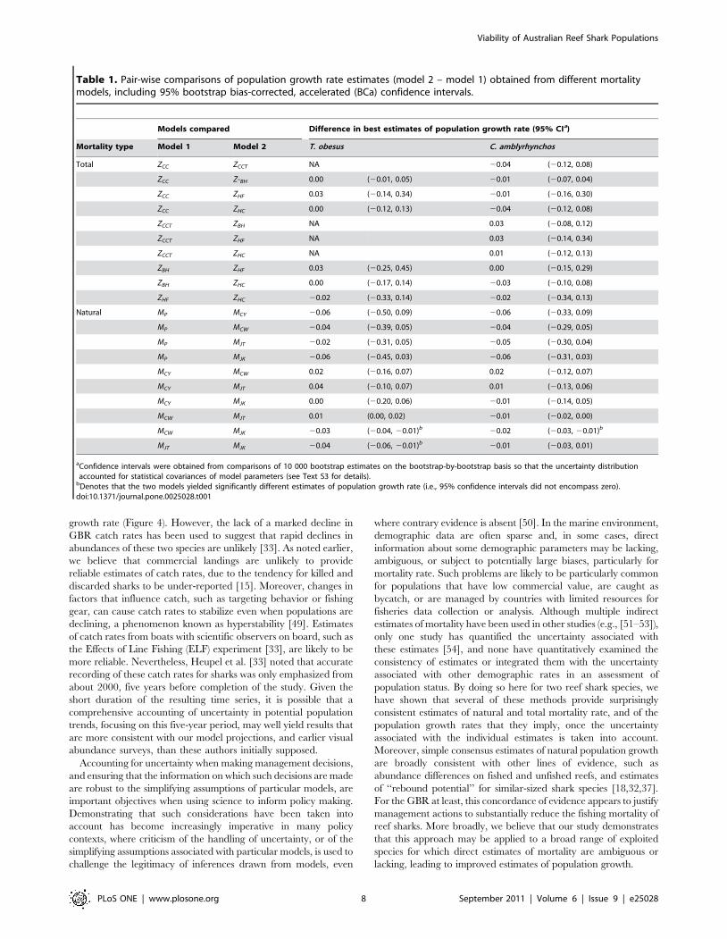
Population Growth RatesMedian bias-corrected estimates of total population growth

were highly consistent, ranging from 0.91–0.94 year21 for T.

obesus, and 0.89–0.93 year21 for C. amblyrhynchos (Figure 3). Indeed,

when uncertainty was accounted for, none of the estimates differed

significantly from one another (Table 1). For natural population

growth rate, bias-corrected estimates tended to be lower for MP

than for the life history-based estimates, but, again, after

accounting for uncertainty, MP did not differ significantly from

any of the alternatives (Table 1). Nevertheless, for T. obesus, MJK

differed significantly from MJT and MCW, and for C. amblyrhynchos,

MCW differed significantly from MJK (Table 1). However, this

difference was due to the very narrow confidence intervals

associated with these three estimates, rather than differences that

were large in magnitude (median differences were ,2% in these

cases).

Consensus estimates of total population growth indicated strong

support for the conclusion that both populations are in decline,

with at least 95% confidence (Figure 4). For T. obesus, the median

bias-corrected consensus estimate was 0.94, and for C. amblyr-

hynchos, it was 0.91. Although decreasing longevity to 19 years, or

using the bootstrap distribution of tl (Equation 5), which implies

much greater longevity (50+ years), decreased and increased these

population growth rates, respectively, the effects were relatively

small: median bias-corrected total population growth rate, and

95% confidence limits, changed by only 1% for T. obesus, and 2–

3% for C. amblyrhynchos (Figure 4).

Consensus estimates of natural population growth indicated the

potential for population growth in the absence of fishing: median

bias-corrected estimates were 1.06 for T. obesus, and 1.02 for C.

amblyrhynchos, although 95% confidence limits on the popula-

tion growth rate of C. amblyrhynchos did include values below

replacement (Figure 4). Again, using alternative longevity

measures did not change estimated natural population growth

rates, or their 95% confidence limits, by more than ,2%.

Projection of Abundance DifferencesConsensus estimates of natural and total population growth rate

imply a per-annum density-independent long-run rate of change

in the ratio of abundances in fished and unfished populations of

0.88 for T. obesus, and 0.89 for C. amblyrhynchos. When used to

project abundance differences over time, these rates yielded

estimates of the ratio of abundances on fished versus unfished reefs

that were consistent with previously obtained UVS data (Figure 5),

although the C. amblyrhynchos data of Robbins et al. [18] suggest

Figure 2. Estimates of natural and total mortality rate for two reef shark species. These estimates were calculated for (A) T. obesus and (B)C. amblyrhynchos on the Great Barrier Reef. For each method, an open circle indicates the (raw) sample estimate, which was obtained using maximumlikelihood parameter estimates from analysis of the empirical data, a closed circle indicates the bootstrap bias-corrected estimate, and whiskersindicate 95% bias-corrected, accelerated (BCa) bootstrap confidence intervals. For methods that produced age-specific estimates of mortality rate(ZCC for C. amblyrhynchos, and M-CW for both species), an age-averaged mortality rate is shown (i.e., weighted according to the fraction of thepopulation at each age in the stable age distribution). Note that the vertical axis is plotted on log-scale.doi:10.1371/journal.pone.0025028.g002



potentially greater abundance differences than our model

projections (Figure 5B).

Discussion

Ongoing, rapid declines in many shark species worldwide,

coupled with evidence that shark depletion can have substantial,

cascading effects on community structure and dynamics, have

made assessing the status and trends of shark populations a high

priority in conservation biology [5]. This study shows how a robust

assessment of mortality and population growth rates can be made

using indirect estimates of mortality rate, and can thereby provide

essential information for the sustainable management of sharks,

and potentially other exploited species for which direct estimates of

mortality are unavailable. More specifically, it highlights the

vulnerability of reef sharks to overfishing, even in well-managed

reef systems like the GBR. Our use of multiple models to estimate

rates of population decline, and potential natural population

growth, reveals a high degree of concordance between several

indirect methods of estimating these two quantities. For total

population growth, none of the model estimates differed

significantly from one another. For natural population growth,

model estimates either did not differ significantly, or differences

were very small in magnitude. Our results were also surprisingly

insensitive to longevity: even pessimistic (19 years) and very

optimistic (50+ years) estimates changed consensus estimates of

population growth rate only by 1–3%. The range of longevities

explored here almost certainly exceeds the reasonable range.

Clearly, since 19-year old sharks were observed in the catch data,

longevity cannot be less than this. Conversely, the longevity of our

optimistic scenario (50+ years) is highly unlikely, given that no

shark older than 19 years appeared in the 333 sharks in the

combined commercial and research catches (including line and

spear fishing), and that no shark of either species older than 25

years has been reported anywhere in the world [42]. In any case,

the conclusion that substantial population declines in T. obesus and

C. amblyrhynchos have been occurring, largely as a consequence of

increased mortality from fishing, appears highly robust to the

available indirect methods of estimating total mortality rate for

these species.

None of our estimates of total population growth rate differed

significantly from one another, despite differences in assumptions

associated with our different estimates of total mortality rate.

Catch curve analysis assumes the catch composition is represen-

tative of the survivorship of the underlying population (i.e., if the

catch curve indicates 30% fewer individuals at one age than the

next-younger age, this indicates that survival between these ages is

70%). This assumption requires that there are no consistent

temporal trends in numbers recruiting to the fishery, or post-

recruitment age differences in catchability. A trend of declining

recruitment, or greater susceptibility of older individuals to fishing,

for instance, both tend to make fitted catch curves shallow, relative

to the underlying survivorship pattern, and thus under-estimate

mortality. The Beverton-Holt method is likely to be similarly

biased by trends in recruitment or age-dependent post-recruitment

catchability, because mean age in the catch (inversely related to

ZBH) would be biased high in the same cases where ZCC would be

biased low. In particular, it is possible that the high abundance of

Figure 3. Estimates of natural and total population growth rate for two reef shark species. These estimates were calculated for (A)T. obesus and (B) C. amblyrhynchos on the Great Barrier Reef. For each method, an open circle indicates the (raw) sample estimate, which wasobtained using maximum likelihood parameter estimates from analysis of the empirical data, a closed circle indicates the bootstrap bias-correctedestimate, and whiskers indicate 95% bias-corrected, accelerated (BCa) bootstrap confidence intervals. Dashed lines indicate the threshold betweenpopulation growth (above) and decline (below).doi:10.1371/journal.pone.0025028.g003



very young C. amblyrhynchos in the catch indicates over-represen-

tation (due, for instance, to naivete or a tendency for older sharks

to spend less time in shallow water, where fishing activity is

greater). Such an effect would bias ZCC high. However, there is no

evidence of such over-representation in the T. obesus catch data;

moreover, this species is less aggressive towards bait than C.

amblyrhynchos [18,35]. Thus, if anything, we would expect ZCCT (use

of the T. obesus catch curve as an estimate of C. amblyrhynchos

mortality rate) to be biased low. The fact that our estimates of

population growth rate for C. amblyrhynchos did not differ

significantly, regardless of which catch curve we used, suggests

that any associated biases are probably small, relative to the

uncertainties. Moreover, Hoenig’s method, which yields estimates

that do not differ from ZBH, ZCC, or ZCCT, is based on empirical

relationships that hold across species, and does not require any

assumptions about the representativeness of the catch data for our

study species. Hoenig’s method should only be biased if our study

species are outliers, relative to the species used in the construction

of the regression model. We have minimized the risk of this by

applying both relationships calibrated for fish (ZHF) and cetaceans

(ZHC); moreover, the two elasmobranch species used in the

construction of the ZHF regression model are not outliers [27].

For natural mortality, the only assumption shared by all methods is

that growth is well-characterized by the von Bertalanffy function:

VBGF growth parameters are covariates in the regression model used

to calculate MP, and putative life-history relationships involving

VBGF parameters are involved in the derivation of the other

estimates. However, this assumption is well-met for these species (Text

S1). The derivation of MCY, MJT, and MJK all require an assumption

of constant mortality rate, but MCW explicitly incorporates age-

dependent mortality rates. Moreover, MP, like Hoenig’s method, is

empirical and not derived from any life-history assumptions. For

estimates of natural population growth rate obtained from these

methods, we found significant differences involving only Jensen’s

estimates. We suspect that these estimates, which had very narrow

confidence limits, underestimate the true uncertainty associated with

the use of proposed life-history invariants to estimate demographic

rates. In particular, as the term implies, application of this method

assumes that, for all species, natural mortality rate follows Equation 9

or Equation 10 exactly, and thus the only uncertainty associated with

this estimate is the uncertainty associated with the estimation of the

von Bertalanffy growth parameters K and t0, and age at maturity tm.

However, there is an emerging consensus that these quantities are not

truly invariant, but instead represent a central tendency or average

across species, with individual species deviating somewhat from these

average relationships [48]. The magnitude of this interspecific

variation has not yet, to our knowledge, been estimated, but it

implies that the uncertainties around MJK and MJT (and, by

implication, the consensus estimate of natural population growth)

are likely to be underestimated to some extent.

The consensus estimates of natural and total population growth

imply population growth rates consistent with other lines of

evidence. For instance, our projections of abundance differences

are consistent with UVS estimates on the GBR (Figure 5). In

addition, Smith et al. [37] estimated natural population growth

rates of approximately 4–6% per year for similarly sized sharks

(including T. obesus and C. amblyrhynchos), which is in good

agreement with our consensus estimates of natural population

Figure 4. Estimates of consensus natural and total population growth rate for two reef shark species. Estimates were obtained withmodels with longevity set to 25 years, 19 years and time to achieve 95% of L‘ (sample estimate: 52 and 50 years, respectively) for (A) T. obesus and (B)C. amblyrhynchos on the Great Barrier Reef. For each method, an open circle indicates the (raw) sample estimate, which was obtained using maximumlikelihood parameter estimates from analysis of the empirical data, a closed circle indicates the bootstrap bias-corrected estimate, and whiskersindicate 95% bias-corrected, accelerated (BCa) bootstrap confidence intervals. Dashed lines indicate the threshold between population growth(above) and decline (below).doi:10.1371/journal.pone.0025028.g004



growth rate (Figure 4). However, the lack of a marked decline in

GBR catch rates has been used to suggest that rapid declines in

abundances of these two species are unlikely [33]. As noted earlier,

we believe that commercial landings are unlikely to provide

reliable estimates of catch rates, due to the tendency for killed and

discarded sharks to be under-reported [15]. Moreover, changes in

factors that influence catch, such as targeting behavior or fishing

gear, can cause catch rates to stabilize even when populations are

declining, a phenomenon known as hyperstability [49]. Estimates

of catch rates from boats with scientific observers on board, such as

the Effects of Line Fishing (ELF) experiment [33], are likely to be

more reliable. Nevertheless, Heupel et al. [33] noted that accurate

recording of these catch rates for sharks was only emphasized from

about 2000, five years before completion of the study. Given the

short duration of the resulting time series, it is possible that a

comprehensive accounting of uncertainty in potential population

trends, focusing on this five-year period, may well yield results that

are more consistent with our model projections, and earlier visual

abundance surveys, than these authors initially supposed.

Accounting for uncertainty when making management decisions,

and ensuring that the information on which such decisions are made

are robust to the simplifying assumptions of particular models, are

important objectives when using science to inform policy making.

Demonstrating that such considerations have been taken into

account has become increasingly imperative in many policy

contexts, where criticism of the handling of uncertainty, or of the

simplifying assumptions associated with particular models, is used to

challenge the legitimacy of inferences drawn from models, even

where contrary evidence is absent [50]. In the marine environment,

demographic data are often sparse and, in some cases, direct

information about some demographic parameters may be lacking,

ambiguous, or subject to potentially large biases, particularly for

mortality rate. Such problems are likely to be particularly common

for populations that have low commercial value, are caught as

bycatch, or are managed by countries with limited resources for

fisheries data collection or analysis. Although multiple indirect

estimates of mortality have been used in other studies (e.g., [51–53]),

only one study has quantified the uncertainty associated with

these estimates [54], and none have quantitatively examined the

consistency of estimates or integrated them with the uncertainty

associated with other demographic rates in an assessment of

population status. By doing so here for two reef shark species, we

have shown that several of these methods provide surprisingly

consistent estimates of natural and total mortality rate, and of the

population growth rates that they imply, once the uncertainty

associated with the individual estimates is taken into account.

Moreover, simple consensus estimates of natural population growth

are broadly consistent with other lines of evidence, such as

abundance differences on fished and unfished reefs, and estimates

of ‘‘rebound potential’’ for similar-sized shark species [18,32,37].

For the GBR at least, this concordance of evidence appears to justify

management actions to substantially reduce the fishing mortality of

reef sharks. More broadly, we believe that our study demonstrates

that this approach may be applied to a broad range of exploited

species for which direct estimates of mortality are ambiguous or

lacking, leading to improved estimates of population growth.

Table 1. Pair-wise comparisons of population growth rate estimates (model 2 – model 1) obtained from different mortalitymodels, including 95% bootstrap bias-corrected, accelerated (BCa) confidence intervals.

Models compared Difference in best estimates of population growth rate (95% CIa)

Mortality type Model 1 Model 2 T. obesus C. amblyrhynchos

Total ZCC ZCCT NA 20.04 (20.12, 0.08)

ZCC Z-BH 0.00 (20.01, 0.05) 20.01 (20.07, 0.04)

ZCC ZHF 0.03 (20.14, 0.34) 20.01 (20.16, 0.30)

ZCC ZHC 0.00 (20.12, 0.13) 20.04 (20.12, 0.08)

ZCCT ZBH NA 0.03 (20.08, 0.12)

ZCCT ZHF NA 0.03 (20.14, 0.34)

ZCCT ZHC NA 0.01 (20.12, 0.13)

ZBH ZHF 0.03 (20.25, 0.45) 0.00 (20.15, 0.29)

ZBH ZHC 0.00 (20.17, 0.14) 20.03 (20.10, 0.08)

ZHF ZHC 20.02 (20.33, 0.14) 20.02 (20.34, 0.13)

Natural MP MCY 20.06 (20.50, 0.09) 20.06 (20.33, 0.09)

MP MCW 20.04 (20.39, 0.05) 20.04 (20.29, 0.05)

MP MJT 20.02 (20.31, 0.05) 20.05 (20.30, 0.04)

MP MJK 20.06 (20.45, 0.03) 20.06 (20.31, 0.03)

MCY MCW 0.02 (20.16, 0.07) 0.02 (20.12, 0.07)

MCY MJT 0.04 (20.10, 0.07) 0.01 (20.13, 0.06)

MCY MJK 0.00 (20.20, 0.06) 20.01 (20.14, 0.05)

MCW MJT 0.01 (0.00, 0.02) 20.01 (20.02, 0.00)

MCW MJK 20.03 (20.04, 20.01)b 20.02 (20.03, 20.01)b

MJT MJK 20.04 (20.06, 20.01)b 20.01 (20.03, 0.01)

aConfidence intervals were obtained from comparisons of 10 000 bootstrap estimates on the bootstrap-by-bootstrap basis so that the uncertainty distributionaccounted for statistical covariances of model parameters (see Text S3 for details).

bDenotes that the two models yielded significantly different estimates of population growth rate (i.e., 95% confidence intervals did not encompass zero).doi:10.1371/journal.pone.0025028.t001



Supporting Information

Text S1 Demographic data and parameter estimation.(DOC)

Text S2 Population model framework.(DOC)

Text S3 Bootstrap algorithms for characterization ofuncertainty.(DOC)

Acknowledgments

We thank J.H. Choat, P.L. Munday, and N. Graham for helpful

suggestions, and R. Berkelmans for use of the photo reproduced in Figure 1.

Author Contributions

Analyzed the data: MH. Wrote the paper: MH SRC. Obtained the data

used in analysis: WDR. Conceived and designed the modeling method:

MH SRC.

References

1. Stevens JD, Bonfil R, Dulvy NK, Walker PA (2000) The effects of fishing on

sharks, rays, and chimaeras (chondrichthyans), and the implications for marineecosystems. ICES Journal of Marine Science 57: 476–494.

2. Lack M, Sant G (2006) World shark catch, production and trade 1990-2003.

Canberra: TRAFFIC Oceania and Australian Department of the Environmentand Heritage. pp 29.

3. Lack M, Sant G (2009) Trends in global shark catch and recent developments in

management. Cambridge: TRAFFIC International. 29 p.

4. Myers RA, Baum JK, Shepherd TD, Powers SP, Peterson CH (2007) Cascading

effects of the loss of apex predatory sharks from a coastal ocean. Science 315:1846–1850.

5. Barker MJ, Schluessel V (2005) Managing global shark fisheries: suggestions for

prioritising management strategies. Aquatic Conservation: Marine and Fresh-water Ecosystems 15: 325–347.

6. IUCN (International Union for Conservation of Nature). (2010) IUCN Red List

of Threatened Species. Version 2010.4. IUCN, Cambridge. Available: http://

www.iucnredlist.org via the Internet. Accessed 08 March 2011.

7. Cavanagh RD, Kyne PM, Fowler SL, Musick JA, Bennett MB (2003) Theconservation status of Australasian chondrichthyans: Report of the IUCN Shark

Specialist Group Australian and Oceania Regional Red List Workshop.Brisbane: The University of Queensland. 170 p.

8. DeMartini EE, Friedlander AM, Sandin SA, Sala E (2008) Differences in fish-

assemblage structure between fished and unfished atolls in the northern Line

Islands, central Pacific. Marine Ecology Progress Series 365: 199–215.

9. Sandin SA, Smith JE, DeMartini EE, Dinsdale EA, Donner SD, et al. (2008)

Baselines and degradation of coral reefs in the northern Line Islands. PLoS ONE3: e1548. DOI: 10.1371/journal.pone.0001548.

10. Bascompte J, Melian CJ, Sala E (2005) Interaction strength combinations and

the overfishing of a marine food web. Proceedings of the National Academy ofSciences of the United States of America 15: 5443–5447.

11. Fowler SL, Cavanagh RD, Camhi M, Burgess GH, Cailliet GM, et al. (2005)

Sharks, rays and chimaeras: the status of the chondrichthyan fishes. Status survey.

IUCN/SSC Shark Specialist Group. Gland and Cambridge: IUCN. 461 p.

12. Clarke SC, McAllister MK, Milner-Gulland EJ, Kirkwood GP, Michielsens CGJ,et al. (2006) Global estimates of shark catches using trade records from

commercial markets. Ecology Letters 9: 1115–1126.

13. Salini J, Giles J, Holmes B, Last P, Marshall L, et al. (2007) Species identificationfrom shark fins – Phase 1. AFMA Report R05/0538. Cleveland: CSIRO Marine

and Atmospheric Research. 149 p.

14. Graham NAJ, Spalding MD, Sheppard CRC (2010) Reef shark declines in

remote atolls highlight the need for multi-faceted conservation action. AquaticConservation: Marine and Freshwater Ecosystems 20: 543–548.

15. Bromhead D, Ackerman J, Graham S, Wight M, Wise B, et al. (2005)

Byproduct: catch, economics and co-occurrence in Australia’s pelagic longlinefisheries. Canberra: Bureau of Rural Sciences. 21 p.

16. Ellis JR, Dulvy NK, Jennings S, Parker-Humphreys M, Rogers SI (2005)

Assessing the status of demersal elasmobranchs in UK waters: a review. Journal

of the Marine Biological Association of the United Kingdom 85: 1025–1047.

Figure 5. Estimates of ratio of fished to unfished abundances over time for two reef shark species. These estimates were calculated for(A) T. obesus and (B) C. amblyrhynchos on the Great Barrier Reef, from our bootstrap bias-corrected consensus estimates of long-term total and naturalpopulation growth rates (Equation 11). The dashed lines indicate 95% bias-corrected, accelerated (BCa) bootstrap confidence intervals on theseabundance ratios. The mean differences between surveyed abundances on open fishing and unfished (no-entry) reefs are plotted as triangles andsquares for the data in Robbins et al. [18] and Ayling and Choat [31], respectively. Location of triangles and squares on the horizontal axis reflects thenumber of years elapsed between establishment of the relevant no-entry zones, and the underwater surveys. For Robbins et al. [18], horizontalwhiskers reflect the fact that surveys took place over a multi-year period (2001–2004). Vertical whiskers indicate 95% bootstrap confidence intervalson these abundance ratios, generated by Monte-Carlo simulation, as described in the Methods.doi:10.1371/journal.pone.0025028.g005



17. Friedlander AM, DeMartini EE (2002) Contrasts in density, size, and biomass of

reef fishes between the northwestern and the main Hawaiian islands: the effectsof fishing down apex predators. Marine Ecology Progress Series 230: 253–264.

18. Robbins WD, Hisano M, Connolly SR, Choat JH (2006) Ongoing collapse of

coral-reef shark populations. Current Biology 16: 2314–2319.19. Watson RA, Carlos GM, Samoilys MA (1995) Bias introduced by the non-

random movement of fish in visual transect surveys. Ecological Modelling 77:205–214.

20. Willis TJ, Millar RB, Babcock RC (2000) Detection of spatial variability in

relative density of fishes: comparison of visual census, angling, and baitedunderwater video. Marine Ecology Progress Series 198: 249–260.

21. Ward-Paige C, Flemming JM, Lotze HK (2010) Overestimating fish counts bynon-instantaneous visual censuses: consequences for population and community

descriptions. PLoS ONE 5: e11722. DOI: 10.1371/journal.pone.0011722.22. Kulbicki M (1998) How the acquired behavior of commercial reef fishes may

influence the results obtained from visual censuses. Journal of Experimental

Marine Biology and Ecology 222: 11–30.23. Kohler NE, Turner PA (2001) Shark tagging: a review of conventional methods

and studies. Environmental Biology of Fishes 60: 191–223.24. Campana SE, Marks L, Joyce W, Kohler N (2005) Catch, by-catch and indices

of population status of blue shark (Prionace glauca) in the Canadian Atlantic.

ICCAT Collective Volume of Scientific Papers 58: 891–934.25. Fischer AJ, Baker MSJ, Wilson CA, Nieland DL (2005) Age, growth, mortality,

and radiometric age validation of gray snapper (Lutjanus griseus) from Louisiana.Fishery Bulletin 103: 307–319.

26. Pauly D (1980) On the interrelationships between natural mortality, growthparameters, and mean environmental temperature in 175 fish stocks. ICES

Journal of Marine Science 39: 175–192.

27. Hoenig JM (1983) Empirical use of longevity data to estimate mortality rates.Fishery Bulletin 82: 898–903.

28. Jensen AL (1996) Beverton and Holt life history invariants result from optimaltrade-off of reproduction and survival. Canadian Journal of Fisheries and

Aquatic Sciences 53: 820–822.

29. Blakesley JA, Seamans ME, Conner MM, Franklin AB, White GC, et al. (2010)Population dynamics of spotted owls in the Sierra Nevada, California. Wildlife

Monographs 174: 1–36.30. Grueber CE, Laws RJ, Nakagawa S, Jamieson IG (2010) Inbreeding depression

accumulation across life-history stages of the endangered Takahe. ConservationBiology 24: 1617–1625.

31. Annan JD, Hargreaves JC (2006) Using multiple observationally based

constraints to estimate climate sensitivity. Geophysical Research Letters 33:L06704.

32. Ayling AM, Choat JH (2008) Abundance patterns of reef sharks and predatoryfishes on differently zoned reefs in the offshore Townsville region: final report to

the Great Barrier Reef Marine Park Authority. Research publication N-91.

Townsville: Great Barrier Reef Marine Park Authority. 32 p.33. Heupel MR, Williams AJ, Welch DJ, Ballagh A, Mapstone BD, et al. (2009)

Effects of fishing on tropical reef associated shark populations on the GreatBarrier Reef. Fisheries Research 93: 350–361.

34. Bertalanffy L von (1938) A quantitative theory of organic growth (inquiries ongrowth laws. II). Human Biology 10: 181–213.

35. Hobson ES (1963) Feeding behavior in three species of sharks. Pacific Science

17: 171–194.

36. Beverton RJH, Holt SJ (1957) On the dynamics of exploited fish populations.

Fishery Investigations Series II. London: G.B. Ministry of Agriculture, Fisheries

and Food N-19: 533.

37. Smith SE, Au DW, Show C (1998) Intrinsic rebound potentials of 26 species of

Pacific sharks. Marine and Freshwater Research 49: 663–678.

38. Lough JM (2007) Climate and climate change on the Great Barrier Reef. In

Johnson JE, Marshall PA, eds. Climate change and the Great Barrier Reef: A

vulnerability assessment. Townsville: Great Barrier Reef Marine Park Authority

and the Australian Greenhouse Office. pp 15–50.

39. Chen P, Yuan W (2006) Demographic analysis based on the growth parameter

of sharks. Fisheries Research 78: 374–379.

40. Chen S, Watanabe S (1989) Age dependence of natural mortality coefficient in

fish population dynamics. Nippon Suisan Gakkaishi 55: 205–208.

41. Charnov EL (1993) Life history invariants. Oxford: Oxford University Press.

184 p.

42. Compagno LJV (1984) Sharks of the world: an annotated and illustrated

catalogue of shark species known to data. Rome: United Nations Development

Programme. 10 p.

43. Randall JE (1977) Contribution to the biology of the whitetip reef shark

(Triaenodon obesus). Pacific Science 31: 143–164.

44. Burnham KP, Anderson DR (1998) Model selection and multimodel inference: a

practical information-theoretic approach. 2nd edition. New York: Springer.

488 p.

45. Hilborn R, Mangel M (1997) The ecological detective: Confronting models with

data. Princeton: Princeton University Press. 315 p.

46. Efron B, Tibshirani RJ (1998) An introduction to the bootstrap. Boca Raton:

Chapman and Hall. 436 p.

47. Davison AC, Hinkley DV (1997) Bootstrap methods and their application

(Cambridge series in statistical and probabilistic mathematics, No 1). Cam-

bridge: Cambridge University Press. 582 p.

48. Savage VM, White EP, Moses ME, Morgan Ernest SK, Enquist BJ, et al. (2006)

Comment on ‘‘the illusion of invariant quantities in life histories.’’ Science 312:

198.

49. Maunder MN, Sibert JR, Fonteneau A, Hampton J, Kleiber P, et al. (2006)

Interpreting catch per unit effort data to assess the status of individual stocks and

communities. ICES Journal of Marine Science 63: 1373–1385.

50. Van der Sluijs JP (2007) Uncertainty and precaution in environmental

management: Insights from the UPEM conference. Environmental Modelling

& Software 22: 590–598.

51. Hewitt DA, Lambert DM, Hoenig JM, Lipcius RN, Bunnell DB, et al. (2007)

Direct and indirect estimates of natural mortality for Chesapeake Bay blue crab.

Transactions of the American Fisheries Society 136: 1030–1040.

52. Tsai W-P, Liu K-M, Joung S-J (2010) Demographic analysis of the pelagic

thresher shark, Alopias pelagicus, in the north-western Pacific using a stochastic

stage-based model. Marine and Freshwater Research 61: 1056–1066.

53. Smith WD, Cailliet GM, Cortes E (2008) Demography and elasticity of the

diamond stingray, Dasyatis dipterura: parameter uncertainty and resilience to

fishing pressure. Marine and Freshwater Research 59: 575–586.

54. Quiroz JC, Wiff R, Caneco B (2010) Incorporating uncertainty into estimation

of natural mortality for two species of Rajidae fished in Chile. Fisheries Research

102: 297–304.



Population Growth Rates of Reef Sharks with and without Fishing on the Great Barrier Reef: Robust...

Documents

Transcript of Population Growth Rates of Reef Sharks with and without Fishing on the Great Barrier Reef: Robust...