Planning for the persistence of river biodiversity: exploring alternative futures using...

Planning for the persistence of river biodiversity:exploring alternative futures using process-based models

EREN TURAK*, SIMON FERRIER* , †, TOM BARRETT‡, EDWINA MESLEY*, MICHAEL

DRIELSMA ‡, GLENN MANION‡, GAVIN DOYLE § , JANET STEIN– AND GEOFF GORDON*

*Department of Environment, Climate Change and Water, Sydney NSW, Australia†CSIRO Entomology, Canberra, ACT, Australia‡Department of Environment, Climate Change and Water, Armidale NSW, Australia§Hunter-Central Rivers CMA, Paterson NSW, Australia–The Fenner School of Environment and Society, Australian National University, Canberra, ACT, Australia

SUMMARY

1. Planning for the conservation of river biodiversity must involve a wide range of

management options and account for the complication that the effects of many

actions are spatially removed from these actions. Reserve design algorithms widely

used in conservation planning today are not well equipped to address such

complexities.

2. We used process-based models to estimate the expected persistence of river biodiversity

under alternative catchment-wide management scenarios and applied it in the Hunter

Region (37 000 km2) in southeastern Australia.

3. The biological condition of 12 197 subcatchments was estimated using a multiple linear

regression model that related assessments of the integrity of macroinvertebrate assem-

blages to human-induced disturbances at river sites. The best-fit model (R2 = 0.76) used

measures of both local and catchment-wide disturbances as well as elevation and distance

from source as predictor variables. Based on the outputs of this model, we estimated that

substantial loss of river biodiversity had occurred in some parts of the coastal fringes and

the lower parts of the larger river systems. The most affected river type was small, low-

gradient streams.

4. The predicted biodiversity condition together with river types based on macroinver-

tebrate assemblages and abiotic attributes was used to estimate a biodiversity persistence

index (BDI).

5. A priority value for each subcatchment was calculated for different actions by changing

the disturbance values for that subcatchment and calculating the resulting marginal

change in regional BDI. Maps were thereby created for three different types of priority:

catchment protection priority, catchment restoration priority and river section conserva-

tion priority.

6. The subcatchments of high catchment protection priority for river biodiversity were

mostly in the uplands and within protected areas. The river sections of high conservation

priority included many coastal lowland rivers in and around protected areas as well as

many upland headwater streams. Subcatchments of high priority for catchment restoration

were mostly in coastal areas or lowland floodplains.

Correspondence: Eren Turak, Department of Environment, Climate Change and Water, 59-61 Goulburn St, Sydney, New South Wales

2000, Australia. E-mail: [email protected]

Freshwater Biology (2011) 56, 39–56 doi:10.1111/j.1365-2427.2009.02394.x

� 2010 Blackwell Publishing Ltd 39

7. This approach may be particularly well suited to guide the integrated implementation of

three place-based protection strategies proposed for freshwaters: focal areas, critical

management zones and catchment management zones.

Keywords: conservation planning, persistence, rivers, scenario modelling

Introduction

Freshwater biodiversity is imperilled across the world

(e.g. Malmqvist & Rundle, 2002; Dudgeon et al., 2006).

While interest in conserving river biodiversity is not

new, only recently, systematic approaches aimed at

selecting a complementary set of sites for conservation

at the scale of broad geographical regions (e.g.

Margules & Pressey, 2000) have been proposed for

rivers (e.g. Linke et al., 2007; Thieme et al., 2007;

Moilanen, Leathwick & Elith, 2008).

The central goal of systematic conservation plan-

ning is to allow representative examples of the

biodiversity of the planning region to persist (Mar-

gules & Pressey, 2000). To allow persistence, conser-

vation areas must be spatially configured to

accommodate ecological processes such as dispersal,

local extinctions and recolonisations and possible

adjustments of species distributions to climate change

(Sarkar et al., 2006). Systematic conservation planning

typically involves first identifying measureable fea-

tures of biodiversity (biodiversity surrogates; Mar-

gules & Pressey, 2000; Sarkar & Margules, 2002) and

then setting quantitative targets for including these

features in areas where protection measures will be

applied (Margules & Pressey, 2000). The setting of

these targets is based on assumptions about the

conservation return expected from protecting an area

of a given size. The world conservation union (IUCN)

has officially adopted a guideline that 10% of each

biome should be included in protected areas (McNe-

ely, 1993), leading to the widespread use of the target

of 10% of any biodiversity surrogate in conservation

plans at a wide range of spatial scales (Soule &

Sanjayan, 1998; Pressey, Cowling & Rouget, 2003;

Brooks et al., 2004). This target is loosely based on a

theoretical premise that a 10-fold increase in area will

double the number of species and hence 10% of an

area protects 50% of species (Diamond & May, 1976).

However, the unreserved and indiscriminate applica-

tion of this target has been questioned on the basis

that protecting 50% of species cannot universally be

considered as a satisfactory target (Soule & Sanjayan,

1998; Rodrigues & Gaston, 2001; Pressey et al., 2003)

and because the requirement for protection would

necessarily vary among species and ecosystem types

(Pressey et al., 2003; Desmet & Cowling, 2004). For

rivers, a specified percentage of the length of river

type has been used in several studies in this volume:

15% (P. C. Esselman & J. D. Allan, in review), 20%

(J. L. Nel, B. Reyers, D. J. Roux & R. M. Cowling, in

review) and different values depending on river size

(N. A. Rivers-Moore, P. S. Goodman & J. L. Nel, in

review). These targets were assigned on the basis of

expert opinion. While one of these was defined for

fish (P. C. Esselman & J. D. Allan, in review), the other

targets were not specifically assigned for any taxo-

nomic group but were considered to address the

protection of all river biodiversity (J. L. Nel, B. Reyers,

D. J. Roux & R. M. Cowling, in review; N. A. Rivers-

Moore, P. S. Goodman & J. L. Nel, in review).

Arbitrary targets without any ecological basis may

lead to inadequate protection (Soule & Sanjayan, 1998;

Pressey et al., 2003). Also, such targets do not explic-

itly recognise the additional contribution to biodiver-

sity of going beyond a target nor the contribution of

features that are below target (Arponen et al., 2005;

Ferrier et al., 2009). One solution when working with

community-level surrogates – e.g. vegetation types or

river types – is to explicitly model the proportion of

biodiversity expected to be retained in each surrogate

class as a continuously increasing function of the

proportion of that class conserved (e.g. Ferrier et al.,

2004; Allnutt et al., 2008; Faith, Ferrier & Williams,

2008). This is achieved using some form of species–

area relationship (SAR), most commonly formulated

as a power function (Arrhenius, 1921):

S = CAz

where S is number of species, A is habitat area and C

and z are constants. This formulation enables, for each

surrogate class, the proportion of species expected to

be retained in a given retained proportion of original

habitat to be estimated as:

Sretained ⁄Soriginal = (Aretained ⁄AOriginal)z

40 E. Turak et al.

� 2010 Blackwell Publishing Ltd, Freshwater Biology, 56, 39–56

Recent extensions to this approach also allow

information on overlap (similarity) in species compo-

sition between surrogate classes to be considered in

estimating the overall proportion of species retained

across all classes within a region (e.g. Ferrier et al.,

2004, 2009; Faith et al., 2008).

Another challenge confronting systematic conser-

vation planning is to develop effective ways to

account for the impacts (both positive and negative)

of multiple forms of off-reserve land use and man-

agement on conservation outcomes for biodiversity at

a regional scale (Sarkar et al., 2006). This problem

takes on an added level of complexity when dealing

with rivers because of the large influence that human

activities in the catchment can have on biodiversity in

downstream sections of river. Management actions,

therefore, must often be applied at locations spatially

removed (i.e. upstream) from the biodiversity features

intended to benefit from these actions.

The usefulness of conservation planning methods

and tools also depends on how they are linked to

implementation and hence to governance of conser-

vation. In most countries and regions, the governance

of freshwater conservation involves multiple agencies

and stakeholders. For example, in New South Wales,

Australia’s most populous state, three important areas

of natural resource management [(i) spatial configu-

ration and management of reserves, (ii) major water

allocation and sharing arrangements and (iii) land

management decisions at the scale of individual

properties] are the responsibility of different govern-

ment agencies. A tool that evaluates the effects of

management actions on river biodiversity in terms of

a single currency is likely to allow for greater

coordination and congruence among stakeholders in

taking action. It would also help to bring transparency

to trade-offs made between biodiversity and other

values.

In this article, we describe a new method for

prioritising actions to conserve river biodiversity,

based on process-based modelling of the level of

persistence of biodiversity expected under alternative

catchment-wide management scenarios. The method

is derived from an existing process-based modelling

approach to conservation planning employed widely

in terrestrial environments in New South Wales over

recent years (e.g. Ferrier, 2005; Drielsma & Ferrier,

2006; DECC 2007a). In adapting this approach to river

environments, we model the condition of river

sections as a function of upstream disturbance factors

(Stein, Stein & Nix, 1998, 2002). We then model the

consequences of predicted changes in river condition

for the persistence of biodiversity at a regional level,

using a SAR-based analysis with multi-attribute eco-

logical river types (Turak & Koop, 2008) serving as

broad surrogates for river biodiversity.

The method we describe here can be used to

generate three main types of output that may help

protect and improve river biodiversity in a planning

region:

1 maps that help identify spatial priorities for

different types of management actions under hypo-

thetical, region-wide management scenarios;

2 quantitative evaluation of specific solutions

involving a suite of management actions at multiple

locations; and

3 optimisation of the spatial configuration of spe-

cific management interventions, e.g. design of fresh-

water protected areas.

Here, we demonstrate the application of the method

to generate the first of these outputs (priority maps)

for the Hunter Region in southeastern Australia.

Methods

We constructed a model to predict river biodiversity

for alternative land management scenarios. We mod-

elled the condition (state) of local instream biodiver-

sity at a river section as a function of local and

upstream disturbance, allowing future change in this

condition to be predicted from anticipated future

change in disturbance resulting from proposed man-

agement actions. The conservation return of these

actions was then estimated in terms of the expected

change in persistence of biodiversity across the entire

region.

Study area

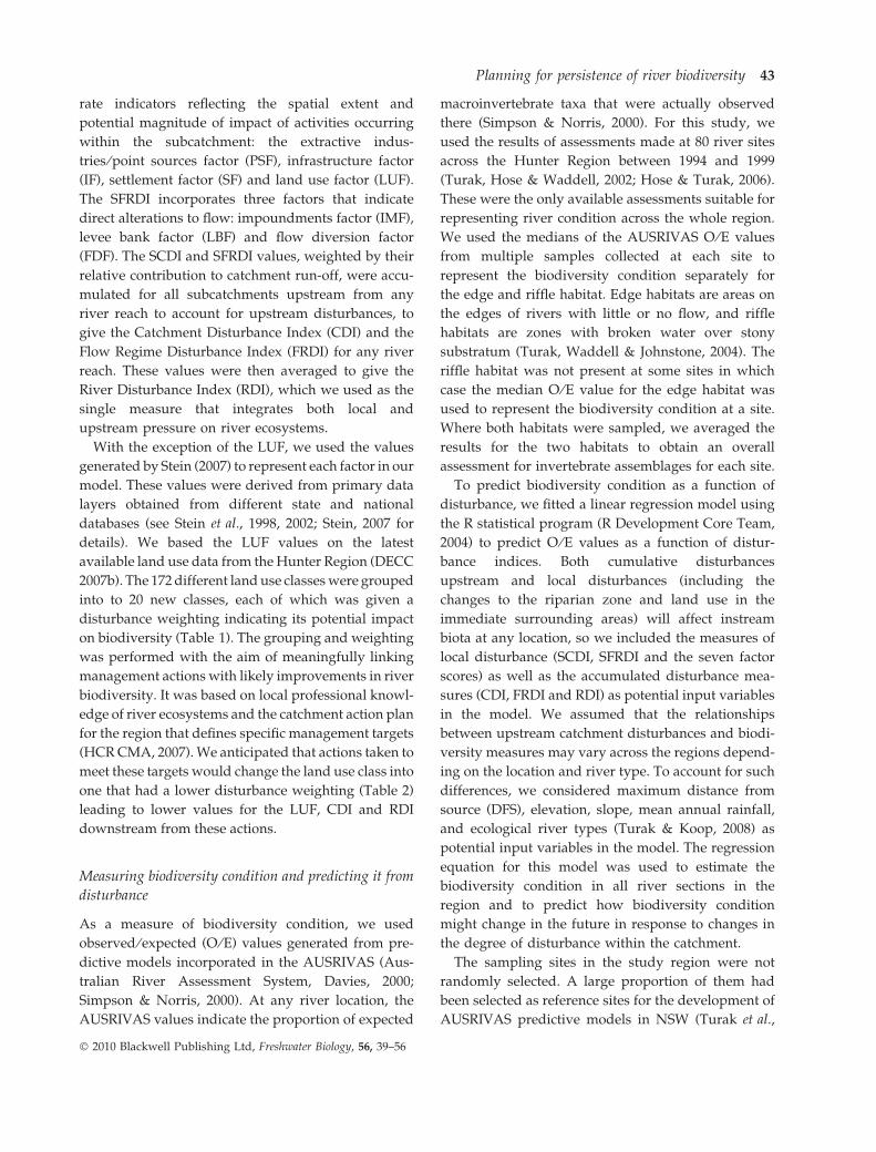
We applied this approach in the Hunter-Central

Rivers Region (37 000 km2) in New South Wales in

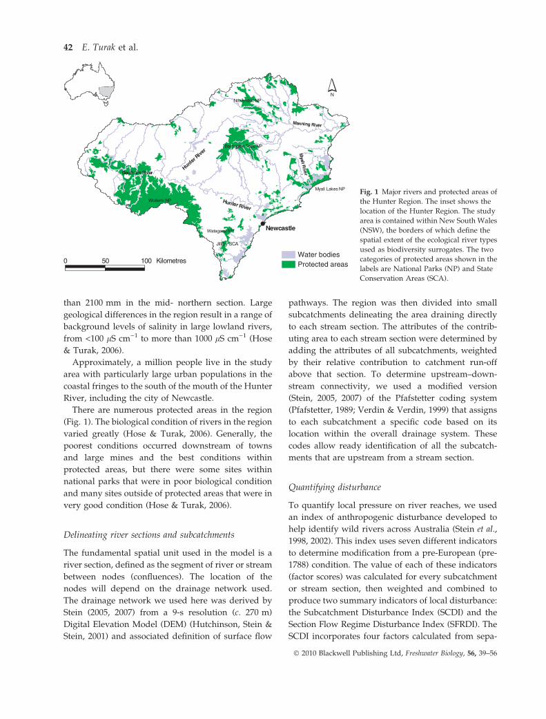
southeastern Australia (Fig. 1). The region covers a

variety of landscape types from the sub-alpine Bar-

rington Tops area (highest point, Brumlow Top,

1586 m) to the low-rainfall zones in the upper Hunter

Valley, and lowland swamps and coastal lakes in the

east of the region. Mean annual rainfall varies across

the region from below 700 mm in the west to more

Planning for persistence of river biodiversity 41


than 2100 mm in the mid- northern section. Large

geological differences in the region result in a range of

background levels of salinity in large lowland rivers,

from <100 lS cm)1 to more than 1000 lS cm)1 (Hose

& Turak, 2006).

Approximately, a million people live in the study

area with particularly large urban populations in the

coastal fringes to the south of the mouth of the Hunter

River, including the city of Newcastle.

There are numerous protected areas in the region

(Fig. 1). The biological condition of rivers in the region

varied greatly (Hose & Turak, 2006). Generally, the

poorest conditions occurred downstream of towns

and large mines and the best conditions within

protected areas, but there were some sites within

national parks that were in poor biological condition

and many sites outside of protected areas that were in

very good condition (Hose & Turak, 2006).

Delineating river sections and subcatchments

The fundamental spatial unit used in the model is a

river section, defined as the segment of river or stream

between nodes (confluences). The location of the

nodes will depend on the drainage network used.

The drainage network we used here was derived by

Stein (2005, 2007) from a 9-s resolution (c. 270 m)

Digital Elevation Model (DEM) (Hutchinson, Stein &

Stein, 2001) and associated definition of surface flow

pathways. The region was then divided into small

subcatchments delineating the area draining directly

to each stream section. The attributes of the contrib-

uting area to each stream section were determined by

adding the attributes of all subcatchments, weighted

by their relative contribution to catchment run-off

above that section. To determine upstream–down-

stream connectivity, we used a modified version

(Stein, 2005, 2007) of the Pfafstetter coding system

(Pfafstetter, 1989; Verdin & Verdin, 1999) that assigns

to each subcatchment a specific code based on its

location within the overall drainage system. These

codes allow ready identification of all the subcatch-

ments that are upstream from a stream section.

Quantifying disturbance

To quantify local pressure on river reaches, we used

an index of anthropogenic disturbance developed to

help identify wild rivers across Australia (Stein et al.,

1998, 2002). This index uses seven different indicators

to determine modification from a pre-European (pre-

1788) condition. The value of each of these indicators

(factor scores) was calculated for every subcatchment

or stream section, then weighted and combined to

produce two summary indicators of local disturbance:

the Subcatchment Disturbance Index (SCDI) and the

Section Flow Regime Disturbance Index (SFRDI). The

SCDI incorporates four factors calculated from sepa-

Wollemi NP

Myall Lakes NP

Barrington Tops NP

Nowendoc NP

Watagans NP

Jilliby SCA

Hunter River

Manning River

Goulburn RiverHunt

erRive

r

Newcastle

Myall R

iver

N

Protected areasWater bodies

0 50 100 Kilometres

Fig. 1 Major rivers and protected areas of

the Hunter Region. The inset shows the

location of the Hunter Region. The study

area is contained within New South Wales

(NSW), the borders of which define the

spatial extent of the ecological river types

used as biodiversity surrogates. The two

categories of protected areas shown in the

labels are National Parks (NP) and State

Conservation Areas (SCA).

42 E. Turak et al.


rate indicators reflecting the spatial extent and

potential magnitude of impact of activities occurring

within the subcatchment: the extractive indus-

tries ⁄point sources factor (PSF), infrastructure factor

(IF), settlement factor (SF) and land use factor (LUF).

The SFRDI incorporates three factors that indicate

direct alterations to flow: impoundments factor (IMF),

levee bank factor (LBF) and flow diversion factor

(FDF). The SCDI and SFRDI values, weighted by their

relative contribution to catchment run-off, were accu-

mulated for all subcatchments upstream from any

river reach to account for upstream disturbances, to

give the Catchment Disturbance Index (CDI) and the

Flow Regime Disturbance Index (FRDI) for any river

reach. These values were then averaged to give the

River Disturbance Index (RDI), which we used as the

single measure that integrates both local and

upstream pressure on river ecosystems.

With the exception of the LUF, we used the values

generated by Stein (2007) to represent each factor in our

model. These values were derived from primary data

layers obtained from different state and national

databases (see Stein et al., 1998, 2002; Stein, 2007 for

details). We based the LUF values on the latest

available land use data from the Hunter Region (DECC

2007b). The 172 different land use classes were grouped

into to 20 new classes, each of which was given a

disturbance weighting indicating its potential impact

on biodiversity (Table 1). The grouping and weighting

was performed with the aim of meaningfully linking

management actions with likely improvements in river

biodiversity. It was based on local professional knowl-

edge of river ecosystems and the catchment action plan

for the region that defines specific management targets

(HCR CMA, 2007). We anticipated that actions taken to

meet these targets would change the land use class into

one that had a lower disturbance weighting (Table 2)

leading to lower values for the LUF, CDI and RDI

downstream from these actions.

Measuring biodiversity condition and predicting it from

disturbance

As a measure of biodiversity condition, we used

observed ⁄expected (O ⁄E) values generated from pre-

dictive models incorporated in the AUSRIVAS (Aus-

tralian River Assessment System, Davies, 2000;

Simpson & Norris, 2000). At any river location, the

AUSRIVAS values indicate the proportion of expected

macroinvertebrate taxa that were actually observed

there (Simpson & Norris, 2000). For this study, we

used the results of assessments made at 80 river sites

across the Hunter Region between 1994 and 1999

(Turak, Hose & Waddell, 2002; Hose & Turak, 2006).

These were the only available assessments suitable for

representing river condition across the whole region.

We used the medians of the AUSRIVAS O ⁄E values

from multiple samples collected at each site to

represent the biodiversity condition separately for

the edge and riffle habitat. Edge habitats are areas on

the edges of rivers with little or no flow, and riffle

habitats are zones with broken water over stony

substratum (Turak, Waddell & Johnstone, 2004). The

riffle habitat was not present at some sites in which

case the median O ⁄E value for the edge habitat was

used to represent the biodiversity condition at a site.

Where both habitats were sampled, we averaged the

results for the two habitats to obtain an overall

assessment for invertebrate assemblages for each site.

To predict biodiversity condition as a function of

disturbance, we fitted a linear regression model using

the R statistical program (R Development Core Team,

2004) to predict O ⁄E values as a function of distur-

bance indices. Both cumulative disturbances

upstream and local disturbances (including the

changes to the riparian zone and land use in the

immediate surrounding areas) will affect instream

biota at any location, so we included the measures of

local disturbance (SCDI, SFRDI and the seven factor

scores) as well as the accumulated disturbance mea-

sures (CDI, FRDI and RDI) as potential input variables

in the model. We assumed that the relationships

between upstream catchment disturbances and biodi-

versity measures may vary across the regions depend-

ing on the location and river type. To account for such

differences, we considered maximum distance from

source (DFS), elevation, slope, mean annual rainfall,

and ecological river types (Turak & Koop, 2008) as

potential input variables in the model. The regression

equation for this model was used to estimate the

biodiversity condition in all river sections in the

region and to predict how biodiversity condition

might change in the future in response to changes in

the degree of disturbance within the catchment.

The sampling sites in the study region were not

randomly selected. A large proportion of them had

been selected as reference sites for the development of

AUSRIVAS predictive models in NSW (Turak et al.,



1999, 2002) and were, therefore, presumed in very

good condition. This left very few sites in poor

condition. For details of condition assessments of

these sites, see Hose & Turak (2006). A graph of the

O ⁄E values predicted from the linear regression

against the actual O ⁄E values suggested that the

Table 1 The land use categories used for computing the land use factor (LUF) and the weights given to each category. These

categories were generated by grouping the 172 land use classes identified in detailed land use maps for the Hunter Region (DECC

2007b). The weights given to each category are scaled from 0 to 1 and indicate the potential impacts of that land use on aquatic

biodiversity

LC Name Weight Explanation ⁄ description

1 Recreation ⁄ park 0.30 Relatively high use areas with large proportions of planted

grass where fertilizer use is common

2 Grazing-low tree cover 0.50 Light or no tree cover (<30%). Nutrient and sediment impacts on streams are likely

3 High vegetation cover 0.00 High tree cover (>70%). Optimum catchment condition for aquatic ecosystems

4 Low vegetation cover 0.40 Light tree cover (<30%) but little or no grazing.

Nutrient and sediment impacts are likely

5 Medium vegetation

cover

0.15 Medium tree cover (30–70%). Short-term target condition for replanting activities

6 Cropping 0.75 Heavy tillage operations. Significant potential for nutrient,

sediment and chemical impacts

7 Grazing – irrigated 0.55 Intensive grazing usually associated with dairying (usually nil tree cover)

8 Grazing – medium

tree cover

0.40 Medium tree cover in grazing areas. Some impacts from stock (30–70% cover)

9 Grazing – heavy tree cover 0.25 Heavy tree cover in grazing areas (>70% cover)

10 Horticulture 0.60 Intensive agriculture with likely input of nutrients and chemicals into streams

11 Organic pollution

source

1.00 Intensive animal production, abattoirs or sewage

ponds with discharges into waterways

12 Mining 0.90 Significant sediment input and acid, saline discharges in to streams are likely

13 Industrial 0.90 Intensive land use with multiple disturbances

(e.g. hydrological, sediments, contaminants)

14 Waterways 0.00 All water courses. They are not differentiated by condition

15 Urban – low density 0.50 Rural residential areas. Similar to grazing with possible nutrient impacts (septic)

16 Urban – high density 0.85 High hydrological impacts and nutrient and sediment inputs into streams

17 Wetlands 0.00 Freshwater and estuarine wetlands and coastal lakes.

They are not differentiated by condition

18 Grazing – sustainable * 0.25 Best management practice for grazing. Limited nutrient and

sediment impacts on the streams

19 Regrowth 0.15 Regrowth after clearing or native plantations

20 Exotic plantations 0.25 Softwood and poplar plantations

*This land use class does not exist among current land use but is equivalent to LC 9 in terms of its impact on stream.

Table 2 Management targets in the Catchment Action Plan for the Hunter Region (HCR CMA 2007), which are likely to influence

river biodiversity through changes in the land use. Actions taken to meet these targets in any of the small subcatchments are expected

to reduce the contribution of that subcatchment to river disturbance. This is quantified as the reduction in the value of the land use

factor (LUF) resulting from changing land use codes (LC, Table 1)

Target Management target Corresponding land use change

MT01 Protect native vegetation LC remains at 3 (prevent change)

MT02 Regenerate native vegetation LC changes from 2, 4, 5, 8 or 9 to 3

MT10 Revegetate highly erodible soils LC changes to 8 or 3

MT11 Stabilise actively eroding soils LC changes to 5

MT12 Salinity revegetation LC changes to 5

MT13 Manage nutrient run-off LC changes from 11 to 7

MT14 Stabilise salt-affected areas LC changes from 2 to 5

MT15 Sustainable grazing management LC changes from 2 or 8 to 18 (or 9 in existing classes)

MT17 Protect native riparian vegetation LC remains at 3 (prevent change)

MT18 Regenerate native riparian Vegetation LC changed to 3

44 E. Turak et al.


regression relationship was dominated by the large

number of sites having good condition. Given the

current lack of sufficient data from sites with poor

condition, as a temporary ‘work-around’, we

weighted the regression relationship between biolog-

ical condition and disturbance to give more weight to

the relatively small number of poor condition sites.

An ad hoc weighting was used – all points were

weighted inversely according to their observed O ⁄Evalues. This meant that the lower the observed O ⁄Evalue of a site, the greater was its influence on the

regression.

Because insufficient data were available to test the

predictions of the regressions on an independent

data set, we used two cross-validation approaches

to ensure that there was no over-fitting and that

model predictions were well grounded. In the first

approach, the model was used repeatedly with a

single point at a time dropped from the data and

the prediction for the data point dropped compared

with the actual value. In the second approach, a

folded cross-validation was used, in which one-

tenth of the data was removed at a time, and

predictions for the group dropped compared with

their actual values. The cross-validations were per-

formed using the cv.glm function of the R library

‘boot’ (Canty & Ripley, 2009), with a mean square

prediction error. The cross-validations were used to

compare the prediction efficiencies of alternative

models to check that steps taken to improve the

goodness of fit (weighting and the removal of high

leverage points) did not result in over-fitting.

We used a stepwise variable selection procedure,

using both forward and backward selection, to select

the most appropriate models for both unweighted and

weighted regressions. This was performed using the

function stepAIC of the R library MASS (Venables &

Ripley, 2002), which uses the Akaike Information

Criterion as a selection criterion to select the most

parsimonious fits. We also used diagnostic plots to

identify high leverage points. In some cases, a small

number of these points were removed from the data.

This was only performed in exceptional circum-

stances, namely, when assessments were based on

just one or two samples, when there was evidence that

samples had been poorly collected, or when the site in

question had been subject to an impact of a type that

would not be well accounted for by the disturbance

indicators of Stein et al. (2002).

This regression was then used to make predictions

for the remaining of the 12 197 subcatchments, for

which no biological assessment data were available.

The resulting predicted O ⁄E values were then stan-

dardised, so that their values all lay between 0 and 1,

by dividing them by the maximum predicted value in

the catchment. The standardised values were mapped

using different colour bands to represent seven

biodiversity condition categories: reference (0.95–1),

very good (0.85–0.95), good (0.65–0.85), moderate

(0.35–0.65), poor (0.15–0.35), very poor (0.05–0.15)

and extremely poor (0–0.05). We refer to scores above

0.95 as ‘reference’ because the biodiversity condition

scores were predicted from site assessments based on

comparisons with best available reference sites (Turak

et al., 1999; Simpson & Norris, 2000). The number

of condition categories and the score intervals repre-

senting these categories were chosen to be consistent

with the rank priority categories for subcatchments

explained later in this section. These biodiversity

condition categories are used only for visually repre-

senting the spatial patterns in predicted biodiversity

condition.

Mapping ecological river types

Ecological river types (Turak, 2007; Turak & Koop,

2008) were used as surrogate features for river

biodiversity composition. It was necessary to map

them in the study area, so that each river section could

be assigned to a river type. This was performed using

identification keys based on slope, elevation, maxi-

mum DFS, mean annual rainfall and latitude (Turak,

2007). To do this, first a comprehensive drainage

network in the Hunter Region was determined using

ESRI’s ArcHydro extension in ArcGIS (ESRI, 2005).

This hydrological analysis used existing high-resolu-

tion drainage data and created a network of river

reaches with contributing catchment area ‡1.6 km2.

Maximum DFS was calculated for the catchment

using Arcview 3.3¢s Hydrotools extension (ESRI,

1999). Values along the network for DFS, elevation

and rainfall were extracted from a drainage data layer

of the Department of Water and Energy, of NSW, a

25 m DEM and some NSW-wide annual rainfall data,

respectively. River reach slope was calculated using

the elevation network grid and a method involving

neighbourhood analysis undertaken in ArcGIS (ESRI,

2005).



For this study, we used two of the four river

typologies defined by Turak & Koop (2008). These are

the macroinvertebrate edge and abiotic typologies. We

will refer to the macroinvertebrate edge river types as

‘macroinvertebrate types’ throughout this article.

The biodiversity persistence index (BDI)

The common currency by which the regional status of

biodiversity condition in rivers was estimated is the

BDI. Calculations of BDI values were based on

the concept of the original habitat area (OHA) and

the effective habitat area (EHA) for each subcatch-

ment, where the former represents a condition in

which all river types are in an undisturbed state (i.e.

has an RDI value of 0) and the latter represents the

current state. Given the linearity of rivers, we have

used river length as a surrogate for habitat area.

The original and EHAs were calculated for each

river type i within a river typology (abiotic and

macroinvertebrate) as follows.

oi ¼Xn

j¼1

length of river type i in river section j ð1Þ

ei ¼Xn

j¼1

condition in river section j

� length of river type i in section j ð2Þ

Given that we are using river length as a surrogate

of habitat area, here

oi and ei represent OHA for river type i and EHA for

river type i, respectively, and n is the number of river

sections in the region.

The values for the original and EHAs for all river

types in a given typology were then used to derive the

BDI representing the persistence of biodiversity for

the region as a whole under specified land manage-

ment scenarios. This was achieved using the approach

described by Ferrier et al. (2004) reformulated slightly

by Allnutt et al. (2008) to work with discrete types of

vegetation communities rather than a continuum of

compositional turnover. We estimated the proportion

of biodiversity historically occurring in a river type

that is more likely to have persisted as follows.

pi ¼Xn

j¼1

sijej

,Xn

j¼1

sijoj

24

35

z

ð3Þ

where pi is the proportion of biodiversity predicted to

persist in river type i, sij is a surrogate for similarity

among river types i and j, and was computed as 1 – dij, dij

being the dissimilarity in species composition between

river types i and j. These were estimated as Bray-Curtis

dissimilarities between classes from the numerical

classification of macroinvertebrate assemblages, and

generalised squared distances between classes from

numerical classification based on abiotic variables

(Turak, 2007). This is based on the assumption that that

each river type shares species with other river types.

The species–area exponent z (Arrhenius, 1921)

accounts for diminishing biodiversity benefit (conser-

vation return) for increases in EHA. Here, the z value

represents river biodiversity as a whole rather than a

specific taxonomic group. Specific z values have not

been determined for estimating loss of river biodiver-

sity in a fragmented landscape for given habitat loss in

rivers. Hence, we chose a z value of 0.25 which has also

been used in similar applications in other ecosystem

types (e.g. Zurlini, Grossi & Rossi, 2002; Ferrier et al.,

2004 and A.-G. E. Ausseil, W. L. Chadderton, R. T.

Stephens, P. Gerbeux & J. Leathwick, in review

Following from eqn 3, the persistence of river

biodiversity may be computed as the proportion of

persisting species for all river types together. How-

ever, given that the contribution of a river type to

regional river biodiversity will decrease with the

proportion of species that are shared with other river

types, it is necessary to weight river types using the

proportion of shared species. The weight factor for

each river type was computed as follows:

wi ¼oiPn

j¼1

sijoj

� � ð4Þ

The BDI can then be computed as the weighted sum of

p forallrivertypes,scaledtorangefrom0to1bydividing

it by the sum of the weighting factors as follows:

BDI ¼

Pni¼1

wipi

Pni¼1

wi

ð5Þ

Alternative futures

Alternative futures may be explored through sce-

nario modelling which allows biodiversity outcomes

46 E. Turak et al.


to be forecast for a range of alternative management

regimes (Peterson, Cumming & Carpenter, 2003;

Drielsma & Ferrier, 2006). Scenario modelling

involves hypothetically manipulating actions with

known or expected links to outcomes of interest. In

the context of conservation planning for rivers, the

outcome of greatest interest is river biodiversity. One

application of scenario evaluation is the generation of

priority maps for specific types of management

actions. This involves hypothetically making a par-

ticular type of change to the land use across the

entire landscape, ranking every river section in terms

of the effect the changes in them have on regional

river biodiversity and converting these rankings into

a priority map. To generate such maps for the

Hunter Region, we made changes in the LUF by

changing the land use types on the land use data

layer. Some changes in the other disturbance factors

were made by altering the tabulated values for each

subcatchment directly. The steps taken to generate

three priority values for the Hunter Region are given

below.

1. Protection priority maps for subcatchments:

These are intended to help identify subcatchments to

target for protection. They provide an estimate of the

relative contribution that protecting each subcatch-

ment makes to the maintenance of current river

biodiversity in the region based on the consequences

of this action on the biodiversity of river sections

downstream. The priority value for each subcatch-

ment was determined as follows:

• The ‘current BDI’ was calculated using current

LUF, SF and IF factor values.

• Degraded condition was simulated by systemat-

ically changing the LUF, SF and IF factors of each

subcatchment to 1 (irrespective of current value).

• BDI value under this degraded condition was

calculated for the whole region.

• Priority value is the difference between current

and ‘degraded BDI’.

This priority value is a measure of the impact of

degrading the current condition of each subcatch-

ment, in terms of expected change in regional biodi-

versity status. It, therefore, indicates the priority for

preventing further loss of condition within each

subcatchment (but only for changes that affect the

LUF, SF and IF factors).

2. Restoration priority maps for subcatchments:

These are intended to help identify subcatchments to

target for restorative, remedial action. They provide

an estimate of the relative contributions of such

actions based on their predicted effect on river

biodiversity downstream. Calculations were made as

follows.

• Current BDI was calculated using current LUF, SF

and IF factor values.

• Improvement in condition was simulated in

accordance with the following rules for each of

the LUF, SF and IF factors:

(i) If factor value £0.2, then it was adjusted to 0.

(ii) If factor value >0.2, then 0.1 was subtracted from

factor value.

• BDI was then re-calculated for the whole scenario.

• Priority value is the difference between current

and ‘restored’ BDI.

This priority value is a measure of the impact of

improving the condition of each subcatchment, in

terms of expected change in regional biodiversity

status. It, therefore, indicates the priority for restora-

tion or improving the condition within each subcatch-

ment (but only for changes that affect the LUF, SF and

IF factors).

3. Conservation priority maps for river sections:

These are intended to help identify river sections that

have high conservation value because of the signifi-

cance of their biodiversity for the region. Because it is

particularly important to protect the biodiversity in

these river sections, they may be suitable for inclusion

into freshwater protected areas and be the focus of

intensive and costly protection and restoration activ-

ities both within that river section and across its entire

catchment. To estimate the importance of an individ-

ual river section, regional biodiversity persistence

(BDI) with and without that river section was calculated.

The difference between these two scenarios divided

by the subcatchment area can be taken as the relative

importance of that river section within the region.

Priority = (BDIwith river section ) BDIwithout river sec-

tion) ⁄area of subcatchment.

The priority index values were converted into rank

percentiles and these were then mapped across the

region under seven priority categories (1 being the

highest and 7 the lowest) as follows. 1:0.95–1, 2: 0.85–

095, 3: 0.65–0.85, 4:0.35–0.65, 5:0.15–0.35, 6:0.05–0.15,

7:0–0.05. In choosing these categories, we used an

approach developed for producing similar priority

maps to conserve or repair terrestrial biodiversity in

the Northern Rivers Region (DECC 2009) based on the



normal distribution of ranked priority values of all

grid cells in the planning regions (A. Steed, Pers.

Comm.).

Results

Relationship between disturbance and local biodiversity

condition

The measure of biodiversity condition (O ⁄E) was

highly correlated with measures of disturbance

(R2 = 0.76, adjusted R2 = 0.74). The selected regres-

sion model used three local disturbance factors, (SF,

PSF and SFRDI), the overall accumulated catchment

disturbance factor that incorporates disturbances

upstream from the site (CDI), maximum DFS and

minimum elevation of the river section (Table 3).

Weighting provided a better fit compared with the

unweighted regression that gave R2 = 0.63. There was

no evidence that the weighting resulted in over-

fitting. The mean square prediction error obtained in

the cross-validation procedure for the weighted

regression model was low (0.021) and did not differ

greatly from those obtained for the unweighted

regression (0.02).

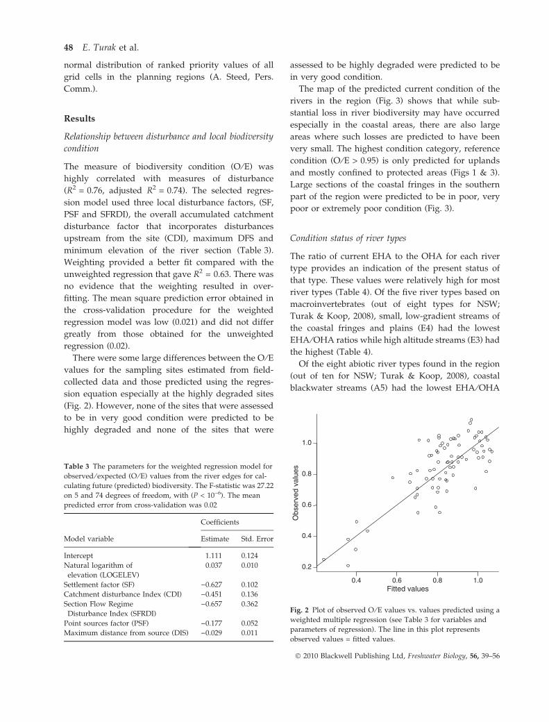
There were some large differences between the O ⁄Evalues for the sampling sites estimated from field-

collected data and those predicted using the regres-

sion equation especially at the highly degraded sites

(Fig. 2). However, none of the sites that were assessed

to be in very good condition were predicted to be

highly degraded and none of the sites that were

assessed to be highly degraded were predicted to be

in very good condition.

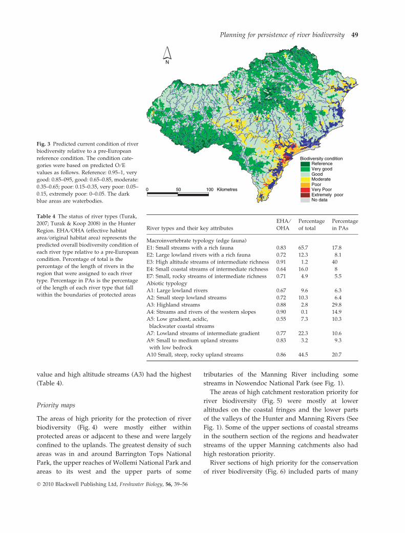
The map of the predicted current condition of the

rivers in the region (Fig. 3) shows that while sub-

stantial loss in river biodiversity may have occurred

especially in the coastal areas, there are also large

areas where such losses are predicted to have been

very small. The highest condition category, reference

condition (O ⁄E > 0.95) is only predicted for uplands

and mostly confined to protected areas (Figs 1 & 3).

Large sections of the coastal fringes in the southern

part of the region were predicted to be in poor, very

poor or extremely poor condition (Fig. 3).

Condition status of river types

The ratio of current EHA to the OHA for each river

type provides an indication of the present status of

that type. These values were relatively high for most

river types (Table 4). Of the five river types based on

macroinvertebrates (out of eight types for NSW;

Turak & Koop, 2008), small, low-gradient streams of

the coastal fringes and plains (E4) had the lowest

EHA ⁄OHA ratios while high altitude streams (E3) had

the highest (Table 4).

Of the eight abiotic river types found in the region

(out of ten for NSW; Turak & Koop, 2008), coastal

blackwater streams (A5) had the lowest EHA ⁄OHA

Table 3 The parameters for the weighted regression model for

observed ⁄ expected (O ⁄ E) values from the river edges for cal-

culating future (predicted) biodiversity. The F-statistic was 27.22

on 5 and 74 degrees of freedom, with (P < 10)6). The mean

predicted error from cross-validation was 0.02

Model variable

Coefficients

Estimate Std. Error

Intercept 1.111 0.124

Natural logarithm of

elevation (LOGELEV)

0.037 0.010

Settlement factor (SF) )0.627 0.102

Catchment disturbance Index (CDI) )0.451 0.136

Section Flow Regime

Disturbance Index (SFRDI)

)0.657 0.362

Point sources factor (PSF) )0.177 0.052

Maximum distance from source (DIS) )0.029 0.011

0.4 0.6 0.8 1.0

0.2

0.4

0.6

0.8

1.0

Fitted values

Obs

erve

d va

lues

Fig. 2 Plot of observed O ⁄ E values vs. values predicted using a

weighted multiple regression (see Table 3 for variables and

parameters of regression). The line in this plot represents

observed values = fitted values.

48 E. Turak et al.


value and high altitude streams (A3) had the highest

(Table 4).

Priority maps

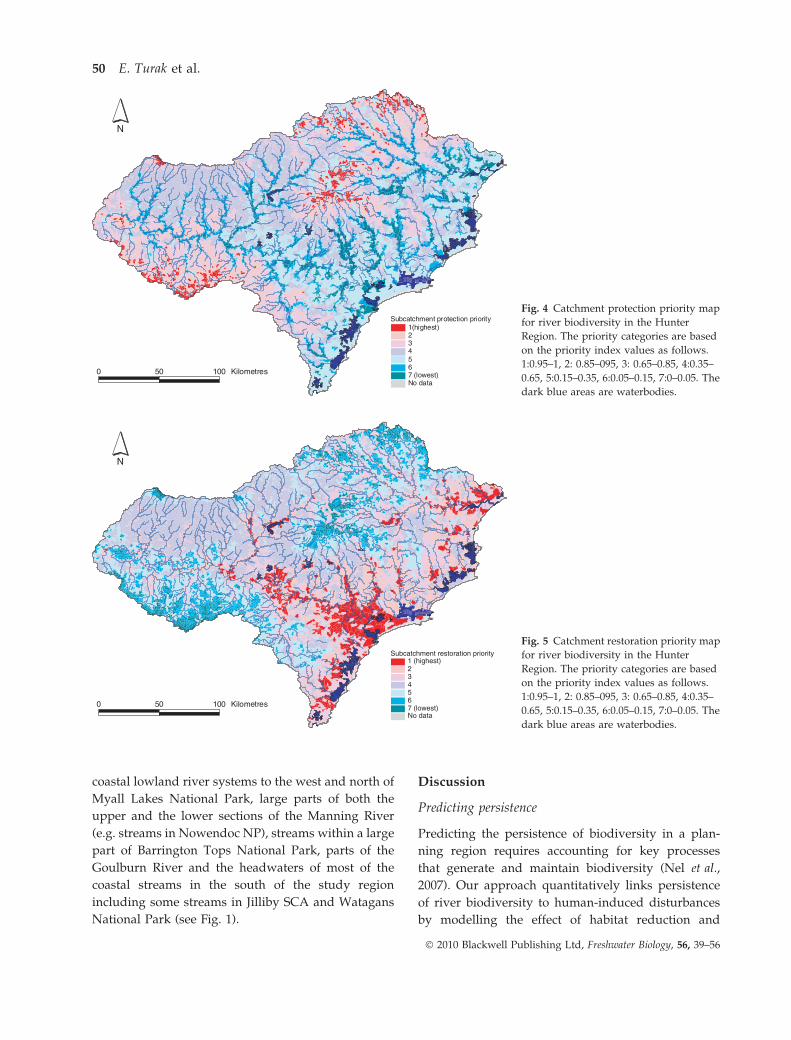
The areas of high priority for the protection of river

biodiversity (Fig. 4) were mostly either within

protected areas or adjacent to these and were largely

confined to the uplands. The greatest density of such

areas was in and around Barrington Tops National

Park, the upper reaches of Wollemi National Park and

areas to its west and the upper parts of some

tributaries of the Manning River including some

streams in Nowendoc National Park (see Fig. 1).

The areas of high catchment restoration priority for

river biodiversity (Fig. 5) were mostly at lower

altitudes on the coastal fringes and the lower parts

of the valleys of the Hunter and Manning Rivers (See

Fig. 1). Some of the upper sections of coastal streams

in the southern section of the regions and headwater

streams of the upper Manning catchments also had

high restoration priority.

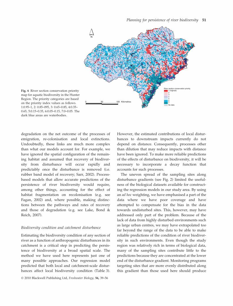
River sections of high priority for the conservation

of river biodiversity (Fig. 6) included parts of many

N

No data

Biodiversity conditionReferenceVery goodGoodModeratePoorVery PoorExtremely poor

0 50 100 Kilometres

Fig. 3 Predicted current condition of river

biodiversity relative to a pre-European

reference condition. The condition cate-

gories were based on predicted O ⁄ Evalues as follows. Reference: 0.95–1, very

good: 0.85–095, good: 0.65–0.85, moderate:

0.35–0.65; poor: 0.15–0.35, very poor: 0.05–

0.15, extremely poor: 0–0.05. The dark

blue areas are waterbodies.

Table 4 The status of river types (Turak,

2007; Turak & Koop 2008) in the Hunter

Region. EHA ⁄ OHA (effective habitat

area ⁄ original habitat area) represents the

predicted overall biodiversity condition of

each river type relative to a pre-European

condition. Percentage of total is the

percentage of the length of rivers in the

region that were assigned to each river

type. Percentage in PAs is the percentage

of the length of each river type that fall

within the boundaries of protected areas

River types and their key attributes

EHA ⁄OHA

Percentage

of total

Percentage

in PAs

Macroinvertebrate typology (edge fauna)

E1: Small streams with a rich fauna 0.83 65.7 17.8

E2: Large lowland rivers with a rich fauna 0.72 12.3 8.1

E3: High altitude streams of intermediate richness 0.91 1.2 40

E4: Small coastal streams of intermediate richness 0.64 16.0 8

E7: Small, rocky streams of intermediate richness 0.71 4.9 5.5

Abiotic typology

A1: Large lowland rivers 0.67 9.6 6.3

A2: Small steep lowland streams 0.72 10.3 6.4

A3: Highland streams 0.88 2.8 29.8

A4: Streams and rivers of the western slopes 0.90 0.1 14.9

A5: Low gradient, acidic,

blackwater coastal streams

0.55 7.3 10.3

A7: Lowland streams of intermediate gradient 0.77 22.3 10.6

A9: Small to medium upland streams

with low bedrock

0.83 3.2 9.3

A10 Small, steep, rocky upland streams 0.86 44.5 20.7



coastal lowland river systems to the west and north of

Myall Lakes National Park, large parts of both the

upper and the lower sections of the Manning River

(e.g. streams in Nowendoc NP), streams within a large

part of Barrington Tops National Park, parts of the

Goulburn River and the headwaters of most of the

coastal streams in the south of the study region

including some streams in Jilliby SCA and Watagans

National Park (see Fig. 1).

Discussion

Predicting persistence

Predicting the persistence of biodiversity in a plan-

ning region requires accounting for key processes

that generate and maintain biodiversity (Nel et al.,

2007). Our approach quantitatively links persistence

of river biodiversity to human-induced disturbances

by modelling the effect of habitat reduction and

0 50 100 Kilometres

N

No data

Subcatchment protection priority1(highest)234567 (lowest)

Fig. 4 Catchment protection priority map

for river biodiversity in the Hunter

Region. The priority categories are based

on the priority index values as follows.

1:0.95–1, 2: 0.85–095, 3: 0.65–0.85, 4:0.35–

0.65, 5:0.15–0.35, 6:0.05–0.15, 7:0–0.05. The

dark blue areas are waterbodies.

0 50 100 Kilometres

N

No data

Subcatchment restoration priority1 (highest)234567 (lowest)

Fig. 5 Catchment restoration priority map

for river biodiversity in the Hunter



1:0.95–1, 2: 0.85–095, 3: 0.65–0.85, 4:0.35–

0.65, 5:0.15–0.35, 6:0.05–0.15, 7:0–0.05. The


50 E. Turak et al.


degradation on the net outcome of the processes of

emigration, re-colonisation and local extinctions.

Undoubtedly, these links are much more complex

than what our models account for. For example, we

have ignored the spatial configuration of the remain-

ing habitat and assumed that recovery of biodiver-

sity from disturbance will occur rapidly and

predictably once the disturbance is removed (i.e.

rubber band model of recovery; Sarr, 2002). Process-

based models that allow accurate predictions of the

persistence of river biodiversity would require,

among other things, accounting for the effect of

habitat fragmentation on recolonisation (e.g. see

Fagan, 2002) and, where possible, making distinc-

tions between the pathways and rates of recovery

and those of degradation (e.g. see Lake, Bond &

Reich, 2007).

Biodiversity condition and catchment disturbance

Estimating the biodiversity condition of any section of

river as a function of anthropogenic disturbances in its

catchment is a critical step in predicting the persis-

tence of biodiversity at a broad spatial scale. The

method we have used here represents just one of

many possible approaches. Our regression model

predicted that both local and catchment-scale distur-

bances affect local biodiversity condition (Table 3).

However, the estimated contributions of local distur-

bances to downstream impacts currently do not

depend on distance. Consequently, processes other

than dilution that may reduce impacts with distance

have been ignored. To make more reliable predictions

of the effects of disturbance on biodiversity, it will be

necessary to incorporate a decay function that

accounts for such processes.

The uneven spread of the sampling sites along

disturbance gradients (see Fig. 2) limited the useful-

ness of the biological datasets available for construct-

ing the regression models in our study area. By using

an ad hoc weighting, we have emphasised a part of the

data where we have poor coverage and have

attempted to compensate for the bias in the data

towards undisturbed sites. This, however, may have

addressed only part of the problem. Because of the

lack of data from highly disturbed environments such

as large urban centres, we may have extrapolated too

far beyond the range of the data to be able to make

reliable predictions of the condition of river biodiver-

sity in such environments. Even though the study

region was relatively rich in terms of biological data,

many of the sampling sites contribute little to the

predictions because they are concentrated at the lower

end of the disturbance gradient. Monitoring programs

targeting sites that are more evenly distributed along

this gradient than those used here should produce

0 50 100 Kilometres

N

No data

River section conservation priority1 (highest)234567

Fig. 6 River section conservation priority

map for aquatic biodiversity in the Hunter



1:0.95–1, 2: 0.85–095, 3: 0.65–0.85, 4:0.35–

0.65, 5:0.15–0.35, 6:0.05–0.15, 7:0–0.05. The




much better input data for predicting biodiversity

condition across the region with considerably less

sampling effort.

Our ability to predict biodiversity condition from

measures of disturbance may be improved by refining

the methods. Steps that can be taken in this direction

include: lowering the taxa probability threshold in

calculating the AUSRIVAS O ⁄E values (Turak &

Koop, 2003); constructing new predictive models that

use only rare taxa (Linke & Norris, 2003); replacing

the disturbance factors determined at a continental

scale (Stein et al., 1998, 2002) with those that better

account for the effects of local land management

practices on river ecosystems; and incorporating

additional disturbance indicators for riparian condi-

tion and instream barriers. The predictions may also

be improved by replacing the linear regressions used

here with more complex relationships, such as gener-

alised additive models (Wood, 2006), which allow for

nonlinearities in response to predictor variables, or

geostatistical models generated for stream networks

(e.g. Peterson, Theobald & Ver Hoef, 2007), which

allow for spatial correlations among sites, or a

combination of such approaches.

Our predictive model was developed in a relatively

data-rich context especially in terms of biological data.

However, the input variables in the model are either

known topographical variables or indices that depend

on land management data which should in principle

be available from remote sensing data independently

of field observations. If our predictive model is

sufficiently robust to be used in other nearby catch-

ments, then the approach we have used may be

extended to catchments elsewhere. The potential to

extend our approach using only remotely obtained

data needs to be explored further.

Estimating conservation return

In our approach, the conservation benefit, or return,

from any management action is estimated in the

currency of the BDI. We used river types based on

abiotic attributes or family-level assemblage structure

of macroinvertebrates (Turak, 2007; Turak & Koop,

2008) to represent the likely influence of climate,

geology, topography and geography on river biodi-

versity at a broad spatial scale. Given that large

sections of the study area such as the southeastern

corner had poor values for biodiversity condition

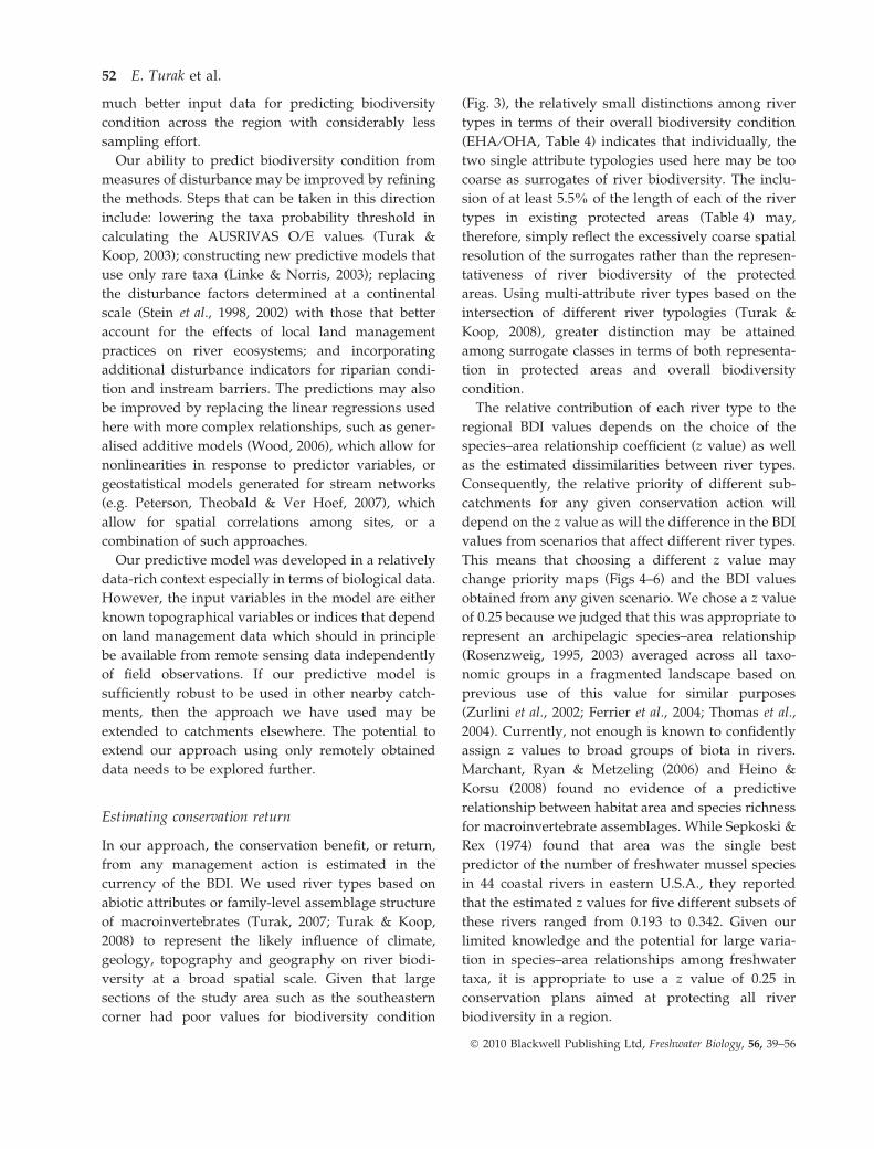
(Fig. 3), the relatively small distinctions among river

types in terms of their overall biodiversity condition

(EHA ⁄OHA, Table 4) indicates that individually, the

two single attribute typologies used here may be too

coarse as surrogates of river biodiversity. The inclu-

sion of at least 5.5% of the length of each of the river

types in existing protected areas (Table 4) may,

therefore, simply reflect the excessively coarse spatial

resolution of the surrogates rather than the represen-

tativeness of river biodiversity of the protected

areas. Using multi-attribute river types based on the

intersection of different river typologies (Turak &

Koop, 2008), greater distinction may be attained

among surrogate classes in terms of both representa-

tion in protected areas and overall biodiversity

condition.

The relative contribution of each river type to the

regional BDI values depends on the choice of the

species–area relationship coefficient (z value) as well

as the estimated dissimilarities between river types.

Consequently, the relative priority of different sub-

catchments for any given conservation action will

depend on the z value as will the difference in the BDI

values from scenarios that affect different river types.

This means that choosing a different z value may

change priority maps (Figs 4–6) and the BDI values

obtained from any given scenario. We chose a z value

of 0.25 because we judged that this was appropriate to

represent an archipelagic species–area relationship

(Rosenzweig, 1995, 2003) averaged across all taxo-

nomic groups in a fragmented landscape based on

previous use of this value for similar purposes

(Zurlini et al., 2002; Ferrier et al., 2004; Thomas et al.,

2004). Currently, not enough is known to confidently

assign z values to broad groups of biota in rivers.

Marchant, Ryan & Metzeling (2006) and Heino &

Korsu (2008) found no evidence of a predictive

relationship between habitat area and species richness

for macroinvertebrate assemblages. While Sepkoski &

Rex (1974) found that area was the single best

predictor of the number of freshwater mussel species

in 44 coastal rivers in eastern U.S.A., they reported

that the estimated z values for five different subsets of

these rivers ranged from 0.193 to 0.342. Given our

limited knowledge and the potential for large varia-

tion in species–area relationships among freshwater

taxa, it is appropriate to use a z value of 0.25 in

conservation plans aimed at protecting all river

biodiversity in a region.

52 E. Turak et al.


Translating predictions of persistence into conservation

actions

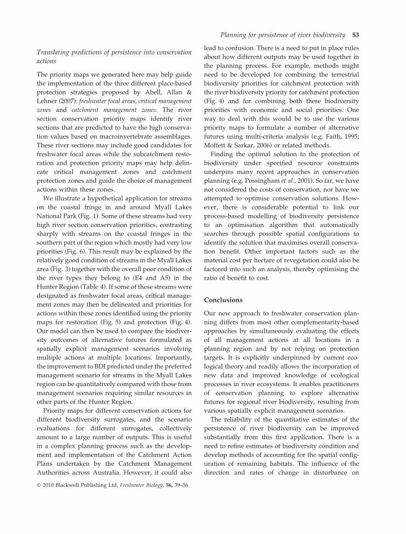
The priority maps we generated here may help guide

the implementation of the three different place-based

protection strategies proposed by Abell, Allan &

Lehner (2007): freshwater focal areas, critical management

zones and catchment management zones. The river

section conservation priority maps identify river

sections that are predicted to have the high conserva-

tion values based on macroinvertebrate assemblages.

These river sections may include good candidates for

freshwater focal areas while the subcatchment resto-

ration and protection priority maps may help delin-

eate critical management zones and catchment

protection zones and guide the choice of management

actions within these zones.

We illustrate a hypothetical application for streams

on the coastal fringe in and around Myall Lakes

National Park (Fig. 1). Some of these streams had very

high river section conservation priorities, contrasting

sharply with streams on the coastal fringes in the

southern part of the region which mostly had very low

priorities (Fig. 6). This result may be explained by the

relatively good condition of streams in the Myall Lakes

area (Fig. 3) together with the overall poor condition of

the river types they belong to (E4 and A5) in the

Hunter Region (Table 4). If some of these streams were

designated as freshwater focal areas, critical manage-

ment zones may then be delineated and priorities for

actions within these zones identified using the priority

maps for restoration (Fig. 5) and protection (Fig. 4).

Our model can then be used to compare the biodiver-

sity outcomes of alternative futures formulated as

spatially explicit management scenarios involving

multiple actions at multiple locations. Importantly,

the improvement to BDI predicted under the preferred

management scenario for streams in the Myall Lakes

region can be quantitatively compared with those from

management scenarios requiring similar resources in

other parts of the Hunter Region.

Priority maps for different conservation actions for

different biodiversity surrogates, and the scenario

evaluations for different surrogates, collectively

amount to a large number of outputs. This is useful

in a complex planning process such as the develop-

ment and implementation of the Catchment Action

Plans undertaken by the Catchment Management

Authorities across Australia. However, it could also

lead to confusion. There is a need to put in place rules

about how different outputs may be used together in

the planning process. For example, methods might

need to be developed for combining the terrestrial

biodiversity priorities for catchment protection with

the river biodiversity priority for catchment protection

(Fig. 4) and for combining both these biodiversity

priorities with economic and social priorities. One

way to deal with this would be to use the various

priority maps to formulate a number of alternative

futures using multi-criteria analysis (e.g. Faith, 1995;

Moffett & Sarkar, 2006) or related methods.

Finding the optimal solution to the protection of

biodiversity under specified resource constraints

underpins many recent approaches in conservation

planning (e.g. Possingham et al., 2001). So far, we have

not considered the costs of conservation, nor have we

attempted to optimise conservation solutions. How-

ever, there is considerable potential to link our

process-based modelling of biodiversity persistence

to an optimisation algorithm that automatically

searches through possible spatial configurations to

identify the solution that maximises overall conserva-

tion benefit. Other important factors such as the

material cost per hectare of revegetation could also be

factored into such an analysis, thereby optimising the

ratio of benefit to cost.

Conclusions

Our new approach to freshwater conservation plan-

ning differs from most other complementarity-based

approaches by simultaneously evaluating the effects

of all management actions at all locations in a

planning region and by not relying on protection

targets. It is explicitly underpinned by current eco-

logical theory and readily allows the incorporation of

new data and improved knowledge of ecological

processes in river ecosystems. It enables practitioners

of conservation planning to explore alternative

futures for regional river biodiversity, resulting from

various spatially explicit management scenarios.

The reliability of the quantitative estimates of the

persistence of river biodiversity can be improved

substantially from this first application. There is a

need to refine estimates of biodiversity condition and

develop methods of accounting for the spatial config-

uration of remaining habitats. The influence of the

direction and rates of change in disturbance on



biodiversity condition and the likely end points of

restoration activities must also be taken into consid-

eration. These – together with refinements of bio-

diversity surrogates – are likely to greatly improve the

utility of our methods in freshwater conservation

planning.

Acknowledgments

This work was partly funded by the Australian

Commonwealth under the Natural Heritage Trust

Funding. We thank Klaus Koop for comments on the

manuscript.

References

Abell R., Allan J.D. & Lehner B. (2007) Unlocking the

potential of protected areas for freshwaters. Biological

Conservation, 134, 48–63.

Allnutt T.F., Ferrier S., Manion G. et al. (2008) A method

for quantifying biodiversity loss and its application to

a 50-year record of deforestation across Madagascar.

Conservation Letters, 1, 173–181.

Arponen A., Heikkinen R.K., Thomas C.D. & Moilanen

A. (2005) The value of biodiversity in reserve selection:

representation, species weighting, and benefit func-

tions. Conservation Biology, 19, 2009–2014.

Arrhenius O. (1921) Species and area. Journal of Ecology,

9, 95–99.

Brooks T.M., Bakarr M.I., Boucher T. et al. (2004) Cover-

age provided by the Global Protected-Area System: is

it enough? BioScience, 54, 1081–1091.

Canty A. & Ripley B.D. (2009) boot: Bootstrap R (S-PLUS)

Functions. R package version 1.2–35. Available at:

http://CRAN.R-project.org/package=boot.(lastaccessed

on 30 December 2009).

Davies P.E. (2000) Development of the National River

Bioassessment System (AUSRIVAS) in Australia. In:

Assessing the Biological Quality of Freshwaters: RIVPACS

and Other Techniques (Eds J.F. Wright, D.W. Sutcliffe, &

M.T. Furse), pp. 113–124. Freshwater Biological Asso-

ciation, Cumbria, UK.

DECC (2007a) Lord Howe Island Biodiversity Management

Plan. NSW Department of Environment and Climate Change.

Available at: http://www.environment.nsw.gov.au/

parkmanagement/LordHoweBiodiversityMgmtplan

Draft.htm. (last accessed on 30 December 2009).

DECC (2007b) 100m Land use Grid for Hunter-Central

Rivers CMA (ANZLIC v1.2 Metadata Standard). NSW

Department of Environment and Climate Change.

Sydney.

DECC (2009) Working Draft Northern Rivers Region Biodi-

versity Management Plan, National Recovery Plan for the

Northern Rivers Region. Department of Environment

and Climate Change NSW, Sydney.

Desmet P. & Cowling R. (2004) Using the species-area

relationship to set baseline targets for conservation.

Ecology and Society 9: 11. Available at: http://www.

ecologyandsociety.org/vol9/iss2/art11/ (last accessed

on 30 December 2009).

Diamond J. & May R. (1976) Island biogeography and the

design of natural reserves. In: Theoretical Ecology:

Principles and Applications (Ed. R. May), pp. 163–186.

Blackwell Scientific Publications, Oxford, UK.

Drielsma M. & Ferrier S. (2006) Landscape scenario

modelling of vegetation condition. Ecological Manage-

ment and Restoration, 7, S45–S52.

Dudgeon D., Arthington A.H., Gessner M.O. et al. (2006)

Freshwater biodiversity: importance, threats, status and

conservation challenges. Biological Reviews, 81, 163–182.

ESRI (1999) ArcView Version 3.2. Environmental Systems

Research Institute, Inc., Redlands, CA.

ESRI (2005) ArcGIS Version 9.1. Environmental Systems

Research Institute, Inc, Redlands, CA.

Fagan W.F. (2002) Connectivity, fragmentation and

extinction risks in dendritic populations. Ecology, 83,

3243–3249.

Faith D.P. (1995) Biodiversity and Regional Sustainability

Analysis. CSIRO Division of Wildlife and Ecology,

Lyneham, Australia.

Faith D.P., Ferrier S. & Williams K.J. (2008) Getting

biodiversity intactness indices right: ensuring that

‘biodiversity’ reflects ‘diversity’. Global Change Biology

14, 207–217.

Ferrier S. (2005) An Integrated Approach to Addressing

Terrestrial Biodiversity in NRM Investment Planning and

Evaluation Across State, Catchment and Property Scales.

NSW Department of Environment and Conservation,

February 2005. Available at: http://www.nrc.nsw.gov.

au/content/documents/Submission%20-%20ST%20-%

20DEC%20Biodiversity.pdf (last accessed on 30 Dec-

ember 2009).

Ferrier S., Powell G.V.N., Richardson K.S. et al. (2004)

Mapping more of terrestrial biodiversity for Global

Conservation Assessment. BioScience, 54, 1101–1109.

Ferrier S., Faith D.P., Arponen A. & Drielsma M. (2009)

Community-level approaches to spatial conservation

prioritization. In: Spatial Conservation Prioritization:

Quantitative Methods and Computational Tools (Eds. A.

Moilanen, H. Possingham, K. Wilson), pp 94–109.

Oxford University Press, Oxford.

HCR CMA (2007) Hunter-Central Rivers Catchment Action

Plan. Hunter-Central Rivers Catchment Management

54 E. Turak et al.


Authority, New South Wales, Australia. Available at:

http://www.hcr.cma.nsw.gov.au/catchmentactionplan.

php3 (last accessed on 30 December 2009).

Heino J. & Korsu K. (2008) Testing species-stone area and

species-bryophyte cover relationships in riverine macr-

oinvertebrates at small scales. Freshwater Biology, 53,

558–568.

HoseG.&TurakE.(2006)RiverHealth intheNewSouthWales

Lower North Coast, Hunter and Central Coast Catchments.

River Health Bioassessment Report No. 41 Department

of the Environment and Heritage, and NSW Department

of Environment and Conservation. Available at: http://

www.environment.gov.au/water/publications/envi

ronmental/rivers/nrhp/catchments-nsw/index.html

(last accessed on 30 December 2009).

Hutchinson M.F., Stein J. & Stein J. (2001) Upgrade of the 9

Second Australian Digital Elevation Model. A Joint Project

of CRES and AUSLIG. Retrieved 2nd, August, 2004.

Available at: http://cres.anu.edu.au/dem/index.

php#4 (last accessed on 30 December 2009).

Lake P.S., Bond N. & Reich P. (2007) Linking ecological

theory with stream restoration. Freshwater Biology, 52,

597–615.

Linke S. & Norris R.H. (2003) Biodiversity: bridging the

gap between condition and conservation. Hydrobiolo-

gia, 500, 203–211.

Linke S., Pressey R.L., Bailey R.C. & Norris R.H. (2007)

Management options for river conservation planning.

Freshwater Biology, 5, 918–938.

Malmqvist B. & Rundle S. (2002) Threats to running

water ecosystems of the world. Environmental Conser-

vation, 29, 134–153.

Marchant R., Ryan D. & Metzeling L. (2006) Regional and

local species diversity patterns for lotic invertebrates

across multiple drainage basins in Victoria. Marine and

Freshwater Research, 47, 675–684.

Margules C.R. & Pressey R.L. (2000) Systematic conser-

vation planning. Nature, 405, 243–253.

McNeely J.A.Ed. (1993) Parks for Life: Report of the IVth

World Congress on National Parks and Protected Areas.

IUCN Communications Division, Gland (Switzerland).

Moffett A. & Sarkar S. (2006) Incorporating multiple

criteria into the design of conservation area networks:

a mini review with recommendations. Diversity and

Distributions, 12, 125–137.

Moilanen A., Leathwick J. & Elith J. (2008) A method for

spatial freshwater conservation prioritization. Freshwa-

ter Biology, 53, 577–592.

Nel J.L., Roux D.J., Maree G., Kleynhans C.J., Moolman J.,

Reyers B., Rouget M. & Cowling R.M. (2007) Rivers in

peril inside and outside protected areas: a systematic

approach to conservation assessment of river ecosys-

tems. Diversity and Distributions, 13, 341–352.

Peterson G.D., Cumming G.S. & Carpenter S.R. (2003)

Scenario planning: a tool for conservation in an

uncertain world. Conservation Biology, 17, 358–366.

Peterson E.E., Theobald D.M. & Ver Hoef J.M. (2007)

Geostatistical modelling on stream networks: develop-

ing valid covariance matrices based on hydrologic

distance and stream flow. Freshwater Biology, 52, 267–

269.

Pfafstetter O. (1989) Classification of hydrographic

basins: coding methodology, unpublished manuscript,

Departamento Nacional de Obras de Saneamento,

August 18, 1989, Rio de Janeiro; available from J.P.

Verdin, U.S. Geological Survey, EROS Data Center,

Sioux Falls, South Dakota 57198 USA.

Possingham H.P., Andelman S.J., Noon B.R., Trombulak

S. & Pulliam H.R. (2001) Making smart conservation

decisions. In: Conservation Biology: Research Priorities for

the Next Decade (Eds M.E. Soule & G.H. Orians), pp.

225–244. Island Press, Washington, DC.

Pressey R.L., Cowling R.M. & Rouget M. (2003) Formu-

lating conservation targets for biodiversity pattern and

process in the Cape Floristic Region, South Africa.

Biological Conservation, 112, 99–127.

R Development Core Team (2004) R: A Language and

Environment for Statistical Computing. R Foundation for

Statistical Computing, Vienna. ISBN 3-900051-00-3.

Available at: http://www.R-project.org (last accessed

30 December 2009).

Rodrigues A.S.L. & Gaston K.J. (2001) How large do

reserve networks need to be? Ecology Letters, 4, 602–

609.

Rosenzweig M.L. (1995) Species Diversity in Space and

Time. Cambridge University Press, Cambridge, UK.

Rosenzweig M.L. (2003) Reconciliation ecology and the

future of species diversity. Oryx, 37, 194–205.

Sarkar S. & Margules C. (2002) Operationalizing biodi-

versity for conservation planning. Journal of Biosciences,

27, 299–308.

Sarkar S., Pressey R.L., Faith D.P. et al. (2006) Biodiver-

sity conservation planning tools: present status and

challenges for the future. Annual Review of Environment

and Resources, 31, 123–159.

Sarr D.A. (2002) Riparian livestock exclosure research in

the Western United States: a critique and some

recommendations. Environmental Management, 30,

516–526.

Sepkoski J.J. Jr & Rex M.A. (1974) Distribution of

freshwater mussels: coastal rivers as biogeographic

islands. Systematic Zoology, 23, 165–188.

Simpson J.C. & Norris R.H. (2000) Biological assessment

of river quality: development of AUSRIVAS models

and outputs. In: Assessing the Biological Quality

of Freshwaters: RIVPACS and Other Techniques (Eds



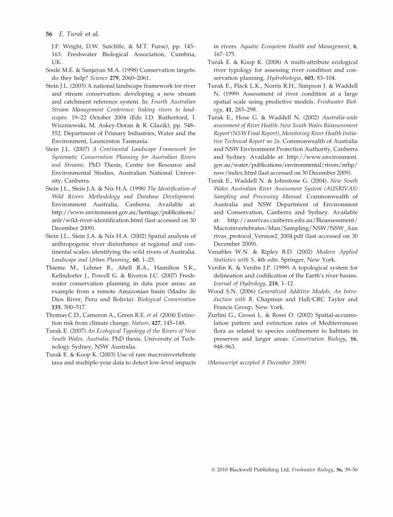
J.F. Wright, D.W. Sutcliffe, & M.T. Furse), pp. 143–

163. Freshwater Biological Association, Cumbria,

UK.

Soule M.E. & Sanjayan M.A. (1998) Conservation targets:

do they help? Science 279, 2060–2061.

Stein J.L. (2005) A national landscape framework for river

and stream conservation: developing a new stream

and catchment reference system. In: Fourth Australian

Stream Management Conference: linking rivers to land-

scapes. 19–22 October 2004 (Eds I.D. Rutherford, I.

Wiszniewski, M. Askey-Doran & R. Glazik), pp. 548–

552. Department of Primary Industries, Water and the

Environment, Launceston Tasmania.

Stein J.L. (2007) A Continental Landscape Framework for

Systematic Conservation Planning for Australian Rivers

and Streams. PhD Thesis, Centre for Resource and

Environmental Studies, Australian National Univer-

sity, Canberra.

Stein J.L., Stein J.A. & Nix H.A. (1998) The Identification of

Wild Rivers: Methodology and Database Development.

Environment Australia, Canberra. Available at:

http://www.environment.gov.au/heritage/publications/

anlr/wild-river-identification.html (last accessed on 30

December 2009).

Stein J.L., Stein J.A. & Nix H.A. (2002) Spatial analysis of

anthropogenic river disturbance at regional and con-

tinental scales: identifying the wild rivers of Australia.

Landscape and Urban Planning, 60, 1–25.

Thieme M., Lehner B., Abell R.A., Hamilton S.K.,

Kellndorfer J., Powell G. & Riveros J.C. (2007) Fresh-

water conservation planning in data poor areas: an

example from a remote Amazonian basin (Madre de

Dios River, Peru and Bolivia). Biological Conservation

135, 500–517.

Thomas C.D., Cameron A., Green R.E. et al. (2004) Extinc-

tion risk from climate change. Nature, 427, 145–148.

Turak E. (2007) An Ecological Typology of the Rivers of New

South Wales, Australia. PhD thesis. University of Tech-

nology Sydney, NSW Australia.

Turak E. & Koop K. (2003) Use of rare macroinvertebrate

taxa and multiple-year data to detect low-level impacts

in rivers. Aquatic Ecosystem Health and Management, 6,

167–175.

Turak E. & Koop K. (2008) A multi-attribute ecological

river typology for assessing river condition and con-

servation planning. Hydrobiologia, 603, 83–104.

Turak E., Flack L.K., Norris R.H., Simpson J. & Waddell

N. (1999) Assessment of river condition at a large

spatial scale using predictive models. Freshwater Biol-

ogy, 41, 283–298.

Turak E., Hose G. & Waddell N. (2002) Australia-wide

assessment of River Health: New South Wales Bioassessment

Report (NSW Final Report), Monitoring River Health Initia-

tive Technical Report no 2a. Commonwealth of Australia

and NSW Environment Protection Authority, Canberra

and Sydney. Available at: http://www.environment.

gov.au/water/publications/environmental/rivers/nrhp/

nsw/index.html (last accessed on 30 December 2009).

Turak E., Waddell N. & Johnstone G. (2004). New South

Wales Australian River Assessment System (AUSRIVAS)

Sampling and Processing Manual. Commonwealth of

Australia and NSW Department of Environment

and Conservation, Canberra and Sydney. Available

at: http://ausrivas.canberra.edu.au/Bioassessment/

Macroinvertebrates/Man/Sampling/NSW/NSW_Aus

rivas_protocol_Version2_2004.pdf (last accessed on 30

December 2009).

Venables W.N. & Ripley B.D. (2002) Modern Applied

Statistics with S, 4th edn. Springer, New York.

Verdin K. & Verdin J.P. (1999) A topological system for

delineation and codification of the Earth’s river basins.

Journal of Hydrology, 218, 1–12.

Wood S.N. (2006) Generalized Additive Models, An Intro-

duction with R. Chapman and Hall ⁄CRC Taylor and

Francis Group, New York.

Zurlini G., Grossi L. & Rossi O. (2002) Spatial-accumu-

lation pattern and extinction rates of Mediterranean

flora as related to species confinement to habitats in

preserves and larger areas. Conservation Biology, 16,

948–963.

(Manuscript accepted 8 December 2009)

56 E. Turak et al.


Planning for the persistence of river biodiversity: exploring alternative futures using...

Documents

Transcript of Planning for the persistence of river biodiversity: exploring alternative futures using...