Planar Optical Measurement Methods for Gas Turbine ...

(0

UJ I

O

RTO-EN-6 AC/323(AVT)TP/20

NORTH ATLANTIC TREATY ORGANIZATION

RESEARCH AND TECHNOLOGY ORGANIZATION

BP 25, 7 RUE ANCELLE, F-92201 NEUILLY-SUR-SEINE CEDEX, FRANCE

RTO LECTURE SERIES 217

Planar Optical Measurement Methods for Gas Turbine Components (Methodes de mesure optiques planaires pour organes de turbomoteurs)

The material in this publication was assembled to support a Lecture Series under the sponsorship of the Applied Vehicle Technology Panel (AVT) presented on 16-17 September 1999 in Cranfield, UK and 21-22 September 1999 in Cleveland, USA.

DISTRIBUTION STATEMENT A Approved for Public Release

Distribution Unlimited 19991123 085

Published September 1999

Distribution and Availability on Back Cover

Groupe Canada

Communication Communication

Canada Group Membre de la A St. Joseph Corporation St-Joseph Corporation Company

September 1999

ERRATUM NOTICE - RTO-EN-6

To all recipients of RTO publication EN-6 for Lecture Series 216 on "Planar Optical Measurement Methods for Gas Turbine Components".

Paper 6 - "Planar Laser Induced Fluorescence for Investigation of Scalars in Turbulent Reacting Flows"

The author would like to make the following corrections:

Page 6-2, Figure 1

- The concentration on the lower energy level is Ni(t).

Page 6-3, Left-hand column, 3rd paragraph

... the steady state balance equation is dN2/dt=...

Page 6-3, Right-hand column, 3rd paragraph

- In the equation for P(t) the right hand term must be divided by c.

45, boulevard Sacre-Coeur Hull (Quebec) Kl A 0S7

45 Sacre-Coeur Boulevard Hull, Quebec Kl A 0S7

DTIC QUALITY INSPECTED 4

V^^ÖO-Ö?-- 05%(o




BP 25, 7 RUE ANCELLE, F-92201 NEUILLY-SUR-SEINE CEDEX, FRANCE

RTO LECTURE SERIES 217

Planar Optical Measurement Methods for Gas Turbine Components (Methodes de mesure optiques planaires pour organes de turbomoteurs)

The material in this publication was assembled to support a Lecture Series under the sponsorship of the Applied Vehicle Technology Panel (AVT) presented on 16-17 September 1999 in Cranfield, UK and 21-22 September 1999 in Cleveland, USA.

The Research and Technology Organization (RTO) of NATO

RTO is the single focus in NATO for Defence Research and Technology activities. Its mission is to conduct and promote cooperative research and information exchange. The objective is to support the development and effective use of national defence research and technology and to meet the military needs of the Alliance, to maintain a technological lead, and to provide advice to NATO and national decision makers. The RTO performs its mission with the support of an extensive network of national experts. It also ensures effective coordination with other NATO bodies involved in R&T activities.

RTO reports both to the Military Committee of NATO and to the Conference of National Armament Directors. It comprises a Research and Technology Board (RTB) as the highest level of national representation and the Research and Technology Agency (RTA), a dedicated staff with its headquarters in Neuilly, near Paris, France. In order to facilitate contacts with the military users and other NATO activities, a small part of the RTA staff is located in NATO Headquarters in Brussels. The Brussels staff also coordinates RTO's cooperation with nations in Middle and Eastern Europe, to which RTO attaches particular importance especially as working together in the field of research is one of the more promising areas of initial cooperation.

The total spectrum of R&T activities is covered by 7 Panels, dealing with:

• SAS Studies, Analysis and Simulation

• SCI Systems Concepts and Integration

• SET Sensors and Electronics Technology

• 1ST Information Systems Technology

• AVT Applied Vehicle Technology

• HFM Human Factors and Medicine

• MSG Modelling and Simulation

These Panels are made up of national representatives as well as generally recognised 'world class' scientists. The Panels also provide a communication link to military users and other NATO bodies. RTO's scientific and technological work is carried out by Technical Teams, created for specific activities and with a specific duration. Such Technical Teams can organise workshops, symposia, field trials, lecture series and training courses. An important function of these Technical Teams is to ensure the continuity of the expert networks,

RTO builds upon earlier cooperation in defence research and technology as set-up under the Advisory Group for Aerospace Research and Development (AGARD) and the Defence Research Group (DRG). AGARD and the DRG share common roots in that they were both established at the initiative of Dr Theodore von Kärmän, a leading aerospace scientist, who early on recognised the importance of scientific support for the Allied Armed Forces. RTO is capitalising on these common roots in order to provide the Alliance and the NATO nations with a strong scientific and technological basis that will guarantee a solid base for the future.

The content of this publication has been reproduced directly from material supplied by RTO or the authors.

® Printed on recycled paper

Published September 1999

Copyright © RTO/NATO1999 All Rights Reserved

ISBN ISBN 92-837-1019-3

Printed by Canada Communication Group Inc. (A St. Joseph Corporation Company)

45 Sacre-Cceur Blvd., Hull (Quebec), Canada K1A 0S7

Planar Optical Measurement Methods for Gas Turbine Components

(RTOEN-6)

Executive Summary

Future generations of aircraft and missiles require advances in propulsion engines. The demands are higher specific thrust, lower specific fuel consumption and lower development costs while maintaining a high level of security, durability and life time. Because of the need for reduced costs, these advances can be achieved most effectively by cooperative efforts aimed at the improvement of both the numerical simulation methods and the experimental test and measurement techniques.

By comparing theoretical and experimental results it is possible to validate both the physics and the models employed to approximate the physical process. With regard to the measurement techniques the requirements are: non-intrusive measurements, high accuracy and complete data (instationary and 3D).

During the last years much progress has been achieved in various known techniques, and new methods have been developed from which a significant increase of the experimental output of propulsion tests and therefore remarkable cost reduction can be expected. The aim of this lecture series is to bring this status to the knowledge of the propulsion specialists. Its theme is focused on laser measurement methods for the analysis of the internal flow and reaction processes in propulsion engines. It will address techniques for the measurement of flow velocity, flow density, pressure, temperature and species concentration. Only those methods are introduced which are far enough developed to be applicable to the rough test conditions of propulsion experiments. The course will inform the audience about the fundamentals of the advanced measurement techniques, as well as demonstrate their use in the context of practical applications.

The material in this publication was collected from the research centers of the different NATO nations. It will transfer to the propulsion engineers in a condensed manner the information of the newest capabilities of modern test techniques thus providing the knowledge base for tomorrow's measurement instrumentation of propulsion test facilities. NATO's specific interest in sponsoring this event is based on the requirement for engines of extreme performance characteristics which cannot be realized without further improvements of both CFD and measurement technologies.

The material in this publication was assembled to support a Lecture Series under the sponsorship of the Applied Vehicle Technology Panel (AVT) and organised by the Consultant and Exchange Programme of RTA, and presented on 16-17 September 1999 at Cranfield University, UK, and on 21-22 September 1999 at Ohio Aerospace Institute, USA.

Methodes de mesure optiques planaires pour organes de turbomoteurs

(RTOEN-6)

Synthese

Pour realiser les prochaines generations de missiles et d'avions de combat, des ameliorations sont necessaires dans le domaine de la conception des propulseurs. Les exigences peuvent etre resumees ainsi : une poussee specifique importante, une consommation specifique de carburant reduite, et une diminution des coüts de developpement, avec un haut niveau de securite, de longevite et de duree de vie. Etant donnee la necessite de reduire les coüts, les projets de cooperation destines ä ameliorer les methodes de simulation numerique, ainsi que les techniques de mesure et d'essais experimentales, se presentent comme la meilleure fa9on de realiser les avancees necessaires.

La comparaison des resultats experimentaux avec la theorie permettra de valider en meme temps les principes physiques et les modeles utilises pour la representation des precedes physiques. En ce qui concerne les techniques de mesure, les specifications sont les suivantes : - des_ mesures non intrusives, une grande precision et des donnees completes (instationnaires et en trois dimensions).

Au cours des dernieres annees, des progres considerables ont ete realises en ce qui concerne les techniques dejä connues et de nouvelles methodes ont ete developpees, qui devraient permettre de tirer plus d'avantages des essais de propulsion, et, par consequent, d'obtenir des diminutions de coüts appreciables. L'objectif de ce cycle de conferences est de porter ces techniques ä la connaissance des specialistes de la propulsion. Le programme est axe sur les methodes de mesures au laser pour 1'analyse des flux internes et des precedes de reaction dans les propulseurs. Des techniques pour la mesure de la vitesse, la densite, la pression et la temperature de la veine, ainsi que la concentration des especes seront abordees. Seules les methodes suffisamment developpees pour etre applicables aux conditions d'essais eprouvantes des experiences de propulsion sont abordees. Le cours permettra aux participants de s'informer des principes fondamentaux des techniques de mesures avancees, et fournira la demonstration de leurs applications pratiques. Les textes contenus dans cette publication viennent de differents centres de recherche des pays membres de l'OTAN. Ils doivent permettre le transfert aux motoristes, sous forme condensee, des dernieres informations sur les possibilites des techniques d'essais modernes, ainsi que l'etablissement d'une base de connaissances pour 1'instrumentation des essais de propulsion de demain. Cette manifestation a ete organisee par l'OTAN en raison de l'interet porte aux moteurs ayant des caracteristiques de fonctionnement tres poussees dont la construction passe par de nouvelles ameliorations des techniques de CFD et des technologies de mesure. Cette publication a ete redigee pour servir de support de cours pour le Cycle de conferences 217, organise par la Commission RTO sur les technologies appliquees aux vehicules (AVT) du 16 au 17 septembre 1999, ä Cranfield, (Royaume-Uni) et du 21 au 22 septembre ä Cleveland, (Etats-Unis).

Contents

Page

Executive Summary iii

Synthese iv

List of Authors/Speakers vi

Reference

Capabilities of Optical Point Measurement Techniques with Respect to Aero Engine 1 Application

by R. Schodl

Application of Digital Particle Imaging Velocimetry to Turbomachinery 2 by M.P. Wernet

Planar Quantitative Scattering Techniques for the Analysis of Mixing Processes, Shock 3 Wave Structures and Fluid Density

by R. Schodl

Doppler Global Velocimetry 4 by I. Roehle

Surface Measurement Techniques — Temperature and Pressure Sensitive Paints 5 by J.P. Sullivan and T. Liu

Planar Laser Induced Fluorescence for Investigation of Scalars in Turbulent Reacting 6 Flows

by D. Stepowski

Planar Measurements of Fuel Vapour, Liquid Fuel, Liquid Droplet Size and Soot 7 by D.A. Greenhalgh

List of Authors/Speakers

Lecture Series Director: Dr Richard SCHODL Postfach 906958 German Aerospace Centre (DLR) Institute of Propulsion Technology 51170 Cologne Germany

AUTHORS/LECTURERS

Dr Mark WERNET NASA Glenn Research Center MS 77-1 21000 Brookpark Road Cleveland, Ohio 44135 UNITED STATES

Professor D. STEPOWSKI University of Rouen Ura CNRS 230/Coria Place Emile Blondel 76821 Mont Saint Aignan FRANCE

Professor J.P. SULLIVAN School of Aeronautics and Astronautics 1282 Grissom Hall Purdue University West Lafayette IN 47907-1282 USA

Professor Douglas GREENHALGH School of Mechanical Engineering Applied Energy & Optical Diagnostic Group Cranfield University Bedford MK 43-OAL UK

Ingo ROEHLE (Dipl.-Phys.) German Aerospace Centre (DLR) Institute of Propulsion Technology Linder Höhe 51170 Cologne GERMANY

CO-AUTHORS

Mr. Tianshu LIU School of Aeronautics and Astronautics 1282 Grissom Hall Purdue University West Lafayette IN 47907-1282 USA

1-1

Capabilities of Optical Point Measurement Techniques with Respect to Aero Engine Application.

(September 1999)

R. Schodl German Aerospace Centre (DLR)

Institute of Propulsion Technology 51147 Cologne

Germany

Abstract

Concerning the further development of gas turbine engines advances of the aero-thermodynamic design can be achieved most efficiently by co-operative efforts aimed at the improvement of both the numerical simulation methods and the experimental test and measurement techniques. Rapid development of numerical capability is accompanied with increasing demands on experimental data. In this context significant instrumentation research efforts are being conducted to develop the needed measurement technologies. In this paper an overview about the current capabilities of point measurement techniques as LDA, PDA, L2F, CARS under turbomachinery test conditions is presented. Three component laser velocimetry is treated to a great extend pointing out both examples of successful measurements with detailed flow information and in which way applicational related problems were solved. Ex- amples of successful applications of CARS thermometry to jet engine combustors are also given together with an estimation of ist applicational limits. The paper concludes with an evaluation of the power of point measurement techniques in comparison to planar techniques.

1. Introduction

Today advances in the development of gas turbine engines are driven by several technology programs established in different countries among which the US- Integrated High Performance Turbine Engine Program (IHPTEP) has taken the role of a model program for future military and civil propulsion. The common goals of these technology programs are to develop turbine engine technologies for more affordable, more durable, higher performance propulsion engines. The new engine generation is characterised by a

Very high by-pass ratio (> 20) Very high pressures and temperatures (> 50 bar; ~ 2000 K) High thrust to weight ratio (~ 20) Low specific fuel consumption (-20 ... -30 %) Low noise production and low emissions (-10 dB;-90%NOx)

Short development time, reduced manufacturing and maintainability costs.

To achieve this highly advanced goals remarkable progress in all technology regimes as advanced materials, innovative structural design, improved aero- thermodynamics and advanced computational methods are necessary.

Concerning the aero-thermodynamic design of aeroengines advances can be achieved most effectively by co-operative efforts aimed at the improvement of both the numerical simulation methods and the experimental test and measurement techniques.

Rapid development of numerical capability, along with the increased speed and memory of today's computers, allows CFD users to model more and more realistically the real physical processes. In this way they gain insight into complex flow phenomena as 3D-flows, tip clearance flows, secondary flows, vortex generation and development, shock-boundary layer interaction, flow separation, instationary flow of blade row interaction, aero-elasticity and acoustic flow phenomena, mixing and reacting flows and two phase flows a.s.o..

Accompanied with this progress are the increasing demands on experimental data which are needed to improve the understanding of the physical flow processes and to validate the theoretical results.

In this context significant instrumentation research efforts are being conducted to develop the needed measurement technologies. For the analysis of the internal flow and reaction processes optical systems are being developed to make accurate measurements in the harsh environment of engine tests with minimal perturbation of the flow to be investigated.

To bring this status into the knowledge of the propulsion specialists is the aim of this lecture series. Its theme is focused on laser measurement methods for the analysis of the internal flow and reaction processes in propulsion engines. It will address techniques for the measurement of flow velocity, flow density, pressure, temperature and species concentration.

Paper presented at the RTO AVT Lecture Series on "Planar Optical Measurement Methods for Gas Turbine Components", held in Cranfield, UK, -i6-17^September 1999 and

Cleveland, USA, 21-22 September 1999, and published in RTO EN-6.

1-2

Although only those methods are introduced which are far enough developed to be applicable to propulsion tests, a further concentration was necessary to keep the number of contributions within the frame of the lecture series program. Planar measurement methods have been selected because of their progress in the last years. Advanced techniques and new methods have been developed from which a significant increase of experimental output and therefor remarkable cost reduction can be expected.

However, many high quality results have also been generated in the past decade with point measurement devices as PDA, LDA, L2F, CARS a.s.o. They have demonstrated the enormous usefulness of these techniques for the application in rotating turbomachinery components and in combustors. In this overview paper some examples of selected point-measurement techniques and applications are presented to give insight into their capabilities.

2. Laser Velocimetry

The first application of laser velocimetry (LV) to the measurement of turbomachinery flow fields was reported by Wisler and Mosey (1972). In the following years the quality and quantity of data generated by laser velocimeter applications in turbomachinery has continued to increase due to advances in optics, electronics and computer hard- and software and last but not least in response of the needs. Two techniques, the laser Doppler anemometry (LDA) and the laser two focus (L2F) velocimetry have reached importance in this applicational field. The many data collected from investigations in rotor- and stator-cascades of turbines and compressors (axial- and radial-type) and in combustors have contributed a great deal to our improved understanding of turbomachinery internal flow. An overview about publications in this context is given in Strazisar (1986) and Schodl (1986).

Due to the requirements of optical access three component-LV have not been used so often in turbomachinery tests. However, because of the increasing demands on three -component flow data the efforts on the development and application of three-component systems have been strengthened and considerable success could be achieved. This is also true in regard to the analysis of the periodically unsteady flow within the interacting rotor and stator blade rows.

Examples of interesting system design and measurement data are presented in the following.

2.1 Laser Doppler Anemometry

There are many optical configurations which can be constructed for measuring three velocity components.

The publication of Boutier et al (1984) contains a rather complete description of three-component configurations as well as a comparison of the relative mer- its of the different set ups. Today three component LDA systems are implemented by using three colours e.g. of an Ar+-laser to create three measurement channels. A typical set up uses two optical units which are separated by the off-radial angle a as shown in fig. 1.

h= 488 m 7v= 514 nm

Two component

transmittin syste

X= 476 nm

One component

transmitting system

Figure 1: Typical three component LDA-setup used for turbobomachinery applications.

One unit transmits two beam pairs of different colours to generate the two component probe volume, the other unit transmits the beam pair of the third colour to the same measurement location to set up the third component probe volume. The scattered light is collected off- axis from the respective opposite transmission unit to improve flare rejection and reduce the on-axis measurement volume length.

The accuracy with which such systems measure the radial velocity component is directly related to the off- radial separation angle a. Since this angle should be greater than 2a = 30° these systems require a rather large solid angle for optical access. To keep the measurement errors small it is recorrimendable to adjust the orientation of the system arrangement (rotation around radial axis) with the flow vector direction. Such three component LDA systems have been applied successfully to turbomachinery tests from different groups. To give some examples : the authors of Dou- kelis et al. (1997) report about measurements of the flow field in a high speed annular cascade used to study tip clearance effects, a very professional 3D- LDA is described in Edmöns et al. (1997) which is set up to perform in a most efficient way flow analysis in high speed compressors, and measurements taken in a turbine stator annular cascade are presented in Schievelbusch et al. (1994).

1-3

The manner how the problem of optical access was solved are different. Usually plane windows are used in laser velocimetry application to avoid optical distortions. Since turbomachinery casings are curved plane windows can not match the inner casing contour and generate wedges which may cause flow distortions. Therefore the size of the window in circumferential direction is limited and usually too small to enable three component measurements in all regions of the flow channel under research. If one can not tolerate this restrictions other solutions for the optical access must be found.

It could be proved that LDA systems are less sensitive against optical distortions as e.g. L2F systems because

JP*23

LASER VINDQV

Figure 2: Curved window used by A. Doukelis et. al (1997)for implementation into a annular cascade casing.

their beams have not to be focused down so extremely in the probe volume. LDA systems can tolerate such small optical distortions as they are generated i.e. by curved glass plates when they are thin enough. In Fig. 2. the window used for the cascade measurements by Doukelis et al. (1997) is shown. The window which was 1mm in thickness matches the cylindrical inner casing contour and was just wide enough to cover one blade passage. This is a very good solution as long as the thin glass can survive under the test conditions.

(a) (b) Figure 3: Orientations of system arrangement:

A. Doukelis et al. (1997).

Manufacturing of the thin cylindrical glass window is rather complicated and becomes nearly impossible if the window must be curved in two dimensions: forein-

stance for implementation in centrifugal compressor casings. NASA has developed a technique to form any arbitrary shape of a thin glass plate by heating the glass to the point that it becomes flexible and formable to the desired casing contour(T. Strazisar, 1985), and then let it cool down. Since several years measuring windows formed with this technique are in use at NASA Lewis for their laser velocimetry experiments on turbomachinery components. However, large windows don't solve all problems of optical access. To reach any measurement location in a flow channel - foreinstance close to pressure and suction side - change of the orientation of the system arrangement is necessary as shown in fig. 3. For any change of measurement system's orientation the position co-ordinates must be determined very precisely to account for the necessary co-ordinate transformation of the measured data. Very often a readjustment of the optics is additionally required which makes the measurements more complicated. The most detailed three component measurements in a turbomachinery component have been carried out at NASA Lewis R.C. (Hathaway et al. 1992, Chriss et al. 1994). The purpose of the investigation was to provide a detailed experimental study of primary and secondary flow development within an unshrouded centrifugal compressor impeller. A Low Speed Centrifugal Com- pressor (LSCC) which has an exit diameter of 1.52 meters has been specifically designed and commis- sioned to meet this objective. The LSCC was designed to generate a flow field which is aerodynamically similar to that found in high-speed subsonic centrifugal compressors. The large size of the impeller enables the measurement of all three velocity components throughout the impeller blade passage.

The test compressor is a backswept impeller (Fig. 4)

Figure 4: The large low speed impelle

1-4

with an exit corrected design tip speed of 153 m/s. The impeller- has 20 full blades with a backs weep of 55° from the radial. The design mass flow rate is 30 kg/s and the design corrected shaft speed is 1920 rpm. The inlet diameter is 870 mm and the inlet blade height is 218 mm. The exit diameter is 1524 mm and the exit blade height is 141 mm. The tip clearance between the impeller blade and the shroud is 2.54 mm and is constant from inlet to exit. This tip clearance is 1.8% of blade height at the impeller exit and 1.2% at the inlet.

A two-component laser fringe anemometer operating in on-axis backscatter mode was used in this investigation. Frequency shifting was used for both fringe systems to provide directional sensitivity for all velocity measurements.

In order to determine all three components of the total velocity vector at a point in the flow field, two velocity components are measured at each of two different orientations of the laser anemometer optical axis. The two orientations of the optical axis were selected to minimise the amount of the blade passage which is optically blocked by the blade while maintaining a 20-30 degree included angle between the two orientations in order to minimise propagation of uncertainty of the measured velocity components into the calculated components. The resultant four measured components are combined using a least squares fit to yield the total three- dimensional velocity vector.

By the use of digital shaft angle decoders the very fine circumferential resolution of 200 locations per blade pitch could be realised. The meridional measurement location are shown in Fig. 5.

•INDICATES WHERE PART FLOW DATA WERE TAKEN

J = 23

Figure 5: Laser anemometry survey sections.

The development of the meridional flow velocity distribution along the flow path is shown in Fig. 6. In what fine details secondary flow velocities could be analysed is shown on a selected example in Fig. 7. The scale of the secondary flow vector is given in the bottom of the figure, Ut is the tangential speed of the rotor exit. The results show very much details (see en- largements), although only every third of the 200 points across the pitch is plotted for the sake of clarity. One can recognise that the low momentum fluid is migrating outwards toward the tip near the blade surfaces. The inward flow in the pressure surface shroud corner of the passage is caused by the roll-up of end wall fluid near the tip of the blade. The vortical flow near the shroud resides in approximately the same location as the low momentum through flow wake region.

Much more details are given in the cited papers and these demonstrate how valuable this collected data base was for code validation and for the understanding of the flow physics within centrifugal compressors.

A lot of efforts were undertaken to develop three component systems which can tolerate much smaller measurement windows.

A rather complicated three-component LDA system was developed by NASA (Seasholtz, R. G. et al. 1996). It has the same optical access requirements as two component systems and can therefore be used more generally in turbomachinery tests. The anemometer uses a standard fringe configuration with a fluorescent aerosol seed to measure the axial and circumferential velocity components. The radial component is measured with a scanning confocal Fabry-Perot interferometer that analyses the Doppler shift of the scattered light of the particles directly. The two configurations are combined in a single optical system and can operate simultaneously. This method was applied successfully to annular turbine stator facility. However, because of its complexity, limited stability and long data acquisition time requirements it can't be applied to rotor flow measurements and hasn't reached that much importance in turbomachinery flow research.

In the field of combustion research investigations of the aerodynamics of the isothermal, non-reacting flows are very common and important. Since experimental set up for non-reacting flows are much easier assess- able than those for reacting flows extremely meaning- ful LDA measurements have been accomplished.

As an example some results of detailed investigations of the flow field behind a fuel spray nozzle are selected (Lehmann et al. 1998) to show how many details can be deduced from coincident three-component LDA measurements.

The double swirl nozzle was operated without fuel under atmospheric pressure in a cylindrical transparent

1-5

,.0.45

,0.30

0.45

0.30

0.15

c

Figure 6: Distribution of quasi meridional velocity at different meridional measurement stations.

0.5U,

Figure 7: Secondary flow velocity vector plots at meridional station 135. Insets show additional details of tip region flow.

e

60

40

20

0

18 25

0

-25

-50 15

10

5

0

-5

-10

A /\ r :

. - - — ~* \

l\ axial

■ . . . . V ! ■ ... ....

.y\ azimuthal

\

f, radial M 'i

V

\

-25 -20 -15 -10 -5 0 5 10 15 20 25

y/mm

Figure 8: Mean velocity components at x = 3 mm, Lehmann, B. etal.(1998).

1-6

I * 5

Figure 9: rms-values of turbulent fluctuations at x ■■ Lehmann, B. et al. (1998).

: 3 mm,

tube which acts as a model combustor. The tube diameter was 54 mm. The exit diameter of the swirl nozzle which was operated with a pressure drop of 30 mbar was 11 mm. The results presented in the following figures are from measurements 3 mm downstream the nozzle exit. The radial co-ordinate y originates at the tube combustor axis. U, V, W are the mean velocity components of the axial-, radial- and tangential velocity shown in fig. 8. The axial velocity indicates a reverse flow in the nozzle centre, the tangential velocity profile shows the strong swirl and in the outer part of the tube combustor a re-circulation zone is indicated by the radial velocity component. The mean turbulent fluctuations of the velocity components given in rms- values u', v', w' (see fig. 9) show, that compared with the maximum mean velocity, the turbulence intensities do not exceed 40%. The mean values of the cross-correlations of the fluctuating velocity components are referred to the product of the rms-mean values. Even a triple cross-correlation could be deduced from the coincident three component measurements (see fig. 10). Although cross-correlation mean values are very sensitive against smallest measurement errors the quality of the results is surprisingly good. The high maximum value of the double correlations indicate the activity of highly-coherent large structures in the flow. The coherent fluctuations imply periodical movement in the flow which were analysed by means of spectral analysis of the LDA data.

LDA applications in reacting flows are usually more complicated due to the variations of the refractive index which cause beam stearing and probe volume distortions thus influencing the quality and the quantity of measurement data. However, measurements in com-

bustion flows were successfully conducted and many paper have been published in which applications in flames, simplified research combustors and more practical sector combustors are reported. When analysing the test conditions of these published combustion experiments either low pressure conditions or small dimensions of the test object were found under which the effects of refractive index distortions are generally small.

^

3 ■a

->

-> ■3

| -025

•0,50 -25 -20 -15 -10 -5 0 5 10 15 20 25

y/rrm

Figure 10: Normalized double and triple cross-correlation profiles at x = 3 mm. Lehmann, B. et al. (1998).

To simulate the combustion flow of a modern annular jet engine combustor in a sector combustor test rig the geometry and the test conditions must be matched realistically and an adequate size is necessary. To be re- sistant to the thermal load under these realistic operating conditions the measurement windows need to be intensively film cooled with cold air. The shear layer between the cold cooling air and the hot combustion gases causes strong turbulent fluctuations of the gas density and hence the refractive index. This distortions and those caused by the reacting and mixing processes increase with pressure and penetration length of the laser beams within the combustor and can reach distortion levels that LDA measurements might become impossible. In Hassa et al (1998) among others LDA and 3- component PDA (Phase Doppler Anemometry for simultaneous particle size and velocity measurement)

1-7

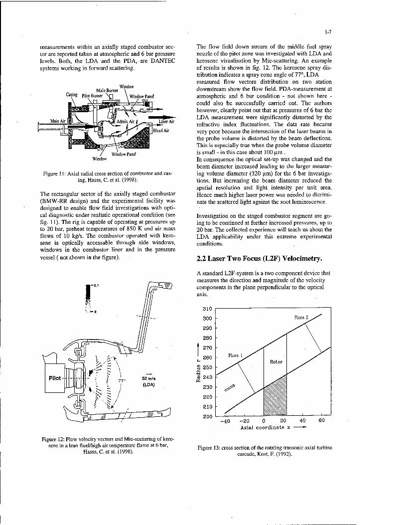
measurements within an axially staged combustor sector are reported taken at atmospheric and 6 bar pressure levels. Both, the LDA and the PDA, are DANTEC systems working in forward scattering.

Main Burner Cas'nS Pilot Burner Vj

Window

Window Window Panel

Figure 11: Axial radial cross section of combustor and casing, Hassa, C. et al. (1998).

The rectangular sector of the axially staged combustor (BMW-RR design) and the experimental facility was designed to enable flow field investigations with optical diagnostic under realistic operational condition (see fig. 11). The rig is capable of operating at pressures up to 20 bar, preheat temperatures of 850 K and air mass flows of 10 kg/s. The combustor operated with kerosene is optically accessable through side windows, windows in the combustor liner and in the pressure

vessel ( not shown in the figure).

The flow field down stream of the middle fuel spray nozzle of the pitot zone was investigated with LDA and kerosene visualisation by Mie-scattering. An example of results is shown in fig. 12. The kerosene spray distribution indicates a spray cone angle of 77°, LDA measured flow vectors distribution on two station downstream show the flow field. PDA-measurement at atmospheric and 6 bar condition - not shown here - could also be successfully carried out. The authors however, clearly point out that at pressures of 6 bar the LDA measurement were significantly distorted by the refractive index fluctuations. The data rate became very poor because the intersection of the laser beams in the probe volume is distorted by the beam deflections. This is especially true when the probe volume diameter is small - in this case about 100 p.m. In consequence the optical set-up was changed and the beam diameter increased leading to the larger measuring volume diameter (320 urn) for the 6 bar investigations. But increasing the beam diameter reduced the spatial resolution and light intensity per unit area. Hence much higher laser power was needed to dicrimi- nate the scattered light against the soot luminescence.

Investigation on the staged combustor segment are going to be continued at further increased pressures, up to 20 bar. The collected experience will teach us about the LDA applicability under this extreme experimental conditions.

2.2 Laser Two Focus (L2F) Velocimetry.

A standard L2F-system is a two component device that measures the direction and magnitude of the velocity components in the plane perpendicular to the optical axis.

310

300

290

280

270

260

3 250

ffl 240

230

220

210

200

- Plane 12^^

Plane \>^

- ^r\ Rotor

■ ^ \« iü 111

-40 -20 0 20 40 60 Axial coordinate x —

Figure 12: Flow velocity vectors and Mie-scattering of kerosene in a lean fluel/high air temperature flame at 6 bar,

Hassa, C. et al. (1998). Figure 13: cross section of the rotating transonic axial turbine

cascade, Kost, F.( 1992).

1-8

0.0 0.2 0.4 0.6 0.8 1.0 y/t -

0.0 0.2 0.4 0.S 0.8 1.0 y/t —

0.2 0.0 0.2 0.4 0.6 y/t —

0.0 0.2 0.4 0.6 0.8 1.0 y/t

124

122

120,

\ J 118 ■ vy 116

^wr

0.0 0.2 0.4 0.6 0.8 1.0 y/t

0.0 0.2 0.4 0.6 0.8 1.0 y/t. —

-0.2 0.0 0.2 0.4 0.6 y/t —

0.0 0.2 0.4 0.6 0.8 1.0 y/t

0.30 0.0 0.2 0.4 0.6 0.8 1.0

y/t — 0.0 0.2 0.4 0.6 0.8 1.0

y/t — -0.2 0.0 0.2 0.4 0.6

y/t -

x/lx = -0.21 X/Ix 0.30 x/lx 0.80

0.0 0.2 0.4 0.6 0.8 1.0 y/t —

x/lx = 1.48

Figure 14: Three component measurement results from mid-span plane - lx is the axial width of the turbine rotor, Kost, F. (1992).

The three component measurements can be made by a standard L2F-system when it is operated successively at a point in the flow field from two different orientations of the optical axis, taking care that the included angle is around 30° for accuracy reasons. The desired velocity vector is determined from a geometric transformation of the two measurement results. Taking account for the collection angle of two component L2F- system the solid angle needed for optical access is as large as required for three component LDA-systems, about 40°. Using this kind of operation three component measurement were made in a rotating transonic axial turbine cascade (Kost, 1992). The rotating cascade (see fig. 13) was equipped with 80 straight blades, the hub and casing was conical (half cone angle 30°). Results from measurements in the mid-section plane at four axial stations are shown in fig. 14. The relative Mach number Maw, the flow turning angle ß and the radial velocity component - represented by the angle a which is measured against the rotational axis - indicate the very interesting secondary flow development. The circumferential co-ordinate y/t originates at the blade leading edge position.

Due to L2F's specific properties it's predominant field of application are high loaded, high speed turbomachines as e.g. centrifugal compressors and turbines. In these cases only those L2F systems which can operate with an extremely small solid angle are applicable for the three component velocity measurements.

Figure 15: Three component L2F-measuring device.

1-9

Three methods on the basis of the L2F technique have been put forward to achieve this objective. The most established system - the principal of which was fist time introduced in 1981 - is on the market today and in use at different European institutions. This system (see fig. 15) is set up from two independent two component L2F systems with tube type optical head construction. The two tubes are mounted to a mechanical rotation unit inclined to the rotational axis with an angle of 7,5°. The location where the laser beams inter- sect each other is on the rotational axis and determines

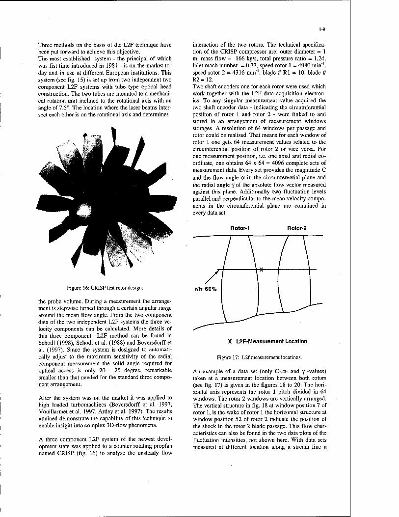
Figure 16: CRISP test rotor design.

the probe volume. During a measurement the arrangement is stepwise turned through a certain angular range around the mean flow angle. From the two component data of the two independent L2F systems the three velocity components can be calculated. More details of this three component L2F method can be found in Schodl (1998), Schodl et al. (1988) and Beversdorff et al. (1997). Since the system is designed to automati- cally adjust to the maximum sensitivity of the radial component measurement the solid angle required for optical access is only 20 - 25 degree, remarkable smaller than that needed for the standard three component arrangement.

After the system was on the market it was applied to high loaded turbomachines (Beversdorff et al. 1997, Vouillarmet et al. 1997, Ardey et al. 1997). The results attained demonstrate the capability of this technique to enable insight into complex 3D-flow phenomena.

A three component L2F system of the newest development state was applied to a counter rotating propfan named CRISP (fig. 16) to analyse the unsteady flow

interaction of the two rotors. The technical specification of the CRISP compressor are: outer diameter = 1 m, mass flow = 166 kg/s, total pressure ratio = 1,24, inlet mach number = 0,77, speed rotor 1 = 4980 min"1, speed rotor 2 = 4316 min"1, blade # Rl = 10, blade # R2=12. Two shaft encoders one for each rotor were used which work together with the L2F data acquisition electronics. To any singular measurement value acquired the two shaft encoder data - indicating the circumferential position of rotor 1 and rotor 2 - were linked to and stored in an arrangement of measurement windows storages. A resolution of 64 windows per passage and rotor could be realised. That means for each window of rotor 1 one gets 64 measurement values related to the circumferential position of rotor 2 or vice versa. For one measurement position, i.e. one axial and radial coordinate, one obtains 64 x 64 = 4096 complete sets of measurement data. Every set provides the magnitude C and the flow angle a in the circumferential plane and the radial angle y of the absolute flow vector measured against this plane. Additionally two fluctuation levels parallel and perpendicular to the mean velocity components in the circumferential plane are contained in every data set.

Rotor-1 Rotor-2

X L2F-Measurement Location

Figure 17: L2f measurement locations.

An example of a data set (only C-,oc- and y -values) taken at a measurement location between both rotors (see fig. 17) is given in the figures 18 to 20. The horizontal axis represents the rotor 1 pitch divided in 64 windows. The rotor 2 windows are vertically arranged. The vertical structure in fig. 18 at window position 7 of rotor 1, is the wake of rotor 1 the horizontal structure at window position 52 of rotor 2 indicate the position of the shock in the rotor 2 blade passage. This flow characteristics can also be found in the two data plots of the fluctuation intensities, not shown here. With data sets measured at different location along a stream line a

1-10

movie can be prepared showing dearly how the flows of the two rotor passages are interacting. A gigantic number of measurement data will arise when the whole field is analysed and strategies need to be developed to perform efficient analysis of the measured data.

ing it with an additional measurement principle, thus making three component measurements possible.

One system works with axially displaced probe volume centres of start and stop beams (Förster et al 1990). In addition to the two component measurements the net

Wake (Rotor-I) Wake (Rotor-I)

8 16 24 32 40 48 56 64 PS-I SS-I Rotor-I

8 16 24 32 40 48 56 64 PS-I SS-I Rotor-I

Figure 18: mean values of absolut velocity C.

Wake (Rotor-I) Shock (Rotor-ll)

8 16 24 32 40 48 56 64 PS-I SS-I Rotor-I

Figure 19: mean values of flow angle a.

There are some applications where either this small solid angle for optical access is still to large or where is not enough space to place and operate the mentioned optical head, hi this cases only two component systems can be used because of their confocal optical set-up (optical access angle 15 -a-18 degree).

Two solutions were found to extend the measurement capability of two component L2F-systems by combi-

Figure 20: mean value of flow angle j (represents radial component).

data rate is collected which yields the information of the third velocity component. This system was working under laboratory conditions very well. However, under practical measurement conditions on a turbomachinery test rig operation of the system was very complicated because of the calibration required that has to account for all details of the test conditions. Therefore this method was not used so often.

Figure 21: Three component Doppler L2F-probe

The second newly developed system combines the standard two component measurement with the frequency analysis of the scattered light. The measured Doppler frequency shift represents the third velocity component along the optical axis of the optical head.

1-11

The Doppler shift is measured by using the frequency depending absorption of iodine in the region of the steep slope of an iodine absorption line - the same physical principle as it is used with the Doppler Global Velocimetry (Roehle et al. 1995).

B ..■■' fe—^Hq

1 1 X vx p --''

Figure 22: Installation of 3C-Doppler-L2F device at turbine test rig.

The system was developed with respect to an application in a low pressure turbine rig and designed in the shape of an optical probe with an outer diameter of 14 mm and a probe throw of about 60 mm. The 3C- Doppler-L2F ma.ed iirobe is shown in fig. 21 with the probe mounted on a support for radial positioning. The complete unit was installed on the turbine rig as shown in fig. 22.

The operation of the system can be explained by the schematics of the 3C-Doppler-L2F-probe shown in fig. 23. While operating in multicolour mode the Ar+- laser was frequency stabilised on the green colour (X = 514 nm). The laser was fibre linked to the probe head. By the use of lenses and dispersion prism multicolour parallel light beams are generated in the probe volume. The scattered light from particles passing these beams is collected, the different colour light is recombined by passing backwards through the dispersion prism and focussed into a single receiving fibre that guides the scattered light to a colour separation unit. The 488 nm and 496 nm laser line was used for the two component time of flight measurement the green 514 nm line is guided to the Doppler frequency analysing unit. The green laser light passes an iodine cell where absorption

514

:;0M:&$!Jiti»l

kxflneeafl ii^j \'U'^ii.,!i;iiijj'i,",'J '/ .Kiv^iül'i ;i.Uii\j:

colour separation unt

D lauwr

framiMnttkt nfahMnaflnn

Figure 23: Schematics of the 3C-Doppler-L2f optics.

1-12

in dependence of the amount of the radial velocity component take place and comes to the photomultiplier which delivers the signal pulse. To determine the amount of absorption the reference pulse with the information of the light intensity entering the iodine cell is necessary. The reference pulse is split off by a beam splitter and guided by a long fibre acting as an optical delay line to the same photomultiplier. The ratio of signal and reference pulse amplitude is a measure of absorption that can be calibrated as a function of amount of radial velocity components. The system is just ready for turbine measurements. It has been operated already very satisfactorily on a free jet. The existing data acquisition and processing method takes the two component L2F-measurements and the frequency analysis to determine the radial component independently, however the method is generally suited to carry out coincident three component measurements.

L2F systems are established in most of all turbomachinery laboratories and are used to perform measurements in compressor and turbine components. For the flow analysis in combustion experiments L2F- measurement systems have not been used because of the high turbulence intensities found there which exceed to a great extend the L2F turbulence measurement capability (< 30%).

3. CARS.

As LDA and PDA are the important methods for the flow field analysis in combustion processes CARS (Coherent Anti-Stokes Raman Spectroscopy) is the well established method for temperature measurements. The CARS-probe volume is generated in a very similar way as the LDA-probe volume by the overlapping of two or more laser beams. By the interaction of

the laser beams of different frequencies the CARS signal is generated. The frequency analysis of the laser- like CARS-signal yields the CARS spectrum that is related to the Raman spectrum of the molecules (usually N2 ) being probed. The temperature is deduced from the spectral shape. Frequency doubled Nd/YAG lasers are usually employed in practical CARS systems which work with a pulse repetition rate of 10 Hz. On a single measurement location 500 to 1000 single-pulse temperature measurements are taken and usually arranged in the form of temperature histograms. A very clear description of the current status of CARS thermometry is given in Black et al. (1997). Because of similarities of LDA and CARS, optical beam path CARS runs into very similar problems as LDA when measurements at high pressures must be performed. Difficulties of optical access and problems with high densities of soot particles and refractive index gradients have prevented successful application in gas turbine combustion rigs operating of high pressure conditions (pressures around 40 bar). However, good spectral data were obtained in combustion rigs running at simulated idle (3,2 bar) or atmospheric pressures (Black et al. 1996, Magre et al. 1996(a), Magre et al. 1996(b), Lückenrath et al. 1997 and Griebel et al. 1997). CARS-measurements have been carried out in a rectangular RQL sector rig fuelled with kerosene running at atmospheric conditions (Griebel et al. 1997). A few of the results obtained were selected to give an example. Fig. 24a shows the liner of RQL combustor with optical windows giving access to the quench zone. The air was preheated up to 850 K, the kerosene was supplied and atomised by two rows of 6 air blast nozzles. The figure 24b shows details of the quench zone with the position Z = 22,5 of the plane indicated where CARS measurement have been taken.

x=100

a) b)

Figure 24: View of the liner and the quench zone geometry.

1-13

The tests were performed at the primary zone equiva- lence ratio of 1.64, which was a compromise between low NOx and CO emissions and soot formation.

Results of CARS measurements taken in the mid section of the quench zone are presented in fig. 25. The x- co-ordinate is in flow direction, the y-co-ordinate represents the full height of the quench zone. The arrows on the top (1, 3) indicate the centreline of the impinging secondary air jets, the holes of the second row of mixing jets are out of the plane (see fig. 24b). The highest temperatures (about 2000 K) and the nar- rowest temperature PDF's (fig. 26a ) were measured in a near centre region where unmixed primary zone exhaust gas still exists.

1. row t 2. rowy 3. rowf

[mm]

The high spatial and temporal resolution of CARS measurements delivers important information to characterise the performance of the combustor, in particular the quality of fuel/air mixing.

number of «vents

200

100

0

x = 93 mm, y ■ 0 mm Tmean r 2016 K RMSfT) » 64 K

a)

800 1200 1600 2000 2400

number of events 1001

KM too mm. y» 20mm Tmean -1371 K RMS(T) « 342 K

800 1200 1600 2000 2400 T[K]

c) number of event*

x« 115 mm, y* 25 mm ISO Tmean = 2085 K

RMSifT) * 97 K 100

50 ,JL 1200 1600 2000 2400

T[K]

e)

number of events

200

150

-llllli- I „LUlllk.

x = 100mm,y«30mm Tmean * 897 K RMS(T) * 68 K

b)

800 1200 1600 2000 2400 T[K]

number of events

100

80

60

40

20

0

xs 107.5 mm, y» 15 mm . ■Tmean = 1778 K .RMSfT) = 227 K |

,,U|||||I 1600

TM

d) number of events

1200 1600 2000 T[K]

Figure 25: Mean temperature of CARS measurement in cross section Z= 22,5 mm.

Other areas of high temperature (about 2000 K) and narrow PDF's (fig. 26e) are the wakes of the air jets where unmixed primary exhaust gas can be found. A narrow and symmetric temperature PDF (fig. 26b) with low mean temperature can be found in regions, where the cores of the secondary air jets are located. The highest RMS temperatures (up to 300 K) were measured in the boundaries of the air jets, where the temperature PDF's are wide and non-symmetric due to the high level of unmixedness. These regions consist of mixtures of primary zone exhaust gas and secondary air. If the primary zone exhaust gas dominates, the maximum in the PDF lies on the high temperature side (fig. 26d). If the secondary air dominates, the maximum lies on the low temperature side (fig. 26c). Before the third row of the secondary air jets is added (x = 128 mm) the progression of the mixing process is nearly completed. Thus the temperature PDF's are symmetric and relatively narrow in this zone (see fig. 26f) and the temperatures are below 1800 K almost over the whole combustor height The distribution of the mean temperature shows no regions of increasing mean temperatures even in the boundaries of the secondary air jets, where the heat release takes place.

Figure 26: Temperature PDF at several locations indicated in fig. 25.

CARS measurement at higher pressures of about 6 to 7 bar just have been obtained in the test rig show in fig. 11 (Hassa et al. 1998) and were carried out some years ago in a can combustor (Black 1992). Problems have been observed as i.e. reduced data rate and even no measurements in some critical positions of high mixing, indicating that CARS may approach its applicational limit when pressure levels are further increased.

Conclusions An overview about three component velocimetry (LDA, PDA, L2F) and CARS application to gas turbine engine test was given. The examples presented demonstrate the current status of development and the actual capabilities of the different nonintrusive point measurement techniques. The quality status of the data measured has proved its high level - measurement error typically don't exceed some few percent - and system development has enable access to nearly all flow regions - even of the most complex designed test rigs. There is no doubt that these techniques deliver just that quality of data what is nowadays required for code validation with the only exception of gas turbine com-

1-14

bustors operating at high pressure levels where laser beam distortion cannot be avoided.

However, the time and costs requirements for a detailed flow analysis are very high which lead to the fact that the number of full field data sets are not very numerous. In recent years planar measurement techniques have reached a remarkable development status that now is the time for applying them to aero engine components. It can be expected that with these planar techniques a more complete insight into turbomachinery flow can be realised on a acceptable experimental cost basis. Fur- thermore it is expected that they are less sensitive to optical distortions enabling hopefully successful applications where point measurement systems presumably fail. But because of limitations in the measurement accuracy planar method will not drive out the point measurement techniques which will surely further be used to collect more precise measurements on carefully selected flow locations.

List of References

Wisler, D.C. and Mossey, P.W., 1972 "Gas Velocity Measurements Within a Compressor Rotor Passage Using the Laser Doppier Velocimeter", ASME Paper No 72-WA/GT-2.

Strazisar, A., 1986 "Laser Fringe Anemometry for Aero Engine Components", AGARD CP 399 Advances Instrumentation for Aero Engine Components, Phila- delphia, Pennsylvania, USA, 19-3 March.

Schodl.R., 1986 "Laser-Two-Focus Velocimetry", AGARD CP 399 Advances Instrumentation for Aero Engine Components, Philadelphia, Pennsylvania, USA, 19-23 March.

Boutier, A., D'Humieres, Ch., and Soulevant, D., 1984 "Three Dimensional Laser Velocity: A Review", Sec- ond International Symposium on Applications of Laser Anemometry to Fluid Mechanics, Lisbon, Portugal, July.

Doukelis, A., Mathioudakis, K., Founti, M. and Papailiou, K., 1997 "3D LDA Measurements In A An- nular Cascade For Studying Tip Clearance Effects", AGARD-CP-598 Advanced Non-Intrusive Instrumen- tation for PROPULSION Engines, Brussels, Belgium, 20-24 Oct.

Edmonds, J. D., Wiseall, S.S., and Harvey D., 1997 "Recent Developments in the Application of Laser Doppler Anemometry to Compressor Rigs", AGARD- CP-598 Advanced Non-Intrusive Instrumentation for PROPULSION Engines, Brussels, Belgium, 20-24 Oct.

Schievelbusch, V., Bütefisch, K.A. Sauerland, K.H., Gieß, P.A., 1994 "3-D-LDA-Messungen an einem gastubinenleitradgitter", Lasermethoden in der Strömungsmeßtechnik, 3. GALA Tagung, Verlag Shaker, Aachen.

Straziser, T., 1985 "Application of Laser Anemometry to Turbomachinery Flowfield Measurements", VKI Lecture Series 1985-03, Measurement Techniques in Turbomachines. Feb. 25 - March 1.

Hathaway, M.D., Chriss, R.M., Wood, J.R. and Strazisar, A.J., 1992 "Experimental and Computational Investigation of the MASA Low-Speed Centrifugal Compressor Flow Field", ASME Paper No 92-GT- 213.

Chriss, R.M., Harhaway. M.D., and Wood, J.R., 1994 "Experimental and Computational Results From The NASA Low-Speed Centrifugal Impeller At Design And Part Flow Conditions", ASME Paper No 94-GT- 213.

Saesholtz, R.G. Goldman, L.J.M., 1996 "Combined Fringe And Fabry-Perot Laser Anemometer For Three Component Velocity Measurements In Turbine Stator Cascade Facility", AGARD CP 399 Advances Instru- mentation for Aero Engine Components, Philadelphia, Pennsylvania, USA, 19-23 March.

Lehnmann, B., Roehle, I., 1998 "A Comparison of Velocity-Field Data Behind a Double-Swirl Nozzle Measured by Means of Doppler-Global and Conven- tional Three-Component LDA Techniques", July 13- 16, Lisbon, Portugal.

Hassa, C, Carl, M., Frodermann. M., Behrendt, T., Heinze, J., Roehle, I., Brehm, N., Schilling, Th., Doerr, Th., 1998 "Experimental Investigation of an Axially Staged Combustor Sector with Optical Diagnostics at Realistic Operating Conditions", RTO - Applied Vehi- cle Technology Panel, Symposium on Gas Turbine En- gine Combustion, Emissions and Alternative Fuels, Lisbon, 12-16 October.

Kost, F., 1992 "Three Dimensional Transonic Flow Measurements in an Axial Turbine with Conical Walls", ASME paper No 92-GT-61, Cologne, Ger- many, June 1-4.

Schodl, R. and Förster, W., 1988 "A Multi-Color Fi- beroptic Laser-Two-Focus Velocimeter for 3- Dimensional Flow Analysis", In Fourth Intl. Symp. on Appl. of Laser Anemometry to Fluid Mechanics (Lis- bon).

Schodl, R., 1998 "Laser Two Focus Techniques", VKI- Lecture Series 1998-05, Brussels, Belgium.

1-15

Beversdorff, M., Matziol, L., Blaha, C, 1997 "Appli- cation of 3D-Laser Two Focus Velocimetry in Turbo- machine Investigations", AGARD-CP-598 Advanced Non-Intrusive Instrumentation for PROPULSION En- gines, Brussels, Belgium, 20-24 Oct.

Vouillarmet, A., Charpenel, S., 1997 "Laser Two Fo- cus Anemometry (L2F-3D) for Three-Dimensional Flow Analysis in an Axial Compressor", AGARD-CP- 598 Advanced Non-Intrusive Instrumentation for PROPULSION Engines, Brussels, Belgium, 20-24 Oct.

Ardeg, S., Fottner, L., Beversdorff, M., Weyer, H.B., 1997 "Laser-2-Focus Measurements on a Turbine Cas- cade with Leading Edge Film Cooling", AGARD-CP- 598 Advanced Non-Intrusive Instrumentation for Pro- pulsion Engines, Brussels, Belgium, 20-24 Oct.

Förster, W., Schodl, R. Beversdorff, M., Klemmer, T., Rijmenants, E., 1990 "Design and Experimental Verifi- cation of 3-D Velocimeters based on the Laser-2-Focus Technique", presented at the 5th Int. Symp. on Appl. of Laser Anemometry to Fluid Mechanics in Lisbon, Portugal.

Roehle, I., Schodl, R., 1995 "Method for Measuring Flow Vectors in Gas Flow", UK-Patent GB 2 295 670 A.

Griebel, P. et al, 1997 "Experimental Investigation of an Atmospheric Rectangular Rich Quench Lean Com- bustor Sector for Aeroengines", ASME, Turbo Expo 97, Orlando, Florida, June 2-5.

Black, J.D., 1992 "CARS Gas Temperature Measure- ments in SNECMA Tubular Combustor", BRITE/EURAM Low Emissions Combustor Pro- gramme, Rolls-Royce report number RR(OH)1220.

Black, J.D., Wiseall, S.S., 1997 "CARS Diagnostics on Model Gas Turbine Combustor Rigs", AGARD- CP-598 Advanced Non-Intrusive Instrumentation for Propulsion Engines, Brussels, Belgium, 20-24 Oct.

Black, J.D., Brocklehurst, H.T., and Priddin C.H. , 1996 "Non-Instrusive Thermometry in Liquid Fuelled Combustor Sector rigs Using Coherent Anti-Stokes Raman (CARS) and Comparison with CFD Tempera- ture Predictions", ASME-IGTI Paper No. 96-GT-185

Magre P., G. Collin, D. Ansart, C. Baudouin, and Y Bouchie ,1991 "Mesures de Temperature par DRASC et Validation d'un Code de Calcul sur Foyer de Turbo- reacteur", 3eme Forum Europeen sur la Propulsion Aeronautique EPF91, ONER A, Paris

Magre, P., G. Collin, and P. Moreau , 1996(a) "CARS Temperature Measurements in a 3-Sector Combustor Chamber", ONERA Report Number RT 11/3608 EY.

Magre, P., P. Moreau, and M. Poirot, 1996(b) "Tem- perature Measurements on a RQL Combustor", ON- ERA Report Number RT 8/3608 EY.

Liickenrath, R. Bergmnann, V., Strieker, W., 1997 "Characterization of Gas Turbine Combustion Cham- bers with single Pulse CARS Thermometry", AGARD- CP-598 Advanced Non-Intrusive Instrumentation for PROPULSION Engines, Brussels, Belgium, 20-24 Oct.

2-1

APPLICATION OF DIGITAL PARTICLE IMAGING VELOCIMETRY

TO TURBOMACHINERY

Mark P. Wernet

National Aeronautics and Space Administration Glenn Research Center Cleveland, OH U.S.A.

SUMMARY Digital Particle Imaging Velocimetry (DPIV) is a powerful measurement technique, which can be used as an alternative or complementary approach to Laser Doppler Velocimetry (LDV) in a wide range of research applications. The instantaneous planar velocity measurements obtained with PIV make it an attractive technique for use in the study of the complex flow fields encountered in turbomachinery. Many of the same issues encountered in the application of LDV to rotating machinery apply in the application of PIV. Techniques for optical access, light sheet delivery, CCD camera technology and particulate seeding are discussed. Results from the successful application of the PIV technique to both the blade passage region of a transonic axial compressor and the diffuser region of a high speed centrifugal compressor are presented. Both instantaneous and time-averaged flow fields were obtained. The 95% confidence intervals for the time-averaged velocity estimates were also determined. Results from the use of PIV to study surge in a centrifugal compressor are discussed. In addition, combined correlation/particle tracking results yielding super-resolution velocity measurements are presented.

1.0 INTRODUCTION DPIV provides near real-time flow field measurements through the use of refined data processing techniques combined with continuous increases in computational power and advances in CCD sensor technology. DPrV is a planar measurement technique wherein a pulsed laser light sheet is used to illuminate a flow field seeded with tracer particles small enough to accurately follow the flow. The light sheet is pulsed at two very closely spaced instants in time and the positions of the particles are recorded on a cross-correlation digital CCD camera. In high-speed flows, pulsed lasers are required to provide sufficient light energy in short duration pulses to record unblurred images of the particles entrained in the flow. The cross-correlation camera is the critical element for making PIV measurements in high speed flows since it enables capturing a pair of single exposure image frames very closely spaced in time. The data processing consists of determining the average displacement of the particles over a small interrogation region in the image or by determining the individual particle displacements. Knowledge of the time interval between light sheet pulses

then permits computation of the flow velocity. For a general overview of the various perturbations of the PIV technique see Adrian, 1986 and Grant, 1997, or Raffel et. al., 1998.

Turbomachines are used in a wide variety of engineering applications for power generation, pumping and aeropropulsion. The need to reduce acquisition and operating costs of aeropropulsion systems drives the effort to improve propulsion system performance. Improving the efficiency in turbomachines requires understanding the flow phenomena occurring within rotating machinery. Detailed investigation of flow fields within rotating machinery have been performed using Laser Doppler Velocimetry (LDV) for the last 25 years. The LDV measurements are usually time and ensemble averaged over all of the blade passages (Strazisar, 1986, O'Rourke and Artt, 1994, Skoch et al., 1997) to improve the statistical confidence of the measurements. These detailed velocity mapping studies are required to improve the fidelity and accuracy of Computational Fluid Dynamics (CFD) code predictions (Ucer, 1994). In addition to understanding the design condition flow, work is also underway to expand the stable operating range of compressors. Compressor stall is a catastrophic breakdown of the flow in a compressor, which can lead to a loss of engine power, large pressure transients in the inlet/nacelle and engine flameout. The distance on a performance map between the operating point of a compressor and its stall point is referred to as the "stall margin". Stall margin is required to account for increased clearances within the compressor caused by throttle transients and component deterioration with age. Optimal engine designs tend towards minimal stall margins since modifications to increase the stall margin typically result in heavier, less efficient and less loaded compressors. However, if instead active or passive stall control is employed, stable operation over a wider range of flow conditions (improved stall margin) can be obtained with a minimal loss in performance as demonstrated by Weigl et al. (1997). Traditionally, dynamic pressure measurements have been utilized to decipher the flow changes occurring during stall/surge events. These measurements yield vague indications of the kinematic changes in the flow field. The instantaneous flow field capture capability of DPIV is better suited to the task of studying the change in flow conditions surrounding the

Paper presented at the RTO AVT Lecture Series on "Planar Optical Measurement Methods for Gas Turbine Components", held in Cranfield, UK, 16-17 September 1999 and


2-2

development of stall precursors, stall cell propagation and eventually compressor surge.

Obtaining normal incidence backscatter LDV measurements near the blade tip or rotor hub in turbomachinery is very difficult due to scattering from the hub surface and reflections from the casing window. The task is exacerbated in the exit of a centrifugal compressor where the blade passage height is very small. Digital Particle Imaging Velocimetry (DPIV) offers the potential to obtain measurements closer to surfaces than those obtained using LDV, since the light sheet propagation direction can be made parallel to the hub and casing surfaces. A series of instantaneous spatial velocity measurements obtained via DPIV can be averaged together to compute the time-mean flow field. These time-averaged flow field measurements can be used to augment previous studies performed using LDV in turbomachinery for the assessment of CFD code predictions. In addition, the instantaneous flow field capture capability of PIV can be optimally utilized such as in the study of stall cell propagation in compressors. Simultaneous capture of dynamic pressure and planar velocity measurements would be a significant improvement over traditional approaches based solely on pressure measurements. The other impetus for using PIV in turbomachinery flow field measurements is the need to reduce facility testing time and cost. Planar measurement techniques offer significantly reduced data acquisition times over traditional point based measurement techniques.

Numerous researchers have employed various PIV techniques to study the unsteady flows in rotating machines, covering both pumps and compressors. Liquid based experimental setups have been used for pump studies and some fan studies. Rothlübbers et al, 1996, used digital PIV to study the flow in a radial pump. Low seed particle concentrations were identified as not suitable for rotating machine studies, where high spatial resolution measurements are required. Oldenburg and Pap, 1996, used a DPIV setup to investigate the flow field in the impeller and volute of a centrifugal pump. The lab scale facility used water as the working fluid and a transparent impeller. Shepherd et al, 1994 used photographic PIV to study the flows inside both centrifugal and axial fans. These test setups employed water as the working fluid and hence were restricted to low rotational speeds.

There has been considerable work performed in low to moderate speed rotating applications using air as the working fluid. Paone et al., 1988, used PIV to make velocity measurements in the blade-to-blade plane in a centrifugal compressor. Tisserant and Breugelmans, 1997 used a digital PIV technique to measure the flow field in a subsonic (30-70 m/s, 3000-6000rpm) axial fan. They noted that an optical periscope type probe (similar to that

used by Bryanston-Cross, et al 1992) is required for introducing the light sheet into the flow and that out-of- plane velocities are sometimes significant, causing a loss of correlation of the in-plane velocities. As an extension of the work by Post et al., 1991, Gogineni et al., 1997 have described a two color digital PIV technique which should be applicable to turbomachinery applications. A high resolution (3000x2000 pixel) single CCD sensor color camera is employed to record the particle images at two instants in time on a single CCD image frame using red and green illumination pulses. Measurements using this two color technique in an automotive radiator fan have been successfully demonstrated by Estevadeordal, et al. 1998. Day-Treml and Lawless, 1998 have used a high resolution (2000x2000 pixel) digital camera to obtain PIV measurements of rotor-stator interactions in a low speed turbine facility. A light sheet probe was used to introduce the light sheet into the flow and the measured velocities were on the order of 30 m/s.

Very little work has been published describing the use of PIV in high speed rotating applications. Although not a rotating machine application, Bryanston-Cross et al., 1992 described photographic PIV measurements obtained in a transonic turbine cascade rig. This was the first demonstration of the advantages obtained by introducing the light sheet into the flow via an 8.0 mm diameter hollow turbulence generating bar which was already part of the experimental rig. Post et al., 1991 also discuss PIV measurements in a turbine cascade using photographic film. In this work color film was employed and the light sheet pulses were of two distinct wavelengths. Bryanston-Cross et al., 1997 demonstrated high speed PIV measurements in the stator trailing edge region in a transonic axial compressor blowdown facility. Particle seeding was sparse and the data were reduced via particle tracking. Wernet, 1997 demonstrated successful DPIV measurements in the rotor blade passage of a transonic axial compressor, where both instantaneous and time- averaged cross-correlation processed vector maps were obtained. Wernet, 1998 has also demonstrated the use of DPIV in the diffuser of a high speed centrifugal compressor. Wernet and Bright, 1999 have used DPIV combined with dynamic pressure measurements to study the unsteady flows that occur during centrifugal compressor surge events. In these last three applications, DPIV has been used to record absolute flow field speeds in the 200 to 625 m/s range.

DPIV is being used in centrifugal compressor research at NASA Glenn Research Center (formerly NASA Lewis Research Center) in a three phase program wherein 2-D PIV was initially applied to resolve issues regarding optical access, light sheet delivery and flow seeding. A complete 2-D DPIV velocity mapping campaign in the diffuser region of a centrifugal compressor has recently been completed and will be used to augment previous surveys obtained using Laser Doppler Velocimetry

2-3

(LDV) in both the diffuser and impeller regions. The DPIV measurements have been obtained from 6 to 95% span, which is an order of magnitude closer to the diffuser hub than was possible using LDV. These stable operating point DPIV measurements were used to generate time- averaged, phase-stepped velocity vector maps of the impeller relative to the diffuser vanes. The time-averaged measurements illustrate that PIV yields high accuracy velocity vector maps in over an order of magnitude less time than traditional LDV techniques. The second phase of the program involves the use of PIV to study the onset of compressor stall. A series of fast response pressure transducers have been inserted around the perimeter of the centrifugal compressor casing to record the fluctuating pressure during compressor stall/surge events. The simultaneous capture of instantaneous flow field data along with dynamic pressure measurements enables a study of the coupling between the kinematic and pressure changes experienced during surge. In the third phase of the program, a stereo viewing optical system employing tilted CCD sensor planes which satisfy the Scheimpflug condition will be used to acquire planar, 3-component velocity measurements. The stereo viewing planar, 3- component PIV technique utilizing Fuzzy inference for maximized data recovery has been previously demonstrated in a supersonic nozzle flow at LeRC by Wernet, 1996. The ability to measure instantaneous 3- component velocity vector fields is critical to enhancing the knowledge base of performance limiting tip clearance flows in turbomachinery.

In this paper, the successful application of 2-D DPIV in both transonic axial and high speed centrifugal compressors at GRC will be discussed. Measurements obtained in a single stage 508 mm diameter transonic axial compressor using a periscope light sheet generating probe for upstream and downstream illumination of the blade-to-blade plane are presented. Measurements obtained in the diffuser section of a 431 mm diameter 4:1 pressure ratio centrifugal compressor facility are also presented. A brief description of the optical setup and some results are presented. Techniques for generating time-averaged velocity vector maps from instantaneous vector maps containing spurious vectors are also presented and discussed. The 95% confidence intervals of the uncertainties in the averaged velocity estimates were computed. Combined correlation/particle tracking results yielding super-resolution velocity measurements will also be presented. Results from the simultaneous capture of instantaneous flow field data along with dynamic pressure measurements to diagnose the range of flow conditions experienced during surge are also presented.

2.0 OPTICAL ACCESS AND COMPRESSOR FACILITIES The standard PIV technique requires that the light scattered by the particles traversing the light sheet be

collected at 90° from the plane of the light sheet. The desired measurement plane in the studies described herein was the blade-to-blade plane, hence the light sheet propagated along the flow direction and the image recording camera was mounted perpendicular to the flow path. The recording camera viewed the illumination plane through an optical access port mounted in the compressor casing. Ideally, the optical access port will permit the collection of light scattered from particulates in the flow without significantly disturbing the flow. In order not to disturb the flow the optical access window was curved to match the compressor casing shape. Next, the two compressor facilities used in this work will be described along with their optical access features.

2.1 Axial Compressor The transonic axial compressor is a 508 mm diameter, single stage axial compressor with a design speed of 17,188 rpm and a maximum mass flow rate of 20.19 kg/s. The operating pressure ratio at design conditions is 2.05. The rotor has 36 blades with a span of 75 mm at the leading edge and 56 mm at the trailing edge. The blade stagger angle is 41° at the hub and 61° at the tip. The casing is fitted with a large optical access window (200x100 mm) which is molded to the complex contour of the casing. The glass thickness is 3 mm and produces a very small amount of optical distortion. None of the optical distortion effects will be considered here. A schematic diagram of the PIV installation is shown in figure 1. The light sheet probe is inserted upstream of the rotor and the light sheet propagates along the blade stagger angle. The pulsed Nd:YAG laser and articulated arm are also shown in the diagram. The articulated arm, which has mirrors at each knuckled joint, is used to deliver the pulsed laser beam from the laser to the light sheet probe. A CCD camera is used to record the light scattered by particles through the viewing port in the compressor casing.

2.2 Centrifugal Compressor The centrifugal compressor is a Rolls Royce-Allison design that was scaled to a flow size of 4.54 kg/s from the original size of 1.66 kg/s. The impeller and vaned diffuser were designed to produce a pressure ratio of 4:1 at the design mass flow. The standard day corrected speed for the design flow condition is 21,789 rpm with an exit tip speed of 492 m/s. The impeller contains 15 main blades with 15 splitter blades and has 50 degrees of backsweep from radial at the discharge. The splitter blade leading edge, located at 30 percent of the main blade chord, is offset slightly toward the main blade suction surface to provide an even flow split. The inlet tip diameter is 210 mm and the inlet blade height is 64 mm. The exit diameter is 431 mm and the exit blade height is 17 mm. The vaned diffuser consists of 24 two- dimensional wedge vanes with the leading edge located at a radius ratio of 108% relative to the impeller exit. The diffuser has an overall area ratio of 2.75 with a total

2-4

divergence angle of 7.8°. The diffuser exit radius is 363 mm and dumps directly into a 90° annular bend. The nominal operating impeller exit clearance is 0.4 mm, or 2.4% of the passage height at the exit. The compressor flow is subsonic under stable operating point conditions where the local speed of sound at the diffuser throat is 357 m/s based on a static temperature of 108°C. The compressor can be driven into stall by backpressuring the compressor via the collector valve. The compressor enters stall at a mass flow rate just below 4.26 kg/s.

A test-rig cross section showing the flow path through the impeller and diffuser can be seen in figure 2a, while figure 2b shows a frontal view of the impeller and diffuser. The rig casing is designed to accept 4 separate window frame inserts; each containing a different set of windows with interspersed locations to provide access all along the flow path from the impeller entrance to the diffuser. A flat 70x70 mm clear aperture window port has been designed to enable optical access over the impeller exit/diffuser section of the compressor, as is shown in figure 2a. There is insufficient space near the compressor rig for the PIV CCD camera to view the illuminated flow passage directly. A mirror is therefore mounted at 45° to the illumination plane to provide the CCD recording camera with a view of the illuminated flow passages. The left-right image reversal caused by viewing through the 45° mirror was compensated for in the data processing.

The compressor casing was fitted with dynamic pressure transducers (three 340 kPa and one 100 kPa Kulite transducers) at four locations. The transducer circumferential locations are referenced in degrees from top-dead-center, proceeding in a clock-wise direction. The center of the optical access viewing port is located at 270°. The locations of the three 340 kPa Kulite transducers are indicated in figure 2. Two transducers were located in the vaneless space between the impeller and the vaned diffuser (from 100 to 108% of the impeller radius). Transducer #1 was located at 343° and #2 was located at 35°. Transducer #3 was located in the diffuser throat at 43° from top-dead-center. Transducer #4, a 100 kPa Kulite which is not shown in figure 2, was located roughly 25 mm upstream of the impeller at 338° from top-dead-center. Only four transducers were used during these initial measurements, due to the concern over seed particle contamination. However, no degradation of the dynamic pressure transducers resulting from the flow seeding has been observed in the course of this work.

In order to measure the incipient stalling mechanisms, dynamic pressure measurements of the stall precursors were collected in the centrifugal compressor facility before the DPIV measurements were obtained. Dynamic pressure data were collected at several operating conditions. The measurements were obtained around the circumference of the compressor from transducers

mounted in the compressor casing ahead of the impeller, in the vaneless passage, and in the diffuser throat. These measurements illustrated that rotating stall cells travel at approximately 25% to 33% of the impeller rotational speed. Measurements also indicate that at partial speed conditions the stall cell begins in the impeller region, whereas at design speed the stall originates in the diffuser.

3.0 LIGHT SHEET DELIVERY A pulsed Nd:YAG laser beam is required to provide sufficient illumination energy (200mJ/pulse) and short pulses (5 ns) to record unblurred images of the particles in the flow. A two-head Nd:YAG laser system was used in this work to avoid limitations on the minimum time separation between the illumination pulses. The laser system is capable of producing pairs of light pulses at a 10 Hz repetition rate. The two laser oscillators were housed in a common case and the beams from the two laser heads were combined into a coaxial beam before frequency doubling.

In order to introduce the light sheet along the flow path in these two compressor facilities, a compact light sheet delivery system was constructed using a periscope type configuration as shown in figure 3a. The pulsed Nd:YAG laser beam is directed down the bore of the tube which contains light sheet forming optics and a 90° turning mirror. The periscope probe has an outside diameter of 12.7 mm and utilizes 8 mm diameter spherical and cylindrical optics to form the Nd:YAG laser beam into a laser sheet. The light sheet exits the probe through a window which keeps the optics inside the probe protected from contamination by seed material. An implementation of this NASA designed and constructed probe is shown in operation in figure 3b.

An articulated light arm with mirror joints was used to easily and reliably direct the beam down the bore of the periscope probe. Articulated light arms for Nd:YAG laser beam delivery are commercially available and permit the full energy range of the laser to be used (200 mJ/pulse at 532 run). Use of the light arm simplifies the coupling of the Nd:YAG beam to the periscope and also adds an increased level of safety to the installation since the beam is entirely enclosed when outside of the compressor casing. The light sheet delivery probe coupled to the light arm has been used to deliver up to 125 mJ pulsed illumination. Although the articulated arm provides a safe and convenient coupling of the laser beam to the rig, there is a tendency of the laser beam to "wander" inside the arm as the arm is moved. In operation, the beam is aligned at the desired measurement location, then the light arm flexible joints are immobilized to stabilize the location of the light sheet.

2-5

3.1 Axial Compressor Installation The small diameter periscope probe is inserted through the compressor casing upstream or downstream of the measurement location. The periscope probe was equipped with a 200 mm focal length spherical and -25 mm focal length cylindrical lens to form the Nd:YAG laser beam into a laser sheet of approximately 45x0.5 mm in the compressor blade row. Moving the probe in and out through the casing changes the spanwise location of the illumination plane. In order to align the propagation direction of the light sheet along the blade stagger angle, the light sheet probe is inserted below the horizontal rig centerline. This insertion location also ensures that the light sheet probe does not disturb the flow upstream of the actual measurement location. The mounting base which attaches the probe to the casing is designed so that the light sheet generating probe is oriented horizontally, even though the entrance point through the rig casing window is below the horizontal centerline of the rig for upstream illumination, see figure 1. For downstream illumination the light sheet probe is inserted through the casing above the rig horizontal centerline. Maintaining a horizontal entry ensures that the plane of the light sheet will remain parallel with the axis of the compressor, simplifying the recording system requirements. Figure 4 shows a photograph of the PIV system installation in the compressor rig. Downstream illumination is being used in this configuration. The Nd:YAG laser is observed in the lower left corner of the picture along with an articulated arm which extends from the laser over to the light sheet probe. The compressor blade rows can be seen through the casing window and the PIV camera is mounted next to the rig.

3.2 Centrifugal Compressor Installation For this installation the periscope probe was equipped with a 256 mm focal length spherical and -102 mm focal length cylindrical lens to form the Nd:YAG laser beam into a laser sheet of approximately 13x0.5 mm at a distance of 240 mm. The periscope probe is inserted through the compressor casing downstream of the diffuser vanes at the 90° bend in the flow passage, as shown in figure 2a. Five insertion holes where machined into the collector housing to permit illumination of four different diffuser vane passages. The four illuminated diffuser vane passages are successively higher in the optical viewport window, providing access to both the pressure and suction sides of the diffuser passages and the space between the exit of the impeller and the diffuser, see figure 2b. The optical viewing port is also shown in figure 2b. Moving the probe in and out through the collector housing changes the spanwise location of the illumination plane. The insertion holes were machined so that approximately half of the probe diameter was recessed in the housing wall. These insertion locations ensure that the light sheet probe does not disturb the flow at the actual measurement location, nor does it choke the

flow through the diffuser vanes. The axial compressor rig operates at just above room temperature, however, the centrifugal compressor casing near the diffuser approaches 175°C. The temperature itself is not problematic, but the repeated hot/cold thermal cycling did degrade the anti-reflection coating on the light sheet probe optics. Uncoated optics have therefore been used to avoid thermal degradation in the centrifugal compressor PIV installation.

4.0 SEEDING A uniformly dispersed and sufficiently high concentration of flow seeding is the most critical element in any PIV experiment. If the number of particles recorded on the CCD image frame is too low, then correlation techniques cannot be applied, although particle tracking could still be utilized. As discussed previously, particle tracking does not typically provide a sufficient density of measurements necessary to adequately characterize the complex flows encountered in turbomachinery (Rothlübbers et al, 1996). However, provided the particle concentration is sufficiently high to support correlation computations particle tracking can be combined with the correlation technique results to provide high spatial resolution velocity estimates (Keane and Adrian, 1993, Wernet, 1995).

4.1 Axial Compressor The global facility seeding system developed for use in laser anemometry measurement programs in the transonic compressor facility was inadequate for PIV measurements. A sample calculation reveals the inadequacy. An LDV experiment utilizing a probe volume that is 100 um in diameter by 500 |jm long to measure a 200 m/s flow may achieve a data rate of 2KHz. This measurement rate is obtained by using a seed particle concentration of 0.2 particles/mm3. Conversely, in a digital PIV experiment where the field of view is 50x50 mm (yielding a spatial resolution of about 50 pirn/pixel), the light sheet thickness is 1 mm, and the interrogation region size is 32x32 pixels, the required seed particle concentration to ensure that there are 15 particles per interrogation region(or 15 particle pairs for double exposure image capture) is 6 particles/mm. Hence, the seeding requirements for PIV are more than an order of magnitude higher than that required for LDV.

Global seeding of a non-recirculating, large scale facility with high mass flow rates for PIV measurements is impractical. Instead, the seed material must be introduced locally near the measurement plane. For transonic flows, sub-micron particles are required for accurately following the flow. A multiple jet atomizer seeding system employing smoke juice and producing particles with a nominal diameter of 0.7 ^m seeds the flow field via a small diameter tube through the compressor casing. Locating the seed injection tube many tube diameters (> 70) upstream of the measurement

2-6

Station provided sufficient seed particle concentrations for correlation processing of the collected PIV images. Melling, 1997 computed the frequency response and particle lag distance behind an oblique shock for various seed materials. Using his results, the seed particles used here would have >10kHz frequency response and exhibit a velocity lagging that of the flow for a distance of 6 mm downstream of any oblique shocks in the flow. These particles have adequate flow following attributes for the flow field characteristics to be encountered in the transonic compressor flow.

4.2 Centrifugal Compressor Seeding the high temperature flow encountered in the diffuser of the centrifugal compressor presented a different set of challenges. In a previous LDV velocity mapping program conducted in this centrifugal compressor facility, a seeding system was specifically designed to enable measurements in the high temperature flows (175°C) encountered in the diffuser region. Attempts to use PSL seeding failed due to the seed material collecting and then melting on the optical access ports. Instead, a technique employing pH stabilized dispersions of alumina in ethanol was used as described by Wernet and Wernet, 1994. The dispersions of alumina were injected into the facility via two commercial spray nozzles mounted in the plenum tank, approximately 10 meters upstream of the impeller. The alumina powder had a mean particle size of 0.7 ± 0.2 jun. The concentration of alumina powder used in the dispersions was approximately 25 grams/liter. The resulting mass loading of seed material in the compressor flow field at the measurement location was approximately 0.4%. A side benefit of the alumina seeding is that it does not have a tendency to adhere to the optical access ports at design conditions, permitting long rig run times without contamination of the view ports. As discussed above, the high mass flow rates of the transonic compressor required localized seed injection instead of global seeding. However, the lower mass flow and higher compression ratio of the centrifugal compressor relative to the transonic axial compressor enabled a global seeding technique to produce sufficiently high seed particle concentrations to support correlation based data reduction. Again using Melling's particle dynamics analysis for these alumina particles, we find that the particles have a frequency response on the order of 3 kHz. No shocks are expected in the stable operating point centrifugal compressor flow field, hence these alumina particles should provide adequate flow following ability.

5.0 IMAGE ACQUISITION AND DATA PROCESSING A commercial PIV system was used in this measurement program, which provided electronic image acquisition with near real-time feedback of the experimental

parameters such as: laser pulse energy; seed particle concentration; assessment of flare light from blade surfaces and camera inter-exposure time. Electronic image acquisition has been demonstrated to provide adequate spatial resolution velocity measurements in the narrow flow passages encountered in turbomachinery. Cross-correlation data reduction is the optimal data reduction technique for PIV since it offers directionally resolved velocity vectors, no self correlation peak and hence no restriction on the minimum particle displacement between exposures. Another advantage gained by using cross-correlation is the use of subregion shifting, which enables smaller sized subregions to be used (resulting in increased spatial resolution) while still maintaining the V* displacement rule, Westerweel, 1997.

5.1 Cross-Correlation Camera A pair of single exposure image frames are required to enable cross-correlation data processing. A pair of CCD cameras and orthogonally polarized light sheets can be used to obtain single exposure image data as shown by Wernet, 1995. However, a possible drawback of this approach is that the independently acquired image frames must be warped to ensure alignment and polarization separation of the scattered light may not always provide good image exposure separation. Acquisition of a pair of single exposure image frames using a single CCD camera would normally not be possible were it not for the development of the "frame-straddling" technique first demonstrated by Wernet, 1991. Refinement of the technique has led to the development of commercial PIV cameras which permit a pair of image frames to be acquired with a very small inter-frame period (<1 jxsec). The cameras employed are standard RS-170, 60 fields/sec video cameras or high resolution full frame CCD imagers running at 30 frames/sec. Full frame CCD cameras have both a light sensitive frame integration area and also a frame storage area. After integration, the entire image is shifted into the frame storage area in a very short time interval (<1 usec). The information in the storage area is readout while a new frame is being collected in the light sensitive region of the CCD. Using the "frame- straddling" technique, full frame camera systems offer inter-frame exposure intervals of 1/30 sec down to < 1 ^isec. These inter-frame exposure values are obtained by adjusting the laser pulse timing to occur such that two successive single exposure image frames are obtained from the CCD camera. The first laser pulse is made to occur just at the end of one video frame integration period and the second laser pulse at the beginning of the next frame integration period. The minimum time separation between laser pulses is limited by the frame transfer period (the time it takes to shift a video frame down to the camera's storage register) of the camera. Using this technique, single exposure image frames with time separations < 1 |Jsec have been obtained.

2-7

5.2 Image Synchronization In the axial compressor facility, a digital delay generator triggered from a once-per-rev signal on the impeller drive shaft was used to trigger image acquisition and laser firing, permitting PIV data to be recorded from a selected blade passage on the impeller. In the axial compressor installation there were no stator vanes in the rig, hence no phase stepping of the rotor position was performed. In the centrifugal compressor facility, an electronic shaft angle encoder was used to synchronize image acquisition with the impeller position. In the centrifugal compressor installation, increasing or decreasing the trigger delay time enabled collecting velocity vector maps at different impeller phasing positions relative to the diffuser vanes. Delay time increments of 1/180th of the revolution time were used to provide uniform circumferential sampling (or phase stepping) of the 15 main impeller blades relative to the 24 diffuser vanes. Using this time increment, a series of 12 successive phase steps resulted in one impeller main blade and one splitter blade passing by the diffuser vane under study. The camera image acquisition and laser firing were all software controlled via a commercial synchronizer. The DPIV control and data acquisition computer was located next to the compressor rig. Remote operation was accomplished through the use of a remote PC box, which enables a remotely located monitor, keyboard and mouse to control the DPIV computer from the facility control room.

5.3 Image Acquisition The image acquisition software used in the PIV system enables acquisition of a single image frame pair or alternatively, a sequence of image frame pairs. Efficient data acquisition was achieved by acquiring 32 frame sequences and saving them directly to the hard disk. The acquired image sequences were used to compute time- averaged velocity vector maps. Correlation processing of the images was performed off-line after the experiment was completed. The image acquisition rate was 10 frame pairs/sec (limited by the Nd:YAG laser repetition rate) and the time to store each image to disk was approximately 1 second. This data acquisition mode minimized the rig run time and offered maximum flexibility in the selection of the appropriate post processing of the acquired images.

5.4 Compressor Surge Image Acquisition The onset of compressor stall is a random event, which cannot be precisely predicted. Therefore, the DPIV image sequence acquisition was initiated before the compressor went into surge, capturing images of stall precursors, rotating stall and the compressor surge flow. The DPIV image data acquired were not a priori synchronized to the compressor stall and surge events. PIV image data were asynchronously acquired throughout the full range of the stall/surge process. A separate computer was used to digitize the signals from the dynamic pressure transducers in order to measure the unsteady pressures which

occurred during compressor stall events. The Nd:YAG laser Q-switch firing signals were also digitized by the same computer. The laser Q-switches are only fired when image data are being acquired from the cross-correlation CCD camera. This data acquisition strategy enabled a posteri synchronization of the PIV data with the unsteady pressure data. The digitized laser Q-switch signals.and dynamic pressure data were examined to determine when a PIV image pair acquisition coincided with the passage of a stall precursor or a surge event.

5.5 Data Processing The commercial PIV system used to collect the data offers on-line data visualization capabilities that are extremely useful for optimizing the experiment parameters. However, the commercial system lacked some features necessary to expedite processing the large volumes (gigabytes) of data acquired in this measurement program. A custom Windows 95/NT application interface program based on cross-correlation data processing was written to process the large volumes of data in batch mode, automating many steps that would otherwise have to be done manually. The software is also capable of performing a fuzzy inference based particle tracking. The FORTRAN based data reduction software incorporated left/right image reversal correction, image gain scaling, region of interest processing, fuzzy logic data validation and on-line graphical display of the velocity vector maps as they are processed.

Averaging a sequence of PIV image pairs acquired at one compressor operating condition creates a more complete time-averaged velocity vector map. If all of the PIV images were uniformly seeded and of good quality this would be a straightforward process. However, while the seed density is reasonably uniform in general, some image frames are acquired with sparse or non-uniform seeding. When processed, these frames yield velocity vector maps that are incomplete or have spurious vectors where the seed density is inadequate for proper correlation processing. These spurious vectors have a detrimental effect on the computed mean flow properties, and therefore a procedure for judiciously removing them is required.

The procedure devised for computing the mean flow quantities from a series of processed PIV image velocity vector maps utilizes both hard velocity cutoff limits and an automated procedure for identifying outliers. The high and low velocity cutoff limits set by the user are applied and then the mean and standard deviation are computed at each grid point in the velocity vector map. The automated procedure for removing outliers is based on Chauvenet's criterion, (Taylor, 1982) in which the probability of occurrence of a given point deviating from the mean is computed. The main assumption here is that the parent velocity distribution is Gaussian. The number of standard deviations that a given point lies from the

2-8

mean is first computed. Then the probability that a given point could deviate from the mean by this many standard deviations is computed from the error integral and

. multiplied by the number of points in the distribution. If the computed probability is less than a preset level then the point is removed. This technique may not be appropriate in instances where the parent distribution is not Gaussian, such as in the vicinity of a shock where the distribution of velocity measurements may be bimodal. In a single instantaneous PIV image acquisition, other criteria such as the ratio of the correlation peak to the first noise peak must be used, which can mistakenly remove good data points from the image maps. An advantage of this averaging technique is that it relies on the computed mean flow properties over several independent image frames to discriminate spurious vectors.

Submicron particles are required to faithfully follow the flow in transonic turbomachinery. Although the geometric image of the seed particles is much smaller than the 9 um CCD pixel size, diffraction effects of the optical system may produce particle images which are on the order of the CCD sensor pixel size. For example: a PIV image recording system using an f/5.6 camera lens operating at a magnification of 0.16 and using an illumination wavelength of 0.532 ijm yields a 9 (im diameter point spread function on the CCD sensor. Although the spatial resolution of the optical system at this magnification is 56 Jim/pixel, diffraction effects prevent the optical system from being able to distinguish point particles on the object plane from geometrically imaged particles of 56 jam in diameter. The 0.7 um diameter seed particles end up being imaged to objects on the order of the CCD pixel size and hence will result in a minimal correlation peak centroid estimation error (Wernet and Pline, 1993).

Flare light reaching the CCD camera can cause significant amounts of blooming, leaving large areas of the imaged field useless and even damaging the CCD sensor. In the axial compressor installation, the light sheet propagation direction was selected to align the light sheet with the blade stagger angle in order to minimize the intersection of the light sheet with the blades, hence, significantly reducing the amount of surface flare light. The sheet forming optics in the centrifugal compressor installation were selected to produce a light sheet width that matched the diffuser throat opening of 13 mm. The light sheet probe mounting holes were positioned circumferentially around the collector housing to ensure that the light sheet could be directed along the diffuser vane without actually intersecting the diffuser vane surface. Again, aligning the light sheet along the diffuser vane stagger angle minimizes the intersection area of the light sheet with the vane surface. Painting the diffuser hub black also significantly improves the signal to noise ratio in the recorded images. Some flare light from the impeller blades and diffuser vane surfaces is desirable for

referencing since it marks the position of these surfaces in the recorded images.

6.0 CORRELATION PROCESSING AND MEASUREMENT ACCURACY The PIV image data obtained in these studies can be used to obtain both instantaneous and time-averaged velocity vector maps. In the correlation processing of the particle image data the velocity is determined by spatial averaging over the correlation subregion. The errors inherent to the PIV technique will limit the accuracy of the instantaneous, single shot velocity vector maps. In general, these errors can be minimized by proper setup of the experiment (Westerweel, 1997), yielding velocity estimates accurate to 1% of full scale.

Several factors must be optimized in order to obtain both high accuracy and high spatial resolution measurements and yet avoid some of the systematic errors inherent in DPIV. Some of these factors have to be addressed before the data are acquired and some are addressed in the data processing. The minimum error in estimating the displacement correlation peak is obtained when the imaged particle size on the CCD sensor is on the order of 1-2 pixels (Wernet and Pline, 1993). Proper selection of the recording camera lens f/number can be used to ensure that diffracted particle images are recorded which have the optimum particle diameter to pixel width ratio (as described in the previous section). If the particle images are recorded on the order of 1-2 pixels, then the correlation peak will be on the order of at least 2-3 pixels. Variations in particle size and velocity will further broaden the correlation peak. If a 3-point centroid estimator is used to compute the correlation peak position, there is a tendency for the estimator to bias the displacement estimate to integer pixel values. This phenomenon is known as "peak locking" and can be minimized by using an estimator that more accurately approximates the correlation peak shape (Westerweel, 1997). A 3-point Gaussian peak estimator has been used in this work to minimize "peak locking" effects. A second factor to consider at the image recording stage is that the seed particle concentration be sufficiently high. The ultimate spatial resolution of the processed velocity vector maps will depend on the seed particle concentration, as discussed below.

In the data processing stage, there is a trade off between resolution and accuracy in PIV measurements; however, we can attempt to maximize both by judicious design of the experiment. Following the discussion by Westerweel, 1997 the reliability of the PIV estimate from a processed subregion improves as the number of particle image pairs increases. The correlation peak signal to noise ratio is proportional to the total number of particle image pairs in the subregion. Increasing the number of particles in the subregions improves both the visibility of the correlation

2-9

peak and reduces the relative noise in the correlation peak, which results in higher accuracy velocity estimates.

The error in the PIV estimates stems from the timing of the laser light sheet pulses and the estimate of the particle displacement. The laser timing is very accurate and does not significantly contribute to the error in the velocity estimates. The accuracy of PIV displacement estimates aD is primarily determined by the ratio of the correlation peak width dr to the average particle displacement across the subregion D:

(1)

The full scale measurement error, which will be the lowest error, is limited by the maximum displacement permitted on the subregion. To avoid aliasing in the correlation plane, the displacement search region must be restricted to V* of the subregion size (Adrian, 1986). By using interpolation techniques, the correlation peak position can be estimated to sub-pixel accuracy (Westerweel, 1997). Nominal values for the peak position error are on the order of 0.1 pixel for 3-point Gaussian peak estimators and particle images spanning 1- 2 pixels. Combining the V* rule with the peak position accuracy sets the full scale accuracy of the PIV velocity estimates. Assuming a PIV subregion size of 642 pixels with 16 pixel particle displacements and applying the V4 rule described above, the relative error in the displacement measurement is approximately 0.1/16 ~ 0.6% of full scale. For a 1024x1024 pixel image, processed with 50% overlapped subregions, a 32x32 grid of vectors would be obtained. In this case we have optimized the measurement accuracy while sacrificing spatial resolution.

The lower limit on the spatial resolution of the velocity measurements is set by the actual particle displacement between the illumination pulses. Large displacements between exposures are desirable in order to achieve high accuracy velocity estimates. In standard correlation processing, subregions that are larger than the spatial scale of the particle displacement are used in order not to violate the V* rule. By incorporating subregion shifting in the data processing procedure reasonable accuracy velocity estimates can still be obtained while simultaneously increasing the spatial resolution of the measurements. In cross-correlation processing, the second correlation subregion can be spatially shifted with respect to the first subregion by an amount equal to the mean flow displacement between exposures, which keeps the correlation peak at the center of the correlation plane and minimizes any distortion effects caused by the windowing of the FFT based correlation operation. Subregion image shifting ensures that most of the particles in the first exposure subregion are also in the second exposure subregion, which results in an improved signal to noise ratio. Employing subregion shifting also

enables the use of smaller interrogation regions, provided the smaller subregions still contain a sufficient number of particles to provide a correlation result. Therefore, subregion shifting enables the measurement of displacements larger than prescribed by the V4 rule. If we now use a 322 pixel subregion to process the same 1024x1024 pixel image using 50% overlapped subregions and an 8 pixel subregion shift, then the accuracy of the velocity estimate is 0.1/8 = 1.25%, and the processed velocity vector map now contains 64x64 grid points. The velocity accuracy has been cut in half (still very acceptable at 1.25% of F. S.), however we have increased the spatial resolution by a factor of 2 in each dimension. The spatial resolution now matches the lower limit spatial resolution set by the particle displacement (assuming the particle displacements were on the order of 16 pixels for the two cases described above and 16 pixel spacing between subregion centers). Other error sources contribute to these single shot vector maps such as particle lag effects, o^g, however, for steady, unaccelerating flows, these effects can be minimal (<1%).

Instantaneous velocity vector maps over a regular grid of points are obtained after correlation processing of the particle image data. The time-average mean of the flow can be computed for both the u- and v-components of velocity at each spatial location in the processed i,j grid of velocity estimates. The time-average mean velocity is computed across a series of N processed velocity vector maps. The time-average mean in the «-component of velocity at each grid point for the series of N vector maps

*.=-&■ "I,J N (2)

The estimate of the standard deviation in the u- component of the velocity can also be computed across the i,j grid of velocity estimates for the N frames via:

°,,=i Eh,«-"«] 1=1

iV-1 (3)

The time-averaged mean and standard deviation in the v- component of velocity are also computed via equations 2 and 3. Assuming that the u and v components of velocity are uncorrelated, the standard deviation in the time- averaged velocity vector magnitude can be written as:

ij K + s: (4)

The relative standard deviation, which is the standard deviation normalized by the time-averaged vector magnitude will be a more convenient measure to use:

2-10

S = K + s,

VH 2+v2 mag

(5)

where we have dropped the grid indices for simplicity, although their existence will be implied throughout the remainder of the text. The use of the relative standard deviation will enable us to combine errors from different sources. There is one deficiency in using the relative standard deviation to indicate error levels. If the absolute standard deviation is constant over an entire data set, but the velocity changes markedly, then the relative standard deviation will indicate large uncertainties in regions of low velocity even though there may have been no increase in the actual error levels. For the axial compressor results to be discussed below, a fixed value of the velocity will be used to obtain the relative standard deviations in order to circumvent this deficiency.

The time-averaged velocity measurement error is composed of both statistical and systematic errors. Although the statistical errors can be reduced by averaging, the systematic errors cannot be minimized. If we assume that the flow turbulence is isotropic and normally distributed and that the other error sources are independent, then we can set the relative standard deviation in equation 5, which is computed from the measurements, equal to the known error contributions to obtain:

s2 = <72n + a%, + a2^ + a2

Syn 'TI (6)

where the statistical errors are the flow turbulence intensity aTI and the particle displacement measurement error o~ß. The systematic errors are the particle lag error Oiag, which arises from the polydisperse seeding and the velocity gradients in the flow and the image synchronization error aSyn. The relative standard deviation can then be used to estimate aT! and the error in the averaged velocity estimates ov .

'mag

The particle lag velocity will be assumed to be negligible, except in regions of high acceleration or deceleration. We know aD to be on the order of 1.25% of full scale, and we will assume no synchronization error in the axial compressor measurements. Hence, in regions of uniform velocity we can solve equation 6 for the turbulence intensity aTi-

Image synchronization was based on the assumption of the impeller maintaining constant rotational speed. In the axial compressor measurements, use of the digital delay generator to synchronize image acquisition worked very well, resulting in no noticeable synchronization errors. In the centrifugal compressor installation, an electronic shaft angle encoder was used to synchronize image acquisition resulting in minimal synchronization errors.

The standard convention is to employ the ^-distribution in circumstances where the standard deviation is itself an unknown quantity, which must be computed from the measurements. However, since we will be working with sample sizes >30, we will instead assume a normal parent distribution in the measured mean velocities. As the sample size N increases, the ^-distribution approaches the normal distribution and the difference in the confidence factors are negligible with respect to the error levels we are computing. Therefore, we will compute the uncertainty in the parent population mean velocity via:

(7) ■JN

where zc is the confidence factor (zc=1.96 for the 95% confidence interval) and N is the total number of images in the series. Equation 7 is only valid in the case where there are no systematic errors, which is the case we will be examining. Again with the same assumption regarding the absence of systematic errors, we can compute the uncertainty in the estimate of the population relative standard deviation via:

<*,=Zr V27/V

(8)

7.0 COMBINED CORRELATION PROCESSING AND PARTICLE TRACKING There are two competing techniques which yield unambiguous velocity vector direction information that have been widely used for reducing single exposure, multiple image PIV data: cross-correlation and particle tracking. Correlation techniques yield averaged velocity estimates over subregions of the flow, whereas particle tracking techniques give individual particle velocity estimates. The two techniques can be used in a complimentary manner as follows. Correlation peaks are correctly identified in both high and low seed density cases via the judicious selection of the appropriate subregion size. The correlation velocity vector maps are then used as a guide for the particle tracking. Fuzzy logic techniques are used to identify the correct particle image pairings between exposures to determine particle displacements, and thus velocity. The advantage of this technique is the improved spatial resolution which is available from the particle tracking operation. Particle tracking alone may not be possible in the high seed density images typically required for achieving good results from the correlation technique. This two staged approach offers a velocimetric technique capable of measuring particle velocities with high spatial resolution over a broad range of seeding densities.

7.1 Fuzzy Logic Particle Tracking The use of fuzzy inference to track particles from a pair of digitally recorded, single exposure image frames has

2-11

previously been described by Wernet, 1993. Briefly, the technique is simply the application of the rules of flow continuity. Velocity vectors located close to each other must be of similar magnitude and point in roughly the same direction. In the application to particle tracking, all possible second exposure particles located within a nominal 10 pixel region about a first exposure particle are deemed candidate velocity vectors and stored in an array. Some of the independent initial exposure particles will compete with each other for the same second exposure particle; therefore they must be close enough to follow the continuity rules above. All pairs of vectors from this interacting set of initial particles are then compared on a pair-wise basis. The pair of vectors possessing the most similar qualities (magnitude, flow angle, particle size and shape) are deemed to be the correct particle displacement pair and assigned a confidence weighting by a fuzzy inference engine based on the degree of similarity. The process is repeated for all interacting vectors. The vectors for each initial particle with the highest weight are the correct displacements. The fuzzy inference engine runs completely in software and processes an image pair in a matter of seconds. The fuzzy weights in the rule base and membership functions are generic and applicable to a wide class of flow fields.

7.2 Combined Fuzzy Correlation Peak Detection with Particle Tracking The availability of a high quality velocity vector map obtained from the cross-correlation operation offers the opportunity to perform particle tracking on length scales smaller than the correlation subregion size. Instead of using the nearest neighbor and flow continuity approach to track particles, the correlation velocity vector map can be used as a guide for the particle tracking. Using the same two single exposure image frames from the computed cross-correlation step, the first exposure image is scanned for particle centroids. All second exposure particles located within a user specified search region around each first exposure particle are detected and stored. Next, the fuzzy inference engine is employed to determine which detected particle pairings are correct. The first exposure particles and their associated list of candidate second exposure particles are now individually examined. The eight velocity vectors which are nearest neighbors to the initial particle location are found in the cross-correlation vector map and used to compute a spatially weighted mean velocity vector, called a "benchmark vector". The benchmark vector is then used in a pairwise fuzzy comparison with all of the candidate vectors in the list for this initial particle. The candidate vector most similar to the benchmark vector is assigned the highest confidence weighting. Benchmark vectors are computed for all remaining initial particle locations and used to identify the most probable velocity vector for each initial particle.

The combined technique minimizes the sensitivity of PIV measurements to seed particle concentration. For high seed particle concentrations, cross-correlations are performed on small subregions and the particle tracking step improves the spatial resolution of the measured velocity vectors. For moderate to low seed particle cases the correlation subregion sizes are increased so that enough particles are present within the subregion to yield a good correlation. The particle tracking step is again applied to increase the spatial resolution of the measurements to be better than could be obtained via cross-correlation alone. The results of applying the combined correlation/particle tracking technique to some of the high speed compressor flow measurements will be shown below. The resulting high spatial resolution velocity vector maps reveal interesting information on the underlying particle dynamics.

8.0 DISCUSSION

8.1 Axial Compressor Measurements For the upstream illumination case the camera image scale factor was 56 (xm/pixel, yielding a 56x56 mm field of view, and the inter-frame time was 2.67 \is. The light sheet illumination covered most of a blade passage in the circumferential direction at a passage height of 46 mm from the hub (70% span). The plane of the light sheet intersected the lower blade in each image at constant radius, but was slightly inclined along the pressure surface of the upper blade. The compressor was operated at 17,150 rpm and a mass flow rate of 20.14 kg/s, yielding a pressure ratio of 1.86. The flow velocity upstream of the rotor was 190 m/s and the blade speed at the measurement plane was 390 m/s. The flow direction is from left to right and the rotational direction is from top to bottom in each image. A single exposure raw PIV image is shown in figure 5a and a processed instantaneous velocity vector map is shown in figure 5b. Figure 5a shows the relative positions of the blades (overdrawn on the image) and the level of particulate seeding. Tape has been placed on the windows to reduce the flare light scattered off of the blade surfaces. The blade profiles at the measurement plane location are shown in figures 5b- d. The vectors in figures 5b-c are shown in the relative frame (wheel speed has been added) and are scaled in proportion to velocity vector magnitude and also color coded by vector magnitude. The correlation sub-region size was 32x32 pixels (1.8x1.8 mm subregions) with 50% overlap (0.9 mm spacing between subregions). Subregion shifting of x=10 , y=0 pixels was used so that 322 pixel subregions could be used to compute the large (12-14 pixel) particle displacements and not violate the Vt rule. Spurious vectors located around the blade surfaces and in the periphery of the image have been removed. No interpolation or data filling has been applied. Figure 5c shows the average velocity vector map from a 96 frame

2-12

average of processed velocity vector maps. Under these rig operating conditions a strong shock forms off the upper blade leading edge and spans the blade passage. The position of the blade passage shock is readily observed by the sharp drop in vector magnitude within the blade passage (pink to blue shading). A bow wave also forms off of each blade leading edge extending outward (up and to the left). The bow wave from both the lower and upper blades are observed in the left portion of the image. There is also a significant change in velocity magnitude across the bow waves as indicated by the color shading (yellow vectors). The average velocity vector map in figure 5c is smoother and has more filled in areas than the instantaneous vector map shown in figure 5b. Flare light from the suction surface of the lower blade leading edge causes a region of spurious vectors that are observed at the base of the bow wave emanating from the lower blade. No measurements were obtained close to the pressure side of the upper blade due to the oblique viewing direction of this blade and flare light from the blade surface.

From the data used to compute the time-averaged vector map shown in figure 5c we can now compute the relative standard deviation map shown in figure 5d. Due to the large variation in velocity across the shocks in the compressor flow, a constant velocity magnitude of 190 m/s (upstream velocity in absolute reference frame) was used to compute the relative standard deviations shown in figure 5d. The magnitude of the relative standard deviations is coded by color. Upstream of the rotor and downstream of the shocks we observe a relative standard deviation of approximately 5%. In these regions we can assume negligible particle lag effects and obtain a value for the free stream turbulence intensity of 4.8%.

The expected flow turbulence in the axial compressor facility is on the order of 2-3%. However, from the discussion above, in regions away from the shocks the observed flow turbulence was closer to 5%. The larger than expected flow turbulence is most probably caused by the seed particle injection tube. Although it was located more than 70 diameters upstream, the turbulence generated by the tube may not have fully decayed before the measurement station. The 95% confidence interval for the estimated time-averaged velocity as given by equation 7 is V^±l%- The corresponding 95%

confidence interval for the population standard deviation is given by equation 8 as 5±0.7%.

The large relative standard deviation (15%) observed at the bow wave leading edges is due to the movement of the shock, particle lag effects and the concomitant drop in velocity across the shock. In the region of the strong normal shock in the blade passage throat, the relative standard deviation is approximately 27%. In both of these cases of strong and weak shocks, the particle lag errors are believed to be the dominant contributors to the

observed relative standard deviations. In the previous discussion of particle dynamics in flows we showed that the 0.7 |xm diameter smoke juice particles should follow the flow fluctuations with good fidelity, but a lag region of approximately 6 mm would occur behind a strong shock. The particle lag behind the bow wave shown in figure 5d is on the order of 2-3 grid points, which translates to 1.8 to 2.7 mm. The particle lag behind the strong normal shock in the blade throat is approximately 4-5 grid points, which translates to 3.6-4.5 mm. The measurement results agree very favorably with the anticipated particle behavior, and the observed particle dynamics are acceptable for accurately characterizing the compressor flow field.

Previous LDV measurements (Suder, 1998) acquired in the same facility under similar conditions will be used to assess the quality and accuracy of the time-averaged PIV data. The vertical line inside the blade profiles in figure 5c indicates the 20% chord position along the blade at 70% span. Figure 6a compares the relative Mach number versus % pitch measurements obtained using PIV and LDV at this location. The LDV measurements were obtained at a higher sampling density across the blade pitch (200 points) and are closer to the blade surfaces than the PIV measurements (29 points). Both systems show the blade-to-blade shock occurring at approximately 65% pitch. Both sets of measurements show the shock spanning about 15% of pitch. Figures 6b shows the absolute flow angle versus % pitch measurements obtained using PIV and LDV. Again the measurements between the two techniques are in very good agreement, spanning essentially the same range and exhibiting similar features. The reader should note that the entire time- averaged vector map obtained in figure 5c was collected in the same amount of time as the single pitchwise LDV data slice shown in figure 6.

For the downstream illumination case the camera image scale factor was 53 ^m/pixel, yielding roughly a 53x53 mm field of view. The light sheet illumination covered most of a blade passage in the circumferential direction at a passage height of 50 mm from the hub at the blade trailing edge and 70 mm from the hub at the blade leading edge (nominally 91% span). The inter-frame acquisition time was 1.53 |J,s and the correlation sub-region size was again 32x32 pixels with 50% overlap. For these measurements the compressor was operated at 13,800 rpm and a mass flow rate of 15.4 kg/s, yielding a pressure ratio of 1.58. The blade speed at the measurement plane is 345 m/s. Figure 7 shows the computed vorticity field downstream from the blade, where the blade wake flow is clearly evident. The location of the blade wakes in the instantaneous images randomly meandered about. One of the benefits of acquiring instantaneous vector fields using the PIV technique is the ability to study the instantaneous changes in spatial flow features and the interaction between compressor components.

2-13

8.2 Centrifugal Compressor The light sheet probe worked very well for providing the requisite 13 mm wide light sheet with minimal scattering from the diffuser vanes and impeller. After a run, the metallic sections of the light sheet probe are covered in seed material, except for the exit window glass, which remains clean. The alumina powder does not appear to adhere to glass surfaces, as was observed by the lack of seed material buildup on the optical access port window. The optical access port and probe exit window only remained clean if the seeder was turned on after the compressor was operated at its design speed long enough for the casing temperature to reach thermal equilibrium. At design conditions the tip clearance gap is 0.4 mm and the compressor casing temperature near the diffuser reaches 175°C. If the seeder was turned on at less than design speed then the optical access ports became coated with seed material in a matter of seconds. Hence, the seeder was only operated after the compressor had reached design speed and thermal equilibrium.

The compressor was operated at the design condition of 4.54 kg/s mass flow and 21,750 rpm. Only data from illumination port #4 are presented here. The camera field of view for the PIV measurements in figure 9 and 10 was approximately 48x48 mm, yielding a spatial resolution of 48 urn/pixel. The data shown in figure 11 used a larger field of view, resulting in a spatial resolution of 61 Urn/pixel. The CCD camera was operated in "frame- straddling" cross-correlation mode with a time delay AT=1.72 [xs between image acquisitions. The data were processed using 32x32 pixel sub-regions with a 50% overlap and subregion shifting of x=-10,y=-2 pixels. Velocity measurements were obtained from 6 to 95% span (0% span is at the hub, while 100% span at the blade tip). The blade tip speed at the exit of the impeller is 490 m/s. In the following figures, the x-direction corresponds primarily to the compressor radial coordinate, while the y-direction corresponds to the circumferential compressor coordinate.

8.3 CFD Prediction The CFD prediction of the centrifugal compressor impeller flow field, shown in figure 8, was obtained using the BTOB3D 3-D Navier-Stokes CFD code (Dawes, 1988) and shows the relative frame velocity field normalized by the blade tip speed (Skoch et al., 1997). The blades on the left and right are splitter blades and the blade in the center is a main impeller blade. Tip clearance flow migrates over the impeller blade tips from the pressure side of the blade over to the suction side of the blade. Once over the blade, this low momentum fluid tries to migrate across the blade passage over to the pressure blade surface, however the cross passage pressure gradient (low pressure at suction surface, high pressure at pressure surface) prevents the low momentum fluid from reaching the pressure surface. Instead, the low

momentum fluid (blue region surrounded by green) exits the blade passage at approximately mid-pitch, as illustrated in the CFD result shown in figure 8. Also note that there is more tip clearance flow migrating over the splitter blade (center blade) than over the main blade.

8.4 Phase Stepped Time-Averaged Vector Fields The next data sets were obtained from light sheet insertion port #4 with the compressor operating at design conditions. The once-per-rev signal from the impeller shaft was used to synchronize the image acquisition with the impeller orientation, so that phase stepped images of the impeller relative to the diffuser vane could be obtained. The data presented here represent preliminary measurements and are shown to verify our ability to acquire measurements of the unsteady flow field in the diffuser of a high speed centrifugal compressor. A more thorough measurement campaign to fully map the diffuser vane flow field has recently been completed. Image sequences of 48 image pairs in length were obtained at each of 12 phase steps. A time increment of 23 (is was used between the phase steps for the data shown in figure 9. The data shown in figures 10 and 11 utilized time steps of 31 [is. The data in each of the series were processed and used to generate 12 time-averaged velocity vector maps. The details of the time-averaging and outlier removal procedure were discussed above. The light sheet probe developed a small leak around the exit window for the data shown in figures 9 and 10. Therefore, at later time steps the optics in the probe became coated with seed material, which reduced the transmitted light sheet intensity. The vector maps later in the series show a slightly narrower coverage of the flow field due to this seed material contamination. The light sheet probe has subsequently been thoroughly sealed to prevent contamination by seed material. The data shown in figure 11 were obtained using a larger optical viewing port window, so the field of view for these plots is larger than in the other figures.

All of the PIV velocity data measured in the diffuser are presented in the absolute reference frame, which should be distinguished from the CFD prediction above which was inside the impeller, and therefore in the relative frame. The black velocity vectors are overlaid on a color contour plot of the velocity vector magnitudes, which enhances the changes in flow magnitude. The impeller wheel and blades are shown on the right side of the plots, along with a reference vector near the top of the plots. Low momentum fluid in the relative frame has a low through-flow velocity, which is dark blue in the CFD result. In the absolute reference frame of figures 9-11, this fluid has a small streamwise velocity component, and therefore has a high absolute velocity component in the circumferential direction. High momentum fluid leaving the impeller has more of a streamwise component and thus has a lower absolute velocity magnitude than the low momentum fluid. The 88% span data shown in figure 9,

2-14

shows a high velocity fluid packet exiting the impeller. At this time we do not have the ability to distinguish between the main and splitter blades. However, based on the CFD and LDV results, the flow in the passage following the splitter blade exhibits a larger momentum deficit (dark blue region in figure 8). Therefore we believe that the blade captured at phase steps of 0 through 46 (xs is the splitter blade. In figures 9-11, the splitter blades are labeled 'S' and the main blades are labeled 'M'. In figure 9 the blade tip clearance flow packets exiting the impeller are labeled 'MCF' for main clearance flow and 'SCF' for splitter clearance flow. In the first phase stepped image (T=0 |0s), the high velocity SCF fluid packet (pink region) is observed in the upper portion of the image. In the subsequent phase steps (T=23 and 46 (is), the splitter blade moves down and the high velocity SCF fluid packet is observed behind the blade. In front of the blade in the first three phase stepped maps, the high velocity fluid packet from the previous main blade (MCF) is observed by the orange/yellow fluid packet. This lower velocity MCF fluid packet has migrated further out into the diffuser and started to mix in with the rest of the flow. The last three phase steps (T=69, 92 and 115 |as) show the next main blade entering into the field of view from the top of the image. We also observe the high velocity fluid packet (SCF) from the splitter blade (at time steps 0, 23 and 46 ps) migrating out into the diffuser and mixing in with the flow. A new high speed fluid packet (MCF) is detected following the main blade, although the magnitude of the momentum deficit is not as large as the SCF fluid packet emerging from the splitter blade. At T=23 |is, the yellow vectors above the diffuser vane represent the clean core flow from the impeller with a nominal flow angle of 60° as measured from the centerline of the compressor in the horizontal radial direction. Then at T=46 (is, this core flow feels the presence of the vane, turns to 70° to match the diffuser vane angle and slows down, as indicated by the green colored region in front of the diffuser vane. At later time steps, this low velocity fluid packet migrates down the diffuser vane surface, as shown in the T=69 and 92 \is time steps.

Figure 10 shows the diffuser flow at 50% span, where the blade thickness is 7 mm. The light sheet is skewed towards the diffuser vane surface, hence the coverage of the flow path is not as full as in the 88% span case. Also remember that the time steps in figures 10 and 11 are different than from the data shown in figure 9. The CFD result predicts an accumulation of low momentum tip clearance flow on the suction side of the blade passages. In this series of images we see a mostly clean core flow from the impeller (green region). There is still a remnant of the tip clearance flow observed at this immersion into the blade passage. The high velocity fluid packet observed at the top of the T=31 \is time step contains the remnants of the low momentum fluid that has left the impeller and is slowly migrating towards the diffuser

vane. In the same time step, the low momentum fluid from the previous main blade (out of the field of view) is observed just ahead of the splitter blade. The fluid exiting the impeller does not have the same circumferential velocity as the impeller, and hence falls behind. Similar flow features are observed in the T=123 [xs time step. A small amount of flare light is generated around the vane tip at this immersion and causes a region of data dropout. Again the flow upstream of the vane is observed to turn and follow the vane angle as the flow encounters the diffuser vane.

In figure 11, the velocity vector plots are shown at 12% span, where now the impeller blades are fairly thick (15 mm). The CFD predicts a relatively clean flow in the impeller passage at this immersion. The measured flow fields are mainly dominated by the clean core flow exiting the impeller (green region). The red colored high speed regions (again these will be low through-flow momentum fluid in the absolute frame) are believed to result from the large viscous blade wake anticipated at this deep immersion and the development of the blade boundary layer. There is no perceptible difference in the flow fields observed behind the main blade or the splitter blade. At this deep immersion there is no influence from the tip clearance flow so we expect the flow in both the main and splitter blade passages to be similar.

8.4.1 Measurement Uncertainty The time-averaged vector fields enable the computation of the relative standard deviations in the measurements. The computed relative standard deviations contain the effects of flow turbulence, the measurement errors of the PIV technique, the errors in the once-per-rev trigger signal and any particle seeding variations or particle lag effects. The average relative standard deviations across the measurement region for the data shown in figures 9, 10 and 11 are nominally 8.5%, 7.5% and 7%, respectively. The seed particle concentration was very uniform and dense in all of the image data, resulting in high quality velocity vector maps. Using equation 7, the error in the time-averaged mean velocity fields is approximately 1.2%. The expected measurement errors from the PIV technique are on the order of 1% of full scale for the instantaneous PIV images. Therefore, the relative standard deviations for the data shown in figures 9 through 11 are believed to result mostly from the flow turbulence. The contribution to the measured relative standard deviations arising from errors in the once-per- rev signal timing are expected to be on the order of 1%, and only really pronounced in regions where the velocity changes rapidly. The image synchronization did not appear to adversely affect the measured velocity field since several high velocity fluid packets were observed with clearly defined boundaries. The remaining particle lag errors arising from non-uniform particle seeding or particle lag are also assumed to be less than 1%.

2-15

8.5 Compressor Surge The compressor was next operated just above stall at approximately 4.26 kg/s mass flow and 21,750 rpm. The camera field of view for the DPIV measurements was approximately 61x61 mm, yielding a spatial resolution of 61 ^im/pixel. Image frame pairs were acquired with an intra-frame time of 1.8 jus. The data were processed using 64x64 pixel sub-regions, subregion image shifting and with 75% overlap to ensure that high quality velocity vector maps with minimal data dropout were obtained. Particle image displacements ranged from 0 to over 16 pixels for the data presented here. Velocity measurements were obtained at 12, 30, 50, 90 and 95% span (0% span is at the hub, while 100% span is at the blade tip) on both the suction and pressure surfaces of the diffuser vanes.

The compressor was driven into stall by restricting the flow in the compressor via the downstream collector valve. After the compressor entered stall the collector valve was then reopened to allow the compressor to recover. Approximately 3-5 surge cycles occurred between entering and exiting surge. As described above, the dynamic pressure transducer measurements were used to reconcile the acquired DPIV image data with the time evolution of the rotating stall and surge events. Both the laser Q-switch and pressure transducer signals were digitized at a 3 kHz sampling rate for a period of 15 seconds. The DPIV image sequence acquisition lasted about 10 seconds. The data were acquired by first starting the pressure signal digitization. Then the DPIV image sequence acquisition was initiated (this ensured that the DPIV data was contained within the 15 second pressure data record). While these measurements were being acquired, the collector valve was closed down, driving the compressor into surge.

A section of the digitized signals from the laser Q-switch and the #3 pressure transducer signal (located in the diffuser throat region) are shown in figure 12. DPIV image acquisition and Kulite signal digitization both preceded and followed the surge events. The delta function spikes represent the laser Q-switch firing times. The observed spacing between laser firings is slightly irregular, since the once-per-rev signal from the compressor was used to initiate the laser firing. The compressor surge events are illustrated by the large high to low pressure fluctuations observed in the data. Surge events were differentiated from rotating stall by the simultaneous occurrence of large high to low pressure fluctuations on all three dynamic pressure transducers located in the diffuser. The stable operating point pressure in the diffuser throat was approximately 280 kPa and the observed surge fluctuations contained peak pressure levels of 540 kPa and minimum pressure readings of 170 kPa. Each surge cycle consists of an initial large spike in pressure in the diffuser. The increasing backpressure caused by closing down the

collector valve decreases the mass flow, which results in flow separation on both the pressure and suction sides of the diffuser passage. As will be shown in the discussion below, an indication of low momentum fluid on the pressure side of the passage is observed at the bottom portion of the velocity vector plot in figure 13A. Other velocity vector data (not shown here) obtained using optical insertion port #2 revealed an even larger low momentum region on the suction side of the diffuser passage. The low momentum flow on both sides of the passage reduces the effective flow area in the diffuser, which we believe leads to the large rise in pressure at the start of the surge event. This high pressure fluid in the diffuser rushes back upstream into the vaneless space, resulting in a sharp drop in pressure in the diffuser. The pressure then slowly recovers from the minimum value back to the stable operating point pressure level before the next surge cycle begins. The frequency of the surge cycles is approximately 3 Hz. The impeller makes roughly 100 revolutions during each surge cycle. The stable operating pressure level before the surge event is higher than the pressure level following surge since the collector valve has been opened up wider than the pre- stall position to allow quick recovery. An indication of rotating stall in the pressure trace shown in figure 12 is observed in the steadily increasing amplitude of the sinusoidal variation of the pressure readings just prior to the first surge cycle. The frequency of the rotating stall cells is approximately 29 Hz. The lifetime of the rotating stall cells is directly influenced by the rate at which the collector valve is closed. Our goal was to capture both rotating stall and surge events within the 10 second PIV system data acquisition window. As a result, not much rotating stall information prior to the onset of surge is contained in the pressure data.

The dynamic pressure transducer data enabled the DPIV measurements to be reconciled with the flow field observed at the PIV measurement location during surge events. Figure 13 shows a surge cycle pressure fluctuation and four processed DPIV velocity vector maps. The four velocity vector maps are from different data sets, combined here to illustrate the evolution of the flow during the high pressure portion of the surge cycle. The four delta function spikes (labeled A, B, C, and D) in the pressure data plot mark the relative location of the image acquisitions during the surge event. The image synchronization technique breaks down during the surge event since the radical changes in compressor loading cause deviations in the rotational speed of the impeller, which also affects the triggering of the DPIV system. The loss of synchronization is manifested in the impeller blades being captured at random positions. Figure 13A shows the velocity field prior to surge, at 90% span and stable operating point flow conditions. Under stabla operating conditions, the high speed flow outside of the diffuser is observed to slow once it enters the diffuser.

2-16

During the sharp pressure rise at the beginning of the surge cycle the flow reverses in the diffuser. Two main factors influence the characteristics of the reversing flow. During backflow, the diffuser vane passage acts as a 1-D nozzle. In the absence of the impeller and with a steady- state AP from diffuser throat to exit, we would expect to see an accelerating flow in the diffuser vane passage with the maximum velocity occurring at the throat of the diffuser. However, the pressure gradient along the diffuser passage is changing with time, therefore, the magnitude of the reversing flow will be a function of the driving pressure gradient in the diffuser, which is in turn a function of time (or where we are in the surge cycle). Secondly, the backflowing fluid appears to occur in waves or packets. The packets are best described as transitions from low to high velocity within the diffuser. The high velocity packet fronts appeared to be correlated with the passing impeller blade positions. Potential pressure fields emanate from the impeller blades. They also can be generated at the diffuser vane leading edge due to the high incidence angles that occur during surge. The strength of these potential pressure fields (which will be referred to here as pressure waves) drops off exponentially away from the blades. These pressure waves appear to interact with the backflowing fluid in the diffuser. The character of the reversing flow exiting the diffuser is influenced by the relative orientation of the impeller blades and hence the pressure waves relative to the diffuser vane leading edge. In the data shown below, we are able to identify the time of the PIV image acquisitions with respect to the time dependent pressure gradient along the diffuser; however, the impeller is still captured at random orientations relative to the diffuser vane leading edge.

The velocity data shown in figures 13B-D was obtained at 95% span. In order to enhance the details of the lower dynamic range flow, the color scale and vector magnitudes in figures 13B-D are different from the data in figure 13 A. Figure 13B shows the flow field corresponding to the highest pressure condition in the diffuser, where the packet velocities range from 50 to 225 m/s. Under these conditions, the highest velocity flow (denoted by red/pink region) is observed just at the diffuser throat. Flare light around the diffuser vane leading edge is the source of the data dropout in the leading edge region. The flow is observed to turn sharply as it clears the diffuser vane leading edge and flow up into the vaneless space. Two impeller blades are observed in this figure. The pressure wave from the upper blade is seen to be encroaching on the high velocity fluid exiting the diffuser and a complete flow reversal is observed just behind the upper blade's pressure wave. The lower blade is also observed to have an effect on the flow deep into the diffuser. The high velocity front of the lower fluid packet in the diffuser appears to be correlated with the lower blade position.

In figure 13C, the pressure trace data indicates that the DPIV image data were acquired on the falling edge of the high pressure spike, at a point roughly equal to the stable operating point pressure level. The pressure gradient driving the flow is smaller than in the case of the flow shown in figure 13B. The processed velocity vector map shows moderate velocity fluid packets, 30 to 150 m/s, and the phase fronts of the fluid packets (orange/yellow region) are still correlated with the impeller blade locations. Again the flow is observed to turn sharply as it clears the diffuser vane and flow up into the vaneless space. In this image, the impeller blade is below the vane tip and the flow is gradually turning into the vaneless space. Recall that the characteristics of the instantaneous flow field are influenced by the relative strength of the pressure gradient along the diffuser and the impeller circumferential orientation at the time of the PIV image acquisition. Therefore, each instantaneous velocity vector map will be unique unless the instantaneous pressure gradient along the diffuser and impeller orientation are identical, which is not the case for any of the data presented here.

Figure 13D shows the backflowing condition near the end of the high pressure spike, just before the pressure in the diffuser makes the sharp drop to its lowest point. The pressure gradient driving the reverse flow has dropped to nearly zero. Here we see that in each fluid packet the flow velocity starts out at approximately 0 m/s and accelerates up to about 70 m/s. The high velocity front of the fluid packet is aligned with the pressure surface of the impeller blade. The fluid exiting the diffuser turns sharply to the right and flows into the constricted region of the vaneless space defined by the pressure wave from the upper blade and the vane leading edge. The fluid packet corresponding to the lower blade is slightly lagging behind the blade. These reverse flow vector plots are representative of the over 100 DPIV image frames that were acquired depicting backflow in the diffuser passage. Additional DPIV measurements at 12, 30 and 50% span during compressor surge verified that the backflow condition shown here occurs across the entire diffuser vane passage from hub to tip.

Figure 14 shows the surge cycle pressure fluctuation and four processed DPIV velocity vector maps acquired as the compressor recovers from surge. The four velocity vector maps are again from different data sets, combined here to illustrate the evolution of the flow during the low pressure portion of the surge cycle. The four delta function spikes (labeled E, F, G, and H) in the pressure data plot mark the relative location of the image acquisitions during recovery from the surge event. Note that the velocity scales in figures 14E-F are different than those in figures 14G-H to again better accentuate the flow features. As shown by the results in figure 13, the backflow condition appears to last in the diffuser until the pressure reaches the point marked by laser pulse E in figure 14. Prior to

2-17

this point the pressure has been gradually falling in the diffuser. However, at laser pulse E we observe an almost instantaneous 70 kPa drop in pressure. At this point in the surge cycle forward flow appears to reestablish in the diffuser.

Figure 14E shows the velocity field at laser firing pulse E, corresponding to the point just prior to the minimum in pressure in the diffuser. The sharp drop in pressure causes a rush of air to flow into the diffuser. As shown in the velocity vector map, the diffuser throat acts as a convergent/divergent nozzle and supersonic flow with velocities on the order of 550 m/s (corresponding to a Mach number of 1.5) is obtained within the diffuser. Although this Mach number is based on the stable operating point temperature in the diffuser throat, any temperature variations during surge would have minimal impact on the local Mach number. Just below the supersonic shock front a region of nearly stagnated flow is observed (indicated by the blue/green region). This stagnated region is the last remnant of the reversed flow shown in figure 13D, which occurs near the end of the high pressure portion of the surge cycle.

Figure 14F shows the highest velocity flow that was observed during the low pressure condition in the diffuser. The DPIV image acquisition corresponds to the laser Q-switch pulse F indicated in the pressure trace plot at the top of figure 14. The location of the laser Q-switch firing pulse relative to the Kulite #3 signal shows that the DPIV image pair has been acquired a short time after the lowest pressure was recorded at the diffuser throat. The maximum velocity achieved at this condition was 625 m/s, corresponding to a flow Mach number of 1.7. The relatively uniform flow outside of the diffuser steadily accelerates as it enters the diffuser throat. The propagation of the shock front (pink colored region) is readily observed just above the low velocity flow region (green/yellow region). Figure 14F shows the last remnants of the low velocity region in the diffuser (near the bottom of the image). This region is smaller and further down in the diffuser than in the velocity field shown in figure 14E. Figures 14E-H illustrate the start of the process which reestablishes forward flow and pressure recovery within the diffuser prior to the next surge cycle.

Figures 14G and H show the velocity field in the diffuser as the pressure continues to recover from the minimum level. This gradual pressure rise is the longest portion of the surge cycle. Figure 14G corresponds to the point where the pressure has recovered from the pressure minima to approximately 80% of the stable operating point value and shows a region of high speed flow still down inside the diffuser. The flow in the diffuser is no longer supersonic, but is relaxing back to the stable operating point conditions as the pressure recovers. Figure 14H shows the flow field when the pressure has recovered to nearly the stable operation level. In this

vector plot the flow closely resembles the stable operating point flow shown in figure 13A, where the high speed flow is mostly outside of the diffuser. The collection of velocity vector plots in figures 13 and 14 describe the changes in the flow occurring within a single surge cycle in the diffuser of this centrifugal compressor.

We have no conclusive evidence that the flow reversing in the diffuser flows all the way out through the front of the impeller. The data shown here on the pressure side of the diffuser passage does not actually show the reversed flow going up through the impeller. Other PIV data collected on the suction side of the diffuser passage (which is not shown here) shows that during surge, the reverse flow propagates into the vaneless space towards the impeller, but not actually into the impeller. The lack of conclusive evidence of the flow reversing through the impeller may only be the result of not capturing the surge flow at the right instant in time.

We have several pieces of evidence that may lead us to believe that the fluid from the diffuser may actually reverse all the way up and out of the impeller. Evidence of flow reversal at the front of the impeller was obtained via pressure data from Kulites #3 (in the diffuser throat) and #4 (at the impeller inlet) during several surge cycles. The pressure traces showed that a pressure disturbance is detected at the impeller inlet a short time after the pressure spike is observed in the diffuser. The pressure rise at the irtlet (peaking at approximately 120 kPa) is higher than the stable operating point plenum pressure of 83 kPa, which, indicates that the flow is reversing out through the front of the impeller during surge. Note that the pressure disturbance at the inlet terminates, indicating a return to stable operating point flow conditions, when the pressure in the diffuser reaches a minimum.

A second compelling indication of full flow reversal was obtained by taking additional PIV measurements upstream of the impeller. A small LDV optical access port in the casing enabled PIV image data to be recorded approximately. 25 mm upstream from the impeller at approximately 10% span. The stable operating point seed particle concentration upstream of the impeller is very low compared to the concentration in the high pressure diffuser region, but still sufficient to obtain correlation results. Under stable operating conditions the PIV data show a uniform 110 m/s flow field entering the impeller. During a surge event, as the pressure starts to rise in the impeller inlet, the low seed concentration flow slows and starts to turn in the direction of rotation of the impeller. As the pressure peaks in the inlet, the flow reverses out of the impeller and moves tangentially with the impeller. The fluid reversing out of the impeller contains an order of magnitude more seed particles than the stable operating point flow entering the impeller, which agrees with the high seed concentration observed in the diffuser region during the reverse flow condition. This suggests

2-18

that the fluid coming out of the impeller inlet originates in the diffuser. After the flow reversal there appears to be a brief period where the flow moves in a direction opposite the impeller rotation direction. At this point we cannot offer an explanation for this phenomena, but it has been measured on several occasions. After this counter-rotating flow is observed, the flow quickly resumes the uniform stable operating point flow profile.

The 3 kHz sampling rate used to digitize the signals from the Kulites is insufficient to prove that the pressure waves from the impeller blades are correlated with the fluid packets observed in the diffuser. The highest sampling rate at which the Kulite signals could be digitized with the PC based A/D board was 10 kHz. The minimum sampling rate to avoid aliasing of pressure disturbances phase locked to the impeller blade passing frequency of 10,875 Hz would be at least 22 kHz. A high speed digital storage oscilloscope was therefore used to record a pressure surge cycle from Kulite #3 at a sampling rate of 25 kHz. The recorded Kulite signal showed a high frequency oscillation (on the order of 10.8 kHz) on top of the low frequency surge waveform. These high frequency oscillations confirm that the pressure waves from the blades are strong enough to significantly impact the character of the reversing flow during the high to low pressure transition portion of the surge cycle. We therefore believe that the observed wave packets within the reversing flow originate from the interaction of the pressure waves and the reversing flow.

8.6 Particle Tracking The cross-correlation processed velocity vector map shown in figure 14F was used as the benchmark vector map in order to perform a particle tracking operation on the same image data. The particle tracking result is shown in figure 15, where over 4000 velocity vectors have been tracked. The full range of the velocities measured agrees with the correlation results. The lower velocity flow outside of the diffuser is observed to steadily accelerate once it enters the diffuser throat. Again, a supersonic front is observed to push a low momentum region of fluid out of the diffuser. Near the bottom of the figure we see that the seed particle concentration is low (low pressure remnant of the reversing flow), since there are no tracked vectors in this region. The correlation result has filled in this region by extrapolating (via the large subregion size) from the surrounding particle rich areas. Particle tracking does not yield measurements where particles do not exist. Another feature of note in the particle tracking result, which is probably not detectable in this reproduction, is that some of the velocity vectors observed outside of the diffuser throat have a smaller flow angle than the mean flow (meaning they point more towards the upper vane than along the lower vane pressure surface). Similar particle flow behavior is observed just inside the diffuser throat

where the accelerating mean flow (yellow/orange vectors) turns to match the diffuser vane angle, but some low velocity vectors are observed to maintain a shallow flow angle. These shallow flow angle particle trajectories are believed to result from large, high mass particles which do not have good flow following fidelity. Their numbers are not significant enough to affect the spatially averaged mean flow estimates from the correlation processing. Their presence does confirm that the majority of the particles do follow the flow and that large particles would exhibit significant particle lag effects.

7.0 CONCLUSIONS DPIV measurements have been successfully obtained in a both a transonic axial and a high speed centrifugal compressor yielding both instantaneous snapshots and time averaged velocity vector maps of the complex turbomachinery flows. Digital image acquisition combined with subregion image shifting processing has demonstrated that high spatial resolution velocity measurements are obtained. Light sheet illumination was obtained by inserting a light sheet generation probe through the compressor casing. Localized and global seeding of the flow was required in the axial and centrifugal compressors respectively, to provide sufficiently high seed particle concentrations to support correlation data reduction. Seed material contamination of the optical access port and light sheet generating probe was not significant, even for downstream illumination configurations. Techniques were demonstrated for phase stepping the impeller relative to the diffuser and for computing time-averaged velocity vector maps using data containing spurious vectors resulting from varying amounts of particulate seeding in the captured images. The average velocity vector maps obtained here in just a matter of minutes have previously taken a factor of 13 longer to obtain via LDV in similar facilities. DPIV measurements were obtained closer to the diffuser hub in the centrifugal compressor installation than previously obtainable using a normal incidence LDV system.

The time-averaged axial compressor measurements enabled the verification of flow field turbulence levels and investigation of particle dynamic errors in the vicinity of shocks. The instantaneous vector maps illustrated the power of the DPIV technique by displaying the meandering nature of the blade wakes. The nominal relative standard deviation in the DPIV measurements were shown to be roughly 5%, except near shocks. The DPIV measurement errors have been shown to be less than variations caused by flow turbulence. By using flow field data upstream and downstream of the shock locations the ability of the DPIV technique to accurately characterize the flow and the spatial extent of the particle lag in the region of the shocks was determined.

2-19

The time-averaged centrifugal compressor DPIV results show clear evidence of the high velocity fluid packets emerging from the impeller and the flow turning around the diffuser vanes. These high velocity fluid packets are characteristic signatures of tip clearance flow and comparison with CFD results confirmed that the DPIV data are of high fidelity and accurately represent the flow. The nominal relative standard deviation in the DPIV

• measurements were computed to be on the order of 8% for the 88, 50 and 12% span cases, most of which results from the flow turbulence.

Previous investigations of surge in compressors had to rely only on dynamic pressure data as an indicator of the flow conditions within the compressor. DPIV has been shown to be a remarkably powerful technique for capturing instantaneous flow field phenomena, enabling a study of the time evolution of flow variations occurring during the compressor surge cycle. The dynamic pressure data illustrate that a typical surge event consists of high pressure spike followed by a sharp drop in pressure and then a slow recovery back to the stable operating point pressure. DPIV measurements indicate that a significant low momentum fluid blockage develops in the diffuser at a stable operating point just above the stalling mass flow. With a further constriction of the mass flow, the blockage in the diffuser appears to cause the large pressure spike observed at the start of the surge cycle. Furthermore, the- DPIV measurements show that during the high pressure spike, the flow in the diffuser completely reverses and flows up into the vaneless space. At the point of minimum pressure in the diffuser, forward flow is reestablished in the form of a supersonic shock frönt that propagates back down through the diffuser. The supersonic shock front forces the remnants of the reversing flow out of the diffuser. As the pressure slowly recovers in the diffuser, the high speed flow subsides and the flow field approaches the stable operating point conditions of high speed flow entering the diffuser and low speed flow within the diffuser. High seed particle concentration flow was noted to occur in the diffuser during the period of reverse flow. High seed particle concentration fluid is also observed to exit the front of the impeller during surge. We cannot conclusively say that full flow reversal occurs throughout the diffuser/impeller, but the evidence compels us to believe that it may be possible. The DPIV image data also indicates that the reverse flow occurring during compressor surge is influenced by the pressure waves emanating from the passing impeller blades. After the DPIV data alerted us to the existence of the pressure waves influencing the reversing flow, high frequency dynamic pressure data were collected which confirmed that these fluctuations are caused by pressure waves emanating from the impeller blades. These pressure waves in turn cause the wave packets observed in the reversing flow within the diffuser.

The combination of correlation processing with particle tracking has shown that super-resolution velocity measurements can be obtained in addition to an increased understanding of the particle dynamics. Over 4000 particles were identified and the computationally efficient particle tracking operation takes less time than required to perform the correlation processing. The particle tracking results show that some of the particles in the flow are too large to faithfully follow the changes in flow angle and magnitude; however their numbers were too small to significantly influence the spatially averaged correlation processing results.

ACKNOWLEDGMENTS I would like to thank Gary Skoch, Michelle Bright, Sue Prahst, Tony Zaldana, Angela Surgenor, Stephen Heiland, Tom Jett and Richard Brokopp for their support in operation of the centrifugal compressor facility and Dave Williams and Tony Strazisar for their help in the operation of the transonic compressor facility. I would also like to thank Mr. W. T. John for his assistance in the setup and installation of the PIV system.

8.0 REFERENCES Adrian, R. J., 1986 "Multi-Point Optical Measurements of Simultaneous Vectors in Unsteady Flow -A Review", Int. J. of Heat and Fluid Flow, Vol. 7, pp 127-145.

Bryanston-Cross, P. J., Towers, C. E., Judge, T. R., Towers, D. P., Harasgama, S. P., Hopwood, S. T., 1992 "The Application of Particle Image Velocimetry (PIV) in a Short-Duration Transonic Annular Turbine Cascade", ASME J. of Turbomachinery, Vol. 114, pp 504-509, April.

Bryanston-Cross, P. J., Burnett, M., Lee, W. K., Udrea, D. D., Chana, K., Anderson, S. J., 1997 "Transonic PIV (Particle Image Velocimetry) Measurements Made in The Stator Trailing Edge and Rotor Region of the ILPF (Isentropic Light Piston Facility) at Pyestock Farnborough", SPIE Conference on Optical Diagnostics in Fluid and Thermal Flow III, Vol. 3172, pp561-574, July 27-August 1.

Day-Treml, K. D., Lawless, P. B., 1998 "Particle Image Velocimetry of Vane-Rotor Interaction in a Turbine Stage", AIAA-98-3599, 34'h Joint Propulsion Conference, Cleveland, Oh, July 13-15.

Dawes, W. N., 1988 "Development of a 3-D Navier Stokes Solver for Application to All Types of Turbomachinery", ASME Paper No. 88-GT-70.

Estevadeordal, J., Gogineni, S., Copenhaver, W., Bloch, G., Brendel, M., 1998 " Flow Structure in a Low-Speed Axial Fan: a DPIV Investigation", AIAA98-2905, 29th

AIAA Fluid Dynamics Conference, Albuquerque, NM, June 15-18.

2-20

Gogineni, S., Goss, L., Copenhaver, W., Gorrell, S., 1997 "Development of Digital Two-Color PIV for Turbomachinery Applications", AIAA-97-0494, AIAA 35th Aerospace Sciences Meeting, January 6-10, Reno NV.

Grant, I., 1997 "Particle Imaging Velocimetry: a Review", Proc. Instn Mech Engrs, Vol. 211, Part C, pp 55-76.

Keane, R.D., Adrian, R.J., 1993 "Prospects for Super- Resolution with Particle Image Velocimetry", SPIE Conference on Optical Diagnostics in Fluid and Thermal Flow, Vol. 2005, San Diego, CA, pp 283-293, July 14- 16.

Melling, A., 1997 'Tracer Particles and Seeding for Particle Image Velocimetry", Measurement Science and Technology, Vol. 8, ppl406-1416.

Oldenburg, M. and Pap, E., 1996 "Velocity Measurement in the Impeller and in the Volute of a Centrifugal Pump by Particle Image Displacement Velocimetry", Eighth International Symposium on Applications of Laser Techniques to Fluid Mechanics, Lisbon, Portugal, July 8- 11, pp 8.2.1-8.2.5.

O'Rourke, M. J. and Artt, D. W., 1994 "Considerations Involving the Application of the Laser Doppler Velocimetry Technique to Fluid Measurements Within a Radial Inflow Turbocharger Rotor", Seventh International Symposium on Applications of Laser Techniques to Fluid Mechanics, Lisbon, Portugal, July 11-14, pp 3.1.1-3.1.5.

Paone, N., Riethmuller, M. L., Van den Braembussche, R. A., 1988 "Application of Particle Image Displacement Velocimetry to a Centrifugal Pump", Fourth International Symposium on Applications of Laser Techniques to Fluid Mechanics, Lisbon, Portugal, July 11-14, pp 6.

Post, M. E., Goss, L. P., Brainard, L. F., 1991 "Two- Color Particle Imaging Velocimetry in a Turbine Cascade", AIAA 91-0274, Proceedings of the AIAA Aerospace Sciences Mtg, Jan 7-10.

Raffel, M., Willert, C, Kompenhans, J., 1998 Particle Image Velocimetry, A Practical Guide, Springer, New York.

Rothliibbers, C, Scheffler, T., Orglmeister, R., Siekmann, H., 1996 'Tarticle Tracking Velocimetry Measurements in a Radial Pump with Particle Pair Detection Using the Hough Transform", Eighth International Symposium on Applications of Laser Techniques to Fluid Mechanics, Lisbon, Portugal, July 8-11, pp 8.6.1-8.6.6.

Shepherd, I. C, La Fontaine, R. F., Welch, L. W., Downie, R. J., 1994 "Velocity Measurement in Fan Rotors Using Particle Imaging Velocimetry", ASME Conference on Laser Anemometry - 1994: Advances and Applications, Vol. 191, pp 179-183.

Skoch, G. J., Prahst, P. S„ Wernet, M. P., Wood, J. R., Strazisar, A. J., 1997 "Laser Anemometer Measurements of the Flow Field in a 4:1 Pressure Ratio Centrifugal Impeller", ASME 97-GT-342, June.

Strazisar, A.J., 1986 "Laser Fringe Anemometry for Aero Engine Components", in AGARD CP-399, Advanced Instrumentation for Aero Engine Components.

Suder, K. L., 1998 "Blockage Development in a Transonic Axial Compressor Rotor", ASME J. of Turbomachinery, Vol. 120, No. 3, pp465-476, July.

Taylor, J. R., An Introduction to Error Analysis, University Science Books, Oxford University Press, Mill Valley, CA, 1982.

Tisserant, D. and Breugelmans, F. A. E., 1997 "Rotor Blade-to-Blade Measurements Using Particle Image Velocimetry", ASME J. of Turbomachinery, Vol. 119, pp 176-181, April.

Ucer, A., Editor, 1994 "Turbomachinery Design Using CFD", AGARD Lecture Series 195, May.

Weigl, H.J., Paduano, J.D., Frechette, L.G., Epstein, A.H., Greitzer, E.M., Bright, M.M., and Strazisar, A.J., 1997 "Active Stabilization of Rotating Stall and Surge in a Transonic Single Stage Axial Compressor", ASME Paper No. 97-GT-411, June.

Wernet, M. P., 1991 "Particle Displacement Tracking Applied to Air Flows", Fourth International Conference on Laser Anemometry, Cleveland, OH, pp 327-335, August 5-9.

Wernet, M. P., Pline, A, 1993 "Particle Displacement Tracking Technique and Cramer-Rao Lower Bound Error in Centroid Estimates From CCD Imagery", Experiments in Fluids, Vol. 15,295-307.

Wernet, M. P., 1993 "Fuzzy Logic Particle Tracking Velocimetry", Proceedings of the SPIE conference on Optical Diagnostics in Fluid and Thermal Flow, San Diego, California, July 11-16.

Wernet, J. H. and Wernet, M. P., 1994 "Stabilized Alumina/Ethanol Colloidal Dispersion for Seeding High Temperature Air Flows", Proceedings of the ASME Symposium on Laser Anemometry: Advances and Applications, Lake Tahoe, NV, June 19-23.

2-21

Wernet, M. P., 1995 "Fuzzy Inference Enhanced Information Recovery from Digital PIV Using Cross- Correlation Combined with Particle Tracking", SPIE Conference on Optical Diagnostics in Fluid and Thermal Flow, Vol. 2546, July 9-14.

Wernet, M. P., 1996 "Stereo Viewing 3-Component, Planar PIV Utilizing Fuzzy Inference", AIAA-96-2268, June 17-20.

Wernet, M. P., 1997 "PIV for Turbomachinery Applications", SPIE Conference on Optical Diagnostics in Fluid and Thermal Flow III, Vol. 3172, ppl-16, July 27-August 1.

Wernet, M. P., 1998 "Digital PIV measurements in the Diffuser of a High Speed Centrifugal Compressor", AIAA-98-2777, 2Cfh AIAA Advanced Measurement and Ground Testing Technology Conference, Albuquerque, NM, June 15-18.

Wernet, M. P. and Bright, M. M., 1999 "Dissection of Surge in a High Speed Centrifugal Compressor Using Digital PIV", AIAA-99-0270, 37th AIAA Aerospace Sciences Meeting, Reno, NV, January 11-14.

Westerweel, J., 1997 Image Velocimetry", ppl379-1392.

'Fundamentals of Digital Particle Meas. Sei. Techno!., Vol. 8,

Casing Window

Flow

CCD Camera

Articulated Arm

Figure 1: Schematic drawing illustrating the installation of the PIV system in the axial compressor. The light from the Nd: YAG laser is transmitted to the light sheet probe via the articulated arm. A CCD camera is used to record the light scattered from particles through the optical access port in the compressor casing.

2-22

a) Light Sheet Probe-^

b) ulite Locations

Light Sheet 4 Insertion Ports 5

Figure 2: a) Schematic cross section of centrifugal compressor facility. Optical access port and CCD camera mounting configuration are shown. Light sheet insertion and recession into compressor casing is also illustrated, b) Frontal view of vaned diffuser and impeller. Light sheet probe insertion locations and light sheet extents are indicated in the figure. The optical viewing port and Kulite insertion locations are also shown.

2-23

a) Side View Front View

Sheet Forming Optics

Mirror N

b)

Window

Figure 3: a) Cutaway view of the light sheet periscope probe showing lenses, mirror and exit window; b) Picture of light sheet probe in operation where the light sheet emerges from the probe horizontally, note the articulated arm which directs the Nd:YAG laser beam down the bore of the periscope probe.

Figure 4: PIV system installation in axial compressor facility. Note laser in lower left corner and articulated arm connecting to light sheet probe at the upper right of the figure.

2-24

10 20 30 40 Axial-Position [mm]

(a) (b)

ßjgyHfl| ■BRESTS MfluMititf' ..;..

50 ^^■n ^_^ O^j K;II WWaFi £ .§,40 i y c fcgE'TOHj o S

| 30 -L

p*:::ra| KB Ifcfl

■p. Magnitude [m/s]

Ipi H 485.0. (B ■ 460.0

■E ■k,::^ ?&# ■ 43S.0

? ?n iKf F)H P 410.0 0) ^Hjx.'r'^'iflHi jjKJJ- Mi 365.0

1 3

K H BrejKfSiff Sfctf'ü ■ aso.n BC'T^KJ^I Es?«*.1 ■ 335.0

5 10

^8 B^n plis'

■ 310.0 ■ 2S5.0 ■ 260.0

'-*:sf: |||§|lll§il§l 0

E ,§, c o £ V) O 0.

1

.a

!.;■'■"■ '('•'<

50 H-'- ürÄ

40 i)MHp:'lji;iäHr: u

-" ^W^^KUäJ^äm' #5; 30 v—¥ vfl»^^K&3' Rel. Std. Dev.

■1 0.30 ■ 0.27

R;: ■. TL. ■ ::: ir.'rfJBHHääMJV"- ■ 0.24 vi ■ flL . . :

::JHHH^H ■ 0.21

■ 0.18 ■ 0.15

m °-12 ™ 0.09

10

KakirSraH

Mk °-06

H 0.03 ■ 0.00

0 mamtm ' 1 1 I.,I.,L'JJ:

10 20 30 40 Axial-Position [mm]

50 10 20 30 40 Axial-Position [mm]

50

(C) (d)

Figure 5: a) Raw single exposure CCD camera image of seed particles in compressor flow, tape has been placed on the casing window over the blades to block surface flare light; b) Instantaneous PIV image of the particle field shown in (a); c) Average of 96 processed vector maps; d) Relative standard deviation of the 96 frame average shown in (c).

2-25

a)

CD n E 3

Ü CO

<D

_CO CD rr

1.6

1.5

1.4

1.3

1.2

1.1

1.0 -

0.9 -

0.8

0.7

i r

-0.1

Suction Surface

QO-OO-Q, -Ü— LDV -o— PIV

ftVA

J L J L J_

0.0 0.1 0.2 0.3 0.4 0.5 0.6 0.7 0.8 0.9 1.0

Pressure Surface

% Pitch

b)

CO CD CD L. O) CD

a c <

o

CD

o CO

<

50

40 -

30 -

20 -

10 -

0 -

-10 -0.1 0.0

Suction Surface

■

I I I I

—□— LDV

i i i 1 1

-

—o— PIV i "

-

BDninnmTmR£22!?"0"°5rfMifl

A

i i

-

i i i i i i i

0.1 0.2 0.3 0.4 0.5 0.6 0.7 0.8 0.9 1.0

Pressure Surface

% Pitch

Figure 6: Comparison of PIV and LDV measurements at 20% chord for the velocity vector maps shown in figure 5: a) Relative Mach number versus % Pitch for PP7 and LDV; b) Flow angle versus % Pitch for PrV and LDV.

2-26

■ ■ ■ ■ i ■ ■ i i » ■ ' ■ ' I. » i ' i » ■ i i i I .1 .1

10 20 30 40 50 Axial-Position [mm]

Figure 7: Computed vorticity field downstream from the rotor blade. The rotor blade wake is readily observed downstream of the blade. The wide disturbance just above the blade is due to flare light off of die blade surface and is not part of die blade wake flow.

Vqm/CUp

M

0% Chord

84% Chord

96% Chord

Figure 8: CFD solution of centrifugal compressor flow field using BtoB3D code. The blades on the left and right are main blades (denoted by 'M') and die one in the middle (denoted by 'S') is a splitter blade. The velocity contours are shown at 10, 84 and 96% chord. The measured velocities are shown in die relative frame, normalized by die wheel tip speed.

2-27

Time = 0 microsec Time = 69 microsec

E e c o

'5> o a.

X-Position [mm] X-Position [mm] Figure 9: Six phase stepped velocity vector maps at 88% span are shown with time steps of 23 us. The impeller tip speed is 492 m/s. The main and splitter blades are labeled as are the Main Clearance Flow (MCF) and Splitter Clearance Flow (SCF) fluid packets. The data show evidence of tip clearance flows leaving the impeller and stagnation and turning of the flow around the tip of the vane.

2-28


Velocity m/s

20 30

X-Position [mm] 20 30

X-Position [mm]

Figure 10: Six phase stepped velocity vector maps at 50% span are shown with time steps of 31 jus. Little evidence of the tip clearance flows is observed at this deeper immersion. Most of the flow is the clean core flow from the impeller. Flare light from the vane tip region is causing a dropout of vectors.

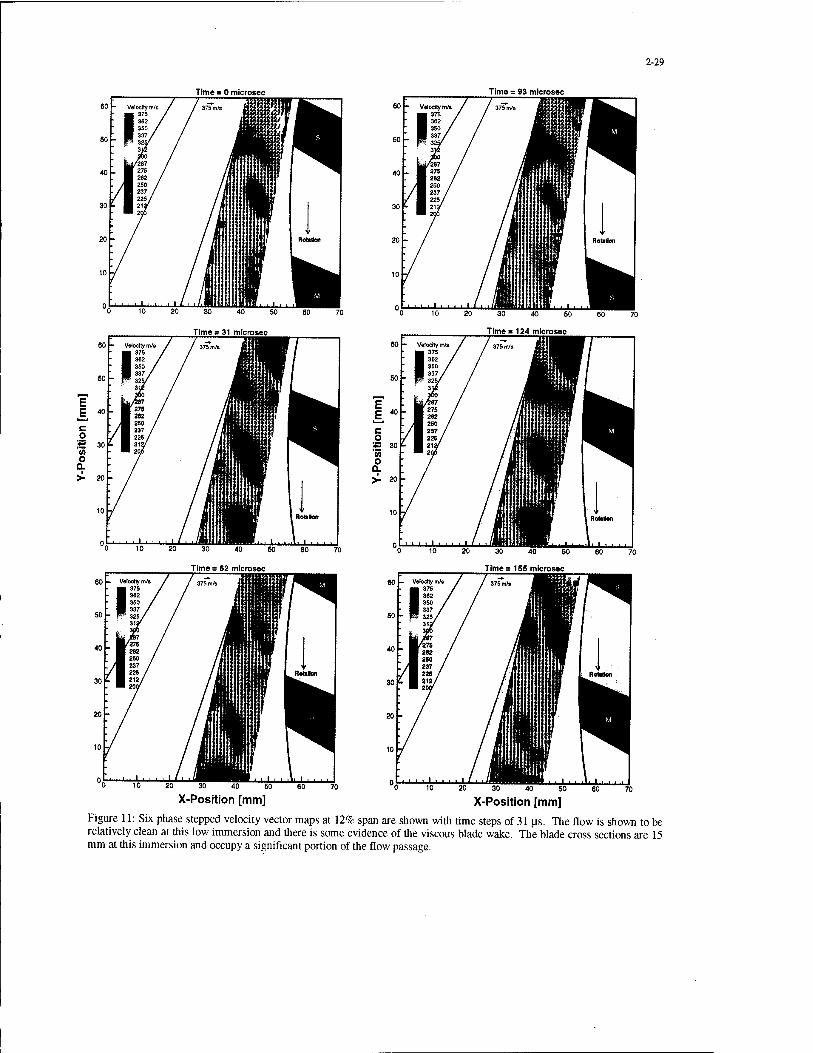
2-29


I .L .L .lit I ■ ■ . . 10 20 30 40 60 60

Time= 62 microsec

X-Position [mm] X-Position [mm]

Figure 11: Six phase stepped velocity vector maps at 12% span are shown with time steps of 31 jas. The flow is shown to be relatively clean at this low immersion and there is some evidence of the viscous blade wake. The blade cross sections are 15 mm at this immersion and occupy a significant portion of the flow passage.

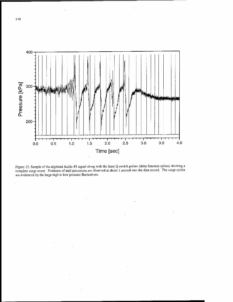
2-30

400

^ 300-

CD

(/) C/) (D

200-

l—|—i—i—i—I—|—i—i—I—r

3.0 3.5 4.0

Time [sec]

Figure 12: Sample of the digitized Kulite #3 signal along with the laser Q-switch pulses (delta function spikes) showing a complete surge event. Evidence of stall precursors are observed at about 1 second into the data record. The surge cycles are evidenced by the large high to low pressure fluctuations.

2-31

500

Time [sec]

A 60 - Vtloeily mit 1375

387 336 321 304 231

»7»m/i

1 I I I I I I I III 20 30 40 50

X-Posltion [mm] 20 30 40 50

X-Position [mm]

■ ' ■ ' ■ ' ' ■ ' ' ' ' 30 40

X-Position [mm]

R Notation

228 m/t mml*

30 40 X-Position [mm]

50

Rotation

uBhl^iJ. 60 70

Figure 13: Pressure time history during a surge event is shown across top, where the labeled laser Q-switch pulses indicate time location in surge cycle of each respective velocity vector plot (velocity scale in plot A is not the same as the scales in plots B-D): a) Normal flow before the onset of surge, note that the flow slows as it enters the diffuser; b) Reverse flow field at peak of high pressure surge cycle, note the effect of the upper blade on the flow exiting the diffuser; c) Reverse flow field on the falling edge of the high pressure surge cycle, velocities are lower than for previous case and fluid packet front is correlated with blade position; d) Reverse flow at the transition between the high pressure and low pressure cycles, lowest velocities are near zero and packet fronts are again correlated with blade positions.

2-32

500

Time [sec]

AiiiUiiittiii 625 m/s ffMititiititt* ittmtitt'

* ■ ■ ■ ■ * ■ ■ ■ ■ ' 20 ~~" 30 40 50

X-Position [mm]

J-JU eo 70

N Rotation


30 40 X-Posiöon [mm]

50

Figure 14: Pressure time history during a surge event is shown across top, where the labeled laser Q-switch pulses indicate time location in surge cycle of each respective velocity vector plot (velocity scales in plots E and F are the same, scales in plots G and H are the same): e) As pressure drops further backflow changes to supersonic flow into the diffuser, note that the supersonic shock front pushes the remnants of the backflowing fluid out of the diffuser; f) At minimum pressure highest velocity in diffuser of Mach 1.7 is reached; g) As the pressure begins to recover, the high speed flow recedes back out of the diffuser; h) Pressure is now close to the stable operating point value and the flow appears close to the presurge condition shown in figure 13a.

2-33

Velocity m/s 625 595 564 534 504

Rotation

11111


50 60 70

Figure 15: Combined correlation/particle tracking result. Over 4000 velocity vectors have been tracked. This data corresponds to the same correlation processed vector map shown in figure 14B, which was used as an input for die particle tracking operation.

3-1

Planar Quantitative Scattering Techniques for the Analysis of Mixing Processes, Shock Wave Structures and Fluid Density.

(September 1999)

R. Schodl German Aerospace Center (DLR) Institute of Propulsion Technology Postfach 906058, 51170 Cologne

Germany

Abstract.

Quantitative Visualization Techniques (QVT) considered in this contribution are planar measurement techniques' which make use of laser light sheet and CCD-camera and deliver quantitative information of flow properties. The elastic scattering of laser light either on seeding particles or molecules is used for the measurement. Three different methods are treated:

The Quantitative Light Sheet (QLS) technique for mass-fraction measurement of mixing processes, The Tracer based Shock Visualization (TSV) for the measurement of shape and structure of compression shocks and UV-Rayleigh Scattering for flow density measurements.

Results of measurements in a model combustor, in a transonic compressor and in a turbine cascade are presented and discussed.

1. Quantitative Light Sheet (QLS) technique

Mixing processes in aero engines occur in the first stages of the high pressure turbines where film cooling air jets interact with the hot boundary layer flow of the turbine blades but predominantly in the combustors where the air jets intruding via injection holes in the liner casing impinge with the cross flow of the internal main flow. The quantitative distribution of the concentration of air jets in main flow is very important for the understanding of the mixing processes, for the optimization of the mixing hole configurations and for code validations. Most of the existing techniques for concentration measurements are based on pointwise measurements, like chemical of thermal probe sampling. It is obvious that probe sampling underlies severe drawbacks in combustion research, since the method is time consuming and the probe influences the mixing process where it is most

intense: in the high gradient regions. Optical techniques are promising, since they have the potential to give planar information about the mixing process without disturbing the flow field. The QLS-technique described in this chapter was published by P. Voigt and R. Schodl (1997), P. Voigt (1998) and C. Hassa et al. (1998). The light sheet method uses scattering of light by small particles marking the flow. The inflow must consist of at least two separate streams, allowing to inject tracer particles to only one of them: the other streams must remain unseeded. The mixing of the seeded injection flow (index 1) with the unseeded main flow (index 2) is analyzed by illuminating the interaction region with a laser light sheet and recording the scattered light from this region on a camera film or CCD-chip (fig. 1.1).

Camera axis

Laser light sheet

Optical access

Figure 1.1: Typical setup of QLS in a combustor .

Under specific test condition which will be specified in the following the gray values of the detected image correspond to the main concentration of the seeded flow in the mixture.

1.1 Measurement principle

The imaging of the light sheet onto the CCD camera chip is shown schematically in fig. 1.2. Depending on the imaging scale a single pixel on the chip with the area Axim • Ayim correspond to a



3-2

certain area element Ax • Ay in the light sheet at position (x,y). By the thickness Az of the light sheet a volume element is determined in which a certain number Np(x,y) of particles is contained. As long as the flow conditions are stationary and seeding is constant this number Np is constant with time and independent of the flow velocity (with increased velocity e.g. more particles per unit time enter the volume element but also leave it) and depends only

Volume Element

hftj. i#Az

Figure 1.2: Imaging the light sheet onto the CCD camera chip.

on particle concentration Cp and local fluid density pf(x,y). The grey level g(x,y) indicated by each pixel is proportional to the scattering power PSca(x,y) collected by the camera lens from all particles in the volume element and the exposure time At. In the simplified case of uniform particle distribution the grey level which represents the collected light energy is:

g(x,y)~At-Psca(x,y)NP{Xiy). (1.1)

Considering a mixing of two flow components the mass concentration of component one Q is determined by

f ~ \ Cx(x,y)=

m. (1.2).

\ l z Jx,y This value is equivalent to the ratio of the total mass portion M within the volme element,

f Cl(x,y) =

Mi

Ml+M2

(1.3)

Jx,y

Since flow component 2 is unseeded, the total number Np(x,y) of particles in the volume element correspond only to the mass portion Mi(x,y), so

Np(x,y) = Cpl-Ml(x,y) . (1.4)

Cpi is the particle concentration of flow component 1 which is supposed to be constant. The particle size distribution should also not vary when mixing with the unseeded air:

CP1*CPl(x.y)

With equation (1.3) and (1.4) and the mass contained in the volume element

(M{+M2)x,y =Pf(x,y)-Ax-AyAz (1.5)

the relation 1.1 can be transformed into

g(x ,y)~At- Psca (x, y) ■ CPl ■ pf (x, y)

■Ax-AyAzM-Cifay) (1.6)

The collected scattered light form a single particle is given by

Psca(x>y) ~ Csca(dp>x> PL(x>y)

(1.7) '"»yi"'Ay.My)

with Csca(dp,x) the scattering cross section as a function of particle diameter and scattering direction (which varies with the x-coordinate) and the local laser power Pi.(x,y). In general the scattering cross section depends also to a small extend on the direction determined by the y- coordinate because of polarization effects. When unpolarized or circular polarized laser light is used this dependency can be neglected. The grey level proportionality is then given by

g(x, y) ~ At- Csca (dp, x) ■ PL(x, y)

■ Cpi ■ p(x,y)- Ax-Cx(x,y) (1.8)

It is remarkable that the grey level is independent of the light sheet thickness Az. With increasing Az the volume of the element and the number of particles therein increase but the light intensity is lowered in the same ratio. Since it is practically impossible to calibrate the grey level g against mass concentration Q because of too many parameters influencing the light detection the QLS technique has been set up as a relative method meaning that all grey values in the detected image are related to the value at the location (x0,yo ) of the injection jets, where the seeded particle flow penetrates the cross flow. This reference point (index 0) is used as a measure of 100 percent jet flow concentration.

The grey value ratio results to

g(x,y)

8(x0,y0)

CSCa(dp,x) PL(x,y)

Csca(dp,x0) PL(XQ,y0)

Pf(x,y) Q(jc,y) (1.9)

Pf(x0,y0) QUo.yo)

Since both grey values are taken form the same image the exposure time can be eliminated. Because of the constant particle concentration of flow component 1 and not changing size

3-3

distribution the scattering correction remains only depending on x-coordinate

Csca(dp,x) = Csca{x)

Csca (dp , XQ) Csca (xQ)

and equation 1.9 can be reduced to

g(x,y) _ Csca(x) PL(x,y)

(1.10)

g(xQ,yQ) Csca(x0) PL(x0,y0)

Pf(x,y) (1.11)

Pf(x0,y0) C}(x,y)

The concentration C^xo.yo) in core of the seeded jet flow is set to 1.0 which equals 100%. We assume that the laser power distribution in the light sheet as well as the direction dependency of the scattering cross section is known. Then the grey level ratio is only a measure of mass concentration when either the flow density distribution is known or constant in the measurement region. The latter case is considered for QLS applications and equation 1.11 become

C](x,y) = CsJx0) CsJx)

PL(x<»yJ g(x,y)

(1.12)

pL(x>y) g(xo>y0)

That means the QLS-technique is restricted to isothermal mixing processes under constant pressure conditions of flow components of the same fluid.

The influence of scattering direction is significant and requires corrections. In fig. 1.3 a typical QLS setup is shown with a CCD camera observing a certain region G of a light sheet and detecting the scattered light particles.

forward scatter

CCD

With different position x in the region G the scattering angle •$ between incident laser beam and observation direction varies, thus on the right corner of region G low intensity backscatter light and on the left corner high intensity forward scatter light is observed. This effect which increases with increasing viewing angle is show in fig. 1.4, where the scattering intensity 1(15) is plotted as a function of $ over the entire range of the region G. This measurement can be made eather at the actual experimental set up if homogeneous seeding of the flow in the measurement region is possible or in a separate experimental set up where care must be taken to keep the general arrangement and the seeding properties identical. The result is the distribution Csca(x) which is needed in equation 1.12 for corrections.

w

SH- i

Wrr

IM-

iss-

ue-

v*»* «**£

ICC-

es-

B K !S S3 » VK I»

Figure 1.4: Scattering intensity as a function of scattering direction ■&.

The Laser power distribution in the laser sheet is the second parameter to be known. It is mainly determined by the light sheet generation. A constant intensity distribution over the light sheet height (y- coordinate) is very much appreciated in order to achieve best accuracy with a given dynamic range of the camera sensitivity.

Sweeping - by use of a rotating polygon mirror - a laser beam periodically over the light sheet height is a rather efficient solution to approach very close the constant intensity distribution. In this case a CW- laser, as foreinstance an Ar+-Laser, must be used as a light source. The sweep-period time should be significantly shorter than the exposure time or a full number part of it. The light sheet generating optics can be such designed that the laser beam direction remains constant while the beam is moved up and down. In this way a parallel light sheet is formed with constant not varying intensity along the propagation direction x. The intensity distribution along the light sheet height can be measured. With the known value

PL(x,y) = PL(y) (1.13)

Figure 1.3: Influence of scattering direction (fl = tf(x)). equation (1.12) is finally determined.

3-4

However this conclusion cannot generally be drawn because there are two physical phenomena related to the particle laser light interaction which have been not considered yet. They influence the laser power distribution as well as the scattering characteristics in the measurement region.

1.2 Considerations about measurement errors.

One effect is extinction, which is the attenuation of a propagating light beam by the scattered light emitted from particles. As shown by P. Voigt (1998) one can correct for this intensity loss along x-coordinate when the laser power distribution PL(y) is known at the entrance and exit of the measurement region and when extinction is the only existing effect. However in the case of light scattering on particles there are in parallel effects of multiple scattering overlapping the extinction rendering these corrections impossible. Multiple scattering is a secondary effect in scattering experiments. It denotes the fact that scattering particles can be light sources for adjacent particles. This effect depends on the particle load. The existence of secondary scattering has been proven in a number of experiments and different aspects have been simulated numerically. An example of multiple scattering effects is shown in fig (1.5) by the virtual thickening of a laser beam.

T = 100%

T = 80 %

T = 90 %

T = 75 %

Figure 1.5: Multiple scattering corona around a stationary laser beam

A laser beam passes through a chamber with homogeneous seeding. The laser beam enters from the left side. On the outlet side the transmission ratio T is measured by a photodiode. The chamber is seeded with four different particle loads and images have been taken. In the upper left image no extinction could be measured. The beam looks thin. For the following experiments the seeding was intensified successively. As a result the laser beam in the image increases accordingly it's thickness.

But this expansion is not constant along the beam. In the first quarter of the path the expansion increases, due to the strong secondary scattering in the forward direction. After reaching the maximum diameter, the expansion decreases, caused by the coexisting extinction effect on the centerline.

The correction of multiple scattering is the most challenging part of the post processing, since the effects are fully three dimensional. A number of different approaches have been tested already, but none of them with sufficient results yet. Since extinction and multiple scattering exist at the same time correction algorithms are even more complicated and not available yet.

Being no able to correct for them there is only one solution: to keep these errors small. For this reason the seeding must be adjusted to the lowest possible level which can be accepted with regard to the camera sensitivity. For practical seeding levels the remaining measurement error of the QLS-technique was found (see P. Voigt and R.Schodl, 1997) to be about 5%, sufficiently small as required for most of the mixing analysis experiments.

1.3 Experimental set up

The experimental set up consists of an Ar+-laser (1W power) fiber linked to a light sheet generating box in which a polygon scanner with20 facets is rotating with controllable speed. The scanning laser beam generates the light sheet propagating with constant hight (max. height = 120 mm).

A Peltier-cooled CCD camera with a dynamic range of 12 bit takes the picture normally viewing to the light sheet.

When light reflection on model surfaces can not be avoided these were painted with fluorescent dye and a laser line filter was inserted to the camera objective in order to reduce these reflections to a great extend. The measurements start with a background image taken with the conditions: laser on and seeding off. From the signal image taken with seeding on in one flow component the background image is subtracted and different correction procedures for pixel sensitivity, image distortion and scaling, scattering direction and laser power distribution are applied. After that, the reference value g(x0,y0) indicating the 100% level in the in the image is determined and the corrected mass concentration map is established. Further application of various graphical procedures deliver the final mass concentration contour plot. Being restricted to low seeding levels even high sensitive cooled CCD camera require several

3-5

seconds of exposure time to achieve results of good quality supposing an Ar-laser is used as a light source. That limits the QLS-technique to mean value measurements which, however, are still of interest today. Instantaneous measurements with much shorter exposure time (~70us) have also been carried out but require intensified CCD camera and are less accurate.

1.4 QLS applications.

As an example of concentration measurement in combustors figure 1.6 shows the mixing field in the RQL combustion chamber shown in fig. 1.1. The rectangular model with optical access was equipped with multiple air blast atomizers at the chamber head which ensure a very homogeneous flow field at the primary zone outlet. The mixing sector where the measurements have been taken had 3rows of staggered injection holes. Tests were carried out under atmospheric non preheated conditions. Only the secondary air was seeded. The light sheet was positioned axially and parallel to the flow direction illuminating the upper part of the mixing region.

vzzzzzzzzzzzzzzzzzzzzzzzzzzz MCMdarr Sow Medad)

90 1Ö0 110 120 13« 140 ISO X [mm]

Figure 1.6: Isothermal mixing in RQL chamber.

The core of the jets of the first and the third row of secondary air jets can be seen clearly. The penetration of the secondary air jets is strong enough to ensure a satisfactory mixing in the whole quench zone. Since these measurements take a very short time many pictures of the 3D-mixing field can be collected at different light sheet positions, providing mass concentration values of the whole volume of the combuster chamber. Short exposure measurement have also been taken in a very similar combustor model of RQL type. An intensified CCD camera was used. The exposure time was 70us and equals the time for a single sweep of an Ar-laser beam needed to generate the light sheet. Several thousand images were taken from the same mixing region each of them delivering the instantaneous mass concentration distribution. Fig. 1.7 and 1.8 show mean value and RMS values of mass concentration evaluated from this set of data.

The numerous images taken allow to set up at each location of the mixing field histograms of the unsteady fluctuating mass concentration the shape of which delivers valuable information for code development. An enlarged view from the marked region of fig. 1.7 and 1.8 is shown in figure 1.9 representing an instantaneous distribution.

Figurel.7: Concentration distribution averaged over 10 000 images.

Figure 1.8: RMS values of the mass concentration fluctuation averaged over 10 000 images.

Figure 1.9: Typical image of instantaneous concentration distribution.

Valuable information can be extract from the visualized structures which vary from image to image. QLS was also applied to a turbine Stator to visualize and quantify the cooling film penetration and development. The optical set up is shown in fig. 1.10. A window was placed in the turbine casing.

3-6

Main and cooling air were adjusted to the same temperature. Only the cooling air was seeded. Fig. 1.11 shows an unprocessed black and white image of the cooling air mixing. The quantitative mass concentration which are achieved after further image processing allow for evaluation of cooling efficiency and temperature load at the turbine blade surface.

Hght fiber

cooling air

Figure 1.10: Schematic sketch of visualisation technique

Ejected Cooling Air

/ ^ V <r /

Injection Hole

Figure 1.11: Original video shot of cooling air ejection.

Considering that QLS-results could be collected in a very short time, the light sheet method has proven it's qualification for development tests and is at this time used as a tool for the optimization of mixing and cooling hole configurations for combustors and turbine blades.

2. 3D-Shock Visualization in a Transonic Compressor Rotor.

A new optical non intrusive technique to visualize the position and the structure of shock waves is presented in this chapter. The number per volume density of particles which were added to the flow and with it the density of the fluid are visualized with a laser light sheet and an intensified CCD Camera. Structures like normal and oblique shocks, X.-shock structures and separation regions can be clearly identified although the presented technique is not suited for quantitative density measurements as e.g. the Rayleigh scattering method is. But it's

handling in praxis is comparatively easier and optical access problems are less severe. The following description of the technique is mainly related to the publication of I. Roehle et al. (1999).

2.1 Principle of Tracer based Shock Visualization.

A shock wave is characterized by a sudden increase of the density across the shock. To visualize this, the flow is seeded homogeneously with particles, which can be visualized easily with a laser light sheet. The particles in the light sheet scatter the laser light. The integral scattered light intensity from one volume element is proportional to the number of particles in the volume element and therefore also proportional to the density of the fluid. The light sheet is observed with a camera. In the captured image the region downstream the shock is brighter than the region upstream the shock. The shock position is identified by the sudden change of the brightness (see figure 2.1).

To carry out such measurements in the blade passage of a rotating compressor, the time of a single exposure of the image needs to be short compared to the blade period, so that a frozen picture with a fixed blade position is obtained. Intensified CCD-cameras perform sufficiently short exposure times. Furthermore, this sort of camera enable multiple exposures so that an 'on ship integration' of lots of single exposures from the same phase locked position of a periodically changing flow can be taken. This feature renders possible to use a scanning light sheet, e.g. a light sheet generated by a sweeping laser beam. While the laser beam is sweeping slowly across the region of interest the camera integrates lots of single exposures (figure 2.2).

The result is an image of an evenly illuminated light sheet plane with a homogeneous intensity distribution and sharp edges, two very convenient features for the shock visualization in a blade passage.

The laser beam from a CW-YAG-laser is guided via fiber to a rotatable probe which forms the light sheet plane at a selected radial position. A measurement time of some seconds is necessary to obtain an image representing the shape and position of shock waves at a particular plane in the blade passage. By taking more pictures at different radial positions the 3D-shock structure of the blade passage flow is visualized.

2.2 The compressor test rig

The presented measurements were carried out in a transonic axial compressor fitted on the ERECA

3-7

homogeneous particle seeding

laserbeam

particle number _ . .. Image intensrty ~ ^olume element ~fl°w density

Figure 2.1: Shock visualization in turbulent high speed flow.

Probe

Particles

Shock

ICCD-Camera

Probe

Laser Beam

Window

Blade

Figure 2.2: Perpendicular and perspective view of the blade passage with the I

sheet probe, the window and the camera

Blade

facility of ONERA - Palaiseau. This is a closed loop facility having a heat exchanger and a throttling valve to regulate the back pressure. The compressor consists of a rotor with 23 blades and a stator located several chords downstream of the rotor (Figure 2.3). There were no inlet guide vanes. This configuration is particularly interesting for basic research because complex unsteady rotor-stator interactions do not occur. Consequently the flow field

can be considered as stationary in the relative frame of the rotor. At rotor entrance position the casing radius is 123 mm and the hub radius is 78 mm. The design speed of rotation is 33.000 rpm. At the design mass flow rate of 5.8 Kg/s the relative Mach number varies from 1.406 at the tip to 0.998 at the hub.

3-8

Rotor Stator

Figure 2.3: cross section of the test compressor.

1.7

1.8

1.8

tv

Paint 3 y i

tPoint 2

Point 4

A \ Point 1 V \ No

3.06 No

1_ 0-b|t

5 8.5 fl Kg/s

Figure 2.4: Performance map with operating points

The visualization experiments were carried out at four different characteristic points of operation (Figure 2.4): • At the design mass flow rate (point 1) • At the midrange operating point (point 2) • Near the surge (point 3) • At 95% of the design rotational speed (point 4)

2.3 The TSV-set-up on the compressor test rig.

Seeding of the flow was provided by a Laskin nozzle generator which was operated with the same grease oil as it was provided for the rotor bearings. The mean particle size was about o,5um. The seeding was introduced through a small tube 1.5 m upstream the rotor. A diode pumped frequency doubled cw YAG laser with a power of 400 mW was used as a light source. To generate the light sheet inside the machine a laser beam probe shown in Figure 2.3 was applied. This probe consisted of a tube with a 45 ° mirror placed at the outlet tube end. The laser light beam propagating along the tube center line, was reflected by this mirror and left the probe perpendicularly through a hole in the tube. An optical multi-mode fiber (lOum in diameter) was used to guide the laser light to the probe. The plug at the fiber end which was mounted to the probe contained a collimator lens that collimated the light

emerging from the fiber and focussed it to the measurement region (diameter « 0,4mm). The probe passed through the casing via a 6mm hole located down stream the blade passage (figure 2.3). The probe was mounted in a traversing unit and could be rotated and radially moved. The light sheet was performed by turning the probe around it's axis over a small angular range (see fig. 2.2).

The blade passage was observed through a casing window with a diameter of 24 mm. The camera took the images through this window. The blade trigger was accomplished by an optical sensor giving a short pulse for each blade. Apart from this a so called 'one per revoluting' signal was also available so that together with the blade trigger each individual blade passage could be identified. The camera was triggered on one particular blade. Since the rotational frequency was about 550 Hz, the camera was gated 550 times a second. A delay was set to adjust the position of the blade passage to the window position. Since the blade period was about 80 H-s a gate width of the camera of lp.s («80 p.s) was chosen, short enough to freeze the blade position. The multiple exposure and the process of turning the probe for the light sheet generation were started and stopped synchronously. Turning the laser beam from the pressure side of the blade passage to the suction side or vice versa took about 20 seconds. During this time the camera was integrating about 550*20=11000 exposures. The captured images were stored and post processed in a computer. Before the measurement at a certain radial position, the minimum and maximum angle of rotation of the probe needed to be determined, so that the laser beam did not hit the blade surfaces at neither one of the extreme positions. This was necessary to avoid distortions by laser reflections. To determine the position of the blades, one image illuminated with the light of an external light source was taken in order to get a picture of the tip of the blades. This picture was later used for spatial calibration. In the signal image itself the blades were not always quite visible. A dark image without particles was taken before each individual measurement to correct for background radiation. Post-processing was performed using digital image processing software.

2.4 TSV Results & Comparison to Pressure Measurements and CFD- Calculations.

Examples of measurement results are shown in the following figures. Figure 2.5 and 2.6 show the shock structure at the design mass flow rate at a depth of h/H =0.95 and 0.64. An oblique shock wave starting at the leading edge of the blade and a normal shock wave in the center of the blade channel can be identified. Also a

3-9

Separation Region

Figure 2.5,2.6,2.7: TSV images at the design point (point 1, see figure 2.4) at a relative blade bight of h/H=0.95 and at h/H=0.64 (figure 2.5,2.6) and at surge (point 3) at h/H=0.79 (figure 2.7).

JWT •J

^Wtfv'i us

&JL 8

—J— • it6'

1258 " l-ieoe n

s

•■_. .--.••'• t

-250

:-24/

Fig. 2.8: Intensity profile across the normal shock wave (see dashed line in figure 2.5)

?i-shock structure near the leading edge on the pressure side was observed.

At the operating point 3 near the surge a separation of the shear layer on the suction side behind the shock was observed (Figure 2.7). In the wake region the luminosity was very low. Of course this can not be interpreted as a very low density. It is rather due to the fact that the air in the separation zone is less seeded. This effect is well known from lots of velocimetry experiments. Although it is not fully understood, this effect is quite helpful for visualizing purposes like in this experiment.

An intensity profile across a vertical shock presented in fig. 2.8 (see dashed line in figure 2.5) shows a transient region with a thickness of about 3 mm. This shape was very repetitive. The rather wide transient region might be explained by unsteady shock fluctuations. The estimated fluctuation amplitude is about 1mm.

The transient region becomes significantly wider when pictures were taken by integrating over all blade passages. That means that some minor geometrical differences may exist between the different blade channels. One blade channel was selected to be representative for the test rotor where most of the measurements were taken.

Figure 2.10 shows a measurement of the wall pressure distribution at the design point of the compressor. This measurement was accomplished by fast pressure sensors, see Fradin, G., et al. (1995) and (1994). Figure 2.11 shows a Navier Stokes calculation of the density distribution in a plane about 2mm from the casing, see Billonet, G. (1995).

These two pictures should be compared to figure 2.9, the TSV picture taken at a distance of about 2 mm from the casing. Deviations between this result can be identified as well as good agreements. These data demonstrate that TSV is well suited for quantitative flow analysis and delivers valuable information for code validation.

In order to give an impression of the 3D-shape of the shock wave the shock position at different radial positions (h/H) is plotted together with the corresponding blade profile in figure 2.12. The experimental shock position (solid line) and the shock position extracted from the CFD-calculations are shown for the compressor operating point 1. The results agree very well and show that in this case the shape of the shock wave is very flat. The development of the interaction of the oblique shock from the blade tips with the normal passage shock can also clearly be identified.

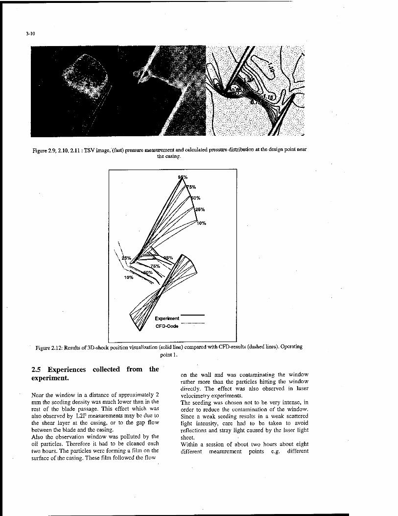
3-10

Figure 2.9, 2.10,2.11: TSV image, (fast) pressure measurement and calculated pressure distribution at the design point near the casing.

Figure 2.12: Results of 3D-shock position visualization (solid line) compared with CFD-results (dashed lines). Operating point 1.

2.5 Experiences collected from the experiment.

Near the window in a distance of approximately 2 mm the seeding density was much lower than in the rest of the blade passage. This effect which was also observed by L2F measurements may be due to the shear layer at the casing, or to the gap flow between the blade and the casing. Also the observation window was polluted by the oil particles. Therefore it had to be cleaned each two hours. The particles were forming a film on the surface of the casing. These film followed the flow

on the wall and was contaminating the window rather more than the particles hitting the window directly. The effect was also observed in laser velocimetry experiments. The seeding was chosen not to be very intense, in order to reduce the contamination of the window. Since a weak seeding results in a weak scattered light intensity, care had to be taken to avoid reflections and stray light caused by the laser light sheet. Within a session of about two hours about eight different measurement points e.g. different

3-11

operational points and/or different radial positions were taken. The reasons for this limited acquisition speed were, that the acquisition process was not automated, that several images were taken on each measurement point to check the reproducibility, that one sweep of the probe took 20 seconds and had always been repeated, once for the dark image and once for the final image and never the less that it took time to change the operational point of the compressor. The further development of technique will result in a significantly shorter measurement time.

Since the requirement for a quantitative density visualization technique can not be fulfilled in practice, as e.g. stable homogeneous seeding, stable intensity in the light sheet, no coagulation and contamination of particles inside the test rig and stable observation condition (clean windows), TSV is only a qualitative density visualization technique. However it is well suited to identify shock locations in transonic flows and this information is well suited for quantitative validation of numerical data and for the evaluation of transonic flow phenomena. The accuracy of the position detection depends on the contrast achieved within the detected images. The influencing parameters are

quality of light sheet (thin and stable) suppression of background flow cleanness of observation window stability of shock structures length of exposure time seeding with small particles that follow the steep velocity gradient across the shock stability of instrumental set up

and these vary from test rig-to test rig. Therefor a general specification of the measurement accuracy can hardly be given. This technique is applicable not only in turbomachines but also in any kind of transonic flows as e.g. wind tunnels, cascade wind tunnel and delivers the 3D-shape of transonic shock formations.

Also instantaneous measurements might be possible when pulsed laser and light sheet forming probe devices are applied.

3. UV Rayleigh Scattering for Density Measurements in a Turbine Stator.

As shown in the preceeding chapters the Mie- scattering technique in general is suited for quantitative flow density determination but problems of seeding, extinction and multiple scattering limit the achievable measurement accuracy. Even well optimized Mie-scatter experiments will not enable quantitative measurements especially in regions of rather small

density variations as they occur in the turbine and compressor blade passages. Not having the advantages as ease of handling and high signal level as Mie-scattering techniques Rayleigh scattering is the suitable high resolution technique for quantitative, high resolution flow density measurements well proven and applied to fluid mechanic investigations, e.g., to mixing processes in gas jets presented by M.C. Escoda and M.B. Long (1983) and B. Shirinzadeh et a. (1992) and to shock wave and boundary layer structures shown by M. Smith et al. (1989) and R. Miles, W. Lempert (1990).

The following description of the method and presented results are closely related to the publications of O. Sieber (1998).

3.1 Rayleigh Scattering.

The physical process of light scattering on molecules is named Rayleigh scattering. The molecules illuminated by a light beam absorb a certain amount of light energy and release it immediately without change of their status. By this process, called elastic scattering, the light frequency and polarization status remains unchanged but the direction of the scattering light is changed. It is emitted all over the space independent of the direction of the incident beam.

In comparison to Mie-scattering Rayleigh scattering is several orders of magnitude weaker in intensity. Therefore extinction and multiple scattering effects can practically be neglected which is the main reason for the superiority of Rayleigh scattering against Mie-scattering in view of density measurements. If molecules are randomly spread in the measuring volume and multiple scattering intensity emitted from all molecules in the probe volume is given by

I~Csca-N-I0. (3.1) It depends on the incident laser intensity I0, the number of molecules N, and from the scattering cross section Csca.

If molecules are considered as dielectric spheres with diameter smaller than the wavelength of the incident light and when the probe volume is illuminated in one direction with monochromatic linear polarized light the scattering cross section is given by

sin2 77 sca ~ A4 ' (3.2)

(proportie s of molecules)

with X the wave length of the light source and r\ the angle of the electric field vector of the polarized light and the scattering direction.

3-12

When a illuminating light sheet is considered with the direction of the linear polarization parallel to it's height and when a camera is looking normal to the sheet then r\ becomes 90° and directional dependency of Csca within the given small aperture range of the camera objective can be neglected. This kind of arrangement is considered to be the recommended optical set up for Rayleigh scattering experiments. The properties of molecules of fluid gas applied determine predominantly the scattering cross section. Theoretically existing additional influences of temperature and pressure are negligible in most practical applications as shown by O. Sieber (1996). The scattering cross section dependency on the wave length indicate that short wave length are recommendable to overcome the problem of the low scattering intensity. From this considerations the following conclusion can be drawn: in case of non reacting flows where fluid properties remain constant and when the recommended optical arrangement is applied the scattering cross section becomes a constant value,

CSca = const (3.3)

and the Rayleigh scattering intensity is than only depending on

I~N-I0

3.2 Measurement Principle.

(3.4)

When imaging Rayleigh scattering signals the recorded light energy of each pixel of a CCD-chip is related to the energy g(x,y) emitted from the number of molecules N(x,y) in the volume element Ax • Ay ■ Az of the light sheet during the exposure time At

g(x,y)~I0(x,y)-N(x,y)-At (3.5)

This equation does not account for background flare and reflections because it is very difficult or even impossible to model these effects theoretically. Therefor, when setting up an experiment, care must be taken to avoid or reduce these distortions that they become small compared to the Rayleigh signal. Assuming the size of the volume element to be constant, with

N(x,y)~p(x,y)Ax-AyAz (3.6)

equation (3.5) can be rewritten as

g(x,y)~IQ(x,y)-p(x,y)At (3.7)

The evaluation of the Rayleigh scattering signals is based on a relative measurement, because with this kind of evaluation potential sources of error, such

as incident light inhomogenities and spatially dependent sensitivity of the imaging optics, can be eliminated. Therefore, first a wind-on image is taken, i.e., during wind tunnel operation. The recorded signals contain the information on density variation given by

gj (x, y) ~ I0l (x, y) • px (x, y)Atx (3.8)

Additionally, a wind-off image is taken under standard conditions, i.e., across the whole field of view the density has to be on the same level and exactly known:

PQ = const. The grey level distribution in this reference image is then given by

g0(x,y)~I0Q(x,y)-p0-At. (3.9)

Assuming equal exposure times Atj _ Ato than the pixelwise division of the two signals yields the related grey level distribution

F(x,y) = gi(x,y) =

g0(x>y)

io/x>y)-Pi(x-y)

h0(x>y)-Po

(3.10)

In Rayleigh scatter experiments pulsed laser are used. Their beam energy and the energy distribution may fluctuate from pulse to pulse. Typically the signal of lots of laser pulses are integrated on the camera during the exposure time. By this kind of meaning the energy distribution variations are meaned out and becomes very constant but the energy level often differs because the two images are not taken at the same time and mean laser power may change. To account for this effect an optical energy monitor can be used as described later which figures the actual energy level 0EM onto a certain part of each image taken. With the values from both the wind-on image (0EMO and the wind-off image (0EM2) the intensity distribution ratio becomes

hx{x,y) _0EMA

I0Q(x,y) 0EMo

(3.11)

and equation 3.10 can be rewritten to determine the density field:

p(x'y)=p°S-nx'y)-(3i2)

As it is mentioned by C. Jakiel et al. (1998), without taking the laser energy into consideration, . the average values of the density ratio deviate up to 6% from their mean value although they were measured at the same flow conditions. But with

3-13

energy monitor calibration the deviation can be reduced to less than 1%. Usually the ratio 0EMo/ 0EM, varies from 0.94 to 1.02

30

25

20 o o o

(o 15

- I Laser Beam , WIND ON

- ■" 1 ""

Evaluation Range WIND-OFF

; 1" y

; ! '"V \\ " It \\

:

\\ E nerg onitc

n y r

- J I j , t i i

100 200 Pixel x-Direction

300

Figure 3.1: Intensity distribution in x-direction

Figure 3.1 shows a typical intensity profile of the measuring volume and of the energy monitor. The differences in density between the wind-on and the wind-off image can bee seen as distances between the two profiles within the range of the laser beam. Likewise, these two profiles with similar behavior elucidate the necessity of a relative measurement, since the intensity differences caused by the density variation are smaller than the differences caused by the beam inhomogenities. The intensities in the area of the energy monitor are about two times inferior to the Rayleigh scattering intensities in this case, but they are one order of magnitude higher than the signals from the areas not being evaluated. Thus, a clear distinction of the areas is possible. It can be seen clearly that the evaluation range has to be smaller than the width of the laser beam, because the laser intensities decline rapidly at the lateral borders of the beam, and so the signal-to-noise ratio is too low in these areas.

3.3 Experimental Set up.

Rayleigh scattering experiment reported by O. Sieber (1997) were performed in a turbine cascade wind tunnel. The cascade used was of the type VKI-1 which is typical for cooled gas turbine rotor blades designed for transonic flow. The blade chord was 32,6 mm the blade height 100 mm. An excimer laser (Lambda-Physik LPX HOi), modified with a polarizer, was employed as light source. The ArF laser worked in the deep UV at 193nm. This high frequency yielded Rayleigh signals stronger by one to two orders of magnitude compared to lasers working in the visible range.

The emitted Rayleigh light was imaged by a 12-bit intensified charge-coupled device (ICCD) camera (LaVision) via an UV-Light-sensitivity lens (UV- Nikkor 105 mm, f/4.5). The cooled CCD chip had a spatial resolution of 384 x 286 pixels. A 486 personal computer with special purpose software (LaVision) controled the complete system, i.e., it synchronized laser and imaging system, and it recorded and stored the images. The optical arrangement setup for density measurements behind the plane turbine cascade is shown in figure 3;2.

Figure 3.2: Optical Setup.

The laser beam was blanked out by a double aperture directly after emerging. With the help of three mirrors the beam was positioned to the direction parallel to the endwalls and parallel to the trailing edge plane. Two cylinder lenses focused the laser beam to reduce the thickness under 0.5 mm at a width of about 20 mm. One adjustable aperture was used to suppress direct irradiation of the trailing edges. The distance to the trailing edge plane was chosen as small as possible and fixed for this study. To make precise monitoring of the beam energy possible, some laser light was split off at the third mirror and, after transformation to longer wavelength, led through a liquid light guide. The transformation is necessary, because the light wave guide is only transparent for wavelengths longer than X = 260 nm. The second exit of the light pipe was fixed opposite to the measuring window, so that the camera can image the transmitted energy signal while taking the images (see Fig. 3.3). It was proved by experiments that the recorded energy signals show a linear dependence on the laser output energy within the range of possible beam energy fluctuations of maximum +/- 5% from pulse to pulse.

3-14

Stetes

Energy Monitor

• Figure 3.3: Camera view.

The material for the background insert was selected to minimize direct reflections of scattered light to the camera. Silica glass was found to be very suitable, because influences of surface reflections were smallest when using this window. To reduce the influence of light scattered outside the test section, the laser beam was covered as far as possible. In these experiments, altogether 2500 laser shots were summed up for both wind-on and wind-off images. This number basically has been yielded from 50 shots summed up on chip. The intensities of 10 of those integrated images were read out, added by software, and stored on hard disk. This process needing about 20 seconds was completed five times. The result of averaging these five data sets yielded the information of the density field.

3.4 Measurement results.

The density measurement have been carried out at different isotropic outlet Mach numbers. The results obtained demonstrate a good periodicity of the cascade and a general good agreement with 3D calculations. Effects of side wall influence could clearly identified.

In fig.3.4 measured density distributions taken at an isotropic outlet Mach number of 1.0 are presented.

The shock wave can be seen very clearly in midspan, the structure develops as it is expected for transonic turbine cascades. The shock wave crosses the wake and hardly widens up to the end of the evaluation area at x/1 = 0.6. Near the endwall the shock wave dissolves and the density filed differs qualitatively and quantitatively from midspan plane because of secondary flow effects.

The results show that the combination of density fields from different blade heights affords an insight into the three-dimensional flow field behind the plane turbine cascade. Next aim concerning this system is the realization of measurements within the passage. .............v..„.....„,.,,^...>.............. ..............

;j;5l<gATi3

Fig. 3.4: Measured density fields [kg/m3] at Ma2is= 1.00.

3.5 System Capabilities and Limits.

The measurement accuracy of the Rayleigh scattering technique depends to a great deal to the care taken to setup and adjust the system and on the experimental environment and conditions.

When the following conditions are maintained, as 1. direct reflection of laser light on

surfaces must be avoided, 2. background flare has to be

reduced as much as possible, 3. any change of geometry and

flare condition between wind-on and wind-off image must be avoided,

4. due to of their very strong Mie- scattering particle can not be tolerated in the measurement region (test air needs to be carefully filtered and when high Mach number expansion flow is considered also the humidity level must be controlled to avoid ice particle generation),

then the sensitivity of density measurement is beyond 1% according to the ambient density and the uncertainly in reproducibility was found to be smaller than ± 1.5% which includes all system uncertainties, as e.g. energy monitoring or determining the reference density p0.

Because of these properties the Rayleigh scattering technique is suitable for investigations not only in transonic and supersonic but also in subsonic flows.

3-15

4. Conclusion

It was reported about three planar measurement methods which have been successfully used for quantitative visualization of various flow characteristics. These methods take advantage of light scattering on particles or molecules. Since light sheet imaging depend on so many parameters influencing the signal level none of the techniques is capable to take an absolute measure of a fluid property. However, when refering the signal image to specific references, e.g. a reference point in the signal image of known quantity, a reference image taken under well quantifiable conditions, relative values of rather high accuracy can be achieved which deliver together with the known reference value absolute measurement data. Even the shock visualization technique that doesn't acquire any references it takes advantage from only localizing steep gradients instead of quantifying intensities thus delivering the quantitative data of the shock wave shape and position. The common properties of these techniques are:

rather easy to handle, quick in collecting data. provide overview about 3D-flow characteristics

and therefore can be considered as efficient tools for development tests.

Acknowledgements.

The presented research project on tracer based shock visualization was set up in the frame of a collaboration between ONERA and DLR. The excellent support given by Mr. A. Le Guevel and Mr. C. Fradin is highly acknowledged.

In context with the preparation of the Rayleigh scattering contribution the author would like to thank Prof. K. Fiedler and Dr. C. Jakiel for their support and friendly disposition of material.

References

Billonnet, G., 1995, „Synthese des calculs CANARI appliques au rotor isole C007 du banc ERECA", RTS ONERA n° 130/7103 EY.

Escoda, M. C, Long; M. B., (1983) "Rayleigh Scattering Measurements of the Gas Concentration Field in Turbulent Jets", AIAA Journal, Vol. 21, No. l,pp. 81-84.

Fradin, C; Le Guevel, A., Billonnet, G., 1995, „Activites Scientifiques et Techniques 1994", ONERA, Mars.

Fradin, C.; Le Guevel, A, 1994, „Analyse d'ecoulement du fluide dans le rotor axial transsonique TURBOMECA C007 implante sur le banc d'essais ERECA- Deuxieme Campagne", RTS ONERA n°7/3694EY.

C. Hassa, C. E. S. S. Migueis, P. Voight, 1998, "Design Principles for the Quench Zone of Rich- Quench-Lean Combustors", AGARD-PEP- Symposium on Design Principles and Methods for Aircraft Gas Turbines Engines, Toulouse.

Jakiel, C, Fiedler, K., Sieber, O, 1998, "A Quantitative 2D Density Measuring System Using UV Rayleigh Scattering at an Atmospheric Wind Tunnel", AGARD-CP-598 Advanced Non-Intrusive Instrumentation for Propulsion Engines, Brüssel, Belgium, 20-24 Oct.

Miles, R., Lempert, W., 1990, "Two-Dimensional Measurement of Density, Velocity and Temperature in Turbulent High-Speed Air Flows by UV Rayleigh Scattering", Applied Physics B, Vol. 51, pp. 1-7.

Roehle, I., Le Guevel, A., Fradin, C, 1999, "3D- Shock Visualisation in a Transonic Compressor Rotor", to be published in a special issue of Optics and Laser Technology, Elsevier Science, Oxford.

Sieber, O., 1996, "Quantitative Dichtefeldmessung mit Rayleigh-Streulicht am Laufschaufelprofil VKI-1 und Vergleich mit einer numerischen Simulation", Vol. 301, Fortschrittsberichte VDI Reihe 7, VDI-Verlag, Düsseldorf, Germany.

Shirinzadeh, B., Hillard, M. E., Jeffrey Balla, R., Waitz, I. A., Anders, J. B., Exton, R. J., 1992, "Planar Rayleigh scattering results in helium-air mixing experiments in a Mach-6 wind tunnel", Appleid Optics, Vol. 31, No. 30, pp. 6529-6534.

Smits, M., Smits, A., Miles, R., 1989, "Compres- sible Boundary-Layer Density Cross Sections by UV Rayleigh Scattering", Optics Letters, Vol. 14, No. 17, pp. 916-918.

P. Voigt, R. Schodl, 1997, "Using the Laser Light Sheet Technique in Combustion Research", 90th

AGARD-PEP-Symposium on Non-Intrusive Measurement Techniques for Propulsion Engines, Brussels, Belgium.

P. Voigt, 1998, "Non-linear effects in planar scattering techniques: proof of existence, simulation and numerical corrections of extinction and multiple scattering", 9th International Symposium on Applications of Laser Techniques to Fluid Mechanics, Lisbon, Portugal.

4-1

Doppier Global Velocimetry

Dipl. -Phys. Ingo Roehle1

German Aerospace Research Establishment (DLR) Institute for Propulsion Technology

Linder Höhe 51140 Cologne

Germany

Introduction This text accompanies two lectures about a relatively new planar laser measurement technique which is mostly known under the name Doppler Global Velo- cimetry (DGV). Doppler Global Velocimetry is an imaging anemometer. First the text will describe the basic idea of DGV. Next, the DGV system, which was set up in the Institute of Propulsion Technology will be described in detail as well as the experimental experiences which were gained in practical applications. It is a system optimised for time averaged three component velocity measurements. The text will also show a variety of applications, a short accuracy analysis of DGV and a comparison between DGV and PIV.

By know there are also two other names for DGV used in the recent literature. One is Planar Doppler Velocimetry (PDV), the other one is Global Doppler Velocimetry (GDV). The DGV technique was in- vented by H. Komine at Northrob Resurch Center. J Meyers from NASA Langley was the first scientist who picked up this idea and turned it into a usable tool for aerodynamic research. It was also him who named the technique DGV. Therefor the author will stick to this name.

The motivation for a new planar anemometer The spatially resolved measurement of flow velocities is of great importance for experimental studies in the field of energetics, aeronautics and astronautics. Ex- perimental data is needed to validate and improve numerical codes and to analyse unknown flow phenomena. Typical objects of investigation are for example jet engine or rocket engine components such as combustion chambers, engine inlets or propulsion nozzles. Quite often only nonintrusive, optical techniques are applicable to such objects. Point techniques like La- ser Doppler, Phase Doppler and Laser-2-Focus Ane-

mometry are very accurate and have reached a high level of development. However the detailed analysis of three dimensional flows is rather time consuming, since numerous measurements at different locations are needed, therefore these techniques are rarely applied to research facilities with either short run times or high operational costs. Light sheet techniques, especially Particle Image Velocimetry (PIV) are capable of measuring velocity fields at one instant of time and are therefore in principle better suited to analyse 3D-flow structures. However to obtain the mean flow velocity with PIV, a large series of pictures need to be taken and processed, which is also time consuming. Aside from this, the 3D-capability of this technique is still restricted and PIV also requires quite proper experimental conditions. The new technique Doppler Global Velocimetry (DGV) has, at least in principle, more convenient features. DGV measures all three components of the flow vector in the light sheet plane. DGV is fast concerning acquisition and processing (nearly on-line) and it is also applicable to rough experimental conditions. DGV was first presented in 1990 [1] and 1991 [2]. The published results indicate that the DGV technique fulfils the mentioned requirements, however, it's measurement accuracy is still under investigation by several research groups.

Also in 1991 another technique named Filtered Ray- leigh Scattering (FRS) was published by R.B. Miles [3]. This technique has got strong similarities to DGV except it is based on Raleigh scattering. On the one hand this renders possible to measure not only the velocity but temperature and pressure of a flow. On the other hand this induces a lot higher complexity. Therefore FRS war hardly applied except laboratory experiments.

Tel.: 02203 / 601- 4549 or -2416 Fax: 02203 / 634395 E-Mail: [email protected]



4-2 .

Principle of Doppler Global Ve- locimetry Like LDA or PIV, DGV also measures the velocity of tracer particles which have to be added to the flow. With one orientation of the laser light sheet and one direction of observation, one component of the flow velocity is measured. DGV takes advantage of the fact, that the frequency of the scattered light is shifted in frequency due to the Doppler effect:

Av=v-v0 (1)

Vo

V

Av

Laser frequency Scattered light frequency Doppler shift

This shift depends on the particle velocity V, the light

sheet direction / and the direction of observation Ö (figure 1):

Av _v i lv (2)

The first basic idea of DGV is to measure the scattered light frequency v by transmitting the scattered light through an iodine cell (figure 2). Iodine has strong absorption lines, which are used as a frequency to transmission converter. These lines interfere for example with the 514 nm line of the Ar+-Laser as well as the 532 nm line of the frequency doubled YAG- Laser. Consider the frequency v to be on the slope of one absorption line (figure 3 a). Then v can be determined by measuring the iodine cell transmission of the scattered light. Therefore two detectors are required to measure the light intensity before and after the cell. To do this the transmission profile T(v) of the iodine cell must be known.

The laser frequency v0 must be known and stabilised precisely, so that the Doppler shift Av can be calculated according to equation (1). With equation (2), one component of the vector V can be calculated. It

is the component in the direction of Ö — / (called

V0_,), the bisector of the angle formed by the direc-

tion of the laser light and the direction of observation (figure 1).

The second basic idea of DGV is to use two CCD- cameras as detectors, both watching the same section of a laser light sheet (figure 2). By pixel wise division of the two pictures and further post processing a map of one velocity component in the light sheet is obtained. Depending on the type of laser (cw or pulsed), the result is either a time averaged or frozen velocity picture. The second and the third velocity components are measured by changing the arrangement of the optical set-up. There are two alternative ways to accomplish this:

With one light sheet direction and three synchro- nised camera systems in different positions which simultaneously capture momentary pictures, the momentary 3D-velocity distribution can be obtained. Such a configuration is needed to investigate instationary 3D-flow structures [4]. The second alternative is to use only one camera system in a fixed position and three light sheets with different orientations (figure 3 b). The three pictures of the three light sheets have to be taken one after the other, with the consequence that this method is restricted to stationary flows only.

laser beam direction I

T direction of the measured velocity component o-l

Figure 1: Direction of the measured velocity component depending on the laser light direction and the direction of observation.

CZZß-fzQ W LighSeet

Figure 2: The Doppler Global Velocimetry set-up. Cell

i transmission

T => v ; v0-v => v0_i

Figure 3 a: Transmission profile of the iodine cell.

4-3

Light sheet generator

Field of view

Observation vector

(to camera)

Figure 3 b: Light sheet arrangement used for time- averaging DGV

The second method is well suited for long exposure times of the camera system. By working with long exposure times, the turbulent velocity fluctuations are integrated in each pixel of the camera chip. In this way the fluctuations are averaged and the result is a picture of the mean velocity distribution. Since the exposure times are in the order of several seconds, even the low light sheet intensities achieved with an Ar+-Laser give sufficient illumination of the DGV pictures. The second method is also simpler, concerning set-up and handling, while the long integration times allow a sparser seeding. Because of these advantages, and with special regards to the experimental applications, the second method was chosen for the set-up described next.

The Highlights of DGV

• DGV gives velocity pictures. • The technique is nearly on-line because of the fast

data acquisition and the fast and simple post processing.

• DGV does not need to detect single particles. That means that very small particles like dust or soot with very good flow following behaviour can also be used. The optical access does not need to be brilliant. Windows for example do not have to have optical quality, but may have slightly uneven or curved surfaces. Endoscopes can also be used to solve more serious access problems.

Performance of the DGV-System A DGV-system consists of the following components: the laser with frequency stabilisation, light sheet generating optics, camera system and digital image acquisition and processing devices. These components will be described in the following paragraphs.

The laser & frequency control with a reference iodine cell An Ar+-Lasers with Etalon operating at 514 nm wavelength is in general suited as light sources for DGV measurements (an alternative would be a cw- doubled YAG laser operating at 532 nm). Its insufficient frequency stability, however, must be improved. Necessary requirements for accurate DGV measurements are to adjust the laserfrequency v0 to the transmission profile T(v) of the iodine cell very precisely and to keep both things very stable during the measurement procedure.

.The following example gives an estimation of the required stability: If the camera system is looking at the light sheet under an angle of 90° the measured component is pointing along the bisector of this angle, 45° to the light sheet. A resolution of 1 m/s of this component equals to a frequency shift of Av = 2.7 MHz. The Etalon selects one mode of the = 70 modes of the laser (figure 4). It functions as a second resonator inside the laser resonator. Each mode is weakened by this resonator. The mode which matches best the optical length l0 of the etalon is weakened least. This one mode is therefore winning the mode concurrence. In this way the laser is running monomode.

/„ = l(T) ■ n(T)

1= geometrical length of.the etalon, /„= optical length n= refractive index,T= temperature

The mode can be chosen and changed by changing the temperature of the Etalon. It should be stressed that by changing the etalon temperature only, the frequency is not continuos scanned. The laser "hops" form one mode to the other in steps of the free spectral range FSR (typically 150 MHz).

FSR c

2L c: Speed of light

L: length of laser resonator

The laser mode has a very small line width but a time dependent fast frequency jitter and long term drift Figure 5 and 6. The jitter has an amplitude of typically 4 MHz with a jitter frequency in the range of 1 KHz. Since The DGV images are usually integrated over a time interval of several seconds (see next paragraphs) this frequency jitter is getting averaged out. In contrast to this, the long term drift of a commercially available Ar+-Laser is far too big to resolve the small frequency differences of a doppler image. Because of this it is necessary to enhance at least the long term frequency stability of the laser. Therefore the rear mirror of the resonator is placed on a piezo translator to rapidly change the length of the resonator (figure 8 a). The change frequency of the

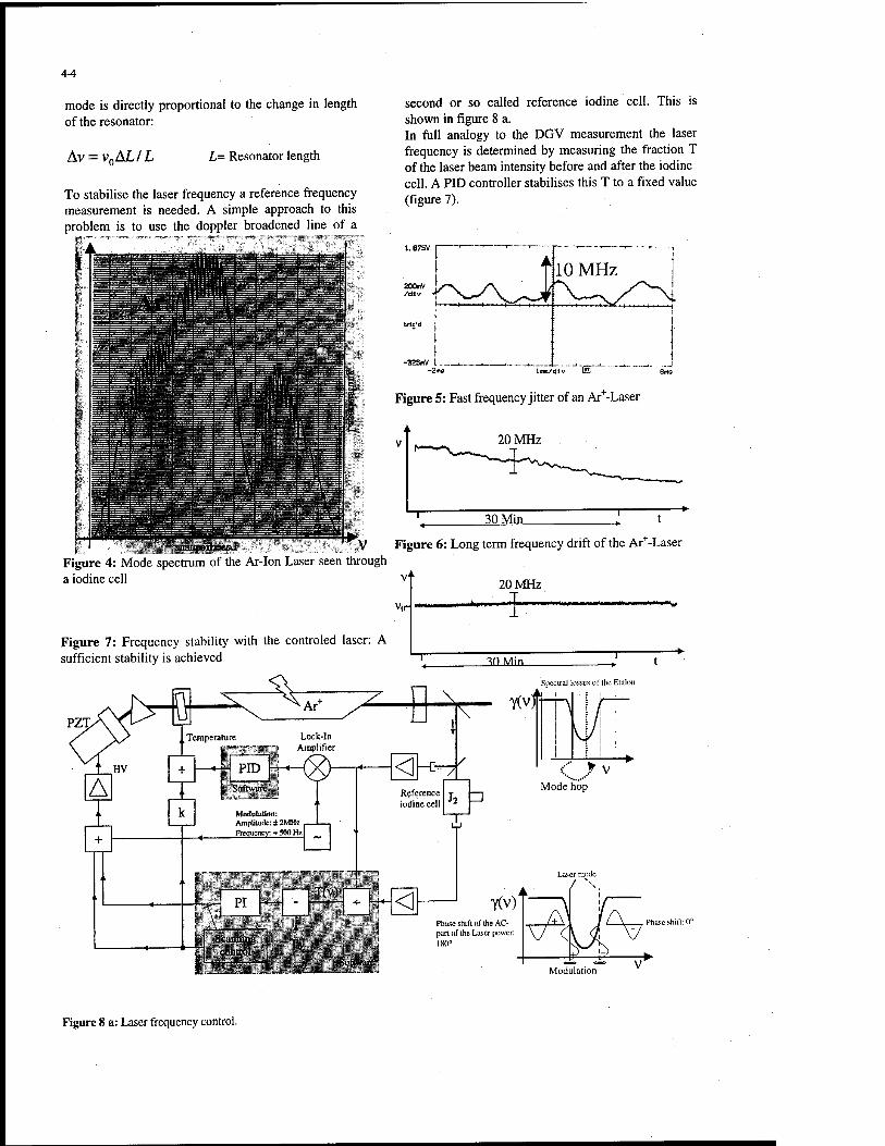
44

mode is directly proportional to the change in length of the resonator:

Av = vnAL/L L= Resonator length

To stabilise the laser frequency a reference frequency measurement is needed. A simple approach to this problem is to use the doppler broadened line of a

second or so called reference iodine cell. This is shown in figure 8 a. In full analogy to the DGV measurement the laser frequency is determined by measuring the fraction T of the laser beam intensity before and after the iodine cell. A PID controller stabilises this T to a fixed value (figure 7).

trtä'i

10 MHz

"isr

Figure 5: Fast frequency jitter of an Ar+-Laser

20 MHz

30 Min

•iWftipsihwj .1

Figure 4: Mode spectrum of the Ar-Ion Laser seen through a iodine cell v

I' Figure 6: Long term frequency drift of the Ar+-Laser

20 MHz

Vir

Figure 7: Frequency stability with the controled laser: A sufficient stability is achieved

PZT

j*f + ^0 Min

Spectral losses of the Etalon

Y(vt—

Phase shift: 0°

Modulation

Figure 8 a: Laser frequency control.

4-5

Apart of this the etalon temperature also needs to be stabilised in order to avoid mode hops. The next paragraphs will describe this as well as a sophisticated technique to calibrat the iodine cells.

Etalon anti mode-hop control A slight frequency modulation with a modulation amplitude of about 2 MHz and a frequency of about 500 Hz is used to stabilize the etalon transmission (figure 8). (It is important not to chose a modulation frequency equal to n-50Hz)- By detecting the laser output power with an lock-in amplifier, the first derivative of the modulated laser power is generated and fed in a Pi-controller to tune the etalon to maximum transmission. In this way the transmission of the intercavity etalon is stabilized on the laser frequency to avoid mode hopping and to be able to tune the laser over frequency intervals greater than the free spectral range of the laser.

Frequency stabized laser

Tunable laser

Piczo 0 Etalon V Anti mode hop control

PI Spectrum analyser

-ft

Ramp generation

Data acquisition

Frequency _d counter

ttt Signals of iodine cells

\ Iodine cells

-P- Reference

—Q Fibrexflupler

"% Single mode fibre\

Fast diode (\L

Fouricr- Analycr

o

Calibration of the iodine cells The iodine cells are filled with a small amount of iodine. At a certain temperature TSat the iodine crystal is fully evaporated. The cell is operated above this temperature level, so that the vapour density inside the cell is constant and independent of the exact temperature.

The frequency positions of the absorption lines of iodine are determined by the quantum mechanics of the molecule. They are very well known and very insensitive to any kind of outer influences. In contrast to this, the strength and the width of these lines is very sensitive to the temperature changes and to changes of the gas pressure inside the iodine cell. In addition to this the presents of other gases influences the shape of these lines as well. Because of this, the transmission profile of each cell needs to be calibrated individually.

The set-up for the calibration is shown in figure 8 b. Two argon lasers are needed; the first laser is stabilised as described above while the second laser is pre- stabilised on an interferometer. This interferometer is continuously and linear tuned in frequency. In this way the laser is tuned in frequency as well. The light of the two lasers is coupled into a single mode fibre which serves as a mixer. Because of the two different light frequencies a beat frequency arises, which equals the frequency difference between the two lasers. This difference frequency is measured with a frequency counter.

The light of the scanning laser is also used to measure the transmission of the iodine cells. While the laser is tuned, a data acquisition board in a PC acquires the cell Transmission T as well as the difference frequency v. In this way the transmission profile T(v) of several iodine cells is measured (figure 8 b).

Figure 8 b: Optical and electronical schematics of the iodine cell calibration set-up.

Light sheet generation To generate the light sheet the laser beam is guided through a fibre to a light sheet box which contains all the optics (figure 12 a and b). The height of the light sheet and the distance of the waist can both be adjusted. The maximum height is 140 mm, the waist is smaller than 1 mm with hardly any practical limits to the waist distance. Because of the separation of laser and the optic, the alignment of the laser light sheet relative to the object of investigation is quite simple.

beam adjust '

Figure 12 a: The light sheet box for a scanning light sheet. Side view.

Cylinder Plan convex lense f, = 450

$mß^> Vertikal displacement

Figure 12 b: The light sheet box for a scanning light sheet. View from top.

4-6

The light sheet optics are also optimised for long exposure times. The light sheet has a flat top-hat intensity profile, generated by a scanning technique with a modulation frequency of 10 to 20 Hz. A top- hat profile minimises the intensity dynamics in the measured picture with positive influence on the measurement accuracy. The SNR problems cased by a gaussian light sheet are shown in figure 13.

Nonnalised Position Across Ugjrt Sfaeet

Figure 13 (From[15]): The NSR (error bounds) of a DGV image when using a Gaussian light sheet. This problem is one important reason to use a scanning light sheet (= flat top intensity profile).

Three light sheet boxes are available to establish the three light sheets. An opto-mechanical switch is used to direct the light to either one of the light sheet boxes (figure 14).

Opto-Mechanical-Switch \.y jun^'*; ■ V.- ■ " Fiber •

4 Switch- L»nchCT .

;-«;»'>»r4;4- ->*44,

>.•"■:'* « .. ....'.■-' >

'•■>•:. *>.•*:.- ■■> ' >

"V °Y~^«4 .;■?'■:* .. * *i'> y.*>.v .■..„.j/w,;-'«'«!?

-1V-V .'•-./ -: - •■<■-■•

•i *'. '■ '.

oil ̂

^_ Fiber

^i- - - ■Hr*-'-

m i: *Ai.-tJ

> -*;"■: W- ■ •"!»**! MÖAMM ' >L '» ■ n'l^^^B '

■' ■>•!'.■: HHTT -.

'*'• *■'.;■■'■

lSit.:±.

?":*:■ ,v" . ■• ,'

Figure 14: Opto- mechanical switch. The laser light is coupled in one of the three fibres which supply one light sheet box each.

The DGV-camera system The performance of the camera system equals in principle the set-up in Figure 15 a. One collecting lens generates an intermediate picture, which is transferred by a transfer lens to the chips of the two cameras. A non polarising beam spliter plate is used to

reduce polarisation influences. A laser line filter reduces ambient light. A pair of 12-Bit cooled slow scan CCD cameras are used because of their good signal to noise ratio (SNR) and their linear sensitivity characteristics. Normal video CCD cameras usually do not have a SNR better than 100 (= 7 Bit) and show nonlinear behaviour for high intensities. By cooling the chip of the slow scan camera long exposure times of several seconds are possible without integrating too much dark current. Therefore they are the ideal choice for a DGV-System which is optimised for time averaged measurements performed by long exposure times. In order to get identical pictures from both cameras, the cameras are mounted on micro positioning devices to allow precise alignment. An additional software alignment enhances the quality of the measurement further more. Figure 15 b shows a photograph of the camera system.

ft iMttApmtKT ■ S?atur

I

IP r-Hh—p ,* -1.4, •0

^- -D-qJ ft Figure 15 a: The DGV-camera system.

Figure 15 b: The DGV-camera system.

The iodine cell The iodine cell is made from quartz glass (figure 16), evacuated and filled with a small iodine crystal. A high performance of this cell is strongly recommended, because other gases, for example air entering the cell by a small leak, are changing (broadening) the line profile. (In some exceptional cases people take advantage of this fact and add a small well defined amount of buffer gas to influence the cells transmission profile). The cell is placed in a temperature controlled oven. The vapour pressure of iodine depends strongly on the temperature and therewith also the density of the vapour in the cell. This is demonstrated by figure 17 a. It is very important that the transmis-

4-7

sion profile T(v) is constant in time during the measurement. One way to achieve this is to stabilise the cell temperature better than AT=0.1 K°. An alternative way to achieve a constant profile T(v) is described next:

At a certain temperature all of the iodine crystal is evaporated (in our case 60°C), so that the gas density remains constant at temperatures exceeding this level. In this way an easy density stabilisation is achieved. The way the calibration curve T(v) of the cell is obtained was descriebed above (figure 8b). No further experimental calibration is needed. The calibration profile does not change over time intervals up to years. Figure 17 b shows two calibration curves of the same cell. The second one was taken 36 month after the first one. The scanned profile is fitted with a polimom. With the fit function a software look-up table is generated which is used in the image processing of the DGV image to convert the measured transmission-image TC,R into the frequency image VC,R (figure 18). The cell temperature is fixed and can be reproduced in the experiment.

PT 100:

heater

Cold finger

Air slit T Iodine cell window

Figure 16: The iodine cell

Jodzelle bei Kf-Themp,^22,35,55.77 C Z.-Themp=110 C

22° :Cold finger temperati re

in Celsii s

0 2000 Frequenz / MHz

Figure 17 a: Measured cell profile as a function of temperature.

-600 -400 -200

Frequenz- [MHz]

Figure 17 b: Two calibration curves, taken in a temporal distance of 36 month. The reproducebility is obviously very high.

Why iodine? For most applications steep flanks of the line filter are required in order to achieve a good velocity resolution. The derivative on the flank of an atomic or molecular line is nearly proportional to the square root of the mass of the atom or molecule.

T: transmission m: mass V: Frequency

Iodine is a very heavy molecule with an atomic mass of 256 u. Therefore it has got steep flanks. Apart of this, the lines of the atom or molecule need to be strong and they have to match a line of strong laser. Iodine has a very dens line spectrum. In the green these lines are intensive. Because of this, the 514 nm line of an Ar-Ion-Laser or the 532 nm line of a frequency doubled YAG-laser can be used for DGV. Last not least, iodine cells are easy to handle. The cell temperatures needed are modest. Sodium or Caesium cells for example have to be heated up to several hundred C° to serve in the same manner for a velocity measurement.

The image processing The image processing is either performend with the software of the data acquisition system or with a programs written in language like C++ or IDL. Figure 18 shows the flow chart of data processing beginning with the row images and ending up with a three component velocity image in cartesian co-ordinates.

Steps of processing: • Background subtraction (ambient light and laser

reflexes) • Division of the content of the two pictures • Pixel specific sensitivity correction • The mapping T-W (T): Look up table • The mapping v-»v (v): Equation (2) • Combination of three one component measure-

ments to one 3D-measurement • Vector or false colour representation of

the results

4-8

This post processing takes less than 30 seconds and The final result is stored in a format readable with can be started immediately after the DGV pictures are other software for example TecPlot taken. In this way the technique is nearly on-line

3-componet measurement As pointed out above, one DGV image is a one component measurement. The measured component is in the direction of the bisector of the angle between the direction of the laser beam and the direction of observation. A 3-component measurement can be carried out by taking three pairs of DGV images with different light sheet directions (all light sheets in the same plane, see figure 3b). For each measurement i

(i=1..3) the vector (Ö — I )s is pointing in a different

direction. The three directions (Ö — I )-, induce a non cartesien co-ordinate system. The three frequency shift measurements AVj are combined in a vector Av (nue frequency). This vector is multiplied with the matrix [M] to be transformed into Cartesian coordinates.

Av=%5-/;) (o-l2) (o-F,)]v c

c

&v = — [Af]Av all(C,R) vo

The image Vc R is the result of one DGV measure-

ment. If the light sheets are divergent or if the camera is

close to the light sheet, O and /,- become functions in

space: 5C R li . That means that o and /• depend

on the index (C,R):=(Colum,Row). In this case each elements mkJ (k,l=l,2,3) of the matrix [M] is an image m; j,c,r.

If lots of DGV measurements are performed at different positions, for example if a flow volume is scanned by taking DGV images slices one next to the other, the three dimensional volumetric flow field can be measured. This procedure is shown in the flow chart in figurel9.

The different measurements are combined into one big file. In this file each point has got three co-

ordinates x,y,z and three velocity components vx, vy,

vz. Usually it becomes necessary to reduce the number of pixels at this point, in order to keep the data files handy. Furthermore it is usually necessary to dewarp the data and to take out wrong vectors. The dewarping has to be performed with respect to the geometry. For the validation the user has to set validation criteria according to error sources of the experiment.

4-9

Background Image

Jodine Cell Image

Background Image

Laser Frequency v0

Direction of Light Sheet & Camera

I Matrix

Elements

Sensitivity p. Image

Calibration Curve J, ^

■R,C

LUT

Av< Av,

Reference Image

Av,

V = — [M]Av v0

R.C

Figure 18: Processing of DGV images

4-10

Geometry x

1 Coefficients

Validation Criteria

'R,CX x: x-Position of the Light Sheet

I Dewarping

»R,CX rR,C,

Reduction of Number of

Pixels R -> R' C ->C

Image of Object

Different Positions of Light Sheet

x + Ax x + 2Ax x + nAx

VR',CX 'W.C;

Validation Data Sets from

different Spatial Regions

Spatial Combination and Superposition of Data Sets

ASCII File X,Y,Z,U,V,W

Result

► Tec Plot "* Data to bo displayed,

e.q. Test Point Number

View Graf

Figure 19: Processing of volumetric DGV data

4-11

Applications of DGV In this section the applicability of DGV will be demonstrated by several test rig and wind tunnel applications.

DGV in the Flow of a Swirler The flow field of a fuel atomisation nozzle was investigated. Such nozzles are an important component of combustion chambers of jet engines. Two circular air flows pass two swirl generators and are combined in the exit of the nozzle. In this way a recirculating flow with strong shear stresses is generated. These shear stresses atomise the fuel film tearing off the atomisation lip of the nozzle. The fuel injector is placed in the center of the nozzle but is not used in the experiment. The atomisation nozzle has a outlet diameter of 11 mm. It was operated under atmospheric pressure with a pressure drop of 30 mbar and was inserted in a tube with a diameter of 54 mm. The 3D-flow field in the pipe downstream the nozzle was investigated. Figure 20 shows the experimental arrangement. A slit in the tube at the light sheet location avoids measurement disturbances, caused by reflections. Therefore the windows, which are needed to avoid flow leakage, are recessed from the inner wall. The light sheet and camera location Was fixed. The nozzle was moved to change the axial position of the measurement. The direction of the velocity component vxr measured with the setup is also indicated in Figure 5. The other two velocity components needed to determine the 3D- vector could be measured by two further DGV- pictures taken with two other light sheets overlapping at the same location, with the light sheet direction rotated 120° and 240° around the pipe axis. However these two additional measurements are unnecessary, because of the cylindrical symmetry of the flow. The resulting measurement pictures equal the first velocity picture apart from a respective rotation around the pipe axis. This means that in a flow with cylindrical symmetry only one DGV-picture is sufficient to describe the 3D-flow. The other two components can be generated in the computer. Of course this simplified method may only be applied to measure mean values. The instantaneous flow distribution never shows any symmetry because of turbulent fluctuations. The presented experiment has got a cylindrical symmetry and only the time averaged flow field is of interest. Therefore the DGV-system optimised for the measurement of mean flow velocities was used to analyse the flow field. The light sheet illuminated the whole cross section. The Laser power was 300 mW. The air was seeded with glycerine particles with an average diameter of 0.2 |0.m. The particle density was so low that, with the flow switched on, the scattered light could hardly be seen by the eye. To achieve sufficient image quality, an exposure time from 1 to 5 seconds was needed. This time is sufficient to integrate the turbulent velocity fluctuations.

DGV-camera

light sheet

swirlers

, v axial positioning nozzle r a

Figure 20: Set-up for DGV measurements in the flow field of a swirl nozzle

Results of the swirler measurements The result of a DGV-measurement at a certain axial position x is shown in Figure 21. The upper part shows the image of the camera behind the iodine cell and the lower part the picture of the reference camera. First the background light is subtracted, then the pictures are divided and the divided picture is corrected in accordance with the pixel specific sensitivity differences. Then, by the use of the calibration function T(v) and with regards to the geometry of the optical arrangement, the distribution of the velocity component vxr is obtained (Figure 22). In the next step the user marks the symmetry centre of the picture and the computer calculates the two other velocity pictures by turning the resultant picture 120° and 240° around the symmetry centre. These three pictures are combined to a 3D-vector field which is shown in Figure 23. The components in the light sheet are represented by a vector plot and the axial component is represented by a so called „luminescence plot". This result is obtained after about 30 seconds, the measurement takes 5 seconds, the post processing requires 25 seconds. The full volumetric flow field can be acquired within a few minutes by stepwise changing the axial position of the light sheet. As an example, Figure 24a shows the vector field in the plane along the tube axis. Fig- ure 24 b shows the distribution of the circumferential velocity. The pictures indicate quite clearly how fast the swirl flow in the tube is smoothed. Secondary flow structures can be observed, especially the recirculation torus in the corners at the bottom of the tube and the axial recirculation. Both effects are very important for

4-12

the combustion because they are needed to stabilise the flame.

These results show, that this method is an excellent tool for fast analysis of complex flow fields. The resolution is between 1 and 2 m/s, since the smallest vectors which still make sense have a length of 1.5 m/s.

Reliable statements concerning the accuracy of DGV are not yet possible. Among many other potential

error sources [4], we assume that reflections of the laser, reflections of the scattered light and multi- scattering may affect the accuracy as well as high turbulence in combination with non linearity of the iodine line and inhomogeneous seeding causing non linear averaging. If such error sources can be avoided, the absolute accuracy can be estimated to be at least smaller than 3m/s..

Figure 22: Result of a DGV-measurement. The distribution of one velocity component.

Figure 21: Signal and reference DGV picture

:—.w\\\ ,.

''' \ \ \>■> ;\ \ v L L ,

U\^ / //'/''

Axial component

Flow vectors in the light sheet plane

Figure 23: 3D-velocity distribution of the flow 2 mm above the swirl nozzle.

4-13

3D-DGV

Radial-Axial

Velocity Figure 24 (a,b): Flow field

of the fuel spray nozzle.

Circumferential Velocity

Radial Position

DGV measurements in the wake region of a car model Car designers have to pay special attention to aerodynamic properties such as drag, lift and side forces, aerodynamic noise and dirt deposition. The design procedure is an iterative experimental process. The shape of a clay car model (typical scale 1:5 or 1:4) is stepwise optimised by a series of short wind tunnel tests. The purpose of each test is to examine the aerodynamic effect of the last variations of the model. To evaluate the actual performance of the model, force balance measurements, stream line seeding and wool tuft visualisation are used in the first place. The power of these classic techniques is not always sufficient. The force balance gives only a few integrated values that cannot be directly related to a certain flow phenomena. Stream line seeding and wool tufts only work up to Reynolds numbers which represent a velocity of 6 km/h of the full size car.

To measure flow structures at realistic Reynolds numbers, LDA measurements can generally be carried out, but it takes at least 10 seconds to 2 minutes to measure only one LDA point. The reason for this is, that it is necessary to integrate the low frequency turbulent

fluctuations. Therefore LDA can not be constantly used to support the aerodynamic optimisation process of the car model, but will only be applied to some exemplary test cases. This demonstrates that there is still the need for another technique. This technique might be DGV, because it enables quick 3D-measurement within less than 30 seconds in quite a large plane in the flow with no restrictions to the Reynolds number.

The DGV system was used to investigate the wake region of an experimental 1:5 car model in a 1.8m x 1.3m low speed wind tunnel at Mercedes Benz in Sindelfin- gen/Stuttgart. The light sheet boxes were installed left, right and above the open test section (Figure 25 b), illuminating a plane perpendicular to the main flow direction 150 mm behind the model. The model had a length of 800 mm. This plane was observed from down-stream the flow. It had a size of 140 x 140 mm2. The free stream velocity was 50 m/s. A fog generator placed in the settling chamber was used for seeding the flow.

A sequential 3D-DGV measurement was carried out. The exposure time for each picture pair was ten seconds, so that the final results were obtained after one minute, 30 seconds taken by the image acquisition and another 30 seconds for the post processing. The power in the light sheet was 150 mW.

4-14

3D-DGV

main stream velocity

Vz

80.00 m/s

70.00

60.00

50.00

40.00

30.00

20.00

10.00

0.00

-10.00

-20.00

> 45 m/s

-200 -150 -100 -50 o mm

Figure25 a: 3D-DGV measurement in the wake region of a car model. (Acquisition time :30 seconds)

Figure 26 : 3D-LDA measurements at the location of the DGV measurements in Figure 25.

■Ulf— Measurement

DGV-Camera

Light Sheet Box

Figure 25 b: Set-up of the light sheet boxes aned the camera system

Results of the car measurements Figure 25 shows the DGV results. A recirculation zone with a vortex was observed, which is a typical structure in the wake region of a car. The main stream velocity component increased twards the top, bottom and left side of the measurement region because of the influence of the free stream. These results are in good agreement with 3D-LDA data of the same flow at the same location (Figure 26 ) [7]. • The vortices are detected at approximately the

same location. • The shape of the isolines are similar.

• The amplitudes of the recirculation are around minus 20m/s concerning both, the DGV and the LDA measurements.

Obviously the data density of the DGV measurement is much higher since it is an imaging technique. Therefor smaller structures like the recirculation vortex are observed more clearly. The LDA picture took approximately 2 hours acquisition time, which is very long compared to the DGV-acquisition time of only 30 seconds. A detailed comparison between the LDA and DGV results was not possible, because the model was not placed at exactly the same position in the test section and the boundary layer suction was not switched on

4-15

during the DGV measurement. Especially the wake region of the car is very sensitive to such small changes of the aerodynamic boundary conditions, so this may be an explanation for the differences of the LDA and DGV data.

An important observation was, that a lot of care had to be taken concerning the homogeneity of the seeding, in order to avoid biasing caused by correlated fluctuations of seeding density and velocity. This effect is generally well known in wind tunnel research. Homogeneous seeding also helps to keep the images in the dynamic range of the camera.

DGV Measurements in the Model of an DASA- Engine Inlet Stationary and wind tunnel experiments The flow inside a model of an engine inlet was investigated with DGV. The experiments carried out were aimed to evaluate in how far DGV measurements could be a helpful tool for the development of an engine inlet. The engine inlet of a fighter aircraft is usually curved and long compared to it's diameter. Therefor the flow inside shows typical pipe flow phenomena which have to be examined and quantified in order to ensure a sufficient air supply of the turbo engine. Velocity inhomogenities such as the vorticity and the loss of total pressure have to be measured as a function of the mass flux and angle of attack of the air plane.

The set-up is shown in Figure 27 and 28.

In a first approach the inlet was tested with a stationary set-up. A Seeding box with a blower and the fog generator inside was used generate a homogenous seeding. The seeded air was sagged in the inlet. The inlet was mounted on a so called optical module, which was used to investigate the flow at the exit of the inlet e.g. at the interface plane to the turbo engine. A glass ring serves as a window for the three light sheets. A stem with a mirror and a flexible endoscope is placed further down stream watching the light sheet. The endoscope transfers the image to the camera system. The mass flow rate and the stationary pressures at the wall near the light sheet were measured with pressure probes.

The three light sheet boxes generated three light sheets forming an angle of 120°. For each measurement three pictures were taken, each with an exposure time of 5 seconds.

The inlet was blocked on one side to simulate an aerodynamic disturbance causing strong secondary structures. Figure 29 shows the result of a measurement. A strong vortex was measured. The distribution of the axial velocity was measured as well and is represented by grey values.

The axial velocities were used to determine the mass flow rate, the mach number, the total pressure distribution. Important design parameters were derived from this data, such as the total pressure loss, the total pressure distortion and the vortisity angle.

Figure 30 shows the reduced mass flow rate measured with DGV versus the mass flow rate measured with an aperture. The correlation is quite good except for the large flow rates. An interesting result was, that deviations showed up right at the point when a the flow velocities in the smallest cross section became sonic. Unfortunately the effect is not fully understood jet.

The results were compared to Laser-2-Focus measurements and to measurements with pressure probes. The results were promising. Therefor the technique was applied on a model in a wind tunnel next.

Second approach

The same investigations were carried out with the inlet placed in a 1:10 model of a military plane which itself was placed in a 3m x3m wind tunnel (figure 28, 29).

Figure 30 shows one result of such a DGV measurement. Serveral parameters were varied such as the angle of attack of the plane, the mass flow rate or the geometry of the inlet.

It should be stressed that these are the first imaging velocimetry experiments using a flexible endoscope. This is an important characteristic of DGV since in this way, DGV can also be applied to flows with pour optical excess.

4-16

-Optical Module

Camera Stem Endoscope

Figure 27: DASA-engineinlet (one side was blocked), optical module, camera stem and endoscope

-HP-

Figure 28: Optical DGV-module. The pipe flow inside Figure29: Flow field in the optical modle. Ground test an aircraft inlet was investigated. The optical module was placed in the model of a military fighter aircraft which itself was placed in a large wind tunnel.

WPPS

■Hll Wm IBS! &$&tMi

i^BBB^KfflB

i^^^

gBffl BBH

0 20 to Q. <D O

1 15

S 10 to CO 0

E 5 5

_o w w to

0

Mass flow +10% //'■ measured

with an / / ' aperture ' / /

■

/ / / /

ODGV '. DL2F ADGV

JF& ,....,....' 0 5 10 15 20

Mass flow measured with DGV and L2F

Figure 31: Flow inside the intake of the model of a Figure 30: Reduced mass flow rate measured with DGV military aircraft placed in a 3m X 3m Windtunnel at the versus the reduced mass flow rate measured with an DLR / DNW Braunschweig aperture. DGV measurement: O ,□

L2F measuremet: A

4-17

DGV Measurements in a Combustion Chamber

This application was performed in a double-staged combustion chamber consisting of two main and three pilot burners (figure 31) with optical access from at least three sides at a time. The chamber itself represents a segment of an annular combustion chamber for use in the engine of a transport aircraft. One of the principle aims here was to obtain a data base to validate CFD codes. Since the flow structure inside a combustion chamber is very complex it is desirable to acquire the entire three-dimensional volume data set - a task very tedious to accomplish with single point measurement techniques (e.g. LDA).

For the measurement the light sheets were introduced from either side as well as from the top or bottom of the chamber. A mirror was placed downstream of the combustion chamber exit such that the camera was not directly exposed to the flow. The entire DGV equipment, camera and light sheet devices, were mounted on a common translation stage, such that the interior flow field could be mapped in a tomographic manner at increments of Ax = 2 mm. Up to 50 adjacent planes were recorded in this manner resulting in volumetric data sets containing up to 120 x 60 x 50 distinct data points at a spacing of 1 x 1 x 2 mm'.

The DGV measurements were restricted to the 'cold' (unfired) flow under atmospheric conditions. Measurements in the hot, burning flame were not possible due to the self-luminosity of the seeding particles as well as glowing soot which requires the use of intensifier-gated CCD cameras and pulsed, frequency-stabilised lasers, both of which were not available at the time.

Figures 32, 33, 34, 35 and 36 give an impression of the quality of the recovered data by showing various cross-sections through the flow. The interaction between the swirling burner flows and the and mixing jets of the secondary air can be easily recognised. Swirls within the mixing jets are also visible and are surprisingly similar to the CFD results (data not presented in this context). A comparison between DGV data and LDA data obtained for the swirler nozzle flow is presented in [18].

With the DGV technique the flow structure in nearly the entire chamber was measured by stepwise scanning the light sheet across the volume. In this way the mess of the measured data points is so dense, that 3D- iso-surfaces can be drawn. That are surfaces on which one velocity component has a certain value (figure 36).

4-18

I I I I I I I I I I I I I I I I I I I I I'M I I I I I I I I I I I I I I I I I I I I I I I I 6 10 20 30 40 60 60 70 60

xlnfmm]

Figure 31: Double-staged combustion chamber with Figure 32: XY-plane extracted from the pilot zone glass windows used in DGV investigation velocity data set, intersection with one of the pilot

burners.

Figure 33: Selected YZ cross-sections through the volumetric three-component velocity data obtained for the main zone (upper zone) of the combustion chamber. The contours indicate the out-of-plane velocity component, vx.

4-19

Figure 34: Selected XY cross-sections through the volumetric three-component velocity data obtained for the main zone (upper zone) of the combustion chamber. The contours indicate the out-of-plane velocity component, vy.

Figure 35: Detail from the XZ-plane intersection with Figure 36: Iso-surface plot of the the velocity surface the centerline of the main burners. The contours indi- with vy=30 m/s (blue) and another surface with vz= cate the out of plane velocity component. 25 m/s (red).

4-20

Accuracy of DGV An accuracy Studie of DGV was performed [19].

The axial velocity of a free jet was measured near the exit of a free jet nozzle. The flow of the nozzle was seeded with glycerol/ethanol particles generated by a laskin nozzle. The laser beam crossed the jet at an angle of vP=(-l,v)=45° and the scattered light was observed at 90° so that the measured component v0.] was pointing in the direction of the nozzle's axis (figure 39).

The probe volume was placed in a distance of about one time the nozzle diameter d in the center of the potential core. The flow speed was varied from 40 m/s up to 130 m/s.

The uncertainty of the DGV setup was determined by comparing the DGV-data with the velocity calculated from pressure and temperature measurements. The measurement error of the DGV-method was found to be about ±0.7 m/s.

Under ideal conditions, the accuracy of the system is limited by changes of the polarization of the scattered light in combination with the small, remaining polarization sensitivity of the beam splitter plate.

If polarization effects are avoided, for example by using polarization filters, the noise level of the DGV- measurement was found to be only ± 0.4 m/s.

In practical applications the accuracy tends to be less good. Due to lots of experimental experiences became clear, that multi scattering, reflexes of the laser light on surfaces and windows and scattered light that is reflected from surfaces influences the measurement accuracy far more, than imperfections of the system itself. According to this, the achieved accuracy depends on the concrete object of investigation. There fore it is rather difficult to make general statements. If

all kind of reflexes can be reduced to a minimum and if the seeding density is not very high, a resolution of ± 1 m/s should be feasible (and was feasible in the past).

Temperature mp.acnrempnt

Pressure measurement: Ap

Measured velocity component

Figure 39: DGV-Setup and reference measurement.

> a D

0 20 40 60 80 100 120 140

Aus Druckmessung berechnete Geschwindigkeit [m/s]

Figure 40: Correlation of the DGV and the reference measurements.

4-21

Comparison between DGV and PIV

DGV PIV

Time averaged Velocity Maps

(cw -Laser)

Single Shot Velocity Maps

(pulsed Laser)

Online Information Flow Structure Information

Absolute Error Relative Error

Typical one Component

(up to three possible)

Two Components

Superposition of the scattered Light of an Ensemble

of Particles

Detection of single Particles

Pseudo continuous in Space Measures in discrete Points

Any Flow Direction Planar Flows in the Light Sheet Plane

Conclusion: DGV and PIV are more supplementary rather than alternative measurement methods.

Acknowledgements The author acknowledges the help of Mrs. Elsa Ri- jmenants in preparing the illustrations. The presented DGV measurements were carried out with the unre- nounceable help of Mr. Dipl.-Ing. Manfred Bevers- dorff and Mr. Dipl.-Ing. Winfriedb Unger who carried out the constructions and were responsible for the seeding.

The investigations of the BMW&RR combustion chamber were supported by the German Ministry of Science and Technology. The representation of these DGV measurements were carried out by Dr. Dipl.- Ing. Chris Willert and Mr. Dipl.-Ing. Martin Carl.

References [1] H. Komine: „System for measuring velocity field

of fluid flow'utilising a laser-doppler spectral image converter ",US Patent 4 919 536, 1990.

[2] J.F. Meyers, H. Komine: „Doppler Global Velo- cimetry - A New Way to Look at Velocity", ASME Fourth International Conference on Laser Anemometry, Cleveland Ohio, August. 1991.

[3] R.B. Miles: „Instantaneous Velocity Field and Background Suppression by Filtered Raleigh Scattering", AIAA paper, No. AIAA-91-0357, 1991.

[4] J.F. Meyers: „Evolution of Doppler Global Velo- cimetry Date Processing", Proceeding, Eighth In- ternational Symposium on Applications of Laser Techniques to Fluid Mechanics", Lisbon, 8-11 Julie, 1996

[5] I. Röhle, R. Schodl: „Laser-Doppler-Velocimetry auf der Basis frequenzselektiver Absorption", Diplomarbeit, DLR interner Bericht Nr. IB-325-8-93, 1993.

[6] I. Röhle, R.Schodl: „Evaluation of the Accuracy of the Doppler Global Technique", Proceeding. Optical Methods and Data Processing in Heat and Fluid Flow, London 14/15 April, pp. 155-161, 1994.

[7] J. Schmitt: LDA measurements in the wake region of a car model, Private communication, Mercedes Benz Sindelfingen, 1994.

[8] I.Röhle: „Three Dimensional Doppler Global Velocimetry in the Flow of a Fuel Spray Nozzle and in the Wake Region of a Car", Flow Measu- rement and Instrumentation, Elsevier Science Ltd, 1997,Oxford.

[9] SPEEWECK, F. Entwicklung eines Laser-Frequenznormals hoher Präzision im sichtbaren Spektralbereich bei 582 THz. PTB-Mitteilungen 91, May 1981, p. 336-343.

[10] CAMY, G. Frequency stabilization of an Argon Laser at 582.49 THz using saturated absorption in l27I2, Metrologia 13, 1977, p. 145-148.

[11] CHEBOTAYEV, V.P. Argon ion laser with high frequency stability, Metrologia 27,1990, p. 61-64.

[12] SOREM. M.S. saturation spectroscopy in molecular iodine by intermodulated fluorescence. Optical Communications, June 1972, Vol. 5, No. 3, p. 148-151.

4-22

[13] GILL, P. Iodine saturation spectroscopy for multi- wavelength stabilization of an argon/krypton ion laser. Metrologia 15, 1979, p. 117-123.

[14] Documents concerning the new definition of the meter. Metrologia 19,1984, p. 163-177.

[15] R. Ainthworth, S.T. Thorpe: "The development of Doppler Global Velocimety for Transsonic Turbine Applications", ASME conference proceeding, 94-GT-146, The Hague, June 1994.

[16] B.Lehmann: LDA measuremens in the flow of a BMW&RR swirl nozzle built in model of the combustion chamber, DLR, Berlin 1997, Privat Comunication.

[17] A. Mack, H. Wassenberg: CFD-calculatins of the flow in the BMW&RR combustion chamber, post processing and representation of the DGV measurements and comparison between CFD, DGV, LDA and PDA, BMW&RR, Dahlewitz 1997, Privat Comunication.

[18] Lehmann, B.; Röhle, I.: A Comparison of velocity- field data behind a double-swirl nozzle measured by means of Doppler-Global and conventional three-component LDA techniqus; Nineth international symposium on applications of laser techniques to fluid mechanics; Proceeding, Paper 33.2, Lisbon; 1998.

[19] Röhle, I.: Laser Doppler Velocimetry auf der Basis frequenzselektiver Absorption: Aufbau und Einsatzt eines Doppler Global Velocimeters, Dissertation at Uni-Bochum and DLR-report, to be printed, 1999.

5-1

Surface Measurement Techniques Temperature and Pressure Sensitive Paints

John P. Sullivan and Tianshu Liu School of Aeronautics and Astronautics

Purdue University West Lafayette, Indiana 47907-1282, USA

Summary Luminescent molecular probes imbedded in a polymer binder form a temperature or pressure paint. On excitation by light of the proper wavelength, the luminescence, which is quenched either thermally or by oxygen, is detected by a camera or photodetector. From the detected luminescent intensity, temperature and pressure can be determined. The basic photophysics, calibration, accuracy and time response of a luminescent paints is described followed by applications in wind tunnels and in rotating machinery.

Introduction The use of luminescent molecular probes for measuring surface temperature and pressure on wind tunnel models and flight vehicles offers the promise of enhanced spatial resolution and lower costs compared to traditional techniques. These new sensors are called temperature- sensitive paint (TSP) and pressure-sensitive paint (PSP). Traditionally, arrays of thermocouples and pressure taps have been used to obtain surface temperature and pressure distributions. These techniques can be very labor-intensive and model/flight vehicle preparation costs are high when detailed maps of temperature and pressure are desired. Further, the spatial resolution is limited by the number of instrumentation locations chosen. By comparison, the TSP and PSP techniques provide a way to obtain simple, inexpensive, full-field measurements of temperature and pressure with much higher spatial resolution. Both TSP and PSP incorporate luminescent molecules in a paint which can be applied to any aerodynamic model surface. Figure 1 shows a schematic of a paint layer incorporating a luminescent molecule. The paint layer is composed of luminescent molecules and a polymer binder material. The resulting 'paint' can be applied to a surface using a brush or sprayer. As the paint dries, the solvent evaporates and leaves behind a polymer matrix with luminescent molecules embedded in it. Light of the proper wavelength to excite the luminescent molecules in the paint is directed at the model and luminescent light of a longer wavelength is emitted by the molecules. Figure 2 shows the spectra for a typical luminescent ruthenium molecule. Using the proper filters, the excitation light and luminescent emission light can be separated and the intensity of the luminescent light can be

determined using a photodetector. Through the photophysical processes known as thermal- and oxygen- quenching, the luminescent intensity of the paint emission is related to temperature or pressure. Hence, from the detected luminescent intensity, temperature and pressure can be determined. The polymer binder is an important ingredient of a luminescent paint used to adhere the paint to the surface of interest. In some cases, the polymer matrix is a passive anchor. In other cases, however, the polymer may affect significantly the photophysical behavior of the paint through a complicated interaction between the luminescent molecules and the macro-molecules of the polymer. A good polymer binder should be robust enough to sustain skin friction and other forces on the surface of an aerodynamic model. Also, it must be easy to apply to the surface in a smooth, thin film and easy to repair. For TSPs, many commercially available resins and epoxies can be chosen as polymer binders if they are not oxygen permeable and do not degrade the activity of the luminophore molecules. In contrast, a good polymer binder for a PSP must have high oxygen permeability besides being robust and easy to apply. Two recent papers (Liu et al. 1997 and Gouterman 1997 ) provide excellent reviews of the foundations and history of TSP and PSP and contain extensive reference lists.

Measurement Systems The measurement systems are the same for both TSPs and PSPs. The essential elements of the systems include illumination sources, optical filters, photodetectors and data acquisition/processing units. This section provides a brief description of two measurement systems: the CCD camera system and the laser scanning system. Intensity based measurements are considered first and then lifetime and multi-luminophore systems.

CCD Camera System The CCD camera system for luminescent paints is the most commonly used in aerodynamic testing. A schematic of this system is shown in Figure 3. The luminescent paint (TSP or PSP) is coated on the surface of the model. The paint is excited to luminesce by the illumination source, such as a lamp or a laser. The luminescent intensity image is filtered optically to eliminate the illuminating light and



5-2

then captured by a CCD camera and transferred to a computer with a frame grabber board for image processing. Both wind-on image (at temperature and pressure to be determined) and wind-off image (at a known constant temperature and pressure) are obtained. The ratio between the wind-on and wind-off images is taken after the dark current level image is subtracted from both images, yielding a relative luminescent intensity image. Using the calibration relations, the surface temperature and pressure distributions can be computed from the relative luminescent intensity image. Selection of the appropriate illumination sources depends on the absorption spectrum of the paint and the optical access of the facility. The source must provide a large number of photons in the wavelength band of absorption. A variety of illumination sources are available. Lasers with fiber-optic delivery systems have been used in wind tunnel tests (Morris et al. 1993b, Crites 1993, Bukov et al.. 1992, Engler et al. 1995). Other light sources reported in literature include a xenon arc light with a blue filter (McLachlan et al. 1993a), incandescent tungsten/halogen lamps (Dowgwillo et al. 1994) and fluorescent UV lamps (Liu et al. 1995a, 1995b). Morris et al. (1993a) and Crites (1993) discussed the characteristics of some illumination sources. For imaging the surface, scientific grade cooled CCD digital cameras can provide high intensity resolution (12 and 16 bits) and high spatial resolution (up to 2048 x 2048 pixels). Since the scientific grade CCD camera exhibits good linearity and high signal-to-noise ratio (SNR), it is particularly suitable to quantitative luminescent intensity measurements. A necessary step in data processing is taking the ratio between the wind-on luminescence image and the wind-off reference image at a known reference temperature and pressure. The image ratio process can eliminate the effects of spatial non-uniformity in illumination light, coating thickness, and luminophore concentration. However, since aerodynamic forces may cause model motion and deformation in high-speed wind tunnel tests, the wind-on image may not align with the wind-off image. The ratio between the non-aligned images leads to considerable errors in calculating temperature and pressure using the calibration relations. Also, some distinct flow characteristics, such as shocks, transition and separation locations, could be smeared. In order to correct this non- alignment, an image registration method was suggested by Bell and McLachlan (1996) and Donovan et al. (1993).

Laser Scanning System A laser scanning system for TSPs and PSPs is shown in Figure 4. A low power laser is focused to a small point and scanned over the surface of the model using computer controlled mirrors The laser illumination excites the paint on the model and luminescence is detected by a low noise photodetector (e.g. a PMT). The photodetector signal is digitized with a high resolution A/D converter and

processed to obtain temperature and pressure. The mirror is synchronized to the data acquisition so that the position of the laser spot on the model is accurately known. Compared with the CCD camera system, it takes longer to obtain full-surface temperature and pressure distributions using the laser scanning system. However, this system has some advantages. (Hamner et al. 1994) (i) Luminescence is detected by a low noise photodetector.

Before the analog output from the PMT is digitized, filtering and other SNR enhancement techniques are available to improve the measurement resolution. The signal is then digitized with a high resolution (12 to 24 bit) A/D converter. Additional noise reduction can be accomplished by using a lock-in amplifier if the laser intensity is modulated,

(ii) The laser scanning system can be used for measurement in a facility where optical access is very limited and the CCD camera system is difficult to use.

(iii) The system provides uniform illumination over the surface by scanning a single light spot,

(iv) The system can be easily adapted for measurement of luminescent lifetime or phase shift if a pulsed laser or modulated laser is used.

Lifetime-based detection systems A promising method for making temperature and pressure measurements is to determine the luminescent lifetime of the paint rather than the luminescent intensity. Compared with the intensity-based method, the greatest advantage of this method is that the lifetime-temperature or -pressure relation is not dependent on illumination intensity. Therefore, the calibration relation is intrinsic for a particular paint and the image ratio process is not required. Also, the lifetime measurement is insensitive to luminophore concentration, paint thickness, photodegradation, tubid paint surface and dirty optical surfaces. The temperature and pressure can be directly obtained from the measured lifetime. The lifetime measurement technique in photochemistry is well- developed (Szmacinski and Lakowicz 1995, Papkovsky 1995). The basic configuration of this system is similar to either the CCD camera or the laser scanning system, except a pulsed excitation light is used. After each pulse, the luminescence decay is detected and acquired by a computer. Then, temperature or pressure is obtained by using the calibration relation. Using a lifetime detection system, Davies et al. (1995) measured the pressure distributions on a cylinder in subsonic flow and on a wedge at Mach 2. Comparison with data obtained by conventional pressure taps was favorable. A frequency-domain method detects the phase angle between the luminescence emission and harmonically modulated excitation light. If the modulation frequency is fixed, the phase angle is a function of the lifetime and hence is dependent on temperature and pressure. The phase angle can be measured using a lock-in amplifier. Campbell et al. (1994) gave a calibration between phase

5-3

angle and temperature for Ru(bpy)-Shellac paint at 100 kHz modulation frequency. A simple phase detection system using blue LED excitation was used to measure surface temperature on an electrically heated steel foil on which a round air jet impinged (Campbell et al. 1994). Torgerson et al. (1996) measured the pressure distribution in a low-speed impinging jet using a laser scanning system with an optical modulator.

Multi-Luminophore System Use of the normal CCD camera or laser scanning system requires a ratio between the wind-on and wind-off luminescent images. This image ratio method inevitably causes inaccuracy in determining temperature and pressure because the image registration is never perfect. A two- color luminophore paint would eliminate the need for a wind-off reference image. Two-color luminescent TSP is made by combining a temperature-sensitive luminophore with a temperature-insensitive reference luminophore. Similarly, two-color luminescent PSP consists of a pressure- sensitive luminophore with a pressure-insensitive reference luminophore. The probe luminophore and reference luminophore can be excited by the same illumination. However, there is ideally no overlap between the emission spectra of the probe luminophore and reference luminophore such that two color luminescent images can be completely separated by optical filters. The ratio between these two color images can eliminate effects of spatial non- uniformity in illumination, paint thickness and luminophore concentration. Besides the aforementioned combinations, a temperature sensitive luminophore which is not quenched by oxygen can be combined with an oxygen sensitive luminophore. This dual luminophore temperature/pressure paint can be used for temperature correction in PSP measurement. Furthermore, a multi- color PSP can be developed to correct simultaneously the effects of both temperature variation and non-uniformities in lighting, paint thickness and concentration. Some preliminary experiments indeed indicate that a two- color PSP can correct variations in illumination (Oglesby et al. 1995, Harris and Gouterman 1995). Three pressure sensitive paints with internal temperature sensitive luminophore have also been tested by Oglesby et al. (1996). Their results show that the dual luminophore paint enables point-by-point correction of temperature effects of PSP measurement. Only recently, a two-color PSP was used to measure pressure distribution in a low speed impinging jet (Torgerson et al. 1996).

Temperature Sensitive Paints This section will describe the photophysics, calibration, accuracy, time response of temperature sensitive paint.

Photophysics

For a TSP, it is assumed that the paint layer is not oxygen- permeable so that [02] = 0. Hence, the quantum yield is simply given by

I kt o = —= I, kL + kD

= k Ll0 (1)

The deactivation term kD may be decomposed into a temperature-independent part ko and a temperature- dependent part ki that is related to thermally activated intersystem crossing (i.e. kD = ko + ki). The rate ki can be assumed to have an Arrhenius form (Bennett and McCartin 1966, Schanze et al. (1997) k, = C exp(-E/RT) (2)

ln- 1

Tref J (3)

where C is a constant, E is the Arrhenius activation energy, R is the universal gas constant and T is the thermodynamic temperature (in Kelvin). The relation (1) can be approximately written in the simple Arrhenius form

KT) ~f • • ^ i(Tref) :

Theoretically speaking, the Arrhenius plot of ln[I(T)/I(Tref)] versus 1/T gives a straight line of slope E/R. Tests indicate that the simple Arrhenius relation does fit experimental data over a certain temperature range. However, for some paints, the data may not fully obey the simple Arrhenius relation over a wider range of temperature. As an alternative, the relation between the luminescence intensity and temperature can be expressed in a functional form

KT) = F(T/Tref) (4)

I(Tref) The empirical expression F(T/Tref) could be a polynomial, exponential or other functions to fit the experimental data over a certain temperature range. Both (3) and (4) are operational forms of the calibration relation for a TSP used for data reduction in practical applications. TSP Calibration In order to quantitatively measure temperature with the TSP coatings, a calibration relating luminescent intensity or lifetime to temperature is needed. A calibration rig consists of a temperature controlled sample and appropriate illumination source and luminescent detector. Typical temperature dependencies of luminescent intensity are shown in Figure 5 for some TSPs. Several TSPs have high temperature sensitivity in cryogenic temperature range. Others can be used in a temperature range from -20 to 105 °C. Figure 6 gives a lifetime calibration of two TSPs. Accuracy The accuracy of the temperature measurement has been shown to depend primarily on calibration accuracy, but is in the range of 1 degree. ( see Liu et al. 1995b for a detailed analysis) Time Response There are two characteristic time scales that are related to the time response of the paint. One is the luminescent lifetime which represents an intrinsic physical limit for the achievable temporal resolution of the paint. Luminescent

5-4

paint usually has a lifetime ranging from 10"10 seconds to milliseconds. Another is the time scale of the thermal diffusion in the TSP layer. In a forced convection- dominated case, the thermal diffusion time can be expressed by t = pet I h, where, p is the density, c is the

specific heat, t is the paint thickness and h is the convection heat transfer coefficient. In general, the diffusion time is much larger than the lifetimes of most luminescent paints. Therefore, the time response of the luminescent paint is mainly limited by the diffusion processes for both TSP and PSP measurements. Figure 7 shows a the temperature response of the TSP paint subjected to the pulsed laser heating.( Liu et al.,1995c). The surface temperature increases rapidly after the pulsed laser beam is turned on and then gradually decays due to natural convection. By fitting the experimental data with the asymptotic solutions, it is found that xi = 0.25 ms(heating) and x2 = 25 ms (cooling).

TSP Applications

Transition Detection TSP has also been utilized as an approach to flow transition detection (Campbell 1994, McLachlan et al. 1993b), Since convective heat transfer is much higher in turbulent flow than in laminar flow, TSP can visualize the surface temperature difference between turbulent and laminar regions. In low speed wind tunnel tests, the model is typically heated or cooled to enhance temperature variation across the transition line. Using EuTTA-dope paint, Campbell et al. (1992, 1993) visualized transition patterns on a symmetric NACA 654-021 airfoil in a low-speed wind tunnel. (Figure 8). Recently, a cryogenic TSP systems have been developed at Purdue, the University of Florida NASA Langley and National Aerospace Laboratory (NAL), Japan. Several TSP formulations have been successfully used to detect transition on airfoils in a 0.1m transonic cryogenic wind tunnel at the NAL in Japan (Figure 9 from Asai et al. 1997a) and a 0.3m cryogenic wind tunnel at NASA- Langley (Figure 10 from Popernack et al.). Quantitative Heat Transfer Global surface heat transfer mapping on a waverider model in Mach 10 flow has been obtained using EuTTA-dope paint (Liu et al. 1995b). A thin Mylar insulating layer covered the windward side of the model, and EuTTA-dope paint was applied on the insulating layer. The temporal evolution of surface temperature distributions was obtained and then heat flux was calculated using a simple heat transfer model. Figure 11 shows a representative map of heat flux on the windward side of the waverider. The bright and dark regions correspond to high and low heat transfer, respectively. The low heat transfer region near the leading edge corresponds to laminar flow. Transition from laminar to turbulent flow can be easily identified by an abrupt change from low to high heat transfer. Figure 12 shows a typical heat transfer

history. The TSP measurement is in good agreement with data obtained by thermocouples.

Pressure Sensitive Paints This section will describe the photophysics, calibration, accuracy, time response of pressure sensitive paint. Photophysics PSP operation is based on the principle that certain fluorescent molecules are quenched by the presence of oxygen. In the molecules of interest, oxygen interacts with the excited molecules and the excess energy is transferred to the oxygen in a collisional process, with no photons being emitted. This process, known as oxygen quenching, is the basis for the pressure sensitive paint method.

Calibration curves for common paint formulations (platinum porphrin, ruthenium complex and perlene/pyrene) are shown in Fig. 13.

The luminescent intensity (7) is proportional to the absorption intensity (70) and the quantum efficiency (rf)

I = Ia1. (5) Here, the quantum efficiency is defined as

k

where kr is the radiative rate constant, k„r is the non- radiative deactivation rate constant, kq is the radiative rate constant, and [02] is the oxygen concentration. According to Henry's law, the concentration of oxygen is proportional to the oxygen partial pressure (P02) and air pressure (P)

[02] = SP02=SaP, (7)

where S is the solubility of oxygen and a is the volume fraction of oxygen in air. Combination of Eqs. (5), (6), and (7) yield the well-known Stern-Volmer relation

lS-=l + KP, (8)

where I0 is the luminescent intensity in the absence of

oxygen and K is the Stern-Volmer constant defined as

K = kqSa

kr +knr

The Stern-Volmer relation connects the luminescent intensity I with air pressure P.

In aerodynamic tests, however, the intensity I0 in the absence of oxygen is Therefore, another form of the Stern-Volmer relation is often used, that is,

luminescent not known.

're/ A + B- (9)

where I„, and P„f are

rref

the reference and w auU ,ref „„ » ,«„«»*, intensity

pressure, respectively. The coefficients A and B, which are also called the Stern-Volmer constants, are related to K

A=- 1 + KP,

and B =■ KP, ref

ref 1 + KP, ref

5-5

Obviously, a constraint is A(Tref) + B(Tref) = 1, where

Tref is a reference temperature. The Stern-Volmer relation

(9) and its extended forms have been widely used as operational calibration relations for PSP measurements in aerodynamic tests.

The Stern-Volmer coefficients A and B are temperature-dependent. Temperature affects two physical processes: non-radiative deactivation and oxygen diffusion in a polymer. An Arrhenius model for the non-radiative rate constant knr is given, that is, knr = knrO+knrleXP(-Enr/RT)> where knrO and k„rl ÜTC the non-radiative deactivation rate constants, Enr is the Arrhenius activation energy for the non-radiative process, R is the universal gas constant, and T is the thermodynamic temperature in Kelvin. On the other hand, temperature can also affect the oxygen diffusion in a polymer. For a diffusion-limited quenching reaction, the quenching rate constant kq is described by the Smoluchowski equation kg = 4icNp0 Dq, where Dq is the diffusion coefficient of

the quencher [02\ in the pofymer, N is the number of molecules per millimole, and p0 is a factor that depends on the quenching mechanism. Furthermore, the diffusion coefficient can be described by an Arrhenius model Dq = exp(- Eq /RT), where Eq is the activation energy

for the diffusion of the quencher [02]. Based on the above models for knr and kq, the Stern-

Volmer coefficients^(T) and B(T) can be expressed as

A(T)=A(Tref)

B(T)=B(Tref)

kr+k„r(T) kr +knr(Tref) = MTrcf)

l + $e -B„r/RT

ref

K<Tref) ■B(Tref)e

l + £e

(Eq/RTnf)(Tref/T-l)

where £ = knrl/(kr+knr0). For small temperature

differences and £, »1, the Stern-Volmer coefficients

A(T) and B(T) are approximately expressed as linear

functions of temperature

E„, A(T)=A(Tref)

B(T): (10)

The formula (10) has important physical implications. The temperature dependence of A(T) is due to the thermal quenching as in TSP, while the temperature dependence of B(T) is related to the temperature dependence of the oxygen diffusivity in a polymer. In general, the coefficient B(T) has a stronger temperature dependence than A(T). This means that the temperature dependence of PSP is dominated by the temperature effect on the oxygen diffusion process in the polymer. This finding has important implications for the design of low-temperature-sensitive PSP formulations. The low-temperature-sensitive PSP should have a polymer

binder with low activation energy Eq for the oxygen diffusion.

For a typical PSP (Bath Ruth + silica gel in GE RTV 118), the calibration results are shown in Fig. 14. The coefficients in Eq. (10) obtained by fitting the experimental data are A(Tref) = 0.13, B(Tref) = 0.87,

and En /RTr„f = 4.32 over a Enr / RTref =2.82, Eq/RTref=4.32 over

temperature range from 293K to 333K, where the reference temperature is Trej- = 298K . Furthermore, the

activation energy Eq for the oxygen diffusion and the activation energy E„r for the non-radiative process can be calculated. The estimated values are Eq = 2.56 kcal/mole and E„r = 1.67 kcal/mole. A similar calibration is given in Figure 15 for PtTFPP in polystrene. Accuracy To estimate the uncertainty of the PSP measurement with a scientific-grade CCD camera system, Morris et al. (1993a) conducted a series of calibration experiments focused on a proprietary PSP paint sample in a pressure vessel which controlled both the temperature and pressure. After averaging a 32 sequential images to improve the SNR, they found that the minimum pressure resolution near atmospheric pressure (13 to 16 psia) is about ± 0.05 psid for their system. Note that the above uncertainty estimates do not contain the contributions from some major error sources such as the temperature effects and model displacement. The uncertainty of PSP measurements depends strongly on a systematic error source associated with the temperature dependence of the paint. An analysis by Sajben (1993) indicates that the temperature uncertainty dominates the PSP measurement errors. Another major error source is model motion between the wind on and wind off images. To date, it has been necessary to perform an in-situ calibration of the PSP using standard pressure taps on the model in order to obtain reasonable accuracy.

A detailed model and error analysis of a PSP system was recently presented by Liu et al (1999). The model used is shown in Fig. 16.

The detector output calculated from this model is v = ncnfßXjhq0>1(P,T), (ii)

The parameters IJC and 17f are related to the imaging

system performance and filter parameters, respectively. In PSP applications, the intensity ratio method is currently used as a typical procedure to eliminate effect of spatial variation in illumination intensity. When a ratio between the wind-on and reference wind-off images is taken, air pressure P can be expressed in terms of the system's outputs and other variables

Vref(t,x) Pref A(T)Pref P = U,

V(t'.x') B(T) B(T) (12)

where

5-6

U = nc Uf h(x') c(x') q0(t',X') ^

' ncref nfref href(x) cref(x) q0ref(t,X) '

where x = (x,y)T and x' = (x',y'f are the coordinates in

the wind-off and wind-on images, respectively,

X = (X,Y,Z)T and X'= (Xl,Y',Z'f are the object space coordinates in the wind-off and wind-on cases, respectively, and t and V are the instants at which the wind-off and wind-on images are taken, respectively. The paint thickness is h(x), paint concentration c(x) and the incident illumination is q(x).

When the uncertainty in pressure is solely dominated by the photon shot noise, the error propagation equation contains only two terms related to V and Vref, and the

variance of P is -i2r . ,

var(P) _ GhvB

V ref 1 +

A(T) Pref B(T) P

1 + A(T) + B(T)- rref

where G and B are the gain and bandwidth of the photodetector system. Assuming that the integration time for a detector such as a CCD camera is tim=l/B. The total number of the

photoelectrons collected over the integration time is

•-■ob (13)

When the detector achieves the maximum capability such as the full well capacity of a CCD, one obtains the minimum pressure difference that the detector can measure from a single realization of data (or image)

WPL. ] + A(T)Pr

■vl"peref 'max

1 + A(T) + B(T)

B(T) P

P

'ref

(14)

where (nperef)max the maximum number of photoelectrons

collected by a detector in the reference condition (e.g. the full well capacity of a CCD).

When the full well capacity of a CCD is 500,000 electrons and Bath Ruth + silica-gel in GE RTV 118 is used as a PSP, the minimum pressure uncertainty (AP)min/ P is

shown in Fig. 17 as a function of P/Pref for different

temperatures. It is indicated that an increasing temperature degrades the limiting pressure resolution. Figure 18 shows

4(»pi„f)mJAP)mJP as a function of P/Pref for

different values of the Stern-Volmer coefficient B(T).

Clearly, a larger B(T) leads to a smaller limiting pressure

uncertainty (AP)ml„/ P. This PSP system model provides a framework for

estimating various elemental errors and calculating the total uncertainty in PSP measurement. The analysis and modeling yield a general functional relation between the

imaging system's output and the performance parameters of the imaging system and the physical properties of PSP (Eq. 12). This relation allows identifying various elemental error sources in PSP measurement and evaluating their sensitivity coefficients in error propagation. The accuracy of PSP measurement is limited by the photon shot noise of a photodetector. When a detector is the photon shot noise limited, a useful formula (Eq.14) is given for the minimum pressure difference that a PSP measurement system can measure. The elemental errors induced by model deformation are estimated, including the uncertainty caused by a change in illumination intensity on the model surface after the model moves with respect to light sources. Other major elemental error sources that have been estimated include temperature effects, calibration errors, temporal variations in luminescence and illumination, spectral variability, and pressure mapping. The total uncertainty contributed by these elemental errors is calculated using the error propagation equation.

Time Response Based on the transient solution of the diffusion equation, the oxygen diffusion time for a thin PSP coating is on the

order of T = £2 I Dm, where £ is the coating thickness

and Dm is the mass diffusivity of oxygen in the paint layer. Baron et al. (1993) studied the time response to oxygen concentration changes of several PSPs using a pressure jump apparatus. The PSPs that they investigated are PtOEP in GP-197 and MAX-100 polymer binders and H2TFPP in Silica-W, Silica-B and TLC binders. They found that the response times for GP-197 and MAX-100 binder are 2.45 s and 0.4 s, respectively. The Silica-W and Silica-B show response times of 11 ms and 1.5 ms, respectively. The response time of the TLC is about 25 us. Recently, using a similar set-up, Carroll et al. (1996) measured the step response of three PSPs: a proprietary PSP from McDonnell Douglas, PtOEP on a white primer layer, and PtOEP in GP- 197, For the McDonnell Douglas paint with thickness ranging from 13 to 35 urn, the response time varies from 0.042 s to 0.42 s. The response time of PtOEP on a white primer layer is 45 ms. For PtOEP in GP-197, the response times are 1.4 s, 1.6 s and 2.6 s for the paint thickness of 22 Urn, 26 urn and 32 urn, respectively. Bukov et al. (1992) reported that a proprietary fast-responding PSP coating developed by TsAGI has a time constant of 5 ms. Clearly, the diverse time constants of various PSPs result from the effects of the different polymer diffusivity, coating thickness and structure of the paint.

Figure 19a shows the response of bathophen ruthenium in RTV (about 0.05mm in thickness) to step change of pressure generated by a shock tube. The pressure change is shown on a normalized basis from the minimum to the maximum pressures. The response time of the PSP was 172ms determined from the first order system response. Figure 19b shows the response of Pt(II) meso- tetra(pentafluorophenyl)porphine (PtTFPP) in porous

5-7

polymer/ceramic composites obtained from Scroggin et al.. The response time is 349|as for this PSP. A PSP with anodized aluminum as a binder (AA-PSP) has been developed through joint experiments between Purdue University and National Aerospace Laboratory (Japan). Anodized aluminum has 20 to lOOnm micropores distributed on the anodized aluminum surface, which increase the mass diffusivity of oxygen . Mosharov et al. reported that the response time of AA-PSP is in a range of 18 to 90(is depending on the luminophore used and on some features of the anodization process. The pressure response to a step change is shown in Fig. 19c fro the AA- PSP and a comparison is made with PSP with TLC plate (TLC-PSP), which used bathophen ruthenium as a luminophore. The observed response time of AA-PSP was 80ns and that of TLC-PSP was 70|is.

PSP Applications Most of PSP measurements on aerodynamic models have been conducted in transonic and supersonic wind tunnels. Recently, the PSP technique has been used for pressure measurements in low-speed flows and rotating machinery. Tests in Wind Tunnels PSPs have been applied to pressure measurements in wind tunnel tests over a wide range of Mach numbers in order to examine the feasibility of this method. Kavandi et al. (1990) and McLachlan et al. (1993a) tested a two- dimensional airfoil (NACA-0012) over a Mach number range of 0.3 to 0.66. McLachlan et al. (1995a, 1995b) also tested a large generic transport wing/body configuration in transonic Mach number from 0.7 to 0.9. The PSP data not only provide good quantitative chordwise pressure results, but also show complicated two-dimensional pressure maps that would be difficult to deduce from the usual discrete tap data. Some experiments conducted in the McDonnell Douglas Research Laboratories (Morris et al. 1993b) include pressure measurements on a generic wing/body model (Mach number = 2 and angle of attack = 8 degree), a model of a high performance fighter (Mach number = 1.2), and a two-dimensional converging/diverging nozzle. Sellers and Brill (1994) conducted a demonstration test of a PSP in the Arnold Engineering Development Center transonic wind tunnel for an aircraft model. Using fast-responding PSP coatings developed at TsAGI, Troyanovsky et al. (1993) carried out a semi-quantitative pressure visualization for a shock/body interaction in a Mach 8 shock tube with 0.1 s duration, and Borovoy et al. (1995) determined the pressure distributions on a cylinder at Mach 6 in a shock wind tunnel with about 40 ms duration. In general, the PSP technique works well in high Mach number subsonic flows and supersonic flows since static pressure change is typically large. Morris (1995) and Shimbo et al. (1997) measured the pressure on delta wings at low Mach numbers ranging from 0.05 to 0.2. These results indicate the low pressure regions induced by leading edge vortices.

Figure 20 shows a typical surface pressure map in the interaction of a cylinder mounted normal to a flat floor with a supersonic turbulent boundary layer at a freestream Mach number of 2.5. In this test carried out in the Purdue University supersonic wind tunnel, the incoming boundary layer thickness is 4 mm, the cylinder height is 15 mm, and the cylinder diameter is 4.8 mm. The PSP, Ru(ph2-phen) in GE RTV 118, was applied to the floor surface for pressure measurement. The pressure map clearly indicates a pressure rise induced by a bow shock ahead the cylinder and a low pressure region in the turbulent wake behind the cylinder. Transonic Airfoil - Lifetime Method The laser scanning method for pressure and temperature sensitive paints was demonstrated in the Boeing Company model transonic wind tunnel. (Torgerson 1997) The arifoil was 10% thick with a sharp leading edge and a small amount of camber. It had 19 pressure taps along the upper surface to compare with the pressures found from the paints. The laser used was a small air-cooled argon-ion laser. The beam was modulated using an electro-optic modulator, enabling the signal to be processed by a two phase lock-in amplifier. Both intensity and phase were recorded during the scan over the airfoil, so that a comparison between intensity and lifetime methods could be made. Results in Figure 21 show both methods compare favorably with the pressure tap data. The phase measurements have the advantage that wind off data is not required. Rotating Machinery

PSP is a promising non-contact technique for measuring surface pressure distributions on high-speed rotating blades in rotating machinery where conventional instrumentation is particularly difficult. PSP measurements on rotating machinery were conducted by Burns and Sullivan (1995) with a laser scanning system. They obtained the pressure distributions on a small wooden propeller at a rotational speed of 3120 rpm and a TRW Hartzeil propeller at a rotational speed of 2360 rpm. The PSP-derived pressure coefficient distributions across the blades show a reasonable trend. Using the laser-scanning system, Liu et al. (1997b) and Torgerson et al. (1997) performed PSP measurements on rotor blades in a high- speed axial flow compressor and an Allied Signal F109 turbofan engine. PSP and TSP were applied to alternating blades, where TSP provides the temperature distributions on the blades for temperature correction of PSP. They obtained the pressure and temperature maps on the blade surfaces at different rotational speeds. The pressure distributions clearly indicate the formation of a shock on the surface as rotational speed is increased. Moshasrov et al. (1997) described PSP measurements on propellers and rotating machinery at TsAGI. Using a CCD camera system with a pulse light source, they obtained pressure distributions on propellers. PSP measurements on the helicopter rotor blades were carried out at TsAGI (Moshasrov et al. 1997) and NASA Ames.

5-8

The PSP/TSP technique provides a promising tool for measuring surface pressure distributions on a high- speed rotating blade at a high spatial resolution. Instrumentation is particularly difficult in the rotating environment and the pressure taps weaken the structure of the rotating blade. Recently, a test was performed to measure the chordwise pressure distributions on the rotor blades of a high speed axial flow compressor shown in Figure 22 (Liu et al 1996b). TSP (Ru(bpy)-Shellac) and PSP (Ru(ph2-phen) in GE RTV 118) were applied to alternating blades. The TSP provided the temperature distributions on the blades for temperature correction of the PSP results. A scanning laser system was used for excitation and detection of luminescence. Both the TSP and PSP were excited with an Argon laser and luminescence was detected with a Hamamatsu PMT. A composite map of the temperature and pressure distributions is shown in Fig. 23. The pressure map of Figure 23 shows a strong suction surface shock wave. Comparisons to CFD over a range of rotational speeds (Figure 25) show good correlation but require care in interpretation since the error in the PSP is ~. 1 psia because an in-situ calibration was not possible. The same system was on used on an Allied Signal F109 gas turbine engine (Figure 26) giving the suction surface pressure map at 14000 rpm shown in Figure 27.

Full field rotating pressure and temperature measurements were made on blades of a 24-inch diameter scale-model fan in the NASA Lewis Research Center 9-foot by 15-foot low speed wind tunnel at rotational speeds as high as 9500 RPM (Bencic 1997). The 25% scale model used for this work was a single rotation, ultra high bypass fan. The intent of this particular test article was to evaluate a reduced tip speed fan for its acoustic signature while keeping fan performance similar to higher speed fans. The experiment was carried out by painting two blades, one with TSP and the other with PSP. The fan was operated over its designed conditions and data taken at each condition of interest. The traditional intensity based method for PSP and TSP acquisition was used requiring two images for each paint, a reference image and a data were used to determine the pressure and temperature profiles. The illumination of the PSP and TSP was performed by multiple filtered and focused xenon flashlamps. A two microseconds flash duration yielded approximately 0.5mm of blurring at the highest speeds. This amount was deemed acceptable for this test. Images were acquired using multiple flashes integrated over two hundred revolutions while the camera shutter was kept open to achieve an acceptable CCD well capacity. The painted fan blades installed in the fan test rig are shown in Figure 28. The TSP images were used to correct temperature effect on the PSP data. The temperature profiles at four speeds on the fan operating line are shown in Figure 8 and the corresponding temperature-corrected pressure images are shown in Figure 29.

Conclusion The fundamentals and applications of the TSP and PSP techniques have been discussed in this paper. The TSP technique has been used not only to visualize surface flow features such as boundary layer transition, shocks and separation, but also to obtain quantitative surface temperature and heat transfer maps with good accuracy. Applications of the PSP technique are focused on surface pressure measurements on airfoils, generic wing-body models aircraft models and turbomachinery over a wide range of Mach numbers. The field mapping capability of the TSP and PSP techniques is able to provide information about complicated flow characteristics that cannot be easily acquired using more conventional methods. Much effort has being made to improve essential elements of the measurement system including paint formulation, illumination, imaging, and data acquisition/processing hardware and software. Many groups are working to extend and refine TSP and PSP measurements so they will become a routine procedure in aerodynamics testing. Acknowledgment: This work was supported by ONR, AFOSR, NASA Langley, NASA Ames, NASA Lewis and the Boeing Company. REFERENCES Asai, K., Kanda, H., Kunimasu, T., Liu, T. and Sullivan, J. (1997a),

Detection of Boundary-Layer Transition in a Cryogenic Wind Tunnel by Using Luminescent Paint, J. of Aircraft Vol. 34, No. 1,34-42.

Asai, K., Kanda, Cunningham, C. ,Erausquinn, R.. and Sullivan, J. (1997b), Surface Pressure Measurement in a Cryogenic Wind Tunnel Using a Luminescent Coating, 17th Int. Cong. Instrumentation in Aerospace Simulation Facilities (ICIASF), Institute of Electrical and Electronics Engineers, Monterey CA, USA.

Baron, A E., Danielson, J. D., Gouterman, M., Wan, J., Callis, J. B. and McLachlan, B. (1993), Submillisecond Response Times of Oxygen- Quenching Luminescent Coatings, Rev. Sei. Instrum. 64(12), 3394-3402.

Bell, J. H. and McLachlan, B. G. (1996), Image Registration for Luminescent Paint Sensors, EXP FLUIDS 22: (1) 78-86

Bencic, T. (1997), Rotating pressure measurements on a scale model high- by-pass ratio fan using PSP at NASA LeRC, Proceeding of the Sixth Annual Pressure Sensitive Paint Workshop, Arnold Engineering Development Center, Tullahoma, Tennessee, May 14-16.

Bennett, R. G. and McCartin, P. J. (1966), Radiationless Deactivation of the Fluorescent State of Substituted Anthracences, The Journal of Chemical Physics, Vol. 44, No. 5,1969-1973.

Birch, D. J: S. and Iinhof, R. E. (1991), Time-Domain Fluorescence Spectroscopy Using Time-Correlated Single-Photon Counting, Topics in Fluorescence Spectroscopy, Volume 1: Techniques, edited by J. R. Lakowicz, Plenum Press, New York, Chapter 1.

Borovoy, V., Bykov, A, Mosharov, V., Orlov, A, Radchenko, V. and Phonov, S. (1995), Pressure Sensitive Paint Application in Shock Wind Tunnel, Proc. 16th Int. Cong. Instrumentation in Aerospace Simulation Facilities (ICIASF), Institute of Electrical and Electronics Engineers, Wright-Patterson Air Force Base, Dayton, OH, USA 34.1-34.4.

Bukov, A, Mosharov, V., Orlov, A, Pesetsky, V., Radchenko, V., Phonov, S., Matyash, S., Kuzmin, M. and Sadovsky, N. (1993), Optical Surface Pressure Measurements: Accuracy and Application Field Evaluation, 73th AGARD Fluid Dynamics Panel Meeting

Campbell, B., Liu, T. and Sullivan, J. (1994), Temperature Sensitive Fluorescent Paint System, AIAA Paper 94-2483.

Carroll, B. F., Abbitt, J. D., Lukas, E. W. and Morris, M. J. (1996), Step Response of Pressure Sensitive Paints, AIAA J, Vol. 34, No. 3, 521-526.

Crites, B. C. (1993), Measurement Techniques — Pressure Sensitive Paint Technique, Lecture Series 1993-05, von Kaiman Institute for Fluid Dynamics.

5-9

Davies, A. G., Bedwell, D., Dunleavy, M. and Brownjohn, N. (1995), Pressure Sensitive Paint Measurements Using a Phosphorescence Lifetime Method, presented at Seventh International Symposium on Flow Visualization, September 11-14, Seattle, Washington.

Donovan, J. F., Morris, M. J., Pal, A., Benne, M. E. and Crites, R. C. (1993), Data Analysis Techniques for Pressure- and Temperature- Sensitive Paint, AI AA Paper 93-0176.

Dowgwillo, R. M., Morris, M. J., Donovan, J. F. and Benne, M. E. (1996), Pressure sensitive paint in transonic wind-tunnel testing of the F-, J AIRCRAFT 33: (1) 109-116 J AIRCRAFT 33: (1) 109-116.

Engler, R. H. (1995), Further Developments of Pressure Sensitive Paint (OPMS) for Non Flat Models in Steady Transonic Flow and Unsteady Conditions, Proc. 16th Int. Cong. Instrumentation in Aerospace Simulation Facilities (ICIASF), IEEE , Wright-Patterson Air Force Base, Dayton, OH, USA 33.1-33.8.

Gouterman M, (1997)Oxygen quenching of luminescence of pressure sensitive paint for wind tunnel research, J Chem Educ 74: (6) 697-702

Hamner, M., Campbell, B., Liu, T. and Sullivan, J. (1994), A Scanning Laser System for Temperature and Pressure Sensitive Paint, AIAA Paper 94-0728.

Harris, J. and Gouterman, M. (1995), Referenced Pressure Sensitive Paint, Flow Visualization VII, Proceeding of the Seventh International Symposium on Flow Visualization, edited by J. Crowder, Seattle, Washington, p.802.

Kavandi, J., Callis, J. B., Gouterman, M. P., Khali!, G, Wright, D., Green, E., Burns, D. and McLachlan, B. (1990), Luminescent Barometry in Wind Tunnels, Rev. Sei. Instrum. 61(11), 3340-3347.

Liu, T., Campbell, B. and Sullivan, J. (1995a), Fluorescent Paint for Measurement of Heat Transfer in Shock-Turbulent Boundary Layer Interaction, Experimental Thermal and Fluid Science 10,101-112.

Liu, T., Campbell, B. Sullivan, J. .Lafferty, J., and Yanta, W„ (1995b), Heat Transfer Measurements on a Waverider Model at Mach 10 Using Fluorescent Paint, J. Thermophys. and Heat Trans, Vol 9,No.4,605-611.

Liu, T., Campbell, B. and Sullivan, J. (1995c), Accuracy of Temperature- Sensitive Fluorescent Paint for Heat Transfer Measurements, AIAA Paper 95-2042.

Liu, T. and Sullivan, J. (1996a), Heat Transfer and Flow Structures in an Excited Circular Impinging Jet, Int. J. Heat Mass Trans. Vol.39,No,17, 3695-3706.

Liu, T., Johnston, R., Torgerson, S., Fleeter, S. and Sullivan, J. (1996b), Rotor Blade Pressure Measurement in a High Speed Axial Compressor Using Pressure and Temperature Sensitive Paint, AIAA Paper 97-0162.

Liu, T., Campbell, T. Bums, S. ,and Sullivan, J. (1997), Temperature and Pressure Sensitive Luminescent Paints in Aerodynamics, App Mech. Rev. Vol 50, No 4,227-246.

Liu, T., Guille, M., and Sullivan, J. (1999), Accuracy of Pressure Sensitive Paint, AIAA Paper 99-3785.

McLachlan, B. G, Kavandi, J. L., Callis, J. B., Gouterman, M., Green, E. and Khalil, G. (1993a), Surface Pressure Field Mapping Using Luminescent Coatings, Experiments in Fluids 14,33-41.

McLachlan, B. G., Bell, J. H, Gallery, J., Gouterman, M. and Callis, J. (1993b), Boundary Layer Transition Detection by Luminescence Imaging, AIAA Paper 93-0177.

McLachlan, B. G. and Bell, J. H. (1995a), Pressure-Sensitive Paint in Aerodynamic Testing, Experimental Thermal and Fluid Science, 10, 470- 485.

McLachlan, B. G, Bell, J. H., Park, H., Kennelly, R. A, Schreiner, J. A, Smith, S. C, Strong, J. M., Gallery, J. and Gouterman, M. (1995b), Pressure-Sensitive Paint Measurements on Supersonic High-Sweep Oblique Wing Model, Journal of Aircraft, Vol. 32, No. 2, March-April, 217-227.

Morris, M. J., Benne, M. E., Crites, R. C. and Donovan, J. F. (1993a), Aerodynamics Measurements Based on Photoluminescence, AIAA Paper 93-0175.

Morris, M. J., Donovan, J. F., Kegelman, J. T., Schwab, S. D., Levy, R. L. and Crites, R. C. (1993b), Aerodynamic Applications of Pressure Sensitive Paint, AIAA Journal, Vol. 31, No. 3, March, 419-425.

Morris, M. J. (1995), Use of Pressure-Sensitive Paints in Low-Speed Flows, Proc. 16th Int. Cong. Instrumentation in Aerospace Simulation Facilities (ICIASF), Institute of Electrical and Electronics Engineers, Wright- Patterson Air Force Base, Dayton, OH, USA 31.1-31.10.

Mosharov, V. E., Radchenko, V. N. and Fonov, S. D. (1997), Luminescent Pressure Sensors in Aerodynamic Experiments, Central Aerohydrodynamic Institute (TsAGI), CWA International Corporation, Moscow.

Oglesby, D. M., Leighty, B. D. and Unchurch, B. T. (1995), Pressure Sensitive Paint With an Internal Reference Luminiphore, Proceedings of the 41st International Instrumentation Symposium, Instrument Society of America, Denver, CO, 381-395.

Oglesby, D. M„ Upchurch, B. T., Leighty, B. D. and Simmons, K. A (1996), Pressure Sensitive Paint With Internal Temperature Sensing Luminiphore, Proceedings of the 42nd International Instrumentation Symposium, Instrument Society of America, San Diego, CA.

Popemack, T, .Owens, L, Hamner, M. .Morris, M.,(1997) Application of Temperature Sensitive Paint for Detection of Boundary Layer Transition, 17tli Int. Cong. Instrumentation in Aerospace Simulation Facilities (ICIASF), Institute of Electrical and Electronics Engineers, Monterey CA., USA.

Papkovsky, D. B. (1995), New Oxygen Sensors and Their Application to Biosensing, Sensors and Actuators B, 29,213-218.

Sajben, M. (1993), Uncertainty Estimates for Pressure Sensitive Paint Measurements, AIAA J., Vol. 31, No. 11,2105-2110.

Schanze KS, Carroll BF, Korotkevitch S, et al.,(1997) Temperature dependence of pressure sensitive paints, AIAA J 35: (2) 306-310

Scroggin, A M., Slamovich, E. B., Crafton, J. W., Lachendro, N., Sullivan, J. P. (1999) "Porous Polymer / Ceramic Composites for Luminescence- Based Temperature and Pressure Measurement", Materials Research Society Symposium Proceedings,

Shimbo, Y. , Mehta, R. Cantwell, B. (1997), Vortical Flowfield Investigation Using Pressure Sensitive Painnt Technique at Low Speed, AIAA Paper 97-0388.

Sellers, M. E. and Brill, J. A (1994), Demonstration Test of Pressure Sensitive Paint in the AEDC 16-ft Transonic Wind Tunnel Using the TST Model, AIAA Paper 94-2481.

Szmacinski, H. and Lakowicz, J. R. (1995), Fluorescence Lifetime-Based Sensing and Imaging, Sensors and Actuators B, 29,16-24.

Torgerson, S. D., Liu, T. and Sullivan, J. P. (1996), Use of Pressure Sensitive Paints in Low Speed Flows, AIAA Paper 96-2184.

Torgerson, S. D. (1997), Laser Scanning System for use with pressure and temperature sensitive paint. MS Thesis, Sch of Aero and Astro, Purdue Univ, W. Lafayette IN.

Excitation UVlamp Detector laser ± _, . . C\CCD

flash lamYL, EmlSS,°n r^ MT PD

Fluorescent Molecule

Figure 1: Schematic of TSP/PSP Layer

Wavelength (nm)

Figure 2: Excitation and Emission spectra of a Ruthenium based molecule

5-10

Computer with

1 Frame Grabber

I TV

-Monitor

CCD camera painted wind tunnel model

-C Lamp-SS or Flash

Figure 3: Schematic of CCD camera system I 1 PC with I | A/D

1 board

painted wind tunnel model

computer controlled scanning mirror

Figure 4: Schematic of laser scanning system

-150 -100 -50 0 50 100 150

T(deg.C)

Figure 5.Temperature dependence of luminescence intensity for several TSP formulations: (1) Ru(trpy) in Ethanol/ Methanol, (2) Ru(trpy)(phtrpy) in GP-197, (3) Ru(VH127) in GP-197, (4) Ru(trpy) in Du Pont Chroma Clear, (5) Ru(trpy)/Zeolite in GP-197, (6) EuTTA in dope, (7) Ru(bpy) in Du Pont Chroma Clear, (8) Perylenedicarboximide in Sucrose Octaacetate. (Tref = -150 °C).

0 20 40 60 eo

Temperature (degree C)

Figure 6 Lifetime-temperature relations for Ru(bpy)-Shellac and EuTTA-dope paints.

25

20 paint measurement 16erfc[(Vt)°"S],t1 = 0.25 ms 16exp(-2t/tj), t; = 25 ms

25 i 1 1 r 5 10 15 20

time (ms) Figure 7 Temperature response of Ru(bpy)-Shellac paint to pulsed laser heating on steel foil.

Figure 8. Transition at low speed on a NACA 65-021 Airfoil

5-11

wHiilTpla

It P8MHB '"'"AIM

IBI :s

■SaHSKw^''"-''''' IHHS^Nr------

mmm BJKI3P3F*3I

Figure 9. Transition on a NACA 64A021 at M=.82 and T=120 K in NAL cryogenic wind tunnel.

Figure 10. Transition on a HSNLF in the NASA .3 meter cryogenic wind tunnel.

Figure 11. Transition on a Waverider model at M=10. 140

120

100

• Thermocouple at T7G Paint

1 2 Time (sec)

Figure 12 Heat transfer history on a Mach 10 waverider model at location T7G.

Figure 13 Stern-Volmer plots for several PSPs at ambient temperature (22 °C), where Pref is the ambient pressure and Iref is the luminescence intensity at ambient conditions.

1.8

to —i 1—

0.4 0.6 0.8

Figure 14. Calibration of Ruthenium based PSP.

0.0 0.1 0.2 0.3 0.4 0.5 0.6 0.7 0.8 0.9 1.0

Figure 15. Calibration of PtTFPP pressure paint.

5-12

kwwwwwwwwwwwwv : 3 Incident Light Luminescent Light

Scattered from Scattered from Undercoat Undercoat

1 Undercoat Layer

Figure 16. PSP system model.

^, 04(1 s—**

£■ r 'm 0.36 ■c a> u c 3 0 3? 4) L_ 3 0) in Si 0.28 D. E 3 t 0.24

\ ; T = 60°C :

\ I;=40°C \^<^1. \ : T = 20t : \ J^^J^>-^

0.20 0.0 0.2 0.4 0.6 0.8 1.0 1.2 1.4 1.6 1.8 2.0

Figure 17. Shot noise limited error in PSP measurement. 7-

Figure 18. Effect of Stern-Volmer constant on shot noise limited error.

50 100 150 200 250 300 350 400

time (ms)

a. The response time isl72 ms.for Ru(dpp) in RTV.

time (ms)

b. The response time is 349)is (PtTFPP) in porous polymer/ceramic composites.

time (ms) c. The response time is 70 (isec for TLC-PSP and 80 usec

forAA-PSP. Figure 19. Time response of various paints from shock tube

measurements.

0 100 200 300 (mmHg)

Figure 20. Pressure map for cylinder/boundary layer interaction at M=2.5.

400

5-13

• : ;

Intensity

• Pressure taps

M=0 80 ;

/ I ..i

i. i "V.; ^ ...il. X 1 , ^*s TV<

J.i ~ :

Figure 22. Transonic compressor rig with laser scanning system

0.0 0.2 0.4 0.6 0.8 1.0

xfc

Figure 21. Pressure distribution on a transonic airfoil using both intensity and lifetime based methods.

9

2 a 6 oj H

xfc .05-05 paint

yfc

Figure 23. Temperature and pressure distribution on transonic compressor blades.

SufKt PmnnDnmxKn «17.100 RPM

Figure24. Compressor blade suction surface pressure map at 17,800 rpm (scale in psia). 0.0 0.2 0.4 0.6 0.8

X/c

Figure 25. Comparison of PSP data and CFD results.

5-14

•<«es«

Figure 26. Allied F109 turbofan engine.

I "WE1*' **iZZ

1 \ 1 I

I Figure 27. Fan blade pressure distribution at 14,000rpm

(scale in psia).

ä ,_ £ (a).Test point 4950 B

r mI . *'--">

(b).T«t point 5800 B

PIA'

(c).Tcst point 7450 B (d).Test point 7875 B

Figure 28. Temperature profiles of the TSP blade at four rig speeds.

i flR

m

i (a).Test point 4950 B (bJ.Tcst point 5800 B

I

O-Ssjl

(c).Test point 7450 B (if).Test point 7875 B

Figure 29. Normalized pressure profiles of the temperature corrected PSP blade at four rig speeds.

6-1

Planar Laser Induced Fluorescence for Investigation of Scalars in Turbulent Reacting Flows

D.Stepowski Universite de Rouen

UMR-CNRS 6614 / CORIA Place Emile Blondel

76821 Mont Saint Aignan France

SUMMARY

The basic principles of Laser Induced Fluorescence are described with progressive presentation of simple and multi-level interaction Schemas providing the relationship between the fluorescence signal and the local concentration of the investigated species in the laser field. Essential differences between Laser Induced Fluorescence and flame Chemiluminescence emissions are given. Techniques for imaging in the Planar LIF configuration and procedures for calibration of the fluorescence intensity in absolute concentration values are described. Then, examples of imaging applications are given for instantaneous mapping of OH, CH, 02, and temperature fields in turbulent reacting flows. In spite of uncertainties mainly due to collisional quenching effects, these imaging experiments are useful to interprete the interaction processes involved in turbulent combustion especially when several quantities can be simultaneously or conditionally registered.

INTRODUCTION

Laser Induced Fluorescence (LIF) is the spontaneous isotropic emission of light by which the molecules of a given species that have been selectively driven onto an excited electronic state by tuned laser excitation (optical pumping) relaxe to their ground state. The fluorescence power is then direcly proportional to the excited state population through the Einstein probability coefficient A for spontaneous emission. In hot reacting media collisions and chemical reactions can also populate excited states, but the excited populations and the subsequent emissions induced by these processes are much lower than those induced by pulsed optical pumping.

Absorption of the laser photons by molecules is directly responsible for the population of the excited state in the laser field which is a thin sheet of light in the Planar Laser induced Fluorescence (PLIF) technique. Besides relaxation by spontaneous emission of fluorescence at rate A, other de-excitation processes such as stimulated emission, collisional quenching, energy transfers or predissociations (at global rate Q in a simplified two- level schema) are competitively involved in the

interaction. The dynamics of the population transfer must be carefully examined to obtain the concentration of the investigated species in excited state as a function of its global concentration. Then it is made possible to derive that global concentration from the measured intensity of the laser induced fluorescence emission.

Emphasis will be put on the simple regimes for which the fluorescence emission is locally proportional to the laser irradiance and to the molecular population in its lower state. Different calibration procedures may be used to determine the proportionality coefficient in order to derive absolute concentration data from measured fluorescence intensity. In many cases a simple reference sample of the investigated molecular species is not currently available (radical species...) and the calibration must be performed in a particular zone of a reacting flow where the absolute concentration of the molecule has been calculated or can be measured by an other technique such as absorption spectroscopy.

Complementary to fluorescence emission, absorption of the laser excitation light is involved in the interaction process. From an energy balance, the fluorescence emitted over a spatial domaine D of the laser field can be considered as a partial recovery of the small laser energy that is absorbed by the molecules over that domain D and over the spectral width of the absorption line. This energy recovering is partial with the Stern-Volmer factor, A/(A+Q), that accounts for the part A which is radiatively relaxed, relative to the total de-excitation rate A+Q. Thus in situ calibration of the global efficiency of a fluorescence system (operating in linear regime) can be made with the line of sight absorption method by measuring the attenuation of the same laser over the absorption linewidth and over an enlarged optical path where the investigated concentration is homogeneous or has a known relative profile. This complementary point of vue shows up that the laser irradiance may suffer significant attenuation when progressing in the absorbing medium which in turn would make the local level of fluorescence emission be lower than expected. Great care must be taken to minimize such a bias with a proper pumping configuration. Same kind of bias may occur if the emitted fluorescence light is significantly trapped by self-absorption before to be detected ; as well as for laser attenuation, we will describe configurations that can minimize fluorescence trapping.



6-2

When the three main problems (ie attenuation of the laser irradiance, determination of the local fluorescence efficiency, trapping of the emitted fluorescence) are more or less solved, one must examine how the specific population probed by the laser in a particular energy level of the ground state can be related to the global population of the investigated molecule. In the ground state, the populations are distibuted over the rotational sublevels according to Boltzmann statistics - which is not true in the upper state where the distribution over the sublevels is strongly perturbed by the laser pumping. Accordingly, rotational temperature can be derived from successive (with short delay) fluorescence measurements at different laser wavelengths probing the same molecule on different rotational sublevels of its ground state. The sensitivity of this two-line thermometry is better when the probed sublevels are set wider apart on each side of the maximum of the Boltzmann distribution. On the other hand, when performing a simple concentration measurement that should be independent of temperature it is recommended to probe the population of a sublevel close to the maximum of the distribution.

This lecture will present examples of imaging applications in turbulent non-premixed reacting flows by Planar Laser Induced Fluorescence of OH , CH , toluene, and 02. In many cases, maps of a single or simple scalar is not sufficient to provide a relevant interpretation of an experiment. Therefore the described applications are often performed with simultaneous imaging of two quantities, OH and CH , OH and velocity , fuel/air ratio , which is fruitful to investigate the interacting processes involved in turbulent combustion.

PRINCIPLES OF LIF INTERACTION

This section presents the bases of Laser Induced Fluorescence ' in order to put in evidence its potential and its limitations as diagnostic method. The medium is schematically described by energy levels over which the population of the investigated species is distributed, and the action of the tuned laser pulse is described as a perturbation of the distribution using detailed balance for the population transfers.

Two-level model In this very simple model the medium is described by two electronic energy levels E] and E2 over which the molecular concentration N is distributed with cocentrations Ni and N2 respectively (Ni+ N2= N ) as shown in Fig.l . The laser radiation tuned on the transition frequency V=(E2 -Ei)/h is characterized by its spectral energy density Uv which quantifies the number

density of photons with the suitable frequency. Uv = I/c.8v where I is the local irradiance of the laser

in Watt/cm2, and ÖV is the spectral width of the laser radiation as far as it is larger than that of the covered absorption line.

Several elementary processes can induce transitions between the energy levels: Collisions at rate NiQi2

populate the upper level which is competitively depopulated by collisional relaxation, called Quenching, at rate N2Q21 , and by spontaneous emission of isotropic light with frequency V at rate N2A . A is a spectroscopic constant of the investigated molecule whereas Q terms due to collisions with other molecular species are given

by Q = T^cTiCV^Ni. Oi is the specific cross section of

Energy levels (J) -3 0-1 rate of transfer (m "3 s"1) Concentrations (nv3)

r-E, N2(t) -,

E2. E^hv <

LE,

r^BUv \ N2 BUV \N2A N,Q >N=N1(t)+N2(t) = ct

-N2(t)

abs stim. Emiss Fluor Quenching

FIGURE 1 : Two-level schema

6-3

collision partner i, Vj is the relative velocity that scales as VT , and Nj is the concentration of partner i . Therefore Q terms are linearly increasing with pressure, and at atmospheric pressure Q21 is much higher than A.

Absorption at rate NiBi2Uv populates the upper level which is simultaneously depopulated by stimulated emission of coherent light in the laser direction at rate N2B2iUv . In a simple model with two single states Bi2

=B2i=B.

At initial condition where Uv- 0 , the steady state balance equation is

dN dt

J- = N,Q12-N2(Q21 + A) = 0

which yields

N2/Ni=Qi2/(Q2, + A)-QI2/Q2,.

The corresponding Boltzmann equilibrium statistics gives

Nj/N, =exp[-(E2 -EjVkT].

For a typical electronic transition in the UV around 300nm, and at a typical flame temperature around 1700K, one obtains Qi2/Q21 = 10~3, and N2 is negligible. Thus for initial condition one can set N2=0, and N,=N.

When the medium is submitted to tuned laser irradiance, the detailed balance equation is

^. = N1(BUV+Q12)-N2(BUV+A + Q21) dt

As BUV»Q12, and Q21»A , the excited concentration increases according to

N2(t) = J^[l-exp-(2BUv+Q)t]

where Q is a shortcut expression for Q2i. The first factor gives the excited concentration at steady state which is reached after a short delay called pumping time, x = 1/(2BUV + Q). At atmospheric and higher pressure T is much shorter than the duration of the laser pulse (At> 10ns), and N2(t) follows a quasi-steady state evolution as a function of Uv(t) during the laser excitation.

At any instant the rate of spontaneous emission of fluorescence photons per unit volume is given by

— = N2A , such that the power of the quasi-steady state

fluorescence emission is

P(t) = NBUv(t) Q

-AVhv 2BUv(t) + Q 4JI

where V is the interaction volume, and Q, is the solid angle in which the fluorescence is emitted. Thus the

fluorescence emission is proportional to the population NV in the probed volume V which is determinated by the imaged section of the laser field, but it may still depend on the concentration of other species involved in the collisional quenching Q.

To overcome this quenching dependence it has been proposed 2 to saturate the transition with a very strong laser pulse (BUV»Q) such that the strong fluorescence power would become ( P=NAVh,v4i/8^) independent of quenching and laser power. Unfortunately this ideal full saturated regime is not actually achievable3

(especially over a laser sheet as in planar LIF), and partial saturation (ie non linearity with respect to Uv) has more drawbacks than advantages.

In the regime of linear laser excitation where Q12«BUV«Q, the power of the fluorescence emission reduces to

~, s „™~ , * A ,_ AQ hv P(t) = NBP0(t)-AL — — Q 47t 8v

where AL is the length of the section of the laser field from which the fluorescence is emitted, and P0(t) is the power of the laser over that section. The linearity with the laser power is an essential and useful feature of this regime 4 because the fluorescence emission is then independent of the focusing degree of the laser (the transverse thickness of the laser is difficult to measure and to keep constant). It allows for simple calibration and referencing procedures as will be described in a next section. However one must insure that the local laser power P0 has not been significantly attenuated by absorption during its propagation up to the probed zone. In low pressure flames where the pumping time can be longer than the duration of the laser pulse (1/Q>At), the excited concentration increases linearly with time during the laser excitation up to a peak level which is independent of collisional quenching, N2(At)=NBUvAt. This peak is followed by an exponential decay of N2(t), and of the subsequent fluorescence, at rate Q 5. This particular time resolved regime of LIF has been useful to obtain quenching data and to perform parametric studies of its global behaviour in low pressure premixed flames as a function of air/fuel ratio and reaction progress6.

Multi-level models Actually each electronic state is composed of several vibrational levels which are themselves composed of rotational sublevels. These sublevels are coupled by collisional energy transfer processes, and the gound state population is distributed over the sublevels according to the equilibrium Boltzmann statistics. A hundred of collisions are required to reach equilibrium over the vibrational structure while few collisions insure equilibrium among the rotational sublevels. In flame, around 1700K, Boltzmann statistics indicates that the equilibrium population of the lower vibrational level v=0 is about 95% of the total. Thus, in a first step, we will only consider the fundamental vibrational states as illustrated in Figure 2.

6-4

Rot.Ener.Tr.

N

N

N'=SN J

non.equ.distr.

j"

NMNjn

Boltzm. distr.

Rot.Ener.Tr.

Abs Rot.En.Tr. Quenching Fluor

FIGURE 2 : Multi-level schema

The laser is tuned on a particular line which couples a rotational level J " of the ground state with a rotational level J' of the excited electronic state. Within the ground state the relative population of the J" absorbing level is still determined by the Boltzmann equilibrium distribution during the optical pumping in linear regime as insured by the strong collisional coupling (Rotational Energy Transfer) between the rotational sublevels. Within the exited state the excess population brought by the laser onto the particular sublevel J' is progressively redistributed by rotational energy transfer over the neighbor sublevels, but competitively all the upper population is quenched toward the ground state. Therefore the relative population among the upper sublevels cannot reach -equilibrium Boltzmann distribution during the laser excitation since the rate of rotational energy transfer is only a few times higher than the rate of electronic quenching (and both are linearly increasing with pressure in the same way).

In the regime of linear laser excitation where BUV«Q, the evolution of the global excited concentration follows

dEN,,

dt ^ - Nj„BUv ■ ■£NJ.QJ

As far as the relaxation rates Aj- and Qj- are not too much dependent of J' over the range covered by rotational energy transfer, one can define and use mean relaxation rates A and Q over this range. Then, provided that the fluorescence is spectrally collected over a large band issuing from all the excited sublevels 7, the global fluorescence intensity is the same as for a two-level mode excepted that it is now proportional to the

concentration Nj„ on the particular ground state sublevel

probed by the laser.

The relative population of that particular sublevel is given by the Boltzmann equilibrium distribution that prevails on the ground state

N,„ 2J"+1 ( Ej„ —— = exp —— N kT \ kT

To have a fluorescence intensity proportional to the total concentration and independent of temperature it is then necessary to pump a J " level for which the relative population is nearly constant over the expected temperature range. This is obtained when Ej.. = kT. For example when measuring OH with a laser tuned on the Q18 line, the ratio N8/N varies by less than 5% over the temperature range 1300K-2000K 8. On the other hand the relative population of that rotational level J"=8, is close to the maximum of the distribution and one must take care that absorption does not significantly attenuate the laser power.

In an opposite strategy, the Boltzmann distibution over the ground state can be used to determine the local temperature of the medium. LIF of a given species is then performed at different wavelengths to probe its relative population on different rotational sublevels of the ground state. An example of this local thermometric technique with two lines of OH will be given in the next.

Chemiluminescence In non sooting flame natural UV-visible emission, called chemiluminescence, is the spontaneous emission from radical species (OH, CH, C2, ...) which have been

6-5

partially created by chemical reaction in excited electronic state (in weak proportions and for complex reasons). If we consider such an elementary reaction (beyond many others), as A+B->C, there is a weak probability y to have A+B->C . C is created on a particular sublevel of its excited state and, as previously explained, has no time to be equitably redistributed over the neighbor sublevels because of the fast electronic quenching toward the ground state. A balance shows (as was previously made with optical pumping instead of chemical reaction) that the steady state value of the chemiluminescence intensity scales as C =yAB/Q. This intensity is then a qualitative measure of the conjunction of the parent species A and B, rather than an estimate of concentration C. When radical species C is chemically created it can diffuse or be convected downstream before to recombine, whereas its excited fraction C is quenched to the ground state before it can be significantly transported. Therefore the chimiluminescence is constricted at the birth place of C -the reaction zone-. Instead LIF can probe transported C at any location in the laser field. This essential difference between the two processes is illustrated in Figure 3 .

MEASUREMENT TECHNIQUES BY PLANAR LIF

Examples of suitable interaction Schemas Here we present spectral arrangements for laser excitation and subsequent fluorescence detection that have proven to be efficient to minimize some of the difficulties met in the laser induced fluorescence method. OH radical will be taken as typical example of molecular species to be probed and imaged by PLIF in turbulent reacting flow.

285 nm

A2S

313 nm 2

X 71

FIGURE 4 : Interaction schema (0->l),(l-*0) for OH LIF

A first technique, schematized in Figure 4, is to excite OH through the weak v'-0, v-1 band (A.=285 nm). The laser attenuation is then negligible while the probed population of the v"=0 level is still a very high and significant fraction of the total population. The fluorescence is then detected around 313 nm through the strong v'=l, v"=l band of emission whose trapping is weak as the absorbing population on v"=l is very low 9,io,n yjjjg Spectrai configuration is useful and very efficient for mapping experiments because elastic scattering noise at the laser wavelength can be easily rejected by placing a proper bandwidth or high pass filter before the camera. However some fluorescence emitted through the P branch of the (0,0) band via vibrational energy transfer may be detected within the bandwidth of filter 12.

An other technique schematized in Figure 5 is to pump OH through the weak v"=0, v'=3 band (k=248 nm) into the v'=3 predissociative level of the excited electronic state whose life time is ten times shorter than the collisional quenching time at atmospheric pressure. The

In the reaction after transport

A+B ►C

\y C*Q ^C*A *

c*'=o

\ no emission

CJ'

A+B ^ cj"

C*'

/BU \J/CQ^CA 7B U NILC'Q ^ CQ1CA

C

FIGURE 3 : Comparative Schemas for Chimiluminescence (top) and Laser Induced Fluorescence (bottom)

6-6

collision free fluorescence emitted through the (3,2) band is detected around 297 nm. This configuration has many advantages : The fluorescence is linear and basically insensitive to collisions since the collisional quenching rate Q is dominated by the constant rate of predissociation P which is ten times higher ; on the other hand the fluorescence efficiency is then ten times lower, and this must be compensated by using a strong laser irradiance 13. As in the previous (0,1)-(11) schema, laser attenuation by absorption and fluorescence trapping are negligible for the same reasons. However the required strong UV laser induces signifiant oxygen fluorescence in the lean high temperature zones of the reacting flow 14. The resulting interferences around 297 nm must be subtracted by monitoring the 02 fluorescence at an other wavelength (337 nm).

V'=

3 2'.

1 : V"=)'

S 248nm l297nm

FIGURE 5 : Interaction schema (0->3),(3->2) for predissociated OH LIF

As will be seen later, this predissociative fluorescence schema applies also for oxygen when excited in the UV around 193 nm.

The same kind of strong non-collisional transfer in the excited state is also occurring for acetone. It can be used

with similar benefit to excite the blue fluorescence of gazeous acetone (as a tracer) with a UV laser around 275nm 15.

Planar imaging systems Pulsed laser sources are directly available with eximere lasers that provide suitable pulsed UV radiations (At«25ns) for excitation of predissociated OH with KrF, or predissociated 02 with ArF. The second harmonics of pulsed YAG laser at 532nm is used to excite a tunable dye laser in the visible. This dye laser beam is then frequency doubled to generate the tunable pulsed radiation (Afr=8ns) for UV laser excitation of OH fluorescence. To excite the fluorescence of CH which has very low absorption in the blue around 430nm, a tunable laser with high pulsed energy is required. In order to avoid optical breakdown induced by too high irradiance, use is made of long duration (At=4.5us) flash lamp-pumped dye laser (Diana system of the Sandia Lab). In any case the spectral width of the tunable laser is made significantly larger than that of the absorption line to minimize effects of spectral drift of dye laser from shot to shot.

Typical arrangement for planar LIF is schematized in Fig.6 : A system of cylindrical and spherical lenses is used to focus the laser beam onto a sheet of light that is typically 0.3mm thick by 4cm high. The fluorescence emission is collected at 90° of the laser sheet, and imaged on a gated intensified ccd camera with typically 100mm-f/4 objective lens. A spectral pass-band filter is interposed in front of the camera to reject elastic scattering at the laser wavelength and to select the suitable fluorescence. In the UV, butylacetate liquid filter may be used as high pass to reject the laser radiation with very high efficiency 13. Typical camera format is 500x500 array, 25ux25u. pixels.

turb. react.flow

tunable pulsed laser source

gated.intens ccd camera

A

timing

FIGURE 6 : Typical arrangement for Planar LIF

6-7

A diode array may be used to measure the distribution of laser irradiance over the height of the light sheet in order to correct for non uniform laser excitation (flat fielding procedure) as well as to account for drift and fluctuation of the laser power. A trigger system is required to drive the pulsed laser and the synchronous amplification of the ccd over a suitable gate duration . This temporal discrimination improve the rejection of flame luminosity that was partly made by spectral filtering.

Calibrations In the regime of linear laser excitation, the quasi-steady state fluorescence signal is proportional to the laser power and to the local population of the investigated molecule in the laser sheet. But it is also inversely proportional to the local rate of electronic quenching which has to be known as a function of the different collision partners. Thus calibrations are required to investigate the local influence of this quenching on the concentration measurement.

The quenching rate can be calculated in various flames using available data for the specific quenching cross sections and ponderation by the local mole fractions of these different collision partners 16,17. An other approach is to perform direct determination of the local effective quenching rate in low pressure premixed flames by measuring the decay rate of the time resolved fluorescence signals. Both experiments and calculations in laminar premixed flames show that the effective quenching rate of OH and CH is nearly constant over the flames 6'18, which indicates that quenching is practically insensitive to the degree of reaction progress for a given mixture. In addition equilibrium calculations of OH and CH quenching in non premixed flame show low variations over the range of mixture fraction where a significant concentration of OH or CH is predicted 19,2°. However OH is often found in superequilibrium concentration and over a broader range of mixture fraction (especially on the fuel rich side) than calculated with equilibrium assumption.

In any case a global calibration of the imaging system (including laser spectral energy, effective probed volume, solid angle of fluorescence detection, sensitivity of the detection system...) must be achieved to derive absolute concentration data from the local level of fluorescence signal. This is usually performed with the same imaging system in a particular zone of a simple reacting flow (often in the burnt gases of a premixed flame) where the absolute concentration of the investigated molecule can be calculated 20 or can be measured by an other technique such as line of sight absorption spectroscopy21.

Calibration by absorption spectroscopy can be performed in situ with the LIF imaging system by using laser induced fluorescence as a local non intrusive spectrometer which probes the laser irradiance over the absorption line provided that the absorbing concentration is constant. Such a technique has been used in laminar diffusion flame where the radial profiles of imaged OH

fluorescence show two peaks corresponding to the two intersections of the conical flame by the laser. As shown in Figure 7 the first peak (on the laser side) was always slighly higher than the second one. The relative difference between the two peak areas is then a direct measure of the optical depth due to OH absorption over the thickness of the first flame front. This technique provides the absolute OH concentration integrated aver a peak, which can be used to calibrate the radial profiles of fluorescence signal in profiles of absolute OH concentration.

/ r^f /n;

FIGURE 7 : Asymmetry of OH fluorescence peaks in a diffusion flame

EXAMPLES OF APPLICATIONS

OH and CH maps in jet flame Simultaneous mapping of OH and CH fluorescence in turbulent jet flames of methane has been performed at Sandia laboratories by Schefer et al. u'22. Two pulsed laser beams (^i=431.5nm, Ati=1.8us ; A.2=285.4nm, At2=8ns) were combined into a common optical axis by a dichroic mirror and formed into an overlapping sheet (0.3mm thick) by a multipass cell. The laser sheet at Xi excites the (v"=0, v'=0 ) band of the A2A -X2n system of CH. The fluorescence emitted at 90° to the laser sheet via the (v'=0, v"=l) transition is selected by a lOnm bandwidth filter centered at 489nm and focused onto a gated intensified ccd camera. The CH4 Raman scattering that is simultaneously induced near 489nm by excitation at X-i is also detected by this camera. This Raman signal could be rejected using a polarizer but, as its contribution to the total signal is less than 10% in the reacting zone, it

6-8

«4-C

00

£

■8

3

o

a? o a o

s o 'S. 3 o 1)

O

6-9

can be simultaneously used without ambiguity to quantify the concentration of CH4 in the fuel-rich region.

The laser sheet at X2 excites the Qj8 line of the (v"=0, v'=l) band of the A2E , X2n system of OH. The (1,1) band fluorescence emitted at 90° to the laser sheet in opposite direction is selected by a lOnm bandwidth filter centered at 312nm and focused onto a second camera.

This arrangement provided a spatial resolution of 0.4mmx0.4mm over a field of 47mm long x 15mm heigh. The two opposite imaging systems were aligned using an object frame in the test section. Both laser attenuation and fluorescence trapping were less than 5%. The CH4 Raman data were normalized by the number density of pure methane at room temperature. In this study the CH-CH4 system was sometimes operated without a filter to observe the strong CH resonance fluorescence signal along with the Rayleigh scattering signal. This last strategy provided qualitative information on density variation in the flame. The OH fluorescence system was calibrated using a flat flame burner, but no attempt was made to derive absolute CH concentrations. The simultaneous images as illustrated in Figure 8 show that, while the fuel consumption zone marked by CH is thin in all the flames investigated, the zones of high OH concentration that marks the region where H2 and CO burnout occurs with radical recombination, is often broad enough to have internal turbulence structure, which cannot be accounted for by the strained laminar flamelet approach.

OH and velocity maps in lifted flame Simultaneous mapping of OH fluorescence and velocity field has been performed in the stabilisation region of a turbulent lifted jet flame by Cessou at al.23. The objective of the experiment was to investigate the flow dynamics where the reaction takes place, and to determine the particular location where the instantaneous velocity must be measured for relevant comparison with the different models proposed to explain the stabilisation process of lifted jet flame24'25'26.

Planar LIF of OH was excited over the light sheet (120mm high x 0.4mm thick) of a pulsed dye laser (At=10ns, F=10Hz, E=20mJ/pulse) tuned on the Q16 line of the (0,1) vibrational band of the (X2n - A2E ) system at 283.9 nm. The fluorescence was imaged onto a gated intensified ccd camera (576 x 384 x 14 bit, 50ns gate) with a 105mm, F/4.5 objective lens preceded by a pass- band filter selecting the fluorescence from the (1,1) band around 315nm.

The jet fluid and a slow air coflow were seeded with 1 u. Zr02 particles that are expected to mark the flow velocity. Particle Image Velocity (PIV) was performed by cross correlation of two successive pictures obtained by imaging elastic (Mie) scattering of a double-pulse laser sheet (3cm high x 0.3mm thick, X.=532nm, lOus delay). The scattered light was collected at 90° of the

sheet in opposite direction to the fluorescence detector, and focused on a ccd array (736 x 576 pixels) through an interferencial filter. The two successive images were respectively stored on the odd and even frames of the ccd. Each instantaneous velocity vector represents the ensemble average over a 2mm x 2mm x 0.3mm cell. The UV laser sheet and the geen laser sheets were superposed on the same plane, and a timing monitor trigged the UV laser pulse between the green pulses.

Figure 9 shows the superposition of an instantaneous velocity field and the simultaneous OH fluorescence image. In the stabilization region the structure of the OH field is quite complex with a very sharp edge in the inner part of its base. Experimental results of Schefer et al.27

Show that a lifted flame can return to upstream location when it has been carried downstream by vortical structure ; thus a premixed reaction structure able to propagate must exist (as responsible for the flame stabilization) in the lower part of the reactive zone. In addition, the flame stabilized in a layer where the mixture is stoichiometric28.

«Oe-l

E

Stn/s

$&-/:••

$Q +

55 70 85 100116130145160175190 205 220 335 250

FIGURE 9 : Simultaneous pictures of OH and velocity fields in the stabilisation

region of a lifted jet flame (ref.23)

6-10

In a premixed propagating flame OH profile is characterized by a sharp increase on the fresh gases side followed by a long trail in the burnt gases side due to slow three-body recombination. In a diffusion flame OH profile is smoother and much more symmetric. Therefore on the instantaneous pictures of OH the precise location G of flame stabilisation has been determined where the gradient of OH is maximum whereas in previous studies

•30 it was merely determined at the bottom M of the OH contour. Accordingly the relevant flow velocity is taken as the projection of the velocity vector at G normal to the enveloppe, whereas in previous studies it was merely taken as the axial velocity at the bottom M .

With this refined conditional measurement at G the statistical distribution of velocity spreads quite symmetrically, with a most probable value close to the laminar deflagration velocity (SL=0.43m/s) of a premixed methane-air flame at stoichiometric which corresponds to a sustained flame. The occurrences of negative velocities corresponds to events for which the combustible mixture is locally entrained into the jet by a vortical structure.

With simple measurement of the axial velocity component at the bottom of the OH contour, the velocity distribution is dissymetric with a most probable value higher than SL, and no occurrence of negative value.

This example of PLIF application shows up the great benefit that can be obtained by performing simultaneous planar measurement of two quantities, allowing for investigation of conditional data, together with instantaneous gradients.

PLIF of fuel/air ratio in engine In some particular cases the local composition dependence of collisional quenching involved in LIF can be a useful feature to map the relative composition field of several species in a turbulent mixing flow. LIF of toluene is an example of such a capability.

Toluene presents a large and homogeneous absorption band in the UV which can be excited in linear mode by a broad-band pulsed KrF eximere laser (X«248nm). Fluorescence is then induced over a red-shifted emission band (265nm - 340nm). The intensity of the steady state fluorescence emission is basically proportional to the concentration of probed toluene fuel [F], to the spectral laser irradiance L, , and to the Stern-Volmer efficiency factor A/(A'+Q), where A' is a spectroscopic constant including all the rates of intrinsec relaxation of the excited fluorescent state, while Q is the rate of collisional quenching. Experiments performed in cell31

filled with various collisions partners (02, H2Os C02, N2...) at different partial pressures show that Oxygen is by far the most efficient quencher of laser excited toluene. The intensity of the fluorescence emission can be expressed as

SF = ABIV[F]/(A'+Q) = ABIv[F]/(A'+a[02]).

Under high pressure condition where A'«Q , as reached in the engine above 3 bar, the fluorescence signal is then basically a linear function of the local fuel/air ratio.

SF=ABIv[Fy[02].

However this relationship is slightly affected by temperature variation since oxygen quenching efficiency a and toluene absorption are functions of the local temperature. Tests performed in the compression stroke of an engine between 300° crank angle and 350° CA showed that the relative effects of mean temperature increase with crank angle on the mean fluorescence intensity resulted in a linear decay of about 1% per CA, allowing for mean correction of this temperature bias. Figure 10 shows examples of maps of fuel/air ratios conditioned on crank angle in the combustion chamber of a spark-ignition engine during the compression stroke 32. The fuel was natural gas dopped with toluene vapor. In addition the mean velocity field obtained by PIV conditioned on the same crank angles has been superimposed on each picture.

Such conditional diagnostics may be helpful to investigate the effects of inhomogeneities of fuel/air ratio near the spark plug onto the cycle-to-cycle fuctuation of the combustion ecpecially when operating under fuel-lean regime as required for low pollution.

Two-line OH temperature field The fluorescence of a given species can be successively excited by two laser pulses (with a short delay over which the medium stays frozen) of irradiances Ii and I2

tuned on two rotational lines of a given absorption band. The intensity ratio of the fluorescence signals is then related to the rotational temperature T according to the Boltzmann distribution that prevails over the ground state:

SF1 _BH I, gl (2Jt+l)

SF2 B2jI2g2 (2J2+1) exp

kT

Here, Ji and J2 are the rotational quantum numbers of sublevels 1 and 2 with energies Ei and E2 in the ground state. Bii and B2j are the Einstein absorption coefficients for (l-»i) and (2—>j) electronic transitions, gi and g2 are the spectral overlap integrals between absorption and laser profiles, respectively,

This expression implies several assumptions : The transmission characteristics of the two detection systems have to be identical, the laser excitations are not saturated, and the fluorescence quantum yields (in other words, the collisional rates for electronic quenching) are identical for both excited states.

The expression above holds as well in a reference medium with known temperature TR . The temperature can therefore be obtained from a pair of two-line fluorescence measurements of the same species in the

6-11

o *">W0T 10 Hi 77V7V / //

/

20 V1 30

■r*. As

*;** &•,.

40 50

i

1.20 1.18 1.16 1.14 1.12 1.09 1.07 1.05 1.03 1.01

| 0.00 0.07 0.95 0.93 0.91 0.88 0.88 0.84 0.82 0.80

330 WOT. 20 30 40

i^'vi'-. l

50

/ »

/ 7 / / 7 / // 7/

— 1.20 H 1.18 H 1.16 m 1.14 P" 1.12 L* 1.09 fin 1.07 H 1.05 H 1.03 H 1.01 H 0.99 H 0.97 H 0.95 H 0.03 H 0.91 H 0.88 H 0.88 H 0.84 H 0.82

■ 0.80

FIGURE 10 : Maps of fuel/air ratio and velocity field for different crank angles in the compression stroke of an engine

6-12

investigated medium and in a reference flame with known temperature TR:

T = J_ klnR

El-E2 with R: $F1 SR2

Here, SFi , SF2 , SRI , SR2 are the intensities of the normalized fluorescence signals induced by lasers 1, and 2 in the investigated medium (subscript F) and reference flame (subscript R), respectively. Normalisation is performed with respect to laser intensity in each measurement.

spark plug

pentroof window

quartz liner

piston window

camera

FIGURE 11 : Engine with optical access

The use of OH radical as probed species for planar two- line LIF imaging of rotational temperature in engine has been performed by U.Meier 33'34. OH presents one drawback but has important advantages for LIF thermometry in high pressure reacting flows : Temperature is accessible only above approximately 1500K at high pressure in the flame front and post-flame where significant levels of OH fluorescence are detected. Preliminar experiments in iso-octane flames showed that when exciting OH fluorescence by different rotational lines of the (0->l) absorption band around 283nm, the

signal to noise ratio (estimated by laser detuning) was excellent showing no interference signal from other species. Tests performed in a high pressure burner up to 60 bar showed that the excitation spectra are still able to resolve the rotational structure of OH. This advantage is due to the large line spacing of the lines and to their low pressure broadening coefficient (0.08cm"7bar). Additional tests performed in engine operating conditions showed that attenuation of the laser irradiance due to OH absorption was about 6% when tuned on the Q]8 line which has the higher absorption coefficient in the (0-»l) band.

To perform Two-line PLIF in the engine fueled with iso- octane, superposition of two laser beams with wavelengths close together onto a common axis was achieved by a polarising beam splitter. The combined beam was formed into a sheet of about 0.3mm thickness which traversed the cylinder in a plane parallel to the piston surface 5mm below the pentroof of the combustion chamber (see Fig. 11). On the detection side, the fluorescence was collected through a quartz window in the piston, passed over an inclined (45°) mirror, colimated by a lens and then separated by a 50% beam splitter. Each of the splitted beams was then focused on a ccd camera with an achromatic UV lens (105mm, f/2). Interference filters entered at 312nm were used to reject scattered laser light and flame luminosity. The cameras were aligned carefully for identical field of view. The laser pulses were temporally separated by 500ns, which is much shorter than the time scale for the fastest transport processes in the flame and insures adequate time resolution of the two fluorescence signals. The temporal gates of the intensifiers of the two cameras were adjusted such that each camera recorded only the fluorescence induced by one of the two pulsed lasers, respectively. Figure 12 shows a schematic overview of the experimental arrangement.

YAGIJSH Dye 1

YAG 2 ' SH Dye 2

SHGhe- "^

SHG

UV beam ■ splitter

polar. x

rotator

pol. photo- beam diode combiner (energy monitor)

cam. 2 the cylinder was filled with acetone vapour to record the sheet prof le; The reference burner was placed in the cylinder for reference flame measurement.

FIGURE 12 : Experimental arrangement for two-line PLIF

6-13

Since models predicted peak temperatures above 2500K in the engine, a pair of lines with large energy spacing in the ground state had to be selected. The pair P^ / PM14 of the (0->l) band of the A-X system of OH with AE=3800cm"1 has been chosen. Both lines are spectrally isolated even at pressure well above the engine peak pressure, which is an essential advantage.

Non-uniformity of laser irradiance over the light sheet was measured and then corrected for on average basis : An average irradiance distribution was recorded for each laser sheet before and after a set of experiments by filling the cylinder homogeneously with acetone vapour, and recording the pictures of acetone fluorescence (above 400nm) induced by the same laser sheets as used for OH excitations. The temperature was determined from the intensity ratio of the fluorescences induced by the two lasers relative to the value of this ratio in a reference flame. A premixed methane/air flame burning on a simple stainless steel tube (4mm diameter) was placed inside the cylinder of the engine to keep all experimental parameters constant. The temperature of this reference flame was independently measured by CARS spectroscopy to be 2130+50K.

Series of 40 pairs of fluorescence images were recorded in the engine for various operating conditions. Figure 13 shows typical instantaneous images of temperature field for different crank angles. The engine speed was 1200rpm with ignition at 300°CA. Later than 370°CA the snr became too poor for reliable temperature measurement due to strong quenching with rising

pressure. On the other hand, unburnt gases regions where no OH is detected appear black on these images. It can be seen how the flame propagates from a region near the spark plug through the chamber with increasing crank angle. For each image, a space average temperature was calculated over a region behind each flame front where the temperature is relatively homogeneous. The ensemble average of this temperaure increases significantly with crank angle from 2330K at 342°CA to 3015K at 366°CA, with cycle-to-cycle rms fluctuation about 200K. However the accuracy for the absolute temperature measurement is about 130K at 2200K, and about 215K at 2800K. Such data are usefull in as much as the average flame speed can be simultaneously obtained as a function of the crank angle to investigate correlations between temperature, deflagration velocity, and pressure in the engine.

PLIF of oxygen in turbulent 02/H2 jet flame Planar LIF of oxygen has been performed by Stepowski et al. in a turbulent non-premixed 02/H2 flame using a broadband ArF eximere laser 35. For a given oxygen concentration laser absorption and subsequent fluorescence emission are strongly increasing with the temperature. The reverse configuration of the investigated flame with axial injection of oxygen in a fast coflow of hydrogen is particularly well suited to investigation by 02 LIF : The laser irradiance has not been attenuated by cumulative absorption when it reaches the reaction zone where the hot and weak amounts of 02 are detected with a maximum sensitivity. Assuming a fast H2-02 reaction, the conditional rate of

HI ilfjtpH Bp^jSpM

^Hfißrft i i '»•.:; £*K^H

■til

CA: 342e

3500 K

1000 K

position 7 mm above TDC position; 1200 rpm, ignition 330°

Exhaust valves V"spark plug

348° 354° 366° ^intake valves

FIGURE 13 : Examples of OH temperature fields for different crank angles

6-14

scalar dissipation (then, the rate of oxygen consumption) can be derived from measurement of the fluorescence gradient at the stoichiometric surface.

The rates of reaction in turbulent non-premixed flames are strongly dependent on the mixing dynamics so much as the chemical kinetics are fast relative to the mixing. When the mixing is dominated by turbulence all species and enthalpy are transported at the same rate, and all of the concentrations and temperature can be related to a single conserved scalar, called mixture fraction Z , wich is the local mass fraction of fluid originated in fuel feed. This can be introduced 36 in the species conservation equations to express the reaction rate in a simple form

Mi = -pD|VZ| 2 3^

az2

where p is the density, Y; is the mass fraction of species i and D is the molecular diffusivity. This simple form of CO; shows a mixing contribution through the scalar

dissipation % = 2D|VZ| , and a chemical contribution

as92Yj/3Z2 . If the chemistry can be resumed by a fast single reaction the reactants cannot coexist and

32Y;/3Z2is constricted in an infinitely thin reaction sheet, the stoichiometric surface Z=ZS . The average consumption rate of oxygen is then given by

C0O2 = _PsY, 02

2Ze JV(X,Zs)dx

Thus even with a simplified schema of turbulent combustion knowledge of mean and fluctuation fields is not sufficient as the average rate of reaction depends on the conditioned (by Z=ZS) average dissipation noted in

short cut Xs ■ Use of coupling functions between

species mass fractions, temperature and mixture fraction in the flame with assumptions of high Damkohler number and unit Lewis number for a fast H2-O2 reaction constricted at Z=Zs=l/9 provides the relation between VZ and V|02| about stoichiometric. Then measurement of the gradient of the fluorescence signal SiN at its inflection in the instantaneous thin reaction zone provides the conditioned dissipation rate

Xs = 2DS

25ßs

|VS IN]

where ß is the global coefficient relating the fluorescence signal to the local mole fraction of oxygen. ß depends on experimental parameters (laser irradiance, detection efficiency...) and on the cross section a(T) for the 02-laser interaction. ßs is the value of ß at the stoichiometric temperature (Ts «2900K) where the conditional measurement of %s is made on each fluorescence picture. The next paragraph is devoted to the study of a(T) when oxygen fluorescence is excited by a broad-band ArF laser37.

Prediss

200-280nm

=^>

FIGURE 14 : Interaction schema for broadband LIF of 02

As schematized in Fig. 14, many lines with absorption coefficients ay. are reached by a broadband ArF laser (193.0nm<X<193.8nm) in the X3Sg->B3Eu electronic transition system of oxygen. The excited state population can be transfered to a predissociated state at rate P (which is an intrinsec constant of oxygen) or collisionally quenched at rate Q, or radiatively relaxed by spontaneous emission of fluorescence (200nm- 280nm) at rate A. The global fluorescence quantum yield A/(P+Q+A) is then practically constant (=A/P) as predissociation dominates all other deexcitation

processes (P=*10u s"1) at atmospheric pressure. The fluorescence signal is given by

S = —[n0a04 + n1aI5+n2a26+...]N

where n; =Nj/N is the relative population of ground state sublevel i . Owing to the relative position of potential energy curves in X3E and B3£ states and to the Frank- Condon principle for transition probability, the absorption coefficients ay are strongly increasing with vibrational number i . As the relative populations n; of the sublevels with high i are also increasing with temperature according to the Boltzmann distribution law, the global absorption over all the lines in the laser profile (as well of the subsequent fluorescence intensity) is an increasing function of the temperature. Figure 15 shows the calculated evolution of the effective absorption cross section a(T) for a broadband ArF laser as a function of the oxygen temperature.

0.5

0.4

0.3

0.2

0.1

0.0

_ -23 2 <7(T) (10 m )

2000 K 3000 K

FIGURE 15 : Absorption cross section of a broadband ArF laser versus oxygen temperature

6-15

The spectrum of the emitted fluorescence contains a number of lines (over a 80nm range on the red side of the laser wavelength) increasing with the temperature. But as the temperature increases the red spectral shift of the fluorescence decreases and the fluorescence spectrum happens to overlap the laser frequency. The global transmission of the fluorescence, as it is selected by the high-pass filter rejecting the laser radiation, must be calculated as a function of the temperature, using a library of fluorescence spectra, to be finally accounted in the global sensitivity ß(T) of the LIF system.

The experiment has been performed at ONERA on the MASCOTTE test bench 38. The coaxial injector consisted of a central tube of 5mm fed with liquid oxygen at 50g/l surrounded by a parallel annular duct of 16mm fed with hydrogen at 300K and 15g/l flow rate under atmospheric pressure. This injector was located at the base of a horizontal open chamber (55mm x 55mm x 156mm) equipped with four quartz windows cooled by helium flow film. The duration of each run, about one minute, allowed registration of 500 single shot fluorescence pictures.

The pulsed radiation (X.=193nm, AA.=0.8nm, W=170mJ, At=15ns, f=10Hz) of an ArF laser (Lambda Physik LPX100) was focused into a vertical light sheet (100mm high x 800mm thick) passing through the jet axis. The focalization mounting was placed in a tube fed with nitrogen to avoid laser absorption. The fluorescence was imaged at 90° to the laser sheet onto a gated intensified ccd camera (At gate=50ns) with a 105mm f/4.5 objective lens. A high-pass filter with a blocking ratio of 108 for 220nm/193nm transmission was interposed in front of the camera to reject elastic scattering or parasitic reflections of the laser. Before each run, Rayleigh scattering picures were registered (without high-pass filter) to obtain the mean irradiance field over the laser sheet, then 02 fluorescence images from a side jet of heated oxygen were registered to calibrate the global sensitivity ß(TR) of the imaging system at the reference temperature TR = 800K.

Figure 16 shows an example of single shot image of oxygene fluorescence in the reacting flow. As expected no fluorescence is detected from the liquid dart of injected oxygen which vaporizes shortly. Owing to the

53.5 mm 42 mm 11mm

FIGURE 16 : Example of single shot image of 02 PLIF in the turbulent jet flame

6-16

high efficiency of 02 LIF in the hot reactive zone (without prior cumulated laser absorption) the thin reaction surface is depicted by the sharp rise of the LIF signal when the laser sheet reaches it. The detectivity limit due to the background noise level of the imaging system is about 2% of oxygen mass fraction in the reaction zone. After this sharp rise at the reaction surface, the radial evolution of the fluorescence signal toward the burner axis results from a complex competition between |02| increase, temperature decrease, and laser irradiance decay due to cumulative absorption.

On each of the 500 registered images, the radial gradient of the fluorescence signal was locally measured at inflection along with the local angle of the contour with the burner axis. The azimuthal component of the gradient was approximated by the mean of its axial component at the same section. Figure 17 shows the derived map of the mean oxygen consumption rate of oxygen in the turbulent flow. Close to the injector the reaction rate exhibits a bimodal structure that could be due to instabilities. The axial growth of the cumulated oxygen consumption was then derived by spatial integration of the planar map of mean reaction rate and with assumption of mean axisymmetry. The results indicate that about 40% of the injected mass flow rate of oxygen is consumed over 50mm before the flame reaches the walls of the burner.

CONCLUSIONS

Planar laser induced fluorescence pictures of a given species can be converted into concentrations maps provided that a suitable configuration is used to minimize laser absorption and fluorescence trapping biases and collisional quenching dependence. The accuracy of the diagnostic in term of absolute concentration data is dependent on the precision of the calibration procedure for the global imaging system; whereas uncertainties on the relative spatial distributions still depend on the validity of the assumptions and calculations for the collisional quenching behaviour.

Examples of imaging applications have been given for OH , CH , 02 , and temperature fields in turbulent reacting flows. These examples are far from constituting an exhaustive review, fluorescence of NO and other major pollutant species are missing. Emphasis has been put on the great potential of planar LIF diagnostic to investigate instantaneous conditional data (concentration & gradient, concentration & temperature, concentration & concentration, concentration & velocity fields ...). These correlated space-resolved data are useful and allow relevant interpretations of an experiment with a deeper access to the interaction phenomena involved in turbulent reacting flows.

53.5 mm 42 mm 11mm

FIGURE 17 : Maps of average reaction rate in the turbulent flame (over 500 shots)

6-17

A cknowledgments

The author is grateful to A.Cessou, F.Medaerts, R.Schefer, and U.Meier for their help.

REFERENCES

1 ECKBRETH, A.C., Laser diagnostics for combustion temperature and species, In Energy and Engineering Sciences Series, Vol.7, Abaccus press (1988).

2 DAILY, J.W., Applied Optics 16. 568 (1977).

3 STEPOWSKI, D. and COTTEREAU, ML, 9th

ICODERS, Poitiers.F, In Dynamics of flames and reacting systems, Prog. Astronautics Aeronautics, 642 (1985).

4 STEPOWSKI, D., Prog. Energy Combust. Sei. Vol.18, pp. 463-491.(1992).

5 STEPOWSKI, D., COTTEREAU, ML, Applied Optics. 18,354(1979).

6 STEPOWSKI, D., COTTEREAU, ML, Combustion and Flame 40, 65 (19S\).

7 CROSLEY, D.R., Optics Eng. 20, 511 (1981).

8 CATTOLICA, R.L, Combustion and flame 44, 43- 59(1982).

9 CATTOLICA, R.L and VOSEN, S.R., 20,h

Symposium on Combustion, p. 1273, The Combustion Institute, Pittsburgh (1984).

10 ALLEN, M.G. and HANSON, R.K., 21s' Symposium on Combustion, p. 1755, The Combustion Institute, Pittsburgh (1986).

11 SCHEFER, R.W., NAMAZIAN, M. and KELLY,L, 23rrf Symposium on Combustion, p. 669, The Combustion Institute, Pittsburgh (1990).

12 SMITH, G.P. and CROSLEY, D.R., Applied optics 22 (10), p. 1428(1983).

13 CHENG, T.S., CHAO, Y.C., WU, D.C., YUAN, T., LU, C.C., CHENG, C.R. and CHANG, J.M., Journal of Flow Vis. And Image Processing Vol. 5, pp. 239-247 (1998).

14 CHENG, T.S., WEHRMEYER, LA. and PITZ, R.W., 29"" Aerospace Science Meeting, Reno, Reno, Nevada. AIAA paper 91-0181, Junary (1981).

15 LOZANO, A., YIP, B. and HANSON, R.K., Experiments in Fluids 18,369-376 (1992).

16 FAIRCHILD, P.W., SMITH, G.P., CROSLEY, D.R., J. Chem . Phys. 79,1795 (1983).

17 KOHSE-HOINGHAUS, K., Prog . Energy Combust. Sei. Vol. 20, pp. 203-279 (1994).

18 CATTOLICA, R.L, STEPOWSKI, D., PUECHBERTY, D., COTTEREAU, ML, J. Quant. Spectr. Radiat. Transfer 32,363 (1984).

19 NGUYEN, Q.V. and PAUL, Ph.H. 26"" Symposium on Combustion p. 357, The Combustion Institute, Pittsburgh (1996).

20 BARLOW, R.S., DIBBLE, R.W., CHEN, J.Y., LUCHT, R.P., 27"" Aerospace Sciences Meeting, Reno, Nevada, Junary 9-12, 1997, AIAA paper 890061 (1989).

21 DYER, M.L and CROSLEY, D.R., Optics Lett. 7, 382 (1982).

22 BARLOW, R.S., DIBBLE, R.W., STARNER, S.H., BILGER, R.W., FOURGUETTE, D.C. and LONG, M.B., 28''' Aerospace Sciences Meeting, Reno, Nevada, AIAA paper 90-0732 (1990).

23 MAUREY, C, CESSOU, A. and STEPOWSKI, D., 9'h Symposium on Applications of Laser Techniques to Fluid Mechanics Lisbon (1998).

24 VANQUICKENBORNE, F., VANTIGGELEN, A., Combustion and Flame, Vol. 10, pp. 59-69 (1966).

25 MIAKE-LYE, R.C., HAMMER, LA. 22"rf

Symposium on Combustion, pp. 817-824, The Combustion Institute, Pittsburgh (1988).

26 PETERS, N., WILLIAMS, F., AIAA Jnl. Vol.21, N° 3 (1983).

27 SCHEFER, R.W., NAMAZIAN, M., FILTOPOULOS, E.E.L, KELLY, L, 25"" Symposium on Combustion, pp. 1223-1231, The Combustion Institute, Pittsburgh (1994).

28 KAPLAN, C.R., ORAN, E.S., BAEK, 25'A

Symposium on Combustion, pp. 1183-1189, The Combustion Institute, Pittsburgh (1994).

29 MUNIZ, L., MUNGAL, M.G., Combustion and Flame, Vol. Ill, pp. 16-31 (1997).

30 SCHEFER, R.W., GOIX, P.L, Combustion and Flame, Vol. 112, pp. 559-574 (1998).

31 REBOUX, L, PUECHBERTY, D. and DIONNET, F., SAE paper 961205 (1996).

32 MEDAERTS, F., PUECHBERTY, D. SAE paper 982524 (1998).

33 KOHSE-HOINGHAUS, K. and MEIER, U., Non- intrusive Combustion Diagnostics (K.Kuo, T.Parr Eds.), Begell House Inc. , New York/ Wallingford, pp. 53-64 (1994).

34 ZODIAC Project, Final Report, CEE Programme Joule III, JOF3-CT95-0025 (1997).

6-18

35 GUERRE, S., BAZILE, R., STEPOWSKI, D., 26'" Symposium on Combustion, p. 105, The Combustion Institute, Pittsburgh (1996).

36 BILGER, R.W., Combustion and Flame 30, pp. 277-284(1977).

37 LEE, M.P., and HANSON, R.K., J; Quant. Spectrosc. Radiat. Transfer 36, N° 5, pp. 425-440 (1986).

38 GDR 1075 (CNES, CNRS, ONERA, SEP- SNECMA), Actes du 6ime Colloque, SEP DGPL, Foret de Vernon, BP 802,27202 Vemon Cedex, F.

7-1

Planar Measurements of Fuel Vapour, Liquid Fuel, Liquid Droplet Size and Soot

Douglas A. Greenhalgh Department of Automotive, Combustion and Energy Engineering School of Mechanical Engineering Cranfield University,

Bedford, MK43 OAL. U.K.

ABSTRACT

The design of combustors requires high combustion efficiency with both low NOx and low soot emissions coupled to reliable ignition and good weak stability. Fuel placement resulting from fuel injection is critical to ail these factors. In most combustors the fuel enters as a liquid and its subsequently evaporated and burnt. Diagnostics, which can readily map the pattemation of liquid and vapour phases of fuel, are therefore of immense practical value to the combustor engineer. In addition the performance of the atomiser can be assessed through the resulting droplet size. This paper introduces and describes two laser sheet imaging methods for the measurement of fuel in its liquid and vapour phases (LIF or Laser Induced Fluorescence and LSD or Laser Sheet dropsizing) and a method for imaging soot, namely LII or laser Induced Incandescence.

INTRODUCTION Whilst mechanical means exist for the measurement of fuel pattemation from fuel injectors [Lefebvre 1989], laser diagnostics generally offer significant advantages since they are both non-intrusive, fast and can be deployed in realistic geometries [Eckbreth 1988, Seitzman 1993, Greenhalgh 1994 & Greenhalgh 1997J. Further these methods may be applied to both single and two-phase flow measurements [Andresen 1990, Arnold 1992 & 1993, Berckmüller 1994, 1996 & 1997, Farrugia 1997, Greenhalgh 1997, Harding 1998a & 1998b, Hodges 1991, Le Gal 1998, Locke« 1998, Sankar 1997, Serpenguzel 1992 Tait 1992 &1993, Talley 1996, Yeh 1996 and Zelina 1998]:

One critical issue concerns the measurement of the liquid phase and in particular the droplet sizes. The first generation of practical optical techniques was based on small angle diffraction [Lefebvre 1989]. This type of instrument is relatively cheap and simple but provides only a line-of-sight analysis and has problems with complex droplet size distributions. More recently the method of choice has been the Phase Doppler Anemometer (PDA) [Bachalo 1980, Bachalo 1984 and Wigley 1994]. The latter has the ability to size individual droplets and simultaneously record droplet

velocity. It remains the most accurate method to date and is ideal for an in-depth study of fuel injector aerodynamics. The primary limitations of PDA are high cost, complexity and a limitation in probing dense sprays of genuine practical interest to gas turbine engineers. Very recently a third generation method, Laser Sheet Dropsizing or LSD, has been proposed [Le Gal 1998 & 1999]. The new method is capable of imaging Sauter Mean Diameters (SMD) and imaging liquid volume fraction or local liquid AFR.

Three-dimensional scalar measurement techniques [Long 1993 and Mass 1995] have been demonstrated but are still some way from being applicable to operating gas turbine combustors. Whilst this will change as laser technology develops there already exist several, proven, two- dimensional fuel-imaging techniques. Typically 2D imaging is achieved by illuminating the region of interest with a thin laser sheet and detecting the orthogonally scattered light imaged on a suitable camera. Photographic film can be used, offering simplicity and very high spatial resolution [Zheng 1996], but the response to incident light is nonlinear limiting quantitative analysis and image processing involves extensive manual effort. The use of a CCD camera, with its linear response, prompt display and digital processing techniques, overcomes these problems. Data sets of hundreds



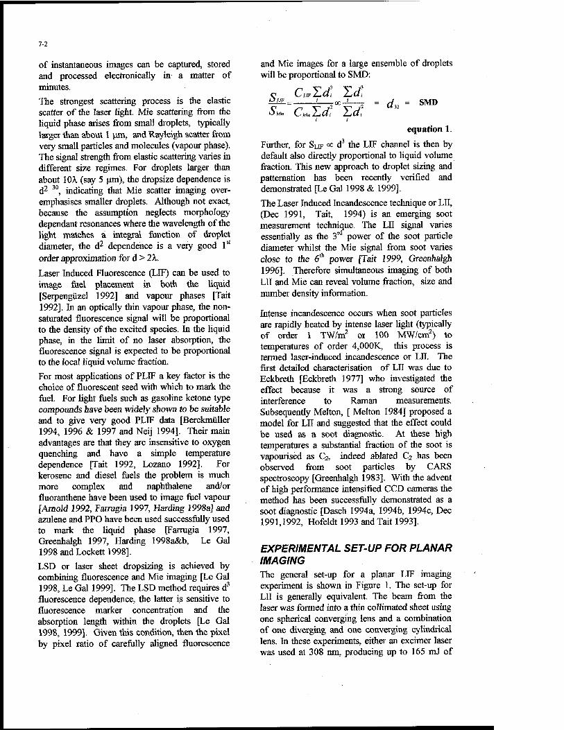
7-2

of instantaneous images can be captured, stored and processed electronically in a matter of minutes.

The strongest scattering process is the elastic scatter of the laser light. Mie scattering from the liquid phase arises from small droplets, typically larger than about 1 urn, and Rayleigh scatter from very small particles and molecules (vapour phase). The signal strength from elastic scattering varies in different size regimes. For droplets larger than about 10Ä. (say 5 pm), the dropsize dependence is d2 30, indicating that Mie scatter imaging over- emphasises smaller droplets. Although not exact, because the assumption neglects morphology dependant resonances where the wavelength of the light matches ä integral function of droplet diameter, the d2 dependence is a very good 1st

order approximation for d > Tk.

Laser Induced Fluorescence (LIF) can be used to image fuel placement in both the liquid [Serpengüzel 1992] and vapour phases [Tait 1992]. In an optically thin vapour phase, the non- saturated fluorescence signal will be proportional to the density of the excited species. In the liquid phase, in the limit of no laser absorption, the fluorescence signal is expected to be proportional to the local liquid volume fraction.

For most applications of PLIF a key factor is the choice of fluorescent seed with which to mark the fuel. For light fuels such as gasoline ketone type compounds have been widely shown to be suitable and to give very good PLIF data [Berckmiiller 1994, 1996 & 1997 and Neij 1994]. Their main advantages are that they are insensitive to oxygen quenching and have a simple temperature dependence [Tait 1992, Lozano 1992]. For kerosene and diesel fuels the problem is much more complex and naphthalene and/or fluoranthene have been used to image fuel vapour [Arnold 1992, Farrugia 1997, Harding 1998a] and azulene and PPO have been used successfully used to mark the liquid phase [Farrugia 1997, Greenhalgh 1997, Harding 1998a&b, Le Gal 1998 and Locke« 1998].

LSD or laser sheet dropsizing is achieved by combining fluorescence and Mie imaging [Le Gal 1998, Le Gal 1999]. The LSD method requires d3

fluorescence dependence, the latter is sensitive to fluorescence marker concentration and the absorption length within the droplets [Le Gal 1998, 1999]. Given this condition, then the pixel by pixel ratio of carefully aligned fluorescence

and Mie images for a large ensemble of droplets will be proportional to SMD:

LSUF 2-i@i 2-iCli

OMie KsMieZ-lÜi Z-lCli = d3

SMD

equation 1.

Further, for SLIF <* d3 the LIF channel is then by default also directly proportional to liquid volume fraction. This new approach to droplet sizing and patternation has been recently verified and demonstrated [Le Gal 1998 & 1999].

The Laser Induced Incandescence technique or LII, (Dec 1991, Tait, 1994) is an emerging soot measurement technique. The LII signal varies essentially as the 3td power of the soot particle diameter whilst the Mie signal from soot varies close to the 6th power [Tait 1999, Greenhalgh 1996]. Therefore simultaneous imaging of both LII and Mie can reveal volume fraction, size and number density information.

Intense incandescence occurs when soot particles are rapidly heated by intense laser light (typically of order 1 TW/m2 or 100 MW/cm2) to temperatures of order 4,000K, this process is termed laser-induced incandescence or LII. The first detailed characterisation of LII was due to Eckbreth [Eckbreth 1977] who investigated the effect because it was a strong source of interference to Raman measurements. Subsequently Melton, [ Melton 1984J proposed a model for LII and suggested that the effect could be used as a soot diagnostic. At these high temperatures a substantial fraction of the soot is vapourised as C2, indeed ablated C2 has been observed from soot particles by CARS spectroscopy [Greenhalgh 1983]. With the advent of high performance intensified CCD cameras the method has been successfully demonstrated as a soot diagnostic [Dasch 1994a, 1994b, 1994c, Dec 1991,1992, Hofeldt 1993 and Tait 1993].

EXPERIMENTAL SET-UP FOR PLANAR IMAGING The general set-up for a planar LIF imaging experiment is shown in Figure 1. The set-up for LII is generally equivalent. The beam from the laser was formed into a thin collimated sheet using one spherical converging lens and a combination of one diverging and one converging cylindrical lens. In these experiments, either an excimer laser was used at 308 nm, producing up to 165 mJ of

7-3

energy per 20 ns duration pulse or to 80 mJ per pulse in approximately 8 ns. Since these lasers produce ultra-violet output, fused silica sheet- forming lenses were used the 4th harmonic of a

Nd:YAG at 266nm with up. For the enclosed combustors, the laser sheet was introduced to the measurement region and the signal was collected through windows.

+ve. Cyl. Lens

";, Pulsed Tuneable Laser

■^g^&ii^it^^^^B^'iimä^i^^

■■ Electronics to time Laser, Camera

;:■ and mtensifler Gate

Raw Imafles via Ethernet to Workstations for Image Processing and Image Analysis

Figure 1 Schematic of General Set-up for Planar LIF Imaging Experiment

An intensified CCD camera positioned orthogonally to the laser sheet imaged the fluorescence signal. Such cameras have a linear response to the fluorescence signal and allow datasheets of hundreds of single shot images to be rapidly acquired and stored. The cameras used in the two studies described had chip sizes of 600 x 400 and 578 x 384 pixels respectively and had 15 bit grey-scale resolution. Elastic (Mie) scattering was discriminated out through the use of a long- pass filter in front of the CCD camera.

The PLIF images must be corrected TOT background scatter, variations in the laser sheet intensity profile and variations of the intensifier gain function [Long 1993, Greenhalgh 1997]. The laser sheet profile was normally obtained by flooding the combustor with homogeneous acetone vapour. For the jet experiments a large thin enclosure was filled with acetone vapour and used to record the laser sheet profile of the measured region.

The LSD experiments [Le Gal 1999] and the calibration of the fluorescence [Harding 1998a] have been described extensively elsewhere. Basically the experiment consists of simultaneously imaging the Mie and the liquid

only LIF signals from a fuel spray. Once the two images have been corrected for background scatter their ratio can be used to estimate SMD.

FUEL VAPOUR IMAGING The first example is taken from a fuel-air mixing study in an LPP duct [Harding 1994a]. A schematic of the combustor is shown in figure 2.

Using PLIF imaging of the fuel it has been possible to characterise the mixing process duct [Harding 1994a]. Kerosene LIF images of fuel vapour were measured in axial and radial sections of the premixer. One hundred radial images were stored at 5 axial stations along the length of the premixer (Figure 3).

7-4

Kerosene. Injector

• 1 K

Fused Silica Sections

Figure 2. The LPP Combustor

The mean images show that most of the fuel is present in a thick annulus between the core flow and die premixer wall. These mean image also show an apparent asymmetry. The rich spot in the plane of the laser sheet is due to a slightly enhanced feed of one of the discrete fuel jets which is most likely a gravity effect since the injector is horizontal.

These measured data were then processed to calculate the fluctuating root mean square (rms) component of fuel concentration. The rms values measured in the axial plane agreed very weil with those measured in the radial plane. Along the duct the rms declines from 40% of the mean to 30%, figure 3. The instantaneous, mean and rms images clearly show how the mixing progresses along the premixer. The level of fuel concentration rms at the final measurement station near the exit of the duct is slightly higher than at the neck of the duct, this is probably due to the enhanced turbulence associated with the vortical transition from the premixer to the combustor. The velocity measurements [Harding 1998a] also show a similar rms peak close the duct exit. The position of the highest fuel concentration rms is away from the centreline towards the wall of the duct. This richer zone also has a high rms velocity [Harding 1998a] and will be where the mixing is fastest.

In order to distinguish between the temporal fuel concentration fluctuation and the total (spatial plus temporal) the temporal component was calculated

separately. By calculating the rms of the total quantity of fuel present in each image, the spatial distribution of rms in that image could be estimated. This showed that the fluctuation in fuel concentration is approximately 27 % temporal and 73 % spatial.

Kerosene laser induced fluorescence arises from a wide range of aromatics present in the fuel, which have uncharacterised fluorescence behaviours and encompass a wide range of boiling points. LIF measurements using naphthalene dissolved into a non-fluorescing (mineral spirits) show the distribution of vapour fuel in the premixer of a more representative fraction of the bulk of the fuel. Naphthalene fluorescence has a strong temperature dependence and its fluorescence is strongly quenching by oxygen. However for an LPP premixer it is reasonable to assume that the gradients in both temperature and oxygen are too small to significant impact the fluorescence measurements. Measurements have also been made using 4% by mass naphthalene in mineral spirits (Figure 4). Naphthalene boils at 218 °C. These images confirm that the fuel is located in a thick annulus within the premixer.

The spatial placement of heavy fuel fractions within the kerosene has also been estimated by LIF. Fuel doped with 0.4% fluoranthene (boiling point 380 °C) by mass in mineral spirits was used. The resulting images are shown in figure 4.

Discrete jets of fuel from the injector are clearly visible in the fluoranthene LIF images (figure 4). The mean fluoranthene LIF image shows a rich spot of fuel rotating through 3/4 of a turn as it progresses along the duct. This agrees with the measured swirl number of 0.74 [Harding 1998a]. The high boiling point seed survives along the full length of the duct. The radial droplet jets from the fuel injector also impinge upon the prefilmer where secondary atomisation enhances their dispersion. These jet structures propagate downstream with high fuel concentration gradients are their edges indicating poor mixing. The levels of rms fluctuations are typically 70 % for fluoranthene of the mean compared to 25 % for naphthalene.

7-5

Radial sections

(s) instantaneous (s) mean

Axial Sections IS"

rms / mean

(m) instantaneous (m) mean

mean

(e) instantaneous (e) mean

Infinity 15.3 7.7

Scale: AFR

Infinity 0%

5.1 3.8 (inst.).

5.4 (mean) 100% (rms)

Figure 3. Kerosene LIF Images in the Premixer. L.H.S. Radial Sections at Start (s), Middle (m), and End (e) of Duct. R.H.S. Axial sections.

7-6

Napthalene Fluoranthene

J»*6, '%

(e)

Figure 4. Naphthalene (b.p. 218 °C) and Fluoranthene (b.p. 380 °C) LIF Images from the Premixing Duct (s=start, m=middle, e=end).

Clearly the placement of fuel in the premixer is highly dependent on the boiling point of the particular fraction of fuel. High boiling point fractions survive longer in the liquid phase and travel further as droplets. Thus these fractions have more ballistic momentum allowing them to travel further outboard where they remain poorly mixed at the end of the duct.

The consequence of this behaviour is that multi- component fuels will become spatially fractionated. The time history of each fraction will be different and this has important consequences for the modelling of the mixing in these ducts. Measurements are also possible in conventional combustors [Farrugia 1997]. Planar fluorescence imaging of liquid fuel was performed on the

combusting spray from an air-blast atomiser in a double annular combustor, running at an intermediate inlet pressure of 3 bar. Fused silica windows allowed optical access for both axial and radial imaging. A sample image is shown in figure 5. Vapour measurements with napthalene are generally not as useful. Although the fluorescence from napthalene in the liquid state is relatively weak the dense nature of the spray means that it is not possible to distinguish liquid and vapour easily simply using LIF. The solution to these lies in tiie simultaneous use of elastic scattering which permits the positive identification of the liquid phase. Since the liquid phase patternation dominates the mixing of these devices this is discussed in the next section.

7-7

Figure 5 Axial instantaneous LIF Image of Naphthalene Seeded Mineral Spirits - Liquid and Vapour Phases.

SPRAY IMAGING As outlined in the introduction, the LSD technique provides images of both volume fraction and SMD. To illustrate the technique the fust example given here is data from a small Delavan pressure- swirl atomiser which has been directly compared with PDA [Le Gal 1999], Figure 6. To obtain good LIF data it is essential to properly calibrate the fluorescence, in particular to ensure that the droplets are optically thin to the laser wavelength

[Le Gal 1999]. Otherwise the LIF signal which should ideally scale as dt will scale as <f where n is plotted versus concentration for the dye PTP excited at 266nm in Figure 7. Figure 6 shows mean LIF & Mie images, which are not corrected for laser profile variations. Since the profiles are ratioed to obtain SMD, systematic laser profile features and camera viewing factors will all cancel to first order.

Mean LIF (3,000 laser shots) Mean Mie (3,000 laser shots)

(False colours scale in counts)

Figure 6. LIF and Mie Images from a Delavan Pressure Swirl Atomiser Spray.

7-8

3-

2.8'

2.6

2.4-

2.2

2- 0 0.05 0.1 0.15 0.2 0.25 0.3 0.35 0.4 0.45 0.5

PPTP] concentration (g/1)

Figure 7 Variation of index n as a function of dye concentration.

The LSD (LIF/Mie ratio) image can be validated qualitatively against PDA calibrations of the same injector. Figure 8 shows the comparison of radial traverses though the injector centreline for one downstream traverse. The PDA data corresponds to two orthogonal traverses (in the "xO" and "yO" planes), each PDA point representing the D32

(SMD) of a sample of 3,000 droplets. The LSD profile has been linearly scaled to give a best fit. The agreement between the two PDA profiles and the LSD profile is excellent. The final LSD image of SMD is shown in figure 9.

50 -

*k k 45" \A 40

»VS. 35 -

nPk 301

^k 25

V 20 -

^Av 15

5

i 1 H e- 1- 1 ■—i

•YO Plane -LIF/MIE •XO Plane

-15 -10 10 15

Figure 8. Comparison of LSD and PDA Traverses 20 mm Downstream of the Injector Face.

The problem with Mie images is there dependence on d2; this results in average Mie images of sprays being a measure of liquid surface fraction. The main advantage of LIF (correctly calibrated) is that it provides droplet volume fraction. The marked differences between LIF & Mie are exemplified in figure 6.

The method has also been applied to an air-spray injector [Le Gal 1998]. Example results are shown in figure 10 for LSD again with a comparison to PDA data. In this case some of the PDA data is suspect and these points are highlighted by larger symbols. Note that these are the only points to

slightly disagree with the LSD, which shows a more continuous curve. This data is an indication that LSD may be applicable to dense sprays where PDA is likely to fail. Further work is in hand to investigate this potential advantage. Very recently the LSD method has been demonstrated in an operating Diesel engine [Lockert 1998] where spray densities are very high. This data further supports the view that LSD will become an important method for analysing dense sprays.

Finally it is worth noting that LEF alone provides a very useful method for pattemation. To illustrate this a comparison of data for a pintle and air-spray

injectors for the same combustor [Harding 1998b] are given in figure 11.

7-9

5 nun

i

53.5

40.12

03

I o s

CO VH

26.75 »

13.37

Q Ö at u

i CO

Figure 9. Calibrated SMD Image form Delavan Pressure Swirl Spray Recorded by LSD

25

5

(Q CO

10

5 -

-30.00 -20.00 -10.00 0.00 10.00

traverse position (mm)

LSD -*-- PDA

20.00 30.00

(b) Figure 10: Comparison of LSD and PDA for the Same Air-spray.

7-10

Radial Images Radial Images @ Idle @ Max. Power

Pintle Injector

Air-spray Injector

Axial Images @ Max. Power

Figure II: Comparison of LIF Patternation Data for a Pintle and Air-spray Injectors.

LASER INDUCED INCANDESENCE (Lll) In this section the LII technique is introduced. The aim of the first part is to present a basic model which characterises LII and the Mie signal from soot subject to intense laser pulses. The LII signal can be shown to vary essentially as the 3rd power of the soot particle diameter. The Mie signal, since the particles are small compared to the wavelength of the light, vary close to the 6th power. Therefore simultaneous imaging of both LII and Mie can give relative volume fraction, size and number density for soot.

Intense incandescence occurs when soot particles are rapidly heated by intense laser light (typically of order 1 TW/m2 or 100 MW/cm2) to temperatures of order 4,000K, this process is termed laser-induced incandescence or LII. The first detailed characterisation of LII was due to Eckbreth [Eckbreth 1977] who investigated the effect because it was a strong source of interference to Raman measurements. Subsequently Melton, [Melton 1984] proposed a model for LII and suggested that the effect could be used as a soot diagnostic. At these high temperatures a substantial fraction of the soot is vapourised as C2, indeed ablated C2 has been observed from soot particles by CARS spectroscopy [Greenhalgh 1983]. With the advent

of high performance intensified CCD cameras the method has been successfully demonstrated as a soot diagnostic: [Dasch 1993, 1994a, 1994b, Dec 1991,1992, Hofeldt 1993, Tait 1993].

A model developed by Tait [Tait 1993, 1996] which is an extension of the work of Melton [Melton 1984] has been developed and is outlined below. Laser energy is absorbed by the soot particle over a cross sectional area:

<Iabs = Kabs™2F equation 2

where Kahs is the absorption coefficient for soot, a is the particle radius (m) and F is the laser power density (Wnr2).

Energy is dissipated to the surrounding (bath) gas by conduction, vaporisation and radiation. The conduction term is:

qcon = -4™2(T-T0)Al

equation 3

n where T is the soot particle's temperature (K), is the temperature of the bath gas (K), Langmuir Heat Transfer Coefficient [Kennard 1938].

A[ is the

7-11

A/=-

aP0(C0--^-)

<j2nP0p0

equation 4

where a is the accommodation coefficient, P0 the pressure of the bath gas, C0 the specific heat capacity of bath gases (JmoWK-1) and p0 the density of bath gas (kg nr3). The accommodation coefficient would be unity if all molecules colliding with the particle surface condensed. The coefficient has been determined by experiment [Zavitsanos 1970] to be 0.25.

Heat is also dissipated by vaporisation:

"vap

&HvdM

Ws dt equation 5.

AHV is the heat of vaporisation of soot (J mol"1), Ws the molecular weight of soot (kg mol"1), M the mass of the soot particle (kg) and t time (s).

The model assumes that soot has similar properties to solid graphite and that most of the vaporised material is in the form of C2 with the vapour behaving as an ideal gas, so that:

W.. T-f

RTT equation 6

taken as the thermal velocity from the theory of Langmuir, [Kennard 1938]:

" V2(T equation 8.

Wv is the molecular mass of vaporised material. From equation 8 and by estimating pv from the ideal gas law and the Clausius-Clapeyron equation the energy transfer through vaporisation can be determined.

The LII signal is effectively the energy loss by radiation which is given by the Planck Radiation Law:

9rad - -j 2%2hc2

X5[exp(-hc/MbT)-l] a e(a,X)dX

equation 9

where c is the speed of light, h Planck's Constant, A the emitted wavelength, kb Boltzmann's Constant and s the emissivity. For an ideal blackbody the emissivity is equivalent to the absorption Kabs. This energy term is small compared to heat loss through vaporisation and conduction and can be simplified to become independent of wavelength if the wavelengths are long compared to the absorption length of soot particles. In this latter regime [Hall 1988] has shown that:

here the Clausius-Clapeyron equation has been used to find the vapour pressure. Pv is the carbon vapour pressure (Pa), p^ the density of carbon vapour (kgnr3), RQ the Universal Gas Constant (JK^mol"1), Wy, the molecular weight of carbon (C2) vapour (kg) and P* is the vapour pressure at the corresponding reference (sublimation point) temperature T*.

Mass continuity at the soot particle surface requires that:

dM dV da . 2 da . y dt da dt

equation 7

where Vis tite volume of a spherical soot particle and ps is the density of soot. The final term is the mass loss of vaporised material from a spherical soot particle; vv being the vapour velocity and is

qraa*c?T*> equation 10.

Melton (Melton 1984) described the dependence of the LII signal on particle size as:

qroc^a 3+1.54xl0_7A equation 11

Given that all soot particles achieve the same temperature this cubic dependence on diameter predicts that LII signals will be essentially linear dependant on soot volume fraction.

The internal energy rise of the soot particle acts as a further heat sink

9i int 4 3 _ dT

equation 12

where Cs is the heat capacity of soot. The overall energy balance for LII is therefore:

7-12

Kadsna2F-4™2(T-T0h

oP0 C0 - ^PQT.

\j2nP0p0

-WÄ 2R0T

exp Mt T-T

RQTT'

4 3 n dT n

equation 13.

The spatial laser pulse intensity distribution used in the model is rectangular or top hat. The model does however allow the signal to be calculated regularly spaced rectangular distributions within a defined envelope, such as a Gaussian. This was used to investigate the effect of laser intensity distribution on LII signals.

A thermodynamic database is used to determine the heat capacity of soot. Absorption efficiencies are determined by LorenzMie theory. The Mie scattering signal is calculated after the determination of absorption efficiency at the excitation wavelength. The LII signal is determined after calculation of the absorption efficiency at the collection wavelength. The vaporisation term causes the greatest uncertainty, with limited data on graphite used as an approximation. Investigations have been performed in graphite equilibrium vaporisation experiments [Steel 1970] and Langmuir free evaporation experiments [Zavitsanos 1970]. Both types of investigation find an accommodation coefficient less than unity. This reflects that each collision of vaporised material does not result in condensation. Equilibrium experiments conclude that C3 is the dominant vaporised species. Free evaporation experiments concluded C2 was the dominant species. The values of Zavitsanos, a =0.25, [Zavitsanos 1970] are used in the model, which is found to be relatively insensitive to the assigned value. The latent heat of Gaumet [Gaumet 1994] is used in the model, which determines the laser-induced vaporisation from a graphite target. Importantly LII modelled signals have been demonstrated by Tait [Tait 1999] to be less sensitive to refractive index than in scattering/absorption measurements.

Figure 12a: Time evolution of signals for a 4Jcnv2 laser fluence.

6000-q *y

Figure 12b: Time evolution of signals for a 10Jem2 laser fluence.

Figure 12c: Time evolution of signals for a 20Jcnr2 laser fluence.

The model was employed to demonstrate the predicted effects for a range of experimental conditions. Later, (he model was modified to

7-13

study the effect of changes in model parameters and specific beam intensity distributions. The main concepts important to imaging studies are how the signals vary with soot particle size, time, and laser intensity distribution. The soot particle size distribution regime accessible to the technique is dependent on a combination of the chosen collection duration and the laser power.

Figure 12 shows the time evolution of signals for a 30nm particle. Because the evolution of the signal is the key parameter the plots have all been normalised to accommodate mem on the same graph, the abscissa is soot particle temperature.

Figure 12a shows die evolution in parameters for a fluence of 4Jcnr2. In mis laser fluence regime, the soot particle is heated to a significant temperature above the bath gas [as displayed by the temperature evolution] but no significant change in particle size occurs. The particle does not vaporise and so emits an enhanced LII signal which slowly decays as the particle cools by conduction. The rate of cooling will be dependent primarily on balance between heat loss mechanisms to the environment. This in turn will be determined by the local composition and temperature of die bath gas. The Mie signal matches the temporal envelope of the laser pulse, where scattering is proportional to laser fluence. The rise in internal energy of the particle is slower than the time scale of the laser pulse whilst the scattering is immediate. Hence there is a time lag introduced into the LII signal.

Figure 12b shows the effect of an increased laser fluence of lOJcnr2. In this regime the particle is heated rapidly to a temperature above the sublimation point. The particle shrinks and consequently cools rapidly due to the dominant mechanism of vaporisation. Once the particle cools to a temperature below the sublimation point, the particle loses heat by the less rapid mechanism of conduction. As a result the enhanced radiation of LII follows the trend in temperature: a rapid decay during vaporisation followed by a slow tail through conduction. The Mie signal is reduced somewhat near the latter stage of the laser pulse. This is due to the fact that the particles are smaller by this point.

Figure 12c shows the effect at the laser fluence 20Jcnr2. Here the laser power is in excess, sufficient to vaporise the particle completely. Both

Mie and LII signals occur near the beginning of the pulse. This measurement strategy would be limited to pointwise or very small sheet imaging. Such fluences would be difficult to achieve for typical laser sheet imaging.

Figure 13 illustrates the temporal trace for different sized particles for the laser fluence of 4Jcm"2.

«oo- 2

? 3000

2000

1000

-UJOnni

LU_20nm UHOm

TJOrm T_20nm T40nm

1 ~1 i-

20 30 40 T

50 Sme{ns)

60 70 ~! ! 1

80 90 100

Figure 13: Time evolution of temperature and LII for three particle sizes.

The highest temperature is achieved by the largest particle (40nm) and after the longest time, consequently LII signals of larger particles peak later than small particles. Also the rate of conduction after the peak in temperature is greatest for the smaller particles. Particles small compared to the excitation wavelength (the Rayleigh regime) absorb through their whole volume rather than as a surface cross sectional area. For such particles the primary mechanism for heat loss is through surface conduction. Because the surface area to volume ratio is greater for small particles die enhanced heat loss results in cooler particles and therefore a lower LII signal. For particles large enough to be heated above the sublimation temperature («4,000K) cooling is dominated by vaporisation. Larger particles reaching slightiy higher temperatures also undergo greater mass loss. The increase in LII signal at higher temperatures therefore, tends to be balanced by the resulting reduction in radiating volume. The combined effects are illustrated in Figure 13.

7-14

Figure 15 shows the dependence of LII and Mie signals with fluence for a laser pulse of rectangular spatial distribution. The Mie signal rises linearly from die origin, whilst the LII signal is not detected. The LII signal does not increase significantly until the laser fluence is sufficient to heat the particles above the bath gas temperature. A peak in die signal is reached when die majority of the particles are heated to the maximum temperature without significant vaporisation. At greater fluences particles are vaporised, on a decreasing time scale, to a point where the particles are fully vaporised well before the end of the laser pulse.

Figure 14: Signal dependencies on particle size: TIT is collected over 50ns, fluence lOJcnr2,

*LII_shortjgate', 50ns, 4Jcm2 and 'LII long gate* 500ns, 4Jcm \

The simultaneous Mie signal is less dependent on mass loss because it appears prompdy and is dominated by die initial, largest, size of the soot particles, it therefore varies almost as the 6* power of particle diameter over the size range 10 to lOOnm. At intermediate fluences (»10 mJcrn2) and for a 50ns gate, the LII signal is found to have an approximate cubic dependence on particle size. For lower fluences this does not hold. The peak signal from large particles occurs at increasingly longer times after the laser pulse (figure 13) hence a higher order power dependence of the LII signal for particle size is observed for a long collection interval. Conversely, a greater dependence for small particles is observed for short, prompt collection intervals (figure 14).

•1ff"(U)

1 r~ 4 5 6

Figure 15: Signal fluence dependence: "LII_shorr" is collected prompt within 50ns, "LEMUrag "is collected prompt within 500ns.

turbulent diffusion flame

sheet-forming opt»

aluminium

$- narrowband mirrors

narrowband filter

intensified CCD camera

Figure 16: The simultaneous imaging technique.

The rate of increase in Mie signal with fluence trails off around the point of maximum LII signal, where the particles shrink during the envelope of the laser pulse. The graph also illustrates differences between die signals for different collection times. The characteristic of die Mie signal does not change, as the signal occurs promptly with die laser pulse. On die other hand the asymptote for the LII signal is reached where all the soot is ablated by the end of the laser pulse. The low fluence signal is most sensitive to the signal collection interval, a more prominent peak in the LII signal, shifted slighdy towards lower fluence is seen for long gate times. This trend is further exaggerated when collecting at wavelengths around 600nm because the ration spectrum peaks around this wavelength for temperatures around the vaporisation threshold of 3500-4000K. 600nm. This peak in the spectrum moves towards the IR as the particle cools. Therefore care has to be taken in the selection of

7-15

signal collection wavelength, bandwidth and collection interval.

collection

The utility of LII and Mie imaging can be more readily appreciated from the work of Bryce [Bryce 1996]. A series of studies have been performed in

a simple ethylene jet flame, in these measurements the LII and Mie signals were recorded simultaneously. The optical configuration required for simultaneous imaging is illustrated in Figure 16.

number

LII Mie

number

Figure 17: False colour images of LII (^relative soot volume fraction), Mie, relative soot particle size and relative soot number density for a 3.1 mm ethylene jet flame. Re. No. = 8,600, images measured at

(a) x/d=110 and (b) x/d=60.

Figure 17 shows some example images, the method clearly provides considerable detailed data

on soot in turbulent flows. Pdf data has also been extracted from such images [Bryce 1996] and the

7-16

results of particle size are consistent with those of Dasch [Dasch 1991] who used light scattering. These images cleanly demonstrate the power of the LII technique especially when combined with Mie imaging. The demonstration of LII in a diesel by Dec [Dec 1991,1992] also shows that the methods have a practical utility.

Demonstration in a gas turbine is now under way. The main outstanding problems for LII concern operation in optically thick environments such as the primary zone of high pressure combustors where laser an signal attenuation will be a serious problem.

CONCLUSIONS Fuel vapour and fuel droplet imaging techniques have been presented based on Planar Laser Induced Fluorescence for fuel vapour and Laser Sheet Dropsizing for fuel droplets. The latter being a combination of LIF and Mie scattering.

Soot imaging using Laser Induced Incandescence has also been presented. The latter is capable of also providing some relative data on soot particle size when combined with simultaneous Mie scattering. These experiments collectively demonslrate the ability of planar imaging methods for, in particular quantitative and semi-quantitative patternation of fuel sprays in operating combustors. I believe these methods have the potential for routine use in testing fuel injectors and for "in situ" evaluation of fuel patternation.

ACKNOWLEDGEMENTS The authors would like to gratefully acknowledge the support of Rolls-Royce pic and DERA. Parts of the work were sponsored by CEC B-E project AER2-CT92-0036: "Low-NOX II" and by EPSRC grant numbers GR/H78238 and GR/K37215.

REFERENCES Andresen [1990], P., Meijer, G, Schlüter, H., Voges, H., Koch, A., Hentschel, W. Oppermann, W., Rothe, E.: Fluorescence Imaging Inside an Internal Combustion Engine using Tuneable Excimer Lasers, Applied Optics, 29, 2392-2404 (1990).

Arnold [1992], A., Dinkelacker, F., Heitzmann, T., Monkhouse, P., Schäfer, M, Sick, V., Wolfrum, J.,: DI Diesel Engine Combustion

Visualised by Combined Laser Techniques, Twenty-Fourth Symposium (International) on Combustion/The Combustion Institute, pp 1605- 1612 (1992).

Arnold [1993], A., Buschmann, A., Cousyn, B., Decker, M., Vannobel, F., Sick, V., Wolfrum, J.: Simultaneous Imaging of Fuel and Hydroxyl Radicals in an In-Line Four Cylinder Si-Engine, SAE 932696, (1993).

Bachalo [1980], W. D.: Appl. Opt. 19, 3, 363-370 (1980).

Bachalo [1984], W. D. and Houser, M. J.: Phase/Doppler spray analyser for simultaneous measurements of drop size and velocity distributions, Opt. Engin., 23, 583-590 (1984).

Berckmiiller [1994], M., Tait, N. P., Locke«, R. D., Greenhalgh, D. A., Ishii, K., Urata, Y., Umiyama, H., Yoshida. K.: In-Cylinder Crank- Angle-Resolved Imaging of Fuel Concentration in a Firing SI Engine Using Planar Laser-Induced Fluorescence, Twenty-Fifth Symposium (International) on Combustion, The Combustion Institute, pp. 155-156, (1994).

Berckmiiller [1996], M., Tait, N. P. and Greenhalgh, D. A.: The Time History of the Mixture Formation Process in a Lean Burn Stratified-Charge Engine, SAE Paper No. 9619*29 (1996).

Berckmiiller [1997], M., Tait, N. P. and Greenhalgh, D. A.: The Influence of Local Fuel Concentration on Cyclic variability of a Lean Burn Stratified-Charge, SAE Paper No. 970826 (1997).

Dasch [1984a], C. J. "Continuous-wave Probe Laser Investigation of Laser Vaporisation of Small Soot Particles in a Flame" Applied Optics 23, 2209-2215 (1984a).

Dasch [1984b], C. J. "Spatially Resolved Soot- Absorption Measurements in Flames using Laser Vaporisation of Particles" Optics Letters 9, 214- 216(1984).

Dasch [1984c], C. J. New Soot Diagnostics in Flames Based on Laser Vaporisation of Soot" Twentieth Symposium (International) on Combustion/The Combustion Institute pp 1231- 1237(1984).

Dasch, [1991], C. J. and Heffelfinger, D. M.: Planar Imaging of Soot Formation in Turbulent Ethylene Diffusion Flames: Fluctuations and

7-17

Integral Scales Combustion and Flame 85, 389- 402 (1991).

Dec [1991], J. E., zur Loye, A. O., Siebers, D. L.: Soot Distribution in a D.I. Diesel Engine Using 2- D Laser-induced Incandescence Imaging SAE Technical Paper Series 910224 (1991).

Dec [1992], J. E.: Soot Distribution in a D.I. Diesel Engine Using 2-D Imaging of Laser- induced Incandescence, Elastic Scattering , and Flame Luminosity SAE Technical Paper Series 920115 (1992).

Eckbreth [1977], A. C: Effects of Laser- modulated Particulate Incandescence on Raman Scattering Diagnostics. Journal of Applied Physics 48(11), 4473-4479 (1977).

Eckbreth [1988], A. C: Laser Diagnostics for Combustion Temperature and Species. Abacus Press (1988).

Farrugia [1997], N., Lockert, R. D., Harding, S. C. and Greenhalgh, D. A.: LIF Imaging of Fuel Distribution in Gas Turbine Combustors, Proc ILASS-Europe 97, 299-305, Florence, Italy (1997).

Gaumet [1994], J J, Müller J F, Wakisaku A, Shumitzu Y, Tamori Y Study on the Mechanism of Carbon Cluster (Cn

+) Formation by Laser Vaporisation of a Graphite Target:Energy Density and Wavelength Influence, J. Aerosol. Sei. 25, pp 1363 (1994).

Greenhalgh [1983], D. A.: Resonant-Enhanced CARS from C2 Produced by Laser Ablation of Soot Particles. Applied Optics 22, 1128-1130 (1983).

Greenhalgh [1994], D. A.: Inelastic Scattering Laser Diagnostics; CARS, Planar LIF and Planar LII. in "Optical Diagnostics for Flow Processes" (Eds. L. Lading, P. Buchave and G. Wigley) Plenum Press, N.Y., (1994).

Greenhalgh [1996], D. A., Tait, N. P., Lockert, R. D., Bryce, Bush, R. D., Berckmüller, M and Harding, S. C. Laser Imaging Diagnostics for Scalar Combustion Measurememnts Proc. First Australian Conf. on Laser Diagnostics in Fluid Mechanics and Combustion pp 1-28 (1996).

Greenhalgh [1997], D. A., Bryce, D. J., Lockert, R. D., and Harding, S. C: Developmement of Planar Laser Induced Fluoresence for Fuel: Application to Gas Turbine Combustion, AGARD-CP-598 Paper 25 (1997).

Hall R J [1988] Computation of the Radiative Power Loss in a Sooting Diffusion Flame. Appl. Opt. 27(5), 809-811(1988).

Harding [1998a], S. C. and Greenhalgh, D. A: Fuel-air Mixing and Combustion in an Optical, Lean, Premixed Prevapourised Gas Turbine Combustor. ASME 98-GT-553 (1998).

Harding [1998b], S.C., Farrugia, N., Le Gal, P., Nimmo, G.A., and Greenhalgh, D.A.: Fuel Flux, Droplet Size and Velocity Measurements Made on Pintle and Air-spray Injectors. Proc. ILASS- Europe '98 pp. 463-468 (1998).

Hodges [1991], J.T., Baritaud, T.A., and Heinze, T.A. : Planar liquid and gas fuel and droplet size visualisation in a DI engine, SAE 910726, Detroit, Michigan (1991).

HoMdt [1993], D.L.: Real -Time Soot Concentration Measurement Technique for Engine Exhaust Streams. SAE Technical Paper Series 930079 (1993).

Kemvard [1938], E.H.: Kinetic Theory of Gases. McGraw-Hill New York and London (1938).

Le Gal [1998], P., Farrugia, N., and Greenhalgh, D.A.: Development of Laser Sheet Dropsizing (LSD) for Spray Characterisation. Proc. ILASS- Europe '98 pp.469-474 (1998).

Le Gal [1999], P., Farrugia, N., and Greenhalgh, D.A.: Laser Sheet Dropsizing of Dense Sprays. Optics & Laser Technology, 31, 75-83 (1999).

Lefebvre [1989], A. H: Atomisation and Sprays. Taylor and Francis (1989).

Lockert [1998], R.D., Richter J., and Greenhalgh D. A.: The Characterisation of a Diesel Spray using Combined Laser Induced Fluorescence and Laser Sheet Dropsizing. CWC2, Proc. CLEO/Europe '98, IEEE Cat. No. 98TH8326 (1998).

Long [1993], M. B.: Multidimensional Imaging in Combusting Flows by Lorenz-Mie, RayJeigh and Raman Scattering" Chapter from "Instrumentation for Flows with Combustion" (Ed.: AMKP Taylor), Academic Press Ltd. (1993).

Lozanao [1992], A., Yip, B. and Hanson, R.K.: Acetone: a Tracer for Concentration Measurements in Gaseous Flows by Planar Laser-Induced Fluorescence Experiments in Fluids Vol 13 pp 369-376 (1992).

7-18

Maas [1995], H-G. and Gruen, A.: Opt. Eng. 34, 1970-1976 (1995).

Melton [1984], L.A.: Soot Diagnostics Based on Laser Heating. Applied Optics Vol. 23(13) pp 2201-2208 (1984).

Neij [1994], H., Johansson, B. and Alden, M.: Development and Demonstration of 2D-LIF for studies of Mixture Preparation in SI Engines, Comb, and Flame 99, 449-457 (1994).

Sankar [1997], S.V., Mäher, K.E., Robart, D.M. and Bachalo, W.D.: Spray characterisation using a planar droplet sizing technique, Proc ICLASS- 97, Seoul, Korea (1997).

Seitzman [1993], J.M., and Hanson, R.K.,: Planar Fluorescence Imaging in Gases. Chapter from "Instrumentation for Flows with Combustion" (Ed.: AMKP Taylor), Academic Press Ltd. (1993).

Serpengiizel 11992]A., Swindal, J.C., Chang R.K. and Acker, W.P.: Appl. Opt., 31, 18, 3543-3551 (1992).

Tait [1992], N. P. and Greenhalgh, D. A.: Twenty- Fourth Symposium (Int.) on Combustion. The Combustion Institute. 1621-1628 (1992).

Tait [1993], N. P. and Greenhalgh, D. A: PLIF Imaging of Fuel Fraction in Practical Devices and LII Imaging of Soot. Ber. Bun.-Ges. Phys. Chem., 97, 1619-1625 (1993).

Tait [1999], N. P.: Results to be Published.

Talley [1996], D.G., Verdieck, J.F., Lee, S.W, McDonell, V.G. and Samuelsen, G.S.: Accounting for laser sheet extinction in applying PLIF to sprays. AIAA 96-0469 (1996).

Wigley [1994], G: Chapter in Optical Diagnostics for Flow Processes (ed. L. Lading, G. Wigley, P. Buchhave) Plenum Press (1994).

Yeh [1996], C-N., Kosaka, H., and Kamimoto, T: Measurement of drop sizes in unsteady sprays, Recent Adv. in Spray Comb. "Spray Atomisation and Drop Burning Phen.", Prog, in Astro, and Aero., 1, 297-308 (1996).

Zelina [1998], J., Rodrigue, A., and Sankar, S.V.: Fuel injector characterisation using laser diagnostics at atmospheric and elevated pressures, AIAA 98-0148, 36th Aerospace Sciences Meeting & Exhibit, Reno, N.V. (1998).

Zheng [1996], Q. P. Jasuja, A. K. and Lefebvre, A. H.: Twenty-Sixth Symposium (Int.) on Combustion. The Combustion Institute (1996).

Zavitsanos [1970] Vaporisation of Pyrolytic Graphite Dynamic Mass Spectroscopy 1, 1-13, (1970).

Steel [1970] Studies of Graphite Vaporisation Using a Modulated Beam Spectrometer AFML- TR-70-67

Bryce [1996], D J Development and Application of Planar Laser Techniques for Isothermal flow and Soot Diagnostics. PHD Thesis, Cranfield University (1996).

REPORT DOCUMENTATION PAGE

1. Recipient's Reference 2. Originator's References


3. Further Reference

ISBN 92-837-1019-3

4. Security Classification of Document UNCLASSIFIED/ UNLIMITED

5. Originator Research and Technology Organization North Atlantic Treaty Organization BP 25, 7 rue Ancelle, F-92201 Neuilly-sur-Seine Cedex, France

6. Title Planar Optical Measurement Methods for Gas Turbine Components

7. Presented at/sponsored by the Applied Vehicle Technology Panel (AVT) and held in Cranfield, UK, 16-17 September 1999 and in Cleveland, USA, 21-22 September 1999.

8. Author(s)/Editor(s)

Multiple

9. Date

September 1999

10. Author's/Editor's Address

Multiple

11. Pages

146

12. Distribution Statement There are no restrictions on the distribution of this document. Information about the availability of this and other RTO unclassified publications is given on the back cover.

13. Keywords/Descriptors

Optical measurement Aircraft engines Gas turbine engines Laser Doppler Velocimetry Flow visualization Measuring instruments Lasers Planar devices Velocity measurement PrV (Particle Image Velocimetry)

Paints Pressure sensors Temperature measuring instruments Laser induced fluorescence Fuels Drops (liquids) Soot Tests Test facilities Cost engineering

14. Abstract

This lecture series covers the recent advances of planar optical measurement techniques with respect to their applicability to gas turbine component tests.

During the last years much progress has been achieved in various known techniques, and new methods have been developed from which a significant increase of the experimental output of propulsion tests and therefore remarkable cost reduction can be expected. To bring this status into the knowledge of the propulsion specialists is the aim of this lecture series. Its theme is focused on laser measurement methods for the analysis of the internal flow and reaction processes in propulsion engines. It will address techniques for the measurement of flow velocity, flow density, pressure, temperature and species concentration. Only those methods are introduced which are far enough developed to be applicable to the rough test conditions of propulsion experiments. The course will inform the audience about the fundamentals of the advanced measurement techniques, as well as demonstrate their use in the context of practical applications.

The material in this publication was collected from the research centers of the different NATO nations. It will transfer to the propulsion engineers in a condensed manner the information of the newest capabilities of modern test techniques thus providing the knowledge base for tomorrow's measurement instrumentation of propulsion test facilities. NATO's specific interest in sponsoring this event is based on the requirement for engines of extreme performance characteristics which cannot be realised without further improvements of both CFD and measurement technologies.

This publication was prepared to support the Lecture Series 217 organised by the Applied Vehicle Technology Panel (AVT).



BP 25 • 7 RUE ANCELLE F-92201 NEUILLY-SUR-SEINE CEDEX • FRANCE

Telöcopie 0(1)55.61.22.99 • E-mail mailbox® rta.nato.int

DIFFUSION DES PUBLICATIONS

RTO NON CLASSD7IEES

L'Organisation pour la recherche et la technologie de l'OTAN (RTO), detient un stock limite de certaines de ses publications recerites, ainsi que de celles de l'ancien AGARD (Groupe consultatif pour la recherche et les r6alisations aerospatiales de l'OTAN). Celles-ci pourront 6ventuellement etre obtenues sous forme de copie papier. Pour de plus amples renseignements concernant l'achat de ces ouvrages, adressez-vous par lettre ou par t61ecopie ä l'adresse indiqu6e ci-dessus. Veuillez ne pas telephoner.

Des exemplaires supplementaires peuvent parfois etre obtenus aupres des centres nationaux de distribution indiques ci-dessous. Si vous souhaitez recevoir toutes les publications de la RTO, ou simplement celles qui concernent certains Panels, vous pouvez demander d'etre inclus sur la liste d'envoi de Tun de ces centres.

Les publications de la RTO et de l'AGARD sont en vente aupres des agences de vente indiqudes ci-dessous, sous forme de photocopie ou de microfiche. Certains originaux peuvent 6galement etre obtenus aupres de CASI.

CENTRES DE DIFFUSION NATIONAUX

ALLEMAGNE Fachinformationszentrum Karlsruhe D-76344 Eggenstein-Leopoldshafen 2

BELGIQUE Coordinateur RTO - VSL/RTO Etat-Major de la Force Aerienne Quartier Reine Elisabeth Rue d'Evere, B-1140 Bruxelles

CANADA Directeur - Recherche et developpement

Communications et gestion de rinformation - DRDCGI 3

Ministere de la Defense nationale Ottawa, Ontario K1A 0K2

DANEMARK Danish Defence Research Establishment Ryvangs Alle 1, P.O. Box 2715 DK-2100 Copenhagen 0

ESPAGNE INTA (RTO/AGARD Publications) Carretera de Torrejön a Ajalvir, Pk.4 28850 Torrejön de Ardoz - Madrid

ETATS-UNIS NASA Center for AeroSpace

Information (CASI) Parkway Center 7121 Standard Drive Hanover, MD 21076-1320

FRANCE O.N.E.R.A. (ISP) 29, Avenue de la Division Leclerc BP 72, 92322 Chätillon Cedex

GRECE Hellenic Air Force Air War College Scientific and Technical Library Dekelia Air Force Base Dekelia, Athens TGA 1010

HONGRIE Department for Scientific Analysis Institute of Military Technology Ministry of Defence H-1525 Budapest P O Box 26

ISLANDE Director of Aviation c/o Flugrad Reykjavik

ITALBE Centra documentazione tecnico-scientifica della Difesa

Via Marsala 104 00185 Roma

LUXEMBOURG Voir Belgique

NORVEGE Norwegian Defence Research Establishment

Attn: Biblioteket P.O. Box 25 NO-2007 Kjeller

PAYS-BAS NDRCC DGM/DWOO P.O. Box 20701 2500 ES Den Haag

POLOGNE Chief of International Cooperation

Division Research & Development Department 218 Niepodleglosci Av. 00-911 Warsaw

PORTUGAL Estado Maior da Forca Aerea SDFA - Centra de Documenta9äo Alfragide P-2720 Amadora

REPUBLIQUE TCHEQUE VTÜL a PVO Praha /

Air Force Research Institute Prague Narodni informacnf stfedisko

obranneho vyzkumu (NISCR) Mladoboleslavskä ul., 197 06 Praha 9

ROYAUME-UNI Defence Research Information Centre Kentigern House 65 Brown Street Glasgow G2 8EX

TURQUIE Mill! Savunma Baskanligi (MSB) ARGE Dairesi Baskanligi (MSB) 06650 Bakanliklar - Ankara

NASA Center for AeroSpace Information (CASI)

Parkway Center 7121 Standard Drive Hanover, MD 21076-1320 Etats-Unis

AGENCES DE VENTE

The British Library Document Supply Centre

Boston Spa, Wetherby West Yorkshire LS23 7BQ Royaume-Uni

Canada Institute for Scientific and Technical Information (CISTI)

National Research Council Document Delivery Montreal Road, Building M-55 Ottawa K1A 0S2 Canada

Les demandes de documents RTO ou AGARD doivent comporter la denomination "RTO" ou "AGARD" selon le cas, suivie du numero de serie (par exemple AGARD-AG-315). Des informations analogues, telles que le titre et la date de publication sont souhaitables. Des r6ferences bibliographiques completes ainsi que des resumes des publications RTO et AGARD figurent dans les journaux suivants:

Scientific and Technical Aerospace Reports (STAR) STAR peut etre consulte en ligne au localisateur de ressources uniformes (URL) suivant:

http://www.sti.nasa.gov/Pubs/star/Star.html STAR est edite par CASI dans le cadre du programme NASA d'information scientifique et technique (STI) STI Program Office, MS 157A NASA Langley Research Center Hampton, Virginia 23681-0001 Etats-Unis

Government Reports Announcements & Index (GRA&I) publie par le National Technical Information Service Springfield Virginia 2216 Etats-Unis (accessible egalement en mode interactif dans la base de donnees bibliographiques en ligne du NTIS, et sur CD-ROM)

Imprime' par le Groupe Communication Canada Inc. (membre de la Corporation St-Joseph)

45, boul. Sacre-Cceur, Hull (Quebec), Canada K1A 0S7



BP 25 • 7 RUE ANCELLE F-92201 NEUILLY-SUR-SEINE CEDEX • FRANCE

Telefax 0(1)55.61.22.99 • E-mail mailbox® rta.nato.int

DISTRIBUTION OF UNCLASSIFIED RTO PUBLICATIONS

NATO's Research and Technology Organization (RTO) holds limited quantities of some of its recent publications and those of the former AGARD (Advisory Group for Aerospace Research & Development of NATO), and these may be available for purchase in hard copy form. For more information, write or send a telefax to the address given above. Please do not telephone. Further copies are sometimes available from the National Distribution Centres listed below. If you wish to receive all RTO publications, or just those relating to one or more specific RTO Panels, they may be willing to include you (or your organisation) in their distribution. RTO and AGARD publications may be purchased from the Sales Agencies listed below, in photocopy or microfiche form. Original copies of some publications may be available from CASI.

NATIONAL DISTRIBUTION CENTRES

BELGIUM Coordinateur RTO - VSL/RTO Etat-Major de la Force Aerienne Quartier Reine Elisabeth Rue d'Evere, B-1140 Bruxelles

CANADA Director Research & Development Communications & Information Management - DRDCM 3

Dept of National Defence Ottawa, Ontario K1A 0K2

CZECH REPUBLIC VTÜL a PVO Praha /

Air Force Research Institute Prague Narodni informacni stredisko

obrann6ho vyzkumu (NISCR) Mladoboleslavskä ul., 197 06 Praha 9

DENMARK Danish Defence Research Establishment

Ryvangs Alle 1, P.O. Box 2715 DK-2100 Copenhagen 0

FRANCE O.N.E.R.A. (ISP) 29 Avenue de la Division Leclerc BP 72, 92322 Chätillon Cedex

GERMANY Fachinformationszentrum Karlsruhe D-76344 Eggenstein-Leopoldshafen 2

GREECE Hellenic Air Force Air War College Scientific and Technical Library Dekelia Air Force Base Dekelia, Athens TGA 1010

HUNGARY Department for Scientific Analysis Institute of Military Technology Ministry of Defence H-1525 Budapest P O Box 26

ICELAND Director of Aviation c/o Flugrad Reykjavik

ITALY Centro documentazione tecnico-scientifica della Difesa

Via Marsala 104 00185 Roma

LUXEMBOURG See Belgium

NETHERLANDS NDRCC DGM/DWOO P.O. Box 20701 2500 ES Den Haag

NORWAY Norwegian Defence Research

Establishment Attn: Biblioteket P.O. Box 25 NO-2007 Kjeller

POLAND Chief of International Cooperation

Division Research & Development

Department 218 Niepodleglosci Av. 00-911 Warsaw

PORTUGAL Estado Maior da Fprca Aerea SDFA - Centro de Documentagäo Alfragide P-2720 Amadora

SPAIN INTA (RTO/AGARD Publications) Carretera de Torrejön a Ajalvir, Pk.4 28850 Torrejön de Ardoz - Madrid

TURKEY Milli Savunma Baskanligi (MSB) ARGE Dairesi Baskanligi (MSB) 06650 Bakanliklar - Ankara

UNITED KINGDOM Defence Research Information

Centre Kentigern House 65 Brown Street Glasgow G2 8EX

UNITED STATES NASA Center for AeroSpace

Information (CASI) Parkway Center 7121 Standard Drive Hanover, MD 21076-1320

NASA Center for AeroSpace Information (CASI)

Parkway Center 7121 Standard Drive Hanover, MD 21076-1320 United States

SALES AGENCIES The British Library Document

Supply Centre Boston Spa, Wetherby West Yorkshire LS23 7BQ United Kingdom

Canada Institute for Scientific and Technical Information (CISTI)

National Research Council Document Delivery Montreal Road, Building M-55 Ottawa K1A 0S2 Canada

Requests for RTO or AGARD documents should include the word 'RTO' or 'AGARD', as appropriate, followed by the serial number (for example AGARD-AG-315). Collateral information such as title and publication date is desirable. Full bibliographical references and abstracts of RTO and AGARD publications are given in the following journals:

Scientific and Technical Aerospace Reports (STAR) STAR is available on-line at the following uniform resource locator:

http://www.sti.nasa.gov/Pubs/star/Star.html STAR is published by CASI for the NASA Scientific and Technical Information (STI) Program STI Program Office, MS 157A NASA Langley Research Center Hampton, Virginia 23681-0001 United States

Government Reports Announcements & Index (GRA&I) published by the National Technical Information Service Springfield Virginia 22161 United States (also available online in the NTIS Bibliographic Database or on CD-ROM)

Printed by Canada Communication Group Inc. (A St. Joseph Corporation Company)

45 Sacre-Caeur Blvd., Hull (Quibec), Canada K1A 0S7

ISBN 92-837-1019-3

Planar Optical Measurement Methods for Gas Turbine ...

Documents

Transcript of Planar Optical Measurement Methods for Gas Turbine ...