RESEARCH ARTICLE

PIV studies of coherent structures generated at the endof a stack of parallel plates in a standing wave acoustic field

Xiaoan Mao Æ Zhibin Yu ÆArtur J. Jaworski Æ David Marx

Received: 15 March 2006 / Revised: 27 January 2008 / Accepted: 2 April 2008 / Published online: 25 April 2008

� Springer-Verlag 2008

Abstract Oscillating flow near the end of a stack of

parallel plates placed in a standing wave resonator is

investigated using particle image velocimetry (PIV). The

Reynolds number, Red, based on the plate thickness and the

velocity amplitude at the entrance to the stack, is controlled

by varying the acoustic excitation (so-called drive ratio)

and by using two configurations of the stacks. As the

Reynolds number changes, a range of distinct flow patterns

is reported for the fluid being ejected from the stack.

Symmetrical and asymmetrical vortex shedding phenom-

ena are shown and two distinct modes of generating

‘‘vortex streets’’ are identified.

1 Introduction

Flow structures generated by steady flows past bluff bodies

have been a subject of many theoretical and experimental

studies, the classic example being formation of the von

Karman ‘‘vortex street’’ behind circular cylinders (Kov-

asznay 1949). This class of phenomena is important in

many industrial problems including: aerospace flows, civil

and marine engineering, design of heat exchangers or the

behaviour of overhead power cables. Somewhat more

complex situation arises when steady flows are replaced by

oscillatory flows (with or without the steady component),

the fundamental difference being that vortices shed in one

half of the cycle impinge on the bluff body when the flow

reverses and may interact with vortices shed during the

other half of the cycle. This may lead to interesting ‘‘lock-

on’’ effects resulting in an interaction between the flow and

the structural components within (Chung and Kang 2003;

Barbi et al. 1986).

Within the class of purely oscillatory flows, by far the

most studied geometrical configurations were flows past

circular cylinders (Obasaju et al. 1988; Iliadis and Anag-

nostopoulos 1998) although other geometries have been

considered including a square cross-section (inclined at

various angles to the flow) or a flat plate perpendicular to

the flow (Bearman et al. 1985; Okajima et al. 1997) and

triangular and T-shaped geometries (Al-Asmi and Castro

1992). Other studies investigated the effects of the prox-

imity of the external boundaries on the flow (Sumer et al.

1991). ‘‘External’’ flows as well as ‘‘internal’’ oscillatory

flows have been investigated. These include oscillatory

flows in pipes with ‘‘wavy’’ walls (Ralph 1986), internally

placed orifices (De Bernardinis et al. 1981) or internally

baffled channels (Roberts and Mackley 1996).

It is widely accepted that the morphology of the flow

structures present within oscillatory flows is governed by

three similarity numbers: the Reynolds number (Re), the

Keulegan-Carpenter number (KC) and the Stokes number

(b), although only two out of these are really independent,

as Stokes number can be expressed as the ratio of Reynolds

number to KC number. Tatsuno and Bearman (1990)

studied the morphology of the flows generated from the

oscillatory cylinder as a function of KC and b while similar

studies were performed by Okajima et al. (1997) for square

cylinders. These have shown a range of flow regimes

ranging from fully attached symmetrical pair of vortices

through to symmetrical and alternating vortex shedding.

X. Mao � Z. Yu � A. J. Jaworski (&) � D. Marx

School of Mechanical, Aerospace and Civil Engineering,

The University of Manchester, Sackville Street, PO Box 88,

Manchester M60 1QD, UK

e-mail: a.jaworski@manchester.ac.uk

123

Exp Fluids (2008) 45:833–846

DOI 10.1007/s00348-008-0503-7

In all of the experimental studies mentioned above, the

typical setup includes either the bluff body being oscillated

through the stationary fluid, using some form of mechani-

cal drive, or an oscillating incompressible fluid within U-

tube type of water tunnel, with the bluff body being held

stationary. However, it should be noted that similar flow

problems including vortex shedding phenomena also arise

in acoustic systems when the level of acoustic excitation is

relatively high. These include systems such as pulse tube

refrigerators, standing or travelling wave thermoacoustic

devices or their components such as jet pumps, Stirling

engines and refrigerators and others, where high intensity

acoustic wave (or oscillatory flows in general) encounter

sudden discontinuities in the cross-section of an acoustic

duct.

The initial motivation for the current paper came from

the need to understand the behaviour of the flow in a

standing wave thermoacoustic device in the vicinity of the

so called ‘‘thermoacoustic core’’. This typically comprises

of a stack of parallel plates (thermoacoustic stack) sand-

wiched between two heat exchangers (often also

constructed as a set of shorter but thicker parallel plates

with a somewhat larger pitch). The role of the thermoa-

coustic core is to either produce acoustic power due to the

temperature gradient imposed by the heat exchangers or to

consume externally supplied acoustic power in order to

facilitate heat pumping from cold to hot heat exchanger by

virtue of the so-called thermoacoustic effect (Swift 2002).

In the high-intensity acoustic field, the flow structures at

the end of the stack, or the heat exchanger (or in the region

in between) are very complex due to the discontinuities of

the cross section and the oscillatory nature of the flow.

Clearly, the energy transfer taking place within the ther-

moacoustic core will be affected by ‘‘entrance effects’’,

vortex shedding and generation (or suppression) of turbu-

lence over different parts of the acoustic cycle. The

existing models to calculate the performance of the ther-

moacoustic systems are based on the linear acoustic models

(for example DeltaE, as described by Ward and Swift

2001) with only some corrections being made to account

for non-linear acoustics effects such as turbulence. The

development of such codes is hindered by the lack of

understanding of the fundamental thermal-fluid processes.

Despite being rooted in the area of thermoacoustics, the

current investigation should be seen on a more general

level, namely the fundamental fluid dynamical processes of

interest to a wider audience. This is the reason why the

current research covers somewhat larger parameter space

than would be expected from the point of view of ther-

moacoustic stacks alone and covers the range characteristic

for finned heat exchangers and possibly beyond.

The experimental studies of the above phenomena in the

context of thermoacoustics are very limited. Gopinath and

Harder (2000) studied the heat transfer effects from a

single circular cylinder placed in an acoustic resonator

(with a possible application to thermoacoustic heat

exchangers). They identified two flow regimes: the laminar

attached flow regime and the less understood regime where

the vortex shedding is prevalent with much higher heat

transfer coefficients. Blanc-Benon et al. (2003) used PIV

measurements to investigate the flow field around and

vortex shedding from a stack of parallel plates for rela-

tively low drive ratios 1.0–1.5% and compared the

experimental results to CFD simulations. They have shown

the presence of symmetrical vortices, which on their two

experimental configurations (‘‘thin’’ and ‘‘thick’’ plates)

took an ‘‘elongated’’ and ‘‘concentrated’’ form, respec-

tively, but never fully detached from the plates. Mao et al.

(2005) conducted similar PIV studies using a somewhat

larger geometrical arrangement and higher drive ratios (up

to 3%) and showed that at higher drive ratios the sym-

metrical vortices are replaced by alternately shed vortices.

The current paper is an extension of this early work by

providing more complete experimental data and its more

detailed discussion and analysis.

2 Experimental apparatus and procedure

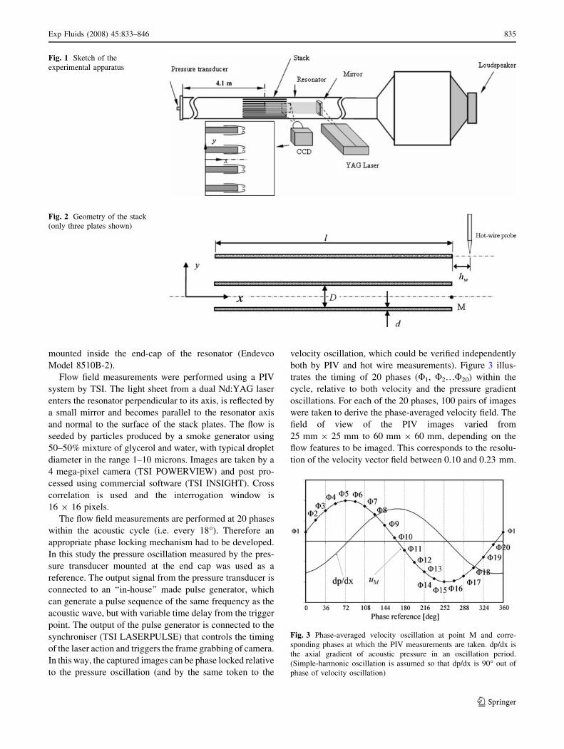
The experimental apparatus used in the current study

(Fig. 1) was discussed in some detail by Marx et al. (2006)

and therefore only a brief description is given here. Its

main part is a 7.4-m long transparent Perspex pipe, with the

internal cross-section 134 9 134 mm, and the wall thick-

ness of 8 mm. One end of the pipe (to the left of Fig. 1) is

closed by an ‘‘end-cap’’ with a flush mounted pressure

transducer. The other end is connected to a relatively large

‘‘loudspeaker box’’ (600 9 600 9 600 mm) through a

0.3 m long pyramidal section to match the change in cross-

sectional dimensions. The resonator is filled with air at

atmospheric pressure and room temperature. The first mode

of operation (quarter-wavelength) has a fundamental fre-

quency f = 13.1 Hz.

The experiments were conducted for two stacks of plates

(shown schematically in Fig. 2). The length, l, of both

stacks was 200 mm, while their width was 132 mm (some

clearance had to be left between the stack and the internal

resonator wall). Stack I comprised of 21 Perspex plates of

thickness d = 1.1 mm with the plate-to-plate spacing

D = 5 mm. Stack II was made out of eight Perspex plates

with d = 5 mm and D = 10 mm. Both stacks were placed

in the resonator 4.1 m from the end as schematically shown

in Fig. 1. The drive ratio in the experiments was varied by

changing the excitation voltage of the loudspeaker and

controlled by measuring the amplitude of pressure oscil-

lations recorded by the dynamic pressure transducer

834 Exp Fluids (2008) 45:833–846

123

mounted inside the end-cap of the resonator (Endevco

Model 8510B-2).

Flow field measurements were performed using a PIV

system by TSI. The light sheet from a dual Nd:YAG laser

enters the resonator perpendicular to its axis, is reflected by

a small mirror and becomes parallel to the resonator axis

and normal to the surface of the stack plates. The flow is

seeded by particles produced by a smoke generator using

50–50% mixture of glycerol and water, with typical droplet

diameter in the range 1–10 microns. Images are taken by a

4 mega-pixel camera (TSI POWERVIEW) and post pro-

cessed using commercial software (TSI INSIGHT). Cross

correlation is used and the interrogation window is

16 9 16 pixels.

The flow field measurements are performed at 20 phases

within the acoustic cycle (i.e. every 18�). Therefore an

appropriate phase locking mechanism had to be developed.

In this study the pressure oscillation measured by the pres-

sure transducer mounted at the end cap was used as a

reference. The output signal from the pressure transducer is

connected to an ‘‘in-house’’ made pulse generator, which

can generate a pulse sequence of the same frequency as the

acoustic wave, but with variable time delay from the trigger

point. The output of the pulse generator is connected to the

synchroniser (TSI LASERPULSE) that controls the timing

of the laser action and triggers the frame grabbing of camera.

In this way, the captured images can be phase locked relative

to the pressure oscillation (and by the same token to the

velocity oscillation, which could be verified independently

both by PIV and hot wire measurements). Figure 3 illus-

trates the timing of 20 phases (U1, U2…U20) within the

cycle, relative to both velocity and the pressure gradient

oscillations. For each of the 20 phases, 100 pairs of images

were taken to derive the phase-averaged velocity field. The

field of view of the PIV images varied from

25 mm 9 25 mm to 60 mm 9 60 mm, depending on the

flow features to be imaged. This corresponds to the resolu-

tion of the velocity vector field between 0.10 and 0.23 mm.

Fig. 1 Sketch of the

experimental apparatus

Fig. 2 Geometry of the stack

(only three plates shown)

Fig. 3 Phase-averaged velocity oscillation at point M and corre-

sponding phases at which the PIV measurements are taken. dp/dx is

the axial gradient of acoustic pressure in an oscillation period.

(Simple-harmonic oscillation is assumed so that dp/dx is 90� out of

phase of velocity oscillation)

Exp Fluids (2008) 45:833–846 835

123

Due to its nature, the PIV technique is not sufficiently

‘‘time-resolved’’ to permit measurements of the fluctuating

components of velocity. Therefore the investigations of the

vortex shedding frequencies, to be used in estimating typ-

ical Strouhal numbers, had to be conducted using standard

hot wire methods. Velocity fluctuations were measured with

SN type hot-wire probe (DANTEC) operated in the con-

stant-temperature mode using a TSI IFA300 system. The

probe is placed normal to the plate, while the sensor is

normal to the axis of the resonator. The position of the probe

is schematically shown in Fig. 2. For Stack I, the sensor is

placed 2d from the edge of the plate, while for Stack II this

distance is 4d because the large diameter of the probe

support prevents the sensor to be closer to the plate end (the

distance from the plate is denoted in Fig. 2 as hw). A high-

pass filter set at 30 Hz is used to remove the signal com-

ponent related to the fundamental frequency of 13.1 Hz.

Both the filtered signal and the unfiltered signal are recor-

ded with a sampling frequency of 5,000 Hz. 16,384 data

points are acquired in a typical experimental condition.

3 Experimental results

3.1 Overview of the experimental parameters

and conditions

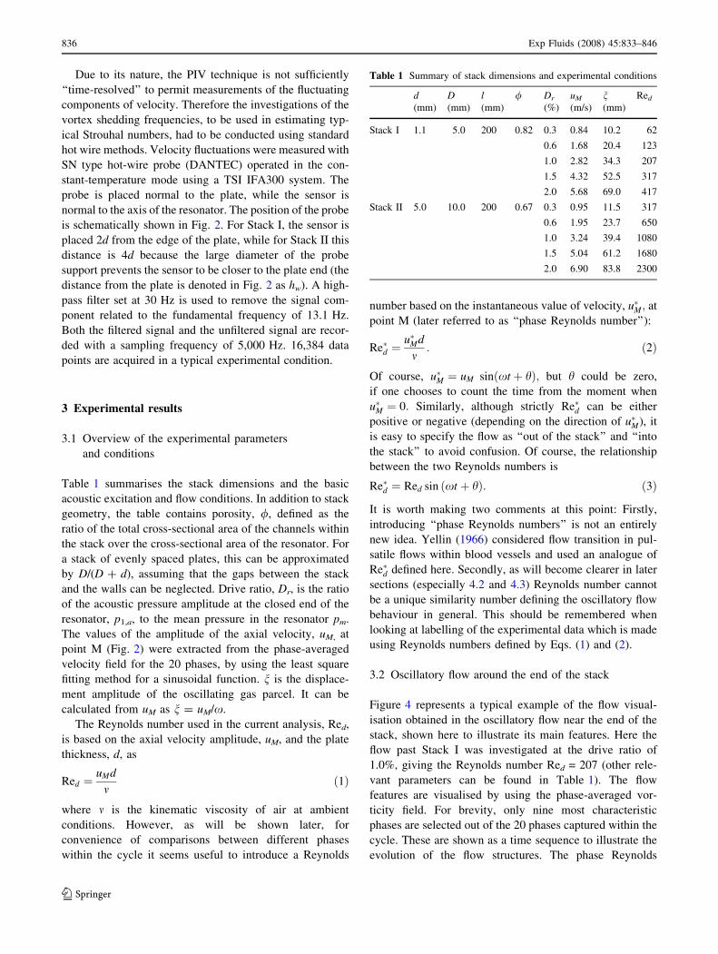
Table 1 summarises the stack dimensions and the basic

acoustic excitation and flow conditions. In addition to stack

geometry, the table contains porosity, /, defined as the

ratio of the total cross-sectional area of the channels within

the stack over the cross-sectional area of the resonator. For

a stack of evenly spaced plates, this can be approximated

by D/(D + d), assuming that the gaps between the stack

and the walls can be neglected. Drive ratio, Dr, is the ratio

of the acoustic pressure amplitude at the closed end of the

resonator, p1,a, to the mean pressure in the resonator pm.

The values of the amplitude of the axial velocity, uM, at

point M (Fig. 2) were extracted from the phase-averaged

velocity field for the 20 phases, by using the least square

fitting method for a sinusoidal function. n is the displace-

ment amplitude of the oscillating gas parcel. It can be

calculated from uM as n = uM/x.

The Reynolds number used in the current analysis, Red,

is based on the axial velocity amplitude, uM, and the plate

thickness, d, as

Red ¼uMd

mð1Þ

where m is the kinematic viscosity of air at ambient

conditions. However, as will be shown later, for

convenience of comparisons between different phases

within the cycle it seems useful to introduce a Reynolds

number based on the instantaneous value of velocity, u�M ; at

point M (later referred to as ‘‘phase Reynolds number’’):

Re�d ¼u�Md

m: ð2Þ

Of course, u�M ¼ uM sinðxt þ hÞ; but h could be zero,

if one chooses to count the time from the moment when

u�M ¼ 0: Similarly, although strictly Re�d can be either

positive or negative (depending on the direction of u�M), it

is easy to specify the flow as ‘‘out of the stack’’ and ‘‘into

the stack’’ to avoid confusion. Of course, the relationship

between the two Reynolds numbers is

Re�d ¼ Red sin xt þ hð Þ: ð3Þ

It is worth making two comments at this point: Firstly,

introducing ‘‘phase Reynolds numbers’’ is not an entirely

new idea. Yellin (1966) considered flow transition in pul-

satile flows within blood vessels and used an analogue of

Re�d defined here. Secondly, as will become clearer in later

sections (especially 4.2 and 4.3) Reynolds number cannot

be a unique similarity number defining the oscillatory flow

behaviour in general. This should be remembered when

looking at labelling of the experimental data which is made

using Reynolds numbers defined by Eqs. (1) and (2).

3.2 Oscillatory flow around the end of the stack

Figure 4 represents a typical example of the flow visual-

isation obtained in the oscillatory flow near the end of the

stack, shown here to illustrate its main features. Here the

flow past Stack I was investigated at the drive ratio of

1.0%, giving the Reynolds number Red = 207 (other rele-

vant parameters can be found in Table 1). The flow

features are visualised by using the phase-averaged vor-

ticity field. For brevity, only nine most characteristic

phases are selected out of the 20 phases captured within the

cycle. These are shown as a time sequence to illustrate the

evolution of the flow structures. The phase Reynolds

Table 1 Summary of stack dimensions and experimental conditions

d(mm)

D(mm)

l(mm)

/ Dr

(%)

uM

(m/s)

n(mm)

Red

Stack I 1.1 5.0 200 0.82 0.3 0.84 10.2 62

0.6 1.68 20.4 123

1.0 2.82 34.3 207

1.5 4.32 52.5 317

2.0 5.68 69.0 417

Stack II 5.0 10.0 200 0.67 0.3 0.95 11.5 317

0.6 1.95 23.7 650

1.0 3.24 39.4 1080

1.5 5.04 61.2 1680

2.0 6.90 83.8 2300

836 Exp Fluids (2008) 45:833–846

123

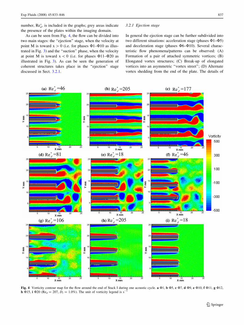
number, Re�d; is included in the graphs; grey areas indicate

the presence of the plates within the imaging domain.

As can be seen from Fig. 4, the flow can be divided into

two main stages: the ‘‘ejection’’ stage, when the velocity at

point M is toward x [ 0 (i.e. for phases U1–U10 as illus-

trated in Fig. 3) and the ‘‘suction’’ phase, when the velocity

at point M is toward x \ 0 (i.e. for phases U11–U20 as

illustrated in Fig. 3). As can be seen the generation of

coherent structures takes place in the ‘‘ejection’’ stage

discussed in Sect. 3.2.1.

3.2.1 Ejection stage

In general the ejection stage can be further subdivided into

two different situations: acceleration stage (phases U1–U5)

and deceleration stage (phases U6–U10). Several charac-

teristic flow phenomena/patterns can be observed: (A)

Formation of a pair of attached symmetric vortices; (B)

Elongated vortex structures; (C) Break-up of elongated

vortices into an asymmetric ‘‘vortex street’’; (D) Alternate

vortex shedding from the end of the plate. The details of

Fig. 4 Vorticity contour map for the flow around the end of Stack I during one acoustic cycle. a U1, b U5, c U7, d U9, e U10, f U11, g U12,

h U15, i U20 (Red = 207, Dr = 1.0%). The unit of vorticity legend is s-1

Exp Fluids (2008) 45:833–846 837

123

these characteristic flow patterns are described with refer-

ence to Fig. 4a–e.

3.2.1.1 Formation of a pair of attached symmetric vorti-

ces The flow in phase U1 (Fig. 4a) has a positive velocity

and starts to accelerate. Based on the instantaneous

velocity at point M, the corresponding phase Reynolds

number, Re�d; is about 47. A pair of vortex structures is

formed at the end the plate. They are symmetrical relative

to the centre-line of the plate in the x-y plane. Similarly as

in the classic case of the wake behind a plate with a square

trailing edge (as found in Bachelor 2000), a recirculation

region is formed at the end of the plate, where the pair of

vortices remains attached. In the inner region of the

channel formed by two neighbouring plates, there is a pair

of shear layers with their vorticity in an opposite direction

to the vorticity within the plate boundary layer.

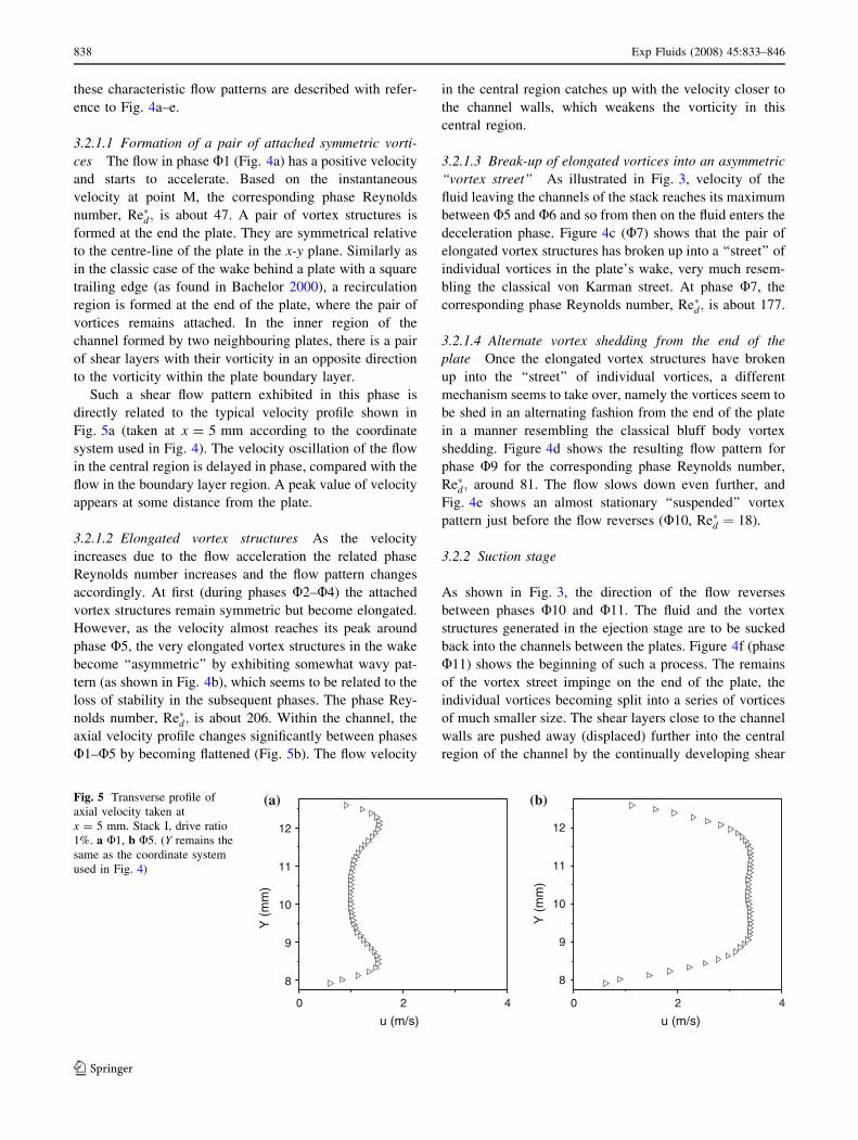
Such a shear flow pattern exhibited in this phase is

directly related to the typical velocity profile shown in

Fig. 5a (taken at x = 5 mm according to the coordinate

system used in Fig. 4). The velocity oscillation of the flow

in the central region is delayed in phase, compared with the

flow in the boundary layer region. A peak value of velocity

appears at some distance from the plate.

3.2.1.2 Elongated vortex structures As the velocity

increases due to the flow acceleration the related phase

Reynolds number increases and the flow pattern changes

accordingly. At first (during phases U2–U4) the attached

vortex structures remain symmetric but become elongated.

However, as the velocity almost reaches its peak around

phase U5, the very elongated vortex structures in the wake

become ‘‘asymmetric’’ by exhibiting somewhat wavy pat-

tern (as shown in Fig. 4b), which seems to be related to the

loss of stability in the subsequent phases. The phase Rey-

nolds number, Re�d; is about 206. Within the channel, the

axial velocity profile changes significantly between phases

U1–U5 by becoming flattened (Fig. 5b). The flow velocity

in the central region catches up with the velocity closer to

the channel walls, which weakens the vorticity in this

central region.

3.2.1.3 Break-up of elongated vortices into an asymmetric

‘‘vortex street’’ As illustrated in Fig. 3, velocity of the

fluid leaving the channels of the stack reaches its maximum

between U5 and U6 and so from then on the fluid enters the

deceleration phase. Figure 4c (U7) shows that the pair of

elongated vortex structures has broken up into a ‘‘street’’ of

individual vortices in the plate’s wake, very much resem-

bling the classical von Karman street. At phase U7, the

corresponding phase Reynolds number, Re�d; is about 177.

3.2.1.4 Alternate vortex shedding from the end of the

plate Once the elongated vortex structures have broken

up into the ‘‘street’’ of individual vortices, a different

mechanism seems to take over, namely the vortices seem to

be shed in an alternating fashion from the end of the plate

in a manner resembling the classical bluff body vortex

shedding. Figure 4d shows the resulting flow pattern for

phase U9 for the corresponding phase Reynolds number,

Re�d; around 81. The flow slows down even further, and

Fig. 4e shows an almost stationary ‘‘suspended’’ vortex

pattern just before the flow reverses (U10, Re�d ¼ 18).

3.2.2 Suction stage

As shown in Fig. 3, the direction of the flow reverses

between phases U10 and U11. The fluid and the vortex

structures generated in the ejection stage are to be sucked

back into the channels between the plates. Figure 4f (phase

U11) shows the beginning of such a process. The remains

of the vortex street impinge on the end of the plate, the

individual vortices becoming split into a series of vortices

of much smaller size. The shear layers close to the channel

walls are pushed away (displaced) further into the central

region of the channel by the continually developing shear

8

0 2 4 0 2 4

9

10

11

12

u (m/s)

Y (

mm

)

8

9

10

11

12

u (m/s)

Y (

mm

)

(a) (b)Fig. 5 Transverse profile of

axial velocity taken at

x = 5 mm. Stack I, drive ratio

1%. a U1, b U5. (Y remains the

same as the coordinate system

used in Fig. 4)

838 Exp Fluids (2008) 45:833–846

123

layers in an opposite direction—see the channels in Fig. 4f.

In addition, in the region near the end of the plate, the entry

flow generates a strong shear region, which pushes back

(eliminates) the shear layer formed in the ejection stage of

the cycle.

In Fig. 4g (U12), the displaced shear layer (which was

originally formed in the ejection stage) and the scattered

remains of the small vortices finally die out. The newly

generated shear layer corresponding to the direction of the

suction flow grows and develops.

In Fig. 4h (U15), the negative flow velocity is at its peak

value. The unsteadiness of the shear layer still visible in

Fig. 4g and the scattered remains of the weak vortices close

to the channel centre have disappeared. In general the shear

layer next to the surface of the plates is quite similar with the

developing boundary layer on a flat plate in the steady flow.

Following phase U15 the suction flow starts to decel-

erate and the negative velocity approaches zero at about

U20 (see Fig. 4i). The flow direction is about to change,

when the flow enters the ejection stage of the next cycle.

3.3 Comparisons between flows at various peak

Reynolds numbers, Red

To gain further insight into the Reynolds number effects on

the flow structure, the flow around the end of the stack was

studied at four more drive ratios (0.3, 0.6, 1.5 and 2.0%). In

this section, the discussion will focus on the flow structures

in the ejecting stages for varying drive ratios.

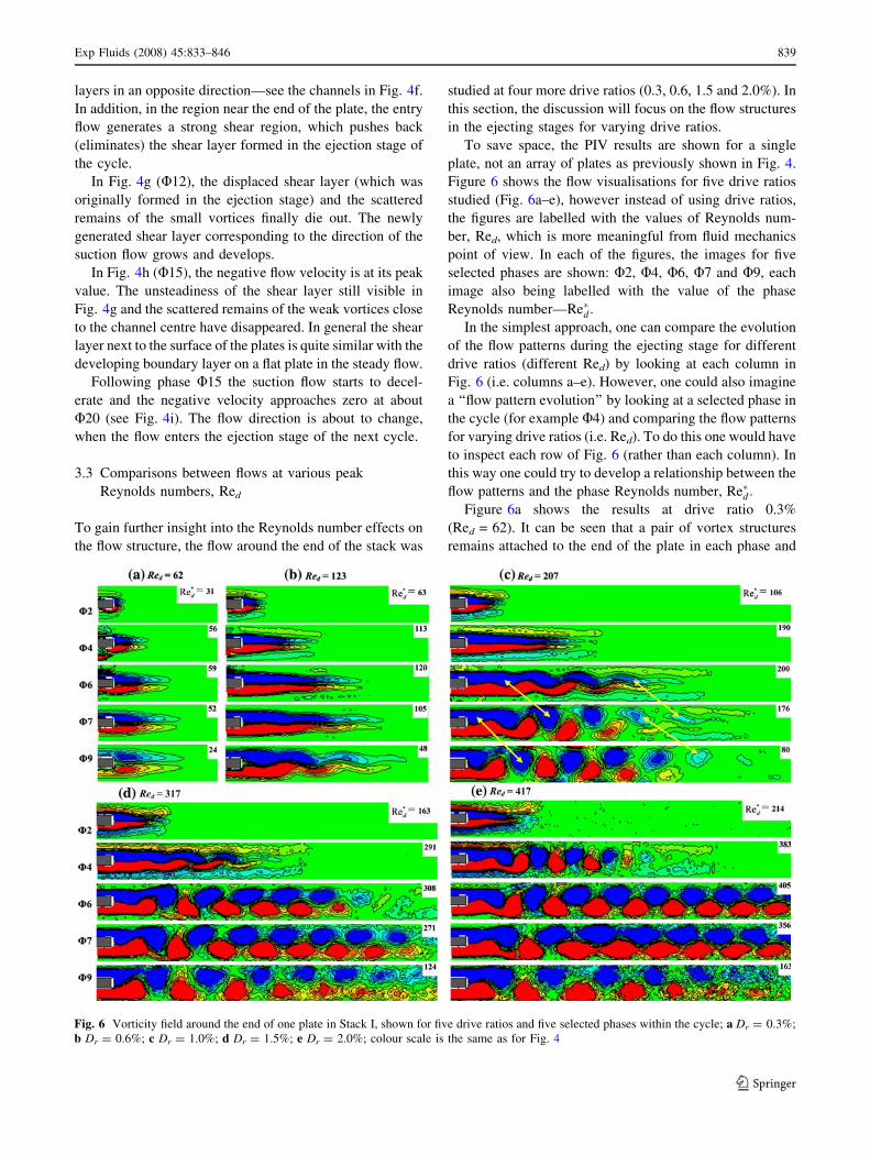
To save space, the PIV results are shown for a single

plate, not an array of plates as previously shown in Fig. 4.

Figure 6 shows the flow visualisations for five drive ratios

studied (Fig. 6a–e), however instead of using drive ratios,

the figures are labelled with the values of Reynolds num-

ber, Red, which is more meaningful from fluid mechanics

point of view. In each of the figures, the images for five

selected phases are shown: U2, U4, U6, U7 and U9, each

image also being labelled with the value of the phase

Reynolds number—Re�d:In the simplest approach, one can compare the evolution

of the flow patterns during the ejecting stage for different

drive ratios (different Red) by looking at each column in

Fig. 6 (i.e. columns a–e). However, one could also imagine

a ‘‘flow pattern evolution’’ by looking at a selected phase in

the cycle (for example U4) and comparing the flow patterns

for varying drive ratios (i.e. Red). To do this one would have

to inspect each row of Fig. 6 (rather than each column). In

this way one could try to develop a relationship between the

flow patterns and the phase Reynolds number, Re�d:Figure 6a shows the results at drive ratio 0.3%

(Red = 62). It can be seen that a pair of vortex structures

remains attached to the end of the plate in each phase and

Fig. 6 Vorticity field around the end of one plate in Stack I, shown for five drive ratios and five selected phases within the cycle; a Dr = 0.3%;

b Dr = 0.6%; c Dr = 1.0%; d Dr = 1.5%; e Dr = 2.0%; colour scale is the same as for Fig. 4

Exp Fluids (2008) 45:833–846 839

123

remains symmetric relative to the centre line in all phases.

The size and strength of the vortices clearly increases as the

phase Reynolds number increases throughout the acceler-

ating stage (see U2 and U4) and increases further in the

decelerating flow up until phases U6 or U7. As the vorticity

fed from the plate boundary layer decreases, so does the

strength of the vortices (see U9).

Figure 6b shows the results at drive ratio 0.6%

(Red = 123). Compared with the vortex structures in

Fig. 6a, the vortices become more and more elongated in

the accelerating stage. Eventually (around phase U7), the

previously symmetrical structures become wavy and this

‘‘instability’’ amplifies in the deceleration phase (see the

asymmetric wavy structure in phase U9).

Figure 6c shows the results at drive ratio 1.0%

(Red = 207). They correspond to the results already shown

in Fig. 4. From both figures, one can find that the vortex

structure exhibits asymmetry in phases U5 and U6, that is

at an earlier phase than in Fig. 6b. The break-up of this

wavy pattern into a vortex ‘‘street’’ and subsequent shed-

ding from the plate occurs between phases U7 and U9.

Quite similar results can be seen in Fig. 6d, for drive

ratio 1.5% (Red = 317). The vortex structures become

unstable even earlier (U4). Further increase of drive ratio,

as illustrated in Fig. 6e (2.0%, Red = 417), leads to even

earlier break-up of the initial symmetrical structures—by

phase U4 a vortex ‘‘street’’ is already in place).

One could attempt a qualitative analysis by comparing

images in Fig. 6 ‘‘row by row’’; that is by looking at

increasing drive ratios for a fixed phase. For example, the

first row of figures shows phase U2. From Fig. 6a to Fig. 6e

the phase Reynolds number increases from 31 to 214. One

can find that, the attached pair of vortices elongates, but

remains symmetric as the phase Reynolds number increases.

The second row of figures shows the ‘‘flow behaviour’’

for phase U4, as the phase Reynolds number increases from

56 to 383. One can clearly see an ‘‘evolution’’ of the flow

patterns similar to phase-by-phase evolution: a pair of

symmetric vortices (6a/U4), elongated symmetric vortices

(6b/U4 and 6c/U4) unstable/wavy elongated structure

(6d/U4) and alternate vortex shedding (6e/U4).

The third, fourth and fifth rows show the flow pattern

‘‘evolution’’ for phases U6, U7 and U9, respectively.

Similar trends in the ‘‘development’’ of the flow patterns

can be observed. However, clearly, the vortex shedding

pattern is present ‘‘earlier’’ when comparing drive ratios

left to right.

3.4 Comparisons between flows around Stack I

and Stack II

Similar experiments to those described with reference to

Stack I were carried out for the second configuration: Stack

II (see Table 1 for details). The main reason for selecting

this configuration was a further increase in the Reynolds

number (Red) and a change in the porosity of the stack. The

same drive ratios were tested which, given a different

porosity, resulted in somewhat modified velocities and

displacements. The Reynolds numbers were increased

roughly about five-fold.

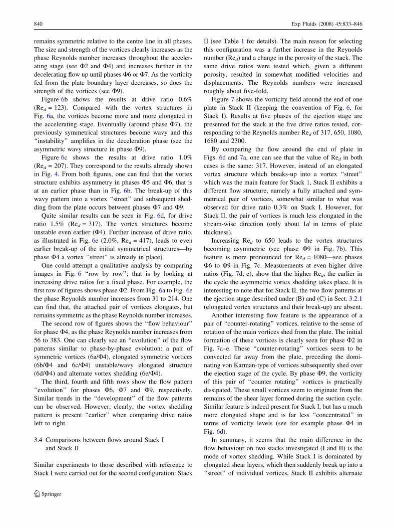
Figure 7 shows the vorticity field around the end of one

plate in Stack II (keeping the convention of Fig. 6, for

Stack I). Results at five phases of the ejection stage are

presented for the stack at the five drive ratios tested, cor-

responding to the Reynolds number Red of 317, 650, 1080,

1680 and 2300.

By comparing the flow around the end of plate in

Figs. 6d and 7a, one can see that the value of Red in both

cases is the same: 317. However, instead of an elongated

vortex structure which breaks-up into a vortex ‘‘street’’

which was the main feature for Stack 1, Stack II exhibits a

different flow structure, namely a fully attached and sym-

metrical pair of vortices, somewhat similar to what was

observed for drive ratio 0.3% on Stack I. However, for

Stack II, the pair of vortices is much less elongated in the

stream-wise direction (only about 1d in terms of plate

thickness).

Increasing Red to 650 leads to the vortex structures

becoming asymmetric (see phase U9 in Fig. 7b). This

feature is more pronounced for Red = 1080—see phases

U6 to U9 in Fig. 7c. Measurements at even higher drive

ratios (Fig. 7d, e), show that the higher Red, the earlier in

the cycle the asymmetric vortex shedding takes place. It is

interesting to note that for Stack II, the two flow patterns at

the ejection stage described under (B) and (C) in Sect. 3.2.1

(elongated vortex structures and their break-up) are absent.

Another interesting flow feature is the appearance of a

pair of ‘‘counter-rotating’’ vortices, relative to the sense of

rotation of the main vortices shed from the plate. The initial

formation of these vortices is clearly seen for phase U2 in

Fig. 7a–e. These ‘‘counter-rotating’’ vortices seem to be

convected far away from the plate, preceding the domi-

nating von Karman-type of vortices subsequently shed over

the ejection stage of the cycle. By phase U9, the vorticity

of this pair of ‘‘counter rotating’’ vortices is practically

dissipated. These small vortices seem to originate from the

remains of the shear layer formed during the suction cycle.

Similar feature is indeed present for Stack I, but has a much

more elongated shape and is far less ‘‘concentrated’’ in

terms of vorticity levels (see for example phase U4 in

Fig. 6d).

In summary, it seems that the main difference in the

flow behaviour on two stacks investigated (I and II) is the

mode of vortex shedding. While Stack I is dominated by

elongated shear layers, which then suddenly break up into a

‘‘street’’ of individual vortices, Stack II exhibits alternate

840 Exp Fluids (2008) 45:833–846

123

(bluff-body type) shedding very early on within the cycle

(as long as the Reynolds number is large enough). This

may well be responsible for the differences in Strouhal

numbers discussed in Sect. 3.5.

3.5 Frequency of vortex shedding

As illustrated in the previous sections, for both stacks, the

vortices will start to shed in an alternate fashion for a

sufficiently large Reynolds number, Red. This behaviour is

similar to vortex shedding from bluff bodies in steady

flows. This part of the study looked at the dependence of

vortex shedding frequency (and thus the Strouhal number)

on the Reynolds number, Red, and the geometry of the

stack. The measurements were performed using standard

hot-wire anemometry methods (Sect. 2) in order to collect

the fluctuating velocity signal behind the stack of plates.

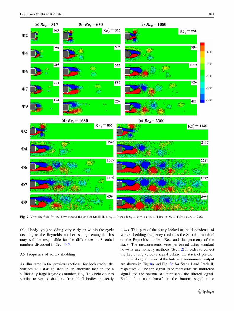
Typical signal traces of the hot-wire anemometer output

are shown in Fig. 8a and Fig. 8c for Stack I and Stack II,

respectively. The top signal trace represents the unfiltered

signal and the bottom one represents the filtered signal.

Each ‘‘fluctuation burst’’ in the bottom signal trace

Fig. 7 Vorticity field for the flow around the end of Stack II. a Dr = 0.3%; b Dr = 0.6%; c Dr = 1.0%; d Dr = 1.5%; e Dr = 2.0%

Exp Fluids (2008) 45:833–846 841

123

represents an event of vortex shedding in the ejection stage

of the acoustic cycle.

The frequency spectrum of the filtered signal trace is

analyzed using Fast Fourier Transform (FFT). The signal

trace is divided into data blocks, which contain 256 data

points, starting at the same phase of an acoustic cycle, and

including the whole ‘‘fluctuation burst’’ event. For each

block of data, a frequency spectrum is obtained. Subse-

quently all such frequency spectra, obtained for a given

experimental run, are ensemble-averaged and a mean fre-

quency spectrum is obtained. This enables extracting a

characteristic peak frequency. Figure 8b, d shows the mean

frequency spectra of the corresponding signal traces in the

left column of Fig. 8. As can be seen from the plots, the

curve covers a narrow band of frequencies, as opposed to a

sharp spike which would normally be obtained in steady

flows past bluff bodies. This is most likely due to variations

in the shedding frequency as the instantaneous velocity uM

changes over the ejection stage, but it may also reflect the

fact that vortex shedding is ‘‘quasi-periodic’’ with the

pattern changing slightly from cycle to cycle.

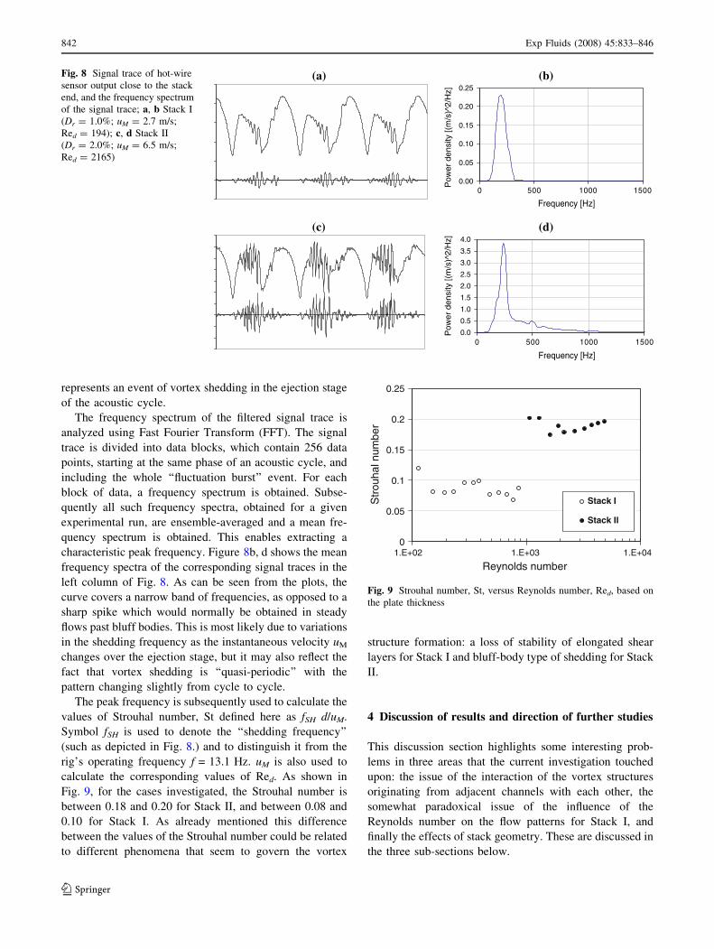
The peak frequency is subsequently used to calculate the

values of Strouhal number, St defined here as fSH d/uM.

Symbol fSH is used to denote the ‘‘shedding frequency’’

(such as depicted in Fig. 8.) and to distinguish it from the

rig’s operating frequency f = 13.1 Hz. uM is also used to

calculate the corresponding values of Red. As shown in

Fig. 9, for the cases investigated, the Strouhal number is

between 0.18 and 0.20 for Stack II, and between 0.08 and

0.10 for Stack I. As already mentioned this difference

between the values of the Strouhal number could be related

to different phenomena that seem to govern the vortex

structure formation: a loss of stability of elongated shear

layers for Stack I and bluff-body type of shedding for Stack

II.

4 Discussion of results and direction of further studies

This discussion section highlights some interesting prob-

lems in three areas that the current investigation touched

upon: the issue of the interaction of the vortex structures

originating from adjacent channels with each other, the

somewhat paradoxical issue of the influence of the

Reynolds number on the flow patterns for Stack I, and

finally the effects of stack geometry. These are discussed in

the three sub-sections below.

0.00

0.05

0.10

0.15

0.20

0.25

0 500 1000 1500

Frequency [Hz]

Frequency [Hz]

Pow

er d

ensi

ty [(

m/s

)^2/

Hz]

0.0

0.5

1.0

1.5

2.0

2.5

3.0

3.5

4.0

0 500 1000 1500

Pow

er d

ensi

ty [(

m/s

)^2/

Hz]

(a) (b)

(c) (d)

Fig. 8 Signal trace of hot-wire

sensor output close to the stack

end, and the frequency spectrum

of the signal trace; a, b Stack I

(Dr = 1.0%; uM = 2.7 m/s;

Red = 194); c, d Stack II

(Dr = 2.0%; uM = 6.5 m/s;

Red = 2165)

0

0.05

0.1

0.15

0.2

0.25

1.E+02 1.E+03 1.E+04

Reynolds number

Str

ouha

l num

ber

Stack I

Stack II

Fig. 9 Strouhal number, St, versus Reynolds number, Red, based on

the plate thickness

842 Exp Fluids (2008) 45:833–846

123

4.1 ‘‘Mirror’’ versus ‘‘translational’’ symmetries

between adjacent vortex streets

When inspecting the flow patterns generated by the stack of

plates such as those shown in Fig. 4d, e, it is clear that the

resulting vortex ‘‘streets’’ may exhibit either ‘‘mirror’’ or

‘‘translational’’ symmetries in relation to the channels’

centrelines. For example, looking at Fig. 4d, and counting

the channels from the bottom of the graph, it is clear that

for the first and second channels, the vortex streets have

‘‘mirror’’ symmetries, relative to the channel centre-line.

However, for the third channel the symmetry is ‘‘transla-

tional’’ (or there is an ‘‘anti-symmetry’’) in that the vortex

pattern shed from the third plate could be overlapped with

the vortex pattern shed from the fourth plate if the image

was simply shifted upwards. It should be noted that similar

problems are encountered in the steady flows past an array

of plates (e.g. Guillaume and LaRue 2002). The future

studies should investigate how the spacing between the

plates within the stack influences this kind of symmetrical

or anti-symmetrical alignment of vortices, and whether

there is some kind of a ‘‘lock-on’’ effect when the plates are

sufficiently close to one another. This relates to the ques-

tion of porosity values addressed in Sect. 4.3.

4.2 Reynolds number paradox

When Fig. 6 is studied ‘‘row-by-row’’, that is for different

drive ratios, but the same phase, one can see that as the

phase Reynolds number increases the flow pattern

‘‘evolves’’ through the stages that are described as (A)–(D)

in Sect. 3.2.1. The latter pattern (D) occurs at higher phase

Reynolds number than patterns (A)–(C). However, when

the flow patterns are studied ‘‘column-by-column’’, that is

for different phase Reynolds numbers within the same drive

ratio, the relationship between the flow pattern and the

phase Reynolds number is somewhat different. For example

in Fig. 6c, the flow becomes unstable at U6 (Re�d ¼ 200),

and the vortex shedding is observed at U7 (Re�d ¼ 176) and

U9 (Re�d ¼ 80). This indicates that the flow pattern that

usually corresponds to a high Reynolds at an earlier phase

can take place at a lower Reynolds number in the deceler-

ating stage. One can find more examples of this

phenomenon in Fig. 6. In Fig. 6e, Re�d is 214 at U2, and the

flow has a pair of elongated symmetric vortex structure. On

the other hand, in Fig. 6b, Re�d equals 48 at U9, and the flow

shows a pair of elongated wavy vortices. This clearly

illustrates that the transition between different flow patterns

cannot be defined by Reynolds numbers alone.

There are at least two explanations for this flow

behaviour (referred to here for brevity as ‘‘Reynolds

number paradox’’). The first factor could be the oscillating

pressure gradient. It is well known that a favourable

pressure gradient (responsible for the flow acceleration)

tends to suppress flow instabilities, while the adverse

pressure gradient (responsible for the flow deceleration)

tends to amplify them (e.g. Lee and Budwig 1991). This

may explain why the vortex structures represented in

Fig. 6c break up into a vortex street after phase U6.

However, an alternative explanation could be found for the

flows with higher Reynolds numbers (e.g. Fig. 6d, e, where

the break-up occurs in the accelerating phase): namely that

the vorticity generated on the surface of the plates is too

strong to be convected downstream in the form of an

elongated vortex structure and breaks-up so that the flow

may assume a more efficient form (vortex street) to convect

the vorticity downstream. It is likely that it is the combi-

nation of these two factors that decides on the exact nature

of the transition between the flow patterns. These aspects of

the flow could be studied by means of a rigorous flow

stability analysis, which however is somewhat beyond the

scope of the current experimental studies.

4.3 Similarity issues—geometry and flow parameters

The geometry of a stack of parallel plates (in the 2D

‘‘cross-sectional’’ sense) can be described by three

parameters: the plate thickness, d, the spacing between

plates, D and the length of plates, l. In all tests presented

here, the displacement amplitude of the oscillating gas

parcel, n, is much smaller than the length of the plates l.

Therefore, the effect of the stack length on the flow around

the end of the stack can be neglected (Swift 1988). Fur-

thermore, the stack porosity / can be defined as

D/(D + d), when the plates of the stack are placed evenly.

In this case any two of the three parameters, i.e. d, D and /,

can uniquely define the stack geometry.

It is also obvious from the current experimental results

that changing the Reynolds number, Red, can drastically

change the observed flow patterns. However, a triad of two

geometrical parameters and a velocity related parameter

(Reynolds number or velocity itself) are not sufficient to

define the problem entirely. Indeed a large body of litera-

ture related to the oscillatory flows past cylinders (Bearman

et al. 1985; Badr et al. 1995; Lin et al. 1996; Iliadis and

Anagnostopoulos 1998) suggests that frequency of the

forcing flow must appear in the problem description in one

form or another. A widely accepted parameter of this kind

is Keulegan-Carpenter number (KC), usually defined as

(velocity)/(frequency 9 dimension). It is easy to show that

this can be expressed here as the ratio of the displacement

amplitude to the thickness of the plate, n/d. Of course n can

be calculated from uM as n = uM /x, where x = 2pf is the

angular frequency of the acoustic oscillation.

Unfortunately, the data available in the open literature,

related to the geometry discussed in this paper (parallel

Exp Fluids (2008) 45:833–846 843

123

plates), is rather scarce and thus insufficient to perform

meaningful similarity studies. The already mentioned paper

by Blanc-Benon et al. (2003) allows extracting two

experimental ‘‘cases’’ (which are only for relatively small

drive ratios). The current work provides a few more

‘‘cases’’, but there is no independent data to verify any

similarities for larger drive ratios. It is therefore hoped that

the current work will motivate other researchers to carry

out similar studies in flow rigs of different designs.

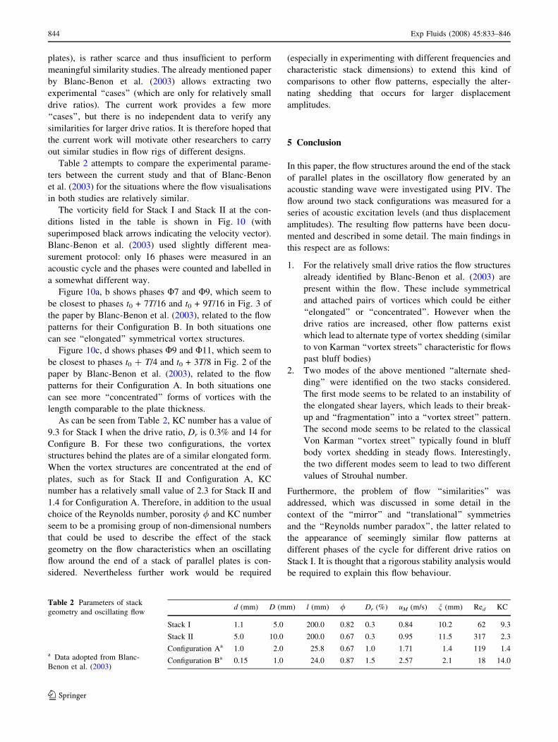
Table 2 attempts to compare the experimental parame-

ters between the current study and that of Blanc-Benon

et al. (2003) for the situations where the flow visualisations

in both studies are relatively similar.

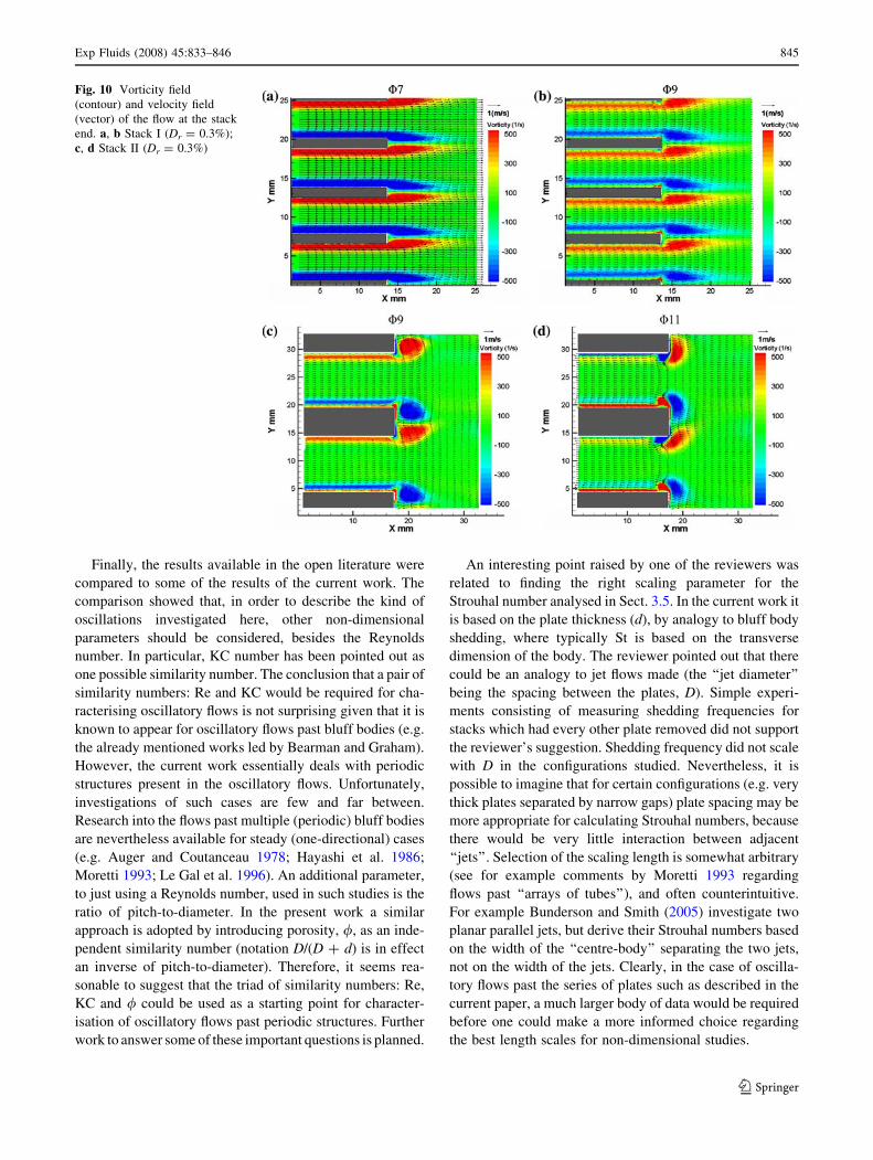
The vorticity field for Stack I and Stack II at the con-

ditions listed in the table is shown in Fig. 10 (with

superimposed black arrows indicating the velocity vector).

Blanc-Benon et al. (2003) used slightly different mea-

surement protocol: only 16 phases were measured in an

acoustic cycle and the phases were counted and labelled in

a somewhat different way.

Figure 10a, b shows phases U7 and U9, which seem to

be closest to phases t0 + 7T/16 and t0 + 9T/16 in Fig. 3 of

the paper by Blanc-Benon et al. (2003), related to the flow

patterns for their Configuration B. In both situations one

can see ‘‘elongated’’ symmetrical vortex structures.

Figure 10c, d shows phases U9 and U11, which seem to

be closest to phases t0 + T/4 and t0 + 3T/8 in Fig. 2 of the

paper by Blanc-Benon et al. (2003), related to the flow

patterns for their Configuration A. In both situations one

can see more ‘‘concentrated’’ forms of vortices with the

length comparable to the plate thickness.

As can be seen from Table 2, KC number has a value of

9.3 for Stack I when the drive ratio, Dr is 0.3% and 14 for

Configure B. For these two configurations, the vortex

structures behind the plates are of a similar elongated form.

When the vortex structures are concentrated at the end of

plates, such as for Stack II and Configuration A, KC

number has a relatively small value of 2.3 for Stack II and

1.4 for Configuration A. Therefore, in addition to the usual

choice of the Reynolds number, porosity / and KC number

seem to be a promising group of non-dimensional numbers

that could be used to describe the effect of the stack

geometry on the flow characteristics when an oscillating

flow around the end of a stack of parallel plates is con-

sidered. Nevertheless further work would be required

(especially in experimenting with different frequencies and

characteristic stack dimensions) to extend this kind of

comparisons to other flow patterns, especially the alter-

nating shedding that occurs for larger displacement

amplitudes.

5 Conclusion

In this paper, the flow structures around the end of the stack

of parallel plates in the oscillatory flow generated by an

acoustic standing wave were investigated using PIV. The

flow around two stack configurations was measured for a

series of acoustic excitation levels (and thus displacement

amplitudes). The resulting flow patterns have been docu-

mented and described in some detail. The main findings in

this respect are as follows:

1. For the relatively small drive ratios the flow structures

already identified by Blanc-Benon et al. (2003) are

present within the flow. These include symmetrical

and attached pairs of vortices which could be either

‘‘elongated’’ or ‘‘concentrated’’. However when the

drive ratios are increased, other flow patterns exist

which lead to alternate type of vortex shedding (similar

to von Karman ‘‘vortex streets’’ characteristic for flows

past bluff bodies)

2. Two modes of the above mentioned ‘‘alternate shed-

ding’’ were identified on the two stacks considered.

The first mode seems to be related to an instability of

the elongated shear layers, which leads to their break-

up and ‘‘fragmentation’’ into a ‘‘vortex street’’ pattern.

The second mode seems to be related to the classical

Von Karman ‘‘vortex street’’ typically found in bluff

body vortex shedding in steady flows. Interestingly,

the two different modes seem to lead to two different

values of Strouhal number.

Furthermore, the problem of flow ‘‘similarities’’ was

addressed, which was discussed in some detail in the

context of the ‘‘mirror’’ and ‘‘translational’’ symmetries

and the ‘‘Reynolds number paradox’’, the latter related to

the appearance of seemingly similar flow patterns at

different phases of the cycle for different drive ratios on

Stack I. It is thought that a rigorous stability analysis would

be required to explain this flow behaviour.

Table 2 Parameters of stack

geometry and oscillating flow

a Data adopted from Blanc-

Benon et al. (2003)

d (mm) D (mm) l (mm) / Dr (%) uM (m/s) n (mm) Red KC

Stack I 1.1 5.0 200.0 0.82 0.3 0.84 10.2 62 9.3

Stack II 5.0 10.0 200.0 0.67 0.3 0.95 11.5 317 2.3

Configuration Aa 1.0 2.0 25.8 0.67 1.0 1.71 1.4 119 1.4

Configuration Ba 0.15 1.0 24.0 0.87 1.5 2.57 2.1 18 14.0

844 Exp Fluids (2008) 45:833–846

123

Finally, the results available in the open literature were

compared to some of the results of the current work. The

comparison showed that, in order to describe the kind of

oscillations investigated here, other non-dimensional

parameters should be considered, besides the Reynolds

number. In particular, KC number has been pointed out as

one possible similarity number. The conclusion that a pair of

similarity numbers: Re and KC would be required for cha-

racterising oscillatory flows is not surprising given that it is

known to appear for oscillatory flows past bluff bodies (e.g.

the already mentioned works led by Bearman and Graham).

However, the current work essentially deals with periodic

structures present in the oscillatory flows. Unfortunately,

investigations of such cases are few and far between.

Research into the flows past multiple (periodic) bluff bodies

are nevertheless available for steady (one-directional) cases

(e.g. Auger and Coutanceau 1978; Hayashi et al. 1986;

Moretti 1993; Le Gal et al. 1996). An additional parameter,

to just using a Reynolds number, used in such studies is the

ratio of pitch-to-diameter. In the present work a similar

approach is adopted by introducing porosity, /, as an inde-

pendent similarity number (notation D/(D + d) is in effect

an inverse of pitch-to-diameter). Therefore, it seems rea-

sonable to suggest that the triad of similarity numbers: Re,

KC and / could be used as a starting point for character-

isation of oscillatory flows past periodic structures. Further

work to answer some of these important questions is planned.

An interesting point raised by one of the reviewers was

related to finding the right scaling parameter for the

Strouhal number analysed in Sect. 3.5. In the current work it

is based on the plate thickness (d), by analogy to bluff body

shedding, where typically St is based on the transverse

dimension of the body. The reviewer pointed out that there

could be an analogy to jet flows made (the ‘‘jet diameter’’

being the spacing between the plates, D). Simple experi-

ments consisting of measuring shedding frequencies for

stacks which had every other plate removed did not support

the reviewer’s suggestion. Shedding frequency did not scale

with D in the configurations studied. Nevertheless, it is

possible to imagine that for certain configurations (e.g. very

thick plates separated by narrow gaps) plate spacing may be

more appropriate for calculating Strouhal numbers, because

there would be very little interaction between adjacent

‘‘jets’’. Selection of the scaling length is somewhat arbitrary

(see for example comments by Moretti 1993 regarding

flows past ‘‘arrays of tubes’’), and often counterintuitive.

For example Bunderson and Smith (2005) investigate two

planar parallel jets, but derive their Strouhal numbers based

on the width of the ‘‘centre-body’’ separating the two jets,

not on the width of the jets. Clearly, in the case of oscilla-

tory flows past the series of plates such as described in the

current paper, a much larger body of data would be required

before one could make a more informed choice regarding

the best length scales for non-dimensional studies.

Fig. 10 Vorticity field

(contour) and velocity field

(vector) of the flow at the stack

end. a, b Stack I (Dr = 0.3%);

c, d Stack II (Dr = 0.3%)

Exp Fluids (2008) 45:833–846 845

123

Acknowledgments The authors would like to acknowledge the

support received from the Engineering and Physical Sciences

Research Council (EPSRC), UK and Universities, UK.

References

Al-Asmi K, Castro IP (1992) Vortex shedding in oscillatory flow:

geometrical effects. Flow Meas Instrum 3:187–202

Auger JL, Coutanceau J (1978) On the complex structure of the

downstream flow of cylindrical tube rows at various spacings,

Mech Res Commun 5:297–302

Bachelor GK (2000) An introduction to fluid dynamics. Cambridge

University Press, Cambridge

Badr HM, Dennis SCR, Kocabiyik S, Nguyen P (1995) Viscous

oscillatory flow about a circular cylinder at small to moderate

Strouhal number. J Fluid Mech 303:215–232

Barbi C, Favier DP, Maresca CA, Telionis DP (1986) Vortex

shedding and lock-on of a circular cylinder in oscillatory flow.

J Fluid Mech 170:527–544

Bearman PW, Downie MJ, Graham JMR, Obasaju ED (1985) Forces

on cylinders in viscous oscillatory flow at low Keulegan-

Carpenter numbers. J Fluid Mech 154:337–356

Blanc-Benon Ph, Besnoin E, Knio O (2003) Experimental and

computational visualization of the flow field in a thermoacoustic

stack. C.R. Mecanique 331:17–24

Bunderson NE, Smith BL (2005) Passive mixing control of plane

parallel jets. Exp Fluid 39:66–74

Chung YJ, Kang SH (2003) A study on the vortex shedding and lock-

on behind a square cylinder in an oscillatory incoming flow.

JSME Int J Ser B 46:250–261

De Bernardinis B, Graham JMR, Parker KH (1981) Oscillatory flow

around disks and through orifices. J Fluid Mech 102:279–299

Gopinath A, Harder DR (2000) An experimental study of heat transfer

from a cylinder in low-amplitude zero-mean oscillatory Flows.

Int J Heat Mass Transf 43:505–520

Guillaume DW, LaRue JC (2002) Comparison of the numerical and

experimental flowfield downstream of a plate array. Trans

ASME J Fluid Eng 124:284–286

Hayashi M, Sakurai A, Ohya J (1986) Wake interference of a row of

normal flat plates arranged side by side in a uniform flow. J Fluid

Mech 164:1–25

Iliadis G, Anagnostopoulos P (1998) Viscous oscillatory flow around

a circular cylinder at low Keulegan-Carpenter numbers and

frequency parameters. Int J Numer Method Fluid 26:403–442

Kovasznay LSG (1949) Hot-Wire Investigation of the Wake behind

Cylinders at Low Reynolds Numbers, Proceedings of the Royal

Society of London. Ser A Math Phys Sci 198(1053):174–190

Lee T, Budwig R (1991) The onset and development of circular-

cylinder vortex wakes in uniformly accelerating flows. J Fluid

Mech 232:611–627

Le Gal P, Peschard I, Chauve MP, Takeda Y (1996) Collective

behaviour of wakes downstream a row of cylinders. Phys Fluid

8:2097–2106

Lin XW, Bearman PW, Graham JMR (1996) A numerical study of

oscillatory flow about a circular cylinder for low values of beta

parameter. J Fluid Struct 10:501–526

Mao X, Marx D, Jaworski AJ (2005) PIV measurement of coherent

structures and turbulence created by an oscillating flow at the

end of a thermoacoustic stack. In: Proceedings of the iTi

conference in turbulence, Bad-Zwishenahn, Germany, 25–28

September

Marx D, Mao X, Jaworski AJ (2006) Acoustic coupling between the

loudspeaker and the resonator in a standing-wave thermoacoustic

device. Appl Acoust 67:402–419

Moretti PM (1993) Flow induced vibrations in arrays of cylinders.

Annu Rev Fluid Mech 25:99–114

Obasaju ED, Bearman PW, Graham JMR (1988) A study of forces,

circulation and vortex patterns around a circular cylinder in

oscillating flow. J Fluid Mech 196:467–494

Okajima A, Matsumoto T, Kimura S (1997) Force measurements and

flow visualization of bluff bodies in oscillatory flow. J Wind Eng

Ind Aerodynamics 69–71:213–228

Ralph ME (1986) Oscillatory flows in wavy-walled tubes. J Fluid

Mech 168:518–540

Roberts EPL, Mackley MR (1996) The development of asymmetry

and period doubling for oscillatory flow in baffled channels.

J Fluid Mech 328:19–48

Sumer BM, Jensen BL, Fredsbe J (1991) Effect of a plane boundary

on oscillatory flow around a circular cylinder. J Fluid Mech

225:271–300

Swift GW (1988) Thermoacoustic engines. J Acoust Soc Am

84:1145–1180

Swift GW (2002) Thermoacoustics: a unifying perspective for some

engines and refrigerators. Acoustical Society of America, New

York

Tatsuno M, Bearman PW (1990) A visual study of the flow around an

oscillating circular cylinder at low Keulegan-Carpenter numbers

and low Stokes numbers. J Fluid Mech 211:157–182

Ward B, Swift GW (2001) Design environment for low-amplitude

thermoacoustic engines (DeltaE). Tutorial and User’s Guide, Los

Alamos National Laboratory

Yellin EL (1966) Laminar-turbulent transition process in pulsatile

flow. Circ Res 19:791–804

846 Exp Fluids (2008) 45:833–846

123