
Munoz O. (2007) - Rapport de l'étude anthropologique préliminaire des restes osseux du Tumulus VIII.
Upload
khangminh22Category
view
3download
0
THESE DE DOCTORAT DE L’ECOLE DOCTORALE DE L’ECOLEPOLYTECHNIQUE
présentée par
Pierre RUYERIngénieur de l’Ecole Centrale de Lyon
SpécialitéMécanique
Laboratoire d’accueil :Commissariat à l’Energie AtomiqueDirection de l’Energie NucléaireDépartement d’Etude des RéacteursService de Simulation en THermohydrauliqueLaboratoire de Modélisation et de Développements de Logiciels
Sujet :
Modèle de champ de phasepour l’étude de l’ébullition
Thèse dirigée par M. Lev TRUSKINOVSKY
Soutenue le 17 juillet 2006 devant le jury composé de :
M. Sergey GAVRILYUK, Université Aix-Marseille III RapporteurM. Didier JAMET, CEA Grenoble Ingénieur responsableM. Samuel KOKH, CEA Saclay ExaminateurM. Chaouqi MISBAH, Université Joseph Fourier Grenoble I Rapporteur, PrésidentM. Mathis PLAPP, CNRS Ecole Polytechnique ExaminateurM. Lev TRUSKINOVSKY, CNRS Ecole Polytechnique Directeur de thèse


iii
THESE DE DOCTORAT DE L’ECOLE DOCTORALE DE L’ECOLEPOLYTECHNIQUE
présentée par
Pierre RUYERIngénieur de l’Ecole Centrale de Lyon
SpécialitéMécanique
Laboratoire d’accueil :Commissariat à l’Energie AtomiqueDirection de l’Energie NucléaireDépartement d’Etude des RéacteursService de Simulation en THermohydrauliqueLaboratoire de Modélisation et de Développements de Logiciels
Sujet :
Modèle de champ de phasepour l’étude de l’ébullition
Thèse dirigée par M. Lev TRUSKINOVSKY
Soutenue le 17 juillet 2006 devant le jury composé de :
M. Sergey GAVRILYUK, Université Aix-Marseille III RapporteurM. Didier JAMET, CEA Grenoble Ingénieur responsableM. Samuel KOKH, CEA Saclay ExaminateurM. Chaouqi MISBAH, Université Joseph Fourier Grenoble I Rapporteur, PrésidentM. Mathis PLAPP, CNRS Ecole Polytechnique ExaminateurM. Lev TRUSKINOVSKY, CNRS Ecole Polytechnique Directeur de thèse

Remerciements
Je tiens à remercier chaleureusement Monsieur Didier Jamet, ingénieur chercheur au C.E.A. et encadrant dece travail. Ses grandes qualités scientifiques, pédagogiques et humaines m’ont apporté à la fois de nombreuxenseignements, des conseils formateurs, une écoute patiente et disponible, et enfin un précieux soutien.
Je remercie également Monsieur Lev Truskinovsky, directeur de recherche au C.N.R.S. qui a assuré la di-rection de cette thèse. Sa rigueur et son exigence scientifique ont déterminé pour beaucoup l’orientation de cestravaux.
Je remercie particulièrement Monsieur Sergey Gavrilyuk, professeur à l’université Aix-Marseille, et Mon-sieur Chaouqi Misbah, professeur à l’université Joseph Fourier de Grenoble, d’avoir accepté de lire et de jugerce document en tant que rapporteurs. Je remercie également Monsieur Samuel Koch, ingénieur chercheur auC.E.A., et Monsieur Mathis Plapp chargé de recherche au C.N.R.S., pour leur participation au jury de cette thèse.
Ces travaux se sont déroulés au sein du Service de Simulation en Thermohydraulique au centre C.E.A. deGrenoble. Je remercie Messieurs Christian Chauliac et Bernard Faydide, chefs successifs de ce service, dem’avoir accueilli. Je remercie également Messieurs Fabien Boulanger et Frédéric Ducros, chefs successifs dulaboratoire d’accueil, pour le soutien qu’il m’ont accordé depuis ma candidature jusqu’à ma soutenance.
Je remercie enfin toutes les personnes de l’équipe du C.E.A. Grenoble qui m’ont entouré pendant ces annéesde thèse. Merci aussi à Adrien Pesenti pour la collaboration qu’il apporté à ce travail lors d’un stage.

Contents
1 Study of nucleate wall boiling near boiling crisis 31.1 The boiling regimes and the boiling crisis . . . . . . . . . . . . . . . . . . . . . . . . . . . . . 4
1.1.1 The Nukiyama curve . . . . . . . . . . . . . . . . . . . . . . . . . . . . . . . . . . . . 41.1.2 Vapor production and vapor release processes versus solid/fluid contact . . . . . . . . . 51.1.3 A few remarks about the boiling regimes and the boiling transition . . . . . . . . . . . . 61.1.4 Conclusion on the presentation of the boiling regimes . . . . . . . . . . . . . . . . . . . 7
1.2 Length scales and physical mechanisms . . . . . . . . . . . . . . . . . . . . . . . . . . . . . . 81.2.1 The three different scales . . . . . . . . . . . . . . . . . . . . . . . . . . . . . . . . . . 81.2.2 Two-phase flow scale . . . . . . . . . . . . . . . . . . . . . . . . . . . . . . . . . . . 91.2.3 “Mean bubble growth” scale . . . . . . . . . . . . . . . . . . . . . . . . . . . . . . . . 101.2.4 Local bubble description . . . . . . . . . . . . . . . . . . . . . . . . . . . . . . . . . . 121.2.5 Conclusion on the analysis of the different mechanisms related to NB regime near BC
conditions . . . . . . . . . . . . . . . . . . . . . . . . . . . . . . . . . . . . . . . . . . 121.3 Models of the boiling crisis mechanism . . . . . . . . . . . . . . . . . . . . . . . . . . . . . . 13
1.3.1 Boiling crisis’ mechanisms at the “two-phase flow” scale . . . . . . . . . . . . . . . . . 141.3.2 Boiling crisis’ mechanisms at the “mean bubble growth” scale . . . . . . . . . . . . . . 161.3.3 Boiling crisis’ mechanisms at the “local” scale . . . . . . . . . . . . . . . . . . . . . . 181.3.4 Conclusion on the presentation of the models for the BC mechanism . . . . . . . . . . . 22
1.4 Report of experimental observations . . . . . . . . . . . . . . . . . . . . . . . . . . . . . . . . 231.4.1 NB regime at high heat fluxes . . . . . . . . . . . . . . . . . . . . . . . . . . . . . . . 231.4.2 Interpretation of the experimental results: a local interpretation of the Zuber correlation 271.4.3 Conclusion on the study of local observations . . . . . . . . . . . . . . . . . . . . . . . 30
1.5 Study of the instability of a bubble growth . . . . . . . . . . . . . . . . . . . . . . . . . . . . . 301.5.1 A scenario at the DNB conditions . . . . . . . . . . . . . . . . . . . . . . . . . . . . . 301.5.2 Numerical simulation as a way to gain in understanding for the basic mechanism occur-
ring at DNB . . . . . . . . . . . . . . . . . . . . . . . . . . . . . . . . . . . . . . . . . 321.6 Conclusion on the study of the BC mechanism . . . . . . . . . . . . . . . . . . . . . . . . . . . 32
2 Solving the nucleate boiling flows, a review 352.1 The boiling as a free boundary problem . . . . . . . . . . . . . . . . . . . . . . . . . . . . . . 35
2.1.1 Necessity of a specific numerical treatment of the interface . . . . . . . . . . . . . . . . 352.1.2 Explicit tracking of the interfaces . . . . . . . . . . . . . . . . . . . . . . . . . . . . . 362.1.3 Interface capturing and diffuse interfaces . . . . . . . . . . . . . . . . . . . . . . . . . 372.1.4 General presentation of the diffuse interface models . . . . . . . . . . . . . . . . . . . . 382.1.5 Diffuse interface models versus sharp interface models . . . . . . . . . . . . . . . . . . 39
Conclusion on the numerical methods for the simulation of nucleate boiling . . . . . . . . . . . . . . 422.2 The second gradient method . . . . . . . . . . . . . . . . . . . . . . . . . . . . . . . . . . . . 42
2.2.1 From a diffuse interface model to a numerical method . . . . . . . . . . . . . . . . . . 422.2.2 The thermodynamic model . . . . . . . . . . . . . . . . . . . . . . . . . . . . . . . . . 422.2.3 Modifications and associated limitation of use . . . . . . . . . . . . . . . . . . . . . . . 462.2.4 The need for another thermodynamic model . . . . . . . . . . . . . . . . . . . . . . . . 48
2.3 Phase field models . . . . . . . . . . . . . . . . . . . . . . . . . . . . . . . . . . . . . . . . . 492.3.1 General presentation . . . . . . . . . . . . . . . . . . . . . . . . . . . . . . . . . . . . 49
v

vi CONTENTS
2.3.2 Constraints on the diffuse interface model for the nucleate boiling simulation . . . . . . 532.3.3 Review of the phase field models dedicated to phase transitions with density difference . 542.3.4 Conclusion : the need for a new phase field formulation . . . . . . . . . . . . . . . . . 57
2.4 Conclusion . . . . . . . . . . . . . . . . . . . . . . . . . . . . . . . . . . . . . . . . . . . . . 59
3 Phase field model: thermodynamic derivation 613.1 Thermodynamic modeling of multi-phase systems . . . . . . . . . . . . . . . . . . . . . . . . . 62
3.1.1 Single-phase state and equation of state . . . . . . . . . . . . . . . . . . . . . . . . . . 623.1.2 Multi-phase system and equations of state: Density difference and incompressibility of
the bulk phases . . . . . . . . . . . . . . . . . . . . . . . . . . . . . . . . . . . . . . . 643.1.3 The main variables of the phase field model . . . . . . . . . . . . . . . . . . . . . . . . 68
3.2 Introduction of a phase field thermodynamic variable . . . . . . . . . . . . . . . . . . . . . . . 703.2.1 A color function . . . . . . . . . . . . . . . . . . . . . . . . . . . . . . . . . . . . . . 703.2.2 Derivation of the equilibrium equations . . . . . . . . . . . . . . . . . . . . . . . . . . 703.2.3 Stability and equilibrium of single-phase states . . . . . . . . . . . . . . . . . . . . . . 743.2.4 Two-phase equilibrium: capillarity and equilibrium profiles . . . . . . . . . . . . . . . 76
3.3 Constitutive expression for the Gibbs free energy . . . . . . . . . . . . . . . . . . . . . . . . . 783.3.1 Isothermal constitutive form . . . . . . . . . . . . . . . . . . . . . . . . . . . . . . . . 783.3.2 Non-isothermal EOS . . . . . . . . . . . . . . . . . . . . . . . . . . . . . . . . . . . 79
3.4 Properties of the constitutive form of the thermodynamic potentials . . . . . . . . . . . . . . . 823.4.1 Single-phase states . . . . . . . . . . . . . . . . . . . . . . . . . . . . . . . . . . . . . 823.4.2 Specific heat capacity at constant pressure cP . . . . . . . . . . . . . . . . . . . . . . . 863.4.3 Latent heat and Clapeyron relation . . . . . . . . . . . . . . . . . . . . . . . . . . . . 873.4.4 Structure of an equilibrium planar interface . . . . . . . . . . . . . . . . . . . . . . . . 87
3.5 Conclusion about the derivation of the phase field model . . . . . . . . . . . . . . . . . . . . . 89
4 Study of the spherical symmetry problem 914.1 Review of the study of spherical equilibrium with diffuse interface models . . . . . . . . . . . . 914.2 General study of a spherical inclusion at equilibrium . . . . . . . . . . . . . . . . . . . . . . . 92
4.2.1 Equilibrium relations . . . . . . . . . . . . . . . . . . . . . . . . . . . . . . . . . . . . 924.2.2 Phase field and pressure values inside and ouside the spherical inclusion . . . . . . . . . 934.2.3 Surface tension and Laplace formula . . . . . . . . . . . . . . . . . . . . . . . . . . . . 95
4.3 Determination of the phase field profile . . . . . . . . . . . . . . . . . . . . . . . . . . . . . . 984.3.1 Analysis of the spherical symmetric equilibrium equation . . . . . . . . . . . . . . . . . 994.3.2 Analytical solving of the spherical symmetric equilibrium using piece-wise quadratic
approximations . . . . . . . . . . . . . . . . . . . . . . . . . . . . . . . . . . . . . . . 1004.3.3 Solving of the spherical symmetric equilibrium in a closed domain using finite difference
methods . . . . . . . . . . . . . . . . . . . . . . . . . . . . . . . . . . . . . . . . . . . 1044.4 Conclusion on the study of spherical inclusions at equilibrium . . . . . . . . . . . . . . . . . . 109
5 Derivation and study of the dynamics 1115.1 Dissipation free, compressible and isothermal case . . . . . . . . . . . . . . . . . . . . . . . . 111
5.1.1 Presentation of the variational principle . . . . . . . . . . . . . . . . . . . . . . . . . . 1115.1.2 Derivation of the system of governing equations . . . . . . . . . . . . . . . . . . . . . 115Conclusion on the study of the dissipation free isothermal compressible fluid dynamics . . . . . 118
5.2 Non-isothermal dynamics and dissipative processes . . . . . . . . . . . . . . . . . . . . . . . . 1185.2.1 Thermodynamic first principles . . . . . . . . . . . . . . . . . . . . . . . . . . . . . . 1195.2.2 Dissipative processes . . . . . . . . . . . . . . . . . . . . . . . . . . . . . . . . . . . . 121
5.3 The system of governing equations . . . . . . . . . . . . . . . . . . . . . . . . . . . . . . . . . 1245.3.1 Equation of evolution of the temperature . . . . . . . . . . . . . . . . . . . . . . . . . 1245.3.2 Non-dimensional equations . . . . . . . . . . . . . . . . . . . . . . . . . . . . . . . . 1255.3.3 Final writing of the governing equations . . . . . . . . . . . . . . . . . . . . . . . . . . 1285.3.4 Scaling of the system of governing equations in view of the study of the sharp interface
limit . . . . . . . . . . . . . . . . . . . . . . . . . . . . . . . . . . . . . . . . . . . . . 131

CONTENTS vii
6 Study of the stability of homogeneous states 1356.1 Review of the study of the stability of homogeneous states . . . . . . . . . . . . . . . . . . . . 135
6.1.1 Stability of homogeneous states using classical diffuse interface models . . . . . . . . . 1366.1.2 Study of the stability of homogeneous states with the phase field models . . . . . . . . . 137
6.2 General study of the perturbation of homogeneous states . . . . . . . . . . . . . . . . . . . . . 1386.2.1 System of governing equations . . . . . . . . . . . . . . . . . . . . . . . . . . . . . . . 1396.2.2 Parameter of the homogeneous state at equilibrium . . . . . . . . . . . . . . . . . . . . 1396.2.3 Linear stage of perturbation . . . . . . . . . . . . . . . . . . . . . . . . . . . . . . . . 1406.2.4 Linear system for the amplitudes . . . . . . . . . . . . . . . . . . . . . . . . . . . . . . 1406.2.5 Matrix of the system of linear equations . . . . . . . . . . . . . . . . . . . . . . . . . . 1416.2.6 The dispersion relation in the general case . . . . . . . . . . . . . . . . . . . . . . . . 141
6.3 General study of the dispersion relation . . . . . . . . . . . . . . . . . . . . . . . . . . . . . . 1426.3.1 Non-isothermal dissipative case . . . . . . . . . . . . . . . . . . . . . . . . . . . . . . 1426.3.2 Isothermal case . . . . . . . . . . . . . . . . . . . . . . . . . . . . . . . . . . . . . . . 1456.3.3 The influence of the dissipative processes on the stability of the state hs . . . . . . . . . 147
6.4 Stability of homogeneous states using linear interpolation . . . . . . . . . . . . . . . . . . . . . 1496.4.1 Non-isothermal dissipative case, the necessary and sufficient condition of stability . . . 1506.4.2 Non dissipative and isothermal case . . . . . . . . . . . . . . . . . . . . . . . . . . . . 1506.4.3 Dissipative isothermal case . . . . . . . . . . . . . . . . . . . . . . . . . . . . . . . . . 1506.4.4 Non-heat conducting case . . . . . . . . . . . . . . . . . . . . . . . . . . . . . . . . . 1516.4.5 Conclusion on the study of the linear interpolation . . . . . . . . . . . . . . . . . . . . 151
6.5 Stability with non-linear interpolation functions . . . . . . . . . . . . . . . . . . . . . . . . . . 1526.5.1 Liquid and vapor phase . . . . . . . . . . . . . . . . . . . . . . . . . . . . . . . . . . . 1526.5.2 Stability of homogeneous states for ϕhs different from 0 or 1 . . . . . . . . . . . . . . . 154
6.6 Conclusion on the study of the stability of homogeneous states . . . . . . . . . . . . . . . . . . 156
7 Analytical study of one-dimensional dynamics 1597.1 Sharp interface models . . . . . . . . . . . . . . . . . . . . . . . . . . . . . . . . . . . . . . . 159
7.1.1 Rankine-Hugoniot jump conditions . . . . . . . . . . . . . . . . . . . . . . . . . . . . 1607.1.2 Interface entropy production and non-equilibrium Clapeyron relations . . . . . . . . . . 161
7.2 Matched asymptotic expansions . . . . . . . . . . . . . . . . . . . . . . . . . . . . . . . . . . 1627.3 Uniform density phase transition . . . . . . . . . . . . . . . . . . . . . . . . . . . . . . . . . . 164
7.3.1 Phase-field and temperature solutions . . . . . . . . . . . . . . . . . . . . . . . . . . . 1647.3.2 Kinetic relation . . . . . . . . . . . . . . . . . . . . . . . . . . . . . . . . . . . . . . . 1687.3.3 Conclusion on the study of the solid-liquid one-dimensional phase change . . . . . . . . 171
7.4 Isothermal liquid-vapor flow with phase change . . . . . . . . . . . . . . . . . . . . . . . . . . 1717.4.1 Leading orders phase-field profile . . . . . . . . . . . . . . . . . . . . . . . . . . . . . 1727.4.2 Leading order pressure and velocity . . . . . . . . . . . . . . . . . . . . . . . . . . . . 1727.4.3 Kinetic relation . . . . . . . . . . . . . . . . . . . . . . . . . . . . . . . . . . . . . . . 173
7.5 Non-isothermal liquid-vapor flow with phase change . . . . . . . . . . . . . . . . . . . . . . . 1747.5.1 Leading order solutions . . . . . . . . . . . . . . . . . . . . . . . . . . . . . . . . . . . 1757.5.2 Kinetic relation . . . . . . . . . . . . . . . . . . . . . . . . . . . . . . . . . . . . . . . 176
7.6 Sharp interface limit for far from equilibrium phase transition . . . . . . . . . . . . . . . . . . . 1787.6.1 Leading order phase field equation and kinetic relation . . . . . . . . . . . . . . . . . . 1797.6.2 Illustrative example of non-linear leading order kinetic relation . . . . . . . . . . . . . . 180
7.7 Conclusion . . . . . . . . . . . . . . . . . . . . . . . . . . . . . . . . . . . . . . . . . . . . . 182
8 Numerical resolution of the system of governing equations 1838.1 Liquid-solid phase transition without mechanics . . . . . . . . . . . . . . . . . . . . . . . . . . 183
8.1.1 Time discretization scheme . . . . . . . . . . . . . . . . . . . . . . . . . . . . . . . . 1848.1.2 Steady-state one-dimensional phase change . . . . . . . . . . . . . . . . . . . . . . . . 1858.1.3 Unsteady phase-transition . . . . . . . . . . . . . . . . . . . . . . . . . . . . . . . . . 1898.1.4 Spherical symmetry . . . . . . . . . . . . . . . . . . . . . . . . . . . . . . . . . . . . 1928.1.5 Two-dimensional phase separation . . . . . . . . . . . . . . . . . . . . . . . . . . . . 193

viii CONTENTS
8.1.6 Two-dimensional solid-liquid phase transition . . . . . . . . . . . . . . . . . . . . . . . 1938.1.7 Conclusions . . . . . . . . . . . . . . . . . . . . . . . . . . . . . . . . . . . . . . . . . 196
8.2 Isothermal phase change . . . . . . . . . . . . . . . . . . . . . . . . . . . . . . . . . . . . . . 1968.2.1 Resolution algorithm . . . . . . . . . . . . . . . . . . . . . . . . . . . . . . . . . . . . 1968.2.2 One-dimensional isothermal steady state phase change . . . . . . . . . . . . . . . . . . 1978.2.3 Two-dimensional numerical simulation . . . . . . . . . . . . . . . . . . . . . . . . . . 200
8.3 Non-isothermal dissipative liquid-vapor flows with phase change . . . . . . . . . . . . . . . . . 2028.3.1 Saturation curve . . . . . . . . . . . . . . . . . . . . . . . . . . . . . . . . . . . . . . 2028.3.2 Dynamic phase change in an open system . . . . . . . . . . . . . . . . . . . . . . . . . 2028.3.3 Attempts to solve two-dimensional phase change problems . . . . . . . . . . . . . . . . 205
8.4 Conclusions and perspectives . . . . . . . . . . . . . . . . . . . . . . . . . . . . . . . . . . . . 209
A Sharp model 217A.1 Equivalent sharp interface . . . . . . . . . . . . . . . . . . . . . . . . . . . . . . . . . . . . . 217
A.1.1 Interface values . . . . . . . . . . . . . . . . . . . . . . . . . . . . . . . . . . . . . . . 217A.1.2 Excess quantities and interface location . . . . . . . . . . . . . . . . . . . . . . . . . . 218A.1.3 Surface tension coefficient . . . . . . . . . . . . . . . . . . . . . . . . . . . . . . . . . 219
A.2 Rankine Hugoniot and kinetic relations . . . . . . . . . . . . . . . . . . . . . . . . . . . . . . 222A.2.1 Liquid-vapor interface jump conditions . . . . . . . . . . . . . . . . . . . . . . . . . . 222A.2.2 Interface entropy production . . . . . . . . . . . . . . . . . . . . . . . . . . . . . . . . 223A.2.3 Kinetic relations and laws for the interface temperature and pressure . . . . . . . . . . . 225A.2.4 Sharp interface model inherited from the outer problem of matched asymptotic expansions228A.2.5 Conclusion . . . . . . . . . . . . . . . . . . . . . . . . . . . . . . . . . . . . . . . . . 228
B Matched asymptotic expansions 229B.1 The method of matched asymptotic expansions . . . . . . . . . . . . . . . . . . . . . . . . . . 229
B.1.1 Principle . . . . . . . . . . . . . . . . . . . . . . . . . . . . . . . . . . . . . . . . . . 229B.1.2 Inner and outer solutions, expansions, and matching . . . . . . . . . . . . . . . . . . . 230
B.2 First system of equations, uniform density case . . . . . . . . . . . . . . . . . . . . . . . . . . 232B.2.1 Solutions of the outer problem at order O(1) . . . . . . . . . . . . . . . . . . . . . . . . 232B.2.2 Outer problem at order O(ε) . . . . . . . . . . . . . . . . . . . . . . . . . . . . . . . . 233B.2.3 Order parameter profile at order O(1) . . . . . . . . . . . . . . . . . . . . . . . . . . . 233B.2.4 Temperature profile at order O(1) . . . . . . . . . . . . . . . . . . . . . . . . . . . . . 234B.2.5 System of equations for the inner problem at order O(ε) . . . . . . . . . . . . . . . . . 234B.2.6 Interface temperature T i
0 . . . . . . . . . . . . . . . . . . . . . . . . . . . . . . . . . . 235B.2.7 Phase-field inner profile at order O(ε), ϕ1(x) . . . . . . . . . . . . . . . . . . . . . . . . 236B.2.8 The leading order term for the jump in heat flux, Jq0K . . . . . . . . . . . . . . . . . . . 239B.2.9 Determination of JT1K . . . . . . . . . . . . . . . . . . . . . . . . . . . . . . . . . . . 240B.2.10 Study of the profile of T1(x) . . . . . . . . . . . . . . . . . . . . . . . . . . . . . . . . 241B.2.11 System of inner equations at order O(ε)2 . . . . . . . . . . . . . . . . . . . . . . . . . 242B.2.12 Determination of Jq1K . . . . . . . . . . . . . . . . . . . . . . . . . . . . . . . . . . . 242B.2.13 Determination of T1(0) and of T1 . . . . . . . . . . . . . . . . . . . . . . . . . . . . 242
B.3 Isothermal approximation . . . . . . . . . . . . . . . . . . . . . . . . . . . . . . . . . . . . . . 243B.3.1 Outer problem . . . . . . . . . . . . . . . . . . . . . . . . . . . . . . . . . . . . . . . 244B.3.2 Leading order system of governing equations of the inner problem . . . . . . . . . . . . 244B.3.3 Order parameter inner profile at order O(1) . . . . . . . . . . . . . . . . . . . . . . . . 245B.3.4 Velocity inner profile at leading order . . . . . . . . . . . . . . . . . . . . . . . . . . . 245B.3.5 Pressure inner profile at leading order . . . . . . . . . . . . . . . . . . . . . . . . . . . 246B.3.6 Determination of second order inner profile for the velocity and pressure V1 and P1 . . . 249B.3.7 Determination of P1 . . . . . . . . . . . . . . . . . . . . . . . . . . . . . . . . . . . 250
B.4 Liquid-vapor non-isothermal non-viscous case . . . . . . . . . . . . . . . . . . . . . . . . . . . 251B.4.1 First order inner problem . . . . . . . . . . . . . . . . . . . . . . . . . . . . . . . . . . 251B.4.2 Second order inner problem . . . . . . . . . . . . . . . . . . . . . . . . . . . . . . . . 252B.4.3 Jump in outer temperature at order O(ε) . . . . . . . . . . . . . . . . . . . . . . . . . . 253

CONTENTS ix
B.4.4 Relation between P1 and T1 . . . . . . . . . . . . . . . . . . . . . . . . . . . . . . 253B.4.5 Jump in heat flux at order O(ε), Jq1K . . . . . . . . . . . . . . . . . . . . . . . . . . . . 254B.4.6 Concluding remarks . . . . . . . . . . . . . . . . . . . . . . . . . . . . . . . . . . . . 255
C Spatial and time discretization schemes 257C.1 Time stepping: the Euler scheme . . . . . . . . . . . . . . . . . . . . . . . . . . . . . . . . . . 257C.2 Spatial discretization scheme . . . . . . . . . . . . . . . . . . . . . . . . . . . . . . . . . . . . 258C.3 Solving alogorithm . . . . . . . . . . . . . . . . . . . . . . . . . . . . . . . . . . . . . . . . . 259
Résumé en français 261I Étude de la crise d’ébullition . . . . . . . . . . . . . . . . . . . . . . . . . . . . . . . . . . . . 264
I.1 Crise d’ébullition et régimes d’ébullition . . . . . . . . . . . . . . . . . . . . . . . . . 264I.2 Mécanismes physiques . . . . . . . . . . . . . . . . . . . . . . . . . . . . . . . . . . . 265I.3 Modélisation de la crise d’ébullition . . . . . . . . . . . . . . . . . . . . . . . . . . . . 267I.4 Un mécanisme pour la crise d’ébullition à l’échelle locale . . . . . . . . . . . . . . . . 268I.5 Conclusion de notre étude de la crise d’ébullition . . . . . . . . . . . . . . . . . . . . . 270
II Méthodes numériques pour l’étude des écoulements liquide-vapeur . . . . . . . . . . . . . . . . 271II.1 Les familles de méthodes . . . . . . . . . . . . . . . . . . . . . . . . . . . . . . . . . . 271II.2 Modèle à interface diffuse et méthode numérique . . . . . . . . . . . . . . . . . . . . . 271II.3 Modèle de van der Waals . . . . . . . . . . . . . . . . . . . . . . . . . . . . . . . . . . 271II.4 Modèles de champ de phase . . . . . . . . . . . . . . . . . . . . . . . . . . . . . . . . 272II.5 Liste de contraintes pour le modèle de champ de phase . . . . . . . . . . . . . . . . . . 273II.6 Modèles de champ de phase existants . . . . . . . . . . . . . . . . . . . . . . . . . . . 274
III Fermeture thermodynamique du modèle . . . . . . . . . . . . . . . . . . . . . . . . . . . . . . 274III.1 Description thermodynamique d’un système multiphasique . . . . . . . . . . . . . . . . 274III.2 Introduction d’une variable thermodynamique de type champ de phase . . . . . . . . . . 275III.3 Expression de l’enthalpie libre massique . . . . . . . . . . . . . . . . . . . . . . . . . . 278
IV Symétrie sphérique . . . . . . . . . . . . . . . . . . . . . . . . . . . . . . . . . . . . . . . . . 283IV.1 Introduction et problématique . . . . . . . . . . . . . . . . . . . . . . . . . . . . . . . 283IV.2 Équation d’équilibre . . . . . . . . . . . . . . . . . . . . . . . . . . . . . . . . . . . . 283IV.3 Détermination de la solution d’équilibre . . . . . . . . . . . . . . . . . . . . . . . . . . 285IV.4 Solution numérique pour un domaine de longueur finie . . . . . . . . . . . . . . . . . . 287
V Dynamique des fluides . . . . . . . . . . . . . . . . . . . . . . . . . . . . . . . . . . . . . . . 291V.1 Cas non-dissipatif et compressible . . . . . . . . . . . . . . . . . . . . . . . . . . . . . 291V.2 Cas dissipatif anisotherme . . . . . . . . . . . . . . . . . . . . . . . . . . . . . . . . . 293V.3 Étude du système d’équations . . . . . . . . . . . . . . . . . . . . . . . . . . . . . . . 294
VI Stabilité des états homogènes . . . . . . . . . . . . . . . . . . . . . . . . . . . . . . . . . . . . 299VI.1 Étude bibliographique . . . . . . . . . . . . . . . . . . . . . . . . . . . . . . . . . . . 299VI.2 Perturbation d’un état homogène . . . . . . . . . . . . . . . . . . . . . . . . . . . . . . 299VI.3 Stade d’évolution linéaire d’une perturbation . . . . . . . . . . . . . . . . . . . . . . . 300VI.4 Étude générale de la relation de dispersion . . . . . . . . . . . . . . . . . . . . . . . . . 301VI.5 Cas d’une interpolation linéaire des fonctions d’état . . . . . . . . . . . . . . . . . . . . 303VI.6 Cas d’une interpolation non-linéaire . . . . . . . . . . . . . . . . . . . . . . . . . . . . 303VI.7 Conclusion . . . . . . . . . . . . . . . . . . . . . . . . . . . . . . . . . . . . . . . . . 304
VII Étude analytique de la dynamique de changement de phase . . . . . . . . . . . . . . . . . . . . 305VII.1 Modélisation de type interface-discontinue . . . . . . . . . . . . . . . . . . . . . . . . 305VII.2 Développements asymptotiques raccordés . . . . . . . . . . . . . . . . . . . . . . . . . 306VII.3 Transition de phase et masse volumique uniforme . . . . . . . . . . . . . . . . . . . . . 307VII.4 Transition de phase isotherme . . . . . . . . . . . . . . . . . . . . . . . . . . . . . . . 308VII.5 Transition de phase liquide-vapeur anisotherme . . . . . . . . . . . . . . . . . . . . . . 308
VIII Étude numérique du modèle . . . . . . . . . . . . . . . . . . . . . . . . . . . . . . . . . . . . 311VIII.1 Transition de phase sans écoulement . . . . . . . . . . . . . . . . . . . . . . . . . . . . 311VIII.2 Transition de phase isotherme . . . . . . . . . . . . . . . . . . . . . . . . . . . . . . . 312VIII.3 Transition de phase anisotherme . . . . . . . . . . . . . . . . . . . . . . . . . . . . . . 313

x CONTENTS
VIII.4 Conclusion . . . . . . . . . . . . . . . . . . . . . . . . . . . . . . . . . . . . . . . . . 316IX Conclusion et perspectives . . . . . . . . . . . . . . . . . . . . . . . . . . . . . . . . . . . . . 317

CONTENTS xi
Notations
Latin letters
At Atwood numberA numerical constantcP specific heat capacity at constant pressureC constant ofintegratione specific internal energyf specific Helmholtz free energyF volumetric helmholtz free energyFr Froude numberg specific Gibbs free energyG volumetric Gibbs free energyG modified pressureG driving force~g0 gravityh specific enthalpyh interface thicknessI identity matrixk heat conductivitykx wave numberL latent heatL LagrangeanL lenght scaleL linear operatorM matrix~n unitary vector along the normal to an interfaceP pressureP modified pressurePe Peclet numberq heat fluxr radial coordinater non-dimensional coordinateRe Reynolds numberRs Interface entropy productions specific entropyS t Stefan numbert timeT temperaturev specific volume~V velocity fieldW double well functionW rate of workWe Weber number(x, y, z) cartesian coordinatesx non-dimensional abscissa

xii CONTENTS
Greek lettersα non-dimensional kinetic parameterαP coefficient of thermal expansionγ non-dimensional numberΓ mass transfer rateδ variationδ variational derivativeε non-dimensional interface thicknessε parameter for the variation of the pathη viscosityθ non-dimensional temperature differenceκ mobility coefficientλ capillarity coefficientΛ linear operatorµ thermodynamic potentialµ variational thermodynamic potentialν interpolation functionξ Lagrangean coordinateΠ pressure levelρ densityσ coefficient of surface tensionτ stress tensorϕ phase field variableΦ non-local dependence coefficientχT coefficient of isothermal compressibility~Ψ non-local dependenceω growth rateΩ volume

Introduction
Context
Boiling flows involve both two-phase fluid mechanics and phase change process. They are present in a vast vari-ety of heat exchangers from micro-heat-pipes to large industrial facilities. The use of boiling fluids is motivatedby the efficiency of the nucleate boiling regime to extract heat from a heated wall. Indeed, in boiling systems,in addition to the single phase sensible heat transport, the latent heat transport plays a major role. Moreover, theheat transfer process occurs at a quasi-constant temperature: the saturation temperature. In the nuclear industry,phase change process are of interest mainly in the study of potential accidental scenarii, where phenomena likethe boiling crisis can occur. The improvement and control (mainly for safety reasons) of industrial facilities isconstrained by the understanding of the boiling process. Both large scale mechanisms (averaged bubbly flow)and small scale mechanisms (at the scale of individual bubbles) play an important role in the boiling heat transferprocess, e.g. Carey [28]. As a consequence, the study of the boiling process is scientifically challenging.
The study of industrial configurations requires the use of large scale analysis tools of the boiling process.The corresponding models are based on space and time averaged governing equations. As a consequence of thisaveraging procedure, the models must be supplemented by closure laws to be solved. These specific closure lawsare generally based on experimental data. But these laws are often devoted to specific configurations and have alimited range of validity, which limits the accuracy and versatility of their use. There is thus a need of closurelaws inherited from the study of the local scale phenomena. Experiments at the bubble scale are (i) complexto set-up and (ii) difficult to analyze because of the difficulty to get local measurements. The use of directnumerical simulation does not bear this latter limitation and is therefore a promising tool to get improved closurelaws. Direct numerical simulation takes into account the whole spectrum of space and time scales. Its use isthus restricted by the computers’ limitations to length scales of the order of magnitude of the centimeter andtime scales of the order of magnitude of the second. As a consequence, it cannot be used directly for the studyof industrial configurations. Nevertheless, it can be used to study bubble scale phenomena and then to developvalidated larger scale models, for example dedicated to the boiling crisis.
Boiling crisis
The phenomenon Beyond a particular high value of the wall heat flux, called the critical heat flux, a transitionof the boiling regime suddently occurs: this is called the boiling crisis. This transition leads to a very fast andvery large increase of the wall temperature. This increase can eventually lead to the melting of the wall: this iscalled the burnout. The physical mechanism at the origin of this transition is nowadays still not well understood.Its understanding is in itself an interesting scientific challenge. Moreover, its consequence, namely the burnout,can further lead to the destruction of the heat exchanger: boiling crisis must be thus avoided for safety reasons.In this study, we focus on this particular phenomenon of the boiling process.
Study of the boiling crisis There is a long history of the study of the boiling crisis and several attempts havebeen made to model its mechanisms. However, there is a lack of experimental evidence that could support anyof these theories. More generally, there is a large number of experimental efforts that need to be pursued in orderto have a clear understanding of the phenomenon, e.g. Sadavisan et al. [117]. In chapter 1, we study the currentunderstanding of the boiling crisis and identify the major physical mechanisms potentially involved. It leads usto define a target problem to study: the possible transition in the bubble growth regime at high wall heat flux.According to the physical mechanisms involved in this process, numerical simulation is proposed as the mostrelevant tool. This intermediate conclusion motivates the developments made in the remainder of the study.
1

2 CONTENTS
A diffuse interface model for the numerical study of the boiling flows at the bubble scale
The goal of this part of the study is to develop a model that can be used as a numerical method for the computationof boiling flows. The different numerical methods allowing the study of a bubble growth or more generallyof liquid-vapor flows with phase change at the bubble scale are presented and analyzed in chapter 2. Mostof the methods are based on the Gibbs theory of the interface: the interface is sharp, i.e. it is modeled as asurface of discontinuity. The difficulties of the computation of boiling flows are related to the management ofthe interface motion especially when phase change occurs. The methods based on diffuse interface models, forwhich the interface is viewed as a volumetric transition layer, propose a thermodynamically consistent settingof the computed governing equations, including the liquid-vapor interface dynamics. This induces numericalmethods that are easier to handle since, contrarily to the methods based on sharp interface models, no particulartreatment of the interface is required. However, the physical thickness of the interface transition layer is of theorder of magnitude of the Ångströms as soon as the system is far from the critical conditions. As a consequence,the direct use of the diffuse interface models is irrelevant for simulations of mechanisms at the bubble scale. Wethus turn our attention toward phase field methods. The thermodynamic model used in these methods is basedon the introduction of an additional abstract variable or internal parameter, called the phase field, to describemulti-phase or multi-component systems, as introduced by Truskinovsky [136]. Existing phase field methodsare mainly devoted to the study of solid-liquid or solid-solid phase transitions. They allow to deal with anartificial but thermodynamically consistent smearing of the interface. This latter property is attractive from bothmodeling and computational points of view. However, the review of the existing models shows that there is aneed to derive a new formulation adapted to the study of the liquid-vapor transition.
In chapter 3, we first study the phase field thermodynamic model. We propose a constitutive form for thethermodynamic potential that allows to control both the diffuse interface description and the bulk phase physicalproperties. The structure of the interface for the planar and spherical symmetric two-phase equilibrium cases arestudied in chapters 3 and 4. In particular, it is shown that the description of spherical inclusions is consistent withthe Laplace theory. We then study dynamics and introduce dissipative processes in the model in chapter 5. Wethus derive the thermodynamically consistent set of governing equations that includes the model for the interfacedynamics. The set of governing equations is then studied in two theoretical configurations: the stability ofhomogeneous states (see chapter 6) and the one-dimensional steady state phase change process (see chapter 7).In particular, we study the equivalent sharp interface model and derive its kinetic relation that is a necessaryclosure relation, e.g. Truskinovsky [134]. The use of this formalism provides a clear interpretation of the sharplimit of phase field equations. Finally, in chapter 8, we present first computations and study the ability of themodel to be used for the study of bubble growth dynamics.

Chapter 1
Study of nucleate wall boiling near boilingcrisis conditions:Toward a gain in understanding
Introduction
Boiling crisis (BC) is an instability of the heat transfer process between a hot wall and a boiling fluid that leadsto a sudden transition in the behavior of the boiling system. The consequences of this transition can lead to walldamages (burnout). The efficiency and design of industrial heat exchangers using boiling fluids (and in particularnuclear power plants for safety reasons) is therefore constrained by the fact that the BC phenomenon must notoccur to prevent the destruction of the facility, should it be partial. Despite more than 70 years of study, themechanism leading to the BC still remains obscure. Its understanding is important from an industrial point ofview and scientifically challenging. This study proposes a review of the models and experimental observationsconcerning the mechanisms of the BC and aims at identifying some potential triggering instabilities in the patternof the nucleate boiling regime near the BC conditions. The goal is to deduce from this study a target problem tosolve (and some ways to study it) that could help improving the understanding of the BC phenomenon. This leadsus naturally to the motivation of the numerical simulation of bubble growth and the subsequent development ofa numerical method dedicated to it.
This chapter is organized as follows. In section 1.1, we briefly introduce the classical description of thedifferent regimes of boiling heat transfer. The boiling crisis is defined as the departure (transition) from thenucleate boiling regime (DNB) that occurs at large heat flux and is associated to the drying of the heating surface.In the following, we therefore focus on this regime. In section 1.2, we distinguish three different length scalesfor the study of the nucleate boiling regime and define the main physical mechanisms associated to each lengthscale. The goal is to define a framework for the analysis of the boiling crisis phenomenon as being triggeredby an instability that takes place at one of these length scales. In section 1.3, we establish the state of the artof the modeling of the boiling crisis. We introduce the Zuber correlation, which is one of the most efficientcorrelation to predict the DNB, and we establish the main open questions concerning the nature of the BCinstability. In section 1.4, we briefly report some recent experimental results attesting the existence of a specificregime in the near-wall region close to the BC conditions. We then suggest a local interpretation of the Zubercorrelation consistent with these recent direct observations. In section 1.5, we review the existing models for theboiling crisis that can be related to the local interpretation of the Zuber correlation and conclude on the necessityof pursuing the analysis of the instabilities of a bubble growing over a heated wall. Due to the nature of theequations describing such a bubble growth, simplifying models allowing analytical results can be viewed as toorigid and it appears as useful to study the whole system of governing equations using numerical simulations. Thislast statement constitutes the motivation for the developments presented in the remainder of this study.
3

4 CHAPTER 1. STUDY OF NUCLEATE WALL BOILING NEAR BOILING CRISIS
1.1 The boiling regimes and the boiling crisis
In this section, we present the classical description of the boiling regimes and introduce the BC phenomenonas the transition between two different boiling regimes. This section reproduces classical considerations aboutboiling systems and is therefore devoted to readers unaware of these questions. A more detailed presentation ofthe boiling process can be found in [28] or in [45] among others.
This section is organized as follows. First, we introduce the different boiling regimes with the help of theclassical representation of the Nukiyama curve ( section 1.1.1). Then we describe more precisely the maincharacteristics of the different regimes by describing the different nature of the physical processes occurring in anear wall region (section 1.1.2).
1.1.1 The Nukiyama curve
Let us consider the heat transfer process from a heated solid to a boiling fluid. In 1934, Nukiyama [103] ex-perimentally studied the heat transfer coefficient of the process for a pool configuration and first introduced itsessential features including observation of the process instabilities. The pool boiling experimental set-up consistsin a boiling fluid confined in a pool and therefore does not include any external mean flow. The heating solid iseither a plane plate, a wire, a ribbon or one of the bounding wall of the pool. It is required that its dimensionsexceed the characteristic dimension of the vapor inclusion (typical bubble radius) in order to ignore size effects.In the remainder of this study, we consider by default the pool boiling of pure fluids with an heated horizontalwall at the bottom of the pool as represented on figure 1.1. Let us introduce the amount of heat transmittedthrough the solid-fluid contact area q and the mean temperature 〈T 〉 of the wall. There exists a typical value ofthe temperature at the liquid-vapor interface at thermodynamic equilibrium at the pressure P of the system, sayTsat(P). This temperature is considered as reached asymptotically, i.e. sufficiently far from the heated wall. Itappears as naturally relevant, since we describe boiling systems as a heat exchange process, to characterize thewall temperature by 〈∆T 〉 = 〈T 〉 − T sat(P) instead of 〈T 〉; 〈∆T 〉 is called the wall superheat. The heat transfercoefficient of the process reads hboiling = q/〈∆T 〉. For a given system, the Nukiyama curve is a plot of the heatflux q as a function of the mean temperature 〈∆T 〉. A typical Nukiyama curve is reproduced on figure 1.1.
q
〈∆T 〉
q
DNB
MHFONB
CHF
NBFBTB
〈∆T 〉
VAPOR PHASELIQUID PHASE
Figure 1.1: Nukiyama curve
Different portions of the curve, namely (NB), (T B), and (FB), allow to clearly identify three different boilingregimes. In the following we describe these different regimes.
Nucleate boiling regime (NB) The nucleate boiling regime corresponds to low wall superheats 〈T 〉 and to alimited range of wall heat flux q. The lower limit in terms of both q and 〈∆T 〉 is the onset of the boiling (ONB)and thus corresponds to the limit of the convective regime. ONB corresponds to a transition between the non-boiling and the boiling regimes. It is worth noting that the NB regime is a very efficient heat exchange mechanismsince large amounts of heat can be extracted through a wall while keeping its temperature at low levels (i.e. ofthe order of magnitude of the saturation temperature of the boiling fluid). This explains the wide use of boilingfluids in heat exchangers. The limit of the NB regime associated to the high values of q is called departure fromnucleate boiling (DNB) and corresponds to a transition between the different boiling regimes. The associatedvalue for the heat flux is called the critical heat flux (CHF).
Film boiling regime (FB) If at DNB, the heat flux is increased above the CHF value, the system shifts to thefilm boiling regime (FB). The FB regime corresponds to high values of the wall superheat and to heat transfer

1.1. THE BOILING REGIMES AND THE BOILING CRISIS 5
coefficients that are lower than in the NB regime. The transition from NB to FB is the boiling crisis BC of interestin this study. It is characterized by a very sudden and very large increase of the wall temperature. Typically theorder of magnitude of this increase can reach several hundreds of Kelvin. This increase is at the origin of thepotential burnout of the wall.
Transition boiling regime (TB) The lower limit of FB is characterized by the minimal heat flux (MHF) thatcorresponds to the transition to the third boiling regime, the transition boiling (TB). The domain of existence ofTB joins the CHF and the MHF points and concerns intermediate values of wall temperature. For this regime,the local wall heat flux and/or temperature fluctuate violently around their mean values. For these reasons, TBis hard to characterize in itself and is often modeled as an unstable mix between the NB and FB regimes. It isworth noting that steady-state TB regime can be experimentally reached by imposing the wall temperature andnot the heat flux. If the heat flux q is experimentally imposed, this regime is unstable and therefore unaccessible.We discuss this point in more details in section 1.1.3.
In the next section, we present more precisely the boiling process of the different regimes.
1.1.2 Vapor production and vapor release processes versus solid/fluid contact
In this section, we present how the regime distinction in terms of wall temperature and wall heat flux is relatedto different boiling flow patterns in the near wall region, where the major part of the vapor is generated. Thedenomination of the boiling regimes explicitly describes the corresponding near wall configuration. Figure 1.2provides a schematic representation of near-wall boiling process for the different regimes.
Increasing time→
q
nucleation
departure
heterogeneous growth waiting time
(a) NB
1
1
2 3
2 3 4
q q
(b) FB
q
(c) TBFigure 1.2: Boiling regimes
NB regime The formation of the vapor bubbles in the NB regime is the result of successive nucleation eventsand consecutive heterogeneous bubble growth dynamics until the departure of the bubble from the wall. Themajor part of the wall is in contact with the liquid phase even if high void fractions can be reached right abovethe wall. As a consequence, the wall superheat is low (since liquid temperature cannot reach large superheatsvalues). Due to the agitation associated with bubble growth and motion, the efficiency of the convective heatexchange is greatly enhanced with regard to a single-phase case. This basic picture of the NB regime is studiedmore precisely in the next sections where we focus on the large heat transfer regime.
FB regime In the FB regime, the wall is covered by a vapor film. At the liquid-vapor interface, a dynamicprocess of vapor generation and release occurs. Due to the Rayleigh Taylor instability (RTI), the surface of thevapor film is wavy and is the location of a cyclic process of bubble formation as represented on figure 1.2(b).The heat flux is transmitted from the wall to the liquid-vapor interface (whose temperature can be approximatedby the saturation temperature) through a combination of radiative, conductive and convective transfers across the

6 CHAPTER 1. STUDY OF NUCLEATE WALL BOILING NEAR BOILING CRISIS
vapor layer. The low value of the vapor thermal diffusivity (with regard to the liquid one), explains the higherwall temperature in the FB regime than in the NB regime.
TB regime At the MHF, while decreasing 〈∆T 〉 and coming from the TB regime, the film configuration be-comes unstable and locally breaks (i.e. locally some liquid comes into contact with the wall). As a consequence,wetted (covered by the liquid phase) area appears on the solid surface. In the transition boiling regime, thefluid/solid contact surface is the place of large and intermittent wetting and drying dynamics, i.e. it is coveredalternatively by the liquid (wet) or the vapor (dry) phases. These hydrodynamic events are related to the largefluctuations of 〈∆T 〉 and q.
Distinction of the boiling regimes in terms of the nature of wall-fluid contact As a consequence of theirabove classical descriptions, the main boiling regimes can be characterized by the ratio of the wetted solid/liquidarea with the total wall surface. We can thus associate each regime transition (DNB and MHF) with a dryingtransition. DNB (and therefore BC) corresponds to the appearance of large dry areas whereas MHF correspondsto the collapse of a vapor film over the wall.
1.1.3 A few remarks about the boiling regimes and the boiling transition
In this section, we provide to the reader a set of remarks about the validity of the very general presentation of theboiling regimes made in the sections 1.1.1 and 1.1.2 using the pool boiling as a representation of a typical boilingsystem.
In the following, we consider several singularities of the pool-boiling configuration considered and discussbriefly their influence on the NB features. Most of the experimental facilities considered in the remainder ofthis study are built such that a steady-state uniform heat flux q is imposed at the wall. The influence of such anexperimental set-up is discussed concerning
? the wall temperature field,
? the existence of the TB regime,
? the fact that transient heat conditions are not taken into account,
? and the neglect of the influence of more realistic characteristics of an industrial heat exchanger on the NBfeatures (such that the heater orientation and geometry or the existence of a mean fluid flow, currentlyinside a loop)
Wall heat flux controlled and wall temperature In most of the experimental facilities considered, the heatflux q is imposed as being spatially and temporally constant. The boiling process takes place in the near wallregion. On the one hand, the temperature at the liquid-vapor interface of a growing bubble is close to the equi-librium temperature T sat(P), this interface is locally in contact with the wall (at the so-called triple line region)where it imposes the temperature. On the other hand, in the surrounding liquid, and due to heat conduction, thetemperature is larger than T sat(P). As a consequence, the wall temperature is neither uniform nor constant intime. This explains why we choose to introduce the notation 〈∆T 〉 for the wall temperature thus explicitly refer-ring to a mean (in space and time) temperature. Experimental data (e.g. [130]) show that the wall temperature inthe NB regime can encounter large fluctuations (up to several tens of Kelvin near the BC conditions); this will bediscussed in more details in section 1.4.
Transition Boiling regime When the heat flux is imposed, the TB regime is unstable and therefore unobserv-able. The boiling curve thus reduces to the two regimes of NB and FB, the transition from one regime to anotherbeing still defined by the same CHF and MHF points. Let us consider a cyclic (supposed quasi-steady for thesake of simplicity) in terms of evolution of the heat flux q where the maximum, resp. minimum, value say qmax,resp. qmin, is larger, resp. lower, than CHF, resp. MHF. The evolution of the system is typically a hysteresisphenomenon since the sequence over a period qmin → qmax → qmin reads
? NB regime on qmin → CHF

1.1. THE BOILING REGIMES AND THE BOILING CRISIS 7
? FB on CHF→ qmax and qmax →MHF
? NB on MHF→ qmin
It is worth noting that experiments of pool boiling with a controlled wall temperature can also be performed (cf.[44] or [7] whose experimental results are partially reported in section 1.4). In this case, the whole Nukiyamacurve, including the TB regime is accessible. It is observed that the space and time variations of the temperatureat the heater-fluid interface are rather small (of the order of 1K maximal) but that the corresponding space andtime variations of the wall heat flux q can be very large.
Transient conditions The third point concerns the validity of the study of the BC mechanism for industrialsituations. In an industrial situation, the heat flux is not necessarily steady and the BC condition is often reachedunder transient conditions. The value of the CHF should depend on the characteristic time of this transient.Let us note that the value of the transient CHF is classically considered as being larger than or equal to thesteady-state value, e.g. [14]. The study of the CHF under transient conditions is not considered in this study.However, in the context of the heat exchange with a fluid that does not boil in the nominal condition (of interestfor the targeted applications concerning the study of nuclear power plants safety), this tendency needs to bestudied more carefully for very rapid transients as stated by Berthoud [14] and according to the results of theexperimental study of Sakurai [118] briefly presented in section 1.3.4. In the following we will not consider suchvery rapid transients but only BC that may occur from less rapid transients, those latter conditions being quiterelevant as well for many accidental situations in the study of nuclear power plants safety.
Industrial configuration In the industrial situation where the boiling system is a heat exchanger, the boilingfluid flows inside a loop and the heating element consists in one part of the loop. This situation is different fromthe pool boiling experimental facility. However, the two regimes of NB and FB are still observed, as well as thetransition that takes place at the BC. The question that arises reads: Does the nature of the experimental facilityhave an influence on the BC? Experimentally the value of the CHF differs for different facilities. Neverthelessthe mechanism leading to the BC is not necessarily different. Indeed if a similar BC mechanism is valid for anyfacility, the difference between the CHF values can be attributed to secondary effects of the facility on the NBprocess. The assumption of a single mechanism for the BC is made in the following and will be justified in moredetails in section 1.3.4. It is also interesting to mention that the geometry of the heating element as well as itsorientation with respect to the gravitational direction have at least a parametric influence on all the phenomenaconsidered. Nevertheless their influence is secondary since they are not considered as the primary parametersthat are at the origin of the BC.
Concluding remarks We have briefly considered a few remarks concerning the a priori validity of the follow-ing developments. We have clarified the real nature of the variables q and 〈T 〉 used to parameterize the boilingcurve by specifying their meaning in two experimental configurations: wall heat flux or wall temperature con-trolled. Then we have mentioned that our study does not apply for very rapid transients conditions (such situationcan also lead to BC and eventually corresponds to certain scenarii of accidents). Finally we have introduced theproblematic of the existence of a single mechanism for the BC , i.e. that should not depend on the experimentalconfiguration investigated. We assume that the BC mechanism corresponding to the pool-boiling configurationstudied in the following corresponds to the mechanism in other configurations as well. This point will be justifiedin more details in section 1.3.4.
In the remainder of this study, we consider by default the pool boiling configuration with a horizontal planeheater and with a controlled heat flux q at steady state. The reader will be explicitly informed when otherconfigurations are considered.
1.1.4 Conclusion on the presentation of the boiling regimes
The different boiling regimes, as well as the different transitions between these regimes, have been introducedfrom the classical representation of the heat exchange process between a hot wall and a boiling fluid. Then, wehave described the near-wall process for the different regimes. We have identified the boiling crisis (BC) as beingrelated to a drying transition at the wall. We have determined the validity of our study of the BC mechanism in

8 CHAPTER 1. STUDY OF NUCLEATE WALL BOILING NEAR BOILING CRISIS
the particular pool boiling configuration by assuming a single (independent from the configuration) mechanismfor the BC .
It is worth noting that, despite more than a half century of studies devoted to its understanding, the BCmechanism is nowadays still not well understood.
In the following, we reduce our attention to the study of the pool boiling at conditions near the BC, i.e. theNB regime at high heat flux.
1.2 Length scales and physical mechanisms
Let us first study the main physical mechanisms of the NB process at high heat fluxes. The goal of this studyis to introduce the different physical mechanisms liable to the BC. To study these physical mechanisms, we firstintroduce three different length scales as determining three levels of description of the NB process. For eachscale we then identify the major physical mechanisms that have been associated to a possible BC mechanism.We will then in section 1.3, on the basis of a review of the previous models for the BC, study the pertinence ofconsidering these physical mechanism as being at the origin of the BC phenomenon.
This section is organized as follows. First in section 1.2.1, we introduce and motivate the classification ofthe NB mechanism according to three different length scales. Then in section 1.2.2, we present the first lengthscale denoted “two-phase flow” scale and that corresponds to the most idealized model for the NB process. Insection 1.2.3, we study the “mean bubble growth” scale that corresponds to a more rich and more local descriptionof the NB process with regard to the “two-phase flow” scale. We introduce the main physical mechanisms thatare taken into account at this level of description. Finally, in section 1.2.4 we present the most precise level ofdescription of the NB process that refers to the “local” length scale. We determine the main additional physicalmechanisms considered at this scale with regard to the two other levels of description.
1.2.1 The three different scales
An exhaustive description of the NB mechanism in view of the study of the single BC mechanism Atthis stage, it seems important to expose the motivations for the exhaustive presentation of the NB mechanisms,whereas only the study of BC is targeted. This exhaustive presentation is justified by a currently recognizedexperimental observation: the value of the CHF is influenced by all the parameters of the NB process regardlessthe nature of this parameter (from the micro-structure of the wall to the intensity of the convective flow far abovethe wall), e.g. Sadavisan et al. [117]. Therefore, no physical phenomenon involved in the NB regime can be apriori disregarded to determine the potential instability mechanism related to the BC. It also means that somemore precise information, than the above mentioned single knowledge of the influence of a parameter on thevalue of CHF, is required to conclude on the nature of the instability. Such a more precise information could lie,for example, on the knowledge of the sequence of events associated to the drying of the wall or on the analysisof successful correlation for the value of the CHF. We will indeed in section 1.4 study some recent experimentalobservations that provide a way to improve the actual understanding of the NB regime process at high heat fluxand as a consequence can be used to determine the BC mechanism.
The classification of the mechanisms according to three levels of description In the following, we definethree different levels of description of the NB process, each of this level being related to a different typical lengthscale for the bubble description. For each scale different physical mechanisms can be identified. Let us brieflyintroduce the different scales considered.
In the previous section, we have clearly distinguished the different regimes of the pool boiling by consideringthe process in a near wall region. The typical size of this region is of the order of magnitude of a few bubblediameters. This sets the bubble as the natural basic element of the NB process. The three different length scalescan be defined from three different levels of modeling bubbles. At the first level of description, denoted “two-phase flow scale”, (see section 1.2.2), the bubbles are considered as fixed in geometry and size. This is mainlyrelevant far from the wall, i.e. when the main part of the bubble growth is achieved. This level of descriptiontherefore ignores the bubble growth dynamics. At the second level of description, denoted “mean bubble growthscale”, (see section 1.2.3), the bubble are considered as fixed in geometry but not in size. For instance the bubbleis assimilated to a sphere whose size depends on time, the dynamics of bubble formation is therefore taken into

1.2. LENGTH SCALES AND PHYSICAL MECHANISMS 9
account. At the third level of description, denoted “local scale”, (see section 1.2.4), both the geometry and sizeof the bubble are considered as time dependent. The dynamics of bubble formation is therefore described moreprecisely (with more degrees of freedom) than at the “mean bubble growth scale”. An illustration of these threelevels of description of the NB process is provided on figure 1.3.
TWO-PHASE FLOW SCALE
MEAN BUBBLE GROWTH SCALE
LOCAL SCALE
VAPOR PHASELIQUID PHASE
nucleation
departure
heterogeneous growth waiting time
Figure 1.3: Three different levels of description, the “two-phase flow scale”, the “mean bubble growth” scale andthe “local scale”
In our attempt to identify a mechanism of instability in the NB process, the classification of the differentmechanisms according to the scale they refer lies on a formal scale separation hypothesis. Let us note howeverthat this scale separation is not inconsistent with the above mentioned sensitivity of the value of the CHF with allscales parameter.
This classification constitutes, to our own point of view, a gain in understanding for the analysis of thepotential mechanism for the BC by allowing to provide a grouping of phenomena that could directly interact.
Sadavisan et al. [117] proposed an interesting study of the physical mechanisms that are relevant for thestudy of NB regime at high heat flux. The goal pursued by Sadavisan et al. [117] is to “highlight specific areason which [they] believe experimental efforts should focus to obtain improved mechanistic models of CHF”. Theauthors defined three categories related to three main “actors” of the nucleate pool boiling process, namely, thefluid, the heater, and the heater-fluid interface. In our own study of the physical mechanisms of the NB regimethat are supposed to be related to the BC, we consider a similar set of mechanisms however with a differentclassification. The difference between these classifications lies on the goal pursued. The goal pursued in [117] issomewhat different from our goal since by considering the same set of actors of the NB process we indeed alsotry to identify the potential BC mechanism.
Let us consider one by one the different scales and the mechanisms of the NB related to the correspondinglevel of description.
1.2.2 Two-phase flow scale
This scale is the largest one in our classification and is associated to the most idealized level of the modeling ofthe NB process. The basic picture considers a population of bubbles coming from the wall and having constantsize and geometry. Mean space and time frequencies of bubble emission are modeled. The rate of vapor incomingfrom the wall is related to the value of the wall heat flux q. It is worth noting that this scale does not actually“see” the wall. At this level, instability in the boiling process refers to a hydrodynamic instability in the two-phase flow generated by these bubbles as presented in section 1.3. This kind of large scale analysis of the boilingflows has been used for example by Zuber [157] to derive a correlation for the low heat transfer NB regime(“region of isolated bubbles” where bubbles do not interact with each other). At larger heat flux, bubbles become

10 CHAPTER 1. STUDY OF NUCLEATE WALL BOILING NEAR BOILING CRISIS
so numerous that their interactions are no longer negligible. The large number of individual bubbles generatedin the near wall region coalesce each other and somewhat form big masses of vapor flowing away from the wall.These big masses can be idealized by a somewhat continuous vapor channel, the vapor columns. The model of thetwo-phase flow far above the wall is therefore idealized by a counter-current flow of vapor inside these channelsand of liquid around those columns. Since this large scale is only roughly considered in the following study ofBC mechanisms, we deliberately do not describe more precisely the details of the two-phase flow formulation.The reader interested by this approach can refer to Carey [28].
1.2.3 “Mean bubble growth” scale
In this section, we study the physical mechanisms related to the level of description at the “mean bubble growth”scale. These physical mechanisms are potentially related to the mechanism of the BC itself, as it will be shownin the review of the BC models in section 1.3. The goal of this section is therefore to introduce these mainmechanisms of the NB regime in view of this review.
Presentation of the scale At this scale, the near wall NB process is described in such a way that the bubbleformation is evaluated through modeling. From the study of the bubble growth process, several heat-exchangemechanisms can be identified and evaluated. The global correlation q = f(〈T 〉) is then recovered by integrationof these mechanisms. The influence of physical phenomena occurring in a near wall region (that were ignored atthe “two-phase flow” scale) are therefore entering the model.
At this level of description the NB process is idealized as a set of sub-phenomena. The main one is thecyclic process of bubble formation near the heated wall. It is idealized by a sequence of events (nucleation,growth and departure). Each of these sub-phenomena have been the object of specific studies, either based onanalytical models or on correlation issued from experimental observations. In the following we present the mainsub-phenomena and provide to the reader interested the corresponding main references.
Description of the heat transfer process of the NB regime Let us consider the description of the global heattransfer process of the NB regime. The wall heat flux contributes to different sub-heat transfer mechanisms, thepartition between these heat transfer mechanisms being a function of the wall heat flux, e.g. Dhir [45]. Themost specific heat transfer mechanism of the boiling process is the latent heat transport which corresponds to theamount of heat necessary to create the bubbles that will flow outward the wall carrying this amount of heat. Inaddition to the latent heat transport, two different heat transfer processes can be identified. The first one is theclassical convective heat transfer. It is worth noting that in absence of any mean convective flow (as in the poolboiling configuration) the fluid motion is essentiallly driven by the bubbles motion. The second one is specificof the NB regime and corresponds to a transient heat transfer mechanism associated to the process of bubbleformation and departure. As the bubble leaves the wall, the thermal boundary layer that has formed above thewall is destroyed and colder liquid is brought into contact with the heated wall: the bubble motion in the nearwall region acts as a pump that mixes hot liquid of the near wall thermal boundary layer with cold liquid far fromthe wall. This dynamics is at the origin of a transient heat conduction mechanism. Both latent heat transport andtransient heat conduction are clearly related to the process of bubble formation. It is hard to actually determinethe partition between these different heat transfer mechanisms. It is however classically assumed that at high heatfluxes NB regime the latent heat transport is dominant.
As a partial conclusion, the NB regime heat transfer process is mainly determined by the bubble growthdynamics. Let us now consider the idealization of this latter process at the “mean bubble growth scale”.
The models for the bubble formation This bubble formation is considered as a sequence of events occurringat the wall. Let us first consider the model for the space location of the event of bubble formation.
Nucleation site density At least at low heat flux NB regime, the bubbles are experimentally observedas generated on preferential locations of the wall, the so-called nucleation sites. This phenomenon has beenmodeled through the definition of a nucleation site density, NSD, for a given wall. The surface of a given wallis characterized by a discrete set of cavities being of specific size and shape. Models for the activation as anucleation site of a given size of shape of cavity can be found in Hibiki and Ishii [61]. NSD has also been studied

1.2. LENGTH SCALES AND PHYSICAL MECHANISMS 11
experimentally, e.g. the experimental study of Benjamin and Balakrishnan [12]. For a given wall, NSD is afunction of the wall superheat (and as a consequence of the wall heat flux).
As a partial conclusion, the NSD characterizes the space location of the bubble formation events for a givenwall heat flux.
The bubble formation cycle at a given nucleation site Bubble are thus considered as being generatedfrom given locations. The cyclic process occurring at a given activated nucleation site is the following: thebubble first nucleate, then it grows and finally it departs from the wall, a delay exists between the departure ofthe bubble and the next nucleation event.
Let us first consider the models for the bubble growth. It is classically modeled as being made of two differentstages, the growth being first inertially controlled and then thermally controlled, e.g. Mikic et al. [93]. Duringthese stages, the bubble is idealized as having constant geometry, being first hemispherical (inertially controlled)and then spherical (thermally controlled). As a consequence the growing bubble is described with the help ofa single parameter: its radius. In [93], the classical models for the growth rate for the two stages are derivedthat reduce to the time evolution of the bubble radius R. More complex models including the effect of a liquidmicro-layer underneath the bubble on the thermally controlled stage have been later developed by Cooper andLloyd [40] among others.
The end of the bubble growth process in the near wall region corresponds to the departure of the bubble.Classically the size of the bubble (its radius) at departure is modeled using a force balance1. The most classicallyand widely used model is due to Fritz [55] but let us also refer to the most recent review proposed by Thorncroftet al. [132]. It is worth noting that the departure of the bubble from the wall is thus classically modeled asindependent from the growth dynamics.
As the bubble departs from the wall, there exists, at low heat flux at least, a delay before a new nucleationoccurs, this delay is called the “waiting time”, e.g. the model of the NB regime proposed by Kolev [79]. Thiswaiting time enters the whole bubble formation cycle such that together with the bubble growth rate and the sizeat departure, the frequency of bubble emission from a given activated site is defined. Together with the NSD, wetherefore have a complete description of the bubble formation process of the NB regime.
Interaction between bubble formations process at neighboring sites Let us note that the previouslydescribed bubble growth formation mechanisms are valid as long as each nucleation site can be considered asisolated from its surrounding. The interaction between sites has been also investigated, e.g. the interestingexperimental work of Zhang and Shoji [154]. The interaction can be considered as being of three types: thermal,hydrodynamic, or coalescence. The relative effect and its nature (as being either promotive or inhibitive) of eachinteraction on the bubble departure frequency depends on the spacing between the sites as well as on the wallheat flux. However let us note that too little is known on these interactions at high heat fluxes.
Conclusion on the main physical phenomena of the description of the NB regime at the “mean bubblegrowth” scale The list of table 1.1 summarizes the main physical phenomena associated to the “mean bubblegrowth” scale. From all these “sub”-models it then possible to model the whole NB heat transfer, as it has beendone for example by He et al. [60].
As a partial conclusion, we have introduced the main physical mechanisms corresponding to the descriptionof the NB regime at the “mean bubble growth” scale. The bubble formation cycle has been shown to be the keyphenomenon of the NB regime process at this level of description. The corresponding models for the bubblegrowth and dynamics are however still rigid since the bubbles are described as being either spherical or hemi-spherical. As a consequence, the models at the “mean bubble growth” scale do not bear the ability to describe aspreading of the bubble. We will refer in the following to these bubbles as “regular” bubbles. A priori, none ofthe mechanisms determining the NB regime can be disregarded as being at the origin of the BC.
1Let us mention the interesting attempt of Buyevich and Webbon [22] to introduce less rigid description of the bubble shape (twoparameters, namely bubble volume and wall contact area of the bubble foot, instead of the single bubble radius in the classical models)to evaluate the bubble growth dynamics. The model studied is very interesting since it includes the departure mechanism as a fullyconsistent part of the whole bubble growth process. Due to its ability to consider a time evolution of the geometry of the bubble, thismodel is in fact at the boundary between the “mean bubble growth” scale and the “local” scale. In this model, the surface tension is shownto promote the departure of the bubble. There still exists an open debate about the role of surface tension as either promoting or impedingthe departure e.g. [45]. Let us note that numerical simulations appear as a possible relevant tool for improving this understanding.

12 CHAPTER 1. STUDY OF NUCLEATE WALL BOILING NEAR BOILING CRISIS
1. partition of the wall heat flux between different heat transfer processes
(a) latent heat transport (evaporation) (eventually two parts around bubble and micro-layercontribution)
(b) transient conduction
(c) natural convection
2. spatial frequency of the bubble formation process, the nucleation site density NSD, NSD(〈T 〉)
3. bubble growth rate
4. bubble departure size
5. waiting time
6. bubble interactions: thermal, hydrodynamic, and coalescence
Table 1.1: Physical mechanisms at the “mean bubble growth” scale
It is worth noting that from all these mechanisms, it is possible to imagine a variety of possible events leadingto the BC mechanisms. The review of the corresponding models is provided in section 1.3.
1.2.4 Local bubble description
The previous level of description at the “mean bubble growth” scale describes the bubble growth on an idealizedway which is relevant for the description of the mean bubble formation process at least at low heat flux NBregime. However, as it is shown in the section 1.4, at the high heat fluxes NB regime, there exists a populationof bubbles whose behavior is apparently very different from this regular behavior: these bubbles are more spreadover the wall before their departure. This irregular bubble dynamics will be shown to be potentially related withthe BC event, and is therefore of interest in this study. The model of NB process at the “mean bubble” scale istoo rigid to describe such a behavior (according to the fact that the bubble shape is imposed to be either sphericalor hemispherical). We must therefore consider a smaller level of modeling of the NB process. The present levelof description takes into account the fully time and space dependent bubble shape. It is worth noting that theamount of modeling is therefore quasi-vanishing since we now consider the full set of non-isothermal Navier-Stokes equations and interface jump conditions (cf. our presentation of the interface jump conditions in theappendix A.2). In the list 1.2, we consider the main physical mechanisms that are taken into account at this“local” scale in addition to the physical mechanisms considered at the “mean bubble growth scale” and providesome references. To take into account the whole set of mechanisms and the complex time dependent geometryof the bubble at this level of description, it is required to use numerical methods. Several numerical simulationsof bubble growth dynamics using different numerical methods can be found in the literature, e.g. Son et al. [128]for the level-set method, Welch and Wilson [147] for the VOF method, Juric and Tryggvason [69] for the fronttracking method (the application proposed in the two latter mentionned article only concern the FB regime), Yanget al. [151] for Lattice-Boltzmann model based numerical method or Fouillet and Jamet [54] for diffuse interfacemodel based numerical method.
As a partial conclusion, in order to describe certain features of the NB regime at high heat fluxes, it isnecessary to consider the full problem of the bubble growth as having time dependent geometry.
1.2.5 Conclusion on the analysis of the different mechanisms related to NB regime near BCconditions
In this section we have studied the main physical mechanisms of the NB mechanisms in view of the determinationof the BC mechanism.

1.3. MODELS OF THE BOILING CRISIS MECHANISM 13
1. Local curvature of the bubble and capillary forces
2. Pressure recoil at the interface: the jump in pressure JPK = −Γ2J1/ρK where Γ is the local masstransfer rate (cf. our study of the jump conditions in appendix A.2)
3. Triple line dynamics (static-dynamic contact angle) and associated quasi-singular heat transfer(cf. Anderson and Davis [3] or Mathieu et al. [92])
4. Gravity: effect of the hydrostatic pressure gradient on the bubble shape and consequently on itsdeparture dynamics (cf. Shikhmurzaev [125] whose model considers the time dependent shapeof the bubble and also includes a model for the contact line dynamics)
5. Local heat conduction problem inside the area of contact between wall and vapor at the dry footof a bubble (cf. Blum et al. [16])
Table 1.2: Physical mechanisms at the local scale
To do, we have first introduced a classification of the different mechanism according to different levels ofdescriptions of the NB regime process. At the largest scale, the “two-phase flow scale”, the near wall process arenot considered but rather the mean bubbly flow above it. At the “mean bubble growth” scale, the NB process isdescribed as a sum of bubble growth events. Each bubble growth event is described with the help of semi-rigidmodels allowing to consider the time dependent size of the bubble. The physical mechanisms correspondingto this level of description are summarized on table 1.1. However, this level of description is not sufficient inorder to describe some irregular bubble growth events that could be associated with the BC mechanism. Todescribe these irregular bubbles it is required to use the level of description at the “local” scale. At this scale ofanalysis, the whole set of Navier-Stokes equations as well as the interface jump conditions are considered. As aconsequence, additional physical mechanisms can be taken into account in the model of the bubble growth andtherefore explain the irregular bubble growth. These physical mechanisms are summarized on table 1.2.
Now that the main physical mechanisms of the NB regime have been introduced, it is possible to considerthe different models for the BC mechanisms.
1.3 Models of the boiling crisis mechanism
Introduction
The question about the BC that arises from our presentation of the physical mechanisms at different scales is thefollowing: At which scale does the triggering mechanisms of the DNB2 transition take place ? However, otheropen issues about the nature of the BC phenomenon can be identified. They are briefly discussed in the last partof this section.
In this section we study the different models that have been proposed to explain the mechanism of the BC.The goal is to provide, through the analysis of these models, an analysis of the potential mechanisms for theboiling crisis. This analysis will help us to justify the fact we disregard some mechanisms as being actors of theBC and finally redirect our investigation on a specific scale. We therefore deliberately report the extended fieldof research devoted to the study of the BC mechanism.
The different models for the BC are grouped according to the scale to which belong the physical mechanismconsidered as being at the origin of the BC. Our presentation is not exhaustive but deliberately contains a largeamount of information and illustrates the wide range of possible mechanisms for the BC. This analysis will thenbe used to determine what we believe to be the most relevant elementary target problem. Our main goal is thusnot to present each model in detail but rather to identify, for each model, what are the main NB mechanismsconsidered as being at the origin of the BC. The reader interested on a specific model can refer to the references
2It is worth noting that whatever the initial scale of the mechanism its consequences have an influence mainly on the near-wall processwhere it leads to a total dry-out.

14 CHAPTER 1. STUDY OF NUCLEATE WALL BOILING NEAR BOILING CRISIS
provided for each model or on more general articles that propose a review of the BC modeling like [45] or [74]among others.
This section is organized as follows. First in section 1.3.1 we present and analyze the Zuber’s model andits consequent correlation for the CHF. Then in section 1.3.2 we present the BC mechanisms related to theNB mechanisms considered at the “mean bubble growth” scale (cf. their presentation in section 1.2.3). Insection 1.3.3 we present the model for the BC mechanism that require the more precise level of descriptionof the NB regime related to the “local” scale. Finally in section 1.3.4, from the analyze of all these models,we determine our motivation to investigate more precisely the BC mechanisms related to the “local” scale andpropose the analyze of some experimental results (provided in section 1.4) as a way to gain in understanding ofthe NB regime at high heat fluxes.
1.3.1 Boiling crisis’ mechanisms at the “two-phase flow” scale:the hydrodynamic theory and the Zuber’s correlation
In this section, we study the hydrodynamic theory, that is, to our knowledge, the only mechanism for the boil-ing crisis that considers that the mechanism of the BC takes place at the “two-phase flow” scale defined insection 1.2.2.
In a first part, we present the main lines of the hydrodynamic theory developed by Zuber [156] including theidealization of the NB process and of the BC phenomenon. It leads us to introduce the Zuber’s correlation (1958)which is still today one of the most efficient predictive correlation for the CHF. In a second part, we show thatthe hydrodynamic model for the BC is not attested experimentally. In a third part, we draw our own conclusionsabout the interpretation of the Zuber’s results.
The Zuber model and the Kutateladze correlation Zuber [156] proposed a model of the NB process at highheat flux that allows to derive a correlation for the CHF3. Experimental observation of the NB process at highheat flux in pool boiling indicates that, above the wall, a large amount of vapor almost covers the surface. It isworth noting that in the original context “covers the surface” meant covers the wall; in section 1.4, we analyze atwhich level of description this picture is actually relevant. Such a large amount of vapor is modeled by Zuber as acontinuum of vapor, say a film. Vapor bubbles escape from the film and flows in the pool away from the wall. TheRayleigh-Taylor instability (RTI) is relevantly supposed to describe dynamics of the upper surface of the vaporfilm. The typical size of the bubbles is assumed to equal the most unstable wavelength of the RTI, say λRT I . Theflow made of the train of bubbles thus created is idealized by a net of discrete vertical channels, called columns.Such a representation of the NB process is reproduced on figure 1.4. The characteristic scale of these columnsand of their spacing is supposed to be λRT I (λ0 on the figure). Each column, as an idealization of the train ofbubbles, is idealized as a vapor jet bearing a wavy surface, the wave number being given by the characteristicbubble size λRT I . The vapor flows across a liquid which, because of the density contrast, is supposed to be atrest. The wavy liquid-vapor interface is subject to the Kelvin-Helmholtz instability. Therefore there exists acritical vapor flow rate for which the wave destabilizes. This two-phase flow instability corresponds to the limitof validity of the (idealized picture of the) NB process and is associated to the BC. For higher mass flow ratesthan the critical one, the NB process can no longer be sustained. Since the vapor flow rate is obviously related tothe wall heat flux, it allows to determine the value of the CHF. The model does consider that the wall heat flux istotally transmitted to the fluid through latent heat transport (i.e. formation of vapor), which appears in fact as agood approximation for the NB regime at high heat flux4. The resulting expression for the CHF reads
qCHF Zuber =π
24Lρv 4
√
σg(ρl − ρv)ρ2v
√
ρl + ρv
ρl(1.1)
where L is the latent heat of evaporation, σ the surface tension coefficient, ρ the density of the phases denoted vfor the vapor and l for the liquid, and g the gravity. The present writing of the Zuber formula is dimensional, butit seems justified to present it in this form since it corresponds, to our knowledge, to the most widely used one.
3It is worth noting that, using a model of the NB process, Zuber recovered the results derived initially by Kutateladze [82] using anon-dimensional analysis.
4This does mean that, in this model, the wall-fluid thermal interaction is not considered as a limiting mechanism of the NB process.

1.3. MODELS OF THE BOILING CRISIS MECHANISM 15
Figure 1.4: Schematic representation of the NB process in Zuber’s model for the BC
This model is called the hydrodynamic model and has been, thereafter, improved and adapted to include adependence on parameters that do not appear in the original formula (for example the shape and orientation ofthe heater, the static wetting properties of the fluid on the heater . . . ). For a more detailed presentation on theseimprovements of the initial Zuber’s model, the interested reader can refer to the work of Moissis and Berenson[95] or of Lienhard and Dhir [87, 86].
It is worth noting that the Zuber formula, despite its simple expression, provides a good predictive tool for thevalue of the CHF in many different situations. Zuber’s correlation is most often retained in classical presentationsof the CHF. This correlation is one of the most important gain in the analysis of the BC because of the efficiencyof such a simple expression as a predictive tool (with regard to the number of physical mechanisms of the NBregime). Indeed, it allows to identify the main key physical mechanisms that play a role in the instability of theNB regime. This formula is analyzed in this sense in section 1.4.2.
An unrecognized two-phase flow instability Despite the wide use and attested efficiency of the Zuber correla-tion, scepticism exists about the validity of the Zuber model to describe the real process of the BC phenomenon.Experimental observations (such as those reported by Chung and No [37], for instance that are presented in sec-tion 1.4) more accurate than the ones Zuber had at his disposal when he developed his model5, do not provideany experimental evidence of any instability in the bubbly two-phase flow at BC conditions far from the verynear wall region.
Katto and Otokuni [75] performed experiments that simulate the bubbly vapor flow above the wall in highheat flux NB regime using discharges of air. No abrupt change is observed in the two-phase flow pattern with air,even though the velocity of the air coming out from the wall is “increased considerably beyond the magnitudecorresponding to CHF condition”. The authors concluded that there should not be any hydrodynamic instabilityof the escaping vapor flow at the origin of the BC.
In a report on the actual observations concerning the boiling crisis in sub-cooled6 flow boiling, Celata et al.[31] reported “no evidence of a macroscopic change of the bulk flow pattern if the boiling crisis occurs”.
As a conclusion, there is no experimental evidence of the two-phase flow instability predicted by Zuber (orany other one) at CHF conditions. As a consequence, we disregard in the following of this study the hypothesisof a BC mechanism at the “two-phase flow” scale.
Conclusion In this section we have studied the hydrodynamic theory for the mechanism of the BC with thehelp of the Zuber model. This model considers that the mechanism of the BC takes place at the “two-phaseflow” scale. We have briefly describe the main hypothesis used by Zuber in order to deduce the Kutateladzeformula from a schematic representation of the NB two-phase flow. We have outlined the efficiency of the Zuber
5Namely the work of Westwater and Santangelo [148]. It appears clearly in this article that the information about the near-wallprocesses of the NB regime at high heat fluxes was still poor compared to the experimental observations we now have at our disposal.
6Sub-cooled refers to the fact that the mean temperature of the convective flow is below the saturation temperature.

16 CHAPTER 1. STUDY OF NUCLEATE WALL BOILING NEAR BOILING CRISIS
correlation as a predictive tool for the CHF. According to the above statements, it is worth noting that the Zubercorrelation allows to predict the value CHF very well even though the pre-supposed mechanism used to justifythe formula is inconsistent with experimental observations. In the following, we therefore consider that the BCmechanism is not associated to any two-phase flow instability at the “two-phase flow” scale. The main questionsuggested by these statements is the following: How can Zuber’s formula catch the correct scaling of the CHF,i.e. of an instability whose nature is different from the large scale instability from which his formula has beeninitially derived?
We present in section 1.4 an interpretation of the Zuber formula at the local scale that could answer thisquestion.
1.3.2 Boiling crisis’ mechanisms at the “mean bubble growth” scale
In this section, we present a few models that consider mechanisms occurring at the “mean bubble growth” scaleas being at the origin of the BC.
A large number of models for the BC that are related to this scale exist in the literature; however some of themare only different versions of the same original idea. In this section, we provide to the reader one example of eachmain family of models since it is sufficient in order to analyze the pertinence of the BC mechanism considered.For another review of models at this scale, let us refer to Celata [30] that includes the description of other modelsof a given family than the one described in the following. Celata [30] retained mainly three categories of models,namely
1. The vapor removal limit and the near-wall bubbles crowding theory: turbulent motion of individual bubblesand high density of bubbles in a near wall region become so important near the BC conditions that liquidcan supposedly no longer reach the wall, leading to its dry-out.
2. Liquid sublayer dry-out model: As a thin vapor blanket (elongated bubble) flows over the wall, the liquidtrapped between the wall and the bubble evaporates. For sufficiently high heat flux, i.e. at BC conditions,the liquid disappears leading to the dry-out of the film.
3. Super-heated layer vapor replenishment model: this model is only devoted to boiling systems where a sub-cooled convective flow exists. In this case, there exists a layer above the wall of a given thickness wherevapor bubbles can exist (because of the sub-cooling far above the wall), the so-called super-heated layer.The vapor generated at the wall accumulates in a big bubble inside this layer. BC occurs when the vaporgeneration is so high that this bubble reaches the wall.
To our point of view, the following list does not consider the whole set of relevant models for the BC at this“mean bubble growth” scale. In the following, we present also some (often more recent than the review proposedin [30]) models related to other categories of models for the BC mechanism.
BC mechanism based on a critical NSD, illustration of the near-wall bubble crowding theory Ha and No[59, 58] proposed a phenomenological model for the dry-out of the wall at high heat flux NB (and subsequentlyfor the BC) based on the limited liquid resupply of the near wall region due to the increasing nucleation sitedensity (NSD). This limitation is due to a local accumulation of vapor bubbles that limits the liquid feedingof the zone and therefore induces a local dryness of the wall. The authors consider a statistical distributionof nucleation sites and model the activation of each site. They introduce a maximum value for the number ofactivated sites on a given sub-area of the heater that induces a local dryness and therefore a limitation of the wallheat flux possibly extracted. As a consequence, the efficiency of the NB regime is limited at high heat fluxes andthere exists a maximum heat flux that the regime can extract from the wall, the CHF.
The limitation of the liquid resupply in the very near wall region is often called upon to explain the dryingtransition that occurs at the BC. If apparently intuitive, there exists, to our knowledge, no experimental evidenceof this phenomenon. Moreover, as it will be shown in section 1.4, there already exists, at heat flux lower than thevalue of the CHF, a very large accumulation of vapor above the wall, that obviously does not prevent the liquidto reach the wall7. Moreover local precursor drying events observed in [130] before the CHF is reached occur
7Let us note that due to the large density difference between vapor and liquid it is hard to experimentally visualize the path of theliquid through a bubble layer. However, since the wall will be shown to be still wet even when a large accumulation of bubbles existsabove the wall, the liquid is always able to flow across this layer downward the wall.

1.3. MODELS OF THE BOILING CRISIS MECHANISM 17
preferentially in regions previously not populated with active bubble sites.As a partial conclusion, the origin of a local dryness associated with a critical local value of the NSD is not
attested experimentally. To our point of view, the phenomenological mechanisms based on a drying transitioninitiated by a critical value for the NSD are questionable because inconsistent with the experimental observationsreported in [130].
BC mechanism based on a critical coalescence Bang et al. [9] proposed a model that can be linked up withthe family of ideas mentioned by Celata [30] and reported in the introduction of the present section. Accordingto Bang et al. [9], coalescence phenomena in a very near wall region increase with the heat flux and cause localdryness of the heater at sufficiently high heat flux. The presence of a large vapor bubble over the wall is supposedto hinder significantly the liquid flow toward the wall. The combination of these two effects leads to the existenceof a critical value for the heat flux at which the heater dries out.
Even if NSD is not called upon for this mechanism, the main idea is a bit similar to the model of Ha andNo [59] discussed previously. In the model of Bang et al. [9] the coalescence is said to promote local drynessof the wall. The effect of coalescence on the dryness of the wall is in itself an open question: either, as forexample Bang et al. [9] proposes, it promotes the dryness by promoting the existence of large vapor masses ina near wall region, or, as for example Zhao et al. [155] proposes (see in section 1.3.3 the presentation of thecorresponding model), it promotes the departure of this larger vapor mass (with regard to the initial bubble size)and as a consequence impedes wall dryness. Too little is known concerning the effect of coalescence on thedryness of the wall. Nevertheless, according once again to the experimental results reported in [130], the localdryness of the wall is associated to an irregular bubble growth event which is independent of any coalescenceevent (because it occurs preferentially in regions not previously populated by bubbles).
As a partial conclusion, the initiation of a local dryness of the wall associated to either bubble coalescence oraccumulation of bubbles is questionable, because not attested experimentally.
BC mechanism based on an instability of the bubbles flowing in the liquid This model is contemporary ofthe Zuber’ s model. Chang [32] studied the stability of the NB regime, by considering that the heat transfer islimited by a maximum rate of bubbles generated per unit area. The latent heat transport is assumed as the dom-inant heat transfer mode. The instability of the bubbles is related to the stability of a plane interface (Helmholtzstability). Such an instable bubble is said to break up into several smaller bubbles of various size. The dry-out ofthe wall is then postulated to be related to the fact that, when this instability occurs near the heater, small bubbleswill partially flow toward the heater and cover it.
The author performed a force balance on a growing bubble to determine its characteristic size at departure,say R. A critical velocity (Helmholtz stability) for the bubbles flowing in the liquid is determined using thepostulate that the surface tension force (' σR where σ is the surface tension coefficient) stabilizes the bubblewhile the dynamic force (ρV2R2 where V is the “resultant velocity at which the liquid pushes the bubble”, that isevaluated differently by the author according to the intensity of the convective flow) destabilizes it. From theseconsiderations, it is possible to estimate the critical heat flux corresponding to the triggering of this instability.It is interesting to note that the author recovered exactly the same formula as Zuber (i.e. as Kutateladze cf.equation (1.1)). We discuss this remark in section 1.4.2.
Nevertheless such a bubble instability in a near wall region has never been, to our knowledge, observedexperimentally. As a consequence, this mechanism for the BC is not, to our point of view, considered as realisticand is therefore disregarded in the following of this study.
BC mechanism based on a limitation of the NB heat transfer mode Kolev [79] considered an originalphenomenological model of the pool boiling NB regime based on the idea that the heat transfer is related tothe turbulence induced by bubble growth and departure in a near wall boundary layer. The turbulent lengthscale is assumed to be of the order of the RTI wavelength, λRT I . The author derived a model for the NB heattransfer process, i.e. the relation q(〈T 〉) between the wall heat flux q and the wall temperature 〈T 〉. The otheringredients of this model are more common and include classical models for the NSD, bubble growth rate, bubbledeparture size, and a waiting time (time between departure of a bubble from a given nucleation site and nextnucleation event). From these models, the author derives the expression for q(〈T 〉), that has a maximum valuefor q, associated to the CHF. Let us now consider the mechanism for this limitation of the NB regime at high heat

18 CHAPTER 1. STUDY OF NUCLEATE WALL BOILING NEAR BOILING CRISIS
fluxes. The mechanism identified by the author for this limitation reads as follows: as the wall temperature 〈T 〉increases, the NSD increases sharply that leads to a decrease of both the size and time of the bubbles at departure.More comprehensively, it can be shown from an analysis of the correlation q(〈T 〉) obtained that this limitationof the NB regime efficiency is associated to a sharp increase, at high wall temperature, of the ratio of the waitingtime with the growth time at a given site. Indeed, this sharp increase yields that the bubble production rate at agiven site is limited. While we suppose that the waiting time is always negligible with regard to the growth time,the limitation disappear.
The experimental results of Theofanous et al. [130] do not attest the existence of such a limiting effect ofa waiting time for the bubble formation at high heat flux NB process. It is indeed observed that the bubbleemission frequency at a given site monotonously increase with the heat flux even in conditions near the CHF.As a consequence, even though the model of Kolev [79] actually allows to predict well the NB process, themechanism associated to its limitation at high heat flux (that is associated to the BC by the author) is not attestedexperimentally and will be in the following disregarded.
Partial conclusion on the study of the BC mechanisms at the “mean bubble growth” scale We have studiedthe main families of models for the BC mechanism inherited from a description of the NB regime at the “meanbubble growth” scale. It has been shown that the phenomenological BC mechanisms proposed at this level ofdescription cannot be attested experimentally. Moreover, they are contradictory with the experimental resultsof Theofanous et al. [130]. As a main consequence, it appears as essential to pursue the experimental observationof the BC phenomenon in order to attest the pertinence of these models.. As a consequence for the present study,we try in the following to identify BC mechanisms that are consistent with experimental observations. The lackof experimental evidence as well as the contradiction with the experimental observations reported in [130] istherefore sufficient to ignore the hereinabove studied BC mechanisms as good subjects of study.
As a partial conclusion, there is a lack of experimental results to support BC mechanisms at the “mean bubblegrowth” scale. Therefore we consider that none of the hereinabove studied models for the BC are sufficientlyconsistent with experimental observations to pursue their analysis in the present work.
1.3.3 Boiling crisis’ mechanisms at the “local” scale
In this section we study the BC mechanisms related to the description of the NB regime at the “local” scale.Keeping in mind our goal to identify a potential mechanism for the BC that is consistent with experiments,we review the corresponding models and analyze the proposed BC mechanisms as being related to attestedexperimental observations.
In the previous models, the BC mechanism was associated either to phenomenological sequence of events(coalescence, limit of the liquid resupply) or to an instability of the bubbles itself as it flows inside the liquid(cf. the models of Zuber [156] or Chang [32]) At the level of description corresponding to the “local” scale, theBC mechanism is evaluated using a quantitative model of the bubble growth dynamics when it is still pinned tothe wall. In other words, the “local” scale BC models are based on the evaluation of local balances (thermal,mechanical or both) that determine the bubble growth dynamics inside the near wall region as it is still pinnedto the wall. The value of the wall heat flux q enters the balance considered. When a critical value of the wallheat flux q is reached, it leads to the transition to another mode for the bubble growth. This irregular modefor the bubble growth will be shown to lead to its spreading along the wall and therefore to a drying transition.The origin of the BC mechanisms considered is thus associated to this specific bubble growth mode. Since it isinitiated by a critical wall heat flux value, it indeed determines the CHF.
Recoil instability I Based on experimental observations of the dynamics of the interface of bubbles at highheat fluxes (cf. [71]), Kandlikar [70] proposed a model for the CHF based on a force balance on the interface of abubble at departure. This model follows approximatively the same idea as that developed by Sefiane et al. [120]and that leads to the model reviewed in the next paragraph.
According to the author, at the contact line, the recoil force tends the bubble to spread along the wall, whereasother forces acting on the bubble tend to make the bubble become spherical and/or depart from the heater, lettingthe liquid re-wet the heater. Indeed the recoil force tends locally the vapor to push the liquid away and is anincreasing function of the local mass transfer rate. As a consequence, when the recoil force dominates, the

1.3. MODELS OF THE BOILING CRISIS MECHANISM 19
bubble grows preferentially in the normal direction to the interface where the mass transfer rates is the largest.Since the region of high mass transfer rates is near the foot of the bubble, the recoil force is postulated to globallyresult in a force that tends the bubble to grow tangentially to the wall, and consequently to spread (i.e. to enlargeits dry area). The author considers a balance of forces acting on a bubble at departure conditions taking intoaccount the recoil, surface tension and gravity forces. The bubble at departure is initially considered as spherical.The bubble size at departure is assumed to be given by the most unstable wavelength of the RTI, λRT I . The masstransfer rate at the interface used to evaluate the recoil force is supposed to be related to the wall heat flux throughthe definition of an influence area of the heater around a bubble where the bubble removes the heat as it grows.The CHF is associated to the condition at which the recoil force becomes larger than the sum of the gravitationaland surface tension forces. For a horizontal heater and a contact angle of π/2, the resulting expression for theCHF is equivalent to the Zuber correlation. The interesting property of the model to allow to recover the Zubercorrelation will be analyzed in section 1.4.2.
The development of the model is based on an interesting analysis of experimental observations of the dy-namics of spreading of vapor on a hot wall. The model proposed for the BC mechanism considers the spreadingof a bubble to be governed by a balance of momentum. Nevertheless this balance of momentum is performedusing an evaluation of the bubble size at departure as equal to λRT I . This evaluation is not a priori realistic since,according to the experimental results reported in section 1.4, the typical size at departure of the bubbles is lessby an order of magnitude at least from λRT I .
As a partial conclusion, even though the mechanism of spreading initiated by a critical value of the wall heatflux is an interesting mechanism for the BC, the model of Kandlikar [70] in itself is nevertheless, to our point ofview, not satisfactory because it is not based on a realistic evaluation of the mechanical balance.
Recoil instability II This model is more or less of the same spirit as the Kandlikar’s model presented in theprevious paragraph. The main difference, to our point of view, comes from the description of the geometry ofthe bubble, which is less rigid. Following the idea developed by Sefiane et al. [120], Nikolayev and Beysens,[101, 100] proposed the mechanism of the BC to be related to an instability (the so-called recoil instability) atthe liquid-vapor interface of a growing bubble pinned to the wall.
The recoil instability is related to the pressure jump condition at an interface undergoing a mass transfer (cf.the study of the jump conditions in the appendix A.2) and has been successfully used by Palmer [106] to describethe de-stabilization of plane evaporation fronts in the study of steady rapid evaporation at reduced pressure. Inthe context of the BC, Sefiane et al. [120] proposed the same destabilizing mechanism to explain the occurrenceof the BC. Let us consider a bubble growing on a hot plate. The mass transfer rate is known to be locally moreintense in a near wall region in the vicinity of the triple line. Thus, the maximum effect of the recoil pressure onthe momentum balance at the interface is located in this region. The destabilizing effect of the recoil pressure isthen supposed to induce, above a critical value of the mass transfer rate (obviously related to a critical wall heatflux), a centrifugal force on the interface that tends to make the bubble spread instead of keep a quasi-sphericalform (which is the case when the effect of capillary forces is dominant). This is supposed to initiate a spreadingdynamics (formation of a large “dry spot” under the bubble), leading to a drying transition and therefore to bethe mechanism of the BC.
According to the complex geometry of a realistic description of such a bubble dynamics, it is not possible(contrarily to the initial work of Palmer [106] for plane fronts) to get any result analytically. Nikolayev et al. [100]therefore use numerical simulations of the interface balances of momentum and energy coupled with the liquidthermal problem. These calculation, performed without gravity, actually reproduce the dynamics of spreading ofsuch a growing bubble and moreover establish an important dependence of this spreading dynamics on the wallheat flux value.
However and according to the authors these numerical simulations allow to show “that at some typical timethe dry spot under the bubbles begins to grow rapidly under the action of the vapor recoil. Such a bubblecan eventually spread into a vapor film that can separate the liquid from the heater thus triggering the boilingcrisis (critical heat flux)”. Therefore the numerical simulations, proposed to illustrate the model, do not allow toreproduce the drying transition that occurs at DNB, but only a supposed precursor event. Indeed, since the two-phase flow is not taken into account in these numerical simulations, there do not exist any departure mechanismthat would impede this spreading dynamics. To our point of view, the model therefore proposes an interestingmechanism for a precursor event of the drying transition that should be supplemented by taking into account the

20 CHAPTER 1. STUDY OF NUCLEATE WALL BOILING NEAR BOILING CRISIS
coupling with the bulk phases fluid mechanics to balance the spreading by a departure mechanism. The conditionof BC would therefore be the one for which the dynamics of spreading prevails on the dynamics of departure.
The original idea of Sefiane et al. [120] for the BC mechanism is based on the irregular bubble growth at highheat fluxes leading to a partial dryness of the wall and finally, above a critical value for the heat flux to the BCitself. The consistency of this hypothesis will be discussed as we report experimental observations of the nearwall NB process at high heat fluxes in section 1.4.
BC mechanism based on the evaporation of the liquid entrapped under a bubble In the model of Zhaoet al. [155], the mechanism of the BC is associated to the dry out of the micro-layer of liquid trapped betweenthe bubble and the heater. The bubble growth is decomposed into two stages: a first thermal stage followed bya second mechanical stage. A classical calculation of the initial growth of the bubble based on the micro-layerevaporation constitutes the first and in fact determines the initial profile (radial thickness) for the micro-layer.During the second stage of evolution of the bubble, the micro-layer is supposed to be formed and a competitionbetween inertial, gravity and capillary forces (including a model of vertical coalescence with a large bubble layerover the growing bubble) determines the dynamics of the bubble growth until its departure. During the twostages, the total evaporation of radial crowns of the micro-layer at high heat flux causes a dryness under thebubble. This evaporation is evaluated using an energy balance at the liquid-vapor interface of the micro-layer.Let us note that, in this model, coalescence with a larger bubble is said to promote the departure of the bubbleand thus to prevent the wall from a possible dry-out, which is actually far from the ideas of the models based ona critical coalescence. The unknown of this model is the typical size of a bubble after the initial stage of growing(thermal growth). Zhao et al. [155] obtain a relation for the heat flux q as a function of local superheat and thisbubble size to describe the NB regime at high heat flux. It has a maximum in q and therefore allows to predictthe CHF as the limitation of this idealized NB regime.
In this model, and by difference with the previous other models, the mechanics determines the departure ofthe bubble, whereas the spreading of the dry area is only associated with an energy balance inside the micro-layer.The first stage of the dynamics of the bubble is only phenomenologically described. As a consequence, the sizeof the bubble after its initial growth, which appears as a key parameter in the final correlation, is unknown. Toour point of view, this study needs to be supplemented by a more accurate model for this initial stage in orderto actually attest the validity of such a two-stage bubble growth dynamics and thereafter of the suggested BCmechanism. Moreover the fact that the second stage of bubble growth is only governed by mechanics is subjectof question since it actually contradicts the most recognized model for the last stage of bubble growth which issaid to be heat-transfer controlled (e.g. [28]).
As a partial conclusion, this model for the BC mechanism is questionable according to the validity of thetwo-stage bubble growth idealization on which it lies.
Purely thermal model of the BC Blum et al. [16] proposed a model for the CHF based on an initial idea ofvan Ouwerkerk [145]. They postulate that the instability of the NB regime is governed by the thermal problemof a growing dry area over a heated plate. The following thermal problem is studied. They consider the heatingelement as a plate of given thickness. At the lower part of the plate, a constant heat flux, namely q, is imposed.The upper part of the plate is in contact with the boiling fluid and is locally either dry or wet. This local stateof the wall-fluid interface is modeled by its temperature with the help of a limit value, say Tw/d for the wet-drytransition. The surface is dry, resp. wet, if T > Tw/d, resp. T < Tw/d. The heat exchange coefficient of the wet,resp. dry, area is considered as given by the NB, resp. FB, part of the Nukiyama curve. In the course of time, apoint of the upper surface can pass from wet to dry or reversely according to its temperature. Now, consider aninitial circular dry area of a size D. This represents a typical foot of a bubble growing on a wall. By performingthermal calculation inside two-dimensional plates, the authors show that there exists a critical value for q suchthat the initial dry area grows without any limit. This critical value is therefore associated to the CHF.
This model actually highly differs from the previous ones because no bubble growth dynamics is consideredby the authors. Even though the use of the global correlation (either the one of the NB or the one of the FB regimeaccording to the local dryness of the wall) for the heat exchange coefficient appears as an interesting idealizationof the local heat transfer process, the neglect of any fluid mechanics is to our point of view, the major default ofthis model. Indeed, it is classically recognized that the mechanism of departure and therefore of re-wetting of adry zone is mainly governed by fluid mechanics (e.g. Buyevich and Webbon [22]). Moreover this model fails

1.3. MODELS OF THE BOILING CRISIS MECHANISM 21
to explain the drying transition that still occurs at DNB for temperature controlled experiments (for the sameCHF value of the mean heat flux extracted from the wall). Indeed in this latter case, no local increase of the walltemperature at the location of dry areas exist. According to the model considered, no drying transition shouldtherefore occur. As a consequence the model is not able to explain this drying transition. In the temperaturecontrolled case, (if, as the authors suggested, only the very near wall process determines the drying transitionmechanism) only the mass transfer rate existing at the liquid-vapor interface and the consequent growth of thebubble is able, to our point of view, to explain the drying transition and therefore the DNB mechanism.
As a partial conclusion, the purely thermal model of the BC mechanism is unable to explain the dryingtransition that occurs at DNB. Indeed this drying transition results to either the BC for a heat-controlled systemor the transition toward TB regime for a temperature-controlled system. The model of Blum et al. [16] for the BCmechanism fails to explain this latter situation although the mechanism of the drying transition at DNB shouldbe unique.
Thermal balance inside a dry spot and critical level of temperature Bricard et al. [20] proposed to investi-gate the models of Kirby et al. [78] and Fiori and Bergles [50] for the study of the BC mechanism in sub-cooledflow boiling. The model of Fiori and Bergles [50] considers the influence, in convective flow boiling conditions,of the existence of a large vapor mass on the persistence of a dry area on the wall. It is not considered in thefollowing presentation of the work of Bricard et al. [20] since it appears only as a parametric effect on the BCmechanism itself. The model of Kirby et al. [78] considers that in the NB regime, a nucleus of vapor is lefton the wall at each bubble departure having the form of a flat film. The subsequent dry area is then re-wetted.Kirby et al. postulate that, at the BC, the local increase of the wall temperature at a dry location is such thatliquid is no longer able to wet this zone and that, moreover, conditions are such that the dry zone spreads overthe wall. Bricard [19] studied this model, developed a criterion for this critical wall temperature level based onan analogy of the physical situation with the Leidenfrost phenomenon 8 and finally provided a CHF calculationbased on a heat balance in the wall under a dry patch. The Leidenfrost temperature is, according to the author,a rough approximation for the critical value of the temperature for the dry regions since the actual situation isobviously different. The order of magnitude is however suggested to be still valid, for water on classical steels, itis estimated as being equal to T sat + 150.
The same criticism as for the previous purely thermal problem can apply to this model. Indeed the Leidenfrosttemperature is far from being reached for temperature-controlled experiments when the drying transition occurs.Such purely thermal models will therefore be disregarded in the following.
A critical heat flux for the drying of the liquid film at the boundary of a large dry area Yagov [150]developed a model based on the idea that the efficient heat transfer that exists at the boundary of the dry areaat the bubbles’ foot both explain the efficiency of the NB regime and “bears the possibility of terminating thenucleate boiling”. According to Yagov [150], the origin of large dry spots is associated to the lateral coalescenceof the bubbles due to the increase of the NSD. The author considered a balance between the liquid inflow atthe boundary of such a large dry spot and the evaporation mass transfer rate at this same boundary. The authordetermined the heat flux necessary to evaporate the entire film at the dry spot boundary. As the wall heat fluxreaches this critical value, the dry-out of the heater is assumed and therefore we are in conditions of the BC.
The main differences between this model and the models based on the recoil instability, are first that the dryspot are said to originate from a lateral coalescence and secondly that the spreading of the dry spot is supposedlygoverned by the balances of mass and energy and is therefore independent from the balance of momentum. Themain default of this model is that it does not consider any departure mechanism that should impede the initiatedspreading, which is, to our point of view unrealistic.
Conclusion concerning the analysis of the BC mechanisms related to the “local” scale NB mechanismsWe have presented the models for the BC mechanisms that considers some irregular bubble growth events as theorigin of the drying transition. The models of Kandlikar [70] and Nikolayev et al. [100] based on a spreading
8This phenomenon is also commonly known as the calefaction. Leidenfrost [84] first brought to light this effect: a small liquid dropdeposited over a sufficiently hot wall does not fall and wet the wall but rather levitates over it. The evaporation flow at the surface of thedrop that faces the hot wall forms an air-cushion between the wall and the drop. The reader interested can refer to the excellent article ofBiance et al. [15] for more details.

22 CHAPTER 1. STUDY OF NUCLEATE WALL BOILING NEAR BOILING CRISIS
of bubbles initiated by the recoil instability (original idea of Sefiane et al. [120]) as well as the model proposedby Yagov [150] have been shown to be not sufficiently complete. Indeed no mechanism of departure is consideredthat should balance the initiation of the spreading of such an irregular bubble. The relevance of the main hypoth-esis (mechanical instability leading to the spreading of the bubble) with regard to the experimental observationof the NB regime at high heat fluxes will be studied in the following section. The models of Blum et al. [16]or Bricard [19] based on purely thermal criterion for the initiation of spreading of a dry area have been shownto fail to explain the drying transition at DNB and that leads to the transition toward the TB regime. Since theDNB transition is the more general phenomenon that leads to the BC in the case of heat controlled experiments,the models related to such a thermal criterion are disregarded in the following of this study.
1.3.4 Conclusion on the presentation of the models for the BC mechanism
Some other open questions We have deliberately presented first the NB process in the context of a poolboiling set-up with an imposed wall heat flux q. It is worth noting that this configuration differs from industrialheat exchangers mainly because of the non-existence of any transient phenomenon in the power supply and of theabsence of any convective flow. The validity of the previous developments lies indeed on an important modelinghypothesis. In other words there exists another open question about the nature of the BC phenomenon: Is the BCindependent of the flow configuration?The fact that different instabilities could trigger the drying of the wall according to the set of dominant physicalmechanisms at play in the NB process is indeed not trivial to answer. Our point of view is that the mechanismis unique. This assumption is based on the following argument. Let us consider the evolution of the CHF withregard to a given parameter, say Z (such that for example the convective mass flow rate, the mean void fraction,the wetting properties of the fluid on the hot wall, or the sub-cooling). The curve CHF(Z) is relatively smoothand of constant slope (cf. chapter 12.5 of [28] or the review of the parametric trends of the CHF value by Celata[30] based on 2000 data points). If one assumes that the mechanism is modified by changing the configuration,one would have expected a clear modification of these curve: discontinuity of the value of of the slope. Such amodification is not observed.
According to our hypothesis of the existence of a single mechanism for the BC, the pool boiling configurationis the most relevant and simple configuration to study to understand the BC.
A parte for the sake of generality It is worth noting that Sakurai [118] proofed the existence of two mech-anisms for the transition toward TB in experiments of transient heating (increasing wall heat inputs, exponentialin time, in pool boiling). In this case the parameter Z considered is the characteristic time τ of the heat input(q ' et/τ). However, the existence of two mechanisms is attributed to the fact that, according to the characteristictime τ , we observe either a direct transition from a non-boiling state to TB (which corresponds to small valuesof τ) or a “double transition”, first from non-boiling to NB and then to the transition from NB to TB, of interestin this study (which corresponds to larger values of τ).
Toward the motivation for an analysis of the local scale phenomena The issues associated to the under-standing of the BC mechanism has been until this point, deliberately widely open. It has been illustrated by thevariety of types of mechanisms in the NB process and subsequently of the types of models developed for theBC mechanism, that a lot of questions about the BC are still open. Indeed it has been shown by the analyze ofthe BC models that a vast majority of the supposed mechanisms are not attested experimentally or even contra-dictory with some experimental results. It is worth noting that a better understanding of the BC phenomenon isconstrained by an improvement of the knowledge of the process through experimental observations as it has beenstated by Sadavisan et al. [117] among others.
In the following, we present our analysis of a model of the CHF as being related to an instability at thelocal scale. Let us justify our choice to focus on the analysis of the local scale models instead of any otherchoice among all the tracks that need to be pursued. Recently there has been an important improvement in theobservation of the near wall process (reported in section 1.4). The re-examen of the local scale mechanisms forthe BC in view of these results is therefore necessary. Such a work should provide an improved understandingof the different models for the BC. As mentioned by Chung and No [37]: “The current CHF models are mainlybased on the postulation on the CHF phenomena without physical observation. The new CHF models need to be

1.4. REPORT OF EXPERIMENTAL OBSERVATIONS 23
consistent with the direct observation on CHF. Also, as several investigators suggested [59, 117], a realistic CHFmodel would be the one that gives a natural outcome for the description of the high-heat flux nucleate-boilingregion in contrast to the traditional view of CHF as independent phenomena distinct from the nucleate boiling”.We therefore begin by reporting some experimental observations of the near wall process that could help us todetermine such a model.
1.4 Report of experimental observations
In this section, we present some recent results of experimental observations that allow to get a more preciseknowledge of the NB regime at large heat fluxes (i.e. close to the BC conditions). These results focus mainlyon the description of a very near wall region that is very difficult to visualize without any advanced experimentaltechniques. The reader interested by this experimental problematic can refer to the work of Kenning [76].
Based on these observations, we then present an analysis, of a near wall mechanism of instability that is
? consistent with these experimental observations
? a potential mechanism for the BC
? consistent with the successful Zuber’s correlation
This section is organized as follows. In a first part (see section 1.4.1), we report some experimental observa-tions, which provides a representation of the NB process in pool boiling near BC conditions9. It is shown that thehypothesis of scale separation between the two-phase flow scale and the bubble production zone is justified. Thenwe report the observation of some local drying events that occur for wall heat fluxes less than the CHF and thatare identified as precursor events of the drying dynamics that leads to the BC. It is then shown that these dryingevents are associated with irregular behavior during the bubble growth process at the wall. In a second part (seesection 1.4.2), we postulate that these observations actually correspond to the BC mechanism. This leads us toconsider the mechanism for the BC to be related to the “local” length scale and we discuss an interpretation ofthe Zuber correlation at this scale.
1.4.1 NB regime at high heat fluxes
In this section, we report some experimental observations that allow to determine the validity of the scale sep-aration hypothesis made for the classification of the BC mechanisms. They allow above all to specify the nearwall NB process at BC conditions. In a first part, we report lateral visualization of the NB process. Differentlayers are clearly distinguished. Then we supplement the description of these layers by the report of void fractionmeasurements. In a second part, we report experimental observations of the local dryness of the wall near BCconditions using different experimental techniques and/or heating modes (q or Tw controlled). Finally we providea synthesis of these observations that allows to describe the NB process near BC conditions. This will be used todeduce an elementary target problem whose study can provide a gain in understanding of the BC mechanism.
The basic picture from a lateral visualization
Comments on the nature of the pool boiling experiments for the two first experiments reported In thefirst two parts, we present the NB process at high heat flux observed in pool boiling experiments using refrigerantsas the boiling fluids. According to the low density contrast between their liquid and vapor states (ρl/ρv ' 200to be compared to water at atmospheric pressure ρl/ρv ' 1000), these fluids allow an easier visualization of theNB process. Special caution has been taken by the authors so that their boiling apparatus (the heated wall is veryreduced in its lateral dimension) does not induce specific mechanisms and that the observed value of the CHF isactually well predicted by the Zuber correlation.
9It is worth noting that some other very interesting results about the local mechanisms of the NB process are presented by Rule andKim [116], Yaddanapudi and Kim [149], Demiray and Kim [44] among others. They are not reported here because they do not concernthe near BC conditions of interest in this study.

24 CHAPTER 1. STUDY OF NUCLEATE WALL BOILING NEAR BOILING CRISIS
Near wall NB process A lateral picture of the NB process is obtained by Nishio et al. [102] that isreproduced on figure 1.5. Those pictures correspond to the NB process at a heat flux closed to the CHF(q = 0.92 CHF). One the left hand side (LHS) picture, a sequence of several snapshots (taken at 1000 frames/s)of the NB process are represented, the time between them being given under each snapshot in milliseconds. Oneach snapshot, the vapor bubbles can be identified as the black forms over a white frame (continuum of liquid).At the bottom part of each picture, the wavy black line corresponds to a liquid-vapor interface, the liquid phasebeing on the upper side of this line. By considering the sequence of snapshots, it can be seen that several bigbubbles are generated from a quasi-continuous film of vapor that exists above the wall. It is worth noting thatthese big bubbles, by their size and spatial spacing, can be identified as being generated by a Rayleigh-Taylorinstability on the surface of the vapor film. This part of the picture is therefore consistent with the idealizationmade by Zuber for the generation of bubbles. Let us now consider the right hand side (RHS) picture. It corre-sponds to a close-up picture of the LHS process in a region very close to the wall. The scale is such that the upperpart of the RHS picture corresponds more or less to the unclear dark region at the bottom of the LHS pictures.The white continuum on top of the RHS picture is therefore the big vapor mass (film-wise bubble on the picture)whose upper boundary is the wavy thin black line on the LHS pictures and whose bottom boundary is the thickblack line on the RHS picture. Under this big vapor mass, there exists a liquid film, that itself contains bubbleslike the one clearly identified by the arrow. Therefore, even though from a far point of view (LHS pictures),vapor covers the wall, there still exists a continuous liquid film in contact with the wall. Inside this liquid film,numerous bubbles are generated that coalesce to form the vapor film. In a following paragraph we study thenature of the fluid-solid contact for such an high heat flux.
Figure 1.5: Lateral visualization of the NB process reproduced from [102]
As a consequence of these observations, the big bubbles that can be observed as flowing outward the wallare not the bubbles generated in the very near wall region. Indeed, as they detach from the wall, the bubbles firstcoalesce with each other and form a big vapor mass above the wall. This vapor mass is not a continuum sinceliquid is still able to reach the wall. From this big vapor mass, and due to the RTI, big bubbles actually flow

1.4. REPORT OF EXPERIMENTAL OBSERVATIONS 25
outward the wall10. Moreover the growth of the bubble pinned to the wall actually appears as independent of theabove bubbly two-phase flow which justifies the scale separation.
Two-phase flow scale at CHF Let us now consider the experimental results of Chung and No [37] whosomewhat used a similar boiling apparatus and visualization technique. Their study provide somewhat similarlateral visualizations of the NB process to the LHS pictures of figure 1.5 described in the previous paragraph.However, their study provides also a visualization of the boiling process before, when and after the CHF isreached (cf. figures 1.6). It is worth noting that the visible transition in the boiling process takes place rather inthe near-wall region than in the two-phase flow scale region. No noticeable change can be identified betweenpost- and pre-CHF observations of the two-phase flow configuration above the vapor “film” that could attest anyregime transition at this scale. This result therefore contradicts the hydrodynamic theory and confirms the nearwall region as being the location of the BC mechanism.
Void fraction measurements In order to attest the validity of the previous observations, it seems interest-ing to compare those results with those obtained by Auracher and Marquardt [7] with other fluids such as therefrigerant FC-72 and the isopropanol and in other experimental conditions. In this case, lateral observations ofthe flow are, to our knowledge, not available. The authors provide void fraction measurements at high heat-fluxesup to the CHF. It is worth noting that contrarily to the previous results, the wall temperature 〈T 〉 is imposed (in-stead of the heat flux q) and that they actually observed the TB and thus the drying transition that occurs at DNB.Their results attest the existence of a layer in the very near wall region that is must richer in liquid (correspondingby analogy to the liquid film with bubbles in the previously presented results) than the layer just above it thatis very rich in vapor (corresponding by analogy to the vapor “film”). This attests therefore the validity of thepicture of the NB process at high heat fluxes proposed in [102] or in [37].
BC and precursor local drying events In the following, we report experimental observations about the natureof the fluid-solid contact during pool boiling experiments in the NB regime near and at CHF. It is worth notingthat such drying events have been reported by experimentalists from a long time (cf. [56], [145], or [152] amongothers). Here we refer to experimental observations obtained using more recent techniques, that provide a morequantitative and accurate description of these events.
Theofanous et al. [130, 131] studied experimentally the pool boiling of water at atmospheric pressure. Usinga sub-micron metallic film deposited on a glass as a heater, the authors have been able to visualize, among otherquantities, the wall temperature field, i.e. T instead of 〈T 〉, using infrared thermographic techniques. Such mapsof the temperature field are reproduced on figure 1.7(a) for different wall heat fluxes q (namely from left to rightq = 406, 536, and 807 kW m−2, whereas the CHF value is about 1 MW m−2 in these conditions). Black, resp.white, regions concerns low, resp. high, levels of wall temperature. The nucleation and bubble growth events canbe identified by low temperature regions of circular form as it can be seen on the LHS picture of figure 1.7(a).The low temperature is associated with the very efficient heat transfer process of the phase change phenomenonthat takes place as the bubble forms and grows. To our point of view, one of the most interesting results of thisstudy is the observation of the temperature field under a growing bubble at wall heat fluxes near BC conditions.In these conditions, it can be seen (cf. the RHS graph on figure 1.7(a)), at the center of the low temperature region(associated to a bubble growth event), a circular zone of very high temperature that has been clearly identifiedwith a dry region (cf. the study in [130]). On figure 1.7(b) is reproduced a sequence of such a bubble growthevent. At the beginning (LHS top picture) the dark region is the cooling associated to the beginning of the bubblegrowth event. At the center of this low temperature region it can be seen on the next pictures a white circle (hightemperature) that first grows and then shrinks before the bubble finally departs (last picture bottom RHS). Thegraph on the RHS represents the time evolution of the temperature at the center of the hot and dry zone. Theparticularly high levels of temperature (up to T sat+130) reached at this point allow to clearly identify this regionas being dry. The authors reported the dynamics of such dry spots and their analysis allows to draw the followingconclusion:
? Such drying events occur more frequently as the wall heat flux increases and as the wall temperature isinitially locally higher and not surrounded by previous bubble nucleation events
10As a consequence, the evaluation of the bubble size at departure from the wall made by Kandlikar [70] appears actually as irrelevant.

26 CHAPTER 1. STUDY OF NUCLEATE WALL BOILING NEAR BOILING CRISIS
Figure 1.6: Lateral visualization of the CHF reproduced from [37]
1.4. REPORT OF EXPERIMENTAL OBSERVATIONS 27
? For (relatively) low heat fluxes, the spreading-shrinking dynamics of the dry area follows the mean bubblecycle.
? At higher wall heat fluxes, some of the drying events are much more violent and, even though they finallydo not lead to the dry-out of the wall, their characteristic life time and size are no longer correlated to themean bubble cycle, i.e. drying events have their own dynamics.
? At the CHF, such a dry spot begins to spread without limit, finally leading to the burnout of the wall. Sucha behavior is reproduced on figure 1.7(c).
In the following, we consider other experimental results that attest the validity of these observations withdifferent boiling configurations.
The boiling apparatus used by Chung and No [37] allows to get information about the wetting of the wallthrough optical measurements. The boiling fluid is a refrigerant and the heated wall is a sapphire plate coveredby a transparent electro-conducted film. The authors also report that they identified the dry spots events withnucleation events.
Buchholz et al. [21] performed pool boiling experiments with saturated iso-propanol11. Contrarily to all theprevious experiments (except [7]), the wall temperature 〈T 〉 (instead of the heat flux q) is controlled. Time depen-dent temperature fields are calculated using a net of thermocouples installed inside the heater. It is worth notingthat, before CHF is reached, large drying events can be identified through the temperature fields measurements.Since temperature is controlled, the nucleation points, resp. the dry areas, correspond to slightly lower, resp.higher temperature regions than in the experiments of [130, 131] (of the order of 1K with respect to the meantemperature value instead of few tens of Kelvins) but are still clearly identifiable.
Conclusion about these experimental observations The NB process at high heat fluxes has been described inmore details using experimental observations of pool boiling experiments. The near-wall region has been shownto consist in
? a thin liquid layer in contact with the wall where nucleation events and bubble growth take place;
? a very rich vapor layer created by the coalescence of the bubbles that form in the liquid film, this layer isobviously discontinuous since the feeding of the underneath liquid film is maintained.
? above this rich vapor layer, a bubbly two-phase flow region exists, bubbles are generated by the RTIoccurring at the upper surface of the vapor layer.
It has been shown that somewhat large drying events can exist before CHF, i.e. without leading to the DNB. Thetriggering of these drying events is associated with nucleation events and leads, at sufficiently high heat fluxes, to“irregular”12 bubble growth with respect to the mean (or “regular”) bubble growth events. At CHF, one or severalof these dry spots suddenly spread over the wall, leading to the DNB. These irregular bubbles are not associatedwith bubble coalescence, since they occur preferentially in regions not previously populated by other nucleationevents. These regions correspond therefore to high liquid superheat.
In the following, we interpret these experimental results to determine a potential mechanism for the BC.
1.4.2 Interpretation of the experimental results: a local interpretation of the Zuber correlation
In the following, we postulate that the experimental observations of drying events reported above are actually re-lated to the drying transition that occurs at the BC. Let us justify this postulate. It is worth noting that even thoughthese results have been obtained with particular experimental set-ups (especially concerning the wall thermal andaspect characteristics), the CHF is of the same order of magnitude as for more classical pool configurations (i.e.well predicted by the Zuber correlation). As a consequence, the specific configuration is assumed to have only aparametric effect on the CHF value, and therefore the mechanisms of the BC is assumed not to be modified bythe configuration.
11These results correspond actually to the same set of experiments as in [7] whose void fraction measurements have been reported inthe previous study of the basic picture from a lateral visualization.
12We here reproduce the distinction between regular and irregular bubbles introduced in [130] to characterize the experimental obser-vations of the bubble growth processes.

28 CHAPTER 1. STUDY OF NUCLEATE WALL BOILING NEAR BOILING CRISIS
(a) Temperature field
(b) Dry spot at the center of a bubble (c) Burnout
Figure 1.7: Wall temperature at high heat flux NB regime, figures extracted from [130, 131]

1.4. REPORT OF EXPERIMENTAL OBSERVATIONS 29
Let us now examine the consequences of our postulate. The precursor drying events have been said tooriginate in a nucleation event and to be related with the growth of a bubble pinned to the wall. Therefore, thedrying transition at the BC must be related to a certain mode of bubble growth on a heated wall, that is activatedonly for NB regime close to the DNB conditions (i.e. for the two types of controlled experiments considered,either wall temperature or wall heat flux imposed uniformly). This contradicts therefore the hypothesis that thedryness is associated to coalescence phenomena in a near wall region, which is the other common postulate13.
Rewriting of the Zuber correlation For the sake of simplicity, we will not use the original Zuber formula (1.1)but rather a simplified formula that reads
qCHF Zuber 'π
24L 4
√
σgρlρ2v (1.2)
Both formula (1.1) and (1.2) are equivalent as long as the density ratio satisfies ρl/ρv 1 which is the casefor the boiling fluids considered. Let us decompose this formula using the widely used energy balance at theinterface (cf. our study of the jump conditions in the appendix A.2) q = Γ L, where Γ is a mass transfer rate andL is the latent heat of vaporization. Let us also introduce, instead of the RTI wavelength λRT I , the most genericcapillary length λcap defined as
λcap =
√
σ
ρlg
Thus the Zuber correlation can be written asN0 =
π
24where the non-dimensional number N0 is defined as
N0 =Γ2 λcap
ρv σ
It is worth noting that, using this writing, it appears as natural to consider the Zuber correlation at different lengthscales since two of the three basic elements it is made of, namely the capillary length, and the interface energybalance, are characteristic of the analysis of any boiling system. The third one, which is the non-dimensionalnumber N0, needs to be more specifically studied.
Different scales, different interpretations In the original context of the Zuber model, Γ is the mean transferrate of the NB process and is therefore related to a mean vapor flow rate and thus to the velocity Vv of the vaporflow across the liquid. Let Γ reads as ρv Vv, thenN0 refers to the classical non-dimensional critical parameter forthe Kelvin instability. Let us now consider models at the “mean bubble growth” scale where bubbles keep theirintegrity in the model of the NB process. When considering a bubble instability, λcap is the bubble diameter, andΓ = ρv Vv where Vv refers to the velocity of individual bubbles rising in the liquid. In this case N0 refers to theclassical Weber number. It is actually a Weber number that used Chang [32] in the derivation of his correlationfor the CHF, that is equivalent to the Zuber’s one. When Γ is related to a local mass transfer rate at a liquid-vaporinterface, the block Γ2/ρv is the measure of the recoil force, which is the destabilizing force in the idea of Sefianeet al. [120]. This explains the result of Kandlikar [70]. Let us also mention the model of Mokrushin [96] (notreported here) that considered a balance of force acting on the film of liquid trapped under a growing bubble(micro-layer) as determining the occurrence of the DNB drying transition. Its resulting correlation for the valueof the CHF is similar to the Zuber correlation. According to Mokrushin [96], and to our own point of view theagreement between all these expressions for the CHF “is not surprising. It shows that the principal forces actingon the vapor bubble were accounted for in [all] cases.”.
The two interpretations of the Zuber correlation (at a global or local scale) can be represented by the twofollowing diagrams. At the bubble scale λcap defined by the competition between surface tension, the drying
13There is a long history of debate on this point, already revealed in the 50’s of the twentieth century by Jakob [64]: “whether thespheroidal state is always initiated by coalescence or is spontaneously initiated will be difficult to decide”. The spheroidal state is theability of a liquid not to contact a hot wall, i.e. the calefaction, (cf. the footnote 8 on page 21). Let us note that, in the case of rapidtransients, the spheroidal state has been observed to spontaneously initiate (cf. Sakurai [118]). This at least proves the ability of this statenot to be always induced by coalescence.

30 CHAPTER 1. STUDY OF NUCLEATE WALL BOILING NEAR BOILING CRISIS
transition being governed by a competition between recoil and capillary forces, whereas the departure dynamicsis governed by buoyancy and capillarity. At the flow scale the gravitational and surface energies defines thelength scale λRT I . For this type of scales, at CHF a wave of typical length λRT I is destabilized by a flow of kineticenergy m V2 (existence of a critical Kelvin or Weber number according to the fact the bubbles keep their integrityor not).
σ/R
∆ρ g R
λcap;;wwwwwwwww
oo // Γ2 ∆(1/ρ)$$
recoilddJJJJJJJJJ
∆P at the “local” scale
σA
m gR
RT I;;wwwwwwwww
oo // m V2##
Kelvin or WeberccFFFFFFFF
Energy scales at the “two-phase flow” scale
It has been shown how to relate the Zuber correlation to mechanisms for the BC at different scales. As aconsequence, and since interesting experimental results have been shown to be related to the “local scale”, itseems all the more interesting to focus on a study of the potential mechanism of the BC at this “local” scale.
1.4.3 Conclusion on the study of local observations
According to the experimental observations presented in the beginning of this section, the NB process at highwall heat flux has been specified. Some local drying events have been identified as related to irregular bubblegrowth events leading at CHF to the dry-out of the wall. These events have been related to a very near wall scale,and therefore it has been postulated that this scale was the scale of the BC mechanism. The Zuber correlation,that allows to predict the CHF with a good accuracy, has been related to an interpretation at different scales,including this local scale. As a consequence the Zuber correlation is not associated with the “two-phase” flowscale at which it has been initially associated. In the following, we study a way to get an improved understandingof the BC mechanism by studying the spreading dynamics of the dry area that forms under an irregular bubble.
1.5 Study of the instability of a bubble growth on an hot wall leading to thespreading of a dry spot
The goal of this section is to define an elementary target problem whose study could help to understand the basicmechanisms of the BC. Since it has been shown in the previous sections that it was justified to consider themechanism of the BC as being related to an irregular bubble growth event, we therefore propose to study thisphenomenon.
This section is organized as follows. First we define a BC mechanism at the “local” scale consistent withthe experimental observations and for which the governing physical mechanisms are consistent with the Zuber’smodel. We analyze this model in comparison with the other BC models that have been shown in section 1.3 tobe related to the dynamics of a dry area. Then we propose the numerical simulation of a bubble growing on a hotwall as an interesting subject of study in order to clarify the competition between the spreading and the departuredynamics.
1.5.1 A scenario at the DNB conditions
In order to illustrate the possible gain in understanding for the potential mechanism for the BC at the local scale,we study a BC mechanism based on the spreading of a dry area located under an irregular bubble. Severalmodels have been reviewed in section 1.3.3 for such a BC mechanism. These models have been criticized insection 1.3.3, we consider again this criticism in view of the comparison with the model proposed and show howit allows to overcome their limitations.
A BC mechanism The corresponding BC mechanism is represented on figure 1.8. The initial configurationconsiders an irregular bubble (central picture of figure 1.8) that has a large dry area at his foot (as it has beenobserved in [130]). The origin of this irregular behavior can be related to the recoil instability as suggestedby Sefiane et al. [120] and shown by the numerical results of Nikolayev et al. [100]. Its latter evolution is then

1.5. STUDY OF THE INSTABILITY OF A BUBBLE GROWTH 31
supposed to depend on the wall heat flux q. Either q < CHF, the bubble stops to spread and finally departs fromthe wall (RHS picture of figure 1.8). We are therefore still in the NB regime. Or q = CHF (DNB conditions)in which case the bubble continues to spread along the wall and as a consequence begins to form a thin vaporfilm in contact with the wall (LHS picture). The further evolution of this film depends on the wall heating mode.If the temperature is controlled, the film locally breaks down under the action of the RTI. As a consequence weobserve a succession of large drying events and of re-wetting events. This spreading dynamics is supposed to stillexists for higher wall temperatures, this corresponds actually to the classical TB regime (bottom LHS picture).At MHF, the temperature of the wall is classically considered as sufficiently high in order the vapor film not to bebroken by the unset of the RTI. As a consequence, if the heat flux is controlled at DNB conditions, the wall belowthe vapor film that establishes becomes rapidly hot (as observed in [130]) and its temperature rapidly becomeslarger than the MHF’s value. Therefore, the film is not destroyed by the unset of the RTI, the RTI is at the originof a bubble release process. The wall keeps in contact with a continuum of vapor and its temperature is large.This situation corresponds to the FB regime (top LHS picture).
TB
NBDNB
Initial configuration
FB
Irregular bubble
Figure 1.8: A BC mechanism at the “local” scale
Comparison of this local mechanism for the BC with regard to the previous models at the “local” scaleLet us consider the main differences between the proposed BC mechanism and the models for the BC reviewedin section 1.3.3.
The explanation of the drying transition toward TB regime Let us note that the criterion of a sufficientlylarge wall temperature under the vapor film only concerns the stability of the drying transition (TB or FB regime)but not the drying transition itself (DNB). This hypothesis is therefore different from the ones suggested in [16]or [19] and actually allows the mechanism to explain both the transition toward FB and TB regimes as the wallheat flux reaches the value of CHF.
Departure versus spreading It is important to note that for this scenario of the BC mechanism, DNB con-ditions corresponds to the condition when the spreading dynamics is no more balanced by a departure dynamics.As a consequence, DNB conditions are not the conditions when the spreading initiates (as supposed in [100]).The interpretation of the DNB event is fully consistent with the experimental observations of Theofanous et al.[131] since drying events have been actually observed at NB conditions below the CHF.
Target problem The balance between spreading and departure of an irregular bubble has been shown in sec-tion 1.3.3, not to be captured by the previous attempts to model irregular bubble growths (namely the modelsstudied in [70] or in [100]). As a consequence, it remains, to our point of view, of primary interest to be able tomodel this competition. In the following we consider a way to study this elementary target problem.

32 CHAPTER 1. STUDY OF NUCLEATE WALL BOILING NEAR BOILING CRISIS
1.5.2 Numerical simulation as a way to gain in understanding for the basic mechanism occur-ring at DNB
It is worth noting that since “local” scale mechanism have to be taken into account and moreover since thegeometry of irregular bubbles is supposed to be complex during its growth, the use of analytical models for thestudy of the dynamics of such an irregular bubble is out of reach. We rather propose to follow the approachof Nikolayev et al. [100] who used numerical simulations to study the initiation of the spreading dynamics.However since the numerical method used in [100] neglects the mechanisms of departure of the bubble, it needsto be supplemented. To study our target problem, we therefore need to consider a more complete model for thebubble growth that includes the whole two-phase flow dynamics. As a consequence, we turn our attention towardnumerical methods able to solve the non-isothermal liquid-vapor flows with phase change at the local scale.
The use of numerical simulation is not expected to provide a gain in understanding in itself. However, oncea given mechanism is supposed, numerical simulation provides an interesting tool in order to attest the validityof the assumptions. It has been said previously that performing experimental measurements at high heat flux NBis a hard and touchy task. The use of numerical simulation as numerical experiments is therefore motivated alsoby this limitation of use of other experiments.
To solve the problem of the bubble growth, the numerical method must obviously be based on a model forthe non-isothermal liquid-vapor flows with phase-change. The main physical phenomena the numerical methodshould be able to reproduce read
1. two phase flow induced by recoil, buoyancy and capillarity
2. conductive and convective heat transfer at least inside the liquid phase
3. interface jump conditions
(a) energy balance: latent heat
(b) momentum: recoil and capillary forces
(c) mass: phase change induced flow
4. ability to treat the triple line (contact between solid, liquid and vapor)
It is worth noting that the compressibility of the bulk phases is not considered as a key parameter for the de-scription of the NB flows. Indeed, even though it classically plays a major role only in the nucleation stage, e.g.[28], compressibility of the liquid and vapor does not appear neither in the main physical mechanisms of theNB regime (cf. our presentation in section 1.2) nor in all the BC models considered (cf. in section 1.3) or moreespecially in the Zuber correlation for the CHF. As a consequence, and in order the numerical method not to beun-necessary complex, the ability of the model to take into account the compressibility of either the liquid or thevapor phase is not required. The neglect of compressibility of the liquid and vapor phases will be shown to leadto an interesting simplification in the numerical methods. These methods are reviewed in the following chapterin view of their application to solve the target problem defined in the present chapter.
1.6 Conclusion on the study of the BC mechanism
In section 1.1, we have defined the boiling crisis (BC) as a departure from the nucleate boiling regime andjustified the interest of studying such a phenomenon. The BC mechanism is nowadays not well understoodalthough its understanding is of primary interest for the study of the nuclear power plants safety as well as for theunderstanding of the boiling process at high heat flux in general. We have in section 1.2 introduced the differentphysical mechanisms that actually play an important role in the NB regime at conditions near the BC and thatcould a priori be related to the BC phenomenon. These different mechanisms have been classified accordingto three different length scales corresponding to three different levels of description of the NB regime. Indeedaccording to the BC mechanism considered, a different level of description of the NB regime is required. Wehave reviewed in section 1.3 the different BC models. The analysis of the different BC models has revealed thelack of understanding of the nature of the BC phenomenon. Indeed no experimental evidence can sufficientlysupport any BC model and that for each level of description of the NB regime considered. As a consequence,
1.6. CONCLUSION ON THE STUDY OF THE BC MECHANISM 33
experimental investigations need to be pursued in order to get a real improvement in the understanding of the BC.Nevertheless there has been recently an interesting improvement in experimental techniques that allows to gain inunderstanding of some NB mechanisms near BC conditions in a very near wall region. We have analyzed thesemechanisms in section 1.4 in order to evaluate the consistency of the BC models with regard to experimentalobservations. The following conclusions have been drawn:
? there exists actually a valid scale separation between the near wall region where bubbles first nucleate andgrow as they are still pinned to the wall and a far wall region where larger bubbles flow inside a continuumof liquid and whose size is dictated by the RTI
? local drying transitions of the wall occur in the NB regime for heat fluxes below the CHF value and havebeen identified as precursor events of the larger drying transition that occurs at DNB.
? these local drying events are associated with irregular bubble growth events and are a priori not related toany lateral coalescence event
As a consequence the location of the BC mechanism has been related to a very near wall region where theseirregular bubble growths take place. These irregular bubbles can only be modeled with the help of a high levelof decription of the NB regime corresponding to our “local” scale. Moreover it has been shown that the Zubercorrelation, that allows to well predict the value of the CHF and that is initially inherited from a description of theNB regime at the “two-phase flow” scale, is in fact not associated with any particular level of description of theNB regime. As a consequence, the study of the NB regime at the “local” scale has been shown to be of primaryinterest for the understanding of the BC phenomenon.
Based on these results, we have thus proposed to study a BC mechanism at the “local” scale that is consistentwith the experimental observations reported in section 1.4. In section 1.5, we have defined such a mechanism forthe BC. This mechanism is based on the competition between the spreading dynamics of an irregular bubble (thatcan be related to the recoil instability proposed in [70, 100, 120]) and the dynamics of departure of this bubblefrom the wall (that can be related to the combination of both capillary and gravity forces). It has been postulatedthat at DNB conditions the spreading dynamics is no more balanced by the departure dynamics, leading to adrying transition (the establishment of a thin vapor film in contact with the wall). This mechanisms has beenshown to be consistent with the experimental observations and to be able to explain both the transition from theNB regime toward the TB and FB regimes. Moreover the main physical mechanisms involved are consistent withthe successfull Zuber correlation.
As a consequence, to attest this BC mechanism or at least to provide a gain in understanding of the mech-anisms of the high heat fluxes NB regime, the study of the growth dynamics of an irregular bubble has beenproposed as an interesting target problem. Due to the complex and time dependent geometry of such a bubble,the use of numerical simulation has been proposed to study this problem adequatly. Moreover we have specifiedthe main physical phenomena that the numerical method used should be able to reproduce. It is interesting tonote that it is a priori not required to deal with a compressible model of the liquid and vapor phases.
In the following, we review the available numerical methods for the resolution of the liquid-vapor flows withphase-change and introduce our motivation for the development of a new method.

34 CHAPTER 1. STUDY OF NUCLEATE WALL BOILING NEAR BOILING CRISIS
Chapter 2
Solving the nucleate boiling flows, a review
In this chapter, we study the different numerical methods allowing to study the dynamics of a bubble growth.This chapter is organized as follows. First we introduce the problematic of the solving of the bubble growth
dynamics. We then consider the different numerical techniques allowing to solve this dynamics (see section 2.1).Each of them has advantages and limitations. We redirect our attention on the numerical methods based ondiffuse interface models and motivate this choice. In section 2.2 we consider the ability to use the classical vander Waals model for the study of the boiling flows of interest in this study. We show that the use of the vander Waals model for such a mesoscopic problem is too limited. We therefore consider another family of diffuseinterface models based on the introduction of an abstract “order parameter” for the description of a two-phasesystem: the so-called phase field models (see section 2.3). We present the main features of these models and theirability to provide a much more useful regularization of the boiling problem than the van der Waals model as soonas mesoscopic studies are targeted. We then specify the main properties such a model should satisfy in order toenvisage numerical simulations of the nucleate boiling flows. The phase field models devoted to the descriptionof the liquid-vapor phase transition are then reviewed and it is shown that none of the existing models actuallysatisfies the whole set of required properties. As a consequence we propose in the next chapter to derive newphase field model devoted to the study of the nucleate boiling flows.
2.1 The boiling as a free boundary problem
In this section we study the main families of numerical methods devoted to the study of nucleate boiling flows.They are mainly of two types according to the mathematical representation (either explicit or implicit) of theliquid-vapor interface. We first consider the methods using an explicit representation of the location interfaceand then the one using an implicit representation of the location of the interface.
2.1.1 Necessity of a specific numerical treatment of the interface
In this section, we establish the necessity of a specific numerical treatment of the liquid-vapor interface to solvethe boiling flows and introduce the main mathematical techniques for the representation of the interface.
The governing equations of the nucleate boiling flow The boiling fluid is locally either liquid or vapor. Fromthe mathematical point of view, the two phases can be considered as a field that has two single phase regions,with moving boundaries that separate the phases. The differential equations, say the Navier-Stokes equations,hold for each of the fields separately, but cannot be applied to the whole field without violating the condition ofcontinuity at the boundaries of each of the fields, the interface location. These boundaries, i.e. the geometry ofthe interfaces is unknown a priori as a function of time and space. At the interface a set of jump conditions areactually satisfied, the Rankine-Hugoniot jump conditions. These jump conditions are studied in the appendix,section A.2. The main problematic of solving the boiling flow is thus to take into account the interface as amoving boundary. Let us consider the mathematical representation of the interface.
35

36 CHAPTER 2. SOLVING THE NUCLEATE BOILING FLOWS, A REVIEW
Representation of the interface location The location of an interface xi in a three space dimensions systemcan always1 be related to the location of a surface. The mathematical description of a surface can be eitherexplicit, i.e. xi = f (t), or implicit, i.e. F(xi, t) = 0, where xi denotes the position of the surface. This distinctionis at the basis of two families of numerical method for the solving of the boiling flows. In the first family, theexplicit representation of the interface is used which implies to track the surface along the numerical simulation.The corresponding methods are therefore denoted tracking methods. They are presented in the next section. Inthe second family, the implicit representation of the interface is used. The field F is not unique and only its zeroiso-contour determines the location of the interface. As a consequence the location of the interface is only a partof the field F. The knowledge of the field F is sufficient to “capture” the interface location. The correspondingmethods are denoted “front capturing” methods. Since the definition of F can be extended to the whole two-phasesystem as an Eulerian field, F can be numerically treated as any other physical main variable of the two-phasefluid description and there is no need to use a specific numerical discretization for the interface. These methodsare presented in section 2.1.3 and following.
2.1.2 Explicit tracking of the interfaces
When the interface is represented explicitly, its location is tracked with the help of a moving mesh. Thereexists two main ways of tracking the interface dynamically. Either a part of a the discretized elements used fordescribing the physical domain represents the interface, or a moving additional Lagrangian grid is superposedto the fixed Eulerian grid. In the first case, the method is either purely Lagrangian or mixed (methods arbitraryLagrangian Eulerian, ALE). In the second case, the resolution on the Eulerian grid must be coupled with thetime dependent position of an additional Lagrangian grid which represents the interface. These are the so-calledfront-tracking methods.
Lagrangian and ALE methods The most inconvenient featureof the purely Lagrangian methods is that the mesh becomes rapidlyhighly distorted. As a consequence they, are to our knowledge, notapplicable to the study of the liquid-vapor phase change simula-tions. For the second category of method, namely the ALE meth-ods, cf. [27], a particular sub-element of the mesh is associated tothe interface as represented on the figure on the left. The interfacebeing of time dependent geometry, the mesh is distorted with time.As a consequence the governing equations need to be solved on a
curvilinear moving mesh. If this method allows actually a very accurate description of the interface its numeri-cal handling is costly and complex. Moreover the ability to take into account topological transitions as well asseveral bubbles is really limited.
1i.e. for the two different cases where the interface is considered either as a sharp discontinuity or as a volumetric transition zone. TheGibbs’ representation of the interfaces provides the formalism allowing to switch from one representation to the other one.

2.1. THE BOILING AS A FREE BOUNDARY PROBLEM 37
fluid 1
fluid 2
Front-tracking method In these methods the geometry of the interface is describedwith the help of a Lagrangian mesh (dots on the RHS figure) superposed on a fixed Eu-lerian grid (squares on the RHS figure), e.g. [140]. In the algorithm, the motion of theinterface is an independent step of the calculation. This engenders major difficultiesto apply constraints to this motion that are consistent with the main physical balances(mass, momentum, energy), e.g. [91]. The distortion of the Lagrangian mesh due tothe motion of the interfaces requires to regularly reconstruct this mesh, e.g. [126]. Moreover, even though the interface is represented as a sharp surface, a necessarysmearing of some source terms, like the surface tension force2 , must be introduced inorder the solving of the governing equations on the Eulerian grid takes into accountthe physics of the interface. This smearing is numerically controlled and its consequences on the main balancescannot be analyzed. The topological transitions are not naturally taken into account.
Concluding remarks As a partial conclusion, the use of an explicit representation of the interface leads to nu-merical difficulties for the treatment of the interface motion. As a consequence the accuracy of the main balancescan be difficult to handle. Moreover even though the interface is sharply represented, it is necessary to smearits properties in order to take them into account in the physical balance equations. This smearing is numericallyconstrained and its consequences on the consistency of the governing equations cannot be analyzed. As a con-clusion the main difficulties of dealing with these methods lies in the handling of the numerical representation ofthe interface. We see in the following that the difficulties are of different nature with interface capturing methods.
2.1.3 Interface capturing and diffuse interfaces
General presentation The main idea behind interface capturing methods is to use an implicit definition of asurface to describe the interface, rather than an explicit definition. This makes easier the numerical determinationof the time dependent location of the interfaces. In this section 2.1.3, we provide a short presentation of the basicideas allowing such an interface description. Two main families of such methods exist namely the level-setand diffuse interface methods. Level-set method is presented in the following. In section 2.1.4, we present theformalism of the diffuse interface models and the relevance for their use in numerical simulation.
In the implicit description, the function F is not unique, since only its zero iso-contour is relevant, but it canbe smooth in the entire domain. If V i is the speed of displacement of the surface, the motion of the surface isthen described either by dxi/dt = Vi or by ∂F/∂t + Vi · ∇F = 0 where ∇ denotes the spatial Eulerian gradientoperator. Provided that the velocity V i defined at the surface can be continuously extended in a neighborhoodaround the surface 3, the latter equation is valid in the entire domain and involves only smooth functions, whichis numerically much easier to handle. Moreover, the resolution of this equation is similar to any other balanceequation, which makes its resolution easy and efficient (which is more especially interesting in view of threespace dimensions simulations and for parallel computations). To enable this efficiency, it is therefore requiredto provide a well-defined smearing of the velocity of the interface. This idea is the key of interface capturingmethods as opposed to interface tracking methods. Among the interface capturing methods, the most popularis the level-set method. The diffuse interface methods also belong to this class of interface capturing methods.The main difference between the level-set and diffuse interface methods is that the latter is thermodynamicallyconsistent and is better suited for flows in which capillary phenomena cannot be neglected. F as well as thesmeared velocity field Vi can be either purely numerical (level-set) or more physical (diffuse interface). Theequation of evolution for F, thus determining its Lagrangian derivative (dF/dt) and the motion of the interface,is then different, even though the main idea remains the same. Let us also precise that since the time evolutionof the location of the interface is implicit, the topological transitions are automatically taken into account, eventhough their occurrence may not always be relevant or accurate. It is worth noting that the main efforts of theinterface capturing methods (with regard to the interface tracking presented in section 2.1.2), are reported on thedefinition and computational management of the smearing of the fields around the interface location.
2The surface tension is most of the time taken into account using the continuous surface force CSF method [18].3For instance in a two-phase flow without interface mass transfer, the velocity field of the bulk phases can be used for such an
extension. Indeed, in this case, as stated by the Rankine Hugoniot jump condition corresponding to the mass balance (cf. the study ofthe Rankine Hugoniot jump conditions in the appendix, section A.2), the bulk velocities at the interface are both equal to the interfacevelocity.

38 CHAPTER 2. SOLVING THE NUCLEATE BOILING FLOWS, A REVIEW
Level set methods This method is for sure the most popular of the interface capturing methods, e.g. [123]. Inthese methods the necessary smooth extension of the main variables around the sharp interface is made using anumerical distance function as the field F. To control the smearing of this field, it is regularly re-initialized. Oneof the difficulties of the level-set method is to ensure that the mass is actually conserved when the smearing of thedistance function is such re-initialized. To improve the mass conservation, the coupling of the re-initializationwith a Lagrangian displacement of particles can be used, e.g. [48]. It is worth pointing out that the use of theso-called “ghost-fluid” method, e.g. Liu et al. [88], allows to accurately take into account the jump conditionsin the normal direction to the interface. However the accurate taking into account of the surface tension is still achallenging problem.
2.1.4 General presentation of the diffuse interface models
Let us consider a two-phase system where the bulk phases are separated by an interface. In diffuse interfacemodels, the interface is considered as a continuous transition zone. The main issue is then to describe thebehavior of fluid particles that are located within the transition region. To do that, the two-phase system is firststudied thermodynamically and the corresponding equations of motion are then derived. In this chapter and inchapter 3, we focus only on the thermodynamic modeling; the corresponding equations of motion are derivedand analytically studied in chapter 5.
In this section we present the basic formalism of the diffuse interface thermodynamic modeling and introducethe main diffuse interface models.
X
X2
X1
X
E0
Figure 2.1: Original energy functional
Thermodynamic modeling using local dependence with regard tothe “order parameter” Let X be the main thermodynamic variablethat allows to distinguish the bulk phases of the system, say the localmass density ρ for liquid-vapor phases of a pure substance or the localmass fraction for two non-miscible phases (water and oil for instance).The values of X within the bulk phases are different (by definition) andthese values are thus characteristic of the bulk phases (for instance, ρ 'ρsatv in the vapor phase and ρ ' ρsat
l in the liquid phase for a liquid-vaporsystem). X is therefore an intensive variable. The spatial average of theX field over the system volume is meaningful and defines the meanvalue 〈X〉 for X. As classically done in diffuse interface modeling, thevariable X is called the order parameter of the phase transition, eventhough the use of this concept can be viewed as abusive. Let us also consider that the entire system can bedescribed by a single energy functional E depending, as a first modeling step, on the local value of X, sayE = E0(X) (for instance the Helmholtz free energy F(ρ) for the liquid-vapor system)4. Let us present an E0function allowing to describe a two-phase system. Let us denote 1 and 2 the two different phases. E0 is convexaround the characteristic bulk values for X, say X1 and X2, such as illustrated on figure 2.1. Let us remarkthat, for a range of intermediate values of X where E0(X) is non-convex, such as X on figure 2.1, the systemcannot exist as a homogeneous single-phase state because it is thermodynamically unstable. Therefore only agiven range of X values is locally accessible, which corresponds to the convex parts of the function E0(X). Forinstance, let us consider a system where the mean value 〈X〉 of X is such that 〈X〉 = X. This means that the mean〈X〉 value cannot correspond to any local X value. The system is therefore separated in domains, say the bulkphases, where the local values of X belong to the ranges where the function E0(X) is convex. The continuousenergetic description E0(X) is therefore sufficient to model the phase separation process. Moreover between twobulk domains, X cannot adopt the intermediate values corresponding to the non-convex part of E0. The fieldX undergoes thus a jump at the boundary between the bulk domains. The function E0 provides therefore thedescription of the interface as a sharp discontinuity. As a partial conclusion, the thermodynamic modeling of amulti-phase system based on an energy functional depending solely on the local value of the “order parameter”allows to model the phase separation process with a sharp interface description. Since this latter characteristic isnot the one desired, let us go a step further in our thermodynamic modeling of the two-phase system considered.
4the dependence with any other relevant thermodynamic variables is omitted for the sake of simplicity

2.1. THE BOILING AS A FREE BOUNDARY PROBLEM 39
Thermodynamic modeling of the structure for the interface as a volumetric transition layer Across aninterface, X varies continuously on a small length scale, defining a volumetric transition zone, actually sharpfrom a macroscopic point of view. The states of the particles inside this transition layer are not modeled byE0(X). In order to model the structure of this layer with the help of a purely conservative model (or moregenerally with the conservative part of the constitutive model, i.e. without considering any dissipative effect), alength scale is introduced in the energy functional that we have imagined to originally reduce to E = E0(X). Thesimplest non local generalization refers to the van der Waals’ theory of capillarity [142] (1894) and reads
E(X,∇X)
Let us briefly illustrate how this dependence leads to define a thickness to the interface structure. In order to bemore specific, let us consider the following expression for E
E(X,∇X) = E0(X) + e1 (∇X)2
where E0(X) represents the original model and e1 is a positive parameter (the capillarity coefficient in the liquid-vapor transition). The description of the homogeneous states, i.e. where ∇X = 0, is not concerned by theadditional non-local contribution. The single-phase model of the system is therefore unaffected by the existenceof the non local contribution. Let us study the modification of the two-phase states of the system. In orderto illustrate, we consider again the system of given X mean value 〈X〉 = X (i.e. corresponding to an unstablehomogeneous state). Let us study the state that minimizes the total energy of the system. Since E is composedof two parts, namely the, say local, contribution E0 and the non-local e1 (∇X)2, let us begin by considering eachpart separately. As already expressed, under the constraint 〈X〉 = X, the system should be made of separatedbulk phases in order to minimize E0. The nonlocal contribution e1 (∇X)2 introduces an energetic penalty forthe non-homogeneous states. Between the bulk phases, the field X can therefore not undergo a sharp jump thatwould induce an infinite local value for the square gradient term, but rather a smooth variation. With the singlee1 (∇X)2, the state minimizing the energy of the system is the homogeneous X = 〈X〉 field. The two differentstates minimizing each energy contribution are thus incompatible while 〈X〉 = X. Let us consider that the nonlocal contribution tends to smooth the X variations between the bulks. In the region where X varies from the bulkvalues X1 and X2, X takes locally some values penalizing the E0 energy part. Therefore a large spatial extent ofthis transition region is energetically penalizing. The final state corresponds to an optimization of the extent ofthis layer, therefore defining a thickness for the transition layer.
Thus, the dependence of the energy functional with respect to X and ∇X provides a model for the coexistenceof bulk phases together with a model for the structure of an interface layer. All the diffuse interface models arebased on such a thermodynamic modeling, using basically the same formalism. Let us note that the nonlocalcontribution term ∇X to the energy of the system can be justified by a study of the interaction particle using themean field theory, e.g. Rowlinson and Widom [115].
The main diffuse interface models For the liquid-vapor phase transition, the corresponding diffuse interfacemodel is the so-called van der Waals’ model inherited from the theory of capillarity of van der Waals [142]. In thiscase, the density ρ is the natural ”order parameter“. The presentation of this model, also called second-gradient,in the scope of our targeted numerical applications is the subject of the section 2.2. For binary mixtures, thelocal mass fraction of one component of the mixture is the natural ”order parameter“. The corresponding diffuseinterface model is due to the work of Cahn and Hilliard [26, 25]. For further details, Anderson et al. [4] providea review of diffuse interface methods in fluid mechanics. The phase field models are diffuse interface modelswhere an abstract ”order parameter“ is used. They are widely used in materials science while studying solid-solidor solid-liquid phase transitions. For a detailed presentation of phase field methods in materials science, we canrefer to Emmerich [47]. Phase field methods are presented and reviewed in view of our application in section 2.3.
2.1.5 Diffuse interface models versus sharp interface models
The main difference between the the sharp and diffuse interface models lies on the original (say physical) repre-sentation of the interface. But this has not only consequences on the compared relevance of the physics modeledbut also on its computation. Let us consider the problematic for solving the temporal evolution of a multi-phasesystem.

40 CHAPTER 2. SOLVING THE NUCLEATE BOILING FLOWS, A REVIEW
Sharp interface methods presented in sections 2.1.2 and 2.1.3 are based on the Gibbs’ theory of interfaces.The interfaces are thus modeled as sharp discontinuities possibly endowed with interface properties (such assurface quantities). The Gibbs’ theory does not consider the fine structure of an interface layer as in diffuseinterface models presented hereinabove. This theory therefore provides an interesting simplification of the morecomplete diffuse interface one. However, from a numerical point of view, the sharp modeling induces somecomplexity in the algorithms as mentioned in section 2.1.2. The introduction of a diffuse interface layer providesa physically inherited smearing of the interface allowing the use of more easily handleable algorithms, say acomputational simplification (cf. 2.1.3). Therefore two simplifications of different nature can be consideredwhile comparing the two models. It allows to consider the multi-phase model under the two different angles
? the physical problem of the interface layer
? the mathematical problem of dealing with free boundaries and the associated computational problem
We therefore propose to present in the following the sharp and diffuse interface models in view of these differentangles. This defines the relevance of use of these models for different applications.
Physical relevance of the description of an interface as diffuse As stated hereinabove an interface has acharacteristic physical thickness, denoted h in the following. The typical value of h far from the critical pointlies between the nanoscopic and the microscopic scale. Let us consider a physical process where other physicallength scales L are involved (typically the extent of the bulk phases). The Gibbs’ theory provides a way to avoidthe complex problem of determining the fine structure of an interface in the case where h L. Therefore thesharp interface model is relevant for the description of mesoscopic physical processes, such as the dynamics ofone or several developed inclusions whose size L satisfies h L. This is the case while dealing with boilingflows including several bubbles or drops, say of mesoscale in the following.
The scale separation h L constitutes a limit for the physical relevance of the use of diffuse interfacemodels. Diffuse interface methods are required when, for example, the extent of bulk phases (either the distanceseparating two interfaces or the radius of curvature of an inclusion) is locally of the order of magnitude ofthe interface thickness. It is then required to determine the governing equations for the fluid particles insidethe interface layer (the diffuse interface model provides such a description of the fluid). This is the case whiledealing with coalescence (reconnection, merging . . . ), break-up (pinch-off, fragmentation . . . ), appearance (phaseseparation, i.e. nucleation or spinodal decomposition) or disappearance (collapse) of one or several inclusion(s).Conditions close to the critical point are also concerned by this relevance since the interface thickness undergoesmesoscopic values while approaching the critical conditions, say h ' L. Let us also mention the moving contactline problem (triple line, contact angle, wetting . . . ) addressing the description of a fluid-fluid interface in contactwith a solid, i.e. the common boundary of three different phases (e.g. [62, 111, 112]).
We have therefore presented the physical relevance of the use of either diffuse or sharp model for an interface.It is based on the relevance of determining the fine structure of the interface layer. While the internal dynamicsof the structure can be considered as not interacting with the rest of the physical process the simplification of thesharp theory is justified.
Numerical relevance of diffuse interface models out of the domain of its physical relevance Let us considera mesoscale physical process for which the physical relevance of the description of the interface layer does nothold i.e. L h. As mentioned in section 2.1.3, the implicit description of the interface is numerically attractive.Diffuse interface models enable this implicit formulation, adding the interesting property of thermodynamicconsistency for the description of the diffuse layer. However the use of the physical model of the interface layercan be numerically irrelevant. Indeed, in numerical simulations, a third length scale exists (apart from L and h):the size of the mesh cells discretizing the system under study, say Dx. It is obvious that the condition Dx < Lmust be satisfied. The interface layer needs to be captured by the mesh, which imposes that the condition Dx ≤ hmust also be satisfied. The scale separation between the mesoscale of the system and the micro-scale h inducesan unreasonable (and unreachable) number of mesh cells, say L >> h ⇒ Dx << L. Indeed, let us for instanceconsider the thickness for the interface takes the typical value of 10 Å (Ångströms) and a physical system of sizeL = 10 µm. This implies the size of the mesh cell Dx to satisfy L/Dx ' L/h ' 104 and for three dimensionalcomputations, the required number of cells is of the order of magnitude of 1012. Therefore while the physical

2.1. THE BOILING AS A FREE BOUNDARY PROBLEM 41
relevance of the diffuse interface models does not hold, the scale separation induces an irrelevant number of cellsin order to capture the fine interface structure. Even though the use of the natural diffuse interface model is inthis case numerically irrelevant, the use of a diffuse interface model is numerically attractive. Let us consider inthe following how it is possible to deal with a numerical diffuse interface model out of its physical relevance.
Diffuse interface models with an artificial interface thickness To use a diffuse interface, the interface thick-ness must approach a reasonable size Dx of a mesh cell. In this case the interface thickness is no longer con-strained by the physics but rather by the numerics. It requires to develop a model for an artificial diffuse interface;this can be called a diffuse interface method.
Since we aim at determining a set of equations of motion fully compatible with the desired smearing, thissmearing should be based on first physical principles. The main idea is then to use the formalism developedto describe the physical structure of the interface layer in order to develop the diffuse interface method. In thisregard, diffuse interface models appear as a particularly well-suited framework. At this point, it is clear thatthe smearing of the interfaces is not physical and thus artificial but nevertheless it originates from a physicallyconsistent description. Two possible paths can be followed to develop a diffuse interface method:
? adaptation of an existing physical diffuse interface model, like the Cahn-Hilliard or the second-gradientmodels.
? development of a diffuse interface model equivalent to the sharp interface model, like the phase fieldmodels.
As a conclusion for mesoscopic numerical simulations it is possible to deal with diffuse interfaces whose artificialstructure is numerically tractable and obtained from a physically consistent model.
Advantage of a theoretical framework for the diffuse interface computation As mentioned in the previoussections, most of the numerical methods dealing with free boundary problems, induce an effective and numericalsmearing of the interfaces. The lack of a theoretical framework allowing to analyze this smearing constitutesa major difference compared to the diffuse interface methods. Indeed, the theoretical framework of the diffuseinterface models can be very helpful and inspiring to design numerical algorithms. As an example, let us mentionthe issue of parasitic currents that exists in all current numerical methods dealing with capillary flows. Toillustrate this issue, let us consider the basic problem of a bubble in a closed box without any external force. Atequilibrium, the bubble should be spherical and the entire fluid should be at rest. However, the correspondingnumerical result shows the persistence of a flow made of several currents concentrated at the interface. Theseare the so-called “parasitic currents”. For some physical problems, the intensity of these parasitic currents canbe larger than that of the main physical flow. In such cases, these numerical methods cannot be applied. Forinstance, for the study of nucleate boiling, they can dominate the convective heat transfer process in the vicinityof the interface and therefore lead to an unrealistic estimation of the phase transition process. Jamet et al. [68]proposed a numerical scheme to reduce these parasitic currents to round-off using the second gradient model.The analysis framework of this work is provided by the ability to control the energy exchanges in the entirecomputational domain. Therefore, to obtain such a result, it is necessary that the interface zone is energeticallyconsistent. Thus, the formalism of the diffuse interface models provides an efficient analysis tool that can givethe benefit to the other methods.
Conclusions on the use of diffuse interface models for the numerical simulation As a first conclusion,from a computational point of view, diffuse interface models provide an attractive (because continuous andthermodynamically consistent) set of governing equations for a free boundary problem. However, the direct useof the original diffuse interface models for mesoscopic applications is irrelevant. A well suited thermodynamicdescription must be used in order the solving of the structure of the interface layer being actually relevant andnumerically tractable. This thermodynamic model is based on the formalism of the diffuse interface models butinduces an artificial interface thickness. The resulting structure of the interface layer needs then to be carefullystudied in order to control the consequences of the artificial smearing on the interface properties. However thethermodynamic consistency of the smearing induces an interesting framework for the study of the numericalscheme and the comparison with (and eventual improvements of) the other numerical methods based on a sharpinterface model.
42 CHAPTER 2. SOLVING THE NUCLEATE BOILING FLOWS, A REVIEW
Conclusion on the numerical methods for the simulation of nucleate boiling
Different numerical methods that can be used to study the nucleate boiling flows have been presented. The maindifference between the diffuse interface methods and the other methods lies on the nature of the difficulty oftheir use. The interface tracking methods have been shown to have mainly difficulties to manage the interfacedisplacements. The level set methods have difficulties to take into account a consistent smearing of the distancefunction. In the diffuse interface methods the difficulty lies on the necessary thermodynamic description of theinterface layer. However, the gain in consistency with regard to the other method and its ability to model naturallythe topological transitions provides some supplementary advantages. For this reason, it appears as benefit to usea numerical method based on this formalism. Its analysis should brings some interesting results for the othernumerical methods. In the following of this study of simulation of boiling flows, we therefore choose to use adiffuse interface method. As mentioned by Sethian [123] in his review of the level set methods when presentingthe different techniques for computing problems with moving interfaces, (...) the strict delineations betweenvarious approaches is not meant to imply that the various techniques have not influenced each other. (...) Goodnumerics is ultimately getting things to work; the slavish and blind devotion to one approach above all others isusually a sign of unfamiliarity with the range of troubles and challenges presented by real applications.
Let us review the existing diffuse interface models for the liquid-vapor flows with phase change.
2.2 The second gradient method
2.2.1 From a diffuse interface model to a numerical method
The most natural diffuse interface model dedicated to liquid-vapor flows with phase change is the second gradientmodel. This model comes from the van der Waals theory of capillarity [142]. In this theory, the fluid densityρ is considered as the natural “order parameter” for the liquid-vapor phase transition. The dependence of thefluid free energy with respect to the non local field (∇ρ)2 is justified using a mean field theory in order todescribe the particle interaction inside the interface layer, e.g. Rowlinson and Widom [115]. The capillary stresstensor depends on both the density ρ and the local gradient of density ∇ρ as shown by Korteweg [80]. Thismodel is currently used for the theoretical study of the liquid-vapor phase transition, e.g. [111, 127]. Thismodel can be used as a numerical method to simulate liquid-vapor flows with phase change, e.g. [104, 97].However, while dealing with boiling flows far from the critical point, the direct use of this method leads toprohibitive computational costs due to the very small interface thickness compared to the typical radius of thebubbles. Jamet [66] proposed a modification of the thermodynamic closure relations allowing to go beyond thisnumerical limitation while keeping the main features of the liquid-vapor fluid description. This modification ofthe thermodynamic behavior is briefly presented in section 2.2.3. Two-dimensional computations of isothermaltwo-phase flows, namely bubble coalescence and contact line motion, are provided by Jamet et al. [67] usingthis modification. Fouillet [53] more particularly studied the second gradient method in the context of wallnucleate boiling simulations (which corresponds to our own goal). This study provided qualitatively satisfactorynumerical results. But it revealed also quantitative limitations for the use of the method for high wall heat fluxesand subsequent large superheats of the liquid bulk phase. In section 2.2.2, we recall the basic features of theoriginal model allowing to understand the induced numerical problems. The possible modifications consideredto get rid of some of the numerical limitations and the subsequent changes in the fluid macroscopic propertiesare presented in section 2.2.3. These induced changes finally renders the method inapplicable for the targetedapplications as stated in section 2.2.3.
2.2.2 The thermodynamic model
The model is based on the van der Waals [142] theory of capillarity. The Helmholtz free energy F of the fluid issupposed to be made of two main contributions,
F = Fcl(ρ,T ) + Fcap(∇ρ2) (2.1)
The second term of the right hand side, Fcap, implies that the fluid is endowed with capillarity and provides aninternal structure to the interface that separates the bulk phases. The Fcl part of the energy corresponds to the

2.2. THE SECOND GRADIENT METHOD 43
more widely known van der Waals equation of state (EOS vdW), P(ρ,T ), for a pure fluid. Let us recall that P(ρ,T )is defined from the Helmholtz free energy of the fluid Fcl(ρ,T ) as follows
P = ρ∂F∂ρ |T,(∇ρ)2=0
− F = ρ2 ∂ f∂ρ |T,(∇ρ)2=0
(2.2)
where f = F/ρ is the specific Helmholtz free energy. For the sake of simplicity, let us consider an isothermalsystem at a temperature T0 smaller than the critical temperature of the fluid. In the following, we first present thebasic features of this equation of state. Secondly we present the description of the two-phase equilibrium, andthirdly the interface structure with the help of the van der Waals theory. Finally, we present the main reasons forthe inability of the model to be used as it is for numerical simulations of boiling flows.
Single-phase states with the van der Waals equation of state For the isothermal case, the EOS vdW reducesto a non-monotonic function P(ρ) as plotted on the figure 2.2. The function P(ρ) is made of two increasing parts
Fcl(ρ)
ρ
F
(a) Free energy
P(ρ)
ρMρm ρ
P
(b) PressureFigure 2.2: Van der Waals’ model
describing the two possible single-phase states, liquid and vapor. The decreasing part of the EOS vdW , (i.e. therange of density [ρm : ρM] of figure 2.2(b)), is inaccessible for homogeneous single-phase states since they arethermodynamically unstable. Let us recall that the isothermal compressibility χT defined as
χT = −1V
(
∂V∂P
)
T=
1ρ
∂ρ
∂P |T(2.3)
must satisfy the Gibbs Duhem criterion of stability
χT ≥ 0 (2.4)
for a single-phase state to exist, e.g. Papon and Leblond [107]. Using the relation (2.2) defining the pressureP from the Helmholtz free energy F and the definition of the compressibility coefficient χT , the unstable statescorrespond to a non-convex part of Fcl (see figure 2.3(a)).
ρl,satρv,sat
−Peq
ρMρm
ρ
F
(a)
vaporliquid
unstable
Plim,v
Plim,lPeq
ρMρm ρ
P
(b)Figure 2.3: Van der Waals’ model
Two-phase equilibrium At two-phase thermodynamic equilibrium across a planar interface, the bulk values ofthe pressure and of the specific Gibbs free energy, g (also denoted the chemical potential µ in the following) areequal and take specific values (depending on the equilibrium temperature). For the van der Waals EOS vdW these

44 CHAPTER 2. SOLVING THE NUCLEATE BOILING FLOWS, A REVIEW
equilibrium conditions are equivalent to the existence of a common tangent to the Fcl Helmholtz free energy atthe two representative points of the single-phase states as illustrated on figure 2.3(a). The associated equilibriumvalue for the bulk pressure, namely the saturation pressure, is denoted Peq(T0). At this pressure, the density ofthe single-phase states are denoted ρv,sat(T0) and ρl,sat(T0).
In order to illustrate analytically these features, let us make explicit the expression for the Helmholtz freeenergy part Fcl(ρ) that is valid in vicinity of the critical point
Fcl(ρ,T0) = A(T0) W(ρ) + µsat(T0) ρ − Peq(T0) (2.5)
where µsat is the common bulk value of the chemical potential at two-phase equilibrium and W(ρ) is given by5
W(ρ) =(
ρ − ρv,sat(T0))2 (
ρ − ρl,sat(T0))2 (2.6)
It is straightforward to show that this expression for Fcl(ρ,T0) satisfies the relation (2.2) for ρv,sat(T0) and ρl,sat(T0)for the same pressure Peq(T0), µsat(T0) being the slope of the common tangent of Fcl for these two values forthe density. Therefore they correspond to the densities values at which the two-phase equilibrium condition ofcommon tangent is satisfied.
Metastability limit The single-phase states can only exist for a given range of pressures, bounded by themaximum value Plim,v(T0) for the vapor phase and by the minimum value Plim,l(T0) for the liquid phase asillustrated on figure 2.3(b). This range of pressures defined here for T0, actually depends on the temperature. Fora given pressure, a corresponding range of possible temperatures for the single-phase states can be defined bybijection. Figure 2.4 provides an illustrative representation of the domain of existence of the bulk phases on a(P,T ) plane.
P
T
Plim,v(T ) Peq(T )
Plim,l(T )
Vapor
Vaporunstable
domainLiquid
Liquiddomain
unstable
Figure 2.4: Stability domains
The bound of each bulk domain (Plim) is called the limit of metastability and the corresponding curve on a(P, ρ) plane obtained by varying the temperature is called the spinodal curve. In nucleate pool boiling flows, as ithas been shown in chapter 1, the liquid near the wall is locally super-heated (T > Teq(P0) where P0 is a pressurereference). When the fluid (initially liquid) locally reaches the limit of superheat the only possible state (at theseconditions of pressure and temperature) is then the vapor. This leads to a bubble nucleation, e.g. [28]. As aconsequence it is important for the two-phase flow model to control the value of this limit of superheat in orderto envisage its use for quantitative numerical simulations of nucleate boiling. More particularly, if the limit ofsuperheat of the model is too low with regard to its physical value, bubbles will naturally but undesirably nucleatein the near wall region where the liquid is the most super-heated.
It is important to note that, as shown hereinabove, the super-heat limit is closely related to the shape of thefunction Fcl(ρ) between the saturation densities. Indeed ρm and ρM are the characteristic densities at which Fcl
shifts from concave to convex and therefore at which the bulk phases shift from stable to unstable.
Interface structure and capillarity The modeling of the internal structure of the interface layer is made pos-sible by considering the dependence of the Helmholtz free energy F with respect to the non local contribution
5The figure 2.3(a) is indeed obtained with such an analytic expression.

2.2. THE SECOND GRADIENT METHOD 45
(∇ρ)2, Fcap. A classical model for Fcap is a linear dependence in (∇ρ)2 as
Fcap =λ
2(∇ρ)2 (2.7)
where λ is the capillary coefficient and is considered as constant in the remainder of this presentation. Sucha fluid is said to be endowed with internal capillarity. The non local dependence introduces a specific internallength scale in the thermodynamic model related to the thickness h of the interface layer at equilibrium. Besides,an excess free energy is associated to this transition layer which is interpreted as the surface tension σ, e.g.Rowlinson and Widom [115]. For the definition of the excess quantities, let us refer to our presentation inappendix A.1. The physical parameter σ must be accurately modeled since it plays a major role in the boilingphenomenon.
It is worth noting that the range of values [ρm : ρM] is now accessible for non-homogeneous states of thefluid, i.e. across the interface. Let us precise that both the surface tension and the interface thickness are definedthrough two features of the free energy F: its dependence with respect to (∇ρ)2 and its dependence with respectto ρ between ρv,sat(T0) and ρl,sat(T0). This last dependence includes the range [ρm : ρM] where Fcl is concave.
Analytical example From the given simple analytical expressions for Fcl (2.5) and Fcap (2.7), we propose toderive some illustrative examples of the previous statements. The generalized chemical potential µvdW is definedas
µvdW =δFδρ
(2.8)
where δ denotes the standard variational derivative
δ
δ . . .=∂
∂ . . .− ∇ ·
(
∂
∂∇ . . .
)
(2.9)
It can be shown that at two-phase equilibrium, the chemical potential µvdW is uniform (cf. the study of theequilibrium relations in section 3.2.2). For the given expression of F (2.1), it reads
µvdW =∂Fcl
∂ρ− ∇ · (λ∇ρ) (2.10)
Using the particular polynomial expression for Fcl (2.5) yields
µvdW = µsat + 2 A(T0)(
ρ − ρv,sat(T0)) (
ρ − ρl,sat(T0))
(
ρ − ρv,sat(T0) + ρl,sat(T0)2
)
− ∇ · (λ∇ρ) (2.11)
In the bulk phases, µvdW = µsat. Therefore, the uniformity of the chemical potential implies that, for the specificanalytical expression of F proposed, the density field ρ satisfies the following differential equation
2 A(T0)(
ρ − ρv,sat(T0)) (
ρ − ρl,sat(T0))
(
ρ − ρv,sat(T0) + ρl,sat(T0)2
)
− ∇ · (λ∇ρ) = 0 (2.12)
For a planar interface normal to an arbitrary x-axis, the ρ profile has the analytical expression
ρ(x) =ρl + ρv
2− ρl − ρv
2tanh
ρl − ρv2
√
2 Aλ
x
(2.13)
where we have arbitrarily set the center of the profile in x = 0 and the liquid, resp. vapor, phases at x = −∞,resp. x = +∞. This profile has a characteristic thickness h that can be defined as
h=ρl − ρv
max |dρ/dx| (2.14)
From the ρ profile (2.13), one gets
h =4
ρl − ρv
√
λ
2 A(2.15)
It can be shown (cf. appendix A.1) that the excess Helmholtz free energy induced by the equilibrium profileρ(x) (2.13) provides the following value for the surface tension coefficient σ
σ =(ρl − ρv)3
6
√2 A λ (2.16)

46 CHAPTER 2. SOLVING THE NUCLEATE BOILING FLOWS, A REVIEW
The number of parameters entering the expression for F in order to recover the main physical propertiesrequired for the model of the liquid-vapor isothermal flow It has been shown with the help of a particularexpression for F that the main features of the isothermal liquid-vapor equilibrium can be modeled with a set of 6main parameters, namely
? the bulk density values ρl,sat and ρv,sat
? the two parameters A and λ defining σ and h
? the two equilibrium values for the chemical potential and pressure, Peq and µsat
The compressibility coefficient of the bulk phases and their metastability limit are then consequences of thesechoices. Let us remark that with these 6 parameters these relations are quite simple and easy to handle 6.
The original model as a numerical method As stated in the introduction of diffuse interface models (seesection 2.1.4), the use of diffuse interface models can be considered either as physically relevant or numericallyrelevant. The van der Waals model allows to deal with liquid-vapor flows with phase change. Let us defineits domain of physical relevance and how it is related to our targeted applications of numerical simulations ofnucleate boiling flows. As stated in the section 2.1.4, the physical relevance is ensured by a common length scalefor both the bulk phases extension and the interface thickness. Let us mention some examples of application ofthe second gradient method for numerical simulation of two-phase flows. The work of Onuki [104] provides anexample of use of the second gradient model for the numerical simulation of thermo-capillary flows near criticalconditions in a zero gravity environment. Nadiga and Zaleski [97] studied the instability of a liquid jet at highReynolds number and the spinodal decomposition with the help of an isothermal second gradient model.
The case of nucleate boiling flow It has been shown in chapter 1 that the study of interest in this work is thenumerical simulation of a bubble growth in high heat fluxes NB regime conditions. The typical length scale forthe simulation targeted is therefore of the order of a bubble diameter, i.e. of 1mm. This bubble diameter has tobe compared with the interface thickness h. The typical value of h far from the critical point (our own rangeof application for the boiling study) is of the order of magnitude of a few molecular layers, say a few tens ofÅngströms. The criterion of the physical relevance of the model is not satisfied. Let us state quantitatively thatthe numerical use of the model is however out of reach. The necessity of solving the internal structure of theinterface layer induces small mesh cells in the transition zone where about 5 discretization elements in the normaldirection to the interface are required. The scale separation between the domain size and the necessary cell sizeis huge (of the order of 10−6 that has to be accounted for in the three directions). Even with the help of numericalmethods for local and necessarily dynamic (since we are dealing with a free boundary problem) mesh refinementin these inhomogeneous zones, it induces a prohibitive number of cells (on the order of 1020). For these reasons,the direct use of the van der Waals model as a numerical tool for boiling flows is out of reach. This justifies toconsider the original van der Waals model as the basis of a more useful and artificial model that could be usedfor the numerical simulations of nucleate boiling flows. The presentation of the subsequent modified model isprovided in the next section.
2.2.3 Modifications and associated limitation of use
The basic idea of the modification We present the numerically motivated modifications of the van der Waalsmodel. The modified model is based on the physical original model and keeps its essential features includingthe mathematical structure described in the previous section. In order to overcome the limitations of use of theoriginal model, Jamet et al. [68] proposed to artificially increase the interface thickness. Since this length scaleis defined with the help of both the concave part of F with respect to ρ and its dependence with regard to (∇ρ)2,the increase is made possible by modifying the thermodynamic description of the fluid. Let us illustrate thismodification with the help of the analytical expression proposed for Fcl (2.5), and Fcap (2.7). The interfacethickness h is a function of the bulk density and of the two parameters λ and A. Let us recall that the expression
6Even though the number of controlled parameters entering the expression of Fcl is increased, it can be shown that we indeed recoverthe same basic features presented hereinabove as well as the same limitations when dealing with a modification of the original model aspresented in section 2.2.3.

2.2. THE SECOND GRADIENT METHOD 47
for the surface tension coefficient σ implies same parameters. The surface tension and the bulk densities areessential properties of the fluid description that must be kept unchanged while enlarging artificially the interface.Therefore, in order to modify h, the ratio of the two parameters A and λ must be modified while their productmust be kept unchanged.
h0 =4ρl−ρv
√
λ02 A0
σ0(ρl−ρv)3 =
√2 A0 λ0
6
modification−−−−−−−−−→
hmod =4ρl−ρv
√
λmod2 Amod
= K h0
σmod
(ρl−ρv)3 =√
2 Amod λmod6 =
σ0(ρl−ρv)3
⇒
λmodAmod= K2 λ0
A0
λmodλ0=
A0Amod
hmod = K h0 ⇒
λmod = K λ0
Amod = K−1 A0
(2.17)
More generally, in order to keep the physical value of σ, while enlarging the interface, we get a two equations(the artificial h and the physical σ to be fixed) and two-unknowns (the two different parts Fcl and Fcap of F)problem to solve. For the analytical example provided hereinabove, these two unknowns are more precisely theparameters λ and A. This renders the thermodynamic modification doable. Such a modification is illustratedby (2.17) in the case of the simple six parameters van der Waals model presented in the previous section. Weintroduced a proportionality coefficient K for the ratio of the original interface thickness h0 with the artificialthickness hmod. We’d like the model to induce, K = hmod/h0 1. Simple calculations of (2.17) show how toget the value hmod for the interface thickness while keeping the values of the bulk densities ρl and ρv and of thesurface tension coefficient σ unchanged: the capillary coefficient must be multiplied by the factor K whereasthe coefficient A must be divided by the same factor K, other parameters (namely ρl,sat, ρv,sat, Peq, µsat) enteringthe expression for Fcl remaining unchanged. In [66], Jamet studied the consequences of such an increase ofh on the dynamics of the internal structure of an interface during a liquid-vapor phase-change process. Thisstudy showed that the modification of the thermodynamic had a limited influence on this process. However it isworth emphasizing that, for the method to be numerically tractable for nucleate boiling simulations, the interfacethickness must be increased by a huge factor, typically of the order of K = 105. This implies that the order ofmagnitude of the modification of the parameters, say the ratio Amod/A0, is of 10−5. The analytical formulation isnot unique and classes of functions other than the one presented can be used. Nevertheless, it turns out that onealways deals with equivalent problematic.
Limitation of the modifications of the thermodynamic model
A modified limit of metastability The modification of Fcl necessary to artificially increase h must at leastbe effective on a part of the range [ρv,sat : ρl,sat]. As a consequence of the increase of h of a factor K ' 105, ithas been shown that it is required the parameter A to decrease of a factor K−1 ' 10−5. From the expression (2.5)for Fcl it implies the ratio of the non-linear contribution W(ρ) with regard to the linear contribution µsatρ tobe decreased by the same factor K−1. It therefore implies a flattening (tends to a quasi-linear function) of thevariations of the function Fcl(ρ) between the bulk densities ρv,sat and ρl,sat. As a consequence, the curve P(ρ)is also flattened as represented by the curve “P(ρ) modified” on figure 2.5. This flattening has direct visibleconsequences on the single-phase description since it induces a higher compressibility of the fluid. In order to
P(ρ) partially flattenedP(ρ) modified
P(ρ)
ρ
P
Figure 2.5: Modified van der Waals model
keep the compressibility equal to its physical value within the bulk phases, it is possible to modify the EOS only

48 CHAPTER 2. SOLVING THE NUCLEATE BOILING FLOWS, A REVIEW
on a reduced range of ρ values (as for example the “partially flattened” function P(ρ) on figure 2.5). Nevertheless,the modification always affects the concave part of Fcl. Therefore, the limits of metastability of the bulk phases,namely the values of Plim,l(T0) and of Plim,v(T0), are also affected, and it can be shown that we have |Plim −Peq|mod = K−1|Plim − Peq|0. As a partial conclusion the limit of metastability at constant temperature T0 isreduced by a factor K−1 ' 10−5.
Keeping unchanged the limit of superheat around a pressure value Let us consider the implication ofthese modifications of the limit of metastability on the limit of superheat. Indeed, an essential property of thenucleation process has been said to be the limit of superheat of the liquid. For the sake of simplicity, we heredo not provide the fully explicit study of the limit of superheat as a function of the modifications envisaged butrather provide only the most important steps of the reasoning. The detailed study of the limit of superheat for themodified van der Waals model can be found in [53].
It can be shown that, when the isothermal variations of the Helmholtz free energy are given, the limit ofsuperheat at a given pressure T0 is defined by two functions of the temperature namely the saturation curvePeq(T ) and the variations of the density with respect to temperature characterized by the coefficient of thermalexpansion αP of the single-phases defined as
αP =1V
(
∂V∂T
)
P= −1ρ
(
∂ρ
∂T
)
P(2.18)
If αP and Peq(T ) are not modified, it turns out that if the limit of metastability is reduced by a factor K−1, the limitof superheat at a given pressure is reduced by the same factor K−1. This decrease of the limit of superheat for thestudy of nucleate boiling flows is not desirable since it leads to undesirable nucleation events in the super-heatednear wall region.
In order to overcome these difficulties, Fouillet [53] proposed to modify the coefficient of thermal expansion7
αP to recover a correct scaling of the limit of superheat at a given reference pressure, say P0. As a consequencefor boiling systems whose pressure is always near P0 the limit of superheat is controlled. However let us notethat the limit of superheat is very sensitive with respect to the the variations of pressure.
For nucleate pool boiling flows, the range of pressure variations around a mean reference pressure, say P0 isin fact dictated by an “external” scale: the hydrostatic pressure. As a consequence, even though the correct limitof superheat is recovered at the pressure P0, the limit of superheat cannot be controlled for the whole range ofpressures values of the boiling system. As a partial conclusion, the previous modification of the van der Waalsmodel does not allow to control the limit of superheat and as a consequence quantitative numerical simulationsof nucleate boiling flows cannot be performed with the help of this model.
We do not provide the complete set of possible modifications allowing to go further beyond some limitationswhich can be found in [53]. It is important to understand that whatever the way of changing h while keeping σ,it modifies the single-phase description by changing at least one of its “classical” properties, namely the densityvariations with (P,T ), and/or the limit of stability.
Concluding remark on the attempt to modify the van der Waals model As a conclusion, there is no wayto modify easily the thermodynamic description of the fluid F(ρ,T, (∇ρ)2) in order to deal with an artificiallyenlarged interface layer while keeping unchanged the main fluid properties involved in the boiling heat transferprocess, i.e. ρ, σ, L and the limit of superheat. Therefore, the second gradient formulation does not allow to dealwith numerical simulation of nucleate boiling flows with a diffuse interface model which is our actual goal.
2.2.4 The need for another thermodynamic model
The limitations of use of the second gradient method while dealing with boiling flows far from the criticalpoint are induced by the necessary modifications of the thermodynamic description of the fluid. It turns out
7It is worth noting that the modification of the saturation curve Peq(T ) is not possible since its slope indeed defines the latent heat ofevaporation L that must be kept unchanged for the study of boiling flows, cf. the Clapeyron relation
dPeq
dT=
LT (1/ρv − 1/ρv)
This relation is studied in more details in the presentation of our model in section 3.4.

2.3. PHASE FIELD MODELS 49
that the modifications necessary to enlarge the interface transition layer inevitably affect the single-phase stateproperties. Therefore the limitations are mainly attributed to the way the transition layer is modeled, namelythrough the use of the density dependence of the Helmholtz free energy. The fluid description appears to betoo much constrained: the interface model and the bulk phase model are too closely related through the densitydependence. This suggests to develop a diffuse interface model with more degrees of freedom. Since it hasbeen shown to be impossible using the classical thermodynamic variables, say density ρ and temperature T , theintroduction of an additional variable might help to solve the problem. This idea constitutes the starting directionof research of the present work. Among the diffuse interface models, the widely used phase field methods arebased on the use of a purely abstract variable mainly devoted to the description of the interface layer and the localdistinction of the phases. The formalism is closely related to our own problem. The following section is devotedto the presentation and review of the phase field methods.
2.3 Phase field models
In phase field models, the single-phase states of a material are associated to given and constant values of an addi-tional and abstract thermodynamic variable, namely the phase field, denoted ϕ in the following. In section 2.3.1,after having presented the basic idea of the phase field models, we provide an illustrative example of the phasefield thermodynamic description. In section 2.3.2, we then precise explicitly the desired features for a diffuseinterface model dedicated to the numerical simulation of nucleate boiling. This allows us to review the existingphase field formulations in view of our problematic in section 2.3.3 and to conclude on the necessity to developa specific formulation in section 2.3.4.
2.3.1 General presentation
The role of the phase field variable The phase field diffuse interface model is widely inspired by the vander Waals’ theory of capillarity and indeed uses basically the same formalism. The phase field plays the roleof the order parameter of the phase transition described (as the density does in the van der Waals model). Thisvariable is devoted to the description of the interface layer. To model the structure of the interface layer, anadditional nonlocal contribution to the thermodynamic potentials is introduced, most often through a dependencewith respect to ∇ϕ. The physical relevance of the introduction of the phase field variable for the purpose ofdescribing the phase transition, instead of more classical physical parameters, is not always provided nor justifiedas mentioned by Boettinger et al. [17]. In some cases, this introduction is clearly motivated by numerical reasonsand the phase field method is presented as a computational technique. As a conclusion, the introduction of thephase field variable in the thermodynamic model is unnecessary a priori for the description of the phase transitionbut useful for its use as a numerical method. We propose in the following to illustrate the subsequent advantagesof this introduction. Let us refer to our presentation of the diffuse interface models in section 2.1.4 and recallthat the goal of the artificial diffuse interface models is to provide a thermodynamically consistent smearing ofthe fields across the interface layer.
The phase field model Whatever the purpose for which ϕ is introduced, the numerical advantages resultingfrom the diffuse interface formulation, constitute an essential part of the current success of these methods. In thepresent section we focus only on the thermodynamic modeling the phase field models (our study of the dynamicsgoverning equations is the subject of chapter 5). The goal is to illustrate how the introduction of a phase fieldthermodynamic variable provides additional degrees of freedom for the thermodynamic description of multi-phase systems.8. For this purpose, and since phase field models are most often devoted to the phase transition inmaterials science, let us consider the thermodynamic description of a solid-solid phase transition. We study inthe following how we can deduce the widely used phase field formulation from a more primitive thermodynamicmodel of the phase transition using only classical thermodynamic variables. Let us precise that the correspondingprimitive modeling of the solid-solid transition is not classical even though it is based on very general features ofthe thermodynamic modeling of multi-phase material.
8A more detailed study of the phase field formalism and of the consequences of the introduction of ϕ in the thermodynamic descriptionis provided while deriving the proposed model in the section 3.2

50 CHAPTER 2. SOLVING THE NUCLEATE BOILING FLOWS, A REVIEW
A primitive modeling of the solid-solid phase transition Let us denote ecl and s the specific energy andentropy of the material. The two single-phase states are denoted 1 and 2. In order to justify the main features ofthe two-phase model presented, let us refer to the van der Waals’ model previously presented in section 2.2.2 andestablish the following analogy
P ↔ Tρ ↔ sχT ↔ cP
(2.19)
Let us suppose that a continuous variation of the energy e with respect to s is meaningful. As illustrated onfigure 2.6, the equation of state T (s) describing the two-phase material is composed of two parts describing thesingle-phase states 1 and 2 and a third one referring to unstable homogeneous states. The EOS of the single
s
T
phase 2phase 1
unstable
s2,eqs1,eq
Teq
sMsm
sT
Figure 2.6: Natural EOS s(T ) shape for a solid-solid two-phase material
phase state 1, resp. 2, say T1(s), resp. T2(s), corresponds thus to the function T (s) for s ∈ [−∞ : sm], resp.s ∈ [sM : +∞]. Let us recall that the third part, say Tu corresponding to s ∈ [sm : sM] concerns states thatcan only exist in an interface layer (instable as homogeneous). Let us denote Teq the temperature at which thetwo-phase equilibrium is possible, the two-phases being separated by a planar interface. At planar two-phaseequilibrium the temperature in the bulk phases equals Teq and the specific entropy jumps from s1,eq to s2,eq acrossthe interface, i.e. Teq = T1(s1,eq) = T2(s2,eq).
As a partial conclusion, we have introduced a model for the two-phase material by considering an equationof state T (s) and therefore only classical thermodynamic variables.
A diffuse interface model using only classical variables Using a similar formalism than for the van derWaals model, it is possible to consider a diffuse interface modeling of this two-phase material by introducing anadditional dependence of the energy
e = ecl(s) + λs (∇s)2
This additional energy contribution, namely a capillary contribution, “provides” the structure of the interfacelayer. In this case the function Tu(s) is meaningful since it actually describes states inside the interface layer.However, if such a choice is made, as stated by Jamet [65], limitations appear due to the modification of themodel while attempting to increase the interface thickness for numerical applications. The problem is similar tothe one described for the second gradient model in section 2.2.3.
As a partial conclusion, the model using classical thermodynamic variables cannot be used with an artificialthickness.
Introduction of the phase field for the diffuse interface modeling In the phase field formulation, the de-pendence of the energy with respect to ϕ and the norm of its spatial gradient (∇ϕ)2 is introduced9, thereforee(s, ϕ, (∇ϕ)2). The values ϕ1 and ϕ2 are arbitrarily associated with the corresponding single-phase states. As aconsequence the value ϕ1 corresponds to the EOS T1(s) and the value ϕ2 corresponds to the EOS T2(s). Two“classical” contributions, a double well function W(ϕ) and a capillary coefficient λ allow to define the equilibriumstructure of the interface layer, i.e. the associated thickness of the layer and the free excess energy (leading to the
9For the sake of simplicity, we do not consider any anisotropic dependence of the energy.

2.3. PHASE FIELD MODELS 51
ϕ s
TT
s
Figure 2.8: Single phase EOS with the phase field formulation
macroscopic surface tension). The form generally considered in the phase field models reads
e(s, ϕ, (∇ϕ)2) = W(ϕ) +λ
2(∇ϕ)2 + e(s, ϕ)
where e(s, ϕ) will be related to the EOS T1 and T2 in the following. Let us recall that a similar capillary coefficientwas considered in the non local contribution to the Helmholtz free energy Fcap in the van der Waals model (cf.section 2.2.2). The double well function W has to be related to the isothermal expression for the Helmholtz freeenergy Fcl. These energy contributions, namely the double well function and the capillary contribution, providethe structure of the interface layer. It is worth noting that it can be shown that the structure of the interface layeris not affected by the function e(s, ϕ) (cf. the derivation of our thermodynamic model in chapter 3).
As a partial conclusion we have introduced two parameters, namely W and λ that are function of the singlephase field variable and that define the structure of the interface layer independently of the function e(s, ϕ).
Equation of state In the present phase field formulation, the energy contribution e remains to be specified. Letus consider the EOS of the material described by the phase field formulation defined as
T (s, ϕ) =∂e∂s |ϕ,(∇ϕ)2
=∂e∂s |ϕ
Let us note that the EOS T is a function of two variables s and ϕ instead of only s for the EOS T (s) of theprimitive model. This additional property, characteristic of the phase field models, provides the most importantadvantage of the thermodynamic description of a multi-phase system.
ϕ2ϕ1
ν(ϕ
)
1
0.8
0.6
0.4
0.2
0
Figure 2.7: Interpolation function
In order the material described by the single phase states of thephase field model ϕ = ϕ1 and ϕ = ϕ2 to correspond to the single phasestates 1 and 2 of the primitive model it is required that
T (s, ϕ1) = T1(s)
T (s, ϕ2) = T2(s)
The single equation of state T (s) for the material is split into the twosingle-phase equations of state T (ϕ1, s) and T (ϕ2, s) with the help ofthe additional dimension ϕ. This is represented on figure 2.8.
The function T (s, ϕ) needs then to be determined for any ϕ valuesdifferent from ϕ1 and ϕ2. In order to match the correct single-phaseones, the equation of states reads
T (s, ϕ) = T (s, ϕ1) + (T (s, ϕ2) − T (s, ϕ1))ν(ϕ) (2.20)
where ν(ϕ) is an interpolation function taking the values 0 for ϕ1 and 1 for ϕ2 as represented on figure 2.7. Theresulting EOS T (s, ϕ) is illustrated on figure 2.9(b).
However, let us note that the introduction of the phase field in the thermodynamic description of the materialand the corresponding choice of the interpolation function ν(ϕ) has consequences on the thermodynamic behaviorof the material. The detailed study of the consequences of the introduction of ϕ is the subject of more formal

52 CHAPTER 2. SOLVING THE NUCLEATE BOILING FLOWS, A REVIEW
s
T
ϕ
(a)
T = TeqT
ϕ s
T
ϕ s
(b)
Figure 2.9: The phase field T (s, ϕ) EOS
developments in the section 3.2. In order to be more specific, let us just precise that in order that the EOS of thesingle phase states actually reduce to the EOS T1(s) and T2(s), some analytical properties of the interpolationfunction ν(ϕ) are required, the one being then determined as the most convenient numerically.
As a partial conclusion the function e(s, ϕ) can be chosen such that the correct single phase EOS are recoveredfor the single-phase states 1 and 2.
Remarks on the modeling of the unstable homogeneous states Let us precise that, with such a diffuse inter-face model, the planar two-phase equilibrium is characterized by
? a monotonic ϕ profile linking ϕ1 and ϕ2 of finite thickness and a subsequent excess free energy, bothresulting from the choice of W(ϕ) and λ
? a constant and uniform temperature T = Teq
The variation of entropy across a planar interface at equilibrium (i.e. at uniform temperature Teq) is formallydescribed by the function Teq = T (s, ϕ) which links the specific entropies of the single-phase states s(ϕ1,Teq) =s1,eq and s(ϕ2,Teq) = s2,eq. This is represented by the transverse curve in the (s, ϕ) plane of equation T = Teq onfigure 2.9(a). Let us note that as a consequence the primitive unstable part of Tu(s) is not entering the phase fieldformulation.
Main properties of the phase field formulation The whole function e(s, ϕ, (∇ϕ)2) is determined using thebasic ingredients W(ϕ), ν(ϕ) and λ. W and λ manage the interface structure while the EOS is defined indepen-dently through the function ν(ϕ), including the description of the bulk phases 1 and 2. It is worth noting thatthe description of the single-phase state on each side of the interface is independent from the description of theinterface layer. This represents an effective new degree of freedom and an advantage from the computationalpoint of view: the interface layer can be modeled (more specifically the choice for the artificial thickness and thecontrol of the surface tension coefficient) according to numerical constraints without modifying the EOS .
Phase field model for the liquid-vapor transition Let us apply the previous analysis of the phase field for-mulation to the liquid-vapor transition (of interest in this work). Let us recall the analogy 2.19 existing betweenthe solid-solid transition described hereinabove and the isothermal van der Waals’ model. For the isothermalliquid-vapor phase transition, a phase field ϕ can thus be introduced easily by analogy. For a non-isothermalthermodynamic description of the liquid-vapor transition, the basic ideas are the same.
As a partial conclusion it is a priori possible to use the same phase field formalism for the liquid-vapor phasetransition as in the previous example for a solid-solid. As a consequence, it appears as doable using the phasefield formalism to actually describe the structure of the interface layer independently from the bulk EOS .
Concluding remark The possibility to decouple the description of the single-phase from that of the interfacelayer constitutes the degree of freedom lacking while attempting to modify the van der Waals equation of state.A phase field description appears therefore as a good candidate in order to model the liquid-vapor transition fornucleate boiling simulations.

2.3. PHASE FIELD MODELS 53
The analysis presented previously did not take special caution of the consequences of the introduction of ϕin the thermodynamic model. This more complete study involves more complex and formal developments. Thechapter 3 provides a more rigorous study of the derivation of the phase field models.
Several phase field models can describe the liquid-vapor phase transition, they are presented in section 2.3.3.However the specific application we aspire, namely nucleate wall boiling simulations, requires some specificconstraints to be satisfied. They are presented in the next section.
2.3.2 Constraints on the diffuse interface model for the nucleate boiling simulation
The numerical advantage of dealing with a single system of governing equations for the liquid-vapor flow withphase change has a cost: it requires to capture the internal structure of the interface layer. The goal of the ther-modynamic coherent description of the interface is not to deal with a more accurate description of the physicalprocesses occurring inside this transition layer but rather to provide a coherent smearing of the equations corre-sponding to the classical sharp interface model, made of the Navier-Stokes equations in the bulk phases and ofthe Rankine-Hugoniot jump conditions. Therefore, it is required to show that the diffuse interface model pro-vides an equivalent formulation of the two-phase flow. The model must be sufficiently generic in order to be ableto deal with various assumptions concerning the thermodynamic description of the bulk phases, e.g. thermody-namic stability, compressibility. Moreover, the use of this diffuse interface model should not lead to additionaldifficulties and requires to be easily implemented and handled numerically. Let us present the main features ofthe diffuse interface model allowing to fulfill these requirements.
The smearing of the sharp formulation must result in controlled smooth profiles across the interface. It mustbe possible to define a typical thickness of the artificial transition layer compatible with an acceptable spatialdiscretization of the mesoscopic problem under study. The model of the interface layer should be independentof the description of the bulk phases and should be based on a simple set of parameters allowing to reproduce itsmacroscopic characteristic (e.g. surface tension . . . ). The model must provide the ability to include various bulkEOS. Moreover, in nucleate boiling the liquid phase undergoes local superheat and special attention must be paidon the limit of metastability induced by the formulation (since it has been shown to be a major difficulty with thesecond gradient method). The different constraints can be summarized as follows:
1. monotonic ϕ profile through an interface at equilibrium (numerical constraint)
2. monotonic density profile through an interface at equilibrium (numerical constraint)
3. easy parametric choice for the interface layer thickness (numerical constraint)
4. easy parametric choice for the excess free energy of an interface at equilibrium (physical con-straint)
5. recovery of classical pressure jump conditions (physical constraint)
(a) Laplace relation
(b) recoil pressure
6. parametric control of the P,T domains of stability and metastability of the bulk phases (phys-ical constraint)
7. control of the equations of state of the bulk phases ( ρ(P,T ) and s(P,T )) (physical constraint),for example
(a) compressible bulk phases
(b) incompressible bulk phases
This set of properties concerns a priori all the set of governing equations including the model of the dissipativeprocess and a fortiori some statics features defined by the thermodynamic model. These statics features (equi-librium states) are the subject of chapter 3. The study of the dynamics is then provided in chapter 5. Following

54 CHAPTER 2. SOLVING THE NUCLEATE BOILING FLOWS, A REVIEW
these constraints we search for an optimal phase field model.
Diffuse interface models versus these constraints It has been shown that the second gradient method doesnot fulfill all the hereinabove constraints. Let us consider the classical phase field models for solidification. Asimilar list of design constraints has been used by Wang et al. [146] for the derivation of phase field models forthe crystallization of a pure material from its melt. In [146] the constraint concerning the arbitrary choice ofthe interface thickness is however not considered even though, to our point of view, it is clearly one of the mostimportant motivation to deal with such a diffuse description of the interface layer. Naturally the constraints morespecifically related to the liquid-vapor phase transition are not considered. It is worth noting that none of thecurrent phase field models applicable to the liquid-vapor phase transition matches all these constraints; this willbe discussed in more details in section 2.3.3. This shows the necessity to develop a specific phase field modeldevoted to its use as a numerical method for the simulation of the liquid-vapor flows with phase change. Ourmain goal is to take the desired properties as constraints for the derivation of a phase field model. We believe thatthis modeling approach is not restricted to liquid-vapor phase transitions but can actually be applied to any othermulti-phase system.
Remarks on the single-phase equations of state The last constraint (item 7) of the above list actually requiresthat the EOS of the bulk phases can be chosen arbitrarily, which is an important degree of freedom of the finalmodel, especially for our application. This choice concerns the modeling of the compressibility of the fluid bulkphases. The compressible nature of the fluid (as described by the van der Waals model) induces a constrainton the maximal value for the numerical time step which induces an important computational cost10. Nucleateboiling flow characteristics are mostly determined by latent heat, capillarity and buoyancy as shown in chapter 1.Therefore, single-phase compressibility does not appear as a dominant factor of the boiling process. Most ofthe sharp interface methods devoted to the simulation of nucleate boiling deal with incompressible single-phasestates, e.g. [69], which appears as a reasonable first order approximation of the boiling process. The possibilityto model the liquid and vapor phases as incompressible in a diffuse interface model is therefore relevant (andmoreover computationally interesting). The final formulation should therefore provide the possibility to deal withcompressible and incompressible bulk phases. A detailed study of the single-phase equations of state compatiblewith a multi-phase thermodynamic description is provided in section 3.1.1.
2.3.3 Review of the phase field models dedicated to phase transitions with density difference
On the one hand, the phase field models devoted to the numerical simulations of two-phase flows (e.g. [8, 35,51, 52, 63, 77, 112, 153]) most of the time do not consider phase change or non-isothermal effects. On theother hand, the phase field models devoted to phase transitions most of the time do not consider any flow or,if any, no density difference between the bulk phases is accounted for. The phase field models dedicated to thestudy of solidification are widely used. Only a few consider flow in the liquid phase, and even less consider adensity difference. Let us consider the latter category of models. Even though these models are not dedicatedto the liquid-vapor phase transition, the models actually allow to describe this transition, if one considers a largedensity difference and a finite viscosity in the bulk phase. Among the large number of phase field models, ourreview focuses on the few non-isothermal models of a pure material undergoing phase transition with flow anddensity difference. We only present the thermodynamic formulation proposed in view of the constraints expressedon page 53. The methods reviewed have been derived for specific applications and very few correspond to ours.Nevertheless, we analyze their possible adequateness to the study of nucleate boiling.
A phase field model dedicated to liquid-vapor flows with phase change
Caro [29] studied mathematically and numerically the system of governing equations of a diffuse interface modeldedicated to the liquid-vapor transition. The phase transition is described with the help of a thermodynamic phasefield variable ϕ. In this model, ϕ is introduced as an abstract order parameter supposed to be equal to 0 in the
10Let us note that, since, for the second gradient model, the density is considered as the order parameter of the transition, this compress-ibility is intrinsic to the model. The ability to model thermodynamically a two-phase system with density between two incompressiblesingle-phase states will be studied in more details in section 3.1.1

2.3. PHASE FIELD MODELS 55
liquid phase and 1 in the vapor phase at two-phase equilibrium. This model is therefore very closely related toours. The proposed expression for the internal energy (ρ u) in the non-isothermal case reads
ρ u =(
ρvap uvap − ρliq uliq)
ϕ + ρliq uliq +W(ϕ) +ε2
2(∇ϕ)2 (2.21)
where the density ρ is given byρ = ρliq +
(
ρvap − ρliq)
ϕ (2.22)
The double well function W and the capillarity coefficient λ are introduced similarly to what has been presentedin section 2.3.1. Using this model with W = 0 and ε = 0, numerical simulations of the nucleation process areprovided but let us specify that, due to the nullity of both W and ε no capillary flow is taken into account.
The model provides an interesting modification of the original second gradient model using the introductionof the abstract parameter ϕ. In the formulation (2.21), the EOS of the single-phase states, uvap and uliq appearas explicitly linked through a linear dependence with respect to ϕ. This characteristic actually correspondsto the advantageous property of the phase field models presented in section 2.3.1. At planar equilibrium, theinterface thickness and the surface tension coefficient can be chosen independently of the density differencewhich correspond to some required properties of the desired model. As a modification of the second gradientmodel, the proposed phase field formulation deals with an intrinsically compressible fluid. This property doesnot match the last constraint expressed in the list of section 2.3.2 and more particularly does not bring the abilityof the model to deal with incompressible single-phase states.
The interpolation function chosen in this formulation is a linear dependence of both ρ u and ρ with respect toϕ. This choice has consequences on the thermodynamic behavior of the fluid out of the two-phase equilibriumconditions of a planar interface. First, the values of ϕ, 0 and 1, inside the bulk phases are only ensured at theseequilibrium conditions. It is shown in section 3.2.3 that this property of the phase field model is actually inducedby the choice of the interpolation function. Therefore, the EOS of the bulk phases are different from uvap or uliq
and thus controlled with difficulty. Moreover, it is shown in chapter 6 that such a linear dependence does notprovide any control of the thermodynamic stability domains of the bulk phases, which thus appear to be highlydependent on the choices made for the interface thickness. This reduces therefore the range of application of themodel for quantitative numerical simulations of the nucleate boiling process.
As a conclusion, the phase field model proposed provides an interesting framework for dealing with liquid-vapor flows with phase change. However, the consequences of the introduction of the phase field variable on thefluid thermodynamic behavior need to be more deeply controlled such that the required properties expressed insection 2.3.2 (page 53) are satisfied. This is the subject of study of the model derivation in chapter 3.
A diffuse interface model dedicated to solid-liquid phase-change with flow, quasi-compressible formulation
Phase field models have been proposed to take into account the convective effects on the solid/liquid phasetransition, e.g. [11, 17] or [98, 133] for monotectic alloys. These models are based on the introduction of bothan external flow and a viscosity depending on ϕ but do not consider any density difference. Anderson et al. [5, 6]have proposed a phase field model with convection that “ incorporates in a thermodynamically consistent waythe density effect in a phase field description of solidification as well as the appropriate form of the Kortewegstress term in the momentum equation”. The corresponding specific Gibbs free energy reads
g(T, P, ϕ, (∇ϕ)2) =[
e0 − cP TM − ν(ϕ)L − wm(ϕ)]
(
1 − TTM
)
−cP T lnT
TM+ wm(ϕ) +
P − P0
ρ(ϕ)+ε2
ρ(ϕ)(∇ϕ)2 (2.23)
where ν(ϕ) is a monotonic interpolation function that defines also the function ρ(ϕ), L is the specific latent heat,cP is the specific heat capacity at constant pressure common to the two-phases, T M is the melting temperature atthe pressure P = P0, and wm(ϕ) is a double well function. At equilibrium of a planar interface along an arbitraryx-axis and at a given equilibrium temperature T , the differential equation governing the profile ϕ(x) reads
ε2 ϕ,xx + ρ
(
∂1/ρ∂ϕ
)
ε2
2ϕ2,x − ρ(ϕ)
(
TTM
∂wm
∂ϕ
)
+∂ν
∂ϕL
(
1 − TTM
) (
ρ(ϕ)(
1ρS− 1ρL
)
− (ρS − ρL)ρ(ϕ)
)
= 0 (2.24)

56 CHAPTER 2. SOLVING THE NUCLEATE BOILING FLOWS, A REVIEW
where ·,x denotes the spatial derivative with respect to x and the subscripts S , resp. L, refer to the solid, resp.liquid, bulk phases. The pressure profile, determining the surface tension coefficient as shown in 3.2.4, satisfies
P = P∞ −ε2
2ϕ2,x (2.25)
the value of the bulk pressure P∞ satisfying the following Clapeyron relation
(P0 − P∞)(
1ρS− 1ρL
)
= L(
1 − TTM
)
(2.26)
Let us comment the above relations in view of our applications.
Single-phase description Let us note that the pressure P is chosen as the main thermodynamic variable andthat the density of the material is the subsequent ρ(ϕ) function defined as
1/ρ =∂g
∂P(2.27)
As a consequence of the linear dependence of the specific Gibbs free energy with respect to P, the density is afunction of ϕ and actually reads
ρ(ϕ) = ρL + (ρS − ρL) ν(ϕ) (2.28)
Let us note that the single phases are incompressible, since the density ρ does not depend on the pressure. Thisproperty refers to the hypothesis of quasi-compressible liquid as introduced by Lowengrub and Truskinovsky[89], which is presented in the study of the multi-phase thermodynamic description in section 3.1. No extensionof the formulation to compressible EOS is proposed.
The interpolation function ν is considered as being polynomials of degree 1 or 3. The choice of a polynomialof degree 1 implies similar consequences on the thermodynamic behavior of the fluid as presented hereinabovefor the model of Caro [29]. We show in our study of the phase field interpolation functions in section 3.4.1that the polynomial of degree 3 ensures the bulk phases to correspond to the fixed values of ϕ 0 and 1 even outof the two-phase equilibrium conditions T = TM and P = P0. However, it is also shown in chapter 6 that thethermodynamic stability of the single-phase states is governed by the choices made for the interface thicknessat T = TM. As a consequence, the single-phase states can only be stable for a given range of pressure andtemperature values, the extent of this range being a decreasing function of the interface thickness11. This limitof metastability constitutes a limitation in the use of the model since it is controlled by the a priori arbitrarilychosen h value12.
Interface description Let us consider the planar equilibrium equation (2.24) for the phase field profile ϕ(x).In [6], two different expressions for wm are prescribed, one allowing to consider the interface equilibrium profileas being independent of the density ratio between the phases at T = T M and thus only parameterized by thefunction wm and the capillary coefficient ε. This property is interesting since as a consequence the artificialthickness can be easily controlled (which corresponds actually to the point 3 of our own constraints).
Let us now consider the equilibrium equation (2.24) for an equilibrium temperature different from the refer-ence temperature T , TM. It is straightforward that in this case the second line of equation (2.24) is non-zero.As a consequence, the thickness of the interface layer at a equilibrium temperature T , T , T M , deviates from theone obtained with an equilibrium at T = TM. Since not physically motivated, this variation of the equilibriumprofile is not desirable.
11This induces a metastability limit that does not correspond to the classical one presented with the second gradient model in section 2.2(i.e. associated to the Gibbs-Duhem criterion on compressibility (2.4)). This characteristic of phase field formulation is studied in moredetails in chapter 6
12We provide in the section 6 a study of the thermodynamic stability of the single-phase states with the phase field models and presentthe common way to model a controlled limit of metastability (even infinite).

2.3. PHASE FIELD MODELS 57
Concluding remarks This model shows an interesting way to take into account the density difference in aphase field model of a pure material with incompressible bulk phases. The classical Clapeyron relation, animportant characteristic of the liquid-vapor phase transition, is recovered. Moreover, the interface thickness canbe chosen independently of the density ratio for T = TM. However some important features of the liquid-vaporphase transition are not considered, such as the possible compressible nature of the fluid or the difference of thecP between the bulk phases. The control of the interface thickness dependence with temperature as well as thecontrol of the metastability of the bulk phases are not ensured (points 3 and 6 of the constraints expressed onpage 53). This constitutes an intrinsic limitation of use of the model for our own applications. As a conclusion,although the proposed model takes into account phase change with flow and density ratio between the phases, itcannot be used as an efficient method for the numerical study of the liquid-vapor flows with phase change in ourboiling conditions. However this model already presents the main features of a phase field formulation devotedto liquid-vapor phase change. Our model constitutes a modification and extension of this formulation.
Pressure effect on the crystal growth, a compressible phase field model for liquid/solid phase transition
As mentioned by Conti [39], the phenomenology of the solidification process is not only governed by the super-cooling imposed but also by density changes and associated pressure levels variations induced by the local con-traction of the material. In order to model the phase transition including these effects, Conti [38] proposed aphase field model. The Helmholtz free energy density reads
f =Wρ,ϕ(ρ, ϕ)ρ
+ ν(ϕ)LTm − TTm
+ Psat(T ) +ε2ρ
2(∇ρ)2 +
ε2ϕ
2(∇ϕ)2 (2.29)
where the function Wρ,ϕ reads
Wρ,ϕ = α(
ϕ2 + b (ρ − ρS )2) (
(ϕ − 1)2 + b(ρ − ρL)2)
(2.30)
This formulation both includes a van der Waals type EOS in order to include compressible effects (let us referto the analytical expression for the Helmholtz free energy Fcl presented in 2.2.2) and the classical features ofthe typical phase field formulations for solidification (as presented in 2.3.1). The expression for the Helmholtzfree energy (2.29) yields to the following differential equation for the ϕ profile at equilibrium along an arbitraryx-axis
ε2 ϕ,xx −(∂Wρ,ϕ∂ϕ
− ∂ν∂ϕρ L
(
T − Tsat(P)T0
))
= 0 (2.31)
and to the following expression for the non-dissipative part of the stress tensor T components (i, k)
Ti k = δi k
−P + ρε2ρ∇2ρ +
ε2ρ
2(∇ρ)2 +
ε2ϕ
2(∇ϕ)2
− ε2ρρ,iρ,k − ε2
ϕϕiϕk (2.32)
where ,i indicates spatial derivative with respect to the coordinate xi and δik is the Kronecker symbol.This model does not provide sufficiently generic formulation for the EOS in view of our application since
it cannot reduce to a quasi-compressible formulation. The dependence of the formulation with respect to twonon-local fields (∇ρ)2 and (∇ϕ)2 induces complexity in the resulting expression of the governing equations (cf.the expression of the non-dissipative stress tensor (2.32)). In order to model capillarity, a single dependence hasbeen shown to be sufficient. A more adequate way to model the fact that both ρ and ϕ undergo strong variationsacross the interface should be, as made in the Caro [29] and the Anderson et al. [5] models to more deeply enslaveboth variations through an explicit dependence of the density with respect to the phase field ϕ.
As a conclusion, this model implies a useless complexity for our targeted applications and moreover cannotreduce to the description of incompressible bulk phases. It will be therefore disregarded in the following of thiswork.
2.3.4 Conclusion : the need for a new phase field formulation
The main properties of the phase field thermodynamic description have been presented. Specific properties of aphase field model dedicated to the simulation of nucleate boiling have been presented. A review of the existing

58 CHAPTER 2. SOLVING THE NUCLEATE BOILING FLOWS, A REVIEW
diffuse interface models has revealed that their properties do not match the ones required. The existing diffuseinterface models do not provide for the moment a sufficiently efficient numerical method for dealing with boilingflows. In view of this previous study, the need for a new model has therefore been stated. The phase fieldformulation has shown to provide the most flexible way to describe the phase transition in the scope of numericaluse. This solution is therefore retained in the remainder of the study. The required properties presented onpage 53 are used as constraints while designing the present model.

2.4. CONCLUSION 59
2.4 Conclusion on the review of numerical methods for the simulation of nucle-ate boiling
In chapter 1, we have defined the study of a bubble growth in nucleate pool boiling configuration as a targetproblem of primary interest for the understanding of the mechanism of the boiling crisis. The use of numericalsimulations to study this problem has been proposed. In this chapter we have thus studied the different existingnumerical methods for the simulation of liquid-vapor flows with phase change. Two different families of numer-ical method have been considered according to two different ways to represent the liquid-vapor interface: eitherthe interface is tracked and needs to be explicitly located, or the interface is captured (see section 2.1.1).
In section 2.1.2, we have first considered the methods using an explicit tracking of the interface. In sec-tion 2.1.3 we have then considered the main families of interface capturing methods and presented the level-setmethod. All these methods lie on a sharp model for the interface. This is the most relevant model from a physicalpoint of view. However it yields some mathematical and/or numerical difficulties to ensure both an easy handlingof the solving of the equations and a displacement of the interface consistent with the conservation principle ofthe main physical quantities.
The thermodynamic formalism of diffuse interface models allows to deal with a smeared interface layer anda local consistency of the governing equations: it guarantees local positive entropy production. It has been shownthat these properties of the model are quite attractive, since there is no need of additional numerical recipes toconstrain the structure of the interface layer: its smearing is naturally and physically controlled. However, thediffuse interface models are classically devoted to the fine description of the interface layer, which is not ouractual goal. As a consequence, we have considered an alternative way to smear the interface: the smearing of theinterface is inherited from a thermodynamic modeling but the typical thickness of the interface layer is artificialand can be chosen as numerically convenient. Therefore the formalism of diffuse interface model is used toprovide a consistent regularization of an initially sharp interface model. Two ways have been defined in orderto build such a model: either a classical model for the liquid-vapor phase transition (such that the van der Waalsmodel) is modified in order to induce an enlargement of the interface thickness, or an artificial diffuse interfacemodel is built from the primitive sharp interface formulation, the smearing of the interface being governed by theintroduction of an additional abstract thermodynamic variable, the so-called phase field formulation.
In section 2.2 we have studied the ability to modify the van der Waals model. We have first recall themain features of the isothermal van der Waals model in section 2.2.2 and shown how the formulation lies ona number of 6 parameters allowing to model the physical mechanisms we’d like to take into account, namelydensity difference, capillarity, smearing of the interface layer. However the physical small value of the interfacethickness far from the critical point has been shown to lead to an impossible use of the model for the study ofnucleate pool boiling flows. In section 2.2.3 we have studied how these parameters can be modified to artificiallyenlarge the thickness of the interface layer while keeping unchanged the other parameters. It has been shown thatthis modification inevitably affect the limit of metastability. In the non-isothermal case, the limit of super-heatis as a consequence modified. It has been said that this modification is not desirable for the targeted numericalsimulation of nucleate boiling flows because it induces artificial nucleation events in a near wall region that wouldimpede a correct simulation of a single bubble growth. As a consequence, the attempt to modify a classicaldiffuse interface model has been shown to be unfruitful and we turned our attention toward the second possibleway defined: the phase field formulation.
To introduce the phase field formulation, we have first provided in section 2.3.1 an illustrative example toshow how the description of the interface layer, if thermodynamically consistent, is actually de-coupled from thethermodynamic description of the bulk phases. This property adds therefore an additional degree of freedom inthe thermodynamic model of the interface layer that was lacking with the van der Waals model.
We have specified in section 2.3.2 the main desired features of the diffuse interface model in view of its usefor the targeted study of nucleate boiling flows. These features have been summarized on the form of a constraintslist, of page 53, that can be used to attest the validity of the phase field model.
Based on this framework for the analysis of the phase field model we have reviewed in section 2.3.3 thepreviously existing phase field model allowing to model a liquid-vapor phase transition. None of these modelsmatches all the desired features for our study of the nucleate boiling flows. As a consequence, a new phase fieldmodel for the study of the liquid-vapor flows with phase change needs to be derived. This derivation is the subjectof the following chapters.

60 CHAPTER 2. SOLVING THE NUCLEATE BOILING FLOWS, A REVIEW

Chapter 3
Phase field model: thermodynamic derivation
As stated in chapter 2, existing diffuse interface models are not well suited for the numerical simulation ofnucleate wall boiling. It is necessary to develop phase field models for the study of this problem. In the presentchapter, we derive the thermodynamic part of the proposed model and study its main features. The goal is tostudy
? the introduction of a phase field in the thermodynamic description of the fluid, its interpretation and theconsequences on the equilibrium states
? the derivation of a generic phase field thermodynamic model
? the subsequent main properties of the bulk phases and of the interface layer
In fact we are looking for an optimal phase field model with minimal interference between the description of thebulk phases and the one of the interface layer. This chapter is organized as follows.
In section 3.1, we study the thermodynamic modeling of a multi-phase fluid. We study the compatibility ofcompressible or incompressible bulk EOS with a multi-phase model. The choice of the main thermodynamicvariables is shown to be related with this problematic of compatibility and the classical van der Waals model doesnot bear the ability to deal with incompressible bulk phases. It is shown that this limitation is removed whileusing an additional “order parameter” such as the phase field variable using the quasi compressible hypothesis.This study introduces and justifies the choice of the main thermodynamic variables used in the model presented1
In section 3.2, we study the introduction of the phase field as a main thermodynamic variable. The goal isto express the required properties of the model (cf. the list on page 53) as analytical conditions for the thermo-dynamic model. We first specify the meaning of the phase field variable and the goal of its introduction. Wethen study the conditions of thermodynamic stability of the corresponding phase field multi-phase system (seesection 3.2.2). From this study, we derive analytical relations that must be satisfied by the phase field thermo-dynamic model in order to fulfill the equilibrium requirements expressed on page 53 of section 2.3.2. Theseconditions concern the ability of the model to actually control both the single-phase states EOS and the structureof the interface.
In section 3.3, we introduce the analytical expression for the phase field thermodynamic model proposedand compare it with the models presented in chapter 2. We first consider an isothermal case and introduce thephase field functions of our model. We then study the non-isothermal case. This model is then compared to theclassical phase field models, including the widely used models for the solid-liquid phase transition that considerthe density as being uniform.
In section 3.4, we show that the model proposed has actually all the required properties. More particularly, weshow that the single phase states of the model are actually described by classical EOS and that the main classicalthermodynamic relations of the description of the liquid-vapor phase transition are thus recovered. Then we showthat the structure of the interface is actually easily controlled.
1This point has already been introduced in section 2.3.1 and is studied in more details in section 3.1.
61

62 CHAPTER 3. PHASE FIELD MODEL: THERMODYNAMIC DERIVATION
3.1 Thermodynamic modeling of multi-phase systems
In this section, we study the possibility to construct explicit equations of state for the model of a multi-phasesystem and their compatibility with different classes of bulk EOS (i.e. compressible, incompressible). Thegoal is to present the choice of the main thermodynamic variable for our model. Therefore we focus morespecifically on the thermodynamic description of phases with different densities and on the ability to deal witheither compressible or incompressible bulk phases. Indeed, as expressed in section 2.3.2, we need to recover foreach single-phase state described with the phase field formulation some classical equations of state and moreoverto get a degree of freedom for their choice (point 7 of the list of constraints defined on page 53).
3.1.1 Single-phase state and equation of state
The single-phase EOS are the basic thermodynamic relations describing the behavior of the bulk phases. Let usstudy their main characteristics in the compressible and incompressible isothermal cases.
Thermodynamic potentials and main variable Let us denote G, (respectively F), and g, (respectively f ) thevolumetric and specific Gibbs (respectively Helmholtz) free energies of the fluid described. The correspondingmain variable for the Gibbs, resp. Helmholtz, energies is the pressure P, resp. the density ρ. Both descriptionsF(ρ) and G(P), are equivalent and well defined if and only if the relation linking P to ρ is a bijection. If it isthe case, the switch from one description (e.g. F(ρ)) to the other (e.g. G(P)) through the associated Legendretransformation is mathematically well-posed and one gets
F = ρ f = G − P = ρ(
g − Pρ
)
(3.1)
In the following, we show that if ρ is chosen as the main variable, the single-phase are characterized by the EOSF(ρ) which defines P(ρ); if P is chosen as the main variable, the single-phase are characterized by the EOS G(P)which defines ρ(P)
Let us start with the case where the density ρ is the main variable. Let us recall (cf. equation (2.2)) that thepressure is defined from the Helmholtz free energy by
P = ρ∂F∂ρ− F = ρ2 ∂ f
∂ρ(3.2)
The relation (3.2) is illustrated on figure 3.1(a). The equilibrium pressure P0 at a fluid density ρ = ρ0, isthe opposite of the ordinate at origin of the local tangent to the curve F(ρ). This description of the fluid iswell defined as long as the fluid isothermal compressibility χT (defined by equation (2.3)) is non zero. Thevan der Waals’ model is, for example, based on this type of fluid representation.
−P0
F
ρ0 ρ0
(a) F(ρ) diagram
θ
v0 = tan θ
P0 P
g
(b) g(P) diagramFigure 3.1: Main thermodynamic potentials for an isothermal fluid
Let us now consider the case where the pressure P is chosen as the main variable. The correspondingthermodynamic potential is the Gibbs free energy G which variation with respect to the pressure is linked tothe isothermal compressibility of the fluid through
∂G∂P= 1 +G χT (3.3)

3.1. THERMODYNAMIC MODELING OF MULTI-PHASE SYSTEMS 63
which can be expressed in terms of specific Gibbs free energy as
v(P) =1ρ
(P) =∂g
∂P(3.4)
where v denotes the specific volume of the fluid. The relation (3.4) is illustrated on figure 3.1(b).The main thermodynamic relations for the isothermal description of a fluid have been introduced. According
to the choice for the main variable (ρ or P), two descriptions of a fluid bulk phase are possible. Let us considertwo cases where one of them (i.e. ρ or P as being the main variable) degenerates i.e. when the equivalencebetween the choice of the density ρ or the pressure P is not satisfied:
? the van der Waals model,
? the incompressible case.
Van der Waals’ model In the van der Waals’ model, presented in section 2.2, the function P(ρ) is obviouslymulti-valued, since for instance two different densities ρl,sat and ρv,sat corresponds to the same equilibrium pres-sure Peq (cf. the figure 2.2(b) in section 2.2.2). The Gibbs free energy is therefore also not single-valued as
P
g
(a)P
g
Peq
(b)Figure 3.2: Specific Gibbs free energy for the van der Waals’model
illustrated on figure 3.2. The pressure P cannot be chosen as the main thermodynamic variable describing thefluid.
Vapor
v
LiquidP
Figure 3.3: Compressible and incompressible phases on a Clapeyron diagram
The incompressible limit Let us consider the incompressible limit which we have shown in section 2.3.2 tobe of interest for the model and numerical simulation of boiling flows. On the Clapeyron diagram plotted onfigure 3.3, a compressible vapor phase and an incompressible liquid one (χT = 0) are represented.
For an incompressible phase (say liquid on figure 3.3) the isothermal EOS reads
ρ(P) = ρL

64 CHAPTER 3. PHASE FIELD MODEL: THERMODYNAMIC DERIVATION
and the pressure is obviously the main variable. Let us study the expression for the Gibbs free energy (i.e. thethermodynamic potential corresponding to the main variable P). We get from the relation (3.3)
G(P) = P − P0
where P0 is a reference pressure (constant of integration), or equivalently using the relation (3.4)
g(P) =P − P0
ρL
The Gibbs free energy G is therefore well-defined even if χT = 0. However, the description using the density ρas the main variable is degenerate: it is impossible to define the Helmholtz free energy F (or the pressure P) as afunction of the density ρ. F is undefined out of the line ρ = ρL.2
As already said in chapter 2 (point 7b of the list of constraints page 53), and according to our study of the mainphysical mechanisms of nucleate boiling flows in chapter 1, the possibility to describe incompressible fluids withthe phase field model is targeted. In this case, the main variable is therefore the pressure and the thermodynamicdescription in terms of density is degenerate.
General cases More generally, the ability to get an explicit analytic expression for F or G lies on the propertyof bijectivity of the function linking ρ and P (in other words, it lies on the well-posedness of the Legendretransformation). We can consider three main different cases
1. ρ(P) is injective but not surjective: g is well-defined and the pressure P is the main variable (incompressiblecase for example)
2. ρ(P) is surjective but not injective: f is well-defined and the density ρ is the main variable (van der Waals’ modelfor example)
3. ρ(P) is bijective: f and g are both well-defined (ideal gas EOS for example)
Concluding remarks The main thermodynamic potentials have been introduced as well as the choice of themain variables with regard to the properties of the EOS of the bulk phases. The Gibbs G, resp. Helmholtz F,free energies describe classically the isothermal single-phase states of a fluid in the case where the pressure P,resp. the density ρ, is chosen as the main variable. For the modeling of a multi-phase system, a choice for themain thermodynamic variable must be done. As shown in the following section, this choice has consequences onthe degree of freedom for the choice of the corresponding single-phase EOS .
3.1.2 Multi-phase system and equations of state: Density difference and incompressibility of thebulk phases
The goal of this section is to study the choice of the main thermodynamic variables for the model of a two-phasefluid whose phases have different densities but can either be incompressible or compressible.
Introduction to the problematic In this section, we study the thermodynamic modeling of a multi-phasesystem with a diffuse interface model. We show that the use of classical thermodynamic variables (e.g. ρ or P)for the multi-phase model leads to some restrictions on the choice of the bulk EOS . This characteristic is specificof the diffuse interface model for which the modeling of both the bulk phases and of the interface lies on a single,explicit, and continuous expression for the thermodynamic potential. In sharp interface models, this expressionis not required and the bulk EOS can be chosen arbitrarily and independently of the interface properties. Thisdifference between the two modelings can induce limitations in the use of the diffuse interface models dealingwith classical thermodynamic variables (as it is the case with the van der Waals’ model). However, we show inthe following that, while dealing with a phase field formulation, this limitation is removed.
The section is organized as follows. We study the modeling of the liquid-vapor phase transition in both theisothermal and the non-isothermal cases. It is shown the incompatibility of the incompressible bulk EOS with
2Let us note that even though the pressure can no longer be defined classically from the Helmholtz free energy, it can be related to thenon-dissipative stress tensor as it is shown in section 5.2.

3.1. THERMODYNAMIC MODELING OF MULTI-PHASE SYSTEMS 65
the classical diffuse isothermal interface modeling. Then we study the multi-phase model of a phase transitionusing other main variables than the single density or the single pressure. We first consider the classical non-isothermal van der Waals model in order to introduce the main features of the non-isothermal description of theliquid-vapor two-phase fluid. We show then the possibility to model a non-isothermal two-phase system withdensity difference and incompressibility of the bulk phases as soon as the specific entropy s instead of the densityρ is considered as the order parameter of the phase transition. It leads us to introduce the quasi-compressiblelimit.
Incompatibility between the diffuse interface model and some bulk EOS : the illustrative example of bulkincompressibility In order to exemplify the problematic, we consider a liquid-vapor transition and study theimpossibility of dealing with incompressible bulk phases together with an isothermal diffuse interface model. Inthis case, and since the system is isothermal, only either the pressure P or the density ρ can be considered as themain thermodynamic variable.
Let us consider the classical van der Waals’ model. The isothermal van der Waals’ equation of state EOS vdW ,presented in section 2.2.2, models a liquid-vapor system with a single function P(ρ) which is injective but notsurjective (cf. figure 2.2). As shown in the previous section, F can be expressed explicitly while G, like ρ(P),can only be given implicitly since it is multi-valued. Since the density ρ is the main variable, it is not possible todegenerate it in order to get incompressible single-phase states.
Let us now consider another model of the liquid-vapor transition choosing the pressure P as the main variable.In order to consider incompressible single-phase states and a possible two-phase equilibrium, it is possible todefine a specific Gibbs free energy function g(P) as represented in figure 3.4. Each linear branch correspondsto a single-phase state. The specific volume (v = 1/ρ), defined by the Gibbs free energy first derivative (cf.relation (3.4)), is not continuous at the pressure Peq: the phases have therefore different densities ρL and ρv. Thetwo-phase equilibrium, characterized by the equality of the specific Gibbs free energy of each single-phase state(cf. the presentation of the van der Waals model in section 2.2.2), is only possible at the equilibrium pressurePeq. The main features of the sharp description of the liquid-vapor transition are thus recovered. However, itis not possible to define a thermodynamic description of the fluid for values of the density ρ between its bulkvalues ρL and ρv. For this reason, a diffuse interface model based on such a formulation is not possible since nothermodynamic main variable is aimed to get continuous variations across the interface.
liquidvapor
PeqP
g
Figure 3.4: Incompressible liquid-vapor isothermal model
As a conclusion, the following set of constraints are incompatible all together
? incompressible single-phase states
? diffuse interface model of the liquid-vapor phase transition
? classical and isothermal thermodynamic description, i.e. ρ or P as the single main variable.
It is shown in the following how this incompatibility can be removed by modifying the last statement, e.g. byconsidering a non-isothermal description and therefore by considering an additional thermodynamic variable(namely the temperature T or the specific entropy s).
Non isothermal liquid-vapor phase transition: entropy difference and arbitrary heat capacity Let usconsider now the non-isothermal van der Waals’ model and choose the temperature T (instead of the specificentropy s) as the second (in addition to the density ρ) main variable. The planar two-phase equilibrium is

66 CHAPTER 3. PHASE FIELD MODEL: THERMODYNAMIC DERIVATION
characterized by an additional relation Teq(Peq) linking equilibrium values of the pressure and of the temperature.Let us introduce the specific entropy s of the fluid defined as
s = − 1ρ
∂F∂T |ρ
(3.5)
For the liquid-vapor phase transition considered, there exists a characteristic entropy difference at two-phaseequilibrium between the bulk phases. A subsequent latent heat L of evaporation defined as
L = Teq(
sv,sat − sl,sat)
(3.6)
is associated to the phase transformation and it is important that the model recovers this feature (cf. our studyof nucleate boiling flows in chapter 1). Let us study how this characteristic is modeled using the F(ρ,T ) ex-pression. A priori, the entropy difference can be analytically enslaved to the density difference, since, using itsdefinition (3.5), one can express the entropy as s(ρ,T ). Let us provide a basic expression for F allowing to modelthe latent heat. By integration of the equation (3.5), the volumetric Helmholtz free energy can be written as
F(ρ,T ) = F(ρ,T0) −∫ T
T0
ρ s(ρ, u) du
where T0 is an arbitrary reference temperature. Thus using a Taylor expansion of F around T = T0
F(ρ,T ) ' F(ρ,T0) − ρ s(ρ,T0) (T − T0) + O (T − T0)2 (3.7)
For a given equilibrium temperature, say T0, the specific entropy differenceL/T0 is related to the function s(ρ,T )through the above relations
sl,sat = s(ρl,sat,T0) & sv,sat = s(ρv,sat,T0)
Therefore the specific entropy difference is formally related to the density difference. The linear dependenceof the Helmholtz free energy with respect to temperature , i.e. the neglect of the terms of order O (T − T0)2 inthe expression (3.7), is sufficient to model the desired entropy difference. Next (i.e. second) order temperaturedependence of F is related to the heat capacity cv defined as
cv = T(
∂s∂T
)
ρ
and once the latent heat L has been modeled by the linear dependency, cv can be modeled independently usingthe quadratic dependency. Therefore it is possible to deal with an arbitrary (non negative, according to theGibbs-Duhem criterion of thermodynamic stability) heat capacity cv for the single-phase states.
We have presented the non-isothermal van der Waals’ description of the liquid-vapor transition. It has beenshown that the model describe well the specific entropy s difference between the bulk phases, independently ofthe choice for the specific heat capacity. In the following, we use the analogy (2.19) presented in section 2.3.1 inorder to introduce a model for the liquid-vapor phase transition with incompressible bulk phases.
A diffuse interface model for the liquid-vapor transition with possible incompressible bulk phases Letus remark that since the specific entropy has characteristic values in the bulk phases, it can be considered as arelevant “order parameter” for the non-isothermal liquid-vapor phase transition. In order to model this transition,we therefore have the choice between two main variables the density ρ or the specific entropy s. This constitutesthe main idea of the following development.
Let us recall the analogy (2.19) presented in section 2.3.1:
P ↔ Tρ ↔ sχT ↔ cP
or χs ↔ cv
(3.8)

3.1. THERMODYNAMIC MODELING OF MULTI-PHASE SYSTEMS 67
Let us apply again this analogy3 to the non-isothermal van der Waals model presented hereinabove: the entropyis considered as the order parameter of the phase transition, the pressure is chosen as the second main variableand the corresponding thermodynamic potential is chosen as the specific enthalpy h(s, P). The density ρ is thendefined as
1ρ=∂h∂P |s
and is therefore a function ρ(s, P). It is possible to consider a density difference between the bulk phases
ρl,sat = ρ(sl,sat, P0) & ρv,sat = ρ(sv,sat, P0)
such that the specific enthalpy h reads
h(s, P) ' h(s, P0) − (P − P0)ρ(s, P0)
+ O (P − P0)2
This models ensures therefore a density difference between the vapor and liquid phases and the terms of higherorder in pressure define the adiabatic compressibility coefficient
χs =1ρ
∂ρ
∂P |s
which is related to the isothermal compressibility χT (cf. its definition (2.3)) and the thermal expansion αP (cf.its definition (2.18)) coefficients by
χs = χT − αP∂T∂P |s
As a consequence, the density difference can be considered while dealing with an arbitrary χ s. Since χs canbe chosen arbitrarily, it can be chosen such that χT = 0, which implies the bulk phases to be incompressible.Let us precise that the fluid described has all the features of a non-isothermal liquid-vapor system (i.e. densitydifference, specific entropy difference, saturation curve i.e. the relation between the pressure and the temperatureat two-phase equilibrium. . . ).
The desired, i.e. incompressible, bulk EOS are thus compatible with a description of the liquid-vapor transi-tion while another thermodynamic main variable is chosen as the “order parameter” (the specific entropy s in thehereinabove case) instead of the more “natural” one, the density. This description of a multi-phase system withdensity difference but incompressible single-phase states is known as the quasi-compressible limit which is moregenerally presented in the following.
The quasi-compressible limit In order to model the density variations of a fluid without taking into accountthe acoustic waves (i.e. the isothermal compressibility) a quasi compressibility (or quasi incompressibility, de-pending on the authors and on the context) assumption can be made. This assumption consists in considering thedensity as independent on the local pressure but still dependent on the other thermodynamic variable (such as thespecific entropy in the hereinabove presented case).
In single-phase systems, this approximation of the compressible equations is valid at low Mach4 number.The local value of the density variations is for instance defined from a classical perfect gas EOS considering thelocal value of the temperature field but a mean value of the pressure field, e.g. Paillere et al. [105].
In the diffuse interface models of a multi-phase system, the quasi-incompressible limit has been introducedby Lowengrub and Truskinovsky [89] for the study of binary fluids. In this case, the local mass fraction c of onecomponent of the mixture is the natural “order parameter” and the main thermodynamic variable are chosen as(c,T, P). The density ρ is considered as a function ρ(c,T ) instead of ρ(c,T, P).
More generally for the modeling of multi-phase materials, as soon as a second thermodynamic variable (likec or s) is introduced that could “play the role” of an “order parameter”, the quasi-incompressible limit can be
3Using this analogy the isothermal van der Waals model based on F(ρ) is equivalent to the incompressible model based on an energye(s) presented in the introduction of the phase field models in section 2.3.1. For instance, an analogue incompatibility exists with thee(s) model: since s is the main variable of this thermodynamic model, it is not possible to deal with single-phase states with a zero heatcapacity.
4the Mach number is the ratio of the flow velocity over the local speed of sound, itself directly related to the isothermal compressibilityof the fluid

68 CHAPTER 3. PHASE FIELD MODEL: THERMODYNAMIC DERIVATION
introduced. We have presented in our review of the exiting phase field models in section 2.3.3 how it has beenused by Anderson et al. [5] for the study of the solidification process with a phase field formulation. In this casethe main variables are chosen as (ϕ,T, P) and the density ρ is considered as a function ρ(ϕ) (the hypothesis ofa null coefficient of thermal expansion being additionally considered). Therefore in our phase field model forthe liquid-vapor phase transition, a similar hypothesis is made possible by choosing the main thermodynamicvariables as being (ϕ, P, s) or (ϕ, P,T ).
We have presented the quasi-(in)compressible assumption in different fields of application. This assumptionallows to filter out the acoustic waves of a physical process while considering the density as varying. This ismade possible by considering the pressure as the main thermodynamic variable instead of the density (which canthen be considered as independent on the pressure).
Conclusion on the model of a two-“incompressible”-phase fluid with density difference We have shownthat this model is not possible as soon as the choice of the density as the “order parameter” of the phase transitionis made. We have then introduced using analogy the model of the non-isothermal liquid-vapor phase transitionwhere the specific entropy is the “order parameter” and that can deal with incompressible single phase. Wehave presented the more generic hypothesis of quasi-compressible fluid which concerns the model of fluid withnon-uniform density but zero compressibility. Since it has been shown in chapter 1 that compressibility is nota primary physical mechanism of the nucleate boiling flows and since moreover a gain in numerical handlingexists while dealing with incompressible fluids, the phase field model derived must be able to deal with quasi-compressibility.
3.1.3 The main variables of the phase field model
Let us consider now the model we derive for the study of the liquid-vapor phase transition with the help of thephase field method and define its main thermodynamic variables. The first main variable considered is the phasefield ϕ.
Compressibility Let us consider the choice between either P or ρ as one of the main variable. We have shownin the previous sections that both are possible if we wish model a density difference between the bulk phases andthat the choice is dictated by the desired model for the compressibility of the bulk phases. The “or” is thereforenot a fortiori inclusive. Since the general formulation depending of ϕmust reduce to the single-phase EOS to bemodeled, we must be able to write both (liquid and vapor EOS ) in terms of the same variables. The followingtable presents the type of general EOS ( f or g or b for both or Ø for none) we can model with the phase fielddescription of a liquid-vapor system.
PP
PP
PP
PPP
liquidvapor
ρ(P) not injective ρ(P) not surjective ρ(P) bijective
ρ(P) not injective f (ρ, ϕ) Ø f (ρ, ϕ)ρ(P) not surjective Ø g(P, ϕ) g(P, ϕ)ρ(P) bijective f (ρ, ϕ) g(P, ϕ) b
This table seems a bit naive but actually shows that it is possible to construct a quasi-compressible formulation,or to introduce the same kind of metastability limit than in the van der Waals’ model for both phases (P(ρ)injective but not surjective). However it also shows that we cannot model one incompressible phase and a second“van der Waals” type phase with a single phase field model. If the quasi-compressible limit of the formulationis targeted, the density ρ cannot be considered as a main thermodynamic variable, the pressure P is consideredas being the corresponding main variable. This choice is therefore made in the remainder of this study andespecially in the analytical and numerical studies presented in the chapters 5 and 8.
Non-isothermal description In order to deal with more classical description of the liquid-vapor transition,we consider the temperature T as the second main thermodynamic variable instead of its conjugate variable s.Moreover, for numerical application the choice of a main variable that is uniform at thermodynamic equilibrium,(like the temperature T in our phase field model according to the equilibrium relation (3.28a) shown in thefollowing of this chapter), is accurate. Let us recall that for a phase transition, the entropy is multi-valued (cf.

3.1. THERMODYNAMIC MODELING OF MULTI-PHASE SYSTEMS 69
the latent heat L) at the equilibrium temperature. Therefore, classically, the function s(T ) cannot be analyticallyexplicitly expressed. This should justify the choice of s as the main thermodynamic variable (like it should leadto the same statement concerning the density ρ). However, the introduction of the phase field variable allows toundergo this limitation in the model of multi-phase system as stated hereinabove and the variable T is preferred.
The thermodynamic potential corresponding to the variables (P,T ) is therefore the Gibbs free energy.
Non-local dependence For isotropic reason, the non local energetic contribution must not depend on the systemof coordinates, and the energy of the fluid is supposed to be a function of the norm5 of ∇ϕ. For our present studyof the thermodynamic model devoted to the liquid-vapor transition, and as it is classically done in phase fieldmodels, the non local field considered is the norm associated to the Cartesian scalar product of ∇ϕ, (∇ϕ)2 =
∇ϕ · ∇ϕ.
Specific Gibbs free energy Let us consider the primary thermodynamic potential as being the specific Gibbsfree energy g
(
ϕ, P,T, (∇ϕ)2)
as a function of the set of main variables: the pressure P, the temperature T , thephase field ϕ, and (∇ϕ)2. The partial derivatives of g with respect to these variables are defined as follows
µ =∂g
∂ϕ(3.9a)
v =∂g
∂P(3.9b)
s = − ∂g∂T
(3.9c)
Φ =∂g
∂ (∇ϕ)2 (3.9d)
where v is the specific volume (v = 1/ρ where ρ is the density), s the specific entropy. We assume , as it is doneclassically in the capillary theory, that g is linear with respect to (∇ϕ)2. Thus
∂2g
∂((∇ϕ)2)2= 0 (3.10)
and Φ is therefore a function of (P,T, ϕ). The specific internal energy u(ρ, s, ϕ, (∇ϕ)2) is then obtained by thefollowing double Legendre transformation (while it is valid)
u = g + T s − Pv (3.11)
Let us also define the per unit volume internal energy U by
U = ρu (3.12)
The other classical thermodynamic potential are then similarly defined from the Gibbs free energy.
Conclusion on the main variables for our phase field model of the liquid-vapor phase transition Themain thermodynamic variables and the associated definitions of the thermodynamic main functions have beenintroduced as being (P,Tϕ, (∇ϕ)2) in accordance to the desired EOS for the bulk phases.
5This is not the most general case, and interface tension anisotropy is often considered in the solid-solid phase transitions and modeledby introducing a direction dependent non local contribution to the energy. The most general case of an energy dependence with respectto a gradient term is considered while deriving the dynamics using an Hamiltonian principle in section 5.1. It is also worth noting thatanother category of non-local thermodynamic constitutive forms can be considered in diffuse interface models, e.g. [10, 23, 34, 36] whereinstead of the dependence with respect to |∇ϕ|2 of the thermodynamic potential, the non-locality is taken into account as
∫
3J (x − y) (ϕ(x) − ϕ(y))2 dy
where J is a smooth function.
70 CHAPTER 3. PHASE FIELD MODEL: THERMODYNAMIC DERIVATION
3.2 Introduction of a phase field thermodynamic variable
The goal of this section is to study the thermodynamic description of a fluid with a phase field model in order tointroduce the way the requirements presented on page 53 can actually be satisfied. In other words, we expressthe constraints in the form of analytical conditions applying to the thermodynamic potential g.
This section is organized as follows. In section 3.2.1 we introduce our definition of the phase field variableand specify its role. In section 3.2.2 we study the general formulation for the thermodynamic stability of theequilibrium states described with the help of our phase field formulation (Gibbs-Duhem criteria). In section 3.2.3we use the previously derived relations to study the homogeneous equilibrium states. We deduce therefore therelations that the specific Gibbs free energy must satisfy in order the phase field single-phase states EOS tobe actually controlled (point 7 of the list of constraints). In section 3.2.4 we study the structure of the diffuseinterface at planar equilibrium with the help of our phase field model. In order to control the thickness of theinterface and the surface tension coefficient, it is proposed that the equilibrium relations derived in section 3.2.2reduce to a set of two simple ODEs that should be valid at any two-phase planar equilibrium conditions, i.e.along the saturation curve Peq(T ).
3.2.1 A color function
The difficulty encountered with the numerical use of the van der Waals’ model is mainly due to the inability tomodify the characteristics of the transition layer without modifying other bulk physical properties as presentedin section 2.2. The main idea behind the development of the present model is that the phase field variable ϕintroduced allows to describe the transition layer between single-phase states independently of the other physicalproperties. We consider that ϕ is introduced for purely numerical reasons and its role must therefore be comparedto the indicator or color functions classically used in numerical methods based on sharp interface models (such asfront-tracking, level-set or VOF cf. their presentation in sections 2.1.2 ). This color function takes specified andarbitrary values in the single-phase domains (where the fluid is in an homogeneous thermodynamically stablestate).
Let us now consider the ability to describe single-phase states in phase field models. Since the value of ϕ isnot in itself physically meaningful, the most simple and easy to handle interpretation of its value is the following:a particular value for ϕ is associated to each single-phase state. The scaling of ϕ is thus arbitrary and this variableis not meant to have any variation in single-phase states. Let us set
ϕ = 0 ↔ liquid phase
ϕ = 1 ↔ vapor phase
The intermediate values of ϕ are not meant to refer to a mix between liquid and vapor but rather to states locatedinside the transition layer between single-phase domains (namely the diffuse interface). The thermodynamicdescription of the corresponding states is thus chosen adequately with the desired structure of the interface. Thedependence of the thermodynamic potentials out of ϕ = 0 and ϕ = 1 (interpolation of the material propertiesbetween the bulk with the help of the ϕ variable) is thus dictated by this consideration.
As a consequence, the constitutive form for g must lead to classical EOS for ϕ ∈ 0; 1 and to a controlledinterface structure for ϕ ∈ [0 : 1]. Let us consider the single phase states to be described by the specific Gibbsfree energies gvapor(P,T ) and gliquid(P,T ). We can introduce an intuitive pre-supposed form for the specific Gibbsfree enthalpy g as
g = ν(ϕ)(
gvapor(P,T ) − gliquid(P,T ))
+ gliquid(P,T ) + gm(ϕ) + Φ(ϕ) (∇ϕ)2 (3.13)
where ν is the interpolation function introduced in section 2.3.1 and gm is zero in the liquid and vapor bulk phases(ϕ ∈ 0; 1) and, together with Φ(ϕ), is mainly devoted to the model of the structure of the transition layer.
3.2.2 Gibbs-Duhem stability criterionDerivation of the equilibrium equations
In this section we study the thermodynamic stability of equilibrium states and derive the equilibrium relationscorresponding to our phase field model. These equilibrium relations will then be used in the following sectionsto express analytically the list of constraints for the phase field model defined on page 53.

3.2. INTRODUCTION OF A PHASE FIELD THERMODYNAMIC VARIABLE 71
∂Ω
Ω
Figure 3.5: Thermodynamic system
Let us consider the equilibrium of a closed and isolated system Ω of fixed boundary ∂Ω. Therefore neitherexchange of energy (through work or heat transfer) nor of mass are considered through the boundary ∂Ω. TheGibbs-Duhem criterion of stability states that the corresponding entropy ofΩ is maximal, e.g. Papon and Leblond[107]. We propose to derive here the equilibrium relations using the variation of the total entropy of the systemwith respect to local variations δ of the main thermodynamic variables (ρ, S , ϕ) around the equilibrium state.We introduce L1 and L2 the two Lagrange multipliers associated with the two constraints of conservation oftotal internal energy
∫
ΩUdV and of total mass
∫
ΩρdV in the volume Ω. On the boundary ∂Ω we introduce an
interaction energy Ub which is assumed to depend only on ϕ, i.e. on the nature of the phase in contact with theboundary. The introduction of this interaction energy is justified by the derivation of the governing dynamicalequations using variational principles in section 5.1. The variation of entropy around the equilibrium state of aclosed and isolated system reads thus
δS = δ∫
Ω
(S + L1 U + L2ρ) dV + δ∫
∂Ω
(L1 Ub) dA (3.14)
where S = ρs is the entropy per unit volume. Since S is locally maximal around a stable equilibrium state, forany variation, the following relation are satisfied
δS = 0δ2 S ≤ 0
(3.15)
The first condition is the equilibrium condition of the state considered. Second order expansion provides thestability conditions of this equilibrium state. Stability of the homogeneous states is studied in section 3.2.3 inthe simple case of the neglect of any non-local dependence (Φ = 0) and from the complete set of governingequations in chapter 6.
Equilibrium condition Let us study the equilibrium condition
δS = 0 (3.16)
Using the definition (3.12) of the energy U, we can write
δU = u δρ + ρ δu (3.17)
and using the definition (3.11) of u
δU = (g − Pv) δρ + ρ δ(g − Pv) + T δ(ρs) + ρs δT (3.18)
The definition (3.9) of the partial derivatives of g yields
δg = v δP − s δT + µ δϕ + Φ δ (∇ϕ)2 (3.19)
Since vδρ = −ρδv, we have
v δP = δ(Pv) − v δρρ

72 CHAPTER 3. PHASE FIELD MODEL: THERMODYNAMIC DERIVATION
Multiplying by ρ the variation (3.19) of g and using the above relation yields the following relation between thedifferent variations
−Pv δρ + ρ δ(g − Pv) + ρs δT = ρ(
µ δϕ + Φ δ (∇ϕ)2)
And thus, using the above relation, the variation (3.18) of U reads
δU = g δρ + ρ(
µ δϕ + Φ δ (∇ϕ)2)
+ T δ(ρs) (3.20)
Let us link the variation of the non local field (∇ϕ)2 to the variation of ϕ. The variation of the norm of ∇ϕ can beexpanded as
δ (∇ϕ)2 = 2∇ϕ . δ∇ϕ (3.21)
The operator δ and ∇ commute, therefore the LHS of the above equation can be rewritten as
2∇ϕ . δ∇ϕ = 2∇ϕ .∇(δϕ)
For any scalar a and vector ~b fields, the following identity holds
∇ ·(
a ~b)
= a ∇ · ~b + ∇a · ~b (3.22)
Using this relation with a = δϕ and ~b = ∇ϕ yields for the variation (3.21) of (∇ϕ)2
δ (∇ϕ)2 = 2∇ · (δϕ∇ϕ) − 2∇ · (∇ϕ) δϕ (3.23)
This relation implies that although ϕ and (∇ϕ)2 can be considered as two independent thermodynamic variable,their evolution during a transformation δ are related. Let us now rewrite the term of the variation (3.20) of internalenergy δ U involving this non local contribution variation
ρΦ δ (∇ϕ)2 = 2 ρΦ (∇ · (δϕ∇ϕ) − ∇ · (∇ϕ) δϕ) (3.24)
Using the identity (3.22) for the first term of the right hand side yields
ρΦ δ (∇ϕ)2 = 2 (∇ · (ρΦ δϕ∇ϕ) − ∇ (ρΦ) · (δϕ∇ϕ) − ρΦ ∇ · (∇ϕ) δϕ) (3.25)
The variation of the entropy ofΩ under the energy and mass conservation constraints (3.16) can be expressedusing the relations (3.20) and (3.25), uniquely in terms of variation with respect to S , ρ and ϕ. It reads
∫
Ω
[(L1 T + 1) δS + (L2 + L1g) δρ
]
dV
+
∫
Ω
[
L1ρ (µ − 2Φ∆ϕ − 2 v∇(ρΦ) · ∇ϕ)]
δϕ dV
+
∫
∂Ω
L1
(
2~n · (ρΦ∇ϕ) +dUb
dϕ
)
δϕ dA = 0
where ~n is the local normal to ∂Ω and where we have used the divergence theorem. So since equation (3.14)must be satisfied for any variation of the independent thermodynamic variable (S , ϕ, ρ)
1 + L1 T = 0 (3.26a)(L2 + L1g) = 0 (3.26b)
L1ρ (µ − 2Φ∆ϕ − 2 v∇(ρΦ) · ∇ϕ) = 0 (3.26c)
L1
(
2 ρΦ~n.∇ϕ + dUb
dϕ
)
= 0 on ∂Ω (3.26d)
Let us denote µ the variational derivative of the specific Gibbs free energy with respect to ϕ (cf. the definition (2.9)of the variational derivative)
µ =1ρ
δGδϕ
=1ρ
δρ g
δϕ
=∂g
∂ϕ− 1ρ∇ ·
(
ρ∂g
∂∇ϕ
)
= µ − 2Φ∆ϕ − 2 v∇(ρΦ) · ∇ϕ (3.27)
such that the equilibrium relation (3.26c) reads µ = 0. Thus at equilibrium

3.2. INTRODUCTION OF A PHASE FIELD THERMODYNAMIC VARIABLE 73
? the specific Gibbs free energy g is uniform
? the temperature T is uniform,
? and the quantity µ is zero.
Local equilibrium relations The equilibrium conditions inside the domain read
∇T = 0 (3.28a)
∇g = 0 (3.28b)
µ = 0 (3.28c)
On the boundary of the domain, at equilibrium(
2 ρΦ~n.∇ϕ + dUb
dϕ
)
= 0 (3.29)
The equilibrium relation (3.28b) is non-conventional but can be related to the classical hydrostatic equilibriumrelation. As it will be studied in chapter 5, in presence of capillarity, the stress tensor is not spherical, and, atequilibrium, the pressure is not uniform.
Comparison with the classical two-phase equilibrium conditions The classical multi-phase Gibbs relationsfor a planar interface at equilibrium are the equalities of (e.g. [107])
? the temperature on each side of the interface
? the pressure on each side of the interface
? the specific Gibbs free energy on each side of the interface
As a consequence our equilibrium relations a priori differs from the classical about the equality of pressure. Ifthe multi-phase fluid is described by a single energy functional using classical variables (i.e. without ϕ). Letus remark that thus the uniformity of g implies the uniformity of the pressure P since the Gibbs free energy g"reduces" to a function of (P,T ). This does not correspond a priori to our own case where only the uniformity ofg is recovered. However, if the phase field single-phase states correspond actually to classical single phase states(control of the EOS ), the equality of pressure across a planar interface is recovered.
The thermodynamic equilibrium relation (3.28c) is additional with respect to conventional. It is actuallyrelated to ϕ variations.
The equilibrium conditions (3.28) are used to ensure that the ϕ values 0 and 1 effectively correspond tothermodynamically stable single-phase states in the following.
Boundary conditions We only briefly comment here the equilibrium boundary condition (3.29) which is stud-ied in more details in section 5.1.2. If the interaction energy Ub does not depend on ϕ, the equilibrium boundarycondition (3.29) yields
~n · ∇ϕ = 0
which corresponds to a static contact angle (angle between the interface and the boundary) of π/2. Otherwise thecontact angle is different from π/2 and therefore express a specific affinity (i.e. for example Ub(0) < Ub(1)) ofthe boundary ∂Ω with respect to one of the bulk phase.
Conclusion on the derivation of the general expression for the equilibrium relations We have thereforederived the equilibrium relations of a fluid described with the help of a phase field specific Gibbs free energyg(P,T, ϕ, (∇ϕ)2). In addition to the classical sharp interface equilibrium relations, the nullity of the variationalderivative µ of g with respect to ϕ is satisfied at equilibrium. This additional relation results directly from thefact we have considered the additional phase field thermodynamic variable. We show in the following how it canbe related to the ability of the model to control the EOS of the single phase states as well as the structure of theinterface.

74 CHAPTER 3. PHASE FIELD MODEL: THERMODYNAMIC DERIVATION
3.2.3 Stability and equilibrium of single-phase states
In this section we consider the equilibrium condition for single-phase states and derive the analytical conditionsfor which the single-phase states actually correspond to ϕ ∈ 0; 1
Single-phase states and the associated ϕ value Homogeneous states in terms of ϕ (i.e. where ∇ϕ = ~0) mustcorrespond to single-phase states and satisfy the equilibrium relation (3.28c). Following our interpretation of theintroduction of ϕ as a color function, (3.28c) must be satisfied at least for ϕ equals to 0 and 1. Therefore theformulation must ensure that
µ(ϕ ∈ 0; 1, P,T, (∇ϕ)2 = 0) = 0 (3.30)
i.e. since (∇ϕ)2 = 0,µ(ϕ ∈ 0; 1, P,T, (∇ϕ)2 = 0) = 0 (3.31)
As a consequence, this conditions expressed in terms of the derivative of the specific free energies reads(
∂g
∂ϕ
)
P,T,(∇ϕ)2(ϕ ∈ 0; 1, P,T, (∇ϕ)2 = 0) =
(
∂ f∂ϕ
)
ρ,T,(∇ϕ)2(ϕ ∈ 0; 1, ρ,T, (∇ϕ)2 = 0) = 0 (3.32)
As a partial conclusion, the additional equilibrium relation induced by the introduction of ϕ implies the freeenergy to be an extrema at the specific single-phase values of the color function 0 and 1.
Stability of homogeneous states As already mentioned, since we are dealing with first order expansion aroundan equilibrium state, the above study of equilibrium conditions only imply S to reach an extrema. The morecomplete equilibrium study involves stability conditions that implies that S reaches a maxima and involves aquadratic expression in all the variations considered. In this section we restrict the study of thermodynamic sta-bility to the desired single-phase state, namely liquid or vapor (ϕ = 0 or 1) and neglect any non-local dependencei.e. Φ = 0 (cf. the definition (3.9) of the derivative of g with respect to (∇ϕ)2). The equilibrium conditionsderived hereinabove are supposed to be satisfied and the general stability criterion reads
δ2S ≤ 0 (3.33)
and in terms of the main variations∫
Ω
(1 + L1T ) (δS )2 + αS ρ δS δρ + αρρ(δρ)2 + αSϕδϕ δS + αρϕδϕ δρ + αϕϕ(δϕ)2 ≤ 0 (3.34)
where αXY are coefficients that will be specified in the following. Let us study the cross variation terms includingδϕ, namely δϕ δS and δϕ δρ. The corresponding coefficient of the quadratic expression are the second orderpartial derivatives
αSϕ = L1∂2U∂ϕ∂S
αρϕ = L1
(
ρ∂2u∂ϕ∂ρ
+∂u∂ϕ
)
that can be rewritten using µ as
αSϕ = L1∂ρµ
∂S
αρϕ = L1
(
ρ∂µ
∂ρ+ µ
)
In ϕ = 0 or 1, since the equilibrium condition (3.31) is supposed to be satisfied for all S and ρ values, thesecoefficient are null. Is is worth pointing out that this property is only valid for the equilibrium states 0 and 1. Theonly variation of ϕ remaining in the expression of δ2S is therefore (δϕ)2 whose coefficient is L1 ρ(∂µ/∂ϕ). Wecan therefore consider the ϕ variations independently of the other variations. Since the stability condition (3.33)

3.2. INTRODUCTION OF A PHASE FIELD THERMODYNAMIC VARIABLE 75
must be ensured for any set of variations, it must be satisfied if one considers only ϕ variations (i.e. whenδS = δρ = 0). The corresponding stability conditions reads
L1 ρ∂µ
∂ϕ |S ,ρ(δϕ)2 ≤ 0
Since 1 + L1 T = 0 and since the temperature is positive, the Lagrange multiplier L1 is negative and the stabilitycondition reads
∂µ
∂ϕ |S ,ρ≥ 0 (3.35)
It is a straightforward calculation to show that as soon as µ = 0 is ensured for ϕ ∈ 0; 1 for any temperature andpressure we get
∂µ
∂ϕ |S ,ρ(ϕ ∈ 0; 1) = ∂µ
∂ϕ |T,ρ(ϕ ∈ 0; 1) = ∂µ
∂ϕ |T,P(ϕ ∈ 0; 1)
Therefore we generalize the result of Umantsev [141] (that studied the stability of homogeneous states at equi-librium in incompressible phase field materials, this result is discussed in more detail in chapter 6), the adiabaticcondition of thermodynamic stability coincides with the isothermal condition of thermodynamic stability andreads
(
∂2 f∂ϕ2
)
ρ,T,(∇ϕ)2(ϕ ∈ 0; 1, ρ,T, (∇ϕ)2 = 0) > 0 (3.36)
where f denotes the Gibbs free energy. The isobaric and isothermal condition of thermodynamic stability reads
(
∂2g
∂ϕ2
)
P,T,(∇ϕ)2(ϕ ∈ 0; 1, P,T, (∇ϕ)2 = 0) > 0 (3.37)
Condition for the phase field single phase states to correspond to ϕ ∈ 0; 1 As a partial conclusion, andusing the equilibrium conditions (3.32), the phase field values 0 and 1 are ensured to correspond to stable single-phase state at (P,T ) if they are local minima of g(ϕ, P,T, (∇ϕ)2 = 0) with respect to ϕ. We here do not study thefact other values of ϕ could correspond to stable equilibrium states, this will be done in the following.
Other classical stability conditions The remaining terms of the stability conditions (3.33) for homogeneousstates do not involve ϕ variations. They constitute thus the classical quadratic expression of the Gibbs-Duhemstudy and imply the classical stability conditions in terms of non negativity of the heat capacity and the com-pressibility coefficient, e.g. [107]. Since the EOS for ϕ ∈ 0; 1 are supposed to be classical EOS , as soon as 0and 1 are minima of the specific Gibbs free enthalpy, the stability conditions reduce to the classical conditions ofstability.
Conclusion on the study of equilibrium and stability conditions of the single phase states ϕ ∈ 0; 1 Thenecessary conditions for which an homogeneous state at a given ϕ corresponds to an homogeneous stable equi-librium states read
∂g
∂ϕ |P=∂ f∂ϕ |ρ
= 0 (3.38a)
∂2g
∂ϕ2 |P=∂2 f∂ϕ2 |ρ
≥ 0 (3.38b)
and imply the thermodynamic potentials to be minimal in this ϕ value. The respect of these conditions for andonly for the values ϕ = 0, 1 ensures that the only possible single-phase states correspond actually to the statesdescribed by the EOS (P,T, ϕ = 0) and EOS (P,T, ϕ = 1). As a consequence the stability condition of thesingle-phase states are equivalent to the classical conditions of stability applying to these EOS .

76 CHAPTER 3. PHASE FIELD MODEL: THERMODYNAMIC DERIVATION
3.2.4 Two-phase equilibrium: capillarity and equilibrium profiles
Let us study the structure of the interface at two-phase equilibrium. We study the academic case of a planarinterface. To do we introduce simple relations allowing to easily control the features of the two-phase equilibriumi.e. the thickness of the interface and the surface tension coefficient (points 3 and 4 of the list of constraints onpage 53). The general equilibrium relations (3.28) are desired to reduce to these relations in order our model tofit these constraints.
Two parameters for the interface thickness and surface tension coefficient at planar equilibrium It isrequired that the model admits a solution describing the structure of an isolated planar interface between two-phases along an arbitrary direction (say an x-axis). The color function profile ϕ(x), and the pressure profileP(x) between the two-phases are determined by the solutions of the coupled system of differential equations(3.28b,3.28c). For numerical applications we are especially interested by the determination of the ϕ profile atequilibrium (cf. point 3 of the constraints). The surface tension coefficient is classically defined as an excessvolumetric Helmholtz free energy across the interface which is in fact related to the equilibrium profile of P(cf. our study of the excess quantities and of the definition of the surface tension coefficient in the appendix,section A.1). As a consequence, both the pressure and phase field profiles at planar equilibrium need to becontrolled in order to ensure a control of the thickness of the interface and of the surface tension coefficient.
Classically, diffuse interface models yield to simple relations for the order parameter profile and for thesurface tension coefficient, e.g. our presentation of the isothermal van der Waals model in section 2.2.2 wherethese quantities have been shown to be defined with the help of a double well function W(ρ) and two parametersA and the capillary coefficient λ. We therefore simply require our model to recover such simple relations in orderto easily control these quantities.
Phase field profile The classical ϕ profiles allowing an easy parametric control in diffuse interface model-ing correspond to monotonic profiles of characteristic thickness h along the x-axis normal to the interface linkingthe bulk ϕ values 0 and 1. The corresponding plot of the variations of ϕ(x) and ϕ,x(x) (where ·,x = (∂ · /∂x) ) aregiven on figure 3.6. This is the solution of the differential equation, e.g. Rocard [113]
h2 (ϕ,x)2 = 2 W(ϕ) (3.39)
where W(ϕ) is a positive double well function satisfying
W(0) = W(1) = 0dWdϕ
(0) =dWdϕ
(1) = 0∫ 1
0
√
2 W(ϕ) dϕ = 1
(3.40)
and represented on figure 3.7. Let us remark that the differential equation (3.39) is equivalent to the differentialequation obtained by taking the spatial derivative of (3.39) with respect to x and dividing by ϕ,x that reads
h2 ϕ,xx =dWdϕ
(3.41)
The widely used order 4 polynomial for W
WP4(ϕ) = 18 ϕ2 (ϕ − 1)2 (3.42)
provides a profile for a planar interface along an arbitrary x−axis given by
ϕ(x) =12± 1
2tanh
(
2 xh
)
(3.43)
where the thickness h of the profile is defined as
h =1
max |ϕ,x|

3.2. INTRODUCTION OF A PHASE FIELD THERMODYNAMIC VARIABLE 77
h
x
ϕ
(a)x
ϕ,x
(b)
Figure 3.6: Diffuse interface profile for the phase field ϕ
and its relation to the parameter h is therefore
h =23
h (3.44)
As a partial conclusion, the differential equation (3.39) actually allows to control easily the thickness of thephase field profile at planar equilibrium and is therefore retained in the following as being a targeted equilibriumrelation resulting from the constitutive expression of the thermodynamic potentials.
W(ϕ)
1.210.80.60.40.20-0.2
3
2.5
2
1.5
1
0.5
0
Figure 3.7: Double well function
Pressure profile and surface tension coefficient The surface tension coefficient σ (defined as an excessfree Helmholtz energy) is related to the pressure profile across the interface as (cf. equation (A.11))
σ =
∫ +∞
−∞Peq − P(x)dx
For the sake of simplicity and in order the surface tension to be induced only by ϕ variations, we introduce thefollowing differential equation for the pressure profile at planar equilibrium
P(x) = Peq − λ (ϕ,x)2 (3.45)
where λ is the capillarity coefficient. Let us remark that, as soon as the differential equation (3.45) is satisfied,one recovers the classical jump condition across a planar interface at equilibrium of zero pressure jump i.e.JPK = 0.The surface tension coefficient σ is then given by
σ = λ
∫ +∞
−∞(ϕ,x)2 dx (3.46)

78 CHAPTER 3. PHASE FIELD MODEL: THERMODYNAMIC DERIVATION
Using the differential equation (3.39), the change of variable ϕ ↔ x, i.e. dϕ ↔ ϕ,x dx and the fact that the bulkvalues of the phase field are attained at infinity (i.e. ϕ(±∞) = 0 or = 1), we get
σ =λ
h
∫ 1
0
√
2 W(ϕ) dϕ (3.47)
Since W(ϕ) satisfies the properties (3.40), σ is related to h and λ by
σ =λ
h(3.48)
This relation is simple.As a partial conclusion, as soon as the equilibrium conditions imply the relations (3.39) and (3.45) to be
satisfied, the surface tension coefficient of a planar interface at equilibrium is defined by the single ratio of twoparameters λ/h entering these relations. This is for sure a simple relation and actually allows to control the valueof the surface tension coefficient σ induced by the phase-field formulation.
Conclusion concerning the structure of the interface at planar equilibrium In order to control the sur-face tension coefficient and the thickness of the interface, as required for the model (cf. the discussion of thesection 2.3.2) the equilibrium conditions (3.28b) and (3.28c) are desired to be equivalent to the system of twodifferential equations (3.39) and (3.45). In addition of a double well function W(ϕ) two parameters should enterthe phase field formulation which are therefore λ and h. As a consequence, the thickness h of the phase fieldprofile and the value of the surface tension coefficient σ are simply related to these parameters. For example,when W(ϕ) is the polynomial of degree 4 (3.42) we get
h =23
h
σ =λ
h
Let us recall that in the second gradient analytical formulation presented 2.2.2, a similar set of two parameters,namely A and λ defined the thickness and the surface tension coefficient.
3.3 Constitutive expression for the Gibbs free energy
In this section, we present the constitutive form of the thermodynamic potential of the phase field fluid that allowsto fit the constraints desired for our model of the liquid-vapor phase transition.
3.3.1 Isothermal constitutive form
Let us first consider the isothermal case. The bulk phases EOS of the liquid gliq(P) and vapor phases gvap(P)read
gliq(P) =∫ P−Peq
01/ρliq(P) + geq
gvap(P) =∫ P−Peq
01/ρvap(P) + geq
where geq is a common value of the specific Gibbs free energy at the planar two-phase equilibrium pressurePeq. In the following, we assume the density ρliq and ρvap of the bulk phases to be constants thanks to theincompressibility hypothesis. The specific volume v = 1/ρ of the phase field fluid is then defined as
v(ϕ) = 1/ρliq(Peq) + ν(ϕ)(
1/ρvap(Peq) − 1/ρliq(Peq))
(3.50)
where ν is a monotonic interpolation function satisfying
ν(0) = 0 & ν(1) = 1 (3.51)

3.3. CONSTITUTIVE EXPRESSION FOR THE GIBBS FREE ENERGY 79
as the one introduced in the presentation of the phase field models in section 2.3.1 and plotted on figure 2.7.The interpolation function will be determined to ensure the thermodynamic stability of the equilibrium of thesingle-phase states in section 3.4.1. We now specify the dependence for g in ϕ and (∇ϕ)2 such that the phase fieldmodel for the quasi-compressible case reads
g = v(ϕ)[
P − Peq +λ
2(∇ϕ)2 +
λ
h2 W(ϕ)]
+ geq (3.52)
where W(ϕ), λ and h refer to the double well function, the coefficient of capillarity and the interface thicknesspresented in the section 3.2.4. It is a straightforward calculation to show that the specific Gibbs free enthalpygiven by equation (3.52) can be written as
g = gliq(P) + ν(ϕ)(
gvap(P) − gliq(P))
+ v(ϕ)(λ
h2 W(ϕ) +λ
2(∇ϕ)2
)
(3.53)
As a consequence the single-phase thermodynamic potentials gliq and gvap are recovered for ϕ = 0 and ϕ = 1
gliq(P) = g(P, ϕ = 0, (∇ϕ)2 = 0)
gvap(P) = g(P, ϕ = 1, (∇ϕ)2 = 0)
In the expression (3.53) for g, the interpolation function ν appears explicitly as linking the single-phase ther-modynamic potentials gliq and gvap on the first line whereas the second line is related to the description of theinterface structure.
3.3.2 Non-isothermal EOS
The temperature dependencies that need to be taken into account for the study of the nucleate boiling flows arethe following (cf. the study of the nucleate boiling flows in chapter 1):
? Equilibrium pressure as a function of temperature, i.e. the saturation curve Peq(T ) since it leads to thedefinition of the latent heat of evaporation L
? Specific heat capacities of the single-phase states at constant pressure cP since it is a primary parameter forthe convective heat transfer in the bulk phases
Let us note that the introduction of a non-zero coefficient of thermal expansion αP of the single-phase states willbe related to the model of the specific heat capacity in section 3.4.2.
It is worth pointing out that the model could also take into account the possible dependence of the surfacetension coefficient with respect to temperature that induces the Marangoni effect, e.g. [28] and a possible depen-dence of the interface thickness with temperature that could become infinite at a critical temperature. Since thesephysical phenomena are not considered as associated to primary physical mechanism of the nucleate boilingflows at high heat fluxes, they are not considered in the following.
Constitutive form for the specific Gibbs free energy The expression for the specific Gibbs energy g(ϕ, P,T, (∇ϕ)2)in the quasi compressible case reads as follows
g(ϕ, P,T, (∇ϕ)2) = vϕ,T )(
P − Peq(T ) + λ(
W(ϕ)h2 +
(∇ϕ)2
2
))
+ geq(T ) (3.55)
where, in comparison with the isothermal case formulation (3.52), Peq is now the saturation pressure Peq(T ), thespecific volume of the bulk phases given by v(ϕ,T ) is now the specific volume of the fluid that reads
v(ϕ,T ) = vliq(T ) +(
vvap(T ) − vliq(T ))
ν(ϕ) (3.56)
where vliq and vvap can thus eventually depend on the temperature T and are interpolated by the same interpolationfunction ν(ϕ). Moreover the specific Gibbs free energy at planar two phase equilibrium geq(T ) is supposed to

80 CHAPTER 3. PHASE FIELD MODEL: THERMODYNAMIC DERIVATION
depend on temperature. This dependence will be related to the specific heat capacity at constant pressure insection 3.4.2. All the variations of g with respect to ϕ are equivalent to the isothermal case.
The relevant physical parameters for the thermodynamic description are the bulk phase value of the pressureand of the temperature, they define the bulk value for the specific Gibbs free energy g(P,T, ϕ ∈ 0; 1, (∇ϕ)2 = 0).The level of the specific Gibbs free energy as well as the level of the pressure are not in them self meaningful.We therefore introduce a measure of their shift to the equilibrium value, that is temperature dependent, with thehelp of the starred variables
g∗ = g − geq(T ) (3.57a)
P∗ = P − Peq(T ) (3.57b)
such that the specific Gibbs free energy (3.55) now reads
g∗ = v(ϕ,T )[
P∗ +λ
h2 W(ϕ) +λ
2(∇ϕ)2
]
(3.58)
It is worth noting that since at equilibrium both temperature and specific Gibbs free energy are uniform, thequantity g∗ is uniform as well. This writing will be used in the following.
Comparison with the model of Anderson et al. [5] Let us consider the difference of the proposed phase fieldmodel with the analogous model of Anderson et al. [5] that has been studied in section 2.3.3. The expression forthe specific Gibbs free energy considered in [5] reads (cf. equation (2.23))
g(T, P, ϕ, (∇ϕ)2) = v(ϕ)[
P − Peq(T )ξν(ϕ) + λ(T )(
W(ϕ)h(T )2 +
(∇ϕ)2
2
)]
+ geq(T )
where for the sake of legibility we have used our own writing for the set of parameters and functions and whereξν(ϕ) reads
ξν(ϕ) =[(
1 − ρl
ρv
)
+
(
2 − ρvρl− ρl
ρv
)
ν(ϕ)]
ν(ϕ)
v(ϕ) reads1/v(ϕ) = ρl + (ρv − ρl) ν(ϕ)
and geq(T ) reads
geq(T ) = [e0 − cP T0](
1 − TT0
)
− cP T lnTT0
Let us also note that we have used the Clapeyron relation in order to express the formulation in terms of Peq(T )instead of L.
Our model is different from the model of Anderson et al. [5] according to three respects:
1. the density instead of the specific volume is interpolated by the function ν(ϕ) which is chosen as a polyno-mial of degree 3
2. the existence of a function ξν(ϕ) as soon as ρl , ρv
3. the existence of a temperature dependence of the coefficients h and λ
Concerning the point 1 of the above list, it is worth noting that since only derivatives of the interpolation functionwill be shown to be of interest in order to control the single phase states as being always 0 and 1, the choiceof either the specific volume or the density as being a polynomial has no consequences on the main propertiesof the model. Nevertheless the choice of a polynomial of degree 3 will be shown to be insufficient in order tocontrol the stability of the bulk phases (cf. section 3.4.1 or the chapter 6). Moreover it will be shown in chapter 4that the choice of a polynomial of degree 3 has also undesirable consequences on the physical behavior of smallspherical inclusions.
Concerning the point 2 of the above list of differences, it is worth pointing out that in our case the functionξν reduces to 1. In this latter case, and only in this case, the phase field profile and the surface tension coefficientcan be easily controlled along the whole saturation curve, which has been already said to be of primary interest

3.3. CONSTITUTIVE EXPRESSION FOR THE GIBBS FREE ENERGY 81
for our applications (points 3 and 4 of the list of constraints for the model expressed on page 53). The thirdpoint concerns the ability to make both the surface tension coefficient and the interface thickness vary along thesaturation curve and can be of interest for an easy control only in the case where ξν = 1. This feature is of nointerest for our targeted applications
As a conclusion, the constitutive form of our model mainly differs from the model of Anderson et al. [5] bythe fact we consider no additional function (ξν) of ϕ in front of the saturation pressure Peq(T ). This additionalfunction has no a priori physical meaning and moreover induces a variation of the planar equilibrium profilesalong the saturation curve (cf. our presentation of the model considered in [5] in section 2.3.3). This additionalproperty of the model is therefore not desirable for our applications and it justifies therefore our constitutive formas being more accurate for the study of the liquid-vapor flows with phase change.
Comparison with the standard phase field models for solid-liquid transitions We propose to compare thedegeneracy of our model when the density difference between the bulk phases is set to zero to the widely usedform of the phase field models for the study of the solid-liquid phase transition.
For the sake of simplicity, let us first consider the density, as being independent of the temperature T andof the pressure T , and without any loss of generality. We therefore consider the quasi compressible form of ourmodel where veq reduces to a function of ϕ. The specific Gibbs free energy reads
g(ϕ, P,T, (∇ϕ)2) = v(ϕ)(
P − Peq(T ) +W(ϕ) +λ
2(∇ϕ)2
)
+ geq(T )
The solid liquid transition can be described by assuming the density difference between the bulk phases equals0. However it is not equivalent as simply replacing v(ϕ) by a constant since, according to the Clapeyron relationthe product δv dPeq/dT equals L(T )/T which is non-zero even if δv = 0. Indeed from s = −∂g/∂T we have
v(ϕ)(Peq(T ) − Peq(T0)) + geq(T0) − geq(T ) =∫ T
T0
s(ϕ, τ) dτ
From this expression, we identify the part associated to the description of the liquid state and rewrite left andright hand side of the above equation as follows
ν(ϕ) δv (Peq(T ) − Peq(T0)) + geq(T0) − geq(T ) + vliquid (Peq(T ) − Peq(T0))
=
ν(ϕ)∫ T
T0
(svapor(τ) − sliquid(τ)) dτ −∫ T
T0
sliquid(τ) dτ
and thus the specific Gibbs free energy reads
g(ϕ, P,T, (∇ϕ)2) = v(ϕ)(
P − Peq(T0) +W(ϕ) +λ
2(∇ϕ)2
)
+ geq(T0)
−ν(ϕ)∫ T
T0
(svapor(τ) − sliquid(τ)) dτ −∫ T
T0
sliquid(τ) dτ
It is then possible to assume veq(ϕ) as being the specific constant volume of the material considered v0 and torecover the classical phase field formulation for the specific free energy, e.g. [1]
f (T, ϕ, (∇ϕ)2) = W(ϕ) +λ
2(∇ϕ)2 + geq(T0) − ν(ϕ)
∫ T
T0
L(τ)τ
dτ −∫ T
T0
ssolid(τ) dτ (3.59)
where L =T(
sliquid − ssolid)
> 0 is the latent heat of the phase transition. Let us note that solid substitutes liquidin the context of solid-liquid phase transition since its entropy is the lowest one.
As a conclusion, the proposed phase field model is a generalization of the classical phase field model forsolidification allowing to consider a density difference between the single-phase states.

82 CHAPTER 3. PHASE FIELD MODEL: THERMODYNAMIC DERIVATION
3.4 Properties of the constitutive form of the thermodynamic potentials
The goal of this section is to show that the constitutive form for the Gibbs free energy introduced in the previoussection actually satisfy the set of constraints defined on page 53. We therefore use the analytical conditionsderived in section 3.2 in order to analyze the expression (3.55) for g.
We first show that as soon as the interpolation function is chosen adequately, the phase field values ϕ ∈ 0; 1always correspond to stable equilibrium homogeneous states (see section 3.4.1). Then we study the meaningof geq as being related to the bulk specific heat capacities cP,liq and cP,vap (see section 3.4.2) as well as theexpression for the latent heat of evaporation L (see section 3.4.3), both being important parameters for the studyof the nucleate boiling flows. Finally we show that the differential equations (3.39) and (3.45) allowing to controlthe structure of the interface are actually satisfied at planar two-phase equilibrium (see section 3.4.4).
3.4.1 Single-phase states
Let us study the stability and equilibrium relations for the homogeneous states corresponding to the phase fieldvalues 0 and 1. We first introduce the more widely used expressions for the interpolation function ν(ϕ). We thenstudy how the choice for the interpolation function is related to the description of the single phase states in phasefield models.
The interpolation function Let us present the most current interpolation functions ν used in phase field mod-els. They are polynomials of degree 1, 3 and 5, namely
P1(ϕ) = ϕ (3.60a)
P3(ϕ) = ϕ2 (3 − 2ϕ) (3.60b)
P5(ϕ) = ϕ3(6ϕ2 − 15ϕ + 10) (3.60c)
They are represented on figure 3.8. All these interpolation functions (P1, P3, P5) satisfy (3.51).
ν(ϕ) = P1ν(ϕ) = P3ν(ϕ) = P5
ϕ
ν
1.210.80.60.40.20-0.2
1.21
0.80.60.40.2
0-0.2
Figure 3.8: Interpolation function
Equilibrium and stability Let us state how the interpolation function choice is related to the equilibrium andstability relations (3.38a,3.38b) that ensure the single-phase states to be associated to the discrete values 0 and 1of ϕ.
Equilibrium condition The equilibrium condition (3.38a) reads
∂g
∂ϕ |P,T (∇ϕ)2(ϕ ∈ 0; 1, P,T, (∇ϕ)2 = 0) = 0
Using the constitutive form (3.55) for g and using the properties (3.40) of the function W(ϕ) this condition reads
dνdϕ
(ϕ ∈ 0; 1)(
P − Peq(T )) (
1/ρvap(T ) − 1/ρliq(T ))
= 0

3.4. PROPERTIES OF THE CONSTITUTIVE FORM OF THE THERMODYNAMIC POTENTIALS 83
As a consequence only the derivative of the interpolation function ν is concerned by the condition for ϕ ∈ 0; 1to correspond to equilibrium single-phase states.
It is worth pointing out that as soon as P , Peq(T ) the choice ν = P1 does not allow to satisfy this condition.This choice will therefore be disregarded in the following. Otherwise the choices P3 and P5 actually allows thestates ϕ = 0 and ϕ = 1 to always correspond to equilibrium states.
Stability condition The stability condition (3.38b) reads
∂2g
∂ϕ2 |P,T,(∇ϕ)2(ϕ ∈ 0; 1, P,T, (∇ϕ)2 = 0) = 0
Therefore using the expression (3.55) for g as well as the properties (3.40) and the fact that ϕ ∈ 0; 1 areequilibrium states (i.e. as shown hereinabove that (dν/dϕ)(0; 1) = 0), the stability condition reads
d2ν
dϕ2 (0; 1)(
P − Peq(T )) (
1/ρvap(T ) − 1/ρliq(T ))
+d2Wdϕ2 (0; 1)
λ
h2 v(0; 1,T )
≥ 0 (3.61)
Since the double well function W(ϕ) is minimal at ϕ = 0 and 1, we have
d2Wdϕ2 (0; 1) > 0
Since the specific volume of the phase is positive, all the second line of equation (3.61) is positive.Let us now consider the influence of the choice for the interpolation function. P3, that ensures that (3.38a) is
satisfied, ensures (3.38b) to be satisfied only for a given range of P,T values introducing in a way a metastabilitylimit. This metastability limit depends on λ/h2 i.e. on σ/h and on the density of the bulk phases. As a conse-quence it is a decreasing function of the interface thickness h other parameters being fixed. This property is notdesirable for our application. The use of P3 as the interpolation function limits therefore the range of use of themodel. This point will be studied in more details in chapter 6.
P5 ensures both (3.38a) and (3.38b) to be satisfied for any values of (P,T ). This is the motivation for choosingP5 as an interpolation function, following the choices made in most of the phase field models dedicated to liquid-solid transitions.
Density or specific volume as polynomials It is worth noting that only the derivative of the interpolationfunction at ϕ = 0 or 1 are involved in the equilibrium and stability of the single phase states. We have firstconsidered that the function ν(ϕ) that interpolates the specific Gibbs free energy as well as the specific volumewas polynomials Pn, n= 1, 3, 5. It is a straightforward calculation to show that 0 and 1 are still single phasestates if the density ρ instead of the specific volume v is chosen as the polynomial P5. In this case, the densityreads
ρ(ϕ) = ρl + (ρv − ρl) Pn(ϕ)
and the interpolation function ν(ϕ) is then given by
ν(ϕ) =Pn
ρl/ρv + (1 − ρl/ρv) Pn
For the study of the spherical symmetric case (cf. chapter 4) and the study of the stability of homogeneous states(cf. chapter 6) , the density will be considered as being interpolated by polynomials.
Other possible equilibrium states In the previous study of the ability to control the EOS of the single phasestates, we have only considered the conditions for which ϕ = 0 and ϕ = 1 are equilibrium solutions. It is worthpointing out that other equilibrium solutions (solutions of uniform ϕ of the equation (3.38a) µ = 0) than 0 and1 exists as soon as P , Peq(T ). Since they do not correspond to desirable single phase states it is required that

84 CHAPTER 3. PHASE FIELD MODEL: THERMODYNAMIC DERIVATION
the model leads to their instability. Let us study these other solutions. Their stability is studied in more details inchapter 6.
We study the value of the phase-field ϕ as a function of the specific Gibbs free energy g∗ for the homogeneousstates. Therefore we precise the relation between these parameters at equilibrium. To do this, we study theequilibrium relation of an homogeneous state µ = 0. It reads
∂v
∂ϕ
[
P∗ +λ
h2 W(ϕ)]
+ vλ
h2
dWdϕ= 0
where P∗ is viewed as a parameter for the equilibrium state. And therefore multiplying by ρ and using thequantity g∗, it is a straightforward calculation that the equilibrium equation is equivalent to
−∂ρ∂ϕg∗ +
λ
h2
dWdϕ= 0 (3.62)
where g∗ is viewed as a parameter for the equilibrium state. This writing of the equilibrium equation is attractivesince it is less complex than the primitive one. For the sake of simplicity, we consider that αP = 0 and we do notconsider the case where the specific volume v is interpolated by polynomials, but only the case when the densityρ is interpolated by polynomials. However the results are, if not quantitatively, qualitatively exactly similar inboth cases.
We then introduce a non-dimensional writing of the equilibrium equation (3.62) using the non-dimensionalnumber g that reads
g =(ρl − ρv) h2 g∗
λ=
(ρl − ρv) h g∗
σ(3.63)
Since ρ(ϕ) readsρ(ϕ) = ρl + (ρv − ρl) Pn(ϕ)
n being one of the following values 1, 3, or 5, the equilibrium equation (3.62) reads
gdPn
dϕ+
dWdϕ= 0 (3.64)
Let us note that g has the same sign than g∗ and that g = 0 corresponds to the planar interface equilibriumcondition. This parameter will be used in the following to characterize the equilibrium solution instead of g∗
which is the classical physical parameter describing the state. It is worth pointing out that when the physicalparameters ρl, ρv, g∗ andσ are fixed, g is a function of the artificial thickness h. As a consequence, the equilibriumphase field solutions of equation (3.64) corresponding to fixed physical parameters are functions of the artificialthickness h. This influence of the artificial parameter h on the fluid description must be controlled and we showin the following how it affects the equilibrium solutions.
We consider that the double well function W(ϕ) is given by (3.42). Therefore, by construction, 0 , resp. 1,the value of the phase field associated with the liquid, resp. vapor, phase, is solution of the equation (3.64) forg = 0. Figure 3.9 illustrates the solution of the equilibrium equation (3.64) in the cases where ρ is interpolatedby one of the three polynomials considered. Let us note that the solutions are odd with respect to ϕ−1/2 (centralsymmetry of center (g = 0;ϕ = 1/2)).
Polynomial of degree 1 Let us consider the case when ρ is interpolated by P1. In this case (dP1/dϕ)hs = 1.For small values of the parameter g we can approximate solutions for ϕ around the bulk phase values 0 or 1(corresponding to the planar two-phase equilibrium value i.e. g = 0) as follows
ϕ ' 1/2 ± 1/2 − 36 g (3.65)
and around the center of the spinodal region (1/2)
ϕ ' 1/2 + 18 g (3.66)
More generally, there exists a finite range of possible values for g for each case:
? ϕ ∈ [−∞; 1/2 −√
3/6], i.e. “liquid” phase corresponds to g ∈ [−2√
3;+∞]

3.4. PROPERTIES OF THE CONSTITUTIVE FORM OF THE THERMODYNAMIC POTENTIALS 85
ν = P1ν = P3ν = P5
for ρinterpolation
vaporliquid
ϕ − 1/2
g
3210-1-2-3
40
30
20
10
0
-10
-20
-30
-40
ν = P1ν = P3ν = P5
√3/6−
√3/6
ϕ − 1/2
g
0.40.20-0.2-0.4
10
5
0
-5
-10
Figure 3.9: Solutions of equation (3.64), the lower picture proposes a zoom in the interval ϕ ∈ [0 : 1]
? ϕ ∈ [1/2 −√
3/6;+∞], i.e. “vapor” phase corresponds to g ∈ [−∞; 2√
3]
? ϕ ∈ [1/2 −√
3/6; 1/2 +√
3/6], i.e. “spinodal” phase corresponds to g ∈ [−2√
3; 2√
3]
The existence (the equilibrium condition is satisfied) of solutions for a given phase (say liquid or vapor) only fora given range of g values is similar to the classical model of phase transitions (cf. the van der Waals’ model forexample, where for a given value of the pressure P, either one or two stable states can exist, see section 2.2.2).Let us remark that, the density of the equilibrium state deviates from the value desired and controlled (i.e. cor-responding to ϕ = 0 or ϕ = 1) as soon as g , 0, i.e. as soon as equilibrium conditions deviates from planarcase. Moreover since g is an increasing function of the artificial thickness h, all other physical parameters beingfixed, that deviation is emphasized when h is artificially increased. The metastability limit (range of values of g∗
around zero for which a phase can exist at equilibrium) is also a decreasing function of the artificial thicknessh. This dependence of the metastability limit is therefore equivalent to the one of the modified van der Waals’model presented in section 2.2.3 and is not desirable for the applications targeted. When ρ is linear with respectto ϕ, the model reproduces the van der Waals’ model.
Third order polynomial Let us consider the case where ρ is interpolated by P3. For the sake of clarity, wehave omitted to represent the solutions 0 and 1 on the figure 3.9, but they are solutions for any value of theparameter g. Since (g dP3/dϕ+dW/dϕ) is a third degree polynomial, there exists a single other solution of (3.64)for any value of g, this solution satisfies
ϕ = 1/2 − g12

86 CHAPTER 3. PHASE FIELD MODEL: THERMODYNAMIC DERIVATION
and it varies linearly with respect to the parameter g. As a consequence, it diverges from the values 0 and 1 assoon as |g| increases, or equivalently when physical parameters are fixed, when the artificial thickness h increased.
Fifth degree polynomial Let us consider the case where ρ is interpolated by P5. It is worth noting that thereare actually 4 solutions for ϕ for a given value of g. For the sake of legibility, we omitted to represent on figure 3.9the set of solutions 0 and 1. The two other solutions satisfy
g 5ϕ (ϕ − 1) + 12 (ϕ − 1/2) = 0
and are of two types whether ϕ is inside or outside the interval [0 : 1]. Solutions outside this interval divergeas g tends to zero and approach the values 0 or 1 only as |g| tends to infinity. The solutions inside the interval[0 : 1] are close to the center (ϕ = 1/2) of the “spinodal” region for low values of g and approach the values 0or 1 only as |g| tends to infinity. This corresponds to a property exactly opposite to what is obtained for the twoother polynomials considered where the solution ϕ diverges from the solution 0 and 1 as |g| tends to infinity. As aconsequence, when the interface thickness h is increased, the phase field value ϕ corresponding to a given valueof g∗ tends to one of the two values 0 and 1.
Conclusion on the study of the single-phase states
We have shown the choice of the polynomial for the interpolation function ν(ϕ) to have consequences on theequilibrium value ϕ for a given value of the parameter g∗. If ρ(ϕ) is chosen to be linear , the values 0 and 1are solution of the equilibrium relation (6.2) only at conditions of planar two-phase equilibrium (i.e. g∗ = 0).For other values of g∗ the value of the phase field is different from 0 and 1 and as a consequence the physicalproperties of this equilibrium state also change from the targeted value, this variations being more important asthe artificial thickness h increases.
When the interpolation function is chosen as being P3 or P5, the values 0 and 1 are equilibrium solutions forany value of g∗ and moreover are stable for any g∗ values if the interpolation function is chosen as the polynomialP5 of degree 5. This choice will thus be retained in the following. The mapping of the other equilibrium solutionsdiffers between the two polynomials: the solution diverges from the solutions 0 and 1 in the P3 case but convergesto these solutions in the P5 case. We study the stability condition of these other possible equilibrium states indetails in chapter 6 where we study the stability of the homogeneous states from the system of equations includingthe out-of-equilibrium processes.
3.4.2 Specific heat capacity at constant pressure cP
Let us study the specific heat capacity at constant pressure of the single phase states of our model. The expres-sion (3.55) for g is determined for a given fluid if one can easily determine the functions Peq(T ) and geq(T ). SincePeq(T ) can be found in classical tables, let us examine the case of geq(T ) and show it is related to the specificheat capacity at constant pressure cP of the phases. cP is defined by
cP = T∂s∂T |P,ϕ,(∇ϕ)2
(3.67)
From the definition (3.9c) of the specific entropy s, cP reads
cP = −T∂2g
∂T 2 (3.68)
Therefore using the expression (3.55) for the specific Gibbs free energy g in the non-isothermal quasi-compressiblecase, we get cP(ϕ, P,T, (∇ϕ)2)
cP = −T
d2geq
dT 2 +∂2
∂T 2
[
v(ϕ,T )(
P − Peq(T ) +λ
h2 W(ϕ) +λ
2(∇ϕ)2
)]
(3.69)
So in a phase, say liquid i.e. when ϕ = 0, and (∇ϕ)2 = 0, using the expression (3.56) for v and since W(0) = 0(cf. equation (3.40)), we get
cP,liquid = −T
d2geq
dT 2 +d2vliquid(T )
(
P − Peq(T ))
dT 2
(3.70)
3.4. PROPERTIES OF THE CONSTITUTIVE FORM OF THE THERMODYNAMIC POTENTIALS 87
Since vliquid(T ) and Peq(T ) are given, geq(T ) defines the value of the cP of the fluid.
cP difference between the phases Let us note that the cP is interpolated by the same ν(ϕ) interpolation function.The difference of cP between the single-phase states, namely δcP reads
δcP(P,T ) =∂2
∂T 2
(
δv(T )(
P − Peq(T )))
=d2δv
dT 2
(
P − Peq(T ))
− 2dδvdT
dPeq
dT− δv
d2Peq
dT(3.71)
where δv(T ) =vvap(T )− vliq(T ) At planar two-phase equilibrium, where both bulk pressures equal Peq(T ), we gettherefore
δcP(Peq(T ),T ) = −2dδvdT
dPeq
dT− δv
d2Peq
dT(3.72)
Therefore δcP is, like for more classical EOS , related to the temperature variation of both Peq and δv(T ). Asa consequence, the difference between specific heat capacities is clearly related to the coefficient of thermalexpansion αP of the liquid and vapor phases that determines δv(T ). For the sake of simplicity, we will considerin section 5.3.3 that the saturation pressure is linear with respect to temperature, as a consequence, a non-zerodifference between the bulk heat capacities lies on a non zero αP.
3.4.3 Latent heat and Clapeyron relation
In this section we study the specific density difference at planar two phase equilibrium and relate it to the satura-tion curve Peq(T ).
At two phase planar equilibrium, the two bulk pressures are equal to Peq(T ). The specific entropy s ofthe fluid in each bulk phase (ϕ ∈ 0; 1) reads therefore (cf. the definition (3.9c) of the specific entropy s andthe expression (3.55) of the specific Gibbs free energy g with the fact that W(0) = W(1) = 0 according toequation (3.40) and that ν(0) = 0 and ν(1) = 1 according to equation (3.51))
s(ϕ = 0, Peq(T ),T, (∇ϕ)2 = 0) = vliq(T )dPeqdT− dgeq
dT
s(ϕ = 1, Peq(T ),T, (∇ϕ)2 = 0) = vvap(T )dPeqdT− dgeq
dT
Let us introduce the latent heat L(T ) of the liquid-vapor phase transition (cf. equation (3.6))
L(T ) = T(
s(ϕ = 1, Peq(T ),T, (∇ϕ)2 = 0) − s(ϕ = 0, Peq(T ),T, (∇ϕ)2 = 0))
As a consequence, we have
L(T ) = T(
δ vdPeqdT
)
That can be rewritten on a more classical form
dPeq(T )dT
=L
T δv(3.73)
This relation is the classical Clapeyron relation, e.g. [107] that is thus recovered by our model.
3.4.4 Structure of an equilibrium planar interface
Let us study the interface structure at planar equilibrium and show that the equilibrium relations reduce to thebasic different differential equations (3.39) and (3.45) presented in 3.2.4.
Let us refer to the planar interface along an arbitrary x-axis as introduced in 3.2.4. The equilibrium conditionsof interest in this study are the nullity of µ (cf. equation (3.28c)) and the uniformity of g (cf. equation (3.28b)).The temperature is uniform (cf. the equilibrium equation (3.28a)). Let us consider the expressions for g and µone by one and show that if the differential equations (3.39) and (3.45) are satisfied the equilibrium conditionsare actually recovered.

88 CHAPTER 3. PHASE FIELD MODEL: THERMODYNAMIC DERIVATION
Uniformity of g Let us consider the expression (3.55) of the specific Gibbs free energy g. It is a straightforwardcalculation to show that if the phase field and pressure profiles satisfy the differential equations (3.39) and (3.45),we get
g(
ϕ, P = Peq(T ) − 2λ
h2 W(ϕ),T, (∇ϕ)2 = 2λ
h2 W(ϕ))
= geq(T )
which is actually uniform.As a consequence the equilibrium relation (3.28b) is satisfied if the differential equations (3.39) and (3.45)
are satsified which was required in order to control easily the thickness of the interface and the surface tensioncoefficient. It is worth noting that as a consequence of the uniformity of both g and T , g∗ is uniform as well, andmoreover null.
Nullity of the variational derivative µ Using the expression (3.58) for g∗ a straightforward calculation leadsto the following expression for the variational derivative µ (cf. equation (3.27))
µ =1ρ
[
−g∗ dρdϕ+λ
h2
(
dWdϕ− h2ϕ,xx
)]
(3.74)
Since g∗ = 0 at planar two phase equilibrium, the equilibrium equation µ = 0 yields
dWdϕ− h2ϕ,xx = 0 (3.75)
that is actually the differential equation (3.41) equivalent to the differential equation (3.39) targeted.
Concluding remark As a conclusion, the equilibrium conditions (3.28) admit the differential equations (3.39)and (3.45) as solutions. As a consequence, the different constraints our model must satisfy are recovered at planartwo phase equilibrium along the whole saturation curve Peq(T ) (cf. the list on page 53), i.e. :
? the phase field profile is monotonic (point 1)
? the density profile is monotonic (point 2) (since it is enslaved to the ϕ profile through the function ν(ϕ))
? the thickness of the phase field profile is controlled (point 3)
? the surface tension coefficient is controlled (point 4)

3.5. CONCLUSION ABOUT THE DERIVATION OF THE PHASE FIELD MODEL 89
3.5 Conclusion about the derivation of the constitutive form of a phase fieldmodel for the liquid-vapor flows with phase change
In this chapter, we have derived the constitutive form of the phase field model. The following conclusion can bedrawn.
It has been shown that it was possible to deal with a diffuse interface model of the liquid-vapor phase transi-tion with an arbitrary density difference between incompressible single-phase states using the quasi-compressiblehypothesis. This hypothesis has been related to the ability to consider another order parameter for the phasetransition instead of the density (see section 3.1) which is actually the case with phase field model. The thermo-dynamic variables of our model are then (ϕ, P,T, (∇ϕ)2).
We have then studied the introduction of a phase field as a thermodynamic variable (see section 3.2). Itsmeaning has been specified as follows
1. the phase field is a purely abstract field whose introduction is devoted to the ability to decouple the de-scription of the structure of the interface from the description of the single phase states
2. according to this role the most simple choice is therefore to associate discrete values of the phase field tothe single phase states and we set
(a) ϕ = 0 ↔ liquid phase
(b) ϕ = 1 ↔ vapor phase
In order to analytically express the required properties of our phase field model (cf. the list on page 53), we havethen derived the equilibrium equations of the phase field thermodynamic description of the liquid-vapor fluid.In addition to the classical equilibrium relations, an additional equilibrium relation, specific of the phase fieldformulation, is the nullity of the variational derivative µ of g with respect to ϕ.
In order the single phase states, as stable equilibrium states, to actually correspond to the values 0 and 1of the phase field, it has been shown that the specific Gibbs free energy must be minimal for these values forany (P,T ) value. In order to allow an easy control of the structure of the interface, simple relations for theinterface thickness and for the surface tension coefficients have been introduced. These relations are inspired bythe classical equilibrium relations in diffuse interface model. The equilibrium relations of the model reduce tothese relations at planar two-phase equilibrium.
The corresponding constitutive form of the phase field model is based on the classical features of the phasefield models i.e.
1. an interpolation function ν(ϕ)
2. a double well function W(ϕ)
3. a nonlocal contribution in (∇ϕ)2
It is worth pointing out that the two functions W and ν are required to be non-linear in order the propertiestargeted of the phase field model to be satisfied. The phase field specific Gibbs free energy reads
g(ϕ, P,T, (∇ϕ)2) = v(ϕ)(
P − Peq(T ) +λ
2(∇ϕ)2 +
λ
h2 W(ϕ))
+ geq(T )
where v(ϕ) is the specific volume of the fluid as an interpolation by the function ν(ϕ) of the corresponding bulkphase values. The parameters h and λ determine the thickness of the interface as well as the surface tensioncoefficient at planar equilibrium.
By comparison with the quasi-compressible model of Anderson et al. [5], our model considers a most simpleanalytical dependence with respect to the phase field which allows to more easily control the structure of theinterface along the saturation curve. It has been shown that our model reduces to the widely used phase fieldmodel for the study of the solid-liquid phase transition when the density difference between the bulk phases isset to zero.
The model has actually all the following required properties:

90 CHAPTER 3. PHASE FIELD MODEL: THERMODYNAMIC DERIVATION
1. the liquid and vapor phase states are actually represented by the phase field values 0 and 1and their EOScan be chosen independently from the structure of the interface. This property has been related to anaccurate choice for the interpolation function ν(ϕ) which has been proposed to be the polynomial of degree5 P5(ϕ) (cf. equation (3.60c))
2. at planar two phase equilibrium
(a) the profiles of the density and of the phase field are monotonic and of controlled thickness
(b) the surface tension coefficient is easily parameterized
(c) it is worth pointing out that at planar two phase equilibrium, the interpolation function ν does notinterfere with the description of the interface structure
3. the classical Clapeyron relation is valid for our phase field model
We now need to study the model in other configurations than the simple and academic cases of equilibriumsingle phase states and planar two-phase equilibrium. We first study in the next chapter the spherical symmetriccase.

Chapter 4
Study of the spherical symmetry problem
Introduction
The goal of this study is to investigate the ability of the model to deal with multi-dimensional liquid-vaporflows with phase-change. For this purpose, we consider a spherical symmetric two-phase system and study theequilibrium of a spherical inclusion. Since our model aims at being a consistent regularization of the sharpinterface model with incompressible phases, two main points need more particularly to be studied:
? Does the model allow to recover a description of the spherical inclusions consistent with the sharp descrip-tion ?
? Does the model, like any other diffuse interface formulation, provide the ability to describe very smallspherical inclusions (nucleation process) ?
These two questions will drive the following study of the spherical inclusions. This chapter is organized asfollows. We first briefly review the previous studies of the spherical equilibrium using diffuse interface models(see section 4.1). In section 4.2, we derive the equilibrium conditions characteristic of a spherical inclusion. Weformally define the equivalent sharp interface model and define the criteria of evaluation of our model. We definespecifically the equivalent sharp radius of the inclusion, the surface tension coefficient, and the pressure jump. Toquantitatively determined these features it is required to solve a unique ordinary differential equation (ODE) forthe phase field profile ϕ(r), say the equilibrium equation of a spherical inclusion. In section 4.3, we first analyzethe ODE using a classical analogy with a standard problem of particle mechanics. Then we solve the equilibriumprofile in an infinite domain using approximations for the interpolation function ν(ϕ) and for the double wellfunction W(ϕ). Then we solve numerically the equilibrium equation for a domain of finite extent using finitedifference method. We get phase field profiles at equilibrium and consequently evaluate the equivalent sharpinterface properties (surface tension coefficient, pressure jump and radius of the inclusion). These results arecompared to those obtained with other more classical diffuse interface models and the sharp interface model.They show that the model allows to compute consistently spherical inclusions and moreover constitutes a firststep toward numerical simulations of out of equilibrium dynamics of spherical symmetric systems.
4.1 Review of the study of spherical equilibrium with diffuse interface models
The equilibrium of spherical inclusions using diffuse interface models has been studied by several authors. Thestudy of spherical liquid-vapor inclusions at equilibrium using the van der Waals diffuse interface model hasbeen already extensively studied, e.g. Truskinovsky [135] for theoretical developments and Dell’Isola et al.[43] for numerical applications. In these studies, the surface tension coefficient and a sharp equivalent radiusof the diffuse interface profiles are studied as a function of the value of the chemical potential: it allows tocharacterize the relation between the sharp Laplace formula and the van der Waals model of capillarity. Identicalstudy with our phase field model should therefore provide an interesting way to study the relation of our modelboth with the sharp model and with the classical diffuse interface model. Lowengrub and Truskinovsky [89]studied the equilibrium of a spherical inclusion using a quasi-incompressible model dedicated to binary fluidswith density difference. This quasi-incompressible model is much closer to our own model since, contrarily to the
91

92 CHAPTER 4. STUDY OF THE SPHERICAL SYMMETRY PROBLEM
van der Waals model, the bulk phases are supposed to be incompressible. In [89], the equilibrium solutions arestudied analytically using piece-wise quadratic approximations for the Helmholtz free energy in the case wherethe density difference is zero and numerically in presence of density difference. A physical behavior of smallspherical inclusions similar to the one obtained with the van der Waals model is recovered: the effective surfacetension varies with curvature which impedes the pressure at the center of a spherical inclusion to diverge forvanishing spherical inclusion (as predicted by the Laplace formula). As a consequence, and contrarily to the sharpinterface models, diffuse interface models can deal with vanishing interfaces. Mainly because of the additionalnon-linearity of the specific Gibbs free energy with regard to the phase field ϕ (associated to the interpolationfunction ν(ϕ)), the property of the spherical inclusion with our phase-field model is somewhat different to theone obtained with the hereinabove mentioned models. For example, the value of the order parameter in the bulkphase outside, resp. inside, the inclusion are shown to be independent, resp. weakly dependent1, of the equivalentsharp radius of the inclusion. This property is considered as an important feature of the present model. Indeedit actually corresponds to the property of the classical sharp interface model with incompressible bulk phases.Let us recall that our model claims to be a thermodynamically consistent regularization of this sharp model. Toour knowledge, studies of spherical symmetry case with phase field models of two-phase fluids with densitydifference only studied the recovery of the Laplace formula for large inclusions (or the Gibbs-Thomson formulain the solid-liquid case), e.g. [6, 24, 94]. The present study allows to investigate more deeply the consequencesof the phase field formulation on the description of spherical inclusions.
4.2 General study of a spherical inclusion at equilibrium
In this section, we study the general features of a spherical inclusion at equilibrium described by the phase-fieldmodel derived in chapter 3.
4.2.1 Equilibrium relations
General form of the equilibrium relations Let us refer to the system of equilibrium relations (3.28) derivedfrom our study of the thermodynamic model in section 3.2.2. The equilibrium condition (3.28a) is trivial andleads to a uniform value for the temperature field, say T = Teq. In the following of this study, we suppose thatthe temperature is uniform and neglect all temperature dependences in the expressions used. The equilibriumtemperature Teq is a parameter of the solution. The remaining (isothermal) equilibrium conditions read
µ = 0 (4.1a)
ρ∇g = 0 (4.1b)
⇔∇ · (PI + ρΦ∇ϕ ⊗ ∇ϕ) = 0 (4.1c)
where the equivalence between the two expressions for the conservative stress tensor has been shown in sec-tion 5.1.2. According to the relation (4.1b), the specific Gibbs free energy is uniform. Its value at equilibrium,say g, is therefore introduced as a second parameter. We show in the following that once one of the two pa-rameters, either g or Teq, is known, it is more convenient to use the uniform quantity g∗ = g − geq(Teq) toparameterize the equilibrium (we recall that geq(T ) is the equilibrium value of the specific Gibbs free energy atplanar equilibrium).
Main parameter of the problem Let r be the radial coordinate and denote ·,r = ∂ · /∂r. Using the compactnotation ∗, we recall that our quasi compressible model reads (cf. equation (3.58))
g∗ =P∗ + (λ/h2)W(ϕ) + (λ/2)
(
ϕ,r)2
ρ(ϕ)(4.2)
and that as a consequence, the variational derivative µ reads using non-dimensional radial coordinates r =r/h (cf.equation (3.74))
µ =1ρ
[
−g∗ dρdϕ+λ
h2
(
dWdϕ− h2ϕ,xx
)]
1at least as long as the ratio of the radius of the inclusion with the artificial thickness h is larger than 1, see section 4.3.3.

4.2. GENERAL STUDY OF A SPHERICAL INCLUSION AT EQUILIBRIUM 93
In this chapter, we consider that the density is interpolated by the degree 5 polynomial P5, therefore it is straith-forward to show that the equilibrium equation µ = 0 is equivalent to
gdP5
dϕ+
dWdϕ− ϕ,rr − 2
ϕ,r
r= 0 (4.3)
where[
g (dP5/ϕ) + (dW/dϕ)]
is a polynomial of degree 4. This equation is parameterized by the single non-dimensional parameter g (introduced in the derivation of the model, cf. equation (3.63)).
The boundary conditions to use to solve this differential equation are the following
∀n ∈ ∗, ϕ,rn(r = ∞) = 0 (4.4a)
ϕ,r (r = 0) = 0 (4.4b)
The equation (4.3) allows to determine the phase field profile ϕ(r). It is worth noting that the single parameterfor this profile is g. Moreover, when g → 0, this differential equation tends to the equilibrium equation for theplanar two-phase equilibrium (3.41). The writing of this differential equation is quite simple and it must becompared to the classical equilibrium equation for spherical inclusions with the van der Waals model, e.g. [135],[43]
g(ρ) − g(ρL) − λ(
ρ,r2 +2rρ,r
)
= 0
which has already been investigated by several authors (Rocard [113], Cahn and Hilliard [26], . . . ).As a partial conclusion the equilibrium of a spherical inclusion is governed by a single ordinary differential
equation (ODE) in the phase field ϕ of order two with non-constant coefficients. This differential equation isparameterized by only one non-dimensional number g. This equation contains fourth degree polynomials inϕ and cannot be solved analytically. Let us now study phase field and pressure values inside and outside thespherical inclusion.
4.2.2 Phase field and pressure values inside and ouside the spherical inclusion
In this part we study the phase field and pressure values inside and outside the spherical inclusion by letting rtends to zero and infinity in the equilibrium equation (4.3). We compare these results with the relations of thesharp interface model and study their dependence with respect to the parameter g.
State at infinity Let us first study the state of the fluid in the outer phase, say in r = ∞. Let us denoteϕ∞ = ϕ(r = ∞). Using the differential equation (4.3) for ϕ(r) and the boundary condition (4.4a), the phase fieldvalue at infinity satisfies
gdP5
dϕ(ϕ∞) +
dWdϕ
(ϕ∞) = 0 (4.5)
This equation is actually equivalent to the equation (3.64) that governs the equilibrium of a homogeneous state.Its general solutions have been studied in section 3.4.1 and their stability in section 6.5. Using the results of thesesections, the state at infinity corresponds to one of the two possible stable single phase states, namely ϕ∞ = 0 or1. We remind that this result is valid for any value of the parameter g. It will be shown in the following that thevalue of ϕ∞ (0 or 1) is in fact fully determined by the sign of the parameter g in the case of non uniform solutions.
It is worth pointing out that the fact that the outer state always corresponds to one of the bulk phases isvery attractive. It allows the diffuse interface formulation not to induce a variation of the bulk phase propertiesoutside a spherical inclusion. This result is non-classical in diffuse interface models where the state at infinity isa function of the equilibrium state, e.g. [43] for the van der Waals model or [89] for the Cahn-Hilliard model.This result is however fully consistent with the sharp model with incompressible bulk phases, for which the sameresult holds.
State at the center of the inclusion The spherical symmetry of the system yields that at the center of theinclusion ϕ,r(r = 0) = P,r(r = 0) = 0. It is obvious ϕ = ϕ∞ and P∗ = P∗∞ = P∗(r = ∞) is a trivial solution

94 CHAPTER 4. STUDY OF THE SPHERICAL SYMMETRY PROBLEM
of the problem (cf. the equilibrium relations (4.3) and (4.1c)). We now search for non trivial solutions that wecharacterize by
ϕ(r = 0) = ϕ0
P∗(r = 0) = P∗0
Let us consider the phase field value at the center of the inclusion ϕ0. According to the boundary condition (4.4b),it satisfies the following equilibrium relation (cf. equation (4.3))
gdP5
dϕ(ϕ0) +
dWdϕ
(ϕ0) = ϕ,r2(r = 0)
The LHS of the above equation is non-zero ϕ,r2(r = 0) , 0 and since the bulk values are solution of this equationfor a zero LHS, this equilibrium relation yields that the phase field value at the center of the inclusion is differentfrom the bulk phases value, ϕ0 , 0 or 1. However, as soon as the radius of the spherical inclusion (i.e. the typicalradius where the transition layer is located) is sufficiently large (which remains to be specified, which is done insection 4.3), the value of ϕ,r2(r = 0) tends to zero, and therefore ϕ0 tends to the bulk values at planar equilibrium.
In the sharp interface model with incompressible bulk phases, the value of the density inside a sphericalinclusion is considered to be equal to that of the bulk phases. This approximation is physically relevant as longas the inclusion is sufficiently large2. In our model, this should correspond to ϕ0 = 0 or 1. We therefore need toinvestigate the dependence of the value ϕ0 with respect to the spherical inclusion considered, i.e. with respect tog and more especially for large values of this parameter (i.e. small inclusions).
Pressure jump and pressure profile Let us study the pressure profile at equilibrium. The integration betweenr and∞ of the equilibrium condition (4.1c) yields
P(r) = P∞ − λ(
(ϕ,r)2 + 2∫ r
∞
(ϕ,r)2
ηdη
)
(4.6)
where we have used the boundary condition (4.4a) and the identity (ϕ2,r),r = 2ϕ,r2ϕ,r. Evaluating the above
relation at r = 0 and using the boundary condition (4.4b) implies that
P0 = P∞ + 2 λ∫ ∞
0
(ϕ,r)2
rdr
Therefore, using the jump notation (J·K = ·(r = 0) − ·(r = ∞)), the above equation reads
JP∗K = JPK = 2 λ∫ ∞
0
(ϕ,r)2
rdr (4.7)
It is worth noting that JPK is strictly positive. Moreover it can be shown that its value is always finite, even forvanishing spherical inclusions (cf. the footnote 4 on page 96). Moreover equations (4.6) and (4.7) show that theknowledge of the phase field profile ϕ(r) is sufficient to determine the pressure profile P(r) and the pressure jumpJPK.
Relation between ϕ∞ and g∗ Using the expression (4.2) for g∗ in r = 0 and r = ∞ yields
v0
(
P∗0 + λW0
h2
)
= v∞ P∗∞ = g∗ (4.8)
where we have used that ϕ∞ = 1/2 ± 1/2 and the boundary conditions (4.4) and where W0 = W(ϕ0). Using thepressure jump JPK, we deduce from the above relation, the following relation for g∗
g∗ =v0v∞v∞ − v0
(
JPK + λh2 W0
)
=JPK + λh2 W0
JρK (4.9)
2The inside pressure of the center of the inclusion must be sufficiently close to the saturation pressure, otherwise the influence of thecompressibility (namely the validity of the relation ρ(P) ' ρ(Peq)) on the inside state can no longer be neglected. In this study, we do nottarget any quantitative study of the nucleation process, and we therefore consider that this approximation is valid

4.2. GENERAL STUDY OF A SPHERICAL INCLUSION AT EQUILIBRIUM 95
Let us note that since both JPK and W0 are strictly positive (cf. the equation (4.7) for the pressure jump and theproperty (3.40) satisfied by the double well function W), the sign of g∗ is thus fully determined by the sign of JρK.Since ρ(ϕ) (interpolated by the polynomial −P5) is a monotonic decreasing function, the sign of JρK is determinedby the sign of JϕK and therefore by the value of ϕ∞. Therefore, as soon as the equilibrium solution is not thetrivial solution ϕ(r) = ϕ∞ (in which case JρK = 0 and it is obvious from equation (4.9) that the determination ofthe value g∗ degenerates), the value of ϕ∞ is determined by the single sign of the parameter g∗ or equivalently bythe sign of g.
As a partial conclusion, the sign of the parameter g determines the value of the phase field at infinity ϕ∞ asbeing one of the two possible bulk phase values 0 or 1:
g∗ > 0 ⇔ ϕ∞ = 1
g∗ < 0 ⇔ ϕ∞ = 0
Pressures at the center of the inclusion and at infinity versus the pressure jump From equation (4.8)and (4.9) it is straightforward to show that
P∗0 =v∞v∞ − v0
(
JPK + v0v∞
λ
h2 W0
)
(4.10a)
P∗∞ =v0
v∞ − v0
(
JPK + λh2 W0
)
(4.10b)
From the above expressions of P∗0 and P∗∞ we then distinguish two cases
? Bubble at equilibrium:In this case v∞ = vliq, ( i.e. ϕ∞ = 0), v0 ' vvap > v∞: we have P∗0,∞ < 0 and g∗ < 0
? Drop at equilibrium:In this case v∞ = vvap, (ϕ∞ = 1), v0 ' vliq > v∞: we have P∗0,∞ > 0 and g∗ > 0
As a consequence, in the bubble, resp. drop case, the absolute values of the pressure in the phases and of thespecific Gibbs free energy are smaller, reps. larger than the value corresponding to a planar equilibrium. Forthe classical sharp interface model with incompressible bulk phases, the corresponding formula giving the ex-pressions for the pressure inside and outside a spherical inclusion have been derived from the Rankine-Hugoniotjump conditions in the appendix (see section A.2, equation (A.25)). It is worth noting that with our phase fieldmodel, these values (cf. equations (4.10)) are fully consistent with the sharp relations as soon as ϕ0 is sufficientlyclose to the bulk values (i.e. the quantity (λ/h2) W0 is small compared to (ρl/ρv) JPK). As a consequence the studyof the value of ϕ0 as a function of the parameter g is of primary interest and more especially for large values of|g| (since when g ' 0, we have shown that ϕ0 actually tends to the bulk phase values).
4.2.3 Surface tension and Laplace formula
In the sharp interface formulation, in addition to the hereinabove studied relation between the values of thepressures and the pressure jump, the equilibrium of a spherical inclusion is characterized by two other features,namely the radius of the inclusion and the value of the pressure jump. The pressure jump is given by the Laplacerelation
JPK = 2σRsharp
(4.11)
where σ is the surface tension coefficient3 and Rsharp is the radius of the inclusion. The expression for the jumpin pressure in our model has already been formally derived (cf. equation (4.7)). The goal of this section is todefine the relation between this pressure jump, the surface tension coefficient and the radius of the interface withour model in order to compare it with the Laplace relation. Let us now define the radius and the effective surfacetension of our phase field model for a spherical inclusion at equilibrium.
3It is worth noting that this value of σ corresponds to the value of the excess Helmholtz free energy at planar two-phase equilibriumrecovered by our model

96 CHAPTER 4. STUDY OF THE SPHERICAL SYMMETRY PROBLEM
Radius of the inclusion Let us define arbitrarily the equivalent sharp interface position Rρ such that the excessmass is zero, i.e.
ρexRρ =
1R2ρ
∫ Rρ
0(ρ − ρ0) r2 dr +
∫ ∞
Rρ(ρ − ρ∞) r2 dr
= 0 (4.12)
where ρ0 = ρ(ϕ0) and ρ∞ = ρ(ϕ∞). It is worth pointing out that, since the profile ϕ(r) (and thus the profile ρ(r))is parameterized by g, Rρ is formally a function of the parameter g.
This definition is classical in diffuse interface models (e.g. [89]) and is moreover consistent with the sharpinterface models in which the interface is considered as a non-material surface. The definition (4.12) of thesharp interface radius Rρ does not allow to simply derive its value from a given phase field profile ϕ(r) since it isobviously an implicit equation in Rρ. Using a straightforward calculation, we get (cf. [89])
Rρ =
3∫ ∞
0
[
ρ(ϕ) − ρ∞ρ0 − ρ∞
]
r2 dr1/3
(4.13)
which will be used in section 4.3 to derive the value of Rρ from the solved phase field profiles.This is not the only interesting definition for the equivalent sharp radius to our point of view. Indeed, in the
sharp interface models, the state inside the inclusion is supposed to have a density, say ρsharp(r = 0) independentof the radius. This is not the case with our model since it has been shown in section 4.2.1 that the value ofthe phase field at the center of the inclusion, and as a consequence ρ0 depends on the parameter g. Thereforeρsharp(r = 0) = ρ(1 − ϕ∞) , ρ0. As a consequence, the mass of the diffuse interface solution is not equal tothe mass of the sharp system with a spherical inclusion of radius Rρ described with the classical sharp interfaceincompressible model. We therefore introduce a second relevant equivalent sharp interface radius denoted Rsρ,defined such that the mass inherited from our quasi-compressible diffuse model and that inherited from the sharpinterface incompressible model are equal, i.e.
1Rs2ρ
∫ Rsρ
0(ρ − ρ(1 − ϕ∞)) r2 dr +
∫ ∞
Rsρ(ρ − ρ∞) r2 dr
= 0 (4.14)
As a consequence Rsρ is more a Laplacean measure of the radius of a spherical inclusion of given mass. It isstraightforward that the two sharp radius Rsρ and Rρ are related by
R3ρ (ρ0 − ρ∞) = Rs3
ρ (ρ(1 − ϕ∞) − ρ∞)
and thatϕ0 → 1 − ϕ∞ ⇒ Rρ → Rsρ
Let us now study the surface tension coefficient corresponding to the diffuse profile at equilibrium.
Surface tension coefficient Let us consider the definition of the surface tension coefficient for a sphericalinclusion at equilibrium. Using the definition of the interface location (4.12), the definition of the surface tensioncoefficient σFex as an excess free energy is well defined and we get
σFex = FexRρ = −Pex
Rρ =1
R2ρ
∫ Rρ
0(P0 − P) r2 dr +
∫ ∞
Rρ(P∞ − P) r2 dr
(4.15)
where we have used that g is uniform and that ρexRρ= 0. Using the expressions (4.6) for the pressure profile
and (4.7) for the pressure jump, we get4
σFex =1
R2ρ
∫ Rρ
0r2JPK dr + λ
∫ ∞
0
(ϕ,r)2 + 2∫ r
∞
(ϕ,η)2
ηd η
r2 dr
=Rρ3
JPK + λR2ρ
∫ ∞
0
(ϕ,r)2 + 2∫ r
∞
(ϕ,η)2
ηd η
r2 dr
=Rρ3
JPK + λ
3 R2ρ
∫ ∞
0r2(ϕ,r)2 dr
=λ
3
∫ ∞
0(ϕ,r)2
2 Rρr+
r2
R2ρ
dr > 0 (4.16)
4

4.2. GENERAL STUDY OF A SPHERICAL INCLUSION AT EQUILIBRIUM 97
This last expression shows that the surface tension coefficient σFex is always positive. An expression similar toexpression (4.16) has been derived in the quasi-incompressible model for Cahn-Hilliard fluids in [89]. Howeveran interesting difference is that the expression (4.16) for σFex does not depend on the density function ρ(ϕ) andtherefore on the density contrast. It is therefore a simplification.
Keeping in mind the comparison with the incompressible sharp interface model, we introduce a seconddefinition of the surface tension denoted σJPK by analogy with the Laplace relation (4.11), i.e.
σJPK = JPK Rρ2= λ
∫ ∞
0(ϕ,r)2 Rρ
rdr (4.17)
where we have used the expression (4.7) for the pressure jump.
Agreement of the different definitions with each other and with the Laplace formula In this paragraph, westudy in which coniditions the different definitons for the sharp interface radii Rρ and Rsρ and the surface tensioncoefficients σFex and σJPK agree with each other and moreover with the Laplace formula.
It has already been said that as soon as g → 0, Rρ → Rsρ. Let us now consider the conditions under whichthe different expressions for the surface tension coefficient σJPK and σFex agree. Let us consider the case wherethe radius Rρ is large with respect to the characteristic thickness of the transition layer. We show in the followingthat this case corresponds to g → 0 and that in this case the characteristic thickness is of the order of h and thatRρ h. In this case the following approximation holds
∫ ∞
0r2 (ϕ,r)2 dr ' R3
ρ
∫ ∞
0
(ϕ,r)2
rdr ' R2
ρ
∫ ∞
0(ϕ,r)2 dr
Therefore, according to the expression (4.7) for the pressure jump JPK, we have
JPK ' 2 λRρ
∫ ∞
0(ϕ,r)2 dr
which yields (cf. the definition (4.17) of σJPK)
σJPK ' λ∫ ∞
0(ϕ,r)2 dr
and according to the expression (4.16) for σFex
σFex ' λ∫ ∞
0(ϕ,r)2 dr
The equivalence between the second and third line in the deriva-tion for the expression (4.16) for the surface tension coefficient σFex
is based on the following identity∫ ∞
0r2
∫ r
∞
(ϕ,η)2
ηd η dr =
∫ ∞
0
(
r3
3
)
,r
∫ r
∞
(ϕ,η)2
ηd η dr
=
[
r3
3
∫ r
∞
(ϕ,η)2
ηd η
]∞
0−
∫ ∞
0
r2
3(ϕ,r)2 dr
and on the fact that A =[
r3
3
∫ r
∞(ϕ,η)2
ηd η
]∞
0= 0. Let us show the
relation A = 0. In order to show this relation, we need to find anequivalent for ϕ(r) around 0 and ∞. In r = 0 and r = ∞, we use aquadratic approximation for W and ρ (cf. section 4.3.2), therefore
ϕ(r) − ϕ0 ∼0
sinh(r)r
and ϕ(r) − ϕ∞ ∼∞e−r
r
As a consequence
(ϕ,r)2
r∼0
(cosh(r)
r − sinh(r)r2
)2
rand
(ϕ,r)2
r∼∞
e−2r
r5
that are both integrable functions. As a first consequence
0 <∫ ∞
0
(ϕ,r)2
rdr
(
=JPK
2 λ
)
< ∞
which justifies the existence of a finite pressure jump (cf. equa-tion (4.7)). It justifies also that
limr→0
[
r3
3
∫ 0
∞
(ϕ,η)2
ηd η
]
= 0
Using the hereinabove relation we have∫ r
∞
(ϕ,η)2
ηd η ∼
∞
−e−2r
2 r5
and as a consequence
limr→∞
[
r3
3
∫ 0
∞
(ϕ,η)2
ηd η
]
= 0
and finally A = 0.
98 CHAPTER 4. STUDY OF THE SPHERICAL SYMMETRY PROBLEM
Let us now consider the phase field profile ϕ(r) (since it appears explicitly in the above relations). According tothe hypothesis Rρ h and the hypothesis g ' 0, we have
gdP5
dϕ dW
dϕϕ,r
r ϕr2
the equilibrium equation (4.1) is therefore similar to the equilibrium equation for the planar interface pro-file (3.41). The profile ϕ(r) can thus be accurately approximated by a hyperbolic tangent (cf. section 3.2.4)and the surface tension coefficients can be both approximated by σ (cf. equation (3.46)). As a partial conclusion,using the fact that a priori g→ 0⇒ ϕ0 → 1/2 ± 1/2, we have
g→ 0⇒
Rρ ' Rsρ
JPK ' 2σRρ
σFex ' σJPK ' σ(4.18)
Therefore, as long as the non-dimensional parameter g is sufficiently small, the different equivalent sharp interfacemodels are equivalent and moreover agree with the classical sharp interface model. The limit of validity (in termsof g values) of this agreement will be studied using the equilibrium phase field profiles computed in section 4.3.
Relation between g and the sharp interface radius Let us consider the relation (4.9) between JPK, JρK andg∗ in the case where the Laplace formula (4.11) is a good approximation of the relation between the equivalentsharp radius and the pressure jump (that we have associated to small values of g in the above presentation). Inthis case, it is justified to consider W0 ' 0 and JρK ' ± (ρl − ρv), and, using the approximated expression (4.11)for JPK, we have
g∗ ' ± 2σRρ (ρl − ρv)
Using the definition (3.63) of g, we therefore have that, in this limit,
|g| ' 2h
Rρ(4.19)
This is fully consistent with the hypothesis made to obtain the previous result (4.18) since g → 0 actuallycorresponds to Rρ h.
Concluding remarks As a partial conclusion, we have introduced two relevant measures for the surface tensioncoefficient, the first one being related to the excess Helmholtz free energy (cf. equation (4.15)) and the secondone to the Laplace relation (cf. equation (4.17)). The parameter g has been shown to be an approximation of2 h/Rρ ( i.e. twice the inverse of the normalized sharp radius). As a consequence, small values of |g| correspondto spherical inclusion whose radius is larger than the interface thickness h. In this limit, the two definitions forthe surface tension coefficient agree and the Laplace relation is satisfied. It remains therefore to study the exactlimit of validity of these statements (i.e. to study the dependence of these relations with respect to larger valuesof |g|). This is studied in section 4.3 using the profiles ϕ(r) obtained numerically.
It is worth noting that these relations cannot be solved without the knowledge of the phase field profile ϕ(r)(cf. the definitions (4.12) and (4.14) of the sharp interface radii, the equation (4.7) for the pressure jump andthe definitions (4.16) and (4.17) of the surface tension coefficients). In the following we solve the equilibriumequation (4.3) for different values of the non-dimensional parameter g to determine the agreement of our diffuseinterface solution with the classical sharp interface models.
4.3 Determination of the phase field profile ϕ(r)
The goal of this section is to solve the differential equation (4.3) to determine ϕ(r) (and therefore all the quantitiesmentioned above) as a function of the non-dimensional parameter g.

4.3. DETERMINATION OF THE PHASE FIELD PROFILE 99
Let us precise that, in this study, we are more particularly interested in the equilibrium states corresponding tolarge values of the parameter |g| > 1. Indeed they correspond to small normalized radii and therefore characterizethe limit of use of the model to describe an inclusion of a given size when the artificial thickness h is increased.We use finite difference methods to solve the equilibrium ODE in a closed domain for various values of theparameter g. The numerical resolution is easy enough to provide the equilibrium solutions for a large range ofvalues for the non-dimensional parameter g. These results are therefore used to test the validity of the a prioriestimates made in section 4.2 about the dependence of the radius of the inclusion and of the surface tensioncoefficients as a function of the parameter g. Moreover, this study constitutes a first numerical test for the solvingof dynamics case with the spherical symmetry hypothesis.
4.3.1 Analysis of the spherical symmetric equilibrium equation
The goal of this study is to analyze the equilibrium relation (4.3) using an analogy with particle mechanics.This analysis has been already used for the study of two-phase spherical inclusions with diffuse interface
models, e.g. Dell’Isola et al. [43] for the van der Waals’ model. The structure of our ODE is very similar to theone studied in [43], the only difference being actually the particular choice for the interpolation function P5(ϕ)and W(ϕ) (in [43] a set of two parameters equations of state are considered that can be related to the classical vander Waals model). Therefore, the same qualitative analysis of the equilibrium equation based on the mechanicalinterpretation of this equation (originally introduced by van Kampen in 1964 [144]) holds: it can be seen as theequation of a particle of mass 1 moving in the potential −(g P5(ϕ) + W(ϕ)) with the “viscous” time dependentforce 2ϕ,r/r, the motion starting from the “time” r = 0 with zero “velocity” (cf. the boundary condition (4.4b))and with an initial “position” ϕ = ϕ0.
Shape of the potential with our phase-field model As a consequence of this analogy it is interesting torepresent the potential −(g Pn(ϕ)+W(ϕ)) and to study the influence of the particular choice P5 for the interpolationfunction on the nature of this potential. A graphical representation of this potential is given on figure 4.1 for the
increasing |g|interpolation function P5
ϕ1.510.50-0.5
0
-5
-10
-15
increasing |g|
interpolation function P3
ϕ1.510.50-0.5
0
-5
-10
-15
Figure 4.1: Potential −(g Pn +W) for g > 0, the interpolation function Pn being either P3 or P5
two interpolation functions P3 and P5 for different values of the parameter g (g > 0, i.e. drop case). Let us firstnote that there is no influence of the sign of g on this study, indeed its sign only define the final state which isϕ = 1 in the drop case and ϕ = 0 in the bubble case.
For both the case P3 and P5, the potential have the same property: the bulk values 0 and 1 are always localextrema for the potential whatever the value for g5. Since g > 0, the departure point (initial “time” r = 0)corresponds to the state ϕ0 ' 0. The final state (infinite “time” r = ∞) always corresponds to ϕ∞ = 1 that isan extrema of the potential. In the P5 case, the state ϕ = 1 corresponds to a local maximum for any value of g.There exists therefore another extrema (local minimum) between the two values 0 and 1. This extrema is located
5This property is not satisfied by the much “simpler” choice P1 or more generally for the other diffuse interface model such that thevan der Waals’ model considered in [43]. In this latter case, the density value corresponding to potential extrema changes with the valueof g (the chemical potential or specific Gibbs free energy µ∞ in the original context). In the context of the van der Waals’ model, thisproperty is physically consistent and is indeed associated to the compressibility of the bulk phases.

100 CHAPTER 4. STUDY OF THE SPHERICAL SYMMETRY PROBLEM
at ϕ = 1/2 for g = 0 and tends to 1 as g tends to +∞. Therefore at the limit of very large g, the state 1 correspondsto an inflexion point. In the P3 case, the situation is rather different. For low values of the parameter g, the state1 is a maximum, and there exists, as in the P5 case, a local minimum in the potential between 0 and 1. However,for a finite value of g, the location of this minimum actually reaches the value 1, which therefore becomes aninflexion point. By increasing further the parameter g, the state 1 is always a local minimum whereas the localmaximum deviates to larger values of ϕ.
Finding the separatrix solution Let us now consider the use of this analogy to find the equilibrium solutionϕ(r) for a given value of the parameter g (which is our present goal). The solution is searched by trying to findthe initial state (“position” ϕ0) that actually allows to exactly reach the final state being either 0 or 1 (let us recallthat according to our study of the state at infinity in section 4.2.1, we have always such a state at infinity). Ifthe initial position is too close of the final “position” targeted, the particle won’t have a sufficiently large enoughinitial acceleration to reach the final position and will rather fall back into the local minimum located betweenfinal and initial position. On the contrary, if the initial position is too far from the final “position” targeted, theparticle will reach this position with a non-zero velocity and then fall down in the higher positions region. Usinga standard dichotomy it is therefore possible to approximate the correct initial position and therefore the correctsolution, the so-called separatrix solution.
We have analyzed our equilibrium ODE (4.3) using an analogy with particle mechanics. The potential corre-sponding to the motion of this particle has been presented. According to the choice for the interpolation functionP5, it has been shown to have different characteristics compared to the potential of more classical diffuse interfacemodels: the final state is always a minimum for the potential. This illustrates the sensitivity of the characteris-tic of the spherical equilibrium with regard to the choice for the thermodynamic potential. It will be shown insection 4.3.3 that the physical properties of small spherical inclusions are indeed sensitive to the choice for theinterpolation function for the density (chosen as being P5 in our model). This analysis can be used to derivethe equilibrium solution using standard shooting numerical methods, e.g. Dell’Isola et al. [43] for the van derWaals model or Lowengrub and Truskinovsky [89] for the Cahn-Hilliard model. However we will rather usefinite difference methods to solve the equilibrium equation in a finite domain, this method turns out to be moreeasy to handle.
4.3.2 Analytical solving of the spherical symmetric equilibrium using piece-wise quadratic ap-proximations
The ODE (4.3) can be solved analytically as soon as the potential is either quadratic or linear with respect toϕ. This is not the general case since, at least the double well function W is classicaly modeled by a polynomialof degree 4 (in which case the potential is at least a polynomial of degree 3). In the following we therefore usepiece-wise quadratic functions to approximate the potential. Such approximations have already been used inthe study of the spherical symmetric equilibrium, e.g. Lowengrub and Truskinovsky [89] for the Cahn-Hilliardmodel without density difference.
In order to be able to solve analytically the ODE (4.3) in ϕ(r), we prescribe a piecewise quadratic double wellfunction denoted WpwP2 as an approximation of the prescribed fourth degree polynomial WP4 (3.42) presentedin section 3.2.4. The simplest double well function WpwP2 satisfying the properties (3.40) and containing a nonconvex region is composed of three parabola and reads
WpwP2(ϕ) =
w ϕ2, ϕ ≤ 16 ,
w[
112 − 1
2
(
ϕ − 12
)2]
, 16 < ϕ <
56 ,
w (ϕ − 1)2 , ϕ ≥ 56 .
(4.20)
where w ' 13.02 . WpwP2 is a function of class C1 and is represented on figure 4.2.Let us also introduce a piecewise quadratic interpolation function denoted P2 pw used instead of P5 for the

4.3. DETERMINATION OF THE PHASE FIELD PROFILE 101
WpwP2WP4
ϕ1.210.80.60.40.20-0.2
1.2
1
0.8
0.6
0.4
0.2
0
Figure 4.2: Non dimensional double well functions W = ρ gm satisfying (3.40) as fourth order polynomial (WP4,equation (3.42)) or as piecewise quadratic (WpwP2, equation (4.20))
definition of the density ρ(ϕ) (that therefore reads ρ = ρv + (ρv − ρl) P2 pw)6
P2 pw(ϕ) =
2 ϕ2, ϕ ≤ 12 ,
−2 (ϕ − 1)2 + 1, ϕ ≥ 12 .
(4.21)
which is of class C1 and is represented on figure 4.3.The piecewise function P2 pw satisfies
dP2 pw
dϕ(1/2 ± 1/2) = 0
As a consequence the condition (3.38a) is satisfied for any value of g, 0 and 1 are always solutions of the equilib-rium equation for homogeneous states (3.64) which ensures therefore the state at infinity ϕ∞ to always correspondto one of the bulk values 0 or 1 whatever the value of g (cf. the corresponding discussion in section 4.2.1).
P2pwP1P5P3
ϕ
ν(ϕ
)
1.210.80.60.40.20-0.2
1
0.8
0.6
0.4
0.2
0
Figure 4.3: Non dimensional interpolation function for the density as a function of the phase field satisfying (3.51)as a fifth, third, or first degree polynomials (P5,P3 or P1 as defined by equation (3.60)), or as piecewise quadratic(P2pw, equation (4.21))
Using the expression (4.20) and (4.21), the ODE (4.3) reduces to a system of four linear equations for ϕ(r)corresponding to each C∞ domains of the three parabola for W cross those of the two parabola for ρ. It is
6It is worth noting that an even simpler approximation for the interpolation function would be to choose the linear interpolation func-tion P1. However, with this choice, we would loose the interesting property that ensures that the state at infinity is always characterizedby ϕ = 0 or ϕ = 1.

102 CHAPTER 4. STUDY OF THE SPHERICAL SYMMETRY PROBLEM
straightforward7, by matching the sub-solutions, to get the entire solution ensuring ϕ to be also of class C1. Thesolution obtained is the following
ϕ(r) =
ϕ∞ ±R∞e 6 r
e−r/R∞ , ϕ ≤ |ϕ∞ − 16 | , i.e. r ∈ [R∞ : ∞[
ϕ∞ −g
|g|w/2w + 8|g] +
α1 sin(
rR|ϕ∞− 1
2 |
)
+ α2 cos(
rR|ϕ∞− 1
2 |
)
r/R|ϕ∞− 12 |
, ϕ ∈ [|ϕ∞ − 16 | : |ϕ∞ − 1
2 |] ,
i.e. r ∈ [R|ϕ∞− 12 |
: R∞[
1 − ϕ∞ +g
|g|w/2w − 8|g] +
α3 sin(
rR|ϕ∞− 1
2 |
)
+ α4 cos(
rR|ϕ∞− 1
2 |
)
r/R|ϕ∞− 12 |
, ϕ ∈ [|ϕ∞ − 56 | : |ϕ∞ − 1
2 |],
i.e. r ∈ [R|ϕ∞− 56 |
: R|ϕ∞− 12 |
[
ϕ0 ±|ϕ∞ − 5
6 |sinh(1)
sinh(
r/R|ϕ∞− 56 |
)
r/R|ϕ∞− 56 |
, ϕ ≥ 56 , i.e. r ∈ [0 : R|ϕ∞− 5
6 |: ∞]
(4.22)
where, for the sake of simplicity, we have considered that the value of g is sufficiently large (|g| > w/8 ' 1.7) sothat ϕ0 satisfies 1/3 < |ϕ0 − 1/2| and so that, therefore, the phase field values of the profile actually crosses thefour different domains. In this case the boudary and matching conditions provide a set of 8 algebraic equationsparameterized by g that we have to solve to determine the solution (cf. the footnote 7 on page 102).
Let us also note that, for any value of g, the state at the center is always such that |ϕ0 − 1/2| < 1/2, i.e.ϕ0 ∈ [0 : 1]. This latter property is satisfied for the fully non-linear problem as well.
The general solution for the profile ϕ(r) is a monotonic piecewise function of r of class C1. On figure 4.4,the solution ϕ(r) corresponding to three different values of the non-dimensional parameter g are represented. Thefirst figure (top) corresponds to g = −0.05, and therefore to Rρ ' 10 h according to the results in the limit ofsmall values for g (cf. the equation (4.19)). It is worth noting that ϕ0 ' 1. The sharp equivalent radii Rρ andRsρ are both equal to Rρ = 10.77 h which is actually close to the predicted value. Additionally to the analyticalsolution, the planar equilibrium profile (hyperbolic tangent) centered on the radius Rρ is represented by the curve“tanh”. It is clear that the phase field profile in the radial direction is very close to this planar profile. The secondfigure (bottom left) corresponds to g = −0.5. This figure shows that Rρ ' 1 (actually Rρ = Rsρ = 1.08) and stillϕ0 ' 1. The last figure (bottom right) corresponds to a larger value of g, g = −2.04. This value is less than theupper limit −1.7 for ϕ0 to be larger than 5/6. Indeed, the value of ϕ0 is approximatively 0.584. The two sharpsolutions corresponding to the definition of the sharp radii Rρ and Rsρ are represented on the figure. For such arelatively high value of g, the two definition begin to slightly disagree, Rρ being larger than Rsρ. The behavior ofsmall spherical inclusions is in fact different for different choices for the interpolation function and the influenceof the piece-wise approximation on the solution is non-negligible. A deviation between the results obtained withquadratic approximations and the higher order expression for the potential has already been found in [89]. Weshow in section 4.3.3 that the spherical inclusions for high values of g behave differently when the polynomial is
7In each sub-domain i, the differential equation is of the form
ai ϕ + bi =
(
ϕ,rr + 2ϕ,r
r
)
where the value of the coefficients ai and bi depend on the parameter g. Therefore we introduce solutions for ϕi(r) of the form ϕi(r) =βi +
∑1j=0
(
αi, j/r)
er/Ri, j that needs to satisfy boundary (4.4) and matching conditions (continuity of the solution and of its first spatialderivative). A straightforward calculation yields
βi = −bi
ai
Ri, j=0;1 = ±√
1/ai
It is worth noting that, according to the sign of ai and therefore of the value of g, Ri, j=0;1 ∈ ∪ I. The boundary and matching conditionsare used to determine the value of the coefficient αi, j (and as a consequence the r location of the matching). In the general case, we havea set of 8 coefficients to determine, the boundary conditions (4.4) applied to the general form for the solution ϕi(r) provide two relationswhereas the three matching conditions provide 6 additional relations. We therefore have a system of 8 algebraic equations to solve. Thisis made using standard numerical methods.

4.3. DETERMINATION OF THE PHASE FIELD PROFILE 103
tanhanalytical
r/h
ϕ
121086420
1
0.8
0.6
0.4
0.2
0
tanhanalytical
r/h
ϕ
32.521.510.50
1
0.8
0.6
0.4
0.2
0
RsρRρ
tanhanalytical
r/h
ϕ
1.41.210.80.60.40.20
1
0.8
0.6
0.4
0.2
0
Figure 4.4: Equilibrium profiles obtained analytically using piecewise quadratic approximations.
chosen as being either P3 or P5. To correctly determine this behavior we therefore use finite difference methodsin the following.

104 CHAPTER 4. STUDY OF THE SPHERICAL SYMMETRY PROBLEM
4.3.3 Solving of the spherical symmetric equilibrium in a closed domain using finite differencemethods
The equilibrium profile ϕ(r) is determined by solving the equilibrium conditions in a spherical system of coordi-nates and in a domain of finite extent (20 h) using a non-linear solver8. The mass of the system is given and theprofile ϕ(r) is initially approximated by a hyperbolic tangent. In this study, and without any loss in generality, thevapor is considered as being at the center of the inclusion (bubble case) and the parameter g is therefore alwaysnegative. The main variables of the system solved are the discretized values of the phase-field (function of r)and the specific Gibbs free energy g∗ at equilibrium (real). The boundary conditions at r = 0 and at r = 20 hare ϕ,r = 0. The profile is then numerically relaxed toward equilibrium. At convergence, the specific Gibbs freeenergy reaches a steady-state value and the norm of µ on the whole domain reaches the threshold of convergence.The profile is discretized by many points9, which ensures the convergence of the solution.
In this section, we also study the influence of the choice of the particular interpolation function P5 on theresults by comparing them with those obtained when the density ρ is interpolated by the polynomial P3 of degree3. Indeed it will be shown that the physical behavior of the small spherical inclusions deviates from that observedwith other classical (van der Waals, Cahn-Hilliard) diffuse interface models when P5 is used instead of P3: noincrease of the equivalent sharp radius Rρ is observed when the mass of the spherical inclusion tends to zero.
Profiles at equilibrium The profiles obtained are shown in figure 4.5 for different values of the total mass ofthe system. This figure shows that the equilibrium profile is very close to a hyperbolic tangent, i.e. the profilecorresponding to a planar interface, as long as the radius of the inclusion is somewhat larger than the interfacethickness. Let us now consider the density profiles. For the sake of simplicity, we have chosen to consider ρv = 1and ρl = 2. Let us note however that the density difference modifies the results only by changing the order ofmagnitude of g∗, all the other parameters (g, σ, h) being fixed. The density profiles ρ(r) provided on figure 4.5are less diffuse than the phase-field ones, it is due to the shape of the interpolation function P5 (cf. figure 4.3). Onthis figure, the sharp interface solution corresponding to the definition of Rρ has been reproduced. The variationof the density value at the center of the inclusion is comparatively less pronounced for large values of |g| (smallradii) than the corresponding phase field value. This is due to the interpolation function shape near 0 and 1. It isworth noting that for small values of Rρ the density at the center of the inclusion is comparatively less affected bythe fact Rρ reaches values close to h than the phase field profile. It is worth noting that the state at the extremityof the closed domain (r/h = 20) is always a bulk phase state (in the present case ϕ = 0). The state at this radiuswill therefore be considered as a good approximation to the state at infinity. Let us now consider the pressureprofiles. To determine these profiles, we use the expression (4.2), and the non-dimensional pressure (scaled by
8The spatial discretization scheme is of MAC type, i.e. the scalar fields of r are located on the nodes (integer indexes i ∈ from 1 toN, the number of cells) and the “vector” fields (such as the gradient ∇ϕ = ϕ,r ~er) are located on the faces (indexes i − 1/2). The center ofspherical symmetry, r = 0 is the face 1/2. The spacing between nodes is constant and is denoted ∆r such that the radial coordinate of anode, resp. a face, reads ri = i∆r + 1/2, resp. ri−1/2 = i∆r. The numerical scheme for the discretization of the gradient operator appliedon a field a simply reads
(∇a)i+1/2 =ai+1 − ai
∆rwhereas the discretization of the scalar product of two vectors b1~er and b2~er reads
(
b1~er · b2~er)
i =r2
i+1/2 b1i+1/2 b2i+1/2 + r2i−1/2 b1i−1/2 b2i−1/2
2 r2i
and the divergence operator of a radial vectorial field b~er reads
(∇ · b~er)
i =r2
i+1/2 bi+1/2 − r2i−1/2 bi − 1/2
r2i ∆r
The discretized operators are thus ensured to satisfy the continuous identity for a scalar a and vector ~b
∇ ·(
a~b)
= a∇ · ~b + ∇a · ~b
that is of interest in order to ensure basic conservations of a quantity inside the domain.9Let us note that the large number of discretization cells (about 500 for a domain of length 20 h, i.e. about 30 points inside the
transition layer) used in the present study was introduced to ensure a very good precision for the present results. It is shown in the studyof out of equilibrium dynamics that this number can actually be reduced without affecting the results significantly (e.g. the presentationof the dynamical numerical results in section 8.1.4).

4.3. DETERMINATION OF THE PHASE FIELD PROFILE 105
r/h
ϕ20151050
10.80.60.40.2
0
r/h
ρ
20151050
21.81.61.41.2
1
Figure 4.5: Equilibrium profiles of the phase-field and of the density for different masses of the system.
σ/h), reads
P∗ =ρ(ϕ)ρl − ρv
g −W(ϕ) − 12
(
ϕ,r)2
P∗ =ρ(ϕ)ρl − ρv
g −(
W(ϕ) − 12
(
ϕ,r)2)
where P∗ = P∗ +(
ϕ,r)2. P corresponds to the variable homogeneous to a pressure that is uniform in the planar
equilibrium case (cf. its introduction in section 5.3.3). The corresponding profiles are represented on figure 4.6.It can be seen that the pressure jump decreases when the bubble radius increases, which is fully consistent with
r/h
P
20181614121086420
0-0.1-0.2-0.3-0.4-0.5
r/h
P
20181614121086420
0-0.1-0.2-0.3-0.4-0.5
Figure 4.6: Equilibrium profiles of the pressure for different masses of the system.
the Laplace formula. Moreover, there exists a negative excess in pressure related to the positive surface tensioncoefficient defined as an excess Helmholtz free energy (i.e. minus an excess pressure, cf. the definition (4.15) ofthe surface tension coefficient σFex). The pressure P∗ is monotonic and has the same jump as the pressure P∗.

106 CHAPTER 4. STUDY OF THE SPHERICAL SYMMETRY PROBLEM
This is consistent with the equation for the profile of P
P(r) = P∞ + 2∫ ∞
r
(ϕ,η)2
ηdη
inherited from the pressure profile equation (4.6)10.
Phase field value at the center of the inclusion Let us consider the variation of the phase field value at thecenter of the inclusion, ϕ0, as a function of the sharp interface radius Rsρ. On figure 4.7 is represented this lattervariation for the set of equilibrium profiles obtained and represented on figure 4.5. It is worth noting that the value
P3P5
Rsρ/h
ϕ0
1614121086420
10.80.60.40.2
0
Figure 4.7: Variation of the state at the center of the inclusion as a function of its size.
ϕ0 deviates significantly from the bulk value only for small normalized sharp radii, the limiting value being wellapproximated by Rsρ/h ' 4. It is worth pointing out that the total mass of the system is in fact linear with Rs3
ρ,which precises the relevant meaning of this sharp interface radius. Below this value, the value of the phase fieldat the center of the spherical inclusion evolves monotonically toward the other bulk phase value correspondingto the state at infinity. The interpolation function has a weak influence on this behavior for large radii. For smallradii, the evolution toward the outside state is sharper in the case of the interpolation function P3. The deviationoccurs for a relatively small value of Rsρ/h. This property is interesting since it means that relatively smallbubbles or drops can be represented even when their size is close to the interface thickness. Let us note that, asa consequence (cf. our discusssion at the end of section 4.2.3), for Rsρ/h > 4, the absolute values of the pressureinside and outside the inclusion (cf. equation (4.10)) are actually fully consistent with the corresponding classicalsharp relations equation (A.25). Let us now consider the equivalent sharp quantities of the corresponding results.
Relation between the sharp radius Rsρ and the non-dimensional number g. Let us consider the validity ofthe relation (4.19) that reads
|g| ' 2 h/Rsρ
and which has been shown to be valid at least for small radii. We have represented on figure 4.8 the calculatedvalues for g and Rsρ for the set of profiles ϕ(r) presented hereinabove. The right hand side of the curve (largevalues of h/Rsρ) corresponds therefore to the smallest inclusions. We have also represented on the RHS figure thesimilar results obtained when the density ρ(ϕ) is interpolated by the degree 3 polynomial P3 (cf. equation (3.60b))instead of P5 (that is the choice retained in our model). It is worth noting that the correlation (4.19) between theparameter g and the sharp interface equivalent radius of the inclusion (and which has been associated to lowvalues of g) holds for a larger range of large g values (or equivalently of small Rsρ values) in the P5 case than inthe P3 case. The deviation between the behavior with P3 and with P5 is analyzed in more details in the following.
As a partial conclusion, the correlation (4.19) between the parameter g and the sharp interface radius Rsρwhich has been associated to the satisfaction of the Laplace formula (cf. its derivation), holds for a large rangeof normalized (by the artificial thickness h) inclusion sizes.
10It is worth noting that, as a consequence, the variable P is more spatially regular than the pressure P. This property jusitifes to chooseP or G as the main variables in our numerical computations as it will be introduced in section 5.3.3.

4.3. DETERMINATION OF THE PHASE FIELD PROFILE 107
P5
h/Rsρ
−g6543210
1086420
P3
h/Rsρ
−g
0.80.60.40.20
1.6
1.2
0.8
0.4
0
Figure 4.8: Correlation between the parameter g and the normalized radius h/Rsρ
Sharp interface radii for spherical equilibrium solutions Let us consider the sharp interface radii Rρ (definedby equation (4.12)) and Rsρ (defined by equation (4.14)). They are represented on figure 4.9 for the differentequilibrium profiles already presented in the hereinabove discussion, as well as for the two interpolation functions
P3P5
Rsρ/h
Rρ/h
1614121086420
1614121086420
Figure 4.9: Correlation between the two different sharp radii Rsρ and Rρ
P3 and P5 considered in the present study. For large radii (i.e. Rsρ/h > 2), the two definitions for the radiusagree for both interpolation functions. For vanishing bubbles (Rsρ → 0), the equivalent sharp radius Rρ basedon the nullity of the excess mass behaves differently for the P3 and the P5 cases. In the P3 case, the radius Rρdiverges from the value of the radius Rsρ and moreover increases with decreasing mass. Whereas in the P5 casethe agreement between the two radii is still valid for small bubbles.
The sharp increase of the normalized radius Rρ in the P3 case can be related to the existence of a “minimalnucleation radius”11 in the second-gradient theory, e.g. Dell’Isola et al. [43]. The same behavior holds with binaryfluids described with a quasi-compressible model (and an interpolation function of type P1), e.g. Lowengrub andTruskinovsky [89]. Our model (with P5) does not include such a feature. Let us note however that, if ourmodel could reproduce a “minimal nucleation radius”, the order of magnitude of this radius would be scaled bythe artificial thickness h, which does not allow to recover the correct physical scale. In this sense, the resultsobtained with our model are consistent with the classical sharp interface model with incompressible bulk phases(that does not include such a deviatoric of the radius for small inclusions). Moreover the nucleation process canstill take place with our model, that constitutes an additional advantage with regard to the sharp model. Indeedwe show in the following that, with our model like with other diffuse interface models, the pressure jump doesnot diverge as the size of the spherical inclusion tends to zero.
Pressure jump and Laplace formula Let us consider the pressure jump JPK as a function of the inversenormalized radius h/Rρ. According to the Laplace formula the pressure jump should be linear with respectto this inverse radius at least for large radii. The pressure jump for the different ϕ profiles investigated havebeen represented on figure 4.10. Let us first consider the case of the P5 interpolation function. In this case,the linearity of the pressure jump with the inverse radius can be considered as valid till a critical value of thenormalized radius, say Rρ/h ' 2.5 = 1/0.4. Below this critical value, the pressure jump actually tends to
11“i.e. the minimal equilibrium radius of a bubble or a droplet necessary for nucleation in the other phase” [43]

108 CHAPTER 4. STUDY OF THE SPHERICAL SYMMETRY PROBLEM
P3P5
h/Rρ
J PK
1.41.210.80.60.40.20
0.180.160.140.120.1
0.080.060.040.02
0
Figure 4.10: Pressure jump JPK as a function of the inverse of the normalized sharp radius h/Rρ for the twointerpolation functions considered P3 and P5.
zero, which is consistent with the results obtained with similar diffuse interface models. It is worth noting thatthe critical value at which the pressure jump deviates from the Laplace formula corresponds to larger sphericalinclusions (normalized critical radius Rρ/h ' 4 = 1/0.25) than for the P3 case. This is an additional advantageof dealing with the interpolation function P5.
Surface tension coefficients Let us now study the surface tension coefficients σFex and σJPK. The surfacetension coefficient σFex is evaluated using its original expression (4.15) with the following expression for Pex
(that is easier to use numerically than the integration of the expression (4.6)) inherited from the expression (4.2)
Pex =1
R2ρ
∫ R∞
0
(
W(ϕ(r)) +λ
2(ϕ,r)2
)
r2 dr − R3∞3
W(ϕ(R∞)) −R3ρ
3
(
W0 − W(ϕ(R∞)))
(4.23)
where R∞ is the radius of the finite domain, in our case R∞ = 20 h. The evolution of the surface tensioncoefficients as a function of the sharp interface radius Rρ is reproduced on figure 4.11.
σJPK P3σFex , P3
σJPK P5σFex , P5
Rρ/h
σ
1614121086420
0.25
0.2
0.15
0.1
0.05
0
Figure 4.11: Surface tension coefficients σFex and σJPK as a function of the normalized sharp radius Rρ/h for thetwo interpolation functions considered P3 and P5.
The results corresponding to the interpolation function P5 illustrate that the two different definitions for thesurface tension coefficient agree for the entire range of radii investigated (and therefore the entire range of gvalues). Moreover, the surface tension coefficient is very close to the planar equilibrium value σ (asymptoticvalue for large Rρ) as soon as Rρ/h > 4 which is a limit of use of the present model as soon as the Laplace

4.4. CONCLUSION ON THE STUDY OF SPHERICAL INCLUSIONS AT EQUILIBRIUM 109
relation (4.11) is targeted. The surface tension actually decreases for decreasing radii below this limit, which isconsistent with the classical features of diffuse interface models.
The results corresponding to the P3 interpolation function are quite similar, except that the deviation of thesurface tension coefficient σFex slightly deviates from the asymptotic value σ for larger values of the normalizedradius Rρ/h ' 10. The two surface tension coefficients agree again when they reach lower values.
As a partial conclusion, for the interpolation function P5 considered, the surface tension coefficients σFex
and σJPK agree well over the range of spherical inclusions’ radii investigated. Moreover their deviation from theplanar interface value σ occurs for a rather low value of the normalized radius Rρ/h (' 4) .
4.4 Conclusion on the study of spherical inclusions at equilibrium
In this chapter, we studied the two-phase equilibrium in a spherical symmetric system with the help of our phase-field model. This study constitutes a first step to demonstrate the ability of our model (i) to deal with multi-dimensional liquid-vapor systems and (ii) to be consistent with the classical sharp interface model of which itaims at being a regularization.
First we showed that the study of the equilibrium of a spherical inclusion lies on the solving of an ordinarydifferential equation (4.3) that determines the equilibrium radial phase field profile ϕ(r). This equation is parame-terized by a single non-dimensional number g. We showed that the state outside the inclusion always correspondsto one of the bulk phases (ϕ = 0 or ϕ = 1), which is consistent with the classical sharp model. We analyzed theequilibrium equation using an analogy with particle mechanics (see section 4.3.1). Due to the particular choiceof the interpolation function, the initial and final “locations” of the particle are always maxima of the potentialdriving the motion of the particle for any value of the non-dimensional parameter g. Then we introduced piece-wise quadratic approximations for the functions W(ϕ) and ρ(ϕ) entering the equilibrium equation. This allowsto determine the analytical expression for the equilibrium profile. To our knowledge, this result has never beenobtained for a phase field model accounting for a density difference between the bulk phases. To evaluate thelimit of validity of the model for vanishing inclusions, and since the influence of the piecewise quadratic inter-polation function on the description of small inclusions is non negligible, we solved the equilibrium profile in afinite domain using a standard finite difference method. As soon as the radius is a few times larger (Rρ/h > 4)than the arbitrary thickness, the model allows to recover the main features of the classical sharp interface modelwith incompressible bulk phases, i.e.
? the state inside the inclusion is a phase and does not depend on the size of the inclusion
? the surface tension coefficient is well approximated by its planar value
? the pressure jump is related to the surface tension coefficient through the Laplace formula
Moreover it has been shown that for spherical inclusions of radius close or less than the arbitrary interfacethickness
? the pressure jump is still related to an excess Helmholtz free energy (which proves the thermodynamicconsistency of the model)
? the pressure jump does not diverge as the size of the inclusion tends to zero, which actually allows todeal with vanishing bulk phases without any problem, a property that is not shared by the sharp model,and therefore constitutes an additional advantage of our diffuse model by allowing to take into accountnucleation events
? the equivalent sharp interface location does not diverge even for vanishing spherical inclusions
The latter result is not classical for diffuse interface models where a minimal nucleation radius exists as the sizeof the inclusion approaches the characteristic size of planar interface thickness, e.g. [43]. Our present modeltherefore does not take into account this phenomenon. It is actually of interest for our applications since, due tothe arbitrary choice of the interface thickness h, the “minimal nucleation radius” would be scaled by h, which isphysically irrelevant. It would be of interest to investigate the origin of this deviation of the physical behavioraccording to the choice of the expression of the specific Gibbs free energy of a fluid.

110 CHAPTER 4. STUDY OF THE SPHERICAL SYMMETRY PROBLEM
As a conclusion, the proposed phase-field model is a consistent regularization of arbitrary length h of theclassical sharp interface model with incompressible bulk phases even for vanishing spherical inclusions at leastas far as the equilibrium features of a spherical inclusion are concerned.

Chapter 5
Phase-field model: Derivation and study ofthe dynamics
In this chapter, we derive the thermodynamically consistent set of governing equations corresponding to themulti-phase system described by the phase field thermodynamic model derived in chapter 3. The goal is to derivethe continuous formulation of our diffuse interface method for the numerical simulation of liquid-vapor flow withphase change by specifying the closure relations for the stress tensor and the rate of entropy production.
This chapter is organized as follows. In section 5.1, using a variational principle, we derive the form ofthe non-dissipative stress tensor and the boundary conditions in the compressible case. In section 5.2, usingthe first and second laws of thermodynamics we derive the set of governing equations for the dissipative non-isothermal dynamics of the quasi-compressible model. The study of the compressible case in section 5.1 suggeststhe constitutive form of the non-dissipative rate of work used in this derivation. The general consistent form ofthe dissipative processes in phase field models is studied. We then present the form retained in our model. Insection 5.3, we derive the non-dimensional form of the governing equations. Some simplifying assumptions ofthe thermodynamic description are presented, which allow to recover the main features of the liquid-vapor phasetransition while the corresponding writing of the equations is simplified in view of their numerical resolution.We then precise the final form of the equations of evolution for the main variables.
5.1 Dissipation free, compressible and isothermal case
In this section, we derive the set of governing equations in the compressible, isothermal, and non dissipativecase using a variational principle. We suppose that the isothermal Helmholtz free energy of the fluid depends,in addition to the density ρ, on both a scalar ϕ and its spatial gradient ∇ϕ; the phase field ϕ describes the localstate of the fluid in the sense introduced in section 3.2. The goal of this study is to derive the form of the non-dissipative part of the stress tensor consistent with this two-phase model. However with the quasi-compressiblethermodynamic model it is no longer possible to use this formalism according to the fact that the description interms of Helmholtz free energy is degenerate (cf. section 3.1). The expression for the stress tensor obtained inthe compressible case (present study) is used to suggest the form for the rate of work while deriving the set ofgoverning equation in the quasi-compressible non-isothermal dissipative case (see section 5.2).
This section is organized as follows. In section 5.1.1 we introduce the main notions necessary in usingvariational principle. In section 5.1.2, we derive the governing equations and present the corresponding non-dissipative part of the stress tensor and the boundary conditions.
5.1.1 Presentation of the variational principle
In this section, we define the system studied, its Lagrangian and the variations considered. Then we introduce themain relations allowing to study the variation of the Lagrangian of the system. General studies of the variationalprinciple in fluid mechanics are given in [119, 122]. Similar studies dedicated to the derivation of the dynamicsof a fluid described by a compressible thermodynamic model of a diffuse interface can be found in [89, 138].
111

112 CHAPTER 5. DERIVATION AND STUDY OF THE DYNAMICS
Description of the instantaneous position of material particles Let us consider material particles of currentposition ~x. ~x is written in the form ~x(~ξ, t), where ~ξ is the initial position of the material particles ~ξ = ~x(~ξ, 0). Letus denote ~V(~ξ, t) the velocity field of the particles defined by
~V(~ξ, t) =∂~x∂t |ξ
Let us consider the time derivative ∂/∂t|ξ (denoted d/dt in the following for the sake of the simplicity) appearingin the above expression. The time derivative of a field a defined as a Eulerian field a(~x, t) reads (since ~x(~ξ, t))
da(~x, t)dt |~ξ
=∂a∂t |~x+∂~x∂t |ξ· ∂a∂~x |t
and therefore using the definition (5.1.1) of ~V
da(~x, t)dt
=∂a∂t |~x+ ~V · ∂a
∂~x |t
which corresponds to the classical relation relating the particle time derivative of a variable (i.e. at constant ~ξ, orLagrangian) to the local partial derivatives of the Eulerian field of this variable.
Thermodynamic model and expression for the Lagrangian For an isothermal flow (T = T0), the unknownfields are ~x, ρ and ϕ. Let us introduce f (ρ, ϕ,∇ϕ) as the specific Helmholtz free energy at the temperature T = T0and its partial derivatives
∂ f∂ρ
=Pρ2
∂ f∂ϕ
= µ
~∂ f∂∇ϕ = ~Ψ
(5.1)
The governing equations for the dissipation free isothermal flow can be obtained from a variational principlewhere the Lagrangian takes the classical following form
L =
∫ t f
ti
∫
Ω
ρ
(
V2
2− f
)
dV dt
where
? Ω(t) is an arbitrary volume of fluid particles which is moving with the fluid (i.e. composed at all times ofthe same particles)
? dV is the contraction of the three-dimensional elementary volume dV = dx1 dx2 dx3
?V2
2=
12~V · ~V is the specific kinetic energy
? and ti and t f are endpoints (initial and final) times where the variations will be supposed to be zero (whichis the framework of the Hamilton’s principle followed in this study).
Definition of the variation considered In order to derive the governing equations for the flow using the funda-mental d’Alembert-Lagrange variational principle, it is necessary to define the variations considered. Accordingto the thermodynamic model of the fluid considered, we vary the path ~x and state ϕ of the material particlesindependently. It is shown in the following that the variation of the other main thermodynamic variables, namelythe density ρ and the non-local field ∇ϕ, are functions of the, say primary, variations of the state ϕ and path ~x.Let us consider a set of paths ~x(~ξ, t, ε) parameterized by ε, ε = 0 being the path investigated. Let us introduce thevariation δ around the path ε = 0 by
δ =∂
∂ε |ε=0,~ξ,t

5.1. DISSIPATION FREE, COMPRESSIBLE AND ISOTHERMAL CASE 113
δ~x is thus a virtual displacement of the fluid particles from their instantaneous position ~x. The field ϕ(~ξ, t) isvaried independently since no conservation principle applies a priori on it and we thus define the set of statesϕ(~ξ, t, ε) parameterized by the same ε. Now that the variation of state and path of the fluid particles have beendefined, one must relate the variation of the thermodynamic variables (ρ,∇ϕ) to the two independent variationsconsidered on ~x and ϕ.
Continuity equation Let us relate the variation of the density δρ to the variation of the instantaneous positionof the particles δ~x, i.e. derive the variational continuity equation. The density of the fluid ρ(~x) is defined by
ρ(~ξ, t) =ρ0(~ξ)
det |d~x/d~ξ|
where ρ0(ξ) is the initial density distribution. Let us denote J the determinant det |d~x/d~ξ |. The density thus reads
ρ =ρ0
J
Let us study the variation δρ of the density. Since ρ0 is a function only of ~ξ, its variation δρ0 satisfies δρ0 = 0.The variation of density δρ reads thus
δρ = −ρ0 δJJ2 (5.2)
Using the definition of J as a determinant, the variation δJ reads 1 where we have used the expression for(d~x/d~ξ )−1
i, j = (dξi/dx j) and the commutativity of δ and ∂/∂ξ j
δJ = J∂ξ j
∂xi
∂δxi
∂ξ j
and thus using the operator nabla ∇:δJ = J ∇ · (δx) (5.3)
Using the above relation in the expression (5.2) for the variation of density implies that the varied motions satisfythe following continuity equation:
δρ = −ρ∇ · (δ~x) (5.4)
which is actually a relation linking δρ to δ~x.
Variation of the non-local field ∇ϕ The variation of ∇ϕ, which is one of the main thermodynamic variableconsidered, is linked to the variations of ϕ and ~x. Using vectorial identities 2 and the commutation of (∂/∂ε)|~xwith the nabla operator, we get
δ∇ϕ = ∇(δϕ) − (∇(δ~x)) ∇ϕ (5.5)
that is effectively a relation linking δ∇ϕ to δ~x and δϕ. Let us note that the second term of the RHS correspondsto a matrix vector product.
Once the variation of the main thermodynamic variables have been defined and related each other, we deriveother variational relations necessary to express the variation of the Lagrangian L .
Transport theorem We begin with using the continuity equation (5.4) to relate the variation of the integral overa given volume of a volumetric quantity (for instance the volumetric Helmholtz free energy F = ρ f appearingin the Lagrangian L ) to the corresponding specific quantity (for instance f ). This latter relation is known as thetransport theorem. Let us A(~x, t, ε) be an arbitrary volumetric quantity. Its volume integral
∫
Ω(t)A(~x, t, ε) dV
1cf. the Jacobi’s formula for the derivative ∂ of a determinant of a an invertible square matrix A of adjugate matrix B,∂(det A) = Bi, j∂Ai, j = Tr
(
B∂A)
= det A Tr(
A−1∂A)
2especially ∇(
~b1 · ~b2
)
= ~b1 ×(
∇ × ~b2
)
+ ~b2 ×(
∇ × ~b1
)
+(
~b1 · ∇)
~b2 +(
~b2 · ∇)
~b1 ,
∇ × ∇a = ~0 and ∇ϕ × (∇ × δ~x) + (∇ϕ · ∇) δ~x =(∇δ~x)∇ϕ

114 CHAPTER 5. DERIVATION AND STUDY OF THE DYNAMICS
is a well-defined function of time. Let us vary this integral quantity. ~ξ is introduced as the new variable ofintegration. The corresponding volume of integration is then Ω0 = Ω(0) and
∫
Ω(t)A(~x, t, ε) dV =
∫
Ω0
A(~ξ, t, ε) J dV0
Since dV = J dV0 relates the element of volume respectively in the ~x and ~ξ variables,
δ
∫
Ω(t)A(~x, t, ε) dV =
∫
Ω0
(
J δA(~ξ, t, ε) + A(~ξ, t, ε) δJ)
dV0
Since δJ is given by (5.3), one gets
δ
∫
Ω(t)A(~x, t, ε) dV =
∫
Ω0
(
δA(~ξ, t, ε) + A(~ξ, t, ε)∇ · (δx))
J dV0
Thus
δ
∫
Ω(t)A(~x, t, ε) dV =
∫
Ω
(
δA(~x, t, ε) + A(~x, t, ε)∇ · (δx))
dV
If we further introduce the specific quantity a(~x, t, ε) = A(~x, t, ε)/ρ(~x, t), using the continuity equation (5.4), weget
δ
∫
Ω(t)A(~x, t, ε) dV =
∫
Ω(t)ρ δa(~x, t, ε) dV (5.6)
This relation is known as the transport theorem. It will be used when calculating the variation of the LagrangianL .
Variation of the velocity field, classical continuity equation and transport theorem To express the variationof the specific kinetic energy (V2/2), we study the variation of the velocity field ~V . Using the definition (5.1.1)of ~V and the fact that the partial derivative with respect to ε, δ = (d/dε)|~ξ,t,ε=0 and to t, (d/dt)|~ξ applied on ~x(~ξ, t)commute, the following identity holds
δ~V = δ(
d~xdt
)
=d δ~xdt
(5.7)
Let us take the benefit of having presented this commutative properties to introduce other useful relations for thestudy of the variation of the Lagrangian of the fluid. Let us recall that the derivation of the continuity equationwas based on the commutation of partial derivatives with respect to ε and t of the field ~x(~ξ, t). The reasoningthat lead to the continuity equation (5.4) and the transport theorem (5.6) can be reproduced using the followinganalogy
ε ↔ t
δ ↔ ddt
δ~x ↔ ~V
(5.8)
It leads to the classical continuity equationdρdt= −ρ∇ · (~V) (5.9)
that is one of the main evolution equations of the fluid dynamics. Let us note that, as a consequence:
ddt |ξ
∫
Ω
A(~x, t) dV =∫
Ω
ρddt |ξ
a(~x, t) dV (5.10)
which is a transport theorem (similar to its variational version (5.6)) that is used in the following in order toexpress the variation of the kinetic energy of the fluid.

5.1. DISSIPATION FREE, COMPRESSIBLE AND ISOTHERMAL CASE 115
Main results from the introduction of the variations of state and path We have defined the system consid-ered as well as its Lagrangian. Then we have introduced the primary variations of the fluid path ~x and state ϕ.The main relations linking the variations of the variables of the thermodynamic model ρ and ∇ϕ to the primaryvariations, namely δ~x and δϕ, have been derived. Additional variational relations, useful for the following calcu-lations, have been also derived. Moreover, we have derived the continuity equation (5.9), which constitutes oneof the governing equations for the flow. Let us now vary the Lagrangian of the system in view of applying thefundamental d’Alembert-Lagrange variational principle.
5.1.2 Derivation of the system of governing equations
We first derive the expression for the variation of the Lagrangian L using the relation derived in the previoussection. Then, using the fundamental d’Alembert-Lagrange variational principle, we derive the dissipation freeequations for the isothermal flow of the fluid described by the diffuse interface compressible thermodynamicmodel introduced. Thereafter, we discuss the expression for the corresponding stress tensor and boundary con-ditions.
First variation of the Lagrangian Let us introduce the first variation (δL ) of the Lagrangian L . Using thetransport theorem (5.6), this variation reads
δL =
∫ t f
ti
∫
Ω
ρ δ
(
V2
2− f
)
dV dt (5.11)
Let us first study the term ρ δ f . Using the definition (5.1) of the partial derivatives of the specific Helmholtzfree energy f with respect to the set of main variables (ϕ, ρ,∇ϕ), the first variation δ f of f reads
δ f =Pρ2 δρ + µ δϕ +
~Ψ · δ∇ϕ (5.12)
Let us relate the variation of f to the two independent primary variations considered δϕ and δ~x using the iden-tities (5.4) and (5.5) derived in the previous section. Using the variational continuity equation (5.4) and thevectorial identity ∇ ·
(
a ~b)
= a ∇ · ~b + ∇a · ~b, the term (P/ρ) δρ reads
Pρδρ = −P∇ · (δ~x)
= ∇P · δ~x − ∇ · (P δ~x) (5.13)
Let us study the term ρ(
µ δϕ + ~Ψ · δ∇ϕ)
. Using once again the vectorial identity and the relation (5.5), we get
ρ ~Ψ · δ∇ϕ = ρ ~Ψ · (∇δϕ−(∇(δ~x) )∇ϕ) (5.14)
= ∇ ·(
ρ~Ψδϕ)
− ∇ ·(
ρ~Ψ)
δϕ − ∇ ·(
ρ~Ψ(∇ϕ · δ~x)
)
+ ∇ ·(
ρ~Ψ ⊗ ∇ϕ)
δ~x
Let us define µ as follows
µ = µ −∇ ·
(
ρ~Ψ)
ρ(5.15)
Using the relation (5.14) together with the definition (5.15) for µ, we get
ρ(
µ δϕ + ~Ψ · δ∇ϕ)
= ρ µ δϕ + ∇ ·(
ρ~Ψ ⊗ ∇ϕ)
δ~x + ∇ ·(
ρδϕ~Ψ − ρ~Ψ (∇ϕ · δ~x))
(5.16)
which is function only of the primary variations considered δ~x and δϕ.Let us remark that, in the case (considered in chapter 3) where the thermodynamic potentials, like for instance
f in the present case, is supposed to depend on the isotropic non local field (∇ϕ)2, a norm for ∇ϕ, the twodefinitions for µ, namely (3.27) and (5.15), are equivalent. Indeed, in this case, the following relation holds
~Ψ = 2Φ∇ϕ

116 CHAPTER 5. DERIVATION AND STUDY OF THE DYNAMICS
where we recall Φ to be defined by (3.9d) as Φ = ∂g/∂ (∇ϕ)2 = ∂ f /∂ (∇ϕ)2. In this case the quantity µ corre-sponds to the variational derivative δ (defined by equation (2.9)) of the specific thermodynamic potential f or gwith respect to ϕ.
µ =δ fδϕ |T,ρ
=δg
δϕ |T,P
Let us now study the kinetic energy term ρ δ(V2/2). Using the expression (5.7) and thereafter the distributiveproperty for the derivative of a scalar product, we get
ρ δV2
2= ρ ~V · δ(~V)
= ρ ~V · ddt
(δ~x)
= ρddt
(
~V · δ~x)
− ρ d~Vdt· δ~x (5.17)
Using the relations (5.13), (5.16), and (5.17), we can now express the first variation of the Lagrangian δLas a function of the two independent primary variations δϕ and δ~x. Using the divergence theorem, (5.11) reads
δL =
∫ t f
ti
∫
Ω
−
∇ ·(
ρ~Ψ ⊗ ∇ϕ)
+ ∇P + ρd~Vdt
· δ~x dV dt
−∫ t f
ti
∫
Ω
ρ µ δϕ dV dt +∫ t f
ti
∫
Ω
ρddt
(
~V · δ~x)
dV dt
+
∫ t f
ti
∫
∂Ω
[
P δ~x +(∇ϕ · δ~x) ρ~Ψ − ρ δϕ ~Ψ
]
· ~n dS dt (5.18)
where ~n is the vector unity normal to the boundary surface ∂Ω of the volume Ω. Using vectorial identities , thethird line of (5.18) reads
∫ t f
ti
∫
∂Ω
~n ·[(
P I + ρ~Ψ ⊗ ∇ϕ)
δ~x]
−(
ρ ~Ψ · δϕ~n)
dS dt
where I is the identity matrix. Using the transport theorem (5.10) the last term of the second line of (5.18) reads
[∫
Ω
ρ(
~V · δ~x)
dV]t f
ti
This latter quantity is identically null since variations (and more particularly δ~x) cancels in ti and t f . The latterexpression (5.18) for δL is used to derive the set of governing equations as shown in the following.
System of governing equations The fundamental d’Alembert-Lagrange variational principle states that a fluidmoves in such a way that the first variation of its Lagrangian δL equals zero. From the expression (5.18) ofδL , and since the variations δϕ and δ~x are independent, the application of the d’Alembert-Lagrange principleδL = 0 leads to the following set of equations governing for the flow
? Mass balance equationdρdt= −ρ∇ · (~V)
which is the continuity equation (5.9)
? Momentum balance equation
ρd~Vdt= −∇ ·
(
ρ~Ψ ⊗ ∇ϕ)
− ∇P (5.19)
where the term ∇ ·(
ρ~Ψ ⊗ ∇ϕ)
of the non dissipative part of the stress tensor is the capillary (Korteweg)stress tensor

5.1. DISSIPATION FREE, COMPRESSIBLE AND ISOTHERMAL CASE 117
? Thermodynamic equilibriumµ = 0 (5.20)
this relation is consistent with the equilibrium relation (3.28c) derived in the analysis of thermodynamicstability of the equilibrium states in section 3.2.2.
? Boundary conditions:
– specification of a surface force that works on the variations of ϕ on ∂Ω:
ρ ~Ψ (5.21)
– surface rate of work associated to the scalar product of the virtual displacement of the boundary δ~xwith the generalized non-hydrostatic dissipation free stress tensor
(
PI + ρ ~Ψ ⊗ ∇ϕ)
(5.22)
In the following we discuss the boundary conditions derived and relate them to the more classical contact angleboundary condition of sharp formulations.
The equilibrium boundary condition (5.21) and the contact angle Let us relate the force ρ~Ψ applying on ϕvariations on ∂Ω to the sharp interface boundary condition considering a static contact angle. Let us consider,(as introduced in section 3.2.2) an interaction energy Ub at the system boundary ∂Ω depending on the phase incontact with ∂Ω, i.e. Ub(ϕ). This dependence models the affinity of the boundary with respect to the bulk phases,then the variational principle study yields
ρ~Ψ · ~n + dUb
dϕ= 0
Let us consider an isotropic dependence of the specific Helmholtz free energy f , and for example prescribe ~Ψ as~Ψ = (λ/ρ)∇ϕ which is actually the expression corresponding to the thermodynamic closure defined in chapter 3.Moreover and for the sake of simplicity, let us consider that Ub is linear with respect to ϕ. Then the boundarycondition reads
∇ϕ · ~n = −1ρ λ
dUb
dϕ
It is a Neumann-type boundary condition on ∂Ω. Let us consider that the length scale of spatial variations of ϕreads h = 1/|∇ϕ|. Then the absolute value of h/(ρ λ)(dUb/dϕ) is equal or less than unity and we introduce theangle ϑ such that cosϑ = −h/(ρ λ)(dUb/dϕ). The boundary condition reads
∇ϕ|∇ϕ| · ~n = cosϑ
and is the diffuse version of the sharp specification of the static contact angle ϑ at the triple line location. If Ub
does not depend on ϕ, the boundary condition (5.21) reads
∇ϕ · ~n = 0
which specifies the contact angle as taking the value ϑ = π/2. It is worth noting that in this case, the rate of workof the capillary stress tensor on a virtual displacement of the boundary equals zero since
~n ·[(
P I + ρ~Ψ ⊗ ∇ϕ)
δ~x]
= λ(∇ϕ · δ~x)∇ϕ · ~n = 0
As a conclusion the specification of the contact angle in the sharp formulation has been shown to be related to theprescription of an interaction energy that depends on ϕ and that represents the affinity of a surface with regard tothe different phases.

118 CHAPTER 5. DERIVATION AND STUDY OF THE DYNAMICS
Momentum balance equation and specific Gibbs free energy The specific Gibbs free energy g is defined as(cf. the equations (3.1) and (3.2))
g = f + ρ∂ f∂ρ
From the differential (5.1) of f , we get the following identity
∇g = µ∇ϕ + 1ρ∇P + ~Ψ · ∇∇ϕ
Using the following vectorial identity
ρ~Ψ · ∇∇ϕ = ∇ ·(
ρ~Ψ ⊗ ∇ϕ)
− ∇ ·(
ρ~Ψ)
∇ϕ
one has
−∇P − ∇ ·(
ρ~Ψ∇ϕ ⊗ ∇ϕ)
= −ρ∇g + ρµ∇ϕ
The momentum balance equation (5.19) can thus be re-written in the form
d~Vdt= µ ∇ϕ − ∇g
In the non-dissipative case considered, where (5.20) applies, the momentum balance equation reads therefore
d~Vdt= −∇g (5.23)
The specific Gibbs free energy g is therefore a first integral for the motion of the fluid. We therefore recover aresult already stated for fluid flows with non-local free energies, e.g. Roshchin and Truskinovsky [114]. Let usnote that this result is consistent with the equilibrium equations (3.28) derived in the study of the equilibriumstates in section 3.2.2.
Conclusion on the study of the dissipation free isothermal compressible fluid dynamics with aphase-field (diffuse interface) model
A variational principle applied to a fluid has been used to derive the set of governing equations. In addition tothe classical non-dissipative stress tensor PI, a capillary (Korteweg) stress tensor exists due to the dependenceof the Helmholtz free energy with respect to the non-local field ∇ϕ. Specific boundary conditions have beenderived and related to the classical sharp interface boundary conditions of contact angle. It is worth pointingout that this study allowed to identify the term ∇ ·
(
δϕ ρ~Ψ)
appearing in the expression of the variation of theLagrangian (cf. equation (5.18) where this term has been rewritten using the divergence theorem) as a rate ofwork. This result is a natural outcome of this study of the dissipation free dynamics, e.g. [138]. However forincompressible phase field models, the widely used derivation of the dissipative dynamics (cf. [33, 49, 109, 110]) does not identify this term as a rate of work. We consider in the following the consequences of this remark. Theequilibrium relations derived in the thermodynamic study in section 3.2.2 have been shown to be consistent withthe hereinabove derived set of governing equations.
5.2 Non-isothermal dynamics and dissipative processes: the quasi-compressiblecase
In this section, the dissipative form of the governing equations is derived by application of thermodynamic firstprinciples. First we derive the expression for the entropy production. Then we study the dissipative processesconsistent with the positivity of the entropy production.
5.2. NON-ISOTHERMAL DYNAMICS AND DISSIPATIVE PROCESSES 119
5.2.1 Thermodynamic first principles
As shown in section 3.1, for the quasi-compressible case, the thermodynamic description of the fluid in terms off is degenerate since
∂ρ
∂P= 0 (5.24)
Due to the incomplete description in terms of Helmholtz free energy f , it is not possible to derive the set ofgoverning equations following the variational principle presented in the previous section. As an additional con-sequence, the pressure P appearing in the conservative part of the stress tensor, as stated by the previous study,cannot be defined from its thermodynamic definition. However, as already stated by Lowengrub and Truski-novsky [89] in their study of quasi-incompressible binary fluids, it is possible to derive the governing equationsfollowing an approach based on the first and second laws of thermodynamics. In the following, we propose toapply the first and second thermodynamic laws to our proposed phase field model.
Thermodynamic description and suggested form for the rate of work To apply the first and second laws ofthermodynamics, we define the main thermodynamic quantities characterizing a given fluid system, total energy,entropy and the surface heat transfer and work.
Let us first define the specific internal energy and entropy of the fluid. The specific Gibbs energy g as afunction of (P, ϕ,T,∇ϕ) is well-defined in the quasi-compressible case, as shown in section 3.1. Due to thequasi-compressible hypothesis (5.24), g is a linear function of the pressure P. The specific internal energy u isdefined as
u = g + T s − P v (5.25)
and is a function of (P, ϕ,T,∇ϕ) where s is the specific entropy that is defined as (cf. equation (3.9))
s = − ∂g∂T
(5.26)
Let us now define the rate of workW on a material volume Ω of boundary ∂Ω. The study of the compressiblenon-dissipative dynamics in section 5.1 leads to the definition of two specific boundary conditions for the fluidflow (5.21) and (5.22). This property suggests the following expression forW
W =
∫
∂Ω
[
−P ~V −(
~V · ∇ϕ)
ρ~Ψ + ρ~Ψdϕdt
]
· ~n dS (5.27)
Let us also introduce the heat Q supplied to the system through ∂Ω,
Q = −∫
∂Ω
~q · ~n dS (5.28)
where ~q is the heat flux. We have therefore introduced the main thermodynamic definitions allowing to apply thefirst law of thermodynamics to the fluid system considered.
First law of thermodynamics According to the first law of thermodynamics, the time evolution of the totalenergy contained in a volume Ω of fluid particles is equal to the sum of the rate of workW and the heat flux Qsupplied to this volume. Therefore
ddt
∫
Ω
ρ
(
u +V2
2
)
dV = Q +W (5.29)
It is worth pointing out that in the widely used derivation of the thermodynamically consistent incompressiblephase field equations (cf. [33, 49, 109, 110] ) the rate of workW is not considered. In our derivation, since theprevious study has allowed to identify a rate of work associated with the introduction of the nonlocal dependenceof f with respect to ϕ (i.e. ~Ψ , ~0), we consider the corresponding terms in the expression (5.27) for W.Let us express the corresponding evolution equation for the specific entropy of the fluid in order to apply the

120 CHAPTER 5. DERIVATION AND STUDY OF THE DYNAMICS
Clausius-Duhem inequality. Using the transport theorem (5.10) and the partial derivative of u resulting from itsdefinition (5.25), the first law of thermodynamics (5.29) reads
∫
Ω
ρ
µdϕdt+ ~Ψ · d∇ϕ
dt+
Pρ2
dρdt+ T
dsdt+ ~V · d~V
dt
dV = Q +W (5.30)
We now introduce the suggested expression (5.27) forW and use the expression (5.28) for Q. Using the diver-gence theorem, the RHS of equation (5.26) reads
Q +W =
∫
Ω
∇ ·(
~q − P ~V −(
~V · ∇ϕ)
ρ~Ψ + ρ~Ψdϕdt
)
dV (5.31)
Let us now study the LHS of (5.29). Using the continuity equation (5.9)
Pρ2
dρdt= −Pρ∇ · ~V
Using the analogy (5.8), and the relation (5.14), the following identity holds
ρ ~Ψ · d∇ϕdt
= ∇ ·(
ρ~Ψdϕdt
)
− ∇ ·(
ρ~Ψ) dϕ
dt− ∇ ·
((
~V · ∇ϕ)
ρ~Ψ)
+ ∇ ·(
ρ~Ψ ⊗ ∇ϕ)
· ~V
Thus, using the quantity µ defined by (5.15) the above equation reads
ρ
(
µdϕdt+ ~Ψ · d∇ϕ
dt
)
= ρ
(
µdϕdt+ ∇ ·
(
ρ~Ψ
[
dϕdt− ~V · ∇ϕ
])
+ ∇ ·(
ρ~Ψ ⊗ ∇ϕ)
· ~V)
Using the above expression for ρ(µ(dϕ/dt)+~Ψ·(d∇ϕ/dt)) and the expression (5.31) forW+Q, the equation (5.30)for the first law reads
∫
Ω
ρµdϕdt+ ρT
dsdt+ ~V ·
ρd~Vdt+ ∇P + ∇ ·
(
ρ~Ψ ⊗ ∇ϕ)
dV =∫
Ω
−∇ · ~q dV (5.32)
In a local form, equation (5.32) yields
ρTdsdt= −ρµ dϕ
dt− ~V ·
ρd~Vdt+ ∇P + ∇ ·
(
ρ~Ψ ⊗ ∇ϕ)
− ∇ · ~q (5.33)
This equation is the evolution equation for the specific entropy of the fluid that was sought for. In the following,using the second law of thermodynamics, we derive the set of governing equations and the consistent expressionfor the dissipative processes.
Clausius-Duhem inequality Let us introduce the internal dissipation, or rate of entropy production, Rs
Rs = ρdsdt+ ∇ · ~qs
where ~qs is an entropy flux. The second law of thermodynamics (Clausius-Duhem inequality) implies that therate of entropy production Rs satisfies
Rs ≥ 0 (5.34)
Therefore, since the temperature is positive, the latter condition implies T Rs ≥ 0. We assume the entropy flux~qs to be equal to ~q/T , as classically, e.g. [107], therefore the condition (5.34) reads
ρTdsdt+ T ∇ ·
(
~qT
)
≥ 0
It is worth pointing out that in the widely used incompressible derivation of phase field models, as a consequenceof the neglect of the rate of work in the application of the first principle, the entropy flux can no longer beconsidered as equal to ~q/T but rather to (~q+ρ ~Ψ (dϕ/dt))/T , e.g. Charach and Fife [33]. It has also consequences

5.2. NON-ISOTHERMAL DYNAMICS AND DISSIPATIVE PROCESSES 121
on the consequent expression for the heat flux ~q (that can no more reduce to the single classical Fourier conductionterm) when, as in our case, (∂e/∂ (∇ϕ)2) , 0.
Using the energy balance equation (5.33) inherited from the application of the first law of thermodynamic asan expression for the time derivative of the specific entropy, the Clausius-Duhem inequality (5.34)
−ρµ dϕdt− ~V ·
ρd~Vdt+ ∇P + ∇ ·
(
ρ~Ψ ⊗ ∇ϕ)
− ∇ · ~q + T ∇ ·(
~qT
)
≥ 0
Thus
−ρµ dϕdt− ~V ·
(
ρdVdt+ ∇P + ∇ ·
(
ρ~Ψ ⊗ ∇ϕ))
− ~qT· ∇T ≥ 0 (5.35)
This inequality is the Clausius-Duhem inequality valid for the quasi-compressible fluid considered.
Remarks on the non-dissipative set of governing equations The isothermal and dissipation free dynamicsis obtained by considering the temperature T as uniform, i.e. ∇T = 0, and the internal dissipation as null, i.e.Rs = 0. Considering the subsequent Clausius-Duhem inequality in the quasi-compressible case (5.35), yields thecorresponding set of governing equations reads
ρdVdt= −∇P − ∇ · (ρΨ ⊗ ∇ϕ) (5.36a)
µ = 0 (5.36b)
Another equivalent form for the non-dissipative part of the stress tensor can be derived as it has been done toobtain equation (5.23) in the isothermal case, it yields
−∇P − ∇ · (ρΨ ⊗ ∇ϕ) = −ρ∇g − ρs∇T − ρ∇µ (5.37)
The use for the expression (5.27) (suggested by our study of the compressible case in section 5.1) for the rate ofworkW allows therefore to recover equivalent equations for both the compressible (equations (5.19) and (5.20))and the quasi-compressible (5.36) isothermal and dissipation free dynamics.
Conclusion The application of the first and second laws of the thermodynamics to our phase field quasi-compressible model leads to the writing of the expression (5.35) for the rate of internal dissipation. It has beenshown that the use of the expression for the rate of work suggested by the study of the compressible isothermalnon dissipative case leads to a similar set of governing equations for the corresponding quasi-compressible case.In the following, we study the dissipative processes consistent with the hereinabove derived Clausius-Duheminequality (5.35).
5.2.2 Dissipative processes
In this section, we study the kinetic equations corresponding to the hereinabove derived Clausius-Duhem in-equality.
Let us introduce dissipative contribution ¯τD for the stress tensor. This leads to the following momentumbalance equation
ρdVdt= −∇P − ∇ ·
(
ρ~Ψ ⊗ ∇ϕ)
+ ∇ · ¯τD (5.38)
and to a modified expression for the rate of work W which, in addition to the expression (5.27), includes thework associated to the dissipative part ¯τD of the stress tensor. The Clausius-Duhem inequality (5.35) on the rateof entropy production Rs therefore reads
−ρµ dϕdt+ ¯τD : ∇~V − ~q
T· ∇T ≥ 0 (5.39)
In the following we study the kinetic equations compatible with the condition (5.39).
122 CHAPTER 5. DERIVATION AND STUDY OF THE DYNAMICS
Comments on the choice for the dissipative mechanisms To our knowledge, no information exists on thephysical relevance of any particular choice for the dissipative processes across the liquid-vapor interface as avolumetric transition Only a “global” effect of the internal rate of entropy production can be identified experi-mentally. This is shown as being related to the kinetic relation defined in the appendix A. The kinetic relationresulting from our regularized model of the liquid-vapor flows with phase change is studied in the chapter 7.
General form of the isotropic kinetic relations We consider the linear approximation of the thermodynamicsof the irreversible processes and begin with some simplifying assumptions concerning the nature of the dissi-pative mechanisms. According to this linear approximation, the Clausius-Duhem inequality in this form (5.39)corresponds to a bilinear function of the fluxes ¯τD/T , (dϕ/dt)/T and ~q/T by the forces (∂~Vi/∂x j), −(∂T/∂xi)and µ. The general form for the kinetic equations satisfying the Clausius-Duhem inequality (5.39) has beenstudied by Roshchin and Truskinovsky [114]. In the isotropic case (relevant for our study of boiling flows) anumber, say nkin, nkin = 14 of kinetic parameters needs to be defined and must satisfy some conditions in orderthe condition (5.39) to be fulfilled. In the remainder of this study we reduce our analysis to this isotropic case.
Let us consider a second simplifying assumption. In the remainder of this study, we do not consider any crossdependence between the dissipative processes, i.e. each flux/force product of the Clausius-Duhem inequality isconsidered independently. Separately, each product refers therefore to a classical dissipative process
−ρµ dϕdt
︸ ︷︷ ︸
Phase field
+ ¯τD : ∇~V︸ ︷︷ ︸
Mechanical
− ~qT· ∇T
︸ ︷︷ ︸
Thermal
≥ 0
In the case considered of the relative independence of the dissipative mechanisms, the number nkin of kineticparameters equals (see Roshchin and Truskinovsky [114])
nkin = 1 + 5 + 2 = 8
(Phase field) (Mechanical) (Thermal)
and let us remark that this simplifying assumptions allows therefore to reduce the number of kinetic parametersfrom 14 to 8. Let us note also that the non-local character of the thermodynamic variable (∇ϕ)2 considered leadsto an increased number of coefficient with regard to the classical study. Indeed in the linear approximation ofthe thermodynamics of the irreversible processes and when only local thermodynamic variables are consideredthe mechanical dissipative process is known to be described by two (the classical viscosities) parameters (insteadof five in our own case) and the thermal dissipative process is know to be described by one single parameter(instead of two in our own case). This result is consistent with the results of the derivation of the dissipativemechanisms for the liquid-vapor phase transition using the van der Waals model (where the “phase- field” dissi-pative mechanism does not hold). With the van der Waals model nkin = 7 = (8 − 1) kinetics parameters have tobe defined in the isotropic case and under the assumption of independence (de-coupling) of the thermal (Fourier)and mechanical (Newton) dissipative mechanisms, e.g. [121].
In the following, we present the most classical kinetic relations considered concerning first the phase fielddissipation mechanism in the phase-field methods for phase change and then the thermal and mechanical dissi-pations in diffuse interface models for the phase transition processes and/or for two-phase flows.
Phase field dissipative process The “phase-field” flux/force product appearing in the Clausius-Duhem inequal-ity does not appear in the classical study of the dissipation mechanisms for the liquid-vapor phase transition, e.g.[121]. This mechanism is therefore specific to the present phase-field model. Nevertheless, in the remainder ofthis study, we consider the possibility of taking into account the corresponding dissipation mechanism in orderto study its influence on the out of equilibrium structure of the artificial diffuse interface (cf. the analytical studyin section 7) and the resulting kinetic relation. The introduction of a phase-field dissipation mechanism hasbeen shown to provide interesting properties for the kinetic relation (obtaining of a regularization of the Stefanproblem including a kinetic Gibbs-Thomson equation, cf. our study of the sharp kinetic relations in section A.2)

5.2. NON-ISOTHERMAL DYNAMICS AND DISSIPATIVE PROCESSES 123
in phase-field methods dedicated to the liquid-solid phase transition (cf. the analytical study of the interfacestructure out of equilibrium by Karma and Rappel [72]).3
In the case where a phase-field ϕ is introduced as an indicator function for phase-change problems (i.e. nonconserved order parameter), the most widely studied and used kinetic relation corresponds to a Ginzburg-Landautype relaxation4. A relaxation equation or AC (Allen-Cahn) equation governs the evolution of the order parameterthat reads
dϕdt= −κµ (5.40)
where κ is a positive coefficient classically called mobility. This equation represents a relaxation of the ϕ fieldtoward the equilibrium condition (5.20). Two non dissipative processes are limiting cases of this relaxationprocess. They correspond to κ → ∞, which yields the equilibrium relation (5.20) as a governing equation (cf. thesystem of non-dissipative equations (5.36)), and to κ → 0, which freezes the evolution of the “order parameter”.The positivity of the “phase field” dissipative term is ensured since
−ρµ dϕdt= ρκµ2 ≥ 0
It is worth noting that a Ginzburg-Landau relaxation mechanism has been also considered to model the dissipativeprocesses in a near interface region using a classical thermodynamic description (i.e. without any phase field) ofthe liquid-vapor flow, e.g. Shikhmurzaev [124] and Pomeau [111].
In the remainder of this study, we choose to consider the AC equation as the possible additional dissipationmechanism in our diffuse interface model for the liquid-vapor phase transition. In chapter 7, we study analyticallythe consequences of the introduction of the AC equation on the dynamics of phase change (kinetic relation).
Viscosity and thermal conductivity Let us consider the mechanical and thermal terms of the Clausius-Duheminequality. Let us remark that, due to the non-local terms, the introduction of viscosity and heat conductivity(“mechanical” and “thermal” dissipative mechanisms), yields to kinetic coefficients which are a priori tensorsrather than scalars. Nevertheless, to our knowledge, no attempt has been made to introduce more complex kineticcoefficients than a generalization of the standard and scalar single-phase one, namely the Newtonian viscousstress and the Fourier heat flux
¯τD = η(∇~V + ∇~VT ) − η 23∇ · ~V I (5.41a)
~q = −k∇T (5.41b)
where the thermal conductivity k and the dynamic viscosity η depend eventually on ϕ in order to match the bulkvalues of these dissipative coefficients. The analytical study of the ϕ dependence of the thermal conductivityk for the solid-liquid phase transition are provided in [1, 49]. Concerning the Newtonian viscosity coefficient,it has been considered as non-constant only for diffuse-interface models without phase change. For example,Badalassi et al. [8] studied numerically isothermal flows of binary density-matched fluids with a variable viscositycoefficient. To our knowledge there exists no analytical study of the consequences of such a choice. Let us alsomention the work of Nestler et al. [98] for the study of density matched liquid-solid phase transition with aviscous liquid flow.
Contact line model with the diffuse interface models It is worth noting that similarly to the existence ofa volumetric “phase-field” dissipative mechanism, it is possible to introduce a surface dissipative mechanismrelated to a relaxation toward the equilibrium boundary condition, e.g. [112] for the Cahn-Hilliard model,
ρ ~Ψ +dUb
dϕ= 0
3In fact the phase-field dissipative mechanism allows to recover the classical sharp kinetic relation, the out of equilibrium Gibbs-Thomson relation (presented in section A). However it must be noted that when the entropy flux does not equal q/T it is no longerpossible to relate the Gibbs Thomson equation to a kinetic relation in the sense introduced in the appendix A.2.
4Other dissipation mechanisms consistent with the condition (5.39) have been studied by Truskinovsky [138] but we do not considerthem in the remainder of this study.

124 CHAPTER 5. DERIVATION AND STUDY OF THE DYNAMICS
derived in our study of the non-dissipative set of governing equations in section 5.1. This boundary conditionhas been shown to be related to the sharp boundary condition of static contact angle. It has been experimentallyattested that the model of a static contact angle is insufficient in many physical situations, e.g. Qian et al. [112]. However, our actual study won’t consider this additional complexity, since it is not considered as a primaryphysical mechanism for the mechanism of the boiling crisis (cf. our study of chapter 1).
Final form for the set of governing equations Now that the kinetic equations considered in this model havebeen specified, the final form for the equations of the non isothermal dissipative fluid flow described by thequasi-compressible phase field model can be written. Let us introduce the buoyancy ~Fg as the single externalforce relevant for our targeted study of nucleate boiling flows and the associated potential energy. The system ofgoverning equations reads
dϕdt= −κ µ (5.42a)
dρdt= −ρ∇ · ~V (5.42b)
ρd~Vdt
= −∇P −(
ρ ~Ψ ⊗ ∇ϕ)
+ ~Fg + ∇ ·(
η(∇~V + ∇~VT ) − η 23∇ · ~V I
)
(5.42c)
ρTdsdT
= ∇ · (k∇T ) + ρ κ µ2 − ~V ·[
∇ ·(
η(∇~V + ∇~VT ) − η 23∇ · ~V I
)]
(5.42d)
5.3 Study of the system of governing equations, the evolution equations for themain variables
In this section, we derive the final writing of the non-dimensional system of equations corresponding to thenon-isothermal quasi-compressible phase-field model dedicated to liquid-vapor phase transition. This section isorganized as follows. In section 5.3.1, from the general form of the governing equations obtained in section 5.2,we derive the governing equation for the temperature T , that has been chosen as a main variable in the thermody-namic model (see section 3.1). In section 5.3.2, we study the non-dimensional form for the set of the governingequations. Then we prescribe the closure relations concerning the temperature dependences of the thermody-namic model. We introduce some assumptions allowing a more simple writing of the equations while the mainphysical mechanisms of the liquid-vapor phase transition necessary for the study of nucleate boiling flows arestill taken into account.
5.3.1 Equation of evolution of the temperature
The temperature T is chosen as the main variable instead of the specific entropy s. In the following we thusre-write the equation of evolution of the entropy (5.33) as an equation of evolution for the temperature. In orderto switch the main variable from s to T , we consider the native definition (3.9c) for s (recalled in equation (5.26)).Therefore, s is a function of (ϕ, (∇ϕ)2 , P,T ), and one has
dsdt= −
(
∂2g
∂T 2
dTdt+∂2g
∂T∂ϕdϕdt+∂2g
∂T∂∇ϕd∇ϕdt+∂2g
∂T∂PdPdt
)
(5.43)
Let us recall that the specific heat capacity cP is defined by (cf. equation (3.67))
cP = − T∂2g
∂T 2 (5.44)
Let us also recall from (3.9) that the partial derivative of g with respect to (ϕ, P,∇ϕ) are
∂g
∂ϕ= µ
∂g
∂∇ϕ = ~Ψ
∂g
∂P= v =
1ρ

5.3. THE SYSTEM OF GOVERNING EQUATIONS 125
Thus, equation (5.43) readsdsdt=
cP
TdTdt−
∂µ
∂Tdϕdt+∂~Ψ
∂T· d∇ϕ
dt+∂v
∂TdPdt
Using the constitutive equations (5.40), (5.41a) , and (5.41b) for the dissipative mechanisms, and the hereinaboveexpression for ds/dt, equation (5.33) reads
cP
TdTdt=
∂µ
∂Tdϕdt+∂~Ψ
∂T· d∇ϕ
dt+∂v
∂TdPdt
+1
Tρ
(
¯τD : ∇~V − ρµ dϕdt
)
− ∇ · ~qTρ
Multiplying the above relation by ρT yields
ρcPdTdt= ρT
∂µ
∂Tdϕdt+∂~Ψ
∂T· d∇ϕ
dt︸ ︷︷ ︸
phase field
+∂v
∂TdPdt
+ ¯τD : ∇~V −ρµ dϕdt
︸ ︷︷ ︸
phase field
−∇ · ~q (5.45)
Equation (5.45) actually corresponds to the evolution equation for the temperature where specific terms due to thephase-field model are specified. These terms are studied and related to the regularization of some classical sharpinterface terms in section 5.3.3, where the expression for the thermodynamic potential g derived in section 3 isused. It is worth noting that the dissipative term ρµ (dϕ/dt) is often not taken into account in the most widely usedphase-field system of governing equations (e.g. [72]). This neglect renders inconsistent the system of evolutionequations. The consequences on the interface dissipative process are studied in section 7.3 where we considerthe equivalent sharp kinetic relation of the phase-field model.
As a partial conclusion we have introduced the equation of evolution of the temperature which is one ofthe main variables for the description of the liquid-vapor flow with phase change. Let us now consider themain physical scales of the boiling process in order to define the non-dimensional numbers characteristic of theprocess.
5.3.2 Non-dimensional equations
This study is organized as follows. First we introduce the main physical scales of the nucleate boiling process.Then using the Pi theorem we introduce the set of dimensional numbers characteristic of our model of the nucleateboiling process. Using these non-dimensional numbers we then derive the scaling of the secondary parametersentering the governing equations. Finally we present the non-dimensional writing of the system of governingequations.
Relevant physical scales According to our review of chapter 1, the relevant physical scales corresponding tothe description of the nucleate boiling flow with our phase-field diffuse interface model are listed below:
? length L
? velocity U, the time scale is then [t] = L/U
? density ρ0 (arbitrarily chosen as the vapor density for analytical convenience)
? δv specific volume difference between vapor and liquid
? surface tension σ
? Tre f the reference level of temperature and ∆T a characteristic temperature difference
? specific latent heat at Tre f : L = T (svap − sliq)
? specific heat capacity at constant pressure cP0
? thermal conductivity k
? g0, the gravitational acceleration

126 CHAPTER 5. DERIVATION AND STUDY OF THE DYNAMICS
? viscosity η
In addition, the following scales are more specific to our phase field model
? the scale for the order parameter is set to 1 and has no physical meaning; for the sake of simplicity, let usrecall that we assume that ϕ = 0 characterizes the liquid phase and that ϕ = 1 characterizes the vapor phase
? interface thickness h; let us recall that, though physically consistent, this thickness has a scale dictated bynumerical motivations (cf. the discussion on the diffuse interface methods in section 2.1.5)
? interface dissipation associated to the Ginzburg relaxation toward the equilibrium condition µ = 0. This isscaled by the mobility κ and will be related to the kinetic relation of the phase transition in chapter 7
We defined 14 different physical scales expressed with the help of 4 independent units (m, s,K, kg). Followingthe Pi theorem, we then use 14 − 4 = 10 dimensionless numbers. Let us note that 2 physical scales are onlyrelated to the diffuse model for the interface, namely h and κ. Only two dimensional numbers will therefore bechosen as including these scales.
Non dimensional numbers and variables The following list provides the 10 non dimensional numbers usedfor our phase field model for the liquid-vapor phase transition.
? Reynolds: Re =U L ρ0
η
? Froude: Fr =U2
g0 L
? Peclet: Pe =ρ0 U L cP0
k
? Stefan: S t =cP0 ∆TL
? Atwood: At = δvρ0 , At ∈[0; 1[
? Weber: We =ρ0 U2 Lσ
? θ =Tre f
∆T
? γ =σ
L ρ0 cP0 ∆T
? ε =hL
? κ∗ =κ σ LU h ρ0
Let us study the different non classical numbers appearing in this list, namely γ, θ, ε, and κ∗.The non dimensional number γ is non-classical in the study of the boiling process, it is the ratio of the latent
heat to the excess energy (surface tension coefficient). Its choice for the writing of the non dimensional systemlays on the necessity to scale the energy terms relative to the balance of momentum (5.36a) and to the balance ofentropy (5.45), i.e. the kinetic energy and the thermodynamic potentials. Indeed, to our knowledge, in classicaldescription of the boiling process, these scales are not considered as being highly coupled, the growth of thebubble being considered as either purely thermal or purely mechanical. However our model, since consistent,consider such a coupling. The introduction of γ instead of other non dimensional numbers is preferred for theinduced simplified writing of the equations it induces. It can be related to the more classical Eckert number E,E = U2/(cP0∆T ) since γ = E/We. However we will see that, using the non-dimensional number γ the final formof the equation for the evolution of the temperature is much simple.
For typical saturated nucleate boiling flows, the superheat of the liquid is low and the vapor can be consideredas being near the saturation temperature, the non dimensional number θ is large with respect to 1. The nondimensional number ε is specific of our phase field model and is chosen according to numerical constraints, itsvalue being less than 1. The non dimensional number κ∗ is chosen in accordance with the targeted kinetic relationas studied in chapter 7.
Let us precise how the different terms of the system of equations (5.9-5.38, 5.40-5.45), and not directlylinked to the physical scales listed hereinabove, are scaled. In the following list the upper-script ·∗ denotes nondimensional quantities and the brackets [ · ] denotes the scaling for a given quantity. The non dimensionalquantity X∗ is therefore related to the corresponding dimensional quantity X through X = X∗ [X]. We write
? time: [t] = L/U
? spatial derivatives: [∇] = 1/L
? capillarity coefficient λ in front of the double well function W and the non local field (∇ϕ)2: [λ] = σ haccording to the study for the excess free energy of section 3.2.4

5.3. THE SYSTEM OF GOVERNING EQUATIONS 127
? partial µ and variational µ derivatives of g with respect to ϕ: [µ] = [µ] = σ/(ρ0 h)their scaling is chosen in accordance to the scaling for the excess free energy, [σ] = [
∫
Fdx] = ρ0 [g] h andto the fact that [µ] = [g]
? pressure: its scale is dynamic [P] = ρ0U2 and P∗ = (P − Peq(Tre f ))/[P]
? saturation pressure: P∗eq(T ∗) = (Peq(T ) − Peq(Tre f )/[∆Peq] with [∆Peq] = L∆T/(Tre f δv = L/(θ δv) since∆Peq ' ∆T dPeq/dT (Tre f )
? equilibrium value for the Gibbs free energy geq(T ): since geq has been shown to be related to the specificheat capacity cP (cf. equation (5.44) or section 3.4.2) , [geq] = (∆T )2 cP0/Tre f
Let us precise that we use a reduced temperature defined as T ∗ = (T − Tre f )/∆T .Now that the non dimensional quantities have been defined, we use in the remainder of this study the follow-
ing non dimensional form for the set of governing equations and the thermodynamic model and therefore omitthe upper-script ∗ for the sake of simplicity.
Non dimensional form for the equations Using the different scalings defined above as well as the set ofnon-dimensional numbers, the non-dimensional system of equations (5.42) reads:
dϕdt= −κ µ (5.46a)
ρd~Vdt
= −∇P +∇ · (τD)
Re+ρ~g
Fr− ε
We∇ · (∇ϕ ⊗ ∇ϕ) (5.46b)
ρ cPdTdt
= Pe−1 ∇ · (k∇T ) + (γWe/Re) τD : ∇V
−(γWe/Fr) ρ g · V + (κ γ/ε) ρ µ2
+(γWe) ρ (T + θ)∂v
∂TdPdt
+(γε) ρ (θ + T )(
∂v
∂Td (∇ϕ)2
dt
)
+(γ/ε) ρ (θ + T )(
∂µ
∂Tdϕdt
)
(5.46c)
dρdt= −ρ∇ · V (5.46d)
with, according to the study of chapter 3, the expressions for the quasi-compressible thermodynamic quantitiesv = 1/ρ, µ, µ and cP read
v = (1 − At)vvap(T ) + At δv(T ) ν(ϕ) (5.47a)
µ =∂v
∂ϕ
(
ε2
2(∇ϕ)2 + εWe
[
P −Peq(T )
At S t γWe θ
])
+∂ (vW)∂ϕ
(5.47b)
µ = µ − ε2 v∇(∇ϕ) (5.47c)
cP = − (T + θ)γε
∂2v
∂T 2
[
W +ε2
2(∇ϕ)2
]
−We γ (T + θ)∂2v
∂T 2 P (5.47d)
+T + θAt S t θ
∂2v Peq
∂T 2 − (1 + T/θ)d2geq
dT 2
It is worth pointing out that the scaling chosen leads to a term of order O (ε) in the scaling of the “bulk part” ofthe specific Gibbs free energy with respect to the scaling of g
g = ε
[
v(ϕ)We(
P −Peq(T )
At S t γWe θ
)
+θ
γgeq(T )
]
︸ ︷︷ ︸
gliq(P,T )+ν(ϕ)(gvap(P,T )−gliq(P,T ))
+ v
(
W +ε2
2(∇ϕ)2
)
︸ ︷︷ ︸
structure of the interface at equilibrium
(5.48)
As a consequence, the parameter ε actually appears as a measure of the scaling of the equilibrium structure ofthe interface versus the classical EOS . We study in more details this scaling when we study analytically the outof equilibrium structure of the interface in section 7.

128 CHAPTER 5. DERIVATION AND STUDY OF THE DYNAMICS
Residual closure relations We now need to prescribe the expression and/or value for the different secondaryfunctions and coefficients appearing in the hereinabove equations, namely
Dissipative coefficients Thermodynamic temperature dependences
k(ϕ) δv(T ) Peq(T ), i.e. L(T )
¯τD, i.e. η(ϕ) vvap(T ) cP(T ), i.e. geq(T )
The first (left) column refers to the study of the dissipative processes. These coefficients are chosen such thatthe classical bulk phase values are matched in ϕ = 0 and ϕ = 1, between these values, they are interpolated byclassical polynomials. The influence of the choice for the function k(ϕ) on the properties of the out of equilibriuminterface structure is studied analytically in section 7 and numerically in section 8.1.2. The second (right) columnrefers to thermodynamic quantities. For a given fluid they can be found classically in thermodynamic tables. Inour case, they are defined using simplifying assumptions in the following section.
5.3.3 Final writing of the governing equations
The goal of this section is to derive the final writing of the system of governing equations.In this section we specify the complete dependence for g i.e. its temperature dependence. To do that we
based our choice on the study of the nucleate boiling regime in chapter 1. Then we derive the final form forthe evolution equation for temperature (5.46c). We then discuss the choice of a more accurate variable than thepressure P. Finally we present the final form of the system of governing equations as well as how it degeneratesin the isothermal case and in the uniform density cases.
Neglect of the coefficient of thermal expansion In the nucleate boiling regime the dominant density variationto consider is the density contrast between the bulk phases. Except for one test case (cf. section 8.3.1) wetherefore consider the density as a function of the single variable ϕ: its dependence in P and T are then neglected.As a consequence, (dv/dT ) = 0, and δv(T ) = vvap(T ) = 1.
According to the expression (5.47a), (∂v/∂ϕ) reads
dvdϕ= At
dνdϕ
and the time derivative of v reads (dv/dt) = At (dϕ/dt). The continuity equation (5.9) therefore reads
∇ · ~ρV = −dρdϕ∂ϕ
∂t= ρ2 At
∂ν(ϕ)∂t
(5.49)
or∇ · ~V = −v dρ
dϕdϕdt= ρ At
dν(ϕ)dt
(5.50)
The choice between the forms (5.49) and (5.50) for the continuity equation depends on the choice for the mainvariable between respectively ~ρV and ~V . Numerically, ~ρV is chosen as the main variable. In the analytical studyof the equations in the next section, the velocity field ~V is chosen as the main variable.
Let us now study the resulting expression for the equation of evolution of the temperature. If v is chosen asindependent of T , it is a straightforward calculation to show from the expression (5.47b) for µ that
∂µ
∂T= −ε/(γ θ) dν
dϕdPeq
dT1S t
Using the hereinabove simplified expressions, the equation of evolution of the temperature (5.46c) reads
ρ cPdTdt=∇ · (k∇T )
Pe+ γWe
¯τD : ∇VRe
− ρ~g ·~V
Fr
+γ
ερκµ2 − ρ (1 + T/θ)
S tdνdϕ
dPeq
dTdϕdt
︸ ︷︷ ︸
ΓL
(5.51)

5.3. THE SYSTEM OF GOVERNING EQUATIONS 129
and the term under-braced corresponds to a regularization of the sharp interface term ΓL (where Γ is the masstransfer rate and L is the latent heat) classically introduced in the sharp interface methods, e.g. Juric and Tryg-gvason [69].
As a partial conclusion we have neglected any other density variation than the one associated to the phasetransition. As a consequence the continuity equation simplifies since it actually concerns the single main variable~V (or ~ρV) and the phase field ϕ. Moreover the term (γ/ε) ρ (θ + T )(∂µ/∂T )(dϕ/dt) of the equation of evolutionof the temperature has been clearly related to a regularization across the interface of the product of the latent heatby the mass transfer rate ΓL.
Specific heat capacity and saturation curve From the expression (5.47d) for the specific heat capacity cP, theindependence of v with respect to the temperature T implies the independence of cP with respect to the pressureP as well as to the non-local term (∇ϕ)2. Its expression (5.47d) therefore reads
cP = vT + θAt S t θ
d2Peq
dT 2 − (1 + T/θ)d2geq
dT 2 (5.52)
and using the expression (5.47a) for v, one gets
cP = (1 − At)T + θAt S t θ
d2Peq
dT 2 − (1 + T/θ)d2geq
dT 2
dνdϕ
T + θS t θ
d2Peq
dT 2 (5.53)
The first line depends only on the temperature. The second line corresponds to the difference between the bulkvalues for the specific heat capacity. This difference is related to the second order derivative of the saturationpressure Peq with respect to the temperature T and is independent of the density contrast modeled by the Atwoodnumber At (cf. the study of section 3.4.2). As a consequence the cP is determined by both the saturation pressurePeq(T ) and the function geq(T ). Let us first consider a simple closure law for the saturation pressure Peq(T ).
According to the Clapeyron relation (3.73), to have a non zero latent heat, it is necessary that (dPeq/dT ) , 0.Moreover, as shown by its expression (5.53), the specific heat capacity contrast is related to its second derivative.Therefore, the function Peq(T ) defines main physical parameters (L and δcP) of the liquid-vapor phase transfor-mation. However in order to simplify first the numerical resolution, and since the main heat transport phenomenain nucleate boiling is assumed to be the latent heat transport (cf. chapter 1), the function Peq is assumed to beonly a linear function of the temperature. Let us note that a similar simplifying assumption has been made andjustified by Fouillet [53]. Let us now consider the consequences of such a choice on the model of the specificheat capacity cP.
In order to define the specific heat capacity cP, it remains the temperature dependence of geq to specify (cf.equation (5.53)). Now that the saturation pressure has been chosen as a linear function of the temperature, it isobvious from equation (5.53) that only geq defines the specific heat capacity of the fluid. As a first approximation,we do not consider the variation of cP with the temperature, and therefore cP = 1. The expression for geq(T )therefore reads
geq(T ) = − θ (T + θ) (ln (T + θ) − 1)
This expression is actually equivalent to the one proposed by Anderson et al. [5], cf. section 3.3.2. As a con-sequence of these choices (d2Peq/dT 2 = 0 and cP = 1), the equation (5.51) of evolution of the temperaturereads
ρdTdt=∇ · (k∇T )
Pe+ γWe
¯τD : ∇VRe
− ρ~g ·~V
Fr
+γ
ερκµ2 − ρ (1 + T/θ)
S tdνdϕ
dϕdt
(5.54)
where the expression of µ now reads (cf. equation (5.47c))
µ =dvdϕ
(
ε2
2(∇ϕ)2 + εWe
[
P − TAt S t γWe θ
])
+d (vW)
dϕ− ε2 v∇(∇ϕ) (5.55)
It is interesting to note that, due to the independence of v with respect to T , the main variable P only appearsexplicitly in the equation of evolution for the temperature (5.54) in the expression of κµ2 which itself can bere-written as (dϕ/dt)2/κ thanks to the AC equation (5.46a). Moreover the expression of µ is now linear withrespect to both the pressure P and the temperature T which is interesting in view of the AC equation resolution.

130 CHAPTER 5. DERIVATION AND STUDY OF THE DYNAMICS
Pressure and capillarity, the choice for another main variable Due to the existence of a capillary stresstensor, the pressure field is non uniform at equilibrium. In the following, we introduce a variable that is morenumerically convenient.
The following vectorial identity holds
∇ · (ϕ ⊗ ∇ϕ) =(
∇[
(∇ϕ)2
2
]
+ ∆ϕ∇ϕ)
Using the identity
∇W − d Wd ϕ∇ϕ = 0
the momentum balance equation (5.46b) reads
ρd~Vdt= −∇
P +
W + ε2
2 (∇ϕ)2
εWe
︸ ︷︷ ︸
∇G
+
(dWdϕ − ε2∆ϕ
)
εWe︸ ︷︷ ︸
=0 at planar equilibrium
∇ϕ + ∇ ·¯τD
Re+ρ~g
Fr
At two-phase planar equilibrium, according to the simplified differential equations (3.39) and (3.45) satisfied bythe present phase field model (cf. section 3.2.4) the under-braced terms are uniformly null. This property leadsus to define another main variable instead of P, namely G
G = P +W + ε
2
2 (∇ϕ)2
εWe
G is uniform at planar two-phase equilibrium. The conservative part of the stress tensor in the balance of mo-mentum is thus simplified. Let us note that the variable G is in fact the isothermal volumetric Gibbs free energyof the fluid, G = ρ (g(ϕ, P,T = T0, (∇ϕ)2) − geq(T0)). Using the variable G, the expression (5.55) for µ reads
µ =dνdϕ
(
(At εWe) G − ε
S t γ θT)
+ v
(
dWdϕ− ε2∆ϕ
)
This writing is interesting since the term in (∇ϕ)2 and W have disappeared; both terms can be numerically costlyto evaluate implicitly due to the diffuse nature of the (∇ϕ)2 and to the non-linearity of W(ϕ). Let us note thatanother interesting variable could be P
P = P + ε2 (∇ϕ)2
which is also uniform at planar equilibrium. This latter variable is used in the analytical study of one-dimensionalphase change using the isothermal model in chapter 7.
Concluding remarks The main variables for the governing equations have been specified as being (ϕ,T,G, ~ρV)and the expressions for all the coefficient of the thermodynamic model derived in chapter 3 have been specified.Simplifying assumptions have been made that are motivated by the necessity for the equations to be easilyhandled. The final writing of the equations reads
dϕdt= −κ
[
dνdϕ
(
(At εWe) G − ε
S t γ θT)
+ v
(
dWdϕ− ε2∆ϕ
)]
(5.56a)
∇ · ~ρV = ρ2 At∂ν(ϕ)∂t
(5.56b)
ρd~Vdt
= −∇G +
(dWdϕ − ε2∆ϕ
)
εWe∇ϕ + ∇ ·
¯τD
Re+ρ~g
Fr(5.56c)
ρdTdt
=∇ · (k∇T )
Pe− ρ (1 + T/θ)
S tdνdϕ
dϕdt
(5.56d)
+γWe
¯τD : ∇VRe
− ρ~g ·~V
Fr
+γ
ε κρ
(
dϕdt
)2
The properties of this system of equations are the following

5.3. THE SYSTEM OF GOVERNING EQUATIONS 131
? the modified pressure G is the isothermal volumetric Gibbs free energy. It does not appear in the equationof evolution of the temperature. The AC equation as well as the momentum balance equation are linearwith respect to G
? the temperature T does not appear in the momentum balance equation and appears linearly in the expres-sion for µ in the AC equation as well as in the evolution equation for the temperature (in the convectiveand in the diffusive terms)
? the field ϕ defines solely the density and therefore the continuity equation relates the divergence of themomentum field to the rate of phase change (∂ϕ/∂t) independently of other variables.
In the following we write the degeneracy of this system of equations in two cases. In the first case, the density isconsidered as uniform, as a consequence, the continuity and momentum balance equations are trivial; this caseallows to study the coupling between the thermal problem and the mass transfer rate. The system of governingequations is then equivalent to the one used for the study of the liquid-solid phase transition. In the second case,the thermal part is neglected. As a consequence the degenerated system of equation allows to study the couplingbetween fluid mechanics and mass transfer rate. These two elementary sub-problems will be studied analytically(see chapter 7) and numerically (see chapter 8) before we present the solving of the complete system of equations.
The system of governing equations for the study of the uniform density case reads
dϕdt= −κ
[
− dνdϕ
ε
S t γ θT +
dWdϕ− ε2∆ϕ
]
(5.57a)
dTdt
=∇ · (k∇T )
Pe− ρ (1 + T/θ)
S tdνdϕ
dϕdt+γ
ε κ
(
dϕdt
)2
(5.57b)
The system of governing equations for the study of the isothermal case reads
dϕdt= −κ
[
dνdϕ
(At εWe) G + v(
dWdϕ− ε2∆ϕ
)]
(5.58a)
∇ · ~ρV = ρ2 At∂ν(ϕ)∂t
(5.58b)
ρd~Vdt
= −∇G +
(dWdϕ − ε2∆ϕ
)
εWe∇ϕ + ∇ ·
¯τD
Re+ρ~g
Fr(5.58c)
The latter scaling of the equations with the set of ten non-dimensional numbers concerns their parameteri-zation for the solving of a boundary conditions problem. It will be used in the numerical study of liquid-vaporflows with phase change in chapter 8.
5.3.4 Scaling of the system of governing equations in view of the study of the sharp interfacelimit
We now turn to the scaling of the equations in view of the asymptotic analysis of the system of governingequations in the limit when the interface layer is thin and isolated. This study is provided in chapter 7.
The sharp interface limit involves taking the non-dimensional parameter ε → 0 where the length scale L isthe typical length scale of the bulk phase processes. To have in this limit finite latent heat, surface tension, densitydifference, and interface entropy production, it is required to define the scaling of the different non-dimensionalparameters entering the system of governing equations (5.56). In particular we set
? the density difference (cf. δv) at the scale of the vapor density ρ0, as a consequence the Atwood numberreads At = 1
? the typical temperature difference ∆T at the scale of the temperature level Tre f , as a consequence thenon-dimensional number θ satisfies θ = 1
? the latent heat scale L at the scale of the sensible heat cP ∆T , as a consequence [T ] = [L/cP] and theStefan number reads S t = 1

132 CHAPTER 5. DERIVATION AND STUDY OF THE DYNAMICS
? the pressure scale at the scale of the saturation pressure, as a consequence, [P] = [Psat(T )] = [ρ0L] andthe velocity scale is thus [ρU2] = [P]⇒ [U] = [
√L], thus the Weber number reads We = ρ0L L/σ
In the following we use the pressure P = P + ε2 (∇ϕ)2 as the main variable.Two length scales can be defined from the conservative part of the model
h ; l =σ
ρL
The length scale h is the typical thickness of the interface as a transition layer, whereas the length scale l is thecapillary length typical of the bulk phase process. As a consequence the typical length L is chosen as equal tol and their ratio, the non-dimensional number ε = h/l, is considered as a parameter. As a consequence the nondimensional number γ reads γ = 1 and the Weber number reads We = 1. Let us now consider the dissipativeprocesses. We now take κ ∼ αε−2, and Re = ∞. The scaling of κ is equivalent to the following restriction on themobility κ 1/(U L) and is commonly considered in the studies of the phase field sharp limits, e.g. Karma andRappel [72]. Let us consider a one-dimensional steady state traveling wave of speedD along an arbitrary X-axiscarried by the normal of the interface layer. The non-dimensional abscissa x is scaled by l such that x =X/l, andwe denote
·,x =∂·∂x
the system of governing equations reads
ε2
α(D− V) ϕ,x = ε
dνdϕ
(
P − T)
+ v
(
dWdϕ− ε2ϕ,xx
)
+dνdϕ
(
W − ε2
2ϕ2,x
)
(5.59a)
(ρV),x = −ρ2 ∂ν
∂ϕ(D− V)ϕ,x (5.59b)
(V −D) ρV,x = −P,x (5.59c)
(V −D) ρT,x =
(
k T,x)
,x
Pe− (V −D) ρ (1 + T )
dνdϕϕ,x + (D− V)2 ρε
α
(
ϕ,x)2 (5.59d)
It is worth noting that the writing of the LHS of the momentum balance equation (5.59c) lies on the followingidentity valid for a one dimensional system
ϕ2,x
2
,x= ϕ,xx ϕ,x
For the canonical case of uniform density, the system reads (cf. the system (5.57))
ε2
αDϕ,x = ε
dνdϕ
T −(
dWdϕ− ε2ϕ,xx
)
(5.60a)
DT,x =
(
k T,x)
,x
Pe− D (1 + T )
dνdϕϕ,x +D2 ε
α
(
ϕ,x)2 (5.60b)
whereas for the isothermal model, it reads (cf. the system (5.58))
ε2
α(D− V) ϕ,x = ε
dνdϕ
P + v(
dWdϕ− ε2ϕ,xx
)
+dνdϕ
(
W − ε2
2ϕ2,x
)
(5.61a)
(ρV),x = −ρ2 ∂ν
∂ϕ(D− V)ϕ,x (5.61b)
(V −D) ρV,x = −P,x (5.61c)
Conclusion on the derivation of the system of governing equations
In this chapter we have derived the system of governing equations for the liquid-vapor flows with phase change.We have derived the expression for the non-dissipative stress tensor as well as the boundary conditions in the
compressible case using an Hamiltonian principle (see section 5.1). We have identified the expression for the
5.3. THE SYSTEM OF GOVERNING EQUATIONS 133
rate of work. Based on this results we have derived the dissipative system of governing equations in the quasi-compressible case using the first and second principles of thermodynamics (see section 5.2). Using the linearapproximation of the thermodynamics of the irreversible processes, we have specified the dissipative processesconsidered. In addition to the classical Fourier heat conductivity and Newtonian viscosity, we also consider aGinzburg-Landau relaxation toward the equilibrium condition µ = 0. This additional dissipative process will berelated to the kinetic relation of the liquid-vapor phase transition in chapter 7. We have then introduced the mainscales of the description of the nucleate boiling flow with the help of a phase field model (see section 5.3). Thenon-dimensional writing of the system of governing equations has been introduced. Finally we have specified thetemperature dependences of the thermodynamic model and introduced the variable G which will be used insteadof the pressure in the numerical study. The subsequent final writing of the system (5.56) of governing equationshas been shown to be more easy to handle thanks to the simplifications considered although it allows to modelthe essential features of the nucleate boiling flows. It contains a set of ten non-dimensional numbers allowing toparameterize a study of nucleate boiling flow. To study the steady state mass transfer rate, we have introduced ascaling of these parameters to derive the non-dimensional system of governing equations (5.59), that in additionto the two parameters for the dissipative processes (α for the kinetics and Pe for the heat conduction), depends onthe ratio of the interface thickness with the capillary length ε. We solve this system of equations using matchedasymptotic expansions in chapter 7.

134 CHAPTER 5. DERIVATION AND STUDY OF THE DYNAMICS

Chapter 6
Study of the stability of homogeneous states
The study of the stability of homogeneous states constitutes a first test of the physical behavior of our two-phasefluid model. We consider the quasi-compressible non-isothermal phase-field model for the liquid-vapor dissipa-tive flows with phase change1 . In this model the bulk phases liquid and vapor are considered as incompressible,and this model claims thus to be a consistent regularization of the classical sharp interface model with incom-pressible bulk phases. In this sharp model, since the compressibility χT of the fluid is zero, the liquid and thevapor are modeled as unconditionally marginally stable (cf. the Gibbs-Duhem criterion of stability (2.4) pre-sented in the framework of the van der Waals’ model). The goal of this chapter is to demonstrate the importantproperties of our model concerning its ability to recover such a description of the stability of the homogeneousstates. This is indeed one of the desired properties for the model (point 6 of the requirements expressed inpage 53). In particular, the choice for a fifth degree polynomial for the interpolation function ν(ϕ) will be thusfully justified.
This chapter is organized as follows. First we motivate this study of the stability of the homogeneous states byreviewing the previous and related studies of the stability of homogeneous states using diffuse interface models(see section 6.1). We show that the influence of the thermodynamic formulation on the bulk phase stabilityproperties has been insufficiently determined. We study in section 6.2 the general set of governing equations forthe problem of the stability of homogeneous phases. We derive the dispersion relation that governs the stability.Then, in section 6.3, we first derive the condition of stability for the non-isothermal dissipative case. It is shownthat for most simple cases (isothermal, non-dissipative, non-heat-conducting material, or no density differencebetween the phases), it is also possible to provide a more precise analysis of the dynamics (than the single studyof the stability condition), including the study of its dispersive nature. From the conditions of stability in all thesecases is derived a definition for a ϕ−spinodal region: the belonging of the homogeneous state to this ϕ−spinodalregion determines its stability. The possible equilibrium states have been studied in section 3.4.1 for differentinterpolation functions for the density ρ(ϕ). Using these results, we first study in section 6.4 the case of the linearinterpolation of the density ρ with respect to the phase field ϕ that illustrates the main properties of the generalexpression for the dispersion relation. We then study in section 6.5 the stability of the homogeneous states withhigher order polynomials for the function ρ(ϕ). We show how the dispersion relation, and therefore the conditionof stability of the homogeneous states, is greatly modified by this choice and show how it allows to actuallycontrol the limit of metastability of the bulk phases.
6.1 Review of the study of the stability of homogeneous states using diffuse in-terface models
The stability of homogeneous states with a diffuse interface formulation has already been investigated by severalauthors. In the following we first briefly review some studies of the stability in the context of “classical” diffuseinterface models. Then we focus on the special case of phase field models (as “artificial” diffuse interface modelsintroduced to regularize a sharp interface formulation). The main difference between these two categories of
1whose thermodynamic expression (3.55) has been derived in chapter 3 and whose system of dynamics equations (5.56) has beenderived in chapter 5
135

136 CHAPTER 6. STUDY OF THE STABILITY OF HOMOGENEOUS STATES
models lies indeed on the meaning of the order parameter2. As a consequence the thermodynamic potential hasa different structure in the phase field case as in the “classical” case (dependence of the thermodynamic potentialwith respect to the order parameter: in our model it is the phase field ϕ, the dependence concerns the choice forthe double well function W(ϕ) and of the interpolation function ν(ϕ) ). It is necessary to determine the influenceof this specific structure on the condition of stability of a given homogeneous state. This influence has not been,to our knowledge, fully determined, and its determination is indeed the goal of the present study.
To provide a common framework for the following review of the study of the condition of stability of ho-mogeneous states, let us introduce a generic two-phase diffuse interface model (the non-local dependence is notconsidered in the following discussion and is therefore not included in this generic model even though it is a keyingredient for the diffuse interface model)
K(X) = K1 + (K2 − K1) νK(X) + Km(X)
where
? K is the thermodynamic potential relevant for description of the phase transition considered
? X is the order parameter of the phase transition
? the subscripts 1 and 2 refers to the two possible bulk states considered
? Km is a model for the mixture that is actually a double well function which is minimal in X1 and X2,Km(X1) = Km(X2) = dKm/dX(X1) = dKm/dX(X2) = 0
? νK is an interpolation function whose value is 0 for X = X1 and 1 for X = X2
For the sake of simplicity we do not consider any dependence of K with respect to other thermodynamic variables.
6.1.1 Stability of homogeneous states using classical diffuse interface models
By classical diffuse interface models, we refer to diffuse interface models for which the order parameter of thephase transition is a classical thermodynamic variable, e.g. the density X = ρ in the van der Waals’ model. Letus briefly review the corresponding studies of stability of homogeneous states.
Compressible materials: a model related to the van der Waals’ model Ngan and Truskinovsky [99] pro-posed a purely dissipative regularization to model the martensitic phase transitions (which is in fact a modelsimilar to the non-isothermal van der Waals’ model)3. In this model, the double well function Km(X) is thefunction W of our model (cf. equation (3.42)) and the interpolation function νK(X) is considered as linear. Nganand Truskinovsky studied the stability condition for homogeneous states for viscous heat-conducting materials.The authors derived the expression of the relation dispersion that characterizes the linear stage of evolution of aperturbation of an homogeneous state. Using the Hurwitz criterion, this condition is shown to be the positivity ofthe isothermal acoustic velocity. This result is consistent with the classical Gibbs-Duhem criterion of stability forcompressible fluids. In the case of non-heat conducting materials, the stability condition is shown to be related tothe positivity of the adiabatic acoustic velocity, which is shown to be less restrictive than the isothermal stabilitycondition. The choice for a linear interpolation function differs mainly from our actual choice of a fifth orderpolynomial. Moreover the incompressibility of the bulk phase considered in our model implies the classicalGibbs-Duhem criterion to be irrelevant. This study is therefore not of interest for our model. However similarresults should be obtained while dealing with compressible phase field model.
2This differentiation between the two categories (“classical” and “artificial”) of diffuse interface models has been introduced in sec-tion 2.1.5 when we presented the motivation for the development of the present phase field model.
3Since model studied in [99] is related to the van der Waals’ model, the reader can refer to our presentation of the model in sec-tion 2.2.2: In the expression (2.5) for the thermodynamic potential, namely the Helmholtz free energy K(X) = Fcl(ρ), the double wellfunction Fm is W(ρ) and the interpolation function νF is linear µsat(T0) ρ. This expression is actually the one considered in [99].

6.1. REVIEW OF THE STUDY OF THE STABILITY OF HOMOGENEOUS STATES 137
Quasi-incompressible fluids Lowengrub and Truskinovsky [89] proposed a quasi-incompressible Cahn-Hilliardmodel for the binary fluids. This quasi-incompressibility is in fact similar to the property of our model that dealswith incompressible liquid and vapor phases (that we call quasi-compressibility in the context of liquid-vaporphase transition). The order parameter of the phase transition is the concentration c of one physical species andis therefore conserved, it obeys a Cahn-Hilliard evolution equation. The density of the fluid is considered asvarying linearly with respect to the concentration. This linear interpolation of the density can be shown to beequivalent to a linear choice for the interpolation function νK(c). In [89] and [83], using this model, the stabilityof both homogeneous states and two-phase equilibrium solution is studied for a two-dimensional system bothanalytically and numerically in the isothermal non-viscous case. Since this model is closely related to our quasi-compressible phase field model, we therefore need to extend this study to the non-isothermal viscous case andmoreover to study the influence of our choice of a fifth order polynomial for the interpolation function of thedensity.
Fully incompressible fluids Krekhov and Kramer [81] proposed an analysis of the Cahn-Hilliard and Allen-Cahn spinodal decomposition dynamics using both analytical (one-dimensional) and numerical (two-dimensional)studies of the process. In the model studied in [81], the expression of the Helmholtz free energy F can be re-lated to our generic expression for the thermodynamic potential K = F where νF(ϕ) is a linear function. Onceagain this latter choice (linearity of the interpolation function) differs of our actual choice and the consequencestherefore needs to be investigated.
Let us also note that the stability of phase transition fronts with diffuse interface models has also been inves-tigated for several models, e.g. Benzoni-Gavage et al. [13] for the study of the isothermal van der Waals’ model.The model studied in [13] has not a prescribed expression for Fcl and therefore does not consider the influenceof its choice on the stability.
The stability of homogeneous states using “classical” diffuse interface models versus the stability usingphase field models In all these studies of stability of homogeneous states, the “mixture” energy K that modelsthe states inside the spinodal region is the sum of a double well function Km and of a linear interpolation νK be-tween the bulk energies with respect to the order parameter of the transition. It is worth noting that for the lattermodels, the choice of a linear interpolation seems natural and justified since they deal with classical thermody-namic variables (either concentration or density) as the order parameter of the phase transition. Nevertheless,in the context of phase field models (X = ϕ), this linearity induces the existence of undesirable equilibriumstates (phase field value different from X1 = ϕ1 or X2 = ϕ2, see section 3.4.1) that can actually be stable (seesection 6.4).
6.1.2 Study of the stability of homogeneous states with the phase field models
The general choice for the interpolation function νK(ϕ) In phase-field models, of interest in the present work,high degree (degree 3 or 5) polynomials are commonly used as interpolation functions for the modeling of theenergy of mixture, e.g. [146]. This choice is classically justified by the study of stability of the homogeneousstates, i.e. corresponding to the bulk phase field values 0 and 1. The justification of the choice for fifth degreepolynomials is indeed based on the single study of stability of the homogeneous states 0 and 1 using the Gibbs-Duhem stability analysis (a justification similar to the one provided in section 3.2.3), e.g. Wang et al. [146]. Asa consequence this justification does not consider the stability of other possible equilibrium states. Moreover itdoes not allow to analyze the particular dynamics of the linear stage of the phase separation process.
Let us briefly review some more complete studies of the stability of homogeneous states with the help ofphase field (or related) models.
Weakly non-local compressible media Roshchin and Truskinovsky [114] studied the model of a weakly non-local compressible medium by considering the internal energy u of the medium to depend, in addition to theclassical thermodynamic variables (density ρ and specific entropy s) on an abstract additional degree of freedomas well as on its spatial derivatives. The latter additional dependence can thus be related to the introduction ofthe phase field variable considered in our model. In [114], the study of the stability of homogeneous state isconsidered for non-viscous, non-thermally conducting medium with a generic expression for the thermodynamic

138 CHAPTER 6. STUDY OF THE STABILITY OF HOMOGENEOUS STATES
potential. The relation dispersion that characterizes the linear stage of evolution of a perturbation of an homo-geneous state is derived. However the influence of heat conductivity (that needs to be taken into account in ourmodel) and of viscosity on the stability condition is not considered. Moreover, the influence of the choice of anyparticular dependence of the thermodynamic potential with respect to the phase field variable is not considered.The condition of stability derived is therefore attempted to be quite different with our phase field model wherethe compressibility is not taken into account but where the thermal conductivity is.
The control of the equilibrium states Umantsev [141] studied the stability condition of homogeneous statesin the case of thermodynamic systems governed by the temperature and an ordering field, that can be formallyrelated to our artificial phase field variable. This study establishes the stability conditions in both isothermaland adiabatic conditions. It is shown that the homogeneous and inhomogeneous states of equilibrium which areunstable under isothermal conditions can be stable under adiabatic conditions. This property will be studied withour model in the case of homogeneous states of equilibrium, that in addition to the Umantsev’s model, takes intoaccount a density difference between incompressible bulk phases (quasi-compressible case).
In [141], an expression for the thermodynamic potential is proposed where the interpolation function ν(ϕ)is a primitive of the square root of the double well function
√W (i.e. in our case where W is a polynomial of
degree 4, ν(ϕ) is a polynomial of degree 3). This choice for the interpolation function provides a necessary gainin the control of the possible equilibrium states. Indeed the phase field values 0 and 1 are always equilibriumsolutions (cf. section 3.4.1). Nevertheless it will be shown in section 6.5, that this is not sufficient to control thestability of the homogeneous states when the parameter for the interface thickness h is considered as artificial,which is the case in the present study. In the model considered in [141] there exists another possible equilibriumstate in addition to the equilibrium states 0 and 1. This state is shown to be stable for temperature values out ofa finite range around the two-phase equilibrium. This is not desirable for our model, since only the states 0 and1 are actually meaningful. We will study how the choice of a fifth order polynomial, made for the interpolationfunction of our model, modifies the stability of such additional equilibrium states.
General remarks concerning the existence of additional equilibrium states For a phase-field model withhigh degree polynomials, other phase field values than 0 or 1 correspond to equilibrium states. This is in contrastwith the classical sharp interface models where only two “discrete” phases are considered. For given classicalthermodynamic conditions (say given pressure P and temperature T ) and since these latter states do not corre-spond to any of the bulk phases considered, they should likely be unstable. To our knowledge, the ability of aphase field model to provide the instability of these other possible equilibrium states has never been studied in thecase of a fifth order polynomial interpolation function and when a density difference between the phases is takeninto account; this situation corresponds to our quasi-compressible phase field model and we therefore propose tostudy this point.
In order to emphasize the influence of the choice of the polynomial for the interpolation function on the dy-namics of the phase separation process, we also consider the case of linear and third degree polynomial interpo-lations. The comparison between the stability properties of a phase field model with these different interpolationfunctions, allows to show the necessity of dealing with a polynomial of degree (at least) 5. Moreover the unstableprocesses of phase separation in the case of higher degree polynomials has similar features to the linear case andwe use this similarity to characterize this dynamics.
6.2 General study of the perturbation of homogeneous states:The derivation of the dispersion relation
In this section we derive from the set of governing equations (5.42) derived in chapter 5 the expression of thedispersion relation corresponding to the linear stage of evolution of a perturbation of an homogeneous state atequilibrium.

6.2. GENERAL STUDY OF THE PERTURBATION OF HOMOGENEOUS STATES 139
6.2.1 System of governing equations
Let us consider the fluid to be described by the Gibbs free energy of our quasi-compressible model4 and all theset of simplifications presented in section 5.3.3 (in particular the neglect of the thermal expansion). For the sakeof generality, we consider a Ginzburg-Landau relaxation i.e. κ , +∞. The system of governing equations forthe one-dimensional problem considered (along an arbitrary x−axis) therefore reads (cf. the set of governingequations (5.56))
−ρ V,x =dρdϕ
(
ϕ,t + V ϕ,x)
(6.1a)
(
V,t + V V,x)
= −g,x + µ ϕ,x − s T,x +
(
η V,x)
,x
ρ(6.1b)
ρ cP(
T,t + V T,x)
=(
k T,x)
,x − ρTdPsat
dTdvdϕ
(
ϕ,t + V ϕ,x)
+ρκ
(
dρdϕg∗ + λ
(
ϕ,xx −1h2
dWdϕ
))2
(6.1c)
ρ(
ϕ,t + V ϕ,x)
κ=
dρdϕg∗ + λ
(
ϕ,xx −1h2
dWdϕ
)
(6.1d)
where g∗ is the gap between the value of the specific Gibbs free energy g with regard to its value geq(T ) attwo-phase planar equilibrium, i.e. g∗ = g − geq(T ), V is the x component of the velocity ~V and where thepartial derivative with respect to time t, resp. x, are denoted ·,t, resp. ·,x. Let us note that the expression for thenon-dissipative part of the stress tensor in the momentum balance equation (6.1b) corresponds to equation (5.37).
6.2.2 Parameter of the homogeneous state at equilibrium
We study the perturbation around a homogeneous state at equilibrium (the corresponding equilibrium quantitiesare denoted ·hs). Let us first define this state and then linearize the variables around this state.
According to our study of the equilibrium states, we have (cf. section 3.2.2)
g∗(x, t) = g∗hs
ϕ(x, t) = ϕhs
T (x, t) = T hs
V(x, t) = Vhs
For the sake of simplicity, we do not consider any overall bulk motion, i.e. V hs = 0. The study of the stability ofthe state hs is therefore parameterized by the nature of the bulk phase considered, i.e. the value ϕhs, and the valuesof the classical thermodynamic variables, namely the specific Gibbs free energy g∗hs and the temperature T hs.The parameters ϕhs and g∗hs are related by the equilibrium condition (3.28c) µ = 0. This relation has been studiedin section 3.4.1 where it has been shown that the equilibrium condition can be written as (cf. equation (3.62))
ρhs µ(ϕhs, g∗hs) = 0
⇔λ
h2
dWdϕ
hs− dρ
dϕ
hsg∗hs = 0 (6.2)
The results derived in section 3.4.1 will be used in sections 6.4 and 6.5 where we determine the stability ofhomogeneous states for given values of the physical parameters g∗ and T .
4derived in chapter 3, cf. equation (3.55) i.e. from the generic expression of the diffuse interface model introduced in section 6.1,we consider the thermodynamic potential as being the specific Gibbs free energy, K = g. The double well function reads gm(ϕ) = vWwhere v is the specific volume interpolated by the function ν(ϕ) and W(ϕ) is the order 4 polynomial defined by equation (3.42). Thepotential g is interpolated by the same function ν(ϕ). In addition, the non-local dependence considered corresponds to Φ = vλ/2 whereΦ = (∂g/∂ (∇ϕ)2).

140 CHAPTER 6. STUDY OF THE STABILITY OF HOMOGENEOUS STATES
6.2.3 Linear stage of perturbation
Let us linearize the system of governing equations (6.1) around the state hs by introducing small perturbations,denoted ·′, of all the fields. Since Vhs = 0, the velocity V = V ′ is itself a perturbed quantity. The set of linearizedequations reads
−ρhs V ′,x =dρdϕ
hsϕ′,t (6.3a)
V ′,t = −shs T ′,x − g′,x +(
η
ρ
)hs
V ′,xx (6.3b)
(ρcP)hs T ′,t = khs T ′,xx +T hs
ρhs
dPsat
dTdρdϕ
hsϕ′,t (6.3c)
ρhs
κϕ′,t = −
∂ρµ
∂ϕϕ′ − ∂ρµ
∂g∗g∗′+ λϕ′,xx (6.3d)
where g∗′= g′ − T ′ (ρdgeq/dT )hs and where, since ρ µ reads
ρµ = −dρdϕg∗ +
λ
h2
dWdϕ
we have
∂ρµ
∂g∗ |ϕ= −dρ
dϕ
hs(6.4a)
−∂ρµ∂ϕ |P,T
=d2ρ
dϕ2
hs
g∗hs − λh2
d2Wdϕ2
hs
(6.4b)
It is worth noting that the term of the balance of energy (6.1c) associated with the Ginzburg-Landau dissipation(second line of its RHS) does not appear in its linearized form (6.3c). Indeed, because it is quadratic in µ (andbecause µhs = µhs = 0 by definition of an homogeneous state at equilibrium) this linearized term is zero. For thesame reason (because µhs = 0 and (ϕ,x)hs = 0)), the linearized expression for the stress tensor simplifies becausethe linearized contribution of µ ϕ,x around its hs value is zero.
6.2.4 Linear system for the amplitudes
For the sake of simplicity, we consider that the system is of infinite extend. We introduce solutions proportionalto eωt+Ikx x, where the wave number kx is thus a real, i.e. =(kx) = 0 and where ω is the angular frequency. Thehomogeneous state will be said to be unconditionally stable if for any wave number kx, the angular frequencyω has a non-positive real (growth rate) part, i.e. <(ω) < 0. The system of linearized equations (6.3) for theamplitudes of the perturbed solutions reads (using, for the sake of simplicity, the same notation for the coefficientas for the variable it corresponds to, i.e. for a variable y, y = yeωt+Ikx x)
ωdρdϕ
hsϕ′ + Ikxρ
hs V ′ = 0
Ikxshs T ′ + Ikx g′ +
(
k2x
(ηρ
)hs+ ω
)
V ′ = 0
ωT hs
ρhs
dPsat
dTdρdϕ
hsϕ′ −
(
ω (ρcP)hs + k2x khs
)
T ′ = 0
αϕ,ϕ ϕ′ +
dρdϕ
hs dgeq
dTT ′ − dρ
dϕ
hsg′ = 0
(6.5)
where the coefficient αϕ,ϕ reads
αϕ,ϕ = ωρhs
κ+ λ k2
x +λ
h2
d2Wdϕ2
hs
− d2ρ
dϕ2
hs
g∗ hs
We are looking for non-trivial solutions (ϕ′,T ′, g′,V ′) , 0 of the linear system (6.5) of equations. Therefore, inthe following, we study the conditions of nullity of the determinant of this linear system.

6.2. GENERAL STUDY OF THE PERTURBATION OF HOMOGENEOUS STATES 141
6.2.5 Matrix of the system of linear equations
A simple relation between the velocity and phase-field perturbations For the sake of simplicity and withoutany loss of generality, let us use the first equation (6.3a) of the linearized system (continuity equation) to expressV ′ as follows
V ′ =Iω
kxρhs
dρdϕ
hsϕ′ (6.6)
This relation shows that the perturbed velocity is directly proportional to the perturbation of the phase field(and has a phase difference of π/2). This property is characteristic of the present quasi-compressible model.It is indeed due to the neglect of all compressible effects in the model 5 . As soon as compressibility is takeninto account, we have (dρ/dt) , (∂ρ/∂ϕ)(dϕ/dt) which therefore modifies the continuity equation (6.3a) byintroducing an additional coupling between V ′, ϕ′ and g′. In this case, the stability of an homogeneous state willalso be concerned by the classical stability conditions χT > 0 and cv > 0 which are degenerated in the presentmodel.
Matrix of the system We now use the expression (6.6) for V ′ (valid for any kx , 0, which is not restrictive) inthe momentum balance equation (second equation of the system (6.5)). Let us reverse the order of the equationsand divide the resulting expression for the momentum balance equation by I for the sake of legibility and withoutany loss of generality. We now adopt a matrix notation for the linear system of equations which thus readsMX = 0 where X is the vector of unknowns (ϕ′,T ′, g′,V ′). The matrix M reads
M =
ωρhs
κ+ λ k2
x +λ
h2
d2Wdϕ2
hs
− d2ρ
dϕ2
hs
g∗ hs dρdϕ
hs dgeq
dT
hs
−dρdϕ
hs0
ωT hs
ρhs
dPsat
dTdρdϕ
hs−
(
ω (ρcP)hs + k2x khs
)
0 0
ω
kxρhs
dρdϕ
hs
k2x
(
η
ρ
)hs
+ ω
kxshs kx 0
ωdρdϕ
hs0 0 Ikxρ
hs
(6.7)
At this point, we can determine the dispersion relation for the linear perturbation and therefore determine theconditions of stability of the homogeneous states by studying the determinant of the matrix M.
6.2.6 The dispersion relation in the general case
The determinant of the matrix M (6.7), denoted det M, can be expressed as follows
det M(ω, kx) = Ikxρhs
ω kxT hs
ρhs
dPsat
dT
(
dρdϕ
hs)2
dgeq
dT
hs
+ shs
+ kx(
ω (ρcP)hs + k2x khs
)
det isoth
where
det isoth(ω, kx) =
ωρhs
κ+ λ k2
x +λ
h2
d2Wdϕ2
hs
− d2ρ
dϕ2
hs
g∗ hs
−dρdϕ
hs
ω
ρhs
dρdϕ
hs
(
η
ρ
)hs
+ω
k2x
1
= ω2
(
dρdϕ
hs)21
k2x ρ
hs
+ ω
ρhs
κ−
(
dρdϕ
hs)2 (
η
ρ2
)hs
+λ
k2x +
1h2
d2Wdϕ2
hs
− d2ρ
dϕ2
hsg∗ hs
λ
(6.8)
5We do not consider any dependence of the density with respect to either P (according to the quasi compressible hypothesis) or T i.e.we neglect the coefficient of thermal expansion αP defined by equation (2.18), cf. the set of simplifications considered in section 5.3.3.

142 CHAPTER 6. STUDY OF THE STABILITY OF HOMOGENEOUS STATES
det isoth(ω, kx) is a polynomial expression in ω of degree 2 and will be related to the determinant of the systemin the isothermal case in section 6.3.2. According to the study of the set of simplifications considered in sec-tion 5.3.3, the neglect of the dependence of the surface tension with the temperature and of the thermal expansion,yields (cf. the general expression (3.9c) for the specific entropy)
shs =1ρhs
dPsat
dT−
dgeq
dT
Therefore, the expression for det M reads
det M(ω, kx) = Ik2xρ
hs
ωT hs
ρ2 hs
(
dPsat
dT
)2 (
dρdϕ
hs)2
+(
ω (ρcP)hs + k2x khs
)
det isoth(ω, kx)
(6.9)
Thus det M is a third degree polynomial in ω. Since kx only appears as quadratic, in the following, we consideronly the case<(kx) > 0 without any loss of generality. Let us introduce
det M∗(ω, kx) = det M(ω, kx)/(
Ik2xρ
hs)
that has the same roots as det M. The dispersion relation to study reads therefore det M∗ = 0 and is a polynomialof degree 3 in the angular frequency ω. It is worth noting that as soon as the compressibility of the fluid is takeninto account (i.e. (∂ρ/∂P) , 0) the dispersion relation of such a phase field model is a polynomial of degree 4,e.g. the dispersion obtained by Roshchin and Truskinovsky [114]. This difference illustrates the influence of ourquasi-compressible hypothesis on the nature of the perturbation waves.
6.3 General study of the dispersion relation
In this section we study the dispersion relation det M = 0 (where det M is given by (6.9)) and show how it ispossible to derive from its general expression, some criteria determining the nature of the linear stage of evolutionof the perturbation of the state hs.
6.3.1 Non-isothermal dissipative case:the use of the Routh-Hurwitz criterion of stability
In the non-isothermal dissipative case studied in the previous section, the study of the the linear stage of pertur-bation has been shown to reduce to the study of the roots ω of the third degree polynomial det M∗(ω, kx) as afunction of kx. Let us study the stability (i.e. the condition under which <(ω(kx)) < 0) with the help of the socalled Hurwitz criterion6 . In our case the different coefficients of the polynomial det M∗(ω, kx) =
∑3i=0 ai(kx)ωi
read
a3 =
(
dρdϕ
hs)2 chsP
k2x
(6.10a)
a2 =
(
kρ
)hs (dρdϕ
hs)2
+ (ρcP)hs
ρhs
κ+
(
dρdϕ
hs)2 (
η
ρ2
)hs (6.10b)
a1 =T hs
ρ2 hs
(
dPsat
dT
)2 (
dρdϕ
hs)2
+ k2x khs
ρhs
κ+
(
dρdϕ
hs)2 (
η
ρ2
)hs
+(ρcP)hsλ
k2x +
1h2
d2Wdϕ2
hs
− d2ρ
dϕ2
hsg∗ hs
λ
(6.10c)
a0 = k2x khs λ
k2x +
1h2
d2Wdϕ2
hs
− d2ρ
dϕ2
hsg∗ hs
λ
(6.10d)
6 A polynomial is said to be stable if all its roots lie in the open left half plane (i.e. <(ω) < 0). A necessary condition for a polynomial∑n
i=0 ai Xi of real coefficients ai (which corresponds to our case) to be stable is that all these coefficients are of same sign, that is supposedto be + in the following without any loss of generality. Once this necessary condition is fulfilled, the Routh-Hurwitz criterion states anecessary and sufficient condition for the stability of the polynomial. Let us consider the n × n Hurwitz matrix of the coefficients that

6.3. GENERAL STUDY OF THE DISPERSION RELATION 143
The necessary condition of stability states that
all the coefficients ai must be of same sign
When this condition is fulfilled the sufficient and necessary condition of stability reads (sign of the odd determi-nant ∆3 )
a1 a2 − a0 a3 > 0 (6.11)
The necessary condition of stability The coefficient a3 is obviously positive (cf. equation (6.10a)), the poly-nomial is thus stable only if all the other coefficients are also positive. The coefficient a2 (cf. equation (6.10b))is clearly associated with only dissipative coefficients, namely the heat conductivity k of the Fourier heat con-duction, the mobility κ of the Ginzburg-Landau relaxation, and the viscosity η. The coefficient a2 is there-fore null if no dissipation is considered and strictly positive otherwise. The coefficient a1 is only conditionallypositive (cf. equation (6.10c)). The coefficient a0 (cf. equation (6.10d)) is, like the coefficient a1 only condi-tionally positive. It is worth noting that in absence of thermal dissipation (Fourier heat conductivity khs null),this coefficient is zero. The corresponding non-heat-conducting case will be considered in section 6.3.3, weassume in the following that khs > 0. The coefficient a0 is thus unconditionally positive (∀kx) if and only if(d2W/dϕ2)hs/h2 − (d2ρ/dϕ2)hs g∗ hs/λ > 0. Otherwise, there exists sufficient low values for kx such that a0 < 0.The condition of positivity of the coefficient a0 is more restrictive than the condition of positivity of the coefficienta1. Therefore a0 > 0⇒ a1 > 0.
The necessary condition for the stability of the polynomial det M∗ reads thus
a0 > 0
reads
a1 a3 a5 . . . 0 0
a0 a2 a4 . . . 0 0
0 a1 a3 . . . 0 0
. . . . . . . . . . . . . . . 0
0 0 0 . . . 0 0
0 0 0 . . . an 0
0 0 0 . . . an−1 0
0 0 0 . . . an−2 an
and introduce the n diagonal minor determinants
∆1 = a1; ∆2 =
∣∣∣∣∣∣∣∣∣∣∣∣
a1 a3
a0 a2
∣∣∣∣∣∣∣∣∣∣∣∣
; ∆3 =
∣∣∣∣∣∣∣∣∣∣∣∣∣∣∣∣∣∣
a1 a3 a5
a0 a2 a4
0 a1 a3
∣∣∣∣∣∣∣∣∣∣∣∣∣∣∣∣∣∣
; . . .
For the polynomial (such that ∀i, ai > 0) to be stable it is necessary and sufficient that
All the even determinants, ∆2 k be positive
⇔
All the odd determinants, ∆2 k+1 be positive
Let us also mention a sufficient condition for a polynomial to be stable that is an > an−1 > · · · > a0 > 0.
144 CHAPTER 6. STUDY OF THE STABILITY OF HOMOGENEOUS STATES
The necessary and sufficient condition of stability Let us consider the condition (6.11). In our case, (a1 a2 −a0 a3) reads (cf. the expressions (6.10) of the coefficients of the polynomial)
T hs
ρ2 hs
(
dPsat
dT
)2 (
dρdϕ
hs)2
+ k2x khsϑisoth
diss
a2 +
(
(ρ cP)hs 2
k2x khs
ϑisothdiss
)
a0
where the parameter ϑisothdiss is defined by
ϑisothdiss =
ρhs
κ+
(
dρdϕ
hs)2 (
η
ρ2
)hs
(6.12)
and is a measure of the isothermal dissipation. Let us note that ϑisothdiss is positive and that (a1 a2−a0 a3) is therefore
positive.As a consequence, the necessary and sufficient condition of stability of the polynomial det M∗ reads
a0 > 0
The condition of stability expressed as the belonging of the state hs to a ϕ-spinodal region According tothe expression (6.10d) of the coefficient a0, we introduce the critical wave number kc defined by
(
kc)2= − 1
h2
d2Wdϕ2
hs
+d2ρ
dϕ2
hsg∗ hs
λ(6.13)
such that
∀kx, a0 > 0 ⇔ (
kc)2 < 0
Let us note that kc is either a pure real or a pure imaginary, i.e. kc ∈ ∪ I. If (kc)2 is positive (kc ∈ ),the lower wave number for a stable evolution of the perturbation of the state hs is therefore kc. Otherwise((kc)2 < 0⇒ kc ∈ I) the state hs is unconditionally stable.
Let us now interpret the expression (6.13) for (kc)2 whose sign has been related to the condition of stabilityof the state hs. Let us relate this latter critical wave number to a thermodynamic quantity. We indeed search adefinition of a “spinodal” region related to the phase-field description of the fluid. The expression for kc indeedoriginates from the expression (6.4b) of the derivative of ρµ with respect to ϕ:
∂ρµ
∂ϕ
hs
|P,T=λ
h2
d2Wdϕ2
hs
− d2ρ
dϕ2
hs
g∗hs
Using the fact that µhs = 0 (the state hs is at equilibrium cf. equation (6.2)) we get using the definition (6.13) forthe critical wave number kc
(
kc)2= −ρ
hs
λ
∂µ
∂ϕ
hs
|P,T(6.14)
and we define the ϕ−spinodal region of positivity of (∂µ/∂ϕ)hs|P,T . Since, by definition, µ = (∂g)(∂ϕ)|P,T,ϕ2
,x, the
thermodynamic quantity ρhs(∂µ/∂ϕ)hs|P,T is clearly related to a convexity of the specific Gibbs free energy. This
thermodynamic quantity can be related to its analogous in more classical thermodynamic models such as theisothermal compressibility7 χT for the compressible fluids since we obviously have
ϕ ↔ ρ
g ↔ F
µ =∂g
∂ϕ |T↔ P = ρ
∂F∂ρ |T
− F = ρ µvdW − F
ρ∂µ
∂ϕ |T↔ ρ
∂µvdw
∂ρ |T=∂P∂ρ |T
=1ρ χT
7The condition χT > 0 is the classical Gibbs-Duhem criterion of stability (2.4), we recall the definition (2.3) of the isothermalcompressibility
χT = −1V
(
∂V∂P
)
T=
1ρ
∂ρ
∂P |T

6.3. GENERAL STUDY OF THE DISPERSION RELATION 145
Since the condition of stability of the state hs has been previously related to the sign of (kc)2 (cf. the above studyof the condition of stability a0 > 0), we have thus shown the condition of stability to be related to the belongingof the state hs to a convex region of the specific Gibbs free energy as a function of the phase-field ϕ. Let us drawa few consequences of this definition
? a state outside the ϕ−spinodal region is unconditionally stable
? a state inside the ϕ−spinodal region is conditionally stable, indeed it is unstable for any perturbation whosewave number kx is less than the critical wavelength kc defined by equation (6.13)
It is worth noting that a state hs has been said to be parameterized by the parameters (ϕhs, g∗hs,T hs) (cf. sec-tion 6.2.2). It is therefore of interest to determine the ranges of these parameters for which the state hs corre-sponds actually to the ϕ−spinodal region.
The study of stability using the Hurwitz criterion does not allow to study more precisely the linear stageof evolution of a perturbation. In the following, we propose to consider different physical sub-cases for whichthe different branches of the dispersion relation (the growth rate ω as a function of the wave number kx) can bestudied analytically.
6.3.2 Isothermal case
System of governing equations in the isothermal case Let us consider the isothermal case (i.e. obtainedby considering T ′ as uniformly null). The system of governing equations (6.1) reduce to the continuity equa-tion (6.1a), the momentum balance equation (6.1b) where the non-dissipative part of the stress tensor now reduceto (−ρ g,x + ρµϕ,x) (cf. its expression (5.23)) derived in chapter 5), and the AC equation (6.1d) where the temper-ature dependence of g∗ is irrelevant (geq(T ) = cste). The system of equation reads thus
−ρ V ′,x =dρdϕ
(
ϕ,t + V ′ ϕ,x)
(6.15a)
(
V ′,t + V ′ V ′,x)
= −g,x + µ ϕ,x +
(
η V ′,x)
,x
ρ(6.15b)
ρ(
ϕ,t + V ′ ϕ,x)
κ=
dρdϕg∗ + λ
(
ϕ,xx −1h2
dWdϕ
)
(6.15c)
Using the reasoning followed in section 6.2.1, the determinant of the system of linear equations for the ampli-tude of the perturbed variables in the isothermal dissipative case can be shown to have the same roots than thedeterminant det isoth defined by equation (6.8).
Isothermal dispersion relation, the roots of det isoth Let us consider the study of the polynomial det isoth
of degree 2 in ω. Equation (6.8) shows that the coefficient of the linear term in ω of det isoth is the parameterϑisoth
diss (defined by equation (6.12)) and is therefore related to the isothermal dissipative mechanisms, namely theGinzburg-Landau relaxation (mobility κ) and the viscous dissipation η. Using the parameters ϑisoth
diss and (kc)2,det isoth reads
det isoth = ω2
(
dρdϕ
hs)21
k2x ρ
hs
+ ωϑisothdiss + σ h
(
k2x −
(
kc)2)
(6.16)
It is worth noting that a similar dispersion relation has been derived in [89] where, by difference with our case,(dρ/dϕ)hs is considered as constant and where ϑisoth
diss is related to the dissipative Cahn-Hilliard diffusivity (ratherthan the viscous dissipation and Ginzburg-Landau relaxation of our model). The roots ω± of this second orderpolynomial read
ω± =k2
x ρhs
2
(
dρdϕ
hs)−2
−ϑisoth
diss ±
√
(
ϑisothdiss
)2 − 4σ hρhs
(
dρdϕ
hs)2 (
1 − (kc)2
k2x
)
(6.17)
There exists therefore two branches ω+ and ω− for the dispersion relation. Let us study these two branches.
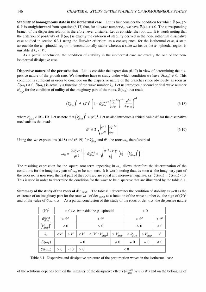
146 CHAPTER 6. STUDY OF THE STABILITY OF HOMOGENEOUS STATES
Stability of homogeneous state in the isothermal case Let us first consider the condition for which<(ω±) >0. It is straightforward from equation (6.17) that, for all wave number kx, we have<(ω−) < 0. The correspondingbranch of the dispersion relation is therefore never unstable. Let us consider the root ω+. It is worth noting thatthe criterion of positivity of <(ω+) is exactly the criterion of stability derived in the non-isothermal dissipativecase studied in section 6.3.1 using the Hurwitz criterion: as a consequence, for the isothermal case, a statehs outside the ϕ−spinodal region is unconditionally stable whereas a state hs inside the ϕ−spinodal region isunstable if kx < kc.
As a partial conclusion, the condition of stability in the isothermal case are exactly the one of the non-isothermal dissipative case.
Dispersive nature of the perturbation Let us consider the expression (6.17) in view of determining the dis-persive nature of the growth rate. We therefore have to study under which condition we have =(ω±) , 0. Thiscondition is sufficient in order to conclude on the dispersive nature of the branches since obviously, as soon as=(ω±) , 0, =(ω±) is actually a function of the wave number kx. Let us introduce a second critical wave numberkc
disp for the condition of nullity of the imaginary part of the roots, =(ω±) that reads
(
kcdisp
)2=
(
kc)2
1 − ϑisoth 2diss
(
dρdϕ
hs)−2ρhs
4σ h
−1
(6.18)
where kcdisp ∈ ∪ I. Let us note that
(
kcdisp
)2> (kc)2. Let us also introduce a critical value ϑc for the dissipative
mechanisms that reads
ϑc = 2
√
σ hρhs
∣∣∣∣∣∣
dρdϕ
hs∣∣∣∣∣∣
(6.19)
Using the two expressions (6.18) and (6.19) for kcdisp and ϑc, the roots ω± therefore read
ω± =2 k2
x σ hϑc 2
−ϑisoth
diss ±
√
ϑc 2 (kc)2
k2x
(
k2x −
(
kcdisp
)2)
The resulting expression for the square root term appearing in ω± allows therefore the determination of theconditions for the imaginary part of ω± to be non-zero. It is worth noting that, as soon as the imaginary part ofthe roots ω± is non zero, the real part of the roots ω± are equal and moreover negative, i.e. <(ω+) = <(ω−) < 0.This is used in order to determine the condition for the wave to be dispersive that are illustrated by the table 6.1.
Summary of the study of the roots of det isoth The table 6.1 determines the condition of stability as well as theexistence of an imaginary part for the roots ω± of det isoth as a function of the wave number kx, the sign of (kc)2
and of the value of ϑdiss isoth. As a partial conclusion of this study of the roots of det isoth, the dispersive nature
(kc)2 > 0 i.e. hs inside the ϕ−spinodal < 0
ϑisothdiss > ϑc < ϑc > ϑc < ϑc
(
kcdisp
)2< 0 > 0 > 0 < 0
kx < kc > kc < kc ∈ [kc : kcdisp] > kc
disp < kcdisp > kc
disp ∀
=(ω±) = 0 , 0 , 0 = 0 , 0
<(ω+) > 0 < 0 > 0 < 0
Table 6.1: Dispersive and dissipative structure of the perturbation waves in the isothermal case
of the solutions depends both on the intensity of the dissipative effects (ϑisothdiss versus ϑc) and on the belonging of

6.3. GENERAL STUDY OF THE DISPERSION RELATION 147
the hs state to the ϕ−spinodal region (sign of (kc)2). The stability condition only depends on the belonging of thehs state (like in the non-isothermal dissipative case).
Therefore, it is required to study the belonging of the state hs to the ϕ−spinodal region as a function of theparameters for the state hs in order to conclude on the dispersive/stable nature of a perturbation of a state hs inthe isothermal case.
6.3.3 The influence of the dissipative processes on the stability of the state hs
We consider now the absence of any dissipative process, i.e. khs = 0, κ = +∞ and η = 0. In this case theexpression for the dispersion relation det M∗ = 0 still holds and is therefore a polynomial of degree 3. Howevera2 = 0, a0 = 0 (cf. their expressions (6.10b) and (6.10d)) and ϑisoth
diss = 0 (cf. its definition (6.12)) which simplifiesnotably the study of this polynomial. According to the study of the Hurwitz criterion of the stability of det M∗,the necessary and sufficient condition of stability thus reduces to the condition a1 > 0 where a1 reads (cf. itsexpression (6.10c))
a1 =T hs
ρhs
(
dPsat
dT
)2 (
dρdϕ
hs)2
+ (ρcP)hsλ
k2x +
1h2
d2Wdϕ2
hs
− d2ρ
dϕ2
hsg∗ hs
λ
We introduce the critical wave number(
kcdiss=0
)2for the positivity of a1 defined by
(
kcdiss=0
)2=
(
kc)2 − T hs
λ ρ3 hschsP hσ
(
dPsat
dT
)2 (
dρdϕ
hs)2
(6.20)
where kcdiss=0 ∈ ∪ I.
Since a0 = 0, ω = 0 is a trivial root of det M∗ and the dispersion relation to study reads (cf. equation (6.9))
det M∗(ω, kx)ω
= σ h (ρcP)hs(
k2x −
(
kcdiss=0
)2)
+ ω2(
dρdϕ
hs)2(ρcP)hs
k2x ρ
hs(6.21)
Let us consider the two branches ω± corresponding to the roots of this simple second order polynomial. Theyread
ω± = ± k2x σ h ρhs
(
dρdϕ
hs)−2 (
k2x −
(
kcdiss=0
)2)
(6.22)
It is obvious that we have ω+ = −ω− and that the existence of a non-zero real part is simply related to the
condition(
k2x −
(
kcdiss=0
)2)
> 0. It is worth noting that, according to equation (6.20)(
kcdiss=0
)2< (kc)2. Therefore,
the necessary condition of stability is less restrictive than in the dissipative case. As a consequence, any state hsthat is unconditionally stable in the dissipative case is also unconditionally stable in the non-dissipative case. Onthe other hand, any state hs that is conditionally stable in the non-dissipative case is also conditionally stable inthe dissipative case. The existence of dissipative mechanisms destabilizes thus some states that should be stablein absence of any dissipative mechanism. The crucial role of the heat conductivity on this property (with regardto the other isothermal dissipative mechanism) is shown in the next paragraph.
Let us also note that when (dρ/dϕ)hs = 0 (which will be shown to be of interest when the interpolationfunctions for the density ρ(ϕ) are either P3 or P5) both critical wave numbers are equal (kc
diss=0 = kc) andtherefore the existence of dissipative terms has no influence on the stability of the corresponding states. Thisresult has already been stated by Umantsev [141] in the case where no density difference between the phases istaken into account.
In the non-dissipative case, the different cases we have to consider can be summarized by the following table(
kcdiss=0
)2> 0 i.e. hs inside the non-dissipative ϕ−spinodal < 0
kx < kcdiss=0 > kc
diss=0 ∀
<(ω+) > 0 < 0
=(ω±) = 0 , 0

148 CHAPTER 6. STUDY OF THE STABILITY OF HOMOGENEOUS STATES
The non-heat-conducting case As soon as khs = 0, (since it yields a0 = 0), the stability condition readsa1 > 0. Therefore, for a non-heat conducting material, the critical wave number for the stability is always kc
diss=0.However, when other dissipative mechanisms are considered (η , 0 and/or κ , ∞ i.e. ϑisoth
diss , 0), the dispersionrelation differs from the one studied hereinabove and the polynomial to study reads
det M∗(ω, kx)ω
= ω2
(
dρdϕ
hs)2(ρcP)hs
k2x ρ
hs
+ ω[
(ρcP)hsϑisothdiss
]
+ σ h (ρcP)hs(
k2x −
(
kcdiss=0
)2)
and is of degree 2 in ω. It can be shown that the above results are modified as follows
? the critical wave number for the stability is still kcdiss=0
? the existence of dispersive perturbations is related to the same critical wave number kcdisp than in the
isothermal case (cf. its definition (6.18) where kc must be understood as kcdiss=0). Moreover, since |kc| <
|kcdisp| and |kc
diss=0| < |kc|,we have |kcdiss=0| < |kc
disp|, which is similar to the isothermal case.
? the domain of existence of dispersive perturbations is subject to the same influence of the magnitude of thedissipative mechanism than in the isothermal case (i.e. to the condition ϑisoth
diss < ϑc where ϑc is defined by
equation (6.19))
As a consequence, the structure of the perturbation can be summarized by exactly the same table than the table 6.1holding for the isothermal case; only the value of kc must be replaced by kc
diss = 0.The absence of any dissipative thermal process (non-heat-conducting material) in the non-isothermal case has
therefore the single consequence to shift the wave number for the critical wave length to lower values (|kcdiss=0| <
|kc|). As a consequence, a state inside the ϕ−spinodal region (unstable in the heat-conducting case) can be stablein the non-heat conducting case. The heat conductivity has therefore a destabilizing influence on the evolutionof an equilibrium homogeneous state submitted to perturbations. This influence of the heat conductivity on thestability is indeed fully consistent with the results obtained by Ngan and Truskinovsky [99] where the stabilityof homogeneous states with a model equivalent to the van der Waals’ model is studied: in the heat-conductingcase the stability condition is the positivity of the isothermal compressibility (χT > 0) whereas in the non-heat-conducting case the stability condition is the positivity of the adiabatic compressibility 8 (χs > 0) and we have(χs > χT ).
It is worth noting that as a consequence the condition of stability is no more related to the belonging of thestate hs to the ϕ−spinodal region defined in the heat-conducting case. Let us study how the stability conditionkx > <(kc
diss=0) can still be related to a spinodal region. To do this, we first recall the result obtained when wedefined the first ϕ−spinodal region that reads
(
kc)2= −ρ
hs
λ
∂µ
∂ϕ
hs
|P,T
which is therefore the isothermal (at constant temperature T ) derivative of the chemical potential µ with regardto the phase field variable.
Let us now consider the adiabatic derivative of the chemical potential µ. We have
∂µ
∂ϕ |s=∂µ
∂ϕ |T+∂µ
∂T |ϕ∂T∂ϕ |s
The following relations hold
∂µ
∂T |ϕ= − ∂s∂ϕ |T
= − 1ρ2
∂ρ
∂ϕ
dPsat
dT∂s∂T |ϕ
=TcP
8The adiabatic compressibility χs is defined as
χs = −1V
(
∂V∂P
)
s= ρ∂ρ
∂P |s
6.4. STABILITY OF HOMOGENEOUS STATES USING LINEAR INTERPOLATION 149
and let us note that (∂s/∂P) is zero in the considered case where the thermal expansion is null. Therefore, usingthe definition (6.20) of kc
diss=0
λ(
kcdiss=0
)2= −ρhs ∂µ
∂ϕ
hs
|P,T− T hs
ρ3 hschsP hσ
(
dPsat
dT
)2 (
dρdϕ
hs)2
= −ρhs ∂µ
∂ϕ
hs
|P,T+ ρhs (∂s/∂ϕ)|T
(∂s/∂T )|ϕ
∂µ
∂T
hs
|ϕ
= −ρhs ∂µ
∂ϕ
hs
|P,s
The adiabatic ϕ−spinodal region, as the set of states hs for which (∂µ/∂ϕ)|P,s < 0 can thus be defined by analogywith the ϕ−spinodal region considered in the isothermal case. The adiabatic ϕ−spinodal region is less extendedthan the isothermal ϕ−spinodal region. This extends therefore the results obtained by Umantsev [141] to the casewhere a density difference between the phases is considered.
Conclusion concerning the study of the general form for the dispersion relation
In the dissipative non-isothermal case (see section 6.3.1), using the Hurwitz criterion of stability, we have shownthat the necessary and sufficient condition of stability is the non-belonging of the homogeneous state hs to theϕ−spinodal region i.e.
∂µ
∂ϕ
hs
|P,T> 0s
Inside the ϕ−spinodal region, the homogeneous state is unstable to small wave-number perturbations, the critical
value for the wave number being equal to kc =
√
−(∂µ/∂ϕ)hs|P,T .
We have then defined a set of sub-cases for which a more complete analytical study of the linear stage ofevolution of the perturbation of homogeneous states is possible. Let us summarize the corresponding results.First, as soon as the heat conductivity is non-zero, the condition of stability for the state hs is exactly similar tothe one corresponding to the non-isothermal dissipative case presented above. If the heat conductivity is null,the condition of stability is related to the non-belonging of the homogeneous state hs to the adiabatic ϕ−spinodalregion i.e.
∂µ
∂ϕ
hs
|P,s> 0
It has been shown that the condition of stability is indeed less restrictive than in the heat-conducting case.Let us now consider the condition of dispersive evolution of the perturbation. It has been shown than in the
isothermal case, as well as in the non-heat-conducting case, the condition of existence of dispersive waves isrelated to the belonging of the state hs to the ϕ−spinodal region as well as on the intensity of the dissipativemechanisms. The corresponding results are given on table 6.1. In the absence of any dissipative mechanism, theperturbation is dispersive as soon as it is damped.
In the following, we consider different choices for the interpolation function ρ(ϕ) to study how it affects thebelonging to the ϕ−spinodal region for given thermodynamic conditions (g∗ and T ) and show how the choice forthe polynomial P5 actually allows to control the stability of the single-phase states.
6.4 Stability of homogeneous states using linear interpolation
When the interpolation function ρ(ϕ) is linear, (dρ/dϕ) = (ρv − ρl) and (d2ρ/dϕ2) = 0. (dρ/dϕ) and (d2ρ/dϕ2)are independent of the state hs considered. In the following, we take advantage of this property to simplify thegeneral expressions for the conditions under which the perturbation wave is dispersive/unstable that have beenderived in section 6.3.

150 CHAPTER 6. STUDY OF THE STABILITY OF HOMOGENEOUS STATES
6.4.1 Non-isothermal dissipative case, the necessary and sufficient condition of stability
In the linear interpolation case, the expression for the critical wave number kc simplifies and reads
(
kc)2=−(d2W/dϕ2)hs
h2
The equilibrium phase field value is determined by the value of the single parameter g = g∗ σ/[h(ρl − ρv)](see section 3.4.1) and equals 0 or 1 only for g = 0. It is straightforward to show that the ϕ−spinodal regioncorresponds to |g| < 2
√3. The metastability limit of the liquid state (ϕ < 1/2 −
√3/6), resp. vapor state state
(ϕ > 1/2 +√
3/6), is thus defined by g∗lim,l = −2√
3σ/[h (ρl − ρv)], resp. g∗lim,v = 2√
3σ/[h (ρl − ρv)]. It is thusnot controlled since h dependent.
6.4.2 Non dissipative and isothermal case
Let us express the growth rate ω in the isothermal case. Let us consider at first the case of zero dissipativeprocesses, ϑdiss = 0 (i.e. κ = ∞ and η = 0). The growth rate reads
ωdiss free = ±√σ/h kx
ρl − ρv
√
(kc)2 − k2x
where the critical wave length kc has the same expression than in the previous studied general case. We haveeither pure imaginary (<(ωdiss free) = 0, dispersive wave) or pure real (either damped or unstable) growth rates(=(ωdiss free) = 0) . Let us state for which state hs, unstable growth of the perturbation can occur.
For ϕhs outside the spinodal region, we have<(ωdiss free) = 0 and there exists only purely dispersive evolutionof the perturbation. For ϕhs inside the spinodal region there exists a critical wave length, namely kc, such as thereexists non-dispersive unstable perturbations for kx < kc and purely dispersive for kx > kc.
As a partial conclusion for non-dissipative isothermal cases, the states out of the spinodal region (uncondi-tionally stable) are purely dispersive whereas in the spinodal region unstable growth rates corresponds to lowvalues of kx, the critical value for the wave number kc being scaled by the inverse of the artificial thickness,namely 1/h.
6.4.3 Dissipative isothermal case
Let us study how the isothermal linear stage of evolution is modified in presence of dissipative effects (i.e. ϑisothdiss ,
0). For non-zero dissipative processes (i.e. κ , ∞ and/or η , 0), there exists two branches in the dispersionrelation (cf. equation (6.17)) and the critical wave length for dispersive solutions is given by equation (6.18). Itis worth noting that dispersive (=(ω±) , 0) solutions, always correspond to damped perturbations (<(ω±) < 0)whatever the initial state considered. Let us now study the states corresponding to either dispersive or non-dispersive perturbations. We refer to the table of cases presented in section 6.3.2
Let us consider a state hs outside the spinodal region. In this case, we have kc 2isoth < 0. Non-dispersive
growth rate (=(ω±) = 0) exists only if the dissipative terms ϑdiss is less than ϑc. If this condition is fulfilled,non-dispersive growth rates are possible for large kx (k2
x > kc 2disp) where kc 2
disp is given by (6.18).For states inside the spinodal region, we have unstable growth rate (<(ω+) > 0) for kx < kc. There are two
different cases according to the value of ϑisothdiss . If ϑisoth
diss is larger than ϑc, solutions are always non dispersive(=(ω) = 0). If ϑisoth
diss is less than ϑc, the non-dispersive solutions correspond for kx < kc disp.Such a dispersion relation is illustrated on figure 6.1 where the real part of the growth rate as a function of
the wave number is represented. It is worth noting that when the wave is dispersive, we have only one branch(instead of two) for the real part (i.e. =(ω±) = 0⇒<(ω+) = <(ω−)).
As a conclusion for the dissipative isothermal case, states out of the spinodal region are purely dispersivefor low or zero dissipation. For sufficiently large dissipation, they are purely damped for low values of the wavelength kx < kc
diss and dispersive otherwise. States inside the ϕ−spinodal region are dispersive.

6.4. STABILITY OF HOMOGENEOUS STATES USING LINEAR INTERPOLATION 151
spin −spin +
kc kcdisp
−
+
±
spin diss−
spin diss +
spin diss±
kx
<(ω
)
0 0.2 0.4 0.8 1
0
-0.4
-0.8
Figure 6.1: Real part of the growth rate ω . The “spin” case corresponds to the spinodal case when ϑdiss < ϑc
while the “±” and “spin diss” cases correspond to large dissipation rate ϑdiss > ϑc
6.4.4 Non-heat conducting case
We consider the case of zero heat conductivity, therefore a0 = 0 and the dispersion relation reads (cf. equa-tion (6.21))
ω2[
(ρl − ρv)2
ρhs k2x
]
+ ω ϑdiss +
λ
1h2
d2Wdϕ2
hs
+ k2x
+T hs (ρl − ρv)2 (dPsat/dT )2
(ρ cP)hs (ρhs)2
= 0 (6.23)
For non-dissipative (ϑdiss = 0) processes, we get similar results than for the non-isothermal dissipation free case,i.e. :
? outside the spinodal region, hs is unconditionally stable and we have dispersive solutions
? inside the spinodal region the states are unstable for low wave numbers kx < kcdiss=0, kc
diss=0 being lowerthan its isothermal value (cf. equation (6.20)) and dispersive otherwise. Let us note that kc
diss=0 caneven become unconditionally negative (in which case no more unstable growth is possible) for h >ρhs 2chs
P σ |Min(d2W/dϕ2)|/(T hs(dPsat/dT )2 (ρl − ρv)2). In the present case |Min(d2W/dϕ2)| = 18.
It is therefore worth noting that, as h increases, the value of the critical wave number under which the spin-odal phase become unstable decreases and can even reach zero. As a consequence, the stability of adiabatichomogeneous states is clearly not controlled since it is h dependent.
Let us now consider the case with zero heat conductivity but still other isothermal dissipative mechanisms.Then it is straightforward that the structure of the dispersion relation is strictly identical than in the dissipativeisothermal case, and we refer to the corresponding study.
6.4.5 Conclusion on the study of the linear interpolation
The unstable and dispersive properties of the linear stage of evolution of a perturbation have been studied. Forthe isothermal, non-dissipative, non-heat conducting or without density differences cases, we have determinedthe spectrum of wavelengths of both dispersive and unstable perturbations. The ϕ−spinodal region correspondsin this case to a finite range of g∗ values around zero, this range being a decreasing function of the artificialthickness h. The liquid and vapor states are always outside the spinodal. Their domain of existence is boundedby a limiting g∗ value. At the limit h = +∞, there only exists liquid phase for g∗ > 0 and vapor phase for g∗ < 0.It does mean that the limit of superheat is a decreasing function of the artificial thickness. This property is notdesirable for our phase field model (cf. the corresponding discussion in the study of the limitation of the van derWaals model for the study of mesoscopic boiling systems in section 2.2). As a consequence, we disregard thechoice of a linear interpolation function in the remainder of this study.

152 CHAPTER 6. STUDY OF THE STABILITY OF HOMOGENEOUS STATES
However this study has allowed to illustrate the characteristic of the general dispersion relation. These resultswill be used in the following to characterize the perturbation of the hs states corresponding to ϕ , 0 or 1 whenthe interpolation function is not linear.
6.5 Stability of homogeneous states using non-linear interpolation functions
In this case the nature of the instability differs mainly according to the fact that the initial phase field value ϕhs
equals either the values 0 and 1 or not. We therefore first study the stability of the liquid and vapor phases insection 6.5.1. Then we study the stability of the other equilibrium solutions in section 6.5.2.
6.5.1 Liquid and vapor phase
Let us note also that all these results are still valid if the specific volume v instead of the density ρ is interpolatedby either P3 or P5.
In the case where ρ is interpolated by either P3 or P5, ϕhs = 0 or 1 are solutions of the equilibrium condi-tion (6.2) for any value of the parameter g∗hs (cf. section 3.4.1). In the following, we study the stability of thesetwo possible states as a function of the parameter g∗hs. It is worth noting that in this case, (dρ/dϕ)hs = 0. Thiscondition considerably modifies the system of equations (6.3) linearized around the state hs and as a consequencethe nature of the physical response of this state to perturbations.
A system of governing equations considerably modified In the case where (dρ/dϕ)hs = 0, the linearized setof governing equations (6.3) for the perturbation reads
ρhs V ′,x = 0
V ′,t = −g′,x − shsT ′,x + (η/ρ)hs V ′,xx
(ρ cP)hs T ′,t = khsT ′,xx
ρhs ϕ′,tκ
=
d2ρ
dϕ2
hs
g∗hs − λh2
d2Wdϕ2
hsϕ′ + λ ϕ′,xx
This set of linearized equations is very different from the set (6.3) obtained in the general case. Particularlythe main variables are less-coupled: the linearized continuity equation only depends on the perturbed velocity,the energy balance equation only depends on the perturbed temperature and the AC equation only depends onthe perturbed phase field. This has of course consequences on the determinant of the linear system. Introducingsolutions proportional to eωt+Ikx x and adopting the matrix notation used in section 6.2.5, the system reads MX = 0with X = (ϕ′,T ′, g′,V ′) and where M reads
M =
ωρhs
κ+ λ
(
k2x −
(
kc)2)
0 0 0
0(
ω (ρcP)hs + k2x khs
)
0 0
0 kxshs kx
(
ω + k2xη
ρ
hs)
0 0 0 Ikxρhs
It is clear from this matrix notation that the perturbed velocity is always zero.
Dispersion relation The study of the roots of the determinant det M reduces to the study of the followingpolynomial in ω
(
(ρ cP)hs ω + khs k2x
) (
ρhs ω
λ κ− (
kc)2+ k2
x
)
= 0 (6.24)
which has obviously two roots ω1 and ω2
ω1 = − khsk2x
(ρ cP)hs
ω2 = −λ κρhs
(
k2x −
(
kc)2)

6.5. STABILITY WITH NON-LINEAR INTERPOLATION FUNCTIONS 153
The root ω1 is a negative real and corresponds to a non-zero temperature perturbation as soon as ω1 , 0. Inthis case, and only in this case, the perturbed specific Gibbs free energy is non-zero, i.e. g′ , 0. The root ω2 ofthis polynomial corresponds to a non-zero phase field perturbation. It is either pure real or pure imaginary (ω2 ∈∪ I). The dispersion relation (6.24) implies that unstable perturbations of the homogeneous state hs can onlybe achieved for a zero Fourier amplitude of the temperature field, i.e. <(ω) > 0 ⇒ ω = ω2 ⇒ T ′ = 0 & g′ = 0.Moreover since V ′ = 0 in the linear stage of the instability, the single dissipative process affecting the stabilityof bulk phases homogeneous states is therefore the Ginzburg-Landau relaxation. The dispersion relation (6.24)implies that unstable perturbations of the homogeneous state hs can only be achieved for low values of the wavenumber k2
x ≤ (kc)2, which is fully consistent with our study of the general necessary and sufficient condition ofstability in section 6.3.1. Let us note that for non-heat-conducting fluids (khs = 0) the stability condition is notmodified, i.e. kc
diss=0 = kc. In the purely non-dissipative case (κ = +∞ and khs = 0), the growth rate is strictlynull, ω = 0. When only the Ginzburg-Landau relaxation is neglected (κ = ∞), the perturbation is always purelydamped (ω = ω1).
The stability condition Let us now study the stability condition. We therefore study the value of (kc)2 theinterpolation function being either P5 or P3. Let us note that (d2W/dϕ2)hs = 36.
? P5:
in this case (d2ρ/dϕ2)hs = 0 and thus from the expression (6.13) of kc, we have (kc)2 = −(d2W/dϕ2)hs/h2 <
0 and no perturbation can linearly destabilize the state hs
? P3:
we consider two sub-cases whether ϕhs = 0, hs = liquid or ϕhs = 1, hs = vapor
– hs = liquid:In this case (d2ρ/dϕ2)liquid = 6 (ρvap − ρliq) < 0, the condition of stability (kc)2 < 0 reads 36σ/h +6 (ρliq − ρvap)g∗liquid > 0 i.e. g > −6. As a consequence the liquid phase is unconditionally stable forany value of g∗liquid satisfying g∗liquid > −6 (ρliq−ρvap)−1σ/h, i.e. P > Peq(Teq)−6 (1−ρvap/ρliq)−1σ/h.
– hs = vapor:In this case (d2ρ/dϕ2)vapor = 6 (ρliq − ρvap) > 0, and the vapor phase is unconditionally stable for anyvalue of g∗vapor satisfying g∗vapor < 6 (ρliq − ρvap)−1σ/h, i.e. P < Peq(Teq) + 6 (ρliq/ρvap − 1)−1σ/h.
It is worth noting that in the case when the specific volume v is chosen as a polynomial instead of the densityρ, we still have (dρ/dϕ) = 0 and for P5 (d2ρ/dϕ2) = 0, for P3 the value is modified as (d2ρ/dϕ2)liquid =
−6 (ρliq)2 (vvap−vliq) < 0 and (d2ρ/dϕ2)vapor = 6 (ρvap)2 (vvap−vliq) > 0, the whole analysis remaining unchanged.
The stability condition of the liquid and vapor phase in view of our applications of the model Let uscomment these results. In the P5 case, the liquid and vapor phases are unconditionally stable which is exactlythe property targeted since it actually corresponds to the one of the incompressible sharp interface model. Onthe contrary, in the P3 case, at a given temperature T , there exists a finite range of stable pressure values aroundthe equilibrium pressure Peq(T ). The liquid phase is always stable for pressures above Peq(T ) which is fullyconsistent with the classical model of the stability of this phase. However, the liquid phase is also stable for afinite range of pressure below the saturation pressure. The lower limit Plim, l(T ) of this range corresponds to theclassical definition for the limit of metastability (cf. its presentation in section 2.2.2) and reads
Plim, l(T ) = 6σ
h (1 − ρvap/ρliq)
As a consequence, even though this value is finite, it is possible to have a liquid phase that exists below thesaturation pressure which is physically consistent. Let us consider we have access to an empirical value forPlim, l(T ), we’d like our model to reproduce. Let us note that, in this case, the phase field model has an additionalproperty with regard to the sharp interface model with incompressible phases. Indeed, in this sharp model, theredoes not exist any way to model such a limit of metastability. Let us comment this property in view of ourtargeted use of the model as a numerical method. In this case the artificial thickness for the interface h is dictated

154 CHAPTER 6. STUDY OF THE STABILITY OF HOMOGENEOUS STATES
by numerical constraints. As a consequence, the model is too constrained in order to be able to reproduce thecorrect scaling for the metastability limit Plim, l(T ).
A similar reasoning applies concerning the stability of the vapor phase in the P3 case. The same reasoningcan also be reproduced when we consider the pressure as being fixed and study the range of temperature forwhich a phase is stable.
As a partial conclusion, only the choice P5 for the interpolation function satisfies our requirements. Indeedin this case the liquid and vapor phase are unconditionally stable.
The ability to impose a fixed value for the metastability limit Let us consider again the existence of anempirical value for the metastability limit of the phases, say Plim, l(T ), we’d like our model to reproduce. Letus consider the condition (∂ρ/∂ϕ)(ϕ = 0) = 0 satisfied. In this case, the liquid phase is actually an equilibriumsolution for any value of the pressure. Therefore we arrive, following the same reasoning as in the beginning ofthis section to the stability condition for the liquid phase that reads
−6σ
h− (1 − ρvap/ρliq) (P − Psat(T ))
d2Pdϕ2 (ϕ = 0) < 0
where we have considered the density as being interpolated by a function P. The stability condition of the liquidphase is therefore related to the single value of (d2P/dϕ2)(ϕ = 0). To impose a stability condition for the liquidphase as
P > Plim, l(T )
where Plim, l(T ) < Psat(T ) it is therefore sufficient to satisfy
d2Pdϕ2 (ϕ = 0) =
h (1 − ρvap/ρliq)6σ
(
Psat(T ) − Plim, l(T )) = ζliq
where we have introduced the non-dimensional quantity ζliq in order to simplify the writing of this condition. Forthe sake of simplicity, let us ignore the eventual temperature dependence of this quantity. Since the same type ofrelations have to be considered for the vapor phase, the function P needs to satisfy the following 6 conditions
P(0) = 0 & P(1) = 1 Interpolation functiondPdϕ
(0) =dPdϕ
(1) = 0 Liquid and vapor always equilibrium states
d2Pdϕ2 (0) = ζliq &
d2Pdϕ2 (1) = ζvap Control of the metastability limit
Let us note that as soon as Plim, l(T ) = Plim, v(T ) = ∞, i.e. when we consider an unconditional stability of theliquid and vapor phases, we have ζliq = ζvap = 0 and we recover the conditions satisfied by the polynomial P5. Itis worth noting that, since 6 conditions need to be satisfied by the function P, by choosing adequately ρ(ϕ) as apolynomial of degree 5, it is thus possible to control and reproduce an empirical limit of metastability. Moreoverthis can be done for an arbitrary value of the artificial thickness h which was not possible in the P3 case as shownin the previous paragraph.
As a partial conclusion, we have shown that it was possible to deal with a quasi-compressible phase fieldmodel, i.e. with incompressible bulk phases, and to reproduce an empirical limit of metastability of the bulkphases vapor and liquid. This property of the formulation must therefore be viewed as an advantage with respectto the native sharp interface model with incompressible bulk phases. Indeed the consequent phase field modelconstitutes a consistent regularization of this sharp interface model and in addition holds the ability to modelempirically the stability of homogeneous states, and that for an arbitrary choice for the artificial thickness h ofthe interface.
6.5.2 Stability of homogeneous states for ϕhs different from 0 or 1
Determination of the sign of (kc)2, the extent of the ϕ−spinodal region It has been shown that the state hsis unconditionally stable if and only if (kc)2 < 0. Using the fact that ϕhs is a function of the non-dimensional

6.5. STABILITY WITH NON-LINEAR INTERPOLATION FUNCTIONS 155
parameter g, the critical wave number (kc)2 reads (cf. equation (6.13))
(
kc)2= − 1
h2
(
d2Wdϕ2 (ϕhs(g)) + g
d2Pn
dϕ2 (ϕhs(g)))
It is straightforward to show that when ρ is interpolated by either P3 or P5, g(d2Pn/dϕ2)(ϕhs(g)) is negative. Inthe P3 or P5 cases, g2 (kc)2 is therefore positive for ϕhs ∈ [1/2−
√3/6 : 1/2+
√3/6] (where d2W/dϕ2 is positive)
but is a priori undetermined otherwise. The value of the non-dimensional parameter h2 (kc)2 as a function of thesingle variable g is represented on the figures 6.2. We have represented the results for the P1 case that corresponds
√3/6−
√3/6
ϕhs(g) − 1/2
h2( k
c )2
10.50-0.5-1
100
50
0
-50
-100
-150
-200
ν = P1ν = P3ν = P5
ϕhs(g) − 1/2
h2( k
c )2
-0.6-0.8-1-1.2-1.4
200
100
0
-100
-200
-300
-400
-500
Figure 6.2: Value of h2 (kc)2 for the solutions ϕhs(g) of equation (6.2)
to the result derived in section 6.4.Let us consider the P3 case. As it has been previously stated, h2 (kc)2 is positive for ϕhs ∈ [1/2 −
√3/6 :
1/2 +√
3/6]. Moreover it is positive inside the whole interval [0 : 1]. However, as soon as ϕhs ∈] − ∞ : 0[∪]1 :+∞[, h2 (kc)2 is positive9. The necessary and sufficient condition of stability is therefore satisfied. The state hscorresponding to |g| > 6 (and therefore |g∗hs| > 6σ/[h(ρl − ρv)] and ϕhs
< [0 : 1]) is therefore unconditionallystable. Since the corresponding states do not correspond to desired stable homogeneous states, this property isnot desirable. Moreover it is worth noting that the lower bound of physical values of |g∗hs| that corresponds tothese undesirable states approaches 0 as h is artificially increased.
Let us now consider the P5 case. It is clear from figure 6.2 that h2 (kc)2 is strictly positive whatever the valueof ϕhs and subsequently of g∗hs. The ϕ−spinodal region is therefore of infinite ϕ extent. The necessary conditionof stability for any state different from 0 or 1 is therefore never satisfied as soon as the solution is different from
9Let us precise that the solutions 0 and 1 represented here do not correspond to the solutions 0 and 1 valid for any value of g∗hs
considered in section 6.5.1, but to the particular case when ϕhs actually depends on g∗hs. This explains why in this case h2 (kc)2 is fullydetermined and is null for ϕhs = 1/2 ± 1/2. In the previous case, where g∗hs was an independent parameter, the value of h2 (kc)2 forϕhs = 1/2 ± 1/2 actually depends on g∗hs.
156 CHAPTER 6. STUDY OF THE STABILITY OF HOMOGENEOUS STATES
the values 0 and 1 considered in section 6.5.1. Therefore these states are always unstable to low wave numbersperturbations10.
As a consequence of these results, when ρ is interpolated by P5, the states that correspond to ϕhs, 0 or 1 are
always conditionally stable (unstable for low wave numbers). This is the result targeted for these states.
Sub-cases allowing an analytical study of the growth rate ω as a function of hs and kx Let us now considerthe different physical sub-cases for which the analytical expression of the growth rate ω can be easily derived. Insections 6.3.2-6.3.3, we have derived some very general features for the study of these physical sub-cases. Theyhave been applied to the study of the stability of homogeneous states in the case of a linear interpolation functionin section 6.4. In the present case, the same features are still valid, since the only modified parameter is theexpression for (kc)2 which has been studied hereinabove. As a consequence, using this similarity the followingconclusions can be drawn
? in the P5 case the hs states are always inside the isothermal ϕ−spinodal region. We then refer to the LHSof table 6.1 that allows to characterize the dispersive nature of the perturbation wave for states inside theisothermal ϕ−spinodal region. When isothermal dissipative mechanisms are taken into account, two sub-cases can be distinguished. Either the isothermal dissipation is large (ϑisoth
diss > ϑc) and the perturbation
wave is never dispersive, either it is low and the perturbation wave is dispersive for large wave numbers(corresponding to dissipative waves).
? in the P3 case we have still two cases whether the state is inside the ϕ−spinodal region (ϕhs ∈ [0 : 1] or|g| ∈ [6 : +∞[) or outside this region. We are therefore exactly in the same case than the one studied forthe linear interpolation case, and as a consequence we refer to the study of these cases in section 6.4.
As a partial conclusion, the dispersive nature of the perturbation wave for homogeneous equilibrium statesdifferent from liquid and vapor has already been fully determined in the study of the linear interpolation case.In the P3 case, since the state hs is either inside or outside the isothermal ϕ−spinodal region, the whole resultsobtained for the linear interpolation case is relevant. In the P5 case, since the states hs are always inside theisothermal ϕ−spinodal region, only the corresponding results must be taken into account. As a consequence, inthe P5 case, dispersive perturbation waves only corresponds to large isothermal dissipation and to large wavenumbers corresponding to damped perturbations.
6.6 Conclusion on the study of the stability of homogeneous states
We have studied the linear stage of evolution of the perturbations of a one dimensional homogeneous state atequilibrium using our quasi-compressible phase field model of the liquid-vapor flows with phase-change. Firstwe have motivated this study by the desire to justify the choice for a fifth order polynomial for the interpolationfunction that enters the expression for the specific Gibbs free energy of the model. The study of the dynamics ofa perturbation of an homogeneous equilibrium state including a discussion on the influence of the interpolationfunction on this dynamics has, to our knowledge, never been presented for the diffuse interface models withdensity contrast between the phases.
We have derived the expression for the dispersion relation for the perturbation in the non-isothermal dissi-pative case. Using the Hurwitz criterion, we have determined a necessary and sufficient condition of stability.We have shown that this condition is related to the belonging of the state to a ϕ−spinodal region defined as(∂2g/∂ϕ2) < 0. We have then studied the dispersive nature of the perturbation wave for a set of relevant physi-cal sub-cases, namely the isothermal, without density difference, non-dissipative and non heat-conducting cases.More generally, the states inside the ϕ−spinodal region are unstable for low wave number perturbations, whereas
10It is worth noting that from figure 6.2 it can be seen that h2 (kc)2 remains positive when ϕhs approaches 1/2± 1/2. This could appearas inconsistent with the study of the stability of the liquid and vapor states in section 6.5.1. Indeed we have shown that for ϕhs = 1/2±1/2,we had ∀g, (kc)2 < 0. For the liquid and vapor states ϕhs = 1/2 ± 1/2 we have actually g (∂2P5/∂ϕ
2) = 0. In the present case consideredwe have |g| → +∞ ⇒ ϕhs → 1/2 ± 1/2, as it has been shown in section 3.4.1 (cf. figure 3.9). However ϕhs is then a function of g andas a consequence (∂2P5/∂ϕ
2)hs is also a function of g. Therefore, even though we have still |g| → +∞ ⇒ (∂2P5/∂ϕ2)hs → 0, we have
indeed |g| → +∞ ⇒ g (∂2P5/∂ϕ2)hs → 72 which is finite and positive and actually yields to |g| → +∞ ⇒ (kc)2 → 36 as it can be seen
on figure 6.2. Since this value is positive, the states corresponding to |g| as big as we want, even though they actually tend to the phasefield values (of the stable liquid and vapor phases) are still unstable.

6.6. CONCLUSION ON THE STUDY OF THE STABILITY OF HOMOGENEOUS STATES 157
outside this region they are unconditionally stable. It has been shown that the ϕ−spinodal region correspondsindeed to a range of values for the physical parameter g∗.
The choice for the interpolation function determines the different possible equilibrium states and as a conse-quence the extend of the ϕ−spinodal region. When it is chosen as P1 or P3, it corresponds to a finite range of g∗
values, this range being a decreasing function of the artificial thickness. As a consequence undesired states (i.e.ϕ , 0 or 1) can actually become stable. Moreover the domain of existence or stability (limit of metastability) ofthe liquid and vapor phase are also decreasing with the artificial thickness. As a consequence the stability of thedesired states (ϕ = 0 or 1) is not controlled. When the interpolation function is chosen as P5, all the equilibriumhomogeneous states different from the liquid and vapor are inside the ϕ−spinodal region. As a consequence,apart from the liquid and vapor phases which are then unconditionally stable, all the other equilibrium states areonly conditionally stable. This justifies the choice for a polynomial of degree 5 for the interpolation function.Indeed it provides an interesting property for the model since it allows actually to recover the infinite limit ofmetastability consistent with the incompressible nature of the bulk phase considered.
Let us note that the dynamics of phase separation in the solid-liquid case using the fifth order polynomial P5for the interpolation function is illustrated using two-dimensional numerical simulations in section 8.1.5.
Moreover the number of degrees of freedom determining the interpolation function with a fifth order poly-nomial (i.e. 6) has been shown to be sufficient to control the stability of the liquid and vapor states i.e. to imposean empirical domain of stability of g∗ values for which the state is stable. The subsequent model has thereforean interesting additional property compared to the native sharp interface model for which it provides a consis-tent regularization: it is possible to include a limit of metastability. The consequences of such a choice for theinterpolation function on the stability of the equilibrium states different from the liquid and vapor has not beeninvestigated. It would be interesting to study it.

158 CHAPTER 6. STUDY OF THE STABILITY OF HOMOGENEOUS STATES

Chapter 7
Analytical study of one-dimensional dynamics
In this chapter, we study analytically, with our phase field model, out of equilibrium one-dimensional phasechange when the transition front is a traveling wave. The goal of this analytical study is two-fold. First, thisstudy allows to determine an approximation of the internal structure of the diffuse interface in non-equilibriumconditions. We derive approximate solutions for the profiles of the main variables in the bulk phases and withinthe interface transition layer. We study the dependence of these solutions on the value of the non-dimensionalthickness of the interface ε. Secondly, we determine the relation between this internal structure and the largerscale phase transition process. This corresponds to the determination of the equivalent sharp interface model, orsharp interface limit of our diffuse interface model.
In a first part, we study the sharp interface model for liquid-vapor flows with phase change (see section 7.1).From the general writing of the Rankine-Hugoniot jump conditions, the interface entropy production must bespecified, e.g. Truskinovsky [134]. The model for the interface entropy production provides a kinetic relationfor the phase transition. It is shown that this kinetic relation actually defines a closure law for the interfacetemperature and pressure, namely an out of equilibrium Clapeyron relation (or Gibbs-Thomson equation in theuniform density case). This result is used in the following to study the sharp interface limit of our phase fieldmodel. In a second part, we derive this limit. The technique of matched asymptotic expansions is applied for thesolving of the system of governing equations (5.59) for a steady state phase change process (see section 7.2). Inthis system, the parameter ε, defined as the ratio of the interface thickness to the capillary length l, is consideredas a small parameter. The solution is the sum of an outer solution (bulk phase) and an inner solution (interfacetransition layer). Solutions in both the bulk phases and the interface transition layer are expanded with respectto ε and leading order terms are derived. Three canonical systems are studied. First, the density is consideredas uniform and we study the coupling between the thermal and phase field parts of the model (see section 7.3).Second, we study the isothermal phase field model and the coupling between mechanics and phase field (seesection 7.4). Finally, we study our phase field model dedicated to liquid-vapor flows with phase change includingthermal, mechanical and phase field parts of the model (see section 7.5). All the leading order results of this studyare consistent with a particular sharp interface model known as the normal growth approximation mostly justifiedfor slow phase boundaries. In a third part (see section 7.6), we study how this latter result is in fact related to theparticular choice made for the scaling of the mobility α in section 5.3.4. Using another choice for this scaling,we demonstrate the ability of the phase field model to deal with kinetic relations that are more accurate for fastkinetics.
7.1 Sharp interface models
In this section, we study the sharp interface model for the liquid vapor phase transition. The goal is to study theinterface jump conditions in order to compare the sharp interface limit of the phase field model with the sharpinterface model. In particular, we show how the non-equilibrium relation giving the interface temperature andpressure can be related to the interface entropy production thanks to the formalism of the kinetic relations. Thedetailed derivation of the following results can be found in the appendix A.2.
For the sharp interface model, a variable Y takes specific values on each side of the interface, say + and −.These values are denoted Y+ and Y− in the following. The Y jump and the value of Y at the interface are defined
159

160 CHAPTER 7. ANALYTICAL STUDY OF ONE-DIMENSIONAL DYNAMICS
as follows
JYK = Y+ − Y−
Y = Y+ + Y−
2
7.1.1 Rankine-Hugoniot jump conditions
General writing Let us consider a one-dimensional traveling wave of constant speed D. Integral of theNavier-Stokes equations over the interface discontinuity, yields the general form of the Rankine-Hugoniot jumpconditions:
Jρ (D− V)K = 0 (7.1a)
JPK +qρ (D− V)2y = 0 (7.1b)
ρ (D− V)s
V2
2+ e
− JqK − JPVK = 0 (7.1c)
r qT
z− ρ (D− V) JsK = Rs (7.1d)
where V is the velocity, q the heat flux, e the specific internal energy, s the specific entropy and R s the interfaceentropy production that satisfies the Clausius Duhem inequality
Rs ≥ 0
It is worth pointing out that Rs needs to be specified to close the problem, its study is the subject of the followingdevelopments.
Pressure and velocity jumps Let us introduce the constant mass transfer rate Γ
Γ =D− V1/ρ = ρl (D− Vl) = ρv (D− Vv)
where the second equality is obtained thanks to equation (7.1a) (cf. equation (A.15)). From the jump condi-tions (7.1), it is straightforward to show that the following jump conditions are satisfied
JVK = −Γs
1ρ
(7.2a)
JPK = −Γ2s
1ρ
(7.2b)
The latter pressure jump classically called pressure recoil. It is shown in the following study that, in the sharplimit of our phase field model, these relations are satisfied.
Kinetic relation and interface entropy production The interface entropy production Rs can be rewritten asa product of a flux by a force, where the flux is the mass transfer rate Γ. To show this, we transform the LHSof equation (7.1d). The detailed derivation is provided in the appendix A.2.2. Introducing the internal energy edefined as
e = g + T s − Pρ
it is straightforward to show that
JsKT = JeK − JgK − JTKs +s
Pρ
Therefore, using the energy jump condition (7.1c) as well as the identities (7.2), the interface entropy produc-tion (7.1d) reads
Rs T = Γ
JgK + JTKs +q
(V −D)2y
2
− JqK +r q
T
zT

7.1. SHARP INTERFACE MODELS 161
It yields naturally to the introduction of a driving force G defined as (cf. equation (A.20))
G = JgK + JTKs +q
(V −D)2y
2(7.3)
such that Rs reads (cf. equation (A.21))
Rs T = ΓG − JTK q
T
+ JqK(
T
1T
− 1)
(7.4)
Two canonical sharp interface models can be considered, the process being either isothermal (JTK = 0) oradiabatic q = 0. In these two limits, we get
T Rs = ΓG (7.5)
The kinetic relation is the closure law that gives the driving force as a function of the mass transfer rate, i.e.G (Γ). In the following we consider the two isothermal and adiabatic limits for the phase change process and thusassume equation (7.5) to be satisfied.
7.1.2 Interface entropy production and non-equilibrium Clapeyron relations
Models for Rs Two simple models for the interface entropy production can be considered. The first one as-sumes that the interface is at equilibrium, i.e.
Rs = 0
As a consequence, the driving force is itself zero. It is worth pointing out that, as a consequence, in the adiabaticor isothermal limits, the following jump condition is satisfied (cf. equation (7.1d))
JqK = ΓL
where L = T JsK is the latent heat. This relation is classical in the sharp interface models.The second model assumes that the interface entropy production is quadratic in Γ
Rs ∝ Γ2
as a consequence, the driving force is linear in Γ
G ∝ Γ
This latter model is classically known as the normal growth theory.In the following, we relate this latter theory to the models for the interface pressure and temperature.
Out of equilibrium Gibbs-Thomson and Clapeyron relations In sharp interface models of phase transition,the relation between the interface pressure and the interface temperature as a function of the mass transfer ratecan be given as closure laws. These closure laws can be related to the closure law for the interface entropyproduction.
Let us assume that, in the evaluation of the interface jump conditions, the compressibility of the bulk phasescan be neglected compared to the density difference between the bulk phases. Similarly, let us assume that thesensible heat is negligible compared to the latent heat. In appendix A.2.3, we show that these assumptions yield(cf. equation (A.26))
G '(
P − Peq)
J1/ρK −(
T − Teq)
JsK (7.6)
where Peq and Teq are arbitrary references for the pressure and temperature, (Peq,Teq) being located on thesaturation curve. It is clear that the latter expression at equilibrium (Rs = 0 ⇒ G = 0) is a Clapeyron relation.According to the normal growth theory (G ∝ Γ), it is straightforward that
(
P − Peq)
J1/ρK −(
T − Teq)
JsK ∝ Γ
This relation is clearly non-equilibrium Clapeyron relation. Let us consider the reduction of our model in theuniform density case. Then J1/ρK = 0 and it yields
(
T − Teq)
JsK ∝ Γ

162 CHAPTER 7. ANALYTICAL STUDY OF ONE-DIMENSIONAL DYNAMICS
The latter relation is thus the classical Gibbs-Thomson kinetic relation. For the isothermal model, we get arelation for the interface pressure level as
(
P − Peq)
J1/ρK ∝ Γ
Targeted relations As a consequence of the previous developments, the sharp interface models are closed by amodel for the kinetic relation G (Γ). It has been shown that this relation defines the interface entropy productionand is also related to a non-equilibrium relation between the interface pressure and the interface temperature.In the following study of the sharp limit of our phase field model, we therefore target to make these relationsexplicit. It is worth pointing out that with diffuse interface models we can derive rather than postulate the kineticrelation. We then compare the obtained kinetic relation with the normal growth approximation.
7.2 Matched asymptotic expansions
Let us introduce the use of matched asymptotic expansions to study steady state one-dimensional liquid-vaporphase transitions. Matched asymptotic expansions are classically used for the study of diffuse interface models(e.g. [1, 5, 47, 73, 49] for the phase field models dedicated to the solid-liquid phase transition and [89, 108] forthe Cahn-Hilliard model dedicated to binary fluids) and more generally in fluid mechanics, e.g. [143]. A moredetailed presentation of this formalism is provided in the appendix B.1.
Our goal is to solve the system of governing equations (5.59) for a constant speed of displacement of theinterfaceD and whose main variables are (ϕ, P,T,V). This system reads
α ε2 (D− V) ϕ,x = ε ∂ϕν(
P − T)
+ v(
∂ϕW − ε2ϕ,xx)
+ ∂ϕν
(
W − ε2
2ϕ2,x
)
(7.7a)
(ρV),x = −ρ2 ∂ϕν (D− V)ϕ,x (7.7b)(V −D) ρV,x = −P,x (7.7c)
(V −D) ρT,x =
(
k T,x)
,x
Pe− (V −D) ρ (1 + T ) ∂ϕν ϕ,x + (D− V)2 ρε
α
(
ϕ,x)2 (7.7d)
where we introduced the notation ∂ϕ f = ∂ f /∂ϕ for the sake of legibility. The parameter ε is the ratio of the inter-face thickness to the capillary length l. The two parameters α and Pe are kinetic parameters corresponding to thedissipative processes considered, namely the Ginzburg-Landau relaxation for α and the Fourier heat conductivityfor Pe (cf. their definition in section 5.3).
Pe =σ√L(k/cP)
α = κ h ρ√L
Scale separation hypothesis The fields behave qualitatively differently close and far from the interface. Inthe interface region they vary rapidly over distances of the order of magnitude of the interface thickness O(h)(i.e. O(ε) in non-dimensional length) while far from the interface they vary on a scale O(l) (i.e. O(1) in non-dimensional length). We denote these zones as, respectively, the inner and outer regions and there exists a validscale separation between these regions as long as ε 1. Therefore, it is relevant to consider and derive twosub-problems, namely the inner and outer problems. We expand the corresponding solutions (i.e. the profiles ofthe main variables) in powers of the small parameter ε. For any variable Y , the solution therefore reads
Y(x, ε) = Y0(x) + εY1(x) + O(ε2)
The approximate solutions retained correspond to the leading order terms of these expansions. We assume theexistence of an intermediate zone where both expansions are valid and where the inner and outer solutions match.We are thus able to define boundary conditions for both the outer and the inner problems through the assumptionof continuity of the global solution; these are the matching conditions.
7.2. MATCHED ASYMPTOTIC EXPANSIONS 163
Outer problem Since the typical length scale of the outer problem is l, the system of governing equations isgiven by (7.7). Indeed, the non-dimensional form (7.7) of the system of governing equations has been derivedby considering l as the relevant length scale (cf. section 5.3.4). The outer problem is valid on each side of theinterface, i.e. the bulk phase domains + and −, the transition layer being viewed as a sharp discontinuity of theouter solutions. The sharp position of the interface xi is considered as the position where ϕ(xi) = 1/2; thereforeD = dxi/dt. Let us note that another relevant definition of the interface position could be such that theexcess mass is zero. However, this latter definition cannot be used in the uniform density case. Nevertheless, thedefinition of the interface position is somewhat arbitrary. Therefore, in the remainder of this study, we discuss, ifthe case arises, the dependence of the results to the definition of the interface position.
For the outer problem, the interface is viewed as a sharp discontinuity and xi(t) denotes its position. Sincethe solution is a traveling wave, the value ofD is constant. In each bulk phase, this position is therefore viewedas a boundary. It is worth pointing out that the outer problem is a sharp problem. In order not to be confusingwhile considering the outer fields values at the interface, the position of the interface is denoted x−i for the bulkdomain contained in [0; xi] and x+i for the one in [xi; 1]. The outer variable, say Y at x+i , resp. x−i is denoted Y+,resp. Y−.
Inner problem The inner problem concerns the study of the interface transition layer. We consider thereforethe inner abscissa x defined as
x =x − xi(t)ε
and we write
Y ′ =∂Y∂x
The bulk domains are considered as the external boundaries of the inner domain. The bulk phase contained inthe domain −, resp. +, is thus reached asymptotically at x = −∞, resp. x = +∞. Using this new scaling for theabscissa, it is easy to show that the system of governing equations for the inner problem reads
α ε (D− V) ϕ′ = ε ∂ϕν(
P − T)
+ v(
∂ϕW − ϕ′′)
+ ∂ϕν
(
W − (ϕ′)2
2
)
(7.8a)
(ρV)′ = −ρ2 ∂ϕν (D− V)ϕ′ (7.8b)(V −D) ρV ′ = −P′ (7.8c)
ε (V −D) ρT ′ =(k T ′)′
Pe− ε (V −D) ρ (1 + T ) ∂ϕν ϕ′ + (D− V)2 ρε
α
(
ϕ′)2 (7.8d)
It is worth pointing out that the scaling in ε of the different terms of the AC equation (7.8a) and of the entropyequation (7.8d) differs from the one of system (7.7) while the scaling of the momentum balance (7.8c) andcontinuity equations (7.8b) remains unchanged.
Matching conditions The matching conditions between inner f and outer f ext solutions read
limx→x±i
f ext0 = lim
x→±∞f0 (7.9a)
limx→±∞
f ′0 = 0 (7.9b)
(7.9c)
limx→x±i
f ext0 ,x = lim
x→±∞f ′1 (7.9d)
limx→x±i
f ext1 = lim
x→±∞
[
f1 − x limx→x±i
f ext0 ,x
]
(7.9e)
limx→±∞
f ′′0 = 0 (7.9f)
limx→±∞
f ′′1 = 0 (7.9g)

164 CHAPTER 7. ANALYTICAL STUDY OF ONE-DIMENSIONAL DYNAMICS
7.3 Uniform density phase transition
In this section, we study the phase-field model for the liquid-solid phase transition. This model is easily obtainedfrom the general model presented in the previous section by assuming that the density ρ is constant (cf. itspresentation in section 3.3.2). It is easy to show that the corresponding system of governing equations for theouter problem reads (cf. equations (5.60))
α ε2Dϕ,x = ε ∂ϕν(ϕ) T −(
∂ϕW(ϕ) − ε2ϕ,xx)
(7.10a)
DT,x =
(
k T,x)
,x
Pe+ D (1 + T ) ∂ϕν(ϕ)ϕ,x −D2 ε
α
(
ϕ,x)2 (7.10b)
and that the corresponding inner problem reads
α εDϕ′ = ε ∂ϕν(ϕ) T −(
∂ϕW(ϕ) − ϕ′′)
(7.11a)
εDT ′ =(k T ′)′
Pe+ D ε (1 + T ) ∂ϕν(ϕ)ϕ′ −D2 ε
α
(
ϕ′)2 (7.11b)
It is worth noting that this model corresponds to the most widely used phase field model devoted to the studyof the liquid-solid phase transitions. The internal structure of the transition layer has been already extensivelystudied, e.g. Karma and Rappel [73]. However, the entropy equation (7.11b) corresponding to our model differsfrom the widely used one, since it incorporates the dissipative term associated to the Ginzburg-Landau relaxation(−D2ε(ϕ′)2/α). We therefore determine in the following the effect of this additional term on the structure of theinterface as an internal layer as well as on the resulting equivalent sharp representation of its internal dynamics.
In the following, we first solve the leading order solutions of ϕ(x, ε) and T (x, ε) in ε (see section 7.3.1).We then use these results to determine the leading order kinetic relation for the equivalent sharp model (seesection 7.3.2) and show how it is associated to the Ginzburg Landau relaxation and to the model for the heatconductivity k(ϕ).
7.3.1 Phase-field and temperature solutions
Outer phase field problem In the outer problem, and at leading order in ε, equation (7.10a) reads
∂ϕW(ϕ0) = 0
It implies the phase field value is necessarily equal to the bulk phases values (i.e. ϕ± = 0 or 1). Moreover, it canbe shown that this result is valid at any order in ε (cf. section B.2.2). As a consequence, even in non-equilibriumconditions, the bulk phase values are 0 or 1. Therefore, the jump of the phase field at the interface satisfies
JϕK = ±1
This property is of major interest since it means that the bulk states are controlled even in out of equilibriumsituations.
Inner phase field problem At leading order in ε, the AC equation (7.11a) reads
∂ϕW(ϕ0) − ϕ′′0 = 0 (7.12)
This equation is the equilibrium equation for a planar two-phase equilibrium (3.41) (cf. section B.2.3). As aconsequence, the phase-field inner profile ϕ0 is the equilibrium profile and the inner phase field profile at leadingorder in ε therefore reads (cf. section B.2.3)
ϕ0(x) = 1/2 + (JϕK/2) tanh (3 x)
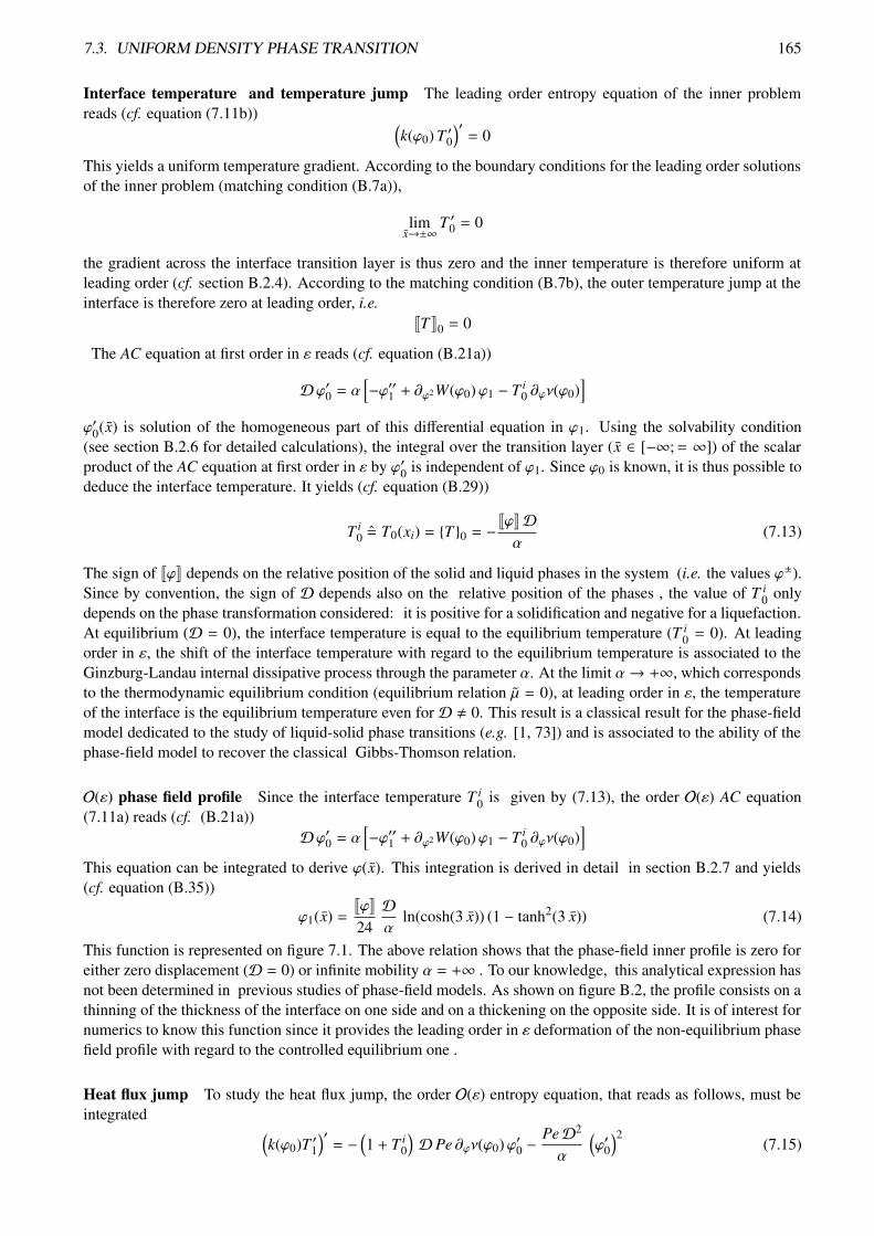
7.3. UNIFORM DENSITY PHASE TRANSITION 165
Interface temperature and temperature jump The leading order entropy equation of the inner problemreads (cf. equation (7.11b))
(
k(ϕ0) T ′0)′= 0
This yields a uniform temperature gradient. According to the boundary conditions for the leading order solutionsof the inner problem (matching condition (B.7a)),
limx→±∞
T ′0 = 0
the gradient across the interface transition layer is thus zero and the inner temperature is therefore uniform atleading order (cf. section B.2.4). According to the matching condition (B.7b), the outer temperature jump at theinterface is therefore zero at leading order, i.e.
JTK0 = 0
The AC equation at first order in ε reads (cf. equation (B.21a))
Dϕ′0 = α[
−ϕ′′1 + ∂ϕ2W(ϕ0)ϕ1 − T i0 ∂ϕν(ϕ0)
]
ϕ′0(x) is solution of the homogeneous part of this differential equation in ϕ1. Using the solvability condition(see section B.2.6 for detailed calculations), the integral over the transition layer (x ∈ [−∞;= ∞]) of the scalarproduct of the AC equation at first order in ε by ϕ′0 is independent of ϕ1. Since ϕ0 is known, it is thus possible todeduce the interface temperature. It yields (cf. equation (B.29))
T i0 = T0(xi) = T 0 = −
JϕKDα
(7.13)
The sign of JϕK depends on the relative position of the solid and liquid phases in the system (i.e. the values ϕ±).Since by convention, the sign of D depends also on the relative position of the phases , the value of T i
0 onlydepends on the phase transformation considered: it is positive for a solidification and negative for a liquefaction.At equilibrium (D = 0), the interface temperature is equal to the equilibrium temperature (T i
0 = 0). At leadingorder in ε, the shift of the interface temperature with regard to the equilibrium temperature is associated to theGinzburg-Landau internal dissipative process through the parameter α. At the limit α→ +∞, which correspondsto the thermodynamic equilibrium condition (equilibrium relation µ = 0), at leading order in ε, the temperatureof the interface is the equilibrium temperature even forD , 0. This result is a classical result for the phase-fieldmodel dedicated to the study of liquid-solid phase transitions (e.g. [1, 73]) and is associated to the ability of thephase-field model to recover the classical Gibbs-Thomson relation.
O(ε) phase field profile Since the interface temperature T i0 is given by (7.13), the order O(ε) AC equation
(7.11a) reads (cf. (B.21a))Dϕ′0 = α
[
−ϕ′′1 + ∂ϕ2W(ϕ0)ϕ1 − T i0 ∂ϕν(ϕ0)
]
This equation can be integrated to derive ϕ(x). This integration is derived in detail in section B.2.7 and yields(cf. equation (B.35))
ϕ1(x) =JϕK24Dα
ln(cosh(3 x)) (1 − tanh2(3 x)) (7.14)
This function is represented on figure 7.1. The above relation shows that the phase-field inner profile is zero foreither zero displacement (D = 0) or infinite mobility α = +∞ . To our knowledge, this analytical expression hasnot been determined in previous studies of phase-field models. As shown on figure B.2, the profile consists on athinning of the thickness of the interface on one side and on a thickening on the opposite side. It is of interest fornumerics to know this function since it provides the leading order in ε deformation of the non-equilibrium phasefield profile with regard to the controlled equilibrium one .
Heat flux jump To study the heat flux jump, the order O(ε) entropy equation, that reads as follows, must beintegrated
(
k(ϕ0)T ′1)′= −
(
1 + T i0
)
D Pe ∂ϕν(ϕ0)ϕ′0 −PeD2
α
(
ϕ′0)2
(7.15)
166 CHAPTER 7. ANALYTICAL STUDY OF ONE-DIMENSIONAL DYNAMICS
1/24(ln(cosh(3x))(1 − tanh(3x)2)
x
Φ1(
x)
3210-1-2-3
0.0080.0070.0060.0050.0040.0030.0020.001
0
Figure 7.1: function ϕ1(x)
The matching conditions yield (cf. equation (B.8a))
Jq0K = limx→∞
[
k(ϕ0(x)) T ′1(x) − k(ϕ0(−x)) T ′1(−x)]
Using an integration of equation (7.15) between x = ±∞ and using the expression (7.13) for T i0, we get (detailed
calculations can be found in section B.2.8) for the leading order outer heat flux jump (cf. (B.40))
Jq0K = −T i0 Peα
= JϕKPeD (7.16)
The first expression provides the interface boundary condition that, in addition to JT0K = 0, allows to solve theleading order outer thermal problem. The second writing is associated to the dimensional classical relation
JqK = DL
where L is the latent heat. This relation corresponds to the jump condition of the classical Stefan problem and isthus recovered at leading order in ε by our model.
To determine the leading order terms of the kinetic relation of the sharp problem in the non-equilibriumsituations where there is zero phase change but non-zero heat flux, it is required to study the equation of evolutionof the temperature up to O(ε). This study is the purpose of the following.
Solutions at O(ε) Let us first derive the outer temperature jump at first order in ε, JT1K (the details of thederivation is provided in section B.2.9). An integration of the entropy equation (7.15) at order O(ε) yields to theintroduction of the constant of integration Φth defined as
−Φth = k(ϕ0) T ′1 +D Pe(
1 + T i0
)
ν(ϕ0) +PeD2
α
∫ xϕ′20 dξ (7.17)
The matching conditions yield (cf. equation (B.7d))
limx→x±i
T ext1 = lim
x→±∞
[
T1 − x limx→x±i
T ext′0
]
Using this matching condition and the expression (7.13) for T i0, integration of equation (7.17) then yields (cf.
equation (B.43))
JT1K = −Φth
(
1k
)ex
0− PeD
(ν
k
)ex
0+ JϕK PeD2
α
(ν − P3
k
)ex
0(7.18)
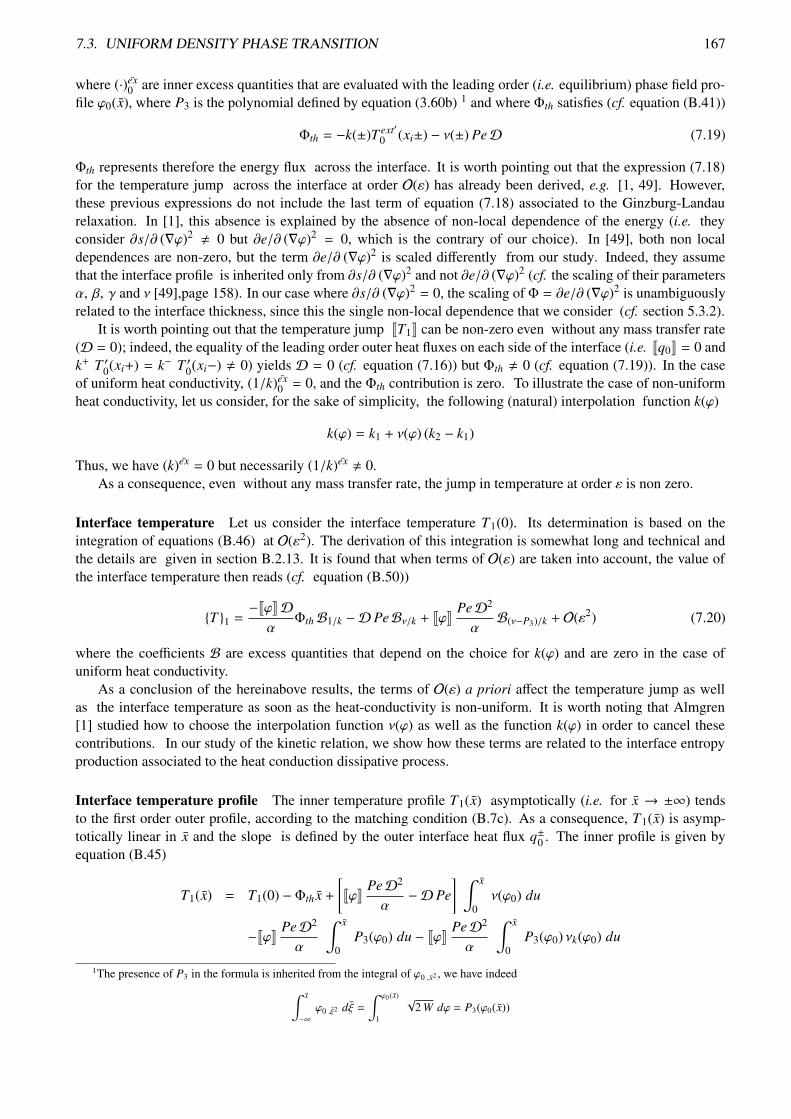
7.3. UNIFORM DENSITY PHASE TRANSITION 167
where (·)ex0 are inner excess quantities that are evaluated with the leading order (i.e. equilibrium) phase field pro-
file ϕ0(x), where P3 is the polynomial defined by equation (3.60b) 1 and where Φth satisfies (cf. equation (B.41))
Φth = −k(±)T ext′0 (xi±) − ν(±) PeD (7.19)
Φth represents therefore the energy flux across the interface. It is worth pointing out that the expression (7.18)for the temperature jump across the interface at order O(ε) has already been derived, e.g. [1, 49]. However,these previous expressions do not include the last term of equation (7.18) associated to the Ginzburg-Landaurelaxation. In [1], this absence is explained by the absence of non-local dependence of the energy (i.e. theyconsider ∂s/∂ (∇ϕ)2
, 0 but ∂e/∂ (∇ϕ)2 = 0, which is the contrary of our choice). In [49], both non localdependences are non-zero, but the term ∂e/∂ (∇ϕ)2 is scaled differently from our study. Indeed, they assumethat the interface profile is inherited only from ∂s/∂ (∇ϕ)2 and not ∂e/∂ (∇ϕ)2 (cf. the scaling of their parametersα, β, γ and ν [49],page 158). In our case where ∂s/∂ (∇ϕ)2 = 0, the scaling of Φ = ∂e/∂ (∇ϕ)2 is unambiguouslyrelated to the interface thickness, since this the single non-local dependence that we consider (cf. section 5.3.2).
It is worth pointing out that the temperature jump JT1K can be non-zero even without any mass transfer rate(D = 0); indeed, the equality of the leading order outer heat fluxes on each side of the interface (i.e. Jq0K = 0 andk+ T ′0(xi+) = k− T ′0(xi−) , 0) yields D = 0 (cf. equation (7.16)) but Φth , 0 (cf. equation (7.19)). In the caseof uniform heat conductivity, (1/k)ex
0 = 0, and the Φth contribution is zero. To illustrate the case of non-uniformheat conductivity, let us consider, for the sake of simplicity, the following (natural) interpolation function k(ϕ)
k(ϕ) = k1 + ν(ϕ) (k2 − k1)
Thus, we have (k)ex = 0 but necessarily (1/k)ex, 0.
As a consequence, even without any mass transfer rate, the jump in temperature at order ε is non zero.
Interface temperature Let us consider the interface temperature T1(0). Its determination is based on theintegration of equations (B.46) at O(ε2). The derivation of this integration is somewhat long and technical andthe details are given in section B.2.13. It is found that when terms of O(ε) are taken into account, the value ofthe interface temperature then reads (cf. equation (B.50))
T 1 =−JϕKDαΦthB1/k −D PeBν/k + JϕK PeD2
αB(ν−P3)/k + O(ε2) (7.20)
where the coefficients B are excess quantities that depend on the choice for k(ϕ) and are zero in the case ofuniform heat conductivity.
As a conclusion of the hereinabove results, the terms of O(ε) a priori affect the temperature jump as wellas the interface temperature as soon as the heat-conductivity is non-uniform. It is worth noting that Almgren[1] studied how to choose the interpolation function ν(ϕ) as well as the function k(ϕ) in order to cancel thesecontributions. In our study of the kinetic relation, we show how these terms are related to the interface entropyproduction associated to the heat conduction dissipative process.
Interface temperature profile The inner temperature profile T1(x) asymptotically (i.e. for x → ±∞) tendsto the first order outer profile, according to the matching condition (B.7c). As a consequence, T1(x) is asymp-totically linear in x and the slope is defined by the outer interface heat flux q±0 . The inner profile is given byequation (B.45)
T1(x) = T1(0) − Φth x +[
JϕK PeD2
α−D Pe
] ∫ x
0ν(ϕ0) du
−JϕK PeD2
α
∫ x
0P3(ϕ0) du − JϕK PeD2
α
∫ x
0P3(ϕ0) νk(ϕ0) du
1The presence of P3 in the formula is inherited from the integral of ϕ0 ,x2 , we have indeed∫ x
−∞ϕ0 ,ξ2 dξ =
∫ ϕ0(x)
1
√2 W dϕ = P3(ϕ0(x))

168 CHAPTER 7. ANALYTICAL STUDY OF ONE-DIMENSIONAL DYNAMICS
in the case of uniform heat conductivity and by equation (B.44)
T1(x) = T1(0) − Φth
klx − Φth (1 − 1/kl)
∫ x
0νk(ϕ0) du +
1kl
[
JϕK PeD2
α−D Pe
] ∫ x
0ν(ϕ0) du
−JϕK PeD2
αkl
∫ x
0P3(ϕ0) du
+
[
JϕK PeD2
α−D Pe
]
(1 − 1/kl)∫ x
0ν(ϕ0)νk(ϕ0) du − JϕK PeD2
αkl
∫ x
0P3(ϕ0) νk(ϕ0) du
in the case of variable heat conductivity. It is worth noting that this profile is determined by the leading orderprofile of the phase-field variable ϕ0(x) and by the choice for the interpolation function k(ϕ). A graphical repre-sentation of this profile is given on figure 8.2 of section 8.1.2 where the analytical results of matched asymptoticexpansions are compared with numerical results. On figure 8.3 the influence of the function k(ϕ) on the innertemperature profile is represented.
7.3.2 Kinetic relation
In this section, using the results derived in the previous section, we derive the kinetic relation of the sharpinterface model equivalent to our phase field model in the case of uniform density.
Leading order interface entropy production Let us study the expression for the surface entropy produc-tion (7.1d). Using non-dimensional writing2 it reads
Rs =
11 + T
JqK − Pe Γ JsK + q JTK1 + T
11 + T
(7.21)
Let us study the the interface entropy production at O(1) denoted Rs0. At leading order in ε, the temperaturejump is zero and therefore the last term of the expression for Rs0 is zero. According to our result of matchedasymptotic expansion, the order O(1) contribution of JqK reads (cf. equation (7.16))
Jq0K = JϕK PeD
Let us study the expression for JsK at leading order. In the uniform density case, the (assumed) linearity of Peq(T )is equivalent to the linearity of the latent heat L(T ), i.e. L/T = cste = Lre f /Teq. Therefore, according to thegeneral expression (3.59) for the specific Helmholtz free energy f , and following the non-dimensional analysismade for g (cf. equation (5.48)), we get
f (T, ϕ, ϕ,x2) = W(ϕ) +12ϕx2 − ε ν(ϕ) T − ε
∫ T
Tre f
ssolid(τ) dτ + geq(Tre f )
where Tre f is a reference temperature. And the non-dimensional entropy s = −(1/ε) (∂ f /∂T ) reads
s(ϕ,T ) = ν(ϕ) + ssolid(T ) (7.22)
ThereforeJsK = JϕK + Jssolid(T )K
where Jssolid(T )K , 0 if and only if JTK , 0. Therefore, since JTK0 = 0 at leading order in ε, the entropy jumpacross the interface reads
Js0K = JϕK
According to the hereinabove expressions for Jq0K and Js0K, the interface entropy production at leading orderreads
Rs 0 =PeD2
α(7.23)
2where Tre f is chosen as equal to Teq, Γ by ρ0D and where the surface entropy production has been scaled as [Rs] = [k/L]

7.3. UNIFORM DENSITY PHASE TRANSITION 169
Let us first remark that this expression for the leading order contribution to the interface entropy productionsatisfies
Rs 0 ≥ 0
This result is logical: since proportionnal to 1/α, the leading order dissipative terms are associated to theGinzburg-Landau relaxation, whose contribution is zero in the bulk phases (where µ = 0 since µ(0) = µ(1) = 0by construction and since ϕ,x = 0) and necessarily positive across the interface (according to the Clausius-Duheminequality). Therefore, Rs0 is an excess quantity of a zero jump quantity, and is therefore independent of the in-terface position (cf. our study of the excess quantities in section A.1). It is worth pointing out that such a kineticrelation is based on the classical Rankine-Hugoniot jump conditions for which the entropy flux q s is supposedto be equal to q/T . As a consequence, this results does not hold for the most widely used phase field modelswhere the entropy flux is defined differently (cf. our discussion in section 5.2). The Ginzburg-Landau relaxationequation provides a shift of interface temperature with regard to the equilibrium temperature proportional to therate of interface mass transfer and as a direct consequence a Gibbs free energy jump (the equilibrium relationJgK = 0 is not satisfied while JTK is still 0). It is worth pointing out that (since quadratic inD) this expression isconsistent with the normal growth theory or the classical Gibbs-Thomson equation (cf. equation (A.29)).
Next order for the dissipative terms, the dissipation associated with non-uniform thermal conductivityLet us consider the next order terms of the interface entropy production, denoted Rs1. It is worth noting that inthe case of infinite α or when D = 0, we have Rs0 = 0 (cf. equation (7.23)) and Rs1 corresponds to the leadingorder term for the interface entropy production.
According to the general expression (7.21) for Rs, and using the fact that JT0K = 0, we get
Rs1 = −q0JT1K(T0)2 +
Jq1K1 + T0
− Pe Γ Js1K (7.24)
Let us first study Js1K. Since we have Jϕ1K = 0, equation (7.22) shows that
Js1K = Jssolid, 1K = JT1Kdssolid
dT(T i
0) (7.25)
To derive the expression for Jq1K it is necessary to consider the entropy equation (B.46b) at order O(ε2) that reads
−D cP(T i0) T ′1 =
1Pe
(
k(ϕ0) T ′2 +(
∂ϕk(ϕ0)ϕ1)′
T ′1)′
+D(
∂ϕν(ϕ0)ϕ′1 + ∂ϕ2ν(ϕ0)ϕ1 ϕ′0
)
+ 2D2 Peαϕ′0 ϕ
′1
Jq1K is then obtained by integration of this equation, i.e. on a similar way than the expression (7.16) for Jq0K wasobtained from equation (7.15) (see section B.2.12 for detailed calculations). It yields (cf. equation (B.47))
Jq1K = cP(T i0) D Pe JT1K
The contribution to Rs1 of Jq1K is then compared to the contribution of Js1K. According to the definition of cP
and to the simplified expression (5.52) for cP (corresponding to the linearity of L(T )), we have
cP(T i0) = −
(
T i0 + 1
) d2geq
dT 2 =(
T i0 + 1
) dssolid
dT(T i
0)
It is therefore straightforward that it cancels the contribution of Js1K to Rs1. Let us now study the expression forq0 JT1K. According to the expression (7.19) for the constant Φth and using the identity ν = 1/2, we get
q0 = Φth +12
PeD
Using the expression (7.18) for JT1K yields
−q0 JT1K =(
Φth +PeD
2
)
Φth
(
1k
)ex
0+ PeD
(ν
k
)ex
0−
JϕKD(ν−P3
k
)ex
0
α
(7.26)

170 CHAPTER 7. ANALYTICAL STUDY OF ONE-DIMENSIONAL DYNAMICS
As already mentioned in the introduction of this paragraph, the term Rs 1 is dominant if and only if the term Rs 0is zero i.e. if either α = ∞ or ifD = 0. In the following , we consider that α = ∞, and thus T i
0 = 0 and therefore
Rs1 = −q0 JT1K
i.e.
Rs 1 = Φ2th
(
1k
)ex
0+ Φth PeD
12
(
1k
)ex
0+
(ν
k
)ex
0
−Pe2D2
2
(ν
k
)ex
0
The hereinabove relation implies that there exists a non-zero surface entropy production due to the non-uniformityof the heat conductivity. This result is consistent with the definition of Rs as an excess quantity (cf. the discussionon the equivalent sharp interface models in section A.2.4): when the heat conductivity is uniform, the sharp in-terface is equivalent to a medium of same heat conductivity as the surrounding bulk phases. There is no specificdissipation due to heat conductivity across the interface and the excess interface entropy production is zero. Inthe case of non-uniform heat conductivity the dissipation across the diffuse interface layer (a given volume) iseither less or larger than the dissipation of the bulk phase extended (over the same volume) toward the sharpinterface. As a consequence, there is no reason for the excess interface entropy production to be positive. R s1is a priori not signed since it involves the excess quantity (1/k)ex
0 , whose sign depends on the choice for thefunction k(ϕ).
When D = 0, the heat flux jump is zero Jq0K = 0, and q0 = Φth. Therefore, in this particular case theinterface entropy production reads
Rs1 = (1/k)ex0 Φ
2th
As a consequence, even without any mass transfer rate, the interface entropy production is non-zero. In classicalphase field models, the authors try to cancel the jump in temperature JTK1 so that their model is equivalentto the classical Stefan problem. The temperature discontinuity can be interpreted as a thermal trapping effect,e.g. Fadden et al. [49]. Using the framework of phase field models together with a consistent definition for theentropy flux, we show that this temperature jump is related to the excess interface entropy production inside theinterface.
Thus, a non-uniform heat conductivity is the source of an interface entropy production. This interface entropyproduction, as an excess quantity, is not a priori signed and its value can be controlled by choosing accuratelythe function k(ϕ). We have related this result with the classical phase field result about the temperature jump.This provides an interpretation of this result.
Kinetic relation at next orders in ε: contribution of the Ginzburg-Landau relaxation In this paragraph,in order to focus on the single effect of the Ginzburg-Landau relaxation, we consider the heat conductivity asuniform3. It is worth pointing out that when the heat conductivity is uniform there is no O(ε) contribution of theGinzburg-Landau relaxation to the interface entropy production. In the following, we show that, nevertheless,the Ginzburg-Landau relaxation is not limited to a contribution of order O(1) to Rs.
The leading order term of the interface entropy production, associated to the Ginzburg-Landau relaxation, hasbeen evaluated using the outer expressions for the temperature and heat flux interface values and jumps (cf. thederivation of equation (7.23) from equation (7.21) for example). However, it is also possible to express R s as theintegral across the interface of the local entropy production rate. This rate has been specified when we introducedthe Ginzburg-Landau dissipation mechanism in section 5.2. Let us consider the consequent expression of R s
Rs =D2 Peα
(
ϕ′2)ex
And therefore
Rs =D2 Peα
[∫ +∞
−∞ϕ′20 d x + ε
∫ +∞
−∞ϕ′0ϕ
′1 d x + ε2
∫ +∞
−∞
(
ϕ′21 + ϕ′0ϕ′2
)
d x + O(ε3)]
(7.27)
3Without this assumption, the contribution of both dissipative processes is more complex. Indeed, there exists a coupling between thetwo processes as attested by the last term of the expression (7.18) of JT1K which is non-zero if (i) the heat conductivity is non-uniformand (ii) α is finite.

7.4. ISOTHERMAL LIQUID-VAPOR FLOW WITH PHASE CHANGE 171
It is worth pointing out that ϕ(x) depends on D (ϕ1(x) is proportional to D as shown by equation (7.14)). As aconsequence, the expression for Rs is a priori not limited to quadratic terms in D. However, since the leadingorder phase field profile, which is the equilibrium profile, does not depend on D, at leading order, the rate ofentropy production is quadratic in D. Let us now draw the limit of this consistency and consider the next ordercontribution to the interface rate of entropy production.
The O(ε) is the integral of ϕ0 ,x ϕ1 ,x. The integration over the inner region of this contribution is zero (cf.section B.2.12)
∫ +∞
−∞ϕ0 ,x ϕ1 ,x dx = 0
It explains the absence of any Ginzburg-Landau contribution to Rs 1 as soon as the heat conductivity is uniform(cf. equation (7.26)).
At O(ε2), two contributions, namely ϕ2 ,x ϕ0 ,x and ϕ21 ,x, appear in the expression for the rate of entropy
production. The integral of (dϕ1/dx)2 is non-zero as soon as D , 0 and α < ∞. It is worth noting that since ϕ1is proportional to D/α (cf. equation (7.14)), the corresponding contribution to the interface entropy productionscales as ε2 D4/α3.
Thus, we have shown that the Ginzburg-Landau contribution to the interface entropy production is not limitedto the leading order term and moreover includes additional terms that deviate from the normal growth theory (i.e.not quadratic inD) as soon as the thickness of the diffuse interface remains finite.
7.3.3 Conclusion on the study of the solid-liquid one-dimensional phase change
In this section, we studied the one-dimensional phase transition process in the case of a uniform density usingmatched asymptotic expansions. The leading order temperature and phase field profiles have been determinedanalytically (cf. section 7.3.1). At O(1) in ε, these profiles are equivalent to equilibrium profiles (uniformtemperature, and hyperbolic tangent for the phase field). Nevertheless, the order O(1) rate of entropy productionis non-zero and its expression is consistent with the normal growth theory. However, the expression for the rateof entropy production has been shown not to reduce to these terms. It has been shown that, as soon as the outerheat fluxes are non-zero and the heat conductivity is non uniform, there exists a contribution to the rate of entropyproduction associated with the Fourier heat conduction. As an excess quantity, this contribution is a priori notsigned, and depends on the function k(ϕ). Moreover, the Ginzburg-Landau relaxation generates higher orderterms than the quadratic terms in D, and therefore reduces to the normal growth theory only at the limit ε = 0.It is worth pointing out that as a consequence the formalism of kinetic relations provided a clear interpretation ofthe different leading order results.
Moreover, the outer states have been shown to correspond to the phase field values 0 and 1 even for out ofequilibrium situations. This is an interesting property to control their physical properties.
7.4 Isothermal liquid-vapor flow with phase change
In this section, we study our quasi-compressible phase-field model for the liquid-vapor phase transition in thecase where the system is supposed to be isothermal and where the viscous dissipation is neglected.
For the sake of legibility, only the main results are given and discussed in this section. The reader interestedin the detailed derivation of these results can refer to section B.3 where all the calculations corresponding to thisstudy are provided .
In the isothermal and inviscid case considered here, the system of governing equations for the outer problemreads (cf. system (5.61))
α ε2 (D− V) ϕ,x = ε ∂ϕνP + v(
∂ϕW − ε2ϕ,xx)
+ ∂ϕν
(
W − ε2
2ϕ2,x
)
(7.28a)
(ρV),x = −ρ2 ∂ϕν (D− V)ϕ,x (7.28b)(V −D) ρV,x = −P,x (7.28c)
For the inner problem, only the AC equation has a modified scaling in ε and reads
α ε (D− V) ϕ′ = ε ∂ϕνP + v(
∂ϕW − ϕ′′)
+ ∂ϕν
(
W − (ϕ′)2
2
)
(7.29)

172 CHAPTER 7. ANALYTICAL STUDY OF ONE-DIMENSIONAL DYNAMICS
7.4.1 Leading orders phase-field profile
In the outer domains, the leading order AC equation (7.28a) reads
∂ϕW0 = 0
Therefore, as in the uniform density case we get that ϕ± is equal to either 0 or 1 and introduce JϕK = ±1. Theleading order inner AC equation (7.29) reads
v0(
∂ϕW0 − ϕ′′0)
+ ∂ϕν0
W0 −(ϕ′0)2
2
= 0
where we remind that v(ϕ) is the specific volume and where the function ν(ϕ) is the interpolation function used,in particular, to interpolate the density within the interface zone. Using the fact that ϕ equals 0 or 1 in theouter domains, it is a straightforward calculation to show (cf. the appendix section B.3.3) that this equation isequivalent to the leading order equation in the uniform density case studied in the hereinabove section 7.3
∂ϕW0 − ϕ′′0 = 0
Therefore, the leading order solution for the inner phase-field profile is the equilibrium profile, i.e. a hyperbolictangent profile for our model that is thus independent of the density difference. At the next order in ε (i.e. O(ε)),it can be shown that the equation for the phase field profile ϕ1(x) reads
ϕ1∂ϕ(vW)(ϕ0) − ϕ′1v′(ϕ0) − v(ϕ0)ϕ′′1 =Γ v(ϕ0)ϕ′0α
−(
A1Γ
α+Γ2
2
)
∂ϕv(ϕ0)
where Γ is the interface mass transfer rate and where
A1 = JϕK∫ +∞
−∞ν(ϕ0)ϕ′20 dx = 1/12 (7.30)
The integration of this differential equation (cf. section B.3.5) yields the sum of two profiles, one being propor-tional to Γ/α and the second one being proportional to Γ2 that reads
ϕ1(x) =Γ
αϕ′0
∫∫
(Gα) dx(
ϕ′0)2 dx + Γ2 ϕ′0
∫∫
(Gα∞) dx(
ϕ′0)2 dx (7.31)
where the functions Gα and Gα∞ satisfy
(v(ϕ0) Gα)′ =(
A1v(ϕ0)′ − v(ϕ0)ϕ′20)
(v(ϕ0) Gα∞)′ =(
1/2v(ϕ0)′ − v(ϕ0) v(ϕ0)′)
The first contribution is associated to the Ginzburg-Landau relaxation and vanishes as soon as the non-dimensionalmobility α is infinite. The second one is associated to the pressure recoil (cf. the results of the next section con-cerning the leading order pressure solution) and it is quadratic in the mass transfer rate Γ.
7.4.2 Leading order pressure and velocity
Velocity field At leading order in ε, the continuity equation (7.28b) reads
(ρ(ϕ0)V0)′ = −ρ20 ∂ϕν(ϕ0) (D− V0)ϕ′0
Its integration simply yieldsV0 −D = −Γ v(ϕ0) (7.32)
where Γ is the interface mass transfer rate.This relation implies that the outer velocity jump reads
JV0K = −Γ J1/ρK (7.33)
This condition corresponds to the sharp interface jump condition (7.2a) derived from the Rankine-Hugoniot jumpconditions.

7.4. ISOTHERMAL LIQUID-VAPOR FLOW WITH PHASE CHANGE 173
Pressure field At leading order in ε, the momentum equation (7.28c) reads
(V0 −D) ρ(ϕ0)V ′0 = −P′0
Using the expression (7.32) for the velocity, the pressure profile P0 simply reads (cf. equation (B.59))
P0 − Π = −Γ2 v(ϕ0) (7.34)
where Π is a constant of integration related to P0. Its determination (see section B.3.5) is based on the use ofthe solvability condition for the following expression for the O(ε) AC equation
ϕ1(
∂ϕv(ϕ0) ∂ϕW(ϕ0) + v(ϕ0) ∂ϕ2W(ϕ0))
− ∂ϕv(ϕ0)ϕ′1 ϕ′0 − v(ϕ0)ϕ′′1 =
D− V0
αϕ′0 − P0 ∂ϕv(ϕ0)
Multiplying this equation by ϕ′0 and integrating over yields a quantity that is independent of ϕ1(x). Using thehereinabove derived expressions for ϕ0, P0 and V0 allows then to determine the constant Π. We thus use exactlythe same method as for the determination of the interface temperature level T i
0 in the uniform density case. Ityields (cf. equation (B.66) and equation (B.68))
Π = A1Γ
α+ Γ2/2 (7.35a)
P0 = A1Γ
α(7.35b)
Using the matching condition (B.51b), equation (7.34) shows that the outer pressure jump readsq
Pext0
y= −Γ2 J1/ρK
This condition corresponds to the classical sharp interface jump condition (cf. equation (7.2b)), which is relatedto the pressure recoil effect. This effect is thus recovered by our model at leading order in ε.. Thus, we showedthat at leading order in ε, the jump conditions of the equivalent sharp model are the classical jump conditions (i.e.the jump in velocity is related to the mass conservation and the pressure jump is related to the pressure recoil).They are consistent with the jump conditions (7.2) derived from the Rankine Hugoniot jump conditions. Inaddition, a shift of the interface pressure from the equilibrium pressure is due to the Ginzburg-Landau relaxation.We study in the following the consequence of this out of equilibrium structure of the diffuse interface on thekinetic relation of the equivalent sharp interface model.
7.4.3 Kinetic relation
In this section, we study the kinetic relation from the leading order solutions derived in the previous section.We determine the expression for the surface entropy production Rs at leading order in ε and relate it to an “outof equilibrium Clapeyron relation”.
It is important to note that, in the isothermal case, it is not possible to use the native expression for R s
(equation (7.1d)) since no direct information is available concerning either the entropy flux q s = q/T or thespecific entropy s. Let us thus consider the expression for Rs as a function of the driving force G that reads (cf.equation (7.4))
RsTeq = ΓG
where the driving force G reads (cf. equation (7.3))
G = JgK +s
(V −D)2
2
This latter quantity can thus be studied in the isothermal case studied. Moreover, since the relation
1/ρ JPK = −s
(V −D)2
2

174 CHAPTER 7. ANALYTICAL STUDY OF ONE-DIMENSIONAL DYNAMICS
is satisfied by the O(1) solutions of the pressure and velocity and, since the compressibility of the bulk phases isnot considered in our phase-field model, we have thus (cf. equation (A.26))
Rs Teq = Γ P J1/ρK
And the study of the interface entropy production is therefore related to the study of the shift of the interfacepressure with regard to the equilibrium pressure P. It is worth pointing out that this expression, that involvesexplicitly the interface pressure level P is an “out of equilibrium Clapeyron relation”.
Let us now derive the leading order expression for the interface entropy production. According to the leadingorder solution for the pressure (cf. equation (7.35b)), the above relation yields
Rs0 Teq =Γ2
αA1 (7.36)
which satisfiesRs0 > 0
Since the only dissipative mechanism considered is the Ginzburg-Landau relaxation, interface entropy sourcevanishes as α→ +∞. Since this dissipative mechanism only exists inside the interface zone (i.e. zero contributionin the bulk phases), it is consistent to have a positive Rs0. Since, at leading order in ε, the interface entropy sourceRs0 is quadratic in Γ, its expression (7.36) is consistent with the normal growth theory.
It is worth pointing out that, like in the uniform density case, the Ginzburg-Landau relaxation implies a highercontribution to the interface entropy production (cf. our discussion at the end of section 7.3.2). Indeed, we haveJ1/ρK1 = 0 and at O(ε), the value of the interface entropy production reads
Teq Rs 1 = Γ P1 JϕK
where the expression for P1 reads
P1 =2 JϕKΓα
∫ +∞
−∞ϕ′0(x)ϕ′1(x) dx
We have shown that ϕ1(x) was made of two parts, the first one being scaled by Γ/α and the second one by Γ2 (cf.equation (7.31)). It can be shown that the contribution to P1 of ϕ′1ϕ
′0 scaled by Γ2 is zero. As a consequence
only the part of ϕ′1 scaled by Γ/α remains and we get
Teq Rs 1 = 2Γ3
α2 JϕK Aα (7.37)
This relation shows that, at O(ε), the kinetic relation deviates from the normal growth theory as soon as the masstransfer rate is sufficiently large. We have finally (cf. equations (7.36) and (7.37))
Teq Rs =Γ2
αA1 + ε 2
Γ3
α2 JϕK Aα + O(ε2)
This study of the non-equilibrium structure of the diffuse interface in the isothermal case showed that theclassical Rankine-Hugoniot jump conditions on the pressure and velocity are recovered by the equivalent sharpinterface model. Besides, similarly to the uniform density case studied in section 7.3, we showed that the interfaceentropy production is not null and that it is due to the Ginzburg-Landau relaxation.
7.5 Non-isothermal liquid-vapor flow with phase change
In this section, we study the out of equilibrium structure of the interface in the case of a non-isothermal phasetransition, which is characteristic of boiling flows. The system of governing equations corresponds to the sys-

7.5. NON-ISOTHERMAL LIQUID-VAPOR FLOW WITH PHASE CHANGE 175
tem (5.59) that reads
α ε2 (D− V) ϕ,x = εdνdϕ
(
P − T)
+ v
(
dWdϕ− ε2ϕ,xx
)
+dνdϕ
(
W − ε2
2ϕ2,x
)
(7.38a)
(ρV),x = −ρ2 ∂ν
∂ϕ(D− V)ϕ,x (7.38b)
(V −D) ρV,x = −P,x (7.38c)
(V −D) ρT,x =
(
k T,x)
,x
Pe− (V −D) ρ (1 + T )
dνdϕϕ,x + (D− V)2 ρε
α
(
ϕ,x)2 (7.38d)
It is worth noting that, compared to the systems studied in the previous sections (uniform density and isothermalcases), these equations are only slightly modified by the coupling between thermal and mechanical physicalmechanisms. For example the momentum and continuity equations are exactly similar to the one studied insection 7.4 whereas the equation of evolution of the temperature reads exactly the same than the one studied insection 7.3. In fact only the presence of both pressure and temperature in the AC equation makes a real differencewith the previously studied equations. As a consequence, we only comment the differences for the solutionsassociated with this coupling (see section 7.5.1). Then, in section 7.5.2, we study in more details the expressionfor both the interface entropy production and the driving force of the equivalent sharp interface model.
7.5.1 Leading order solutions
The complete calculation of the leading order solutions takes advantage of the similarity of the equations withthe one studied in the two degenerate cases considered (cf. the appendix B.4). As a consequence, we do notrecall the detailed calculations that can be found in the previous sections.
The leading order solutions of the inner profiles as well as the outer jump conditions and interface valueshave similar expressions to those obtained in the previous sections where we studied degenerated forms of ourmodel. They read (cf. the equations (B.80), (B.81b), (B.86), (B.87), (B.84) and (B.85))
ϕ0(x) = 1/2 + (JϕK/2) tanh (3 x) (7.39a)
P0(x) = P0 + v0Γ2 − v(ϕ0(x))Γ2 (7.39b)
V0(x) = D− Γ v(ϕ0(x)) (7.39c)
P0 = T i0 + Γ
A1
α(7.39d)
JT0K = 0 (7.39e)
T0 = T i0 (7.39f)
Jq0K = PeΓ(
1 + T i0
)
JϕK + Γ2 |A1| (7.39g)
whereA1 is given by (7.30).
Therefore, at leading order in ε, equations (7.39e) and (7.39f) show that the temperature is uniform and thephase field profile is the equilibrium one. Equation (7.39b) shows that the pressure satisfies the classical jumpcondition (pressure recoil). Equation (7.39d) shows that the pressure at the interface P0 differs from thesaturation pressure at the interface temperature and that the shift is proportional to Γ/α. It is worth noting thatwhenever the outer heat flux jump Jq0K equals zero, the mass transfer rate can still be non-zero. Indeed we havefrom equation (7.39g)
Jq0K = 0⇒ Γ = PeJϕK|A1|
(
1 + T i0
)
The corresponding mass transfer rate is actually an adiabatic phase transition process as studied in the previoussection.
Thus, the leading order solution of the non-isothermal case with density difference is such that the classicaljump conditions on velocity and pressure (7.2) are recovered by the equivalent sharp model. Moreover, the bulkphase field values are always 0 or 1, which allows to clearly control the physical properties of the single-phasestates even in out of equilibrium conditions. The interface pressure is related to the temperature of the interface

176 CHAPTER 7. ANALYTICAL STUDY OF ONE-DIMENSIONAL DYNAMICS
through an “out of equilibrium Clapeyron relation”. It is worth noting that this result has already been obtainedby Anderson et al. [6] with the model presented in section 2.3.3. In the following, we study the consequencesof this internal structure of the interface on the kinetic relation.
7.5.2 Kinetic relation
This section is organized as follows. First, we show that the leading order expression of the interface entropyproduction is associated only to the Ginzburg-Landau dissipative process. Then, it is shown that it is possible toderive a good approximation of the interface entropy production using an approximate expression of the interfaceentropy production. The use of this approximate expression is shown to be of interest since it allows to clearlyrelate the kinetic relation to an “out of equilibrium Clapeyron relation”. We then study the next order expressionof the kinetic relation and show how it is related to a non-uniform heat conductivity across the interface. Finally,we derive the expression for the kinetic relation in terms of the driving force, which is another way to interpretthese results.
Leading order kinetic relation, the Ginzburg-Landau relaxation Let us study the kinetic relation at O(1) .According to our study of the sharp interface problem, the general expression for the interface entropy productionRs reads (cf. (7.1d))4
Rs = −qJTK1 + T
11 + T
+
11 + T
JqK − Pe Γ JsK (7.40)
The leading order outer temperature jump is zero (cf. equation (7.39e)) and, as a consequence, the first term ofthe above expression is zero at leading order. The value of the leading order contribution to the heat flux jump isgiven by equation (7.39g). The only term that remains to be studied is the entropy jump.
The non-dimensional expression for the quasi-compressible Gibbs free energy reads (equation (5.48)) wherewe have considered that Peq is linear
g = ε v(ϕ) [P − T ] + v(
W +ε2
2(∇ϕ)2
)
+ ε geq(T )
Since s = −(∂g/∂T ) we get
s = ν(ϕ) −dgeq
dTThus at leading order, we get Js0K = JϕK. Since JT0K = 0 and using the expression (7.39g) for Jq0K we get for theleading order of the interface entropy production (cf. equation (7.40))
Rs0 = Γ2 PeαA1
11 + T0
(7.41)
This expression is identical to the expression (7.36) derived in the isothermal case.
Thus, the kinetic relation of the equivalent sharp interface model at leading order is only related to theGinzburg-Landau relaxation. As a consequence, the corresponding interface entropy production is strictly posi-tive. Moreover, it is quadratic in Γ, which makes this relation consistent with the normal growth theory. It hasbeen shown that a non-zero interface entropy production is at the origin of an “out of equilibrium Clapeyronrelation” satisfied by the interface pressure and interface temperature.
Kinetic relation at next order The interface entropy production at O(ε) is defined by equation (7.24). Forthe sake of simplicity, in the following, we consider only the case α = ∞, knowing that in any other case, theleading order term of the interface entropy production associated to the Ginzburg-Landau relaxation has alreadybeen derived. Jq1K is derived from an integration of the order ε2 equation of evolution for the temperature (seesection B.4.5). In the case α = ∞, Jq1K reads (cf. equation (B.94))
Jq1K = cP(T i0) Γ Pe JT1K
4Rs, resp. s, is scaled by [k/L], resp. [L/T ].

7.5. NON-ISOTHERMAL LIQUID-VAPOR FLOW WITH PHASE CHANGE 177
and according to the expression (7.25) for Js1K, the contribution to the interface entropy production of JsK1 iscanceled by the Jq1K contribution. It yields
(
T i0
)2 Rs 1 = −Jq0K JT1K
Jq0K is given by equation (7.39g). Let us analyze the expressions for JT1K. The expression for JT1K is derived byintegration of the order ε equation of evolution for the temperature on the same way than in the uniform densitycase (cf. section B.4.3). The expression for µ and T i
0 being different than in the uniform density case, it yields(cf. equation (B.89))
JT1K = −Φth
(
1k
)ex
0− PeΓ
(
1 + T i0
) (ν
k
)ex
0− 2 JϕK PeΓ
α
∫
(vW(ϕ0)dξ)
k(ϕ0)
ex
(7.42)
It is worth pointing out that this expression is very similar to the one obtained in the uniform density case (cf.equation (7.18)) as involving excess quantities related to the thermal conductivity. Moreover, when α is infinite,the temperature jump has an expression similar to the one obtained with the van der Waals model (cf. the matchedasymptotic expansions derived in [53]). Using the expression (7.39g) for Jq0K, we get therefore
Rs 1 =(
PeΓ(
1 + T i0
)
JϕK + Γ2 |A1|)
Φth
(
1k
)ex
0+ PeΓ
(
1 + T i0
) (ν
k
)ex
0
Similarly to the case of uniform density (cf. section 7.3.2), this expression shows thatRs 1 is identically zero if theheat conductivity is uniform. This O(ε) interface entropy production is related to an excess Fourier dissipationacross the interface and is a priori not signed. We remind that this result is valid in the case α → ∞. Thestudy of the O(ε) interface entropy production associated to the Ginzburg-Landau relaxation is carried out in thefollowing paragraphs.
Thus, from order ε the interface entropy production is related to the heat conduction across the interfaceand is a priori not null as soon as the heat conductivity is non-uniform. The classical kinetic relation is oftenpresented in terms of the driving force instead of the interface entropy production. In the following paragraph,we study the expression for the driving force as a function of the mass transfer rate.
Driving force as a function of the mass transfer rate Let us study the general expression for the leadingorder kinetic relation as a relation between the driving force G and the mass transfer rate Γ. In the section 7.1),we have defined the driving force G such that
Rs T + 1 = Γ Pe G − JTK q
T
+ JqK(
T
1T
− 1)
where G has been scaled by V2. Such a driving force has been shown to be defined by (cf. equation (7.3))
G = JgK + s JTK + Γ2
1ρ
s1ρ
Therefore, using the results (7.39) at leading order, we get
G0 =Γ
αA1
When sensible heat is neglected with regard to the latent heat in the evaluation of JgK the approximate expressionfor the driving force (7.6) reads
G ' P J1/ρK − T JsK
Since J1/ρ0K = Js0K = JϕK, we have
P1J1/ρ0K − T1Js0K = JϕK (P1 − T1)

178 CHAPTER 7. ANALYTICAL STUDY OF ONE-DIMENSIONAL DYNAMICS
and the leading order of the driving force reads
G ' JϕK (P0 − T 0)
+ε[JϕK (P1 − T 1) − T0 Js1K
]
+O(ε2)
where Js1K is given by (cf. section 7.3.2)
Js1K = JT1K cP(T i0)
(
1 + T i0
)
where JT1K is given by equation (7.42). In the appendix section B.4.4, we study the scaling of the different termsof the AC equation (B.91) at order ε2. Applying the solvability condition to this equation allows to determine thedifferent terms entering the expression of P1 − T1. Using the expressions for the leading order solution of theinner problem (7.39) for P0 and T0, we get
G ' ΓA1
αJϕK
+ε
[
JϕK(
Γ2
α2 βΓ2/α2 + Φth βΦth + Γ Pe βPe +Γ2 PeαβΓ2 Pe/α +
Γ3
αβΓ3/ α
)
+ cP(T i0)
(
1 + T i0
)
Φth
(
1k
)ex
0+ PeΓ
(
1 + T i0
) (ν
k
)ex
0+ JϕK PeΓ
αβΓ Pe/α
+O(ε2) (7.43)
where the coefficients β are of order unity and are excess quantities. βΓ2/α2 and βΓ3/ α vanishes in the uniformdensity case, whereas all the other coefficients vanish for a uniform heat conductivity. The driving force is madeof two different parts: the first one that depends on the mobility as 1/α is associated to the Ginzburg-Landaurelaxation, and the second one that is related to non-uniform heat conductivity is associated to the Fourier heatconduction.
In this section, we derived approximate expressions for the interface entropy production and for the drivingforce. They show that the non-uniformity of the heat conductivity as well as the existence of a Ginzburg-Landaurelaxation determine the relation between the interface pressure and the interface temperature of the equivalentsharp interface model. At leading order, this relation is consistent with the normal growth theory (i.e. the interfaceentropy production quadratic in Γ or, equivalently, the driving force is linear in Γ), and the kinetics are associatedto the Ginzburg-Landau relaxation as shown by the order 1 term of equation (7.43). However at next order, it isshown to deviate from this theory as shown by the order ε term of equation (7.43).
7.6 Sharp interface limit for far from equilibrium phase transition
In this section, we study a different sharp interface limit of our phase field model that is more accurate for farfrom equilibrium phase transitions. Indeed, the results obtained so far are based on a particular scaling of themobility, i.e. of the dissipative coefficient associated to the Ginzburg-Landau relaxation. As a consequence, thekinetic relation reads as the linearity of the driving force with the interface mass transfer rate at leading order andthat even for large mass transfer rates, e.g. equation (7.43). This linearity is consistent with the normal growthapproximation that has been related in section 7.1 to a “close to equilibrium” model for the kinetics of phasetransition. It is worth noting that an even lower level of modeling of the entropy interface production correspondsto set it to zero that corresponds in our case to set α to infinity. To deviate from the normal growth theory,we showed that it was necessary to consider higher order terms of the matched asymptotic expansion, i.e. theeffect of a finite thickness for the interface transition layer (the so-called thin interface limit introduced by Karmaand Rappel [72]). This characteristic of the kinetic relation of the model can be attractive, for example when aregularization of the Stefan model where latent heat removal is the limiting stage is targeted (as it is the case ofthe widely used phase field methods). Nevertheless we know that the normal growth theory is only a model forslow phase boundaries and such a linear kinetic relation could also be viewed as a limit of the model.

7.6. SHARP INTERFACE LIMIT FOR FAR FROM EQUILIBRIUM PHASE TRANSITION 179
In the following, we derive the kinetic relation of the phase field model, considering a different scalingand show how it yields to a more complex kinetic relation. This shows how one can deal with non-linear kineticrelation as sharp interface limit as soon as the scaling of the mobility is chosen accurately. This thus demonstratesthat the phase field model are not limited to a regularization of the normal growth theory but can also generatemore realistic kinetic relations.
7.6.1 Leading order phase field equation and kinetic relation
We now turn our attention to the case where the normalized dissipative coefficient of the Ginzburg Landaurelaxation is a fixed independent parameter, say α = α/ε. We denote the scaling α, resp. α, of the mobilityas the close, resp. far from equilibrium scalings. Following the far from equilibrium scaling, the system ofequation (5.59) then reads
α ε (D− V) ϕ,x = εdνdϕ
(
P − T)
+ v
(
dWdϕ− ε2ϕ,xx
)
+dνdϕ
(
W − ε2
2ϕ2,x
)
(7.44a)
(ρV),x = −ρ2 ∂ν
∂ϕ(D− V)ϕ,x (7.44b)
(V −D) ρV,x = −P,x (7.44c)
(V −D) ρT,x =
(
k T,x)
,x
Pe− (V −D) ρ (1 + T )
dνdϕϕ,x + (D− V)2 ρ
α
(
ϕ,x)2 (7.44d)
In order to focus on kinetics we consider a purely phase field model and thus ignore the coupling with pressureand temperature. The system of governing equations reduces therefore to the single AC equation (7.44a) and thesingle dissipative mechanism considered is thus the Ginzburg-Landau relaxation. The inner leading order ACequation (7.44a) is an ODE in ϕ0(x) that reads
D ϕ′0 =(
∂g
∂ϕ
)
0− ϕ′′0 (7.45)
where we introduced the normalized velocity of the phase transition front D
D = Dα
Equation (7.45) has already been studied by Truskinovsky [137], see also [139] in the context of kinetic relations.Let us first analyze the out of equilibrium ODE (7.45), and reproduce the analogy used in the study of the
spherical equilibrium case (cf. section 4.3.1). We thus consider the motion of a particle in a one dimensionalsystem of coordinates ϕ, the time being associated to the abscissa x. The LHS of equation (7.45) is then aviscous dissipation for the particle motion. It is worth pointing out that using the “close to equilibrium scaling“the leading order out of equilibrium ODE governing the phase field profile was non-viscous, e.g. equation (7.12)(zero LHS in equation (7.45)) and thus ϕ0(x) was the planar equilibrium profile. In the present case, we recoverthe equilibrium profile only in the limit of small D where the LHS term of equation (7.45) can be neglected.
Let us now consider the kinetic relation of this model. In this case, entropy and density jumps are zero andthe driving force simply reads (cf. its definition (7.3)).
G = JgK
and is thus equal to the specific Gibbs free energy jump across the interface transition layer. It is a straightforwardcalculation (multiplying by ϕ′ and integrating over ) to show from equation (7.45) that
JgK = D∫ +∞
−∞ϕ′2(x) d x (7.46)
This relation is the kinetic relation of the phase field model considered. It shows that at and only at equilibriumboth D and JgK are zero. Let us now consider the integral term. It is worth pointing out that for the “close toequilibrium” scaling of the mobility, ϕ0(x) was the planar equilibrium profile. As a consequence the integral wasindependent of the out of equilibrium parameter (JgK or D), and thus at leading order the driving force was linearin D. This obviously no more the case with the “far from equilibrium” scaling as illustrated in the following.

180 CHAPTER 7. ANALYTICAL STUDY OF ONE-DIMENSIONAL DYNAMICS
7.6.2 Illustrative example of non-linear leading order kinetic relation
As an illustrative example, let us consider a simple model for the potential µ(ϕ0) using piecewise quadratic ap-proximation for the specific Gibbs free energy as represented on figure 7.2. Since we consider out of equilibriumprocess, we have JgK0 , 0. At infinity, homogeneous single phase states are reached. According to the propertiesof our model, these single phase states correspond to the phase field values 0 and 1 as shown in chapter 6. Topropose a simple model consistent with the main features of our phase field model, we set
∂g
∂ϕ(0) = µ(0) = 0
∂g
∂ϕ(1) = µ(1) = 0
The piecewise potential then simply reads
µ(ϕ) =
ϕ, ϕ ≤ 12 ,
2(
1 + 4 JgK) (ϕ − 1) , ϕ > 12 .
(7.47)
and is thus discontinous at ϕ = 1/2. The potential µ as well as the specific Gibbs free energy g are representedon figure 7.2. To solve the ODE (7.45) we now need to solve two linear second order differential equations for
JgK
ϕ
g
1.510.50-0.5
0.40.2
0-0.2-0.4-0.6-0.8
-1
ϕ
µ
1.510.50-0.5
6420
-2-4-6
Figure 7.2: Piece wise thermodynamic potential
each domain ϕ0(x) ∈ [0 : 1/2] and ϕ0(x) ∈ [1/2 : 1]. We set ϕ0(−∞) = 0, ϕ0(+∞) = 1 and ϕ0(0) = 1/2. As aconsequence the out of equilibrium ODE (7.45) has the solution
ϕ0(x) =
12 e a0 x, x ≤ 0,1 − 1
2 e−a1 x, x ≥ 0.(7.48)
where the positive coefficients a0 and a1 read
a0 =−D +
√D2 + 4
2
a1 =D +
√
D2 + 8(
1 + 4 JgK)
2
We can thus evaluate the integral entering the kinetic relation (7.46), it yields
∫ +∞
−∞ϕ′20 (x) d x =
∫ 0
−∞
a20
4e 2 a0 x d x +
∫ +∞
0
a21
4e− 2 a1 x d x
=a0
8+
a1
8
and thus
JgK = 116D
[√
D2 + 4 +√
D2 + 8(
1 + 4 JgK)]

7.6. SHARP INTERFACE LIMIT FOR FAR FROM EQUILIBRIUM PHASE TRANSITION 181
that is obviously a non-linear relation between D and the driving force. As a consequence, the kinetic relationinherited from the “far from equilibrium” scaling for the mobility deviates from the normal growth theory forlarge interface mass transfer rates.
The non-linearity of the kinetic relation between the driving force and the interface mass transfer is morephysically realistic than the linearity inherited from the “close to equilibrium” scaling of the mobility that is thenat leading order restricted to the normal growth approximation. Nevertheless as long as a single regularizationof the Stefan problem at low mass transfer rates is targeted, the “close to equilibrium” scaling is mathematicallysatisfying. It would be of interest to further investigate the consequences of the “far from equilibrium” scaling ofthe phase field equations for the model including pressure and temperature dependences.

182 CHAPTER 7. ANALYTICAL STUDY OF ONE-DIMENSIONAL DYNAMICS
7.7 Conclusion
In this chapter, we studied the non-equilibrium internal structure of the interface using approximate solutions(matched asymptotic expansions) of the governing equations for a steady-state one-dimensional phase changeproblem. The leading order profiles of the main variables have been derived. It has been shown that the equivalentsharp interface representation of our model satisfies the classical jump conditions (mass, momentum, energy).Moreover, in the outer bulk phases, the phase field value is always 0 or 1, which allows to easily control theirphysical properties. In addition, we have derived the kinetic relation of our model. At leading order, the interfaceentropy production is consistent with the normal growth theory, i.e. the interface entropy production is quadraticin the mass transfer rate. As a consequence, the classical Gibbs-Thomson equation is recovered for low masstransfer rates in the case of uniform density. When density difference is taken into account, a non-equilibriumClapeyron relation has been derived. However, the kinetic relation has been shown not to reduce to thenormal growth theory. Indeed, when higher order terms are taken into account, the interface entropy productionis no longer quadratic in the mass transfer rate. The entropy production has been clearly shown to be madeof two contributions corresponding to the two dissipative processes considered in this study. The first one isrelated to the Ginzburg-Landau relaxation and is non-zero as soon as the mobility is finite. Since this dissipativeprocess only takes place inside the interface, the associated interface entropy production is positive. The secondcontribution is associated to heat conduction. This dissipation is non-zero both in the bulk phases and across theinterface. It has been shown that the associated interface entropy production is an excess quantity that is non-zeroonly if the heat conductivity is non-uniform. If it is non-uniform, the sign of the interface entropy production ofthe equivalent sharp interface model depends on the choice for the function k(ϕ). This is consistent with the factit is an excess quantity since the dissipation associated to heat conduction that takes place across the interfacecan be either smaller or larger than the sum of its equivalent representation by two separated bulk domains anda sharp interface.
We note that the consistency of the leading order solutions with the normal growth approximation limits theuse of the model for fast kinetics where the phase transition occurs far from equilibrium. By introducing anotherscaling for the mobility coefficient, we derived another sharp interface limit for a purely phase field model. Withthis scaling, the kinetic relations deviates from the normal growth approximation as soon as the mass transfer rateis sufficiently large and that even in a sharp interface limit (i.e. without considering secondary order terms in theexpansion). This deviation at large mass transfer rate is more physically realistic and we therefore draw a pathallowing to consider other kinetic relations for our phase field model devoted to the study of boiling process.
Let us note that we know that for boiling phase transition, in addition to heat conductivity and Ginzburg-Landau relaxation, the viscosity, as a third dissipative mechanism has to be taken into account. Due to thedensity difference between the single phase states, the associated interface entropy production is non-zero andvisco-elasticity can actually also control the kinetics of the phase transition. It would be of interest to study thisinterface dissipation for our phase field model.
Nevertheless, it is worth pointing out that there is a lack of knowledge and of understanding of the kineticrelation in the case of liquid-vapor interfaces. If several models exist for the case of high mass transfer ratesassociated to vaporization (e.g. the interface resistance, cf. the Knudsen layer model [28]), none is consistentwith the classical jump condition for the pressure recoil. As mentioned by Anderson et al. [2] it remains to havea sound target for the kinetic relation.
As a final conclusion let us remark that, to our knowledge and even though matched asymptotic expansionsare widely used to study phase field models, the use of the formalism of kinetic relation has never been presented,although it allows, to our point of view, to derive a clear analysis of the properties of these models. Indeed, weshowed how the relation between interface pressure and temperature (“non-equilibrium Clapeyron relation”) isrelated to the interface entropy production.

Chapter 8
Numerical resolution of the system ofgoverning equations
In this chapter, we solve numerically the system of governing equations corresponding to the quasi-compressiblephase field model dedicated to liquid-vapor flows with phase change derived in chapter 3. The goal is to developan algorithm for the solving of the governing equations and to study the consistency of the numerical results withthe analytical developments made in the previous chapters . In particular we study the ability of the model
? to control the stability of the liquid and vapor homogeneous states (cf. the corresponding analytical studyof the stability of homogeneous states in chapter 6)
? to reproduce a given kinetic relation and to recover the classical out of equilibrium jump conditions (cf.the corresponding analytical study of the one-dimensional phase transition dynamics in chapter 7)
? to deal with capillarity and curvature (cf. the corresponding analytical and numerical study of the sphericalsymmetry equilibrium in chapter 4)
We propose to consider three different canonical systems of governing equations. We follow the approachused to derive the analytical results of one-dimensional phase transition. We first focus on the purely thermalpart of the phase transition by studying the phase transition with uniform density and, as a consequence, withoutmechanics (cf. section 8.1). Then, we study the coupling between phase change and fluid mechanics by consid-ering the isothermal model (cf. section 8.2). Finally, we study the fully non-isothermal dissipative model (cf.section 8.3). Let us note that, the main numerical schemes and notations used in the following numerical studyare introduced in the appendix C.
8.1 Liquid-solid phase transition without mechanics
In this section, we present the numerical simulation of the phase transition in the case of uniform density forone- and two-dimensional systems. The goal is to study the coupling between the energy balance equation andthe Allen-Cahn equation. The resolution of this coupling allows to take into account a major ingredient ofthe boiling flows: the unsteady phase transition associated to thermal effects. Indeed, the classical models of thebubble growth in nucleate boiling flows assume that the last stage of the process is governed by a thermal effects,e.g. Mikic et al. [93]. Moreover, the results of this section allow to illustrate some of the key ingredients of ourmodel, namely
? the modeling of the interfaces as transition zones of characteristic thickness h
? the separation of the domain in single phase domains characterized by constant values of the phase-field(ϕ = 0 and ϕ = 1)
? the ability of the model to deal with capillarity, curvature and topological changes
? the dynamics of phase transition
183

184 CHAPTER 8. NUMERICAL RESOLUTION OF THE SYSTEM OF GOVERNING EQUATIONS
? the kinetic relation associated to the Ginzburg-Landau and thermal conductivity dissipation mechanisms(cf. chapter 7)
It is worth noting that, since the density is assumed to be uniform, the model corresponds to a solid-liquidphase transition. It is worth pointing out that the goal of this numerical study is to define an algorithm for thecoupling between thermal and phase field parts of the model before to adress the coupling with mechanics. Asa consequence we limit our study to a rather more qualitative than quantitative analysis of the results obtained.The satisfaction criteria will be based on the consistency of the results with the analytical results derived in theprevious chapters. We therefore won’t provide a detailed study of the phase transition without density differencesuch as it is done with phase field models devoted to this study.
This section is organized as follows. First, in section 8.1.1, we analyze the system and discuss the approx-imations introduced to develop an efficient and accurate algorithm to solve it. Then in section 8.1.2, we studyone-dimensional steady-state phase change problem. We justify the main approximations used in the algorithmby a comparison with both analytical results and more accurate computations. We study the temperature andphase field profiles and compare them with the corresponding analytical results obtained in chapter 7. In sec-tion 8.1.3, we illustrate the ability of our model to deal with unsteady phase change problems. The influence ofthe Ginzburg-Landau relaxation on this result as well as the corresponding kinetic relation are analyzed. Two-dimensional computations are then proposed. In section 8.1.4 we first solve an unsteady phase change problemin spherical symmetry. Then in section 8.1.5, we illustrate the dynamic of phase separation and interface recon-nection with our phase field model studied in chapter 6. We then study in section 8.1.6 the unsteady phase changeprocess in a two-dimensional system that illustrates the effect of capillarity on the process.
8.1.1 Time discretization scheme
In this section, we identify the terms of the governing equations that need to be treated as implicit in time andthose that can remain explicit. This identification is based on the physical anlysis of the couplings of theseequations that have to be accounted for. Once these couplings are identified, a linear approximation of theterms involved is proposed as a valuable approximation. This approximation will be justified through numericalcomputations presented in the next section.
The system of equations The expression considered for the Helmholtz free energy corresponds to the re-duction of our quasi-compressible model in the case where the bulk phase densities are equal; this expressioncorresponds to the classical phase-field model for solidification (cf. section 3.3.2). No dynamics is consid-ered, i.e. it is assumed that ~V is uniformly null. Moreover, following the set of simplifications considered insection 5.3.3, the bulk heat capacities are assumed to be equal, and the latent heat is assumed to be a linearfunction of the temperature. The set of governing equations therefore reduce to the system of equations (5.57)that reads
dϕdt= −κ
[
− dνdϕ
ε
S t γ θT +
dWdϕ− ε2∆ϕ
]
(8.1a)
dTdt
=∇ · (k∇T )
Pe− ρ (1 + T/θ)
S tdνdϕ
dϕdt+γ
ε κ
(
dϕdt
)2
(8.1b)
Implicit treatment of the diffusive terms We consider that the main variable of the AC equation 8.1a, resp.equation of evolution of the temperature 8.1b, is the phase-field variable ϕ, resp. the temperature T . Bothequations have a purely diffusive term, namely the non-local term of the expression of µ in the AC equation, andthe heat conduction term in the equation of evolution of the temperature. According to the numerical stabilitycriteria for the solving of diffusive equations using Euler time stepping, it is required that the diffusive terms aremade implicit for the scheme to be unconditionally stable. In the following, the diffusive terms are considered asimplicit.
Implicit coupling and linear approximation The system of equations 8.1 contains highly non-linear termsin ϕ, namely dW/dϕ and dν/dϕ in the AC equation and the term (dν/dϕ)(dϕ/dt) in the equation of evolution ofthe temperature. The implicit computation of this terms is computationally expensive, even though we observed

8.1. LIQUID-SOLID PHASE TRANSITION WITHOUT MECHANICS 185
that it is required to preserve the accuracy of the solution. Some phase field methods use simplified expressionsfor the latent heat source term (dν/dϕ)(dϕ/dt), the expression of the function ν(ϕ) being modified only forthis term, e.g. [73]. This simplification allows a significant gain in numerical resolution even though the setof governing equations is thus no longer thermodynamically consistent. In this study, we choose to keep thethermodynamic consistency of our model. We thus use a simplified numerical scheme that allows to keep theexpression for the interpolation function ν(ϕ) in the latent heat source term. Indeed, numerical tests showed thatit is sufficient to at least partially consider the term (dν/dϕ)(dϕ/dt) as implicit. Similarly, we observed that itis possible to make the non-linear functions dW/dϕ and dν/dϕ appearing in the AC equation partially implicitusing Taylor expansions . The final writing of the system of equations solved reads
ϕn+1 − ϕn
Dt= −κ
[
− dνdϕ
n ε
S t γ θT n+1 +
dWdϕ
n+
(
ϕn+1 − ϕn)
(
− d2ν
dϕ2
nε
S t γ θT n +
d2Wdϕ2
n)
− ε2∆ϕn+1]
(8.2a)
T n+1 − T n
Dt=∇ ·
(
k∇T n+1)
Pe− ρ (1 + T n/θ)
S t
[
dνdϕ
n ϕn+1 − ϕn
Dt
]
+γ κ
ε
(
µn)2 (8.2b)
It is worth pointing out that the above system of equations is linear in(
ϕn+1,T n+1)
. Efficient linear solverscan thus be used to solve it. The accuracy of the solution can be assessed by comparing it to the fully non-linear, fully implicit solution; the results reported in section 8.1.2 show good agreement between the twosolutions. Numerical tests show that further simplifications ( where some terms are made explicit instead ofimplicit) modify significantly the solution and are therefore not envisaged. When a density difference is takeninto account, the expression for µ is more complex (cf. equation (5.47c)) but the terms are linearized similarly.
Numerical values of the non-dimensional parameters Since numerical simulations of nucleate boilingflows under nuclear power plant conditions are targeted, the values of the parameters are evaluated using thephysical properties of pure water at the saturation pressure of 150 bar. Without taking into account any densitydifference, the At, We, Re and Fr numbers are irrelevant. As a consequence, the remaining non-dimensionalparameters are the following
Non-dimensional number Pe γ S t θ
Value 1e0 3e−6 7e−2 6e2
The non-dimensional numbers κ and ε are not specified, since, in the following, we make them vary to studytheir influence on the solution.
It is worth noting that the space discretization scheme is a standard MAC scheme where the discretization ofthe space derivative operators is such that the identity
∇ ·(
a~b)
= ∇ a · ~b + a∇ · ~b
is satisfied at the discrete level for any scalar a and vector ~b (cf. the presentation of the scheme in appendix C.2).
8.1.2 A first-test case : steady-state one-dimensional phase change
The time discretization scheme presented in the previous section is assessed on a steady-state one-dimensionalphase transition problem. This problem corresponds to the analytical study performed in section 7.3 and wetherefore compare the numerical results with the approximate analytical solutions derived in this study.
The numerical setting of the problem is the following. The computed domain is of non-dimensional size 1and the value of the parameter ε, which is a measure of the interface thickness at equilibrium, is first set to 0.05.The boundary conditions is a zero heat flux at the LHS of the domain and a non-zero constant heat flux at theRHS. We impose a Neumann boundary condition for the phase-field: ∂ϕ/∂z = 0. The phase field has initially anequilibrium profile at the center of the domain. The temperature is initially a piecewise linear profile satisfyingthe boundary conditions and having its slope break at the center of the phase field profile. The system is firstsolved using the fully non-linear and fully implicit system of equations and without any variation of the thermalconductivity. This solution is then compared to the solution obtained with the linearized system (8.2).

186 CHAPTER 8. NUMERICAL RESOLUTION OF THE SYSTEM OF GOVERNING EQUATIONS
Out of equilibrium profiles Let us consider the temperature and phase field profiles after a few iterations, suchthat they have converged to their steady-state shape. The phase field profile is represented on figure 8.1 togetherwith the analytical solution for the equilibrium profile (which has been shown in section 7.3 to correspond tothe out of equilibrium profile at leading order in ε). It is clear that both agree. Let us remark that only a fewmesh points are necessary to capture the profile (about 5). Let us now consider the temperature profile that is
ϕ(xi)1/2 + 1/2 tanh(3x)
x
ϕ
0.020-0.02-0.04-0.06-0.08
1
0.8
0.6
0.4
0.2
0
Figure 8.1: Phase field profile: numerical vs analytical solution (solid curve), ε = 0.05
represented on figure 8.2. The numerical profile is compared with the analytical solution at leading order in εthat has been derived using matched asymptotic expansions (cf. equation (B.45)). It is worth noting that bothprofiles agree.
T (xi)ε ∗ T1(x)
x
T
0.20-0.2-0.4-0.6-0.8
0.080.070.060.050.040.030.020.01
0-0.01
Figure 8.2: Temperature profile: numerical vs analytical solution (solid curve), ε = 0.05
Mass transfer rate Interface temperature Thickness of the interfaceκ = 1 -0.00141516 2.9165e-05 0.0436395κ = 102 -0.00141766 2.85051e-05 0.0434851κ = 104 -0.00141782 2.84983e-05 0.0434809κ = 106 -0.00141782 2.84982e-05 0.0434809κ = 108 -0.00141782 2.84982e-05 0.0434809
Table 8.1: Numerical results for the one-dimensional steady-state phase transition
The numerical value of the mass transfer rate has been evaluated using the following procedure. The location

8.1. LIQUID-SOLID PHASE TRANSITION WITHOUT MECHANICS 187
of the center of the interface xi(nDt) at the iteration n is defined as the position where ϕ = 1/2. The masstransfer rate Γ, i.e. in this uniform density case the speed of displacement of the interface D = Γ, is then themean slope of the curve formed by the points xi(nDt). The corresponding values are given on table 8.1. Thetheoretical value of the mass transfer rate Γtheor has been evaluated from the external boundary conditions on theheat flux q using equation (7.16)
Γtheor = JϕK S t JqKPe
= −1.4 10−3
that has been shown to be valid for low mass transfer rates (cf. section 7.3). From the results of table 8.1, thenumerical value of the mass transfer rate agrees with the theoretical one to a precision of about 1.2%
The numerical value of the interface temperature T i is evaluated at the interface location using linear inter-polation. It can be seen from the results of table 8.1 that its value is very close to the equilibrium temperature 0(with regard to the order of magnitude of 1 of the temperature variations across the domain). Its value vary withregard to the mobility κ only when the mobility approaches 0. This result is characteristic of low mass transferrates where the kinetic relation (7.13)
T i = −JϕKΓ θ S tγα
' −JϕKΓ θ S tγε2κ
(8.3)
derived in section 7.3 has a negligible effect on the temperature field with regard to the conductive profile.The thickness of the interface is evaluated using the tangent of the phase field profile at ϕ = 1/2. The
numerical value of the interface thickness must be compared with the value 0.05 of the parameter ε used in thesecalculations. The results reported in table 8.1 show that the interface thickness remains close to its equilibriumvalue for all the values of κ investigated.
Linearized solving The previous results have been obtained using a fully implicit non-linear solving of thesystem of equations. We show in the following that such a complex formulation is not required to get anaccurate numerical solution. With the linearized system of equations (8.2) , we get the following results
Mass transfer rate Interface temperature Thickness of the interfaceκ = 108 -0.001406 2.839e-05 0.0436
The results obtained are thus in good agreement with those obtained with the fully implicit scheme (cf. ta-ble 8.1). Moreover the use of the linear system of equations, and the consequent ability to use efficient solvers,allows a noticeable gain in computational costs, of the order of at least ten, even in this simple one-dimensionalcalculation. It thus justifies the use the linearized approximation for the non-linear implicit terms in the compu-tation of a phase-change problem.
These results show that the most important coupling have been identified and are accurately taken intoaccount if they are linearized in time. In the following, we solve the linearized system (8.2) instead of the fullyimplicit one.
Variable heat conductivity Let us consider a contrast between the bulk values of the thermal diffusivity k(ϕ).The phase field profiles and mass transfer rates presented in the previous paragraphs are still valid but thetemperature profile is modified as it will be shown in the following. It has been shown in section 7.3 that thechoice for the interpolation function k(ϕ) has an influence on the value of the jump of the outer temperatureprofile at the interface (which is zero in the previous case of uniform thermal conductivity, cf. equation (7.18)).To emphasize the influence of the interpolation of the thermal conductivity between the bulk phases on theresulting temperature profile, we propose to consider various types of functions k(ϕ) that are reproduced on thetop graph of figure 8.3. For the P3 case the thermal conductivity is interpolated by a monotonic polynomial. Inthe P+3 and in the P−3 a non-monotonic variation is added as
k(ϕ) = P±3 = (1 − δk) + δk P3(ϕ) ± knon monot ϕ2 (3 − 2ϕ)
In the P+3 case for example, for phase field values right below the liquid value (1), the heat conductivity firstsharply decreases. Various amplitudes of the non-monotonicity have been considered that yield to the temper-ature profiles represented on the bottom graph of figure 8.3. It is worth noting that the situation differs mainly

188 CHAPTER 8. NUMERICAL RESOLUTION OF THE SYSTEM OF GOVERNING EQUATIONS
k(ϕ) = P+3
k(ϕ) = P3
k(ϕ) = P−3
ϕ
k(ϕ
)
10.80.60.40.20
4.5
4
3.5
3
2.5
2
1.5
1
0.5
k(ϕ) = P+3
k(ϕ) = P−3
k(ϕ) = P−3
k(ϕ) = P−3
k(ϕ) = P3
0
x
T(x
)
-0.04-0.08-0.12-0.16-0.2
0.160.140.120.1
0.080.060.040.02
0-0.02
Figure 8.3: Variable thermal diffusivity and interface jump in temperature. For the three P−3 cases, the amplitudeknon monot of the non-monotonic variation is varied from first low to high.
between the different interpolation functions considered and that even though the interface position is alwaysidentical the outer profile are actually affected by the internal thermal dissipation. For the P+3 case for example,the heat conductivity increases more when ϕ becomes inferior to 1 in the P−3 cases than in the monotonic P3 case,and that all the more that the amplitude of the non-monotonic function is increased. As a consequence, on theRHS of the interface location where the heat flux can be considered as quasi-constant, the temperature gradientdecreases rapidly. This can be clearly seen on figure 8.3. It is worth pointing out that as a consequence the jumpin temperature at the interface location is non-zero: it can be seen on figure 8.3 if one considers the location ofthe sharp interface at x ' −0.07 and extend the linear temperature profiles in the bulk phase to this location, thejump in temperature being then null for the P3 case, positive for the P+3 case and negative for the P−3 cases. Letus recall the result derived in our analytical study (cf. equation (7.18))
JT1K = −Φth
(
1k
)ex
0− PeD
(ν
k
)ex
0+ JϕK PeD2
α
(ν − P3
k
)ex
0
that relates the temperature jump to the heat conductivity profile (ϕ0(x) being the equilibrium profile for thephase field) and where in our case Φth = 0 (cf. equation (7.19)). It is worth ponting out that for the P3 case,the excess quantities are identically zero, that is no more the case for the P±3 cases. The existence of a non-zero temperature jump in the corresponding computations is therefore qualitatively consistent with the analyticalresults: the choice for the interpolation function k(ϕ) induces a particular thermal dissipation inside the transitionlayer that has consequences on the jump of the outer temperature at the interface.

8.1. LIQUID-SOLID PHASE TRANSITION WITHOUT MECHANICS 189
8.1.3 Unsteady phase-transition
Setting of the problem The test case considered corresponds to a uniformly superheated liquid phase put intocontact with a solid phase at saturation. The analytical solution of the sharp interface problem correspondingto this situation is known, e.g. Lemonnier et al. [85], and will be compared to our numerical results. The phasefield profile is initialized with an equilibrium profile. The temperature is initially a discontinuous profile at thecenter of the interface (ϕ = 1/2).
at t/tcond = 1e − 2at t/tcond = 5e − 3at t/tcond = 1e − 3at t/tcond = 5e − 4
Abscissa
T
0.50.40.30.20.10-0.1-0.2
1
0.8
0.6
0.4
0.2
0
Figure 8.4: Unsteady temperature profiles at various times: numerical vs analytical solution (solid curves), theparameter ε equals 0.05
Comparison between numerical and analytical temperature profiles The numerical and analytical temper-ature profiles are represented on figure 8.4 at different times and show good agreement. However, it is importantto note that such a good agreement is obtained thanks to a fine discretization of the interface layer: the inter-face is discretized by about 16 mesh cells. In the following, we analyze the results as a function of the spatialdiscretization.
Accuracy of the mass transfer rate as a function of the spatial discretization Let us consider the instan-taneous mass transfer rate corresponding to this problem. The analytical expression for the time evolution ofthe mass transfer rate is known, e.g. Lemonnier et al. [85]. On figure 8.5 is represented the time evolution ofboth the analytical and numerical mass transfer rates for different spatial discretizations. The typical number ofdiscretization nodes used to capture the diffuse interface varies from about 1 to about 16. The numerical masstransfer rate agrees well with the theoretical value. However it oscillates around the theoretical value for thecoarser mesh (∆x = 0.03333) and that it converges toward the theoretical value when the spatial discretization isrefined. More quantitative results are presented on figure 8.6 where the time evolution of the difference betweenthe theoretical and the numerical mass transfer rates is represented. This figure shows that the numerical masstransfer rate converges to a common value as the spatial discretization is refined. The oscillations in time vanishefor ∆x ≤ 0.002, i.e. when the interface layer is discretized with about 8 mesh cells. However, at convergence (i.e.when ∆x ≤ 0.002), the error does not vanish. This is because, in the present computation, we use a finite valueof κ, which implies that the interface temperature is not at equilibrium (cf. section 7.3). Now, in the theoreticalmodel, the interface is assumed to be at saturation conditions. However, the effect of the Ginzburg-Landaurelaxation is weak since it only affects the results by about 5%
Interface temperature and kinetic relation According to our study of the one-dimensional steady-state phasetransition, the value of the interface temperature is a function of the mass transfer rate and differs from theequilibrium value 0. This result is also valid for the unsteady phase transition, as shown on figure 8.7 wherethe time evolution of the interface temperature is represented . This figure shows that the interface temperatureconverges to a monotonic function of time as the convergence in spatial discretization is reached (∆x = 0.001 for

190 CHAPTER 8. NUMERICAL RESOLUTION OF THE SYSTEM OF GOVERNING EQUATIONS
analytical solution∆x = 0.002∆x = 0.01∆x = 0.02∆x = 0.0333
t
Γ
0.010.0080.0060.0040.0020
0
-50
-100
-150
-200
Figure 8.5: Unsteady mass transfer rate as a function of time for various spatial discretizations: numerical vsanalytical solution (solid curve)
∆x = 0.001∆x = 0.002∆x = 0.01∆x = 0.02∆x = 0.0333
(Γ − Γtheor)/Γtheor
t0.010.0080.0060.0040.0020
1
0.1
0.01
0.001
1e-04
Figure 8.6: Difference between the theoretical and the numerical unsteady mass transfer rates as a function oftime and for various spatial discretization
∆x = 0.001∆x = 0.002∆x = 0.01∆x = 0.02∆x = 0.0333
t
Ti
0.010.0080.0060.0040.0020
0.01
0.008
0.006
0.004
0.002
0
-0.002
-0.004
Figure 8.7: Interface temperature as a function of time for an unsteady phase transition: numerical results forvarious spatial discretization

8.1. LIQUID-SOLID PHASE TRANSITION WITHOUT MECHANICS 191
example). The correlation between the intantaneous interface temperature and mass transfer rate is representedon figure 8.8 for the three finest grids. For the two finest grids (∆x = 0.001 and ∆x = 0.002) the results are
∆x = 0.001∆x = 0.002∆x = 0.01
Γ
Ti
300250200150100500
0
-0.0005
-0.001
-0.0015
-0.002
-0.0025
-0.003
-0.0035
Figure 8.8: Correlation between interface temperature and mass transfer rate for unsteady phase change processand for various spatial discretization
identical even for large mass transfer rates and we consider that they actually correspond to a converged result.In the region of low mass transfer rates, the interface temperature T i varies linearly with the mass transfer rate Γ.This is fully consistent with the leading order solution for the interface temperature derived in section 7.3.1 (cf.equation (8.3)). This approximation has been shown to be consistent with the normal growth theory. However,for larger mass transfer rates, the results diverge from this linear law. This confirms that the leading order resultsis valid for low mass transfer rates for which the phase field profile is close to the equilibrium one.
Influence of the mobility In section 7.3, we showed that the relation between the interface temperature andthe mass transfer rate studied in the previous paragraph reads (cf. equation (7.13))
T i0 =Γ ε2
κ
and is thus scaled by the inverse of the mobility κ. Therefore, such a dependence should be captured numeri-cally. The time evolution of the unsteady mass transfer rate for various values of the mobility is represented onfigure 8.9. This figure shows that when the mobility κ tends to infinity, the phase transition process convergeswhere the only dissipation is due to heat conduction. However, for low values of the mobility, the effect of theGinzburg-Landau relaxation on the intensity of the mass transfer rate is non-negligible.
107 κ0106 κ0104 κ0102 κ010 κ0κ0
t
Γ
0.0010.00080.00060.00040.00020
0-0.5
-1-1.5
-2-2.5
-3-3.5
-4-4.5
Figure 8.9: Effect of the value of the mobility on the mass transfer rate

192 CHAPTER 8. NUMERICAL RESOLUTION OF THE SYSTEM OF GOVERNING EQUATIONS
8.1.4 Spherical symmetry
In this paragraph, we study a phase-transition process for a spherically symmetric system. The heat flux at theouter boundary is imposed constant. The equations of evolution of ϕ and T are solved simultaneously using animplicit scheme where the main couplings have been linearized as presented in section 8.1.1.
The profiles at the end of the simulation are shown in figure 8.10. It is worth noting that the interface isdiscretized by a relatively small number of mesh points i.e. about 5.
Nx=200
r
ϕ
1.210.80.60.40.20
10.80.60.40.2
0
(a) Phase-field ϕ
Nx=200
r
T
1.210.80.60.40.20
0.0250.02
0.0150.01
0.0050
-0.005
(b) Temperature T
Figure 8.10: Profiles at the end of the simulation.
The time evolution of the interface position, velocity, temperature and interface thickness are shown in fig-ure 8.11. This figure shows that the interface motion is not regular (which is clearly shown by the interfacevelocity). This is due to the discretization in space. However, the results get smoother as the grid is refined.
Nx=200Nx=100Nx= 50
t
Ri
181614121086420
0.520.5
0.480.460.440.420.4
0.380.36
(a) Interface positiont
Vi
181614121086420
0.020.01
0-0.01-0.02-0.03-0.04-0.05
(b) Interface velocity
t
Ti
181614121086420
0.00070.00060.00050.00040.00030.00020.0001
0-0.0001
(c) Interface temperaturet
h
181614121086420
0.070.060.050.040.030.020.01
(d) Interface thickness
Figure 8.11: Time evolution of the interface position, velocity, temperature and thickness.
Moreover the interface temperature as well as the interface thickness converge to a fixed value as theinterface is better discretized.
As a partial conclusion, the phase transition process in spherical symmetric system is qualitatitevely wellpredicted by the model.

8.1. LIQUID-SOLID PHASE TRANSITION WITHOUT MECHANICS 193
8.1.5 Two-dimensional phase separation
In this section, we illustrate the phase separation process as well as the reconnection dynamics associated to ourphase field model. Both phase field and temperature are initially randomly perturbed around a constant value.The values of the phase field are arbitrarily in the interval [−1/2 : 1/2] (the equilibrium phase field values havebeen shifted of −1/2 from the values 0 and 1 without any consequences on the model) and the temperature fieldin the interval [−0.01; 0.01]. Zero fluxes are imposed on the external boundaries. The domain is discretized bya regular 50 × 50 mesh. Snapshots of the spatial phase field are represented on figure 8.12. The color scale
Figure 8.12: Dynamics of phase separation
varies linearly from ϕ = −0.5 to ϕ = 0.5. The black lines correspond to the iso-values −0.49, 0 and 0.49 ofthe phase field. This figure shows that the phase field value always remains in the interval [−0.5 : 0; 5]. Theboundary condition ∇ϕ = 0 corresponds to a contact angle of π/2, which is indeed observed on the figures.The separation of the physical domain into sub-domains characterized by ϕ = ±1/2 separated by a diffuseinterface of controlled thickness can be clearly observed as time increases. Moreover the effect of capillarity onthe process can be identified since high interface curvatures region tend to disappear with time.
This simulation shows the ability of the model to deal with nucleation processes even though we here con-sidered a very large amplitude perturbation.
8.1.6 Two-dimensional solid-liquid phase transition
The following two-dimensional test cases illustrate the ability of the model to deal with two-dimensional outof equilibrium situations. The initial shape of the solid grain is deliberately considered as non-spherical toemphasize the influence of local curvature on the phase transition process.

194 CHAPTER 8. NUMERICAL RESOLUTION OF THE SYSTEM OF GOVERNING EQUATIONS
Isolated system We consider a two-dimensional square domain. Because of symmetry, we compute onlythe top right quarter of the domain, symmetric conditions being imposed on the bottom and left boundaries ofthe computationnal domain. In this computation the heat flux is imposed null on the top and right externalboundaries. A solid grain is set at the center of the domain. The solid grain is initially at the equilibriumtemperature whereas the surrounding liquid is sub-cooled. The temperature varies smoothly between these twodomains across the interface. The domain is discretized by a regular 100 × 100 mesh. Snapshots of the phase
Figure 8.13: Growth of a solid grain in a sub-cooled liquid, the heat flux is imposed to be zero at the externalboundary
transition process are reproduced on figure 8.13. The color field is the temperature field and the scale varieslinearly between a value right above the equilibrium temperature 0.004 and the sub-cooled temperature −1,except for the last picture where the temperature scale is between 0.004 and −0.004. Black lines correspond tothe iso-values 0.45, 0.5 and 0.55 of the phase field. As time increases, the temperature in both the liquid and thesolid phases tends to be uniform and, as a consequence, the grain growth slows down. A change of scale oftemperature on the last picture shows that the dependance of the interface temperature with the local curvatureof the interface: regions of positive, resp. negative curvature, have a temperature above, resp. below the meantemperature.
This computation demonstrates the ability of the model to deal with multi-dimensional unsteady phasetransitions .
Sub-cooled external temperature In this study, the temperature at the external (top and right) boundaries isimposed constant at a value lower than the equilibrium temperature. All the other parameters of the computationsare identical to the previous one. Due to the square shape of the domain, the heat flux toward the interface islower along the diagonal than along the vertical or horizontal directions. As a consequence, the grain growsfaster along the axes of symmetry (bottom and left boundaries). Snapshots of the phase transition process arereproduced on figure 8.14. The color field is the temperature field and the scale varies linearly between a valueright above the equilibrium temperature 0.004 and the sub-cooled temperature −1. The lines corresponds to theiso-values 0.45, 0.5 and 0.55 of the phase field. As time increases the points of the interface closest to theexternal boundary grow faster and faster as it approaches the external boundary . On the contrary, the point ofthe interface located the farthest from the boundary is quasi-immobile. It is worth noting that dendritic shapesare generated in this computation. They can be associated to the Mullins-Sekerka instability: as soon as thecurvature is locally non-constant the interface temperature is non-uniform along the interface. This local variationof the interface temperature tends to emphasize the growth of regions corresponding to positive curvatures (such

8.1. LIQUID-SOLID PHASE TRANSITION WITHOUT MECHANICS 195
Figure 8.14: Growth of a solid grain, the temperature at the external boundary is imposed as being less than thetwo-phase equilibrium temperature
as the tip of the dendrites) compared to the regions of negative curvature (such as the the point of the interfacelocated in the diagonal direction of the domain). Let us note that this tendency is deliberately emphasized bythe initial shape of the grain. When the solid phase reaches the external boundary, it grows very fast along thedirection tangent to this boundary, and finally reconnects at the top right angle. As a consequence, a liquid dropis trapped at the center of the domain that then progressively disappears.
This calculation demonstrates the ability of the model to deal with multi-dimensional unsteady phase transi-tions with reconnection.

196 CHAPTER 8. NUMERICAL RESOLUTION OF THE SYSTEM OF GOVERNING EQUATIONS
8.1.7 Conclusions
We have numerically solved the set of governing equations of our model when the density is assumed to beuniform. It has been shown that a necessary coupling between the AC equation and the equation of evolution ofthe temperature must be taken into account in order to accurately compute the phase change process. Howeverthis coupling can be linearized, which makes the computation more efficient.
It has been shown that the analytical results derived in chapter 7 were actually recovered. As a consequence,the model is able to take into account a kinetic relation of Gibbs-Thomson type at leading order in the interfacethickness ε. Moreover, the choice for the heat conductivity k(ϕ) has been shown to be related to the jump intemperature at the interface, which is zero when k(ϕ) is constant, which is consistent with the analytical resultsderived in section 7.3. In two dimensions, simulations of the phase separation process attest the results derivedin chapter 6: the single-phase states domain correspond to the phase field values 0 and 1 separated by a diffuseinterface of thickness ε. The simulation of the growth of a solid grain has shown the ability of the model to dealwith curvature, reconnection and capillarity; the interface temperature has been shown to be correctly curvaturedependent.
The numerical results presented in this section show the ability of the model to take into account the couplingbetween the bulk phase thermal problem and the diffuse interface dynamics. The numerical algorithm used isefficient due to the linearized terms. We did not pursue further the analysis of the uniform density case since forthe targeted study it is necessary to include dynamics. In the next section we study the ability of the model totake into account the coupling between interface dynamics and two-phase fluid dynamics.
8.2 Isothermal phase change
In this section, we study isothermal liquid-vapor flows with phase change with the help of our quasi-compressiblephase-field model (cf. its presentation in section 3.3, and the system of governing equations (5.58)). The goal isto develop a numerical method allowing to couple the phase change process with the fluid mechanics.
This section is organized as follows. We first introduce the algorithm for the solving of the coupling betweenthe mechanics and phase field parts of the model (see section 8.2.1). In section 8.2.2, we solve a one-dimensionalsteady-state athermal phase transition which has been studied analytically in section 7.4. Then in section 8.2.3, anumerical simulation of the isothermal motion of a bubble in a closed two-dimensional system is investigated .
8.2.1 Resolution algorithm
The algorithm is based on the projection method.
Projection method The projection method is a widely used method for solving the coupling between continuityequation and momentum balance equations for incompressible flows. As a result of this method, a single Poissonequation on the pressure has to be solved in order to compute both the pressure and the velocity (or momentum)fields. The original method is based on the fact that the incompressibility constrains the velocity field to bedivergence free. In our case of liquid-vapor flows with phase change, the divergence of the velocity fluid is nonzero due to the phase transformation even though the single phase states are incompressible. Nevertheless, sincethe bulk phases are incompressible, the only way the density can evolve along a current line is through phasechange. Phase change rate is (dϕ/dt) and since ρ is only a function of ϕ, it is directly linked to the field (dρ/dt).As a consequence, if we assume ϕn+1 to be given, we get (cf. the continuity equation (5.56b))
∇ · ~ρVn+1= −dρ
dϕ
nϕn+1 − ϕn
Dt(8.4)
The momentum balance equation reads (cf. equation (5.56c) where for the sake of simplicity we set Fr = ∞ andRe = ∞)
ρ~ρV
n+1 − ~ρVn
Dt+ ∇ · (ρV · V)n = −∇Gn+1 +
(dWdϕ
n − ε2∆ϕn)
εWe∇ϕn (8.5)

8.2. ISOTHERMAL PHASE CHANGE 197
where G = = P +(
W + ε2
2 (∇ϕ)2)
/(εWe). Let us now take the divergence of the momentum balance equa-tion (8.5), it yields
∇ · (ρV)n+1 − ∇ · (ρV)n
Dt+ ∇ · (ρV · V)n = −∆Gn+1 + ∇ ·
(dWdϕ
n − ε2∆ϕn)
εWe∇ϕn
(8.6)
Using equation (8.4), equation (8.6) reads thus
dρdϕ
nϕn+1 − ϕn
Dt2 − ∇ · (ρV)n
Dt+ ∇ · (ρV · V)n = ∆Gn+1 − ∇ ·
(dWdϕ
n − ε2∆ϕn)
εWe∇ϕn
(8.7)
This is a Poisson equation in Gn+1 that can thus be solved using linear solvers.
Main algorithm The main algorithm consists thus in the solving of the linear system in (ϕn+1,Gn+1) made ofthe AC equation
ϕn+1 − ϕn
Dt+ ~Vn · ∇ϕn = −κ
[
dνdϕ
n(At εWe) Gn+1 +
d2ν
dϕ2
n(
ϕn+1 − ϕn)
(At εWe) Gn
+ vn(
dWdϕ
n+
d2Wdϕ2
n(
ϕn+1 − ϕn)
− ε2∆ϕn+1)]
(8.8)
and of the Poisson equation (8.7).It is worth pointing out that for a closed domain, since no pressure level is imposed on the boundaries , the
Poisson equation in pressure used in the projection method is ill posed. Nevertheless the system made of theequations (8.8) and (8.7) is well-posed. Indeed the presence of the pressure in the AC equation, that fixes its levelat the interface. This point is illustrated in section 8.2.3.
In the case of open systems, an interesting simplification of the algorihtm can be introduced. Let us introducethe approximate value for the phase field ϕ∗ that satisfies the AC equation (8.8) with Gn+1 = Gn. As a conse-quence, equation (8.8) is a linear equation in the single variable ϕ∗. In the case of open systems, we assume thatϕn+1 = ϕ∗ and we solve thus the two steps algorithm:
1. calculation of the new phase field by solving the linear equation (8.8)
2. calculation of the new modified pressure Gn+1 by solving the linear Poisson equation (8.7)
The momentum field is then simply computed using the momentum balance equation (8.5) and is ensured tosatisfy the continuity equation (8.4).
It is worth noting that this numerical scheme, here used for the solving of phase-field equations, is very similarto the one used in sharp methods for incompressible bulk phases (e.g. Juric and Tryggvason [69]). Contrarily tothese methods, it is not required to smooth out the source terms associated with neither the mass transfer rate northe surface tension.
8.2.2 One-dimensional isothermal steady state phase change
Presentation of the test case The domain is a one-dimensional system of length 1 . Initially, vapor fills thehalf-domain (x ∈ [−0.25 : 0.25]) and the system is supposed to be symmetric with regard to its midpoint x = 0.The velocity is imposed constant on the left boundary and the pressure is imposed constant on the right boundary.The pressure level inside the system (and therefore the level imposed at the right boundary) is computed suchthat the total mass variation of the system is twice that which corresponds to the mass variation induced by thevelocity imposed on the left boundary. This condition ensures that the computed velocity on the right boundaryis exactly opposite to that imposed on the left boundary, which thus ensures the symmetry of the system. This“trick” is used to impose a value of the pressure on one of the boundaries, which is necessary for the problem tobe numerically well-posed. The numerical results of this test case are presented in the following.

198 CHAPTER 8. NUMERICAL RESOLUTION OF THE SYSTEM OF GOVERNING EQUATIONS
Phase field and density profiles On figure 8.15 is represented the phase field profiles at various times. Itshows that the phase field values are actually 0 near the external boundaries (liquid phase) and 1 at the center ofthe system (vapor phase). As times increases, the vapor phase disappears at the benefit of the liquid phase. Thesystem remains symmetric about its center, which shows the validity of the algorithm to conserve mass throughthe particular pressure boundary condition computed. It is worth pointing out that the thickness of the diffuse
n = 5200n = 5100n = 4800n = 3700n = 2500n = 200
x
ϕ
0.60.40.20-0.2-0.4-0.6
1
0.8
0.6
0.4
0.2
0
Figure 8.15: Numerical phase field profiles at various iterations n
interface remains approximatively constant throughout the computation. When the size of the vapor domain getsabout the size of the interface thickness, the phase field value at the center of the domain deviates from the vaporvalue (ϕ = 1) and tends to the liquid value (ϕ = 0). This shows the ability of the model to deal with vanishingphases. The computation is stopped when the phase field at the center of the system approaches 0. Indeed whenvapor has disappeared, and because of to the incompressibility of the liquid phase, the system cannot sustainthe constant mass flux imposed; the system reaches the limitations of the basic formulation of our model . On
n = 5200n = 5100n = 4800n = 3700n = 2500n = 200
x
ρ
0.60.40.20-0.2-0.4-0.6
600
500
400
300
200
100
Figure 8.16: Numerical density profiles at various iterations n
figure 8.16 is represented the density field. It is worth noting that the typical thickness of the density profileacross the interface is sharper than the corresponding phase field profile. This is due to the choice ν(ϕ) = P5(ϕ)for the interpolation function for the specific volume.
Pressure and velocity profiles The main variable of the system solved is chosen to be the modified pressureP = P + (ε2/We) (∇ϕ)2 that is uniform at planar equilibrium. In the presence of constant mass transfer rate, ithas been shown (cf. section 7.4.2 that the pressure jump is associated to the recoil force, i.e.
qPy= Γ2J1/ρK
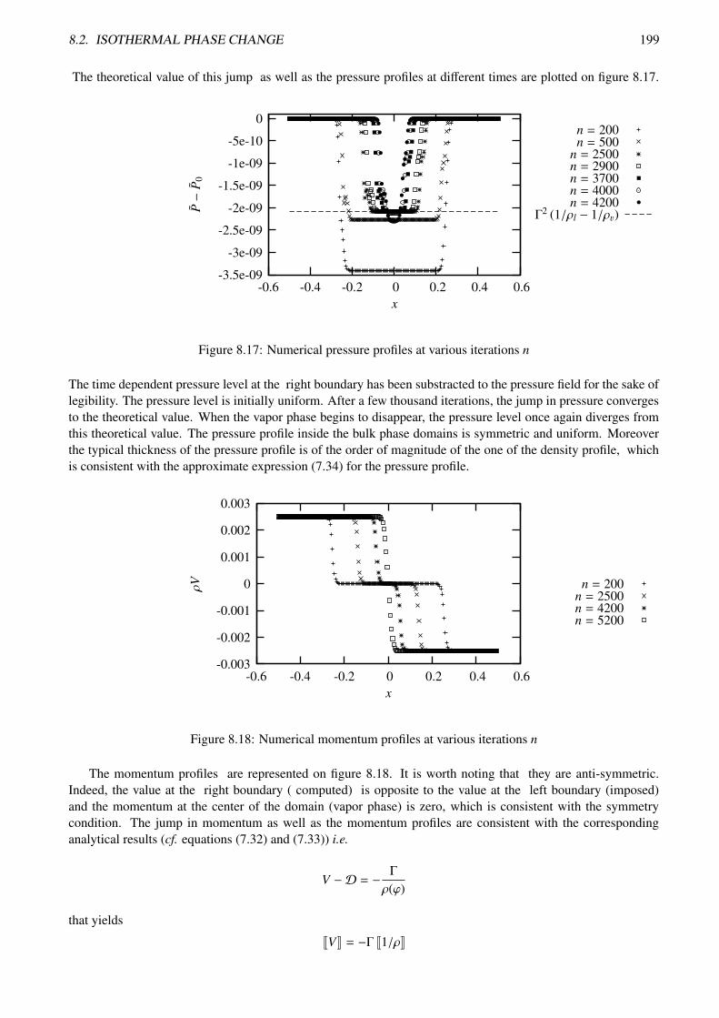
8.2. ISOTHERMAL PHASE CHANGE 199
The theoretical value of this jump as well as the pressure profiles at different times are plotted on figure 8.17.
Γ2 (1/ρl − 1/ρv)n = 4200n = 4000n = 3700n = 2900n = 2500
n = 500n = 200
x
P−
P0
0.60.40.20-0.2-0.4-0.6
0
-5e-10
-1e-09
-1.5e-09
-2e-09
-2.5e-09
-3e-09
-3.5e-09
Figure 8.17: Numerical pressure profiles at various iterations n
The time dependent pressure level at the right boundary has been substracted to the pressure field for the sake oflegibility. The pressure level is initially uniform. After a few thousand iterations, the jump in pressure convergesto the theoretical value. When the vapor phase begins to disappear, the pressure level once again diverges fromthis theoretical value. The pressure profile inside the bulk phase domains is symmetric and uniform. Moreoverthe typical thickness of the pressure profile is of the order of magnitude of the one of the density profile, whichis consistent with the approximate expression (7.34) for the pressure profile.
n = 5200n = 4200n = 2500n = 200
x
ρV
0.60.40.20-0.2-0.4-0.6
0.003
0.002
0.001
0
-0.001
-0.002
-0.003
Figure 8.18: Numerical momentum profiles at various iterations n
The momentum profiles are represented on figure 8.18. It is worth noting that they are anti-symmetric.Indeed, the value at the right boundary ( computed) is opposite to the value at the left boundary (imposed)and the momentum at the center of the domain (vapor phase) is zero, which is consistent with the symmetrycondition. The jump in momentum as well as the momentum profiles are consistent with the correspondinganalytical results (cf. equations (7.32) and (7.33)) i.e.
V −D = − Γρ(ϕ)
that yields
JVK = −Γ J1/ρK

200 CHAPTER 8. NUMERICAL RESOLUTION OF THE SYSTEM OF GOVERNING EQUATIONS
Isothermal kinetic relation In section 7.4.3, we showed that the interface pressure is linear in Γ/α = Γ/(κ ε2).To study this relation and in particular its dependence in κ, we computed the previously steady-state isothermalphase change process for various values of the mobility, other parameters being fixed. The interface pressure Pi
Pi
κ
P
10.10.01
100000
10000
1000
100
Figure 8.19: Interface pressure for a given mass transfer rate as a function of the mobility κ
is defined asPi = P(xi)
where xi is a sharp interface location such that ϕ(xi) = 1/2. Pi as a function of the mobility is represented onfigure 8.19. This figure shows that the approximate relation (cf. equation (7.35b))
Pi ∝Γ
κ
is satisfied for sufficiently large values of the mobility κ but deviates from this approximate relation for lowervalues of the mobility. The numerical result is consistent with the analytical results derived in section 7.4.2.
Conclusion Using numerical simulations, we showed that the solution of a one-dimensional isothermal steadystate phase change process using our phase field model is consistent with the analytical results derived in sec-tion 7.4. As a consequence, the diffuse profiles are of controlled thickness (which is of the order of the parameterε) and the bulk phases correspond to the targeted phase field values 0 and 1. Moreover the equivalent sharpinterface representation satisfies the classical jump conditions on mass and momentum. The kinetic relation isconsistent with the normal growth theory as long as the ratio Γ/α is sufficiently small, which is the actual limit ofvalidity of the normal growth theory. It means that the algorithm developed is actually satisfying for the study ofone dimensional isothermal phase change process. As a consequence, we retain it in the remainder of this studyto solve the coupling between phase field and mechanics.
8.2.3 Two-dimensional numerical simulation
Bubble detachment and rise To study the ability of the model to deal with two-phase flows, we study numer-ically the motion of a bubble inside a closed box under the action of both capillarity and buoyancy. Since the boxis closed, the total mass transfer rate is zero, even though local interface mass transfer rate can occur.
Initially, a hemispherical bubble is set at the bottom of the box in contact with the bottom surface. Thevelocity is imposed constant and zero on all the boundaries. The phase field boundary condition corresponds toa contact angle of π/2. The numerical discretization is a two-dimensional regular Eulerian grid of 60× 60 nodes.
On figure 8.20, snapshots of the numerical simulation are represented. The color field corresponds to thephase field, light color around ϕ = 1 (vapor) and dark around ϕ = 0 (liquid). The iso-value ϕ = 0.5 (interface)is represented by the black line. The black arrows correspond to the momentum vector field. From top left tobottom right the following sequence of events can be seen. Due to the action of buoyancy, the center of gravity

8.2. ISOTHERMAL PHASE CHANGE 201
Figure 8.20: Isothermal bubble rise inside a closed box

202 CHAPTER 8. NUMERICAL RESOLUTION OF THE SYSTEM OF GOVERNING EQUATIONS
of the bubble begins to rise. Due to the density difference between vapor and liquid, along a current line, themomentum is larger in the liquid phase than in the vapor phase, which attests the fact that the local mass transferrate, if any, is negligible with respect to the local dynamics. As the center of gravity of the bubble rises up, thesummit of the bubble keeps a quasi spherical shape under the action of the capillarity; however, at the foot ofthe bubble, the interface is perpendicular to the wall according to the π/2 contact angle. The surface of contactbetween vapor and the bottom wall continuously decreases till it vanishes (4th snapshot): at this instant thebubble departs from the wall. Under the action of capillarity, the foot part of the bubble made of a high curvatureregion rapidly disappears and the bubble shape gets closer to a spherical cap. As the bubble reaches the top wall,it spreads into a film whose interface progressively becomes planar, that corresponds to the final equilibriumstate.
This simulation shows that the model correctly describes the dynamics of bubble departure from a wall underthe action of both capillarity and buoyancy. Even though these results are only qualitative, they are importanttowards the study of the bubble growth dynamics (cf. chapter 1). It indeeds validate the use of the algorithmproposed in section 8.2.1. This algorithm has the advantage to reduce to the solving of a linear system ofequations and to be well-posed in the case of closed domains.
8.3 Non-isothermal dissipative liquid-vapor flows with phase change
In this section, we solve numerically the complete set of governing equations (5.56). The goal is to studythe coupling between the thermal and mechanical parts of the model , both having been studied and validatedindependently in the previous sections.
8.3.1 Saturation curve
Presentation of the test case The system studied is a heated and closed one-dimensional two-phase system.The goal is to study the ability of the model and of the numerical algorithm to take into account the saturationcurvei.e. an increase of the mean pressure of a system with its mean temperature. To illustrate this point, wefirst consider a weak coupling between the thermal and mechanical problems . Indeed, we simplify the thermalproblem by considering that the temperature is uniform is space uniform but that its value is time dependent. Theremaining equations to solve are thus the AC, momentum balance and continuity equations. As a consequence,the system studied can be solved using an algorithm similar to that used in the isothermal case presented in theprevious section: only the level of temperature is added as an additional parameter. To study the coupling withthe phase change process, we consider a non-zero coefficient of thermal expansion αP for the vapor phase. As aconsequence, when the temperature of the system increases, the interface pressure follows the saturation curve,and due to mass conservation inside the closed domain (of fixed volume), the interface moves to take into accountthe variation of the vapor density. It is worth noting that the problem studied reproduces the physical situation ofa pressure cooker.
Numerical results The time dependent interface pressure is represented on figure 8.21 together with the satu-ration pressure at the interface temperature. It shows that the pressure consistently follows the saturation curve.It has been shown that the quasi-compressible model allows to introduce the notion of saturation curve, this testcase shows the ability of the algorithm proposed to take it into account in the computations.
Due to the non-zero coefficient of thermal expansion of the vapor phase, the volume ratio of the liquid andvapor phases inside the closed domain evolves in time. Since the temperature of the system is imposed, the timedependent position of the interface can be derived analytically. On figure 8.22 the computed interface position iscompared to this analytical prediction. It shows good agreement , attesting the ability of the model to take intoaccount a non-zero coefficient of thermal expansion.
8.3.2 Dynamic phase change in an open system
The algorithm The algorithm for the computation of the coupling between thermal, mechanical and phase fieldparts of the model is inspired by the algorithms developed for the studies of the uniform density and isothermalcases. It is thus based on the use of the projection method as presented in section 8.2.1. For open systems thealgorithm is made of two main steps
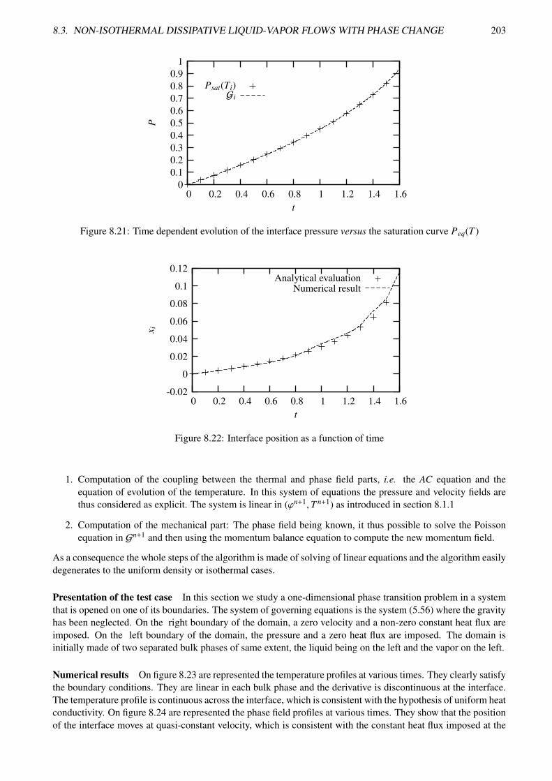
8.3. NON-ISOTHERMAL DISSIPATIVE LIQUID-VAPOR FLOWS WITH PHASE CHANGE 203
GiPsat(Ti)
t
P
1.61.41.210.80.60.40.20
10.90.80.70.60.50.40.30.20.1
0
Figure 8.21: Time dependent evolution of the interface pressure versus the saturation curve Peq(T )
Numerical resultAnalytical evaluation
t
x i
1.61.41.210.80.60.40.20
0.12
0.1
0.08
0.06
0.04
0.02
0
-0.02
Figure 8.22: Interface position as a function of time
1. Computation of the coupling between the thermal and phase field parts, i.e. the AC equation and theequation of evolution of the temperature. In this system of equations the pressure and velocity fields arethus considered as explicit. The system is linear in (ϕn+1,T n+1) as introduced in section 8.1.1
2. Computation of the mechanical part: The phase field being known, it thus possible to solve the Poissonequation in Gn+1 and then using the momentum balance equation to compute the new momentum field.
As a consequence the whole steps of the algorithm is made of solving of linear equations and the algorithm easilydegenerates to the uniform density or isothermal cases.
Presentation of the test case In this section we study a one-dimensional phase transition problem in a systemthat is opened on one of its boundaries. The system of governing equations is the system (5.56) where the gravityhas been neglected. On the right boundary of the domain, a zero velocity and a non-zero constant heat flux areimposed. On the left boundary of the domain, the pressure and a zero heat flux are imposed. The domain isinitially made of two separated bulk phases of same extent, the liquid being on the left and the vapor on the left.
Numerical results On figure 8.23 are represented the temperature profiles at various times. They clearly satisfythe boundary conditions. They are linear in each bulk phase and the derivative is discontinuous at the interface.The temperature profile is continuous across the interface, which is consistent with the hypothesis of uniform heatconductivity. On figure 8.24 are represented the phase field profiles at various times. They show that the positionof the interface moves at quasi-constant velocity, which is consistent with the constant heat flux imposed at the

204 CHAPTER 8. NUMERICAL RESOLUTION OF THE SYSTEM OF GOVERNING EQUATIONS
t = 4.5t = 3.0t = 1.5t = 0.0
x
T
0.50.40.30.20.10-0.1-0.2-0.3-0.4-0.5
0.20
-0.2-0.4-0.6-0.8
-1-1.2-1.4-1.6-1.8
Figure 8.23: Temperature profiles at various instants
right boundary. The interface thickness is approximatively constant throughout the simulation. On figure 8.25
t = 4.5t = 3.0t = 1.5t = 0.0
x
ϕ
0.50.40.30.20.10-0.1-0.2-0.3-0.4-0.5
1
0.8
0.6
0.4
0.2
0
Figure 8.24: Phase field profiles at various instants
are represented the momentum profiles at various times. Initially the momentum is set to zero. The momentum iszero inside the liquid domain, which is consistent with the right boundary condition. The momentum is uniformand positive on the vapor side, which is consistent with the fact that the liquid condensates (vapor enters intothe domain). However, its value is not constant in time. Indeed, as it will be seen on the pressure profile, theinterface pressure varies with time whereas the interface temperature is quasi constant. The variation of theinterface pressure is associated to the fact that the pressure imposed on the right boundary does not correspond tothat of a steady state phase transition process. As a consequence, the mass transfer rate is not exactly constant andactually slightly decreases with time (as the boundary condition of imposed pressure gets closer to the interface).
On figure 8.26 are represented the pressure profiles at various times. The pressure jump across the interfaceis quasi-constant, which is consistent with the quasi-constant mass transfer rate (recoil force). The pressure isuniform in the liquid phase, which is consistent with the boundary condition imposed on the right boundary.At the left boundary, the boundary condition of constant pressure is satisfied. In the vapor phase there existsa non-zero uniform pressure gradient. This is consistent with the previously described momentum profile, thevalue of the pressure gradient being related to the time derivative of the momentum (cf. the momentum balanceequation).

8.3. NON-ISOTHERMAL DISSIPATIVE LIQUID-VAPOR FLOWS WITH PHASE CHANGE 205
t = 4.5t = 3.0t = 1.5t = 0.0
x
ρV
0.50.40.30.20.10-0.1-0.2-0.3-0.4-0.5-0.6
0.0450.04
0.0350.03
0.0250.02
0.0150.01
0.0050
-0.005
Figure 8.25: Momentum profiles at various instants
t = 4.5t = 3.0t = 1.5t = 0.0
x
G
0.50.40.30.20.10-0.1-0.2-0.3-0.4-0.5
0.0090.0080.0070.0060.0050.0040.0030.0020.001
0
Figure 8.26: Profiles of the modified pressure G at various instants
Conclusion As a partial conclusion, the numerical profiles are consistent with the analytical results derived insection 7.5. Moreover these results show that the algorithm is able to taken into account the coupling between allthe parts of the model.
8.3.3 Attempts to solve two-dimensional phase change problems
The one- and two-dimensional studies presented in the previous sections aimed at studying the different cou-plings of the equations and to validate the algorithm developped to account for these couplings. In particular, insection 8.2.3, we showed that the numerical method develop to account for the coupling between the AC equationand the momemtum and mass balance equations gives good qualitative results in fully multi-dimensional sim-ulations. In section 8.3.2, we showed that the algorithm developped to solve the complete system of equationsgives good both qualitative and quantitative results in one-dimension. Therefore, it is reasonnable to think thatthis algorithm would give good results in two dimensions as well. It turns out that we faced severe numericaldifficulties in two dimensions. These difficulties are believed to be related to fundamental numerical issues andare thus reported and analyzed in this section.
To illustrate these difficulties, we analyze the numerical resolution of the one-dimensional problem of phasetransition one studied in section 8.3.2. In this section, this one-dimensional system is studied using a two-dimensional system, with only a few mesh cells in the direction tangential to the interface. All the initialprofiles are one-dimensional in the direction normal to the interface and the problem should therefore remainone-dimensional in this direction. However, as shown in the following, the system develops numerical instabili-

206 CHAPTER 8. NUMERICAL RESOLUTION OF THE SYSTEM OF GOVERNING EQUATIONS
ties in the direction tangential to the interface. We describe several attempts to overcome these difficulties that,even though unfruitful, have nevertheless allowed to clearly identify the origin of the numerical difficulties of thenumerical method.
Instable growth of parasitic currents The problem we have to solve is purely one-dimensional. However,by considering a two-dimensional mesh, we add degrees of freedom in the system. The corresponding setting isrepresented on the top graph of figure 8.27. The colored field is the phase field, or equivalently the density field.The small lines indicate the faces of the mesh elements. Vertical black lines correspond to iso-values 0.01, 0.5and 0.99 of the phase field. Black arrows correspond to the velocity field, which is initially set to zero but rapidlyconverges to a mainly horizontally oriented field.
Let us now consider the two-dimensional velocity field. Since the velocity field is initially one-dimensional,we represent on figure 8.27 a modified velocity field for the sake of legibility. This velocity field is obtainedby subtracting to the original velocity field the normal component of the velocity at the bottom of the domain.The corresponding snapshots correspond to the second (from top) and following (to bottom) pictures. The scaleseparation at the beginning of the computation between the original and modified velocity fields is huge: as itcan be seen on the pictures, the norm (max) of the original momentum is 1011 times larger than the norm ofthe modified field. The tangential component of the velocity field is therefore negligible and can be attributedto numerical truncation errors. The snapshots show that the modified velocity field is made of rotating currentslocated in the vicinity of the interface. As a consequence, the modified velocity field, that should be zero, is notonly made of numerical truncature errors, but is rather organized (even though the structure of the “flow” evolvesin time as shown on figure 8.27). Since, contrarily to the physical velocity field that should be purely normal, thecomputed velocity field is two-dimensional, we characterize in the following this difference by considering thenorm of the computed tangential component of the velocity field.
Unstable evolution of the velocity field Even though, as it has been shown in the previous paragraph, the initialtangential component of the velocity is of many orders of magnitude less than its normal component, its temporalevolution is unstable. On figure 8.28 are represented the kinetic energy contribution of both the tangential andnormal components of the velocity to the total kinetic energy of the fluid as a function of the numerical iterations.This figure shows that the kinetic energy associated to the normal component of the velocity rapidly convergesto a value of the order of unity. This value actually corresponds to the value of the kinetic energy of the previousone-dimensional computation. As a consequence, the normal velocity component actually converges toward thephysical solution. Let us now consider the tangential component. On figure 8.28, several different numericalresults are represented. They correspond to several different numerical algorithms that are discussed in thefollowing. The computation n4 corresponds to the simplest algorithm. It can clearly be seen that, in this case,the norm of the tangential component of the velocity has an exponential growth with time, which is characteristicof a numerical instability. As a consequence, the initial scale separation between the normal and tangentialcomponents of the velocity is no longer valid at a finite time (iteration 500 on the figure). Beyond this time, thecomputation rapidly diverges and is no longer physically meaningful. It is worth emphasizing that at this time,the interface has not moved from more than one node. As a consequence, when this instability arises, there is noway to compute any phase change process.
Attempts to stabilize the scheme In order to solve this test case problem numerically and to understand theorigin of the numerical instability described above, we designed and used several different schemes. In thepresent study, we only propose to summarize the different learnings from these numerical tests about the originof the instability. It is worth pointing out that capillarity should not play any physical role in this one-dimensionalproblem. However, it turns out that the computation of the test case in the two dimensional system is stable ifone cancels the capillary part of the stress tensor. As a consequence, the observed instability is clearly relatedto the capillary stress tensor. Nevertheless, for a one-dimensional phase field, the capillary stress tensor shouldnot yield to a non-zero tangential component of the velocity. It turns out that numerical truncation errors arisingfrom the computation of the phase field is sufficient to trigger the instability. In the following we analyze thealgorithm to understand the way capillary stress tensor can induce this instability.
In the original algorithm, the first step that is used to compute (ϕ,T ) takes into acccount the velocity on anexplicit way. As a consequence it does not takes into account the capillary stress tensor on an implicit way.

8.3. NON-ISOTHERMAL DISSIPATIVE LIQUID-VAPOR FLOWS WITH PHASE CHANGE 207
Figure 8.27: Illustration of the parasitic currents, on the top figure, the whole velocity field is represented,whereas on the other figures, the (U) component normal to the interface of the velocity field at the bottom meshline of the domain has been substracted to the velocity field, that allows to illustrate the parasitic currents. Inabsence of these currents, the velocity field should not have any tangential component.
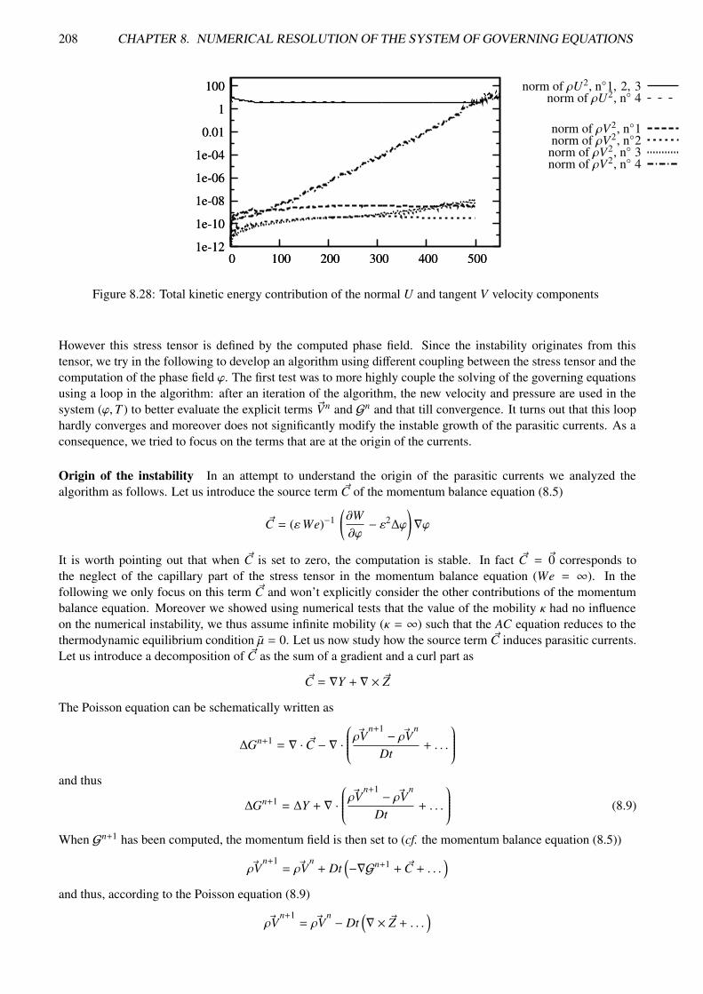
208 CHAPTER 8. NUMERICAL RESOLUTION OF THE SYSTEM OF GOVERNING EQUATIONS
norm of ρV2, n 4norm of ρV2, n 3norm of ρV2, n2norm of ρV2, n1
5004003002001000
100
1
0.01
1e-04
1e-06
1e-08
1e-10
1e-12
norm of ρU2, n 4norm of ρU2, n1, 2, 3
5004003002001000
100
1
0.01
1e-04
1e-06
1e-08
1e-10
1e-12
Figure 8.28: Total kinetic energy contribution of the normal U and tangent V velocity components
However this stress tensor is defined by the computed phase field. Since the instability originates from thistensor, we try in the following to develop an algorithm using different coupling between the stress tensor and thecomputation of the phase field ϕ. The first test was to more highly couple the solving of the governing equationsusing a loop in the algorithm: after an iteration of the algorithm, the new velocity and pressure are used in thesystem (ϕ,T ) to better evaluate the explicit terms ~Vn and Gn and that till convergence. It turns out that this loophardly converges and moreover does not significantly modify the instable growth of the parasitic currents. As aconsequence, we tried to focus on the terms that are at the origin of the currents.
Origin of the instability In an attempt to understand the origin of the parasitic currents we analyzed thealgorithm as follows. Let us introduce the source term ~C of the momentum balance equation (8.5)
~C = (εWe)−1(
∂W∂ϕ− ε2∆ϕ
)
∇ϕ
It is worth pointing out that when ~C is set to zero, the computation is stable. In fact ~C = ~0 corresponds tothe neglect of the capillary part of the stress tensor in the momentum balance equation (We = ∞). In thefollowing we only focus on this term ~C and won’t explicitly consider the other contributions of the momentumbalance equation. Moreover we showed using numerical tests that the value of the mobility κ had no influenceon the numerical instability, we thus assume infinite mobility (κ = ∞) such that the AC equation reduces to thethermodynamic equilibrium condition µ = 0. Let us now study how the source term ~C induces parasitic currents.Let us introduce a decomposition of ~C as the sum of a gradient and a curl part as
~C = ∇Y + ∇ × ~Z
The Poisson equation can be schematically written as
∆Gn+1 = ∇ · ~C − ∇ ·
~ρVn+1 − ~ρVn
Dt+ . . .
and thus
∆Gn+1 = ∆Y + ∇ ·
~ρVn+1 − ~ρVn
Dt+ . . .
(8.9)
When Gn+1 has been computed, the momentum field is then set to (cf. the momentum balance equation (8.5))
~ρVn+1= ~ρV
n+ Dt
(
−∇Gn+1 + ~C + . . .)
and thus, according to the Poisson equation (8.9)
~ρVn+1= ~ρV
n − Dt(
∇ × ~Z + . . .)

8.4. CONCLUSIONS AND PERSPECTIVES 209
As a consequence, it appears clearly that only the component ∇ × ~Z of the capillary term ~C contributes to thevelocity field and can induce parasitic currents.
A way to stabilize the parasitic currents The basic idea is then to work on the coupling between ∇ × ~Z andthe computation of the phase field. To do we introduce an estimation of the velocity field ~V∗. We ignore the othercontributions than ∇ × ~Z in the momentum balance equation to compute ~V∗ and define
~V∗ = ~Vn − Dt∇ × ~Z(ϕn+1)
This velocity is used to compute (ϕ,T ) in the first step of the algorithm instead of ~Vn. An iterative procedure isintroduced where (i) the phase field and temperature are first computed, (ii) the velocity ~V∗ is deduced from ϕ,this velocity being used to improve the calculation of (ϕ,T ) (back to step (i)) and so on till convergence. It isa straightforward computation to deduce ∇ × ~Z from the knowledge of ϕ and thus of ~C. However it remains aPoisson equation to solve, and as a consequence this step is numerically costly. Using numerical tests it has beenshown that it was necessary and sufficient for the resolution to be stable to use ~V∗ only in the phase change termof the equation of evolution of the temperature such that the step (i) is the solving of
vn(
∂W∂ϕ
n− ε2∆ϕn+1
)
+∂ν
∂ϕ
n (
(At εWe) Gn − ε
S t γ θT n+1
)
+(
ϕn+1 − ϕn)(
vn∂2W∂ϕ2
n
+∂2ν
∂ϕ2
n (
(At εWe) Gn − ε
S t γ θT n
))
= 0
ρn(
T n+1 − T n
Dt+ ~Vn · ∇T n
)
−∇ ·
(
k∇T n+1)
Pe+ρ (1 + T n/θ)
S tdνdϕ
(
ϕn+1 − ϕn
Dt+ ~V∗ · ∇ϕn
)
= 0
At convergence of the loop, the fields ϕn+1 and T n+1 are known. The projection method is then used to computethe fields Gn+1 and ~ρV
n+1. It is worth pointing out that this algorithm, if complex, is the only way we found
among numerous other attempts to stabilize the resolution. The resulting time evolution of the kinetic energy isrepresented on figure 8.28 calculations n2 − 4. It shows that the order of magnitude of the tangential kineticenergy, even though non-zero stays very low and as a consequence, it does not interact with the physical solution.We thus managed to get rid of the instability. But the computation remains very sensitive to numerical accuracy.Moreover the first step is considerably costly and computations of larger systems, such that the one presentedin section 8.2.3 were out of reach. Nevertheless, this shows that we clearly identified the origin of the parasiticcurrents. Since it is attributed to a non-trivial coupling (implicitation of the capillary stress tensor in the phasechange term of the equation of evolution of the temperature) we face a severe numerical problem. The basic ideaof the original algorithm was mainly based on the use of the projection method. Since it has been shown thatthe use of this method does not allow to control easily the capillary part ~C of the stress tensor, we propose toinvestigate the use of other methods to compute the momentum balance equation, such that curl-decompositionmethods.
8.4 Conclusions and perspectives
In this chapter, we studied numerically the system of governing equations of our phase field model for theliquid-vapor flows with phase change. By studying one dimensional phase change problems, we showed thatthe numerical results are actually consistent with the analytical results derived in chapter 7. We also showedthat the model was able to take into account capillarity in two-dimensional systems in the uniform density andisothermal cases. Numerical computations of bubble departure from a wall isothermal dynamics showed themodel qualitatively reproduce the main physical mechanisms (capillarity and buoyancy). As a consequence thealgorithm developped is able to take into account the major coupling of the models. Nevertheless, we have notbeen able to compute multi-dimensional non-isothermal phase transition problems with density difference. Thelimitation of the numerical method for such a computation has been shown to be associated to the capillarystress tensor. The use of the projection method for the solving of the momentum balance equation is potentiallyresponsible of a numerical instability that we have not been able to avoid unless by using a costly and complexalgorithm. As a consequence, we believe that another numerical method for the computation of the momentum

210 CHAPTER 8. NUMERICAL RESOLUTION OF THE SYSTEM OF GOVERNING EQUATIONS
balance equation in the non-isothermal case should be used. In particular, we believe that the use of a methodbased on a curl- decomposition of the velocity field should be investigated.

Conclusion and perspectives
The study of the basic physical mechanisms occuring in boiling flows and more especially at the boiling crisisis still challenging. Indeed, despite more than 70 years of valuable scientific studies, the physical mechanismsat the origin of the boiling crisis have not been clearly identified yet. To analyze the current understanding ofthe boiling crisis, we proposed in chapter 1 to classify the mechanisms potentially involved in the phenomenonaccording to three different levels of description of the nucleate boiling regime. The first level deals with the mostidealized level of description of the bubbly flow, the bubbles are modeled with the help of a mean volumetricvapor fraction. The bubbles are therefore not considered as individual entities. At the second level of descriptionthe bubbles are modeled as a set of growing spheres, they are rigid in shape but not in size. At the finest andthird level of description the bubble geometry is time and space dependent. According to this classification,we studied the different existing theories for the boiling crisis. This analysis revealed the need, at each levelof description, for both experimental investigation and modeling efforts to improve the understanding of thephysical features of high heat flux nucleate boiling . Nevertheless, among all the mechanisms that remain to beclarified, we clearly identified one mechanism potentially related to the boiling crisis: the “irregular” bubblegrowth event. Indeed, at high wall heat flux, a bubble pinned to the wall can spread over the wall instead ofdeparting from it. This mechanism refers to the finest level of description of the nucleate boiling regime. It hasbeen shown, by an analysis of experimental observations as well as of the successful Zuber correlation for theprediction of the boiling crisis, that “irregular” bubble growth can indeed be at the origin of the drying transitionof the hot wall that leads to the transition of the boiling regime. The bubble growth and departure from thewall processes are governed by local curvature of the bubble shape as well as local heat and mass transfer. As aconsequence, the numerical simulation is the most relevant tool to study the “irregular” bubble growth dynamics.The compressibility of the liquid and vapor phases are not considered as leading physical mechanisms for thisdynamics. As a consequence, the bulk phases can be modeled as incompressible. Since this assumption inducesa computational simplification, the numerical method can thus take benefit of it.
In chapter 2, we analyzed the numerical methods that could be used for the computation of boiling flowsand turned our attention toward diffuse interface methods. These methods are based on models that considerthe interface as a volumetric transition layer across which all the physical variables have continuous variations.The set of governing equations includes, in a thermodynamically consistent way, the model for the interfacedynamics. As a consequence, and contrarily to the numerical methods based on sharp interface models, thereis no need to develop a specific computational treatment devoted to the interface dynamics. This constitutes anadvantage from the computational point of view. Nevertheless, the physical thickness of the interface transitionlayer is of many orders of magnitude smaller than the typical bubble size. In order that these models can beused for the bubble scale simulation targeted, it is required to control the typical thickness of the transition layer.Indeed, the interface layer must be captured by a few mesh cells and the size of the interface must therefore bea free parameter of the model, whose typical size is that of a mesh cell. The van der Waals model is the mostnatural diffuse interface model for the liquid-vapor phase transition. However, it has been shown that it is notpossible to increase the interface thickness from a modification of the van der Waals model without altering thedescription of the liquid-vapor states. For the study of the solid-liquid phase transition with a diffuse interfacemodel, the phase field models are commonly used. These models are based on the introduction of an abstractinternal parameter, called phase field, in the thermodynamic description of the system. It allows to deal witha smearing of the interface of arbitrary thickness together with a degree of freedom for the description of thephysical parameters of the phase transition. This advantage was lacking when dealing with a modification of thevan der Waals model and we thus choose to adapt this approach for the study of liquid-vapor flows with phasechange. We first defined the properties that such a model should be endowed with to study the bubble growthdynamics. In particular, the introduction of the phase field in the thermodynamic description of the fluid should
211

212 CHAPTER 8. NUMERICAL RESOLUTION OF THE SYSTEM OF GOVERNING EQUATIONS
be only devoted to the modeling of the internal structure of the interface layer. As a consequence, the phase fieldpart of the model must have minimal interference with the description of the single phase states. The latter mustbe described by the classical thermodynamic variables, namely the pressure and the temperature. Moreover, thesingle phase states should be incompressible. We showed that the existing phase field models are not well suitedfor our applications since they do not fulfill all the required properties. We need therefore to adapt these modelsto our own requirements. In the remainder of the study the goal is thus to develop and study a phase field modelfor liquid-vapor flows with phase change.
In chapter 3, we developped the thermodynamic part of our phase-field model. We first showed that it is pos-sible to deal with a density difference between incompressible single phase states using the quasi-compressiblehypothesis as first introduced by Lowengrub and Truskinovsky [89]. We then studied the introduction of thephase field ϕ as a thermodynamic variable. We specified its role: the phase field variable has no signification out-side the transition layer and it is therefore assumed (i) to take arbitrary fixed values in the bulk phases (ii) to varysmoothly between these two values across the interface transition layer. The typical thickness of this variationmust be controlled for computational motivations. We then derived the equilibrium conditions to express analyt-ically these two constraints. In comparison with the classical equilibrium relations, the nullity of the variationalderivative of the specific Gibbs free energy with respect to the phase field is an additional equilibrium condition.We then considered the constitutive form of the thermodynamic potential that allows to fulfill these constraints.The expression for the phase field specific Gibbs free energy is based on the interpolation of the specific Gibbsfree energies of the single phase states by a non-linear function of the phase field ϕ (cf. equation (3.53)). Thisinterpolation is at the basis of the phase field model. The specific volume as well as the entropy are interpo-lated by the same non-linear function. In addition, the expression for the thermodynamic potential is made ofthe product of the specific volume by both a volumetric double well function of ϕ and a dependence in (∇ϕ)2.The double well function is, together with the non-local dependence in (∇ϕ)2, devoted to the description of theinterface structure at planar equilibrium. The constitutive form of our phase field model yields the followingproperty: the phase field profile of across a plnar interface equilibrium is governed by a differential equation thatis independent of the physical parameters of the phase transition (saturation curve i.e. equilibrium conditions ,density difference, specific heat capacities of the bulk phase or surface tension coefficient). Moreover, it is inde-pendent of the interpolation function. As a consequence, the thickness of the interface transition layer is easilycontrolled. The surface tension coefficient is simply related to the scaling of both the double well function andof the dependence in (∇ϕ)2. We clearly related the choice of a non-linear interpolation function to the abilityof the model to control the physical properties of the single phase states. Indeed we studied in chapter 6 thestability of homogeneous equilibrium states and it has been shown that using at least a polynomial of degree 5for this interpolation function allows to have fixed phase field values associated with the liquid and vapor phases.In particular we showed that these values correspond to unconditionally stable single phase states whereas allthe other phase field values either do not correspond to equilibrium states or correspond to unstable equilibriumstates. This property cannot be satisfied with lower degree polynomials as interpolation functions. Moreover weshowed that using polynomial of degree 5, it is possible to reproduce phenomenologically a metastability limitfor the bulk phases. This study of the thermodynamic phase field model has thus allowed to clearly establish themeaning as well as the optimal expression for the phase field dependence of the thermodynamic potentials.
We then studied spherical inclusions at equilibrium in chapter 4. With our model, the equilibrium equationin the spherical symmetric case is simple enough to derive approximate analytical solutions. It is worth notingthat both the double well and the interpolation function enter this equilibrium equation. As a consequence theinterpolation function plays a role in the description of spherical inclusions. We have defined the equivalentsharp interface model of our diffuse model. We showed that this sharp model is consistent with the Laplacetheory as soon as the radius of the spherical inclusion is a few times larger than the typical interface thickness.This result is satisfying for the studies targeted and it shows the ability of the phase field models to provide athermodynamically consistent regularization of the sharp interface model. As the radii of the spherical inclusiondecreases below the order of magnitude of the interface thickness the effective surface tension as well as thepressure jump decrease. This decrease of the pressure jump allows to model vanishing spherical inclusions thatis not possible with the sharp interface model. It is worth noting that the results concerning the small radii havebeen shown to be sensistive to the choice for the interpolation function.
In chapter 5, we derived the dynamic system of equations corresponding to our thermodynamic model. Thederivation of the governing equations has been made in two steps. First we introduced a formal compressible

8.4. CONCLUSIONS AND PERSPECTIVES 213
isothermal phase field model. Using the fundamental d’Alembert-Lagrange principle, we derived the conserva-tive set of governing equations. We identified the capillary part of the stress tensor and derived a constitutiveexpression for the rate of work. Then, using the thermodynamic first principles together with the previouslysuggested expression for the rate of work, the dissipative governing equations have been derived for our quasi-compressible non-isothermal model. In addition to the classical Fourier heat conduction and Newton viscositydissipative mechanisms, we introduced a Ginzburg-Landau relaxation toward the additional phase field equi-librium condition. This introduces a phase field kinetic part in the model. As a consequence, in addition to themass, momentum and entropy balance equations, the set of governing equations includes an Allen-Cahn equation(cf. the system of equations (5.42)). Using the Pi theorem, the non-dimensional form of the governing equationshas been derived for the study of a boundary condition problem. We then proposed a simplification of the tem-perature dependence of the model: the saturation pressure is linear in temperature and the coefficient of thermalexpansion is neglected. As a consequence, no difference between the heat capacities of the liquid and vapor isconsidered. It is worth emphasizing that this assumption is not a fundamental limitation of our model. However,it allows to simplify both the analytical and numerical studies of the governing equations and the latent heat isstill non-zero. Finally, the set of governing equations contains a reduced number of non-linearities and takes intoaccount the physical mechanisms governing the bubble growth dynamics.
We then studied our model in non-equilibrium cases in chapter 7. We first introduced the formalism ofkinetic relations for the equivalent sharp interface model. We showed that the non-equilibrium Gibbs Thomsonand Clapeyron relations are related to the “normal growth” theory for the interface entropy production. We thenderived approximate non-equilibrium solutions for a one-dimensional phase transition when the transition frontis a traveling wave. We assumed that the phase field varies mostly over a narrow transition zone (inner region) ofthe order of the thickness of the interface at planar equilibrium whereas in the bulk phases, the physical variablesvary over larger distances (outer domains) that contain less significant variations of the phase field. Matchedasymptotic expansions are then used to solve the coupled set of governing equations in both the inner and outerzones. The solutions are expanded with respect to a small parameter defined as the ratio of the typical inner lengthscale to the typical outer length scale. We then derived the inner profiles of the variable at the first and secondleading orders. The following conclusions can be drawn from this study. At leading order, the phase transition isisothermal and the phase field profile is the equilibrium one, these results being classical with phase field models.We have derived the corresponding kinetic relation that provides a clear interpretation of these results. It has beenshown that at leading order the interface entropy production is quadratic in the mass transfer rate and the drivingforce linear in the mass transfer rate. These results are thus consistent with the “normal growth” theory. TheGinzburg-Landau relaxation is the dissipation mechanism that governs the leading order kinetics. At next order,it has been shown that the interface temperature jump is non zero. This is commonly associated to a thermaltrapping effect. We showed that it is related to an excess interface entropy production inherited from the phasefield interpolation of the heat conductivity coefficient. Moreover, we showed that the leading order solutionsare consistent with the classical sharp interface pressure and velocity jump conditions. We also showed that theconsistency of the leading order kinetic relation with the normal growth approximation is directly related to aparticular choice for the scaling of the Ginzburg Landau dissipative coefficient. By considering another scalingfor this coefficient, we derived a leading order kinetic relation for a purely phase field model that deviates fromthe normal growth approximation at high mass transfer rates which is more physically consistent when study offast phase boundaries is targeted.
The chapter 8 was devoted to the numerical resolution of the system of governing equations. The goal was todevelop an algorithm to take into account the coupling between the thermal, mechanical, and phase field parts ofthe model. Successful algorithms developed to solve the coupling have been presented in two simplified cases:(i) uniform density and (ii) isothermal. The algorithms use a linear approximation of the terms that inducesan improved efficiency of the solvers. The results are consistent with the analytical developments and two-dimensional computations are qualitatively satisfying. They attest the ability of the model to be at the basis of anumerical method. Based on these results, we defined an algorithm for the resolution of the complete coupling.This algorithm allows to study phase change process as attested by one-dimensional computations. However,numerical instabilities occur for two-dimensional computations. An analysis of the algorithm allowed to identifythe origin of the instability as a numerical issue. Currently, we have not found a way to avoid the instability.
This study can be considered as an attempt to use phase field models for the study of boiling flows. It firstprovided a justification for the use of numerical simulation to improve the understanding of the boiling process,

214 CHAPTER 8. NUMERICAL RESOLUTION OF THE SYSTEM OF GOVERNING EQUATIONS
and more particularly the boiling crisis. Secondly, we have been able to develop a diffuse interface model with aclear set of parameters and functions that allows to deal (i) with the main features of boiling flows and (ii) withcontrolled characteristics of the interface transition layer. In this study, we took special care of the consequencesof the introduction of the phase field variable on the description of the liquid-vapor phase transition. We alsoprovided a precise analysis of the equivalent sharp interface model and showed that our phase field model is athermodynamically consistent regularization of the classical sharp model with incompressible bulk phases. Ournumerical study, if finally unsuccessful, has drawn the first steps toward the solving of the complete model andthus the study of nucleate wall boiling.
Our study revealed that the study of the very near wall boiling processes is of primary interest for the under-standing of the basic mechanisms of the boiling crisis. Experimental observation of the near wall layer (wherenucleation and bubble growth take place) at near boiling crisis conditions should provide lacking informationon the origin of the precursor drying events observed in [130]. This suggests the use of an experimental set-upallowing to simultaneously observe the nature of the wall-fluid contact (using for example infrared camera) andthe bubble growth dynamics (using lateral visualization).
We have distinguished two categories of methods for the computation of boiling flows using an implicittracking of the interface: the level set method that is based on a sharp interface model and the diffuse interfacemodels. The phase field variable is formally very close to the indicator or color function used in level setmethods. It allows to introduce a first formal link between the two classes of methods. It is worth pointing outthat the relaxation of the distance function used in the level set methods to keep the level set function equal to asigned distance function has close similarities with our AC equation. In a study of the numerical computation ofdiffuse interface models, Glasner [57] proposed to work on a “distance” function rather than directly on the phasefield variable. This change of variable makes the phase field formulation very close to the level set formulation.It would benefit to both methods to investigate more deeply the formal link between them.
The phase field model developed in this study has been deliberately devoted to the description of incompress-ible bulk phases. It would be of interest to derive a more generic phase field formulation for compressible bulkphases. Our quasi-compressible model should then reduce to a natural outcome of this compressible formulation.We believe that the basis of this compressible formulation should read, as our model does, as the interpolation ofthe bulk phase equation of states. As soon as the bulk phases are compressible, the dependence of the Gibbs freeenergy with respect to the pressure is non-linear. The consequences of this non-linearity on the ability to easilycontrol the interface thickness should be investigated. It is worth pointing out that the quasi-compressible model,since taking into account a non-zero density difference between the bulk phases, can be applied to the study ofthe solid-liquid with convection. More generally, it would be of interest to study how the structure we proposedfor the phase field model can be used for different models of multi-phase and/or multi-component systems ofarbitrary equations of state. In particular, in the case of immiscible fluids, it would be also of interest to study asimilar model that would have interest on the mass diffusion equation instead of our entropy equation.
The kinetic relation of our model has been derived using matched asymptotic expansions. This methodsallows to get approximate solutions for the one-dimensional phase transition. It would be of interest to study thekinetic relation, i.e. the driving force as a function of the mass transfer rate, more accurately using numericalsimulations.
It is worth noting that the choice for the interpolation function plays a particular role on the features of smallinclusions: when it is not a polynomial of degree 5, the sharp interface equivalent radius diverges as the mass ofthe spherical inclusion vanishes (cf. section 4.3.3). As a consequence, this feature is not associated to a diffuseinterface formulation. A better understanding of the origin of this latter phenomenon could lie on the study ofthe influence of the interpolation function on the spherical symmetric equilibrium equation. Moreover, still aboutthe interpolation function, we defined a way to impose a phenomenological metastability limit even in the caseof incompressible bulk phases (cf. section 6.5.1). We showed that it was sufficient to use a polynomial of degree5 whose coefficients depends on the thickness of the interface layer to get this property. It yields an additionalfeature of the phase field model with regard to the sharp interface formulation. It would be of interest to studythe consequences of this choice on the other properties of the model.
The projection method is currently used in the numerical methods for the study of two-phase flows even inpresence of phase change. Nevertheless our numerical study has shown that the use of the projection method forthe study of two-dimensional phase change problems with capillarity can induce severe numerical difficulties.As a consequence, it would be of interest to develop algorithms based on another resolution method for the

8.4. CONCLUSIONS AND PERSPECTIVES 215
momentum balance equation such as the curl decomposition. Another perspective of work could be to deal witha more simplified writing of the equation, that even though it would fail to be thermodynamically consistent,would take benefit of simplifications from the point of view of computational efficiency. This pragmatic approachis commonly used with phase field methods.

216 CHAPTER 8. NUMERICAL RESOLUTION OF THE SYSTEM OF GOVERNING EQUATIONS

Appendix A
Sharp model for the liquid-vapor flows withphase change
In this appendix we study the sharp interface models for the liquid-vapor phase transition. The goal is to study theformalism allowing to compare our phase field model with more classical models for the liquid-vapor flows withphase change. This study allows therefore to analyze the results of our phase field model as a thermodynamicallyconsistent regularization of the sharp interface model.
First we study the model of the variables at the interface in sharp interface models and more particularly therelation between the definition of the interface location, as a moving free boundary, and the value of the jumpof the variables and of excess quantities at this discontinuity (see section A.1). Then we study the Rankine-Hugoniot jump conditions that apply at the interface. We study the relation between closure laws at the interface(such that “out of equilibrium” Clapeyron relation) and the value of the interface entropy production. This studyallows thus to relate the sharp closure laws to the definition of the interface dissipative processes that is made indiffuse interface models (see section A.2).
A.1 Equivalent sharp interface
A.1.1 Interface values
Equilibrium case For the sake of simplicity, let us consider a one-dimensional two phase system along anarbitrary x−axis. Let us specify with the superscripts + and − the phases reached at large distance from thetransition layer, say respectively +∞ and −∞.
In the diffuse interface theory, all the variables are continuous in particular along the direction normal to theinterface, say the x-axis. In the Gibbs theory of sharp interfaces, an equivalent surface (in the planar case, anabscissa xi) models the volumetric continuous transition layer between the phases. Let us consider a variableq that is uniform in the bulk phase states + and −. The variable q varies continuously between the bulk phasevalues q− and q+. In the sharp interface model, the boundary condition applying at the sharp interface location
xxi
q
q−
q+
xi
q
x
JqK q
h
⇔
Figure A.1: Interface value and jump
217

218 APPENDIX A. SHARP MODEL
xi to the variable q can be defined thanks to a jump JqK and an interface value q defined as follows
JqK = q+ − q− (A.1a)
q = q+ + q−
2(A.1b)
These quantities are represented on figure A.1. For a zero jump we have q+ = q− = q = qi. Let us introducethe relation
Jq1 q2K = q1 Jq2K + q2Jq1K (A.2)
which is valid for any arbitrary quantities q1 and q2 and which is often used in the following.It is clear from figure A.1, that in the case where q+ and q− can be clearly defined, JqK and q are defined
unambiguously and are independent from the definition of the interface location xi. However, we see in thefollowing that this is not the general case.
Out of equilibrium case All the previous definition are unambiguous and independent of the interface locationxi as long as the variable q takes specific values in the bulk phase domains. Let us now consider an out ofequilibrium situation where the variable q, say the temperature for example, varies spatially in the directionnormal to the interface over distance δ larger than the interface thickness h, say a thermal boundary layer on oneside of the interface. This typical situation is represented on figure A.2 where the variable q is non-uniform onthe LHS of the interface (domain −). On a scale of the thickness of the interface (zoom on the figure), and sinceδ h, the variation of the variable q is assumed as linear with respect to x on the LHS. This corresponds toa constant heat flux in the thermal case. On the RHS q is uniform (zero heat flux). In this case the jump andinterface value of the variable q depends on the interface location. On figure A.2, three different locations arerepresented, for each location the jump in heat flux is the same, but it is clear that the jump and interface valuediffer. As a consequence, it appears that it is not sufficient to describe the physical situation in all cases with the
x1
x2
x3
JqK1< 0
q1 > q+
JqK2= 0
q2 = q+
JqK3> 0
q3 < q+
xi
q
x
δ h
h
x1 x3x2
Figure A.2: Case of a non-uniform variable on one side of the interface
help of the single specification of the jump and the interface value without studying their relation to the interfacelocation.
A.1.2 Excess quantities and interface location
Definition of excess quantities When modeling the volumetric transition layer as a surface of discontinuity,the fine description of the internal variations is neglected. However the sharp interface can bear some physical

A.1. EQUIVALENT SHARP INTERFACE 219
information with the help of surface quantities also called Gibbs excesses. These surface quantities are the reflectof the internal physics of the diffuse transition layer. The reader interested to this formalism can refer to Edwardset al. [46]. Let us take the example of a volumetric physical quantity, say q, taking some specific values in thephases, say q+ and q−, and undergoing spatial variations inside the interface. The excess of a given volumetricquantity measures the difference between the sharp profile and the continuous one. For a given position xi of thesharp interface, the excess quantity qex of the volumetric physical quantity q is defined as
qex =
∫ +∞
xi
(q(x) − q+) dx +∫ xi
−∞(q(x) − q−) dx (A.3)
the table A.1 provides an illustrative representation of the jump and excess quantities.
Relation between interface location and excess quantities The position itself of the sharp interface mustbe defined through an equivalence principle whose choice is arbitrary. This can be done, as classically, byconsidering that the location of the sharp interface xi is such that a given excess quantity is null. In the followingwe denote such a specified location xq. The associated excess value and the location of the interface are thusinterdependent. Let us consider a shift of the interface location from xi to x′i . It is straightforward that the newexcess quantity qex′ becomes
qex′ = qex +
∫ xi
x′i
(q+ − q−) dx = qex + JqK (xi − x′i) (A.4)
If the jump is zero, the volumetric quantity q has a specific interface value that is well defined (i.e. independentof the choice for the interface location xi), q = q+ = q−, and it is obvious from (A.4), that the excess quantitydoes not depend on the interface location. The value of an excess quantity undergoing a non-zero jump dependsof the arbitrary definition of the sharp interface location xi. Let us consider that the interface location is definedsuch as the excess density is zero, i.e. xi = xρ. This definition is classical in sharp interface models, it leadsto an interface that does not bear any mass and is a non-material surface. Let us denote by the subscript ρ thecorresponding value for the excess quantities
qexρ =
∫ +∞
xρ(q(x) − q+) dx +
∫ xρ
−∞(q(x) − q−) dx
then, since by definition qexq = 0, and using the relation (A.4) we have
qexρ = JqK (xq − xρ) (A.5)
Let us note, that as soon as the quantity undergoes a jump across the interface, it is possible to define a locationsuch that its excess quantity is zero, which is impossible as soon as the jump is zero.
Intrinsic excess quantities However, while considering a volumetric variable undergoing a jump across theinterface, it is possible to define a physically homogeneous variable whose excess quantity is independent of theinterface location, i.e. whose jump is zero. This excess quantity is therefore more intrinsic to the interface layer.As an example, let us consider two volumetric quantities q and Q of non-zero jump across the interface, JqK andJQK, the quantity Q defined as
Q = Q − JQKJqK q (A.6)
is such thatq
Qy= 0. In the following we illustrate this point with the help of the definition of the surface tension
coefficient for a planar interface, of interest for our applications.
A.1.3 Surface tension coefficient
The most typical excess quantity of concern for liquid-vapor phase transition is the surface tension coefficient σ.In the following we study how it is related to an excess quantity.

220 APPENDIX A. SHARP MODEL
q0
xxi
q
q−
q+Jq0K = q+0 − q−0qex
0 = 0The jump is non zero but theexcess quantity is zero
q1
xxi
qq−
q+Jq1K = q+1 − q−1qex
1 , 0The jump and the excessquantity are non zero
q2
x
q
q+
q−
xi x′i
q2(x) = q0(x + (xi − x′i )),the interface location is shiftedfrom xi to x′iJq2K = Jq0Kbutqex
2 , qex0
q3
xxi
q
qi Jq3K = 0qex
3 , 0The jump is equal to zero but theexcess quantity is non zero
q4 ! ! ! ! ! ! ! ! ! !! ! ! ! ! ! ! ! ! !! ! ! ! ! ! ! ! ! !! ! ! ! ! ! ! ! ! !! ! ! ! ! ! ! ! ! !" " " " " " " " " "" " " " " " " " " "" " " " " " " " " "" " " " " " " " " "" " " " " " " " " "
xxi
q
qi
x′i
q4(x) = q3(x + (xi − x′i )),the interface location is shiftedfrom xi to x′iJq4K = Jq3K = 0andqex
4 = qex3
the excess quantities are stillequal
Table A.1: Excess quantities as a function of interface location

A.1. EQUIVALENT SHARP INTERFACE 221
Surface tension as an excess volumetric free energy independent from the interface location Let us con-sider the volumetric quantity Helmholtz free energy in the isothermal van der Waals model as presented in 2.2.2.The planar two-phase equilibrium condition implies the existence of a common tangent to the Helmholtz freeenergy F(ρ)1 at the two bulk densities ρ+ and ρ− Therefore
dFcl
dρ
+
ρ+ − F+cl =dFcl
dρ
−ρ− − F−cl
dFcl
dρ
+
=dFcl
dρ
−=geq
(A.7)
where geq is the specific Gibbs free energy value at equilibrium. The first equality is a pressure equality P+ = P−
sinceP =
dFcl
dρρ − F
The jump in Helmholtz free energy JFK reads
JFK = geqJρK (A.8)
Setting q = F and Q = ρ, we can define the quantity F homogeneous to the volumetric excess free energy F as
F =F − geq ρ (A.9)
and an intrinsic measure of the excess free energy, i.e. the surface tension coefficient σ, is
σ = Fex − geq ρex (A.10)
Fouillet [53] stated that this definition is independent of the interface location xi. This definition ofσ is classicallyused [90].
Surface tension as an excess pressure Let us note that the pressure P has a zero jump for the planar interfacecase. The excess pressure can be related to the surface tension as
σP = − Pex (A.11)
This definition of the free excess energy is related to the equivalent representation of the surface tension as aforce (cf. [68]) and is also therefore classically used.
Equivalence between the two definitions in the two-phase equilibrium planar case Definition (A.11) of thesurface tension is different from the definition (A.10) but is actually equivalent in the case of a planar interface.Let us state how both definitions of σ are related. Let us specify the location of the interface as the abscissa xi by
ρex =
∫ +∞
xi
(ρ(x) − ρ+) dx +∫ xi
−∞(ρ(x) − ρ−) dx = 0 (A.12)
Since F = ρ g − P, the excess Helmholtz free energy Fex across a planar interface is given by
Fex =
∫ +∞
xi(ρ(g − Pv) − ρ+(g+ − P+v+)) dx +
∫ xi
−∞(ρ(g − Pv) − ρ−(g− − P−v−)) dx
Since, as stated by (3.28b), the specific Gibbs free energy g is uniform at equilibrium, we get g = g+ = g− = geq
and Fex reads
Fex =
∫ +∞
xi(P+ − P) dx +
∫ xi
−∞(P− − P) dx + geqρ
ex
Using the definition of the interface location xi (A.12), we get
Fexρ = −Pex
And therefore−Pex = Fex
and we get thusσ = σP
The two definitions (A.9) (A.11) of the surface tension coefficient have thus been shown to be equivalent.1Since (∇ρ)2 = 0 in the bulk phases, this is indeed a common tangent to Fcl

222 APPENDIX A. SHARP MODEL
A.2 Rankine Hugoniot and kinetic relations
The goal of this section is to present the classical sharp formulation for the out of equilibrium description of aliquid-vapor interface. We establish from very general relations the nature of the closure relations that need tobe specified in order to determine the evolution of a sharp solution. We study the relation between the surfaceinternal dissipation rate and the kinetic relation in form of an out of equilibrium Clapeyron relation. and considerthe influence of considering incompressible bulk phases.
A.2.1 Liquid-vapor interface jump conditions
The dynamics of the two bulk phases are coupled through the mass (A.13a), momentum (A.13b-A.13c), energy(A.13d) and entropy (A.13e) jump conditions applying at the interface location. These relations are the so-calledRankine-Hugoniot jump conditions and read
Liquid-vapor interface
~n
D
Liquid
Vapor
Jρ (D− Vn)K = 0 (A.13a)
JPK +qρ (D− Vn)2y = 0 (A.13b)
ρ (D− Vn) JVτK = 0 (A.13c)
ρ (D− Vn)s
V2
2+ e
− JqK − JPVnK = 0 (A.13d)
r qT
z− ρ (D− Vn) JsK = Rs (A.13e)
whereD is the local speed of displacement of the free interface, Vn, resp. Vτ, the component of the velocity alongthe local normal ~n, resp. tangent, to the interface profile, q the projection of the local heat flux along ~n, e thespecific internal energy, s the specific entropy, and Rs the surface entropy production associated with the interfaceinternal dissipative effects. The tangential momentum jump condition (A.13c) is a non-slip condition implyingthe equality of the tangent component of the velocity field on each side of the interface, therefore Vτ,l = Vτ,v. Inthe following we consider that Vτ = 0 and therefore V = Vn. Zeroes on the RHS of (A.13a,A.13d) imply thatwe do not consider any surface supply of mass, momentum and energy. As a consequence, the single non-zeroRHS term of the jump conditions concerns the interface entropy production that remains finite even for sharprepresentation (vanishing thickness of the interface layer) and is related to the kinetic relation in the following.
It is worth noting that it is also possible to consider the momentum supply associated with surface tension asfollows
JPK +qρ (D− Vn)2y = σK (A.14)
where K is the local curvature, and σ is the surface tension coefficient,
General relations from the Rankine-Hugoniot jump conditions Since the two-phase considered are theliquid and vapor one, we also denote the phases + and − by l and v for the relations that are not function of theirrelative position. According to the first jump condition (A.13a), let us define the mass transfer rate Γ by
Γ =D− V1/ρ = ρl (D− Vl) = ρv (D− Vv) (A.15)
the different equalities being obtained using the mass jump condition (A.13a). According to this convention, Γ istherefore positive for evaporation. The normal component of the velocity at the interface location in the phase ±therefore reads
V± = D− Γρ±
(A.16)
The jump in the normal component of the velocity field JVK appearing on the LHS of the momentum jumpcondition (A.13b) reads using (A.16)
JVK = −s
1ρ
Γ (A.17)

A.2. RANKINE HUGONIOT AND KINETIC RELATIONS 223
Let us study the expression for the jump in pressure. We deduce from the momentum jump condition (A.13b)the expression for the jump in pressure
JPK = Jρ (D− V)K V + ρ (D− V) JVKUsing the mass jump condition (A.13a) and the expression for the velocity jump (A.17), yields the expressionfor the pressure jump undergoing mass transfer
JPK = −Γ2s
1ρ
(A.18)
where the RHS term is classically called vapor recoil. When curvature is negligible, the bulk value of the pressureis therefore always larger in the liquid than in the vapor.
When surface tension is taken into account, the pressure jump reads
JPK = −Γ2s
1ρ
+ σK (A.19)
where the second term on the RHS concerns the Laplace relation.
A.2.2 Interface entropy production
In this section we more specifically study the interface entropy production Rs. We derive some general relationsbetween Rs and the jump of thermodynamic quantities and introduce a driving force for the liquid vapor phasetransition. We then briefly comment some basic closure laws for Rs.
Definition of the driving force The surface entropy production Rs is defined by the entropy jump condi-tion (A.13e) but needs to be specified in order to close the problem. In the case of our diffuse interface model,since the internal structure of the interface is described, we can derive an expression for Rs. In order to compareit with classical kinetic relations, let us first write the surface entropy production Rs as the product of a force bythe flux Γ. This force is denoted the driving force G in the following.
To derive the expression for G , let us rewrite (A.13e) as
Rs T = −Γ JsKT +r q
T
zT
Using the identity (A.2), we haveJsKT = JT sK − JTKs
Therefore using the fact that
e = g + T s − Pρ
we have
JsKT = JeK − JgK − JTKs +s
Pρ
Using the latter expression and the energy jump condition (A.13d) for the expression of JeK, we get thus
Rs T = Γ(JgK + JTKs) + Γ
sV2
2
− JP VK − Γ
sPρ
︸ ︷︷ ︸
mechanical
−JqK +r q
T
zT
︸ ︷︷ ︸
thermal
Let us now consider the “mechanical” group of terms of the above expression and relate it to a kinetic energyrelative to the interface displacement. We thus use the two different identities
JP VK = JP (V −D)K + JPKD
=
sPρρ (V −D)
+ JPKD
= −Γs
Pρ
+ JPKD
= Γ
(
JVKD−s
Pρ
)

224 APPENDIX A. SHARP MODEL
where we have used the expression (A.18) for the pressure jump andq
V2y
2− JVKD = JVK V −D
= JV −DK V −D
As a consequence, the interface entropy production reads
Rs T = Γ
JgK + JTKs +q
(V −D)2y
2
−JqK +r q
T
zT
︸ ︷︷ ︸
thermal
We now introduce another writing for the “thermal” part of this expression using the identity
r qT
z= JqK
(
1T
− 1T
)
− JTK qT
1T
+JqKT
The interface entropy production now reads
Rs T = Γ
JgK + JTKs +q
(V −D)2y
2
2 −JTK
qT
+ JqK(
T
1T
− 1)
︸ ︷︷ ︸
thermal
and let us note that since JTK = 0⇒ 1/T − 1/T = 0, the “thermal” part cancels as soon as the temperature iscontinuous across the interface, i.e. JTK = 0.
We now define the driving force G as
G = JgK + JTKs +q
(V −D)2y
2(A.20)
such that the surface entropy production now reads
Rs T = ΓG − JTK q
T
+ JqK(
T
1T
− 1)
(A.21)
This driving force is therefore composed of a thermodynamic part JgK+JTK s and a kinetic energy contribution.It refers thus to a total energy formulation.
Another writing of the driving force reads
G = JgK + JTKs + Γ2
1ρ
s1ρ
where we have used the interface mass balance (A.16) such thatq
(V −D)2y
2= JV −DKV −D= −Γ JV −DK1/ρ= Γ2 J1/ρK1/ρ
As a consequence of this second writing, for phase transitions without density contrast the kinetic contribution iszero (since J1/ρK = 0).
Closure relation for the interface entorpy production or for the driving force The interface entropy pro-duction satisfies the Clausius Duhem inequality
Rs ≥ 0
due to dissipative processes, and the expression (A.21) allows thus to relate this dissipation to the jump of thedifferent thermodynamic variables across the interface. It is worth noting that the solution of the phase transition

A.2. RANKINE HUGONIOT AND KINETIC RELATIONS 225
moving free boundary problem is not unique unless Rs is not specified. A constitutive relation for the surfaceentropy production provides an additional jump condition which does not follows from the system of generaljump conditions (A.13) and uniquely specifies a solution for the moving free boundary problem. A “natural”assumption for the constitutive relation is that the surface entropy production Rs depends on the mass flux Γ,Rs(Γ).
Let us first ignore the part of equation (A.21) related to the curvature and assume, as it is generally done thatJTK = 0. Thus equation (A.21) reads
T Rs = Γ G
It is straightforward that in this case, the interface entropy production is zero when the mass transfer rate is zero.We show in the study of the kinetic relation that it is not the general case: in fact, when the interface is crossedby a heat flux, it is possible to have Γ = 0 but Rs , 0, and it is thus obvious from (A.21) that the dissipation leadsto a non-zero temperature jump.
Let us now consider the simplest kinetic relation that ignores any interface entropy production, i.e. R s = 0.In this case, it is clear from the kinetic relation that we have also G = 0 for any mass transfer rate Γ. As aconsequence, we get
JgK = −Γ2s
1ρ
1ρ
The equilibrium relation JgK = 0 is therefore recovered when Γ = 0 but also for phase transition without densitycontrast. It is worth pointing out that Rs = 0 also leads to
JqK = ΓL
where L is the latent heat L = T JsK. This latter relation is classicaly used in sharp interface models.Let us now consider the normal growth theory that models the interface entropy production as quadratic in Γ
(such that the Clausius Duhem inequality is satisfied), i.e.
Rs ∝ Γ2
Then the driving force is obviously linear in the mass transfer rate. In the following we establish the link betweenthe normal growth theory and the commonly used out of equilibrium kinetic relations on the form of out ofequilibrium Gibbs-Thomson and Clapeyron relations.
A.2.3 Kinetic relations and laws for the interface temperature and pressure
Isothermal model Let us consider a simple isothermal model (JTK = 0, T = Teq) for g in the bulk phases
gl =
∫ P(1/ρl) dP
gv =
∫ P(1/ρv) dP
For the sake of simplicity and without any loss of generality, let us consider that the reference pressure is theequilibrium value for the pressure at planar equilibrium Peq (i.e. that geq = 0 where geq is such that geq =
gl(Peq) = gv(Peq)). For sufficiently low values for
P − Peq
and JPK, we have
1/ρ±(P±) = 1/ρ(Peq) + (P± − Peq)(
∂ρ
∂P
)±, P±=Peq
+ O(P± − Peq)2
Let us introduce a certain interpretation for the neglect of the compressibility (i.e. of the dependence of thespecific volume 1/ρl or v with respect to the pressure P) of the bulk phases in the context of the study of theliquid-vapor phase transition, that reads
(
Pl or v − Peq
) (
∂ρ
∂P
)
l or v, P=Peq
ρl or v(Peq) (A.22)

226 APPENDIX A. SHARP MODEL
Following this approximation, we get
JgK ' (Pl − Peq)(1/ρl) − (Pv − Peq)(1/ρv) =q
(P − Peq) 1/ρy
and thus we getJgK '
(
P − Peq)
J1/ρK + JPK1/ρ (A.23)
Since JPK is given by equation (A.18), we get
JgK '(
P − Peq)
J1/ρK − Γ2J1/ρK1/ρ
and therefore, from the definition of G by equation (A.20)
G '(
P − Peq)
J1/ρK
As a partial conclusion, if compressibility can be neglected (in the sense of (A.22)), the driving force is propor-tional to the shift of the middle value of the bulk pressures with regard to the equilibrium value. Pursuing ourhypothesis on the neglect of the compressibility of the bulk phases, J1/ρK is considered as independent of themass flux Γ. It yields for the expression of the surface entropy production Rs
Rs ' Γ(
P − Peq)
J1/ρK (A.24)
In this context, the normal growth theorie suggests therefore that
P − Peq ∝ Γ
The hypothesis of the neglect of compressible effects (A.22) in JgK is thus consistent with the normal growththeory, that is valid for low values of the mass flux Γ. Therefore in the scope of the normal growth theory, theshift of the middle value of the bulk pressures with regard to its equilibrium value, as well as the driving forceare linear in Γ.
It is worth pointing out that this approximation is exact for incompressible bulk phases. As a conclusion,when the compressibility of the bulk phases is neglected, the normal growth theory (interface entropy productionquadratic in the mass transfer rate) is equivalent to the linearity in Γ of P − Peq.
Absolute values of the bulk pressures It is possible to deduce some very general relations about the absolutevalue of the bulk pressure according to the approximation (A.22). It is straightforward that
P± = Peq ±JPK2+
(
P − Peq)
From (A.23), we get the general relation
P± ' Peq + JPK(
±12− 1/ρJ1/ρK
)
+JgK
J1/ρK
It is worth noting that at mechanical equilibrium (JgK = 0)
P± ' Peq − JPK (1/ρ)∓
J1/ρK (A.25)
the shift of the bulk pressures with regard to the planar equilibrium value have both the same sign. As a conse-quence, the pressure in the vapor is always closer to the planar equilibrium value than the one of the liquid. Ityields to classical results (e.g. Stephan [129]) for a spherical inclusion at equilibrium: let us consider the pressurejump to be given by the Laplace relation (cf. equation (A.14) with Γ = 0), and set ± to the liquid and vapor valuesthen we get
Pl ' Peq + σKρl
ρl − ρvPv ' Peq + σK
ρv
ρl − ρv

A.2. RANKINE HUGONIOT AND KINETIC RELATIONS 227
Out of equilibrium situations when the driving force equals zero G = 0 (absence of dissipative process), we haveP = Peq and the bulk pressure are equally shifted from the equilibrium value, i.e.
P± ' Peq ±JPK2
This situation corresponds classicaly to a good model for the partition of the effect of recoil pressure on theabsoulte values of the bulk pressures.
The non-isothermal case Let us now consider the non-isothermal case. We make the approximation
∂s∂T ±
(
T± − Teq)
s±
that is equivalent to the neglect of the sensible heat (i.e. the heat capacity (cP = T (∂s/∂T )) with regard to thelatent heat (associated to JsK) in the expression for JgK. We get
G '(
P − Peq)
J1/ρK −(
T − Teq)
JsK (A.26)
and therefore
Rs T ' Γ((
P − Peq)
J1/ρK −(
T − Teq)
JsK)
− JTK q
T
+ JqK(
T
1T
− 1)
(A.27)
This approximation is exact for zero bulk compressibility and specific heat capacity at constant pressure. Atequilibrium G = 0 and JTK = 0 and the kinetic relation (A.27) yields the following approximation for theClapeyron relation
(
P − Peq)
J1/ρK =(
T − Teq)
JsKi.e.
∆P∆T=
LT (1/ρv − 1/ρl)
In the context of the normal growth theory where the jump in temperature is neglected JTK ' 0, equation (A.27)provides a generalization of the Clapeyron relation for out of equilibrium cases
(
P − Peq)
J1/ρK −(
T − Teq)
JsK ∝ Γ
It is worth noting that if the case is isothermal (or iso-bar), the value for Peq (or Teq) unambiguously refer to thevalue of pressure (or temperature) at planar two-phase equilibrium. For the most complete case, they refer to thereference pressure and temperature related together by the saturation curve, i.e. Peq = Psat(Teq).
Let us assume mechanical equilibrium (JPK = 0) or (equivalent) consider phase transition without densitydifference between the bulk phases (iso-bar approximation)2. In this case the kinetic relation (A.21) reads
Rs T ' −Γ(
T − Teq)
JsK − JTK q
T
+ JqK(
T
1T
− 1)
(A.28)
For a non-zero surface entropy production, the sharp interface temperature is characterized by both a non zerojump and a shift of the middle value with respect to the equilibrium value. These two features depend on thedissipative mechanism considered and are both modeled with our phase-field model. In the classical models bothcan be modeled. For example Delhaye [42] derived the interface jump conditions by assuming the temperatureto be continuous across the interface. The reader interested by the problematic of dealing with discontinuoustemperature across the interface can refer to the theoretical work of Danescu [41].
In the context of the normal growth theory and when the contribution of the jump in temperature is neglected,this relation is consistent with the classical generalization of the Gibbs-Thomson relation for out of equilibriumsituations
Ti − Teq ∝ Γ (A.29)
2even though this case deals with a somewhat far different situation from our liquid-vapor flow with phase change problem, this corre-sponds to one of the possible reduction of our model and is the one of our subject of our study of the model, cf. the section 7.3 dedicatedto the solving of stationary one-dimensional problem using matched asymptotic expansions or section 8.1 for numerical simulations

228 APPENDIX A. SHARP MODEL
It is worth noting that from the definition for Rs the approximated kinetic relation (A.28) implies in the contextof neglect of JTK contributions
JqKTi− Γ JsK '
(
Ti − Teq)
JsK⇒ JqK ' ΓTeqJsK
which is a simplified kinetic relation commonly used in sharp models of phase transition.
A.2.4 Sharp interface model inherited from the outer problem of matched asymptotic expan-sions
In the classical derivation of the Rankine-Hugoniot jump conditions, the interface layer is presumed to bebounded by two surfaces which are parallel to the interface but are located in the corresponding bulk phases,e.g. [28]. The interface entropy production Rs refers to the one inside the transition layer. However in the sharpinterface production, the finite thickness, say δ of the transition layer is set to zero. As a consequence, the zoneof thickness δ around the interface is replaced by a surface and the extension of the two bulk domains toward thissurface. As a consequence, the notion itself of the layer of thickness δ disappears. The formalism derived in theprevious sections can still be used since at the surface of discontinuity as well as on each side of the transitionlayer of thickness δ it is possible to define jump and interface values for a given variable. However the RHS of thejump conditions written as Rankine-Hugoniot jump conditions (A.13) now refers to excess quantities. Indeed,inside the bulk extensions, there exists an interface entropy production associated to the bulk phases dissipa-tion processes. As a consequence, the surface entropy production beared by the interface is the excess quantitycorresponding to the difference between the interface entropy production over the transition layer of thicknessδ and the bulk entropy production over this same thickness δ. Even though both entropy production satisfy theClausius-Duhem inequality, their difference does not.
In matched asymptotic expansions, cf. their presentation in appendix B, the diffuse profiles are formallyseparated in two parts. The first one, say the inner problem corresponds to the study of the transition layer ofthickness δ. The second one, say the outer problem, corresponds to a sharp two-phase problem. Inner and outerproblems are matched at the interface location and the whole solution is the sum of both sub-problems. As aconsequence, the surface entropy production that can be defined with the help of the discontinuous outer fieldscorresponds to an excess quantity and as a consequence the Clausius-Duhem inequality does not apply to it.
A.2.5 Conclusion
In this appendix we have studied the sharp interface model and shown how the interface entropy production isrelated to closure laws for the interface pressure and temperature. In the analytical study of one dimensionalphase transition (see chapter 7), these results are used to analyze the interface structure obtained with the phasefield model proposed.

Appendix B
Matched asymptotic expansions
Introduction
In this appendix, we study analytically using matched asymptotic expansions the solutions for the one-dimensionalliquid-vapor phase change problem with the help of the phase field model derived in chapters 3 and 5. In thefollowing sections we present detailed calculations of this analytical study, the main results being summarizedand discussed in chapter 7. The goal is to derive the leading orders solutions and to study their dependence withrespect to the parameters specific of our model, i.e. the non dimensional number ε and the set of functions of thephase-field variable (namely ν and W for the conservative part of the model and k(ϕ), and κ for the dissipativeprocesses considered).
This appendix is organized as follows. In section B.1 we present the main principles of the matched asymp-totic expansions. The notations are introduced as well as the identities and relations used in the following. Insection B.2, we study the uniform density case and derive the phase field and temperature solutions. In sec-tion B.3 we study the phase field, velocity and pressure solutions in the quasi-compressible isothermal case. Insection B.4 we then use these different results to derive the solution in the non-isothermal quasi-compressiblecase.
B.1 The method of matched asymptotic expansions
B.1.1 Principle
The principle of the matched asymptotic expansions can be found in van Dyke [143]. This method applies forthe solving of differential equations including a small parameter. The solving domain, as a spatial domain, isseparated between different regions or layers where the main variables of the system vary either rapidly or moresmoothly.
The fields behave qualitatively differently close and far from the volumetric transition layer, namely thediffuse interface. In the region close to the interface they vary rapidly over distances O(ε L) while far from theinterface they vary on a scale O(L), where L is the length-scale characteristic of the bulk phases and ε=h/L,where h is the interface thickness. The parameter ε appears therefore naturally as a small parameter. We refer tothese zones as respectively the inner and outer regions. We consider a one-dimensional problem. The inner andouter problems correspond to the system of governing equations obtained when abscissa is scaled either by h orL. The associated solutions are expanded in powers of the small parameter ε in order to study the influence of theartificial thickness h on the solutions. We assume the existence of an intermediate zone (as a function of the smallparameter value) where both expansions are valid and where the inner and outer solutions match. We are thenable to define boundary conditions for both the outer and inner problems through the assumption of continuity ofthe global solution.
229

230 APPENDIX B. MATCHED ASYMPTOTIC EXPANSIONS
XXi
x = 0
Outer zone − Outer zone +
x = 1x = xiX0 X0 + L
Interface0
x
Figure B.1: system of coordinates
B.1.2 Inner and outer solutions, expansions, and matching
System of coordinates Let us consider a one-dimensional system and denote X the dimensional space variable.We introduce two non-dimensional variables x and x as
x =X − X0
L
x =X − Xi(t)
h=
x − xi(t)ε
as represented on figure B.1
Expansion of the variables Let f be a variable of the system, f ext denotes the variable in the outer zone. Inthe inner zone, the variable f = f (x) varies more smoothly than f ext. The differential equations of the phase fieldliquid- vapor system are solved in each zone separately using Taylor expansion in the small parameter ε, i.e.
f ext(x, ε) = f ext0 (x) + ε f ext
1 (x) + O(ε2)
f (x, ε) = f ext0 (x) + ε f1(x) + O(ε2)
Matching conditions The two different solutions have boundary conditions insuring the continuity of the so-lution f , these boundary (or matching) conditions applying at the interface location xi such that
limx→x+i
f ext = limx→+∞
f = f +i
limx→x−i
f ext = limx→−∞
f = f −i
For the outer zone, the interface located in xi is a discontinuity located either at x+i or xi− whereas in the innerzoner, the outer zones are assumed to be reached asymptotically at x = ±∞. f ±i denotes the value of the variablef at the interface. Since we compare our results with classical sharp interface conditions, we introduce
J f K = f +i − f −i
f =f +i + f −i
2
Let us denote the spatial derivatives as
f ext,x =
∂ f ext
∂x
f ′ =∂ f∂x

B.1. THE METHOD OF MATCHED ASYMPTOTIC EXPANSIONS 231
Using the Taylor expansions of the outer and inner expression of the f , we get the following set of matchingconditions at leading orders in the small parameter ε
limx→x±i
f ext0 = lim
x→±∞f0 (B.1a)
limx→±∞
f ′0 = 0 (B.1b)
(B.1c)
limx→x±i
f ext0 ,x = lim
x→±∞f ′1 (B.1d)
limx→x±i
f ext1 = lim
x→±∞
[
f1 − x limx→x±i
f ext0 ,x
]
(B.1e)
limx→±∞
f ′′0 = 0 (B.1f)
limx→±∞
f ′′1 = 0 (B.1g)
Steady state mass transfer rate In this study, we consider steady-state mass transfer process. As a conse-quence the location xi of the interface is such that
dxi
dt= D = cste
whereD is the dimensionless constant speed of displacement of the interface. As a consequence the Lagrangiantime derivative of the variable f in the inner referential reads
∂ f∂t= −D
εf ′
Function of the variable Let us consider a function F of a variable, say ϕ (such that the interpolation functionF = ν(ϕ) entering the expression of the thermodynamic potential of our model). The expansion of the functionwith respect to the small parameter ε reads
F (ϕ) =+∞∑
k=0
(ϕ − ϕ0)k
k!dkFdϕk (ϕ0) (B.2)
Since
ϕ − ϕ0 =
+∞∑
n=1
εnϕn (B.3)
we get(ϕ − ϕ0)k = O(εk) (B.4)
So we can write
F (ϕ) = F (ϕ0)
+ε(
ϕ1∂ϕF (ϕ0))
+ε2
ϕ2∂ϕF (ϕ0) +ϕ2
1
2∂ϕ2F (ϕ0)
+O(ε3)
Let us introduce the identity valid for a given function F and a given profile ϕ0(x) which is used in the followingcalculations
f ′(ϕ0) = ∂ϕf (ϕ0) ϕ′0 (B.5)
Now that the main notations and relations have been introduced, let us consider the solving of the differentialequations of our phase field model for the liquid-vapor phase flows with phase change. Let us note that in thisstudy, we consider the interpolation function ν(ϕ) to be given by polynomials.

232 APPENDIX B. MATCHED ASYMPTOTIC EXPANSIONS
B.2 First system of equations, uniform density case
We first solve the traveling wave problem obtained by assuming that the fluid density is constant and uniform (cf.the system of equations (5.60))
α ε2Dϕ,x = ε ∂ϕν T −(
∂ϕW − ε2ϕ,xx)
(B.6a)
DT,x = −(
k T,x)
,x
Pe− D (1 + T ) ∂ϕν ϕ,x −
εD2
α
(
ϕ,x)2 (B.6b)
The system of governing equations for the inner problem reads
D ε ϕ′ = α[
∂ϕW(ϕ) − ϕ′′ − εT ∂ϕν(ϕ)]
−Dε
T ′ =1
Pe ε2
(
k T ′)′+Dε∂ϕν(ϕ)ϕ′ +
D2
α ε
(
ϕ′)2
According to the general expression for the matching conditions (B.1), the matching conditions for the thermalproblem at leading orders read
limx→±∞
T ′0 = 0 (B.7a)
limx→x±i
T ext0 = lim
x→±∞T0 (B.7b)
limx→x±i
T ext′0 = lim
x→±∞T ′1 (B.7c)
limx→x±i
T ext1 = lim
x→±∞
[
T1 − x limx→x±i
T ext′0
]
(B.7d)
Concerning the jump in outer heat flux, of interest for our study of the kinetic relations, we have
Jq0K = limx→∞
[
k(ϕ0(x)) T ′1(x) − k(ϕ0(−x)) T ′1(−x)]
(B.8a)
Jq1K = limx→xi
[(
k0 T ext′1 + ∂ϕk0 ϕ
ext1 T ext′
0
)
(x+) −(
k0 T ext′1 + ∂ϕk0 ϕ
ext1 T ext′
0
)
(x−)]
= limx→∞
[
k(ϕ0(x)) T ′2(x) + ∂ϕk(ϕ0(x))ϕ1(x) T ′1(x)
−k(ϕ0(−x)) T ′2(−x) − ∂ϕk(ϕ0(−x))ϕ1(−x) T ′1(−x)]
− limx→∞
[
x limx→xi
(
T ext′′0 (x+) − T ext′′
0 (x−))]
(B.8b)
For the phase-field solution we have the following set of matching conditions
limx→±∞
ϕ′0 = 0 (B.9a)
limx→x±iϕext
0 = limx→±∞
ϕ0 (B.9b)
limx→x±iϕext′
0 = limx→±∞
ϕ′1 (B.9c)
limx→x±iϕext
1 = limx→±∞
ϕ1 − x limx→x±iϕext′
0 (B.9d)
B.2.1 Solutions of the outer problem at order O(1)
We have to solve two outer problems, one on [0; xi(t)] and the other on [xi(t); 1]. The first order outer problemreads
∂ϕW(ϕext0 ) = 0
dT ext0
dt=
(
k(ϕext0 )T ext
0 ,x
)
,x
Pe− ∂ϕν(ϕext
0 )dϕext
0
dt

B.2. FIRST SYSTEM OF EQUATIONS, UNIFORM DENSITY CASE 233
Solving the order parameter equation leads to a constant function ϕext0 in the two bulk regions since ∂ϕW is only
locally null. These solutions are consistent with the outer boundary condition ϕ′ = 0. From the defintion (3.42) ofthe double-well function W, ϕext
0 could only be 0, 0.5 or 1. According to our study of the stability of homogeneousbulk phases in section 6, only the value 0 and 1 correspond to thermodynamically stable phases. We thereforeonly consider 0 and 1 as the possible values for ϕext
0 and introduce the phase field jump JϕK
JϕK = ±1
When ν(ϕ) is either P3 or P5, we have∂ϕν(ϕext
0 ) = W(ϕext0 ) = 0 (B.10)
According to the above identity, the outer balance of entropy reads
dT ext0
dt=
(
k(ϕext0 )T ext
0 ,x
)
,x
Pe(B.11)
We therefore have to solve two coupled problems of conduction with the boundary conditions to be specified atx = 0 and x = 1 and matching conditions (B.7) at x = x−i and x = x+i . According to the expression of thesematching conditions, it is required to solve the inner problem at order O(1) and O(ε) has to be known.
B.2.2 Outer problem at order O(ε)
The system of equation reads
∂ϕ2W(ϕext0 )ϕext
1 = T ext0 ∂ϕν(ϕ
ext0 ) (B.12a)
dT ext1
dt=
1Pe
(
k(ϕext0 ) T ext
1 ,x + ϕext1 ∂ϕk(ϕext
0 ) T ext0 ,x
)
,x
−(
∂ϕν(ϕext0 )
dϕext1
dt+ ϕext
1 ∂ϕ2ν(ϕext0 )
dϕext1
dt
)
(B.12b)
Since ∂ϕ2W(ϕext0 ) , 0 and ∂ϕν(ϕext
0 ) = 0ϕext
1 = 0 (B.13)
Thus equation (B.12b) reads
dT ext1
dt=
(
k(ϕext0 ) T ext
1 ,x
)
,x
Pe(B.14)
In the following of this study, we derive the expressions for T1 (cf. section B.2.13), JT1K (cf. section B.2.9) andJq1K (cf. section B.2.12) as a function of the solution at order O(1) that are necessary and sufficient in order tosolve this equation.
B.2.3 Order parameter profile at order O(1)
For the order parameter we get the following second order nonlinear differential equation in ϕ0.
∂ϕW(ϕ0) = ϕ′′0 (B.15)
It is worth noting that this equation is satisfied at two-phase planar equilibrium. Multiplying equation (B.15) byϕ′0 and integrating over the domain leads to
∫
∂ϕW ϕ′0 dx =
(
ϕ′0)2
2(B.16)
Finally we get
2 (W(ϕ0(x)) −W(ϕ0(∞))) =(
ϕ′0)2 −
(
ϕ′0(∞))2

234 APPENDIX B. MATCHED ASYMPTOTIC EXPANSIONS
As soon as the function W satisfies the set of properties (3.40), we have W(ϕ0(+∞)) = W(ϕ0(−∞)) = 0. Usingthe matching condition (B.9a) yields
2 W(ϕ0(x)) =(
ϕ′0)2
(B.17)
If the function W is given by (3.42), a classical integration yields
ϕ0 =1 + JϕK tanh (3 x)
2(B.18)
where JϕK denotes for the outer phase field jump.It is worth pointing out that the leading order profile for the phase field is exactly the profile at two-phase
planar equilibrium. This property is numerically attractive since it allows to control the out of equilibrium phasefield profile by letting ε tends to zero.
B.2.4 Temperature profile at order O(1)
At leading order, the equation of temperature reads(
k(ϕ0)T ′0)′= 0 (B.19)
It yields the uniformity of k(ϕ0)T ′0. Using the matching condition (B.7a), T0(x) is therefore uniform and itsvalue remains to be specified through the analysis of higher order. This uniform temperature is denoted T i
0 in thefollowing. This result supposes that in view of the external problem, temperature is continuous. It means thatusing (B.7b) we get
limx→x+i
T ext0 = lim
x→x−iT ext
0 = T0 = T0(x) = T i0 (B.20a)
JT0K = 0 (B.20b)
Equation (B.20b) specifies a part of the jump condition for the thermal outer problem at leading order. However,this is not sufficient in order to solve this problem since no information is available neither on heat flux jumpnor on the value for T i
0. Informations on these quantities can only be inherited from the study of next ordersequations for the inner problem which is the subject of study of the following sections.
The main result of the resolution of the leading order inner balance of entropy is that temperature can beviewed as continuous for the equivalent sharp interface model. This result is consistent with some classical kineticrelations as studied in section 7 and has therefore important consequences on the property of the equivalent sharpinterface model.
B.2.5 System of equations for the inner problem at order O(ε)
The corresponding system of equations read
Dϕ′0 = α[
−ϕ′′1 + ∂ϕ2W(ϕ0)ϕ1 − T i0 ∂ϕν(ϕ0)
]
(B.21a)(
k(ϕ0)T ′1)′
Pe= −
(
1 + T i0
)
D ∂ϕν(ϕ0)ϕ′0 −D2
α
(
ϕ′0)2
(B.21b)
where we have used that according to (B.20a), T ′0 = 0. The value of the interface temperature at leading orderT i
0, that is still undetermined, appears in equation (B.21a). This property is used in the following section in orderto determine its value. Then we study in section B.2.7 the equation (B.21a) in order to determine ϕ1 and thus theleading order deformation of the phase field solution with respect to the planar equilibrium solution that equals ϕ0as shown in section B.2.3. In order to be able to solve the thermal outer problem at leading order, it is necessaryto determine the value for Jq0K, which according to the matching condition (B.8a) is related to the knowledgeof T ′1. Therefore we study in section B.2.8 the equation (B.21b) in order to determine Jq0K. The leading orderspatial variation of the temperature across the interface are associated to T1(x) since T ′0 = 0. In the case of infiniteα, it is shown in section 7 that the leading order interface entropy production is related to the value of JT1K andT1. Therefore we study in section B.2.9 the equation (B.21b) in order to determine JT1K. In section B.2.10 westudy the leading order inner temperature profile T1(x).

B.2. FIRST SYSTEM OF EQUATIONS, UNIFORM DENSITY CASE 235
B.2.6 Interface temperature T i0
In order to determine T i0 independently from the knowledge of ϕ1, we use some properties of equation (B.21a)1.
Equation (B.21a) is a second order ordinary linear differential equation for ϕ1. The solution of such an equationis the sum of a particular solution and a linear combination of two independent solutions of its homogeneouspart. Since ϕ0 satisfies (B.15), by differentiating this equation with respect to x, we get
ϕ′′′0 = ∂ϕ2W(ϕ0)ϕ′0 (B.22)
This relation shows that ϕ′0 is solution of the homogeneous part of equation (B.21a).Let us define the linear operator L on the set of functions f : → as follows
L(f) = ∂ϕ2W(ϕ0) f − f′′ (B.23)
Equation (B.22) implies that ϕ′0 is in the kernel of L. Let us define a scalar product on the domain of definitionof L by
∫ +∞
−∞f1 · f2dx
For any function f1 in the kernel of L and for any function f2 in the domain of definition of L, the followingrelation is satisfied
∫ +∞
−∞f1 · L(f2) dx =
∫ +∞
−∞L(f1) · f2 dx
= 0(B.24)
Thus using relation (B.24) with f1 = ϕ′0 and f2 = ϕ1 it is possible to determine the value of T i
0. Indeed, let usmultiply equation (B.21a) by ϕ′0 and integrate between minus and plus infinity. Accounting for the relation (B.24),yields
∫ +∞
−∞Dϕ′20 dx = −
∫ +∞
−∞αT i
0 ∂ϕν(ϕ0)ϕ′0 dx (B.25)
Let us introduce the constantA defined by
A = −∫ +∞−∞ ϕ
′20 dx
∫ +∞−∞ ∂ϕν(ϕ0)ϕ′0 dx
Equation (B.25) reads therefore
T i0 =ADα
Let us now study the value of A. Using the notation introduced while determining ϕ0(x) in section B.2.3, wewrite
∫ +∞
−∞∂ϕν(ϕ0)ϕ′0 dx = JϕK
Let us study the value of∫ +∞−∞ ϕ
′20 dx. We introduce the change of variable valid according to the expression (B.18)
for ϕ0(x)
x ↔ ϕ0ϕ′0dx ↔ dϕ0
(B.26)
1This analytical handling of differential equations is currently known as the solvability theory

236 APPENDIX B. MATCHED ASYMPTOTIC EXPANSIONS
According to equation (B.17), we have
∫ +∞
−∞ϕ′20 dx =
∫ +∞
−∞ϕ′0
(
ϕ′0dx)
= JϕK∫ +∞
−∞
√
2 W(ϕ0)(
ϕ′0dx)
= JϕK∫ ϕ0(+∞)
ϕ0(−∞)
√
2 W(ϕ) dϕ
=
∫ 1
0
√2 Wdϕ
While W satisfies (3.40), we get∫ +∞
−∞ϕ′20 dx = 1 (B.27)
ThusA = − JϕK (B.28)
T i0 = −
JϕKDα
(B.29)
For a given transformation (say solidification or liquefaction), the sign ofD depends on the relative positionof the phases too. This finally gives a result for T i
0 dependent only of the transformation. For a solidification, T i0
is positive and for a liquefaction it is negative. The relation (B.29) between T i0 andD is not sufficient to solve the
outer problem, sinceD is still undetermined. Solving the outer problem at leading order in temperature supposesto determine the jump in the first spatial derivative at the location of the interface.
B.2.7 Phase-field inner profile at order O(ε), ϕ1(x)
The determination of the first order phase-field profile gives an estimation of the out of equilibrium deformationof the interface and its dependence with α. In this section, we solve the differential equation (B.21a) using thevariation of parameters.
Using the expression (B.29) for T i0 yields for equation (B.21a)
Dϕ′0 = α[
−ϕ′′1 + ∂ϕ2W(ϕ0)ϕ1 −D JϕK∂ϕν(ϕ0)
α
]
Let us take benefit of some properties of the equation already derived in the previous section while studying thevalue of T i
0. Since we know that ϕ′0 is a solution of the homogeneous part of equation (B.21a), we introduce Y0
Y0 =ϕ1
ϕ′0(B.30)
Thus the equation (B.15) in ϕ1 is equivalent to the following equation in Y0
−ϕ′′′0 Y0 − 2ϕ′′0 Y ′0 − ϕ′0 Y ′′0 + ∂ϕ2W(ϕ0)ϕ′0 Y0 =Dα
[
ϕ′0 − JϕK ∂ϕν (ϕ0)]
where the expression (B.29) has been used to express T i0. Finally using (B.22)
−2ϕ′′0 Y ′0 − ϕ′0 Y ′′0 =Dα
[
ϕ′0 − JϕK ∂ϕν(ϕ0)]
(B.31)
Equation (B.31) is a linear ordinary differential equation in Y0. Since the following identity holds
1(
ϕ′0)2
′
= −2ϕ′′0(
ϕ′0)3

B.2. FIRST SYSTEM OF EQUATIONS, UNIFORM DENSITY CASE 237
a solution of its homogeneous part is
Y ′0 =1
(
ϕ′0)2
As a consequence, the function ϕ′0∫
dx/(ϕ′0)2 is a solution of the homogeneous part of equation (B.21a). There-fore, in order to determine a solution Y0 of equation (B.31) let us take benefit of this result and introduce Y1defined as
Y ′0 =Y1
(
ϕ′0)2 (B.32)
And the equation (B.31) reads with the unknown Y1
Y ′1ϕ′0= − Dα
[
ϕ′0 − JϕK ∂ϕν(ϕ0)]
It is then possible to integrate this differential equation. Let us now denote Y1 as this solution. The correspondingsolution of the equation (B.31) in Y0, Y0 reads
Y0 =
∫
Y1(
ϕ′0)2 dx
and Φ1 given byΦ1 = Y0 ϕ
′0
is a solution of equation (B.21a) that could be rewritten as
Φ1 = −Dαϕ′0
∫∫ (
ϕ′20 − JϕK ν′(ϕ0))
dx(
ϕ′0)2 dx (B.33)
Since (i) Φ1 is a particular solution of equation (B.21a), and (ii) ϕ′0 and ϕ′0∫
dx/(ϕ′0)2 are two independent2
solutions of its homogeneous part , the solution for ϕ1 is necessarily
ϕ1 = Φ1 + λ11 ϕ′0 + λ
21 ϕ′0
∫
dx(
ϕ′0)2 (B.34)
λ11 and λ2
1 are two reals whose values which are to be determined.Let us determine these two constants Let us show that the function ϕ′0
∫dx
(ϕ′0)2 does not verify the boundary
condition for ϕ1 in ±∞. Let us find an equivalent of ϕ′0∫
dx(ϕ′0)
2 . We make the change of variable defined by (B.26).
Thus ∫
dx(
ϕ′0)2 =
∫
dϕ0(
ϕ′0)3
Since according to equation (B.17)ϕ′0 ∝
√
W(ϕ0)
let us define n asW(ϕ) ∼
ϕ0(±∞)
(
ϕ − ϕ±∞0
)n
Thus ∫
dx(
ϕ′0)2 ∼
(
ϕ − ϕ±∞0
)−3n/2+1
andϕ′0
∫
dx(
ϕ′0)2 ∼
(
ϕ − ϕ±∞0
)1−n/2
2it can be shown easily by considering the integral over of their product that it is nonzero

238 APPENDIX B. MATCHED ASYMPTOTIC EXPANSIONS
So for n = 2 or superior (which is the minimum required to ensure that W satisfies (3.40) i.e. W(ϕext0 ) =
∂ϕW(ϕext0 ) = 0), ϕ′0
∫
dx/(
ϕ′0)2
has a non-zero limit in ±∞. Let us remark that in the case where the expressionfor W is given by (3.42) n = 2. According to our study of the order O(ε) AC equation (B.12a) of the outerproblem in section B.2.2, ϕext
1 = 0. Moreover, since ϕext0 = 1/2 ± 1/2, we have limx→x±i
xϕ′ext0 = 0. Therefore
according to the matching condition (B.9d), ϕ1 must satisfy limx→±∞ ϕ1 = 0. It is shown in the following thatlimx→±∞Φ1 + λ
11 ϕ′0 = 0. The function ϕ′0
∫
dx/(
ϕ′0)2
does not have a zero limit in x = ±∞ since n is obviouslysuperior or equal to 2. This implies that λ2
1 = 0.Let us study the constant λ1
1. Since
ϕ′0 = JϕK 32
(1 − tanh2(3 x))
this function does not satisfy the constraint concerning the interface location, ϕ(x = 0) = ϕ0(x = 0) = 1/2. It isshown in the following that Φ(0) = 0, therefore λ1
1 = 0. The two constants λ11 and λ2
1 are thus determined.The next step consists in obtaining an analytical formulation for the function Φ1 appearing on the right hand
side of the general expression (B.34) for ϕ1(x). In the case where the expression for ν(ϕ) is given by P5 (3.60c)itsatisfies
dνdϕ=
53
W(ϕ)
and solving the differential equation (B.33) leads to
Φ1(x) =JϕK24Dα
ln(cosh(3 x)) (1 − tanh2(3 x)) (B.35)
The even function −αΦ1/D(x) is represented on figure B.2. Φ1 corresponds to a thinning of the order parameterprofile on the side of created phase and a thickening on the opposite side. In the case where the expression for
1/24(ln(cosh(3x))(1 − tanh(3x)2)
x
Φ1(
x)
3210-1-2-3
0.0080.0070.0060.0050.0040.0030.0020.001
0
Figure B.2: function Φ1
ν(ϕ) is given by the polynomial P3 (3.60b) the following identity is satisfied
(
dP3
dϕ
)2
= 2 W (B.36)
and therefore using (B.17) and the identity (B.5)
ϕ′20 − JϕK P′3(ϕ0) = ϕ′0(
ϕ′0 − JϕK ∂ϕP3(ϕ0))
= JϕKϕ′0( √
2 W(ϕ0) − ∂ϕP3(ϕ0))
= 0
So equation (B.21a) becomes homogeneous and it implies that the function Φ1 ≡ 0

B.2. FIRST SYSTEM OF EQUATIONS, UNIFORM DENSITY CASE 239
Introduction to the study of the order O(ε) balance of entropy (equation (B.21b)) of the innerproblem
In this section we study the orderO(ε) entropy equation (B.21b) of the inner problem in order to get an expressionfor Jq0K which is necessary to solve the order O(1) outer thermal problem, JT1K and T1(x) which are the leadingorder solutions for the inner problem as soon as D = 0 or in the case of infinite α. The value of T1 is, as wellas we determined T0, related to the study of next order (i.e. O(ε2)) AC equation and is done in another section.
B.2.8 The leading order term for the jump in heat flux, Jq0K
According to the matching condition (B.7c), the gradient of outer temperature at order O(1) T ext′0 is related to
the value of the gradient of inner temperature at order O(ε) T ′1. Therefore it is necessary to study the order O(ε)equation for the inner temperature (B.21b) in order to determine the leading order jump in heat flux Jq0K. Thisequation reads
(
k(ϕ0)T ′1)′= −
(
1 + T i0
)
D Pe ∂ϕν(ϕ0)ϕ′0 −PeD2
α
(
ϕ′0)2
Let us introduce the constant of integration Φth defined as (cf. the integration of equation (B.21b))
−Φth = k(ϕ0) T ′1 +D Pe(
1 + T i0
)
ν(ϕ0) +PeD2
α
∫ xϕ′20 dξ (B.37)
= k(ϕ0) T ′1 +(
D Pe − JϕK PeD2
α
)
ν(ϕ0) +PeD2
α
∫ xϕ′20 dξ
the second expression (where D is used instead of T i0, cf. equation (B.29)) is used when results concerning the
kinetic relation are targeted in the section 7.Using the equality of the first expression for Φth in x = ±∞ yields
k+ T ′1(+∞) − k− T ′1(−∞) = − JϕK(
1 + T i0
)
PeD− PeD2
α
where we have used the matching condition (B.9b) and the identity (B.5) and equation (B.27). Using the matchingcondition (B.7c), it yields
k+ T ext′0 (x+i ) − k− T ext′
0 (x−i ) = −JϕK(
1 + T i0
)
PeD− Pe D2
α(B.38)
Therefore
Jq0K = JϕK(
1 + T i0
)
PeD + PeD2
α(B.39)
that is used to evaluate the expression for the interface entropy production (kinetic relation) in section 7.3. Thisrelation is also used to provide an enclosed system of equation (i.e. to provide the interface boundary conditionin addition to
qT ext
0
y= 0) for the outer thermal problem at leading order. By using the equation (B.29) the
undetermined constantD disappears, we obtain
Jq0K = −T i0 Peα (B.40)
The hereinabove relation yieldsJq0K = JϕKD Pe
which is the non-dimensional equivalent to the classical relation
JqK = ΓL
We are now in position to determine the spatial variations of T1(x) and therefore the value for JT1K.

240 APPENDIX B. MATCHED ASYMPTOTIC EXPANSIONS
B.2.9 Determination of JT1KLet us study the expression for T1(x). Equation (B.37) provides an expression for T ′1(x). Using the change ofvariable (B.26), and equations (B.17) and (B.36), we have
∫ xϕ′20 dξ =
∫ ϕ0(x)ϕ′0dϕ =
∫ ϕ0(x)JϕK√
2 Wdϕ = JϕK P3(ϕ0)
Let us express the constant Φth using (B.37) in x = ±∞ and the fact that P3± = ν±
Φth = −k(±)T ext′0 (xi±) − ν(ϕ±) PeD (B.41)
This equation is a balance of energy at the interface location, Φth represents therefore the energy flux at theinterface. By integration of (B.37) between x and 0 we get
T1(x) − T1(0) = −∫ x
0
Φth
k(ϕ0)du −D Pe
∫ x
0
ν
k(ϕ0) du + JϕK PeD2
α
∫ x
0
(ν − P3)k
(ϕ0) du (B.42)
Let us note that this expression for T1(x) is used in the following for the study of the T1 profile. In order to studythe jump JT1K we use the following equation to get
T1(x) − T1(−x) = −∫ x
−x
Φth
k(ϕ0)du −D Pe
∫ x
−x
ν
k(ϕ0) du
+JϕKPeD2
α
∫ x
−x
(ν − P3)k
(ϕ0) du
Using the two expressions for Φth (cf. equation (B.41)), we add to the RHS of the above equation
±∫ ±x
0
(−Φth
k±− T ext′
0 (xi±) −D Pe(ν
k
)±)
du = 0
it yields
T1(x) + x T ext′0 (xi+) − T1(−x) − x T ext′
0 (xi−)
=
−Φth
[ ∫ x
0
(
1k(ϕ0)
− 1k+
)
du +∫ 0
−x
(
1k(ϕ0)
− 1k−
)
du]
−D Pe[ ∫ x
0
(ν
k(ϕ0) − ν
k+
)
du +∫ 0
−x
(ν
k(ϕ0) − ν
k−
)
du]
+JϕK PeD2
α
[ ∫ x
0
(ν − P3)k
(ϕ0) du +∫ 0
−x
(ν − P3)k
(ϕ0) du]
Taking the limit of the hereinabove equation when x→ +∞ and using the matching condition (B.7d) and the factthat ν(±∞) = P3(±∞), gives
JT1K = −Φth
(
1k(ϕ0)
)ex
−D Pe(ν
k(ϕ0)
)ex+ JϕK PeD2
α
(ν − P3
k(ϕ0)
)ex(B.43)
where ·ex denotes for inner excess quantities
qexxi=
∫ +∞
xi
(
q(x) − qext(xi+))
dx +∫ xi
−∞
(
q(x) − qext(xi−))
dx
where xi = 0 in the present case. It is worth noting that the expression for JT1K is indeed dependent on the choicefor xi. It has been shown that while the bulk phase values are well determined, the jump of a given quantity, suchas ϕext
0 , is well defined. However, for a field which is non-uniform in the bulk domains, this is no more the case.The non-uniformity of T ext
0 (x) is associated with the jump in T1 as revealed by the matching conditions (B.7).This point is the subject of study of the last paragraph of section A.1.

B.2. FIRST SYSTEM OF EQUATIONS, UNIFORM DENSITY CASE 241
∫
P25
∫
P3 P5
∫
P23
∫
P5
∫
P3
∫ ϕ0(x)0 f (u) du
x0.40.20-0.2-0.4
0.4
0.3
0.2
0.1
0
-0.1
Figure B.3: Different functions entering the expression of T1(x) for different choices for ν and νk
B.2.10 Study of the profile of T1(x)
According to the matching conditions, it is straightforward that asymptotically (x → ±∞), T1 is linear in x. Wenow illustrate the influence of the choice for k(ϕ) on T1(x). Let us consider the expression (B.42) for T1(x). Forthe sake of simplicity, we consider the function 1/k(ϕ) to be interpolated by a function νk, i.e.
k(ϕ) =kl
1 + (kl − 1) νk(ϕ)
and consider that it can be chosen either as P3 or P5 (cf. equations (3.60)). Then T1(x) reads (cf. equation (B.42))
T1(x) = T1(0) − Φth
klx − Φth (1 − 1/kl)
∫ x
0νk(ϕ0) du +
1kl
[
JϕK PeD2
α−D Pe
] ∫ x
0ν(ϕ0) du
−JϕK PeD2
αkl
∫ x
0P3(ϕ0) du
+
[
JϕK PeD2
α−D Pe
]
(1 − 1/kl)∫ x
0ν(ϕ0)νk(ϕ0) du − JϕK PeD2
αkl
∫ x
0P3(ϕ0) νk(ϕ0) du(B.44)
The different functions appearing in the previous equation are represented on figure B.3 where νk, as well asν have been assumed to equal either P3or P5. It is worth noting that this expression is simplified when theconductivity is considered as uniform (kl = 1), it yields
T1(x) = T1(0) − Φth x +[
JϕK PeD2
α−D Pe
] ∫ x
0ν(ϕ0) du
−JϕK PeD2
α
∫ x
0P3(ϕ0) du − JϕK PeD2
α
∫ x
0P3(ϕ0) νk(ϕ0) du (B.45)
These analytical results are compared with numerical results in section 8.1.2.

242 APPENDIX B. MATCHED ASYMPTOTIC EXPANSIONS
B.2.11 System of inner equations at order O(ε)2
In order to determine T1(0), we use the next order equations. These are given by
Dϕ′1 = α
ϕ21
2∂ϕ3W(ϕ0) + ϕ2∂ϕ2W(ϕ0) − ϕ′′2 − T i
0ϕ1∂ϕ2ν(ϕ0) − T1∂ϕν(ϕ0)
(B.46a)
−D cP(T i0) T ′1 =
1Pe
(
k(ϕ0) T ′2 +(
∂ϕk(ϕ0)ϕ1)′
T ′1)′
+D(
∂ϕν(ϕ0)ϕ′1 + ∂ϕ2ν(ϕ0)ϕ1 ϕ′0
)
+ 2D2 Peαϕ′0 ϕ
′1 (B.46b)
B.2.12 Determination of Jq1KLet us consider the integration of equation (B.46b) between x = +∞ and x = −∞. Using the fact that
limx=±∞
ϕ1 = limx=xi±ϕext
1 = 0
we get,
k(ϕ0) T ′2(+∞) − k(ϕ0) T ′2(−∞) = cP(T i0) D Pe [T1]+∞−∞
−PeD∫ +∞
−∞
(
∂ϕν(ϕ0) ϕ′1 + ∂ϕ2ν(ϕ0)ϕ′0 ϕ1)
dx
−2D2 Peα
∫ +∞
−∞ϕ′0 ϕ
′1 dx
According to the equation (B.11) where we have taken the limit at x→ xi±,
−D cP(T i0) T ext′
0 (xi±) = Pe k(ϕext0 ) T ext′′
0 (xi±)
Taking into account the matching condition (B.7d) for T1(±∞) and the expression (B.8b) for Jq1K yields therefore
Jq1K = cP(T i0) D Pe JT1K − PeD
∫ +∞
−∞
(
∂ϕν(ϕ0) ϕ′1 + ∂ϕ2ν(ϕ0)ϕ′0 ϕ1)
dx − 2D2 Peα
∫ +∞
−∞ϕ′0 ϕ
′1 dx
According to our study of the even or odd property of functions ϕ0 (cf. table B.1), ϕ1 and combinations, it can beshown that the two integrals appearing on the RHS of the above expression for JqK1 are identically zero, therefore
Jq1K = cP(T i0) D Pe JT1K (B.47)
B.2.13 Determination of T1(0) and of T1We first determine the relation between T1 and T1(0) by solving the entropy equation at order O(ε) (B.42) andthen determine the value of T1(0) by integration of the order O(ε2) AC equation (B.46a).
The mean value T1 By definition, the middle value of T ext1 , namely T1 reads
T1 =T ext
1 (xi+) + T ext1 (xi−)
2Therefore using matching condition (B.7d), it reads
T1 = limx→∞
T1(x) + T1(−x) − x(
T ext′0 (xi+) + T ext′
0 (xi+))
2Using equation (B.42), we therefore have
T1 = T1(0)−Φth
2
[ ∫ +∞
0
(
1k(ϕ0)
− 1k+
)
du +∫ −∞
0
(
1k(ϕ0)
− 1k−
)
du]
−PeD2
[ ∫ +∞
0
(ν
k(ϕ0) − ν
k+
)
du +∫ −∞
0
(ν
k(ϕ0) − ν
k−
)
du]
+JϕK PeD2
2α
[ ∫ +∞
0
(ν − P3)k
(ϕ0) du +∫ −∞
0
(ν − P3)k
(ϕ0) du]
(B.48)

B.3. ISOTHERMAL APPROXIMATION 243
function odd even function odd even function odd even
ϕ1 = Φ1 X ∂ϕ3W(ϕ0) X ϕ′1 X
ϕ21 X ϕ2
1 ∂ϕ3W(ϕ0) X ϕ21 ∂ϕ3W(ϕ0)ϕ′0 X
∂ϕν(ϕ0) X ∂ϕ2ν(ϕ0) X ϕ1 ∂ϕ2ν(ϕ0)ϕ′0 X
ϕ′0 X ϕ1 ∂ϕ2ν(ϕ0) X ∂ϕν(ϕ0)ϕ′0 X
Table B.1: Table of even and odd properties of inner profiles
where we have used the fact that ν± = P3±.The constant of integration T1(0) has to be determined
Determination of T1(0) In order to determine T1(0), it is necessary to study the orderO(ε2) AC equation (B.46a).This is done in the following, where we used somewhat exactly the same method that provide us a relation be-tween T i
0 andD.Let us first remark that AC equations of order O(ε2) (B.46a) and O(ε) (B.21a) have the same homogeneous
part and therefore the same homogeneous solution ϕ′0. So using relation (B.24) with f = ϕ′0 yields∫ +∞
−∞
Dϕ′1 − α
ϕ21
2∂ϕ3W(ϕ0) − T i
0ϕ1∂ϕ2ν(ϕ0) − T1∂ϕν(ϕ0)
ϕ′0dx = 0 (B.49)
We use the following properties of the different functions present in equation (B.49) and the fact that the integralof an odd function between +∞ and −∞ is zero. Equation (B.49) reads
∫ +∞
−∞T1(x)∂ϕν(ϕ0)ϕ′0dx = 0
Thus using the expression (B.42) for T1(x) − T1(0) yields (It is worth noting that since T1 is asymptoticallyequivalent to x, the function ∂ϕν(ϕ0)T1(x) is equivalent to an integrable function and T1(0) is finite.)
T1(0) = −∫ +∞−∞ (T1(x) − T1(0)) ∂ϕν(ϕ0)ϕ′0dx
∫ +∞−∞ ∂ϕν(ϕ0)ϕ′0dx
= −JϕK∫ +∞
−∞
[
−∫ x
0
(
Φth
k(ϕ0)−D Pe
ν
k(ϕ0) + JϕK PeD2
α
(ν − P3)k
(ϕ0))
du]
ν′(ϕ0) dx
The important result is that the expression for T1(0) a linear combination of Φth,D andD2, the coefficient beingrelated to the choices for W, ν and k. The expression (B.48) for T1 reads therefore
T1 = ΦthB1/k −D PeBν/k + JϕK PeD2
αB(ν−P3)/k (B.50)
where the coefficientsB depends on the choice for k and of the interface location. The expression for the interfacetemperature T1(0) has the same structure.
B.3 Isothermal approximation
In this section we study the system of equation obtained by studying the isothermal phase field model (5.61))that reads for the outer problem
α ε2 (D− V) ϕ,x = εdνdϕ
P + v(
dWdϕ− ε2ϕ,xx
)
+dνdϕ
(
W − ε2
2ϕ2,x
)
(ρV),x = −ρ2 ∂ν
∂ϕ(D− V)ϕ,x
(V −D) ρV,x = −P,x

244 APPENDIX B. MATCHED ASYMPTOTIC EXPANSIONS
and that reads for the inner problem
α ε (D− V) ϕ′ = εdνdϕ
P + v(
dWdϕ− ϕ′′
)
+dνdϕ
(
W − (ϕ′)2
2
)
(ρV)′ = −ρ2 ∂ν
∂ϕ(D− V)ϕ′
(V −D) ρV ′ = −P′
The following matching conditions determines the values for V ext0 and ˜Pext
0 ,x as a function of inner solutions.
limx→x±i
Vext0 = lim
x→±∞V0 (B.51a)
limx→x±i
˜Pext0 = lim
x→±∞P0 (B.51b)
limx→x±i
˜Pext0 ,x = lim
x→±∞P′1 (B.51c)
The matching conditions concerning the phase field are exactly similar to the one obtained in our previous study(cf. the set of matching conditions (B.9)).
B.3.1 Outer problem
The system of governing equations for the outer problem at leading order reads
∂ϕ(vW)(ϕext0 ) = 0 (B.52a)
dVext0
dt= −v(ϕext
0 ) ˜Pext0 ,x (B.52b)
dv(ϕext0 )
dt= v(ϕext
0 ) Vext0 ,x (B.52c)
Leading order of the outer AC equation (B.52a) implies that ϕext0 is a uniform field on each side of the interface.
For the stationary solutions under study, the leading order outer continuity equation (B.52c) yields
Vext0 ,x = 0 (B.53)
This solenoidal condition is due to the choice of the incompressibility of the phases. V ext0 is therefore uniform
in each bulk phase domain. From the steady-state hypothesis, we get from the leading order momentum equa-tion (B.52b) that ˜Pext
0 ,x = 0 and therefore that ˜Pext0 has a uniform value in each bulk domain. According to the set
of matching conditions (B.51), the whole determination of the solutions lies on the solving of the inner problem.
B.3.2 Leading order system of governing equations of the inner problem
At order O(1), we obtain the following system of governing equations for the solution of the inner problem
0 = v(ϕ0)[
∂ϕW(ϕ0) − ϕ′′0]
+ ∂ϕv(ϕ0)
W(ϕ0) −
(
ϕ′0)2
2
(B.54a)
(V0 −D) V ′0 = −v(ϕ0)P′0 (B.54b)(V0 −D) v(ϕ0)′ = v(ϕ0)V ′0 (B.54c)
The Allen-Cahn equation (B.54a) is decoupled from the mass and momentum equations (B.54b) and (B.54c)since ϕ0 is the only unknown appearing in this equation. Therefore, the profile ϕ0(x) is the solution of a non-linearordinary differential equation in ϕ0 of order two that is solved in section B.3.3. The momentum equation (B.54b)shows that it is necessary to know the velocity field at leading order V0 (determined in section B.3.4) in order todetermine the pressure profile at leading order P0 (cf. section B.3.5).

B.3. ISOTHERMAL APPROXIMATION 245
The system of equations of the inner problem verified at order O(ε) reads
ϕ1[
AC0 + ∂ϕ(vW)(ϕ0)]
− ϕ′1v′(ϕ0) − v(ϕ0)ϕ′′1 =(D− V0) ϕ′0
α− P0∂ϕv(ϕ0) (B.55a)
[(V0 −D) V1]′ = −v(ϕ0) P′1 − ϕ1 ∂ϕv(ϕ0) P′0 (B.55b)
V1 v(ϕ0)′ + (V0 −D)(
ϕ′1 ∂ϕv(ϕ0) + ϕ1 ∂ϕv(ϕ0)′)
= ϕ1 ∂ϕv (ϕ0) V ′0 + v(ϕ0) V ′1 (B.55c)
where AC0 reads
AC0 = ∂ϕv(ϕ0)[
∂ϕW(ϕ0) − ϕ′′0]
+ ∂ϕ2v(ϕ0)[
W(ϕ0) − 12
(
ϕ′0)2
]
and will be shown to be zero while ϕ0 satisfies the leading order AC equation for the inner problem (B.54a).
B.3.3 Order parameter inner profile at order O(1)
To solve equation (B.54a), let us multiply this equation by ϕ′0, assuming it is never null; we get
0 = ϕ′0 v(ϕ0)[
∂ϕW(ϕ0) − ϕ′′0]
+ v′(ϕ0)
W(ϕ0) −
(
ϕ′0)2
2
(B.56)
Since ϕ0 satisfies (B.54a) the following identity holds
W(ϕ0) −
(
ϕ′0)2
2
′
= ϕ′0[
∂ϕW(ϕ0) − ϕ′′0]
and therefore equation (B.56) reads
v(ϕ0)[
W(ϕ0) − 12
(ϕ′0)2]′= 0
Therefore, ϕ0 is a solution of equation (B.54a) if
v(ϕ0)[
W(ϕ0) − 12
(
ϕ′0)2
]
= cste (B.57)
According to the equation (B.10) and to the matching condition (B.9a), v(ϕ0)[
W(ϕ0) − 1/2(
ϕ′0)2
]
is zero at±∞. Therefore, using equation (B.57) it is zero everywhere. Since the specific volume is strictly positive,equation (B.54a) is equivalent to equation (B.15) already solved in the solidification case. Thus ϕ0 is givenby (B.18) if W is defined by (3.42) and the assumption on the non nullity of ϕ′0 is verified a posteriori. Let usnote that there is no influence of the curvature on this solution. The leading order inner profile of the phase fieldis therefore the equilibrium solution.
B.3.4 Velocity inner profile at leading order
The continuity equation (B.54c) can be integrated to give
V0 −D ∝ v(ϕ0)
Let us introduce the constant mass transfer rate Γ and rewrite
V0 −D = −Γ v(ϕ0) (B.58)
It is worth noting that this equation is fully consistent with the jump condition (A.17) inherited from classical RHjump conditions. Equation (B.58) provides a boundary condition for the resolution of the outer problem usingthe matching condition (B.51a). The determination ofD or Γ is still not achieved and is related to the solving ofthe leading order outer problem.

246 APPENDIX B. MATCHED ASYMPTOTIC EXPANSIONS
B.3.5 Pressure inner profile at leading order
The momentum equation (B.54b) reads using the leading order velocity profile (B.58)
v(ϕ0)P0′= −Γ2 v(ϕ0) v(ϕ0)′
This yieldsP0 − Π = −Γ2 v(ϕ0) (B.59)
where Π is a constant of integration that has to be determined as well as Γ. This result provides a first boundarycondition for the resolution of the outer problem using the matching condition (B.51b)
˜Pext+0 − ˜Pext−
0 = Γ2(
v(ϕext−0 ) − v(ϕext+
0 ))
The specific volume readsv(ϕ) = 1 + ν(ϕ) (B.60)
ThereforeJP0K = −Γ2 JϕK
This relation shows that at leading order, the model recovers the vapor recoil effect (cf. equation (A.18) of ourstudy of the sharp interface models). Let us solve the next order equations.
The AC equation at order O(ε)
In order to study the phase-field inner profile of order O(ε), i.e. to determine the function ϕ1, and to be able todetermine the relation between the two constants Π and Γ, we follow the same formalism than in our previousstudy of the solid-liquid phase transition while we determined ϕ1 and a relation between T i
0 andD, i.e. we studythe AC equation (B.55a) at order O(ε). The only order O(ε) terms appearing in this equation are effectivelyrelated to ϕ1, other terms of order O(1) being already studied and related to the constants Π and Γ. In this section,we establish the equivalence between the homogeneous part of the differential equation (B.55a) under study withthe AC equation at order O(ε) (B.21a) obtained in the study of the solid-liquid system.
Since ϕ0 is solution of equation (B.15), the first part of equation (B.55a) (the first term ϕ1 [AC0]) is null andthe equation (B.55a) reads
ϕ1(
∂ϕv(ϕ0) ∂ϕW(ϕ0) + v(ϕ0) ∂ϕ2W(ϕ0))
− ∂ϕv(ϕ0)ϕ′1 ϕ′0 − v(ϕ0)ϕ′′1 =
D− V0
αϕ′0 − P0 ∂ϕv(ϕ0) (B.61)
or using the linear differential operator L defined by (B.23)
v(ϕ0) L(ϕ1) + ∂ϕv(ϕ0)(
ϕ1 ∂ϕW(ϕ0) − ϕ′1 ϕ′0)
=D− V0
αϕ′0 − P0 ∂ϕv(ϕ0) (B.62)
This equation is decoupled from the mass and momentum balance equations at same order since only ϕ1 appearsas being of order O(ε). Equation (B.62) is a second order differential equation in ϕ1. Let us show that thehomogeneous part of equation (B.62) is equivalent to the homogeneous part of the equation (B.21a) in ϕ1 forwhich we already know the solutions. Let us define the linear operator Λ
Λ(f) = −ϕ′0 f′ + ∂ϕW(ϕ0) f
so that the homogeneous part of differential equation (B.62) reads
v(ϕ0) L(ϕ1) + ∂ϕv(ϕ0)Λ(ϕ1) = 0
Let us show that L is the result of the application of the linear operator ′ to the linear operator Λ divided by ϕ′0.If we apply the linear operator ′ to the linear operator Λ, we get
Λ(f)′ = −ϕ′′0 f′ − ϕ′0 f′′ + ∂ϕW(ϕ0) f′ + ∂ϕW(ϕ0)′ f (B.63)

B.3. ISOTHERMAL APPROXIMATION 247
Using the identity (B.5), we have∂ϕW(ϕ0)′ = ∂ϕ2W(ϕ0)ϕ′0
Therefore, equation (B.63) reads using equation (B.15)
Λ(f)′ = ϕ′0 L(f)
The kernel of the operator Λ is thus included in the kernel of operator L.
ker(Λ) ⊂ ker(L) (B.64)
Thus sinceker(v(ϕ0) L + ∂ϕv(ϕ0)Λ) = ker(Λ) ⊕ ker(L)
we get, using (B.64)ker(v(ϕ0) L + ∂ϕv(ϕ0)Λ) = ker(L)
The solutions of the homogeneous part of equation (B.55a) are in the kernel of the operator v(ϕ0) L + ∂ϕv(ϕ0)Λ,they are therefore in the kernel of the operator L and thus the same than those of the homogeneous part ofequation (B.21a). Using the results obtained while solving equation (B.21a) in section B.2.7, the function ϕ1reads
ϕ1 = Φ1 + λ11 ϕ′0 + λ
21 ϕ′0
∫
dx(
ϕ′0)2
where Φ1 is a particular solution of equation (B.55a) that still needs to be determined (cf. section B.3.5 wherethe method of variation of parameters is used) and λ1
1 and λ21 are two reals whose values are zero for the same
reasons as in section B.2.7.Once the nature of equation (B.55a) has shown some important similarities with equation (B.21a), we de-
termine a relation between the constant of integration Π and the mass transfer rate following a similar approachthan the one used to determine the relation between T i
0 andD in section B.2.6.
Determination of the constant of integration Π
In order to determine a relation between Π and the mass transfer rate Γ, the same calculation as for the determi-nation of T i
0 (cf. section B.2.6) is done. Using the results obtained in section B.3.5, we know that ϕ′0 is a solutionof the homogeneous part of equation (B.55a). Thus by multiplying this equation by ϕ′0 and integrate between+∞ and −∞ we get using relation (B.24)
∫ +∞
−∞
D− V0
αϕ′20 dx =
∫ +∞
−∞P0 v(ϕ0)′ dx
Using the expression (B.58) for V0 and (B.59) for and P0 yields
−Γα
∫ +∞
−∞v(ϕ0)ϕ′20 dx + Γ2
∫ +∞
−∞v(ϕ0) v(ϕ0)′ dx = Π
∫ +∞
−∞v(ϕ0)′ dx
Let us introduce the following two integral quantitiesA1 andA2
A1 =
∫ +∞−∞ v(ϕ0)ϕ′20 dx∫ +∞−∞ v(ϕ0)′ dx
A2 =
∫ +∞−∞ v(ϕ0) v(ϕ0)′ dx∫ +∞−∞ v(ϕ0)′ dx
According to the definition (B.60) of v(ϕ), we have∫ +∞
−∞v(ϕ0)′ dx = JvK = JϕK

248 APPENDIX B. MATCHED ASYMPTOTIC EXPANSIONS
∫ +∞
−∞v(ϕ0) v(ϕ0)′ dx =
sv2
2
= v JvK
So
A2 = v
Let us study A1. Since v(ϕ0)ϕ′20 is a strictly positive function, A1 has the sign of JϕK. Using equation (B.60),A1 reads
A1 = JϕK∫ +∞
−∞ν(ϕ0)ϕ′20
According to the fact that ϕ0 satisfies equation (B.17), we have
∫ +∞
−∞ν(ϕ0)ϕ′20 dx = JϕK
∫ ϕ0(+∞)
ϕ0(−∞)ν(ϕ)
√
2 W(ϕ) dϕ =∫ 1
0ν(ϕ)
√
2 W(ϕ) dϕ
Therefore
A1 = JϕK∫ 1
0ν(ϕ)
√
2 W(ϕ) dϕ (B.65)
Let us consider that W is given by equation (3.42). If ν = P3(ϕ), we get A1 = JϕK /2 If ν = P5(ϕ), we getA1 = JϕK /12.
Let us recall that the sign of Γ as well as the sign of JϕK depend on the relative position of the bulk phases.Therefore the sign of Π depends only on the nature of the phase transformation (evaporation or condensation).
Π = A1Γ
α+Γ2
2(B.66)
It yields for the bulk values of the pressure, using the inner solution for the pressure (B.59) and the matchingcondition (B.51b)
Pext±0 = A1
Γ
α+ Γ2 (v± − v) (B.67)
and therefore, using the fact that v = (v+ + v−)/2
P0 = A1Γ
α= JϕK Γ
α
[
ν√
2 W]1
0(B.68)
The sign of P0 actually depends on the sign of the phase-change: it is positive for condensation and negativefor evaporation. It is worth noting that in classical sharp interface models where an interface is supposed to be atlocal thermodynamic equilibrium P = 0. The fact that this term is inversely proportional to α is consistent withthis approximation.
P
xxi
vapor
liquid evaporation
condensationα→ ∞
Figure B.4: Pressure profile across an interface during a steady-state phase-change.

B.3. ISOTHERMAL APPROXIMATION 249
Phase-field inner profile of order O(ε), determination of ϕ1(x)
The simplification of equation (B.61) in order to find a particular solution follows exactly the one done in sectionB.2.7. We introduce the function F defined by (B.30) and equation (B.61) becomes
−v(ϕ0)(
F′′ ϕ′0 + 2 F′ ϕ′′0)
− ∂ϕv(ϕ0)(
ϕ′0)2
F′ =D− V0
αϕ′0 − P0 ∂ϕv(ϕ0) (B.69)
Then we introduce G defined by (B.32) and equation (B.61) reads
−v(ϕ0)G′
ϕ′0− ∂ϕv(ϕ0) G =
D− V0
αϕ′0 − P0 ∂ϕv(ϕ0)
In order to integrate the equation to determine G, the equation is multiplied by ϕ′0 and using the relation (B.5))applied to v(ϕ0) it becomes
(v(ϕ0) G)′ =V0 −Dα
ϕ′20 + P0 v(ϕ0)′
Using the solution for P0 (B.59) and for V0 (B.58), we get
(v(ϕ0) G)′ = Π v(ϕ0)′ − Γαv(ϕ0)ϕ′20 − Γ2 v(ϕ0) v(ϕ0)′
Thus using the expression (B.66) for Π, we get
(v(ϕ0) G)′ =Γ
α
(
A1v(ϕ0)′ − v(ϕ0)ϕ′20)
+ Γ2 (
1/2v(ϕ0)′ − v(ϕ0) v(ϕ0)′)
Let us denote Gα∞ the solution of
(v(ϕ0) Gα∞)′ =(
1/2v(ϕ0)′ − v(ϕ0) v(ϕ0)′)
and by Gα the solution of(v(ϕ0) Gα)′ =
(
A1v(ϕ0)′ − v(ϕ0)ϕ′20)
Thus the particular solution Φ1 readsΦ1 = Φ1α∞ + Φ1α (B.70)
with
Φ1α∞ = Γ2 ϕ′0
∫∫
(Gα∞) dx(
ϕ′0)2 dx (B.71)
Φ1α =Γ
αϕ′0
∫∫
(Gα) dx(
ϕ′0)2 dx (B.72)
For Φ1α∞,
Gα∞ =(
1/2 − 12v(ϕ0) +
C0
v(ϕ0)
)
(B.73)
where C0 is a constant of integration. And even if the calculation has not been made, Φ1α∞ is a non-zerocontribution to the deformation of the profile whatever the choice for ν.
B.3.6 Determination of second order inner profile for the velocity and pressure V1 and P1
Let us solve the balance of momentum and continuity equations (B.55b) and (B.55c). Equation (B.55c) gives
V1 v(ϕ0)′ − v(ϕ0) V ′1 = ϕ1 ∂ϕv(ϕ0) (V0 −D)′ −(
ϕ1 ∂ϕv(ϕ0))′
(V0 −D)
Let us divide by −v(ϕ0)2 and use the equation (B.58) for V0, it reads

250 APPENDIX B. MATCHED ASYMPTOTIC EXPANSIONS
(
V1
v(ϕ0)
)′= −Γ
(ϕ1 ∂ϕv(ϕ0)v(ϕ0)
)′
that can be integrated
V1
v(ϕ0)= −Γ
ϕ1 ∂ϕv(ϕ0)v(ϕ0)
+ CV1 (B.74)
where CV1 is a constant of integration.Equation (B.55b) could then be integrated.
[(V0 −D) V1]′ = −v(ϕ0) P′1 − ϕ1 ∂ϕv(ϕ0) P′0Using the expression (B.58) for (V0 −D) it becomes
[
Γ v(ϕ0) V1]′= v(ϕ0) P′1 + ϕ1 ∂ϕv(ϕ0) P′0
Using the expression (B.59) for P0 it becomes[
Γ v(ϕ0) V1]′= v(ϕ0) P′1 − Γ2 ϕ1 ∂ϕv(ϕ0) v(ϕ0)′
Using the expression (B.74) for V1 it becomes[
−Γ2 ϕ1 ∂ϕv(ϕ0) v(ϕ0) + ΓCV1 v(ϕ0)2]′= v(ϕ0) P′1 − Γ2 ϕ1 ∂ϕv(ϕ0) v(ϕ0)′
that could be re-written as−Γ2
[
ϕ1 ∂ϕv(ϕ0)]′+ 2ΓCV1 v(ϕ0)′ = P′1 (B.75)
Finally we get for P1P1 = 2ΓCV1 v(ϕ0) + Γ2 ϕ1 ∂ϕv(ϕ0) + CP1 (B.76)
where CP1 is a constant of integration to be determined.
B.3.7 Determination of P1In order to determine P1 an integration of the AC equation at order O(2) and a formalism similar to the oneused in order to determine T1 in section B.2.13.
However, such a complex calculation is not required since, like in this simplified isothermal and non-viscouscase, the only dissipative process is associated with the Ginzburg-Landau relaxation. Indeed, in our case wherethe bulk compressibility are zero, we have, according to our study of the sharp jump conditions in the ap-pendix A.2
G = PJ1/ρK = 1κ Γ
∫ +∞
−∞(dϕ/dt)2 dx
By considering our own expansion in ε of both P and ϕ(x), we therefore recover that at order O(1)
P0 = A1Γ
α
a result that has already been established using the integration of the AC equation at order O(ε). At order O(ε)we have
P1 =2 JϕKΓα
∫ +∞
−∞ϕ′0Φ
′1 dx
The function Φ1 has been determined in section B.3.5 as the sum of two functions, Φ1 = Φ1α +Φ1α∞. From theeven/odd properties of respectively Φ1α and Φ1α∞, it can be shown that
∫ +∞
−∞ϕ′0Φ
′1 dx =
∫ +∞
−∞ϕ′0Φ
′1α dx
i.e. that the function Φ1α∞ does not contribute to the mid value of the interface pressure at order O(ε), namelyP1. This implies that Φ1α∞ does not contributes to the driving force, i.e. to the rate of interface entropy

B.4. LIQUID-VAPOR NON-ISOTHERMAL NON-VISCOUS CASE 251
production. This result is fully consistent with the fact that the rate of interface production Rs = ΓG/T mustcancels for α = ∞. Since Φ1α is scaled by Γ/α, we get
P1 =2Γ2
α2 Aα (B.77)
whereAα is of order unity.
Conclusion
We have determined the solutions for the pressure, the velocity and the phase field of the inner and outer problemsat leading order in the isothermal case. These results are discussed and analyzed in section 7.4. The outerproblem satisfies classical jump conditions on pressure and velocity. In particular we study the kinetic relationfor the sharp model equivalent to our phase field formulation.
B.4 Liquid-vapor non-isothermal non-viscous case
In this section we study steady-state one-dimensional mass transfer rate with the non-isothermal quasi-compressiblemodel that we derived for the study of boiling flows. The non-dimensional system of equations reads (cf. thesystem 5.59) for the outer problem
α ε2 (D− V) ϕ,x = εdνdϕ
(
P − T)
+ v
(
dWdϕ− ε2ϕ,xx
)
+dνdϕ
(
W − ε2
2ϕ2,x
)
(B.78a)
(ρV),x = −ρ2 ∂ν
∂ϕ(D− V)ϕ,x (B.78b)
(V −D) ρV,x = −P,x (B.78c)
(V −D) ρT,x =
(
k T,x)
,x
Pe− (V −D) ρ (1 + T )
dνdϕϕ,x + (D− V)2 ρε
α
(
ϕ,x)2 (B.78d)
and for the inner problem
α ε (D− V) ϕ′ = εdνdϕ
(
P − T)
+ v
(
dWdϕ− ϕ′′
)
+dνdϕ
(
W − (ϕ′)2
2
)
(B.79a)
(ρV)′ = −ρ2 ∂ν
∂ϕ(D− V)ϕ′ (B.79b)
(V −D) ρV ′ = −P′ (B.79c)
ε (V −D) ρT ′ =(k T ′)′
Pe− ε (V −D) ρ (1 + T )
dνdϕϕ′ + (D− V)2 ρε
α
(
ϕ′)2 (B.79d)
It is worth noting that each equation has strong similarities with the one studied in the previous sections andcorresponding to the uniform density or isothermal case. The derivation of the solutions is thus made easier sincewe can use the results obtained in the corresponding previous studies.
B.4.1 First order inner problem
For the Allen-Cahn, momentum and continuity equations we get the same results as for the isothermal approxi-mation. Therefore
ϕ0 = 1/2 + (JϕK/2) tanh (3 x) (B.80a)
P0 = Π − Γ2 v(ϕ0) (B.80b)
V0 = D− Γ v(ϕ0) (B.80c)
where Π is a constant of integration that needs to be determined and Γ is the constant rate of mass transfer.

252 APPENDIX B. MATCHED ASYMPTOTIC EXPANSIONS
The temperature equation is at leading order exactly identical to the solidification equation. Therefore we get
T ′0 = 0 (B.81a)
JT0K = 0 (B.81b)
and we denote T i0 the value of the uniform temperature field across the interface region.
Second order resolution is necessary to determine the relation between Π, T i0,D and Γ.
B.4.2 Second order inner problem
The system of equation reads
ϕ1(
∂ϕv(ϕ0) ∂ϕW(ϕ0) + v(ϕ0) ∂ϕ2W(ϕ0))
− ∂ϕv(ϕ0)ϕ′1 ϕ′0 − v(ϕ0)ϕ′′1 =
D− V0
αϕ′0 +
(
T i0 − P0
)
∂ϕv(ϕ0) (B.82a)
(V0 −D) V ′1 − V1V ′0 = −v(ϕ0)P′1 − ϕ1∂ϕv(ϕ0)P′0 (B.82b)
V1 v(ϕ0)′ + (V0 −D)(
ϕ1 ∂ϕv(ϕ0))′= ϕ1 ∂ϕv(ϕ0) V ′0 + v(ϕ0) V ′1 (B.82c)
(
k(ϕ0) T ′1)′= −
(
1 + T i0
) (D− V0) Pev(ϕ0)
∂ϕν(ϕ0)ϕ′0
− (D− V0)2 Peα
ϕ′20v(ϕ0)
(B.82d)
Determination of a relation between T0 and Π
This relation is obtained with exactly the same processes used in section B.3.5. We use the similarities betweenequations (B.82a)) and (B.61). Let us introduce the real constant Π0 defined by
Π0 = Π − T i0
Therefore, using equation (B.80b), the LHS of order O(ε) AC equation for the inner problem (B.82a) reads
D− V0
αϕ′0 −
(
Π0 − Γ2 ϕ0)
∂ϕv(ϕ0)
It is thus possible to determine the relation between Π0 and Γ exactly by the same calculation used for Π in theisothermal case (cf. section B.3.5), we get
Π0 = A1Γ
α+ v Γ2 (B.83)
whereA1 is given by equation (B.65). The expression for P0 reads therefore
P0 = T i0 +A1
Γ
αv Γ2 − v(ϕ0)Γ2 (B.84)
and we get
P0 = T i0 +A1
Γ
α(B.85)
that implies that
P0 = Peq(T i0) +A1
Γ
α
or equivalently
T0 = T i0 = Teq(P0) −A1
Γ
α(B.86)
where Peq, resp. Teq, denotes the saturation curve. The shift of the “interface state” with regard to the two-phase planar equilibrium characterized by P0 = Peq(T i
0) is there associated to the Ginzburg-Landau relaxationdissipative mechanism. It is worth noting that while the interface location is associated with the location of thezero value of the phase field (or equivalently at leading order (ν)ex
xν = 0), the corresponding value of the pressureat the interface is the average of the bulk pressure values, i.e. Pi
ν = P0.

B.4. LIQUID-VAPOR NON-ISOTHERMAL NON-VISCOUS CASE 253
Leading order value for the interface jump in heat flux, Jq0K
Since V0 −D is given by (B.80c) equation (B.82d) reads
(
k(ϕ0)T ′1)′= −Γ Pe
(
1 + T i0
)
∂ϕν(ϕ0)ϕ′0 − Γ2 Peαv(ϕ0)ϕ′20
By integration between x = +∞ and x = −∞ and using the matching condition (B.7c), we get
Jq0K = PeΓ(
1 + T i0
)
JϕK + Γ2 Peα
∫ 1
0ν(ϕ)
√
2 W(ϕ) dϕ (B.87)
According to the expression (B.86), the expression for Jq0K reads
Jq0K = PeΓ(
1 + Teq(P0))
JϕK
B.4.3 Jump in outer temperature at order O(ε)
The determination of the JT1K takes advantage of the very similar structure of equations (B.82d) and (B.21b) andfollows exactly the same formalism than developed in section B.2.9. Therefore, it yields to the definition of Φth
as the constant of integration of (B.82d) whose value is
−Φth = k(ϕ0) T ′1 + PeΓ(
1 + T i0
)
ν(ϕ0) +PeΓ2
α
∫ xv(ϕ0)ϕ′20 dξ (B.88)
and therefore
JT1K = −Φth
(
1k(ϕ0)
)ex
− PeΓ(
1 + T i0
) (ν
k(ϕ0)
)ex− 2 JϕK PeΓ
α
∫
(vW(ϕ0)dξ)
k(ϕ0)
ex
(B.89)
Moreover we deduce a somewhat compact form for the expression for T1(x), derived by analogy with the studyof section B.2.10
T1(x) − T1(0) =(
1 + T i0
)
PeD∫ x
0
(ν(−∞) − ν(ϕ0(x)))k(ϕ0(x))
dx − T ext′0 (x−i )
∫ x
0
k(−∞)k(ϕ0(x))
dx
−2 JϕK PeΓα
∫ x
0
∫
(vW(ϕ0(ξ))dξ)
k(ϕ0(x))dx (B.90)
B.4.4 Relation between P1 and T1Let us consider the value of P1J1/ρK − T1Js0K that is required for the expression for approximated expressionof the driving force. Unfortunately, it is not possible to determine a priori this value in such an easy way as it hasbeen done in the isothermal case (cf. section B.3.7) since different dissipative processes (namely, heat conductionand Ginzburg Landau relaxation) take place in the transition region.
In order to get its expression, it is necessary to integrate the order O(ε)2 AC equation that reads
(D− V0 ) ϕ′1 − V1 ϕ′0 − α AC1(ϕ1) = α
[ (
v(ϕ0) L(ϕ2) + ∂ϕv(ϕ0)Λ(ϕ2))
+(
P0 − T i0
)
ϕ1∂ϕ2v(ϕ0)
+(
P1 − T1)
∂ϕv(ϕ0)]
(B.91)
where AC1(ϕ1) is given by
AC1(ϕ1) =ϕ2
1
2
[
v0∂ϕ3W0 + 3 ∂ϕv0∂ϕ2W0 + 3 ∂ϕ2v0 ∂ϕW0 +W0 ∂ϕ3v0
−(
∂ϕ3v0 ϕ′20 + ∂ϕ2v0ϕ
′′0
)]
−ϕ1 ϕ′′1 ∂ϕv0 − ϕ1 ϕ
′1 ∂ϕ2v0 ϕ
′0 − ϕ
′21 ∂ϕv0/2 (B.92)

254 APPENDIX B. MATCHED ASYMPTOTIC EXPANSIONS
Let us multiply equation (B.91) by ϕ′0 in order to use the property (B.24). All the expressions of the quantitiesappearing in this equation are known at least up to a constant. Our goal is not to provide the exact calculation forP1J1/ρK − T1Js0K but rather to scale all the terms that are entering in it.
Let us use the expression (B.76) for P1(x) and (B.90) for T1(x) and derive P1 and T1 by integration.According to the two functions Φ1α and Φ1α∞ entering the expression of ϕ1(x), the integral of ϕ′0AC1(ϕ1) iscomposed of three different terms, let say
∫ +∞
−∞ϕ′0(x)AC1(ϕ1)(x) d x =
Γ2
α2 βΓ2/α2 +Γ3
αβΓ3/α
where β are coefficients of order unity. SinceD− V0 scales as Γ we have∫ +∞
−∞ϕ′0(x) (D− V0 ) ϕ′1(x)d x =
Γ2
αβΓ2α + Γ3 βΓ3
According to equation (B.74) V1 scales as Γϕ1 i.e. according to the expression for ϕ1 is made of two contribu-tions, and therefore
∫ +∞
−∞ϕ′0(x)V1(x)d x =
Γ2
αβΓ2/α + Γ
3 βΓ3
The group of terms P0 − T i0 equals
(
Γ2 v(ϕ0) + Π0)
. According to the expression (B.83) it yields∫ +∞
−∞ϕ′0(x) (P0 − T i
0)ϕ1(x) ∂ϕ2v(ϕ0)(x) dx =Γ3
αβΓ3/α
According to equation (B.90) T1 is composed of three terms that scale as Φth, Γ Pe and Γ2 Pe/α. In the expres-sion (B.76) for P1 the term Γ2v(ϕ0)ϕ1 yields to
∫ +∞
−∞ϕ′0(x) P1(x) dx =
Γ3
αβΓ3/ α
Using the different scalings of the terms of equation (B.91) and since J1/ρ0K = Js0K = JϕK, the use of thesolvability condition (B.24) yields
P1J1/ρ0K − T1Js0K = JϕK[
Γ2
α2 βΓ2/α2 + ΦthβΦth + Γ Pe βΓ Pe +Γ2 PeαβΓ2 Pe/α +
Γ3
αβΓ3/ α
]
(B.93)
where the coefficients β are all of order unity.
B.4.5 Jump in heat flux at order O(ε), Jq1KLet us study Jq1K of interest in the study of the interface entropy production. The order O(ε2) equation oftemperature reads
−D cP(T i0) T ′1 =
1Pe
(
k(ϕ0) T ′2 +(
∂ϕk(ϕ0)ϕ1)′
T ′1)′
+D(
∂ϕν(ϕ0)ϕ′1 + ∂ϕ2ν(ϕ0)ϕ1 ϕ′0
)
+ 2D2 Peα
(
v(ϕ0)ϕ′0 ϕ′1 + ∂ϕv(ϕ0)ϕ
′ 20 ϕ1
)
An integration yields (cf. the study of Jq1K in the solid-liquid case in section B.2.12)
Jq1K = cP(T i0) Γ Pe JT1K − PeΓ
(
1 + T i0
)∫ +∞
−∞
(
∂ϕν(ϕ0) ϕ′1 + ∂ϕ2ν(ϕ0)ϕ′0 ϕ1)
dx
− Γ2 Peα
∫ +∞
−∞
(
2 v(ϕ0) ϕ′0 ϕ′1 + ∂ϕv(ϕ0)ϕ1 ϕ
′ 20
)
dx
Using the following identity based on the property of both ϕ0 and ϕ1∫ +∞
−∞
(
∂ϕν(ϕ0) ϕ′1 + ∂ϕ2ν(ϕ0)ϕ′0 ϕ1)
dx =[
∂ϕν(ϕ0) ϕ1]+∞−∞ = 0
the expression of Jq1K reads
Jq1K = cP(T i0) Γ Pe JT1K −
Γ2 Peα
∫ +∞
−∞
(
2 v(ϕ0) ϕ′0 ϕ′1 + ∂ϕv(ϕ0)ϕ1 ϕ
′ 20
)
dx (B.94)

B.4. LIQUID-VAPOR NON-ISOTHERMAL NON-VISCOUS CASE 255
B.4.6 Concluding remarks
We have been able to derive the leading order solutions for the temperature, pressure, velocity and phase fieldvariables. These solutions are very similar to the one obtained in the isothermal or uniform density case. Theseresults are discussed in section 7.5 where in particular we study the sharp interface model equivalent to our phasefield formulation.

256 APPENDIX B. MATCHED ASYMPTOTIC EXPANSIONS

Appendix C
General schemes and notations for the spatialdiscretization and the time steppingconsidered in this numerical study
In this appendix, we present the numerical schemes and the numerical algorithm used in the numerical study ofliquid-vapor flows with phase change that is presented in chapter 8.
C.1 Time stepping: the Euler scheme
Let us first consider the time discretization scheme and introduce the main approximations used to solve theadvance in time of the system of equation computed.
Notation The time step is considered as constant and denoted Dt. The discretization of time of a Eulerianvariable X is denoted Xn where the integer upper-script n is the number of the iteration of the solver. Thereforeafter an iteration of the whole algorithm, the value of the variable X(t) is transformed from X(t) = Xn to X(t+Dt) =Xn+1.
Scheme for the advective terms Let us consider the time discretization of the partial derivative of the variableX with respect to time (∂X/∂t). The scheme adopted in order to compute this derivative in the following numericalcomputation is the classical Euler scheme that reads
∂X∂t' Xn+1 − Xn
Dt
Implicit and explicit source terms Let us consider a simple generic continuum equation for the evolution ofthe variable X
∂X∂t= E(X) + I(X)
where E and I are two “source terms” that depends on the field X. We consider the following numerical schemefor the solving of this generic equation
Xn+1 − Xn
Dt= E(Xn) + I(Xn+1)
where the source term E is evaluated using the value of the variable X at the instant n and the source term I isevaluated using the value of the variable X at the instant n + 1. We denote the evaluation of the term E as explicitand of the term I as implicit.
257

258 APPENDIX C. SPATIAL AND TIME DISCRETIZATION SCHEMES
Linear approximation of implicit source terms In the system of governing equations (5.56) some functionsof the phase-field variable are non-linear (e.g. the double well function W(ϕ) or the interpolation function ν(ϕ)).These non-linearities are necessary for the properties of the phase field model, e.g. the control of the bulk phasephysical properties for the non-linear function ν (cf. chapter 3). Some of these terms are required to be taken intoaccount on an implicit way to preserve the accuracy of the solution (cf. section 8.1.2). Since the computation ofnon-linear terms is numerically costly, we introduce a quasi-implicit evaluation of these terms using an expansionof the advance in time that reads
I(Xn+1) ' ∂I∂X
n (
Xn+1 − Xn)
The consequence of this approximation on the numerical computation of the system of governing equations is ofinterest, since it allows the use of solvers of linear systems that are more performing than the non-linear ones.
C.2 Spatial discretization scheme
The MAC scheme In this numerical study we use the classical MAC scheme, that is represented on figure C.1.The physical domain is split in squared cells (for two dimensional simulations) of constant size Dx. The scalar
i + 12i
j − 12
j + 12
j
i − 12
vx
vy
P
Figure C.1: Schematic representation of the MAC space discretization scheme
fields (pressure, temperature and phase field) are discretized at the center of the cells (black nodes indexed byintegers) whereas the vectors (~V , ∇ϕ, . . . ) are discretized on the faces of the cell (black arrows indexed byintegers plus or minus a half). The faces are directed along the directions ~ex and ~ey. The decomposition of avector on the basis (~ex, ~ey) is denoted ~V = Vx ~ex + Vy ~ey in the following. This scheme allows to easily controlsome vectorial identites as shown in the following.
Discretization of the spatial derivatives operators The discretization of the gradient ∇a of a scalar a isnaturally
(∇a)x (i + 1/2; j) =a(i + 1; j) − a(i; j)
Dx
(∇a)y (i; j + 1/2) =a(i; j + 1) − a(i; j)
Dx
The scalar product of two vectors ~b1 and ~b2 reads
(
~b1 · ~b2)
(i; j) =b1x(i − 1/2; j)b2x(i − 1/2; j) + b1x(i + 1/2; j)b2x(i + 1/2; j)
2
+b1y(i; j − 1/2)b2y(i; j − 1/2) + b1y(i; j + 1/2)b2y(i; j + 1/2)
2
The divergence of a vector ~b reads
∇ · ~bi; j =bx(i + 1/2; j) − bx(i − 1/2; j)
Dx+
by(i; j + 1/2) − by(i; j − 1/2)Dx

C.3. SOLVING ALOGORITHM 259
As a consequence, our numerical scheme allows the continuous vectorial identity for any scalar a and vector ~b
∇ ·(
a~b)
= ∇ a · ~b + a∇ · ~b
to be satisfied by the discrete scheme. This vectorial identity is of interest for our diffuse interface model sinceits satisfaction is a key element in the study of the consistency of the balance of discrete energy, e.g. Jamet et al.[68].
C.3 Solving alogorithm
Let us present the algorithm used in the numerical study of the system of governing equations. This algorithm isbased on the projection method that is widely used in numerical simulations of incompressible flows (includingtwo-phase flows with phase change) and that has been adapted to our quasi-compressible phase-field model forliquid-vapor flows with phase change.
The numerical algorithm is split into two main parts:
1. Evaluation of the mass transfer rate: ϕn+1 and T n+1
2. Computation of the dynamics: Gn+1 and ~Vn+1
Calculation of the mass transfer rate In the numerical algorithm proposed, the mass transfer rate is calculatedusing the coupling between the equation of evolution of the temperature (5.56d) and the AC equation (5.56a). Inthe uniform density case, since the governing equations reduce to these two equations (cf. system (5.57)), thealgorithm reduces to this step. In the isothermal case, this step reduces to the solving of single AC equation.This equation takes into account both pressure (appearing in the expression of µ) and velocity (appearing in theconvective part of dϕ/dt) on an explicit way. The main variable of this system is therefore (ϕ(~x),T (~x)) reducingto ϕ(~x) in the isothermal case. Once the new phase field ϕn+1is known, the phase change rate of the correspondingtime step is given and one is able to use the projection method.
Projection method The projection method is a widely used method for solving the coupling between continuityequation and momentum balance equations for incompressible flows. As a result of this method, a single Poissonequation on the pressure has to be solved in order to compute both the pressure and the velocity (or momentum)fields. The original method is based on the fact that the incompressibility constrains the velocity field to bedivergence free. In our case of liquid-vapor flows with phase change, the divergence of the velocity fluid is nonzero due to the phase transformation even though the single phase states are incompressible. Nevertheless, sincethe bulk phases are incompressible, the only way the density can evolve along a current line is through phasechange. Phase change rate is (dϕ/dt) and since ρ is only a function of ϕ, it is directly linked to the field (dρ/dt).As a consequence, since ϕn+1 is given, we set (cf. the continuity equation (5.56b))
∇ · ~ρVn+1=
dρdϕ
nϕn+1 − ϕn
Dt(C.1)
Let us now take the divergence of the momentum balance equation (5.56c), (where for the sake of simplicty weset Fr = ∞ and Re = ∞) it yields
∇ · (ρV)n+1 − ∇ · (ρV)n
Dt+ ∇ · (ρV · V)n = −∆Gn+1 +
(
dWdϕ
n+1 − ε2∆ϕn+1)
εWe∇ϕn (C.2)
Using equation (C.1), equation (C.2) is a Poisson equation in Gn+1 that can thus be solved using linear solvers.It is worth noting that this numerical scheme, here used in the solving of phase-field equations, is very similar
to the one used in sharp methods for incompressible bulk phases (e.g. Juric and Tryggvason [69]). Contrarily tothese methods, it is not required to smooth out the source terms associated with neither the mass transfer rate northe surface tension.

260 APPENDIX C. SPATIAL AND TIME DISCRETIZATION SCHEMES

Résumé en français
Introduction
Dans ce mémoire, nous étudions un modèle de champ de phase dédié à l’étude de l’ébullition. Cette partieconstitue un résumé en français de cette étude.
Contexte
L’étude des écoulements liquide vapeur avec changement de phase concerne à la fois la mécanique des flu-ides diphasique et la dynamique de transition de phase. Les écoulements bouillants sont rencontrés dans unelarge gamme d’échangeurs de chaleur depuis les micro-caloducs jusqu’à de grandes structures industrielles.L’utilisation de fluides bouillants est motivée par la grande efficacité du transfert de chaleur procurée par lerégime dit d’ébullition nucléée. En effet, lorsqu’un fluide bout, le transport de chaleur latente, permettant de con-vecter de grandes quantités de chaleur, vient s’ajouter au phénomène de transport de chaleur sensible. De plus, leprocessus de changement de phase s’effectue à température quasiment constante : la température de saturation.Dans l’industrie nucléaire, les phénomènes de changement de phase sont plus principalement impliqués lors del’étude des situations incidentelles pendant lesquelles des phénomènes tels que la crise d’ébullition peuvent seproduire. L’amélioration et le contrôle (principalement pour des raisons de sûreté) des installations industriellesest ainsi contraint par la compréhension du processus d’ébullition. Les mécanismes impliqués dans ce processuscouvrent une large gamme d’échelle spatiale depuis l’échelle des écoulements moyennés jusqu’à l’échelle de labulle elle-même, e.g. Carey [28]. Pour cette raison, l’étude des écoulements bouillants reste de nos jours un défiscientifique.
L’étude des installations industrielles passe par l’utilisation d’outils d’analyse des grandes échelles desécoulements bouillants ; les modèles correspondants sont basés sur une représentation moyennée en temps et enespace de l’écoulement. Il est alors nécessaire de renseigner certains termes à l’aide de modèles pour représenterla physique se passant à des échelles inférieures à celle de la moyenne. Ces modèles, ou encore lois de fermeture,sont généralement issus de travaux expérimentaux. Mais ces lois sont trop souvent établies pour des configura-tions spécifiques, ce qui limite le domaine de validité de leur usage. Ainsi, il reste à ce jour un réel besoin de loisde fermeture concernant les phénomènes à petite échelle. Les expériences à cette échelle sont (i) difficile à mettreen œuvre et (ii) difficiles à interpréter de par la difficulté d’obtenir certaines mesures localement. L’utilisationde la simulation numérique n’est pas limitée par ces dernières contraintes et cet outil apparaît ainsi comme unesource complémentaire d’information. La simulation numérique directe prend en compte le spectre completd’échelles de temps et d’espace. Les limitations actuelles des moyens de calcul ne permettent pas d’envisagerla résolution d’un tel spectre pour des systèmes de la taille d’une installation industrielle. On peut par contreenvisager l’étude de systèmes de la taille de l’ordre du centimètre et ce pour des temps physiques de l’ordre de laseconde (qui correspondent à des systèmes contenant une population de bulles durant l’ensemble de leur phasede croissance). Ainsi l’utilisation de la simulation numérique directe est tout à fait adaptée au développement età la validation de modèles de lois de fermeture, ainsi que de modèles de mécanisme de phénomènes tels que lacrise d’ébullition.
Crise d’ébullition
Le phénomène Au delà d’une certaine valeur du flux de chaleur pariétal, appelée flux critique, se produit unetransition soudaine de régime d’ébullition : la crise d’ébullition. Cette transition induit une élévation brusqueet très importante de la température pariétale ; cette élévation peut entraîner la fonte de la paroi. Le mécanisme
261

262 RÉSUMÉ EN FRANÇAIS
physique à l’origine de cette transition est à ce jour mal compris. Sa compréhension est en soi un défi scien-tifique. Ses conséquences, en particulier l’embrasement de la paroi, peuvent causer des dommages irrémédiablesconcernant l’intégrité de l’échangeur de chaleur : dans une installation nucléaire la crise d’ébullition doit êtreévitée pour des raisons de sûreté. Ceci justifie l’intérêt industriel de son étude.
Dans notre étude des écoulements bouillants au chapitre I, nous nous intéresserons plus particulièrement à cephénomène.
Étude de la crise d’ébullition La crise d’ébullition est un sujet d’étude depuis plusieurs décennies et de nom-breuses tentatives ont été faites afin de la modéliser. En raison d’un manque de preuves expérimentales, aucunen’a pu à ce jour être retenue. De manière plus générale, il reste beaucoup à attendre d’observations expérimen-tales afin de comprendre plus clairement le phénomène comme l’a souligné Sadavisan et al. [117]. Le premierchapitre de cette étude est ainsi dédié à la présentation et à l’étude de la compréhension actuelle de la crised’ébullition en vue d’identifier les mécanismes physiques susceptibles d’être à son origine. Ceci nous permetentre autre de définir un problème dont l’étude est propre à éclairer notre connaissance de la crise d’ébullition :une transition dans le régime de croissance de bulle en paroi pour des conditions de fort flux pariétal. Étant don-nés les phénomènes physiques impliqués dans cette dynamique, la simulation numérique est considérée commel’outil d’étude le plus pertinent. Cette conclusion intermédiaire sert alors de motivation pour le reste de notreétude.
Un modèle d’interface diffuse pour la simulation numérique des écoulements bouillants à l’échellede la bulle
Le but de cette partie est de développer un modèle à même d’être utilisé pour la simulation numérique d’écoulementsbouillants et plus particulièrement la dynamique de croissance de bulles en paroi. Les différentes méthodesnumériques permettant l’étude d’écoulements liquide vapeur avec changement de phase à l’échelle de la bullesont présentées et analysées au chapitre II. La plupart de ces méthodes se basent sur un modèle de type Gibbsdes interfaces : l’interface est dite étroite i.e. est modélisée comme une surface de discontinuité. Les difficultésrencontrées dans les méthodes se basant sur ce formalisme sont principalement associées à la difficulté de gérernumériquement le déplacement de cette frontière libre, d’autant plus lorsqu’elle est le lieu d’une transition dephase. Les méthodes basées sur les modèles d’interface diffuse, pour lesquels l’interface est vue comme unezone de transition volumique, proposent un système d’équations continues thermodynamiquement cohérent in-cluant la description du mouvement des interfaces. Par conséquent le traitement numérique de l’écoulementpolyphasique s’en trouve simplifié puisque, contrairement aux méthodes évoquées précédemment, il n’est pasrequis d’utiliser une gestion spécifique de l’interface. Néanmoins l’épaisseur caractéristique de la zone de tran-sition correspondant à l’interface a un ordre de grandeur de quelques Ångströms aussitôt que l’on s’éloigne dupoint critique. L’utilisation d’un tel modèle pour l’étude de phénomènes à l’échelle de l’ordre du millimètre,comme une croissance de bulle, perd alors toute sa pertinence. Ce constat nous amène à considérer les modèlesde type champ de phase. Le modèle thermodynamique utilisé dans ces méthodes est basé sur l’introduction d’unevariable additionnelle et abstraite, un paramètre interne à la zone de régularisation, appelé champ de phase, quipermet de décrire un système multiphasique ou multi-composant, comme introduit par Truskinovsky [136]. Lesmodèles de champ de phase préexistants sont pour majeure partie dédiés à la transition de phase solide-liquide ousolide-solide. Selon notre interprétation, ces modèles permettent de régulariser l’interface de manière artificiellemais néanmoins thermodynamiquement cohérente. Cette dernière propriété est particulièrement attractive tantdu point de vue de la modélisation que du point de vue de la résolution numérique. Pour autant, notre revue bibli-ographique des modèles existants montre le besoin de développer une nouvelle formulation de modèle de champde phase adaptée à l’étude de la transition de phase liquide-vapeur, les phases étant supposées incompressibles.
Au chapitre III, nous étudions dans un premier temps le modèle thermodynamique de champ de phase. Nousproposons une expression pour le potentiel thermodynamique permettant à la fois de contrôler les propriétésphysiques des phases et la description de la zone interfaciale. La structure de l’interface à l’équilibre dans les casplan et de symétrie sphérique est étudiée aux chapitres III et IV respectivement. En particulier, nous montronsque le modèle est cohérent avec la théorie de Laplace. Nous étudions alors des situations hors équilibre et intro-duisons des mécanismes dissipatifs dans le modèle au chapitre V. Nous établissons le système d’équations ther-modynamiquement cohérent qui inclut la modélisation de la dynamique de l’interface. Ce système d’équationsest ensuite étudié dans deux configurations théoriques : la stabilité des états homogènes (cf. chapitre VI) et le
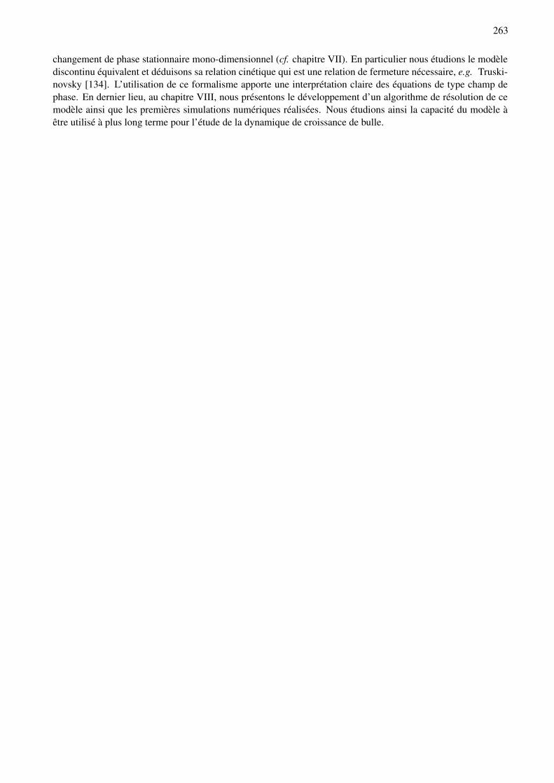
263
changement de phase stationnaire mono-dimensionnel (cf. chapitre VII). En particulier nous étudions le modèlediscontinu équivalent et déduisons sa relation cinétique qui est une relation de fermeture nécessaire, e.g. Truski-novsky [134]. L’utilisation de ce formalisme apporte une interprétation claire des équations de type champ dephase. En dernier lieu, au chapitre VIII, nous présentons le développement d’un algorithme de résolution de cemodèle ainsi que les premières simulations numériques réalisées. Nous étudions ainsi la capacité du modèle àêtre utilisé à plus long terme pour l’étude de la dynamique de croissance de bulle.

264 RÉSUMÉ EN FRANÇAIS
I Étude de la crise d’ébullition
Nous étudions dans cette partie le phénomène de crise d’ébullition. Il s’agit d’une instabilité dans le processusd’échange de chaleur entre un élément chaud et un fluide bouillant. Cette instabilité est à l’origine d’une éléva-tion brutale de la température de l’élément chauffant ce qui peut fortement l’endommager. La crise d’ébullitionest un des phénomènes envisagés dans les scenarii incidentels se rapportant à l’étude de la sûreté des centralesnucléaires. A ce jour, l’origine physique de la crise d’ébullition est mal comprise. Le but de la présente partie dumémoire est de définir, à partir des connaissances actuelles, un objet d’étude permettant d’améliorer la connais-sance de ce phénomène. Pour ce faire, on propose une étude critique de la modélisation de la crise d’ébullitionpermettant d’identifier les aspects de l’ébullition les plus pertinents à éclaircir.
I.1 Crise d’ébullition et régimes d’ébullition
On considère dans la suite de cette étude l’ébullition en vase d’un fluide pur. Ainsi on ne considère pasd’écoulement moyen. Nous proposons tout d’abord de reprendre la présentation générale de l’ébullition en vase.Nukiyama [103] a étudié le transfert de chaleur entre un élément chauffant et un fluide environnant, introduisantle premier ses principales caractéristiques.
Considérons premièrement que la paroi inférieure du vase est l’élément chauffant. Nous notons q le fluxde chaleur transmis au fluide par cette plaque et 〈∆T 〉 = 〈T − T sat〉 l’écart moyen de température de la paroipar rapport à la température de saturation1. Ces deux grandeurs caractérisent le régime d’ébullition considérécomme nous le voyons par la suite. L’ébullition en vase est caractérisée par trois différents régimes d’ébullition.La figure C.2 donne l’allure des variations du flux q échangé à travers la paroi en fonction de sa température〈∆T 〉. Cette courbe est appelée courbe de Nukiyama et on y distingue clairement les trois différents régimesNB, T B, FB par les trois différentes portions de courbe.
############################################################$$$$$$$$$$$$$$$$$$$$$$$$$$$$$$$$$$$$$$$$$$$$$$$$$$$$$$$$$$$$
q
〈∆T 〉
q
DNB
MHFONB
CHF
NBFBTB
〈∆T 〉
PHASE VAPEURPHASE LIQUIDE
Figure C.2: Courbe de Nukiyama
Différents régimes d’ébullition
Ébullition nucléée Considérons premièrement le régime d’ébullition nucléée (NB sur la figure C.2). Cerégime est caractérisé par de faibles valeurs de la surchauffe pariétale 〈∆T 〉. Pour cette raison, l’ébullition nuclééeest un processus efficace de transfert de chaleur. Ceci explique l’usage répandu de fluides bouillants dans leséchangeurs industriels. Ce régime se déclenche à la suite du régime de convection naturelle (point ONB). Desbulles de vapeur se forment alors en proche paroi avant de s’en détacher et de s’écouler dans la partie liquidesupérieure. L’ébullition nucléée connaît une limite aux forts flux de chaleur q (point DNB). La valeur du fluxcorrespondant à cette limite est le flux critique (CHF). Il est important de noter que, contrairement aux autresrégimes d’ébullition, la paroi est couverte par une couche quasiment continue de liquide.
Ébullition en film Dans le régime d’ébullition en film, un film de vapeur couvre entièrement la paroi. Onconsidère que l’interface du film en contact avec le liquide est à la température de saturation. Cette interfaceliquide vapeur est le lieu d’un processus cyclique de formation (croissance puis départ) de bulles gouverné parl’instabilité de Rayleigh Taylor. Il s’agit aussi du lieu de la transition de phase liquide-vapeur. Le flux de chaleur
1La température de saturation est la température à laquelle le liquide et sa vapeur sont à l’équilibre thermodynamique.

I. ÉTUDE DE LA CRISE D’ÉBULLITION 265
pariétal traverse ainsi une couche de vapeur avant d’atteindre l’interface où il est le "moteur" de la transition dephase. La diffusivité thermique de la vapeur étant bien moindre que celle du liquide, ce régime est caractérisépar des valeurs élevées de la température de paroi.
Lorsque le flux critique, CHF, est atteint, le système opère une transition entre le régime d’ébullition nuclééeet le régime d’ébullition en film. Cette transition est caractérisée par une soudaine et importante élévation de latempérature de paroi pouvant atteindre plusieurs centaines de degrés Kelvin. La crise d’ébullition est cette mêmetransition ; étant donnée la description précédente des régimes d’ébullition, la crise d’ébullition est associée à unassèchement total de la paroi.
Ébullition de transition Lors d’une ébullition en régime de transition, la paroi chaude est alternativementasséchée puis remouillée. Ce régime est difficile à modéliser en tant que tel et on l’associe le plus souvent à unesuperposition des régimes d’ébullition nucléée et en film. Ce régime est instable lorsque le flux de chaleur q estimposé et ne peut être observé que si la température moyenne de la paroi est imposée. Du fait des assèchementsintermittents les valeurs locales instantanées du flux et de la température varient fortement.
Précisions et remarques
Transitoire Dans une situation industrielle, la crise d’ébullition se produit en conditions transitoires. Enprésence de transitoires très rapides, il est justifié, comme souligné par Berthoud [14], de considérer des mécan-ismes de crise d’ébullition différents. Dans la suite de cette étude, nous considérons donc le cadre de transitoireslents, au sens précisé par l’étude expérimentale de Sakurai [118].
Écoulement moyen Les échangeurs industriels sont le plus souvent des boucles au sein desquelles le fluidecalo-porteur s’écoule, la partie chauffante ne constituant qu’une portion de cette boucle. Cette situation est doncen de nombreux points différentes de la configuration plus académique de l’ébullition en vase. Néanmoins,l’influence des “paramètres” de configuration sur la crise d’ébullition peut être considérée comme secondaire: la valeur du flux critique dépend de la configuration mais le mécanisme physique peut être similaire. Nousrevenons plus en détail sur cette hypothèse lorsque nous abordons plus précisément les principaux mécanismespotentiellement en jeu lors de la crise d’ébullition (cf. section I.3).
Conclusion Le processus d’ébullition a été introduit comme un mécanisme de transfert de chaleur dont l’efficacitéest grande tant que l’on observe le régime d’ébullition nucléée, i.e. tant que la paroi chaude est recouverte deliquide. La transition de régime correspondant à un assèchement partiel ou total de la paroi est un phénomèneviolent appelé crise d’ébullition pour lequel nous supposons que le mécanisme physique ne dépend pas de laconfiguration de l’écoulement bouillant.
I.2 Mécanismes physiques
Après avoir introduit les principales caractéristiques de l’ébullition en vase, nous nous intéressons de plus prèsà l’ébullition nucléée dans des conditions proches de la crise d’ébullition. Par l’étude des phénomènes qui s’yrapportent, nous souhaitons identifier les causes potentielles de la crise d’ébullition.
Un premier constat motive plus précisément notre approche : tout paramètre (la micro-structure de la paroiaussi bien que l’intensité de l’écoulement convectif dans la conduite) ayant une influence sur l’ébullition nuclééemodifie la valeur du flux critique. Ceci justifie donc l’étude exhaustive des phénomènes ayant trait à l’ébullitionnucléée à fort flux. Une meilleure compréhension du phénomène doit ainsi permettre d’identifier les mécanismesayant un effet paramétrique sur la crise d’ébullition de ceux qui en sont la cause même.
On distinguera les différents phénomènes de l’ébullition en paroi selon trois différents niveaux de descriptiondu processus. Chaque niveau de description se rapporte à une échelle spatiale caractéristique : ainsi cette clas-sification permet de considérer les phénomènes pouvant effectivement interagir, initier une instabilité du régimeet donc finalement être à l’origine de la crise d’ébullition. La cellule de base du phénomène d’ébullition est labulle et les échelles caractéristiques de chaque niveau de description se définissent naturellement par rapport audiamètre caractéristique d’une bulle.

266 RÉSUMÉ EN FRANÇAIS
Échelle de l’écoulement diphasique Ce niveau de description est le moins détaillé, et par là même le plusidéalisé des trois niveaux considérés. Il correspond à une vision moyennée du système liquide-vapeur. L’échellecaractéristique est supérieure à celle de la bulle, cette dernière n’étant pas considérée comme une entité à partentière. Le flot de bulles généré en proche paroi est vu comme un canal de vapeur et les phénomènes proche paroicomme la dynamique de croissance des bulles sont ignorés. A ce niveau d’analyse on considère principalementles phénomènes hydrodynamiques diphasiques. Par la suite on s’intéresse peu à ce niveau de description et onne détaille donc pas plus les principaux phénomènes lui étant associés.
Échelle de la bulle moyenne L’échelle caractéristique de ce niveau de description est celle de la bulle. Cettedernière est considérée comme étant de géométrie fixée mais de taille variable. Ainsi on modélise sa phasede croissance en paroi. Ceci permet de modéliser plus finement les différents phénomènes jouant un rôle dansl’échange de chaleur fluide/paroi. On distingue notamment le transport de chaleur latente ainsi que l’influencede la présence de bulles sur l’intensité des échanges convectifs. La création de bulles est modélisée comme unmécanisme cyclique localisé (sur des sites) constitué d’une suite d’événements : nucléation, croissance, départ,attente. En outre certains modèles considèrent l’interaction inter-sites. Cette échelle d’analyse regroupe unegrande palette de phénomènes pouvant être associés à un scenario hypothétique de la crise d’ébullition commenous le montrons au paragraphe 1.2.3. Leur énumération est reprise dans la liste suivante. On remarquera enparticulier la nature très variée des phénomènes, thermiques, mécaniques, géométriques.
1. répartition du flux de chaleur pariétal parmi différents mécanismes de transfert de chaleur
(a) transport de chaleur latente (évaporation) (éventuellement deux sous-contributions : lo-calisé dans une micro-couche de liquide coincée entre bulle et paroi versus autour de labulle)
(b) conduction transitoire
(c) convection naturelle
2. fréquence spatiale du processus de croissance de bulle, concept de densité de site de nucléation(NSD fonction de la surchauffe pariétale)
3. taux de croissance des bulles
4. taille des bulles au départ de la paroi
5. temps d’attente entre deux formations de bulle sur un même site
6. interaction entre bulles (thermique, hydrodynamique, coalescence)
7. agitation et instabilité des bulles
Table C.1: Mécanismes physiques à l’échelle de la bulle
Échelle locale Ce niveau de description est le plus fin, l’échelle caractéristique des phénomènes considérésétant inférieure à celle de la bulle. Ainsi la géométrie complète de la bulle est prise en compte, c’est à direla description fine de la position de l’interface liquide-vapeur. À ce niveau d’analyse l’ensemble des équationsde Navier-Stokes doivent être résolues au sein de chaque phase (liquide ou vapeur), phase dont les frontières(interface) sont libres. Cette résolution nécessite d’avoir recours à des méthodes numériques. Les phénomènesphysiques à cette échelle sont repris dans la liste C.2. Ce niveau de description peut-être nécessaire pour décrirecertaines instabilités dans le processus de croissance de bulle en paroi qui, nous le verrons, peuvent être à l’originede la crise d’ébullition et qui ne sont pas captées aux échelles supérieures de modélisation.

I. ÉTUDE DE LA CRISE D’ÉBULLITION 267
1. Courbure locale de la bulle et force capillaire
2. Pression de recul à l’interface : le saut de pression vaut JPK = −Γ2J1/ρK où Γ est le taux detransfert de masse local (cf. notre étude des conditions de saut à l’interface en section VII.1)
3. Dynamique de la ligne de contact (angle de contact statique-dynamique) et flux de chaleursingulier associé (cf. Anderson and Davis [3] ou Mathieu et al. [92])
4. Pesanteur : effet du gradient de pression hydrostatique sur la forme de la bulle et conséquem-ment sur sa dynamique de départ (cf. Shikhmurzaev [125] dont le modèle prend en compteune forme de bulle dépendant du temps ainsi qu’un modèle spécifique pour la dynamique de laligne de contact)
5. Conduction transitoire locale au sein de l’aire de contact entre la paroi et la vapeur en pied debulle (cf. Blum et al. [16])
Table C.2: Mécanismes physiques à l’échelle locale
I.3 Modélisation de la crise d’ébullition
La question induite par notre présentation du régime d’ébullition nucléée est la suivante : quel niveau de descrip-tion de l’ébullition est à même de capturer le mécanisme physique à l’origine de la crise d’ébullition ? D’autresquestions ouvertes concernant la crise d’ébullition sont abordées dans cette étude. Précisons que nous consid-érons la crise d’ébullition comme un mécanisme à l’origine d’un assèchement en paroi se produisant au point deDNB, et ce indépendemment du type de conditions thermiques (flux ou température imposé). Ainsi un mêmemécanisme est supposé pouvoir expliquer la crise du régime d’ébullition nucléée qui initie une transition verssoit le régime d’ébullition en film, soit le régime d’ébullition de transition.
Dans cette partie de l’étude, nous étudions les différents modèles proposés dans la littérature pour expliquerle mécanisme de la crise d’ébullition. Ils sont regroupés selon le niveau de description auquel ils se réfèrent. Lebut de cette présentation est d’utiliser les diverses informations que nous proposent ces modèles afin de définirun problème élémentaire dont la résolution permettrait d’améliorer la compréhension du phénomène de crised’ébullition. Cette analyse permettra plus particulièrement de définir un cahier des charges pour le modèle de latransition de phase liquide-vapeur que nous étudions dans les chapitres suivants.
Modèle hydrodynamique de Zuber La corrélation de Zuber [156] permet d’obtenir une estimation de lavaleur du flux critique dont la validité est relativement bonne. Zuber [156] a proposé un mécanisme pour la crised’ébullition associé á l’échelle de l’écoulement moyen. L’étude de l’excitation de l’instabilité de type Kelvin-Helmoltz par la longueur d’onde la plus instable de Rayleigh-Taylor au sein de l’écoulement à bulles permet dedéduire l’expression suivante du flux critique :
qCHF Zuber =π
24Lρv 4
√
σg(ρl − ρv)ρ2v
√
ρl + ρv
ρl(I.3)
où L est la chaleur latente associée au changement de phase liquide-vapeur, σ est la tension interfaciale, ρ estla masse volumique des phases liquide (l) et vapeur (v), et g est la gravité. Néanmoins, le modèle de Zuber, s’ilpermet effectivement de déduire une bonne approximation du flux critique, n’est pas basé sur une descriptionréaliste des événements relatifs à la crise d’ébullition comme le montre, par exemple, l’étude expérimentalede Katto and Otokuni [75]. Nous verrons par la suite comment il est possible d’interpréter le succès de laformule (I.3) (déduite d’une analyse à l’échelle de l’écoulement moyen) en considérant que l’instabilité se produità l’échelle locale.
Limite des mécanismes associés à l’échelle de la “bulle moyenne” Dans la partie 1.3.2, nous étudions endétail différents modèles pour la crise d’ébullition rattachés à une modélisation de l’ébullition nucléée à l’échelle

268 RÉSUMÉ EN FRANÇAIS
de la bulle moyenne. Cette étude montre la variété de mécanismes pouvant mener à une instabilité du régimed’ébullition nucléée. Ainsi la transition de régime est alternativement associée à des instabilités thermiques (cf.Kolev [79]), hydrodynamiques (cf. Chang [32]), ou encore à une trop forte densité de population de bullesen proche paroi donnant lieu à des phénomènes de coalescence (cf. Bang et al. [9]). Néanmoins, il apparaîtclairement qu’aucun de ces phénomènes (et a fortiori de ces scenarii) ne peut être soutenu par des observationsexpérimentales de l’ébullition nucléée à des conditions proches de celles du DNB. En outre, certains aspects deces modèles sont contradictoires avec des observations fines de l’ébullition en paroi comme celles rapportéespar Theofanous et al. [131]. Notre analyse ne retient donc aucun mécanisme de crise d’ébullition pouvant êtredécrit à l’échelle de la bulle moyenne et soutenu par l’expérience. Ces conclusions nous amènent à considérerles phénomènes associés à l’échelle locale.
Mécanismes locaux pour la crise d’ébullition Cette famille de modèles regroupe des scenarii pour lesquels latransition de régime d’ébullition est contrôlée par la dynamique d’une bulle isolée lors de sa phase de croissanceen proche paroi. On distingue notamment différentes sous catégories de modèles.
? Modèles basés sur l’instabilité de recul. Le saut de pression à l’interface comprend un terme, dit de recul,quadratique en le taux de transfert de masse. Les modèles de Kandlikar [70] ou Nikolayev et al. [100],suivant l’idée de Sefiane et al. [120], supposent qu’aux conditions du flux critique la pression de reculconstitue la force dominante du bilan de quantité de mouvement à l’interface. Elle induit une dynamiqued’étalement de la zone sèche correspondant au pied d’une bulle, cette dynamique menant finalement à lacrise d’ébullition.
? Modèles basés sur un bilan thermique au sein de la zone sèche. L’idée repose sur l’hypothèse qu’au delàd’un certain flux critique, la paroi en contact avec la vapeur sous le pied d’une bulle devient suffisammentchaude pour empêcher tout re-mouillage ultérieur. On cite par exemple les modèles de Bricard et al.[20] ou de Blum et al. [16]. Ces modèles ne sont pas considérés comme réalistes car ils ne permettentpas d’expliquer la transition du régime d’ébullition nucléée vers l’ébullition de transition qui correspondpour autant à une dynamique d’assèchement local similaire à la crise d’ébullition mais se produisant pourdes températures de paroi faibles. Dans ce cas la dynamique d’assèchement ne résulte donc pas d’unetempérature très élevée au sein de la zone sèche.
En ce qui concerne les modèles basés sur l’instabilité de recul, nous avons montré dans la section 1.3 que lesrésultats obtenus ne sont pas suffisamment probants car il leur manque la prise en compte d’un mécanisme dedépart de la paroi à même de contrebalancer la dynamique d’amorçage de l’étalement décrite.
Conclusion sur l’étude de la modélisation actuelle de la crise d’ébullition Nous avons montré par cette étudequ’il est important de considérer la crise d’ébullition comme étant une conséquence logique de la description del’ébullition nucléée plutôt qu’un phénomène indépendant de ce dernier. En effet, dans ce cadre de travail, ilest possible de discriminer un modèle d’un autre en se basant sur des observations expérimentales du régimed’ébullition nucléée à fort flux, ce qui demeure impossible sinon.
I.4 Un mécanisme pour la crise d’ébullition à l’échelle locale
Croissance instable d’une bulle en proche paroi Dans la partie 1.4 du mémoire nous reportons et analysonsdes observations expérimentales (en particulier les travaux de Theofanous et al. [130, 131]) des phénomènesproche paroi dans des conditions de flux critique. Les conclusions suivantes en sont tirées
1. La séparation d’échelle utilisée lors de notre présentation des mécanismes du régime d’ébullition nuclééeest attestée expérimentalement même à très fort flux : quelle que soit la quantité de vapeur formée unefine couche de liquide couvre la paroi, au sein de cette couche se produit une ébullition nuclée intense.Au dessus de cette couche liquide, les bulles formées coalescent et forment de grosses masses de vapeurdont la taille caractéristique semble déterminée par l’instabilité de Rayleigh Taylor. La couche liquide esttoujours approvisionnée et les phénomènes s’y produisant peuvent être considérés indépendamment de ladescription du reste de l’écoulement diphasique.

I. ÉTUDE DE LA CRISE D’ÉBULLITION 269
2. Dans des conditions de fort flux pariétal la dynamique de croissance de bulle dans cette couche liquidepeut être “irrégulière” : cette irrégularité correspond à un assèchement local en pied de bulle qui modifiegrandement les échelles et temps caractéristiques des bulles ainsi formées. La fréquence d’apparition deces phénomènes irréguliers est d’autant plus importante qu’on s’approche des conditions du flux critique.Au flux critique, il a été observé qu’une des taches sèches ainsi formée s’étale, menant finalement à unetransition de régime.
Ainsi nous avons montré à l’aide de résultats expérimentaux que la crise d’ébullition peut être vraisemblablementassociée à des phénomènes à l’échelle dite “locale”.
Un scénario pour l’instabilité du régime d’ébullition nucléée Nous proposons un mécanisme pour la crised’ébullition basé sur une instabilité dans la croissance de bulle en proche paroi. Comme représenté sur la fig-ure C.3, on s’intéresse à l’évolution d’une bulle ayant initialement une grande surface de contact avec la paroi(image de la configuration initiale). Cette configuration “étalée” correspond à une première phase dans le scé-nario d’instabilité cohérent avec le modèle de Nikolayev et al. [100] : la pression de recul domine la pressioncapillaire et le pied de bulle s’étale. Dans le régime d’ébullition nucléée, les forces capillaire et hydrostatiquepromeuvent suffisamment l’élévation de la bulle pour engendrer finalement la formation d’une bulle ressemblantà un gros champignon quittant la paroi (image de droite sur la figure C.3). Aux conditions du DNB au contraire,sous l’action de la pression de recul, la bulle continue de s’étaler en un film de vapeur. Suivant les conditions ther-miques en paroi, ce film de vapeur est stable (flux imposé supérieur au flux critique, transition vers l’ébullitionen film, image en haut à gauche) ou instable (température imposée correspondant au DNB et donc inférieure auMHF, régime d’ébullition de transition, image en bas à gauche). Ce scénario permet donc de décrire la crised’ébullition comme une instabilité dans le régime d’ébullition nucléée qui conduit naturellement vers les autresrégimes d’ébullition. Nous montrons en outre au paragraphe 1.4.2 que ce scénario est cohérent avec la corrélationde Zuber (I.3) pour le flux critique. En effet les grandeurs physiques caractéristiques de ce mécanisme sont cellesde la corrélation. Même si cette dernière a pu être déduite d’une étude à l’échelle de l’écoulement diphasique,nous montrons donc qu’elle peut être interprétée à l’échelle locale.
TB
NBDNB
Configuration initiale
FB
Bulle irrégulière
Figure C.3: Un mécanisme de la crise d’ébullition à l’échelle “locale”
L’étude de la dynamique de croissance d’une bulle Pour étudier la dynamique de la croissance de bullecorrespondant au scénario instable décrit par la figure C.3, il est nécessaire de résoudre un problème à frontièrelibre (l’interface liquide-vapeur) et de prendre en compte les phénomènes suivants :
? courbure locale et force capillaire
? pression de recul
? effet de la pression hydrostatique sur la dynamique de départ d’une bulle (cf. les travaux de Shikhmurzaev[124])
270 RÉSUMÉ EN FRANÇAIS
? conduction de la chaleur dans le liquide en proche paroi, chaleur latente de changement d’état
Il est important de noter que la compressibilité des phases liquide et vapeur n’apparaît pas en tant que paramètrephysique dans la corrélation de Zuber (I.3) ni comme un mécanisme prépondérant dans notre scenario ou danstout autre des scenarii que nous avons analysé. Ainsi on suppose dans la suite de cet étude que l’hypothèsed’incompressibilité des phases liquide et vapeur est justifiée pour l’étude du mécanisme de crise d’ébullition.Ainsi, même si les effets compressibles jouent un rôle important dans l’initiation de la croissance d’une bulle(phase de nucléation et début de croissance, e.g. Mikic et al. [93]), son rôle est supposé comme non déterminanten ce qui concerne le scénario d’instabilité proposé. Étant donné la géométrie complexe de l’interface, ainsique la nécessité de prendre en compte des couplages entre des phénomènes thermiques (conduction et chaleurlatente) et mécanique (pression de recul, capillaire), l’utilisation d’une approche numérique pour résoudre cetécoulement diphasique s’impose.
I.5 Conclusion de notre étude de la crise d’ébullition
Après avoir présenté de manière générale les écoulements bouillants, nous avons introduit la problématique dela crise d’ébullition, phénomène limitant l’efficacité du transfert de chaleur et dont le mécanisme reste à ce jourmal compris. Nous avons alors analysé l’état de l’art de la modélisation de la crise d’ébullition : cette étudea révélé que la principale faiblesse de ces modèles est liée au manque d’informations expérimentales à mêmede les avérer. Notre analyse d’observations récentes des phénomènes proche paroi en ébullition nucléée à fortflux nous a permis d’identifier une instabilité dans le dynamique de croissance de bulle. Nous en avons déduitun scénario pour la crise d’ébullition. Les mécanismes physiques en jeu dans cette instabilité sont cohérentsavec la corrélation de Zuber pour le flux critique, corrélation permettant d’obtenir une estimation de la valeur duflux critique. Pour étudier cette dynamique, il est nécessaire d’avoir recours à la simulation numérique et nousavons clairement défini l’ensemble des phénomènes physiques nécessaires et suffisants à cette étude. En parti-culier, nous avons montré que la compressibilité des phases liquide et vapeur n’est pas un mécanisme physiqueprépondérant pour l’étude du mécanisme présupposé pour la crise d’ébullition. Par la suite nous nous intéressonsaux méthodes numériques permettant une telle étude.

II. MÉTHODES NUMÉRIQUES POUR L’ÉTUDE DES ÉCOULEMENTS LIQUIDE-VAPEUR 271
II Méthodes numériques pour l’étude des écoulements liquide-vapeur
II.1 Les familles de méthodes
On s’intéresse dans ce chapitre aux méthodes permettant de résoudre les écoulements bouillants à l’échelle de labulle, i.e. permettant de résoudre les équations de Navier-Stokes au sein des phases liquide et vapeur en prenanten compte la frontière libre que constitue l’interface entre ces deux domaines. On distingue dans un premiertemps deux descriptions mathématiques de la position xi de cette interface.
? La représentation explicite xi = f (t) qui donne lieu aux méthodes purement lagrangiennes (cf. la méthodeALE [27]) , ou lagrangiennes mixtes (cf. la méthode front tracking [140]). Ces méthodes nécessitent ledéveloppement d’un traitement spécifique du maillage de l’interface. Ceci est à l’origine d’une complexitédans la méthode numérique ne permettant pas de vérifier les bilans de masse, quantité de mouvement,énergie à chaque étape de l’algorithme et notamment lors du déplacement de l’interface (e.g. [126]).
? La représentation implicite i.e. F(xi, t) = 0 pour laquelle le champ F n’est pas unique qui donne lieu auxméthodes de type level set (basées sur l’utilisation d’une fonction distance à l’interface, cf. [123]) ou auxméthodes correspondant à l’utilisation d’une modélisation de l’interface comme diffuse. Dans ces deux casle système d’équations continues est défini en tout point de l’espace incluant la description des interfacesce qui constitue un avantage sur le plan de leur résolution numérique. On fera, pour cette raison, le choixd’utiliser une représentation implicite dans la suite de ce mémoire.
Dans les méthodes de type level set, il est nécessaire de définir des extensions des champs interfaciaux (comme lavitesse de l’interface ou la tension interfaciale) en les étalant numériquement. Ces méthodes ne proposent pas àce jour une manière satisfaisante de prendre en compte la tension de surface. Contrairement aux autres méthodesles méthodes d’interface diffuse ne sont pas basées sur le modèle de Gibbs pour lequel les interfaces sont dessurface de discontinuité des propriétés physiques du fluide mais elles considèrent plutôt l’interface comme unezone volumique de transition à travers laquelle l’ensemble des grandeurs varient continûment. Cette descriptionest issue d’une modélisation thermodynamique du fluide comprenant une dépendance en des termes non-locaux(le plus fréquemment des gradients). Les équations du mouvement d’un tel fluide sont déduites de l’applicationdes principes fondamentaux de la thermodynamique, le système d’équations permettant la représentation desphases et de l’interface est ainsi dit “thermodynamiquement cohérent”. Cette caractéristique permet un contrôleplus aisé des différents bilans comme l’a montré Jamet et al. [68] pour ce qui concerne la prise en compte de latension interfaciale. Pour ces raisons on fait le choix dans la suite de cette étude d’utiliser une modélisation detype interface diffuse pour étudier la dynamique de croissance d’une bulle.
II.2 Modèle à interface diffuse et méthode numérique
Principe des modèles à interface diffuse Les modèles à interface diffuse proposent une régularisation d’unproblème discontinu basée sur une description thermodynamique particulière du fluide. Cette description reposesur deux ingrédients principaux. Supposons tout d’abord un système diphasique, une variable thermodynamiqueintensive X prenant une valeur caractéristique au sein de chaque phase (on peut penser naturellement à la massevolumique dans le cas liquide-vapeur). On considère alors le fluide décrit par une unique énergie fonction de X.Le premier ingrédient correspond à l’existence d’une partie non-convexe des variations de l’énergie du fluide enfonction du paramètre X entre les valeurs caractéristiques des phases. En utilisant le critère de Gibbs-Duhem, onmontre que cette non-convexité induit la séparation du système en deux phases. La régularisation de l’interfaceentre ces phases repose sur l’introduction d’une dépendance de l’énergie en des termes non-locaux tel que ∇X.Cette contribution pénalise énergétiquement les états pour lesquels X varie fortement spatialement et n’autoriseainsi pas l’interface à être une surface de discontinuité. Une telle description thermodynamique définit l’interfacecomme une zone de transition ayant une épaisseur caractéristique et une énergie associée.
Par conséquent ces modèles permettent une description explicite des interfaces tout en introduisant unephysique “interfaciale” supplémentaire par le biais du seul modèle thermodynamique du fluide.
II.3 Modèle de van der Waals
Pour décrire un fluide pouvant exister sous deux états liquide et vapeur et étant doué de capillarité, le modèlede van der Waals est a priori le plus à propos. Nous montrons ici que pour autant il n’est pas approprié à la

272 RÉSUMÉ EN FRANÇAIS
simulation numérique de la dynamique de croissance de bulles pour laquelle notre modèle est développé.
Un modèle complet Le modèle de van der Waals, encore appelé modèle du second gradient, est basé surl’expression de l’énergie libre F en fonction de la masse volumique ρ. On considérera, dans un premier temps,uniquement les aspects isothermes de ce modèle.
Une épaisseur de l’interface trop faible La valeur physique de l’épaisseur de l’interface h est de l’ordre dequelques Å (Ångströms) aussitôt que les conditions thermodynamiques s’éloignent de celles du point critique.Par conséquent la taille caractéristique de la zone de transition est très largement inférieure à celle de la bullequ’on souhaite étudier (un facteur 105 environ). Capturer numériquement les deux échelles nécessiterait desmoyens de calcul hors de portée. En outre la pertinence de la description de phénomènes à une si petite échellen’est pas assurée. Pour pouvoir envisager la régularisation de la description des écoulements liquide vapeur enutilisant le modèle de van der Waals Jamet [66] a proposé de modifier la valeur du paramètre h en modifiantla fermeture thermodynamique, i.e. l’expression analytique de F(ρ,∇ρ). Cette modification affecte plus partic-ulièrement la partie non-convexe de F qui décrit les états du fluide à travers l’interface. Jamet [66] s’est assuréqu’il était possible de choisir librement l’épaisseur de l’interface tout en fixant l’énergie libre en excès associée,cette dernière étant à l’origine de la tension de surface. Nous reprenons en section 2.2.3 cette analyse. Nousmontrons en particulier que, si elle permet effectivement le contrôle de l’épaisseur et de la tension de surface,cette modification affecte d’autres caractéristiques du fluide.
Un modèle trop contraint En effet nous montrons, en reprenant l’analyse décrite par Fouillet [53], que toutemodification de l’énergie libre induit des répercussions sur la limite de métastabilité des phases pures. La limi-tation de la modification vient alors qu’il n’est pas possible d’avoir conjointement (i) une interface d’épaisseurraisonnable, (ii) des phases liquide et vapeur ayant toutes les propriétés physiques nécessaires à une descrip-tion fidèle des écoulements bouillants à la bonne valeur (en particulier, masse volumique, capacité calorifiquecourbe de saturation et limite de métastabilité, cette dernière étant intimement liée aux valeurs des coefficientsde compressibilité isotherme et d’expansion thermique), et (iii) des fonctions thermodynamiques suffisammentrégulières (des cassures trop brusques dans les variations induisent des difficultés numériques).
Nous pouvons alors retenir la conclusion suivante quant à l’utilisation du modèle de van der Waals pourl’étude des écoulements bouillants. Dans un premier temps, le modèle comprend effectivement l’ensemble desphénomènes que nous souhaitons reproduire. Néanmoins son utilisation pour l’étude numérique de la croissancede bulle de taille millimétrique ne peut être envisagée. Cette limitation est interprétée comme suit : la régu-larisation de l’interface est associée au rôle particulier que joue la masse volumique dans le modèle de van derWaals, disons le rôle de paramètre d’ordre ; mais la masse volumique est aussi un paramètre macroscopiqued’importance pour la physique du fluide. Ainsi en essayant de modifier la description de l’interface, il n’estpas envisageable de ne pas modifier la description des phases. Cette analyse permet de mettre en évidence unepiste de modélisation, il s’agit d’introduire une régularisation de l’interface de manière plus indépendante de ladescription des phases.
II.4 Modèles de champ de phase
Nous tournons alors notre attention sur la modélisation de type champ de phase dont nous exposons dans unpremier temps le principe général.
Principe général Dans les modèles champ de phase un paramètre, appelé champ de phase, est introduit entant que variable thermodynamique et permet à la fois de distinguer les domaines phasiques et de décrire la zonede transition. Notre interprétation d’un tel modèle va dans le sens de notre but de modélisation : cette variabledoit permettre d’introduire une régularisation de la zone interfaciale et l’existence d’une variable additionnelled’introduire suffisamment de degré de liberté dans le modèle pour que la structure de l’interface puisse êtrechoisie indépendamment de la description des phases du système.
Nous prenons ainsi l’exemple, plus simple, de la description d’un système diphasique solide-solide. Nousintroduisons alors la modélisation champ de phase de la manière suivante :
? introduction d’une équation d’état unique pour l’ensemble du système diphasique de la forme T (s)

II. MÉTHODES NUMÉRIQUES POUR L’ÉTUDE DES ÉCOULEMENTS LIQUIDE-VAPEUR 273
? identification des équations d’état des phases et séparation formelle de l’équation d’état
? introduction de la variable champ de phase pour décrire les états intermédiaires à ces états phasiques
Cette dernière partie de la modélisation se base sur un certain nombre d’ingrédients similaires à ceux du modèlede van der Waals (introduction de la séparation de phase par une non-convexité du potentiel thermodynamique,dépendance en des termes non-locaux pour régulariser la description de la zone interfaciale) et des ingrédientsplus spécifiques à l’utilisation d’un paramètre d’ordre artificiel (fonction d’interpolation des propriétés physiquesdu matériau entre les valeurs au sein des phases). Ce dernier point permet de comprendre intuitivement legain de liberté d’une telle modélisation car permettant de décorréler la modélisation de l’interface de celle desphases. Encore faut il s’assurer que la formulation retenue induit effectivement la description souhaitée et quel’interférence entre la description de l’interface et l’interpolation des propriétés physiques au sein d’un mêmemodèle permet effectivement de modéliser le matériau souhaité. On s’attachera donc par la suite à comprendrequels sont les propriétés d’un tel matériau et en particulier à montrer quels sont les états monophasiques décritspar ce modèle (retrouve-t-on effectivement les phases souhaitées et n’y a-t-il pas d’autres états du matériaupossibles). Nous verrons par la suite que de telles propriétés d’un modèle champ de phase reposent sur un choixjudicieux des dépendances en la variable champ de phase du potentiel thermodynamique.
II.5 Liste de contraintes pour le modèle de champ de phase
Notre souhait d’utiliser un modèle de type interface diffuse et en particulier de champ de phase pour la descrip-tion des écoulements liquide-vapeur avec changement de phase est avant tout dicté par des motivations d’ordrenumérique. Ainsi l’introduction de la variable champ de phase dans la description du fluide n’est pas censéeinterférer avec celle des états liquide et vapeur qui sont par ailleurs décrits naturellement à l’aide des variablesthermodynamiques classiques (pression et température par exemple). En effet l’introduction de cette variablesupplémentaire est dédiée à la régularisation du système discontinu composé des seuls états monophasiques.
Évidemment en introduisant cette nouvelle variable dans la description thermodynamique d’un fluide, nousdisposons d’un large degré de liberté supplémentaire ; nous souhaitons pour autant contrôler les conséquences decette introduction. Pour ce faire, nous proposons tout d’abord de dresser une liste des propriétés souhaitées pourle modèle, sorte de cahier des charges pour son utilisation comme base d’une méthode numérique. On distinguedonc les principales propriétés du modèle comme suit
1. profil monotone de la variable champ de phase ϕ (contrainte numérique)
2. profil monotone de la masse volumique (contrainte numérique)
3. contrôle aisé de l’épaisseur de la zone de transition interfaciale (contrainte numérique)
4. contrôle aisé de l’énergie libre en excès pour une interface à l’équilibre (contrainte physique)
5. saut de pression à l’interface satisfaisant les relations classiques (contrainte physique)
(a) relation de Laplace
(b) pression de recul
6. contrôle paramétrique des domaines (en pression température) de stabilité et de métastabilité des phasesliquide et vapeur (contrainte physique)
7. contrôle des équations d’état des états monophasiques (ρ(P,T ) et s(P,T )) (contrainte physique), par exem-ple
(a) phases compressibles
(b) phases incompressibles
Cette liste nous permettra par la suite de justifier des choix parfois arbitraires faits dans l’expression analytiquedes potentiels thermodynamiques de notre fluide “champ de phase”. Notons que cette liste se limite à la de-scription des états d’équilibre de notre modèle ; nous étudierons plus en détail les aspects dynamiques et plusparticulièrement les phénomènes dissipatifs à partir du chapitre V.

274 RÉSUMÉ EN FRANÇAIS
II.6 Modèles de champ de phase existants
Dans la section 2.3.3 de notre étude, nous considérons différents modèles de type champ de phase décrivant deuxphases de masse volumique différente. Nous analysons leur propriétés en fonction de la liste de contraintes quel’on souhaite satisfaire. Il ressort de cette étude qu’aucun des modèles existants ne permet à la fois de maîtriseraisément la description des états monophasiques (contrainte physique) et de contrôler les caractéristiques de lazone interfaciale (contrainte numérique). Pour autant le modèle de Anderson et al. [5] propose une formulationparticulièrement intéressante car permettant de prendre en compte la description de deux états fluides incom-pressibles mais de masse volumique différente. Cette propriété est basée sur l’hypothèse de quasi-compressibilitéinitialement introduite par Lowengrub and Truskinovsky [89] pour la modélisation des mélanges binaires. Elleest discutée plus en détail dans la section 3.1.2. Néanmoins le choix de l’expression de l’enthalpie libre dansle modèle de Anderson et al. [5] ne permet pas, par exemple, de définir une structure unique pour l’interface àl’équilibre plan le long de la courbe de saturation, preuve d’une trop importante interférence entre les descrip-tions de l’interface et du matériau. D’où notre but pour la suite de cette étude de développer une formulation detype champ de phase plus adéquate à la description de la croissance de bulle.
Conclusion
Dans ce chapitre nous avons présenté notre choix d’utiliser une méthode numérique des écoulements bouillantsbasée sur une représentation implicite, diffuse et thermodynamiquement cohérente de l’interface liquide vapeur.Pour ce faire nous avons montré qu’il est nécessaire que le modèle du fluide permette une régularisation de laformulation discontinue dont les propriétés peuvent être choisies arbitrairement. Nous avons alors montré qu’unetelle modélisation ne peut être obtenue en utilisant uniquement les variables thermodynamiques classiques pourdécrire le système (cf. notre présentation des limitations du modèle de van der Waals). Nous nous sommesalors tourné vers la famille de modèles de type champ de phase qui se base sur l’introduction d’une variablethermodynamique supplémentaire. Nous avons alors analysé dans un premier temps le gain de modélisation quecette introduction représente. Puis nous avons dressé un cahier des charges pour le modèle que nous souhaitonsutiliser via la liste de contraintes exprimées en page 273. Nous avons alors constaté que les modèles existants nesatisfont pas à l’ensemble de ces contraintes. Par la suite nous proposons ainsi une formulation de type champde phase permettant de satisfaire la liste de ces contraintes
III Fermeture thermodynamique du modèle
Dans ce chapitre nous précisons la fermeture thermodynamique de type champ de phase de notre modèle. Nousmontrons comment notre choix permet de contrôler à la fois et de manière indépendante les propriétés physiquesde notre fluide diphasique (masse volumique, capacité thermique des phases liquide et vapeur, chaleur latente etcourbe de saturation . . . ) et la description de la zone interfaciale (profils d’équilibre et épaisseur caractéristique).Notre but est tout d’abord (section 3.1) de justifier le choix que nous faisons pour les variables principales denotre description. Puis nous considérons les conséquences de l’introduction de la variable champ de phase surla thermodynamique des états d’équilibre (cf. section 3.2). Cette étude nous permet de comprendre l’intérêt demaîtriser les variations des fonction d’état en fonction de la variable d’état ϕ. Enfin nous présentons (section 3.3)la formulation que nous avons développée pour la modélisation de type champ de phase de la transition liquide-vapeur.
III.1 Description thermodynamique d’un système multiphasique
Description de la compressibilité du fluide Dans un premier temps (section 3.1.1) nous nous intéressons à laproblématique de la description thermodynamique d’un système multiphasique à l’aide d’une unique expressiondu potentiel thermodynamique. Nous considérons en particulier la description de la compressibilité isothermeχT du fluide donnée par
χT = −1V
(
∂V∂P
)
T=
1ρ
(
∂ρ
∂P
)
T
Rappelons que notre but est entre autre de pouvoir modéliser librement ce paramètre physique et en particulierde considérer les phases liquide et vapeur comme incompressibles (χT = 0) point 6 et 7 de la liste page 273.

III. FERMETURE THERMODYNAMIQUE DU MODÈLE 275
En effet notre analyse de la crise d’ébullition au chapitre I suggère une telle hypothèse. Un premier choix demodélisation se pose suivant que l’on considère soit la pression P (auquel cas le potentiel thermodynamiqueest naturellement l’enthalpie libre G) soit la masse volumique ρ (auquel cas le potentiel thermodynamique estnaturellement l’énergie libre F) en tant que variable principale. L’équivalence entre les deux descriptions n’étantvalable que si une bijection relie P à ρ. Dans le cas où ρ est variable principale, la pression est donnée par (cf.équation (2.2))
P = ρ∂F∂ρ− F = ρ2 ∂ f
∂ρ(III.4)
et la compressibilité isotherme est nécessairement non nulle. C’est le cas du modèle de van der Waals pour lequella description avec P en tant que variable principale n’est pas possible. Dans le cas où P est variable principale,la masse volumique est donnée par
v(P) =1ρ
(P) =∂g
∂P(III.5)
où v est le volume massique du fluide. Il est alors possible de considérer la compressibilité χT du fluide commenulle, auquel cas l’enthalpie libre massique g est linéaire en P. Par contre, en l’absence d’autre variable thermo-dynamique pour décrire le système, nous montrons que ce modèle n’est pas utilisable pour un modèle d’interfacediffuse.
Ainsi nous avons introduit la problématique du choix des variables thermodynamiques principales dansle cadre d’une description continue des propriétés d’un fluide multiphasique. En particulier nous montronsl’impossibilité de modéliser des phases incompressibles isothermes et une interface diffuse à l’aide d’un modèleisotherme du fluide n’utilisant que la variable thermodynamique classique ρ.
L’hypothèse quasi-compressible Dans un deuxième temps (section 3.1.2) nous montrons comment l’introductiond’une variable thermodynamique supplémentaire dans notre description du fluide permet de lever cet obstacle.
A titre d’exemple illustratif, nous considérons l’introduction d’effets anisothermes dans le modèle de vander Waals pour lequel on considère désormais une dépendance de l’énergie libre volumique F en fonction dela température T . On montre comment il est alors possible de modéliser la chaleur latente L librement, i.e.une différence entre les entropies liquide et vapeur à saturation tout en considérant un libre choix des capacitésthermiques cV des phases. Ce modèle est classique (cf. sa présentation section 2.2). Nous introduisons alorsl’analogie suivante entre la description des effets compressibles et anisothermes d’un système thermodynamique
P ↔ Tρ ↔ sχT ↔ cP
ou χs ↔ cv
(III.6)
Nous montrons alors qu’il est possible d’inverser les variables principales du modèle T et ρ pour considérerdésormais l’entropie s comme paramètre d’ordre. Tout comme avec la chaleur latente, on introduit une différencede masse volumique entre les phases liquide et vapeur dont la compressibilité peut alors être choisie librement.
Nous faisons alors le lien entre notre exemple illustratif et l’hypothèse de quasi-compressibilité du fluideintroduite à l’origine par Lowengrub and Truskinovsky [89] dans le cadre des mélanges binaires. Cette hypothèsepermet de considérer une description à interface diffuse d’un fluide dont les phases, bien qu’ayant des massesvolumiques différentes, sont incompressibles. Pouvoir considérer cette hypothèse repose sur la possibilité dechoisir une autre variable thermodynamique que la masse volumique comme paramètre d’ordre de la transitionde phase : la concentration c dans le cadre originel, l’entropie s pour notre exemple illustratif, la variable champde phase ϕ en ce qui concerne le modèle que nous développons. Dans le cadre de notre modèle de champ dephase nous posons cette même hypothèse et choisissons donc la pression P comme étant l’une de nos variablesprincipales. Les autres variables principales sont la température T , variable expérimentale naturelle, et la variablechamp de phase ϕ introduite à des fins de régularisation. Le potentiel thermodynamique correspondant à cesvariables thermodynamiques est donc l’enthalpie libre G.
III.2 Introduction d’une variable thermodynamique de type champ de phase
Il s’agit d’étudier les propriétés d’un fluide décrit à l’aide d’une variable thermodynamique additionnelle de typechamp de phase. Nous étudions formellement les conséquences de l’introduction d’une telle variable thermody-

276 RÉSUMÉ EN FRANÇAIS
namique sur la description des états d’équilibre d’un système.
Une fonction couleur Comme exposé au chapitre 3.2, l’introduction d’une telle variable est avant tout mo-tivée par des raisons numériques. Rappelons en effet que l’ensemble de la physique nécessaire à la descriptiondes écoulements liquide-vapeur avec changement de phase est déjà décrite par le modèle de van der Waalsanisotherme. Le but de cette introduction est de bénéficier de plus de souplesse dans la régularisation notammenten ce qui concerne les propriétés de la zone volumétrique de transition entre les deux phases. Par conséquent lavariable champ de phase est dédiée à cette description de l’interface, et la description des domaines phasiquesn’est pas censée s’en ressentir. En particulier des variations de ϕ au sein de ces domaines ne sont associées àaucune physique et ne sont donc pas souhaitables. Pour ce faire nous imposons qu’une valeur purement abstraitede ϕ soit associée à chaque phase, ainsi par un choix arbitraire nous posons
ϕ = 0 ↔ phase liquide
ϕ = 1 ↔ phase vapeur
Les valeurs de ϕ entre ces deux valeurs sont donc implicitement associées à la zone interfaciale.
Équations d’équilibre
Une relation d’équilibre supplémentaire Dans la section 3.2.2 nous appliquons le critère d’équilibre etde stabilité de Gibbs-Duhem à un volume fluide décrit par notre modèle de champ de phase. Nous définissonstout d’abord les différents potentiels thermodynamiques comme suit
µ =∂g
∂ϕ(III.7a)
v =∂g
∂P(III.7b)
s = − ∂g∂T
(III.7c)
Φ =∂g
∂ (∇ϕ)2 (III.7d)
où v est le volume massique (v = 1/ρ où ρ est la masse volumique), s est l’entropie massique. Nous consid-érons, pour des raisons physiques que la dépendance en ∇ϕ est isotrope. En outre, nous supposons, commeclassiquement en ce qui concerne la théorie capillaire, que g est linéaire en (∇ϕ)2. Ainsi
∂2g
∂((∇ϕ)2)2= 0 (III.8)
et Φ se réduit à une fonction de (P,T, ϕ). Nous montrons alors qu’un état d’équilibre, i.e. correspondant à unextremum d’entropie, satisfait les équations d’équilibre suivantes (cf. équations (3.28))
∇T = 0 (III.9a)
∇g = 0 (III.9b)
µ = 0 (III.9c)
où µ est un potentiel thermodynamique correspondant à la dérivée variationnelle δ du potentiel thermodynamiqueG par rapport à la variable champ de phase ϕ, i.e. est défini par
µ =1ρ
δGδϕ
=1ρ
δρ g
δϕ
=∂g
∂ϕ− 1ρ∇ ·
(
ρ∂g
∂∇ϕ
)
= µ − 2Φ∆ϕ − 2 v∇(ρΦ) · ∇ϕ (III.10)

III. FERMETURE THERMODYNAMIQUE DU MODÈLE 277
Sur la frontière du domaine fluide considéré, la condition d’équilibre suivante est satisfaite
(
2 ρΦ~n.∇ϕ + dUb
dϕ
)
= 0 (III.11)
où Ub est l’énergie d’interaction avec la frontière. La condition d’équilibre thermique (III.9a) est classique. Lacondition d’équilibre mécanique (III.9b) sera associée par la suite à l’expression du tenseur des contraintes nondissipatif de notre fluide. Nous montrerons en particulier qu’en plus du tenseur sphérique associé à la pression, ceterme comprend un tenseur de type Korteweg dû à la dépendance en (∇ϕ)2 introduite. Ce dernier est à l’originede la force capillaire. La dernière équation d’équilibre (III.9c) est une relation supplémentaire par rapport àla description classique d’un fluide (e.g. le modèle de van der Waals). Elle est la conséquence naturelle del’introduction des variables supplémentaires ϕ et ∇ϕ dans la description du fluide. Nous montrons par la suitecomment nous associons cette relation plus particulièrement à la description de la zone interfaciale, i.e. que nousl’interprétons comme une condition d’équilibre propre à la zone volumétrique interfaciale. On montre commentla relation d’équilibre (III.11) valable sur la frontière permet de définir un angle de contact entre une paroi etl’interface. En effet la dépendance de Ub avec ϕ permet d’introduire une plus ou moins grande affinité d’unesurface vis à vis d’une ou l’autre des phases.
Par la suite (cf. section 3.2.3) nous étudions la condition d’équilibre stable d’un état monophasique (i.e.uniforme en ϕ). Nous montrons que la condition concerne les variations de g en ϕ (cf. la première partie de larelation µ = 0). Ainsi les conditions analytiques suivantes (cf. équation (3.38))
∂g
∂ϕ |P=∂ f∂ϕ |ρ
= 0
∂2g
∂ϕ2 |P=∂2 f∂ϕ2 |ρ
≥ 0
sont satisfaites pour chaque état monophasique. Ainsi, dans notre cas et suite à la discussion de la sectionprécédente, notre modèle se doit de satisfaire ces relations pour et uniquement pour les valeurs particulièresϕ = 0 et ϕ = 1.
Une relation pour la régularisation de l’interface Considérons la relation d’équilibre supplémentaire (III.9c).il s’agit d’une équation différentielle en ϕ constituée de deux parties
? La première est associée à la dépendance de g en ϕ. Cette variable a été introduite afin de modéliser laséparation du fluide en différentes phases. Ainsi cette partie de la relation d’équilibre peut être associée àl’introduction de variations non convexes du potentiel thermodynamique en ϕ. Classiquement cette non-convexité est introduite à l’aide d’une fonction double-puits W(ϕ) satisfaisant les conditions analytiquessuivantes
W(0) = W(1) = 0dWdϕ
(0) =dWdϕ
(1) = 0∫ 1
0
√
2 W(ϕ) dϕ = 1
(III.12)
comme par exemple le polynôme de degré 4 suivant
WP4(ϕ) = 18 ϕ2 (ϕ − 1)2 (III.13)
représenté sur la figure C.5.
? La seconde partie est liée à l’introduction de la dépendance en des termes non-locaux. La vocation de cettedépendance est de régulariser l’interface en une zone de transition volumique. Classiquement une équationdifférentielle du type suivant, e.g. Rocard [113]
h2 (ϕ,x)2 = 2 W(ϕ) (III.14)

278 RÉSUMÉ EN FRANÇAIS
est satisfaite par le profil du paramètre d’ordre à la traversée d’une interface plane selon un axe ~x. Cetteéquation différentielle est paramétrée par h qui caractérise l’épaisseur h du profil du paramètre d’ordredéfinie par (cf. figure C.4)
h =1
max |ϕ,x|Tout comme la relation d’équilibre µ = 0 l’équation différentielle (III.14) est constituée de deux parties,l’une concernant des variations en ϕ, l’autre en ses dérivées spatiales.
Nous avons introduit deux ingrédients classiques (fonction double-puits et équation différentielle) qui ont undouble mérite. Le premier est de gérer la séparation des phases. Le second est de contrôler les propriétés del’interface et en particulier son épaisseur ce qui est primordial pour les applications numériques envisagées. Cesont les deux propriétés du modèle champ de phase recherchées. Nous souhaitons donc les satisfaire et pource faire nous imposons à notre modèle qu’à l’équilibre l’équation différentielle (III.14) soit satisfaite. Puisquela relation µ = 0 est "libre d’interprétation" nous lui assignons ce rôle. Nous comprenons alors qu’il nous fautdéfinir les variations de g en ϕ et en (∇ϕ)2 de sorte que la relation µ = 0 se réduise effectivement à l’équationdifférentielle souhaitée.
h
x
ϕ
(a)x
ϕ,x
(b)
Figure C.4: Profils diffus pour la variable champ de phase ϕ
W(ϕ)
1.210.80.60.40.20-0.2
3
2.5
2
1.5
1
0.5
0
Figure C.5: Fonction double-puits
III.3 Expression de l’enthalpie libre massique
Nous avons précédemment introduit certaines spécificités que le modèle se doit de satisfaire afin de respecter lescontraintes explicitées dans la liste page 273. Nous présentons la fermeture thermodynamique de notre modèlepuis montrons comment elle permet effectivement de respecter ces contraintes. Dans un premier temps nousprésentons la fermeture thermodynamique sous sa forme isotherme afin d’insister sur les propriétés essentiellesdu modèle liées à l’introduction de la variable champ de phase ainsi qu’à la modélisation de la compressibilitédu fluide. Nous considérons une décomposition de l’enthalpie libre massique g en la somme de deux parties i.e.
g = gphase(P, ϕ) + ginter f ace(ϕ, (∇ϕ)2)

III. FERMETURE THERMODYNAMIQUE DU MODÈLE 279
La première gphase correspond à la description des états monophasiques et comprend uniquement des variationsde g avec les variables P et ϕ. La seconde est dédiée à la description de la zone interfaciale et comprenduniquement des variations selon ϕ et (∇ϕ)2.
Équations d’état des phases liquide et vapeur Introduisons tout d’abord les équations d’état souhaitées pourles états liquide et vapeur. Les phases étant considérées chacune comme incompressible nous introduisons lesenthalpies libres massiques gliq(P), resp. gvap(P), des phases liquide, resp. vapeur, qui sont toutes deux linéairesen pression et qui sont égales entre elles à geq en la pression de saturation P = Peq, i.e.
gliq = vliq(
P − Peq)
+ geq
gvap = vvap(
P − Peq)
+ geq
Ces deux fonctions sont, idéalement, souhaitées être retrouvées pour les seuls états monophasiques possible dufluide, i.e. les valeurs ϕ = 0 et ϕ = 1 de la variable champ de phase. Nous introduisons donc une première partiegphase de l’expression de l’enthalpie libre g
gphase = gvap(P)ν(ϕ) + gliq(P) (1 − ν(ϕ)) (III.15)
qui est simplement une interpolation des fonctions d’état par la fonction ν(ϕ). A ce stade d’analyse du modèlenous souhaitons retrouver les valeurs correctes de l’enthalpie libre pour ϕ = 0 et ϕ = 1. Ceci impose simplementque
ν(0) = 0 & ν(1) = 1 (III.16)
Nous comprenons intuitivement que nous avons alors un réel degré de liberté dans le choix de cette fonction ν(ϕ); nous verrons par la suite comment le fait que 0 et 1 soient les seuls états monophasique possibles du fluide nousguide pour déterminer cette fonction ν selon des arguments clairs.
Remarquons que le volume massique de notre fluide défini par (III.7b) s’écrit désormais à l’aide de la fonctionν apparaissant dans l’expression (III.15) de g
v(ϕ) = vvapν(ϕ) + vliq (1 − ν(ϕ)) (III.17)
Il s’agit donc d’une fonction de la seule variable champ de phase ce qui permet à la fois
? de considérer le fluide comme incompressible
? de considérer deux phases de volume massique différent
ce qui correspond à notre hypothèse quasi-compressible (conformément à propriété n7.b de la liste page 273).La fonction gphase permet donc de retrouver une modélisation des phases liquide et vapeur classique.
On considère désormais l’introduction des effets anisothermes dans le modèle. On considère donc simple-ment la dépendance des fonctions gliq et gvap qui s’écrivent
gliq(P,T ) = vliq(
P − Peq(T ))
+ geq(T )
gvap(P,T ) = vvap(
P − Peq(T ))
+ geq(T )
La fonction gphase fonction de (P,T, ϕ) s’en déduit selon une formule équivalente à (III.15). Nous avons icisupposé en outre que les volumes massiques des phases ne dépendent pas de la température. Il s’agit d’unesimplification à la fois justifiée physiquement pour l’étude de la croissance d’une bulle que l’on souhaite étudier(les variations de température au sein de la vapeur sont faibles et le liquide peu dilatable) et permettant uneécriture plus simple du modèle. Néanmoins il ne s’agit en aucun cas d’une limitation du modèle en lui-même.On montre alors facilement que l’introduction d’une dépendance en température de la pression de saturationPeq(T ) permet d’introduire une chaleur latente L de changement d’état, cf. la relation de Clapeyron
dPeq
dT=
LT
(
vvap − vliq)

280 RÉSUMÉ EN FRANÇAIS
i.e. une différence entre les entropies massiques s du liquide et de la vapeur
sliq =∂g
∂T(ϕ = 0) & svap =
∂g
∂T(ϕ = 1)
cf. équation (III.7c). En outre nous montrons (section 3.4.2) comment la dépendance de l’enthalpie libred’équilibre geq(T ) permet de contrôler l’échelle des capacités calorifiques massiques.
Ainsi cette première partie gphase de la fonction g permet d’introduire dans le modèle les propriétés physiquesdes états monophasiques liquide et vapeur qui sont nécessaires à l’étude de l’ébullition en paroi (comme démontréau chapitre I).
Modèle champ de phase pour la régularisation de l’interface Nous considérons désormais la seconde partieginter f ace de l’enthalpie libre massique. Elle se base sur notre étude des propriétés classiques des modèles àinterface diffuse et on propose
ginter f ace(ϕ, (∇ϕ)2) = v(ϕ)λ[
W(ϕ) +h2
2(∇ϕ)2
]
où v est le volume massique du fluide champ de phase i.e. interpolée par la fonction ν(ϕ) (cf. équation (III.17),W(ϕ) une fonction double-puits satisfaisant les propriétés (III.12), λ le coefficient de capillarité du fluide eth un paramètre que l’on reliera à l’épaisseur caractéristique de la zone interfaciale. Elle est donc constituéedes deux ingrédients classiques, à savoir la fonction W et le terme capillaire en (∇ϕ)2, ces deux ingrédientspermettant d’introduire les phénomènes de séparation des phases ainsi que de régulariser l’interface comme unezone volumique de transition dotée de capillarité.
Ainsi l’enthalpie libre massique de notre fluide champ de phase s’écrit
g = v(ϕ)(
P − Peq(T ) + λ[
W(ϕ) +h2
2(∇ϕ)2
])
+ geq(T ) (III.18)
La particularité essentielle de notre modèle réside dans la formulation choisie qui considère la multiplication dubloc classique par la fonction v(ϕ). Cette propriété permet d’écrire l’écart g∗ de l’enthalpie massique à sa valeurà l’équilibre geq(T ) comme
g∗ = g − geq(T ) = v(ϕ)[
P∗ + λ(
W(ϕ) +h2
2(∇ϕ)2
)]
P∗ = P − Peq(T )
i.e. sous une forme faisant apparaître le rôle particulier du volume massique comme étant en facteur de l’ensemblede la fonction g∗. Nous montrons par la suite que l’avantage majeur de cette formulation réside dans la séparationentre les descriptions des phases et de l’interface qu’elle procure.
Propriétés de la formulation
États monophasiques Nous nous intéressons aux principales propriétés de cette formulation et considéronsdans un premier temps la modélisation des états monophasiques. Dans un souci de simplicité nous étudionsuniquement les solutions d’équilibre (équations (III.9)) satisfaisant en outre à la condition d’uniformité de lavariable champ de phase
∇ϕ = 0
Nous considérons les valeurs de la variable champ de phase correspondant à des états d’équilibre comme l’inconnueprincipale de cette étude. La fonction d’interpolation ν(ϕ) joue un rôle particulier dans cette étude et nous con-sidérons par la suite quelques cas particuliers permettant de l’illustrer. Nous introduisons ainsi les polynômesP1, P3 et P5 de degré 1, 3 et 5 définis par
P1(ϕ) = ϕ (III.19a)
P3(ϕ) = ϕ2 (3 − 2ϕ) (III.19b)
P5(ϕ) = ϕ3(6ϕ2 − 15ϕ + 10) (III.19c)

III. FERMETURE THERMODYNAMIQUE DU MODÈLE 281
ν(ϕ) = P1ν(ϕ) = P3ν(ϕ) = P5
ϕ
ν
1.210.80.60.40.20-0.2
1.21
0.80.60.40.2
0-0.2
Figure C.6: Fonction d’interpolation
Ils sont représentés sur la figure C.6. et satisfaisant tous à la condition (III.16). Nous considérons alors que lamasse volumique ρ est interpolée par ces polynômes, i.e. ce qui implique pour la fonction ν servant à interpolerle volume massique v(ϕ) (cf. équation (III.17))
ν(ϕ) =Pn(ϕ)
ρl/ρv + (1 − ρl/ρv) Pn(ϕ)
Nous montrons tout d’abord que le seul paramètre pertinent de cette étude est l’écart à la saturation g défini par
g =(ρl − ρv) h2 g∗
λ=
(ρl − ρv) h g∗
σ(III.20)
(g∗ étant uniforme à l’équilibre, nul aux conditions de saturation) qui permet de réduire la résolution de ceproblème à l’étude de l’équation suivante écrite sous forme adimensionnelle
gdPn
dϕ+
dWdϕ= 0
Notons d’ailleurs qu’à saturation g = 0 et de par les propriétés (III.12) de la fonction double-puits W, les seuleset uniques solutions d’équilibre sont les valeurs 0 et 1. Hors de cette condition g = 0 nous montrons que lessolutions diffèrent grandement suivant le choix de la fonction d’interpolation. Le choix, apparemment natureld’une interpolation linéaire (polynôme P1) est par exemple à exclure car il ne permet pas aux états monophasiquesd’être associés aux valeurs ϕ = 0 et ϕ = 1. Ainsi les états monophasiques n’ont pas comme fonction d’état lesfonction gliq et gvap souhaitées. Dans les deux autres cas présentés (P3 et P5), nous montrons que les états 0 et1 sont effectivement des états d’équilibre monophasiques, i.e. des minima locaux de l’enthalpie libre massiquemais
? la stabilité de ces états d’équilibre n’a pas été établie
? ce ne sont pas les seules solutions d’équilibre et les autres solutions se doivent d’être instables
Ainsi il apparaît comme primordial d’étudier plus en détail la stabilité des états homogènes et nous proposonspar la suite de nous intéresser à ce sujet. Néanmoins comme nous souhaitons inclure dans cette étude l’influencedes phénomènes dissipatifs, elle sera menée au chapitre VI. La principale conclusion à retenir de cette étude (ence qui concerne la présente étude) est qu’afin que 0 et 1 soient des états stables, et ce sur tout les domaines destabilité respectifs de gliq(P,T ) et de gvap(P,T ), et afin que ces états soient effectivement décrits par ces fonctionsd’état, 6 conditions analytiques doivent être satisfaites par la fonction d’interpolation. Ces conditions impliquentque 0 et 1 soient des minima locaux de la fonction ν, conditions satisfaites par la fonction P5. Nous montrons enoutre que le choix de la fonction P5 assure qu’aucune autre valeur de la variable champ de phase ne correspondà un état stable, condition qui n’est pas satisfaite par exemple par les fonctions P3 ou P1.
Profils d’équilibre En utilisant l’équation d’équilibre (III.9b), il est facile de montrer que l’équation d’équilibre (III.9c)µ = 0 est équivalente à l’équation différentielle (III.14) dans le cas d’une interface plane ; cette propriété est
? due à notre choix particulier de l’expression analytique de l’enthalpie libre massique g et plus précisémentau fait de considérer le volume massique v en facteur dans l’expression de ginter f ace ;

282 RÉSUMÉ EN FRANÇAIS
? intéressante du point de vue de la modélisation car permettant de considérer une équation différentiellepour la gestion du profil de l’interface comme ne dépendant que des caractéristiques "champ de phase" dumodèle et surtout totalement indépendante du reste de la description du fluide diphasique.
Nous montrons en outre que la solution diffuse en la variable champ de phase génère une tension de surface σ,définie comme une énergie libre en excès, donnée par
σ =λ
h
Le paramètre h étant relié à l’épaisseur de l’interface, il reste, afin de contrôler la valeur de σ le paramètre λ.Nous montrons donc que le modèle présente suffisamment de paramètres pour définir l’ensemble des paramètresphysiques primordiaux des écoulements liquide vapeur avec changement de phase.
Comparaison avec les autres modèles champ de phase existants Le modèle le plus proche du nôtre estle modèle développé par Anderson et al. [5]. Nous montrons que la principale différence entre les deux modèlesréside dans l’expression des variations de g avec ϕ. Nous avons été capables d’écrire un modèle pour lequel lafonction d’interpolation ν apparaît clairement en facteur de l’ensemble de la formulation, chose rendue impossi-ble par le choix fait par les auteurs de [5]. Les conséquences de cette différence portent sur la possibilité de définirdes propriétés de la zone de régularisation indépendamment de la description physique des états monophasiques,ce qui peut mener à des difficultés d’utilisation du modèle. En particulier l’équation gouvernant le profil de lavariable champ de phase du modèle de [5] varie selon les conditions d’équilibre sans que cet effet ne soit motivépar une réalité physique. Cette variation est en fait induite par des choix relatifs à la description champ de phasedu fluide. Ils ne sont pas souhaités dans notre cas et ne sont pas reproduits dans notre modèle.
En outre notre formulation possède l’avantage suivant de pouvoir se réduire à la formulation classique desmodèles de champ de phase utilisés pour l’étude de la transition solide-liquide. En effet nous montrons sec-tion 3.3.2 qu’en supposant que la masse volumique des deux phases liquide et vapeur sont égales nous retrouvonsune formulation identique à celle présentée par [1] par exemple. Ceci prouve qu’en utilisant la décompositiondu modèle présentée précédemment nous avons été capables d’étendre son utilisation à un autre champ de laphysique, les écoulements liquide-vapeur. Nous pouvons donc penser à raison qu’en utilisant le même procédénous pourrions ainsi étendre aisément notre formulation à la modélisation d’autres écoulements pour lesquels parexemple la compressibilité des phases jouerait un rôle primordial.
Conclusion
Les caractéristiques numériques de notre modèle comme l’épaisseur de la zone de transition peuvent être choisiestotalement indépendamment du reste de la modélisation physique des propriétés à l’équilibre des phases. Nousétudions plus en détail par la suite les conséquences de cette régularisation sur d’autres aspects de la modélisationdes écoulements liquide-vapeur avec changement de phase, notamment les équations de la dynamique et lesmécanismes dissipatifs.

IV. SYMÉTRIE SPHÉRIQUE 283
IV Symétrie sphérique
IV.1 Introduction et problématique
Nous avons vu précédemment qu’une tension de surface σ était associée à la zone interfaciale dont la valeurpeut être choisie librement via le paramètre λ de notre modèle thermodynamique (cf. l’expression (III.18)). Latension de surface n’agit qu’en présence de courbure. Pour les courbures d’interface typiquement rencontréesdans la dynamique de croissance de bulles décrite au chapitre 1, la relation de Laplace
JPK = 2σR
est satisfaite. Cette relation est issue de la modélisation discontinue des interfaces liquide-vapeur. Dans le cadrede cette théorie il est impossible de prédire l’apparition ou la disparition d’inclusions sphériques étant donnéque, d’après la relation de Laplace, le saut de pression JPK à la traversée de l’interface diverge lorsque son rayonde courbure R tend vers zéro. Cette divergence, non physique, n’est pas observée avec les modèles à interfacediffuse classiques (van der Waals ou Cahn Hilliard, cf. notre étude bibliographique à ce sujet en section 4.1).
L’objet de ce chapitre est d’étudier les phénomènes susmentionnés à l’aide de notre modèle champ de phaseet de montrer comment ce dernier permet à la fois d’être cohérent avec la théorie de Laplace et de décrire lesinclusions sphériques de faible rayon. Pour ce faire nous faisons l’hypothèse d’un système à symétrie sphériqueet étudions les solutions d’équilibre pour lesquelles la variable champ de phase n’est pas uniforme.
IV.2 Équation d’équilibre
L’équation sous forme adimensionnelle Nous montrons tout d’abord que l’étude de ce problème se réduit àrésoudre une équation différentielle du second ordre en ϕ(r) (r étant un rayon adimensionnel r = r/h) paramétréepar g (qui représente l’écart adimensionnel aux conditions de saturation pour lesquelles l’équilibre diphasique estcelui d’une interface plane). Cette équation se déduit des conditions d’équilibre (4.3) et s’écrit
gdP5
dϕ+
dWdϕ− ϕ,rr − 2
ϕ,r
r= 0 (IV.21)
où Pn est un polynôme d’interpolation de la masse volumique du fluide, supposé égal à P5 afin de contrôler lespropriétés physiques des états monophasiques (cf. chapitre VI). Les conditions limites s’écrivent
∀n ∈ ∗, ϕ,rn(r = ∞) = 0
ϕ,r (r = 0) = 0
La structure mathématique de ce problème est similaire à celle obtenue avec d’autres modèles à interface diffuse.Pour autant il est intéressant de noter que la structure de l’équation (IV.21) reste simple malgré le nombre dephénomènes physiques pris en compte dans le modèle. En particulier, elle n’implique qu’un seul paramètre gtraduisant les conditions d’équilibre et apparaissant en facteur d’un seul terme. Ceci permet d’envisager uneétude synthétique des propriétés de notre régularisation de type champ de phase dans le contexte des inclusionssphériques. Ceci démontre aussi le faible degré d’interaction entre cette régularisation et la description du restede la physique des écoulements liquide-vapeur.
Étude des états intérieurs et extérieurs, limite aux grands rayons Contrairement au cas de l’équilibred’une interface plane, il n’est malheureusement pas possible de résoudre analytiquement l’équation différen-tielle (IV.21). Nous utiliserons par la suite différentes méthodes de résolution pour ce problème. Pour autant ilest possible de déduire certaines informations analytiques sur la solution de (IV.21).
Valeur asymptotique de la variable champ de phase Dans la section 4.2.2, nous étudions en ce sensl’équation (IV.21) et nous montrons dans un premier temps une propriété intéressante de notre modèle : l’étatatteint asymptotiquement en r = +∞ correspond soit à la phase liquide (ϕ = 0) soit à la phase vapeur (ϕ = 1)et ce qu’elles que soient les conditions d’équilibre (i.e. quelque soit la valeur du paramètre g). Il s’agit d’unespécificité recherchée pour notre modèle : nous montrons qu’elle est associée au choix particulier que nous avons

284 RÉSUMÉ EN FRANÇAIS
fait pour la fermeture thermodynamique, en particulier le choix de la fonction d’interpolation ν(ϕ). En effet lesmodèles à interface diffuse induisent communément une variation de la valeur du paramètre d’ordre en r = +∞en fonction des conditions d’équilibre, variation justifiable physiquement tant que la valeur du paramètre d’ordrea effectivement une signification physique macroscopique ; dans notre cas nous ne souhaitons pas observer unetelle variation mais au contraire conserver la description d’un état classique (liquide ou vapeur) à l’extérieurd’une inclusion sphérique. Ce résultat est cohérent avec le modèle discontinu des inclusions sphériques valablepour les échelles de bulles considérées au chapitre I et il est effectivement obtenu à l’aide de notre modèle.
A contrario, nous montrons que la valeur, notée ϕ0, de la variable champ de phase en r = 0 est différent de 0ou 1 et varie selon les conditions d’équilibre. Ainsi au centre d’une inclusion on ne retrouve pas exactement unétat liquide ou vapeur. Ce constat justifie l’étude de ϕ0 en fonction du paramètre g qui est faîte par la suite.
Pressions intérieure et extérieure Le saut et les valeurs absolues de pression de part et d’autre d’uneinterface courbe sont des grandeurs physiquement importantes. Notre étude analytique permet de montrer dansun premier temps que le saut de pression JPK défini par
JPK = P(r = 0) − P(r = ∞)
est toujours positif ce qui est cohérent avec la relation de Laplace. En outre nous montrons que les valeursabsolues des pressions (i.e. l’écart à la pression de saturation2 qui est la valeur de la pression au sein desphases dans le cas d’une interface plane à l’équilibre) sont, dans la mesure où la valeur de ϕ0 est proche de0 ou 1, cohérentes avec le résultat classique (valable pour le modèle discontinu et démontré en annexe A.2,équation (A.25)). Ainsi
? pour une bulle à l’équilibreles pressions intérieure et extérieure sont inférieures à la pression de saturation
? pour une goutte à l’équilibreles pressions intérieure et extérieure sont supérieures à la pression de saturation
Ce résultat dépendant de ϕ0 il apparaît comme essentiel d’enrichir notre analyse d’une étude de cette valeur.
Rayon discontinu et tension de surface Nous définissons des grandeurs discontinues équivalentes asso-ciées à notre solution diffuse, en particulier deux rayons Rρ et RS ρ.
? Le rayon Rρ compare notre solution diffuse à une solution discontinue pour laquelle la masse en excèsserait nulle tout en conservant les mêmes valeurs asymptotiques de la masse volumique
ρexRρ =
1R2ρ
∫ Rρ
0(ρ − ρ0) r2 dr +
∫ ∞
Rρ(ρ − ρ∞) r2 dr
= 0 (IV.22)
Cette définition est classique pour les modèles à interface diffuse pour lesquels la variation du paramètred’ordre au centre de l’inclusion a une interprétation physique.
? Le rayon RS ρ est le rayon qu’aurait une inclusion “discontinue" à l’intérieur, resp. à l’extérieur, de laquellela valeur de la variable champ de phase vaudrait uniformément 0 ou 1 et qui porterait la même masse quela solution diffuse considérée, i.e.
1Rs2ρ
∫ Rsρ
0(ρ − ρ(1 − ϕ∞)) r2 dr +
∫ ∞
Rsρ(ρ − ρ∞) r2 dr
= 0 (IV.23)
Cette définition est adaptée à la comparaison de notre modèle avec le modèle discontinu classique à phasesincompressibles pour lequel les états (et donc les masses volumiques) intérieur comme extérieur sontsupposés être indépendant des conditions d’équilibre (rayon de l’inclusion ou de manière équivalentevaleur de l’enthalpie libre massique ou pression à l’intérieur ou à l’extérieur). Notons que l’hypothèsed’incompressibilité n’est certainement plus valide pour de très faibles rayons.
2Nous raisonnons par défaut à température constante, l’équilibre étant implicitement supposé isotherme (équation d’équilibre (III.9a)

IV. SYMÉTRIE SPHÉRIQUE 285
Remarquons donc que la différence entre les deux rayons est indirectement une mesure de l’écart de ϕ0 avec0 ou 1, i.e. avec le fait qu’on retrouve effectivement une phase au centre de l’inclusion ; l’existence de cesdeux définitions traduit l’ambivalence de notre modèle, bénéficiant des propriétés des modèles à interface diffusemais se voulant à la fois une régularisation d’un modèle discontinu. Rappelons que ce modèle discontinu estsatisfaisant pour la description de la physique des bulles, tant que la question numérique n’est pas considérée (cf.notre discussion au chapitre II).
De manière similaire nous définissons deux coefficients de tension de surface σFex et σJPK.
? Le premier correspond à l’énergie libre volumique en excès associé à la solution diffuse
σFex = FexRρ = −Pex
Rρ =1
R2ρ
∫ Rρ
0(P0 − P) r2 dr +
∫ ∞
Rρ(P∞ − P) r2 dr
(IV.24)
Ce coefficient porte donc le sens premier de la tension de surface en tant que quantité portée par l’interface.
? Le second est basé sur une analogie avec la relation de Laplace et s’écrit
σJPK = JPK Rρ2= λ
∫ ∞
0(ϕ,r)2 Rρ
rdr (IV.25)
La différence entre ces deux coefficients mesure donc l’écart de notre modèle avec une relation de type Laplace3
i.e. la cohérence entre le saut de pression et l’énergie en excès portée par l’interface.
Limite aux grands rayons Nous démontrons que le paramètre g peut être interprété comme l’inversedu rayon Rρ normalisé par l’épaisseur d’une interface plane h. Nous montrons alors que lorsque le rayon del’inclusion est suffisamment grand (environ 4 h) la valeur de ϕ0 tend vers les valeurs phasiques 0 ou 1, les deuxrayons Rρ et Rs ρ coïncident et la relation de Laplace est vérifiée, i.e.
σJPK ' σFex ' limRρ→∞
σJPK 'JPK Rρ
2
Par la suite nous souhaitons évaluer plus exactement les limites de validité de ces apprximations pour des rayonsplus faibles, notamment lorsqu’ils approchent la valeur caractéristique de l’épaisseur artificielle de l’interface h,qui constitue a priori la limite de validité de notre modèle.
IV.3 Détermination de la solution d’équilibre
Il s’agit de résoudre l’équation différentielle (IV.21) de manière approchée.
Analyse de l’équation différentielle Nous commençons notre étude de l’équation en proposant une analogiedu problème à résoudre avec un problème de mécanique du point (cf. section 4.3.1). Cette analogie, initialementintroduite par van Kampen [144] considère le mouvement d’une particule de masse unité. La position ϕ de cetteparticule dépend du temps r et elle évolue au sein d’un champ de potentiel −(gP5(ϕ)+W(ϕ)) tout en étant soumiseà une force visqueuse 2ϕ,r/r ; initialement cette particule a une vitesse nulle (condition aux limites (IV.22a) enr = 0). Cette analogie est utilisée afin d’illustrer la spécificité induite par notre fermeture thermodynamique: le potentiel thermodynamique est tel que, pour toute valeur de g, l’état ϕ = 0 ou 1 est un minimum localdu potentiel et donc un état d’équilibre final. Cette analogie peut être utilisée pour résoudre numériquementl’équation d’équilibre en utilisant une méthode de tir. Il s’avère néanmoins que, pour les paramètres que nousavons testés, la recherche de la solution à l’aide d’une telle méthode reste très délicate. On lui préférera par lasuite d’autres méthodes numériques plus proches de l’utilisation finale du modèle dans un code de mécaniquedes fluides.
3et non la relation de Laplace elle-même qui ne considèrerait pas un σ variable mais comme étant égal à la valeur pour une interfaceplane.

286 RÉSUMÉ EN FRANÇAIS
Solution analytique approchée L’équation du mouvement de la particule peut être résolue analytiquementtant que le potentiel est un polynôme de degré au plus deux. Nous considérons dans cette étude analytiquedes approximations des fonctions W et Pn à l’aide de fonctions par morceaux, continues à dérivée continue,constituées de polynômes de degré 2 (cf. les fonctions P2 pw et WpwP2 définies par (4.20) et (4.21)). Nousmontrons que
? le potentiel en résultant conserve l’importante propriété de notre modèle : en r = ∞ la variable champ dephase vaut 0 ou 1
? l’ensemble des propriétés physiques du modèle sont reproduites par ce modèle "approché par morceaux"en particulier le contraste de masse volumique entre les deux phases ; pour autant nous ne conservons pasavec l’approximation P2 pw l’ensemble des propriétés analytiques de la fonction d’interpolation permettantde maîtriser la stabilité des états monophasiques.
Le fait d’obtenir une solution analytique pour la solution d’équilibre dans l’hypothèse de symétrie sphériquen’a, à notre connaissance, jamais été obtenu dans la communauté scientifique des modèles à interface diffuse enprésence d’un contraste de masse volumique entre les phases (cf. Lowengrub and Truskinovsky [89] pour unrésultat similaire pour les mélanges binaires avec masse volumique uniforme). Ceci prouve la robustesse de notreformulation qui se "dégrade" peu avec les hypothèses simplificatrices faites pour permettre cette résolution.
Utiliser cette approximation nous a permis de déterminer la solution d’équilibre pour des rayons Rρ del’inclusion petits devant l’épaisseur de l’interface plane h comme illustré sur la figure C.7. Mais cette approxima-tion est basée néanmoins sur une modification du potentiel et il apparaîtra par la suite que la solution d’équilibrereste très sensible à cette fonction.
tanhanalytical
r/h
ϕ
121086420
1
0.8
0.6
0.4
0.2
0
tanhanalytical
r/h
ϕ
32.521.510.50
1
0.8
0.6
0.4
0.2
0
RsρRρ
tanhanalytical
r/h
ϕ
1.41.210.80.60.40.20
1
0.8
0.6
0.4
0.2
0
Figure C.7: Profils d’équilibre obtenus en utilisant des approximations quadratiques par morceaux

IV. SYMÉTRIE SPHÉRIQUE 287
IV.4 Solution numérique pour un domaine de longueur finie
Nous étudions désormais le problème d’une inclusion sphérique à l’équilibre dans un domaine fermé4. Nousnous intéressons aux solutions pour lesquelles le rayon de l’inclusion est petit devant la dimension du domaineconsidéré, elle-même grande devant l’épaisseur caractéristique de l’interface (égale à 20 h). Nous résolvonsalors l’équation d’équilibre en utilisant une discrétisation de type différence finie de la variable ϕ(r). En outrenous utilisons un schéma particulier pour les opérateurs de dérivation spatiale permettant à la relation vectorielle∇ · (a~b) = a∇ · ~b + ∇a · ~b d’être satisfaite par les champs discrets.
Profils d’équilibre La figure C.8 représente les profils radiaux à l’équilibre de la variable champ de phase,de la masse volumique et de la pression obtenus pour différentes valeurs du paramètre g (négatives, cas de labulle). Les profils de masse volumique sont plus raides que ceux de la variable champ de phase. Ceci est dûà notre choix pour la fonction d’interpolation ν. Les profils de pression illustrent à la fois le saut de pression àla traversée de l’interface, l’existence d’une pression en excès, et l’écart de la valeur absolue de la pression à lapression de saturation (on représente ici la variable réduite P∗ = P − Psat(T0)).
r/h
ϕ
20151050
10.80.60.40.2
0
r/h
ρ
20151050
21.81.61.41.2
1
r/h
P
20181614121086420
0-0.1-0.2-0.3-0.4-0.5
Figure C.8: Profils à l’équilibre de la variable champ de phase, de la masse volumique et de la pression pourdifférentes masses du système.
Ces résultats permettent de distinguer deux types de solutions. Le premier type de solution correspond à unrayon typique des variations qui est grand devant l’épaisseur de l’interface. Nous montrons que ces solutionscorrespondent à de faibles valeurs de g et sont caractérisées par
? un profil de ϕ à la traversée de l’interface proche d’une tangente hyperbolique (qui est la solution pour unrayon de courbure infini)
4La physique d’une telle inclusion est différente de celle précédemment décrite dans le contexte d’un domaine infini. En effet dans lecas précédent nous étudions un équilibre instable (e.g. Carey [28]) tandis que l’étude actuelle concerne un état d’équilibre stable.

288 RÉSUMÉ EN FRANÇAIS
? une valeur de ϕ au centre de l’inclusion très proche de 0
Ces points montrent que notre modèle propose une régularisation satisfaisante de la description discontinued’une bulle. Le second type de solution correspond aux faibles rayons (de l’ordre de grandeur de l’épaisseur del’interface). Ces solutions correspondent à de grandes valeurs de g et sont caractérisées par
? un profil de la variable champ de phase qui varie continûment de celui d’une bulle de grand rayon (profilquasiment équivalent au cas d’équilibre plan) à un profil uniforme liquide
? une valeur de ϕ au centre de l’inclusion qui varie continûment de 0 à 1
Ces propriétés attestent que le modèle est capable de décrire les inclusions de faible rayon, i.e. de reproduire lesphénomènes de nucléation/collapse. Nous étudions par la suite les grandeurs intégrales de la solution discontinueéquivalente se déduisant des profils diffus.
P3P5
h/Rρ
J PK
1.41.210.80.60.40.20
0.180.160.140.120.1
0.080.060.040.02
0
σJPK P3σFex , P3
σJPK P5σFex , P5
Rρ/h
σ
1614121086420
0.25
0.2
0.15
0.1
0.05
0
Figure C.9: Saut de pression JPK et tensions interfaciales σFex et σJPK en fonction du rayon discontinu Rρ/h pourles deux fonctions P3 et P5 considérées pour l’interpolation de la masse volumique
Rayon et tension interfaciale, la relation de Laplace Sur la figure C.9 est représenté le saut de pressionJPK ainsi que les tensions de surface σJPK et σFex en fonction du rayon discontinu équivalent pour les solutionsd’équilibre correspondant aux profils de la figure C.8. Nous distinguons clairement deux parties dans ces courbes,parties correspondant aux deux types de solutions décrits dans le paragraphe précédent.
? Pour les grands rayonsLe saut de pression est inversement proportionnel au rayon de l’inclusion, la constante valant la tensionde surface d’une interface plane (limR→∞ σJPK = σ) ce qui est cohérent avec la théorie de Laplace. Cetteconstante représente bien une énergie libre en excès (σFex ' σJPK)

IV. SYMÉTRIE SPHÉRIQUE 289
? Pour les faibles rayons (i.e. Rρ/h . 4)Le saut de pression dévie de la relation de Laplace. Ainsi, et contrairement à la théorie de Laplace, JPKne diverge pas à l’approche de R = 0 mais tend vers zéro. La figure représentant les tensions interfacialesmontre alors que cette valeur du saut de pression peut toujours être reliée à une énergie libre en excès, cettedernière tendant elle aussi vers zéro à l’approche de R = 0.
Cette dernière propriété permet au modèle de décrire de manière cohérente les disparition et apparition de phaseassociées aux phénomènes physiques de nucléation et collapse. Il est important de préciser que le modèle nepermet pas de reproduire la véritable physique de ces phénomènes qui nécessite la prise en compte, pour lemoins, des effets compressibles des phases et d’une valeur physiquement réaliste de l’épaisseur de l’interface.Nous montrons par ailleurs les propriétés suivantes
? La valeur ϕ0 vaut quasiment 1 dès que le rayon de l’inclusion dépasse environ 6 fois l’épaisseur h. Sinonelle varie continûment de 1 à 0 comme précédemment illustré sur la figure C.8.
? Le rayon de l’interface est directement proportionnel à l’inverse du paramètre g comme suggéré dans notreanalyse de l’équation différentielle.
? Les deux rayons discontinus définis Rρ et Rsρ sont équivalents pour la gamme de conditions d’équilibre gconsidérées ce qui prouve la cohérence de notre description avec une description discontinue même pourdes inclusions de faible masse (ou rayon)
Sur les figures C.9, nous avons représenté les mêmes quantités discontinues dans le cas où la fonction d’interpolationn’est pas choisie égale au polynôme P5 de degré 5 que nous préconisons mais au polynôme P3 de degré 3 (cf.équation (III.19b)). Dans ce cas les résultats diffèrent comme suit
? Le rayon discontinu équivalent Rρ (cf. figure 4.9) diverge lorsque la masse de l’inclusion (Rsρ) tend verszéro. Ce comportement est fréquemment observé dans les modèles à interface diffuse5 sans qu’il ne luisoit attribué une signification claire. Dans notre cas, nous ne souhaitons pas reproduire ce comportementcar aucune physique ne lui est associée.
? En ce qui concerne les saut de pression et les valeurs de la tension interfaciale, les résultats sont un peumoins satisfaisants que dans le cas P5 étant donné que les courbes dévient de la relation de Laplace, quel’on souhaite reproduire jusqu’à approcher les faibles rayons, pour des rayons plus importants.
Ainsi nous pouvons conclure que les résultats obtenus avec notre modèle sont pour partie dus à notre choixconcernant la fermeture thermodynamique. En outre, ces résultats satisfaisants semblent se dégrader si l’ons’écarte des choix préconisés. Ceci justifie a posteriori le choix de poursuivre numériquement l’étude faiteanalytiquement en section 4.3.2 et utilisant des fonctions continues par morceaux comme approximation de lafermeture thermodynamique.
Conclusion
L’étude de l’équilibre sous hypothèse de symétrie sphérique du système nous a permis de caractériser la descrip-tion des interfaces courbes à l’aide de notre modèle de champ de phase pour les écoulements liquide vapeur avecchangement de phase.
Notre premier constat repose sur une analyse des équations d’équilibre de notre modèle. Elle montre que lafermeture thermodynamique que nous proposons conduit à la résolution d’une unique équation différentielle enle champ de phase paramétrée par le seul nombre adimensionnel g traduisant les conditions d’équilibre. Cetteéquation
? a toujours pour solution ϕ = 0 ou ϕ = 1 en r = ∞ ce qui assure une description fidèle des états extérieursd’une inclusion
? peut se simplifier pour obtenir des solutions analytiques d’équilibre , et ce quelle que soit la physique desphases décrites (notamment le contraste de masse volumique, résultat qui n’est pas possible si d’autreschoix concernant la fermeture thermodynamique sont faits)
5Existence d’un rayon minimal de nucléation, e.g. [43, 89]

290 RÉSUMÉ EN FRANÇAIS
Nous avons pu résoudre numériquement à l’aide d’une discrétisation spatiale de type différence finie la solutiond’équilibre dans le cas d’un domaine sphérique fermé. Pour les grands rayons nous avons montré que le profilde ϕ à la traversée de l’interface a une épaisseur caractéristique de l’ordre du paramètre h ce qui est avantageuxdu point de vue numérique. Étant donnés les phénomènes physiques que le modèle doit décrire (cf. notre étudedu chapitre I), la relation de Laplace doit être vérifiée tant que le rayon de courbure est grand devant l’épaisseurde l’interface. Nous avons montré que notre modèle permet effectivement de satisfaire une telle relation. Enoutre nous avons montré que le comportement de notre modèle aux faibles rayons est avantageusement différentdu modèle discontinu classique ou bien que d’autres modèles à interface diffuse. En effet, le modèle permet dedécrire les inclusions sphériques à la limite R→ 0 sans que ni le saut de pression ni le rayon discontinu équivalentne divergent. Ceci permet de reproduire si ce n’est quantitativement, du moins qualitativement, les phénomènesde nucléation et de collapse qui sont des limites naturelles de la description d’une inclusion sphérique lorsqueson rayon tend vers zéro.
V. DYNAMIQUE DES FLUIDES 291
V Dynamique des fluides
Au chapitre 5 nous déduisons les équations de la dynamique du fluide décrit par notre modèle thermodynamiquede champ de phase. Nous précisons la modélisation des processus de retour à l’équilibre (introduction desphénomènes dissipatifs). Puis nous commentons les différents termes et couplages du système d’équation etproposons une forme adimensionnelle pour ce dernier. Nous montrons comment l’usage d’un modèle thermody-namique de champ de phase permet d’introduire une régularisation des différents "termes sources" utilisés pourla résolution numérique des équations de bilan basées sur un modèle discontinu de l’interface. En outre nousmontrons comment notre modèle de champ de phase permet d’introduire un mécanisme dissipatif additionnellocalisé au sein de la zone interfaciale et associé à la dynamique de changement de phase. Nous étudierons lesconséquences de ce mécanisme additionnel sur la modélisation de la dynamique du changement de phase auchapitre VII.
V.1 Cas non-dissipatif et compressible
Dans un premier temps nous considérons la dynamique d’un fluide compressible6 décrit par un modèle de champde phase. Cette étude permet de suggérer une expression pour le travail appliqué sur un volume fluide. Elle serautilisée par la suite (cf. section V.2) lors de l’étude de la dynamique dissipative anisotherme et quasi-compressibledu fluide.
La déduction des équations du mouvement dans l’hypothèse non dissipative isotherme se base sur l’applicationdu principe variationnel de d’Alembert-Lagrange. Elle est détaillée dans la section 5.1 du corps de texte. Nousreprenons dans ce résumé uniquement les étapes principales de la démonstration. Précisons que dans cette étude,et pour rester le plus général possible, nous envisageons la dépendance de la description thermodynamique enfonction du gradient ∇ϕ (plutôt qu’en la norme (∇ϕ)2 comme précédemment) et posons
~Ψ =∂ f∂∇ϕ
Nous considérons ainsi une description Lagrangienne du champ de déplacement des particules du fluide deposition ~x. Nous introduisons la variation δ du mouvement fluide, paramétrée par ε. La première étape consiste àrelier les variations des différentes variables de description aux deux variations primaires et indépendantes con-sidérées, à savoir δ~x et δϕ (variation de position et variation d’état). Nous en déduisons les relations (classiques)suivantes
? équation de continuité (cf. la démonstration de la relation (5.4))
δρ = −ρ∇ · (δ~x)
? relation liant les variations de ∇ϕ aux autres variations (cf. la démonstration de la relation (5.5))
δ∇ϕ = ∇(δϕ) − (∇(δ~x)) ∇ϕ
le deuxième terme correspondant à un produit matrice vecteur. Nous sommes alors en mesure d’étudier lavariation δL du lagrangien L défini par
L =
∫ t f
ti
∫
Ω
ρ
(
V2
2− f
)
dV dt
où
? f est l’énergie libre massique du fluide
? Ω(t) est un volume arbitraire de particules fluides se déplaçant avec le fluide (i.e. composé à chaque instantdes mêmes particules)
6La variable ϕ étant interprétée comme le paramètre d’ordre, on peut penser à une généralisation de notre modèle au cas compressible,les fonctions gliq et gvap n’étant plus linéaires en P. On n’étudie pas ici les modifications à envisager en ce qui concerne les variationsen ϕ d’une telle fermeture thermodynamique. En effet le résultat recherché est indépendant de tout choix analytique pour le potentielthermodynamique compressible.

292 RÉSUMÉ EN FRANÇAIS
? dV est la contraction du volume élémentaire en trois dimensions dV = dx1 dx2 dx3
?V2
2=
12~V · ~V est l’énergie cinétique par unité de masse
? et ti et t f sont les temps initial et final pour lesquels les variations sont supposées nulles (conformémentaux hypothèses de travail nécessaires à l’application du principe d’Hamilton utilisé dans cette étude)
Nous en déduisons les équations de la dynamique suivantes
? Équation de bilan de massedρdt= −ρ∇ · (~V)
? Équation de bilan de quantité de mouvement
ρd~Vdt= −∇ ·
(
ρ~Ψ ⊗ ∇ϕ)
− ∇P (V.26)
où le terme ∇ ·(
ρ~Ψ ⊗ ∇ϕ)
du tenseur des contraintes non-dissipatif est un tenseur capillaire de type deKorteweg.
? Condition d’équilibre thermodynamiqueµ = 0 (V.27)
Cette équation est cohérente avec la condition d’équilibre (III.9c) déduite lors de notre analyse de la sta-bilité thermodynamique des états d’équilibre en section 3.2.2.
? Les conditions limites :
– spécification d’une force surfacique travaillant selon les variations de la variable champ de phase ϕsur la frontière ∂Ω du volume Ω :
ρ ~Ψ (V.28)
– taux de travail surfacique associé au produit scalaire du déplacement virtuel de la frontière δ~x avec letenseur des contraintes non-dissipatif généralisé (cf. équation (V.26))
(
PI + ρ ~Ψ ⊗ ∇ϕ)
(V.29)
Nous montrons que ces conditions aux limites peuvent s’interpréter en terme d’angle de contact ϑ entre l’interfaceet la frontière ∂Ω. Il s’agit de la fermeture généralement utilisée pour la formulation discontinue du problème,i.e.
∇ϕ|∇ϕ| · ~n = cos(ϑ)
Notons dès à présent que via l’introduction des phénomènes dissipatifs, il est possible d’introduire une relaxationthermodynamiquement cohérente vers cette condition d’équilibre permettant de reproduire la physique d’un an-gle de contact dynamique et du phénomène d’hystérésis d’angle de contact.
L’équation de bilan de quantité de mouvement (V.26) est cohérente avec l’équation d’équilibre (III.9b). Eneffet nous montrons en utilisant les différentielles de l’énergie libre que le tenseur des contraintes peut se ré-écrirede sorte que l’équation (V.26) s’écrive
d~Vdt= µ∇ϕ − ∇g
et donc, en utilisant la relation d’équilibre (V.27), nous montrons que l’enthalpie libre massique est une premièreintégrale du mouvement de notre fluide. Remarquons que d’un point de vue numérique, il peut être alors plusavantageux de résoudre en g (qui est uniforme à l’équilibre) plutôt qu’en pression P, ce qui ne sera plus vrai pourle cas anisotherme.

V. DYNAMIQUE DES FLUIDES 293
V.2 Cas dissipatif anisotherme
Nous considérons désormais la fermeture anisotherme quasi-compressible de notre modèle. Les équations dela dynamique correspondantes sont déduites de l’application des premier et second principes de la thermody-namique. Nous reprenons ici les principales étapes de cette démonstration.
Premier principe Nous introduisons pour ce faire le travailW des efforts non dissipatifs sur un volume fluideΩ (dont l’expression nous est suggérée par l’étude compressible et conservative précédente) ainsi que le flux dechaleur ~q à travers la frontière ∂Ω. Le premier principe s’écrit alors
ddt
∫
Ω
ρ(
u + V2)
dV = −∫
∂Ω
(
~q · ~n +W)
dS
où u est l’énergie interne massique du fluide (cf. (5.29)). Nous en déduisons l’expression (5.33) pour l’équationd’évolution de l’entropie de notre fluide
ρTdsdt= −ρµ dϕ
dt− ~V ·
ρd~Vdt+ ∇P + ∇ ·
(
ρ~Ψ ⊗ ∇ϕ)
− ∇ · ~q
Second principe Introduisons Rs la source d’entropie définie par
Rs = ρdsdt+ ∇ · ~qs
où ~qs est un flux d’entropie que nous définissons classiquement (e.g. [107]) par ~qs = ~q/T . Le second principe dela thermodynamique stipule la positivité de Rs
Rs ≥ 0 (V.30)
et nous montrons comment, dans le cadre d’une description thermodynamique de type champ de phase, l’inégalité (V.30)peut s’écrire
−ρµ dϕdt+ ¯τD : ∇~V − ~q
T· ∇T ≥ 0 (V.31)
où ¯τD est le tenseur des contraintes dissipatives introduit dans l’équation de bilan de quantité de mouvement, i.e.(cf. équation (5.38))
ρdVdt= −∇P − ∇ ·
(
ρ~Ψ ⊗ ∇ϕ)
+ ∇ · ¯τD
L’inégalité (V.31) est la somme de trois termes. Les deux derniers termes sont classiquement rencontrés en mé-canique des fluides et correspondent aux dissipations mécanique et thermique ; le premier est une contributionqui est clairement associée à notre introduction de la variable champ de phase dans la description thermody-namique, en effet nous y retrouvons le produit du terme µ, dérivée variationnelle du potentiel thermodynamiquepar rapport à ϕ, avec le terme dϕ/dt, qui selon le sens donné à ϕ représente le taux de changement de phase local.
Fermeture dissipative Afin de satisfaire l’inégalité (V.31), nous considérons l’approximation linéaire de lathermodynamique des processus irréversibles. Dans ce contexte, comme l’a montré Roshchin and Truskinovsky[114], nous disposons d’un ensemble de 14 paramètres cinétiques pour définir le triplet ( ¯τD, ~q, dϕ/dt). Étantdonné le manque de connaissance concernant la nature des processus dissipatifs se produisant à l’interface, iln’est pas possible de renseigner ces paramètres, nous considérons par la suite une fermeture simple pour cetriplet. En particulier pour assurer la positivité des trois termes de l’inégalité, nous considérons trois processusdissipatifs indépendants, assurant chacun la positivité d’un des termes. Ainsi nous considérons
? une viscosité de type Newton, i.e. nous définissons ¯τD par
¯τD = η(∇~V + ∇~VT ) − η 23∇ · ~V I
où η est la viscosité dynamique du fluide qui peut dépendre de ϕ afin de retrouver les valeurs physiques ausein des phases. Nous n’étudierons pas les conséquences de ce choix.
294 RÉSUMÉ EN FRANÇAIS
? une loi de type pour Fourier pour la conduction
~q = −k∇T
où k est la conductivité thermique du fluide qui peut dépendre de ϕ afin de retrouver les valeurs physiquesau sein des phases. Nous étudions les conséquences du choix d’une conductivité variable k(ϕ) sur ladynamique du changement de phase dans le chapitre 7.
? une relaxation de type Ginzburg-Landau vers la condition d’équilibre µ = 0
dϕdt= −κµ
où κ est une mobilité, cette équation est communément appelée équation d’Allen-Cahn dans la commu-nauté des modèles de champ de phase.
Cette fermeture des processus dissipatifs nous permet de retrouver au sein des phases (où ϕ est constant etoù ainsi la contribution de la relaxation de Ginzburg-Landau est nulle), les modèles de Newton et de Fourierclassiquement utilisés pour décrire les phases liquide et vapeur.
Équations du mouvement dissipatives Les processus dissipatifs ayant été précisés, nous sommes à mêmed’écrire le système complet d’équations du mouvement de notre fluide
dϕdt= −κ µ (V.32a)
dρdt= −ρ∇ · ~V (V.32b)
ρd~Vdt
= −∇P −(
ρ ~Ψ ⊗ ∇ϕ)
+ ~Fg + ∇ ·(
η(∇~V + ∇~VT ) − η 23∇ · ~V I
)
(V.32c)
ρTdsdT
= ∇ · (k∇T ) − ρ κ µ2 − ~V ·[
∇ ·(
η(∇~V + ∇~VT ) − η 23∇ · ~V I
)]
(V.32d)
où nous avons introduit la force gravitationnelle ~Fg = −ρ ~g0. Nous remarquons que l’ensemble de ces équationsne font pas intervenir explicitement les variables principales choisies pour le modèle (à savoir (P,T, ϕ, ~V)). Par lasuite nous étudions la forme de ces équations ré-écrites en fonction de ces seules variables afin de mieux analyserles différents termes de chaque équation ainsi que les couplages existant entre ces dernières.
V.3 Étude du système d’équations
Équation d’évolution en température Nous montrons dans la section 5.3.1 comment l’équation d’évolutionde l’entropie (V.32d) peut en fait être ré-écrite comme suit
ρcPdTdt= ρT
∂µ
∂Tdϕdt+∂~Ψ
∂T· d∇ϕ
dt︸ ︷︷ ︸
champ de phase
+∂v
∂TdPdt
+ ¯τD : ∇~V −ρµ dϕdt
︸ ︷︷ ︸
champ de phase
−∇ · ~q (V.33)
Les premiers termes "champ de phase" seront rapprochés d’une régularisation du terme source de chaleur latenteassocié à la transition de phase. Le dernier terme "champ de phase" correspond à la dissipation induite parle mécanisme de relaxation de Ginzburg-Landau. Dans le corps du texte, nous soulignons l’importance de laprésence des différents termes associés à l’introduction de la variable champ de phase. En effet ils assurentla cohérence thermodynamique de notre modèle. Nous constatons que l’équation (V.33) diffère (toutes chosesétant supposées égales en ce qui concerne la fermeture thermodynamique) de celle utilisée communément dansles modèles de type champ de phase pour l’étude de la transition de phase solide-liquide. A cela deux raisonsprincipales. La première concerne un choix différent pour le flux d’entropie ~qs qui n’est alors plus égal à sa formeclassique ~q/T sans qu’une justification claire de cette différence ne soit fournie (e.g. Charach and Fife [33]). Laseconde concerne la négligence volontaire de certains termes fortement non-linéaires (comme µ (dϕ/dt) = µ2)dans le système d’équations résolu numériquement de manière à augmenter l’efficacité des solveurs utilisés(e.g. Karma and Rappel [73]). Concernant notre modèle, nous souhaitons conserver dans un premier temps lacohérence du système d’équations résolues.

V. DYNAMIQUE DES FLUIDES 295
Théorème Pi de Vaschy-Buckingham Dans la section 5.3.2, nous définissons les échelles physiques princi-pales propres à la description de l’ébullition nucléée et celles qu’il est nécessaire de considérer en supplémentdans le cadre de notre modélisation de type champ de phase. Elles sont au nombre de 14, utilisant 4 unitésphysiques indépendantes (à savoir m, s,K, kg) et nous introduisons ainsi les 10 nombres adimensionnels perti-nents pour une simulation de la croissance d’une bulle à l’aide de notre modèle champ de phase
? Reynolds : Re =U L ρ0
η
? Froude : Fr =U2
g0 L
? Peclet: Pe =ρ0 U L cP0
k
? Stefan : S t =cP0 ∆TL
? Atwood: At = δvρ0 , At ∈[0; 1[
? Weber : We =ρ0 U2 Lσ
? θ =Tre f
∆T
? γ =σ
L ρ0 cP0 ∆T
? ε =hL
? κ∗ =κ σ LU h ρ0
Commentons brièvement les nombres adimensionnels qui ne sont pas classiques
? Le nombre γ est nécessaire dans notre modélisation du processus d’ébullition car les échelles thermo-dynamiques "thermique" et "mécanique" sont couplées, ce qui n’est pas classiquement considéré dans ladescription du processus d’ébullition, e.g. Mikic et al. [93].
? Le nombre θ mesure la surchauffe ou le sous-refroidissement du fluide, il est typiquement grand devant 1.
? Le nombre ε est une mesure de l’épaisseur de l’interface devant la longueur macroscopique L caractéris-tique du problème étudié ; cette dernière dépend a priori du problème de changement de phase étudié maison peut la supposer égale à la longueur capillaire.
? Le nombre κ∗ caractérise la dissipation interfaciale lors du processus de changement de phase comme nousle montrerons au chapitre VII, il est choisi en accord avec la relation cinétique que l’on souhaite reproduire.
Écriture finale du système d’équations Dans la suite de la section 5.3.3, nous analysons successivement lesdifférents termes du système d’équations adimensionnel (5.46) et introduisons une fermeture simplifiée pour lesaspects thermiques de notre modèle. Cette fermeture suppose une linéarité en température de la pression desaturation Psat(T ) ce qui permet de simplifier l’écriture des termes des équations impliquant la fonction µ, touten introduisant les principales grandeurs nécessaires à la description de l’ébullition, à savoir la chaleur latenteet la capacité thermique des phases. Puis nous considérons une dépendance isotrope en (∇ϕ)2 et négligeons lecoefficient d’expansion thermique des phases. Nous introduisons aussi les variables suivantes qui, utilisées à laplace de la pression, induisent des simplifications des calculs analytiques ou numériques (mais sans pour autantcauser de perte du point de vue de la physique décrite).
? G =P +(
W + (ε2/2) (∇ϕ)2)
(εWe)−1 est l’enthalpie libre volumique isotherme du fluide et est ainsi uni-forme à l’équilibre. L’utilisation de cette variable a le mérite de simplifier l’expression du tenseur descontraintes tout en réduisant le nombre de non-linéarités dans l’expression de µ.
? P = P + ε2 (∇ϕ)2 est uniforme à l’équilibre d’une interface plane et permet de simplifier l’écriture d’unproblème mono-dimensionnel.

296 RÉSUMÉ EN FRANÇAIS
Ainsi le système d’équations du mouvement prend la forme suivante
dϕdt= −κ
[
dνdϕ
(
(At εWe) G − ε
S t γ θT)
+ v
(
dWdϕ− ε2∆ϕ
)]
(V.34a)
∇ · ~ρV = ρ2 At∂ν(ϕ)∂t
(V.34b)
ρd~Vdt
= −∇G +
(dWdϕ − ε2∆ϕ
)
εWe∇ϕ + ∇ ·
¯τD
Re+ρ~g
Fr(V.34c)
ρdTdt
=∇ · (k∇T )
Pe− ρ (1 + T/θ)
S tdνdϕ
dϕdt
(V.34d)
+γWe
¯τD : ∇VRe
− ρ~g ·~V
Fr
+γ
ε κρ
(
dϕdt
)2
Les propriétés d’un tel système d’équations sont les suivantes
? La pression modifiée G n’apparaît pas dans l’équation d’évolution de la température. L’équation d’Allen-Cahn ainsi que l’équation bilan de quantité de mouvement sont linéaires en G.
? La température T n’apparaît pas dans le bilan de quantité de mouvement, apparaît linéairement dansl’expression de µ (cf. l’équation d’Allen-Cahn) ainsi que dans l’équation d’évolution pour la tempéra-ture (dans les termes convectif et diffusif).
? La variable ϕ définit à elle seule la masse volumique (puisque nous négligeons la compressibilité ainsique l’expansion thermique du fluide). Ainsi l’équation de bilan de masse montre que la divergence de laquantité de mouvement ~ρV est directement associée au taux de transfert de phase (∂ϕ/∂t).
? Le second terme du membre de droite de l’équation d’évolution de la température (ρ (1 + T/θ) /S t) est unerégularisation du terme source de chaleur latente, localisé au sein de la zone interfaciale ( où (dν/dϕ) , 0)et associé au taux de transfert de phase (dϕ/dt). Il est à comparer avec des termes sources équivalentsutilisés pour la résolution numérique des problèmes à frontière libre, e.g. Juric and Tryggvason [69].
Nous introduisons aussi la forme simplifiée du système d’équations dans le cas où les phases sont considéréescomme "solides" pour lequel nous avons supposé que la masse volumique est uniforme
dϕdt= −κ
[
− dνdϕ
ε
S t γ θT +
dWdϕ− ε2∆ϕ
]
(V.35a)
dTdt
=∇ · (k∇T )
Pe− ρ (1 + T/θ)
S tdνdϕ
dϕdt+γ
ε κ
(
dϕdt
)2
(V.35b)
ainsi que dans le cas isotherme
dϕdt= −κ
[
dνdϕ
(At εWe) G + v(
dWdϕ− ε2∆ϕ
)]
(V.36a)
∇ · ~ρV = ρ2 At∂ν(ϕ)∂t
(V.36b)
ρd~Vdt
= −∇G +
(dWdϕ − ε2∆ϕ
)
εWe∇ϕ + ∇ ·
¯τD
Re+ρ~g
Fr(V.36c)
Ces sous-systèmes d’équations, obtenus en faisant des hypothèses simplificatrices de la description physique denotre fluide, seront utilisés dans nos études analytiques (cf. section 7) et numériques (cf. section VIII) ultérieurescar ils permettent d’analyser certains sous-problèmes et couplages de manière indépendante.
Analyse de la relaxation de type Ginzburg-Landau avec notre fermeture thermodynamique Considéronsl’expression particulière du mécanisme de relaxation (équation (V.34a)) induite par le choix de notre fermeture

V. DYNAMIQUE DES FLUIDES 297
thermodynamique
dϕdt= −κ
dνdϕ
(
(At εWe) G − ε
S t γ θT)
︸ ︷︷ ︸
saturation
+ v
(
dWdϕ− ε2∆ϕ
)
︸ ︷︷ ︸
profil
Ainsi le changement de phase, i.e. le déplacement de l’interface aussi bien que les variations de la variable champde phase au sein de la zone interfaciale (terme de gauche de l’équation) est gouverné par deux contributions :
? La première (terme "saturation") concerne un retour à l’équilibre thermodynamique diphasique "classique"imposant au sein de la zone interfaciale (où (dν/dϕ) , 0) que le fluide (i.e. les phases liquide et vapeur depart et d’autre de l’interface) soit à saturation (G ∝ T ). Ce terme peut être comparé à ses équivalents dansles méthodes de relaxation numérique et/ou pénalisation permettant d’imposer numériquement la conditionlimite Tinter f ace = Tsat.
? La seconde (terme "profil") concerne la régularisation de l’interface, en effet on identifie facilement ceterme avec l’équation différentielle (III.14) satisfaite à l’équilibre d’une interface plane et permettantd’obtenir un profil de ϕ d’épaisseur ε.
Cette analyse de la dynamique de ϕ avec notre modèle permet d’illustrer comment ce dernier permet à la fois deretrouver un changement de phase "macroscopique" tout en contrôlant la dynamique interne à la zone interfacialequi permet de maintenir une épaisseur caractéristique proche de la valeur d’équilibre.
Forme adimensionnelle en vue de l’étude de la limite "interface discontinue" de notre modèle Les sys-tèmes d’équations (V.34, V.35, V.36) sont rendus adimensionnels en vue de la résolution d’un problème à fron-tière libre mais ne permettent pas, de part le grand nombre de paramètres (10 nombres adimensionnels) d’obtenirune analyse claire de la modélisation champ de phase de la dynamique de changement de phase. Pour cettedernière étude, nous proposons donc une forme plus adéquate des équations adimensionnelles pour laquelle lesgrandeurs physiques utilisées pour la description des phases sont trivialisées (égales à 1). Cette démarche estdétaillée en début de section 5.3.4. Les nombres adimensionnels pertinents pour l’étude asymptotique de la zoneinterfaciale que nous avons retenus sont donc l’épaisseur adimensionnelle de l’interface ε et les 2 paramètres desphénomènes dissipatifs (le nombre de Reynolds Re est considéré comme ∞ dans cette étude), à savoir le nom-bre de Péclet Pe et la mobilité adimensionnelle κ∗. Concernant cette dernière, nous considérons l’équivalenceκ∗ ∼ αε−2 lors du passage à la limite des faibles ε ; nous considérerons les conséquences de cette hypothèseen section VII.5. Nous étudions alors une solution mono-dimensionnelle de type onde progressive de vitesse Dselon un axe arbitraire X perpendiculaire à l’interface, l’abscisse x étant normalisée par la longueur capillaire l
l =σ
ρL
Le système d’équations du mouvement s’écrit7(nous notons ·,x = (∂ · /∂x))
ε2
α(D− V) ϕ,x = ε
dνdϕ
(
P − T)
+ v
(
dWdϕ− ε2ϕ,xx
)
+dνdϕ
(
W − ε2
2ϕ2,x
)
(V.37a)
(ρV),x = −ρ2 ∂ν
∂ϕ(D− V)ϕ,x (V.37b)
(V −D) ρV,x = −P,x (V.37c)
(V −D) ρT,x =
(
k T,x)
,x
Pe− (V −D) ρ (1 + T )
dνdϕϕ,x + (D− V)2 ρε
α
(
ϕ,x)2 (V.37d)
Nous montrons au chapitre VII que ce système est compatible avec le modèle incompressible discontinu dans lalimite asymptotique des faibles ε.
7L’écriture du membre de gauche de l’équation de bilan de quantité de mouvement (V.37c) repose sur l’identité suivante et n’estvalable que pour un système mono-dimensionnel
(
ϕ2,x/2
)
,x= ϕ,xx ϕ,x

298 RÉSUMÉ EN FRANÇAIS
Conclusion Dans ce chapitre nous avons déduitle système d’équations du mouvement d’un fluide quasi-compressibleen se basant sur des principes clairs, assurant ainsi sa cohérence thermodynamique. Nous avons interprétéphysiquement l’ensemble des termes issus de l’introduction de la variable champ de phase et de son gradientcomme variables thermodynamiques. Nous avons ainsi montré que l’ensemble de la physique liée au change-ment de phase est reproduite. En outre nous avons défini les mécanismes dissipatifs au sein de la zone interfacialeet introduit un mécanisme de type relaxation de Ginzburg-Landau qui est spécifique à la modélisation de typechamp de phase. Nous étudierons au chapitre VII comment ce mécanisme permet de définir la relation ciné-tique de la transition de phase liquide-vapeur dans le cas non-visqueux. Finalement nous avons proposé uneécriture adimensionnelle simple du système d’équations permettant d’illustrer les principaux couplages entre leséquations.

VI. STABILITÉ DES ÉTATS HOMOGÈNES 299
VI Stabilité des états homogènes
Dans ce chapitre, nous étudions la stabilité des états homogènes décrits par notre modèle de champ de phase.Notre but est de démontrer que les états liquide et vapeur sont effectivement les seuls états monophasiques admis-sibles pour le fluide. En outre nous étudions l’influence du modèle champ de phase sur la définition des domainesde stabilité de ces phases. Étant donnée notre hypothèse quasi-compressible, les phases liquide et vapeur sontdécrites par des équations d’état incompressibles (gliq et gvap). Ainsi dans le cadre d’une modélisation classiqueces phases devraient exister pour toute valeur de pression et température (condition de Gibbs-Duhem classique).Dans le cadre d’une modélisation champ de phase, cette physique se traduit par la stabilité thermodynamiqueinconditionnelle des états ϕ = 0 et ϕ = 1. En particulier nous déterminons dans le cadre de cette étude commentde telles propriétés d’un modèle champ de phase reposent sur le choix fait pour la dépendance en ϕ de la descrip-tion thermodynamique. Nous montrons que le choix que nous proposons permet effectivement de satisfaire lesobjectifs susmentionnés.
VI.1 Étude bibliographique
Notre première contribution à l’analyse de la stabilité des états homogènes est une étude bibliographique desétudes de ce problème dans la famille des modèles à interface diffuse (cf. section 6.1 du corps de texte).
Nous distinguons dans un premier temps les modèles à interface diffuse dits classiques des modèles à inter-face diffuse utilisant la variable champ de phase comme paramètre d’ordre. Afin d’analyser ces résultats, nousconsidérons que la fermeture thermodynamique peut-être formellement divisée en deux parties, une premièreportant la non-convexité qui induit la dynamique de séparation des phases et une seconde consistant en une in-terpolation en fonction du paramètre d’ordre de la description thermodynamique des différentes phases. Nousverrons par la suite que le choix de la fonction d’interpolation conditionne plus particulièrement les propriétésde stabilité des états homogènes.
Modèles classiques Pour la première catégorie de modèles, regroupant les modèles de type van der Waals etles modèles de type Cahn-Hilliard, les précédentes analyses de stabilité ont considéré majoritairement le casd’une fonction d’interpolation linéaire en le paramètre d’ordre. Nous montrerons que cette linéarité n’est pascompatible avec notre interprétation de la variable champ de phase.
Modèles champ de phase ou apparentés Roshchin and Truskinovsky [114] étudie la condition de stabilitéd’un état homogène dans le cas d’une description de type champ de phase d’un fluide. Pour autant l’influence dela fermeture thermodynamique sur cette condition n’est pas considèrée, point qui apparaît comme crucial dès lorsque des applications "quantitatives" du modèle sont visées. Umantsev [141] propose une analyse plus pousséede l’influence de la fonction d’interpolation pour un modèle de type champ de phase (isobare). Umantsev [141]montre en particulier l’influence de cette fonction sur les domaines de stabilité des états monophasiques. Pourautant, le choix retenu ne permet pas d’assurer la stabilité inconditionnelle des états ϕ = 0 et ϕ = 1. Ce constatjustifie la nécessité de poursuivre cette analyse plus avant.
En outre, nous constatons que les précédentes études ne considèrent pas la stabilité éventuelle d’autres étatshomogènes (différents de ϕ = 0 ou ϕ = 1). Nous considérons que le modèle (et en particulier la fermeturethermodynamique) ne doit pas conduire à l’existence de tels états pour lesquels aucune physique n’est asso-ciée. Finalement nous souhaitons aussi considérer dans cette étude l’influence des phénomènes dissipatifs surla dynamique de croissance d’une instabilité d’un état homogène, cette analyse permettant d’appréhender ladynamique de séparation des phases à l’aide de notre modèle.
VI.2 Perturbation d’un état homogène
Dans cette partie, nous considérons l’étude analytique de l’évolution d’une perturbation d’un état homogène(∇ϕ = ~0) à l’équilibre (cf. les équations d’équilibre (III.9)) sans mouvement. On considère alors un systèmemono-dimensionnel selon une abscisse arbitraire x. Cet état est caractérisé par deux paramètres principaux quisont ainsi les paramètres de cette étude, à savoir
? la valeur de l’écart de l’enthalpie libre massique par rapport à sa valeur à saturation, g∗hs;

300 RÉSUMÉ EN FRANÇAIS
? la valeur de la variable champ de phase ϕhs.
Ces deux paramètres sont tels que l’état est à l’équilibre et donc en particulier satisfont la relation (cf. équa-tion (6.2))
λ
h2
dWdϕ
hs− dρ
dϕ
hsg∗hs = 0
dont les solutions ont été étudiées en section 3.4.1 en fonction de la fonction d’interpolation ν. Nous rappelonsdans la suite les principaux enseignements de cette étude nous concernant présentement. Les deux paramètresg∗hs et ϕhs doivent ou non être considérés comme indépendants, selon le choix fait pour ν et l’état considéré. Eneffet si la fonction d’interpolation pour la masse volumique est choisie comme étant les polynômes P3 ou P5, lesvaleurs ϕ = 0 et ϕ = 1 sont solutions d’équilibre quelle que soit la valeur de g∗hs. En effet ces fonctions entraînentla propriété suivante pour l’enthalpie libre massique : 0 et 1 sont toujours des extrema locaux. Hors de ce cas, (i.e.ϕhs, 1/2 ± 1/2 et/ou 0 et 1 pas toujours extrema locaux) il existe une relation (pas obligatoirement bijective)
liant les deux valeurs et nous considérerons arbitrairement g∗hs comme étant l’unique paramètre pertinent (eneffet il se rapporte à des grandeurs physiques tandis que la valeur de ϕhs est purement abstraite). Nous avonsalors ϕhs(g∗hs). Pour éviter toute ambiguïté nous considérons dans un premier temps les deux paramètres commeindépendants.
Notons dès à présent une conséquence importante de cette propriété du potentiel thermodynamique : il existedes états d’équilibre différents de 0 ou 1, et ce quel que soit le choix de la fermeture thermodynamique champde phase. Les états monophasiques correspondant ont donc une équation d’état différente de celle visée pour lesétats liquide ou vapeur. Nous ne souhaitons pas observer ces états "parasites" et le modèle se doit donc d’assurerqu’ils sont instables.
VI.3 Stade d’évolution linéaire d’une perturbation
Ecriture matricielle du système d’équations pour les amplitudes de la perturbation Nous considérons dé-sormais que l’état d’équilibre homogène considéré est soumis à une perturbation infinitésimale et nous linéarisonsle système d’équations du mouvement autour de l’état d’équilibre. Nous obtenons alors le système d’équationssuivant pour la perturbation (cf. l’obtention du système (6.3) )
−ρhs V ′,x =dρdϕ
hsϕ′,t (VI.38a)
V ′,t = −shs T ′,x − g′,x +(
η
ρ
)hs
V ′,xx (VI.38b)
(ρcP)hs T ′,t = khs T ′,xx +T hs
ρhs
dPsat
dTdρdϕ
hsϕ′,t (VI.38c)
ρhs
κϕ′,t = −
∂ρµ
∂ϕϕ′ − ∂ρµ
∂g∗g∗′+ λϕ′,xx (VI.38d)
Posons alors la perturbation comme étant une onde progressive, i.e. comme étant proportionnelle à eωt+Ikx x,où le nombre d’onde kx est un réel, i.e. =(kx) = 0 et où ω est la fréquence angulaire. L’état homogène hsconsidéré dans cette étude est considéré comme inconditionnellement stable si et seulement si pour toute valeurde kx, la fréquence angulaire ω a une partie réelle (taux de croissance) strictement négative, i.e. <(ω) < 0. Lesystème d’équations (6.5) pour les 4 amplitudes de cette perturbation (correspondant aux 4 variables principales(g,T, ϕ,V)) se déduit facilement du système (VI.38).
Particularité de la fermeture quasi-compressible Nous remarquons que la structure du système d’équationsest fortement influencée par l’hypothèse de quasi-compressibilité (nous la comparons avec un système d’équationéquivalent obtenu dans un cas compressible comme le considère Roshchin and Truskinovsky [114] par exemple).En effet l’amplitude de la perturbation en vitesse V ′ se déduit trivialement de l’amplitude de la perturbation enchamp de phase ϕ′, selon la relation (6.6)
V ′ =Iω
kxρhs
dρdϕ
hsϕ′
VI. STABILITÉ DES ÉTATS HOMOGÈNES 301
Ceci est dû à l’expression particulière de l’équation de bilan de masse : puisque les phases sont incompressibles,la divergence du champ de quantité de mouvement est directement et uniquement associée au changement dephase. Ceci modifie aussi la structure de la relation de dispersion traduisant la stabilité d’une perturbation : laperturbation V ′ sont simplement proportionnelles à ω fois la perturbation ϕ′, ce qui trivialise la détermination deV ′, ainsi plutôt qu’un polynôme de degré 4 en ω, nous obtenons un polynôme de degré 3 par élimination de lasolution triviale ω = 0.
Relation de dispersion et condition de stabilité Il s’agit alors de déterminer les solutions non trivialementnulles pour les amplitudes de la perturbation. Pour ce faire nous étudions le déterminant du système écrit sousforme matricielle. Il s’agit de la relation de dispersion, reliant kx et ω qui s’écrit (cf. équation (6.9))
det M(ω, kx) = Ik2xρ
hs
ωT hs
ρ2 hs
(
dPsat
dT
)2 (
dρdϕ
hs)2
+(
ω (ρcP)hs + k2x khs
)
det isoth(ω, kx)
(VI.39)
où
det isoth(ω, kx) =
ωρhs
κ+ λ k2
x +λ
h2
d2Wdϕ2
hs
− d2ρ
dϕ2
hs
g∗ hs
−dρdϕ
hs
ω
ρhs
dρdϕ
hs
(
η
ρ
)hs
+ω
k2x
1
= ω2
(
dρdϕ
hs)21
k2x ρ
hs
+ ω
ρhs
κ−
(
dρdϕ
hs)2 (
η
ρ2
)hs
+λ
k2x +
1h2
d2Wdϕ2
hs
− d2ρ
dϕ2
hsg∗ hs
λ
(VI.40)
det isoth(ω, kx) est un polynôme de degré 2 enω et det isoth(ω, kx) = 0 correspond en fait à la relation de dispersionobtenue dans le cas isotherme comme montré en section 6.3.2.
Il s’agit donc désormais d’étudier les racines du polynôme det M.
VI.4 Étude générale de la relation de dispersion
Dans un premier temps nous considérons l’étude générale de la relation de dispersion d’un modèle champ dephase quasi-compressible. Cette étude permet de dégager les principales propriétés de ce modèle et de mettre enévidence l’influence de la partie champ de phase de la fermeture thermodynamique sur la description des étatsmonophasiques, ce qui servira à jutifier le choix fait dans notre modèle par la suite.
Condition de stabilité dans le cas dissipatif anisotherme Notons tout d’abord que dans ce cas, il n’est paspossible de déduire la relation de dispersion pour l’évolution de la perturbation puisque sa connaissance reposesur la résolution du polynôme de degré 3 en ω det M = 0. Pour autant, il est possible d’obtenir analytiquementles conditions pour lesquelles les solutions sont stables en utilisant le critère de Routh-Hurwitz rappelé en note 6de la page 142.
L’expression du critère de stabilité nous amène à l’introduction d’une notion de région spinodale associé à laconvexité du potentiel thermodynamique vis à vis des variations en ϕ. Ainsi nous définissons la longueur d’ondede coupure kc par (cf. équation (6.14))
(
kc)2= −ρ
hs
λ
∂µ
∂ϕ
hs
|P,T(VI.41)
Les états appartenant à la région spinodale ( ∂µ∂ϕhs
|P,T < 0) sont conditionnellement instables (i.e. instable pourtoute perturbation dont la longueur d’onde est à kc qui est réel) tandis que les états hors de cette région sontinconditionnellement stables (kc imaginaire pur). Une simple analogie ϕ ↔ ρ permet de relier formellement laquantité kc à l’inverse de la compressibilité χT dont la positivité est une condition classique de stabilité d’unephase.

302 RÉSUMÉ EN FRANÇAIS
Il ressort de cette étude que les propriétés de stabilité d’un état d’équilibre vont dépendre de la relation(g∗hs, ϕhs) et donc du choix pour la fonction d’interpolation.
Dans la suite de cette étude nous considérons différents cas physiques pour lesquels la relation de dispersionest suffisamment dégénérée pour pouvoir déduire analytiquement plus d’informations concernant l’évolutionlinéaire de la perturbation d’un état monophasique à l’équilibre.
Cas isotherme Nous montrons tout d’abord que dans ce cas la résolution du système d’équations linéarisé desamplitudes des variables perturbées est simplifiée. En effet il se ramène à la résolution du polynôme detisoth = 0défini par (VI.40) qui est de degré 2 en ω.
La structure (signe des parties réelle < et imaginaire =) des deux branches ω+ et ω− de la relation dedispersion peut ainsi aisément s’établir et est résumée dans la table de vérité ci-dessous (cf. l’établissement de latable 6.1).
(kc)2 > 0 i.e. hs dans la région spinodale < 0
ϑisothdiss > ϑc < ϑc > ϑc < ϑc
(
kcdisp
)2< 0 > 0 > 0 < 0
kx < kc > kc < kc ∈ [kc : kcdisp] > kc
disp < kcdisp > kc
disp ∀
=(ω±) = 0 , 0 , 0 = 0 , 0
<(ω+) > 0 < 0 > 0 < 0
Table C.3: Nature dispersive et dissipative de la perturbation dans le cas isotherme
Les paramètres kcdisp et ϑc apparaissant dans cette table sont donnés par (cf. équations (6.12, 6.18, 6.19))
(
kcdisp
)2=
(
kc)2
1 − ϑisoth 2diss
(
dρdϕ
hs)−2ρhs
4σ h
−1
; ϑisothdiss =
ρhs
κ +
(dρdϕ
hs)2 (
η
ρ2
)hs; ϑc = 2
√
σ hρhs
∣∣∣∣∣∣
dρdϕ
hs∣∣∣∣∣∣
Notons que ϑisothdiss est une mesure des processus dissipatifs isothermes et vaut zéro dans la limite conservative ce
qui entraîne kcdisp = kc.
Influence des processus dissipatifs La remarque précédente nous amène naturellement à considérer l’influencedes processus dissipatifs sur la stabilité des états d’équilibre. Nous montrons que dans le cas conservatif (κ = ∞,khs = ηhs = 0), la relation de dispersion est constituée de trois branches, la première étant trivialement ω = 0 etles deux autres étant de signe opposé mais de même module, ce dernier ayant été déterminé analytiquement (cf.équation (6.22)). Par contre la fréquence de coupure kc
diss=0 (qui comme kc dans le cas non-dissipatif définit unerégion spinodale) a une expression différente de kc (cf. équation (6.20))
(
kcdiss=0
)2=
(
kc)2 − T hs
λ ρ3 hschsP hσ
(
dPsat
dT
)2 (
dρdϕ
hs)2
Il est alors facile de montrer que la condition de stabilité dans le cas non-dissipatif est moins restrictive quedans le cas conservatif, résultat cohérent avec ceux de Ngan and Truskinovsky [99] ou encore ceux de Umantsev[141]. En outre nous montrons que cette propriété est liée à la seule nullité de la conductivité thermique et nousmontrons que la région spinodale ainsi définie est une région adiabatique, i.e. liée au signe de
λ(
kcdiss=0
)2= −ρhs ∂µ
∂ϕ
hs
|P,s
Tout comme dans le cas isotherme nous établissons par analogie (ϕ ↔ ρ) le lien avec la condition de positivitéde la compressibilité adiabatique χs.
La suite de cette étude détermine l’influence du choix de la thermodynamique de type champ de phase sur lamaîtrise des possibles états d’équilibre pour le fluide.

VI. STABILITÉ DES ÉTATS HOMOGÈNES 303
VI.5 Cas d’une interpolation linéaire des fonctions d’état
Afin d’illustrer notre propos justifiant le choix d’un polynôme d’ordre élevé pour l’interpolation des fonctionsd’état, nous considérons (section 6.4) dans un premier temps le cas d’une interpolation de la masse volumique(fonction ρ(ϕ)) par une fonction linéaire. Ce cas permet d’illustrer la relation de dispersion dans le cas instable,cas que l’on souhaite retrouver pour les états ne correspondant ni à ϕ = 0 ni à ϕ = 1. Les conclusions principalessuivantes peuvent être retenues.
? Outre le fait que la valeur de la variable champ de phase à l’équilibre n’est pas égale à 0 ou 1, cettevaleur (et par là même les propriétés physiques des états monophasiques) est dépendante du paramètre h,paramètre permettant d’imposer une valeur arbitraire à l’épaisseur de l’interface.
? Les états monophasiques pseudo-liquide et pseudo-vapeur ont des domaines de métastabilité qui sont eux-même h-dépendants, leur étendue étant une fonction strictement décroissante de ce paramètre.
Ces conclusions suffisent à justifier le fait de ne pas considérer une interpolation linéaire pour ρ(ϕ), la propriétéde stabilité des états liquide et vapeur que l’on souhaite décrire n’étant assurée qu’à saturation.
VI.6 Cas d’une interpolation non-linéaire
On considère les cas particuliers où la fonction ρ(ϕ) est bâtie à l’aide des polynômes P3 ou P5, les résultatssuivants étant valides dès que la fonction d’interpolation choisie est équivalente à ces polynômes autour de 0 ou1 et régulière ailleurs. Dans ce cas nous avons établi (cf. section 3.4.1) que les états uniformes ϕ = 0 et ϕ = 1 sontdes états d’équilibre pour tout couple pression-température mais que ce ne sont pas les seuls pour des conditionspression, température, données.
États vapeur et liquide Nous montrons dans un premier temps que pour les cas particuliers ϕ = 0 ou 1le système d’équations gouvernant l’évolution d’une perturbation d’un état homogène à l’équilibre est modi-fié en profondeur, les couplages entre les variables étant moindres. Ainsi la relation de dispersion est simpli-fiée (par comparaison avec l’expression générale de det M, équation (6.9)) et s’écrit (cf. la démonstration del’équation (6.24))
(
(ρ cP)hs ω + khs k2x
) (
ρhs ω
λ κ− (
kc)2+ k2
x
)
= 0 (VI.42)
Il est trivial de déterminer les racines d’un tel polynôme, elles confèrent les propriétés suivantes à l’évolutiond’une perturbation.
? Toute perturbation instable n’affecte, lors de l’étape linéaire, que la variable champ de phase, les autresperturbations (des champs “physiques" de température, vitesse, pression) étant identiquement nulles (pro-priété valable dès que 0 et 1 sont des extrema locaux de la fonction d’interpolation).
? Contrairement au cas plus général, il n’y a aucun effet à considérer le cas non-conductif sur la conditionde stabilité, par contre dans le cas non-dissipatif l’état ne peut qu’être marginalement stable et dans le casoù la mobilité κ est infinie elle est toujours atténuée (ω ≤ 0) (propriétés valables dès que 0 et 1 sont desextrema locaux de la fonction d’interpolation).
? Pour le cas dissipatif κ < ∞,
– dans le cas P5les états liquide et vapeur sont inconditionnellement stables
– dans le cas P3les états liquide et vapeur sont conditionnellement stables et les domaines de métastabilité sont dépen-dant du paramètre h pour des conditions (P,T ) données
Ce dernier résultat est suffisant pour écarter de notre attention le choix P3. Le premier résultat concernant P5peut s’étendre à toutes les fonctions d’interpolation pour lesquelles les valeurs 0 et 1 sont des points d’inflexion.
304 RÉSUMÉ EN FRANÇAIS
Ainsi nous avons montré que dans le cas P5 nous retrouvons effectivement les propriétés souhaitées pour lemodèle champ de phase qui consiste à associer sans condition les états liquide et vapeur à des valeurs discrètesde la variable ϕ ce qui permet de contrôler leurs propriétés physiques.
Nous montrons par la suite qu’il est en outre possible d’introduire un pseudo-domaine de métastabilité con-trôlé en jouant sur les coefficients de la fonction d’interpolation dès lors que cette dernière est au moins dedegré 5. Cette propriété peut être intéressante si on souhaite introduire une limite de métastabilité d’un étatmonophasique sans pour autant introduire les conditions classiques de déséquilibre, notamment concernant notrecas sans introduire de compressibilité.
Stabilité des états autres que 0 ou 1 Dans cette étude (section 6.5.2) nous étudions la stabilité des solutionsd’équilibre correspondant à des valeurs de ϕ différentes de 0 ou 1. Nous montrons que dans le cas P5, et con-trairement au cas P3, ces solutions correspondent à des états instables. Cette propriété du modèle est primordialepuisqu’elle permet d’assurer qu’aucun autre état que les états liquide et vapeur ne sont viables. En effet nous nesaurions associer aucune physique à cet état monophasique supplémentaire.
VI.7 Conclusion
Dans ce chapitre nous avons étudié analytiquement l’évolution linéaire d’une perturbation d’un état homogène àl’équilibre. Il s’agissait de montrer qu’avec le modèle proposé seuls les états liquide et vapeur sont stables.
Nous avons établi que ce résultat est effectivement retrouvé avec la formulation proposée qui préconise entreautre l’utilisation de polynômes de degré au moins 5 comme fonction d’interpolation. Nous avons clairementmontré que ce résultat est fortement dépendant du choix fait pour cette fonction d’interpolation et notammentque d’autres choix classiquement faits dans les modèles de champ de phase (polynômes de degré 3 ou fonctionlinéaire) induisent des propriétés néfastes au modèle. En particulier ces choix différents ne permettent pas decontrôler les états monophasiques qui sont soit de domaine de métastabilité dépendant du paramètre h, soit depropriété physique non maîtrisée.
Une étude aussi détaillée et complète des conséquences des choix faits pour les fonctions de champ de phaseutilisées dans la fermeture thermodynamique sur la modélisation des états d’équilibre stables n’avait pas été, ànotre connaissance, réalisée.

VII. ÉTUDE ANALYTIQUE DE LA DYNAMIQUE DE CHANGEMENT DE PHASE 305
VII Étude analytique de la dynamique de changement de phase
Dans ce chapitre nous considérons l’étude analytique de la dynamique de changement de phase dans le cadreformel d’un problème mono-dimensionnel. Le système étudié se compose donc des équations (V.37). Cette étudeest organisée comme suit. Dans un premier temps nous étudions les relations principales d’une modélisation detype interface discontinue de la dynamique de changement de phase, en particulier nous nous intéressons à la re-lation cinétique induite par la création d’entropie à l’interface. Ce formalisme établi, nous étudions la descriptiondiffuse de l’interface en dynamique et déterminons à l’aide de la méthode des développements asymptotiquesraccordés la description discontinue équivalente. Nous montrons ainsi comment notre modèle de type champ dephase est cohérent avec la description classique de la dynamique de changement de phase et permet, de par laprise en compte du mécanisme dissipatif de relaxation de Ginzburg-Landau, de contrôler la relation cinétique.Les effets visqueux sont négligés dans cette étude.
VII.1 Modélisation de type interface-discontinue
Cette partie de notre étude s’intéresse à la modélisation discontinue de la transition de phase liquide-vapeur.Nous étudions les conditions de saut s’appliquant à la traversée d’une interface. En particulier nous montronscomment on peut définir pression et température de l’interface hors équilibre. Nous relions ces valeurs à lacréation d’entropie à l’interface grâce à l’utilisation du formalisme de la relation cinétique, e.g. Truskinovsky[134]. Nous noterons par la suite par les exposants ± les valeurs prises par une variable de part et d’autre d’uneinterface discontinue, nous définissons alors le saut JYK et la valeur interfaciale Y de cette variable Y par
JYK = Y+ − Y−
Y = Y+ + Y−
2
Relations de Rankine-Hugoniot Nous considérons une onde progressive de célérité constante D. Par inté-gration des équations de Navier Stokes à la traversée d’un volume fluide, on obtient les relations de Rankine-Hugoniot suivantes
Jρ (D− V)K = 0 (VII.43a)
JPK +qρ (D− V)2y = 0 (VII.43b)
ρ (D− V)s
V2
2+ e
− JqK − JPVK = 0 (VII.43c)
r qT
z− ρ (D− V) JsK = Rs (VII.43d)
où V est la vitesse, q le flux de chaleur, e et s les énergie et entropie massiques et Rs la production d’entropie àl’interface qui satisfait le second principe de la thermodynamique, i.e.
Rs ≥ 0
Il est important à ce stade de préciser que, en ce qui concerne la résolution d’un problème de transition de phaseà l’aide de ce formalisme, il est nécessaire de préciser (i.e. de fermer) la valeur de Rs de sorte que le problèmesoit correctement posé. L’étude de cette fermeture fait l’objet des développements suivants. Introduisons pour cefaire le taux de transfert de masse Γ défini par
Γ=D− V1/ρ
Nous montrons tout d’abord que les relations de saut classiques concernant la vitesse et la pression sontsatisfaites, i.e. que
JVK = −Γs
1ρ
(VII.44a)
JPK = −Γ2s
1ρ
(VII.44b)

306 RÉSUMÉ EN FRANÇAIS
En utilisant des relations thermodynamiques nous montrons que Rs s’exprime comme suit
Rs T = Γ
JgK + JTKs +q
(V −D)2y
2
− JqK +r q
T
zT
Dans la suite, et sauf précision contraire, on se limitera pour le modèle discontinu à l’étude des transitions dephase isothermes JTK = 0 ou adiabatiques q = 0, pour lesquelles il est alors naturel d’introduire la force motriceG suivante
G = JgK + JTKs +q
(V −D)2y
2(VII.45)
telle que Rs se rapporte au produit de cette force par le flux caractéristique de la transition de phase Γ
Rs T = ΓG (VII.46)
La relation cinétique que nous cherchons à caractériser s’écrit naturellement comme G (Γ). On distingue dif-férents modèles classiques pour cette relation, à savoir un modèle d’équilibre pour lequel R s = 0 et un modèlepour faibles déséquilibres, la théorie de croissance normale, pour lequel Rs ∝ Γ2. Or nous montrons que pour unfluide faiblement compressible (faible variation de ρ au sein des phases par rapport à l’écart de masse volumiqueentre ces dernières) et pour lequel les variations de chaleur sensibles sont négligeables devant la chaleur latente,il vient
G '(
P − Peq)
J1/ρK −(
T − Teq)
JsK (VII.47)
où Peq et Teq sont un couple de pression température à saturation de référence. Il est alors trivial de montrer quela théorie de croissance normale implique la relation de fermeture suivante
(
P − Peq)
J1/ρK −(
T − Teq)
JsK ∝ Γ
qui se réduit à la relation de Clapeyron à l’équilibre (Γ = 0).Nous avons ainsi démontré les relations fondamentales du modèle discontinu de la transition de phase liquide-
vapeur. Notre but est désormais de déduire des relations équivalentes à l’aide de notre modèle de champ de phaseafin de caractériser sa relation cinétique.
VII.2 Développements asymptotiques raccordés
En vue de la résolution du système d’équations caractérisant une transition de phase mono-dimensionnelle nousutilisons la technique des développements asymptotiques raccordés qui considère une séparation d’échelle entreun domaine intérieur (correspondant à la zone interfaciale) et un domaine extérieur (correspondant aux domainesphasiques de part et d’autre de l’interface). Cette séparation d’échelle est caractérisée par le petit paramètreadimensionnel ε défini page 295. Nous sommes alors en mesure de déduire les ordres dominants des solutionsen terme de développement limité en puissance de ε, i.e. les premiers termes de
Y = Y0 + εY1 + O(ε2)
Néanmoins, afin de résoudre le problème complet, il est à la fois utile8 et intéressant de se limiter dans unpremier temps à deux cas particuliers, à savoir le cas pour lequel la masse volumique est uniforme et le casisotherme. En effet ces sous-cas permettent de comprendre le lien particulier existant entre les variables physiques(pression, température, vitesse) et artificielle (champ de phase) et les couplages entre les équations principales.Ces résolutions guident alors la résolution du problème complet.
8Utile d’un point de vue mathématique, étant donné que la structure des équations de chaque cas est simplifiée et permet une résolutionplus aisée des sous-systèmes d’équations.

VII. ÉTUDE ANALYTIQUE DE LA DYNAMIQUE DE CHANGEMENT DE PHASE 307
VII.3 Transition de phase et masse volumique uniforme
Il s’agit ici de résoudre le couplage entre l’équation d’Allen-Cahn avec l’équation d’entropie écrite en tantqu’évolution du champ de température. Ce système s’écrit pour le problème intérieur (cf. système (7.11))
α εDϕ′ = ε ∂ϕν(ϕ) T −(
∂ϕW(ϕ) − ϕ′′)
(VII.48a)
εDT ′ =(k T ′)′
Pe+ D ε (1 + T ) ∂ϕν(ϕ)ϕ′ −D2 ε
α
(
ϕ′)2 (VII.48b)
où ∂ϕ· est une notation abrégée de ∂ · /∂ϕ. Il s’agit en fait d’une version thermodynamiquement cohérente dumodèle utilisé pour l’étude de la transition solide/liquide.
Champ de phase et température Le premier résultat issu de la résolution des équations correspond aux profilsdes variables principales à l’ordre dominant en ε (obtenu en résolvant le système d’équations (VII.48) pourlequels seuls les termes dominants en ε sont retenus).Nous montrons alors que le champ de phase ϕ0 satisfait l’équation satisfaite à l’équilibre plan, i.e.
∂ϕW(ϕ0) − ϕ′′0 = 0 (VII.49)
et le profil est donc en tangente hyperbolique.La température au sein de la zone interfaciale est uniforme à l’ordre dominant, son niveau peut alors être déter-miné en intégrant sur le produit de l’équation d’Allen-Cahn à l’ordre supérieur en ε par une solution de sapartie homogène (en l’occurrence ϕ′0(x)), il vient ainsi (cf. équation (7.13))
JTK0 = 0 T i0 = T0(xi) = T 0 = −
JϕKDα
Ainsi la transition de phase décrite par notre modèle a pour limite discontinue (quand ε → 0) une transitionde phase isotherme pour laquelle l’interface a un profil d’équilibre. Nous avons pu déterminer alors les ordressupérieurs des profils ; la contribution au profil de champ de phase à cet ordre est non nulle uniquement enprésence de transfert de masse et d’une relaxation de type Ginzburg-Landau (cf. équation (7.14)). La températureest discontinue à l’ordre supérieur dès que les flux de chaleur de part et d’autre de l’interface sont non nuls et lesaut de température à la traversée de l’interface est associé à la non-uniformité de la conductivité thermique ausein de la zone interfaciale (cf. équation (7.18)).
Relation cinétique Nous avons alors analysé ces résultats sous le regard du formalisme de la relation cinétique.A l’ordre dominant, la production d’entropie interfaciale s’écrit (cf. équation (7.23))
Rs 0 =PeD2
α
Elle est donc associée au mécanisme dissipatif de relaxation de Ginzburg-Landau. A ce titre il s’agit donc d’unedissipation purement interfaciale et Rs0, en tant que quantité en excès est, conformément au second principe,bien strictement positive. En outre elle est quadratique en le taux de transfert de masse ce qui rejoint l’hypothèsefaite dans la théorie de la croissance normale. A l’ordre supérieur, la création d’entropie est en partie due àla dissipation de type conductive. La contribution interfaciale est, selon le choix fait pour la dépendance de laconductivité thermique en ϕ, soit supérieure, soit inférieure à la contribution des phases. La quantité en excèsRs1 associée à la conduction n’est pas signée et s’écrit
Rs 1 = Φ2th
(
1k
)ex
0+ Φth PeD
12
(
1k
)ex
0+
(ν
k
)ex
0
−Pe2D2
2
(ν
k
)ex
0
Conclusion Nous avons ainsi pu analyser le couplage entre thermique et champ de phase dans le cadre théoriqued’une transition de phase mono-dimensionnelle et sous l’angle du formalisme de la relation cinétique. Cette étudepermet de mettre en évidence le rôle du mécanisme dissipatif de type Ginzburg-Landau sur la modélisation duchangement de phase.

308 RÉSUMÉ EN FRANÇAIS
VII.4 Transition de phase isotherme
Nous étudions ici la réduction isotherme de notre modèle. Dans ce cas le système d’équations pour la régionintérieure s’écrit
α ε (D− V) ϕ′ = ε ∂ϕνP + v(
∂ϕW − ϕ′′)
+ ∂ϕν
(
W − (ϕ′)2
2
)
(ρV),x = −ρ2 ∂ϕν (D− V)ϕ,x(V −D) ρV,x = −P,x
Champ de phase, pression et vitesse De la même manière que dans le cas précédent où la masse volumiqueétait supposée uniforme, il est possible de résoudre analytiquement les premiers ordres en ε des solutions in-térieures. Nous retiendrons quelques résultats en particulier.
Le profil de la variable champ de phase est à l’ordre dominant le profil d’équilibre plan (solution de l’équationdifférentielle (VII.49)) tandis que la pression et la vitesse satisfont les relations classiques de saut à la traverséede l’interface, c’est à dire
JV0K = −Γ J1/ρKqPext
0
y= −Γ2 J1/ρK
Relation cinétique Nous montrons qu’il est possible dans ce cadre isotherme de définir une relation cinétiqueexprimant la force motrice G en fonction du taux de transfert de masse et ainsi de définir une création d’entropieinterfaciale (cf. équation (VII.46)). A l’ordre dominant cette création d’entropie est quadratique en Γ et inverse-ment proportionnelle au coefficient cinétique de Ginzburg-Landau α , i.e.
Rs0 Teq =Γ2
αA1
où A1 est une constante définie par (7.30) et dépendant des fonctions thermodynamiques de la variable champde phase. Nous avons relié cette relation à l’écart du niveau de pression de l’interface par rapport à la pressiond’équilibre. A l’ordre dominant, la relation cinétique est donc encore une fois associée au mécanisme dissipatifde Ginzburg-Landau et cohérente avec la théorie de "croissance normale".
Les résultats précédents nous permettent de mieux analyser les résultats obtenus dans le cas complet ainsique de simplifier sa résolution.
VII.5 Transition de phase liquide-vapeur anisotherme
Le système d’équations à résoudre pour le problème extérieur s’écrit
α ε2 (D− V) ϕ,x = εdνdϕ
(
P − T)
+ v
(
dWdϕ− ε2ϕ,xx
)
+dνdϕ
(
W − ε2
2ϕ2,x
)
(VII.50a)
(ρV),x = −ρ2 ∂ν
∂ϕ(D− V)ϕ,x (VII.50b)
(V −D) ρV,x = −P,x (VII.50c)
(V −D) ρT,x =
(
k T,x)
,x
Pe− (V −D) ρ (1 + T )
dνdϕϕ,x + (D− V)2 ρε
α
(
ϕ,x)2 (VII.50d)

VII. ÉTUDE ANALYTIQUE DE LA DYNAMIQUE DE CHANGEMENT DE PHASE 309
Solution à l’ordre dominant En s’inspirant des développements précédents, nous montrons que les solutionsà l’ordre dominant s’écrivent comme suit
ϕ0(x) = 1/2 + (JϕK/2) tanh (3 x) (VII.51a)
P0(x) = P0 + v0Γ2 − v(ϕ0(x))Γ2 (VII.51b)
V0(x) = D− Γ v(ϕ0(x)) (VII.51c)
P0 = T i0 + Γ
A1
α(VII.51d)
JT0K = 0 (VII.51e)
T0 = T i0 (VII.51f)
Jq0K = PeΓ(
1 + T i0
)
JϕK + Γ2 |A1| (VII.51g)
En particulier le profil de champ de phase est toujours le profil à l’équilibre plan, le saut de température est nul,et les sauts de vitesse et pression sont cohérents avec les relations discontinues. Les valeurs de la température etde la pression à l’interface s’écarte de la valeur à saturation en présence de changement de phase. Ce phénomèneest dû à la dissipation de Ginzburg-Landau. Le saut de flux de chaleur à l’interface comprend deux contributionsen Γ et Γ2, il peut ainsi être nul même en présence de changement de phase (changement de phase isothermeobtenu dans notre étude isotherme). Nous avons aussi pu déterminer certains résultats à l’ordre supérieur quisont utilisés par la suite dans l’étude de la relation cinétique du modèle.
Relation cinétique Utilisant les développements précédents, il est possible de déduire l’expression des pre-miers ordres du développement limité en ε de la création d’entropie interfaciale qui s’écrit comme suit
Rs = Γ2 PeαA1
11 + T0
+ ε(
PeΓ(
1 + T i0
)
JϕK + Γ2 |A1|)
Φth
(
1k
)ex
0+ PeΓ
(
1 + T i0
) (ν
k
)ex
0
+ Oε2
Ainsi à l’ordre dominant, le modèle est équivalent à la théorie de "croissance normale" qui suppose que la créationd’entropie à l’interface est quadratique en le transfert de masse. Cette contribution est uniquement associée aumécanisme dissipatif de Ginzburg-Landau. A l’ordre supérieur la contribution est fonction de grandeurs en excèsqui concernent la modélisation du transfert de chaleur conductif.
Une limite discontinue pour les transitions fortement hors équilibre Dans la section 7.6, nous étudions uneautre limite discontinue de notre modèle obtenue en considérant une variation différente de la mobilité dans lalimite ε → 0: α = α/ε est considéré comme fini dans cette limite. Nous n’étudions cette limite que dans lecas très simple où le modèle se réduit à sa part champ de phase (ni thermique ni mécanique). Nous montronsalors qu’à l’ordre dominant en ε (limite discontinue) la relation cinétique n’est pas équivalente à la théorie de"croissance normale". Par contre nous montrons qu’elle s’y réduit dans la limite des faibles taux de transfert demasse (Γ→ 0) ce qui est physiquement cohérent.
Cette étude montre ainsi que les modèles champ de phase dotés du mécanisme dissipatif de relaxation deGinzburg-Landau ne se réduisent pas à une régularisation de la théorie de "croissance normale" qui n’est valableque pour les transitions de phase proche de l’équilibre.
Conclusion
Cette étude nous a permis d’analyser notre modèle dans une situation hors équilibre. Nous avons en effet pu, grâceà l’utilisation de la technique des développements asymptotiques raccordés, déduire des solutions approchées desprofils des variables au sein de la zone interfaciale pour une dynamique de changement de phase de type ondeprogressive mono-dimensionnelle. En particulier nous avons montré que les résultats obtenus sont cohérentsavec les résultats discontinus, et en ce qui concerne la variable champ de phase, proche de ceux à l’équilibre.Nous avons déterminé la relation cinétique de notre modèle, qui comme nous l’avons montré en début de chapitreest une relation essentielle pour la caractérisation de la dynamique de changement de phase. Cette dernière estcohérente avec la théorie de "croissance normale" dans la limite des faibles épaisseurs d’interface. Nous avonsaussi montré que ce résultat dépend d’une hypothèse faite sur la variation de la mobilité dans la limite des faiblesépaisseurs. La création d’entropie a été clairement analysée comme héritant de deux contributions. La première

310 RÉSUMÉ EN FRANÇAIS
est due uniquement à la dissipation de type Ginzburg-Landau et est à l’origine du terme dominant, la seconde serapporte au phénomène de conduction thermique et induit un saut de température au second ordre en ε. Cettedernière contribution est dépendante du choix fait pour l’interpolation de la conductivité thermique par la fonctionchamp de phase k(ϕ).
Il serait intéressant de compléter cette analyse par la prise en compte du mécanisme dissipatif de viscosité,ce qui complique l’analyse. En outre nous soulignons la nécessité de faire le lien entre les modèles de différentenature concernant la relation cinétique (comme les modèles de résistance d’interface, comme ceux de type couchede Knudsen [28]). De manière générale la connaissance de la relation cinétique pour le mécanisme d’ébullitionn’est pas satisfaisante comme souligné par Anderson et al. [2]. Finalement nous soulignons que notre analyse dela modélisation champ de phase par le biais du formalisme de relation cinétique apporte un éclairage nouveau etenrichissant pour cette famille de modèles en permettant de relier la modélisation des phénomènes dissipatifs etla relation hors équilibre entre température et pression d’interface.

VIII. ÉTUDE NUMÉRIQUE DU MODÈLE 311
VIII Étude numérique du modèle
Dans ce chapitre nous étudions la résolution numérique du système d’équations du mouvement de notre modèlede champ de phase. Le but est de développer un algorithme de résolution et d’étudier la cohérence entre les sim-ulations et les résultats analytiques obtenus dans les chapitres précédents. En particulier nous étudions commentnotre modèle permet
? de contrôler la stabilité des phases liquide et vapeur (cf. notre étude du chapitre VI) ;
? de reproduire une relation cinétique ainsi que de retrouver les conditions de saut classiques à la traverséed’une interface (cf. notre étude du chapitre VII) ;
? de traiter un écoulement capillaire en présence de courbure (cf. notre étude du chapitre IV).
Nous considérons la résolution de trois systèmes d’équations différents, suivant ainsi l’approche du chapitreprécédent. Nous commençons par considérer la partie purement thermique de notre modèle de transition dephase en supposant la masse volumique comme uniforme (cf. section VIII.1), i.e. en ne prenant pas en comptede mécanique. Puis nous étudions le couplage entre transition de phase et mécanique des fluides à l’aide dumodèle isotherme (cf. section VIII.2). Enfin nous étudions le modèle de champ de phase pour la transition dephase liquide-vapeur (cf. section VIII.3). Précisons que la présentation des notations et principaux schémasnumériques utilisés par la suite est proposée en annexe C.
VIII.1 Transition de phase sans écoulement
Algorithme, couplage et approximations Afin de trouver un compromis entre efficacité de la résolutionnumérique et précision du résultat, nous avons, à l’aide de tests numériques, déterminé un schéma de résolu-tion partiellement implicite du système d’équations s’écrivant
ϕn+1 − ϕn
Dt= −κ
[
− dνdϕ
n ε
S t γ θT n+1 +
dWdϕ
n+
(
ϕn+1 − ϕn)
(
− d2ν
dϕ2
nε
S t γ θT n +
d2Wdϕ2
n)
− ε2∆ϕn+1]
(VIII.52a)
T n+1 − T n
Dt=∇ ·
(
k∇T n+1)
Pe− ρ (1 + T n/θ)
S t
[
dνdϕ
n ϕn+1 − ϕn
Dt
]
+γ κ
ε
(
µn)2 (VIII.52b)
Remarquons que cette écriture linéaire en les inconnues (T n+1, ϕn+1) permet d’envisager une résolution efficace.
Changement de phase stationnaire L’étude de la dynamique de changement de phase stationnaire pour unsystème mono-dimensionnel est présentée en section 8.1.1. Pour ce faire nous imposons un flux de chaleurconstant aux frontières du domaine simulé. Cette étude montre que
? la vitesse de propagation de l’interface est conforme à l’estimation théorique, i.e. à la formule
Γtheor = JϕK S t JqKPe
? les profils de la variable de champ de phase et de température varient à la traversée de l’interface confor-mément aux ordres dominants des développements asymptotiques déterminés au chapitre VII
? la température de l’interface est cohérente avec l’estimation théorique de type "théorie de la croissancenormale" valable pour les faibles transferts de masse considérés
? l’influence de l’interpolation des conductivités thermiques par ϕ sur la dissipation au sein de l’interface etpar là même sur le saut de température est qualitativement cohérente avec la prédiction théorique
Ainsi nous validons notre algorithme de résolution dans ce cas stationnaire.

312 RÉSUMÉ EN FRANÇAIS
Changement de phase instationnaire Nous étudions en section 8.1.2 le problème mono-dimensionnel de lamise en contact "brutale" d’une phase liquide surchauffée avec un solide à saturation, cas test instationnaire pourlequel une solution analytique est connue dans l’hypothèse d’une transition de phase proche de l’équilibre (cf.Lemonnier et al. [85]).
Au travers de cette étude nous étudions plus particulièrement la capacité de l’algorithme à prendre en compteun phénomène instationnaire. Les résultats numériques sont proches du résultat théorique comme l’atteste lafigure 8.10.
Séparation de phase Nous présentons en section 8.1.5 les résultats d’une simulation d’un système diphasiquepour lequel la variable champ de phase est initialement aléatoirement réparti spatialement. L’évolution du calculmontre la formation de domaines phasiques où la valeur de la variable champ de phase est uniformément égaleaux valeurs théoriques. Ces domaines sont séparés par une zone de transition d’épaisseur constante et de l’ordrede grandeur de l’épaisseur théorique. Au cours de la simulation on peut observer un grand nombre de transitionsde topologie ce qui atteste de la capacité du modèle, tout comme de la méthode numérique, de prendre en compteces phénomènes.
Courbure et transition de phase Nous présentons en section 8.1.6 les simulations de changement de phasepour un domaine bidimensionnel et sous deux conditions limites différentes. Dans chaque cas un "noyau" solideà la température d’équilibre préexiste au centre d’un domaine carré et baigne dans un liquide à une températureinitialement uniforme et inférieure à la température d’équilibre. Dans le premier cas un flux de chaleur nul estimposé à la frontière extérieure. Ainsi le noyau solide grandit dans un premier temps avant que la température duliquide ne rejoigne la température d’équilibre. Tant que le noyau solide n’a pas une forme circulaire, la tempéra-ture de l’interface n’est pas uniforme et la transition de phase se poursuit. Dans le second cas une températureuniforme inférieure à la température d’équilibre est imposée sur la frontière du domaine. La dynamique de crois-sance du grain solide est alors bien différente. En particulier la vitesse de l’interface s’accélère au fur et à mesurequ’elle se rapproche de la frontière. En outre on observe que les protubérances de l’interface ont tendance às’exacerber ce qui correspond au phénomène de croissance dendritique, aussi connu sous le nom d’instabilité deMullins-Sekerka.
L’ensemble de ces comportements sont satisfaisants qualitativement.
Conclusion Nous avons montré à l’aide des différentes études numériques que l’algorithme développé pour larésolution de notre modèle de champ de phase à masse volumique uniforme permettait de reproduire la physiquedu changement de phase et la dynamique de l’interface incluant des transitions de topologie ; Nous retiendronsplus particulièrement qu’il est nécessaire pour cela de résoudre de manière fortement couplée (implicite) lecouplage entre équation d’entropie et d’Allen-Cahn mais qu’il est possible (et avantageux) de linéariser certainstermes de ce couplage pour les évaluer implicitement.
VIII.2 Transition de phase isotherme
La méthode de projection La résolution du modèle isotherme repose sur l’utilisation d’une méthode de projec-tion pour le traitement des équations de bilan de masse et de quantité de mouvement. Cette méthode de projectionpeut être utilisée grâce à l’hypothèse de quasi-compressibilité. Dans un premier temps nous présentons commentnous avons pu adapter la méthode de projection, classiquement utilisée pour la résolution d’écoulements pourlesquels la masse volumique est uniforme. Supposons tout d’abord dans un souci de simplicité que l’avancée entemps du champ de phase est connue. Ainsi en utilisant une écriture discrète approchée de l’équation de bilan demasse, on peut écrire la divergence du champ de quantité de mouvement
∇ · ~ρVn+1= −dρ
dϕ
nϕn+1 − ϕn
Dt
En prenant la divergence de l’équation de bilan de quantité de mouvement et en utilisant l’identité ci-dessus, ilest aisé de montrer que
dρdϕ
nϕn+1 − ϕn
Dt2 − ∇ · (ρV)n
Dt+ ∇ · (ρV · V)n = ∆Gn+1 − ∇ ·
(dWdϕ
n − ε2∆ϕn)
εWe∇ϕn

VIII. ÉTUDE NUMÉRIQUE DU MODÈLE 313
Nous disposons alors d’une équation de type Poisson en la variable Gn+1 et indépendante du champ de vitesseVn+1. Une fois cette équation résolue, il est alors possible de calculer V n+1 en utilisant l’équation de bilan dequantité de mouvement sous son écriture originelle. En outre l’équation d’Allen-Cahn peut s’écrire
ϕn+1 − ϕn
Dt+ ~Vn · ∇ϕn = −κ
[
dνdϕ
n(At εWe) Gn+1 +
d2ν
dϕ2
n(
ϕn+1 − ϕn)
(At εWe) Gn
+ vn(
dWdϕ
n+
d2Wdϕ2
n(
ϕn+1 − ϕn)
− ε2∆ϕn+1)]
et elle est ainsi linéaire en (ϕn+1,Gn+1). Ceci permet d’envisager un algorithme d’une seule étape implicite basésur la résolution du système d’équations de Poisson et d’Allen-Cahn, toutes deux linéaires en (ϕn+1,Gn+1). Cetalgorithme ou sa version en deux temps, résolution d’Allen-Cahn avec pression explicite, puis de Poisson, sontutilisés par la suite afin de résoudre des problèmes de changement de phase isothermes.
Calculs mono-dimensionnels Nous présentons en section 8.2.2 un cas test de changement de phase isotherme.Le système considéré est ouvert, mono-dimensionnel et symétrique ; il est initialement rempli de vapeur en soncentre et de liquide en périphérie. Sur les frontières on impose un débit constant de liquide. L’augmentation dela masse du système à volume constant est donc à l’origine d’un changement de phase qui se poursuit jusqu’àdisparition complète de la phase vapeur au profit de la phase liquide. Les résultats numériques montrent lacohérence des profils obtenus avec les résultats analytiques démontrés au chapitre VII. En particulier nousretrouvons bien les sauts de pression et de vitesse classiques et le profil de la variable champ de phase est prochede celui à l’équilibre, les deux phase existant étant effectivement les états ϕ = 0 et ϕ = 1. En outre nous montronsque la variation du niveau de pression de l’interface avec la dissipation de Ginzbirg-Landau est conforme à laprédiction théorique.
Simulation de la dynamique isotherme d’une bulle Nous étudions ici la dynamique d’une bulle sous l’actionde la pesanteur et des forces capillaires. Pour ce faire nous considérons l’écoulement d’une bulle initialementhémisphérique en paroi basse d’une boîte close bi-dimensionnelle et soumise à un champ de gravité uniforme. Lavitesse est imposée nulle sur toutes les frontières du domaine. Notons que le problème reste mathématiquementbien posé dès lors que nous écrivons le couplage entre les équations d’Allen-Cahn et l’équation de Poisson. Cen’est plus vrai si l’on écrit la seule équation de Poisson dans le cas d’une modélisation discontinue de l’interfaceséparant deux phases incompressibles (indétermination du niveau de pression). La condition limite en champde phase est un flux en paroi nul, ou encore un angle de contact de π/2. notons que la discrétisation spatialedu domaine simulé est faible (60 × 60 éléments). Quelques instantanés de la simulation sont reproduits sur lafigure C.10. Ils représentent en couleur la variable champ de phase qui est claire pour ϕ = 1 (vapeur) et sombrepour ϕ = 0 (liquide). La ligne noire continue correspond à l’isovaleur ϕ = 0.5 et peut représenter la positionde l’interface. Les flèches noires représentent le champ de quantité de mouvement. Le changement de normede celui-ci à la traversée de l’interface illustre le fait que la dynamique de changement de phase est négligeabledevant les déplacements de l’interface associés aux autres effets mécaniques, à savoir pesanteur et capillarité, i.e.JρKV ρJVK (notons que le changement de phase global est nul). Dans une première phase le centre degravité s’élève sous l’action de la pesanteur ce qui a pour effet de modifier la courbure locale de la bulle et dediminuer sa surface de contact avec la paroi. Celle-ci va alors s’annuler la bulle ayant alors un pied comme pincé.Sous l’action des forces capillaires ce pied va être élastiquement ramené vers le centre de gravité de la bulle demanière à ce que celle-ci adopte une forme plus circulaire. Puis la bulle atteint le sommet du domaine simulé.Elle s’étale alors en un film continu couvrant le sommet de la boîte. L’interface de ce film d’abord mouvementéese stabilise progressivement. L’ensemble de cette dynamique est qualitativement cohérente. Elle atteste de lavalidité de l’algorihtme proposé à prendre en compte une dynamique complexe d’un écoulement liquide-vapeurà l’échelle de la bulle.
VIII.3 Transition de phase anisotherme
Simulations mono-dimensionnelles Dans un premier temps nous résolvons un problème de changement dephase mono-dimensionnel dans un système fermé. L’algorithme utilisé s’inspire des développements effectuésdans les études précédentes. Il est basé sur l’utilisation d’une méthode de projection ainsi que d’une écriture
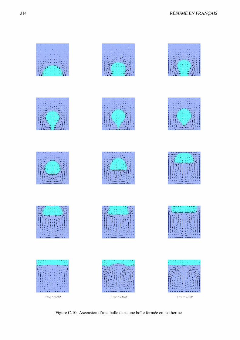
314 RÉSUMÉ EN FRANÇAIS
Figure C.10: Ascension d’une bulle dans une boîte fermée en isotherme

VIII. ÉTUDE NUMÉRIQUE DU MODÈLE 315
linéarisée de l’avancée en temps des termes de couplages non-linéaires implicites entre les équations de tem-pérature et d’Allen-Cahn. Le système fermé et chauffé voit ses niveaux de température et pression augmentertout comme dans la situation physique d’un auto-cuiseur. Nous avons alors montré que pression et températuresuivent la courbe de saturation. Ce cas test permet d’illustrer comment notre modèle, bien que considérant lesphases liquide et vapeur comme incompressibles, donne une signification physique claire au niveau de pression.
Dans un second temps nous étudions un phénomène de condensation dans un système semi-ouvert (vapeurà saturation) en contact avec une paroi refroidie par un flux de chaleur constant. Les figures C.11 montrent lesprofils des variables principales à différents instants. Le champ de température illustre le saut de flux de chaleurqui existe à la traversée de l’interface dû au changement de phase tandis que la température est continue, résultatscohérents avec notre étude analytique à l’ordre dominant du chapitre VII. Le profil de champ de phase est proched’un profil à l’équilibre et la vitesse de déplacement de l’isovaleur ϕ = 0.5 est tout à fait cohérente avec la valeurdu flux de chaleur imposé. Les profils de vitesse et pression sont cohérents avec les prédictions théoriques.
x
T
0.40.20-0.2-0.4
0.40
-0.4-0.8-1.2-1.6
-2
t = 4.5t = 3.0t = 1.5t = 0.0
x
ϕ
0.40.20-0.2-0.4
10.80.60.40.2
0
x
G
0.40.20-0.2-0.4
0.01
0.008
0.006
0.004
0.002
0
x
ρV
0.40.20-0.2-0.4
0.050.040.030.020.01
0-0.01
Figure C.11: Changement de phase en milieu ouvert
L’algorithme développé dans cette étude permet donc de prendre en compte la dynamique de changement dephase liquide-vapeur pour un système mono-dimensionnel.
Simulations bidimensionnelles Nous avons donc naturellement tenté d’appliquer cet algorithme à la résolu-tion d’un problème bi-dimensionnel, mais nous nous sommes heurtés à une difficulté numérique majeure. Dansla suite nous présentons les résultats obtenus ainsi que l’analyse que nous en avons fait. Cette dernière nousa permis d’identifier l’origine de la difficulté et d’envisager des perspectives de travail afin de surmonter ceproblème.
Afin d’illustrer la difficulté numérique nous considérons un problème similaire au problème mono-dimensionnelde condensation résolu précédemment. Nous introduisons alors une discrétisation bi-dimensionnelle du domaine,le problème restant physiquement purement mono-dimensionnel. Au cours de la simulation et dès les toutes pre-mières itérations un courant d’origine parasite composé de cellules centrées sur la zone interfaciale s’établit.L’intensité de ces courants croît exponentiellement au fur et à mesure des itérations jusqu’à devenir dominant etfinalement déstabiliser la résolution. L’origine de ces courants est purement numérique. Notre analyse présentéeen section 8.3.3 a permis d’identifier le terme capillaire comme en étant responsable. Mais ce terme existaitdéjà pour les simulations isothermes présentées en section VIII.2. L’origine de l’instabilité provient en fait plusprécisément du couplage entre ce terme capillaire et la détermination de la dynamique de changement de phaseanisotherme. Nous avons pu forcer artificiellement ce couplage à être satisfait avec une très grande précision ce

316 RÉSUMÉ EN FRANÇAIS
qui a effectivement permis de détruire cette instabilité. Pour autant la méthode utilisée ne peut se généraliser àdes écoulements physiquement bi-dimensionnels.
Le couplage mis en cause et la nature rotationnelle de l’écoulement parasite mettent directement en causeun des ingrédients majeurs de notre algorithme à savoir l’utilisation d’une méthode de projection. Ainsi nousproposons comme perspective d’étude de développer un algorithme basé sur une formulation de type vorticité.
VIII.4 Conclusion
Nous avons montré à l’aide de résolutions numériques que le modèle de champ de phase développé peut aisémentse résoudre à l’aide d’algorithmes simples. Ces algorithmes utilisent une écriture linéarisée de certains termesafin de diminuer les temps de calcul. Nous nous sommes assurés que la physique du changement de phaseainsi que de l’écoulement diphasique ne s’en trouve pas affectée. En particulier nous avons observé une bonnecohérence entre les profils numériques des variables principales du modèle et leurs analogues analytiques quiont été démontré au chapitre précédent. Malheureusement nous n’avons pas pu mettre au point d’algorithmepermettant la résolution d’un écoulement anisotherme bi-dimensionnel. Nous avons néanmoins analysé la causede cette limitation ; elle provient d’une instabilité numérique provoquée par le couplage, via la méthode deprojection, entre la dynamique de changement de phase et le terme de force capillaire. Ainsi nous avons proposécomme perspective l’utilisation d’une approche basée sur une formulation de type vorticité.

IX. CONCLUSION ET PERSPECTIVES 317
IX Conclusion et perspectives
L’étude des phénomènes prépondérants au sein des écoulements bouillants et plus particulièrement près des con-ditions de crise d’ébullition reste un problème scientifique d’actualité. Ainsi le mécanisme de la crise d’ébullitiondemeure aujourd’hui encore largement mal compris et ce malgré plus de soixante-dix années de recherche. Afind’analyser le niveau de compréhension du phénomène, nous avons proposé au chapitre 1 une analyse de la com-préhension actuelle de la crise d’ébullition en considérant les différentes théories existant. Cette étude révèle unmanque de connaissance expérimentale, et par conséquence de modèles, des mécanismes de base de l’ébullitionnucléée à fort flux de chaleur. Des avancées dans ce domaine sont des pré-requis à toute tentative de modéliser lacrise d’ébullition de manière réaliste. Néanmoins, parmi l’ensemble des points restant à éclaircir, nous avons puidentifier un mécanisme potentiellement relié à la crise d’ébullition : la croissance “irrégulière” d’une bulle. Eneffet, à fort flux de chaleur pariétal, une bulle attachée en paroi peut s’étaler le long de cette dernière plutôt quede s’en détacheret être ainsi à l’origine de l’assèchement d’une paroi chaude, ce dernier déclenchant la transitionde régime d’ébullition. La croissance, l’étalement et le détachement d’une bulle en paroi sont gouvernés par lacourbure locale de la forme de la bulle ainsi que par les transferts de masse, quantité de mouvement et d’énergielocalisés à l’interface. Par conséquent, la simulation numérique est l’outil le plus pertinent pour réaliser l’étudede cette dynamique de croissance de bulle. Notons que les compressibilités des phases vapeur et liquide ne sontpas considérés comme des mécanismes fondamentaux en ce qui concerne la dynamique d’étalement. Ainsi ilest envisageable de supposer ces phases comme incompressibles. Cette hypothèse induit une simplification dutraitement numérique des équations du mouvement, simplification dont nous souhaitons bénéficier.
Au chapitre 2 nous étudions les méthodes numériques existantes à même d’étudier les écoulements bouil-lants. Nous portons alors notre attention vers les méthodes dites d’interface diffuse. Ces méthodes sont baséessur une modélisation de l’interface comme une zone de transition volumique au travers de laquelle l’ensembledes variables physiques sont continues. Ainsi le système d’équations du mouvement, valable en tout point del’espace, décrit de manière thermodynamiquement cohérente la dynamique des interfaces. Cette zone de transi-tion devant être résolue par quelques éléments du maillage il est nécessaire que l’épaisseur de l’interface soit unparamètre libre dans la modélisation, tout paramètre physique de la description du système liquide vapeur étantdonné. Il a été montré que le modèle de van der Waals, qui est le modèle à interface diffuse classiquement dédiéà la description de la transition de phase liquide-vapeur, n’offre pas cette souplesse. Les modèles à interfacediffuse de type de champ de phase sont largement utilisés pour la simulation numérique de la transition de phasesolide-liquide. Le principe de cette modélisation repose sur l’introduction d’une variable de description ther-modynamique abstraite du système, nommément le champ de phase. Grâce à cette formulation, il est possiblede régulariser la zone interfaciale indépendamment (et donc artificiellement) de la description de la physique dela transition de phase. Nous avons montré que les modèles de champ de phase existants ne sont pas adaptés àl’étude de la transition de phase liquide-vapeur à l’échelle de la croissance de bulle. Nous proposons par la suiteune formulation de champ de phase plus adéquate.
Au chapitre 3, nous avons développé la partie thermodynamique de notre modèle de champ de phase.Nous avons tout d’abord montré comment, grâce à l’hypothèse de quasi-compressibilité introduite initialementpar Lowengrub and Truskinovsky [89], on modélise la transition entre deux phases de masse volumique dif-férente bien que toutes deux incompressibles. Nous avons alors étudié l’introduction de la variable champ dephase dans une description thermodynamique. Nous avons précisé son rôle : la variable de champ de phasen’a d’autre signification que de varier à la traversée de l’interface et nous supposons alors (i) qu’elle prend unevaleur caractéristique et arbitraire au sein des phases et (ii) qu’elle varie continûment entre ces deux valeurs à latraversée de l’interface. Nous avons alors exprimé analytiquement ces différentes propriétés en étudiant les con-ditions d’équilibre d’un fluide de type champ de phase. Ces dernières comprennent une relation supplémentaire(par rapport aux relations d’équilibre classiques) qui assure la nullité de la dérivée variationnelle de l’enthalpielibre massique par rapport à la variable champ de phase ϕ. Nous avons proposé une fermeture thermodynamiquepermettant de satisfaire les contraintes que l’on impose au modèle. L’écriture de l’enthalpie libre se base surl’interpolation des enthalpies libres des phases liquide et vapeur par une fonction non linéaire de la variable ϕ(cf. (III.18)). Cette fonction d’interpolation est à la base de notre modèle de champ de phase. La formulationretenue comprend en plus de cette interpolation des enthalpies libres phasiques une partie dédiée à la descriptionde la structure de l’interface à l’équilibre plan ; cette partie s’exprime comme le produit par le volume spéci-fique de la somme d’une fonction double-puits en la variable ϕ et d’une dépendance en (∇ϕ)2. Cette expressionpour l’enthalpie libre permet de satisfaire la propriété suivante : l’épaisseur de l’interface à l’équilibre plan est

318 RÉSUMÉ EN FRANÇAIS
indépendante des paramètres physiques (i.e. en particulier les conditions d’équilibre, en l’occurrence la courbede saturation, la masse volumique des phases ainsi que leur capacité calorifique ou bien le coefficient de tensionde surface) ce qui était un des buts recherchés. Nous avons étudié au chapitre 6 la stabilité des états d’équilibrehomogènes et nous avons montré qu’il est nécessaire que la fonction d’interpolation satisfasse à 6 conditionsanalytiques (polynôme de degré 5) pour contrôler les propriétés physiques des phases liquide et vapeur qui sontassociées à des valeurs fixes de ϕ. Ces valeurs son en outre les seules qui correspondent à des états monophasiquesinconditionnellement stables à toute perturbation (stabilité linéaire). Cette propriété ne peut pas être satisfaitepar des polynômes de degré inférieur à 5. En outre nous avons montré qu’il est possible de reproduire une valeurphysique de la limite de métastabilité en choisissant de manière adéquate la fonction d’interpolation de degré5. Cette étude de la modélisation thermodynamique de type champ de phase a permis d’associer un sens clairà chaque élément du potentiel thermodynamique, et finalement de pouvoir aisément maîtriser les propriétés enrésultant.
Nous avons alors étudié l’équilibre d’inclusions sphériques au chapitre 4. L’expression particulière de notremodèle permet à l’équation d’équilibre sous hypothèse de symétrie sphérique d’être suffisamment simple pouren déduire des solutions analytiques approchées. Nous avons montré que le modèle discontinu équivalent à notreformulation diffuse est cohérent avec la relation de Laplace tant que le rayon de l’inclusion est 4 fois supérieur àl’épaisseur de l’interface à l’équilibre plan. Ce résultat est satisfaisant pour les études envisagées et ceci montreque le modèle propose effectivement une régularisation thermodynamiquement cohérente de la formulation dis-continue. Lorsque le rayon de l’inclusion devient inférieur à l’épaisseur caractéristique de l’interface, la tensionde surface associée à l’interface ainsi que le saut de pression à sa traversée tendent vers zéro. Cette décroissancedu saut de pression permet au modèle de prendre en compte les apparitions/disparitions d’inclusions, ce qui n’estpas possible à l’aide de la formulation discontinue classique. Notons que nous avons mis en évidence que ladescription des inclusions de faible rayon est sensible au choix fait pour la fonction d’interpolation.
Le système d’équations de la dynamique du fluide correspondant à notre modèle thermodynamique a été dé-montré au chapitre 5. Cette démonstration a été réalisée en deux étapes. Dans un premier temps nous avons étudiéformellement un modèle champ de phase pour une thermodynamique compressible et isotherme. A l’aide duprincipe fondamental de d’Alembert-Lagrange nous avons déduit la forme conservative du système d’équationsdu mouvement. Nous avons ainsi pu identifier la partie capillaire du tenseur des contraintes et déduire une expres-sion pour le travail des efforts conservatifs. Dans un deuxième temps, nous avons utilisé les résultats précédentslors de l’application des principes fondamentaux de la thermodynamique. Ceci nous a permis de déduire le sys-tème d’équations du mouvement pour notre modèle quasi-compressible et anisotherme. Outre les mécanismesde dissipation de conduction de type Fourier et de viscosité de type Newton, le modèle prend en compte unmécanisme de relaxation de type Ginzburg-Landau vers la condition d’équilibre additionnelle de notre modèlechamp de phase. Ce mécanisme permet d’introduire une cinétique propre à la variable champ de phase, cinétiquequi a été étudiée au chapitre 7. Par conséquent, le système d’équations se compose des équations de bilan demasse, quantité de mouvement, d’entropie et d’une équation non-classique de type Allen-Cahn (cf. le systèmed’équations (V.34)). Nous avons alors démontré une écriture des équations du mouvement contenant un nombreréduit de non-linéarités et reproduisant l’ensemble des phénomènes majeurs de la dynamique de croissance d’unebulle.
Le chapitre 7 a été consacré à l’étude des solutions hors équilibre. Dans un premier temps nous avonsproprement introduit le formalisme de la relation cinétique pour un modèle discontinu équivalent à notre formu-lation. Nous avons montré en particulier que les relations hors équilibre de type Gibbs-Thomson et Clapeyrongénéralisées peuvent être aisément reliées au modèle de type "croissance normale" pour la création d’entropie in-terfaciale. Nous avons alors étudié la situation hors-équilibre d’une transition de phase de type onde progressivemono-dimensionnelle à l’aide de développements asymptotiques raccordés, les solutions étant apprchées par desdéveloppements limités en le petit paramètre donné par le rapport entre l’épaisseur caractéristique de l’interfaceet la longueur caractéristique de la région extérieure. Les profils des variables principales au sein de la régionintérieure aux premier et second ordre en ce paramètre ont été montrés ainsi que la relation cinétique correspon-dante permettant une analyse claire de ces résultats : elle satisfait la théorie de "croissance normale" valable pourdes faibles déséquilibres, la relaxation de Ginzburg-Landau constituant le mécanisme dissipatif dominant. Auxordres supérieurs le saut de température n’est plus nul ce qui est associé à une dissipation de type conductiveau sein de la zone interfaciale. Nous avons en outre établi qu’un tel résultat est lié au choix particulier fait clas-siquement pour l’échelle de la mobilité qui est le coefficient dissipatif de la relaxation de Ginzburg-Landau, un

IX. CONCLUSION ET PERSPECTIVES 319
choix différent modifie la relation cinétique qui n’est plus cohérente avec la théorie de "croissance normale" qu’àla limite des faibles transferts de masse et s’en écarte pour des situations plus franchement hors équilibre, ce quiest physiquement satisfaisant.
Le chapitre 8 fut dédié à la résolution numérique du système d’équations du mouvement. Le but est dedévelopper un algorithme de résolution permettant de prendre en compte les couplages essentiels de notre mod-èle entre thermique, mécanique et dynamique de champ de phase. Nous avons présenté des algorithmes à mêmede résoudre ces couplages dans deux cas simplifiés à savoir les cas (i) à masse volumique uniforme (sans écoule-ment) et (ii) isotherme. Ces algorithmes sont basés sur une linéarisation de l’avancée en temps de certainstermes de couplage ce qui permet d’obtenir des résultats précis en un temps de calcul raisonnable. Les résultatsobtenus sont cohérents avec les résultats analytiques obtenus précédemment. En outre nous avons validé quali-tativement des simulations bidimensionnelles. Ces résultats prouvent la capacité du modèle à être utilisé commebase d’une méthode numérique. Un algorithme de résolution du système complet a été déduit de ces étudespréliminaires. Cet algorithme permet effectivement de résoudre une dynamique de changement de phase commel’attestent les résultats obtenus pour un système mono-dimensionnel. Néanmoins des instabilités numériquess’établissent dès lors que le système étudié est bidimensionnel. Ces instabilités ne nous ont pas permis d’étudierdes dynamiques de bulles non-isothermes. Nous avons analysé l’origine de ces instabilités et montré leur originepurement numérique mais n’avons pas pu les passer outre.
L’ensemble de cette étude doit être vu comme une tentative d’utiliser les modèles de champ de phase pourl’étude des phénomènes d’ébullition. Cette étude propose dans un premier temps une justification claire dela nécessité de l’utilisation de la simulation numérique afin d’améliorer notre connaissance des écoulementsbouillants et plus particulièrement du phénomène de crise d’ébullition. En outre elle a permis d’identifier claire-ment les phénomènes primordiaux qu’une telle méthode se doit de reproduire. Dans un deuxième temps nousavons développé un modèle de type interface diffuse utilisant un ensemble de paramètres et de fonctions au rôleclairement identifié et permettant notamment (i) de reproduire les caractéristiques principales des écoulementsbouillants tout en (ii) contrôlant les caractéristiques de la zone de transition interfaciale. Dans cette étude nousavons porté une attention particulière aux conséquences de l’introduction d’une variable de type champ de phasedans le modèle thermodynamique sur la description de la transition de phase liquide-vapeur. Nous avons aussiproduit une analyse détaillée du modèle discontinu équivalent, ce qui a permis de montrer que notre modèlepropose une régularisation thermodynamiquement cohérente du modèle discontinu classique avec des phasesincompressibles. Finalement notre étude numérique, bien qu’infructueuse sur la fin, a permis de déterminer lesprincipales étapes de résolution du système complet, et d’envisager ainsi l’étude numérique des écoulementsbouillants.
Notre étude a révélé que la connaissance des phénomènes d’ébullition prenant place dans une région trèsproche de la paroi et en des conditions de fort flux pariétal est primordiale en vue d’accroître notre niveaude compréhension des mécanismes fondamentaux de la crise d’ébullition. L’observation expérimentale de cesphénomènes proche paroi (où nucléation et croissance de bulle se produisent) dans des conditions proches duflux critique devraient apporter une information sur l’origine exacte des crises d’assèchement telles qu’observéesdans [130] et qui sont des événements précurseurs de la crise d’ébullition elle-même. Cette remarque sug-gère l’utilisation de techniques expérimentales permettant l’observation simultanée de la nature des contactsfluide/paroi (en utilisant une caméra infrarouge par exemple), et de la dynamique de croissance de bulle (enutilisant une visualisation latérale).
Notre étude des méthodes numériques a distingué deux catégories de méthodes de résolution d’un problèmeà frontière libre permettant un suivi implicite de l’interface : les méthodes dites "level-set", basées sur unemodélisation de type discontinue, et les modèles d’interface diffuse, famille à laquelle notre modèle appartient.Or on peut considérer que la variable de champ de phase est similaire à la variable indicatrice de phase, oufonction couleur, utilisée dans les méthodes "level set". Ceci permet d’introduire un premier lien formel entreles deux familles de méthodes. Il est intéressant alors de souligner que les équations de relaxation de la fonctiondistance, classiquement utilisées dans les méthodes level set, ont de grandes similarités avec notre équationd’Allen-Cahn. Dans une étude des méthodes numériques pour la résolution de modèles à interface diffuse de typechamp de phase, Glasner [57] propose ainsi de travailler sur une fonction de type distance plutôt que directementsur la variable champ de phase. Ce changement de variable rapproche encore plus les deux formalismes. De

320 RÉSUMÉ EN FRANÇAIS
notre point de vue il serait bénéfique pour les deux familles de méthode d’étudier plus en profondeur le lienformel qui les relie afin de conjuguer les avantages réciproques.
Le modèle champ de phase développé dans cette étude a été délibérément dédié à la description de phasesincompressibles. Pour autant il est nombre de situations physiques pour lequel cette hypothèse ne serait pas justi-fiée. A ce titre il serait de tout premier intérêt d’étudier une formulation prenant en compte la compressibilité desphases. La formulation quasi-compressible que nous proposons serait alors une réduction naturelle de cette for-mulation. Nous pensons que la base de cette formulation compressible devrait s’écrire comme une interpolationdes équations d’état des phases. Notons que, dès lors que la compressibilité est non nulle, l’enthalpie libre n’estplus linéaire en pression. Les conséquences de cette non linéarité sur le contrôle des propriétés de régularisation(profil des variables à la traversée de la zone interfaciale) devra plus particulièrement être étudiée. Il est intéres-sant de souligner que notre modèle, puisque considérant les phases comme incompressibles peut s’appliquer àl’étude de la transition de phase solide-liquide avec convection. De manière plus générale, il serait intéressantd’étudier dans quelle mesure la structure de notre modèle champ de phase peut être utilisée pour différents sys-tèmes multi-phasiques ou multi-composants d’équations d’état arbitraires. En particulier, le cas des fluides nonmiscibles semble suffisamment similaire à notre cas si on établit un parallèle entre notre équation d’entropie etune équation de diffusion de masse.
La relation cinétique de notre modèle a été déduite en utilisant la méthode des développements asymp-totiques. Cette méthode permet d’obtenir des solutions analytiques approchées pour une transition de phasemono-dimensionnelle dans la limite où le petit paramètre considéré tend vers zéro. Il serait intéressant d’étudiercette relation cinétique plus systématiquement en utilisant une résolution numérique par exemple.
Il est important de noter que la fonction d’interpolation utilisée dans la formulation thermodynamique denote modèle joue un rôle important en ce qui concerne l’équilibre des inclusions sphériques. Lorsqu’elle n’estpas choisie comme un polynôme de degré 5, le rayon discontinu équivalent diverge quand la masse équivalentede l’inclusion tend vers zéro (cf. section IV.4). Par conséquent cette dernière caractéristique n’est nullementassociée aux méthodes d’interface diffuse en général bien qu’elle se retrouve dans une majorité de modèles. Unemeilleure compréhension de l’origine de ce phénomène passe ainsi par une étude de l’influence qu’a la fonctiond’interpolation sur l’équation d’équilibre sous hypothèse de symétrie sphérique. Concernant toujours l’influencede la fonction d’interpolation sur les propriétés du modèle, nous avons introduit une manière d’introduire dansle modèle une limite de métastabilité phénoménologique (cf. section VI.6). Nous avons montré que pour obtenircette propriété, il est suffisant d’utiliser un polynôme de degré 5 dont les coefficients dépendent de l’épaisseurde l’interface. Ainsi le modèle champ de phase possède une propriété supplémentaire intéressante par rapportau modèle discontinu équivalent. Il serait alors nécessaire d’étudier les conséquences de ce choix sur les autrespropriétés du modèle pour s’assurer qu’elles sont conservées.
La méthode de projection est couramment utilisée dans les méthodes numériques dédiées à l’étude desécoulements diphasiques, même en présence de changement de phase, dès lors que les phases sont incompress-ibles. Néanmoins, notre étude numérique a montré que l’utilisation de cette méthode pour l’étude de transition dephase bidimensionnelles en présence de phénomènes capillaires, est à l’origine de difficultés numériques impor-tantes. Ainsi pour ce type d’écoulement, il serait intéressant de développer un algorithme utilisant une méthodede résolution alternative pour le couplage bilan de quantité de mouvement, bilan de masse. On peut notammentpenser à l’utilisation de méthodes basées sur une formulation en vorticité. Une autre perspective serait d’utiliserune simplification des termes non-linéaires des équations. Sacrifiant ainsi à la cohérence thermodynamique deséquations, il est possible d’envisager un gain sur le plan de la résolution numérique. Cette approche pragmatiquea d’ores et déjà été mise en pratique pour d’autre modèles de champ de phase, e.g. Karma and Rappel [73].

Bibliography
[1] R.F. Almgren. Second-order phase-field asymptotics for unequal conductivities. SIAM J. Appl. Math., 59:2086–2107, 1999.
[2] D. M. Anderson, P. Cermelli, E. Fried, M.E. Gurtin, and G.B. McFadden. General dynamical sharp-interface conditions for phase transformations in viscous heat-conducting fluids. submitted to J. FluidMech.
[3] D.M. Anderson and S.H. Davis. Local fluid and heat flow near contact lines. J. Fluid Mech., 268:231–265,1994.
[4] D.M. Anderson, G.B. McFadden, and A.A. Wheeler. Diffuse-interface models in fluid mechanics. Ann.Rev. Fluid Mech., 30:139–165, 1998.
[5] D.M. Anderson, G.B. Mc Fadden, and A.A. Wheeler. A phase-field model of solidification with convec-tion. Physica D, 135:175–194, 2000.
[6] D.M. Anderson, G.B. Mc Fadden, and A.A. Wheeler. A phase-field model with convection: sharp-interface asymptotics. Physica D, 151:305–331, 2001.
[7] H. Auracher and W. Marquardt. Heat transfer characterisitcs and mechanisms along entire boiling curvesunder steady-state and transient conditions. Int. J. Heat Fluid Flow, 25:223–242, 2004.
[8] V.E. Badalassi, H.D. Ceniceros, and S. Banerjee. Computation of multiphase system with phase fieldmodels. J. Comp. Physics, 190:371–397, 2003.
[9] I.C. Bang, S.H. Chang, and W.-P. Baek. Visualization of the subcooled flow boiling of R-134a in a verticalrectangular channel with an electrically heated wall. Int. J. Heat and Mass Transfer, 47:4349–4363, 2004.
[10] P. Bates and F. Chen. Periodic traveling waves for a non-local integro-differential model. Electronic J. ofDifferential Equations, 26:1–19, 1999.
[11] C. Beckermann, H.-J. Diepers, I.Steinbach, A. Karma, and X. Tong. Modeling melt convection in phase-field simulations of solidification. J. Comp. Physics, 154:468–496, 1999.
[12] R.J. Benjamin and A.R. Balakrishnan. Nucleation site density in pool boiling of saturated pure liquids:effect of surface microroughness and surface and liquid physical properties. Exp. Thermal and FluidScience, 15:32–42, 1997.
[13] S. Benzoni-Gavage, R. Danchin, S. Descombes, and D. Jamet. Structure of Korteweg models and stabilityof diffuse interfaces. Interfaces Free Boundaries, 7:371–414, 2005.
[14] G. Berthoud. Etude du flux critique en chauffage transitoire. Technical Note DEN/DTN/SE2T/2006-01,CEA, 2006.
[15] A.L. Biance, C. Clanet, and D. Quéré. Leidenfrost drops. Phys. Fluids, 15(6):1632–7, 2003.
[16] J. Blum, T. Lüttich, and W. Marquardt. Temperature wave propagation as a route from nucleate to filmboiling. In G.P. Celata, P. Di Marco, and R.K. Shah, editors, 2nd Internatinal Symposium on two-phaseflow modelling and experimentation, volume 1, pages 137–144. Edizioni ETS, Pisa, 1999.
321

322 BIBLIOGRAPHY
[17] W.J. Boettinger, J.A. Warren, C. Beckermann, and A. Karma. Phase-field simulation of solidification.Annual Review of Materials Research, 32:163–194, 2002.
[18] J. U. Brackbill, D. B. Kothe, and C. Zemach. A continuum method for modeling surface tension. J. Com-put. Phys., 100(2):335–354, 1992. ISSN 0021-9991. doi: http://dx.doi.org/10.1016/0021-9991(92)90240-Y.
[19] P. Bricard. Modélisation du mécanisme de crise d’ébullition par assèchement d’un site de nucléation.Technical Report 96NB00119, EDF, 1996.
[20] P. Bricard, P. Péturaud, and J.M. Delhaye. Understanding and modelling DNB in forced convective boiling:Modelling of a mechanism based on nucleation site dryout. Multiphase Science and Technology, 9:329–379, 1997.
[21] M. Buchholz, T. Lüttich, H. Auracher, and W. Marquardt. Experimental investigation of local processesin pool boiling along the entire boiling curve. Int. J. Heat Fluid Flow, 25:243–261, 2004.
[22] YU.A. Buyevich and B.W. Webbon. Dynamics of vapour bubbles in nucleate boiling. Int. J. Heat andMass Transfer, 39(12):2409–2426, 1996.
[23] G. Caginalp. Dynamical renormalization group calculation of a two-phase sharp interface model. PhysicalReview E, 6:R6267–R6270, 1999.
[24] G. Caginalp and E.A. Socolovsky. Computation of sharp phase boundaries by spreading: the planar andspherically symmetric cases. J. Comput. Phys., 95:85–100, 1991.
[25] J.W. Cahn. On spinodal decomposition. Acta Mettalurgica, 9:795–801, 1961.
[26] J.W. Cahn and J.E. Hilliard. Free energy of a nonuniform system. I. interfacial free energy. J. ChemicalPhysics, 28(2):258–267, 1958.
[27] I. Calmet and J. Magnaudet. Large-eddy simulation of high-schmidt number mass transfer in a turbulentchannel. Phys. Fluids, 9(2):438–455, 1997.
[28] Van P. Carey. Liquid-vapor phase-change phenomena. Taylor and Francis, 1992.
[29] F. Caro. Modélisation et simulation numérique des transitions de phase liquide-vapeur. Thèse de doctorat,Ecole Polytechnique, 2004.
[30] G.P. Celata. Critical heat flux in subcooled flow boiling. Heat and Technology, 16(1):11–27, 1998.
[31] G.P. Celata, M. Cumo, A. Mariani, and G. Zummo. Visual investigation of boiling crisis in subcooled flowboiling. The Arabian Journal for Science and Engineering, 27(2C):67–89, 2002.
[32] Y-P Chang. Some possible critical conditions in nucleate boiling. J. Heat Transfer, transactions of theASME, May:89–100, 1963.
[33] C. Charach and P.C. Fife. On thermodynamically consistent schemes for phase field equations. OpenSystems and Information Dynamics, 5:99–123, 1998.
[34] C. Charach, C.K. Chen, and P.C. Fife. Developments in phase-field modeling of thermoelastic and two-component materials. J. Stat. Physics, 95:1141–1164, 1999.
[35] R. Chella and J. Viñals. Mixing of a two-phase fluid by cavity flow. Physical Review E, 53(4):3832–3840,1996.
[36] H-Y Chen, D. Jasnow, and J. Viñals. Interface and contact-line motion in a two phase fluid under shearflow. Physical Review letters, 85(8):1686–1689, 2000.
[37] H.J. Chung and H.C. No. Simultaneous visualization of dry spots and bubbles for pool boiling of r-113 ona horizontal heater. Int. J. Heat and Mass Transfer, 46:2239–2251, 2003.

BIBLIOGRAPHY 323
[38] M. Conti. Density change effects on crystal growth from the melt. Physical Review E, 64:051601, 2001.
[39] M. Conti. Pressure effects for crystal growth in a closed system. Physical Review E, 70:031602, 2004.
[40] M.G. Cooper and A.J.P. Lloyd. The microlayer in nucleate boiling. Int. J. Heat Mass Transfer, 12:895–913, 1969.
[41] A. Danescu. Generalized stefan models accounting for a discontinuous temperature field. ContinuumMech. Thermodyn., 16:427–439, 2004.
[42] J.M. Delhaye. Jump conditions and entropy sources in two-phase systems. Local instant formulation. Int.J. Multiphase Flow, 1:395–409, 1974.
[43] F. Dell’Isola, H. Gouin, and G. Rotoli. Nucleation of spherical shell-like interfaces by second gradienttheory: numerical simulations. Eur. J. Mech. B/Fluids, 15(4):545–568, 1996.
[44] F. Demiray and J. Kim. Heat-transfer from a single nucleation site during saturated pool boiling of fc-72using an array of 100 micron heaters. In Proceedings of the AIAA/ASME Thermophysics and heat transferconference, St. Louise, M.O., June 2002.
[45] V.K. Dhir. Boiling heat transfer. Ann. Rev. Fluid Mech., 30:365–401, 1998.
[46] D.A. Edwards, H. Brenner, and D.T. Wasan. Interfacial transport processes and rheology. Butterworth-Heinemann, 1991.
[47] H. Emmerich. The diffuse interface approach in material science. Thermodynamic concepts and applil-cations of phase-field models. Springer,Berlin, 2003.
[48] D. Enright, R. Fedkiw, J. Ferziger, and I. Mitchell. A hybrid particle level set method for improvedinterface capturing. J. Comp. Phys., 183:83–116, 2002.
[49] G.B. Mc Fadden, A.A. Wheeler, and D.M. Anderson. Thin interface asymptotics for an energy/entropyapproach to phase-field models with unequal conductivities. Physica D, 144:154–168, 2000.
[50] M.P. Fiori and A.F. Bergles. Model of critical heat flux in subcooled flow boiling. In Proceedings of the4th Heat Transfer Conference, Versailles, volume 9, 1970.
[51] R. Folch, J. Casademunt, A. Hernández-Machado, and L. Ramírez-Piscina. Phase-field model for Hele-Shaw flows with arbitrary viscosity contrast. I. Theoretical approach. Physical Review E, 60(2):1724–1733, 1999.
[52] R. Folch, J. Casademunt, A. Hernández-Machado, and L. Ramírez-Piscina. Phase-field model for Hele-Shaw flows with arbitrary viscosity contrast. II. Numerical study. Physical Review E, 60(2):1734–1740,1999.
[53] C. Fouillet. Généralisation à des mélanges binaires de la méthode du second gradient et application à lasimulation numérique directe de l’ébullition nucléée. Thèse de doctorat, Université Paris VI, 2003.
[54] C. Fouillet and D. Jamet. Generalization of the second gradient method to binary mixtures and investiga-tion of the direct numerical simulation of nucleate boiling flows. In Proceedings of the 11th internationaltopical meeting on nuclear thermal-hydraulics (NURETH 11), number 364, October 2005.
[55] W. Fritz. Berechnung des maxiamlvolume von dampfblasen. Phys. Z., 36:379–388, 1935.
[56] Gaertner. Photographic study of nucleate pool boiling on a horizontal surface. J. Heat Transfer, transac-tions of the ASME, 65(02):17–29, 1965.
[57] K. Glasner. Nonlinear preconditioning for diffuse interfaces. J. Comp. Physics, 174:695–711, 2001.
[58] S.J. Ha and H.C. No. A dry-spot model of critical heat flux applicable to both pool boiling and subcooledforced convection boiling. Int. J. Heat and Mass Transfer, 43:241–250, 2000.

324 BIBLIOGRAPHY
[59] S.J. Ha and H.C. No. A dry-spot model of critical heat flux in pool boiling and forced convection boiling.Int. J. Heat and Mass Transfer, 41(2):303–311, 1997.
[60] Y. He, M. Shoji, and S. Maruyama. Numerical study of high heat flux pool boiling heat transfer. Int. J.Heat and Mass Transfer, 44:2357–2373, 2001.
[61] T. Hibiki and M. Ishii. Active nucleation site density in boiling systems. Int. J. Heat and Mass Transfer,46:2587–2601, 2003.
[62] D. Jacqmin. Contact-line dynamics of a diffuse fluid interface. J. Fluid Mech., 402:57–88, 2000.
[63] D. Jacqmin. Calculation of two-phase navier-stokes flows using phase-field modeling. J. Comp. Physics,155:96–127, 1999.
[64] Jakob. Heat transfer part 1. John Wiley NY, 1950.
[65] D. Jamet. A solid-liquid diffuse interface model based on an entropy order parameter. in preparation.
[66] D. Jamet. Etude des potentialités de la théorie du second gradient pour la simulation numérique directedes écoulements liquide-vapeur avec changement de phase. Thèse de doctorat, Ecole Centrale Paris, 1998.
[67] D. Jamet, O. Lebaigue, N. Coutris, and J.M. Delhaye. The second gradient method for the direct numericalsimulation of liquid-vapor flows with phase change. J. Comp. Physics, 169:624–651, 2001.
[68] D. Jamet, D. Torres, and J.U. Brackbill. On the theory and computation of surface tension: the eliminationof parasitic currents through energy conservation in the second-gradient method. J. Comp. Physics, 182:262–276, 2002.
[69] D. Juric and G. Tryggvason. Computations of boiling flows. Int. J. Multiphase Flow, 24(3):387–410,1998.
[70] S.G. Kandlikar. A theoretical model to predict pool boiling CHF incorporating effects of contact angleand orientation. J. Heat Transfer, transactions of the ASME, 123:1071–1079, 2001.
[71] S.G. Kandlikar and M.E. Steinke. Contact angles and interface behavior during rapid evaporation of liquidon a heated surface. Int. J. Heat and Mass Transfer, 45:3771–3780, 2002.
[72] A. Karma and W.-J. Rappel. Phase-field method for computationnaly efficient modeling of solidificationwith arbitrary interface kinetics. Physical Review E, 53(4):R3017–R3019, 1996.
[73] A. Karma and W.-J. Rappel. Quantitative phase-field modeling of dendritic growth in two and threedimensions. Physical Review E, 57(4):4323–4349, April 1998.
[74] Y. Katto. Critical heat flux. Int. J. Multiphase Flow, (20 Suppl.):53–90, 1994.
[75] Y. Katto and S. Otokuni. Behavior of vapor masses on a vertical flat surface of comparatively large heightnear critical heat flux conditions in saturated pool boiling. Int. J. Heat and Mass Transfer, 37:255–263,1994.
[76] D.B.R Kenning. Optical studies of boiling heat transfer: insights and limitations. Int. J. Heat Fluid Flow,25:209–222, 2004.
[77] J. Kim, K. Kang, and J. Lowengrub. Conservative multigrid methods for Cahn-Hilliard fluids. J. Comp.Physics, 193:511–543, 2004.
[78] G.J. Kirby, R. Staniforth, and J.H. Kinneir. A visual study of forced convection boiling - part 2. Flowpatterns and burnout for a round test section. Technical Report AEEW-R-506, Winfrith, 1967.
[79] N.I. Kolev. How accurately can we predict nucleate boiling? Exp. Thermal and Fluid Science, 10:370–378, 1995.

BIBLIOGRAPHY 325
[80] D.J. Korteweg. Sur la forme que prennent les équations du mouvement des fluides si l’on tient compte desforces capillaires causées par des variations de densité considérables mais continues et sur la théorie de lacapillarité dans l’hypothèse d’une variation continue de la densité. Arch. Néerl. Sci. Exactes Nat., 6:1–24,1901.
[81] A.P. Krekhov and L. Kramer. Phase separation in the presence of spatially periodic forcing. PhysicalReview E, 70, 2004.
[82] S.S. Kutateladze. A hydrodynamic theory of changes in the boiling process under free convection condi-tions. Izv. Akademia nauk Otledarie Tkh. (AEC-TR-1441), 4:529–536, 1951.
[83] H-G. Lee, J.S. Lowengrub, and J. Goodman. Modeling pinchoff and reconnection in a Hele-Shaw cell. I.The models and their calibration. Phys. Fluids, 14(2):492–513, 2002.
[84] J.G. Leidenfrost. On the fixation of water in diverse fire (first publication in 1756). Int. J. Heat and MassTransfer, 9:1153–1166, 1966.
[85] H. Lemonnier, D. Jamet, and O. Lebaigue. Validation of advanced computational methods for multiphaseflow. Begell House, 2005.
[86] J.H. Lienhard and V.K. Dhir. Hydrodynamic prediction of peak pool-boiling heat fluxes from finite bodies.J. Heat Transfer, transactions of the ASME, may:152–158, 1973.
[87] J.H. Lienhard and V.K. Dhir. Extended hydrodynamic theory of the peak and minimum pool boiling heatfluxes. CR 2270, NASA, 1973.
[88] X.-D. Liu, R. Fedkiw, and M.Kang. A boundary condition capturing method for Poisson’s equation onirregular domains. J. Comp. Phys., 160:151–178, 2000.
[89] J. Lowengrub and L. Truskinovsky. Quasi-incompressible Cahn-Hilliard fluids and topological transitions.Proc. R. Soc. Lond. A, 454:2617–2654, 1998.
[90] C.H.P. Lupis. Chemical thermodynamics of materials. North-Holland, New-York, 1983.
[91] B. Mathieu. Etudes physique, expérimentale et numérique des mécanismes de base intervenant dans lesécoulements diphasiques. Thèse de doctorat, Université de Provence, 2003.
[92] B. Mathieu, O. Lebaigue, and L. Tadrist. Influence of a dynamic contatc line model on the characteristicsof nucleate wall boiling computed with a dns approach. In Proceedings of the 5th international conferenceon Multiphse flow, ICMF’04, Yokohama Japan, number paper n439, 2004.
[93] B.B. Mikic, W.M. Rohsenow, and P. Griffith. On bubble growth rates. Int. J. Heat and Mass Transfer, 13:657–666, 1970.
[94] N. Moelans, B. Blanpain, and P. Wollants. A phase-field model for the simulation of grain growth inmaterials containing finely dispersed incoherent second-phase particles. Acta Materialia, 53:1171–1781,2005.
[95] R. Moissis and P.J. Berenson. On the hydrodynamic transitions in nucleate boiling. J. Heat Transfer,transactions of the ASME, 85:221–229, 1963.
[96] S.A. Mokrushin. The boiling crisis in nucleate pool boiling of liquids. Heat transfer Soviet Research, 20(1):65–68, 1988.
[97] B.T. Nadiga and S. Zaleski. Investigations of a two-phase fluid model. Euro. J. Mech. B/Fluid, 15(2):885–896, 1996.
[98] B. Nestler, A. Wheeler, L. Ratke, and C. Stöcker. Phase-field model for solidification of a monotecticalloy with convection. Physica D, 141:133–154, 2000.

326 BIBLIOGRAPHY
[99] S-H Ngan and L. Truskinovsky. Thermal trapping and kinetics of martensitic phase boundaries. Mechanicsand Physics of Solids, 47:141–172, 1999.
[100] V. S. Nikolayev, D. A. Beysens, G.-L. Lagier, and J. Hegseth. Growth of a dry spot under a vapor bubbleat high heat flux and high pressure. Int. J. Heat and Mass Transfer, 44:3499–3511, 2001.
[101] V.S. Nikolayev and D.A. Beysens. Boiling crisis and non-equilibirum drying transition. EurophysicsLetters, 47(3):345–351, 1999.
[102] S. Nishio, T. Gotoh, and N. Nagai. Observation of boiling structures in high heat-flux boiling. Int. J. Heatand Mass Transfer, 41:3191–3201, 1998.
[103] S. Nukiyama. The maximum and minimum values of the heat Q transmitted from metal to boiling waterunder atmospheric pressure (english translation of the original paper published in Journal Japan Soc. Mech.Engrs vol. 37 ,367-374 (1934)). Int. J. Heat and Mass Transfer, 9:1419–1433, 1966.
[104] A. Onuki. Dynamic van der Waals theory of two-phase fluids in heat flow. Physical Review Letters, 94:054501, 2005.
[105] H. Paillere, C. Viozat, A. Kumbaro, and I. Toumi. Comparison of low Mach number models for naturalconvection problems. Heat and mass transfer, 36:567–573, 2000.
[106] H.J. Palmer. The hydrodynamic stability of rapidly evaporating liquids at reduced pressure. J. Fluid Mech.,75:487–511, 1976.
[107] P. Papon and J. Leblond. Thermodynamique des états de la matière. Hermann, 1990.
[108] R.L. Pego. Front migration in the nonlinear Cahn-Hilliard equation. Proc. Roy. Soc. Lond. A, 422:261–278, 1989.
[109] O. Penrose and P.C. Fife. Thermodynamically consistent models of phase-field type for the kinetics ofphase transitions. Physica D, 43:44–62, 1990.
[110] O. Penrose and P.C. Fife. On the relation between the standard phase-field model and a “thermodynami-cally consistent” phase-field model. Physica D, 69:107–113, 1993.
[111] Y. Pomeau. Recent progress in the moving contact line problem: a review. C.R. Mécanique, 330:207–222,2002.
[112] T. Qian, X.-P. Wang, and P. Sheng. Molecular scale contact line hydrodynamics of immiscible flows.Physical Review E, 68, 2003.
[113] Y. Rocard. Thermodynamique. Masson Paris, 1967.
[114] A.B. Roshchin and L.M. Truskinovsky. Model of a weakly non-local relaxing compressible medium.PMM U.S.S.R., 53(6):715–20, 1989.
[115] J.S. Rowlinson and B. Widom. Molecular theory of capillarity. Clarendon press, 1982.
[116] T.D. Rule and J. Kim. Heat transfer behavior on small horizonal heaters during pool boiling of FC-72. J.Heat Transfer, transactions of the ASME, 121:386–393, 1999.
[117] P. Sadavisan, C. Unal, and R. Nelson. Perspective : Issues in CHF modeling - The need for new experi-ments. J. Heat Transfer, transactions of the ASME, 117:558–567, 1995.
[118] A. Sakurai. Mechanisms of transitions to film boiling at CHFs in subcooled and pressurized liquids dueto steady and increasing heat inputs. Nuclear Eng. Design, 197:301–356, 2000.
[119] R. Salmon. Hamiltonian fluid mechanics. Ann. Rev. Fluid Mech., 20:225–256, 1988.
[120] K. Sefiane, D. Benielli, and A. Steinchen. A new mechanism for pool boiling crisis, recoil instability andcontact angle influence. Colloids surf., 142:361–373, 1998.

BIBLIOGRAPHY 327
[121] P. Seppecher. Etude d’une modélisation des zones capillaires fluides: interfaces et lignes de contact.Thèse de doctorat, Université Paris VI, 1987.
[122] J. Serrin. Mathematical Principles of Classical Fluid Dynamics, volume VIII/1 of Handbuch der Physik.Springer-Verlag, Berlin,Gottingen, Heidelberg, 1959.
[123] J.A. Sethian. Evolution, implementation and application of level set and fast marching methods for ad-vancing fronts. J. Comp. Physics, 169:503–555, 2001.
[124] Y.D. Shikhmurzaev. Moving contact lines in liquid/liquid/solid systems. J. Fluid Mech., 334:211–249,1997.
[125] Y.D. Shikhmurzaev. On the initial stage of the bubble growth on a plate. In Proc. of the second int. symp.on two-phase flow modelling and experimentation, volume 2, pages 907–914, 1999.
[126] S. Shin and D. Juric. Modeling three-dimensional multiphase flow using a level contour reconstructionmethod for front tracking without connectivity. J. Comp. Phys., 180:427–470, 2002.
[127] M. Slemrod. Admissibility criteria for propagating phase boundaries in a van der waals fluid. Arch. Nat.Mech. Anal., 81(4):301–315, 1983.
[128] G. Son, N. Ramanujapu, and V.K. Dhir. Numerical simulation of bubble merger process on a singlenucleation site during pool nucleate boiling. Int. J. Heat and Mass Transfer, 124:51–62, 2002.
[129] K. Stephan. Heat transfer in condensation and boiling. Springer Verlag, 1992.
[130] T.G. Theofanous, T.N. Dinh, J.P. Tu, and A.T. Dinh. The boiling crisis phenomenon part I: nucleation andnucleate boiling heat transfer. Exp. Thermal and Fluid Science, 26:775–792, 2002.
[131] T.G. Theofanous, T.N. Dinh, J.P. Tu, and A.T. Dinh. The boiling crisis phenomenon part II: dryoutdynamics and burnout. Exp. Thermal and Fluid Science, 26:793–810, 2002.
[132] G.E. Thorncroft, J.F. Klausner, and R. Mei. Bubbles forces and detachment models. Multiphase Scienceand Technology, 13(3 and 4):35–76, 2001.
[133] X. Tong, C. Beckermann, A. Karma, and Q. Li. Phase-field simulations of dendritic crystal growth in aforced flow. Physical Review E, 63, 2001.
[134] L. Truskinovsky. Equilibrium phase interfaces. Sov. Phys. Dokl., 27(7):551–553, 1982.
[135] L. Truskinovsky. Critical nuclei in the van der waals model. Sov. Phys. Dokl, 28(3):248–250, 1983.
[136] L. Truskinovsky. Dynamics of non-equilibrium phase boundaries in the heat-conductive nonlinear elasticmedium. J. Appl. Math. & Mech. (PMM), 51(6):777–784, 1987.
[137] L. Truskinovsky. Nonequilibrium phase boundaries in the earth’s mantle. Dokl. Akad. Nauk. SSSR, 303(6):1337–1342, 1988.
[138] L. Truskinovsky. Kinks versus shocks. In J.E. Dunn, R. Fosdick, and M. Slemrod, editors, Shock inducedtransitions and phase structure in general media, pages 185–229. Springer-Verlag, 1993.
[139] L. Truskinovsky. About the “normal growth” approximation in the dynamical theory of phase transitions.Cont. Mech. Thermodyn., 6:185–208, 1994.
[140] G. Tryggvason, B. Brunner, A. Esmaeeli, D. Juric, N. Al-Rahawi, W. Tauber, J. Han ans S. Has, and Y.-H.Jan. A front-tracking method for the computations of multiphase flow. J. Comp. Phys., 204:708–759,2001.
[141] A. Umantsev. Thermodynamic stability of phases and transition kinetics under adiabatic conditions. J.Chemical Physics, 96(1):605–617, 1992.

328 BIBLIOGRAPHY
[142] J.D. van der Waals. Thermodynamische Theorie der Kapillarität unter Voraussetzung stetiger Dichtean-derung. Z. Phys. Chem., 13:657–725, 1894. Traduction française dans Arch. Néerl. Sci. Exactes Nat.,28:121-209.
[143] M. van Dyke. Perturbation methods in fluid mechanics, chapter V. The method of matched asymptoticexpansions. The parabolic press, Stanford,California, 1975.
[144] N.G. van Kampen. Condensation of a classical gas with long range attraction. Physical Review, 135:A362–A369, 1964.
[145] H.J. van Ouwerkerk. Burnout in pool boiling. the stability of boiling mechanisms. Int. J. Heat and MassTransfer, 15:25–34, 1972.
[146] S.-L. Wang, R.F. Sekerka, A.A. Wheeler, B.T. Murray, S.R. Coriell, R.J. Braun, and G.B. McFadden.Thermodynamically-consistent phase-field models for solidification. Physica D, 69:189–200, 1993.
[147] S.W.J. Welch and J. Wilson. A volume of fluid based method for fluid flows withphase change. J. Comp.Physics, 160:662–682, 2000.
[148] J.W. Westwater and J.G. Santangelo. Photographic study of boiling. Industrial and engineering chemistry,47(8):1605–1610, 1955.
[149] N. Yaddanapudi and J. Kim. Single bubble heat transfer in saurated pool boiling of FC-72. MultiphaseScience and Technology, 12(3 and 4):47–63, 2000.
[150] V.V. Yagov. The mechanism of the pool boiling crisis. Thermal Engineering, 50(3):175–183, 2003.
[151] Z.L. Yang, T.N. Dinh, R.R. Nourgaliev, and B.R. Sehgal. Numerical investigation of bubble growth anddetachment by the lattice-Boltzmann method. Int. J. Heat and Mass Transfer, 44:195–206, 2001.
[152] C.-L. Yu and R.B. Mesler. A study of nucleate boiling near the peak heat flux through measurements oftransient surface temperature. Int. J. Heat and Mass Transfer, 20:827–840, 1977.
[153] P. Yue, J.J. Feng, C. Liu, and J. Shen. A diffuse-interface method for simulating two-phase flows ofcomplex fluids. J. Fluid Mech., 515:293–317, 2004.
[154] L. Zhang and M. Shoji. Nucleation site interaction in pool boiling on the artificial surface. Int. J. Heatand Mass Transfer, 46:513–522, 2003.
[155] Y.-H. Zhao, T. Masuoka, and T. Tsuruta. Unified theoretical prediction of fully developed nucleate boilingand critical heat flux based on a dynamic microlayer model. Int. J. Heat and Mass Transfer, 45:3189–3197,2002.
[156] N. Zuber. On the stability of boiling heat transfer. J. Heat Transfer, transactions of the ASME, 80(2):711–720, 1958.
[157] N. Zuber. Nucleate boiling. the region of isolated bubbles and the similarity with natural convection. Int.J. Heat and Mass Transfer, 6:53–78, 1963.

RésuméDans cette étude nous considérons l’ébullition en paroi sous les angles de la modélisation et de la simulation
numérique. Dans un premier temps nous proposons une revue bibliographique au sujet du régime d’ébullitionnucléée à fort flux de chaleur pariétal et analysons plus particulièrement la compréhension du phénomène decrise d’ébullition de type caléfaction. Nous en déduisons une motivation pour l’étude de la dynamique de crois-sance de bulle au moyen de la simulation numérique. L’essentiel du travail concerne alors le développement d’unmodèle de type champ de phase pour l’étude des écoulements liquide-vapeur avec changement de phase. Nousproposons une fermeture thermodynamique quasi-compressible dont les propriétés sont adaptées aux simula-tions envisagées. Le système d’équations du mouvement qui s’en déduit constitue une régularisation thermody-namiquement cohérente de la description discontinue du système diphasique, ce qui est l’avantage des modèlesà interfaces diffuses. Nous démontrons que la formulation retenue permet de définir l’épaisseur de la zone régu-larisée indépendamment de la description thermodynamique des phases, ce qui est intéressant numériquement.Nous établissons la relation cinétique et analysons ainsi la modélisation champ de phase des mécanismes dis-sipatifs. Finalement nous étudions la résolution numérique du modèle à l’aide de simulations de transition dephase en configuration simple et de dynamique de bulle en isotherme.
Mots-cléChangement de phase liquide-vapeur, ébullition nucléée, simulation numérique, interface diffuse, champ de
phase, quasi-compressible, crise d’ébullition.
AbstractThis study concerns both the modeling and the numerical simulation of boiling flows. First we propose a
review concerning nucleate boiling at high wall heat flux and focus more particularly on the current understandingof the boiling crisis. From this analysis we deduce a motivation for the numerical simulation of bubble growthdynamics. The main and remaining part of this study is then devoted to the development and analyze of a phasefield model for the liquid-vapor flows with phase change. We propose a thermodynamic quasi-compressibleformulation whose properties match the one required fot the numerical study envizaged. The system of governingequations is a thermodynamically consistent regularization of the sharp interface model, that is the advantageof the diffuse interface models. We show that the thickness of the interface transition layer can be definedindependently from the thermodynamic description of the bulk phases, a property that is numerically attractive.We derive the kinetic relation that allows to analyze the consequences of the phase field formulation on themodel of the dissipative mechanisms. Finally we study the numerical resolution of the model with the help ofsimulations of phase transition in simple configurations as well as of isothermal bubble dynamics.
KeywordsPhase change, nucleate boiling, numerical simulation, diffuse interface, phase field, quasi-compressible, boil-
ing crisis.
Copyright © 2022 FDOKUMEN