physiological telemetric sensing systems for medical

PHYSIOLOGICAL TELEMETRIC SENSING SYSTEMS FOR MEDICAL

APPLICATIONS

by

LUN-CHEN HSU

Presented to the Faculty of the Graduate School of

The University of Texas at Arlington in Partial Fulfillment

of the Requirements

for the Degree of

DOCTOR OF PHILOSOPHY

THE UNIVERSITY OF TEXAS AT ARLINGTON

December 2009

iii

ACKNOWLEDGEMENTS

My deepest gratitude goes to my supervising professor Dr. J.-C. Chiao, who

gave me opportunities to work on interdisciplinary research projects and always

motivated me to explore my capabilities to do research. Without his support and

guidance, I couldn’t have completed my dissertation and couldn’t have chance to get

into MEMS and biomedical research fields.

I would like to thank Dr. Shou-Jiang Tang and Ms. Deborah Hogg for their help

on the animal experiments. I also thank my dissertation committee: Dr. H.F. Tibbals,

Dr. W. Alan Davis, Dr. Samir Iqbal and Dr. Weidong Zhou for their interest in my

research and for taking time to serve in my dissertation committee.

I wish to thank all of my friends at UTA and colleagues in iMEMS group. Your

friendship and support are my valuable assets. I would also like to thank the staff and

researchers in UTA NanoFab, and Automation Robotic Research Institute (ARRI) for

enriching my experience during my Ph.D. training. I would also like to express my

sincere appreciation to Texas Instruments for financial support on the research project.

Finally, I would like to express my appreciation and thanks to my family for

their unceasing support and encouragement throughout my career.

November 2, 2009

iv

ABSTRACT

PHYSIOLOGICAL TELEMETRIC SENSING SYSTEMS FOR MEDICAL

APPLICATION

Lun-Chen Hsu, PhD

The University of Texas at Arlington, 2009

Supervising Professor: Jung-Chih Chiao

A batteryless, wireless, sensing system, suitable for biomedical applications,

was studied in this dissertation. The sensing system contains a reader and a transponder

and the working principle is based on passive RFID systems. The transponder harvests

the RF energy from the reader to power up the frequency generator circuit which is

modulated by sensor signals. Sensor signals are encoded into frequency shifts to

provide the immunity to motion artifacts and the robust performances of sensing system

are demonstrated. The sensing platform can also be used for multiple sensor integration

for different medical applications. In this dissertation, the physiological measurements

are categorized into two groups - external and internal ones - depending on the

deployment of the sensing devices. Two physiological sensing systems were studied to

demonstrate the system architecture. An external application of pressure sensing for

v

pressure sore monitoring and an internal application for gastroesophageal reflux

diagnosis were investigated.

For external physiological sensing application, a wireless batteryless

piezoresistive pressure sensing system was presented for applications of monitoring

pressure sore development in paralyzed patients who might be in beds or in

wheelchairs. The transponder device included an energy harvesting circuit, a force

sensing resistor, a resistance-to-frequency converter, and an antenna. The reader

provided power to the device remotely and measures the sensor values in terms of

frequency shift simultaneously. The experimental results showed good linearity,

sensitivity, and resolution in the pressure range form 0 to 10 psi while the

corresponding frequency shift detected by the reader was between 7.35 and 8.55 kHz

depending on different testing scenarios. Stability tests of the sensor were carried out

for long-term monitoring. The experimental results indicated that the drifting of reading

was smaller than the readings of high-pressure indications so the sensors can be used for

a long period of time. A pressure sensor array was arranged to detect pressure

distribution in a certain area for sensing wound condition applications. The sensors

were able to identify high pressure points dynamically.

For internal physiological sensing applications, an integration of impedance and

pH sensors was presented for diagnosis of gastroesophageal reflux disease that affects

approximately 15% of adult population in the United States. Our system included an

implantable transponder that had impedance- and pH- sensing electrodes, and a

wearable, external reader that wirelessly powered the transponder and recorded the

vi

radio-frequency signals transmitted by the transponder. We tested our system by placing

the sensor on the wall of the tube flushing with different liquids with known pH values,

and by attaching the sensor to the esophagus wall of a live pig, after which those same

liquids were flushed through the esophagus. In both cases, the external reader was

positioned properly to record the impedance/pH data continuously from implanted

capsule. The data were compared with those recorded discretely by an adjacently-placed

Bravo capsule.

The experiment results showed that the impedance sensor picked up every

simulated reflux episode and the pH sensor indicated the pH value of each episode. Our

dual sensors responded to the stimulated reflux episodes immediately while Bravo pH

sensor remained the same reading during the short simulated reflux episodes. Our

impedance sensor was able to pick up the episodes with the pH value of 7 and the Bravo

pH sensor failed to detect those events. The Bravo pH sensor malfunctioned when pH

values were greater than 10, and our pH sensor still can detect those episodes. Our

implantable, batteryless, wireless sensing system can detect acid and nonacid reflux

episodes providing both impedance and pH information simultaneously for GERD

monitoring. The in vivo statistical data of our dual sensors also showed good reliability

and repeatability, with the standard deviation less than 0.16 kHz for impedance sensor,

and the pH values of 0.33 for pH sensor in most of the cases.

In this dissertation, two medical sensing systems were designed, fabricated, and

tested. The robustness of the sensing system were characterized and demonstrated with

vii

both in vitro and in vivo experiments. The capability of the sensing platform to integrate

with multiple sensors was also demonstrated.

viii

TABLE OF CONTENTS

ACKNOWLEDGEMENTS ............................................................................................. iii

ABSTRACT .................................................................................................................... iv

LIST OF ILLUSTRATIONS .......................................................................................... xii

LIST OF TABLES .......................................................................................................... xv

Chapter Page

1. INTRODUCTION .................................................................................................... 1

1.1 Motivations and Objectives ................................................................................ 1

1.2 Enabling Technologies ....................................................................................... 2

1.2.1 Sensing Transducers .................................................................................. 2

1.2.2 Wireless Technologies ............................................................................... 3

1.3 Importance of Batteryless Wireless Sensing Systems for Medical Applications ...................................................................... 5

1.4 Dissertation Architecture .................................................................................... 5

2. A BATTERYLESS, WIRELESS SENSING PLATFORM OVER A PASSIVE RFID COMMUNICATION SYSTEM FOR BIOMEDICAL APPLICATIONS ................................................................... 7

2.1 Introduction ......................................................................................................... 7

2.2 Proposed Sensing System ................................................................................... 8

2.2.1 System Overview ....................................................................................... 8

2.2.2 Transponder ............................................................................................. 10

ix

2.2.3 Reader ...................................................................................................... 13

2.2.4 Read Distance .......................................................................................... 15

2.3 Multiple Sensor Integration .............................................................................. 18

2.4 Summary ........................................................................................................... 19

3. A WIRELESS BATTERYLESS PIEZORESISTIVE PRESSURE SENSING SYSTEM FOR PRESSURE SORE PREVENTION APPLICATIONS .............................................................. 21

3.1 Motivation......................................................................................................... 21

3.2 System Design .................................................................................................. 23

3.2.1 Pressure Measurement System ................................................................ 23

3.2.1.1 Mechanical Design……………………………………….. ........ 24

3.2.1.2 Force Sensing Resistor…………………………………… ........ 27

3.2.1.3 Pressure Sensing Array……………………………………..…...27

3.2.1.4 Experimental Results…………………………………………....30

3.2.2 Batteryless Telemetry Monitoring System .............................................. 33

3.2.2.1 Transponder Architecture……………………………………… 34

3.2.2.2 Reader Configuration………………………………………….. . 34

3.2.2.3 Experiment Results…………………………………………….. 35

3.3 Summary ........................................................................................................... 36

4. AN IMPLANTABLE, BATTERYLESS AND WIRELESS CAPSULE WITH INTEGRATED IMPEDANCE AND PH SENSORS FOR GASTROESOPHAGEAL REFLUX MONITORING ...................................................................................................... 37

4.1 Introduction ....................................................................................................... 37

x

4.2 Methods ............................................................................................................ 40

4.2.1 System Overview ..................................................................................... 40

4.2.2 A Batteryless, Wireless Sensing Platform ............................................... 41

4.2.3 Impedance Sensor .................................................................................... 43

4.2.4 pH Sensor ................................................................................................. 44

4.2.5 Dual Sensor Integration ........................................................................... 44

4.2.6 Transponder Design ................................................................................. 45

4.2.7 Reader Design .......................................................................................... 49

4.3 Experiment Results ........................................................................................... 50

4.3.1 In Vitro Benchtop Experiment ................................................................. 50

4.3.1.1 Dual Sensor Performance………………………………………. 50

4.3.1.2 Unidirectional Detection……………………………………….. 52

4.3.1.3 Short Episode and Repeatability Tests…………………………. 53

4.3.1.4 Calibration……………………………………………………… 56

4.3.1.5 Motion Artifacts………………………………………………... 58

4.3.1.6 Temperature Dependence………………………………………. 61

4.3.2 In Vivo Animal Experiments ................................................................... 64

4.3.2.1 Animal Preparation……………………………………………...64

4.3.2.2 Experiment Procedure………………………………………….. 64

4.3.2.3 Dual Sensor Performance………………………………………. 66

4.3.2.4 Short Episodes and Repeatability Tests………………………... 68

4.3.2.5 In Vivo Experiment Results and Data Interpretation……. .......... 70

xi

4.3.2.6 Data Analysis……………………………………………………76

4.4 Summary ........................................................................................................... 76

5. CONCLUSIONS AND FUTURE WORK ............................................................. 78

5.1 Conclusions....................................................................................................... 78

5.2 Future Work ...................................................................................................... 80

APPENDIX

A. A SYSTEMATIC APPROACH TO OPTIMIZE THE POWERING EFFICIENCY OF INDUCTIVE LINKS FOR BIOMEDICAL APPLICATIONS ................................................................ 84

B. A BENCHTOP SPECTRUM ANALYZER LABVIEW PROGRAM ................ 105

REFERENCES ............................................................................................................. 107

BIOGRAPHICAL INFORMATION............................................................................ 125

xii

LIST OF ILLUSTRATIONS

Figure Page

2.1 System diagram of the system. ................................................................................. 9

2.2 (a) A batteryless wireless sensing platform. (b) Signals at the reader coil. ............ 10

2.3 Voltage multiplier and regulator circuits. ............................................................... 11

2.4 Relaxation oscillator circuit to interface with both resistive and capacitive type of the sensors, represented as Rs and Cs. ....................................... 12

2.5 A circuit diagram of Class-E power amplifier. ....................................................... 13

2.6 Envelope detector and low pass filter circuit. ......................................................... 14

2.7 Read ranges vs. tag sizes for (a) proximity applications, and (b) long range applications [2.32, 2.33]. .......................................................... 15

2.8 (a) Prototype of the batteryless wireless sensing device. (b) Prototype of the remote reader system. ............................................................. 16

2.9 Illustration of read distance characterization. ......................................................... 17

2.10 Topologies for multiple sensor integration with one reader system, and (a) one frequency generator, (b) multiple frequency generators as sensor interfacing circuits. ............................................... 19

3.1 Systematic diagram of the proposed pressure monitoring system. .......................... 24

3.2 Cross section of the pressure sensing system and its capability for pressure and shear force measurements. ............................................................ 25

3.3 (a) Physical structure of force sensing resistor, and its (b) typical characteristic curve of resistance versus force [3.13]. ............................................. 26

xiii

3.4 (a) Top view of the proposed pressure sensing array. (b) Cross section view to illustrate the normal and shear force measurements. ................................................................................................ 29

3.5 (a) Geometry and loading of the thin plate. (b) ANSYS simulation of the stress-strain behavior of the mat plate structure. ........................................... 30

3.6 Nine force sensing resistors with their corresponding (a) Characteristic curves. (b) Sensor long-term stability tests for 7 days with two data points taken per day. ................................................ 31

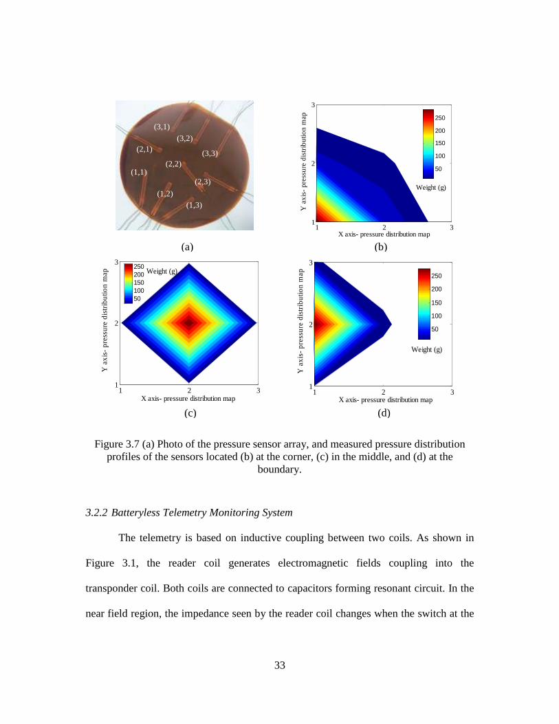
3.7 (a) Photo of the pressure sensor array, and measured pressure distribution profiles of the sensors located (b) at the corner, (c) in the middle, and (d) at the boundary. .............................................................. 33

3.8 The transponder integrated with piezoresistvie force sensing resistor. ................... 35

3.9 The measured frequency shift as a function of pressure change. ............................ 35

4.1 Schematics of the wireless batteryless sensing system consisting of an implant sensor and an external reader………………………………………. 39

4.2 System diagram of the proposed system………………………………………….. 41

4.3 Typical detected frequencies for (a) impedance sensor, and (b) pH sensor in air environment………………………………………………….. 42

4.4 (a) The prototype of the implantable, batteryless, wireless capsule integrated with impedance and pH sensors. (b) Umbrella structure for unidirectional reflux activities monitoring……………………………………. 48

4.5 In Vitro dual sensor performances…………………………………………………51

4.6 In Vitro unidirectional detection performances…………………………………… 53

4.7 In Vitro simulated short reflux episode and repeatability test with (a) pH=3 solution compared with Bravo reading, and (b) pH=11 solution while Bravo indicated out of range……………………………………….55

4.8 Calibration of frequency readings corresponding to pH buffer solutions for (a) impedance sensor, and (b) pH sensor…………………………... 57

xiv

4.9 Coordinate x-, y-, and z-axis, tilt angle α, and pan angle β to characterize motion artifacts……………………………………………………….58

4.10 Sensor output frequencies at (a) different distance, (b) different x-y coordinate, (c) different tilt angle, and (d) different pan angle…………………... 60

4.11 Temperature dependence effects of (a) commercial pH sensor, (b) our pH sensor, and (c) our impedance sensor………………………………… 63

4.12 Recorded data in biological environment………………………………………… 66

4.13 In Vivo dual sensor performance…………………………………………………. 67

4.14 In Vivo simulated short reflux episode and repeatability test with (a) pH=3 solution, and (b) pH=11 solution………………………………………. 69

4.15 In vivo animal experiment results………………………………………………… 72

4.16 pH values of the events (a) pH sensor, and (b) impedance sensor………………. 74

4.17 Statistical data analysis of (a) pH sensor and (b) impedance sensor……………... 75

5.1 Multiple sensor integration topology. (a) Transmitter block diagram. (b) Spectrum of multiple sensors. (c) Spectrum of transmitted sensor signals…… 81

5.2 Receiver block diagram to extract multiple sensor signals……………………….. 82

xv

LIST OF TABLES

Table Page

3.1 Mechanical properties of the materials. .................................................................... 25

4.1 Comparison of different GERD monitoring technologies………………………….39

1

CHAPTER 1

INTRODUCTION

1.1 Motivations and Objectives

Physiological signals contain vital information about the physiological activities

in organs that can provide useful information for diagnosis and treatment in healthcare

[1.1]. Therefore, using a scientific method to measure those physiological signals

correctly and effectively is important. Sensing transducers can be used to detect those

physiological signals and transduce into electrical signals for analysis [1.2-1.4].

However, the corresponding sensor interfacing circuits need to be designed properly so

that the sensor signals can be processed correctly. A wireless transceiver offers a

beneficial method to carry out the measured in vivo information by implanted

transducers or the measured in vitro data by wearable transducers in many healthcare

applications. Furthermore, for continuous healthcare monitoring and biomedical

applications, a batteryless wireless sensing transceiver opens new opportunities for

long-term physiological monitoring uses.

Sensor technology has been applied in various fields and played an important

role to provide researchers meaningful measurement data [1.5, 1.6]. In physiological

measurement applications, it provides us a scientific tool to characterize the

physiological parameters to better understand the conditions of our bodies [1.1]. On the

2

other hand, Radio Frequency Identification (RFID) technology has brought great

impacts to several different fields, including medical care applications [1.7-1.9]. It

provides an effective and useful way to track and monitor various information with its

identification ability and the data are transmitted wirelessly via radio frequency. While

operated in its passive mode, the transponder can even work without a battery in it.

Therefore, to integrate the sensor technology with the RFID technology for medical

applications is the main interest of this study.

1.2 Enabling Technologies

1.2.1 Sensing Transducers

A sensing transducer is defined as a functional element that detects and converts

one form of energy to another [1.2]. Transducers in a different way can be categorized

into two broad classes depending on how they interact with the environment: passive

and active transducers [1.3]. Passive transducers do not need energy added from

external sources as part of the measurement process but may consume energy during

their operation. Active transducers require energy to be added in the measurement

environment as part of the measurement process.

Sensing transducers are based on various principles: electromagnetic,

electrochemical, and electromechanical are the most common ones used in

physiological instruments [1.2, 1.3]. Electromechanical transducers convert mechanical

changes such as deformations into electrical signals. For example, pressure sensing

transducers consist of a deformable membrane which converts a pressure difference into

a movement or strain of the membrane, which in turn transforms into a varying

3

resistance by a strain gauge or a varying capacitance by parallel plate/interdigitated

finger capacitor. The resultant varying resistance or impedance can then be incorporated

in a circuit to enable electrical measurements of the pressure. Electrochemical

transducers convert chemical energy changes such as redox potentials to electrical

signals. A pH probe measuring pH values during the activity of hydrogen ions at its tip

of a thin-wall glass bulb is an example. The probe produces a small potential produced

from ion exchanges. The pH probe combined with electrical amplifiers transduces the

potentials to measureable currents.

The future of physiological sensing would be on miniaturization and integration

[1.5]. MEMS stands for MicroElectroMechanical Systems that consists of sensors,

actuators, and systems. With MEMS technology, sensors are designed and fabricated

using microfabrication and micromachining technologies that enable miniaturization

and integrated solutions to advanced sensor problems [1.4-1.6]. MEMS applied to

medical care is often called BioMEMS [1.10, 1.11]. Typical applications of BioMEMS

are a variety of lab-on-a-chip methods that analyze biological or physiological

parameters [1.10]. With the advancement of MEMS and BioMEMS technologies, the

sensing transducers can be designed more effectively to meet the requirements of the

medical applications.

1.2.2 Wireless Technologies

The deployment of sensing transducers and electronics in healthcare plays a

significant role to overcome many problems in disease treatment and diagnosis [1.5].

For advanced applications like implantable devices, wireless solutions are preferred.

4

The wireless technologies offer a competitive method for therapy or diagnosis, when

wires are often bulky, unsafe, uncomfortable or even impossible to be deployed in some

circumstances [1.12]. Wireless monitoring and communication allows patient mobility

and efficient response in emergency situations.

The wireless communication methods can be categorized into active and passive

groups, depending on the power sources required to operate electronics [1.13]. The

active devices draw power directly from a battery, while the passive devices harvest

power from external or internal sources. This is often called energy harvesting or

scavenging. Usually, the active ones have longer communication ranges since the power

uses are more efficient while the passive ones need to harvest energy indirectly from

environments having in return a shorter communication range due to power limitation.

IEEE has initiated a new working group for wireless personal area networks

(WPANs) or Wireless Body Area Network (WBAN), mainly targeted at medical

applications [1.14]. It consists of a set of sensing devices, either wearable or implanted

into the human body, with a protocol that can communicate to each other to monitor

vital body parameters and activities [1.15, 1.16]. It is a short range communication

protocol and it has low power consumption requirements. There are several

technologies, like Bluetooth, ZigBee, etc. proposed in this working group; however,

passive RFID technology would also be a competitive candidate since it does not need a

battery in the transponder to operate. Therefore, passive RFID technology has

advantages for long-term monitoring compared to other battery based technologies.

5

1.3 Importance of Batteryless Wireless Sensing Systems for Medical Applications

Wireless communication technologies that use radio frequency to communicate

between sensing transducers, measurement instruments, and base stations, etc. provide a

better way than the one with wire connections between them. The physical wire

connections will limit the mobility of the devices and sometimes cause hazards. This is

especially important in such environment like an intensive care unit (ICU) or an

operating room (OR) where space is limited. Wireless communication technologies not

only solve the cumbersome wire connection problem for external wearable devices but

also provide a feasible and comfortable way for implant applications. In addition, some

physiological activities require long-term monitoring for proper diagnosis of the

diseases, so the low power consumption requirement of the devices is critically

important. A wireless sensing transducer that can be operated without a battery in it can

definitely prolong the monitoring duration. Overall, a batteryless, wireless sensing

system brings significant impacts for medical applications especially for implant

applications.

1.4 Dissertation Architecture

Based on different positions of physiological sensing device deployment, it can

be divided into either an external or implantable one. For external deployment

applications, the physiological devices are attached to the body to read the biological

signals. A batteryless wireless pressure monitoring system for sensing wound

conditions was demonstrated for this type of applications. For implant deployment

applications, the physiological sensing devices are placed inside the body without a

6

tethered wire to bring the signals outside. An implantable batteryless wireless

impedance and pH sensing system for gastroesophageal reflux diagnosis was

demonstrated for this type of applications.

In the first part of this dissertation, a batteryless, wireless sensing platform based

on passive RFID working principles is presented. Based on this platform, two medical

applications are targeted. In the second part of this dissertation, a wireless pressure

sensor array is made to monitor the pressure distribution in a certain area without the

need of a battery. This pressure sensor array is suitable for long term monitoring of

pressure sore development. In the third part of this dissertation, a wireless implantable

sensing device is made to monitor reflux episodes in esophagus. This single device

consisted of two sensors and presents an accurate way for in vivo GERD diagnosis. The

passive wireless communication mechanism was demonstrated for multiple transducers

integrated in a single transponder device. Finally, a systematic approach on the

optimization of the system powering efficiency is attempted and the results are

discussed in the Appendix.

7

CHAPTER 2

A BATTERYLESS, WIRELESS SENSING PLATFORM OVER A PASSIVE RFID COMMUNICATION SYSTEM FOR BIOMEDICAL APPLICATIONS

2.1 Introduction

A telemetry sensing system based on passive RFID technologies has brought

great attentions, especially in biomedical applications, due to its sensing capability,

wireless communication ability, and without the need of battery for operation in the

transponder [2.1-2.8]. It provides a better way to deploy the sensing transponder devices

since there is no wire connection between the transponder and the remote reader system.

It also provides a feasible way for long term monitoring since the transponder does not

need a battery for operation. The sensing systems based on passive RFID technologies

can be categorized into two types: by detecting either the resonant frequency changes or

the modulated frequency changes [2.9-2.16]. In both cases, the frequency changes of the

transponder are modulated by the variations of sensors when sensor characteristics are

modified by external conditions. In the first type of sensing system that detects resonant

frequency changes, a reference circuit of the remote sensing transponder needs to be

configured to produce a reference signal for usage in conjunction with the sensor signal

[2.17]. It requires very precise measurements on resonant frequency changes to

distinguish different target objects of interest. The second type of sensing system is

based on the detection of the modulated frequency changes from the transponder. While

8

the sensor signals are encoded into frequency variation data, this type of sensing system

is more reliable and robust for practical medical applications [2.18-2.20].

Furthermore, the RFID circuit used in the transponder that integrates with the

sensors can be realized either in transistor level integrated circuit design or board level

circuit design. To demonstrate the capability of our sensing platform that can be used in

different medical applications, studied in this dissertation, the approach of using board

level circuit design to interface with the sensor is used.

2.2 Proposed Sensing System

2.2.1 System Overview

The proposed sensing system design is based on passive RFID working

principles [2.21]. The sensing system includes a transponder and a reader in which the

communication is based on inductive link between two coil antennas. Figure 2.1 shows

the system block diagram of our sensing system. The working principle of the system

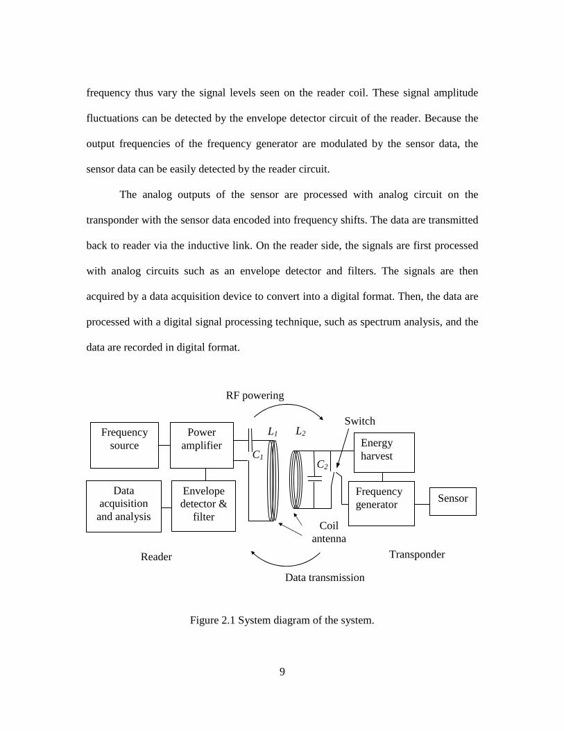
consists of two parts, which are RF powering and data transmission. From the reader

side, the interrogator frequency source is fed into the power amplifier and radiates the

RF energy coupled into the transponder through the resonant circuits. This RF energy is

then harvested by the energy harvest circuit of the transponder and builds up the

required DC voltage to power up the rest of the circuits on the transponder, such as the

frequency generator. The output from the frequency generator has a rectangular

waveform with high and low amplitude levels, as shown in Figure 2.2. These high/low

signal levels can turn on and off the switch circuit and these loading modulation

processes will tune and detune the resonant circuit of the transponder to its resonant

9

frequency thus vary the signal levels seen on the reader coil. These signal amplitude

fluctuations can be detected by the envelope detector circuit of the reader. Because the

output frequencies of the frequency generator are modulated by the sensor data, the

sensor data can be easily detected by the reader circuit.

The analog outputs of the sensor are processed with analog circuit on the

transponder with the sensor data encoded into frequency shifts. The data are transmitted

back to reader via the inductive link. On the reader side, the signals are first processed

with analog circuits such as an envelope detector and filters. The signals are then

acquired by a data acquisition device to convert into a digital format. Then, the data are

processed with a digital signal processing technique, such as spectrum analysis, and the

data are recorded in digital format.

Figure 2.1 System diagram of the system.

C1 C2

Transponder Reader

Coil antenna

Frequency source

Power amplifier

Envelope detector &

filter

Energy harvest

Frequency generator

Sensor Data

acquisition and analysis

RF powering

Data transmission

L1 L2 Switch

10

Figure 2.2 (a) A batteryless wireless sensing platform. (b) Signals at the reader coil.

2.2.2 Transponder

The front end of the transponder consists of a coil antenna, denoted as L2, and a

tuning capacitor, denotes as C2, forming a resonant circuit used to receive RF power

from the reader. The transponder circuit was designed on a 4-layer printed circuit board

(PCB). A coil antenna with inductance value of 22 µH was made from a 34 AWG

magnet wire (Belden Wire & Cable) wound around the PCB. The designed operating

frequency was at 1.34 MHz. This is based on the recommended maximum permissible

exposure (MPE) of magnetic field is the highest in the frequency ranges from 1.34 to 30

MHz [2.22]. The calculated tuning capacitor was done with a capacitance value of 640

pF based on the formula

where f0 represents the resonant frequency.

(b)

(a) Transponder Reader

Frequency generator

Sensor

Frequency source

Switch ON/OFF: f (sensor output)

Low High

Low High

Low High

Low switching frequency

High switching frequency

LCf

π21

0 = (2.1)

11

The energy-harvesting unit was designed using voltage multiplier circuitry,

including a series of diodes and capacitors with the capacitance values of 100 pF that

can build up the DC voltage from the received RF energy. A regulator circuit was

implemented (S-817A20ANB, Seiko Instruments) to guarantee a constant DC level for

biasing the circuits. Figure 2.3 shows the energy-harvesting circuit which consists of a

voltage multiplier and a regulator.

Figure 2.3 Voltage multiplier and regulator circuits.

The frequency generator unit was realized with a relaxation oscillator circuit

using comparator ICs (TLV3012, Texas Instruments). The relaxation oscillator circuit

consists of a comparator, a capacitor and several resistors. The output frequency of the

oscillator was reversely proportional to the time constant at the inverting input and can

be calculated from the resistance and capacitance values in the feedback loop of the

circuit [2.23]. The frequency generator circuit can be used to interface with both

resistive and capacitive type of the sensors [2.24]. Figure 2.4 shows the circuit diagram

of the relaxation oscillator. The modulated frequency can be found as

VCC

OUTIN

Voltageregulator

12

Figure 2.4 Relaxation oscillator circuit to interface with both resistive and capacitive type of the sensors, represented as Rs and Cs.

where RS and CS represent the resistive and capacitive type of the sensors connected in

parallel, RA, RB and C1 are lumped components. The resistors RA and RB have the

resistance values of 12 and 10 kΩ, respectively, the capacitor C1 has the capacitance

value of 2.2 nF. With RS in the range of 0-40 MΩ and CS in the range of 0-2 pF, the

modulated frequencies had the frequency range from 9.5 to 16.8 kHz. Thus, the sensor

data were encoded into frequency shifts. The resistors R1, R2, and R3 were designed with

the same resistance value of 1 MΩ resulting in a duty-cycle of 50% on the output

waveform from the relaxation oscillator. This time domain symmetric output waveform

has the optimal amplitude on its power spectrum in frequency domain. Thus, the signal

( )[ ] 1////

1

CRCRRf

BSSA ×+∝ (2.2)

13

C1

M1

VDC

1

2

L1

R

C21

2

L2Functiongenerator

to noise ratio can be optimized under the same noise level when we perform spectrum

analysis on the reader side.

2.2.3 Reader

In this work, a class-E power amplifier was chosen and built for its high

efficiency. Because the voltage and current of the amplifier circuit are 180° out of

phase, the theoretical power consumption is zero [2.25]. The class-E power amplifiers

have been used in other RF power amplifier for biomedical implant applications [2.26-

2.28]. The circuit diagram of the class-E amplifier is shown in Figure 2.5.

Figure 2.5 A circuit diagram of Class-E power amplifier.

A function generator provided a 0-5 V square wave signals to drive the

MOSFET switch M1 (IRL510A, Fairchild Semiconductor), that had low threshold

voltage of 1 Volt. A duty-cycle of 30% was chosen to minimize DC power

consumption. A portable reader can be powered by batteries eventually. A coil antenna

14

100k

D1N4936 4.7k

1n100p

1n

100k

Vss

VCC

+5

-6

V+4

V-11

OUT7

with a size of 9×12 cm2 was made from an AWG26 magnet wire wound around a frame

resulting in an inductance of 17 µH and a high quality factor Q of 70. Following the

calculation procedures for a high quality factor Q approximation in [2.29], the values of

C1 and C2 were chosen to be 10 nF and 900 pF, respectively.

Figure 2.6 shows the circuit of envelope detector, that includes a diode and RC

networks, and a low pass filter for sensor data detection. The diode (1N4936, Vishay

Semiconductors) rectified the high voltages at the coil antenna of the class-E amplifier.

The time constant of the 100 kΩ resistor and 100 pF capacitor gave a modulation

frequency of 0.1 MHz that was suitable for a carrier frequency above 1 MHz. The 4.7

kΩ resistor and 1 nF capacitor suppressed the high-amplitudes of the high-frequency

carrier signals. The 1 nF capacitor and 100 kΩ resistor form a low-pass filter to reduce

the DC level before the signals were fed into an op-amp buffer. The sensor data were

then acquired and logged into a computer by a data acquisition device (NI USB-6210

DAQ, National Instruments) with 16 bit resolution, and the sampling rate of 250 kS/s

that was sufficient enough to detect the signal. A system level LabVIEW program was

used to implement the benchtop spectrum analysis mechanism.

Figure 2.6 Envelope detector and low pass filter circuit.

15

(a)

(b)

2.2.4 Read Distance

The read distance of a passive RFID system depends on several factors, such as

the supply current at the reader, the power consumption of the transponder circuit,

antenna size, coupling efficiency between the two resonant circuits, and quality factor

(Q) of the antenna, etc [2.30, 2.31]. The typical read distances of the inductive coupling

RFID device are shown in Figure 2.7 [2.32, 2.33].

Figure 2.7 Read ranges vs. tag sizes for (a) proximity applications, and (b) long range applications [2.32, 2.33].

16

Figure 2.8(a) shows the prototype of the sensing device packaged with

biocompatible material, Polydimethylsiloxane (PDMS). The device dimensions were

2.5×0.8×0.5 cm3 with the coil antenna wound around the PCB. The transponder circuit

was design on a four-layer PCB, consisting of the voltage multiplier, regulator, and

frequency generator circuit. The surface mount devices (SMD) were used, while the

size of our prototype can be further reduced by IC technology. Figure 2.8(b) shows the

reader system with a 9×12-cm2 coil antenna.

Figure 2.8 (a) Prototype of the batteryless wireless sensing device. (b) Prototype of the

remote reader system.

(a)

(b)

17

The optimization of the read distance for inductive coupling passive RFID was

discussed in [2.34]. The optimization approaches are twofold. First, the transponder

must receive enough power from the reader to be able to operate properly. Second, the

reader, on the other hand, must have enough sensitivity to extract the signal from the

transponder. The read distance depends on the noise level in the environment as well.

The signal to noise ratio of the received signal will degrade along with the distance due

to the power budget and environmental noise between the inductive links. Therefore, it

is important to characterize the minimal acceptable signal to noise ratio with the

maximum read distance to make sure an acceptable signal quality can be obtained. We

characterized the minimum acceptable signal to noise ratio by increasing the distance

between transponder and reader antenna and measured S/N ratio, as shown in Figure

2.9. The signal to noise ratio was determined by the measured signal amplitude

compared to the noise level presented. The measurements on amplitude of frequency

spectrum and noise level were performed by using spectrum analyzer (E4403B,

Agilent).

Figure 2.9 Illustration of read distance characterization.

x

y

z

Reader coil antenna

Transponder coil antenna Movement direction

18

We obtained the maximum read distance of 13cm with minimum distinguishable

signal to noise ratio of 2.95 dB. Compared to the typical RFID tag with the size of 2.54

cm in diameter can be read at 10.16 cm from the 7.62×15.24 cm2 antenna [2.32], our

transponder achieved the same range with smaller transponder size and smaller reader

antenna.

2.3 Multiple Sensor Integration

Multisensor measurements give more accurate measurements since they provide

more information than single sensor measurement [2.35, 2.36]. Multiple sensor data can

be used to correlate and calibrate to each other and thus more reliable and correct

measurements can be achieved [2.37, 2.38]. Our sensing platform can also be used to

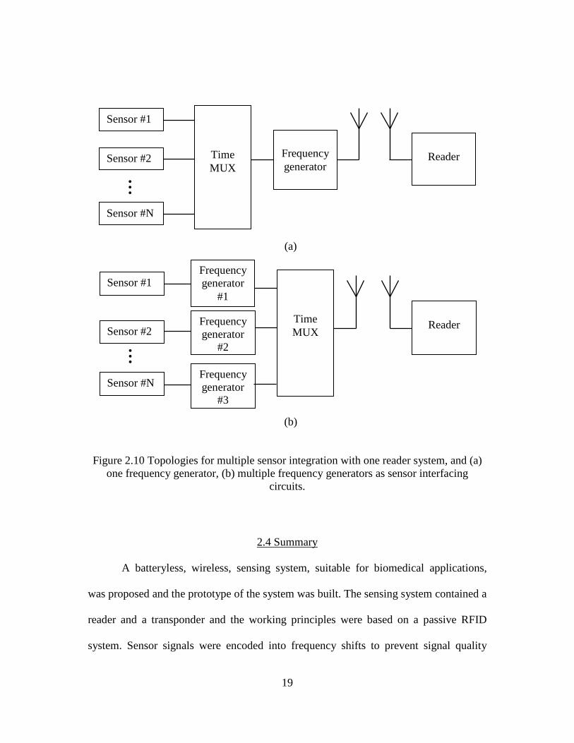
integrate with multiple sensors for multisensor measurements. A time-multiplexing

switch mechanism is used to multiplex the sensor data; therefore, a sequence of sensor

data can be read by using only one reader system. Figure 2.10 shows two topologies

used for multiple sensor integration in our study. In the first integration topology, as

shown in Figure 2.10(a), we used one frequency generator to process multiple sensor

data that were coordinated into a sequence of data stream by a time-multiplexing

switch. In this topology, all sensors had the same type of output signal so one frequency

generator was used as sensor interfacing circuit. In the second sensor integration

topology, all sensors needed to be interfaced with their corresponding frequency

generators first, because all sensors had different types of output signals that needed to

be processed properly first, as shown in Figure 2.10(b).

19

Figure 2.10 Topologies for multiple sensor integration with one reader system, and (a) one frequency generator, (b) multiple frequency generators as sensor interfacing

circuits.

2.4 Summary

A batteryless, wireless, sensing system, suitable for biomedical applications,

was proposed and the prototype of the system was built. The sensing system contained a

reader and a transponder and the working principles were based on a passive RFID

system. Sensor signals were encoded into frequency shifts to prevent signal quality

Sensor #1

Sensor #2

Sensor #N

...

Time MUX

Frequency generator

Reader

(a)

Sensor #1

Sensor #2

Sensor #N

...

Time MUX

Frequency generator

#1

Reader Frequency generator

#2

Frequency generator

#3

(b)

20

degradation due to the misalignments between two coil antennas that might be caused

from motion artifacts in real physiological environment. Our system had competitive

performances in read ranges, compared to typical RFID system, with even smaller

antenna size in both transponder and reader. Our sensing platform can also be extended

to multiple sensor integration suitable for different medical applications that will be

studied in this dissertation.

21

CHAPTER 3

A WIRELESS BATTERYLESS PIEZORESISTIVE PRESSURE SENSING SYSTEM FOR PRESSURE SORE PREVENTION APPLICATIONS

3.1 Motivation

Pressure sores is an important health and economic problem. They affect a large

part of hospitalized patients [3.1], and the cost has been estimated more than 6.4 billion

dollars per year in United States [3.2]. Several risk factors have been identified for the

development of pressure sores classified as extrinsic and intrinsic factors. Extrinsic

factors include interface pressure, shear forces, friction, moisture, etc. Intrinsic factors

are related to the nutritional state of the patient, age, infection, diseases, etc. Three main

mechanical factors are thought to play a part in the development of pressure sores:

pressure, friction and shear [3.3]. A prolonged and unrelieved pressure will collapse the

vessels while shear and friction will bend the vessels. This will result in the occlusion of

blood flow and damage the tissues. Hence, using technologies to detect those factors

effectively to prevent pressure sores development is necessary for those patients.

A pressure sensing system for pressure sores monitoring is important for

patients who might have higher risks to develop pressure sores. There are several

technologies for pressure sores prevention. The seat cushion method is to reduce and

redistribute interface pressures for the patient by supplying a compliant support at the

patient-seat interface. However, Ferguson-Pell presented an extended review of the seat

22

cushion selection and noted that no single cushion meets the needs of all users [3.4].

Braden scale is a well-known method to check if the patients have high risks to develop

pressure sores [3.5]. Nevertheless, mastering this method relies on professional

experience. Using conventional pressure sensors to design tools for interface pressure

measurement is also a popular topic. These conventional pressure sensors include

conductive polymer sensors, semiconductor and metal strain gages, capacitive, and

optoelectronic sensors [3.6, 3.7]. Each of them has its pros and cons, considering its

cost, size, repeatability, linearity, hysteresis, temperature dependence, and ease of use,

etc [3.6]. The development of pressure mapping systems has enhanced pressure sores

risk assessment. This is due to their ability to objectively measure interface pressure and

provide computer generated data that are not based on subjective opinions [3.8, 3.9].

Therefore, a pressure sensing system that can show the pressure profiles by taking

advantage of conventional sensors has been studied in this work.

In this research, a force sensing resistor is used as the sensing element due to its

sensitivity, planar substrate, small size, and relative low cost and [3.6]. The force

sensing resistors are laid out in such a way that the pressure mapping system can be

realized to visually monitor the pressure points. In addition, in pressure sores prevention

applications, a wireless approach is preferred because the wired one creates limitation

for patient mobility. Furthermore, a batteryless sensing device provides a good way for

long-term use without the need to change batteries. Hence, a prototype of a wireless

batteryless pressure sensing system was proposed.

23

3.2 System Design

The wireless batteryless pressure sensing system consists of force sensing

resistors, transponder devices, and a monitoring reader system. The force sensing

resistors were in an array format to measure the pressure distribution across an aperture.

Resistors were connected to a switching unit to time-multiplex the signals. The pressure

information in the format of resistance values was fed into the transponder device to be

converted into frequency shift information. The transponder and reader system are

based on the passive radio-frequency identification (RFID) principle, hence the pressure

information can be wirelessly transmitted to the reader without the need of a battery.

The frequency shifts then were extracted by the reader circuit and recorded by a

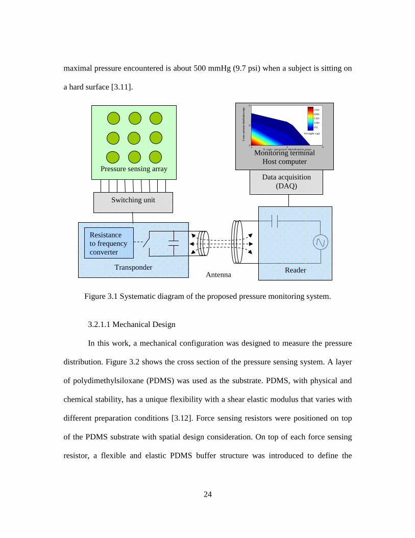
monitoring terminal. Figure 3.1 shows the systematic diagram of our proposed

telemetric pressure monitor system.

3.2.1 Pressure Measurement System

Measuring the pressures and shears is the main interest because they are the

main factors to cause pressure sores [3.6, 3.10]. A force sensor was chosen to be

embedded into a specially designed mechanical structure that can measure both pressure

and shear forces. A force sensor responds to forces regardless of the area over which the

force is applied while a pressure sensor responds to pressure, which gives an output

inversely proportional to the area under a constant force. Therefore, while using force

sensors in pressure sensing applications, care must be taken to ensure that the force is

applied over the same area [3.6]. In this study, a weight is applied on top of the sensor

array to measure the pressure distribution. For this interface pressure measurement, the

24

maximal pressure encountered is about 500 mmHg (9.7 psi) when a subject is sitting on

a hard surface [3.11].

Figure 3.1 Systematic diagram of the proposed pressure monitoring system.

3.2.1.1 Mechanical Design

In this work, a mechanical configuration was designed to measure the pressure

distribution. Figure 3.2 shows the cross section of the pressure sensing system. A layer

of polydimethylsiloxane (PDMS) was used as the substrate. PDMS, with physical and

chemical stability, has a unique flexibility with a shear elastic modulus that varies with

different preparation conditions [3.12]. Force sensing resistors were positioned on top

of the PDMS substrate with spatial design consideration. On top of each force sensing

resistor, a flexible and elastic PDMS buffer structure was introduced to define the

Pressure sensing array

Switching unit

Transponder Antenna

Resistance to frequency converter

Data acquisition (DAQ)

Reader

Monitoring terminal Host computer

X axis- pressure distribution map

Y a

xis- pre

ssure

distributio

n m

ap

1 2 31

2

3

50

100

150

200

250

Weight (g)

25

sensing area. This buffer structure not only converts forces into pressures but also

measures the shear force due to its elastic properties. Then, a layer of polyimide film

was introduced to provide the correlative link between the neighboring sensors. Table

3.1 lists the mechanical properties of the materials used in this study. The polyimide

layer not only provides sufficient support strength for objects sitting on top of the

structure but also plays a role for measuring shear forces. Finally, a layer of PDMS was

introduced on top of the polyimide to protect the pressure sensing structure and provide

a soft contact interface with the object.

Table 3.1 Mechanical properties of the materials.

PDMS Polyimide

Modulus 360-870 kPa 2.5-15 GPa

Poisson ratio 0.5 0.34

Mass density 0.97 kg/m3 1420 kg/m3

Figure 3.2 Cross section of the pressure sensing system and its capability for pressure

and shear force measurements.

As shown in Figure 3.2, when a force is applied directly on top of the sensing

area of the force sensing resistor, the force will be converted into pressure that is

Normal force

Tangential force

Interface of the measured object

Force sensing resistor

PDMS Polyimide

PDMS

PDMS

Force

26

defined by the buffer PDMS structure. Moreover, the effects of off-axis loading which

contain shear forces information can also be measured in this pressure sensing structure

as shown on the right side of Figure 3.2. The mat structure conforms to a deformed

surface and the force can be spitted into the normal and tangential components. The

normal force will be measured by the sensor underneath and the shear force will

contribute to the readings of the neighboring sensors that are connected by the

polyimide structure.

Figure 3.3 (a) Physical structure of force sensing resistor, and its (b) typical characteristic curve of resistance versus force [3.13].

A B

A B

Semiconducting polymer film

Interdigitated electrode

forceR ∝

(a) (b)

27

3.2.1.2 Force Sensing Resistor

The force sensing resistor is a flat, flexible device that exhibits a decreasing

electrical resistance with increasing force applied normal to its surface [3.13]. The

physical structure of a typical force sensing resistor is shown in Figure 3.3(a). An

interdigitated finger electrode is deposited on top of the semiconducting polymer film

that changes its electrical resistance corresponding to different values of force applied

on top of it. When no force is applied to the sensing film, the resistance between the

interdigitated finger electrodes is quite high, usually 1 MΩ or more. With increasing

force, the resistance drops following an approximate power law. A typical plot of

resistance versus force is shown in Figure 3.3(b) [3.13].

3.2.1.3 Pressure Sensing Array

A pressure mapping system that can objectively measure interface pressure and

provide the recorded data instead of subjective opinions would enhance pressure sore

risk assessment [3.8]. As shown in Figure 3.4(a), our pressure sensing array is

composed of 9 force sensing resistors to demonstrate the working principle. The array

size can be easily scaled for various applications. For accurate measurements of

pressure distributions, a dense sensor array will be necessary. In our design, each force

sensing resistor was spaced evenly on top of the PDMS layer with a 3-cm spacing. The

spatial resolution then is 9 cm2. A flexible mat structure was placed on top of the sensor

array as the interface. When a weight is on top of the mat structure, the sensor directly

underneath the object will respond to the normal pressure reading, while the

neighboring sensors will show force information related to shear forces. Figure 3.4(b)

28

shows that when a force, F, is applied on the mat structure, the closer sensor will show a

higher pressure while the other ones show lower readings. This force can be

decomposed into normal and tangential forces respectively, to be measured.

The readings related to the shear force could be measured by the closer

neighboring sensors. As shown in Figure 3.4(b), when a force, F, was applied on the

mat structure, the shear forces, FL and FR, were induced. These two forces were further

decomposed into their normal and tangential forces, respectively.

FL,normal = FLsinθ (3.1)

FL,tangential = FLcosθ (3.2)

FR,normal = FRsinα (3.3)

FR,tangential = FRcosα (3.4)

The two normal forces, FL,normal and FR,normal, are measured by the sensors underneath

with the readings WL and WR, respectively. The two tangential forces, FL,tangential and

FR,tangential, contribute to the shear stress-strain distribution of the mat structure can also

be calculated. Assuming that the displacement, ∆, is relatively small so the distance, x,

can be expressed as

RL

L

WW

LWx

+≅

(3.5)

Hence, the force, FR, can be obtained from

+∆≅

−

L

RL

RR

LW

WW

WF

)(tansin 1

(3.6)

So, the shear stress, τ, can be calculated as

29

Force sensing resistors (a)

F

FL FL, normal

FL, tangential

θ α FR

FR, normal

FR, tangential

(b)

3cm 3cm

3cm

3cm

Object contact

x L-x

WL WR

α ∆

Drawing not to scale Sensing area, A

5mm

A

F R≡τ (3.7)

where A is the sensing area of the force sensing resistor.

Figure 3.4 (a) Top view of the proposed pressure sensing array. (b) Cross section view to illustrate the normal and shear force measurements.

The stress-strain behavior of the mat structure was simulated using the finite

element method ANSYS. Figure 3.5(a) shows the simulation configuration with a thin

plate supported at its four corners that is subjected to a force F on the plate. L1 and L2

are the length of the plate with a dimension of 3×10-2 m and t is the thickness with a

dimension of 2×10-3 m. E1 and E2 are the distances with a dimension of 1.5×10-2 m and

a contact area of 0.2 cm2 to the mat structure are defined. The polyimide plate was

assumed to be an isotropically and linearly elastic material. As shown in Figure 3.5(b),

the corners and the center encountered the highest stress-strain force of 1.89×106 Pa

with a 4.35×10-4 m displacement. Hence the mat structure can provide enough

30

(a) (b)

Z Y

X

L2

L1

t

F

E1

E2

Supporting structure Contact area

supporting stress-strain force within the desired pressure range of 0-10 psi.

Figure 3.5 (a) Geometry and loading of the thin plate. (b) ANSYS simulation of the stress-strain behavior of the mat plate structure.

3.2.1.4 Experimental Results

Nine sensors were calibrated with objects weighted from 0 to 400 grams to

obtain their individual characteristic curves. Force sensing resistors yield a decrease in

resistance with increasing force and their corresponding plots are shown in Figure

3.6(a). After obtaining the curve for each sensor, we can convert the resistance reading

back to the weight information. Then a weighted 300 gram object was placed on top of

the mat structure to examine the long-term stability performance of piezoresistive type

force sensors due to the concern in value drifting issue [3.13]. As shown in Figure

3.6(b), for a period of 7 days, 14 data points were taken to examine the resistance

drifting. The maximum resistance drifting is 0.44 kΩ (4.3%). This value is considered

31

small compared to that for an object weighted in the range of 100 grams which usually

yields more than 5 kΩ resistance change. Therefore, the drifts will not be a factor

affecting force readings. In addition, in pressure sores prevention application, when the

sensor readings have no abrupt and large changes for a long time, which means that the

patient has remained in the same position for some time and needs to be rotated to

change his/her lying position.

Figure 3.6 Nine force sensing resistors with their corresponding (a) Characteristic curves. (b) Sensor long-term stability tests for 7 days with two data points taken per

day.

The pressure sensor array was further examined on its ability to identify high

pressure points. Figure 3.7(a) shows a photo of the pressure sensor array with nine

sensor locations indicated. A weight of 300 grams was placed on top of the pressure

sensor array in different locations. Figures 3.7(b)-(d) show measured weight

distributions when a weight was applied at different locations on the array. Figure

(a) (b)

1 2 3 4 5 6 7 8 9 10 11 12 13 146

7

8

9

10

11

12

13

14

15

Sampled data

Res

ista

nce

(K

Oh

ms)

100 150 200 250 300 350 400 450

6

8

10

12

1416

18

20

22

24

Weight (Grams)

Res

ista

nce

(K

Oh

ms)

Sensor1

Sensor2

Sensor3

Sensor4

Sensor5

Sensor6

Sensor7

Sensor8

Sensor9

32

3.7(b) shows the weight distribution when the object was placed at the location (1,1),

the sensor at this location indicated that there was a 298-gram weight. The object has a

contact area of 19.64 cm2 to the sensor array. The neighboring sensors (1,2), (2,1), and

(2,2) indicated the shear forces induced by the finite contact area with the readings of

42, 35, and 17 grams, respectively. Sensor locations at (3,1), (3,2), (3,3), (1,3) and (2,3)

indicated no force since the object was far away from these positions. In Figure 3.7(c),

when the 300-gram object was placed on top of the sensor (2,2), it indicated that the

object was on top of it with a 290 grams reading and its closer neighboring sensors

(1,2), (2,1), (2,3), and (3,2) had the readings of 16, 15, 17, and 15 grams, respectively.

Sensor locations at (1,1), (1,3), (3,1), and (3,3) indicated no force occurred at those

points. Similarly, in Figure 3.7(d), the sensor position (1,2) indicated that a 293 grams

object was placed on top of it and its closer neighboring sensors (1,1), (1,3) and (2,2)

had the readings of 23, 25, and 20 grams, respectively. Sensor locations at (2,1), (2,3),

(3,1), (3,2), and (3,3) indicated no force occurred at these points.

A weight of 300 grams with a contact area of 0.2 cm2 to the sensor array was

placed in the center among the locations (1,1), (1,2), (2,1), and (2,2) to examine the

shear force. Sensor locations (1,1), (1,2), (2,1), and (2,2) had the readings of 76, 78, 75,

and 76 grams, respectively. Sensor locations at (1,3), (2,3), (3,1), (3,2), and (3,3)

indicated no force occurred at these points. From equation 3.6, the force, FR, was

estimated as 36.75 N . The shear stress can be obtained as 1.81×106 N/m2 (Pa) from

equation 3.7. This value is close to the result in the ANSYS simulation.

33

(a) (b)

(c) (d)

(1,1)

(1,2) (1,3)

(2,1)

(2,2)

(2,3)

(3,1)

(3,2)

(3,3)


Y a

xis-

pre

ssu

re d

istr

ibu

tion

ma

p

1 2 31

2

3

50

100

150

200

250

Weight (g)


Y a

xis-

pre

ssu

re d

istr

ibu

tion

ma

p

1 2 31

2

3

50100150200250

Weight (g)


Y a

xis-

pre

ssu

re d

istr

ibu

tion

ma

p

1 2 31

2

3

50

100

150

200

250

Weight (g)

Figure 3.7 (a) Photo of the pressure sensor array, and measured pressure distribution profiles of the sensors located (b) at the corner, (c) in the middle, and (d) at the

boundary.

3.2.2 Batteryless Telemetry Monitoring System

The telemetry is based on inductive coupling between two coils. As shown in

Figure 3.1, the reader coil generates electromagnetic fields coupling into the

transponder coil. Both coils are connected to capacitors forming resonant circuit. In the

near field region, the impedance seen by the reader coil changes when the switch at the

34

transponder opens or closes. This load modulation alters the voltage level at the reader

coil. As a result, the transponder switching frequency can be extracted at the reader

using envelope detection [3.14].

3.2.2.1 Transponder Architecture

The transponder consists of an antenna, a tuning capacitor to receive power and

modulate sensor data, a voltage multiplier and a regulator to build up a constant DC

voltage, and a relaxation oscillator to transduce resistance variations to frequency-

varying signals. The frequency (f) of the relaxation oscillator can be calculated as

[ ] 1)//(

1

CRRRf

BSA ×+∝ (3.8)

with a piezoresistive force sensor RS and lumped components RA, RB and C. A low-

power op-amp was used as a comparator and the resistors RA and RB are 20 kΩ and 10

kΩ, respectively. The capacitor C1 is 1 nF. With RS in the range of 0-40 MΩ, the

modulation frequency ranges between 7.5 and 16.8 kHz.

3.2.2.2 Reader Configuration

The reader includes a class-E power amplifier to generate high electromagnetic

fields and an envelope detector to read the load modulation signals. A frequency source

provides the carrier signal feeding the amplifier at the resonance frequency resulting in

a high voltage at the reader coil. With the modulation, the voltage levels at the reader

coil fluctuate. The pressure sensor resistance signal is extracted by an envelope detector

and fed through a band-pass filter to suppress the high frequency carrier.

35

0 1 2 3 4 5 6 7 8 9 10 11 127.3

7.4

7.5

7.6

7.7

7.8

7.9

8

8.1

8.2

8.3

8.4

8.5

8.6

Pressure (psi)

Fre

qu

en

cy (

kHz)

3.2.2.3 Experiment Results

A transponder device was made on a 4-layer printed circuit board (PCB). Figure

3.8 shows the prototype of the transponder integrated with the force sensing resistor. A

coil antenna of 22 µH was made from a 32 AWG magnet wire wound around the PCB.

Figure 3.8 The transponder integrated with piezoresistvie force sensing resistor.

Figure 3.9 The measured frequency shift as a function of pressure change.

Force sensing resistor (FSR)

Transponder

36

When connected to a capacitor of 680 pF, the device operated at 1.3 MHz. The

pressure sensing transponder device was characterized with a pressure range from 0 to

10 psi. By adding weights onto the sensing area the corresponding frequency shifts were

measured. The reader was placed 12 cm away from the transponder device. Figure 3.9

shows the frequency over the pressure range from 0 to 10 psi along with the respective

sensor resistance changes. The reading frequency increased from 7.35 to 8.55kHz with

a 0.12 kHz/psi resolution. The device is capable of reading the pressure wirelessly

without a battery at the sensor.

3.3 Summary

A wireless batteryless sensing system that can monitor pressure distribution was

presented. In this work, a pressure sensor array was built to detect pressure distribution

in a certain area for sensing wound condition in pressure sore prevention applications.

The experimental results showed that the system can not only indicate the high pressure

points but also indicate shear force information over a contact area. Stability tests of the

sensor were carried out for long-term use purposes. The experimental results indicated

that the drifting of reading was smaller than the readings for high pressure indications.

The pressure information was sent to the reader system wirelessly without the need of a

battery in the sensing device. The experimental results showed that the reading

frequency increased from 7.35 to 8.55 kHz over the pressure range from 0 to 10 psi

linearly.

37

CHAPTER 4

AN IMPLANTABLE, BATTERYLESS AND WIRELESS CAPSULE WITH INTEGRATED IMPEDANCE AND PH SENSORS FOR GASTROESOPHAGEAL

REFLUX MONITORING

4.1 Introduction

Gastroesophageal Reflux Disease (GERD) is a medical condition that affects

approximately 15% of adult population in the United States and is one of the most

prevalent clinical conditions afflicting the gastrointestinal tract [4.1]. GERD refers to

symptoms or tissue damage caused by the reflux of stomach contents into the esophagus

and pharynx. The reflux contents are both acidic and nonacidic [4.2-4.4]. GERD has

been associated with a major risk factor for esophageal cancers which have the fastest

growing incidence rate of all cancers in the developed countries [4.5]. Therefore,

monitoring GERD symptoms accurately, reliably and comfortably is important for

treatment screening.

Multichannel intraluminal impedance (MII) probe is a currently available

instrument that has been used to correlate symptoms with episodes of gastroesophageal

reflux [4.6]. Whereas electric conductivity is directly related to the ionic concentration

of the intraluminal content, materials with high ionic concentrations (e.g. gastric juice

or food residues) have relatively low impedance compared with that of the esophageal

lining or air [4.7]. Although the MII probe system brings more accurate monitoring

38

results compared to the conventional pH meter alone, patient tolerability is too low for

patient to complete the test [4.8]. The tethered sensor probe requires a transnasal

insertion procedure and the wire, connecting from the electrodes that stay inside the

esophagus to the external electronic unit worn by the patient, stays transnasally for 24 to

48 hours while the patient supposedly resumes normal daily activities. The wired

feature limits the clinical utility and accuracy of this technique for protracted

monitoring of gastroesophageal reflux. A miniature wireless device that does not

require tethered external connections is thus preferred for esophageal reflux monitoring.

To date, a wireless pH monitoring capsule (Bravo, Medtronic) has been used in

some clinical practices [4.9]. However, it cannot detect non-acid reflux and has a

limited battery life of 48 hours unless prolonged [4.8, 4.17]. Recent studies and reviews

have suggested combined pH and impedance monitoring increased the accuracy of

GERD diagnosis [4.10, 4.11]. Lately, a combined impedance and pH sensor capsule

that could detect both acid and non-acid reflux was developed using a microcontroller

and a wireless transmitter [4.12]. However, the device has limited sampling rates to

conserve battery energy and may miss reflux episodes between sampling. The limited

battery lifetime prohibits the possibility of prolonged measurements that in some

clinical cases are needed for increased diagnosis accuracy [4.13]. Table 4.1 compares

different sensing technologies for GERD monitoring.

In this work, passive telemetry was demonstrated to achieve the reflux

monitoring wirelessly. The system configuration is shown in Figure 4.1. The implanted

sensor harvests radio frequency (RF) power transmitted from an external reader and

39

Sensor Esophagus

Stomach

Reflux External reader

RF power

Sensor data

sends the modulated impedance and pH data as frequency shifts back to the reader. A

prototype of the implantable, batteryless, wireless capsule integrated with impedance

and pH sensors along with its external reader unit was designed. The whole system was

tested with benchtop experiments and in vivo live pig animal experiments to validate the

system performances.

Table 4.1 Comparison of different GERD monitoring technologies.

Conventional Esophageal

Impedance and pH Study

Commercially Available

Wireless pH Sensor

Usage Catheter based with transnasal

wire connection [4.6, 4.7, 4.17,

4.18].

Wireless communication

between sensor and reader [4.8,

4.9, 4.17, 4.18].

Capability Detect acid and non-acid

reflux episodes [4.2, 4.3, 4.4,

4.17, 4.18].

Only detect acid reflux episodes

[4.2, 4.3, 4.4, 4.17, 4.18].

Limitation Patient tolerability is low [4.8,

4.17].

Require batteries, up to 48hrs

unless prolonged [4.8, 4.13,

4.17].

Figure 4.1 Schematics of the wireless batteryless sensing system consisting of an implant sensor and an external reader.

40

4.2 Methods

4.2.1 System Overview

The sensing system includes a transponder and a reader in which the

communication is based on inductive coupling between two coil antennas. This

technique has been widely used in passive RFID (radio frequency identification)

systems [4.19]. Figure 4.2 shows the system blocks diagram of our proposed system. It

consists of coil antennas, denote as L, and the tuning capacitors, denote as C, forming a

resonant circuit and they are tuned to the resonant frequency to optimize the coupling

efficiency. This resonant circuit uses the inductive link between reader and transponder

for radiating RF power and transmitting sensor data. To power up the transponder, the

reader has an interrogatory frequency source to provide the desired operation carrier

frequency and a high efficiency power amplifier circuit suitable for powering the

implant in biomedical applications. To detect the data, the reader has the envelope

detector and filter unit to recognize the data and filter out the noise. The data are

acquired by a data acquisition device and then investigated by spectrum analysis

methods. The transponder has the energy harvest unit to harvest the RF energy

generated from the reader and provides the required power for the rest of the circuitry

on the transponder. The impedance and pH sensor are connected to their corresponding

frequency generators with proper sensor interfacing circuitry. The modulated frequency

of impedance and pH data stream is time-multiplexed and then transmitted back to the

reader.

41

Figure 4.2 System diagram of the proposed system.

4.2.2 A Batteryless, Wireless Sensing Platform

A batteryless wireless sensing platform consists of an embedded sensor

transponder and a remote reader system, as shown in Figure 4.2. On the reader side, the

interrogatory frequency source generates electromagnetic fields through the reader coil

antenna and coupling into the transponder coil antenna. The transponder can harvest the

electromagnetic energy to power the frequency generator circuit without the need of

battery. The frequency generator circuits are designed as interfaces of the sensors so the

sensor data are encoded into frequency shifts. A relaxation oscillator is designed to

implement the frequency generator, which consists of a comparator, a capacitor and

several resistors [4.20]. The output frequency of the oscillator is reversely proportional

to the time constant at the inverting input and can be calculated from the resistance and

capacitance values in the circuit. Thus, the sensor data are encoded into frequency

C

Transponder Reader Coil

antenna

C

Interrogatory frequency

source

Power amplifier

Envelope detector & filter

Data acquisition &

analysis

Energy harvest

Time MUX

Impedance to frequency generator

Voltage to frequency generator

Impedance sensor

pH sensor

L L

Switch

42

shifts. The frequency generator circuit can process both resistive and capacitive type of

the sensors [4.21]. An unit gain buffer amplifier along with the frequency generator

circuit is used as an interface of the pH sensor. Therefore, the action potential generated

from pH sensor can also be encoded into frequency shifts. The output from the

frequency generator has a rectangular waveform that can turn on and off the switch.

These loading variations will tune and detune the transponder resonant circuit to its

resonant frequency and cause the signals seen from the reader to have different signal

levels, high and low, respectively. These high and low signal levels can be detected by

the circuitry of the reader and recorded by the monitoring unit. Since the output of

frequency generator is modulated by the sensor data, the data can then be detected by

the reader circuit. Figure 4.3 shows the typical detected frequencies of impedance and

pH sensor when the sensors are positioned in air environment.

Figure 4.3 Typical detected frequencies for (a) impedance sensor, and (b) pH sensor in air environment.

(a) (b)

43

4.2.3 Impedance Sensor

In this research, the interdigitated electrode is designed to realize the impedance

sensor because of its sensitivity to impedance changes [4.22]. The electrode contains 6

fingers that are 0.18-mm long, 0.18-mm wide and with a 0.18-mm spacing with a

printed circuit board design. The material of our sensing electrodes is made of copper.

The electrical property of the electrode can be represented by variable resistors and

variable capacitors in parallel [4.23]. The resistance variations are due to the

conductivity change while the capacitance variations are due to the dielectric constant

changes of different tested materials. The material with low impedance such as acid has

low resistance and high capacitance resulting in a high-frequency output. For high

impedance material such as air, the resistance is high and the capacitance is low

resulting in a low-frequency output.

It is known that a lower pH number indicates higher H+ concentration which

reduces the impedance [4.24]. However, it is important to realize that the measured

frequencies of the impedance sensor are based on the ion concentrations of the

solutions. The measured high frequency could be a result from either acid or non-acid

materials as long as it contains high concentration of ion. For this reason, it is important

that an impedance sensor deployed along with a pH sensor to verify the acidity of the

reflux.

44

4.2.4 pH Sensor

Bravo pH monitoring devices have prominent and stiff glass electrodes outside

the capsules and they need to be calibrated before use which is not convenient for

doctors and patients [4.25]. MII-pH monitoring electrode has a pH catheter structure, to

be inserted transnasally into the esophagus, which is not comfortable for the patients

[4.8]. In this work, an iridium oxide (IrOx) based pH sensing electrodes are made on the

thin flexible substrates that can be easily embedded into an implantable device. Both

iridium oxide sensing films and Ag/AgCl reference electrodes are formed on a single

polyimide flexible substrate by sol-gel, dip-coating and thermal oxidation processes.

Fabrication processes for our deformable potentiometric pH electrodes were presented

in [4.26]. The IrOx pH sensors, with a nanoscale amorphous surface, exhibited super-

Nernstian responses of sensitivity between –69.6 and –71.6 mV/pH in the pH range

from 1.9 to 12 at 25°C. For acid solution, our pH sensor has a higher action potential

level resulting in a high output frequency in our pH sensor circuit. For alkaline solution,

our pH sensor has a lower action potential level resulting in a low output frequency in

our pH sensor circuit.

4.2.5 Dual Sensor Integration

To integrate impedance sensor and pH sensor for GERD monitoring is

important, since it provides a complete solution for detecting both acid and non-acid

materials [4.15-4.17]. For implant application, to read the data from impedance and pH

sensors, it is preferable to have only one implant connected to two sensors, rather than

having two implants with their impedance or pH sensor separately. This way the size of

45

the implant can be minimized. In addition, to detect GERD episode properly, both

sensors should be positioned as close as possible so that the reflux activities can be

measured correctly within the same spatial region.

A simple and reliable architecture to integrate both impedance and pH sensors

with a time-multiplexing scheme is used in this study. As shown in Figure 4.2, the

impedance and pH sensors are interfaced with their corresponding frequency generators

while each of them generates different frequency ranges for each sensor. The frequency

gap between the variations of impedance and pH sensor is properly designed so that the

frequency ranges of these two data will not overlap and cause error readings. Then, the

modulated sensor data are coordinated into a sequence to be transmitted with time-

multiplexing scheme. Thus, we can use one reader to monitor dual sensors that are

integrated into a single implantable capsule. The time-multiplexing scheme can be

realized using a switch mechanism and its control signal can be adjusted to satisfy the

required sampling rate needed for the monitoring. The sweeping frequency between two

sensors is designed for 1 Hz.

4.2.6 Transponder Design

The transponder circuit was designed on a 4-layer printed circuit board (PCB).

A coil antenna with the inductance value of 22 µH was made from a 34 AWG magnet

wire (Belden Wire & Cable) wound around the PCB. We designed our operating

frequency at 1.34 MHz owing to the recommended maximum permissible exposure

(MPE) of magnetic field is the highest in the frequency ranges from 1.34 MHz to 30

MHz [4.27]. The calculated tuning capacitor was 640 pF based on the formula

46

where f0 represents the resonant frequency.

The energy harvesting circuit, consisting of a series of diodes and capacitors with the

capacitance value of 100 pF, builds up the DC voltage from received RF energy. A

regulator circuit is implemented (S-817A20ANB, Seiko Instruments) to guarantee a

constant DC level for biasing the circuits. Two frequency generators for impedance

sensor and pH sensor are designed correspondingly, that are realized with relaxation

oscillator circuits using comparator ICs (TLV3492, Texas Instruments). For impedance

sensor, its modulated frequency (fimpedance) can be found as

where impedance sensor represented by RS and CS in parallel, and RA, RB and C1 are

lumped components. The resistors RA and RB are with the resistance values of 12 kΩ

and 10 kΩ, respectively, the capacitor C1 is with the capacitance value of 2.2 nF, along

with impedance sensor parameters, RS and CS, forming a feedback loop to its inverting

terminal of the comparator. With RS in the range of 0-40 MΩ and CS in the range of 0-2

pF, the modulation frequencies vary from 9.5 to 16.8 kHz. For pH sensor, its modulated

frequency (fpH) can be found as

LCf

π2

10 = (4.1)

( )[ ] 1////

1

CRCRRf

BSSAimpedance ×+

∝ (4.2)

11

1

CRf pH ×

∝ (4.3)

47

where R1 and C1 are the resistor and capacitor with the values of 13 kΩ and 1 nF

forming a feedback loop to the inverting terminal of the comparator. An unit gain buffer

amplifier is designed using low input bias current op-amp (LMV301, National

Semiconductor) that serves as an interface between the pH sensor and the relaxation

oscillator circuit. When the pH values change from 1 to 12, a pH sensor generates

output potential voltages from 0.5 mV to -0.1 mV, the modulated frequencies are from

30.95 to 24.25 kHz.

The output signals from frequency generator circuits of impedance and pH

sensor are fed into one of the switch sets of a quad SPDT switch (TS3A44159PWR,

Texas Instruments) to multiplex the data. Therefore, the impedance sensor and pH

sensor data are coordinated into a sequence of data stream. To ensure the performance

of the dual sensor, the impedance and pH electrodes are isolated using the rest of the

switch sets of a qual SPDT to prevent the sensor cross talk interference.

Figure 4.4(a) shows a transponder prototype with a size of 1×1.2×3.8 cm3. The

circuits are designed using the surface mounted (SMD) passive components and the off-

the-shelf discrete IC components on printed circuit board to demonstrate the feasibility

and performances, while the size can be further reduced by designing the transistor level

integrated circuit. The board was then coated with biocompatible material,

polydimethylsiloxane (PDMS), for implant applications so as to prevent short circuit

when placed in the esophagus. The small windows expose the sensing electrodes to

make contact with the refluxant. The impedance sensor and pH sensors were positioned

close to each other so the episodes of the refluxant can be detected correctly.

48

Figure 4.4 (a) The prototype of the implantable, batteryless, wireless capsule integrated with impedance and pH sensors. (b) Umbrella structure for unidirectional reflux

activities monitoring.

In order to distinguish the direction of reflux episodes correctly, an umbrella

structure was designed. The direction of the refluxant coming out from the stomach is

from bottom to top, while the direction of drinking liquids from the mouth is from top

to bottom. We need to filter out the data caused by the drinking water. Therefore, an

umbrella structure made of polyimide was designed to provide a simple and feasible

way for unidirectional detection of the reflux activities, as shown in Figure 4.4(b).

When the liquids flushed from bottom to top, the liquids can touch with the impedance

and pH sensing electrodes and gave the readings of the tested liquids, correspondingly.

When the liquids flushed from top to bottom, the impedance and pH sensing electrodes

will be protected from touching the liquids, therefore, the readings of both sensors will

not be affected by the tested liquids. Hence, a simple and feasible method for

unidirectional monitoring on reflux activities was performed.

(a) (b)

Umbrella structure

Bottom

Top pH sensor Impedance sensor

PDMS packaging

49

4.2.7 Reader Design

The reader includes a power amplifier, which generates high electromagnetic

fields coupling into the transponder, and an envelope detector to read the load

modulation signals. As shown in Figure 4.2, a frequency source provides carrier signals

feeding to the amplifier. The source is adjusted to the resonant frequency of the LC

circuit resulting in a high voltage at the reader coil. When modulation occurs, the signal

levels at the reader coil fluctuate. The signal is extracted by the envelope detector and

fed through a band-pass filter to suppress the high frequency carrier. Then, the signal

was amplified and processed.

In this work, a class-E power amplifier was chosen and built for its high

efficiency. The class-E power amplifiers have been used in RF power transfer for

biomedical implant applications [4.28-4.30]. A frequency source provided 0-5 V square

wave signals with a duty-cycle of 30% to minimize DC power consumption. A coil

antenna with a size of 15×15 cm2 was made from an AWG 26 magnet wire wound

around a frame resulting in an inductance of 17 µH and a high quality factor Q of 70.

Following the calculation procedures for a high quality factor Q approximation in

[4.31], the values of C1 and C2 were chosen to be 10 nF and 900 pF, respectively. The

designed envelope detector includes a diode and RC networks. The diode rectifies the

high voltages at the coil antenna of the class-E amplifier. The time constant of the 100-

kΩ resistor and 100-pF capacitor gives a modulation frequency of 0.1 MHz that is

suitable for a carrier frequency above 1 MHz. A bandpass filter was designed in the

frequency bandwidth of 6 to 35 kHz to read the data from the transponder using op-

50

amps. The dual sensor data were then acquired and logged into a computer through a

data acquisition device (NI USB-6210 DAQ, National Instruments). A system level

LabVIEW program was used to implement the spectrum analysis mechanism. The

modulated frequencies for both impedance and pH sensor was detected and recorded

into a computer for data analysis.

4.3 Experiment Results

4.3.1 In Vitro Benchtop Experiment

System performances were characterized and calibrated first with benchtop

experiments to insure the fidelity of our system. In this section, the dual sensor

performances were demonstrated first and then the performances on unidirectional flow

detection, short reflux episode recognition and repeatability were characterized. We also

calibrated the dual sensor with known pH value solutions. The motion artifacts and

temperature dependence effects were also characterized.

4.3.1.1 Dual Sensor Performance

The dual sensor performances were demonstrated first. We placed the dual-

sensor capsule on the wall of a tube mimicking esophagus environments and flushed

different liquids with known pH values of 2, 3, 5, 11, and 7 to demonstrate the

performances of our dual sensors. The data of dual sensors in terms of frequency shifts

were detected by the reader system and logged into a computer via a data acquisition

device. Figure 4.5 shows the experiment results. The baseline frequencies for the

impedance and pH sensor were obtained for around 20 sec with the frequencies of 9.51

and 25.36 kHz, respectively. The liquids with pH=2, 3, 5, 11 and 7 were flushed

51

through the capsule at the time stamps of 20, 55, 90, 125, and 160 sec, respectively. The

experiment results showed that impedance sensor can identify each reflux episode with

the modulated frequencies of 14.8, 13.9, 13.5, 13.6 and 12.5 kHz, respectively. In the

mean time, pH sensor can indicate the pH levels for each reflux episode with the

modulated frequencies of 29.5, 29, 27.6, 24.5, and 26.13 kHz, respectively. The

impedance sensor showed good performance to identify each simulated reflux episode

while the pH sensor provided the functionality to recognize the pH levels of the

corresponding reflux episodes. The pH sensor readings after each episode will be

transient to high frequency saturation point first and then gradually return to the base

line due to the transitions of electrochemical reactions between liquids and air [4.12,

4.32].

Figure 4.5 In Vitro dual sensor performances.

pH=2 pH=3 pH=5 pH=11 pH=7

14.8 13.9 13.5 13.6 12.5

29.5 29 27.6 24.5 26.13

52

4.3.1.2 Unidirectional Detection

Due to the fact that the direction of the refluxant from the stomach is from

bottom to top, and the direction of drinking liquids from the mouth is from top to

bottom. We need to distinguish these two activities so the reflux episodes can be

detected correctly. To demonstrate the unidirectional reflux detection, an umbrella

structure made of polyimide was affixed to the sensing capsule, as shown in Figure

4.4(b). We positioned our dual sensor on the wall of a tube mimicking esophagus

environments. First, we continuously flushed the liquids, from top to bottom, creating

several simulated episodes like drinking liquids. Then, we created the simulated reflux

episodes, from bottom to top by using U-tube principle by which the liquid was filled

into the tube by adjusting the pressure level inside the tube. The capsule were immersed

into the tested liquid when the pressure level inside the tube is high and the capsule was

released from the liquid when the pressure level inside the tube is low, thus we can

generate the reflux episodes. Figure 4.6 shows the experiment results. During the time

period from 30 to 120 sec, several simulated episodes, from top to bottom, were created

using the liquid with pH value of 5. The sensing electrodes of dual sensors were

protected by the umbrella structure so the readings of dual sensors remained the same

frequency of 9.56 kHz for impedance sensor and 25.28 kHz for pH sensor. At the time

stamps of 133, 140 and 148 sec, the simulated reflux episodes from bottom to top were

introduced, and the modulated frequency of 13.48 kHz for impedance sensor and 27.69

kHz for pH sensor were observed. Therefore, the unidirectional reflux detection was

demonstrated with a mechanical umbrella structure. The umbrella structure was not

53

affixed to our sensing capsule in the in vivo animal experiment, since we established our

experiment protocol by flushing the tested liquids from one direction to generate

simulated reflux episodes. We will discuss our in vivo animal experiments in section

4.3.2.

Figure 4.6 In Vitro unidirectional detection performances.

4.3.1.3 Short Episode and Repeatability Tests

Several reflux episodes may happen within a short period of time. To address

this issue, the performances on short episodes detection were examined. In the same

time, the performances on repeatability of our dual sensor were also examined using

both acid and alkaline solutions with pH values of 3 and 11. We removed the umbrella

structure from the capsule and placed the dual-sensor capsule together with the Bravo

pH sensor on the wall of a tube mimicking esophagus environments. First we flushed

Several simulated episodes, from top to bottom

Simulated reflux episodes,

from bottom to top

54

the liquid with a pH value of 3 and the experiment results were shown in Figure 4.7(a).

Each short episode lasted for 5 sec and then paused for 5 sec break. Sensors were

exposed to air between episodes. The Bravo readings were recorded from its external

reader and our dual sensor readings were detected by the reader system and logged into

a computer through the data acquisition device. In the experiment, the baseline

frequencies of our dual sensors were obtained for 15 sec as a reference first with

frequencies of 9.5 kHz for impedance sensor and 25.34 kHz for pH sensor. At the time

stamp of 15, 25, and 35 sec, we flushed liquid with a pH value of 3 for 5 sec and then

paused for 5 sec break. In the mean time, we also monitored the readings of Bravo pH

sensor and recorded its pH readings. Our dual sensors responded to every simulated

reflux episode immediately with modulated frequencies of 13.94 kHz for impedance

sensor and 29.05 kHz for pH sensor, respectively. The commercially available Bravo

pH sensor remained the same reading with the pH value of 3.2 during the test period.

The experiment results showed that our dual sensor were able to generate the same

modulated frequency for both impedance and pH sensor with respect to the same tested

liquid with the tolerance less than ±0.1 kHz. While the frequency shifts for the episodes

were more than 2 kHz, the ±0.1 kHz frequency variation is considered small. The

experiment results for the alkaline solution were with the frequencies of 13.58 kHz for

impedance sensor and 24.52 kHz for pH sensor with the tolerance less than ±0.1 kHz.

Figure 4.7(b) showed the experiment results for the pH=11 solution. The Bravo pH

sensor failed to detect the alkaline solution with a pH value of 11.

55

Figure 4.7 In Vitro simulated short reflux episode and repeatability test with (a) pH=3 solution compared with Bravo reading, and (b) pH=11 solution while Bravo indicated

out of range.

.

(a)

pH=3 pH=3 pH=3

5sec 5sec 5sec 5sec 5sec

Bravo pH sensor remained the same as pH reading of 3.2

(b)

pH=11 pH=11 pH=11

5sec 5sec 5sec 5sec 5sec

56

4.3.1.4 Calibration

We calibrated the modulated frequency of our impedance sensor using solutions

with different pH levels. The solutions with pH values of 2, 3, 4, 5, 6, and 7 were made

by mixing the concentrated HCl acid with tap water while the solutions with pH values

of 9 and 11 were made by mixing KOH with tap water. All pH readings of the solutions

were verified by commercial Hanna pH meter (Hanna Instruments). The tested liquids

with different pH values were dropped onto the impedance sensor and the

corresponding modulated frequencies were detected by the reader. The relationship

curve of modulated frequency as a function of pH values for impedance sensor was

plotted in Figure 4.8(a). The modulated frequencies for pH=2, 3, 4, 5, 6, 7, 9, and 11

solutions were with the frequencies of 14.82, 13.94, 13.72, 13.5, 12.9, 12.51, 13.1, and

13.61 kHz, respectively. The working principle for impedance sensor is based on the

detection of different ion concentrations of the electrode. The solution with pH=2

contained more H+ ions than the one with pH=7, which was tap water, it gave higher

modulated frequencies than the one with pH=7 in our sensing system. The alkaline

solution with pH=11 also gave a higher modulated frequency than the one with pH=9.

The modulated frequencies of impedance sensor for different pH solutions showed that

when the solutions were more acid or alkaline, it gave higher frequencies since it

contained more H+ ions. Note that the modulated frequencies for pH=11 and pH=4

solutions were similar due to the fact that they might contains the same amount of ions

in the solutions. Therefore, a pH sensor is needed to distinguish the acid and alkaline

solutions

57

Figure 4.8 Calibration of frequency readings corresponding to pH buffer solutions for (a) impedance sensor, and (b) pH sensor.

We also calibrated our pH sensor with pH buffer solutions (Cole-Parmer) so we

can map the modulated frequency to pH values. The pH buffer solutions with different

pH values of 1, 2, 4, 5, 7, 9, 10, and 12 were dropped on top of our pH sensing

electrodes, and the corresponding modulated frequencies were detected by the reader.

Therefore, the modulated frequencies corresponding to different pH values were

obtained and plotted as frequencies as a function of pH values. A near-linear

relationship of frequencies versus pH values was shown in Figure 4.8(b). For pH=1, 2, 4

5, 7, 9, 10, and 12 buffer solutions, the frequencies of 30.11, 29.59, 28.7, 27.66, 26.02,

(a) (b)

y=-0.556x+30.85 y=-0.4254x+15.479

y=0.275x+10.598

(x)

(y)

(x) (y

)

58

25.4, 25, 24.36 kHz were measured, respectively. Thus, we can map the obtained

frequency shifts to their corresponding pH values.

4.3.1.5 Motion Artifacts

We characterized our system robust performance with simulated motion

artifacts mimicking physiological environments. We tested our sensing system

performance in various scenarios, including the movements in z direction, the motion

artifacts in x-y plane, and the misalignments between two antennas, defined as tilt and

pan angle, α and β, respectively, as shown in Figure 4.9.

Figure 4.9 Coordinate x-, y-, and z-axis, tilt angle α, and pan angle β to characterize motion artifacts.

The coil antennas of the reader and transponder were first positioned in parallel.

Then, we moved the transponder in z direction away from the reader and measured the

modulated frequency at the reader. The frequency readings remained stable until the

distance exceeded the maximum reading distance, which was 13 cm, in this experiment.

x

y

z

Reader coil antenna

Transponder coil antenna

α β

59

The signal drop was because the received energy was not enough to power the

transponder circuit. The experiment results showed that the system had stable frequency

readings within the reading distance, with the tolerance frequency (δf) less than ±0.1

kHz, as shown in Figure 4.10(a). Considering that the frequency shifts related to the

episodes were usually more than 2 kHz, the small frequency shifts less than ±0.1 kHz

was the acceptable tolerance. We also characterized the system performance by moving

the transponder across the x-y plane and measured the frequency shifts. Figure 4.10(b)

showed the area of our measurement results that had stable frequency readings within

the area with a size of 14×14 cm2, and the tolerance frequency (δf) less than ±0.1 kHz.

The frequency readings outside this area were not stable due to the fact that the acquired

energy may not be enough to power up the transponder circuit properly. For example,

the frequency readings on the boundary of the reader antenna were not stable that had

the frequency drops more than 4 kHz. This was due to the weak inductive coupling

between two coil antennas in this area. The frequency readings of four rectangular areas

outside this area indicated that the transponder can also obtain the frequency shifts with

tolerance less than ±0.1 kHz, however, the size of these four rectangular areas will vary

along with the distance between the reader and transponder antenna. It is suggested to

position the transponder inside the area of 14×14 cm2 to ensure stable modulated

frequency is obtained. We also characterized the system performance by orientating the

transponder antenna to different angles with respect to the reader antenna and measured

the frequency shifts. The measurement results showed that the system had stable

frequency readings with the tolerance frequency (δf) less than ±0.1 kHz except from

60

60 degree to 120 degree, and from 240 degree to 300 degree in both tilt and pan angles

measurements, as shown in Figure 4.10(c) and (d). The frequency readings within those

ranges were not correct because the coupling energy is not sufficient to power the

transponder circuit due to the misalignments between the reader and transponder coil

antenna.

Figure 4.10 Sensor output frequencies at (a) different distance, (b) different x-y coordinate, (c) different tilt angle, and (d) different pan angle.

(a) (b)

(c) (d)

61

The experiment results demonstrated a robust sensing system with the sensor

data encoded into modulated frequency. The system performance remained stable with

the proper powering conditions. The system is robust enough to resist the attacks of

motion artifacts across x-y plane, the distance variations in z direction, and the

orientations in both tilt and pan angle.

4.3.1.6 Temperature Dependence

It is known that the pH levels of the solutions change as the temperatures change

[4.24]. There are two types of temperature effects: one is the solution temperature

effects, and the other is pH electrode temperature effect. While the solution temperature

effect indicates the true pH of the solution at the new temperature, there is no need to

correct or compensate for this temperature effect. However, if the temperature

variations change the electrode’s responses to pH readings, it is necessary to perform

temperature compensation procedures to correct it. Therefore, we also measured the

temperature dependence effects of the system and compared to the commercial pH

sensors for possible temperature compensation processes.

We dipped Bravo pH senor together with our dual sensors into different pH

buffer solutions with the pH values of 2, 4, 7, 10, and 12 under different temperature

conditions ranging from 10°C, 20°C, 30°C, 40°C, and 50°C. The Bravo pH sensor

malfunctioned at pH =10 and pH=12, so we used commercial Hanna pH meter as a

substitute. Figure 4.11(a) shows the experiment results on the commercial pH meter at

different temperatures. When the temperatures of the solutions increased, the pH

solutions became more acid. Therefore, new calibration curves along with different

62

temperatures were plotted for the usage at different temperate ranges. It was noticed that

the pH variations were smaller at pH=10 and 12 solutions when commercial Hanna pH

meter was used for measurements, providing the fact that it has auto temperature

compensation mechanism.

Figure 4.11(b) shows the frequency readings of our pH sensor tested with

various pH buffer solutions under different temperature ranges. The experiment results

also indicated that when the temperature increased, the solutions became more acid.

However, the variations of pH readings are larger than those measured with commercial

pH meters, especially those with pH values of 10, and 12. A temperature compensation

process was required to correct this temperature effect. However, due to the size

constraint of our implant, without adding more circuitry to it, a manual temperature

compensation process was performed in different temperature conditions. Also, our

sensor is positioned inside the body, where the body temperature is around 37˚C.

Figure 4.11(c) shows frequency readings on the impedance sensor tested with

various pH buffer solutions in different temperature conditions. When the temperature

increased, the frequency readings also increased on each tested pH buffer solution. This

was because the ion activities were more energetic when temperatures increased.

Hence, there were more ions detected by impedance sensing electrodes. The

conductivity of the impedance sensor increased, therefore, the modulated frequency of

our circuit also increased.

63

Figure 4.11 Temperature dependence effects of (a) commercial pH sensor, (b) our pH sensor, and (c) our impedance sensor.

(a)

(b)

(c)

64

4.3.2 In Vivo Animal Experiments

The system performances were further verified with in vivo animal experiments

to demonstrate the abilities of our implantable sensing capsule in living biological

environment. We tested our batteryless, wireless, dual sensor capsule together with the

commercial wireless pH sensor and compared the performances to each other.

4.3.2.1 Animal Preparation

The animal experiments in this study were approved by Institutional Animal

Care and Use Committee (IACUC). The protocol number is 20080266. The animal

studies were conducted in the animal lab at the Southwestern Center for Minimally

Invasive Surgery, University of Texas Southwestern. The surgeries were performed by

Dr. Shou-Jiang Tang and assisted by Ms. Deborah Hogg. Three live female pigs were

used in our experiments with the average weight of 105 lb/47.62 kg and average chest

perimeter of 31 in/78.74 cm measuring at the level of mid-sternum. The pigs were under

anesthesia for 5-8 hours. We maintained the pigs’ life activities with life supporting

system while the heart beat rates were measured by ECG with the reading of 96, the

oxygen saturation SpO2 were measured on ear by oximeter with the readings of 96-

99%, and the blood pressure were measured by non-invasive blood pressure (NIBP)

with the readings of 66/24 mmHg.

4.3.2.2 Experiment Procedure

The test solutions were flushed using a syringe pump from the mouth passing

the sensor into the stomach which was cut open to drain the test solutions and also to

insert the devices. A great amount of tap water was used to flush through the esophagus

65

to clean out the residues inside the esophagus first. The devices were positioned on the

esophagus wall, few centimeters above gastroesophageal (GE) junction. An open

gastrostomy was created through the anterior gastric wall in the body of the stomach.

The gastroscope (Olympus GIF160) was then advanced into the stomach to remove

excessive gastric fluid and content. The sensors were placed in the distal esophagus

about 3 cm proximal to the GE junction under direct endoscopic guidance. The

measurement of the distance was based on the markings on the shaft of endoscope.

The reader antenna was attached to the pig’s skin outside the body around the

chest. With the transponder in the esophagus, the motion artifact effects of live pigs

were tested and the sensor signals did not fluctuate. A 16-French nasogastric (NG) tube

was advanced through the mouth, larynx and into the mid esophagus for flushing

various solutions. The intralumenal location of the NG tube was confirmed by

endoscopic visualization. The NG tube was then secured externally to the skin by

forceps.

Several solutions, including stimulated acid with the pH values of 2, 3, 5,

alkaline with a pH value of 11, DI water, salt water, and tap water with the pH value of

7, and orange juice with pulp, OJ(P), without pulp, OJ(W), with the pH value of 4 were

used to test the dual sensor performance. Tap water was flushed in between test

solutions to clean out the residues. A surgical suction tube with continuous suction was

placed inside the stomach to remove excessive solution. After each flushing of solution

through the esophageal tube, intermittent suction was also applied though the accessory

channel of the endoscope to remove excessive fluids in the distal esophagus right below

66

the implant sensors.

The implant location and fluidic activities were monitored under direct

endoscopic visualization. Dual sensor signals were recorded continuously with a data

acquisition device. The Bravo results were recorded discretely with the constraints of its

specific sampling time. The Bravo sampling rate is one sample every 30 seconds.

Figure 4.12 Recorded data in biological environment.

4.3.2.3 Dual Sensor Performance

Our dual sensor capsule was implanted inside the esophagus in live pig body,

together with wireless Bravo pH sensing device. The RF energy generated from the

reader was able to penetrate through the pig tissue to power up the sensing transponder

and the sensor signals in terms of modulated frequencies from the transponder were

able to be detected by the reader system. There were a lot of biological activities going

on, such as heartbeats, blood circulation, breathing, and motion artifacts, and the

recorded data from such living biological environment are shown in Figure 4.12. The

recorded data suggested that our sensing system was robust enough to resist such

Biological activities, heartbeat, blood circulation, breathing.

67

biological motion artifacts and was able to provide the stable and reliable modulated

frequency signals.

The in vivo dual sensor performances were also tested using solutions with

known pH values. The experiment results are shown in Figure 4.13. The baseline

frequency of impedance sensor increased from 9.5 kHz to 10.85 kHz, compared to the

one with in vitro benchtop experiment where the electrode was surrounded by the air.

This meant that the impedance values inside the esophagus have lower impedance

values than those in air. The baseline frequency for pH sensor was similar to the one

with in vitro benchtop experiment with a frequency of 25.74 kHz. Then we flushed with

different pH solutions. With the pH=2, 3, 5, 11, and 7 liquids, the pH sensor responded

at 29.63, 28.82, 27.75, 24.66 and 26.12 kHz, respectively, while the impedance sensor

gave modulated frequencies of 14.99, 13.95, 13.67, 13.75 and 12.61 kHz. The results

were similar to those in the in vitro bench top experiments except that the frequency

shifts for impedance sensor were smaller than those in the in vivo experiment. However,

the frequency shifts were sufficiently clear to identify every flushing episode.

Figure 4.13 In Vivo dual sensor performance.

29.63 28.82 27.75 24.66 26.12

pH=2 pH=3 pH=5 pH=11 pH=7

14.99 13.95 13.67 13.75 12.61

68

4.3.2.4 Short Episodes and Repeatability Tests

The in vivo dual sensor performances on short episodes detection and

repeatability test were examined using both acid and alkaline solutions with pH values

of 3 and 11. The Bravo readings were recorded from its external reader and our dual

sensor readings were detected by the reader system and logged into a computer through

the data acquisition device. The baseline frequency was obtained at the frequencies of

10.85 kHz for impedance sensor and 25.74 kHz for pH sensor, respectively. We used

pH=3 solution to flush into the esophagus at the time stamps of 10, 20 and 30 sec,

creating the simulated short reflux episodes, each short episode lasted for 5 sec and then

paused for 5sec break. The experiment results are shown in Figure 4.14(a). There was a

few second delay after flushing the liquids due to the liquid flow time from the mouth.

Our dual sensors responded to every simulated reflux episode immediately with

modulated frequencies of 14.06 kHz for impedance sensor and 29.15 kHz for pH

sensor, respectively. The Bravo pH sensor remained the same reading with the pH value

of 3.1 during the test period. Also, by examining the experiment results of those three

short simulated reflux episodes, it also indicated that our dual sensor was able to

generate the same modulated frequencies for both impedance and pH sensor with

respect to the same tested liquid with the tolerance less than ±0.4 kHz. The experiment

results for the alkaline solution with a pH value of 11 are shown in Figure 4.14(b). The

pH=11 liquid was flushed into the esophagus at the time stamps of 15, 25 and 35 sec. At

time stamp 33 sec, there was a small amount of alkaline liquid passed through the

electrodes due to miss timing flushing. Our dual sensor responded to those simulated

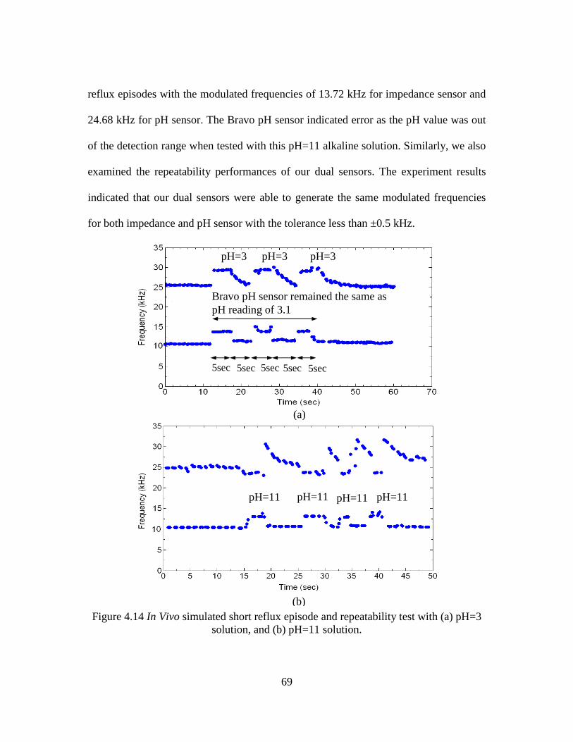
69

reflux episodes with the modulated frequencies of 13.72 kHz for impedance sensor and

24.68 kHz for pH sensor. The Bravo pH sensor indicated error as the pH value was out

of the detection range when tested with this pH=11 alkaline solution. Similarly, we also

examined the repeatability performances of our dual sensors. The experiment results

indicated that our dual sensors were able to generate the same modulated frequencies

for both impedance and pH sensor with the tolerance less than ±0.5 kHz.

Figure 4.14 In Vivo simulated short reflux episode and repeatability test with (a) pH=3 solution, and (b) pH=11 solution.

(a)

(b)

pH=3 pH=3 pH=3

5sec 5sec 5sec 5sec

Bravo pH sensor remained the same as pH reading of 3.1

5sec

pH=11 pH=11 pH=11 pH=11

70

4.3.2.5 In Vivo Experiment Results and Data Interpretation

Figure 4.15 shows the typical measurement results of our Batteryless

Endoluminal Sensing Telemeter (BEST) capsule with integrated impedance and pH

sensor, and compars to the performances of the Bravo pH sensor capsule in the

esophagus. The frequency readings of the pH sensors were converted to the pH readings

using the calibration curve and the impedance sensor data were presented as the

modulated frequency shifts. The Bravo readings were recorded discretely along with the

simulated reflux episodes to verify the pH readings measured by our pH sensor in the

esophagus. The experiment results showed good correlation on the pH readings between

our pH sensor and Bravo pH sensor with differences less than ±0.4. However, Bravo

failed to indicate the correct pH value for the alkaline solution with a pH value of 11.

The reading on the Bravo indicated an error symbol “HI” while our pH sensor indicated

a pH value of 10.8. It was also noted that the readings of our pH sensors were measured

continuously along with each simulated reflux episode. After each episode, the readings

of our pH sensor gradually came back to its original state, indicating the period of reflux

episodes as well, while the readings of Bravo pH sensor remained the same due to the

constraint of its low data sampling rate.

Between flushing events, the frequencies from the impedance sensor dropped

and pH sensor gradually decreased when the liquid left the electrode. However, the

frequencies did not go back to the baseline frequency because there were still some

liquid residues left on the electrodes. The frequency drop amounts were also not the

same after every flushing due to unpredictable amounts of residue that might stay on the

71

electrodes. The frequency drops however were sufficiently clear to identify every

flushing episode. The phenomena of liquid residue left on the electrode were also

observed in the pH values of Bravo. After the liquid flushing events, tap water flushing

was not able to bring the pH values back to 7. This indicated that there was a

phenomenon of residue left on both devices when doing in vivo animal experiment.

The measurement results of our impedance sensor for the episodes with the pH

values of 2, 3, and 5 were with the frequencies of 14.99, 14.08, and 13.51 kHz,

respectively. The experiment results showed that when the tested solutions were more

acid, which contained more H+ ions in the solutions, the modulated frequency of our

impedance sensor were higher. To demonstrate that the impedance sensor is sensitive to

the ion concentrations, we used salt water, that contained a lot of ions, and DI water,

that contained almost zero ions in the solution, to do the experiment. The modulated

frequency of impedance sensors were with the values of 15.89 and 10.85 kHz, for salt

water and DI water, respectively. The salt water solution which has low impedance

generated a high modulated frequency; however, it did not significantly change the pH

values therefore cannot be detected from the pH sensor. Also, when the tap water with a

pH value of 7 was flushed into the esophagus twice to serve as multiple reflux episodes,

the readings of Bravo pH sensor did not indicate these events while our impedance

sensor indicated these two episodes with the frequency shifts of 12.51 and 12.35 kHz,

respectively.

72

Figure 4.15 In vivo animal experiment results.

73

Two liquid juices, orange juice with pulp, OJ(P), and orange juice without pulp,

OJ(W), with the measured pH values of 4.1 and 4.2, were also used to test the sensor

performances. The purpose of using these two liquids was to examine whether the pulp

materials will affect our measurement results or not. The experiment results showed that

the modulated frequencies of our impedance sensor were with the frequencies of 13.81

and 13.78 kHz for OJ(P) and OJ(W), respectively. The pH readings of our pH sensor

were also around the pH values of 4 for both OJ(P) and OJ(W). The experiment results

suggested that the pulp materials didn’t make differences on the sensor performances.

In Figure 4.16(a), the pH readings for Bravo pH sensor and our pH sensor are

plotted as a function of each tested episode. It indicats that our pH sensor readings had

good agreement with the commercial Bravo pH sensor with pH value differences less

than ±0.4 in most of the cases. However, our pH sensor can indicate the alkaline

solution with a pH value of 10.8 while Bravo pH sensor gave the error readings.

Furthermore, we used the impedance calibration curve to convert the tested simulated

episodes to pH values. The purpose of doing this was to find out the correlation between

the pH values and the impedance sensor readings. In Figure 4.16(b), it shows that the

impedance sensor can also indicate pH values of the test liquids. However, for the

solution with a pH value of 11, the impedance sensor readings might be confusing. It

could be converted into pH=4 or pH=11. The modulated frequencies for both cases

were similar because they might contain similar amount of the ion in the solutions.

Furthermore, the impedance sensor gave the wrong pH readings on salt water and DI

water. These again pointed out the importance of the integration of both pH sensor and

74

impedance sensor into a single sensing device.

Figure 4.16 pH values of the events (a) pH sensor, and (b) impedance sensor.

(b)

(a)

75

Figure 4.17 Statistical data analysis of (a) pH sensor and (b) impedance sensor.

(a)

(b)

76

4.3.2.6 Data Analysis

We carried out the experiments on three different days and each day we

performed the experiments on one pig to validate the system performances. We

obtained 5 sets of data and performed the statistic data analysis to verify the reliability

of our sensing system. First, we calculated the mean values from the readings of BEST

pH sensor and BEST impedance sensor for each tested solutions and calculated the

corresponding standard deviations. Figure 4.17 showed the analysis results. For BEST

impedance sensor, we obtained the standard deviation less than 0.16 kHz among all the

tested liquids except for tap water with the standard deviation values of 0.37 kHz. For

BEST pH sensor, we obtained less than 0.33 on the pH value variation, except for tap

water with the pH value variation of 0.48. The reason that tap water had larger standard

deviation was because it was used to clean out the residue. Our experiment results

indicated that the reliability of our dual sensors is pretty good with the standard

deviations less than the frequency shift of 0.16 kHz for impedance sensor, and the pH

value of 0.33 for pH sensor in most of the cases.

4.4 Summary

An implantable, batteryless, and wireless capsule integrated with impedance and

pH sensors for gastroesophageal reflux monitoring has been designed, fabricated and

validated. The approach on the integration of impedance and pH sensors provides a

complete solution for gastroesophageal reflux monitoring. Our wireless device does not

require a battery so there is no time limit for monitoring compared to battery powered

wireless devices. The device was tested in live pigs demonstrating the feasibility and

77

accuracy of detecting various simulated reflux episodes. The read range was

demonstrated with the reader at a 13-cm distance from the transponder in a beaker and

through the pigs’ body with an average chest perimeter of 78.74 cm. The signals kept

the same accuracy even under the attacks of motion artifacts. Our dual sensor can

identify the short reflux episode while the commercial pH sensor gave the same reading

during the short test period. The experiment results showed comparable performance to

the commercial wireless pH sensors with our pH sensor. Furthermore, the impedance

sensing method was able to detect non-acid reflux episodes as it could distinguish air,

acid, alkaline and salt solutions from water. The experiment results showed that our

dual sensor can detect both acid and non-acid reflux episodes providing both impedance

and pH sensor information simultaneously for GERD monitoring.

78

CHAPTER 5

CONCLUSIONS AND FUTURE WORK

5.1 Conclusions

In this dissertation, a batteryless, wireless sensing platform was investigated.

The sensing platform consists of a sensing device and a remote reader system. The

remote reader radiates the RF energy to power up the sensing device and records the

data from it. The sensing device can process either resistive, capacitive, or voltage type

of sensor inputs and encode into frequency shifts without the need of battery in it. The

sensing platform is robust enough to provide the immunity to the motion artifacts

suitable for physiological environment usage. The system performances were

demonstrated in two medical applications, one is external and the other one is internal.

A pressure sensor array that can monitor the pressure profile for pressure sore

development monitoring is for external application and an implantable integrated

impedance and pH sensor capsule for gastroesophageal reflux monitoring is for internal

application.

For external physiological sensing application, a batteryless wireless

piezoresistive pressure sensing system was presented for applications of monitoring

pressure sore development in paralyzed patients who might be in beds or in

wheelchairs. A piezoresistive force sensing resistor was chosen as the sensing element

79

due to its good sensitivity. The mechanical design knowledge was exercised first to

convert the force signals, measured by the force sensing resistors, into pressure data.

The sensing elements were then arranged in an array format with spatial design

consideration to monitor the pressure distribution profile accordingly. The sensors were

able to identify high pressure points dynamically. Stability tests of the sensor were

carried out for long-term monitoring purposes. The experimental results indicated that

the drifting of reading was smaller than the readings of high-pressure indications so the

sensors can be used for a long period of time. Then the electrical design knowledge was

employed for sensor interfacing circuit. The sensing device includes an energy

harvesting circuit, a force sensing resistor, a resistance-to-frequency converter, and an

antenna. The reader provides power to the device remotely and measures the sensor

values in terms of frequency shift simultaneously. The experimental results showed

good linearity, sensitivity, and resolution in the tested pressure range.

For internal physiological sensing application, an implantable, batteryless, and

wireless capsule integrated with impedance and pH sensors for gastroesophageal reflux

monitoring has been designed, fabricated and validated. The prototype of dual sensor

transponder was implanted into esophagus, wirelessly transmitting the modulated sensor

signals to the external reader. The impedance sensor picked up every simulated reflux

episode and the pH sensor recognized the pH readings of each reflux episode. The

wireless device does not require a battery so there is no time limit for monitoring,

superior to the commercial wireless pH sensors that are limited by battery life time. The

device was tested in live pigs and demonstrated the feasibility and accuracy of detecting

80

the simulated reflux episodes in real physiological environment. The signals kept the

same accuracy without being affected by motion artifacts. The experiment results

showed superior performance than the commercial wireless pH sensors with our pH

sensor. Furthermore, the impedance sensing method was able to detect non-acid reflux

episodes as it could distinguish air, acid, alkaline and salt solutions from water. Our

dual sensor responded to the short simulated reflux episodes immediately while the

commercial wireless pH sensor remained the same reading due to the slow sampling

rate of the device. Our batteryless, wireless and integrated sensor capsule system can

detect acid and nonacid reflux episodes providing both impedance and pH information

simultaneously for GERD monitoring.

5.2 Future Work

In this research, we used time-multiplexing scheme to coordinate multiple

sensor input data. Our system was designed to be simple using a time switch

mechanism to switch between sensor input data. The purpose of this was to minimize

the size of device and to reduce the power consumption with less active components

added into the circuit, especially when our sensing device was designed to be

implantable. However, by using time-multiplexing scheme, each sensor was shared one

time slot within every scanning cycle. Some data points measured from the sensor were

lost when not in that time slot. Thus, we would like to lay out the other topology for the

integration of multiple sensors as future work when transistor level integrated circuit

design tool is used to realize the transponder circuit in a smaller scale.

81

Figure 5.1 Multiple sensor integration topology. (a) Transmitter block diagram. (b) Spectrum of multiple sensors. (c) Spectrum of transmitted sensor signals.

Frequency generator

#1

Frequency generator

#2

Frequency generator

#N

Sensor #1

Sensor #2

Sensor #N

…

∑

…

+ +

+

×

Accos(2πfct) Carrier wave

(a)

T(f)

S(f)

f

≈

fc

T(f)

fc+fs1

fc+fs2

fc+fsN

fc-fs1

fc-fs2

fc-fsN

(c)

fs1 f fs2 fsN

Ws1 Ws2 WsN

W S(f)

(b)

82

Figure 5.1(a) shows the transmitter block diagram on the topology for multiple

sensor integration. The output frequencies from frequency generators are modulated by

sensors first. They are designed to have different modulated frequencies of, fs1, fs2, and

fsN, with bandwidths of Ws1, Ws2, and WsN, correspondingly, and they are not overlapped

to each other. In frequency domain, the frequency spectrums of those sensors can be

added up and are considered as a baseband signal with bandwidth of W, as shown in

Figure 5.2(b). Then, the baseband signal spectrum, S(f), is multiplied by the carrier

wave Accos(2πfct) with carrier frequency, fc, and the modulated sensor signal is ready to

be transmitted with the transmitted spectrum T(f), as shown in Figure 5.1(c). On the

receiver end, we need to demodulate the received signal and extract the sensor signals

correctly. Figure 5.2 shows the receiver block diagram. The received signal with the

spectrum R(f) is first multiplied by the carrier wave frequency. Then the band pass filter

with the center frequencies, fs1, fs2, and fsN are designed with the bandwidth of W to

extract the sensor signal, correspondingly.

Figure 5.2 Receiver block diagram to extract multiple sensor signals.

R(f) Band Pass filter fs1

Sensor #1

…

×

Accos(2πfct) Carrier wave

Band Pass filter fs2

Band Pass filter fsN

Sensor #2

Sensor #N

83

In Figure 5.1 and Figure 5.2, the main topology of the transceiver for multiple

sensor integration is depicted. The future work should focus on implementing the

topology to demonstrate the capability of this architecture for system integration.

The miniaturization of the circuitry into a single chip would also be the future

work and it can be done either by using a custom ASIC chip or transistor level

integrated circuit design. The small size of the chip allows the integration of multiple

sensors without adding extra size on the transponder while using board level circuit

design has its limitations. Furthermore, with digital circuit design, the sensor data could

contain identification information for better tracking of the information.

84

APPENDIX A

A SYSTEMATIC APPROACH TO OPTIMIZE THE POWERING EFFICIENCY OF INDUCTIVE LINKS FOR BIOMEDICAL APPLICATIONS

85

A.1 Introduction

Passive RFID technology that uses the inductive links for RF powering and data

transmission between the reader and transponder realizes a batteryless, and wireless

communication system [A.1]. Moreover, to supply energy to implanted devices,

wireless electromagnetic energy transfer is an effective and proven technique [A.2-

A.4]. Low-frequency electromagnetic energy transfer is currently used in cochlear

implants [A.5-A.6], radio-frequency identification (RFID) implants [A.7], retinal

prosthetics [A.8], and neurostimulators [A.9-A.11], etc. However, how to improve the

powering efficiency, especially for implantable biomedical systems, has been an

important issue for researchers to solve [A.12, A.13]. For small implanted applications,

where volume limitations constraint the size of the receive coil, the practical range of

energy transfer is limited to a few centimeters. So, researchers have worked on design

optimization and invention of new techniques to increase the read distance and coupling

efficiency. However, the optimization approaches were either confined to some specific

constraints [A.14-A.20], or used consecutive planning methods to optimize the system

performances [A.21-A.23]. Therefore, in this section, a systematic approach was

attempted to optimize the powering efficiency based on one governing equation that

will fine tune all the parameters to optimize the system performances. Theoretical

assumptions and mathematical formula derivations were performed first and followed

by the experiment results to verify the correctness and completeness of the theoretical

86

modeling approaches.

A.2 Equivalent Circuit

Figure A.1 shows the equivalent circuit of inductive coupling resonant circuit. It

consists of two coil antennas with the inductance values of L1 and L2, an AC source Vin

with specified operating frequency, f0, and two tuning capacitors, C1 and C2, calculated

from the formula of resonant frequency

(A.1)

M represents the mutual inductance between two coil antennas while it can be

calculated by

(A.2)

where k is the coupling coefficient that varies between .

k=0 means full decoupling, that might due to great distance or magnetic shielding, and

k=1 means total coupling while both coils are subject to the same magnetic flux.

Equivalent series resistors (ESR), R1 and R2, account for the resistance values of the

inductors for reader and transponder, respectively, and RACload represents the load

impedance of the transponder circuit.

LCf

π2

10 =

21 LLkM ⋅=

10 ≤≤ k

Figure A.1 Equivalent circuit of inductive coupling resonant circuit. Reader Transponder

87

A.3 Formula Derivation

To optimize the coupling coefficient of the resonant circuit, we define the

coupling efficiency, ηc, as the ratio of power received by RACload versus the power drawn

from the input source Vin.

(A.3)

where the voltage gain expression from Vin to Vout can be expressed as [A.24, A.25]

(A.4)

and angular frequency .

By plugging (A.4) into (A.3), an expression for ηc can be derived as

(A.5)

Knowing the facts that the values of R1, R2, L2, and mutual inductance, M, will vary

while the number of the turns of the coil antenna change; we need to find the

expressions to describe their relationships. In the literatures [A.21-A.23, A.26], the

equations to describe the relations between number of turns and the parameters, such as

self inductance, L, mutual inductance, M, and equivalent series resistance, R, can be

ACloadin

out

in

ACload

out

Vin

outC R

R

V

V

R

V

R

V

P

P 1

2

1

2

2

2

2

===η

( ) ( )20

220

121

220

MR

LRRR

ML

V

VA

ACload

in

outV

ωωω

++

==

( ) ( ) ACload

ACload

C R

R

MR

LRRR

ML 1

2

20

220

121

220

++

=

ωωω

η

00 2 fπω =

88

found as

(A.6)

(A.7)

(A.8)

where N represents the number of turns of the coil antenna; L0 and R0 represent the

single-turn resistance and inductance; rR and rTag represent the radii of reader and tag

coil antennas; and x represents the distance between two antennas. Using (A.6), (A.7),

and (A.8) in tandem with (A.5), the coupling efficiency formula can be derived as

(A.9)

This formula contains the parameters, such as N1 and N2, which give us some degrees of

freedom to perform the optimization strategy. Therefore, we took the derivative of ηc

with respect to N1 and N2, and set the equations equal to zero to find their optimal

values. By setting , and solving for N2, we can get

(A.10)

Similarly, by setting , and solving for N1, we can get

02LNL =

( )322

2221

2 xr

rrNNM

R

RTag

+=

µπ

0NRR =

( )( )

( )ACload

R

RTag

ACload

R

RTag

C R

RN

xr

rrNN

R

LNRNRNRN

LNxr

rrNN

101

2

2

322

2221

0

2

20220

101202101

2022322

22212

0

2

2

+++

+=

µπω

ω

µπω

η

02

=∂∂N

cη

3220

20

202

2

L

RRN ACload

ω=

01

=∂∂N

cη

89

(A.11)

(A.10) and (A.11) describe the behaviors about number of turns of the coil antennas on

the transponder and reader, respectively.

First, we explored the theoretical plot of N2 based on equation (A.10). However,

to begin with the optimization process, we need to fix some parameters first. Since the

operating frequency is usually defined by the regulation, we fixed the frequency at 1.34

MHz first; due to the fact that the recommended maximum permissible exposure (MPE)

of magnetic field is the highest in the frequency ranges from 1.34 MHz to 30 MHz

[A.27]. Then, the size of the transponder coil antenna was determined by the size of our

PCB board design. The area was around 4.5 cm2, so we can calculate the transponder

radius with the value of 1.2 cm. We made the coil antenna by using the AWG 34

magnet wire. Then, we made a single-turn circular shape coil antenna with the radius

1.2 cm and used the impedance meter (HP 4192AF) to measure its parameters, R20, L20,

and the Quality factor (Q) with the values of 0.262 Ω, 0.283 µH, and 8.8, respectively.

With those parameters, we were ready to explore the theoretical plot of N2 as a function

of different RACload value.

( )

( )

2

2/322

222

0

22020

1022010

1

2

+

+=

xr

rrN

R

LNRNRR

N

R

RTag

ACload

µπω

ω

90

Figure A.2 Theoretical plot on N2 as a function of RACload.

Figure A.2 shows the theoretical plot on the number of turns, N2, as a function of

RACload. When the load impedance RACload increases, the required number of turns, N2,

also needs to be increased, therefore, more voltage can be induced in the transponder.

The induced voltage, V, in the transponder antenna coil can be found as

(A.12)

where Φ is the total magnetic flux through surface of transponder antenna coil.

When the RACload were with the resistance values of 100, 200, 400, 600, 800, 1000,

1200, 1400, and 1600 kΩ, the required numbers of turns, N2, were with the values of 21,

27, 34, 39, 43, 46, 49, 51, and 54, respectively. Note that the values of N2 were round

into the closest integer.

Then, we would like to explore the theoretical plot of N1 based on the equation

(A.11). Also, equation (A.13) can be obtained from (A.11) under the assumption when

x>>r R,

dt

dNV

Φ−=

91

Figure A.3 Theoretical plot on N1 as a function of rR.

(A.13)

To explore the theoretical plot of N1, we had L20=0.283 µH, R20=0.262 Ω, Q=8.8 and

rTag=1.2 cm. Then, we chose a pair of RACload and N2 with the values of 100 kΩ and 21

earlier from tag. To proceed with the verification process, we fixed the distance

between the reader and transponder at the distance of 10 cm. Then, a circular shape coil

antenna with the radius of 1cm was made from AWG 26 magnet wire. The measured

equivalent series resistance of single-turn resistor, R10, was with the value of 0.051 Ω.

Note that the resistance values for different size of coil antennas will be proportional to

their radii. Now, we can plot the theoretical plot of N1 as a function of different radii, rR.

First, we plotted equation (A.11) and the curve was shown in Figure A.3.

We also plotted equation (A.13) and obtained the curve of N1 as a function of

different radii of reader coil antennas, as shown in Figure A.4.

( )

R

RTag

ACload rx

x

rrN

R

LNRNRR

N >>

+= ,

2

2

6

222

0

22020

1022010

1µπ

ω

ω

92

Figure A.4 Theoretical plot on N1 as a function of rR under the assumption when x>>r R.

A.4 Experiment Results

A.4.1 Measured Parameters Approach

To verify the theoretical plot, the experiments were performed on the test bench

circuit mentioned in Figure A.1. N1 curves were examined first in the following

procedures. First, the reader and transponder coil antennas were positioned in parallel

apart from each other with a distance of 10 cm. The resonant frequency, f0, was set to

the frequency of 1.34 MHz, the parameters on the transponder, such as rTag, RACload, N2,

L2, and the calculated tuning capacitor, C2, were with the values of 1.2 cm, 100 kΩ, 22,

21.45 µH, and 700 pF, respectively. Then, a combination of various numbers of turns

coil antennas were made on different sizes of the reader frames with the radii of 4, 5, 6,

7, 8, and 9 cm. The inductance values of each combination were measured by

impedance meter and the values of tuning capacitor, C1, were calculated

correspondingly. Then, the oscilloscope was used to measure the output voltage across

93

0 2 4 6 8 10 120.00

0.05

0.10

0.15

0.20

0.25

0.30

0.35

4cm5cm6cm7cm8cm9cm

Figure A.5 Measurement results on the combinations of N1 and rR to find optimal Vout.

the RACload to find out which combination gave the optimal output voltage.

Figure A.5 shows the measurement results on the combinations of N1 and rR

with their corresponding output voltage Vout. The experiment results showed that the

optimal output voltage was with the value of 0.32 V on the combination of the radius of

8cm along with 4-turns reader antenna. Hence, we plotted the measurement results on

the combinations of N1 and rR that gave the maximum output voltage along with

equation (A.11) and equation (A.13), as shown in Figure A.6. Note that the values are

rounded into the closest integers. Obviously, the experiment results didn’t match with

either one of the theoretical estimation equations. However, equation (A.13) is closer to

the measurement results. There were some issues that might contribute to this

discrepancy, for example, we can only use the tuning capacitors with the closest value

to the theoretical ones while they are available. The coil antenna quality wound around

N1

Vou

t

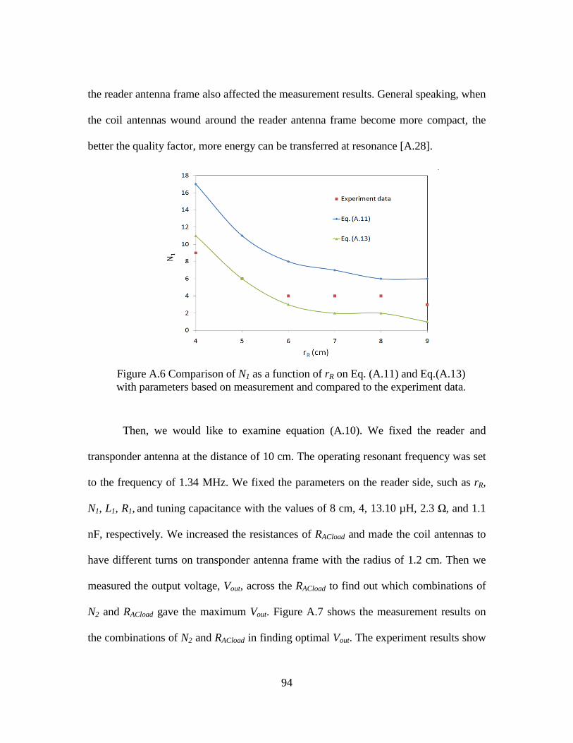
94

the reader antenna frame also affected the measurement results. General speaking, when

the coil antennas wound around the reader antenna frame become more compact, the

better the quality factor, more energy can be transferred at resonance [A.28].

Then, we would like to examine equation (A.10). We fixed the reader and

transponder antenna at the distance of 10 cm. The operating resonant frequency was set

to the frequency of 1.34 MHz. We fixed the parameters on the reader side, such as rR,

N1, L1, R1, and tuning capacitance with the values of 8 cm, 4, 13.10 µH, 2.3 Ω, and 1.1

nF, respectively. We increased the resistances of RACload and made the coil antennas to

have different turns on transponder antenna frame with the radius of 1.2 cm. Then we

measured the output voltage, Vout, across the RACload to find out which combinations of

N2 and RACload gave the maximum Vout. Figure A.7 shows the measurement results on

the combinations of N2 and RACload in finding optimal Vout. The experiment results show

Figure A.6 Comparison of N1 as a function of rR on Eq. (A.11) and Eq.(A.13) with parameters based on measurement and compared to the experiment data.

95

that when the RACload was with the resistance of 0.6 MΩ and with N2=44 gave the

maximum Vout with the reading of 0.42 V.

We plotted the measurement results on the pairs of RACload and N2 that gave the

maximum output voltage along with equation (A.10), as shown in Figure A.8. Again,

the experiment results didn’t match with the theoretical estimation. However, the trends

of the plots for experiment data and theoretical estimation were both mono tone

increasing. The values of N2 increased along with the increments of RACload, therefore

more voltage can be induced to drive larger load impedance. Since the parameters we

used to plug into the equations were based on the measurement data, there might be

some errors occurred either due to the equipment limitations or simply measurement

errors. Therefore, we explored the theoretical parameters of the coil antenna on its self

inductance values and equivalent series resistances in next section.

20 30 40 50 60 700.2

0.25

0.3

0.35

0.4

0.45

0.1M

0.2M0.4M

0.6M

0.8M

1.0M

1.2M1.4M

1.6M

Figure A.7 Measurement results on the combinations of N2 and RACload to find optimal Vout.

N2

Vou

t

96

A.4.2 Theoretical Parameters Approach

A.4.2.1 AC Resistance

When the wire of the coil antenna is used at high frequency, its resistance value

will increase due to the skin effect of the conductor wire [A.29]. The formula of AC

resistance, Rac, that describe this phenomenon can be found as [A.30]

(A.14)

where rw is the radius of the wire, δ is the skin depth, σ is the conductibility of the

material, l is the total length of the wire, f is the frequency, µ is the permeability.

The skin depth formula can be found as

(A.15) µσπ

δf

1=

πσµ

δσπf

r

l

r

lR

wwac 22

=≈

Figure A.8 N2 as a function of RACload on Eq. (A.10) with parameters based on measurement and compared to the experiment data.

97

A.4.2.2 Inductance of Circular Antenna

Figure A.9 shows a single-turn circular coil antenna with its radius of r and the

wire diameter of 2rw.

Then, the low frequency inductance formula for a circular coil antenna can be found as

[A.30]

(A.16)

and K(k) and E(k) are the complete elliptic integrals of the first and second kind defined

as

(A.17)

where µr is the relative permeability.

( )

w

w

r

w

w

rr

rrrk

r

rrL

rkEkKk

rrL

−

−=

+−

×=

×+

−

−−×=

−

−

2

)(2

42

8ln104

10)()(2

12104

7

72

7

µπ

µππ , if r>r w

, if r>>r w

where

θθθ

θ ππ

dkkEk

dkK ∫∫ −=

−=

2/

0

222/

022

sin1)(,sin1

)(

Figure A.9 A single-turn circular coil antenna.

r

2rw

98

The high frequency inductance can be found as [A.30]

(A.18)

A.4.2.3 Experiment Results

Based on parameters from AWG wire chart [A.31], the single turn AC

resistance, R10 and R20, and inductance, L10 and L20, can be calculated as

Along with other parameters we obtained earlier, such as

By plugging those parameters into equations (A.10), (A.11) and (A.13) to have the new

curve on N2 as a function of RACload and N1 as a function of rR, respectively. Therefore,

we can obtain the new curves that were all based on the theoretical calculation. Then we

compared those new curves to the measurement results again. Figure A.10 shows the

curve of N1 as a function of rR based on equations (A.11) and (A.13) along with the

measurement data, while Figure A.11 shows the curve of N2 as a function of RACload

based on equation (A.10) along with the measurement results. However, the theoretical

( )

−

×=

−

−−×=

−

−

28

ln104

)()(2

12104

7

27

w

w

r

rrL

kEkKk

rrL

π

π , if r>r w

, if r>>r w

HL

R

HL

R

µ

µ

083.0

0136.0

11.0

04.0

10

10

20

20

=

Ω=

=

Ω=

Ω=

=

=

=

Ω=

=

50000

17

2.1

10

50000

3.1

2

ACload

Tag

ACload

R

N

cmr

cmx

R

MHzf

99

exploration plots still couldn’t match with the experiment results. Therefore, the third

approach of using the scale factor was introduced to adjust the theoretical curve trying

to describe the experiment data.

Figure A.11 N2 as a function of RACload on Eq. (A.10) with parameters based on calculation and compared to experiment data.

Figure A.10 Comparison of N1 as a function of rR plots on Eq. (A.11) and Eq. (A.13) with parameters based on calculation and compared to the experiment data.

100

A.4.3 Scale Factor Approach

Since the trends for both theoretical plots and the measurement data were the

same, there were just discrepancies between the two. The scale factors α, β, and t were

used to adjust our hypothesis equations to better fit the measurement results. The scale

factor, α, was used to scale the equivalent series resistance, R2, and the scale factor, β,

was used to scale the self inductance, L2,on the transponder side. The scale factor, t, was

used to scale up the equivalent series resistance, R1, on the reader side. Therefore the

new hypothesis equations became

(A.19)

(A.20)

(A.21)

Therefore, the new formulas for N1 and N2 can be derived as

(A.22)

(A.23)

The formula for N2 was scaled by a factor of , while the formula for N1 was

scaled by the factor of t.

1011

20222

2022

RtNR

LNL

RNR

=

=

=

β

α

3220

20

203

22

2

L

RRN ACload

ωβα

=

( )

( )

2

2/322

2220

2

2

2022

20210

1

22

+

+

=

xr

rrNf

RLfN

RNRr

tN

R

RTag

ACloadR

µπ

ππ

32β

α

101

Next, we would like to find out the values of the scale factor to see if they can

be used to adjust the theoretical curves to fit the measured data. The AWG 34 magnet

wire was used to make the transponder coil antenna with different number of turns, N2,

on the transponder frame with the radius of 1.2 cm. Then, we used impedance meter

(HP 4192AF) to measure the corresponding AC equivalent series resistance, R2, with

respect to different number of turns. Figure A.12 shows the plots of AC equivalent

series resistance, R2, as a function of N2, on the transponder side. The plot of the

theoretical value was explored based on the equation (A.19), while the single turn AC

equivalent series resistance, R20, was calculated earlier with a resistance of 0.04 Ω.

Then, the values of R2 were obtained by multiplying to the number of turns to the single

turn AC equivalent series resistance.

In Figure A.12, the theoretical value is too far away from the impedance meter

measurement data, especially when the number of turns increases to larger numbers.

This is due to the current in the adjacent coil wires cause a magnetic field resulting in an

asymmetric current distribution. Therefore, in order to determine the AC resistance

accurately, numerical methods have to be applied [A.22]. The theoretical values based

on the equation (A.8) are valid only when DC resistance is considered. In addition, the

scale factor, α, in this case will be varied with respect to different number of turns.

However, we still continued this process to see if we can obtain a value of β that can

compensate the value of α, so the final scale factor K= is able to fine tune and

complete our hypothesis equations.

32β

α

102

Thus, we continue to explore the theoretical plot for self inductance, L2, with

respect to different number of turns by using the equation (A.20). The values of L2 were

obtained by multiplying N22 to the single turn self inductance, L20. The single-turn self

inductance was with a value of 0.11 µH that we obtained earlier. Figure A.13 shows the

plots of self inductance, L2, as a function of N2. The inductance values of L2 were also

measured by the impedance meter and compared to the theoretical values. The

theoretical curve and the measurement data were not agreed to each other, especially

when the number of turns became too large. This is again due to the adjacent coil wires

generate a magnetic field resulting in an asymmetric current distribution [A.30].

Therefore, in order to determine the multi-turn self inductance accurately, numerical

methods have to be applied [A.32].

Figure A.12 Theoretical and measurement plots on R2 as a function of N2.

103

Overall, when we put together the scale factor α and β into the final scale factor

K= , and plot as a function of N2, as shown in Figure A.14. The final scale factor

still couldn’t help us to fine tune the theoretical curve to match with the measurement

data since its values vary with N2. When N2 increases, it requires larger scale factor that

will make the required number of turns even larger.

32β

α

Figure A.13 Theoretical and measurement plots on L2 as a function of N2.

Figure A.14 The scale factor K= 32β

α as a function of N2.

104

A.5 Summary

In this study, three different approaches were used to optimize the coupling

efficiency of inductive coupling resonant circuit. Those approaches were based on a

single governing equation derived from the system point of view. Under the

assumptions that the parameters, either measureable or can be calculated from formulas,

would be proportional to the number of turns of the coil antenna. The optimization

processes were based on the theoretical exploration of the formulas compared to the

physical measurement data. The optimization approaches used in this study didn’t

match with the measurement data; however, the efforts to optimize the coupling

efficiency of an inductive coupling resonant circuit from scientific point of view were

made. The methodology suggested a systematic way to characterize the parameters

toward the optimization of inductive coupling resonant circuit.

To continue this research, some issues need to be exercised, such as the quality

of the coil antenna made, the tuning capacitances used, and the limitations of the

equipments, etc. These factors also need to be taken into consideration so that the

discrepancies between the measurement data and the theoretical exploration would be

minimized. In the mean time, a numerical method that determines the multi-turn self

inductance and equivalent series resistor needs to be studied to relate the theoretical and

measurement data.

105

APPENDIX B

A BENCHTOP SPECTRUM ANALYZER LABVIEW PROGRAM

106

Auto Power Spectrum

The two-sided power spectrum is computed from the FFT as follows

where FFT*(signal) denotes the complex conjugate of FFT(signal) and N is the number

of points in the signal taken into calculation.

Frequency Estimate

Estimated frequency of the peak in the input Power Spectrum and is computed as

for j = I – span/2, …I + span/2,

where I = peak index, Power Spectrum (j) = power at j, and df = frequency span width.

( )2

)()(

N

signalFFTsignalFFTfSsignal

∗•=

( )( )∑

∑ ∗∗=

)(_

)()(__

jspectrumPower

dfjjspectrumPowerfrequencyEstimate

107

REFERENCES

[1.1] John Enderle, Susan Blanchard, and Joseph Bronzino, Introduction to

biomedical engineering, Elsevier Academic Press, 2nd edition, 2005.

[1.2] R.S. Khandpur, Biomedical instrumentation: technology and applications,

McGraw-Hill, 1st edition, 2005.

[1.3] Tatsuo Togawa, Toshiyo Tamura, and P. Ǻke Öberg, Biomedical transducers

and instruments, CRC PRESS, 1st edition, 1997.

[1.4] P. Åke Öberg, Tatsuo Togawa, and Francis A. Spelman, Sensors Applications,

Volume 3, Sensors in Medicine and Health Care, Wiley-VCH, 1st edition, 2004.

[1.5] Rogier A.M. Receveur, Fred W. Lindemans, and Nicolaas F. de Rooij,

"Microsystem technologies for implantable applications," Journal of

Micromechanics and Microengineering, Vol. 17, pp. R50–R80, 2007.

[1.6] Gregory T. A. Kovacs, Micromachined transducers sourcebook, McGraw-Hill,

1st edition, 1998.

[1.7] K. Finkenzeller, RFID handbook: fundamentals and applications in contactless

smart cards and identification, Chichester, England, New York, Wiley, 2nd

edition, 2003.

[1.8] Steven Shepard, RFID: Radio frequency identification, McGraw-Hill, 1st

edition, 2004.

[1.9] Dennis E. Brown, RFID implementation, McGraw-Hill, 1st edition, 2006.

108

[1.10] Amy C. Richards Grayson, Rebecca S. Shawgo, Audrey M. Johnson, Nolan T.

Flynn, Yawen Li, Michael J. Cima, And Robert Langer, "A BioMEMS review:

MEMS technology for physiologically integrated devices," Proceedings of the

IEEE, Vol. 92, No. 1, pp. 6-21, January 2004.

[1.11] F.E.H. Tay, Microfluidics and bioMEMS applications, Kluwer, 1st edition, 2002.

[1.12] Robert S.H. Istepanian, Swamy Laxminarayan, and S. Pattichis Constantinos,

M-health: emerging mobile health systems, Springer, 1st edition, 2005.

[1.13] Krzysztof Iniewski, Wireless technologies: circuits, systems, and devices, CRC,

1st edition, 2007.

[1.14] IEEE 802.15 Working Group for Wireless Personal Area Networks (WPANs)

[1.15] Guang-Zhong Yang and M. Yacoub, Body sensor networks, Springer, 1st

edition, 2006.

[1.16] T. O'Donovan, J. O'Donoghue, C. Sreenan, P. O'Reilly, D. Sammon, and K.

O'Connor, “A context aware wireless body area network (BAN),” Proc. 3rd

International Conference on Pervasive Computing Technologies for Healthcare,

2009.

[2.1] S. Chatzandroulis, D. Tsoukalas, and P.A. Neukomn, “Miniature pressure

system with a capacitive sensor and a passive telemetry link for use in

implantable applications,” Journal of Microelectrmmechanical Systems, 9(1),

pp. 18-23, 2000.

[2.2] C. Hierold, B. clasbrummel, D. Behrend, T. Scheiter, M. Steger, K. Oppermann,

H. Kapels, E. Landgraf, D. Wenzel, and Etzrodt, “Implantable low power

109

integrated pressure sensor system for minimal invasive telemetric patient

monitoring,” Proceedings of the IEEE Micro Mechanical Systems (MEMS),

Heidelberg, Germany, pp. 568-573, Feb. 1998.

[2.3] A. DeHennis, and K. D. Wise, “A double-sided single-chip wireless pressure

sensor,” in Proceedings of the IEE Micro Electro Mechanical Systems

Conference, Las Vegas, NV, pp. 252-255, Feb. 2002.

[2.4] Q. Huang, and M. Oberle, “0.5-mW passive telemetry IC for biomedical

applications,” IEEE of Solid-State Circuits, Vol. 33, pp937-946, 1998.

[2.5] David W. Kuhns, M., and Benton Free, “System and methods for remote

sensing using inductively coupled transducers” Patent, Pub. No.: 2008/0012579

A1, Pub. Date: Jan.17, 2008.

[2.6] Roy Want, “Enabling ubiquitous sensing with RFID,” Computer, 37(4), pp. 84-

86, 2004.

[2.7] Olivier Chevalerias, Terence O’Donnell, Daithi Power, Neil O’Donovan, Gerald

Duffy, Gary Grant, and Sean Cian O’Mathuna, “Inductive telemetry of multiple

sensor modules,” IEEE Pervasive Computing, 4(1), pp. 46-52, 2005.

[2.8] Matthai Philipose, Joshua R. Smith, Bing Jiang, Alexander Mamishev, Sumit

Roy, and Kishore Sundara-Rajan, “Battery-free wireless identification and

sensing,” IEEE Pervasive Computing, 4(1), pp. 37-45, 2005.

[2.9] S. Chatzandroulis and D. Tsoukalas, “Capacitance to frequency converter

suitable for sensor applications using telemetry,” Analog Integrated Circuits and

Signal Processing, Volume 27, Numbers 1-2, pp. 31-38, 2001.

110

[2.10] T. Roz and V. Fuentes., “Using low power transponders and tags for RFID

applications,” 2004.

[2.11] Hongwei Shen, Lilan Li, and Yumei Zhou, “Fully integrated passive UHF RFID

tag with temperature sensor for environment monitoring,” ASIC, 2007. ASICON

’07. 7th International Conference on, pp. 360-363, 2007.

[2.12] Tomohiro Yamada, Takumi Uezono, Hirotaka Sugawara, Kenichi Okada,

Kazuya Masu, Akio Oki, and Yasuhiro Horiike, “Battery-less wireless

communication system through human body for in-vivo healthcare chip,” IEEE

Topical Meeting on Silicon Monolithic Integrated Circuits in RF Systems, pp.

322-325, 2004.

[2.13] William H. Moore, Daniel P. Holschneider, Tina K. Givrad, and Jean-Michel I.

Maarek, “Transcutaneous RF-powered implantable minipump driven by a Class-

E transmitter,” IEEE Trans. Biomed. Eng., 53(8), pp. 1705–1708, 2006.

[2.14] Radislav A. Potyrailo and William G. Morris, “Multianalyte chemical

identification and quantitation using a single radio frequency identification

sensor,” Analytical Chemistry, Vol. 79, No. 1, pp. 45-51, January 1, 2007.

[2.15] M. Nowak, N. Delorme, F. Conseil, and G. Jacquemod, “A novel architecture

for remote interrogation of wireless battery-free capacitive sensors,” Electronics,

Circuits and Systems, 2006. ICECS ’06. 13th IEEE International Conference on,

pp. 1236-1239, 10-13, Dec. 2006.

[2.16] Andrew D. DeHennis and Kensall D. Wise, “A fully integrated multisite

pressure sensor for wireless arterial flow characterization,” Journal of

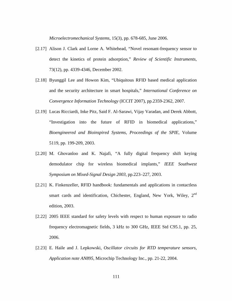
111

Microelectromechanical Systems, 15(3), pp. 678-685, June 2006.

[2.17] Alison J. Clark and Lorne A. Whitehead, “Novel resonant-frequency sensor to

detect the kinetics of protein adsorption,” Review of Scientific Instruments,

73(12), pp. 4339-4346, December 2002.

[2.18] Byunggil Lee and Howon Kim, “Ubiquitous RFID based medical application

and the security architecture in smart hospitals,” International Conference on

Convergence Information Technology (ICCIT 2007), pp.2359-2362, 2007.

[2.19] Lucas Ricciardi, Inke Pitz, Said F. Al-Sarawi, Vijay Varadan, and Derek Abbott,

“Investigation into the future of RFID in biomedical applications,”

Bioengineered and Bioinspired Systems, Proceedings of the SPIE, Volume

5119, pp. 199-209, 2003.

[2.20] M. Ghovanloo and K. Najafi, “A fully digital frequency shift keying

demodulator chip for wireless biomedical implants,” IEEE Southwest

Symposium on Mixed-Signal Design 2003, pp.223–227, 2003.



edition, 2003.

[2.22] 2005 IEEE standard for safety levels with respect to human exposure to radio

frequency electromagnetic fields, 3 kHz to 300 GHz, IEEE Std C95.1, pp. 25,

2006.

[2.23] E. Haile and J. Lepkowski, Oscillator circuits for RTD temperature sensors,

Application note AN895, Microchip Technology Inc., pp. 21-22, 2004.

112

[2.24] T. Ativanichayaphong, J. Wang, W. Huang, S. Rao, and J.-C. Chiao, “A simple

wireless batteryless sensing platform for resistive and capacitive sensors,” IEEE

Sensors 2007 Conference, Atlanta, Georgia, pp. 139-142, Oct. 26-28, 2007.

[2.25] P. Troyk, and M. Schwan, “Closed-loop class E transcutaneous power and data

link for microimplants,” IEEE Transactions on Biomedical Engineering, Vol.

39(6), pp. 589-599, June 1992.

[2.26] P.R. Troyk and G.A. DeMichele, “Inductively-coupled power and data link for

neural prostheses using a class-E oscillator and FSK modulation,” IEEE

International Conference Engineering in Medicine and Biology Society, Vol. 4,

pp. 3376-3379, Sept. 2003.

[2.27] N. Chaimanonart, D.J. Young, “Remote RF powering system for wireless

MEMS strain sensors,” IEEE Sensors Journal, Vol. 6(2), pp. 484-489, April

2006.

[2.28] Zoubir Hamici, Roland Itti, and Jacques Champier, “A high-efficiency power

and data transmission system for biomedical implanted electronic devices,”

Measurement Science and Technology, 7, pp. 192–201, 1996.

[2.29] P.R. Troyk, and M.A. Schwan, “Class E driver for transcutaneous power and

data Link for implanted electric device,” Medical & Biological Engineering &

Computing, 30, pp. 69-75, January 1992.

[2.30] Zhijun Tang, Yigang He, Zhouguo Hou, Bing Li, “The effects of antenna

properties on read distance in passive backscatter RFID systems,” Wireless

Communications and Trusted Computing, International Conference on Networks

113

Security, Vol. 1, pp.120-123, 2009.

[2.31] S.C.Q. Chen and V. Thomas, “Optimization of inductive RFID technology,”

Proceedings of the 2001 IEEE International Symposium on Electronics and the

Environment, pp. 82-87, 2001.

[2.32] microID® 125 kHz RFID System Design Guide, Microchip Technology Inc.,

2004.

[2.33] microID® 13.56MHz RFID System Design Guide, Microchip Technology Inc.,

2004.

[2.34] P. Sorrells, “Optimizing read range in RFID systems,” Electronics Design,

Strategy, News (EDN), pp.173-184, Dec 7, 2000.

[2.35] David Lee Hall, Sonya A. H. McMullen, Mathematical techniques in

microsystems data fusion, Norwood Massachusetts, Artech House Inc., 2nd

edition, 2004.

[2.36] Luca Catarinucci, Mauro Cappelli, Riccardo Colella, Luciano Tarricone, “A

novel low-cost icrosystems-tag for RFID applications in healthcare,”

Microwave and Optical Technology Letters, 50(11), pp. 2877 – 2880, August

2008.

[2.37] C.S. Fraser, M.R. Shortis, and G. Ganci, “Multi-sensor system self-calibration,”

SPIE Videometrics IV, Vol. 2598, pp. 2-18, 1995.

[2.38] Christopher Immer, Anthony Eckhoff, John Lane, Jose Perotti, John Randazzo,

Norman Blalock, and Jeff fiees, “Multisensor arrays for greater reliability and

accuracy,” NASA Tech Briefs, July 2004.

114

[3.1] C.W. Oomens, O.F.J.T. Bressers, E.M.H. Bosboom, C.V.C. Bouten, and D.L.

Bader, “Can loaded interface characteristics influence strain distribution in

muscle adjacent to bony prominences,” Computer Methods in Biomechanics and

Biomedical Eng., 6(3), pp. 171-180, 2003.

[3.2] C.W. Oomens, R.G. Breuls, C.V.C. Bouten, F.P.T. Baaijens, and D.L. Bader, “A

hierarchical approach to study damage evolution in skeletal muscle - a

contribution to pressure ulcer research,” Summer Bioengineering Conference,

pp. 299-300, 2003.

[3.3] C. Gehin, E. Brusseau, R. Meffre, P.M. Schmitt, J.F. Deprez, and A. Dittmar,

“Which techniques to improve the early detection and prevention of pressure

ulcers?,” Proceedings of the 28th IEEE, EMBS Annual International Conference,

pp. 6057-6060, 2006.

[3.4] M.W. Ferguson-Pell, “Seat cushion selection,” Journal of Rehab. Res. Dev.,

Clin. Suppl., pp. 49-73, 1990.

[3.5] J. Braden Barbara and Maklebust Joann, “Wound wise: preventing pressure

ulcers with the braden scale,” American Journal of Nursing, 105(6), pp. 70-72,

2005.

[3.6] J.G. Webster, Prevention of pressure sores: engineering and clinical aspects,

Adam Hilger, 1991.

[3.7] Y.K. Jan and D.M. Brienza, “Technology for pressure ulcer prevention,” Topics

in Spinal Cord Injury Rehabilitation, 11(4), pp. 30-41, 2006.

115

[3.8] V.C. Taylor, “Force sensing array: seating solutions through pressure mapping,”

Rehab & Community Care Management, p. 68, 1999.

[3.9] S.A. Crawford, B. Strain, B. Gregg, D.M. Walsh, and A.P. Porter-Armstrong,

“An investigation of the impact of the force sensing array pressure mapping

system on the clinical judgment of occupational therapists,” Clinical

Rehabilitation, 19(2), pp. 224-231, 2005.

[3.10] G.M. Yarkony, “Pressure ulcers: A review,” Archives of Physical Medicine and

Rehabilitation, 75, pp. 908-917, 1994.

[3.11] M.W. Ferguson-Pell, “Design criteria for measurement of pressure at

body/support interfaces,” Eng. In Medicine, 9(4), pp. 209-214, 1980.

[3.12] J.C. Löttersy, W. Olthuis, P.H. Veltink, and P. Bergveld, “The mechanical

properties of the rubber elastic polymer polydimethylsiloxane for sensor

applications,” J. Micromech. Microeng., 7, pp. 145-147, 1997.

[3.13] S.I. Yaniger, “Force sensing resistors: A review of the technology,” Electro. Int.,

pp. 666-668, 1991.



Sensors 2007 Conference, pp. 139-142, 2007.

[4.1] Peter J. Kahrilas and John E. Pandolifino "The epidemiology and

pathophysiology of gastroesphageal reflux disease," Managing failed anti-reflux

therapy, Chapter 1, pp. 1-14, 2006.

116

[4.2] Kenneth R. DeVault and Donald O. Castell, "Updated guideline for the

diagnosis and treatment of gastroesophageal reflux disease," American Journal

of Gastroenterology, Vol. 100, pp. 190-200, 2005.

[4.3] D. Sifrim, R. Holloway, J. Silny, Z. Xin, J. Tack, A. Lerut, and J. Janssens,

"Acid, nonacid, and gas reflux in patients with gastroesophageal reflux disease

during ambulatory 24-hour pH-impedance recordings," Gastroenterology,

120(7), pp. 1588-1598, 2001.

[4.4] I. Mainie, R. Tutuian, S. Shay, M. Vela, X. Zhang, D. Sifrim, and D.O. Castell,

"Acid and non-acid reflux in patients with persistent symptoms despite acid

suppressive therapy: a multicentre study using combined ambulatory

impedance-pH monitoring," An International Journal of Gastroenterology and

Hepatology, Vol. 55, pp. 1398-1402, 2006.

[4.5] Joshua J. Ofman, “The relation between gastroesophageal reflux disease and

esophageal and head and neck cancers: a critical appraisal of epidemiologic

literature,” The American Journal of Medicine, 111(8), pp. 124-129, 2001.

[4.6] F. Vela Marcelo and Michael F. Vaezi, "The role of multichannel intraluminal

impedance and pH monitoring in the diagnosis of gastroesophageal reflux

disease," US Gastroenterology Review, Issue II, pp.75-77, October 2007.

[4.7] R. Tutuian, M. Vela, S. Shay and D. Castell, “Multichannel intraluminal

impedance in esophageal function testing and gastroesophageal reflux

monitoring,” Journal of Clinical Gastroenterology, 37(3), pp. 206-215, Sept.

2003.

117

[4.8] Monika Kwiatek and John Pandolfino, “Prolonged reflux monitoring:

capabilities of bravo pH and impedance-pH systems,” Current GERD Reports,

Vol. 1, No. 3, pp. 165-170.

[4.9] J. Pandolfino, J. Richter, T. Ours, J. Guardino, J. Chapman and P. Kahrilas,

“Ambulatory esophageal pH monitoring using a wireless system,” The American

Journal of Gastroenterology, 98(4), pp. 740-749, April 2003.

[4.10] O. Kawamura, M. Aslam, T. Rittmann, C. Hofmann and R. Shaker, “Physical

and pH properties of gastroesopharyngeal refluxate: a 24-hour simultaneous

ambulatory impedance and pH monitoring study,” The American Journal of

Gastroenterology, 99(6), pp. 1000-1010, June 2004.

[4.11] D. Castell and M. Vela, “Combined multichannel intraluminal impedance and

pH-metry: an evolving technique to measure type and proximal extent of

gastroesophageal reflux,” The American Journal of Medicine, 11(8), pp. 157-

159, Dec. 2001.

[4.12] J. Gonzalez-Guillaumin, D. Sadowski, K. Kaler and M. Mintchev, “Ingestible

capsule for impedance and pH monitoring in the esophagus,” IEEE Transactions

on Biomedical Engineering, 54(12), pp. 2231-2236, Dec. 2007.

[4.13] G. Scarpulla, S. Camilleri, P. Galante, M. Manganaro and M. Fox, “The impact

of prolonged pH measurements on the diagnosis of gastroesophageal reflux

disease: 4-day wireless pH studies,” The American Journal of Gastroenterology,

102(12), pp. 2642-2647, Dec. 2007.

118

[4.14] Y. Salvatore, S. MC. Vieira, B. Hauser, “Will esophageal impedance replace pH

monitoring? Review,” Pediatrics, 119(1), pp. 118-22, 2007.

[4.15] Steven Shay, “Esophageal impedance monitoring: the ups and downs of a new

test,” The American Journal of Gastroenterology, 99(6), pp. 1020-1022, June

2004.

[4.16] I. Hirano, “Modern technology in the diagnosis of gastroesophageal reflux

disease: bilitec, intraluminal impedance and bravo capsule pH monitoring,”

Alimentary pharmacology & therapeutics, 23(1), pp. 12-24, 2006.

[4.17] John E. Pandolfino, Marcelo F. Vela, “Esophageal-reflux monitoring,”

Gastrointestinal Endoscopy, Volume 69, Issue 4, pp. 767-986, April 2009.

[4.18] Radu Tutuian and Donald O. Castell, “Gastroesophageal reflux monitoring: pH

and impedance,” GI Motility online, 2006.


smart cards and identification, Chichester, England, New York, Wiley, 2003.

[4.20] E. Haile and J. Lepkowski, Oscillator circuits for RTD temperature sensors,

Application note AN895, Microchip Technology Inc., pp. 21-22, 2004.



Sensors 2007 Conference, Atlanta, Georgia, pp. 139-142, Oct. 26-28, 2007.

[4.22] G. Kim, M. Morgan, B. K. Hahm, A. Bhunia, J. H. Mun, and A. S. Om,

"Interdigitated microelectrode based impedance biosensor for detection of

119

salmonella enteritidis in food samples," Journal of Physics: Conference Series,

100, 052044, 2008.

[4.23] Alexander V. Mamishev, Kishore Sundara-Rajan, Fumin Yang, Yanqing Di,

and Markus Zahn, "Interdigital sensors and transducers," Proceedings of the

IEEE, 92(5), pp. 808-845, 2004.

[4.24] David R. Lide, CRC handbook of chemistry and physics, 86th edition, CRC

Press, 2005.

[4.25] I. Hirano, Q. Zhang, J. Pandolfino, and P. Kahrilas, "Four-day Bravo pH capsule

monitoring with and without proton pump inhibitor therapy," Clinical

Gastroenterology and Hepatology, 3(11), pp. 1083-1088, 2005.

[4.26] W.-D. Huang, J. Wang, T. Ativanichayaphong, L.-C. Hsu, S. Deb, M. Chiao and

J.-C. Chiao “Investigation of repeatability of sol-gel iridium oxide ph sensor on

flexible substrate,” SPIE Proc. Vol. 7269, 726916, 2008.

[4.27] 2005 IEEE standard for safety levels with respect to human exposure to radio

frequency electromagnetic fields, 3 kHz to 300 GHz, IEEE Std C95.1, 2006.

[4.28] K. Wise, D. Anderson, J. Hetke, D. Kipke, K. Najafi, “Wireless implantable

microsystems: high-density electronic interfaces to the nervous system,” Proc.

IEEE, 92(1), pp. 76-97, Jan. 2004.

[4.29] P. R. Troyk and G. A. DeMichele, “Inductively-coupled power and data link for

neural prostheses using a class-E oscillator and FSK modulation,” IEEE

International Conference Engineering in Medicine and Biology Society, Vol. 4,

pp. 3376-3379, Sept. 2003.

120

[4.30] N. Chaimanonart, D.J. Young, “Remote RF powering system for wireless

MEMS strain sensors,” IEEE Sensors Journal, 6(2), pp. 484-489, April 2006.

[4.31] P. R. Troyk, and M. A. Schwan, “Class E driver for transcutaneous power and

data link for implanted electric device,” Medical & Biological Engineering &

Computing, 30, pp. 69-75, January 1992.

[4.32] E.A. Johannessen, L. Wang, C. Wyse, D.R.S. Cumming, and J.M. Cooper,

“Biocompatibility of a lab-on-a-pill sensor in artificial gastrointestinal

environments,” IEEE Transactions on Biomedical Engineering, 53 (11), pp.

2333-2340, 2006.

[A.1] K. Finkenzeller, RFID handbook: fundamentals and applications in contactless


edition, 2003.

[A.2] K. Fotopoulou and B.W. Flynn, “Wireless powering of implanted sensors using

RF inductive coupling,” 5th IEEE Conference on Sensors, pp. 765-768, Oct.

2006.

[A.3] Wen H. Ko, Sheau Pyng Liang, “RF-powered cage system for implant

biotelemetry,” IEEE Transactions on Biomedical Engineering, Volume BME-

27, Issue 8, pp. 460-467, 1980.

[A.4] Wen H. Ko, Sheau P. Liang, and Cliff D. F. Fung, “Design of radio-frequency

powered coils for implant instruments,” Medical and Biological Engineering

and Computing, 15(6), pp. 634-640, 1977.

121

[A.5] Zhihua Wang, Songping Mai, and Chun Zhang, “Power issues on circuit design

for cochlear implants,” 4th IEEE International Symposium on Electronic Design,

Test and Applications, pp.163-166, 2008.

[A.6] D.J. Young, M.A. Zurcher, W.H. Ko, M. Semaan, and C.A. Megerian,

“Implantable MEMS accelerometer microphone for cochlear prosthesis,” ISCAS

2007, IEEE International Symposium on Circuits and Systems, pp. 3119-3122,

May 2007.

[A.7] H.S. Ng, M.L. Sim, C.M. Tan, and C.C. Wong, “Wireless technologies for

telemedicine,” BT Technology Journal, Volume 24, Number 2, pp. 130-137,

April 2006.

[A.8] R. Bashirullah, Wentai Liu, Ying Ji, A. Kendir, M. Sivaprakasam, Guoxing

Wang, and B. Pundi, “A smart bi-directional telemetry unit for retinal prosthetic

device,” ISCAS ’03. Proceedings of the 2003 International Symposium on

Circuits and Systems, Volume 5, pp. V-5- V-8, 2003.

[A.9] W.T. Liu, K. Vichienchom, M. Clements, S.C. DeMarco, C. Hughes, E.

McGucken, M. S. Humayun, E. De Juan, J.D. Weiland, and R. Greenberg, “A

neuro-stimulus chip with telemetry unit for retinal prosthetic device,” IEEE

Journal of Solid-state Circuits, 35(10), pp. 1487-1497, 2000.

[A.10] J. Holleman, D. Yeager, R. Prasad, J.R. Smith, and B. Otis, “NeuralWISP: An

energy-harvesting wireless neural interface with 1-m range,” Biomedical

Circuits and Systems Conference, BioCAS 2008 IEEE, pp. 37-40, Nov. 2008.

122

[A.11] Mingui Sun, Gusphyl A. Justin, Paul A. Roche, Jun Zhao, Brian L. Wessel,

Yingze Zhang, and Robert J. Sclabassi, “Passing data and supplying power to

neural implants,” IEEE Engineering In Medicine And Biology Magazine, Vol.

25, Issue 5, pp. 39-46, September/October, 2006.

[A.12] S.C.Q. Chen and V. Thomas, “Optimization of inductive RFID technology,”

Proceedings of the 2001 IEEE International Symposium on Electronics and the

Environment, pp. 82-87, 2001.

[A.13] P. Sorrells, “Optimizing read range in RFID systems,” Electronics Design,

Strategy, News (EDN), pp.173-184, Dec 7, 2000.

[A.14] Ma Guanying, Yan Guozheng and He Xiu, “Power transmission for

gastrointestinal icrosystems using inductive coupling,” Physiolgical

Measurement, Vol. 28, pp. N9–N18, 2007.

[A.15] Bing Jiang, J.R. Smith, M. Philipose, S. Roy, K. Sundara-Rajan, and A.V.

Mamishev, “Energy scavenging for inductively coupled passive RFID systems,”

IEEE Transactions on Instrumentation and Measurement, Vol. 56, No. 1, pp.

118-125, February 2007.

[A.16] Mark D. Zimmerman, Nattapon Chaimanonart, and Darrin J. Young, “In vivo

RF powering for advanced biological research,” Proceedings of the 28th IEEE,

EMBS Annual International Conference, pp. 2506-2509, Aug 30-Sept 3, 2006.

[A.17] Bing Jiang, J.R. Smith, M. Philipose, S. Roy, K. Sundara-Rajan, A.V.

Mamishev, "Energy scavenging for inductively coupled passive RFID systems,"

123

Instrumentation and Measurement Technology Conference, 2005. IMTC 2005.

Proceedings of the IEEE, pp. 984-989, May 2005.

[A.18] Thierry Roz and Vincent Fuentes, “Using low power transponders and tags for

RFID applications” EM Microelectronic Marin SA, Switzerland.

[A.19] C.M. Zierhofer and E.S. Hochmair, “Geometric approach for coupling

enhancement of magnetically coupled coils,” IEEE Transactions on Biomedical

Engineering, Volume 43, Issue 7, pp. 708-714, 1996.

[A.20] M. Hakozaki, H. Oasa, and H. Shinoda, “Telemetric robot skin,” 1999 IEEE

International Conference on Robotics and Automation, Proceedings of the 1999

IEEE, Volume 2, pp. 957-961, 1999.

[A.21] Peter Scholz, Christian Reinhold, Werner John, and Ulrich Hilleringmann,

“Analysis of energy transmission for inductive coupled RFID tags,” 2007 IEEE

International Conference on RFID, pp.183-190 , March 26-28, 2007.

[A.22] Christian Reinhold, Peter Scholz, Werner John, Ulrich Hilleringmann, “Efficient

antenna design of inductive coupled RFID-systems with high power demand,”

Journal of Communications, Vol. 2, No. 6, pp. 14-23, November 2007

[A.23] Bert Lenaerts and Robert Puers, Omnidirectional inductive powering for

biomedical implants, analog circuits and signal processing, Springer, 1st edition,

2009.

[A.24] N. Chaimanonart, W.H. Ko, D.J. Young, “Remote RF powering system for

MEMS strain sensors,” Proceedings of IEEE Sensors, Vol. 3, pp. 1522- 1525,

2004.

124

[A.25] Mark David Zimmerman, In vivo RF powering for advanced biological

research,” Master thesis, Department of Electrical Engineering and Computer

Science, Case Western Reserve University, 2008.

[A.26] K. Van Schuylenbergh, Optimization of inductive powering of small bio-

telemetry implants, Ph.D. thesis, K.U. Leuven, Belgium, 1998.

[A.27] 2005 IEEE standard for safety levels with respect to human exposure to radio

frequency electromagnetic fields, 3 kHz to 300 GHz, IEEE Std C95.1, pp. 25,

2006.

[A.28] Dan Wang, Lei Xu, Huiming Huang, Daoheng Sun, “Optimization of tag

antenna for RFID system,” 2009 International Conference on Information

Technology and Computer Science, Vol. 2, pp.36-39, 2009.

[A.29] P. Waldow and I. Wolff, “The skin-effect at high frequencies,” IEEE

Transactions on Microwave Theory and Techniques, 33(10), pp. 1076-

1082,1985.

[A.30] Kenneth L. Kaiser, Electromagnetic compatibility handbook, CRC Press, 2005.

[A.31] Youbok Lee, Microchip Antenna Circuit Design for RFID Applications, AN710,

Microchip Technology Inc, 1999.

[A.32] Marc T. Thompson, Inductance calculation technique- Part II: Approximations

and handbook methods power control and intelligent motion, December 1999.

125

BIOGRAPHICAL INFORMATION

LUN-CHEN HSU received his BEEE degree from Feng Chia University,

Taichung, Taiwan in 1998, and MS degree from Institute of Communication

Engineering, Tatung University, Taipei, Taiwan in 2001. He worked at Central

Research Institute, Tatung Corp for 2 years as a R&D engineer in the DSP division. He

received his Ph.D. in the Department of Electrical Engineering, The University of Texas

at Arlington. During his Ph.D. study, he has authored and coauthored more than 20

papers in technical journals and conferences, and obtained a pending patent. His

research interests include medical devices, MEMS, sensors, wireless technologies,

systematic characterization methods.

physiological telemetric sensing systems for medical

Documents

Transcript of physiological telemetric sensing systems for medical