PHYSICAL PROPERTIES OF SPECTROSCOPICALLY CONFIRMED GALAXIES AT z ⩾ 6. II. MORPHOLOGY OF THE...
31
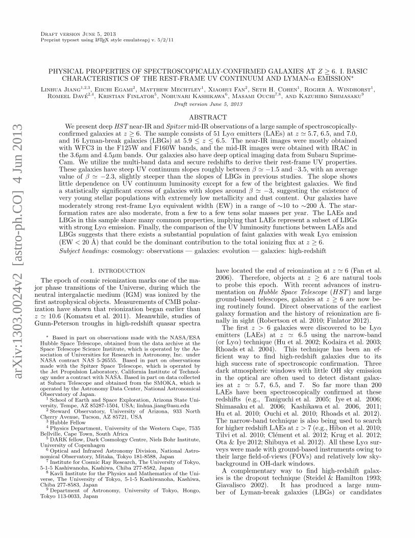
arXiv:1303.0024v2 [astro-ph.CO] 4 Jun 2013 Draft version June 5, 2013 Preprint typeset using L A T E X style emulateapj v. 5/2/11 PHYSICAL PROPERTIES OF SPECTROSCOPICALLY-CONFIRMED GALAXIES AT Z ≥ 6. I. BASIC CHARACTERISTICS OF THE REST-FRAME UV CONTINUUM AND LYMAN-α EMISSION ∗ Linhua Jiang 1,2,3 , Eiichi Egami 2 , Matthew Mechtley 1 , Xiaohui Fan 2 , Seth H. Cohen 1 , Rogier A. Windhorst 1 , Romeel Dav´ e 2,4 , Kristian Finlator 5 , Nobunari Kashikawa 6 , Masami Ouchi 7,8 , and Kazuhiro Shimasaku 9 Draft version June 5, 2013 ABSTRACT We present deep HST near-IR and Spitzer mid-IR observations of a large sample of spectroscopically- confirmed galaxies at z ≥ 6. The sample consists of 51 Lyα emitters (LAEs) at z ≃ 5.7, 6.5, and 7.0, and 16 Lyman-break galaxies (LBGs) at 5.9 ≤ z ≤ 6.5. The near-IR images were mostly obtained with WFC3 in the F125W and F160W bands, and the mid-IR images were obtained with IRAC in the 3.6μm and 4.5μm bands. Our galaxies also have deep optical imaging data from Subaru Suprime- Cam. We utilize the multi-band data and secure redshifts to derive their rest-frame UV properties. These galaxies have steep UV continuum slopes roughly between β ≃−1.5 and –3.5, with an average value of β ≃−2.3, slightly steeper than the slopes of LBGs in previous studies. The slope shows little dependence on UV continuum luminosity except for a few of the brightest galaxies. We find a statistically significant excess of galaxies with slopes around β ≃−3, suggesting the existence of very young stellar populations with extremely low metallicity and dust content. Our galaxies have moderately strong rest-frame Lyα equivalent width (EW) in a range of ∼10 to ∼200 ˚ A. The star- formation rates are also moderate, from a few to a few tens solar masses per year. The LAEs and LBGs in this sample share many common properties, implying that LAEs represent a subset of LBGs with strong Lyα emission. Finally, the comparison of the UV luminosity functions between LAEs and LBGs suggests that there exists a substantial population of faint galaxies with weak Lyα emission (EW < 20 ˚ A) that could be the dominant contribution to the total ionizing flux at z ≥ 6. Subject headings: cosmology: observations — galaxies: evolution — galaxies: high-redshift 1. INTRODUCTION The epoch of cosmic reionization marks one of the ma- jor phase transitions of the Universe, during which the neutral intergalactic medium (IGM) was ionized by the first astrophysical objects. Measurements of CMB polar- ization have shown that reionization began earlier than z ≃ 10.6 (Komatsu et al. 2011). Meanwhile, studies of Gunn-Peterson troughs in high-redshift quasar spectra ∗ Based in part on observations made with the NASA/ESA Hubble Space Telescope, obtained from the data archive at the Space Telescope Science Institute, which is operated by the As- sociation of Universities for Research in Astronomy, Inc. under NASA contract NAS 5-26555. Based in part on observations made with the Spitzer Space Telescope, which is operated by the Jet Propulsion Laboratory, California Institute of Technol- ogy under a contract with NASA. Based in part on data collected at Subaru Telescope and obtained from the SMOKA, which is operated by the Astronomy Data Center, National Astronomical Observatory of Japan. 1 School of Earth and Space Exploration, Arizona State Uni- versity, Tempe, AZ 85287-1504, USA; [email protected] 2 Steward Observatory, University of Arizona, 933 North Cherry Avenue, Tucson, AZ 85721, USA 3 Hubble Fellow 4 Physics Department, University of the Western Cape, 7535 Bellville, Cape Town, South Africa 5 DARK fellow, Dark Cosmology Centre, Niels Bohr Institute, University of Copenhagen 6 Optical and Infrared Astronomy Division, National Astro- nomical Observatory, Mitaka, Tokyo 181-8588, Japan 7 Institute for Cosmic Ray Research, The University of Tokyo, 5-1-5 Kashiwanoha, Kashiwa, Chiba 277-8582, Japan 8 Kavli Institute for the Physics and Mathematics of the Uni- verse, The University of Tokyo, 5-1-5 Kashiwanoha, Kashiwa, Chiba 277-8583, Japan 9 Department of Astronomy, University of Tokyo, Hongo, Tokyo 113-0033, Japan have located the end of reionization at z ≃ 6 (Fan et al. 2006). Therefore, objects at z ≥ 6 are natural tools to probe this epoch. With recent advances of instru- mentation on Hubble Space Telescope (HST ) and large ground-based telescopes, galaxies at z ≥ 6 are now be- ing routinely found. Direct observations of the earliest galaxy formation and the history of reionization are fi- nally in sight (Robertson et al. 2010; Finlator 2012). The first z> 6 galaxies were discovered to be Lyα emitters (LAEs) at z ≃ 6.5 using the narrow-band (or Lyα) technique (Hu et al. 2002; Kodaira et al. 2003; Rhoads et al. 2004). This technique has been an ef- ficient way to find high-redshift galaxies due to its high success rate of spectroscopic confirmation. Three dark atmospheric windows with little OH sky emission in the optical are often used to detect distant galax- ies at z ≃ 5.7, 6.5, and 7. So far more than 200 LAEs have been spectroscopically confirmed at these redshifts (e.g., Taniguchi et al. 2005; Iye et al. 2006; Shimasaku et al. 2006; Kashikawa et al. 2006, 2011; Hu et al. 2010; Ouchi et al. 2010; Rhoads et al. 2012). The narrow-band technique is also being used to search for higher redshift LAEs at z> 7 (e.g., Hibon et al. 2010; Tilvi et al. 2010; Cl´ ement et al. 2012; Krug et al. 2012; Ota & Iye 2012; Shibuya et al. 2012). All these Lyα sur- veys were made with ground-based instruments owing to their large field-of-views (FOVs) and relatively low sky- background in OH-dark windows. A complementary way to find high-redshift galax- ies is the dropout technique (Steidel & Hamilton 1993; Giavalisco 2002). It has produced a large num- ber of Lyman-break galaxies (LBGs) or candidates
-
Upload
independent -
Category
Documents
-
view
2 -
download
0
Transcript of PHYSICAL PROPERTIES OF SPECTROSCOPICALLY CONFIRMED GALAXIES AT z ⩾ 6. II. MORPHOLOGY OF THE...
arX
iv:1
303.
0024
v2 [
astr
o-ph
.CO
] 4
Jun
201
3Draft version June 5, 2013Preprint typeset using LATEX style emulateapj v. 5/2/11
PHYSICAL PROPERTIES OF SPECTROSCOPICALLY-CONFIRMED GALAXIES AT Z ≥ 6. I. BASICCHARACTERISTICS OF THE REST-FRAME UV CONTINUUM AND LYMAN-α EMISSION∗
Linhua Jiang1,2,3, Eiichi Egami2, Matthew Mechtley1, Xiaohui Fan2, Seth H. Cohen1, Rogier A. Windhorst1,Romeel Dave2,4, Kristian Finlator5, Nobunari Kashikawa6, Masami Ouchi7,8, and Kazuhiro Shimasaku9
Draft version June 5, 2013
ABSTRACT
We present deep HST near-IR and Spitzermid-IR observations of a large sample of spectroscopically-confirmed galaxies at z ≥ 6. The sample consists of 51 Lyα emitters (LAEs) at z ≃ 5.7, 6.5, and 7.0,and 16 Lyman-break galaxies (LBGs) at 5.9 ≤ z ≤ 6.5. The near-IR images were mostly obtainedwith WFC3 in the F125W and F160W bands, and the mid-IR images were obtained with IRAC inthe 3.6µm and 4.5µm bands. Our galaxies also have deep optical imaging data from Subaru Suprime-Cam. We utilize the multi-band data and secure redshifts to derive their rest-frame UV properties.These galaxies have steep UV continuum slopes roughly between β ≃ −1.5 and –3.5, with an averagevalue of β ≃ −2.3, slightly steeper than the slopes of LBGs in previous studies. The slope showslittle dependence on UV continuum luminosity except for a few of the brightest galaxies. We finda statistically significant excess of galaxies with slopes around β ≃ −3, suggesting the existence ofvery young stellar populations with extremely low metallicity and dust content. Our galaxies havemoderately strong rest-frame Lyα equivalent width (EW) in a range of ∼10 to ∼200 A. The star-formation rates are also moderate, from a few to a few tens solar masses per year. The LAEs andLBGs in this sample share many common properties, implying that LAEs represent a subset of LBGswith strong Lyα emission. Finally, the comparison of the UV luminosity functions between LAEs andLBGs suggests that there exists a substantial population of faint galaxies with weak Lyα emission(EW < 20 A) that could be the dominant contribution to the total ionizing flux at z ≥ 6.
Subject headings: cosmology: observations — galaxies: evolution — galaxies: high-redshift
1. INTRODUCTION
The epoch of cosmic reionization marks one of the ma-jor phase transitions of the Universe, during which theneutral intergalactic medium (IGM) was ionized by thefirst astrophysical objects. Measurements of CMB polar-ization have shown that reionization began earlier thanz ≃ 10.6 (Komatsu et al. 2011). Meanwhile, studies ofGunn-Peterson troughs in high-redshift quasar spectra
∗ Based in part on observations made with the NASA/ESAHubble Space Telescope, obtained from the data archive at theSpace Telescope Science Institute, which is operated by the As-sociation of Universities for Research in Astronomy, Inc. underNASA contract NAS 5-26555. Based in part on observationsmade with the Spitzer Space Telescope, which is operated bythe Jet Propulsion Laboratory, California Institute of Technol-ogy under a contract with NASA. Based in part on data collectedat Subaru Telescope and obtained from the SMOKA, which isoperated by the Astronomy Data Center, National AstronomicalObservatory of Japan.
1 School of Earth and Space Exploration, Arizona State Uni-versity, Tempe, AZ 85287-1504, USA; [email protected]
2 Steward Observatory, University of Arizona, 933 NorthCherry Avenue, Tucson, AZ 85721, USA
3 Hubble Fellow4 Physics Department, University of the Western Cape, 7535
Bellville, Cape Town, South Africa5 DARK fellow, Dark Cosmology Centre, Niels Bohr Institute,
University of Copenhagen6 Optical and Infrared Astronomy Division, National Astro-
nomical Observatory, Mitaka, Tokyo 181-8588, Japan7 Institute for Cosmic Ray Research, The University of Tokyo,
5-1-5 Kashiwanoha, Kashiwa, Chiba 277-8582, Japan8 Kavli Institute for the Physics and Mathematics of the Uni-
verse, The University of Tokyo, 5-1-5 Kashiwanoha, Kashiwa,Chiba 277-8583, Japan
9 Department of Astronomy, University of Tokyo, Hongo,Tokyo 113-0033, Japan
have located the end of reionization at z ≃ 6 (Fan et al.2006). Therefore, objects at z ≥ 6 are natural toolsto probe this epoch. With recent advances of instru-mentation on Hubble Space Telescope (HST ) and largeground-based telescopes, galaxies at z ≥ 6 are now be-ing routinely found. Direct observations of the earliestgalaxy formation and the history of reionization are fi-nally in sight (Robertson et al. 2010; Finlator 2012).The first z > 6 galaxies were discovered to be Lyα
emitters (LAEs) at z ≃ 6.5 using the narrow-band(or Lyα) technique (Hu et al. 2002; Kodaira et al. 2003;Rhoads et al. 2004). This technique has been an ef-ficient way to find high-redshift galaxies due to itshigh success rate of spectroscopic confirmation. Threedark atmospheric windows with little OH sky emissionin the optical are often used to detect distant galax-ies at z ≃ 5.7, 6.5, and 7. So far more than 200LAEs have been spectroscopically confirmed at theseredshifts (e.g., Taniguchi et al. 2005; Iye et al. 2006;Shimasaku et al. 2006; Kashikawa et al. 2006, 2011;Hu et al. 2010; Ouchi et al. 2010; Rhoads et al. 2012).The narrow-band technique is also being used to searchfor higher redshift LAEs at z > 7 (e.g., Hibon et al. 2010;Tilvi et al. 2010; Clement et al. 2012; Krug et al. 2012;Ota & Iye 2012; Shibuya et al. 2012). All these Lyα sur-veys were made with ground-based instruments owing totheir large field-of-views (FOVs) and relatively low sky-background in OH-dark windows.A complementary way to find high-redshift galax-
ies is the dropout technique (Steidel & Hamilton 1993;Giavalisco 2002). It has produced a large num-ber of Lyman-break galaxies (LBGs) or candidates

2
at z ≥ 6. While large-area ground-based ob-servations are efficient to select bright LBGs (e.g.,Nagao et al. 2007; Bowler et al. 2012; Curtis-Lake et al.2012; Hsieh et al. 2012; Willott et al. 2013), the ma-jority of the faint LBGs at z ≥ 6 known so farwere discovered by HST (e.g., Bunker et al. 2004;Dickinson et al. 2004; Yan & Windhorst 2004). In par-ticular, with the power of the new HST WFC3 in-frared camera, a few hundred galaxies at 6 ≤ z ≤ 12have been detected recently (e.g., Bunker et al. 2010;Finkelstein et al. 2010; McLure et al. 2010; Oesch et al.2010; Wilkins et al. 2010; Yan et al. 2010; Bouwens et al.2011; Lorenzoni et al. 2011; Ellis et al. 2013). Althoughmost of the LBG candidates are too faint for follow-up identification, some of them have been spectro-scopically confirmed with deep ground-based observa-tions (e.g., Stark et al. 2010, 2011; Jiang et al. 2011;Vanzella et al. 2011; Pentericci et al. 2011; Ono et al.2012; Schenker et al. 2012).With the large samples of galaxies (and candi-
dates) at z ≥ 6, the UV continuum luminosity func-tion (LF) and Lyα LF are being established (e.g.,Hu et al. 2010; Jiang et al. 2011; Kashikawa et al. 2011;Bradley et al. 2012; Bouwens et al. 2012a; Henry et al.2012; Laporte et al. 2012; Oesch et al. 2012). It is foundthat the faint-end slope of the UV LFs are very steep(α ≃ −2), so dwarf galaxies could provide enough UVphotons for reionization (also depending on the ionizingphoton escape fraction and the ionized gas clumping fac-tor). For individual galaxies, their physical propertiesare also being investigated. At z ≥ 6, the rest-frameUV/optical light moves to the infrared range. Therefore,infrared observations, especially the combination ofHSTand Spitzer Space Telescope (Spitzer), are essential tomeasure properties of these high-redshift galaxies. HSTnear-IR data constrain the slope of the rest-frame UVspectrum and help to decipher the properties of youngstellar populations. Recent HST WFC3 near-IR obser-vations have shown that high-redshift LBGs have bluerest-frame UV slopes β (fλ ∝ λβ). The typical val-ues of β are close to or smaller (bluer) than –2 (e.g.,Wilkins et al. 2011; Bouwens et al. 2012b; Dunlop et al.2012a; Finkelstein et al. 2012). Though the selectioncriteria of LBGs and the approaches to UV slopes areslightly different in the different studies in the litera-ture, it is believed that z ≥ 6 galaxies are bluer thanlow-redshift galaxies, implying that they are generallyyounger and have low dust extinction.More detailed physical properties (e.g. age and stel-
lar mass) of high-redshift galaxies have come from SEDmodeling based on broad-band photometry of HST andSpitzer as well as optical data. Spitzer IRAC pro-vides mid-IR photometry. When combined with HSTnear-IR data, it measures the amplitude of the Balmerbreak and constrains the properties of mature popu-lations. The early results on z ≃ 6 LBGs showedIRAC detections, and emphasized galaxies with es-tablished stellar populations (e.g., Egami et al. 2005;Eyles et al. 2005; Yan et al. 2005). Later studies foundthat most LBGs were actually not detected in moder-ately deep IRAC images, suggesting that these galax-ies were considerably younger and less massive (e.g.,Yan et al. 2006; Eyles et al. 2007). LAEs may repre-sent an even more extreme population with ages of
only a few million years (e.g., Pirzkal et al. 2007). Asthe number of galaxies known at z ≥ 6 increasessteadily, extensive studies are being carried out on vari-ous galaxy samples (e.g., Gonzalez et al. 2010; Ono et al.2010; Schaerer & de Barros 2010; McLure et al. 2011;Pirzkal et al. 2012). A diversity of physical propertiesare found among these galaxies, although the Universe isyounger than one billion years.Despite the progress that has been made on proper-
ties of high-redshift galaxies, there is a lack of a large,reliable sample of z ≥ 6 galaxies with spectroscopic red-shifts and high-quality infrared photometry. The reasonis twofold. For galaxies found by ground-based telescopes— although they are relatively bright and have spec-troscopic redshifts — they often do not have measuredinfrared (rest-frame UV/optical) information. For ex-ample, only a small amount of LAEs at z ≥ 6 have beenobserved in the near-IR bands byHST (e.g., Cowie et al.2011a). On the other hand, galaxies found by HST (e.g.those in the GOODS fields), do have near-IR photome-try, but most of them are too faint for follow-up spec-troscopic identification by current facilities. So they donot have secure redshifts, making it difficult for accu-rate SED modeling. A model SED derived from a fewphotometric points without a secure redshift is usuallyhighly degenerate. Therefore, determination of the phys-ical properties of z ≥ 6 galaxies demands a large sampleof galaxies with both spectroscopic redshifts and high-quality infrared photometry.In this paper we will present deep HST and Spitzer
observations of 67 spectroscopically-confirmed (hereafterspec-confirmed) galaxies at z ≥ 6. This galaxy sam-ple contains 51 LAEs and 16 LBGs, and is the largestcollection of spec-confirmed galaxies in this redshiftrange. The spectroscopic redshifts of the sample pro-vide great advantages for measuring the physical proper-ties of galaxies. First, this sample is uncontaminated byinterlopers. A photometrically-selected (hereafter photo-selected) sample of high-redshift galaxies may be contam-inated by interlopers such as low-redshift red or dustygalaxies and Galactic late-type dwarf stars, which maycause various bias on measurements of physical proper-ties. Second, spectroscopic redshifts remove one criti-cal free parameter for SED modeling. For the brightestgalaxies at z ≥ 6, there are usually only 4–5 broad-bandphotometric points available (e.g., two HST bands, twoSpitzer IRAC bands, and one optical band) for produc-ing stellar population models. Given the limited degreesof freedom, a spectroscopic redshift will significantly im-prove SED modeling, especially when nebular emissionis considered. At z ≥ 6, strong nebular emission linessuch as [O iii] λ5007, Hβ, and Hα enter IRAC 1 and2 channels, which affect our estimate of stellar popu-lations (e.g., Schaerer & de Barros 2010; Finlator et al.2011; de Barros et al. 2012; Stark et al. 2013). Photo-metric redshifts with large uncertainties may place thesenebular lines in wrong bands during SED fitting. Withspectroscopic redshifts, the positions of nebular lines aresecured (see Stark et al. 2012 for more discussion). Fi-nally, we currently have little knowledge of stellar pop-ulations in z ≥ 5.5 LAEs. This is because almost allthe known LAEs were discovered by ground-based tele-scopes, and most of them do not have infrared observa-tions. Our paper includes a large sample of LAEs. This

3
allows us, for the first time, to systematically study stel-lar populations in LAEs.This paper is the first in a series presenting the phys-
ical properties of these galaxies based on observationsfrom HST , Spitzer, and the Subaru telescope. The vastmajority of the galaxies were discovered in the SubaruDeep Field (SDF; Kashikawa et al. 2004). The SDF isa unique and ideal field to study the distant Universe:it covers an area of over 800 arcmin2 and has the deep-est optical images among all ground-based imaging data.The SDF project has been highly successful in search-ing for high-redshift galaxies. It has identified more than100 LAEs and LBGs at z ≥ 6 (e.g., Taniguchi et al. 2005;Iye et al. 2006; Shimasaku et al. 2006; Nagao et al. 2007;Ota et al. 2008; Jiang et al. 2011; Kashikawa et al. 2011;Toshikawa et al. 2012). These galaxies are spectroscopi-cally confirmed and represent the most luminous galax-ies in this redshift range. In this paper we present theHST and Spitzer observations, and use these data to-gether with the optical data from Subaru to derive therest-frame UV properties, such as their UV continuumslopes β and Lyα luminosities. In the subsequent papersof this series we will present rest-frame UV morphologyand measure stellar populations for these galaxies.The structure of the paper is as follows. In Section 2,
we present our galaxy sample. We also describe our opti-cal/infrared observations and data reduction. In Section3, we derive the rest-frame UV continuum properties ofthe galaxies. In Section 4, we measure the propertiesof Lyα emission lines. We discuss our results in Section5 and summarize the paper in Section 6. Throughoutthe paper we use a Λ-dominated flat cosmology withH0 = 70 km s−1 Mpc−1, Ωm = 0.3, and ΩΛ = 0.7(Komatsu et al. 2011). All magnitudes are on the ABsystem (Oke & Gunn 1983).
2. OBSERVATIONS AND DATA REDUCTION
2.1. Galaxy Sample
Table 1 shows the list of the galaxies presented in thispaper. There are a total of 67 spec-confirmed galaxies at5.6 ≤ z ≤ 7: 62 of them are from the SDF and the re-maining 5 are from the Subaru XMM-Newton Deep Sur-vey (SXDS; Furusawa et al. 2008) field. They representthe most luminous galaxies in terms of Lyα luminosityfor LAEs or UV continuum luminosity for LBGs in thisredshift range.The SDF covers an area of ∼ 876 arcmin2, and its op-
tical imaging data were taken with Subaru Suprime-Camin a series of broad and narrow bands (Kashikawa et al.2004). Especially noteworthy are the deep observationswith three narrow-band (NB) filters, NB816, NB921,and NB973, corresponding to the detection of LAEs atz ≃ 5.7, 6.5, and 7. The full widths at half maxi-mum (FWHM) of the three filters are 120, 132, and200 A, respectively. So far the SDF project has spec-troscopically confirmed more than 100 LAEs at z ≃
5.7, 6.5, 7, and more than 40 LBGs at 6 ≤ z ≤ 7.Our SDF galaxy sample contains 22 LAEs at z ≃ 5.7(Shimasaku et al. 2006; Kashikawa et al. 2011), 25 LAEsat z ≃ 6.5 (Taniguchi et al. 2005; Kashikawa et al. 2006,2011), and the z = 6.96 LAE (Iye et al. 2006). The LAEsat z ≃ 5.7 and 6.5 were selected in a similar way, andhave a relatively uniform magnitude limit of 26 mag in
the narrow bands NB816 and NB921, so they are froma well-defined flux-limited sample. Our SDF sample alsocontains 14 LBGs at 5.9 ≤ z ≤ 6.5 (Nagao et al. 2004,2005, 2007; Ota et al. 2008; Jiang et al. 2011); two ofthem have not been previously published. These LBGswere selected with different criteria and thus have in-homogeneous depth. The z′-band magnitude limit is26.1 mag in Nagao et al. papers, 26.5 mag in Ota et al.(2008), and 27 mag in Jiang et al. (2011). For the de-tails of candidate selection and follow-up spectroscopy,see the original galaxy discovery papers above.Five galaxies in our sample, including 2 LBGs at
z ≃ 6 (Curtis-Lake et al. 2012) and 3 LAEs at z ≃ 6.5(Ouchi et al. 2010), are from the SXDS. The two LBGsare very bright (z′ < 25 mag) and have been analyzedby Curtis-Lake et al. (2013). The SXDS optical imagingdata were also taken with Subaru Suprime-Cam in thesame broad and narrow bands, but cover five times largerarea than the SDF does (Furusawa et al. 2008).In Table 1, the first 62 galaxies are from the SDF and
the last 5 galaxies are from the SXDS. Columns 2 and 3list the object coordinates. They are re-calculated fromour own stacked optical images (see Section 2.2), andare fully consistent with those given in the galaxy dis-covery papers (typical difference < 0.′′1). Column 4 liststhe redshifts, measured from the Lyα emission lines ofthe galaxies. The galaxy discovery papers used differ-ent values for the rest-frame Lyα wavelengths (i.e. 1215,1215.67, or 1216 A) for redshift measurements. We con-vert all these redshifts to the redshifts listed in Table 1 byassuming a rest-frame Lyα line center of 1215.67 A. Thelast column shows the reference papers of the objects.We will explain the rest of the table in the following sub-sections.
2.2. Optical Imaging Data
The galaxies in this paper were discovered in the SDFand the SXDS. The SDF public imaging data includestacked images in five broad bands BV Ri′z′ and two nar-row bands NB816 and NB921. The flux limits for thesedata are given in Kashikawa et al. (2004). However, thepublic data do not include the data taken recently (alsoby Subaru Suprime-Cam), and the data taken in they and NB973 bands. Therefore, we produced our ownstacked images by including all available images in theSubaru archive, as explained below.Our data processing began with the raw images ob-
tained from the archival server SMOKA (Baba et al.2002). Raw images with point spread function (PSF)sizes greater than 1.′′2 were rejected. The data werereduced, re-sampled, and co-added using a combina-tion of the Suprime-Cam Deep Field REDuction package(SDFRED; Yagi et al. 2002; Ouchi et al. 2004) and our ownIDL routines. Each image was bias (overscan) correctedand flat-fielded using SDFRED. Then bad pixel masks werecreated from flat-field images. Cosmic rays were identi-fied and interpolated using L.A. Cosmic (van Dokkum2001). Saturated pixels and bleeding trails were alsoidentified and interpolated. For each image, a weightmask was generated to include all above mentioned de-fective pixels. We then used SDFRED to correct the im-age distortion, subtract the sky-background, and maskout the pixels affected by the Auto-Guider probe. After

4
individual images were processed, we extracted sourcesusing SExtractor (Bertin & Arnouts 1996) and calcu-lated astrometric and photometric solutions using SCAMP(Bertin 2006) for the final image co-addition. In orderto match the public SDF images, we used the public R-band image as the astrometric reference catalog in SCAMP.Both science and weight-map images were scaled and up-dated using the astrometric and photometric solutionsmeasured from SCAMP. Instead of homogenizing PSFs toa certain value as was done for the public data, we incor-porated PSF information into the weight image so thatthe weight was proportional to the inverse of the squareof the PSF FWHM. We re-sampled and co-added imagesusing SWARP (Bertin et al. 2002). The re-sampling inter-polations for science and weight images were LANCZOS3and BILINEAR, respectively. We modified SWARP so thatit performs sigma-clipping (5σ rejection) of outliers whenco-adding images.We produced images in the six broad bands BV Ri′z′y
and three narrow bands NB816, NB921, and NB973. Thefinal products are a stacked science image, and its cor-responding weight image, for each band. The pixel andimage sizes of our products are the same as those of thepublic SDF images. The typical PSF FWHM is 0.′′6−0.′′7.We determined photometric zero points from the publicSDF images whose zero points were known. The SXDSoptical imaging data were reduced in the same way aswe did for the SDF.Our SDF broad-band images are deeper than the pub-
lic images in the Ri′z′ bands, because the SDF teamobtained more imaging data from Subaru recently, andwe included all the available data above. For example,the public z′-band image has a depth of z′ = 26.1 mag(5σ detection in a 2′′ diameter aperture) with a total in-tegration time of ∼7 hr. To date, the total z′-band dataamount to ∼29 hr. Our new z′-band image has a depthof ∼27.0 mag, 0.9 mag deeper than the public image. Inaddition, the public data do not have images in the yand NB973 bands. The SDF y-band imaging data weretaken with two different sets of CCDs (MIT and Hama-matsu), and have been used to search for z ≃ 7 LBGs(Ouchi et al. 2009). Although the fully-depleted Hama-matsu CCDs are twice as sensitive as the MIT CCDs inthe y band, their sensitivity (quantum efficiency) curveshave similar shapes. Therefore, we stacked all the imagestaken with both sets of CCDs, as Ouchi et al. (2009) didin their work. The total integration time was 24 hr, andthe depth was about 26.0 mag.In Table 1, Columns 5 to 7 show the total magni-
tudes of the galaxies in one of the three narrow bands(NB816, NB921, or NB973, depending on redshift) andtwo broad bands z′y. For a given object in a given fil-ter, its total magnitude is measured as follows. We firstuse SExtractor to measure the aperture photometry ofthe object in a circular 2.′′0 diameter, after the local sky-background is subtracted. In cases where galaxies areclose to their neighbors, we use a circular 1.′′6 diameter.Then an aperture correction is applied to correct for lightloss. The aperture correction is determined from morethan 100 bright, but unsaturated point sources in thesame image. Almost all our galaxies are point-like ob-jects and are not resolved in the SDF images. In caseswhere galaxies clearly show extended features, we useMAG AUTO magnitudes as the best estimates of the
total magnitudes. In Table 1, we did not list broad-bandphotometry for the galaxies with weak detections (< 5σ)in the J band. These galaxies are excluded in most ofour analysis in this paper. Detections below 3σ in anyof these bands are not listed as well. We carefully checkeach object, and find that object no. 12, a z ≃ 5.7 LAE,is overlapped by a bright foreground star (this was alsopointed out in the galaxy discovery paper). The separa-tion between the two objects is only ∼ 0.′′25, so we arenot able to do photometry for this galaxy. We will notuse this galaxy in the following analysis.Figure 1 shows the transmission curves of six Subaru
Suprime-Cam filters, including three broad-band filtersi′z′y and three narrow-band filters NB816, NB921, andNB973. We do not show the other three bluer filtersBV R, because our galaxies were not detected in thesebands. In Appendix A, we show the thumbnail imagesof the galaxies in one of the three Subaru Suprime-Camnarrow bands and the three broad bands i, z′, and y.
2.3. HST Near-IR Imaging Data
We obtained HST near-IR imaging data for a largesample of spectroscopically confirmed SDF galaxies at5.6 ≤ z ≤ 7 from three HST GO programs 11149 (PI:E. Egami), 12329 and 12616 (PI: L. Jiang). The threeprograms together with our Spitzer programs (see thenext subsection) were designed to characterize the phys-ical properties of these high-redshift galaxies. The HSTobservations were made with a mix of strategies. Asthe proposal for GO program 11149 was written, HSTWFC3 had not yet been installed. Our plan was to ob-serve 20 bright galaxies with NICMOS in the F110W(hereafter J110) and F160W (hereafter H160) bands. Theobservations were made with camera NIC3. The expo-sure time was two orbits per band per pointing (or perobject), split into four exposures. The total on-sourceintegration per band was about 5400 sec. We performedsub-pixel dithering during the four NICMOS exposuresto improve the PSF sampling and to remove bad pixelsand cosmic rays.After we finished several targets, NICMOS failed, and
then WFC3 was installed in May 2009. Since WFC3has much higher sensitivity, the rest of the galaxies inGO 11149 and all the galaxies in GO 12329 and 12616were observed with WFC3. Because of the larger FOVof WFC3 and the increasing number of known z ≥ 6galaxies in the SDF, we changed our observing strategyfor GO 12329 and 12616. We chose the regions that coverat least 3 galaxies (up to 5) per HST /WFC3 pointing.By doing this we were able to observe many galaxies ina small number of telescope pointings. We used F125W(hereafter J125) and H160 in these two programs. In GO12329, the exposure time was one orbit per filter perpointing. We found that some galaxies in our samplewere barely detected with this depth. Therefore in GO12616, all new WFC3 pointings had a depth of two orbits(on-source integration ∼ 4800 sec; see Windhorst et al.2011 for the anticipated sensitivity in two-orbit WFC3exposures). We also re-observed most galaxies that wereobserved in GO 12329, so that they have a total of two-orbit depth per band. As in the NICMOS observationsabove, theWFC3 observation of each pointing (per band)was split into four exposures. Sub-pixel dithering duringthe exposures was also performed to improve the PSF

5
sampling and to remove bad pixels and cosmic rays. Thetransmission curves of the three WFC3 filters are plottedin Figure 1.As we mentioned above, several galaxies in our sam-
ple were found in the SXDS. They were covered by theUKIDSS Ultra-Deep Survey (UDS). Their HST WFC3near-IR data were obtained from the Cosmic AssemblyNear-infrared Deep Extragalactic Legacy Survey (CAN-DELS; Grogin et al. 2011; Koekemoer et al. 2011). Theexposure depth of the CANDELS UDS data is 1900 secin the J125 band and 3300 sec in the H160 band. Theyare shallower than our WFC3 data for the SDF.In Appendix A we show the thumbnail images of the
galaxies in the twoHST near-IR bands J110 (or J125) andH160. Note that the J125-band image of the z = 6.96LAE (no. 62) was obtained from GO program 11587(Cai et al. 2011). This image also covers another twoobjects (no. 2 and no. 59) in our sample. Due to thehigh sensitivity of WFC3, the majority of the galaxiesin our sample are detected with high significance in thenear-IR images. Only 15 of them — among the faintestin the optical bands — have weak detections (< 5σ) inthe J band.Our WFC3 data processing began with individual flat-
fielded, flux calibrated WFC3 infrared exposures deliv-ered by the HST archive. Each pointing used a standard4-point dither pattern to obtain uniform half-pixel sam-pling. All exposures for each pointing were combined us-ing the software Multidrizzle (Koekemoer et al. 2002),with an output plate scale of 0.′′06 per pixel and apixfrac parameter of 0.8. For our observations, thisprovides Nyquist sampling of the PSF and relatively uni-form weighting of individual pixels. RMS maps were alsoderived from the Multidrizzle weight-map images, fol-lowing the procedure used in Dickinson et al. (2004) thataccounts for correlated noise in the final images.Our NICMOS NIC3 data were reduced using a fully
automated pipeline NICRED (Magee et al. 2007). NI-CRED starts its processing with raw science data andcalibration files, and sequentially runs a set of stepsfrom basic calibration to final mosaic generation. Themost important part of the reduction is the basic cali-bration, because the NICMOS data suffer from variablebias, electronic ghosts, and cosmic-ray persistence. Thebasic procedure is as follows. NICRED first removes elec-tronic ghosts, handles variable bias, rejects cosmic rays,and subtracts sky background. It then removes possi-ble cosmic-ray persistence and residual instrument sig-natures. The rest of the procedure are common steps,including flat fielding, a non-linearity correction, imagealignment and registration, etc. It finally creates driz-zled images and the corresponding weight maps. Thepixel size in the final products is 0.′′1, a half of the nativesize.We list the near-IR photometry of the galaxies in
Columns 8 to 10 in Table 1. All galaxies were observedin the H160 band and one or two of the J bands (J110and/or J125). We perform photometry using SExtractorin dual-image mode with RMS map weighting. The J-band is used as the detection image. A single set ofparameters is used for detection in all images. We com-pute the total magnitudes of the objects in both filtersby using MAG AUTO elliptical apertures, with a Kronfactor of 1.8 and a minimum aperture of 2.5 semi-major
radius, then applying aperture corrections. The aperturecorrections are calculated by running SExtractor againwith five Kron factors between 2.0 and 4.0, analyzingthousands of sources in the range J < 26 mag. We cal-culate a sequence of median correction vs. Kron factor,which we extend to infinite radius with an exponentialfit. All final photometry apertures are visually inspected,to screen against contamination from nearby objects orspurious detections. Detections below 5σ in the J band,or detections below 3σ in the H band, are not listed inTable 1.
2.4. Spitzer Mid-IR Imaging Data
We obtained Spitzer IRAC imaging data for the SDFfrom two GO programs 40026 (PI: E. Egami) and 70094(PI: L. Jiang). In GO 40026, we observed 20 luminousgalaxies at z ≥ 6, which were also the targets of ourHST program 11149. The observations were made inIRAC channel 1 (3.6 µm) and channel 2 (4.5 µm). Theother two channels (5.8 and 8.0 µm) were observed si-multaneously. We used the cycling dither pattern withmedium steps and a frame exposure time of 100 sec. Theon-source integration time per channel per pointing is 3hr. In GO 70094 (during the Spitzer warm mission),we modified our observing strategy and observed highgalaxy surface density regions, so that we can observe alarge number of galaxies with slightly more than 10 tele-scope pointings. The cycling dither pattern with smallsteps was used with a frame exposure time of 100 sec.We focused on IRAC channel 1 and increased on-sourceintegration time to ∼6 hr per pointing. The two pro-grams imaged roughly 70% of the SDF to a depth of 3–6hours. They covered all the 62 SDF galaxies in channel1 and 51 (out of 62) galaxies in channel 2.The IRAC Data processing began with the cBCD (cor-
rected BCD) products and associated mask and uncer-tainty images delivered by the Spitzer Science Center(SSC) archive. The image fits headers were updated tomatch the astrometry in the SDF optical images. Thenthe images were processed, drizzled, and co-added us-ing using the SSC pipeline MOPEX. This is a fully auto-mated procedure. The final images have a pixel size of0.′′6, roughly a half of the IRAC native pixel scale. TheIRAC images for the SXDS galaxies were obtained fromthe SSC archive (programs 60022 and 80057). The datawere reduced in the same way above. In Appendix (thelast two columns) we show the thumbnail images of thegalaxies in the two IRAC channels.Mid-IR photometry is complicated by source confu-
sion. Galaxies in deep IRAC images are often blendedwith nearby neighbors, so accurate photometry requiresproper deblending and removing neighbors. We willpresent IRAC photometry of our galaxies in the secondpaper of this series.
3. REST-FRAME UV CONTINUUM PROPERTIES
With the narrow- and broad-band photometry fromthe NB816 to the H160 band, we are able to measure thespectral properties, such as Lyα flux and UV continuumslopes, for most of the galaxies in this sample. In orderto measure the rest-frame UV properties, we produce amodel spectrum for each of these galaxies. The modelspectrum fgal (in units of erg s−1 cm−2 A−1, like com-monly used fλ) is the sum of a Lyα emission line and a

6
power-law UV continuum with a slope β,
fgal = A× SLyα +B × λβ , (1)
where A and B are scaling factors in units oferg s−1 cm−2 A−1, and SLyα (dimensionless) is the Lyαemission line profile. In the redshift range and wave-length range considered here, other nebular lines such asHe ii λ1640 can be safely ignored (e.g., Cai et al. 2011).We first determine the continuum parametersB and β byfitting the continuum fcon,λ = B×λβ (or fcon,ν ∝ λβ+2)with the broad-band data that do not cover the Lyαemission. Because AB magnitude mAB and Log(λ) havethe simplest linear relation mAB ∝ (β+2)×Log(λ), thecontinuum fitting is performed on mAB and Log(λ) usingthe IDL routine linfit.pro. This routine takes Log(λ),mAB, and the errors in mAB, and performs a standard(weighted) least-squares linear regression by minimizingthe chi-square error statistic. The errors propagate tothe final parameters.In order to reliably measure continuum slopes, we only
consider the galaxies with > 5σ detections in the J band(the deepest band). We further require that these galax-ies have > 3σ detections in at least one more broad bandthat does not cover the Lyα emission. Detections be-low 3σ are not used here. For the galaxies at z < 6.1,four broad bands z′yJH can be used. As shown in Table1, the z < 6.1 galaxies with > 5σ detections in the Jband and with > 3σ detections in another band are usu-ally detected (> 3σ) in the other two bands, so all fourbroad bands are used for most of the galaxies at z < 6.1.For the galaxies at z > 6.1, the z′ band covers Lyα, soonly three broad bands yJH can be used. However, al-most half of the z > 6.1 galaxies with J-band detections(> 5σ) are not detected at > 3σ in the y band. Forthese galaxies, we use only the JH bands to derive theirUV slopes. The information (or upper limits) from they-band photometry is ignored, because the JH-band im-ages are much deeper (by 1–1.5 mag) than the y-bandimages, and the y-band upper limits provide little addi-tional constraint on β. In addition, in rare cases wheresome galaxies in the crowded optical images are signifi-cantly affected by their environments like bright neigh-bors (e.g., no. 2 and no. 4), their optical data are notused.We then determine parameter A for Lyα emission line.
Kashikawa et al. (2011) generated two composite Lyαemission line profiles for their z ≃ 5.7 and 6.5 LAEs,and found that the two profiles were very similar, show-ing no significant evolution from z ≃ 5.7 to 6.5 (see alsoHu et al. 2010). We use the two composite line profiles asour model Lyα emission lines in Eq. 1: we use the z ≃ 5.7profile for the galaxies at z ≤ 6.2 and the z ≃ 6.5 profilefor the galaxies at z > 6.2. The shape of the Lyα emis-sion lines has negligible impact on our results, becauseeven the three narrow-band filters used for Lyα detectionare much wider than the typical Lyα line width. We ap-ply IGM absorption to the model spectrum (the IGMabsorption has already been taken into account in thecomposite Lyα emission lines). The neutral IGM fractionincreases dramatically from z = 5.5 to z = 6.5, causingcomplete Gunn-Peterson troughs in some z > 6 quasarspectra (Fan et al. 2006). It is thus important to includeIGM absorption in the model spectrum. We calculate
IGM absorption in the same way as Fan et al. (2001).The IGM-absorbed model spectrum is convolved withthe total system response, such as filter transmission andCCD quantum efficiency. Finally, the Lyα emission flux(or parameter A) is calculated by matching the modelspectrum to the narrow-band photometry (for LAEs) orthe z′-band photometry (for LBGs). For LBGs, we willsee in Section 4.1 that even small z′-band photometric er-rors will cause large uncertainties on measurements of A,so we adopt the Lyα flux of the LBGs from the galaxiesdiscovery papers, which were derived from deep opticalspectra.Figure 2 illustrates our procedure by showing our
model fit to the photometric data points of two LAEsat z ≃ 5.7 and z ≃ 6.5, respectively. For the z ≃ 5.7LAE in this specific case, we use the photometric datain the z′yJ110H160 bands (red circles) to fit the modelcontinuum. When the continuum (strength B and slopeβ) is derived, we apply IGM absorption. The continuumflux at the blue side of the Lyα line (the dashed linein the figure) is absorbed. Finally the factor A is de-termined by scaling the Lyα emission line to match theNB816-band photometry. For the z ≃ 6.5 LAE in Figure2, we use the data in the yJ125H160 bands to computeits continuum, and use the NB921-band photometry tomeasure its Lyα emission. After A, B, and β are de-termined, other physical quantities such as Lyα and UVluminosities, rest-frame Lyα equivalent width (EW), andstar formation rates (SFRs) are also calculated. The re-sults are shown in Table 2.
3.1. UV Continuum Slope β
The rest-frame UV-continuum slope provides key infor-mation to constrain young stellar populations in galaxies.For z ≥ 6 LBGs in the literature, especially those se-lected from HST photometric samples, their UV slopesare usually measured from two broad bands J125 andH160 that do not cover Lyα emission. Recent stud-ies show that high-redshift LBGs generally have steepUV slopes and low dust content (e.g., Bouwens et al.2009, 2012b; Dunlop et al. 2012a; Finkelstein et al. 2012;Gonzalez et al. 2012; Walter et al. 2012). For exam-ple, Bouwens et al. (2009) found that β decreases fromβ ≃ −1.5 at z ≃ 2 to β ≃ −2 at z ≃ 6. Finkelstein et al.(2012) showed that β changed from β ≃ −1.8 at z ≃ 4to β ≃ −2.4 at z ≃ 7. Extremely steep slopes ofβ ≃ −3 have been reported in very faint z ≃ 7 galax-ies (e.g., Bouwens et al. 2010). It was also found thatlower-luminosity galaxies tend to have steeper slopes(e.g., Bouwens et al. 2012b; Gonzalez et al. 2012). Re-cently the results on the blue colors in high-redshiftLBGs have been questioned by Dunlop et al. (2012a) andMcLure et al. (2011), who claimed that previous mea-surements were significantly affected by contaminantsin the photo-selected LBG samples and the low signal-to-noise (S/N) ratios of faint objects, and that the ex-tremely steep slopes were caused by the so-called “βbias”. This bias is partly produced by the removal ofgalaxies with larger (redder) β values from the sample aslower-redshift interlopers, which would preferentially re-move flux-boosted sources in the H160 band and skew theβ distribution to smaller (i.e., bluer) values as a result.As pointed out by Bouwens et al. (2012b), this β bias canbe large if the same bands (J125 and H160) are also used

7
to select LBGs. With a more restricted selection of LBGscandidates from the same HST data set, Dunlop et al.(2012a) and McLure et al. (2011) found that the averageslope of z ≃ 7 LBGs is β ≃ −2, which is not steeperthan the bluest galaxies at z ≤ 4. They further foundno relation between β and the UV continuum luminos-ity. As the debate is still going on (e.g., Bouwens et al.2012b; Finkelstein et al. 2012; Dunlop et al. 2012b), thekey is to construct a high-redshift galaxy sample that isfree from such a bias.Our galaxy sample presented here is unlikely to be
strongly affected by this β bias, not only because thesegalaxies have spectroscopic redshifts but also because ouroriginal source selection did not utilize any informationon the rest-frame UV continuum slope. Furthermore,we did not include weak detections in our analysis. Formany galaxies, especially the z ≃ 5.7 LAEs and z ≃ 6LBGs, β was measured from more than two bands. Itshould be pointed out, however, our LBGs were spec-confirmed to have strong Lyα emission, which could biasthe LBG sample to galaxies with lower extinction andthus to those with bluer UV continuum slopes.Figure 3(a) shows the rest-frame UV continuum slopes
β as a function of M1500, the absolute AB magnitude ofthe continuum at rest-frame 1500 A. M1500 is calculatedfrom B×λβ in Eq. 1. Figure 3 only includes the galaxiesthat have measured β in Table 2. These galaxies coverthe brightest UV luminosity range M1500 < −19.5 mag.For the galaxies that do not have measured β, they donot have reliable detections (< 5σ) in the near-IR bands,so they are usually fainter than M1500 = −19.5 mag (seeSection 4.2 and Figure 6). The green circles in Figure3(a) represent the LBGs at z ≃ 6, and the blue and redcircles represent the LAEs at z ≃ 5.7 and 6.5 (includingz ≃ 7), respectively. The values of M1500 and β are alsolisted in Columns 2 and 3 of Table 2. Our measurementsof β are reliable because of the secure redshifts and multi-band photometry. As we addressed above, the slopes arecalculated from all available broad-band data that do notcover the Lyα emission line. For any β that was derivedfrom more than two bands, its error is usually smallerthan 0.4. So most of the z ≃ 5.7 LAEs and z ≃ 6 LBGshave relatively small errors on β. For the z ≃ 6.5 LAEs,their slope errors are generally larger, as many of themwere only detected in the two near-IR bands in additionto NB921.The galaxies in Figure 3 apparently have steep
UV-continuum slopes that are roughly between β ≃
−1.5 and β ≃ −3.5. The weighted mean is β =−2.29, and the median value is β = −2.35. Thisslope is slightly steeper than those from previous ob-servations (e.g., Bouwens et al. 2012b; Dunlop et al.2012a,b; Finkelstein et al. 2012) and simulations (e.g.,Finlator et al. 2011; Dayal & Ferrara 2012) in the lit-erature. The slope β also appears to show weak de-pendence on M1500 that lower-luminosity galaxies havesteeper slopes. The dashed line is the best linear fit toall the data points. This trend is caused by the severalmost luminous galaxies at M1500 ≃ −22 mag. These lu-minous galaxies have red colors β ≃ −1.8. If we excludethese galaxies in our fit, the trend almost disappears.The dash-dotted line in the figure illustrate the result bydisplaying the best fit to the galaxies at M1500 > −21.7
mag, and its slope is consistent with zero.In the above analysis, galaxies with near-IR detections
below 5σ in the J band were discarded. This has negligi-ble impact on our results. Our HST near-IR data haverelatively uniform depth (two orbits per band per point-ing), so the 5σ detection cut indeed puts a flux limit onM1500 in Figure 3(a), which does not affect our resultsin the bright region M1500 < −19.5 mag. We also per-form two simple tests to investigate whether large errorson photometry or β have strong impact on our results.In the first test we stack the images of 9 galaxies whoseerrors of β (σβ) are greater than 0.8 in Figure 3, andthen measure photometry and calculate β on the stackedimages in the J125 and H160 bands. The input imagesare scaled so that the galaxies have the same magnitudein the J125 band before stacking, otherwise the final im-age would be dominated by the brightest objects. Thestacked images have much higher signal-to-noise (S/N)ratios. The 9 galaxies have a median slope of β ≃ −2.1.The slope for the stacked object is β = −2.2±0.2, whichagrees with the median value of the individual galaxies.The result is shown as the magenta star in Figure 4,where the gray circles represent the same galaxies shownin Figure 3(a). In the second test there are 10 galaxieswith β < −2.8 that have both J125 andH160 images. Themedian value of their slopes is β ≃ −3.0. We stack theirimages in the same way as we did above. The slope forthe combined object is β = −2.9±0.2, which is also con-sistent with the median value of the individual galaxies.The magenta square in Figure 4 represents the combinedobject. From these tests, our measurements of β are notbiased even for faint objects with relatively large photo-metric errors.
3.2. β-M1500 Relation
It is generally believed that high-redshift galaxies havesteep UV slopes β, and β changes with redshift: higher-redshift galaxies tend to be bluer due to less dust ex-tinction. The relation between β and UV luminos-ity (MUV, or M1500 in this paper) is still controver-sial. In Figure 4 we compare our results with re-cent studies (Bouwens et al. 2012b; Dunlop et al. 2012a;Finkelstein et al. 2012). Bouwens et al. (2012b) found acorrelation between β and MUV at all redshifts in a rangeof 4 < z < 7. They claim that galaxies have bluer UVcolors at lower luminosities. The green triangles in Fig-ure 4 represent the average slopes at z ∼ 6 from theirstudy. Dunlop et al. (2012a) used a more restricted se-lection of LBGs by excluding low S/N detections froma similar HST data set. They found that high-redshiftgalaxies have an average slope of β ≃ −2, and it doesnot change with MUV. The blue crosses in Figure 4 rep-resent the average slopes at 5 < z < 7 from their study.Finkelstein et al. (2012) also found that β shows minorrelation with M1500 in the redshift range from z = 4 to8. The red diamonds in Figure 4 represent the averageslopes at z ≃ 6 from their study.Figures 3 and 4 suggest that in our sample there is little
dependence of β on M1500 in the range of M1500 < −19.5mag. The three studies mentioned above were all basedon HST data that are ∼ 1 − 2 mag deeper than ours.In the luminosity range of M1500 < −19.5 mag, thesestudies do not show evidence of a significant correlationeither, though there is likely a weak trend at the fainter

8
range M1500 > −19.5 mag. Therefore, it is possible thatthe reported correlation between β and MUV, if exists,is mainly driven by very faint galaxies.The mean value of our measured β is –2.3. It is slightly
steeper than β = 2.1 − 2.2 by Bouwens et al. (2012b)in the same luminosity range, and is also steeper thanβ ≃ −2 by Dunlop et al. (2012a) and Finkelstein et al.(2012). This is due to the nature of our sample. Thegalaxies in the previous studies are photo-selected LBGs.Our galaxies are spectroscopically confirmed and havestrong Lyα emission lines, suggesting that they likelyhave lower dust extinction, and thus steeper UV slopes.
3.3. Slopes in LAEs
It is not clear whether high-redshift LAEs and LBGsrepresent physically different galaxy populations. Earlyobservations found that LAEs at z = 5 ∼ 6 are smallerand less massive compared to LBGs, and thus constituteyounger stellar populations (e.g., Dow-Hygelund et al.2007; Pirzkal et al. 2007). However, this apparent dif-ference could be a direct result of selection effects, andLAEs may represent a subset of LBGs with strong Lyαemission lines (e.g., Dayal & Ferrara 2012). Whether ornot LAEs and LBGs have similar populations will bereflected in their physical properties. For example, ifLAEs are substantially younger, they are expected tohave steeper UV slopes.In Figures 3 and 4 the distribution of our slopes β for
the z ≃ 5.7 and z ≃ 6.5 LAEs are β = −2.3 ± 0.5 andβ = −2.0± 0.8, respectively. The β distribution for theLBGs is β = −2.5±0.4. Although the scatters are large,the LAE slopes are apparently not steeper than the LBGslopes in our sample. They are also not steeper thanthe slopes of the LBGs in previous studies mentionedabove, which is contrary to the assumption that LAEscontain younger stellar populations than LBGs do. Thisindicates that most LAEs are probably not as young aswhat was previously suggested.
3.4. Galaxies with Extreme UV Slopes
The majority of our galaxies have slopes β > −2.7 inFigure 3(a). There are a fraction of galaxies whose slopesare steeper than –2.7. Some of them have relatively smallerrors around σβ ∼ 0.4. The existence of these β ≃ −3galaxies are statistically robust (not a distribution tail).In Figure 3(b) our statistical test shows that the distribu-tion of the observed β is broader and flatter than the dis-tribution of β expected if all the galaxies have an intrinsicβ = −2.3 with the observed uncertainties. It clearly in-dicates a statistically significant excess of galaxies withβ ≃ −3. These galaxies do not show distinct propertiesin many aspects such as Lyα EW and UV morphology.The existence of these β ≃ −3 galaxies in our sampleis intriguing. The UV colors cannot be arbitrarily bluefor a given initial mass function (IMF). For the com-monly used Salpeter IMF, a β ≃ −3 usually means avery young stellar population with extremely low metal-licity and no dust content, regardless of star-formationhistories (e.g., Finlator et al. 2011; Wilkins et al. 2011).In particular, the β < −3 galaxies, if confirmed by fu-ture deeper observations, will be challenging for currentsimulations (Finlator et al. 2011). In addition, the broaddistribution of the observed β also suggests significant in-trinsic scatter in dust and/or age. Detailed discussion is
deferred to the next paper when we perform SED mod-eling with the IRAC data.From Figure 3 the five most luminous galaxies at
M1500 ≃ −22 mag have UV slopes β ≃ −1.8, which issignificantly redder than the mean value β = −2.3 of thesample. The measurements of β are robust since thesegalaxies are very bright and detected in almost all thebroad bands redward of Lyα. In particular, they are alldetected at high significance in the IRAC bands. TheirLyα emission is relatively small compared to their UVcontinuum emission. From the HST images, they havevery extended morphologies, even with double or mul-tiple cores, suggesting that they are interacting systemswith enough amounts of dust to redden their UV col-ors. These galaxies are similar to the luminous galaxiesat z ∼ 6 found by Willott et al. (2013) in the CFHTLegacy Survey. Willott et al. (2013) selected a sample ofluminous galaxies with MUV ≃ −22 in a 4 sq. degreearea and found that their galaxies have very red colorswith a typical slope β = −1.4, which is caused by largedust reddening of AV > 0.5.
4. Lyα PROPERTIES
4.1. Lyα Luminosity
Spectroscopic data generally provide reliable line lumi-nosities, but this becomes complicated for z ≥ 6 galaxies.During the spectroscopic observations of these galaxies,the total integration time is at least a few hours per ob-ject or per slit mask. Sometimes the images of one objectare taken in different nights. Light loss varies with manyparameters, such as varying seeing, different observingconditions, possible offsets between targets and slits, andeven the sizes of targets. So it is difficult to accuratelycorrect for light loss. In addition, even with a few hourintegration on the largest telescopes, the spectral qualityof many galaxies are still poor, simply because they arefaint. All of the above effects can easily result in largeuncertainties in the measurements of their Lyα luminosi-ties.Photometric data provide an alternative way to mea-
sure the observed Lyα flux, especially for LAEs. Wehave high-quality narrow-band and broad-band photom-etry and secure redshifts. Our procedure used all avail-able data and was straightforward. The Lyα luminositiesof the LAEs were derived from narrow-band photometryafter their underlying continua were subtracted. For themajority of the LAEs in our sample (EW ≥ 20A), theirnarrow-band photometry is dominated by Lyα emission,meaning that the real Lyα emission is smaller — but notmuch smaller — than the total narrow-band photometry.Therefore, we neither significantly overestimate the Lyαluminosity (the maximum is the total narrow-band emis-sion), nor significantly underestimate it (the minimum isat least a half of the maximum for most LAEs).The measurements of our Lyα luminosities for LBGs
are less accurate. For most of the LAEs, their narrow-band photometry is dominated by the Lyα emission, sotheir Lyα luminosities can be well determined. For theLBGs, Lyα luminosities were calculated from the z′-bandphotometry. The z′ band is very broad, and its photom-etry is almost completely dominated by the UV contin-uum flux. Therefore, even small uncertainties on the z′-band photometry or on measurements of UV continuum
9
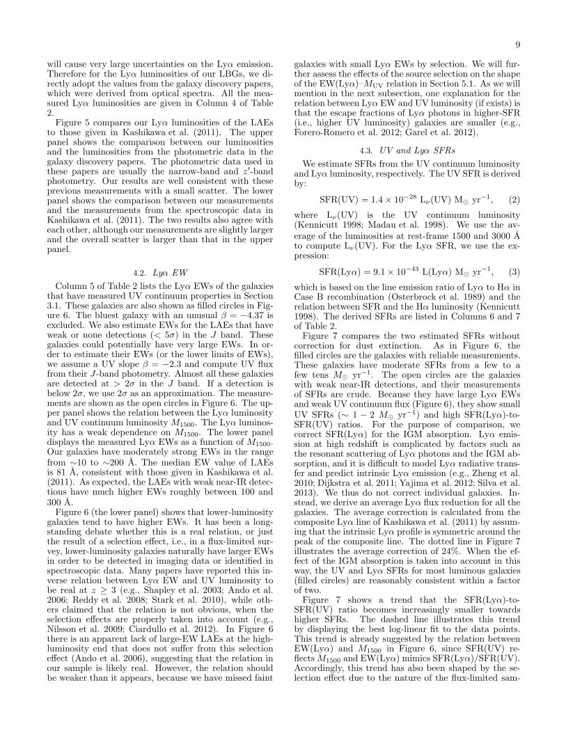
will cause very large uncertainties on the Lyα emission.Therefore for the Lyα luminosities of our LBGs, we di-rectly adopt the values from the galaxy discovery papers,which were derived from optical spectra. All the mea-sured Lyα luminosities are given in Column 4 of Table2.Figure 5 compares our Lyα luminosities of the LAEs
to those given in Kashikawa et al. (2011). The upperpanel shows the comparison between our luminositiesand the luminosities from the photometric data in thegalaxy discovery papers. The photometric data used inthese papers are usually the narrow-band and z′-bandphotometry. Our results are well consistent with theseprevious measurements with a small scatter. The lowerpanel shows the comparison between our measurementsand the measurements from the spectroscopic data inKashikawa et al. (2011). The two results also agree witheach other, although our measurements are slightly largerand the overall scatter is larger than that in the upperpanel.
4.2. Lyα EW
Column 5 of Table 2 lists the Lyα EWs of the galaxiesthat have measured UV continuum properties in Section3.1. These galaxies are also shown as filled circles in Fig-ure 6. The bluest galaxy with an unusual β = −4.37 isexcluded. We also estimate EWs for the LAEs that haveweak or none detections (< 5σ) in the J band. Thesegalaxies could potentially have very large EWs. In or-der to estimate their EWs (or the lower limits of EWs),we assume a UV slope β = −2.3 and compute UV fluxfrom their J-band photometry. Almost all these galaxiesare detected at > 2σ in the J band. If a detection isbelow 2σ, we use 2σ as an approximation. The measure-ments are shown as the open circles in Figure 6. The up-per panel shows the relation between the Lyα luminosityand UV continuum luminosity M1500. The Lyα luminos-ity has a weak dependence on M1500. The lower paneldisplays the measured Lyα EWs as a function of M1500.Our galaxies have moderately strong EWs in the rangefrom ∼10 to ∼200 A. The median EW value of LAEsis 81 A, consistent with those given in Kashikawa et al.(2011). As expected, the LAEs with weak near-IR detec-tions have much higher EWs roughly between 100 and300 A.Figure 6 (the lower panel) shows that lower-luminosity
galaxies tend to have higher EWs. It has been a long-standing debate whether this is a real relation, or justthe result of a selection effect, i.e., in a flux-limited sur-vey, lower-luminosity galaxies naturally have larger EWsin order to be detected in imaging data or identified inspectroscopic data. Many papers have reported this in-verse relation between Lyα EW and UV luminosity tobe real at z ≥ 3 (e.g., Shapley et al. 2003; Ando et al.2006; Reddy et al. 2008; Stark et al. 2010), while oth-ers claimed that the relation is not obvious, when theselection effects are properly taken into account (e.g.,Nilsson et al. 2009; Ciardullo et al. 2012). In Figure 6there is an apparent lack of large-EW LAEs at the high-luminosity end that does not suffer from this selectioneffect (Ando et al. 2006), suggesting that the relation inour sample is likely real. However, the relation shouldbe weaker than it appears, because we have missed faint
galaxies with small Lyα EWs by selection. We will fur-ther assess the effects of the source selection on the shapeof the EW(Lyα)–MUV relation in Section 5.1. As we willmention in the next subsection, one explanation for therelation between Lyα EW and UV luminosity (if exists) isthat the escape fractions of Lyα photons in higher-SFR(i.e., higher UV luminosity) galaxies are smaller (e.g.,Forero-Romero et al. 2012; Garel et al. 2012).
4.3. UV and Lyα SFRs
We estimate SFRs from the UV continuum luminosityand Lyα luminosity, respectively. The UV SFR is derivedby:
SFR(UV) = 1.4× 10⁻²⁸ Lν(UV) M⊙ yr−1, (2)
where Lν(UV) is the UV continuum luminosity(Kennicutt 1998; Madau et al. 1998). We use the av-erage of the luminosities at rest-frame 1500 and 3000 Ato compute Lν(UV). For the Lyα SFR, we use the ex-pression:
SFR(Lyα) = 9.1× 10−43 L(Lyα) M⊙ yr−1, (3)
which is based on the line emission ratio of Lyα to Hα inCase B recombination (Osterbrock et al. 1989) and therelation between SFR and the Hα luminosity (Kennicutt1998). The derived SFRs are listed in Columns 6 and 7of Table 2.Figure 7 compares the two estimated SFRs without
correction for dust extinction. As in Figure 6, thefilled circles are the galaxies with reliable measurements.These galaxies have moderate SFRs from a few to afew tens M⊙ yr−1. The open circles are the galaxieswith weak near-IR detections, and their measurementsof SFRs are crude. Because they have large Lyα EWsand weak UV continuum flux (Figure 6), they show smallUV SFRs (∼ 1 − 2 M⊙ yr−1) and high SFR(Lyα)-to-SFR(UV) ratios. For the purpose of comparison, wecorrect SFR(Lyα) for the IGM absorption. Lyα emis-sion at high redshift is complicated by factors such asthe resonant scattering of Lyα photons and the IGM ab-sorption, and it is difficult to model Lyα radiative trans-fer and predict intrinsic Lyα emission (e.g., Zheng et al.2010; Dijkstra et al. 2011; Yajima et al. 2012; Silva et al.2013). We thus do not correct individual galaxies. In-stead, we derive an average Lyα flux reduction for all thegalaxies. The average correction is calculated from thecomposite Lyα line of Kashikawa et al. (2011) by assum-ing that the intrinsic Lyα profile is symmetric around thepeak of the composite line. The dotted line in Figure 7illustrates the average correction of 24%. When the ef-fect of the IGM absorption is taken into account in thisway, the UV and Lyα SFRs for most luminous galaxies(filled circles) are reasonably consistent within a factorof two.Figure 7 shows a trend that the SFR(Lyα)-to-
SFR(UV) ratio becomes increasingly smaller towardshigher SFRs. The dashed line illustrates this trendby displaying the best log-linear fit to the data points.This trend is already suggested by the relation betweenEW(Lyα) and M1500 in Figure 6, since SFR(UV) re-flectsM1500 and EW(Lyα) mimics SFR(Lyα)/SFR(UV).Accordingly, this trend has also been shaped by the se-lection effect due to the nature of the flux-limited sam-

10
ple, i.e., we have missed low SFR(UV) galaxies with lowSFR(Lyα)-to-SFR(UV) ratios. Therefore, the real trendof the SFR(Lyα)-to-SFR(UV) ratio, if exists, should bemuch weaker than it appears. This trend could alsobe due partly to the relation between SFRs and the es-cape fractions of Lyα photons. The model of Garel et al.(2012) predicts that at high redshift, the escape fractionsof Lyα photons in low-SFR galaxies are close to 1, butbecome smaller in galaxies with higher SFRs (see alsoe.g., Forero-Romero et al. 2012). This is also consistentwith Curtis-Lake et al. (2012), who found that in a sam-ple of luminous (high SFRs) z ≥ 6 LBGs, the Lyα SFRsare only ∼ 40% of the UV SFRs.
5. DISCUSSION
5.1. EW(Lyα) – M1500 Correlation for LAEs
Figure 6 shows an apparent correlation betweenEW(Lyα) and M1500 in our sample. As we already men-tioned, the relation is affected by the nature of the flux-limited sample, i.e., the limiting Lyα line flux (and there-fore the limiting line luminosity) associated with bothnarrow-band and spectroscopic observations. In Fig-ure 8(a), we plot the current LAE samples at z ≃ 5.7and 6.5, as well as those from another large LAE sur-vey at z ≃ 3.1, 3.7, and 5.7 by Ouchi et al. (2008). Thediagonal dotted line is defined by a Lyα luminosity of2.5×1042 erg s−1, which roughly corresponds to the lim-its of these surveys. The figure illustrates that the slopeof the EW(Lyα)–MUV relation is largely shaped by thelimiting luminosity, which censors sources that would fallbelow the diagonal dotted line. In addition, as pointedout by Ciardullo et al. (2012), EW is a derived quantityfrom the emission line and underlying continuum, so anyrelation between EW and the line (or continuum) fluxmay suffer from correlated errors. Such correlated errorscould result in an apparent relation by scattering objectstowards one direction (Ciardullo et al. 2012).Although nothing definite can be said about the prop-
erties of high-redshift LAEs below our detection limit,it is natural to expect that the distribution of LAEs ex-tends toward smaller EW(Lyα). Therefore, it would beinteresting to see how the population of low-redshift low-luminosity LAEs compares with the high-redshift popu-lation shown in Figure 8(a). In Figure 8(b), we includethe sample of GALEX-selected z ≃ 0.2 − 0.4 LAEs pre-sented by Cowie, Barger, & Hu (2010, 2011b). The fig-ure shows that this low-redshift LAE sample containsthe kind of LAEs that would be missed at high redshift(i.e., below the dotted line). Once these low-luminosityLAEs are included, the EW(Lyα)–MUV correlation coulddiminish. This is consistent with the fact that no evo-lution has been established with the EW distribution ofLAEs from z ≃ 0.2− 0.4 to z ≃ 3 (Cowie, Barger, & Hu2010) and from z ≃ 3.1 to 5.7 (Ouchi et al. 2008). Thismay suggest the possibility that although bright LAEsare more abundant at high redshift, the underlying LyαEW distribution may be fairly invariant. However, wealso caution that the lack of a correlation in Figure 8(b)is partly caused by another selection effect in these LAEsamples, namely EW(Lyα) ≥ 20 A, which produces asharp horizontal boundary at the bottom. In addition,the mix of different samples in Figure 8 could dilute in-trinsic relations (if exist).
Given these selection effects, it is difficult to deter-mine with the current LAE samples how strong the cor-relation between EW(Lyα) and MUV is. To performsuch an analysis in a statistically meaningful manner,we will need a much larger LAE sample, as pointed outby Nilsson et al. (2009). For the discussion in the sub-sequent sections, we will assume two extreme cases: (1)the slope of the EW(Lyα)–MUV correlation is as steepas seen in Figure 6 (the dashed line in the lower panel);(2) the slope of the EW(Lyα)–MUV correlation is com-pletely flat. As we shall see, these two limiting cases willminimize/maximize the size of the LAE population andtherefore their contribution to the rest-frame UV lumi-nosity density.
5.2. LAEs and LBGs
In this paper we call galaxies found by the narrow-bandtechnique LAEs and those found by the dropout tech-nique LBGs. This is a widely used definition. Strictlyspeaking, this LAE/LBG classification only reflects themethodology that we employ to select galaxies. It doesnot necessarily mean that the two types of galaxies areintrinsically different. A galaxy with strong Lyα emis-sion could be detected by the both techniques. Anotherpopular definition of LAEs is based on the rest-frame EWof the Lyα emission line. One galaxy is a LAE if its LyαEW is greater than, for example, 20 A. With this defi-nition, almost all the galaxies in our sample are LAEs,as seen from Figure 6. This definition with Lyα EW isphysically more meaningful. However, the measurementsof Lyα EWs are usually accompanied with large errors.Furthermore, one can easily obtain a flux-limited sample,but not a EW-limited sample.It is not yet totally clear whether high-redshift LAEs
and LBGs represent physically different populations. Di-rect comparison between LAEs and LBGs is difficult.The procedure of obtaining a spectroscopic sample ofLAEs is relatively straightforward. LAE candidates areselected based on their Lyα luminosities (and one ormore broad-band photometry), and follow-up spectro-scopic identification is also based on their Lyα lumi-nosities. This results in a complete flux-limited sam-ple in terms of Lyα luminosity. For LBGs at z ≥ 6,candidate selection is based on broad-band colors, butspectroscopic identification is based on Lyα luminosity.Therefore, the resultant LBG sample is inhomogeneousin depth of either Lyα luminosity or UV continuum lumi-nosity, and represents only a subset of LBGs with strongLyα emission.So far, we did not find significant differences between
our LAEs and LBGs in the UV luminosity range ofM1500 < −19.5 mag. Figures 3 and 4 have shown thatthey have similar UV continuum slopes. The LAEs donot exhibit steeper slopes than the LBGs, indicating thattheir underlying stellar populations are not very differ-ent. To examine the relation between LAEs and LBGsfurther, one useful tool is the EW(Lyα)–MUV plot in theform of Figures 6 and 8. We expect the two populationsto have a large overlap, but the focus here is on the non-overlapping population(s) that can be picked up by oneselection method but not by the other. For example,the LAE selection may pick up galaxies with extremelylarge EW(Lyα) whose continuum emission is so faint thatthey will drop out of LBG samples. Alternatively, the

11
LBG selection can pick up galaxies with small EW(Lyα)which do not show up in LAE samples. Therefore, wewould like to know how significant/insignificant suchnon-overlapping populations between LAEs and LBGsare.Figure 9 plots EW(Lyα) and MUV of high-redshift
LAEs (from Figure 8) and LBGs together. The lat-ter sample comes from this work (z ≃ 6) and fromStark et al. (2010) (z ≃ 3− 6). The figure suggests thatthere is no significant difference between the LAE andLBG populations in terms of the EW(Lyα) and MUV
distributions. The two populations occupy roughly thesame region on the plot. For example, we do not see anysign of enhanced Lyα strengths among the LAE popu-lation. This implies that the LBG selection would al-most fully recover the LAE population. In other words,there are very few LAEs with exceptionally large LyαEWs that would drop out of the LBG selection due totheir faintness in continuum. The reverse (i.e., LBGsthat would escape the LAE selection due to weak Lyαemission) is difficult to assess with our current samplebecause our spectroscopic program was not designed asan extensive follow-up of LBGs. In the next section, wewill construct the UV continuum LF of LAEs and ex-amine how it compares with the UV continuum LF ofLBGs.
5.3. UV Continuum Luminosity Function of LAEs
Because of the deep HST images, we were able to de-tect almost all the LAEs at a significance of > 2σ. Thisallows us to derive the UV continuum LF of LAEs di-rectly from the data. The UV LF of LAEs together withthe UV LF of LBGs will help us estimate the fraction ofgalaxies that have strong Lyα emission, and constrain thecontribution of LAEs to the total UV ionizing photons.Our LAEs are from a Lyα flux-limited (not EW-limited)sample, so they have different detection limits of LyαEWs at different UV luminosities (see Figures 8 and 9).In this subsection, we will derive the UV LF of LAEswith Lyα EWs greater than 20 A, by extrapolating theobserved LAE population down to this EW threshold.We first compute the number densities of the LAEs
without extrapolating the LAE population to the EWthreshold of 20 A. The area covered by our LAEs is cal-culated from the area of the whole LAE sample givenin Kashikawa et al. (2011), by matching the number ofour LAEs to the number of the whole LAE sample. Wedo not use the actual area that our HST observationscovered, because we selected high surface-density regionsof galaxies for the HST programs (see Section 2.3).We then incorporate the completeness corrections fromKashikawa et al. (2011). Completeness is calculated forindividual galaxies, as it is a function of narrow-bandmagnitude. The resultant number densities are shownas the thick blue and red lines in Figure 10. They set theabsolute lower limits on the UV LF of LAEs at z = 5.7and 6.5.We then extrapolate the densities to EW = 20 A using
the Lyα EW distribution function. Figure 11 shows theLyα EW distribution of the LAEs in our sample. Weassume that the EW distribution is an exponential func-tion n ∝ e−w/w0 , where w is EW and w0 is the e-foldingwidth. It is often assumed that w0 is correlated with
UV luminosity (e.g. Kashikawa et al. 2011; Stark et al.2011). We assume that w0 is a log-linear function ofM1500: log(w0) = a+ b× (M1500+20), where a and b arescaling factors. Given the small numbers of the galax-ies, it is not realistic to obtain reliable measurements forboth a and b. Therefore, we consider the two extremecases mentioned in Section 5.1: (1) b = 0.225, where weassume that the slope of the EW(Lyα)–M1500 correla-tion is as steep as seen in Figure 6 (the dashed line inthe lower panel); (2) b = 0, where the slope of the cor-relation is completely flat. These two limiting cases willminimize (b = 0.225)/maximize (b = 0) the size of theLAE population. The real b value is between 0 and 0.225.We then determine a by fitting the exponential functionto the EW distribution of the LAEs with M1500 < −19.5mag in our sample. The best fit is shown in the top panelof Figure 11. With the derived a and assumed b we cancalculate the Lyα EW distribution at any luminosity.The other panels in Figure 11 show the predicted EWdistributions for the two extreme cases with the dashed(b = 0.225) and dash-dotted (b = 0) lines.The shaded regions in Figure 10 show the UV LFs of
LAEs corrected to EW(Lyα) = 20 A for the two extremecases. Their lower and upper boundaries represent thelower and upper limits of the LFs. The 1σ statisticaluncertainties have been included. At M1500 < −20.5mag, no correction is actually applied, because our sam-ple is complete at EW = 20 A down to this magnitude.Towards fainter magnitudes, the correction becomes in-creasingly larger, and the difference of correction betweenthe two cases also becomes larger. In the faintest end,the difference of the number densities between the lowerand upper limits is larger than a factor of 3.The cyan and green curves in Figure 10 show
the UV LFs of photo-selected LBGs from the liter-ature (Bouwens et al. 2007, 2011; McLure et al. 2009;Ouchi et al. 2009), compared to our results. At thebright end, the LAE UV LFs are roughly comparable tothe LBG LFs11, consistent with similar results reportedby Ouchi et al. (2008) and Kashikawa et al. (2011). Thissuggests a large fraction of LAEs among the bright-est LBGs. Such high fraction has been observed byCurtis-Lake et al. (2012), who found that the LAE frac-tion in a sample of very bright (MUV ≤ −21 mag) UDSLBGs is about 50%. Stark et al. (2011) reported a lowerfraction (20 ± 8%) of LAEs with EW(Lyα) > 25 A in asample of bright z ∼ 6 LBGs (−21.75 < MUV < −20.25).We note, however, their sample contains a small fraction(10%) of LAEs with MUV < −21 mag, so their LAEfraction is dominated by the galaxies at MUV > −21mag. Our LAE fraction (∼ 35%) in a similar range of−21 < MUV < −20 is not much different from theirs,given their slightly higher EW limit. Note that themeasurements of the LAE fraction among the brightestgalaxies are subject to large uncertainties owing to thesmall numbers of galaxies available.In Figure 10, the UV LF of LAEs at the faint end is
even more uncertain, as it depends critically on how weextend the EW(Lyα) distribution toward EW = 20 A,
11 Strictly speaking, our first HST GO program 11149 slightlyfavored galaxies with bright continuum flux. This could increasethe number densities by up to 50% in the bright end, but is notlarge enough to change the basic conclusion.

12
which is far below our detection limits. Current ground-based spectroscopy is not yet able to reach this regime.Depending on the value of b we assume, the faint-endslope of the LAE UV LF could be almost as steep asthat of the LBG UV LF (b ∼ 0) or significantly flatter(b > 0). If we maximize the LAE UV LF by assumingb ∼ 0, we have to apply a large incompleteness correction(> ×10 at the faintest end) to account for LAEs downto EW(Lyα) = 20 A. It means that the Lyα EW dis-tribution must be highly concentrated on small EWs, sothat the observed LAEs represent a small sub-group ofhigh-EW galaxies that constitutes a tiny fraction of theoverall LAE population. Despite this uncertainty, it isreasonable to conclude with Figure 10 that the numberdensity of LAEs falls significantly short of that of LBGsat the faint end. This result could have an importantimplication for the population of galaxies that were re-sponsible for cosmic reionization. It implies the existenceof a large population of LBGs with weak Lyα emission(EW < 20 A). Because the UV LF slope of LBGs is steep,the vast majority of the UV photons would come fromvery faint galaxies (far below L∗). This suggests that theLBG population with weak Lyα emission dominate theUV photon budget for cosmic reionization.In Figure 10, the comparison between the UV LFs of
LAEs at z ≃ 5.7 and 6.5 is straightforward, and it showslittle evolution. This supports the previous claim thatthe Lyα LF evolution from z ∼ 5.7 to 6.5 is due to anincreasing neutral fraction of the IGM between the tworedshifts and not due to the evolution of the LAE galaxypopulation (Kashikawa et al. 2006, 2011). These studiesshowed that the Lyα LF evolves rapidly from z ∼ 5.7 to6.5, and pointed out in particular that there is a lack ofluminous LAEs at z ∼ 6.5. In contrast, the evolution ofthe UV LF of LAEs between the two redshifts is muchmore modest. This was explained by the increasing neu-tral fraction of IGM from z ∼ 5.7 to 6.5 that attenuatesLyα emission. In these studies, the UV continuum lu-minosities were measured from the SDF z′-band imagingdata, which can only detect bright LAEs, and are alsocontaminated by Lyα emission (and Lyman break) forz ≃ 6.5 LAEs. Our HST data were deep enough to de-tect almost all the LAEs in our sample, so our measure-ments of UV continuum luminosities are more robust.We confirm the consistency of the UV LFs of LAEs atz ≃ 5.7 and 6.5, which rules out the possibility of a strongintrinsic galaxy evolution between the two redshifts, andstrengthens the interpretation that the increasing neu-tral fraction of IGM causes the strong evolution of theLyα LF towards z ≃ 6.5.
6. SUMMARY
We have carried out deep HST near-IR and Spitzermid-IR observations of a large sample of spec-confirmedgalaxies at 5.6 ≤ z ≤ 7. The sample contains 51 LAEsand 16 LBGs, representing the most luminous galaxies inthis redshift range. The LAEs were from a complete flux-limited sample. The LBGs have quite different depth,and only contain those with strong Lyα emission. Themajority of the galaxies (62 out of 67) were discovered inthe SDF, and the remaining were found in the SXDS. TheHST observations of the SDF galaxies were made withWFC3 and NICMOS in the J (F110W or F125W) andH(F160W) bands. The depth is two HST orbits per band
for most of the objects. With such depth nearly 80% ofthe galaxies were detected at high significance (> 5σ) inthe J band. The Spitzer observations of the SDF weremade in two IRAC channels 1 and 2. The depth variesacross the field from ∼3 hrs to ∼6 hrs. The infrareddata of the five SXDS galaxies were taken from the HSTand Spitzer archive. In addition to the infrared data,we also have extremely deep optical images in a seriesof broad bands (BV Ri′z′y) and narrow bands (NB816,NB921, and NB973). We have used the combination ofthe optical and infrared data to derive the properties ofrest-frame UV continuum and Lyα emission, such as UVcontinuum luminosities and slopes, Lyα luminosities andEWs, and SFRs etc.While the whole sample covers a large UV continuum
luminosity range fromM1500 ≤ −22 mag toM1500 ≥ −18mag, the galaxies with significant detections (> 5σ) inthe J band cover a bright range of M1500 ≤ −19.5 mag.These galaxies have steep UV continuum slopes roughlybetween β ≃ −1.5 and β ≃ −3.5, with a weighted meanof β ≃ −2.3. This value is slightly steeper than the slopesof photo-selected LBGs reported in previous studies inthe literature. This is due to the fact that our galaxieshave strong Lyα emission, and thus lower dust extinctionand steeper UV slopes. The slope β shows little trendwith the UV luminosity when the several brightest galax-ies are excluded. The LAEs do not display significantlybluer slopes than the LBGs in this sample and those inprevious studies, suggesting that most LAEs are proba-bly not younger than LBGs as expected previously. Asmall fraction of our galaxies have extremely steep UVslopes with β ≃ −3. Stellar populations in these galax-ies could be very young with extremely low metallicityand dust content. Our galaxies have moderately strongLyα EWs in a wide range of ∼10 to ∼200 A. The SFRsestimated from the Lyα and UV luminosities are alsomoderate, from a few to a few tens M⊙ yr−1.We have also derived the UV LFs of LAEs with EW >
20 A at z ≃ 5.7 and 6.5, using our deep HST near-IR data. We have confirmed that the number densityof LAEs (EW > 20 A) is comparable to that of LBGsat the bright end. This suggests that the LAE fractionamong bright LBGs is very high. We also concluded thatthe number density of LAEs cannot be as high as that ofLBGs at the faint end, even if we maximize the former byadjusting a model parameter b (i.e., b = 0). This impliesthat there exists a substantial population of faint LBGswith weak Lyα emission (EW < 20 A) that could bethe dominant contribution to the total UV luminositydensity at z ≥ 6.The LAEs and LBGs in this sample are indistinguish-
able in many aspects of the Lyα and UV continuum prop-erties. In fact, in the EW(Lyα)–MUV diagram, the dis-tributions of the two populations are quite similar, show-ing no sign of enhanced Lyα strengths among the LAEpopulation. All these seem to indicate that LAEs can beconsidered as a subset of LBGs with strong Lyα emissionlines.
Support for this work was provided by NASA throughHubble Fellowship grant HST-HF-51291.01 awarded bythe Space Telescope Science Institute (STScI), which isoperated by the Association of Universities for Research

13
in Astronomy, Inc., for NASA, under contract NAS 5-26555. L.J., E.E., M.M, and S.C. also acknowledge thesupport from NASA through awards issued by STScI(HST PID: 11149,12329,12616) and by JPL/Caltech
(Spitzer PID: 40026,70094). We thank Richard S. El-lis and Daniel P. Stark for valuable discussions.Facilities: HST (NICMOS,WFC3), Spitzer (IRAC),
Subaru (Suprime-Cam)
APPENDIX
THUMBNAIL IMAGES OF THE GALAXIES
Thumbnail images of the galaxies in one of the three Subaru Suprime-Cam narrow bands (NB816, NB921, andNB973, depending on redshift), three Suprime-Cam broad bands iz′y, two HST near-IR bands J125 (or J110) andH160, and two Spitzer IRAC bands. The galaxies are in the middle of the images. The size of the images is 6.′′6× 6.′′6(north is up and east to the left).
REFERENCES
Ando, M., Ohta, K., Iwata, I., et al. 2006, ApJ, 645, L9Baba, H., Yasuda, N., Ichikawa, S.-I., et al. 2002, Astronomical
Data Analysis Software and Systems XI, 281, 298Bertin, E., & Arnouts, S. 1996, A&AS, 117, 393Bertin, E., Mellier, Y., Radovich, M., et al. 2002, Astronomical
Data Analysis Software and Systems XI, 281, 228Bertin, E. 2006, Astronomical Data Analysis Software and
Systems XV, 351, 112Bradley, L. D., Trenti, M., Oesch, P. A., et al. 2012, ApJ, 760, 108Bouwens, R. J., Illingworth, G. D., Franx, M., & Ford, H. 2007,
ApJ, 670, 928Bouwens, R. J., Illingworth, G. D., Franx, M., et al. 2009, ApJ,
705, 936Bouwens, R. J., Illingworth, G. D., Oesch, P. A., et al. 2010, ApJ,
708, L69Bouwens, R. J., Illingworth, G. D., Oesch, P. A., et al. 2011, ApJ,
737, 90Bouwens, R. J., Illingworth, G. D., Oesch, P. A., et al. 2012, ApJ,
752, L5Bouwens, R. J., Illingworth, G. D., Oesch, P. A., et al. 2012, ApJ,
754, 83Bowler, R. A. A., Dunlop, J. S., McLure, R. J., et al. 2012,
MNRAS, 426, 2772Bunker, A. J., Stanway, E. R., Ellis, R. S., & McMahon, R. G.
2004, MNRAS, 355, 374Bunker, A. J., Wilkins, S., Ellis, R. S., et al. 2010, MNRAS, 409,
855Cai, Z., Fan, X., Jiang, L., et al. 2011, ApJ, 736, L28Ciardullo, R., Gronwall, C., Wolf, C., et al. 2012, ApJ, 744, 110Clement, B., Cuby, J.-G., Courbin, F., et al. 2012, A&A, 538, A66Cowie, L. L., Barger, A. J., & Hu, E. M. 2010, ApJ, 711, 928Cowie, L. L., Barger, A. J., & Hu, E. M. 2011, ApJ, 738, 136Cowie, L. L., Hu, E. M., & Songaila, A. 2011, ApJ, 735, L38Curtis-Lake, E., McLure, R. J., Pearce, H. J., et al. 2012,
MNRAS, 422, 1425Curtis-Lake, E., McLure, R. J., Dunlop, J. S., et al. 2013,
MNRAS, 429, 302Dayal, P., & Ferrara, A. 2012, MNRAS, 421, 2568de Barros, S., Schaerer, D., & Stark, D. P. 2012, arXiv:1207.3663Dickinson, M., et al. 2004, ApJ, 600, L99Dijkstra, M., Mesinger, A., & Wyithe, J. S. B. 2011, MNRAS,
414, 2139Dow-Hygelund, C. C., Holden, B. P., Bouwens, R. J., et al. 2007,
ApJ, 660, 47Dunlop, J. S., McLure, R. J., Robertson, B. E., et al. 2012,
MNRAS, 420, 901Dunlop, J. S., Rogers, A. B., McLure, R. J., et al. 2012,
arXiv:1212.0860Egami, E., Kneib, J.-P., Rieke, G. H., et al. 2005, ApJ, 618, L5Ellis, R. S, McLure, R. J, Dunlop, J. S, et al. 2013, ApJ, 763, L7Eyles, L. P., Bunker, A. J., Stanway, E. R., et al. 2005, MNRAS,
364, 443Eyles, L. P., Bunker, A. J., Ellis, R. S., et al. 2007, MNRAS, 374,
910Fan, X., Narayanan, V. K., Lupton, R. H., et al. 2001, AJ, 122,
2833Fan, X., Carilli, C. L., & Keating, B. 2006, ARA&A, 44, 415Finkelstein, S. L., Papovich, C., Giavalisco, M., et al. 2010, ApJ,
719, 1250
Finkelstein, S. L., Papovich, C., Salmon, B., et al. 2012, ApJ,756, 164
Finlator, K., Oppenheimer, B. D., & Dave, R. 2011, MNRAS,410, 1703
Finlator, K. 2012, arXiv:1203.4862Forero-Romero, J. E., Yepes, G., Gottlober, S., & Prada, F. 2012,
MNRAS, 419, 952Furusawa, H., Kosugi, G., Akiyama, M., et al. 2008, ApJS, 176, 1Garel, T., Blaizot, J., Guiderdoni, B., et al. 2012, MNRAS, 422,
310Giavalisco, M. 2002, ARA&A, 40, 579Gonzalez, V., Labbe, I., Bouwens, R. J., et al. 2010, ApJ, 713, 115Gonzalez, V., Bouwens, R., Labbe, I., et al. 2012, ApJ, 755, 148Grogin, N. A., Kocevski, D. D., Faber, S. M., et al. 2011, ApJS,
197, 35Henry, A. L., Martin, C. L., Dressler, A., Sawicki, M., &
McCarthy, P. 2012, ApJ, 744, 149Hibon, P., et al. 2010, A&A, 515, 97Hu, E. M., Cowie, L. L., McMahon, R. G., et al. 2002, ApJ, 568,
L75Hu, E. M., Cowie, L. L., Barger, A. J., et al. 2010, ApJ, 725, 394Hsieh, B.-C., Wang, W.-H., Yan, H., et al. 2012, ApJ, 749, 88Iye, M., Ota, K., Kashikawa, N., et al. 2006, Nature, 443, 186Jiang, L., Egami, E., Kashikawa, N., et al. 2011, ApJ, 743, 65Kashikawa, N., Shimasaku, K., Yasuda, N., et al. 2004, PASJ, 56,
1011Kashikawa, N., Shimasaku, K., Malkan, M. A., et al. 2006, ApJ,
648, 7Kashikawa, N., Shimasaku, K., Matsuda, Y., et al. 2011, ApJ,
734, 119Kennicutt, R. C., Jr. 1998, ARA&A, 36, 189Kodaira, K., Taniguchi, Y., Kashikawa, N., et al. 2003, PASJ, 55,
L17Koekemoer, A. M., Fruchter, A. S., Hook, R. N., & Hack, W.
2002, The 2002 HST Calibration Workshop : Hubble after theInstallation of the ACS and the NICMOS Cooling System, 337
Koekemoer, A. M., Faber, S. M., Ferguson, H. C., et al. 2011,ApJS, 197, 36
Komatsu, E., Smith, K. M., Dunkley, J., et al. 2011, ApJS, 192,18
Krug, H. B., Veilleux, S., Tilvi, V., et al. 2012, ApJ, 745, 122Laporte, N., Pello, R., Hayes, M., et al. 2012, A&A, 542, L31Lorenzoni, S., Bunker, A. J., Wilkins, S. M., et al. 2011, MNRAS,
414, 1455Madau, P., Pozzetti, L., & Dickinson, M. 1998, ApJ, 498, 106Magee, D. K., Bouwens, R. J., & Illingworth, G. D. 2007, in ASP
Conf. Ser. 376, Astronomical Data Analysis Software andSystems XVI, ed. R. A. Shaw, F. Hill, & D. J. Bell (SanFrancisco: ASP), 261
McLure, R. J., Cirasuolo, M., Dunlop, J. S., Foucaud, S., &Almaini, O. 2009, MNRAS, 395, 2196
McLure, R. J., Dunlop, J. S., Cirasuolo, M., et al. 2010, MNRAS,403, 960
McLure, R. J., Dunlop, J. S., de Ravel, L., et al. 2011, MNRAS,418, 2074
Morrissey, P., et al. 2007, ApJS, 173, 682Nagao, T., Taniguchi, Y., Kashikawa, N., et al. 2004, ApJ, 613, L9Nagao, T., Kashikawa, N., Malkan, M. A., et al. 2005, ApJ, 634,
142

14
Nagao, T., Murayama, T., Maiolino, R., et al. 2007, A&A, 468,877
Nilsson, K. K., Moller-Nilsson, O., Møller, P., Fynbo, J. P. U., &Shapley, A. E. 2009, MNRAS, 400, 232
Oesch, P. A., Bouwens, R. J., Illingworth, G. D., et al. 2010, ApJ,709, L16
Oesch, P. A., Bouwens, R. J., Illingworth, G. D., et al. 2012, ApJ,759, 135
Oke, J. B., & Gunn, J. E. 1983, ApJ, 266, 713Ono, Y., Ouchi, M., Shimasaku, K., et al. 2010, ApJ, 724, 1524Ono, Y., Ouchi, M., Mobasher, B., et al. 2012, ApJ, 744, 83Osterbrock, D. E. 1989, Astrophysics of Gaseous Nebulae and
Active Galactic Nuclei (Mill Valley, CA: Univ. Science Books)Ota, K., Kashikawa, N., Malkan, M. A., et al. 2008,
arXiv:0804.3448Ota, K., & Iye, M. 2012, MNRAS, 423, 444Ouchi, M., Shimasaku, K., Okamura, S., et al. 2004, ApJ, 611, 660Ouchi, M., Shimasaku, K., Akiyama, M., et al. 2008, ApJS, 176,
301Ouchi, M., Mobasher, B., Shimasaku, K., et al. 2009, ApJ, 706,
1136Ouchi, M., Shimasaku, K., Furusawa, H., et al. 2010, ApJ, 723,
869Pentericci, L., Fontana, A., Vanzella, E., et al. 2011, ApJ, 743, 132Pirzkal, N., Malhotra, S., Rhoads, J. E., & Xu, C. 2007, ApJ,
667, 49Pirzkal, N., Rothberg, B., Nilsson, K. K., et al. 2012, ApJ, 748,
122Reddy, N. A., Steidel, C. C., Pettini, M., et al. 2008, ApJS, 175,
48Rhoads, J. E., Xu, C., Dawson, S., et al. 2004, ApJ, 611, 59Rhoads, J. E., Hibon, P., Malhotra, S., Cooper, M., & Weiner, B.
2012, ApJ, 752, L28Robertson, B. E., Ellis, R. S., Dunlop, J. S., McLure, R. J., &
Stark, D. P. 2010, Nature, 468, 49Schaerer, D., & de Barros, S. 2010, A&A, 515, A73Schenker, M. A., Stark, D. P., Ellis, R. S., et al. 2012, ApJ, 744,
179
Shapley, A. E., Steidel, C. C., Pettini, M., & Adelberger, K. L.2003, ApJ, 588, 65
Shibuya, T., Kashikawa, N., Ota, K., et al. 2012, ApJ, 752, 114Shimasaku, K., Kashikawa, N., Doi, M., et al. 2006, PASJ, 58, 313Silva, M., Santos, M. G., Gong, Y., & Cooray, A. 2013, ApJ, 763,
132Stark, D. P., Ellis, R. S., Chiu, K., Ouchi, M., & Bunker, A. 2010,
MNRAS, 408, 1628Stark, D. P., Ellis, R. S., & Ouchi, M. 2011, ApJ, 728, L2Stark, D. P., Schenker, M. A., Ellis, R. S., et al. 2013, ApJ, 763,
129Steidel, C. C., & Hamilton, D. 1993, AJ, 105, 2017Taniguchi, Y., Ajiki, M., Nagao, T., et al. 2005, PASJ, 57, 165Tilvi, V., Rhoads, J. E., Hibon, P., et al. 2010, ApJ, 721, 1853Toshikawa, J., Kashikawa, N., Ota, K., et al. 2012, ApJ, 750, 137Vanzella, E., Pentericci, L., Fontana, A., et al. 2011, ApJ, 730,
L35van Dokkum, P. G. 2001, PASP, 113, 1420Walter, F., Decarli, R., Carilli, C., et al. 2012, ApJ, 752, 93Wilkins, S. M., Bunker, A. J., Ellis, R. S., et al. 2010, MNRAS,
403, 938Wilkins, S. M., Bunker, A. J., Stanway, E., Lorenzoni, S., &
Caruana, J. 2011, MNRAS, 417, 717Willott, C. J., McLure, R. J., Hibon, P., et al. 2013, AJ, 145, 4Windhorst, R. A., et al. 2011, ApJS, 193, 27Yagi, M., Kashikawa, N., Sekiguchi, M., et al. 2002, AJ, 123, 66Yajima, H., Li, Y., Zhu, Q., & Abel, T. 2012, MNRAS, 424, 884Yan, H., & Windhorst, R. A. 2004, ApJ, 612, L93Yan, H., Dickinson, M., Stern, D., et al. 2005, ApJ, 634, 109Yan, H., Dickinson, M., Giavalisco, M., et al. 2006, ApJ, 651, 24Yan, H., Windhorst, R., Hathi, N., et al. 2010, Res. Astron.
Astrophys., 10, 867Zheng, Z., Cen, R., Trac, H., & Miralda-Escude, J. 2010, ApJ,
716, 574

15
TABLE 1Optical and Near-IR Photometry of the Galaxies
No. R.A. Decl. Redshift NBa z′ y F110W F125W F160W Ref.b
(J2000.0) (J2000.0) (mag) (mag) (mag) (mag) (mag) (mag)
1 13:24:38.940 +27:13:40.95 5.645 25.88±0.15 . . . . . . . . . . . . . . . 12 13:23:54.601 +27:24:12.72 5.654 25.01±0.07 26.46±0.14 26.29±0.27 27.11±0.10 27.05±0.12 27.13±0.13 13 13:24:16.468 +27:19:07.65 5.665 24.35±0.04 25.10±0.04 25.03±0.08 25.24±0.04 . . . 25.26±0.07 14 13:24:32.885 +27:30:08.82 5.671 24.75±0.04 25.29±0.05 25.31±0.14 . . . 26.09±0.11 26.08±0.14 25 13:24:11.887 +27:41:31.81 5.681 24.65±0.05 26.40±0.13 26.62±0.36 . . . 26.81±0.11 26.95±0.17 16 13:24:11.868 +27:19:48.23 5.682 25.41±0.09 . . . . . . . . . 27.90±0.18 . . . 17 13:24:15.987 +27:16:11.05 5.691 24.74±0.05 26.37±0.11 26.74±0.27 . . . 26.66±0.12 27.06±0.20 18 13:23:47.120 +27:24:13.82 5.692 26.10±0.17 . . . . . . . . . . . . . . . 29 13:24:28.313 +27:30:12.17 5.693 25.41±0.09 . . . . . . . . . . . . . . . 210 13:24:33.097 +27:29:38.58 5.696 25.69±0.11 26.92±0.20 26.63±0.35 . . . 27.11±0.13 27.40±0.23 111 13:25:20.192 +27:18:42.27 5.697 25.91±0.16 . . . . . . . . . . . . . . . 212 13:24:16.128 +27:44:11.62 5.698 24.11±0.04 24.71±0.04 24.28±0.04 24.26±0.03 . . . 24.23±0.04 113 13:24:18.082 +27:16:38.93 5.698 25.83±0.13 . . . . . . . . . . . . . . . 214 13:25:23.411 +27:17:01.34 5.705 24.66±0.06 25.33±0.05 25.32±0.13 25.36±0.10 . . . 25.47±0.19 115 13:24:23.705 +27:33:24.82 5.710 23.57±0.03 24.67±0.03 24.74±0.06 24.65±0.03 . . . 24.87±0.06 116 13:24:13.004 +27:41:45.80 5.715 25.90±0.15 . . . . . . . . . . . . . . . 117 13:23:44.747 +27:24:26.81 5.716 25.64±0.11 . . . . . . . . . 26.86±0.13 27.09±0.21 218 13:24:37.191 +27:35:02.36 5.717 25.60±0.11 . . . . . . . . . . . . . . . 119 13:25:22.120 +27:35:46.87 5.718 25.41±0.09 26.20±0.10 26.64±0.36 . . . 25.98±0.12 26.03±0.16 120 13:24:40.527 +27:13:57.91 5.724 24.10±0.04 26.21±0.11 26.27±0.27 . . . 26.04±0.09 26.05±0.11 121 13:24:30.633 +27:29:34.61 5.738 25.64±0.11 26.59±0.13 . . . . . . 27.17±0.14 27.19±0.18 122 13:24:41.264 +27:26:49.09 5.743 25.63±0.10 26.69±0.16 . . . . . . 26.81±0.17 26.81±0.21 223 13:24:18.450 +27:16:32.56 5.922 . . . 25.43±0.05 25.66±0.14 . . . 25.58±0.05 25.64±0.07 324 13:25:19.463 +27:18:28.51 6.002 . . . 25.40±0.05 25.55±0.14 25.59±0.08 . . . 25.70±0.14 425 13:24:26.559 +27:15:59.72 6.032 . . . 25.24±0.05 25.28±0.10 25.86±0.12 . . . 25.60±0.11 526 13:24:31.551 +27:15:08.72 6.032 . . . 25.85±0.09 . . . . . . . . . . . . 327 13:24:10.766 +27:19:03.95 6.040 . . . 26.56±0.15 . . . . . . 26.42±0.11 26.81±0.19 628 13:24:42.452 +27:24:23.35 6.042 . . . 25.75±0.07 . . . 25.84±0.10 . . . 26.74±0.35 529 13:24:05.895 +27:18:37.72 6.049 . . . 27.00±0.20 . . . . . . 27.27±0.13 27.35±0.18 630 13:24:00.301 +27:32:37.95 6.062 . . . 25.78±0.07 26.11±0.23 26.11±0.13 . . . 26.69±0.26 ∗31 13:23:45.632 +27:17:00.53 6.112 . . . 25.09±0.04 . . . 26.24±0.14 . . . 26.40±0.19 432 13:24:55.583 +27:39:20.89 6.127 . . . 26.79±0.19 . . . . . . . . . . . . 633 13:24:20.628 +27:16:40.47 6.269 . . . 26.63±0.16 . . . . . . 26.79±0.13 26.88±0.17 634 13:23:45.757 +27:32:51.30 6.315 . . . 25.55±0.06 25.04±0.08 . . . 24.90±0.04 24.90±0.04 635 13:24:40.643 +27:36:06.94 6.332 . . . 25.55±0.06 . . . . . . 25.45±0.06 25.52±0.07 736 13:23:45.937 +27:25:18.06 6.482 . . . 25.71±0.07 25.34±0.12 . . . 25.75±0.07 25.69±0.08 ∗37 13:24:18.416 +27:33:44.97 6.508 25.09±0.06 26.69±0.17 26.56±0.34 26.77±0.16 . . . 26.82±0.28 838 13:24:34.284 +27:40:56.32 6.519 25.71±0.12 . . . . . . . . . . . . . . . 239 13:23:43.190 +27:24:52.04 6.534 24.44±0.04 26.77±0.20 . . . . . . 26.59±0.13 26.52±0.15 240 13:24:55.772 +27:40:15.31 6.534 25.82±0.11 27.39±0.33 26.13±0.24 . . . 26.69±0.12 27.25±0.25 241 13:24:58.508 +27:39:12.92 6.537 25.49±0.08 . . . . . . . . . . . . . . . 942 13:23:49.186 +27:32:11.39 6.539 25.60±0.09 . . . . . . . . . . . . . . . 243 13:23:53.054 +27:16:30.75 6.542 25.18±0.06 26.38±0.13 26.04±0.21 . . . 26.23±0.08 26.50±0.12 844 13:24:15.678 +27:30:57.79 6.543 23.92±0.03 25.51±0.05 25.10±0.05 . . . 25.12±0.05 24.99±0.06 8,1145 13:24:40.239 +27:25:53.11 6.544 25.70±0.10 . . . . . . . . . 26.98±0.19 27.28±0.30 246 13:23:52.680 +27:16:21.76 6.545 25.59±0.09 . . . . . . . . . 26.69±0.13 26.66±0.16 847 13:24:10.817 +27:19:28.08 6.547 24.66±0.07 26.19±0.10 25.02±0.08 . . . 24.65±0.03 24.67±0.04 948 13:23:48.922 +27:15:30.33 6.548 25.45±0.08 . . . . . . . . . 27.20±0.19 27.22±0.25 249 13:24:17.909 +27:17:45.94 6.548 25.19±0.07 27.23±0.30 26.43±0.32 . . . 26.32±0.10 26.35±0.13 250 13:23:44.896 +27:31:44.90 6.550 24.82±0.05 26.36±0.13 26.27±0.23 . . . 26.70±0.12 26.61±0.14 251 13:23:47.710 +27:23:59.63 6.553 25.47±0.08 . . . . . . . . . 27.05±0.19 . . . 252 13:24:35.005 +27:39:57.43 6.554 25.28±0.07 27.32±0.31 . . . . . . 27.57±0.15 27.67±0.21 253 13:24:28.652 +27:30:49.24 6.555 25.58±0.10 . . . . . . . . . . . . . . . 254 13:24:08.313 +27:15:43.49 6.556 24.34±0.04 25.87±0.08 25.55±0.13 . . . 25.96±0.14 25.82±0.15 855 13:24:19.326 +27:41:24.82 6.564 25.31±0.08 . . . . . . . . . 27.94±0.19 . . . 256 13:25:23.326 +27:16:12.44 6.567 25.17±0.08 . . . . . . 26.85±0.17 . . . . . . 257 13:25:18.763 +27:30:43.45 6.580 25.14±0.06 . . . . . . . . . . . . . . . 858 13:24:43.427 +27:26:32.62 6.583 25.30±0.07 26.62±0.15 25.74±0.17 . . . 25.77±0.09 25.69±0.10 259 13:23:57.128 +27:24:47.63 6.585 25.46±0.08 26.93±0.21 . . . 27.43±0.19 . . . 27.25±0.21 960 13:25:20.446 +27:34:59.29 6.592 25.36±0.07 . . . . . . . . . . . . . . . 961 13:25:22.291 +27:35:19.95 6.599 24.71±0.04 26.49±0.13 25.57±0.10 . . . 25.93±0.14 26.26±0.24 862 13:23:59.766 +27:24:55.75 6.964 24.57±0.08 26.99±0.29 24.91±0.09 25.50±0.04 25.42±0.05 25.44±0.05 1063 02:18:00.899 -05:11:37.69 6.023 . . . 24.91±0.06 25.01±0.15 . . . 25.16±0.06 25.38±0.09 1264 02:17:35.337 -05:10:32.50 6.116 . . . 25.35±0.09 25.22±0.18 . . . 25.22±0.07 25.56±0.09 1265 02:18:19.420 -05:09:00.57 6.563 25.30±0.12 . . . . . . . . . . . . . . . 1366 02:18:20.701 -05:11:09.89 6.575 24.97±0.09 . . . . . . . . . 26.72±0.20 26.68±0.23 1367 02:17:57.585 -05:08:44.72 6.595 23.99±0.04 25.82±0.15 25.03±0.15 . . . 24.61±0.08 24.80±0.08 13,14
Note. — The first 62 galaxies are from the SDF, and the last 5 galaxies are from the SXDS.a NB = NB816 for z ≃ 5.7 LAEs, NB = NB921 for z ≃ 6.5 LAEs, NB = NB973 for the z ≃ 7 LAE.b References: (1) Shimasaku et al. (2006); (2) Kashikawa et al. (2011); (3) Ota et al. (2008); (4) Nagao et al. (2007); (5) Nagao et al.(2005); (6) Jiang et al. (2011); (7) Nagao et al. (2004); (8) Taniguchi et al. (2005); (9) Kashikawa et al. (2006); (10) Iye et al. (2006); (11)Kodaira et al. (2003); (12) Curtis-Lake et al. (2012); (13) Ouchi et al. (2010); (14) Ouchi et al. (2009); (∗) unpublished.

16
TABLE 2Spectral Properties of the Galaxies
No. M1500 UV Slope L(Lyα) EW(Lyα) SFR(UV) SFR(Lyα)(mag) (β) (1042 erg s−1) (A) (M⊙ yr−1) (M⊙ yr−1)
2 −19.53 ± 0.15 −2.09± 0.52 13.5± 1.2 231.3± 38.6 3.8± 0.5 12.3± 1.13 −21.46 ± 0.03 −2.36± 0.13 10.5± 0.5 28.6± 1.6 20.9± 0.5 9.5± 0.54 −20.50 ± 0.27 −1.96± 0.79 8.7± 0.5 62.7 ± 16.0 9.9± 2.5 8.0± 0.45 −20.07 ± 0.09 −3.00± 0.35 8.7± 0.6 75.2± 8.0 4.9± 0.4 7.9± 0.57 −20.12 ± 0.08 −3.01± 0.34 7.3± 0.5 60.2± 5.9 5.1± 0.4 6.7± 0.410 −19.69 ± 0.13 −2.89± 0.49 2.7± 0.4 33.8± 6.3 3.5± 0.4 2.5± 0.414 −21.27 ± 0.04 −2.19± 0.28 6.4± 0.5 21.6± 1.9 18.4± 0.7 5.8± 0.515 −21.94 ± 0.02 −2.21± 0.11 20.8± 0.8 37.8± 1.7 33.9± 0.6 19.0± 0.717 −19.99 ± 0.34 −3.02± 1.10 3.0± 0.4 28.0± 9.7 4.5± 1.4 2.8± 0.419 −20.46 ± 0.08 −1.57± 0.30 4.0± 0.5 32.0± 4.4 10.9± 0.8 3.6± 0.420 −20.46 ± 0.08 −1.68± 0.26 16.5± 0.9 131.1± 11.4 10.5± 0.7 15.1± 0.821 −19.85 ± 0.10 −3.18± 0.37 4.4± 0.6 44.9± 7.6 3.8± 0.3 4.0± 0.622 −19.90 ± 0.12 −2.24± 0.44 5.1± 0.7 60.9 ± 10.4 5.1± 0.6 4.7± 0.623 −21.17 ± 0.03 −2.35± 0.14 5.0± 0.8 18.0± 2.8 16.0± 0.5 4.6± 0.724 −21.19 ± 0.04 −2.58± 0.22 13.6± 0.8 45.6± 3.1 15.2± 0.5 12.4± 0.725 −21.30 ± 0.04 −2.82± 0.20 14.6± 1.2 42.0± 3.8 15.9± 0.6 13.3± 1.126 . . . . . . 17.4± 1.2 . . . . . . 15.8± 1.127 −20.20 ± 0.09 −2.20± 0.40 6.9± 0.8 59.5± 8.6 6.9± 0.6 6.3± 0.728 −20.85 ± 0.06 −2.81± 0.39 18.3± 1.2 80.7± 7.1 10.4± 0.6 16.6± 1.129 −19.58 ± 0.12 −2.62± 0.47 2.9± 0.8 41.3 ± 12.6 3.4± 0.4 2.6± 0.730 −20.68 ± 0.07 −3.45± 0.38 4.6± 0.8 20.5± 3.9 7.8± 0.5 4.2± 0.831 −20.53 ± 0.19 −2.51± 0.76 18.8± 0.4 117.4± 20.2 8.4± 1.4 17.1± 0.432 . . . . . . 5.9± 0.8 . . . . . . 5.3± 0.833 −20.03 ± 0.24 −2.40± 0.95 4.4± 0.9 44.7 ± 13.4 5.5± 1.2 4.0± 0.834 −21.82 ± 0.04 −1.79± 0.17 4.1± 0.9 8.6± 1.9 35.0± 1.4 3.7± 0.835 −21.37 ± 0.11 −2.31± 0.41 18.1± 0.5 54.2± 5.5 19.5± 1.9 16.5± 0.436 −21.25 ± 0.07 −2.57± 0.30 2.8± 1.0 8.9± 3.1 16.1± 1.0 2.5± 0.937 −20.19 ± 0.26 −2.55± 0.94 12.6± 1.0 106.5± 26.6 6.1± 1.4 11.5± 0.939 −20.21 ± 0.20 −1.69± 0.88 16.1± 0.8 161.1± 31.3 8.3± 1.6 14.7± 0.840 −20.39 ± 0.12 −4.37± 0.73 1.4± 0.2 6.8± 1.2 5.2± 0.6 1.3± 0.243 −20.70 ± 0.09 −3.05± 0.47 5.2± 0.4 24.6± 2.9 8.6± 0.7 4.7± 0.444 −21.74 ± 0.03 −1.79± 0.16 19.9± 0.8 47.4± 2.3 32.6± 1.0 18.1± 0.745 −19.99 ± 0.31 −3.33± 1.57 3.4± 0.4 28.9± 9.2 4.2± 1.2 3.1± 0.446 −20.13 ± 0.21 −1.87± 0.91 4.1± 0.5 42.7± 9.5 7.2± 1.4 3.8± 0.447 −22.08 ± 0.03 −1.57± 0.17 5.4± 0.5 9.8± 0.9 48.4± 1.5 4.9± 0.448 −19.64 ± 0.30 −2.09± 1.39 5.2± 0.5 80.8 ± 24.2 4.3± 1.2 4.8± 0.549 −20.49 ± 0.13 −1.98± 0.59 5.9± 0.5 42.5± 6.3 9.7± 1.1 5.4± 0.550 −20.09 ± 0.19 −1.60± 0.82 9.6± 0.6 108.7± 20.2 7.7± 1.3 8.7± 0.652 −19.31 ± 0.24 −2.44± 1.14 6.3± 0.6 121.6± 29.1 2.8± 0.6 5.7± 0.554 −21.12 ± 0.09 −2.64± 0.42 13.0± 0.7 45.6± 4.3 14.1± 1.1 11.8± 0.658 −21.08 ± 0.09 −1.84± 0.40 5.3± 0.5 23.1± 2.8 17.5± 1.4 4.9± 0.461 −21.06 ± 0.08 −3.47± 0.48 12.6± 0.7 39.3± 3.5 11.0± 0.8 11.4± 0.662 −21.51 ± 0.06 −2.09± 0.31 15.1± 1.6 41.5± 5.0 23.9± 1.4 13.7± 1.463 −21.67 ± 0.04 −2.78± 0.17 18.2± 3.0 37.7± 6.3 22.4± 0.8 16.5± 2.764 −21.62 ± 0.10 −3.01± 0.38 13.0± 1.1 26.6± 3.3 20.2± 1.9 11.8± 1.066 −20.10 ± 0.31 −1.82± 1.35 8.3± 1.0 89.2 ± 27.5 7.1± 2.0 7.6± 0.967 −22.08 ± 0.08 −1.87± 0.33 22.9± 1.2 39.3± 3.5 43.3± 3.1 20.8± 1.1
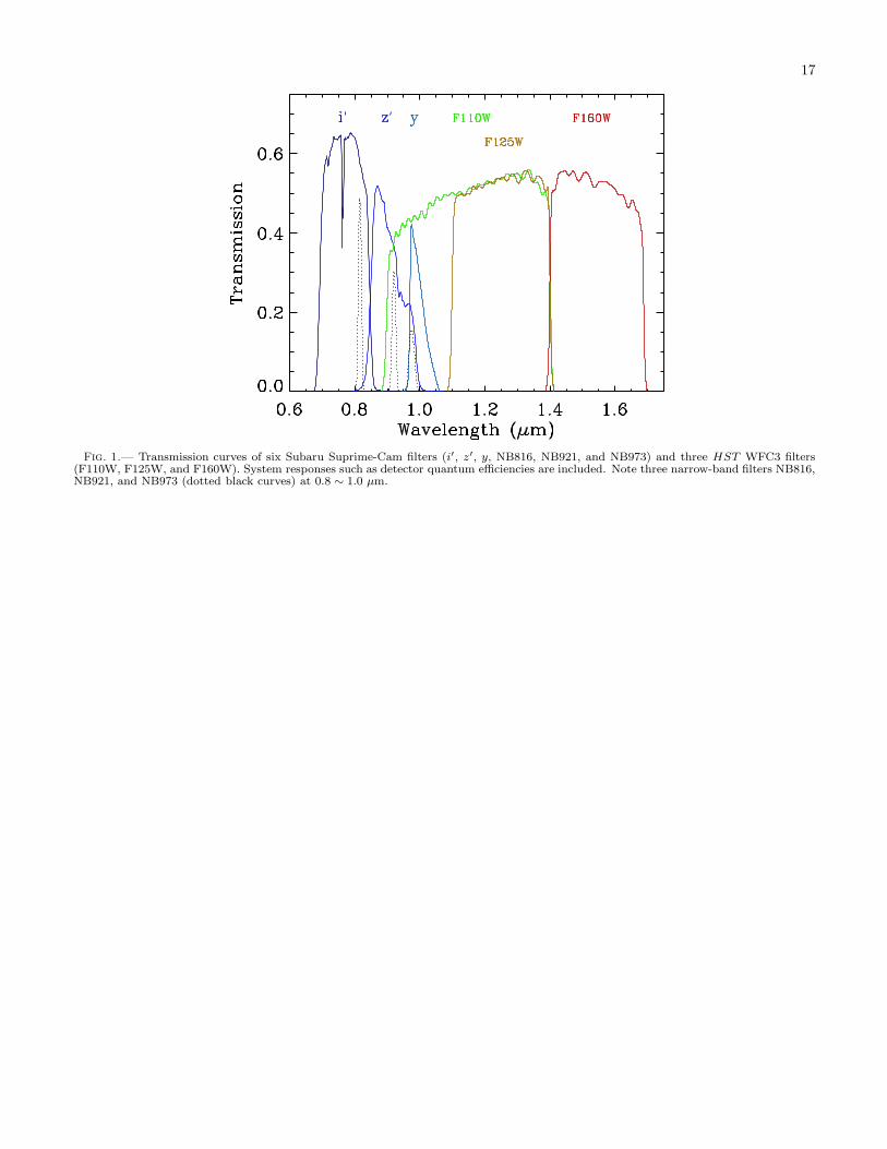
17
Fig. 1.— Transmission curves of six Subaru Suprime-Cam filters (i′, z′, y, NB816, NB921, and NB973) and three HST WFC3 filters(F110W, F125W, and F160W). System responses such as detector quantum efficiencies are included. Note three narrow-band filters NB816,NB921, and NB973 (dotted black curves) at 0.8 ∼ 1.0 µm.

18
Fig. 2.— Examples of measuring UV continuum and Lyα line emission. The upper panel illustrates our model fit to a LAE at z = 5.710.The red circles are the photometric points that we use. The broad-band data in the z′yJ110H160 bands are used to fit the power-lawcontinuum (see Eq. 1). The horizontal bars indicate the wavelength coverage of the broad bands. The photometric error bars are alsoshown, but the errors are very small. When IGM absorption is applied, the continuum flux at the blue side of the Lyα line is absorbed(the dashed line). The region around the Lyα emission line (the dotted line) is zoomed in to show this absorption. Finally the factor A inEq. 1 is calculated by scaling the Lyα emission line to match the NB816-band photometry. The solid profile is the final model spectrum(continuum + Lyα) for this galaxy. The lower panel shows our model fit to a LAE at z = 6.543. In this case we use the data in theyJ125H160 bands to compute its continuum, and use the NB921-band photometry to measure its Lyα emission.
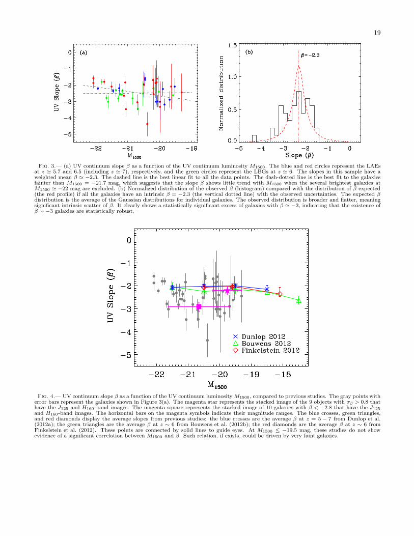
19
Fig. 3.— (a) UV continuum slope β as a function of the UV continuum luminosity M1500. The blue and red circles represent the LAEsat z ≃ 5.7 and 6.5 (including z ≃ 7), respectively, and the green circles represent the LBGs at z ≃ 6. The slopes in this sample have aweighted mean β ≃ −2.3. The dashed line is the best linear fit to all the data points. The dash-dotted line is the best fit to the galaxiesfainter than M1500 = −21.7 mag, which suggests that the slope β shows little trend with M1500 when the several brightest galaxies atM1500 ≃ −22 mag are excluded. (b) Normalized distribution of the observed β (histogram) compared with the distribution of β expected(the red profile) if all the galaxies have an intrinsic β = −2.3 (the vertical dotted line) with the observed uncertainties. The expected βdistribution is the average of the Gaussian distributions for individual galaxies. The observed distribution is broader and flatter, meaningsignificant intrinsic scatter of β. It clearly shows a statistically significant excess of galaxies with β ≃ −3, indicating that the existence ofβ ∼ −3 galaxies are statistically robust.
Fig. 4.— UV continuum slope β as a function of the UV continuum luminosity M1500, compared to previous studies. The gray points witherror bars represent the galaxies shown in Figure 3(a). The magenta star represents the stacked image of the 9 objects with σβ > 0.8 thathave the J125 and H160-band images. The magenta square represents the stacked image of 10 galaxies with β < −2.8 that have the J125and H160-band images. The horizontal bars on the magenta symbols indicate their magnitude ranges. The blue crosses, green triangles,and red diamonds display the average slopes from previous studies: the blue crosses are the average β at z = 5 − 7 from Dunlop et al.(2012a); the green triangles are the average β at z ∼ 6 from Bouwens et al. (2012b); the red diamonds are the average β at z ∼ 6 fromFinkelstein et al. (2012). These points are connected by solid lines to guide eyes. At M1500 ≤ −19.5 mag, these studies do not showevidence of a significant correlation between M1500 and β. Such relation, if exists, could be driven by very faint galaxies.

20
Fig. 5.— Comparison between the observed Lyα luminosities of the LAEs in our paper and the Lyα luminosities given in Kashikawa et al.(2011). The upper panel compares our luminosities to those derived from the photometric data in the galaxy discovery papers. Thephotometric data used in these papers are usually the narrow-band and z′-band photometry. The blue and red circles represent the LAEsat z ≃ 5.7 and 6.5, respectively. The dotted line is the locus where the two measurements are equal. The error bars are typical measurementerrors. The two measurements agree well with each other. The lower panel shows the comparison between our results and the results fromthe spectroscopic data in Kashikawa et al. (2011). The two are also consistent, with a slightly larger scatter than that in the upper panel.

21
Fig. 6.— Lyα luminosity and rest-frame EW (A) as a function of UV luminosity M1500. The color-coded filled circles have the samemeaning as in Figure 3. The open circles represent the LAEs with weak detections (< 5σ) in the J band, and their measurements ofphysical quantities are crude (see Section 4.2). The dashed lines are the best linear fit to the filled circles. The Lyα luminosity shows weakdependence on M1500 in the upper panel. The lower panel shows that lower-luminosity galaxies tend to have higher Lyα EWs. The realrelation should be weaker than it appears due to the nature of the flux-limited sample. There is no significant difference between LAEsand LBGs in the range of M1500 < −19.5 mag.

22
Fig. 7.— SFRs estimated from UV continuum luminosities and Lyα luminosities in units of M⊙ yr−1. The color-coded symbols havethe same meaning as in Figure 6. The solid line represents the position where the two measurements are equal. The dotted line is theexpected ratio of the Lyα SFRs to the UV SFRs assuming that Lyα is absorbed by 24% on average. The dashed line is the best linearfit (in logarithmic space) to the relatively robust measurements (filled circles). The Lyα SFRs are increasingly smaller than the UV SFRstowards higher SFRs, mostly due to the selection effect shown in Figure 6. It could also be due partly to the smaller escape fractions ofLyα photons in higher-SFR galaxies.
−24 −23 −22 −21 −20 −19 −18 −17Muv
1
10
100
1000
EW
(Lya
) (A
ngst
rom
)
L(Ly
a)=2.
5e42
erg
/sLAE z=5.7 (this work)LAE z=6.5 (this work)LAE z=3.1 (Ouchi08)LAE z=3.7 (Ouchi08)LAE z=5.7 (Ouchi08)
(a) LAEs: High−z
−24 −23 −22 −21 −20 −19 −18 −17Muv
1
10
100
1000
EW
(Lya
) (A
ngst
rom
)
L(Ly
a)=2.
5e42
erg
/sLAE z=5.7 (this work)LAE z=6.5 (this work)LAE z=3.1 (Ouchi08)LAE z=3.7 (Ouchi08)LAE z=5.7 (Ouchi08)LAE z~0.2−0.4 (Cowie11)
(b) LAEs: Low−z & High−z
Fig. 8.— EW(Lyα) vs. MUV for LAEs. (a) EW(Lyα) is plotted as a function of MUV for the z ≃ 5.7 and 6.5 LAEs in our sample, as wellas for the z ∼ 3.1, 3.7, and 5.7 LAEs by Ouchi et al. (2008). As for MUV, we used M1500 listed in Table 2 for our sample. For the sampleof Ouchi et al. (2008), we used the published MUV, which correspond to M1300−1600 depending on redshift. The diagonal dotted line isdefined by a limiting Lyα line luminosity of 2.5× 1042 erg s−1, which roughly corresponds to the limits of these LAE surveys. The slope ofthe EW(Lyα)–MUV correlation is largely shaped by the limiting luminosity. (b) GALEX-selected z ≃ 0.2−0.4 LAEs (Cowie, Barger, & Hu2011b) are added for comparison. MUV was derived from the GALEX near-UV photometry in Cowie, Barger, & Hu (2010). The effectivewavelength of the near-UV band is 2315.7 A (Morrissey et al. 2007), so at redshifts z ≃ 0.2−0.4, the near-UV band is sampling ∼1650–1930A in the rest-frame. The near-UV, instead of the far-UV band, was used because the latter contains the redshifted Lyα emission. Thefigure indicates that the EW(Lyα)–MUV relation is largely shaped by the limiting luminosity.
23
−24 −23 −22 −21 −20 −19 −18 −17Muv
1
10
100
1000
EW
(Lya
) (A
ngst
rom
)
L(Ly
a)=2.
5e42
erg
/sLAE z=5.7 (this work)LAE z=6.5 (this work)
LBG z ~ 6 (this work)
LAE z=3.1 (Ouchi08)LAE z=3.7 (Ouchi08)LAE z=5.7 (Ouchi08)
LBG z=3−6 (Stark10)
High−z LAEs vs. LBGs
Fig. 9.— Same as Figure 8, but for LBGs from this work (z ≃ 6) and from Stark et al. (2010) (z ≃ 3 − 6). A number of LBGs fromStark et al. (2010) fall below the L(Lyα)= 2.5 × 1042 erg s−1 line, reflecting the deeper limiting Lyα line flux of the data. The overalldistribution of the points appears similar between the LAE and LBG samples.
Fig. 10.— UV continuum LFs of LAEs with EW > 20 A at z ≃ 5.7 and 6.5. The thick blue and red lines represent the spatial densitiesof the LAEs in our sample, without incompleteness correction to EW = 20 A. The shaded regions show the UV LFs of LAEs corrected toEW(Lyα)= 20 A. Their lower and upper boundaries represent the lower and upper limits of the LFs. The 1σ statistical uncertainties havebeen included. The cyan and green curves represent the UV LFs of LBGs at z ≃ 5.9 and 6.8 (Bouwens et al. 2007, 2011; McLure et al.2009; Ouchi et al. 2009). Compared to LBGs, LAEs have comparable spatial densities in the bright end, but significantly lower densitiesin the faint end.

24
Fig. 11.— Normalized Lyα EW distribution of the LAEs in our sample. The vertical dotted lines represent the approximate EW limitsfor complete LAE samples at the given M1500 ranges. We use an exponential function to fit the EW distribution. We adopt two extremee-folding widths (b = 0.225 and 0) in Section 5.3. The solid curve in the top panel is the best fit to the LAEs at M1500 < −19.5 mag (it isthe same for the two cases). The dashed (b = 0.225) and dash-dotted (b = 0) curves in the other panels are the predicted EW distributionsfor the two extreme cases. The real distribution should be between the two.

25
Fig. 12.— Thumbnail images of the galaxies in our sample. The galaxies are in the middle of the images. The size of the images is6.′′6× 6.′′6 (north is up and east to the left). An image is blank if the data is either not available or meaningless in this band.
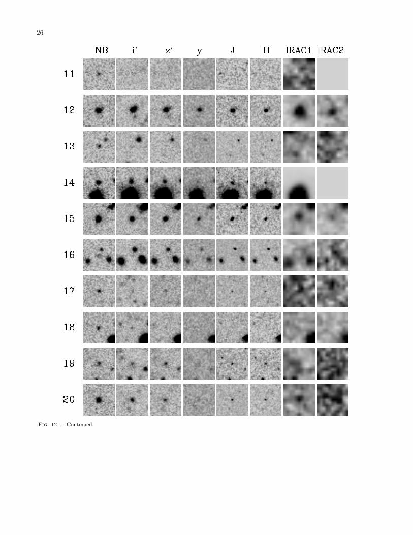
26
Fig. 12.— Continued.

27
Fig. 12.— Continued.

28
Fig. 12.— Continued.

29
Fig. 12.— Continued.

30
Fig. 12.— Continued.

31
Fig. 12.— Continued.