Phylogenetic Stochastic Mapping without Matrix ... - arXiv

Phylogenetic Stochastic Mapping without MatrixExponentiation

Jan Irvahn1 and Vladimir N. Minin1,2,∗

1Department of Statistics and 2Department of BiologyUniversity of Washington, Seattle

∗corresponding author: [email protected]

Abstract

Phylogenetic stochastic mapping is a method for reconstructing the history of traitchanges on a phylogenetic tree relating species/organisms carrying the trait. State-of-the-art methods assume that the trait evolves according to a continuous-time Markovchain (CTMC) and work well for small state spaces. The computations slow downconsiderably for larger state spaces (e.g. space of codons), because current methodol-ogy relies on exponentiating CTMC infinitesimal rate matrices — an operation whosecomputational complexity grows as the size of the CTMC state space cubed. In thiswork, we introduce a new approach, based on a CTMC technique called uniformiza-tion, that does not use matrix exponentiation for phylogenetic stochastic mapping.Our method is based on a new Markov chain Monte Carlo (MCMC) algorithm thattargets the distribution of trait histories conditional on the trait data observed at thetips of the tree. The computational complexity of our MCMC method grows as thesize of the CTMC state space squared. Moreover, in contrast to competing matrixexponentiation methods, if the rate matrix is sparse, we can leverage this sparsity andincrease the computational efficiency of our algorithm further. Using simulated data,we illustrate advantages of our MCMC algorithm and investigate how large the statespace needs to be for our method to outperform matrix exponentiation approaches.We show that even on the moderately large state space of codons our MCMC methodcan be significantly faster than currently used matrix exponentiation methods.

1 Introduction

Phylogenetic stochastic mapping aims at reconstructing the history of trait changes on a phy-logenetic tree that describes evolutionary relationships among organisms of interest. Suchtrait mapping on phylogenies has become a key element in computational evolutionary bi-ology analyses. Stochastic mapping has been used successfully to enable computationalanalyses of complex models of protein evolution (Rodrigue et al., 2008, 2010), to reconstructgeographical movements of ancestral populations (Pereira et al., 2007; Lemey et al., 2009),and to test hypotheses about morphological trait evolution (Huelsenbeck et al., 2003; Ren-ner et al., 2007). Another testimony to the usefulness of stochastic mapping is the fact thatthis relatively new method has already been implemented in multiple widely used softwarepackages: SIMMAP (Bollback, 2006), PhyloBayes (Lartillot et al., 2009), Bio++ libraries(Gueguen et al., 2013), and BEAST (Drummond et al., 2012). Despite all these successes ofstochastic mapping, this technique remains computationally challenging when the numberof states that a trait can assume is large. Here, we present a new phylogenetic stochasticmapping algorithm that scales well with the size of the state space.

1

arX

iv:1

403.

5040

v1 [

stat

.CO

] 2

0 M

ar 2

014

[email protected]

Stochastic mapping, initially developed by Nielsen (2002) and subsequently refined byothers (Lartillot, 2006; Hobolth, 2008), assumes that discrete traits of interest evolve accord-ing to a continuous-time Markov chain (CTMC). Random sampling of evolutionary histo-ries, conditional on the observed data, is accomplished by an algorithm akin to the forwardfiltering-backward sampling algorithm for hidden Markov models (HMMs) (Scott, 2002).However, since stochastic mapping operates in continuous-time, all current stochastic map-ping algorithms require computing CTMC transition probabilities via matrix exponentiation— a time consuming and potentially numerically unstable operation, when the CTMC statespace grows large. de Koning et al. (2010) recognized the computational burden of the exist-ing techniques and developed a faster, but approximate, stochastic mapping method basedon time-discretization. We propose an alternative, exact stochastic mapping algorithm thatrelies on recent developments in the continuous-time HMM literature.

Rao and Teh (2011) used a CTMC technique called uniformization to develop a methodfor sampling hidden trajectories in continuous time HMMs. The use of uniformization inthis context is not new, but all previous methods produced independent samples of hiddentrajectories with the help of matrix exponentiation — an operation with algorithmic com-plexity O(s3), where s is the size of the CTMC state space (Fearnhead and Sherlock, 2006).Rao and Teh (2011) constructed a Markov chain Monte Carlo (MCMC) algorithm targetingthe posterior distribution of hidden trajectories. Their new method eliminates the need formatrix exponentiation and results in an algorithm with complexity O(s2). Moreover, themethod of Rao and Teh (2011) can further increase its computational efficiency by takingadvantage of sparsity of the CTMC rate matrix. Here, we take the method of Rao and Teh(2011) and extend it to phylogenetic stochastic mapping.

As in the original method of Rao and Teh (2011), our new stochastic mapping methodmust pay a price for bypassing the matrix exponentiation step. The cost of the improvedalgorithmic complexity is the replacement of Monte Carlo in the state-of-the-art stochasticmapping with MCMC. Since Monte Carlo, if practical, is generally preferable to MCMC, itis not immediately clear that our new algorithm should be an improvement on the originalmethod in all situations. We perform an extensive simulation study, comparing performanceof our new MCMC method with a matrix exponentiation method for different sizes of thestate space. We conclude that, after accounting for dependence of trait history samples, ournew MCMC algorithm can outperform existing approaches even on only moderately largestate spaces (s ∼ 30). We demonstrate additional computational efficiency of our algorithmwhen taking advantage of sparsity of the CTMC rate matrix. Since we suspect that our newmethod can speed up computations during studies of protein evolution, we examine in detaila standard GY94 codon substitution model (s = 61) (Goldman and Yang, 1994). We showthat our new method can reduce computing times of state-of-the-art stochastic mapping byat least of factor of ten when working with this model. The last finding is important, becausestate-of-the-art statistical methods based on codon models often grind to a halt when appliedto large datasets (Valle et al., 2014).

2

2 Methods

2.1 CTMC model of evolution

We start with a trait of interest, X(t), and a rooted phylogenetic tree with n tips and 2n−2branches. We assume that the phylogeny and its branch lengths, β = (β1, . . . , β2n−2), areknown to us. The trait can be in one of s distinct states, 1, . . . , s, at any particular place onthe tree. We follow standard phylogenetics practice and assume that the trait evolves alongthe phylogenetic tree by the following stochastic process. First, a trait value is drawn at theroot of the tree from an initial distribution π = (π1, . . . , πs). Next, starting at the root state,we use a CTMC with an infinitesimal s×s rate matrix Q = qkh to produce two independentCTMC trajectories along the branches leading to the two immediate descendants of the rootnode. After generating a CTMC trajectory along a branch we necessarily have generated astate for the child node of the branch. The procedure proceeds recursively by conditioning ona parent node and evolving the same CTMC independently along the two branches leadingto the parent’s children nodes. The random process stops when we reach the tips — nodesthat have no descendants. Trait states at the tips of the tree are observed, while the traitvalues everywhere else on the tree are considered missing data. We collect the observed datainto a vector y.

A substitution history for a phylogenetic tree is the complete list of transition events(CTMC jumps), including the time of each event (location on the tree) and the type ofthe transition event (e.g., 2 → 1 transition). This state history can be encoded in a set ofvectors, two vectors for each branch. Suppose branch i has ni transitions so the full statehistory for branch i can be described by a vector of state labels, si = (si0, ..., sini

), and avector of intertransition times, ti = (ti0, ..., tini

). Let S be the collection of all the si vectorsand let T be the collection of all the ti vectors, forming the full substitution history, (S, T ).See plot 3 in Figure 1 for a substitution history example. The tree in Figure 1 has fourbranches so the collection of state labels is S = s1, s2, s3, s4, where s1 = (1), s2 = (1, 2),s3 = (3), and s4 = (3, 1). The collection of intertransition times is T = t1, t2, t3, t4, wheret1 = (3.2), t2 = (0.64, 2.56), t3 = (8), and t4 = (2.4, 2.4).

The goal of stochastic mapping is to be able to compute properties of the distribution ofthe substitution history of a phylogenetic tree conditional on the observed states at the tipsof the tree, p(S, T |y).

2.2 Nielsen’s Monte Carlo Sampler

Nielsen (2002) proposed the basic framework that state-of-the-art phylogenetic stochasticmapping currently uses. His approach samples directly from the conditional distribution,p(S, T |y), in three steps. First, one calculates partial likelihoods using Felsenstein’s algo-rithm (Felsenstein, 1981). The partial likelihood matrix records the likelihood of the observeddata at the tips of the tree beneath each node after conditioning on the state of said node.This requires calculating transition probabilities for each branch via matrix exponentiation.Second, one recursively samples internal node states, starting from the root of the tree.Third, one draws realizations of CTMC trajectories on each branch conditional on the sam-pled states at the branch’s parent and child nodes. The last step can be accomplished by

3

multiple algorithms reviewed in (Hobolth and Stone, 2009). In order to avoid matrix expo-nentiation while approximating p(S, T |y) we will need a data augmentation technique calleduniformization.

2.3 CTMC Uniformization

An alternative way to describe the CTMC model of evolution on a phylogenetic tree usesa homogenous Poisson process coupled with a discrete time Markov chain (DTMC) that isindependent from the Poisson process. The intensity of the homogenous Poisson process, Ω,must be greater than the largest rate of leaving a state, maxk|qkk|. The generative processthat produces a substitution history on a phylogenetic tree first samples the total numberof DTMC transitions over the tree, N , drawn from a Poisson distribution with mean equalto Ω

∑2n−2i=1 βi — the product of the Poisson intensity and the sum of all the branch lengths.

The locations/times of the N transitions are then distributed uniformly at random across allthe branches of the tree. These transition time points separate each branch into segments.The intertransition times (the length of each segment) for branch i compose the vector,wi, where the sum of elements of this vector equal the branch length βi. The state ofeach segment evolves according to a DTMC with transition probability matrix B = bkhsatisfying B = I + Q/Ω.

Again, the uniformized generative process samples a state at the root of the tree andworks down the tree sampling the state of each branch segment sequentially. Conditionalon the previous/ancestral segment being in state k, we sample the current segment’s statefrom a multinomial distribution with probabilities (bk1, . . . , bks). The states of each segmentof branch i compose the vector, vi. It is important to note that the stochastic transitionmatrix B allows the DTMC to transition from state k to state k, i.e., self transitions areallowed. Intuitively, the dominating homogenous Poisson process produces more transitionevents (on average) than we would expect under the CTMC model of evolution. The DTMCallows some of the transitions generated by the Poisson process to be self transitions so thatthe remaining “real” transitions and times between them yield the exact CTMC trajectorieswe desire (Jensen, 1953).

An augmented substitution history of a phylogenetic tree encodes all the information in(S, T ) and adds virtual jump times as seen in plot 4 of Figure 1. The notation describingan augmented substitution history is similar to the notation used to describe a substitutionhistory. One branch is fully described by two vectors. Let branch i have mi jumps (realand virtual) and again, vi = (vi0, ..., vimi

) is a vector of state labels, wi = (wi0, ..., wimi)

is a vector of intertransition times, V is the collection of all the vi vectors, and W is thecollection of all the wi vectors. The augmented state history is (V ,W). The tree in plot 4of Figure 1 has four branches so the collection of state labels is V = v1,v2,v3,v4, wherev1 = (1, 1), v2 = (1, 2), v3 = (3, 3), and v4 = (3, 1). The collection of intertransitiontimes is W = w1,w2,w3,w4, where w1 = (1.6, 1.6), w2 = (0.64, 2.56), w3 = (7, 1), andw4 = (2.4, 2.4). The locations/times of each virtual jump on branch i is represented by avector ui = (ui1, .., ui(mi−ni)). For example, the distance from the parent node of branch i tothe dth virtual jump is uid. The collection of the ui vectors, fully determined by (V ,W), isdenoted by U . In plot 4 of Figure 1 the collection of virtual jump times is U = u1,u2,u3,u4where u1 = (1.6), u2 = (), u3 = (7), and u4 = ().

4

2.4 New MCMC Sampler

Equipped with notation describing the CTMC model of evolution and a companion uni-formization process, we now turn our attention to making inference about a phylogenetictree state history conditional on observed data. We investigate the situation where the treetopology is fixed, branch lengths are fixed, and the rate matrix parameters are all knownand fixed. The goal is to construct an ergodic Markov chain on the state space of augmentedsubstitution histories with the stationary distribution p(V ,W|y).

Our MCMC sampler uses two Markov kernels to create a Markov chain whose stationarydistribution is p(V ,W|y). The first kernel samples from p(V|W ,y) — the distribution ofstates on the tree conditional on tip states and the jump locations on each branch. A Markovchain that sequentially draws from this full conditional has p(V ,W|y) as its stationarydistribution. This kernel alone is not ergodic because the set of transition times, W , is notupdated. To create an ergodic Markov chain we introduce a second Markov kernel to samplefrom p(U|S, T ,y) — the distribution of virtual transitions conditional on the substitutionhistory. Again, drawing from the full conditional of U ensures that p(V ,W|y) is a stationarydistribution of this kernel. This kernel alone is not ergodic either but when the two kernelsare combined we create an ergodic Markov chain with the desired stationary distribution.In general, it takes two sequential applications of the above kernels before the probabilitydensity of transitioning between two arbitrary augmented substitution histories becomesnonzero.

2.4.1 Sampling States from p(V|W ,y)

Our strategy for sampling states V is to make a draw from the full conditional of internalnode states and then to sample the states along each branch conditional on the branch’sparent and child nodes. It is useful to remember that when conditioning on the numberof virtual and real jumps, and locations of these jumps on the tree, our data generatingprocess becomes a DTMC with transition probability matrix B and a known number oftransitions on each branch. Alternatively, we can think of the trait evolving along eachbranch i according a branch-specific DTMC with transition probability matrix Bmi , wheremi is the number of transitions on branch i. This is similar to representing a regular,non-uniformized, CTMC model as a collection of branch-specific DTMCs with transitionprobability matrices P(β1), . . . ,P(β2n−2). This analogy allows us to use standard algorithmsfor sampling internal node states on a phylogenetic tree by replacing in these algorithmsP(βi) with Bmi for all i = 1, . . . , 2n − 2. For completeness, we make this substitutionexplicit below.

We start by using Felsenstein’s algorithm to compute a partial likelihood matrix L =ljk, where ljk is the probability of the observed tip states below node j given that node j isin state k (Felsenstein, 1981). The matrix L has (2n− 1) rows and s columns because thereare (2n− 1) nodes (including the tips) and there are s states. Starting at the tips, we workour way up the tree calculating partial likelihoods at internal nodes as we go. We need tocalculate the partial likelihood at both child nodes before calculating the partial likelihoodat a parent node because of the recursive nature of the Felsenstein algorithm. The algorithmis initialized by setting each row corresponding to a tip node to zeros everywhere except for

5

the column corresponding to the observed state of that tip. The matrix value at this entryis set to 1. Next, we calculate the partial likelihoods for all the internal nodes. Supposebranch i connecting parent node p to child node c has mi jumps so the probability transitionmatrix for branch i is E(mi) ≡ Bmi . The probability of transitioning from state h to statek along branch i is e(i)hk, the (h, k)th element of E(mi). We refer to the state of node j asyj. The probability of observing the tip states below node c conditional on node p being instate h is

gpch =s∑

k=1

Pr(yc = k|yp = h)lck = (e(mi)h−) (lc−)T ,

where lc− = (lc1, . . . , lcs). If node c is a tip then conditioning on the tip states below c isthe same as conditioning on the state of tip c. We combine the probabilities, gpch, for eachstate h into a single vector, gpc−, and then create the same type of vector for the secondbranch below node p, gpd−. Element wise multiplication of the two vectors yields the vectorof partial likelihoods for node p:

(lp−)T = gpc− ∗ gpd−.

After working our way up the tree we have the matrix of partial likelihoods, L.

Sampling internal node states Starting at the root we work our way down the treesampling the states of internal nodes conditional on tip states, the number of jumps on eachbranch, and previously sampled internal node states. The prior probability that the root isin state k is the kth element of the probability vector π. The probability that the root is instate k given the states of all the tip nodes is,

Pr(yroot = k|y) =Pr(yroot = k & y)

Pr(y)=

Pr(yroot = k)Pr(y|yroot = k)∑sh=1 Pr(yroot = h)Pr(y|yroot = h)

=πkl(root k)

l(root -)π.

Once we calculate the probability of the root being in each possible state we sample the stateof the root from the multinomial distribution with probabilities we just computed. Next,we sample all non-root, non-tip nodes. Without loss of generality, let us consider node cconnected to its parent node, node p, by branch i. Suppose node p’s previously sampledstate is h and the number of jumps on branch i is mi. The vector containing observed tipstates at the eventual descendants of node c is dc. The probability that node c is in state kgiven node p is in state h and given the state of the tips below node c is

Pr(yc = k|yp = h & dc) =Pr(yc = k|yp = h)Pr(dc|yc = k)∑sk=1 Pr(yc = k|yp = h)Pr(dc|yc = k)

=e(mi)hklck

e(mi)h−(lc−)T. (1)

Starting with the root we can now work our way down the tree sampling the states of eachnode from the multinomial distributions with probabilities we just described. Equation (1)may suggest that sampling internal nodes has algorithmic complexity O(s3), because raisinga matrix to a power requires O(s3) multiplications. It is important to note that we neverneed to calculate Bm as we only need Bm × vector, which requires O(s2) multiplications.

6

Sampling branch states We sample the states on each branch separately, conditioningboth on previously sampled internal nodes states and on the number of transitions on eachbranch. Conditioning on the internal node states means the starting and ending state of eachbranch are set so we only sample internal segments of the branches. Conditioning on thenumber of transitions on a branch means we are sampling states of the discrete time Markovchain with transition matrix B. Suppose branch i starts in state vi0 and ends in state vimi

(oryc). We sample each segment of the branch in turn, starting with the second segment becausethe first segment has to be in the same state as the parent node of the branch. The stateof each segment is sampled conditional on the state of the previous segment, the numberof transitions until the end of the branch, and the ending state of the branch, vimi

= yc.The state of the dth segement is sampled from a multinomial distribution with probabilitiescalculated according to the following formula:

Pr(vid = k|vi(d−1) = h, vimi= yc) =

Pr(vi(d−1) = h, vid = k, vimi= yc)

Pr(vi(d−1) = h, vimi= yc)

=Pr(vi(d−1) = h)Pr(vid = k|vi(d−1) = h)Pr(vimi

= yc|vid = k)

Pr(vi(d−1) = h)Pr(vimi= yc|vi(d−1) = h)

=bhke(mi − d)kyce(mi − d+ 1)hyc

.

After sampling the states along each branch we have completed one cycle through the firstMarkov kernel by sampling from p(V|W ,y). The second Markov kernel requires us to samplevirtual transitions conditional on the current substitution history (not augmented by virtualjumps).

2.4.2 Sampling Virtual Jumps from p(U|S, T ,y)

After sampling the states on each branch, V , we resample virtual jumps, U , on each branchseparately. Without loss of generality consider a branch with a newly sampled substitutionhistory, (s, t), which is the augmented substitution history with all the virtual jumps re-moved. Suppose the branch contains n real transitions. Resampling virtual jumps for thebranch involves resampling virtual jumps for each of the n + 1 segments of the branch sep-arately. To sample the ath segment of the branch we need to sample the number of virtualjumps, µa, and the locations of these virtual jumps. After sampling virtual jumps for eachof the n + 1 branch segments we have m transitions total, both real and virtual, so thatm = n +

∑na=0 µa. Careful examination of the likelihood of the dominating homogenous

Poisson process for a single branch of the tree allows us to derive the distribution of virtualjumps conditional on the substitution history of the branch.

Suppose there are m jumps along a branch including real transitions and virtual transi-tions. Let vd be the state of the chain after the dth transition and let π′v0 be the probabilitythat the branch starts in state v0. The density of the augmented substitution history is

p(v,w) = π′v0e−Ωt(Ωt)m

m!

m!

tm

m∏d=1

Bvd−1,vd . (2)

The density as written above has four parts, the probability of starting in state v0 = s0,the probability of m transition points, the density of the locations of m unordered points

7

conditional on there being m points, and the probability of each transition in a discrete timeMarkov chain with transition matrix B.

The density of the augmented substitution history of one branch, p(v,w), can be rewrit-ten as p(u, s, t), because the substitution history, (s, t) combined with the virtual jumplocations, u, form the augmented substitution history. To derive the full conditional for u,we follow Rao and Teh (2011) and rewrite density (2) as follows:

p(u, s, t) = p(v,w) =n∏a=0

(rµaa e

−rata)π′s0

(n∏z=1

|qsz−1 |eqsz−1 tz−1qsz−1sz

|qsz−1|

)eqsn tn =

n∏a=0

(rµaa e

−rata)

p(s, t),

where qsa ≡ qsasa and ra = Ω + qsa . Therefore,

p(u|s, t,y) = p(u|s, t) =p(u, s, t)

p(s, t)=

n∏a=0

(rµaa e

−rata)

=n∏a=0

e−rata(rata)µa

µa!

µa!

tµaa. (3)

The full conditional density (3) is a density of an inhomogenous Poisson process withintensity r(t) = Ω + qX(t). This intensity is piecewise constant so we can add self transitionlocations/times to a branch segment in state sa by drawing a realization of a homogenousPoisson process with rate ra = Ω + qsa . More specifically, we sample the number of selftransitions, µa, on this segment by sampling from a Poisson distribution with mean rata andthen distributing the locations/times of the µa self transitions uniformly at random acrossthe segment. This procedure is repeated independently for all segments on all branches ofthe phylogenetic tree, concluding our MCMC development, summarized in Algorithm 1 andillustrated in Figure 1.

Algorithm 1 MCMC for phylogenetic stochastic mapping

1: Start with an augmented substitution history, (V0,W0)2: for γ ∈ 1, 3, 5, . . . , 2N − 1 do3: sample from p(Vγ|Wγ−1,y) producing a new substitution history (Sγ, Tγ)

(i) sample internal node states conditional on y and the number of jumps on eachbranch

(a) starting at the tips work up the tree calculating partial likelihoods

(b) starting at the root work down the tree sampling internal node states

(ii) sample segmental states conditional on end states and number of jumps

4: sample from p(Uγ+1|Sγ, Tγ), producing (Vγ+1,Wγ+1)

(i) remove virtual jumps

(ii) sample virtual jumps conditional on substitution history

5: end for6: return (V0,W0), (V2,W2), . . . , (V2N ,W2N)

8

state 1 state 2 state 3

augmented

substitution history

1)

resample states

2)

remove virtual jumps

3)

1 2

3

4

sample new virtual jumps

4)

Figure 1: An example of applying the two Markov kernels of our MCMC sampler to anaugmented substitution history. The diamonds represent virtual transitions. 1) shows aninitial augmented substitution history; 2) shows the substitution history after resamplingstates on the phylogeny conditional on tip node states and the transition points (both realand virtual); 3) shows the substitution history seen in 2) with no virtual jumps; 4) showsthe augmented substitution history after resampling virtual jumps conditional on the sub-stitution history seen in 3). The transition from 1) to 2) shows the effect of the first Markovkernel, sampling from p(V|W ,y). The transition from 3) to 4) shows the effect of the secondMarkov kernel, sampling from p(U|S, T ).

3 Assessing Computational Efficiency

3.1 Algorithm Complexity

State-of-the-art stochastic mapping approaches rely on exponentiating CTMC rate matrices,requiring O(s3) operations. Our MCMC algorithm uses only matrix-by-vector multiplica-tions, allowing us to accomplish the same task in O(s2) operations. Moreover, if the CTMCrate matrix is sparse, the algorithmic complexity of our method can go down further. Forexample, if Q is a tri-diagonal matrix, as in the birth-death CTMCs used to model evolu-tion of gene family sizes (Spencer et al., 2006), then our MCMC achieves an algorithmiccomplexity of O(s). In contrast, even after disregarding the cost of matrix exponentiation,approaches relying on this operation require at least O(s2) operations, because eQt is a densematrix regardless of the sparsity of Q. However, since the number of matrix-by-vector mul-tiplications is a random variable in our algorithm, the algorithmic complexity with respectto the state space size does not tell the whole story, prompting us to perform an empiricalcomparison of the two approaches in a set of simulation studies. In these simulation studies,we need to compare state-of-the-art Monte Carlo algorithms and our MCMC in a principledway, which we describe in the next subsection.

3.2 Effective Sample Size

When comparing timing results of our MCMC approach and a matrix exponentiation ap-proach, we need to account for the fact that our MCMC algorithm produces correlated

9

substitution histories. One standard way to compare computational efficiency of MCMCalgorithms is by reporting CPU time divided by effective sample size (ESS), where ESS is ameasure of the autocorrelation in a stationary time series (Holmes and Held, 2006; Girolamiand Calderhead, 2011). More formally, the ESS of a stationary time series of size N withstationary distribution ν is an integer Neff such that Neff independent realizations from νhave the same sample variance as the sample variance of the time series. The ESS of astationary time series of size N is generally less than N and is equal to N if the time seriesconsists of independent draws from ν.

In MCMC literature, ESSs are usually calculated for model parameters, latent variables,and the log-likelihood. Since we are fixing model parameters in this paper, we monitor ESSsfor our latent variables — augmented substitution history summaries — and log p(S, T ) —the log-density of the substitution history. Although the amount of time spent in each stateover the entire tree and the numbers of transitions between each possible pair of states aresufficient statistics of a fully observed CTMC (Guttorp, 1995), it is impractical to use allof these summaries for ESS calculations. This stems from the fact that we are interestedin the parameter regimes under which we expect a small number of CTMC transitions overthe entire tree. In such regimes, some of the states are never visited so the amount oftime spent in these states is zero, which creates an impression that the MCMC is mixingpoorly. To avoid this problem, we restrict our attention to the amount of time spent (overthe entire tree) in each of the states that are observed at the tips. Similarly, we restrict ourattention to transition counts between observed tip states. Each of the univariate statis-tics, including the log-density of the substitution history, yields a potentially different ESS,which we calculate with the help of the R package coda (Plummer et al., 2006). We followGirolami and Calderhead (2011) and conservatively use the minimum of these univariateESSs to normalize the CPU time of running our MCMC sampler. More specifically, in allour numerical experiments, we generate 10,000 substitution histories via both MCMC andmatrix exponentiation methods and then multiply the CPU time of our MCMC sampler by10, 000/min(univariate ESSs).

3.3 Matrix Exponentiation

In all our simulations we compare timing results of our new MCMC approach with anotherCTMC uniformization approach that relies on matrix exponentiation (Lartillot, 2006). Forthe matrix exponentiation approach we recalculate the partial likelihood matrix at eachiteration, which involves re-exponentiating the rate matrix. We do so in order to learnhow our MCMC method will compare to the matrix exponentiation method in situationswhere the parameters of the rate matrix are updated during a MCMC that targets the jointposterior of substitution histories and CTMC parameters (Lartillot, 2006; Rodrigue et al.,2008). Since matrix exponentiation is a potentially unstable operation (Moler and Van Loan,1978), we do not repeat it at each iteration in our simulations. Instead, we pre-compute aneigen decomposition of the CTMC rate matrix once, cache this decomposition and thenuse it to exponentiate Q at each iteration. Even though exponentiating Q using its pre-computed eigen decomposition is an O(s3) operation, our simulations do not fully mimic amore realistic procedure that repeatedly re-exponentiates the rate matrix. Skipping the eigendecomposition operation at each iteration of stochastic mapping increases computational

10

efficiency of the matrix exponentiation method, making our timing comparisons conservative.In one of our simulation studies, when we consider the effect of sparsity in the rate

matrix, we depart from this matrix exponentiation regime. Instead of exponentiating therate matrix at each iteration we exponentiate the rate matrix Q and compute the partiallikelihood matrix once, sampling substitution histories at each iteration without recalculatingbranch-specific transition probabilities or partial likelihoods. We refer to this method as“EXP once.” We do not believe that our MCMC method is the most appropriate in thisregime, but we are interested in how our new method compares to state-of-the-art methodswhen the calculations requiring O(s3) operations were not involved.

3.4 Implementation

We have implemented our new MCMC approach in an R package phylomap, available athttps://github.com/vnminin/phylomap. The package also contains our implementationof the matrix exponentiation-based uniformization method of Lartillot (2006). We reused asmuch code as possible between these two stochastic mapping methods in order to minimizethe impact of implementation on our time comparison results. We coded all computationallyintensive parts in C++ with the help of the Rcpp package (Eddelbuettel and Francois, 2011).We used the RcppArmadillo package to perform sparse matrix calculations (Eddelbuetteland Sanderson, 2014).

4 Numerical Experiments

4.1 General Set Up

We started all of our simulations by creating a random tree with 50 or 100 tips using thediversitree R package (FitzJohn, 2012). For each simulation that required the construc-tion of a rate matrix, we set the transition rates between all state pairs to be identical. Wethen scaled the rate matrix for each tree so that the number of expected CTMC transitionsper tree was either 2 or 6. These two values were intended to mimic slow and fast ratesof evolution. Six expected transitions in molecular evolution settings is usually consideredunreasonably high but six transitions (or more) is reasonable in other settings like phylo-geography. For example, investigations of Lemey et al. (2009) into the geographical spreadof human influenza H5N1 found on the order of 40 CTMC transitions on their phylogenies.To obtain each set of trait data we simulated one full state history after creating a tree anda rate matrix. We used this full state history as the starting augmented substitution historyfor our MCMC algorithm.

To ensure our implementation of the matrix exponentiation approach properly sam-pled from p(S, T |y) and to ensure the stationary distribution of our MCMC approach wasp(V ,W|y), we compared distributions of univariate statistics produced by our implementa-tions to the same distributions obtained by using diversitree’s implementation of phylo-genetic stochastic mapping. We found that all implementations, including diversitree’s,appeared to produce the same distributions. Boxplots and histograms showing the resultsof our investigations can be found in Appendix A of the Supplementary Materials.

11

https://github.com/vnminin/phylomap

4.2 MCMC Convergence

Although we have outlined a strategy for taking MCMC mixing into account via the normal-ization by ESS, we have not addressed possible problems with convergence of our MCMC.Examination of MCMC chains with an initial distribution different from the stationary dis-tribution showed very rapid convergence to stationarity, as illustrated in Figure C-1 in theSupplementary Materials. Such rapid convergence is not surprising in light of the fact thatwe jointly update a large number of components in our MCMC state space without resortingto Metropolis-Hastings updates.

4.3 Effect of State Space Size

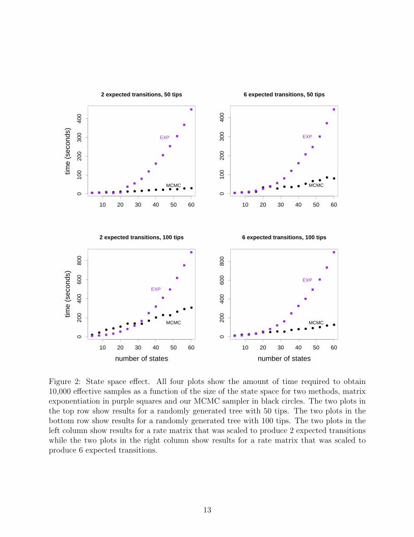
Our MCMC method scales more efficiently with the size of the state space than matrixexponentiation methods so we were first interested in comparing running times of the twoapproaches as the size of the CTMC state space increased. In Figure 2, we show the amountof time it took the matrix exponentiation method to obtain 10,000 samples for different statespace sizes and we show the amount of time it took our MCMC method to obtain an ESSof 10,000 for different state space sizes. The size of the state space varied between 4 statesand 60 states. The tuning parameter, Ω, was set to 0.2, ranging between 15 and 103 timeslarger than the largest rate of leaving a state.

Figure 2 contains timing results for four different scenarios. We considered two differentrates of evolution corresponding to 2 expected transitions per tree and 6 expected transitionsper tree and we considered two different tree tip counts, 50 and 100. The MCMC approachstarted to run faster than the matrix exponentiation approach when the size of the statespace entered the 25 to 35 state range. At 60 states the MCMC approach was clearly fasterin all four scenarios. For the senario involving 100 tips, 2 expected transtions, and 60 statesthe MCMC method was almost 3 times faster than the matrix exponentiation approach. Forthe scenario involving 50 tips, 2 expected transtions, and 60 states the MCMC method wasabout 15 times faster than the matrix exponentiation approach.

Our MCMC approach scales well beyond state spaces of size 60 though matrix expo-nentiation does not. Timing results for our MCMC approach at larger state space sizescan be found in Figure D-1 of the Supplementary Materials. Matrix exponentiation-basedstochastic mapping was prohibitively slow on state spaces reported in Figure D-1.

4.4 Effect of the Dominating Poisson Process Rate

Our tuning parameter, the dominating Poisson process rate Ω, balances speed against mixingfor our MCMC approach. The larger Ω is the slower the MCMC runs and the better it mixes.The optimal value for Ω depends on the CTMC state space and on the entries of the CTMCrate matrix. In our experience, it is not difficult to find a reasonable value for Ω for afixed tree and a fixed rate matrix by trying different Ω values. We show the results of thisexploration in Figure 3 for two different values of the state space size, 4 and 60, and for twodifferent trees, with 50 and 100 tips.

The top left plot in Figure 3 shows the balance between speed and mixing most clearly.The optimal value for Ω appears to be around 0.2 for 4 states and 50 tips. Our MCMC

12

10 20 30 40 50 60

010

020

030

040

0

2 expected transitions, 50 tips

time

(sec

onds

)

MCMC

EXP

10 20 30 40 50 60

010

020

030

040

0


MCMC

EXP

10 20 30 40 50 60

020

040

060

080

0


number of states

time

(sec

onds

)

MCMC

EXP

10 20 30 40 50 60

020

040

060

080

0


number of states

MCMC

EXP

Figure 2: State space effect. All four plots show the amount of time required to obtain10,000 effective samples as a function of the size of the state space for two methods, matrixexponentiation in purple squares and our MCMC sampler in black circles. The two plots inthe top row show results for a randomly generated tree with 50 tips. The two plots in thebottom row show results for a randomly generated tree with 100 tips. The two plots in theleft column show results for a rate matrix that was scaled to produce 2 expected transitionswhile the two plots in the right column show results for a rate matrix that was scaled toproduce 6 expected transitions.

13

0.2 0.4 0.6 0.8

56

78

910

4 states, 50 tips

time

(sec

onds

)

EXP

MCMC

0.2 0.4 0.6 0.8

100

200

300

400

60 states, 50 tips

EXP

MCMC

0.2 0.4 0.6 0.8

1020

3040

5060

4 states, 100 tips

Omega

time

(sec

onds

)

EXP

MCMC

0.2 0.4 0.6 0.8

200

400

600

800

60 states, 100 tips

Omega

EXP

MCMC

Figure 3: Time to obtain 10,000 effective samples as a function of the dominating Poissonprocess rate, Ω. All four plots show results of our MCMC sampler in black. Timing resultsfor the matrix exponentiation method are represented by a purple horizontal line becausethe matrix exponentiation result does not vary as a function of Ω. The two plots in the toprow show results for a randomly generated tree with 50 tips. The two plots in the bottomrow show results for a randomly generated tree with 100 tips. The rate matrix for the plotsin the left column had 4 states. The rate matrix for the plots in the right column had 60states.

14

approach is clearly faster than the matrix exponentiation approach for a wide range of Ωvalues when the size of the state space is 60. When the size of the state space is 4 the matrixexponentiation approach can be faster, which is not surprising given the small size of thestate space. Matrix exponentiation is about two times faster than our MCMC approach forthe 100 tip tree with 4 states. Our MCMC approach can yield comparable speeds to thematrix exponentiation approach for the 50 tip tree with 4 states.

4.5 Effect of Sparsity

Unlike matrix exponentiation methods, our new MCMC sampler is able to take advantageof sparsity in the CTMC rate matrix. There are three steps in our algorithm that cantake advantage of sparsity: computing the partial likelihood matrix, sampling internal nodestates, and resampling branch states. In all three situations we need to multiply BM bya vector of length s – the size of the state space. For a dense matrix this takes O(Ms2)operations. When matrix B is sparse, the above multiplication requires fewer operations.For example, multiplying a vector by BM takes O(Ms) operations when B is triadiagonal.It is interesting to note that while matrix exponentiation approaches cannot take advantageof sparsity when creating the partial likelihood matrix they can use sparsity when samplingbranches via the uniformization technique of Lartillot (2006).

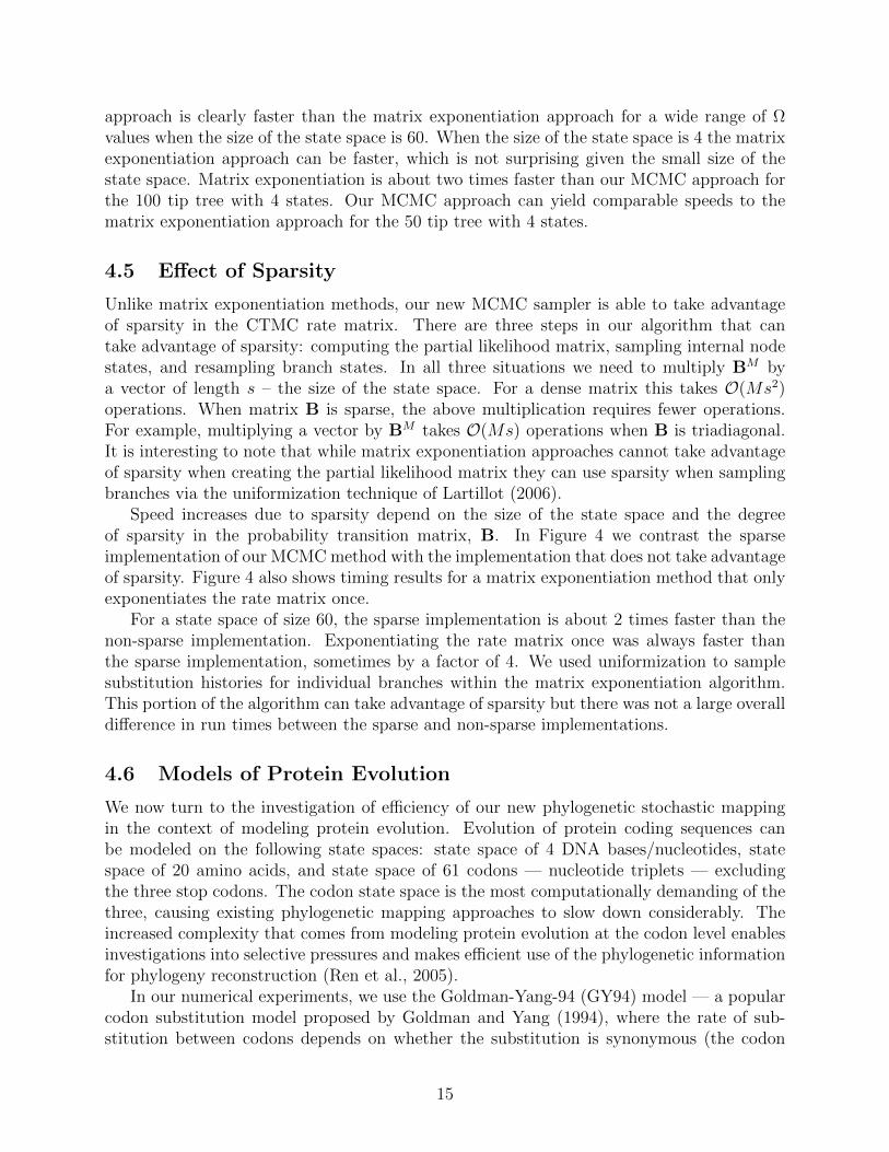
Speed increases due to sparsity depend on the size of the state space and the degreeof sparsity in the probability transition matrix, B. In Figure 4 we contrast the sparseimplementation of our MCMC method with the implementation that does not take advantageof sparsity. Figure 4 also shows timing results for a matrix exponentiation method that onlyexponentiates the rate matrix once.

For a state space of size 60, the sparse implementation is about 2 times faster than thenon-sparse implementation. Exponentiating the rate matrix once was always faster thanthe sparse implementation, sometimes by a factor of 4. We used uniformization to samplesubstitution histories for individual branches within the matrix exponentiation algorithm.This portion of the algorithm can take advantage of sparsity but there was not a large overalldifference in run times between the sparse and non-sparse implementations.

4.6 Models of Protein Evolution

We now turn to the investigation of efficiency of our new phylogenetic stochastic mappingin the context of modeling protein evolution. Evolution of protein coding sequences canbe modeled on the following state spaces: state space of 4 DNA bases/nucleotides, statespace of 20 amino acids, and state space of 61 codons — nucleotide triplets — excludingthe three stop codons. The codon state space is the most computationally demanding of thethree, causing existing phylogenetic mapping approaches to slow down considerably. Theincreased complexity that comes from modeling protein evolution at the codon level enablesinvestigations into selective pressures and makes efficient use of the phylogenetic informationfor phylogeny reconstruction (Ren et al., 2005).

In our numerical experiments, we use the Goldman-Yang-94 (GY94) model — a popularcodon substitution model proposed by Goldman and Yang (1994), where the rate of sub-stitution between codons depends on whether the substitution is synonymous (the codon

15

10 20 30 40 50 60

510

1520

2530


time

(sec

onds

) MCMC

sparse MCMC

EXP once

10 20 30 40 50 60

1020

3040

5060

70


MCMC

sparse MCMC

EXP once

10 20 30 40 50 60

2040

6080

100


number of states

time

(sec

onds

)

MCMC

sparse MCMC

EXP once

10 20 30 40 50 60

2040

6080


number of states

MCMC

sparse MCMC

EXP once

Figure 4: Time to obtain 10,000 effective samples as a function of the size of the state space.All four plots show results for three different implementations, our MCMC sampler in black,a sparse version of our MCMC sampler in red, and a matrix exponentiation approach thatonly exponentiates the rate matrix once per branch in blue. The rate matrix is tridiagonaland scaled to produce 2 expected transitions per tree (in the left column) or 6 expectedtransitions per tree (in the right column). The two plots in the top row show results for arandomly generated tree with 50 tips. The two plots in the bottom row show results for arandomly generated tree with 100 tips. The dominating Poisson process rate, Ω, is 0.2.

16

0.2 0.4 0.6 0.8 1.0

010

030

050

0


time

(sec

onds

)

EXP

MCMC

sparse MCMC

0.2 0.4 0.6 0.8 1.0

100

200

300

400

500


EXP

MCMC

sparse MCMC

0.2 0.4 0.6 0.8 1.0

200

400

600

800


Omega

time

(sec

onds

)

EXP

MCMC

sparse MCMC

0.2 0.4 0.6 0.8 1.0

200

400

600

800


Omega

EXP

MCMC

sparse MCMC

Figure 5: Time to obtain 10,000 effective samples as a function of the dominating Poissonprocess rate, Ω, for the GY94 codon rate matrix. All four plots show results for three differentimplementations: our MCMC sampler in black, a sparse version of our MCMC sampler inred, and a matrix exponentiation approach in purple. The GY94 rate matrix was scaled toproduce 2 expected transitions per tree (in the left column) or 6 expected transitions per tree(in the right column). The two plots in the top row show results for a randomly generatedtree with 50 tips. The two plots in the bottom row show results for a randomly generatedtree with 100 tips.

17

codes for the same amino acid before and after the substitution) or nonsynonymous andwhether the change is a transition (A ↔ G, C ↔ T ) or a transversion. The rate matrixis parameterized by a synonymous/nonsynonymous rate ratio, ω, a transition/transversionratio, κ, and a stationary distribution of the CTMC, πc. The non-diagonal entries of theGY94 rate matrix, as described are

qab =

ωκπcb if a→ b is a non-synonymous transition,ωπcb if a→ b is a non-synonymous transversion,κπcb if a→ b is a synonymous transition,πcb if a→ b is a synonymous transversion,0 if a and b differ by 2 or 3 nucleotides.

The diagonal rates are determined by the fact that the rows of Q must sum to zero. Inour simulations, we used the default GY94 rate matrix as found in the phylosim R package(Sipos et al., 2011). The dominating Poisson process rate, our tuning parameter Ω, rangedbetween being 8 times larger than the largest rate of leaving a state to being 80 times larger.Timing results for the GY94 codon model rate matrix can be found in Figure 5. GY94contains structural zeros allowing our MCMC sampler to take advantage of sparsity andimprove running times. Our MCMC approach was about 5 times faster than exponentiatingthe rate matrix at each iteration. A sparse version of our MCMC approach was about tentimes faster than the matrix exponentiation method.

Encouraged by the computational advantage of our method on the codon state space, wealso compared our new algorithm and the matrix exponentiation method on the amino acidstate space. We used an amino acid substitution model called JTT, proposed by Jones et al.(1992). The results can be found in Figure B-1 of the Supplementary Materials. We foundthat our MCMC approach is competitive even on the amino acid state space, but does notclearly outperform the matrix exponentiation method. This finding is not surprising in lightof the fact that the size of the amino acid state space is three times smaller than the size ofthe codon state space.

5 Discussion

We have extended the work of Rao and Teh (2011) on continuous time HMMs to phylogeneticstochastic mapping. Our new method avoids matrix exponentiation, an operation that allcurrent state-of-the-art methods rely on. There are two advantages to avoiding matrixexponentiation: 1) matrix exponentiation is computationally expensive for large CTMCstate spaces; 2) matrix exponentiation can be numerically unstable. In this manuscript,we concentrated on the former advantage, because it is easier to quantify. However, itshould be noted that numerical stability of matrix exponentiation is an obstacle faced byall phylogenetic inference methods. Currently, the most popular approach is to employ areversible CTMC model, whose infinitesimal generator is similar to a symmetric matrix andtherefore, can be robustly exponentiated via eigendecomposition (Schabauer et al., 2012).Researchers typically shy away from non-reversible CTMC models, to a large extent, becauseof instability of the matrix exponentiation of these models’ infinitesimal generators (Lemeyet al., 2009). In our new approach to phylogenetic stochastic mapping, we do not rely on

18

properties of reversible CTMCs, making our method equally attractive for reversible andnonreversible models of evolution.

We believe our new method will be most useful when integrated into a larger MCMCtargeting a joint distribution of phylogenetic tree topology, branch lengths, and substitu-tion model parameters. Our optimism stems from the fact that stochastic mapping hasalready been successfully used in this manner in the context of complex models of proteinevolution (Lartillot, 2006; Rodrigue et al., 2008). These authors alternate between usingstochastic mapping to impute unobserved substitution histories and updating model param-eters conditional on these histories. We plan to incorporate our new MCMC algorithm intoa conjugate Gibbs framework of Lartillot (2006) and Rodrigue et al. (2008). Since such aMCMC algorithm will operate on the state space of augmented substitution histories andmodel parameters, replacing Monte Carlo with MCMC in phylogenetic stochastic mappingmay have very little impact on the overall MCMC mixing and convergence. A careful studyof properties of this new MCMC will be needed to justify this claim.

The computational advances made in (Lartillot, 2006; Rodrigue et al., 2008) are examplesof considerable research activity aimed at speeding up statistical inference under complexmodels of protein evolution, prompted by the emergence of large amounts of sequence data(Lartillot et al., 2013; Valle et al., 2014). Challenges encountered in these applications alsoappear in statistical applications of many other models of evolution that operate on largestate spaces: models of microsatellite evolution (Wu and Drummond, 2011), models of genefamily size evolution (Spencer et al., 2006), phylogeography models (Lemey et al., 2009),and covarion models (Penny et al., 2001; Galtier, 2001). Our new phylogenetic stochasticmapping without matrix exponentiation should be a boon for researchers using these modelsand should enable new analyses that, until now, were too computationally intensive to beattempted.

Acknowledgments

We thank Jeff Thorne and Alex Griffing for helpful discussions and for their feedback on anearly version of this manuscript and Jane Lange for pointing us to the work of Rao and Teh(2011). VNM was supported in part by the National Science Foundation grant DMS-0856099and by the National Institute of Health grant R01-AI107034. JI was supported in part bythe UW NIGMS sponsored Statistical Genetics Training grant# NIGMS T32GM081062.

References

Bollback JP. 2006. SIMMAP: stochastic character mapping of discrete traits on phylogenies.BMC Bioinformatics 7:88.

de Koning AJ, Gu W, Pollock DD. 2010. Rapid likelihood analysis on large phylogenies usingpartial sampling of substitution histories. Molecular Biology and Evolution 27(2):249–265.

Drummond AJ, Suchard MA, Xie D, Rambaut A. 2012. Bayesian phylogenetics with BEAUtiand the BEAST 1.7. Molecular Biology and Evolution 29(8):1969–1973.

19

Eddelbuettel D, Francois R. 2011. Rcpp: Seamless R and C++ integration. Journal ofStatistical Software 40(8):1–18.

Eddelbuettel D, Sanderson C. 2014. RcppArmadillo: Accelerating R with high-performanceC++linear algebra. Computational Statistics & Data Analysis 71:1054–1063.

Fearnhead P, Sherlock C. 2006. An exact Gibbs sampler for the Markov-modulated Poissonprocess. Journal of the Royal Statistical Society, Series B 68(5):767–784.

Felsenstein J. 1981. Evolutionary trees from DNA sequences: a maximum likelihood ap-proach. Journal of Molecular Evolution 17(6):368–376.

FitzJohn RG. 2012. Diversitree: comparative phylogenetic analyses of diversification in R.Methods in Ecology and Evolution 3(6):1084–1092.

Galtier N. 2001. Maximum-likelihood phylogenetic analysis under a covarion-like model.Molecular Biology and Evolution 18(5):866–873.

Girolami M, Calderhead B. 2011. Riemann manifold Langevin and Hamiltonian Monte Carlomethods. Journal of the Royal Statistical Society: Series B 73:123–214.

Goldman N, Yang Z. 1994. A codon-based model of nucleotide substitution for protein-codingDNA sequences. Molecular Biology and Evolution 11(5):725–736.

Gueguen L, Gaillard S, Boussau B, et al. 2013. Bio++: efficient extensible libraries and toolsfor computational molecular evolution. Molecular Biology and Evolution 30(8):1745–1750.

Guttorp P. 1995. Stochastic Modeling of Scientific Data. Suffolk, Great Britain: Chapman& Hall.

Hobolth A. 2008. A Markov chain Monte Carlo expectation maximization algorithm forstatistical analysis of DNA sequence evolution with neighbor-dependent substitution rates.Journal of Computational and Graphical Statistics 17(1):138–162.

Hobolth A, Stone EA. 2009. Simulation from endpoint-conditioned, continuous-time Markovchains on a finite state space, with applications to molecular evolution. The Annals ofApplied Statistics 3(3):1204.

Holmes CC, Held L. 2006. Bayesian auxiliary variable models for binary and multinomialregression. Bayesian Analysis 1:145–168.

Huelsenbeck JP, Nielsen R, Bollback JP. 2003. Stochastic mapping of morphological charac-ters. Systematic Biology 52(2):131–158.

Jensen A. 1953. Markoff chains as an aid in the study of Markoff processes. ScandinavianActuarial Journal 1953(sup1):87–91.

Jones DT, Taylor WR, Thornton JM. 1992. The rapid generation of mutation data matricesfrom protein sequences. Computer applications in the biosciences: CABIOS 8(3):275–282.

20

Lartillot N. 2006. Conjugate Gibbs sampling for Bayesian phylogenetic models. Journal ofComputational Biology 13(10):1701–1722.

Lartillot N, Lepage T, Blanquart S. 2009. PhyloBayes 3: a Bayesian software package forphylogenetic reconstruction and molecular dating. Bioinformatics 25(17):2286–2288.

Lartillot N, Rodrigue N, Stubbs D, Richer J. 2013. PhyloBayes MPI: Phylogenetic recon-struction with infinite mixtures of profiles in a parallel environment. Systematic Biology62(4):611–615.

Lemey P, Rambaut A, Drummond AJ, Suchard MA. 2009. Bayesian phylogeography findsits roots. PLoS Computational Biology 5(9):e1000520.

Moler C, Van Loan C. 1978. Nineteen dubious ways to compute the exponential of a matrix.SIAM Review 20(4):801–836.

Nielsen R. 2002. Mapping mutations on phylogenies. Systematic Biology 51(5):729–739.

Penny D, McComish BJ, Charleston MA, Hendy MD. 2001. Mathematical elegance withbiochemical realism: the covarion model of molecular evolution. Journal of MolecularEvolution 53(6):711–723.

Pereira SL, Johnson KP, Clayton DH, Baker AJ. 2007. Mitochondrial and nuclear DNAsequences support a Cretaceous origin of Columbiformes and a dispersal-driven radiationin the paleogene. Systematic Biology 56(4):656–672.

Plummer M, Best N, Cowles K, Vines K. 2006. Coda: Convergence diagnosis and outputanalysis for MCMC. R News 6(1):7–11.

Rao V, Teh YW. 2011. Fast MCMC sampling for Markov jump processes and continuous timeBayesian networks. In: Proceedings of the Twenty-Seventh Conference Annual Conferenceon Uncertainty in Artificial Intelligence (UAI-11), Corvallis, Oregon: AUAI Press.

Ren F, Tanaka H, Yang Z. 2005. An empirical examination of the utility of codon-substitutionmodels in phylogeny reconstruction. Systematic Biology 54(5):808–818.

Renner S, Beenken L, Grimm G, Kocyan A, Ricklefs R. 2007. The evolution of dioecy,heterodichogamy, and labile sex expression in Acer. Evolution 61(11):2701–2719.

Rodrigue N, Philippe H, Lartillot N. 2008. Uniformization for sampling realizations ofMarkov processes: applications to Bayesian implementations of codon substitution models.Bioinformatics 24(1):56–62.

Rodrigue N, Philippe H, Lartillot N. 2010. Mutation-selection models of coding sequenceevolution with site-heterogeneous amino acid fitness profiles. Proceedings of the NationalAcademy of Sciences, USA 107(10):4629–4634.

21

Schabauer H, Valle M, Pacher C, Stockinger H, Stamatakis A, Robinson-Rechavi M, YangZ, Salamin N. 2012. SlimCodeML: An optimized version of CodeML for the branch-site model. In: Parallel and Distributed Processing Symposium Workshops PhD Forum(IPDPSW), 2012 IEEE 26th International, pp. 706–714.

Scott SL. 2002. Bayesian methods for hidden Markov models. Journal of the AmericanStatistical Association 97(457):337–351.

Sipos B, Massingham T, Jordan GE, Goldman N. 2011. PhyloSim-Monte Carlo simulationof sequence evolution in the R statistical computing environment. BMC bioinformatics12(1):104.

Spencer M, Susko E, Roger AJ. 2006. Modelling prokaryote gene content. EvolutionaryBioinformatics Online 2:165–186.

Valle M, Schabauer H, Pacher C, Stockinger H, Stamatakis A, Robinson-Rechavi M, SalaminN. 2014. Optimization strategies for fast detection of positive selection on phylogenetictrees. Bioinformatics in press, doi:10.1093/bioinformatics/btt760.

Wu CH, Drummond AJ. 2011. Joint inference of microsatellite mutation models, popula-tion history and genealogies using transdimensional Markov chain Monte Carlo. Genetics188:151–164.

22

Appendix A

We present evidence supporting the claim that the stationary distribution of our new MCMCsampler is the posterior distribution, p(V ,W|Y). This posterior has many aspects that couldbe examined, but for simplicity we focus on univariate statistics: the amount of time spentin each state and the number of transitions between each pair of states.

We compare the results of five different implementations. The first is a sampler imple-mented in the diversitree package (FitzJohn, 2012), labeled diversitree or DIV. The secondis our version of the same method, labeled EXP. The third is the same method that onlyexponentiates the rate matrix once, labeled EXP ONCE or ONCE. The fourth is our newmethod, labeled MCMC. The fifth is a sparse version of our new method, labeled SPARSEor SPA.

We present results for four regimes, two different sizes of state spaces, and two differentsets of transition rates. The smaller state space has 4 states and the larger has 20. Thelower transition rates correspond to 2 expected transitions per tree and the higher transitionrates correspond to 20 expected transitions per tree. In an effort to reduce the number ofplots we focus only on states that were observed at the tips of the tree. All four simulatedtrees had 20 tips.

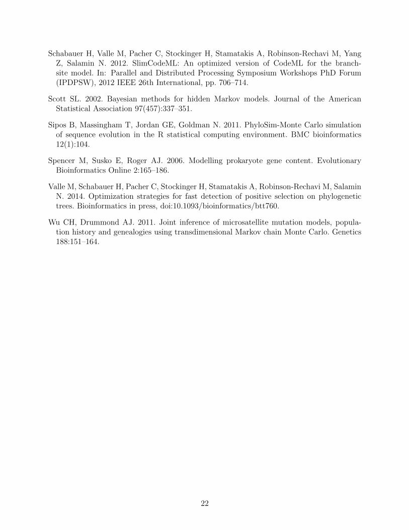
Our first example used the smaller state size, 4, with the smaller number of expectedtransitions per tree, 2. A random simulation resulted in two unique tip states, states 1 and3. For each method we produced 100,000 state history samples. Figure A-1 contains plotsof four univariate statistics pulled from the posterior distributions. All five implementationsproduced the same results.

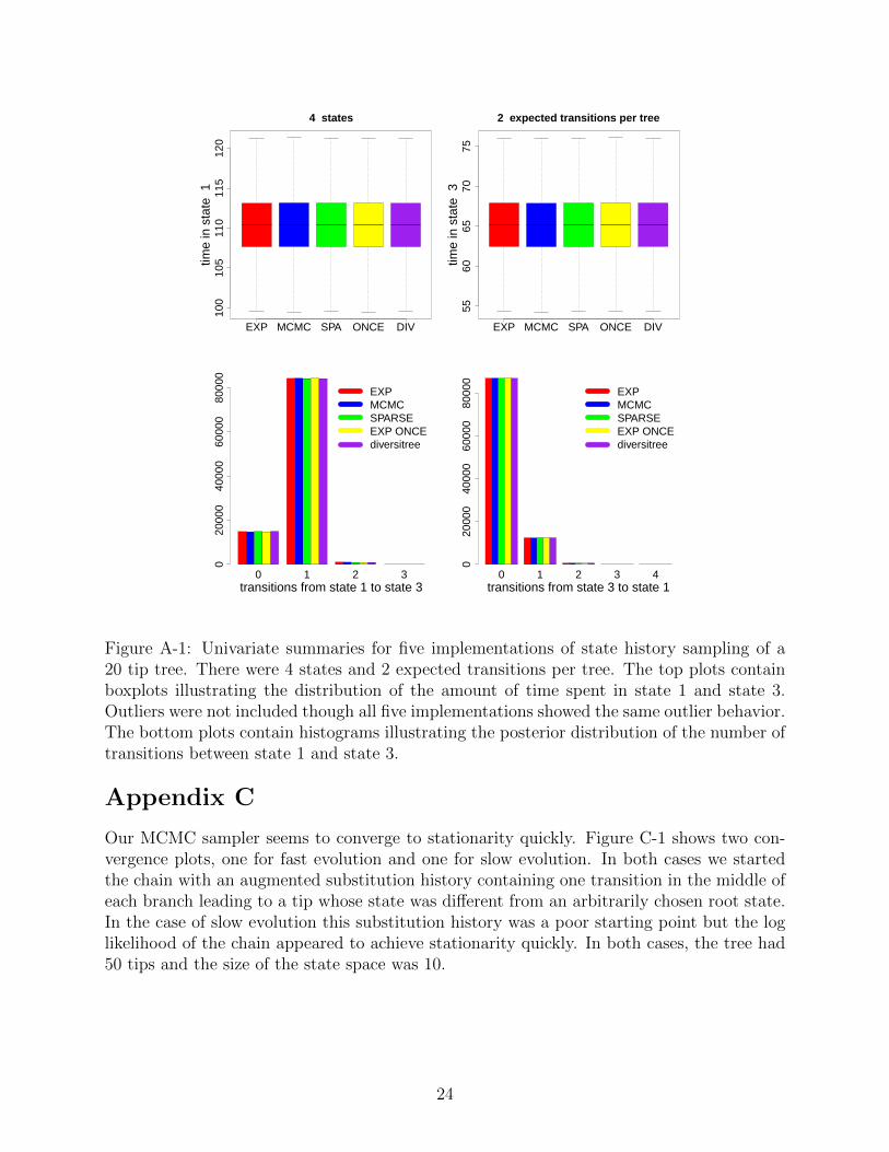
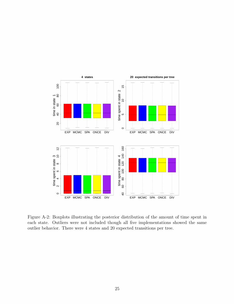
Our second example used the smaller state size, 4, with the larger number of expectedtransitions per tree, 20. A random simulation resulted in three unique tip states, states 1,2, and 4. Figure A-2 contains four boxplots pulled from the posterior distributions. FigureA-3 contains six histograms pulled from the posterior distributions.

Our third example used the larger state size, 20, with the smaller number of expectedtransitions per tree, 2. A random simulation resulted in two unique tip states, states 1 and 5.Figure A-4 contains plots of four univariate statistics pulled from the posterior distributions

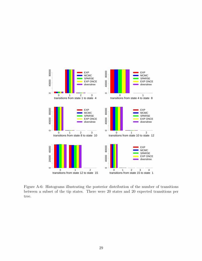
Our fourth example used the larger state size, 20, with the larger number of expectedtransitions per tree, 20. A random simulation resulted in six unique tip states, states 1, 4,8, 10, 12, and 15. Figure A-5 contains six boxplots pulled from the posterior distributions.Figure A-6 contains six histograms pulled from the posterior distributions.

Appendix B

One state space of interest in molecular evolution is the amino acid state space. Jones et al.(1992) proposed a rate matrix for an amino acid CTMC substitution model, called JTT.Figure B-1 contains timing results for this rate matrix and a tree with 40 tips. When ourMCMC approach used an appropriately tuned value of Ω we saw slightly faster runningtimes as compared to the matrix exponentiation approach. We examined other scenarios forthe JTT rate matrix in which we saw faster running times with the matrix exponentiationapproach.

23

EXP MCMC SPA ONCE DIV

100

105

110

115

120

4 states

time

in s

tate

1


5560

6570

75

2 expected transitions per tree

time

in s

tate

3

0 1 2 3transitions from state 1 to state 3

020

000

4000

060

000

8000

0

EXPMCMCSPARSEEXP ONCEdiversitree

0 1 2 3 4transitions from state 3 to state 1

020

000

4000

060

000

8000

0


Figure A-1: Univariate summaries for five implementations of state history sampling of a20 tip tree. There were 4 states and 2 expected transitions per tree. The top plots containboxplots illustrating the distribution of the amount of time spent in state 1 and state 3.Outliers were not included though all five implementations showed the same outlier behavior.The bottom plots contain histograms illustrating the posterior distribution of the number oftransitions between state 1 and state 3.

Appendix C

Our MCMC sampler seems to converge to stationarity quickly. Figure C-1 shows two con-vergence plots, one for fast evolution and one for slow evolution. In both cases we startedthe chain with an augmented substitution history containing one transition in the middle ofeach branch leading to a tip whose state was different from an arbitrarily chosen root state.In the case of slow evolution this substitution history was a poor starting point but the loglikelihood of the chain appeared to achieve stationarity quickly. In both cases, the tree had50 tips and the size of the state space was 10.

24


2040

6080

100

4 states

time

in s

tate

1


05

1015


time

spen

t in

stat

e 2


02

46

810

12tim

e sp

ent i

n st

ate

3


4060

8010

012

014

016

0tim

e sp

ent i

n st

ate

4

Figure A-2: Boxplots illustrating the posterior distribution of the amount of time spent ineach state. Outliers were not included though all five implementations showed the sameoutlier behavior. There were 4 states and 20 expected transitions per tree.

25

0 1 2 3 4 5transitions from state 1 to state 2

040

000


0 1 2 3 4 5 6 7 8 9transitions from state 1 to state 4

010

000

2500

0


0 1 2 3 4 5 6 7transitions from state 2 to state 1

020

000

5000

0 EXPMCMCSPARSEEXP ONCEdiversitree

0 1 2 3 4 5 6 7 8transitions from state 2 to state 4

020

000

5000


0 1 2 3 4 5 6 7 8 9transitions from state 4 to state 1

010

000

2500

0


0 1 2 3 4 5 6 7 8transitions from state 4 to state 2

020

000

5000

0


Figure A-3: Histograms illustrating the posterior distribution of the number of transitionsbetween states 1, 2, and 4. There were 4 states and 20 expected transitions per tree.

26


100

105

110

115

120

20 states

time

in s

tate

1

EXP MCMC SPA ONCE DIV55

6065

7075


time

in s

tate

5

0 1 2transitions from state 1 to state 5

020

000

4000

060

000

8000

0


020

000

4000

060

000

8000

0


Figure A-4: Univariate summaries for 5 implementations of state history sampling of a 20tip tree. There were 20 states and 2 expected transitions per tree. The top plots containboxplots illustrating the posterior distribution of the amount of time spent in state 1 andstate 5. Outliers were not included though all five implementations showed the same outlierbehavior. The bottom plots contain histograms illustrating the posterior distribution of thenumber of transitions between state 1 and state 5.

27


8010

012

0

20 states

time

in s

tate

1


02

46


time

in s

tate

4


01

23

4tim

e in

sta

te 8


4050

6070

time

in s

tate

10


05

1015

time

in s

tate

12


04

812

time

in s

tate

15

Figure A-5: Boxplots illustrating the posterior distribution of the amount of time spent ineach tip state. Outliers were not included though all five implementations showed the sameoutlier behavior. There were 20 states and 20 expected transitions per tree.

28


040

000

8000

0


0 1transitions from state 4 to state 8

040

000

8000



040

000

8000



040

000

8000



020

000

4000

0

0 1 2 3 4transitions from state 15 to state 1

040

000

8000


Figure A-6: Histograms illustrating the posterior distribution of the number of transitionsbetween a subset of the tip states. There were 20 states and 20 expected transitions pertree.

29

0.5 1.0 1.5 2.0

1015

2025

3035

JTT rate matrix, 2 expected transitions

Omega

time

(sec

onds

)

EXP

MCMC

0.5 1.0 1.5 2.0

2025

3035

40

JTT rate matrix, 6 expected transitions

Omega

time

(sec

onds

)

EXP

MCMC

Figure B-1: Time to obtain 10,000 effective samples as a function of the dominating Poissonprocess rate, Ω, for the JTT amino acid rate matrix as found in the phylosim R package.Results for our MCMC sampler are shown in black. Timing results for the matrix exponenti-ation method are represented by a purple horizontal line because the matrix exponentiationresult does not vary as a function of Ω. The randomly generated tree had 40 tips. The JTTrate matrix was scaled to produce 2 expected transtions in the left hand plot. The JTT ratematrix was scaled to produce 6 expected transtions in the right hand plot.

30

0 2000 4000 6000 8000 10000

−40

00−

3000

fast evolution

iteration

log

likel

ihoo

d

0 2000 4000 6000 8000 10000

−36

0−

345

−33

0

slow evolution

iteration

log

likel

ihoo

d

Figure C-1: MCMC trace plots. We show the log density of substitution histories for twoMCMC chains at every tenth iteration. The top plot shows results for a trait that evolvedquickly (with 6 expected substitutions). The bottom plot shows results for a trait thatevolved slowly (with 2 expected substitutions). In both cases, the tree had 50 tips and thesize of the state space was 10.

31

Appendix D

Our MCMC method scales well with the size of the state space even when state space sizesexceed 100. Figure D-1 shows timing results for state space sizes going out to 300. We showresults for our MCMC method and a sparse version of our MCMC method using tridiagonalrate matrices.

32

0 50 100 150 200 250 300

010

020

030

040

0


time

(sec

onds

)

MCMC

sparse MCMC

0 50 100 150 200 250 300

020

040

060

080

0


MCMC

sparse MCMC

0 50 100 150 200 250 300

050

010

0015

00


number of states

time

(sec

onds

)

MCMC

sparse MCMC

0 50 100 150 200 250 300

020

060

010

00


number of states

MCMC

sparse MCMC

Figure D-1: State space effect for a tridiagonal rate matrix. All four plots show the amountof time required to obtain 10,000 effective samples as a function of the size of the state spacefor two methods, our MCMC sampler in black circles and a sparse version of our MCMCsampler in red triangles. The two plots in the top row show results for a randomly generatedtree with 50 tips. The two plots in the bottom row show results for a randomly generatedtree with 100 tips. The two plots in the left column show results for a rate matrix that wasscaled to produce 2 expected transitions while the two plots in the right column show resultsfor a rate matrix that was scaled to produce 6 expected transitions.

33

Phylogenetic Stochastic Mapping without Matrix ... - arXiv

Documents

Transcript of Phylogenetic Stochastic Mapping without Matrix ... - arXiv