arX

iv:p

hysi

cs/0

4040

28v1

[ph

ysic

s.at

m-c

lus]

7 A

pr 2

004

Photoassociation of cold atoms with chirped laser pulses:

time-dependent calculations and analysis of the adiabatic transfer

within a two-state model.

E Luc-Koenig1, R. Kosloff2, F. Masnou-Seeuws1 and M. Vatasescu1,3

1Laboratoire Aime Cotton, Bat. 505,

Campus d’Orsay, 91405 Orsay Cedex, France

2Fritz Haber Research Center for Molecular Dynamics,

the Hebrew University of Jerusalem, Jerusalem 91904, Israel

3Institute of Space Sciences, MG-23,

77125 Bucharest-Magurele, Romania

(Dated: February 2, 2008)

Abstract

This theoretical paper presents numerical calculations for photoassociation of ultracold cesium

atoms with a chirped laser pulse and detailed analysis of the results. In contrast with earlier

work, the initial state is represented by a stationary continuum wavefunction. In the chosen

example, it is shown that an important population transfer is achieved to ≈ 15 vibrational levels

in the vicinity of the v=98 bound level in the external well of the 0−g (6s + 6p3/2) potential. Such

levels lie in the energy range swept by the instantaneous frequency of the pulse, thus defining a

“photoassociation window”. Levels outside this window may be significantly excited during the

pulse, but no population remains there after the pulse. Finally, the population transfer to the

last vibrational levels of the ground a3Σ+u (6s + 6s) is significant, making stable molecules. The

results are interpreted in the framework of a two state model as an adiabatic inversion mechanism,

efficient only within the photoassociation window. The large value found for the photoassociation

rate suggests promising applications. The present chirp has been designed in view of creating a

vibrational wavepacket in the excited state which is focussing at the barrier of the double well

potential.

PACS numbers:

1

I. INTRODUCTION

After ultracold atoms, ultracold molecules are presently a subject of constant interest,

stimulated further by the recent observation of molecular condensates [1, 2, 3]. This is why

the various routes leading to the formation of ultracold molecules are actively explored [4].

Starting from molecular beams, two non-optical techniques, buffer gas cooling of molecules

[5, 6] and Stark deceleration of polar molecules [7, 8] now reach temperatures well below 1K.

Another route relies on optical techniques: laser fields are used to cool down alkali atoms, and

to create molecules via the photoassociation reaction [9]. Short-lived molecules formed in an

excited electronic state must then be stabilized, by spontaneous emission or other radiative

coupling, into bound vibrational levels of the ground electronic state [10, 11, 12, 13, 14, 15].

The translational temperatures are much lower (T ≤ 20µK) and higher densities are to be

expected than with non-optical techniques. An important drawback, however, is that the

stable molecules are produced in a superposition of vibrational levels, among which some are

very excited. Bringing such molecules to the v =0 level of the ground electronic state, thus

reaching ultralow vibrational temperatures, is therefore an important issue. More generally,

finding new photoassociation and stabilization schemes is an interesting research subject.

Up to now, photoassociation experiments have mostly been using continuous lasers: a

more active role of the radiation would be to optimize the reaction by shaping laser pulses.

The aim of the present paper and of the following ones is to explore the feasibility and ad-

vantages of experiments using chirped pulses to form ultracold molecules, therefore bridging

the gap between the subjects of ultracold matter and coherent control.

The field of coherent control has developed both theoretically [16, 17, 18, 19, 20] and

experimentally [21, 22, 23] with quite different applications, such as photodissociation of

molecules. It has indeed been demonstrated that shaping laser pulses could enhance consid-

erably the yield of a photodissociation reaction, so that a similar effect is expected for the

reverse reaction.

Very few papers consider the photoassociation reaction with pulsed lasers: in the ther-

mal regime, ultrafast photoassociation has been studied [24, 25, 27], showing the validity of

the impulsive approximation. In the ultracold regime, several theoretical and experimental

papers have proposed a time-dependent study of the photoassociation reaction [26, 28, 29],

eventually considering also the formation of long-lived ultracold molecules [30]. Most the-

2

oretical calculations are using a wavepacket representation for the initial state of the two

colliding atoms. In this framework, considering a wavepacket localized at the outer classical

turning point of the photoassociated level, our group has discussed the characteristic times

for photoassociation of cold cesium atoms [31] and the separation of time scales.

Photoassociation of cold atoms with a chirped-pulsed-laser field was first theoretically

explored by Vala et al [36]: appreciating the slow nuclear relative motion in ultracold colli-

sions, a chirped pulse was optimized to achieve total transfer of population under adiabatic

following conditions proposed by Cao, Bardeen and Wilson [34, 35]. In these calculations

the initial state was represented by a gaussian wavepacket and a total population trans-

fer was indeed obtained in the region of distances where this wavepacket is localized. The

drawback of both this study and Ref. [31] was that they overlooked the precise nature of

the initial continuum state. Since the collision energy is so close to threshold, a plane wave

description or a superposition of Gaussian wavepackets do not address the actual shape of

the wavefunction. A correct representation of the initial continuum state of two ultracold

colliding atoms should be a stationary continuum state: indeed, experiments with continu-

ous photoassociation lasers identify several nodes of the stationary wavefunction as minima

in the photoassociation signal [10, 32].

The aim of the present paper is to go further in that direction, considering now pho-

toassociation with chirped laser pulses when the initial state is a delocalized continuum

wavefunction representing the relative motion of two atoms at very low collision energies

kT . Such a wavefunction displays very slow oscillations at large distances, and numerical

calculations must then use large spatial grids. On the other hand, for ultracold processes,

where the initial continuum state is very close to threshold, even a very weak light field

couples the last bound vibrational levels of the ground electronic surface, which must also

be correctly represented on the grid. Then, the numerical calculations need a mapping

procedure in order to reduce the number of grid points [37, 38].

It should be appreciated that the vibrational levels of the photoassociated molecule, being

close to the dissociation limit, are physically very different from lower lying vibrational

states. Their vibrational periods are orders of magnitude longer and most of the amplitude

is concentrated in the outer turning point. As a result, for even weak light fields, the Rabi

period associated with population transfer to the excited state can be shorter than the typical

vibrational periods. For short enough pulses, the relative motion of the two atoms during

3

the pulse duration can be neglected, thus allowing simple interpretations in the framework

of the impulsive limit for light-matter interaction [33]. This implies that, during the pulse,

the wavefunction at each nuclear separation can be decoupled from other positions, so that

each distance can be considered as a radiation coupled two-level-system, where transfer of

population is analyzed. Another limit now emerging is the limit of adiabatic transfer, where

the intensity of the light is sufficient so that the associated Rabi period is smaller than all

other relevant timescales.

The paper shows how a two-state model can be developed to provide analysis of the

results within an adiabatic population inversion mechanism, effective only within a range

of energies defining a photoassociation window. Also discussed is the possibility of avoiding

population transfer outside this window. An example of application is the focussing process,

where photoassociation is creating in the excited electronic state a vibrational wavepacket

optimized for transfer to a vibrational level of the ground state via a second pulse.

The paper is organized as follows: in Section II we recall the theoretical model for pho-

toassociation with chirped laser pulses. In Section III we discuss the various timescales of

the problem. In Section IV we give an example of numerical calculations for Cs2 0−g pho-

toassociation, with a chosen chirped pulse, where a few neighbouring vibrational levels stay

populated after the pulse. For interpretation, section V develops, in the framework of the

impulsive limit, a two-state adiabatic model for population inversion within a photoasso-

ciation window. In Section VI, the validity of this adiabatic approximation is discussed.

Section VII is the discussion of the numerical results in the frame of the simple model for

adiabatic population transfer. Finally, in Section VIII we show how the chirp parameter can

be chosen in view of focussing a vibrational wavepacket of the photoassociated molecules,

such as control of the formation of stable ultracold molecules can be performed. Section IX

is the conclusion.

In a forthcoming paper, hereafter referred to as paper II, we shall give more examples

for numerical calculations and discuss optimization of the photoassociation yield and of the

cold molecule formation rates.

4

II. THEORETICAL MODEL

A. The photoassociation reaction

The photoassociation reaction starts from two cold atoms, at a temperature T , colliding

in the ground state potential Vground, and which absorb a photon red-detuned compared to

a resonance line to yield a molecule in a vibrational level of the excited electronic potential

Vexc. We shall consider the example of two cold cesium atoms colliding in the lower triplet

a3Σ+u (6s + 6s) potential, and forming a molecule in a vibrational level of the 0−g (6s + 6p3/2)

potential:

Cs(6s2S1/2) + Cs(6s2S1/2) + hωL → Cs2(0−

g (6s2S1/2 + 6p2P3/2; v, J)). (1)

The reaction (1) is the usual representation of the photoassociation, using a continuous laser

red-detuned by δatL relative to the D2 resonance line:

hωL = hωat − δatL , (2)

where hωat is the energy of the atomic transition 6s → 6p3/2, which excites a single

vibrational level of the 0−g electronic state. In the present work, we shall treat excitation

with a chirped laser pulse characterized by time-dependent frequency ω(t) or detuning

δatL (t), and which populates several vibrational levels.

As indicated in Fig.1, the 0−g (6s + 6p2P3/2) potential curve displays a double well

structure with a hump located around 15 a0. The levels populated by the photoassociation

reaction correspond to vibrational motion in the outer well: vtot is the vibrational quantum

number in the full potential, while v is the numbering of the levels in the external well.

In the experimental photoassociation spectrum, vibrational levels from v=0 to v=132 are

identified [39]. For two levels, a tunneling effect is present which has been analyzed from

the photoassociation spectrum [40].

The theoretical model that we are presenting is of course not connected to the particular

shape of the excited potential Vexc.

5

B. The two-channel coupled equations

The dynamics in the ground state and the excited state is described by the time-dependent

Schrodinger equation

HΨ(R, t) = [Hmol + W(t)]Ψ(R, t) = ih∂

∂tΨ(R, t). (3)

where Ψ(R, t) is a two-component wavefunction, with Ψground(R, t) and Ψexc(R, t) describing

the radial relative motion of the nuclei in the ground and excited potential respectively.

The molecular Hamiltonian Hmol = T + Vel is the sum of the kinetic energy operator T

and electronic potential energy operator Vel. The coupling term is written in the dipole

approximation:

W(t) = − ~D(R) · ~eL E(t) (4)

involving the dipole moment operator ~D(R) and the electric field defined by a polarization

vector ~eL (assumed to be constant) and by an amplitude E(t). We define ~Dge(R) from

the matrix elements of the dipole moment operator components between the ground and

the excited molecular electronic states. Since the photoassociation reaction occurs at large

distances, we shall neglect the R− dependence, using the asymptotic value ~Dge(R)· ~eL ≈ D ~eL

ge

deduced from standard long-range calculations [41]. For this reason, the formulas below are

written for a R-independent coupling.

1. Excitation by a continuous laser

For a continuous laser with constant frequency ωL/2π, the electric field is

E(t) = E0 cos(ωLt) (5)

where E0 is the amplitude of the field.

The explicit temporal dependence of the Hamiltonian H is eliminated in the framework

of the rotating wave approximation, defining new radial wavefunctions in both excited and

ground state channels through

ΨωL

e (R, t) = exp(iωLt

2)Ψexc(R, t)

ΨωL

g (R, t) = exp(−iωLt

2)Ψground(R, t), (6)

6

and neglecting the high frequency component in the coupling term. This allows to write the

radial coupled equations as

ih∂

∂t

ΨωL

e (R, t)

ΨωL

g (R, t)

=

T + V′

e (R) WL

WL T + V′

g (R)

ΨωL

e (R, t)

ΨωL

g (R, t)

. (7)

In Eqs. (7), the two non diagonal terms are identical and time-independent,

WL = hΩL = −1

2E0D

~eL

ge = −1

2

√

2I

cǫ0D ~eL

ge (8)

where I is the constant laser intensity, c the velocity of the light and ǫ0 the vacuum permi-

tivity.

The diagonal terms in Eqs. (7) involve the dressed potentials

V′

e (R) = Vexc(R)− hωL/2 = V (R) + ∆L(R), V′

g (R) = Vground(R) + hωL/2 = V (R)−∆L(R).

(9)

In Eq. (9), we have introduced the difference between the two dressed potentials:

2∆L(R) = V′

e (R) − V′

g (R) = Vexc(R) − Vground(R) − hωL, (10)

where 2∆L(R) → δatL for large R, and the mean potential

V (R) =Vexc(R) + Vground(R)

2. (11)

When the dressed-potentials are crossing at a large distance RL (V′

e (RL) = V′

g (RL))

∆L(RL) = 0, (12)

the resonance condition for photoassociation into a vibrational level with binding energy ELv

may be estimated through [4]

V′

e (RL) − V′

e (∞) ≈ −ELv , (13)

where we have neglected the kinetic energy of the initial continuum state. Therefore, the

outer classical turning point of the photoassociated level should be located close to RL.

2. Chirped pulse and transform-limited pulse

In order to optimize the formation rate of molecules, we shall consider gaussian ”chirped”

pulses [34], where the laser field E(t) has a quadratic time-dependent phase ϕ(t), hence a

7

time-dependent frequency ω(t) together with a time-dependent amplitude E0f(t). We have

to note that the discussion reported here is general and can be adapted for other types of

temporal envelopes than the gaussian one employed here, as for more general chirp rates

that could be defined, beyond the linear approximation (Eq.(18)) used in the present paper.

• the field is

E(t) = E0f(t) cos[ωLt + ϕ(t)], (14)

where the amplitude involves a gaussian envelope f(t) centered at t = tP ,

f(t) =

√

τL

τC

exp[−2 ln 2(t − tP

τC

)2], (15)

τL =τC

√

1 + (χτ 2C/4 ln 2)2

≤ τC (16)

with the temporal width τC defined as the full width at half maximum (FWHM) of

the temporal intensity profile E20f(t)2.

• the phase ϕ(t) in Eq. (14) has a second derivative equal to the linear chirp rate

χ = d2ϕdt2

,

ϕ(t) =1

2χ(t − tP )2 − 1

2arccos

τL

τC− ωLtP . (17)

• the frequency of the field, related to the derivative of the phase, varies linearly around

the carrier frequency ωL:

ω(t) = ωL +dϕ

dt= ωL + χ(t − tP ), (18)

Each pulse is thus defined in the temporal domain by five parameters which are the

carrier frequency ωL, the chirp rate χ, the temporal center tP , the width τC , and E0. In

the present study of photoassociation, the carrier frequency ωL is perfectly defined from an

atomic resonance frequency in terms of the detuning δatL (see Eq. (2)).

Concerning the two last parameters, we must note that for χ = 0, τL = τC , defining

a transform limited pulse with FWHM of |f(t)|2 equal to τL, and maximum amplitude

of the field E0. Therefore the maximum amplitude of the chirped pulse, EM = E0

√

τL

τC

, is

always smaller than E0: the chirp increases the time-width of the pulse while decreasing its

maximum amplitude. The coupling in Eqs.(7) now becomes time-dependent and reads

WLf(t) ≤ Wmax = WL

√

τL

τC= −

√

τL

τC

1

2

√

2IL

cǫ0|D ~eL

ge | (19)

8

where we have defined a peak intensity IL = cǫ02E2

0 .

In the following, we shall assume that the relative phase of the ground and excited electronic

wavefunctions is such that WL > 0.

• In contrast, the chirp does not modify the width of the pulse in the frequency domain,

which stays proportional to 1/τL. Indeed, E(ω), which is the Fourier transform of E(t),

displays a gaussian profile with FWHM√

2δω= 4√

2 ln 2/τL, and a phase Φ(ω) which

is a quadratic function of the frequency, leading to the definition of a linear chirp rate

in the frequency domain

Φ′′ =d2Φ

dω2= χ

τ 2Cτ 2

L

(4 ln 2)2. (20)

Consequently one has

τ 2C = τ 2

L[1 + (4 ln 2)2 (Φ′′)2

τ 4L

]. (21)

• Finally, the chirp does not change the energy Epulse carried by the field, which is

proportional to the square of the amplitude E0 and to the temporal width τL of the

transform limited pulse

Epulse =cǫ0

2

∫ +∞

−∞

|E(t)|2dt =cǫ0

2E2

0 τL

√

π

4 ln 2=

ILτL

2

√

π

ln 2, (22)

• This allows us to define a time window, since for a gaussian pulse 98 % of the energy

is carried during the time interval [−τC , +τC ]:

cǫ0

2

∫ +τC

−τC

|E(t)|2dt = 0.98Epulse (23)

Since from Eq.(15) f(tP ±τC) = 14

√

τL

τC, we may also define a lower limit to the coupling

term during the temporal window and write

∀(t − tP ) ∈ [−τC , +τC ] → 1

4WL

√

τL

τC

≤ WLf(t) ≤ WL

√

τL

τC

= Wmax. (24)

The definition of such a time window will reveal very useful for the analysis of the

dynamics.

We have represented in Fig. 2a the typical variation of the amplitude of a transform limited

pulse and of the pulse obtained through linear chirp, illustrating both the stretching of the

temporal width from τL to τC , the reduction of the peak intensity, and the conservation of

the energy carried by the field. The energy range swept during the time-variation of the

frequency (see Eq.(18)) is illustrated in Fig. 2b.

9

3. Coupled radial equations for excitation with a chirped pulse

When considering excitation via a chirped pulse, we may apply the rotating wave approx-

imation as previously at the carrier frequency ωL. Once the terms oscillating as exp[±2iωLt]

are eliminated, the resulting coupling term is time-dependent with a phase variation, so that

the coupled equations now are

ih∂

∂t

ΨωL

e (R, t)

ΨωL

g (R, t)

=

T + V (R) + ∆L(R) WLf(t) exp[−iϕ(t)]

WLf(t) exp[iϕ(t)] T + V (R) − ∆L(R)

ΨωL

e (R, t)

ΨωL

g (R, t)

. (25)

However, the existence of a complex coupling term makes the discussion intricated: it is

therefore convenient to modify further the rotating frame by defining new wavefunctions for

the excited and the ground state,

Ψωe (R, t) = exp(iϕ/2) × ΨωL

e (R, t) = exp(iωLt + ϕ

2)Ψexc(R, t),

Ψωg (R, t) = exp(−iϕ/2) × ΨωL

g (R, t) = exp(−iωLt + ϕ

2)Ψground(R, t), (26)

thus performing the rotating wave approximation with the instantaneous frequency. The

coupled equations now read

ih∂

∂t

Ψωe (R, t)

Ψωg (R, t)

=

T + V (R) + ∆L(R) − h2

dϕdt

WLf(t)

WLf(t) T + V (R) − ∆L(R) + h2

dϕdt

Ψωe (R, t)

Ψωg (R, t)

. (27)

In the following, we shall call W (t) the real time-dependent quantity

W (t) = WLf(t), (28)

and 2∆(R, t) the time-dependent energy difference such that

2∆(R, t) = 2∆L(R) − hdϕ

dt= 2∆L(R) − hχ(t − tP ) (29)

10

4. Resonance window and spectral width

It is important to note that, in contrast with cw excitation, the relative position of the

two potential curves at a given distance R now varies linearly as a function of t. Hence, at

some distances the upper curve may become the lower or vice versa, while the position of

their crossing point RC(t), such that

∆(RC(t), t) = 0; RC(tP ) = RL (30)

varies with time around the distance RL defined in Eq. (12).

We shall consider situations where during the time window [tP − τC , tP + τC ], the crossing

distance RC(t) is spanning a range of distances

Rmin ≤ R ≤ Rmax

Rmin = RC(tP − χ

|χ|τC) ⇒ 2∆L(Rmin) = −h|χ|τC ,

Rmax = RC(tP +χ

|χ|τC) ⇒ 2∆L(Rmax) = h|χ|τC . (31)

The definition of such a resonance window requires two conditions on the width of the pulse

and its frequency, to ensure that the curves keep crossing:

h|χ|τC ≤ Umineg (32)

h|χ|τC ≤ δatL (33)

where −Umineg is the minimum value of the difference potential 2∆L(R) at R ≤ RL , while

δatL the asymptotic splitting. The resonance window is defined independently of the pulse

intensity. However, it depends upon our choice for the temporal window, and this point will

be further discussed below.

Writing the resonance condition from Eq.(30), which depends upon the central frequency

of the pulse, would be misleading: due to the spectral width, a range of levels in the

neighbourhood of the resonant level can be excited. We shall discuss in more details these

two aspects of the excitation with a particular example.

11

III. TIME SCALES

A. Time scales related to the radiation

The two radiative phenomena in our problem are the spontaneous emission time Tspont

and the Rabi period associated to the coupling with the laser. We shall study phenomena

at a time scale short compared to Tspont. For a cw laser, the period TLRabi of the “Rabi

oscillations” associated with the coupling WL between the two states resonantly coupled is

TLRabi =

hπ

WL

. (34)

Once a pulsed laser is introduced, due to the variation of the peak intensity, this time

constant is modified. We define two similar time constants, at the maximum intensity

(t = tP ), and at the edges of the time window (t = tP ± τC), characterizing the dynamics in

the vicinity of the instantaneous crossing points RL, Rmin, Rmax:

TCRabi(tP ) =

hπ

Wmax=

√

τC

τLTL

Rabi

TCRabi(tP ± τC) =

4hπ

Wmax

= 4TCRabi(tP ) (35)

As a generalization, following Ref.[42], we shall also use a local time-dependent Rabi period

defined by

τRab(R, t) =hπ

√

W 2(t) + ∆2(R, t)(36)

Obviously the pulse duration τC is also an important characteristic of the pulse. For the

discussion of the adiabaticity condition, and for the optimization of the pulse, it is interesting

to evaluate the time constant associated with the energy range swept during the time window

Tchirp =2π

2|χ|τC(37)

This quantity should be compared to the width of the energy distribution |E(ω)|2, which

is δω = 4 ln 2/τL, and does not depend on the chirp rate. A time scale caracteristic of the

spectral width is then introduced as

Tspect =2π

δω=

2π

4 ln 2τL = 2.26τL. (38)

12

The ratio ρ between those two time constants is bounded, since

ρ =Tspect

Tchirp

=2|χ|τC

δω=

2x√1 + x2

(39)

x =|χ|(τC)2

4 ln 2(40)

0 ≤ ρ ≤ 2. (41)

Therefore the frequency band swept by the central frequency due to the chirp is never

larger than twice the spectral width. This is an important parameter in the description of

the chirp process.

B. Time constants associated with the dynamics.

When discussing the vibrational motion of a vibrational level v, with binding energy Ev

in the excited state, we shall consider the classical vibrational period estimated from

Tvib(v) ≈ 2πh∂v

∂E≈ 4πh

Ev+1 − Ev−1. (42)

For the discussion on optimization of the chirped pulse, it is also relevant to consider the

revival period, defined [43] as

Trev(v) ≈ 4πh

Ev+1 − 2Ev + Ev−1

. (43)

For the ground state, we shall consider the motion at a low collision energy E, described by

a scattering length L corresponding to a time-delay

τ = h∂δ(E)

∂E∼ µL

hk, (44)

where we have introduced the elastic phaseshift δ(E) = Arctg(−kL), the reduced mass µ

and the wavenumber k.

IV. AN EXAMPLE OF NUMERICAL CALCULATIONS FOR PHOTOASSOCIA-

TION WITH A CHIRPED PULSE.

Since the pulse depends upon many parameters, the way of optimizing them is not

straightforward. We give results of numerical calculations in the example already presented

in Section IIA of photoassociation into several bound levels in the external well of the Cs2

0−g potential, populated by a chirped pulse.

13

A. The physical problem and its time scales

The photoassociation reaction uses a chirped laser pulse linearly polarized, already illus-

trated in Fig.2, for which the parameters are reported in Table I.

δatL IL WL hδω τL τC hχ Φ′′

2.656 cm−1 120 kW cm−2 0.7396 cm−1 0.98 cm−1 15 ps 34.8 ps -0.025 cm−1 ps−1 -170 ps2

1.21×10−5 au 3.37 ×10−6 au χ=-0.28 × 10−11 au

χ=-4.79× 10−3 ps−2

TABLE I: Parameters for the pulse excitation considered in the present paper (see section IIB 2

and Fig. 2): detuning δatL , intensity IL, coupling WL, energy associated to the spectral width hδω,

temporal widths τL and τC , linear chirp parameters χ and Φ′′.

The detuning δatL of the carrier frequency corresponds to resonant excitation at

t = tP of the level v=98 of the Cs2 0−g (6s + 6p3/2) potential, and to a crossing point

RL = 93.7 a0. Calculations have also been performed by changing the sign of the

chirp. For a continuous laser excitation with π polarization between the electronic states

3Σ+u (6s, 6s) and 0−g (6s + 6p3/2), and neglecting the R-variation of the dipole coupling, the

intensity is related to the coupling WL by Eq. (8), giving WL(au) = 9.74×10−9√

IW/cm2 [41].

The time scales associated with the radiation are reported in Table II. They appear to

be of the same order of magnitude: in particular, Tchirp and Tspect are similar, since for the

present pulse, the resonance width 2|χ|τc is nearly twice the spectral width δω, leading to a

value ρ = 1.8 close to the maximum value which is 2.

The lifetime of the atomic level Cs(6p2P3/2) being 30.462 ns, the radiative lifetime of

the photoassociated levels in the external well of the 0−g (6s + 6p3/2) curve is ≈ 30 ns. In

the present calculations where spontaneous emission is not introduced, we shall study the

evolution of the system at much shorter time scales. Through incertainty relations, it

means that the definition of the energy is larger than the natural linewidth of the cesium

14

Tspont TLRabi TC

Rabi(tP ) TCRabi(tP ± τC) τRab(∞, tP ) τRab(R = 15a0, tP ) Tchirp Tspect ρ

30 ns 22.5 ps 34.3 ps 137 ps 12 ps 0.18 ps 18.9 ps 33.9 ps 1.8

TABLE II: Time scales associated with the radiative coupling: spontaneous emission time Tspont,

Rabi period TLRabi, chirped Rabi periods TC

Rabi(tP ) and TCRabi(tP ± τC) defined in Eqs.( 34- 35).

Besides, we have reported the time-dependent local Rabi period τRab at the maximum tP of the

pulse for R = 15 a0 and R → ∞. Finally, the time constant characteristic of the spectral width of

the pulse Tspect is reported together with the chirped characteristic time Tchirp as defined in Eqs.

(37,38). ρ is the ratio between the resonance width and the spectral width defined in Eq.(39)

atom resonance line ∆E= 1.7 10−4 cm−1= 5.3 MHz. The hyperfine structure splitting of

9193 MHz will not be considered in the present paper, but it has a significant value at the

time scale of the problem.

At resonance (∆ = 0) and for a cw laser, the intensity of the pulse would correspond to a

Rabi period of 22.5 ps. However, due to the streching factor τC/τL reducing the maximum

intensity, it is increased to 34.3 ps at t = tP . In the wings of the pulse, this time constant is

further increased, reaching the value 137 ps at the times tP ± τC . Such characteristic times

should be compared to the times scales associated to the vibrational motion, and to the

collision time.

For the excited potential Vexc(R), the outer well in the 0−g (6s + 6p3/2) curve was fitted to

photoassociation spectra by Amiot et al [44]. The latter was obtained [45] by matching to

ab initio calculations at short and intermediate range. The lower triplet state potential

3Σ+u (6s, 6s) has been chosen in order to ensure a correct value of the scattering length L,

here taken as L ≈ 525 a0: the asymptotic behaviour being C6/R6, where C6= 6828 au

[44], the short range part extracted from [46] had to be slightly modified [45] for that purpose.

Under the conditions illustrated by the Table I, the time-dependent energy difference

∆(R, t) between the two dressed potentials, defined in Eq. (29), is drawn in Fig.4.

The long range splitting between the two potential curves is 2∆L(∞) = δatL =2.6 cm−1,

15

resulting at t = tP into a local Rabi period of 12 ps in the asymptotic region, as reported

in Table II. The energy difference reaches large values at short distances, yielding a

very small local Rabi period of 0.18 ps at R= 15 a0. The instantaneous crossing point

(defined by ∆(R, t) = 0) varies with time, and we have indicated in the Figure the

values Rmin=85, RL=93.7 and Rmax=107.4 a0 defined above in Eqs.(31) and discussed

in Section IIB 4. Such distances are close to the outer turning points of the vibrational

levels v=92, 98 and 106 respectively, for which Table III displays parameters such as

binding energies and vibrational periods. The pulse with negative chirp value described

in Table I has an intantaneous frequency resonant with the v=106 level at t = tP − τC ,

with v=98 at t = tP , and v=92 at t = tP + τC . Alternatively, when the chirp becomes

positive, the resonant condition is verified first by v=92 and finally by the upper level v=106.

vtot v Rout (a0) Ev (au) Ev (cm−1) Tvib Trev

122 92 85,5 ≈ Rmin -1.62 × 10−5 -3.57 196 ps 10 ns

129 98 93.7 ≈ RL - 1.21 × 10−5 -2.65 250 ps 15.3 ns

137 106 107.48 ≈ Rmax - 0.79 × 10−5 -1.74 350 ps 15.7 ns

TABLE III: Characteristic constants for three levels in the outer well of the 0−g (P3/2) potential

curve. vtot is the vibrational number, while the numbering v is restricted to the levels in the outer

well. −Ev is the binding energy, Rout is the outer turning point, Tvib and Trev are respectively the

classical vibrational period and the revival period as defined in Eqs. (42-43) in text. The level

v=98 is identical to the (v0+2) level considered in Ref. [47] on tunneling.

Due to the linear chirp parameter, an energy range of about 2h|χ|τC = 1.74 cm−1 is

swept by the laser frequency, corresponding to 15 vibrational levels in the vicinity of v= 98,

for which we have reported data. However, due to the spectral width of the pulse, levels in

an energy range of 0.98 cm−1on both sides can also be excited, and this will be analyzed

with the numerical results.

Since the coupling with the ground state may be involving the last least bound levels

16

in the ground state potential curve, we also report in Table IV the binding energies and

vibrational periods for those levels, together with the time-delay for the continuum level at

T =54.3 µK, as defined in Eq. (44).

v E (au) E (cm−1) Tvib

v′′=50 -3.87× 10−7 E=-.084 cm−1 Tvib=581 ps

v′′=51 -1.23× 10−7 E=-0.027 cm−1 Tvib=1460 ps

v′′=52 -1.94× 10−8 E=-0.042 cm−1 Tvib=7.8 ns

v′′=53 -2.43× 10−11 E=-5× 10 −6 cm−1

continuum + 1.71 × 10−10 E=+3.77× 10−5 cm−1 τ ∼ 476 ns

TABLE IV: Constants for the last levels in the 3Σ+u (6s+6s) potentials. The present calculations

are not including the hyperfine structure.

The classical vibrational period has no meaning for the last level, since the wavefunction

mainly extends in the classically forbidden region. We should note the very high value

of the time delay in the present problem, due to the large value of the scattering length,

demonstrates the strongly resonant character of the collision, and makes the collision time

by far the largest characteristic time in the problem. Looking at Tables IV and II, we see

that the spacing between the level v′′=53 of the ground state and the continuum level with

collision energy E = kT= 54.3 µK ≈ 3.77 × 10−5 cm−1can be considered as negligible at the

scale of the energy uncertainty imposed by ≈ 30 ns radiative lifetime of the excited state.

B. Description of the initial state

The initial continuum state is represented by a stationary wavefunction in the ground

state potential curve and describing the collision of two cold Cs atoms at the energy kT

corresponding to T = 54.3 µK . It is chosen with a node at the external boundary LR of

the spatial grid (see below). This wavefunction is drawn in Fig. 3, together with a typical

gaussian wavepacket, showing how unlocalized is the initial state in the present work. This

is an important modification compared to previous calculations [31, 36] using a gaussian

wavepacket: the population transfer can occur in a very wide range of internuclear distances,

17

well outside the resonance window, and in particular at large internuclear distances where

a large density probability is localized. No velocity distribution is considered in the present

work, this effect being treated in paper II.

C. Numerical methods

Details on the numerical calculations will also be given in paper II: they involve mapped

grid methods [37] to represent the radial wavefunctions, using a sine expansion [38] rather

than the usual Fourier expansion, in order to avoid the occurrence of ghost states. The

introduction of adaptive coordinates is necessary to implement a spatial grid with few points

(1023), but with a large extension LR = 19250 a0 allowing representation of initial continuum

states at ultra-low collision energy. Due to the large size of the grid, and the very small

kinetic energy of the problem, it is not necessary to put an absorbing boundary condition at

the edge of the grid. Since the initial state wavefunction is normalized in a box, the results

given below will be depending on the value chosen for LR.

The time-dependent Schrodinger equation is solved by expanding the evolution operator

exp[−iHt/h] in Chebyschev polynomia [48]. The time propagation is realized by discrete

steps with a time increase much shorter than the characteristic times of the problem, already

discussed in Sec. IIIA and reported in the Tables II-IV. In the present problem, the smallest

time scale is the local Rabi period at small distances, ≈ 0.18 ps, which controls the time step

∆t. In typical calculations, we have chosen ∆t ≈ 0.05 ps, the quantity HΨ being evaluated

112 times at each time step.

The dynamics of propagation of the wavepackets in the ground and excited potentials is

analyzed by studying the evolution of the population in both surfaces:

Pe(t) =< Ψe(R, t)|Ψe(R, t) >, Pg(t) =< Ψg(R, t)|Ψg(R, t) > (45)

A more detailed information is provided by the decomposition of the wavepackets on the

unperturbed vibrationals states v of both potential surfaces S = a3Σ+u or 0−g :

PSv(t) = | < ΨSv(R)|Ψe,g(R, t) > |2 (46)

18

D. Results

All the numerical results presented below are obtained from an initial state wavefunction

normalized to unit in a large box of size LR=19250 a0. They correspond to branching ratios

of the photoassociation process towards different final vibrational levels, eigenstates of the

Hamiltonian for the unperturbed molecule. Due to the linear character of the Schrodinger

equation, the population transferred to a given level is proportional to the normalization

factor for the initial state. Therefore, in order to deduce the populations corresponding

to an energy-normalized initial continuum state, for E= 1.71 × 10−10 au (T=54 µK), the

computed populations should be multiplied by the density of states dn/dE=1/(8.87×10−12).

Besides, since the calculations concern only one pair of atoms, and are not velocity averaged,

the values for Pe(t) should be scaled to get an estimation of the population transfer due to

a single pulse in a trap containing N atoms: this will be done in Section VII.

The results of the calculations for the time-dependence of the populations are presented in

Fig. 5, both for a negative and a positive linear chirp parameter. The main conclusions are:

• There is a population transfer from the ground 3Σ+u state to the excited 0−g state which

decreases by two orders of magnitude from Pe(tP ) ≈0.032 near the maximum of the

pulse, to Pe(t ≥ tP + τC) = 3.2× 10−4 at the end of the pulse (see Fig. 5a,b).

• Calculations considering the same laser pulse with an initial state represented by a

gaussian wavepacket normalized to unity yield a much larger value (≈ 0.59) for the

final population in the excited state. However, the ratios between this final population

and the probability density in the range 85 ≤ R ≤ 110 a0 are similar (0.69 for the

gaussian wavepacket, 0.73 for the continuum eigenstate). This result is a signature for

the predominant contribution of the resonance window.

• The maximum of the transferred population occurs ≈ 5 ps before the maximum of

the pulse for a negative chirp, and ≈ 5 ps after this maximum for a positive chirp (see

Fig. 5a,b).

• After the pulse, most of the population in the ground state is going back to the

initial continuum state, but a small fraction (≈ 3 × 10−4) is transferred to the last

vibrational levels in the 3Σ+u potential, v′′=51-53 ( Fig. 5d). This remaining population

19

is independent of the sign of the chirp. The population transfers towards bound levels

of the excited 0−g and of the ground 3Σ+u state are comparable.

• While many bound levels in the excited 0−g potential are excited during the pulse,

essentially the levels from v= 92 till v= 106 remain populated after the pulse (see Fig.

5e). They correspond to the range of energy around v= 98 swept by the laser during

the time window and presented above as a “resonance window”.

• In contrast, highly excited levels from v=122 to v = 137 are significantly populated

during the pulse (see Fig. 5e), but the population vanishes at the end of the pulse.

• Whereas the oscillatory pattern during the time window markedly depends upon the

sign of the chirp, the final population in the excited state, as well as the vibrational

distribution, is nearly independent upon this sign.

Such results demonstrate the existence of a “photoassociation window” including all the

levels in the energy range between v= 92 and v= 106 where population transfer is taking

place. We shall provide interpretation for this result in the following section.

V. A TWO-STATE MODEL FOR ADIABATIC POPULATION INVERSION.

A. Impulsive approximation.

For all the following developments, we shall use the impulsive approximation [33], as-

suming that the relative motion of the two nuclei is frozen during the pulse duration. The

kinetic energy operator being neglected in Eq. (27), the two-level Hamiltonian becomes

H ∼ H− T = Hi =

V 0

0 V

+

∆(R, t) W (t)

W (t) −∆(R, t)

(47)

where the first term introduces a R-dependent phase while the dynamics is contained in the

second term.

B. The adiabatic basis

When the impulsive approximation is valid, diagonalization of the hamiltonian Hi(R, t)

at each distance R will define a new representation, in the framework of a standard radiation-

20

driven two-level system [42, 49]. In Eqs.(47), the notations W and ∆ are similar to the ones

used in the textbook by Cohen-Tannoudji et al [50] to describe a two-state model. Defining

a time-dependent local Rabi frequency

hΩ(R, t) =√

∆2(R, t) + W 2(t), (48)

diagonalization of Hi yields two eigenenergies E+ and E−

E±(R, t) = V (R, t) ± hΩ(R, t) (49)

with two eigenfunctions, hereafter referred to as adiabatic, Fω+, Fω

−.

The set of two adiabatic functions is deduced from the diabatic functions Ψωe , Ψω

g by a

rotation R [50]:

Fω+

Fω−

= R

Ψωe

Ψωg

;R =

cos θ2

sin θ2

− sin θ2

cos θ2

the angle θ being defined by the relations:

sin[θ(R, t)] =|W (t)|

hΩ(R, t), cos[θ(R, t)] =

∆(R, t)

hΩ(R, t), tan[θ(R, t)] =

|W (t)|∆(R, t)

(50)

The two-channel wavefunction representing the evolution of the system can then be writ-

ten in the adiabatic representation as

|Ψ(R, t) >= a+(R, t)|Fω+ > +a−(R, t)|Fω

−> (51)

where a+(R, t) and a−(R, t) verify

ih∂

∂t

a+(R, t)

a−(R, t)

=

E+(R, t) 0

0 E−(R, t)

a+(R, t)

a−(R, t)

+ih

2

∂θ(R, t)

∂t

0 1

−1 0

a+(R, t)

a−(R, t)

.

(52)

We shall discuss now adiabatic evolution when the second term in the r.h.s. of Eq.(52) is

negligible. The validity of such an hypothesis will be discussed below in Sec.VIA.

C. Condition for population inversion during the pulse duration.

We assume that the effect of the pulse is negligible outside the time interval tP − τF ≤t ≤ tP + τF , without assumption on the value of τF . Considering only the first term in the

21

r.h.s. of Eq.(52), the solution of Eq. (52) becomes straighforward : assuming that before

the beginning of the pulse, at t = tP − τF , there is no population in the excited state, the

evolution of the diabatic wavefunctions is described by

Ψωe (R, t)

Ψωg (R, t)

=

cos θ(R,t)2

− sin θ(R,t)2

sin θ(R,t)2

cos θ(R,t)2

e−

i

h

∫

t

tP −τF

E+(R,t′)dt′

0

0 e−

i

h

∫

t

tP −τF

E−(R,t′)dt′

×

cos θ(R,tP −τF )2

sin θ(R,tP −τF )2

− sin θ(R,tP −τF )2

cos θ(R,tP −τF )2

0

Ψωg (R, tP − τF )

(53)

Introducing the accumulated angle

α(R, t) =i

h

∫ t

tP−τF

E+(R, t′)dt′ (54)

the two diabatic wavefunctions at time t are

Ψωe (R, t) = −[i sin

θt + θi

2sin α(R, t) + sin

θt − θi

2cos α(R, t)] Ψω

g (R, tP − τF ),

Ψωg (R, t) = [i cos

θt + θi

2sin α(R, t) + cos

θt − θi

2cos α(R, t)] Ψω

g (R, tP − τF ), (55)

where we have introduced the time-dependent angles

θi = θ(R, tP − τF ), (56)

θt = θ(R, t). (57)

1. Pulse of finite duration 2 τF

We are interested in the conditions leading to population transfer, at internuclear distance

R, from the ground to the excited state, for a pulse starting at t = tP − τF and stopping at

t = tP + τF :

W (tP − τF ) = W (tP + τF ) ≈ 0. (58)

From Eqs.(50), we see that the rotation angles are such that

sin θ(R, tP − τF ) = sin θ(R, tP + τF ) = 0 (59)

cos θ(R, tP − τF ) =∆(R, tP − τF )

|∆(R, tP − τF )| ; cos θ(R, tP + τF ) =∆(R, tP + τF )

|∆(R, tP + τF )| (60)

According to the sign of the time-dependent energy-splitting, the angles θ(tP − τF ) and

θ(tP + τF ) can take the values 0 or π. When the two angles have the same value, the

22

correspondance between diabatic and adiabatic states is the same before and after the pulse,

i.e |Ψωg,e(R, tP + τF )| = |Ψω

g,e(R, tP − τF )|. In contrast, when the sign of ∆(R, t) defined in

Eq. (29) changes during the pulse, the two states are reversed. This population inversion

takes place at a distance R provided that the level splitting between the dressed potentials

verifies

2|∆L(R)| < h|χ|τF . (61)

Then,

|θ(R, tP + τF ) − θ(R, tP − τF )| = π ⇒ |Ψωe (R, tP + τF ) = |Ψω

g (R, tP − τF )|. (62)

For a given pulse (fixed values for δatL , χ and τF ), the condition (61) for population inversion

shows that the transfer will take place in a region of internuclear distances around RL (such

as ∆L(RL) = 0), the extension of which depends upon the difference 2|∆L(R)| between the

two potentials and upon the energy range h|χ|τF swept during the pulse.

In most photoassociation experiments the lasers are tuned so that RL is located at large

distances, where the difference 2|∆L(R)| between the ground and excited potential curves is

very small, so that we may predict a large photoassociation window.

2. Extension to a gaussian pulse.

As it was shown in Sec.II B 2, when the chirped pulse is gaussian, most of the intensity is

carried during the time window (t − tP ) ∈ [−τC , +τC ], which suggests that the population

inversion is mainly realized during this temporal window. Therefore, the condition for

population inversion during the time window is written introducing τC instead of τF in the

relation (61).

• For internuclear distances R such that ∆(R, tP − τc) > 0, the angle θi(R, tP − τC) ≈ 0,

and the diabatic functions are

Ψωe (R, t) = − sin

θt

2e+iα(R,t)Ψω

g (R, tP − τC)

Ψωg (R, t) = cos

θt

2e+iα(R,t)Ψω

g (R, tP − τC) (63)

23

• In contrast, when ∆(R, tP − τc) < 0, θi(R, tP − τC) ≈ π, and

Ψωe (R, t) = cos

θt

2e−iα(R,t)Ψω

g (R, tP − τC)

Ψωg (R, t) = sin

θt

2e−iα(R,t)Ψω

g (R, tP − τC) (64)

Let us emphasize that in the adiabatic following of an instantaneous eigenstate of the

system, since the angle θi stays strictly equal either to 0 or π, the population in the ground or

in the excited state does not depend upon the accumulated phase α(R, t). This is not valid

when sin θi 6= 0, cos θi 6= ±1, since the population at a given R value in the excited channel

exhibits Rabi oscillations with a time period corresponding to a π variation of the accu-

mulated angle α(R, t). The latter situation requires that the laser field is turned on suddenly.

The population inversion condition defines a range of distances where photoassoci-

ation is taking place, equivalent to the resonance window defined above in Eqs. (31).

However, the validity of such an interpretation relies upon the validity of the adiabatic ap-

proximation both inside and outside the window, and of the choice for the temporal window.

The conclusions are independent of the sign of the chirp, which is no longer true when

non-adiabatic effects are involved.

VI. ADIABATICITY REGIME IN THE PHOTOASSOCIATION WINDOW AND

CONDITION TO AVOID RABI CYCLING AT LONG RANGE

A. The adiabaticity condition

From Eq.(52), we see that the system will present an adiabatic evolution provided the

non-diagonal term is negligible compared to the energy difference (E+ − E−):

|∂θ

∂t| ≪ 4Ω(R, t) (65)

From Eq. (50) we may derive ∂θ/∂t = [∆(dW/dt) − W (∂∆/∂t)]/[(hΩ)2]). From Eqs.

(28,29), the time-derivatives of the coupling term W (t) and of the level-splitting ∆(R, t) are

easily derived, leading to the explicit form of the condition (65),

h| − 4 ln 2

τ 2c

(t − tP )∆(R, t) +hχ

2| ≪ 4[(∆(R, t))2 + (W (t))2]3/2

W (t)= 4

[hΩ(R, t)]3

W (t), (66)

24

that we wrote as an inequality between two quantities with the dimension of an energy-

square. The quantity in the left-hand side becomes large in the wings of the pulse (when

dW/dt is large), far from resonance (when ∆(R, t)) is large) and for a large value of the chirp

rate χ. The quantity in the right-hand side is the smallest at the instantaneous crossing

point RC(t) such that ∆(RC , t) = 0, where hΩ(RC , t) = W (t).

The condition (66) takes simple forms if one chooses particular values of R or t:

1. At t = tP , when the coupling reaches the maximum Wmax = WL

√

τL

τC, one can write

an adiabaticity condition function of R:

h2|χ| ≪8[(∆L(R))2 + (WL)2 τL

τC]3/2

WL

√

τL/τC

(67)

2. In particular, when both t = tP and ∆L(RL) = 0, the condition at the ”crossing point”

RL for the two dressed potentials, when the coupling reaches its maximum value, reads

h|χ|τC ≪ 8W 2L

τL

h. (68)

3. It is also worhtwhile to consider the very strict adiabaticity condition at the

instantaneous crossing point RC(t):

h2|χ| ≪ 8(W (t))2. (69)

The condition (69) will not be verified in the wings of a gaussian pulse. Nevertheless,

if we consider the time window |t − tP | < τC already defined above, the coupling

parameter has the lower bound 14Wmax, so that during the time window the condition

is simply:

h|χ|τC ≪ W 2L

τL

2h. (70)

The validity of such hypothesis will be discussed below.

B. Validity range of the adiabaticity condition

We shall first ensure that, during the temporal window, the adiabaticity condition is

indeed valid all across the photoassociation window, defined both by Eq. (31) and by the

relation (61) in which τF = τC . Then we shall check that no population transfer is occuring

outside the window, therefore justifying the definition of a window.

25

1. Adiabaticity condition within the photoassociation window

From Eq.(66), we define an adiabaticity parameter, which should be ≪ 1, as

X(R, t) =Xn

Xd

=(h/τC)| − 4 ln 2(t − tP )/(τC)∆(R, t) + hχτC/2|

4[hΩ(R, t)]3/W (t). (71)

During the time window, and within the photoassociation window, the local instantaneous

level splitting verifies |∆(R, t)| ≤ |hχτC |, so that the numerator Xn has an upper limit

Xn ≤ h2|χ|(4 ln 2 + 1/2), reached at the edges of both the time window and the distance

window. Under the same conditions, a lower limit of the denominator can be found from

the pulse shape, considering both the upper and the lower limits on the coupling during the

time window, defined above in Eq. (24). Therefore, a sufficient condition for adiabaticity

within the photoassociation window is

16 × (h|χ|τC)h(4 ln 2 + 1/2)

τL= 52.36h2|χ|

√

√

√

√1 +χ2τ 4

C

(4 ln 2)2≪ W 2

L ⇒ X(R, t) ≪ 1. (72)

The condition (72) means that the laser intensity is sufficient to yield a coupling much larger

than the geometric average between the energy range swept by the pulse (2h|χ|τC) and the

energy width of the power spectrum |E(ω)|2, which is (h4 ln 2/τL). The same condition may

be written as an upper limit on the energy swept by the chirped pulse through

52.36h2|χ|τC ≪ W 2LτL, (73)

where in the rhs of Eq. (73) we recognize the quantity W 2LτL, proportional to the energy

carried by the field. This energy should be sufficient to cause adiabatic transfer.

Finally, it is instructive to rewrite the condition (73) in terms of the time scales TLRabi and

Tchirp, introduced above in Eqs.(34,37), as well as the width τL or the time scale Tspect

associated to the spectral width of the pulse through Eq.(38):

TLRabi ≪ 0.24

√

TchirpτL = 0.16√

TchirpTspect. (74)

Optimizing the adiabaticity condition requires the increase of the intensity of the pulse or

the reduction either of the photoassociation window (large value of Tchirp) or of the spectral

width of the pulse (large value of τL or Tspect). Since the population transfer will depend

upon the width of the photoassociation window, a compromise has to be chosen.

26

2. Adiabaticity in the asymptotic region

It is often convenient to ensure that no population is transferred outside the photoasso-

ciation window, in the region of distances where the two dressed curves never cross during

the time interval (t − tP ) ∈ [−τC , +τC ]. In particular, we have considered the long distance

region, where 2∆L(R → ∞) = δatL , δat

L being the detuning relative to the atomic transi-

tion, as it is defined in Eq. (1). In this region, considering upper and lower limits of the

coupling and of the level splitting, as in the previous section, the validity of the adiabatic

approximation is ensured under the condition

Xas(t) =hWmax

4τC[(

δatL

2− h|χ|τC

2)2 + (

Wmax

4)2]−3/2|2 ln 2δat

L +h|χ|τC(4 ln 2 + 1)

2| ≪ 1. (75)

This condition can be simplified under some circumstances, which depend upon the rel-

ative values of Wmax, δatL , and h|χ|τC .

VII. DISCUSSION

From the simple model developped above, we shall analyse further the numerical results

of Sec. IV.

A. Analysis of the numerical results in the framework of the two-state model

First, we have represented in Fig.6 the variation of the local frequency Ω(R, t), defined

in Eq.(48), as a function of R for three choices of the time t = tP , tP ± τC . The long

range minimum in Ω(R, t) moves from Rmax = 110 a0 to Rmin =85 a0 during the temporal

window [−35, +35] ps. Such minima occur at the distances where the local time-dependent

energy splitting ∆(R, t) goes through 0, as illustrated in Fig.4, and therefore define the

photoassociation window. Further minima in the local frequency occur at shorter range,

corresponding to inner crossings of the two dressed curves which do not play a role in

the photoassociation process, since the amplitude of the initial wavefunction |Ψinit(R)|is negligible at such distances. Also indicated in Fig.6a are the values of the local Rabi

period at time t = tP , further illustrating the wide range of variation with R, from 12 ps

at infinity to 34 ps at RL, with very small values (0.18 ps) and larger ones (28 ps) at short

27

range where the two curves part and cross again. This behaviour is linked to the particular

shape of the potential curves, with a double well behaviour for the excited one. Looking at

Fig. 6b, it is clear that due to the reduction of the pulse intensity in the wings, reducing

W (t) by a factor of 4 at tP ± τC , the minima in Ω(R, tP ± τC) are deeper at the borders

of the time window, multiplying the Rabi frequency by a factor of 4. This is why it will

be difficult to verify the adiabaticity condition at the borders of the time window and the

photoassociation window.

When the adiabatic approximation is valid, the impulsive two-state model described in

Sec. V predicts population inversion within a photoassociation window characterized by a

change of π between the angle θ(R, tP − τC) and the angle θ(R, tP + τC), where θ(R, t) is

defined in Eq. (50). The variation of the angle θ(R, t) as a function of R is represented in

Fig.7 for the same three choices of the time. We see that in a range of distances extending

from 85 to 110 a0, θ varies approximately by π from tP − τC till tP + τC : a population

inversion can indeed be predicted.

The rather good agreement between numerical calculations and the predictions of a simple

two-state model seems to indicate that the adiabatic approximation is indeed valid in our

problem. In order to get more insight, we have studied the variations of the adiabaticity

parameter X(R, t) defined above in Eq.71, which are represented in Fig. 8.

The adiabaticity parameter takes maximum values at the border of the time window (t =

tP ± τC) and of the photoassociation window R = Rmin, Rmax, as illustrated in Fig.8(a).

For the pulse with negative chirp described here, we find two adiabatic regions and one

non-adiabatic:

• The adiabaticity condition is verified within the photoassociation window, as illus-

trated in Fig. 8(b);

• It is only approximately verified at R ≈ Rmin for t ∼ (tP + τC) and at R ≈ Rmax for

t ∼ (tP − τC), where |X(R=100 a0, tP − τC)| reaches the value 0.5, as illustrated in

Fig.8(b);

• It is not verified out of the photoassociation window, in the vicinity of Rmax and Rmin,

at distances R=110 and 85 a0 as illustrated in Fig.8(c);

28

• In contrast, the adiabaticity condition is well verified in the asymptotic region, as illus-

trated in Fig.8(d). We should note however that the present pulse has been optimized

for that purpose. Other choices yield an important population population transfer at

large distances.

The present discussion of the adiabaticity criteria can be attenuated when using a nar-

rower time window, our choice of [tP − τC , tP + τC ], corresponding to transfer of as much as

98 % of the energy in the pulse, being probably too severe. A sufficient choice considers the

time window |t− tP | ≤ 0.6τC , limited by the two inflexion points in the coupling term W (t),

during which 84% of the intensity is transferred. Better boundaries for the adiabaticity

parameter are then obtained:

|t − tP | ≤ τC → 1.99 × 10−3 < |X| < 29.99

|t − tP | ≤ 0.6τC → 13.3 × 10−3 < |X| < 1.3849 (76)

B. Discussion

It is instructive at this stage to refine our interpretation of the numerical results

presented above in Fig.5. Due to the coupling by the laser, vibrational levels in the 0−g (P3/2)

are excited. We shall call “resonant levels” the v=92-106 levels, corresponding to the

range of energy swept by the instantaneous frequency ω(t) during the time window, and

“off-resonance levels” the other ones, corresponding to energies swept by the wings of the

spectral distribution during the time window, or by the whole spectral distribution outside

of the time window. Among them, excited levels are numerous, such as the v=122-137

range, due to the high density of levels close to the dissociation limit, and to the good

Franck-Condon overlap with the initial state.

When the chirp is negative, the instantaneous crossing point is moving from Rmax to Rmin,

so that the most excited levels are populated first. This is illustrated for the “resonant

levels” in Fig.5(c). In contrast, for a positive chirp, since the resonance window is swept

from Rmin to Rmax, the lower levels are populated first, as illustrated for the resonant levels

in Fig.5(f).

For the “off resonance” levels in the excited state, a maximum in the population Pv(t)

29

(see Eq. 46) appears, independently of the level, 4.45 ps before tP for χ < 0, and 4.45 ps

after tP for χ > 0 (Fig.5(e)). A quantitative evaluation of this advance (resp. delay) can

be obtained from analysis of the adiabatic population transfer at large distance R ≥ 150

a0, where 2∆L(R) ≈ δatL , the adiabatic parameter being such that |X(R, t)| < 0.03 (Fig.8).

The diabatic wavefunction in the excited potential 0−g is given by Eq.(63) where both the

angle θ(R, t) and the accumulated angle α(R, t) are independent of R. Furthermore the

vibrational wavefunction in the excited potential curve is strongly localized in the asymptotic

region. Therefore the time-dependence of the population Pe(t) as defined in Eq.(45) scales as

sin2 θ2(∞, t), reaching a maximum for a time tm satisfying dθ

dt(∞, tm)=0, and corresponding

to a zero value of the adiabaticity parameter. Trivial calculations yield the condition

tm − tP ∼ hχτ 2C

4 ln 2δatL

(77)

which gives -4.37 ps for the present pulse with negative chirp, and explains the symmetry

when changing to a positive chirp. The excellent agreement between this estimation and

the ±4.45 ps value found in numerical calculations is a signature of the validity both of

the adiabatic approximation and of the impulsive approximation in the asymptotic region.

Indeed, the vibrational period for levels v > 122 is Tvib(v) ≥ 780 ps. The maximum is also

visible in the variation of total population in Fig.5(b), therefore dominated by asymptotic

excitation.

For the “resonant” levels, oscillations in Pv(t) appear only for the levels which come

to resonance with the instantaneous frequency ω(t) before the maximum of the pulse, at

a time tC(v) such that tC(v) < tP . For χ < 0, oscillations are therefore observed for the

highest levels, like v=107 and 102 in Fig.5(c). For χ > 0, the population of the lowest

levels, like v=95 in Fig.5(f) is oscillating. For the v=98 level, resonant at the maximum

of the pulse, the time-dependence of the population does not depend upon the sign of the

chirp (red curve in Fig.5(c,f)), and oscillates weakly. Such oscillations are a signature of

significant non-adiabatic effects in the population transfer at the instantaneous crossing

point around t = tP − τC . We have shown in Sec.VI how the adiabaticity criterion is

most difficult to verify at the instantaneous crossing point and in the wings of the pulse.

Away from the adiabatic regime, the passage through resonance does not lead to a total

population transfer: coherent excitation of a two-level system with linearly chirped pulses

30

results in “coherent transients” previously studied in the perturbative limit [49, 51, 52].

Such transients are governed by interferences between the population amplitude transferred

at resonance t = tC(v), and population amplitude transferred after, for t > tC(v). The latter

amplitude is significant provided the maximum of the pulse occurs after the resonance,

so that tP > tC(v), resulting into the observed oscillations. The values of the observed

periods can correspond to a Rabi period at the instantaneous crossing point: for v=98,

resonant at t = tP , the period of 36 ps is close to τRab(RL, tP )= 34 ps; for the level v=102

with a negative chirp, or v=95 with a positive chirp, the 25 ps period is associated to a π

variation of the accumulated angle α(R, t) calculated at R distances corresponding to the

outer turning points of these vibrational levels.

Looking back to the derivation of the equations describing adiabatic transfer in Sec.V,

we see that in the case when sin θi 6= 0 ( or π), i.e. when the adiabatic evolution starts only

once the laser has been turned on for a while, the evolution of the population in the excited

state is no longer described by Eq. (63) (or Eq.(64)), but verifies

|Ψωe (R, t)|2 = [sin2 θt

2cos2 θi

2+ cos2 θt

2sin2 θi

2− 1

2sin θt sin θi cos[2α(R, t)]|Ψω

g (R, tP − τad|2

(78)

for χ < 0, where we have called tP − τad > tP − τC the time where the adiabatic evolution

starts (a similar equation can be written for χ > 0, with change of sin into cos).

The total population at a given R value in the excited channel therefore exhibits

Rabi oscillations, with a time period corresponding to a π variation of the accumulated

angle α(R, t). The modulation rates appearing in Fig.5(c) for the high resonant vibrational

levels with large vibrational periods Tvib ∼ 350 ps, which are the first populated with

a negative chirp, are much larger than those observed in Fig.5(f) for the low resonant

vibrational levels, with Tvib ∼ 200 ps, the first populated with a positive chirp. Rabi

oscillations being manifested in cases where the vibrational period is much larger than the

Rabi period, a frailty in the impulsive approximation can be supposed for levels for which

these two characteristic times become comparable. Besides, as discussed by Banin et al

(1994) [33], the wavepacket created in the excited state being accelerated towards short

internuclear distances, the breakdown of the impulsive approximation is more severe for

31

χ < 0 than for χ > 0. Indeed, for χ < 0, the instantaneous frequency of the laser remains

resonant during the motion of the wavepacket and then recycles the population back to

ground state [35].

Therefore, the simple model for two-state adiabatic population inversion, developped in the

impulsive limit, allows a qualitative interpretation of the numerical results. In particular,

the vibrational levels in the excited state where population remains transferred after the

pulse are well predicted by this model. Also is the weak dependence of the final population

as a function of the sign of the chirp. However, the phase of the probability amplitude on

each level is not independent of the sign of the chirp, so that after the pulse the vibrational

wavepacket evolves in a very different way for positive and for negative chirp. Furthermore,

detailed analysis of the numerical results indicates the limits of both the impulsive model

and the adiabatic population transfer.

VIII. APPLICATION: CONTROLLING THE FORMATION OF ULTRACOLD

MOLECULES VIA FOCUSSING AND IMPROVING PRESENT EXPERIMENTAL

SCHEMES

A. Focussed vibrational wavepacket

The pulse described in Table I, with negative linear chirp parameter χ, has been designed

in order to achieve focussing of the vibrational wavepacket at a time tP + Tvib/2, where

Tvib/2= 125 ps is half the vibrational period of the level v=98. The levels in the range

from approximately v=106 till v=92 are populated in turn, the chirp parameter necessary

to compensate the dispersion in the vibrational period of the wavepacket being chosen as

χ = −2πTrev/(Tvib)3, i.e. adjusted to match the revival period Trev (see Eq.(43)) of the

resonant level v=98. Indeed, for χ satisfying χv0= −2πTrev(v0)/[Tvib(v0)]

3, the amplitude

resonantly transferred at t = tC(v) creates a wavepacket at the outer turning point of each

vibrational level v ≈ v0, which reaches the inner turning point at time t = tP + Tvib(v0)

independently of v. The evolution of the wavepacket after the pulse has been computed,

and we have represented in Fig.9 a snapshot of the wavepacket in the excited state at time

tP + Tvib/2.

• An important focussing effect is visible for a negative chirp, the wavepacket presenting

32

a peak in the vicinity of the inner turning point of the v=98 level.

• This effect is reduced when a positive chirp is used, a large part of the population

being in the large distance region, due to the late excitation of the upper levels v=

98-107, with a much larger vibrational period.

• When there is no chirp, the population transfer is much smaller, the factor ≈ 3 on the

maximum amplitude resulting into one order of magnitude in the transfer probability

( 4 ×10 −5 instead of 3.5× 10 −4). Besides the wavepacket is no longer focussed since

the levels that have been populated are no longer in the vicinity of v=98, but belong

to the domain v > 103 of very excited levels; from the behaviour of this wavepacket

it is clear, as illustrated in Fig.9(b), that the levels have a large vibrational period.

The distribution of vibrational levels is governed by the spectral width hδω and by

the overlap integral between the initial and final wavefunctions, which is dominant for

v ≈ 130.

• Focussing of the wavepacket on the inner classical turning point of the vibrational

levels will allow to consider population transfer towards bound levels of the ground

triplet state potential curve via a second laser, in a two colour pump-probe experiment.

It should then be possible to populate efficiently low v′′ levels in the ground state.

• For such purpose, the optimization of the pulse can be achieved through analytical

formula, considering the revival period, and the scaling laws governing the dynamics

of long range molecules [4, 53].

B. Towards new experiments

A proper estimation of the photoassociation rate requires incoherent average over a ther-

mal distribution of energy normalized initial states. These energy-normalized continuum

wavefunctions are deduced from wavefunctions normalized to unit in the box of size LR,

accounting for the density of states in this box. Furthermore, following Ref.[26], for low

temperature, it is possible to estimate the photoassociation yield by assuming a weak vari-

ation of the population as a function of the initial energy. For an assembly of atoms in a

volume V = 5× 10−4 cm3, with density Nat=1011 cm−3, the number of molecules formed in

33

one pulse under the conditions discussed in the present paper is 0.690. With a repetition

rate of 108 Hz, the yield is 6.9× 107 molecules per second, which is significant larger that

rates obtained with continuous lasers [4].

IX. CONCLUSION

The present theoretical paper has investigated the possibility offered by replacing con-

tinuous lasers by chirped laser pulses in ultracold photoassociation experiments. We have

performed and analyzed numerical calculations of the population transfer due to a chirped

pulse, from a continuum state (T ≈ 54µK) of the ground triplet state Cs2 a3Σ+u (6s + 6s),

to high excited vibrational levels in the external well of the 0−g (6s + 6p3/2) potential. The

central frequency of the pulse was chosen resonant with the level v=98 of the 0−g external

well, bound by 2.65 cm−1. We have used a pulse with gaussian envelope, having a peak

intensity IL ≈ 120 kW cm−2, a linear chirp parameter of -4.79 × 10−3 ps−2, and temporal

width τC = 34.8 ps. Due to the linear chirp parameter, a range of energy of 2 × 0.87 cm−1

is swept by the laser frequency, corresponding to resonance with 15 vibrational levels in the

vicinity of v= 98, and referred to as “resonance window”. The spectral width of the pulse,

which remains independent of the chirp, covers a typical range of energies of ∼ 0.98 cm−1on

both sides.

The initial state of two colliding ultracold cesium atoms is represented by a continuum

stationary wavefunction, with a realistic scattering length and nodal structure. This is

possible owing to use of a mapped sine grid method recently developed by Willner et al

[38]. The time-dependent Schrodinger equation is solved through expansion in Chebyschev

polynomia [48].

Due to the large value of the scattering length, the initial wavefunction has a large

density probability at large distances, resulting into a large Franck-Condon overlap with

vibrational levels in the excited state close to the dissociation limit. Numerical calculations

show that, during the pulse, a large amount of population is indeed transferred to levels

close to the Cs2 (6s + 6p3/2) dissociation limit: however, with the particular choice of the

chirp, we have shown that this population is going back to the ground state after the pulse.

In contrast, the 15 levels within the photoassociation window are coherently populated,

and part of the population remains after the pulse. The same conclusion is obtained by

34

changing the sign of the chirp. Besides, an interesting result is that, due to the coupling at

large distances between the two electronic states, a strong population transfer to the last

vibrational levels of the ground a3Σ+u (6s + 6s) is realized, making stable molecules with a

rate as important as for the photoassociation into the excited state. This result should be

further explored.

The interpretation of the strong population transfer towards the 15 levels in the resonance

window, independent of the sign of the chirp, is given within the impulsive limit, in the

framework of a two-state adiabatic population inversion model. The numerical results can

be qualitatively and even quantitatively interpreted by this model, defining the conditions

for full population transfer within a “photoassociation window” covering a range of distances

85 a0 ≤ R ≤ 110 a0, and no transfer outside. Therefore the chosen chirped pulse is capable

of controlling the population transfer towards the excited state, ensuring that no transfer

occurs outside a chosen energy range. We have discussed the general conditions for adiabatic

population inversion during a “time window” [tP − τC , tP + τC ] centered at the time tP of

the maximum of the gaussian pulse, and corresponding to 98 % of the energy transferred by

the pulse. The adiabaticity condition within the “photoassociation window” and “during

the time window” requires that the coupling should be larger than a quantity proportional

to the geometric average between the energy range swept by the instantaneous frequency of

the chirped pulse and its spectral energy width. To keep adiabaticity, a compromise between

increasing the laser intensity and decreasing the width of the photoassociation window must

therefore be found, and it can be discussed within the model we propose. Even though in

the present calculations the adiabaticity condition is verified within the photoassociation

window, a few non adiabatic effects were identified and interpreted. Further work will

estimate more thoroughly the lower limit for intensity.

As an example of control, the present pulse has been chosen in order to achieve focussing

of the excited vibrational wavepacket at the inner turning point of the v=98 level, at a time

delay after the pulse maximum equal to half the classical vibrational period Tvib(v = 98).

The relevant chirp parameter was optimised from the revival time. Such calculations suggest

a scheme for a two colour experiment where a second pulse, delayed by Tvib/2, would transfer

photoassociation population to low v′′ levels of the ground triplet state, now forming stable

molecules in low vibrational levels.

35

In a forthcoming paper, we shall give more quantitative results for comparison with

experiment by averaging on the initial state velocity distribution to compute the photoasso-

ciation rate for a series of pulses with a variable repetition rate, considering different choices

of the final vibrational levels by varying the detuning, and different laser intensities. We

shall propose various schemes to optimize the efficiency of the population transfer, taking

advantage of the conclusion of the present paper where we have shown that it is possible

to design chirped laser pulses so that the photoassociation reaction is restricted to a well

defined window.

From the present calculations it is already possible to conclude that photoassociation

with a chirped laser pulse is a very promising scheme. In the present example where the

peak intensity of the laser was chosen IL ≈ 120 kW cm−2, the estimated rate of ∼ 7 × 107

molecules per second in typical experimental conditions is definitely larger than what has

been computed and measured for cw lasers. Since the present calculations were performed

in a frequency domain close to a photoassociation minimum, much higher rates are to be

expected by varying the detuning, and this will be the subject of a forthcoming paper.

Acknowledgements

This work was peformed in the framework of the Franco-Israeli binational cooperation

program Arc en Ciel-Keshet 2003-2004, under contract no. 23, and of the European Research

Training Network “Cold Molecules”, funded by the European Commission under contract

HPRN CT 2002 00290. M.V. acknowledges for a three months post-doctoral stay in Orsay

funded by this contract.

[1] S. Jochim, M. Bartenstein, A. Altmeyer, G. Hendl, S. Riedl, C. Chin, J. Hecker Denschlag,

and R. Grimm, Science 302, 2101-2103 (2003).

[2] M. Greiner, C.A. Regal, and D.S. Jin, Nature 426, 537 (2003).

[3] M.W. Zwierlein, C.A. Stan, C.H. Schunck, S.M.F. Raupach, S. Gupta, Z. Hadzibabic, and W.

Ketterle, Phys. Rev. Lett., 91, 250401 (2003).

[4] F. Masnou-Seeuws and P. Pillet, Formation of ultracold molecules (T< 200 µK) via photoas-

sociation in a gas of laser-cooled atoms, Adv. Atomic. Mol. Opt. Phys., 47, 53–127 (2001).

36

[5] J. D. Weinstein, R. de Carvalho, T. Guillet, B. Friedrich, and J. M. Doyle, Magnetic trapping

of calcium monohydride molecules at millikelvin temperatures, Nature, 395, 148 (1998).

[6] R. de Carvalho, J. M. Doyle, B. Friedrich, T. Guillet, J. Kim, D. Patterson, and J. D. Wein-

stein, Buffer-gas loaded magnetic traps for atoms and molecules: A primer, Eur. Phys. J. D,

7, 289–309 (1999).

[7] H. L. Bethlem, G. Berden, and G. Meijer, Decelerating neutral dipolar molecules, Phys. Rev.

Lett., 83, 1558–61 (1999).

[8] H. L. Bethlem, F. M. H. Crompvoets, R. T. Jongma, S. Y. T. van de Meerakker, and G. Meijer,

Deceleration and trapping of ammonia using time-varying electric fields, Phys. Rev. A, 65,

053416 (2002).

[9] H. R. Thorsheim, J. Weiner, and P. S. Julienne, Laser-induced photoassociation of ultracold

sodium atoms, Phys. Rev. Lett., 58, 2420 (1987).

[10] A. Fioretti, D. Comparat, A. Crubellier, O. Dulieu, F. Masnou-Seeuws, and P. Pillet, Forma-

tion of cold Cs2 molecules through photoassociation, Phys. Rev. Lett., 80, 4402–4405 (1998).

[11] T. Takekoshi, B. M. Patterson, and R. J. Knize, Observation of optically trapped cold cesium

molecules, Phys. Rev. Lett., 81, 5105–08 (1999).

[12] N. Nikolov, E. E. Eyler, X.T. Wang, J. Li, H. Wang, W. C. Stwalley, and Ph. Gould, Obser-

vation of translationally ultracold ground state potassium molecules, Phys. Rev. Lett., 82,

703–6 (1999).

[13] A. N. Nikolov, J. R. Ensher, E. E. Eyler, H. Wang, W. C. Stwalley, and Ph. Gould, Effi-

cient production of ground-state potassium molecules at sub-mk temperatures by two-step

photoassociation, Phys. Rev. Lett., 84, 246–249 (2000).

[14] C. Gabbanini, A. Fioretti, A. Lucchesini, S. Gozzini, and M. Mazzoni, Observation of trans-

lationally cold ground state rubidium molecules, Phys. Rev. Lett., 84, 2814–2817 (2000).

[15] A. J. Kerman, J. M. Sage, S. Sainis, T. bergeman, and D. DeMille, Production of ultracold

polar RbCs* molecules via photoassociation, Phys. Rev. Lett., 195, 033004 (2003).

[16] R. Kosloff, S. A. Rice, P. Gaspard, S. Tersigni and D.Tannor, Wavepacket Dancing: Achieving

Chemical Selectivity by Shaping Light Pulses, Chem. Phys. 139, 201–220 (1989).

[17] W. Zhu, J. Botina, and H. Rabitz, J. Chem. Phys., 108, 1953 (1998).

[18] S. A. Rice and M. Zhao, Optimal Control of Molecular Dynamics, ((John Wiley & Sons,

Inc.), New York, 2000).

37

[19] M. Shapiro and P. Brumer, Principles of the Quantum Control of Molecular Processes, ((John

Wiley & Sons, Inc.), New Jersey, 2003).

[20] W. Zhu and H. Rabitz, J. Chem. Phys., 109, 385 (1998).

[21] A. Assion, T. Baumert, M. Bergt, T. Brixner, B. Kiefer, V. Seyfried, M. Strehle, and G. Ger-

ber, Control of chemical reactions by feedback-optimized phase-shaped femtosecond laser

pulses, Science, 282 (5390), 919–922 (1998).

[22] T. Brixner and G. Gerber, Quantum control of gas-phase and liquid-phase femtochemistry,

Chem. Phys. Phys. Chem.., 4, 418–438 (2003).

[23] C. Lupulescu, A. Lindinger, M. Plewicki, A.Merli, S. M. Weber, and L. Woste, Frequency

dependent optimization of the ionization process in NaK by means of fs-pulses, Chemical

Physics Physical Chemistry, 296, 63–69 (2004).

[24] U. Marvert and M. Dantus, Femtosecond photoassociation spectroscopy: coherent bond for-

mation, Chem. Phys. Lett., 245, 393 (1995).

[25] P. Backhaus, B. Schmidt, and M. Dantus, Control of photoassociation yield : a quantum-

dynamical study of the mercury system to explore the role of pulse duration from nanoseconds

to femtoseconds, Phys. Rev. Lett., 306, 18 (1999).

[26] M. Mackhholm, A. Giusti-Suzor, and F. H. Mies, Photoassociation of atoms in ultracold

collisions probed by wavepacket dynamics, Phys. Rev. A, 50, 5025–36 (1994).

[27] M.V. Korolkov, J. Manz, G. K. Paramonov, and B. Schmidt, Vibrationally state-selective

photoassociation by infrared sub- picosecond laser pulses : model simulation for O + H →

OH(v), Chem. Phys. Lett., 260, 604 (1996).

[28] H.M.J.M. Boesten, C. C. Tsai, B. J. Verhaar, and D. J. Heinzen, Observation of a shape

resonance in cold-atom scattering by pulsed photoassociation, Phys. Rev. Lett., 77, 5194

(1996).

[29] S. D. Gensemmer and P. L. Gould, Ultracold collisions observed in real time, Phys. Rev.

Lett., 80, 457 (1998).

[30] A. Vardi, D. Abrashkevich, E. Frishman, and M. Shapiro, Theory of radiative recombina-

tion with strong laser pulses and the formation of ultracold molecules via stimulated photo-

recombination of cold atoms, J. Chem. Phys., 107, 6166–74 (1997).

[31] M. Vatasescu, O. Dulieu, R. Kosloff, and F. Masnou-Seeuws, Toward optimal control of

photoassociation of cold atoms and photodissociation of long range molecules: characteristic

38

times for wavepacket propagation, Phys. Rev. A, 63 033407 (2001).

[32] E. R. I. Abraham, W. I. McAlexander, J. M. Gerton, R. G. Hulet, R. Cote, and A. Dalgarno,

Triplet s-wave resonance in 6Li collisions and scattering lengths of 6Li and 7Li, Phys. Rev. A,

55, R3299 (1997).

[33] U. Banin, A. Bartana, S. Ruhman and R. Kosloff, Impulsive excitation of coherent vibrational

motion ground surface dynamics induced by intense laser pulses, J. Chem. Phys., 101, 8461

(1994).

[34] J. Cao, Ch. J. Bardeen and K. Wilson, Molecular Π Pulses for total inversion of electronic

state population, Phys. Rev. Lett., 80, 1406 (1998).

[35] J. Cao, Ch. J. Bardeen and K. Wilson, Molecular Π Pulses: Population inversion with

positively chirped short pulses”, J. Chem. Phys., 113, 1898 (2000).

[36] J. Vala, O. Dulieu, F. Masnou-Seeuws, P. Pillet, and R. Kosloff, Coherent control of cold

molecule formation through photoassociation using chirped pulsed laser field, Phys. Rev. A,

63, 013412 (2001).

[37] V. Kokoouline, O. Dulieu, R. Kosloff, and F. Masnou-Seeuws, Mapped Fourier methods for

long range molecules: Application to perturbations in the Rb2(0+u ) spectrum, J. Chem. Phys.,

110, 9865–76 (1999).

[38] K. Willner, O. Dulieu, and F. Masnou-Seeuws, A mapped sine grid method for long range

molecules and cold collisions, J. Chem. Phys., 120, 548–561 (2004).

[39] A. Fioretti, D. Comparat, C. Drag, C. Amiot, O. Dulieu, F. Masnou-Seeuws, and P. Pillet,

Photoassociative spectroscopy of the Cs2 0−g long range state, Eur. Phys. J. D, 5, 389–403

(1999).

[40] M. Vatasescu, O. Dulieu, C. Amiot, D. Comparat, C. Drag, V. Kokoouline, F. Masnou-Seeuws,

and P. Pillet, Multichannel tunneling in the Cs2 0−g photoassociation spectrum, Phys. Rev.

A, 61, 044701 (2000).

[41] M. Vatasescu, Etude theorique de la reaction de photoassociation entre deux atomes de cesium

refroidis : mise en evidence d’un effet tunnel et traitement dependant du temps, Ph. D. Thesis,

unpublished, Universite Paris XI, Laboratoire Aime Cotton, (1999).

[42] Guy Ashkenazi, Uri Banin, Allon Bartana, Ronnie Kosloff and Sanford Ruhman, Quantum

Description of the Impulsive Photodissociation Dynamics of I−3 in Solution, Adv. Chem. Phys.,

100, 229–315 (1997).

39

[43] I. Sh. Averbukh and N. F. Perelman, Fractional revivals: Universality in the long-term

evolution of quantum wave-packets beyond the correspondance principle dynamics, Physics

Letters A 139, 449 (1989).

[44] C. Amiot, O. Dulieu, R. Gutteres, and F. Masnou-Seeuws, Determination of the Cs2 0−g (p3/2)

state and of the Cs 6P1/2,3/2 atomic radiative lifetimes from photoassociation spectroscopy,

Phys. Rev. A, 66, 052506 (2002).

[45] Ph. Pellegrini, Ph.D Thesis, Universite Paris XI, Laboratoire Aime Cotton, (2003).

[46] N. Spies, Ph.d thesis, Fachbereich Chemie, Universitat Kaiserslautern, (1989).

[47] M. Vatasescu and F. Masnou-Seeuws, Time-dependent analysis of tunneling effect in the

formation of ultracold molecules via photoassociation of laser-cooled atoms, Eur. Phys. J. D,

21, 191–204 (2002).

[48] R. Kosloff, Propagation Methods for Quantum Molecular Dynamics, Annu. Rev. Phys. Chem.,

45, 145–178 (1994).

[49] L. Allen and J.H. Eberly, Optical resonance and two-level atoms, (Dover, 1987).

[50] F. Laloe, C. Cohen-Tannoudji and B. Diu, Mecanique Quantique, Hermann, Paris, 1973.

[51] S. Zamith, J. Degert, S. Stock, B. de Beauvoir, V. Blanchet, M. Aziz Bouchene, and B. Girard,

Observation of coherent transients in ultrashort chirped excitation of an undamped two-level

system, Phys. Rev. Lett., 87, 033001 (2001).

[52] J. Degert, W. Wohlleben, B. Chatel, M. Motzkus, and B. Girard, Realization of a time-domain

Fresnel lens with coherent control, Phys. Rev. Lett., 89, 203003 (2002).

[53] W. C. Stwalley, Expectation values of the kinetic and potential energy of a diatomic molecule,

J. Chem. Phys., 58, 3867–70 (1973).

40

0g

−

3Σu

+

t

6s+6s

v

6s+6p3/2

δL

at

RL

h_ ωat

t=tP

χ<0

h−ωL

FIG. 1: Scheme of the photoassociation process with a negative chirped pulse considered in the

present work, illustrated in the case of Cs2. The potentials curves correspond to the ground triplet

state a3Σ+u (6s + 6s) and to 0−g (6s + 6p3/2) excited electronic state. In the present work, the

energy of the initial continuum state is neglected in the definition of the resonance condition. The

double well behaviour in the excited curve is a particular feature of the chosen symmetry.

41

FIG. 2: Properties of a chirped pulse. (a) Stretching of the temporal width from τL to τC :

variation of the amplitude for a transform-limited pulse of width τL = 15 ps ( solid line), and for

the chirped pulse (broken line) obtained with linear chirp |χ| = 170 ps−2. Note the reduction of the

intensity at maximum, as described in Eq.(21) in text, and the broadening to τC = 34.8 ps. The

time window [tP − τC , tP + τC ] is indicated by the horizontal line. (b) Central frequency sweeping:

assuming that the carrier frequency ωL at t = tP is at resonance with the vibrational level v = 98

in the Cs2 0−g external well potential, we have indicated the variation of ω(t) (see Eq.(18) in text)

around ωL by χ(t − tP ).42

0 200 4000.00

0.01

0.02

0.03

(c)

R(au)

0 200 400 600 8000

0.05

0.1

0.15

0.2

0.25

R(au)

(a)

Rg

|Ψ(R)|

50 70 90 110 1300

0.2

0.4

0.6

0.8

1

(b)

R(au)Rg

FIG. 3: Wavefunction of the system before the pulse; the range of distances [Rmin = 85 a0, Rmax =

110 a0], later on referred to as “photoassociation window” is indicated on the upper horizontal scale,

the crossing point RL=93.7 a0 on the lower one.

a) Variation of 10 × |ΨωLg (R, 0)| (broken line), the continuum wavefunction describing the relative

motion of two Cs atoms in the potential a3Σ+u at energy E = kT = 1.72× 10−10au, T = 54µK.

For visibility, this wavefunction, normalized to unit in a box of size 19 250 a0, is multiplied by

10. An energy-normalized function can be deduced by dividing the unit normalized function by√

dE/dn =√

8.87 × 10−12. Also represented is a gaussian wavepacket of width σ = 15 au, centered

at Rg = 95 a0 ≈ RL.

b) and c) Integrated density of probability∫ R0 |Ψ|2dR for the localized gaussian wavepacket (b)

and the delocalized continuum wavefunction (c) : note that in the region 85 a0 ≤ R ≤ 110 a0, the

probability density is only 0.00044 in the last case, while it is 0.86 for the localized wavepacket.

43

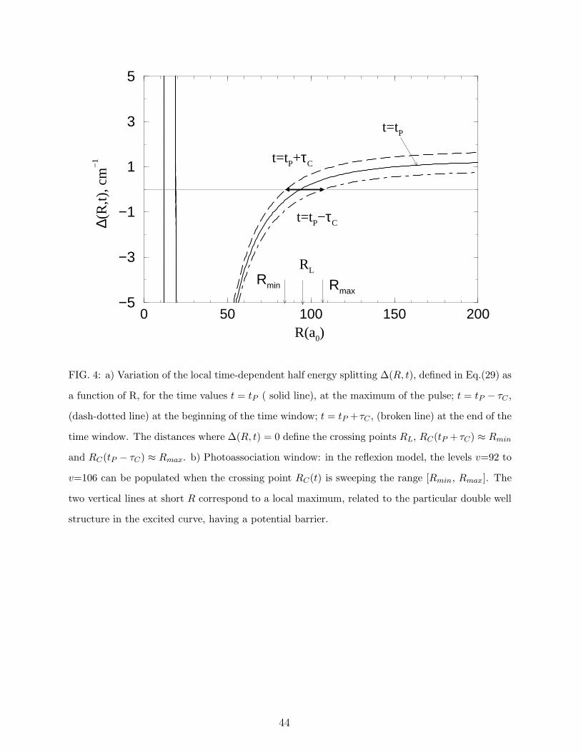
0 50 100 150 200R(a0)

−5

−3

−1

1

3

5

∆(R

,t), c

m−

1

RmaxRmin

t=tP−τC

t=tP+τC

t=tP

RL

FIG. 4: a) Variation of the local time-dependent half energy splitting ∆(R, t), defined in Eq.(29) as

a function of R, for the time values t = tP ( solid line), at the maximum of the pulse; t = tP − τC ,

(dash-dotted line) at the beginning of the time window; t = tP +τC , (broken line) at the end of the

time window. The distances where ∆(R, t) = 0 define the crossing points RL, RC(tP + τC) ≈ Rmin

and RC(tP − τC) ≈ Rmax. b) Photoassociation window: in the reflexion model, the levels v=92 to

v=106 can be populated when the crossing point RC(t) is sweeping the range [Rmin, Rmax]. The

two vertical lines at short R correspond to a local maximum, related to the particular double well

structure in the excited curve, having a potential barrier.

44

FIG. 5: Time-variation of the computed populations for the ground 3Σ+u and excited 0−g electronic states

during the pulse duration. The pulse is centered at tP = 150 ps. Black lines in Fig. (a), (b), (d), (e)

correspond to negative chirp, and blue lines to positive chirp. (a) Full lines: variation of the total population

in the ground 3Σ+u state. Note that the minimum occurs ≈ 5 ps earlier than tP = 150 ps with negative

chirp, and ≈ 5 ps later with positive chirp. Broken lines: variation of the population in the initial continuum

level, at E=1.72 × 10−10au. (b) Variation of the total population in the excited 0−g state for negative (dark)

and positive chirp (blue). (d) Population of the three last bound levels of the 3Σ+u state: full line v′′=51,

long-dashed line v′′=52, dash-dotted line v′′=53. (e) Variation of the partial sums of populations on the

bound vibrational levels in the 0−g potential: full line for low excited levels, v=95 to 107, resonanly excited

during the temporal window; dashed line: highly excited levels, v= 122 to 135, off-resonance. Black and

blue correspond to negative and positive chirp. (c) Details on the variation of the individual populations

of the 0−g levels resonantly excited during the temporal window, for negative chirp: in particular red curve,

v=98, resonant at t = t , blue v=95, dark blue v=102, green v=107. (f) Same as (c) for a positive chirp.

45

0 50 100 150 200R(a0)

−1.5

−0.5

0.5

1.5

2.5

log 10

Ω(R

,t=t P)

, cm

−1

(a)

τRab=12ps

τRab=34ps

RL

τRab=0.50ps

τRab=0.18ps

τRab=10psτRab=28ps

0 50 100 150 200R(a0)

−2

−1

0

1

2

log 10

Ω(R

,t), c

m−

1

(b)

RmaxRmin

t=tP−τC

t=tP+τC

t=tP

Tc

Rabi=137 psT

c

Rabi=137 ps

Tvib=350 psTvib=196 ps

Tvib=250 ps

Tc

Rabi=34 ps

FIG. 6: Variation of the local Rabi frequency Ω(R, t), defined in Eq.(48) and corresponding to the

pulse defined in Table I, as a function of the distance R, for three values of time. (a) Solid line:

at t = tP , at the maximum of the pulse. Also indicated are the values of the corresponding local

Rabi period τRab, see Eq.(36) in text. (b) Dash-dotted line: t = tP − τC , at the beginning of the

time window. Broken line : t = tP + τC , at the end of the time window. Also indicated are the

values of the characteristic times Tvib and TCRabi(tP , tP ± τC) significant for the vibrational levels

resonantly excited at the moments tP + τC , tP , tP − τC , which have the outer turning points in

Rmin, RL, Rmax.

46

0 50 100 150 200R(a0)

−0.2

0

0.2

0.4

0.6

0.8

1

1.2θ(

R,t)

,rd

RmaxRmin

t=tP+τC

t=tP−τC

t=tP

FIG. 7: Population inversion and photoassociation window. a) Variation of the angle θ(R, t),

defined in Eq.(50) for the same three time values as in Fig. 6. The domain where θ(R, t− τC) and

θ(R, t+ τC) differ by π is indicated by an horizontal arrow: it corresponds to population inversion,

as discussed in Section V C.

47

50 75 100 125 150−1.25

−0.75

−0.25

0.25X(R)

R(au)

Rmin RL Rmax

(a)

tP−τCtP+τC

t=tP

−2 −1 0 1 2−0.5

−0.4

−0.3

−0.2

−0.1

X(t)

(t−tp)/τc

(b)R=100 a0

R=90 a0

R=RL

−2 −1 0 1 2−0.02

−0.01

0

0.01

0.02

0.03X(t)

(t−tp)/τc

(d)

R=150 a0

R=1023 a0

−2 −1 0 1 2−3

−2

−1

0

(t−tp)/τc

X(t)

(c)

R=85 a0

R=110 a0

FIG. 8: Interpretation of the calculations: validity of the adiabatic approximation within the pho-

toassociation window. The adiabaticity parameter X(R,t), defined in Eq.(71) in text, is represented

for various values of time and distance.

(a) Variation of X(R, t) as a function of R for t = tP (solid line), t = tP − τC (dash-dotted curve),

t = tP + τC (broken curve).

(b) Adiabatic behaviour within the photoassociation window : Variation of X(R, t) as a function

of time for R = RL (solid curve), R = 90 a0 (broken curve), R = 100 a0 (dash-dotted curve). Note

that maximum values are reached for |t − tP | = τC .

(c) Non-adiabatic behaviour at the border of the window: same as Fig.8b for R=85 a0 (broken

curve) and R=110 a0 (dash-dotted curve).

(d) Adiabatic behaviour in the asymptotic region: same as Fig.8b for R=150 a (dotted curve)

48

FIG. 9: Optimization of the chirp in view of focussing. Variation of the amplitude of the wavefunc-

tion in the excited state |Ψexc(R, t = tP + 125)| , at a delay Tvib/2 = 125 ps after the maximum of

the pulse (i.e. well out of the time window), where Tvib is the classical vibrational period for the

resonant level v=98. (a) negative chirp, for the pulse defined in Table I; (b) same with χ=0; (c)

same with positive chirp parameter. 49