phd-thesis-dtyordanovphd.pdf - Departement Natuurkunde en ...
154
Instituut voor Kern- en Stralingsfysica Departement Natuurkunde en Sterrenkunde Faculteit Wetenschappen LEUVEN KATHOLIEKE UNIVERSITEIT From 27 Mg to 33 Mg: transition to the Island of inversion Promotor: Prof. Dr. G. Neyens Proefschrift ingediend tot het be- halen van de graad van doctor in de wetenschappen door Deyan Todorov Yordanov 2007
-
Upload
khangminh22 -
Category
Documents
-
view
0 -
download
0
Transcript of phd-thesis-dtyordanovphd.pdf - Departement Natuurkunde en ...

Instituut voorKern- en StralingsfysicaDepartement Natuurkunde en SterrenkundeFaculteit Wetenschappen LEUVEN
KATHOLIEKE UNIVERSITEIT
From 27Mg to 33Mg: transition to theIsland of inversion
Promotor:Prof. Dr. G. Neyens
Proefschrift ingediend tot het be-halen van de graad van doctor inde wetenschappen door
Deyan Todorov Yordanov
2007


Contents
1 Introduction 11.1 Physics motivation . . . . . . . . . . . . . . . . . . . . . . . . . 11.2 This work . . . . . . . . . . . . . . . . . . . . . . . . . . . . . . 3
2 Measurement of nuclear moments and radii 52.1 Electromagnetic moments . . . . . . . . . . . . . . . . . . . . . 52.2 Nuclear deformations . . . . . . . . . . . . . . . . . . . . . . . . 82.3 Atomic hyperfine structure . . . . . . . . . . . . . . . . . . . . 102.4 Isotope shifts and charge radii . . . . . . . . . . . . . . . . . . . 132.5 Nuclear magnetic resonance . . . . . . . . . . . . . . . . . . . . 162.6 NMR lineshapes with modulation . . . . . . . . . . . . . . . . . 18
3 Laser spectroscopy 213.1 Collinear laser spectroscopy at ISOLDE . . . . . . . . . . . . . 213.2 Einstein coefficients . . . . . . . . . . . . . . . . . . . . . . . . . 233.3 Simulation of optical spectra . . . . . . . . . . . . . . . . . . . 263.4 Transition strengths . . . . . . . . . . . . . . . . . . . . . . . . 313.5 Power broadening . . . . . . . . . . . . . . . . . . . . . . . . . . 333.6 Doppler broadening . . . . . . . . . . . . . . . . . . . . . . . . 343.7 Voigt profile . . . . . . . . . . . . . . . . . . . . . . . . . . . . . 363.8 Nuclear polarization with optical pumping . . . . . . . . . . . . 36
4 Optical spectroscopy 454.1 Hyperfine structure of stable Mg ii . . . . . . . . . . . . . . . . 454.2 Magnetic moment and hyperfine structure of 27Mg ii . . . . . . 47
5 β-decay spectroscopy and nuclear magnetic resonance 515.1 Magnetic moments of 29,31Mg . . . . . . . . . . . . . . . . . . . 515.2 31Mg: transition to the Island of inversion . . . . . . . . . . . . 535.3 Spin and magnetic moment of 33Mg . . . . . . . . . . . . . . . 555.4 Solid-state aspects of NMR . . . . . . . . . . . . . . . . . . . . 64

ii CONTENTS
5.5 Quadrupole moment of 29Mg . . . . . . . . . . . . . . . . . . . 66
6 Conclusions and outlook 71
A Specialities 73A.1 Systematic error and total probability density distribution . . . 73A.2 Individual NMR measurements on 33Mg . . . . . . . . . . . . . 75A.3 Individual HFS measurements on 27Mg ii . . . . . . . . . . . . 79A.4 Coupling of angular momenta . . . . . . . . . . . . . . . . . . . 79
B Numerical functions 85B.1 Realistic decay rate function . . . . . . . . . . . . . . . . . . . . 85B.2 Pseudo Voigt function . . . . . . . . . . . . . . . . . . . . . . . 91B.3 Realistic polarization function . . . . . . . . . . . . . . . . . . . 92
Bibliography 99
Acknowledgments 103

List of Tables
2.1 Gamow-Teller β asymmetries . . . . . . . . . . . . . . . . . . . 17
3.1 ISOLDE yields and half-lifes of neutron-rich Mg isotopes . . . . 22
4.1 Hyperfine parameters of 25Mg ii . . . . . . . . . . . . . . . . . . 454.2 Magnetic hyperfine parameters ratios for Mg ii . . . . . . . . . 474.3 Hyperfine parameters of 27Mg ii . . . . . . . . . . . . . . . . . . 474.4 Nuclear ground-state properties of 27Mg . . . . . . . . . . . . . 484.5 Magnetic moments of the even-odd N = 15 isotones . . . . . . 49
5.1 NMR frequencies of 29,31Mg and 8Li . . . . . . . . . . . . . . . 525.2 Nuclear ground-state properties of 29,31Mg . . . . . . . . . . . . 525.3 NMR frequencies of 33Mg in Pt and MgO . . . . . . . . . . . . 585.4 Nuclear ground-state properties of 33Mg . . . . . . . . . . . . . 585.5 Shell-model calculations for 33Mg . . . . . . . . . . . . . . . . . 595.6 Calculated levels of 33Mg . . . . . . . . . . . . . . . . . . . . . 605.7 Knight shift of Mg in Pt . . . . . . . . . . . . . . . . . . . . . . 645.8 Relaxation times of 31Mg in Pt and MgO at room temperature 665.9 Quadrupole hyperfine parameter of 29Mg ii . . . . . . . . . . . 675.10 Shell-model calculations for 29Mg . . . . . . . . . . . . . . . . . 69
6.1 Spins and magnetic moments of 27,29,31,33Mg . . . . . . . . . . 71
A.1 Confidence levels for the magnetic moment of 31Mg . . . . . . . 75A.2 Confidence levels for the magnetic moment of 33Mg . . . . . . . 75A.3 Individual NMR frequencies of 33Mg . . . . . . . . . . . . . . . 76A.4 Individual A-factor measurements in 27Mg ii . . . . . . . . . . . 79

iv LIST OF TABLES

List of Figures
1.1 Island of inversion . . . . . . . . . . . . . . . . . . . . . . . . . 2
2.1 Theoretical NMR curves with frequency modulation . . . . . . 20
3.1 COLLAPS . . . . . . . . . . . . . . . . . . . . . . . . . . . . . . 213.2 Two-level atomic system . . . . . . . . . . . . . . . . . . . . . . 243.3 Simulated fluorescence of 25Mg ii in the D1 and D2 lines . . . . 283.4 Simulated fluorescence of 27Mg ii in the D1 and D2 lines . . . . 293.5 Simulated fluorescence of 29Mg ii in the D1 and D2 lines . . . . 303.6 Doppler broadening . . . . . . . . . . . . . . . . . . . . . . . . 353.7 Optical pumping . . . . . . . . . . . . . . . . . . . . . . . . . . 373.8 Magnetic field effect on the hyperfine structure . . . . . . . . . 373.9 Simulated experimental β asymmetry of 29Mg ii in the D1 line 383.10 Simulated experimental β asymmetry of 29Mg ii in the D2 line 393.11 Simulated experimental β asymmetry of 31Mg ii in the D1 line 403.12 Simulated experimental β asymmetry of 31Mg ii in the D2 line 413.13 Simulated experimental β asymmetry of 33Mg ii in the D1 line 423.14 Simulated experimental β asymmetry of 33Mg ii in the D2 line 43
4.1 Hyperfine structure of 25Mg ii in the D1 and D2 lines . . . . . . 464.2 Hyperfine structure of 27Mg ii in the D1 line . . . . . . . . . . . 484.3 Magnetic moments of the even-odd N = 15 isotones . . . . . . 49
5.1 HFS (D2 line) and NMR of 31Mg ii . . . . . . . . . . . . . . . . 545.2 HFS of 33Mg ii in the D2 line . . . . . . . . . . . . . . . . . . . 565.3 NMR spectrum of 33Mg . . . . . . . . . . . . . . . . . . . . . . 575.4 Nilsson diagram . . . . . . . . . . . . . . . . . . . . . . . . . . . 615.5 Level scheme of 33Mg established in the β decay of 33Na . . . . 625.6 Modified decay scheme of 33Mg . . . . . . . . . . . . . . . . . . 635.7 Relaxation times of 31Mg in Pt and MgO at room temperature 655.8 Hyperfine structure of 29Mg ii in the D2 line . . . . . . . . . . . 68

vi LIST OF FIGURES
A.1 Probability densities for the magnetic moment of 31Mg . . . . . 74A.2 NMR of 33Mg in Pt . . . . . . . . . . . . . . . . . . . . . . . . 76A.3 NMR spectra of 33Mg in MgO with small frequency modulation 77A.4 NMR spectra of 33Mg in MgO with large frequency modulation 78

Chapter 1
Introduction
Every atomic nucleus is associated with a unique set of macroscopic proper-ties: mass, angular momentum, excitation energies, electromagnetic moments,etc. Studies of these observables led to discoveries of global phenomena, suchas the zero angular momentum of even-even nuclei or the increase in bindingenergy per nucleon at certain, “ magic ”, numbers of protons and neutrons. Ina phenomenological sense this implies that the nuclei have intrinsic structure,which is something that the early models, like the liquid drop model, could notaccount for. The modern theories consider the nucleus as a many-boby quan-tum system, providing insights into the nuclear structure through studyingmacroscopic observables - nuclear moments in particular. A phenomenologicalapproach to the problems in nuclear physics is an alternative to a complete fun-damental theory as well as its natural precursor. It is the better understandingof the nuclear structure in neutron rich Magnesium (Mg) isotopes, that is themain objective of this doctoral dissertation.
1.1 Physics motivation
The nuclear shell model has been successful in reproducing the magic numbersas well as predicting spins of odd-mass nuclei, especially in the light and in-termediate mass regions. However, properties of nuclei with 150 < A < 190or A > 230 are not correctly described by the spherical shell model, since inthese regions collective phenomena associated with nuclear shapes departingfrom spherical take place. The Nilsson model [1] is dealing with the problemof single-particle motion in a deformed potential. Many odd-mass nuclei areproperly described by coupling the odd-particle motion to the rotations of adeformed core [2]. A natural question is: “ does deformation play a role inlight nuclear systems? ”. A positive answer has been acquired with the early

2 Introduction
Figure 1.1: Nuclear chart in the region of the Island of inversion.Experimental evidence for pure intruder ground states are indicated with black-ened corners. Mixed wave functions are noted with a black strip. Unmarkedboxes indicate a lack of conclusive experimental data or belonging outside theisland. The results from the present work concerning 27,29,31,33Mg are takeninto account.
investigation of the stable 19F, 20Ne, 23Na and 24Mg. It has been shown thatthe deficiency of both protons and neutrons in a major shell is causing strongα-type correlations, resulting in well-defined prolate deformations, for instance20Ne and 24Mg in the sd shell [2] (vol. 2, p. 99). When one or both typesof particles are filling to the middle or the end of a major shell there is acompetition between prolate and oblate shapes [3], as it is in the cases of thestable 28Si, 32S and 36Ar. Advances in technology in the last two decades madeavailable many exotic nuclear species, enabling studies of systems with a filledneutron sd shell, while maintaining the proton sd shell almost unoccupied.The mass measurements of 31,32Na [4] indeed showed an increase in their bind-ing energies, unexpected within the frame of the sd shell model. ConstrainedHartree-Fock calculations [5] reproduced these irregularities by allowing neu-tron promotion from the ν 1d3/2 orbit to the ν 1f7/2 orbit, which resulted inprolate deformations in these two isotopes. The ground-state spin of 31Na [6]was another parameter incompatible with theoretical predictions, which gavereasons to discuss a “ collapse of the conventional shell-model ordering in thevery neutron-rich isotopes ” [7]. The necessity of taking into account the ν 1f7/2
[8] and the ν 2p3/2 [9] orbitals, which are being populated before the sd shell isfull, indicated the disappearance of the N = 20 shell closure and gave rise to

1.2 This work 3
the expression Island of inversion. Two mechanisms have been justified to playan important role in the inversion of the “ normal ” 0 ~ω (0p-0h) and intrudern ~ω (np-nh) states [3]: (i) A reduction of the shell gap; (ii) An increase in theneutron-neutron and proton-neutron interactions; The diminishing predictivepower of the nuclear models in the island have stimulated extensive experi-mental studies, providing inputs for the theoretical modeling of the region. Itwas originally thought that the Island of inversion initiates with the N = 20isotones of Ne, Na and Mg and extends up to N = 22 or beyond. However, ex-perimental studies determined that 28Ne18 [10, 11], 29Na18 [12–14] and 31Mg19
[15, 16] mark the beginning of the island. The maximum Z borderline alsoneeds to be modified, since g-factor measurements [17, 18] detected a consid-erable amount of intruder components into the ground-state wave functions of33,34Al. The available experimental facts are summarized in Fig. 1.1. The col-lectivity of the even-even 32,34Mg is presently well established [19–24], whereasthe nuclear structure of the odd-mass 33Mg is rather unknown. A β-decaystudy [25] suggests a 1p-1h configuration with spin and parity Iπ = 3/2+ incontrast to Iπ = 5/2+ (1p-1h) from intermediate energy Coulomb excitation[26] and proton inelastic scattering [27] experiments. The systematics of theregion, on the other hand, is evident for 2p-2h ground states [10, 22, 24, 28, 29].Due to the close competition between different particle-hole excitations, onlyexperimental studies can reveal the true ground-state configuration of 33Mg.
1.2 This work
Measurements of nuclear moments are highly beneficial for studies of the nu-clear structure, since these are extremely sensitive to the composition of thenuclear wave function. The establishment of the nuclear spin and magneticmoment of 31Mg indicates the disappearance of the N = 20 shell closure forMg, extends the Island of inversion to N = 19 and provides evidence for anuclear deformation. These findings are essential for the development of theshell model in the vicinity of the island. The results on 31Mg are publishedin Ref. [15, 30, 31], the full texts of which are included at the end of this dis-sertation. While the first paper is focused on the interpretation of the resultin terms of large-scale shell-model calculations, the latter two concentrate onthe experimental technique, describing the apparatus and the reference mea-surements on 8Li. A comprehensive discussion on the establishment of the signof the magnetic moment is given in Ref. [30]. This discussion further extendson studying the nature of the low-lying excited states. Preparatory work forthe measurements on 31Mg is described in Ref. [31], namely the studies ofthe experimental β asymmetry in different hosts (Au, Pt and MgO) and as afunction of the laser intensity. The latter paper concentrates on the atomicphysics, more specifically on understanding the relative intensities of the hy-

4 Introduction
perfine structure components. The present thesis presents additional studies of31Mg. The physics case is discussed in terms of nuclear-structure evolution overthe Mg chain and transition to the Island of inversion. The magnetic momentsof 29,31Mg [15, 16, 30, 31] are reevaluated. The optical transition strengthsand the process of optical pumping for Mg ii are understood, based on the pi-oneering work described in Ref. [12]. Computer codes simulating optical andβ-asymmetry spectra are published for the first time (open source).
The main objective of this dissertation is to unambiguously determine theground-state spin and magnetic moment of 33Mg by means of laser spectroscopyin combination with nuclear magnetic resonance. Large-scale shell-model cal-culations are outlined and used to draw conclusions through a comparison withthe experimental results. An alternative interpretation of former experimentalstudies is given within the frame of the Nilsson and particle plus rotor models.Additional research is done in order to understand the generated NMR line-shapes with modulation. The essence of the present studies on 33Mg is sum-marized in a preliminary version of a publication [32], the full text of which isincluded at the end of this thesis.
The hyperfine parameters of the stable 25Mg ii in the D1 and D2 lines areobtained by means of fluorescence spectroscopy. The magnetic moment of27Mg and an estimate of the quadrupole moment of 29Mg, extracted from thehyperfine structure of their singly-ionized atoms, are reported for the first time.The case of 27Mg is also a central topic in a publication in preparation [33].

Chapter 2
Measurement of nuclearmoments and radii
2.1 Electromagnetic momentsThe electromagnetic moments are defined by the general expression:
Mλµ=0 = 〈I,M = I|A∑
k=1
Tλµ=0(k)|I,M = I〉, (2.1)
where Tλµ is a one-body tensor operator of rank λ, describing the interactionof the nucleus with an external electromagnetic field. It stands for either Qλµ
when giving rise to the electric moments associated with the static charge dis-tribution, or Mλµ when giving rise the magnetic moments associated with thecharge currents. The multipole operators Qλµ and Mλµ can be expressed withthe spherical harmonics Yλµ(θ, φ) [34] (p. 583). Their parities are (−)λ and(−)λ+1, thus requiring λ-even for the static moments and λ-odd for the mag-netic moments due to the parity conservation. For spherical tensor operatorsthe M -state dependence of the matrix elements reduces to a dependence onthe Clebsch-GordanA or 3j coefficient via the Wigner-Eckart theorem:
〈IM |Tλµ|IM〉 = (−1)I−M
(I λ I
−M µ M
)〈I||Tλ||I〉, (2.2)
where 〈I||Tλ||I〉 is the reduced matrix element. According to the propertiesof the 3j coefficients, µ = 0 and λ must satisfy the triangle condition ∆(IIλ)
A The relation between the Clebsch-Gordan and the 3j coefficients (A.14), together withtheir numerical implementation, is given in Appendix A.4.

6 Measurement of nuclear moments and radii
(A.6), where I is the nuclear spin. The maximum value of λ is therefore λmax =2I. The only moment for I = 0 is the electric monopole moment
∑Ak=1 ek
(λ = 0), which represents the total charge of the nucleus. The magnetic dipolemoment (λ = 1) is defined for I ≥ 1/2 and the electric quadrupole moment(λ = 2) for I ≥ 1.
The magnetic dipole moment operator for a single nucleon in a static bindingfield is:
µ = µN
(gtz
l l + gtzs s)/ ~, (2.3)
where gtz
l and gtzs are the orbital and spin gyromagnetic ratios of the nucleon in
terms of nuclear magnetons µN = e~/2mp = 5.05078317(20)× 10−27 J/T [35].The index tz represents the isospin of the particle, tz(p) = −1/2 for protons(π) and tz(n) = 1/2 for neutrons (ν). Since the nuclear magneton is definedwith e and mp, the proton charge and rest mass, the orbital g factors become:
gπl = 1 , gν
l = 0 . (2.4)
The latest experimental proton and neutron g factors, taken from Ref. [35],are:
gπs = 5.585694675(57) , gν
s = −3.82608545(90) . (2.5)
The fact that gs of the uncharged neutron is different from zero and that ofthe proton is far from two, the expectation value from the Dirac equation fora point particle with spin 1/2, is an indication that they are not elementarypoint particles but have an internal structure. The observable magnetic mo-ment of a single nucleon in a shell-model orbit is the expectation value of themagnetic moment operator (2.3) in the state with maximum projection of an-gular momentum, as defined in (2.1). According to the projection theorem [36](p. 7):
〈jj|µ|jj〉 =〈jj|µ · j|jj〉⟨jj∣∣j2∣∣ jj⟩ 〈jj|j|jj〉 (2.6)
the components of the vector µ perpendicular to j average out. Thus, theprojection on the third axis is 〈jj|µz|jj〉 = 〈jj|µ · j|jj〉〈jj|jz|jj〉/〈jj|j
2|jj〉.Since 〈jj|jz|jj〉 = j ~, 〈jj|j2|jj〉 = j(j+1)~2 and using the squaring of j = l+sto express the product operators one finds:
〈jj|µ · j|jj〉 = µN
⟨jj∣∣ gtz
l j2 +(gtz
s − gtz
l
) (j2 − l2 + s2
)/ 2∣∣ jj⟩ / ~ .
It is now straightforward to evaluate the single-particle magnetic moments:
µ = j
(gtz
l ±gtz
s − gtz
l
2l + 1
)µN , j = l ± 1
2. (2.7)

2.1 Electromagnetic moments 7
The latter are also known as the Schmidt values. In the extreme shell-modelpicture the ground states of odd-mass nuclei are considered to be determinedmainly by the odd particle, which alone gives rise to the nuclear magneticmoment. Comparison with experiments shows that the Schmidt values aregenerally larger in magnitude. One explanation for this could be that gs fora bound nucleon is different than the free-nucleon value. A common approachis to consider effective g factors derived by fitting to experimental data in theprecise region of interest. In general gtz
s effective ≈ 0.7 gtzs free yields reasonable
results. The nuclear gyromagnetic ratio of a state with an angular momentumI is defined with:
〈µI〉 = gI I µN/ ~ ⇒ µI = gI I µN . (2.8)
The electric quadrupole moment operator of a point particle is defined as:
eQzz = etze(3z2 − r2
)= etze
√16π5r2Y20(r) , (2.9)
where etz is the charge of the carrier, a proton (π) or a neutron (ν), in units e.This definition is based on the third diagonal component of the tensor: Qij =q(3rirj − r2δij), known from the Classical Electrodynamics. For a free nucleonit is expected to have eπ = gπ
l = 1 and eν = gνl = 0. Experimental quadrupole
moments of nuclei with an odd neutron are indeed smaller than those with anodd proton, but are definitely different from zero. One can account for sucheffects by introducing proton and neutron effective charges, denoted here withetz . The operator defined with (2.9) does not include the elementary chargee and therefore has the dimension of a surfaceA. All quadrupole moments inthis thesis will be given in units b (barnB). The single-particle quadrupolemoments are given with the expression:
eQ = 〈jj|eQzz|jj〉 = ∓2j − 12j + 1
⟨r2⟩etze , (2.10)
where 〈r2〉 is the mean-square radius of the nucleon. A derivation can befollowed for instance in Ref. [37–39]. The sign corresponds to a particle (−) ora hole (+). The more general expression:
〈jm|eQzz|jm〉 = ±j(j + 1)− 3m2
2j(j + 1)⟨r2⟩etze , (2.11)
can be obtained with the use of (2.2). By summing (2.11) over allm statesC oneA The quantity Q defined with (2.9) still contains the same information on the nuclear
structure as the quadrupole moment eQ, namely the geometrical distribution of the charge.In order to avoid the inclusion of e in the value of eQ the elementary charge is embedded inthe units (emb or efm2). By doing so the actual values become identical: Q(mb) = eQ(emb)or Q(fm2) = eQ(e fm2).
B 1b = 10−28m2. Commonly used are mb or fm2 (1mb = 10−31m2, 1fm2 = 10−30m2).C Use the relation
Pjm=−j m2 = j(j + 1)(2j + 1)/3.

8 Measurement of nuclear moments and radii
finds that the total quadrupole moment of a full orbit vanishes. Furthermore,since a pair of nucleons couple to a zero angular momentum they have nopreferential orientation in space in which case their wavefunction has a sphericalsymmetry |ψ(r)|2 = |ψ(r)|2. Hence the expectation values of the coordinatesare one third of the mean-square radius 〈x2〉 = 〈y2〉 = 〈z2〉 = 〈r2〉/3 in whichcase the quadrupole moment (2.9) vanishes.
2.2 Nuclear deformationsThe observation of very large quadrupole moments, far from the single-particleestimates, is attributed to collective phenomena resulting in deformation of thenuclear core. In the case of quadrupole deformations (λ = 2) the nuclear shapeis parametrized with:
Rkk=1, 2, 3
= R0
[1 +
√54π
β cos(γ − 2kπ
3
)], (2.12)
where β and γ are the Hill-Wheeler coordinates [40]. The parameter β deter-mines the quadrupole deformation and γ the deviation from axial symmetry.In the axially symmetric case (γ = 0 ⇔ R1 = R2 = R⊥) the following relationexists:
R3 −R⊥R0
=3β4
√5π. (2.13)
The quadrupole momentA in the reference frame of the nucleus is given by:
Q0 =43
⟨ Z∑k=1
r2k
⟩δ , (2.14)
where δ is the distortion parameter, which for a uniformly charged spheroidalnucleus with a sharp surface is given by:
δ =32R2
3 −R2⊥
R23 + 2R2
⊥≈ ∆R
R+
16
(∆RR
)2
+ . . . , (2.15)
with ∆R = R3 − R⊥ and R ≈ R0. Equations (2.12) and (2.14), (2.15) arejustified in Ref. [34] (p. 7) and Ref. [2] (vol. 2, p. 47), respectively. Using(2.13), (2.14) and (2.15) one finds a relation, between the intrinsic quadrupolemoment and the deformation, based on the shape (2.12) with axial symmetry:
Q0 = Z⟨r2⟩β
√5π
(1 +
β
8
√5π
), (2.16)
A Attention must be paid since “ quadrupole moment ” is used for either Q or eQ.

2.2 Nuclear deformations 9
where the second radial moment is related to the mass number as:⟨r2⟩
=35(1.12A1/3
)2(1 + 3.84A−2/3 + . . .)≈ 3
5(1.2A1/3
)2 (fm2) , (2.17)
according to Ref. [2] (vol. 1, p. 161).Extensive studies in the regions of deformation reveal that the low-energy
states in odd-A nuclei, despite the complexity of the spectra, can be classified asa number of rotational bands characterized by an intrinsic angular momentumA
K and a parity π. A typical example is the case of 25Mg. A summary of theexperimental data and an interpretation, as well as references to the originalwork can be found in Ref. [2] (vol. 2, p. 284). The band with Kπ = 1/2+,based on the Nilsson 1/2 [200] orbital, is of a particular interest, since theground state of 31Mg was found to be 1/2+ [15], based on the same orbital,hence making it a candidate for one of the low-lying states observed in 33Mg[20, 25]. The energy levels of a rotational band in an odd-A nucleus with astrong deformation (strong coupling limit) are described by:
EK(I) = E0K +
~2
2I
[I(I + 1) + a (−1)I+1/2(I + 1/2)δK,1/2
], (2.18)
where I is the moment of inertia, E0K is the bandhead and a is the decoupling
parameter associated with the odd particle. The explicit form of a is givenin Ref. [34] (p. 112). A table with calculated a values for different orbitals insd−pf nuclei at a prolate deformation β = 0.4 can be found in Ref. [2] (vol. 2,p. 290). The magnetic dipole moment of an odd-A nucleus has two contribu-tions, gR representing the gyromagnetic ratio of the rotor (µR = gR RµN ) andgK , rising from the single-particle motion:
µ = gRI + (gK − gR)K2
I + 1. (2.19)
This equation is valid only for bands with K 6= 1/2. In the case of K = 1/2one must use:
µ = gRI +gK − gR
4(I + 1)
[1 + b (2I + 1)(−1)I+1/2
], (2.20)
where b is the magnetic decoupling parameterB . The reduced transition pro-babilities for magnetic dipole radiation, can be obtained from Ref. [2] (vol. 2,p. 56, 57). In the strong coupling limit the projection Ω of the total momentumof the odd nucleon on the symmetry axis equals the projection K of the total
A The angular momenta quantum numbers are referred to as angular momenta. ThePlanck’s constant ~ in such sentences is implicit.
B The parameters a and b are related: (gK−gR) b = −(gl−gR) a−(−1)l(gs +gK−2gl)/2[see Ref. [2] (vol. 2, p. 303)].

10 Measurement of nuclear moments and radii
angular momentum I (Ω = K). The single-particle g factor can be calculatedas:
gK =1K〈K|µ3|K〉 , (2.21)
where µ3 = µN (gtz
l l3 + gtzs s3) is the magnetic moment operator in the body-
fixed frame and |K〉 are the Nilsson wave functions. The g factor of a solidrotor is approximately equal to the density of protons gR ≈ Z/A [2] (vol. 2,p. 54). The observable or spectroscopic quadrupole moment and the intrinsicquadrupole moment (2.14) are related as:
Q = 〈IK20|IK〉〈II20|II〉Q0 =3K2 − I(I + 1)(I + 1)(2I + 3)
Q0 . (2.22)
Knowledge on the deformation of even-even nuclei, 30,32,34Mg being of a par-ticular interest in this thesis, can be obtained through the reduced transitionprobabilities, either from Coulomb excitation cross sections, or from lifetimemeasurements:
B(E2;KIi → KIf ) =1
2Ii + 1|〈KIf ||M (E2)||KIi〉|2
=5
16πe2Q2
0 〈IiK20|IfK〉2 ,(2.23)
where Ii and If are the initial and the final angular momenta and the operatorM (E2) =
∫ρ(r) r2 Y20(r) dτ is the general form of (2.9) with ρ(r) representing
the charge density. The treatment leading to (2.22) and (2.23) can be followedin Ref. [2] (vol. 2, p. 45). The Clebsch-Gordan coefficients involved can becalculated with the tools given in Appendix A.4.
2.3 Atomic hyperfine structure
The hyperfine structure (HFS) observed in atomic spectra results from the in-teraction of the nuclear multipole moments with the charge and current distri-butions associated with the moments of the electron environment. The Hamil-tonian in the most general form is:
HHFS = H(M1) +H(E2) + . . . (2.24)
The hyperfine interaction couples the angular momenta of the nucleus and theelectrons I and J , being no longer integrals of motion, to the total angularmomentum operator F = I + J . Thus the quantum number F is used todescribe the quantum states |JIFMF 〉. F satisfies the triangle condition (A.6)

2.3 Atomic hyperfine structure 11
and therefore the number of states in a hyperfine multiplet is 2I + 1 for J > Iand 2J + 1 for I > J . The magnetic dipole term in (2.24) is:
H(M1) = −〈µI〉 · 〈BJ〉 = AI · J~2
, (2.25)
where 〈µI〉 is given by (2.8) and BJ is the magnetic field, associated with thetotal magnetic moment of the electrons µJ :
〈µJ〉 = −gJ J µB/ ~ ⇒ µJ = −gJ J µB . (2.26)
The Bohr magneton is defined as µB = e~/2me = 927.400899(37)× 10−26 J/T[35] and gJ is given by the Landé formula:
gJ = gLJ(J + 1) + L(L+ 1)− S(S + 1)
2J(J + 1)
+ gSJ(J + 1)− L(L+ 1) + S(S + 1)
2J(J + 1).
(2.27)
The g factors gL = 1 and gS = 2.0023193043617(15) [41] are associated withthe magnetic moments of the orbital and spin motions of the electrons
µL = −gL LµB/ ~ , µS = −gS S µB/ ~ , (2.28)
the coupling of which gives rise to the atomic fine structure (FS). One canwrite:
〈BJ〉 = −〈B(0)〉J/ ~J , (2.29)
where 〈B(0)〉 is a scalar quantity representing the average flux density of themagnetic field at the nucleus. For a single electron or an electron outside aclosed shell (alkali-like atoms) the general direction of µJ , and so the one of BJ
at the nucleus, is antiparallel to the angular momentum J , as can be concludedfrom (2.26) and (2.27). Thus in alkali-like atoms 〈B(0)〉 > 0. Calculated valuesof 〈B(0)〉 due to the alkalies valence electrons are presented in Ref. [42] (p. 132).The energy levels depend on the product I · J , which can be expressed as afunction of J2, I2 and F 2 by squaring F = I + J . Using (2.8) and (2.29) themagnetic dipole hyperfine parameter becomes:
A =gI µN 〈B(0)〉
J. (2.30)
A formal expression for the term H(E2) in (2.24) is given by (2.55). However,a more complex treatment is required in order to extract the contribution ofthe quadrupole interaction to the atomic energies. A detailed description can

12 Measurement of nuclear moments and radii
be followed in Refs. [42, 43]. The energy levels of the hyperfine structure,according to Ref. [42] (p. 15), are given with:
EF = EJ +Aξ
2+B
3ξ(ξ + 1)− 4I(I + 1)J(J + 1)8I(2I − 1)J(2J − 1)
,
ξ = F (F + 1)− I(I + 1)− J(J + 1) ,(2.31)
where EJ represents the energy of the fine-structure level. The parameter B,called the electric quadrupole hyperfine parameter, has the form:
B = eQ 〈VJJ(0)〉 , (2.32)
where eQ is the nuclear spectroscopic quadrupole moment and 〈VJJ(0)〉 isthe average field gradient at the nucleus induced by the electrons, having acylindrical symmetry about the J axis [43] (p. 13). The quadrupole hyperfineparameter B, and therefore the second term in (2.31), vanishes for either J =1/2 or I = 1/2. If one neglects the volume changes along an isotopic chainone can approximate that the average magnetic field 〈B(0)〉 and electric fieldgradient 〈VJJ(0)〉 are identical for all the atoms in the chain. Thus using (2.30)and (2.32) for two isotopes one arrives with:
A1/A2 = g1/g2 , (2.33)B1/B2 = Q1/Q2 . (2.34)
The above equations are used for extraction of nuclear moments through atomicspectroscopy. However, these have as important application if used in theopposite direction. Measurements of nuclear moments with other techniquesallow the determination of A and B. Equation (2.33) is, in this respect, essentialfor the extraction of nuclear spins from the hyperfine structure, as demonstratedin Section 5.3.
While the atomic hyperfine structure originates from the interaction of thenucleus with the natural electromagnetic field associated with the charge andcurrent distributions of the atomic electrons, many experimental techniquesrequire the employment of external fields. It is important for measurementsbased on the hyperfine structure to understand the influence of these fields.The Hamiltonian (2.25) in the presence of an applied magnetic field B0 takesthe form:
H(M1) = AI · J~2
− 〈µI〉 ·B0 − 〈µJ〉 ·B0 , (2.35)
where 〈µI〉 and 〈µJ〉 are the magnetic moments given with (2.8) and (2.26),respectively. The effect on the energy levels is referred to as the Zeeman effect.In the case with µJ B0 A the magnetic components of the F states (MF =−F , −F + 1 , . . . , F − 1 , F ) obtain different energies proportional to theexternal field:
EMF= EF + gF µB B0MF . (2.36)

2.4 Isotope shifts and charge radii 13
The corresponding g factor in analogy with (2.27) is given with the expression:
gF = gJF (F + 1) + J(J + 1)− I(I + 1)
2F (F + 1)
− gIµN
µB
F (F + 1)− J(J + 1) + I(I + 1)2F (F + 1)
.
(2.37)
The second term describing the nuclear contribution is often neglected dueto the factor µN/µB = me/mp = 5.446170232(12) × 10−4 [35]. In a strongmagnetic field I and J are decoupled and the proper description of the statesis no longer given by F and MF , but by I, MI , J and MJ :
EMI MJ= AMI MJ + gJ µB B0MJ − gI µN B0MI . (2.38)
The Zeeman effect in this limit is called the Paschen-Back effect. At inter-mediate fields the energy levels follow the rule that two states never cross ifthey have the same magnetic number M , where M = MF for low fields andM = MI +MJ for high fields. A detailed treatment of the Zeeman effect forall fields can be found for instance in Ref. [42] (p. 19-27).
The selection rules for dipole transitions between hyperfine-structure com-ponents of two different multiplets, rising directly from the triangle condition(A.6), are:
∆F = 0 , ±1 ; F + F ′ ≥ 1 . (2.39)
Electric-dipole radiation within the same multiplet is forbidden by the parityselection rule.
2.4 Isotope shifts and charge radiiThe isotope shift is defined as the difference between the fine-structure splittingof two isotopes of the same element:
δνAA′
i = νAi − νA′
i . (2.40)
The index i denotes the atomic transition, for instance i : 32S1/2 → 32P3/2.The short spectroscopic notation n2S+1LJ is being used throughout this thesis.A and A′ in (2.40) are the mass numbers of the two isotopes. The isotope shifthas two contributions:
δνAA′
i = δνAA′
i , MS + δνAA′
i , FS , (2.41)
where δνAA′
i , MS represents the mass shift (MS), rising from the motion of thenucleus in the center of mass system, and δνAA′
i , FS stands for the field shift(FS), corresponding to changes in the nuclear volume and shape and therefore

14 Measurement of nuclear moments and radii
influencing the Coulomb attraction. The field effect is largest in transitionsinvolving s electrons since their density at the nucleus is the highest. In thecenter of mass system the total momentum is:
P +∑
k
pk = 0 , (2.42)
where P and pk are the momenta of the nucleus and the electrons, respectively.The total kinetic energy is given by:
EK =P 2
2M+∑
k
p2k
2me
=∑
k
p2k
2M+∑k 6=l
pk · pl
2M+∑
k
p2k
2me.
(2.43)
Since the nuclear massM is much larger than the mass of the electrons, in a firstapproximation the nucleus can be considered as stationary and later accountfor its motion by perturbation theory [43]. With this approach, changes of Mdo not influence the electron momenta pk. According to the virial theoremthe average total energy of an atom equals the average kinetic energy with theopposite sign: 〈E〉 = −〈EK〉. The mass shift with the use of (2.43), becomes:
δνAA′
i , MS =12h
M −M ′
MM ′
[⟨∑k
p2k
⟩i+⟨∑
k 6=l
pk · pl
⟩i
]. (2.44)
The first and the second term in (2.44) are called normal mass shift (NMS)and specific mass shift (SMS):
δνAA′
i , MS = δνAA′
i , NMS + δνAA′
i , SMS . (2.45)
The transition hνi for a nucleus with an infinite mass, with the aid of (2.43),becomes hνi =
⟨∑k p2
k
⟩i/ 2me. Making this substitution in (2.44) and approx-
imating the nuclear with the atomic masses M = MA and M ′ = MA′ one findsthe normal mass shift:
δνAA′
i , NMS = νimeMA −MA′
MAMA′. (2.46)
This formula is usually rearranged in order to use the dimensionless atomicmassesA:
δνAA′
i , NMS = νime
u
mA −mA′
mAmA′, (2.47)
A mA = MA/u, u = 1.66053873(13)× 10−27 kg [35].

2.4 Isotope shifts and charge radii 15
where u is the unified atomic mass. Correlations between the electrons, con-tributing in the second term in (2.44), need a more sophisticated approach. Adetailed description can be found in Refs. [42, 44]. The field shift is given by:
δνAA′
i , FS = Fi
(δ⟨r2⟩AA′
+c2c1δ⟨r4⟩AA′
+c3c1δ⟨r6⟩AA′
+ . . .
), (2.48)
with the convention that δ〈rn〉AA′= 〈rn〉A − 〈rn〉A′
and the radial moments:
〈rn〉 =∫ρ(r) rndτ∫ρ(r) dτ
, (2.49)
as described in Ref. [45]. The quantity Fi in (2.48) is the electronic factor, whichis proportional to the change of the electronic charge density at the nucleusfor the transition of interest i, ρ(r) represents the nuclear charge distributiondensity and 〈r2〉 is called the mean-square charge radius, giving the largestcontribution to the field shift in (2.48). For most applications the isotope shift(2.40) is written as:
δνAA′
i = KimA −mA′
mAmA′+ Fi δ
⟨r2⟩AA′
, (2.50)
where Ki is the total mass-shift coefficient. Note that the quantities mA andmA′ are dimensionless and thereforeKi has the dimension of a frequencyA. Thelinear dependence δνAA′
i
(δ〈r2〉AA′)
(2.50) allows the determination of mean-square charge radii through isotope shift measurements. The coefficients Ki
and Fi must be obtained, either from reference measurements on at least threeisotopes with known mean-square charge radii, or based on theory or otherexperimental data. A common approach to improve the precision of Ki and Fi
is to perform measurements on the reference isotopes in two transitions i andj, for instance i : 32S1/2 → 32P1/2 and j : 32S1/2 → 32P3/2. Then by writing(2.50) for both and rearranging in the form:
mAmA′
mA −mA′δνAA′
i︸ ︷︷ ︸Y
=Fi
Fj︸︷︷︸a
mAmA′
mA −mA′δνAA′
j︸ ︷︷ ︸X
+Ki −KjFi
Fj︸ ︷︷ ︸b
, (2.51)
one obtains additional conditions a = Fi/Fj and b = Ki − aKj , being used toreduce the errors of Ki and Fi. Plots of data according to (2.50) and (2.51)are known as King plots. More information can be found in Refs. [44, 45].
A If the atomic masses MA = mA u are used in (2.50) instead of mA, Ki acquires thedimension s−1kg, in which case it is usually quoted in units s−1u, such that the actual valueremains the same.

16 Measurement of nuclear moments and radii
2.5 Nuclear magnetic resonanceThe concept of the nuclear spin I rests on the fact that the nucleons coupletogether so strongly, that for most applications the nucleus can be consideredas a single spinning particle. Thus an external magnetic field does not have thestrength to break the nucleon coupling and results in a nuclear energy splittingaccording to the normal Zeeman effect. The formalism of the nuclear magneticresonance (NMR) was implicitly introduced in Section 2.3. By substituting(2.30) in (2.38) one obtains the atomic energies in a strong magnetic field inthe form:
EMI MJ= gJ µB B0MJ − gI µN (B0 − 〈B(0)〉MJ/ J)MI , (2.52)
and therefore:EMI+1 − EMI
= −gI µN B , (2.53)
where B is the attenuated magnetic field at the nucleus. High precision mea-surements, as those described in this dissertation, must account for the shieldingeffects of the electron environment. The energy splitting (2.53) is equidistant.Thus at a resonance frequency, photons with energy:
h νL = |gI |µN B , (2.54)
will be absorbed by the atom. The absorption frequency νL, known as theLarmor frequency, describes the precession of the average nuclear magneticmoment, and so the nuclear spin, around the magnetic field axis. Magneticresonance measurements are often done in solids with a cubic crystal structure,since they provide a homogeneous electric field and hence no quadrupole split-ting. However, if the subject of interest is the nuclear quadrupole moment,crystal structures violating the cubic symmetry are the only environments gen-erating large enough electric-field gradientsA and detectable quadrupole inter-actions. The latter are described by the second term in (2.24):
H(E2) =hνQ
4I(2I − 1) ~2
[3I2
z − I2 + η(I2
x − I2y
)], (2.55)
whereνQ = eQVzz/ h (2.56)
is the quadrupole frequency and η = (Vxx−Vyy)/ Vzz is the asymmetry parame-ter of the electric-field gradient. The energy levels for η = 0 according to (2.55)
A The electric-field gradient tensor is V = Gradˆgrad ϕ(r)
˜= ∇∇ϕ(r), where ϕ(r) is
the electric potential. In the principle axis system (PAS) Vij = ∂2ϕ(r)/∂ri∂rj = 0 for i 6= j
and tr(V ) = 0. Thus V is described by only two parameters Vzz and η = (Vxx − Vyy)/ Vzz .In PAS |Vzz | ≥ |Vyy | ≥ |Vxx| and therefore η ∈ [0, 1].

2.5 Nuclear magnetic resonance 17
are:EMI
=hνQ
4I(2I − 1)[3M2
I − I(I + 1)]
(2.57)
and therefore:EMI+1 − EMI
=3hνQ
4I(2I − 1)(2MI + 1). (2.58)
The sum of (2.53) and (2.58) fully describes the energy splitting of a nucleuswith a spin I in an electromagnetic field, characterized only by B and Vzz.More information about magnetic and quadrupole resonance can be found indedicated texts, for instance Ref. [46].
The magnetic resonance measurements, described in this dissertation, arebased on the anisotropy of the β decay of an oriented nuclear ensemble. Theangular distribution of the emitted β± particles, as described in Ref. [47], is:
W (θ) = 1 +υ
cAβP cos θ , (2.59)
where
P =I∑
MI=−I
p (MI)MI/ I , (2.60)
with p (MI) being the probability for occupation of the MI state, is the nuclearpolarization, Aβ is the β-asymmetry parameter, υ is the velocity of the emittedparticles and θ is the polar angle towards the orientation axis. The physicalmeaning of W (θ) is that the probability for emission in any direction withinthe solid angle Ω is given by:
PΩ =∫
Ω
W (θ)4π
dΩ . (2.61)
With other words W (θ)/4π is the probability density associated with one par-ticular directionA. The β-asymmetry parameter is a specific property of every
A The direction through the elementary solid angle dΩ = sin θ dθ dϕ.
Table 2.1: Asymmetry parameter Aβ for allowed Gamow-Teller β transitions.The upper sign corresponds to an electron decay.
Ii → If Aβ∓
If = Ii + 1 ± IiIi + 1
If = Ii − 1 ∓1
If = Ii ∓ 1Ii + 1

18 Measurement of nuclear moments and radii
β-decaying state. In the case of allowed Gamow-Teller transitions it can becalculated asA:
Aβ =∑
f
bif Aifβ , (2.62)
where bif denote the branching fractions and Aifβ are the partial β asymmetries
from Tab. 2.1. Experimentally the β-decay anisotropy can be monitored withtwo scintillation detectors placed at 0 and 180 with respect to the orientationaxis. The quantity:
A =N(0)−N(180)N(0) +N(180)
≈ υ
cAβP (2.63)
is called experimental β asymmetryB and it has the advantage to be propor-tional to both, the β-asymmetry parameter and the nuclear polarization (2.60).The approximation sign in (2.63) results from the assumption that the detec-tor surfaces cover small solid angles, for which the assumption W (θ) ≈ constis valid. A proper calculation of the number of counts N would involve theevaluation of (2.61) according to the geometry of the experimental setup. Theratio υ/c, especially for exotic species with Qβ of the order of several MeV, isoften substituted with unity.
Finally by monitoring the experimental β asymmetry (2.63) one is sensitiveto the amount of nuclear polarization. By applying an external radio-frequency(RF) field, matching the energy splitting given by the sum of (2.53) and (2.58),one induces transitions between the MI states, equalizingC their population.As a result a resonant drop occurs in the polarization |P | and therefore inthe observable |A|, yielding the exact energy splitting and thus the nuclearmoments of the state.
2.6 NMR lineshapes with modulationFollowing from the phenomenological Bloch equations [46], the nuclear absorp-tion profile is described by the Lorentzian function (3.48)D. Since the ab-sorbed energy is proportional to the change in the nuclear polarization (2.60),
A Equation (2.62) has the more general form υAβ =P
f bif υif Aifβ if one accounts for
the different particle velocities υif depending on the energies of the final states. The latterexpression for υAβ can be directly substituted in (2.59). Abbreviation: i - initial, f - final.
B The magnetic dipole hyperfine parameter, the β-asymmetry parameter and the exper-imental β asymmetry have been historically denoted with the same letter. Here they arediscriminated through the notation A, Aβ and A, respectively.
C Excitation and induced emission have the same probability. Levels with higher popu-lation p (MI) will be excited or induced to decay, per unit time, proportionally to p (MI),thus resulting in their depopulation.
D The Lorentzian profile (3.48) is given centered around x = 0. For the purposes in thissection one must make the substitution x = ν − ν0.

2.6 NMR lineshapes with modulation 19
the NMR lineshapes observed through the experimental β asymmetry (2.63)are also Lorentzian. There are several major mechanisms of broadening andmodification of this profile, related to the specific experimental conditions, asdescribed in Ref. [48]. The following text is dedicated to the specific problemof the frequency-modulation effect on the NMR lineshapes.
Lets consider a frequency modulation ξ = ν+Mϕ(t), where ν is the appliedcentral frequency, M is the modulation amplitude and ϕ(t) ∈ [−1, 1] ∀t is aperiodic reversible function. The time spent for each frequency is:∣∣∣∣ dtdξ
∣∣∣∣ = ∣∣∣∣ ddξ[ϕ−1
(ξ − ν
M
)]∣∣∣∣ . (2.64)
The total absorption profile is then given, with a precision to a constant coef-ficient, as:
f(ν ; ν0, Γ, M) ∼∫ ν+M
ν−M
L(ξ − ν0; Γ)∣∣∣∣ dtdξ∣∣∣∣ dξ , (2.65)
where L(ξ−ν0; Γ) is the Lorentzian profile (3.48). One can change the variableswith the substitution τ = (ξ − ν)/M , leading to:
f(ν ; ν0, Γ, M) ∼∫ 1
−1
L(Mτ + ν − ν0; Γ)∣∣∣∣ ddτ [ϕ−1(τ)
]∣∣∣∣ dτ . (2.66)
For the purpose of fitting experimental spectra one needs a function with anamplitude of a unity. It is therefore more convenient to consider the functiong(ν ; ν0, Γ, M) = f(ν ; ν0, Γ, M)/f(ν0; ν0, Γ, M). Thus one can make all theconsiderations with a precision to a constant parameter, without any loss ofgenerality. Lets consider first the case of a ramp modulation:
ϕ(t) =2T
(t− kT ), t ∈[−T
2+ kT,
T
2+ kT
], ∀k ∈ Z ; (2.67)
where T is the period of the modulation. Substituting (2.67) and (3.48) into(2.66), one obtains an analytical expression for the line profile:
f(ν ; ν0, Γ, M) ∼[arctg
2(ν − ν0 +M)Γ
− arctg2(ν − ν0 −M)
Γ
]. (2.68)
In the case of a sinusoidal modulation ϕ−1(τ) = arcsin(τ), the integral (2.66)reduces to:
f(ν ; ν0, Γ, M) ∼∫ 1
−1
1 +
[2(Mτ + ν − ν0)
Γ
]2−1dτ√
1− τ2. (2.69)
The integral (2.69) is absolutely convergent, despite the singularities at τ =±1. The theoretical profiles (2.68) and (2.69), with M = Γ, are drawn in

20 Measurement of nuclear moments and radii
ν00
0.2
0.4
0.6
0.8
1(3)
(2)
(1)
ν
Figure 2.1: Theoretical NMR curves with a frequency modulation M = Γ.(1) The natural Lorentzian NMR profile; (2) Line profile for a ramp modulation[the normalized function (2.68)]; (3) Line profile for a sin modulation [thenormalized function (2.69)];
Fig. 2.1. The second function is treated numerically using Bode’s rule fromRefs. [49, 50]. Both functions can be used for fitting experimental data. Sincethe frequency generators available at COLLAPS provide a sinusoidal modula-tion, (2.69) played an important role in bringing consistency between the NMRspectra of 33Mg, obtained with different frequency modulations. The very firstNMR spectrum of 33Mg, detected with a frequency modulation of 20 kHz, muchlarger than the Lorentzian width of the resonance, is drawn in Fig. A.4 (a).

Chapter 3
Laser spectroscopy
3.1 Collinear laser spectroscopy at ISOLDE
The neutron rich Mg isotopes are produced at ISOLDE - CERN [51] by 1.4 GeVprotons impinging on a thick UCx/graphite target. By maintaining the targetat a temperature of ≈ 2000C, the diffusion is accelerated and release times ofthe order of a few hundred milliseconds are achieved, enabling the extractionof short-lived species. Laser ionization is applied to chemically select Mg [52]with partial yields according to Tab. 3.1. The radioactive beams are typically
1
2
4
5
3
6
7
9 8
Figure 3.1: Collinear laser spectroscopy setup (COLLAPS) at ISOLDE - CERN1. Incoming singly ionized atoms; 2. Laser beam overlapped with the ion beam;3. Electrostatic-deflection plates; 4. Post-acceleration lenses; 5. Photo tubes;6. Guiding-field coils; 7. Magnet poles; 8. Scintillation detectors; 9. Host crystaland RF coil;

22 Laser spectroscopy
accelerated to 60 keV, mass analyzed with the general purpose separator (GPS)and delivered to the collinear laser spectroscopy setup COLLAPS, drawn inFig. 3.1.
Optical spectroscopy at COLLAPS involves the first section of the appa-ratus, up to the optical detection (5) in Fig. 3.1. The singly ionized Mg(Mg ii) resonantly interacts with linearly polarizedA UV (≈ 280 nm) laser ra-diation. The laser setup consists of an Ar+ laser, pumping a ring dye laserusing Pyrromethene 556 as the lasing medium, which is in turn coupled to afrequency doubler. The hyperfine structure is studied through the atomic fluo-rescence, detected with the phototubes (5), as a function of the laser frequencyin the reference frame of the beamB :
ν = ν01± β√1− β2
, (3.1)
A One must discriminate the spin polarization from the optical polarization. The latterdescribes the behavior of the electromagnetic waves intensity vectors in time.
B This is a specific case of the relativistic Doppler effect ν = ν0(1 − β cos φ)/p
1− β2,where φ is the angle between the propagation direction of the radiation and the velocity ~υ ofthe observer (β = |~υ|/c).
Table 3.1: ISOLDE yields and half-lifes of neutron-rich Mg isotopes.Maximum beam intensities of 29,...,33Mg established with the β detection ofthe COLLAPS setup. The quoted values represent the number of particlesper proton pulse (ppp) injected in the apparatus and correspond to bunchesof 2.7 × 10¹³ protons. The β detectors cover ≈ 10 % of the solid angle andaccordingly detect the same fraction of the quoted yields. The half-life of 31Mgis calculated as the weighted mean from the values in Refs. [53, 54]. The oneof 33Mg is taken from Ref. [55]. The other half-lifes are according to Ref. [53].
29Mg 30Mg 31Mg 32Mg 33Mg
τ1/2 1.30(12) s 335(17) ms 233(16) ms 120(20) ms 90.5(16) ms
ppp ≈ 5× 10⁶ ≈ 2× 10⁶ ≈ 6.3× 10⁵ ≈ 1.8× 10⁵ ≈ 2.3× 10⁴
The long-lived beams were observed as continuous currents on a Faraday cupat the entrance of the apparatus. These measurements were done with anothertarget, with a factor of ≈ 2 worse performance, than the one used for themeasurements above. The beam currents correspond to pulses of 1.5 × 10¹³
protons, every 1.2 s.27Mg 28Mg
τ1/2 9.458(12) m 29.91(3) h
pA ≈ 40 > 10

3.2 Einstein coefficients 23
with ν0 being the laser frequency in the space-fixed frame. The signs 〈+〉and 〈−〉 pertain to anti-collinear and collinear beam-laser alignment (in ourcase collinear, therefore the sign 〈−〉 must be considered). Using the energyincrement E − E0 = Uq, one obtains the ratio of the beam velocity over thespeed of light:
β =|~υ|c
=
√1− M2
0 c4
(Uq +M0c2)2. (3.2)
Here U is the total acceleration voltage, q is the charge of the ions and M0 istheir rest massA. Hence by scanning U , through varying the potential of theelectrodes (4) in Fig. 3.1, one observes the fluorescence from the transitions ofthe hyperfine structure and obtains the energy splittings in accordance with(2.31). The latter enables the extraction of the hyperfine parameters (2.30)and (2.32) and consequently the associated nuclear moments through the useof (2.33) and (2.34).
β-decay spectroscopy and nuclear magnetic resonance demands additionalsteps. The laser radiation, now circularly polarized, interacts with the atoms,when the Doppler-shifted laser frequency (3.1) coincides with a transition of thehyperfine structure. Optical pumping takes place, polarizing the atomic beamin the direction of the photons momentum, parallel to an applied weak magneticfield of ≈ 0.6 mT. The latter is produced by the coils (6) in Fig. 3.1 and has thepurpose of maintaining the atomic orientation. The field is gradually increasedby the magnet (7) to ≈ 0.3 T, perpendicular to the propagation axis, causingan adiabatic decoupling of the electron and nuclear spins and resulting in anuclear polarization (2.60). After an implantation in a crystal (9), the β-decayanisotropy is monitored with two telescopes of ∆E scintillators (8), placed at 0
and 180 with respect to the orientation axis. The experimental β asymmetry(2.63), constructed from the coincidence events, is monitored as a functionof the laser frequency in the reference frame of the beam or as a function ofan external radio frequency field. In this manner one obtains independentlythe hyperfine structure, by scanning the total acceleration voltage, and thenuclear moments, by means of nuclear magnetic and quadrupole resonance.The combination of the two techniques is used for direct measurements ofground-state nuclear spins as described in Section 5.3.
3.2 Einstein coefficients
For the purpose of simulating hyperfine-structure spectra, one must calculatethe Einstein coefficients. First consider a two-level atomic system (Fig. 3.2),
A The ion rest mass M0 can be calculated from the atomic mass MA by using MAc2+Ei =Mec2 + M0c2, where Ei = 7.646238(5) eV is the ionization energy of Mg i from Ref. [56] andMe is the electron rest mass.

24 Laser spectroscopy
Aif Bif Bfi
i
f
Ni
Nf
Figure 3.2: Two-level atomic system.
with states denoted by |i〉 (initial) and |f〉 (final) and population densities Ni
and Nf , respectively. The latter represent the number of atoms in a particularstate per unit volume. The probability for a spontaneous decay from |i〉 to|f〉 per unit time is called the spontaneous emission coefficient or Einstein Acoefficient:
Aif =dP(spontaneous : |i〉 → |f〉
)dt
. (3.3)
If an atom is subjected into a field with a spectral energy densityA ρ(ν), theprobabilities per unit time for absorption or emission are given by:
ρ(νif )Bfi =dP(absorption : |f〉 → |i〉
)dt
, (3.4)
ρ(νif )Bif =dP(induced : |i〉 → |f〉
)dt
. (3.5)
The Einstein’s B coefficients Bfi and Bif are referred to as absorption co-efficient and induced emission coefficient. Directly from the definitions (3.3),(3.4) and (3.5) one finds the change in the populations in time:∣∣∣∣∣∣∣
dNi
dt= −Aif Ni − ρ(νif )Bif Ni + ρ(νif )BfiNf
dNf
dt= −dNi
dt,
(3.6)
where the second equation is written shortly with the aid of Ni + Nf = N =const. The relation between the Einstein coefficients can be derived for anarbitrary field, for instance a thermal radiation, and since they are constantsthat only depend on the atomic properties and not on the field, the result willbe valid in general. In a stationary state dNi/dt = dNf/dt = 0. Thus from(3.6) directly follows:
ρ(νif ) =Aif/Bif
Nf
Ni
Bfi
Bif− 1
. (3.7)
A ρ(ν) dν is the energy deposited in a unit volume in the frequency range dν.

3.2 Einstein coefficients 25
Using the Boltzmann distribution:
Nf
Ni=gf
giehν/kT , (3.8)
where gi and gf are the degeneracy factors, and identifying (3.7) with thePlanck’s law:
ρ(ν) =8πν2
c3hν
ehν/kT − 1, (3.9)
for all νif , one arrives with:
Aif =8πhν3
c3Bif , (3.10)
Bfi =gi
gfBif . (3.11)
When considering the transitions between the magnetic states |JIFMF 〉 ofthe hyperfine structure, the degeneracy factors must be substituted by unitygi = gf = 1. More information can be found in Ref. [57].
The physical meaning of the A coefficient (3.3) is the number of spontaneousdecays per level per unit time, with other words Aif = −dNif/(Nif dt) = 1/τif ,where τ−1
if is the decay rate or the inverse lifetime, associated with the transition|i〉 → |f〉. Lets consider now that the state |i〉 can decay to a number of finalstates |fj〉. In this case, generalizing (3.6), the change in the population densitydue to the spontaneous decays is dNi/dt = −Ni
∑j Aij and so the inverse
lifetime of the state |i〉 for decaying to all the states |fj〉 is the sum of theinversed partial lifetimes. In terms of spontaneous emission coefficients this is:
Ai =∑
j
Aij =∑
j
1/τij = 1/τi . (3.12)
The total decay rate between the magnetic components |JIFM〉 of the hyper-fine structure is given by:
Aif = Cν3 |〈JfIFfMf |Dλµ|JiIFiMi〉|2 , (3.13)
where Dλµ (λ = 1, µ = Mf − Mi) represent the spherical components ofthe electric dipole moment D and C is a combination of physical constantsA.Details about polarization and angular distribution of the fluorescence canbe found in Ref. [43]. Since the hyperfine structure splitting is many ordersin magnitude smaller than the energy of the transitionsB , νif = ν can beconsidered a constant. Applying the Wigner-Eckart theorem (2.2):
〈JfIFfMf |D1µ|JiIFiMi〉 =(
Ff 1 Fi
−Mf µ Mi
)〈JfIFf ||D1||JiIFi〉 (3.14)
A C = 4α(2π)3/(3c2e2) [43] (p. 307), where α is the fine-structure constant.B For Mg ii is ∆E(32S1/2)/hν ≈ 10−6.

26 Laser spectroscopy
and using the reduced matrix element:
〈JfIFf ||D1||JiIFi〉 = (−1)Fi+Jf +I+1√
(2Fi + 1)(2Ff + 1)
×Jf Ff IFi Ji 1
〈Jf ||D1||Ji〉
(3.15)
from Ref. [43] (p. 91), one finds an expression for Aif that can be summed overall final states:
Aif = Cν3 |〈Jf ||D1||Ji〉|2
× (2Fi + 1)(2Ff + 1)(
Ff 1 Fi
−Mf µ Mi
)2Jf Ff IFi Ji 1
2 (3.16)
Using (3.12) and following the sum rules (A.17) and (A.22) one finds the decayrate of the initial state:
1τi
=∑
Mf µ Ff
Aif = Cν3 |〈Jf ||D1||Ji〉|2
(2Ji + 1). (3.17)
Remarkably, this result does not depend on Fi and Mi and therefore all thestates in the |Ji〉 multiplet are associated with the same lifetime τ = τi. Ex-perimental values for Mg ii can be found in Ref. [58]:
τ(32P1/2) = 3.854(30) ns , τ(32P3/2) = 3.810(40) ns .
Substituting (3.17) into (3.16) yields a final expression for the spontaneousemission coefficient:Aif = τ−1(2Ji + 1)(2Fi + 1)(2Ff + 1)
×(
Ff 1 Fi
−Mf Mf −Mi Mi
)2Jf Ff IFi Ji 1
2 (3.18)
From the properties of the 3j and 6j symbols immediately follow the selectionrules for electric dipole radiation:
|Jf − Ji| ≤ 1 ≤ Ji + Jf ⇒ ∆J = 0 , ±1 ∧ Ji + Jf 6= 0 (3.19)|Ff − Fi| ≤ 1 ≤ Fi + Ff ⇒ ∆F = 0 , ±1 ∧ Fi + Ff 6= 0 (3.20)
∆M = 0 , ±1 (3.21)
3.3 Simulation of optical spectraThe absorption cross section equals the absorbed energy per unit time dividedby the intensityA of the incoming radiation:
σ(ν) =Bfi ρ(ν)hν
I. (3.22)
A The intensity I is the power of the radiation source per unit area.

3.3 Simulation of optical spectra 27
An expression for σ(ν) can be derived from the optical Bloch equations [59](p. 137-140). It is of the form:
σ(ν) = Aifc2
8πν20
1π
Γ/4π(ν − ν0)2 + (Γ/4π)2
, (3.23)
where Γ/ 2π = τ−1/ 2π is the natural linewidth of the decaying state and ν0 isthe transition frequency. Having the coefficients Aif (3.18) and
Dif(fi) = Bif(fi) ρ(ν) , (3.24)
through (3.22) and (3.23), one can write the rate equations (3.6) for the mul-titude of initial and final states |JiIFiMi〉 and |JfIFfMf 〉:∣∣∣∣∣∣∣∣∣∣∣Ni = −Ni
g−1∑j=g′
(Aij +Dij) +g−1∑j=g′
NjDji , ∀ i = 0 , 1 , . . . , g′ − 1
Ni =g′−1∑j=0
Nj(Aji +Dji)−Ni
g′−1∑j=0
Dji , ∀ i = g′ , g′ + 1 , . . . , g − 1
(3.25)
The degeneracy factorsA of the two states are g′ = (2I + 1)(2Ji + 1) andg′′ = (2I+1)(2Jf +1). The total number of states is g = g′+g′′. The notation|i〉 and |f〉 is abandoned in (3.25), since the aim is to write this system of lineardifferential equations with constant coefficients in the form:
N = M ·N , (3.26)
where N is the vector of the population densities, N = dN/dt and M is a g×gmatrix. Electric dipole radiation within any of the multiplets is forbidden bythe parity selection rule. Thus one can formally write:∣∣∣∣ 0 ≤ i ≤ g′ − 1
0 ≤ j ≤ g′ − 1 ∨∣∣∣∣ g′ ≤ i ≤ g − 1g′ ≤ j ≤ g − 1 ⇒ Aij = Dij = 0 (3.27)
Using (3.27), the more general form of (3.25) becomes:∣∣∣∣∣∣∣∣∣∣∣Ni = −Ni
g−1∑j=0
(Aij +Dij) +g−1∑j=0
NjDji , 0 ≤ i ≤ g′ − 1
Ni =g−1∑j=0
Nj(Aji +Dji)−Ni
g−1∑j=0
Dji , g′ ≤ i ≤ g − 1 .
(3.28)
A The degeneracy factor represents the number of magnetic states in a hyperfine multipletg =
PJ+IF=|J−I|(2F + 1) = (2I + 1)(2J + 1).

28 Laser spectroscopy
RN
(s−1)
a)
-1500 -1000 -500 0 500 10000
20
40
60
80
100
120
140
160310×
(23)
(22)
(33)
(32)
δν (MHz)
RN
(s−1)
b)
-1500 -1000 -500 0 500 10000
50
100
150
200
250
300
350
400310×
(23)
(22)
(21)
(34)
(33)
(32)
δν (MHz)
Figure 3.3: Total decay rate of 25Mg ii (I = 5/2, A < 0) in the D1 and D2
lines, (a) and (b) respectively.

3.3 Simulation of optical spectra 29
RN
(s−1)
a)
-1500 -1000 -500 0 500 10000
50
100
150
200
250310×
(01)
(11)
(10)
δν (MHz)
RN
(s−1)
b)
-1500 -1000 -500 0 500 10000
100
200
300
400
500
600
310×
(01)
(12)
(11)
δν (MHz)
Figure 3.4: Total decay rate of 27Mg ii (I = 1/2, A < 0) in the D1 and D2
lines, (a) and (b) respectively.

30 Laser spectroscopy
RN
(s−1)
a)
-1500 -1000 -500 0 500 1000 1500 20000
20
40
60
80
100
120
140
310×
(21) (22)
(11)
(12)
δν (MHz)
RN
(s−1)
b)
-1500 -1000 -500 0 500 1000 1500 20000
50
100
150
200
250
300
350
400
450310×
(21)
(22)
(23)
(10)
(11) (12)
δν (MHz)
Figure 3.5: Total decay rate of 29Mg ii (I = 3/2, A > 0) in the D1 and D2
lines, (a) and (b) respectively.

3.4 Transition strengths 31
The only difference with (3.25) is that the summing now goes over the totalnumber of states. Hence, the matrix M has the explicit form:
Mij0≤i≤g′−1
=Dji ,
Dji −∑g−1
k=0(Aik +Dik) ,j 6= ij = i
Mijg′≤i≤g−1
=Aji +Dji ,
Aji +Dji −∑g−1
k=0Dki ,
j 6= ij = i
(3.29)
One can solve the system of differential equations (3.26) and find the popula-tion densities, which finally enables the calculation of the total decay rate perunit volume, regardless of the polarization and the angular distribution of thefluorescence:
R =∑
0≤i≤g′−1g′≤j≤g−1
NiAij . (3.30)
The solution of the system differential equations (3.26) can be obtainednumerically. A procedure for calculating the population densities has alreadybeen implemented in a computer code and outlined in Ref. [12]. Followingsimilar procedure, the code presented in Appendix B.1 is developed indepen-dently. It provides for the first time facilities to perform realistic simulationsof fluorescence spectra. The hyperfine parameters for the simulated spectra of25,27Mg ii in Figs. 3.3 and 3.4 are taken from Tab. 4.1 and Tab. 4.3. The pa-rameters of 29Mg ii are calculated with the aid of (2.33) and the g factors fromTab. 5.2 and Ref. [60]. The B factor is substituted with the lower value given inSection 5.5. The other parameters in (B.1), apart from the quantum numbers,are given the following values: ν0 from Ref. [56], τ - from Ref. [58], B = 0,Il = 80 W/m2 and ∆M = 0 - linear polarization. The most valuable applica-tion of the realistic rate function (B.1) is that it correctly accounts for the effectof simultaneously pumping in two different transitions, which is of significantimportance for Mg ii in the D2 line (32S1/2 → 32P3/2), where the transitionsare not completely resolved - Fig. 3.3 (b), Fig. 3.4 (b) and Fig. 3.5 (b). Fur-thermore it automatically yields the transition strengths and the effect of thelaser intensity. These are considered in details in Section 3.4 and Section 3.5,respectively.
3.4 Transition strengthsLooking at Figs. 3.3, 3.4 and 3.5 one makes a notice that the strongest transitionin the D2 line (32S1/2 → 32P3/2) is stronger, with the same factor for thedifferent spins, than the strongest transition in the D1 (32S1/2 → 32P1/2)line. It is often useful to know the transition strengths without doing thetime-consuming calculations described in Section 3.3. Lets consider now that

32 Laser spectroscopy
the optical lines are resolved, so that one can neglect the effect of pumpingsimultaneously several transitions. Consider also that the external radiation ispolarized. Then the excitation of only one magnetic state Mf = Mi− p, wherep = −1, 0, 1 is the laser polarization, will cause a population of the state Mi.Hence one can write the rate equation for this state in the following way:
Ni︸︷︷︸0
= −Ni
∑Mf µ Ff
(Aif +Dif )︸ ︷︷ ︸≈Aif︸ ︷︷ ︸
=1/τ
+NfDfi , (3.31)
where there is no summing over the term the most to the right. In a steady stateNi = 0. The final, but most important consideration is that Aif Dif = Dfi,which enables the transformation of the second term to just −Ni/τ . Thisquantity, taken with the opposite sign, gives the decay rate per unit volume ofthe Mi state. Finally summing over all Mi states, effectively summing on bothMi and Mf , since they are locked together by the laser polarization (Mf =Mi − p), one finds the total decay rate per unit volume:
R = Nf
∑Mi Mf
γAif . (3.32)
The dimensionless quantity γ is the ratio, between induced and spontaneousemission Dfi = Dif = γAif . It can be calculated explicitly from equations(3.22), (3.23) and (3.24):
γ =Ic2
8πh νν20︸︷︷︸
≈ν30
1π
Γ/4π(ν − ν0)2 + (Γ/4π)2
. (3.33)
According to the Boltzmann distribution, the population densities Nf are al-most equal. Since the degeneracy of the state is g′′ = (2I + 1)(2Jf + 1) ⇒Nf = N/g′′. Finally, using the sum rule (A.17), one arrives with the decayrate per atom:
RN
=γ
3τ(2Ji + 1)(2Fi + 1)(2Ff + 1)
(2I + 1)(2Jf + 1)
Jf Ff IFi Ji 1
2
. (3.34)
Take a note that everywhere in this thesis |i〉 is the excited state. The indexesi (initial) and f (final) are given relative to the spontaneous emission (Aif :i→ f). One can comprehend the transition intensities in Figs. 3.3, 3.4 and 3.5based on the expression (3.34). It can easily be calculated with the tools givenin Appendix A.4.

3.5 Power broadening 33
3.5 Power broadening
The line shape of the optical lines is governed by the Lorentzian profile of theabsorption cross section (3.23). It was considered in Section 3.4 that the spon-taneous emission is much faster than the induced emission. Thus, whenevera state is populated a quick spontaneous decay brings the atom to a lowerstate, maintaining the population of the excited state negligible. Lets considera two-level system again Fig. 3.2. In a steady state the amounts of emissionand absorption are equal:
Ni︸︷︷︸≈0
= −Ni(Aif +Dif ) +NfDfi . (3.35)
If one substitutes (3.22) and (3.24) into (3.35) one obtains the relation:
R = NiAif =Iσ(ν)hν
(Nf −Ni) . (3.36)
If one eliminates Nf with the aid of Ni +Nf = N , after some rearrangementsone arrives with the decay rate per atom:
RN
=Iσ(ν)hν
1
1 +2Iσ(ν)Aifhν
. (3.37)
There are two Lorentzian profiles in this formula entering through σ(ν). Thequantity Isat(ν) = Aifhν/2σ(ν) is called saturation intensity, although thisterm is more often used for the saturation intensity at resonance I0 = Isat(ν0).One can rearrange (3.37) in the final form:
RN
=Iσ(ν0)hν0
(Γ/4π)2
(ν − ν0)2 +
Γ4π
√1 +
I
I0
2 . (3.38)
Outside the Lorentzian the substitution ν ≈ ν0 is made. One now realizesthat the profile (3.38) is again a Lorentzian profile, but its full width at halfmaximum (FWHM) is increased by a factor of
√1 + I/I0. Thus, performing
experiments at a low intensity I I0 ensures spectral linewidths equal to thenatural linewidth Γ/2π. If the amount of power becomes considerable, one canstill use the Lorentzian profile as the best approach to experimental data. Thepower broadening (3.38) has been confirmed experimentally [61].

34 Laser spectroscopy
3.6 Doppler broadeningThe decay rate (3.38) was derived regardless of the motion of the atoms. Ifthere is a velocity distribution along the axis of propagation f(υz), the resonantfrequency will be different for every velocity fraction (3.1), causing an additionalbroadening. In such a case (3.38) must be written in a differential form:
dR = L(ν − ν0) dN , (3.39)
where the function L(ν − ν0) represents the line profile (3.38) and
dN = Nf(υz) dυz . (3.40)
In this case N represents the particle density in the atomic beam. Here itwas already pointed out that a way of removing the broadening due to thevelocity spread is by producing an atomic beam, accelerated to speeds muchlarger than those associated with the thermal atomic motion. Since the functionf(υz) represents the density of particles with the same speed, it will be the samebefore and after the acceleration. Thus one can write f(υz) = f ′(υz)+f ′(−υz),where f ′(υz) is the Maxwell distribution for one velocity component, which isbasically a Gaussian distribution, leading to:
f(υz) = 2√
m
2πkTe−m(υ2
z − υ20)
2kT . (3.41)
Here the energy conservation mυ2z/2 = mυ′z
2/2 + Uq was used to express the
velocity component υ′z in the target with the minimum beam velocity υ0 =√2Uq/m and υz (0 ≤ υ0 ≤ υz). Using the classical limit of (3.1):
ν = νL(1− υz/c) (3.42)
and substituting (3.40) into (3.39) one arrives with:
RN
= 2√
m
2πkTe
mυ20
2kT∫ ϑc
υ0
L[νL
(1− υz
c
)− ν0
]e−mυ2
z
2kT dυz . (3.43)
With the substitution (3.42) one can write this integral in the form:
RN
= 2c
νL
√m
2πkTe
mυ20
2kT∫ νL(1−υ0/c)
ξ0
L(ν − ν0) e−mc2(ν − νL)2
2kTν2L dν . (3.44)
R/N must be considered as a function of either υ0 or νL. FWHM of theGaussian under the integral (3.44) for νL = ν0 is called the Doppler width:
ΓD = 2√
2 ln 2ν0c
√kT
m. (3.45)

3.6 Doppler broadening 35
a. u.
-200 -150 -100 -50 0 50 100 150 200
δν (MHz)
Figure 3.6: Simulated lineshape for 24Mg ii in the D1 line with Doppler effectaccording to (3.43) and (3.44). Target temperature T = 2000C. Accelerationtension U = 60 kV.
The Doppler width is much larger than the natural linewidth (ΓD τ−1/ 2π).However, by looking at (3.43) one realizes that since the Gaussian is centeredat υz = 0 and the integral is in the interval [υ0, ϑ c) it will only be influencedby the tail of the Gaussian, which is almost flat close to υ0, and thus the twoGaussian factors will cancel out to a large extent. With other words, the largerthe beam velocity the smaller the Doppler contribution. One must make a notethat the lineshapes (3.43) and (3.44) are asymmetric due to the fact that υz ≥υ0. The integral (3.43) is numerically solved, using Bode’s rule [49, 50], andplotted in Fig. 3.6 as a function of the Doppler-shifted laser frequency relativeto the transition frequency in 24Mg ii [56]. The laser frequency was takensuch that 24Mg ii, with an energy of 60 keV, would have maximum absorption(would be in resonance). Fig. 3.6 ilustrates several facts. (i) The lineshape isLorentzian-like; (ii) At acceleration voltage and target temperature U = 60 kVand T = 2000C, typical for the ISOLDE facility, the asymmetry in the lineis small; (iii) There is a considerable shift of a few MHz of the resonancefrequency; However since all the components of the hyperfine structure shiftby a similar amount, this is not crucial for the determination of their relativedistances. Furthermore, broadening occurs in the opposite direction as well,since a considerable fraction of atoms is ionized outside the target-line cavityat a lower potential. Thus the best approach to experimental data is the Voigtprofile, which is considered in Section 3.7.

36 Laser spectroscopy
3.7 Voigt profileA motivation for using the Voigt profile for describing the optical lineshapeswas laid out in Section 3.6. A normalized Voigt:
V (x; σ, ΓL) =∫ +∞
−∞G(t; σ)L(x− t; ΓL) dt , (3.46)
is a convolution of normalized Gaussian and Lorentzian profiles:
G(x; σ) =1
σ√
2πe−x
2/2σ2, ΓG = 2σ
√2 ln(2) ; (3.47)
L(x; ΓL) =1π
ΓL/2x2 + (ΓL/2)2
. (3.48)
The integral (3.43) would indeed have been a Voigt function if the integrationlimits were extending from −∞ to +∞. The numerical handling of (3.46)is time-consuming, thus triggering the development of numerical methods forapproaching the Voigt with a superposition of other symmetric single-peakfunctions as described in Refs. [62, 63]. The FWHM, according to Ref. [62], isgiven with the expression:
ΓV = (Γ5G + 2.69269 Γ4
GΓL + 2.42843 Γ3GΓ2
L
+ 4.47163 Γ2GΓ3
L + 0.07842 ΓGΓ4L + Γ5
L)1/5 ,(3.49)
The analysis of the optical spectroscopy data, described in this thesis, involvedthe use of the extended pseudo-Voigt function. It approximates (3.46) witha superposition of Gaussian, Lorentzian, irrational and hyperbolic functions.The numerical procedure is described in Ref. [63]. A numerical implementationof this procedure is given in Appendix B.2.
3.8 Nuclear polarization with optical pumpingThe process of optical pumping is based on the fact that polarized radiationis associated with a specific selection rule for the increment of the magneticquantum number. The two orientations of the circular polarization, referred asσ± radiation, induce excitations with ∆M = ±1. A specific example is drawnin Fig. 3.7. The thick arrows represent the process of excitation with ∆M = 1(σ+) in a transition Ff = 1 → Fi = 2, between the hyperfine component oftwo multiplets. The laser power is assumed to be small, such that the inducedemission can be neglected. The deexcitation under this assumption is com-pletely governed by the spontaneous emission, with relative rates determinedby the squared 3j symbol in (3.18). The population of the excited states can be

3.8 Nuclear polarization with optical pumping 37
Mf-1 0 1
-1 0 1 2-2 Mi
Figure 3.7: Optical pumping in a transition F : 1 → 2 with σ+.
neglected compared to the population of the lower state. The process describedin Fig. 3.7 leads to the depopulation of the states with Mf = −1, 0 and fillingthe state Mf = 1, thus producing an atomic orientation. In the case of consid-erable power density there would be an induced emission Mi = 0 → Mf = 1,competing with the spontaneous decay, but only increasing the effect on theatomic orientation. However the disadvantage of working in this mode is theresolution deterioration due to the power broadening.
3 S21/2
F=2
F=1
B0
MI MJ-3/2-1/21/23/2
3/21/2
-1/2-3/2
1/2
-1/2
Figure 3.8: Magnetic field effect on the hyperfine structure magnetic substatesin 32S1/2 for I = 3/2, A < 0 and 0 ≤ B |A|/µN .

38 Laser spectroscopy
A
a)
-1500 -1000 -500 0 500 1000 1500 2000
-0.02
-0.01
0
(21)
(12)
(22)
(11)
δν (MHz)
A
b)
-1500 -1000 -500 0 500 1000 1500 2000
0
0.01
0.02
0.03
0.04
(21)
(12)
(22)
(11)
δν (MHz)
Figure 3.9: Simulated hyperfine structure of 29Mg ii (I = 3/2, A > 0), with σ−(a) and σ+ (b) laser polarization, in the D1 line. Plotted is the experimentalβ asymmetry A with Aβ = 0.15.

3.8 Nuclear polarization with optical pumping 39
A
a)
-1500 -1000 -500 0 500 1000 1500 2000-0.03
-0.02
-0.01
0
(21)
(23)
(22)
(10)
(12)
(11)
δν (MHz)
A
b)
-1500 -1000 -500 0 500 1000 1500 2000
0
0.01
0.02
0.03
0.04
(21)
(23)
(22)
(10)
(12)
(11)
δν (MHz)
Figure 3.10: Simulated hyperfine structure of 29Mg ii (I = 3/2, A > 0), withσ− (a) and σ+ (b) laser polarization, in the D2 line. Plotted is the experimentalβ asymmetry A with Aβ = 0.15.

40 Laser spectroscopy
A
a)
-3000 -2000 -1000 0 1000 2000-0.2
-0.1
0
0.1
0.2
0.3
0.4
0.5
0.6
(01)
(11)
(10)
δν (MHz)
A
b)
-3000 -2000 -1000 0 1000 2000
-0.3
-0.25
-0.2
-0.15
-0.1
-0.05
-0
0.05
(01)
(11)
(10)
δν (MHz)
Figure 3.11: Simulated hyperfine structure of 31Mg ii (I = 1/2, A < 0), withσ− (a) and σ+ (b) laser polarization, in the D1 line. Plotted is the experimentalβ asymmetry A under the assumption that Aβ = −1.

3.8 Nuclear polarization with optical pumping 41
A
a)
-3000 -2000 -1000 0 1000 2000-0.2
-0.1
0
0.1
0.2
0.3
0.4
0.5
(01)
(12) (11)
δν (MHz)
A
b)
-3000 -2000 -1000 0 1000 2000
-0.3
-0.2
-0.1
-0
0.1
(01)
(12)
(11)
δν (MHz)
Figure 3.12: Simulated hyperfine structure of 31Mg ii (I = 1/2, A < 0), withσ− (a) and σ+ (b) laser polarization, in the D2 line. Plotted is the experimentalβ asymmetry A under the assumption that Aβ = −1.

42 Laser spectroscopy
A
a)
-1500 -1000 -500 0 500 1000
0
0.05
0.1
0.15
0.2
0.25
(12) (11)
(22)
(21)
δν (MHz)
A
b)
-1500 -1000 -500 0 500 1000
-0.16
-0.14
-0.12
-0.1
-0.08
-0.06
-0.04
-0.02
0
(12)
(11)
(22)
(21)
δν (MHz)
Figure 3.13: Simulated hyperfine structure of 33Mg ii (I = 3/2, A < 0), withσ− (a) and σ+ (b) laser polarization, in the D1 line. Plotted is the experimentalβ asymmetry A under the assumption that Aβ = −1.

3.8 Nuclear polarization with optical pumping 43
A
a)
-1500 -1000 -500 0 500 10000
0.05
0.1
0.15
0.2
0.25(23)
(22)
(12)
(11)(21)(10)
δν (MHz)
A
b)
-1500 -1000 -500 0 500 1000
-0.2
-0.15
-0.1
-0.05
-0
(23)
(22)
(12)
(11)
(21)
(10)
δν (MHz)
Figure 3.14: Simulated hyperfine structure of 33Mg ii (I = 3/2, A < 0), withσ− (a) and σ+ (b) laser polarization, in the D2 line. Plotted is the experimentalβ asymmetry A under the assumption that Aβ = −1.

44 Laser spectroscopy
When performing spectroscopy based on the β-decay anisotropy and NMR,as explained in Sections 2.5 and 3.1, the amplitudes of the resonances are de-termined by the amount of nuclear polarization (2.60). The procedure for cal-culating the population of the magnetic components of the hyperfine levels wasdescribed in Section 3.3. After such a calculation one needs to translate theatomic into nuclear level populations, in order to calculate the polarization.The effect on the atomic energies, caused by the increment of the magneticfield in sections (6) and (7) of the apparatus (Fig 3.1), is demonstrated inFig. 3.8. Since the natural linewidth is smaller than the energy shifts, shortlyafter approaching the section with the strong magnetic field the optical pump-ing is interrupted, due to the change in the resonance frequency. Since thedecoupling of the nuclear and atomic angular momenta is relatively quick, norelaxation process will cause any considerable change in the population of theatomic states. Thus the population of a MF state is exactly equal to thepopulation of the corresponding MI state, describing the level at high fields(Fig. 3.8). Make a note that in Fig. 3.8 the energy levels in the strong fieldlimit, described by (2.38), are drawn with the assumption |A| BµN , suchthat the nuclear splitting is neglected. The latter is done for the simplificationof the figure and does not have an effect on the considerations above.
The first code for simulating polarization spectra was developed by M. Keimfor Na i and outlined in Ref. [12]. The code presented in Appendix B.3 is devel-oped independently, based on the same formalism. The realistic polarizationfunction (B.3) was used to simulate the spectra of 29,31,33Mg ii in Figs. 3.9,3.10, 3.11, 3.12, 3.13 and 3.14. The magnetic hyperfine parameters are calcu-lated with the aid of (2.33) from the parameters of 25Mg ii (Tab. 4.1) and theg factors from Tabs. 5.2, 5.2 and 5.4. The quadrupole hyperfine constant of33Mg ii in the D2 line is neglected for the simulations. In the case of 29Mg iithe B parameter is substituted with the lower value established in Section 5.5and the β-asymmetry parameter is calculated from the branching fractions inRef. [53] with the use of Tab. 2.1. The guiding field in the optical pumpingsection and the laser intensity are taken to be 6× 10⁻⁴ T and 80 W/m2.
The initial work on Mg ii is described in the thesis of M. Kowalska [16].It has not been realized at that time that the MF and MI states must beassociated in a different way for A < 0 and A > 0. The inconsistencies in theσ± assignments and the sign of the β-asymmetry parameter of 31Mg betweenthis dissertation and Ref. [16] are due to omitting this fact in the latter work.

Chapter 4
Optical spectroscopy
The theoretical basis of optical spectroscopy is developed in Chapter 3, togetherwith some specific problems concerning the appropriate lineshapes for dataanalysis, simulations of optical spectra, etc. The content of this chapter isrestricted to the experimental results and their interpretation.
4.1 Hyperfine structure of stable Mg ii
This section considers 25Mg ii, whose experimental hyperfine parameters arelatter used for the investigation of the radioactive Mg isotopes. A discussionon the isotope-shifts between the stable 24,25,26Mg ii, extracted from the sameset of data, is given in the thesis of M. Kowalska [16].
The transitions: 32S1/2 → 32P1/2 and 32S1/2 → 32P3/2, known as theD1 and D2 lines, are studied. Their excitation energies, corresponding to280.353(79) nm and 279.635(78) nm [56], are in the ultraviolet region. 24Mg ii(I = 0), being the most abundant of the three isotopes 78.99 %, is the naturalchoice for a frequency reference. Typical spectra of 25Mg ii (I = 5/2), whichis the only stable atom in the chain with a hyperfine structure, are presentedin Fig. 4.1. There is a remarkable agreement with the theoretical simulationsin Fig. 3.3. A sophisticated procedure for fitting experimental data can bebased on the realistic rate function, developed in Section 3.3. The latter would
Table 4.1: Hyperfine parameters of 25Mg ii (I = 5/2) in MHz.A(32S1/2) A(32P1/2) A(32P3/2) B(32P3/2)
−596.54(26) −102.65(45) −18.99(32) 23.7(10)

46 Optical spectroscopy
# counts
a)
-2000 -1500 -1000 -500 0 500 1000 1500
2000
4000
6000
8000
10000(23)
(22)
(33)
(32)
3
2
3
2
D13 S2
1/2
3 P21/2
δν (MHz)
# counts
b)
-1500 -1000 -500 0 500 1000
2000
2500
3000
3500
4000
4500
5000
(23)
(22)
(21)
(34)
(33)
(32)
D2
3 S21/2
3 P23/2
3
2
43
21
δν (MHz)
Figure 4.1: Hyperfine structure of 25Mg ii (I = 5/2) in the D1 and D2 lines,(a) and (b) respectively. The fitted curves consist of Lorentzian profiles (3.48).

4.2 Magnetic moment and hyperfine structure of 27Mg ii 47
Table 4.2: Magnetic hyperfine parameters ratios for Mg ii.A(32P1/2)/A(32S1/2) A(32P3/2)/A(32S1/2)
0.17208(43) 0.03183(53)
have been beneficial mostly in the D2 line, where the transitions are not re-solved. However, using conventional Lorentz lineshapes (3.48) was consideredthe most adequate way of fitting numerous spectra with a good precision. Inthe D2 line A(32S1/2) was fixed to the value extracted in the D1 line, in orderto obtain reliable results on the hyperfine parameters of the excited state. Theexperimental values are presented in Tab. 4.1. The magnetic moment of 25Mgmust be negative, since the ratio A/g is positive for alkali-like atoms [42]. Thissign has been confirmed by a measurement with another technique [64]. Theratios of the magnetic hyperfine parameters, which are important inputs to theproblems of fitting unresolved or low-statistics spectra, are given in Tab. 4.2.
4.2 Magnetic moment and hyperfine structure of27Mg ii
The hyperfine structure of 27Mg ii was studied in the D1 line. A spectrum,representing one third of the total statistics, is plotted in Fig. 4.2. A comparisonwith the theoretical curves in Figs. 3.3 (a) (I = 5/2), 3.4 (a) (I = 1/2) and3.5 (a) (I = 3/2) provides a clear evidence that the nuclear spin of 27Mg is I =1/2. Not only the lack of a fourth transition, but also the transition strengthsunambiguously point to the latter spin assignment, hence confirming the valuefrom the literature [65]. The solid line in Fig. 4.2 represents a fitting functionconsisting of three Voigt profiles (3.46). The latter was handled numericallywith the procedure from Section 3.7. The Doppler width was extracted fromthe spectra of the reference 24Mg ii and corrected with the factor
√m24/m27,
according to (3.45). The ratio of the A factors was fixed to the value fromTab. 4.2 in order to involve both weak transitions in the determination ofthe ground-state splitting. The results from the individual measurements are
Table 4.3: Hyperfine parameters of 27Mg ii (I = 1/2) in MHz.A(32S1/2) A(32P1/2)
−1432.0(46) −246.4(10)
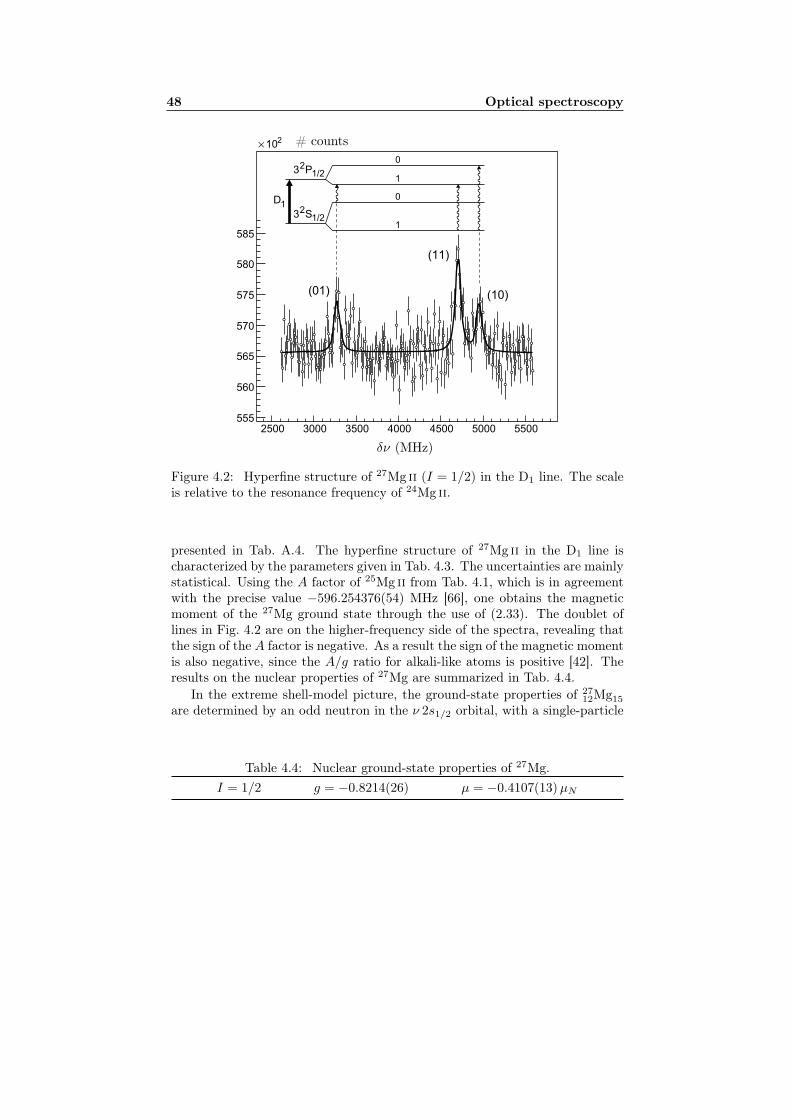
48 Optical spectroscopy
# counts
2500 3000 3500 4000 4500 5000 5500555
560
565
570
575
580
585
210×
(01)
(11)
(10)
1
0
1
0
3 S21/2
3 P21/2
D1
δν (MHz)
Figure 4.2: Hyperfine structure of 27Mg ii (I = 1/2) in the D1 line. The scaleis relative to the resonance frequency of 24Mg ii.
presented in Tab. A.4. The hyperfine structure of 27Mg ii in the D1 line ischaracterized by the parameters given in Tab. 4.3. The uncertainties are mainlystatistical. Using the A factor of 25Mg ii from Tab. 4.1, which is in agreementwith the precise value −596.254376(54) MHz [66], one obtains the magneticmoment of the 27Mg ground state through the use of (2.33). The doublet oflines in Fig. 4.2 are on the higher-frequency side of the spectra, revealing thatthe sign of the A factor is negative. As a result the sign of the magnetic momentis also negative, since the A/g ratio for alkali-like atoms is positive [42]. Theresults on the nuclear properties of 27Mg are summarized in Tab. 4.4.
In the extreme shell-model picture, the ground-state properties of 2712Mg15
are determined by an odd neutron in the ν 2s1/2 orbital, with a single-particle
Table 4.4: Nuclear ground-state properties of 27Mg.I = 1/2 g = −0.8214(26) µ = −0.4107(13)µN

4.2 Magnetic moment and hyperfine structure of 27Mg ii 49
µ(µN )
-1
-0.9
-0.8
-0.7
-0.6
-0.5
-0.4
25Ne 27Mg 29Si 31S 33Ar
Figure 4.3: Magnetic moments of the even-odd N = 15 isotones (I = 1/2).The solid line connects the experimental values. The uncertainties are smallerthan the dots. The dashed line follows the theoretical predictions. The exactvalues are given in Tab. 4.5.
magnetic moment µ(ν 2s1/2) = −1.91µN , according to (2.7). The experimentalspin and sign of the magnetic moment, given in Tab. 4.4, are consistent withthe suggested configuration. However, the magnitude of the magnetic momentis significantly smaller, indicating that the ground-state configuration is rathermixed, including a considerable contribution from the positive Schmidt valueorbitals ν 1d3/2, π 1d5/2, π 2s1/2 and π 1d3/2. The present result completesthe set of experimental magnetic moments of the even-odd N = 15 isotones(I = 1/2) from 25Ne to 33Ar [60, 67, 68]. Complex shell-model calculationsare carried out for the entire sequence in the sd model space with the code
Table 4.5: Experimental (µexp) and theoretical (µth) magnetic moments of theeven-odd N = 15 isotones (I = 1/2).
µexp(µN ) µth(µN )25Ne −1.0062(5) a −0.8527Mg −0.4107(13)b −0.4229Si −0.55529(3)c −0.5031S −0.48793(8)c −0.4033Ar −0.723(6) d −0.72
aFrom Ref. [67]; bTab. 4.4 - this work; cFrom Ref. [60]; dFrom Ref. [68];

50 Optical spectroscopy
Oxbash [69], using the USD Hamiltonian [70]. The results are presented inTab. 4.5 and in Fig. 4.3. The agreement theory-experiment is satisfactory inall cases. The increase in the magnitude of the 25Ne and 33Ar moments isdue to the fact that there are only two protons (proton holes) in the sd shell,leading to less mixed configurations and hence moments closer to the neutronSchmidt value for the ν 2s1/2 orbital (−1.91µN ). The experimental spin-parityassignments 1/2+ → 3/2+ → 5/2+ → 5/2+ corresponding to the states at0 → 984.66 → 1698 → 1940 keV [53] in 27Mg are in good agreement withthe calculations, predicting these levels at 0 → 895 → 1667 → 1978 keV.Experimentally the first negative-parity state in 27Mg is at 3559.5 keV [53],signifying that the pf shell plays a role in the energy spectrum close to 3 MeVand above. The results of this chapter will be discussed in Ref. [33].

Chapter 5
β-decay spectroscopy andnuclear magnetic resonance
The theoretical basis of laser spectroscopy is laid down in Chapter 3, withthe specific subject of nuclear polarization with optical pumping described inSection 3.8. Information on the topic of NMR lineshapes in the presence of afrequency modulation can be found in Section 2.6. This chapter is dedicatedto the β spectroscopy of the odd-mass 29,31,33Mg, concentrating the discussionmainly on the experimental results and their interpretation.
5.1 Magnetic moments of 29,31MgThe magnetic moments of 29,31Mg are essential quantities for the nuclear-structure understanding in the region of the Island of inversion. The caseof 31Mg is presented in a number of publication [15, 30, 31], which are includedat the end of this dissertation. Both cases are discussed in the PhD thesis ofM. Kowalska [16]. A reevaluation of the magnetic moments is performed here,after an offset in the frequency scale by one channel was recently discovered.The improvement of the results precision has no influence on the conclusionsin the above publications.
Polarized beams of 29,31Mg and 8Li were implanted into a MgO crystalduring a period of 82 hours and NMR measurements were performed. Typicalspectra can be found in Refs. [15, 16, 30, 31]. 8Li with its well-known magneticmomentA [71] is used to calibrate the magnetic field. The reevaluated Larmorfrequencies are presented in Tab. 5.1. A source of systematic uncertainty is
A Ref. [71] provides the ratio: ν(8Li)/ν(1H) = 0.1480045(21), which combined withthe proton magnetic moment µ(1H) = 2.792847337(29) µN from [35] yields µ(8Li) =1.653547(29) µN . Diamagnetic corrections are taken into account according to Ref. [60].

52 β-decay spectroscopy and nuclear magnetic resonance
Table 5.1: NMR frequencies of 8Li and 29,31Mg (weighted mean of the indi-vidual measurements for each isotope).
8Li 29Mg 31Mg
ν (kHz) 1806.940(12) 1423.98(86) 3859.624(42)
the possible magnetic-field drift over the time period mention above. Theelectric current through the poles of the magnet was monitored with a high-precision voltmeter measuring the tension over a calibrated resistance. Thedifference between the minimum and maximum voltage recorded during themeasurements over the average voltage yields a relative error ∆U/U = 5.5 ×10⁻⁵. Another source of systematic uncertainty is the inhomogeneity of themagnetic field within the area of implantation. If considerable, this effect wouldresult in a change in the Lorentzian NMR lineshape. The resonances of 31Mgand 8Li are of high quality (Fig. 5.1, [30]) allowing lineshape analysis. Thelatter showed that there is no detectable Gaussian component in the spectra,making a strong argument that the effect of the inhomogeneity is much smallerthan the width of the resonances. The drift on the other hand, which is withinthe relative error of 5.5×10⁻⁵, is a significant fraction of the FWHM (as much as15% compared to the narrowest resonances), making it the dominant source ofsystematic uncertainty in the NMR measurements. The final results for 29,31Mgare presented in Tab. 5.2. The error in the square brackets is the systematicuncertainty, which is comparable with the statistical error only for the high-precision moment of 31Mg and negligible in the case of 29Mg. The matter offinding the total probability density distribution rising from the statistical andsystematic uncertainties is extensively discussed in Appendix A.1. Tab. A.1contains confidence levels associated with a total error on the 31Mg magneticmoment of up to 5 × 10⁻⁵ µN . The spin-parity assignments to the groundstates of 29,31Mg are presented in Tab. 5.2. These are based on the β-decaywork from Refs. [19, 20, 72], in the case of 29Mg, and hyperfine structure andnuclear magnetic resonance measurements on both isotopes [16], which confirm
Table 5.2: Nuclear ground-state properties of 29,31Mg.29Mg 31Mg
Iπ 3/2+ 1/2+
g 0.6520(4) −1.76710(3)[10]µ (µN ) 0.9779(6) −0.88355(2)[5]

5.2 31Mg: transition to the Island of inversion 53
the spin of 29Mg and establish spin 1/2 for the ground state of 31Mg. The caseof 31Mg is extensively discussed in the publications attached at the end ofthis dissertation [15, 30, 31]. Typical HFS and NMR spectra are presented inFig. 5.1.
5.2 31Mg: transition to the Island of inversion
While the neutron rich Mg isotopes up to 30Mg are well understood in theirground states within the sd shell modelA, 31Mg is the first one in the chainwith ground-state properties incompatible with that description. Having fourprotons and eleven neutrons above the core of 16O, 31Mg was originally ex-pected to have a ground-state configuration according to the subsequent fillingof the orbitals forming the sd shell - ν 1d5/2, ν 2s1/2 and ν 1d3/2. In this pic-ture the ground-state is largely determined by the odd neutron in the ν d3/2
orbital, demanding spin and parity Iπ = 3/2+ and a single-particle magneticmoment close to the Schmidt value µ = 1.15µN . Contrary to this conceptthe experimental spin is I = 1/2 [15]B . Moreover, the magnetic moment hasthe opposite sign (see Tab. 5.2). The spherical shell model could account forsuch behavior only by promoting two neutrons to the pf shell. Large-scaleshell-model calculations described in Ref. [15] show that the lowest 2p-2h con-figuration does indeed have the correct spin and magnetic moment close tothe experimental value, making a strong argument that the ground state of31Mg is a pure intruder state. Under this description the largest fraction ofthe wave function involves a single neutron on the ν s1/2 orbital with Schmidtvalue µ = −1.91µN , which gives a simplified explanation of why the spin is1/2 and the magnetic moment is negative. However, the magnitude of themagnetic moment can only be understood within the full calculations, sincethe wave function is rather mixed being considerably influenced also by thepositive single-particle g factor of the ν d3/2 orbital. Another qualitative pic-ture comes from the fact that the calculated g factor of the 1/2+ state in 29Mgwith the USDB interaction (Tab. 5.10) is very close to the experimental valuefor the 31Mg ground state (Tab. 5.2), giving an indication that the two neu-trons in the pf shell are mostly coupled to zero angular momentum and it ismainly the proton-neutron arrangement within the sd shell that determinesthe ground-state properties of 31Mg. The fact that in the calculations pre-sented in [15] the 2p-2h states are higher in energy than the 0p-0h and 1p-1hconfigurations is directly related to the size of the N = 20 shell gap, whichappears to be strongly reduced for the Mg isotopes. In the Nilsson model pic-
A The cases of 27,29Mg are developed in Sections 4.2 and 5.5, respectively. These will bethe main subjects of Ref. [33]. 29Mg is extensively described in Ref. [16]. 30Mg is placedoutside the Island of inversion according to Ref. [73].
B Included at the end of this dissertation.

54 β-decay spectroscopy and nuclear magnetic resonance
A×102 NMR A×102
A×102
ν (MHz)
-3
-2
-1
0
1
A(g) ( +1/2)I
3 S21/2
3 P23/2
F=1
F=0
F=2
F=1
0
1
2
3
4
5
6
λ y 280nm
-3000 -2000 -1000 0 1000 2000 3000
σ -
σ+
3.84 3.86 3.88
0
2
4
6
δν (MHz)
Figure 5.1: HFS of 31Mg ii in the D2 line and NMR in the strongest transition.Notice that the labels σ± are inverted compared to those in Refs. [15, 16, 31],where they are wrongly assigned.
ture the ground state of 31Mg is associated with a large prolate deformationbased on the 1/2 [200] orbital. The odd-neutron occupation is represented bythe segment (a) in Fig. 5.4.
The complete resemblance of the experimental spectra of 31Mg in Fig. 5.1with the theoretical simulations in Fig. 3.12 proves that the β-asymmetry pa-

5.3 Spin and magnetic moment of 33Mg 55
rameter of 31Mg is negative. This conclusion is based on the fact that thetheoretical procedure described in Section 3.8 yields the nuclear polarization,which in turn must be multiplied by the β-asymmetry parameter Aβ to obtainthe observable experimental β asymmetry (2.63). The simulated spectra aredrawn under the condition Aβ = −1, thus proving that the polarization mustbe inverted in order to reproduce the experimental spectra. From the measuredbranching ratios for populating excited states in 31Al via the β decay of 31Mg[54], using the rules in Tab. 2.1 one calculates Aβ = −23 % , which is consis-tent with the considerations above. However, the latter calculation stronglydepends on the spin assignments to the states in 31Al, which are partly estab-lished through a comparison with shell-model calculations.
31Mg is the first isotope in the chain with an intruder ground state. Thestrong impact on the nuclear structure understanding in the vicinity of theIsland of inversion, drawn from data of exceptional quality, highlights 31Mg asone of the emblematic cases in the region.
5.3 Spin and magnetic moment of 33Mg
The central results of the present doctoral dissertation, namely the spin andmagnetic moment of 33Mg, are discussed in this section. The following textcontains a description of the analysis procedures and an interpretation of theresults, consistent with all available studies of this nucleus. An alternativediscussion is presented in a publication in preparation [32] the full text ofwhich is included at the end of this thesis.
Inside the Island of inversion different particle-hole excitations coexist atlow energies, making it difficult to predict which configuration will become theground state. This information needs to be obtained experimentally. A β-decaystudy of 33Na [25] suggests a 1p-1h configuration for the 33Mg ground state withspin and parity Iπ = 3/2+ in contrast to Iπ = 5/2+ (also 1p-1h) from inter-mediate energy Coulomb excitation [26] and proton inelastic scattering [27]experiments. The systematics of the nuclear moments in the region [28], onthe other hand, is consistent with 2p-2h ground states. Theoretical and experi-mental studies of the neighboring even-even Mg isotopes [9, 10, 21, 24] supportthis observation. The above discrepancy in the ground-state spin assignmentof 33Mg and the diminishing predictive power of the shell model in the Islandof inversion serve as a primary motivation for the experimental investigationsdescribed below.
The experimental studies are realized in the D2 line (279.635(78) nm for Mg[56]), which involves the transitions from 32S1/2 to 32P3/2 hyperfine multiplets,shown in Figs. 5.2 (a) and (e). The experimental spectra of 33Mg ii, obtainedwith σ∓ laser polarization are displayed in Figs. 5.2 (b) and (c), respectively.The frequency scale is given relative to the fine-structure splitting of the refer-

56 β-decay spectroscopy and nuclear magnetic resonance
A×102
A×102
A×102
0 500 1000 1500 2000 2500 3000
0
2
4
6
δν33, 31
-A .I/2+εA . (I+1)/2+εΔE = |A| . (I+1/2)
33HFS Mg II
31HFS Mg II
(12) (11)
σ -
σ+
σ -
(a)
(b)
(c)
(d)
NMR
0
1
2
0
-1
-2
10
2
1
3 S21/2
2
3
3 P23/2
ν33
λ ≈ 280 nm
ΔE
εáΔE
F
1
0
2
1
3 S21/2
3 P23/2
ν31
(e) F
δν (MHz)
Figure 5.2: (a) Principle hyperfine structure in the D2 line for I = 3/2 and A <0; (b), (c) Realistic fits of the β-asymmetry spectra of σ∓ polarized 33Mg ii afterimplantation into MgO; (d) β-asymmetry spectrum of σ− polarized 31Mg ii inD2 implanted into MgO; (e) HFS scheme corresponding to (d);

5.3 Spin and magnetic moment of 33Mg 57
A×102
1074 1078 1082 1086 1090
0
-0.1
-0.2
-0.3
-0.4
0.1
0.2
0.3
ν (MHz)
Figure 5.3: NMR spectrum of 33Mg in MgO (zoom of Fig. A.3 (b)).
ence 31Mg ii (I = 1/2) [15]. The distance between the two groups of resonancesin 33Mg ii is determined by the splitting ∆E in the 32S1/2 multiplet. This directobservable is a function of the nuclear spin and the magnetic dipole hyperfineparameter: ∆E = |A| (I + 1/2). Neglecting the hyperfine anomaly, the ratioA/g, where g is the nuclear g factor, is constant for all the isotopes in the chain.This ratio can be calculated from the experimental A and g available for thestable 25Mg ii (I = 5/2) [64, 66]. A g-factor measurement is therefore sufficientto extract the hyperfine parameter of 33Mg ii and unambiguously determine thenuclear spin from the measured hyperfine splitting. Magnetic resonance mea-surements are carried out with σ− laser polarization in the higher frequencytriplet of transitions, as indicated in Fig. 5.2 (b), after implantation in thecubic crystal lattice of MgO (fcc)A or Pt (ccp)B . The produced experimentalasymmetry is ≈ 2 %. A radio-frequency field of a few tenths of a mT is ap-plied perpendicular to the static magnetic field B ≈ 0.3 T. An example NMRspectrum of 33Mg in MgO obtained with a small circular frequency modulationwith an amplitude of 1 kHz is presented in Fig. 5.3. The total statistics includesspectra of similar quality in Pt. All independent measurements are presented
A fcc - face centered cubic.B ccp - cubic close packed.

58 β-decay spectroscopy and nuclear magnetic resonance
Table 5.3: NMR frequencies of 33Mg in Pt and MgO, corresponding to themagnetic field during the reference measurements from Tab. 5.7, and the g-factor ratio g(33Mg)/g(31Mg) = ν(33Mg)/ν(31Mg).
Pt MgO
ν(33Mg) (kHz) 1084.22(76) 1082.41(42)g(33Mg)/g(31Mg) 0.28159(20) 0.28121(11)
in Appendix A.2 together with detailed information on the analysis procedure.The reference probe 31Mg [15] was implanted in both hosts in order to extractthe ratio of the Larmor frequencies (2.54), which is independent of the chemicaland Knight shifts. The results are presented in Tab. 5.3, which contains twoindependent values of the ratio g(33Mg)/g(31Mg). Their weighted mean is usedto calculate the g factor of 33Mg based on the reference 31Mg (Tab. 5.2). Theg factor in combination with the hyperfine splitting determines nuclear spinI = 3/2. The ground-state properties of 33Mg are summarized in Tab. 5.4.Since the systematic uncertainty is significantly smaller than the statistical er-ror, the total error is formed as the sum of the two, yielding the final result|µ| = 0.7456(5)µN . The confidence level associated with the latter uncertaintyis ≈ 76 %, as presented in Tab. A.2.
The experimental HFS spectra in Figs. 5.2 (b) and (c) are fitted with thetheoretical polarization function, described in Section 3.8. The actual fittinghas the main purpose of demonstrating the consistency between theory andexperiment. Due to the low resolution and power broadening, the nuclear qua-drupole moment and β-asymmetry parameter can not be extracted. However,there are important conclusions to be drawn from the realistic polarizationfunction, namely the negative signs of the magnetic hyperfine parameter andthe β-asymmetry parameter. The latter is perhaps easier to comprehend bycomparing the experimental with the simulated spectra in Fig. 3.14 (A < 0,Aβ < 0). A change in the sign of A would invert left and right and a signchange of Aβ inverts up and down.
There is an independent way to confirm the negative sign of the hyperfineparameter. With the use of the total mass shift from Ref. [16] one estimates theisotope shift δν33,31 = 1867 MHz. The uncertainty on this number, including
Table 5.4: Nuclear ground-state properties of 33Mg.I = 3/2 g = −0.4971(3)[1] µ = −0.7456(4)[1]µN

5.3 Spin and magnetic moment of 33Mg 59
Table 5.5: Gyromagnetic ratios and quadrupole moments of different particle-hole excitations in 33Mg (I = 3/2), calculated with the interactions WBMB [3]and SD - PF [74]. Free-nucleon g factors and effective charges eπ = 1.5e andeν = 0.5e are used.
WBMB SD - PF
n ~ω Iπ gfree Q (mb) gfree Q (mb)
0 3/2− −1.47 −83 −1.35 −911 3/2+ 0.75 135 0.78 1402 3/2− −0.45a 147b −0.47a 157b
aExperimental gyromagnetic ratio from this work g = −0.4971(3)[1] (see Tab. 5.4).bQ(βC) = 151(38) mb, calculated from βC (see the text).
the errors on the mass shift and an unknown change between the mean-squarecharge radii, is estimated to be smaller than 50 MHz, which can be neglectedfor the considerations below. Based on the isotope shift one can plot thefine-structure splitting of 33Mg ii relative to the transitions of the hyperfinestructure, the so-called “ center of gravity ”. The latter is represented by thealternating dash-dot line in Fig. 5.2. Closer to the center of gravity are alwaysthe transitions starting from the higher angular momentum state F = I +1/2, which can be verified with the aid of (2.31). In the case of 33Mg ii theirresonances appear at the higher frequency side of the spectra, revealing thatthey start from the lower energy level. The higher angular momentum states arelower in energy only for a negative magnetic hyperfine parameter (2.31). Sincethe ratio A/g is positive for all alkali-like atoms [42], the ground-state nuclearmagnetic moment of 33Mg is negative. The sign of the A factor is demonstratedin Fig. 5.2, where the relative energies of the hyperfine-structure levels in 32S1/2
are represented by the vectors A(I+1)/2+ε < 0 and −AI/2+ε > 0 (|ε| |A|).Their direction towards the frequency axis demands A < 0.
The ground-state of 3312Mg21 is suggested in Ref. [25] to have a 1p-1h intruder
configuration, with spin and parity Iπ = 3/2+. In the extreme shell-modelpicture the properties of such a state are determined by an odd neutron in theν 1d3/2 orbital with a positive single-particle magnetic moment (2.7). In orderto explain the negative sign of µ, an odd number of neutrons must occupy thepf shell, as these have negative Schmidt values for the orbitals ν 1f7/2 andν 2p3/2. The parity of such states is negative, thus providing evidence for anegative ground-state parity of 33Mg. Large-scale shell-model calculations arecarried out in the sd−pf model space with the code Oxbash [69], using theHamiltonians [3, 74] designed particularly to describe the Island of inversion.Mixing of states with a different number of particle-hole excitations (~ω) isnot considered. The neutron configuration space is reduced to ν (sd−1f7/2−

60 β-decay spectroscopy and nuclear magnetic resonance
Table 5.6: Energy levels of 33Mg, calculated with the interactions WBMB[3] and SD - PF [74]. The configuration denoted with 〈?〉 is identified as theground state (see Tab. 5.5).
n ~ω Iπ EWBMBa (keV) E SD− PF
a (keV)
0 1/2− 241711 449012
0 3/2− 7373 237410
0 5/2− 18949 428411
0 7/2− 01 17106
1 1/2+ 208210 19218
1 3/2+ 3992 2832
1 5/2+ 12385 11875
1 7/2+ 15548 17387
2 1/2− 323212 22989
? 2 3/2− 10654 01 ?2 5/2− 13276 4033
2 7/2− 14817 6814
aThe top energy index denotes the level ordering.
2p3/2). Two out of four valence protons are fixed in the π 1d5/2 orbital. Theother two are confined within the sd shell. Calculated nuclear moments of 0,1 and 2 ~ω excitations for I = 3/2 are presented in Tab. 5.5. Clearly, theexperimental g factor is only consistent with the 2p-2h configuration. Thegood agreement between the experimental and theoretical magnetic moments,demonstrated in Tab. 5.5, indicates that the ground state of 33Mg is a nearlypure 2p-2h intruder. Indeed, the 2p-2h 3/2− level is the lowest in the calculationwith the SD - PF Hamoltonian from Ref. [74], as shown in Tab. 5.6. Thetheoretical calculations presented Tabs. 5.5 and 5.6 demonstrate an importantfact. While the excitation energies of corresponding states computed with thetwo Hamiltonians are very different from each other, their nuclear momentsare rather consistent, highlighting the relevance of comparing experimentalmoments with theory.
The charge and matter deformations of 33Mg are experimentally determinedto be βC = 0.52(12) [26] and βM = 0.47(8) [27], which appear to be consistentwith the deformation parameters of the neighboring even-even 32,34Mg [10, 21,23, 24]. One can use βC to evaluate the spectroscopic quadrupole moment of33Mg through (2.16), (2.17) and (2.22) for I = K = 3/2. Hence, under theassumption of an axial symmetry the result is Q = 151(38) mb. This valueis in agreement with the established 2p-2h configuration, as demonstrated inTab. 5.5.
In the frame of the Nilsson model the established spin and parity of 33Mg

5.3 Spin and magnetic moment of 33Mg 61
esp (MeV)
-0.2 -0.1 0.0 0.1 0.2 0.3 0.4 0.5 0.6
-12
-8
-4
0
20
81d5/2
2s 1/2
1d3/2
1f 7/2
2p3/2
5/2[202]
3/2[211]
1/2[220]
1/2[211]
1/2[200]3/2[202] 1/2[330]
3/2[321]
5/2[312]
7/2[303]3/2[312]
1/2[321]
1/2[440]
(b)
(a)
β2
Figure 5.4: Nilsson diagram in the ν (sd−1f7/2−2p3/2) configuration space.The segments (a) and (b) represent the odd neutron occupation in the groundstates of 31,33Mg, respectively.
(Iπ = 3/2−) are consistent with a large prolate deformation and ground-stateproperties determined by a single-particle occupation of the 3/2 [321] orbital- the segment (b) in Fig. 5.4. This range is consistent with the deformationof 31Mg, as suggested in Ref. [15], represented in Fig. 5.4 by the segment (a)of the 1/2 [200] orbital. It is relevant to support these findings by comparingthe experimental magnetic moments with calculated values from the Nilssonmodel. This requires a knowledge on the composition of the Nilsson wavefunctions. Since the configuration mixing coefficients are not available onecan roughly estimate which spherical states contribute the most by looking atFig. 5.4. Thus, large fractions of ν f7/2 and ν p3/2 are expected into the single-particle wave function of the odd neutron in 33Mg and therefore a single-particleg factor (2.21) in between the corresponding Schmidt values (divided by j)A.With the use of (2.19) one calculates the expectation boundaries for the nuclearmagnetic moment of 33Mg to be −0.27 ≤ µ(33Mg)/µN ≤ −0.93. Although thisestimate is very rough, it correctly reproduces the sign and the magnitude of themagnetic moment (Tab. 5.4), thus independently supporting the establishmentof the nuclear deformation according to the segment (b) of the 3/2 [321] orbital.In the case of 31Mg, with I = 1/2, the magnetic moment depends additionally
A The single-particle g factors are obtained by dividing the Schmidt values (2.7) to thetotal angular momentum quantum number j of the spherical state.

62 β-decay spectroscopy and nuclear magnetic resonance
on the magnetic decoupling parameter b [2] (2.20). Taking into account thecontribution of ν s1/2 and ν d3/2 to the prolate side of the 1/2 [200] orbital,one calculates the boundaries for the magnetic moment of 31Mg to be −1.7 ≤µ(31Mg)/µN ≤ −0.17, being consistent with the experimental value in Tab. 5.2.
The results from studying the β-decay of 33Na, as described in Ref. [25],are summarized in Fig. 5.5. The obtained branching fractions with the corre-sponding log ft values, as well as tentative spin-parity assignments based onlarge-scale shell-model calculations are presented next to the level scheme. Theexistence of the 159 keV level appears to be an unsettled feature of the scheme.This state is suggested to be an isomer, since its decay to the ground state hasnot been observed within a β-γ coincidence window of 500 ns.
The conclusions from the β-decay work have not been supported by Cou-lomb excitation [26] and proton inelastic scattering [27] experiments. The lat-ter two studies consistently provide evidence that the parity of the 484 keVlevel is identical to the parity of the ground state. This level is suggestedin Ref. [26] to be a rotational excitation, thus having one unit of angularmomentum higher than the ground state and a similar intrinsic structure.Since the 546 keV gamma has only been detected in the neutron knockoutreaction 1H(34Mg, 33Mg γ) and not in the proton inelastic scattering process1H(33Mg, 33Mg γ), described in Ref. [27], it is concluded that this transitionoriginates from a state with a parity opposite to the parity of the ground state.These experimental facts contradict with Ref. [25] (Fig. 5.5). In the context ofthe firm spin-parity assignment to the ground state Iπ = 3/2− established inthe present work, the experimental results from Refs. [25–27] allow to proposea modified level scheme, as presented in Fig. 5.6 (see the text below). In orderto have an isomeric state at 159 keV, with a lifetime longer than 500 ns, anangular momentum of at least two units larger than the one of the groundstate is required, demanding a spin assignment I = (7/2). If the 484 keV level
705
546
221
484
759
1243
484
1590
705
1243
1p1h0p0h Δ 2p2h
2p2h1p1h
1p1h
(7/2 )-
(5/2)+
5.27(26)
>6.65.20(22)
5.97(25)
log ft
(3/2)-
(3/2)+20(10)
<1.215.9(62)
2.9(12)
Iβ (%)
(1/2 )+
Figure 5.5: 33Mg level scheme, established in the β decay of 33Na, with ten-tative spin-parity assignments according to Ref. [25]. The 159 keV level is notexperimentally observed.

5.3 Spin and magnetic moment of 33Mg 63
484
0
705
1243
546(5/2)-
3/2-
(3/2+)
(5/2+)
(1/2)+
7/2-
>6.6
5.77(16)
5.97(25)
log ft
<1.2
7.0(26)
2.9(12)
Iβ (%)
5.69(16)8.8(33)
Figure 5.6: Modified decay scheme of 33Mg with suggested spin-parity assign-ments, based on the firm assignments to the ground state.
has one unit higher angular momentum than the ground state and the sameparity, resulting in spin-parity assignment Iπ = (5/2)−, the transition to theisomeric state should also be observed, since it would have the same multipo-larity (L = 1) as the transition to the ground state. It is therefore more likelythat the 546 keV gamma is associated with a state at that energy, not a decayto an isomeric state. The branching fractions to the 705 keV and 546 keV levels,presented in Fig. 5.6, are recalculated, based on the γ intensities from Ref. [25].The error on the log ft values to these states includes the uncertainties on thebranching ratios and the half-life of 33Na. The uncertainty on the electronskinetic energy is not taken into account. The large feeding to the ground stateof 33Mg suggested in Ref. [25] (Fig. 5.5) is unlikely, considering a first forbiddenβ transition. Here 33Na is regarded as having 3/2+ or 5/2+, either 0p-0h or2p-2h ground state, based on analogy with 31Na (Iπ = 3/2+ [6]) and shell-model calculations [25]. An indirect confirmation of this assertion comes fromthe fact that the 484 keV level, which has a negative parity, is weakly fed inthe β decay.
The most likely interpretation of the available experimental evidence isthat the observed excited states in 33Mg rise from two rotational bands -one based on a single-particle state with Kπ = 3/2− (3/2 [321]) and an-other with Kπ = 1/2+ (1/2 [200]). This interpretation would explain thespin change between 31Mg (Iπ = 1/2+) and 33Mg (Iπ = 3/2−) with a rel-ative movement of the two bands when adding two neutrons. In the case ofKπ = 3/2−, with the use of (2.18), one can calculate the moment of inertiaand consequently the energy of the next member of the band. The result isEK=3/2(I = 7/2) = 1162 keV. In the case of Kπ = 1/2+, using the theoreti-cal value for the decoupling parameter aβ=0.4 = −0.615 from Ref. [2] (vol. 2,
64 β-decay spectroscopy and nuclear magnetic resonance
p. 290), one calculates EK=1/2(I = 5/2) = 1271 keV. In both cases the com-puted energies are close to the experimental level at 1243 keV, as it is demon-strated in Fig. 5.6, where the calculated energies are represented by the dashedlines. Since the log ft value associated with the 1243 keV level is relativelylow, one tends to assign this state to the band with Kπ = 1/2+. However,belonging to the other band is not completely excluded. The tentative spin-parity assignments in Fig. 5.6, proposed according to this interpretation, areconsistent with the recalculated log ft values.
Recent results on the β decay of 33Mg are presented in Ref. [75]. Theground-state spin and parity of the daughter 33Al are known to be Iπ = 5/2+
(mostly 0p-0h configuration), derived through a comparison of shell-model cal-culations with a g factor measurement [17]. Inelastic nuclear scattering [76]further suggests spin parity-assignment Iπ = 5/2+ (2p-2h configuration) tothe observed excited state at 730(50) keV. In the β decay of 33Mg no feeding tostates below 1.6 MeV has been detected, which is consistent with the conclu-sions of the latter two studies since the 5/2+ levels would be populated fromthe 3/2− ground state of 33Mg with first forbidden β transitions. The nuclearstructure of the excited states in 33Al above 1.6 MeV is unknown. The largefeeding to these levels needs to be understood in the context of the presentwork.
5.4 Solid-state aspects of NMR
NMR measurements of 33Mg were performed in two cubic crystals - Pt (ccp)and the MgO (fcc). The magnetic field in both hosts was calibrated by theNMR resonances of 31Mg, yielding the Knight shift of Mg in Pt. The Knightshift was calculated from the frequencies, given in Tab. 5.7, by solving thesystem: ∣∣∣∣ h νMgO = g µN B0 (1− σ12)
h νPt = g µN B0 (1− σ10 +K) , (5.1)
where g and B0 represent the nuclear g factor and the external magnetic fieldand σ12 and σ10 account for the diamagnetic shielding of the localized elec-trons in the two hosts. Since the valence electrons in a metal are no longer
Table 5.7: NMR frequencies of 31Mg in Pt and MgO crystals and the Knightshift of Mg in Pt.
νPt (kHz) νMgO (kHz) K
3850.40(16) 3849.05(20) 3.4(7)× 10−4

5.4 Solid-state aspects of NMR 65
Pt
A
a)
0 0.02 0.04 0.06 0.08 0.1 0.12 0.14
-210
t (s)
MgO
A
b)
0 0.1 0.2 0.3 0.4 0.5-210
-110
t (s)
Figure 5.7: Relaxation times of 31Mg in Pt and MgO at room temperature.
localized they will only contribute to the Knight shift. Theoretical values forthe shielding factors σ12 and σ10 are given in Refs. [60, 77]. The temperaturedependence of the spin-lattice relaxation (SLR) time T1 in metals is given by:
T1 T =~
K2g2(me/mp)2k π, (5.2)
known as the Korringa relation [78]. The constant factor on the right sideis determined by the nuclear g factor and the Knight shift. Example spectraof 31Mg relaxation in Pt and MgO crystals are shown in Fig. 5.7 and the re-sults of both sets of measurements are presented in Tab. 5.8. With the use of

66 β-decay spectroscopy and nuclear magnetic resonance
Table 5.8: Relaxation times of 31Mg in Pt and MgO at room temperature andexternal magnetic field B = 0.28596(3) T.
Pt MgO
T1 (ms) 80(8) 395(63) T = 293(5) K
T1 T (Ks) 23.4(23) 116(9)
(5.2) and the experimental g and K from Tab. 5.2 and Tab. 5.7 one calculatesT1 = 80(32) ms. This value is in agreement with the direct determination of theasymmetry decay constant in Pt at room temperature, presented in Tab. 5.8.The quantity T1 T g
2, according to (5.2), should be isotope independent, as longas the Knight shift is isotope independent. However, measurements of the SLRof 23Mg in Pt, reported in Ref. [79], established T1 T g
2(23Mg) = 213(18) Ks,to be compared with the present result T1 T g
2(31Mg) = 73(7) Ks. The latterdifference can not be attributed to a field dependence of T1 since the measure-ments performed at 0.27 T and 0.4 T, described in Ref. [79], are consistent.Another possibility is a different orientation of the host crystal in respect tothe external field in the two experiments (see Ref. [48]). The above discrepancyis not understood until now.
5.5 Quadrupole moment of 29Mg
The level scheme of 29Mg is established in the β-decay of 29Na [19, 20, 80].The ground-state spin-parity assignment Iπ = 3/2+ [19, 20, 72] is based onexperimental branching fractions to known states in 29Al. The hyperfine struc-ture and nuclear magnetic resonance measurements on 29Mg ii, described inRefs. [16], determine the nuclear magnetic moment and independently confirmthe spin. The sign of the magnetic moment, as in the cases of 31,33Mg, is anexperimental fact based on the hyperfine structure. The results are summa-rized in Tab. 5.2. The possibilities for extracting additional information fromthe hyperfine structure, namely the quadrupole moment and ground-state de-formation, are discussed in this section. The experimental spectra of 29Mg ii inthe D2 line strongly resemble the theoretical curves plotted in Fig. 3.10. Theβ-asymmetry parameter Aβ = 15 %, substituted in the simulations, is calcu-lated from the branching fractions in Ref. [53] with the use of Tab. 2.1. Theexperimental β asymmetry in Fig. 5.8 is a factor of two smaller than the pre-diction from the theoretical function. The major reason is perhaps the longhalf-life τ1/2 = 1.30(12) s [19, 20, 81], comparable with the relaxation timeT1(29Mg) = 0.59(23) s in MgO at room temperature, calculated with use of

5.5 Quadrupole moment of 29Mg 67
Table 5.9: Quadrupole hyperfine parameter of 29Mg ii in 32S3/2, obtained withthe use of the realistic polarization function (R) and Lorentz profiles (L), withthe corresponding quadrupole moments and deformation parameters.
K = 1/2 K = 3/2
B (MHz) Q (mb) Q0 (mb) β Q0 (mb) β
R −23.2(22) −195(20) 975(100) 0.58(6) −975(100) −0.73(9)L −15.1(19) −126(17) 630(85) 0.39(5) −630(85) −0.45(7)
(5.2). The cluster of the lower energy transitions with σ+ laser polarizationgives the highest experimental asymmetry and relative amplitudes suitable forextraction of the hyperfine parameters of the excited state. The positions of thethree lines (two energy gaps) completely determine the A and B factors. Thisis one of the experimental evidence for the positive sign of the A factor andconsequently the positive magnetic moment. The independent experimentalspectra are fitted with the realistic polarization function from Appendix B.3and using the natural lineshape (3.48). The two fit functions can be comparedin Figs. 5.8 (a) and (b). The value of A is obtained independently through therelation (2.33) and substituted as a constant parameter. At low laser power thetransition F : 2 → 2 is the strongest (Fig. 3.10). The fact that experimentally itis weaker than the transition F : 2 → 3 is evident for oversaturation and simul-taneous optical pumping in the neighboring transitions. These effects are alsocausing the broadening and change in the lineshape of the middle resonance.While the theoretical curve reproduces well these experimental features it failsto account precisely for the relative asymmetry in the transition F : 2 → 1. Thefit function in Fig. 5.8 (b) is a sum of three Lorentzian profiles with amplitudesset as free parameters. This simple approach is unable to account for pumpingin multiple transitions. Thus, the Lorentzian profiles become too broad andthe transitions in the fit function less resolved than they are experimentally. Asa result both fitting procedures converge to a similar χ2. The obtained valuesfor the B parameter are given in Tab. 5.9. The large discrepancy in the twonumbers signifies the importance of the line profiles for the analysis of opticaland polarization spectra. It will be postulated here that the difference in theobtained B factors is a measure for the systematical uncertainty associatedwith the choice of the fitting function. Thus, with the use of (2.34) and thequadrupole moment of 25Mg from Ref. [82], one calculates an expectation rangefor the spectroscopic quadrupole moment Q ∼
(−195(20) mb , −126(17) mb
).
Such an inaccurate estimate is expected to have a minor impact on the un-derstanding of the nuclear structure of 29Mg. However, one can state withconfidence that the sign of the quadrupole moment is negative as well as quan-titatively estimate the nuclear deformation, using relations (2.22) and (2.16).

68 β-decay spectroscopy and nuclear magnetic resonance
A×102
a)
-1200 -1100 -1000 -900 -800 -700 -600 -500 -400-0.5
0
0.5
1.0
1.5
2.0(23)
(22)
(21)
δν (MHz)
A×102
b)
-1200 -1100 -1000 -900 -800 -700 -600 -500 -400-0.5
0
0.5
1.0
1.5
2.0(23)(22)
(21)
δν (MHz)
Figure 5.8: The cluster of lower energy transitions within the hyperfine struc-ture of 29Mg ii (I = 3/2, A > 0) in the D2 line fitted with: (a) The realisticpolarization function from Appendix B.3; (b) Lorentzian profiles;
The results are presented in Tab. 5.9.In the particle plus rotor model the ground state of 29Mg, with spin and
parity Iπ = 3/2+, is built on a single-particle state, based either in the 3/2 [202]or 1/2 [200] Nilsson orbitals (Fig. 5.4). The second option requires a decoupling

5.5 Quadrupole moment of 29Mg 69
Table 5.10: Gyromagnetic ratios and quadrupole moments of the two loweststates in 29Mg, calculated with the interactions USD [70] and USDB [83]. Free-nucleon g factors and effective charges eπ = 1.5e and eν = 0.5e are used.
USD USDB
Iπ E (keV) gfree Q (mb) E (keV) gfree Q (mb)
1/2+ 0 −2 45 −1.653/2+ 40 0.64a −109b 0 0.71a −110b
aExperimental gyromagnetic ratio from this work g = 0.6520(4) (see Tab. 5.2).bQ ∼
`− 195(20) mb , −126(17) mb
´(see the text).
parameter a < −1 in order to invert the energies of the first two membersof the rotational band and have the 3/2+ state as the ground state. Evenprecisely known, the spectroscopic quadrupole moment is not associated witha particular intrinsic deformation. This is clearly demonstrated in Tab. 5.9,where under the assumption of different K one arrives with either positiveor negative β. The study presented in Ref. [72] suggest prolate ground-statedeformation. Under this condition the two lowest levels in 29Mg, according tothe estimates in Tab. 5.9 for K = 1/2, are associated with deformation similarto the one of 31Mg. This supports the earlier argument that similar magneticmoments are to be expected for the first excited state in 29Mg and the groundstate of 31Mg.
Shell-model calculations are carried out in the sd model space with the codeOxbash [69], using the Hamiltonians USD [70] and USDB [83]. The results forthe two lowest levels in 29Mg are presented in Tab. 5.10. The USD interactiongenerates a g factor closer to the experimental value (Tab. 5.2), but fails toaccount for the inversion of the two states. The USDB interaction is successfulin predicting the correct level ordering. It also suggests a g factor for the1/2+ level close to the experimental value of the ground state in 31Mg. Therea is strong experimental evidence that negative parity states occur in 29Mgalready close to 1 MeV [84, 85]. This is an indication that the orbitals of thepf shell play a role in the low-energy spectrum of 29Mg. However, the magneticmoment is well reproduced within the sd shell, meaning that the presence of2p-2h excitations in the ground-state wave function can be neglected. The signof the theoretical quadrupole moment is negative, being consistent with theconsiderations above.

70 β-decay spectroscopy and nuclear magnetic resonance

Chapter 6
Conclusions and outlook
Tab. 6.1 summarizes the experimental results presented in this dissertation.The magnetic moments of 27,33Mg and the spin of 33Mg are reported for the firsttime, completing a sequence of ground-state studies of neutron rich Mg isotopestowards the Island of inversion. Thus, laser spectroscopy in combination withnuclear magnetic resonance provide valuable probes for the development of thetheoretical models in this region. The spin-parity assignments to the groundstates of 27,29Mg are confirmed and no influence from the orbitals of the pf shellin their wave functions is found. However, particle-hole excitations do play arole in the energy spectra of these two isotopes, since negative-parity statesare found around 3 and 1 MeV, respectively [53, 84, 85]. Coulomb excitationstudies [10, 73] appear to be consistent with the sd shell-model description of30Mg. The transition to the Island of inversion therefore occurs at 31Mg, whichwas found to have a nearly pure 2p-2h intruder ground state [15]. The spin andmagnetic moment of 33Mg are the key results of this work, determining a 2p-2hground-state configuration and correspondingly a negative parity. This resultis consistent with a large prolate deformation, based on the 3/2 [321] Nilssonorbital. The outcome of the present work is combined with former experimentalstudies [25–27, 75] under a coherent physical picture. Tentative spin-parity
Table 6.1: Spins and magnetic moments of 27,29,31,33Mg.27Mg 29Mg 31Mg 33Mg
Iπ 1/2+ 3/2+ 1/2+ 3/2−
µ (µN ) −0.4107(13) 0.9779(6) −0.88355(2)[5] −0.7456(4)[1]n ~ω 0 ~ω 0 ~ω 2 ~ω 2 ~ω

72 Conclusions and outlook
assignments are made to the known excited states and an interpretation withinthe particle plus rotor model is proposed.
The ground-state spin of 29Mg is consistent with an odd-neutron occupationbased either on the 3/2 [202] or 1/2 [200] Nilsson orbitals. The second option de-mands a decoupling parameter a < −1 in order to invert the 1/2 and 3/2 statesand arrive with the correct level ordering. Hyperfine structure measurementsof 29Mg ii in the D2 line are performed for the purpose of determining the nu-clear spin and achieving maximum nuclear orientation for NMR measurements.These conditions are not optimal for quadrupole moment measurements dueto the power broadening resulting in a poor resolution. A theoretical study ofthe polarization and optical lineshapes, described in Chapter 3, is beneficial forestimating the quadrupole moment under these conditions. A negative valuewas determined, resulting in either prolate or oblate deformation for K = 1/2or 3/2, respectively, thus being consistent with the predictions from the Nilssonmodel. The knowledge on which is the true configuration must be extractedfrom other studies.
Laser spectroscopy and nuclear magnetic resonance further than 33Mg arepresently impossible, due to the low production rates. Optical measurementswith the current apparatus demand beam intensities in the pA range. In orderto extract root mean-square charge radii of nuclei close to the borderline of theIsland of inversion, one must either improve the efficiency of the optical detec-tion or combine optical with β-decay spectroscopy. Technical capabilities forapplying the second alternative are currently available at COLLAPS (Fig. 3.1).However, this is a new technique in terms of data analysis. The work describedin Chapter 3 is considered an important step in the development of this tech-nique. The first alternative is by no means neglected. A recent developmentson the side of ISOLDE, namely the installation of a cooling and bunching de-vice [86], will be highly beneficial for the laser spectroscopy at COLLAPS. Thebunching will remove a significant part of the laser background and the velocityspread will be reduced, improving the resolution. An off-line ion source will al-low isotope-shift measurements on stable isotopes for calibration and technicalimprovements without interfering with other experiments.
The study of NMR lineshapes with modulation described in Section 2.6enables the interpretation of experimental data collected under specific exper-imental conditions. It is another inseparable piece of work associated with thepresented doctoral research.

Appendix A
Specialities
A.1 Systematic error and total probability den-sity distribution
In this section the problem of obtaining the total probability density distri-bution from the distributions of the statistical and systematic uncertaintieswill be considered. Suppose the quantity x has the experimental value x0 andstatistical and systematic errors σ and δ, respectively. This is usually notedwith x = x0(σ)[ δ ]. The probability of finding the true value in the interval(x, x+ dx) is:
p(x; x0, σ, δ) dx =∑x′
pδ(x′; x0, δ) dx′ pσ(x; x′, σ) dx , (A.1)
where pσ(x; x0, σ) and pδ(x; x0, δ) are the probability density distributionsassociated with σ and δ, and p(x; x0, σ, δ) is the overall resulting distribution.The meaning of (A.1) is that the probability of finding the true value in theinterval (x, x+ dx) equals to the sum over all possible values of the product ofthe probabilities of finding the true value in the interval (x′, x′+dx′), accordingto one of the distributions, and of finding it in the interval (x, x+dx) accordingto the other, now centered on x′ (not x0). It is straightforward to write (A.1)in the continuous case:
p(x; x0, σ, δ) =∫ ∞
−∞pδ(x′; x0, δ) pσ(x; x′, σ) dx′ . (A.2)
It is easy to verify that if both errors are normally distributed, according to(3.47)A, the overall distribution is again a normal distribution with a standard
A Attention must payed to the fact that the Gaussian profile (3.47) is given centeredaround x0 = 0. For the purposes in this section x must be substituted with x− x0.

74 Specialities
p
-0.8837 -0.88365 -0.8836 -0.88355 -0.8835 -0.88345 -0.88340
2
4
6
8
10
12
14
16
18
20
310×
(1)
(2)
(3)
µ (µN )
Figure A.1: Probability densities for the magnetic moment of 31Mg. (1) Thenormal distribution of the statistical error; (2) The constant distribution of thesystematic error; (3) The total probability density distribution;
deviation:ζ =
√σ2 + δ2 . (A.3)
Lets consider now the case of having a constant distribution of the systematicerror:
pδ(x; x0, δ) =
1/2 δ , x ∈ [x0 − δ, x0 + δ]0 , x ∈ (−∞, x0 − δ) ∪ (x0 + δ, ∞) , (A.4)
while the statistical error is normally distributed. Substituting (3.47) and (A.4)into (A.2) yields the total probability density distribution:
p(x; x0, σ, δ) =14 δ
[erf(x0 + δ − x
σ√
2
)+ erf
(x0 − δ − x
σ√
2
)], (A.5)
where erf(x) is the so-called error functionA. Often the statistical and system-atic errors are combined in one number, usually through the relation (A.3) orsimply by summing the two errors. In any case, one is obliged to associatethe quoted error with a certain confidence level. This can be done by integrat-ing p(x; x0, σ, δ), given in the most general case with (A.2), in the interval
A The error function is defined as: erf(x) = 2√π
R x0 e−t2dt.

A.2 Individual NMR measurements on 33Mg 75
Table A.1: Confidence levels for the magnetic moment of 31Mg:µ = −0.88355(ζ)µN
ζ confidence level (%)
1× 10⁻⁵ 19.72× 10⁻⁵ 38.83× 10⁻⁵ 56.74× 10⁻⁵ 72.15× 10⁻⁵ 84
(x0 − ζ, x0 + ζ), where ζ is the quoted error. Lets consider now the magneticmoments of 31,33Mg, with their uncertainties, from Tab. 5.2 and Tab. 5.4. Theexact probability distributions (3.47), (A.4) and (A.5) of 31Mg are drawn inFig. A.1. This case is chosen for an illustration, because the systematic errordominates and there is a significant difference, between the plotted functions.Calculated confidence levels, associated with the experimental magnetic mo-ments of 31,33Mg, are given in Tab. A.1 and Tab. A.2.
Table A.2: Confidence levels for the magnetic moment of 33Mg:µ = −0.7456(ζ)µN
ζ confidence level (%)
1× 10⁻⁴ 18.52× 10⁻⁴ 363× 10−4 51.74× 10⁻⁴ 655× 10−4 75.8
A.2 Individual NMR measurements on 33Mg
All independent NMR spectra of 33Mg are presented in Figs. A.2, A.3 and A.4.The measurements with small frequency modulation (Figs. A.2 and A.3) arefitted with the Lorentzian profile (3.48). The spectra in Fig. A.4 are obtainedwith modulation significantly larger than the natural linewidth. The purposeot these was to locate the resonance and establish a narrower range for the con-sequent measurements. They are treated with the theoretical function (2.69)developed in Section 2.6. The fitting results are presented in Tab. A.3, together

76 Specialities
A
1.076 1.080 1.084 1.088 1.0920.094
0.096
0.098
0.100
0.102
0.104
ν (MHz)
Figure A.2: NMR of 33Mg in Pt.
with the amplitude M of the frequency modulation. The consistency betweenthe independent measurements can be verified by comparing the ratio of theLarmor frequencies of 31,33Mg, which is independent of the magnetic field andthe chemical and Knight shifts. The only value that is more than two stan-dard deviations away from the most precise measurement is derived from thespectrum displayed in Fig. A.4 (a). Due to the lack of points on the right wingof the resonance there could be a systematic deviation in the fit to higher fre-quencies. The measurements with large modulation are given below the line in
Table A.3: Individual NMR frequencies of 33Mg and calibration frequencies of31Mg. The ratio ν(33Mg)/ν(31Mg) = g(33Mg)/g(31Mg) is independent of themagnetic field. The measurements used to obtain the final result are denotedwith 〈?〉 (see the text).
ν(33Mg) (kHz) ν(31Mg) (kHz) g(33Mg)/g(31Mg) M (kHz)
?Fig. A.2 1084.22(76) 3850.40(16) 0.28159(20) 1?Fig. A.3 (a) 1083.0(12) 3849.05(20) 0.28137(31) 4?Fig. A.3 (b) 1082.34(45) the same 0.28120(12) 1
Fig. A.4 (a) 1086.3(12) 3851.51(6) 0.28205(31) 20Fig. A.4 (b) 1086(3) the same 0.28197(78) 10

A.2 Individual NMR measurements on 33Mg 77
A
a)
1.06 1.07 1.08 1.09 1.10 1.11 1.12
-0.040
-0.038
-0.036
-0.034
-0.032
-0.030
ν (MHz)
A
b)
1.070 1.075 1.080 1.085 1.090 1.095 1.100
-0.004
-0.002
0
0.002
0.004
ν (MHz)
Figure A.3: NMR spectra of 33Mg in MgO with small frequency modulation.

78 Specialities
A
a)
0.94 0.96 0.98 1.00 1.02 1.04 1.06 1.08 1.10 1.12 0.08
0.09
0.10
0.11
ν (MHz)
A
b)
1.04 1.06 1.08 1.10 1.12 1.14
0.124
0.126
0.128
0.130
0.132
0.134
ν (MHz)
Figure A.4: NMR spectra of 33Mg in MgO with large frequency modulation.

A.3 Individual HFS measurements on 27Mg ii 79
Tab. A.3. These are not used for obtaining the final result, since the accuracyof (2.69) has not been verified independently (for instance by measuring NMRwith a large modulation in the reference nucleus and comparing the the resultwith those derived from narrow resonance lines). The weighted mean of theLarmor frequencies is MgO (Figs. A.3 (a) and (b)) and the frequency in Pt(Fig. A.2) together with the reference frequencies of 31Mg in the same hostsare displayed in Tab. 5.3. The weighted mean of the two independent ratiosν(33Mg)/ν(31Mg) = g(33Mg)/g(31Mg) is used to calculate the final value ofthe 33Mg g factor.
A.3 Individual HFS measurements on 27Mg ii
The procedure of fitting the fluorescence spectra of 27Mg ii is described inSection 4.2. The weighted mean of three independent measurements yields thefinal value of the ground-state magnetic hyperfine parameter, as presented inTab. A.4. Fig. 4.2 corresponds to the first value in the table. The uncertaintiesare mainly statistical in origin. The A factor of the excited state is calculatedfrom the one of the ground state with the use of the ratio A(32P1/2)/A(32S1/2),given in Tab. 4.2. The final results are presented in Tab. 4.3.
Table A.4: Magnetic hyperfine parameter in the ground state of 27Mg ii fromthree independent measurements.
A(32S1/2) (MHz)
−1433.1(85)−1425.3(80)−1436.9(73)
weighted mean −1432.0(46)
A.4 Coupling of angular momentaThe coupling of two angular momenta J1 and J2 to the total angular momen-tum J = J1 + J2 is considered first. The associated quantum numbers mustsatisfy the triangle condition:
∆(J1J2J) ≡ |J2 − J1| ≤ J ≤ J1 + J2 . (A.6)
J takes either the integer or the half-integer values in that interval, dependingon J1 and J2, so that J1+J2+J is an integer. The Clebsch-Gordan coefficients:
〈J1M1J2M2|J1J2JM〉 ≡ 〈J1M1J2M2|JM〉 , (A.7)

80 Specialities
whereM1, M2 andM are the projection quantum numbers, are used to transferwave functions from |J1J2JM〉 to |J1J2M1M2〉 basis:
|J1J2JM〉 =∑
M1M2
|J1M1J2M2〉〈J1M1J2M2|J1J2JM〉 . (A.8)
These are real numbers with symmetry properties given by:
〈J1M1J2M2|JM〉 = (−1)J1+J2−J〈J2M2J1M1|JM〉 , (A.9)
〈J1M1J2M2|JM〉 = (−1)J1+J2−J〈J1, −M1J2, −M2|J, −M〉 (A.10)
and
〈J1M1J2M2|JM〉 = (−1)J2+M2
√2J + 12J1 + 1
〈J2, −M2JM |J1M1〉 . (A.11)
Their orthogonality conditions are:∑JM
〈J1M1J2M2|JM〉〈J1M′1J2M
′2|JM〉 = δM1 M ′
1δM2 M ′
2, (A.12)∑
M1M2
〈J1M1J2M2|JM〉〈J1M1J2M2|J ′M ′〉 = δJJ ′δMM ′ . (A.13)
The Clebsch-Gordan coefficients are related to the Wigner’s 3j coefficients by:
〈J1M1J2M2|JM〉 = (−1)J1−J2+M√
2J + 1(
J1 J2 JM1 M2 −M
), (A.14)
where M1 +M2 = M . The symmetry properties of the 3j coefficients are givenwith: (
J1 J2 J3
M1 M2 M3
)= (−1)p
(Ja Jb Jc
Ma Mb Mc
), (A.15)
where p = Ja +Jb +Jc when two neighboring columns have been interchanged.This formula is still valid when the top row is unchanged but the bottomrow inverts its sign (Ma = −M1, Mb = −M2, Mc = −M3). Note that the3j symbol is defined only if the triangle condition ∆(J1J2J3) is satisfied andM1 +M2 +M3 = 0, otherwise it equals zero. The orthogonality relations are:∑
JM
(2J + 1)(
J1 J2 JM1 M2 M
)(J1 J2 JM ′
1 M ′2 M
)= δM1 M ′
1δM2 M ′
2,
(A.16)∑M1M2
(2J + 1)(
J1 J2 JM1 M2 M
)(J1 J2 J ′
M1 M2 M ′
)= δJJ ′δMM ′ . (A.17)

A.4 Coupling of angular momenta 81
The 3j symbols, and therefore the Clebsch-Gordan coefficients trough the re-lation (A.14), can be calculated with the formula:(
a b cα β γ
)= (−1)a−b−γ
√∆(abc) × (A.18)√
(a+ α)! (a− α)! (b+ β)! (b− β)! (c+ γ)! (c− γ)! ×∑t
(−1)t
t! (c− b+ t+ α)! (c− a+ t− β)! (a+ b− c− t)! (a− t− α)! (b− t+ β)!,
where the sum is over all integers t for which the factorials have nonnegativearguments. The triangle coefficient ∆(abc) must be distinguished from thetriangle condition (A.6). It can be calculated with:
∆(abc) =(a+ b− c)! (a− b+ c)! (−a+ b+ c)!
(a+ b+ c+ 1)!. (A.19)
In cases of coupling three angular momenta the notation |(J1J2J12)J3JM〉,adopted from Ref. [37], represents Clebsch-Gordan coupling of J1 and J2 toJ12, which in turn undergoes Clebsch-Gordan coupling with J3 to form J .Another way of coupling is to combine J2 and J3:
|J1(J2J3J23)JM〉 =∑J12
|(J1J2J12)J3JM〉〈(J1J2J12)J3JM |J1(J2J3J23)JM〉 . (A.20)
The transformation coefficients in the above relation are independent of theprojection quantum number M . They can be expressed using the Wigner’s 6jcoefficients:
〈(J1J2J12)J3JM |J1(J2J3J23)JM〉 =
(−1)J1+J2+J3+J√
(2J12 + 1)(2J23 + 1)J1 J2 J12
J3 J J23
. (A.21)
An orthogonality condition of the 6j coefficients is:∑j3
(2j3 + 1)(2J3 + 1)
j1 j2 j3J1 J2 J3
j1 j2 j3J1 J2 J ′3
= δJ3J′3
. (A.22)
Their symmetry properties are:j1 j2 j3J1 J2 J3
=
ja jb jcJa Jb Jc
(A.23)

82 Specialities
and j1 j2 j3J1 J2 J3
=J1 J2 j3j1 j2 J3
. (A.24)
The 6j symbol, consider the one in the left column, is defined if each of thetriads (j1j2j3), (j1J2J3), (J1j2J3) and (J1J2j3) satisfies the triangle condition(A.6) and the sum of their elements is an integer number. Otherwise it equalszero. The 6j coefficients can be computed with the formula:
a b cα β γ
=√
∆(abc) ∆(aβγ) ∆(αbγ) ∆(αβc) ×∑t
(−1)t(t+ 1)![(t− a− b− c)! (t− a− β − γ)! ×
(t− α− b− γ)! (t− α− β − c)! (a+ b+ α+ β − t)! ×
(b+ c+ β + γ − t)! (c+ a+ γ + α− t)!]−1
. (A.25)
The above relations as well as a detailed description concerning coupling ofangular momenta can be found in Refs. [37, 38, 43, 87, 88].
The aim of this section is to provide the basics for working with Clebsch-Gordan, 3j and 6j coefficients and, more importantly, to offer a simplified codefor calculating them. Their values are returned by the functions:
CG (J1, M1, J2, M2, J, M) (A.26)TJ (J1, M1, J2, M2, J3, M3) (A.27)SJ (j1, j2, j3, J1, J2, J3) , (A.28)
given in the file functions.h included at the end. Conditioning of the inputparameters has been avoided in order to achieve maximum calculation speed.When using the code below, one should make sure that the input parameters arecorrect. CG() and TJ() have a fault if M1+M2−M 6= 0 and M1+M2+M3 6= 0,respectively. All functions properly give zero when the triangle conditions arenot fulfilled, but have a fault when the input parameters are not integer or halfinteger and give a number or could crush due to the term (−1)t.
//*************//* functions.h *//*************
//**********<<< maximum >>>**********double Max(double x, double y)
if(x>y)return x;
else

A.4 Coupling of angular momenta 83
return y; 10
//**********<<< minimum >>>**********double Min(double x, double y)
if(x<y)return x;
elsereturn y;
//**********<<< factorial >>>**********double frl(double n) 20
double p=fabs(n);if(p==0)
return 1;else
double q=1;for(double i=1;i<=p;i++)
q=q*i;return q;
//**********<<< triangle coefficient >>>********** 30double delta(double j1, double j2, double j3)
return frl(j1+j2−j3)*frl(j1−j2+j3)*frl(−j1+j2+j3)/frl(j1+j2+j3+1);
//**********<<< 3j >>>**********//********** ( j1 j2 j3 ) **********//********** ( m1 m2 m3 ) **********double TJ(double j1, double m1, double j2, double m2, double j3, double m3)
double sum=0;for(double i=Max(Max(0,j2−j3−m1),m2+j1−j3);
i<=Min(Min(j1+j2−j3,j1−m1),j2+m2);i++) 40sum=sum+pow(−1,i)
/frl(i)/frl(j3−j2+i+m1)/frl(j3−j1+i−m2)/frl(j1+j2−j3−i)/frl(j1−i−m1)/frl(j2−i+m2);
return pow(−1,j1−j2−m3)*sqrt(delta(j1,j2,j3)*frl(j1+m1)*frl(j1−m1)*frl(j2+m2)*frl(j2−m2)*frl(j3+m3)*frl(j3−m3))*sum;
//**********<<< 6j >>>**********//********** j1 j2 j3 **********//********** J1 J2 J3 **********double SJ(double j1, double j2, double j3, double J1, double J2, double J3) 50
double sum=0;for(double i=Max(Max(j1+j2+j3,j1+J2+J3),Max(J1+j2+J3,J1+J2+j3));
i<=Min(Min(j1+j2+J1+J2,j2+j3+J2+J3),j3+j1+J3+J1);i++)sum=sum+pow(−1,i)*frl(i+1)
/frl(i−j1−j2−j3)/frl(i−j1−J2−J3)/frl(i−J1−j2−J3)/frl(i−J1−J2−j3)/frl(j1+j2+J1+J2−i)/frl(j2+j3+J2+J3−i)/frl(j3+j1+J3+J1−i);
return sqrt(delta(j1,j2,j3)*delta(j1,J2,J3)*delta(J1,j2,J3)*delta(J1,J2,j3))*sum;
//**********<<< Clebsch-Gordan >>>**********//********** < j1 m1 j2 m2 | j3 m3 > ********** 60double CG(double j1, double m1, double j2, double m2, double j3, double m3)
return pow(−1,j1−j2+m3)*sqrt(2*j3+1)*TJ(j1,m1,j2,m2,j3,−m3);

84 Specialities

Appendix B
Numerical functions
B.1 Realistic decay rate functionThe code presented in this section uses a fifth order Runge-Kutta method withvariable step size [49, 50]. The function:
rate (ν − ν0, ν0, Agr, Aex, Bgr, Bex,
Jgr, Jex, Lgr, Lex, Sgr, Sex, I, τ, B, Il, ∆M) (B.1)
returns the decay rate per atom R/N . The parameters are as follows: ν - thetransition frequency (MHz), ν0 - the fine structure splitting (MHz), follow thehyperfine parameters of the two states in MHz and their quantum numbers, I- the nuclear spin, τ - the lifetime of the decaying state (s), B - the externalmagnetic field (T), Il - the laser intensity (W/m2) and ∆M - the polarizationof the laser (-1, 0, 1, 2 - no polarization).
//*************************//* Optical spectra simulator *//*************************
#include "functions.h"
//**********<<< constants >>>**********const double C=299792457.4; //Speed of light (m/s)const double gL=1; //atomic g factor (muB)const double gS=2.00232; //atomic g factor (muB) 10const double muB=9.27408e−24; //Bohr magneton (J/T)const double h=6.62618e−34; //Planck’s constant (J.s)const double pi=3.14159265;
//**********<<< calculates the energy of a level relative >>>**********//**********<<< to the FSLevel of the ground state >>>**********

86 Numerical functions
double Ener(double fst,double L,double S,double J,double I,double F,double M,double A,double B,double field)//MHz(A and B in MHz, field in T)
double cA=F*(F+1)−I*(I+1)−J*(J+1); 20double cB;if(I!=0.5 && J!=0.5)
cB=(1.5*cA*(cA+1)−2*I*(I+1)*J*(J+1))/(4*I*(2*I−1)*J*(2*J−1));else
cB=0;double gJ,gF;//for the Lande formulasgJ=gL*(J*(J+1)+L*(L+1)−S*(S+1))/(2*J*(J+1))
+gS*(J*(J+1)−L*(L+1)+S*(S+1))/(2*J*(J+1));if(F!=0)
gF=gJ*(F*(F+1)+J*(J+1)−I*(I+1))/(2*F*(F+1)); 30//the nuclear term is neglected
elsegF=0;
return fst+A*cA/2+B*cB+gF*muB*field*M*1.e−6/h;
//**********<<< D = B x Rho >>>**********const double factor=C*C/(32*h*pow(pi,3));double BxRho(double f0,double f,double Aeg,double G,double Il)//s-1(MHz,MHz,s-1,s-1,W/m2) 40
return factor*Aeg*Il*G/(pow(1.e6*(f−f0),2)+pow(G/(4*pi),2))/(pow(f0*1.e6,2)*f*1.e6);
//**********<<< main function >>>**********double rate(double f,double fst,double Agr,double Aex,double Bgr,double Bex,
double Jgr,double Jex,double Lgr,double Lex,double Sgr, double Sex,double I,double lifetime,double field,double Il,double deltaM)//decays per second per atom(6 x MHz,7 x number,s,T,W/m2,number) 50
//**********<<< input parameters >>>**********const double G=1/lifetime; //FWHM in terms of angular frequencyconst double fst gr=0;int Ngr=int((2*Jgr+1)*(2*I+1));int Nex=int((2*Jex+1)*(2*I+1));int N=Ngr+Nex;double E[100]; //state energy in MHzdouble sL[100]; //Ldouble sS[100]; //S 60double sJ[100]; //Jdouble sF[100]; //Fdouble sM[100]; //Mdouble A[100][100]; //spontaneous emission coefficientdouble AT[100]; //Total decay probabilitydouble D[100][100]; //D = B x Rho, absorption/stim. emission coefficientdouble M[100][100]; //Matrix for the rate equationsdouble P[100]; //population of the levels

B.1 Realistic decay rate function 87
//**********<<< initialization to 0 >>>********** 70int i,j;for(i=0;i<N;i++)
P[i]=0;AT[i]=0;for(j=0;j<N;j++)
A[i][j]=0;D[i][j]=0;M[i][j]=0; 80
//**********<<< initialization of E,A,D,sL,sS,sJ,sF,sM >>>**********double Fg,Fe;double Mg,Me;j=0;for(Fg=fabs(Jgr−I);Fg<=Jgr+I;Fg++)
for(Mg=−Fg;Mg<=Fg;Mg++) 90
sL[Nex+j]=Lgr;sS[Nex+j]=Sgr;sJ[Nex+j]=Jgr;sF[Nex+j]=Fg;sM[Nex+j]=Mg;E[Nex+j]=Ener(fst gr,Lgr,Sgr,Jgr,I,Fg,Mg,Agr,Bgr,field);j++;
i=0,j=0;if(deltaM==2) 100
for(Fe=fabs(Jex−I);Fe<=Jex+I;Fe++)
for(Me=−Fe;Me<=Fe;Me++)
sL[i]=Lex;sS[i]=Sex;sJ[i]=Jex;sF[i]=Fe;sM[i]=Me;E[i]=Ener(fst,Lex,Sex,Jex,I,Fe,Me,Aex,Bex,field);j=0;for(Fg=fabs(Jgr−I);Fg<=Jgr+I;Fg++)
for(Mg=−Fg;Mg<=Fg;Mg++) 110
A[i][Nex+j]=(2*Jex+1)*(2*Fe+1)*(2*Fg+1)*pow(TJ(Fg,−Mg,1,Mg−Me,Fe,Me),2)*pow(SJ(Jgr,Fg,I,Fe,Jex,1),2)/lifetime;
if(abs(Mg−Me)<=1)//condition 3j
D[i][Nex+j]=BxRho(fabs(E[i]−E[Nex+j]),f+fst,A[i][Nex+j],G,Il);
D[Nex+j][i]=D[i][Nex+j]; 120j++;

88 Numerical functions
i++;
else
for(Fe=fabs(Jex−I);Fe<=Jex+I;Fe++) 130
for(Me=−Fe;Me<=Fe;Me++)
sL[i]=Lex;sS[i]=Sex;sJ[i]=Jex;sF[i]=Fe;sM[i]=Me;E[i]=Ener(fst,Lex,Sex,Jex,I,Fe,Me,Aex,Bex,field);j=0;for(Fg=fabs(Jgr−I);Fg<=Jgr+I;Fg++)
for(Mg=−Fg;Mg<=Fg;Mg++) 140
A[i][Nex+j]=(2*Jex+1)*(2*Fe+1)*(2*Fg+1)*pow(TJ(Fg,−Mg,1,Mg−Me,Fe,Me),2)*pow(SJ(Jgr,Fg,I,Fe,Jex,1),2)/lifetime;
if(Mg−Me==deltaM)//polarization
D[i][Nex+j]=BxRho(fabs(E[i]−E[Nex+j]),f+fst,A[i][Nex+j],G,Il);
if(Me−Mg==deltaM)//polarization 150
D[Nex+j][i]=BxRho(fabs(E[i]−E[Nex+j]),f+fst,A[i][Nex+j],G,Il);
j++;
i++;
160
//***<<< initialization of M; dNdt = M . N (dNidt=\sum j(Mij.Nj)) >>>***double sum;for(i=0;i<Nex;i++)
sum=0;for(j=0;j<N;j++)
M[i][j]=D[j][i];sum=sum+(A[i][j]+D[i][j]); 170
M[i][i]=M[i][i]−sum;
for(i=Nex;i<N;i++)

B.1 Realistic decay rate function 89
sum=0;for(j=0;j<N;j++)
M[i][j]=A[j][i]+D[j][i];sum=sum+D[i][j]; 180
M[i][i]=M[i][i]−sum;
//******<<< calculationg the population of the levels at time t=0 >>>******for(i=Nex;i<N;i++)
P[i]=1/double(Ngr);
//*******<<< fifth order Runge - Kutta with adaptive step size >>>*******double tof=1.e−7; //time of flight 190double t=0; //timedouble dt=1.e−10; //size of the first stepdouble d0=1.e−8; //precisiondouble d=0; //errordouble delta; //temp. variabledouble k1[100],k2[100],k3[100],k4[100],k5[100],k6[100];//********** Cash - Karp parameters **********double a1=0.,a2=0.2,a3=0.3,a4=0.6,a5=1.0,a6=0.875,
b21=0.2,b31=3./40.,b32=9./40.,b41=0.3,b42=−0.9,b43=1.2,b51=−11./54.,b52=2.5,b53=−70./27.,b54=35./27., 200b61=1631./55296.,b62=175./512.,b63=575./13824.,b64=44275./110592.,b65=253./4096.,c1=37./378.,c2=0.,c3=250./621.,c4=125./594.,c5=0.,c6=512./1771.,dc1=c1−2825./27648.,dc2=0.,dc3=c3−18575./48384.,dc4=c4−13525./55296.,dc5=−277./14336.,dc6=c6−0.25;
while(t<=tof)
for(i=0;i<N;i++)
k1[i]=0; 210for(j=0;j<N;j++)
k1[i]=k1[i]+M[i][j]*P[j];k1[i]=dt*k1[i];
for(i=0;i<N;i++)
k2[i]=0;for(j=0;j<N;j++)
k2[i]=k2[i]+M[i][j]*(P[j]+b21*k1[j]);k2[i]=dt*k2[i]; 220
for(i=0;i<N;i++)
k3[i]=0;for(j=0;j<N;j++)
k3[i]=k3[i]+M[i][j]*(P[j]+b31*k1[j]+b32*k2[j]);k3[i]=dt*k3[i];

90 Numerical functions
for(i=0;i<N;i++) 230
k4[i]=0;for(j=0;j<N;j++)
k4[i]=k4[i]+M[i][j]*(P[j]+b41*k1[j]+b42*k2[j]+b43*k3[j]);k4[i]=dt*k4[i];
for(i=0;i<N;i++)
k5[i]=0;for(j=0;j<N;j++)
k5[i]=k5[i]+M[i][j] 240*(P[j]+b51*k1[j]+b52*k2[j]+b53*k3[j]+b54*k4[j]);
k5[i]=dt*k5[i];for(i=0;i<N;i++)
k6[i]=0;for(j=0;j<N;j++)
k6[i]=k6[i]+M[i][j]*(P[j]+b61*k1[j]+b62*k2[j]+b63*k3[j]+b64*k4[j]+b65*k5[j]);
k6[i]=dt*k6[i]; 250d=0;for(i=0;i<N;i++)
P[i]=P[i]+c1*k1[i]+c2*k2[i]+c3*k3[i]+c4*k4[i]+c5*k5[i]+c6*k6[i];delta=fabs(dc1*k1[i]+dc2*k2[i]+dc3*k3[i]+dc4*k4[i]+dc5*k5[i]+dc6*k6[i]);if(d<delta)
d=delta; 260if(t==tof)
break;dt=dt*pow(d0/d,0.2);if(t+dt>tof)
dt=tof−t;t=t+dt;
//**********<<< calculation of the decay rate >>>**********double rate=0; 270for(i=0;i<Nex;i++)
for(j=Nex;j<N;j++)AT[i]=AT[i]+A[i][j];
rate=rate+P[i]*AT[i];return rate;

B.2 Pseudo Voigt function 91
B.2 Pseudo Voigt functionThe following code offers the function:
ETCH (x, σ, ΓL) , (B.2)
returning, relatively quickly and very accurately, the values of of the Voigtfunction (3.46).
//**********<<< Normalized Gaussian >>>**********const double pi=3.14159265;double G(double x,double s)//s=sigma
double S=fabs(s);return exp(−0.5*pow(x/S,2))/(S*sqrt(2*pi));
//**********<<< Normalized Lorentzian >>>**********double L(double x,double GL)//GL=FWHM
double gl=fabs(GL);return 0.5*gl/(pow(gl/2,2)+pow(x,2))/pi; 10
//**********<<< Normalized Irrational function >>>**********double FI(double x,double gI)
double gi=fabs(gI);return pow(1+pow(x/gi,2),−1.5)/(2*gi);
//**********<<< Normalized Squared Hyperbolic function >>>**********double FP(double x,double gP)
double gp=fabs(gP);return pow(1/cosh(x/gp),2)/(2*gp); 20
//***********//////////////\\\\\\\\\\\\\***********//**********((( Extended Pseudo-Voigt )))**********//***********\\\\\\\\\\\\\\/////////////***********
//**********<<< Extended Pseudo-Voigt function >>>**********double aX[7]=0.66, 0.15021,−1.24984,4.74052,−9.48291,8.48252,−2.95553;double bX[7]=−0.42179,−1.25693,10.30003,−23.45651,29.14158,−16.50453,3.19974;double cX[7]=1.19913,1.43021,−15.36331,47.06071,−73.61822,57.92559,−17.80614;double dX[7]=1.10186,−0.47745,−0.68688,2.76622,−4.55466,4.05475,−1.26571; 30double fX[7]=−0.30165,−1.38927,9.3155,−24.10743,34.96491,−21.18862,3.7029;double gX[7]=0.25437,−0.14107,3.23653,−11.09215,22.10544,−24.12407,9.76947;double hX[7]=1.01579,1.50429,−9.21815,23.59717,−39.71134,32.83023,−10.02142;double ETCH(double x,double s,double GL)
double S=fabs(s),gl=fabs(GL);double GG=2*S*sqrt(2*log(2));double r=gl/(GG+gl);double wG=0,wL=0,wI=0,wP=0;double nL=0,nI=0,nP=0; 40for(int i=0;i<=6;i++)
wG=wG+aX[i]*pow(r,i);

92 Numerical functions
wL=wL+bX[i]*pow(r,i);wI=wI+cX[i]*pow(r,i);wP=wP+dX[i]*pow(r,i);nL=nL+fX[i]*pow(r,i);nI=nI+gX[i]*pow(r,i);nP=nP+hX[i]*pow(r,i);
50wG=(GG+gl)*(1−r*wG);wL=(GG+gl)*(1−(1−r)*wL);wI=(GG+gl)*wI;wP=(GG+gl)*wP;nL=r*(1+(1−r)*nL);nI=r*(1−r)*nI;nP=r*(1−r)*nP;wG=wG/(2*sqrt(2*log(2)));wI=wI*0.5/sqrt(pow(2,2/double(3))−1);wP=wP*0.5/log(sqrt(2)+1); 60return (1−nL−nI−nP)*G(x,wG)+nL*L(x,wL)+nI*FI(x,wI)+nP*FP(x,wP);
B.3 Realistic polarization function
The code presented below is principally identical to the code for the transi-tion rates, given in Appendix B.1, until the point at which the atomic levelpopulations are calculated. There is a difference in the numerical procedurefor solving the system of differential equations (3.26). For the purpose of in-creasing the amount of nuclear polarization, the interaction time with the laserradiation must be considerably longer. This is achieved by inducing opticalpumping in the long section (6) of the apparatus, Fig 3.1. This long inter-action time demands numerous steps for the solution of (3.26). While thefifth order Runge-Kutta method with variable step size is the more elegant ap-proach, it is generally slower, especially for high I and J , than the fourth orderRunge-Kutta method with constant step size, both described in Refs. [49, 50].The second procedure was applied. The function:
polar (ν − ν0, ν0, Agr, Aex, Bex,
Jex, Lgr, Lex, Sgr, Sex, I, τ, B, Il, ∆M) (B.3)
returns the nuclear polarization (2.60). The parameters are as follows: ν - thetransition frequency (MHz), ν0 - the fine structure splitting (MHz), follow thehyperfine parameters of the two states in MHz and their quantum numbers, I- the nuclear spin, τ - the lifetime of the decaying state (s), B - the externalmagnetic field (T), Il - the laser intensity (W/m2) and ∆M - the polarizationof the laser (-1, 0, 1). The code deals with excitations from 32S1/2.

B.3 Realistic polarization function 93
//********************************************************//* This program is designed for optical pumping from 3^2S 1/2 *//********************************************************
#include "functions.h"
//**********<<< constants >>>**********const double C=299792457.4; //Speed of light (m/s)const double gL=1; //atomic g factor (muB)const double gS=2.00232; //atomic g factor (muB) 10const double muB=9.27408e−24; //Bohr magneton (J/T)const double h=6.62618e−34; //Planck’s constant (J.s)const double pi=3.14159265;
//**********<<< calculates the energy of a level relative >>>**********//**********<<< to the FSLevel of the ground state >>>**********double Ener(double fst,double L,double S,double J,double I,double F,double M,
double A,double B,double field)//MHz(A and B in MHz, field in T)
double cA=F*(F+1)−I*(I+1)−J*(J+1); 20double cB;if(I!=0.5 && J!=0.5)
cB=(1.5*cA*(cA+1)−2*I*(I+1)*J*(J+1))/(4*I*(2*I−1)*J*(2*J−1));else
cB=0;double gJ,gF;//for the Lande formulasgJ=gL*(J*(J+1)+L*(L+1)−S*(S+1))/(2*J*(J+1))
+gS*(J*(J+1)−L*(L+1)+S*(S+1))/(2*J*(J+1));if(F!=0)
gF=gJ*(F*(F+1)+J*(J+1)−I*(I+1))/(2*F*(F+1)); 30//the nuclear term is neglected
elsegF=0;
return fst+A*cA/2+B*cB+gF*muB*field*M*1.e−6/h;
//**********<<< D = B x Rho >>>**********const double factor=C*C/(32*h*pow(pi,3));double BxRho(double f0,double f,double Aeg,double G,double Il)//s-1(MHz,MHz,s-1,s-1,W/m2) 40
return factor*Aeg*Il*G/(pow(1.e6*(f−f0),2)+pow(G/(4*pi),2))/(pow(f0*1.e6,2)*f*1.e6);
//**********<<< main function >>>**********double polar(double f,double fst,double Agr,double Aex,double Bex,
double Jex,double Lgr,double Lex,double Sgr, double Sex,double I,double lifetime,double field,double Il,double deltaM)//polarisation(5xMHz,6xnumber,s,T,W/m2,number) 50
//**********<<< input parameters >>>**********

94 Numerical functions
const double G=1/lifetime; //FWHM in terms of angular frequencyconst double fst gr=0;const double Jgr=0.5;const double Bgr=0;int Ngr=int((2*Jgr+1)*(2*I+1));int Nex=int((2*Jex+1)*(2*I+1));int N=Ngr+Nex;double E[100]; //state energy in MHz 60double sL[100]; //Ldouble sS[100]; //Sdouble sJ[100]; //Jdouble sF[100]; //Fdouble sM[100]; //Mdouble A[100][100]; //spontaneous emission coefficientdouble D[100][100]; //D = B x Rho, absorption/stim. emission coefficientdouble M[100][100]; //Matrix for the rate equationsdouble P[100]; //population of the levels
70//**********<<< initialization to 0 >>>**********int i,j;for(i=0;i<N;i++)
P[i]=0;for(j=0;j<N;j++)
A[i][j]=0;D[i][j]=0;M[i][j]=0; 80
//**********<<< initialization of E,A,D,sL,sS,sJ,sF,sM >>>**********double Fg,Fe;double Mg,Me;j=0;for(Fg=fabs(Jgr−I);Fg<=Jgr+I;Fg++)
for(Mg=−Fg;Mg<=Fg;Mg++) 90
sL[Nex+j]=Lgr;sS[Nex+j]=Sgr;sJ[Nex+j]=Jgr;sF[Nex+j]=Fg;sM[Nex+j]=Mg;E[Nex+j]=Ener(fst gr,Lgr,Sgr,Jgr,I,Fg,Mg,Agr,Bgr,field);j++;
i=0,j=0;for(Fe=fabs(Jex−I);Fe<=Jex+I;Fe++) 100
for(Me=−Fe;Me<=Fe;Me++)
sL[i]=Lex;sS[i]=Sex;sJ[i]=Jex;sF[i]=Fe;sM[i]=Me;E[i]=Ener(fst,Lex,Sex,Jex,I,Fe,Me,Aex,Bex,field);j=0;

B.3 Realistic polarization function 95
for(Fg=fabs(Jgr−I);Fg<=Jgr+I;Fg++)
for(Mg=−Fg;Mg<=Fg;Mg++)
A[i][Nex+j]=(2*Jex+1)*(2*Fe+1)*(2*Fg+1) 110*pow(TJ(Fg,−Mg,1,Mg−Me,Fe,Me),2)*pow(SJ(Jgr,Fg,I,Fe,Jex,1),2)/lifetime;
if(Mg−Me==deltaM)//cirqular polarization
D[i][Nex+j]=BxRho(fabs(E[i]−E[Nex+j]),f+fst,A[i][Nex+j],G,Il);
if(Me−Mg==deltaM)//cirqular polarization
D[Nex+j][i]=BxRho(fabs(E[i]−E[Nex+j]), 120f+fst,A[i][Nex+j],G,Il);
j++;
i++;
//**********<<< initialization of M; dNdt = M . N >>>********** 130double sum;for(i=0;i<Nex;i++)
sum=0;for(j=0;j<N;j++)
M[i][j]=D[j][i];sum=sum+(A[i][j]+D[i][j]);
M[i][i]=M[i][i]−sum; 140
for(i=Nex;i<N;i++)
sum=0;for(j=0;j<N;j++)
M[i][j]=A[j][i]+D[j][i];sum=sum+D[i][j];
M[i][i]=M[i][i]−sum; 150
//**********<<< equal population at t=0 >>>**********for(i=Nex;i<N;i++)
P[i]=1/double(Ngr);
//**********<<< fourth order Runge - Kutta >>>**********int nSteps=400; //number of steps

96 Numerical functions
double tof=3.e−6; //time of flightdouble dt=tof/nSteps; //step size 160double k1[100],k2[100],k3[100],k4[100];int q;for(q=0;q<nSteps;q++)
for(i=0;i<N;i++)
k1[i]=0;for(j=0;j<N;j++)
k1[i]=k1[i]+M[i][j]*P[j];k1[i]=dt*k1[i]; 170
for(i=0;i<N;i++)
k2[i]=0;for(j=0;j<N;j++)
k2[i]=k2[i]+M[i][j]*(P[j]+0.5*k1[j]);k2[i]=dt*k2[i];
for(i=0;i<N;i++) 180
k3[i]=0;for(j=0;j<N;j++)
k3[i]=k3[i]+M[i][j]*(P[j]+0.5*k2[j]);k3[i]=dt*k3[i];
for(i=0;i<N;i++)
k4[i]=0;for(j=0;j<N;j++)
k4[i]=k4[i]+M[i][j]*(P[j]+k3[j]); 190k4[i]=dt*k4[i];
for(i=0;i<N;i++)
P[i]=P[i]+k1[i]/6+k2[i]/3+k3[i]/3+k4[i]/6;
//**********<<< I - J decoupling for J = 1/2 >>>**********double MJ;int NI=int(2*I+1);double MI[100]; //m I 200if(Agr>=0)
for(i=Nex;i<Nex+Ngr/2;i++)MI[i]=sM[i]+Jgr;
for(i=Nex+Ngr/2;i<N;i++)MI[i]=sM[i]−Jgr;
else
for(i=Nex;i<Nex+Ngr/2−1;i++) 210MI[i]=sM[i]−Jgr;

B.3 Realistic polarization function 97
for(i=Nex+Ngr/2−1;i<N−1;i++)MI[i]=sM[i]+Jgr;
MI[N−1]=sM[N−1]−Jgr;
//**********<<< calculation the polarization >>>**********double polar=0;for(i=Nex;i<N;i++)
polar=polar+MI[i]*P[i]; 220polar=polar/I;return polar;

98 Numerical functions

Bibliography
[1] S. G. Nilsson, Kgl. Dan. Viden. Selsk. Mat. Fys. Medd. 29, No. 16 (1955).
[2] A. Bohr and B. R. Mottelson, Nuclear Structure (W. A. Benjamin, Inc.,1975).
[3] E. K. Warburton, J. A. Becker, and B. A. Brown, Phys. Rev. C 41, 1147(1990).
[4] C. Thibault et al., Phys. Rev. C 12, 644 (1975).
[5] X. Campi et al., Nucl. Phys. A251, 193 (1975).
[6] G. Huber et al., Phys. Rev. C 18, 2342 (1978).
[7] B. H. Wildenthal and W. Chung, Phys. Rev. C 22, 2260 (1980).
[8] A. Watt et al., J. Phys. G 7, L145 (1981).
[9] A. Poves and J. Retamosa, Phys. Lett. B 184, 311 (1987).
[10] B. V. Pritychenko et al., Phys. Lett. B 461, 322 (1999).
[11] H. Iwasaki et al., Phys. Lett. B 620, 118 (2005).
[12] M. Keim et al., Eur. Phys. J. A 8, 31 (2000).
[13] Y. Utsuno, T. Otsuka, T. Mizusaki, and M. Honma, Phys. Rev. C 70,044307 (2004).
[14] V. Tripathi et al., Phys. Rev. Lett. 94, 162501 (2005).
[15] G. Neyens et al., Phys. Rev. Lett. 94, 022501 (2005).
[16] M. Kowalska, Ph.D. thesis, Institut für Physik, Universität Mainz (2006),ISBN 978 - 92 - 9083 - 282 - 9.
[17] P. Himpe et al., Phys. Lett. B 643, 257 (2006).

100 BIBLIOGRAPHY
[18] P. Himpe et al. (2007), (in preparation).
[19] C. Détraz et al., Phys. Rev. C 19, 164 (1979).
[20] D. Guillemand-Mueller et al., Nucl. Phys. A426, 37 (1984).
[21] T. Motobayashi et al., Phys. Lett. B 346, 9 (1995).
[22] K. Yoneda et al., Phys. Lett. B 499, 233 (2001).
[23] V. Chisté et al., Phys. Lett. B 514, 233 (2001).
[24] H. Iwasaki et al., Phys. Lett. B 522, 227 (2001).
[25] S. Nummela et al., Phys. Rev. C 64, 054313 (2001).
[26] B. V. Pritychenko et al., Phys. Rev. C 65, 061304(R) (2002).
[27] Z. Elekes et al., Phys. Rev. C 73, 044314 (2006).
[28] G. Neyens et al., Eur. Phys. J. A (2007), (proceedings to RNB7 in print).
[29] Y. Yanagisawa et al., Phys. Lett. B 566, 84 (2003).
[30] D. T. Yordanov et al., Balk. Phys. Lett. p. 358 (2004), ISSN 1301 - 8329.
[31] M. Kowalska et al., Eur. Phys. J. A 25, s01, 193 (2005).
[32] D. T. Yordanov et al. (2007), (in preparation).
[33] M. Kowalska et al. (2007), (in preparation).
[34] P. Ring and P. Schuck, The Nuclear Many-Body Problem (Springer-Verlag,1980).
[35] P. J. Mohr and B. N. Taylor, Rev. Mod. Phys. 72, 351 (2000).
[36] B. Castel and I. S. Towner, Modern Theories of Nuclear Moments (Claren-don Press, 1990).
[37] B. A. Brown, Lecture Notes in Nuclear Structure Physics (2005).
[38] K. L. G. Heyde, The Nuclear Shell Model (Springer-Verlag, 1994).
[39] J. M. Eisenberg and W. Greiner, Nuclear Models: Collective and Single-Particle Phenomena (North-Holland, 1987).
[40] D. L. Hill and J. A. Wheeler, Phys. Rev. 89, 1102 (1953).
[41] B. Odom et al., Phys. Rev. Lett. 97, 030801 (2006).

BIBLIOGRAPHY 101
[42] H. Kopfermann and E. E. Schneider, Nuclear Moments (Academic PressInc., 1958).
[43] I. I. Sobel’man, Introduction to the Theory of Atomic Spectra (PergamonPress, 1972).
[44] W. H. King, Isotope Shifts in Atomic Spectra (Plenum Press, 1984).
[45] G. Fricke et al., At. Data Nucl. Data Tables 60, 177 (1995).
[46] C. P. Slichter, Principles of Magnetic Resonance (Springer-Verlag, 1978).
[47] J. D. Jackson, S. B. Treiman, and H. W. Wyld, Phys. Rev. 106, 517(1957).
[48] N. Stone and H. Postma, eds., Low Temperature Nuclear Orientation(North-Holland, 1986).
[49] W. H. Press, S. A. Teukolsky, W. T. Vetterling, and B. P. Flannery, Nu-merical Recipes in C++ (Cambridge University Press, 2002).
[50] http://www.nr.com/.
[51] http://isolde.web.cern.ch/.
[52] U. Köster et al., Nucl. Instr. and Meth. in Phys. Res. B 204, 347 (2003).
[53] R. B. Firestone, Table of Isotopes (John Wiley & Sons, Inc., 1996).
[54] F. Maréchal et al., Phys. Rev. C 72, 044314 (2005).
[55] A. C. Morton et al., Phys. Lett. B 544, 274 (2002).
[56] V. Kaufman and W. C. Martin, J. Phys. Chem. Ref. Data 20, 83 (1991).
[57] W. Demtröder, Laser Spectroscopy (Springer-Verlag, 1996).
[58] W. Ansbacher, Y. Li, and E. H. Pinnington, Phys. Lett. A 139, 165 (1989).
[59] C. J. Foot, Atomic Physics (Oxford University Press, 2005).
[60] P. Raghavan, At. Data Nucl. Data Tables 42, 189 (1989).
[61] M. L. Citron et al., Phys. Rev. A 16, 1507 (1977).
[62] P. Thompson et al., J. Appl. Cryst. 20, 79 (1987).
[63] T. Ida et al., J. Appl. Cryst. 33, 1311 (2000).
[64] F. Alder and F. C. Yu, Phys. Rev. 82, 105 (1951).

102 BIBLIOGRAPHY
[65] P. M. Endt and C. V. der Leun, Nucl. Phys. A310, 1 (1978).
[66] W. M. Itano and D. J. Wineland, Phys. Rev. A 24, 1364 (1981).
[67] W. Geithner et al., Phys. Rev. C 71, 064319 (2005).
[68] A. Klein et al., Nucl. Phys. A607, 1 (1996).
[69] B. A. Brown et al., MSU - NSCL report 1289.
[70] B. H. Wildenthal et al., Prog. Part. Nucl. Phys. 11, 5 (1984).
[71] A. Winnacker et al., Phys. Lett. 67A, 423 (1978).
[72] D. R. Goosman, C. N. Davids, and D. E. Alburger, Phys. Rev. C 8, 1331(1973).
[73] O. Niedermaier et al., Phys. Rev. Lett. 94, 172501 (2005).
[74] S. Nummela et al., Phys. Rev. C 63, 044316 (2001).
[75] J. C. Angélique et al., AIP Conf. Proc. 831, 134 (2006).
[76] W. Mittig et al., Eur. Phys. J. A 15, 157 (2002).
[77] F. D. Feiock and W. R. Johnson, Phys. Rev. 187, 39 (1969).
[78] J. Korringa, Physica 16, 601 (1950).
[79] K. Matsuta et al., Hyp. Interact. 97/98, 501 (1996).
[80] P. Baumann et al., Phys. Rev. C 36, 765 (1987).
[81] E. Roeckl et al., Phys. Rev. C 10, 1181 (1974).
[82] D. Sundholm and J. Olsen, Nucl. Phys. A534, 360 (1991).
[83] B. A. Brown and W. A. Richter, Phys. Rev. C 74, 034315 (2006).
[84] P. Baumann et al., Phys. Rev. C 39, 626 (1989).
[85] L. K. Fifield et al., Nucl. Phys. A437, 141 (1985).
[86] A. Jokinen, M. Lindroos, E. Molin, M. Petersson, and The ISOLDE Col-laboration, Nucl. Instr. and Meth. in Phys. Res. B 204, 86 (2003).
[87] A. Messiah, Quantum mechanics (North-Holland, 1962).
[88] http://mathworld.wolfram.com/.

Acknowledgments
At this place I would like to deeply thank the various people, who during thefour (and a half) years of my research supported all my undertakings on theway of experimental nuclear physics. Without their help and assistance thisdoctoral dissertation would not have developed to the present stage.
Foremost, I would like to express my sincere gratitude to my promoter Prof.Dr. Gerda Neyens, who gave me the opportunity to work in her group andintroduced me in the field of experimental physics with such an interestingresearch topic. I have been able to benefit from her scientific knowledge andexperience throughout the years of my studies. Her balanced way of super-vision enabled me, while having clear objectives, to work independently andtake important decisions myself, which is something to appreciate in personalaspect. I have got used to the friendly atmosphere established in the groupand her enthusiasm and I am looking forward for future collaborations.
I would like to express my sincerest gratitude to Prof. Dr. Dimiter L. Bala-banski, who directed my energy and enthusiasm, when I was a postgraduatestudent at Sofia University without a clear view of the perspectives, on the pathof experimental nuclear physics. I appreciate the fascinating discussions withhim, which in some cases extended even outside the field of science. His ex-perience and confidence during sleepless nights of numerous hard experimentshas kept me (and many of my colleagues) sane and fighting to the last minute.
I am grateful to Dr. Georgi Georgiev under whose vigilant supervision I learnedwhat is to be an experimentalist and more importantly how. I own to him muchof my practical skills and experience with scientific equipment. His support hasbeen crucial for my development as a physicist and in some particular occasionsfor my survival.
I would like to express my gratitude to Prof. Dr. Rainer Neugart from whomI learned most about the experimental technique. Moreover, a few key ideasin the supplement of this dissertation have been based on his experience and

104 Acknowledgments
valuable advices. I am grateful to Prof. Dr. Peter Lievens for the stimulatingdiscussions. He has always been watchful for any imperfections in the exper-imental or analysis procedures, from which the measurements accuracy hasbenefited a number of times. I would like to thank him and Prof. Dr. NathalSeverijns for being members of my supervisory committee and answering manyof my question about physics. I am grateful to Prof. Dr. Klaus Blaum forthe constant support. He is a major driving force for our experiments with hisknowledge and familiarity with the facilities. I have been trying to learn fromhim as much as possible and I look forward for further collaborations.
I am thankful to Dr. Luis M. Fraile, who did not spare efforts to put ourexperiments on track even when this involved taking action in the middle ofthe night. Many thanks go to the ISOLDE technical group and the laser ionsource team for their support and professionalism.
To the people who ran IKS behind the curtains and made the scientific workpossible - Katia, Josee, Sally, Luc and Willy. Thank you very much!
My special thanks go to all my colleagues. Some of you are doctors already, theothers will soon become, so please let me use your first names only as I used todo all these years. Nele, Marieke, Radomira, Iolanda, Magdalena, Dana, Ketel,Kieran, Stephen and 2×Pieter - thank you all for your help, understanding andpatience. I have shared the office, lab and data with you, but most importantly- many nice moments together! Please, do not change. I wish we will continuedoing physics together.
My deepest gratitude goes to my parents, who unconditionally stood behindme and supported all my deeds through this journey. I wish to always see themso energetic and helpful (and only more often).Моята най-дълбока признателност е отправена към моите родители, коитобесусловно стояха зад мен и подкрепяха всичките ми начинания през ця-лото това пътешествие. Пожелавам си да ги виждам все така енергични ипомагащи (и само по-често).
My most precious thank you goes to the most special person in my life - Tanya.
Мои близки, колеги, приятели и Писа, щастлив съм че когато ”понякогавсе пак се срещаме“ всичко е отново така сякаш никога не съм напускалБългария. Благодаря ви!
20 April 2007 Деян Тодоров Йорданов


PH Y S I CA L R EV I EW L ET T ER S 94 022501 (2005)
Measurement of the Spin and Magnetic Moment of 31Mg:Evidence for a Strongly Deformed Intruder Ground State
G. Neyens,1 M. Kowalska,2 D. T. Yordanov,1
K. Blaum,3 P. Himpe,1 P. Lievens,4 S. Mallion,1 R. Neugart,2 N. Vermeulen,1
Y. Utsuno,5 and T. Otsuka6
1Instituut voor Kern- en Stralingsfysica,Katholieke Universiteit Leuven, B-3001 Leuven, Belgium
2Institut fur Physik, Universitat Mainz, D-55099 Mainz, Germany3CERN, Physics Department, CH-1211 Geneva 23, Switzerland
4Laboratorium voor Vaste-Stoffysica en Magnetisme,Katholieke Universiteit Leuven, B-3001 Leuven, Belgium
5Japan Atomic Energy Research Institute, Tokai, Ibaraki 319-1195, Japan6Department of Physics and Center for Nuclear Study,University of Tokyo, Hongo, Tokyo 113-0033, Japan
and RIKEN, Hirosawa, Wako-shi, Saitama 351-0198, Japan
Unambiguous values of the spin and magnetic moment of 31Mg areobtained by combining the results of a hyperfine structure measure-ment and a β-NMR measurement, both performed with an opti-cally polarized ion beam. With a measured nuclear g factor andspin I = 1/2, the magnetic moment µ(31Mg) = −0.88355(15) µN
is deduced. A revised level scheme of 31Mg (Z = 12, N = 19)with ground state spin/parity Iπ = 1/2+ is presented, revealing thecoexistence of 1p-1h and 2p-2h intruder states below 500 keV. Ad-vanced shell-model calculations and the Nilsson model suggest thatthe Iπ = 1/2+ ground state is a strongly prolate deformed intruderstate. This result plays a key role for the understanding of nuclearstructure changes due to the disappearance of the N = 20 shell gapin neutron-rich nuclei.
DOI: 10.1103/PhysRevLett.94.022501
PACS numbers: 21.10.-k, 23.20.-g, 27.30.+t, 32.10.Fn
Since Mayer and Jensen established the concept of shell structure in atomicnuclei, magic nucleon numbers have played a decisive role in describing the nu-clear system [1]. About a quarter century later, the discovery of the anomalousground state properties of 31Na [2, 3] suggested that the magic shell structurecan be broken. Shell-model calculations allowing particle-hole (p-h) excitationsacross the N = 20 shell gap proposed that a group of nuclei with deformedground states appears between Z = 10 − 12 and N = 20 − 22. Because thep-h excited intruder states come lower in energy than the normal shell-model

2
states, this region has been called the “island of inversion” [4]. In fact, β-decayexperiments [5, 6], intermediate energy Coulomb excitation [7], and in-beamγ-ray spectroscopy [8] confirmed the deformation of the even-even nuclei 30Ne,32Mg and 34Mg. Moment measurements revealed that also the ground stateof the N = 19 nucleus 30Na has an anomalous deformation [9] linked to thisnormal-intruder inversion [10]. The following questions thus arise: Where isthe boundary between the normal sd-shell nuclei and nuclei having an intruderground state, and does it clearly exist at all? This general intriguing question,about how widely nuclei with intruder ground states are spread and in whatmanner they become normal has not been answered, either experimentally ortheoretically.
It has been suggested that the N = 20 shell gap is changing from one nu-cleus to another [11, 12] due to changes in the proton-neutron interaction. Theboundary of the island of inversion can thus be shifted or smeared out, and in-truder ground states might appear outside the earlier defined boundaries. Sincethe size of the shell gap is related to the single-particle energies [determinedmainly by the monopole part of the nucleon-nucleon (NN) interaction], themapping of the boundary is linked to one of the most basic and unansweredquestions in present day nuclear structure physics: the microscopic mechanismto determine the monopole part of the NN interaction.
We present in this Letter a measurement of the ground state spin and mag-netic moment of the exotic even-odd nucleus 31Mg (Z = 12, N = 19). Theearlier observed anomalous lifetime and the branching intensities in its β decayhave never been explained [5, 13], although the high level density suggested thepresence of intruder states at low excitation energy [14]. However, unambigu-ous spin/parity assignments are needed in order to establish the coexistence ofnormal sd-shell states with 1p-1h and 2p-2h intruder states. In addition to theground state spin and parity, the magnetic moment value and sign providesdirect information on the odd-neutron configuration.
The spin and magnetic moment of 31Mg are measured by combining theresults from two experimental techniques, based on the atomic hyperfine struc-ture and on the nuclear interaction with external magnetic fields. Both meth-ods rely on an optically polarized beam of 31Mg+ ions which are implantedinto a crystal, where the angular asymmetry in the β decay is detected. Theexperiments were performed at ISOLDE-CERN at the on-line collinear laserspectroscopy setup [15–17]. The 31Mg beam was produced by bombarding athick UC2 target with 1.4 GeV protons (1.2 × 10¹³/s on average) from theCERN PS-Booster. 31Mg was selectively laser ionized with the resonance ion-ization laser ion source [18]. The ions were accelerated to 60 keV, and a massseparated 31Mg+ beam with a typical intensity of 1.5×10⁵ ions/s (and less than5% contamination from surface-ionized 31Na) was guided to the collinear laserspectroscopy setup. The β-decay half-life was measured to be in agreement
3
with the earlier published value of 250(30) ms [5].The Mg+ ions are polarized through optical Zeeman pumping with a cir-
cularly polarized laser beam propagating along the ion beam. The polariza-tion axis parallel to the laser beam is maintained by a weak magnetic guidingfield over the interaction zone. Via the hyperfine interaction and adiabaticdecoupling of the electron and nuclear spins, the resonantly induced electronpolarization is partly transferred to the nucleus. The laser wavelength was setto the Doppler-shifted resonance value for the D2 line (3s2S1/2 ↔ 3p2P3/2;35760.88 cm−1). About 15 mW of UV power (λ ≈ 280 nm) was obtainedfrom an external-cavity frequency doubling ring, coupled to the output of acw dye laser (Pyrromethene 556) which was pumped by an Ar+ laser. Byvarying the velocity of the ions, applying a tunable high voltage to the in-teraction zone, the hyperfine structure was scanned. The optically inducedresonances are observed through the asymmetry in the β decay of the polar-ized 31Mg nuclei, after implantation into a MgO single crystal placed in atransverse magnetic field B. The coincidence counts from two β telescopes(each consisting each of two thin plastic scintillators), placed at 0 and 180
with respect to the magnetic field, allowed the normalized β-decay asymmetry[N(0)−N(180)]/[N(0) + N(180)] to be deduced.
In Figs. 1(a) and 1(b) the β-decay asymmetry is shown as a function of thescanned acceleration voltage, for left-handed (σ−) and right-handed (σ+) po-larized laser light. Apart from the sign changes in the resonance amplitudes,which depend on details of the optical pumping and decoupling process as ex-plained in [9], the line positions are easily understood as arising from the differ-ent hyperfine structure components F of the atomic ground and excited states[Fig. 1(c)]. For example, the splitting between the J = 1/2 ground state levelsequals ∆ν(x) = A(x)[I(x)+1/2] and depends on the nuclear spin I. The hyper-fine constant A(x) depends on the nuclear g factor and the isotope independentmagnetic hyperfine field He [15], A(x) = g(x) µN He/J . To simulate the linepositions, the hyperfine fields induced by the 2S1/2 and 2P3/2 electron statesneed to be known. These have been deduced from hyperfine-structure data onthe stable isotope 25Mg, reported from an optical pumping laser-rf double res-onance experiment in a Penning trap [19]. The essential number is the 3s2S1/2
magnetic hyperfine structure constant Ag.s.(25Mg) = −596.254376(54) MHz.Knowing the spin I = 5/2 and magnetic moment µ = −0.85545(8)µN of 25Mg[20], the hyperfine constant for 31Mg can be deduced with the nuclear g factoras a parameter. Assuming the measured g factor (as described below) with anegative or a positive sign, this results in Ag.s.(31Mg) = ±3079.4(8) MHz. Fora nuclear spin I = 1/2 this gives the line positions as shown in Figs. 1(d) and1(e). The good agreement of Fig. 1(d) with the observed line splitting clearlydecides for the ground state spin I = 1/2 and a negative g factor. Any otherspin assumption would involve a much larger splitting, as shown in Fig. 1(f)

4
β as
ymm
etry
σ+
0.01
0.02
0.03
0.04
0.05
0.06
0.07
(a)
-0.01
0
0.01
0.02
0.03
β as
ymm
etry
(b)
ΔU V( )-500 -450 -400 -350 -300 -250 -200 -150 -100
(11)
(12)(10)
(22)
(23)(21)
2 A(g)
(f)=3/2Ig>0,
(01) (11)(12)
A(g)
(d)=1/2Ig<0,
(01)(12)(11)
A(g)
(e)=1/2Ig>0,
3 S21/2
3 P23/2
D , λ y 280nm2
F=1
F=0
F=2
F=1
(c)
σ-
31 1+HFS Mg
FIG. 1: (a), (b) Hyperfine spectra of σ+/σ− optically polarized 31Mg+ ions, observedvia the asymmetry in the nuclear β decay after implantation into MgO. (c) Hyperfinestructure in the transition 3s2S1/2 → 3p2P3/2 (D2 line) assuming a nuclear spinI = 1/2. (d) - (f) Simulated spectra assuming I = 1/2 or I = 3/2, using the absoluteg factor measured by NMR. The allowed transitions are labelled by the total angularmomenta F of the ground- and excited-state hyperfine levels.
for the example of I = 3/2. The spin I = 1/2 is also manifest in the featurethat only three resonances are detected in the hyperfine-structure scans. Nowthe adopted nuclear g factor remains to be confirmed by a nuclear magnetic

5
3.83 3.84 3.85 3.86 3.87 3.88 3.89
0.04
0.05
0.06
0.07
0.08
0.09
0.1
0.11
ν (MHz)rf
β as
ymm
etry
NMR Mg (MgO)31
FIG. 2: Typical β NMR for 31Mg implanted in MgO.
resonance (NMR) measurement.Maximum polarization of the 31Mg beam is obtained for σ+ light?, with
the Doppler-tuning voltage fixed to the resonance value of the (12) transi-tion defined in Fig. 1(d). This is used for a NMR measurement on 31Mgimplanted into MgO. Resonant destruction of the nuclear polarization is in-duced by a rf magnetic field at the Larmor frequency νL = g µN B/h. Theresonance is recorded by measuring the β asymmetry as a function of the ap-plied rf frequency, as shown in Fig. 2. In total, ten measurements have beenperformed for different rf powers, and a statistical average over the resonancepositions was taken to obtain the Larmor frequency νL(31Mg) = 3859.73(18)kHz. To calibrate the magnetic field, we measured the NMR spectrum for apolarized 8Li beam implanted in the same MgO crystal: νL(8Li) = 1807.03(2)kHz. From both Larmor frequencies, and using g(8Li) = 0.826780(9) [20],the absolute value of the 31Mg g factor is deduced. This value needs to becorrected for diamagnetic shielding, using the numbers from Raghavan’s ta-ble [20], resulting in |g(31Mg)| = 1.7671(3). The error accounts for a pos-sible 5 ×10⁻⁵ magnetic field drift over the 48 h period between the mea-surements and a similar uncertainty due to a possible difference in the beampositions on the crystal. This value, with a negative sign, gives the hyperfine-structure simulation of Fig. 1(d), confirming not only that the ground statespin of 31Mg is I = 1/2 but also that the magnetic moment is negative,namely, µ(31Mg) = −0.88355(15)µN . The sign and magnetic moment valueconfirm the positive parity assigned to this I = 1/2 level (see further).
? There is a confusion in the original text between σ±. A correction must be consideredin Fig. 1, where (a) corresponds to σ− and (b) to σ+.

6
Experiment
7/2-
3/2+
3/2-1/2+
- 1.12
+ 0.65
- 1.82- 0.66
1/2+
(3/2)+
461
221
0
50
(3/2-)
(7/2)-
M1
L=1 L=1
3/2-7/2-
1/2+3/2+
- 1.84- 1.13
- 0.84+ 0.64
3/2+
5/2+
1/2+
+1.34
- 1.37
0
2.5
1
0.5
E (M
eV)
Mixednp-nh
2p-2h1p-1h
0p-0h
FIG. 3: Partial experimental level scheme of 31Mg, with new spin/parity assignments,compared to various shell-model calculations (see text for details). The magneticmoments of theoretical levels are mentioned on the right (units µN ).
Earlier β-decay experiments already assigned a positive parity to the groundstate and most of the low-lying states, based on the fact that they are fedvia the β decay from the positive parity 31Na ground state [14]. One level at461 keV was observed only via the β-delayed neutron decay of 32Na (N = 21)and therefore assigned a negative parity. No firm spin assignments could bemade. Now, with our ground state spin/parity Iπ(31Mg)=1/2+, we can maketentative spin/parity assignments to the first excited states of 31Mg (Fig. 3)using the multipolarity assignments made by Klotz et al. [14]. The negativeparity level at 461 keV is most likely the Iπ=7/2− (1p-1h) intruder state,confirmed recently from a lifetime measurement on the 240 keV γ decay [21].Further, the earlier observed hindered β decay to the ground state of 31Al [14],known to have Iπ=5/2+ [22], can also be understood. A new measurement ofthe 31Mg β decay has revealed an even weaker ground state feeding [23], asexpected for a second forbidden 1/2+ to 5/2+ transition.
The level scheme is compared to recent shell-model calculations in Fig. 3.First we compare to a calculation performed with the USD interaction, whereprotons and neutrons are in the positive parity sd shell only [13]. The lowest1/2+ state is in this case predicted around 2.5 MeV above the normal 3/2+
ground state (labeled 0p-0h in Fig. 3). The complete disagreement with the

7
observed high level density below 500 keV, including both positive and negativeparity states, suggests the need to include neutron excitations into the negativeparity pf shell [14]. Such calculations in the sd − pf model space have beenperformed using two approaches.
With the ANTOINE shell-model code [12], using the interaction describedin [24], calculations are performed in the full sd−pf space. Intruder states arecalculated by blocking, respectively, one or two neutrons in the pf shell (1p-1h, 2p-2h in Fig. 3), resulting in low-lying positive and negative parity statesbelow 1 MeV. While the 1p-1h intruder states are predicted to occur well belowthe 2p-2h states (contrary to the experimental situation), these calculations dopredict the correct ordering within each doublet (1/2+ below 3/2+, and 3/2−
below 7/2−). The calculated magnetic moment (using free-nucleon g factors)of the pure 2p-2h 1/2+ intruder state is in good agreement with the observedvalue (µ = −0.84 µN compared to µexp = −0.88355 µN ), suggesting that thewave function of the observed ground state is close to a pure 2p-2h intruder.The lowest 1/2− state lies around 1.5 MeV and has a positive magnetic momentµ = +1.54 µN .
Another set of calculations, including mixing between normal and intrudernp-nh configurations have been performed with the Monte Carlo shell model(MCSM) [25] in the sd−p3/2f7/2 space (“mixed np-nh” in Fig. 3). The interac-tion for this model space is described in [26] and was used to describe a varietyof nuclei, many of which have intruder dominant low-lying states [10, 26, 27].While these mixed calculations reproduce better the high level density below500 keV, they also cannot reproduce the correct ordering of the intruder le-vels. The magnetic moment for the 1/2+ level (µ = −0.66 µN ), dominated bymore than 90% of 2p-2h intruder configurations, shows a less good agreementwith experiment than for the pure 2p-2h state calculated with the interactionfrom [24]. This shows the sensitivity of the magnetic moment to small changesin the configuration, due to differences in the model space and single-particleenergies.
The fact that the pure intruder calculations with the interaction from Ref.[24] predict the correct ordering within each doublet and reproduce better themagnetic moment than the calculations with the interaction from [26] mayguide us to improve the interactions, particularly in their monopole and/orspin-isospin parts. The spacing between the 1p-1h and 2p-2h states is closelyrelated to the N = 20 sd− pf shell gap. The reduction of this gap from 40Cadown to 32Mg is different for the sd−pf interaction (from 7.5 to 5.3 MeV) andthe sd − p3/2f7/2 interaction (from 6 to 4 MeV). The better agreement of theMCSM calculations with the high experimental level density is an indicationthat indeed the shell gap is strongly reduced in the Mg isotopes. Such a reducedgap creates extensive particle-hole excitations from the sd-shell to the pf -shell,making 31Mg rather soft against deformation and inducing a near degeneracy
8
of 1p-1h and 2p-2h states. In fact, in a Nilsson model picture, the [200] 1/2+
Nilsson orbit is occupied by the last neutron of 31Mg for a large prolate defor-mation (β ∼ +0.4). Thus, the present firm spin value suggests a strong prolatedeformation of the 31Mg ground state. This is confirmed by the shell-modelcalculations, where the quadrupole moment of the mixed np-nh and the pure2p-2h states are calculated to be respectively Q(3/2+)= -13.6 and -14.6 e fm2
and with transition moments B(E2; 3/2+ → 1/2+) = 85 and 87 e2 fm4. TheseE2 quantities are consistent with a prolate deformed K = 1/2 band having anintrinsic quadrupole moment Q0 ∼ 65 fm2 and deformation β ∼ +0.44.
In conclusion, we determined the spin/parity of the 31Mg ground state asIπ=1/2+ and present an updated level scheme with tentative spin/parity as-signments to the lowest excited states. Calculations using the most recentshell-model interactions for the sd− pf shell cannot reproduce the experimen-tally observed level ordering, but they predict the observed coexistence of 1p-1hand 2p-2h intruder configurations at low excitation energy. A comparison ofthe experimental magnetic moment with the calculations for pure intruder andmixed wave functions suggests that the observed 1/2+ ground state is a nearlypure 2p-2h intruder state, which in a Nilsson model approach is related to thestrongly deformed [200] 1/2+ level.
The spin/parity assignments made in this work, together with the staticmoments of this and other odd-A nuclei, are thus providing a key element forfurther investigating the shell gap evolution in this region of the nuclear chart.
This work is part of the Ph.D. theses of M.K. and D.Y. We are very gratefulto F. Nowacki, A. Poves and N.A. Smirnova for help with the ANTOINEcalculations and fruitful discussions about the results. This work has beensupported by the German Ministry for Education and Research (BMBF) undercontract No. 06MZ175, by the IUAP project No. p5-07 of OSCT Belgium andby the FWO-Vlaanderen, by Grant-in-Aid for Specially Promoted Research(13002001) and for Young Scientists (14740176) from the MEXT of Japan.P.H. acknowledges financial support from IWT Flanders. The authors thankthe ISOLDE technical group for their assistance.
[1] M.G. Mayer and J.H.D. Jensen, Elementary Theory of Nuclear Shell Structure(John Wiley and Sons, London, 1955).
[2] C. Thibault et al., Phys. Rev. C 12, 644 (1975).[3] G. Huber et al., Phys. Rev. C 18, 2342 (1978).[4] E.K. Warburton, J.A. Becker, and B.A. Brown, Phys. Rev. C 41, 1147 (1990).[5] C. Detraz et al., Phys. Rev. C 19, 164 (1979).[6] D. Guillemaud-Mueller et al., Nucl. Phys. A426, 37 (1984).[7] T. Motobayashi et al., Phys. Lett. B 346, 9 (1995).[8] B.V. Pritychenko et al., Phys. Rev. C 63, 011305(R) (2000).

9
[9] M. Keim et al., Eur. Phys. J. A 8, 31 (2000).[10] Y. Utsuno et al., Phys. Rev. C 70, 044307 (2004).[11] T. Otsuka et al., Phys. Rev. Lett. 87, 082502 (2001).[12] E. Caurier, F. Nowacki, A. Poves, and J.Retamosa, Phys. Rev. C 58 (1998) 2033.[13] B.H. Wildenthal, M.S. Curtin, and B.A. Brown, Phys. Rev. C 28, 1343 (1983).[14] G. Klotz et al., Phys. Rev. C 47, 2502 (1993).[15] R. Neugart, Nucl. Instrum. Methods Phys. Res. 186, 165 (1981)[16] E. Arnold et al., Phys. Lett. B 197, 311 (1987).[17] W. Geithner et al, Phys. Rev. Lett. 83, 3792 (1999)[18] U. Koster et al., Nucl. Instrum. Methods Phys. Res., Sect. B 204, 347 (2003).[19] W.M. Itano and D.J. Wineland, Phys. Rev. A 24, 1364 (1981).[20] P. Raghavan, At. Data Nucl. Data Tables 42, 189 (1989).[21] H. Mach (private communication)[22] D. Borremans et al., Phys. Lett. B 537, 45 (2002).[23] F. Marechal (private communication)[24] S. Nummela et al., Phys. Rev. C 63, 044316 (2001)[25] T. Otsuka et al., Prog. Part. Nucl. Phys. 47, 319 (2001).[26] Y. Utsuno, T. Otsuka, T. Mizusaki, and M. Honma, Phys. Rev. C 64, 011301(R)
(2001).[27] Y. Utsuno, T. Otsuka, T. Mizusaki, and M. Honma, Phys. Rev. C 60, 054315
(1999).


T O B E S UB M I TT E D
33Mg: determination of a negative parity intruder groundstate via nuclear moments
D. T. Yordanov,1 M. Kowalska,2, 3 K. Blaum,2 M. De Rydt,1 K. Flanagan,1, 3
P. Lievens,4 R. Neugart,2 W. Nortershauser,2 H. H. Stroke,5 and G. Neyens11Instituut voor Kern- en Stralingsfysica,
Katholieke Universiteit Leuven, B-3001 Leuven, Belgium2Institut fur Physik, Universitat Mainz, D-55099 Mainz, Germany
3CERN, Physics Department, CH-1211 Geneva 23, Switzerland4Laboratorium voor Vaste-Stoffysica en Magnetisme,
Katholieke Universiteit Leuven, B-3001 Leuven, Belgium5Department of Physics, New York University,
4 Washington Place, New York, NY 10003, USA
We report on the first unambiguous determination of the nuclearground-state spin of 33Mg, I = 3/2, achieved by combining laserspectroscopy with nuclear magnetic resonance techniques. The mea-sured negative magnetic moment µ = −0.7456(5) µN points to a2p-2h intruder ground state and a negative parity. Discrepancies inthe interpretation of former experimental studies are discussed andbased on the firm spin-parity assignment from this work a correctedset of spins and parities is proposed for the known excited states.An interpretation is given within the deformed shell model and theparticle plus rotor model. The results are consistent with an odd-neutron occupation of the 3/2 [321] Nilsson orbital at a large prolatedeformation.
PACS numbers: 21.10.Hw, 21.10.Ky, 21.60.Cs, 27.30.+t, 32.10.Dk, 32.10.Fn
Since introduced in nuclear physics, the concept of shell structure and magicnumbers has governed our understanding of nuclear matter in atomic nucleiclose to stability. With obtaining an access to more exotic species we couldfollow the nuclear structure evolution towards extreme isospin values, in par-ticular with increasing the neutron excess in light systems. The onset of de-formation in nuclei with a closed neutron sd-shell was discovered via the extrabinding energy and anomalous spin of 31Na [1, 2], and the low-lying first 2+
1
state in 32Mg [3, 4]. Nuclear-reaction experiments directly determined largeprolate deformations in the three N = 20 isotones 30Ne [5], 31Na [6] and 32Mg[7–9]. The observed phenomena are understood as an inversion of the nor-mal spherical ground-state configurations, expected for these nuclei accordingto the traditional shell model, with deformed, “intruder”, states governed byparticle-hole excitations over the N = 20 shell gap. Including Ne, Na and

2
Mg isotopes, the “Island of inversion” initiates with 28Ne [8, 10], 29Na [11–13]and exhibits a sharp boundary between 30,31Mg [14, 15]. Being inside the is-land, where different particle-hole excitations coexist at low energies, the 33Mgground state needs to be probed experimentally. A β-decay study [16] suggestsa 1p-1h ground-state configuration with spin and parity Iπ = 3/2+ in contrastto Iπ = 5/2+ from intermediate energy Coulomb excitation [17] and proton in-elastic scattering [18] experiments. The systematics of nuclear moments in theregion [19] and studies of the neighboring even-even Mg isotopes [7, 8, 20, 21]point to a 2p-2h ground state. This fact and the discrepancy in the spin as-signment served as a motivation to measure the spin and magnetic moment of33Mg and thus unambiguously determine its ground-state configuration. Thisis of high importance for the theoretical modeling of the region, since the strongcompetition between 1p-1h and 2p-2h configurations is directly related to thesize of the N = 20 shell gap.
The neutron rich 31,33Mg were produced in a fragmentation reaction atISOLDE - CERN [22] by 1.4 GeV protons from the Proton Synchrotron Boosterimpinging on a thick UCx/graphite target. Their lifetimes [23, 24] enabled theuse of the shortest cycle of 2 × 10¹³ protons every 1.2 s. When the primarybeam was shared with other experiments the highest pulse intensity of 3×10¹³
protons every 2.4 s was used. Laser ionization was applied to chemically selectMg [25] with an average yield of 2.5× 10³ ions/µC for 33Mg. The radioactivebeams were accelerated to 40 or 50 keV, mass analyzed and delivered to theCollinear Laser Spectroscopy Setup (COLLAPS) [11, 26, 27].
The probe’s Hyperfine Structure (HFS) and nuclear gyromagnetic ratio aremeasured by employing Laser Spectroscopy and Nuclear Magnetic Resonance(NMR). The singly ionized Mg (Mg ii) resonantly interacts with a circularly po-larized UV laser radiation. Optical pumping takes place, polarizing the atomicspins in the direction of the photons momentum, parallel to an applied weakmagnetic field of ≈ 0.6 mT. A strong magnetic field of ≈ 0.3 T, perpendicularto the propagation axis, is causing a decoupling of the electronic and nuclearangular momenta and resulting in a nuclear polarization. After implantationin a cubic crystal, the β-decay anisotropy is monitored with two telescopes ofthin scintillators, placed at 0 and 180 with respect to the orientation axis.The experimental β asymmetry
[N (0)−N (180)
]/[N (0)+N (180)
], con-
structed from the coincidence events, is measured as a function of the laserfrequency in the reference frame of the atomic beam or as a function of anexternal Radio Frequency (RF) field.
The Doppler shifted laser frequency is scanned in the D2 line (279.635 nm forMg [28]), inducing transitions between the 32S1/2 and 32P3/2 hyperfine mul-tiplets, as shown in Figs. 1 (a) and (e). The experimental spectra of 33Mg ii,obtained with σ− and σ+ laser polarization are displayed in Fig. 1 (b) and (c),respectively. The frequency scale is given relative to the fine-structure splitting

3
0 500 1000 1500 2000 2500 3000
0
2
4
6
δν33, 31
≈ -A .I/2>0≈A . (I+1)/2<0ΔE = |A| . (I+1/2)
βas
ymm
etry
(%)
δν (MHz)
33HFS Mg II
31HFS Mg II
(12) (11)
σ -
σ+
σ -
(a)
(b)
(c)
(d)
NMR
0
1
2
0
-1
-2
10
2
1
3 S21/2
2
3
3 P23/2
ν33
λ ≈ 280 nm
ΔE F
1
0
2
1
3 S21/2
3 P23/2
ν31
(e) Fν33
ν31
FIG. 1: (a) Principle hyperfine structure in the D2 line for I = 3/2 and A < 0; (b),(c) Realistic fits of the β-asymmetry spectra of σ− and σ+ polarized 33Mg ii in the D2
line, after implantation into MgO; (d) β-asymmetry spectrum of σ− polarized 31Mg ii(I = 1/2, A < 0) in the D2 line, implanted into MgO; (e) HFS scheme correspondingto (d). The transition F : 0→ 1 falls outside the frequency range of the figure;
of the reference 31Mg ii (I = 1/2 [15]). The distance between the two groupsof resonances in 33Mg ii is determined by the splitting ∆E in the 32S1/2 multi-plet. This direct observable is related to the nuclear spin I and magnetic dipolehyperfine parameter A with the equation: ∆E = |A| (I + 1/2). The ratio A/g,where g is the nuclear g factor, is constant for an isotopic chain and has a

4
1074 1078 1082 1086 1090
0
-0.1
-0.2
-0.3
-0.4
0.1
0.2
0.3
βas
ymm
etry
(%)
ν (kHz)
33NMR Mg (MgO)
FIG. 2: NMR spectrum of 33Mg implanted into MgO, representing 34 % of the totalstatistics.
positive sign for alkali-like atoms [29]. The precise A/g value is established forMg ii by the experimental work on the stable 25Mg ii [30, 31]. Thus a g-factormeasurement in 33Mg leads to the determination of A, which in combinationwith the HFS splitting yields the nuclear ground-state spin. Magnetic reso-nance measurements were carried out with σ− polarized light in the higherfrequency triplet of transitions [Fig. 1 (b)] after implantation into the cubiccrystal lattices of MgO (fcc) and Pt (ccp). The produced experimental asym-metry was ≈ 2 %. A radio frequent magnetic field of a few tenths of a mT wasapplied perpendicularly to the static magnetic field B. In the vicinity of theLarmor frequency νL = g B µN/h the experimental asymmetry is reduced bythe resonant absorption of photons from the RF field. An example NMR spec-trum of 33Mg in MgO, obtained with a small sinusoidal frequency modulationwith an amplitude of 1 kHz, is presented in Fig. 2. The total statistics includesspectra of similar quality in Pt. The reference probe 31Mg was implanted inboth hosts in order to extract the ratio of the Larmor frequencies, which is in-dependent of the chemical and Knight shifts. The nuclear gyromagnetic ratioof 33Mg, found in such manner, is
∣∣g (33Mg
)∣∣ = 0.4971(4). The error includes asystematic uncertainty due to a possible drift of the static magnetic field. Thisspecific value of the g factor, together with the measured HFS splitting ∆E,fix the 33Mg ground-state spin to I = 3/2.
The isotope shift between 31,33Mg ii, using the total mass shift from Ref. [32],was calculated to be δν33,31 = 1867 MHz. The uncertainty on this number,including the errors on the mass shift and an unknown change between the

5
mean-square charge radii, is estimated to be smaller than 50 MHz. Based onthe isotope shift one can plot the fine-structure splitting of 33Mg ii relativeto the transitions of the hyperfine structure, the so-called “center of gravity”.The latter is represented by the alternating dash-dot line ν33 in Fig. 1. Thetransitions starting from the higher angular momentum state F = I + 1/2(F = 2 for I = 3/2) are always closer to the center of gravity. In the caseof 33Mg ii their resonances appear at the higher frequency side of the spectrameaning that they start from the lower energy level. Since the levels in 32S1/2
are inverted the magnetic dipole hyperfine parameter has a negative sign. Thisconclusion is independently confirmed by the theoretical polarization function[11, 33], represented by the fitted curves in Figs. 1 (b) and (c). Since the ratioA/g is positive, the ground-state g factor of 33Mg is negative, resulting in anegative nuclear magnetic moment µ(33Mg) = g I µN = −0.7456(5)µN .
The ground-state configuration of 3312Mg21 suggested in Ref. [16] is character-
ized by spin and parity Iπ = 3/2+, associated with 1p-1h excitation over theN = 20 shell gap. In the extreme shell-model picture, the properties of sucha state are determined by an odd neutron in the ν 1d3/2 orbital, which has apositive single-particle magnetic moment. In order to explain the experimentalnegative sign of the magnetic moment, an odd number of neutrons must occupythe pf -shell, as these have negative Schmidt values for the orbitals ν 1f7/2 andν 2p3/2. In this simplified manner one already arrives with the conclusion thatthe ground-state parity of 33Mg is negative, determined by the negative parityof the latter two orbitals.
Large-scale shell-model calculations are carried out in the sd−pf model spacewith the code Oxbash [36], using the Hamiltonians from Refs. [34, 35], designedspecifically for the island of inversion. Mixing of states with a different numberof particle-hole excitations (hω) is not considered. The neutron configurationspace is reduced to ν (sd−1f7/2−2p3/2), as it is commonly undertaken in this
TABLE I: Gyromagnetic ratios and quadrupole moments of different particle-holeexcitations in 33Mg (I = 3/2), calculated with the interactions WBMB [34] andSD−PF [35]. Free-nucleon g factors are used and effective charges eπ = 1.5 e andeν = 0.5 e.
WBMB SD−PF
n hω Iπ gfree Q (mb) gfree Q (mb)
0 3/2− −1.47 −83 −1.35 −91
1 3/2+ 0.75 135 0.78 140
2 3/2− −0.45a 147b −0.47a 157b
aExperimental gyromagnetic ratio from this work g = −0.4971(4).bQ(βC) = 151(38) mb, calculated from βC [17].

6
β2
-0.2 -0.1 0.0 0.1 0.2 0.3 0.4 0.5 0.6
-12
-8
-4
0
20
81d5/2
2s 1/2
1d3/2
1f 7/2
2p3/2
5/2[202]
3/2[211]
1/2[220]
1/2[211]
1/2[200]3/2[202] 1/2[330]
3/2[321]
5/2[312]
7/2[303]3/2[312]
1/2[321]
1/2[440]
E
(MeV
)sp
(a)
(b)
FIG. 3: Nilsson diagram in the ν (sd−1f7/2−2p3/2) configuration space. (a), (b)
Odd neutron occupation in the ground state of 33Mg and 31Mg, respectively.
region [12, 15, 20, 34, 35]. Two out of four valence protons are fixed on theπ 1d5/2 orbital. The other two are confined within the sd-shell. Calculatednuclear moments of different particle-hole excitations (0, 1 and 2 hω) with spin3/2 are presented in Tab. I. Clearly, the experimental g factor is only consistentwith the 2p-2h configuration. Furthermore, the good agreement between thetheoretical and experimental values indicates that the ground state of 33Mg isa nearly pure 2p-2h intruder.
The charge distribution deformation of 33Mg has been determined viaCoulomb excitation to be βC = 0.52(12) [17]. This number only slightly de-pends on the assumed initial and final spin values (5/2+ → 7/2+) in thatstudy. An axially symmetric rotor with a ground-state spin I = K = 3/2has a spectroscopic quadrupole moment directly related to the deformationparameter, as described in Ref. [37]. The obtained model-dependent valueQ = 151(38) mb is in good agreement with the theoretical number for the 2 hωstate in Tab. I. In a Nilsson model picture the Fermi level for N = 21 coincideswith an orbital having spin and parity Iπ = 3/2− for a deformation in theinterval 0.33 <∼ β2
<∼ 0.52. This is represented in Fig. 3 by the dashed section(a) of the 3/2 [321] orbital. The established range is in good agreement withthe matter deformation βM = 0.47(8) from a proton inelastic scattering study[18]. The neighboring even-even 32,34Mg exhibit similar charge deformations,in accordance with Refs. [7–9] and [21], respectively. Analogous deformationparameters are determined for 31Mg [15], as shown in Fig. 3 (b), 31Na [6] and30Ne [5]. Altogether, the result of this work appears to be consistent with thesystematics in the island of inversion.

7
484
0
705
1243
546(5/2)-
3/2-
(3/2+)
(5/2+)
(1/2)+
7/2-
FIG. 4: Experimental level scheme of 33Mg: two rotational bands with Kπ = 3/2−
and Kπ = 1/2+ (see the text).
In an attempt to compile the current experimental facts in a coherent in-terpretation, we adopt the energy levels at 484, 705 and 1243 keV, identifiedin the β decay of 33Na [4, 16], and propose a different set of spin-parity as-signments. In the latter work [16] a suggestion is made that since the mostintense γ in 33Mg of 546 keV is not found in coincidence with any of the othertransitions it must connect the 705 keV level with an isomeric state at 159 keV.The decay of this state has not been observed within their coincidence windowof 500 ns, thus setting a lower limit for the lifetime of the isomer and conse-quently demanding a spin of at least two units greater than the spin of theground state. Reaction experiments [17, 18] consistently provide evidence thatthe parity of the 484 keV level is identical to the parity of the ground state,contrary to Ref. [16]. This level is suggested in Ref. [17] to be a rotationalexcitation, which according to our firm spin-parity assignment to the groundstate results in spin and parity 5/2− of the first excited state. The transitionfrom the 484 keV level to the isomer, which has the same multipolarity as thetransition to the ground state, has not been experimentally observed. Basedon this fact we consider the hypothesis of having an isomer very unlikely andpostulate a level at 546 keV. The modified level scheme is presented in Fig. 4.We reject the claim of a large β branch to the ground state, which we regardas the source of inconsistencies between Ref. [16] on one side and the presentwork, as well as Refs. [17, 18], on the other. Here the ground-state parityof 33Na is considered positive, based on analogy with 31Na (Iπ = 3/2+ [2])and shell-model calculations predicting either 0 hω or 2 hω configurations. Themost likely interpretation of the available experimental evidence is that theobserved excited states in 33Mg originate from two rotational bands - one withKπ = 3/2− based on the 3/2 [321] Nilsson orbital and another with Kπ = 1/2+
based on the 1/2 [200] orbital, both at a large prolate deformation. This inter-pretation is consistent with the spin-parity change between 31Mg (Iπ = 1/2+)and 33Mg (Iπ = 3/2−). The dashed lines in Fig. 4, both being close to the

8
experimental level at 1243 keV, represent the calculated third members in eachof the bands. The log ft value associated with this state is relatively low [16],suggesting that it belongs to the positive parity band.
In summary, the nuclear ground-state spin and magnetic moment of 33Mghave been experimentally determined to be I = 3/2 and µ = −0.7456(5)µN .This is the first magnetic-moment measurement for a nucleus with 21 neutronsin the island of inversion. Shell-model calculations reveal the 2p-2h natureof the ground state and associate it with a negative parity. The result isconsistent with a large prolate deformation, based on the 3/2 [321] Nilssonorbital. A corrected level scheme with tentative spin-parity assignments isproposed, combining our firm spin-parity assignment to the ground state withthe available evidence from other experimental studies.
We are grateful to B. A. Brown for sharing ideas and valuable insights ofOxbash, as well as to A. Poves for the discussion at the ISOLDE workshop.We acknowledge G. Rainovski for providing the Nilsson diagram. The authorswould like to thank the ISOLDE technical group for their professional assis-tance. This work has been supported by FP6-EURONS project nr. RII3-CT-2004-506065, the IUAP project P5/07 of OSCT Belgium, the FWO-Vlaanderenand the German Federal Ministry for Education and Research (BMBF).
[1] C. Thibault et al., Phys. Rev. C 12, 644 (1975).[2] G. Huber et al., Phys. Rev. C 18, 2342 (1978).[3] C. Detraz et al., Phys. Rev. C 19, 164 (1979).[4] D. Guillemaud-Mueller et al., Nucl. Phys. A426, 37 (1984).[5] Y. Yanagisawa et al., Phys. Lett. B 566, 84 (2003).[6] B. V. Pritychenko et al., Phys. Rev. C 63, 011305(R) (2000).[7] T. Motobayashi et al., Phys. Lett. B 346, 9 (1995).[8] B. V. Pritychenko et al., Phys. Lett. B 461, 322 (1999).[9] V. Chiste et al., Phys. Lett. B 514, 233 (2001).
[10] H. Iwasaki et al., Phys. Lett. B 620, 118 (2005).[11] M. Keim et al., Eur. Phys. J. A 8, 31 (2000).[12] Y. Utsuno, T. Otsuka, T. Mizusaki, and M. Honma, Phys. Rev. C 70, 044307
(2004).[13] V. Tripathi et al., Phys. Rev. Lett. 94, 162501 (2005).[14] O. Niedermaier et al., Phys. Rev. Lett. 94, 172501 (2005).[15] G. Neyens et al., Phys. Rev. Lett. 94, 022501 (2005).[16] S. Nummela et al., Phys. Rev. C 64, 054313 (2001).[17] B. V. Pritychenko et al., Phys. Rev. C 65, 061304(R) (2002).[18] Z. Elekes et al., Phys. Rev. C 73, 044314 (2006).[19] G. Neyens et al., Eur. Phys. J. A (2007), (proceedings to RNB7 in progress).[20] A. Poves and J. Retamosa, Phys. Lett. B 184, 311 (1987).[21] H. Iwasaki et al., Phys. Lett. B 522, 227 (2001).

9
[22] http://isolde.web.cern.ch.[23] F. Marechal et al., Phys. Rev. C 72, 044314 (2005).[24] A. C. Morton et al., Phys. Lett. B 544, 274 (2002).[25] U. Koster et al., Nucl. Instr. and Meth. in Phys. Res. B 204, 347 (2003).[26] D. T. Yordanov et al., Balk. Phys. Lett. p. 358 (2004), ISSN 1301 - 8329.[27] M. Kowalska et al., Eur. Phys. J. A 25, s01, 193 (2005).[28] V. Kaufman and W. C. Martin, J. Phys. Chem. Ref. Data 20, 83 (1991).[29] H. Kopfermann and E. E. Schneider, Nuclear Moments (Academic Press Inc.,
1958).[30] W. M. Itano and D. J. Wineland, Phys. Rev. A 24, 1364 (1981).[31] F. Alder and F. C. Yu, Phys. Rev. 82, 105 (1951).[32] M. Kowalska, Ph.D. thesis, Johannes Gutenberg Univ. Mainz (2006).[33] D. T. Yordanov, Ph.D. thesis, Katholieke Universiteit Leuven (2007), (in prepa-
ration).[34] E. K. Warburton, J. A. Becker, and B. A. Brown, Phys. Rev. C 41, 1147 (1990).[35] S. Nummela et al., Phys. Rev. C 63, 044316 (2001).[36] B. A. Brown et al., MSU - NSCL report 1289.[37] A. Bohr and B. R. Mottelson, Nuclear Structure, vol. 2 (W. A. Benjamin, Inc.,
1975), p. 45 - 47.


B A L K A N P H Y S I C S L E T T E R S ISSN 1301 - 8329, 358 (2004)
SPIN AND MAGNETIC MOMENT OF OPTICALLY POLARIZED 31Mg DETERMINED VIA β-DECAY ASYMMETRY MEASUREMENTS
D.YORDANOV, M.KOWALSKA* ,**, K.BLAUM**, P.HİMPE, P.LİEVENS***,
S.MALLİON, N.VERMEULEN, R.NEUGART* and G.NEYENS
Instituut voor Kern- en Stralingsfysica, K.U.Leuven, Leuven, Belgium * Insititut für Physik, Universität Mainz, Mainz, Germany ** CERN, Physics Department – IS, Geneva, Switzerland
*** Laboratorium voor Vaste-Stoffysica en Magnetisme, K.U.Leuven, Leuven, Belgium
ABSTRACT
The results from a recent measurement of the ground-state spin and magnetic moment of 31Mg are presented. The g-factor value is obtained via nuclear magnetic resonance to be |g(31Mg)| = 1.7671(3). Comparison between the hyperfine splitting in 32S1/2 of 31,25Mg1+ unambiguously determines the ground-state spin I(31Mg) = 1/2 and fixes negative sign to the magnetic moment, which combined with the precise value of the g factor, yields μ(31Mg) = −0.88355(15) μN. Spins and parities are assigned to the first four levels according to former β-decay studies and comparison with advanced shell-model calculations. Based on the calculations and the Nilsson model a significant prolate deformation is deduced for the ground state of 31Mg. Keywords: 31Mg, NMR, Spin, Magnetic moment
Introduction This study is instigated by the interesting phenomenon taking place for neutron rich Na and Mg isotopes around N = 20. There are experimental evidences for deformation and breaking of the shell structure in the region, although these nuclei have a number of neutrons close to a magic number. First, online mass spectrometry suggested the onset of deformation in 31,32Na [1]. Later on, β-decay studies of neutron rich Na isotopes suggested the deformation of 32Mg [2,3]. A direct quadrupole moment measurement indeed confirmed the deformation of 30Na [4]. It is presently established that 30Ne and 34Mg are also deformed. The deformation has been attributed to the fact that the ground states of these nuclei are “intruder states” - with wave functions dominated by particle-hole excitations over the shell gap. With reducing the N = 20 shell gap, these states could decrease in energy and even become the ground state. The earliest shell-model calculations, taking into account (p-h) excitations from the sd to the pf shell, predicted the deformation region to be within the limits (10 ≤ Z ≤ 12 & 20 ≤ N ≤ 22), while more recent calculations

2
enclose different boundaries depending on the used parametrization of the interaction. Since these are exotic nuclei, which became available for research the last years, the borderlines of the so-called “Island of Inversion” are not experimentally revealed - 31Mg in particular. The measured spin and magnetic moment of this nucleus give a valuable contribution to the understanding of the nuclear structure in the region. Experimental technique The ions of the neutron rich 31Mg are produced at ISOLDE-CERN [5] in nuclear reactions induced by high energy protons (1.4 GeV) impinging on a UC2 target. The “chemical” selectivity of the laser ion source RILIS, is used to ionize the Mg atoms [6], making possible their extraction from the ion source with an electrostatic potential of 60 keV. The Mg isotopes are mass separated with the general purpose separator (GPS) and delivered to the collinear laser spectroscopy setup COLLAPS [7] (Fig. 1.).
B →
B װ→
2 1
3
4 6
7
9
5
8
Fig. 1. Collaps; 1.)Incoming 1+ ions; 2.)Ion-beam deflection; 3.)UV-laser beam; 4.)Post-acceleration lenses; 5.)Optical detection; 6.)Coils-weak magnetic field; 7.)Magnet-strong field; 8.)β detectors; 9.)RF Coil;
After a deflection of 10° the ion beam coincides with a UV-laser beam close in frequency to the atomic transitions between the 32S1/2 and either 32P1/2 or 32P3/2 hyperfine multiplets (D1 and D2 lines respectively). By applying an additional acceleration, the Doppler shifted frequency (1.1) sensed by the ions is scanned through all the transitions of the hyperfine structure in the investigated line.
0 (1 v ) /(1 v )c cν ν= − + (1.1) The exotic 31Mg is studied via its β decay. A section with a weak magnetic field causes the Zeeman splitting of the F quantum states (F = I + J), which ensures the optical pumping between the mF states. The produced atomic polarization is maintained during the adiabatic transition from the weak longitudinal to the strong transverse magnetic field, provided that the nuclear and electronic spins do not

3
decouple. The nuclear spin orientation is maintained after implantation in a suitable crystal (MgO with a cubic lattice structure) due to the strong field. The asymmetry in the β-scintillation detectors (1.2) reflects the nuclear polarization (1.4) according to the angular distribution of the β radiation of a polarized ensemble (1.3). ( ) ( ) ( ) ( )0 0 00 180 0 1800N N N⎡ ⎤ ⎡ ⎤= − +⎣ ⎦ ⎣ ⎦a N (1.2)
( ) ( ) ( )1 v cosW c AP θ= + (1.3) θ ( )
I
I Im
m m I=P p∑ (1.4)
Applying a radiofrequency field, corresponding to the equidistant energy splitting of the nuclear Zeeman levels (1.5), changes their population, which destroys the polarization and with that the observed asymmetry.
L I NE h g Bν μΔ = = (1.5) Results Multiple observations of the low-lying hyperfine structure of 31Mg1+ are done with left and right circularly polarized laser light. In the example spectra shown in Fig. 2 a) and b) one can clearly identify three transitions of the D2 line (32S1/2→32P3/2). According to the selection rule ΔF = 0, ±1, such a number of resonances occurs only for spin 1/2. This is not considered as a proof, since at certain conditions, no polarization is created for some of the transitions. In the D1 line for instance F: 1→1 was observed with only one polarization of the laser light. Following the first evidence on the spin, we performed a NMR measurement in the region predicted by shell-model calculations for 1/2+ intruder ground state (Fig. 2. f). The measured resonance frequency is νL(31Mg) = 3859.73(18) kHz. In order to have a magnetic field calibration of at least the same precision, 8Li is implanted in the same crystal (MgO) and investigated with NMR 48 hours later: νL(8Li) = 1807.03(2) kHz (Fig. 2. g). The g factor of the reference 8Li is known with a high precision g(8Li) = 0.826780(9) [8]. Considering proper corrections for the diamagnetic shielding of the electrons [8] and x10-4 additional error accounting for a possible drift of the magnetic field and a change of the beam position on the crystal over the time period we deduce |g(31Mg)| = 1.7671(3). The hyperfine parameters in the same multiplet of two isotopes and their g factors are related (1.6). Knowing that 25Mg has a negative g factor g(25Mg) = −0.342180(32) [8] and a negative hyperfine constant A(25Mg) = −596.254376(54) [9] in 32S1/2, one requires the same sign for the g factor of 31Mg as for its hyperfine constant.
1 2 1 2A A g g= (1.6) If the levels F = 1 and F = 0 in 32S1/2 (Fig. 2. c) are interchanged, than the single transition F: 0→1 would have higher energy than the other two and would occur on the right side of the spectrum. Since it is on the left side, we conclude a negative sign for the hyperfine constant and the g factor of 31Mg. For J = 1/2 the ground state splitting is |A|(I + 1/2). It has been calculated for spins 1/2 and 3/2, using the A

4
factor derived with (1.6), in order to proof that 1/2 is the nuclear spin corresponding to the observed HFS (Fig. 2. d, e). From the firm g factor and spin the magnetic moment is derived μ(31Mg) = −0.88355(15) μN.
1
-1
0
1
2
3
(11)(10)
(22)(23)(21)
2 A(g)
=3/2Ig>0,
(01) (11)(12)A(g) ( +1/2)I
=1/2Ig<0,
3 S21/2
3 P23/2
F=1
F=0
F=2
F=1
1072.089 1072.091 1072.093 1072.095
1234567
610×
(12)
2
1.803 1.805 1.807 1.809 1.811
-3.0
-2.8
-2.6
-2.4
-2.2
-2.0
-1.8
rf
3.83 3.84 3.85 3.86 3.87 3.88 3.89
4
5
6
7
8
9
10
11
rf
NMR 8Li (MgO)
NMR 31Mg (MgO)
HFS 31Mg1+ (D2)
a)
b)
c)
d)
e)
f)
g)
Fig. 2. a, b)HFS of 31Mg1+ in the D2 line with different laser polarization; c)HFS of 31Mg1+ - level scheme; d, e)Transitions calculated from g(31Mg), g(25Mg) and HFS of 25Mg1+ with assumption of the nuclear spin 1/2 and 3/2, respectively; f)NMR of
31Mg in MgO; g)NMR of 8Li in MgO; Discussion A scheme of the first four states in 31Mg as they are fed in the β decay of 31,32Na [10] is shown in Fig. 3. The reported log ft values corresponding to the first two levels are 4.9 and 5.6, respectively, which suggests that they are populated via an allowed β decay and accordingly no change of parity is expected. The 31Na ground state is investigated with laser spectroscopy and tentatively assigned the spin 3/2 [11]. According to shell-model calculations [12] positive parity is accepted and this suggests positive parity for the first two levels in 31Mg. The 1/2+ magnetic moment obtained with the ANTOINE code for a pure 2p-2h intruder closely reproduces the measured value, while the one for 1/2− is in disagreement [13]. Since they are fed

5
through one neutron emission from the 32Na ground state, negative parity is suggested for the 221 and 461 keV levels [10] (the multipolarity assignments come from the same study).
1/2+(3/2)+
461
221
050
(3/2-)
(7/2)-
M1
L=1 L=1
Fig. 3. Partial level scheme of 31Mg. Knowing the spin and parity of the ground state of 31Mg, we have been able to assign spins and parities to the four lowest levels, showing that all of them are intruder states (with a strong competition between 1p-1h and 2p-2h wave functions) [13]. The intruder nature of the 1/2+ ground state follows directly from the large-scale shell-model calculations, which predict this level around 500 keV with a large intrinsic quadrupole moment. The Nilsson orbital 1/2[200] becomes the Fermi level for β > 0.3 and also suggests considerable prolate deformation for the 31Mg ground state. The discussed results are important for the understanding of the competition between normal (0p-0h), and intruder (1p-1h,…, np-nh) states at low energy in this mass region and for determining more accurately the changing N = 20 shell gap as a function of isospin. References [1] C. Thibault et al., Phys. Rev. C 12, 644 (1975) [2] C. Detraz et al., Phys. Rev. C 19, 164 (1979) [3] D. Guillemaud-Mueller et al., Nucl. Phys. A 426, 37 (1984) [4] M. Keim et al., Eur. Phys. J. A 8, 31 (2000) [5] isolde.web.cern.ch [6] U. Köster et al., Nucl. Instr. Meth. B 204, 347 (2003) [7] www.cern.ch/collaps[8] P. Raghavan, At. Data Nucl. Data Tables 42, 189 (1989) [9] W. Itano, D. Wineland, Phys. Rev. A 24, 1364 (1981) [10] G. Klotz et al., Phys. Rev. C 47, 2502 (1993) [11] G. Huber et al., Phys. Rev. C 18, 2342 (1978) [12] A. Poves et al., Phys. Lett. B 184, 311 (1987) [13] G. Neyens et al., Phys. Rev. Lett., accepted December 2004

Eur. Phys. J. A 25, s01, 193− 197 (2005) EPJ A directDOI: 10.1140/epjad/i2005-06-041-1 electronic only
Laser and β-NMR spectroscopy onneutron-rich magnesium isotopes
M. Kowalska1,a, D. Yordanov2, K. Blaum1, D. Borremans2, P. Himpe2,P. Lievens3, S. Mallion2, R. Neugart1, G. Neyens2 and N. Vermeulen2
1 Institut fur Physik, Universitat Mainz, D-55099 Mainz, Germany2 Instituut voor Kern- en Stralingsfysica, K.U.Leuven, B-3001 Leuven, Belgium3 Laboratorium voor Vaste-Stoffysica en Magnetisme, K.U.Leuven, B-3001 Leuven,Belgium
Received: 15 January 2005 / Revised version: 24 February 2005/ Published online: 3 May 2005 − c© Societa Italiana di Fisica/ Springer-Verlag 2005
Abstract. Ground-state properties of neutron-rich 29,31Mg havebeen recently measured at ISOLDE/CERN in the context ofshell structure far from stability. By combining the results of βNMR and hyperfine-structure measurements unambiguous val-ues of the nuclear spin and magnetic moment of 31Mg are ob-tained. Iπ = 1/2+ and µ = −0.88355(15) µN can be explainedonly by an intruder ground state with at least 2p-2h excitations,revealing the weakening of the N = 20 shell gap in this nucleus.This result plays an important role in the understanding of themechanism and boundaries of the so called “island of inversion”.
PACS. 21.10.Hw Spin, parity, and isobaric spin−21.10.Ky Elec-tromagnetic moments −27.30. + t 20 ≤ A ≤ 38 −32.10.Fn Fineand hyperfine structure
1 Introduction
With the advent of radioactive beam facilities the number of nuclei availablefor study became much larger than about 300 stable nuclei investigated before.Among the ways of gaining insight into this vast variety of nuclear systems, oneis to study their ground-state properties. One of the regions of special interest isthe “island of inversion”, comprising highly deformed neutron-rich nuclei with10 to 12 protons and about 20 neutrons. The large deformation in this region
a Conference presenter

2 M. Kowalska: Laser and β-NMR spectroscopy on 29,31Mg
Table 1. Ground-state properties of 29,31,33Mg (before our measurements).
Isotope Half-Life Nuclear spin-parity
29Mg 1.3 s 3/2+
31Mg 230 ms (3/2)+33Mg 90 ms (3/2)+
was first suggested after mass measurement of 31Na [1] and has been since thenobserved also by other methods in some neighbouring nuclei, such as 30Ne [2],30Na [3] or 32Mg [2,4]. The shell model interprets this behaviour as a sign ofweakening, or even disappearance of the N = 20 shell gap between the sd andfp shells. Due to this, particle-hole excitations come very low in energy andeven become the ground state, giving rise to the inversion of classical shell-model levels, thus the name of the region. The exact borders of this “island”are not known. Odd-A neutron-rich radioactive Mg isotopes lie on its onset, orprobably even inside it. Their nuclear moments are not known and only thespin of 29Mg has been firmly assigned [4], and the spins of 31,33Mg have beenassigned tentatively [5,6] (Table 1). It is therefore important to study thesesystems.
2 Experimental procedure and tests
The beams of interest are produced at the ISOLDE mass separator at CERNvia nuclear fragmentation reactions in the UC2 target by a 1.4 GeV pulsedproton beam (about 3 × 10¹³ protons per pulse, every 2.4 seconds). They arenext ionised by stepwise excitation in the resonance ionisation laser ion source[7], accelerated to 60 kV and guided to the collinear laser spectroscopy setup[8], where laser and β-NMR spectroscopy are performed (Fig. 1). The typicalion intensities available are 6.5× 10⁶, 1.5× 10⁵, and 8.9× 10³ ions/s of 29Mg+,31Mg+ and 33Mg+, respectively. In the experimental setup the ions are po-larised, implanted into a crystal lattice and the angular asymmetry of their βdecay is detected [9].
The polarisation is obtained via optical pumping (see [3]). For this purposethe ions are overlapped with circularly polarised cw laser light and their totalspins (electron and nuclear) get polarised due to the interaction with the light inpresence of a weak longitudinal magnetic field. When positive laser polarisationis chosen (σ+), after several excitation-decay cycles the ground-state sublevelwith highest mF (projection of the total atomic spin F in the direction of theguiding magnetic field) is mostly populated. For σ− the population is highest forthe lowest mF = −F (Fig. 2). The electric and nuclear spins are next rotatedin a gradually increasing guiding field and adiabatically decoupled (Fig. 3)before the ions enter the region of a high transversal magnetic field (0.3 T),where they are implanted into a suitable host crystal. With polarised spins theβ decay is anisotropic and the angular asymmetry of the emitted β particles

M. Kowalska: Laser and β-NMR spectroscopy on 29,31Mg 3
,−
10
Fig. 1. Experimental setup for laser and β-NMR spectroscopy on Mg ions. For themeasurements, either the optical detection or the β NMR is used.
can be measured in two detectors, placed at 0 and 180 degrees with respect tothe magnetic field. The hyperfine structure of the ions can be observed in thechange of this asymmetry as a function of the Doppler-tuned optical excitationfrequency.
For the purpose of β-NMR measurements [9,10], the frequency is tuned tothe strongest hyperfine component and the polarisation is destroyed by tran-sitions between different nuclear Zeeman levels caused by irradiation with atunable radio frequency. In a cubic host crystal the nuclear magnetic resonancetakes place when the radio frequency corresponds to the Larmor frequency (νL)of the implanted nucleus. This frequency allows the determination of the nu-clear g factor, since νL = g µN B/h (with B as the magnetic field). A preciseg-factor measurement requires high asymmetries and narrow resonances. Boththe linewidth and amplitude of the observed resonance can depend stronglyon the used implantation crystal. Three cubic crystals were tested. At roomtemperature MgO turned out to be superior to metal hosts (it gave up to 6.7%asymmetry, compared to 3.1% for Pt and 1.8% for Au, all values taken for
Fig. 2. Optical pumping of 31Mg with an assumed spin I = 1/2 and a negativemagnetic moment. The process is shown for F = 1 → F ′ = 2 transitions withpositive and negative laser light polarisation, which populate different mF sublevels.

4 M. Kowalska: Laser and β-NMR spectroscopy on 29,31Mg
Fig. 3. Behaviour of the ground-state hyperfine structure of 31Mg for weak and strongmagnetic field (I = 1/2 and negative µ assumed).
31Mg, with the linewidths comparable for all three crystals) and was thereforeused for further measurements.
3 Hyperfine structure and g factor of 31Mg
The transitions suitable for optical pumping of Mg ions are the excitations fromthe ground state to the two lowest lying excited states, 3s 2S1/2 → 3p 2P1/2 and3p 2P3/2 (D1 and D2 lines). The wavelength (280 nm) is in the ultraviolet range.For better efficiency (about 5%) an external cavity was used to frequency doublethe 560 nm output of a ring dye laser (Pyrromethene 556 as active medium),which was in turn pumped by a multiline Ar+ laser. The UV powers obtainedin this way (about 15 mW) suffice to saturate the transitions (Fig. 4). Withthis setup the hyperfine structure of 31Mg for both lines was recorded for σ+
and σ− polarised light (Fig. 5). The structures reveal 1/2 as the most probablenuclear spin, since this is the only case which can reproduce the observed threehyperfine components for both D1 and D2 lines, as shown in Fig. 6. For all
Fig. 4. β-decay asymmetry as a function of the laser power.

M. Kowalska: Laser and β-NMR spectroscopy on 29,31Mg 5
Fig. 5. Measured hyperfine structure of 31Mg D1 and D2 lines for σ+ and σ− polarisedlight?. The experimental count rate asymmetry is shown as a function of the Dopplertuning voltage.
other spins (e.g. 3/2, 7/2) there should be 4 components in the D1 line (fullyresolved) and 6 in the D2 line (at least partly resolved).
The positive and negative resonances in Fig. 5 reflect the sign of polarisationachieved by optical pumping on the different hyperfine-structure componentsfor which only one example is shown in Fig. 2. For a quantitative explana-tion one has to take into account also the decay from the excited state tothe other ground-state level (with F = 0 in the case of Fig. 2). The distri-bution of population over the different |F,mF 〉 levels can be calculated [3] bysolving rate equations including the relative transition probabilities for the ex-citations |F,mF 〉 → |F ′,mF
′〉 and subsequent decays |F ′,mF′〉 → |F,mF 〉.
Fig. 3 shows the rearrangement of electronic and nuclear spins by the adia-batic decoupling which occurs while the ions enter the strong magnetic fieldregion. Apparently, the effect of σ+ and σ− optical pumping is asymmetric inthe final population of |mJ ,mI〉 levels reached in the Paschen-Back regime.Only the distribution over the nuclear Zeeman levels mI is responsible for theβ-asymmetry signals observed in the spectra. These are different in amplitudeand only partly in sign under reversal of the polarization from σ+ to σ− light.
? There is a confusion in the original publication between σ±. In Fig. 5 and every-where in the text one must consider the opposite sign of the laser polarization.
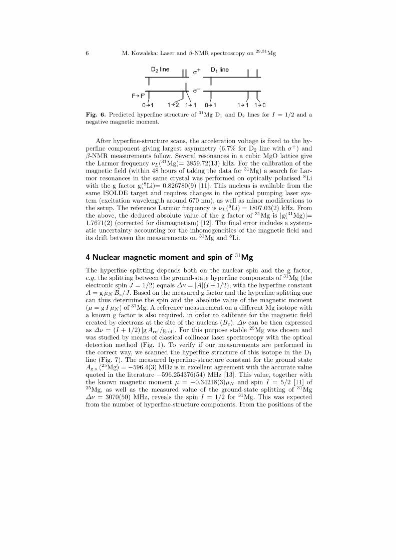
6 M. Kowalska: Laser and β-NMR spectroscopy on 29,31Mg
Fig. 6. Predicted hyperfine structure of 31Mg D1 and D2 lines for I = 1/2 and anegative magnetic moment.
After hyperfine-structure scans, the acceleration voltage is fixed to the hy-perfine component giving largest asymmetry (6.7% for D2 line with σ+) andβ-NMR measurements follow. Several resonances in a cubic MgO lattice givethe Larmor frequency νL(31Mg)= 3859.72(13) kHz. For the calibration of themagnetic field (within 48 hours of taking the data for 31Mg) a search for Lar-mor resonances in the same crystal was performed on optically polarised 8Liwith the g factor g(8Li)= 0.826780(9) [11]. This nucleus is available from thesame ISOLDE target and requires changes in the optical pumping laser sys-tem (excitation wavelength around 670 nm), as well as minor modifications tothe setup. The reference Larmor frequency is νL(8Li) = 1807.03(2) kHz. Fromthe above, the deduced absolute value of the g factor of 31Mg is |g(31Mg)|=1.7671(2) (corrected for diamagnetism) [12]. The final error includes a system-atic uncertainty accounting for the inhomogeneities of the magnetic field andits drift between the measurements on 31Mg and 8Li.
4 Nuclear magnetic moment and spin of 31Mg
The hyperfine splitting depends both on the nuclear spin and the g factor,e.g. the splitting between the ground-state hyperfine components of 31Mg (theelectronic spin J = 1/2) equals ∆ν = |A|(I +1/2), with the hyperfine constantA = g µN Be/J . Based on the measured g factor and the hyperfine splitting onecan thus determine the spin and the absolute value of the magnetic moment(µ = g I µN ) of 31Mg. A reference measurement on a different Mg isotope witha known g factor is also required, in order to calibrate for the magnetic fieldcreated by electrons at the site of the nucleus (Be). ∆ν can be then expressedas ∆ν = (I + 1/2) |g Aref/gref |. For this purpose stable 25Mg was chosen andwas studied by means of classical collinear laser spectroscopy with the opticaldetection method (Fig. 1). To verify if our measurements are performed inthe correct way, we scanned the hyperfine structure of this isotope in the D1
line (Fig. 7). The measured hyperfine-structure constant for the ground stateAg.s.(25Mg) = −596.4(3) MHz is in excellent agreement with the accurate valuequoted in the literature −596.254376(54) MHz [13]. This value, together withthe known magnetic moment µ = −0.34218(3)µN and spin I = 5/2 [11] of25Mg, as well as the measured value of the ground-state splitting of 31Mg∆ν = 3070(50) MHz, reveals the spin I = 1/2 for 31Mg. This was expectedfrom the number of hyperfine-structure components. From the positions of the

M. Kowalska: Laser and β-NMR spectroscopy on 29,31Mg 7
Fig. 7. Hyperfine structure of 25Mg+ recorded by detecting the photons emittedduring the relaxation of the ions in the optical detection part of the setup.
resonances also the sign of the magnetic moment can be deduced (µ < 0). Thenegative value of the magnetic moment implies furthermore a positive parityof this state. It follows both from the earlier β-decay studies [5], as well asfrom the large scale shell-model calculations presented in Neyens et al. [12].Calculations with different interactions, both in the sd and in the extendedsd− pf model spaces, predict a positive magnetic moment for the lowest 1/2−state. Thus our observed negative sign excludes the negative parity option, inagreement with the assignment based on the β decay. Therefore we concludethat µ(31Mg)= −0.88355(10) µN and Iπ(31Mg)= 1/2+.
Shell-model calculations in the sd model space using the USD interaction[14] predict the lowest I = 1/2+ level only at 2.5 MeV excitation energy.More advanced large scale shell model calculations, including excitations ofneutrons into the pf -shell, and using the interactions as described in [15] andin [16], both predict the 1/2+ level below 500 keV and with a magnetic momentclose to our observed value [12]. The wave function of this 1/2+ state consistsmainly of intruder configurations, which places this nucleus inside the “islandof inversion”.
This unambiguous spin-parity measurement allowed us also to make tenta-tive assignments to the lowest lying excited states in 31Mg [12].
Similar measurements have also been performed for 29Mg. They include thenuclear g factor and the ground-state spin I = 3/2, which is well described inthe sd shell model. This measurement places the ground state of 29Mg outsidethe “island of inversion”. Study of shorter-lived 33Mg is planned for the future.
This work has been supported by the German Ministry for Education and Re-search (BMBF) under contract No. 06MZ175, by the IUAP project No. p5-07 of OSCTBelgium and by the FWO-Vlaanderen, by Grant-in-Aid for Specially Promoted Re-search (13002001).

8 M. Kowalska: Laser and β-NMR spectroscopy on 29,31Mg
References
1. C. Thibault et al., Phys. Rev. C 12, 644 (1975).2. C. Detraz et al., Phys. Rev. C 19, 164 (1979).3. M. Keim et al., Eur. Phys. J. A 8, 31 (2000).4. D. Guillemaud-Mueller et al., Nucl. Phys. A426, 37 (1984).5. G. Klotz et al., Phys. Rev. C 47, 2502 (1993).6. S. Nummela et al., Phys. Rev. C 64, 054313 (2001).7. U. Koster et al., Nucl. Instr. Meth. B 204, 347 (2003).8. R. Neugart et al., Nucl. Inst. Meth. 186, 165 (1981).9. W. Geithner et al., Phys. Rev. Lett. 83, 3792 (1999).10. E. Arnold et al., Phys. Lett. B 197, 311 (1987).11. P. Raghavan, At. Data Nucl. Data Tables 42, 189 (1989).12. G. Neyens et al., Phys. Rev. Lett. 94, 22501 (2005).13. W.M. Itano, D.J. Wineland, Phys. Rev. A 24, 1364 (1981).14. B.H. Wildenthal et al., Phys. Rev. C 28, 1343 (1983).15. S. Nummela et al., Phys. Rev. C 63, 44316 (2001).16. Y. Utsuno et al., Phys. Rev. C 64, 11301 (2001).