Phase Field Modeling of Fracture and Composite Materials

Robert Spatschek, Denis Pilipenko, Clemens Muller-Gugenberger, and Efim A. Brener

Institut fur Festkorperforschung, Forschungszentrum Julich, D-52425 Julich, Germany

September 28, 2006

Abstract

The phase field method is a very powerful numerical method to solve moving boundaryproblems. Here we demonstrate how it can be applied to various processes involvingsound propagation and fracture. This approach is related to a new theory of fracturewhich describes in particular the fast growth of cracks. We study the propagationof elastic waves, the determination of stress intensity factors for moving cracks withextended tips, and the interaction and coarsening of cracks. Other examples are theinfluence of elastic effects on phase transitions and the delamination in compositematerials.

Keywords: Fracture Mechanics, Phase Field Methods, Sound propagation, Com-posite materials

1 Introduction

Understanding the phenomenon of fracture, especially in composite materials, is very importantfor many industrial applications. Apart from the development of physically motivated and suitablemodels for crack propagation [1], numerical tools are needed to describe the elastic deformationsin complex materials. Then, for example, the acoustic properties of a composite structure can beused for nondestructive testing.

The aim of this article is to demonstrate the capabilities of the phase field method for theseprocesses. It can be used not only to study the wave propagation in materials consisting of severaldifferent materials or phases, but also to study the crack propagation in homogeneous or compositematerials. This method is numerically very robust and able to describe even difficult topologicalchanges due to phase transitions or merging of cracks.

The general idea of the phase field method is not to track the location of interfaces or defectsexplicitly, but instead to introduce a so called phase field. In the simplest case of a two-phasematerial, which can consist for example of a hard and a soft solid phase, the value φ = 1 isassigned to the hard and φ = 0 to the soft phase. If the transition between the phases is nowsmoothed out on a small numerical length scale ξ (instead of a sharp transition from φ = 0 toφ = 1), the motion of interfaces can be mapped to a partial differential equation for the phasefield on the entire domain. In particular, the boundary conditions at interfaces are automaticallysatisfied.

1

The paper is organized as follows: First, in section 2 we introduce a phase field model whichcan be used to study elastically induced phase transitions and fracture processes. In sections3 and 4 we give two basic applications, the propagation of waves in composite materials andthe determination of stress intensity factors. Here, the phase field dynamics is not relevant andonly the elastic properties are investigated. Starting from section 5, the phase field dynamics isdiscussed e.g. for the interplay of many growing cracks or elastically induced phase transitions. Amore complicated multiphase application is the delamination of two elastic media, as described insection 7. Here, also aspects of nondestructive testing are investigated.

2 Phase field modeling

For simplicity we assume a two-dimensional plane strain situation, linear elastic isotropic mediaand the mass density ρ to be equal in both phases. Let φ denote the phase field with valuesφ = 0 for a “soft” phase inside a crack and φ = 1 for a “hard” phase. We start the descriptionfrom an energy functional, which consists of the following contributions: The elastic energydensity is fel = µ(φ)ε2ij + λ(φ)(εii)2/2, with µ(φ) = h(φ)µ(1) + (1 − h(φ))µ(2) and λ(φ) =h(φ)λ(1) + (1 − h(φ))λ(2), where h(φ) = φ2(3 − 2φ) interpolates between the phases and thesuperscripts denote the bulk values; εik and σik are strain and stress tensor respectively, which areconnected by Hooke’s law for isotropic elasticity, σkj = 2µεkj +λεllδkj , with the Lame coefficientλ and the shear modulus µ. Alternatively, we use Young’s modulus E = µ(3λ + 2µ)/(λ + µ) andthe Poisson ratio ν = λ/2(λ + µ) as elastic constants.

The surface energy is fs(φ) = 3γξ(∇φ)2/2 with the interface width ξ and the surface energydensity γ. Finally, fdw = 6γφ2(1 − φ)2/ξ is a double well potential. Thus the total potentialenergy is

U =∫

dV (fel + fs + fdw) . (1)

The elastodynamic equations are derived from the energy by the variation with respect to thedisplacements ui,

ρui = − δU

δui, (2)

and the dissipative phase fields dynamics follows from

∂φ

∂t= − D

3γξ

δU

δφ(3)

with a kinetic coefficient D with dimension [D] = m2s−1.From these equations, the following sharp interface limit (ξ → 0) can be extracted [2]: With

the premise of coherency at the interface and vanishing elastic constants in the soft phase, the solidmatrix is free of normal and shear stresses at a crack contour, i.e. σnn = σnτ = 0, which servesas boundary conditions (n and τ denote the normal and tangential directions at an interface). Inthe bulk, the elastic displacements ui have to fulfill Newton’s equation of motion,

∂σij

∂xj= ρui. (4)

The motion of the interface is locally expressed by the normal velocity

vn =D

γΩ∆µ (5)

2

Figure 1: Scaling behavior of the parallelized phase-field code. An ideal speedup would correspondto a constant horizontal line. One can see that the parallelization is extremely efficient.

with the same kinetic coefficient D as above, and Ω denotes the atomic volume. Here, thedifference in the chemical potentials between two phases at an interface is [3]

∆µ = Ω(

12σjkεjk − γκ

). (6)

The interface curvature κ is positive if the crack shape is convex.For the numerical realization, we employ explicit representations of both the elastodynamic

equations and the phase field dynamics, where the elastic displacements are defined on a staggeredgrid [4]. We then choose a rectangular strip with fixed displacements at its upper and lowerboundary to study crack growth. In the soft phase, we typically set the elastic constants to onemillionth of the values in the hard phase; however, these values are qualitatively not significant.In the strip geometry, a dimensionless driving force is defined by ∆ = u2

0(λ+2µ)/4Lγ. The fixedvertical displacement u0 is applied to the strip of width L [5, 6]; ∆ = 1 corresponds to the Griffithpoint [7]. Since the phase field approach introduces a new numerical lengthscale to the problem,which is the width of the interface ξ, one has to make sure that all physical lengthscales are muchlarger in order to obtain results that are in quantitative agreement with the corresponding sharpinterface equations. The grid can be shifted horizontally in order to always keep the crack tip inthe center of the system. Thus, crack growth can be studied over long times in relatively smallsystems. Typical dimensions used here are 1000× 500 grid points, the phase field interface widthis ξ = 5∆x (∆x is the lattice unit) and the Poisson ratio is ν = 1/3. For the more advancedmulticrack and multiphase calculations, the grids could be considerably larger (up to 8200×4100).

For being able to handle such large systems, we developed a parallel code using MPI. If we

3

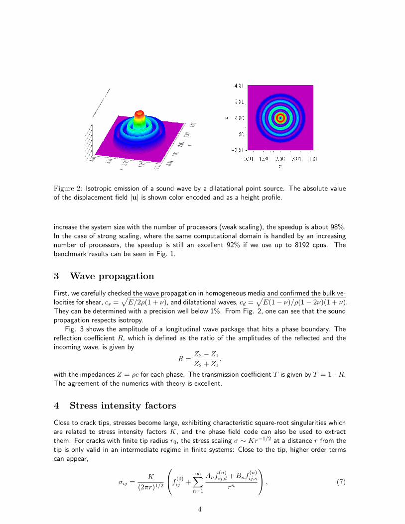
Figure 2: Isotropic emission of a sound wave by a dilatational point source. The absolute valueof the displacement field |u| is shown color encoded and as a height profile.

increase the system size with the number of processors (weak scaling), the speedup is about 98%.In the case of strong scaling, where the same computational domain is handled by an increasingnumber of processors, the speedup is still an excellent 92% if we use up to 8192 cpus. Thebenchmark results can be seen in Fig. 1.

3 Wave propagation

First, we carefully checked the wave propagation in homogeneous media and confirmed the bulk ve-locities for shear, cs =

√E/2ρ(1 + ν), and dilatational waves, cd =

√E(1− ν)/ρ(1− 2ν)(1 + ν).

They can be determined with a precision well below 1%. From Fig. 2, one can see that the soundpropagation respects isotropy.

Fig. 3 shows the amplitude of a longitudinal wave package that hits a phase boundary. Thereflection coefficient R, which is defined as the ratio of the amplitudes of the reflected and theincoming wave, is given by

R =Z2 − Z1

Z2 + Z1,

with the impedances Z = ρc for each phase. The transmission coefficient T is given by T = 1+R.The agreement of the numerics with theory is excellent.

4 Stress intensity factors

Close to crack tips, stresses become large, exhibiting characteristic square-root singularities whichare related to stress intensity factors K, and the phase field code can also be used to extractthem. For cracks with finite tip radius r0, the stress scaling σ ∼ Kr−1/2 at a distance r from thetip is only valid in an intermediate regime in finite systems: Close to the tip, higher order termscan appear,

σij =K

(2πr)1/2

f(0)ij +

∞∑n=1

Anf(n)ij,d + Bnf

(n)ij,s

rn

, (7)

4

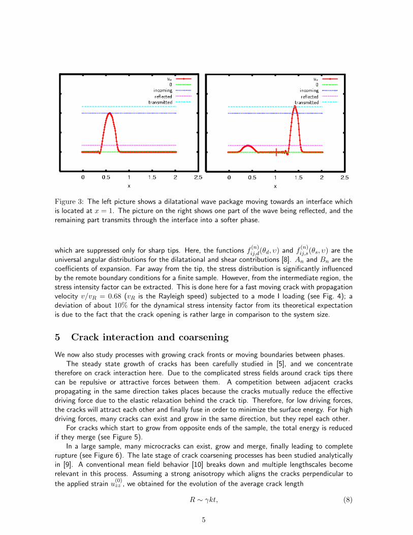
Figure 3: The left picture shows a dilatational wave package moving towards an interface whichis located at x = 1. The picture on the right shows one part of the wave being reflected, and theremaining part transmits through the interface into a softer phase.

which are suppressed only for sharp tips. Here, the functions f(n)ij,d(θd, υ) and f

(n)ij,s(θs, υ) are the

universal angular distributions for the dilatational and shear contributions [8]. An and Bn are thecoefficients of expansion. Far away from the tip, the stress distribution is significantly influencedby the remote boundary conditions for a finite sample. However, from the intermediate region, thestress intensity factor can be extracted. This is done here for a fast moving crack with propagationvelocity v/vR = 0.68 (vR is the Rayleigh speed) subjected to a mode I loading (see Fig. 4); adeviation of about 10% for the dynamical stress intensity factor from its theoretical expectationis due to the fact that the crack opening is rather large in comparison to the system size.

5 Crack interaction and coarsening

We now also study processes with growing crack fronts or moving boundaries between phases.The steady state growth of cracks has been carefully studied in [5], and we concentrate

therefore on crack interaction here. Due to the complicated stress fields around crack tips therecan be repulsive or attractive forces between them. A competition between adjacent crackspropagating in the same direction takes places because the cracks mutually reduce the effectivedriving force due to the elastic relaxation behind the crack tip. Therefore, for low driving forces,the cracks will attract each other and finally fuse in order to minimize the surface energy. For highdriving forces, many cracks can exist and grow in the same direction, but they repel each other.

For cracks which start to grow from opposite ends of the sample, the total energy is reducedif they merge (see Figure 5).

In a large sample, many microcracks can exist, grow and merge, finally leading to completerupture (see Figure 6). The late stage of crack coarsening processes has been studied analyticallyin [9]. A conventional mean field behavior [10] breaks down and multiple lengthscales becomerelevant in this process. Assuming a strong anisotropy which aligns the cracks perpendicular to

the applied strain u(0)zz , we obtained for the evolution of the average crack length

R ∼ γkt, (8)

5

Figure 4: Determination of a dynamical stress intensity factor for the crack shown in the leftpanel. Right panel: The value of the vertical stress component σyy as a function of the distancefrom the tip is shown in a logarithmic presentation. In an intermediate regime, the square-rootbehavior is clearly visible.

Figure 5: Two notches are cut into the sample and grow towards each other. The propagatingtips cannot penetrate the already relaxed region of the opposite crack. Therefore, the cracks restand broaden until they attract each other and fuse. We use D/ξvR = 0.23, the driving force is∆ = 1.8 and the system size is 800× 400 grid points. Time is given in units D/v2

R.

Figure 6: Coarsening of an irregular arrangement of cracks in a uniaxially strained solid withperiodic boundary conditions in lateral direction. Large cracks grow at the expense of smallercracks. The parameters used here are ∆ = 6, D/ξvR = 2.32, and the system size is 1000× 300grid points. Time is given in units D/v2

R.

6

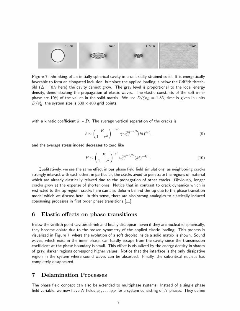
Figure 7: Shrinking of an initially spherical cavity in a uniaxially strained solid. It is energeticallyfavorable to form an elongated inclusion, but since the applied loading is below the Griffith thresh-old (∆ = 0.9 here) the cavity cannot grow. The gray level is proportional to the local energydensity, demonstrating the propagation of elastic waves. The elastic constants of the soft innerphase are 10% of the values in the solid matrix. We use D/ξvR = 1.85, time is given in unitsD/v2

R, the system size is 600× 400 grid points.

with a kinetic coefficient k ∼ D. The average vertical separation of the cracks is

` ∼(

E

1− ν2

)−1/5

γ u(0)zz

−2/5(kt)4/5, (9)

and the average stress indeed decreases to zero like

P ∼(

E

1− ν2

)1/5

u(0)zz

−3/5(kt)−4/5 . (10)

Qualitatively, we see the same effect in our phase field field simulations, as neighboring cracksstrongly interact with each other; in particular, the cracks avoid to penetrate the regions of materialwhich are already elastically relaxed due to the propagation of other cracks. Obviously, longercracks grow at the expense of shorter ones. Notice that in contrast to crack dynamics which isrestricted to the tip region, cracks here can also deform behind the tip due to the phase transitionmodel which we discuss here. In this sense, there are also strong analogies to elastically inducedcoarsening processes in first order phase transitions [11].

6 Elastic effects on phase transitions

Below the Griffith point cavities shrink and finally disappear. Even if they are nucleated spherically,they become oblate due to the broken symmetry of the applied elastic loading. This process isvisualized in Figure 7, where the evolution of a soft droplet inside a solid matrix is shown. Soundwaves, which exist in the inner phase, can hardly escape from the cavity since the transmissioncoefficient at the phase boundary is small. This effect is visualized by the energy density in shadesof gray; darker regions correspond higher values. Notice that the interface is the only dissipativeregion in the system where sound waves can be absorbed. Finally, the subcritical nucleus hascompletely disappeared.

7 Delamination Processes

The phase field concept can also be extended to multiphase systems. Instead of a single phasefield variable, we now have N fields φ1, . . . , φN for a system consisting of N phases. They define

7

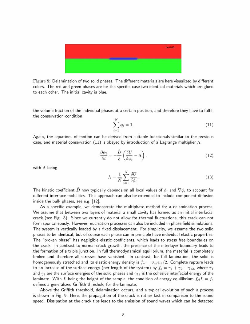
Figure 8: Delamination of two solid phases. The different materials are here visualized by differentcolors. The red and green phases are for the specific case two identical materials which are gluedto each other. The initial cavity is blue.

the volume fraction of the individual phases at a certain position, and therefore they have to fulfillthe conservation condition

N∑i=1

φi = 1. (11)

Again, the equations of motion can be derived from suitable functionals similar to the previouscase, and material conservation (11) is obeyed by introduction of a Lagrange multiplier Λ,

∂φi

∂t= −D

ξ

(δU

δφi− Λ

), (12)

with Λ being

Λ =1N

N∑i=1

δU

δφi. (13)

The kinetic coefficient D now typically depends on all local values of φi and ∇φi to account fordifferent interface mobilities. This approach can also be extended to include component diffusioninside the bulk phases, see e.g. [12].

As a specific example, we demonstrate the multiphase method for a delamination process.We assume that between two layers of material a small cavity has formed as an initial interfacialcrack (see Fig. 8). Since we currently do not allow for thermal fluctuations, this crack can notform spontaneously. However, nucleation processes can also be included in phase field simulations.The system is vertically loaded by a fixed displacement. For simplicity, we assume the two solidphases to be identical, but of course each phase can in principle have individual elastic properties.The “broken phase” has negligible elastic coefficients, which leads to stress free boundaries onthe crack. In contrast to normal crack growth, the presence of the interlayer boundary leads tothe formation of a triple junction. In full thermodynamical equilibrium, the material is completelybroken and therefore all stresses have vanished. In contrast, for full lamination, the solid ishomogeneously stretched and its elastic energy density is fel = σikεik/2. Complete rupture leadsto an increase of the surface energy (per length of the system) by fs = γ1 + γ2 − γ12, where γ1

and γ2 are the surface energies of the solid phases and γ12 is the cohesive interfacial energy of thelaminate. With L being the height of the sample, the condition of energy equilibrium felL = fs

defines a generalized Griffith threshold for the laminate.Above the Griffith threshold, delamination occurs, and a typical evolution of such a process

is shown in Fig. 9. Here, the propagation of the crack is rather fast in comparison to the soundspeed. Dissipation at the crack tips leads to the emission of sound waves which can be detected

8

Figure 9: Delamination of two elastic strips. Time is given in units D/v2R with vR being the

Rayleigh speed of the bulk phases and D the kinetic coefficient for the delamination process. Thedelaminated phase is shown in white. The red component for the color encoding of the elastic wavepropagation is proportional to the horizontal velocity ux and the green component proportionalto the vertical velocity uy.

at the boundaries of the sample. The sound waves are visualized by color encoding.For a nondestructive testing of the laminate the transmission of sound waves through the

sample can be used (see. Fig. 10). Here, we use for example a planar dilatational wave whichenters the composite from the upper boundary. When it hits the cavity, it is partially reflected andrefracted, if the wavelength is not too small in comparison to the size of the crack. The emittedwave intensity is significantly reduced in regions which are shaded by the crack. Notice that forthe case of equal bulk materials the waves travel without scattering through the planar boundarybetween them despite the presence of phase field gradients.

This work has been supported by the Deutsche Forschungsgemeinschaft under grant SPP 1120.

References

[1] L. B. Freund, Dynamic Fracture Mechanics, Cambridge University Press, 1998.

[2] K. Kassner et al., Phys. Rev E 63, 036117 (2001).

[3] P. Nozieres, J. Phys. I France 3, 681 (1993).

[4] J. Virieux, Geophys. 51, 889 (1986).

[5] R. Spatschek, et al., Phys. Rev. Lett. 96, 015502 (2006).

[6] E. A. Brener and R. Spatschek, Phys. Rev. E 67, 016112 (2003).

[7] A. A. Griffith, Philos. Trans. R. Soc. A, 21, 163 (1921).

9

Figure 10: Scattering of a planar dilatational wave at the zone of detachment. Time is given inunits D/v2

R.

[8] J. R. Rice, Mathematical analysis in the mechanics of fracture. In Fracture: An AdvancedTreatise, Liebowitz, H. Ed., vol. 2. Academic, New York, 1968, ch. 3, p. 192.

[9] E. Brener, H. Muller-Krumbhaar, and R. Spatschek, Phys. Rev. Lett. 86, 1291 (2001).

[10] I. M. Lifshitz and Slyozov, J. Chem. Solids 19, 35 (1961); C. Wagner, Z. Elektrochem. 65,581 (1961).

[11] E. Brener, V. Marchenko, H. Muller-Krumbhaar, and R. Spatschek, Phys. Rev. Lett. 84,4914 (2000).

[12] B. Nestler, J. Crystal Growth 204, 224 (1999).

10