PHan phoi student

arX

iv:1

208.

6424

v2 [

mat

h.R

T]

16

Oct

201

2

Cellular structure of q-Brauer algebras

Dung Tien Nguyen

Present address : University of Stuttgart, Institute of Algebra and Number Theory, Pfaffenwaldring 57,

D-70569 Stuttgart, Germany

Permanent address :University of Vinh, Mathematical Faculty, Leduan 182, Vinh city, Vietnam

Abstract

In this paper we consider the q-Brauer algebra over R a commutative noetherian domain.We first construct a new basis for q-Brauer algebras, and we then prove that it is a cellbasis, and thus these algebras are cellular in the sense of Graham and Lehrer. In particular,they are shown to be an iterated inflation of Hecke algebras of type An−1. Moreover, whenR is a field of arbitrary characteristic, we determine for which parameters the q-Braueralgebras are quasi-heredity. So the general theory of cellular algebras and quasi-hereditaryalgebras applies to q-Brauer algebras. As a consequence, we can determine all irreduciblerepresentations of q-Brauer algebras by linear algebra methods.

Keywords: q-Brauer algebra; Algebra with involution q-deformation; Brauer algebra;Hecke algebra; Cellular algebra.

1. Introduction

Schur-Weyl duality relates the representation theory of infinite group GLN (R) withthat of symmetric group Sn via the mutually centralizing actions of two groups on thetensor power space (RN)⊗n. In 1937 Richard Brauer [2] introduced the algebras whichare now called ’Brauer algebra’. These algebras appear in an analogous situation whereGLN(R) is replaced by either a symplectic or an orthogonal group and the group algebraof the symmetric group is replaced by a Brauer algebra. Afterwards, a q-deformationof these algebras has been found in [1] by Birman and Wenzl, and independently byMurakami [21], which is referred nowadays as BMW-algebras, in connection with knottheory and quantum groups.

Recently a new algebra was introduced by Wenzl [24] via generators and relationswho called it the q-Brauer algebra and gave a detailed description of its structure. Thisalgebra is another q-deformation of Brauer algebras and contains the Hecke algebra oftype An−1 as a subalgebra. In particular, he proved that over the field Q(r, q) it issemisimple and isomorphic to the Brauer algebra. Subsequently Wenzl found a numberof applications of q-Brauer algebras, such as in the study of the representation ring of anorthogonal or symplectic group [25], of module categories of fusion categories of type A

Email address: [email protected] (Dung Tien Nguyen)

Preprint submitted to Elsevier October 18, 2012

http://arxiv.org/abs/1208.6424v2

and corresponding subfactors of type II1 in [26]. Another quantum analogue of the Braueralgebra had been introduced by Molev in [18]. He has shown that Wenzl’s q-Brauer algebrais a quotient of his algebra in [19].

It is well known that algebras as the group algebra of symmetric groups, the Heckealgebra of type An−1, the Brauer algebra and its q-deformation the BMW-algebra arecellular algebras in the sense of Graham and Lehrer (see [13, 17, 28]). Hence, a questionarising naturally from this situation is whether the q-Brauer algebra is also a cellularalgebra.

This question will be answered in the positive in this paper via using an equivalentdefinition with that of Graham and Lehrer defined by Koenig and Xi in [15] and theirapproach, called ’iterated inflation’, to cellular structure as in [17] (or [15]). Firstly, wewill construct a basis for q-Brauer algebras which is labeled by a natural basis of Braueralgebras. This basis allows us to find cellular structure on q-Brauer algebras. Also notethat there is a general basis for the q-Brauer algebras introduced in [24] by Wenzl, but itseems that his basis is not suitable to provide a cell basis. Subsequently, we prove thatthese q-Brauer algebras are cellular in the sense of Graham and Lehrer. More precisely, weexhibit on this algebra an iterated inflation structure as that of the Brauer algebra in [17]and of the BMW-algebra in [28]. These results are valid over a commutative noetherianring. These enable us to determine the irreducible representations of q-Brauer algebrasover arbitrary field of any characteristic by using the standard methods in the generaltheory of cellular algebras. As another application, we give the choices for parameters suchthat the corresponding q-Brauer algebras are quasi-hereditary in the sense of [5]. Thus,for those q-Brauer algebras, the finite dimensional left modules form a highest weightcategory with many important homological properties [22]. Under a suitable choice ofparameters all results of the q-Brauer algebra obtained in this paper recover those of theBrauer algebra with non-zero parameter given by Koenig and Xi ([16], [17]).

The paper will be organized as follows: In Section two we recall the definition ofBrauer algebras and of Hecke algebras of type An−1 as well as the axiomatics of cellularalgebras. Some basic results on representations of Brauer algebras are given here. InSection three we indicate the definition of generic q-Brauer algebras as well as collect andextend some basic and necessary properties for later reference. Theorem 3.13 points outa particular basis on the q-Brauer algebras that is then shown a cell basis. In Sectionfour we prove the main result, Theorem 4.17, that the q-Brauer algebras have cellularstructure. Proposition 4.14 tells us that any q-Brauer algebra can be presented as aniterated inflation of certain Hecke algebras of type An−1. The other results are obtainedby applying the theory of cellular algebras. In Section five we determine a necessary andsufficient condition for the q-Brauer algebra to be quasi-hereditary, Theorem 5.2.

2. Basic definitions and preliminaries

In this section we recall the definition of Brauer and Hecke algebras and also that ofcellular algebras.

2

2.1. Brauer algebra

Brauer algebras were introduced first by Richard Brauer [2] in order to study thenth tensor power of the defining representation of the orthogonal groups and symplecticgroups. Afterward, they were studied in more detail by various mathematicians. We referthe reader to work of Brown (see [3, 4]), Hanlon and Wales ([9, 10, 8]) or Graham andLehrer [13], Koenig and Xi [16, 17], Wenzl [23] for more information.

2.1.1. Definition of Brauer algebras

The Brauer algebra is defined over the ring Z[x] via a basis given by diagrams with2n vertices, arranged in two rows with n edges in each row, where each vertex belongsto exactly one edge. The edges which connect two vertices on the same row are calledhorizontal edges. The other ones are called vertical edges. We denote by Dn(x) the Braueralgebra which the vertices of diagrams are numbered 1 to n from left to right in both thetop and the bottom. Two diagrams d1 and d2 are multiplied by concatenation, that is,the bottom vertices of d1 are identified with the top vertices of d2, hence defining diagramd. Then d1 · d2 is defined to be xγ(d1, d2)d, where γ(d1, d2) denote the number of thoseconnected components of the concatenation of d1 and d2 which do not appear in d, thatis, which contain neither a top vertex of d1 nor a bottom vertex of d2.Let us demonstrate this by an example. We multiply two elements in D7(x):

• •

⑧⑧⑧⑧

• •

❖❖❖❖

❖❖❖❖

❖ • • •

♦♦♦♦♦♦♦♦♦

d1

• • • • • • •

•❄❄

❄❄• •

♦♦♦♦♦♦♦♦♦ • • • •

d2

• • • • • • •

and the resulting diagram is

• • • • • • •

•d1.d2 = x1

• • • • • •.

In ([2], Section 5) Brauer points out that each basis diagram on Dn(x) which hasexactly 2k horizontal edges can be obtained in the form ω1e(k)ω2 with ω1 and ω2 arepermutations in the symmetric group Sn, and e(k) is a diagram of the following form:

• • . . . • • • • . . . •

• • . . . • • • • . . . •,

where each row has exactly k horizontal edges.As a consequence, the Brauer algebra can be considered over a polynomial ring over

Z and is defined via generators and relations as follow:Take N to be an indeterminate over Z; Let R = Z[N ] and define the Brauer alge-

bra Dn(N) over R as the associative unital R–algebra generated by the transpositions

3

s1, s2, . . . , sn−1, together with elements e(1), e(2), . . . , e([n/2]), which satisfy the defining re-lations:

(S0) si2 = 1 for 1 ≤ i < n;

(S1) sisi+1si = si+1sisi+1 for 1 ≤ i < n− 1;

(S2) sisj = sjsi for 2 ≤ |i− j|;

(1) e(k)e(i) = e(i)e(k) = N ie(k) for 1 ≤ i ≤ k ≤ [n/2];

(2) e(i)s2je(k) = e(k)s2je(i) = N i−1e(k) for 1 ≤ j ≤ i ≤ k ≤ [n/2];

(3) s2i+1e(k) = e(k)s2i+1 = e(k) for 0 ≤ i < k ≤ [n/2];

(4) e(k)si = sie(k) for 2k < i < n ;

(5) s(2i−1)s2ie(k) = s(2i+1)s2ie(k) for 1 ≤ i < k ≤ k ≤ [n/2];

(6) e(k)s2is(2i−1) = e(k)s2is(2i+1) for 1 ≤ i < k ≤ k ≤ [n/2];

(7) e(k+1) = e(1)s2,2k+1s1,2ke(k) for 1 ≤ k ≤ [n/2]− 1.

Regard the group ring RSn as the subring of Dn(N) generated by the transpositions

{si = (i, i+ 1)for 1 ≤ i < n}.

By Brown ([4], Section 3) the Brauer algebra has a decomposition as direct sum of vectorspaces

Dn(x) ∼=

[n/2]⊕

k=0

Z[x]Sne(k)Sn.

SetI(m) =

⊕

k≥m

Z[x]Sne(k)Sn,

then I(m) is a two-sided ideal in Dn(x) for each m ≤ [n/2].

2.1.2. The modules V ∗k and Vk for Brauer algebras

In this subsection we recall particular modules of Brauer algebras. Dn(N) has adecomposition into Dn(N)−Dn(N) bimodules

Dn(N) ∼=

[n/2]⊕

k=0

Z[N ]Sne(k)Sn + I(k+1)/I(k+1).

Using the same arguments as in Section 1 ([24]), each factor module

Z[N ]Sne(k)ωj + I(k+1)/I(k+1)

is a left Dn(N)-module with a basis given by the basis diagrams of Z[N ]Sne(k)ωj, whereωj ∈ Sn is a diagram such that e(k)ωj is a diagram in Dn(N) with no intersection betweenany two vertical edges. In particular

I(k)/I(k+1) ∼=⊕

j∈P (n,k)

(Z[N ]Sne(k)ωj + I(k+1))/I(k+1), (2.1)

4

where P (n, k) is the set of all possibilities of ωj. As multiplication from the right by ωj

commutes with the Dn(N)-action, it implies that each summand on the right hand sideis isomorphic to the module

V ∗k = (Z[N ]Sne(k) + I(k+1))/I(k+1). (2.2)

Combinatorially, V ∗k is spanned by basis diagrams with exactly k edges in the bottom

row, where the i − th edge is connected the vertices 2i− 1 and 2i. Observe that V ∗k is a

free, finitely generated Z[N ] module with Z[N ]-rank n!/2kk!.Similarly, the right Dn(N)-module is defined

Vk = (Z[N ]e(k)Sn + I(k+1))/I(k+1), (2.3)

where the basis diagrams are obtained from those in V ∗k by an involution, say *, of Dn(N)

which rotates a diagram d ∈ V ∗k around its horizontal axis downward. For convenience

later in Section 4 we use the term V ∗k replacing V

(k)n in [24]. More details for setting up

V ∗k can be found in Section 1 of [24].

Lemma 2.1. ([24], Lemma 1.1(d)). The algebra Dn(N) is faithfully represented on⊕[n/2]

k=0 V ∗k (and also on

⊕[n/2]k=0 Vk).

2.1.3. Length function for Brauer algebras Dn(N)

Generalizing the length of elements in reflection groups, Wenzl [24] defined a lengthfunction for a diagram of Dn(N) as follows:For a diagram d ∈ Dn(N) with exactly 2k horizontal edges, the definition of the lengthℓ(d) is given by

ℓ(d) = min{ℓ(ω1) + ℓ(ω2)| ω1e(k)ω2 = d, ω1, ω2 ∈ Sn}.

We will call the diagrams d of the form ωe(k) where l(ω) = l(d) and ω ∈ Sn basis diagramsof the module V ∗

k .

Remark 2.2. 1. Recall that the length of a permutation ω ∈ Sn is defined by ℓ(ω) = thecardinality of set {(i, j)|(j)ω < (i)ω and 1 ≤ i < j ≤ n}, where the symmetric group actson {1, 2, ..., n} on the right.

2. Given a diagram d, there can be more than one ω satisfying ωe(k) = d and ℓ(ω) =ℓ(d). e.g. s2j−1s2je(k) = s2j+1s2je(k) for 2j + 1 < k. This means that such an expressionof d is not unique with respect to ω ∈ Sn.

For later use, if si = (i, i+ 1) is a transposition in symmetric goup Sn with i, j = 1, ..., klet

si,j =

{

sisi+1...sj if i ≤ j,

sisi−1...sj if i > j.

A permutation ω ∈ Sn can be written uniquely in the form ω = tn−1tn−2...t1, where tj = 1or tj = sij ,j with 1 ≤ ij ≤ j and 1 ≤ j < n. This can be seen as follows: For given ω ∈ Sn,there exists a unique tn−1 such that (n)tn−1 = (n)ω. Hence ω′ = (n)t−1

n−1ω = n, and we

5

can consider ω′ as an element of Sn−1. Repeating this process on n implies the generalclaim. Set

B∗k = {tn−1tn−2...t2kt2k−2t2k−4...t2}. (2.4)

By the definition of tj given above, the number of possibilities of tj is j + 1. A directcomputation shows that B∗

k has n!/2kk! elements. In fact, the number of elements in B∗k

is equal to the number of diagrams d∗ in Dn(N) in which d∗ has k horizontal edges ineach row and one of its rows is fixed like that of e(k).

3. From now on, a permutation of symmetric group is seen as a diagram with nohorizontal edges, and the product ω1ω2 in Sn is seen as a concatenation of two diagramsin Dn(N).

4. Given a basis diagram d∗ = ωe(k) with ℓ(ω) = ℓ(d∗) does not imply that ω ∈ B∗k, but

there does exist ω′ ∈ B∗k such that d∗ = ω′e(k). The latter was already shown by Wenzl

(Lemma 1.2(a), [24]) to exist and to be unique for each basis element of the module V ∗k .

He even got ℓ(d∗) = ℓ(ω) = ℓ(ω′), where ℓ(ω′) is the number of factors for ω′ in B∗k .

Example 2.3. As indicated in remark (2), we choose j = 1, k = 2. Given a basis diagramd∗ in V ∗

2 is in the form:

• • • • • • •

•d∗ =

• • • • • •

•

❖❖❖❖

❖❖❖❖

❖ •

⑧⑧⑧⑧

•

⑧⑧⑧⑧

• • • •s1s2

• • • • • • •

•=

• • • • • •e(2)

• • • • • • •

• •❄❄

❄❄•

❄❄❄❄

•

♦♦♦♦♦♦♦♦♦ • • •

s3s2

• • • • • • •

•=

• • • • • •e(2)

• • • • • • •

In the picture d∗ has two representations d∗ = s1s2e(2) = s3s2e(2) satisfying

ℓ(d∗) = ℓ(s1s2) = ℓ(s3s2) = 2.

However, s1s2 is in B∗2 but s3s2 is not. In general, given a basis diagram d∗ in V ∗

k therealways exists a unique permutation ω ∈ B∗

k such that d∗ = ωek and l(d∗) = l(ω).The statement in the remark (5) is shown in the following lemma.

6

Lemma 2.4. ([24], Lemma 1.2). (a) The module V ∗k has a basis {ωv1 = vωe(k), ω ∈ B∗

k}with ℓ(ωe(k)) = ℓ(ω). Here ℓ(ω) is the number of factors for ω in (2.4), andv1 = (e(k) + I(k + 1))/I(k + 1) ∈ V ∗

k .(b) For any basis element d∗ of V ∗

k , we have |ℓ(sid∗)− ℓ(d∗)| ≤ 1. Equality of lengths

holds only if sid∗ = d∗.

For k ≤ [n/2], let

Bk = {ω−1| ω ∈ B∗k}. (2.5)

The following statement is similar to Lemma 2.4 above.

Lemma 2.5. (a) The module Vk has a basis {v1ω = ve(k)ω, ω ∈ Bk} with ℓ(e(k)ω) = ℓ(ω).Here ℓ(ω) is the number of factors for ω in (2.5), and v1 = (e(k)+I(k+1))/I(k+1) ∈ Vk.

(b) For any basis element d of V(k)n , we have |ℓ(dsi) − ℓ(d)| ≤ 1. Equality of lengths

holds only if dsi = d.

2.2. Hecke algebra

In this section, we recall the definition of the Hecke algebra of type An−1, followingDipper and James [6], and we then review some basic facts which are necessary for oursubsequent work.

Definition 2.6. Let R be a commutative ring with identity 1, and let q be an invertibleelement of R. The Hecke algebra H = HR,q = HR,q(Sn) of the symmetric group Sn

over R is defined as follows. As an R-module, H is free with basis {gω| ω ∈ Sn}. Themultiplication in H satisfies the following relations:

(i) 1 ∈ H ;

(ii) If ω = s1s2...sj is a reduced expression for ω ∈ Sn, then gω = gs1gs2...gsj ;

(iii) g2sj = (q − 1)gsj + q for all transpositions sj, where q = q.1 ∈ H .

Recall that if ω = s1s2...sk with sj = (j, j+1) and k is minimal with this property, thenℓ(ω) = k, and we call s1s2...sk a reduced expression for ω. It is useful to abbreviate gsjby gj. Let R = Z[q, q−1], and let n be a natural number. We use the term Hn to indicateHR,q(Sn). Denote by H2k+1,n the subalgebra of the Hecke algebra which is generatedby elements g2k+1, g2k+2, ..., gn−1 in Hn. As a free R-module, H2k+1,n has an R-basis{gω| ω ∈ S2k+1,n}, where S2k+1,n generated by elements s2k+1, s2k+2, ..., sn−1 is a subgroupof the symmetric group Sn. In the next lemma we collect some basic facts on Hn.

Lemma 2.7. (a) If ω, ω′ ∈ Sn and l(ωω′) = l(ω) + l(ω′), then gωgω′ = gωω′.(b) Let sj be a transposition and ω ∈ Sn, then

gjgω =

{

gsjω if l(sjω) = l(ω) + 1

(q − 1)gω + qgsjω otherwise,

7

and

gωgj =

{

gωsj if l(ωsj) = l(ω) + 1

(q − 1)gω + qgωsj otherwise.

(c) Let ω ∈ Sn. Then gω is invertible in Hn with inverse g−1ω = g−1

j g−1j−1...g

−12 g−1

1 ,where ω = s1s2...sj is a reduced expression for ω, and

g−1j = q−1gj + (q−1 − 1), so gj = qg−1

j + (q − 1) for all sj .

In the literature, the Hecke algebras Hn of type An−1 are commonly defined by gen-erators gi, 1 ≤ i < n and relations

(H1) gigi+1gi = gi+1gigi+1 for 1 ≤ i ≤ n− 1;

(H2) gigj = gjgi for |i− j| > 1.

The next statement is implicit in [6] (or see Lemma 2.3 of [20]).

Lemma 2.8. The R-linear map i: Hn −→ Hn determined by i(gω) = gω−1 for eachω ∈ Sn is an involution on Hn

2.3. Cellular algebras

In this section we recall the original definition of cellular algebras in the sense ofGraham and Lehrer in [13] and an equivalent definition given in [14] by Koenig and Xi.Then we are going to apply the idea and approach in ([17, 28]) to cellular structure toprove that the q-Brauer algebra Brn(r, q) is cellular. In fact, to obtain this result wefirstly construct a basis for Brn(r, q) that is naturally indexed by the basis of Braueralgebra Dn(N). Subsequently, the q-Brauer algebra is shown to be an iterated inflationof Hecke algebras of type An−1. More details about the concept ”iterated inflation” weregiven in [15, 17]. Using the result in this section, we can determine the quasi-hereditaryq-Brauer algebras in Section 5.

Definition 2.9. (Graham and Lehrer, [13]). Let R be a commutative Noetherian integraldomain with identity. A cellular algebra over R is an associative (unital) algebra Atogether with cell datum (Λ,M,C, i), where

(C1) Λ is a partially ordered set (poset) and for each λ ∈ Λ, M(λ) is a finite set suchthat the algebra A has an R-basis Cλ

S,T , where (S, T ) runs through all elements ofM(λ)×M(λ) for all λ ∈ Λ.

(C2) If λ ∈ Λ and S, T ∈ M(λ). Then i is involution of A such that i(CλS,T ) = Cλ

T,S.

(C3) For each λ ∈ Λ and S, T ∈ M(λ) then for any element a ∈ A we have

aCλS,T ≡

∑

U∈M(λ)

ra(U, S)CλU,T (mod A(< λ)),

where ra(U, S) ∈ R is independent of T, and A(< λ) is the R-submodule of Agenerated by {Cµ

S′ ,T ′ |µ < λ; S′

, T′

∈ M(µ)}.

8

The basis {CλS,T} of a cellular algebra A is called as a cell basis. In [13], Graham and

Lehrer defined a bilinear form φλ for each λ ∈ Λ with respect to this basis as follows.

CλS,TC

λU,V ≡ φλ(T, U)Cλ

S,V (mod A < λ).

They also proved that the isomorphism classes of simple modules are parametrized by theset

Λ0 = {λ ∈ Λ| φλ 6= 0}.

The following is an equivalent definition of cellular algebra.

Definition 2.10. (Koenig and Xi, [14]). Let A be an R-algebra where R is a commutativenoetherian integral domain. Assume there is an involution i on A, a two-sided ideal Jin A is called cell ideal if and only if i(J) = J and there exists a left ideal ∆ ⊂ J suchthat ∆ is finitely generated and free over R and such that there is an isomorphism ofA-bimodules α : J ≃ ∆ ⊗R i(∆) (where i(∆) ⊂ J is the i-image of ∆) making thefollowing diagram commutative:

Jα//

i

��

∆⊗R i(∆)

x⊗y 7→i(y)⊗i(x)��

Jα// ∆⊗R i(∆)

The algebra A with the involution i is called cellular if and only if there is anR- module decomposition A = J

′

1 ⊕ J′

2 ⊕ ...J′

n (for some n) with i(J′

j) = J′

j for each j

and such that setting Jj = ⊕jl=1J

′

l gives a chain of two-sided ideals of A: 0 = J0 ⊂ J1 ⊂J2 ⊂ ... ⊂ Jn = A (each of them fixed by i) and for each j (j = 1, ..., n) the quotientJ

′

j = Jj/Jj−1 is a cell ideal (with respect to the involution induced by i on the quotient)of A/Jj−1.

Recall that an involution i is defined as an R-linear anti-automorphism of A withi2 = id. The ∆

′

s obtained from each section Jj/Jj−1 are called cell modules of thecellular algebra A. Note that all simple modules are obtained from cell modules [13].

In [14], Koenig and Xi proved that the two definitions of cellular algebra are equiva-lent. The first definition can be used to check concrete examples, the latter, however, isconvenient to look at the structure of cellular algebras as well as to check cellularity ofan algebra.

Typical examples of cellular algebras are the following: Group algebras of symmetricgroups, Hecke algebras of type An−1 or even of Ariki-Koike finite type [12] (i.e., cyclotomicHecke algebras), Schur algebras of type A, Brauer algebras, Temperley-Lieb and Jonesalgebras which are subalgebras of the Brauer algebra [13], partition algebras [27], BMW-algebras [28], and recently Hecke algebras of finite type [12].

The following results are shown in [13]; see also [17].

Theorem 2.11. The Brauer algebra Dn(x) is cellular for any commutative noetherianintegral domain with identity R and parameter x ∈ R.

9

Theorem 2.12. Let R = Z[q, q−1]. Then R-algebra Hn is a cellular algebra.

Next we will prove that q-Brauer algebras are also cellular. Before doing this, let usintroduce what the q-Brauer algebra is and construct a particular basis in the followingsection.

3. q-Brauer algebras

Firstly, we recall the definition of the generic q-Brauer algebras due to Wenzl [24].Then we collect and extend basic properties of q-Brauer algebras that will be needed inSection 4. The main result of this section is in Subsection 3.2 where a particular basis forq-Brauer algebras is given in Theorem 3.13.

Definition 3.1. Fix N ∈ Z \ {0}, let q and r be invertible elements. Moreover, assumethat if q = 1 then r = qN . The q-Brauer algebra Brn(r, q) is defined over the ringZ[q±1, r±1, ((r − 1)/(q − 1))±1] by generators g1, g2, g3, ..., gn−1 and e and relations

(H) The elements g1, g2, g3, ..., gn−1 satisfy the relations of the Hecke algebra Hn;

(E1) e2 =r − 1

q − 1e;

(E2) egi = gie for i > 2, eg1 = g1e = qe, eg2e = re and eg−12 e = q−1e;

(E3) e(2) = g2g3g−11 g−1

2 e(2) = e(2)g2g3g−11 g−1

2 , where e(2) = e(g2g3g−11 g−1

2 )e.

For 1 ≤ l, k ≤ n, let

g+l,k =

{

glgl+1...gk if l ≤ k,

glgl−1...gk if l > k,

and

g−l,k =

{

g−1l g−1

l+1...g−1k if l ≤ k,

g−1l g−1

l−1...g−1k if l > k.

Now the elements e(k) in Brn(r, q) are defined inductively by e(1) = e and by

e(k+1) = eg+2,2k+1g−1,2ke(k). (3.1)

Note that from the above definition we also obtain the equalities

eg−11 = g−1

1 e = q−1e. (3.2)

Remark 3.2. 1. Another version of the q-Brauer algebra, due to Wenzl (see [24], Definition3.1), is defined as follows: The q-Brauer algebra Brn(N) is defined over the ring Z[q, q−1]with the same generators as before, with relations (H) and (E3) unchanged, and with

(E1)′ e2 = [N ]e where [N ] = 1 + q1 + · · ·+ qN−1;

(E2)′ egi = gie for i > 2, eg1 = g1e = qe, eg2e = qNe and eg−12 e = q−1e.

10

Notice that the parameter [N ] above is different from that in Wenzl’s definition. In [24],Wenzl sets [N ] = (qN − 1)/(q− 1) for N ∈ Z \ {0}. This setting implies that his q-Braueralgebra Brn(N) gets back the Brauer algebra Dn(N) only with respect to the groundrings which admit the limit q → 1, such as the field of real or complex numbers. The newparameter [N ] enables us to study structure and representation theory of the q-Braueralgebra Brn(N) over an arbitrary field of any characteristic, as well as to compare itwith the Brauer algebra even in the case q = 1. More precisely, our choice of the newparameter does not affect the properties of the q-Brauer algebra Brn(N), which werestudied in detail by Wenzl. Moreover, all results on Brn(r, q) in the subsequent sectionshold true for Brn(N) as well.

2. It is obvious that if q = 1 the q-Brauer algebra Brn(N) recovers the classical Braueralgebra Dn(N). In this case gi becomes the simple reflection si and the element e(k) canbe identified with the diagram e(k). Similarly, over the ground field of real or complexnumbers the generic q-Brauer algebra Brn(r, q) coincides with the Brauer algebra Dn(N)when fixing r = qN in the limit q → 1 (see [24], Remark 3.1).

3. A closely related algebra has appeared in Molev’s work. In 2003, Molev [18]introduced a new q-analogue of the Brauer algebra by considering the centralizer of thenatural action in tensors of the nonstandard deformation of the universal envelopingalgebra U(oN ). He defined relations for these algebras and constructed representationsof them on tensor spaces. However, in general these representations are not faithful, andlittle is known about these abstract algebras besides these representations. The q-Braueralgebra, a closely related algebra with that of Molev, was introduced later by Wenzl [24]via generators and relations who gave a detailed description of its structure. In particular,he proved that generically it is semisimple and isomorphic to the Brauer algebra. It canbe checked that the representations of Molev’s algebras in [18] are also representationsof the q-Brauer algebras (see e.g. [26], Section 2.2) and that the relations written downby Molev are also satisfied by the generators of the q-Brauer algebras; but potentially,Molev’s abstractly defined algebras could be larger (see [19]).

The next lemmas will indicate how the Brauer algebra relations extend to the q-Braueralgebra.

Lemma 3.3. ([24], Lemma 3.3) (a) The elements e(k) are well-defined.(b) g+1,2le(k) = g+2l+1,2e(k) and g−1,2le(k) = g−2l+1,2e(k) for l < k.

(c) g2j−1g2je(k) = g2j+1g2je(k) and g−12j−1g

−12j e(k) = g−1

2j+1g−12j e(k) for 1 ≤ j < k.

(d) For any j ≤ k we have e(j)e(k) = e(k)e(j) = (r − 1

q − 1)je(k).

(e) (r − 1

q − 1)j−1e(k+1) = e(j)g

+2j,2k+1g

−2j−1,2ke(k) for 1 ≤ j < k.

(f) e(j)g2je(k) = r(r − 1

q − 1)j−1e(k) for 1 ≤ j ≤ k.

Lemma 3.4. (a) g2j+1g+2,2k+1g

−1,2k = g+2,2k+1g

−1,2kg2j−1, and g−2k,1g

+2k+1,2g2j+1 = g2j−1g

−2k,1g

+2k+1,2

for 1 ≤ j ≤ k.(b) g2j+1e(k) = e(k)g2j+1 = qe(k), and g−1

2j+1e(k) = e(k)g−12j+1 = q−1e(k) for 0 ≤ j < k.

(c) e(k+1) = e(k)g−2k,1g

+2k+1,2e.

11

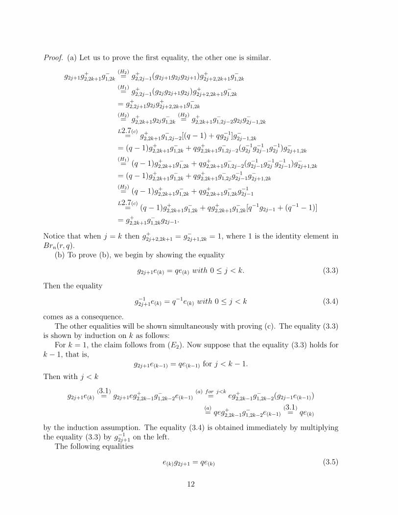
Proof. (a) Let us to prove the first equality, the other one is similar.

g2j+1g+2,2k+1g

−1,2k

(H2)= g+2,2j−1(g2j+1g2jg2j+1)g

+2j+2,2k+1g

−1,2k

(H1)= g+2,2j−1(g2jg2j+1g2j)g

+2j+2,2k+1g

−1,2k

= g+2,2j+1g2jg+2j+2,2k+1g

−1,2k

(H2)= g+2,2k+1g2jg

−1,2k

(H2)= g+2,2k+1g

−1,2j−2g2jg

−2j−1,2k

L2.7(c)= g+2,2k+1g

−1,2j−2[(q − 1) + qg−1

2j ]g−2j−1,2k

= (q − 1)g+2,2k+1g−1,2k + qg+2,2k+1g

−1,2j−2(g

−12j g

−12j−1g

−12j )g

−2j+1,2k

(H1)= (q − 1)g+2,2k+1g

−1,2k + qg+2,2k+1g

−1,2j−2(g

−12j−1g

−12j g

−12j−1)g

−2j+1,2k

= (q − 1)g+2,2k+1g−1,2k + qg+2,2k+1g

−1,2jg

−12j−1g

−2j+1,2k

(H2)= (q − 1)g+2,2k+1g

−1,2k + qg+2,2k+1g

−1,2kg

−12j−1

L2.7(c)= (q − 1)g+2,2k+1g

−1,2k + qg+2,2k+1g

−1,2k[q

−1g2j−1 + (q−1 − 1)]

= g+2,2k+1g−1,2kg2j−1.

Notice that when j = k then g+2j+2,2k+1 = g−2j+1,2k = 1, where 1 is the identity element inBrn(r, q).

(b) To prove (b), we begin by showing the equality

g2j+1e(k) = qe(k) with 0 ≤ j < k. (3.3)

Then the equality

g−12j+1e(k) = q−1e(k) with 0 ≤ j < k (3.4)

comes as a consequence.The other equalities will be shown simultaneously with proving (c). The equality (3.3)

is shown by induction on k as follows:For k = 1, the claim follows from (E2). Now suppose that the equality (3.3) holds for

k − 1, that is,g2j+1e(k−1) = qe(k−1) for j < k − 1.

Then with j < k

g2j+1e(k)(3.1)= g2j+1eg

+2,2k−1g

−1,2k−2e(k−1)

(a) for j<k= eg+2,2k−1g

−1,2k−2(g2j−1e(k−1))

(a)= qeg+2,2k−1g

−1,2k−2e(k−1)

(3.1)= qe(k)

by the induction assumption. The equality (3.4) is obtained immediately by multiplyingthe equality (3.3) by g−1

2j+1 on the left.The following equalities

e(k)g2j+1 = qe(k) (3.5)

12

and

e(k)g−12j+1 = q−1e(k) for 0 ≤ j < k, (3.6)

are proven by induction on k in a combination with (c) in the following way: If (c) holdsfor k − 1 then the equalities (3.5) and (3.6) are proven to hold for k. This result impliesthat (c) holds for k, and hence, the equalities (3.5) and (3.6), again, are true for k + 1.Proceeding in this way, all relations (c), (3.5) and (3.6) are obtained. Indeed, when k = 1(c) follows from direct calculation:

e(2)(E3)= e(g2g3g

−11 g−1

2 )eL2.7(c)= e((q − 1) + qg−1

2 )g3g−11 (q−1g2 − q−1(q − 1))e (3.7)

= q−1(q − 1)eg3g−11 g2e+ eg−1

2 g3g−11 g2e− q−1(q − 1)2eg3(g

−11 e)− (q − 1)eg−1

2 g3(g−11 e)

(E2)= eg−1

2 g3g−11 g2e+ q−1(q − 1)g3(eg

−11 )g2e− q−1(q − 1)2eg3(g

−11 e)− (q − 1)eg−1

2 g3(g−11 e)

(3.2)= eg−1

2 g3g−11 g2e + q−2(q − 1)g3(eg2e)− q−2(q − 1)2eg3e− q−1(q − 1)eg−1

2 g3e

(E2)= eg−1

2 g3g−11 g2e+ q−2(q − 1)rg3e− q−2(q − 1)2e2g3 − q−1(q − 1)eg−1

2 eg3(E1), (E2)

= eg−12 g3g

−11 g2e+ q−2(q − 1)rg3e− q−2(q − 1)(r − 1)eg3 − q−2(q − 1)eg3

= eg−12 g3g

−11 g2e

(H2)= eg−1

2 g−11 g3g2e.

The above equality implies (3.5) for k = 2 and j < 2 in the following way:

e(2)g1(E3)= eg+2,3g

−1,2(eg1)

(E2),(E3)= qe(2);

e(2)g3(3.7)= (eg−1

2 g−11 g3g2e)g3

(E2)= e(g−1

2 g−11 g3g2)g3e

(a) for k=1= (eg1)g

−12 g−1

1 g3g2e(E2)= qeg−1

2 g−11 g3g2e

(3.7)= qe(2).

Therefore, in this case the equality (3.6) follows from multiplying the equality (3.5) withg−12j+1 on the right. As a consequence, (c) is shown to be true for k = 2 by followingcalculation.

e(2)g−4,1g

+5,2e

(E3)= (eg+2,3g

−1,2e)g

−4,1g

+5,2e

(H2)= (eg+2,3g

−1,2e)(g

−4,3g

+5,4)g

−2,1g

+3,2e

(E2)= eg+2,3g

−1,2(g

−4,3g

+5,4)(eg

−2,1g

+3,2e)

(H2),(E3)= eg+2,3g

−14 g5g

−11,3g4e(2)

L2.7(c)= eg+2,3[q

−1g4 + (q−1 − 1)]g5g−1,3[(q − 1) + qg−1

4 ]e(2)= q−1(q − 1)eg+2,5g

−1,3e(2) + eg+2,5g

−1,4e(2) − q−1(q − 1)2eg+2,3g5g

−1,3e(2) − (q − 1)eg+2,3g5g

−1,4e(2)

(3.1)= q−1(q − 1)eg+2,5g

−1,3e(2) + e(3) − q−1(q − 1)2eg+2,3g5g

−1,3e(2) − (q − 1)eg+2,3g5g

−1,4e(2).

Subsequently, it remains to prove that

q−1(q − 1)eg+2,5g−1,3e(2) − q−1(q − 1)2eg+2,3g5g

−1,3e(2) − (q − 1)eg+2,3g5g

−1,4e(2) = 0.

To this end, considering separately each summand in the left hand side of the last equality,

13

it yields

q − 1

qeg+2,5g

−1,3e(2)

(H2)=

q − 1

qeg+2,3g

−1,2g

+4,5(g

−13 e(2)) (3.8)

(3.4) for k=2=

q − 1

q2eg+2,3g

−1,2g

+4,5e(2)

L3.3(d)=

(q − 1)2

q2(r − 1)(eg+2,3g

−1,2)g

+4,5ee(2)

(E2)=

(q − 1)2

q2(r − 1)(eg+2,3g

−1,2e)g

+4,5e(2)

(E3)=

(q − 1)2

q2(r − 1)e(2)g

+4,5e(2)

(E2), (H2)=

(q − 1)2

q2(r − 1)e(2)g4e(2)g5

L3.3(f)=

r(q − 1)3

q2(r − 1)2e(2)g5.

(q − 1)2

qeg+2,3g5g

−1,3e(2)

(E2), (H2)=

(q − 1)2

qeg+2,3g

−1,2(g

−13 e(2))g5 (3.9)

(3.3) for k=2=

(q − 1)2

q2eg+2,3g

−1,2e(2)g5

L3.3(d)=

(q − 1)3

q2(r − 1)(eg+2,3g

−1,2e)e(2)g5

=(q − 1)3

q2(r − 1)e(2)e(2)g5

L3.3(d)=

(q − 1)(r − 1)

q2e(2)g5.

(q − 1)eg+2,3g5g−1,4e(2)

(E2), (H2)= (q − 1)g5eg

+2,3g

−1,2g

−3,4e(2) (3.10)

L3.3(d)=

(q − 1)2

r − 1g5(eg

+2,3g

−1,2)g

−3,4(ee(2))

(E2)=

(q − 1)2

r − 1g5(eg

+2,3g

−1,2e)g

−3,4e(2)

(E3)=

(q − 1)2

r − 1g5(e(2)g

−13 )g−1

4 e(2)

(3.6)for k=2=

(q − 1)2

q(r − 1)g5e(2)g

−14 e(2)

L2.7(c)=

(q − 1)2

q(r − 1)g5e(2)[q

−1g4 + (q−1 − 1)]e(2)

=(q − 1)2

q2(r − 1)g5e(2)g4e(2) −

(q − 1)3

q2(r − 1)g5e(2)e(2)

(E2), (H2), L3.3(d),(f)=

r(q − 1)3

q2(r − 1)2e(2)g5 −

(q − 1)(r − 1)

q2e(2)g5.

By (3.8), (3.9) and (3.10), it implies the equation (c) for k = 2. Now suppose that therelations (3.5) and (3.6) hold for k. We will show that (c) holds for k, and as a consequenceboth (3.5) and (3.6) hold with k + 1. Indeed, we have:

e(k)g−2k,1g

+2k+1,2e

(3.1)= (eg+2,2k−1g

−1,2k−2e(k−1))(g

−12k g

−12k−1g

−2k−2,1)(g2k+1g2kg

+2k−1,2e)

(H2)= (eg+2,2k−1g

−1,2k−2e(k−1))(g

−12k g2k+1)(g

−12k−1g2k)g

−2k−2,1g

+2k−1,2e

(E2), (H2)= eg+2,2k−1g

−1,2k−2(g

−12k g2k+1)(g

−12k−1g2k)e(k−1)g

−2k−2,1g

+2k−1,2e

(H2)= eg+2,2k−1(g

−12k g2k+1)g

−1,2k−2(g

−12k−1g2k)(e(k−1)g

−2k−2,1g

+2k−1,2e).

14

By induction assumption, the last formula is equal to

eg+2,2k−1[q−1g2k + (q−1 − 1)]g2k+1g

−1,2k−1[(q − 1) + qg−1

2k ]e(k),

and direct calculation implies

eg+2,2k+1g−1,2ke(k) + q−1(q − 1)eg+2,2k+1g

−1,2k−1e(k)

− q−1(q − 1)2eg+2,2k−1g2k+1g−1,2k−1e(k) − (q − 1)eg+2,2k−1g2k+1g

−1,2ke(k)

(3.1)= e(k+1) + q−1(q − 1)eg+2,2k+1g

−1,2k−1e(k)

− q−1(q − 1)2eg+2,2k−1g2k+1g−1,2k−1e(k) − (q − 1)eg+2,2k−1g2k+1g

−1,2ke(k).

Applying the same arguments as in the case k = 3, each separate summand in theabove formula can be computed as follows:

q − 1

qeg+2,2k+1g

−1,2k−1e(k) =

q − 1

qeg+2,2k+1g

−1,2k−1(g

−12k−1e(k)) (3.11)

(3.4) for k=

q − 1

q2eg+2,2k+1g

−1,2k−2e(k)

(H2)=

q − 1

q2eg+2,2k−1g

−1,2k−2g

+2k,2k+1e(k)

L3.3(d)=

(q − 1)k

q2(r − 1)k−1(eg+2,2k−1g

−1,2k−2)g

+2k,2k+1(e(k−1)e(k))

(H2), (E2)=

(q − 1)k

q2(r − 1)k−1(eg+2,2k−1g

−1,2k−2e(k−1))g2ke(k)g2k+1

(3.1)=

(q − 1)k

q2(r − 1)k−1e(k)g2ke(k)g2k+1

L3.3(f)=

r(q − 1)2k−1

q2(r − 1)2k−2e(k)g2k+1.

(q − 1)2

qeg+2,2k−1g2k+1g

−1,2k−1e(k)

(H2), (E2)=

(q − 1)2

qg2k+1eg

+2,2k−1g

−1,2k−2(g

−12k−1e(k)) (3.12)

(3.3)for k=

(q − 1)2

q2g2k+1eg

+2,2k−1g

−1,2k−2e(k)

L3.3(d)=

(q − 1)k+1

q2(r − 1)k−1g2k+1(eg

+2,2k−1g

−1,2k−2e(k−1))e(k)

(3.1)=

(q − 1)k+1

q2(r − 1)k−1g2k+1e(k)e(k)

L3.2(d), (E2)=

(q − 1)(r − 1)

q2e(k)g2k+1

(q − 1)eg+2,2k−1g2k+1g−1,2ke(k)

(H2),(E2)= (q − 1)g2k+1(eg

+2,2k−1g

−1,2k−2)g

−2k−1,2ke(k) (3.13)

L3.3(d)=

(q − 1)k

(r − 1)k−1g2k+1(eg

+2,2k−1g

−1,2k−2)g

−2k−1,2k(e(k−1)e(k))

(E2), (H2)=

(q − 1)k

(r − 1)k−1g2k+1(eg

+2,2k−1g

−1,2k−2e(k−1))g

−2k−1,2ke(k)

15

(3.1)=

(q − 1)k

(r − 1)k−1g2k+1(e(k)g

−12k−1)g

−12k e(k)

(3.6) for k=

(q − 1)k

q(r − 1)k−1g2k+1e(k)g

−12k e(k)

L2.7(c)=

(q − 1)k

q(r − 1)k−1g2k+1e(k)[q

−1g2k + (q−1 − 1)]e(k)

=(q − 1)k

q2(r − 1)k−1g2k+1e(k)g2ke(k) −

(q − 1)k+1

q2(r − 1)k−1g2k+1(e(k))

2

L3.3(d),(f)=

r(q − 1)2k−1

q2(r − 1)2k−2e(k)g2k+1 −

(q − 1)(r − 1)

q2e(k)g2k+1.

The above calculations imply that e(k)g−2k,1g

+2k+1,2e = e(k+1). Thus (c) holds with value k.

Using the relation (a), and the equalities (3.5) and (c) for k, it yields the equalities (3.5)and (3.6) for k + 1 as follows:

For j < (k + 1) then

e(k+1)g2j+1(c) for k

= (e(k)g−2k,1g

+2k+1,2e)g2j+1

(E2)= e(k)(g

−2k,1g

+2k+1,2g2j+1)e

(a)for k= (e(k)g2j−1)g

−2k,1g

+2k+1,2e

(3.5) for k= q(e(k)g

−2k,1g

+2k+1,2e)

(c) for k= qe(k+1).

The relation (3.6) for k+1 is obtained by multiplying the relation (3.5) for k+1 by g−12j+1

on the right.

Lemma 3.5. ([24], Lemma 3.4) We have e(j)Hne(k) ⊂ H2j+1,ne(k) +∑

m≥k+1Hne(m)Hn,where j ≤ k. Moreover, if j1 ≥ 2k and j2 ≥ 2k + 1, we also have:

(a) eg+2,j2g+1,j1

e(k) = e(k+1)g+2k+1,j2

g−2k+1,j1, if j1 ≥ 2k and j2 ≥ 2k + 1.

(b) eg+2,j2g+1,j1

is equal to

e(k+1)g+2k+2,j1

g+2k+1,j2+ qN+1(q − 1)

∑kl=1 q

2l−2(g2l+1 + 1)g+2l+2,j2g+2l+1,j1

e(k).

The next lemma is necessary for showing a basis of Brn(r, q).

Lemma 3.6. ([24], Proposition 3.5). The algebra Brn(r, q) is spanned by∑[n/2]

k=0 Hne(k)Hn.In particular, its dimension is at most the one of the Brauer algebra.

3.1. The Brn(r, q)-modules V ∗k

Wenzl [24] defined an action of generators of q-Brauer algebra on module V ∗k as follows:

gjvd =

qvd if sjd = d,

vsjd if l(sjd) > l(d),

(q − 1)vd + qvsjd if l(sjd) < l(d),

and

ehg+2,j2g−1,j1

v1 =

qNhg+3,j2v1 if g−1,j1 = 1,

q−1hg−j2+1,j1v1 if g−1,j1 = 1,

0 if j1 6= 2k and j2 6= 2k + 1,

where v1 is defined as in Lemma 2.4 and h ∈ H3,n.

16

Lemma 3.7. ([24], Proposition 3.6). The action of the elements gj with 1 ≤ j < n ande on V ∗

k as given above defines a representation of Brn(r, q).

3.2. A basis for q-Brauer algebra

We can now find a basis for the q-Brauer algebra that bases on considering diagramsof Brauer algebra. This basis gives a cellular structure on the q-Brauer algebra that willbe shown in the next section. In this section we choose the parameter on the Braueralgebra to be an integer N ∈ Z \ {0}.

Given a diagram d ∈ Dn(N) with exactly 2k horizontal edges, it is considered asconcatenation of three diagrams (d1, ω(d), d2) as follows:

1. d1 is a diagram in which the top row has the positions of horizontal edges as thesein the first row of d, its bottom row is like a row of diagram e(k), and there is no crossingbetween any two vertical edges.

2. Similarly, d2 is a diagram where its bottom row is the same row in d, the other oneis similar to that of e(k), and there is no crossing between any two vertical edges.

3. The diagram ω(d) is described as follows : we enumerate the free vertices, whichjust make vertical edges, in both rows of d from left to right by 2k + 1, 2k + 2, ..., n. Wealso enumerate the vertices in each of two rows of ω(d) from left to right by 1, 2, ..., 2k +1, 2k + 2, ..., n. Assume that each vertical edge in d is connected by i − th vertex of thetop row and j − th vertex of the other one with 2k + 1 ≤ i, j ≤ n. Define ω(d) a diagramwhich has first vertical edges 2k joining m−th points in each of two rows together with1 ≤ m ≤ 2k, and its other vertical edges are obtained by maintaining the vertical edges(i, j) of d.

Example 3.8. For n = 7, k = 2. Given a diagram

•

❚❚❚❚❚❚

❚❚❚❚❚❚

❚ • • • • •

❡❡❡❡❡❡❡❡❡

❡❡❡❡❡❡❡❡❡❡

❡❡❡❡ •

❡❡❡❡❡❡❡❡❡

❡❡❡❡❡❡❡❡❡❡

❡❡❡❡

•d =

• • • • • •

the diagram d can be expressed as product of diagrams in the following:

•

❲❲❲❲❲❲❲❲

❲❲❲❲❲❲❲❲

❲❲ • • • • • •d1

• • • • • • •

• • • • •

❖❖❖❖

❖❖❖❖

❖ •

⑧⑧⑧⑧

•

⑧⑧⑧⑧ ω(d)

• • • • • • •

• • • • •

❣❣❣❣❣❣❣❣

❣❣❣❣❣❣❣❣

❣❣ •

❣❣❣❣❣❣❣❣

❣❣❣❣❣❣❣❣

❣❣ •

❥❥❥❥❥❥

❥❥❥❥❥❥

❥

d2• • • • • • •

.

Thus we have d = (N)−2 · d1ω(d)d2.

Notice that diagram ω(d) can be seen as a permutation of symmetric group S2k+1,n.Since the above expression is unique with respect to each diagram d, the form (d1, ω(d), d2)

17

is determined uniquely. By Lemmas 2.4 and 2.5, there exist unique permutations ω1 ∈ B∗k

and ω2 ∈ Bk such that d1 = ω1e(k) and d2 = e(k)ω2 with ℓ(d1) = ℓ(ω1), ℓ(d2) = ℓ(ω2). Thusa diagram d is uniquely represented by the 3-tuple (ω1, ω(d), ω2) with ω1 ∈ B∗

k, ω2 ∈ Bk

and ω(d) ∈ S2k+1,n such that d = N−kω1e(k)ω(d)e(k)ω2 and ℓ(d) = ℓ(ω1)+ℓ(ω(d))+ℓ(ω2). Wecall such a unique representation a reduced expression of d and briefly write (ω1, ω(d), ω2).

Example 3.9. The above example implies that d1 = ω1e(2) with ω1 = s1,4s2 ∈ B∗2,

d2 = e(2)ω2 with ω2 = s4,1s5,2s6,4 ∈ B2 and ω(d) = s5s6. Thus we obtain

d = N−2(ω1e(2))(s5s6)(e(2)ω2) = ω1e(2)s5s6ω2 = ω1s5s6e(2)ω2.

Hence, d has a unique reduced expression (ω1, s5s6, ω2) = (s1,4s2, s5s6, s4,1s5,2s6,4) with

ℓ(d) = ℓ(ω1) + ℓ(s5s6) + ℓ(ω2) = 5 + 2 + 11 = 18.

Remark 3.10. 1. We abuse notation by denoting e(k) both a certain diagram in the Braueralgebra Dn(N) and an element in the q-Brauer algebra Brn(r, q). Given a diagram d theabove arguments imply that diagrams e(k) and ω(d) commute on the Brauer algebra.Similarly, this also remains on the level of q-Brauer algebra, that is, e(k)gω(d)

= gω(d)e(k).

In particular, since ω(d) ∈ S2k+1,n, it is sufficient to show that

e(k)gi = gie(k) with 2k + 1 ≤ i ≤ n− 1.

Obviously, egi = gie by the equality in (E2). Suppose that e(k−1)gi = gie(k−1), then

e(k)gi(3.1)= (eg+2,2k−1g

−1,2k−2e(k−1))gi = e(g+2,2k−1g

−1,2k−2)gie(k−1)

(H2)= gie(g

+2,2k−1g

−1,2k−2)e(k−1)

(3.1)= gie(k).

2. Wenzl [24] introduced a reduced expression of Brauer diagram d in the general way

ℓ(d) = min{ℓ(δ1) + ℓ(δ2) : d = δ1e(k)δ2, δ1, δ2 ∈ Sn}.

This definition implies several different reduced expressions with respect to a diagramd. In the above construction we give the notation of reduced expression of a diagram dwith a difference. Our definition also bases on the length of diagram d. However, hered is represented by partial diagrams d1, d2 and ω(d) such that d = N−kd1ω(d)d2, and thisallows us to produce a unique reduced expression of d. No surprise that the length of adiagram d is the same in both our description and that of Wenzl, since

d = N−kd1ω(d)d2 = N−k(ω1e(k))ω(d)(e(k)ω2)

= N−k(ω1ω(d))e2(k)ω2 = (ω1ω(d))e(k)ω2

= ω1e(k)(ω(d)ω2) = δ1e(k)δ2

where (δ1, δ2) = (ω1ω(d), ω2) or (δ1, δ2) = (ω1, ω(d)ω2). Therefore

ℓ(d) = ℓ(d1) + ℓ(ω(d)) + ℓ(d2) = min{ℓ(δ1) + ℓ(δ2)}.

18

Example 3.11. We consider the diagram d as in the example 3.8. Using reduced expressiondefinition of Wenzl, d can be rewritten as a product d = δ1e(k)δ2 in the following way:

Case 1.

•

❩❩❩❩❩❩❩❩❩❩

❩❩❩❩❩❩❩❩❩❩

❩❩❩❩❩❩❩ •

⑧⑧⑧⑧

• •

♦♦♦♦♦♦♦♦♦ •

⑧⑧⑧⑧

•

⑧⑧⑧⑧

•

⑧⑧⑧⑧ δ1

• • • • • • •

•

❚❚❚❚❚❚

❚❚❚❚❚❚

❚ • • • • •

❡❡❡❡❡❡❡❡❡❡

❡❡❡❡❡❡❡❡❡❡

❡❡❡ •

❡❡❡❡❡❡❡❡❡❡

❡❡❡❡❡❡❡❡❡❡

❡❡❡

=• • • • • • •

e(2).•

d• • • • • • • • • • • • •

•

❖❖❖❖

❖❖❖❖ •

❚❚❚❚❚❚

❚❚❚❚❚❚

❚ •

❚❚❚❚❚❚

❚❚❚❚❚❚

❚ •

❚❚❚❚❚❚

❚❚❚❚❚❚

❚ •

❣❣❣❣❣❣❣❣

❣❣❣❣❣❣❣❣

❣ •

❣❣❣❣❣❣❣❣

❣❣❣❣❣❣❣❣

❣❣ •

❥❥❥❥❥❥

❥❥❥❥❥❥

❥

δ2• • • • • • •

Where δ1 = ω1s5s6 = s1,4s2s5s6 = s1,6s2 ∈ B∗2 with ℓ(δ1e(2)) = ℓ(δ1) = 7, and

δ2 = ω2 = s4,1s5,2s6,4 ∈ B2, with ℓ(e(2)δ2) = ℓ(δ2) = 11. In this case d has a reducedexpression

(δ1, δ2) = (s1,4s2, s4,1s5,2s6,4)

withℓ(d) = ℓ(δ1) + ℓ(δ2) = 7 + 11 = 18.

Case 2. The diagram d can also be represented by another way as follows:

•

❲❲❲❲❲❲❲❲

❲❲❲❲❲❲❲❲

❲ •

⑧⑧⑧⑧

• •

♦♦♦♦♦♦♦♦♦ •

⑧⑧⑧⑧

• •δ1

• • • • • • •

•

❚❚❚❚❚❚

❚❚❚❚❚❚

❚ • • • • •

❡❡❡❡❡❡❡❡❡

❡❡❡❡❡❡❡❡❡❡

❡❡❡❡ •

❡❡❡❡❡❡❡❡❡

❡❡❡❡❡❡❡❡❡❡

❡❡❡❡

=• • • • • • •

e(2)•

d• • • • • • • • • • • • •

•

❖❖❖❖

❖❖❖❖ •

❚❚❚❚❚❚

❚❚❚❚❚❚

❚ •

❚❚❚❚❚❚

❚❚❚❚❚❚

❚ •

❚❚❚❚❚❚

❚❚❚❚❚❚

❚ •

⑧⑧⑧⑧

•

❡❡❡❡❡❡❡❡

❡❡❡❡❡❡❡❡

❡❡❡❡❡❡ •

❡❡❡❡❡❡❡❡❡❡

❡❡❡❡❡❡❡❡❡❡

❡❡❡

δ2• • • • • • •

.

Where δ1 = ω1 = s1,4s2 ∈ B∗2 with ℓ(δ1e(2)) = ℓ(δ1) = 5,

and δ2 = s5s6ω2 = s5s6s4,1s5,2s6,4 = s4,2s5,1s6,2 ∈ B2 with ℓ(e(2)δ2) = ℓ(δ2) = 13.The reduced expression of d in this case is

(δ1, δ2) = (s1,6s2, s4,2s5,1s6,2)

withℓ(d) = ℓ(δ1) + ℓ(δ2) = 5 + 13 = 18.

Therefore, comparing with the example 3.9 implies that ℓ(d) is the same. Two cases aboveyield that Wenzl’s definition of the reduced expression of a diagram d is not unique since

(s1,4s2, s4,1s5,2s6,4) 6= (s1,6s2, s4,2s5,1s6,2).

19

Definition 3.12. For each diagram d of the Brauer algebra Dn(N), we define a corre-sponding element, say gd, in Brn(r, q) as follows: if d has exactly 2k horizontal edges and(ω1, ω(d), ω2) is a reduced expression of d, then define gd := gω1e(k)gω(d)

gω2. If the diagramd has no horizontal edge, then d is seen as a permutation ω(d) of the symmetric group Sn.And in this case, define gd = gω(d)

.

The main result of this section is stated below.

Theorem 3.13. The q-Brauer algebra Brn(r, q) over the ring R has a basis {gd |d ∈Dn(N)} labeled by diagrams of the Brauer algebra.

Proof. A diagram d of Brauer algebra with exactly 2k horizontal edges has a uniquereduced expression with data (ω1, ω(d), ω2). By the uniqueness of reduced expression withrespect to a diagram d in D(N), the elements gd in Brn(r, q) are well-defined. Observethat these elements gd belong to Hne(k)Hn since gω1, gω(d)

and gω2 are in Hn. Lemma 2.1

shows that there is a faithful representation of the Brauer algebra Dn(N) on⊕[n/2]

k=0 V ∗k .

By Lemma 3.7, this is a specialization of the representation of Brn(r, q) on the same directsum of modules V ∗

k , and hence, the dimension of Brn(r, q) has to be at least the one ofDn(N). Now, the other dimension inequality follows from using the result in Lemma 3.6.The theorem is proved.

The next result provides an involution on the q-Brauer algebra Brn(r, q).

Proposition 3.14. Let i be the map from Brn(r, q) to itself defined by

i(gω) = gω−1 and i(e) = e

for each ω ∈ Sn, extended an anti-homomorphism. Then i is an involution on the q-Brauer algebra Brn(r, q).

Proof. It is sufficient to show that i maps a basis element gd∗ to a basis element i(gd∗) onthe q-Brauer algebra Brn(r, q). If given a diagram d∗ with no horizontal edge, then d∗ isas a permutation in Sn, it implies that obviously i(gd∗) = g(d∗)−1 = gd is a basis elementof the q-Brauer algebra, where d is diagram which is obtained after rotating d∗ downwardvia an horizontal axis. If the diagram d∗ = e(k), then by Definition 3.12 the correspondingbasis element in the q-Brauer algebra is gd∗ = e(k). The equality i(gd∗) = i(e(k)) = e(k)is obtained by induction on k as follows: with k = 1 obviously i(e) = e by definition.Suppose i(e(k−1)) = e(k−1), then

i(e(k))(3.1)= i(eg+2,2k−1g

−1,2k−2e(k−1))

= i(e(k−1))i(g+2,2k−1g

−1,2k−2)i(e)

= e(k−1)g−2k−2,1g

+2k−1,2e

L3.4(c)= e(k).

Now given a reduced expression (ω1, ω(d∗), ω2) of a diagram d∗, where ω1 ∈ B∗k , ω2 ∈ Bk

and ω(d∗) ∈ S2k+1,n, the corresponding basis element on the q-Brauer algebra Brn(r, q) is

20

gd∗ = gω1gω(d∗)e(k)gω2. This yields

i(gd∗) = i(gω1gω(d∗)e(k)gω2) = i(gω2)i(e(k))i(gω(d∗)

)i(gω1) (3.14)

= gω−12e(k)gω−1

(d∗)gω−1

1

Re3.10(1)= gω−1

2gω−1

(d∗)e(k)gω−1

1.

ω1 ∈ B∗k and ω2 ∈ Bk imply that ω−1

1 ∈ Bk and ω−12 ∈ B∗

k . Therefore, by Lemmas2.4 and 2.5, ℓ(e(k)ω

−11 ) = ℓ(ω−1

1 ) and ℓ(ω−12 e(k)) = ℓ(ω−1

2 ). This means that the 3-triple(ω−1

2 , ω−1(d∗), ω

−11 ) is a reduced expression of the diagram d∗ = N−kω−1

2 e(k)ω−1(d∗)e(k)ω

−11 . Thus

i(gd∗) = gω−12gω−1

(d∗)e(k)gω−1

1is a basis element in Brn(r, q) corresponding to the diagram d.

The next corollary is needed for Section 4.

Corollary 3.15. (a) g+2m−1,2je(k) = g+2j+1,2me(k) and g−2m−1,2je(k) = g−2j+1,2me(k)for 1 ≤ m ≤ j < k.

(b) e(k)g+2l,1 = e(k)g

+2,2l+1 and e(k)g

−2l,1 = e(k)g

−2,2l+1 for l < k.

(c) e(k)g+2j,2i−1 = e(k)g

+2i,2j+1 and e(k)g

−2j,2i−1 = e(k)g

−2i,2j+1 for 1 ≤ i ≤ j < k.

(d) (r − 1

q − 1)j−1e(k+1) = e(k)g

−2k,2j−1g

+2k+1,2je(j) for 1 ≤ j < k.

(e) e(k)g2je(j) = r(r − 1

q − 1)j−1e(k) for 1 ≤ j ≤ k.

(f) e(k)Hne(j) ⊂ e(k)H2j+1,n +∑

m≥k+1Hne(m)Hn, where j ≤ k.

Proof. These results, without the relations (a) and (c), are directly deduced from Lemmas3.3 and 3.5 using the property of the above involution. The statement (a) can be provenby induction on m as follow: With m = 1 obviously (a) follows from Lemma 3.3(b) withj = l. Suppose that (a) holds for m− 1, that is,

g+2m−3,2(j−1)e(k) = g+2(j−1)+1,2m−2e(k) and (3.15)

g−2m−3,2(j−1)e(k) = g−2(j−1)+1,2m−2e(k) for 1 ≤ m ≤ j < k. (3.16)

Then

g+2m−1,2je(k) = g−2m−2,2m−3(g+2m−3,2j−2)g

+2j−1,2je(k)

L3.3(c)= g−2m−2,2m−3(g

+2m−3,2j−2)g

+2j+1,2je(k)

(H2)= g−2m−2,2m−3g

+2j+1,2j(g

+2m−3,2j−2)e(k)

(3.15)= g−2m−2,2m−3g

+2j+1,2j(g

+2j−1,2m−2)e(k)

= g−2m−2,2m−3g+2j+1,2m−2e(k)

(H2)= g+2j+1,2mg

−2m−2,2m−3g

+2m−1,2m−2e(k)

L3.3(c)= g+2j+1,2mg

−2m−2,2m−3g

+2m−3,2m−2e(k)

= g+2j+1,2me(k).

21

The other equality is proven similarly. The relation (c) is directly deduced from (a) byusing the involution.

Notice that the equality (c) in Lemma 3.3 is the special case of the above equality (a).

3.3. An algorithm producing basis elements of the q-Brauer algebras

We introduce here an algorithm producing a basis element gd on the q-Brauer algebrasBrn(r, q) from a given diagram d in the Brauer algebra Dn(N). This algorithm’s construc-tion bases on the proof of Lemma 2.4(a) (see Lemma 1.2(a), [24] for a complete proof).From the expression of an arbitrary diagram d as concatenation of three partial diagrams(d1, ω(d), d2) in Subsection 3.2, it is sufficient to consider diagrams d∗ as the form of d1.That is, d∗ has exactly k horizontal edges on each row, its bottom row is like a row ofe(k), and there is no crossing between any two vertical edges. Let D∗

k,n be the set of alldiagrams d∗ above.

Recall that a permutation si,j with 1 ≤ i, j ≤ n− 1 can be considered as a diagram,say d∗(i,j+1) if i ≤ j or d∗(i+1,j) if i > j, in the Brauer algebra such that its free points,including 1, 2,...,i− 1, j + 2, ... n, are fixed.

Example 3.16. In D7(N) the permutation s6,3 corresponds to the diagram

• • •❄❄

❄❄•

❄❄❄❄

•❄❄

❄❄•

❄❄❄❄

•

❣❣❣❣❣❣❣❣

❣❣❣❣❣❣❣❣

❣❣

•d∗(7,3) =

• • • • • •

3.3.1. The algorithm

Given a diagram d∗ of D∗k,n, we number the vertices in both rows of d∗ from left to

right by 1, 2, ..., n. Note that for 2k+1 ≤ i ≤ n if the i-th vertex in its bottom row joinsto the f(i)-th vertex in the top row, then f(i) < f(i + 1) since there is no intersectionbetween any two vertical edges in the diagram d∗. This implies that concatenation ofdiagrams d∗(n,f(n)) and d∗ yields a new diagram

d∗1 = d∗(n,f(n))d∗

whose n-th vertex in the bottom row joins that of the top row and whose other verticaledges retain those of d∗. That is, the diagram d∗1 has the (n− 1)-th vertex in its bottomrow joining to the point f(n − 1)-th vertex in the top row. Again, a concatenation ofdiagrams d∗(n−1,f(n−1)) and d∗1 produces a diagram

d∗2 = d∗(n−1,f(n−1))d∗1 = d∗(n−1,f(n−1))d

∗(n,f(n))d

∗

whose n-th and (n− 1)-th vertices in the bottom row join, respectively, those of the toprow and whose other vertical edges maintain these in d∗.

Proceeding in this way, we determine a series of diagrams d∗(n,f(n)), d∗(n−1,f(n−1)),. . . ,

d∗(2k+1,f(2k+1)) such that

d′ = d∗(2k+1,f(2k+1))...d∗(n−1,f(n−1))d

∗(n,f(n)) d

∗

22

is a diagram in S2ke(k). Here, d′ can be seen as a diagram in D2k(N) with only horizontal

edges to which we add (n−2k) strictly vertical edges to the right. Subsequently, set i2k−2

the label of the vertex in the top row of d′ which is connected with the 2k-th vertex inthe same row and t(2k−2) = si2k−2,2k−2. Then the new diagram

d′1 = t−1(2k−2)d

′

has two vertices 2k-th and (2k− 1)-st in the top row which are connected by a horizontaledge. Proceeding this process, finally d∗ transforms into e(k).

e(k) = t−1(2)...t

−1(2k−4)t

−1(2k−2)d

∗(2k+1,f(2k+1))...d

∗(n−1,f(n−1))d

∗(n,f(n)) d

∗.

Hence, d∗ can be rewritten as d∗ = ωe(k), where

ω = (t−1(2)...t

−1(2k−4)t

−1(2k−2)d

∗(2k+1,f(2k+1))...d

∗(n−1,f(n−1))d

∗(n,f(n)))

−1 (3.17)

= (d∗(2k+1,f(2k+1))...d∗(n−1,f(n−1))d

∗(n,f(n)))

−1(t−1(2)...t

−1(2k−4)t

−1(2k−2))

−1

= d∗(f(n),n)d∗(f(n−1),n−1)... d

∗(f(2k+1),2k+1)t(2k−2)t(2k−4)...t(2)

= sf(n),n−1sf(n−1),n−2... sf(2k+1),2ksi2k−2,2k−2si2k−4,2k−4... si2,2

with f(i) < f(i+ 1) for 2k + 1 ≤ i ≤ n− 1.Notice that the involution ∗ in Dn(N) maps d∗ to the diagram d which is of the form

e(k)ω−1 with

ω−1 = s2,i2 ... s2k−4,i2k−4s2k−2,i2k−2

s2k,f(2k+1)... sn−2,f(n−1)sn−1,f(n).

By Definition 3.12, the corresponding basis elements gd∗ (gd) in the q-Brauer algebra are

gd∗ = gωe(k) and gd = e(k)gω−1 .

Example 3.17. In D7(N) we consider the following diagram d∗

•

❲❲❲❲❲❲❲❲

❲❲❲❲❲❲❲❲

❲❲ •

❲❲❲❲❲❲❲❲

❲❲❲❲❲❲❲❲

❲❲ •

❲❲❲❲❲❲❲❲

❲❲❲❲❲❲❲❲

❲❲ • • • •

•d∗

• • • • • •.

Step 1. Transform d into d′

• • •❄❄

❄❄•

❄❄❄❄

•❄❄

❄❄•

❄❄❄❄

•

❣❣❣❣❣❣❣❣

❣❣❣❣❣❣❣❣

❣❣

•d∗(7, 3)

• • • • • •=

•

❲❲❲❲❲❲❲❲

❲❲❲❲❲❲❲❲

❲❲ •

❲❲❲❲❲❲❲❲

❲❲❲❲❲❲❲❲

❲❲ • • • • •d∗1

•

❲❲❲❲❲❲❲❲

❲❲❲❲❲❲❲❲

❲❲ •

❲❲❲❲❲❲❲❲

❲❲❲❲❲❲❲❲

❲❲ •

❲❲❲❲❲❲❲❲

❲❲❲❲❲❲❲❲

❲❲ • • • • • • • • • • •

•d∗

• • • • • •

;

• •❄❄

❄❄•

❄❄❄❄

•❄❄

❄❄•

❄❄❄❄

•

❣❣❣❣❣❣❣❣

❣❣❣❣❣❣❣❣

❣❣ •

•d∗(6, 2)

• • • • • •=

•

❲❲❲❲❲❲❲❲

❲❲❲❲❲❲❲❲

❲❲ • • • • • •d∗2

•

❲❲❲❲❲❲❲❲

❲❲❲❲❲❲❲❲

❲❲ •

❲❲❲❲❲❲❲❲

❲❲❲❲❲❲❲❲

❲❲ • • • • • • • • • • • •

•d∗1

• • • • • •

;

23

•❄❄

❄❄•

❄❄❄❄•

❄❄❄❄

•❄❄

❄❄•

❣❣❣❣❣❣❣❣

❣❣❣❣❣❣❣❣

❣❣ • •

•d∗(5, 1)

• • • • • •=

• • • • • • •d′

•

❲❲❲❲❲❲❲❲

❲❲❲❲❲❲❲❲

❲❲ • • • • • • • • • • • • •

•d∗2

• • • • • •

;

Step 2. Transform d′ into e(2)

• •❄❄

❄❄•

⑧⑧⑧⑧

• • • •

•t(2)

• • • • • •=

• • • • • • •e(2).

• • • • • • • • • • • • • •

•d′

• • • • • •

Now, the diagram d∗ is rewritten in the form ωe(2), where

ω = (d∗(5, 1)d∗(6, 2)d

∗(7, 3))

−1t(2) = s3,6s2,5s1,4s2.

The corresponding basis element with d∗ in the q-Brauer algebra Br7(r, q) is

gd∗ = gωe(2) = g+3,6g+2,5g

+1,4g2e(2).

Using the involution ∗ in the Brauer algebra Dn(N) yields the resulting diagram d inwhich

d = e(2)ω−1 = e(2)(s3,6s2,5s1,4s2)

−1 = e(2)s2s4,1s5,2s6,3.

Hence,gd = e(2)gω−1 = e(2)g2g

+4,1g

+5,2g

+6,3.

Observe that this result can also be obtained via applying the involution i (see Proposition3.14) on the q-Brauer algebra, that is,

i(gd∗) = i(gωe(2)) = i(g+3,6g+2,5g

+1,4g2e(2)) = e(2)g2g

+4,1g

+5,2g

+6,3 = gd.

Remark 3.18. 1. Combining with Lemma 2.4 the above algorithm implies that given adiagram d∗ of D∗

k,n there exists a unique element ω = tn−1tn−2...t2kt2k−2t2k−4...t2 ∈ B∗k

with tj = sij ,j and ij < ij+1 for 2k+1 ≤ j ≤ n−1, such that d∗ = ωe(k) and ℓ(d∗) = ℓ(ω).Let

B∗k,n = {ω ∈ B∗

k | d∗ = ωe(k) and ℓ(d∗) = ℓ(ω), d∗ ∈ D∗k,n} (3.18)

and

Bk,n = {ω−1| ω ∈ B∗k,n }. (3.19)

24

By Lemma 2.5(a), Bk,n = {ω−1 ∈ Bk| d = e(k)ω−1 and ℓ(d) = ℓ(ω−1), d ∈ Dk,n}, where

Dk,n is the set of all diagrams d which are image of d∗ ∈ D∗k,n via the involution ∗. The

uniqueness of element ω ∈ Bk,n means that |B∗k,n| = |Bk,n| = |Dk,n| = |D∗

k,n|. Given adiagram d∗ in D∗

k,n, since the number of diagrams d∗ is equal to the number of possibilitiesto draw k edges between n vertices on its top row, it implies that,

|B∗k,n| = |Bk,n| =

n!

2k(n− 2k)!k!.

2. For an element ω = tn−1tn−2...t2kt2k−2t2k−4...t2 ∈ B∗k,n if tj = 1 with 2k ≤ j ≤ n− 1

then tj+1 = 1. Indeed, as in (3.17), suppose that tj = sf(j+1),j = 1. This means thecorresponding diagram d∗(f(j+1),j+1) = 1, that is, a diagram with all vertical edges and no

intersection between any two vertical edges. It implies that the (j + 1)-st vertex in thebottom row of diagram d∗ joins the same vertex of the upper one, that is, f(j+1) = j+1.By definition of d∗ in D∗

k,n, the other vertical edges on the right side of the (j + 1)-stvertex of the bottom row has no intersection. This means the (j + 2)-th vertex in thebottom row of diagram d∗ joins the f(j + 2) = (j + 2)-th vertex of the top row. Hence,d∗(f(j+2),j+2) = d∗(j+2,j+2) = 1, that is, tj+1 = sf(j+2),j+1 = sj+2,j+1 = 1.

4. Cellular structure of the q-Brauer algebra Brn(r, q)

This section is devoted to establish cellularity of the q-Brauer algebra. As usual, letk be an integer, 0 ≤ k ≤ [n/2] and denote Dn(N) the Brauer algebra over ring R. DefineV ∗k,n an R-vector space linearly spanned by D∗

k,n. This implies V ∗k,n is an R-submodule

of V ∗k . Hence, by Lemma 2.4(a) a given basis diagram d∗ in V ∗

k,n has a unique reducedexpression in the form d∗ = ωe(k) with ℓ(d∗) = ℓ(ω) and ω ∈ B∗

k,n. Similarly, let Vk,n bean R-vector space linearly spanned by Dk,n, that is, a basis diagram d in Vk,n has exactly2k horizontal edges, its top row is the same as a row of e(k) and there is no intersectionbetween any two vertical edges.The following lemma is directly deduced from definitions.

Lemma 4.1. The R-module V ∗k,n has a basis {d∗ = ωe(k), ω ∈ B∗

k,n}. Dually, the R-module Vk,n has a basis {d = e(k)ω, ω ∈ Bk,n}. Moreover,

dimRVk,n = dimRV∗k,n =

n!

2k(n− 2k)!k!.

Statements below in Lemmas 4.2, 4.4, 4.5 and Corollary 4.3 are needed for laterreference.

Lemma 4.2. Let d∗ be a basis diagram in V ∗k,n and π be a permutation in S2k+1,n. Then

d∗π is a basis diagram in V ∗k satisfying ℓ(d∗π) = ℓ(d∗) + ℓ(π).

Proof. Since d∗ ∈ V ∗k,n, it implies that there exists a unique element ω ∈ B∗

k,n such thatd∗ = ωe(k). Consider π as a diagram in Dn(N) and also observe that two diagrams e(k)and π commute. It follows from concatenation of diagrams d∗ and π that the diagram d∗π

25

is a basis diagram in V ∗k . This yields d∗π = ωe(k)π = ωπe(k). Since the basis diagram d∗

has no intersection between any two vertical edges, the number of intersections of verticaledges in the resulting basis diagram d∗π is equal to that of the diagram π. In fact, thenumber of intersections of vertical edges in the diagram π is equal to its length. Thisproduces ℓ(d∗π) = ℓ(d∗) + ℓ(π).

Corollary 4.3. Let ω be a permutation in B∗k,n and π be a permutation in S2k+1,n. Then

ℓ(ωπ) = ℓ(ω) + ℓ(π) and ωπ ∈ B∗k .

Proof. Set d∗ = ωe(k), then ℓ(d∗) = ℓ(ω) since ω ∈ B∗k,n. Lemma 4.2 implies that ℓ(d∗π) =

ℓ(d∗) + ℓ(π) = ℓ(ω) + ℓ(π) and d∗π = ωπe(k) is a basis diagram in V ∗k . The latter deduces

that ℓ(d∗π) = ℓ(ωπe(k)) ≤ ℓ(ωπ), that is, ℓ(d∗π) ≤ ℓ(ωπ). Immediately, the first equalityfollows from applying the inequality ℓ(ω) + ℓ(π) ≥ ℓ(ωπ).

Let d′ = d∗π ∈ V ∗k , then by Lemma 2.4 there uniquely exists an element ω′ in B∗

k suchthat d′ = ω′e(k) and ℓ(d′) = ℓ(ω′). This implies that

d′ = ωπe(k) = ω′e(k) (4.1)

andℓ(d′) = ℓ(ωπ) = ℓ(ω) + ℓ(π) = ℓ(ω′).

The equality (4.1) yields πe(k) = ω−1ω′e(k). Observe that the basis diagram πe(k) is acombination of two separate parts where the first part includes all horizontal edges onthe left side and the second consists of all vertical edges on the other side. As π and e(k)commute, π corresponds one-to-one with the second part of the basis diagram πe(k). Thisimplies that the basis diagram πe(k) is uniquely presented as a concatenation of diagramsω ∈ S2k+1,n and e(k). Now, the equality πe(k) = ω−1ω′e(k) implies that π = ω−1ω′, that is,ωπ = ω′. So that ωπ ∈ B∗

k .

Lemma 4.4. Let σ be a permutation in B∗k. Then there exists a unique pair (ω′, π′),

where ω′ ∈ B∗k,n and π′ ∈ S2k+1,n, such that σ = ω′π′.

Proof. Observe that σe(k) is a basis diagram in V ∗k in which ℓ(σe(k)) = ℓ(σ) by Lemma

2.4(a). Now suppose that there are two pairs (ω′, π′) and (ω, π) satisfying

σ = ω′π′ = ωπ, (4.2)

where ω, ω′ ∈ B∗k,n and π, π′ ∈ S2k+1,n. Suppose that ω 6= ω′ then ωe(k) 6= ω′e(k)

by definition of B∗k,n. This implies two diagrams ωe(k) and ω′e(k) differ by position of

horizontal edges in their top rows. By definition of diagrams in D∗k,n, the position of

horizontal edges in the top row of the basis diagram ωe(k) (or ω′e(k)) is unchanged after

concatenating it with an arbitrary element of S2k+1,n on the right. This implies thatωe(k)π differs from ω′e(k)π

′, that is, ωπe(k) 6= ω′π′e(k). However, the equality (4.2) yieldsωπe(k) = ω′π′e(k), a contradiction. Thus ω = ω′, and hence, π = π′ by multiplying (4.2)with ω−1 on the left.

26

Lemma 4.5. Let k, l are integers, 0 ≤ l, k ≤ [n/2]. Let ω be a permutation in B∗l,n and

π be a permutation in S2l+1,n. Then there exist ω′ ∈ B∗k,n and π′ ∈ S2k+1,n such that

ωπe(k) = ω′π′e(k).

Proof. Observe that ωπe(k) is a basis diagram in V ∗k by concatenation of diagrams ω, π and e(k).

Using Lemma 2.4(a), there exists a unique element σ ∈ B∗k such that ωπe(k) = σe(k) and

ℓ(ωπe(k)) = ℓ(σ). Lemma 4.4 implies that σ can be rewritten in the form σ = ω′π′, whereω′ and π′ are elements uniquely determined in B∗

k,n and S2k+1,n, respectively. Therefore,σe(k) = ωπe(k) = ω′π′e(k).

Note that given ω ∈ B∗l,n and π ∈ S2l+1,n, Lemma 4.5 can be obtained via a direct

calculation using the defining relations as follows:By Corollary 4.3, ωπ is in the form ωπ = tn−1tn−2...t2lt2l−2t2l−4...t2 ∈ B∗

l , wheretj = 1 or tj = sij ,j for 1 ≤ ij ≤ j ≤ n − 1. Concatenation of ωπ and e(k) will transformωπe(k) into σe(k), where σ = t′n−1t

′n−2...t

′2kt

′2k−2t

′2k−4...t

′2 ∈ B∗

k with t′j = 1 or t′j = sij ,jfor 1 ≤ ij ≤ j ≤ n − 1. This process is done by using defining relations on the Braueralgebra Dn(N), including (S0), (S1), (S2), (3) and (5). In fact, two final relations yieldthe vanishing of some transpositions si in ωπe(k) and the three first imply an rearrangeωπe(k) into σe(k).

Example 4.6. We fix the element ω = s7s5,6s4,5s1,4s2 in B∗2,8 and the element π = s6,7s5 of

S5,8. In the Brauer algebra D8(N) the diagram ωπe(2) corresponds to the diagram d′ = d∗πwhich is the result of concatenating d∗ and π as follows:

•

❲❲❲❲❲❲❲❲

❲❲❲❲❲❲❲❲

❲❲ • • •

❖❖❖❖

❖❖❖❖

❖ •

❖❖❖❖

❖❖❖❖

❖ • •❄❄

❄❄•

•d∗

• • • • • • •=

•

❨❨❨❨❨❨❨❨❨❨

❨❨❨❨❨❨❨❨❨❨

❨❨❨ • • •

❲❲❲❲❲❲❲❲

❲❲❲❲❲❲❲❲

❲❲ • • • •d′.

• • • • •❄❄

❄❄•

❖❖❖❖

❖❖❖❖

❖ •

♦♦♦♦♦♦♦♦♦ •

⑧⑧⑧⑧

• • • • • • • •

•π

• • • • • • •

Using the algorithm in Subsection 3.3, we obtain the element σ = s4,7s6s1,5s3,4s2 ∈ B∗2

satisfyingd′ = σe(2) and ℓ(d′) = ℓ(σ) = 13.

By direct calculation using relations (S1), (S2) on the Brauer algebra Dn(N), it alsotransforms ωπ into σ as follows:

ωπ = (s7s5,6s4,5s1,4s2)(s6,7s5)(S2)= s7s5,6s4,5s6,7s1,5s2

(S2)= s7s5s4(s6s5s6)s7s1,5s2

(S1)= s7s5s4(s5s6s5)s7s1,5s2

(S1)= s7(s4s5s4)s6s5s7s1,5s2

(S2)= s4s5s7s4(s6s7)s5s1,5s2

(S2)= s4s5(s7s6s7)s4s5s1,3s4s5s2

(S1)= s4s5(s6s7s6)s4s1,3(s5s4s5)s2

(S1)= s4,7s6s4s1,3(s4s5s4)s2

(S2)= s4,7s6s1,2(s4s3s4)s5s4s2

(S1)= s4,7s6s1,2(s3s4s3)s5s4s2

(S2)= s4,7s6s1,5s3,4s2.

27

Thus

ωπ = s4,7s6s1,5s3,4s2 ∈ B∗2 . (4.3)

Subsequently, concatenating two diagrams d′ and e(3) produces the diagram d′′

•

❨❨❨❨❨❨❨❨❨❨

❨❨❨❨❨❨❨❨❨❨

❨❨❨ • • •

❲❲❲❲❲❲❲❲

❲❲❲❲❲❲❲❲

❲❲ • • • •

•d′

• • • • • • •=

• • • •

❲❲❲❲❲❲❲❲

❲❲❲❲❲❲❲❲

❲❲ • • • •d′′.

• • • • • • • • • • • • • • • •

•e(3)

• • • • • • •

The algorithm in Section 3.3 identifies a unique element σ′ = s4,7s6s3,4s2 ∈ B∗3 satisfying

d′′ = σ′e(3) and ℓ(d′′) = ℓ(σ′) = 8. In another way, a direct calculation using the definingrelations (S0), (S1), (S2), (3) and (5) also yields the same result. In detail,

ωπe(3) = s4,7s6s1,5s3,4s2e(3)(S2)= s4,7s6s1,4s3s2(s5s4e(3))

(5)= s4,7s6s1,4s3s2(s3s4e(3))

(S1)= s4,7s6s1,4(s2s3s2)s4e(3)

(S2)= s4,7s6s1,3s2(s4s3s4)s2e(3)

(S1)= s4,7s6s1,3s2(s3s4s3)s2e(3)

(S2)= s4,7s6s1,2(s3s2s3)s4(s3s2e(3))

(S1), (5)= s4,7s6s1,2(s2s3s2)s4(s1s2e(3))

(S0), (S2)= s4,7s6s1s3s4(s2s1s2)e(3)

(S1), (S2)= s4,7s6s3s4s1(s1s2s1)e(3)

(S0)= s4,7s6s3,4s2(s1e(3))

(3)= s4,7s6s3,4s2e(3)

(S1), (S2)= s7s4,6s3,4s2(s7e(3))

Thus, we obtain

d′′ = d′e(3) = d∗πe(3) = ωπe(3) = σ′e(3) = ω′π′e(3), (4.4)

where ω′ = s7s4,6s3,4s2 and π′ = s7.

Notice that computing the diagrams σ and σ′ using the algorithm in Section 3.3 is leftfor the reader.

Lemma 4.7. There exists a bijection between the q-Brauer algebra Brn(r, q) and R-vectorspace

⊕[n/2]k=0 V

∗k,n ⊗R Vk,n ⊗R H2k+1,n.

Proof. For a value k the dimension of each V ∗k,n ⊗R Vk,n ⊗R H2k+1,n is calculated by the

formula:

dimRV∗k,n⊗RVk,n⊗RH2k+1,n = dimR(V

∗k,n)·dimR(Vk,n)·dimRH2k+1,n = (

n!

2k(n− 2k)!k!)2·(n−2k)!.

In the Brauer algebra Dn(N) the number of diagrams d which has exactly 2k horizontal

edges is (n!

2k(n− 2k)!k!)2 · (n− 2k)!. Hence

dimR(⊕[n/2]k=0 V

∗k,n ⊗R Vk,n ⊗R H2k+1,n) = dimRDn(N) = 1 · 3 · 5...(2n− 1).

28

Theorem 3.8(a) in [24] implies the dimension of the Brauer algebra and the q-Braueralgebra is the same. Therefore

dimR ⊕[n/2]k=0 V ∗

k,n ⊗R Vk,n ⊗R H2k+1,n = dimRBrn(r, q).

Now an explicit isomorphism will be given. Suppose that d is a diagram with aunique reduced expression (ω1, ω(d), ω2), where ω1 ∈ B∗

k,n, ω2 ∈ Bk,n and ω(d) ∈ S2k+1,n.As indicated in Subsection 3.2, the partial diagrams d1 = ω1e(k) and d2 = e(k)ω2 withℓ(d1) = ℓ(ω1) and ℓ(d2) = ℓ(ω2) are basis diagrams of V ∗

k,n (Vk,n), respectively. Therefore,the diagram d corresponds one-to-one to a basis element

d1 ⊗ d2 ⊗ gω(d)= ω1e(k) ⊗ e(k)ω2 ⊗ gω(d)

of the R-vector space V ∗k,n ⊗R Vk,n ⊗R H2k+1,n. Now, the correspondence between an

arbitrary diagram d in the Brauer algebra and a basis element gd = gω1gω(d)e(k)gω2

of the q-Brauer algebra shown in Theorem 3.13, implies a bijection from Brn(r, q) to

⊕[n/2]k=0 V

∗k,n ⊗R Vk,n ⊗R H2k+1,n linearly spanned by the rule

gd = gω1gω(d)e(k)gω2 7−→ ω1e(k) ⊗ e(k)ω2 ⊗ gω(d)

.

From now on, if no confusion can arise, we will denote by gd both a basis element ofBn(r, q) and its corresponding representation in V ∗

k,n ⊗R Vk,n ⊗R H2k+1,n.

4.1. The R-bilinear form for V ∗k,n ⊗R Vk,n ⊗R H2k+1,n

Now we want to construct an R-bilinear form

ϕk : Vk,n ⊗R V ∗k,n −→ H2k+1,n

for each 0 ≤ k ≤ [n/2].Given elements ω1, ω2 ∈ B∗

k,n, by Lemma 4.7 we form the element Xj := d∗j ⊗dj⊗1 in

V ∗k,n⊗RVk,n⊗RH2k+1,n for j = 1, 2, where d∗j = ωje(k) and dj = e(k)ω

−1j . The corresponding

basis element of Xj in the q-Brauer algebra is Xj = gωje(k)gω−1

j. Then

X1X2 = (gω1e(k)gω−11)(gω2e(k)gω−1

2). (4.5)

Using Lemma 3.5 for j = k implies

e(k)gω−11gω2e(k) ∈ H2k+1,ne(k) +

∑

m≥k+1

Hne(m)Hn.

Hence, e(k)gω−11gω2e(k) can be rewritten as an R-linear combination of the form

e(k)gω−11gω2e(k) =

∑

j

ajgω(cj)e(k) + a′,

29

where aj ∈ R, gω(cj)∈ H2k+1,n, and a′ is a linear combination of basis elements in

∑

m≥k+1Hne(m)Hn. This implies that

X1X2 = gω1(∑

j

ajgω(cj)e(k))gω−1

2+ gω1a

′

gω−12

=∑

j

ajgω1gω(cj)e(k)gω−1

2+ a,

where a is an R-linear combination in∑

m≥k+1Hne(m)Hn. By Definition 3.12, the elementsgω1gω(cj)

e(k)gω−12, denoted by gcj , are basis elements in the q-Brauer algebra, and hence,

the product X1X2 can be rewritten to be∑

j ajgcj + a. Using Lemma 4.7, gcj can beexpressed in the form

gcj = ω1e(k) ⊗ e(k)ω−12 ⊗ gω(cj)

.

Finally, X1X2 can be presented as

X1X2 =∑

j

ω1e(k) ⊗ e(k)ω−12 ⊗ ajgω(cj)

+ a. (4.6)

Subsequently, ϕk : Vk,n ⊗R V ∗k,n −→ H2k+1,n is an R-bilinear form defined by

ϕk(d1, d∗2) =

∑

j

ajgω(cj)∈ H2k+1,n. (4.7)

In a particular case

ϕk(e(k), e(k)) = (r − 1

q − 1)k ∈ H2k+1,n. (4.8)

Also note that, the equality (4.6) and Definition 4.7 yield the product X1X2 in theq-Brauer algebra Brn(r, q)

X1X2 = gω1ϕk(d1, d∗2)e(k)gω−1

2+ a = gω1e(k)ϕk(d1, d

∗2)gω−1

2+ a. (4.9)

We define Jk to be the R−module generated by the basis elements gd in the q-Braueralgebra Brn(r, q), where d is a diagram whose number of vertical edges, say ϑ(d), are lessthan or equal n−2k. It is clear that Jk+1 ⊂ Jk and Jk is an ideal in Brn(r, q). By Lemma

3.6 (see the complete proof in [24]), Jk =∑[n/2]

m=k Hne(m)Hn.

Lemma 4.8. Let gc = c1⊗ c2⊗ gω(c)and gd = d1⊗ d2⊗ gω(d)

, where gω(c), gω(d)

∈ H2k+1,n,c1 = ω1e(k), c2 = e(k)ω2, d1 = δ1e(k), d2 = e(k)δ2 with ω1, δ1 ∈ B∗

k,n and ω2, δ2 ∈ Bk,n.Then

gcgd = c1 ⊗ d2 ⊗ gω(c)ϕk(c2, d1)gω(d)

(mod Jk+1).

Proof. Note that the basis diagram c2 = e(k)ω2 ∈ Vk,n (similarly d1 = δ1e(k) ∈ V ∗k,n) can

be seen as elements

gc2 = e(k) ⊗ e(k)ω2 ⊗ 1 and gd1 = δ1e(k) ⊗ e(k) ⊗ 1

30

in V ∗k,n ⊗R Vk,n ⊗R H2k+1,n. Lemma 4.7 implies that gc2 = e(k)gω2 and gd1 = gδ1e(k) are

corresponding basis elements in the q-Brauer algebra Brn(r, q), respectively. ApplyingLemma 3.5 for j = k, the product of gc2 and gd1 is

gc2gd1 = e(k)gω2gδ1e(k) ∈ H2k+1,ne(k) +∑

m≥k+1

Hne(m)Hn.

Therefore,

gω−12gc2gd1gδ−1

1= (gω−1

2e(k)gω2)(gδ1e(k)gδ−1

1)(4.9)= gω−1

2ϕk(c2, d1)e(k)gδ−1

1+ a,

where a is a linear combination of basis elements in Jk+1 and ϕk(c2, d1) is the abovedefined bilinear form. This means

gc2gd1 = ϕk(c2, d1)e(k) + a′ (4.10)

with a′ = (gω−12)−1a(gδ−1

1)−1 ∈ Jk+1. As a consequence, gcgd is formed as product of basis

elements:

gcgd = (gω1gω(c)e(k)gω2)(gδ1gω(d)

e(k)gδ2)

= gω1gω(c)(e(k)gω2gδ1e(k))gω(d)

gδ2

= gω1gω(c)(gc2gd1)gω(d)

gδ2

(4.10)= gω1gω(c)

(ϕk(c2, d1)e(k) + a′)gω(d)gδ2

= gω1gω(c)ϕk(c2, d1)e(k)gω(d)

gδ2 + a′′

with a′′ ∈ Jk+1. Thus, by Lemma 4.7, gcgd can be expressed as

gcgd ≡ c1 ⊗ d2 ⊗ gω(c)ϕk(c2, d1)gω(d)

(mod Jk+1).

Lemma 4.7 implies that Brn(r, q) has a decomposition as R-modules :

Brn(r, q) = ⊕[n/2]k=0 V

∗k,n ⊗R Vk,n ⊗R H2k+1,n.

Lemma 4.9. Let ω be an arbitrary permutation in B∗k,n and π ∈ S2k+1,n. Then gωgπe(k)

is a basis element in the q-Brauer algebra Brn(r, q).

Proof. Corollary 4.3 yields that the basis diagram d = ωπe(k) satisfies

ℓ(d) = ℓ(ωπ) = ℓ(ω) + ℓ(π).

This means the pair (ω, π) is a reduced expression of d. Therefore, by Definition 3.12 weget the precise statement.

31

Lemma 4.10. Let k, l are integers, 0 ≤ l, k ≤ [n/2]. Let ω be a permutation in B∗l,n and

π a permutation in S2l+1,n. Then

gωgπe(k) =∑

j

ajgω′

jgπ′

je(k),

where aj ∈ R, ω′j ∈ B∗

k,n, and π′j ∈ S2k+1,n.

Proof. Corollary 4.3 implies ℓ(ωπ) = ℓ(ω) + ℓ(π). As a consequence, gωgπ = gωπ byapplying Lemma 2.7(i). The remainder of proof follows from the correspondence betweenthe Brauer algebra Dn(N) and the q-Brauer algebra Brn(r, q) in the following way:

Using the common properties of the Brauer algebra Dn(N) in Section 2 and of theq-Brauer algebra Brn(r, q) shown in whole Section 3, hence, the effect of the basis elementgωπ on e(k) on the left(right) is similar to this of permutation ωπ with respect to diagrame(k), respectively. in the left (right).

In fact, the operations used to move ωπe(k) into ω′π′e(k) in Lemma 4.5 are (S0), (S1),(S2), (3) and (5) on the Brauer algebra Dn(N). In the same way, the product gωπe(k)transforms into the form

∑

j ajgω′

jgπ′

je(k) via using corresponding relations g

2i = (q−1)gi+q

in Definition 2.6(iii), (H1), (H2) on the Hecke algebra of type An−1 as well as two relationsin Lemmas 3.4(b) and 3.3(c).

Example 4.11. Continue considering the same diagram as in Example 4.6 withω = s7s5,6s4,5s1,4s2 ∈ B∗

2,8 and π = s6,7s5 ∈ S5,8.As in 4.3, the product of gω and gπ in the q-Brauer algebra Brn(r, q) is

gωgπL2.7(i)= gωπ

(4.3)= g+4,7g6g

+1,5g

+3,4g2.

Hence,

gωπe(3) = g+4,7g6g+1,5g

+3,4g2e(3)

(H2)= g+4,7g6g

+1,4g3g2(g5g4e(3))

L2.7(c)= g+4,7g6g

+1,4g3g2(g3g4e(3))

(H1)= g+4,7g6g

+1,4(g2g3g2)g4e(3)

(H2)= g+4,7g6g

+1,3g2(g4g3g4)g2e(3)

(H1)= g+4,7g6g1,3g2(g3g4g3)g2e(3)

(H2)= g+4,7g6g

+1,2(g3g2g3)g4(g3g2e(3))

(H1), L3.3(b)= g+4,7g6g

+1,2(g2g3g2)g4(g1g2e(3))

Def2.6(iii), (H2)= g+4,7g6g1((q − 1)g2 + q)g3g4(g2g1g2)e(3)

(H1)= g+4,7g6g1((q − 1)g2 + q)g3g4(g1g2g1)e(3)

L3.4(b)= qg+4,7g6g1((q − 1)g2 + q)g3g4g1g2e(3)

= q(q − 1)g+4,7g6g1g2g3g4g1g2e(3) + q2g+4,7g6g1g3g4g1g2e(3)(H2)= q(q − 1)g+4,7g6g

+1,4g

+1,2e(3) + q2g+4,7g6g

+3,4g1g1g2e(3)

Def2.6(iii)= q(q − 1)g+4,7g6g

+1,4g

+1,2e(3) + q2g+4,7g6g

+3,4((q − 1)g1 + q)g2e(3)

= q(q − 1)g+4,7g6g+1,4g

+1,2e(3) + q2(q − 1)g+4,7g6g

+3,4g

+1,2e(3) + q3g+4,7g6g

+3,4g2e(3)

32

Thus, in the q-Brauer algebra Brn(r, q) the element gωπe(3) is rewritten as an R- linearcombination of elements gωj

e(3) (1 ≤ j ≤ 3), where ωj ∈ B∗3 . Now, using Lemmas 4.5

and 4.9, each element ωj of B∗3 can be uniquely expressed in the form ωj = ω′

jπ′j, where

ω′j ∈ B∗

3,8 and π′j ∈ S7,8, as follows:

gωπe(3) =

3∑

j=1

ajgω′

jgπ′

je(3) =q(q − 1)g7g

+4,6g

+1,4g

+1,2(g7e(3)) (4.11)

+ q2(q − 1)g7g+4,6g

+3,4g

+1,2(g7e(3)) + q3g7g

+4,6g

+3,4g2(g7e(3)).

Note that if fixing r = qN and q → 1, then Brn(r, q) ≡ Dn(N) (see Remark 3.1, [24]).In this case gi becomes the transposition si and the element e(k) can be identified with thediagram e(k). Hence, the last Lemma coincides with Lemma 4.5. This means the equality(4.11) in the above example recovers the equality (4.4) in Example 4.6.

The next statement shows how to get an ideal in Brn(r, q) from an ideal in Heckealgebras.

Proposition 4.12. Let I be an ideal in H2k+1,n. Then Jk+1 + V ∗k,n ⊗R Vk,n ⊗ I is an ideal

in Brn(r, q).

Proof. Given two elements gc = c1 ⊗ c2 ⊗ gω(c)with c ∈ Dn(N) and ϑ(c) = n − 2l, and

gd = d1 ⊗ d2 ⊗ gω(d) with d ∈ Dn(N) and ϑ(d) = n− 2k, we need to prove out that:

(c1 ⊗ c2 ⊗ gω(c))(d1 ⊗ d2 ⊗ gω(d)

) ≡ b⊗ d2 ⊗ agω(d)(mod Jk+1)

for some b ∈ V ∗k , and a is an element in H2k+1,n which is independent of gω(d)

.This property is shown via considering the multiplication of basis elements of the

q-Brauer algebra Brn((r, q) as in the proof of Lemma 4.7. Assume that

gc = gω1e(l)gω(c)gω2 and gd = gδ1e(k)gω(d)

gδ2

are basis elements on Brn(r, q), where ω(d) ∈ S2k+1,n; ω(c) ∈ S2l+1,n; ω1, ω−12 ∈ B∗

l,n and

δ1, δ−12 ∈ B∗

k,n. Then, it implies

gcgd = gω1(e(l)gω(c)gω2gδ1e(k))gω(d)

gδ2 .

In the following we consider two separate cases of l and k.Case 1. If l > k, then Corollary 3.15(f) implies that

e(l)gω(c)gω2gδ1e(k) ∈ e(l)H2k+1,n +

∑

m≥l+1

Hne(m)Hn,

and hence


gδ2 ∈ gω1e(l)H2k+1,ngω(d)gδ2 +

∑

m≥l+1

Hne(m)Hn

⊆ Hne(l)Hn +∑

m≥l+1

Hne(m)Hn

=∑

m≥l

Hne(m)Hn = Jl

l>k⊆ Jk+1.

33

Thus, in this case we obtain gcgd ≡ 0 (mod Jk+1).Case 2. If l ≤ k, then by Lemma 3.5,

e(l)gω(c)gω2gδ1e(k) ∈ H2l+1,ne(k) +

∑

m≥k+1

Hne(m)Hn

and


gδ2 ∈ gω1H2l+1,ne(k)gω(d)gδ2 +

∑

m≥k+1

Hne(m)Hn.

Without loss of generality we may assume that

gcgd = gω1(∑

i

bigω(ci)e(k))gω(d)

gδ2 + b′ =∑

i

bi(gω1gω(ci)e(k))gω(d)

gδ2 + b′,

where bi ∈ R, gω(ci)∈ H2l+1,n, and b′ ∈

∑

m≥k+1Hne(m)Hn.Using Lemma 4.10 with respect to ω1 ∈ Bl and ω(ci) ∈ S2l+1,n, it implies that

gω1gω(ci)e(k) =

∑

j

a(i,j)gω′

(i,j)gπ′

(i,j)e(k),

where a(i,j) ∈ R, ω′

(i,j) ∈ B∗k,n, and π

′

(i,j) ∈ S2k+1,n for l ≤ k.Finally, gcgd can be rewritten as an R - linear combination of basis elements in the

q-Brauer algebra Brn(r, q) as follows:

gcgd =∑

i

bi(gω1gω(ci)e(k))gω(d)

gδ2 + b′

=∑

i

bi(

∑

j

a(i,j)gω′

(i,j)gπ′

(i,j)e(k)

)

gω(d)gδ2 + b′

=∑

i

∑

j

bia(i,j)(gω′

(i,j)gπ′

(i,j)e(k)gω(d)

gδ2) + b′

=∑

i, j

bia(i,j)gω′

(i,j)gπ′

(i,j)gω(d)

e(k)gδ2 + b′,

where π′(i,j) and ω(d) are in S2k+1,n; bia(i,j) ∈ R; ω′

(i,j) ∈ B∗k,n and δ2 ∈ Bk,n. Lemma 4.7

implies that the corresponding element of gcgd in V ∗k,n ⊗R Vk,n ⊗R H2k+1,n is

gcgd ≡∑

i, j

bia(i,j)(ω′(i,j)e(k) ⊗ e(k)δ2 ⊗ gπ′

(i,j)gω(d)

) mod Jk+1

≡∑

i, j

(ω′(i,j)e(k) ⊗ e(k)δ2 ⊗ (bia(i,j))gπ′

(i,j)gω(d)

) mod Jk+1

≡ b⊗ d2 ⊗ agω(d)(mod Jk+1),

where b =∑

i, j ω′(i,j)e(k) ∈ V ∗

k , a =∑

i, j bia(i,j)gπ′

(i,j)∈ H2k+1,n, and d2 = e(k)δ2.

34

The following lemma describes the effect of the involution i of the q-Brauer algebra on

V ∗k,n ⊗R Vk,n ⊗R H2k+1,n.

Lemma 4.13. (a) If gd = d1 ⊗ d2⊗ gω(d)with a reduced expression d = (ω1, ω(d), ω2) in

Dn(N). Theni(gd) = d−1

2 ⊗ d−11 ⊗ i(gω(d)

)

with d−12 = ω−1

2 e(k) ∈ V ∗k,n and d−1

1 = e(k)ω−12 ∈ Vk,n.

(b) The involution i on H2k+1,n and the R − bilinear form ϕk have the followingproperty:

iϕk(c, d) = ϕk(d−1, c−1)

for all c ∈ Vk,n and d ∈ V ∗k,n.

Proof. Part (a). The basis element corresponding to the reduced expression d = (ω1, ω(d), ω2)is gd = gω1e(k)gπ(d)

gω2 . As shown in (3.14) of Proposition 3.14, the image of gd via involu-tion i is

i(gd) = gω−12e(k)gω−1

(d)gω−1

1

with ℓ(d−12 ) = ℓ(ω−1

2 e(k)) = ℓ(ω−12 ) and ℓ(d−1

1 ) = ℓ(e(k)ω−11 ) = ℓ(ω−1

1 ). Definitions ofV ∗k,n and Vk,n imply that d−1

1 ∈ Vk,n and d−12 ∈ V ∗

k,n. Hence, by Lemma 4.2, i(gd) can berewritten as

i(gd) = d−12 ⊗ d−1

1 ⊗ i(gω(d))

in V ∗k,n ⊗R Vk,n ⊗R H2k+1,n.

Part (b). Using the same argument as in the proof of Lemma 4.8, c and d canbe expressed as basis elements in V ∗

k,n ⊗R Vk,n ⊗R H2k+1,n with gc = e(k) ⊗ c ⊗ 1 andgd = d⊗ e(k) ⊗ 1, where 1 is identity in H2k+1,n. As a consequence,

gcgd = (e(k) ⊗ c⊗ 1)(d⊗ e(k) ⊗ 1)L4.8= e(k) ⊗ e(k) ⊗ ϕk(c, d) (mod Jk+1).

This means the corresponding basis element in the q-Brauer algebra is gcgd = e(k)ϕk(c, d)+a with a ∈ Jk+1. And hence,

i(gcgd) = i(e(k)ϕk(c, d) + a) = i(ϕk(c, d))i(e(k)) + i(a)

P3.14= i(ϕk(c, d))e(k) + i(a)

Rem3.10(1)= e(k)i(ϕk(c, d)) + i(a).

Thus, the corresponding element in V ∗k,n ⊗R Vk,n ⊗R H2k+1,n is of the form

i(gcgd) = i(e(k) ⊗ e(k) ⊗ ϕk(c, d)) = e(k) ⊗ e(k) ⊗ iϕk(c, d) (mod Jk+1) (4.12)

since i(a) ∈ Jk+1.In another way, the part (1) implies that i(gc) = c−1 ⊗ e(k) ⊗ 1 and i(gd) = e(k) ⊗ d−1⊗ 1.Therefore,

i(gd)i(gc) = (e(k) ⊗ d−1 ⊗ 1)(c−1 ⊗ e(k) ⊗ 1)L4.8= e(k) ⊗ e(k) ⊗ ϕk(d

−1, c−1) (mod Jk+1).(4.13)

35

Now the equality i(gcgd) = i(gd)i(gc) shows that

e(k) ⊗ e(k) ⊗ iϕk(c, d) = e(k) ⊗ e(k) ⊗ ϕk(d−1, c−1),

that is, iϕk(c, d) = ϕk(d−1, c−1).

The below statement gives an ′iterated inflation′ structure for the q-Brauer algebrasBrn(r, q), and the proof of this comes from above results.

Proposition 4.14. The q-Brauer algebra Brn(r, q) is an iterated inflation of Hecke alge-bras of type An−1. More precisely: as a free R-module, Brn(r, q) is equal to

V ∗0,n ⊗R V0,n ⊗R Hn ⊕ V ∗

1,n ⊗R V1,n ⊗R H3,n ⊕ V ∗2,n ⊗R V2,n ⊗R H5,n ⊕ ...,

and the iterated inflation starts with Hn, inflates it along V ∗k,n ⊗R Vk,n and so on, ending

with an inflation of R = Hn,n or R = Hn+1,n as bottom layer (depending on whether n isodd or even), where H2k+1,n is Hecke algebra with generators g2k+1, g2k+2... gn−1.

Corollary 4.15. The statement in Proposition 4.14 holds on Brn(N).

Before giving the main result we need the following lemma. This lemma is shown in[27] as a condition to ensure that an algebra has cellular structure.

Lemma 4.16. ([27], Lemma 3.3) Let A be a Λ − algebra with an involution i. Supposethere is a decomposition

A = ⊕mj=1V(j) ⊗Λ V(j) ⊗Λ Bj (direct sum of Λ−modules)

where V(j) is a free Λ − modules of finite rank and Bj is a cellular Λ − algebra with

respect to an involution δj and a cell chain J j1 ⊂ J j

2 ... ⊂ J jsj= Bj for each j. Define Jt =

⊕tj=1V(j)⊗Λ V(j)⊗ΛBj. Assume that the restriction of i on ⊕t

j=1V(j)⊗Λ V(j)⊗ΛBj is givenby w⊗v⊗b −→ v⊗w⊗δj(b). If for each j there is a bilinear from ϕj : V(j)⊗Λ V(j) −→ Bj

such that δj(ϕj(w, v)) = ϕj(v, w) for all w, v ∈ V(j) and that the multiplication of twoelements in V(j) ⊗Λ V(j) ⊗Λ Bj is governed by φj modulo Jj−1; that is, for x, y, u, v ∈ V(j),and b, c ∈ Bj, we have

(x⊗ y ⊗ b)(u ⊗ v ⊗ c) = x⊗ v ⊗ bϕj(y, u)c

modulo the ideal Jj−1, and if V(j)⊗Λ V(j)⊗Λ Jjl + Jj−1 is an ideal in A for all l and j, then

A is a cellular algebra.

Theorem 4.17. Suppose that Λ is a commutative noetherian ring which contains R as asubring with the same identity. If q, r and (r − 1)/(q − 1) are invertible in Λ, then theq-Brauer algebra Brn(r, q) over the ring Λ is cellular with respect to the involution i.

36

Proof. From the above construction, we know that V ∗k,n and Vk,n has the same finite rank.

Now apply Lemma 4.16 to the q-Brauer algebra Brn(r, q) with j = k. Set Bn−2k = H2k+1,n

with 0 ≤ k ≤ [n/2], then the q-Brauer algebra Brn(r, q) has a decomposition

Brn(r, q) = V ∗0,n ⊗Λ V0,n ⊗Λ Hn ⊕ V ∗

1,n ⊗Λ V1,n ⊗Λ H3,n ⊕ V ∗2,n ⊗Λ V2,n ⊗Λ H5,n⊕

...⊕ V ∗[n/2]−1,n ⊗Λ V[n/2]−1,n ⊗Λ H2[n/2]−1,n ⊕ V ∗

[n/2],n ⊗Λ V[n/2],n ⊗Λ H2[n/2]+1,n,

where Hn,n = Hn+1,n = Λ and V ∗0,n = V0,n = Λ. Lemmas 4.2, 4.7, 4.8, 4.13, Proposition

4.12 and Theorem 2.12 show that the conditions of the lemma 4.16 applied for q-Braueralgebra are satisfied. Thus, the q-Brauer algebra Brn(r, q) is a cellular algebra.

Corollary 4.18. Suppose that Λ is a commutative noetherian ring which contains R asa subring with the same identity. If q, r and [N ] are invertible in Λ, then the q-Braueralgebra Brn(N) over the ring Λ is cellular with respect to the involution i.

Remark 4.19. By Remark 3.2(2), in the case q = 1 the statements in Corollaries 4.15 and4.18 recover these of the Brauer algebra Dn(N) due to Koenig and Xi (see [17], Theorem5.6).

As a consequence of Theorem 4.17, we have the following parametrization of cellmodules for q-Brauer algebra. Given a natural number n, denote by I the set {(n−2k, λ)|k is a non negative integer with 0 ≤ k ≤ [n/2], λ - a partition of (n− 2k) with the shape(λ1, λ2, ..., λl)}.

Corollary 4.20. Let r, q and (r−1)/(q−1) are invertible over a commutative Noetherianring R. The q-Brauer algebra Brn(r, q) over R has the set of cell modules

{∆k(λ) = V ∗k,n ⊗ dk ⊗∆(λ)|(n− 2k, λ) ∈ I}

where dk is non-zero elements in Vk,n and ∆(λ) are cell modules of the Hecke algebraH2k+1,n corresponding to the partition λ of (n− 2k).

Let us describe here what is the R-bilinear form, say Φ(k,λ), on cellular q-Brauer algebraBrn(r, q). For a general definition of the R-bilinear form induced by cellular algebras werefer the reader to [13].

Definition 4.21. Keep the above notations. Define

Φ(k,λ) : ∆k(λ)×∆k(λ) −→ R

determined by

Φ(k,λ)(d∗k ⊗ b⊗ x, c⊗ dk ⊗ y) := φ(k,λ)(xϕk(b, c), y)

is an R-bilinear form, where (d∗k ⊗ b ⊗ x) and (c ⊗ dk ⊗ y) are in ∆k(λ) and φ(k,λ) is thesymmetric R-bilinear form on the Hecke algebra H2k+1,n.

37

In the following we assume that R is a field which contains non-zero elements q, r.Let e(q) be the least positive integer m such that [m]q = 1 + q + q2...+ qm−1 = 0, if thatexists, let e(q) = ∞ otherwise. Notice that, q can be also seen as an e(q) − th primitiveroot of unity and e(q) = ∞ if q is not an m − th root of unity for all m. Recall that apartition λ = (λ1, λ2, ..., λl) is called e(q)-restricted if λj − λj+1 < e(q), for all j.

Theorem 4.22. Let Brn(r, q) be the q-Brauer algebra over an arbitrary field R withcharacteristic p ≥ 0. More assume that q, r and (r− 1)/(q− 1) are invertible in R. Thenthe non-isomorphic simple Brn(r, q)-modules are parametrized by the set {(n−2k, λ) ∈ I|λ is an e(q)-restricted partition of (n - 2k)}.

Proof. By Theorem 4.17, the q-Brauer algebra Brn(r, q) is cellular. As a consequence,it follows from Corollary 4.20 above and ([13], Theorem 3.4) that the simple Brn(r, q)-modules are parametrized by the set {(n − 2k, λ) ∈ I | Φ(k,λ) 6= 0}. If n − 2k 6= 0,then given a pair of basis elements gc = e(k) ⊗ e(k) ⊗ gω(c)

, gd = e(k) ⊗ e(k) ⊗ gω(d)in

V ∗k,n ⊗R Vk,n ⊗R H2k+1,n with gω(c)

and gω(d)are in ∆(λ), it follows from Definition 4.21

and Lemma 4.8 that

Φ(k,λ)(gc, gd) = Φ(k,λ)(e(k) ⊗ e(k) ⊗ gω(c), e(k) ⊗ e(k) ⊗ gω(d)

)

= φ(k,λ)(gω(c)ϕk(e(k), e(k)), gω(d)

)

(4.8)= (

r − 1

q − 1)kφ(k,λ)(gω(c)

, gω(d)).

The last formula implies that Φ(k,λ) 6= 0 if and only if the corresponding linear form φ(k,λ)

for the cellular algebra H2k+1,n is not zero. By using a result of Dipper and James ([6],Theorem 7.6) that states that φ(k,λ) 6= 0 if and only if λ is an e(q)-restricted partition of(n − 2k) it yields Φ(k,λ) 6= 0 if and only if the partition λ of n-2k is e(d)-restricted. If

n−2k = 0 then the last formula above implies Φ(k,λ) = (r − 1

q − 1)[n/2] 6= 0. Hence, we obtain

the precise statement.

Remark 4.23. The last theorem points out that all simple Brn(r, q)-modules are labeledby Young diagrams [λ] with n, n-2, n-4, ... boxes, where each Young diagram [λ] withe(q)-restricted partition λ of n − 2k indexes a simple module ∆(λ) of the Hecke algebraH2k+1,n

The next consequence follows from applying Theorem 4.17 and a result in ([16], Propo-sition 3.2) on cellular algebras:

Corollary 4.24. Let Brn(r, q) be the q-Brauer algebra over a field R with r, q, and(r− 1)/(q− 1) are invertible elements. Then the determinant of the the Cartan matrix Cof the q-Brauer algebra is a positive integer, where the entries of C are by definition themultiplicities of composition factors in indecomposable projective modules.

As another consequence of Theorem 4.17 and ([13], Theorem 3.8), we obtain thefollowing corollary.

Corollary 4.25. Under the assumption of the Theorem 4.17, the q-Brauer algebra issemisimple if and only if the cell modules are simple and pairwise non-isomorphic.

38

5. Quasi-heredity of Brn(r, q) over a field

Let R be a field and q, r are non-zero elements in R. It is well-known that in someexplicit cases the cellularity of algebras can provide the quasi-hereditary structure onthemselve. More precisely, Koenig and Xi [14, 16] and Xi [27, 28] pointed out that withsuitable choices of parameters Brauer algebras, Partition algebras, Temperley-Lieb alge-bras of type A and BMW algebras are quasi-hereditary. These enable us to be interestedin the existence of the quasi-hereditary structure of the q-Brauer algebra. The questionis that what conditions the q-Brauer algebra is quasi-hereditary. Let us first recall thedefinition of quasi-hereditary algebras introduced in [5] due to Cline, Parshall and Scott.The examples of quasi-hereditary algebras are given in [22, 5].

Definition 5.1. Let A be a finite dimensional R-algebra. An ideal J in A is calleda hereditary ideal if J is idempotent, J(rad(A))J = 0 and J is a projective left (orright) A-module. The algebra A is called quasi-hereditary provided there is a finite chain0 = J0 ⊂ J1 ⊂ J0 ⊂ ... ⊂ Jn = A of ideals in A such that Ji+1/Ji is a hereditary ideal inA/Ji for all i. Such a chain is then called a heredity chain of the quasi-hereditary algebra A.

Subsequently, we give an positive answer with respect to q-Brauer algebras. We statebelow when the q-Brauer algebra is quasi-hereditary. It is well-known that the Heckealgebra Hn is semisimple if and only if e(q) > n. This is shown by Dipper and James (see[6] or [7] for more details).

Theorem 5.2. Let R be any field with 0 6= q, r ∈ R. Assume more that (r−1)/(q−1) 6= 0.Then the q-Brauer algebra Brn(r, q) is quasi-hereditary if and only if e(q) is strictly biggerthan n.

Proof. Suppose that the q-Brauer algebra is quasi-hereditary. For any choices of non-zeroparameter, the q-Brauer algebra has a quotient Hn, the Hecke algebra of type An−1, andthis quotient actually arises as Brn(r, q)/J1 for some ideal in the cell chain. Furthermore,we know by [16] that any cell chain is a hereditary chain and also note that a self-injectivealgebra is quasi-heredity if and only if it is semisimple. Thus, as a consequence, the Heckealgebra Hn is semisimple, that is, e(q) > n.

Conversely, if e(q) is strictly bigger than n, then using Theorem 7.6 [6], Hn is semisim-ple and so, all subalgebras H2k+1,n of Hn are semisimple. To prove that under our assump-tion the algebra Brn(r, q) is quasi-hereditary, we need to show by [16] that the square(V ∗

k,n ⊗R Vk,n ⊗R H2k+1,n)2 is not zero modulo Jk+1 for all 0 ≤ k ≤ [n/2]. Proceed as in

[16], let {gλS,T | λ is a partition of the form (λ1, λ2, ..., λl) and S, T are standard tableauxof shape λ} be a cellular basis of the semisimple cellular algebra H2k+1,n. Then there aretwo elements gλS,T and gλU,V such that gλS,Tg

λU,V is not zero modulo the span of all gµ

S′ ,T ′ ,

where µ strictly smaller than λ and S ′, T ′ are standard tableau of shape µ . Take theelement e(k) in V ∗

k,n (Vk,n) and consider the product of e(k)⊗e(k)⊗gλS,T and e(k)⊗e(k)⊗gλU,V .

39

By Lemma 4.8

x := (e(k) ⊗ e(k) ⊗ gλS,T )(e(k) ⊗ e(k) ⊗ gλU,V )

≡ e(k) ⊗ e(k) ⊗ gλS,Tϕk(e(k), e(k))gλU,V

(4.8)≡ e(k) ⊗ e(k) ⊗ gλS,T (

r − 1

q − 1)kgλU,V

≡ e(k) ⊗ e(k) ⊗ (r − 1

q − 1)k(gλS,Tg

λU,V ) (mod Jk+1).

Sincer − 1

q − 16= 0, x is non-zero modulo Jk+1.

As a consequence of the last theorem and (Theorem 3.1, [16]), we obtain the followingcorollary.

Corollary 5.3. Let R be any field with q, r, and (r − 1)/(q − 1) are simultaneouslynon-zero in R. If e(q) > n, then

(a) Brn(r, q) has finite global dimension.(b) The Cartan determinant of Brn(r, q) is 1.(c) The simple Brn(r, q)−module can be parametrized by the set of all pairs (n−2k, λ)

with 0 ≤ k ≤ [n/2] and λ is an e(q)-restricted partition of (n-2k) of the form (λ1, λ2, ..., λl).

We obtain the similar results for the version Brn(N) as follows:

Corollary 5.4. Let R be any field with q, r, and [N ] are simultaneously non-zero in R.Then the q-Brauer algebra Brn(N) is quasi-hereditary if and only if e(q) is strictly biggerthan n.

Corollary 5.5. Let R be any field with q, r, and [N ] are simultaneously non-zero in R.If e(q) > n, then

(a) Brn(N) has finite global dimension.(b) The Cartan determinant of Brn(N) is 1.(c) The simple Brn(N)−module can be parametrized by the set of all pairs (n−2k, λ)

with 0 ≤ k ≤ [n/2] and λ is an e(q)-restricted partition of (n-2k) of the form (λ1, λ2, ..., λl).

Remark 5.6. Note that if q = 1 then [m]q = 1 + 1 + 12...+ 1m−1 = m = 0 and hence e(q)is equal to the characteristic of R. As a consequence, the result in Corollary 5.4 recoversthis of the Brauer algebra Dn(N) with the nonzero parameter due to Koenig and Xi (see[16], Theorem 1.3).

AcknowledgmentsI would like to thank Professor Hans Wenzl for useful discussions. I am specially

grateful to my supervisor, Professor Steffen Koenig, for constant support and valuableadvice during this work. The research work is financially supported by the Project MOET-322 of the Training and Education Ministry of Vietnam and (partly) by the DFG PriorityProgram SPP-1489. I would also like to express my gratitude for this.

40

References

[1] J. Birman, H. Wenzl, Braids, link polynomials and a new algebra, Trans. Amer.Math. Soc. 313 (1) (1989) 249-273.

[2] R. Brauer, On algebras which are connected with the semisimple continuous groups,Ann. of Math. 63 (1937) 854-872.

[3] W.P. Brown, An algebra related to the orthogonal group, Michigan Math. J. 3 (1955)1-22.

[4] W.P. Brown, The semisimplicity of ωnf , Ann. of Math. (2) 63 (1956) 324 - 335.

[5] E. Cline, B. Parshall, L. Scott, Finite dimensional algebras and highest weight cate-gories, J. Reine Angew. Math. 391 (1988) 85-99.

[6] R. Dipper, G.D. James, Representations of Hecke algebras and general linear groups,Proc.London Math. Soc (3) 52 (1986) 20-52.

[7] R. Dipper, G.D. James, Blocks and idempotents of Hecke algebras and general lineargroups, Proc. London Math. Soc. (3) 54 (1) (1987) 57 - 82.

[8] W. Doran, D. Wales, P. Hanlon, On the semisimplicity of the Brauer centralizeralgebras, J. Algebra. 211 (1999) 647 - 685.

[9] P. Hanlon, D. Wales, On the decomposition of Brauer’s centralizer algebras, J. Al-gebra. 121 (2) (1989) 409 - 445.

[10] P. Hanlon, D. Wales, Computing the discriminants of Brauer’s centralizer algebras,Math. Comp. 54 (1990) 771 - 796.

[11] A.M. Gavrilik, A.U. Klimyk, q-Deformed orthogonal and pseudo-orthogonal algebrasand their representations, Lett. Math. Phys. 21(3) (1991) 215-220.

[12] M. Geck, Hecke algebras of finite type are cellular, Invent. Math. 169 (3) (2007)501-517.

[13] J.J. Graham, G. I. Lehrer, Cellular algebras, Invent. Math. 123 (1) (1996) 1-34.

[14] S. Konig, C. C. Xi, On the structure of cellular algebras. In: Algebras and modulesII (Geiranger 1996), CMS Conf. Proc. 24, Amer. Math. Soc. (1998) 365-386.

[15] S. Konig, C. C. Xi, Cellular algebras: Inflations and Morita equivalences, JournalLondon Math. Soc. (2) 60 (1999) 700-722.

[16] S. Konig, C. C. Xi, When is a cellular algebra quasi-heredity?, Mat. Ann. 315 (1999)281-293.

[17] S. Konig, C. C. Xi, A characteristic free approach to Brauer algebras, Trans. Amer.Math. Soc. 353 (4) (2000)1489-1505.

41

[18] A.I. Molev, A new quantum analog of the Brauer algebra, Czechoslovak J. Phys. 53(2003) 1073-1078.

[19] A.I. Molev, private communication.

[20] E. Murphy, The representations of Hecke algebras of type An, J.Algebra 173(1) (1995)97-121.

[21] J. Murakami, The Kauffman polynomials of links and representation theory, OsakaJ. Math. 24(4) (1987) 745-758.

[22] B. Parshall, L. Scott, Derived categories, quasi-hereditary algebras and algebraicgroups, in “Proceeding of the Ottawa-Moosonee Workshop in Algebra 1987”, Math.Lecture Note series, Carleton University, 1988.(1997) 411-461.

[23] H. Wenzl, On the structure of Brauer’s centralizer algebras, Ann. of Math. 128 (1988)173-193.

[24] H. Wenzl, A q-Brauer algebra, J. Algebra 358 (2012) 102-127.

[25] H. Wenzl, Quotients of representation rings, Represnet. Theory 15 (2011) 385-406.

[26] H. Wenzl, Fusion symmetric spaces and subfactors, preprint, arXiv:1108.1428.

[27] C. C. Xi, Partition algebras are cellular, Compositio Math. 119 (1) (1999) 99-109.

[28] C. C. Xi, On the quasi-heredity of Birman-Wenzl algebras, Adv. Math. 154 (2000)280-298.

42

http://arxiv.org/abs/1108.1428

PHan phoi student

Documents

Transcript of PHan phoi student