Performance measurement of Soft Computing models based on Residual Analysis
23
National Conference on Converging Technologies beyond 2020, (CTB-2020), April 6, 7, 2011 International Journal of Applied Engineering Research, ISSN 0973-4562 Vol.6 No.5 (2011) Organized by: University Institute of Engineering and Technology, Kurukshetra University, Kurukshetra [Page No - 820] Isolation of Pseudomonas aeruginosa Specific Bacteriophage from Sewage Sample Swati Dahiya 1 , Anamika Singh 2 , Deepali Gupta 3 and Neha Sharma 4 Department of Biotechnology Engineering University Institute of Engineering and Technology Kurukshetra University, Kurukshetra (136119), India Email: 1 [email protected], 2 [email protected], 3 [email protected] 4 [email protected] Abstract-The purpose of this study was to isolate Pseudomonas aeruginosa specific bacteriophage. Pseudomonas aeruginosa is an opportunistic, nosocomial pathogen of immunocompromised individuals and causes various diseases due to lack of proper and periodic attention to water quality. The biofilm produced by it causes chronic infections due to pyocyanin present in it.In the present work, bacteriophages specific to P. aeruginosa were isolatedfrom sewage sample taken from Sewage Treatment Plant, Kurukshetra by employing double agar overlay method. The sample was filtered and poured over nutrient agar plates along with overnight grown bacterial culture. Plates were then incubated for 24-48 hr at 37 ᵒ C. Plaques (clear zones) appeared on the plates, which indicated the presence of specific bacteriophage. The phages were isolated and then purified. The purified phages were finally concentrated. So,a sensitive and rapidassay method for the specific detection of Pseudomonas aeruginosa can be developed using these bacteriophages. Bacteriophages can be used to provide specific lysis of the bacteria and aid in the formation of a biosensor to detect the presence of P.aeruginosa. Keywords- Bacteriophage; Sewage sample; Pseudomonas aeruginosa; Biofilm; Multiplicity of infection I. INTRODUCTION Bacteriophages are the viruses of prokaryotes. These are bacterial viruses that invade bacterial cells and are amongst the most abundant living entities on earth playing important roles in maintaining the natural abundance and distribution of microorganisms. Phage for a given bacterium can be isolated wherever that bacterium grows, such as in faeces, sewage, soil, hot springs, oceans, etc. Water from the Ganges (India) has been found to be a rich source of vibrio phages[1]. The problem is not in isolating phage against particular bacteria but in selecting the ones most likely to be useful for clinical purposes. This includes lytic phages that have high efficacy and broad spectrum activity on clinically important strains. These should not be temperate phages that carry toxigenic genes. Phages should be such that they can be readily produced in large quantity and should be stable during storage. One feature that makes bacteriophage so attractive is their highly discriminatory nature. Most of the known bacteriophages are specialists that interact only with a specific set of bacteria that express specific binding sites; bacteria without these receptors are not affected. Pseudomonas aeruginosa is a gram negative free living bacterium and an opportunistic pathogen that can inhabit environments including plants, soil, water and other moist locations[2]. P. aeruginosa nowadays is commonly isolated from cases of nosocomial infections especially from compromised hosts, such as patients suffering from respiratory diseases, cancer, children and young adults with cystic fibrosis and burns. According to the National Nosocomial Infections Surveillance System, P. aeruginosa is the third most common pathogen associated with all hospital acquired infections, accounting for 10.1% of all nosocomial infections and is associated with a high mortality rate[3]. One of the reasons for its increased virulence is its notable resistance to many currently available antibiotics. As a result, novel and most effective approaches for treating infections caused by multidrug-resistant bacteria are urgently required. In this context, one such approach is the possible use of bacteriophages that parasitize and kill the bacteria against which it is targeted. Bacteria often adopt a sessile biofilm lifestyle that is resistant to antimicrobial treatment. Biofilms of P. aeruginosa can cause chronic opportunistic infections. Biofilms seem to protect these bacteria from adverse environmental factors. It is considered a model organism for the study of antibiotic- resistant bacteria. Bacteriophages are widely distributed in the environment and can be isolated from soil,sea water, fresh water and sewage ecosystems. The prevalence of large populations of pathogenic bacteria existing in close proximity in sewage water makes it a relevant source for the isolation of various bacteriophages. Thus, in order to diagnose and preclude the infections caused by biofilm producing P. aeruginosa present in water, its specificbacteriophage can be used. The purpose of this study is to isolate P. aeruginosaspecific bacteriophage from sewage sample. II. MATERIALS AND METHODS A. Bacterial strain and growth media
Transcript of Performance measurement of Soft Computing models based on Residual Analysis
National Conference on Converging Technologies beyond 2020, (CTB-2020), April 6, 7, 2011 International Journal of Applied Engineering Research, ISSN 0973-4562 Vol.6 No.5 (2011)
Organized by: University Institute of Engineering and Technology, Kurukshetra University, Kurukshetra
[Page No - 820]
Isolation of Pseudomonas aeruginosa Specific Bacteriophage from Sewage Sample
Swati Dahiya1, Anamika Singh2, Deepali Gupta3 and Neha Sharma4
Department of Biotechnology Engineering
University Institute of Engineering and Technology
Kurukshetra University, Kurukshetra (136119), India
Email: [email protected], [email protected], [email protected] [email protected]
Abstract-The purpose of this study was to isolate Pseudomonas
aeruginosa specific bacteriophage. Pseudomonas aeruginosa is an
opportunistic, nosocomial pathogen of immunocompromised
individuals and causes various diseases due to lack of proper and
periodic attention to water quality. The biofilm produced by it
causes chronic infections due to pyocyanin present in it.In the
present work, bacteriophages specific to P. aeruginosa were
isolatedfrom sewage sample taken from Sewage Treatment Plant,
Kurukshetra by employing double agar overlay method. The
sample was filtered and poured over nutrient agar plates along
with overnight grown bacterial culture. Plates were then
incubated for 24-48 hr at 37ᵒC. Plaques (clear zones) appeared
on the plates, which indicated the presence of specific
bacteriophage. The phages were isolated and then purified. The
purified phages were finally concentrated. So,a sensitive and
rapidassay method for the specific detection of Pseudomonas
aeruginosa can be developed using these bacteriophages.
Bacteriophages can be used to provide specific lysis of the
bacteria and aid in the formation of a biosensor to detect the
presence of P.aeruginosa.
Keywords- Bacteriophage; Sewage sample; Pseudomonas
aeruginosa; Biofilm; Multiplicity of infection
I. INTRODUCTION Bacteriophages are the viruses of prokaryotes. These are bacterial viruses that invade bacterial cells and are amongst the most abundant living entities on earth playing important roles in maintaining the natural abundance and distribution of microorganisms. Phage for a given bacterium can be isolated wherever that bacterium grows, such as in faeces, sewage, soil, hot springs, oceans, etc. Water from the Ganges (India) has been found to be a rich source of vibrio phages[1]. The problem is not in isolating phage against particular bacteria but in selecting the ones most likely to be useful for clinical purposes. This includes lytic phages that have high efficacy and broad spectrum activity on clinically important strains. These should not be temperate phages that carry toxigenic genes. Phages should be such that they can be readily produced in large quantity and should be stable during storage. One feature that makes bacteriophage so attractive is their highly discriminatory nature. Most of the known bacteriophages are
specialists that interact only with a specific set of bacteria that express specific binding sites; bacteria without these receptors are not affected. Pseudomonas aeruginosa is a gram negative free living bacterium and an opportunistic pathogen that can inhabit environments including plants, soil, water and other moist locations[2]. P. aeruginosa nowadays is commonly isolated from cases of nosocomial infections especially from compromised hosts, such as patients suffering from respiratory diseases, cancer, children and young adults with cystic fibrosis and burns. According to the National Nosocomial Infections Surveillance System, P. aeruginosa is the third most common pathogen associated with all hospital acquired infections, accounting for 10.1% of all nosocomial infections and is associated with a high mortality rate[3]. One of the reasons for its increased virulence is its notable resistance to many currently available antibiotics. As a result, novel and most effective approaches for treating infections caused by multidrug-resistant bacteria are urgently required. In this context, one such approach is the possible use of bacteriophages that parasitize and kill the bacteria against which it is targeted. Bacteria often adopt a sessile biofilm lifestyle that is resistant to antimicrobial treatment. Biofilms of P. aeruginosa can cause chronic opportunistic infections. Biofilms seem to protect these bacteria from adverse environmental factors. It is considered a model organism for the study of antibiotic-resistant bacteria. Bacteriophages are widely distributed in the environment and can be isolated from soil,sea water, fresh water and sewage ecosystems. The prevalence of large populations of pathogenic bacteria existing in close proximity in sewage water makes it a relevant source for the isolation of various bacteriophages. Thus, in order to diagnose and preclude the infections caused by biofilm producing P. aeruginosa present in water, its specificbacteriophage can be used. The purpose of this study is to isolate P. aeruginosaspecific bacteriophage from sewage sample.
II. MATERIALS AND METHODS
A. Bacterial strain and growth media

National Conference on Converging Technologies beyond 2020, (CTB-2020), April 6, 7, 2011 International Journal of Applied Engineering Research, ISSN 0973-4562 Vol.6 No.5 (2011)
Organized by: University Institute of Engineering and Technology, Kurukshetra University, Kurukshetra
[Page No - 821]
Pseudomonas aeruginosa PAO strain MTCC 3163K obtained from Institute of Microbial Technology (IMTECH), Chandigarh and maintained in our laboratory was used in this study. The organism was maintained in nutrient agar and nutrient broth. B. Growth of P. aeruginosa PAO strain
1) Glass ampule containing lyophillised bacterial strain was taken.
2) The culture was revived by first breaking the neck of ampule and then emptying all its content in sterilized nutrient broth flask.
3) The contents of flask were mixed properly and then 500 µl of the culture was inoculated and spreaded over sterilized nutrient agar plates. Plates were incubated overnight at 37ᵒC in BOD incubator for the growth of bacteria. These plates were considered as Master plates.
4) After proper growth of bacteria (24 hr), culture was transferred onto already prepared nutrient agar slants with inoculating loop for the preparation of stock culture and also inoculated in nutrient broth containing sterilized test tubes.
5) The organism was then stored in autoclaved 60% glycerol at -80ᵒC in fumes of liquid nitrogen.
(All work was carried out under aseptic conditions in laminar air flow hood.)
C. Isolation of bacteriophages
Samples were collected from Sewage Treatment Plant, Kurukshetra where drainage of different hospitals getcollected. This site was selected to isolate phages as sewage water is known to harbour many different bacteria and hence the likelihood of prevalence of phages against different organisms. Samples were collected from the site and transferred quickly to the laboratory for phage isolation. Protocol for Bacteriophage Isolation The protocol of Kumariet al. [4] was followed with some modifications.
1) Sewage sample was collected and then filter sterilized (0.22 μm pore size Millipore filter). The
filtrate was collected in sterilized McCartney vials (30ml).
2) Nutrient agar plates were prepared and incubated overnight for checking the presence of any contamination.
3) Phage isolation was carried out by employing double agar overlay technique. In this, 1ml of sample and 1ml host bacterium were mixed with 5.0 ml molten nutrient agar and poured quickly on top of the solidified nutrient agar plate (already prepared).
4) The plates were incubated for 24 to 48 h in BOD incubator at 37 ᵒC.
5) The clear zones appearing on plates (plaques) established the presence of phages in the sample.
6) The number of plaques were counted and then collected in sterilized nutrient broth with sterile Pasteur pipettealongwith surrounding cell mass.
D. Phage propagation and purification
Isolated phages were propagated and purified as per the procedure described by Sambrooket al. [5] with minor modifications.
1) The broths containing phage were centrifuged at 10,000 rpm for 10 min. for the removal of bacteria. The supernatant containing the phage was collected in sterilized micro centrifuge tubes (1.5ml).
2) The supernatant was filter sterilized (0.22µ Millipore filter).
3) To confirm the presence of phages in the supernatant, plaque assay was carried out by double agar overlay method. In this, all the isolated phages were purified by successive single-plaque isolation until homogenous plaques were obtained. Each separated phage was picked with sterile pasture pipette along with the surrounding cell mass and inoculated into 5.0 ml nutrient broth, in which 1% overnight culture of host strain was added and incubated at 37ᵒC. After complete lysis, the mixture was centrifuged (10,000 rpm, 10 min, 4ᵒC) and the supernatant containing purified phages was collected and stored at 4ᵒC
E. Concentration of bacteriophages
Phages were concentrated according to the method of Yamamoto et al. [6] with some modifications.P. aeruginosa
PAO host cells were added to phage preparation at a multiplicity of infection (MOI) of 0.1 and vigorously shaken for 4-5 h at 37ᵒC, resulting in complete lysis of bacteria. MOI is the average number of phage per bacterium. The MOI is determined by simply dividing the number of phage added (ml added x PFU/ml) by the number of bacteria added (ml added x cells/ml). The culture fluid was centrifuged (10,000 rpm for 10 min, 4ᵒC) and filter sterilized. NaCl and polyethyleneglycol (PEG) were added to filtered lysate to a final concentration of 1 M and 10%, respectively and kept at 4ᵒC overnight. The precipitates were collected by centrifugation at 15,000 rpm for 10 min at 4ᵒC, resuspended in 2-3 ml PBS and treated with equal volume of chloroform to remove PEG and bacterial cell debris from the bacteriophage suspension.
III. RESULTS AND DISCUSSION A.Growth of P. aeruginosa PAO strain

National Conference on Converging Technologies beyond 2020, (CTB-2020), April 6, 7, 2011 International Journal of Applied Engineering Research, ISSN 0973-4562 Vol.6 No.5 (2011)
Organized by: University Institute of Engineering and Technology, Kurukshetra University, Kurukshetra
[Page No - 822]
The vial containing lyophilized culture was taken and revived. The culture was inoculated in nutrient broth and nutrient agar slants. Both were incubated overnight. The overnight grown bacterial culture with green colored biofilm is shown in Fig. 1
Fig.1 Overnight grown culture of biofilm producing P. aeruginosa (green color is due to pyocyaninpigment produced by it).
B. Isolation of bacteriophage
The presence of P. aeruginosa in potable water is undesirable as subsequent growth is often associated with deterioration in quality including color, turbidity, taste and odour. The enumeration of P. aeruginosa is required while testing mineral waters for compliance with the Natural Mineral Waters Regulations and also when water of exceptional purity is required as in case of Pharmaceutical products. It may also be the cause of opportunistic infections in humans, especially debilitated patients. Therefore, in order to detect the presence of P. aeruginosa in water, use of bacteriophages can be a novel approach. So, in our project, the bacteriophages specific for P. aeruginosa
PAO were isolated from sewage sample taken from Sewage Treatment Plant of Kurukshetra, which can then be used in a biosensor for the detection of this bacteria.
Fig. 2Pseudomonasaeruginosa specific bacteriophage (plaques)
IV. CONCLUSION
Bacteriophages are ubiquitous in nature and likely to be present in environments with high densities of metabolically active bacteria. Phages are generally isolated from environments that are habitats for the respective host bacteria e.g. sewage, soil, water. Bacteriophages specific to P. aeruginosa PAO were isolated from sewage sample taken from Sewage Treatment Plant, Kurukshetra by double agar overlay technique and purified. The purified phages were concentrated and stored at -20ᵒC in deep freezer for further studies.
ACKNOWLEDGMENT
We would like to thank Kurukshetra University, Kurukshetra for providing the infrastructure and other facilities to carry out this project.
REFERENCES
[1] M. D. Mathur, S. Vidhani and P. L. Mehndiratta, ―Bacteriophage
Therapy: An Alternative to Conventional Antibiotics‖, JAPI, vol. 51, 2003.
[2] A. B. Lang, M. P. Horn, M. Imboden and A. W. Zuercher, ―Prophylaxis and therapy of Pseudomonas aeruginosainfection in cystic fibrosis and immunocompromised patients‖, Vaccine, vol.22(1), pp. S44-S48, 2004.
[3] J. M. Budzik, W. A. Rosche, A. Rietsch and G. A. O‘Toole, ―Isolation and characterization of a generalized transducing phage for Pseudomonas aeruginosastrains PAO1 and PA14‖, J Bacteriol., vol. 186, pp. 3270–3273, 2004.
[4] S. Kumari,K. Harjai and S.Chhibber,―Characterization of Pseudomonas aeruginosaPAO Specific Bacteriophages Isolated from Sewage Samples‖, American Journal of Biomedical Sciences, vol. 1(2), pp. 91-102, 2009.
[5] J. Sambrook, E.F. Fritsch and T. Maniatis, Molecular cloning: a
laboratory manual, 2nd ed., Cold Spring Habor laboratory Press, Cold Spring Harbor, N.Y., 1989.
[6] K.R. Yamamoto, B.M. Alberts, R. Benzinger, L. Lawhorne and G. Treiber, ―Rapid bacteriophage sedimentation in the presence of polyethylene glycol and its application to large scale virus purification‖, Virology, vol 40, pp. 734-744, 1970.
National Conference on Converging Technologies beyond 2020, (CTB-2020), April 6, 7, 2011 International Journal of Applied Engineering Research, ISSN 0973-4562 Vol.6 No.5 (2011)
Organized by: University Institute of Engineering and Technology, Kurukshetra University, Kurukshetra
[Page No - 823]
Performance measurement of Soft Computing models based on Residual Analysis
DHARMPAL SINGH1, J.PAL CHOUDHARY2, MALLIKA DE3 1Department of Computer Sc. & Engineering, JIS College of Engineering,Block ‘A’ Phase III, Kalyani, Nadia-741235, West Bengal,
2Department of Information Technology, Kalyani Govt. Engineering College,,Kalyani, Nadia-741235, West Bengal, INDIA
3Department of Engineering & Technological Studies, Kalyani University
,Kalyani, Nadia-741235, West Bengal, INDIA
Email:#[email protected],*[email protected],&[email protected]
Abstract: Soft Computing models play an important role in
the field of recognition, classification, data prediction, etc
in various application fields. Soft Computing models
include fuzzy logic, neural, network, genetic algorithm,
classification and clustering, etc. The performance of a
particular soft computing model can be ascertained using
a particular data base. The combination of these models
can also be used apart from individual models. Under
fuzzy logic the original data has been fuzzified based on
certain membership functions. After fuzzification certain
methods under fuzzy logic have been applied and finally
defuzzified to get the output data as compatible to original
data. Now the performance of a particular membership
function has been evaluated based on residual analysis.
Here an effort has been made to improve the performance
of the model by using neural network Under neural
network, feed forward back propagation neural
network(FFBP NN) and perceptron neural network have
been attempted. Based on the result of residual analysis,
the particular neural network model has been finally
chosen. In this paper the export of mango of previous
years has been used as a base data. The membership
functions used are bell shaped function, gaussian function,
triangular function, trapezoidal function and Z function.
Keywords: Fuzzy membership function, feed forward back
propagation neural network, perceptron network, bell
shaped function, gaussian function, triangular function,
trapezoidal function, Z function.
I. INTRODUCTION A lot of work has been done by soft computing models in
the field of recognition, classification, data prediction, etc. In [1] Q. Song and B. S. Chissom have applied the fuzzy time series model to forecast the enrollments of the university of Alabama, where a first-order time invariant model has been developed and a step-by-step procedure has been provided. J.
Sullivan and W. H. Woodall [2] has made a comparative study of fuzzy forecasting and markov modelling and suggested that markov model will give better prospects. H. Bintley[4] has successfully applied fuzzy logic and approximate reasoning to a practical case of forecasting, but the concept of fuzzy time series was not applied on the method presented in [4]. Q. Song and B. S. Chissom[5] have used first order time variant models and utilized 3 layer back propagation neural network for defuzzification. G. A. Tagliarini, J. F. Christ and E. W. Page[6] demonstrated that artificial neural networks could achieve high computation rates by employing massive number of simple processing elements of high degree of connectivity between the elements. This paper presented a systematic approach to design neural networks for optimizing applications. But they have not used the different type of fuzzy membership function in field of mango production based on the previous year data. Therefore in said work used fuzzy logic the membership functions like bell shaped function, gaussian function, triangular function, trapezoidal function and Z function.
Now the performance of a particular membership function has been evaluated based on residual analysis. Here an effort has been made to improve the performance of the model by using neural network Under neural network, Feed forward back propagation neural network(FFBP NN) and perceptron neural network have been attempted. Based on the result of residual analysis, the particular neural network model has been finally chosen. In this paper the export of mango of previous years has been used as a base data.
The futuristic mango export can be gathered from the previous year‘s data(Export Statement of APEDA
Report[10]).
National Conference on Converging Technologies beyond 2020, (CTB-2020), April 6, 7, 2011 International Journal of Applied Engineering Research, ISSN 0973-4562 Vol.6 No.5 (2011)
Organized by: University Institute of Engineering and Technology, Kurukshetra University, Kurukshetra
[Page No - 824]
II. METHODOLOGY. Statistical Methods.
A. Least Squares Method Let us consider a system of m equations with unknowns
x1,x2,x3, ….. ,xm as follows :
n ∑ ai j x j = bi (i = 1,2,3,……, m)
j=1 where aij and bi are constants. When m > n , the system
of equations, has no unique solution.
2.1.1 Linear Equation.
Let the equation be , y = a + bx
So, ∑y = ∑a + ∑bx
∑y = na + b∑x .....................(1)
[where n = number of records]
Again , y = a + bx
xy = ax + bx2 [Multiplied both sides by x]
so, ∑xy = a∑x + b∑x2 ……………….(2)
if x in chosen in such a way that ∑x = 0
then , ∑y
a = —
n
and ∑xy b = — ∑ x2
Putting the values of a and b in equation y = a + bx we get ,
∑y ∑xy
y = — + x — ……………………(3)
n ∑ x2
For different values of x, the different values of y have been calculated.
B. Fuzzy Logic.
In fuzzy logic([1] – [5]), unlike standard conditional logic, the truth of any statement is a matter of degree. The notion central to fuzzy systems is that the truth values (in fuzzy logic) or membership values (in fuzzy sets) are indicated by a value on the range [0.0, 1.0], with 0.0 representing absolute False and 1.0 representing absolute Truth.
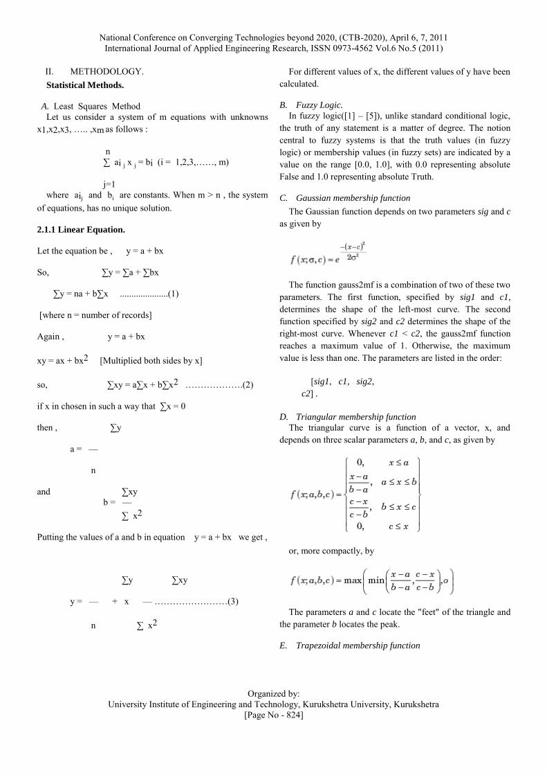
C. Gaussian membership function
The Gaussian function depends on two parameters sig and c as given by
The function gauss2mf is a combination of two of these two parameters. The first function, specified by sig1 and c1, determines the shape of the left-most curve. The second function specified by sig2 and c2 determines the shape of the right-most curve. Whenever c1 < c2, the gauss2mf function reaches a maximum value of 1. Otherwise, the maximum value is less than one. The parameters are listed in the order:
[sig1, c1, sig2, c2] .
D. Triangular membership function
The triangular curve is a function of a vector, x, and depends on three scalar parameters a, b, and c, as given by
or, more compactly, by
The parameters a and c locate the "feet" of the triangle and the parameter b locates the peak.
E. Trapezoidal membership function
National Conference on Converging Technologies beyond 2020, (CTB-2020), April 6, 7, 2011 International Journal of Applied Engineering Research, ISSN 0973-4562 Vol.6 No.5 (2011)
Organized by: University Institute of Engineering and Technology, Kurukshetra University, Kurukshetra
[Page No - 825]
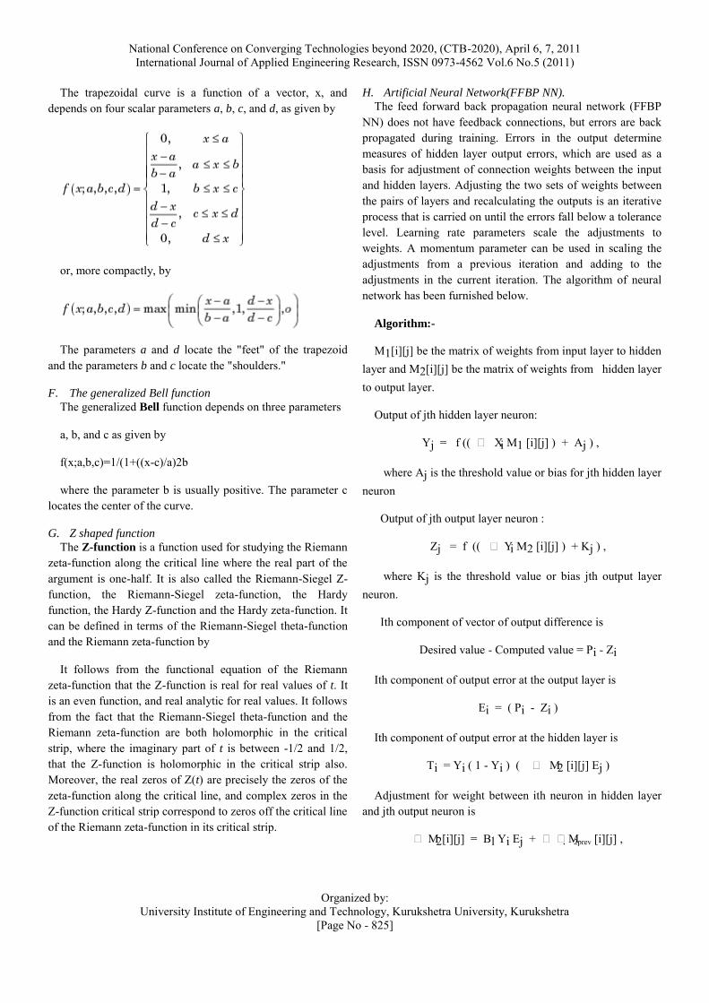
The trapezoidal curve is a function of a vector, x, and depends on four scalar parameters a, b, c, and d, as given by
or, more compactly, by
The parameters a and d locate the "feet" of the trapezoid and the parameters b and c locate the "shoulders."
F. The generalized Bell function
The generalized Bell function depends on three parameters
a, b, and c as given by
f(x;a,b,c)=1/(1+((x-c)/a)2b
where the parameter b is usually positive. The parameter c locates the center of the curve.
G. Z shaped function
The Z-function is a function used for studying the Riemann zeta-function along the critical line where the real part of the argument is one-half. It is also called the Riemann-Siegel Z-function, the Riemann-Siegel zeta-function, the Hardy function, the Hardy Z-function and the Hardy zeta-function. It can be defined in terms of the Riemann-Siegel theta-function and the Riemann zeta-function by
It follows from the functional equation of the Riemann zeta-function that the Z-function is real for real values of t. It is an even function, and real analytic for real values. It follows from the fact that the Riemann-Siegel theta-function and the Riemann zeta-function are both holomorphic in the critical strip, where the imaginary part of t is between -1/2 and 1/2, that the Z-function is holomorphic in the critical strip also. Moreover, the real zeros of Z(t) are precisely the zeros of the zeta-function along the critical line, and complex zeros in the Z-function critical strip correspond to zeros off the critical line of the Riemann zeta-function in its critical strip.
H. Artificial Neural Network(FFBP NN).
The feed forward back propagation neural network (FFBP NN) does not have feedback connections, but errors are back propagated during training. Errors in the output determine measures of hidden layer output errors, which are used as a basis for adjustment of connection weights between the input and hidden layers. Adjusting the two sets of weights between the pairs of layers and recalculating the outputs is an iterative process that is carried on until the errors fall below a tolerance level. Learning rate parameters scale the adjustments to weights. A momentum parameter can be used in scaling the adjustments from a previous iteration and adding to the adjustments in the current iteration. The algorithm of neural network has been furnished below.
Algorithm:-
M1[i][j] be the matrix of weights from input layer to hidden layer and M2[i][j] be the matrix of weights from hidden layer to output layer.
Output of jth hidden layer neuron:
Yj = f (( ᵒ Xi M1 [i][j] ) + Aj ) ,
where Aj is the threshold value or bias for jth hidden layer neuron
Output of jth output layer neuron :
Zj = f (( ᵒ Yi M2 [i][j] ) + Kj ) ,
where Kj is the threshold value or bias jth output layer neuron.
Ith component of vector of output difference is
Desired value - Computed value = Pi - Zi
Ith component of output error at the output layer is
Ei = ( Pi - Zi )
Ith component of output error at the hidden layer is
Ti = Yi ( 1 - Yi ) ( ᵒ M2 [i][j] Ej )
Adjustment for weight between ith neuron in hidden layer and jth output neuron is
ᵒ M2[i][j] = Bl Yi Ej + ᵒ ᵒM2prev [i][j] ,
National Conference on Converging Technologies beyond 2020, (CTB-2020), April 6, 7, 2011 International Journal of Applied Engineering Research, ISSN 0973-4562 Vol.6 No.5 (2011)
Organized by: University Institute of Engineering and Technology, Kurukshetra University, Kurukshetra
[Page No - 826]
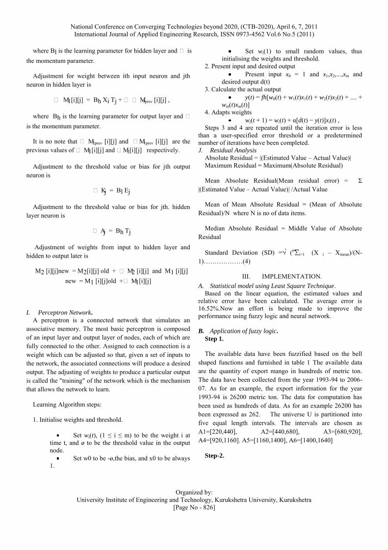
where Bl is the learning parameter for hidden layer and ᵒ is
the momentum parameter.
Adjustment for weight between ith input neuron and jth neuron in hidden layer is
ᵒ M1[i][j] = Bh Xi Tj + ᵒ ᵒ M1prev [i][j] ,
where Bh is the learning parameter for output layer and ᵒ
is the momentum parameter.
It is no note that ᵒ M2prev [i][j] and ᵒM1prev [i][j] are the previous values of ᵒ M1[i][j] and ᵒM2[i][j] respectively.
Adjustment to the threshold value or bias for jth output neuron is
ᵒ Kj = Bl Ej
Adjustment to the threshold value or bias for jth. hidden layer neuron is
ᵒ Aj = Bh Tj
Adjustment of weights from input to hidden layer and hidden to output later is
M2 [i][j]new = M2[i][j] old + ᵒ M2 [i][j] and M1 [i][j] new = M1 [i][j]old +ᵒ M1[i][j]
I. Perceptron Network. A perceptron is a connected network that simulates an
associative memory. The most basic perceptron is composed of an input layer and output layer of nodes, each of which are fully connected to the other. Assigned to each connection is a weight which can be adjusted so that, given a set of inputs to the network, the associated connections will produce a desired output. The adjusting of weights to produce a particular output is called the "training" of the network which is the mechanism that allows the network to learn.
Learning Algorithm steps:
1. Initialise weights and threshold.
Set wi(t), (1 ≤ i ≤ m) to be the weight i at time t, and ø to be the threshold value in the output node.
Set w0 to be -ø,the bias, and x0 to be always 1.
Set wi(1) to small random values, thus initialising the weights and threshold.
2. Present input and desired output Present input x0 = 1 and x1,x2,...,xm and
desired output d(t) 3. Calculate the actual output
y(t) = fh[w0(t) + w1(t)x1(t) + w2(t)x2(t) + .... + wm(t)xm(t)]
4. Adapts weights wi(t + 1) = wi(t) + α[d(t) − y(t)]xi(t) ,
Steps 3 and 4 are repeated until the iteration error is less than a user-specified error threshold or a predetermined number of iterations have been completed. J. Residual Analysis
Absolute Residual = |(Estimated Value – Actual Value)| Maximum Residual = Maximum(Absolute Residual)
Mean Absolute Residual(Mean residual error) = Σ
|(Estimated Value – Actual Value)| /Actual Value
Mean of Mean Absolute Residual = (Mean of Absolute Residual)/N where N is no of data items.
Median Absolute Residual = Middle Value of Absolute Residual
Standard Deviation (SD) = (ni=1 (X i – Xmean)/(N-
1)………………(4)
III. IMPLEMENTATION. A. Statistical model using Least Square Technique.
Based on the linear equation, the estimated values and relative error have been calculated. The average error is 16.52%.Now an effort is being made to improve the performance using fuzzy logic and neural network.
B. Application of fuzzy logic.
Step 1.
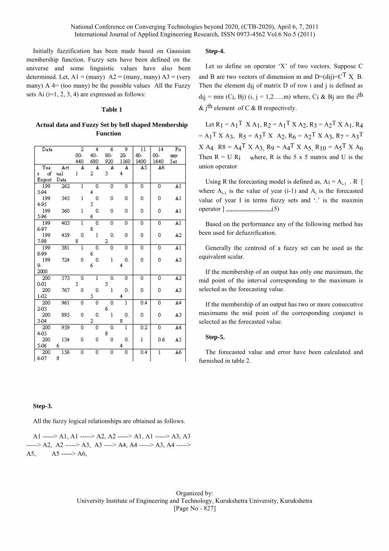
The available data have been fuzzified based on the bell shaped functions and furnished in table 1 The available data are the quantity of export mango in hundreds of metric ton. The data have been collected from the year 1993-94 to 2006-07. As for an example, the export information for the year 1993-94 is 26200 metric ton. The data for computation has been used as hundreds of data. As for an example 26200 has been expressed as 262. The universe U is partitioned into five equal length intervals. The intervals are chosen as A1=[220,440], A2=[440,680], A3=[680,920], A4=[920,1160]. A5=[1160,1400], A6=[1400,1640]
Step-2.
National Conference on Converging Technologies beyond 2020, (CTB-2020), April 6, 7, 2011 International Journal of Applied Engineering Research, ISSN 0973-4562 Vol.6 No.5 (2011)
Organized by: University Institute of Engineering and Technology, Kurukshetra University, Kurukshetra
[Page No - 827]
Initially fuzzification has been made based on Gaussian membership function. Fuzzy sets have been defined on the universe and some linguistic values have also been determined. Let, A1 = (many) A2 = (many, many) A3 = (very many) A 4= (too many) be the possible values All the Fuzzy sets Ai (i=1, 2, 3, 4) are expressed as follows:
Table 1
Actual data and Fuzzy Set by bell shaped Membership
Function
Step-3.
All the fuzzy logical relationships are obtained as follows.
A1 -----> A1, A1 -----> A2, A2 -----> A1, A1 -----> A3, A3 -----> A2, A2 -----> A3, A3 ----> A4, A4 -----> A3, A4 -----> A5, A5 -----> A6,
Step-4.
Let us define on operator ‗X‘ of two vectors. Suppose C
and B are two vectors of dimension m and D=(dij)=CT X B.
Then the element dij of matrix D of row i and j is defined as
dij = min (Ci, Bj) (i, j = 1,2…..m) where, Ci & Bj are the ith
& jth element of C & B respectively.
Let R1 = A1T X A1, R2 = A1T X A2, R3 = A2T X A1, R4
= A1T X A3, R5 = A3T X A2, R6 = A2T X A3, R7 = A3T
X A4 R8 = A4T X A3, R9 = A4T X A5, R10 = A5T X A6 Then R = U Ri where, R is the 5 x 5 matrix and U is the union operator
Using R the forecasting model is defined as, Ai = Ai-1 . R [ where Ai-1
is the value of year (i-1) and Ai is the forecasted value of year I in terms fuzzy sets and ‗.‘ is the maxmin
operator ] ,,,,,,,,,,,,,,,,,,,,,,,,,,,,(5)
Based on the performance any of the following method has been used for defuzzification.
Generally the centroid of a fuzzy set can be used as the equivalent scalar.
If the membership of an output has only one maximum, the mid point of the interval corresponding to the maximum is selected as the forecasting value.
If the membership of an output has two or more consecutive maximums the mid point of the corresponding conjunct is selected as the forecasted value.
Step-5.
The forecasted value and error have been calculated and furnished in table 2.

National Conference on Converging Technologies beyond 2020, (CTB-2020), April 6, 7, 2011 International Journal of Applied Engineering Research, ISSN 0973-4562 Vol.6 No.5 (2011)
Organized by: University Institute of Engineering and Technology, Kurukshetra University, Kurukshetra
[Page No - 828]
Table 2
Actual data, Input Fuzzy data, Output fuzzy data Output
Year of Export
Actual Data
Input Fuzzy Output Fuzzy Output
1993-94
262 [1 .4 0 0 0 0]
1994-95
345 [1 .5 0 0 0 0] [1 1 1 .4 .4 0] 440
1995-96
360 [1 .6 0 0 0 0] [1 1 1 .5 .4 0] 440
1996-97
403 [1 .8 0 0 0 0] [1 1 1 .6 .4 0] 440
1997-98
459 [.8 1 .2 0 0 0] [1 1 1 .6 .4 0] 440
1998-99
381 [1 .6 0 0 0 0] [1 .8 1 .6 .4 .2] 560
1999-2000
724 [0 .8 1 .2 0 0] [1 1 1 .6 .4 0] 440
2000-01
573 [.5 1 .5 0 0 0] [.6 1 .6 1 .4 .4]
560
2001-02
767 [0 .5 1 .4 0 0] [1 .6 1 .6 .4 .5] 560
2002-03
961 [0 0 .6 1 .4 0] [.5 1 .6 1 .8 .6]
840
2003-04
895 [0 .2 1 .8 0 0] [.4 .6 1 .6 1 .6] 840
2004-05
959 [0 0 .8 1 .2 0] [.4 1 .6 1 .8 .6 ]
840
2005-06
1346 [0 0 0 .4 1 .6] [.4 .8 1 .8 1 .8]
1280
2006-07
1568 [0 0 0 0 .4 1] [.2 .4.4 .4 .6 1] 1520
National Conference on Converging Technologies beyond 2020, (CTB-2020), April 6, 7, 2011 International Journal of Applied Engineering Research, ISSN 0973-4562 Vol.6 No.5 (2011)
Organized by: University Institute of Engineering and Technology, Kurukshetra University, Kurukshetra
[Page No - 829]
Step-6
The same steps(step 1 to step 5) have been repeated using gaussian membership function..
Step-7
The same steps(step 1 to step 5) have been repeated using triangular membership function..
Step-8
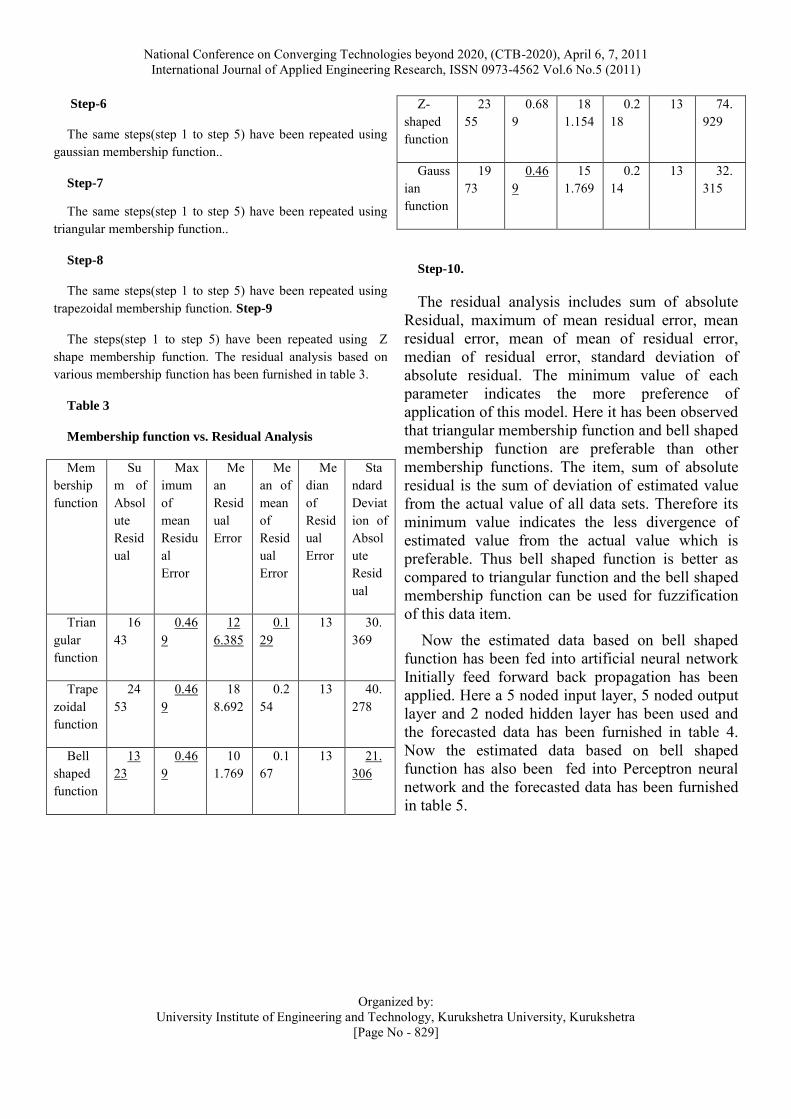
The same steps(step 1 to step 5) have been repeated using trapezoidal membership function. Step-9
The steps(step 1 to step 5) have been repeated using Z shape membership function. The residual analysis based on various membership function has been furnished in table 3.
Table 3
Membership function vs. Residual Analysis
Membership function
Sum of Absolute Residual
Maximum of mean Residual Error
Mean Residual Error
Mean of mean of Residual Error
Median of Residual Error
Standard Deviation of Absolute Residual
Triangular function
1643
0.469
126.385
0.129
13 30.369
Trapezoidal function
2453
0.469
188.692
0.254
13 40.278
Bell shaped function
1323
0.469
101.769
0.167
13 21.306
Z-shaped function
2355
0.689
181.154
0.218
13 74.929
Gaussian function
1973
0.469
151.769
0.214
13 32.315
Step-10.
The residual analysis includes sum of absolute Residual, maximum of mean residual error, mean residual error, mean of mean of residual error, median of residual error, standard deviation of absolute residual. The minimum value of each parameter indicates the more preference of application of this model. Here it has been observed that triangular membership function and bell shaped membership function are preferable than other membership functions. The item, sum of absolute residual is the sum of deviation of estimated value from the actual value of all data sets. Therefore its minimum value indicates the less divergence of estimated value from the actual value which is preferable. Thus bell shaped function is better as compared to triangular function and the bell shaped membership function can be used for fuzzification of this data item.
Now the estimated data based on bell shaped function has been fed into artificial neural network Initially feed forward back propagation has been applied. Here a 5 noded input layer, 5 noded output layer and 2 noded hidden layer has been used and the forecasted data has been furnished in table 4. Now the estimated data based on bell shaped function has also been fed into Perceptron neural network and the forecasted data has been furnished in table 5.

National Conference on Converging Technologies beyond 2020, (CTB-2020), April 6, 7, 2011 International Journal of Applied Engineering Research, ISSN 0973-4562 Vol.6 No.5 (2011)
Organized by: University Institute of Engineering and Technology, Kurukshetra University, Kurukshetra
[Page No - 830]
Table 4 Actual data and Forecasted Data based on FFBP Neural Network
Year of Export Actual Data Forecasted Data
1993-94 262
1994-95 345 320
1995-96 360 320
1996-97 403 320
1997-98 459 560
1998-99 381 320
1999-2000 724 800
2000-01 573 560
2001-02 767 800
2002-03 961 1040
2003-04 895 800
2004-05 959 1040
2005-06 1346 1280
2006-07 1568 1520
Step 12
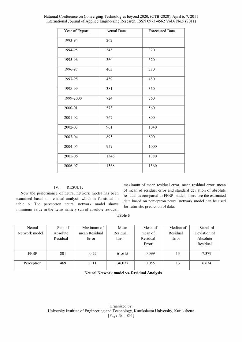
Table 5 Actual data, Forecasted Data based on Perceptron network
National Conference on Converging Technologies beyond 2020, (CTB-2020), April 6, 7, 2011 International Journal of Applied Engineering Research, ISSN 0973-4562 Vol.6 No.5 (2011)
Organized by: University Institute of Engineering and Technology, Kurukshetra University, Kurukshetra
[Page No - 831]
Year of Export Actual Data Forecasted Data
1993-94 262
1994-95 345 320
1995-96 360 320
1996-97 403 380
1997-98 459 480
1998-99 381 360
1999-2000 724 760
2000-01 573 560
2001-02 767 800
2002-03 961 1040
2003-04 895 800
2004-05 959 1000
2005-06 1346 1380
2006-07 1568 1560
IV. RESULT. Now the performance of neural network model has been
examined based on residual analysis which is furnished in table 6. The perceptron neural network model shows minimum value in the items namely sun of absolute residual,
maximum of mean residual error, mean residual error, mean of mean of residual error and standard deviation of absolute residual as compared to FFBP model. Therefore the estimated data based on perceptron neural network model can be used for futuristic prediction of data.
Table 6
Neural Network model vs. Residual Analysis
Neural Network model
Sum of Absolute Residual
Maximum of mean Residual
Error
Mean Residual
Error
Mean of mean of Residual
Error
Median of Residual
Error
Standard Deviation of
Absolute Residual
FFBP 801 0.22 61.615 0.099 13 7.379
Perceptron 469 0.11 36.077 0.055 13 6.634
National Conference on Converging Technologies beyond 2020, (CTB-2020), April 6, 7, 2011 International Journal of Applied Engineering Research, ISSN 0973-4562 Vol.6 No.5 (2011)
Organized by: University Institute of Engineering and Technology, Kurukshetra University, Kurukshetra
[Page No - 832]
V. CONCLUSION The particular soft computing model has been selected
based on residual analysis. The data related to export mango has been used as a data base. Thereafter the other data items can be attempted using soft computing model.
The export of an item generates a lot of revenue and that may help in planning various activities of State and Central Government. The export of produced mango generates a lot of revenue by the country among all export items. Thus it becomes necessary to get the predictive information related to export mango item. That is the reason of using export information of mango from the year 1993-94 to 2006-2007. If the futuristic data related to export mango is available in advance, the planning work may be easier.
REFERENCES.
[1]. Q. Song and B. S. Chissom, ―Forecasting enrollments with fuzzy time
series part I‖, Fuzzy Sets and Systems 54(1993) 1 - 9. [2]. J. Sullivan and William H. Woodall, ―A Comparison of Fuzzy
Forecasting and Markov Modelling‖, Fuzzy Sets and Systems
64(1994) 279 - 293. [3]. Q. Song and B. S. Chissom, ―Fuzzy Time Series and its Models‖,
Fuzzy Sets and Systems 54(1993) 269-277. [4]. H. Bintley, ―Time Series analysis with REVEAL‖, Fuzzy Sets and
Systems 23(1987) 97-118. [5]. Q. Song and B. S. Chissom, ―Forecasting enrollments with fuzzy time
series - part II‖, Fuzzy Sets and Systems 62(1994) 1-8. [6]. G. A. Tagliarini, J. F. Christ, E. W. Page, ―Optimization using Neural
Networks, IEEE Transactions on Computers. vol 40. no 12. December ‗91 1347-1358
[7]. Dharmpal Singh, J. Paul Choudhury, ―Assessment of Exported Mango Quantity By Soft Computing Model” in IJITKM-09 International Journal , Kurukshetra University ,pp 393-396 , June-July 2009.
[8]. Dharmpal Singh, J. Paul Choudhury, Mallika De ―Performance
Measurement Of Neural Network Model Considering VariousMembership Functions Under Fuzzy Logic‖ in IJCE, International Journal of Computer and Engineering, Vol1 issue 2,June-July 2010.
[9]. Dharmpal Singh, J. Paul Choudhury,Mallika De ―Prediction Based on
Statistical and Fuzzy Logic Membership Function‖ in PCTE , Journal Of Computer Sciences, Vol 7 issue 1, Punjab, pp 86-90 , June-July 2010.
[10]. Dharmpal Singh, J. Paul Choudhury,Mallika De ―Optimization of Fruit Quantity by comparison between Statistical Model and Fuzzy Logic by Bayesian Network‖ in PCTE , Journal Of Computer Sciences, Vol 7 issue 1, Punjab, pp 91-95 , June-July 2010.
[11]. Dharampal Singh ―Optimization using fuzzy logic membership
function” in DCIT-09 International Conference at Punjab College of Technical Education, Ludhiana, Punjab, May 2009.
[12]. Dharampal Singh ―Assessment of Exported Mango Quantity using
fuzzy logic membership function” in NCMTEE-09 ,National Conference at HETC, West Bengal ,pp 393-396 ,June 2009.
[13]. Dharampal Singh, J. Paul Choudhury, Kalyan Chakrabarti, ―Optimization using soft computing model‖, Proceedings of 12th
Annual Conference of Society of Operations Management, Indian Institute of Technology, Kanpur, pp 33-34, December 2008.

National Conference on Converging Technologies beyond 2020, (CTB-2020), April 6, 7, 2011 International Journal of Applied Engineering Research, ISSN 0973-4562 Vol.6 No.5 (2011)
Organized by: University Institute of Engineering and Technology, Kurukshetra University, Kurukshetra
[Page No - 833]
Switched Diversity with Threshold Control 1Nikhil Marriwala, 2Reena
1Assistant Professor, 2MTech Student Electronics & Communication Department, University Institute of Engineering and Technology, Kurukshetra University,
Kurukshetra
Email: 1 [email protected], [email protected]
Abstract- A numbers of diversity combining methods have been
studied for many years to combine or select uncorrelated faded
signals obtained from diversity branches that are-Maximal ratio
combining, Equal gain combining, selection combining and
switching or scanning combining. In this paper, we study
switched diversity with threshold control that propose the
variation in threshold according to variation in signal using fuzzy
threshold control rather the fixed threshold condition in
switching or scanning diversity combining.
Keywords- switched or scanning diversity combining, fuzzy
system, threshold control
I. INTRODUCTION In wireless digital mobile radio system the multipath fading severely degrades average bit error rate (BER) and probability of error (Pe)[3]. To overcome the effect of multipath fading diversity is a powerful communication technique. Diversity is most effective technique in order to achieve highly reliable digital data transmission without excessive increase in both transmitter power and co-channel reuse distance. In diversity technique there is number of independent signal transmission path named ―diversity branches‖ that carry
the same information but have uncorrelated multipath fading and a circuit is used in diversity to combine the received signal or select the one having the highest instantaneous SNR. There are different types of diversity combining technique having different implementation complexity and are different by there performance [1-3]. There are basically four diversity combining methods, maximal-ratio combining, equal gain combining, selective combining and switched combining. Maximal-ratio combining and equal-gain combining require very complicated analog circuitry. As for maximal-ratio combining and equal-gain combining, ever more complicated analog circuitries are required due to co-phasing. Selective combining and switched combining are two potential techniques in practice due to their simplicity in implementation. Typically, selective combining requires multiple receivers, one for each brand. Likewise, switched diversity combining is less costly since it needs only one receiver.
Table-1 comparison of all diversity combining technique
Technique Circuit
complexity
S/N improvement
factor
Threshold Simple, cheap Single receiver
1+γT/Γexp(-γT/Γ)
selection L receivers 1+1/2+….1/L
EGC L receiver Co-phasing
1+(L-1) /4
MRC L receiver Co-phasing Channel estimator
L
Switched diversity can be of M branch diversity. In such case the received signals are scanned in a sequential order, and the first signal with a power level above a certain threshold is selected. While above the threshold, the selected signal remains at the combiner‘s output, otherwise a scanning
process is switched to another branch [6-7]. Such switch process is further illustrated in Fig.1, where the case of two-branch switched diversity is considered. We assume two independent fading signals, R1 (solid line) and R2 (dashed line) coming from two antennas, which are shown in Fig. 2(a). Suppose the receiver firstly receives R1, it will keep receiving until R1 goes below the pre-determined threshold. When R1 is detected below the threshold, the receiver switches to R2, no matter what the current signal level of R2 is. After R2 becomes below the threshold, the receiver switches to R1, and so on. As a result, the received signal is obtained as shown in Fig. 2(b). [4] test different combining technique that are- Threshold Combining (ThC), Selection Diversity Combining (SDC), Maximum Ratio Combining (MRC), and Equal Gain Combining (EGC) with main focus on ThC. When using ThC all the monitored parameters are influenced by the selected SNR threshold value. In ThC technique the SNR threshold value should be chosen very carefully, SNR threshold influences the bit rate and BER performance of the ThC technique [4-5]. When using ThC all the monitored parameters are influenced by the selected SNR threshold value.

National Conference on Converging Technologies beyond 2020, (CTB-2020), April 6, 7, 2011 International Journal of Applied Engineering Research, ISSN 0973-4562 Vol.6 No.5 (2011)
Organized by: University Institute of Engineering and Technology, Kurukshetra University, Kurukshetra
[Page No - 834]
There are two switched diversity access scheme and these are- Scan-and-wait transmission (SWT) and Switch-and-examine transmission (SET). In these switching from one branch to another occur when signal level falls below a threshold. The difference is that in SET switch to another branch occur if its signal level is above threshold otherwise it will continue to the same signal. The degree of improvement in performance obtained by switching methods depends on the choice of threshold value, and the time delay that arises from the feedback loop of monitoring estimation, decision and switching.
Fig.1: feedback or scanning diversity
Fig.2 Illustration of switched diversity: (a) two independent fading signals, R1 and R2 (b) resultant signal using switch & stay threshold selection (c) Resultant signal using switch and examine.
II. Implementation of Switched Combining-
Fig.3 depicts a concept of two-branch switched diversity system while its algorithm is presented in Fig.4. Initially, the system randomly selects one antenna and computes the ED for every OFDM symbol. ED is calculated as follows. For each OFDM symbol, complex symbols are collected just before the demodulator of the receiver. The deviation of each subcarrier symbol from its nearest constellation point is computed and summed over all subcarriers. This summation is appropriately scaled and is called ED here. The ED is calculated for every
OFDM symbol and compared with a predefined threshold value to choose the best antenna. If the calculated ED of the received signal exceeds a predetermined threshold, the antenna switch is triggered, thus selecting the second branch. If the number of bit errors of the second branch is less than the threshold, switching ceases. If the second branch is also in a fade, a comparison will be made between the ED of the two signals and the lower is selected. However, the switch is enabled every 'X' OFDM symbols in order to test the signal quality of the other antenna until one of them emerges below the threshold (i.e. switch-and examine strategy).
Fig.3 Implementation of switched diversity combining
Fig. 4. Flow chart of the algorithm
The number 'X' is determined based on the difference in computed ED of the two signals. The smaller the difference the smaller the 'X' allowing the system to monitor the signal quality from the other antenna frequently. In this manner the number of switching instances can be reduced. The system performance can be controlled by the choice of the switching threshold. The ED also depends on the fading rate of the propagation channel. If the fading rate is high, X can be made smaller in order to check the signal of the other antenna more frequently. Similarly, if the computed ED values are of the
Choose
Antenna
Compute error
distanc
e
Keep
currrent
antenna
ED>Thr
Switch to
other antenn
a
Compute errro
r distance
ED >
Thr
Compute erro
r distanc
e
ED > thr
Counter= X??
To receiver
No
No
No N
o
Choose ant. With lower ED
RF &IF units
FFT
equalizer
Control unit
SNR calculator
Ant.1 A
nt.2
combiner
To demodulator
switc
h
Rx
Threshol
d
Level
Comparator
r
Resulted signal

National Conference on Converging Technologies beyond 2020, (CTB-2020), April 6, 7, 2011 International Journal of Applied Engineering Research, ISSN 0973-4562 Vol.6 No.5 (2011)
Organized by: University Institute of Engineering and Technology, Kurukshetra University, Kurukshetra
[Page No - 835]
same order, again X can be made smaller. In this manner one can adaptively change the value of X in order to enhance the performance.[7]
Fig.5 Operation of switch and examine combining with post examine
Switch and Examine Combining (SEC) has less signal discontinuities as compared to the switch and stay strategies as shown by fig. 2. In this system the receiver tries to use acceptable path by examining as many paths as necessary, when no acceptable path is accepted, the receiver switch to the strongest of M-1 other signals only if it is level exceeds the threshold. Since all available diversity paths have been examined. If there are no paths has a SNR greater than the threshold, a more preferred alternative would to use the strongest one among all these unacceptable paths is called Switch and Examine Combining with Post examining selection (SECPS). Path switching with SECPS occur only when the SNR of the current path is less than the threshold and the SNR of the new path is better than the used path. Fig.5 shows operation of switch and examine combining with post examine where Γ=max {γ1, γ2... γi} denotes the event that an i-branch is used. Receiver now continue to use the current path for data reception (Γ= γ1) until its SNR is fall below a threshold (γ1< γth), at that time, the receiver tries to find another acceptable path by sequentially examining the remaining M-1 paths. In the beginning, the second diversity path is examined and its SNR (γ2) is compared with the threshold (γth), if (γ2≥ γth) then the second path is used for data
reception (Γ=γ2). Otherwise, [the receiver now will use the largest one between γ1, γ2] and the receiver begin to examine the third path, if (γ3≥γth) then it is suitable for data reception (Γ=γ3).Otherwise, (the receiver now will use the largest one between γ1, γ2, γ3) until the fourth path is examined in the same manner. If the fourth path is not accepted (γ4< γth), the receiver will use one from the four paths with the highest SNR for data reception. Since the receiver is previously estimate the SNR of all paths [13] . Threshold determination- The proposed method is based on evaluation of the signal distribution in the constellation map [8]. For an optical QAM signal, the procedures are summarized by the following four steps: (1) Obtaining the signal distribution in the constellation map from the histogram evaluated, (2) Searching for the peaks of the histogram in the constellation map and finding the peak positions referred to as symbol locations in the map, (3) Setting thresholds by using the symbol locations obtained by the step (2), and (4) Discrimination of the received signal conversion according to the thresholds determined in step (3). Switched diversity is analyzed in rician fading environment. The performance analysis of switched diversity system operating in wireless fading environment using discrete time model is presented in [9]. [10] describe about the performance analysis of Switch and Stay transmit diversity with feedback errors. The switching rates of dual-branch selection combining diversity and switch-and-stay combining diversity in Rayleigh, Rician and Nakagami-m fading are derived in [11] and the switching rate of selection combining is compared to that of switch-and-stay combining. Switching rate of selection diversity- Let R1(t) and R2(t) denote the fading signal amplitude process of the first and second diversity branch, respectively. Form the random process Z(t) = R1(t) − R2(t). There is Z(t) > 0 when R1(t) > R2(t) and Z(t)< 0 when R2(t) > R1(t). Note further that a zero-crossing from Z(t) < 0 to Z(t) > 0 corresponds to R1(t) becoming greater than R2(t), starting from a state where R2(t)>R1(t). This, in turn, corresponds to the selection combiner switching from antenna two to antenna one that correspond negative going zero crossing. Similarly, a zero-crossing from Z(t)>0 to Z(t) < 0 corresponds to the selection combiner switching from antenna one to antenna two and that will lead to positive going zero crossing. The total switching rate of the selection diversity combiner then equals the sum of the positive-going and negative-going zero-crossing rates of Z(t). Switching rate of switch-and-stay diversity- The switch-and-stay combining strategy avoids excessive switching when

National Conference on Converging Technologies beyond 2020, (CTB-2020), April 6, 7, 2011 International Journal of Applied Engineering Research, ISSN 0973-4562 Vol.6 No.5 (2011)
Organized by: University Institute of Engineering and Technology, Kurukshetra University, Kurukshetra
[Page No - 836]
both antennas are in weak signal conditions. The combiner switches whenever there is a down-going crossing of the switching threshold in the branch signal amplitude and stays with the selected branch regardless of whether the signal amplitude on the selected branch is above or below the switching threshold, until there is a down-going crossing of the switching threshold. The amount of the change in the switching rate is small in the case of switch-and-stay combining both for rician and nakagmi fading. A survey of fuzzy logic application and principles in wireless communication is presented in[12], that highlight the successful usage of fuzzy logic technique in applied telecommunication and signal processing. It can be an efficient tool to be utilized in problems for which knowledge of all factors is insufficient or impossible to obtain, it work with linguistic variables.
III SIMULATION AND RESULT
A fuzzy threshold control is done by using four principal components: a fuzzification interface, a fuzzy rule base, an inference engine, and a defuzzification interface [14]. The fuzzification interface intends to convert the input values, such as the current channel state (signal strength), the channel state variation, and the current threshold, into some linguistic values, i.e., fuzzy sets. The fuzzy rule base, which comprises knowledge of the specific application and the attendant control goals, is used to define linguistic control rules and fuzzy number manipulation in a SDTC (switched diversity with threshold control). Likewise, the inference engine is a decision-making logic mechanism of a SDTC. It has the capability of simulating mobile radio channel based on fuzzy concepts. Fuzzy inference is the process of formulating the mapping from given input to the output using fuzzy logic. Decision can be made on the basis of these mapping. Finally, the defuzzification interface converts fuzzy control decisions into crisp non fuzzy threshold adaptation control signals, which are applied to adjust the threshold level of the switched diversity. Based on these observations, we basically consider four linguistic variables, S, dS, Th and dTh, which denote the present channel state or signal level, the variation of channel state (received signal level), the previous threshold level and the change of threshold level, respectively. The output control linguistic variable is dTh, while the other three variables are used as inputs. Note that this is a 3-input, one- output fuzzy logic control system. The associated fuzzy term sets are {L (Large), M (Medium), S (Small) } for S and Th, and {PL (Positive Large), PM (Positive Medium), PS (Positive Small),
NL (Negative Large), NM (Negative Medium), NS (Negative Small)} for ΔS and ΔTh. The controller used for model is
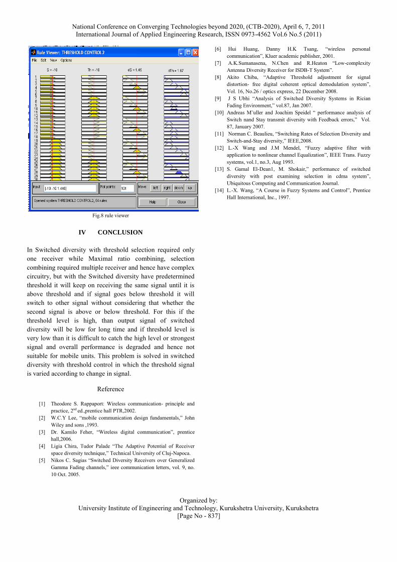
Mamdani model. Based on all these observation 54 fuzzy if-then else rules are made to control threshold variation according to signal. Accordingly there surface graph and rule viewer are as shown in fig.6 and fig.8.
Fig.6 surface graph between S, Th and dTh
Fig.7 graph between dS and dTh
The surface is graph between the input and output as shown in fig.6. Here the surface shows graph between inputs S, Th and output dTh. The surface shows the effect on dTh when S and Th are changing from their upper limit to lower limit.Fig.7 shows that as the signal change the threshold is also varied accordingly and this threshold control according to signal is done by fuzzy system. The rule viewer shows the effect of change in inputs on output more clearly. As shown in fig.8 S and Th are at -10dB, when there is a change in dS of -1.45, changes dTh from 0 to -1.67.
National Conference on Converging Technologies beyond 2020, (CTB-2020), April 6, 7, 2011 International Journal of Applied Engineering Research, ISSN 0973-4562 Vol.6 No.5 (2011)
Organized by: University Institute of Engineering and Technology, Kurukshetra University, Kurukshetra
[Page No - 837]
Fig.8 rule viewer
IV CONCLUSION
In Switched diversity with threshold selection required only one receiver while Maximal ratio combining, selection combining required multiple receiver and hence have complex circuitry, but with the Switched diversity have predetermined threshold it will keep on receiving the same signal until it is above threshold and if signal goes below threshold it will switch to other signal without considering that whether the second signal is above or below threshold. For this if the threshold level is high, than output signal of switched diversity will be low for long time and if threshold level is very low than it is difficult to catch the high level or strongest signal and overall performance is degraded and hence not suitable for mobile units. This problem is solved in switched diversity with threshold control in which the threshold signal is varied according to change in signal.
Reference
[1] Theodore S. Rappaport: Wireless communication- principle and practice, 2nd ed.,prentice hall PTR,2002.
[2] W.C.Y Lee, ―mobile communication design fundamentals,‖ John Wiley and sons ,1993.
[3] Dr. Kamilo Feher, ―Wireless digital communication‖, prentice hall,2006.
[4] Ligia Chira, Tudor Palade ―The Adaptive Potential of Receiver space diversity technique,‖ Technical University of Cluj-Napoca.
[5] Nikos C. Sagias ―Switched Diversity Receivers over Generalized Gamma Fading channels,‖ ieee communication letters, vol. 9, no. 10 Oct. 2005.
[6] Hui Huang, Danny H.K Tsang, ―wireless personal
communication‖, Kluer academic publisher, 2001. [7] A.K.Sumanasena, N.Chen and R.Heaton ―Low-complexity
Antenna Diversity Receiver for ISDB-T System‖. [8] Akito Chiba, ―Adaptive Threshold adjustment for signal
distortion- free digital coherent optical demodulation system‖,
Vol. 16, No.26 / optics express, 22 December 2008. [9] J S Ubhi ―Analysis of Switched Diversity Systems in Rician
Fading Environment,‖ vol.87, Jan 2007. [10] Andreas M¨uller and Joachim Speidel ― performance analysis of
Switch nand Stay transmit diversity with Feedback errors,‖ Vol. 87, January 2007.
[11] Norman C. Beaulieu, ―Switching Rates of Selection Diversity and
Switch-and-Stay diversity,‖ IEEE,2008. [12] L.-X Wang and J.M Mendel, ―Fuzzy adaptive filter with
application to nonlinear channel Equalization‖, IEEE Trans. Fuzzy
systems, vol.1, no.3, Aug 1993. [13] S. Gamal El-Dean1, M. Shokair,‖ performance of switched
diversity with post examining selection in cdma system‖, Ubiquitous Computing and Communication Journal.
[14] L.-X. Wang, ―A Course in Fuzzy Systems and Control‖, Prentice
Hall International, Inc., 1997.
National Conference on Converging Technologies beyond 2020, (CTB-2020), April 6, 7, 2011 International Journal of Applied Engineering Research, ISSN 0973-4562 Vol.6 No.5 (2011)
Organized by: University Institute of Engineering and Technology, Kurukshetra University, Kurukshetra
[Page No - 838]
Performance of 802.16e Using Simulation model #Nikhil Marriwala, *Jyoti Saini
#Assistant Professor Electronics & Communication Department, University Institute of Engineering and Technology,
Kurukshetra University, Kurukshetra *Electronics & Communication Department, University Institute of Engineering and Technology, Kurukshetra University,
Kurukshetra
Email:[email protected], [email protected]
Abstract—The name WiMAX is introduced by the Institute of
Electrical and Electronic Engineers (IEEE) which is standard
selected for 802.16d-2004 (used in fixed wireless applications)
and 802.16e-2005 (mobile wireless) to provide a worldwide
interoperability for microwave access. It contains full mobile
internet access. Various applications have already been applied
so far using WiMAX, as alternative to 3G mobile systems in
developing countries, Wireless Digital Subscriber Line, Wireless
Local Loop. IEEE 802.16e-2005 has been developed for mobile
wireless communication which is based on OFDM technology
and this enables going towards the 4G mobile in the future. In
this review paper, we describe a simulation model based on
802.16e OFDM-PHY baseband and define its each block
function. The different modulation techniques such as BPSK,
QPSK and QAM (Both 16 and 64) is use to find out the best
performance of physical layer for WiMAX Mobile. The noise
channel AWGN, SUI, data randomization techniques, FFT, IFFT
and Adaptive modulation will be use to investigate the effect of
these on WiMAX. We will determine the performance of
WiMAX in terms of BER and SNR using MATLAB.
Keyword-Worldwide interoperable microwave access (WiMAX);
Non Line-of-Sight; Physical layer.
I. INTRODUCTION WiMAX is defined as Worldwide Interoperability for
Microwave Access by the WiMAX Forum, formed in June 2001 to promote conformance and interoperability of the IEEE 802.16 standard, officially known as WirelessMAN. The Forum describes WiMAX as "a standards-based technology enabling the delivery of last mile wireless broadband access as an alternative to cable and DSL. The IEEE ratified the 802.16e amendment to the 802.16 standard in December 2005. This amendment adds the new features and quality to the standard which is necessary to support mobility. The WiMAX Forum is now defining system performance and certification profiles based on the IEEE 802.16e Mobile Amendment and going beyond the air interface, the WiMAX Forum is defining the network architecture necessary for implementing an end-to-end Mobile WiMAX network. With the growth of the global economy and the development in the information technology, more and more users require broadband access to data, voice, and video services. With these advantages of fast network construction, quick investment returns, and broad bandwidth, the broadband wireless access system is the first-choice access technology
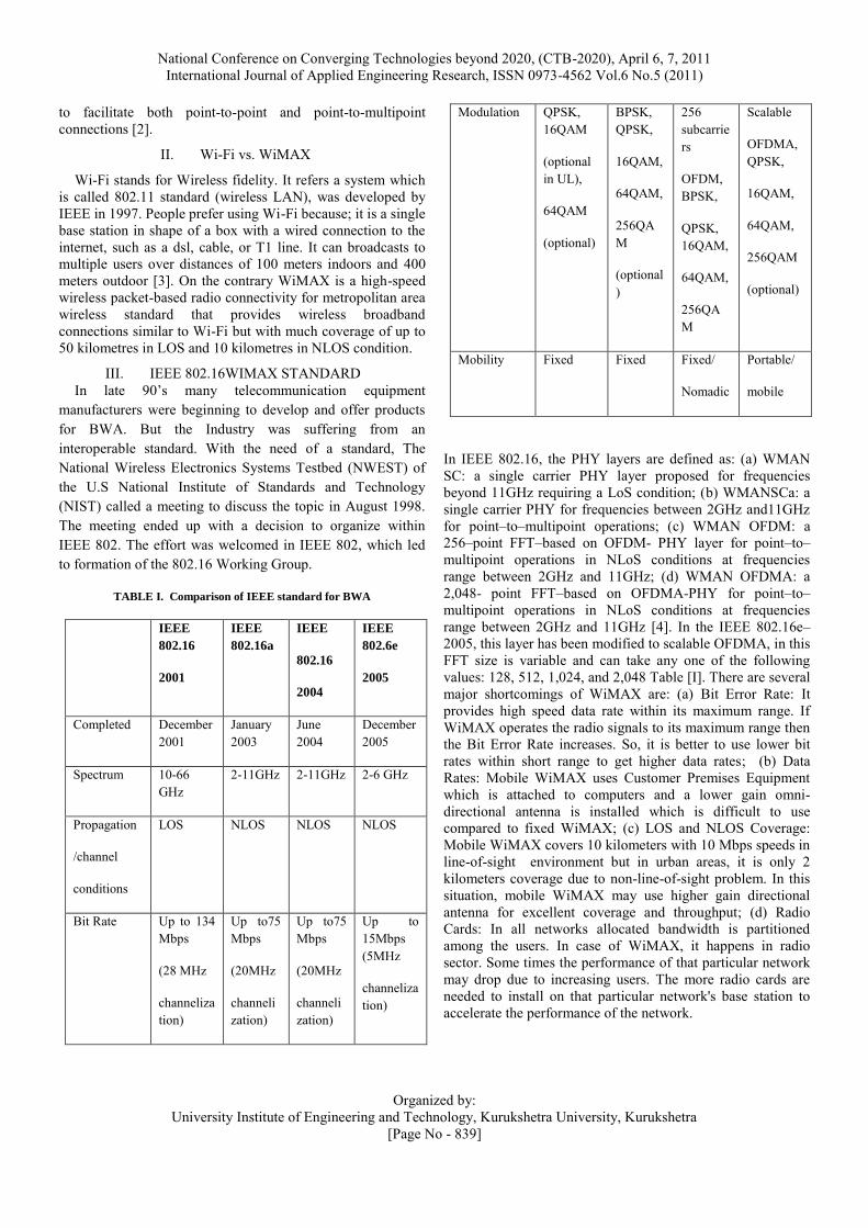
for operators to build broadband MANs.The WiMAX has the following characteristics.
Standard IEEE 802.16e
Carrier Frequency Below 11GHz
Frequency Bands 2.5GHz, 3.5GHz, 5.7GHz
Bandwidth 1.5MHz to 20MHz
Radio Technology OFDM and OFDMA
Data Rate 70 Mbps
The technology's has the ability to serve as a high bandwidth "backhaul" for Internet or cellular phone traffic from remote areas back to an internet backbone. WiMAX can enhance wireless infrastructure in an inexpensive, decentralized, deployment-friendly and effective manner [1]. Mobile WiMAX support some of the salient features are:
It is cost effective. It offers high data rates. Providing Nomadic connectivity. It is easy to deploy and has flexible network
architectures. It supports interoperability with other networks. Connecting Wi-Fi hotspot with each other and to
other parts of the Internet It provides truly a global wireless broadband
network.
WiMAX is capable of working in different frequency ranges but according to the IEEE 802.16, the frequency band is 10 GHz - 66 GHz. A typical architecture of WiMAX includes a base station built on top of a high rise building and communicates on point to multi-point basis with subscriber stations which can be a business organization or a home. The base station is connected through Customer Premise Equipment with the customer. This connection could be a Line-of-Sight or Non-Line-of-Sight.IEEE 802.16 aim to extend the wireless broadband access up to kilometres in order
National Conference on Converging Technologies beyond 2020, (CTB-2020), April 6, 7, 2011 International Journal of Applied Engineering Research, ISSN 0973-4562 Vol.6 No.5 (2011)
Organized by: University Institute of Engineering and Technology, Kurukshetra University, Kurukshetra
[Page No - 839]
to facilitate both point-to-point and point-to-multipoint connections [2].
II. Wi-Fi vs. WiMAX
Wi-Fi stands for Wireless fidelity. It refers a system which is called 802.11 standard (wireless LAN), was developed by IEEE in 1997. People prefer using Wi-Fi because; it is a single base station in shape of a box with a wired connection to the internet, such as a dsl, cable, or T1 line. It can broadcasts to multiple users over distances of 100 meters indoors and 400 meters outdoor [3]. On the contrary WiMAX is a high-speed wireless packet-based radio connectivity for metropolitan area wireless standard that provides wireless broadband connections similar to Wi-Fi but with much coverage of up to 50 kilometres in LOS and 10 kilometres in NLOS condition.
III. IEEE 802.16WIMAX STANDARD In late 90‘s many telecommunication equipment
manufacturers were beginning to develop and offer products for BWA. But the Industry was suffering from an interoperable standard. With the need of a standard, The National Wireless Electronics Systems Testbed (NWEST) of the U.S National Institute of Standards and Technology (NIST) called a meeting to discuss the topic in August 1998. The meeting ended up with a decision to organize within IEEE 802. The effort was welcomed in IEEE 802, which led to formation of the 802.16 Working Group.
TABLE І. Comparison of IEEE standard for BWA
IEEE
802.16
2001
IEEE
802.16a
IEEE
802.16
2004
IEEE
802.6e
2005
Completed December 2001
January 2003
June 2004
December 2005
Spectrum 10-66 GHz
2-11GHz 2-11GHz 2-6 GHz
Propagation
/channel
conditions
LOS NLOS NLOS NLOS
Bit Rate Up to 134 Mbps
(28 MHz
channelization)
Up to75 Mbps
(20MHz
channelization)
Up to75 Mbps
(20MHz
channelization)
Up to 15Mbps (5MHz
channelization)
Modulation QPSK, 16QAM
(optional in UL),
64QAM
(optional)
BPSK, QPSK,
16QAM,
64QAM,
256QAM
(optional)
256 subcarriers
OFDM, BPSK,
QPSK, 16QAM,
64QAM,
256QAM
Scalable
OFDMA, QPSK,
16QAM,
64QAM,
256QAM
(optional)
Mobility Fixed Fixed Fixed/
Nomadic
Portable/
mobile
In IEEE 802.16, the PHY layers are defined as: (a) WMAN SC: a single carrier PHY layer proposed for frequencies beyond 11GHz requiring a LoS condition; (b) WMANSCa: a single carrier PHY for frequencies between 2GHz and11GHz for point–to–multipoint operations; (c) WMAN OFDM: a 256–point FFT–based on OFDM- PHY layer for point–to– multipoint operations in NLoS conditions at frequencies range between 2GHz and 11GHz; (d) WMAN OFDMA: a 2,048- point FFT–based on OFDMA-PHY for point–to–
multipoint operations in NLoS conditions at frequencies range between 2GHz and 11GHz [4]. In the IEEE 802.16e–
2005, this layer has been modified to scalable OFDMA, in this FFT size is variable and can take any one of the following values: 128, 512, 1,024, and 2,048 Table [І]. There are several major shortcomings of WiMAX are: (a) Bit Error Rate: It provides high speed data rate within its maximum range. If WiMAX operates the radio signals to its maximum range then the Bit Error Rate increases. So, it is better to use lower bit rates within short range to get higher data rates; (b) Data Rates: Mobile WiMAX uses Customer Premises Equipment which is attached to computers and a lower gain omni- directional antenna is installed which is difficult to use compared to fixed WiMAX; (c) LOS and NLOS Coverage: Mobile WiMAX covers 10 kilometers with 10 Mbps speeds in line-of-sight environment but in urban areas, it is only 2 kilometers coverage due to non-line-of-sight problem. In this situation, mobile WiMAX may use higher gain directional antenna for excellent coverage and throughput; (d) Radio Cards: In all networks allocated bandwidth is partitioned among the users. In case of WiMAX, it happens in radio sector. Some times the performance of that particular network may drop due to increasing users. The more radio cards are needed to install on that particular network's base station to accelerate the performance of the network.
National Conference on Converging Technologies beyond 2020, (CTB-2020), April 6, 7, 2011 International Journal of Applied Engineering Research, ISSN 0973-4562 Vol.6 No.5 (2011)
Organized by: University Institute of Engineering and Technology, Kurukshetra University, Kurukshetra
[Page No - 840]
IV. WiMAX PHYSICAL LAYER The IEEE 802.16 standard supports multiple physical
specifications due to its flexible nature. The first version of the standard only supported single carrier modulation. Since that time, OFDM and scalable OFDMA have been included to operate in NLOS environment and to provide mobility. The standard has also been extended for use in below 11GHz frequency bands along with initially supported 10-66 GHz bands. Features of physical layer are [TABLE ІI ].
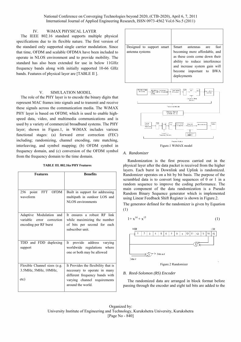
V. SIMULATION MODEL The role of the PHY layer is to encode the binary digits that
represent MAC frames into signals and to transmit and receive these signals across the communication media. The WiMAX PHY layer is based on OFDM; which is used to enable high-speed data, video, and multimedia communications and is used by a variety of commercial broadband systems. The PHY layer; shown in Figure.1, in WiMAX includes various functional stages: (a) forward error correction (FEC) including; randomizing, channel encoding, rate matching, interleaving, and symbol mapping; (b) OFDM symbol in frequency domain, and (c) conversion of the OFDM symbol from the frequency domain to the time domain.
TABLE ІII. 802.16a PHY Features
Features
Benefits
256 point FFT OFDM waveform
Built in support for addressing multipath in outdoor LOS and NLOS environments
Adaptive Modulation and variable error correction encoding per RF burst
It ensures a robust RF link while maximizing the number of bits per second for each subscriber unit.
TDD and FDD duplexing support
It provide address varying worldwide regulations where one or both may be allowed
Flexible Channel sizes (e.g. 3.5MHz, 5MHz, 10MHz,
etc)
It Provides the flexibility that is necessary to operate in many different frequency bands with varying channel requirements around the world.
Designed to support smart antenna systems
Smart antennas are fast becoming more affordable, and as these costs come down their ability to reduce interference and increase system gain will become important to BWA deployments
Figure.1 WiMAX model
A. Randomizer
Randomization is the first process carried out in the physical layer after the data packet is received from the higher layers. Each burst in Downlink and Uplink is randomized. Randomizer operates on a bit by bit basis. The purpose of the scrambled data is to convert long sequences of 0 or 1 in a random sequence to improve the coding performance. The main component of the data randomization is a Pseudo Random Binary Sequence generator which is implemented using Linear Feedback Shift Register is shown in Figure.2. The generator defined for the randomizer is given by Equation (1)
1+ x14 + x15 (1)
Figure.2 Randomizer
B. Reed-Solomon (RS) Encoder
The randomized data are arranged in block format before passing through the encoder and eight tail bits are added to the

National Conference on Converging Technologies beyond 2020, (CTB-2020), April 6, 7, 2011 International Journal of Applied Engineering Research, ISSN 0973-4562 Vol.6 No.5 (2011)
Organized by: University Institute of Engineering and Technology, Kurukshetra University, Kurukshetra
[Page No - 841]
data. The implemented RS encoder is derived from a systematic RS (N=255, K=239, T=8) code using GF (28). The following polynomials are used for code generator and field generator: g(x) = (x +λ
0 )(x +λ1 )(x +λ
2 )...(x +λ2t−1) (2)
p(x) = x8 + x4 + x3 + x2 +1 (3)
where: N is the number of bytes after encoding; K is the data bytes before encoding; T is the number of bytes that can be corrected.
C. Convolutional Encoder (CC)
The outer RS encoded block is fed to inner binary convolutional encoder. The implemented encoder has native rate of 1/2, a constraint length of 7 and the generator polynomial in Equation (4) and (5) to produce its two code bits [5]. The generator is shown in Figure.3. G1 = 171 OCT for X (4)
G2 = 133 OCT for Y (5)
Figure.3 Convolutional Encoder
In order to achieve variable code rate a puncturing operation is performed on the output of the convolutional encoder in accordance to Table ІІІ. In this Table ―1‖ denotes that the corresponding convolutional encoder output is used, while ―0‖ denotes that the corresponding output is not used. At the receiver Viterbi decoder is used to decode the convolutional codes.
TABLE ІІІ. Puncturing configurations for different CC rates
CODE RATE
RATE 1/2 2/3 3/4 5/6
X 1 10 101 10101
Y 1 11 110 11010
XY X1Y1 X1Y1Y2 X1Y1Y2X3 X1Y1Y2X3Y4X5
D. Interleaver
Data interleaving is generally used to scatter error bursts and thus, reduce error concentration to be corrected with the purpose of increasing efficiency of FEC by spreading burst errors introduced by the transmission channel over a longer time. The interleaver is defined by a two-step permutation. First ensures that adjacent coded bits are mapped onto nonadjacent subcarriers. The second permutation insures that adjacent coded bits are mapped alternately onto less or more significant bits of the constellation, thus avoiding long runs of lowly reliable bits [4].
The first permutation is defined by:
Mk = (ncbps/12) kmod + floor (k/12) (6)
The second permutation is defined by:
Jk = s. floor (mk /s) + [mk + ncbps - floor (12.mk /ncbps)]mod(s) (7)
where: k = 0, 1, …, Ncbps; Ncbps is the number of coded bits per subcarrier, i.e., 1, 2, 4 or 6 for BPSK, QPSK, 16– QAM, or 64–QAM, respectively; k is the index of the coded bit before the first permutation; mk is the index of that coded bit after the first and before the second permutation, and Jk is the index after the second permutation, just prior to modulation mapping.
E. Adaptive Modulation
All wireless communication systems use a modulation scheme to map coded bits to a form that can be effectively transmitted over the communication channel. WiMAX supports a variety of modulation and coding schemes and allows for the scheme to change on a burst-by-burst basis per link, depending on channel and interference conditions [4].
F. OFDM Technique
Orthogonal Frequency Division Multiplexing (OFDM) is a multiplexing technique that subdivides the bandwidth into
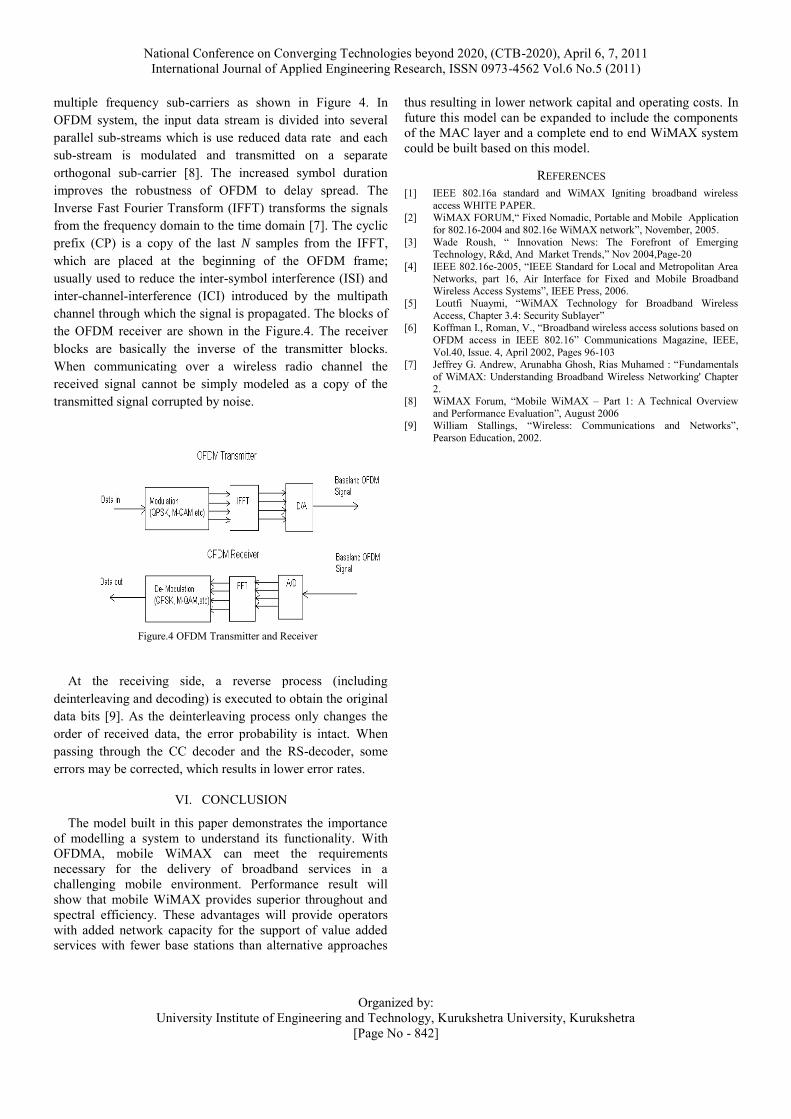
National Conference on Converging Technologies beyond 2020, (CTB-2020), April 6, 7, 2011 International Journal of Applied Engineering Research, ISSN 0973-4562 Vol.6 No.5 (2011)
Organized by: University Institute of Engineering and Technology, Kurukshetra University, Kurukshetra
[Page No - 842]
multiple frequency sub-carriers as shown in Figure 4. In OFDM system, the input data stream is divided into several parallel sub-streams which is use reduced data rate and each sub-stream is modulated and transmitted on a separate orthogonal sub-carrier [8]. The increased symbol duration improves the robustness of OFDM to delay spread. The Inverse Fast Fourier Transform (IFFT) transforms the signals from the frequency domain to the time domain [7]. The cyclic prefix (CP) is a copy of the last N samples from the IFFT, which are placed at the beginning of the OFDM frame; usually used to reduce the inter-symbol interference (ISI) and inter-channel-interference (ICI) introduced by the multipath channel through which the signal is propagated. The blocks of the OFDM receiver are shown in the Figure.4. The receiver blocks are basically the inverse of the transmitter blocks. When communicating over a wireless radio channel the received signal cannot be simply modeled as a copy of the transmitted signal corrupted by noise.
Figure.4 OFDM Transmitter and Receiver
At the receiving side, a reverse process (including deinterleaving and decoding) is executed to obtain the original data bits [9]. As the deinterleaving process only changes the order of received data, the error probability is intact. When passing through the CC decoder and the RS-decoder, some errors may be corrected, which results in lower error rates.
VI. CONCLUSION
The model built in this paper demonstrates the importance of modelling a system to understand its functionality. With OFDMA, mobile WiMAX can meet the requirements necessary for the delivery of broadband services in a challenging mobile environment. Performance result will show that mobile WiMAX provides superior throughout and spectral efficiency. These advantages will provide operators with added network capacity for the support of value added services with fewer base stations than alternative approaches
thus resulting in lower network capital and operating costs. In future this model can be expanded to include the components of the MAC layer and a complete end to end WiMAX system could be built based on this model.
REFERENCES [1] IEEE 802.16a standard and WiMAX Igniting broadband wireless
access WHITE PAPER. [2] WiMAX FORUM,― Fixed Nomadic, Portable and Mobile Application
for 802.16-2004 and 802.16e WiMAX network‖, November, 2005. [3] Wade Roush, ― Innovation News: The Forefront of Emerging
Technology, R&d, And Market Trends,‖ Nov 2004,Page-20 [4] IEEE 802.16e-2005, ―IEEE Standard for Local and Metropolitan Area
Networks, part 16, Air Interface for Fixed and Mobile Broadband Wireless Access Systems‖, IEEE Press, 2006.
[5] Loutfi Nuaymi, ―WiMAX Technology for Broadband Wireless Access, Chapter 3.4: Security Sublayer‖
[6] Koffman I., Roman, V., ―Broadband wireless access solutions based on OFDM access in IEEE 802.16‖ Communications Magazine, IEEE,
Vol.40, Issue. 4, April 2002, Pages 96-103 [7] Jeffrey G. Andrew, Arunabha Ghosh, Rias Muhamed : ―Fundamentals
of WiMAX: Understanding Broadband Wireless Networking' Chapter 2.
[8] WiMAX Forum, ―Mobile WiMAX – Part 1: A Technical Overview and Performance Evaluation‖, August 2006
[9] William Stallings, ―Wireless: Communications and Networks‖, Pearson Education, 2002.