Soft Computing Technique Based Reactive Power Planning using Combining Multi-objective Optimization...

International Electrical Engineering Journal (IEEJ)

Vol. 5 (2014) No.10, pp. 1576-1585

ISSN 2078-2365

http://www.ieejournal.com/

Vadivelu and Marutheswar Soft Computing Technique Based Reactive Power Planning using Combining Multi-objective Optimization with Improved Differential Evolution

1576

Soft Computing Technique Based Reactive

Power Planning using Combining

Multi-objective Optimization with Improved

Differential Evolution 1K.R.Vadivelu and 2Dr.G.V.Marutheswar

[email protected],[email protected]

Abstract:This paper proposes an application of Fast Voltage

Stability Index (FVSI) to Reactive Power Planning (RPP) using

Combining Multi-objective optimization with Improved

Differential Evolution (CMIDE). FVSI is used to identify the

weak buses for the Reactive Power Planning problem which

involves process of experimental by voltage stability analysis

based on the load variation. The point at which Fast Voltage

Stability Index close to unity indicates the maximum possible

connected load and the bus with minimum connected load is

identified as the weakest bus at the point of bifurcation. The

proposed approach has been used in the IEEE 30-busand 72 bus

Indian utility systems. The result obtained by the proposed

algorithm are found to be better than Differential

Evolution(DE) and other algorithms reported in literature in

terms of reduction in system losses and improvement of voltage

stability with the use of Fast Voltage Stability Index combining

Multi-objective Reactive Power Planning with Improved

Differential Evolution.

Key Words:Power systems, Reactive Power Planning, Fast

Voltage Stability Index, Differential Evolution, Improved

Differential Evolution, Multi-objective optimization.

1. INTRODUCTION

During the last decades, there has been a increasing concern

in the Reactive Power problems for the security and economy

of power systems [2]-[7]. Conventional calculus based

optimization algorithms have been used in RPP for years

[2]-[4]. Conventional optimization methods are based on

successive linearization and use the first and second

differentiations of objective function. Since the formulae of

RPP problem are hyper quadric functions, linear and

quadratic treatments induce lots of local minima. The new

methods based on artificial intelligence have been used for

RPP which selects the weak buses randomly or heuristically

[5]-[7].Multi-objective Reactive power planning is a

complex problem in which several problems like power loss,

voltage deviation and Investment cost of the devices. The

Decision making process in Multi-objective is complex and it

faced with multiple objects. The Multiple objectives in a

problem gives out a set of optimal solutions, Known as the

Pareto Optimal solutions.

The Decision Making has to choose an optimal solution by

generating many Parento solution as possible from which

optimal solution can be chosen [1], [3]. The authors in [18]

discussed a hierarchical reactive power planning that

optimizes a set of corrective controls such that solution

satisfies a given voltage stability margin. Evolutionary

algorithms (EAs) Like Genetic Algorithm [GE], Differential

Evolution [3], and Evolutionary programming (EP) have

been widely exploited during the last two decades in the field

of engineering optimization. They are computationally

efficient in finding the global best solution for reactive power

planning and will not to be get trapped in local minima. Such

intelligence combining multi objective optimization with

differential Evolution algorithms [16] are used. This paper

proposes an application of FVSI to identify the weak buses

for the RPP problem using soft computing technique based

combining multi objective optimization with Improved

Differential Evolution(DE) [12],[17].

The variation of slow reactive power loading towards its

maximum point causes the traditional load flow solution to

reach its non-convergence point. Beyond this point, the

ordinary load flow solution does not converge, which in turn

forces the system to reach the voltage stability limit prior to

bifurcation in the system. The margin measured from the

base case solution to the maximum convergence point in the

load flow computation determines the maximum loadability

at a particular bus in the system. Solvability of load flow can

be achieved before a power system network reaches its

bifurcation point [9]-[10],[13]. The Maximum loadabilty is

estimated through voltage stability analysis. Voltage stability

analysis is conducted using the stability index, FVSI [8],

[12],[13]. The reactive power at a particular bus is increased

until it reaches the instability point at bifurcation. At the

instability point, the connected load at the particular bus is

determined as the loadability maximum. The maximum

loadability for each load bus will be sorted in ascending order

with the smallest value being ranked highest. The highest

rank implies the weak bus in the system that has the lowest

sustainable load. The proposed approach has been used in the



Vol. 5 (2014) No.10, pp. 1576-1585

ISSN 2078-2365



1577

RPP problems for the IEEE 30-bus system which consists of

six generator buses, 21 load buses and 41 branches of which

four branches, (6,9), (6,10), (4,12) and (28,27) are under load

tap-setting transformer branches. Based on FVSI technique

the reactive power source installation buses are identified as

30, 26, 29 and 25. There are totally 14 control variables.

2. NOMENCLATURE

Bij=mutual susceptance between bus i and j

CCi=per unit VAr source purchase cost at bus i

dl= duration of load level l

ei= fixed VAr source installment cost at bus i

Gii,Bii= self-conductance and susceptance of bus i

Gij=mutual conductance between bus i and j

gk= conductance of branch k

NB= set of numbers of total buses

NC = Set of numbers of possible VAR source instalment bus

NE= set of branch numbers

Ng= set of generator bus numbers

NI =set of numbers of load level durations

Ni=set of numbers of buses adjacent to bus i including bus i

NPQ= set of PQ bus numbers

NQglim= set of numbers of buses in which reactive power over

limits

NT =set of numbers of tap setting transformer branches

NVlim= set of numbers of buses in which voltage over limits

QCi= VAr source installed at bus i

Qgi= reactive power generation at bus i

Qi= reactive power injected into network at bus i

Tk= Tap setting of branch k

Vi= voltage magnitude at bus i

Ѳij= voltage angle difference between bus i and bus j

h = per unit energy cost

3. PROBLEM FORMULATION

The impartial function [6] in RPP problem includes of two

terms, the total cost of energy loss and the cost of reactive

power source installation which is given by:

Minimize: c c cf W I (1)

The first term W represents the total cost of energy loss as

follows:

l

c l lossl

l N

W h d P

(2)

Where, losslP is the network real power loss during the

period of load level d1and is given be equation:

1

2 2

,1 2loss k i j i j ij

k N

P g V V VV Cos

(3)

The second term cI represents the cost of VAR source

installments which has two components namely a fixed

installation cost and variable cost.

c i ci ci

i Nlc

I e C Q

(4)

Where is ciQ reactive power source installation at bus I and

ciQ can be either positive or negative, depending on whether

the installation is capacitive or reactive. Therefore, absolute

values are used to compute the cost. The above two equations

are put in one equation to obtain a comprehensive one.

Minimization of voltage deviation

Bus voltage is one of the most security and service quality

indices. To improve the voltage profile the load bus voltage

deviation should be minimized. This can be calculated

F3= ∑ |Vi − 1.0|NLi (5)

Where

NL = No. of load buses

Vi = Voltage Magnitude of bus i

The RPP problem is subjected to the following equality and

inequality constraints:

(i) Real power balance equation:

1

cos sin 0;BN

i i j ij ij ij ij

j

P V V G B

11,2,...... Bi N (6)

(ii) Reactive power balance equation:

1

cos sin 0;BN

i i j ij ij ij ij

j

Q V V G B

1,2,...... PQi N (7)

(iii) Slack bus real power generation limit:

min max

s s sP P P

(8)

(iv) Generator reactive power generation limit:

min max

gi gi gi PVQ Q Q i N (9)

(v) Generator bus voltage limit:

min max

gi gi gi BV V V i N (10)

(vi) Capacitor bank reactive power generation limit:

min max

ci ci ci CQ Q Q i N (11)

(vii) Transfer tap setting limit:

min max

k k k Tt t t i N (12)

(viii) Line flow limit:

max

l l lS S l N (13)

The reactive power planning problem is transformed into

voltage stability constrained reactive power planning by

including FVSI in the contingency state as additional

constraint in the problem formulation. Hence from the above

formulation it is found that the VSC-RPP problem is a

combinational non-linear optimization problem. Generator

voltage magnitudes are represented as floating point numbers



Vol. 5 (2014) No.10, pp. 1576-1585

ISSN 2078-2365



1578

and the discrete variables appear in the form of transformer

tap setting and reactive power generation of VAR sources.

4. PROPOSED IMPROVED DIFFERENTIAL

EVOLUTION

Differential Evolution is a population-based stochastic search

algorithm that works in the general framework of

evolutionary algorithms. Unlike traditional evolutionary

algorithms, DE variants perturb the generation population

members with the scaled difference between randomly

selected and distinct population members. The optimization

variables are represented as floating point numbers in the DE

population. The proposed IDE based algorithm is shown in

Figure 4.3. It starts to explore the search space by randomly

choosing the initial candidate solutions within the boundary.

Differential evolution creates new off springs by generating a

noisy replica of each individual of the population.

The individual that performs better from the parent vector

(target) and replica (trail vector) advances to the next

generation. This optimization process is carried out with

three basic optimization process are carried out with three

basic operations namely, mutation, crossover and selection.

The proposed work, DE/rand SF/1/bin strategy with

self-tuned parameter is used to solve the VSC-RPP problem.

Here rand denotes randomly selected vector to be perturbed,

1 denotes the number of difference vectors considered for

perturbation and bin stands for binomial type of crossover

operator. This strategy remains the most competitive scheme

based on accuracy and robustness of results. The details of

these operators are given below:

4.1. INITIALIZATION OF PARAMETER VECTORS

DE begins with a randomly initiated population of NP real

parameter vectors known as genomes/chromosome which

forms a candidate solution to multidimensional optimization

problem and is expressed as:

, 1, , 2, , 3, , , ,, , ,.........i G i G i G i G D i GX x x x x

Where G is the generation number and D is the problem’s

dimension. For each parameter of the problem, there will be

minimum and maximum value within which the parameter

should be restricted hence the jth component of ith vector is

initialized as follows:

, , ,min , ,max ,min0,1 .j i o j i j j jx x rand x x (14)

Where , 0,1i jrand is a uniformly distributed random

number lying between 0 and 1

4.2 MUTATION WITH DIFFERENCE VECTORS

After the population is initialized, the mutation operator is in

charge of introducing new parameters into the population.

The mutation operator creates mutant vectors by perturbing a

randomly selected vector 1rx with the difference of two

other randomly selected vectors 2 3r rx and x . All of

these vectors must be different from each other, requiring the

population to be of at least four individuals to satisfy this

condition. To control the perturbation and improve

convergence, the difference vector is scaled by a user defined

constant. The process can be expressed a follows:

, 1, 2, 3,i G r G r G r GV X F X X (15)

Where, F is scaling constant.

In this work, DERANDSF (DE with Random Scale Factor)

is used in which the scaled parameter F is varied in a random

manner in the range (0.4, 1) by using the relation:

0.5 1 0,1F X rand (16)

Where rand (0, 1) is a uniformly distributed random

number within the range [0, 1]. This allows for the stochastic

variations in the amplification of the difference vector and

thus helps retain population diversity as the search

progresses. The difference vector based mutation is believed

to be the strength of DE because of the automatic adaptation

in improving the convergence of the algorithm which comes

from the idea of difference based recombination operator i.e.,

Blend crossover operator (BLX).

The crossover operator creates the trial vectors which are

used in the selection process. A trial vector is a combination

of mutant vector and a parent vector based on different

distributions like uniform distribution, binomial distribution,

exponential distribution is generated in the range (0, 1) and

compared against a user defined constant referred to as the

crossover constant]. In this work, binomial crossover is

performed on each of the D variables. If the value of the

random number is less or equal to the value of the crossover

constant, the parameter will come from the mutant vector,

otherwise the parameter comes from the parent vector.

The crossover operation maintains diversity in the population

preventing local minima convergence. The crossover

constant must be in the range from 0 to 1.If the value of

crossover constant one then the trial vector will be composed

of entirely mutant vector parameters. If the value of crossover

constant is zero then the trial vector will be composed of

entirely parent vector. Trial vector gets at least one parameter

from the mutant vector even if the crossover constant is set to

zero.

The scheme may be outlined as follows:

,

,

,

( ) (0,1)

( )

i j

i j

i j

V G if rand CR or j qU G

X G otherwise

(17)

Where, q is randomly chosen index in the D dimensional

space.

CR is crossover constant



Vol. 5 (2014) No.10, pp. 1576-1585

ISSN 2078-2365



1579

, ( )i jX G is parent vector

, ( )i jV G is mutant vector

4.3 Selection

To keep the population size constant over subsequent

generations, the selection process determines which one of

the target vector and trial vector will survive in the next

generation and is outlined as follows:

1 ( ) ( ) ( ) ,i i i iX G U G if f U G f X G

( ) ( ) ( )i i iG if f X G f U GX (18)

Where ( )f X is the objective function to be minimized?

So if the new trial vector yields a better value of the fitness

function, it replaces its target in the next generation;

otherwise the target vector is retained in the population.

This process is continued until the convergence criterion is

satisfied. The termination condition is satisfied when the best

fitness of the population does not change appreciably over

successive iterations.

4.4 PROBLEM REPRESENTATION

Generator bus voltages ,giV transformer tap positions

kt and reactive power generation of VAR sources ciQ

are the optimization variables for the VSC-RPP problem. The

generator bus voltages are represented as floating point

numbers, whereas the transformer tap position and the

reactive power generation of FACT Devices are represented

as integers. The transformer tap setting with tapping ranges

of 10% and a tapping step of 0.025 p.u is represented from

the alphabet (0,1,…….8) and the VAR sources with limits of

1 and 5 p.u and step size of 1 p.u is represented from the

alphabet (0,1……..5). With this representation, a typical

chromosome of the RPP problem will look like the following:

0.981 0.97 ….1.05 4 3 ……..1 -2 +1 …+3

V1 V2 Vn QC1 QC2 QC3 t1 t2 tn

4.5 EVOLUTION FUNCTION

In the reactive power optimization problem under

consideration, the objective is to minimize the objective

function which comprises the total cost of energy loss and

FACTS devices installments of the system satisfying a

number of equality and inequality constraints (6-13). For

each individual, the equality constraints are satisfied by

running the Newton Raphson power flow algorithm [33, 80].

The inequality constraints on the control variables are taken

into account in the problem representation itself, and the

constraints on the state variables are taken into consideration

by adding a quadratic penalty function to the objective

function.With the inclusion of penalty function the new

objective function becomes,

Min

1 1 1

PQ lEN NN

c j j j

j j j

f f SP VP QP LP

(19)

Here, SP, jVP , jQP and jLP are the penalty terms for the

reference bus generator active power limit violation, load bus

voltage limit violation, reactive power generation limit

violation and line flow limit violation respectively. These

quantities are defined by the following equations:

2max max

2min min

0

s s s s s

s s s s s

K P P if P P

SP K P P if P P

otherwise

(20)

2max max

2min min

0

v j j j j

j v j j j j

K V V if V

VP K V V if V

otherwise

V

V

(21)

2max max

2min min

0

q j j j j

j q j j j j

K Q Q if Q

QP K Q Q if Q

otherwise

Q

Q

(22)

2max max

0

l l l l lj

K S S if SLP

otherwise

S

(23)

Where, sK , vK , qK and 1K are the penalty factors. The

success of the penalty function approach lies in the proper

penalty function approach, one has to experiment to find a

correct combination of penalty parameters sK , vK , qK

and. In contingency state, Fast Voltage Stability Index

(FVSI) is included as additional constraint in the evaluation

function and weight age is given to voltage stability rather

than VAR cost and helps to improve the voltage security of

the system. Since IDE maximizes the fitness function, the

minimization objective function f is transformed to a fitness

function to be maximized as,

Fitness k

f

Where, k is a large constant.



Vol. 5 (2014) No.10, pp. 1576-1585

ISSN 2078-2365



1580

5. CRITICAL LINES AND BUSES IDENTIFICATION

The Fast Voltage Stability Index (FVSI) is used to identify

the critical lines and buses. The line index in the inter

connected system in which the value that is closed to unity

indicates that the line has reached its instability limit which

could cause sudden voltage drop to the corresponding bus

caused by the reactive load variation. When the line attain

beyond this limit, system bifurcation will be experienced.

The characteristics of the FVSI are same with the existing

techniques proposed by Moghavemmi [11] et al.

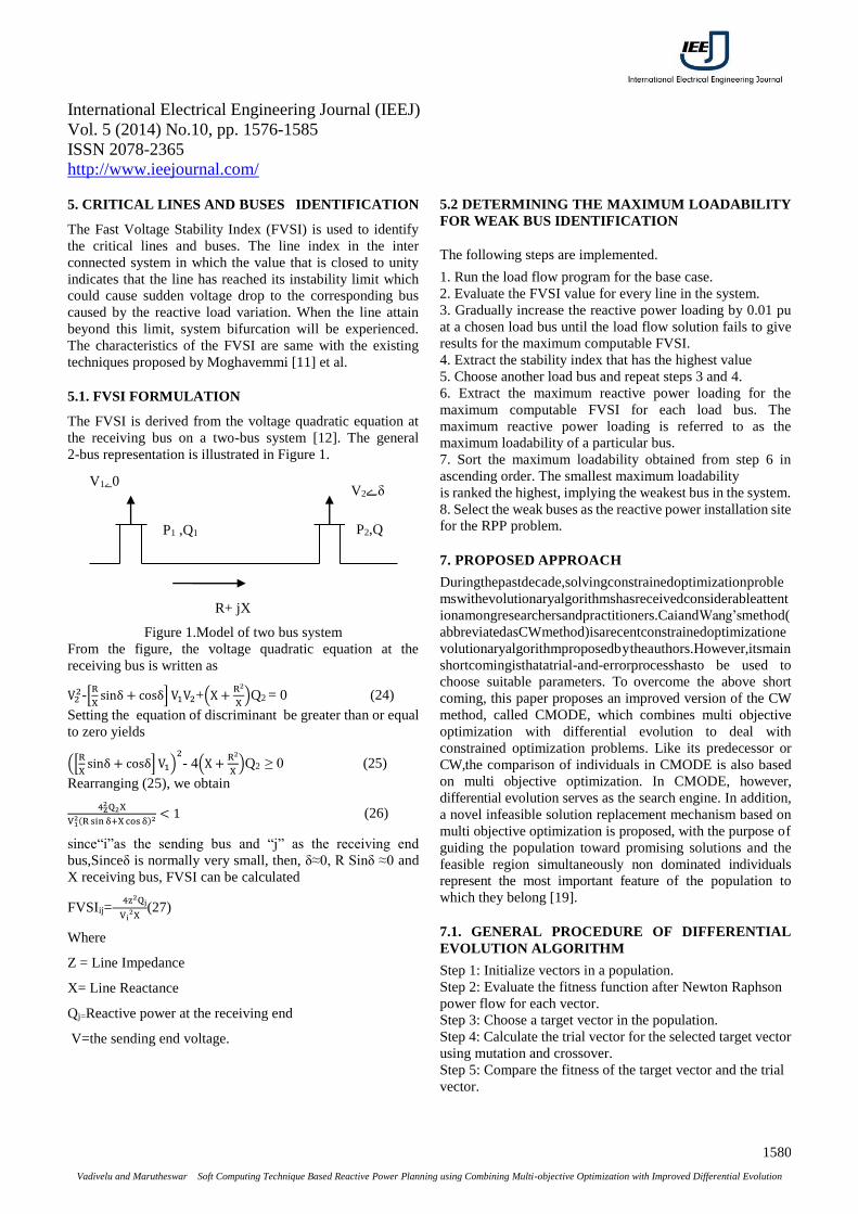
5.1. FVSI FORMULATION

The FVSI is derived from the voltage quadratic equation at

the receiving bus on a two-bus system [12]. The general

2-bus representation is illustrated in Figure 1.

Figure 1.Model of two bus system

From the figure, the voltage quadratic equation at the

receiving bus is written as

V22-[

R

Xsinδ + cosδ] V1V2+(X +

R2

X)Q2 = 0 (24)

Setting the equation of discriminant be greater than or equal

to zero yields

([R

Xsinδ + cosδ] V1)

2- 4(X +

R2

X)Q2 ≥ 0 (25)

Rearranging (25), we obtain

4Z2Q2X

V12(R sin δ+X cos δ)2 < 1 (26)

since“i”as the sending bus and “j” as the receiving end

bus,Sinceδ is normally very small, then, δ≈0, R Sinδ ≈0 and

X receiving bus, FVSI can be calculated

FVSIij= 4z2Qj

Vi2X

(27)

Where

Z = Line Impedance

X= Line Reactance

Qj=Reactive power at the receiving end

V=the sending end voltage.

5.2 DETERMINING THE MAXIMUM LOADABILITY

FOR WEAK BUS IDENTIFICATION

The following steps are implemented.

1. Run the load flow program for the base case.

2. Evaluate the FVSI value for every line in the system.

3. Gradually increase the reactive power loading by 0.01 pu

at a chosen load bus until the load flow solution fails to give

results for the maximum computable FVSI.

4. Extract the stability index that has the highest value

5. Choose another load bus and repeat steps 3 and 4.

6. Extract the maximum reactive power loading for the

maximum computable FVSI for each load bus. The

maximum reactive power loading is referred to as the

maximum loadability of a particular bus.

7. Sort the maximum loadability obtained from step 6 in

ascending order. The smallest maximum loadability

is ranked the highest, implying the weakest bus in the system.

8. Select the weak buses as the reactive power installation site

for the RPP problem.

7. PROPOSED APPROACH

Duringthepastdecade,solvingconstrainedoptimizationproble

mswithevolutionaryalgorithmshasreceivedconsiderableattent

ionamongresearchersandpractitioners.CaiandWang’smethod(

abbreviatedasCWmethod)isarecentconstrainedoptimizatione

volutionaryalgorithmproposedbytheauthors.However,itsmain

shortcomingisthatatrial-and-errorprocesshasto be used to

choose suitable parameters. To overcome the above short

coming, this paper proposes an improved version of the CW

method, called CMODE, which combines multi objective

optimization with differential evolution to deal with

constrained optimization problems. Like its predecessor or

CW,the comparison of individuals in CMODE is also based

on multi objective optimization. In CMODE, however,

differential evolution serves as the search engine. In addition,

a novel infeasible solution replacement mechanism based on

multi objective optimization is proposed, with the purpose of

guiding the population toward promising solutions and the

feasible region simultaneously non dominated individuals

represent the most important feature of the population to

which they belong [19].

7.1. GENERAL PROCEDURE OF DIFFERENTIAL

EVOLUTION ALGORITHM

Step 1: Initialize vectors in a population.

Step 2: Evaluate the fitness function after Newton Raphson

power flow for each vector.

Step 3: Choose a target vector in the population.

Step 4: Calculate the trial vector for the selected target vector

using mutation and crossover.

Step 5: Compare the fitness of the target vector and the trial

vector.

P1 ,Q1 P2,Q

2222

R+ jX

V10ے V2ےδ



Vol. 5 (2014) No.10, pp. 1576-1585

ISSN 2078-2365



1581

Step 6: Select the best fitness vector among them.

Step 7: Repeat step 3 to step 5 till the stopping criteria. The

stopping criterion is number of iterations.

8. RESULT AND DISCUSSION

The proposed combining multi objective IDE based

algorithm has been tested on standard IEEE 30-bus test

system and 72 bus Indian utility systems. In this reactive

power planning problem the optimal solution of the proposed

algorithm can be demonstrated under 100% , 125 % and

150% load in IEEE 30 bus test system,and 72 bus Indian

utility systems.. The real power savings, annual cost savings

and the total costs are calculated as,

PCSave% =

Plossint −Ploss

opt

Plossint x 100 % (28)

WCsave = hdl ( Ploss

int − Plossopt

)

FC= IC + WC

8.1. OPTIMAL REACTIVE POWER PLANNING FOR

IEEE 30 BUS SYSTEM

The IEEE 30 bus system consists of 6 generator-buses, 21

load-buses and 41 branches, of which four branches, (6, 9),

(6, 10), (4, 12) and (28, 27) are under load-tap setting

transformer branches. The buses identified for possible VAR

source installation based on max load buses are 25, 26, 29

and 30 using FVSI method. The optimal parameters used for

simulation of the IDE is the no of decision variables 14,no.of

generations 300,No of population 30,Scaling factor

(0-1),cross over rate (0.4),The parameters ,Limits, Initial

generations and power losses ,optimal VAR source

instalment ,optimal generator bus voltages, optimal

transformer settings are obtained from[6 ] .Three cases have

been studied. Case 1 is of light loads whose loads are the

same as those in [3]. Case 2 and 3 are of heavy loads whose

loads are 1.25% and 1.5% as those of Case 1. The duration of

the load level is 8760 hours in both cases [6].

Initial Power Flow Results

The initial generator bus voltages and transformer taps are set

to 1.0 pu. The loads are given as,

Case 1: Pload= 2.834 and Qload= 1.262

Case 2.Pload= 3.5425 and Qload = 1.5775

Case 3.Pload= 4.251 and Qload = 1.893.

TABLE 1.OPTIMAL GENERATIONS AND POWER LOSSES

Pg Qg Ploss Qloss

Case 1 2.989 1.288 0.159 0.266

Case 2 3.808 1.867 0.266 0.652

Case 3 4.659 2.657 0.417 1.190

TABLE 2.COST COMPARISON

PCsave% WCsave($) fC($)

Case 1 8.644 7,98,070.94 8.4225*106

Case 2 12.452 19,92,758.84 1.4408*107

Case 3 13.311 32,98,528.48

2.2017*107

TABLE 3. OPTIMAL GENERATIONS AND POWER LOSSES FOR CMDE

Pg Qg Ploss Qloss

Case 1 2.823 1.137 0.138 0.193

Case 2 3.712 1.742 0.238 0.526

Case 3 4.531 2.430 0.405 1.048

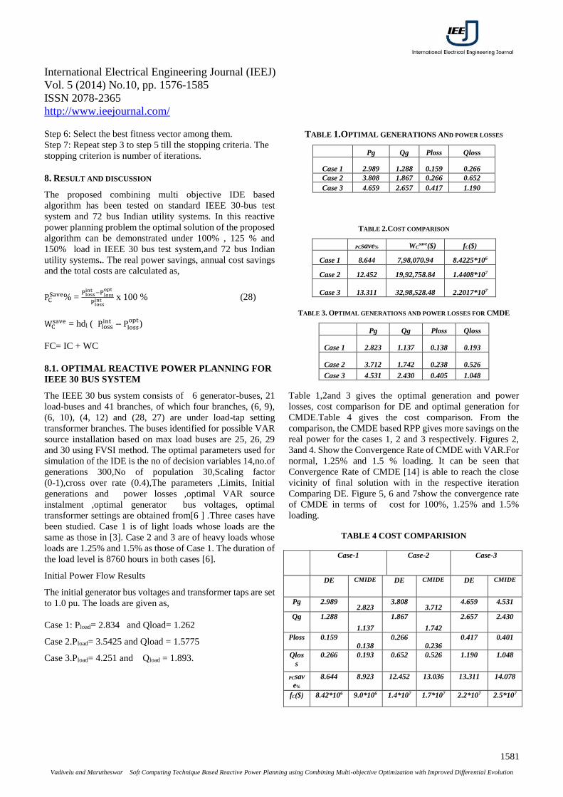
Table 1,2and 3 gives the optimal generation and power

losses, cost comparison for DE and optimal generation for

CMDE.Table 4 gives the cost comparison. From the

comparison, the CMDE based RPP gives more savings on the

real power for the cases 1, 2 and 3 respectively. Figures 2,

3and 4. Show the Convergence Rate of CMDE with VAR.For

normal, 1.25% and 1.5 % loading. It can be seen that

Convergence Rate of CMDE [14] is able to reach the close

vicinity of final solution with in the respective iteration

Comparing DE. Figure 5, 6 and 7show the convergence rate

of CMDE in terms of cost for 100%, 1.25% and 1.5%

loading.

TABLE 4 COST COMPARISION

Case-1 Case-2 Case-3

DE CMIDE DE CMIDE DE CMIDE

Pg 2.989 2.823

3.808 3.712

4.659 4.531

Qg 1.288

1.137

1.867

1.742

2.657 2.430

Ploss 0.159

0.138

0.266

0.236

0.417 0.401

Qlos

s

0.266 0.193 0.652 0.526 1.190 1.048

PCsav

e%

8.644 8.923 12.452 13.036 13.311 14.078

fC($) 8.42*106 9.0*106 1.4*107 1.7*107 2.2*107 2.5*107



Vol. 5 (2014) No.10, pp. 1576-1585

ISSN 2078-2365



1582

Figure 2. Converence Rate of CMDE Algorithm without VAR(100%

loading)

Figure 3. Converence Rate of CMDE Algorithm with VAR(125%

loading)

Figure 4. Converence Rate of CMDE Algorithm witht

VAR(150% loading)

Figure 5. Converence Rate of CMDE Algorithm in terms of cost(100%

loading)

Figure 6. Converence Rate of CMDE Algorithm in terms of cost (125%

loading)

Figure 7. Converence Rate of CMDE Algorithm in terms of cost(150%

loading)

0 50 100 150 200 250 30016

16.2

16.4

16.6

16.8

17

17.2

17.4

--> No. of iterations

-->

Tra

nsm

issio

n lin

e loss (

in M

W)

Convergence Rate of the CMIDE Algorithm

Loss Value at Iteration

0 50 100 150 200 250 30026.5

27

27.5

28

28.5

29

29.5

30

30.5

31


-->

tra

nsm

isson loss (

in M

W)


loss value at iteration

0 50 100 150 200 250 30040.5

41

41.5

42

42.5

43

43.5

44

44.5

45

45.5


-->

Tra

nsm

issio

n lin

e loss (

in M

W)

Convergence Rate of the CMDE Algorithm


0 50 100 150 200 250 3008.4

8.5

8.6

8.7

8.8

8.9

9

9.1x 10

6


-->

fc($

) )


objfunction

total

cost

0 50 100 150 200 250 3001.4

1.45

1.5

1.55

1.6

1.65

1.7

1.75x 10

7


-->

fc($

)


obj-function total cost

0 50 100 150 200 250 3002.2

2.25

2.3

2.35

2.4

2.45

2.5

2.55x 10

7


-->

fc($

)


obj-function total cost



Vol. 5 (2014) No.10, pp. 1576-1585

ISSN 2078-2365



1583

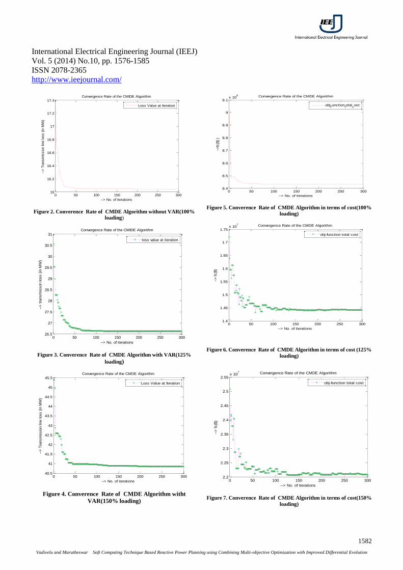
8.1. OPTIMAL REACTIVE POWER PLANNING FOR

INDIAN UTILITY 72 BUS SYSTEM

The Indian Utility 72 bus system consists of 15 PV buses

and 55 PQ buses, 41 branches. The buses identified for

possible VAR source installation based on max load buses

are 38, 49,51and 53 using FVSI method. The optimal

parameters used for simulation of the IDE is the no of

decision variables 14,no.of generations 300,no of population

30,Scaling factor (0-1),cross over rate (0.4),The

parameters,Limits,Initial generations and power losses

,optimal VAR source instalment ,optimal generator bus

voltages, optimal transformer settings are obtained from[6 ]

.Three cases have been studied. Case 1 is of light loads whose

loads are the same as those in [3]. Case 2 and 3 are of heavy

loads whose loads are 1.25% and 1.5% as those of Case 1.

The duration of the load level is 8760 hours in both cases [6].

Figure 8 Converence Rate of CMDE Algorithm with VAR (100%

loading)

Figure 9 Converence Rate of CMDE Algorithm with VAR(125%

loading)

Figure 10 Converence Rate of CMDE Algorithm with VAR (150%

loading)

Figure 11 Convergence Rate of CMDE Algorithm in terms of cost for

Normal loading


0 50 100 150 200 250 30016

16.2

16.4

16.6

16.8

17

17.2

17.4


-->

Tra

nsm

issio

n lin

e loss (

in M

W)



0 50 100 150 200 250 30026.5

27

27.5

28

28.5

29

29.5

30

30.5


-->

Tra

nsm

issio

n lin

e loss (

in M

W)



0 50 100 150 200 250 30040.5

41

41.5

42

42.5

43


-->

Tra

nsm

issio

n lin

e loss (

in M

W)

Convergence Rate of the DE Algorithm


0 50 100 150 200 250 3008.4

8.5

8.6

8.7

8.8

8.9

9

9.1x 10

6

--> iterations

-->

tota

l cost

(in f

c($

))


objfunction

total

cost

0 50 100 150 200 250 3001.4

1.45

1.5

1.55

1.6

1.65

1.7

1.75

1.8x 10

7


-->

tota

l cost

fc($

)


total cost



Vol. 5 (2014) No.10, pp. 1576-1585

ISSN 2078-2365



1584

125% loading


150% loading

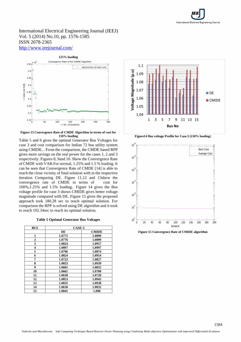
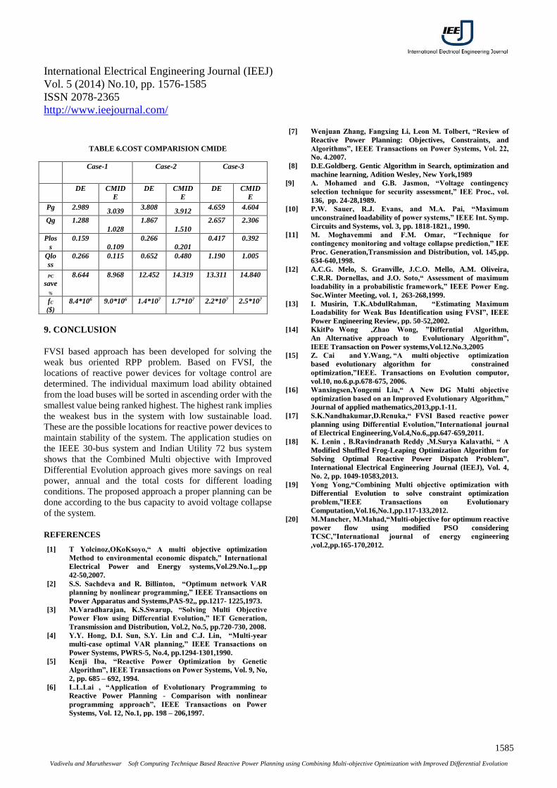
Table 5 and 6 gives the optimal Generator Bus Voltages for

case 3 and cost comparison for Indian 72 bus utility system

using CMIDE... From the comparison, the CMDE based RPP

gives more savings on the real power for the cases 1, 2 and 3

respectively. Figures 8, 9and 10. Show the Convergence Rate

of CMDE with VAR.For normal, 1.25% and 1.5 % loading. It

can be seen that Convergence Rate of CMDE [14] is able to

reach the close vicinity of final solution with in the respective

iteration Comparing DE. Figure 11,12 and 13show the

convergence rate of CMDE in terms of cost for

100%,1.25% and 1.5% loading.. Figure 14 gives the Bus

voltage profile for case 3 shows CMIDE gives better voltage

magnitude compared with DE. Figure 15 gives the proposed

approach took 180.28 sec to reach optimal solution. For

comparison the RPP is solved using DE algorithm and it took

to reach 192.34sec to reach its optimal solution.

Table 5 Optimal Generator Bus Voltages

BUS CASE-3

DE CMIDE

1 1.0771 1.0890

2 1.0776 1.0899

3 1.0824 1.0957

4 1.0897 1.0997

5 1.0796 1.0874

6 1.0824 1.0954

7 1.0723 1.0827

8 1.0853 1.0939

9 1.0601 1.0835

10 1.0661 1.0700

11 1.0638 1.0720

12 1.0853 1.0945

13 1.0835 1.0938

14 1.0630 1.0832

15 1.0841 1.098

Figure14 Bus voltage Profile for Case.3 (150% loading)

Figure 15 Convergence Rate of CMIDE algorithm

0 50 100 150 200 250 3002.15

2.2

2.25

2.3

2.35

2.4

2.45

2.5

2.55x 10

7


-->

tota

l cost

fc($

)


obj-function of total cost

1.04

1.05

1.06

1.07

1.08

1.09

1.1

1 3 5 7 9 11 13 15

Vo

ltag

e M

agn

itu

de

(p

.u)

Bus No

DE

CMIDE

0 20 40 60 80 100 120 140 160 180 20010

8

109

1010

1011

1012

1013

1014

Iteration

Best Cost

Average Cost



Vol. 5 (2014) No.10, pp. 1576-1585

ISSN 2078-2365



1585

TABLE 6.COST COMPARISION CMIDE

Case-1 Case-2 Case-3

DE CMID

E

DE CMID

E

DE CMID

E

Pg 2.989 3.039

3.808 3.912

4.659 4.604

Qg 1.288

1.028

1.867

1.510

2.657 2.306

Plos

s

0.159

0.109

0.266

0.201

0.417 0.392

Qlo

ss

0.266 0.115 0.652 0.480 1.190 1.005

PC

save

%

8.644 8.968 12.452 14.319 13.311 14.840

fC

($)

8.4*106 9.0*106 1.4*107 1.7*107 2.2*107 2.5*107

9. CONCLUSION

FVSI based approach has been developed for solving the

weak bus oriented RPP problem. Based on FVSI, the

locations of reactive power devices for voltage control are

determined. The individual maximum load ability obtained

from the load buses will be sorted in ascending order with the

smallest value being ranked highest. The highest rank implies

the weakest bus in the system with low sustainable load.

These are the possible locations for reactive power devices to

maintain stability of the system. The application studies on

the IEEE 30-bus system and Indian Utility 72 bus system

shows that the Combined Multi objective with Improved

Differential Evolution approach gives more savings on real

power, annual and the total costs for different loading

conditions. The proposed approach a proper planning can be

done according to the bus capacity to avoid voltage collapse

of the system.

REFERENCES

[1] T Yolcinoz,OKoKsoyo,“ A multi objective optimization

Method to environmental economic dispatch,” International

Electrical Power and Energy systems,Vol.29.No.1,,.pp

42-50,2007.

[2] S.S. Sachdeva and R. Billinton, “Optimum network VAR

planning by nonlinear programming,” IEEE Transactions on

Power Apparatus and Systems,PAS-92,, pp.1217- 1225,1973.

[3] M.Varadharajan, K.S.Swarup, “Solving Multi Objective

Power Flow using Differential Evolution,” IET Generation,

Transmission and Distribution, Vol.2, No.5, pp.720-730, 2008.

[4] Y.Y. Hong, D.I. Sun, S.Y. Lin and C.J. Lin, “Multi-year

multi-case optimal VAR planning,” IEEE Transactions on

Power Systems, PWRS-5, No.4, pp.1294-1301,1990.

[5] Kenji Iba, “Reactive Power Optimization by Genetic

Algorithm”, IEEE Transactions on Power Systems, Vol. 9, No,

2, pp. 685 – 692, 1994.

[6] L.L.Lai , “Application of Evolutionary Programming to

Reactive Power Planning - Comparison with nonlinear

programming approach”, IEEE Transactions on Power

Systems, Vol. 12, No.1, pp. 198 – 206,1997.

[7] Wenjuan Zhang, Fangxing Li, Leon M. Tolbert, “Review of

Reactive Power Planning: Objectives, Constraints, and

Algorithms”, IEEE Transactions on Power Systems, Vol. 22,

No. 4.2007.

[8] D.E.Goldberg. Gentic Algorithm in Search, optimization and

machine learning, Adition Wesley, New York,1989

[9] A. Mohamed and G.B. Jasmon, “Voltage contingency

selection technique for security assessment,” IEE Proc., vol.

136, pp. 24-28,1989.

[10] P.W. Sauer, R.J. Evans, and M.A. Pai, “Maximum

unconstrained loadability of power systems,” IEEE Int. Symp.

Circuits and Systems, vol. 3, pp. 1818-1821., 1990.

[11] M. Moghavemmi and F.M. Omar, “Technique for

contingency monitoring and voltage collapse prediction,” IEE

Proc. Generation,Transmission and Distribution, vol. 145,pp.

634-640,1998.

[12] A.C.G. Melo, S. Granville, J.C.O. Mello, A.M. Oliveira,

C.R.R. Dornellas, and J.O. Soto,“ Assessment of maximum

loadability in a probabilistic framework,” IEEE Power Eng.

Soc.Winter Meeting, vol. 1, 263-268,1999.

[13] I. Musirin, T.K.AbdulRahman, “Estimating Maximum

Loadability for Weak Bus Identification using FVSI”, IEEE

Power Engineering Review, pp. 50-52,2002.

[14] KkitPo Wong ,Zhao Wong, ”Differntial Algorithm,

An Alternative approach to Evolutionary Algorithm”,

IEEE Transaction on Power systems,Vol.12.No.3,2005

[15] Z. Cai and Y.Wang, “A multi objective optimization

based evolutionary algorithm for constrained

optimization,”IEEE. Transactions on Evolution computor,

vol.10, no.6.p.p.678-675, 2006.

[16] Wanxingsen,Yongemi Liu,“ A New DG Multi objective

optimization based on an Improved Evolutionary Algorithm,”

Journal of applied mathematics,2013,pp.1-11.

[17] S.K.Nandhakumar,D.Renuka,“ FVSI Based reactive power

planning using Differential Evolution,”International journal

of Electrical Engineering,Vol.4,No.6,,pp.647-659,2011.

[18] K. Lenin , B.Ravindranath Reddy ,M.Surya Kalavathi, “ A

Modified Shuffled Frog-Leaping Optimization Algorithm for

Solving Optimal Reactive Power Dispatch Problem”,

International Electrical Engineering Journal (IEEJ), Vol. 4,

No. 2, pp. 1049-10583,2013.

[19] Yong Yong,“Combining Multi objective optimization with

Differential Evolution to solve constraint optimization

problem,”IEEE Transactions on Evolutionary

Computation,Vol.16,No.1,pp.117-133,2012.

[20] M.Mancher, M.Mahad,“Multi-objective for optimum reactive

power flow using modified PSO considering

TCSC,”International journal of energy engineering

,vol.2,pp.165-170,2012.


Soft Computing Technique Based Reactive Power Planning using Combining Multi-objective Optimization...

Documents

Transcript of Soft Computing Technique Based Reactive Power Planning using Combining Multi-objective Optimization...