Performance evaluation of public and private sector banks in India using DEA approach
31
Int. J. Operational Research, Vol. 18, No. 1, 2013 91 Copyright © 2013 Inderscience Enterprises Ltd. Performance evaluation of public and private sector banks in India using DEA approach Jolly Puri* and Shiv Prasad Yadav Department of Mathematics, IIT Roorkee, Roorkee 247667, India E-mail: [email protected] E-mail: [email protected] *Corresponding author Abstract: This paper seeks to measure the OTE, PTE and SE of PuSBs and PrSBs for the year 2009 to 2010 using DEA. The findings show that: 1) PuSBs outperformed PrSBs in all categories of efficiencies; 2) the contribution of scale inefficiency in overall technical inefficiency has been observed to be smaller than the contribution of pure technical inefficiency; 3) in PuSBs, State Bank of India (SBI) & its Associates outperformed nationalised banks and in PrSBs, new PrSBs outperformed old PrSBs; 4) the highest and lowest levels of average overall technical inefficiency have been seen for old PrSBs (48.8%) and SBI & its Associates (2.2%), respectively; 5) the results of the present study, by sensitivity analysis, are quite robust to discriminate between efficient and inefficient banks. Keywords: efficiency measurement; data envelopment analysis; DEA; public sector banks; PuSBs; private sector banks; PrSBs; India. Reference to this paper should be made as follows: Puri, J. and Yadav, S.P. (2013) ‘Performance evaluation of public and private sector banks in India using DEA approach’, Int. J. Operational Research, Vol. 18, No. 1, pp.91–121. Biographical notes: Jolly Puri is a Research Scholar in the Department of Mathematics, IIT Roorkee, Roorkee, India. She is working on assessing efficiency of banking sector in India by applying DEA techniques. She has interest in fuzzy optimisation also. Shiv Prasad Yadav is an Associate Professor of Mathematics at the Indian Institute of Technology Roorkee, Roorkee, India. He holds a PhD in Optimal Control Theory from the Applied Mathematics Department, Institute of Technology, Banaras Hindu University, Varansi, India. His current research areas include optimal control theory, operations research, data envelopment analysis, fuzzy optimisation and fuzzy reliability studies.
-
Upload
independent -
Category
Documents
-
view
4 -
download
0
Transcript of Performance evaluation of public and private sector banks in India using DEA approach
Int. J. Operational Research, Vol. 18, No. 1, 2013 91
Copyright © 2013 Inderscience Enterprises Ltd.
Performance evaluation of public and private sector banks in India using DEA approach
Jolly Puri* and Shiv Prasad Yadav Department of Mathematics, IIT Roorkee, Roorkee 247667, India E-mail: [email protected] E-mail: [email protected] *Corresponding author
Abstract: This paper seeks to measure the OTE, PTE and SE of PuSBs and PrSBs for the year 2009 to 2010 using DEA. The findings show that: 1) PuSBs outperformed PrSBs in all categories of efficiencies; 2) the contribution of scale inefficiency in overall technical inefficiency has been observed to be smaller than the contribution of pure technical inefficiency; 3) in PuSBs, State Bank of India (SBI) & its Associates outperformed nationalised banks and in PrSBs, new PrSBs outperformed old PrSBs; 4) the highest and lowest levels of average overall technical inefficiency have been seen for old PrSBs (48.8%) and SBI & its Associates (2.2%), respectively; 5) the results of the present study, by sensitivity analysis, are quite robust to discriminate between efficient and inefficient banks.
Keywords: efficiency measurement; data envelopment analysis; DEA; public sector banks; PuSBs; private sector banks; PrSBs; India.
Reference to this paper should be made as follows: Puri, J. and Yadav, S.P. (2013) ‘Performance evaluation of public and private sector banks in India using DEA approach’, Int. J. Operational Research, Vol. 18, No. 1, pp.91–121.
Biographical notes: Jolly Puri is a Research Scholar in the Department of Mathematics, IIT Roorkee, Roorkee, India. She is working on assessing efficiency of banking sector in India by applying DEA techniques. She has interest in fuzzy optimisation also.
Shiv Prasad Yadav is an Associate Professor of Mathematics at the Indian Institute of Technology Roorkee, Roorkee, India. He holds a PhD in Optimal Control Theory from the Applied Mathematics Department, Institute of Technology, Banaras Hindu University, Varansi, India. His current research areas include optimal control theory, operations research, data envelopment analysis, fuzzy optimisation and fuzzy reliability studies.
92 J. Puri and S.P. Yadav
1 Introduction
The performance of banks has become a major concern of planners and policy makers in India. Since early 1990s, the Indian financial sector has noticed various changes in the policies and prudential norms to raise the banking standards in India. The growth and financial stability of the country depends on the financial soundness of its financial institutions. According to Rajan and Zingales (1998), a sound banking system serves as an important medium for achieving economic growth through the mobilisation of financial savings, putting them to productive use, and transforming various risks. Major changes took place in the functioning of banks in India only after liberalisation, globalisation and privatisation. In market environment, PuSBs are facing fierce price and non-price competition from PrSBs and foreign banks (FBs). Increased competition, new information technologies and thereby declining processing costs, and less restrictive governmental regulations have all played a major role for PuSBs in India to forcefully compete with PrSBs and FBs. Due to this increased competition, the share of PuSBs in deposits, advances, investments and assets of banking industry is declining steadily. The efficiency of banks, which reflects the ability of banks in transforming its resources to output by making its best allocation, is essential for the growth of an economy. However, due to the major role played by financial institutions in the development of economy, a study of the efficiency of financial institutions and in particular, of the banks has gained popularity in recent times. Berger and Humphrey (1997) asserted that the information obtained from banking efficiency analyses can be used to reform government policy by assessing the effects of deregulation, mergers, or market structure on efficiency and to improve the managerial performance by identifying the best and worst practices associated with high and low measured efficiency, respectively, and encouraging the former practices and while discouraging the latter. In an economy, banks normally serve as financial intermediaries (Chen and Yeh, 2000). Without an efficient banking system, the economy cannot function efficiently. Both PuSBs and PrSBs play an important role in the development of an Indian economy. Therefore, it has become very mandatory to study and to make a comparative analysis of the services of both PuSBs and PrSBs.
Facing to major economic crisis, India started liberalising its economy in 1991. It resulted into reduction or elimination of controls on various sectors. The government allowed private sector to participate where it was earlier either denied or restricted. Financial sector, including banking sector was also liberalised. After liberalisation the banking industry underwent major changes. In 1992, the government appointed a Narasimham committee to study and recommend reforms for the banking sector. Consequent on the recommendations, a series of reforms were introduced. The economic reforms totally have changed the banking sector. The government allowed new private sector to enter the banking sector from 1993, and further, the FBs from 1994. RBI also permitted new banks to be started in the private sector as per the recommendation of Narasimham committee. Several new PrSBs were established in 1994 to 2005 period and several FBs established their branches or expanded existing network. The Indian banking industry was dominated by PuSBs. But now the situations have changed new generation banks with used of technology and professional management has gained a reasonable position in the banking industry. Important decision taken by government after liberalisation is the reduction of government’s stake of 51% in PuSBs. During 1994 to 1995, permission were given to setup banks like UTI bank (now Axis Bank), IndusInd bank, ICICI bank, Global trust bank Ltd., Centurion bank Ltd., and HDFC bank Ltd.,
Performance evaluation of public and private sector banks in India 93
latter during 1995 to 1996 further new banks like Times bank Ltd., Bank of Punjab Ltd., Development Credit Bank Ltd., and IDBI bank were setup. Earlier, functioning of PuSBs was at a relative disadvantage when compared with the PrSBs, which were offering state-of-the-art facilities such as ATMs, doorstep banking, banking on phone, internet banking, core banking, etc. PuSBs also suffer from huge costs of labour and low levels of automation. For arresting this decline, the PuSBs are now reorienting and redesigning their operational strategies and offering several financial products like internet banking, ATM services, insurance services, etc., to their customers. However, the success of PuSBs and PrSBs mainly depends upon the fact that how efficiently they utilise their financial resources in providing financial services and products.
Keeping in view the importance of performance evaluation of banking industry in India, the present study is conducted to make the comparative analysis of two important categories of banks in India namely PuSBs and PrSBs, and their respective categories. The PuSBs are categorised into two bank groups:
1 nationalised banks
2 SBI & its Associates.
The PrSBs are categorised into two bank groups:
1 old PrSBs
2 new PrSBs.
This paper seeks to measure:
1 the overall technical efficiency (OTE)
2 pure technical efficiency (PTE)
3 scale efficiency (SE)
of individual PuSBs and PrSBs for the year 2009 to 2010 using DEA. This paper also seeks to measure:
1 average overall technical efficiency (AOTE)
2 average pure technical efficiency (APTE)
3 average scale efficiency (ASE)
for PuSBs and PrSBs and, their respective categories of bank groups using DEA. This has been done through the execution of two most popular DEA models: CCR
model (Charnes et al., 1978) and BCC model (Banker et al., 1984). DEA is a linear programming-based non-parametric technique which enables to measure a technical efficiency of all DMUs and, provides benchmarks and targets for the performance improvement of the inefficient DMUs. The choice of DEA in the present study is driven by its intrinsic advantages over the other techniques for measuring the relative efficiency of banks. First, DEA is one of the most popular approaches to measure the relative efficiency of banks. Second, DEA is a non-parametric frontier approach and does not require rigid assumptions regarding production technology or efficiency distribution. Third, DEA identifies the inefficiency in a particular bank by comparing it to similar banks regarded as efficient, rather than trying to associate a bank’s performance with
94 J. Puri and S.P. Yadav
statistical averages that may not be applicable to that bank (Avkiran, 2006). The OTE, PTE and SE scores for individual PuSBs and PrSBs have been measured by employing CCR and BCC models. The primary difference between CCR model and BCC model is the convexity constraint, which represents the returns-to-scale (RTS). RTS reflects the extent to which a proportional change in all inputs changes outputs. Before proceeding further, there is a need to understand the concepts of OTE, PTE and SE according to perspective of the banks. Technical efficiency (TE) relates to the productivity of inputs (Sathye, 2003). According to the banking perspective, TE of the bank is its ability to transform multiple resources into multiple financial services (Bhattacharyya et al., 1997). A measure of TE under constant returns-to-scale (CRS) assumption is known as OTE. The OTE basically helps to determine inefficiency due to the input/output configuration as well as the size of operations. Further, OTE is broken into two components: PTE and SE. The PTE is a measure of efficiency under variable returns-to-scale (VRS). It is a measure which purely reflects the managerial performance to organise the inputs in the production process. Thus, it is a measure of TE without SE. The SE is the ratio of OTE to PTE. It is the ability of the management to choose the scale of production that will attain the expected production level. Inappropriate size of a bank results into technical inefficiency (TIE) and such type of inefficiency is known as scale inefficiency (SIE). It takes two forms: increasing returns-to-scale (IRS) and decreasing returns-to-scale (DRS). IRS means a bank is too small for its scale operations and DRS means a bank is too large to take full advantage of its scale. A bank is scale efficient if it operates at CRS.
To sum up, the aim of the present study is five-fold:
1 to obtain a measure of OTE, PTE and SE for PuSBs and PrSBs
2 to measure AOTE, APTE and ASE for all the four categories of banks, namely, nationalised banks, SBI & its Associates, old PrSBs and new PrSBs
3 to evaluate the average inefficiencies in OTE, PTE and SE
4 to provide benchmarks and targets to improve the efficiency of inefficient banks
5 to apply sensitivity analysis in order to check the robustness of the efficiency results.
This paper is organised as follows: Section 2 presents a brief overview of literature on bank efficiency with particular focus on Indian banking. Section 3 describes the structure of the Indian banking sector with a special reference to PuSBs and PrSBs. Section 4 presents the methodology which includes the description of DEA and it also presents the CCR and BCC models that are used in the present study. The issues relating to selection of input and output variables are discussed in Section 5. Section 6 presents the isotonicity test to check the inter-correlation between input and output variables. Section 7 presents the empirical results and discussion. Finally, Section 8 concludes the findings of our study.
2 Banking efficiency: a brief review of literature in Indian context
Berger and Humphrey (1997) in their wide-ranging international survey pointed out that out of 130 efficiency analyses of financial institutions covering 21 countries, only about 5% examined the banking sectors of developing countries. In the developing country like India, the research on the performance evaluation of banking sector is still in its initial
Performance evaluation of public and private sector banks in India 95
stages. There have been some studies analysing bank efficiency in India and in these studies, bank efficiency has been measured by a number of financial indicators and compared over various categories of banks. The research on the banking efficiency in India is focused mainly on:
1 the effect on the banks performance after deregulation and liberalisation
2 the effect of ownership type on different efficiency measures
3 the performance evaluation of banks using different frontier techniques.
The literature on the performance of PuSBs and PrSBs also focuses on the above three points and we present the literature by keeping in view the above points.
The banking sector in India underwent a significant liberalisation process in early 1990s, which led to reforms in the banking sector and changed the Indian banking structure. Major changes took place in the functioning of Indian Banks only after liberalisation, globalisation and privatisation. Bhattacharyya et al. (1997) studied the impact of policy of liberalising measures taken in 1980s on the performance of various categories of banks and used DEA to measure the productive efficiency of Indian commercial banks in the late 1980s to early 1990s. They found that the Indian PuSBs were the best performing banks, while the new PrSBs were yet to emerge fully in the Indian banking scenario. They asserted that deregulation has led to an improvement in the overall performance of Indian commercial banks. Kumbhakar and Sarkar (2003) found evidence on Indian banks that while PrSBs have improved their performance mainly due to the freedom to expand output, PuSBs have not respond well to the deregulation measures. Ataullah et al. (2004) pointed out that OTE of the banking industry of India and Pakistan improved following the financial liberalisation. Reddy (2004, 2005) reported a rise in OTE of Indian banks during the period of deregulation. Das et al. (2005) found that the efficiency of Indian banks especially of bigger banks has improved during the post-reforms period. Sensarma (2006) found that deregulation has led to the reduction in intermediation costs and improvement in total factor productivity in Indian banks, particularly in PuSBs. Sahoo et al. (2007) examined the productivity performance trends of the Indian commercial banks for the period: 1997–1998 to 2004–2005. They found that the increasing average annual trends in TE for all ownership groups indicate a positive gesture about the effect of the reform process on the performance of the Indian banking sector. Ray and Das (2010) have applied DEA methodology to find the cost efficiency of Indian banks during the post-reform period 1997 to 2003. They found that there is no definite evidence that privatisation enhances efficiency at least in the case of Indian banks.
Sarkar et al. (1998) compared PuSBs, PrSBs and FBs in India to find the effect of ownership type on different efficiency measures. Ram Mohan (2002, 2003) also used financial measures for comparing operational performance of PuSBs and PrSBs over a period of time. Sathye (2003) studied the relative efficiency of Indian banks in the late 1990s and compared the efficiency of Indian banks with that of the banks in other countries. Ram Mohan and Ray (2004) compared the technical, allocative and revenue maximising efficiency of PuSBs, PrSBs and FBs in India. Their study covered the period 1992 to 2000. They found that PuSBs were significantly better than PrSBs. It has also been noted that SBI turned out to be the most efficient in the study period. On the other hand, Chakrabarti and Chawla (2005) compared the relative efficiency of PuSBs and
96 J. Puri and S.P. Yadav
PrSBs during the period 1990 to 2002. They utilised two approaches namely quantity approach and value approach to specify the input-output variables. They found that PrSBs performed better than PuSBs. Sanjeev (2006) studied efficiency of PuSBs, PrSBs and FBs operating in India during the period 1997 to 2001 using DEA. He found that there is an increase in the efficiency in the post-reform period. RBI (2008) found no significant differences in any of the efficiency measures between PuSBs and PrSBs. Gupta et al. (2008) studied productive efficiency of Indian banks for the period 1999 to 2003. They reported that SBI & its Associates have the highest efficiency, followed by PrSBs and the other nationalised banks. Kumar and Gulati (2008) studied the technical efficiency of PuSBs in India using two DEA models, namely, the CCR model (Charnes et al., 1978); and Andersen and Petersen’s (1993) super-efficiency model. The analysis was performed on a cross-section data of 27 PuSBs in the year 2004 to 2005. The results show that the technical efficiency scores range from 0.632 to 1 with an average of 0.885. They found that FBs are more cost-efficient but less profit-efficient relative to domestically owned private banks and state-owned banks. The banks affiliated to SBI group were found to outperform the nationalised banks in terms of operating efficiency.
Kumar and Gulati (2009) studied the technical efficiency of Indian domestic banks for the period 2006 to 2007 and found that the efficiency differences between PuSBs and PrSBs are not statistically significant. Rajput and Gupta (2011) evaluated the technical efficiency of PuSBs during the post-reform period using DEA and found the positive impact of reforms on 20 PuSBs and negative impact on seven PuSBs. Nandy (2012) studied the financial performance of PuSBs using a variety of efficiency measures computed by DEA models in the light of cluster analysis. Bapat (2012) studied the effect of global financial crisis on the efficiency of Indian banks and found that the Indian banking is on a path of revival. Baidya and Mitra (2012) evaluated the technical efficiency of 26 PuSBs from the cross-section data of the financial year 2009 to 2010. They found that the banks which utilise more labour are relatively more inefficient. They observed that SBI is the most efficient bank followed by Indian Bank, corporation Bank on the basis of super-efficiency score, whereas United Bank of India is the most inefficient bank. George and Chattopadhyay (2012) studied the operational performance and service quality of PuSBs. Chowdhury (2012) asserted that Indian banking industry is still struggling to achieve global standards and found that the best rated banks in India are not able to get position within the top hundred banks globally.
In India, Keshari and Paul (1994) were the first to evaluate the efficiency of banks using the frontier methodology. Most of the researchers like Bhattacharyya et al. (1997), Kumbhakar and Sarkar (2003), Shanmugam and Das (2004), Ram Mohan and Ray (2004), Das et al. (2005), Kumar and Gulati (2008), Ray and Das (2010), Rajput and Gupta (2011), Nandy (2012), Bapat (2012), and Baidya and Mitra (2012) applied DEA technique to measure the performance of Indian banking industry. Azadeh et al. (2010) applied DEA approach for ranking and optimisation of technical and management efficiency of a large bank based on financial indicators. A very few researchers applied the techniques other than DEA for evaluating the bank efficiency. Shanmugam and Das (2004) studied banking efficiency using stochastic frontier production function model during the reform period 1992 to 1999. They found that PrSBs and FBs performed better than PuSBs. They also observed that during reform period, Indian banking industry showed a progress in terms of efficiency of raising non-interest income, investments and credits.
Performance evaluation of public and private sector banks in India 97
Keeping in view the above mentioned premise, we can draw the following inferences. First, a majority of studies shows a positive impact of deregulation and the reforms on the performance of the banking sector. Second, the effect of ownership type on different efficiency measures is inconclusive. Third, most of the researchers have used DEA technique in order to evaluate the bank efficiency in India.
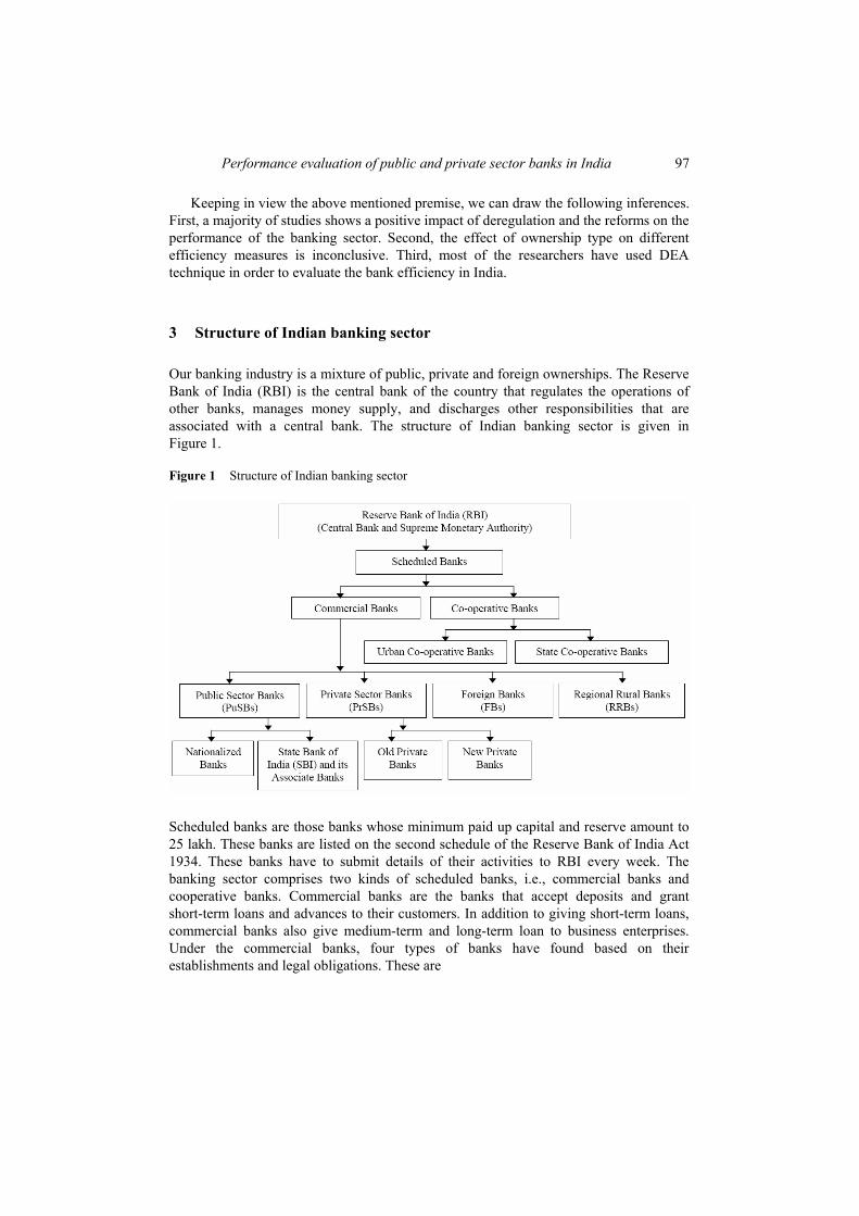
3 Structure of Indian banking sector
Our banking industry is a mixture of public, private and foreign ownerships. The Reserve Bank of India (RBI) is the central bank of the country that regulates the operations of other banks, manages money supply, and discharges other responsibilities that are associated with a central bank. The structure of Indian banking sector is given in Figure 1.
Figure 1 Structure of Indian banking sector
Scheduled banks are those banks whose minimum paid up capital and reserve amount to 25 lakh. These banks are listed on the second schedule of the Reserve Bank of India Act 1934. These banks have to submit details of their activities to RBI every week. The banking sector comprises two kinds of scheduled banks, i.e., commercial banks and cooperative banks. Commercial banks are the banks that accept deposits and grant short-term loans and advances to their customers. In addition to giving short-term loans, commercial banks also give medium-term and long-term loan to business enterprises. Under the commercial banks, four types of banks have found based on their establishments and legal obligations. These are
98 J. Puri and S.P. Yadav
1 Public sector banks (PuSBs) – These are the banks where majority stake is held by the Government of India (GOI) or RBI. The PuSBs include two types of banks: a nationalised banks b State Bank of India (SBI) and its Associate banks.
2 Private sector banks (PrSBs) – In case of PrSBs, majority of share capital of the bank is held by private individuals. These banks are registered as companies with limited liability. The PrSBs include old private banks (established before 1992) and de nova (new) private banks (established after 1992).
3 FBs – These banks are registered and have their headquarters in a foreign country but operate their branches in our country.
4 Regional rural banks (RRBs) – RRBs are jointly owned by GOI, the concerned state government and sponsor banks (scheduled commercial banks and one State Cooperative Bank); the issued capital of a RRB is shared by the owners in the proportion of 50%, 15% and 35% respectively. The RRBs mobilise financial resources from rural/semi-urban areas and grant loans and advances mostly to small and marginal farmers, agricultural labourers and rural artisans.
A cooperative bank is a financial entity which belongs to its members, who are at the same time the owners and the customers of their bank. Cooperative banks are often created by persons belonging to the same local or professional community or sharing a common interest. Cooperative banks generally provide their members with a wide range of banking and financial services. Cooperative Banks in India are registered under the Cooperative Societies Act. The cooperative bank is also regulated by the RBI. They are governed by the Banking Regulations Act 1949 and Banking Laws (Cooperative Societies) Act, 1965. The Cooperative banks consist of urban cooperative banks and state cooperative banks.
In the period 2009 to 2010, there were 27 PuSBs (including IDBI Bank), out of which 21 are nationalised banks and 6 are SBI & its Associates and 21 PrSBs, out of which 14 are old PrSBs and seven are new PrSBs. In the year 2009, the share of the nationalised banks in total bank credit was 50.5% and it increased to 52.0% in 2010. The share of PrSBs was 17.5% in 2010. The nationalised banks had the credit growth at 21.0% in 2010. The SBI & its Associates and PrSBs witnessed growth in credit at 17.7% and 12.9% in 2010, respectively. Of the incremental credit, during 2010, SBI & its Associates, nationalised banks and PrSBs shared 23.4%, 60.5% and 13.4%, respectively. The nationalised banks have a major share in aggregate bank deposits at 51.9% in 2010. The share of SBI & its Associates declined to 22.3% in 2010 as compared to 24.1% in 2009. The deposits of the nationalised banks registered the highest growth of 22.1% followed PrSBs (12.9%) in 2010. All of the above data is taken from RBI (2010b).
4 Methodology
A variety of techniques has been used to study the efficiency of Indian banks. It is found that estimates of efficiency are sensitive to the choice of technique. In literature on

Performance evaluation of public and private sector banks in India 99
banking efficiency, two distinct approaches have been used to measure the efficiency of banks. These approaches are:
1 traditional ratio approach
2 frontier approach.
In ratio approach, various different ratios have been employed by the researchers to examine different aspects of a bank’s performance. For example, a ratio of return on assets (ROA) to return on equity (ROE) has been considered as key ratio for assessing the financial performance of the banks (Avkiran, 2006). Likewise, the ratio of non-interest expenses to average assets is also a measure of efficiency of banks. However, there are certain problems related to this approach, e.g., the choice of ratios, the choice of benchmark against which the performance of the banks has been assessed, etc. On the other hand, frontier approach does not possess such problems. Thus, it gained tremendous popularity in the recent years as a tool to measure the relative efficiency of banks. In the literature, there are five frontier techniques (Bauer et al., 1998):
1 stochastic frontier analysis (SFA)
2 distribution free approach (DFA)
3 thick frontier approach (TFA)
4 data envelopment analysis (DEA)
5 free disposal hull (FDH).
The first three frontier techniques are known as parametric techniques which require explicit specification of production frontier and the remaining two techniques are known as non-parametric techniques which do not require any specification of production frontier. Non-parametric techniques are mainly mathematical programming techniques. The most popular and widely used non-parametric technique in measuring banks efficiency is DEA.
4.1 Data envelopment analysis
DEA is a linear programming technique initially developed by Charnes et al. (1978) to construct a non-parametric piecewise frontier (surface) over the data. Efficiency measure is then calculated relative to this frontier. Using this frontier, DEA computes a maximal performance measure for each decision making unit (DMU) relative to that of all other DMUs with the restriction that each DMU lies on the efficient (extremal) frontier or is enveloped by the frontier. The DMUs which lie on the frontier are the best practice units and attain an efficiency value equal to 1. These are called efficient DMUs. On the other hand, the DMUs which attain an efficiency value between 0 and 1 are called inefficient DMUs. DEA is basically a generalisation of Farrell’s technical efficiency (Cooper et al., 2007) measure to multiple inputs and multiple outputs case. More detailed reviews of the DEA methodology are also presented in Seiford and Thrall (1990), Seiford (1996), Zhu (2003) and Ray (2004). Sherman and Gold (1985) were the first to apply DEA to banking and the application of DEA in banking is also presented in Cooper et al. (2008) and Dharmapala and Edirisuriya (2011) As an efficient frontier technique, DEA identifies the inefficiency in a particular DMU by comparing it with similar DMUs regarded as

100 J. Puri and S.P. Yadav
efficient, rather than trying to associate a DMU’s performance with statistical averages that may not be applicable to that DMU.
In the present study, we use the CCR and BCC models to calculate the efficiency measures. CCR model is corresponding to the assumption of CRS whereas BCC model is corresponding to the assumption of VRS. The efficiency score obtained from CCR model is known as OTE score whereas the efficiency score obtained from BCC model is popularly known as PTE score. SE score can be obtained by a ratio of OTE score to PTE score (i.e., SE = OTE/PTE).
4.1.1 CCR model
To describe DEA efficiency evaluation, assume that the performance of the homogeneous set of n DMUs (DMUj; j = 1, …, n) be measured. The performance of DMUj is characterised by a production process of m inputs (xij; i = 1, …, m) to yield s outputs (yrj; r = 1, …, s). According to Charnes et al. (1978), the ratio of the virtual output to the virtual input of any DMUk called the efficiency Ek of the kth DMU, is to be maximised with the condition that the ratio of the virtual output to the virtual input of every DMU should be less than or equal to unity.
Mathematically,
1
1
1
1
1 1
Max
subject to 1, 1, ..., ,
, , 1, ..., , 1, ..., ,
=
=
=
=
= =
=
≤ ∀ =
≥ ≥ ∀ = ∀ =
∑
∑
∑
∑
∑ ∑
skr rk
rk m
kiki
is
kr rj
rm
kiji
ik kr i
m mk k
ik iki ii i
u yE
v x
u yj n
v x
u vε ε r s i mv x v x
(Model 1)
where k = 1, …, n and yrk is the amount of the rth output produced by the kth DMU; xik is the amount of the ith input used by the kth DMU; , k k
riv u are weights corresponding to the ith input and rth output of the kth DMU respectively; n is the number of DMUs; s is the number of outputs; m is the number of inputs and ε is a non-Archimedean (infinitesimal) constant. The model 1 is popularly known as the classical CCR ratio model named after Charnes, Cooper and Rhodes. The theory of fractional linear programming makes it possible to replace Model 1 by an equivalent linear programming problem by imposing
the condition 1
1=
=∑m
kiki
i
v x which provides:
Performance evaluation of public and private sector banks in India 101
1
1
1 1
Max
subject to 1,
0, 1, ..., ,
, , 1, ..., , 1, ..., ,1, ..., .
=
=
= =
=
=
− ≤ ∀ =
≥ ≥ ∀ = ∀ ==
∑
∑
∑ ∑
sk
k r rkr
mk
ikii
s mk kr rj iji
r ik kr i
E u y
v x
u y v x j n
u ε v ε r s i mk n
(Model 2)
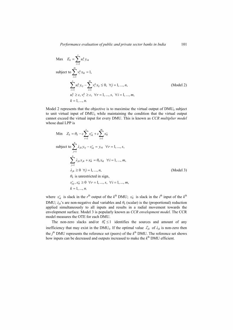
Model 2 represents that the objective is to maximise the virtual output of DMUk subject to unit virtual input of DMUk while maintaining the condition that the virtual output cannot exceed the virtual input for every DMU. This is known as CCR multiplier model whose dual LPP is
1 1
1
1
Min
subject to 1, ..., ,
1, ..., ,
0 1, ..., ,is unrestricted in sign,, 0 1, ..., , 1, ..., ,1, ..., .
+ −
= =
+
=
−
=
+ −
= − +
− = ∀ =
+ = ∀ =
≥ ∀ =
≥ ∀ = ∀ =
=
∑ ∑
∑
∑
s m
k k ikrkr i
n
jk rj rkrkj
n
jk jk ik k ikj
jk
k
ikrk
Z θ ε s ε s
λ y s y r s
λ x s θ x i m
λ j nθs s r s i mk n
(Model 3)
where +rks is slack in the rth output of the kth DMU; −
iks is slack in the ith input of the kth DMU; λjk’s are non-negative dual variables and θk (scalar) is the (proportional) reduction applied simultaneously to all inputs and results in a radial movement towards the envelopment surface. Model 3 is popularly known as CCR envelopment model. The CCR model measures the OTE for each DMU.
The non-zero slacks and/or * 1≤kθ identifies the sources and amount of any inefficiency that may exist in the DMUk. If the optimal value *
jkλ of λjk is non-zero then the jth DMU represents the reference set (peers) of the kth DMU. The reference set shows how inputs can be decreased and outputs increased to make the kth DMU efficient.
102 J. Puri and S.P. Yadav
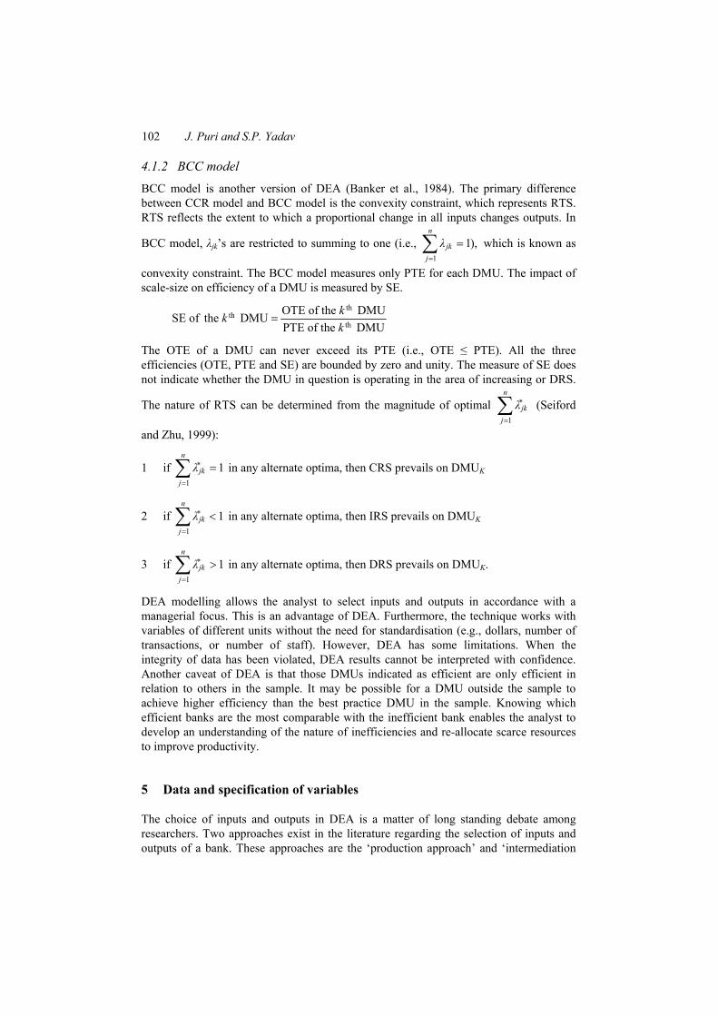
4.1.2 BCC model
BCC model is another version of DEA (Banker et al., 1984). The primary difference between CCR model and BCC model is the convexity constraint, which represents RTS. RTS reflects the extent to which a proportional change in all inputs changes outputs. In
BCC model, λjk’s are restricted to summing to one (i.e., 1
1),=
=∑n
jkj
λ which is known as
convexity constraint. The BCC model measures only PTE for each DMU. The impact of scale-size on efficiency of a DMU is measured by SE.
thth
th
OTE of the DMUSE of the DMUPTE of the DMU
=kkk
The OTE of a DMU can never exceed its PTE (i.e., OTE ≤ PTE). All the three efficiencies (OTE, PTE and SE) are bounded by zero and unity. The measure of SE does not indicate whether the DMU in question is operating in the area of increasing or DRS.
The nature of RTS can be determined from the magnitude of optimal *
1=∑
n
jkj
λ (Seiford
and Zhu, 1999):
1 if *
1
1=
=∑n
jkj
λ in any alternate optima, then CRS prevails on DMUK
2 if *
1
1=
<∑n
jkj
λ in any alternate optima, then IRS prevails on DMUK
3 if *
1
1=
>∑n
jkj
λ in any alternate optima, then DRS prevails on DMUK.
DEA modelling allows the analyst to select inputs and outputs in accordance with a managerial focus. This is an advantage of DEA. Furthermore, the technique works with variables of different units without the need for standardisation (e.g., dollars, number of transactions, or number of staff). However, DEA has some limitations. When the integrity of data has been violated, DEA results cannot be interpreted with confidence. Another caveat of DEA is that those DMUs indicated as efficient are only efficient in relation to others in the sample. It may be possible for a DMU outside the sample to achieve higher efficiency than the best practice DMU in the sample. Knowing which efficient banks are the most comparable with the inefficient bank enables the analyst to develop an understanding of the nature of inefficiencies and re-allocate scarce resources to improve productivity.
5 Data and specification of variables
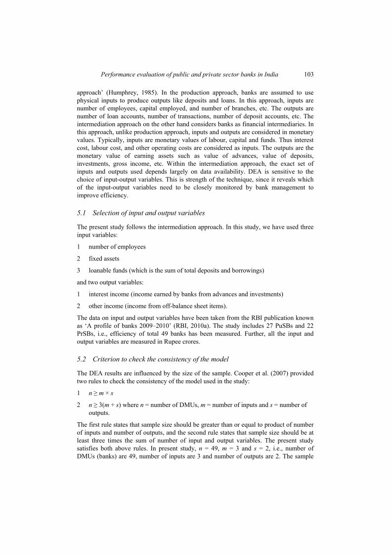
The choice of inputs and outputs in DEA is a matter of long standing debate among researchers. Two approaches exist in the literature regarding the selection of inputs and outputs of a bank. These approaches are the ‘production approach’ and ‘intermediation
Performance evaluation of public and private sector banks in India 103
approach’ (Humphrey, 1985). In the production approach, banks are assumed to use physical inputs to produce outputs like deposits and loans. In this approach, inputs are number of employees, capital employed, and number of branches, etc. The outputs are number of loan accounts, number of transactions, number of deposit accounts, etc. The intermediation approach on the other hand considers banks as financial intermediaries. In this approach, unlike production approach, inputs and outputs are considered in monetary values. Typically, inputs are monetary values of labour, capital and funds. Thus interest cost, labour cost, and other operating costs are considered as inputs. The outputs are the monetary value of earning assets such as value of advances, value of deposits, investments, gross income, etc. Within the intermediation approach, the exact set of inputs and outputs used depends largely on data availability. DEA is sensitive to the choice of input-output variables. This is strength of the technique, since it reveals which of the input-output variables need to be closely monitored by bank management to improve efficiency.
5.1 Selection of input and output variables
The present study follows the intermediation approach. In this study, we have used three input variables:
1 number of employees
2 fixed assets
3 loanable funds (which is the sum of total deposits and borrowings)
and two output variables:
1 interest income (income earned by banks from advances and investments)
2 other income (income from off-balance sheet items).
The data on input and output variables have been taken from the RBI publication known as ‘A profile of banks 2009–2010’ (RBI, 2010a). The study includes 27 PuSBs and 22 PrSBs, i.e., efficiency of total 49 banks has been measured. Further, all the input and output variables are measured in Rupee crores.
5.2 Criterion to check the consistency of the model
The DEA results are influenced by the size of the sample. Cooper et al. (2007) provided two rules to check the consistency of the model used in the study:
1 n ≥ m × s
2 n ≥ 3(m + s) where n = number of DMUs, m = number of inputs and s = number of outputs.
The first rule states that sample size should be greater than or equal to product of number of inputs and number of outputs, and the second rule states that sample size should be at least three times the sum of number of input and output variables. The present study satisfies both above rules. In present study, n = 49, m = 3 and s = 2, i.e., number of DMUs (banks) are 49, number of inputs are 3 and number of outputs are 2. The sample
104 J. Puri and S.P. Yadav
size n exceeds the desirable size as suggested by the above mentioned rules. Thus, the sample size in this study is feasible and we can apply DEA models to get desirable results.
6 Isotonicity test
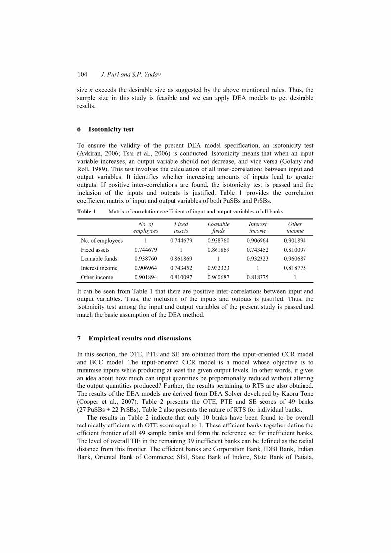
To ensure the validity of the present DEA model specification, an isotonicity test (Avkiran, 2006; Tsai et al., 2006) is conducted. Isotonicity means that when an input variable increases, an output variable should not decrease, and vice versa (Golany and Roll, 1989). This test involves the calculation of all inter-correlations between input and output variables. It identifies whether increasing amounts of inputs lead to greater outputs. If positive inter-correlations are found, the isotonicity test is passed and the inclusion of the inputs and outputs is justified. Table 1 provides the correlation coefficient matrix of input and output variables of both PuSBs and PrSBs. Table 1 Matrix of correlation coefficient of input and output variables of all banks
No. of employees
Fixed assets
Loanable funds
Interest income
Other income
No. of employees 1 0.744679 0.938760 0.906964 0.901894 Fixed assets 0.744679 1 0.861869 0.743452 0.810097 Loanable funds 0.938760 0.861869 1 0.932323 0.960687 Interest income 0.906964 0.743452 0.932323 1 0.818775 Other income 0.901894 0.810097 0.960687 0.818775 1
It can be seen from Table 1 that there are positive inter-correlations between input and output variables. Thus, the inclusion of the inputs and outputs is justified. Thus, the isotonicity test among the input and output variables of the present study is passed and match the basic assumption of the DEA method.
7 Empirical results and discussions
In this section, the OTE, PTE and SE are obtained from the input-oriented CCR model and BCC model. The input-oriented CCR model is a model whose objective is to minimise inputs while producing at least the given output levels. In other words, it gives an idea about how much can input quantities be proportionally reduced without altering the output quantities produced? Further, the results pertaining to RTS are also obtained. The results of the DEA models are derived from DEA Solver developed by Kaoru Tone (Cooper et al., 2007). Table 2 presents the OTE, PTE and SE scores of 49 banks (27 PuSBs + 22 PrSBs). Table 2 also presents the nature of RTS for individual banks.
The results in Table 2 indicate that only 10 banks have been found to be overall technically efficient with OTE score equal to 1. These efficient banks together define the efficient frontier of all 49 sample banks and form the reference set for inefficient banks. The level of overall TIE in the remaining 39 inefficient banks can be defined as the radial distance from this frontier. The efficient banks are Corporation Bank, IDBI Bank, Indian Bank, Oriental Bank of Commerce, SBI, State Bank of Indore, State Bank of Patiala,

Performance evaluation of public and private sector banks in India 105
Axis Bank, ICICI Bank and Yes Bank. Out of these efficient banks, seven are PuSBs and three are PrSBs. The results indicate that the OTE (in %age terms) of PuSBs ranges between 81.7% and 100%. The OTE (in %age terms) of PrSBs ranges between 32.1% and 100%. This implies that all inefficient PuSBs lie near to the frontier whereas the inefficient PrSBs are far away from the frontier. The Table 2 also indicates that 14 banks out 49 are pure technically efficient with PTE score equal to 1. It means there are total 35 banks (19 PuSBs and 16 PrSBs) which are pure technically inefficient. There are 4 banks which are pure technically efficient but overall technically inefficient and these are namely Indian Overseas Bank, Nainital Bank, Ratnakar Bank and SBI Commercial and International Bank. The PTE for PuSBs lies between 81.9% and 100% where as for PrSBs it lies between 36.1% and 100%. Table 2 OTE, PTE, SE and RTS of all banks
Bank code Public sector banks OTE PTE SE RTS
B1 Allahabad Bank 0.939 0.939 1 CRS B2 Andhra Bank 0.942 0.943 0.999 IRS B3 Bank of Baroda 0.847 0.847 1 CRS B4 Bank of India 0.900 0.90 1 CRS B5 Bank of Maharashtra 0.818 0.819 0.999 IRS B6 Canara Bank 0.926 0.963 0.962 DRS B7 Central Bank of India 0.817 0.855 0.956 DRS
B8 Corporation Bank 1 1 1 CRS
B9 Dena Bank 0.887 0.892 0.994 IRS
B10 IDBI Bank 1 1 1 CRS
B11 Indian Bank 1 1 1 CRS
B12 Indian Overseas Bank 0.973 1 0.973 DRS
B13 Oriental Bank of Commerce 1 1 1 CRS
B14 Punjab and Sind Bank 0.873 0.877 0.995 IRS
B15 Punjab National Bank 0.951 0.989 0.962 DRS
B16 Syndicate Bank 0.885 0.932 0.949 DRS
B17 UCO Bank 0.800 0.800 1 CRS B18 Union Bank of India 0.898 0.913 0.984 DRS B19 United Bank of India 0.864 0.865 0.999 IRS B20 Vijaya Bank 0.948 0.949 0.998 IRS B21 State Bank of Bikaner and Jaipur 0.960 0.960 1 CRS B22 State Bank of Hyderabad 0.969 0.969 1 CRS B23 State Bank of India 1 1 1 CRS B24 State Bank of Indore 1 1 1 CRS B25 State Bank of Mysore 0.985 0.990 0.995 IRS B26 State Bank of Patiala 1 1 1 CRS B27 State Bank of Travancore 0.929 0.932 0.997 IRS
106 J. Puri and S.P. Yadav
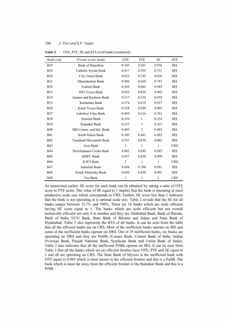
Table 2 OTE, PTE, SE and RTS of all banks (continued)
Bank code Private sector banks OTE PTE SE RTS
B28 Bank of Rajasthan 0.345 0.361 0.956 IRS B29 Catholic Syrian Bank 0.417 0.555 0.751 IRS B30 City Union Bank 0.623 0.745 0.836 IRS B31 Dhanlakshmi Bank 0.488 0.620 0.787 IRS B32 Federal Bank 0.569 0.602 0.945 IRS B33 ING Vysya Bank 0.832 0.839 0.992 IRS B34 Jammu and Kashmir Bank 0.517 0.539 0.959 IRS B35 Karnataka Bank 0.574 0.619 0.927 IRS B36 Karur Vysya Bank 0.528 0.590 0.895 IRS B37 Lakshmi Vilas Bank 0.469 0.616 0.761 IRS B38 Nainital Bank 0.354 1 0.354 IRS B39 Ratnakar Bank 0.327 1 0.327 IRS B40 SBI Comm. and Intl. Bank 0.485 1 0.485 IRS B41 South Indian Bank 0.389 0.441 0.882 IRS B42 Tamilnad Mercantile Bank 0.767 0.870 0.882 IRS B43 Axis Bank 1 1 1 CRS B44 Development Credit Bank 0.802 0.849 0.945 IRS B45 HDFC Bank 0.837 0.838 0.999 IRS B46 ICICI Bank 1 1 1 CRS B47 IndusInd Bank 0.694 0.700 0.991 IRS B48 Kotak Mahindra Bank 0.830 0.838 0.991 IRS B49 Yes Bank 1 1 1 CRS
As mentioned earlier, SE score for each bank can be obtained by taking a ratio of OTE score to PTE score. The value of SE equal to 1 implies that the bank is operating at most productive scale size which corresponds to CRS. Further, SE score less than 1 indicates that the bank is not operating at is optimal scale size. Table 2 reveals that the SE for all banks ranges between 32.7% and 100%. There are 16 banks which are scale efficient having SE score equal to 1. The banks which are scale efficient but not overall technically efficient are only 6 in number and they are Allahabad Bank, Bank of Baroda, Bank of India, UCO Bank, State Bank of Bikaner and Jaipur and State Bank of Hyderabad. Table 2 also represents the RTS of all banks. It can be seen from the table that all the efficient banks are on CRS. Most of the inefficient banks operate on IRS and some of the inefficient banks operate on DRS. Out of 39 inefficient banks, six banks are operating on DRS and they are PuSBs (Canara Bank, Central Bank of India, Indian Overseas Bank, Punjab National Bank, Syndicate Bank and Union Bank of India). Table 2 also indicates that all the inefficient PrSBs operate on IRS. It can be seen from Table 2 that all the banks which are on efficient frontier have OTE, PTE and SE equal to 1 and all are operating on CRS. The State Bank of Mysore is the inefficient bank with OTE equal to 0.985 which is most nearer to the efficient frontier and this is a PuSB. The bank which is most far away from the efficient frontier is the Ratnakar Bank and this is a PrSB.
Performance evaluation of public and private sector banks in India 107
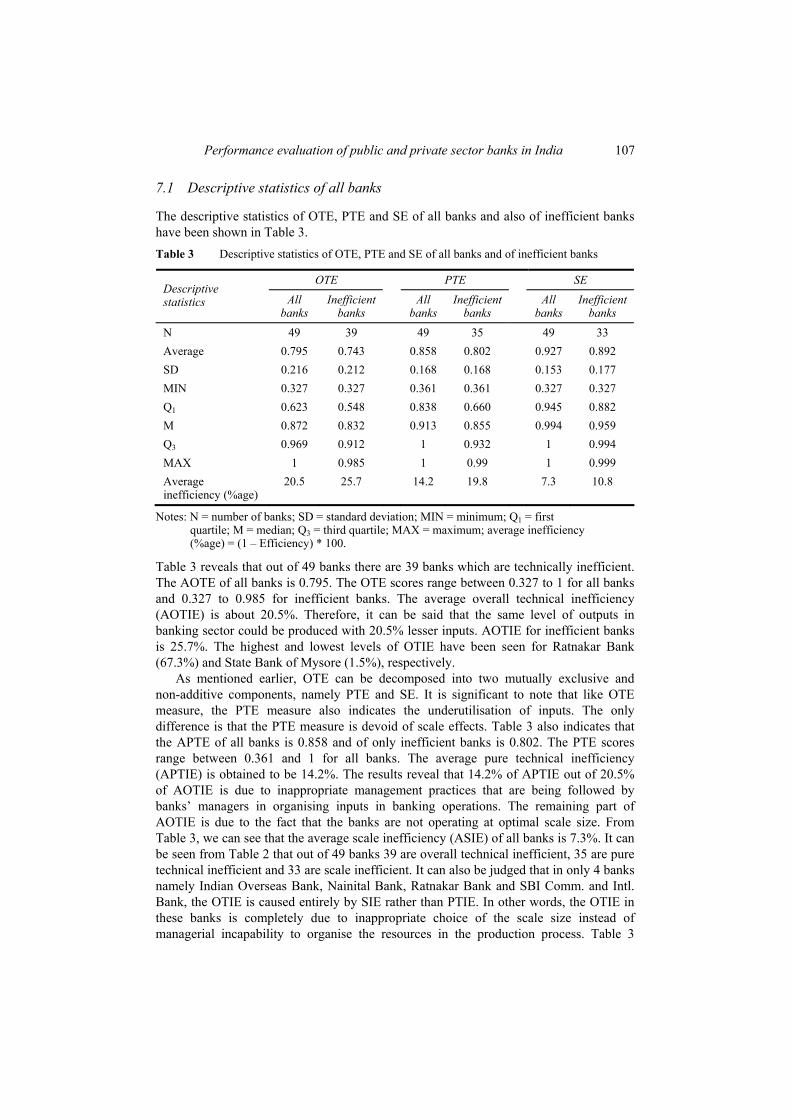
7.1 Descriptive statistics of all banks
The descriptive statistics of OTE, PTE and SE of all banks and also of inefficient banks have been shown in Table 3. Table 3 Descriptive statistics of OTE, PTE and SE of all banks and of inefficient banks
OTE PTE SE Descriptive statistics All
banks Inefficient
banks All
banks Inefficient
banks All
banks Inefficient
banks
N 49 39 49 35 49 33 Average 0.795 0.743 0.858 0.802 0.927 0.892 SD 0.216 0.212 0.168 0.168 0.153 0.177 MIN 0.327 0.327 0.361 0.361 0.327 0.327 Q1 0.623 0.548 0.838 0.660 0.945 0.882 M 0.872 0.832 0.913 0.855 0.994 0.959 Q3 0.969 0.912 1 0.932 1 0.994 MAX 1 0.985 1 0.99 1 0.999 Average inefficiency (%age)
20.5 25.7 14.2 19.8 7.3 10.8
Notes: N = number of banks; SD = standard deviation; MIN = minimum; Q1 = first quartile; M = median; Q3 = third quartile; MAX = maximum; average inefficiency (%age) = (1 – Efficiency) * 100.
Table 3 reveals that out of 49 banks there are 39 banks which are technically inefficient. The AOTE of all banks is 0.795. The OTE scores range between 0.327 to 1 for all banks and 0.327 to 0.985 for inefficient banks. The average overall technical inefficiency (AOTIE) is about 20.5%. Therefore, it can be said that the same level of outputs in banking sector could be produced with 20.5% lesser inputs. AOTIE for inefficient banks is 25.7%. The highest and lowest levels of OTIE have been seen for Ratnakar Bank (67.3%) and State Bank of Mysore (1.5%), respectively.
As mentioned earlier, OTE can be decomposed into two mutually exclusive and non-additive components, namely PTE and SE. It is significant to note that like OTE measure, the PTE measure also indicates the underutilisation of inputs. The only difference is that the PTE measure is devoid of scale effects. Table 3 also indicates that the APTE of all banks is 0.858 and of only inefficient banks is 0.802. The PTE scores range between 0.361 and 1 for all banks. The average pure technical inefficiency (APTIE) is obtained to be 14.2%. The results reveal that 14.2% of APTIE out of 20.5% of AOTIE is due to inappropriate management practices that are being followed by banks’ managers in organising inputs in banking operations. The remaining part of AOTIE is due to the fact that the banks are not operating at optimal scale size. From Table 3, we can see that the average scale inefficiency (ASIE) of all banks is 7.3%. It can be seen from Table 2 that out of 49 banks 39 are overall technical inefficient, 35 are pure technical inefficient and 33 are scale inefficient. It can also be judged that in only 4 banks namely Indian Overseas Bank, Nainital Bank, Ratnakar Bank and SBI Comm. and Intl. Bank, the OTIE is caused entirely by SIE rather than PTIE. In other words, the OTIE in these banks is completely due to inappropriate choice of the scale size instead of managerial incapability to organise the resources in the production process. Table 3
108 J. Puri and S.P. Yadav
reveals that ASE of all banks is 0.927 and SE scores ranges between 0.327 and 1 for all banks.
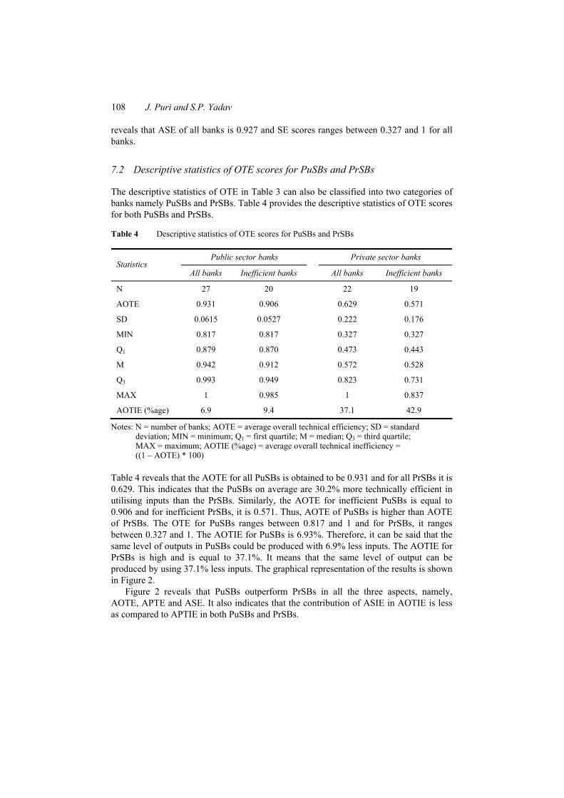
7.2 Descriptive statistics of OTE scores for PuSBs and PrSBs
The descriptive statistics of OTE in Table 3 can also be classified into two categories of banks namely PuSBs and PrSBs. Table 4 provides the descriptive statistics of OTE scores for both PuSBs and PrSBs.
Table 4 Descriptive statistics of OTE scores for PuSBs and PrSBs
Public sector banks Private sector banks Statistics
All banks Inefficient banks All banks Inefficient banks
N 27 20 22 19
AOTE 0.931 0.906 0.629 0.571
SD 0.0615 0.0527 0.222 0.176
MIN 0.817 0.817 0.327 0.327
Q1 0.879 0.870 0.473 0.443
M 0.942 0.912 0.572 0.528
Q3 0.993 0.949 0.823 0.731
MAX 1 0.985 1 0.837
AOTIE (%age) 6.9 9.4 37.1 42.9
Notes: N = number of banks; AOTE = average overall technical efficiency; SD = standard deviation; MIN = minimum; Q1 = first quartile; M = median; Q3 = third quartile; MAX = maximum; AOTIE (%age) = average overall technical inefficiency = ((1 – AOTE) * 100)
Table 4 reveals that the AOTE for all PuSBs is obtained to be 0.931 and for all PrSBs it is 0.629. This indicates that the PuSBs on average are 30.2% more technically efficient in utilising inputs than the PrSBs. Similarly, the AOTE for inefficient PuSBs is equal to 0.906 and for inefficient PrSBs, it is 0.571. Thus, AOTE of PuSBs is higher than AOTE of PrSBs. The OTE for PuSBs ranges between 0.817 and 1 and for PrSBs, it ranges between 0.327 and 1. The AOTIE for PuSBs is 6.93%. Therefore, it can be said that the same level of outputs in PuSBs could be produced with 6.9% less inputs. The AOTIE for PrSBs is high and is equal to 37.1%. It means that the same level of output can be produced by using 37.1% less inputs. The graphical representation of the results is shown in Figure 2.
Figure 2 reveals that PuSBs outperform PrSBs in all the three aspects, namely, AOTE, APTE and ASE. It also indicates that the contribution of ASIE in AOTIE is less as compared to APTIE in both PuSBs and PrSBs.
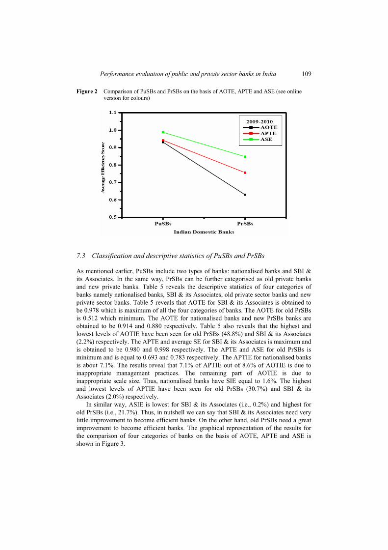
Performance evaluation of public and private sector banks in India 109
Figure 2 Comparison of PuSBs and PrSBs on the basis of AOTE, APTE and ASE (see online version for colours)
7.3 Classification and descriptive statistics of PuSBs and PrSBs
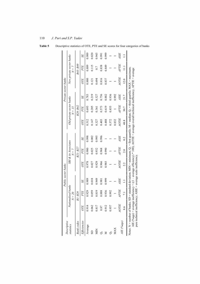
As mentioned earlier, PuSBs include two types of banks: nationalised banks and SBI & its Associates. In the same way, PrSBs can be further categorised as old private banks and new private banks. Table 5 reveals the descriptive statistics of four categories of banks namely nationalised banks, SBI & its Associates, old private sector banks and new private sector banks. Table 5 reveals that AOTE for SBI & its Associates is obtained to be 0.978 which is maximum of all the four categories of banks. The AOTE for old PrSBs is 0.512 which minimum. The AOTE for nationalised banks and new PrSBs banks are obtained to be 0.914 and 0.880 respectively. Table 5 also reveals that the highest and lowest levels of AOTIE have been seen for old PrSBs (48.8%) and SBI & its Associates (2.2%) respectively. The APTE and average SE for SBI & its Associates is maximum and is obtained to be 0.980 and 0.998 respectively. The APTE and ASE for old PrSBs is minimum and is equal to 0.693 and 0.783 respectively. The APTIE for nationalised banks is about 7.1%. The results reveal that 7.1% of APTIE out of 8.6% of AOTIE is due to inappropriate management practices. The remaining part of AOTIE is due to inappropriate scale size. Thus, nationalised banks have SIE equal to 1.6%. The highest and lowest levels of APTIE have been seen for old PrSBs (30.7%) and SBI & its Associates (2.0%) respectively.
In similar way, ASIE is lowest for SBI & its Associates (i.e., 0.2%) and highest for old PrSBs (i.e., 21.7%). Thus, in nutshell we can say that SBI & its Associates need very little improvement to become efficient banks. On the other hand, old PrSBs need a great improvement to become efficient banks. The graphical representation of the results for the comparison of four categories of banks on the basis of AOTE, APTE and ASE is shown in Figure 3.
110 J. Puri and S.P. Yadav
Table 5 Descriptive statistics of OTE, PTE and SE scores for four categories of banks
Publ
ic se
ctor
ban
ks
Pr
ivat
e se
ctor
ban
ks
Des
crip
tive
stat
istic
s N
atio
nalis
ed b
anks
N
= 2
0
SBI &
its A
ssoc
iate
s N
= 7
Old
pri
vate
sect
or b
anks
N
= 1
5
New
pri
vate
sect
or b
anks
N
= 7
Bank
cod
es
B1–B
20
B2
1–B2
7
B28–
B42
B4
3–B4
9
Effic
ienc
ies
OTE
PT
E SE
OTE
PT
E SE
OTE
PT
E SE
OTE
PT
E SE
Ave
rage
0.
914
0.92
9 0.
989
0.
978
0.98
0 0.
998
0.
512
0.69
3 0.
783
0.
880
0.88
9 0.
989
SD
0.06
2 0.
059
0.01
8
0.02
7 0.
025
0.00
2
0.14
7 0.
205
0.21
9
0.12
1 0.
115
0.02
0 M
IN
0.81
7 0.
819
0.94
9
0.92
9 0.
932
0.99
5
0.32
7 0.
361
0.32
7
0.69
4 0.
7 0.
945
Q1
0.87
0.
888
0.98
1
0.96
6 0.
968
0.99
6
0.40
3 0.
573
0.75
6
0.81
6 0.
838
0.99
1 M
0.
912
0.93
6 0.
999
0.
985
0.99
0 1
0.
488
0.61
9 0.
882
0.
837
0.84
9 0.
999
Q3
0.95
7 0.
992
1
1 1
1
0.57
2 0.
855
0.93
6
1 1
1 M
AX
1
1 1
1
1 1
0.
832
1 0.
992
1
1 1
AOTI
E AP
TIE
ASIE
AOTI
E AP
TIE
ASIE
AOTI
E AP
TIE
ASIE
AOTI
E AP
TIE
ASIE
AI
E (%
age)
8.
6 7.
1 1.
1
2.2
2.0
0.2
48
.8
30.7
21
.7
12
.0
11.1
1.
1
Not
es: N
= n
umbe
r of b
anks
; SD
= st
anda
rd d
evia
tion;
MIN
= m
inim
um; Q
1 = fi
rst q
uarti
le; M
= m
edia
n; Q
3 = th
ird q
uarti
le; M
AX
= m
axim
um;
AIE
(%ag
e) =
ave
rage
inef
ficie
ncy
= ((
1 –
aver
age
effic
ienc
y) *
100
); A
OTI
E =
aver
age
over
all t
echn
ical
inef
ficie
ncy;
APT
IE =
ave
rage
pu
re te
chni
cal i
neffi
cien
cy; A
SIE
= av
erag
e sc
ale
inef
ficie
ncy.
Performance evaluation of public and private sector banks in India 111
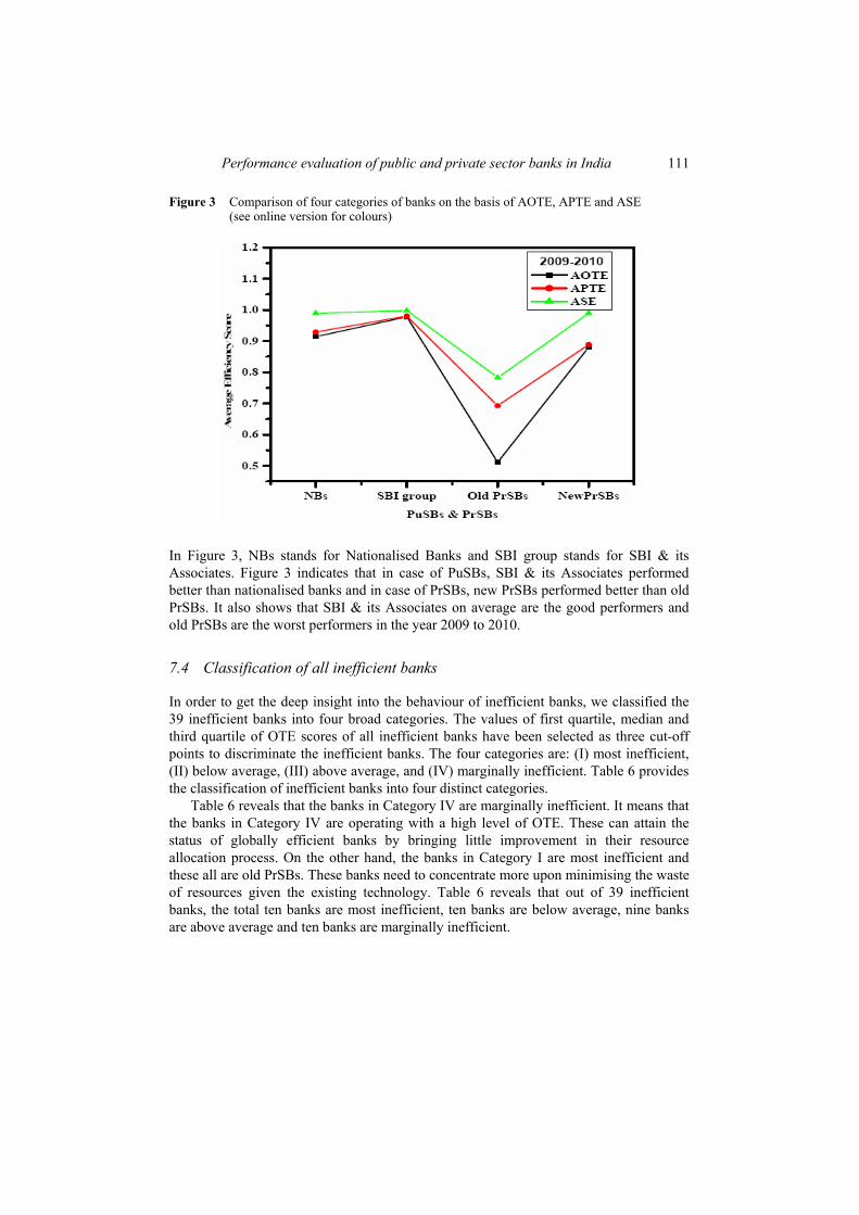
Figure 3 Comparison of four categories of banks on the basis of AOTE, APTE and ASE (see online version for colours)
In Figure 3, NBs stands for Nationalised Banks and SBI group stands for SBI & its Associates. Figure 3 indicates that in case of PuSBs, SBI & its Associates performed better than nationalised banks and in case of PrSBs, new PrSBs performed better than old PrSBs. It also shows that SBI & its Associates on average are the good performers and old PrSBs are the worst performers in the year 2009 to 2010.
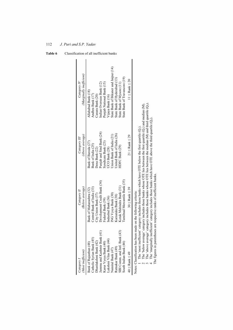
7.4 Classification of all inefficient banks
In order to get the deep insight into the behaviour of inefficient banks, we classified the 39 inefficient banks into four broad categories. The values of first quartile, median and third quartile of OTE scores of all inefficient banks have been selected as three cut-off points to discriminate the inefficient banks. The four categories are: (I) most inefficient, (II) below average, (III) above average, and (IV) marginally inefficient. Table 6 provides the classification of inefficient banks into four distinct categories.
Table 6 reveals that the banks in Category IV are marginally inefficient. It means that the banks in Category IV are operating with a high level of OTE. These can attain the status of globally efficient banks by bringing little improvement in their resource allocation process. On the other hand, the banks in Category I are most inefficient and these all are old PrSBs. These banks need to concentrate more upon minimising the waste of resources given the existing technology. Table 6 reveals that out of 39 inefficient banks, the total ten banks are most inefficient, ten banks are below average, nine banks are above average and ten banks are marginally inefficient.
112 J. Puri and S.P. Yadav
Table 6 Classification of all inefficient banks
Cat
egor
y I
(Mos
t ine
ffici
ent)
Cat
egor
y II
(B
elow
ave
rage
) C
ateg
ory
III
(Abo
ve a
vera
ge)
Cat
egor
y IV
(M
argi
nally
inef
ficie
nt)
Ban
k of
Raj
asth
an (4
8)
Cat
holic
Syr
ian
Ban
k (4
5)
Dha
nlak
shm
i Ban
k (4
2)
Jam
mu
and
Kas
hmir
Ban
k (4
1)
Kar
ur V
ysya
Ban
k (4
0)
Laks
hmi V
ilas B
ank
(44)
N
aini
tal B
ank
(47)
R
atna
kar B
ank
(49)
SB
I Com
m. a
nd In
tl. B
ank
(43)
So
uth
Indi
an B
ank
(46)
Ban
k of
Mah
aras
htra
(32)
C
entra
l Ban
k of
Indi
a (3
3)
City
Uni
on B
ank
(37)
D
evel
opm
ent C
redi
t Ban
k (3
4)
Fede
ral B
ank
(39)
In
dusI
nd B
ank
(36)
IN
G V
ysya
Ban
k (3
0)
Kar
nata
ka B
ank
(38)
K
otak
Mah
indr
a B
ank
(31)
Ta
miln
ad M
erca
ntile
Ban
k (3
5)
Ban
k of
Bar
oda
(27)
B
ank
of In
dia
(25)
D
ena
Ban
k (2
2)
Punj
ab a
nd S
ind
Ban
k (2
4)
Synd
icat
e B
ank
(23)
U
CO
Ban
k (2
8)
Uni
on B
ank
of In
dia
(21)
U
nite
d B
ank
of In
dia
(26)
H
DFC
Ban
k (2
9)
Alla
haba
d B
ank
(18)
A
ndhr
a B
ank
(17)
C
anar
a B
ank
(20)
In
dian
Ove
rsea
s Ban
k (1
2)
Punj
ab N
atio
nal B
ank
(15)
V
ijaya
Ban
k (1
6)
Stat
e B
ank
of B
ikan
er a
nd Ja
ipur
(14)
St
ate
Ban
k of
Hyd
erab
ad (1
3)
Stat
e B
ank
of M
ysor
e (1
1)
Stat
e B
ank
of T
rava
ncor
e (1
9)
40 ≤
Ran
k ≤
49
30 ≤
Ran
k ≤
39
21 ≤
Ran
k ≤
29
11 ≤
Ran
k ≤
20
Not
es: C
lass
ifica
tion
has b
een
mad
e on
the
follo
win
g cr
iteria
: 1
The
‘mos
t ine
ffici
ent’
cate
gory
incl
udes
thos
e ba
nks w
hich
hav
e O
TE b
elow
the
first
qua
rtile
(Q1)
. 2
The
‘bel
ow a
vera
ge’ c
ateg
ory
incl
udes
thos
e ba
nks w
hose
OTE
lies
bet
wee
n th
e fir
st q
uarti
le (Q
1) a
nd m
edia
n (M
). 3
The
‘abo
ve a
vera
ge’ c
ateg
ory
incl
udes
thos
e ba
nks w
hose
OTE
lies
bet
wee
n th
e m
edia
n (M
) and
third
qua
rtile
(Q3)
. 4
The
‘mar
gina
lly in
effic
ient
’ cat
egor
y in
clud
es th
ose
bank
s whi
ch h
ave
OTE
abo
ve th
e th
ird q
uarti
le (Q
3).
The
figur
es in
par
enth
eses
are
resp
ectiv
e ra
nks o
f ine
ffici
ent b
anks
.
Performance evaluation of public and private sector banks in India 113
7.5 Input/output targets to improve the efficiency of inefficient banks
The optimal solution of Model 3 will be of the form * *( , , , ).− +k k k kθ λ s s By using this
optimal solution, the efficiency of inefficient DMUk can be improved if the input values are reduced radially by the ratio *
kθ and the input excesses recorded in −ks are eliminated.
Similarly efficiency can be attained if the output values are augmented by the output shortfalls in .+ks Thus, the formula for improvement is given by equation (1)
* *
*
−
∈
+
∈
⎫= − =⎪⎪⎬
= + = ⎪⎪⎭
∑
∑k
k
k k k k j jj R
k k j jkj R
x θ x s x λ
y y s y λ (1)
where *{ : 0, {1, ..., }}= > ∈k jkR j λ j n is called the reference set (Cooper et al., 2007) for the inefficient DMUk. The kx and ky are the target inputs and target outputs respectively for the kth DMU. The input-output levels ( , )k kx y defined in (1) are the coordinates of the efficient frontier used as a benchmark for evaluating kth DMU. Thus, each of the inefficient banks can become overall efficient by adjusting its operation to the associated target point determined by the efficient bank that defines its reference frontier. Table 7 presents the reference set and the target values of all input and output variables for inefficient banks along with percentage reduction in input variables and percentage addition in output variables. The results that we obtained in Table 7 are by applying input-oriented CCR model. But if we apply output-oriented CCR model then the reference set and efficiencies of all banks remain same. The only difference will be in output augmentation and input reduction values. Output-oriented CCR model means to maximise outputs while using given set of inputs. Thus, output-oriented CCR model will give more output augmentation in outputs than input reduction.
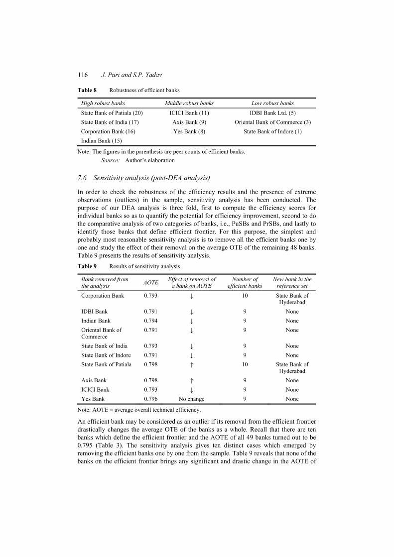
Table 8 presents the robustness of efficient banks. On the basis of frequency in the reference sets (also known as peer count or frequency count), we categorised the efficient banks into three categories:
1 high robust banks
2 middle robust banks
3 low robust banks.
High robust banks are those whose frequency count is relatively more. Table 8 reveals that State Bank of Patiala, SBI, Corporation Bank and Indian Bank are highly robust with frequency counts 20, 17, 16 and 15 respectively. They all are PuSBs. On the other hand, banks in middle robust category are ICICI Bank, Axis Bank and Yes Bank which all are new PrSBs with frequency counts 11, 9 and 8, respectively. The banks in third category, i.e., banks which are low robust are IDBI Bank, Oriental Bank of Commerce and State Bank of Indore with frequency counts 5, 3, and 1, respectively.
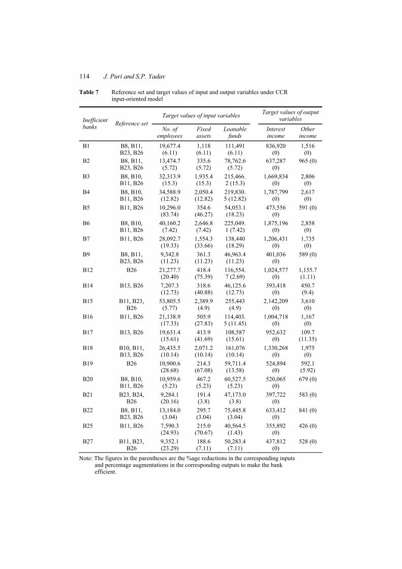
114 J. Puri and S.P. Yadav
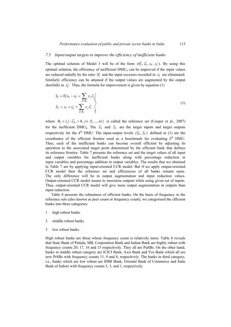
Table 7 Reference set and target values of input and output variables under CCR input-oriented model
Target values of input variables Target values of output variables Inefficient
banks Reference set No. of
employees Fixed assets
Loanable funds
Interest income
Other income
B1 B8, B11, B23, B26
19,677.4 (6.11)
1,118 (6.11)
111,491 (6.11)
836,920 (0)
1,516 (0)
B2 B8, B11, B23, B26
13,474.7 (5.72)
335.6 (5.72)
78,762.6 (5.72)
637,287 (0)
965 (0)
B3 B8, B10, B11, B26
32,313.9 (15.3)
1,935.4 (15.3)
215,466.2 (15.3)
1,669,834 (0)
2,806 (0)
B4 B8, B10, B11, B26
34,588.9 (12.82)
2,050.4 (12.82)
219,830.5 (12.82)
1,787,799 (0)
2,617 (0)
B5 B11, B26 10,296.0 (83.74)
354.6 (46.27)
54,053.1 (18.23)
473,556 (0)
591 (0)
B6 B8, B10, B11, B26
40,160.2 (7.42)
2,646.8 (7.42)
225,049.1 (7.42)
1,875,196 (0)
2,858 (0)
B7 B11, B26 28,092.7 (19.33)
1,554.3 (33.66)
138,440 (18.29)
1,206,431 (0)
1,735 (0)
B9 B8, B11, B23, B26
9,342.8 (11.23)
361.3 (11.23)
46,963.4 (11.23)
401,036 (0)
589 (0)
B12 B26 21,277.7 (20.40)
418.4 (75.39)
116,554.7 (2.69)
1,024,577 (0)
1,155.7 (1.11)
B14 B13, B26 7,207.3 (12.73)
318.6 (40.88)
46,125.6 (12.73)
393,418 (0)
450.7 (9.4)
B15 B11, B23, B26
53,805.5 (5.77)
2,389.9 (4.9)
255,443 (4.9)
2,142,209 (0)
3,610 (0)
B16 B11, B26 21,138.9 (17.33)
505.9 (27.83)
114,403.5 (11.45)
1,004,718 (0)
1,167 (0)
B17 B13, B26 19,631.4 (15.61)
413.9 (41.69)
108,587 (15.61)
952,632 (0)
109.7 (11.35)
B18 B10, B11, B13, B26
26,435.5 (10.14)
2,071.2 (10.14)
161,076 (10.14)
1,330,268 (0)
1,975 (0)
B19 B26 10,900.6 (28.68)
214.3 (67.08)
59,711.4 (13.58)
524,894 (0)
592.1 (5.92)
B20 B8, B10, B11, B26
10,959.6 (5.23)
467.2 (5.23)
60,527.5 (5.23)
520,065 (0)
679 (0)
B21 B23, B24, B26
9,284.1 (20.16)
191.4 (3.8)
47,173.0 (3.8)
397,722 (0)
583 (0)
B22 B8, B11, B23, B26
13,184.0 (3.04)
295.7 (3.04)
75,445.8 (3.04)
633,412 (0)
841 (0)
B25 B11, B26 7,590.3 (24.93)
215.0 (70.67)
40,564.5 (1.43)
355,892 (0)
426 (0)
B27 B11, B23, B26
9,352.1 (23.29)
188.6 (7.11)
50,283.4 (7.11)
437,812 (0)
528 (0)
Note: The figures in the parentheses are the %age reductions in the corresponding inputs and percentage augmentations in the corresponding outputs to make the bank efficient.
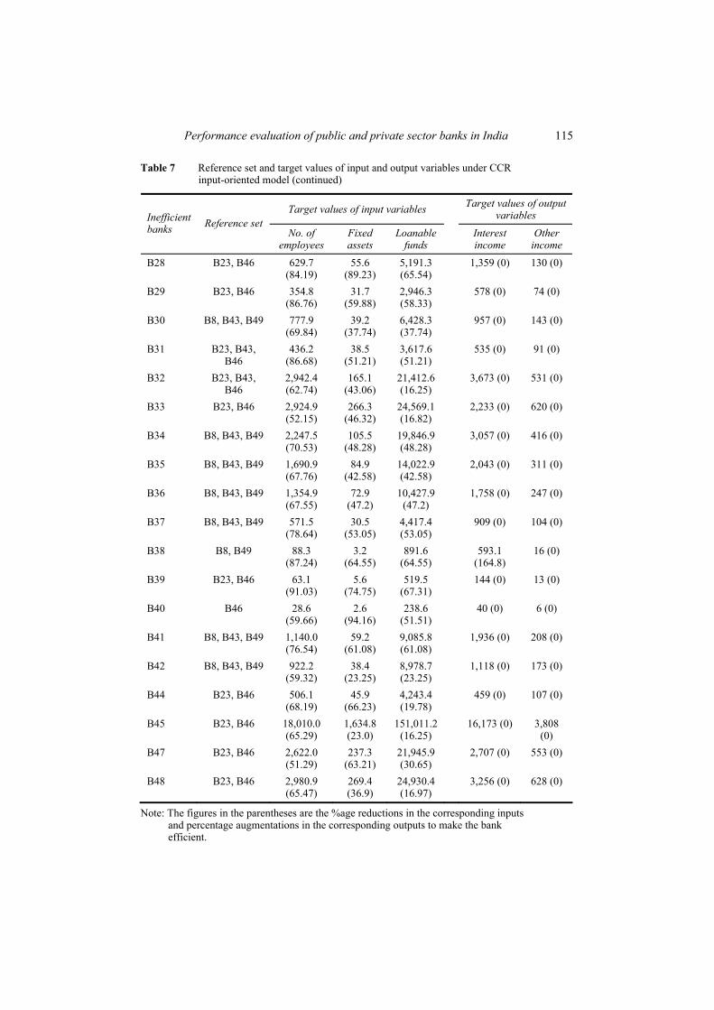
Performance evaluation of public and private sector banks in India 115
Table 7 Reference set and target values of input and output variables under CCR input-oriented model (continued)
Target values of input variables Target values of output variables Inefficient
banks Reference set No. of
employees Fixed assets
Loanable funds
Interest income
Other income
B28 B23, B46 629.7 (84.19)
55.6 (89.23)
5,191.3 (65.54)
1,359 (0) 130 (0)
B29 B23, B46 354.8 (86.76)
31.7 (59.88)
2,946.3 (58.33)
578 (0) 74 (0)
B30 B8, B43, B49 777.9 (69.84)
39.2 (37.74)
6,428.3 (37.74)
957 (0) 143 (0)
B31 B23, B43, B46
436.2 (86.68)
38.5 (51.21)
3,617.6 (51.21)
535 (0) 91 (0)
B32 B23, B43, B46
2,942.4 (62.74)
165.1 (43.06)
21,412.6 (16.25)
3,673 (0) 531 (0)
B33 B23, B46 2,924.9 (52.15)
266.3 (46.32)
24,569.1 (16.82)
2,233 (0) 620 (0)
B34 B8, B43, B49 2,247.5 (70.53)
105.5 (48.28)
19,846.9 (48.28)
3,057 (0) 416 (0)
B35 B8, B43, B49 1,690.9 (67.76)
84.9 (42.58)
14,022.9 (42.58)
2,043 (0) 311 (0)
B36 B8, B43, B49 1,354.9 (67.55)
72.9 (47.2)
10,427.9 (47.2)
1,758 (0) 247 (0)
B37 B8, B43, B49 571.5 (78.64)
30.5 (53.05)
4,417.4 (53.05)
909 (0) 104 (0)
B38 B8, B49 88.3 (87.24)
3.2 (64.55)
891.6 (64.55)
593.1 (164.8)
16 (0)
B39 B23, B46 63.1 (91.03)
5.6 (74.75)
519.5 (67.31)
144 (0) 13 (0)
B40 B46 28.6 (59.66)
2.6 (94.16)
238.6 (51.51)
40 (0) 6 (0)
B41 B8, B43, B49 1,140.0 (76.54)
59.2 (61.08)
9,085.8 (61.08)
1,936 (0) 208 (0)
B42 B8, B43, B49 922.2 (59.32)
38.4 (23.25)
8,978.7 (23.25)
1,118 (0) 173 (0)
B44 B23, B46 506.1 (68.19)
45.9 (66.23)
4,243.4 (19.78)
459 (0) 107 (0)
B45 B23, B46 18,010.0 (65.29)
1,634.8 (23.0)
151,011.2 (16.25)
16,173 (0) 3,808 (0)
B47 B23, B46 2,622.0 (51.29)
237.3 (63.21)
21,945.9 (30.65)
2,707 (0) 553 (0)
B48 B23, B46 2,980.9 (65.47)
269.4 (36.9)
24,930.4 (16.97)
3,256 (0) 628 (0)
Note: The figures in the parentheses are the %age reductions in the corresponding inputs and percentage augmentations in the corresponding outputs to make the bank efficient.
116 J. Puri and S.P. Yadav
Table 8 Robustness of efficient banks
High robust banks Middle robust banks Low robust banks
State Bank of Patiala (20) ICICI Bank (11) IDBI Bank Ltd. (5) State Bank of India (17) Axis Bank (9) Oriental Bank of Commerce (3) Corporation Bank (16) Yes Bank (8) State Bank of Indore (1) Indian Bank (15)
Note: The figures in the parenthesis are peer counts of efficient banks. Source: Author’s elaboration
7.6 Sensitivity analysis (post-DEA analysis)
In order to check the robustness of the efficiency results and the presence of extreme observations (outliers) in the sample, sensitivity analysis has been conducted. The purpose of our DEA analysis is three fold, first to compute the efficiency scores for individual banks so as to quantify the potential for efficiency improvement, second to do the comparative analysis of two categories of banks, i.e., PuSBs and PrSBs, and lastly to identify those banks that define efficient frontier. For this purpose, the simplest and probably most reasonable sensitivity analysis is to remove all the efficient banks one by one and study the effect of their removal on the average OTE of the remaining 48 banks. Table 9 presents the results of sensitivity analysis. Table 9 Results of sensitivity analysis
Bank removed from the analysis AOTE Effect of removal of
a bank on AOTE Number of
efficient banks New bank in the
reference set Corporation Bank 0.793 ↓ 10 State Bank of
Hyderabad IDBI Bank 0.791 ↓ 9 None Indian Bank 0.794 ↓ 9 None Oriental Bank of Commerce
0.791 ↓ 9 None
State Bank of India 0.793 ↓ 9 None State Bank of Indore 0.791 ↓ 9 None State Bank of Patiala 0.798 ↑ 10 State Bank of
Hyderabad Axis Bank 0.798 ↑ 9 None ICICI Bank 0.793 ↓ 9 None Yes Bank 0.796 No change 9 None
Note: AOTE = average overall technical efficiency.
An efficient bank may be considered as an outlier if its removal from the efficient frontier drastically changes the average OTE of the banks as a whole. Recall that there are ten banks which define the efficient frontier and the AOTE of all 49 banks turned out to be 0.795 (Table 3). The sensitivity analysis gives ten distinct cases which emerged by removing the efficient banks one by one from the sample. Table 9 reveals that none of the banks on the efficient frontier brings any significant and drastic change in the AOTE of

Performance evaluation of public and private sector banks in India 117
all banks. The values of the AOTE obtained by removing the efficient banks one by one from the sample ranged between 0.791 and 0.798, and are very close to 0.795 (AOTE value of original DEA analysis). Further, in eight cases, we can see that there is no change in the reference set for inefficient banks. Thus, we can safely infer that the results of the present study are quite robust to discriminate between efficient and inefficient banks.
8 Conclusions
This paper has evaluated the performance of PuSBs and PrSBs through DEA. The Indian domestic banks are categorised into PuSBs and PrSBs. The PuSBs are categorised into two bank groups:
1 nationalised banks
2 SBI & its Associates.
The PrSBs are categorised into two bank groups:
1 old PrSBs
2 new PrSBs.
The principle objective of our study is to analyse the performance assessment of PuSBs and PrSBs group-wise. This means that we want to know which bank group is the best performer and which one is the worst performer. For this purpose, the present study endeavours to evaluate the extent of OTE, PTE and SE in PuSBs and PrSBs using data for 49 banks (27 PuSBs and 22 PrSBs) in the year 2009 to 2010. This study followed an intermediation approach to select input and output variables. We have used three input variables:
1 number of employees
2 fixed assets
3 loanable funds
and two output variables:
1 interest income
2 other income.
After employing the DEA models on the input and output variables, the results indicate that only ten banks have been found to be overall technically efficient with OTE score equal to 1 and form the efficient frontier. Out of these efficient banks, seven are PuSBs and three are PrSBs. This indicates that PuSBs performed better than PrSBs.
Our study provides information about the performance of all PuSBs and PrSBs, and their respective categories. Finally, we can give some concluding remarks and suggestions which policy makers can use to improve the performance of all the categories of Indian domestic banks.
118 J. Puri and S.P. Yadav
• All the 49 banks on average are 14.2% managerial inefficient and 7.3% scale inefficient. So, the efforts to improve the managerial efficiency should be approximately double than the SE.
• The efficient banks, known as the best performer banks, on the efficient frontier are Corporation Bank, IDBI Bank, Indian Bank, Oriental Bank of Commerce, SBI, State Bank of Indore, State Bank of Patiala, Axis Bank, ICICI Bank and Yes Bank.
• On the basis of OTE score, the worst performer banks in the study have been noticed to be Ratnakar Bank, Bank of Rajasthan, Nainital Bank, South Indian Bank, Catholic Syrian Bank, Lakshmi Vilas Bank, SBI Comm. and Intl. Bank, and Dhanlakshmi Bank. We can analyse that all the worst performer banks are PrSBs.
• The PuSBs on average are 30.2% more technically efficient in utilising inputs than the PrSBs.
• The PuSBs on average can produce the same level of outputs with 6.93% less inputs. On the other hand, PrSBs on average can produce the same level of outputs with 37.1% less inputs.
• In PuSBs, SBI & its Associates performed better than nationalised banks and in PrSBs, new PrSBs performed better than old PrSBs. The average managerial inefficiency for nationalised banks, SBI & its Associates, old PrSBs, and new PrSBs are obtained to be 7.1%, 2.0%, 30.7%, and 11.1%, respectively. We can see that old PrSBs are more managerial inefficient, and thus need great improvement in this direction.
• The four categories of banks, namely, nationalised banks, SBI & its Associates, old PrSBs, and new PrSBs on average can produce the same level of outputs with 8.6%, 2.2%, 48.8%, and 12.0% less inputs respectively.
• The banks which fall in the category of the most inefficient and below average need a huge concern and large improvement because these banks lie far away from the efficient frontier. These banks are suggested to reduce their inputs in order to compete with the best performer banks. The maximum reduction should be in number of employees followed by fixed assets and loanable funds in order to get the same level of interest income and other income.
• The results reveal that performance of nationalised banks and SBI & its Associates can be improved by taking care of fixed assets rather than number of employees. On the other hand, number of employees needs more reduction as compared to other inputs to increase the performance of old PrSBs, and new PrSBs.
• On the basis of frequency count in the reference set of inefficient banks, State Bank of Patiala, SBI, Corporation Bank and Indian Bank have been figured out as highly robust banks.
The future scope of our study is very wide. The future research can extend our work in various directions which are not considered in this present study. We plan to extend our study to FBs also and can make the comparative study of domestic and FBs. We also plan to analyse different efficiency measures of individual banks using data over a longer period.
Performance evaluation of public and private sector banks in India 119
Acknowledgements
The authors are thankful to reviewers for their fruitful comments. The first author is also thankful to the University Grants Commission, GOI for financial support.
References Andersen, P. and Petersen, N.C. (1993) ‘A procedure for ranking efficient units in data
envelopment analysis’, Management Science, Vol. 39, No. 10, pp.1261–1264. Ataullah, A., Cockerill, T. and Le, H. (2004) ‘Financial liberalization and bank efficiency: a
comparative analysis of India and Pakistan’, Applied Economics, Vol. 36, No. 17, pp.1915–1924.
Avkiran, N.K. (2006) Productivity Analysis in the Services Sector with Data Envelopment Analysis, 3rd ed., University of Queensland Business School, The University of Queensland, Brisbane.
Azadeh, A., Ghaderi, S.F., Mirjalili, M. and Moghaddam, M. (2010) ‘A DEA approach for ranking and optimization of technical and management efficiency of a large bank based on financial indicators’, International Journal of Operational Research, Vol. 9, No. 2, pp.160–187.
Baidya, M.K. and Mitra, D. (2012) ‘An analysis of the technical efficiency of Indian public sector banks through DEA approach’, International Journal of Business Performance Management, Vol. 13, No. 3, pp.341–365.
Banker, R.D., Charnes, A. and Cooper, W.W. (1984) ‘Some models for estimating technical and scale inefficiencies in DEA’, Management Science, Vol. 30, No. 9, pp.1078–1092.
Bapat, D. (2012) ‘Efficiency for Indian public sector and private sector banks in India: assessment of impact of global financial crisis’, International Journal of Business Performance Management, Vol. 13, No. 3, pp.330–340.
Bauer, P.W., Berger, A.N., Ferrier, G.D. and Humphrey, D.B. (1998) ‘Consistency conditions for regulatory analysis of financial institutions: a comparison of frontier efficiency methods’, Journal of Economics and Business, Vol. 50, No. 2, pp.85–114.
Berger, A.N. and Humphrey, D.B. (1997) ‘Efficiency of financial institutions: international survey and directions for future research’, European Journal of Operational Research, Vol. 98, No. 2, pp.175–212.
Bhattacharyya, A., Lovell, C.A.K. and Sahay, P. (1997) ‘The impact of liberalisation on the productive efficiency of Indian commercial banks’, European Journal of Operations Research, Vol. 98, No. 2, pp.332–345.
Chakrabarti, R. and Chawla, G. (2005) ‘Banking efficiency in India since the reforms: an assessment’, Money and Finance, Vol. 9, No. 2, pp.31–47.
Charnes, A., Cooper, W.W. and Rhodes, E. (1978) ‘Measuring efficiency of decision making units’, European Journal of Operations Research, Vol. 2, No. 6, pp.429–444.
Chen, T.Y. and Yeh, T.L. (2000) ‘Bank’s performance evaluation: combined with financial ratio and DEA method’, Soochow Journal of Economics and Business, Vol. 30, pp.10–42.
Chowdhury, S. (2012) ‘Technical efficiency of Indian commercial banks: an empirical analysis’, International Journal of Business Performance Management, Vol. 13, No. 3, pp.450–472.
Cooper, W.W., Ruefli, T.W., Deng, H., Wu, J. and Zhang, Z. (2008) ‘Are state-owned banks less efficient? A long- vs. short-run data envelopment analysis of Chinese banks’, International Journal of Operational Research, Vol. 3, No. 5, pp.533–556.
Cooper, W.W., Seiford, L.M. and Tone, K. (2007) Data Envelopment Analysis: A Comprehensive Text with Models, Applications, References and DEA-solver Software, 2nd ed., Springer, New York.
Das, A., Nag, A. and Ray, S.C. (2005) ‘Liberalization, ownership and efficiency in Indian banking: a nonparametric analysis’, Economic and Political Weekly, Vol. 40, No. 12, pp.1190–1197.
120 J. Puri and S.P. Yadav
Dharmapala, P.S. and Edirisuriya, P. (2011) ‘A decision model to predict profitability using revised Thompson-Thrall profit ratios in DEA with an application to South Asian banks’, International Journal of Operational Research, Vol. 12, No. 4, pp.407–429.
George, S.A. and Chattopadhyay, N. (2012) ‘An investigative study of operational performance and service quality of Indian public sector banks’, International Journal of Business Performance Management, Vol. 13, No. 3, pp.408–425.
Golany, B. and Roll, Y. (1989) ‘An application procedure for DEA’, Omega, Vol. l7, No. 3, pp.237–250.
Gupta, O.K., Doshit, Y. and Chinubhai, A. (2008) ‘Dynamics of productive efficiency of Indian banks’, International Journal of Operations Research, Vol. 5, No. 2, pp.78–90.
Humphrey, D.B. (1985) ‘Costs and scale economies in bank intermediation’, in Aspinwall, R.C. and Eisenbeis, R.A. (Eds.): Handbook for Banking Strategy, pp.745–783, John Wiley and Sons, New York.
Keshari, P.K. and Paul, M.T. (1994) ‘Relative efficiency of foreign and domestic banks’, Economic and Political Weekly, Vol. 29, No. 9, pp.M31–M36.
Kumar, S. and Gulati, R. (2008) ‘Evaluation of technical efficiency and ranking of public sector banks in India: an analysis from cross-sectional perspective’, International Journal of Productivity and Performance Management, Vol. 57, No. 7, pp.540–568.
Kumar, S. and Gulati, R. (2009) ‘Technical efficiency and its determinants in the Indian domestic banking industry: an application of DEA and Tobit analysis’, American Journal of Finance and Accounting, Vol. 1, No. 3, pp.256–296.
Kumbhakar, S.C. and Sarkar, S. (2003) ‘Deregulation, ownership, and productivity growth: evidence from Indian banks’, Journal of Money, Credit, and Banking, Vol. 35, No. 3, pp.403–424.
Nandy, D. (2012) ‘Efficiency study of Indian public sector banks – an application of data envelopment analysis and cluster analysis’, International Journal of Business Performance Management, Vol. 13, No. 3, pp.312–329.
Rajan, R.G. and Zingales, L. (1998) ‘Financial dependence and growth’, The American Economic Review, Vol. 88, No. 3, pp.559–586.
Rajput, N. and Gupta, M. (2011) ‘Efficiency of public sector banks operating in India: post-reforms period analysis’, Afro-Asian Journal of Finance and Accounting, Vol. 2, No. 4, pp.349–368.
Ram Mohan, T.T. (2002) ‘Deregulation and performance of public sector banks’, Economic and Political Weekly, Vol. 37, No. 5, pp.393–397.
Ram Mohan, T.T. (2003) ‘Long-run performance of public and private sector bank stocks’, Economic and Political Weekly, Vol. 38, No. 8, pp.785–788.
Ram Mohan, T.T. and Ray, S.C. (2004) ‘Comparing performance of public and private sector banks: a revenue maximisation efficiency approach’, Economic and Political Weekly, Vol. 39, No. 12, pp.1271–1276.
Ray, S.C. (2004) Data Envelopment Analysis: Theory and Techniques for Economics and Operations Research, Cambridge University Press, Cambridge.
Ray, S.C. and Das, A. (2010) ‘Distribution of cost and profit efficiency: evidence from Indian banking’, European Journal of Operational Research, Vol. 201, No. 1, pp.297–307.
Reddy, A.A. (2004) ‘Banking sector liberalization and efficiency of Indian banks’, The ICFAI Journal of Bank Management, Vol. 3, No. 2, pp.37–53.
Reddy, A.A. (2005) ‘Banking sector deregulation and productivity change decomposition of Indian banks’, Finance India, Vol. 19, No. 3, pp.983–1001.
Reserve Bank of India (RBI) (2008) ‘Efficiency, productivity and soundness of the banking sector’, Report of Currency and Finance, Vol. 2, No. 2, pp.393–446.
Performance evaluation of public and private sector banks in India 121
Reserve Bank of India (RBI) (2010a) ‘A profile of banks: 2009–2010’, 23 September, available at http://rbidocs.rbi.org.in/rdocs/Publications/PDFs/APRBBA230910.pdf (accessed on 9 November 2011).
Reserve Bank of India (RBI) (2010b) Basic Statistical Returns of Scheduled Commercial Banks in India, March, Vol. 39, available at http://rbidocs.rbi.org.in/rdocs/Publications/PDFs/38FBSRV200820101.pdf (accessed on 9 November 2011).
Sahoo, B.K., Sengupta, J.K. and Mandal, A. (2007) ‘Productive performance evaluation of the banking sector in India using data envelopment analysis’, International Journal of Operations Research, Vol. 4, No. 2, pp.63–79.
Sanjeev, G.M. (2006) ‘Data envelopment analysis (DEA) for measuring technical efficiency of banks’, The Journal of Business Perspective, Vol. 10, No. 1, pp.13–27.
Sarkar, J., Sarkar, S. and Bhaumik, S.K. (1998) ‘Does ownership always matter? Evidence from the Indian banking industry’, Journal of Comparative Economics, Vol. 26, No. 2, pp.262–281.
Sathye, M. (2003) ‘Efficiency of banks in a developing economy: the case of India’, European Journal of Operational Research, Vol. 148, No. 3, pp.662–671.
Seiford, L.M. (1996) ‘Data envelopment analysis: the evolution of a state of the art’, Journal of Productivity Analysis, Vol. 7, No. 2, pp.99–137.
Seiford, L.M. and Thrall, R.M. (1990) ‘Recent developments in DEA: the mathematical programming approach to frontier analysis’, Journal of Econometrics, Vol. 46, Nos. 1–2, pp.7–38.
Seiford, L.M. and Zhu, J. (1999) ‘An investigation of returns-to-scale in data envelopment analysis’, Omega, Vol. 27, No. 1, pp.1–11.
Sensarma, R. (2006) ‘Are foreign banks always the best? Comparison of state-owned, private and foreign banks in India’, Economic Modelling, Vol. 23, No. 4, pp.717–735.
Shanmugam, K.R. and Das, A. (2004) ‘Efficiency of Indian commercial banks during the reform period’, Applied Financial Economics, Vol. 14, No. 9, pp.681–686.
Sherman, H.D. and Gold, F. (1985) ‘Bank branch operating efficiency: evaluation with data envelopment analysis’, Journal of Banking and Finance, Vol. 9, No. 2, pp.297–315.
Tsai, H.C., Chen, C.M. and Tzeng, G.H. (2006) ‘The comparative productivity efficiency for global telecoms’, International Journal of Production Economics, Vol. 103, No. 2, pp.509–526.
Zhu, J. (2003) Quantitative Models for Performance Evaluation and Benchmarking: Data Envelopment Analysis with Spreadsheets and DEA Excel Solver, Kluwer Academic Publishers, USA.