
Perceptual Metrics For Image Database Navigation
177
Transcript of Perceptual Metrics For Image Database Navigation
PERCEPTUAL METRICS FOR
IMAGE DATABASE NAVIGATION
a dissertation
submitted to the department of computer science
and the committee on graduate studies
of stanford university
in partial fulfillment of the requirements
for the degree of
doctor of philosophy
By
Yossi Rubner
May 1999

c Copyright 1999 by Yossi Rubner
All Rights Reserved
ii
I certify that I have read this dissertation and that in
my opinion it is fully adequate, in scope and quality, as
a dissertation for the degree of Doctor of Philosophy.
Carlo Tomasi(Principal Adviser)
I certify that I have read this dissertation and that in
my opinion it is fully adequate, in scope and quality, as
a dissertation for the degree of Doctor of Philosophy.
Leonidas J. Guibas
I certify that I have read this dissertation and that in
my opinion it is fully adequate, in scope and quality, as
a dissertation for the degree of Doctor of Philosophy.
Shmuel Peleg(Computer Science, Hebrew University, Israel)
Approved for the University Committee on Graduate
Studies:
iii
Preface
The increasing amount of information available in today's world raises the need to
retrieve relevant data e�ciently. Unlike text-based retrieval, where keywords are
successfully used to index into documents, content-based image retrieval poses up
front the fundamental questions how to extract useful image features and how to use
them for intuitive retrieval. We present a novel approach to the problem of navigating
through a collection of images for the purpose of image retrieval, which leads to a
new paradigm for image database search. We summarize the appearance of images
by distributions of color or texture features, and we de�ne a metric between any
two such distributions. This metric, which we call the "Earth Mover's Distance"
(EMD), represents the least amount of work that is needed to rearrange the mass
is one distribution in order to obtain the other. We show that the EMD matches
perceptual dissimilarity better than other dissimilarity measures, and argue that it
has many desirable properties for image retrieval. Using this metric, we employ Multi-
Dimensional Scaling techniques to embed a group of images as points in a two- or
three-dimensional Euclidean space so that their distances re ect image dissimilarities
as well as possible. Such geometric embeddings exhibit the structure in the image
set at hand, allowing the user to understand better the result of a database query
and to re�ne the query in a perceptually intuitive way. By iterating this process, the
user can quickly zoom in to the portion of the image space of interest. We also apply
these techniques to other modalities such as mug-shot retrieval.
iv
Acknowledgements
I would like to thank the many people who made my time at Stanford a period I will
treasure.
First and foremost, I would like to thank my advisor, Professor Carlo Tomasi, for
guiding me through the Ph.D. program. From him I learned how to think critically,
how to select problems, how to solve them, and how to present their solutions. His
drive for scienti�c excellence has pushed me to aspire for the same. I thank him also
for the seemingly impossible task of teaching me how to write clearly. Aside from
being my advisor, he was a colleague, a teacher, and most important { a friend.
I would like to thank Professor Leonidas Guibas whom I consider my secondary
advisor. He was always there to provide words of advice and to discuss new research
ideas. His insights always enlightened me.
I would like to thank the other members of my oral committee, Professor Brian
Wandell, Professor Rajeev Montwani, and Professor Shmuel Peleg from Hebrew uni-
versity in Israel who was also a member of my reading committee. Special thanks to
Professor Peleg for his willingness to participate in my oral defense from Germany by
video-conferencing. I would also like to thank Professor Walter Murray and Professor
Serge Plotkin for inspiring discussions on numerical and computational aspects of the
EMD.
I was fortunate to interact with many people at Stanford and at various other
places. These interaction shaped in many ways my understanding of computer vision.
I would like to thank all the members and visitors of the vision group with whom I
interacted, especially Stan Birch�eld, Anat Caspi, Scott Cohen, Aris Gionis, Joachim
Hornegger, Roberto Manduchi, Chuck Richards, Brian Rogo�, Mark Ruzon, Donald
v
Tanguay, John Zhang, and Song-Chun Zhu. Special thanks to Mark for being willing
to proof-read this dissertation. I would like also to thank Professor Yaakov (Toky)
Hel-Or and Professor Hagit (Gigi) Hel-Or for introducing me to the computer vision
community and helping me with my �rst steps in the �eld, and Professor Ron Kimmel
for much good advice. Thanks for Joern Ho�mann for working with me on the
derivation of the Gabor �lters, and to Jan Puzicha from the university of Bonn for
an interesting and fruitful collaboration.
During my studies, I had the opportunity to work at Xerox Palo Alto Research
Center. I would like to thank Professor Guibas for bringing me there, Dr. David Ma-
rimont, whom I consider as my third advisor, for his endless great ideas and support,
and Dr. Michael Black, Dr. Tom Breuel, Dr. Don Kimber, Dr. Ruth Rosenholtz, and
Dr. Randy Trigg for many interesting discussions.
Last but not least, I would like to thank my family. I am grateful to my parents,
Zahava and David, who instilled in me the basic interest in science. Their encour-
agement and support helped me reach the goal of �nishing a Ph.D. I would like to
thank my daughters, Keren and Shir. They brought new dimensions to my life and
keep reminding me that there is much more to life than my work. Above all I am
grateful to my wife, Anat, for her love, support, patience and encouragement. To her
I dedicate this dissertation.
I was supported by the DARPA grant for Stanford's image retrieval project (con-
tract DAAH04-94-G-0284).
vi
Contents
Preface iv
Acknowledgements v
1 Introduction 1
1.1 Background and Motivation . . . . . . . . . . . . . . . . . . . . . . . 1
1.2 Previous Work . . . . . . . . . . . . . . . . . . . . . . . . . . . . . . 3
1.3 Overview of the Dissertation . . . . . . . . . . . . . . . . . . . . . . . 4
1.4 Road Map . . . . . . . . . . . . . . . . . . . . . . . . . . . . . . . . . 5
2 Distribution-Based Dissimilarity Measures 7
2.1 Representing Distributions of Features . . . . . . . . . . . . . . . . . 8
2.1.1 Histograms . . . . . . . . . . . . . . . . . . . . . . . . . . . . 8
2.1.2 Signatures . . . . . . . . . . . . . . . . . . . . . . . . . . . . . 9
2.1.3 Other representations . . . . . . . . . . . . . . . . . . . . . . . 10
2.2 Histogram-Based Dissimilarity Measures . . . . . . . . . . . . . . . . 10
2.2.1 De�nitions . . . . . . . . . . . . . . . . . . . . . . . . . . . . . 11
2.2.2 Bin-by-bin dissimilarity measures . . . . . . . . . . . . . . . . 11
2.2.3 Cross-bin dissimilarity measures . . . . . . . . . . . . . . . . . 14
2.2.4 Parameter-based dissimilarity measures . . . . . . . . . . . . . 17
2.2.5 Properties . . . . . . . . . . . . . . . . . . . . . . . . . . . . . 17
2.3 Summary . . . . . . . . . . . . . . . . . . . . . . . . . . . . . . . . . 19
vii
3 The Earth Mover's Distance 20
3.1 De�nition . . . . . . . . . . . . . . . . . . . . . . . . . . . . . . . . . 22
3.2 Properties . . . . . . . . . . . . . . . . . . . . . . . . . . . . . . . . . 23
3.3 Computation . . . . . . . . . . . . . . . . . . . . . . . . . . . . . . . 26
3.3.1 One-Dimensional EMD . . . . . . . . . . . . . . . . . . . . . . 29
3.3.2 Lower Bound . . . . . . . . . . . . . . . . . . . . . . . . . . . 31
3.4 More on the Ground Distance . . . . . . . . . . . . . . . . . . . . . . 35
3.5 Extensions . . . . . . . . . . . . . . . . . . . . . . . . . . . . . . . . . 38
3.5.1 The Partial EMD (EMD ) . . . . . . . . . . . . . . . . . . . . 38
3.5.2 The Restricted EMD (� -EMD) . . . . . . . . . . . . . . . . . 38
3.6 Summary . . . . . . . . . . . . . . . . . . . . . . . . . . . . . . . . . 39
4 Color-Based Image Similarity 40
4.1 Color Features . . . . . . . . . . . . . . . . . . . . . . . . . . . . . . . 40
4.1.1 Color Spaces . . . . . . . . . . . . . . . . . . . . . . . . . . . 41
4.1.2 Perceptually Uniform Color Spaces . . . . . . . . . . . . . . . 41
4.2 Color Signatures . . . . . . . . . . . . . . . . . . . . . . . . . . . . . 44
4.3 Color-Based Image Retrieval . . . . . . . . . . . . . . . . . . . . . . . 45
4.4 Joint Distribution of Color and Position . . . . . . . . . . . . . . . . 46
4.5 Summary . . . . . . . . . . . . . . . . . . . . . . . . . . . . . . . . . 50
5 Texture-Based Image Similarity 52
5.1 Texture Features . . . . . . . . . . . . . . . . . . . . . . . . . . . . . 52
5.1.1 Gabor Filters . . . . . . . . . . . . . . . . . . . . . . . . . . . 53
5.1.2 Filter Bank Design . . . . . . . . . . . . . . . . . . . . . . . . 55
5.2 Homogeneous Textures . . . . . . . . . . . . . . . . . . . . . . . . . . 58
5.2.1 No Invariance . . . . . . . . . . . . . . . . . . . . . . . . . . . 59
5.2.2 Rotation Invariance . . . . . . . . . . . . . . . . . . . . . . . . 60
5.2.3 Rotation and Scale Invariance . . . . . . . . . . . . . . . . . . 60
5.2.4 Proving that the Distances are Metric . . . . . . . . . . . . . . 61
5.2.5 Examples . . . . . . . . . . . . . . . . . . . . . . . . . . . . . 63
5.3 Non-Homogeneous Textures . . . . . . . . . . . . . . . . . . . . . . . 64
viii
5.3.1 Texture Signatures . . . . . . . . . . . . . . . . . . . . . . . . 66
5.3.2 Texture-Based Retrieval . . . . . . . . . . . . . . . . . . . . . 67
5.3.3 Partial Matches . . . . . . . . . . . . . . . . . . . . . . . . . . 71
5.3.4 Retrieving Natural Images . . . . . . . . . . . . . . . . . . . . 72
5.4 Image Preprocessing . . . . . . . . . . . . . . . . . . . . . . . . . . . 77
5.4.1 Texture Contrast . . . . . . . . . . . . . . . . . . . . . . . . . 78
5.4.2 Edge-Preserving Smoothing . . . . . . . . . . . . . . . . . . . 80
5.5 Summary . . . . . . . . . . . . . . . . . . . . . . . . . . . . . . . . . 85
6 Comparing Dissimilarity Measures 87
6.1 Benchmark Methodology . . . . . . . . . . . . . . . . . . . . . . . . . 87
6.2 Experiments . . . . . . . . . . . . . . . . . . . . . . . . . . . . . . . . 88
6.2.1 Color . . . . . . . . . . . . . . . . . . . . . . . . . . . . . . . . 89
6.2.2 Texture . . . . . . . . . . . . . . . . . . . . . . . . . . . . . . 97
6.3 Summary . . . . . . . . . . . . . . . . . . . . . . . . . . . . . . . . . 98
7 Visualization 99
7.1 Multi-Dimensional Scaling . . . . . . . . . . . . . . . . . . . . . . . . 100
7.2 Examples . . . . . . . . . . . . . . . . . . . . . . . . . . . . . . . . . 101
7.3 Missing Values . . . . . . . . . . . . . . . . . . . . . . . . . . . . . . 102
7.4 Evaluating Dissimilarity Measures . . . . . . . . . . . . . . . . . . . . 104
7.5 Visualization in Three Dimensions . . . . . . . . . . . . . . . . . . . . 109
7.6 Summary . . . . . . . . . . . . . . . . . . . . . . . . . . . . . . . . . 112
8 Navigation 113
8.1 Retrieval by Navigation . . . . . . . . . . . . . . . . . . . . . . . . . 113
8.2 An Example . . . . . . . . . . . . . . . . . . . . . . . . . . . . . . . . 116
8.3 Procrustes Analysis . . . . . . . . . . . . . . . . . . . . . . . . . . . . 116
8.4 Navigating in a Space of Police Mugshots . . . . . . . . . . . . . . . . 120
8.5 A Demonstration System . . . . . . . . . . . . . . . . . . . . . . . . . 124
8.6 Summary . . . . . . . . . . . . . . . . . . . . . . . . . . . . . . . . . 127
ix

9 Conclusion and Future Directions 128
9.1 Conclusion . . . . . . . . . . . . . . . . . . . . . . . . . . . . . . . . . 128
9.2 Future Directions . . . . . . . . . . . . . . . . . . . . . . . . . . . . . 130
A The Standard Deviation of the Gabor Filters 132
A.1 The Radial Standard Deviation . . . . . . . . . . . . . . . . . . . . . 132
A.2 The Angular Standard Deviation . . . . . . . . . . . . . . . . . . . . 133
B Retrieval Performance Plots 136
Bibliography 150
x

List of Tables
2.1 Properties of the di�erent dissimilaritymeasures: Minkowski-form (Lr),
histogram intersection (HI), Kolmogorov-Smirnov (KS), Kullback-Leibler
(KL), Je�rey divergence (JD), �2-statistics (�2), quadratic form (QF),
match distance (MD), and the Earth Mover's Distance (EMD). (1) The
triangle inequality only holds for speci�c ground distances. . . . . . . 18
5.1 Distance matrix of the textures in Figure 5.4. . . . . . . . . . . . . . 64
5.2 Distance matrix of the textures in Figure 5.4 with rotation invariance. 64
5.3 Distance matrix of the textures in Figure 5.4 with rotation and scale
invariance. . . . . . . . . . . . . . . . . . . . . . . . . . . . . . . . . . 65
7.1 Computation time in seconds for the dissimilarity matrix and the MDS.103
8.1 The appearance-based mugshot features used for retrieval. . . . . . . 123
xi
List of Figures
2.1 (a) Color image. (b) Its color signature. . . . . . . . . . . . . . . . . . 9
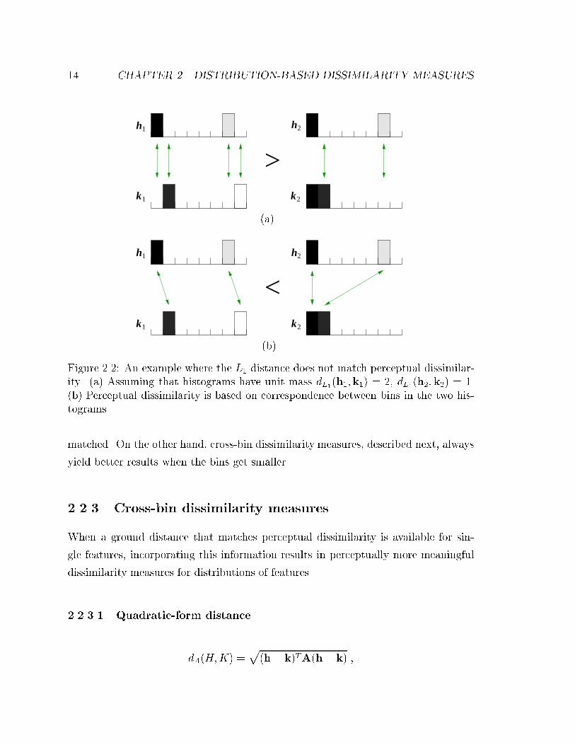
2.2 An example where the L1 distance does not match perceptual dissim-
ilarity. (a) Assuming that histograms have unit mass dL1(h1;k1) = 2,
dL1(h2;k2) = 1. (b) Perceptual dissimilarity is based on correspon-
dence between bins in the two histograms. . . . . . . . . . . . . . . . 14
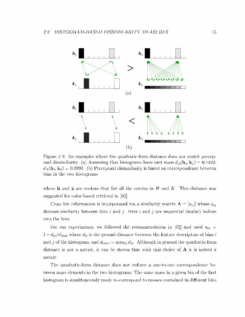
2.3 An examples where the quadratic-form distance does not match per-
ceptual dissimilarity. (a) Assuming that histograms have unit mass
dA(h1;k1) = 0:1429, dA(h3;k3) = 0:0893. (b) Perceptual dissimilarity
is based on correspondence between bins in the two histograms . . . . 15
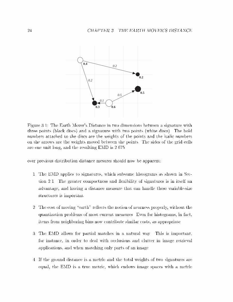
3.1 The Earth Mover's Distance in two dimensions between a signature
with three points (black discs) and a signature with two points (white
discs). The bold numbers attached to the discs are the weights of the
points and the italic numbers on the arrows are the weights moved
between the points. The sides of the grid cells are one unit long, and
the resulting EMD is 2.675. . . . . . . . . . . . . . . . . . . . . . . . 24
3.2 A log-log plot of the average computation time for random signatures
as a function of signature size. . . . . . . . . . . . . . . . . . . . . . . 28
3.3 Log-log plot of the number of EMDs as a function of the number of
images retrieved. The database contains 20,000 images. . . . . . . . . 33
3.4 The saturated ground distances d (solid line), and ~d (dotted line) as
a function of the ground distance dij = d(pi;qj). We assume that
maxi;jdij = 3. . . . . . . . . . . . . . . . . . . . . . . . . . . . . . . . 36
xii
4.1 An example of a color signature. (a) Original image. (b) Color signa-
ture. (c) Rendering the image using the signature colors. . . . . . . . 45
4.2 Examples of color-based image retrieval. The �rst image was used as
the query. (a) Searching for eagles. (b) Searching for elephants. Using
only color, elephants and hippopotamuses are very similar. . . . . . . 47
4.3 More examples. (a) Searching for horses. (b) Searching for owers
using a partial query, shown at the top. . . . . . . . . . . . . . . . . . 48
4.4 A bad example. This is due to the discrepancy between the semantic
query (\beautiful woman") and the syntactic features (the color content). 49
4.5 Using position information (the queries are on the left). (a) 20% green
at the top and 20% blue at the bottom. (b) 20% blue at the top and
20% green at the bottom. . . . . . . . . . . . . . . . . . . . . . . . . 50
4.6 Using the leftmost image of a skier as the query. The six best matches
without position information (a) and with position information (b). . 51
5.1 The components of (x; y). . . . . . . . . . . . . . . . . . . . . . . . 54
5.2 The half-amplitude of Gabor �lters in the frequency domain using four
scales and six orientations. Here we use Uh = 0:3 and Ul = 0:04. . . . 57
5.3 Texture features. Left: Patches from fabric (top) and tile (bottom)
textures. Middle: DFT magnitude. Right: Texture features; the hori-
zontal and vertical axes correspond to orientations and scale respectively. 58
5.4 16 homogeneous textures . . . . . . . . . . . . . . . . . . . . . . . . . 63
5.5 Mapping of image pixels to their nearest texture cluster, di�erentiated
by color. . . . . . . . . . . . . . . . . . . . . . . . . . . . . . . . . . . 67
5.6 (a) Texture patch from the Brodatz album [9]. (b) Average over all
texture features. The Gabor �lter bank consists of four scales and
six orientations. (c) The four clusters in the texture signature. (d)
Pixel assignment using the signature's clusters. Di�erent gray levels
represent di�erent clusters. . . . . . . . . . . . . . . . . . . . . . . . . 68
5.7 The Brodatz album of textures. Only 1/16 of each texture is shown. . 69
5.8 The Brodatz album of textures (continued). . . . . . . . . . . . . . . 70
xiii
5.9 Texture queries. The �rst image in each part was used as the query.
(a) Co�ee beans (D75). All 16 patches from the same texture were
returned �rst. (b) Lace (D41). Here, 15 out of the 16 texture patches
are in the top 18 matches. . . . . . . . . . . . . . . . . . . . . . . . . 71
5.10 Partial texture query. The query was 20% of the texture in part (a)
and 80% \don't care". (b) The 21 best matches: 16 patches from the
same texture (only the �rst and last ones are shown), followed by all
the compositions that contain some part of the queried texture. . . . 72
5.11 Another partial query. The query now contains 10% of each of the two
patches in part (a) and 80% \don't care." (b) The two best matches are
the two compositions that contain the textures in the query, followed
by the patches that contain only one of the queried textures. . . . . . 73
5.12 Looking for zebras. (a) An image of a zebra and a block of zebra stripes
extracted from it. (b) The best matches to a query asking for images
with at least 10% of the texture in (a). The numbers in the thumbnail
captions are indices into Corel CDs. . . . . . . . . . . . . . . . . . . . 74
5.13 Looking for cheetahs. (a) The query. (b) The best matches with at
least 10% of the query texture. The last four images are leopards and
jaguars which have similar texture as cheetahs. However, cheetahs
come �rst. . . . . . . . . . . . . . . . . . . . . . . . . . . . . . . . . . 75
5.14 Looking for leopards and jaguars. (a) The query. (b) The best matches
with at least 10% of the query texture. All but the sixth image are
leopards and jaguars. The sixth image is of cheetahs. . . . . . . . . . 76
5.15 (a) Mosaic of four textures from the Brodatz album. (b) Texture con-
trast before smoothing (dark values correspond to large contrast) and
(c) after 20 iterations. (d) Projection of the texture descriptors onto
the plane of their two most signi�cant principal components before
smoothing and (e) after 20 iterations. . . . . . . . . . . . . . . . . . . 81
5.16 (a) A picture of a lighthouse. (b) Nonigni�cant regions (blackened out)
after ten iterations of smoothing. . . . . . . . . . . . . . . . . . . . . 85
xiv
6.1 The eight closest images for each of the red car images in the �rst
column. The queries were processed by a color-based image retrieval
system using di�erent histogram dissimilarity measures. . . . . . . . . 94
6.2 Ten images of red cars (top) and the average number of relevant images,
for the di�erent dissimilarity measures, that were returned by using
the ten images as the queries with coarse histograms (middle) and �ne
histograms (bottom). The results obtained using signatures is also
shown for reference. . . . . . . . . . . . . . . . . . . . . . . . . . . . . 95
6.3 Ten images of horses (top) and the average number of relevant images,
for the di�erent dissimilarity measures, that were returned by using
ten images as the queries with coarse (middle) and �ne histograms
(bottom). The results obtained by using signatures is also shown for
reference. . . . . . . . . . . . . . . . . . . . . . . . . . . . . . . . . . 96
7.1 Looking for desert images; (a) Traditional display. (b) MDS display. . 102
7.2 A color signature and the MDS display of the 20 best matches. . . . . 103
7.3 Two-dimensional MDS applied to 16 homogeneous textures using no
invariance. The two dominant axes of orientation and coarseness emerge.106
7.4 Two-dimensional MDS applied to 16 homogeneous textures with rota-
tion invariance. The axes are coarseness and directionality. . . . . . . 107
7.5 Two-dimensional MDS applied to 16 homogeneous textures with rota-
tion and scale invariance. The two axis are \scality" and directionality. 108
7.6 Two views of a three-dimensional MDS display applied to 500 random
images. Only color information was used. . . . . . . . . . . . . . . . . 110
7.7 Looking for images with 20% blue. (a) The 500 most relevant images.
(b) Focusing on images of deserts. . . . . . . . . . . . . . . . . . . . 111
8.1 Retrieving skiers: �rst iteration. (a) The query's signature: 20% blue,
20% white, and 60% \don't care" (represented by the checkerboard
pattern). (b) The 10 best matches sorted by similarity to the query.
(c) MDS display of the 100 best matches (STRESS=0.15), where the
relevant region is selected. . . . . . . . . . . . . . . . . . . . . . . . . 117
xv
8.2 Retrieving skiers: second iteration. (a) The generated signature. (b)
The 10 best matches sorted by similarity to the query. (c) MDS of the
20 best matches (STRESS=0.06). . . . . . . . . . . . . . . . . . . . . 118
8.3 Navigation 1: gender vs. skin color. The mugshots are intentionally
blurred for anonymity. . . . . . . . . . . . . . . . . . . . . . . . . . . 122
8.4 Navigation 2: age vs. weight. The mugshots are intentionally blurred
for anonymity. . . . . . . . . . . . . . . . . . . . . . . . . . . . . . . . 123
8.5 Retrieval by navigation. . . . . . . . . . . . . . . . . . . . . . . . . . 124
8.6 A snapshot from the color-based retrieval demonstration system. . . . 125
A.1 Half-amplitude contours of the �lters with orientation � = 0. . . . . . 133
A.2 Half-amplitude contours of two neighboring �lters for di�erent orien-
tations. . . . . . . . . . . . . . . . . . . . . . . . . . . . . . . . . . . . 134
B.1 Retrieving color distributions using 32 bin histograms. . . . . . . . . 137
B.2 Retrieving color distributions using 128 bin histograms. . . . . . . . . 138
B.3 Retrieving color distributions using 512 bin histograms. . . . . . . . . 139
B.4 Retrieving color distributions using 512 bin histograms for non-moderate
similarities. . . . . . . . . . . . . . . . . . . . . . . . . . . . . . . . . 140
B.5 Retrieving texture distributions using 12 �lters and 32 bin histograms. 141
B.6 Retrieving texture distributions using 12 �lters and 128 bin histograms. 142
B.7 Retrieving texture distributions using 12 �lters and 512 bin histograms. 143
B.8 Retrieving texture distributions using 24 �lters and 32 bin histograms. 144
B.9 Retrieving texture distributions using 24 �lters and 128 bin histograms. 145
B.10 Retrieving texture distributions using 24 �lters and 512 bin histograms. 146
B.11 Retrieving texture distributions using 40 �lters and 32 bin histograms. 147
B.12 Retrieving texture distributions using 40 �lters and 128 bin histograms. 148
B.13 Retrieving texture distributions using 40 �lters and 512 bin histograms. 149
xvi

The last think that we discover in
writing a book is to know what to
put at the beginning.
Pascal (1623-1662)
Chapter 1
Introduction
1.1 Background and Motivation
Recent technological advances in disparate �elds of endeavor have combined to make
large databases of digital images accessible. These advances include:
1. Image acquisition devices, such as scanners and digital cameras,
2. Storage units that provide larger capacities for lower costs,
3. Access to enormous numbers of images via the internet, and the rapid growth
of the World-Wide Web where images can be easily added and accessed.
Rummaging through such a large collection of images in search of a particular pic-
ture is unrewarding and time-consuming. Image database retrieval research attempts
to automate parts of the tedious task of retrieving images that are similar to a given
description.
Occasionally, semantic keywords are attached to the images. This can be done
either by manually annotating the images or by automatically extracting the keyword
from the context, for instance, from the the images' captions. When available, such
keywords greatly assist the search. Practically, often images lack keywords and only
the appearance features of the images can be used. Appearance features are useful
1
2 CHAPTER 1. INTRODUCTION
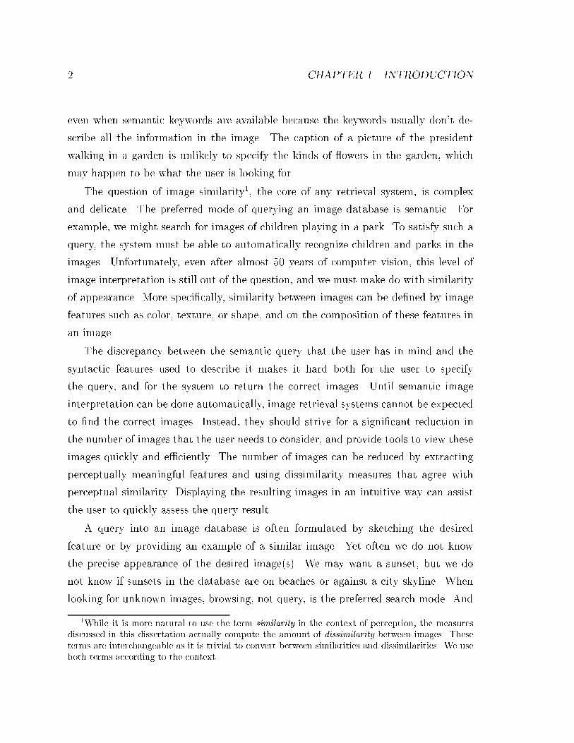
even when semantic keywords are available because the keywords usually don't de-
scribe all the information in the image. The caption of a picture of the president
walking in a garden is unlikely to specify the kinds of owers in the garden, which
may happen to be what the user is looking for.
The question of image similarity1, the core of any retrieval system, is complex
and delicate. The preferred mode of querying an image database is semantic. For
example, we might search for images of children playing in a park. To satisfy such a
query, the system must be able to automatically recognize children and parks in the
images. Unfortunately, even after almost 50 years of computer vision, this level of
image interpretation is still out of the question, and we must make do with similarity
of appearance. More speci�cally, similarity between images can be de�ned by image
features such as color, texture, or shape, and on the composition of these features in
an image.
The discrepancy between the semantic query that the user has in mind and the
syntactic features used to describe it makes it hard both for the user to specify
the query, and for the system to return the correct images. Until semantic image
interpretation can be done automatically, image retrieval systems cannot be expected
to �nd the correct images. Instead, they should strive for a signi�cant reduction in
the number of images that the user needs to consider, and provide tools to view these
images quickly and e�ciently. The number of images can be reduced by extracting
perceptually meaningful features and using dissimilarity measures that agree with
perceptual similarity. Displaying the resulting images in an intuitive way can assist
the user to quickly assess the query result.
A query into an image database is often formulated by sketching the desired
feature or by providing an example of a similar image. Yet often we do not know
the precise appearance of the desired image(s). We may want a sunset, but we do
not know if sunsets in the database are on beaches or against a city skyline. When
looking for unknown images, browsing, not query, is the preferred search mode. And
1While it is more natural to use the term similarity in the context of perception, the measuresdiscussed in this dissertation actually compute the amount of dissimilarity between images. Theseterms are interchangeable as it is trivial to convert between similarities and dissimilarities. We useboth terms according to the context.
1.2. PREVIOUS WORK 3
the key requirement for browsing is that similar images are located nearby. Current
retrieval systems list output images in order of increasing distance from the query.
However, as we show in this dissertation, the distances among the returned images
also convey useful information for browsing.
1.2 Previous Work
The increasing availability of digital imagery has created the need for content-based
image retrieval systems, while the development of computation and storage resources
provides the means for implementing them. This led to extensive research that re-
sulted, in less than a decade, into numerous commercial and research-based systems,
including QBIC [62], Virage [3], Photobook [66], Excalibur [26], Chabot [23], and Vi-
sualSEEK [92]. These systems allow the user to formulate queries using combinations
of low-level image features such as color, texture, and shape. The queries are spec-
i�ed explicitly by providing the desired feature values or implicitly by specifying an
example image. Some systems also use the spatial organization of the image features,
so that similarity is determined not only by the existence of certain features, but
also by their absolute or relative location in the image [40, 3, 95, 92, 18, 11]. Early
systems focused on the search engine (given a query, �nd the best matches) and did
not use previous queries to understand better what the user was looking for. Recent
systems allow the user to re�ne the search by indicating the relevance (or irrelevance)
of images in the returned set. This is known as relevance feedback [81, 59, 92].
In [41], the authors provide an in-depth review of content-based image retrieval
systems. They also identify a number of unanswered key research questions, including
the development of more robust and compact image content features and dissimilarity
measures that model perceptual similarity more accurately. We approach these issues
in Chapters 2-6 and the problem of expanding a content-based image search engine
to an intuitive navigation system in Chapters 7 and 8.
4 CHAPTER 1. INTRODUCTION
1.3 Overview of the Dissertation
We present a novel framework for computing the distance between images and a
set of tools to visualize parts of the database and browse its content intuitively. In
particular, we address the following questions:
� What features describe the content of an image well?
� How to summarize the distribution of these features over an image?
� How to measure the dissimilarity between distributions of features?
� How can we e�ectively display the results of a search?
� How can a user browse the images in the database in an intuitive and e�cient
way?
In this thesis, we focus on the overall color and texture content of images as
the main criterion for similarity. The overall distribution of colors within an image
contributes to the mood of the image in an important way and is a useful clue for
the content of an image. Sunny mountain landscapes, sunsets, cities, faces, jungles,
candy, and �re �ghter scenes lead to images that have di�erent but characteristic
color distributions. While color is a property of single pixels, texture describes the
appearance of bigger regions in the image. Often, semantically similar objects can be
characterized by similar textures.
Summarizing feature distributions has to do with perceptual signi�cance, invari-
ance, and e�ciency. Features should be represented in a way that re ects a human's
appreciation of similarities and di�erences. At the same time, the distributions of the
image features should be represented by a collection of data that is small, for e�-
ciency, but rich enough to reproduce the essential information. The issue of relevance
to human perception has been resolved by the choice of appropriate representations.
For color we choose the CIELab color space, and for texture we use Gabor �lters.
For both we discuss their relations with perceptual similarity. We summarize the
feature distributions by a small collection of weighted points in feature space where
1.4. ROAD MAP 5
the number of points adapts to capture the complexity of the distributions; we call
this set of points a signature.
De�ning a dissimilarity measure between two signatures �rst requires a notion
of distance between the basic features that are aggregated into the signatures. We
call this distance the ground distance. For instance, in the case of color, the ground
distance measures dissimilarity between individual colors. We address the problem of
lifting these distances from individual features to full distributions. In other words,
we want to de�ne a consistent measure of distance, or dissimilarity, between two
distributions in a space endowed with a ground distance. We introduce the Earth
Mover's Distance as a useful and exible metric, thereby addressing the question of
image similarity.
If the pictures in a database can be spatially arranged so that their locations re ect
their di�erences and similarities, browsing the database by navigating in this space
becomes intuitively meaningful. In fact, the database is now endowed with a metric
structure, and can be explored with a sense of continuity and comprehensiveness.
Parts of the database that have undesired distributions need not be traversed; on
the other hand, interesting regions can be explored with a sense of getting closer or
farther away from the desired distribution of colors. In summary, the user can form a
mental, low-detail picture of the entire database, and a more detailed picture of the
more interesting parts of it.
1.4 Road Map
The rest of the dissertation is organized as follows: Chapter 2 addresses the issue
of summarizing distributions of features and surveys some of the most commonly
used distribution-based dissimilarity measures. In Chapter 3 we introduce the Earth
Mover's Distance, which we claim is a preferred dissimilarity measure for image re-
trieval, and discuss its properties. In Chapters 4 and 5, respectively, we de�ne color
and texture features and show that, combined with the EMD, they lead to e�ective
image retrieval. In Chapter 6 we conduct extensive experiments where we compare
the retrieval results, for color and texture, using various dissimilarity measures. The

6 CHAPTER 1. INTRODUCTION
problem of displaying the results of a search in a useful way is approached in Chap-
ter 7. Finally, in Chapter 8 we extend our display technique to a full navigation
system that allows intuitive re�nement of a query.
The di�erence between the right
word and a similar word is the
di�erence between lightning and a
lightning bug.
Mark Twain (1835-1910)
Chapter 2
Distribution-Based Dissimilarity
Measures
In order for an image retrieval system to �nd images that are visually similar to the
given query, it should have both a proper representation of the images visual features
and a measure that can determine how similar or dissimilar the di�erent images are
from the query. Assuming that no textual captions or other manual annotations of
the images are given, the features that can be used are descriptions of the image
content, such as color [97, 62, 96, 91, 4], texture [25, 62, 6, 69, 56, 4], and shape
[42, 62, 31, 44]. These features usually vary substantially over an image, both because
of inherent variations in surface appearance and as a result of changes in illumination,
shading, shadowing, foreshortening, etc. Thus, the appearance of a region is better
described by the distribution of features, rather than by individual feature vectors.
Dissimilarity measures, based on empirical estimates of the distributions of fea-
tures, have been developed and used for di�erent tasks in low-level computer vision
including classi�cation [63], image retrieval [28, 97, 71, 80] and segmentation [32, 39].
In this chapter, we �rst describe di�erent representations for distributions of im-
age features and discuss their advantages and disadvantages. We then survey and
categorize some of the most commonly used dissimilarity measures.
7
8 CHAPTER 2. DISTRIBUTION-BASED DISSIMILARITY MEASURES
2.1 Representing Distributions of Features
2.1.1 Histograms
A histogram fhig is a mapping from a set of d-dimensional integer vectors i to the set
of nonnegative reals. These vectors typically represent bins (or their centers) in a �xed
partitioning of the relevant region of the underlying feature space. The associated
reals are a measure of the mass of the distribution that falls into the corresponding
bin. For instance, in a grey-level histogram, d is equal to one, the set of possible grey
values is split into N intervals, and hi is the number of pixels in an image that have
a grey value in the interval indexed by i (a scalar in this case).
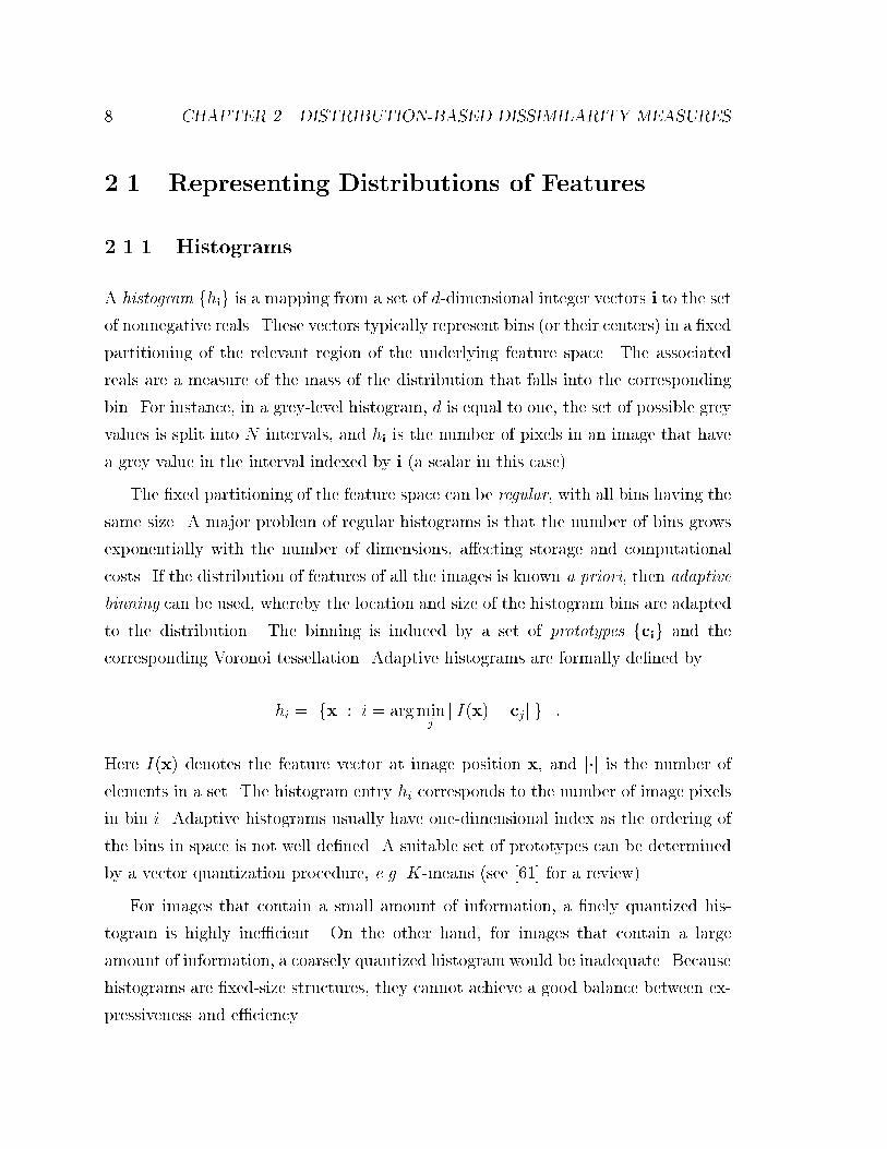
The �xed partitioning of the feature space can be regular, with all bins having the
same size. A major problem of regular histograms is that the number of bins grows
exponentially with the number of dimensions, a�ecting storage and computational
costs. If the distribution of features of all the images is known a priori, then adaptive
binning can be used, whereby the location and size of the histogram bins are adapted
to the distribution. The binning is induced by a set of prototypes fcig and the
corresponding Voronoi tessellation. Adaptive histograms are formally de�ned by
hi =
����fx : i = argminjkI(x)� cjkg
���� :Here I(x) denotes the feature vector at image position x, and j�j is the number of
elements in a set. The histogram entry hi corresponds to the number of image pixels
in bin i. Adaptive histograms usually have one-dimensional index as the ordering of
the bins in space is not well de�ned. A suitable set of prototypes can be determined
by a vector quantization procedure, e.g. K-means (see [61] for a review).
For images that contain a small amount of information, a �nely quantized his-
togram is highly ine�cient. On the other hand, for images that contain a large
amount of information, a coarsely quantized histogram would be inadequate. Because
histograms are �xed-size structures, they cannot achieve a good balance between ex-
pressiveness and e�ciency.
2.1. REPRESENTING DISTRIBUTIONS OF FEATURES 9
2.1.2 Signatures
Unlike histograms, whose bins are de�ned over the entire database, the clusters in
signatures are de�ned for each image individually. A signature fsj = (mj; wmj)g
represents a set of feature clusters. Each cluster is represented by its mean (or mode)
mj and the fraction wmjof pixels that belong to that cluster. The integer subscript
j ranges from one to a value that varies with the complexity of the particular image.
While j is simply an integer, the representative mj is a d-dimensional vector. In
general, the same vector quantization algorithms that are used to compute adaptive
histograms can be used for clustering, as long as they are applied to every image
independently, adapting the number of clusters to the complexity of the individual
images. Simple images have short signatures while complex images have long ones.
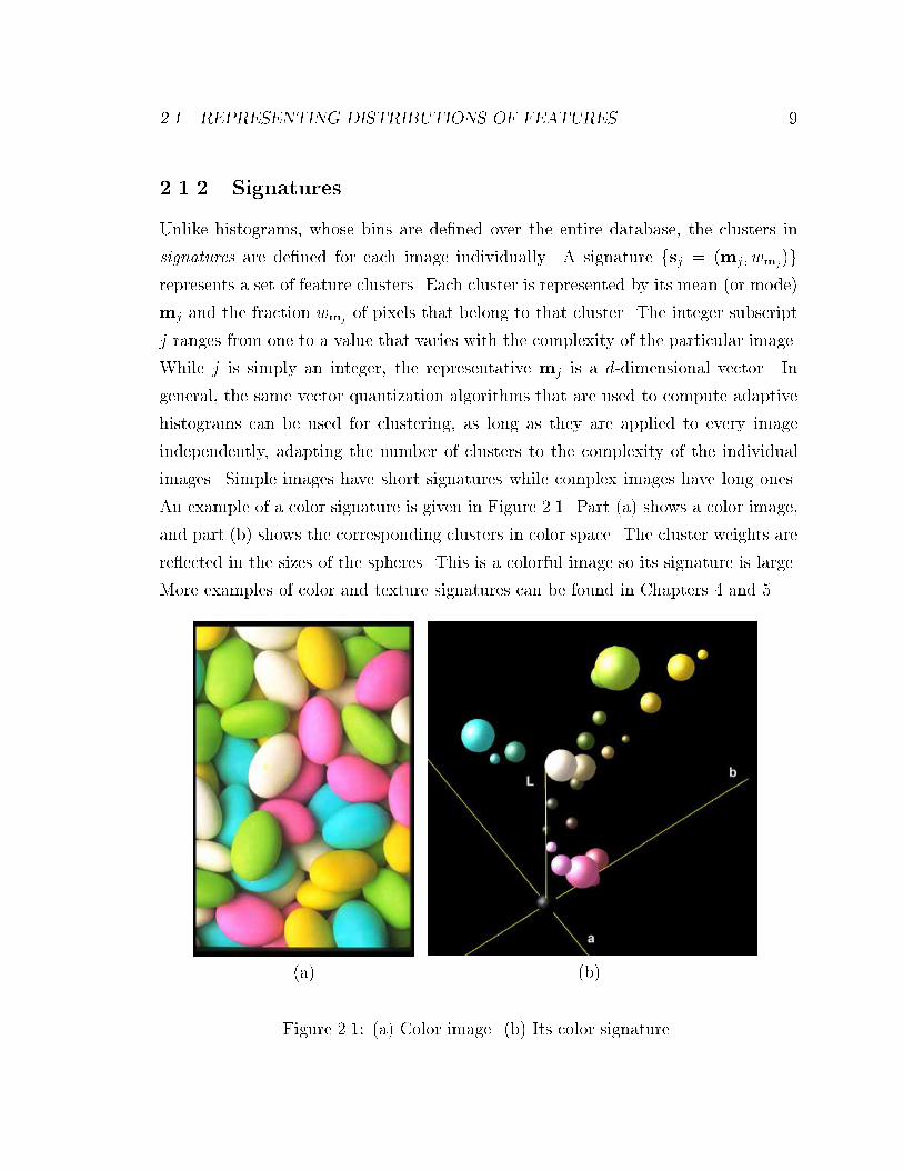
An example of a color signature is given in Figure 2.1. Part (a) shows a color image,
and part (b) shows the corresponding clusters in color space. The cluster weights are
re ected in the sizes of the spheres. This is a colorful image so its signature is large.
More examples of color and texture signatures can be found in Chapters 4 and 5.
(a) (b)
Figure 2.1: (a) Color image. (b) Its color signature.
10 CHAPTER 2. DISTRIBUTION-BASED DISSIMILARITY MEASURES
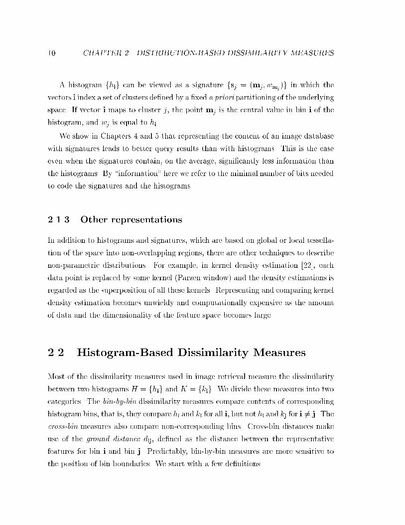
A histogram fhig can be viewed as a signature fsj = (mj; wmj)g in which the
vectors i index a set of clusters de�ned by a �xed a priori partitioning of the underlying
space. If vector i maps to cluster j, the point mj is the central value in bin i of the
histogram, and wj is equal to hi.
We show in Chapters 4 and 5 that representing the content of an image database
with signatures leads to better query results than with histograms. This is the case
even when the signatures contain, on the average, signi�cantly less information than
the histograms. By \information" here we refer to the minimal number of bits needed
to code the signatures and the histograms.
2.1.3 Other representations
In addition to histograms and signatures, which are based on global or local tessella-
tion of the space into non-overlapping regions, there are other techniques to describe
non-parametric distributions. For example, in kernel density estimation [22], each
data point is replaced by some kernel (Parzen window) and the density estimations is
regarded as the superposition of all these kernels. Representing and comparing kernel
density estimation becomes unwieldy and computationally expensive as the amount
of data and the dimensionality of the feature space becomes large.
2.2 Histogram-Based Dissimilarity Measures
Most of the dissimilarity measures used in image retrieval measure the dissimilarity
between two histograms H = fhig and K = fkig. We divide these measures into two
categories. The bin-by-bin dissimilarity measures compare contents of corresponding
histogram bins, that is, they compare hi and ki for all i, but not hi and kj for i 6= j. The
cross-bin measures also compare non-corresponding bins. Cross-bin distances make
use of the ground distance dij, de�ned as the distance between the representative
features for bin i and bin j. Predictably, bin-by-bin measures are more sensitive to
the position of bin boundaries. We start with a few de�nitions.
2.2. HISTOGRAM-BASED DISSIMILARITY MEASURES 11
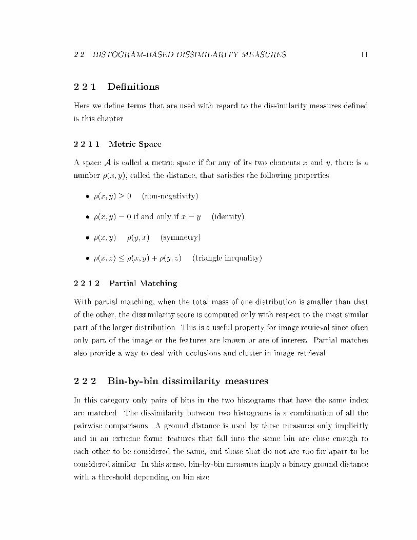
2.2.1 De�nitions
Here we de�ne terms that are used with regard to the dissimilarity measures de�ned
is this chapter.
2.2.1.1 Metric Space
A space A is called a metric space if for any of its two elements x and y, there is a
number �(x; y), called the distance, that satis�es the following properties
� �(x; y) � 0 (non-negativity)
� �(x; y) = 0 if and only if x = y (identity)
� �(x; y) = �(y; x) (symmetry)
� �(x; z) � �(x; y) + �(y; z) (triangle inequality)
2.2.1.2 Partial Matching
With partial matching, when the total mass of one distribution is smaller than that
of the other, the dissimilarity score is computed only with respect to the most similar
part of the larger distribution. This is a useful property for image retrieval since often
only part of the image or the features are known or are of interest. Partial matches
also provide a way to deal with occlusions and clutter in image retrieval.
2.2.2 Bin-by-bin dissimilarity measures
In this category only pairs of bins in the two histograms that have the same index
are matched. The dissimilarity between two histograms is a combination of all the
pairwise comparisons. A ground distance is used by these measures only implicitly
and in an extreme form: features that fall into the same bin are close enough to
each other to be considered the same, and those that do not are too far apart to be
considered similar. In this sense, bin-by-bin measures imply a binary ground distance
with a threshold depending on bin size.
12 CHAPTER 2. DISTRIBUTION-BASED DISSIMILARITY MEASURES
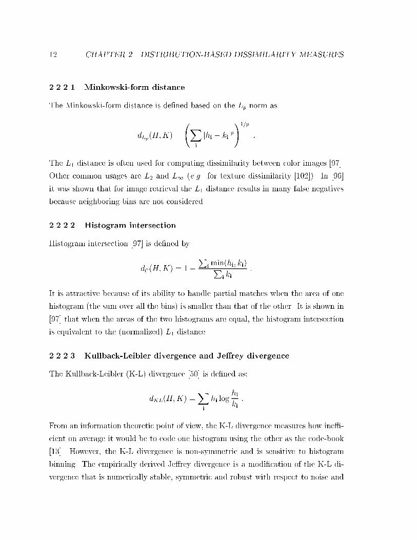
2.2.2.1 Minkowski-form distance
The Minkowski-form distance is de�ned based on the Lp norm as
dLp(H;K) =
Xi
jhi � kijp!1=p
:
The L1 distance is often used for computing dissimilarity between color images [97].
Other common usages are L2 and L1 (e.g. for texture dissimilarity [102]). In [96]
it was shown that for image retrieval the L1 distance results in many false negatives
because neighboring bins are not considered.
2.2.2.2 Histogram intersection
Histogram intersection [97] is de�ned by
d\(H;K) = 1�P
imin(hi; ki)Pi ki
:
It is attractive because of its ability to handle partial matches when the area of one
histogram (the sum over all the bins) is smaller than that of the other. It is shown in
[97] that when the areas of the two histograms are equal, the histogram intersection
is equivalent to the (normalized) L1 distance.
2.2.2.3 Kullback-Leibler divergence and Je�rey divergence
The Kullback-Leibler (K-L) divergence [50] is de�ned as:
dKL(H;K) =Xi
hi loghiki:
From an information theoretic point of view, the K-L divergence measures how ine�-
cient on average it would be to code one histogram using the other as the code-book
[13]. However, the K-L divergence is non-symmetric and is sensitive to histogram
binning. The empirically derived Je�rey divergence is a modi�cation of the K-L di-
vergence that is numerically stable, symmetric and robust with respect to noise and
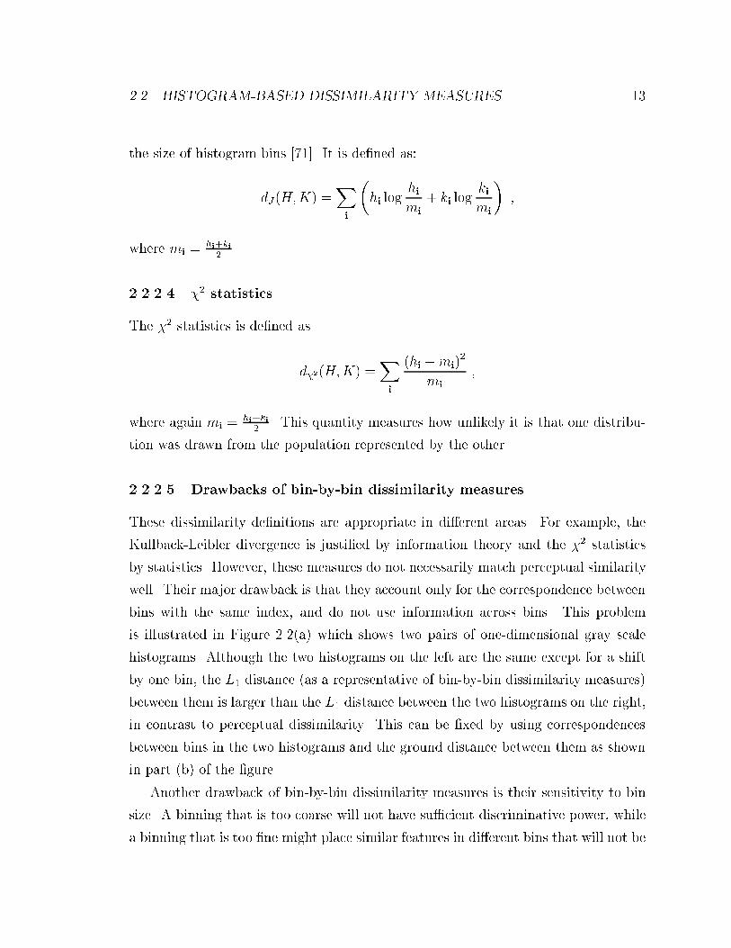
2.2. HISTOGRAM-BASED DISSIMILARITY MEASURES 13
the size of histogram bins [71]. It is de�ned as:
dJ(H;K) =Xi
�hi log
himi
+ ki logkimi
�;
where mi =hi+ki
2.
2.2.2.4 �2 statistics
The �2 statistics is de�ned as
d�2(H;K) =Xi
(hi �mi)2
mi
;
where again mi =hi+ki
2. This quantity measures how unlikely it is that one distribu-
tion was drawn from the population represented by the other.
2.2.2.5 Drawbacks of bin-by-bin dissimilarity measures
These dissimilarity de�nitions are appropriate in di�erent areas. For example, the
Kullback-Leibler divergence is justi�ed by information theory and the �2 statistics
by statistics. However, these measures do not necessarily match perceptual similarity
well. Their major drawback is that they account only for the correspondence between
bins with the same index, and do not use information across bins. This problem
is illustrated in Figure 2.2(a) which shows two pairs of one-dimensional gray scale
histograms. Although the two histograms on the left are the same except for a shift
by one bin, the L1 distance (as a representative of bin-by-bin dissimilarity measures)
between them is larger than the L1 distance between the two histograms on the right,
in contrast to perceptual dissimilarity. This can be �xed by using correspondences
between bins in the two histograms and the ground distance between them as shown
in part (b) of the �gure.
Another drawback of bin-by-bin dissimilarity measures is their sensitivity to bin
size. A binning that is too coarse will not have su�cient discriminative power, while
a binning that is too �ne might place similar features in di�erent bins that will not be
14 CHAPTER 2. DISTRIBUTION-BASED DISSIMILARITY MEASURES
h1
k1
h2
k2
>
(a)
h1
<1
h2
k2k
(b)
Figure 2.2: An example where the L1 distance does not match perceptual dissimilar-ity. (a) Assuming that histograms have unit mass dL1(h1;k1) = 2, dL1(h2;k2) = 1.(b) Perceptual dissimilarity is based on correspondence between bins in the two his-tograms.
matched. On the other hand, cross-bin dissimilarity measures, described next, always
yield better results when the bins get smaller.
2.2.3 Cross-bin dissimilarity measures
When a ground distance that matches perceptual dissimilarity is available for sin-
gle features, incorporating this information results in perceptually more meaningful
dissimilarity measures for distributions of features.
2.2.3.1 Quadratic-form distance
dA(H;K) =p(h� k)TA(h� k) ;
2.2. HISTOGRAM-BASED DISSIMILARITY MEASURES 15
3h
>3k1k
1h
(a)
h1
<k1 k3
3h
(b)
Figure 2.3: An examples where the quadratic-form distance does not match percep-tual dissimilarity. (a) Assuming that histograms have unit mass dA(h1;k1) = 0:1429,dA(h3;k3) = 0:0893. (b) Perceptual dissimilarity is based on correspondence betweenbins in the two histograms
where h and k are vectors that list all the entries in H and K. This distance was
suggested for color-based retrieval in [62].
Cross-bin information is incorporated via a similarity matrix A = [aij] where aij
denotes similarity between bins i and j. Here i and j are sequential (scalar) indices
into the bins.
For our experiments, we followed the recommendation in [62] and used aij =
1�dij=dmax where dij is the ground distance between the feature descriptors of bins i
and j of the histogram, and dmax = maxij dij. Although in general the quadratic-form
distance is not a metric, it can be shown that with this choice of A it is indeed a
metric.
The quadratic-form distance does not enforce a one-to-one correspondence be-
tween mass elements in the two histograms: The same mass in a given bin of the �rst
histogram is simultaneously made to correspond to masses contained in di�erent bins
16 CHAPTER 2. DISTRIBUTION-BASED DISSIMILARITY MEASURES
of the other histogram. This is illustrated in Figure 2.3(a), where the quadratic-form
distance between the two histograms on the left is larger than the distance between
the two histograms on the right. Again, this is clearly at odds with perceptual dis-
similarity. The desired distance here should be based on the correspondences shown
in part (b) of the �gure.
Similar conclusions were obtained in [96], where it was shown that using the
quadratic-form distance in image retrieval results in false positives, because it tends
to overestimate the mutual similarity of color distributions without a pronounced
mode.
2.2.3.2 One-dimensional match distance
dM(H;K) =Xi
jhi � kij ; (2.1)
where hi =P
j�i hj is the cumulative histogram of fhig, and similarly for fkig.
The match distance [87, 105] between two one-dimensional histograms is de�ned
as the L1 distance between their corresponding cumulative histograms. For one-
dimensional histograms with equal areas, this distance is a special case of the EMD,
which we present in Chapter 3, with the important di�erences that the match distance
cannot handle partial matches or other ground distances. The one-dimensional match
distance does not extend to higher dimensions because the relation j � i is not a total
ordering in more than one dimension, and the resulting arbitrariness causes problems.
The match distance is extended in [105] for multi-dimensional histograms by using
graph matching algorithms. This extension is similar in spirit to the EMD, which
can be seen as a generalization of the match distance. In the rest of this chapter,
the term \match distance" refers only to the one-dimensional case, for which analytic
formulation is available.
2.2. HISTOGRAM-BASED DISSIMILARITY MEASURES 17
2.2.3.3 Kolmogorov-Smirnov statistics
dKS(H;K) = maxi(jhi � kij) :
Again, hi and ki are cumulative histograms.
The Kolmogorov-Smirnov statistics is a common statistical measure for unbinned
distributions. Although, for consistency, we use here cumulative histograms, the
Kolmogorov-Smirnov statistics is de�ned on the cumulative distributions so that no
binning is required and it can be applied to continues data. In the case of the
null hypothesis (data sets drawn from the same distribution) the distribution of the
Kolmogorov-Smirnov statistics can be calculated, thus giving the signi�cance of the
result [16]. Similarly to the match distance, it is de�ned only for one dimension.
2.2.4 Parameter-based dissimilarity measures
These methods �rst compute a small set of parameters from the histograms, either
explicitly or implicitly, and then compare these parameters. For instance, the distance
between distributions is computed in [96] as the sum of the weighted distances of the
distributions' �rst three moments. In [18], only the peaks of color histograms are
used for color image retrieval. In [53], textures are compared based on measures of
their periodicity, directionality, and randomness, while in [56] texture distances are
de�ned by comparing their means and standard deviations in a weighted-L1 sense.
Additional dissimilarity measures for image retrieval are evaluated and compared in
[92, 71].
2.2.5 Properties
Table 2.1 compares the main properties of the di�erent measures presented in Sec-
tions 2.2.3 and 2.2.2. For comparison, we include the EMD, which is de�ned in
Chapter 3.
The Kolmogorov-Smirnov statistics and the match distance are de�ned only for
one-dimensional distributions. Thus, they cannot be used for color and texture.
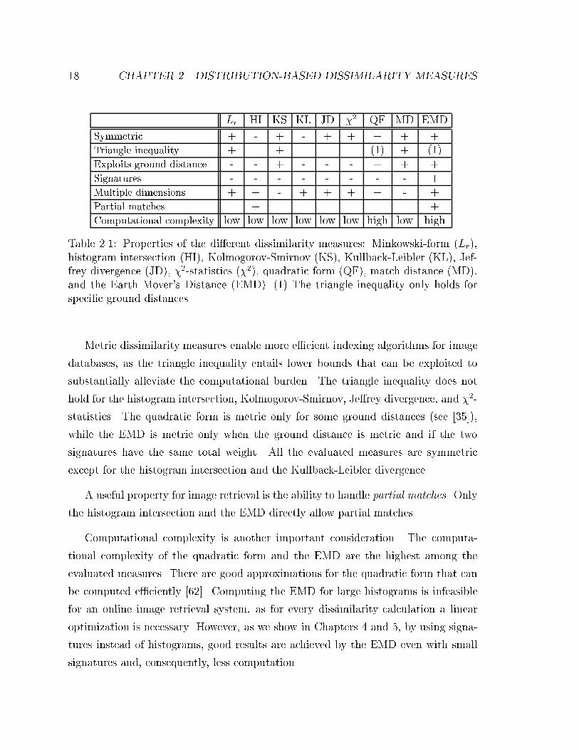
18 CHAPTER 2. DISTRIBUTION-BASED DISSIMILARITY MEASURES
Lr HI KS KL JD �2 QF MD EMD
Symmetric + - + - + + + + +Triangle inequality + - + - - - (1) + (1)Exploits ground distance - - + - - - + + +Signatures - - - - - - - - +Multiple dimensions + + - + + + + - +Partial matches - + - - - - - - +Computational complexity low low low low low low high low high
Table 2.1: Properties of the di�erent dissimilarity measures: Minkowski-form (Lr),histogram intersection (HI), Kolmogorov-Smirnov (KS), Kullback-Leibler (KL), Jef-frey divergence (JD), �2-statistics (�2), quadratic form (QF), match distance (MD),and the Earth Mover's Distance (EMD). (1) The triangle inequality only holds forspeci�c ground distances.
Metric dissimilarity measures enable more e�cient indexing algorithms for image
databases, as the triangle inequality entails lower bounds that can be exploited to
substantially alleviate the computational burden. The triangle inequality does not
hold for the histogram intersection, Kolmogorov-Smirnov, Je�rey divergence, and �2-
statistics. The quadratic form is metric only for some ground distances (see [35]),
while the EMD is metric only when the ground distance is metric and if the two
signatures have the same total weight. All the evaluated measures are symmetric
except for the histogram intersection and the Kullback-Leibler divergence.
A useful property for image retrieval is the ability to handle partial matches. Only
the histogram intersection and the EMD directly allow partial matches.
Computational complexity is another important consideration. The computa-
tional complexity of the quadratic form and the EMD are the highest among the
evaluated measures. There are good approximations for the quadratic form that can
be computed e�ciently [62]. Computing the EMD for large histograms is infeasible
for an online image retrieval system, as for every dissimilarity calculation a linear
optimization is necessary. However, as we show in Chapters 4 and 5, by using signa-
tures instead of histograms, good results are achieved by the EMD even with small
signatures and, consequently, less computation.

2.3. SUMMARY 19
2.3 Summary
In this chapter we presented methods for the representation of distributions of image
features, with histograms being the most common method for image retrieval. We
also surveyed and compared histogram-based dissimilarity measures.
Histograms are in exible: they cannot achieve a good balance between expres-
siveness and e�ciency. Signatures, on the other hand, adjust to the speci�c images.
Unfortunately, most dissimilarity measures cannot be applied to signatures. In the
next chapter we present the Earth Mover's Distance, which is designed for signatures,
and show that it has many desirable properties for image retrieval.
The great God endows his children
variously. To some He gives
intellect{ and they move the earth
...
Mary Roberts Rinehart (1876-1958)
Chapter 3
The Earth Mover's Distance
A ground distance between single visual image features can often be found by psy-
chophysical experiments. For example, perceptual color spaces have been devised
in which the Euclidean distance between two colors approximately matches the hu-
man perception of their di�erence. Measuring perceptual distance becomes more
complicated when sets of features, rather than single features, are being compared.
In Section 2.2 we showed the problems caused by dissimilarity measures that do not
handle correspondences between di�erent bins in the two histograms. Such correspon-
dences are key to a perceptually natural de�nition of the distances between sets of
features. This observation led to distance measures based on bipartite graph match-
ing [65, 108], de�ned as the minimum cost of matching elements between the two
histograms.
In [65] the distance between two gray scale images is computed as follows: every
pixel is represented by n \pebbles" where n is an integer representing the gray level
of that pixel. After normalizing the two images to have the same number of pebbles,
the distance between them is computed as the minimum cost of matching the pebbles
between the two images. The cost of matching two single pebbles is based on their
distance in the image plane. In this section we take a similar approach and derive
the Earth Mover's Distance1 (EMD) as a useful metric between signatures for image
retrieval in di�erent feature spaces.
1The name was suggested by Stol� [94].
20
21
The main di�erence between the two approaches is that we solve the transporta-
tion problem which �nds the optimal match between two distributions where variable-
sized pieces of \mass" are allowed to be moved together, in contrast to the matching
problem where unit elements of �xed size are matched individually. This distinction
signi�cantly increases e�ciency, due to the more compact representation as a result
of clustering pixels in the feature space. The implementation is fast enough for on-
line image retrieval systems. In addition, as we will show, our formulation allows
for partial matches, which are important for image retrieval applications. Finally,
instead of computing image distances based on the cost of moving pixels in the image
space, where the ground distance is perceptually meaningless, we compute distances
in feature spaces, where the ground distances can be perceptually better de�ned.
Intuitively, given two distributions, one can be seen as piles of earth in feature
space, the other as a collection of holes in that same space. The EMD measures
the least amount of work needed to �ll the holes with earth. Here, a unit of work
corresponds to transporting a unit of earth by a unit of ground distance.
Computing the EMD is based on a solution to the well-known transportation
problem [38], also known as the Monge-Kantorovich mass transference problem, which
goes back to 1781 when it was �rst introduced by Monge [60] in the following way:
Split two equally large volumes into in�nitely small particles and then
associate them with each other so that the sum of products of these paths
of the particles to a volume is least. Along what paths must the particles
be transported and what is the smallest transportation cost?
See [72] for an excellent survey of the history of the Monge-Kantorovich mass transfer-
ence problem. This distance was �rst introduced to the computer vision community
by [105].
Suppose that several suppliers, each with a known amount of goods, are required to
supply several consumers, each with a known capacity. For each supplier-consumer
pair, the cost of transporting a single unit of goods is given. The transportation
problem is, then, to �nd a least-expensive ow of goods from the suppliers to the
consumers that satis�es the consumers' demand. Signature matching can be naturally
22 CHAPTER 3. THE EARTH MOVER'S DISTANCE
cast as a transportation problem by de�ning one signature as the supplier and the
other as the consumer, and by setting the cost for a supplier-consumer pair to equal
the ground distance between an element in the �rst signature and an element in
the second. Intuitively, the solution is the minimum amount of \work" required to
transform one signature into the other. In the following we will refer to the supplies
as \mass."
In Section 3.1 we formally de�ne the EMD. We discuss its properties in Sec-
tion 3.2 and specify computational issues, including lower bounds, in Section 3.3. In
Section 3.4 we describe a saturated ground distance and claim better agreement with
psychophysics than simpler distance measures. Finally, in Section 3.5 we mention
some extensions to the EMD.
3.1 De�nition
The EMD is based on the following linear programming problem: Let P = f(p1; wp1);
: : : ; (pm; wpm)g be the �rst signature with m clusters, where pi is the cluster rep-
resentative and wpi is the weight of the cluster; Q = f(q1; wq1); : : : ; (qn; wqn)g the
second signature with n clusters; and D = [dij] the ground distance matrix where
dij = d(pi;qj) is the ground distance between clusters pi and qj.
We want to �nd a ow F = [fij], with fij the ow between pi and qj, that
minimizes the overall cost
WORK(P;Q;F) =mXi=1
nXj=1
d(pi;qj)fij ;
3.2. PROPERTIES 23
subject to the following constraints:
fij � 0 ; 1 � i � m; 1 � j � n ; (3.1)nXj=1
fij � wpi ; 1 � i � m ; (3.2)
mXi=1
fij � wqj ; 1 � j � n ; (3.3)
mXi=1
nXj=1
fij = min(mXi=1
wpi;nX
j=1
wqj ) : (3.4)
Constraint (3.1) allows moving \supplies" from P to Q and not vice versa. Con-
straint (3.2) limits the amount of supplies that can be sent by the clusters in P to
their weights. Constraint (3.3) limits the clusters in Q to receive no more supplies
than their weights; and Constraint (3.4) forces the maximum amount of supplies
possible to be moved. We call this amount the total ow. Once the transportation
problem is solved, and we have found the optimal ow F, the Earth Mover's Distance
is de�ned as the resulting work normalized by the total ow:
EMD(P;Q) =
Pmi=1
Pnj=1 d(pi;qj)fijPm
i=1
Pnj=1 fij
;
The normalization factor is the total weight of the smaller signature, because of
Constraint (3.4). This factor is needed when the two signatures have di�erent to-
tal weights, in order to avoid favoring smaller signatures. An example of a two-
dimensional EMD is shown in Figure 3.1. In general, the ground distance can be any
distance and will be chosen according to the problem at hand. Further discussion of
the ground distance is given in Section 3.4.
3.2 Properties
The EMD naturally extends the notion of a distance between single elements to that
of a distance between sets, or distributions, of elements. The advantages of the EMD
24 CHAPTER 3. THE EARTH MOVER'S DISTANCE
0.5
0.2
0.3
0.5
0.2
0.1
0.2
0.6
0.4
Figure 3.1: The Earth Mover's Distance in two dimensions between a signature withthree points (black discs) and a signature with two points (white discs). The boldnumbers attached to the discs are the weights of the points and the italic numberson the arrows are the weights moved between the points. The sides of the grid cellsare one unit long, and the resulting EMD is 2.675.
over previous distribution distance mesures should now be apparent:
1. The EMD applies to signatures, which subsume histograms as shown in Sec-
tion 2.1. The greater compactness and exibility of signatures is in itself an
advantage, and having a distance measure that can handle these variable-size
structures is important.
2. The cost of moving \earth" re ects the notion of nearness properly, without the
quantization problems of most current measures. Even for histograms, in fact,
items from neighboring bins now contribute similar costs, as appropriate.
3. The EMD allows for partial matches in a natural way. This is important,
for instance, in order to deal with occlusions and clutter in image retrieval
applications, and when matching only parts of an image.
4. If the ground distance is a metric and the total weights of two signatures are
equal, the EMD is a true metric, which endows image spaces with a metric
3.2. PROPERTIES 25
structure. Metric dissimilarity measures allow for e�cient data structures and
search algorithms [8, 10].
We now prove the �nal statement.
Theorem 3.1 If two signatures, P and Q, have equal weights and the ground distance
d(pi;qj) is metric for all pi in P and qj in Q, then EMD(P;Q) is also metric.
Proof: To prove that a distance measure is metric, we must prove the following:
positive de�niteness (EMD(P;Q) � 0 and EMD(P;Q) = 0 i� P � Q), symme-
try (EMD(P;Q) = EMD(Q;P )), and the triangle inequality (for any signature R,
EMD(P;Q) � EMD(P;R) + EMD(R;Q)).
Positive de�niteness and symmetry hold trivially in all cases, so we only need to
prove that the triangle inequality holds. Without loss of generality we assume here
that the total sum of the ows is 1. Let ffijg be the optimal ow from P to R and
fgjkg be the optimal ow from R to Q. Consider the ow P 7! R 7! Q. We now
show how to construct a feasible ow from P to Q that represents no more work than
that of moving mass optimally from P to Q through R. Since the EMD is the least
possible amount of feasible work, this construction proves the triangle inequality.
The largest weight that moves as one unit from pi to rj and from rj to qk de�nes
a ow which we call bijk where i, j and k correspond to pi, rj and qk respectively.
ClearlyP
k bijk = fij, the ow from P to R, andP
i bijk = gjk, the ow from R to Q.
We de�ne
hik4=Xj
bijk
to be a ow from pi to qk. This ow is a feasible one because it satis�es the con-
straints (3.1)-(3.4) in Section 3.1. Constraint (3.1) holds, since bijk > 0 by construc-
tion. Constraints (3.2) and (3.3) hold because
Xk
hik =Xj;k
bijk =Xj
fij = wpi ;
26 CHAPTER 3. THE EARTH MOVER'S DISTANCE
and
Xi
hik =Xi;j
bijk =Xj
gjk = wqk ;
and constraint (3.4) holds because the signatures have equal weights. Since EMD(P;Q)
is the minimal ow from P to Q, and hik is some legal ow from P to Q,
EMD(P;Q) �Xi;k
hikd(pi;qk)
=Xi;j;k
bijkd(pi;qk)
�Xi;j;k
bijkd(pi; rj) +Xi;j;k
bijkd(rj;qk) (because d(�; �) is metric)
=Xi;j
fijd(pi; rj) +Xj;k
gjkd(rj;qk)
= EMD(P;R) + EMD(R;Q) :
�
3.3 Computation
It is important that the EMD be computed e�ciently, especially if it is used for image
retrieval systems where a quick response is essential. Fortunately, e�cient algorithms
for the transportation problem are available. We used the transportation-simplex
method [37], a streamlined simplex algorithm [17] that exploits the special structure
of the transportation problem. We would like signature P (with m clusters) and
signature Q (with n clusters) to have equal weights. If the original weights are not
equal, we add a slack cluster to the smaller signature and set to zero the associated
costs of moving its mass. This gives the appropriate \don't care" behavior. It is easy
to see that for signatures with equal weights, the inequality signs in Constraints 3.2
and 3.3 can be replaced by equality signs. This makes Constraint 3.4 redundant. The
resulting linear program has now mn variables (the ow components fij) and m + n
3.3. COMPUTATION 27
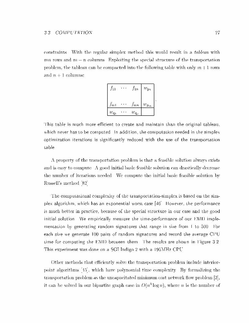
constraints. With the regular simplex method this would result in a tableau with
mn rows and m + n columns. Exploiting the special structure of the transportation
problem, the tableau can be compacted into the following table with only m+1 rows
and n+ 1 columns:
f11 � � � f1n wp1
......
...
fm1 � � � fmn wpm
wq1 � � � wqn
:
This table is much more e�cient to create and maintain than the original tableau,
which never has to be computed. In addition, the computation needed in the simplex
optimization iterations is signi�cantly reduced with the use of the transportation
table.
A property of the transportation problem is that a feasible solution always exists
and is easy to compute. A good initial basic feasible solution can drastically decrease
the number of iterations needed. We compute the initial basic feasible solution by
Russell's method [82].
The computational complexity of the transportation-simplex is based on the sim-
plex algorithm, which has an exponential worst case [46]. However, the performance
is much better in practice, because of the special structure in our case and the good
initial solution. We empirically measure the time-performance of our EMD imple-
mentation by generating random signatures that range in size from 1 to 500. For
each size we generate 100 pairs of random signatures and record the average CPU
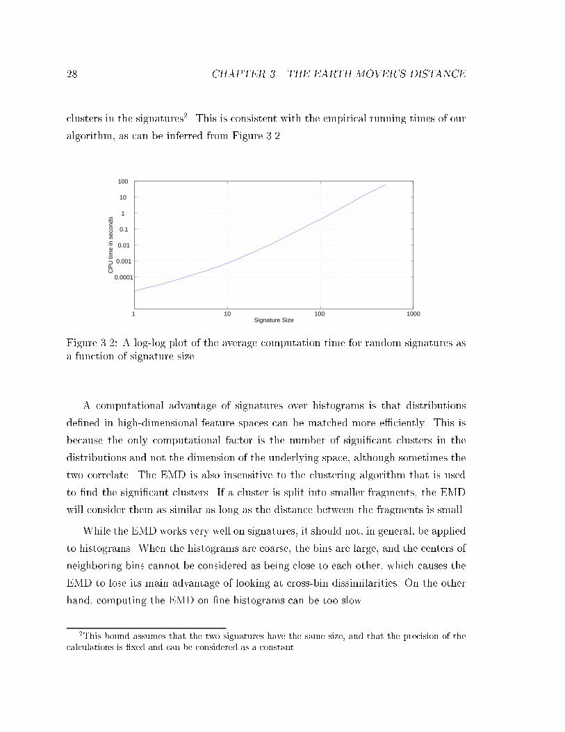
time for computing the EMD between them. The results are shown in Figure 3.2.
This experiment was done on a SGI Indigo 2 with a 195MHz CPU.
Other methods that e�ciently solve the transportation problem include interior-
point algorithms [45], which have polynomial time complexity. By formalizing the
transportation problem as the uncapacitated minimum cost network ow problem [2],
it can be solved in our bipartite graph case in O(n3 logn), where n is the number of
28 CHAPTER 3. THE EARTH MOVER'S DISTANCE
clusters in the signatures2. This is consistent with the empirical running times of our
algorithm, as can be inferred from Figure 3.2.
1 10 100 1000
0.0001
0.001
0.01
0.1
1
10
100
Signature Size
CP
U ti
me
in s
econ
ds
Figure 3.2: A log-log plot of the average computation time for random signatures asa function of signature size.
A computational advantage of signatures over histograms is that distributions
de�ned in high-dimensional feature spaces can be matched more e�ciently. This is
because the only computational factor is the number of signi�cant clusters in the
distributions and not the dimension of the underlying space, although sometimes the
two correlate. The EMD is also insensitive to the clustering algorithm that is used
to �nd the signi�cant clusters. If a cluster is split into smaller fragments, the EMD
will consider them as similar as long as the distance between the fragments is small.
While the EMD works very well on signatures, it should not, in general, be applied
to histograms. When the histograms are coarse, the bins are large, and the centers of
neighboring bins cannot be considered as being close to each other, which causes the
EMD to lose its main advantage of looking at cross-bin dissimilarities. On the other
hand, computing the EMD on �ne histograms can be too slow.
2This bound assumes that the two signatures have the same size, and that the precision of thecalculations is �xed and can be considered as a constant.
3.3. COMPUTATION 29
3.3.1 One-Dimensional EMD
When the feature space is one-dimensional, and the ground distance is the Euclidean
distance, and the two signatures have equal weight, the EMD can be computed fast
without having to solve a linear optimization problem, as in the multi-dimensional
case. In fact, the minimum cost distance between two one-dimensional distributions
f(t) and g(t) is known to be the L1 distance between the cumulative distribution
functions [105, 12]
Z 1
�1
����Z x
�1
f(t)dt�Z x
�1
g(t)dt
���� dx : (3.5)
When the distributions are represented by histograms, Equation (3.5) is the match
distance described in Chapter 2. When representing the distributions by signatures,
the distance can be computed as follows: Let P = f(p1; wp1); : : : ; (pm; wpm)g and
Q = f(q1; wq1); : : : ; (qn; wqn)g be two one-dimensional signatures.
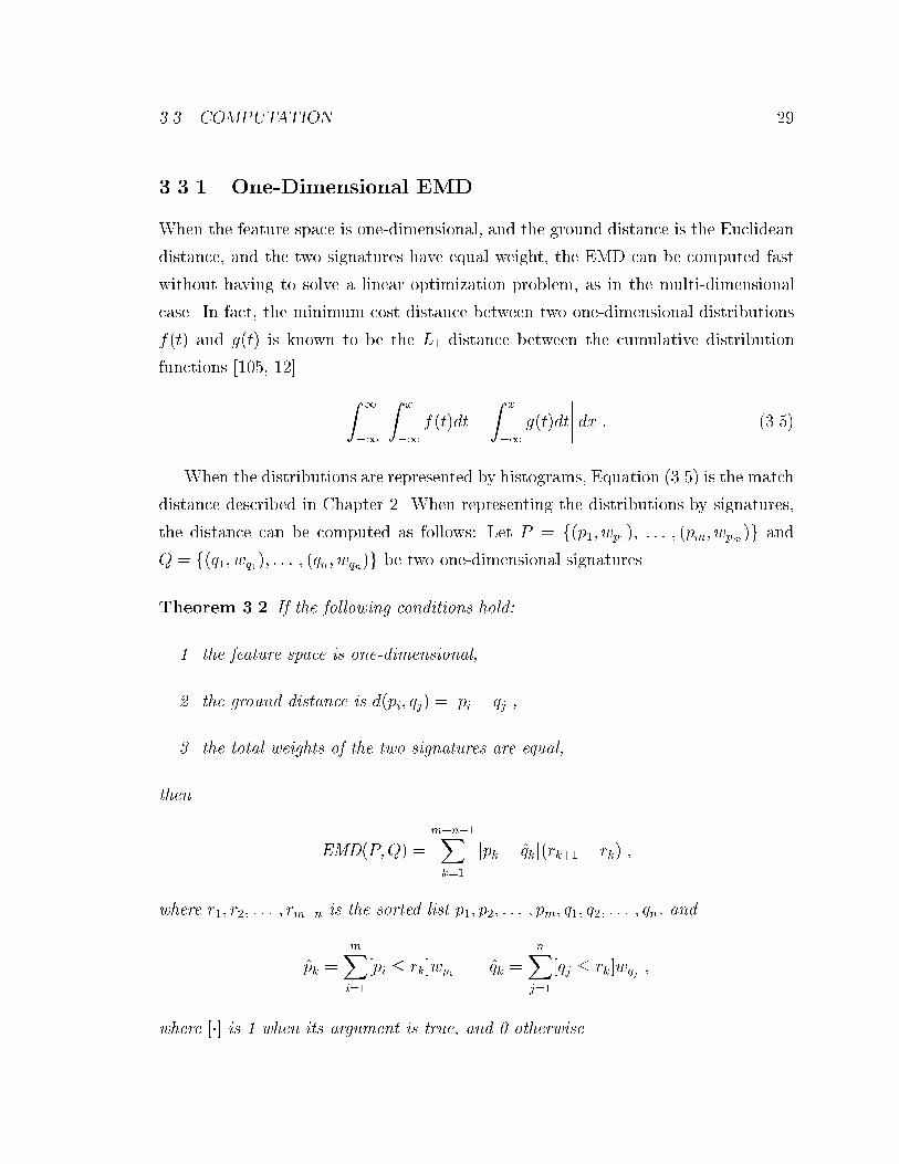
Theorem 3.2 If the following conditions hold:
1. the feature space is one-dimensional,
2. the ground distance is d(pi; qj) = jpi � qjj,
3. the total weights of the two signatures are equal,
then
EMD(P;Q) =m+n�1Xk=1
jpk � qkj(rk+1 � rk) ;
where r1; r2; : : : ; rm+n is the sorted list p1; p2; : : : ; pm; q1; q2; : : : ; qn, and
pk =mXi=1
[pi � rk]wpi qk =nXj=1
[qj � rk]wqj ;
where [�] is 1 when its argument is true, and 0 otherwise.
30 CHAPTER 3. THE EARTH MOVER'S DISTANCE
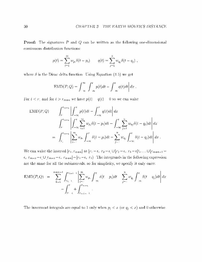
Proof: The signatures P and Q can be written as the following one-dimensional
continuous distribution functions:
p(t) =mXi=1
wpi�(t� pi) q(t) =nX
j=1
wqj�(t� qj) ;
where � is the Dirac delta function. Using Equation (3.5) we get
EMD(P;Q) =
Z 1
�1
����Z x
�1
p(t)dt�Z x
�1
q(t)dt
���� dx :For t < r1 and for t > rm+n we have p(t) = q(t) = 0 so we can write
EMD(P;Q) =
Z rm+n
r1
����Z x
�1
p(t)dt�Z x
�1
q(t)dt
���� dx=
Z rm+n
r1
�����Z x
�1
mXi=1
wpi�(t� pi)dt�Z x
�1
nXj=1
wqj�(t� qj)dt
����� dx=
Z rm+n
r1
�����mXi=1
wpi
Z x
�1
�(t� pi)dt�nXj=1
wqj
Z x
�1
�(t� qj)dt
����� dx :We can write the interval [r1; rm+n] as [r1� �; r2� �][ [r2� �; r3� �][ : : :[ [rm+n�1��; rm+n��][[rm+n��; rm+n]�[r1��; r1). The integrands in the following expressionare the same for all the subintervals, so for simplicity, we specify it only once:
EMD(P;Q) =m+n�1Xk=1
Z rk+1��
rk��
�����mXi=1
wpi
Z x
�1
�(t� pi)dt�nX
j=1
wqj
Z x
�1
�(t� qj)dt
����� dx�Z r1
r1��
+
Z rm+n
rm+n��
:
The innermost integrals are equal to 1 only when pi < x (or qj < x) and 0 otherwise.
3.3. COMPUTATION 31
This occurs only for the subintervals that contain rk where pi � rk (or qj � rk), so
EMD(P;Q) =m+n�1Xk=1
Z rk+1��
rk��
�����mXi=1
wpi[pi � rk]�nX
j=1
wqj [qj � rk]
����� dx�Z r1
r1��
+
Z rm+n
rm+n��
:
We now set �! 0:
EMD(P;Q) =m+n�1Xk=1
Z rk+1
rk
�����mXi=1
wpi[pi � rk]�nX
j=1
wqj [qj � rk]
����� dx=
m+n�1Xk=1
Z rk+1
rk
jpk � qkj dx
=m+n�1Xk=1
jpk � qkj (rk+1 � rk) :
�
3.3.2 Lower Bound
Retrieval speed can be increased if lower bounds to the EMD can be computed at
a low expense. These bounds can signi�cantly reduce the number of EMDs that
actually need to be computed by pre�ltering the database and ignoring images that
are too far from the query. An easy-to-compute lower bound for the EMD between
signatures with equal total weights is the distance between their centers of mass, as
long as the ground distance is induced by a norm.
Theorem 3.3 Given signatures P and Q, let pi and qj be the coordinates of cluster
i in the �rst signature, and cluster j in the second signature respectively. Then if
mXi=1
wpi =nX
j=1
wqj ; (3.6)
32 CHAPTER 3. THE EARTH MOVER'S DISTANCE
then
EMD(P;Q) � k �P � �Qk ;
where k � k is the norm that induces the ground distance, and �P and �Q are the centers
of mass of P and Q respectively:
�P =
Pmi=1wpipiPmi=1wpi
; �Q =
Pnj=1wqjqjPnj=1wqj
:
Proof: Using the notation of equations (3.1)-(3.4),
mXi=1
nXj=1
d(pi;qj)fij =mXi=1
nXj=1
kpi � qjkfij
=mXi=1
nXj=1
kfij(pi � qj)k (fij � 0)
� mX
i=1
nXj=1
fij(pi � qj)
= mX
i=1
� nXj=1
fij�pi �
nXj=1
� mXi=1
fij�qj
=
mXi=1
wpipi �nX
j=1
wqjqj
:
Dividing both sides byPm
i=1
Pnj=1 fij:
Pmi=1
Pnj=1 d(pi;qj)fijPm
i=1
Pnj=1 fij
� Pm
i=1wpipi �Pn
j=1wqjqjPmi=1
Pnj=1 fij
EMD(P;Q) �
Pm
i=1wpipiPmi=1wpi
�Pn
j=1wqjqjPnj=1wqj
(using (3.4) and (3.6))
EMD(P;Q) � k �P � �Qk :
�
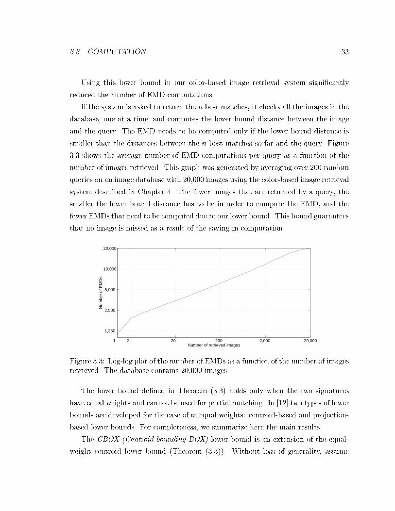
3.3. COMPUTATION 33
Using this lower bound in our color-based image retrieval system signi�cantly
reduced the number of EMD computations.
If the system is asked to return the n best matches, it checks all the images in the
database, one at a time, and computes the lower bound distance between the image
and the query. The EMD needs to be computed only if the lower bound distance is
smaller than the distances between the n best matches so far and the query. Figure
3.3 shows the average number of EMD computations per query as a function of the
number of images retrieved. This graph was generated by averaging over 200 random
queries on an image database with 20,000 images using the color-based image retrieval
system described in Chapter 4. The fewer images that are returned by a query, the
smaller the lower bound distance has to be in order to compute the EMD, and the
fewer EMDs that need to be computed due to our lower bound. This bound guarantees
that no image is missed as a result of the saving in computation.
1 2 20 200 2,000 20,000
1,250
2,500
5,000
10,000
20,000
Number of retrieved images
Num
ber
of E
MD
s
Figure 3.3: Log-log plot of the number of EMDs as a function of the number of imagesretrieved. The database contains 20,000 images.
The lower bound de�ned in Theorem (3.3) holds only when the two signatures
have equal weights and cannot be used for partial matching. In [12] two types of lower
bounds are developed for the case of unequal weights: centroid-based and projection-
based lower bounds. For completeness, we summarize here the main results.
The CBOX (Centroid bounding BOX) lower bound is an extension of the equal-
weight centroid lower bound (Theorem (3.3)). Without loss of generality, assume
34 CHAPTER 3. THE EARTH MOVER'S DISTANCE
that wP > wQ, where wP =Pm
i=1wpi and wQ =Pn
j=1wqj . An optimal feasible
ow matches an amount wQ of the total weight of the heavier distribution P . If
C(P;wQ) is the locus of all centroids of sub-distributions of P of total weight wQ,
then the minimum distance from the centroid of Q to C(P;wQ) is a lower bound on
EMD(P;Q). The same statement holds with a bounding box B(P;wQ) of C(P;wQ)
in place of C(P;wQ). The idea is to pre-compute (i.e. not at query time) a set
of bounding boxes B(P;wQ) for wQ = 5%; 10%; 15%; : : : ; 100% of the weight of P .
When a query Q with smaller weight comes in, the appropriate bounding box is
chosen and the distance from the centroid of Q to this bounding box is computed
(this is a constant time computation with respect to the number of points in P and
Q).
The projection-based lower bounds are used when the ground distance is Euclidean.
These bounds work with the projections of distributions onto lines through the ori-
gin. The Euclidean distance between two points is at least the distance between their
projections onto a line through the origin, so the EMD between the projected distri-
butions is a lower bound on the EMD between the original distributions (the weights
in the projected distribution are the same as the weights in the original distribution).
In the equal-weight case, computing the EMD between distributions along the line
can be done much faster than in the general case. Since it follows from FeaSiBiLity
conditions, the authors call this the FSBL lower bound.
The same technique, described in Section 3.3.1 for computing the EMD in one
dimension, is modi�ed to compute a lower bound on the EMD in one dimension
between unequal-weight distributions. The idea is to record how much mass must
ow over certain intervals if all the mass in the lighter distribution is to be matched.
The projection-based lower bounds proposed in [12] are:
PMAXFSBL(P;Q) = maxv2V
FSBL(projv(P ); projv(Q))
PAMAXFSBL(P;Q) = maxe2E
FSBL(proje(P ); proje(Q))
PASUMFSBL(P;Q) =1pD
Xe2E
FSBL(proje(P ); proje(Q)) :
3.4. MORE ON THE GROUND DISTANCE 35
Here projv(P ) stands for the one-dimensional distribution which is the projection of
P onto the line through the origin in direction v. V is a set of random directions, E is
the set of feature space axes, and D is the dimension of the feature space. This lower
bounds are named by di�erent kinds of projections: Projection MAXimum (PMAX),
Projection Axes MAXimum (PAMAX), and Projection Axes SUM (PASUM).
The hope with the projection-based bounds is that one could quickly tell that
two distributions are very di�erent by looking at one-dimensional projections, which
are fast to compute using the results of Theorem (3.2). These often work well in
cases when the CBOX lower bound does not (i.e. when one cannot tell the di�erence
between distributions by looking at their averages).
More details on and experiments with these bounds can be found in [12].
3.4 More on the Ground Distance
In Section 2.2 we claimed that correspondences between two distributions are essential
to match perceptual similarity. The EMD indeed �nds the best correspondences that
minimize the total transportation cost; however, some of these correspondences might
be between features that are far apart in the feature space, and therefore have large
ground distances. This can have a big impact on the total cost, so that a few, very
di�erent, features can have a big e�ect on the distance between otherwise similar
distributions.
Modifying the ground distance so that it saturates to some value limits the e�ect
far features have on the EMD. An example of such a ground distance is
d(pi;qj) = 1� e��d(pi;qj) ; (3.7)
where d(pi;qj) is the non-saturated ground distance between clusters pi and qj. The
solid line in Figure 3.4 shows d as a function of d (in units of ��1). The value for
� should be chosen speci�cally for the feature space at hand so that it distinguishes
between \close" and \far" distances in the feature space. In this thesis, we use
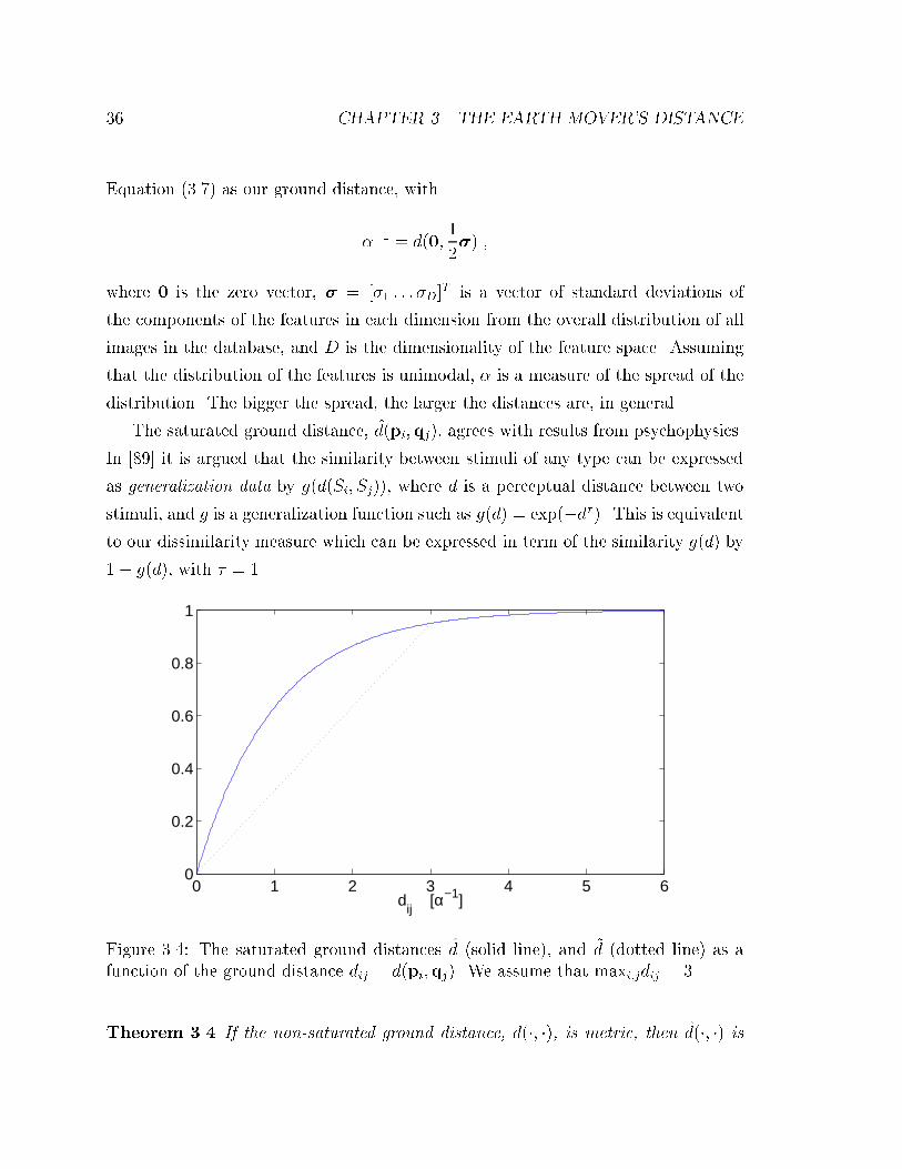
36 CHAPTER 3. THE EARTH MOVER'S DISTANCE
Equation (3.7) as our ground distance, with
��1 = d(0;1
2�) ;
where 0 is the zero vector, � = [�1 : : : �D]T is a vector of standard deviations of
the components of the features in each dimension from the overall distribution of all
images in the database, and D is the dimensionality of the feature space. Assuming
that the distribution of the features is unimodal, � is a measure of the spread of the
distribution. The bigger the spread, the larger the distances are, in general.
The saturated ground distance, d(pi;qj), agrees with results from psychophysics.
In [89] it is argued that the similarity between stimuli of any type can be expressed
as generalization data by g(d(Si; Sj)), where d is a perceptual distance between two
stimuli, and g is a generalization function such as g(d) = exp(�d� ). This is equivalentto our dissimilarity measure which can be expressed in term of the similarity g(d) by
1� g(d), with � = 1.
0 1 2 3 4 5 60
0.2
0.4
0.6
0.8
1
dij [α−1]
Figure 3.4: The saturated ground distances d (solid line), and ~d (dotted line) as afunction of the ground distance dij = d(pi;qj). We assume that maxi;jdij = 3.
Theorem 3.4 If the non-saturated ground distance, d(�; �), is metric, then d(�; �) is
3.4. MORE ON THE GROUND DISTANCE 37
also metric.
Proof: Positive de�niteness and symmetry clearly hold because � � 0. We now
prove that the triangle inequality holds, too. Given that d(p;q) + d(q; r) � d(p; r),
and using positive de�niteness, we can write
0 � d(p;q)d(q; r)
=�1� e��d(p;q)
� �1� e��d(q;r)
�= 1� e��d(p;q) � e��d(q;r) + e��(d(p;q)+d(q;r))
� 1� e��d(p;q) � e��d(q;r) + e��d(p;r)
=�1� e��d(p;q)
�+�1� e��d(q;r)
�� �1� e��d(p;r)�
= d(p;q) + d(q; r)� d(p; r) ;
and hence, d(p;q) + d(q; r) � d(p; r). �
Corollary 3.1 The resulting EMD is metric for signatures of equal weights.
Although metric, d is not induced by a norm, and therefore the lower bound
de�ned in Section 3.3.2 is not valid for the EMD that uses d as its ground distance.
We denote this EMD by [EMD. However, a valid lower bound can be de�ned using
an EMD that uses the following ground distance:
~d(pi;qj) =maxi;j d(pi;qj)
maxi;j d(pi;qj)d(pi;qj) :
We denote the resulting EMD by]EMD. This ground distance is a scaled Euclidean
distance and therefore it is induced by a norm.
Theorem 3.5
[EMD(P;Q) �]EMD(P;Q) � maxi;j d(pi;qj)
maxi;j d(pi;qj)k �P � �Qk :
Proof: The �rst part,[EMD(P;Q) �]EMD(P;Q), holds because d(pi;qj) is convex,
and therefore d(pi;qj) � ~d(pi;qj) for all possible i and j, as shown in Figure 3.4.
38 CHAPTER 3. THE EARTH MOVER'S DISTANCE
The second part,]EMD(P;Q) � maxi;j d(pi;qj)
maxi;j d(pi;qj)k �P � �Qk, results directly from the lower
bound de�ned in Section 3.3.2. �
3.5 Extensions
A few extensions were developed for the EMD [11]. For completeness we now describe
these extensions.
3.5.1 The Partial EMD (EMD )
The partial EMD forces only some given fraction 0 < � 1 of the weight of the lighter
distribution to be matched. The constraint (3.4) for the usual EMD is replaced by
mXi=1
nXj=1
fij = min(mXi=1
wpi ;nX
j=1
wqj) ;
and the minimum work is normalized by min(Pm
i=1wpi;Pn
j=1wqj ). The partial
EMD makes the EMD robust to a fraction 1� missing data/outliers.
3.5.2 The Restricted EMD (�-EMD)
The � -EMD measures the minimum fraction of mass that cannot be matched when
ows are restricted to at most � ground distance units. The extreme values are
� -EMD = 0 when all the mass can be matched, and � -EMD = 1 when none of the
mass can be matched. The de�nition is
� -EMD(P;Q) = 1� maxFP
i;j fij[d(pi;qj) � � ]
min(Pm
i=1wpi;Pn
j=1wqj ):
Here [d(pi;qj) � � ] equals 1 if d(pi;qj) � � and 0 otherwise. The numerator measures
the maximum amount of mass that can be matched. The set of feasible ows over
which the optimization is computed is the same as for the regular EMD.
The � -EMD tells what percentage of the features matches well (if � is set low),
instead of averaging all features, including the bad matches (with correspondences

3.6. SUMMARY 39
over large distances).
3.6 Summary
The Earth Mover's Distance is a general and exible metric and has desirable prop-
erties for image retrieval. It allows for partial matches, and it can be applied to
variable-length representations of distributions. Lower bounds are readily available
for it, and it can be computed e�ciently when the signatures are not too large. The
EMD works better when applied to signatures, than to global histograms. Histograms
with few bins invalidate the ground distances, while EMDs on histograms with many
bins are slow to compute. Because of the advantages of the EMD, we believe that the
EMD can be of use both for understanding vision problems related to distributions,
as exempli�ed in the next two chapters with color and texture, and as a fundamental
element of image retrieval systems.
One should absorb the color of life,
but one should never remember its
detail.
Oscar Wilde (1854-1900)
Chapter 4
Color-Based Image Similarity
Color plays an important role in content-based image retrieval. In this chapter we
de�ne color features in an appropriate, perceptually uniform color space, where color
distributions describe the contents of entire images. Summarizing these distributions
by color signatures and using the Earth Mover's Distance leads to a powerful color-
based retrieval paradigm. Combining the color information of the pixels, with their
positions in the image leads to a distance measure where not only the color contents
matters but also the layout of the color in the image.
4.1 Color Features
Human color perception is based on the incidence of visible light (with wavelengths in
the range of 400 nm to 700 nm) upon the retina. Since there are three types of color
photoreceptor cone cells in the retina, each with a di�erent spectral response curve, all
colors can be completely described by three numbers, corresponding to the outputs of
the cone cells. In 1931, the Commission Internationale de l'�Eclairage (CIE) adopted
standard curves for the color photoreceptor cone cells of a hypothetical standard
observer, and de�ned the CIE XYZ tristimulus values, where all visible colors can be
represented using only positive values of X, Y and Z.
40
4.1. COLOR FEATURES 41
4.1.1 Color Spaces
Color spaces are used to specify, create and visualize color information. While the
CIE XYZ space describes all the colors we can perceive, other color spaces are subsets
of this space and represent fewer colors than we can see. For instance, the RGB color
space, as used by television displays, can be visualized as a cube with red, green and
blue axes. Di�erent applications have di�erent needs which can be handled better
using di�erent color spaces. Many color spaces have been developed including the
following (see [106] for more information):
RGB (Red-Green-Blue) An additive color system, based on adding the three pri-
mary colors. RGB is commonly used by CRT displays where proportions of
excitation of red, green and blue emitting phosphors produce colors when visu-
ally fused.
CMY(K) (Cyan-Magenta-Yellow(-Black)) A subtractive color system commonly
used in printing. The black component is redundant and is used for technical
reasons such as improving the appearance of the black color and reducing costs.
HSL (Hue-Saturation-Lightness) and HSB (Hue-Saturation-Brightness) In-
tuitive spaces that allows users to specify colors easily. Separating the luminance
component has advantages in certain image processing applications.
YIQ, YUV, YCbCr Used for di�erent standards of television transmission (NTSC,
PAL, and digital TV respectively).
Opponent Colors Used for modeling color perception. It is based on the fact that
for color perception, some pairs of hues cannot coexist in a single color sensation
(e.g. red and green) [103].
4.1.2 Perceptually Uniform Color Spaces
For an image retrieval system, it is important to be able to measure di�erences be-
tween colors in a way that matches perceptual similarity as well as possible. This
42 CHAPTER 4. COLOR-BASED IMAGE SIMILARITY
task is simpli�ed by the use of perceptually uniform color spaces. A color space is
perceptually uniform if a small perturbation of a color will produce the same change
in perception anywhere in the color space. In 1976, the CIE standardized two per-
ceptually uniform color spaces (since no single system could be agreed upon), L�u�v�
(CIELuv) and L�a�b� (CIELab). The L� component de�nes the luminance, and the
two other components (u�; v� and a�; b�) de�ne the chrominance. Both spaces are de-
�ned with respect to the CIE XYZ color space, using a reference white [Xn Yn Zn]T .
Following ITU-R Recommendation BT.709, we use D65 as the reference white so that
[Xn Yn Zn] = [0:9504511:088754] (see [70]). In practice, most images are represented
in the RGB color space. The conversions between RGB and CIE-XYZ are linear:
2664X
Y
Z
3775 =
26640:412453 0:357580 0:180423
0:212671 0:715160 0:072169
0:019334 0:119193 0:950227
37752664R
G
B
3775
and 2664R
G
B
3775 =
2664
3:240479 �1:537150 �0:498535�0:969256 1:875992 0:041556
0:055648 �0:204043 1:057311
37752664X
Y
Z
3775
For both the CIELuv and CIELab, the Euclidean distance is used to compute the
distance between (close) colors. In the following we give the transformations from
CIE XYZ:
The luminance is de�ned similarly for both spaces,
L� =
(116 (Y=Yn)
1=3 � 16 if Y=Yn > 0:008856
903:3(Y=Yn) otherwise;
while the chrominances are de�ned di�erently for CIELuv and for CIELab.
4.1. COLOR FEATURES 43
4.1.2.1 CIELuv
u� = 13L�(u0 � u0n) ;
v� = 13L�(v0 � v0n) ;
where
u0 =4X
X + 15Y + 3Z;
v0 =9Y
X + 15Y + 3Z;
and u0n and v0n have the same de�nitions for u0 and v0 but are computed using Xn,
Yn, and Zn.
4.1.2.2 CIELab
a� = 500 (f(X=Xn)� f(Y=Yn)) ;
b� = 200 (f(Y=Yn)� f(Z=Zn)) ;
where
f(t) =
(t1=3 if Y=Yn > 0:008856 ;
7:787t+ 16=116 otherwise ::
4.1.2.3 Spatial Extension
So far, we assumed that the perception of a single color is independent of colors
that surround it. Is general, once the visual angle of a region in a color image gets
smaller than 2 degrees, this assumption does not hold. To account for the spatial
e�ect of color perception the S-CIELab [107] was developed as a spatial extension to
the CIELab color space. A color image is �rst transformed into the opponent-colors
space. Each of the three component images is convolved with a kernel whose shape
is determined by the visual spatial sensitivity in that color band. Finally, the �ltered
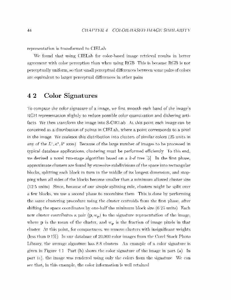
44 CHAPTER 4. COLOR-BASED IMAGE SIMILARITY
representation is transformed to CIELab.
We found that using CIELab for color-based image retrieval results in better
agreement with color perception than when using RGB. This is because RGB is not
perceptually uniform, so that small perceptual di�erences between some pairs of colors
are equivalent to larger perceptual di�erences in other pairs.
4.2 Color Signatures
To compute the color signature of a image, we �rst smooth each band of the image's
RGB representation slightly to reduce possible color quantization and dithering arti-
facts. We then transform the image into S-CIELab. At this point each image can be
conceived as a distribution of points in CIELab, where a point corresponds to a pixel
in the image. We coalesce this distribution into clusters of similar colors (25 units in
any of the L�; a�; b� axes). Because of the large number of images to be processed in
typical database applications, clustering must be performed e�ciently. To this end,
we devised a novel two-stage algorithm based on a k-d tree [5]. In the �rst phase,
approximate clusters are found by excessive subdivisions of the space into rectangular
blocks, splitting each block in turn in the middle of its longest dimension, and stop-
ping when all sides of the blocks become smaller than a minimum allowed cluster size
(12.5 units). Since, because of our simple splitting rule, clusters might be split over
a few blocks, we use a second phase to recombine them. This is done by performing
the same clustering procedure using the cluster centroids from the �rst phase, after
shifting the space coordinates by one-half the minimum block size (6.25 units). Each
new cluster contributes a pair (p; wp) to the signature representation of the image,
where p is the mean of the cluster, and wp is the fraction of image pixels in that
cluster. At this point, for compactness, we remove clusters with insigni�cant weights
(less than 0.1%). In our database of 20,000 color images from the Corel Stock Photo
Library, the average signature has 8.8 clusters. An example of a color signature is
given in Figure 4.1. Part (b) shows the color signature of the image in part (a). In
part (c), the image was rendered using only the colors from the signature. We can
see that, in this example, the color information is well retained.
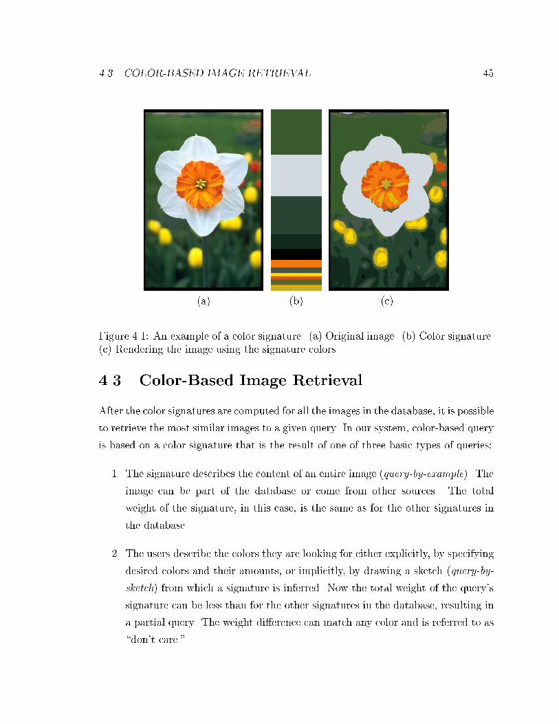
4.3. COLOR-BASED IMAGE RETRIEVAL 45
(a) (b) (c)
Figure 4.1: An example of a color signature. (a) Original image. (b) Color signature.(c) Rendering the image using the signature colors.
4.3 Color-Based Image Retrieval
After the color signatures are computed for all the images in the database, it is possible
to retrieve the most similar images to a given query. In our system, color-based query
is based on a color signature that is the result of one of three basic types of queries:
1. The signature describes the content of an entire image (query-by-example). The
image can be part of the database or come from other sources. The total
weight of the signature, in this case, is the same as for the other signatures in
the database.
2. The users describe the colors they are looking for either explicitly, by specifying
desired colors and their amounts, or implicitly, by drawing a sketch (query-by-
sketch) from which a signature is inferred. Now the total weight of the query's
signature can be less than for the other signatures in the database, resulting in
a partial query. The weight di�erence can match any color and is referred to as
\don't care."
46 CHAPTER 4. COLOR-BASED IMAGE SIMILARITY
3. The signature is generated by the system as a result of some user action. In
Chapter 8 we describe a navigation scheme where the signatures are generated
automatically.
Once the query is represented by a color signature, the retrieval system returns the
images in the database whose signatures have minimum distance from the query.
To compute the distance between color signatures, we use the Earth Mover's
Distance, with the Euclidean distance as a natural choice of ground distance. We
performed our color-based image retrieval on a collection of 20,000 color images.
Figures 4.2 and 4.3 show examples of color-based image retrieval. In the �rst three
examples, the color content of an image was used as the query, while in the last
example a partial query was used: The user looked for owers and speci�ed the query:
\Find images with 20% pink, 40% green, and the rest can be any color." The results
is these examples are good because there is a high correlation between the semantic
queries and the colors used to describe them. A more systematic evaluation of the
EMD for color-based retrieval and a comparison with other dissimilarity measures are
given in Chapter 6.
Color information is usually not su�cient for semantic image retrieval. When the
query cannot be well described in terms of color, there is a discrepancy between the
semantic query and the syntactic features (color), and the query is bound to fail. An
example is given in Figure 4.4 where an image of a woman was given as the query.
Here the system responded with an image of a skunk as the best match. Although
the color contents of the two images are very similar, they are obviously very di�erent
semantically.
4.4 Joint Distribution of Color and Position
In many cases, global color distributions that ignore the positions of the colors in the
image are not su�cient for good retrieval. For example, consider the following two
color images: In the �rst, there are blue skies above a green �eld, while in the other
there is a blue lake below green plants. Although the color distributions might be very
similar, the positions of the colors in the image are very di�erent and may have to be
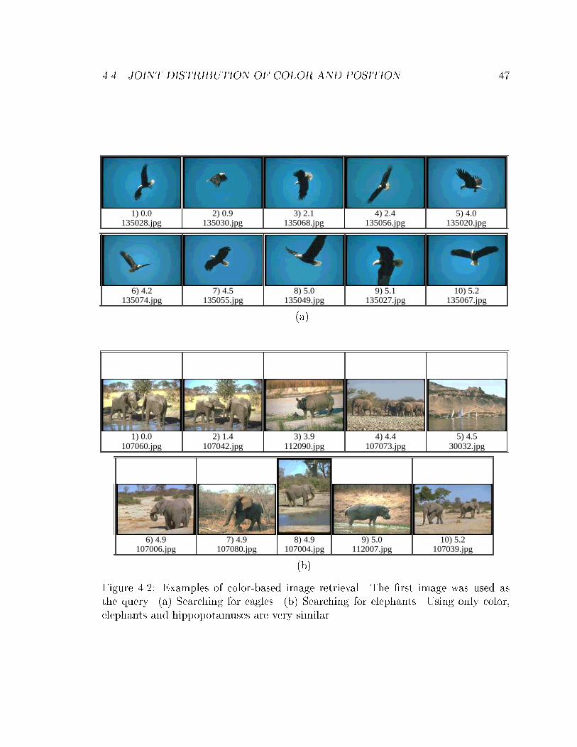
4.4. JOINT DISTRIBUTION OF COLOR AND POSITION 47
1) 0.0135028.jpg
2) 0.9135030.jpg
3) 2.1135068.jpg
4) 2.4135056.jpg
5) 4.0135020.jpg
6) 4.2135074.jpg
7) 4.5135055.jpg
8) 5.0135049.jpg
9) 5.1135027.jpg
10) 5.2135067.jpg
(a)
1) 0.0107060.jpg
2) 1.4107042.jpg
3) 3.9112090.jpg
4) 4.4107073.jpg
5) 4.530032.jpg
6) 4.9107006.jpg
7) 4.9107080.jpg
8) 4.9107004.jpg
9) 5.0112007.jpg
10) 5.2107039.jpg
(b)
Figure 4.2: Examples of color-based image retrieval. The �rst image was used asthe query. (a) Searching for eagles. (b) Searching for elephants. Using only color,elephants and hippopotamuses are very similar.
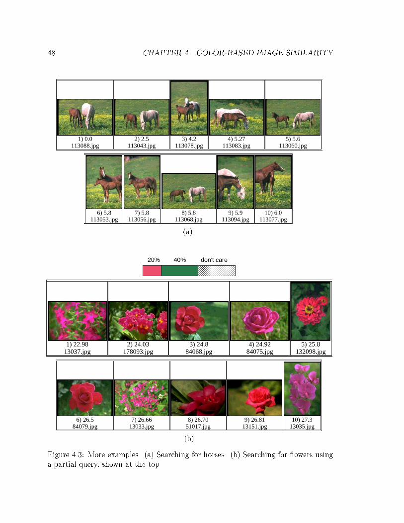
48 CHAPTER 4. COLOR-BASED IMAGE SIMILARITY
1) 0.0113088.jpg
2) 2.5113043.jpg
3) 4.2113078.jpg
4) 5.27113083.jpg
5) 5.6113060.jpg
6) 5.8113053.jpg
7) 5.8113056.jpg
8) 5.8113068.jpg
9) 5.9113094.jpg
10) 6.0113077.jpg
(a)
20% 40% don't care
1) 22.9813037.jpg
2) 24.03178093.jpg
3) 24.884068.jpg
4) 24.9284075.jpg
5) 25.8132098.jpg
6) 26.584079.jpg
7) 26.6613033.jpg
8) 26.7051017.jpg
9) 26.8113151.jpg
10) 27.313035.jpg
(b)
Figure 4.3: More examples. (a) Searching for horses. (b) Searching for owers usinga partial query, shown at the top.
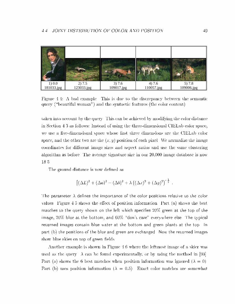
4.4. JOINT DISTRIBUTION OF COLOR AND POSITION 49
1) 0.0181033.jpg
2) 7.5123033.jpg
3) 7.6109017.jpg
4) 7.6110057.jpg
5) 7.8109006.jpg
Figure 4.4: A bad example. This is due to the discrepancy between the semanticquery (\beautiful woman") and the syntactic features (the color content).
taken into account by the query. This can be achieved by modifying the color distance
in Section 4.3 as follows: Instead of using the three-dimensional CIELab color space,
we use a �ve-dimensional space whose �rst three dimensions are the CIELab color
space, and the other two are the (x; y) position of each pixel. We normalize the image
coordinates for di�erent image sizes and aspect ratios and use the same clustering
algorithm as before. The average signature size in our 20,000 image database is now
18.5.
The ground distance is now de�ned as
�(�L)2 + (�a)2 + (�b)2 + �
�(�x)2 + (�y)2
�� 12 :
The parameter � de�nes the importance of the color positions relative to the color
values. Figure 4.5 shows the e�ect of position information. Part (a) shows the best
matches to the query shown on the left which speci�es 20% green at the top of the
image, 20% blue at the bottom, and 60% \don't care" everywhere else. The typical
returned images contain blue water at the bottom and green plants at the top. In
part (b) the positions of the blue and green are exchanged. Now the returned images
show blue skies on top of green �elds.
Another example is shown in Figure 4.6 where the leftmost image of a skier was
used as the query. � can be found experimentally, or by using the method in [93].
Part (a) shows the 6 best matches when position information was ignored (� = 0).
Part (b) uses position information (� = 0:5). Exact color matches are somewhat
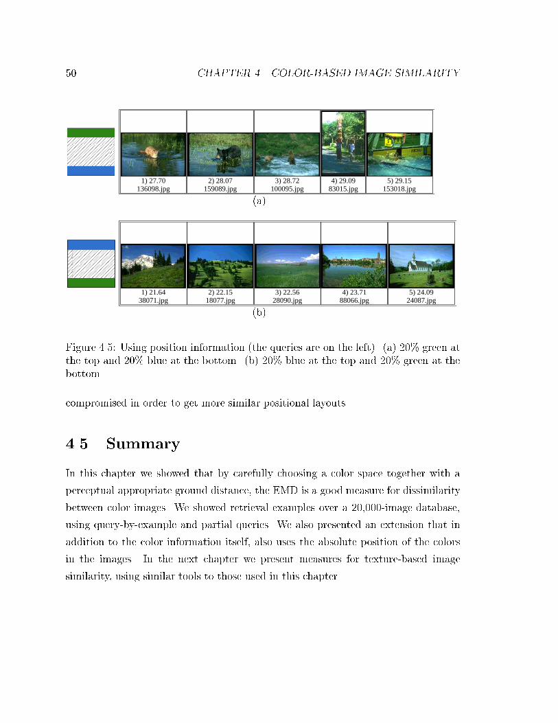
50 CHAPTER 4. COLOR-BASED IMAGE SIMILARITY
1) 27.70136098.jpg
2) 28.07159089.jpg
3) 28.72100095.jpg
4) 29.0983015.jpg
5) 29.15153018.jpg
(a)
1) 21.6438071.jpg
2) 22.1518077.jpg
3) 22.5628090.jpg
4) 23.7188066.jpg
5) 24.0924087.jpg
(b)
Figure 4.5: Using position information (the queries are on the left). (a) 20% green atthe top and 20% blue at the bottom. (b) 20% blue at the top and 20% green at thebottom.
compromised in order to get more similar positional layouts.
4.5 Summary
In this chapter we showed that by carefully choosing a color space together with a
perceptual appropriate ground distance, the EMD is a good measure for dissimilarity
between color images. We showed retrieval examples over a 20,000-image database,
using query-by-example and partial queries. We also presented an extension that in
addition to the color information itself, also uses the absolute position of the colors
in the images. In the next chapter we present measures for texture-based image
similarity, using similar tools to those used in this chapter.
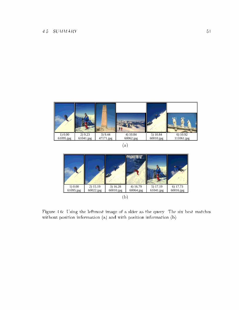
4.5. SUMMARY 51
1) 0.0061095.jpg
2) 9.2361041.jpg
3) 9.4447171.jpg
4) 10.8460062.jpg
5) 10.8460010.jpg
6) 10.92111061.jpg
(a)
1) 0.0061095.jpg
2) 15.1960022.jpg
3) 16.2860010.jpg
4) 16.7960064.jpg
5) 17.1961041.jpg
6) 17.7360016.jpg
(b)
Figure 4.6: Using the leftmost image of a skier as the query. The six best matcheswithout position information (a) and with position information (b).
The imagination is of so delicate a
texture that even words wound it.
Hazlitt (1778-1830)
Chapter 5
Texture-Based Image Similarity
Although the notion of visual texture seems, at �rst, to be familiar and intuitive, there
is no de�nition of texture that is universally accepted. Texture usually refers to a
repetition of a perceptually similar pattern over an image region, such that the region
is perceived as homogeneous by a human observer. Often, for structural textures (in
contrast to statistical ones) such a pattern is referred to as the \texton". A pattern
and its repetition can often be represented well by a spectral decomposition of the
texture which captures the amount of repetition in di�erent scales and in di�erent
orientations. In this chapter we use Gabor �lters to represent texture. We develop
two classes of dissimilarity measures: for homogeneous textures and for images that
contain many textures, such as natural images. Finally, we present a preprocessing
method to enhance the description of the texture content of images.
5.1 Texture Features
While color is a purely pixel-wise property of images, texture involves a notion of
spatial extent: a single point has no texture. To account for spatial neighborhoods,
a texture is commonly computed by the projection of the image intensity function
onto an appropriate basis of functions. This is referred to as a spectral decomposition,
because each of the di�erent basis functions is usually concentrated in a di�erent area
of the two-dimensional spatial frequency domain. In such a representation, a texture is
52
5.1. TEXTURE FEATURES 53
represented by a vector of values, each corresponding to the energy in a speci�ed scale
and orientation subband. Spectral decomposition methods include using quadrature
�lters [47], Gabor �lters [7, 25, 6, 56], oriented derivatives of a Gaussian [67, 36], and
the cortex transform [104].
Gabor �lters [30] have been shown to give good results in comparison to other
texture decompositions [57]. There is strong evidence that simple cells in the primary
visual cortex can be modeled by Gabor functions tuned to detect di�erent orientations
and scales on a log-polar grid [20]. We therefore chose to employ such a set of Gabor
functions to characterize texture.
5.1.1 Gabor Filters
Gabor �lters can be seen as two-dimensional wavelets [19]. When applied on an image
I, the discretization of a two-dimensional wavelet is given by
Wmlpq =
ZZI(x; y) ml (x� p�x; y � q�y) dxdy ;
where �x;�y is the spatial sampling rectangle (we use �x = �y = 1), p; q are image
position, and m and l specify the scale and orientation of the wavelet respectively,
with m = 0; : : : ;M � 1 and l = 0; : : : ; L� 1. The notation
ml(x; y) = a�m (~x; ~y) ; (5.1)
where
~x = a�m(x cos � + y sin �) ;
~y = a�m(�x sin � + y cos �) ;
denotes a dilation of the mother wavelet (x; y) by a�m (a is the scale parameter),
and a rotation by � = l��, where �� = 2�=L is the orientation sampling period.
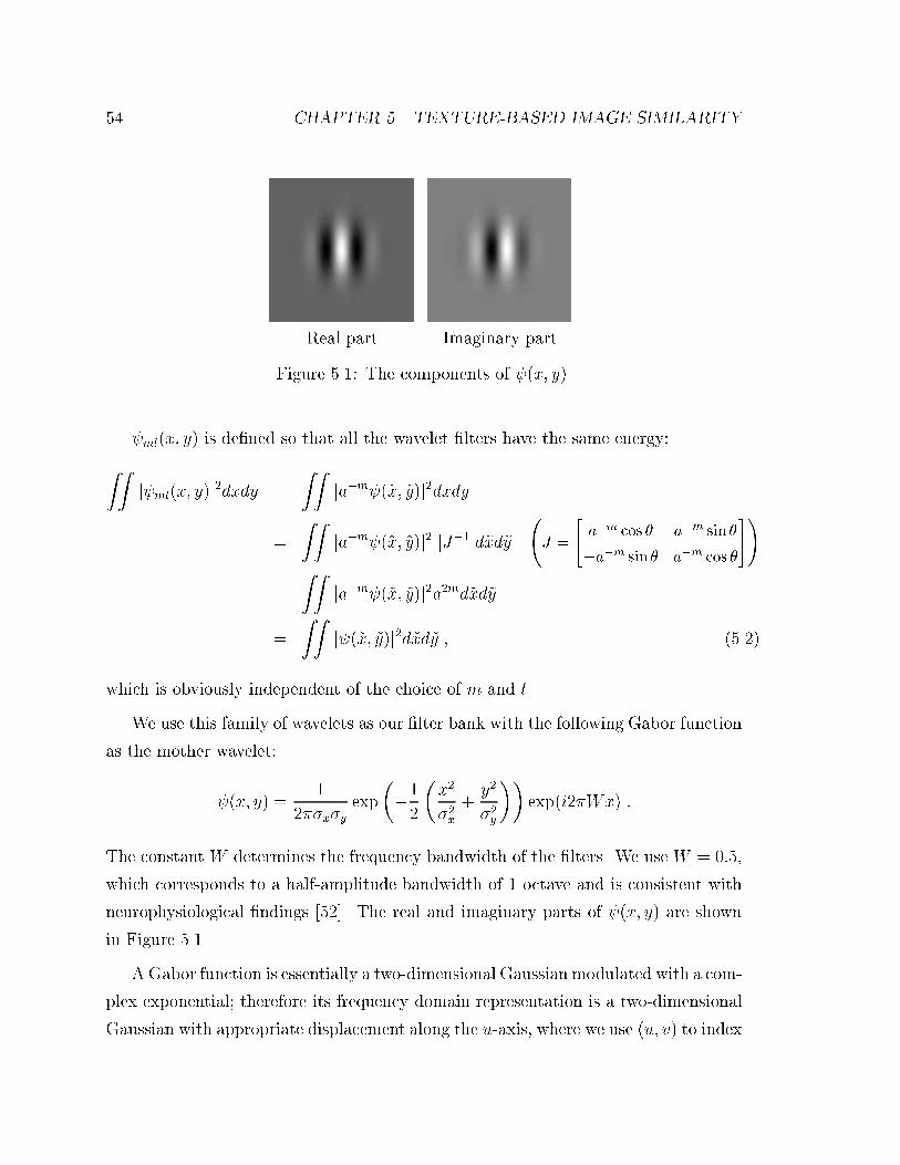
54 CHAPTER 5. TEXTURE-BASED IMAGE SIMILARITY
Real part Imaginary part
Figure 5.1: The components of (x; y).
ml(x; y) is de�ned so that all the wavelet �lters have the same energy:
ZZj ml(x; y)j2dxdy =
ZZja�m (~x; ~y)j2dxdy
=
ZZja�m (~x; ~y)j2 jJ�1jd~xd~y
J =
"a�m cos � a
�m sin �
�a�m sin � a�m cos �
#!
=
ZZja�m (~x; ~y)j2a2md~xd~y
=
ZZj (~x; ~y)j2d~xd~y ; (5.2)
which is obviously independent of the choice of m and l.
We use this family of wavelets as our �lter bank with the following Gabor function
as the mother wavelet:
(x; y) =1
2��x�yexp
��1
2
�x2
�2x+y2
�2y
��exp(i2�Wx) :
The constant W determines the frequency bandwidth of the �lters. We use W = 0:5,
which corresponds to a half-amplitude bandwidth of 1 octave and is consistent with
neurophysiological �ndings [52]. The real and imaginary parts of (x; y) are shown
in Figure 5.1.
A Gabor function is essentially a two-dimensional Gaussian modulated with a com-
plex exponential; therefore its frequency domain representation is a two-dimensional
Gaussian with appropriate displacement along the u-axis, where we use (u; v) to index
5.1. TEXTURE FEATURES 55
the frequency domain
(u; v) = e�2�2(�2xu
2+�2yv2) �� �(u�W )
= exp(�2�2(�2x(u�W )2 + �2yv2))
= exp
��1
2
�(u�W )2
�2u+v2
�2v
��; (5.3)
where �u = (2��x)�1 and �v = (2��y)
�1. We use �� to represent two-dimensional
convolution.
Filters with the same energy, as in Equation (5.2), are desirable for many applica-
tions and are commonly used for texture analysis. However, they are undesirable for
computing the texture dissimilarity of natural images. It was shown that in natural
images the amplitude spectrum typically falls o� as the reciprocal of frequency [27],
which results in smaller responses for high frequency Gabor �lters. This can be �xed
by removing the factor a�m (which corresponds to 1/frequency) from Equation (5.1),
resulting in
ml(x; y) = (~x; ~y) ;
and our two-dimensional wavelet becomes
Wmlpq =
ZZI(x; y) ml (x� p�x; y � q�y) dxdy :
For natural images, similar average amounts of energy will now be captured by all
�lters in all scales, providing a normalized feature space.
5.1.2 Filter Bank Design
We now design a bank of Gabor �lters that tile the frequency space so that an image
texture will be well represented by the set of individual �lter responses. Our design
strategy follows similar principles as in [6, 54]:
1. Uniform separation in orientation. Assuming rotational symmetry, all �lters
in a speci�c scale should have the same angular standard deviation (�v) and
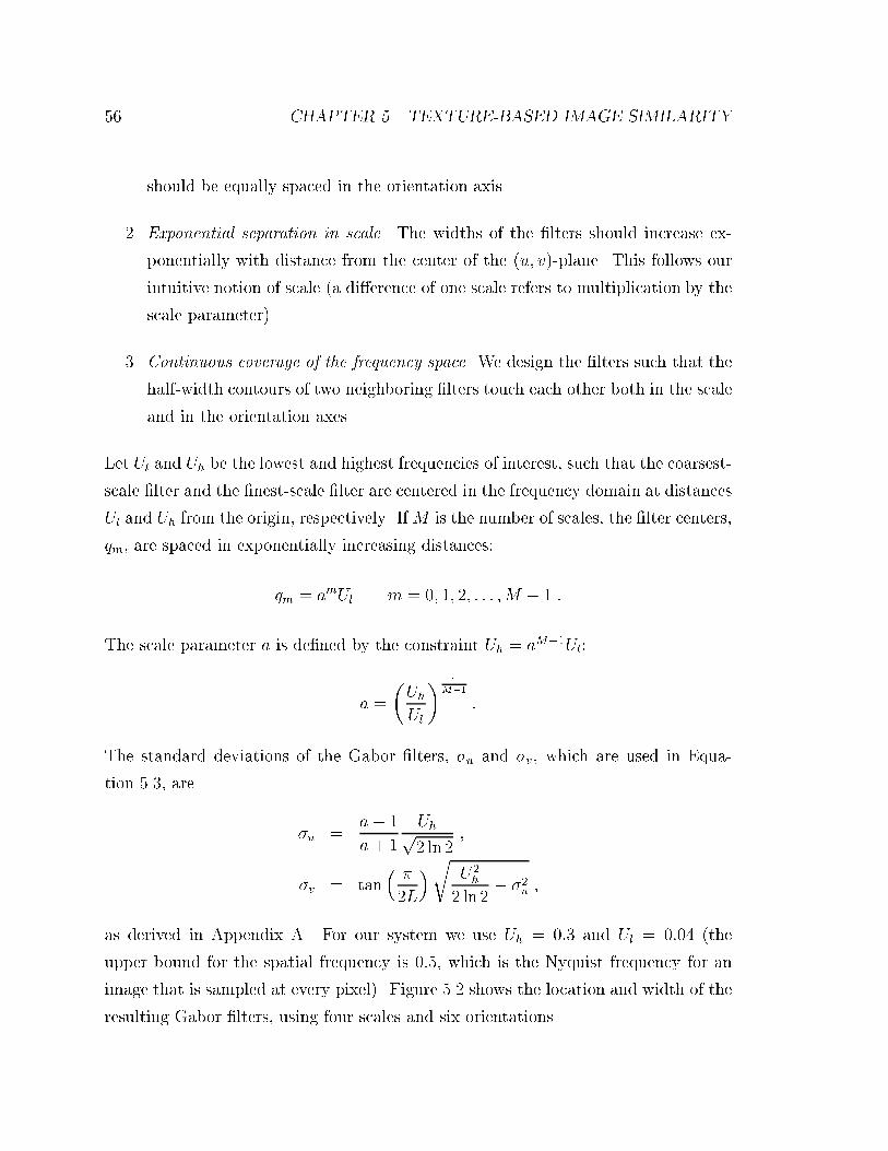
56 CHAPTER 5. TEXTURE-BASED IMAGE SIMILARITY
should be equally spaced in the orientation axis.
2. Exponential separation in scale. The widths of the �lters should increase ex-
ponentially with distance from the center of the (u; v)-plane. This follows our
intuitive notion of scale (a di�erence of one scale refers to multiplication by the
scale parameter).
3. Continuous coverage of the frequency space. We design the �lters such that the
half-width contours of two neighboring �lters touch each other both in the scale
and in the orientation axes.
Let Ul and Uh be the lowest and highest frequencies of interest, such that the coarsest-
scale �lter and the �nest-scale �lter are centered in the frequency domain at distances
Ul and Uh from the origin, respectively. IfM is the number of scales, the �lter centers,
qm, are spaced in exponentially increasing distances:
qm = amUl m = 0; 1; 2; : : : ;M � 1 :
The scale parameter a is de�ned by the constraint Uh = aM�1Ul:
a =
�Uh
Ul
� 1
M�1
:
The standard deviations of the Gabor �lters, �u and �v, which are used in Equa-
tion 5.3, are
�u =a� 1
a+ 1
Uhp2 ln 2
;
�v = tan� �2L
�r U2h
2 ln 2� �2u ;
as derived in Appendix A. For our system we use Uh = 0:3 and Ul = 0:04 (the
upper bound for the spatial frequency is 0:5, which is the Nyquist frequency for an
image that is sampled at every pixel). Figure 5.2 shows the location and width of the
resulting Gabor �lters, using four scales and six orientations.
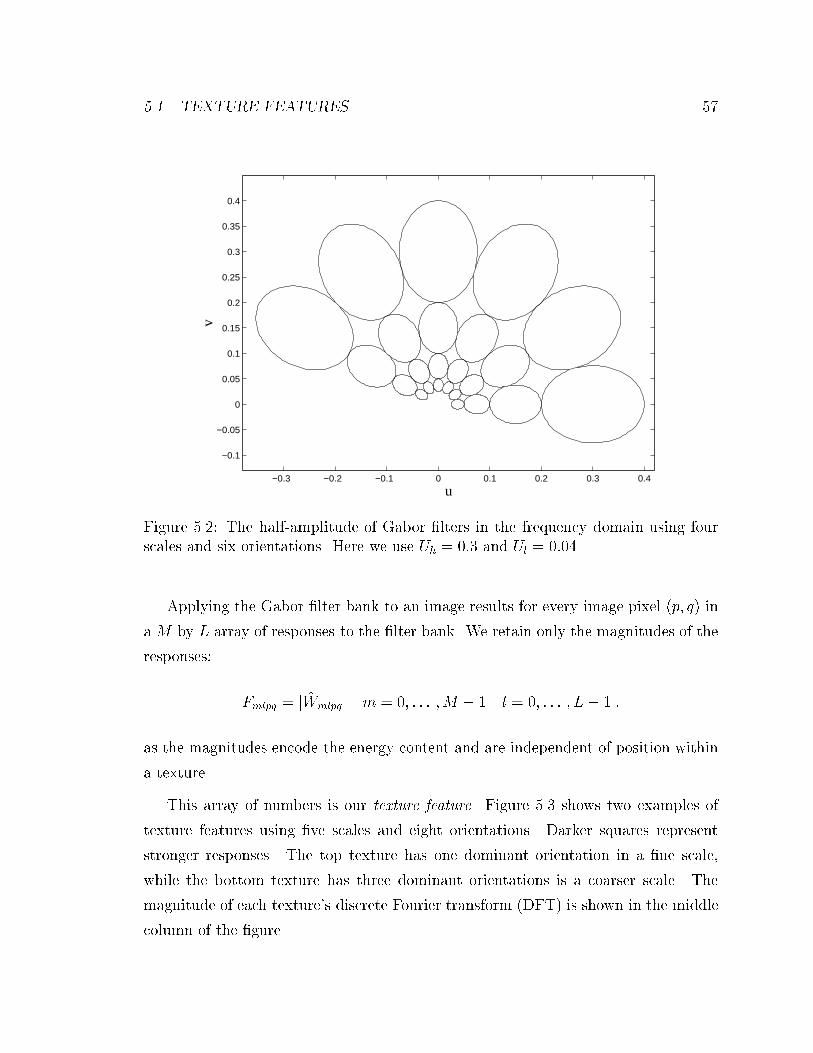
5.1. TEXTURE FEATURES 57
−0.3 −0.2 −0.1 0 0.1 0.2 0.3 0.4
−0.1
−0.05
0
0.05
0.1
0.15
0.2
0.25
0.3
0.35
0.4
u
v
Figure 5.2: The half-amplitude of Gabor �lters in the frequency domain using fourscales and six orientations. Here we use Uh = 0:3 and Ul = 0:04.
Applying the Gabor �lter bank to an image results for every image pixel (p; q) in
a M by L array of responses to the �lter bank. We retain only the magnitudes of the
responses:
Fmlpq = jWmlpqj m = 0; : : : ;M � 1 l = 0; : : : ; L� 1 :
as the magnitudes encode the energy content and are independent of position within
a texture.
This array of numbers is our texture feature. Figure 5.3 shows two examples of
texture features using �ve scales and eight orientations. Darker squares represent
stronger responses. The top texture has one dominant orientation in a �ne scale,
while the bottom texture has three dominant orientations is a coarser scale. The
magnitude of each texture's discrete Fourier transform (DFT) is shown in the middle
column of the �gure.
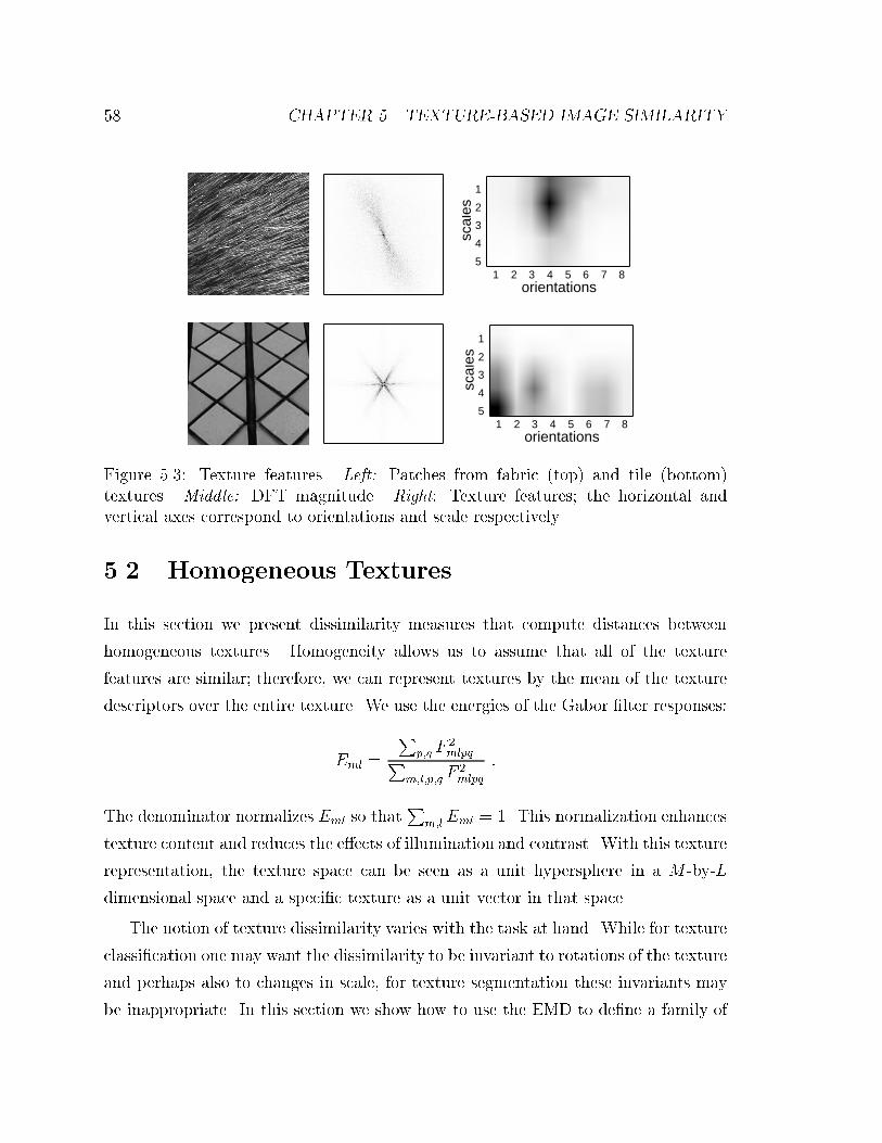
58 CHAPTER 5. TEXTURE-BASED IMAGE SIMILARITY
1 2 3 4 5 6 7 8
1
2
3
4
5
orientations
scal
es
1 2 3 4 5 6 7 8
1
2
3
4
5
orientations
scal
esFigure 5.3: Texture features. Left: Patches from fabric (top) and tile (bottom)textures. Middle: DFT magnitude. Right: Texture features; the horizontal andvertical axes correspond to orientations and scale respectively.
5.2 Homogeneous Textures
In this section we present dissimilarity measures that compute distances between
homogeneous textures. Homogeneity allows us to assume that all of the texture
features are similar; therefore, we can represent textures by the mean of the texture
descriptors over the entire texture. We use the energies of the Gabor �lter responses:
Eml =
Pp;q F
2mlpqP
m;l;p;q F2mlpq
:
The denominator normalizes Eml so thatP
m;l Eml = 1. This normalization enhances
texture content and reduces the e�ects of illumination and contrast. With this texture
representation, the texture space can be seen as a unit hypersphere in a M -by-L
dimensional space and a speci�c texture as a unit vector in that space.
The notion of texture dissimilarity varies with the task at hand. While for texture
classi�cation one may want the dissimilarity to be invariant to rotations of the texture
and perhaps also to changes in scale, for texture segmentation these invariants may
be inappropriate. In this section we show how to use the EMD to de�ne a family of
5.2. HOMOGENEOUS TEXTURES 59
distances between textures. We de�ne three distances: a distance with no invariance,
a rotation-invariant distance and a distance with both rotation and scale invariance.
The homogeneous texture signature in all the distances de�ned in this section is
the texture vector E = fEmlg itself, where every entry Eml corresponds to a cluster in
the two-dimensional, log-polar space, positioned at (m; l) with the value of Eml being
the weight of the cluster. Since for the computation of the EMD the two signatures
do not have to be of the same size, the signatures can be compacted by removing
clusters with zero or very small weights, which have very small in uence on the result
of the EMD. This signi�cantly reduces the size of the EMD problem which can be
computed much faster. In practice, most of the bins for most textures can be pruned
with negligible change in the EMD.
5.2.1 No Invariance
We can use the EMD as a distance measure between two homogeneous texture signa-
tures. To this end, we de�ne our ground distance to be the L1-distance in log-polar
space (similar results were obtained with the Euclidean distance). Since log-polar
space is cylindrical, we have two possible distances between a pair of points. We de-
�ne the ground distance to be the shorter of the two distances. The ground distance
between the points (m1; l1) and (m2; l2) is therefore:
d ((m1; l1); (m2; l2)) = j�lj+ �j�mj ; (5.4)
where
�m = m1 �m2 , �l = min(jl1 � l2j; L� jl1 � l2j) :
The parameter � controls the relative importance of scale versus orientation. We used
� = 1 with good results. Other choices of � can result from applications or from psy-
chophysical experiments. Our ground distance is metric (see proof in Section 5.2.4),
and therefore the de�ned EMD is metric as well, as shown in Section 3.2.
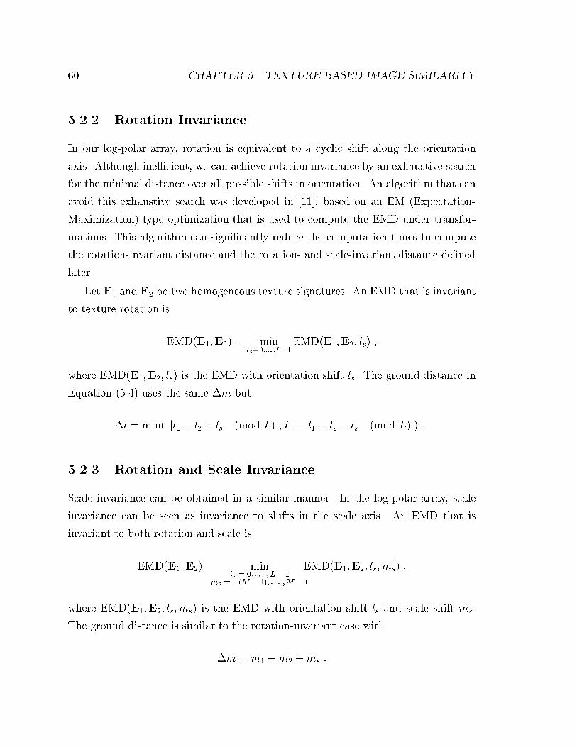
60 CHAPTER 5. TEXTURE-BASED IMAGE SIMILARITY
5.2.2 Rotation Invariance
In our log-polar array, rotation is equivalent to a cyclic shift along the orientation
axis. Although ine�cient, we can achieve rotation invariance by an exhaustive search
for the minimal distance over all possible shifts in orientation. An algorithm that can
avoid this exhaustive search was developed in [11], based on an EM (Expectation-
Maximization) type optimization that is used to compute the EMD under transfor-
mations. This algorithm can signi�cantly reduce the computation times to compute
the rotation-invariant distance and the rotation- and scale-invariant distance de�ned
later.
Let E1 and E2 be two homogeneous texture signatures. An EMD that is invariant
to texture rotation is
EMD(E1;E2) = minls=0;::: ;L�1
EMD(E1;E2; ls) ;
where EMD(E1;E2; ls) is the EMD with orientation shift ls. The ground distance in
Equation (5.4) uses the same �m but
�l = min( jl1 � l2 + ls (mod L)j; L� jl1 � l2 + ls (mod L)j) :
5.2.3 Rotation and Scale Invariance
Scale invariance can be obtained in a similar manner. In the log-polar array, scale
invariance can be seen as invariance to shifts in the scale axis. An EMD that is
invariant to both rotation and scale is
EMD(E1;E2) = minls = 0; : : : ; L� 1
ms = �(M � 1); : : : ;M � 1
EMD(E1;E2; ls; ms) ;
where EMD(E1;E2; ls; ms) is the EMD with orientation shift ls and scale shift ms.
The ground distance is similar to the rotation-invariant case with
�m = m1 �m2 +ms :
5.2. HOMOGENEOUS TEXTURES 61
5.2.4 Proving that the Distances are Metric
Here we prove that all distances de�ned in this section for homogeneous textures
are indeed metric. Nonnegativity and symmetry hold trivially in all cases, so we
only need to prove that the triangle inequality holds. In Section 3.2 it is proven
that if the ground distance is metric, the EMD is metric, so to prove that the non-
invariant distance is metric, we need to show that the ground distance (L1 in our
case) we use in the cylindrical log-polar space is metric. The projection of two points
A and C on the cylinder onto its circular base divides it into two circular arcs (in the
degenerate case one arc can be a point). The projection of a third point B can be
in only one of these two arcs. Now the cylinder can be unfolded into a rectangle by
a vertical cut anywhere through the other arc. Since in this two-dimensional plane
d(A;C) � d(A;B) + d(B;C), the triangle inequality holds also on the cylinder (the
other possible distance from A to C through the cut is chosen only if it makes d(A;C)
shorter). Therefore, our ground distance is metric on a cylinder.
To prove that the EMD is metric in the rotation- and scale-invariant cases, we
notice that in log-polar space, rotation and scale shifts are reduced to translations
(assuming that the ground distance takes care of the cyclic cylinder axis), and we
now prove the following stronger theorem:
Denote the translation-invariant EMD between signatures P and Q by
EMD(P;Q; TPQ) =Xi;j
fijd(pi; qj � TPQ) ;
where fij and TPQ are the ow and translation that minimize the sum.
Theorem 5.1 If signatures P and Q have equal weight then EMD(P;Q; TPQ) is met-
ric.
Proof: Let EMD(P;R; TPR) and EMD(R;Q; TRQ) be the translation-invariant EMD
between signatures P and R, and between signatures R and Q respectively. We need
to prove that
EMD(P;Q; TPQ) � EMD(P;R; TPR) + EMD(R;Q; TRQ) :
62 CHAPTER 5. TEXTURE-BASED IMAGE SIMILARITY
Without loss of generality, we assume that the total sum of the ows is 1. Consider
the ow P 7! R 7! Q. The largest unit of weight that moves together from P to R
and from R to Q de�nes a ow which we call bijk where i, j and k correspond to pi,
rj and qk respectively. ClearlyP
k bijk = fij andP
i bijk = gik. We de�ne
hik4=Xj
bijk
which is a legal ow from i to k since
Xi
hik =Xi;j
bijk =Xj
gjk = wrk ;
and
Xk
hik =Xj;k
bijk =Xj
fij = wpi :
Since EMD(P;Q; TPQ) is the minimal ow from P to Q, and hik is some legal ow
from P to Q,
EMD(P;Q; TPQ) �Xi;k
hikd (pi; qk � (TPR + TRQ))
=Xi;j;k
bijkd (pi; qk � (TPR + TRQ))
�Xi;j;k
bijkd(pi; rj � TPR) +
Xi;j;k
bijkd (rj � TPR; qk � (TPR + TRQ))
=Xi;j;k
bijkd(pi; rj � TPR) +Xi;j;k
bijkd(rj; qk � TRQ)
=Xi;j
fijd(pi; rj � TPR) +Xj;k
gjkd(rj; qk � TRQ)
= EMD(P;R; TPR) + EMD(R;Q; TRQ) :
�
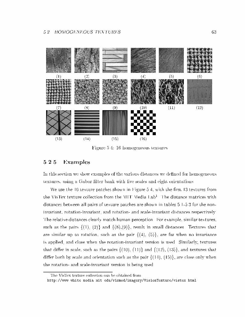
5.2. HOMOGENEOUS TEXTURES 63
(1) (2) (3) (4) (5) (6)
(7) (8) (9) (10) (11) (12)
(13) (14) (15) (16)
Figure 5.4: 16 homogeneous textures
5.2.5 Examples
In this section we show examples of the various distances we de�ned for homogeneous
textures, using a Gabor �lter bank with �ve scales and eight orientations.
We use the 16 texture patches shown in Figure 5.4, with the �rst 13 textures from
the VisTex texture collection from the MIT Media Lab1. The distance matrices with
distances between all pairs of texture patches are shown in tables 5.1-5.3 for the non-
invariant, rotation-invariant, and rotation- and scale-invariant distances respectively.
The relative distances clearly match human perception. For example, similar textures,
such as the pairs f(1), (2)g and f(8),(9)g, result in small distances. Textures that
are similar up to rotation, such as the pair f(4), (5)g, are far when no invariance
is applied, and close when the rotation-invariant version is used. Similarly, textures
that di�er in scale, such as the pairs f(10), (11)g and f(12), (13)g, and textures that
di�er both by scale and orientation such as the pair f(14), (15)g, are close only whenthe rotation- and scale-invariant version is being used.
1The VisTex texture collection can be obtained fromhttp://www-white.media.mit.edu/vismod/imagery/VisionTexture/vistex.html
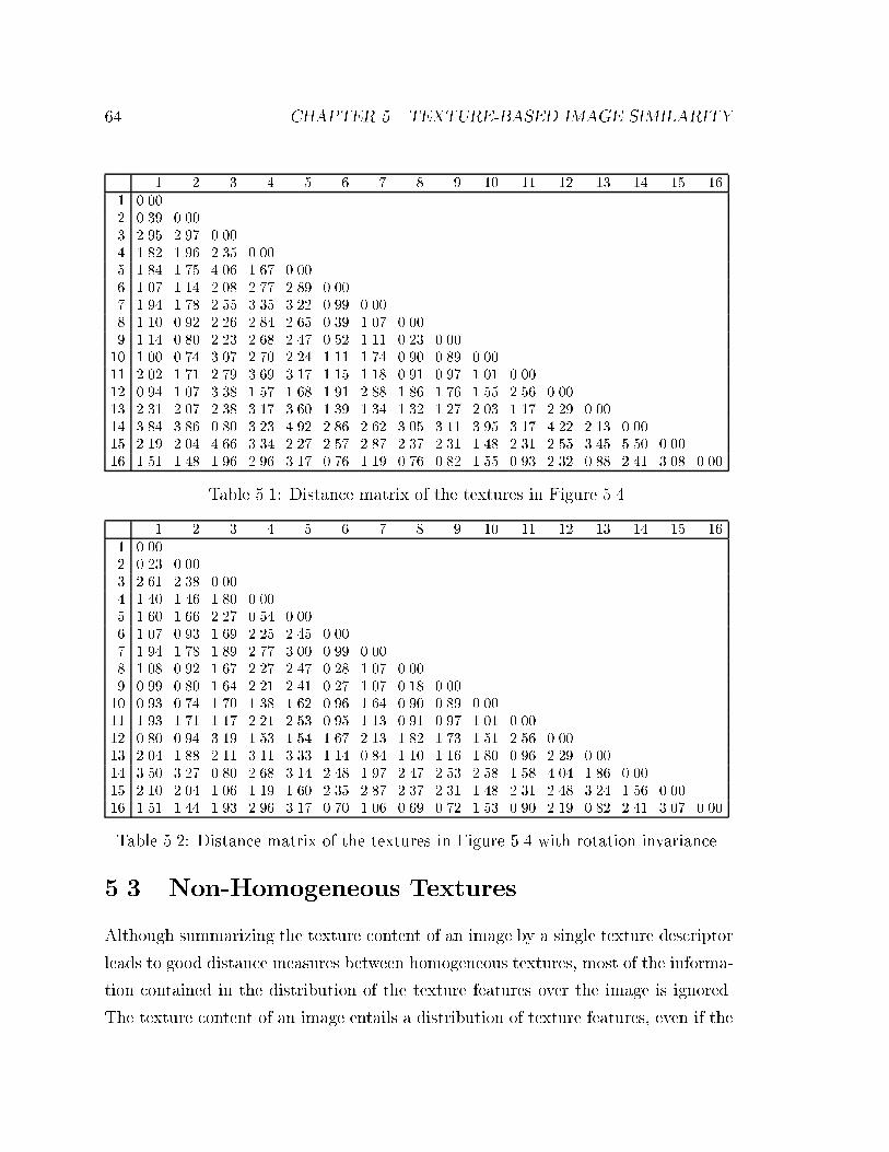
64 CHAPTER 5. TEXTURE-BASED IMAGE SIMILARITY
1 2 3 4 5 6 7 8 9 10 11 12 13 14 15 161 0.002 0.39 0.003 2.95 2.97 0.004 1.82 1.96 2.35 0.005 1.84 1.75 4.06 1.67 0.006 1.07 1.14 2.08 2.77 2.89 0.007 1.94 1.78 2.55 3.35 3.22 0.99 0.008 1.10 0.92 2.26 2.84 2.65 0.39 1.07 0.009 1.14 0.80 2.23 2.68 2.47 0.52 1.11 0.23 0.0010 1.00 0.74 3.07 2.70 2.24 1.11 1.74 0.90 0.89 0.0011 2.02 1.71 2.79 3.69 3.17 1.15 1.18 0.91 0.97 1.01 0.0012 0.94 1.07 3.38 1.57 1.68 1.91 2.88 1.86 1.76 1.55 2.56 0.0013 2.31 2.07 2.38 3.17 3.60 1.39 1.34 1.32 1.27 2.03 1.17 2.29 0.0014 3.84 3.86 0.80 3.23 4.92 2.86 2.62 3.05 3.11 3.95 3.17 4.22 2.13 0.0015 2.19 2.04 4.66 3.34 2.27 2.57 2.87 2.37 2.31 1.48 2.31 2.55 3.45 5.50 0.0016 1.51 1.48 1.96 2.96 3.17 0.76 1.19 0.76 0.82 1.55 0.93 2.32 0.88 2.41 3.08 0.00
Table 5.1: Distance matrix of the textures in Figure 5.4.
1 2 3 4 5 6 7 8 9 10 11 12 13 14 15 161 0.002 0.23 0.003 2.61 2.38 0.004 1.40 1.46 1.80 0.005 1.60 1.66 2.27 0.54 0.006 1.07 0.93 1.69 2.25 2.45 0.007 1.94 1.78 1.89 2.77 3.00 0.99 0.008 1.08 0.92 1.67 2.27 2.47 0.28 1.07 0.009 0.99 0.80 1.64 2.21 2.41 0.27 1.07 0.18 0.0010 0.93 0.74 1.70 1.38 1.62 0.96 1.64 0.90 0.89 0.0011 1.93 1.71 1.17 2.21 2.53 0.95 1.13 0.91 0.97 1.01 0.0012 0.80 0.94 3.19 1.53 1.54 1.67 2.13 1.82 1.73 1.51 2.56 0.0013 2.04 1.88 2.11 3.11 3.33 1.14 0.84 1.10 1.16 1.80 0.96 2.29 0.0014 3.50 3.27 0.80 2.68 3.14 2.48 1.97 2.47 2.53 2.58 1.58 4.04 1.86 0.0015 2.10 2.04 1.06 1.19 1.60 2.35 2.87 2.37 2.31 1.48 2.31 2.48 3.24 1.56 0.0016 1.51 1.44 1.93 2.96 3.17 0.70 1.06 0.69 0.72 1.53 0.90 2.19 0.82 2.41 3.07 0.00
Table 5.2: Distance matrix of the textures in Figure 5.4 with rotation invariance.
5.3 Non-Homogeneous Textures
Although summarizing the texture content of an image by a single texture descriptor
leads to good distance measures between homogeneous textures, most of the informa-
tion contained in the distribution of the texture features over the image is ignored.
The texture content of an image entails a distribution of texture features, even if the
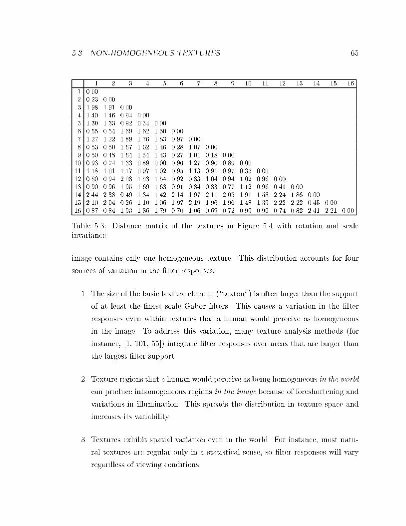
5.3. NON-HOMOGENEOUS TEXTURES 65
1 2 3 4 5 6 7 8 9 10 11 12 13 14 15 161 0.002 0.23 0.003 1.98 1.91 0.004 1.40 1.46 0.94 0.005 1.39 1.33 0.92 0.54 0.006 0.55 0.54 1.69 1.62 1.50 0.007 1.27 1.22 1.89 1.76 1.83 0.97 0.008 0.53 0.50 1.67 1.62 1.46 0.28 1.07 0.009 0.50 0.48 1.64 1.54 1.43 0.27 1.01 0.18 0.0010 0.93 0.74 1.33 0.89 0.90 0.96 1.27 0.90 0.89 0.0011 1.18 1.01 1.17 0.97 1.02 0.95 1.13 0.91 0.97 0.35 0.0012 0.80 0.94 2.08 1.53 1.54 0.92 0.83 1.04 0.94 1.02 0.96 0.0013 0.90 0.96 1.95 1.69 1.63 0.91 0.84 0.83 0.77 1.12 0.96 0.41 0.0014 2.44 2.38 0.49 1.34 1.42 2.14 1.97 2.11 2.05 1.91 1.58 2.24 1.86 0.0015 2.10 2.04 0.26 1.10 1.06 1.97 2.19 1.96 1.96 1.48 1.39 2.22 2.22 0.45 0.0016 0.87 0.84 1.93 1.86 1.79 0.70 1.06 0.69 0.72 0.99 0.90 0.74 0.82 2.41 2.21 0.00
Table 5.3: Distance matrix of the textures in Figure 5.4 with rotation and scaleinvariance.
image contains only one homogeneous texture. This distribution accounts for four
sources of variation in the �lter responses:
1. The size of the basic texture element (\texton") is often larger than the support
of at least the �nest scale Gabor �lters. This causes a variation in the �lter
responses even within textures that a human would perceive as homogeneous
in the image. To address this variation, many texture analysis methods (for
instance, [1, 101, 55]) integrate �lter responses over areas that are larger than
the largest �lter support.
2. Texture regions that a human would perceive as being homogeneous in the world
can produce inhomogeneous regions in the image because of foreshortening and
variations in illumination. This spreads the distribution in texture space and
increases its variability.
3. Textures exhibit spatial variation even in the world. For instance, most natu-
ral textures are regular only in a statistical sense, so �lter responses will vary
regardless of viewing conditions.
66 CHAPTER 5. TEXTURE-BASED IMAGE SIMILARITY
4. Images with multiple textures result in a combination of the distributions of
their constituent textures.
5.3.1 Texture Signatures
Because of these sources of variation, a single image can produce nearly as many
texture vectors as it has pixels. To represent the full distribution of image texture
in a compact way, we �rst �nd dominant clusters in the M � L dimensional texture
space, where M and L are again the number of scales and orientations, respectively,
in our texture representation.
We use a K-means clustering algorithm [33], where the number of clusters, K,
is prede�ned. For simple images, such as those of homogeneous textures, a small
number of clusters su�ces, while complex ones, such as images containing multiple
textures, needs a larger number of cluster to reliably represent the distribution in
texture space.
While this is a simple and fast algorithm, so that large number of images can
be processed quickly, it is conceivable that more sophisticated clustering algorithms
that adjust the number of clusters to the image complexity (e.g., the clustering done
in [4]) can further improve our texture similarity methods. A variable number of
clusters is desirable since the EMD can be applied to signatures of di�erent sizes.
The e�ect of the number of clusters is demonstrated in Figure 5.5 that shows the
pixels' assignments to clusters for a natural image using the clustering algorithm
with 4, 8, and 16 clusters. Clearly, as the number of clusters increases, more subtle
di�erences are captured. For example, when only four clusters are used, one cluster is
used to represent horizontal stripes, and one to represent vertical stripes. Increasing
the number of clusters to sixteen, results in separate clusters for di�erent scales of
horizontal and vertical stripes. Notice also that variation in the grass texture only
starting to get captured with sixteen clusters. As we show in Section 5.3.4, for natural
images we use 32 clusters. In Section 5.4 we show that an appropriate preprocessing
of the images can reduce the number of clusters needed.
The resulting set of cluster centers, together with the fractional cluster weights,
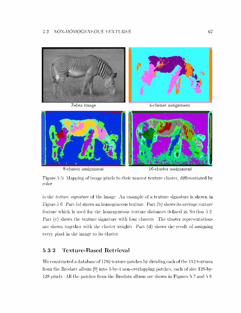
5.3. NON-HOMOGENEOUS TEXTURES 67
Zebra image 4-cluster assignment
8-cluster assignment 16-cluster assignment
Figure 5.5: Mapping of image pixels to their nearest texture cluster, di�erentiated bycolor.
is the texture signature of the image. An example of a texture signature is shown in
Figure 5.6. Part (a) shows an homogeneous texture. Part (b) shows its average texture
feature which is used for the homogeneous texture distances de�ned in Section 5.2.
Part (c) shows the texture signature with four clusters. The cluster representations
are shown together with the cluster weights. Part (d) shows the result of assigning
every pixel in the image to its cluster.
5.3.2 Texture-Based Retrieval
We constructed a database of 1792 texture patches by dividing each of the 112 textures
from the Brodatz album [9] into 4-by-4 non-overlapping patches, each of size 128-by-
128 pixels. All the patches from the Brodatz album are shown in Figures 5.7 and 5.8.
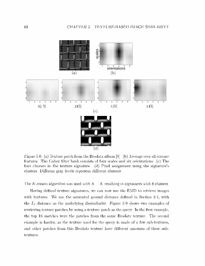
68 CHAPTER 5. TEXTURE-BASED IMAGE SIMILARITY
orientations
scal
es
1 2 3 4 5 6
1
2
3
4
(a) (b)
1 2 3 4 5 6
1
2
3
4
1 2 3 4 5 6
1
2
3
4
1 2 3 4 5 6
1
2
3
4
1 2 3 4 5 6
1
2
3
4
45 % 24% 15% 14%(c)
(d)
Figure 5.6: (a) Texture patch from the Brodatz album [9]. (b) Average over all texturefeatures. The Gabor �lter bank consists of four scales and six orientations. (c) Thefour clusters in the texture signature. (d) Pixel assignment using the signature'sclusters. Di�erent gray levels represent di�erent clusters.
The K-means algorithm was used with K = 8, resulting in signatures with 8 clusters.
Having de�ned texture signatures, we can now use the EMD to retrieve images
with textures. We use the saturated ground distance de�ned in Section 3.4, with
the L1 distance as the underlying dissimilarity. Figure 5.9 shows two examples of
retrieving texture patches by using a texture patch as the query. In the �rst example,
the top 16 matches were the patches from the same Brodatz texture. The second
example is harder, as the texture used for the query is made of a few sub-textures,
and other patches from this Brodatz texture have di�erent amounts of these sub-
textures.
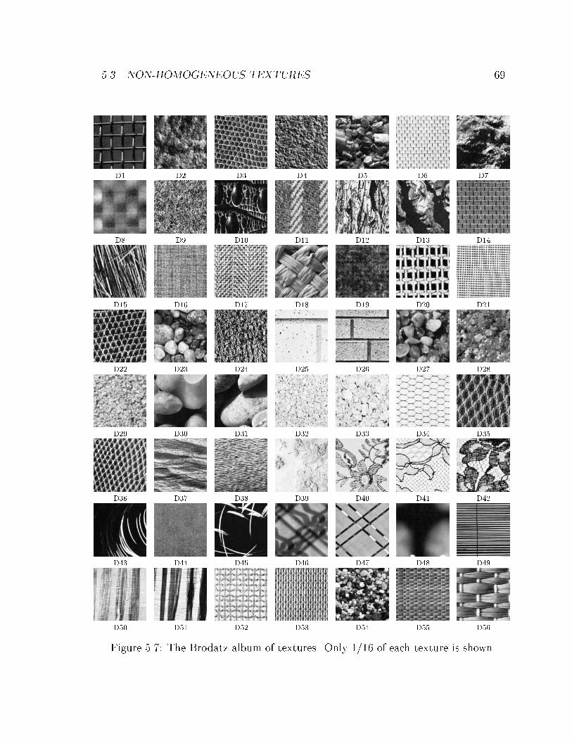
5.3. NON-HOMOGENEOUS TEXTURES 69
D1 D2 D3 D4 D5 D6 D7
D8 D9 D10 D11 D12 D13 D14
D15 D16 D17 D18 D19 D20 D21
D22 D23 D24 D25 D26 D27 D28
D29 D30 D31 D32 D33 D34 D35
D36 D37 D38 D39 D40 D41 D42
D43 D44 D45 D46 D47 D48 D49
D50 D51 D52 D53 D54 D55 D56
Figure 5.7: The Brodatz album of textures. Only 1/16 of each texture is shown.
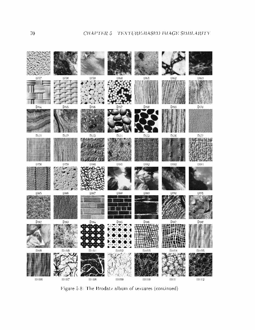
70 CHAPTER 5. TEXTURE-BASED IMAGE SIMILARITY
D57 D58 D59 D60 D61 D62 D63
D64 D65 D66 D67 D68 D69 D70
D71 D72 D73 D74 D75 D76 D77
D78 D79 D80 D81 D82 D83 D84
D85 D86 D87 D88 D89 D90 D91
D92 D93 D94 D95 D96 D97 D98
D99 D100 D101 D102 D103 D104 D105
D106 D107 D108 D109 D110 D111 D112
Figure 5.8: The Brodatz album of textures (continued).
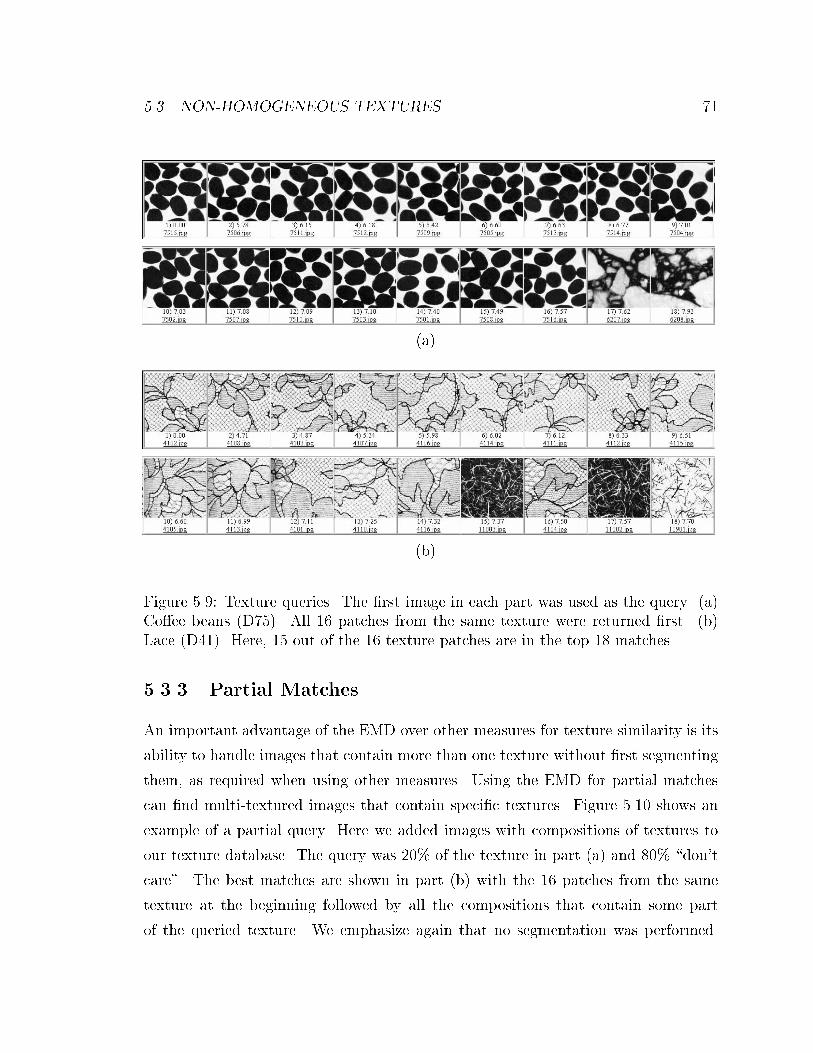
5.3. NON-HOMOGENEOUS TEXTURES 71
(a)
(b)
Figure 5.9: Texture queries. The �rst image in each part was used as the query. (a)Co�ee beans (D75). All 16 patches from the same texture were returned �rst. (b)Lace (D41). Here, 15 out of the 16 texture patches are in the top 18 matches.
5.3.3 Partial Matches
An important advantage of the EMD over other measures for texture similarity is its
ability to handle images that contain more than one texture without �rst segmenting
them, as required when using other measures. Using the EMD for partial matches
can �nd multi-textured images that contain speci�c textures. Figure 5.10 shows an
example of a partial query. Here we added images with compositions of textures to
our texture database. The query was 20% of the texture in part (a) and 80% \don't
care". The best matches are shown in part (b) with the 16 patches from the same
texture at the beginning followed by all the compositions that contain some part
of the queried texture. We emphasize again that no segmentation was performed.
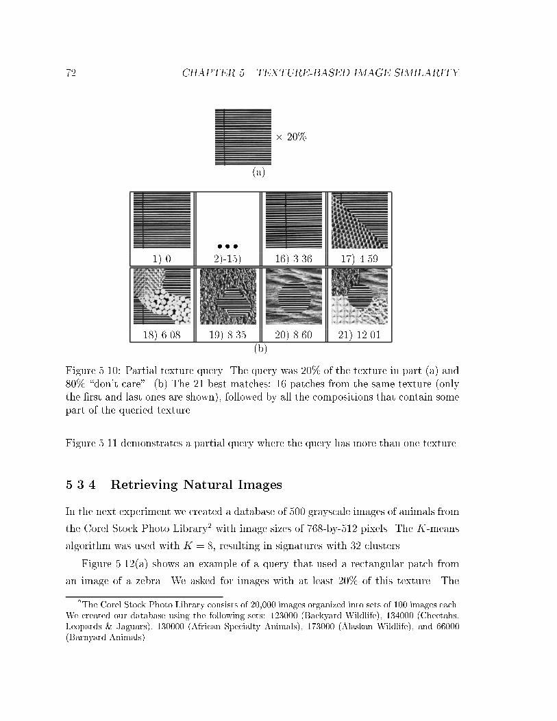
72 CHAPTER 5. TEXTURE-BASED IMAGE SIMILARITY
� 20%
(a)
� � �1) 0 2)-15) 16) 3.36 17) 4.59
18) 6.08 19) 8.35 20) 8.60 21) 12.01(b)
Figure 5.10: Partial texture query. The query was 20% of the texture in part (a) and80% \don't care". (b) The 21 best matches: 16 patches from the same texture (onlythe �rst and last ones are shown), followed by all the compositions that contain somepart of the queried texture.
Figure 5.11 demonstrates a partial query where the query has more than one texture.
5.3.4 Retrieving Natural Images
In the next experiment we created a database of 500 grayscale images of animals from
the Corel Stock Photo Library2 with image sizes of 768-by-512 pixels. The K-means
algorithm was used with K = 8, resulting in signatures with 32 clusters.
Figure 5.12(a) shows an example of a query that used a rectangular patch from
an image of a zebra. We asked for images with at least 20% of this texture. The
2The Corel Stock Photo Library consists of 20,000 images organized into sets of 100 images each.We created our database using the following sets: 123000 (Backyard Wildlife), 134000 (Cheetahs,Leopards & Jaguars), 130000 (African Specialty Animals), 173000 (Alaskan Wildlife), and 66000(Barnyard Animals).
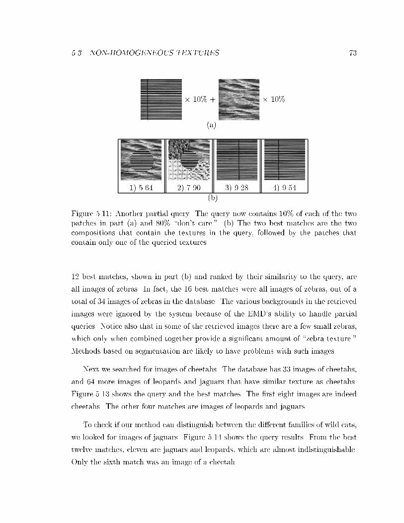
5.3. NON-HOMOGENEOUS TEXTURES 73
� 10% + � 10%
(a)
1) 5.64 2) 7.90 3) 9.28 4) 9.54(b)
Figure 5.11: Another partial query. The query now contains 10% of each of the twopatches in part (a) and 80% \don't care." (b) The two best matches are the twocompositions that contain the textures in the query, followed by the patches thatcontain only one of the queried textures.
12 best matches, shown in part (b) and ranked by their similarity to the query, are
all images of zebras. In fact, the 16 best matches were all images of zebras, out of a
total of 34 images of zebras in the database. The various backgrounds in the retrieved
images were ignored by the system because of the EMD's ability to handle partial
queries. Notice also that in some of the retrieved images there are a few small zebras,
which only when combined together provide a signi�cant amount of \zebra texture."
Methods based on segmentation are likely to have problems with such images.
Next we searched for images of cheetahs. The database has 33 images of cheetahs,
and 64 more images of leopards and jaguars that have similar texture as cheetahs.
Figure 5.13 shows the query and the best matches. The �rst eight images are indeed
cheetahs. The other four matches are images of leopards and jaguars.
To check if our method can distinguish between the di�erent families of wild cats,
we looked for images of jaguars. Figure 5.14 shows the query results. From the best
twelve matches, eleven are jaguars and leopards, which are almost indistinguishable.
Only the sixth match was an image of a cheetah.
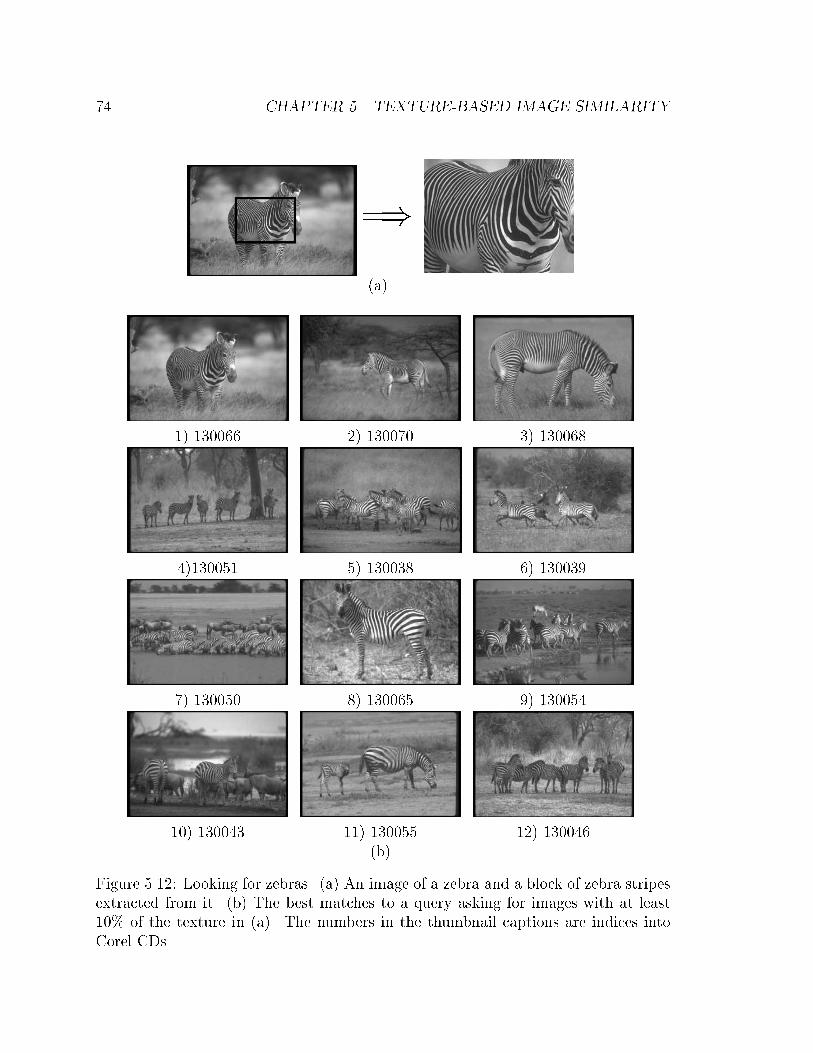
74 CHAPTER 5. TEXTURE-BASED IMAGE SIMILARITY
=)
(a)
1) 130066 2) 130070 3) 130068
4)130051 5) 130038 6) 130039
7) 130050 8) 130065 9) 130054
10) 130043 11) 130055 12) 130046(b)
Figure 5.12: Looking for zebras. (a) An image of a zebra and a block of zebra stripesextracted from it. (b) The best matches to a query asking for images with at least10% of the texture in (a). The numbers in the thumbnail captions are indices intoCorel CDs.
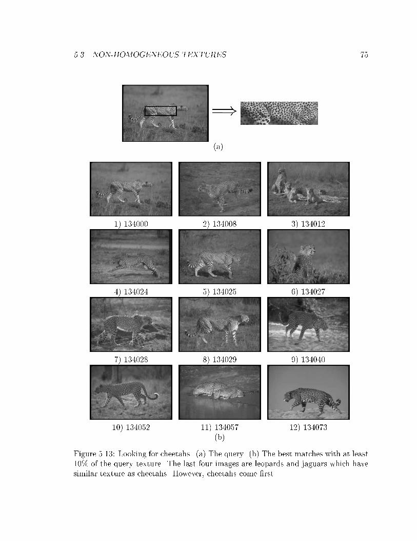
5.3. NON-HOMOGENEOUS TEXTURES 75
=)
(a)
1) 134000 2) 134008 3) 134012
4) 134024 5) 134025 6) 134027
7) 134028 8) 134029 9) 134040
10) 134052 11) 134057 12) 134073(b)
Figure 5.13: Looking for cheetahs. (a) The query. (b) The best matches with at least10% of the query texture. The last four images are leopards and jaguars which havesimilar texture as cheetahs. However, cheetahs come �rst.
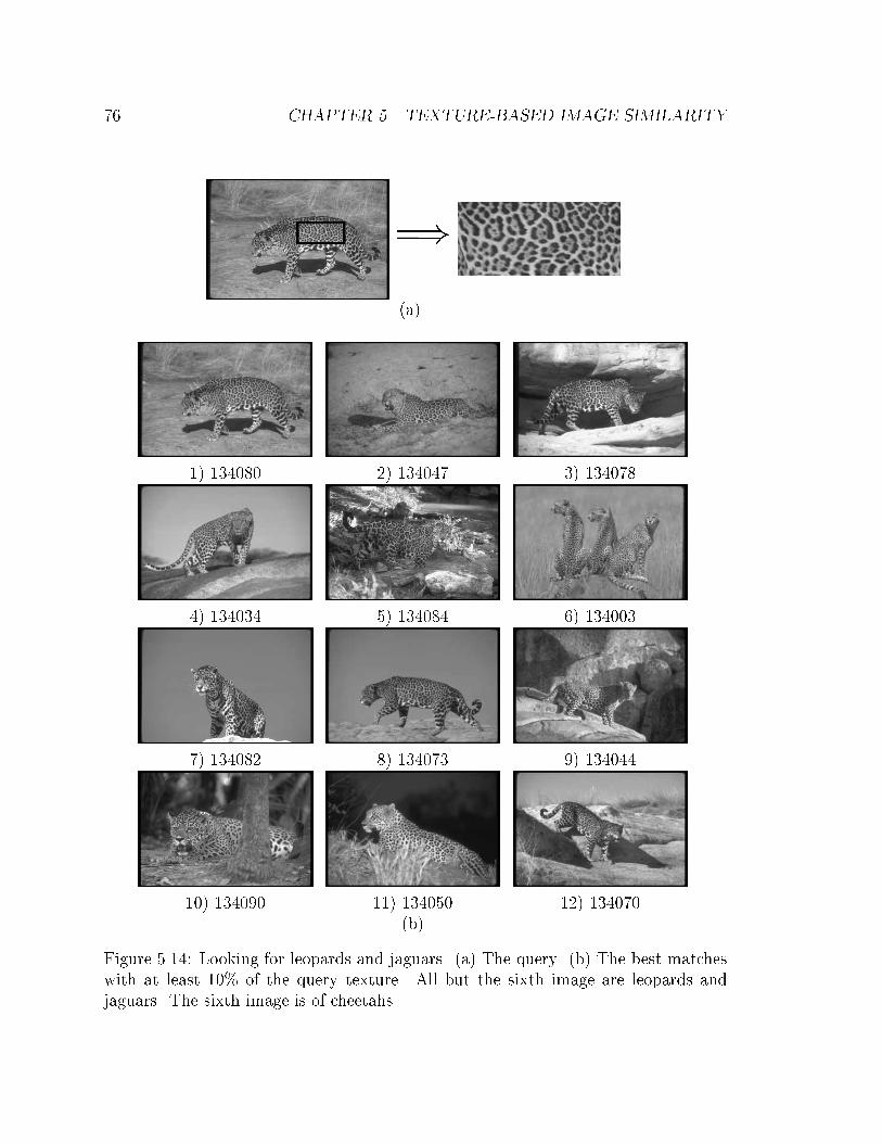
76 CHAPTER 5. TEXTURE-BASED IMAGE SIMILARITY
=)
(a)
1) 134080 2) 134047 3) 134078
4) 134034 5) 134084 6) 134003
7) 134082 8) 134073 9) 134044
10) 134090 11) 134050 12) 134070(b)
Figure 5.14: Looking for leopards and jaguars. (a) The query. (b) The best matcheswith at least 10% of the query texture. All but the sixth image are leopards andjaguars. The sixth image is of cheetahs.
5.4. IMAGE PREPROCESSING 77
5.4 Image Preprocessing
The texture features introduced in Section 5.1 describe the local appearance of small
image neighborhoods. The size of these neighborhoods is equal to that of the supports
of the coarser resolution �lters employed. On the one hand, these supports are large
enough that they can straddle boundaries between di�erent textures. In this case,
they do not describe \pure" textures, and they can convey information that is hard
to interpret and can be misleading. On the other hand, the supports are often too
small for them to \see" enough of a texture to yield a reliable description. In fact, the
basic period of repetition of the underlying texture may be comparable to the �lter
support sizes, so that adjacent �lters see somewhat di�erent parts of the texture,
and the description vectors di�er somewhat. Also, textures exhibit variations in the
world, as well as variations caused by nonuniform viewing parameters.
Before using texture features to compute texture signatures, it is therefore prefer-
able to sift and summarize the information that they convey. Speci�cally, it is de-
sirable to eliminate vectors that describe mixtures of textures, and to average away
some of the variations between adjacent descriptors of similar image patches.
We propose to let descriptors of similar and adjacent texture neighborhoods coa-
lesce into tight clusters. In this approach, texture features are �rst computed for the
image. If two adjacent features describe similar textures, a smoothing process brings
them even closer to each other. If the texture descriptors are very di�erent, however,
then they are modi�ed so that their distance is left unchanged or is even increased.
In other words, we propose to do edge-preserving smoothing, but in the space of
texture vectors rather than image intensities. This requires generalizing the de�nition
of gradient to a vector function, which we do by introducing a measure of texture
contrast. Thanks to this de�nition, we can run the equivalent of anisotropic di�usion
processes [68] to achieve edge-preserving smoothing. We use the texture contrast also
to de�ne signi�cant regions as regions where contrast is low after a few iterations of
the smoothing process. Only texture features that are in a signi�cant region are used
for the computation of the texture signature.
78 CHAPTER 5. TEXTURE-BASED IMAGE SIMILARITY
5.4.1 Texture Contrast
For texture contrast, we employ a notion of \generalized gradient" from di�erential
geometry [48] that has been used for color images in the past few years [21, 15, 86].
The rest of this section discusses this notion as it applies to texture.
Assume that we have a mapping � : S � <n ! <m. Let �i denote the ith
component of �. If � is a texture vector space, for example, then �i, 1 � i � m are
the responses to the Gabor �lters, and n = 2 is the image dimensionality. If � admits
a Taylor expansion we can write
�(x +�x) = �(x) + �0(x)�x + k�xke(x;�x) :
where ke(x;�x)k ! 0 as �x! 0 and �0(x) is the m� n Jacobian matrix of �:
�0(x) = J(x) =
2664
@�1@x1
� � � @�1@xn
......
@�m@x1
� � � @�m@xn
3775 :
If one starts at point x and moves by a small step �x, the distance traveled in the
attribute domain is approximately
d �= k�0(x)�xk =p�xTJTJ�x :
The step direction which maximizes d is the eigenvector of JTJ corresponding to
its largest eigenvalue. The square root of the largest eigenvalue, or, equivalently,
the largest singular value of �0, corresponds to the gradient magnitude, and the
corresponding eigenvector is the gradient direction.
We can give a closed form solution for the eigenvalues in the case that n = 2, as
it is for images. In this case, � is the mapping from the two-dimensional image plane
to the M -by-L dimensional texture space, where M and L are the number of scales
5.4. IMAGE PREPROCESSING 79
and orientations used. The di�erential of � is
d� =2Xi=1
@�
@xidxi :
and so
kd�k2 =2Xi=1
2Xj=1
@�
@xi� @�@xj
dxidxj :
Using the notation from Riemannian geometry [48], we have
kd�k2 =2Xi=1
2Xj=1
gijdxidxj
=hdx1 dx2
i "g11 g12
g21 g22
#"dx1
dx2
#:
where
gij �mXk=1
@�k@xi
@�k@xj :
and g12 = g21. Now let
�� =1
2
�g11 + g22 �
q(g11 � g22)2 + 4g212
�:
be the two eigenvalues in the matrix G =
"g11 g12
g21 g22
#. Since G is real and symmetric,
its eigenvalues are real.
We choose �+ as the generalized gradient magnitude since it corresponds to the
direction of maximum change. We can verify that this magnitude reduces to the
80 CHAPTER 5. TEXTURE-BASED IMAGE SIMILARITY
ordinary gradient norm in the case of a grayscale image (m = 1):
�+ =1
2
��2x + �2
y +q(�2
x � �2y)
2 + 4�2x�
2y
�=
1
2
��2x + �2
y + (�2x + �2
y)�
= �2x + �2
y = kr�k2
where the subscripts x and y denote di�erentiation.
While the application of this de�nition to color is relatively straight forward, mat-
ters are more complicated for texture. Because of the multiscale nature of texture
in general, and of our texture descriptors in particular, di�erent �lters have di�erent
supports. Computing derivatives at di�erent scales requires operators of appropriate
magnitudes and spatial supports in order to yield properly scaled components. For
instance, if di�erentiation is performed by convolution with the derivatives of a Gaus-
sian, the standard deviation of each Gaussian must be proportional to scale, and the
magnitudes must be properly normalized. Figure 5.15(b) shows the texture contrast
of the texture mosaic from Figure 5.15(a). The texture boundaries are characterized
by high contrast.
Figure 5.15(b) shows some areas with relatively high texture contrast even inside
regions that appear to be of the same texture. The sources of these contrast areas
have been discussed at the beginning of Section 5.4, where it was pointed out that
small, low-contrast areas should be smoothed away, while extended ridges of the
contrast function should be maintained. The measure of texture contrast introduced
above allows extending anisotropic di�usion [68] or edge-preserving smoothing [84]
techniques to texture descriptors.
5.4.2 Edge-Preserving Smoothing
Here, we present an e�cient implementation of an edge-preserving smoothing algo-
rithm, which is based on repeatedly convolving each of the spectral subbands of the
image with a separable binomial �lter weighted by a measure of the texture contrast.
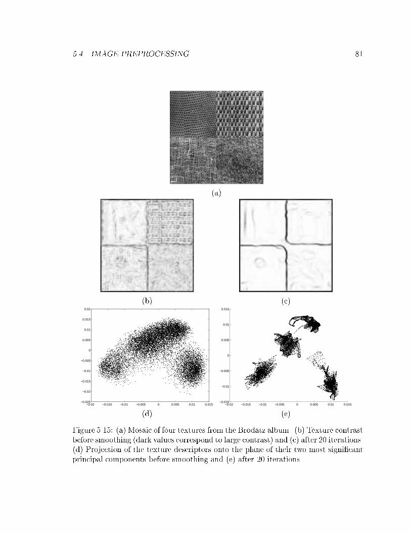
5.4. IMAGE PREPROCESSING 81
(a)
(b) (c)
−0.02 −0.015 −0.01 −0.005 0 0.005 0.01 0.015−0.025
−0.02
−0.015
−0.01
−0.005
0
0.005
0.01
0.015
0.02
−0.02 −0.015 −0.01 −0.005 0 0.005 0.01 0.015−0.015
−0.01
−0.005
0
0.005
0.01
0.015
(d) (e)
Figure 5.15: (a) Mosaic of four textures from the Brodatz album. (b) Texture contrastbefore smoothing (dark values correspond to large contrast) and (c) after 20 iterations.(d) Projection of the texture descriptors onto the plane of their two most signi�cantprincipal components before smoothing and (e) after 20 iterations.
82 CHAPTER 5. TEXTURE-BASED IMAGE SIMILARITY
E�ciency considerations are particularly important in an application like image re-
trieval, where large numbers of images must be processed when they are entered into
the database. After describing the algorithm, we explore its relation with the method
described in [68].
First, the weighting function g(C) is introduced, where C is the texture contrast
de�ned in Section 5.4.1. The function g(C) should be high where the texture is uni-
form and low where the texture is \edgy" and can be any nonnegative monotonically
decreasing function with g(0) = 1. We chose to use
g(C) = e�(jCjk )
2
(5.5)
where k controls the decay rate of g(�) and, as we will see later, determines which of
the edges is preserved.
Smoothing is performed by convolving the spectral subbands of the image with
the binomial �lter
B = BTB ; B =h1 2 1
i;
after it is weighted by g(C). We chose this �lter because it is separable and can
be applied e�ciently. When applied repeatedly, the binomial �lter quickly gives an
approximation of a Gaussian. For brevity, we introduce the following notation:
a �x b =1X
i=�1
a(i)b(x + i; y) ;
a �y b =1X
j=�1
a(j)b(x; y + j) ;
c � b =1X
i=�1
1Xj=�1
c(i; j)b(x + i; y + j) :
A single iteration of the smoothing procedure is computed at time t as follows:
1. Compute the texture contrast C(t).
5.4. IMAGE PREPROCESSING 83
2. Set G(t) = g(C(t)).
3. For 0 � m < M and 0 � l < L do:
(a) Let I(t) be the m-th scale and the l-th orientation subband.
(b) Compute:
K(t) = B �x G(t) ;
J (t) =B �x (G(t)I(t))
K(t);
P (t) = B �y K(t) ;
I(t+1) =B �y (K(t)J (t))
P (t):
(This computation can be simpli�ed. For clarity, we show it in the above form). It is
easy to see that
I(t+1) =B � (G(t)I(t))
B �G(t):
Without the B(i; j) factor, this is similar to the adaptive smoothing proposed in [84],
but implemented, in addition, in a separable fashion for greater e�ciency. In [84],
this iterative process is proven to be stable and to preserve edges. A similar proof can
be applied to our case with straight forward modi�cations. That edges are preserved
is proved by showing that when the contrast is large enough (> k), it increases as the
iterations progress, thereby sharpening the edge. When the contrast is small (< k),
the contrast decreases and the edge is smoothed. This implies that k is equivalent to
a contrast threshold.
In the following, we show that the edge-preserving smoothing iteration is equiva-
lent to an iteration of the anisotropic di�usion proposed by [68]. De�ne
c(t) =G(t)
B �G(t):
Then we have
I(t+1) = B � (c(t)I(t))
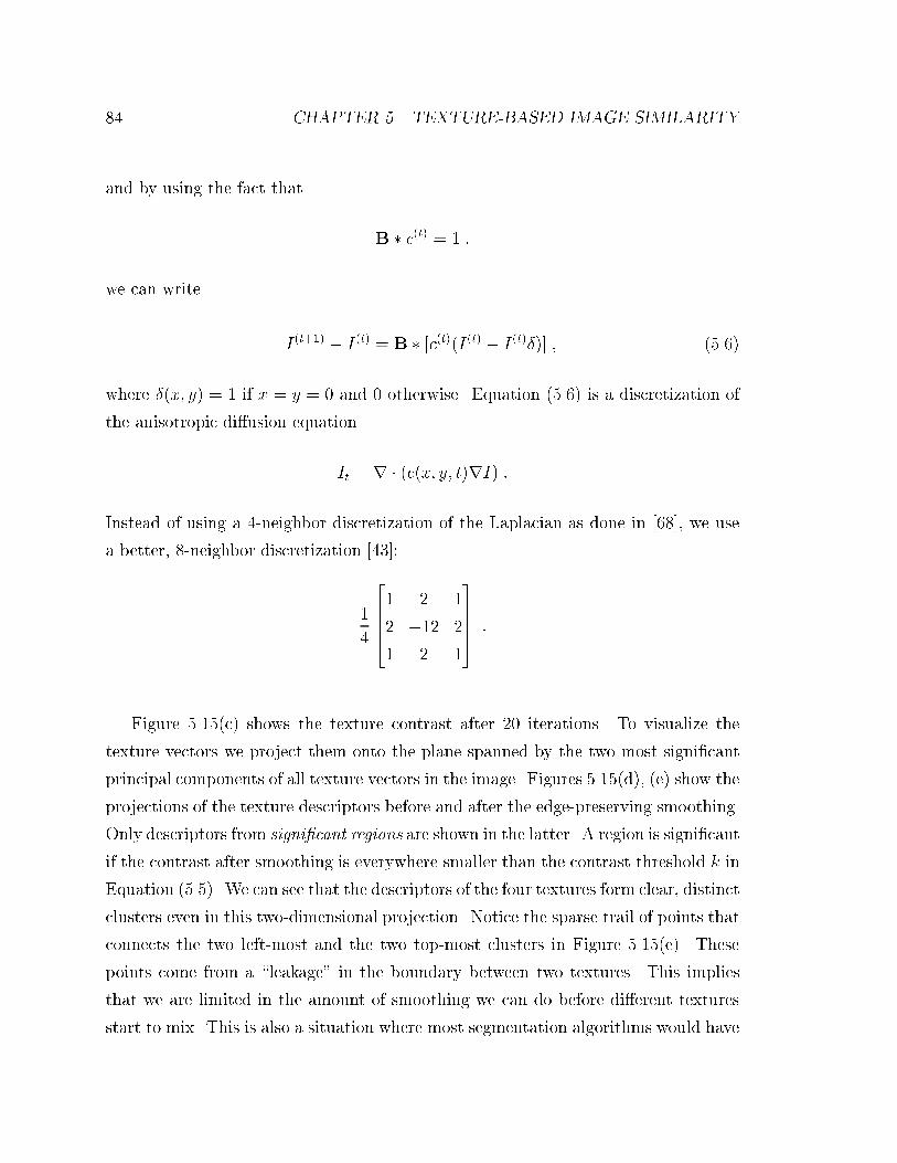
84 CHAPTER 5. TEXTURE-BASED IMAGE SIMILARITY
and by using the fact that
B � c(t) = 1 ;
we can write
I(t+1) � I(t) = B � [c(t)(I(t) � I(t)�)] ; (5.6)
where �(x; y) = 1 if x = y = 0 and 0 otherwise. Equation (5.6) is a discretization of
the anisotropic di�usion equation
It = r � (c(x; y; t)rI) :
Instead of using a 4-neighbor discretization of the Laplacian as done in [68], we use
a better, 8-neighbor discretization [43]:
1
4
26641 2 1
2 �12 2
1 2 1
3775 :
Figure 5.15(c) shows the texture contrast after 20 iterations. To visualize the
texture vectors we project them onto the plane spanned by the two most signi�cant
principal components of all texture vectors in the image. Figures 5.15(d), (e) show the
projections of the texture descriptors before and after the edge-preserving smoothing.
Only descriptors from signi�cant regions are shown in the latter. A region is signi�cant
if the contrast after smoothing is everywhere smaller than the contrast threshold k in
Equation (5.5). We can see that the descriptors of the four textures form clear, distinct
clusters even in this two-dimensional projection. Notice the sparse trail of points that
connects the two left-most and the two top-most clusters in Figure 5.15(e). These
points come from a \leakage" in the boundary between two textures. This implies
that we are limited in the amount of smoothing we can do before di�erent textures
start to mix. This is also a situation where most segmentation algorithms would have
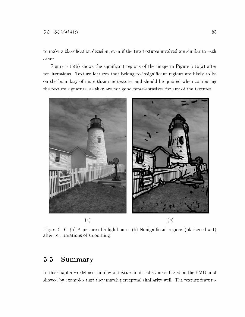
5.5. SUMMARY 85
to make a classi�cation decision, even if the two textures involved are similar to each
other.
Figure 5.16(b) shows the signi�cant regions of the image in Figure 5.16(a) after
ten iterations. Texture features that belong to insigni�cant regions are likely to be
on the boundary of more than one texture, and should be ignored when computing
the texture signature, as they are not good representatives for any of the textures.
(a) (b)
Figure 5.16: (a) A picture of a lighthouse. (b) Nonigni�cant regions (blackened out)after ten iterations of smoothing.
5.5 Summary
In this chapter we de�ned families of texture metric distances, based on the EMD, and
showed by examples that they match perceptual similarity well. The texture features
86 CHAPTER 5. TEXTURE-BASED IMAGE SIMILARITY
are based on carefully designed Gabor �lters. For homogeneous texture patches it was
enough to summarize the texture content by one descriptor, although using the full
distribution of texture features captures the texture content better. We also presented
rotation- and scale-invariant versions of the texture metric for homogeneous textures.
Non-homogeneous textures, such as those found in natural images, required using the
full distribution of the texture features, and introduced problems due to the inherent
spatial extent of texture, such as the blending of adjacent textures that result in
meaningless texture features. We were able to �lter out these features by de�ning
a measure of texture contrast. Using the texture contrast also led to a smoothing
algorithm that coalesced texture features that belonged to the same texture, without
blending features from neighboring textures.
Doubt, the essential preliminary of
all improvement and discovery,
must accompany the stages of man's
onward progress. The faculty of
doubting and questioning, without
which those of comparison and
judgment would be useless, is itself
a divine prerogative of the reason.
Albert Pike (1809-1891)Chapter 6
Comparing Dissimilarity Measures
In Chapter 2 we surveyed distribution-based dissimilarity measures and discussed
their properties, and in Chapter 3 we presented the EMD, which we hypothesized to
be a good choice for image retrieval applications. In Chapters 4 and 5 we showed how
these measures can be instantiated to compare color and texture distributions In this
chapter we compare the results of the di�erent dissimilarity measures when used for
color- and texture-based image retrieval. The main di�culty in such a comparison is
establishing ground truth that will help to determine if a returned image is relevant or
not. To this end, we create databases where the ground truth is known, and use them
to conduct experiments that evaluate the performance of the dissimilarity measures.
6.1 Benchmark Methodology
Any systematic comparison of dissimilarity measures should conform at least to the
following guidelines:
� A meaningful quality measure must be de�ned. Di�erent tasks often entail
di�erent quality measures. For image retrieval, performance is usually measured
by precision, which is the number of relevant images retrieved relative to the
total number of retrieved images, and recall, which is the number of relevant
images retrieved, relative to the total number of relevant images in the database.
87
88 CHAPTER 6. COMPARING DISSIMILARITY MEASURES
Plotting the precision vs. the number of retrieved images, for all dissimilarity
measures, is a good way to compare between them. However, in order to decide
if a particular measure is better for a speci�c task, the precision vs. recall plot
might be of better use as the relative importance of good recall vs. good precision
di�ers according to the task at hand. We therefore show both plots for most of
our experiments.
� Performance comparisons should account for the variety of parameters that can
a�ect the behavior of each measure. These parameters include, in our case, the
number of bins in a histogram; the shape and de�nition of the bins; and for
texture, the number of �lters used to represent the texture. A fair comparison
in the face of this variability can be achieved by giving every measure the best
possible chance to perform well. In our experiments we vary these parameters
and report their e�ect on the di�erent dissimilarity measures.
� Processing steps that a�ect performance independently ought to be evaluated
separately in order to both sharpen insight and reduce complexity. For instance,
the e�ect of di�erent histogram sizes can be understood separately from those
of di�erent dissimilarity measures.
� Ground truth should be available. This is a set of data for which the correct
solution for a particular problem is known. Collecting ground truth is arguably
the hardest problem in benchmarking, because the \correct solution" ought to
be uncontroversial, and the ground-truth data set should be large enough to
allow a statistically signi�cant performance evaluation.
6.2 Experiments
In this section we describe experiments that compare and evaluate the di�erent dis-
similarity measures, discussed in this thesis, for color images and for homogeneous
textures.
6.2. EXPERIMENTS 89
6.2.1 Color
We performed two experiments, each using a di�erent database of color distributions.
The �rst database was constructed such that multiple sets of color distributions were
taken from each of a set of color images. The ground truth was de�ned such that two
distributions belong to the same class if they originate from the same image. The
second database was the 20,000-image database that we used in Chapters 4 and 5.
The ground truth was now established manually by selecting sets of similar images a
priori, both in the semantic meaning and in their color contents.
In our �rst experiment, we randomly chose 94 color images1 from our 20,000
color image database. From each image we created disjoint sets of randomly sampled
pixels and considered these sets as belonging to the same class. While for large
sets of pixels within a class the color distributions are likely to be very similar, for
small sets the variations are larger, mimicking the situation in image retrieval where
images of moderate similarity to the query have to be identi�ed. To get moderate
similarities, we used sets of 8 pixels, and obtained for each image 16 disjoint sets of
random samples, resulting in a ground truth data set of 1504 color distributions with
94 di�erent classes, one class per image.
We represented the color distributions in the database by histograms which were
adapted to optimally represent the combined distribution over the entire database.
To construct the histograms, we ran a K-means clustering algorithm [33] on the com-
bined distribution, resulting in optimal clusters which were used as the histogram
prototypes. Each pixel in every color distribution in this database was then assigned
to a bin by �nding its closest prototype. We repeated this process to compute his-
tograms with 32, 128, and 512 bins, which correspond to coarse, intermediate and �ne
binning, respectively. For the EMD and the Quadratic Form that require a ground
distance, we use the saturated ground distance described in Section 3.4.
In addition to computing histograms, we also computed signatures for all color
distributions. We used the same K-means algorithm as used for histograms, but
instead of computing the optimal prototypes of the combined distribution over the
1We used the same number of images (94) as in the texture case (see Section 6.2.2), so that wecan compare results from both cases.
90 CHAPTER 6. COMPARING DISSIMILARITY MEASURES
entire database, we computed the optimal prototypes for every distribution individ-
ually, asking for the best eight prototypes. This resulted in signatures, all with eight
clusters.
Once the histograms and signatures were computed for all the distributions in
the database, we used the di�erent dissimilarity measures to retrieve and rank the
most similar histograms in the database, where each of the 1504 color distributions
was used, in turn, as the query. The average of the results of these 1504 queries,
for all histogram sizes, was used to evaluate the performance of the dissimilarity
measures. Since the EMD is the only method that takes advantage of signatures,
we applied the EMD on both histograms and signatures. Figures B.1, B.2, and B.3
in Appendix B show the retrieval performance of the di�erent dissimilarity measures
when using histograms with 32, 128, and 512 bins, respectively. We added to each
plot the results of the EMD applied to the signatures (with only 8 clusters). The top
part of each �gure shows the number of relevant distributions in the retrieved set,
as a function of the total number of retrieved distributions. The bottom part of the
�gures shows precision vs. recall.
Analyzing the results leads to the following conclusions:
� Bin-by-bin dissimilarity measures improve by increasing the number of bins up
to a point, after which their performance degrades. Smaller number of bins
results in bigger bins. When the bins are too big, the discrimination power of
the histograms decreases. When the bins are too small, similar pixels might
fall into di�erent bins and will be considered as completely dissimilar. This
problem does not exist for cross-bin dissimilarity measures where the similarity
of the pixels is determined by the ground distance, small in our case, between
the appropriate bins in the feature space.
� For our case of moderate similarities, cross-bin dissimilarity measures perform
better than bin-by-bin measures. The EMD that was applied to signatures per-
formed best in all cases, except for the �ne, 512-bin histograms case, where it
performed slightly better using the histograms. However, for an image retrieval
system, using the EMD on 512-bin histograms is too slow. While the EMD
6.2. EXPERIMENTS 91
on signatures performs best for moderate similarities, once the assumption of
moderate similarities is violated and the dissimilarities between objects in the
same class get smaller with respect to the dissimilarities between objects from
di�erent classes, other dissimilarity measures, such as the �2 statistics and Jef-
frey divergence, might perform better because they were designed to compare
close distributions.
� Although, from an information-theoretic point of view, the signatures in our
experiments carry less information than the histograms and can be encoded
using fewer bits, they usually lead to better results.
� �2 statistics and Je�rey divergence give almost identical results.
� Among the Minkowski-form distances that we tried, the L1 distance gave, in
general, better results than the L2 distance, which was better than L1. No-
tice that we measure distances in the histogram space and not in the color
space where the L2 distance, by construction, matches the perceptual similarity
between colors.
Representing the distributions by signatures leads, in the case of moderate sim-
ilarities, to better results than representing them by histograms. However, when
distributions from the same class are very similar (in contrast to being moderately
similar), adaptive, global histograms perform better than signatures, because features
with minor dissimilarities are likely to be assigned to the same bins. This is demon-
strated in Figure B.4 where sets of 32 random pixels were taken from the images
(instead of 8 pixels as in the case of moderate similarities). Now sets of pixels that
originate from the same image are very similar, and almost every measure performs
well. The EMD applied to signatures performs slightly worse than most other mea-
sures, while the EMD applied to histograms still performs slightly better than the
rest of the measures.
The second experiment was conducted on our full 20,000-image database of color
images. Our goal in this experiment was to compare di�erent dissimilarity measures
using images that are perceived as having similar color content. To do so, we looked
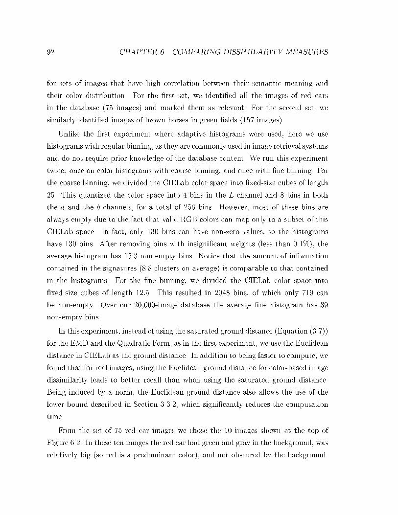
92 CHAPTER 6. COMPARING DISSIMILARITY MEASURES
for sets of images that have high correlation between their semantic meaning and
their color distribution. For the �rst set, we identi�ed all the images of red cars
in the database (75 images) and marked them as relevant. For the second set, we
similarly identi�ed images of brown horses in green �elds (157 images).
Unlike the �rst experiment where adaptive histograms were used, here we use
histograms with regular binning, as they are commonly used in image retrieval systems
and do not require prior knowledge of the database content. We run this experiment
twice: once on color histograms with coarse binning, and once with �ne binning. For
the coarse binning, we divided the CIELab color space into �xed-size cubes of length
25. This quantized the color space into 4 bins in the L channel and 8 bins in both
the a and the b channels, for a total of 256 bins. However, most of these bins are
always empty due to the fact that valid RGB colors can map only to a subset of this
CIELab space. In fact, only 130 bins can have non-zero values, so the histograms
have 130 bins. After removing bins with insigni�cant weights (less than 0.1%), the
average histogram has 15.3 non-empty bins. Notice that the amount of information
contained in the signatures (8.8 clusters on average) is comparable to that contained
in the histograms. For the �ne binning, we divided the CIELab color space into
�xed-size cubes of length 12:5. This resulted in 2048 bins, of which only 719 can
be non-empty. Over our 20,000-image database the average �ne histogram has 39
non-empty bins.
In this experiment, instead of using the saturated ground distance (Equation (3.7))
for the EMD and the Quadratic Form, as in the �rst experiment, we use the Euclidean
distance in CIELab as the ground distance. In addition to being faster to compute, we
found that for real images, using the Euclidean ground distance for color-based image
dissimilarity leads to better recall than when using the saturated ground distance.
Being induced by a norm, the Euclidean ground distance also allows the use of the
lower bound described in Section 3.3.2, which signi�cantly reduces the computation
time.
From the set of 75 red car images we chose the 10 images shown at the top of
Figure 6.2. In these ten images the red car had green and gray in the background, was
relatively big (so red is a predominant color), and not obscured by the background.
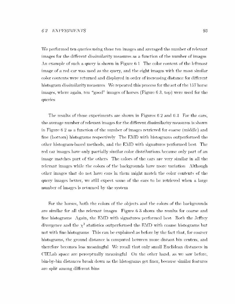
6.2. EXPERIMENTS 93
We performed ten queries using these ten images and averaged the number of relevant
images for the di�erent dissimilarity measures as a function of the number of images.
An example of such a query is shown in Figure 6.1. The color content of the leftmost
image of a red car was used as the query, and the eight images with the most similar
color contents were returned and displayed in order of increasing distance for di�erent
histogram dissimilarity measures. We repeated this process for the set of the 157 horse
images, where again, ten \good" images of horses (Figure 6.3, top) were used for the
queries.
The results of these experiments are shown in Figures 6.2 and 6.3. For the cars,
the average number of relevant images for the di�erent dissimilarity measures is shown
in Figure 6.2 as a function of the number of images retrieved for coarse (middle) and
�ne (bottom) histograms respectively. The EMD with histograms outperformed the
other histogram-based methods, and the EMD with signatures performed best. The
red car images have only partially similar color distributions because only part of an
image matches part of the others. The colors of the cars are very similar in all the
relevant images while the colors of the backgrounds have more variation. Although
other images that do not have cars in them might match the color contents of the
query images better, we still expect some of the cars to be retrieved when a large
number of images is returned by the system.
For the horses, both the colors of the objects and the colors of the backgrounds
are similar for all the relevant images. Figure 6.3 shows the results for coarse and
�ne histograms. Again, the EMD with signatures performed best. Both the Je�rey
divergence and the �2 statistics outperformed the EMD with coarse histograms but
not with �ne histograms. This can be explained as before by the fact that, for coarser
histograms, the ground distance is computed between more distant bin centers, and
therefore becomes less meaningful. We recall that only small Euclidean distances in
CIELab space are perceptually meaningful. On the other hand, as we saw before,
bin-by-bin distances break down as the histograms get �ner, because similar features
are split among di�erent bins.
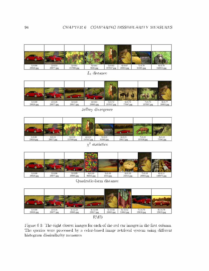
94 CHAPTER 6. COMPARING DISSIMILARITY MEASURES
1) 0.0029020.jpg
2) 0.5329077.jpg
3) 0.61157090.jpg
4) 0.619045.jpg
5) 0.63197037.jpg
6) 0.6720003.jpg
7) 0.7081005.jpg
8) 0.70160053.jpg
L1 distance
1) 0.0029020.jpg
2) 0.2629077.jpg
3) 0.4329017.jpg
4) 0.6129005.jpg
5) 0.72197037.jpg
6) 0.7377047.jpg
7) 0.75197097.jpg
8) 0.7720003.jpg
Je�rey divergence
1) 0.0029020.jpg
2) 0.1129077.jpg
3) 0.19157090.jpg
4) 0.21197037.jpg
5) 0.2181005.jpg
6) 0.2129017.jpg
7) 0.22197058.jpg
8) 0.2277045.jpg
�2 statistics
1) 0.0029020.jpg
2) 0.0629077.jpg
3) 0.0929005.jpg
4) 0.1096035.jpg
5) 0.101033.jpg
6) 0.1025013.jpg
7) 0.1020003.jpg
8) 0.11140075.jpg
Quadratic-form distance
1) 0.0029020.jpg
2) 8.1629077.jpg
3) 12.2329005.jpg
4) 12.6429017.jpg
5) 13.8220003.jpg
6) 14.5253062.jpg
7) 14.7029018.jpg
8) 14.7829019.jpg
EMD
Figure 6.1: The eight closest images for each of the red car images in the �rst column.The queries were processed by a color-based image retrieval system using di�erenthistogram dissimilarity measures.
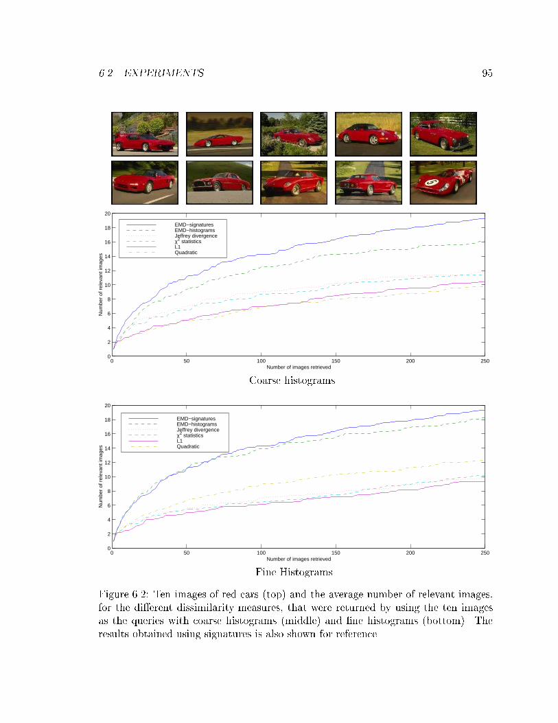
6.2. EXPERIMENTS 95
0 50 100 150 200 2500
2
4
6
8
10
12
14
16
18
20
Number of images retrieved
Num
ber
of r
elev
ant i
mag
es
EMD−signatures EMD−histograms Jeffrey divergenceχ2 statistics L1 Quadratic
Coarse histograms
0 50 100 150 200 2500
2
4
6
8
10
12
14
16
18
20
Number of images retrieved
Num
ber
of r
elev
ant i
mag
es
EMD−signatures EMD−histograms Jeffrey divergenceχ2 statistics L1 Quadratic
Fine Histograms
Figure 6.2: Ten images of red cars (top) and the average number of relevant images,for the di�erent dissimilarity measures, that were returned by using the ten imagesas the queries with coarse histograms (middle) and �ne histograms (bottom). Theresults obtained using signatures is also shown for reference.
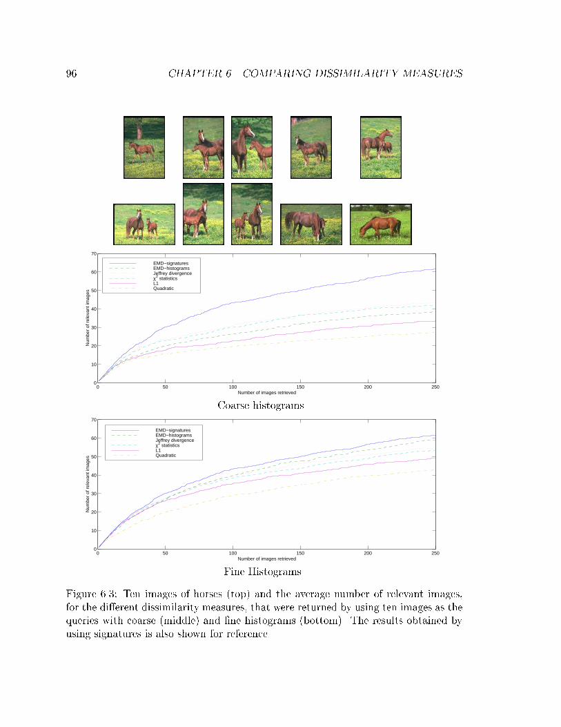
96 CHAPTER 6. COMPARING DISSIMILARITY MEASURES
0 50 100 150 200 2500
10
20
30
40
50
60
70
Number of images retrieved
Num
ber
of r
elev
ant i
mag
es
EMD−signatures EMD−histograms Jeffrey divergenceχ2 statistics L1 Quadratic
Coarse histograms
0 50 100 150 200 2500
10
20
30
40
50
60
70
Number of images retrieved
Num
ber
of r
elev
ant i
mag
es
EMD−signatures EMD−histograms Jeffrey divergenceχ2 statistics L1 Quadratic
Fine Histograms
Figure 6.3: Ten images of horses (top) and the average number of relevant images,for the di�erent dissimilarity measures, that were returned by using ten images as thequeries with coarse (middle) and �ne histograms (bottom). The results obtained byusing signatures is also shown for reference.
6.2. EXPERIMENTS 97
6.2.2 Texture
In order to compare di�erent dissimilarity measures for homogeneous textures, we
used the Brodatz album [9], as it is widely accepted within the texture research
community. Patches from the Brodatz album are shown in Figures 5.7 and 5.8. To
construct an image database with a known ground truth, each image is considered as a
single, separate class. This is a questionable assumption in a few cases, so we a priori
selected 94 Brodatz textures by visual inspection. We excluded the textures D25,
D30-D31, D39-D45, D48, D59, D61, D88-D89, D91, D94, D97 due to the following
two problems: the characterizing scales are too coarse to be captured by our �lters,
or the texture appearance changes over the texture. In these two cases, small blocks
from the same textures will lack similarity.
For each texture, we computed the Gabor texture features described in Section 5.3
and took 16 non-overlapping patches of 8-by-8 pixels with the corresponding texture
features. We chose small patches so that patches from the same texture will not be too
similar and moderate similarity can be assumed. Similarly to the color experiment,
the database contains 1504 texture patches with 94 di�erent classes, each with 16
samples. We used each of the patches in the database as a query, and averaged the
results over all the patches. The retrieval performance of the di�erent dissimilarity
measures are shown in Figures B.5-B.13 in Appendix B for all combinations of �lter
bank size and histogram coarseness. For the �lter banks we used 12 �lters (3 scales/4
orientations), 24 �lters (4/6), or 40 �lters (5/8); the histograms had 32, 128, or 512
bins. Again, for comparison, we added to all the plots the results of the EMD applied
to signatures (with only 8 clusters).
We con�rm that our conclusions from the color experiments hold also for texture,
and in addition:
� For the smallest �lter bank size, the �2 statistics and the Je�rey divergence
give the best results. However, increasing the number of �lters signi�cantly
improves the EMD results, which for the largest �lter bank size gives the best
results overall. For the EMD, similarly to increasing the number of bins, more
�lters implies a better representation of the texture space and therefore better
98 CHAPTER 6. COMPARING DISSIMILARITY MEASURES
results. The performance of the bin-by-bin dissimilarity measures for texture is
similar to that for color: as the number of bins increases, it improves up to a
point and then degrades. For texture, however, the notion of bin size includes
also the number of �lters in the �lter bank. Since increasing the number of
�lters is equivalent to sampling the space of orientations and scales more �nely,
a larger number of �lters improves the discrimination power up to a point after
which the performance degrades. The optimal points depends on the number
of bins used. As can be seen from the graphs, increasing the number of �lters
improves the results only for the coarse histograms (32 bins) while for �ne
histograms (512), the performance degrades.
� Examining the precision vs. recall graphs reveals that applying the EMD to
signatures gives better results when good precision is wanted, while for good
recall, it is better to use the EMD on histograms. Signatures are, by de�nition,
more precise than histograms, so it is natural to expect higher precision in our
queries. On the other hand, globally adapted histograms coalesce to the same
bins features with only moderate similarity, bringing closer images that have
overall moderate similarities between them.
6.3 Summary
A thorough quantitative performance evaluation was presented for distribution-based
image dissimilarity measures. We emphasized image retrieval applications where the
ability to compare moderate similarities is of the greatest importance. The EMD
performed very well in most cases, and exhibited improvements when more data was
available in the form of �ner histograms and, for texture, larger �lter banks. For
the other dissimilarity measures, increasing the amount of data often decreased the
performance as a result of inherent binning problems and the curse of dimensionality.
Nevertheless, the choice of a dissimilarity measure should be made based on the
application at hand and the available data.
One picture is worth a thousand
words.
Fred R. Barnard
If a picture is worth a thousand
words, a picture of an image
database is worth a whole book.
Carlo Tomasi
Chapter 7
Visualization
The images that best match a query should be displayed to the user in a useful
way, that shows immediately if there are any relevant images in the returned set.
Traditional image retrieval systems display the returned images as a list, sorted by
dissimilarity to the query. At this point, the user can examine the images one at a
time, and decide the next action. While this might su�ce if the correct images are in
the returned list, this is usually not the case, even when the user has as exact image
in mind. In many cases, the user has only a vague idea of what he is looking for.
In this cases, the display should convey information as to what kind of images were
returned by the query, what (if anything) went wrong, how to re�ne the query in
order to get closer to the desired images, and whether or not to terminate the search.
There are two shortcomings to the traditional approach. First, when images are
ranked by similarity to the query, related images can appear at separate places in the
list. Often the user would like to have a global view of the returned images in a way
that re ects the relations among the images in the returned set. Second, browsing
and navigating in a large database is disorienting unless the user can form a mental
picture of the entire database. Only having an idea of the surroundings can o�er an
indication of where to go next. The wider the horizon, the more secure navigation
will be. The small pieces of the database, shown by the traditional methods one at a
time, make it harder for the user to form such a picture.
In contrast, we propose a new display technique, which is the main point of this
99
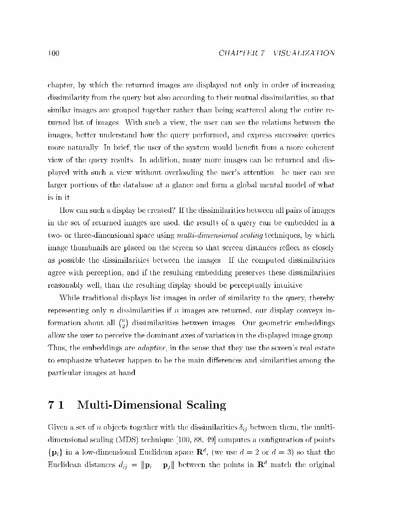
100 CHAPTER 7. VISUALIZATION
chapter, by which the returned images are displayed not only in order of increasing
dissimilarity from the query but also according to their mutual dissimilarities, so that
similar images are grouped together rather than being scattered along the entire re-
turned list of images. With such a view, the user can see the relations between the
images, better understand how the query performed, and express successive queries
more naturally. In brief, the user of the system would bene�t from a more coherent
view of the query results. In addition, many more images can be returned and dis-
played with such a view without overloading the user's attention. he user can see
larger portions of the database at a glance and form a global mental model of what
is in it.
How can such a display be created? If the dissimilarities between all pairs of images
in the set of returned images are used, the results of a query can be embedded in a
two- or three-dimensional space using multi-dimensional scaling techniques, by which
image thumbnails are placed on the screen so that screen distances re ect as closely
as possible the dissimilarities between the images. If the computed dissimilarities
agree with perception, and if the resulting embedding preserves these dissimilarities
reasonably well, than the resulting display should be perceptually intuitive.
While traditional displays list images in order of similarity to the query, thereby
representing only n dissimilarities if n images are returned, our display conveys in-
formation about all�n2
�dissimilarities between images. Our geometric embeddings
allow the user to perceive the dominant axes of variation in the displayed image group.
Thus, the embeddings are adaptive, in the sense that they use the screen's real estate
to emphasize whatever happen to be the main di�erences and similarities among the
particular images at hand.
7.1 Multi-Dimensional Scaling
Given a set of n objects together with the dissimilarities �ij between them, the multi-
dimensional scaling (MDS) technique [100, 88, 49] computes a con�guration of points
fpig in a low-dimensional Euclidean space Rd, (we use d = 2 or d = 3) so that the
Euclidean distances dij = kpi � pjk between the points in Rd match the original
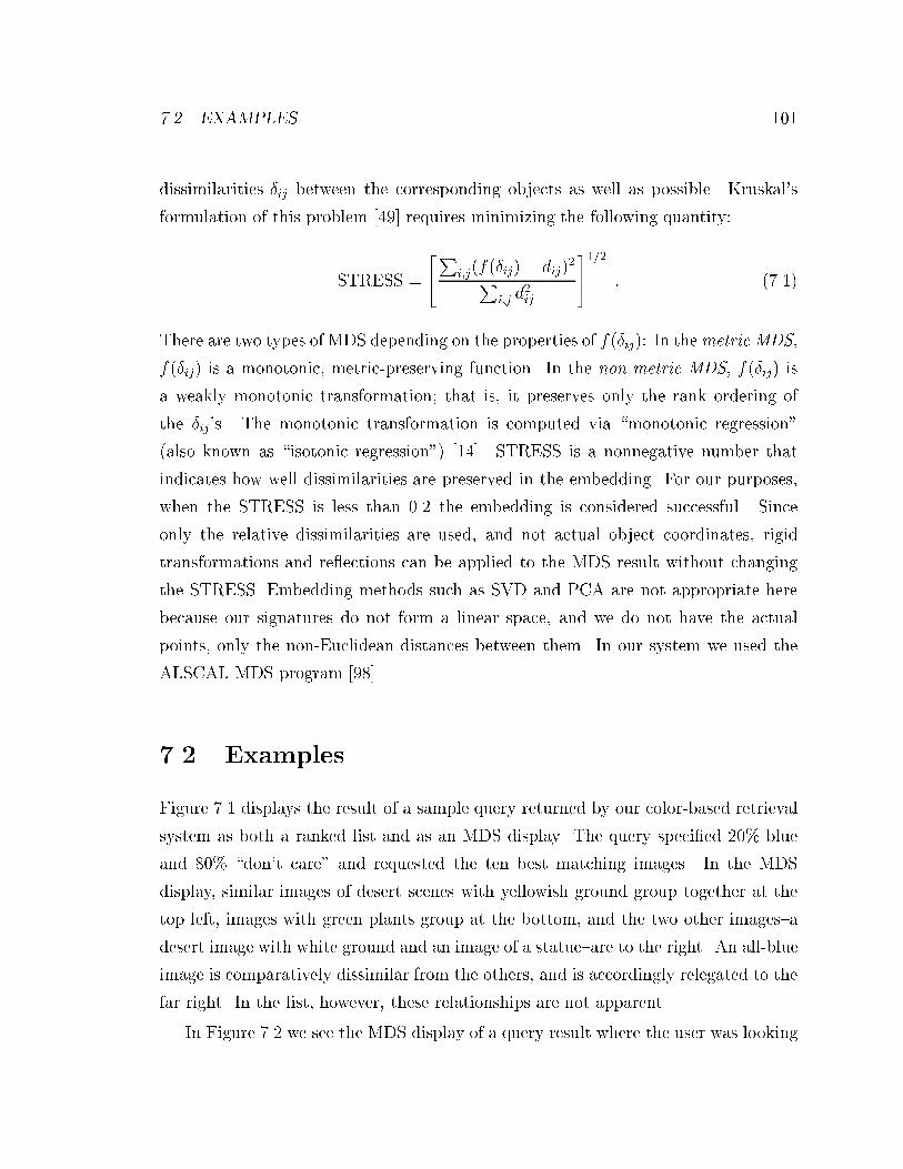
7.2. EXAMPLES 101
dissimilarities �ij between the corresponding objects as well as possible. Kruskal's
formulation of this problem [49] requires minimizing the following quantity:
STRESS =
"Pi;j(f(�ij)� dij)
2Pi;j d
2ij
#1=2: (7.1)
There are two types of MDS depending on the properties of f(�ij): In themetric MDS,
f(�ij) is a monotonic, metric-preserving function. In the non-metric MDS, f(�ij) is
a weakly monotonic transformation; that is, it preserves only the rank ordering of
the �ij's. The monotonic transformation is computed via \monotonic regression"
(also known as \isotonic regression") [14]. STRESS is a nonnegative number that
indicates how well dissimilarities are preserved in the embedding. For our purposes,
when the STRESS is less than 0.2 the embedding is considered successful. Since
only the relative dissimilarities are used, and not actual object coordinates, rigid
transformations and re ections can be applied to the MDS result without changing
the STRESS. Embedding methods such as SVD and PCA are not appropriate here
because our signatures do not form a linear space, and we do not have the actual
points, only the non-Euclidean distances between them. In our system we used the
ALSCAL MDS program [98].
7.2 Examples
Figure 7.1 displays the result of a sample query returned by our color-based retrieval
system as both a ranked list and as an MDS display. The query speci�ed 20% blue
and 80% \don't care" and requested the ten best matching images. In the MDS
display, similar images of desert scenes with yellowish ground group together at the
top left, images with green plants group at the bottom, and the two other images{a
desert image with white ground and an image of a statue{are to the right. An all-blue
image is comparatively dissimilar from the others, and is accordingly relegated to the
far right. In the list, however, these relationships are not apparent.
In Figure 7.2 we see the MDS display of a query result where the user was looking
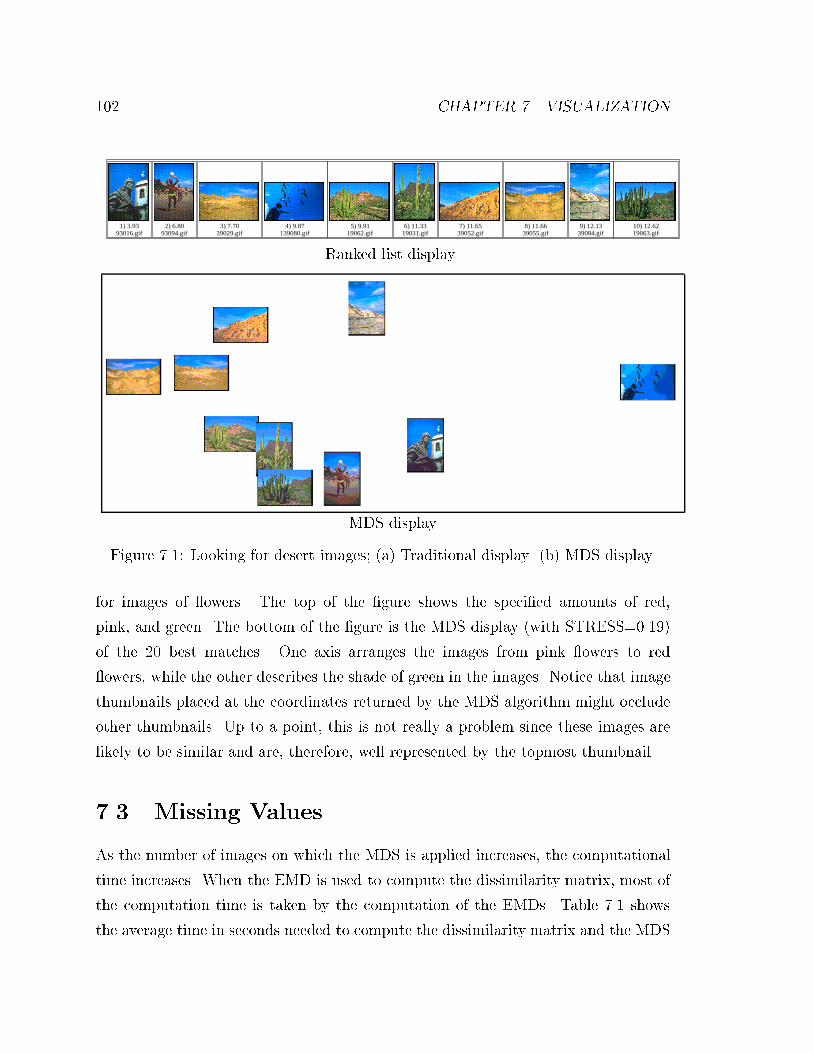
102 CHAPTER 7. VISUALIZATION
1) 3.9393016.gif
2) 6.8093094.gif
3) 7.7039029.gif
4) 9.87139080.gif
5) 9.9119062.gif
6) 11.3319031.gif
7) 11.6539052.gif
8) 11.6639055.gif
9) 12.1339084.gif
10) 12.6219063.gif
Ranked list display
MDS display
Figure 7.1: Looking for desert images; (a) Traditional display. (b) MDS display.
for images of owers. The top of the �gure shows the speci�ed amounts of red,
pink, and green. The bottom of the �gure is the MDS display (with STRESS=0.19)
of the 20 best matches. One axis arranges the images from pink owers to red
owers, while the other describes the shade of green in the images. Notice that image
thumbnails placed at the coordinates returned by the MDS algorithm might occlude
other thumbnails. Up to a point, this is not really a problem since these images are
likely to be similar and are, therefore, well represented by the topmost thumbnail.
7.3 Missing Values
As the number of images on which the MDS is applied increases, the computational
time increases. When the EMD is used to compute the dissimilarity matrix, most of
the computation time is taken by the computation of the EMDs. Table 7.1 shows
the average time in seconds needed to compute the dissimilarity matrix and the MDS
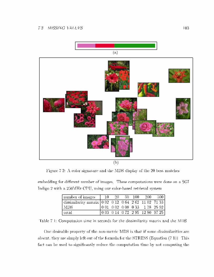
7.3. MISSING VALUES 103
(a)
(b)
Figure 7.2: A color signature and the MDS display of the 20 best matches.
embedding for di�erent number of images,. These computations were done on a SGI
Indigo 2 with a 250MHz CPU, using our color-based retrieval system.
number of images 10 20 50 100 200 500dissimilarity matrix 0.02 0.12 0.64 2.62 11.02 71.33MDS 0.01 0.02 0.08 0.33 1.78 25.92total 0.03 0.14 0.72 2.95 12.80 97.25
Table 7.1: Computation time in seconds for the dissimilarity matrix and the MDS.
One desirable property of the non-metric MDS is that if some dissimilarities are
absent, they are simply left out of the formula for the STRESS (Equation (7.1)). This
fact can be used to signi�cantly reduce the computation time by not computing the
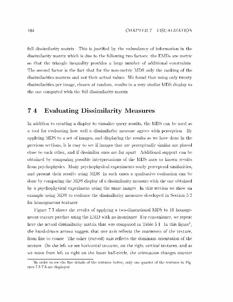
104 CHAPTER 7. VISUALIZATION
full dissimilarity matrix. This is justi�ed by the redundancy of information in the
dissimilarity matrix which is due to the following two factors: the EMDs are metric
so that the triangle inequality provides a large number of additional constraints.
The second factor is the fact that for the non-metric MDS only the ranking of the
dissimilarities matters and not their actual values. We found that using only twenty
dissimilarities per image, chosen at random, results in a very similar MDS display to
the one computed with the full dissimilarity matrix.
7.4 Evaluating Dissimilarity Measures
In addition to creating a display to visualize query results, the MDS can be used as
a tool for evaluating how well a dissimilarity measure agrees with perception. By
applying MDS to a set of images, and displaying the results as we have done in the
previous sections, it is easy to see if images that are perceptually similar are placed
close to each other, and if dissimilar ones are far apart. Additional support can be
obtained by comparing possible interpretations of the MDS axes to known results
from psychophysics. Many psychophysical experiments study perceptual similarities,
and present their results using MDS. In such cases a qualitative evaluation can be
done by comparing the MDS display of a dissimilarity measure with the one obtained
by a psychophysical experiment using the same images. In this section we show an
example using MDS to evaluate the dissimilarity measures developed in Section 5.2
for homogeneous textures.
Figure 7.3 shows the results of applying a two-dimensional MDS to 16 homoge-
neous texture patches using the EMD with no invariance. For convenience, we repeat
here the actual dissimilarity matrix that was computed in Table 5.1. In this �gure1,
the hand-drawn arrows suggest that one axis re ects the coarseness of the texture,
from �ne to coarse. The other (curved) axis re ects the dominant orientation of the
texture. On the left we see horizontal textures, on the right vertical textures, and as
we move from left to right on the lower half-circle, the orientation changes counter
1In order to see the �ne details of the textures better, only one-quarter of the textures in Fig-ures 7.3-7.5 are displayed.
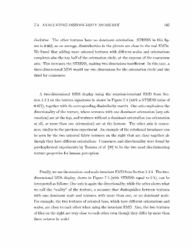
7.4. EVALUATING DISSIMILARITY MEASURES 105
clockwise. The other textures have no dominant orientation. STRESS in this �g-
ure is 0.063, so on average, dissimilarities in the picture are close to the real EMDs.
We found that adding more oriented textures with di�erent scales and orientations
completes also the top half of the orientation circle, at the expense of the coarseness
axis. This increases the STRESS, making two dimensions insu�cient. In this case, a
three-dimensional MDS would use two dimensions for the orientation circle and the
third for coarseness.
A two-dimensional MDS display using the rotation-invariant EMD from Sec-
tion 5.2.2 on the texture signatures in shown in Figure 7.4 (with a STRESS value of
0.077), together with its corresponding dissimilarity matrix. One axis emphasizes the
directionality of the texture, where textures with one dominant orientation (any ori-
entation) are at the top, and textures without a dominant orientation (no orientation
at all, or more than one orientation) are at the bottom. The other axis is coarse-
ness, similar to the previous experiment. An example of the rotational invariance can
be seen by the two oriented fabric textures on the right that are close together al-
though they have di�erent orientations. Coarseness and directionality were found by
psychophysical experiments by Tamura et al. [99] to be the two most discriminating
texture properties for human perception.
Finally, we use the rotation- and scale-invariant EMD from Section 5.2.3. The two-
dimensional MDS display, shown in Figure 7.5 (with STRESS equal to 0.1), can be
interpreted as follows: One axis is again the directionality, while the other shows what
we call the \scality" of the texture, a measure that distinguishes between textures
with one dominant scale and textures with more than one, or no dominant scale.
For example, the two textures of oriented bars, which have di�erent orientations and
scales, are close to each other when using the invariant EMD. Also, the two textures
of tiles on the right are very close to each other even though they di�er by more than
three octaves in scale!
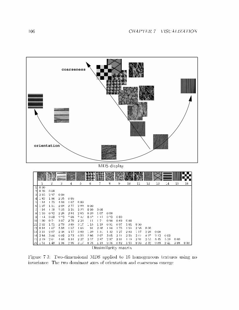
106 CHAPTER 7. VISUALIZATION
orientation
coarseness
MDS display
1 2 3 4 5 6 7 8 9 10 11 12 13 14 15 161 0.002 0.39 0.003 2.95 2.97 0.004 1.82 1.96 2.35 0.005 1.84 1.75 4.06 1.67 0.006 1.07 1.14 2.08 2.77 2.89 0.007 1.94 1.78 2.55 3.35 3.22 0.99 0.008 1.10 0.92 2.26 2.84 2.65 0.39 1.07 0.009 1.14 0.80 2.23 2.68 2.47 0.52 1.11 0.23 0.0010 1.00 0.74 3.07 2.70 2.24 1.11 1.74 0.90 0.89 0.0011 2.02 1.71 2.79 3.69 3.17 1.15 1.18 0.91 0.97 1.01 0.0012 0.94 1.07 3.38 1.57 1.68 1.91 2.88 1.86 1.76 1.55 2.56 0.0013 2.31 2.07 2.38 3.17 3.60 1.39 1.34 1.32 1.27 2.03 1.17 2.29 0.0014 3.84 3.86 0.80 3.23 4.92 2.86 2.62 3.05 3.11 3.95 3.17 4.22 2.13 0.0015 2.19 2.04 4.66 3.34 2.27 2.57 2.87 2.37 2.31 1.48 2.31 2.55 3.45 5.50 0.0016 1.51 1.48 1.96 2.96 3.17 0.76 1.19 0.76 0.82 1.55 0.93 2.32 0.88 2.41 3.08 0.00
Dissimilarity matrix
Figure 7.3: Two-dimensional MDS applied to 16 homogeneous textures using noinvariance. The two dominant axes of orientation and coarseness emerge.
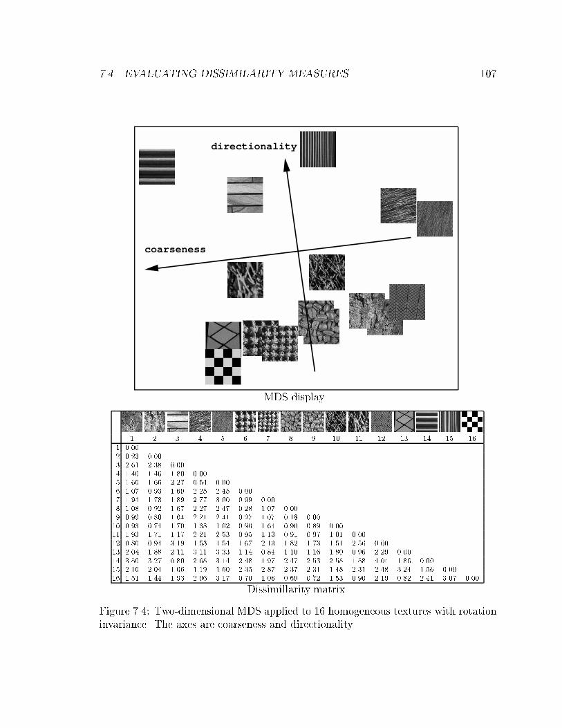
7.4. EVALUATING DISSIMILARITY MEASURES 107
directionality
coarseness
MDS display
1 2 3 4 5 6 7 8 9 10 11 12 13 14 15 161 0.002 0.23 0.003 2.61 2.38 0.004 1.40 1.46 1.80 0.005 1.60 1.66 2.27 0.54 0.006 1.07 0.93 1.69 2.25 2.45 0.007 1.94 1.78 1.89 2.77 3.00 0.99 0.008 1.08 0.92 1.67 2.27 2.47 0.28 1.07 0.009 0.99 0.80 1.64 2.21 2.41 0.27 1.07 0.18 0.0010 0.93 0.74 1.70 1.38 1.62 0.96 1.64 0.90 0.89 0.0011 1.93 1.71 1.17 2.21 2.53 0.95 1.13 0.91 0.97 1.01 0.0012 0.80 0.94 3.19 1.53 1.54 1.67 2.13 1.82 1.73 1.51 2.56 0.0013 2.04 1.88 2.11 3.11 3.33 1.14 0.84 1.10 1.16 1.80 0.96 2.29 0.0014 3.50 3.27 0.80 2.68 3.14 2.48 1.97 2.47 2.53 2.58 1.58 4.04 1.86 0.0015 2.10 2.04 1.06 1.19 1.60 2.35 2.87 2.37 2.31 1.48 2.31 2.48 3.24 1.56 0.0016 1.51 1.44 1.93 2.96 3.17 0.70 1.06 0.69 0.72 1.53 0.90 2.19 0.82 2.41 3.07 0.00
Dissimillarity matrix
Figure 7.4: Two-dimensional MDS applied to 16 homogeneous textures with rotationinvariance. The axes are coarseness and directionality.
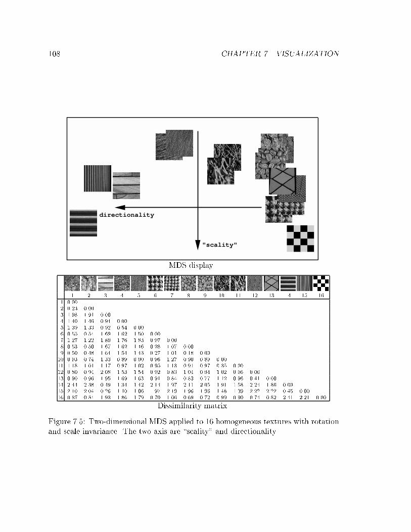
108 CHAPTER 7. VISUALIZATION
directionality
"scality"
MDS display
1 2 3 4 5 6 7 8 9 10 11 12 13 14 15 161 0.002 0.23 0.003 1.98 1.91 0.004 1.40 1.46 0.94 0.005 1.39 1.33 0.92 0.54 0.006 0.55 0.54 1.69 1.62 1.50 0.007 1.27 1.22 1.89 1.76 1.83 0.97 0.008 0.53 0.50 1.67 1.62 1.46 0.28 1.07 0.009 0.50 0.48 1.64 1.54 1.43 0.27 1.01 0.18 0.0010 0.93 0.74 1.33 0.89 0.90 0.96 1.27 0.90 0.89 0.0011 1.18 1.01 1.17 0.97 1.02 0.95 1.13 0.91 0.97 0.35 0.0012 0.80 0.94 2.08 1.53 1.54 0.92 0.83 1.04 0.94 1.02 0.96 0.0013 0.90 0.96 1.95 1.69 1.63 0.91 0.84 0.83 0.77 1.12 0.96 0.41 0.0014 2.44 2.38 0.49 1.34 1.42 2.14 1.97 2.11 2.05 1.91 1.58 2.24 1.86 0.0015 2.10 2.04 0.26 1.10 1.06 1.97 2.19 1.96 1.96 1.48 1.39 2.22 2.22 0.45 0.0016 0.87 0.84 1.93 1.86 1.79 0.70 1.06 0.69 0.72 0.99 0.90 0.74 0.82 2.41 2.21 0.00
Dissimilarity matrix
Figure 7.5: Two-dimensional MDS applied to 16 homogeneous textures with rotationand scale invariance. The two axis are \scality" and directionality.
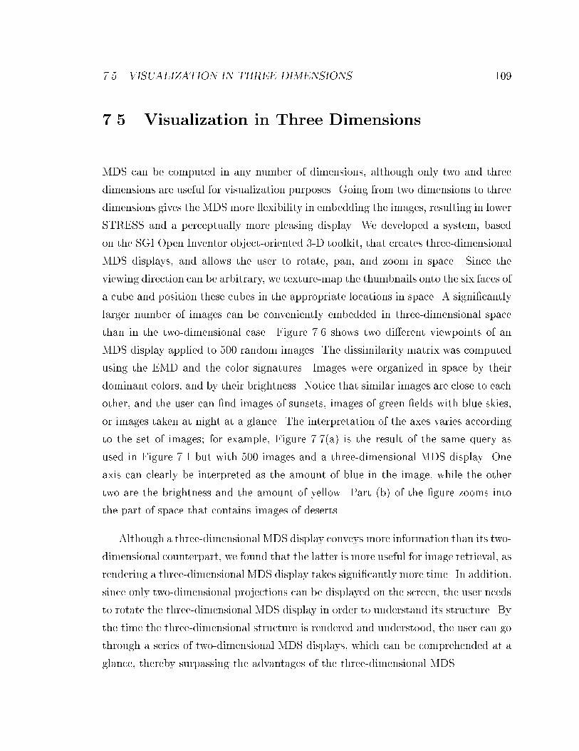
7.5. VISUALIZATION IN THREE DIMENSIONS 109
7.5 Visualization in Three Dimensions
MDS can be computed in any number of dimensions, although only two and three
dimensions are useful for visualization purposes. Going from two dimensions to three
dimensions gives the MDS more exibility in embedding the images, resulting in lower
STRESS and a perceptually more pleasing display. We developed a system, based
on the SGI Open Inventor object-oriented 3-D toolkit, that creates three-dimensional
MDS displays, and allows the user to rotate, pan, and zoom in space. Since the
viewing direction can be arbitrary, we texture-map the thumbnails onto the six faces of
a cube and position these cubes in the appropriate locations in space. A signi�cantly
larger number of images can be conveniently embedded in three-dimensional space
than in the two-dimensional case. Figure 7.6 shows two di�erent viewpoints of an
MDS display applied to 500 random images. The dissimilarity matrix was computed
using the EMD and the color signatures. Images were organized in space by their
dominant colors, and by their brightness. Notice that similar images are close to each
other, and the user can �nd images of sunsets, images of green �elds with blue skies,
or images taken at night at a glance. The interpretation of the axes varies according
to the set of images; for example, Figure 7.7(a) is the result of the same query as
used in Figure 7.1 but with 500 images and a three-dimensional MDS display. One
axis can clearly be interpreted as the amount of blue in the image, while the other
two are the brightness and the amount of yellow. Part (b) of the �gure zooms into
the part of space that contains images of deserts.
Although a three-dimensional MDS display conveys more information than its two-
dimensional counterpart, we found that the latter is more useful for image retrieval, as
rendering a three-dimensional MDS display takes signi�cantly more time. In addition,
since only two-dimensional projections can be displayed on the screen, the user needs
to rotate the three-dimensional MDS display in order to understand its structure. By
the time the three-dimensional structure is rendered and understood, the user can go
through a series of two-dimensional MDS displays, which can be comprehended at a
glance, thereby surpassing the advantages of the three-dimensional MDS.
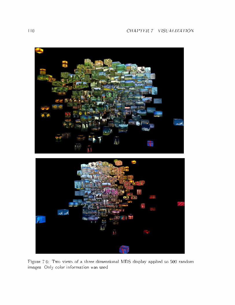
110 CHAPTER 7. VISUALIZATION
Figure 7.6: Two views of a three-dimensional MDS display applied to 500 randomimages. Only color information was used.
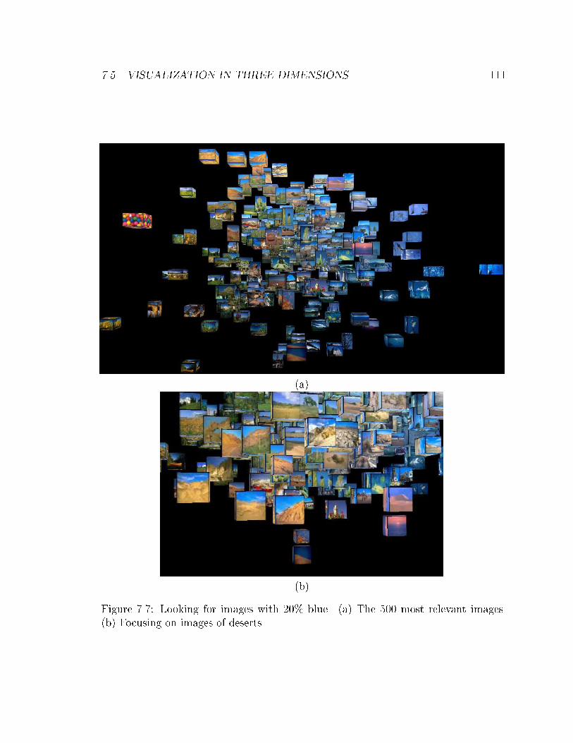
7.5. VISUALIZATION IN THREE DIMENSIONS 111
(a)
(b)
Figure 7.7: Looking for images with 20% blue. (a) The 500 most relevant images.(b) Focusing on images of deserts.
112 CHAPTER 7. VISUALIZATION
7.6 Summary
We showed that by using the mutual dissimilarities between a set of images, the
images from a query result can be displayed in a more intuitive way than with the
traditional methods. The resulting embeddings, in two- and three-dimensions, are
adaptive and re ect the axes of maximum variation. A larger number of images can
displayed, helping the user to form a global mental model of the entire database. In
addition, it is easier to understand what are the commonalities is the returned set of
images and where to go next, as well as when to stop the search.
The idea of an adaptive image embedding can be applied to other modalities be-
sides color and texture, as long as some notion of similarity, metric or not, continuous
or discrete, can be de�ned.
In the next chapter we extend this visualization technique to allow for intuitive
navigation through large collections of images for the purpose of image retrieval.
We're not lost. We're locationally
challenged.
John M. Ford
Chapter 8
Navigation
The MDS-based visualization technique, described in the last chapter, makes it pos-
sible to display a large number of images in an intuitive way that allows the user to
see at a glance the commonalities is the returned set of images and what part of the
display is most relevant. In this chapter, we develop a navigation method based on
this display. Once the user points to the region of interest on the display, the system
zooms in and �nds more images that are similar to the common features of the images
in the region. By iterating this re�nement process, the user can quickly home in to
the relevant parts of the database. We show examples of navigation in a space of
color images and in a space of police mugshots.
8.1 Retrieval by Navigation
The discrepancy that results from using syntactic features, such as color and texture,
to satisfy semantic queries causes a basic problem with the traditional query/response
style of interaction. An overly generic query yields a large jumble of images, which are
hard to examine, while an excessively speci�c query may cause many good images to
be overlooked by the system. This is the traditional trade-o� between good precision
(few false positives) and good recall (few false negatives). Striving for both good
precision and good recall may pose an excessive burden on the de�nition of a \correct"
measure of image similarity. While most image retrieval systems recognize this and
113
114 CHAPTER 8. NAVIGATION
allow for an iterative re�nement of queries, the number of images returned for a
query is usually kept low so that the user can examine them, one at a time, in order
of similarity to the query.
If, as we showed in Chapter 7, images are arranged on the screen so as to re ect
similarities and di�erences between their feature distributions, the initial queries can
be very generic, and return a large number of images. The consequent low initial
precision is an advantage rather than a weakness, as it provides a neighborhood of
images the user can relate to when re�ning the query and deciding where to go next.
In fact, the user can see large portions of the database at a glance, and form a mental
model of what is in it. Rather than following a thin path of images from query
to query, as in the traditional approach, the user now zooms in to the images of
interest. Precision is added incrementally in subsequent query re�nements, and fewer
and fewer images need to be displayed as the desired images are approached. This can
be envisioned as analogous to visiting a bookstore. Books are shelved according to
their subjects, for example, travel-books, cookbooks, poetry, etc. After locating the
right section, say cookbooks, the books are again classi�ed into di�erent categories
such as vegetarian cooking, baking, etc. The books can be further sorted by title
or by author. The last step when searching for a book is to scan the relevant set of
books, one at a time, and �nd the desired one. After a few visits to the bookstore, a
global mental picture of it is formed, with the knowledge of what kinds of books can
be found and where to look for them.
When the user selects the region of interest on the display, a new, more speci�c
query is automatically generated, re ecting the common features of the images in the
selected set. A new set of images is returned and displayed by a new MDS, which
now re ects the new dominant axes of variation. By iterating this process, the user
is able to quickly navigate to the portion of the image space of interest, typically in
very few mouse clicks.
This navigation scheme can be categorized as a relevance feedback system [81, 59,
92] where retrieval is guided by feedback from the user, who marks relevant and non-
relevant images. A major di�erence from other relevance feedback systems is that in
our navigation approach, the relevant images are likely to be displayed close to each
8.1. RETRIEVAL BY NAVIGATION 115
other, and far from ones which are completely irrelevant. This makes the selection
of the relevant set easier and more intuitive, as the user naturally moves his focus to
relevant parts of the display, while in the other methods the user needs to scan the
list of images, one at a time, and decide whether it is relevant or not.
We propose a navigation scheme in which the user starts by specifying a generic
query. Using partial queries is encouraged when the user is not con�dent about certain
features by specifying \don't care" rather than guessing. A large set of images is
returned and embedded in two-dimensional space using MDS. Once the user selects an
area of interest, an appropriate new query is automatically generated and submitted.
Now a smaller number of images is returned by the system. The new set of images
is not necessarily a subset of the previous set, so images which were not returned by
the previous query can still be retrieved at later stages, as the query becomes more
precise. A new MDS display is shown, with new axes of variation based on the new
image set.
To generate the new query, our user interface allows the user to select from the
MDS display images that will be used to form the next query. The selection can consist
of one or multiple regions. The signatures of the selected k images are combined to
generate a signature that will be used as the next query. We want the new signature
to re ect features which are common in these images, and ignore the others by using
\don't care." This is done by representing the clusters of all the signatures in the
return set as points in the feature space and �nding the dominant clusters in that
space. We use a similar clustering algorithm as the one that was used in Section 4.2
to generate the color signatures. We reject clusters that are not represented by points
from at least dk=2e images to insure commonality. Each new cluster is assigned
a weight that is the median of the weights of the points in that cluster. We use
the median instead of the mean for robustness with respect to points that have very
di�erent weights. Finally, we normalize the resulting signature by dividing the weights
of the clusters by the number of points that contributed to it. If the total weight of
the signature is now greater than 100%, we normalize it again. Usually, however, the
total weight of the signature will be less than 100%, so the reminder is marked \don't
care."
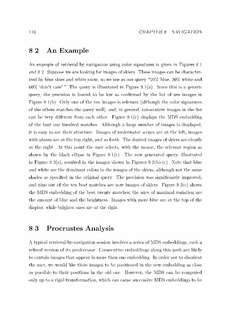
116 CHAPTER 8. NAVIGATION
8.2 An Example
An example of retrieval by navigation using color signatures is given in Figures 8.1
and 8.2. Suppose we are looking for images of skiers. These images can be character-
ized by blue skies and white snow, so we use as our query \20% blue, 20% white and
60% `don't care'." The query is illustrated in Figure 8.1(a). Since this is a generic
query, the precision is bound to be low as con�rmed by the list of ten images in
Figure 8.1(b). Only one of the ten images is relevant (although the color signatures
of the others matches the query well), and, in general, consecutive images in the list
can be very di�erent from each other. Figure 8.1(c) displays the MDS embedding
of the best one hundred matches. Although a large number of images is displayed,
it is easy to see their structure. Images of underwater scenes are at the left, images
with plants are at the top right, and so forth. The desired images of skiers are clearly
at the right. At this point the user selects, with the mouse, the relevant region as
shown by the black ellipse in Figure 8.1(c). The new generated query, illustrated
in Figure 8.2(a), resulted in the images shown in Figures 8.2(b)-(c). Note that blue
and white are the dominant colors in the images of the skiers, although not the same
shades as speci�ed in the original query. The precision was signi�cantly improved,
and nine out of the ten best matches are now images of skiers. Figure 8.2(c) shows
the MDS embedding of the best twenty matches; the axes of maximal variation are
the amount of blue and the brightness. Images with more blue are at the top of the
display, while brighter ones are at the right.
8.3 Procrustes Analysis
A typical retrieval-by-navigation session involves a series of MDS embeddings, each a
re�ned version of its predecessor. Consecutive embeddings along this path are likely
to contain images that appear in more than one embedding. In order not to disorient
the user, we would like these images to be positioned in the new embedding as close
as possible to their positions in the old one. However, the MDS can be computed
only up to a rigid transformation, which can cause successive MDS embeddings to be
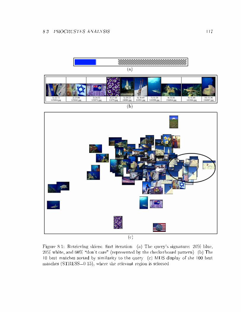
8.3. PROCRUSTES ANALYSIS 117
(a)
1) 22.72125004.jpg
2) 23.86125042.jpg
3) 24.35125072.jpg
4) 27.6411079.jpg
5) 29.5324080.jpg
6) 30.6961091.jpg
7) 31.59141098.jpg
8) 31.81156064.jpg
9) 31.84141066.jpg
10) 31.96156087.jpg
(b)
(c)
Figure 8.1: Retrieving skiers: �rst iteration. (a) The query's signature: 20% blue,20% white, and 60% \don't care" (represented by the checkerboard pattern). (b) The10 best matches sorted by similarity to the query. (c) MDS display of the 100 bestmatches (STRESS=0.15), where the relevant region is selected.
118 CHAPTER 8. NAVIGATION
(a)
1) 0.2561087.jpg
2) 0.2761062.jpg
3) 0.3160010.jpg
4) 0.3460064.jpg
5) 0.3461093.jpg
6) 0.3560016.jpg
7) 0.3761054.jpg
8) 0.37179001.jpg
9) 0.3860042.jpg
10) 0.3961097.jpg
(b)
(c)
Figure 8.2: Retrieving skiers: second iteration. (a) The generated signature. (b) The10 best matches sorted by similarity to the query. (c) MDS of the 20 best matches(STRESS=0.06).
8.3. PROCRUSTES ANALYSIS 119
translated, rotated, scaled, and ipped relative to previous ones. Procrustes analysis
[14, 34] can be used to align one MDS embedding with respect to another. In general,
Procrustes analysis computes the optimal similarity transformation that must be
applied to one embedding in order to match it, as well as possible, to the other. Such
alignment is applied only to images that are in the intersection of the two image sets.
Assume that we are given two consecutive MDS embeddings where n images
participate in both. Let X = [x1; : : : ;xn]T be an n-by-2 matrix representing the
two-dimensional coordinates of the n images in the �rst embedding. Similarly Y =
[y1; : : : ;yn]T represents the coordinates of the n images in the second embedding. In
general, the two embeddings can be in spaces with di�erent dimensions.
We measure the discrepancy between the two embeddings by
D =nX
r=1
(yr � xr)T (yr � xr) ;
Our goal then is to �nd the translation b, the dilation �, and the orthogonal matrix
R that will transform the points yr to
y0r = �RTyr + b ;
such that D will be minimized. The optimal translation and dilation are determined
by our desire to best �ll the screen display area. The optimal orthogonal matrix R
can be found as follows [90]: we want to minimize
D =nX
r=1
(RTyr � xr)T (RTyr � xr)
=nX
r=1
yTr yr +nX
r=1
xTr xr � 2nX
r=1
xTrRyr
= tr(YYT ) + tr(XXT )� 2tr(XRYT ) ;
where tr(�) is the trace of a square matrix.
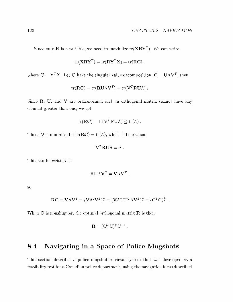
120 CHAPTER 8. NAVIGATION
Since only R is a variable, we need to maximize tr(XRYT ). We can write
tr(XRYT ) = tr(RYTX) = tr(RC) ;
where C = YTX. Let C have the singular value decomposition, C = U�VT , then
tr(RC) = tr(RU�VT ) = tr(VTRU�) :
Since R, U, and V are orthonormal, and an orthogonal matrix cannot have any
element greater than one, we get
tr(RC) = tr(VTRU�) � tr(�) :
Thus, D is minimized if tr(RC) = tr(�), which is true when
VTRU� = � :
This can be written as
RU�VT = V�VT ;
so
RC = V�VT = (V�2VT )1
2 = (V�UUT�VT )1
2 = (CTC)1
2 :
When C is nonsingular, the optimal orthogonal matrix R is then
R = (CTC)1
2C�1 :
8.4 Navigating in a Space of Police Mugshots
This section describes a police mugshot retrieval system that was developed as a
feasibility test for a Canadian police department, using the navigation ideas described
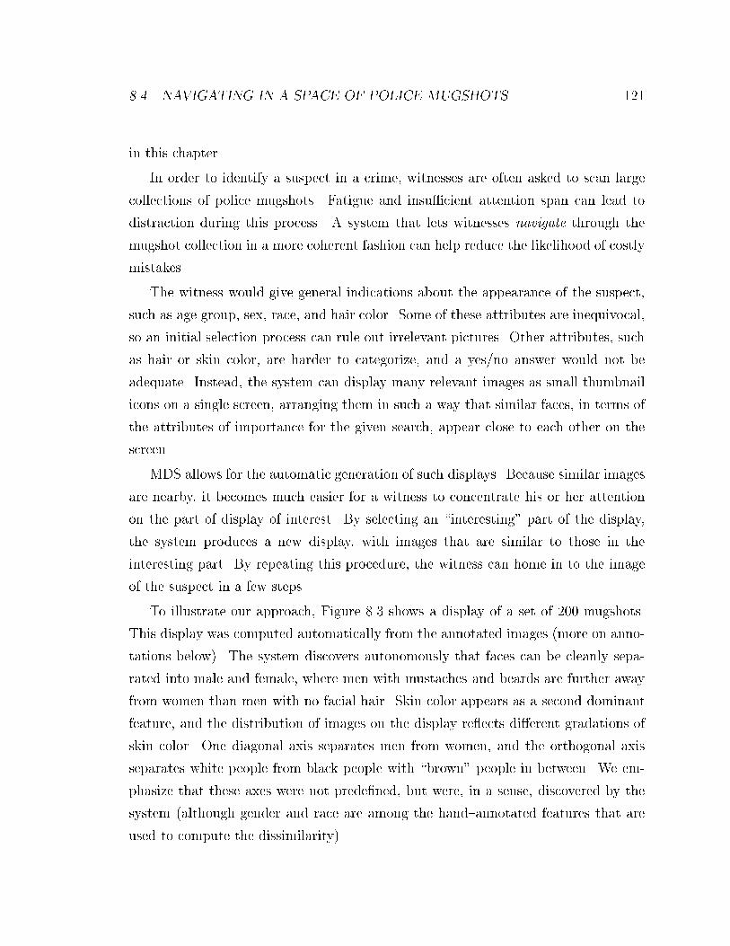
8.4. NAVIGATING IN A SPACE OF POLICE MUGSHOTS 121
in this chapter.
In order to identify a suspect in a crime, witnesses are often asked to scan large
collections of police mugshots. Fatigue and insu�cient attention span can lead to
distraction during this process. A system that lets witnesses navigate through the
mugshot collection in a more coherent fashion can help reduce the likelihood of costly
mistakes.
The witness would give general indications about the appearance of the suspect,
such as age group, sex, race, and hair color. Some of these attributes are inequivocal,
so an initial selection process can rule out irrelevant pictures. Other attributes, such
as hair or skin color, are harder to categorize, and a yes/no answer would not be
adequate. Instead, the system can display many relevant images as small thumbnail
icons on a single screen, arranging them in such a way that similar faces, in terms of
the attributes of importance for the given search, appear close to each other on the
screen.
MDS allows for the automatic generation of such displays. Because similar images
are nearby, it becomes much easier for a witness to concentrate his or her attention
on the part of display of interest. By selecting an \interesting" part of the display,
the system produces a new display, with images that are similar to those in the
interesting part. By repeating this procedure, the witness can home in to the image
of the suspect in a few steps.
To illustrate our approach, Figure 8.3 shows a display of a set of 200 mugshots.
This display was computed automatically from the annotated images (more on anno-
tations below). The system discovers autonomously that faces can be cleanly sepa-
rated into male and female, where men with mustaches and beards are further away
from women than men with no facial hair. Skin color appears as a second dominant
feature, and the distribution of images on the display re ects di�erent gradations of
skin color. One diagonal axis separates men from women, and the orthogonal axis
separates white people from black people with \brown" people in between. We em-
phasize that these axes were not prede�ned, but were, in a sense, discovered by the
system (although gender and race are among the hand{annotated features that are
used to compute the dissimilarity).
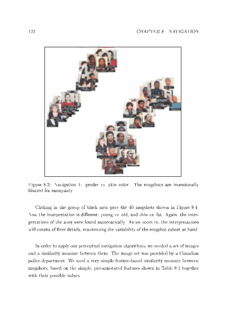
122 CHAPTER 8. NAVIGATION
Figure 8.3: Navigation 1: gender vs. skin color. The mugshots are intentionallyblurred for anonymity.
Clicking in the group of black men gave the 40 mugshots shown in Figure 8.4.
Now the interpretation is di�erent: young vs. old, and thin vs. fat. Again, the inter-
pretations of the axes were found automatically. As we zoom in, the interpretations
will consist of �ner details, maximizing the variability of the mugshot subset at hand.
In order to apply our perceptual navigation algorithms, we needed a set of images
and a similarity measure between them. The image set was provided by a Canadian
police department. We used a very simple feature-based similarity measure between
mugshots, based on the simple, pre-annotated features shown in Table 8.1 together
with their possible values.
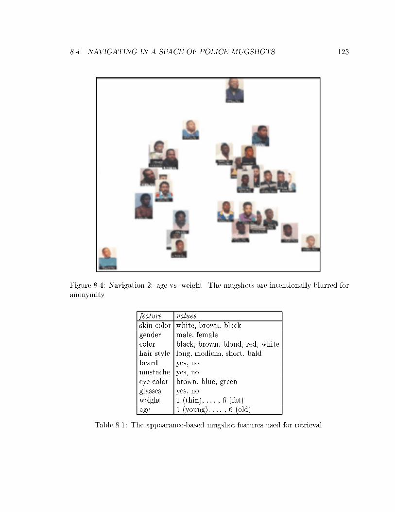
8.4. NAVIGATING IN A SPACE OF POLICE MUGSHOTS 123
Figure 8.4: Navigation 2: age vs. weight. The mugshots are intentionally blurred foranonymity.
feature valuesskin color white, brown, blackgender male, femalecolor black, brown, blond, red, whitehair style long, medium, short, baldbeard yes, nomustache yes, noeye color brown, blue, greenglasses yes, noweight 1 (thin), : : : , 6 (fat)age 1 (young), : : : , 6 (old)
Table 8.1: The appearance-based mugshot features used for retrieval.
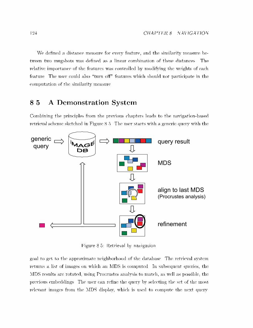
124 CHAPTER 8. NAVIGATION
We de�ned a distance measure for every feature, and the similarity measure be-
tween two mugshots was de�ned as a linear combination of these distances. The
relative importance of the features was controlled by modifying the weights of each
feature. The user could also \turn o�" features which should not participate in the
computation of the similarity measure.
8.5 A Demonstration System
Combining the principles from the previous chapters leads to the navigation-based
retrieval scheme sketched in Figure 8.5. The user starts with a generic query with the
generic
queryquery result
MDS
align to last MDS(Procrustes analysis)
refinement
Figure 8.5: Retrieval by navigation.
goal to get to the approximate neighborhood of the database. The retrieval system
returns a list of images on which an MDS is computed. In subsequent queries, the
MDS results are rotated, using Procrustes analysis to match, as well as possible, the
previous embeddings. The user can re�ne the query by selecting the set of the most
relevant images from the MDS display, which is used to compute the next query.
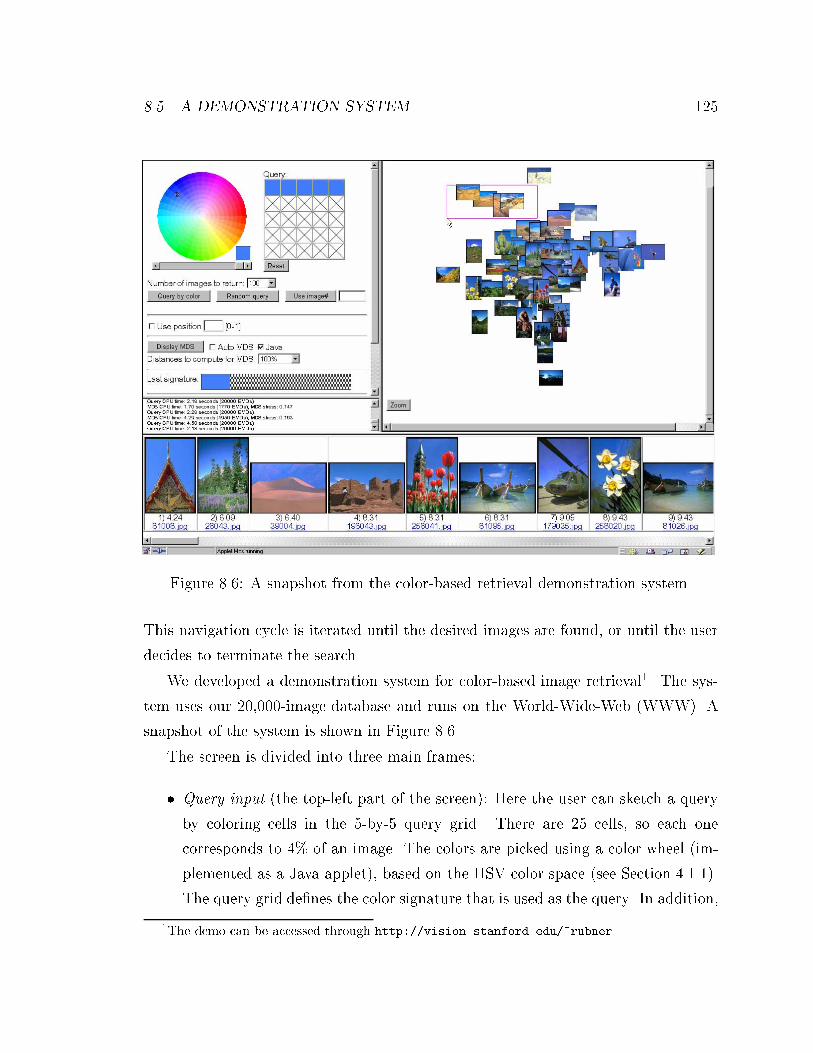
8.5. A DEMONSTRATION SYSTEM 125
Figure 8.6: A snapshot from the color-based retrieval demonstration system.
This navigation cycle is iterated until the desired images are found, or until the user
decides to terminate the search.
We developed a demonstration system for color-based image retrieval1. The sys-
tem uses our 20,000-image database and runs on the World-Wide-Web (WWW). A
snapshot of the system is shown in Figure 8.6.
The screen is divided into three main frames:
� Query input (the top-left part of the screen): Here the user can sketch a query
by coloring cells in the 5-by-5 query grid. There are 25 cells, so each one
corresponds to 4% of an image. The colors are picked using a color wheel (im-
plemented as a Java applet), based on the HSV color space (see Section 4.1.1).
The query grid de�nes the color signature that is used as the query. In addition,
1The demo can be accessed through http://vision.stanford.edu/~rubner.
126 CHAPTER 8. NAVIGATION
the user can specify the number of images the system should return, and other
parameters such as whether to compute the full distance matrix for the MDS
or use the missing values option.
� Query result (the bottom of the screen): This frame displays a scrollable list of
images returned by the last query, sorted by their distances from the query. The
distances and the image numbers are shown together with a small version of the
image. Clicking on the image initiates a new search where the color signature of
that image is used as the query. Clicking on the image number opens a window
with the full size image.
� MDS map (the top-right of the screen): Here the results of the MDS embeddings
are shown using small image thumbnails. Using the mouse, the user can explore
occluded images. The mouse can also be used to select sets of images which
generate the next query. Such a query is generated when the user clicks the
\zoom" button.
The system supports the following queries:
1. Random query: a speci�ed number of random images is returned.
2. Query-by-sketch: the user explicitly speci�es the color signature.
3. Query-by-example: the color signature of an image is used for the query.
4. Query-by-re�nement: the query is generated based on the common features in
a selected set of images.
The example in Figure 8.6 shows the �rst step of a search where the user is looking
for images of deserts. The initial generic query is 20% blue for the sky and 80% \don't
care." The best matches are shown in the results frame, and the MDS embedding of
100 returned images is shown in the MDS frame. The desert images, in the top left,
are selected for the next query.
Currently, our demonstration system satis�es a query by using a linear search
over all the images in the database, comparing their color signatures to the query,
8.6. SUMMARY 127
and keeping the N best matches, where N is speci�ed by the user. When the total
weight of the query is equal to the weights of the signatures, the lower bound from
Section 3.3.2 is used and the EMD between the signature and the current image
signature is computed only when the lower bound between the two is less than the
largest distance between the query and the N best matches so far. To be used as
a full image retrieval system, this demonstration system should be extended to deal
with better indexing, such that the image descriptors are stored in a way that allows a
sub-linear retrieval time. In addition, it should combine other modalities beside color,
including texture, shape, and composition, and should support a query language were
boolean operations are supported.
8.6 Summary
Intuitive image retrieval is a hard and ill-de�ned problem. Our attempt toward a
solution combines the EMD as a dissimilarity measure that agrees with perceptual
similarity, MDS as a better display technique that is easy to comprehend, and a
re�nement process that automatically generates successive queries. This framework
reduces the need to directly deal with image features, as queries can be posed by
the user starting with a vague description or even a random set of images and then
zooming into the relevant parts of the display. Our approach works well for color-
based and police mugshot retrieval.
There will come a time when you
believe everything is �nished. That
will be the beginning.
Louis L'Amour
Chapter 9
Conclusion and Future Directions
9.1 Conclusion
The methods presented in this thesis provide a novel set of tools and opens real
possibilities for content-based image retrieval systems. Tools are provided for image
retrieval, visualization of query results, and navigation in the space of images.
In Chapter 1, we listed questions that were to be addressed in this dissertation.
We now reconsider these questions, each followed by our approach and contributions
towards answering it:
� What features describe the content of an image well?
In Chapters 4 and 5 we focused on color and texture features, respectively. For
both, we carefully chose appropriate feature spaces and ground distances so
that the distances between single features agrees with perception. We showed
that these features lead to e�ective retrieval.
For color, we used the CIELab space, which was designed so that distances
between single colors conform to perceptual similarity. We presented an ex-
tension of the color features that also included the absolute position of colors
within the image. We used this extension when the layout of colors in the image
was important. For texture, we designed Gabor �lters on a log-polar grid to
model the texture content of an image. We developed dissimilarity measures for
128
9.1. CONCLUSION 129
homogeneous textures and for images that comprise many textures. For homo-
geneous textures we also presented dissimilarity measures invariant to changes
in rotation and scale. In Section 7.4 we showed that these texture features lead
to dissimilarity measures that agree with perception.
� How to summarize the distribution of these features over an image?
In Chapter 2 we introduced signatures as a compact and e�cient representation
for feature distributions. We compared signatures to the commonly used his-
tograms and showed, in Chapter 6, that signatures often lead to better results
than histograms, even when the size of the signatures is signi�cantly smaller
than that of the histograms.
� How do we measure the dissimilarity between distributions of features?
The core of any retrieval system is a dissimilarity measure that is able to �nd
and return the most relevant images in a way that conforms to the users' no-
tion of similarity. We made a distinction between the ground distance, which
measures dissimilarity of single features, and the dissimilarity between feature
distributions. In Chapter 3 we developed the EMD to extend the ground dis-
tance to dissimilarities between feature distributions. The EMD is a general and
exible metric and does not su�er from the binning problems of most extant
de�nitions of distribution dissimilarity. It allows for partial matches, and lower
bounds are readily available for it. In addition, as demonstrated in Chapter 6,
for images with moderate similarities, the EMD gave better results than other
dissimilarity measures.
� How can we e�ectively display the results of a search?
Instead of displaying the returned images as a list sorted by dissimilarity from
the query, as done in most image retrieval systems, we use the full dissimilarity
matrix of the images. We showed in Chapter 7 that applying MDS to the
dissimilarity matrix and placing image thumbnails at the coordinates of the
resulting low-dimensional embeddings leads to an intuitive display that conveys
information about how the images relate to each other.
130 CHAPTER 9. CONCLUSION AND FUTURE DIRECTIONS
� How can a user browse the images in the database in an intuitive and e�cient
way?
We coupled the notion of browsing with that of visualization. No browsing
is possible without an appropriate display. Using our display technique we
developed a navigation scheme that allows the user to intuitively retrieve images
by zooming in promising areas of the display, with re�nement of the query done
automatically. We demonstrated this technique for color-based retrieval and for
police mugshot retrieval.
Additional contributions of this dissertation are the following:
� In Chapter 6 we provided an extensive comparison of various dissimilarity
measures that are used in image retrieval systems. Comparisons were made
for di�erent combinations of parameters, such as the number of bins (for the
histogram-based dissimilarity measures), the size of the �lter bank (for texture),
and the balance between precision and recall.
� We presented texture-based retrieval without the need to segment the images
�rst as dome by most methods. This is possible due to the combination of the
texture features with the ability of the EMD to do partial matches.
� We developed a demonstration system, described in Section 8.5, by which peo-
ple can access remotely and experiment with the methods presented in this
dissertation on a 20,000-image database.
9.2 Future Directions
The EMD can be applied to other modalities besides color and texture as long as a
ground distance can be de�ned in the appropriate feature space. Examples include
shape, compositions of objects, eigenimage similarity, among other image features
[3, 24, 29, 64, 66, 85, 96]. A larger ensemble of features from di�erent modalities
can improve the overall performance of an image retrieval system. The EMD can
9.2. FUTURE DIRECTIONS 131
bene�t other applications beside image retrieval. Good results were achieved for the
comparison of vector �elds [51] and for detecting color edges [83].
The idea of adaptive image embedding is also not limited to color and texture
and can be applied to other modalities as long as some notion of similarity, metric or
not, continuous or discrete, can be de�ned. This method was successfully applied to
computer-assisted parameter setting for animation [58], and to visualization of vector
�eld images [51].
In this context, the key question, which we leave for future work, is to determine
whether the embeddings and the main axes of variation \discovered" by MDS for
each of these distances and for various types of image distributions are perceptually
meaningful. We believe that since MDS groups similar images together|and away
from dissimilar ones|this is often the case. We also plan to study more the relations
between the axes chosen by MDS for related or overlapping image sets. Knowing the
correspondence between these `local charts' (in the sense of topology) of the image
space may help provide a better sense of navigation.
Although our experience is that the process of image retrieval is improved by
our navigation scheme, a more principled comparison between database navigation
techniques is needed. Current research that studies the responses of users for di�erent
image retrieval methods [73] reports that most users �nd our navigation method
e�ective1.
A query language that allows more complex queries must be devised for e�ective
image retrieval. Such a language needs to include operators like \and," \or," and
\not." In addition, image retrieval systems need to integrate di�erent modalities
such as color, texture, and shape. The correct combination of these features, and the
adjustment of their relative importance according to the user responses, is another
topic of future research.
1The experiment in [73] used our navigation method with only color information. The users,in general, agreed that although the method is promising, color alone is not su�cient for imageretrieval.
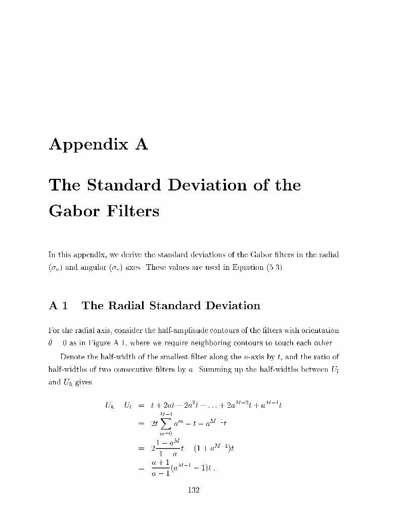
Appendix A
The Standard Deviation of the
Gabor Filters
In this appendix, we derive the standard deviations of the Gabor �lters in the radial
(�u) and angular (�v) axes. These values are used in Equation (5.3).
A.1 The Radial Standard Deviation
For the radial axis, consider the half-amplitude contours of the �lters with orientation
� = 0 as in Figure A.1, where we require neighboring contours to touch each other.
Denote the half-width of the smallest �lter along the u-axis by t, and the ratio of
half-widths of two consecutive �lters by a. Summing up the half-widths between Ul
and Uh gives
Uh � Ul = t + 2at+ 2a2t + : : :+ 2aM�2t+ aM�1t
= 2tM�1Xm=0
am � t� aM�1t
= 21� aM
1� at� (1 + aM�1)t
=a+ 1
a� 1(aM�1 � 1)t :
132
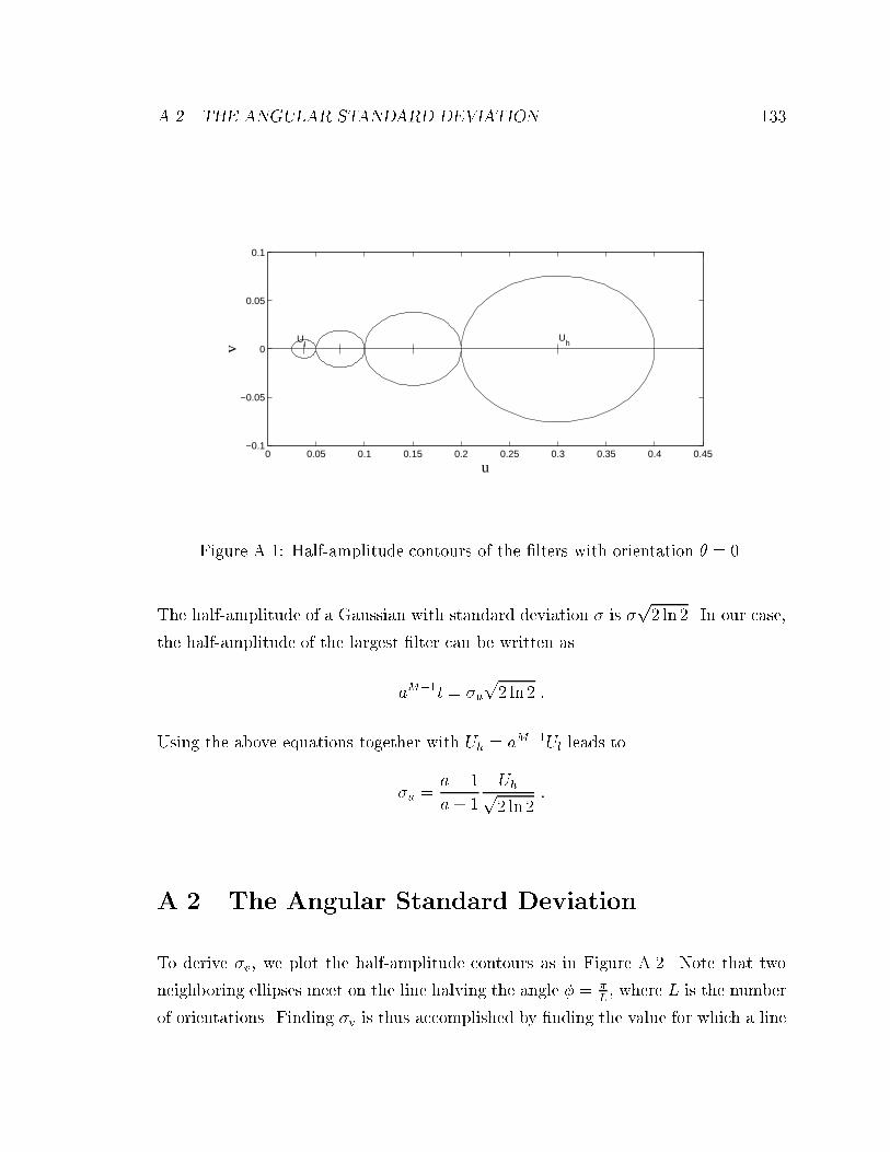
A.2. THE ANGULAR STANDARD DEVIATION 133
0 0.05 0.1 0.15 0.2 0.25 0.3 0.35 0.4 0.45−0.1
−0.05
0
0.05
0.1
u
v
UhU
l
Figure A.1: Half-amplitude contours of the �lters with orientation � = 0.
The half-amplitude of a Gaussian with standard deviation � is �p2 ln 2. In our case,
the half-amplitude of the largest �lter can be written as
aM�1t = �up2 ln 2 :
Using the above equations together with Uh = aM�1Ul leads to
�u =a� 1
a+ 1
Uhp2 ln 2
:
A.2 The Angular Standard Deviation
To derive �v, we plot the half-amplitude contours as in Figure A.2. Note that two
neighboring ellipses meet on the line halving the angle � = �L, where L is the number
of orientations. Finding �v is thus accomplished by �nding the value for which a line
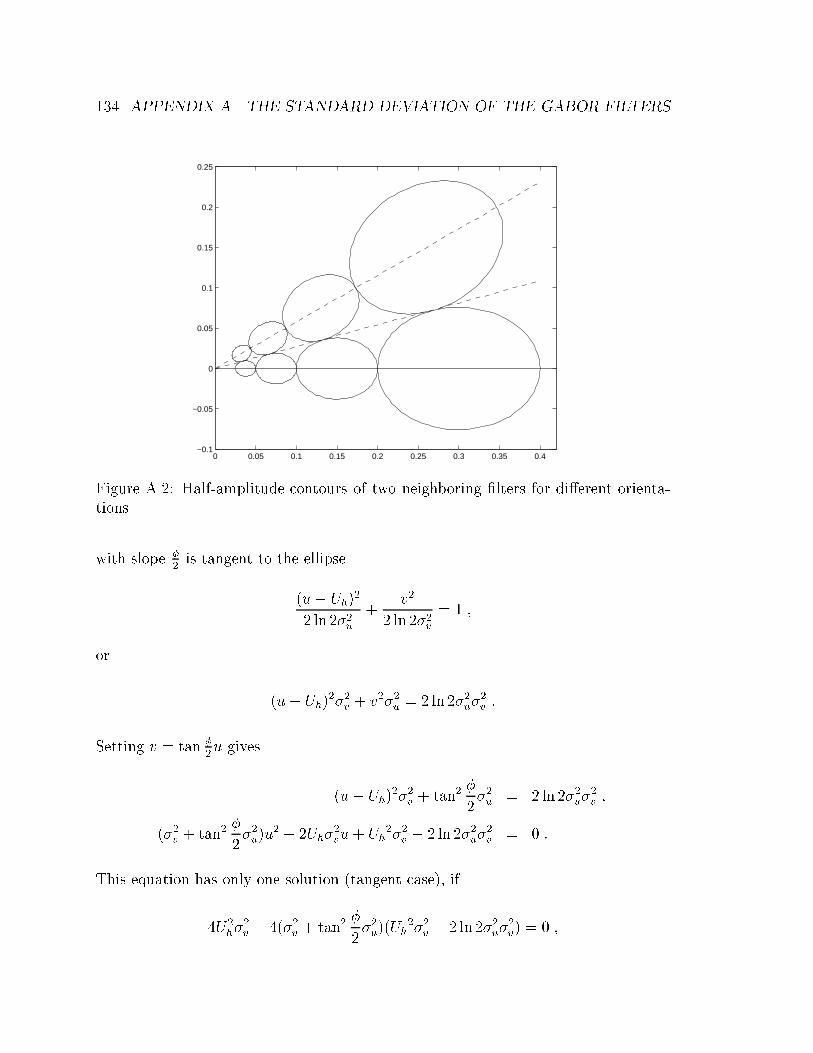
134 APPENDIX A. THE STANDARD DEVIATION OF THE GABOR FILTERS
0 0.05 0.1 0.15 0.2 0.25 0.3 0.35 0.4−0.1
−0.05
0
0.05
0.1
0.15
0.2
0.25
Figure A.2: Half-amplitude contours of two neighboring �lters for di�erent orienta-tions.
with slope �2is tangent to the ellipse
(u� Uh)2
2 ln 2�2u+
v2
2 ln 2�2v= 1 ;
or
(u� Uh)2�2v + v2�2u = 2 ln 2�2u�
2v :
Setting v = tan �2u gives
(u� Uh)2�2v + tan2
�
2�2u = 2 ln 2�2u�
2v ;
(�2v + tan2�
2�2u)u
2 � 2Uh�2vu+ Uh
2�2v � 2 ln 2�2u�2v = 0 :
This equation has only one solution (tangent case), if
4U2h�
2v � 4(�2v + tan2
�
2�2u)(Uh
2�2v � 2 ln 2�2u�2v) = 0 ;

A.2. THE ANGULAR STANDARD DEVIATION 135
which leads to
�v = tan�
2
rU2h
2 ln 2� �2u :
Appendix B
Retrieval Performance Plots
In this appendix we collect plots of the results of the experiments we conducted in
Chapter 6. In these plots, the EMD for signatures is always computed using 8 clusters.
136
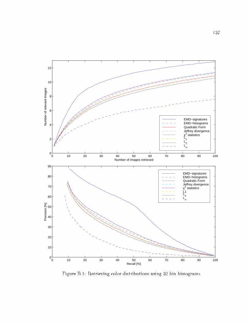
137
0 10 20 30 40 50 60 70 80 90 1000
2
4
6
8
10
12
Number of images retrieved
Num
ber
of r
elev
ant i
mag
es
EMD−signatures EMD−histograms Quadratic Form Jeffrey divergenceχ2 statistics L
1
L2
L∞
0 10 20 30 40 50 60 70 80 90 1000
10
20
30
40
50
60
70
80
90
Recall [%]
Pre
cisi
on [%
]
EMD−signatures EMD−histograms Quadratic Form Jeffrey divergenceχ2 statistics L1 L
2
L∞
Figure B.1: Retrieving color distributions using 32 bin histograms.
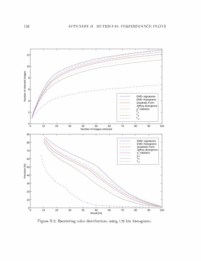
138 APPENDIX B. RETRIEVAL PERFORMANCE PLOTS
0 10 20 30 40 50 60 70 80 90 1000
2
4
6
8
10
12
Number of images retrieved
Num
ber
of r
elev
ant i
mag
es
EMD−signatures EMD−histograms Quadratic Form Jeffrey divergenceχ2 statistics L
1
L2
L∞
0 10 20 30 40 50 60 70 80 90 1000
10
20
30
40
50
60
70
80
90
Recall [%]
Pre
cisi
on [%
]
EMD−signatures EMD−histograms Quadratic Form Jeffrey divergenceχ2 statistics L1 L
2
L∞
Figure B.2: Retrieving color distributions using 128 bin histograms.
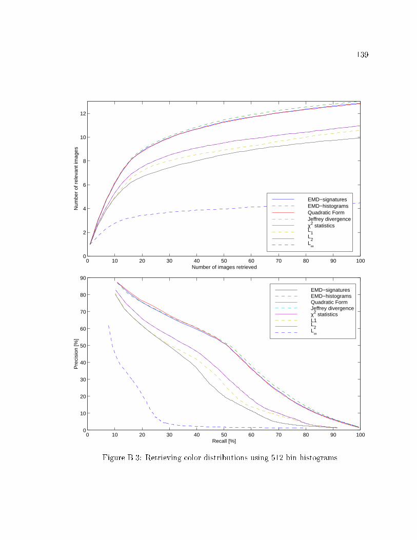
139
0 10 20 30 40 50 60 70 80 90 1000
2
4
6
8
10
12
Number of images retrieved
Num
ber
of r
elev
ant i
mag
es
EMD−signatures EMD−histograms Quadratic Form Jeffrey divergenceχ2 statistics L
1
L2
L∞
0 10 20 30 40 50 60 70 80 90 1000
10
20
30
40
50
60
70
80
90
Recall [%]
Pre
cisi
on [%
]
EMD−signatures EMD−histograms Quadratic Form Jeffrey divergenceχ2 statistics L1 L
2
L∞
Figure B.3: Retrieving color distributions using 512 bin histograms.
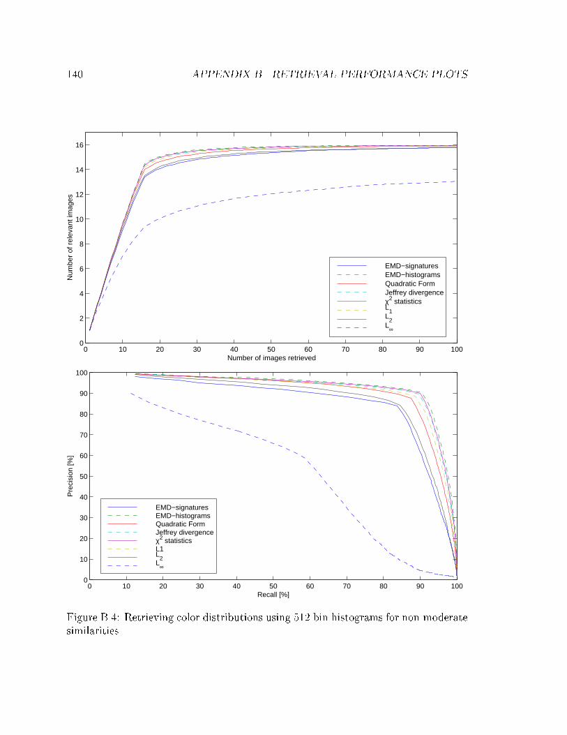
140 APPENDIX B. RETRIEVAL PERFORMANCE PLOTS
0 10 20 30 40 50 60 70 80 90 1000
2
4
6
8
10
12
14
16
Number of images retrieved
Num
ber
of r
elev
ant i
mag
es
EMD−signatures EMD−histograms Quadratic Form Jeffrey divergenceχ2 statistics L
1
L2
L∞
0 10 20 30 40 50 60 70 80 90 1000
10
20
30
40
50
60
70
80
90
100
Recall [%]
Pre
cisi
on [%
]
EMD−signatures EMD−histograms Quadratic Form Jeffrey divergenceχ2 statistics L1 L
2
L∞
Figure B.4: Retrieving color distributions using 512 bin histograms for non-moderatesimilarities.
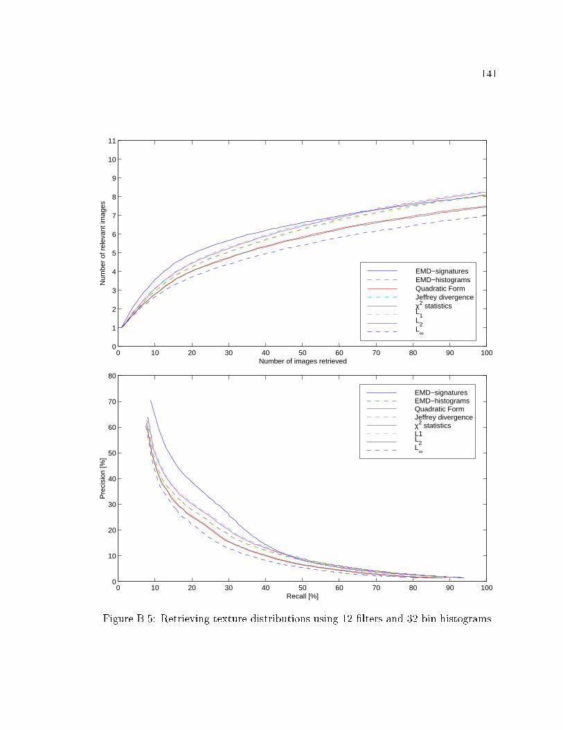
141
0 10 20 30 40 50 60 70 80 90 1000
1
2
3
4
5
6
7
8
9
10
11
Number of images retrieved
Num
ber
of r
elev
ant i
mag
es
EMD−signatures EMD−histograms Quadratic Form Jeffrey divergenceχ2 statistics L
1
L2
L∞
0 10 20 30 40 50 60 70 80 90 1000
10
20
30
40
50
60
70
80
Recall [%]
Pre
cisi
on [%
]
EMD−signatures EMD−histograms Quadratic Form Jeffrey divergenceχ2 statistics L1 L
2
L∞
Figure B.5: Retrieving texture distributions using 12 �lters and 32 bin histograms.
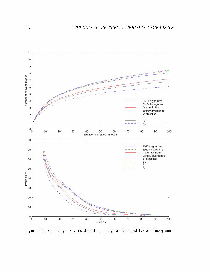
142 APPENDIX B. RETRIEVAL PERFORMANCE PLOTS
0 10 20 30 40 50 60 70 80 90 1000
1
2
3
4
5
6
7
8
9
10
11
Number of images retrieved
Num
ber
of r
elev
ant i
mag
es
EMD−signatures EMD−histograms Quadratic Form Jeffrey divergenceχ2 statistics L
1
L2
L∞
0 10 20 30 40 50 60 70 80 90 1000
10
20
30
40
50
60
70
80
Recall [%]
Pre
cisi
on [%
]
EMD−signatures EMD−histograms Quadratic Form Jeffrey divergenceχ2 statistics L1 L
2
L∞
Figure B.6: Retrieving texture distributions using 12 �lters and 128 bin histograms.
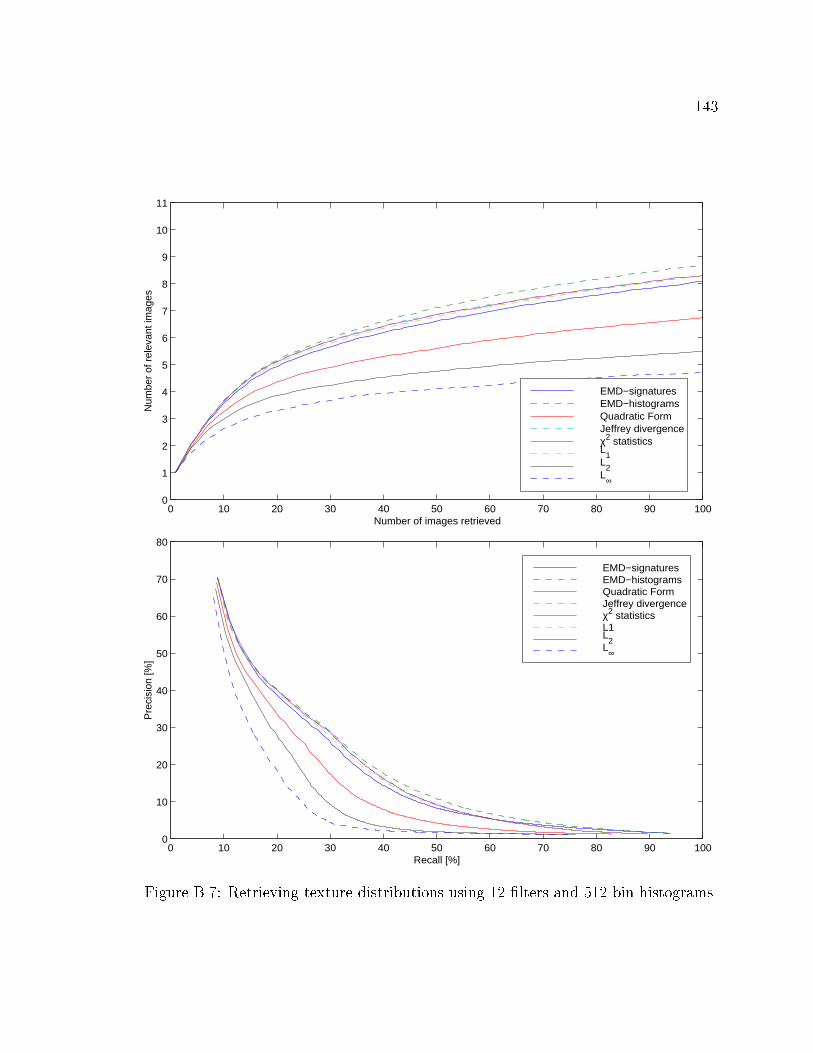
143
0 10 20 30 40 50 60 70 80 90 1000
1
2
3
4
5
6
7
8
9
10
11
Number of images retrieved
Num
ber
of r
elev
ant i
mag
es
EMD−signatures EMD−histograms Quadratic Form Jeffrey divergenceχ2 statistics L
1
L2
L∞
0 10 20 30 40 50 60 70 80 90 1000
10
20
30
40
50
60
70
80
Recall [%]
Pre
cisi
on [%
]
EMD−signatures EMD−histograms Quadratic Form Jeffrey divergenceχ2 statistics L1 L
2
L∞
Figure B.7: Retrieving texture distributions using 12 �lters and 512 bin histograms.
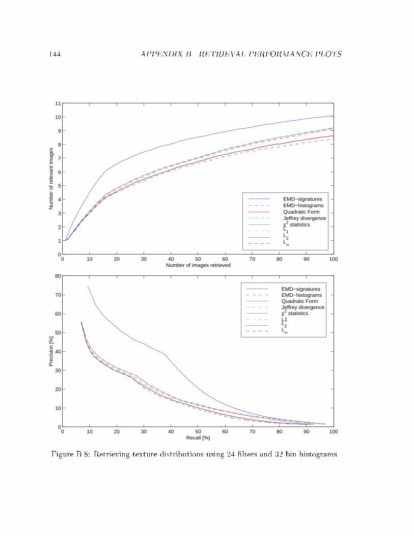
144 APPENDIX B. RETRIEVAL PERFORMANCE PLOTS
0 10 20 30 40 50 60 70 80 90 1000
1
2
3
4
5
6
7
8
9
10
11
Number of images retrieved
Num
ber
of r
elev
ant i
mag
es
EMD−signatures EMD−histograms Quadratic Form Jeffrey divergenceχ2 statistics L
1
L2
L∞
0 10 20 30 40 50 60 70 80 90 1000
10
20
30
40
50
60
70
80
Recall [%]
Pre
cisi
on [%
]
EMD−signatures EMD−histograms Quadratic Form Jeffrey divergenceχ2 statistics L1 L
2
L∞
Figure B.8: Retrieving texture distributions using 24 �lters and 32 bin histograms.
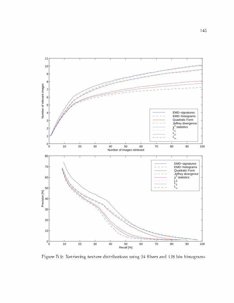
145
0 10 20 30 40 50 60 70 80 90 1000
1
2
3
4
5
6
7
8
9
10
11
Number of images retrieved
Num
ber
of r
elev
ant i
mag
es
EMD−signatures EMD−histograms Quadratic Form Jeffrey divergenceχ2 statistics L
1
L2
L∞
0 10 20 30 40 50 60 70 80 90 1000
10
20
30
40
50
60
70
80
Recall [%]
Pre
cisi
on [%
]
EMD−signatures EMD−histograms Quadratic Form Jeffrey divergenceχ2 statistics L1 L
2
L∞
Figure B.9: Retrieving texture distributions using 24 �lters and 128 bin histograms.
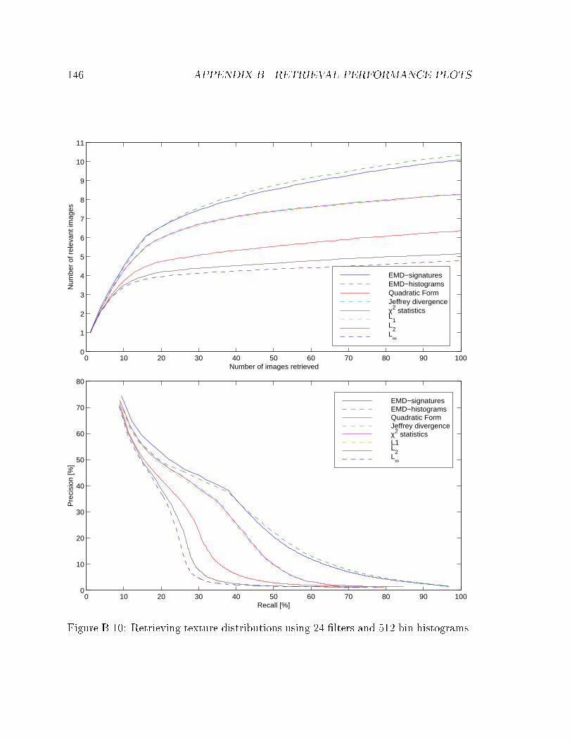
146 APPENDIX B. RETRIEVAL PERFORMANCE PLOTS
0 10 20 30 40 50 60 70 80 90 1000
1
2
3
4
5
6
7
8
9
10
11
Number of images retrieved
Num
ber
of r
elev
ant i
mag
es
EMD−signatures EMD−histograms Quadratic Form Jeffrey divergenceχ2 statistics L
1
L2
L∞
0 10 20 30 40 50 60 70 80 90 1000
10
20
30
40
50
60
70
80
Recall [%]
Pre
cisi
on [%
]
EMD−signatures EMD−histograms Quadratic Form Jeffrey divergenceχ2 statistics L1 L
2
L∞
Figure B.10: Retrieving texture distributions using 24 �lters and 512 bin histograms.
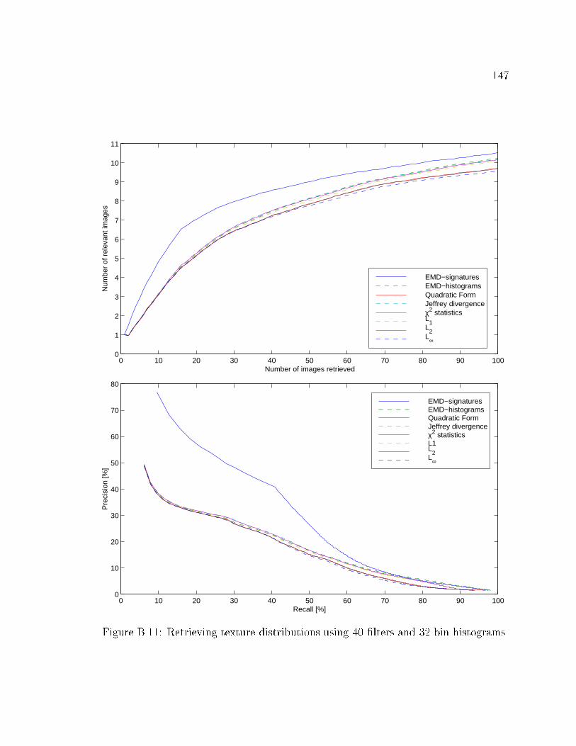
147
0 10 20 30 40 50 60 70 80 90 1000
1
2
3
4
5
6
7
8
9
10
11
Number of images retrieved
Num
ber
of r
elev
ant i
mag
es
EMD−signatures EMD−histograms Quadratic Form Jeffrey divergenceχ2 statistics L
1
L2
L∞
0 10 20 30 40 50 60 70 80 90 1000
10
20
30
40
50
60
70
80
Recall [%]
Pre
cisi
on [%
]
EMD−signatures EMD−histograms Quadratic Form Jeffrey divergenceχ2 statistics L1 L
2
L∞
Figure B.11: Retrieving texture distributions using 40 �lters and 32 bin histograms.
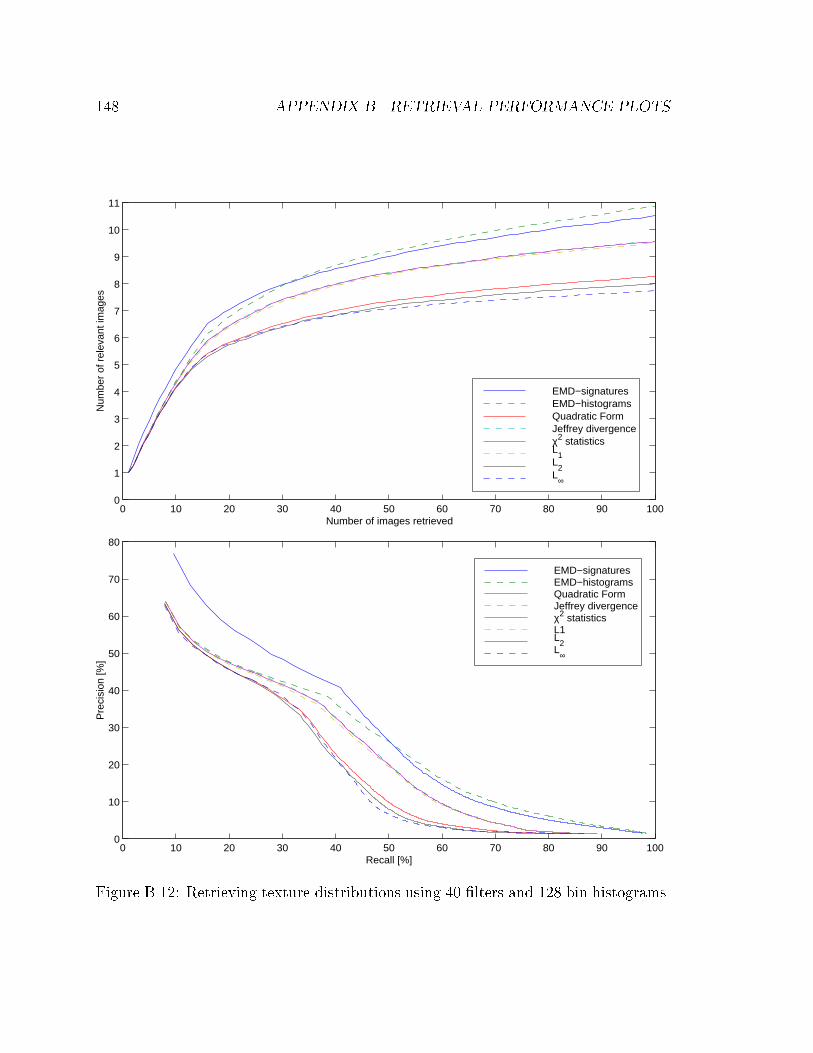
148 APPENDIX B. RETRIEVAL PERFORMANCE PLOTS
0 10 20 30 40 50 60 70 80 90 1000
1
2
3
4
5
6
7
8
9
10
11
Number of images retrieved
Num
ber
of r
elev
ant i
mag
es
EMD−signatures EMD−histograms Quadratic Form Jeffrey divergenceχ2 statistics L
1
L2
L∞
0 10 20 30 40 50 60 70 80 90 1000
10
20
30
40
50
60
70
80
Recall [%]
Pre
cisi
on [%
]
EMD−signatures EMD−histograms Quadratic Form Jeffrey divergenceχ2 statistics L1 L
2
L∞
Figure B.12: Retrieving texture distributions using 40 �lters and 128 bin histograms.
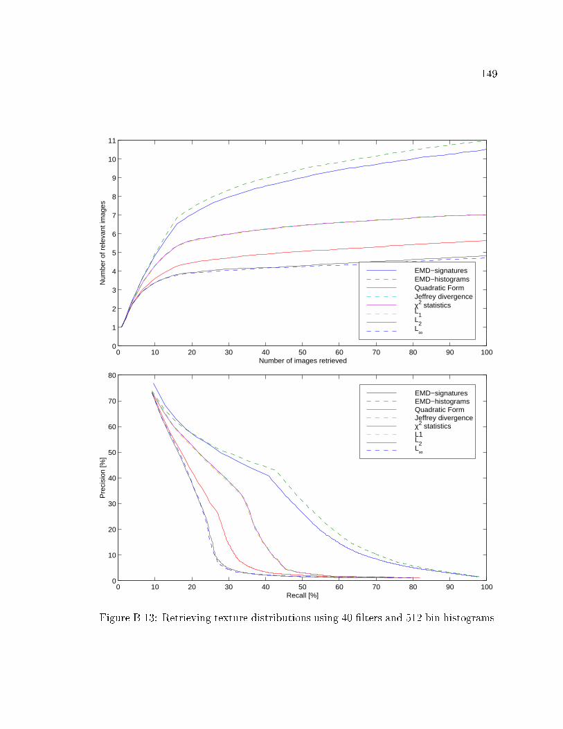
149
0 10 20 30 40 50 60 70 80 90 1000
1
2
3
4
5
6
7
8
9
10
11
Number of images retrieved
Num
ber
of r
elev
ant i
mag
es
EMD−signatures EMD−histograms Quadratic Form Jeffrey divergenceχ2 statistics L
1
L2
L∞
0 10 20 30 40 50 60 70 80 90 1000
10
20
30
40
50
60
70
80
Recall [%]
Pre
cisi
on [%
]
EMD−signatures EMD−histograms Quadratic Form Jeffrey divergenceχ2 statistics L1 L
2
L∞
Figure B.13: Retrieving texture distributions using 40 �lters and 512 bin histograms.
Bibliography
[1] E. H. Adelson and J. R. Bergen. Spatiotemporal energy models for the percep-
tion of motion. Journal of the Optical Society of America A - Optics and Image
Science, 2(2):284{299, February 1985.
[2] R. K. Ahuja, T. L. Magnanti, and J. B. Orlin. Network Flows. Prentice Hall,
Englewood Cli�s, NJ, 1993.
[3] J. R. Bach, C. Fuller, A. Gupta, A. Hampapur, B. Horowitz, R. Humphrey,
R. Jain, and C. Shu. Virage image search engine: an open framework for image
management. In SPIE Conference on Storage and Retrieval for Image and
Video Databases IV, volume 2670, pages 76{87, March 1996.
[4] S. Belongie, C. Carson, H. Greenspan, and J. Malik. Color- and texture-based
image segmentation using EM and its application to content-based image re-
trieval. In IEEE International Conference on Computer Vision, pages 675{682,
Bombay, India, January 1998.
[5] J. L. Bentley. Multidimensional binary search trees used for associative search-
ing. Communications of the ACM, 18:509{517, September 1975.
[6] J. Big�un and J. M. du Buf. N-folded symmetries by complex moments in
Gabor space and their application to unsupervised texture segmentation. IEEE
Transactions on Pattern Analysis and Machine Intelligence, 16(1):80{87, 1994.
[7] A. C. Bovik, M. Clark, and W. S. Geisler. Multichannel texture analysis using
localized spatial �lters. IEEE Transactions on Pattern Analysis and Machine
Intelligence, 12(12):55{73, 1990.
150
BIBLIOGRAPHY 151
[8] T. Bozkaya and M. Ozsoyoglu. Distance-based indexing for high-dimensional
metric spaces. SIGMOD Record (ACM Special Interest Group on Management
of Data), 26(2):357{368, May 1997.
[9] P. Brodatz. Textures: A Photographic Album for Artists and Designers. Dover,
New York, NY, 1966.
[10] K. L. Clarkson. Nearest neighbor queries in metric spaces. In ACM Symposium
on the Theory of Computing, pages 609{617, May 1997.
[11] S. Cohen. Finding Color and Shape Patterns in Images. PhD thesis, Stanford
University, 1999. To be published.
[12] S. D. Cohen and L. J. Guibas. The earth mover's distance: Lower bounds and
invariance under translation. Technical Report STAN-CS-TR-97-1597, Stanford
University, November 1997.
[13] T. M. Cover and J. A. Thomas. Elements of Information Theory. Wiley Series
in Telecommunications. John Wiley & Sons, New York, NY, USA, 1991.
[14] T. F. Cox and M. A. A. Cox. Multidimensional Scaling. Monographs on statis-
tics and applied probability; 59. Chapman and Hall, London, 1994.
[15] A. Cumani. Edge detection in multispectral images. Computer, Vision, Graph-
ics, and Image Processing, 53(1):40{51, 1991.
[16] R. B. D'Agostino and M. A. Stephens, editors. Goodness-of-�t techniques.
Statistics: Textbooks and Monographs, 68. Marcel Dekke, New York, 1986.
[17] G. B. Dantzig. Linear Programming and Extensions. Princeton University
Press, Princeton, NJ, 1963.
[18] M. Das, E. M. Riseman, and B. A. Draper. FOCUS : Searching for multi-colored
objects in a diverse image database. In Proceedings of the IEEE Conference on
Computer Vision and Pattern Recognition, pages 756{761, June 1997.
152 BIBLIOGRAPHY
[19] I. Daubechies. Ten Lectures on Wavelets. Number 61 in CBMS-NSF Regional
Conference Series in Applied Mathematics. Society for Industrial and Applied
Mathematics, Philadelphia, 1992.
[20] J. D. Daugman. Complete discrete 2-d Gabor transforms by neural networks
for image analysis and compression. IEEE Transactions on Acoustics, Speech,
and Signal Processing, 36:1169{1179, 1988.
[21] S. Di Zenzo. A note on the gradient of a multi-image. Computer, Vision,
Graphics, and Image Processing, 33:116{125, 1986.
[22] R. O. Duda and P. E. Hart. Pattern classi�cation and scene analysis. Wiley,
New York, 1973.
[23] O. V. E. and S. M. Chabot: Retrieval from a relational database of images.
Computer, pages 40{48, September 1995.
[24] C. Faloutsos, R. Barber, M. Flickner, J. Hafner, W. Niblack, D. Petkovic, and
W. Equitz. E�cient and e�ective querying by image content. Journal of Intel-
ligent Information Systems, 3:231{262, 1994.
[25] F. Farrokhnia and A. K. Jain. A multi-channel �ltering approach to texture
segmentation. In Proceedings of the IEEE Conference on Computer Vision and
Pattern Recognition, pages 364{370, June 1991.
[26] J. Feder. Image recognition and content-based retrieval for the world wide web.
Advanced Imaging, 11(1):26{28, January 1996.
[27] D. J. Field. Relations between the statistics of natural images and the re-
sponse properties of cortical cells. Journal of the Optical Society of America A,
4(12):2379{2394, December 1987.
[28] M. Flickner, H. S. Sawhney, J. Ashley, Q. Huang, B. Dom, M. Gorkani,
J. Hafner, D. Lee, D. Petkovic, D. Steele, and P. Yanker. Query by image
and video content: The QBIC system. IEEE Computer, 28(9):23{32, Septem-
ber 1995.
BIBLIOGRAPHY 153
[29] D. Forsyth, J. Malik, M. Fleck, H. Greenspan, and T. Leung. Finding pictures
of objects in large collections of images. In International Workshop on Object
Recognition for Computer Vision, Cambridge, UK, April 1996.
[30] D. Gabor. Theory of communication. The Journal of the Institute of Electrical
Engineers, Part III, 93(21):429{457, January 1946.
[31] J. E. Gary and R. Mehrotra. Similar shape retrieval using a structural feature
index. Information Systems, 18(7):525{537, October 1930.
[32] D. Geman, S. Geman, C. Gra�gne, and P. Dong. Boundary detection by
constrained optimization. IEEE Transactions on Pattern Analysis and Machine
Intelligence, 12(7):609{628, 1990.
[33] A. Gersho and R. M. Gray. Vector quantization and signal compression. Kluwer
Academic Publishers, Boston, MA, 1992.
[34] G. H. Golub and C. F. Van Loan. Matrix Computations. The Johns Hopkins
University Press, Baltimore, Md, 1996. 3rd edition.
[35] J. Hafner, H. S. Sawhney, W. Equitz, M. Flickner, and W. Niblack. E�cient
color histogram indexing for quadratic form distance functions. IEEE Transac-
tions on Pattern Analysis and Machine Intelligence, 17(7):729{735, 1995.
[36] D. J. Heeger and J. R. Bergen. Pyramid-based texture analysis/synthesis. In
Computer Graphics, pages 229{238. ACM SIGGRAPH, 1995.
[37] F. S. Hillier and G. J. Lieberman. Introduction to Mathematical Programming.
McGraw-Hill, 1990.
[38] F. L. Hitchcock. The distribution of a product from several sources to numerous
localities. J. Math. Phys., 20:224{230, 1941.
[39] T. Hofmann, J. Puzicha, and J. Buhmann. Unsupervised texture segmentation
in a deterministic annealing framework. IEEE Transactions on Pattern Analysis
and Machine Intelligence, 20(8):803{818, 1998.
154 BIBLIOGRAPHY
[40] T. Y. Hou, A. Hsu, P. Liu, and M. Y. Chiu. A content-based indexing technique
using relative geometry features. In SPIE Conference on Image Storage and
Retrieval Systems, volume 1662, pages 59{68, 1992.
[41] F. Idris and S. Panchanathan. Review of image and video indexing techniques.
Journal of Visual Communication and Image Representation, 8(2):146{166,
June 1997.
[42] H. V. Jagadish. A retrieval technique for similar shapes. In Proceedings of the
1991 ACM SIGMOD International Conference on Management of Data, pages
208{217, Denver, Colorado, 1991. ACM Press.
[43] B. J�ahne. Digital Image Processing. Springer, 1995.
[44] A. K. Jain and A. Vailaya. Image retrieval using color and shape. Pattern
Recognition, 29(8):1233{1244, 1996.
[45] N. Karmarkar. A new polynomial-time algorithm for linear programming. In
Proceedings of the Sixteenth Annual ACM Symposium on Theory of Computing,
pages 302{311, Washington, D.C., April 1984.
[46] V. Klee and G. Minty. How good is the simplex algorithm. In O. Shisha, editor,
Inequalities, volume III, pages 159{175. Academic Press, New York, N.Y., 1972.
[47] H. Knutsson and G. H. Granlund. Texture analysis using two-dimensional
quadrature �lters. IEEE Computer Society Workshop on Computer Architecture
for Pattern Analysis and Image Database Management, 1983.
[48] E. Kreyszing. Di�erential Geometry. University of Toronto Press, Toronto,
1959.
[49] J. B. Kruskal. Multi-dimensional scaling by optimizing goodness-of-�t to a
nonmetric hypothesis. Psychometrika, 29:1{27, 1964.
[50] S. Kullback. Information Theory and Statistics. Dover, New York, NY, 1968.
BIBLIOGRAPHY 155
[51] Y. Lavin, R. Batra, and L. Hesselink. Feature comparisons of vector �elds
using earth mover's distance. In IEEE/ACM Visualization '98, pages 413{415,
October 1998.
[52] T. S. Lee. Image representation using 2d Gabor wavelets. IEEE Transactions
on Pattern Analysis and Machine Intelligence, 18(10):959{971, 1996.
[53] F. Liu and R. W. Picard. Periodicity, directionality, and randomness: Wold fea-
tures for image modeling and retrieval. IEEE Transactions on Pattern Analysis
and Machine Intelligence, 18(7):722{733, 1996.
[54] W. Y. Ma and B. S. Manjunath. Texture features and learning similarity. In
IEEE Conference on Computer Vision and Pattern Recognition, pages 425{430,
San Francisco, CA, 1996.
[55] J. Malik and P. Perona. Preattentive texture discrimination with early vision
mechanisms. Journal of the Optical Society of America A, 7(5):923{932, May
1990.
[56] B. S. Manjunath and W. Y. Ma. Texture features for browsing and retrieval of
image data. IEEE Transactions on Pattern Analysis and Machine Intelligence,
18(8):837{842, 1996.
[57] J. Mao and A. Jain. Texture classi�cation and segmentation using multires-
olution simultaneous autoregressive models. Pattern Recognition, 25:173{188,
1992.
[58] J. Marks, B. Andalman, P. Beardsley, B. Freeman, S. Gibson, J. Hodgins,
T. Kang, B. Mirtich, H. P�ster, W. Ruml, J. Seims, and S. Shieberr. Design
galleries: A general approach to setting parameters for computer graphics and
animation. In SIGGRAPH 97, pages 389{400, Los Angeles CA, 1997.
[59] T. Minka and R. Picard. Interactive learning with a society of models. Pattern
Recognition, 30(4):565{581, April 1997.
156 BIBLIOGRAPHY
[60] G. Monge. M�emoire sur la th�eorie des d�eblais et des remblais. Histoire de
l'Acad�emie des sciences de Paris, avec les M�emoires de math�ematique et de
physique pour la meme ann�ee, pages 666{704, 1781.
[61] N. M. Nasrabad and R. A. King. Image coding using vector quantization: A
review. IEEE Transactions on Communication, 36(8):957{971, August 1988.
[62] W. Niblack, R. Barber, W. Equitz, M. D. Flickner, E. H. Glasman, D. Petkovic,
P. Yanker, C. Faloutsos, G. Taubin, and Y. Heights. Querying images by con-
tent, using color, texture, and shape. In SPIE Conference on Storage and
Retrieval for Image and Video Databases, volume 1908, pages 173{187, April
1993.
[63] T. Ojala, M. Pietik�ainen, and D. Harwood. A comparative study of texture
measures with classi�cation based on feature distributions. Pattern Recognition,
29(1):51{59, 1996.
[64] G. Pass and R. Zabih. Histogram re�nement for content-based image retrieval.
In IEEE Workshop on Applications of Computer Vision, Sarasota, FL, 1996.
[65] S. Peleg, M. Werman, and H. Rom. A uni�ed approach to the change of res-
olution: Space and gray-level. IEEE Transactions on Pattern Analysis and
Machine Intelligence, 11:739{742, 1989.
[66] A. Pentland, R. W. Picard, and S. Sclaro�. Photobook: content-based ma-
nipulation of image databases. International Journal of Computer Vision,
18(3):233{254, June 1996.
[67] P. Perona. Deformable kernels for early vision. In Proceedings of the IEEE
Conference on Computer Vision and Pattern Recognition, pages 222{227, June
1991.
[68] P. Perona and J. Malik. Scale-space and edge detection using anisotropic
di�usion. IEEE Transactions on Pattern Analysis and Machine Intelligence,
12(7):629{939, 1990.
BIBLIOGRAPHY 157
[69] R. W. Picard and T. P. Minka. Vision texture for annotation. Multimedia
Systems, 3:3{14, 1995.
[70] C. Poynton. A Technical Introduction to Digital Video. John Wiley and Sons,
New York, NY, 1996.
[71] J. Puzicha, T. Hofmann, and J. Buhmann. Non-parametric similarity measures
for unsupervised texture segmentation and image retrieval. In Proceedings of the
IEEE Conference on Computer Vision and Pattern Recognition, pages 267{272,
June 1997.
[72] S. T. Rachev. The Monge-Kantorovich mass transference problem and
its stochastic applications. Theory of Probability and its Applications,
XXIX(4):647{676, 1984.
[73] K. Rodden. How do people organise their photographs? In BCS IRSG 21st An-
nual Colloquium on Information Retrieval Research, GLasgow, England, 1999.
to appear.
[74] Y. Rubner, L. J. Guibas, and C. Tomasi. The earth mover's distance, multidi-
mensional scaling, and color-based image retrieval. In Proceedings of the ARPA
Image Understanding Workshop, pages 661{668, New Orleans, LA, 1997.
[75] Y. Rubner and C. Tomasi. Coalescing texture descriptors. In Proceedings of
the ARPA Image Understanding Workshop, pages 927{935, Palm Springs, CA,
February 1996.
[76] Y. Rubner and C. Tomasi. Comparing the emd to other dissimilarity measures
for color images. In Proceedings of the DARPA Image Understanding Workshop,
pages 331{339, Monterey, CA, November 1998.
[77] Y. Rubner and C. Tomasi. Texture metrics. In Proceedings of the IEEE Inter-
national Conference on Systems, Man and Cybernetics, pages 4601{4607, San
Diego, CA, October 1998. IEEE Systems, Man and Cybernetics Society.
158 BIBLIOGRAPHY
[78] Y. Rubner, C. Tomasi, and L. J. Guibas. Adaptive color-image embeddings for
database navigation. In Asian Conference on Computer Vision, pages 104{111,
Hong-Kong, China, January 1998.
[79] Y. Rubner, C. Tomasi, and L. J. Guibas. The earth mover's distance as a metric
for image retrieval. Technical Report STAN-CS-TN-98-86, Computer Science
Department, Stanford University, September 1998.
[80] Y. Rubner, C. Tomasi, and L. J. Guibas. A metric for distributions with ap-
plications to image databases. In IEEE International Conference on Computer
Vision, pages 59{66, Bombay, India, January 1998.
[81] Y. Rui, T. Huang, and S. Mehrotra. Content-based image retrieval with rele-
vance feedback in mars. In IEEE International Conference on Image Processing,
pages II:815{xx, 1997.
[82] E. J. Russell. Extension of Dantzig's algorithm to �nding an initial near-optimal
basis for the transportation problem. Operations Research, 17:187{191, 1969.
[83] M. Ruzon and C. Tomasi. Color edge detection with the compass operator. In
Proceedings of the IEEE Conference on Computer Vision and Pattern Recogni-
tion, 1999. to appear.
[84] P. Saint-Marc, J. S. Chen, and G. Medioni. Adaptive smoothing: A general
tool for early vision. IEEE Transactions on Pattern Analysis and Machine
Intelligence, 13(6):514{529, 1991.
[85] S. Santini and R. Jain. Similarity queries in image databases. In Proceedings
of the IEEE Conference on Computer Vision and Pattern Recognition, pages
646{651, San Francisco, CA, 1996.
[86] G. Sapiro and D. Ringach. Anisotropic di�usion of multivalued images with
applications to color �ltering. IEEE Transactions on Image Processing, 5:1582{
1586, 1996.
BIBLIOGRAPHY 159
[87] H. C. Shen and A. K. C. Wong. Generalized texture representation and metric.
Computer, Vision, Graphics, and Image Processing, 23:187{206, 1983.
[88] R. N. Shepard. The analysis of proximities: Multidimensional scaling with an
unknown distance function, i and ii. Psychometrika, 27:125{140,219{246, 1962.
[89] R. N. Shepard. Toward a universal law of generalization for psychological sci-
ence. Science, 237:1317{1323, 1987.
[90] R. Sibson. Studies in the robutness of multidimensional scaling: Procrustes
statistics. Journal of the Royal Statistic Society, 40:234{238, 1978.
[91] D. Slater and G. Healey. The illumination-invariant recognition of 3D objects
using local color invariants. IEEE Transactions on Pattern Analysis and Ma-
chine Intelligence, 18(2):206{210, 1996.
[92] J. R. Smith. Integrated Spatial and Feature Image Systems: Retrieval, Analysis
and Compression. PhD thesis, Columbia University, 1997.
[93] N. Sochen, R. Kimmel, and R. Malladi. A general framework for low level
vision. IEEE Transactions on Image Processing, 7(2):310{317, 1998.
[94] J. Stol�, 1994. Personal communication.
[95] M. Stricker and A. Dimai. Color indexing with weak spatial constraints. In
SPIE Conference on Storage and Retrieval for Image and Video Databases IV,
volume 2670, pages 29{40, March 1996.
[96] M. Stricker and M. Orengo. Similarity of color images. In SPIE Conference on
Storage and Retrieval for Image and Video Databases III, volume 2420, pages
381{392, February 1995.
[97] M. J. Swain and D. H. Ballard. Color indexing. International Journal of
Computer Vision, 7(1):11{32, 1991.
160 BIBLIOGRAPHY
[98] Y. Takane, F. W. Young, and J. Leeuw. Nonmetric individual di�erences mul-
tidimensional scaling: an alternating least squares method with optimal scaling
features. Psychometrika, 42:7{67, 1977.
[99] H. Tamura, T. Mori, and T. Yamawaki. Textural features corresponding to
visual perception. IEEE Transactions on Systems, Man and Cybernetics, 8:460{
473, June 1978.
[100] W. S. Torgerson. Theory and Methods of Scaling. John Wiley and Sons, New
York, NY, 1958.
[101] H. Voorhees and T. Poggio. Detecting textons and texture boundaries in natural
images. In IEEE International Conference on Computer Vision, pages 250{258,
1987.
[102] H. Voorhees and T. Poggio. Computing texture boundaries from images. Nature,
333:364{367, 1988.
[103] B. A. Wandell. Foundations of Vision. Sinauer Associates, Sunderland, MA,
1995.
[104] A. B. Watson. The cortex transform: rapid computation of simulated neural
images. Computer, Vision, Graphics, and Image Processing, 39:311{327, 1987.
[105] M. Werman, S. Peleg, and A. Rosenfeld. A distance metric for multi-dimensional
histograms. Computer, Vision, Graphics, and Image Processing, 32:328{336,
1985.
[106] G. Wyszecki and W. S. Stiles. Color Science: Concepts and Methods, Quanti-
tative Data and Formulae. John Wiley and Sons, New York, NY, 1982.
[107] X. Zhang and B. A. Wandell. A spatial extension of CIELAB for digital color
image reproduction. In Proceedings of SID, pages 731{734, San Diego, CA, May
1996.

BIBLIOGRAPHY 161
[108] K. Zikan. The Theory and Applications of Algebraic Metric Spaces. PhD thesis,
Stanford University, 1990.